strategies for spread trading using futures contracts
TRANSCRIPT

CHARLES UNIVERSITY
FACULTY OF SOCIAL SCIENCES
Institute of Economic Studies
Oskar Gottlieb
Strategies for Spread Trading
using Futures Contracts
Bachelor thesis
Prague 2017
Author: Oskar Gottlieb
Supervisor: doc. PhDr. Ladislav Kristoufek Ph.D.
Academic Year: 2016/2017 [Year of defense: 2017]

Bibliograficky zaznam
GOTTLIEB, Oskar. Strategies for Spread Trading Using Futures Contracts
Praha 2017. 80 s. Bakalarska prace (Bc.) Univerzita Karlova, Fakulta
socialnıch ved, Institut ekonomickych studiı. Vedoucı diplomove prace doc.
PhDr. Ladislav Kristoufek Ph.D.
Anotace (abstrakt)
Tato prace se zameruje na spready na futuritnıch trzıch, konkretne studuje
obchodnı strategie zalozene na dvou prıstupech - kointegrace otestovana na
inter-komoditnıch spreadech a sezonnost kterou pozorujeme na kalendarnıch
(intra-komoditnıch) spreadech. Na parech kontraktu, ktere jsou kointegrovane
budeme testovat strategie zalozene na navratu k prumeru. Tri strategie
budou vyuzıvat filtr tzv. ‘ferove hodnoty’, jedna bude pracovat s hodnotou
relativnı. Podobnym zpusobem budeme na kalendarnıch spreadech testovat
strategie typu “buy and hold”. Vsechny strategie testujeme na in-sample a
out-of-sample datech. Sezonnı strategie nevygenerovaly dostatecne ziskove
strategie, nektere inter-komoditnı spready se naopak ukazaly jako profitab-
ilnı v obou testovacıch periodach. Vyjimku u inter-komoditnıch spreadu
tvorily zejmena vseobecne zname spready, ktere v out-of-sample testech
neobstaly.
Klıcova slova
Futuritnı kontrakty, kointegrace, sezonnost, strategie zalozene na reverzi k
prumeru, futuritnı spready

Bibliographic note
GOTTLIEB, Oskar. Strategies for Spread Trading Using Futures Contracts
Prague 2017. 80 pp. Bachelor thesis (Bc.) Charles University, Faculty of So-
cial Sciences, Institute of Economic Studies. Thesis supervisor doc. PhDr.
Ladislav Kristoufek Ph.D.
Abstract
The focus of this thesis are futures spreads, more specifically trading strategies
based on two approaches - cointegration tested on inter-commodity spreads
and seasonality observed amongst calendar spreads. Commodity pairs which
we identify to be cointegrated are tested for four mean reversion strategies,
three of them being based on fair value approach, the fourth on the rel-
ative value approach. Similarly calendar spreads exhibiting seasonality are
optimized for naive buy and hold trading strategies. Both approaches are
tested on in-sample and out-of-sample data. Amongst seasonal strategies
we have not found a pattern yielding sufficiently profitable signals in both
in-sample and out-of-sample periods. Inter-commodity spreads on the other
returned profitable strategies on cointegrated spreads which were also sim-
ilar in physical nature. The exception to that rule were spreads known well
in the industry, which failed to deliver positive results in the out-of-sample
period.
Keywords
Futures contracts, cointegration, seasonality, mean-reverting trading strategies,
futures spreads
JEL classification: G13, G14, G17

Declaration of Authorship
I hereby proclaim that I wrote my bachelor thesis on my own under the
leadership of my supervisor and that the references include all resources and
literature I have used.
I grant a permission to reproduce and to distribute copies of this thesis
document in whole or in part.
Prague, 18 May 2017
Signature

Acknowledgment
I would like to express my gratitude to my thesis supervisor doc. PhDr.
Ladislav Kristoufek Ph.D. for his advice and guidance, as well as for the
Data Science with R class, without which this thesis would not exist.

Bachelor Thesis Proposal
Author Oskar Gottlieb
Supervisor doc. PhDr. Ladislav Kristoufek Ph.D.
Proposed topic Strategies for spread trading using futures contracts
Preliminary topic characteristics The objective of this thesis is to
come up with trading strategies robust enough to yield positive results in
the futures markets. Futures spread became an instrument of grande im-
portance, as it systematically mitigates risk, offers lower volatility than the
outright contract and creates space for new trading strategies and approaches
(such as seasonality). We will be focusing on studying longer term strategies,
using the daily charts on some of the major futures exchanges. We will try
to cover examples of intracommodity, intercommodity as well intermarket
(also called inter-exchange) spreads. The strategies would be created with
respect to the tools and conditions that average retail trader has to face (size
of commision per round turn, latency, access to data).
The futures spreads will be created using End of the day time series
data of various futures contracts, the data will be downloaded from vari-
ous exchanges through Quandl.com. The data will be downloaded through
Quandl’s publically available API, using Python and it will be stored in a
Postgresql database. Using the time series analysis, we will be looking for
trends, patterns and general similarities in behaviour accross thousands of
spread combinations. This paper should present basic methods and ideas
applicable in the futures markets. It should also comment on the longer
term trends and possible explanation of the changes futures spread market
has gone through in the last few decades.

Outline
1. Introduction - methodology, literature review
2. Data manipulation
3. Creation of the models
4. Analysis of models and their optimization
5. Conclusion
Core bibliography
1. Malick, W. M. & Ward, R. W. (1987: “Stock effects and seasonality in the fcoj
futures basis.” J. Fut. Mark. 7: pp. 157–167.
2. Simon, D. P. (1999): “The soybean crush spread: Empirical evidence and trading
strategies.” J. Fut. Mark. 19: pp. 271–289.
3. Vaughn, R., Kelly, M. & Hochheimer, F. (1981): “Identifying seasonality in futures
prices using X-11.” J. Fut. Mark. 1: pp. 93–101.
4. Brorsen, B. W. (1989): ‘Liquidity costs and scalping returns in the corn futures
market.” J. Fut. Mark. 9: pp. 225–236.
5. Gay, G. D. & Kim, T.-H. (1987): “An investigation into seasonality in the futures
market.” J. Fut. Mark. 7: pp. 169–181.
6. Sorensen, C. (2002): “ Modeling seasonality in agricultural commodity futures.”
J. Fut. Mark. 22: pp. 393–426.
Author Supervisor

Contents
1 Introduction 3
2 Literature Review 5
3 Data 14
3.1 The dataset . . . . . . . . . . . . . . . . . . . . . . . . . . . 14
3.2 Notable spreads . . . . . . . . . . . . . . . . . . . . . . . . . 15
3.2.1 Crush spread . . . . . . . . . . . . . . . . . . . . . . 15
3.2.2 Crack spread . . . . . . . . . . . . . . . . . . . . . . 16
3.2.3 Feeder cattle spread . . . . . . . . . . . . . . . . . . 17
3.2.4 Other spreads . . . . . . . . . . . . . . . . . . . . . . 17
4 Methodology & Trading Strategies 19
4.1 Cointegration approach . . . . . . . . . . . . . . . . . . . . . 19
4.2 Filter Trading Strategies . . . . . . . . . . . . . . . . . . . . 24
4.3 Moving averages . . . . . . . . . . . . . . . . . . . . . . . . . 25
4.4 Seasonality . . . . . . . . . . . . . . . . . . . . . . . . . . . 26
4.5 General notes - trading . . . . . . . . . . . . . . . . . . . . . 27
5 Empirical results 28
5.1 Mean reversion . . . . . . . . . . . . . . . . . . . . . . . . . 28
5.1.1 Preliminary analysis . . . . . . . . . . . . . . . . . . 28
5.1.2 Trading strategy results . . . . . . . . . . . . . . . . 29
5.1.3 Out-of-sample . . . . . . . . . . . . . . . . . . . . . . 35
5.1.4 Notable case spreads . . . . . . . . . . . . . . . . . . 37
6 Seasonality 39
7 Conclusion 43
References 44
1

List of tables and figures 48
Appendix 49
2

1 Introduction
Futures markets nowadays form a crucial part of the financial systems.
The importance of futures markets has been nicely summarized by Carlton
(1984), who states that they bring a form of certainty to businesses who rely
on the physical delivery of various commodities. Those willing to reduce
their exposure to the market (hedgers), transform the risk to those who are
willing to take it (speculators). He also points out that although futures
markets play a similar role as forward markets, futures outperform them in
terms of transaction costs. Both forward and futures contracts enable any
market participant to hedge themselves against adverse market movements.
Yet the two types of contracts are different in terms of market organization
- forwards are highly customized contracts, traded over the counter. In con-
trast, futures are highly standardized and centralized, therefore they exhibit
higher volumes and allow for lower transaction costs. Higher liquidity then
enables using slightly more complex strategies, such as spreading a posi-
tion. In general terms, a spread means simultaneous purchase and sale of
two assets with the expectation that the difference in their prices will either
increase (in the case of being long - buying the spread) or decrease (in the
case of being short - selling the spread). This is applicable not only to fu-
tures contracts but also to other instruments, such as stocks and to certain
degree to forwards too. Futures contracts thanks to their standardization
provide a reliable, repetitive structure on top of which we can better build
our strategies.
There are three main types of futures spreads, intra-market (also called
calendar spreads), inter-market and inter-exchange. Intra-market spreads
are traded on one exchange, in one contract with different delivery months.
Inter-market are again traded on the same exchange, although multiple con-
tracts can be used. An example of such trade would be buying silver and
selling gold futures, both contracts being quoted on Chicago Mercantile Ex-
change (CME). The last type of spread has legs on multiple exchanges and
3

usually, the respective contracts are different as well. Futures spreads be-
came a popular instrument for both hedgers and speculators. Hedgers can
lock-in abnormal profits as documented by Kenyon and Clay (1987) and
speculators make use of lower margin on spreads (when compared to out-
right positions).
In this thesis I will be looking into potential discrepancies and abnor-
malities in multiple inter-commodity spreads, including the ones which are
important enough to have their own name e.g. crush spread, spark spread or
the crack spread. Based upon the abnormalities we will be forming various
trading strategies which will be tested on both in-sample and out-of-sample
data. This bachelor thesis has the following structure: Chapter 2 sum-
marizes main academic literature concerning futures spreads. It looks into
spread trading of both inter-commodity and calendar spreads. Next it goes
through the theoretical models that we will be applying. Three main types
of methods will be studied, seasonality, mean-reverting and trend follow-
ing approach. Chapter 3 describes the data used and their transformation,
including a brief description of the inter-commodity spreads. Chapter 4
provides general theory of the econometric models and the introduction of
trading strategies. Chapter 5 will summarize results of the co-integration
approach and of the used mean-reverting strategies on both in-sample and
out-of-sample data. Chapter 6 then presents the results of seasonality ap-
proach. Finally, Chapter 7 concludes our findings.
4

2 Literature Review
The economic importance of spreading futures contracts has been studied
throughout the years and it has been approached variously. To mention a few
of these approaches, Daigler (2007) wrote about the important contribution
of spreads to the total volume in the currency market, Kenyon and Clay
(1987), Leuthold and Mokler (1979) looked at ways to decrease the variance
of company’s profits in the hogs and cattle industry, respectively.
One of the first academic papers published on the subject of futures
spread is a paper by Working (1949). Working found empirically, that the
main reason for price differentials between individual futures contracts is
the cost of carry depending on current stock of the respective commodity,
rather than the difference in expectations of the supply and demand of the
two contracts. The relationship between two futures contracts, in this case,
could be represented with this simple formula:
F t10 = F t2
0 + ct (1)
F t10 and F t2
0 are the current prices of the futures contracts expiring at
times t1 and t2 respectively, where t1 < t2. Cost of carry (represented by
ct) includes all the costs necessary for carrying the underlying commodity
(or any other asset for that matter) from one expiration date to the other.
Arbitrage opportunities are present if the price deviates substantially from
the mentioned relationship.
As we already know, we can divide spreads into three main categories, all
of which will be studied in this thesis. Inter-exchange and inter-commodity
will be traded in similar manner, intra-commodity spreads are adepts for
seasonal strategies. Calendar futures spreads (intra-commodity) are gener-
ally regarded as lower risk instruments, mainly when compared with outright
positions, Tucker (2000). This idea is based on the high long-run correlation
between the legs of a spread, exogenous shocks then affect both legs of the
spread, making it less risky by definition. Kawaller et al. (2002) compare
5

the risk and returns of calendar spreads and outright positions. They ar-
gue that spreads should not be regarded as substitute of outright positions,
rather given the low correlation between them and outright positions, the
calendar spreads can be used for portfolio diversification. Next, under as-
sumption of normal distribution of returns of both outright positions and
calendar spreads, they constructed the Value-at-Risk model, adjusting the
number of contracts used in spread to achieve same average return mean as
in the outright counterpart. They found that in order to achieve the same
mean return, volatility of the spreads is greater than that of the outright
positions.
Dutt et al. (1997) divide calendar spreads into two more categories: intra-
crop (contracts expire during one crop) and inter-crop (contracts expire dur-
ing different crops). Their analysis of various agricultural commodities from
July 1983 until August 1991 concludes that even though both intra-crop and
inter-crop spreads are highly correlated, the hypothesis that the correlation
of the two types equals, is rejected. The legs of the inter-crop spread are
less correlated with one another and also more volatile than the second type,
which is a direct consequence of Working’s theory of storage.
Mean-reverting spread trading strategies have been quite extensively
studied in the last few decades, mainly on inter-commodity spreads, which
have an economic significance. Rechner and Poitras (1993) studied the soy-
bean crush spread behavior, they created intra-day strategies based on the
gross processing margin (GPM) which copies the physical relationship and
its output gives the margin in per bushel units. Authors place trades and
hold them only through one day, their ”naive” strategy buys the spread if
the open price is less than previous day’s close and sells the spread if the
opposite is true. In order to limit the number of trades, filters based on the
deviation from GPM are employed. Strategies with 1-cent, 2-cent or 3-cent
filter turned out as profitable over the years 1978 - 1991, it also held true
that higher value of the cent filter leads to higher mean profit per trade as
6

well as fewer trades.
Simon (1999) first tests the behavior of the soybean spread for mean-
reverting toward the 5-day moving average under a GARCH (Generalized
AutoRegressive Conditional Heteroskedasticity) process, as it can deal with
time-varying volatility of the crush spread. Only then does he form strategies,
where the position is opened based on the deviations of X of the spread from
its long-run equilibrium (also referred to as fair value) and/or Y from its 5-
day moving average. The trade is reversed (closed) only if the spread is
X above (below) its moving average in case of long (short) position. Most
of Simon’s strategies in the 1985-1995 period yielded positive results (com-
missions were included), similar conclusion was reached that the number of
trades decreases in number and increases in mean profit, as the size of the
filter figures X and Y increases.
Mitchell (2010) revisits the crush spread a decade later, although his
research paper is based on Simon (1999) there are a couple of differences
between the two. For instance Mitchell argues that even if Simon found
mean-reversion, this does not necessarily imply that the spread will keep
trading around its equilibrium and any larger deviations in the adverse dir-
ection could significantly impact the bottom line. He also introduces trun-
cating trades (closing trades based solely on the duration of the position),
as according to his results winning trades are held on average for shorter
periods than losing trades are. Contrary to Simon, Mitchell failed to find
strategies which would be significantly profitable, even after employing more
advanced techniques such as the already mentioned truncating. He, there-
fore, concluded that ”the soybean crush spread should be considered an
efficient market”.
Liu and Sono (2016) contrary to previous papers study the crush spread
on China’s Dalian Commodity Exchange (DCE). Their motivation is also
driven by the fact that China became the largest soybeans importer in 2009.
Similarly to Simon (1999), authors employ a model which is similar to the
7

Engle and Granger (1987) co-integration model. After rejecting the null
hypothesis of no cointegration relations, mean-reverting trading strategies
are introduced. To be exact, two strategies are introduced and again Simon’s
paper served as the main inspiration. In the first strategy, the trade is
initiated after the distance from the fair value of the crushing margin is larger
than a multiple of X of standard deviation. The second one is triggered if
the position deviates from the moving average by Y . Both strategies, in the
end, yield positive results.
Similarly, other products have been studied as well Emery and Liu (2001)
analyze the spark spread, that is spread between electricity and natural gas
futures. After testing for cointegrated relation, the authors found profitable
strategies for both Palo Verde and California-Oregon electricity contracts.
Their analysis is divided into two samples, one used for in-sample testing,
one as out-of-sample. Their strategy (similar to the ones already mentioned,
based on multiples of the standard deviation from its long-run equilibrium)
turned out as profitable in both periods. Wahab et al. (1994) study the
efficiency of gold-silver spread by looking for potential arbitrage opportun-
ities between the two commodities. Their error correction model does find
some profit, however that is before the transaction costs (commissions) are
accounted for. Moving average based strategy in this model yields negative
results, even before we subtract commissions. Liu (2005) also studied the
hog spread (hog, corn and soybean contracts), finding profitable strategies
for both ex-post and ex-ante simulations. The strategy being the same as the
ones we have already covered. Commodities were not the only assets studied,
Butterworth and Holmes (2002) were investigating the inter-market spread
between the UK stock indices FTSE 100 and Mid 250. According to their
findings, the two markets usually trade within their transaction costs (com-
missions and slippage) boundaries and any potential profit is dismantled by
these costs which appear once we would want to flat the position.
Out of the main spreads, the most popular one in academic literature
8

seems to be the crack spread or other spreads, which include crude oil and
its products. Dunis et al. (2006a) based their research on the paper by But-
terworth and Holmes (2002), extending it by testing 4 different approaches
on the WTI - Brent (both crude oil contracts) spread, both in-sample and
out-of-sample. These approaches are namely the fair-value approach, devi-
ation from moving averages, time series forecasting based on GARCH(4,2),
ARMA(8,8)1 and model and finally neural network regression. For each
of these strategies, standard and correlation filters were applied the former
being the one we already covered in fair-value approach. The latter is in-
troduced with the idea of filtering periods of little to no spread movement
(that is the correlation is increasing) and only looking at periods of spread
divergence (when the correlation is decreasing). The vast majority of their
strategies turned profitable (the exception is the GARCH model) both in-
sample and out-of-sample. The correlation filter has underperformed the
standard one and out of all the various strategies, ARMA and MACD mod-
els came out as winners, MACD even had better performance in one out-
of-sample than in the in-sample period. Very similar paper again by Dunis
et al. (2006b) in the crack spread (WTI crude oil against NYMEX Unleaded
gasoline) employed strategies more focused on neural networks. Both re-
current neural network and higher order neural networks outperformed the
fair-value model, that is however before transactions are accounted for. Due
to the higher number of trades and relatively high commission costs, the
neural networks under various filters were not performing as well. Dunis
et al. (2010) came to the oil based spreads a few years later, using very
similar methods found again inefficiencies which could be exploited. This
time the neural network regression outperformed all the other models in
terms of both in-sample and out-of-sample performance. Next, Westgaard
et al. (2011) studied the co-integration of ICE Brent and gas oil contracts
1The authors present it as ARMA(1245678, 12367) model, as it’s a ARMA(8,8) model
short of 3rd auto regressive term and of the 4th,5th and 8th moving average terms.
9

at various time length to maturity. They found evidence in the 1994-2009
but period of 2002-2009 on its own did not have enough evidence to reject
the null hypothesis of no co-integration. They attribute this to the volatile
period of both the financial crisis and the hurricane Katrina. Finally Lubnau
and Todorova (2015) formed calendar spreads from WTI, gasoline, heating
oil and natural gas contracts. Their strategy was again based on deviation
from the mean, they used Bollinger bands (a technical indicator based on
moving average) to enter trades and exited once the price was at the value
of its moving average again. Let’s now look at the second major way the
future spreads are traded.
Seasonality in the asset markets is not strictly the domain of futures
contracts. In 1964 the magazine Financial times mentioned in an article the
now famous financial adage Sell in May and go away 2.This proverb was
based on rather anecdotal evidence of stock market returns being higher in
the first half of a year than in the rest of the year. It was later investigated
by Bouman and Jacobsen (2002), who found statistically significant higher
returns in January across stock markets. This was in direct contradiction
with the weaker form of efficient market hypothesis (EMH) (Fama, 1970).
Dichtl and Drobetz (2015) later failed to find statistical evidence of Sell
in May and go away in the period following Bouman and Jacobsen’s paper.
Their explanation was that as the original anomaly became easily accessible,
it was also easily exploitable, markets therefore corrected their mispricing in
the years following the publishing.
Another example of seasonality in the stock market is the so-called Janu-
ary effect, according to which markets perform abnormally better during
January than during other months. Gultekin and Gultekin (1983) found
that January effect was significant in 15 out of 17 countries that have been
studied.Similarly Haugen and Jorion (1996) found evidence of January effect
2The excerpt from Bouman and Jacobsen (2002): ”The Stock Exchange world is in a
sort of twilight state at the moment. The potential buyers seem to have ”Sold in May
and gone away”
10

in the S&P 500 index, they however also add that due to transaction costs,
this discrepancy might not be automatically turned into a profitable trading
strategy.
Although stock and commodity (futures) markets differ in terms of gen-
eral structure, January effect has also been found in the futures markets
as documented by Gay and Kim (1987). Their analysis of the Commodity
Research Bureau (CRB) Index yielded a significant result in the 1956-1981
period. They however also add, that this effect ceased to exist in 1981 when
Congress passed the Economic Recovery Act. The taxing of futures contracts
has changed, marking losses with 60% to 40% ratio of them being treated
as long-term and short-term losses, respectively. Also, positions at the end
of the year were treated as marked-to-market, making any tax optimization
techniques practically obsolete. The following period of 1982-1985 failed to
show the significance of January effect.
Seasonality has been further studied mainly in agricultural and electricity-
related commodities. Vaughn et al. (1981) identified statistically significant
seasonal effects in futures contracts such as live cattle, wheat or soybeans.
As the authors point out, their findings, however have to be approached
more ”generally” and a strategy can not be based simply on the market
tendencies. Malick and Ward (1987) found seasonality in the basis of frozen
concentrated orange juice (FCOJ) futures as a function of its stocks. The
already mentioned Emery and Liu (2001) have identified seasonality in the
price of electricity. This behavior has been caused most likely by the in-
creased demand for air conditioning in the summer months. Similarly Ge-
man (2012) finds mild seasonality in cocoa, yet he does not go as far to form
any trading rules around it.
Based on seasonality existing in commodities we can build more com-
plex structures, such as spreads - both intra and inter-commodity have been
studied in the past. Girma and Paulson (1998) studies seasonality in differ-
ent variations of the crack spread, he initiates the position once the spread
11

is at its seasonal peak (trough) and then the authors tested various holding
periods. Spreads turn out to be mainly profitable with the 10 and 12 weeks
long holding periods in both the in-sample and out-of-sample period. How-
ever only the results of the ’main’ 3-2-1 crack spread remain significant in
both testing periods. Cole et al. (1999) look globally at all major crush and
crack spreads, they found strongest seasonality to be present in the oil-based
spreads, not as strong seasonality in soybean crush spreads and only mild
one in the cattle spread. Their strategy was again a simple set of buy and
hold rules, where they bought (sold) the given spread when it was at its
seasonal low (high), held the trade and sold (bought) it back again when
it was at its high (low). The authors distinguish between so-called incre-
mental, expected and deferred spreads. Incremental spreads suppose from
purely theoretical standpoint the immediate delivery, processing, sale and
shipment of the original commodity. Therefore the contracts have the same
or as close delivery dates as possible. On the other hand, expected spreads
are more realistic, as there is a time difference between the time raw material
is delivered and the time products of this material are sold and delivered to
another business or consumer. Last category, differed spreads, are expected
spreads missing the rolling from one set of contracts to another. Contrary to
the results of spread’s seasonality, crack spread strategies incurred losses in
any form, whereas deferred May and incremental cattle crush spreads have
been profitable.
Barrett and Kolb (1995) test various spreads consisting of corn, wheat
and soybeans contracts. The spreads which were picked came from a book-
let provided by Chicago Board of Trade (formerly CBOT, now CME) and
the authors approached them with caution, as they were presented in a
non-academic way with no additional statistic of any sort. They failed to
find any significant regularities which could be exploited systematically and
therefore they did not even go as far as forming any trading rules around
these spreads. Abken (1989) studied the inter-market spreads in heating
12

oil. Their approach is quite simplistic in nature, they constructed multiple
time series for each combination of a deferred (farther away) contract and a
sooner expiring contract. At the end of every month they roll their current
position into a position with the same month differential between the two
legs, making use of the fact that heating oil expires every single month and
is therefore very regular in nature. After dividing their time series into two
samples - winter (November - April) and summer (May - October) they run
their simple strategy which is based on the general backwardation of the
spread, selling the spread at the beginning of each month and rolling the
position as mentioned. In the summer period, all contract months combin-
ations were statistically insignificant with not even one spread being below
10% p-value. In the winter period on the other hand multiple spreads had
significantly positive results (even after accounting for commissions), but
only those which had the sooner expiring leg only one to two months away
from the expiration.
Similarly to the ’strategies’ published by CBOT, there have been also
non-academic publications such as Bernstein (1990) who wrote about vari-
ous calendar spreads but without any significant amount of quantitative or
academic research. Salcedo (2004) also lists a number of spreads with their
basic metrics such as the number of winning and losing days and their av-
erage size in recent years. He, however, fails to mention other important
information such as the variance of these trades, Sharpe ratio or any eco-
nometric model that might be driving this behavior. It will be therefore
interesting to see in our analysis whether these spreads managed to keep
their profitability even years after they have been published.
13
3 Data
3.1 The dataset
The list of used commodities can be seen in Table 1. With the exception
of RBOB Gasoline and TF E-mini Russel contracts, we will be using data
from January 2000 until December 2016. RBOB started trading in 2006
and TF’s dataset prior to 2002 is corrupted. Also two silver contracts had
to be abandoned due to data corruption - SIM03 and SIX11, Silver futures
of June 2003 and November 2011, respectively. The data will be divided into
in-sample and out-of-sample parts, one more calibration part will be added
for the neural network regression. TF’s, periods as well as RBOB’s, will be
shortened and adjusted accordingly. We will use contracts which are listed
on Chicago Mercantile Exchange (CME), New York Mercantile Exchange
(NYMEX) and Intercontinental Exchange (ICE). All data has been gathered
through public databases34 on the Quandl.com website. For each contract,
we will be using the ’settle’ price, which represents the settlement price at
the end of the day (EOD).
The problem with futures contracts is that they expire periodically and
therefore the data for each contract has a short time span. In order to
create continuous contracts, we will need to ’roll-over’ the position from one
month to the other. Rolling forward is a process of closing the soon-to-
expire contract and opening the same position in a different contract. In
literature, a couple of rules are applied. Simon (1999) rolls over on the
first day of the month which precedes the expiration month. Butterworth
and Holmes (2002) use contracts closest to the expiration and rolls them
over at the day of expiration. Finally Adrangi et al. (2006) abandon the
most actively traded contract for the one which expires next on the first
day of the expiration month. We will be using approach similar to this one
3’Intercontinental Exchange Futures Data’: https://www.quandl.com/data/ICE4’Chicago Mercantile Exchange Futures Data’: https://www.quandl.com/data/CME
14

with calendar spreads. Instead of rolling on the first day of the expiration
month we will be rolling on the last day of the month before the expiration
month. It seems to best serve our purpose as we will be looking primarily at
commodities, which tend to get more volatile as the expiration approaches.
Trading these contracts on the last possible day runs into risk of not being
able to liquidate the position. This is something we need to avoid, as a direct
consequence of not being flat after expiration date is an obligation to deliver
the underlying commodity or to have it delivered. On the other hand, we
do not want to roll the position too soon, as we might run into the other
extreme of lack of volume and therefore lack of liquidity.
3.2 Notable spreads
Some spreads became so widely traded and economically important that they
got their own name in the trading industry. These spreads are generally of
commodities which are used in a manufacturing or processing operation.
3.2.1 Crush spread
The crush spread got its name from the process of crushing soybeans into
soybean meal, out of which soybean oil is extracted. The United States
Department of Agriculture report by Lovell (1988) uses the relationship5,
where on average one bushel (equivalent of 60 pounds) is used to produce
48 pounds (80%) of soybean meal, 11 pounds of soybean oil (18.3%) and
1 pound of waste. As Simon (1999) noted, there are two main types of
the crush spread, the poor man’s way and the ”correct”, more precise way.
Given the contract specification the more precise way of trading this spread
is to buy (sell) 10 soybean contracts, sell (buy) 12 meal contract and sell
(buy) 8 oil contracts if we are buying (selling) the spread. As we are not
5The relationship remained constant over time, it has been used lately in a report
by CME: https://www.cmegroup.com/trading/agricultural/files/pm374-cbot-soybeans-
vs-dce-soybean-meal-and-soybean-oil.pdf
15

interested in hedging ourselves as precisely as possible, we will be mainly
looking at the alternative ratio of 1-1-1, which is sufficient for purely specu-
lative purposes. Last characteristic worth mentioning is the discrepancy in
contract distribution at the end of the year. The three contracts all expire
in January, March, May, July, August and September, however oil and meal
then expire in both October and December, whereas soybeans only do in
November. Therefore on the first trading day in September, the September
contract is dropped and we will use November contract for soybeans and
December contract for the other two commodities, bypassing the October
contract altogether. Then at the last trading day of October, January con-
tract is picked up. To be more specific Table 2 displays the contracts used
with their respective roll over dates.
3.2.2 Crack spread
The name for the crack spread came again from processing crude oil into a
range of petroleum products. There are however few types of crack spread,
all of which we will be looking into. The default ”3-2-1” consists of three long
(short) contracts of crude oil, 2 short (long) contracts of unleaded gasoline
and 1 short (long) contract of heating oil. Although this spread is more
popular, an alternative quotation is ”5-3-2”. Similarly, the ”gasoline crack
spread” has a ratio of 1-1-0, long (short) one contract of oil and short (long)
contract of unleaded gasoline. Finally ”heating oil spread” is characterized
by 1-0-1 ratio of one long (short) crude oil contract and one short (long)
contract of heating oil. We can use either WTI, LLS or Brent crude oil.
Given that all three mentioned contracts expire each and every month, we
can simply use the same rule we have applied with calendar spreads. On the
last day of the month prior to expiration month, we will switch from one set
of contracts to the next in line.
16

3.2.3 Feeder cattle spread
Next on the list is feeder cattle spread, sometimes called ”cattle crush”,
though it has nothing to do with crushing cattle. Contrary to the two spreads
we have mentioned before, feeder cattle spread uses more than one commod-
ity as an input and outputs only one. Buying (selling) this spread implies
buying (selling) feeder calves and corn futures and selling (buying) live cattle
futures. The most commonly used ratio of contracts is 2-1-1 respectively,
although sometimes 10-3-5, 8-2-4 or even 4-1-2 are used, even though they
are less precise in their hedging efforts as they over-hedge some commodities
and under-hedge other. Problem which arises with raising cattle is that it
does not happen overnight. There has to be a time difference in the expira-
tion of the cattle contracts. Usually 4 to 6 months is the rule of thumb, with
corn being somewhere around the middle of the two cattle contracts. We
will simplify the situation a little bit, table of contracts with their expiration
months can be seen in Table 3. The rolls are based on rolls of the feeder
cattle contract and other two contracts are picked to fulfil the conditions
mentioned above.
3.2.4 Other spreads
Last we will look at all possible spread combinations to see which pairs
are cointegrated. Although we could just test for the ’obvious’ ones such
as spreads of agricultural commodities, or some stock indices, this way we
could uncover spreads that we might otherwise miss.
The final spread I would like to mention, which unfortunately we will
not be looking into is the spark spread, which consists of selling (buying)
electricity futures and buying (selling) the fuel, mainly gas. The reason
why we will be skipping this spread is the general unavailability of energy
contracts to the retail traders. Other futures can be delivered or can be cash-
settled, however it’s technically impossible for someone without the proper
infrastructure to deliver or have delivered few MWH of electricity. That is
17

why electricity trading is generally restricted only to large energy companies
(such as CEZ).
18

4 Methodology & Trading Strategies
As I have already mentioned, there are two main methodologies we will be
studying. Co-integration analysis on top of which we will be building mean-
reversing kind of trading strategies (that is if the legs of given spreads are
co-integrated) and seasonality which should produce simple buy and hold
trading strategies.
4.1 Cointegration approach
Co-integration is an approach tested quite successfully in the past on various
spreads, as documented in the literature review section of this thesis. Given
that spread in this sense is constructed from two or more co-integrated out-
right contracts, its residuals are stationary and from this mean reverting
trading opportunities arise. Outright contracts on their own are not by any
means stationary and therefore mean-reverting techniques on outrights will
not be tested. To illustrate the stationarity property, an analogy with a dog
on the leash is usually used. In that case, dog and the dog owner are two
objects who move together over time and even though their Euclidean dis-
tance varies over time, it tends to revert back to zero, as they are connected
via the leash - we would call the distance to be a stationary process. Before
looking at co-integration formally, let us first define these terms which we
will need.
Let us have a time series:
{yt}nt=1, n ∈ N (2)
Wooldridge (2013) then defines stationary in the following way: A stochastic
process is stationary if for every set of time indices {t1, t2...tn} the joint distri-
bution of (yt1 , yt2 ...ytn) and (yt1+h, yt2+h
...ytn+h) is the same for h ≥ 1, h ∈ N
19

Figure 1: Stationary and non-stationary time series
From the definition, it is not immediately clear what the intuition for
stationarity is. We can illustrate it then along with a non-stationary process
using two images which can be seen in Figure 1. On the left, the process is a
graphical representation of a Gaussian noise and as such is clearly stationary
and has strong mean-reverting tendencies. On the right-hand side, we see a
representation of a random walk, that is a process which is non-stationary, to
be more precise, a random walk is a special case of a unit-root, I(1) process
(that is an integrated of order 1).
I(1) processes are a prerequisite for cointegration and luckily when it
comes to financial data this condition is frequently satisfied. Empirically we
can see and test that price of a stock, commodity or foreign currency has
the same tendencies to trend as our right image in Figure 1. Generally a
process is integrated of order (d) if it takes us d-times repeated differences of
the variable in order to receive a stationary process. Hence I(0) is stationary
without the need to do differencing, random walk, on the other hand, can
be represented with the equation in (4.1).
yt = α + βyt−1 + εt
ε ∈ N(0, σ2), β = 1(3)
and will yield a stationary series only after first differencing. In theory such
transformation is represented in (4)
20

∆yt = yt − yt−1 = α + (β − 1)yt−1 + εt
∆yt = α + θyt−1 + εt
θ = β − 1 = 0
(4)
Again, to illustrate this transformation in practice, let us look at Figure
which is in nature similar to Figure 1. We will look at Figure 2, where on the
left side we see the chart of the crude oil outright contract and on right-hand
side its transformation, same as we have shown theoretically in (4). As we
will see later on, crude oil (this and other contract months) are truely I(1)
processes.
Figure 2: Crude Oil CLH14 contract before and after differentiation.
There are several ways of testing for stationarity, I will shortly present
the one Engle and Granger have used, that is a unit root test (quite popular
amongst academics) that was first introduced by Dickey and Fuller (1979).
Looking again at (4), we now see that it is an equation whose coefficients
can be estimated using standard ordinary least squares (OLS) regression. α
is the intercept. εt are independent, identically distributed (i.i.d.) errors,
again with mean equal to zero and constant variance σ2, the coefficient of
interest is β or θ if we employ (4) instead. When we want to test for the
presence of stationarity, we will set hypothesis in the following way.
H0 : β = 1 ⇐⇒ θ = 0
H1 : β < 1 ⇐⇒ θ < 0
21

If we fail to reject H0, we can not reject that the time series has a unit
root and the series can be used in further analysis. The case of β > 1
(θ > 0) is not mentioned here, as that would imply an explosive process -
one that can be seen during crashes or boom and bust cycles. However we
are interested in behavior of the assets over longer haul and on our time
frame, such behavior is highly unlikely to occur.
In practice the augmented version of Dickey Fuller (ADF) test is used
more frequently as can be seen in the papers of Simon (1999), Dunis et al.
(2010) and Emery and Liu (2001). As the name suggest, ADF is built on
top of the standard Dickey-Fuller test, usually the differenced version (4)
is the base. We add p lags of the dependent variable (∆yt), accounting for
dynamics in our model, more specifically the intent is to remove any serial
correlation in ∆yt. If we did not account for autocorrelation when it was
present, we would be ommiting an independent variable in our regression.
This would have direct consequence on the efficency of our estimation, as
it would no longer be unbiased. Missing explanatory variable is a direct
violation of the contemporaneous exogeneity assumption (one of the Gauss-
markov assumptions) of E(εt|xt1 , xt2 ...xtn) = 0. The other two conditions of
linearity of parameters and of no perfect colinearity are fullfilled, therefore
correcting for serial correlation implies that we can use the t-statistic for
testing our hypothesis. Not accounting for them results in invalid significant
tests. The ADF test has the following form:
∆yt = α + βt+ θyt−1 +
p∑
i=1
ρi∆yt−i + εt (5)
where β is now the coefficient of time trend, θ again is the coefficient
of the lagged yt variable and |ρi| < 1. The same hypothesis can be tested
and the same significance level apply. The critical values of the regression as
seen in (5) for 1%, 5% and 10% levels of significance are -3.96, -3.41, -3.12,
respectively. Against these levels we can use the t-statistic from performed
OLS regressions.
22

Now as we have defined stationarity and process integrated of order d,
we can move to the main part - cointegration of two or more time series.
We, can therefore, introduce co-integration as has been originally presented
by Engle and Granger (1987):
The components of the vector yt are said to be co-integrated
of order d,b, denoted yt ∼ CI(d, b) if (i) all components yt of
are I(d); (ii) there exists a vector α( 6= 0) so that zt = α′yt ∼
I(d− b), b > 0. The vector α is called co-integrating vector.
We can now formulate an example to illustrate the importance of co-
integration of vectors in spread mean reversion strategies. Let us have
two outright contracts of Brent crude oil and heating oil, both expiring
in September 2015. We run the ADF test on them only to fail to reject
the null hypothesis of a unit root. Now, the two time series could poten-
tially be both I(1), their cointegration by definition would then result in a
stationary, I(0) process. At this point, we still lack the methodology for
determining whether or not the series are in fact co-integrated, hence we
will define it next. Engle-Granger (EG; AEG is also used where A stands
for its augmented version) test is a two-step method:
1. After testing the series y1t, y2t for unit root (and failing to find them
stationary), running the OLS regression y1t = βy2t + εt and saving the
residuals εt
2. Second regression of ∆εt = µ + εt−1 + η, including possibly multiple
lags of ∆εt for the augmented version of EG test.
As we can see, the second part of the AEG test is the already known
ADF test for unit-root. In this case, we are testing for stationarity of the
residuals from the first regression (using equation 5), the same critical levels
apply. The null hypothesis in the AEG test is that the series y1t, y2t are
not co-integrated. The second part of AEG test is crucial, skipping it could
23

leave us with a two spurious regressions, that is those which do look good on
paper (High R2, significant coefficients), but mainly because of the fact that
they trended over time in the same direction, not because they are funda-
mentally related. Especially with commodities, we could find relationships
between commodities which have no economic meaning, only because they
both tended to trend over time.
4.2 Filter Trading Strategies
Once a co-integrated spread is identified, trading it becomes relatively easy.
We will be using the standard filter method and we will also try to enhance
it slightly with a use of a time series analysis referred to as the Relative
Strength Index (RSI). Let us say that we found the WTI-Brent spread to
be co-integrated. The standard filter approach says that we should long the
spread (buying WTI, selling Brent) when WTI < β ∗ CL+X and short it
if the other equality is true. β is the co-integration parameter and X is the
standard filter in the level of fair value. Increasing the size of X typically
yields fewer trades with higher average size of both profits and losses. X
will be optimized, we will be taking multiples of standard deviation of the
spreads. As in this case we would enter the trade once the market is moving
away from its equilibrium, this might evoke the idea that we are trying to
”catch the falling knife”. Instead, we could employ the RSI, which is an
indicator designed for rotating, oscillating markets. RSI is calculated as
follows:
RSI = 100−100
1 +RS(6)
where RS is
RS =SMMA(U, n)
SMMA(D,n)(7)
where SMMA is the smoothed moving average (it is the same as expo-
nential moving average, where α = 1n) of closing prices, for the upward and
24

downward changes. In the case of an upward change, U is calculated as
the difference between current close and previous close and D is 0. The
opposite is true in the case of a downward change. The RSI indicator oscil-
lates between values 0 and 100, where zone below 30 is generally regarded
as ’oversold’ and zone above 70 as ’overbought’.
The idea of combining the filter approach and RSI should ideally result in
filtered signals and lower drawdowns. That is mainly because of the fact that
we would enter the position only if RSI was crossing from the oversold area
(below 30) and at the same time, the market would be below its fair value by
X. The same idea holds for shorting the spread. RSI would generate signals
only once the market starts moving back towards its equilibrium. The trades
will be closed once market achieves its equilibrium again. This is something
we will come to back later, as even though this approach is usually employed
in the academic spheres, it has quite strong drawbacks which we will try to
correct.
4.3 Moving averages
The main drawback of the co-integration method is also the reason why we
were so eager to look into it in the first place - the resulting time series is
stationary. There are many factors, which could make any economic rela-
tionship that exists between the contracts obsolete. In case of commodities,
only a handful of market participants (or countries) could over short period
of time very significantly influence the price by either shutting down a fa-
cility or declaring tariff on some of the goods as an act of protectionism
(e.g. China as the largest Soybeans importer could impose tariffs such that
world’s soybean supply would increase disproportionately). This can be to a
certain degree corrected with the approximated version of fair value - mov-
ing average (MA). The MA in time t of period N will be calculated using
its simple version:
25

MAt(n) =
∑t
t−npt−n
n(8)
where we are summing the n last prices at time t and dividing them by
the number of periods - n. Trading this strategy is again straight forward. As
we will be using this rule in spreads which we expect to be mean-reverting, it
only makes sense to buy the spread once its trades below its moving average
and sell it in case it trades above it. Markets which are not stationary, in
which trends can be identified the opposite would be true, as we would want
to catch moves away from current ’value’. Again, we will be testing various
filter levels in-sample, they will have the same structure as in the previous
trading strategy. Therefore we will buy the spread if pt +X < MAt(n) and
sell it when the opposite inequality is true: pt+X > MAt(n). It is important
to note that the size of the filter on the upside and on the downside can differ
significantly. Although this behaviour is more prone to exist in the stock
market, where down moves are often substantially more volatile than bullish
moves.
4.4 Seasonality
Seasonality is usually an effect we want to get rid off in regressions in order
to figure out what the effect of a specific policy or event was. As we saw
in the literature section, financial markets have in the past been showing
strong seasonality patterns, forming spreads around these tendencies is just
an attempt to capitalise on these tendencies with very naive buy and hold
trading strategies. For simplicity sake, we will be studying only two-legged
spreads, which are at maximum one year apart in terms of their expiration.
Simple regression analysis will be conducted:
yt = α + β1t+52∑
i=2
βiWeek Dummy + εt (9)
where β1 represents the time trend and β2 − β52 will be the coefficients
of dummy variables every week with the exception of week number 52.
26
Based on (9) we will be generating simple naive buy and hold trading
strategies. The easiest case is the one where the regression yields at least
one week with a negative and one with a positive significant coefficient at
least at the 5% significance level. Then the strategy would be to buy (sell)
in the lowest (highest) point and sell (buy) it again at the highest (lowest).
We will mark these strategies as ”2extremes”. Next, ”1extreme” strategy
will be created and tested, they will consist of buying (selling) the spread in
the highest (lowest) significant week and selling (buying) the spread at least
three weeks before or after the extreme week.
4.5 General notes - trading
We will be using the settle prices in all mentioned contracts, with the as-
sumption that we will be able to enter the position exactly at this price. As
is the convenience in academic literature, we will be excluding the highs and
lows from the trading days. Trading is not a frictionless endeavor and as
such we will need to account for fees and commissions paid to the exchange
and to the broker who is the intermediary between us and the various ex-
changes. For simplicity sake we will be assuming $10/RT (round turn - both
buying and selling of one contract, that implies twice the amount of $10/RT
for any given spread consisting of two legs with one contract on each), which
is higher than current least expensive discount brokers, but it leaves some
space for occasional slippage which could occur, hence this amount should
be on average quite realistic. In case of inter-commodity spreads, roll overs
are necessary and therefore we will use $70 as an approximation to possible
position rolls and accompanying fees. We do not expect any other costs of
doing business given that we have used a publicly available database and
that there is no need of larger investment (such as infrastructure) on the
trader’s side.
27

5 Empirical results
5.1 Mean reversion
5.1.1 Preliminary analysis
We will be first looking into the in-sample period of January 1st, 2000 -
December 31st, 2011. The exception form spreads containing RBOB Gas-
oline futures (RB), where the in-sample period will be shifted to November
1st, 2005 - December 31st, 2013 and Russell 2000 e-mini (TF) where the
in-sample starts November 1st, 2001, the rest remains unchanged. The two
named are excluded out of the main table and ADF test of contracts over
the same time span have been conducted separately. The cattle and soybean
crush spreads will be tested for stationarity in a slightly different manner
than other spreads as in their case we will be using time series based on
Table 3 and 2, respectively. In other products, the standard continuation
contracts will be used. The ADF test with three lags of the dependent vari-
able has been used, the results for all products are summarized in Table 4
and the special cases of products of the soybean crush and cattle spread can
be seen in Table 5.
Using the ADF test we could not reject the null hypothesis of stationarity
in most of the continuous data of our products, with the exception of live
cattle and lean hogs at 5% significance level, and swiss franc along with
30Y US T-Bond at the 1% significance level. Looking at the ADF tests
conducted on the special case spreads, we can see that live cattle does not
give enough evidence for rejecting the null hypothesis. Soybean meal, on the
other hand, is stationary at the 10% significance level. Looking at results
of windows around RB and TF contracts, we had to exclude lean hogs and
30Y US T-Bond in the case of Russell 2000 e-mini and lean hogs in the case
of RBOB Gasoline.
We can now take the remaining contracts which are not stationary at
least at the 5% significance level and test them for cointegration. This
28

yields more than one thousand spreads, Table 6 (still excluding RB and
TF) only shows the ones where the ADF t-statistic is significant at the
5% significance level. Not surprisingly a large number of spreads returned
significant coefficient estimates in the first OLS regression but failed to re-
turn them significant in the residual regression. The cointegrated spreads in
Table 6 are partly ones we have mentioned, such as various types of crack
spread, we also see agricultural spreads - combinations of wheat, soybean
oil, corn and ”Hard Red Winter” wheat. Surprisingly we also see that some
spreads which seemingly do not have any direct economic relationship are
also cointegrated. Examples of such spreads is Cotton and Silver (CT-SI) or
Australian dollar - Feeder cattle (AD-FC). Last important thing, the estim-
ate of the coefficient from the first regression also serve as a ratio in which
we will be building the spread. In stocks, we would be able to build the
spread more precisely, as buying an individual stock is usually less capital
intensive than opening hundreds of futures positions. Because of that, we
will be facing slight residual risk due to the position not being completely
in line with the cointegration coefficient. We will also skip some of these
spreads, as the cointegration coefficient yields a position that would be too
capital intensive (buying or selling disproportional amount of one contract).
Otherwise, we will round the coefficient to closest multiple of 0.25 and use
that as an approximate ratio. We have excluded from the table and from our
analysis in general commodities which are co-integrated but yield a highly
disproportional coefficients as this would result in extremely high fees per
trade and such spreads (all containing EuroDollar - ED)
5.1.2 Trading strategy results
Two of the three mean reverting strategies (not counting moving average)
employ the standard filter based on the distance of residuals from the fair
value. We will use the in-sample period to run some basic optimization tech-
niques, testing for the optimal profit, stop loss and distance of the residual
29
from the fair value. We have conducted these tests separately for long and
short positions, as due to the nature of some spreads the opportunities on
the long and the short side could be asymmetric. The strategy based purely
on the fair value filter will be further divided into two - the entry signals
remain the same, but in the first strategy called Filter0 we will be closing
the position either if a stop loss is triggered or if the residual returns back
to the fair value. The other strategy simply called Filter will also have a
stop loss in place, but we will not exit the position once the residual returns
back to value, rather we will be taking a fixed profit based on the multiple
of the standard deviation of the spread series. In the case of Moving average
strategy, we will be optimizing for the deviation of the spread from its mov-
ing average. The optimization range goes from 0.5 to 2 by 0.5 increments in
case of profits, stop loss and filter values will be tested from 0.2 to 1.4 stand-
ard deviation with 0.2 increments. The RSI and Moving average values will
be left constant with 14 being the period of RSI, 70 and 30 the levels where
RSI indicates ”overbought” and ”oversold” areas and the moving average
will have a constant period of 50 days.
30

Figure 3: Visualisation of Filter0 Long Strategy
Figures 3 is a visual representation of the Filter0 strategy. The upper
chart represents the residuals, where the orange horizontal line at y = 0
corresponds to the fair value. The orange dashed line represents the filter
value, that is once market trades below (above) in case of long (short) po-
sition an entry signal is triggered. As we can see, around the year 2001 we
have crossed below the filter value for the first time. On the lower chart
where we can see the actual spread there is first entry signal (marked green,
as we are looking for long signals only) on the day the filter threshold has
been crossed. We got out of this position with a profit as a few weeks later
we traded back to the fair value. Similar graph could be generated for the
Filter strategy, we, however, would have most likely a different exit, depend-
ing on which multiple of the standard deviation of the spread we will be
testing.
31

Results of the four strategies (Filter0, Filter, RSI strategy and MA
strategy) are summarized in Tables 7, 8, 9 and 10, respectively. First four to
five columns are the input parameters, rest is the output based on trades for
the given strategy. The stop loss (SL) and profit (PT) are multiples of the
standard deviation of the spread. Similarly stanard deviation (SD) can be
either a multiple of the standard deviation of the spread (as is the case with
moving average strategy) or a multiple of the std. deviation of the spread
itself (as it is the case of RSI, Filter and Filter0 strategies). Next we have
column identifying whether these parameters have been tested for the long
or the short side. Spread column is self exaplanatory, spreads consisting of
either RB or TF take data from their respective in-sample periods. Max
win and loss columns record the single biggest winning and losing trades.
Win rate is the percentage of winning trades out of all the trades for a given
strategy. Last, Sharpe ratio is a statistic approximating the true Sharpe
ratio. But instead on focusing on relative daily returns on portfolio from
which we subtract the risk-free rate and divide the whole by the standard
deviation of the return of the portfolio, we simply take the mean of all of our
trades and divide it by the standard deviation. Going forward, strategies
based on higher adjusted Sharpe ratio should yield more consistent results
in the out-of-sample period than strategies with the highest average profit.
The Draw down (DD) metric indicates the maximum dollar decline in equity
we would have experienced trading this strategy. For instance, in Table ??
the first spread between Australian Dollar (AD) and feeder cattle (FC) had
a drawdown of more than $45,000. But looking at maximum loss and per-
centage of wins, the drawdown metric is substantially larger. Looking more
closely, we can see that the stop loss (SL) parameter was a 1.4 multiple of
the standard deviation. Therefore, in the end, our maximum loss was rel-
atively small, but at one point we had large unrealized loss. This suddenly
makes us look more realistically at this strategy, as the risk of unrealized
loss turning into realized one is significant.
32

Looking at the general results, we can clearly see that some of the
strategies for trading inter-commodity spreads are capital intensive. There
are three main reasons for that, first, inter-commodity spreads, in general,
tend to move more than their intra-commodity counterparts. That is due
to the fact that we are dealing with two different (even though sometimes
related) commodities and as such these can quite easily diverge significantly
from their short run equilibrium. Next, as we wanted to minimize the resid-
ual risk we are taking larger than normal positions. In some cases, this can
result in 3 contracts in one leg and 4 in the other, as is the case of AD-FC.
Solution for that would be quite simple, decreasing of the position size, in
this case we would open only one contract in each leg. Bearing in mind
that the trade-off dictates that lower position also means higher residual
risk. Last the in-sample window contains data from the 2007-2008 financial
crisis which directly effected (or has been effected by) various futures con-
tracts which we study here. Looking at Table 7 we can see that the Brent -
Heating oil (B-HO) long position had an extreme winner of little more than
$119,000. This trade occurred right after Brent (and WTI) crude oil reached
its peak in 2008 of more than $140 per barrel. Similarly cotton was near
its all time high at the end of our period, E-mini S&P500, Dow Jones and
Russell contracts all suffered heavy losses during the crisis. Going forward
we might consider lowering our stops and profit targets accordingly if the
out-of-sample period turns out to have significantly lower overall volatility.
For each strategy, we wanted to see the at least 10 trades for any given
spread in any of the two directions. Our in-sample period is quite long and
this would leave us with strategies yielding at minimum one trade annually
per side (long/short). Although the sample size of our trades is not ideal it
is a direct consequence of the strategies and time frame we picked. Some of
the holding periods span over multiple months and larger deviations from
the mean are not as common as we would want them to be. We then show
strategies which display highest Sharpe ratio. In most of the spreads, we
33

were able to find profitable strategies, at least in the in-sample window.
We can also see that the results show two main types of strategies - high
probability rate with higher amounts on stop losses than on profit targets
and lower probability trades where the opposite being true. This nicely
illustrates another trade-off we have to face when choosing the strategies -
the trade-off between risk to reward ratio and the winning trade percentage.
This could be extended to ”Draw down impossible trinity”, recalling back
the AD-FC strategy example. This would imply that profitable strategy
can have only two out of three features - low drawdown, high risk to reward
(RRR) ratio or high winning percentage. It will be interesting to see how
various types of strategies will perform on average in the out-of-sample data
set.
There are a couple more general observations we can make when looking
at the data. First, stock indices spreads tend to have smaller average profit
than the rest of spreads, these products even though different are very similar
in structure and therefore do not diverge as much from their equilibrium.
They are specific as very few events could cause the price of one index diverge
significantly from the other (one of the exceptions is the Dot-com bubble,
where the technology stocks dropped more than an average stock).
Given that the tested spreads were cointegrated, it is not as difficult to
find a profitable mean reverting strategy on past data. There are a few
exceptions to this rule and there is no point in keeping the unprofitable
strategies for the out-of-sample test, as clearly we could not even find a
profitable strategy for given spread in the in-sample period. It is therefore
only logical that we want to test the profitable strategies on different time
periods. If the parameters of some given spread yield positive expectancy
both in in-sample and out-of-sample periods, we might consider them for
future trading.
34

5.1.3 Out-of-sample
The in-sample period enabled us to optimize the parameters with respect
to the respective Sharpe ratio. The out-of-sample period is there to test
the robustness of our strategies and of their parameters. We ran an OLS
regression in the in-sample period for each spread, the coefficient served us
as an approximation of the ratio legs of the spread. Similarly, the residuals
from this regression were the basis of the fair-value filter. For us to test the
robustness, we will be using the coefficients from the in-sample period in the
out-of-sample tests. Running a separate OLS regression on the OOS would
go against the logic of testing of robustness, as after all, we want to know
whether the parameters from IS hold in OOS as well. We will, therefore,
take the coefficient from IS, apply it on the time series in OOS and doing
so will result in a newly computed spread. The residuals will be taken as
a difference between the legs of the spread multiplied by the IS coefficient.
Similarly, the standard deviation multiples will not be relative in size to the
standard deviation of the OOS spread, we will take the values as absolute
from the IS analysis. This corresponds to the profit, stop loss and standard
deviation regarding both the spread and the residuals.
Tables 11, 12, 13, 14 summarize the results of the four mean reverting
strategies. We only display results of strategies with more than 5 trades,
the number is smaller this time as the OOS period is shorter. Spreads with
less than 5 trades are automatically disregarded as they do not meet the
required minimum. Out of 124 spreads in Filter0 63 strategies yield more
than 5 trades and 44 have positive average profit. Filter has a total of
144 spreads, 69 with at least the minimum of trades, 53 also have positive
average profit. RSI have 80, 63 and 40 spreads, MA strategies 124, 68 and
24 spreads, respectively.
Interestingly enough, we drop most strategies when applying the min-
imum trade condition. The drop from all trades only to the profitable ones
is usually not as dramatic, with the exception of moving average strategies.
35

Looking at the overall profitability, disregarding the minimum number of
trades condition, the trading strategies have 77, 89, 40 and 46 profitable
spreads. Again with the exception of MA, at least 50% of the strategies are
profitable. Paradoxically the only strategy based on relative, flexible fair
value performed the worst. On the following figure we can see a spread,
which is no longer stationary.
Figure 4: Visualization of out-of-sample AD-FC Trade
The filter0 strategy yielded negative results, as it kept buying the spread
all the way to the bottom. The MA strategy with slightly different para-
meters delivered unsurprisingly similar (hence negative) results. Generally
speaking, there are three main outcomes in the out-of-sample analysis. The
36

first one yields no representative results, due to lack of trades on either side.
This is mainly caused by lower volatility in the out-gof-sample period, which
is in accordance with the already mentioned fact that the in-sample period
contained very turbulent times following the financial crisis of 2007/08. Next
case is represented by spreads where we have enough trades in only one dir-
ection. That would be the case of Figure 4, where we entered enough long
trades but only a couple of shorts due to the trend which has developed
within the spread. This asymmetry can yield both positive and negative
results, but either way, the general underlying of the spread has apparently
changed and as such is not tradable in the future. At least not with the same
parameters. Last remain spreads which yield positive results in both direc-
tions. This implies that the spread parameters withstood the test of OOS
testing period. Interestingly enough, majority of these kinds of spreads are
formed out of similar commodities. We can see combinations of various ag-
ricultural or petroleum based spreads among them. This narrows down our
list further but is logical in the sense that truly related commodities are more
likely to keep a steady cointegration relation. Due to poor performance, we
also have to disregard the MA strategy altogether.
5.1.4 Notable case spreads
The results for spreads which have been mentioned in part 3.2 have been
partially covered in the last subsection. Those were the ones consisting only
of two legs. We have however also mentioned spreads which were three-
legged. Among other things, these spreads are the industry standard, we
will, therefore, ignore their OLS regression coefficients and instead we will
use the ”industry” numbers. Therefore similar approach to computing re-
siduals as in OOS period will be used. We have tested total of 8 three legged
spreads. The Cattle and Crush spreads are the 2-1-1 and 1-1-1 variations,
respectively. Crack spread has used either WTI or Brent crude oil contract
- spreads with Brent are marked with letter B at the end of their name.
37

Other than that, the ratio of the contracts is marked with the three num-
bers. Table 15 displays the results of in-sample analysis, Table 16 contains
data for out-of-sample period. As we can see, we were successful in generat-
ing profitable strategies inside the IS period, however, failed to demonstrate
similar qualities of our strategies in the OOS period.
38

6 Seasonality
We will divide intra commodity spreads into two samples, in this way we
can again conduct an in-sample and out-of-sample analysis. The in-sample
period ends in the year 2013 (Spreads containing RB or TF will therefore
have shorter in-sample period) As we have already mentioned, we will only
consider spreads which are at most one year apart from another in terms
of their expiration. Again, we will compute all spreads which fulfil this
condition and we will aggregate them by transforming them into general
form of Ticker1 Year1 / Ticker2 Year2, where ticker symbols are always of
one commodity only and year 1 and 2 could be either a combination of X/X
(same year) or X/Y (second leg is further apart). An example of such spread
can be seen in Figure 5.
39

Figure 5: Visualisation of seasonal WTI Crude Oil Spread
Here we were able to aggregate all contracts starting with CLQ00-CLG00
and ending with CLQ15-CLG15 into the general form of CLQX-CLGX. The
X axis represents the development of these spreads for every single year and
each year is marked with different color. We have generated a total of 2124
intra-commodity spreads, excluding those whose shortest year is shorter than
40
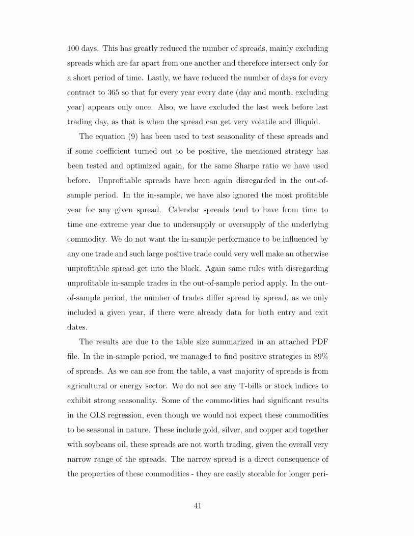
100 days. This has greatly reduced the number of spreads, mainly excluding
spreads which are far apart from one another and therefore intersect only for
a short period of time. Lastly, we have reduced the number of days for every
contract to 365 so that for every year every date (day and month, excluding
year) appears only once. Also, we have excluded the last week before last
trading day, as that is when the spread can get very volatile and illiquid.
The equation (9) has been used to test seasonality of these spreads and
if some coefficient turned out to be positive, the mentioned strategy has
been tested and optimized again, for the same Sharpe ratio we have used
before. Unprofitable spreads have been again disregarded in the out-of-
sample period. In the in-sample, we have also ignored the most profitable
year for any given spread. Calendar spreads tend to have from time to
time one extreme year due to undersupply or oversupply of the underlying
commodity. We do not want the in-sample performance to be influenced by
any one trade and such large positive trade could very well make an otherwise
unprofitable spread get into the black. Again same rules with disregarding
unprofitable in-sample trades in the out-of-sample period apply. In the out-
of-sample period, the number of trades differ spread by spread, as we only
included a given year, if there were already data for both entry and exit
dates.
The results are due to the table size summarized in an attached PDF
file. In the in-sample period, we managed to find positive strategies in 89%
of spreads. As we can see from the table, a vast majority of spreads is from
agricultural or energy sector. We do not see any T-bills or stock indices to
exhibit strong seasonality. Some of the commodities had significant results
in the OLS regression, even though we would not expect these commodities
to be seasonal in nature. These include gold, silver, and copper and together
with soybeans oil, these spreads are not worth trading, given the overall very
narrow range of the spreads. The narrow spread is a direct consequence of
the properties of these commodities - they are easily storable for longer peri-
41

ods of time and therefore their supply and demand is much more predictable
and stable.
As we have already mentioned, the average size of calendar spreads trade
is much lower than of almost any of the inter-commodity spreads. There
are two main reasons for that - first, the calendar spreads consists of two
one-contract legs. The ratio of legs in inter-commodity spreads had to be
adjusted according to the ratio we got from the OLS regression. Secondly, we
are dealing with the same underlying asset in both contracts. The contracts
differ only in the date of delivery, otherwise they have to be the same due
to the specification of futures contracts.
In the OOS period, 60% of spreads were suprisingly still positive, however
the average profit has decreased in 69% of the cases. Although we managed
to find some profitable strategies in both testing periods, additional test and
optimization will be necessary. Naive buy (sell) and hold trading strategies
can yield positive results in some of the spreads, but based on the data we
have, there is hardly a way for us to subset strategies which we can expect
to be profitable going forward. There are no obvious outliers in terms of
products, their contracts or types of strategies (1 vs 2 extremes). Rather
than simple buy and sell strategies the time parameter can be used more
as a filter, where the entry and exit signal will be generated based on some
other information, such as price behavior or deviation from the seasonal
norm. Given our technique, we did not manage to find profitable patterns
in naive purely time-based strategies. This does not necessarly imply that
all tested spreads are efficient from the point of view of seasonality. We
can only conclude that about the commodities which have had very narrow
spreads over the years - be it silver, gold or platinum. Given our transaction
cost, there is simply no seasonal strategy worth pursuing.
42

7 Conclusion
Spreads have been historically quite a popular theme amongst academics and
it was worth looking into various strategies and their effectivness in recent
years. We have tested two main types of approaches - seasonality and mean
reversion. Seasonality tests have been conducted on calendar spreads - their
main advantage is they are relatively less riskier than outright positions.
Simply buy-and-hold strategies, however, failed to deliver desired results.
More specifically there were strategies which were profitable in both IS and
OOS periods, but I did not manage to find a reliable pattern that would
allow us distinguish between winning and losing spreads. Mean reversion
spreads have been tested on two-legged (mostly generic) spreads, as well as
on 3-legged spreads well known in the trading industry. The former yielded
robust strategies on spreads which are not only co-integrated but also have
an underlying economic significance (such as constituencies of two-legged
variations of the crack spread). The latter failed miserably in the out-of-
sample period, one of the reasons is possibly the fact that we have used the
industry coefficient, not ones generated based a OLS regression as was the
case in 2-legged spreads.
43

References
Abken, P. A. (1989). An analysis of intra-market spreads in heating oil
futures. Journal of Futures Markets, vol. 9(issue 1):77–86.
Adrangi, B., Chatrath, A., Song, F., and Szidarovszky, F. (2006). Petroleum
spreads and the term structure of futures prices. Applied Economics, vol.
38(issue 16):1917–1929.
Barrett, W. B. and Kolb, R. W. (1995). Analysis of spreads in agricultural
futures. Journal of Futures Markets, vol. 15(issue 1):69–86.
Bernstein, J. (c1990). Jake Bernstein’s seasonal futures spreads. Wiley, New
York, 1st edition edition.
Bouman, S. and Jacobsen, B. (2002). The halloween indicator, ”sell in
may and go away”: Another puzzle. The American Economic Review,
92(5):1618–1635.
Butterworth, D. and Holmes, P. (2002). Inter-market spread trading. Applied
Financial Economics, vol. 12(issue 11):783–790.
Carlton, D. W. (1984). Futures markets. Journal of Futures Markets, vol.
4(issue 3):237–271.
Cole, C. A., Kastens, T. L., Hampel, F. A., and Gow, L. R. (1999). A
calendar spread trading simulation of seasonal processing spreads. In
NCR-134 Conference: Applied Commodity Price Analysis, Forecasting,
and Market Risk Management: Chicago, Illinois, April 19-20, 1999, page
221.
Daigler, R. T. (2007). Spread volume for currency futures. Journal of
Economics and Finance, vol. 31(issue 1):12–19.
Dichtl, H. and Drobetz, W. (2015). Sell in may and go away. International
Review of Financial Analysis, vol. 38(C):29–43.
44

Dickey, D. A. and Fuller, W. A. (1979). Distribution of the estimators
for autoregressive time series with a unit root. Journal of the American
Statistical Association, vol. 74(366a):427–431.
Dunis, C., Laws, J., and Evans, B. (2006a). Trading futures spreads. Applied
Financial Economics, vol. 16(issue 12):903–914.
Dunis, C. L., Laws, J., and Evans, B. (2006b). Modelling and trading the
gasoline crack spread. Derivatives Use, Trading & Regulation, vol. 12(issue
1):126–145.
Dunis, C. L., Laws, J., and Evans, B. (2010). Trading and filtering futures
spread portfolios. Journal of Derivatives & Hedge Funds, vol. 15(issue
4):274–287.
Dutt, H. R., Fenton, J., Smith, J. D., and Wang, G. H. K. (1997). Crop
year influences and variability of the agricultural futures spreads. Journal
of Futures Markets, vol. 17(issue 3):341–367.
Emery, G. W. and Liu, Q. W. (2001). An analysis of the relationship between
electricity and natural-gas futures prices. Journal of Futures Markets, vol.
22(issue 2):95–.
Engle, R. F. and Granger, C. W. J. (1987). Co-integration and error correc-
tion: Representation, estimation, and testing. Econometrica, 55(2):251–
276.
Fama, E. F. (1970). Efficient capital markets: A review of theory and
empirical work. The Journal of Finance, 25(2):383–417.
Gay, G. D. and Kim, T.-H. (1987). An investigation into seasonality in the
futures market. Journal of Futures Markets, vol. 7(issue 2):169–181.
Geman, H. (2012). Seasonality in cocoa spot and forward markets. Journal
of Agricultural Extension and Rural Development, vol. 4(issue 8):–.
45

Girma, P. B. and Paulson, A. S. (1998). Seasonality in petroleum futures
spreads. Journal of Futures Markets, vol. 18(issue 5):581–598.
Gultekin, M. N. and Gultekin, N. (1983). Stock market seasonality. Journal
of Financial Economics, vol. 12(issue 4):469–481.
Haugen, R. A. and Jorion, P. (1996). The january effect: Still there after all
these years. Financial Analysts Journal, 52(1):27–31.
Kawaller, I. G., Koch, P. D., and Liu, L. (2002). Calendar spreads, outright
futures positions, and risk. The Journal of Alternative Investments, vol.
5(issue 3):59–74.
Kenyon, D. and Clay, J. (1987). Analysis of profit margin hedging strategies
for hog producers. Journal of Futures Markets, vol. 7(issue 2):183–202.
Leuthold, R. M. and Mokler, R. S. (1979). Feeding-margin hedging in the
cattle industry. 6:56–68.
Liu, Q. W. (2005). Price relations among hog, corn, and soybean meal
futures. Journal of Futures Markets, vol. 25(issue 5):491–514.
Liu, Q. W. and Sono, H. H. (2016). Empirical properties, information flow,
and trading strategies of china’s soybean crush spread. Journal of Futures
Markets, vol. 36(issue 11):1057–1075.
Lovell, R. T. (1988). Use of soybean products in diets for aquaculture species.
J. Aquat. Products, 2:27–52.
Lubnau, T. and Todorova, N. (2015). Trading on mean-reversion in energy
futures markets. Energy Economics, vol. 51(51):312–319.
Malick, W. M. and Ward, R. W. (1987). Stock effects and seasonality in the
fcoj futures basis. Journal of Futures Markets, vol. 7(issue 2):157–167.
Mitchell, J. (2010). Soybean futures crush spread arbitrage. Journal of Risk
and Financial Management, vol. 3(issue 1):63–96.
46

Rechner, D. and Poitras, G. (1993). Putting on the crush. Journal of Futures
Markets, vol. 13(issue 1):61–75.
Salcedo, Y. (2004). Spreads for the fall. FUTURES-CEDAR FALLS IOWA
THEN CHICAGO-, 33:54–57.
Simon, D. P. (1999). The soybean crush spread. Journal of Futures Markets,
vol. 19(issue 3):271–289.
Tucker, S. (2000). Spreading the wealth. FUTURES-CEDAR FALLS IOWA
THEN CHICAGO-, 29(1):42–45.
Vaughn, R., Kelly, M., and Hochheimer, F. (1981). Identifying seasonality in
futures prices using x-11. Journal of Futures Markets, vol. 1(issue 1):93–
101.
Wahab, M., Cohn, R., and Lashgari, M. (1994). The gold-silver spread.
Journal of Futures Markets, vol. 14(issue 6):709–756.
Westgaard, S., Estenstad, M., Seim, M., and Frydenberg, S. (2011). Co-
integration of ice gas oil and crude oil futures. Energy Economics, vol.
33(issue 2):311–320.
Wooldridge, J. M. (c2013). Introductory econometrics. South-Western Cen-
gage Learning, Mason, OH, 5th ed. edition.
Working, H. (1949). The theory of price of storage. The American Economic
Review, 39(6):1254.
47

List of tables and figures
List of Figures
1 Stationary and non-stationary time series . . . . . . . . . . . 20
2 Crude Oil CLH14 contract before and after differentiation. . 21
3 Visualisation of Filter0 Long Strategy . . . . . . . . . . . . . 31
4 Visualization of out-of-sample AD-FC Trade . . . . . . . . . 36
5 Visualisation of seasonal WTI Crude Oil Spread . . . . . . . 40
List of Tables
1 List of all products . . . . . . . . . . . . . . . . . . . . . . . 49
2 Crush spread - roll over . . . . . . . . . . . . . . . . . . . . . 51
3 Cattle spread - roll over . . . . . . . . . . . . . . . . . . . . 51
4 Results of ADF test on in-sample data . . . . . . . . . . . . 52
5 Results of ADF test on in-sample data in cattle and soybean
crush spread . . . . . . . . . . . . . . . . . . . . . . . . . . . 53
6 Cointegration test. . . . . . . . . . . . . . . . . . . . . . . . 53
7 Filter0 trading results on in sample data . . . . . . . . . . . 54
8 Filter trading results on in sample data . . . . . . . . . . . . 57
9 RSI trading results on in sample data . . . . . . . . . . . . . 60
10 Moving average trading results on in sample data . . . . . . 62
11 Filter0 trading results out-of-sample data . . . . . . . . . . . 65
12 Filter trading results out-of-sample data . . . . . . . . . . . 67
13 RSI trading results on out-of-sample data . . . . . . . . . . . 69
14 Moving average trading results out-of-sample data . . . . . . 69
15 Notable spreads IS Results . . . . . . . . . . . . . . . . . . . 71
16 Notable spreads OOS Results . . . . . . . . . . . . . . . . . 72
48

Appendix
Table 1: List of all products
BO Soybean Oil Grain/Oilseed FHKNQUVZ 2000
C Corn Grain/Oilseed HKNUZ 2000
HG Copper Metal FGHJKMNQUVXZ 2000
O Oats Grain/Oilseed HKNUZ 2000
S Soybeans Grain/Oilseed FHKNQUX 2000
SM Soybean Meal Grain/Oilseed FHKNQUVZ 2000
W Wheat Grain/Oilseed HKNUZ 2000
SI Silver Metal FGHJKMNQUVXZ 2000
LC Live Cattle Meat/Livestock GJMQVZ 2000
PL Platinum Metal FJNV 2000
CC Cocoa Food/Fibre HKNUZ 2000
FC Feeder Cattle Meat/Livestock FHJKQUVX 2000
LB Lumber Food/Fibre FHKNUX 2000
GC Gold Metal FGHJKMNQUVXZ 2000
BP British Pound Currency HMUZ 2000
SF Swiss Franc Currency HMUZ 2000
JY Japanese Yen Currency HMUZ 2000
KW Wheat KCBT Grain/Oilseed HKNUZ 2000
PA Palladium Metal HMUZ 2000
CD Canadian Dollar Currency HMUZ 2000
US 30Y US T-Bond Interest Rate HMUZ 2000
HO Heating Oil Oil/Energy FGHJKMNQUVXZ 2000
ED Eurodollar Interest Rate FGHJKMNQUVXZ 2000
CL Crude Oil Oil/Energy FGHJKMNQUVXZ 2000
TY 10Y US T-Note Interest Rate HMUZ 2000
DX U.S. Dollar Index Index HMUZ 2000
AD Australian Dollar Currency HMUZ 2000
49

Ticker Name Category Months Year Start
RR Rough Rice Grain/Oilseed FHKNUX 2000
FV 5Y US T-Note Interest Rate HMUZ 2000
NG Natural Gas Oil/Energy FGHJKMNQUVXZ 2000
B Brent Crude Oil Oil/Energy FGHJKMNQUVXZ 2000
TU 2Y US T-Note Interest Rate HMUZ 2000
NE New Zealand Dollar Currency HMUZ 2000
ES S&P 500 mini Index HMUZ 2000
YM mini-sized Dow $5 Index HMUZ 2000
EC Euro FX Currency HMUZ 2000
NQ Nasdaq 100 mini Index HMUZ 2000
CT Cotton #2 Food/Fibre HKNVZ 2000
SB Sugar #11 Food/Fibre HKNV 2000
OJ Orange Juice Food/Fibre FHKNUX 2000
KC Coffee Food/Fibre HKNUZ 2000
RS Canola Grain/Oilseed FHKNX 2000
G Gas Oil Oil/Energy FGHJKMNQUVXZ 2000
TF Russell 2000 mini Index HMUZ 2002
RB RBOB Gasoline Oil/Energy FGHJKMNQUVXZ 2006
LN Lean Hogs Meat/Livestock GJKMNQVZ 2000
W White Sugar Food/Fibre HKQVZ 2000
50

Table 2: Crush spread - roll over
Roll Soybeans Soybean Oil Soybean Meal First Day Last Day
1 January January January Nov 1st Dec 31st
2 March March March Jan 1st Feb 28th/29th
3 May May May Mar 1st Apr 30th
4 July July July May 1st Jun 30th
5 September September September Jul 1st Aug 31st
6 November December December Sept 1st October 31st
Table 3: Cattle spread - roll over
Roll Feeder Cattle Live Cattle Corn First Day Last Day
1 January June March Nov 1st Dec 31st
2 March August May Jan 1st Feb 28th/29th
3 April August May Mar 1st Mar 31st
4 May October July Apr 1st Apr 30th
5 August February September Jun 1st Jul 31st
6 September February December Aug 1st Aug 31st
7 October April December Sep 1st Sep 30th
8 November April March Oct 1st Oct 31st
51

Table 4: Results of ADF test on in-sample data
Root ADF Level ADF Differenced Root ADF Level ADF Differenced
AD 0.27 0.01 LN 0.01 0.01
B 0.49 0.01 NE 0.49 0.01
BO 0.64 0.01 NG 0.39 0.01
BP 0.89 0.01 NQ 0.42 0.01
C 0.56 0.01 O 0.43 0.01
CC 0.10 0.01 OJ 0.66 0.01
CD 0.26 0.01 PA 0.99 0.01
CL 0.44 0.01 PL 0.44 0.01
CT 0.99 0.01 RB 0.30 0.01
DX 0.47 0.01 RR 0.38 0.01
EC 0.54 0.01 RS 0.65 0.01
ED 0.95 0.01 S 0.45 0.01
ES 0.57 0.01 SB 0.95 0.01
FC 0.25 0.01 SF 0.09 0.01
FV 0.50 0.01 SI 0.97 0.01
G 0.56 0.01 SM 0.14 0.01
GC 0.83 0.01 TF 0.68 0.01
HG 0.66 0.01 TU 0.75 0.01
HO 0.51 0.01 TY 0.16 0.01
JY 0.51 0.01 US 0.01 0.01
KC 0.60 0.01 W 0.42 0.01
KW 0.48 0.01 WS 0.91 0.01
LB 0.25 0.01 YM 0.45 0.01
LC 0.02 0.01
52

Table 5: Results of ADF test on in-sample data in cattle
and soybean crush spread
Root ADF Level ADF Differenced
S 0.280 0.01
BO 0.430 0.01
SM 0.060 0.01
FC 0.450 0.01
LC 0.420 0.01
C 0.390 0.01
Table 6: Cointegration test.
Spread Ticker ADF t-statistic Coefficient Spread Ticker ADF t-statistic Coefficient
AD-FC -3.68 1.47 KW-O -3.63 2.3
B-CL -4.19 0.99 KW-RR -3.82 1.23
B-HO -3.76 0.84 KW-RS -3.56 3.23
B-KW -3.58 2.27 KW-S -3.56 0.62
B-NG -3.54 0.85 LB-NE -3.59 0.48
B-PL -3.48 1.08 LB-NG -3.63 0.44
B-W -3.55 2.39 O-W -3.74 0.44
BO-C -4.19 1.14 PL-W -3.51 2.2
BO-KW -4.46 0.73 RR-S -3.98 0.5
BO-RR -3.6 0.91 RR-SM -3.99 0.83
BO-W -4.78 0.77 RR-W -3.94 0.82
BP-NG -3.51 1.57 RS-W -3.83 0.31
C-KW -4.07 0.63 S-W -3.76 1.64
C-O -3.7 1.48 SF-TU -3.64 0.47
C-RS -3.78 2.08 SF-TY -3.82 0.89
C-W -4.12 0.66 TU-TY -4.53 1.88
CD-FC -3.7 1.64 ES-TF -3.54 1.76
CL-G -3.58 1.15 LB-TF -3.92 0.74
CL-HO -4.21 0.85 NG-TF -3.71 1.11
CL-KW -3.48 2.3 TF-YM -3.61 0.64
CL-NG -3.62 0.86 CL-RB -3.68 0.83
CL-PL -3.57 1.1 G-RB -3.54 0.77
CL-RR -3.48 2.92 HG-RB -3.52 0.81
53

CL-W -3.48 2.43 HO-RB -3.86 1.04
CT-SI -3.46 4.99 KW-RB -4.17 0.34
FC-LB -3.58 1.57 NG-RB -3.45 0.5
FV-SF -3.62 1.09 O-RB -4.39 0.15
FV-TY -5.23 0.98 PA-RB -3.74 0.58
G-HO -3.97 0.74 PL-RB -3.67 0.71
G-KW -3.47 2 RB-RR -3.63 3.54
G-NG -3.56 0.75 RB-S -3.51 1.67
HG-OJ -3.46 3.15 RB-SM -3.47 2.75
HO-NG -3.49 1.02 RB-W -3.86 3.02
KC-SI -3.78 0.69
Table 7: Filter0 trading results on in sample data
SL SD L/S Spread Avg $ Max Win Max Loss Win% # DD Sharpe
1.4 0.2 Long AD-FC $6,063 $16,080 $-7,400 0.87 15 $45,050 0.91
1 0.4 Short AD-FC $6,640 $29,740 $-33,210 0.83 12 $62,950 0.44
1 0.8 Long B-CL $1,751 $3,930 $-1,950 0.91 11 $5,190 1.25
1.4 1.2 Short B-CL $1,475 $6,540 $-2,560 0.69 13 $9,080 0.49
0.2 1.4 Long B-HO $29,759 $119,643 $-20,708 0.73 11 $74,704 0.74
0.6 0.6 Short B-HO $9,792 $28,245 $-13,610 0.77 13 $49,857 0.82
1.2 0.2 Long B-KW $57,633 $153,770 $-24,840 0.91 11 $387,410 1.1
0.2 1.4 Short B-KW $46,193 $687,640 $-78,460 0.27 11 $737,580 0.21
0.2 1.4 Long B-NG $12,464 $304,740 $-58,960 0.14 14 $309,200 0.11
0.2 0.8 Short B-NG $1,764 $119,090 $-22,210 0.17 12 $141,300 0.04
1.2 0.8 Long B-PL $8,029 $21,845 $-12,435 0.91 11 $33,395 1.02
1.2 0.6 Short B-PL $4,944 $42,280 $-13,620 0.75 12 $44,050 0.33
0.6 0.2 Long B-W $35,165 $172,685 $-75,165 0.92 12 $218,085 0.59
0.2 1 Short B-W $21,007 $390,010 $-43,215 0.31 13 $421,850 0.18
1.2 0.6 Long BO-C $9,178 $18,480 $-1,150 0.91 11 $32,130 1.72
1.2 1 Short BO-C $8,944 $45,540 $-21,370 0.83 12 $55,120 0.52
0.8 1 Long BO-KW $9,582 $66,834 $-23,428 0.67 12 $70,836 0.35
1.2 0.4 Short BO-KW $4,206 $17,018 $-25,498 0.75 12 $40,546 0.34
0.8 0.8 Long BO-RR $2,218 $8,376 $-3,780 0.73 11 $11,256 0.54
0.2 1.4 Short BO-RR $1,195 $8,280 $-1,838 0.29 14 $10,118 0.33
0.4 1.4 Long BO-W $8,303 $59,758 $-13,750 0.46 13 $61,774 0.33
1.2 0.6 Short BO-W $6,973 $23,978 $-26,540 0.82 11 $45,298 0.55
1.4 0.4 Long BP-NG $16,160 $144,365 $-72,568 0.77 13 $201,863 0.29
0.8 0.8 Short BP-NG $31,446 $113,580 $-36,638 0.82 11 $150,218 0.78
0.6 0.2 Long C-KW $1,138 $89,360 $-24,890 0.55 20 $107,450 0.05
1.4 0.6 Short C-KW $7,892 $25,060 $-20,940 0.83 12 $46,235 0.65
1 0.2 Long C-O $3,171 $13,725 $-2,850 0.84 19 $24,150 0.87
0.6 0.8 Short C-O $5,599 $21,275 $-7,225 0.75 12 $26,613 0.67
1 0.2 Long C-RS $1,731 $7,481 $-2,846 0.87 15 $17,972 0.71
54

0.4 1.2 Short C-RS $1,870 $33,921 $-6,797 0.36 11 $40,718 0.16
0.6 0.4 Long C-W $1,499 $88,860 $-28,615 0.56 16 $110,550 0.06
0.6 0.8 Short C-W $7,693 $24,160 $-15,702 0.73 11 $38,975 0.48
0.8 0.2 Long CD-FC $13,519 $52,630 $-18,790 0.89 19 $87,520 0.81
1.2 0.6 Short CD-FC $15,604 $79,310 $-9,080 0.75 12 $152,480 0.64
1.4 0.4 Long CL-G $8,157 $44,220 $-59,430 0.89 45 $133,530 0.49
1 0.4 Short CL-G $6,759 $24,920 $-38,080 0.82 45 $60,600 0.67
1.2 0.8 Long CL-HO $19,811 $121,578 $-794 0.83 12 $78,996 0.6
0.4 0.6 Short CL-HO $13,715 $53,094 $-3,700 0.89 19 $39,401 1.01
0.6 0.2 Long CL-KW $59,623 $237,410 $-136,600 0.92 13 $328,230 0.67
0.2 1.4 Short CL-KW $46,320 $673,950 $-68,920 0.27 11 $721,850 0.21
0.4 1.4 Long CL-NG $16,013 $314,810 $-59,470 0.18 11 $297,800 0.12
0.6 0.2 Short CL-NG $9,180 $86,570 $-63,270 0.64 11 $167,440 0.17
1.4 0.6 Long CL-PL $7,064 $23,890 $-14,300 0.92 12 $36,810 0.85
0.8 0.4 Short CL-PL $3,903 $40,730 $-9,925 0.72 18 $42,735 0.33
0.2 1.2 Long CL-RR $10,993 $101,680 $-34,850 0.42 12 $108,290 0.26
0.4 1 Short CL-RR $9,889 $113,020 $-36,450 0.45 11 $135,310 0.21
0.6 0.2 Long CL-W $28,984 $152,310 $-80,790 0.94 17 $203,610 0.62
0.2 1.2 Short CL-W $25,867 $377,260 $-37,915 0.27 11 $405,925 0.21
0.6 0.2 Long CT-SI $228,475 $966,585 $-372,335 0.64 11 $1,338,920 0.55
0.2 0.4 Short CT-SI $45,823 $773,780 $-128,035 0.29 14 $1,121,820 0.16
0.6 0.8 Long FC-LB $14,091 $54,587 $-13,669 0.75 12 $67,864 0.69
1.2 0.2 Short FC-LB $3,177 $15,719 $-26,349 0.83 12 $44,983 0.31
0.2 0.8 Long FV-SF $1,512 $20,490 $-3,534 0.23 13 $23,642 0.17
0.2 0.2 Short FV-SF $1,842 $26,341 $-3,792 0.42 12 $30,133 0.22
0.2 1.4 Long FV-TY $1,079 $6,241 $-1,071 0.36 11 $6,984 0.44
1 0.4 Short FV-TY $1,059 $4,304 $-1,946 0.92 12 $6,250 0.75
0.6 1.2 Long G-HO $10,230 $32,029 $-6,059 0.85 27 $54,217 1.09
1.4 0.4 Short G-HO $5,798 $54,042 $-50,014 0.86 138 $131,955 0.59
0.8 0.2 Long G-KW $11,598 $38,178 $-32,773 0.92 12 $66,000 0.65
0.2 1 Short G-KW $6,058 $122,490 $-12,898 0.29 14 $132,250 0.17
0.2 1.4 Long G-NG $15,339 $343,055 $-48,485 0.14 14 $298,190 0.13
0.2 0.8 Short G-NG $555 $95,505 $-20,895 0.17 12 $150,790 0.01
0.2 0.2 Short HG-OJ $8,121 $794,488 $-112,488 0.35 20 $882,718 0.04
0.4 0.4 Long HO-NG $5,886 $72,322 $-13,731 0.42 12 $77,383 0.21
0.2 1 Short HO-NG $343 $60,007 $-8,670 0.13 15 $66,730 0.02
0.4 0.8 Long KC-SI $20,972 $90,504 $-37,218 0.58 12 $127,721 0.43
1.2 0.2 Short KC-SI $22,313 $107,861 $-3,990 0.94 18 $188,618 0.93
0.6 0.6 Long KW-O $15,922 $51,953 $-24,773 0.83 12 $93,203 0.68
0.4 0.6 Short KW-O $9,488 $205,615 $-51,110 0.5 16 $236,788 0.15
1 0.4 Long KW-RR $9,029 $44,683 $-31,735 0.83 18 $73,545 0.45
1.2 0.6 Short KW-RR $6,450 $113,780 $-40,920 0.62 13 $146,845 0.15
0.2 0.2 Long KW-RS $12,566 $66,653 $-28,757 0.73 11 $149,605 0.51
1.4 0.4 Short KW-RS $15,345 $223,181 $-169,057 0.75 12 $362,087 0.13
0.2 1 Long KW-S $7,364 $43,240 $-5,585 0.42 12 $47,938 0.43
0.8 0.4 Short KW-S $7,788 $38,765 $-17,298 0.83 12 $60,010 0.6
55

0.2 0.2 Long LB-NE $-1,398 $32,186 $-6,136 0.15 13 $63,773 -0.13
0.6 0.2 Short LB-NE $4,360 $28,416 $-15,480 0.83 12 $43,896 0.37
0.8 0.6 Long LB-NG $21,199 $149,397 $-51,804 0.67 12 $152,195 0.34
0.8 0.6 Short LB-NG $30,556 $91,158 $-38,891 0.91 11 $127,527 0.87
0.4 0.4 Long O-W $1,452 $41,090 $-8,360 0.58 19 $49,760 0.12
0.4 0.8 Short O-W $5,453 $16,865 $-6,460 0.73 11 $24,523 0.7
1 0.4 Long PL-W $35,755 $269,150 $-166,035 0.92 12 $501,835 0.38
0.2 1.2 Short PL-W $7,153 $204,235 $-59,245 0.31 13 $254,295 0.09
0.6 1 Long RR-S $5,130 $30,675 $-14,030 0.55 11 $43,045 0.29
1.2 0.4 Short RR-S $6,465 $21,840 $-24,940 0.87 15 $46,780 0.62
0.6 1 Long RR-SM $12,160 $43,800 $-13,250 0.58 12 $53,830 0.56
0.4 1.4 Short RR-SM $9,250 $72,620 $-10,050 0.33 12 $82,440 0.32
0.4 1.2 Long RR-W $5,868 $85,780 $-21,700 0.27 11 $95,920 0.18
1.2 0.6 Short RR-W $7,373 $38,540 $-27,110 0.82 11 $68,860 0.38
0.2 1.4 Long RS-W $7,186 $94,768 $-16,184 0.25 12 $91,082 0.2
0.2 0.4 Short RS-W $9,199 $29,264 $-8,684 0.67 12 $38,880 0.67
0.8 0.4 Long S-W $31,824 $137,130 $-17,520 0.92 13 $186,625 0.89
0.4 1 Short S-W $21,570 $148,693 $-32,445 0.5 12 $181,138 0.34
0.2 0.2 Long SF-TU $-402 $19,134 $-3,910 0.17 12 $21,144 -0.06
0.2 0.2 Short SF-TU $-679 $12,465 $-4,054 0.33 12 $30,156 -0.14
0.6 0.2 Long SF-TY $2,687 $17,051 $-7,357 0.82 11 $21,410 0.42
0.2 1 Short SF-TY $2,209 $21,907 $-4,862 0.25 12 $26,769 0.22
0.6 0.4 Long TU-TY $874 $8,174 $-5,138 0.55 11 $13,435 0.21
0.6 0.4 Short TU-TY $-429 $3,752 $-6,185 0.55 11 $9,966 -0.13
0.4 0.6 Long CL-RB $8,423 $85,588 $-25,816 0.43 14 $95,821 0.22
1.2 0.4 Short CL-RB $13,316 $36,599 $-58,066 0.86 14 $124,171 0.56
0.4 1.2 Long G-RB $19,840 $70,209 $-22,040 0.54 13 $90,385 0.51
1.4 0.4 Short G-RB $12,262 $44,712 $-67,462 0.86 14 $112,175 0.34
1.2 0.6 Long HG-RB $39,271 $219,010 $-92,986 0.92 13 $285,289 0.6
1.2 0.2 Short HG-RB $24,209 $107,574 $-81,561 0.94 18 $180,504 0.66
1 0.6 Long HO-RB $5,893 $17,583 $-8,797 0.77 13 $26,195 0.64
1.2 0.2 Short HO-RB $4,157 $18,226 $-11,078 0.83 12 $28,791 0.47
0.4 1 Long KW-RB $37,288 $141,352 $-38,988 0.67 12 $156,320 0.59
0.2 1 Short KW-RB $41,027 $195,510 $-24,876 0.36 11 $220,386 0.43
0.2 0.2 Long NG-RB $-6,706 $36,299 $-20,491 0.23 13 $87,570 -0.4
1.4 0.6 Long O-RB $24,869 $56,962 $-10,218 0.8 15 $166,667 1.23
0.4 0.8 Short O-RB $42,383 $188,240 $-46,549 0.69 13 $196,789 0.55
0.2 1.2 Long PA-RB $10,184 $123,925 $-14,693 0.25 12 $94,749 0.24
0.6 0.2 Short PA-RB $5,539 $84,001 $-22,444 0.58 12 $112,221 0.19
1 0.4 Long PL-RB $36,484 $193,417 $-67,665 0.83 12 $261,082 0.6
1.4 0.2 Short PL-RB $32,888 $98,945 $-15,428 0.94 17 $159,393 1.18
0.4 0.2 Long RB-RR $35,835 $407,521 $-98,576 0.67 18 $463,877 0.28
0.4 1 Short RB-RR $77,165 $269,350 $-72,348 0.55 11 $316,774 0.53
1 0.2 Long RB-S $44,118 $237,896 $-126,749 0.87 15 $302,575 0.55
0.2 1.4 Short RB-S $72,411 $286,236 $-37,667 0.45 11 $318,297 0.56
1 0.2 Long RB-SM $21,963 $119,189 $-72,130 0.91 11 $171,640 0.48
56

0.6 0.8 Short RB-SM $20,818 $216,175 $-51,016 0.54 13 $255,801 0.27
0.6 0.2 Long RB-W $26,074 $125,396 $-53,097 0.73 11 $163,598 0.43
0.2 1 Short RB-W $14,335 $108,779 $-16,931 0.33 15 $121,335 0.31
1.2 0.2 Long ES-TF $994 $59,090 $-56,940 0.58 12 $120,600 0.03
0.2 0.2 Short ES-TF $-1,074 $35,518 $-12,640 0.33 15 $117,515 -0.07
0.2 0.6 Long LB-TF $1,298 $15,441 $-2,698 0.25 12 $18,139 0.21
0.4 0.2 Short LB-TF $1,527 $24,446 $-4,447 0.45 11 $28,264 0.18
0.8 0.2 Long NG-TF $12,766 $54,775 $-36,810 0.95 20 $82,405 0.79
0.4 1.4 Short NG-TF $19,463 $160,430 $-37,710 0.33 12 $171,365 0.27
0.4 0.2 Long TF-YM $1,421 $12,580 $-5,390 0.45 11 $30,295 0.23
0.4 0.2 Short TF-YM $1,053 $21,655 $-4,880 0.54 13 $29,055 0.15
Table 8: Filter trading results on in sample data
PT SL SD L/S Spread Avg $ Max Win Max Loss Win% # DD Sharpe
1.5 0.2 0.6 Long AD-FC $18,562 $48,668 $-6,489 0.45 11 $55,157 0.65
1.5 0.2 1.4 Short AD-FC $7,280 $48,668 $-6,489 0.25 12 $55,157 0.29
1.5 1.4 0.4 Long B-CL $1,897 $2,285 $-2,133 0.92 12 $4,418 1.5
2 1.4 1.2 Short B-CL $1,433 $3,047 $-2,133 0.69 13 $5,180 0.58
0.5 0.2 1.4 Long B-HO $13,228 $23,084 $-9,234 0.7 23 $32,317 0.87
0.5 1.2 0.2 Short B-HO $16,523 $23,084 $-55,401 0.92 12 $78,485 0.73
0.5 0.4 0.2 Long B-KW $69,926 $103,974 $-83,179 0.82 11 $187,153 0.92
1 0.2 1.2 Short B-KW $29,687 $207,948 $-41,590 0.29 14 $249,537 0.25
0.5 1.4 1.2 Long B-NG $27,971 $42,765 $-119,741 0.91 11 $162,505 0.57
0.5 1.2 0.8 Short B-NG $16,308 $42,765 $-102,635 0.82 11 $145,399 0.28
0.5 1.2 0.8 Long B-PL $3,914 $4,918 $-11,802 0.94 17 $16,720 0.97
1.5 0.8 0.4 Short B-PL $6,032 $14,753 $-7,868 0.62 13 $22,621 0.53
0.5 0.2 0.8 Long B-W $36,305 $58,762 $-23,505 0.73 11 $82,266 0.95
0.5 0.2 1.4 Short B-W $8,116 $58,762 $-23,505 0.38 13 $82,266 0.2
0.5 0.4 1.4 Long BO-C $6,098 $8,050 $-6,440 0.87 15 $14,490 1.2
1 0.8 1.2 Short BO-C $8,176 $16,100 $-12,880 0.73 11 $28,980 0.61
1.5 0.2 1.4 Long BO-KW $7,389 $30,310 $-4,041 0.33 18 $34,352 0.44
1 0.4 1.4 Short BO-KW $7,328 $20,207 $-8,083 0.55 11 $28,290 0.5
1 1.2 0.6 Long BO-RR $1,965 $3,309 $-3,971 0.82 11 $7,280 0.67
1 1.2 1 Long BO-RR $1,965 $3,309 $-3,971 0.82 11 $7,280 0.67
0.5 1.4 1 Short BO-RR $1,151 $1,655 $-4,633 0.92 13 $6,287 0.67
1.5 1 1.4 Long BO-W $13,067 $29,447 $-19,631 0.67 12 $49,078 0.54
0.5 1 0.8 Short BO-W $7,342 $9,816 $-19,631 0.92 12 $29,447 0.87
1.5 1.4 0.4 Long BP-NG $27,926 $54,090 $-50,484 0.75 12 $104,574 0.59
1 0.8 1 Short BP-NG $25,222 $36,060 $-28,848 0.83 12 $64,908 1
1.5 0.2 0.2 Long C-KW $5,011 $36,282 $-4,838 0.24 25 $41,120 0.28
0.5 0.2 1.2 Short C-KW $4,378 $12,094 $-4,838 0.55 11 $16,932 0.5
1 0.8 0.6 Long C-O $9,004 $10,790 $-8,632 0.91 11 $18,915 1.54
0.5 0.6 1.2 Short C-O $4,296 $5,395 $-6,474 0.91 11 $11,869 1.21
57

0.5 0.6 0.2 Long C-RS $2,920 $4,900 $-5,880 0.82 11 $10,780 0.67
0.5 1 1.2 Short C-RS $2,207 $4,900 $-9,800 0.82 11 $14,700 0.37
0.5 1 1.4 Short C-RS $2,207 $4,900 $-9,800 0.82 11 $14,700 0.37
1.5 0.2 0.8 Long C-W $5,349 $35,795 $-4,773 0.25 24 $40,567 0.3
0.5 0.8 0.8 Short C-W $9,091 $11,932 $-19,090 0.91 11 $31,022 0.97
0.5 0.2 0.8 Long CD-FC $22,606 $34,809 $-13,924 0.75 12 $48,733 1.03
0.5 0.2 1.2 Short CD-FC $16,046 $34,809 $-13,924 0.62 13 $48,733 0.65
0.5 0.2 1.4 Short CD-FC $16,046 $34,809 $-13,924 0.62 13 $48,733 0.65
0.5 1.4 0.2 Long CL-G $10,107 $18,616 $-52,125 0.88 25 $70,742 0.43
0.5 1.4 0.4 Long CL-G $10,107 $18,616 $-52,125 0.88 25 $70,742 0.43
0.5 0.6 1 Short CL-G $9,145 $18,616 $-22,339 0.77 13 $40,956 0.51
0.5 1 1.2 Long CL-HO $17,764 $23,712 $-47,424 0.92 12 $71,136 0.87
0.5 0.6 0.4 Short CL-HO $19,679 $23,712 $-28,454 0.92 13 $52,166 1.36
0.5 0.6 0.6 Short CL-HO $19,679 $23,712 $-28,454 0.92 13 $52,166 1.36
0.5 0.6 0.6 Long CL-KW $81,420 $101,800 $-122,160 0.91 11 $223,961 1.21
0.5 0.6 0.8 Long CL-KW $81,420 $101,800 $-122,160 0.91 11 $223,961 1.21
1 0.2 1.4 Short CL-KW $40,700 $203,600 $-40,720 0.33 12 $244,321 0.34
1 0.6 1.2 Long CL-NG $32,071 $83,438 $-50,063 0.62 13 $133,500 0.47
0.5 1 1 Short CL-NG $18,943 $41,719 $-83,438 0.82 11 $125,156 0.37
0.5 1.2 0.8 Long CL-PL $4,027 $4,876 $-11,703 0.95 20 $16,580 1.09
2 0.8 0.6 Short CL-PL $8,107 $19,506 $-7,802 0.58 12 $27,308 0.58
0.5 0.6 1 Long CL-RR $17,461 $35,509 $-42,610 0.77 13 $78,119 0.51
0.5 0.2 1 Short CL-RR $1,475 $35,509 $-14,203 0.32 19 $49,712 0.06
0.5 0.4 0.8 Long CL-W $40,267 $57,553 $-46,042 0.83 12 $103,595 1
1 0.2 1.2 Short CL-W $23,001 $115,105 $-23,021 0.33 12 $138,126 0.34
0.5 0.4 1 Long CT-SI $137,559 $196,542 $-157,233 0.83 12 $353,775 1
0.5 0.8 1 Short CT-SI $76,284 $196,542 $-314,467 0.76 17 $511,009 0.34
0.5 0.8 0.8 Long FC-LB $8,695 $10,542 $-16,867 0.93 15 $27,409 1.23
0.5 0.4 1.4 Short FC-LB $7,072 $10,542 $-8,434 0.82 11 $18,976 0.92
0.5 0.2 1 Long FV-SF $1,147 $6,365 $-2,546 0.42 12 $8,911 0.25
1 0.2 0.2 Short FV-SF $3,799 $12,730 $-2,546 0.42 12 $15,275 0.49
0.5 1.2 1 Long FV-TY $596 $834 $-2,002 0.92 13 $2,836 0.78
1 1 0.6 Short FV-TY $1,345 $1,668 $-1,668 0.91 11 $3,337 1.36
0.5 0.4 1.2 Long G-HO $6,855 $26,562 $-21,250 0.59 17 $47,812 0.28
1 0.4 1.4 Short G-HO $22,115 $53,125 $-21,250 0.58 12 $74,375 0.58
0.5 0.4 0.4 Long G-KW $10,979 $19,998 $-15,998 0.75 12 $35,996 0.68
0.5 0.2 1.4 Short G-KW $5,979 $19,998 $-7,999 0.5 16 $27,997 0.41
1 0.6 1.2 Long G-NG $30,181 $78,523 $-47,114 0.62 13 $125,637 0.47
0.5 1.2 0.8 Short G-NG $14,971 $39,262 $-94,228 0.82 11 $133,490 0.28
0.5 0.2 0.2 Long HG-OJ $87,128 $177,524 $-71,010 0.64 11 $248,533 0.7
0.5 0.2 1.4 Short HG-OJ $53,237 $177,524 $-71,010 0.5 12 $248,533 0.41
1 0.4 1.4 Long HO-NG $9,158 $25,239 $-10,095 0.55 11 $35,334 0.5
0.5 0.2 1.4 Short HO-NG $2,504 $12,619 $-5,048 0.43 21 $17,667 0.28
0.5 0.2 1.4 Long KC-SI $14,456 $37,359 $-14,943 0.56 16 $52,302 0.54
0.5 1 0.2 Short KC-SI $30,334 $37,359 $-74,717 0.94 16 $112,076 1.08
0.5 0.2 1.2 Long KW-O $19,389 $36,392 $-14,557 0.67 12 $50,949 0.77
58

0.5 0.2 1 Short KW-O $5,145 $36,392 $-14,557 0.39 31 $50,949 0.2
2 0.2 1.4 Long KW-RR $16,144 $53,879 $-5,388 0.36 11 $59,266 0.54
2 0.2 0.8 Short KW-RR $6,445 $53,879 $-5,388 0.2 25 $59,266 0.27
0.5 0.2 0.2 Long KW-RS $14,407 $58,608 $-23,443 0.46 13 $82,051 0.34
1.5 0.2 1.4 Short KW-RS $16,390 $175,824 $-23,443 0.2 15 $199,267 0.2
0.5 0.4 1.4 Long KW-S $4,682 $9,681 $-7,745 0.71 14 $17,425 0.58
0.5 0.6 1 Short KW-S $8,022 $9,681 $-11,617 0.92 13 $21,298 1.36
0.5 0.4 1 Long LB-NE $1,874 $11,837 $-9,470 0.53 15 $21,307 0.17
0.5 0.6 0.2 Short LB-NE $4,715 $11,837 $-14,205 0.73 11 $26,042 0.39
1.5 0.6 0.6 Long LB-NG $21,317 $71,125 $-28,450 0.5 14 $99,574 0.41
0.5 0.6 1 Short LB-NG $18,947 $23,708 $-28,450 0.91 11 $52,158 1.21
1 0.4 1.2 Long O-W $3,118 $15,688 $-6,275 0.43 14 $21,963 0.28
1 0.4 1.4 Long O-W $3,118 $15,688 $-6,275 0.43 14 $21,963 0.28
0.5 0.4 1 Short O-W $5,471 $7,844 $-6,275 0.83 12 $14,119 1
0.5 0.4 1.2 Short O-W $5,471 $7,844 $-6,275 0.83 12 $14,119 1
0.5 1 0.2 Long PL-W $57,869 $79,597 $-159,194 0.91 11 $238,791 0.8
0.5 0.2 1.4 Short PL-W $5,286 $79,597 $-31,839 0.33 12 $111,436 0.1
1 0.2 1 Long RR-S $1,973 $19,934 $-3,987 0.25 20 $23,920 0.19
0.5 1.2 0.4 Short RR-S $7,526 $9,967 $-23,920 0.93 14 $33,887 0.83
1 1.4 1 Long RR-SM $8,028 $14,278 $-19,989 0.82 11 $34,267 0.58
1.5 1.4 0.2 Short RR-SM $11,046 $21,417 $-19,989 0.75 16 $41,407 0.6
2 0.6 1 Long RR-W $8,710 $43,652 $-13,096 0.38 13 $56,747 0.3
1.5 0.8 0.4 Short RR-W $14,464 $32,739 $-17,461 0.64 11 $50,199 0.57
1.5 0.2 1.4 Long RS-W $8,111 $54,209 $-7,228 0.25 12 $54,753 0.29
0.5 0.6 0.2 Short RS-W $10,822 $18,070 $-21,684 0.82 11 $39,754 0.67
0.5 0.6 0.6 Long S-W $26,075 $31,953 $-38,344 0.92 12 $70,297 1.29
1 0.6 1.2 Short S-W $17,409 $63,906 $-38,344 0.55 11 $102,250 0.33
1.5 0.2 0.2 Long SF-TU $1,072 $19,650 $-2,620 0.17 12 $21,281 0.13
0.5 0.8 0.8 Short SF-TU $2,272 $6,550 $-10,480 0.75 12 $17,030 0.3
0.5 0.6 0.2 Long SF-TY $2,623 $5,874 $-7,049 0.75 12 $12,923 0.45
0.5 0.6 0.8 Short SF-TY $1,878 $5,874 $-7,049 0.69 13 $12,923 0.31
0.5 0.6 0.6 Long TU-TY $1,405 $3,167 $-3,801 0.75 12 $6,968 0.45
1 0.2 0.4 Short TU-TY $233 $6,334 $-1,267 0.2 15 $7,601 0.08
0.5 0.4 1.4 Long CL-RB $13,750 $23,553 $-18,843 0.77 13 $42,396 0.74
2 0.4 0.6 Short CL-RB $28,244 $94,213 $-18,843 0.42 12 $113,055 0.49
2 0.4 0.8 Short CL-RB $28,244 $94,213 $-18,843 0.42 12 $113,055 0.49
1 0.4 1.2 Long G-RB $17,218 $43,096 $-17,238 0.57 14 $60,335 0.56
1.5 1.4 0.2 Short G-RB $33,380 $64,644 $-60,335 0.75 12 $124,979 0.59
0.5 1 0.8 Long HG-RB $26,604 $32,769 $-65,537 0.94 16 $98,306 1.08
1 1.4 0.2 Short HG-RB $51,218 $65,537 $-91,752 0.91 11 $157,289 1.08
0.5 1 1.2 Long HO-RB $3,177 $4,263 $-8,526 0.92 12 $12,788 0.87
0.5 1 1.4 Short HO-RB $3,259 $4,263 $-8,526 0.92 13 $12,788 0.92
0.5 1 1 Long KW-RB $32,329 $44,480 $-88,959 0.91 11 $133,439 0.8
0.5 0.6 1 Short KW-RB $36,305 $44,480 $-53,376 0.92 12 $97,855 1.29
1 0.2 1 Long NG-RB $5,718 $57,379 $-11,476 0.25 12 $68,855 0.18
0.5 0.6 1 Short NG-RB $14,104 $28,689 $-34,427 0.77 13 $63,117 0.51
59

0.5 0.6 1 Long O-RB $20,528 $45,661 $-54,793 0.75 12 $100,454 0.45
0.5 1.2 0.8 Short O-RB $35,938 $45,661 $-109,587 0.94 16 $155,248 0.93
0.5 0.6 1.4 Long PA-RB $10,907 $17,252 $-20,703 0.83 12 $37,955 0.74
0.5 0.4 1.2 Short PA-RB $8,763 $17,252 $-13,802 0.73 11 $31,054 0.61
0.5 1.4 0.2 Long PL-RB $25,139 $33,695 $-94,347 0.93 15 $128,042 0.76
0.5 0.6 1.4 Short PL-RB $26,936 $33,695 $-40,434 0.91 11 $74,130 1.21
1 0.4 0.2 Long RB-RR $61,133 $157,815 $-63,126 0.56 16 $220,941 0.54
0.5 1 0.8 Short RB-RR $57,367 $78,907 $-157,815 0.91 11 $229,713 0.8
0.5 0.8 0.8 Long RB-S $48,830 $62,361 $-99,778 0.92 12 $162,139 1.04
0.5 0.4 1.4 Short RB-S $34,279 $62,361 $-49,889 0.75 12 $112,250 0.68
0.5 1 0.2 Long RB-SM $23,661 $32,562 $-65,123 0.91 11 $97,685 0.8
0.5 0.6 1 Short RB-SM $11,472 $32,562 $-39,074 0.71 17 $71,636 0.34
0.5 1 0.8 Long RB-W $23,977 $32,996 $-65,992 0.91 11 $98,987 0.8
0.5 1 1.2 Short RB-W $24,727 $32,996 $-65,992 0.92 12 $98,987 0.87
0.5 0.2 0.8 Long ES-TF $5,290 $21,574 $-8,629 0.46 13 $30,203 0.34
1 0.4 0.2 Short ES-TF $6,212 $43,147 $-17,259 0.39 18 $60,406 0.21
0.5 0.2 1.2 Long LB-TF $2,814 $4,361 $-1,744 0.75 12 $6,105 1.03
0.5 0.4 1.4 Short LB-TF $2,200 $4,361 $-3,489 0.73 11 $7,849 0.61
0.5 0.6 0.4 Long NG-TF $14,090 $22,279 $-26,735 0.83 12 $49,015 0.74
1 0.8 0.8 Short NG-TF $12,457 $44,559 $-35,647 0.6 15 $80,206 0.31
1 0.8 1 Short NG-TF $12,457 $44,559 $-35,647 0.6 15 $80,206 0.31
0.5 0.6 0.4 Long TF-YM $1,604 $4,777 $-5,732 0.7 20 $10,509 0.33
0.5 0.4 0.6 Short TF-YM $2,111 $4,777 $-3,821 0.69 13 $8,598 0.52
Table 9: RSI trading results on in sample data
PT SL SD L/S Spread Avg $ Max Win Max Loss Win% # DD Sharpe
1.5 0.2 0.4 Long AD-FC $13,165 $51,910 $-8,980 0.36 11 $58,240 0.45
1.5 0.2 0.6 Long AD-FC $13,165 $51,910 $-8,980 0.36 11 $58,240 0.45
2 0.2 0.6 Short AD-FC $-1,103 $71,110 $-8,740 0.08 12 $79,410 -0.05
1.5 1.2 0.2 Long B-CL $1,590 $2,720 $-2,070 0.82 11 $4,340 0.89
0.5 0.2 1 Short B-CL $318 $1,270 $-1,110 0.64 11 $2,380 0.39
0.5 0.2 0.6 Long B-HO $694 $30,584 $-19,562 0.36 14 $49,562 0.04
0.5 0.2 0.8 Short B-KW $-11,141 $114,400 $-83,670 0.27 11 $198,070 -0.14
0.5 0.4 0.8 Long B-NG $-2,969 $64,490 $-65,700 0.45 11 $114,820 -0.06
0.5 0.2 0.2 Short B-NG $829 $58,600 $-30,220 0.31 13 $88,820 0.02
0.5 1.4 0.4 Long B-PL $6,008 $9,520 $0 1 11 $17,820 4.49
0.5 0.2 0.4 Short B-PL $375 $7,380 $-3,920 0.36 11 $10,005 0.09
0.5 0.2 0.8 Short B-W $-6,144 $65,585 $-47,190 0.27 11 $112,775 -0.14
0.5 1 0.2 Long BO-C $6,973 $15,480 $-16,770 0.91 11 $32,250 0.86
0.5 0.4 0.6 Short BO-C $4,987 $15,140 $-7,930 0.73 11 $23,070 0.62
0.5 0.6 1 Long BO-KW $6,865 $15,920 $-15,598 0.82 11 $28,300 0.63
1 0.2 0.2 Short BO-KW $3,256 $21,140 $-7,046 0.33 12 $28,186 0.26
0.5 0.8 0.4 Long BO-RR $1,175 $2,528 $-3,584 0.85 13 $5,848 0.61
60

2 0.2 1 Short BO-RR $1,164 $6,922 $-1,206 0.27 11 $8,128 0.33
0.5 0.2 1.2 Long BO-W $6,704 $22,120 $-9,536 0.64 11 $21,434 0.63
0.5 0.4 0.2 Short BO-W $7,710 $14,754 $-11,994 0.83 12 $23,602 0.9
1.5 1 0.2 Long BP-NG $-4,374 $61,210 $-45,233 0.36 11 $102,384 -0.09
2 0.2 0.8 Short BP-NG $15,378 $88,740 $-11,262 0.27 11 $98,416 0.37
1 0.2 0.8 Long C-KW $6,852 $28,048 $-15,190 0.45 11 $43,238 0.38
0.5 0.4 0.4 Short C-KW $7,473 $19,135 $-11,690 0.73 11 $27,000 0.63
0.5 0.4 0.4 Long C-O $3,507 $7,750 $-5,488 0.75 12 $12,262 0.69
0.5 0.6 0.2 Short C-O $2,107 $6,750 $-8,825 0.73 11 $14,588 0.34
0.5 0.6 0.2 Short C-RS $-256 $6,471 $-7,474 0.55 11 $13,575 -0.04
0.5 0.2 0.4 Long C-W $1,960 $19,473 $-7,978 0.4 15 $21,113 0.19
0.5 0.2 0.6 Short CD-FC $12,459 $38,390 $-19,500 0.55 11 $57,160 0.44
0.5 0.2 0.4 Long CL-HO $1,676 $29,574 $-18,619 0.38 13 $48,193 0.08
0.5 0.2 0.2 Short CL-KW $-15,671 $118,950 $-80,560 0.2 15 $189,390 -0.24
0.5 1 0.2 Long CL-NG $-9,783 $63,560 $-125,420 0.64 11 $175,340 -0.12
1.5 0.2 0.2 Short CL-NG $7,182 $129,690 $-24,720 0.18 11 $154,410 0.12
0.5 1 0.4 Long CL-PL $6,094 $10,600 $0 1 11 $18,015 3.83
1 0.4 0.2 Short CL-PL $963 $11,580 $-6,230 0.36 11 $17,810 0.13
0.5 0.2 0.6 Short CL-RR $-2,096 $37,100 $-28,910 0.29 14 $65,680 -0.08
0.5 0.2 0.6 Short CL-W $-12,549 $65,685 $-44,190 0.18 11 $105,675 -0.33
1.5 0.4 0.2 Short CT-SI $38,298 $685,280 $-259,690 0.27 11 $892,870 0.1
0.5 0.6 0.2 Long FC-LB $4,252 $11,432 $-14,246 0.73 11 $25,678 0.37
0.5 0.6 0.2 Short FC-LB $5,090 $14,682 $-13,998 0.73 11 $28,681 0.42
1 0.2 0.6 Long FV-SF $-16 $14,426 $-4,046 0.18 11 $18,472 0
0.5 0.2 0.4 Long FV-TY $446 $976 $-899 0.69 13 $1,867 0.66
0.5 0.4 0.2 Short FV-TY $541 $1,179 $-1,181 0.82 11 $2,117 0.73
0.5 0.4 0.2 Short G-KW $1,725 $22,665 $-20,335 0.5 12 $42,163 0.09
0.5 0.8 0.8 Long G-NG $10,490 $54,560 $-89,725 0.73 11 $133,150 0.18
0.5 0.2 0.2 Short HG-OJ $4,575 $225,398 $-91,280 0.31 13 $316,678 0.03
0.5 0.2 0.4 Short HG-OJ $4,575 $225,398 $-91,280 0.31 13 $316,678 0.03
0.5 0.2 0.6 Short HG-OJ $4,575 $225,398 $-91,280 0.31 13 $316,678 0.03
2 0.4 0.2 Long HO-NG $-1,742 $51,260 $-18,339 0.18 11 $51,243 -0.07
0.5 0.2 0.2 Short HO-NG $754 $16,863 $-7,605 0.33 15 $24,469 0.08
0.5 0.2 0.8 Short KW-O $2,520 $39,465 $-44,773 0.42 12 $84,238 0.08
0.5 0.8 0.2 Long KW-RR $5,381 $22,845 $-25,558 0.75 12 $48,403 0.3
0.5 1 0.4 Short KW-RR $8,890 $21,670 $-28,635 0.85 13 $45,075 0.53
0.5 0.2 0.6 Short KW-RS $-14,953 $67,642 $-63,041 0.18 17 $130,682 -0.38
2 0.2 0.8 Long KW-S $3,196 $41,078 $-6,548 0.18 11 $46,475 0.18
0.5 0.2 0.2 Short KW-S $2,070 $12,340 $-5,610 0.45 11 $16,338 0.26
0.5 0.2 0.2 Long LB-NE $85 $13,101 $-6,521 0.31 13 $19,622 0.01
0.5 0.2 0.8 Short LB-NE $2,156 $13,635 $-7,187 0.42 12 $20,822 0.23
1.5 0.6 0.4 Long LB-NG $4,404 $73,500 $-53,905 0.36 11 $127,405 0.08
1 0.2 0.2 Short LB-NG $10,129 $48,274 $-13,810 0.36 11 $62,084 0.34
0.5 0.2 0.4 Long O-W $2,634 $9,915 $-5,072 0.53 15 $13,150 0.41
0.5 0.2 0.8 Short PL-W $7,820 $98,165 $-46,785 0.36 11 $133,345 0.13
1 0.2 1 Long RR-S $2,599 $22,240 $-4,485 0.27 11 $26,725 0.22
61

2 0.2 0.2 Short RR-S $6,346 $40,315 $-9,270 0.27 11 $49,475 0.29
0.5 0.6 0.6 Long RR-SM $2,168 $10,100 $-10,940 0.67 12 $21,040 0.25
2 0.4 0.2 Short RR-SM $8,427 $31,300 $-8,480 0.42 12 $38,920 0.44
0.5 1.2 0.2 Long RR-W $5,714 $23,260 $-28,430 0.82 11 $39,980 0.33
0.5 1.2 0.4 Short RR-W $7,997 $13,390 $-32,950 0.91 11 $46,340 0.59
0.5 0.2 0.6 Long RS-W $3,969 $19,700 $-10,722 0.45 11 $30,086 0.28
0.5 0.2 0.2 Long S-W $15,875 $35,330 $-18,120 0.64 11 $52,350 0.64
0.5 0.6 0.4 Short S-W $8,012 $50,105 $-48,095 0.64 11 $98,200 0.2
0.5 0.2 0.4 Short SF-TU $-943 $6,915 $-4,035 0.21 14 $10,950 -0.22
0.5 0.6 0.2 Short SF-TY $-230 $6,319 $-9,024 0.55 11 $15,344 -0.03
0.5 0.2 0.2 Long TU-TY $22 $4,065 $-2,216 0.33 12 $5,531 0.02
2 0.2 0.4 Short TU-TY $-271 $12,612 $-2,779 0.09 11 $14,016 -0.06
2 0.2 0.6 Short TU-TY $-271 $12,612 $-2,779 0.09 11 $14,016 -0.06
1 0.4 0.6 Long CL-RB $13,093 $59,890 $-23,709 0.45 11 $79,783 0.33
0.5 1.2 0.2 Short CL-RB $19,527 $46,492 $-56,876 0.91 11 $103,368 0.75
0.5 1.2 0.4 Short CL-RB $19,527 $46,492 $-56,876 0.91 11 $103,368 0.75
1 0.6 0.2 Long G-RB $5,479 $55,031 $-34,503 0.45 11 $89,534 0.13
2 0.2 0.2 Short G-RB $1,524 $86,525 $-23,789 0.15 13 $110,314 0.04
0.5 0.6 0.2 Long HG-RB $10,348 $45,240 $-42,440 0.64 11 $87,680 0.25
1.5 1.2 0.2 Long HO-RB $7,247 $16,659 $-11,414 0.73 11 $28,073 0.62
1 0.4 0.6 Short HO-RB $4,674 $12,199 $-5,319 0.67 12 $17,518 0.68
0.5 0.4 0.6 Long KW-RB $10,131 $56,667 $-39,325 0.55 11 $92,606 0.22
1.5 0.2 0.4 Short KW-RB $37,236 $151,210 $-31,182 0.36 11 $166,460 0.45
0.5 0.2 0.2 Long NG-RB $-1,969 $35,564 $-21,170 0.27 11 $52,761 -0.09
1 0.2 0.2 Short NG-RB $5,308 $59,861 $-19,650 0.27 11 $73,924 0.15
0.5 0.8 0.2 Long O-RB $39,532 $59,548 $-74,661 0.91 11 $134,209 1.04
2 0.2 0.2 Short O-RB $33,568 $189,920 $-33,132 0.27 11 $223,051 0.34
2 0.4 0.2 Long PA-RB $-3,347 $73,400 $-27,062 0.17 12 $97,172 -0.09
1.5 0.2 0.2 Short PL-RB $33,946 $110,370 $-23,545 0.42 12 $133,916 0.54
0.5 0.4 0.8 Short RB-RR $34,833 $104,754 $-70,917 0.64 11 $175,670 0.43
1.5 0.4 0.6 Short RB-S $34,241 $200,962 $-66,746 0.36 11 $254,750 0.27
1.5 0.4 1 Short RB-SM $17,557 $113,798 $-38,345 0.36 11 $145,502 0.26
1.5 0.2 0.2 Long RB-W $22,497 $100,404 $-22,616 0.33 12 $123,020 0.39
0.5 0.6 0.8 Short RB-W $22,076 $41,970 $-43,624 0.82 11 $83,569 0.68
0.5 0.4 1 Short LB-TF $1,150 $5,551 $-4,192 0.58 12 $9,478 0.26
0.5 0.8 0.6 Short NG-TF $1,148 $39,345 $-54,295 0.64 11 $78,950 0.03
Table 10: Moving average trading results on in sample data
PT SL SD L/S Spread Avg $ Max Win Max Loss Win% # DD Sharpe
1.5 0.2 0.6 Long AD-FC $10,462 $48,668 $-6,489 0.31 13 $55,157 0.4
1.5 0.2 0.4 Short AD-FC $386 $48,668 $-6,489 0.12 24 $55,157 0.02
2 1.2 1 Long B-CL $1,697 $3,047 $-1,828 0.73 11 $4,875 0.75
1.5 1.2 1.4 Short B-CL $1,143 $2,285 $-1,828 0.73 11 $4,113 0.61
62

0.5 0.6 0.4 Long B-HO $8,554 $23,084 $-27,701 0.71 14 $50,784 0.36
1.5 0.2 0.2 Short B-HO $5,840 $69,251 $-9,234 0.19 26 $78,485 0.19
1 0.6 0.2 Long B-KW $56,693 $207,948 $-124,769 0.55 11 $332,716 0.33
1 0.2 0.4 Short B-KW $-20 $207,948 $-41,590 0.17 12 $249,537 0
0.5 1.4 0.6 Long B-NG $29,202 $42,765 $-119,741 0.92 12 $162,505 0.62
1 0.2 0.4 Short B-NG $7,311 $85,529 $-17,106 0.24 42 $102,635 0.17
1 1 0.8 Long B-PL $2,790 $9,835 $-9,835 0.64 14 $19,671 0.29
0.5 0.2 0.4 Short B-PL $621 $4,918 $-1,967 0.38 66 $6,885 0.19
1 0.6 0.2 Long B-W $32,032 $117,523 $-70,514 0.55 11 $188,037 0.33
1 0.2 0.4 Short B-W $-20 $117,523 $-23,505 0.17 12 $141,028 0
0.5 1.4 0.6 Long BO-C $5,249 $8,050 $-22,540 0.91 11 $30,590 0.57
1 0.2 0.6 Short BO-C $1,397 $16,100 $-3,220 0.24 25 $19,320 0.17
1.5 0.4 1 Long BO-KW $14,293 $30,310 $-8,083 0.58 12 $38,393 0.72
2 0.4 0.2 Short BO-KW $8,063 $40,414 $-8,083 0.33 15 $48,496 0.34
2 0.4 1.2 Long BO-RR $1,304 $6,618 $-1,324 0.33 12 $7,942 0.34
0.5 0.2 0.8 Short BO-RR $443 $1,655 $-662 0.49 35 $2,316 0.39
1.5 0.2 1.2 Long BO-W $11,223 $29,447 $-3,926 0.45 11 $33,373 0.65
0.5 1.2 0.2 Short BO-W $5,028 $9,816 $-23,557 0.86 21 $33,373 0.42
0.5 1 1 Long BP-NG $8,995 $18,030 $-36,060 0.83 12 $54,090 0.43
1 0.2 1 Short BP-NG $8,040 $36,060 $-7,212 0.35 17 $43,272 0.38
0.5 0.2 1 Long C-KW $3,608 $12,094 $-4,838 0.5 12 $16,932 0.41
1 0.6 0.2 Short C-KW $6,306 $24,188 $-14,513 0.54 13 $38,701 0.32
1 1.2 0.2 Long C-O $3,466 $10,790 $-12,948 0.69 13 $23,738 0.31
1.5 0.2 0.6 Short C-O $1,261 $16,185 $-2,158 0.19 16 $18,343 0.17
1 0.6 0.2 Long C-RS $2,653 $9,800 $-5,880 0.55 11 $15,680 0.33
2 0.2 0.6 Short C-RS $-440 $19,600 $-1,960 0.07 14 $21,560 -0.07
1.5 0.2 1 Long C-W $9,959 $35,795 $-4,773 0.36 11 $40,567 0.49
0.5 0.8 0.2 Short C-W $4,156 $11,932 $-19,090 0.75 12 $31,022 0.3
1 0.4 0.2 Long CD-FC $25,296 $69,618 $-27,847 0.55 11 $97,465 0.5
0.5 0.2 0.4 Short CD-FC $3,256 $34,809 $-13,924 0.35 17 $48,733 0.14
1 1.4 0.2 Long CL-G $20,966 $37,232 $-52,125 0.82 11 $89,358 0.58
1 1.4 0.4 Long CL-G $20,966 $37,232 $-52,125 0.82 11 $89,358 0.58
0.5 1 0.4 Short CL-G $9,778 $18,616 $-37,232 0.84 19 $55,849 0.47
0.5 0.6 0.4 Long CL-HO $6,303 $23,712 $-28,454 0.67 12 $52,166 0.25
1.5 0.2 0.2 Short CL-HO $8,818 $71,136 $-9,485 0.23 22 $80,621 0.26
0.5 1 0.2 Long CL-KW $31,303 $101,800 $-203,600 0.77 13 $305,401 0.23
2 0.2 0.4 Short CL-KW $-8,746 $407,201 $-40,720 0.07 14 $447,921 -0.07
0.5 1.4 0.6 Long CL-NG $28,488 $41,719 $-116,813 0.92 12 $158,532 0.62
1.5 0.2 0.4 Short CL-NG $8,752 $125,156 $-16,688 0.18 39 $141,844 0.16
1 0.2 0.6 Long CL-PL $1,296 $9,753 $-1,951 0.28 43 $11,703 0.25
0.5 0.6 0.8 Short CL-PL $1,280 $4,876 $-5,852 0.67 18 $10,728 0.25
0.5 0.8 0.2 Long CL-RR $10,869 $35,509 $-56,814 0.73 15 $92,322 0.26
1 0.2 0.4 Short CL-RR $-1,113 $71,017 $-14,203 0.15 13 $85,220 -0.03
1.5 0.2 0.2 Long CL-W $20,443 $172,658 $-23,021 0.22 18 $195,679 0.24
2 0.2 0.4 Short CL-W $-4,953 $230,211 $-23,021 0.07 14 $253,232 -0.07
1 0.8 0.2 Long CT-SI $157,213 $393,084 $-314,467 0.67 12 $707,551 0.45
63

0.5 0.4 1 Short CT-SI $67,876 $196,542 $-157,233 0.64 11 $353,775 0.38
0.5 1.2 0.4 Long FC-LB $8,132 $10,542 $-25,301 0.93 15 $35,843 0.88
0.5 1.4 0.4 Short FC-LB $3,845 $10,542 $-29,518 0.83 12 $40,060 0.25
0.5 0.2 0.2 Long FV-SF $-338 $6,365 $-2,546 0.25 36 $8,911 -0.08
0.5 1.2 0.2 Short FV-SF $4,377 $6,365 $-15,275 0.91 11 $21,640 0.67
2 0.2 0.8 Long FV-TY $776 $3,337 $-334 0.31 13 $3,670 0.45
1 1.4 0.4 Short FV-TY $981 $1,668 $-2,336 0.83 12 $4,004 0.64
0.5 0.2 0.4 Long G-HO $1,751 $26,562 $-10,625 0.33 21 $37,187 0.1
0.5 0.8 0.2 Short G-HO $10,605 $26,562 $-42,500 0.77 13 $69,062 0.35
1.5 0.4 0.2 Long G-KW $7,364 $59,993 $-15,998 0.31 13 $75,991 0.2
0.5 0.2 0.4 Short G-KW $-1,432 $19,998 $-7,999 0.24 17 $27,997 -0.12
1 0.6 0.6 Long G-NG $43,604 $78,523 $-47,114 0.72 18 $125,637 0.75
1 1.2 0.2 Short G-NG $16,806 $78,523 $-94,228 0.64 14 $172,751 0.2
0.5 0.4 0.2 Long HG-OJ $44,361 $177,524 $-142,019 0.58 12 $319,543 0.27
2 0.2 0.2 Short HG-OJ $-18,956 $710,095 $-71,010 0.07 15 $781,105 -0.09
2 0.4 0.6 Long HO-NG $10,075 $50,477 $-10,095 0.33 12 $60,572 0.34
0.5 0.6 0.4 Short HO-NG $2,023 $12,619 $-15,143 0.62 21 $27,762 0.15
0.5 0.2 0.8 Long KC-SI $18,320 $37,359 $-14,943 0.64 11 $52,302 0.7
0.5 0.8 0.2 Short KC-SI $28,508 $37,359 $-59,774 0.91 11 $97,133 0.97
0.5 1.2 0.2 Long KW-O $18,696 $36,392 $-87,342 0.86 14 $123,734 0.42
0.5 0.2 0.6 Short KW-O $6,875 $36,392 $-14,557 0.42 19 $50,949 0.27
2 0.6 0.6 Long KW-RR $13,001 $53,879 $-16,164 0.42 12 $70,042 0.36
1 0.8 1 Short KW-RR $13,695 $26,939 $-21,551 0.73 11 $48,491 0.61
0.5 1.2 0.2 Long KW-RS $25,377 $58,608 $-140,659 0.83 12 $199,267 0.33
0.5 0.2 0.4 Short KW-RS $4,939 $58,608 $-23,443 0.35 26 $82,051 0.12
2 0.2 0.6 Long KW-S $1,119 $38,723 $-3,872 0.12 17 $42,595 0.08
1.5 0.6 0.2 Short KW-S $5,304 $29,042 $-11,617 0.42 12 $40,659 0.25
0.5 0.2 0.4 Long LB-NE $344 $11,837 $-4,735 0.31 13 $16,572 0.05
1 0.4 0.2 Short LB-NE $4,320 $23,675 $-9,470 0.42 12 $33,144 0.25
1 0.4 0.8 Long LB-NG $11,188 $47,416 $-18,967 0.45 11 $66,383 0.32
1.5 0.4 0.6 Short LB-NG $5,584 $71,125 $-18,967 0.27 11 $90,091 0.13
1 0.2 0.8 Long O-W $3,688 $15,688 $-3,138 0.36 11 $18,825 0.39
0.5 1 0.2 Short O-W $4,204 $7,844 $-15,688 0.85 13 $23,532 0.48
2 0.2 0.2 Long PL-W $38,187 $318,388 $-31,839 0.2 15 $350,227 0.26
2 0.2 0.4 Short PL-W $-6,843 $318,388 $-31,839 0.07 14 $350,227 -0.07
1.5 0.4 0.6 Long RR-S $4,631 $29,900 $-7,973 0.33 12 $37,874 0.25
2 0.4 0.6 Short RR-S $9,403 $39,867 $-7,973 0.36 11 $47,841 0.39
1 0.2 1 Long RR-SM $2,632 $14,278 $-2,856 0.32 28 $17,134 0.33
2 0.4 1 Short RR-SM $5,090 $28,556 $-5,711 0.32 19 $34,267 0.31
1 1 1 Long RR-W $13,869 $21,826 $-21,826 0.82 11 $43,652 0.79
2 0.6 0.6 Short RR-W $12,679 $43,652 $-13,096 0.45 11 $56,747 0.43
0.5 0.2 0.6 Long RS-W $4,136 $18,070 $-7,228 0.45 20 $25,298 0.32
0.5 0.2 0.2 Short RS-W $2,871 $18,070 $-7,228 0.4 25 $25,298 0.23
1.5 0.4 0.4 Long S-W $21,118 $95,860 $-25,563 0.38 13 $121,422 0.34
1 0.2 0.8 Short S-W $12,761 $63,906 $-12,781 0.33 12 $76,688 0.34
1.5 0.2 0.4 Long SF-TU $2,927 $19,650 $-2,620 0.25 12 $22,270 0.29
64

0.5 0.4 0.4 Short SF-TU $-347 $6,550 $-5,240 0.42 12 $11,790 -0.05
0.5 1.4 0.2 Long SF-TY $3,825 $5,874 $-16,447 0.91 11 $22,321 0.57
0.5 0.2 0.4 Short SF-TY $621 $5,874 $-2,350 0.36 22 $8,224 0.16
1 0.4 0.2 Long TU-TY $1,141 $6,334 $-2,534 0.42 12 $8,868 0.25
0.5 0.2 0.4 Short TU-TY $653 $3,167 $-1,267 0.44 16 $4,434 0.3
1.5 0.6 0.6 Long CL-RB $14,112 $70,659 $-28,264 0.43 14 $98,923 0.28
2 0.6 0.4 Short CL-RB $18,823 $94,213 $-28,264 0.38 13 $122,476 0.3
2 0.6 0.8 Long G-RB $17,218 $86,192 $-25,858 0.38 13 $112,050 0.3
2 0.8 0.6 Short G-RB $15,190 $86,192 $-34,477 0.41 17 $120,669 0.25
0.5 1.4 0.6 Long HG-RB $11,995 $32,769 $-91,752 0.83 12 $124,520 0.25
1 1 0.6 Short HG-RB $29,770 $65,537 $-65,537 0.73 11 $131,074 0.49
2 1.2 0.8 Long HO-RB $5,664 $17,051 $-10,231 0.58 12 $27,282 0.4
1 0.2 1.2 Short HO-RB $2,210 $8,526 $-1,705 0.38 13 $10,231 0.43
1.5 0.2 0.6 Long KW-RB $6,067 $133,439 $-17,792 0.16 19 $151,231 0.11
1.5 0.6 0.2 Short KW-RB $19,255 $133,439 $-53,376 0.39 18 $186,814 0.21
1 0.2 0.4 Long NG-RB $-903 $57,379 $-11,476 0.15 26 $68,855 -0.03
1 0.8 0.2 Short NG-RB $19,802 $57,379 $-45,903 0.64 11 $103,282 0.38
1.5 0.2 0.6 Long O-RB $1,122 $136,983 $-18,264 0.12 16 $155,248 0.02
1.5 0.2 0.2 Short O-RB $10,314 $136,983 $-18,264 0.18 38 $155,248 0.17
1.5 0.4 0.8 Long PA-RB $8,031 $51,757 $-13,802 0.33 12 $65,559 0.25
2 0.8 0.2 Short PA-RB $12,632 $69,010 $-27,604 0.42 12 $96,614 0.25
2 0.8 0.4 Short PA-RB $12,632 $69,010 $-27,604 0.42 12 $96,614 0.25
1 0.6 0.6 Long PL-RB $17,052 $67,391 $-40,434 0.53 15 $107,825 0.31
1 0.6 0.6 Short PL-RB $24,241 $67,391 $-40,434 0.6 15 $107,825 0.44
1.5 0.8 0.2 Long RB-RR $43,116 $236,722 $-126,252 0.47 15 $362,974 0.23
1.5 0.2 0.6 Short RB-RR $24,898 $236,722 $-31,563 0.21 19 $268,285 0.22
2 0.4 0.4 Long RB-S $28,863 $249,444 $-49,889 0.26 19 $299,333 0.21
1.5 0.2 0.8 Short RB-S $56,585 $187,083 $-24,944 0.38 13 $212,028 0.53
1.5 0.6 0.4 Long RB-SM $15,610 $97,685 $-39,074 0.4 15 $136,759 0.23
1.5 0.4 0.6 Short RB-SM $15,175 $97,685 $-26,049 0.33 12 $123,734 0.25
1.5 1 0.2 Long RB-W $23,977 $98,987 $-65,992 0.55 11 $164,979 0.28
1.5 0.4 0.6 Short RB-W $4,929 $98,987 $-26,397 0.25 12 $125,384 0.09
2 0.2 0.6 Long ES-TF $5,954 $86,295 $-8,629 0.15 13 $94,924 0.17
2 0.2 0.2 Short ES-TF $843 $86,295 $-8,629 0.1 20 $94,924 0.03
1 0.8 0.4 Long LB-TF $2,993 $8,721 $-6,977 0.64 11 $15,698 0.38
0.5 0.8 0.4 Short LB-TF $3,632 $4,361 $-6,977 0.94 16 $11,338 1.29
1.5 0.4 0.6 Long NG-TF $8,206 $66,838 $-17,824 0.31 13 $84,662 0.2
1 0.6 0.6 Short NG-TF $6,150 $44,559 $-26,735 0.46 13 $71,294 0.17
0.5 0.4 0.4 Long TF-YM $848 $4,777 $-3,821 0.55 11 $8,598 0.19
0.5 0.4 0.8 Short TF-YM $1,174 $4,777 $-3,821 0.58 12 $8,598 0.27
Table 11: Filter0 trading results out-of-sample data
SL SD Direction Spread Avg $ Max Win Max Loss Win% # DD Sharpe
65

1.4 0.2 Long AD-FC $-9,102 $36,420 $-49,005 0.67 9 $85,425 -0.3
1.4 1.2 Short B-CL $434 $25,780 $-3,620 0.11 9 $27,320 0.05
0.6 0.6 Short B-HO $8,115 $53,996 $-29,748 0.67 6 $83,743 0.24
1.2 0.2 Long B-KW $7,427 $85,240 $-59,320 0.67 6 $279,030 0.13
0.2 0.8 Short B-NG $-19,521 $0 $-23,870 0 9 $86,440 -9.56
1.2 0.8 Long B-PL $5,019 $20,240 $-13,265 0.67 6 $33,310 0.34
0.6 0.2 Long B-W $-2,038 $105,010 $-74,040 0.67 9 $129,790 -0.03
0.2 1 Short B-W $41,228 $205,360 $-31,965 0.33 6 $200,290 0.38
1.2 0.6 Long BO-C $3,427 $36,980 $-20,350 0.67 9 $57,270 0.16
1.2 0.4 Short BO-KW $3,521 $55,954 $-27,280 0.6 10 $82,240 0.14
0.2 1.4 Short BO-RR $1,864 $10,864 $-1,248 0.29 7 $12,112 0.37
1.2 0.6 Short BO-W $8,082 $42,668 $-24,176 0.78 9 $63,214 0.47
0.6 0.2 Long C-KW $7,919 $15,998 $0 1 6 $24,713 1.55
1 0.2 Long C-O $2 $14,475 $-11,988 0.62 8 $26,500 0
0.6 0.8 Short C-O $3,088 $42,038 $-7,062 0.44 9 $48,900 0.19
1 0.2 Long C-RS $1,766 $3,395 $0 1 7 $12,477 1.72
0.4 1.2 Short C-RS $3,096 $41,389 $-5,060 0.17 6 $26,658 0.17
0.6 0.8 Short C-W $1,980 $35,535 $-17,465 0.5 6 $50,363 0.09
0.8 0.2 Long CD-FC $-52,945 $15,110 $-87,490 0.17 6 $117,970 -1.51
1.4 0.4 Long CL-G $-208 $101,720 $-56,330 0.58 12 $158,050 0
0.6 0.2 Long CL-KW $25,073 $177,870 $-138,430 0.8 15 $276,510 0.27
1.4 0.6 Long CL-PL $4,988 $21,835 $-14,360 0.71 7 $36,080 0.34
0.8 0.4 Short CL-PL $2,171 $25,165 $-9,585 0.5 12 $31,245 0.17
0.2 1.2 Long CL-RR $9,350 $76,970 $-16,760 0.38 8 $61,530 0.25
0.6 0.2 Long CL-W $7,000 $105,110 $-79,440 0.67 12 $160,040 0.12
0.2 1.2 Short CL-W $30,684 $212,710 $-32,690 0.33 9 $171,050 0.33
0.6 0.2 Long CT-SI $-340,615 $0 $-794,195 0 10 $1,160,680 -2.08
0.2 0.4 Short CT-SI $-92,781 $381,175 $-233,445 0.14 7 $774,860 -0.43
1.2 0.2 Short FC-LB $3,337 $173,452 $-30,219 0.22 9 $186,084 0.05
0.2 0.8 Long FV-SF $-4,084 $0 $-10,774 0 10 $24,680 -1.62
0.2 1.4 Long FV-TY $-680 $0 $-1,618 0 11 $7,376 -1.88
0.6 1.2 Long G-HO $19,307 $103,061 $0 1 8 $123,803 0.57
1.4 0.4 Short G-HO $5,633 $30,390 $-22,728 0.78 36 $87,918 0.56
0.8 0.2 Long G-KW $4,203 $33,365 $-33,635 0.73 11 $52,363 0.26
0.2 1 Short G-KW $11,549 $62,215 $-12,472 0.43 7 $56,348 0.39
0.2 0.8 Short G-NG $-18,835 $0 $-22,830 0 8 $81,615 -8.58
0.2 0.2 Short HG-OJ $96,162 $486,063 $-99,298 0.73 11 $559,693 0.58
0.2 1 Short HO-NG $-6,518 $0 $-8,830 0 9 $27,110 -6.09
0.4 0.8 Long KC-SI $6,875 $326,345 $-41,584 0.27 15 $365,989 0.07
1.2 0.2 Short KC-SI $3,267 $73,176 $-93,666 0.88 8 $106,558 0.07
0.6 0.6 Long KW-O $5,920 $90,928 $-59,873 0.69 16 $136,188 0.14
0.4 0.6 Short KW-O $7,245 $23,353 $-42,760 0.83 6 $44,110 0.29
1 0.4 Long KW-RR $13,649 $18,420 $0 1 12 $43,918 3.71
1.2 0.6 Short KW-RR $22,383 $37,835 $0 1 6 $63,838 2.71
0.2 0.2 Long KW-RS $-3,266 $104,469 $-29,429 0.31 13 $132,927 -0.08
0.2 1 Long KW-S $90 $48,578 $-8,085 0.12 17 $56,010 0.01
66

0.6 0.2 Short LB-NE $3,311 $6,603 $0 1 9 $14,338 1.71
0.4 0.4 Long O-W $3,754 $5,602 $0 1 8 $9,262 2.88
0.4 0.8 Short O-W $-546 $16,002 $-8,160 0.42 12 $25,448 -0.06
1 0.4 Long PL-W $23,516 $103,325 $-17,715 0.9 10 $206,185 0.76
0.6 1 Long RR-S $5,611 $52,905 $-16,245 0.5 10 $65,305 0.23
1.2 0.4 Short RR-S $3,942 $9,175 $-1,985 0.83 6 $14,610 1.03
0.6 1 Long RR-SM $4,238 $74,420 $-14,510 0.21 14 $86,930 0.14
0.2 0.4 Short RS-W $-1,719 $42,890 $-9,826 0.25 16 $52,378 -0.11
0.4 1 Short S-W $4,602 $196,405 $-37,258 0.25 8 $241,595 0.06
0.2 1 Short SF-TY $-3,681 $0 $-9,384 0 10 $28,619 -1.74
0.4 0.6 Long CL-RB $554 $89,283 $-43,801 0.33 6 $110,746 0.01
0.4 0.8 Short O-RB $-6,221 $107,967 $-51,664 0.36 11 $152,177 -0.11
1.4 0.2 Short PL-RB $24,125 $43,267 $0 1 6 $110,375 2.23
0.4 0.2 Long RB-RR $-2,821 $165,761 $-84,669 0.44 9 $180,404 -0.03
1 0.2 Long RB-S $-7,616 $138,603 $-140,067 0.67 6 $278,670 -0.07
0.6 0.2 Long RB-W $4,129 $65,728 $-42,586 0.64 11 $85,217 0.13
0.2 0.6 Long LB-TF $-1,099 $14,616 $-2,603 0.07 15 $17,219 -0.25
Table 12: Filter trading results out-of-sample data
PT SL SD Direction Spread Avg $ Max Win Max Loss Win% # DD Sharpe
1.5 0.2 0.6 Long AD-FC $-1,256 $48,668 $-6,489 0.1 21 $55,157 -0.07
2 1.4 1.2 Short B-CL $359 $3,047 $-2,133 0.48 66 $5,180 0.15
0.5 0.2 1.4 Long B-HO $12,291 $23,084 $-9,234 0.67 6 $32,317 0.74
0.5 0.4 0.2 Long B-KW $10,377 $103,974 $-83,179 0.5 10 $187,153 0.11
1 0.2 1.2 Short B-KW $65,335 $207,948 $-41,590 0.43 7 $249,537 0.49
0.5 1.2 0.8 Short B-NG $6,395 $42,765 $-102,635 0.75 8 $145,399 0.1
0.5 1.2 0.8 Long B-PL $1,554 $4,918 $-11,802 0.8 10 $16,720 0.22
1.5 0.8 0.4 Short B-PL $2,552 $14,753 $-7,868 0.46 13 $22,621 0.22
0.5 0.2 0.8 Long B-W $7,325 $58,762 $-23,505 0.38 8 $82,266 0.17
0.5 0.2 1.4 Short B-W $13,869 $58,762 $-23,505 0.45 22 $82,266 0.33
0.5 0.4 1.4 Long BO-C $440 $8,050 $-6,440 0.48 42 $14,490 0.06
1 0.4 1.4 Short BO-KW $2,506 $20,207 $-8,083 0.38 8 $28,290 0.17
1 1.2 0.6 Long BO-RR $1,209 $3,309 $-3,971 0.71 7 $7,280 0.35
0.5 1.4 1 Short BO-RR $1,185 $1,655 $-4,633 0.93 14 $6,287 0.72
0.5 1 0.8 Short BO-W $1,382 $9,816 $-19,631 0.71 14 $29,447 0.1
0.5 0.2 1.2 Short C-KW $-516 $12,094 $-4,838 0.26 39 $16,932 -0.07
1 0.8 0.6 Long C-O $1,059 $10,790 $-8,632 0.5 8 $19,422 0.1
0.5 0.6 1.2 Short C-O $232 $5,395 $-6,474 0.57 30 $11,869 0.04
0.5 1 1.2 Short C-RS $556 $4,900 $-9,800 0.71 17 $14,700 0.08
0.5 1 1.4 Short C-RS $286 $4,900 $-9,800 0.69 16 $14,700 0.04
0.5 0.8 0.8 Short C-W $-1,014 $11,932 $-19,090 0.58 12 $31,022 -0.06
0.5 0.2 0.8 Long CD-FC $-1,448 $34,809 $-13,924 0.26 39 $48,733 -0.07
0.5 1.4 0.2 Long CL-G $-2,626 $18,616 $-52,125 0.7 20 $70,742 -0.08
67

0.5 1.4 0.4 Long CL-G $-2,626 $18,616 $-52,125 0.7 20 $70,742 -0.08
0.5 1 1.2 Long CL-HO $5,908 $23,712 $-47,424 0.75 12 $71,136 0.18
0.5 0.6 0.6 Long CL-KW $12,196 $101,800 $-122,160 0.6 10 $223,961 0.11
0.5 0.6 0.8 Long CL-KW $45,790 $101,800 $-122,160 0.75 8 $223,961 0.44
0.5 1 1 Short CL-NG $13,886 $41,719 $-83,438 0.78 9 $125,156 0.25
0.5 1.2 0.8 Long CL-PL $1,540 $4,876 $-11,703 0.8 15 $16,580 0.23
2 0.8 0.6 Short CL-PL $3,881 $19,506 $-7,802 0.43 7 $27,308 0.27
0.5 0.2 1 Short CL-RR $15,604 $35,509 $-14,203 0.6 10 $49,712 0.61
0.5 0.4 0.8 Long CL-W $13,135 $57,553 $-46,042 0.57 7 $103,595 0.24
1 0.2 1.2 Short CL-W $23,001 $115,105 $-23,021 0.33 9 $138,126 0.33
0.5 0.4 1 Long CT-SI $-21,986 $196,542 $-157,233 0.38 34 $353,775 -0.13
0.5 0.8 1 Short CT-SI $-110,083 $196,542 $-314,467 0.4 10 $511,009 -0.42
0.5 0.4 1.4 Short FC-LB $507 $10,542 $-8,434 0.47 72 $18,976 0.06
0.5 0.2 1 Long FV-SF $340 $6,365 $-2,546 0.33 46 $8,911 0.09
0.5 1.2 1 Long FV-TY $-178 $834 $-2,002 0.65 20 $2,836 -0.11
0.5 0.4 1.2 Long G-HO $6,621 $26,562 $-21,250 0.58 12 $47,812 0.27
0.5 0.4 0.4 Long G-KW $3,980 $19,998 $-15,998 0.56 9 $35,996 0.21
0.5 0.2 1.4 Short G-KW $7,252 $19,998 $-7,999 0.55 11 $27,997 0.5
0.5 0.2 1.4 Short HO-NG $821 $12,619 $-5,048 0.33 42 $17,667 0.1
0.5 0.2 1.4 Long KC-SI $2,881 $37,359 $-14,943 0.34 85 $52,302 0.12
0.5 1 0.2 Short KC-SI $18,659 $37,359 $-74,717 0.83 6 $112,076 0.41
0.5 0.2 1.2 Long KW-O $4,194 $36,392 $-14,557 0.37 19 $50,949 0.17
2 0.2 0.8 Short KW-RR $11,525 $53,879 $-5,388 0.29 7 $59,266 0.4
0.5 0.2 0.2 Long KW-RS $-20 $58,608 $-23,443 0.29 14 $82,051 0
1.5 0.2 1.4 Short KW-RS $61,937 $175,824 $-23,443 0.43 7 $199,267 0.58
0.5 0.4 1.4 Long KW-S $326 $9,681 $-7,745 0.46 28 $17,425 0.04
0.5 0.4 1 Long LB-NE $2,686 $11,837 $-9,470 0.57 7 $21,307 0.24
0.5 0.4 1 Short O-W $123 $7,844 $-6,275 0.45 22 $14,119 0.02
0.5 0.4 1.2 Short O-W $58 $7,844 $-6,275 0.45 20 $14,119 0.01
1 0.2 1 Long RR-S $1,973 $19,934 $-3,987 0.25 32 $23,920 0.19
1 1.4 1 Long RR-SM $1,922 $14,278 $-19,989 0.64 25 $34,267 0.12
1.5 0.8 0.4 Short RR-W $7,619 $32,739 $-17,461 0.5 6 $50,199 0.28
0.5 0.6 0.2 Short RS-W $-3,634 $18,070 $-21,684 0.45 11 $39,754 -0.17
1 0.6 1.2 Short S-W $963 $63,906 $-38,344 0.38 13 $102,250 0.02
0.5 0.8 0.8 Short SF-TU $256 $6,550 $-10,480 0.63 19 $17,030 0.03
0.5 0.6 0.8 Short SF-TY $316 $5,874 $-7,049 0.57 28 $12,923 0.05
0.5 0.6 0.6 Long TU-TY $-1,498 $3,167 $-3,801 0.33 6 $6,968 -0.41
0.5 0.4 1.4 Long CL-RB $9,401 $23,553 $-18,843 0.67 6 $42,396 0.43
0.5 1.2 0.8 Short O-RB $-20,894 $45,661 $-109,587 0.57 7 $155,248 -0.25
0.5 0.4 1.2 Short PA-RB $-3,470 $17,252 $-13,802 0.33 24 $31,054 -0.23
1 0.4 0.2 Long RB-RR $-7,911 $157,815 $-63,126 0.25 8 $220,941 -0.08
0.5 0.8 0.8 Long RB-S $8,295 $62,361 $-99,778 0.67 6 $162,139 0.1
0.5 1 0.2 Long RB-SM $-9,323 $32,562 $-65,123 0.57 7 $97,685 -0.18
0.5 0.2 0.8 Long ES-TF $4,129 $21,574 $-8,629 0.42 52 $30,203 0.28
0.5 0.2 1.2 Long LB-TF $478 $4,361 $-1,744 0.37 49 $6,105 0.17
0.5 0.4 0.6 Short TF-YM $1,126 $4,777 $-3,821 0.58 45 $8,598 0.27
68

Table 13: RSI trading results on out-of-sample data
PT SL SD Direction Spread Avg $ Max Win Max Loss Win% # DD Sharpe
1.5 0.2 0.4 Long AD-FC $-3,766 $49,105 $-8,935 0.07 15 $52,840 -0.26
1.5 0.2 0.6 Long AD-FC $-3,766 $49,105 $-8,935 0.07 15 $52,840 -0.26
0.5 0.2 1 Short B-CL $-130 $1,700 $-950 0.26 19 $2,650 -0.13
0.5 0.2 0.2 Short B-NG $2,243 $46,470 $-22,670 0.33 9 $66,910 0.07
0.5 0.2 0.4 Short B-PL $444 $7,740 $-4,840 0.4 10 $10,515 0.09
0.5 1 0.2 Long BO-C $-169 $13,180 $-17,180 0.62 8 $29,660 -0.01
1 0.2 0.2 Short BO-KW $-2,811 $22,698 $-7,044 0.09 11 $28,388 -0.33
0.5 0.4 0.2 Short BO-W $4,517 $12,664 $-9,392 0.67 9 $21,994 0.45
0.5 0.4 0.4 Short C-KW $3,211 $14,460 $-10,940 0.57 7 $25,238 0.26
0.5 0.4 0.4 Long C-O $-1,374 $5,888 $-5,562 0.33 6 $11,450 -0.25
0.5 0.6 0.2 Short C-O $1,694 $6,388 $-6,988 0.67 9 $13,250 0.26
0.5 0.2 0.4 Long CL-HO $2,121 $26,124 $-14,210 0.38 16 $39,953 0.12
1.5 0.2 0.2 Short CL-NG $-1,314 $128,030 $-22,340 0.12 8 $146,130 -0.02
0.5 1 0.4 Long CL-PL $41 $8,580 $-11,020 0.62 8 $19,600 0.01
1 0.4 0.2 Short CL-PL $1,510 $11,185 $-6,015 0.42 12 $15,925 0.2
0.5 0.6 0.2 Short FC-LB $-6,683 $13,369 $-21,608 0.29 17 $34,977 -0.53
0.5 0.2 0.4 Long FV-TY $-296 $1,187 $-1,618 0.21 24 $1,978 -0.4
0.5 0.4 0.2 Short G-KW $14,747 $22,303 $-16,510 0.83 6 $32,965 0.96
0.5 0.2 0.2 Short HO-NG $969 $14,920 $-8,716 0.36 11 $21,276 0.1
0.5 0.8 0.2 Long KW-RR $9,214 $18,015 $-22,145 0.83 6 $40,160 0.6
0.5 1 0.4 Short KW-RR $7,775 $16,342 $-28,780 0.83 6 $45,123 0.43
2 0.2 0.8 Long KW-S $-5,324 $0 $-7,560 0 12 $28,960 -3.74
1 0.2 0.2 Short LB-NG $-1,805 $48,366 $-10,654 0.14 7 $58,428 -0.08
1 0.2 1 Long RR-S $-2,747 $20,065 $-6,900 0.09 11 $26,965 -0.36
0.5 0.6 0.6 Long RR-SM $762 $11,910 $-12,260 0.57 14 $24,170 0.08
0.5 1.2 0.4 Short RR-W $6,108 $14,950 $-26,440 0.83 6 $41,390 0.38
0.5 0.6 0.4 Short S-W $5,635 $69,468 $-49,783 0.6 10 $113,213 0.12
0.5 0.2 0.2 Long TU-TY $-910 $3,252 $-1,935 0.13 15 $4,922 -0.53
2 0.2 0.2 Short O-RB $-24,261 $0 $-30,417 0 7 $143,842 -4.73
Table 14: Moving average trading results out-of-sample data
PT SL SD Direction Spread Avg $ Max Win Max Loss Win% # DD Sharpe
1.5 0.2 0.6 Long AD-FC $-6,509 $0 $-6,489 0 9 $51,629 -Inf
1.5 0.2 0.4 Short AD-FC $1,977 $48,668 $-6,489 0.15 13 $55,157 0.1
2 1.2 1 Long B-CL $-433 $3,047 $-1,828 0.29 31 $4,875 -0.18
1.5 1.2 1.4 Short B-CL $158 $2,285 $-1,828 0.49 41 $4,113 0.09
1.5 0.2 0.2 Short B-HO $-9,254 $0 $-9,234 0 7 $52,394 -Inf
69

1 0.6 0.2 Long B-KW $-41,610 $207,948 $-124,769 0.25 8 $332,716 -0.27
1 1 0.8 Long B-PL $1,619 $9,835 $-9,835 0.58 12 $19,671 0.16
0.5 0.2 0.4 Short B-PL $503 $4,918 $-1,967 0.36 47 $6,885 0.16
1 0.6 0.2 Long B-W $-23,525 $117,523 $-70,514 0.25 8 $188,037 -0.27
0.5 1.4 0.6 Long BO-C $5,249 $8,050 $-22,540 0.91 11 $30,590 0.57
1 0.2 0.6 Short BO-C $6,420 $16,100 $-3,220 0.5 14 $19,320 0.64
2 0.4 0.2 Short BO-KW $-2,397 $40,414 $-8,083 0.12 17 $48,496 -0.15
0.5 0.2 0.8 Short BO-RR $476 $1,655 $-662 0.5 12 $2,316 0.41
0.5 1.2 0.2 Short BO-W $2,094 $9,816 $-23,557 0.77 13 $33,373 0.14
1 0.6 0.2 Short C-KW $-2,923 $24,188 $-14,513 0.3 10 $38,701 -0.16
1 1.2 0.2 Long C-O $-186 $10,790 $-12,948 0.54 13 $23,738 -0.01
1.5 0.2 0.6 Short C-O $2,138 $16,185 $-2,158 0.24 17 $18,343 0.27
1 0.6 0.2 Long C-RS $-1,196 $9,800 $-5,880 0.3 10 $15,680 -0.16
0.5 0.8 0.2 Short C-W $3,048 $11,932 $-19,090 0.71 7 $31,022 0.2
1 0.4 0.2 Long CD-FC $-10,146 $69,618 $-27,847 0.18 11 $80,017 -0.26
0.5 0.2 0.4 Short CD-FC $3,777 $34,809 $-13,924 0.36 11 $48,733 0.15
1 1.4 0.2 Long CL-G $-7,466 $37,232 $-52,125 0.5 10 $89,358 -0.16
1 1.4 0.4 Long CL-G $-12,431 $37,232 $-52,125 0.44 9 $89,358 -0.26
0.5 1 0.4 Short CL-G $-3,743 $18,616 $-37,232 0.6 10 $55,849 -0.13
0.5 0.6 0.4 Long CL-HO $8,787 $23,712 $-28,454 0.71 7 $52,166 0.35
1.5 0.2 0.2 Short CL-HO $-4,466 $71,136 $-9,485 0.06 16 $80,621 -0.22
0.5 1 0.2 Long CL-KW $-33,953 $101,800 $-203,600 0.56 9 $305,401 -0.21
1.5 0.2 0.4 Short CL-NG $30,574 $125,156 $-16,688 0.33 6 $141,844 0.42
1 0.2 0.6 Long CL-PL $816 $9,753 $-1,951 0.24 42 $11,703 0.17
0.5 0.6 0.8 Short CL-PL $-20 $4,876 $-5,852 0.55 11 $10,728 0
0.5 0.8 0.2 Long CL-RR $-10,673 $35,509 $-56,814 0.5 10 $92,322 -0.22
1.5 0.2 0.2 Long CL-W $-23,041 $0 $-23,021 0 9 $177,696 -Inf
1 0.8 0.2 Long CT-SI $-157,253 $393,084 $-314,467 0.22 9 $707,551 -0.5
0.5 1.2 0.4 Long FC-LB $-7,399 $10,542 $-25,301 0.5 16 $35,843 -0.4
0.5 1.4 0.4 Short FC-LB $-7,967 $10,542 $-29,518 0.54 13 $40,060 -0.38
0.5 1.2 0.2 Short FV-SF $-1,770 $6,365 $-15,275 0.62 8 $21,640 -0.16
2 0.2 0.8 Long FV-TY $171 $3,337 $-334 0.14 14 $3,670 0.14
1 1.4 0.4 Short FV-TY $-68 $1,668 $-2,336 0.57 7 $4,004 -0.02
0.5 0.8 0.2 Short G-HO $-1,082 $26,562 $-42,500 0.6 10 $69,062 -0.03
1.5 0.4 0.2 Long G-KW $-16,018 $0 $-15,998 0 6 $52,898 -Inf
0.5 0.4 0.2 Long HG-OJ $-35,525 $177,524 $-142,019 0.33 6 $319,543 -0.22
0.5 0.2 0.8 Long KC-SI $-4,905 $37,359 $-14,943 0.19 26 $52,302 -0.23
0.5 0.8 0.2 Short KC-SI $-670 $37,359 $-59,774 0.61 23 $97,133 -0.01
0.5 1.2 0.2 Long KW-O $-16,657 $36,392 $-87,342 0.57 7 $123,734 -0.25
0.5 0.2 0.6 Short KW-O $-6,085 $36,392 $-14,557 0.17 6 $40,319 -0.29
2 0.6 0.6 Long KW-RR $-7,428 $53,879 $-16,164 0.12 8 $70,042 -0.3
0.5 1.2 0.2 Long KW-RS $-41,046 $58,608 $-140,659 0.5 6 $199,267 -0.38
0.5 0.2 0.4 Short KW-RS $13,004 $58,608 $-23,443 0.44 9 $82,051 0.3
2 0.2 0.6 Long KW-S $1,432 $38,723 $-3,872 0.12 8 $42,595 0.1
1.5 0.6 0.2 Short KW-S $3,148 $29,042 $-11,617 0.36 11 $40,659 0.15
0.5 1 0.2 Short O-W $-3,942 $7,844 $-15,688 0.5 6 $23,532 -0.3
70

2 0.2 0.2 Long PL-W $-31,859 $0 $-31,839 0 10 $186,814 -Inf
1.5 0.4 0.6 Long RR-S $4,631 $29,900 $-7,973 0.33 6 $37,874 0.24
2 0.4 0.6 Short RR-S $-20 $39,867 $-7,973 0.17 6 $47,841 0
1 0.2 1 Long RR-SM $1,693 $14,278 $-2,856 0.27 30 $17,134 0.22
2 0.4 1 Short RR-SM $1,122 $28,556 $-5,711 0.2 20 $34,267 0.08
0.5 0.2 0.6 Long RS-W $1,185 $18,070 $-7,228 0.33 6 $22,700 0.09
0.5 0.2 0.2 Short RS-W $131 $18,070 $-7,228 0.29 24 $25,298 0.01
1.5 0.4 0.4 Long S-W $18,571 $95,860 $-25,563 0.36 11 $121,422 0.3
0.5 1.4 0.2 Long SF-TY $-1,586 $5,874 $-16,447 0.67 9 $22,321 -0.14
0.5 0.2 0.4 Short SF-TY $-205 $5,874 $-2,350 0.26 19 $8,224 -0.05
1 0.4 0.2 Long TU-TY $-1,287 $6,334 $-2,534 0.14 7 $8,868 -0.38
1.5 0.2 0.2 Short O-RB $-18,284 $0 $-18,264 0 11 $153,947 -Inf
1 0.6 0.6 Short PL-RB $-9,647 $67,391 $-40,434 0.29 7 $107,825 -0.18
2 0.4 0.4 Long RB-S $-49,909 $0 $-49,889 0 7 $280,799 -Inf
2 0.2 0.2 Short ES-TF $-8,649 $0 $-8,629 0 25 $67,154 -Inf
1 0.8 0.4 Long LB-TF $-1,110 $8,721 $-6,977 0.38 8 $15,698 -0.13
0.5 0.4 0.4 Long TF-YM $-674 $4,777 $-3,821 0.37 19 $8,598 -0.15
Table 15: Notable spreads IS Results
Filter0
PT SL SD L/S Spread Avg $ Max Win Max Loss Win% # DD Sharpe
– 0.2 0.2 Long Cattle $1,550 $19,000 $-8,152 0.5 14 $27,153 0.18
– 1.2 0.2 Short Cattle $3,555 $12,798 $-698 0.82 11 $39,641 1
– 1.2 1 Long Crush $955 $3,831 $-1,148 0.77 13 $4,802 0.7
– 1 0.6 Short Crush $480 $2,054 $-1,290 0.79 19 $3,111 0.55
– 0.4 0.2 Long Crack532 $10,107 $104,271 $-93,837 0.82 11 $128,101 0.22
– 0.2 0.2 Short Crack532 $14,117 $56,577 $-16,076 0.82 11 $85,518 0.79
– 1.2 0.8 Long Crack532B $13,766 $50,660 $-26,358 0.82 11 $75,293 0.57
– 1 0.2 Short Crack532B $6,626 $37,990 $-22,679 0.81 27 $59,608 0.44
– 0.4 0.2 Long Crack321 $6,572 $64,863 $-58,892 0.64 11 $78,510 0.23
– 0.4 0.2 Short Crack321 $7,441 $31,375 $-9,229 0.82 11 $50,593 0.75
– 1.2 0.6 Long Crack321B $6,906 $39,070 $-17,339 0.81 16 $52,254 0.44
– 1 0.6 Short Crack321B $6,336 $26,432 $-19,950 0.67 12 $40,934 0.4
– 0.2 0.4 Long Crack111 $1,655 $27,070 $-17,406 0.67 12 $47,026 0.13
– 0.6 0.2 Short Crack111 $4,156 $64,003 $-42,626 0.73 11 $121,588 0.16
– 0.2 1 Long Crack111B $3,625 $28,912 $-20,803 0.55 11 $45,279 0.21
– 0.4 0.2 Short Crack111B $1,460 $43,351 $-30,432 0.69 16 $80,380 0.09
Filter
PT SL SD L/S Spread Aisuvg $ Max Win Max Loss Win% # DD Sharpe
0.5 0.4 0.2 Long Cattle $4,971 $11,188 $-8,950 0.69 13 $20,138 0.52
0.5 0.4 0.6 Short Cattle $3,845 $11,188 $-8,950 0.64 11 $20,138 0.38
71

2 1.2 0.8 Long Crush $937 $1,517 $-910 0.77 13 $2,427 0.9
1 1.2 1.2 Short Crush $599 $758 $-910 0.92 12 $1,669 1.29
0.5 1.4 1 Long Crack532B $6,129 $9,636 $-26,980 0.9 21 $36,616 0.56
0.5 1.4 0.8 Short Crack532B $7,462 $9,636 $-26,980 0.94 17 $35,818 0.84
1 1.2 0.8 Long Crack321B $6,107 $12,444 $-14,933 0.77 13 $27,378 0.51
0.5 0.8 0.8 Short Crack321B $3,891 $6,222 $-9,956 0.86 21 $16,178 0.67
0.5 0.2 0.4 Short Crack111 $9,414 $39,912 $-15,965 0.45 11 $55,877 0.32
0.5 0.2 0.8 Short Crack111 $9,414 $39,912 $-15,965 0.45 11 $55,877 0.32
0.5 0.2 0.2 Long Crack111B $-1,894 $37,482 $-14,993 0.25 12 $52,474 -0.08
RSI
PT SL SD L/S Spread Avg $ Max Win Max Loss Win% # DD Sharpe
0.5 0.2 0.2 Long Cattle $5,941 $12,642 $-7,085 0.67 12 $18,975 0.71
0.5 0.2 0.4 Long Cattle $5,941 $12,642 $-7,085 0.67 12 $18,975 0.71
0.5 0.2 0.2 Short Cattle $2,221 $13,748 $-5,560 0.41 17 $19,308 0.25
0.5 0.2 0.4 Short Cattle $2,221 $13,748 $-5,560 0.41 17 $19,308 0.25
1 0.4 0.6 Long Crush $388 $1,022 $-446 0.64 11 $1,267 0.65
1 0.4 0.8 Long Crush $388 $1,022 $-446 0.64 11 $1,267 0.65
0.5 0.8 0.2 Long Crack532B $10,918 $20,206 $-16,289 0.92 13 $30,116 1.25
0.5 1.4 0.2 Long Crack321B $4,540 $13,567 $-18,607 0.85 13 $24,933 0.44
MA
PT SL SD L/S Spread Avg $ Max Win Max Loss Win% # DD Sharpe
0.5 0.4 0.2 Long Cattle $5,574 $11,188 $-8,950 0.72 18 $20,138 0.6
0.5 0.4 0.2 Short Cattle $1,691 $11,188 $-8,950 0.53 17 $20,138 0.17
2 1 1.2 Long Crush $876 $1,517 $-758 0.73 11 $2,275 0.84
1 1 1.2 Short Crush $601 $758 $-758 0.91 11 $1,517 1.36
1.5 1 1 Long Crack532B $11,368 $28,907 $-19,272 0.64 11 $48,179 0.47
1.5 0.2 1.4 Short Crack532B $5,486 $28,907 $-3,854 0.29 14 $32,762 0.36
1 1 1 Long Crack321B $4,128 $12,444 $-12,444 0.67 12 $24,889 0.34
1.5 0.2 1.4 Short Crack321B $3,536 $18,667 $-2,489 0.29 14 $21,156 0.36
Table 16: Notable spreads OOS Results
Filter0
PT SL SD L/S Spread Avg $ Max Win Max Loss Win% # DD Sharpe
– 1.2 1 Long Crush $569 $3,696 $-2,558 0.67 9 $6,254 0.3
– 1 0.6 Short Crush $990 $3,824 $-924 0.73 11 $2,919 0.7
Filter
PT SL SD L/S Spread Avg $ Max Win Max Loss Win% # DD Sharpe
72

0.5 0.4 0.6 Short Cattle $-427 $11,188 $-8,950 0.42 33 $20,138 -0.04
2 1.2 0.8 Long Crush $325 $1,517 $-910 0.52 29 $2,427 0.28
0.5 1.4 1 Long Crack532B $-2,590 $9,636 $-26,980 0.67 12 $36,616 -0.14
1 1.2 0.8 Long Crack321B $-1,264 $12,444 $-14,933 0.5 8 $27,378 -0.09
RSI
PT SL SD L/S Spread Avg $ Max Win Max Loss Win% # DD Sharpe
0.5 0.2 0.2 Short Cattle $-1,905 $13,670 $-9,455 0.21 19 $23,125 -0.24
0.5 0.2 0.4 Short Cattle $-1,905 $13,670 $-9,455 0.21 19 $23,125 -0.24
1 0.4 0.6 Long Crush $24 $1,105 $-986 0.42 12 $1,951 0.05
1 0.4 0.8 Long Crush $24 $1,105 $-986 0.42 12 $1,951 0.05
MA
PT SL SD L/S Spread Avg $ Max Win Max Loss Win% # DD Sharpe
0.5 0.4 0.2 Long Cattle $-2,677 $11,188 $-8,950 0.31 16 $20,138 -0.28
0.5 0.4 0.2 Short Cattle $-1,863 $11,188 $-8,950 0.35 17 $20,138 -0.19
2 1 1.2 Long Crush $152 $1,517 $-758 0.41 22 $2,275 0.15
1 1 1.2 Short Crush $149 $758 $-758 0.61 18 $1,517 0.22
73