This paper can be downloaded without charge at:

The Fondazione Eni Enrico Mattei Note di Lavoro Series Index:http://www.feem.it/Feem/Pub/Publications/WPapers/default.htm

Social Science Research Network Electronic Paper Collection:http://ssrn.com/abstract=624442

The opinions expressed in this paper do not necessarily reflect the position ofFondazione Eni Enrico Mattei

Corso Magenta, 63, 20123 Milano (I), web site: www.feem.it, e-mail: working.papers@feem.it

Bidding for Incompete ContractsPatrick Bajari, Stephanie Houghton

and Steven Tadelis

NOTA DI LAVORO 141.2004

DECEMBER 2004PRA – Privatisation, Regulation, Antitrust

Patrick Bajari, Duke University and NBERStephanie Houghton, Duke UniversitySteven Tadelis, Stanford University

Bidding for Incompete Contracts

SummaryWhen procurement contracts are incomplete, they are frequently changed after thecontract is awarded to the lowest bidder. This results in a final cost that differs from theinitial price, and may involve significant transaction costs due to renegotiation. Wepropose a stylized model of bidding for incomplete contracts and apply it to data fromhighway repair contracts. We estimate the magnitude of transaction costs and theirimpact using both reduced form and fully structural models. Our results suggest thattransactions costs are a significant and important determinant of observed bids, and thatbidders strategically respond to contractual incompleteness. Our findings point atdisadvantages of the traditional bidding process that are a consequence of transactioncosts from contract adaptations.

Keywords: Procurement, Construction

JEL Classification: D23, D82, H57, L14, L22, L74

This paper was presented at the EuroConference on “Auctions and Market Design:Theory, Evidence and Applications”, organised by Fondazione Eni Enrico Mattei andConsip and sponsored by the EU, Rome, September 23-25, 2004.We thank Jon Levin, Igal Hendel and Frank Wolak for helpful discussions. Thisresearch has been supported by the National Science Foundation.

Address for correspondence:

Patrick BajariDepartment of EconomicsDuke University219B Social Science BuildingDurham, NC 27708-0097USAPhone: 919 660 1887Fax: 919 684 8974E-mail: bajari@econ.duke.edu

1 Introduction

Procurement of goods and services is commonly performed using auctions of one type or

another, the benefits of which are well known and vigorously advocated. Namely, competitive

bidding will result in low prices and sets rules that limit the influence of favoritism and political

ties. When the good being procured is complex and hard to specify, it is often the case that

alterations to the original design are needed after the contract is awarded and production

begins. This may result in considerable discrepancies between the lowest winning bid and the

actual costs that are incurred by the parties. A leading example is the “Big Dig” in Boston

where 12,000 changes to more than 150 design and construction contracts have led to $1.6

billion in cost overruns, much of which can be traced back to unsatisfactory design and site

conditions that differed from expectations.1

It is often argued that changes to an ongoing contract have an impact not only on the direct

costs of production, but also impose significant transactions costs in the form of haggling,

dispute resolution and opportunistic behavior (Williamson, 1985 Ch.1). In this paper we

develop a model of bidding in the face of incomplete contract design, and provide evidence

that bidders respond strategically to contractual incompleteness. More importantly, we present

evidence suggesting that the resulting transaction costs are significant in highway improvement

contracts awarded by the California Department of Transportation (Caltrans). We then offer

some thoughts on how these significant inefficiencies may be reduced.

Highway improvement projects, like many projects in the construction industry, can involve

a fair amount of uncertainty about the final good that will be produced (See, e.g., Bajari and

Tadelis, 2001, and the references therein). This problem of contractual incompleteness and

production uncertainty is common to other industries such as oil drilling (Corts and Singh,

2004), aerospace (Masten, 1984) and defense procurement (Crocker and Reynolds, 1993). That

said, most of the existing theoretical and empirical literature on bidding for procurement

contracts (with a few notable exceptions listed below) abstracts away from incompleteness and

assumes that there is no discrepancy between the ex ante plans and specifications, and what

is actually built ex post.

Our analysis begins by observing that highway improvement projects are often procured

1According to the Boston Globe, “About $1.1 billion of that can be traced back to deficiencies in the designs,

records show: $357 million because contractors found different conditions than appeared on the designs, and

$737 million for labor and materials costs associated with incomplete designs.” Responsibility for these cost

overruns is a subject of heated debate. See

http://www.boston.com/news/specials/bechtel/part 1/

1

that in the private sector, open competitive bidding for fixed price contracts is only infrequently

used because it is perceived to create large and inefficient levels of transactions costs. We

interpret our finding as further empirical evidence that transactions costs are one of the leading

disadvantages of the traditional competitive bidding system.2

A closely related paper is Athey and Levin (2001), which demonstrates that bidders be-

have strategically when the estimated proportions of tree species on a forest timber contract

differ from the actual proportions. Our paper is also related to a growing literature that uses

structural estimation of auction models to infer underlying unobservables.3 We follow in this

tradition by using a similar two-step estimation approach, but with different first order con-

ditions that incorporate the effect of anticipated changes on ex ante bidding behavior. Like

others whom have studied bidding for highway procurement, we find that bidders are asym-

metric and account for this in our empirical models. (See, e.g., Porter and Zona (1993), Hong

and Shum (2002), Bajari and Ye (2003) and Krasnokutskaya and Seim (2004).)

This paper makes three contributions to the literature. First, our results suggest that for

many procurement applications, the standard models of bidding are mis-specified because they

do not account for contractual incompleteness and ex post anticipated changes. Payments

from changes to the contract are substantial, and imply that an important part of a contractor’s

profit is often omitted in standard models. Thus, if the procurement contract is incomplete,

and if contractors incorporate this in their bidding behavior, our analysis suggests that the

most commonly used left hand side variable of estimated costs is incorrect, and furthermore,

that important right hand side variables are omitted.

Second, our approach allows us to estimate contractors’ private information and mark-

ups. Athey and Levin (2001) demonstrated that if bidders are better informed about the final

quantities than the government agencies, bids will be strategically manipulated. However,

their paper does not attempt to recover bidder markups. We estimate an ex ante markup and

decompose it into markups over direct costs and over ex post changes in the contract due to

incompleteness. Our results suggest that markups will be mis-measured, possibly severely, if

we do not account for incompleteness.

Third, our paper contributes to the literature on transactions costs economics by gener-

2Corts and Singh (2004) and Chakravarty and MacLeod (2004) also consider the procurement process when

the original contract is subject to ex post changes, but there focus is more in lines of contractual forms, similar

to Bajari and Tadelis (2001).3See for instance, Hortacsu (2002), Li, Perrigne, and Vuong (2002), Campo, Guerre, Perrigne and Vuong

(2003), Pesendorfer and Jofre-Bonet (2003), Bajari and Ye (2003), Cantillion and Pesendorfer (2003), Hendricks,

Pinkse and Porter (2003), Bajari and Hortacsu (2003).

3

ating estimates of transactions costs from contractual incompleteness. While transaction cost

economics dates back to the arguments laid out by Williamson (1975, 1985), to the best of

our knowledge there are no empirical estimates of the dollar value of these costs. As Pakes

(2003) argues, one of the uses of structural estimation is to recover estimates of costs that are

rarely, if ever, observed in the data. We demonstrate that a standard markup equation can

be modified to yield an estimate of transactions costs, and offer a fully structural approach to

the empirical analysis of transaction costs.

2 Competitive Bidding for Highway Contracts

As described in Hinze (1993) and Clough and Sears (1994), procurement for highway construc-

tion, as well as many other procurements in the public sector, is often done using competitive

bidding on unit price contracts. For such contracts, civil engineers first prepare a list of items

that describe the tasks and materials required for the job. For example, in the contracts we

investigate, items include laying asphalt, installing new sidewalks, and striping the highway.

For each work item, the engineers provide an estimate of the quantity that they anticipate

contractors will need in order to complete the job. For example, they might estimate 25,000

tons of asphalt, 10,000 square yards of sidewalk and 50 rumble strips. The itemized list is

publicly advertised along with a detailed set of plans and specifications that describe exactly

how the project is to be constructed.

A contractor that wishes to bid on the project will propose per unit prices for each of the

work items on the engineer’s list. A contractor’s bid is therefore a vector of unit prices that

specifies his price for each contract item. Figure 1 shows the basic structure of a completed bid,

which must be sealed and submitted prior to a set bid date. When the bids are opened, the

contract is awarded to the contractor with the lowest estimated total bid, defined as the sum

of the estimated individual line item bids (calculated by multiplying the estimated quantities

of each item by the unit prices in the bid).4

4There are situations in which the Department of Transportation (DOT) can choose not to award the contract

to the low bidder. The low bid can be rejected if the bidder is not appropriately bonded or have a sufficient

amount of work awarded to disadvantaged business enterprises as subcontractors. Also, the DOT may reject

bids judged to be highly unbalanced and therefore irregular.

4

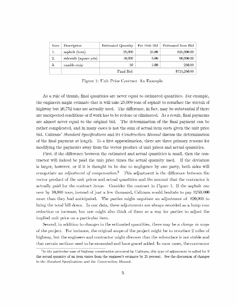
Item Description Estimated Quantity Per Unit Bid Estimated Item Bid

1. asphalt (tons) 25,000 25.00 625,000.00

2. sidewalk (square yds) 10,000 9.00 90,000.00

3. rumble strip 50 5.00 250.00

Final Bid: $715,250.00

Figure 1: Unit Price Contract—An Example.

As a rule of thumb, final quantities are never equal to estimated quantities. For example,

the engineers might estimate that it will take 25,000 tons of asphalt to resurface the stretch of

highway but 26,752 tons are actually used. The difference, in fact, may be substantial if there

are unexpected conditions or if work has to be redone or eliminated. As a result, final payments

are almost never equal to the original bid. The determination of the final payment can be

rather complicated, and in many cases is not the sum of actual item costs given the unit price

bid. Caltrans’ Standard Specifications and its Construction Manual discuss the determination

of the final payment at length. To a first approximation, there are three primary reasons for

modifying the payments away from the vector product of unit prices and actual quantities.

First, if the difference between the estimated and actual quantities is small, then the con-

tractor will indeed be paid the unit price times the actual quantity used. If the deviation

is larger, however, or if it is thought to be due to negligence by one party, both sides will

renegotiate an adjustment of compensation.5 This adjustment is the difference between the

vector product of the unit prices and actual quantities and the amount that the contractor is

actually paid for the contract items. Consider the contract in Figure 1. If the asphalt ran

over by 10,000 tons, instead of just a few thousand, Caltrans would hesitate to pay $250,000

more than they had anticipated. The parties might negotiate an adjustment of -$20,000 to

bring the total bill down. In our data, these adjustments are always recorded as a lump sum

reduction or increase, but one might also think of them as a way for parties to adjust the

implied unit price on a particular item.

Second, in addition to changes in the estimated quantities, there may be a change in scope

of the project. For instance, the original scope of the project might be to resurface 2 miles of

highway, but the engineers and contractor might discover that the subsurface is not stable and

that certain sections need to be excavated and have gravel added. In most cases, the contractor

5In the particular case of highway construstion procured by Caltrans, this type of adjustment is called for if

the actual quantity of an item varies from the engineer’s estimate by 25 percent. See the discussion of changes

in the Standard Specifications and the Construction Manual.

5

and Caltrans will negotiate a change order that amends the scope of the contract as well as

the final payment. If negotiations break down, this may lead to arbitration or a lawsuit.

Payments from changes in scope are recorded as extra work in our data.

Finally, the payment may be altered because of deductions imposed by Caltrans. If work

is not completed on time or if it fails to meet standard specifications then Caltrans may deduct

liquidated damages, which are often a source of disputes. The contractor may argue that the

source of the delay is poor planning or inadequate specifications provided by Caltrans, while

Caltrans might argue that the contractor’s negligence is the source of the problem. The

final deductions imposed may be the outcome of heated negotiations or even lawsuits and

arbitrations between contractors and Caltrans.

It is widely believed in the industry that some contractors attempt to strategically manip-

ulate their bids in anticipation of changes to the payment. Contractors may strategically read

the plans and specifications to forecast the likelihood and magnitude of changes to the contract.

For instance, consider the example of Figure 1, in which the total bid is $715,250. Suppose that

after reading the plans and specifications, the contractor expects asphalt to overrun by 5,000

tons and sidewalk to under-run by 3,000 square feet. If he changes his bid on sidewalk to $5.00

and his bid on asphalt to $26.60 then his total bid will be unchanged. However, this will in-

crease the contractors’ expected total payment to $833,750.00 (26.6×30, 000+5×7000+5×50)

compared to $813,750.00 when bids of $25.00 and $9.00 are entered. A profit maximizing con-

tractor can therefore increase his total payment without increasing his total bid and thus will

not lower his probability of winning the job. A bid is referred to as unbalanced if it has

unusually high unit prices on items that are expected to overrun and unusually low unit prices

on items expected to under-run.

Athey and Levin (2001) note that the optimal strategy for a risk neutral contractor is to

submit a bid that has zero unit prices for some items that are overestimated, and put all the

actual costs on items that are underestimated. This strategy will maximize the expected

ex-post payment while keeping the total bid unaltered. In the data, however, while zero unit

price bids have been observed, they are very uncommon. Athey and Levin argue that risk

aversion is one reason why this might occur, which in the absence of ex post changes seems like

a plausible explanation for bidding behavior. After speaking with some highway contractors

and reading industry sources we believe that for construction contracts other incentives are

more important. Namely, Caltrans is not required to accept the low bid if it is deemed to be

irregular (see Sweet (1994) for an in depth discussion of irregular bids). A highly unbalanced

bid is a sufficient condition for a bid to be deemed irregular. As a result, a bid with a zero

6

unit price is very likely, if not certain to be rejected. In our data, 5 percent of the contracts

are not awarded to the low bidder, and according to industry sources the mostly likely reason

is unbalanced bids.

Also, the Standard Specifications and the Construction Manual indicate that unit prices on

items that overrun by more than 25 percent are open to renegotiation. In these negotiations,

CalTrans engineers will attempt to estimate a fair market value for a particular unit price

based on bids submitted in previous auctions and other data sources. Also, CalTrans may

insist on renegotiating unit prices even if the overrun is less than 25 percent if the unit prices

differ markedly from estimates. This suggests that there are additional limitations on the

benefits of submitting a highly unbalanced bid.

In addition to unbalancing or skewing their unit bid prices, there are other ways in which

contractors may bid strategically when faced with incomplete contracts. For example, they

might notice inadequacies in the plans and specifications and forecast a certain amount of

extra work that will have to be negotiated through change orders. Even if the negotiations

for such change in scopes become arduous or heated (as is often the case), it is still possible

for the contractor to earn some ex post rents. Suppose that the contractor expects a twenty

percent markup on renegotiated work. If the change order leads to a $500,000.00 increase

in compensation, this will lead to a $100,000.00 increase in ex post profits on the part of the

contractor. This additional expected profit makes winning the project more attractive and

hence increases the contractor’s incentive to lower his bid. Similarly, contractors may know

that the monitoring engineer assigned by Caltrans is particularly harsh on deductions, making

the project less attractive and resulting in higher ex ante bids.

3 Bidding for Incompletely Specified Contracts

In this section we use the factual descriptions above to develop a simple variant of a standard

private values auction model that will be the basis for our reduced form and structural empirical

models.

3.1 Basic Setup

A project is characterized by a list of tasks, t = 1, ..., T and a vector of estimated quantities

for each task qet . The actual quantities used to complete the project are qat . We will let

qe = (qe1, ..., qeT ) and q

a = (qa1 , ..., qaT ) denote the vectors of estimated and actual quantities.

Since the focus of our study is on the potential transaction costs from ex post changes

7

and not on the rents that contractors receive due to their private information, we assume

an extreme form of asymmetric information between the buyer and sellers. In particular, we

assume that each contractor in the set of available bidders N has perfect information about

the actual quantities qa while the buyer does not. Since we will assume that contractors are

risk neutral, this specification can be interpreted as contractors not having exact information

about qa, but instead having symmetric uncertainty about the actual quantities, and therefore

they have the same expectations over actual quantities. This interpretation is useful for the

empirical analysis because it generates a source of noise that is not specific to the contractor’s

information or the observable project characteristics.

Despite the fact that contractors all share the same accurate information about qa, they

differ in their private information about their own costs of production. Let cit denote firm i’s per

unit cost to complete task t and let ci = (ci1, ..., cit) denote the vector of i’s unit costs. The total

cost to i for installing the vector of quantities qa will be ci ·qa, the vector product of the costs

and the actual quantities. These costs are known only to bidder i, but the distribution of ci is

common knowledge. This specification, together with the exact information that contractors

have about qa, depicts a situation where contractors know exactly what needs to be done to

meet the contract but they have private information about the costs of production (as in the

most common type of procurement models).

Contractors bid by submitting a unit price vector bi = (bi1, ..., biT ) where b

it is the unit price

bid by contractor i on item t. Contractor i wins the auction and is awarded the contract if

and only if bi ·qe < bj ·qe for all j �= i. That is, the contract is awarded to the lowest bidder,

where the total bid is defined as the vector product of the contractor’s unit price bids and the

estimated quantities.

Let R(bi) be the gross revenue that a contractor expects to receive when he wins with a

bid of bi. If a risk neutral contractor has costs ci then his expected profit from submitting a

bid bi is given by,

πi(bi,ci) =

(R(bi)− ci · qa

)× Pr

{bi · qe < bj · qe for all j �= i

}where the interpretation is standard: the contractor receives the net payoff of revenue less actual

production costs only in the event that all other bidders submit bids with higher estimated

costs as calculated using the estimated quantities.

8

3.2 Revenues and Transaction Costs

If the only source of revenue were the vector product of the unit prices with the actual quan-

tities, then revenues would equal∑T

t=1 bitq

at . As discussed in the previous section, however,

there are three other components that affect the gross revenue of the project: adjustments,

extra work, and deductions. Following our assumption of risk neutrality, and assuming that

the contractors have rational expectations about the distribution of each component, we can

introduce each of these three components as expected values, and include them additively into

the contractors’ profit function.6 We denote the expected income (or loss) from adjustments

as A, from extra work as X, and from deductions as D.

In the absence of transaction costs, the gross revenue would just be the sum

T∑t=1

bitqat +A+X +D.

However, in the presence of transaction costs such as haggling, dispute resolution, and renego-

tiation costs, every dollar earned has less than its full impact on revenues. These transaction

costs can be generated by generated from several sources of inefficiency. One example is bar-

gaining with asymmetric information when ex post changes and adjustments are needed, which

was applied to procurement contracts in Bajari and Tadelis (2001). Another source could be

wasteful investments in srengthening one’s bargaining position, or other wasteful influence

activities that cannot be avoided in equilibrium (see Milgrom, 1988).

In reality, transaction costs are likely to be a combination of all the frictions we mentioned

above. We choose to be agnostic about the exact way in which transaction costs are imposed,

and instead we take a first stab at measuring the role played by transaction costs in bidding

for contracts using a reduced form addition to the standard model described above. We do

this by introducing coefficients that will express the proportional dissipated surplus for each

of the three revenue components from changes.

First, it is useful to distinguish between positive additions to ex post revenues and negative

ones. By definition, any extra work adds compensation to the contractor while any deduction

is an ex post loss incurred by the contractor. This implies that X > 0 and D < 0. The adjust-

ments A, however, can be positive or negative, so we distinguish between positive adjustments,

6Another simplistic way of interpreting this is that contractors have perfect forsight of these components.

We discuss this distinction in Section 5.

9

A+ > 0, and negative ones, A− < 0. We can write down the total ex post revenue as,

T∑t=1

bitqat + (1− α+)A+ + (1 + α−)A− + (1− γ)X + (1 + δ)D. (1)

To interpret (1) first note that for positive ex post income, transaction costs will cause

some fraction of the surplus to be dissipated. The positive coefficients α+ and γ are a measure

of these losses. For negative ex post income, transaction costs mean that the contractor will

suffer a loss above and beyond the accounting loss imposed by the adjustments or deductions.

The positive coefficients α− and δ are a measure of these losses.

If there are no transaction costs involved, then all four coefficients would be equal to

zero. Thus, these coefficients capture a particular linear reduced form of the transaction costs

imposed by ex post changes. This specification may be incorrect if, say, transaction costs are

not linear. Indeed, if one thinks about the stories of haggling and influence cost inefficiencies,

then it is likely that as the stakes are higher, so will be the wasteful effort, maybe resulting in

non-linear transaction costs. As a first step, however, this simple specification is useful in that

the lack of transaction costs will be revealed by the data if the estimated coefficients are zero.

If they are not, however, then this will indicate the presence of transaction costs, the exact

form of which can then be measured with more scrutiny.

To complete the specification of profits, we add a component that captures the loss from

submitting irregular bids that are highly skewed. Athey and Levin (2001) argue that risk

aversion may be one reason for a loss from skewed bids. After speaking with some high-

way contractors and reading industry sources such as Bartholomew (1998), Clough and Sears

(1994), Hinze (1993) and Sweet (1994), it seems that other incentives may be more important

to curtail skewed bidding, and we discussed these in the previous section (the fact that Cal-

Trans is highly likely to reject unbalanced bids). We impose a reduced form penalty that is

increasing in the unbalancedness of the bid. In particular, we impose the following convenient

functional form,

P(bi) = ϕT∑t=1

(bit − bt

)2 ∣∣∣∣qet − qatqet

∣∣∣∣ .To interpret this penalty, the term bt represents the engineer’s estimate for the unit cost

of contract item t. The engineer staff at CalTrans has access to a variety of engineering

cost estimates which are typically average bids for similar items submitted on previous jobs.

This reduced form specification places convexity into the penalty function and makes zero bids

on some items no longer optimal (consistent with Athey and Levin (2001), and with what

10

we observe in our data). Also, it penalizes unbalancing bids for items where the percentage

overruns are likely to be largest. While in principal we could consider a more flexible penalty

function for unbalancing, the number of observations will limit the number of parameters we

can include in this term. This, together with our objective of keeping the structure of the model

as close to the standard literature as possible, is why we introduce this fairly parsimonious

specification. This completes the specification of revenues as,

R(bi) =T∑t=1

bitqat + (1− α+)A+ + (1 + α−)A− + (1− γ)X + (1 + δ)D − P(bi) (2)

3.3 Equilibrium Bidding Behavior

Following standard auction theory, we will consider the Bayesian Nash Equilibrium of the

static first-price sealed-bid auction as our solution concept. The probability that bidder i

wins the auction with bid bi depends on the distribution of the bids of each of the other

j �= i contractors. Let Hj(·) be the cumulative distribution function of contractor j’s total

bid, bj · qe. The probability that contractor i with a total bid of bi · qe bids more than

contractor j is Hj(bi · qe). Thus, the probability that i wins the job with a total bid of bi ·qe

is∏j �=i

(1−Hj(bi · qe)

), and the contractor’s expected profit function is,

πi(bi, ci) =

(R(bi)− ci · qa

)×∏j �=i

(1−Hj(b

i · qe))

Given the cost vector ci, the contractor chooses unit prices to maximize expected utility.

Substituting (2) for R(bi), the partial derivative of profit with respect to the unit price bit is:

∂πi∂bi

t

=(qat − 2ϕ

(bit − bt

) ∣∣∣ qet−qat

qet

∣∣∣)∏j �=i

(1−Hj(b

i· qe)

)+

(∑t

(bit − cit

)qat − ϕ

∑t

(bit − bt

)2 ∣∣∣ qet−qat

qet

∣∣∣+ (1− α+)A+ + (1 + α−)A− + (1− γ)X + (1 + δ)D

)

×

−∑k �=i

∂Hk

∂bqet∏j �=i,k

(1−Hj(b

i· qe)

)Assume that Hj(·) is differentiable with density hj(·), and assume that first order conditions

are necessary and sufficient for describing optimal bidder behavior. Thus, if at the optimum∂πi∂bit= 0 for all t, then we get t equations from the fact that for all t ∈ {1, ..., T},

11

(bi− c

i)· q

a =1

qet

(qat − 2ϕ

(bit − bt

) ∣∣∣∣qet − qatqet

∣∣∣∣)∑

j �=i

hj(bi· qe)

1−Hj(bi· qe)

−1

(3)

+ϕ∑t

(bit − bt

)2 ∣∣∣∣qet − qatqet

∣∣∣∣− (1− α+)A+ − (1 + α−)A− − (1− γ)X − (1 + δ)D

A Bayesian Nash Equilibrium is a collection of bid functions, bi : �T+4 → �T that maps

costs and expectations over changes to unit price bids, and simultaneously satisfied the system

(3) for all bidders i ∈ N . We assume that such an equilibrium exists, and will therefore use

(3) as the basis for our empirical analysis.

The first order condition (3) provides some insight into firm’s optimal bidding strategies,

and relates to the established literature of bidding without transaction costs and changes.

When qe = qa, and when there are no anticipated changes, the first order condition reduces

to:

bi · qe − ci · qe = qet

∑

j �=i

hj(bi · qe)

1−Hj(bi · qe)

−1

(4)

This is the first order condition to the standard first price, asymmetric auction model with

private values. Thus, it is easy to see that our model is a simple variant of the standard

models of bidding for procurement contracts (e.g., Porter and Zona (1993), Pesendorfer and

Jofre-Bonet (2003) and others). That is, the markups should reflect the contractors cost

advantage and informational rents as captured in the right hand side of (4). For example, in

our application markups should depend on whether or not contractor i’s competitor are close

or far from the project, since this determines his relative advantage in the costs of hauling

equipment and material. The markups should also depend on contractor i’s uncertainty about

his competitors costs

The innovation of the first order condition in (3) is the introduction of empirically measur-

able terms that are commonly ignored in previous studies. The first term, −ϕ∑

t

(bit − bt

)2 ∣∣∣ qet−qatqet

∣∣∣ ,reflects i’s perceived penalty from unbalancing his bid so that his unit prices will not differ

substantially from the norm (similar to the effects of risk aversion in Athey and Levin, 2001).

The term −(1− α+)A+ − (1 + α−)A− − (1− γ)X − (1 + δ)D also influences the total ex post

markup. To see this, suppose that the contractor expects a deduction of $1,000. The first

order condition suggest that the contractor will raise his bid by (1+ δ) times $1,000.00. Thus,

the total costs of the deductions, as borne by the firm, are indirectly borne by the buyer,

12

CalTrans.

Clearly, this model abstracts away from what are known to be fundamentally hard problems

such as substituting the perfect foresight assumption on changes and actual quantities with a

common values specification in which each bidder has signals of these variables. Despite these

limitations, however, our first order conditions at a minimum generalize previous models, both

theoretical and empirical, which implicitly impose the assumption that ϕ = α+ = α− = γ =

δ = 0. As we demonstrate shortly, this null hypothesis is strongly rejected by the data, and

we will offer some evidence suggesting that transaction costs of ex post changes may indeed

be the reason.

4 Data

We have constructed a data set of paving contracts procured by Caltrans during 1999. Our

sample includes 162 projects with a value of $369.2 million.7 There were a total number

of 679 bids submitted by 125 general contractors located primarily in California. Over half

of the participating contractors, 70 firms, never won a contract during the period. In fact,

only 7 firms participated in more than 10 percent of the auctions. To account for some

of this asymmetry in size and experience, we will distinguish between top firms and “fringe”

firms, where fringe firms are defined as those who each won less than 2 percent of the value of

contracts awarded. We let FRINGEi be a dummy variable equal to one if firm i is a fringe

firm. Tables 1 and 2 summarize the identities and market shares of the top firms, and Table

3 compares summary statistics of the top firms with those of the fringe.

For each contract, we have collected detailed information from the publicly available bid

summaries and final payment forms that include the contract number, the bidding date, the

location of the job site, the estimated working days required for completion, and other infor-

mation about the nature of the job. They also contain the identities of the bidders and their

itemized bids. Contracts are broken down into an average of 28 items, though some contracts

have as many as 107 items. For each item, we have all bidders’ unit prices, along with the

7The size of the market is defined as the value of the winning bids for the projects in our data set. As

we discussed in section 2, this could be different than the final payments made to the contractors. We focus

on those contracts for which asphalt constituted at least one third of the project’s monetary value. We also

exclude contracts that were not awarded to the lowest bidder since the lowest bid is then not included in our

data. This is usually due to irregularities in the lowest submitted bid, bid relief granted to a contractor who

claimed mistakes were made in his proposal, or other reasons for which the bidder was found to be ineligible.

Such contracts represent about 5 percent of all paving projects under consideration.

13

estimated quantity of the item needed. Additionally, the bid summaries report the engineer’s

estimate of the projects cost. This measure, provided to potential bidders before proposals

are submitted, is intended to represent the “fair and reasonable price” the government expects

to pay for the work to be performed.8 This estimate can be thought of as∑t

btqet , the dot

product of some “Blue Book” prices and the estimated quantities. While we have the total

estimate, we do not have access to the individual bt. We do, however, have the 1999 Contract

Item Cost Data Summary, published by Caltrans’ Division of Office Engineer. These represent

weighted averages of the low bidders’ prices on many of the standard, recurring contract items.

From the final payment forms, we collect data on the actual quantities used for each

item, from which we can construct specific measures of contract incompleteness and overrun.

Additionally, the forms record the adjustments, extra work, and deductions that contribute to

the total price of the contract. These correspond to the variables A, D and X introduced in

the previous section.

To account for the role that geographic proximity plays in determining a firm’s transporta-

tion cost, we construct a measure of distance of firm i to the job site of contract j = 1, ..., J

which we denote as DISTi,j . The contract provides information about the location of the

project, often as detailed as the cross streets at which highway construction begins and ends.9

We combine this with the street address of each bidding firm, and record mileage and travel

time as calculated by Mapquest’s geographic search engine. Contractors may have multiple

locations or branch offices; when this is the case, the location closest to the job site is used.

For those contracts that cover multiple locations, we take the average of the distances and

travel times to each location. Tables 4 and 5 summarize these calculated measures based on

the ranking of bids. As expected, the contractors submitting the lowest bids also tend to have

the shortest travel distances and times, reflecting their cost advantage.

It is clear that a firm’s bidding behavior may be influenced by its production capacity and

project backlog. In particular, firms that are working close to capacity may face a higher

shadow price when considering an additional job. Following the methods used by Porter and

Zona (1993), we construct a measure of backlog from the record of winning bids, bidding dates,

and contract working days. We assume that work proceeds at a constant pace over the length

of the contract, and define the variable BACKLOGi,j to be the remaining dollar value of

8See the “Plans, Specifications, and Estimates Guide,” published by the Caltrans’ Division of Office Engineer

for additional information about the formation of this estimate.9Where the location information is less precise, we use the city’s centroid or a best estimate based on the

post mile markers and highway names included on every contract.

14

contracts won but not yet completed at the time a new bid is submitted.10 We then define

CAPACITYi as the maximum backlog experienced for any day during the sample period, and

the utilization rate UTILi,j as the ratio of backlog to capacity. For those firms that never

won a contract, the backlog, capacity, and utilization rate are all set to 0.

Discussions with industry participants have revealed that firms may take into account

their competitors’ positions when devising their own bids. For this reason, we will include

measures of their closest rival’s distance and utilization rate. Since we treat the distance

from the construction site as a proxy of cost advantage, we define RDISTi,j as the minimum

distance to the job site among bidders on project j, excluding firm i. Likewise, RUTILi,j is

the minimum utilization rate among bidders on project j, excluding firm i.

Summary statistics for the contracts and the bids are provided in Tables 6, 7, and 8. There

is noticeable heterogeneity in the size of contracts awarded: the mean value of the winning bid

is $2.1 million with a standard deviation of $2.4 million. The difference between the first and

second lowest bids averages $149,671, meaning that bidders leave some “money on the table.”

On average, the projects require just under three months to complete, and during this period,

it is clear that several change orders are processed. The final price paid for the work exceeds

the winning bid by an average of $171,341.50, or about 6.4 percent of the estimate. Table

9 decomposes this discrepancy into its primary components and provides summary statistics

that reveal their importance. A significant component can be attributed to overruns and

under-runs on contract items. Not only are there deviations in quantity, but large deviations

also induce a correction to the item’s total price, captured by the value of adjustments. In

our sample, the mean adjustment is $109,382. Extra work negotiated through after-contract

change orders, as well as deductions, contribute to the difference, averaging $130,596 and

-$6,564 respectively. Taken together, the size of these ex-post changes suggests a certain

degree of incompleteness in the original contracts.

10The measure of backlog was constructed using the entire set of asphalt concrete contracts, even though a

few of these were excluded from the econometric analysis. Since we lack information from the previous year,

the calculated backlog will underestimate the true activity of firms during the first few months of 1999; however,

we believe the measure to be a sufficient proxy.

15

5 Empirical Analysis: Reduced Form Estimates

5.1 Standard Bid Regressions

We begin our analysis by performing some reduced form regressions in order to determine

which covariates best explain the total bids. A regression of the total estimated bid, bi ·qe, on

the engineer’s estimate, b · qe yields an R2 of 0.95 and a coefficient almost exactly equal to 1.

This suggests that the engineering cost estimate is an unbiased predictor of the average total

bid and can explain a large fraction of the variation of the bids in the data. This is consistent

with previous papers that have studied this industry.

In Table 10, we regress the total estimated bid on various project characteristics. To

correct for heteroskedasticity related to the overall size of the project, for each project j we

divide each bid bi ·qe by the engineer’s estimate b ·qe. We denote this normalized variable as

NBIDi,j . The explanatory variables include firm i’s distance to the job site, its utilization

rate, the minimum rival distance, the minimum rival utilization rate and Nj , the number of

firms that submit a bid for contract j. In all of our regressions, distance is significant and has

a positive sign as expected. In the first two columns, however, none of the other covariates are

significant. The overall measure of goodness of fit is also not particularly high. In columns III

and IV, we add project and firm fixed effects to the regression. The results suggest that both

of these variables add considerably to goodness of fit, particularly project fixed effects. These

effects capture characteristics of the job that are known to contractors but are unobserved

in our data, such as the condition of the job site, the difficulty of the tasks, and economic

conditions at the time of the contract.

While regressions such as those in Table 10 are common in the literature, equation (3)

suggests that they are mis-specified. A more appropriate reduced form regression would use

bi · qa as the dependent variable. In many cases, the distinction is not trivial. Because

of misestimation on the part of Caltrans engineers, in our sample this value ranges from 44

percent less to 29 percent more than the estimated total bid, bi · qe. Furthermore, in addition

to including variables that shift i’s cost and the costs of its competitors, the right hand side

of the regression should include anticipated change orders, deductions, and expected quantity

overruns. Recall from Section 4 and Table 9 that ex-post payment changes are sizeable. In

our sample, the final payment typically differs from the winning bid by over 6 percent. These

numbers suggest that by ignoring ex-post changes, the total payment to the contractor is often

severely mis-measured in the literature.

16

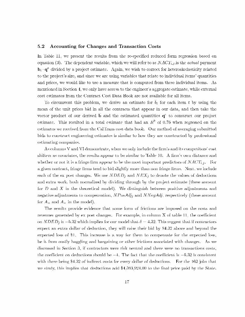
5.2 Accounting for Changes and Transaction Costs

In Table 11, we present the results from the re-specified reduced form regression based on

equation (3). The dependent variable, which we will refer to asNACTi,j ,is the actual payment

bi · qa divided by a project estimate. Again, we wish to correct for heteroskedasticity related

to the project’s size, and since we are using variables that relate to individual items’ quantities

and prices, we would like to use a measure that is computed from these individual items. As

mentioned in Section 4, we only have access to the engineer’s aggregate estimate, while external

cost estimates from the Contract Cost Data Book are not available for all items.

To circumvent this problem, we derive an estimate for bt for each item t by using the

mean of the unit prices bid in all the contracts that appear in our data, and then take the

vector product of our derived b and the estimated quantities qe to construct our project

estimate. This resulted in a total estimate that had an R2 of 0.76 when regressed on the

estimates we received from the CalTrans cost data book. Our method of averaging submitted

bids to construct engineering estimates is similar to how they are constructed by professional

estimating companies.

As columns V andVI demonstrate, when we only include the firm’s and its competitors’ cost

shifters as covariates, the results appear to be similar to Table 10. A firm’s own distance and

whether or not it is a fringe firm appear to be the most important predictors of NACTi,j . For

a given contract, fringe firms tend to bid slightly more than non-fringe firms. Next, we include

each of the ex post changes. We use NDEDj and NEXj to denote the values of deductions

and extra work, both normalized by dividing through by the project estimate (these account

for D and X in the theoretical model). We distinguish between positive adjustments and

negative adjustments to compensation, NPosAdjj and NNegAdj, respectively (these account

for A+ and A− in the model).

The results provide evidence that some form of frictions are imposed on the costs and

revenues generated by ex post changes. For example, in column X of table 11, the coefficient

onNDEDj is −5.32 which implies for our model that δ = 4.32. This suggest that if contractors

expect an extra dollar of deduction, they will raise their bid by $4.32 above and beyond the

expected loss of $1. This increase is a way for them to compensate for the expected loss,

be it from costly haggling and bargaining or other frictions associated with changes. As we

discussed in Section 3, if contractors were risk neutral and there were no transactions costs,

the coefficient on deductions should be −1. The fact that the coefficient is −5.32 is consistent

with there being $4.32 of indirect costs for every dollar of deductions. For the 162 jobs that

we study, this implies that deductions add $4,593,924.00 to the final price paid by the State.

17

On the job with a -$198,000.00 deduction (the largest in our sample), this implies an increased

cost to the state of over $850,000.00.

A similar interpretation may be given to the coefficient of −3 on negative adjustments,

NNegAdjj . When engineers underestimate the quantity of an item required to complete the

job, the State will often negotiate a negative adjustment with a contractor who has bid that

item at a high per unit price. Our regression results suggest that these negotiations carry

with them a $2.00 transaction cost for every dollar in corrections. If bidders anticipate high

downward adjustments of this sort, they tend to raise their bids, not only to recoup the

expected loss, but also to recover the transactions cost they must expend while haggling over

price changes.

If there were no transactions costs and if contractors were risk-neutral, we would expect

to find coefficients on positive adjustments equal to −1, implying that firms lower their bids

by $1 when they expect to receive an additional $1 for work that has already been completed.

The coefficient of 2.09 implies that firms actually tend to raise their bids when they expect this

additional profit. One interpretation of this is that firms expect to spend $3.09 in transactions

costs for every dollar they obtain in adjustment.

The interpretation of the coefficient on extra work is a bit more complicated because in

addition to transactions costs from negotiating change orders, firms must also account for the

direct costs of performing the new work. In our conversations with industry participants,

contractors suggested that a margin of 10 to 20 percent on change orders was a reasonable

number for most firms in the industry. That is, for every $1 of extra work awarded, the firm

makes 10 to 20 cents of profit. Again, if there were no transactions costs and if contractors

were risk-neutral, we would expect firms to lower their bids by 10 to 20 cents, keeping ex post

profit unchanged. Our results suggests that firms instead tend to raise their bids by as much

as $1.67, which is consistent with there being some transactions costs in the magnitude of at

least $2.67 (more, taking the markup into account) for every dolar of extra work.

It is important to note that in reality, contractors do not know the exact deductions,

adjustments, or extra work payments with certainty, but they may be able to forecast them.

If contractors are risk neutral and do not have private information about deductions (so that the

expectations of deductions are common among contractors), then the logic from Euler equation

estimation suggests that we should still be able to use the coefficient on these payments to

find an estimate of the implied transaction costs. The error term would now be interpreted

as capturing the difference between the expected and actual change in payment.11

11That is, if contractors have correct (rational) expectations ke for a change variable k, then the correct

18

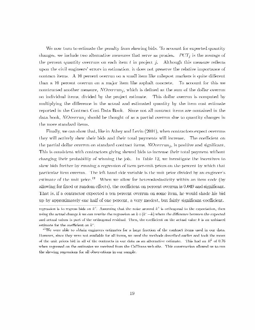
We now turn to estimate the penalty from skewing bids. To account for expected quantity

changes, we include two alternative measures that serve as proxies. PCTj is the average of

the percent quantity overruns on each item t in project j. Although this measure reflects

upon the civil engineers’ errors in estimation, it does not preserve the relative importance of

contract items. A 10 percent overrun on a small item like milepost markers is quite different

than a 10 percent overrun on a major item like asphalt concrete. To account for this we

constructed another measure, NOverrunj , which is defined as the sum of the dollar overrun

on individual items, divided by the project estimate. This dollar overrun is computed by

multiplying the difference in the actual and estimated quantity by the item cost estimate

reported in the Contract Cost Data Book. Since not all contract items are contained in the

data book, NOverrunj should be thought of as a partial overrun due to quantity changes in

the more standard items.

Finally, we can show that, like in Athey and Levin (2001), when contractors expect overruns

they will actively skew their bids and their total payments will increase. The coefficient on

the partial dollar overrun on standard contract items, NOverrunj , is positive and significant.

This is consistent with contractors giving skewed bids to increase their total payment without

changing their probability of winning the job. In Table 12, we investigate the incentives to

skew bids further by running a regression of item per-unit prices on the percent by which that

particular item overran. The left hand side variable is the unit price divided by an engineer’s

estimate of the unit price.12 When we allow for heteroskedasticity within an item code (by

allowing for fixed or random effects), the coefficient on percent overrun is 0.049 and significant.

That is, if a contractor expected a ten percent overrun on some item, he would shade his bid

up by approximately one half of one percent, a very modest, but fairly significant coefficient.

regression is to regress bids on ke. Assuming that the noise around ke is orthogonal to the expectation, then

using the actual change k we can rewrite the regression on k+(ke−k) where the difference between the expected

and actual values is part of the orthogonal residual. Then, the coefficient on the actual value k is an unbiased

estimate for the coefficient on ke.12We were able to obtain engineers estimates for a large fraction of the contract items used in our data.

However, since they were not available for all items, we used the methods described earlier and took the mean

of the unit prices bid in all of the contracts in our data as an alternative estimate. This had an R2 of 0.76

when regressed on the estimates we received from the CalTrans web site. This construction allowed us to run

the skewing regressions for all observations in our sample.

19

5.3 Risk Aversion: An Inconsistent Alternative

Arguably, the expected amount of an increase in compensation may not result in a one-to-one

change of bids even in the absence of transaction costs. For example, if the expected extra

work on a project is $130,500 (which is the mean in our sample) then a risk averse contractor

will lower his bid by less than this amount, which would correspond to a value of γ > 0 (or

(1− γ) < 1), and this may be an alternative explanation for our coefficients.

This story, however, is impossible to justify with any reasonable preferences over risk. If

we think of extra work as a lottery with positive support (recall that extra work is voluntarily

negotiated with the contractor) then the most dissipation risk aversion could impose via a risk

premium is to have such a lottery worth zero (worse-case preferences). Let γ = γr + γTC to

capture both risk and transaction costs. This argument implies an upper bound on how much

of the coefficient γ can be explained by risk aversion, which we can write as γr ≤ 1. This in

turn implies a lower bound on transaction costs above an beyond any possible risk premium,

γTC ≥ 1.67 which means that for every expected dollar of extra work, at least $1.67 is wasted

through transaction costs.

The same argument holds for the estimate of α+, which results in a lower bound of $2.09

in transaction costs for every dollar of positive adjustments. However, a more careful analysis

should treat adjustments as a lottery with positive and negative outcomes. To account for this,

consider the transaction costs we estimate for all adjustments, which from the estimates of α+

and α− are in the order of $2 to $3 of waste for every dollar of change. This is in contrast to

the transaction costs on deductions, where the estimate of δ is $4.32. If these frictions were

accounted for by risk aversion alone, then the higher premium on deductions would imply that

the risk on deductions is higher. From table 9, however, it is easy to see that the lottery of

adjustments is more risky than that from deductions, which is inconsistent with this simple

risk story.

6 Structural Estimation

In this section, we propose a method for structurally estimating the model discussed in sec-

tion 3. The estimation approach builds on Elyakime, Laffont, Loisel and Vuong (1994) and

Guerre, Perrigne and Vuong (2000). In a first stage, the probability distribution of the bids

is estimated. Next, we recover an estimate of ϕ, the coefficient on the penalty from skewing a

bid. Finally, we estimate contractors’ markups over project costs. Our results will allow us

to decompose bi ·qa into three terms. The first is the markup over costs due to market power

20

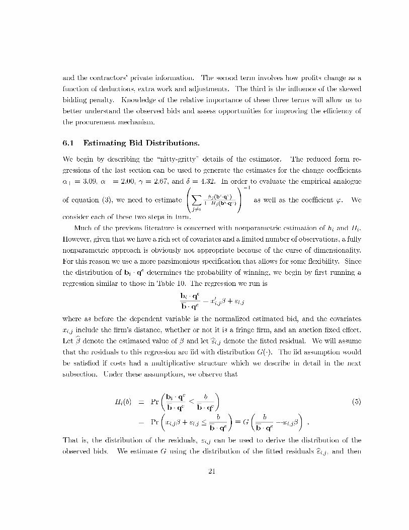
and the contractors’ private information. The second term involves how profits change as a

function of deductions, extra work and adjustments. The third is the influence of the skewed

bidding penalty. Knowledge of the relative importance of these three terms will allow us to

better understand the observed bids and assess opportunities for improving the efficiency of

the procurement mechanism.

6.1 Estimating Bid Distributions.

We begin by describing the “nitty-gritty” details of the estimator. The reduced form re-

gressions of the last section can be used to generate the estimates for the change coefficients

α+ = 3.09, α− = 2.00, γ = 2.67, and δ = 4.32. In order to evaluate the empirical analogue

of equation (3), we need to estimate

∑

j �=i

hj(bi·qe)

1−Hj(bi·qe)

−1

as well as the coefficient ϕ. We

consider each of these two steps in turn.

Much of the previous literature is concerned with nonparametric estimation of hi and Hi.

However, given that we have a rich set of covariates and a limited number of observations, a fully

nonparametric approach is obviously not appropriate because of the curse of dimensionality.

For this reason we use a more parsimonious specification that allows for some flexibility. Since

the distribution of bi · qe determines the probability of winning, we begin by first running a

regression similar to those in Table 10. The regression we run is

bi · qe

b · qe= x′i,jβ + εi,j

where as before the dependent variable is the normalized estimated bid, and the covariates

xi,j include the firm’s distance, whether or not it is a fringe firm, and an auction fixed effect.

Let β denote the estimated value of β and let εi,j denote the fitted residual. We will assume

that the residuals to this regression are iid with distribution G(·). The iid assumption would

be satisfied if costs had a multiplicative structure which we describe in detail in the next

subsection. Under these assumptions, we observe that

Hi(b) ≡ Pr

(bi · qe

b · qe≤

b

b · qe

)(5)

= Pr

(xi,jβ + εi,j ≤

b

b · qe

)≡ G

(b

b · qe− xi,jβ

).

That is, the distribution of the residuals, εi,j can be used to derive the distribution of the

observed bids. We estimate G using the distribution of the fitted residuals εi,j , and then

21

recover an estimate of Hi(b) by substituting in this distribution in place of G. An estimate of

hi(b) can be formed using similar logic. We note that both Hi(b) and hi(b) will be estimated

quite precisely because there are 672 bids in our auction. Given the estimates Hi and hi we

generate an estimate

∑

j �=i

hj(bi·qe)

1− Hj(bi·qe)

−1

.

6.2 Estimating ϕ.

Next, we turn to the problem of estimating ϕ. Our approach will be similar to the identification

of risk preferences described in Campo, Guerre, Perrigne and Vuong (2003). Assume that the

distribution of private costs satisfies the following linear structure:

ci · qa ≡ cib · q

a. (6)

That is, actual total costs can be represented as an independent, scalar random variable ci,

times the engineering estimate b · qa. We will assume that fringe firms may have a different

distribution of ci than non-fringe firms, but that within each of these two classes of firms

the distributions are iid. Let cfi denote the cost random variable for a fringe firm i (we will

suppress the additional notation for non-fringe firms). This assumption seems reasonable since

the fringe dummy variable was the most important bidder specific covariate in our reduced

form regressions. The other bidder specific covariates, while significant, did not contribute

much to the overall goodness of fit. The assumption in (6) is similar to the multiplicative

structure used in Krasnokutskaya (2004) and the location-scale models considered in Hong

and Shum (2001) and Bajari and Hortacsu (2003). A similar assumption is also implicit in

Hendricks, Pinkse and Porter (2001) where the lots are normalized by tract size.

By substituting (6) into (3) and dividing by b · qa we can write

cfi =

(1

b · qa

)bi · qa − qatqet

∑

j �=i

hj(bi · qe)

1−Hj(bi · qe)

−1 (7)

+

(1

b · qa

)[(1− α+)A+ + (1 + α−)A− + (1− γ)X + (1 + δ)D]

−ϕ

(1

b · qa

)∑t

(bit − bt

)2 ∣∣∣∣qet − qatqet

∣∣∣∣− 2 (bit − bt)∣∣∣∣qet − qatqet

∣∣∣∣∑

j �=i

hj(bi · qe)

1−Hj(bi · qe)

−1

22

Notice from (7) that the right hand side can be decomposed into the first two lines that do

not include ϕ, and the last that is linear in ϕ. We therefore can rewrite (7) as,

cfi = f1

(bi,b,qa,qe

)−ϕf2(b

i,b,qa,qe) (8)

where f1 and f2 are shorthand notation for the elements in (7). Since we have already generated

estimates for the distribution and the coefficients on the revenues from changes, the only

unknown on the right hand side of (8) is ϕ. Clearly, there is an analogous equation for the

non-fringe firms that we suppress to save on space and excessive notation.

If ϕ = 0 and qa = qe, then we are in the standard setup where it is known that bid functions

are strictly monotonic in costs. Therefore, our assumption in (6) would imply for the standard

setting that there is a strictly monotonic relationship between cfi and the total bid divided

by the estimate, bi·qa

b·qa. Despite the fact that we do not theoretically prove the monotonicity

of bids in our auction, we will assume that bids are strictly monotonic in costs when ϕ �= 0

and qa �= qe. It would be surprising if this monotonicity would not hold in equilibrium, but a

proof is beyond the scope of this paper. It is somewhat reassuring, however, given the fact that

the contracts we study are open to all qualified bidders and are believed to have fairly tight

margins. This suggests that the relationship between costs and bids cannot have a negative

relationship for a large portion of the bid function since otherwise winning firms would incur

losses.

Note that all of the terms in (8) except for ϕ and cfi can be evaluated given our previous

estimates of the bid distributions and parameters multiplying changes, so we need to substitute

out for cfi in order to identify ϕ. However, cfi is not observed for each firm individually, implying

that we need to use the data to produce at least two independent equations for (8) that would

allow us to cancel out the term associated with cfi .

For example, we can create two sets of bids submitted by fringe firms, the first set including

all fringe bids that were submitted in auctions with no more than three bidders, and the second

set including all fringe bids that were submitted in auctions with more than three bidders. Then

, from our assumption that cfi are iid, it must be the case that the median cfi is the same for

both of these sets of fringe firm bids. From our monotonicity assumption, the median cfi can be

identified from the median normalized bid, bi·qa

b·qa. This allows us to substitute for the median

cfi , and therefore generates two independent sources for the right hand side of (8) that must

be equal. This in turn allows us to identify ϕ by equating the right hand sides for the median

of both sets, which can be done since we can compute an estimate for both f1(bi,b,qa,qe

)and f2(bi,b,qa,qe) for the median of each set of bids, using our previous stages.

23

Note that in addition to the median, similar restrictions must hold for any percentile of cfi .

Following Campo, Guerre, Perrigne and Vuong (2003), we estimate ϕ using restrictions from

a large number of percentiles, not just the median. Let cfρ denote the ρth percentile of cfi .

From (8), and using our monotonicity assumption, the percentile ρ of bi·qa

b·qaidentifies cfρ . Let

bf(3)ρ denote the bid associated with the ρ percentile of the empirical distribution of b

i·qa

b·qafor

the first set of bids. Let bf(4)ρ be the be the ρ percentile for the second set. Since the latent

cost shock cfρ is identical for bf(3)ρ and b

f(4)ρ , equation (8) implies that for every percentile ρ

we choose,

f1

(bf(3)ρ ,b,qa,qe

)− f1

(bf(4)ρ ,b,qa,qe

)= ϕ

(f2(b

f(3)ρ ,b,qa,qe)− f2(b

f(4)ρ ,b,qa,qe)

).

An analogous set of equations holds for the nonfringe firms.

Using the 25th through 75th percentiles, we estimate ϕ using a regression. The value of

ϕ implied by this regression is 0.0007, which is statistically significant at the 6% level, but its

quite small in monetary terms. It implies that if a contractor bids an item at $10 over the

estimated bt and expects an overrun of 20%, then the implied penalty of doing this is only

about one and a half cents.

As an additional robustness check on our results, we use a less elegant method that is

inspired by facts from the industry. In particular, to estimate ϕ we assume that the fringe

firms have a modest profit margin of 1-3 percent. This seems plausible given the fact that

bidding is open to any qualified firm (free entry) and this margin is consistent with industry

sources such as Park and Chapin (1992). This assumption allows us to identify ϕ because it

becomes the only unknown parameter, and this specification led to a similar point estimate.

6.3 Completing the Structural Estimation

We are now in a position to estimate the implied markups for contractors in our dataset. We

form our estimate, ci · qa of i’s total cost for installing the actual quantities by evaluating the

empirical analogue of (3):

(bi − ci

)· qa =

qat − 2ϕ(bit − bt

) ∣∣∣ qat −qetqet

∣∣∣qet

∑

j �=i

hj(bi · qe)

1− Hj(bi · qe)

−1

+ϕ∑t

(bit − bt

)2 ∣∣∣∣qat − qetqet

∣∣∣∣− (1− α+)A+ − (1 + α−)A− − (1− γ)X − (1 + δ)D

24

Using our estimates of H , h, ϕ, α+, α−, γ and δ, it is possible to evaluate the right hand side

of the above equation since all of the terms are either data or are parameters that we have

described how to estimate.

We summarize the estimated markups in Tables 14a and 14b. Table 14a predicts markups

for all contractors who submitted bids while Table 14b predicts the markups for winning

firms only. The median markup over direct costs,(bi − ci

)· qa is $249,582 for all bids and

$465,989.00 for winning bids. The ratio of the markup to the estimate for the median job is

17.6% for all bids and 28.3% for winning bids. This markup may seem high, but it is not the

only component of a firm’s profit margin. Notice that the median contribution of adjustments,

extra work, and deductions to net profit is -$167,062 for all bids and -$194,734 for the winning

bids. Our results suggest that, because of transactions costs, firms lose money on any of

these ex-post changes. Combined with a median skewing penalty of -$93.06, the median net

ex-post profit is estimated at $50,555 for all bids, which is only 3.4% of the project estimate.

For winning bids, this profit is 13%. We shall discuss the implications of these results for the

design of the procurement mechanism in detail in the next subsection.

We compare these estimates with the markups predicted by traditional auction theory.

Using our first stage estimates of Hj(bi · qe) and hj(bi · qe) to calculate informational rents,

we evaluate the empirical analogue of equation (4). These results, summarized in Table 15,

look similar to the total markups reported in the last two columns of Table 14a and 14b. The

median markup is $215,306, or 12.5% of the estimate, among winning bidders.

By breaking down the total payment into its components, however, we gain a much more

informative picture of the components of profits. The reason that our model generates the same

order of markups for the true specification and the mis-specified regression lies in the source of

profits. Since we assume that all the gains and losses from ex post change are bid away (there

is symmetric information about these) then the only source of profits is the informational rents,

which are the focus of the mis-specified estimation.

6.4 Some Limitations

Two possible limitations of our empirical framework are notable. First, our estimates of

α+, α−, γ and δ rely on exogeneity assumptions that could be objectionable. If changes to

the compensation are correlated with omitted project attributes, then our estimates of these

parameters will be biased. In our current work, we are constructing a more detailed data

set that will allow us to sort the data by CalTrans districts. Since each district has partially

autonomous management, we could reasonably expect differences in policies about changes

25

and deductions across districts. We will attempt to use this as an instrument for changes in

compensation. However, it is worth noting that our exogeneity assumptions are weaker than

previous papers who have failed to control for changes to the contract. At a minimum, our

results suggest that excluding changes to compensation is a questionable assumption.

Second, the statistical properties of our estimators need to be more formally developed.

For instance, we have not yet accounted for the first stage error in our nonparametric density

estimates. Also, we would like to estimate α+, α−, γ and δ simultaneously with the other

structural parameters if possible. However, it is worth noting that the density and cdf estimates

are likely to be reasonably precise given that we use 672 observations in estimating these

univariate distributions. Also, our results suggest that the current estimates of α+, α−, γ and

δ are reasonably precise.

7 Discussion

7.1 Lessons for Auction Design.

Our estimates imply some perhaps surprising lessons for the design of highway procurement

auctions. The first is that the existing system seems to do a good job of limiting rents and

promoting competition in that the total markup is fairly modest. The median bidder in our

sample of 679 bids priced contract items so that, if he did win the contract, he could expect a

profit of $50,476, or 3.7% of the estimate. More interesting, though, is how firms make such

a markup. Item-level reduced form regressions suggested that firms shade their bids upward

very slightly when they expect a particular item to run over. Yet, there is another reason

for them to raise their unit price and overall bids when contracts are incomplete. Because

they expect to be penalized with deductions and downward adjustments in compensation, and

because transactions costs erode more than any positive gains through change orders, they

skew their bids upward to extract high rents on pre-specified contract items. Among winning

bidders, the median value of this direct markup, (bi − ci) ·qa, is 28.3% of the project estimate.

Second, our estimates imply that transactions costs are important. Implied transactions

costs on different types of final payment changes range from one and a half dollars to over

four dollars for every dollar in change. When considering the amount of money awarded and

deducted after the initial contract is signed, these costs are significant by any standard. Table

16 reports a lower and an upper bound for the transactions costs on each contract.13 For

13These bounds are determined based on the possible margins that firms may collect on extra work through

change orders. At best, firms receive $1 in profit for every $1 in extra cost (if they have no marginal costs to

26

half of the jobs in the sample, our estimates imply that firms spend as much on transactions

costs as they earn in ex-post profit. In the worst case, transactions costs are over 58% of the

estimate and six times as large as firm profits. Clearly there are inefficiencies in this system.

The state has a particular interest in trying to minimize transactions costs. An implication

of equation (3) is that CalTrans is ultimately responsible for transactions costs on the project,

as they are directly passed on from the bidders. Summing over all 162 contracts, the lower

bound suggests that CalTrans spent $95.3 million on transactions costs alone in 1999. Even

half of that number would be substantial. This point echoes the arguments in Bajari and

Tadelis (2001) who show that the transactions costs from a procurement relationship with ex

ante competition are all borne by the buyer.

Interestingly, one way to reduce these transaction costs may be to commit not to use

deductions and adjustments as frequently. If contractors anticipate a lower frequency of these

actions then they will not need to increase their bids to recoup the expected transaction costs

from ex post changes to the contract. This resonates with Clough and Sears (1994) who argue

that in recent years the level of adversarial relationships have increased dramatically, and have

caused both contractors and buyers to resort to legal dispute resolution which is considered to

be very inefficient and wasteful.

7.2 Concluding Remarks

Most of the existing literature on procurement is focused on designing a contract or auction

that minimizes contractors informational rents while giving appropriate incentives to minimize

moral hazard. Taken literally, in this industry, our analysis suggests that a perhaps more

important problem is to limit transactions costs.

[TO BE COMPLETED]

8 References

References

[1] Athey, S. and Haile, P. (2002) “Identification in Standard Auction Models,” Econometrica,

70(6), 2107-2140.

account for ). This implies a transactions cost γ = 1− (−1.67), or 2.67. The lower bound on transactions cost

is marked by firms operating at a zero profit margin, so that γ = 1.67.

27

[2] Athey, S. and Levin, J. (2001) “Information and Competition in U.S. Forest Service

Timber Auctions,” Journal of Political Economy, 109(2), 375-417.

[3] Bajari, P. and Hortacsu, A. (2003) “Are Structural Estimates of Auction Models Reason-

able? Evidence from Experimental Data,” NBER Working Paper w9889.

[4] Bajari, P., McMillan, R. and Tadelis, S. (2003) “Auctions versus Negotiations in Procure-

ment: An Empirical Analysis,” NBER working paper w9757.

[5] Bajari, P. and Tadelis, S. (2001) “Incentives Versus Transaction Costs: A Theory of

Procurement Contracts,” Rand Journal of Economics, 32(3), 287-307.

[6] Bajari, P. and Ye, L. (2003), “Deciding Between Competition and Collusion,” Review of

Economics and Statistics, 85(4), 971-989.

[7] Bartholomew, S.H. (1998) Construction Contracting: Business and Legal Principles. Up-

per Saddle River, N.J.: Prentice-Hall, Inc., 1998.

[8] Campo, S. (2004) “Attitudes Towards Risk and Asymmetric Bidding: Evidence from

Construction Procurements,” mimeo UNC Chapel Hill.

[9] Campo, S. Guerre, E., Perrigne, E. and Vuong, Q. (2003), “Semiparametric Estimation

of a Model of First-Price Auctions with Risk Averse Bidders,” University of Southern

California Working Paper.

[10] Cantillon, E. and Pesendorfer, M. (2004) “Combination Bidding in Multi-Unit Auctions,”

mimeo, London School of Economics .

[11] Chakravarty, S. and MacLeod, W.B. (2004) “On the Efficiency of Standard Form Con-

tracts: The Case of Construction,” mimeo, University of Southern California.

[12] Clough, R.H. and Sears, G.A. (1994) Construction Contracting, 6th ed. New York: Wiley.

[13] Corts, K. and Singh, J. (2004) “The Effect of Repeated Interaction on Contract Choice:

Evidence from Offshore Drilling,” Journal of Law, Economics and Organization, 20, 230-

260.

[14] Crocker, K.J. and Reynolds, K.J. (1993) “The Efficiency of Incomplete Contracts: An

Empirical Analysis of Air Force Engine Procurement.” Rand Journal of Economics, Vol.

24, 126—146.

28

[15] Elyakime,B., Laffont,J-J., Loisel,P. and Vuong, Q. (1994), “First-Price Sealed-Bid Auc-

tions with Secret Reservation Prices”, Annales D’Economie et de Statistique, 34, 115—141.

[16] Guerre, E., Perrigne, I. and Vuong, Q. (2000), “Optimal Nonparametric Estimation of

First—Price Auctions”, Econometrica, 68, 525—574.

[17] Hinze, J. (1993) Construction Contracts. Boston: Irwin McGraw-Hill, 1993.

[18] Hendricks, K., J. Pinkse, and R. Porter (2003): “Empirical Implications of Equilibrium

Bidding in First-Price, Symmetric, Common-Value Auctions,” Review of Economic Stud-

ies, 70, 115-146.

[19] Hong, H. and Shum, M. (2002) “Increasing Competition and theWinner’s Curse: Evidence

from Procurement,” Review of Economic Studies, 69 (4), 871-898.

[20] Hortacsu, A. “Mechanism Choice and Strategic Bidding in Divisible Good Auctions: An

Empirical Analysis of the Turkish Treasury Auction Market,” University of ChicagoWork-

ing Paper.

[21] Krasnokutskaya, E. (2003) “Identification and Estimation of Auction Models under Un-

observed Auction Heterogeneity,” University of Pennsylvania Working Paper.

[22] Krasnokutskaya, E and Seim, K. (2004) “Auction Participation in Indiana Highway Pro-

curement Auctions,” University of Pennsylvania Working Paper.

[23] Li, T., Perrigne, I. and Vuong, Q. “Structural Estimation of the Affiliated Private Value

Model,” Rand Journal of Economics, 33(2), 171-193.

[24] Masten, S.E. (1984) “The Organization of Production: Evidence from the Aerospace

Industry.” Journal of Law and Economics, Vol. 27, 403—417.

[25] Milgrom, P. (1988) “Employment Contracts, Influence Activities, and Efficient Organiza-

tion Design,” The Journal of Political Economy, 96(1), 42-60.

[26] Pakes, A. (2003) “Common Sense and Simplicity in Empirical Industrial Organization,”

Harvard University Working Paper.

[27] Pesendorfer, M. and Jofre-Bonet, M. (2003) “Estimation of a Dynamic Auction Game,”

Econometrica, 71(5), 1443-1489.

29

[28] Porter, R. and Zona, J.D. (1993), “Detection of Bid Rigging in Procurement Auctions,”

Journal of Political Economy, 101, 518-538.

[29] Sweet, J. (1994) Legal Aspects of Architecture, Engineering and the Construction Process,

5th ed. Minneapolis/St. Paul, Minn.: West Publishing Company.

[30] Williamson, O.E. (1975) Markets and Hierarchies, Analysis and Antitrust Implications.

New York: Free Press.

[31] Williamson, O.E. (1985) The Economic Institutions of Capitalism. New York: Free Press.

30

Table 1: Identities of Top 25 Firms Firm ID

Firm Name Market Share

Firm ID

Firm Name Market Share

49 Granite Construction Co. 26.5% 11 Asphalt Construction Co. Inc. 1.9% 61 J. F. Shea Co. Inc. 9.1% 79 Mercer Fraser Co. 1.8% 65 Kiewit Pacific Co. 7.4% 87 Pavex Construction 1.8%

123 W Jaxon Baker Inc. 6.3% 14 B E C Construction Co. 1.7% 114 Teichert Construction 5.0% 6 All American Asphalt 1.5%

15 Baldwin Contracting Co. Inc. 3.6% 113 Sully Miller Contracting Co. 1.3% 85 Parnum Paving Inc. 2.9% 75 Matich Corporation 1.3% 50 Griffith Co. 2.9% 67 Lee’s Paving Inc. 1.2%

45 George Reed Inc. 2.6%

81 Joint Venture: Nicholas Grant Corp.; CA Commercial Asphalt Corp. 1.1%

119 Union Asphalt Inc. 2.4% 106 Silvia Construction Inc. 1.1% 118 Tullis and Heller Inc. 2.4% 42 Gallagher and Burk Inc. 1.0%

1 A. J. Diani Construction Co. Inc. 2.2% 9 Arcadian Enterprises 1.0% 37 E. L. Yeager Construction Co. Inc. 2.0% TOTAL 92.0%

Note: There were a total of 125 active bidders for asphalt concrete construction contracts in 1999. The firms listed above are the top 25 firms, ranked according to their market share, i.e. the share of total contract dollars awarded.

Table 2: Bidding Activities of Top 25 Firms Conditional on Bidding for a Contract ID No.

of Wins

Total Bid for

Contracts Awarded

Final Payments

on Contracts Awarded

No. of Bids

Entered

Participation Rate

Average Bid

Average Engineer's Estimate

Average Distance (Miles)

Average Time to Job Site (Min)

49 29 87,523,837 97,769,187 104 64.2% 2,871,312 2,881,541 39.9 52.5 61 7 31,359,546 33,577,783 18 11.1% 4,133,522 3,818,085 92.7 112.4 65 3 24,717,559 27,353,158 12 7.4% 5,096,699 4,649,785 129.6 141.7

123 7 21,682,678 23,344,809 40 24.7% 2,845,090 2,861,163 152.3 182.3 114 9 16,597,563 18,590,133 27 16.7% 3,357,218 3,100,162 46.2 59.1 15 3 11,816,642 13,248,400 9 5.6% 4,008,788 3,572,369 47.5 68.4

85 7 9,214,762 10,570,965 11 6.8% 1,215,878 1,234,556 59.6 80.0 50 4 10,016,529 10,570,880 9 5.6% 3,283,336 3,973,770 33.8 38.7 45 5 8,629,916 9,584,688 10 6.2% 1,835,775 1,860,738 37.0 59.8

119 5 8,714,657 9,039,598 8 4.9% 2,318,096 2,744,050 36.6 39.2 118 2 8,564,856 9,006,218 5 3.1% 2,659,350 2,530,333 36.1 43.6

1 2 7,747,488 8,095,949 8 4.9% 1,737,470 1,979,491 43.2 49.9 37 1 7,365,873 7,406,310 4 2.5% 3,166,387 3,561,288 120.8 141.3 11 4 6,837,339 6,919,201 10 6.2% 2,680,773 3,149,691 26.1 36.5

79 6 6,374,092 6,692,809 12 7.4% 1,154,390 1,107,189 38.6 49.8 87 3 6,762,894 6,538,697 8 4.9% 1,814,911 1,678,723 19.0 23.4 14 5 5,796,134 6,195,209 8 4.9% 2,159,010 1,932,623 108.7 141.2 6 7 5,234,879 5,455,337 18 11.1% 651,432 780,152 26.5 30.5

113 4 4,817,976 4,909,594 17 10.5% 1,305,744 1,498,252 61.6 65.4 75 4 4,741,365 4,767,306 14 8.6% 722,983 826,532 53.4 62.7 67 2 3,838,054 4,490,483 4 2.5% 3,323,978 3,485,907 50.2 49.4 81 1 3,832,354 4,058,978 3 1.9% 3,094,679 3,232,977 28.9 37.3

106 1 3,837,510 4,002,519 6 3.7% 2,637,561 2,778,475 151.1 156.5 42 1 3,643,558 3,760,970 1 0.6% 3,643,558 3,849,385 5.5 9.5 9 2 3,726,541 3,735,670 10 6.2% 1,574,171 1,295,312 189.4 199.5

Table 3: Comparison Between Fringe Firms and Firms with Over 2% Market Share

Fringe Firms Non-Fringe Firms

Number of Firms 112 13

Number of Wins 78 84

Average Bid Submitted $ 1,558,965 $ 2,963,763

Average Distance to Job Site (miles) 73.10 67.33

Average Travel Time to Job Site (minutes) 82.98 82.21

Average Capacity $ 606,995 $ 10,271,010

Average Backlog at Time of Bid $ 80,767 $ 3,023,101 Note: The above averages were calculated by first calculating the average for each bidder, then averaging these means over the fringe and non-fringe firms, respectively.

Table 4: Distance to Job Site (in miles)

Mean Std. Dev. Min Max Mean Std. Dev. Min Max

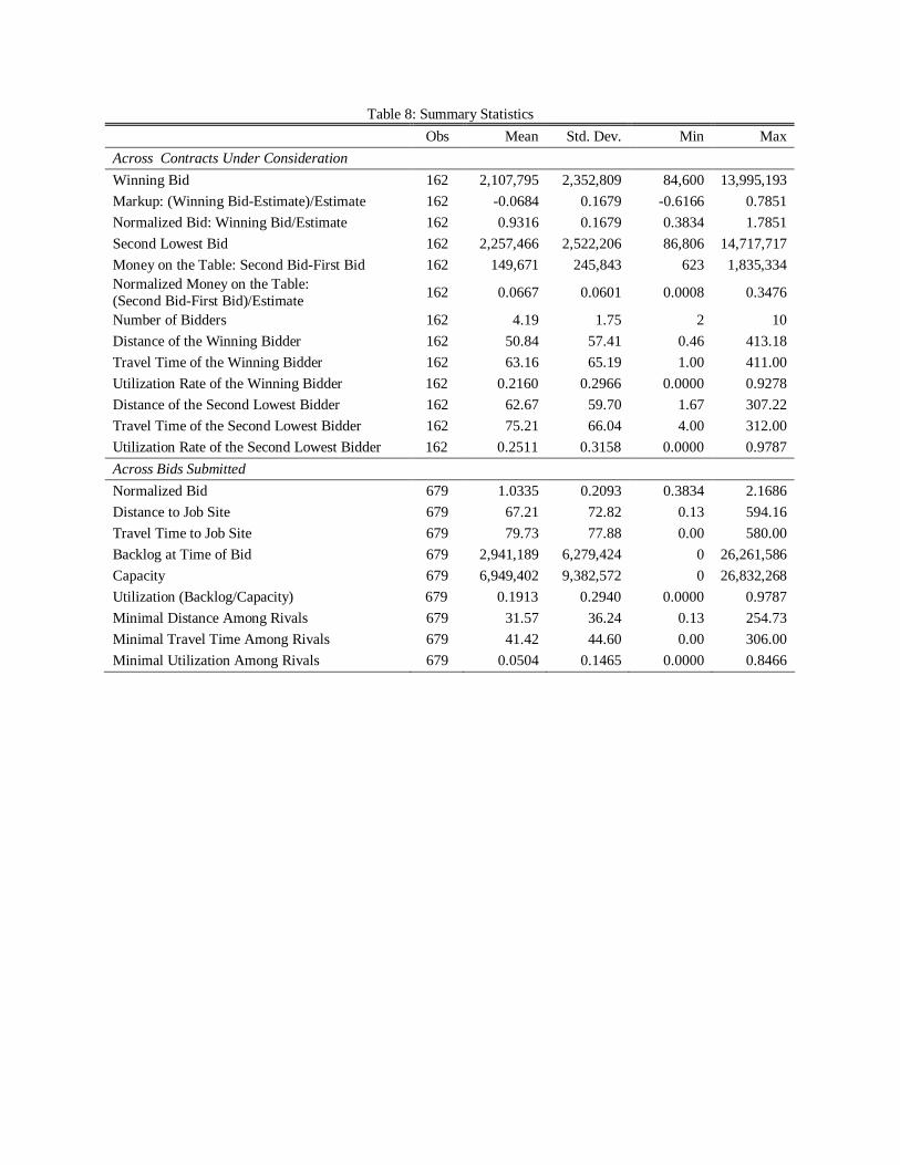
Table 8: Summary Statistics

Obs Mean Std. Dev. Min Max

Across Contracts Under Consideration

Winning Bid 162 2,107,795 2,352,809 84,600 13,995,193

Markup: (Winning Bid-Estimate)/Estimate 162 -0.0684 0.1679 -0.6166 0.7851

Normalized Bid: Winning Bid/Estimate 162 0.9316 0.1679 0.3834 1.7851

Second Lowest Bid 162 2,257,466 2,522,206 86,806 14,717,717

Money on the Table: Second Bid-First Bid 162 149,671 245,843 623 1,835,334 Normalized Money on the Table: (Second Bid-First Bid)/Estimate

162 0.0667 0.0601 0.0008 0.3476

Number of Bidders 162 4.19 1.75 2 10

Distance of the Winning Bidder 162 50.84 57.41 0.46 413.18

Travel Time of the Winning Bidder 162 63.16 65.19 1.00 411.00

Utilization Rate of the Winning Bidder 162 0.2160 0.2966 0.0000 0.9278

Distance of the Second Lowest Bidder 162 62.67 59.70 1.67 307.22

Travel Time of the Second Lowest Bidder 162 75.21 66.04 4.00 312.00

Utilization Rate of the Second Lowest Bidder 162 0.2511 0.3158 0.0000 0.9787

Across Bids Submitted

Normalized Bid 679 1.0335 0.2093 0.3834 2.1686

Distance to Job Site 679 67.21 72.82 0.13 594.16

Travel Time to Job Site 679 79.73 77.88 0.00 580.00

Backlog at Time of Bid 679 2,941,189 6,279,424 0 26,261,586

Capacity 679 6,949,402 9,382,572 0 26,832,268

Utilization (Backlog/Capacity) 679 0.1913 0.2940 0.0000 0.9787

Minimal Distance Among Rivals 679 31.57 36.24 0.13 254.73

Minimal Travel Time Among Rivals 679 41.42 44.60 0.00 306.00

Minimal Utilization Among Rivals 679 0.0504 0.1465 0.0000 0.8466

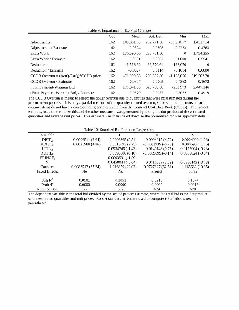
Table 9: Importance of Ex-Post Changes

Obs Mean Std. Dev. Min Max

Adjustments 162 109,381.60 202,771.60 -82,208.57 1,431,714

Adjustments / Estimate 162 0.0324 0.0605 -0.2273 0.4763

Extra Work 162 130,596.20 225,751.60 0 1,454,255

Extra Work / Estimate 162 0.0501 0.0667 0.0000 0.5541

Deductions 162 -6,563.62 26,570.64 -198,070 0

Deduction / Estimate 162 -0.0027 0.0114 -0.1084 0.0000

CCDB Overrun = (ActQ-EstQ)*CCDB price 162 -71,039.98 209,352.80 -1,108,056 319,502.70

CCDB Overrun / Estimate 162 -0.0307 0.0905 -0.4363 0.1672

Final Payment-Winning Bid 162 171,341.50 323,750.00 -252,973 2,447,146

(Final Payment-Winning Bid) / Estimate 162 0.0570 0.0957 -0.3062 0.4919 The CCDB Overrun is meant to reflect the dollar overrun due to quantities that were misestimated during the procurement process. It is only a partial measure of the quantity-related overrun, since some of the nonstandard contract items do not have a corresponding price estimate from the Contract Cost Data Book (CCDB). The project estimate, used to normalize this and the other measures, was generated by taking the dot product of the estimated quantities and average unit prices. This estimate was then scaled down so the normalized bid was approximately 1.

Table 10: Standard Bid Function Regressions Variable I. II. III. IV. DISTi,t 0.0006511 (2.64) 0.0006365 (2.54) 0.0004015 (4.72) 0.0004002 (1.08)

RDISTi,t 0.0021988 (4.86) 0.0013093 (2.75) -0.0001939 (-0.73) 0.0006967 (1.16) UTILi,t -0.0934746 (-1.43) 0.0149143 (0.75) -0.0175904 (-0.23)

RUTILi,t 0.0096606 (0.10) -0.0069699 (-0.14) 0.0039824 (-0.04) FRINGEi -0.0603591 (-1.59)

Nt -0.0458044 (-5.64) 0.0416089 (3.59) -0.0386143 (-3.73) Constant 0.9083513 (37.24) 1.216859 (22.03) 0.9727827 (62.51) 1.165682 (19.35)

Fixed Effects No No Project Firm

Adj R2 0.0581 0.1051 0.9218 0.1874 Prob>F 0.0000 0.0000 0.0000 0.0016

Num. of Obs. 679 679 679 679 The dependent variable is the total bid divided by the scaled project estimate, where the total bid is the dot product of the estimated quantities and unit prices. Robust standard errors are used to compute t-Statistics, shown in parentheses.

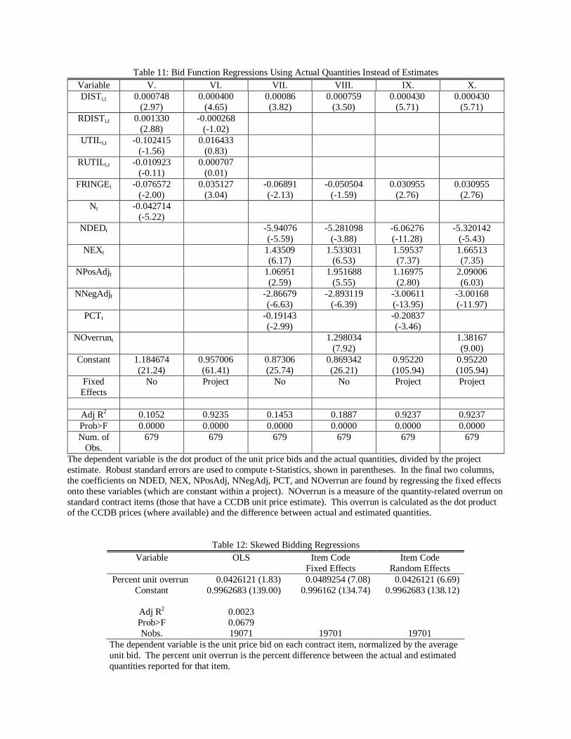
Table 11: Bid Function Regressions Using Actual Quantities Instead of Estimates Variable V. VI. VII. VIII. IX. X. DISTi,t 0.000748

(2.97) 0.000400

(4.65) 0.00086 (3.82)

0.000759 (3.50)

0.000430 (5.71)

0.000430 (5.71)

RDISTi,t 0.001330 (2.88)

-0.000268 (-1.02)

UTILi,t -0.102415 (-1.56)

0.016433 (0.83)

RUTILi,t -0.010923 (-0.11)

0.000707 (0.01)

FRINGEi -0.076572 (-2.00)

0.035127 (3.04)

-0.06891 (-2.13)

-0.050504 (-1.59)

0.030955 (2.76)

0.030955 (2.76)

Nt -0.042714 (-5.22)

NDEDt

-5.94076 (-5.59)

-5.281098 (-3.88)

-6.06276 (-11.28)

-5.320142 (-5.43)

NEXt

1.43509 (6.17)

1.533031 (6.53)

1.59537 (7.37)

1.66513 (7.35)

NPosAdjt

1.06951 (2.59)

1.951688 (5.55)

1.16975 (2.80)

2.09006 (6.03)

NNegAdjt

-2.86679 (-6.63)

-2.893119 (-6.39)

-3.00611 (-13.95)

-3.00168 (-11.97)

PCTt

-0.19143 (-2.99)

-0.20837 (-3.46)

NOverrunt

1.298034 (7.92)

1.38167 (9.00)

Constant 1.184674 (21.24)

0.957006 (61.41)

0.87306 (25.74)

0.869342 (26.21)

0.95220 (105.94)

0.95220 (105.94)

Fixed Effects

No Project No No Project Project

Adj R2 0.1052 0.9235 0.1453 0.1887 0.9237 0.9237 Prob>F 0.0000 0.0000 0.0000 0.0000 0.0000 0.0000 Num. of

Obs. 679 679 679 679 679 679

The dependent variable is the dot product of the unit price bids and the actual quantities, divided by the project estimate. Robust standard errors are used to compute t-Statistics, shown in parentheses. In the final two columns, the coefficients on NDED, NEX, NPosAdj, NNegAdj, PCT, and NOverrun are found by regressing the fixed effects onto these variables (which are constant within a project). NOverrun is a measure of the quantity-related overrun on standard contract items (those that have a CCDB unit price estimate). This overrun is calculated as the dot product of the CCDB prices (where available) and the difference between actual and estimated quantities.

Table 12: Skewed Bidding Regressions Variable OLS Item Code

Fixed Effects Item Code

Random Effects Percent unit overrun 0.0426121 (1.83) 0.0489254 (7.08) 0.0426121 (6.69)

Constant 0.9962683 (139.00) 0.996162 (134.74) 0.9962683 (138.12)

Adj R2 0.0023 Prob>F 0.0679 Nobs. 19071 19701 19701

The dependent variable is the unit price bid on each contract item, normalized by the average unit bid. The percent unit overrun is the percent difference between the actual and estimated quantities reported for that item.

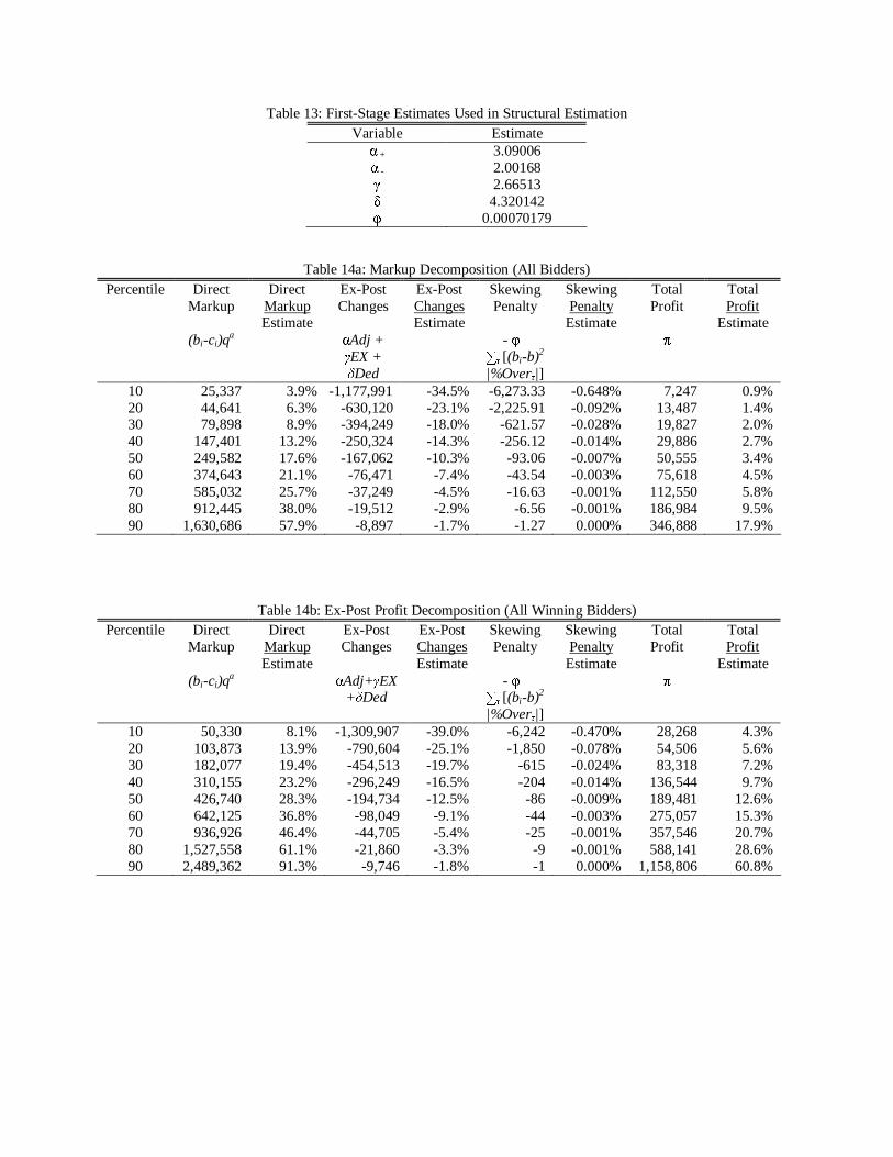
Table 13: First-Stage Estimates Used in Structural Estimation Variable Estimate

α + 3.09006 α - 2.00168 γ 2.66513 δ 4.320142 φ 0.00070179

Table 14a: Markup Decomposition (All Bidders)

Percentile Direct Markup

Direct Markup Estimate

Ex-Post Changes

Ex-Post Changes Estimate

Skewing Penalty

Skewing Penalty

Estimate

Total Profit

Total Profit

Estimate (bi-ci)q

a αAdj + γEX + δDed

- φ · ∑τ [(bi-b)2

|%Overτ|]

π

10 25,337 3.9% -1,177,991 -34.5% -6,273.33 -0.648% 7,247 0.9% 20 44,641 6.3% -630,120 -23.1% -2,225.91 -0.092% 13,487 1.4% 30 79,898 8.9% -394,249 -18.0% -621.57 -0.028% 19,827 2.0% 40 147,401 13.2% -250,324 -14.3% -256.12 -0.014% 29,886 2.7% 50 249,582 17.6% -167,062 -10.3% -93.06 -0.007% 50,555 3.4% 60 374,643 21.1% -76,471 -7.4% -43.54 -0.003% 75,618 4.5% 70 585,032 25.7% -37,249 -4.5% -16.63 -0.001% 112,550 5.8% 80 912,445 38.0% -19,512 -2.9% -6.56 -0.001% 186,984 9.5% 90 1,630,686 57.9% -8,897 -1.7% -1.27 0.000% 346,888 17.9%

Table 14b: Ex-Post Profit Decomposition (All Winning Bidders)

Percentile Direct Markup

Direct Markup Estimate

Ex-Post Changes

Ex-Post Changes Estimate

Skewing Penalty

Skewing Penalty

Estimate

Total Profit

Total Profit

Estimate (bi-ci)q

a αAdj+γEX +δDed

- φ · ∑τ [(bi-b)2

|%Overτ|]

π

10 50,330 8.1% -1,309,907 -39.0% -6,242 -0.470% 28,268 4.3% 20 103,873 13.9% -790,604 -25.1% -1,850 -0.078% 54,506 5.6% 30 182,077 19.4% -454,513 -19.7% -615 -0.024% 83,318 7.2% 40 310,155 23.2% -296,249 -16.5% -204 -0.014% 136,544 9.7% 50 426,740 28.3% -194,734 -12.5% -86 -0.009% 189,481 12.6% 60 642,125 36.8% -98,049 -9.1% -44 -0.003% 275,057 15.3% 70 936,926 46.4% -44,705 -5.4% -25 -0.001% 357,546 20.7% 80 1,527,558 61.1% -21,860 -3.3% -9 -0.001% 588,141 28.6% 90 2,489,362 91.3% -9,746 -1.8% -1 0.000% 1,158,806 60.8%

Table 15: Markups Implied by Standard Model Without Transactions Costs or Ex-Post Changes

Percentile All Bidders Winning Bidders Only Direct

Markup (bi-ci)q

a

Direct Markup Estimate

Direct Markup (bi-ci)q

a

Direct Markup Estimate

10 7,499.27 1.0% 29,457 4.6% 20 13,257.49 1.6% 62,968 5.7% 30 20,354.98 2.1% 89,335 8.4% 40 31,107.43 2.7% 139,978 10.0% 50 51,972.27 3.4% 215,725 12.1% 60 74,405.59 4.4% 279,412 16.2% 70 112,747.60 5.8% 386,614 21.1% 80 185,893.20 9.2% 643,819 29.6% 90 344,865.40 16.9% 1,036,313 60.5%

Table 16: Transactions Costs Lower Bound Upper Bound Percentile

Value

As a Fraction

of the Estimate

As a Fraction

of the Direct

Markup

As a Fraction of Ex-Post

Profit

Value

As a Fraction

of the Estimate

As a Fraction

of the Direct

Markup

As a Fraction of Ex-Post

Profit 10 0 0 0 0 15,017.74 0.02670 0.11405 0.12044 20 0 0 0 0 31,751.91 0.04887 0.24860 0.30914 30 7,224.31 0.00906 0.03305 0.06791 62,659.42 0.08293 0.40116 0.58500 40 41,037.48 0.03547 0.13867 0.19074 142,739.0 0.12942 0.54035 0.92729 50 86,828.42 0.06790 0.21035 0.46725 271,700.6 0.18239 0.67880 1.31758 60 239,042.3 0.10784 0.33661 0.81578 444,468.0 0.24370 0.78135 1.72423 70 362,764.6 0.13468 0.46131 1.09496 705,118.1 0.29116 0.88826 2.28845 80 571,231.3 0.19301 0.58549 1.65807 1,183,804 0.38323 1.00649 3.07917 90 1,057,652 0.26321 0.75258 2.56246 1,979,305 0.58469 1.21379 5.89991

The lower bound for the transactions cost is calculated as (1-α+)PosAdj + (α--1)|NegAdj| + (δ-1)|Ded|. These items alter the final payment, but do not involve additional costs incurred by the contractor. It is a lower bound, for it assumes that the estimate of γ only reflects the profit margin on extra work. If we assume instead that the contractors are performing the extra work at zero profit margin, the estimate of γ reflects pure transactions costs, giving us an upper bound equal to (1-α+)PosAdj + (α--1)|NegAdj| + (δ-1)|Ded| + (1-γ)ExtraWork.

NOTE DI LAVORO DELLA FONDAZIONE ENI ENRICO MATTEIFondazione Eni Enrico Mattei Working Paper Series

Our Note di Lavoro are available on the Internet at the following addresses:http://www.feem.it/Feem/Pub/Publications/WPapers/default.html

http://www.ssrn.com/link/feem.html

NOTE DI LAVORO PUBLISHED IN 2003

PRIV 1.2003 Gabriella CHIESA and Giovanna NICODANO: Privatization and Financial Market Development: TheoreticalIssues

PRIV 2.2003 Ibolya SCHINDELE: Theory of Privatization in Eastern Europe: Literature ReviewPRIV 3.2003 Wietze LISE, Claudia KEMFERT and Richard S.J. TOL: Strategic Action in the Liberalised German Electricity

MarketCLIM 4.2003 Laura MARSILIANI and Thomas I. RENSTRÖM: Environmental Policy and Capital Movements: The Role of

Government CommitmentKNOW 5.2003 Reyer GERLAGH: Induced Technological Change under Technological CompetitionETA 6.2003 Efrem CASTELNUOVO: Squeezing the Interest Rate Smoothing Weight with a Hybrid Expectations ModelSIEV 7.2003 Anna ALBERINI, Alberto LONGO, Stefania TONIN, Francesco TROMBETTA and Margherita TURVANI: The

Role of Liability, Regulation and Economic Incentives in Brownfield Remediation and Redevelopment:Evidence from Surveys of Developers

NRM 8.2003 Elissaios PAPYRAKIS and Reyer GERLAGH: Natural Resources: A Blessing or a Curse?CLIM 9.2003 A. CAPARRÓS, J.-C. PEREAU and T. TAZDAÏT: North-South Climate Change Negotiations: a Sequential Game

with Asymmetric InformationKNOW 10.2003 Giorgio BRUNELLO and Daniele CHECCHI: School Quality and Family Background in ItalyCLIM 11.2003 Efrem CASTELNUOVO and Marzio GALEOTTI: Learning By Doing vs Learning By Researching in a Model of

Climate Change Policy AnalysisKNOW 12.2003 Carole MAIGNAN, Gianmarco OTTAVIANO and Dino PINELLI (eds.): Economic Growth, Innovation, Cultural

Diversity: What are we all talking about? A critical survey of the state-of-the-artKNOW 13.2003 Carole MAIGNAN, Gianmarco OTTAVIANO, Dino PINELLI and Francesco RULLANI (lix): Bio-Ecological

Diversity vs. Socio-Economic Diversity. A Comparison of Existing MeasuresKNOW 14.2003 Maddy JANSSENS and Chris STEYAERT (lix): Theories of Diversity within Organisation Studies: Debates and

Future TrajectoriesKNOW 15.2003 Tuzin BAYCAN LEVENT, Enno MASUREL and Peter NIJKAMP (lix): Diversity in Entrepreneurship: Ethnic and

Female Roles in Urban Economic LifeKNOW 16.2003 Alexandra BITUSIKOVA (lix): Post-Communist City on its Way from Grey to Colourful: The Case Study from

SlovakiaKNOW 17.2003 Billy E. VAUGHN and Katarina MLEKOV (lix): A Stage Model of Developing an Inclusive CommunityKNOW 18.2003 Selma van LONDEN and Arie de RUIJTER (lix): Managing Diversity in a Glocalizing WorldCoalitionTheoryNetwork

19.2003 Sergio CURRARINI: On the Stability of Hierarchies in Games with Externalities

PRIV 20.2003 Giacomo CALZOLARI and Alessandro PAVAN (lx): Monopoly with ResalePRIV 21.2003 Claudio MEZZETTI (lx): Auction Design with Interdependent Valuations: The Generalized Revelation

Principle, Efficiency, Full Surplus Extraction and Information AcquisitionPRIV 22.2003 Marco LiCalzi and Alessandro PAVAN (lx): Tilting the Supply Schedule to Enhance Competition in Uniform-

Price AuctionsPRIV 23.2003 David ETTINGER (lx): Bidding among Friends and EnemiesPRIV 24.2003 Hannu VARTIAINEN (lx): Auction Design without CommitmentPRIV 25.2003 Matti KELOHARJU, Kjell G. NYBORG and Kristian RYDQVIST (lx): Strategic Behavior and Underpricing in

Uniform Price Auctions: Evidence from Finnish Treasury AuctionsPRIV 26.2003 Christine A. PARLOUR and Uday RAJAN (lx): Rationing in IPOsPRIV 27.2003 Kjell G. NYBORG and Ilya A. STREBULAEV (lx): Multiple Unit Auctions and Short SqueezesPRIV 28.2003 Anders LUNANDER and Jan-Eric NILSSON (lx): Taking the Lab to the Field: Experimental Tests of Alternative

Mechanisms to Procure Multiple ContractsPRIV 29.2003 TangaMcDANIEL and Karsten NEUHOFF (lx): Use of Long-term Auctions for Network InvestmentPRIV 30.2003 Emiel MAASLAND and Sander ONDERSTAL (lx): Auctions with Financial ExternalitiesETA 31.2003 Michael FINUS and Bianca RUNDSHAGEN: A Non-cooperative Foundation of Core-Stability in Positive

Externality NTU-Coalition GamesKNOW 32.2003 Michele MORETTO: Competition and Irreversible Investments under Uncertainty_PRIV 33.2003 Philippe QUIRION: Relative Quotas: Correct Answer to Uncertainty or Case of Regulatory Capture?KNOW 34.2003 Giuseppe MEDA, Claudio PIGA and Donald SIEGEL: On the Relationship between R&D and Productivity: A

Treatment Effect AnalysisETA 35.2003 Alessandra DEL BOCA, Marzio GALEOTTI and Paola ROTA: Non-convexities in the Adjustment of Different

Capital Inputs: A Firm-level Investigation

GG 36.2003 Matthieu GLACHANT: Voluntary Agreements under Endogenous Legislative ThreatsPRIV 37.2003 Narjess BOUBAKRI, Jean-Claude COSSET and Omrane GUEDHAMI: Postprivatization Corporate Governance:

the Role of Ownership Structure and Investor ProtectionCLIM 38.2003 Rolf GOLOMBEK and Michael HOEL: Climate Policy under Technology SpilloversKNOW 39.2003 Slim BEN YOUSSEF: Transboundary Pollution, R&D Spillovers and International TradeCTN 40.2003 Carlo CARRARO and Carmen MARCHIORI: Endogenous Strategic Issue Linkage in International NegotiationsKNOW 41.2003 Sonia OREFFICE: Abortion and Female Power in the Household: Evidence from Labor SupplyKNOW 42.2003 Timo GOESCHL and Timothy SWANSON: On Biology and Technology: The Economics of Managing

BiotechnologiesETA 43.2003 Giorgio BUSETTI and Matteo MANERA: STAR-GARCH Models for Stock Market Interactions in the Pacific

Basin Region, Japan and USCLIM 44.2003 Katrin MILLOCK and Céline NAUGES: The French Tax on Air Pollution: Some Preliminary Results on its

EffectivenessPRIV 45.2003 Bernardo BORTOLOTTI and Paolo PINOTTI: The Political Economy of PrivatizationSIEV 46.2003 Elbert DIJKGRAAF and Herman R.J. VOLLEBERGH: Burn or Bury? A Social Cost Comparison of Final Waste

Disposal MethodsETA 47.2003 Jens HORBACH: Employment and Innovations in the Environmental Sector: Determinants and Econometrical

Results for GermanyCLIM 48.2003 Lori SNYDER, Nolan MILLER and Robert STAVINS: The Effects of Environmental Regulation on Technology

Diffusion: The Case of Chlorine ManufacturingCLIM 49.2003 Lori SNYDER, Robert STAVINS and Alexander F. WAGNER: Private Options to Use Public Goods. Exploiting

Revealed Preferences to Estimate Environmental BenefitsCTN 50.2003 László Á. KÓCZY and Luc LAUWERS (lxi): The Minimal Dominant Set is a Non-Empty Core-Extension

CTN 51.2003 Matthew O. JACKSON (lxi):Allocation Rules for Network GamesCTN 52.2003 Ana MAULEON and Vincent VANNETELBOSCH (lxi): Farsightedness and Cautiousness in Coalition FormationCTN 53.2003 Fernando VEGA-REDONDO (lxi): Building Up Social Capital in a Changing World: a network approachCTN 54.2003 Matthew HAAG and Roger LAGUNOFF (lxi): On the Size and Structure of Group CooperationCTN 55.2003 Taiji FURUSAWA and Hideo KONISHI (lxi): Free Trade NetworksCTN 56.2003 Halis Murat YILDIZ (lxi): National Versus International Mergers and Trade LiberalizationCTN 57.2003 Santiago RUBIO and Alistair ULPH (lxi): An Infinite-Horizon Model of Dynamic Membership of International

Environmental AgreementsKNOW 58.2003 Carole MAIGNAN, Dino PINELLI and Gianmarco I.P. OTTAVIANO: ICT, Clusters and Regional Cohesion: A

Summary of Theoretical and Empirical ResearchKNOW 59.2003 Giorgio BELLETTINI and Gianmarco I.P. OTTAVIANO: Special Interests and Technological ChangeETA 60.2003 Ronnie SCHÖB: The Double Dividend Hypothesis of Environmental Taxes: A SurveyCLIM 61.2003 Michael FINUS, Ekko van IERLAND and Robert DELLINK: Stability of Climate Coalitions in a Cartel

Formation GameGG 62.2003 Michael FINUS and Bianca RUNDSHAGEN: How the Rules of Coalition Formation Affect Stability of

International Environmental AgreementsSIEV 63.2003 Alberto PETRUCCI: Taxing Land Rent in an Open EconomyCLIM 64.2003 Joseph E. ALDY, Scott BARRETT and Robert N. STAVINS: Thirteen Plus One: A Comparison of Global Climate

Policy ArchitecturesSIEV 65.2003 Edi DEFRANCESCO: The Beginning of Organic Fish Farming in ItalySIEV 66.2003 Klaus CONRAD: Price Competition and Product Differentiation when Consumers Care for the EnvironmentSIEV 67.2003 Paulo A.L.D. NUNES, Luca ROSSETTO, Arianne DE BLAEIJ: Monetary Value Assessment of Clam Fishing

Management Practices in the Venice Lagoon: Results from a Stated Choice ExerciseCLIM 68.2003 ZhongXiang ZHANG: Open Trade with the U.S. Without Compromising Canada’s Ability to Comply with its

Kyoto TargetKNOW 69.2003 David FRANTZ (lix): Lorenzo Market between Diversity and MutationKNOW 70.2003 Ercole SORI (lix): Mapping Diversity in Social HistoryKNOW 71.2003 Ljiljana DERU SIMIC (lxii): What is Specific about Art/Cultural Projects?KNOW 72.2003 Natalya V. TARANOVA (lxii):The Role of the City in Fostering Intergroup Communication in a Multicultural

Environment: Saint-Petersburg’s CaseKNOW 73.2003 Kristine CRANE (lxii): The City as an Arena for the Expression of Multiple Identities in the Age of

Globalisation and MigrationKNOW 74.2003 Kazuma MATOBA (lxii): Glocal Dialogue- Transformation through Transcultural CommunicationKNOW 75.2003 Catarina REIS OLIVEIRA (lxii): Immigrants’ Entrepreneurial Opportunities: The Case of the Chinese in

PortugalKNOW 76.2003 Sandra WALLMAN (lxii): The Diversity of Diversity - towards a typology of urban systemsKNOW 77.2003 Richard PEARCE (lxii): A Biologist’s View of Individual Cultural Identity for the Study of CitiesKNOW 78.2003 Vincent MERK (lxii): Communication Across Cultures: from Cultural Awareness to Reconciliation of the

DilemmasKNOW 79.2003 Giorgio BELLETTINI, Carlotta BERTI CERONI and Gianmarco I.P.OTTAVIANO: Child Labor and Resistance

to ChangeETA 80.2003 Michele MORETTO, Paolo M. PANTEGHINI and Carlo SCARPA: Investment Size and Firm’s Value under

Profit Sharing Regulation

IEM 81.2003 Alessandro LANZA, Matteo MANERA and Massimo GIOVANNINI: Oil and Product Dynamics in InternationalPetroleum Markets

CLIM 82.2003 Y. Hossein FARZIN and Jinhua ZHAO: Pollution Abatement Investment When Firms Lobby AgainstEnvironmental Regulation

CLIM 83.2003 Giuseppe DI VITA: Is the Discount Rate Relevant in Explaining the Environmental Kuznets Curve?CLIM 84.2003 Reyer GERLAGH and Wietze LISE: Induced Technological Change Under Carbon TaxesNRM 85.2003 Rinaldo BRAU, Alessandro LANZA and Francesco PIGLIARU: How Fast are the Tourism Countries Growing?

The cross-country evidenceKNOW 86.2003 Elena BELLINI, Gianmarco I.P. OTTAVIANO and Dino PINELLI: The ICT Revolution: opportunities and risks

for the MezzogiornoSIEV 87.2003 Lucas BRETSCGHER and Sjak SMULDERS: Sustainability and Substitution of Exhaustible Natural Resources.

How resource prices affect long-term R&D investmentsCLIM 88.2003 Johan EYCKMANS and Michael FINUS: New Roads to International Environmental Agreements: The Case of

Global WarmingCLIM 89.2003 Marzio GALEOTTI: Economic Development and Environmental ProtectionCLIM 90.2003 Marzio GALEOTTI: Environment and Economic Growth: Is Technical Change the Key to Decoupling?CLIM 91.2003 Marzio GALEOTTI and Barbara BUCHNER: Climate Policy and Economic Growth in Developing CountriesIEM 92.2003 A. MARKANDYA, A. GOLUB and E. STRUKOVA: The Influence of Climate Change Considerations on Energy

Policy: The Case of RussiaETA 93.2003 Andrea BELTRATTI: Socially Responsible Investment in General EquilibriumCTN 94.2003 Parkash CHANDER: The γ-Core and Coalition FormationIEM 95.2003 Matteo MANERA and Angelo MARZULLO: Modelling the Load Curve of Aggregate Electricity Consumption

Using Principal ComponentsIEM 96.2003 Alessandro LANZA, Matteo MANERA, Margherita GRASSO and Massimo GIOVANNINI: Long-run Models of

Oil Stock PricesCTN 97.2003 Steven J. BRAMS, Michael A. JONES, and D. Marc KILGOUR: Forming Stable Coalitions: The Process

MattersKNOW 98.2003 John CROWLEY, Marie-Cecile NAVES (lxiii): Anti-Racist Policies in France. From Ideological and Historical

Schemes to Socio-Political RealitiesKNOW 99.2003 Richard THOMPSON FORD (lxiii): Cultural Rights and Civic VirtueKNOW 100.2003 Alaknanda PATEL (lxiii): Cultural Diversity and Conflict in Multicultural CitiesKNOW 101.2003 David MAY (lxiii): The Struggle of Becoming Established in a Deprived Inner-City NeighbourhoodKNOW 102.2003 Sébastien ARCAND, Danielle JUTEAU, Sirma BILGE, and Francine LEMIRE (lxiii) : Municipal Reform on the

Island of Montreal: Tensions Between Two Majority Groups in a Multicultural CityCLIM 103.2003 Barbara BUCHNER and Carlo CARRARO: China and the Evolution of the Present Climate RegimeCLIM 104.2003 Barbara BUCHNER and Carlo CARRARO: Emissions Trading Regimes and Incentives to Participate in

International Climate AgreementsCLIM 105.2003 Anil MARKANDYA and Dirk T.G. RÜBBELKE: Ancillary Benefits of Climate PolicyNRM 106.2003 Anne Sophie CRÉPIN (lxiv): Management Challenges for Multiple-Species Boreal ForestsNRM 107.2003 Anne Sophie CRÉPIN (lxiv): Threshold Effects in Coral Reef FisheriesSIEV 108.2003 Sara ANIYAR ( lxiv): Estimating the Value of Oil Capital in a Small Open Economy: The Venezuela’s ExampleSIEV 109.2003 Kenneth ARROW, Partha DASGUPTA and Karl-Göran MÄLER(lxiv): Evaluating Projects and Assessing

Sustainable Development in Imperfect EconomiesNRM 110.2003 Anastasios XEPAPADEAS and Catarina ROSETA-PALMA(lxiv): Instabilities and Robust Control in FisheriesNRM 111.2003 Charles PERRINGS and Brian WALKER (lxiv): Conservation and Optimal Use of RangelandsETA 112.2003 Jack GOODY (lxiv): Globalisation, Population and EcologyCTN 113.2003 Carlo CARRARO, Carmen MARCHIORI and Sonia OREFFICE: Endogenous Minimum Participation in

International Environmental TreatiesCTN 114.2003 Guillaume HAERINGER and Myrna WOODERS: Decentralized Job MatchingCTN 115.2003 Hideo KONISHI and M. Utku UNVER: Credible Group Stability in Multi-Partner Matching ProblemsCTN 116.2003 Somdeb LAHIRI: Stable Matchings for the Room-Mates ProblemCTN 117.2003 Somdeb LAHIRI: Stable Matchings for a Generalized Marriage ProblemCTN 118.2003 Marita LAUKKANEN: Transboundary Fisheries Management under Implementation UncertaintyCTN 119.2003 Edward CARTWRIGHT and Myrna WOODERS: Social Conformity and Bounded Rationality in Arbitrary

Games with Incomplete Information: Some First ResultsCTN 120.2003 Gianluigi VERNASCA: Dynamic Price Competition with Price Adjustment Costs and Product DifferentiationCTN 121.2003 Myrna WOODERS, Edward CARTWRIGHT and Reinhard SELTEN: Social Conformity in Games with Many

PlayersCTN 122.2003 Edward CARTWRIGHT and Myrna WOODERS: On Equilibrium in Pure Strategies in Games with Many PlayersCTN 123.2003 Edward CARTWRIGHT and Myrna WOODERS: Conformity and Bounded Rationality in Games with Many

Players1000 Carlo CARRARO, Alessandro LANZA and Valeria PAPPONETTI: One Thousand Working Papers

NOTE DI LAVORO PUBLISHED IN 2004

IEM 1.2004 Anil MARKANDYA, Suzette PEDROSO and Alexander GOLUB: Empirical Analysis of National Income andSo2 Emissions in Selected European Countries

ETA 2.2004 Masahisa FUJITA and Shlomo WEBER: Strategic Immigration Policies and Welfare in Heterogeneous CountriesPRA 3.2004 Adolfo DI CARLUCCIO, Giovanni FERRI, Cecilia FRALE and Ottavio RICCHI: Do Privatizations Boost

Household Shareholding? Evidence from ItalyETA 4.2004 Victor GINSBURGH and Shlomo WEBER: Languages Disenfranchisement in the European UnionETA 5.2004 Romano PIRAS: Growth, Congestion of Public Goods, and Second-Best Optimal PolicyCCMP 6.2004 Herman R.J. VOLLEBERGH: Lessons from the Polder: Is Dutch CO2-Taxation OptimalPRA 7.2004 Sandro BRUSCO, Giuseppe LOPOMO and S. VISWANATHAN (lxv): Merger MechanismsPRA 8.2004 Wolfgang AUSSENEGG, Pegaret PICHLER and Alex STOMPER (lxv): IPO Pricing with Bookbuilding, and a

When-Issued MarketPRA 9.2004 Pegaret PICHLER and Alex STOMPER (lxv): Primary Market Design: Direct Mechanisms and MarketsPRA 10.2004 Florian ENGLMAIER, Pablo GUILLEN, Loreto LLORENTE, Sander ONDERSTAL and Rupert SAUSGRUBER

(lxv): The Chopstick Auction: A Study of the Exposure Problem in Multi-Unit AuctionsPRA 11.2004 Bjarne BRENDSTRUP and Harry J. PAARSCH (lxv): Nonparametric Identification and Estimation of Multi-

Unit, Sequential, Oral, Ascending-Price Auctions With Asymmetric BiddersPRA 12.2004 Ohad KADAN (lxv): Equilibrium in the Two Player, k-Double Auction with Affiliated Private ValuesPRA 13.2004 Maarten C.W. JANSSEN (lxv): Auctions as Coordination DevicesPRA 14.2004 Gadi FIBICH, Arieh GAVIOUS and Aner SELA (lxv): All-Pay Auctions with Weakly Risk-Averse BuyersPRA 15.2004 Orly SADE, Charles SCHNITZLEIN and Jaime F. ZENDER (lxv): Competition and Cooperation in Divisible

Good Auctions: An Experimental ExaminationPRA 16.2004 Marta STRYSZOWSKA (lxv): Late and Multiple Bidding in Competing Second Price Internet AuctionsCCMP 17.2004 Slim Ben YOUSSEF: R&D in Cleaner Technology and International TradeNRM 18.2004 Angelo ANTOCI, Simone BORGHESI and Paolo RUSSU (lxvi): Biodiversity and Economic Growth:

Stabilization Versus Preservation of the Ecological DynamhcsSIEV 19.2004 Anna ALBERINI, Paolo ROSATO, Alberto LONGO and Valentina ZANATTA: Information and Willingness to

Pay in a Contingent Valuation Study: The Value of S. Erasmo in the Lagoon of VeniceNRM 20.2004 Guido CANDELA and Roberto CELLINI (lxvii): Investment in Tourism Market: A Dynamic Model of

Differentiated OligopolyNRM 21.2004 Jacqueline M. HAMILTON (lxvii): Climate and the Destination Choice of German TouristsNRM 22.2004 Javier Rey-MAQUIEIRA PALMER, Javier LOZANO IBÁÑEZ and Carlos Mario GÓMEZ GÓMEZ (lxvii):

Land, Environmental Externalities and Tourism DevelopmentNRM 23.2004 Pius ODUNGA and Henk FOLMER (lxvii): Profiling Tourists for Balanced Utilization of Tourism-Based

Resources in KenyaNRM 24.2004 Jean-Jacques NOWAK, Mondher SAHLI and Pasquale M. SGRO (lxvii):Tourism, Trade and Domestic WelfareNRM 25.2004 Riaz SHAREEF (lxvii): Country Risk Ratings of Small Island Tourism EconomiesNRM 26.2004 Juan Luis EUGENIO-MARTÍN, Noelia MARTÍN MORALES and Riccardo SCARPA (lxvii): Tourism and

Economic Growth in Latin American Countries: A Panel Data ApproachNRM 27.2004 Raúl Hernández MARTÍN (lxvii): Impact of Tourism Consumption on GDP. The Role of ImportsCSRM 28.2004 Nicoletta FERRO: Cross-Country Ethical Dilemmas in Business: A Descriptive FrameworkNRM 29.2004 Marian WEBER (lxvi): Assessing the Effectiveness of Tradable Landuse Rights for Biodiversity Conservation:

an Application to Canada's Boreal Mixedwood ForestNRM 30.2004 Trond BJORNDAL, Phoebe KOUNDOURI and Sean PASCOE (lxvi): Output Substitution in Multi-Species

Trawl Fisheries: Implications for Quota SettingCCMP 31.2004 Marzio GALEOTTI, Alessandra GORIA, Paolo MOMBRINI and Evi SPANTIDAKI: Weather Impacts on

Natural, Social and Economic Systems (WISE) Part I: Sectoral Analysis of Climate Impacts in ItalyCCMP 32.2004 Marzio GALEOTTI, Alessandra GORIA ,Paolo MOMBRINI and Evi SPANTIDAKI: Weather Impacts on

Natural, Social and Economic Systems (WISE) Part II: Individual Perception of Climate Extremes in ItalyCTN 33.2004 Wilson PEREZ: Divide and Conquer: Noisy Communication in Networks, Power, and Wealth DistributionKTHC 34.2004 Gianmarco I.P. OTTAVIANO and Giovanni PERI (lxviii): The Economic Value of Cultural Diversity: Evidence

from US CitiesKTHC 35.2004 Linda CHAIB (lxviii): Immigration and Local Urban Participatory Democracy: A Boston-Paris ComparisonKTHC 36.2004 Franca ECKERT COEN and Claudio ROSSI (lxviii): Foreigners, Immigrants, Host Cities: The Policies of

Multi-Ethnicity in Rome. Reading Governance in a Local ContextKTHC 37.2004 Kristine CRANE (lxviii): Governing Migration: Immigrant Groups’ Strategies in Three Italian Cities – Rome,

Naples and BariKTHC 38.2004 Kiflemariam HAMDE (lxviii): Mind in Africa, Body in Europe: The Struggle for Maintaining and Transforming

Cultural Identity - A Note from the Experience of Eritrean Immigrants in StockholmETA 39.2004 Alberto CAVALIERE: Price Competition with Information Disparities in a Vertically Differentiated DuopolyPRA 40.2004 Andrea BIGANO and Stef PROOST: The Opening of the European Electricity Market and Environmental

Policy: Does the Degree of Competition Matter?CCMP 41.2004 Micheal FINUS (lxix): International Cooperation to Resolve International Pollution ProblemsKTHC 42.2004 Francesco CRESPI: Notes on the Determinants of Innovation: A Multi-Perspective Analysis

CTN 43.2004 Sergio CURRARINI and Marco MARINI: Coalition Formation in Games without SynergiesCTN 44.2004 Marc ESCRIHUELA-VILLAR: Cartel Sustainability and Cartel StabilityNRM 45.2004 Sebastian BERVOETS and Nicolas GRAVEL (lxvi): Appraising Diversity with an Ordinal Notion of Similarity:

An Axiomatic ApproachNRM 46.2004 Signe ANTHON and Bo JELLESMARK THORSEN (lxvi): Optimal Afforestation Contracts with Asymmetric

Information on Private Environmental BenefitsNRM 47.2004 John MBURU (lxvi): Wildlife Conservation and Management in Kenya: Towards a Co-management ApproachNRM 48.2004 Ekin BIROL, Ágnes GYOVAI and Melinda SMALE (lxvi): Using a Choice Experiment to Value Agricultural

Biodiversity on Hungarian Small Farms: Agri-Environmental Policies in a Transition al EconomyCCMP 49.2004 Gernot KLEPPER and Sonja PETERSON: The EU Emissions Trading Scheme. Allowance Prices, Trade Flows,

Competitiveness EffectsGG 50.2004 Scott BARRETT and Michael HOEL: Optimal Disease EradicationCTN 51.2004 Dinko DIMITROV, Peter BORM, Ruud HENDRICKX and Shao CHIN SUNG: Simple Priorities and Core

Stability in Hedonic GamesSIEV 52.2004 Francesco RICCI: Channels of Transmission of Environmental Policy to Economic Growth: A Survey of the

TheorySIEV 53.2004 Anna ALBERINI, Maureen CROPPER, Alan KRUPNICK and Nathalie B. SIMON: Willingness to Pay for

Mortality Risk Reductions: Does Latency Matter?NRM 54.2004 Ingo BRÄUER and Rainer MARGGRAF (lxvi): Valuation of Ecosystem Services Provided by Biodiversity

Conservation: An Integrated Hydrological and Economic Model to Value the Enhanced Nitrogen Retention inRenaturated Streams

NRM 55.2004 Timo GOESCHL and Tun LIN (lxvi): Biodiversity Conservation on Private Lands: Information Problems andRegulatory Choices

NRM 56.2004 Tom DEDEURWAERDERE (lxvi): Bioprospection: From the Economics of Contracts to Reflexive GovernanceCCMP 57.2004 Katrin REHDANZ and David MADDISON: The Amenity Value of Climate to German HouseholdsCCMP 58.2004 Koen SMEKENS and Bob VAN DER ZWAAN: Environmental Externalities of Geological Carbon Sequestration

Effects on Energy ScenariosNRM 59.2004 Valentina BOSETTI, Mariaester CASSINELLI and Alessandro LANZA (lxvii): Using Data Envelopment

Analysis to Evaluate Environmentally Conscious Tourism ManagementNRM 60.2004 Timo GOESCHL and Danilo CAMARGO IGLIORI (lxvi):Property Rights Conservation and Development: An

Analysis of Extractive Reserves in the Brazilian AmazonCCMP 61.2004 Barbara BUCHNER and Carlo CARRARO: Economic and Environmental Effectiveness of a

Technology-based Climate ProtocolNRM 62.2004 Elissaios PAPYRAKIS and Reyer GERLAGH: Resource-Abundance and Economic Growth in the U.S.NRM 63.2004 Györgyi BELA, György PATAKI, Melinda SMALE and Mariann HAJDÚ (lxvi): Conserving Crop Genetic

Resources on Smallholder Farms in Hungary: Institutional AnalysisNRM 64.2004 E.C.M. RUIJGROK and E.E.M. NILLESEN (lxvi): The Socio-Economic Value of Natural Riverbanks in the

NetherlandsNRM 65.2004 E.C.M. RUIJGROK (lxvi): Reducing Acidification: The Benefits of Increased Nature Quality. Investigating the

Possibilities of the Contingent Valuation MethodETA 66.2004 Giannis VARDAS and Anastasios XEPAPADEAS: Uncertainty Aversion, Robust Control and Asset HoldingsGG 67.2004 Anastasios XEPAPADEAS and Constadina PASSA: Participation in and Compliance with Public Voluntary

Environmental Programs: An Evolutionary ApproachGG 68.2004 Michael FINUS: Modesty Pays: Sometimes!NRM 69.2004 Trond BJØRNDAL and Ana BRASÃO: The Northern Atlantic Bluefin Tuna Fisheries: Management and Policy

ImplicationsCTN 70.2004 Alejandro CAPARRÓS, Abdelhakim HAMMOUDI and Tarik TAZDAÏT: On Coalition Formation with

Heterogeneous AgentsIEM 71.2004 Massimo GIOVANNINI, Margherita GRASSO, Alessandro LANZA and Matteo MANERA: Conditional

Correlations in the Returns on Oil Companies Stock Prices and Their DeterminantsIEM 72.2004 Alessandro LANZA, Matteo MANERA and Michael MCALEER: Modelling Dynamic Conditional Correlations

in WTI Oil Forward and Futures ReturnsSIEV 73.2004 Margarita GENIUS and Elisabetta STRAZZERA: The Copula Approach to Sample Selection Modelling:

An Application to the Recreational Value of ForestsCCMP 74.2004 Rob DELLINK and Ekko van IERLAND: Pollution Abatement in the Netherlands: A Dynamic Applied General

Equilibrium AssessmentETA 75.2004 Rosella LEVAGGI and Michele MORETTO: Investment in Hospital Care Technology under Different

Purchasing Rules: A Real Option ApproachCTN 76.2004 Salvador BARBERÀ and Matthew O. JACKSON (lxx): On the Weights of Nations: Assigning Voting Weights in

a Heterogeneous UnionCTN 77.2004 Àlex ARENAS, Antonio CABRALES, Albert DÍAZ-GUILERA, Roger GUIMERÀ and Fernando VEGA-

REDONDO (lxx): Optimal Information Transmission in Organizations: Search and CongestionCTN 78.2004 Francis BLOCH and Armando GOMES (lxx): Contracting with Externalities and Outside OptionsCTN 79.2004 Rabah AMIR, Effrosyni DIAMANTOUDI and Licun XUE (lxx): Merger Performance under Uncertain Efficiency

GainsCTN 80.2004 Francis BLOCH and Matthew O. JACKSON (lxx): The Formation of Networks with Transfers among PlayersCTN 81.2004 Daniel DIERMEIER, Hülya ERASLAN and Antonio MERLO (lxx): Bicameralism and Government Formation

CTN 82.2004 Rod GARRATT, James E. PARCO, Cheng-ZHONG QIN and Amnon RAPOPORT (lxx): Potential Maximizationand Coalition Government Formation

CTN 83.2004 Kfir ELIAZ, Debraj RAY and Ronny RAZIN (lxx): Group Decision-Making in the Shadow of DisagreementCTN 84.2004 Sanjeev GOYAL, Marco van der LEIJ and José Luis MORAGA-GONZÁLEZ (lxx): Economics: An Emerging

Small World?CTN 85.2004 Edward CARTWRIGHT (lxx): Learning to Play Approximate Nash Equilibria in Games with Many PlayersIEM 86.2004 Finn R. FØRSUND and Michael HOEL: Properties of a Non-Competitive Electricity Market Dominated by

Hydroelectric PowerKTHC 87.2004 Elissaios PAPYRAKIS and Reyer GERLAGH: Natural Resources, Investment and Long-Term IncomeCCMP 88.2004 Marzio GALEOTTI and Claudia KEMFERT: Interactions between Climate and Trade Policies: A SurveyIEM 89.2004 A. MARKANDYA, S. PEDROSO and D. STREIMIKIENE: Energy Efficiency in Transition Economies: Is There

Convergence Towards the EU Average?GG 90.2004 Rolf GOLOMBEK and Michael HOEL : Climate Agreements and Technology PolicyPRA 91.2004 Sergei IZMALKOV (lxv): Multi-Unit Open Ascending Price Efficient AuctionKTHC 92.2004 Gianmarco I.P. OTTAVIANO and Giovanni PERI: Cities and CulturesKTHC 93.2004 Massimo DEL GATTO: Agglomeration, Integration, and Territorial Authority Scale in a System of Trading

Cities. Centralisation versus devolutionCCMP 94.2004 Pierre-André JOUVET, Philippe MICHEL and Gilles ROTILLON: Equilibrium with a Market of PermitsCCMP 95.2004 Bob van der ZWAAN and Reyer GERLAGH: Climate Uncertainty and the Necessity to Transform Global

Energy SupplyCCMP 96.2004 Francesco BOSELLO, Marco LAZZARIN, Roberto ROSON and Richard S.J. TOL: Economy-Wide Estimates of

the Implications of Climate Change: Sea Level RiseCTN 97.2004 Gustavo BERGANTIÑOS and Juan J. VIDAL-PUGA: Defining Rules in Cost Spanning Tree Problems Through

the Canonical FormCTN 98.2004 Siddhartha BANDYOPADHYAY and Mandar OAK: Party Formation and Coalitional Bargaining in a Model of

Proportional RepresentationGG 99.2004 Hans-Peter WEIKARD, Michael FINUS and Juan-Carlos ALTAMIRANO-CABRERA: The Impact of Surplus

Sharing on the Stability of International Climate AgreementsSIEV 100.2004 Chiara M. TRAVISI and Peter NIJKAMP: Willingness to Pay for Agricultural Environmental Safety: Evidence

from a Survey of Milan, Italy, ResidentsSIEV 101.2004 Chiara M. TRAVISI, Raymond J. G. M. FLORAX and Peter NIJKAMP: A Meta-Analysis of the Willingness to

Pay for Reductions in Pesticide Risk ExposureNRM 102.2004 Valentina BOSETTI and David TOMBERLIN: Real Options Analysis of Fishing Fleet Dynamics: A TestCCMP 103.2004 Alessandra GORIA e Gretel GAMBARELLI: Economic Evaluation of Climate Change Impacts and Adaptability

in ItalyPRA 104.2004 Massimo FLORIO and Mara GRASSENI: The Missing Shock: The Macroeconomic Impact of British

PrivatisationPRA 105.2004 John BENNETT, Saul ESTRIN, James MAW and Giovanni URGA: Privatisation Methods and Economic Growth

in Transition EconomiesPRA 106.2004 Kira BÖRNER: The Political Economy of Privatization: Why Do Governments Want Reforms?PRA 107.2004 Pehr-Johan NORBÄCK and Lars PERSSON: Privatization and Restructuring in Concentrated MarketsSIEV 108.2004 Angela GRANZOTTO, Fabio PRANOVI, Simone LIBRALATO, Patrizia TORRICELLI and Danilo

MAINARDI: Comparison between Artisanal Fishery and Manila Clam Harvesting in the Venice Lagoon byUsing Ecosystem Indicators: An Ecological Economics Perspective

CTN 109.2004 Somdeb LAHIRI: The Cooperative Theory of Two Sided Matching Problems: A Re-examination of SomeResults

NRM 110.2004 Giuseppe DI VITA: Natural Resources Dynamics: Another LookSIEV 111.2004 Anna ALBERINI, Alistair HUNT and Anil MARKANDYA: Willingness to Pay to Reduce Mortality Risks:

Evidence from a Three-Country Contingent Valuation StudyKTHC 112.2004 Valeria PAPPONETTI and Dino PINELLI: Scientific Advice to Public Policy-MakingSIEV 113.2004 Paulo A.L.D. NUNES and Laura ONOFRI: The Economics of Warm Glow: A Note on Consumer’s Behavior

and Public Policy ImplicationsIEM 114.2004 Patrick CAYRADE: Investments in Gas Pipelines and Liquefied Natural Gas Infrastructure What is the Impact

on the Security of Supply?IEM 115.2004 Valeria COSTANTINI and Francesco GRACCEVA: Oil Security. Short- and Long-Term PoliciesIEM 116.2004 Valeria COSTANTINI and Francesco GRACCEVA: Social Costs of Energy DisruptionsIEM 117.2004 Christian EGENHOFER, Kyriakos GIALOGLOU, Giacomo LUCIANI, Maroeska BOOTS, Martin SCHEEPERS,

Valeria COSTANTINI, Francesco GRACCEVA, Anil MARKANDYA and Giorgio VICINI: Market-Based Optionsfor Security of Energy Supply

IEM 118.2004 David FISK: Transport Energy Security. The Unseen Risk?IEM 119.2004 Giacomo LUCIANI: Security of Supply for Natural Gas Markets. What is it and What is it not?IEM 120.2004 L.J. de VRIES and R.A. HAKVOORT: The Question of Generation Adequacy in Liberalised Electricity MarketsKTHC 121.2004 Alberto PETRUCCI: Asset Accumulation, Fertility Choice and Nondegenerate Dynamics in a Small Open

EconomyNRM 122.2004 Carlo GIUPPONI, Jaroslaw MYSIAK and Anita FASSIO: An Integrated Assessment Framework for Water

Resources Management: A DSS Tool and a Pilot Study ApplicationNRM 123.2004 Margaretha BREIL, Anita FASSIO, Carlo GIUPPONI and Paolo ROSATO: Evaluation of Urban Improvement

on the Islands of the Venice Lagoon: A Spatially-Distributed Hedonic-Hierarchical Approach

ETA 124.2004 Paul MENSINK: Instant Efficient Pollution Abatement Under Non-Linear Taxation and AsymmetricInformation: The Differential Tax Revisited

NRM 125.2004 Mauro FABIANO, Gabriella CAMARSA, Rosanna DURSI, Roberta IVALDI, Valentina MARIN and FrancescaPALMISANI: Integrated Environmental Study for Beach Management:A Methodological Approach

PRA 126.2004 Irena GROSFELD and Iraj HASHI: The Emergence of Large Shareholders in Mass Privatized Firms: Evidencefrom Poland and the Czech Republic

CCMP 127.2004 Maria BERRITTELLA, Andrea BIGANO, Roberto ROSON and Richard S.J. TOL: A General EquilibriumAnalysis of Climate Change Impacts on Tourism

CCMP 128.2004 Reyer GERLAGH: A Climate-Change Policy Induced Shift from Innovations in Energy Production to EnergySavings

NRM 129.2004 Elissaios PAPYRAKIS and Reyer GERLAGH: Natural Resources, Innovation, and GrowthPRA 130.2004 Bernardo BORTOLOTTI and Mara FACCIO: Reluctant PrivatizationSIEV 131.2004 Riccardo SCARPA and Mara THIENE: Destination Choice Models for Rock Climbing in the Northeast Alps: A

Latent-Class Approach Based on Intensity of ParticipationSIEV 132.2004 Riccardo SCARPA Kenneth G. WILLIS and Melinda ACUTT: Comparing Individual-Specific Benefit Estimates

for Public Goods: Finite Versus Continuous Mixing in Logit ModelsIEM 133.2004 Santiago J. RUBIO: On Capturing Oil Rents with a National Excise Tax RevisitedETA 134.2004 Ascensión ANDINA DÍAZ: Political Competition when Media Create Candidates’ CharismaSIEV 135.2004 Anna ALBERINI: Robustness of VSL Values from Contingent Valuation SurveysCCMP 136.2004 Gernot KLEPPER and Sonja PETERSON: Marginal Abatement Cost Curves in General Equilibrium: The

Influence of World Energy PricesETA 137.2004 Herbert DAWID, Christophe DEISSENBERG and Pavel ŠEVČIK: Cheap Talk, Gullibility, and Welfare in an

Environmental Taxation GameCCMP 138.2004 ZhongXiang ZHANG: The World Bank’s Prototype Carbon Fund and ChinaCCMP 139.2004 Reyer GERLAGH and Marjan W. HOFKES: Time Profile of Climate Change Stabilization PolicyNRM 140.2004 Chiara D’ALPAOS and Michele MORETTO: The Value of Flexibility in the Italian Water Service Sector: A

Real Option AnalysisPRA 141.2004 Patrick BAJARI, Stephanie HOUGHTON and Steven TADELIS (lxxi): Bidding for Incompete Contracts

(lix) This paper was presented at the ENGIME Workshop on “Mapping Diversity”, Leuven, May 16-17, 2002(lx) This paper was presented at the EuroConference on “Auctions and Market Design: Theory,Evidence and Applications”, organised by the Fondazione Eni Enrico Mattei, Milan, September 26-28, 2002(lxi) This paper was presented at the Eighth Meeting of the Coalition Theory Network organised bythe GREQAM, Aix-en-Provence, France, January 24-25, 2003(lxii) This paper was presented at the ENGIME Workshop on “Communication across Cultures inMulticultural Cities”, The Hague, November 7-8, 2002(lxiii) This paper was presented at the ENGIME Workshop on “Social dynamics and conflicts inmulticultural cities”, Milan, March 20-21, 2003(lxiv) This paper was presented at the International Conference on “Theoretical Topics in EcologicalEconomics”, organised by the Abdus Salam International Centre for Theoretical Physics - ICTP, theBeijer International Institute of Ecological Economics, and Fondazione Eni Enrico Mattei – FEEMTrieste, February 10-21, 2003(lxv) This paper was presented at the EuroConference on “Auctions and Market Design: Theory,Evidence and Applications” organised by Fondazione Eni Enrico Mattei and sponsored by the EU,Milan, September 25-27, 2003(lxvi) This paper has been presented at the 4th BioEcon Workshop on “Economic Analysis ofPolicies for Biodiversity Conservation” organised on behalf of the BIOECON Network byFondazione Eni Enrico Mattei, Venice International University (VIU) and University CollegeLondon (UCL) , Venice, August 28-29, 2003(lxvii) This paper has been presented at the international conference on “Tourism and SustainableEconomic Development – Macro and Micro Economic Issues” jointly organised by CRENoS(Università di Cagliari e Sassari, Italy) and Fondazione Eni Enrico Mattei, and supported by theWorld Bank, Sardinia, September 19-20, 2003(lxviii) This paper was presented at the ENGIME Workshop on “Governance and Policies inMulticultural Cities”, Rome, June 5-6, 2003(lxix) This paper was presented at the Fourth EEP Plenary Workshop and EEP Conference “TheFuture of Climate Policy”, Cagliari, Italy, 27-28 March 2003(lxx) This paper was presented at the 9th Coalition Theory Workshop on “Collective Decisions andInstitutional Design”, organised by the Universitat Autònoma de Barcelona and held in Barcelona,Spain, January 30-31, 2004(lxxi) This paper was presented at the EuroConference on “Auctions and Market Design: Theory,Evidence and Applications”, organised by Fondazione Eni Enrico Mattei and Consip and sponsoredby the EU, Rome, September 23-25, 2004

2003 SERIES

CLIM Climate Change Modelling and Policy (Editor: Marzio Galeotti )

GG Global Governance (Editor: Carlo Carraro)

SIEV Sustainability Indicators and Environmental Valuation (Editor: Anna Alberini)

NRM Natural Resources Management (Editor: Carlo Giupponi)

KNOW Knowledge, Technology, Human Capital (Editor: Gianmarco Ottaviano)

IEM International Energy Markets (Editor: Anil Markandya)

CSRM Corporate Social Responsibility and Management (Editor: Sabina Ratti)

PRIV Privatisation, Regulation, Antitrust (Editor: Bernardo Bortolotti)

ETA Economic Theory and Applications (Editor: Carlo Carraro)

CTN Coalition Theory Network

2004 SERIES

CCMP Climate Change Modelling and Policy (Editor: Marzio Galeotti )

GG Global Governance (Editor: Carlo Carraro)

SIEV Sustainability Indicators and Environmental Valuation (Editor: Anna Alberini)

NRM Natural Resources Management (Editor: Carlo Giupponi)

KTHC Knowledge, Technology, Human Capital (Editor: Gianmarco Ottaviano)

IEM International Energy Markets (Editor: Anil Markandya)

CSRM Corporate Social Responsibility and Management (Editor: Sabina Ratti)

PRA Privatisation, Regulation, Antitrust (Editor: Bernardo Bortolotti)

ETA Economic Theory and Applications (Editor: Carlo Carraro)

CTN Coalition Theory Network