stock market bubbles in the laboratory

Stock Market Bubbles in the Laboratory

David P. Porter and Vernon L. Smith

Trading at prices above the fundamental value of an asset, i.e. a bubble, has been ver-ified and replicated in laboratory asset markets for the past seven years. To date, onlycommon group experience provides minimal conditions for common investor senti-ment and trading at fundamental value. Rational expectations models do not predictthe bubble and crash phenomena found in these experimental markets; such modelsyield only equilibrium predictions and do not articulate a dynamic process that con-verges to fundamental value with experience. The dynamic models proposed byCaginalp et al. do an excellent job of predicting price patterns after calibration with aprevious experimental bubble, given the initial conditions for a new bubble and itscontrolled fundamental value. Several extensions of this basic laboratory asset mar-ket have recently been undertaken which allow for margin buying, short selling, fu-tures contracting, limit price change rules and a host of other changes that could ef-fect price formation in these assets markets. This paper reviews the results of 72laboratory asset market experiments which include experimental treatments fordampening bubbles that are suggested by rational expectations theory or popular pol-icy prescriptions.

Introduction

Rational expectations models predict that if individ-uals have common expectations (or priors) as to thevalue of an asset, and this common value is equal to thedividend value of the asset, then trades, if they occur,will be at prices near the intrinsic dividend value(Tirole [1982]). Consider the data in Figure 1 whichlists the average weekly share price and correspondingnet asset value (NAV) for the Spain Fund. The price ofthe Spain Fund shares from July 1989 to August 1990begins at a discount from NA V and rises to a premiumof 250% over NA V by week 15, and ultimately“crashes” back to a discount by week 61. There ismuch controversy over the behavior of closed-endfunds which still remains a puzzle for a rational expec-tations theory of asset pricing (see Lee et al. [1991]).Explanations of deviations from NA V rely on modelsthat focus on distinct investor types and their expecta-tions. Instead of entering the debate concerning the in-terpretation of the price behavior of closed-end funds,we shall rely on laboratory methods in economics

which allows us to investigate propositions on priceformation in a controlled fundamental value environ-ment. In the economy, control over fundamental valueand investor information is rarely possible, and there-fore minimal conditions for studying the role of expec-tations in stock market valuations cannot be identified.Smith et al. [1988] (hereafter SSW) report the resultsof laboratory asset markets in which each trader re-ceives an initial portfolio of cash and shares of a secu-rity, with a dividend horizon of 15 trading periods. Be-fore the tth trading period, the expected dividend valueof a share, e.g. $0.24(15 – t + 1), is computed and re-ported to all subjects to guard against any possibility ofmisunderstanding. Thus, the situation is like that of astock fund whose net asset value is reported to inves-tors daily or weekly. Each trader is free to trade sharesof the security using double auction trading rules simi-lar to those used on the major stock exchanges. At theend of the experiment, a sum equal to all dividends re-ceived on shares, plus initial cash plus capital gains mi-nus capital losses is paid in US currency to the trader.

The data in Figure 2 shows a typical result from alaboratory asset market. With inexperienced traders,bubbles and crashes are standard fare. However, thisphenomenon disappears as traders become experi-enced. That is, cohort traders who are twice experi-enced in laboratory asset markets will trade at pricesthat reflect fundamental value. Figure 2 contrasts themean contract prices and volume for inexperiencedtraders in a laboratory asset market. The data pointsshow the mean contract for each period and the num-bers next to the price shows the number of contracts

The Journal of Behavioral Finance2003, Vol. 4, No. 1, 7–20

Copyright © 2003 byThe Institute of Psychology and Markets

7

David P. Porter is currently Professor of Economics at GeorgeMason University and a research scholar in the InterdisciplinaryCenter for Economic Science.

Vernon L. Smith, Nobel Prize winner in Economics, 2002, iscurrently Professor of Economics and Law at George Mason Univer-sity, a research scholar in the Interdisciplinary Center for EconomicScience, and a Fellow of the Mercatus Center all in Arlington, VA

The article originally appeared in Applied Mathematical Fi-nance, Volume 1, Number 2, December 1994, pp. 111–127. It is re-printed here with permission from the publisher, Taylor and FrancisGroup (http://www.tandf.co.uk).

8

FIGURE 1Share Price and NAV: The Spain Fund 6/30/89–8/24/90

Note: Price per share, + NAV per share.

FIGURE 2Mean Contract Price and Total Volume

made in that period. Note the substantial reduction inexchange volume with experience.

Two possible explanations for the existence of bub-bles in laboratory asset markets concern the expecta-tions formation of traders and the market structureunder which they operate. The data from these experi-ments suggest that a more dynamic model of price for-mation is required if one is to try to predict price pat-terns that have boom and busts or to develop “policies”that reduce such volatility in asset market. Recently,two models have been developed that focus on investorexpectations and price formation and that allow for awide range of price dynamics.

Day and Huang, [1990] have a model which con-sists of investors who base their buy and sell deci-sions either on the long run investment value of a se-curity (α-investors) along with a weighting functionover possible estimates of market high and lows witha fixed horizon, or more adaptive investors β-inves-tors) who base their decisions on current market fun-damentals. The price adjustment equation is then de-fined as a function of market excess demand in whichmarket makers adjust inventory and prices linearly.Specifically, the excess demand equation for α-inves-tors is based on a fixed parameter, a, of α-investor de-mand along with two parameters that define the sup-port over the market top and bottom for the assetprice; a single parameter, b, for β-investor demand;and finally a parameter, c, which is the speed of priceadjustment based on excess market demand. Thismodel can produce dynamic properties with irregularbull and bear markets and short-run chaotic pricefluctuations. However, this model is of limited appli-cability to the experimental asset markets since mostof the crucial parameters (a, b and e) are exogenousand are unaffected by underlying market variables orstructures.

Caginalp and Ermentrout [1990, 1991], have devel-oped a complete dynamical system for investor behav-ior that results in a system of ordinary differentialequations. The model assumes a kinetic reactionamong investors that relies On a fundamental valuecomponent ζ2, and a trendbased component ζ1. The lat-ter is based on a memory of price history that decays intime, and which captures the tendencies among inves-tors to buy in a recently rising market and sell in a re-cently declining market.

Given that each unit of asset is either in cash, stock,or a transition from stock to cash (stock submitted forsale), or cash to stock (buy order placed for a stock),rate equations can be established for these variables asa function of stock price changes. The transition equa-tions along with the investor sentiment component (ζ1,

ζ2) equations, can be manipulated to obtain a dynami-cal system that can be solved numerically to yield aprice path for the security. Using one of the experi-ments conducted by Porter and Smith [1990] Caginalp

and Balenovich [1993] obtain base line estimates fortwo parameters in the price change equation. Given theparameter estimates, the price path for any experimentcan be determined solely from the intrinsic value of thesecurity and the opening price. They report their pre-dictions of peak prices in nine experiments in Porterand Smith [1989] and find prediction errors rangingfrom 1 to 20%.

The purpose of this paper is to summarize theresults of laboratory asset market bubbles and the ef-fect of proposed changes in the asset market envi-ronment and institution that a priori should miti-gate bubbles. From these results and the dynamicmodels alluded to above, suggestions for furthermodeling directions and specific experiments to in-vestigate the robustness of the Caginalp et al. modelare provided.

Empirical Resultsfrom Laboratory Asset Markets

Figure 3 supplies the structure of the baseline exper-iment of SSW where the theory would predict pricesthat track the fundamental value line. In this environ-ment, inexperienced traders produced high amplitude1

bubbles that are 2–3 times intrinsic value. In addition,the span of a boom tends to be of long duration (10–11periods) with a larger turnover of shares (5–6 times theoutstanding stock of shares over the 15-period experi-ment). In nearly all cases, prices crash to fundamentalvalue by period 15.

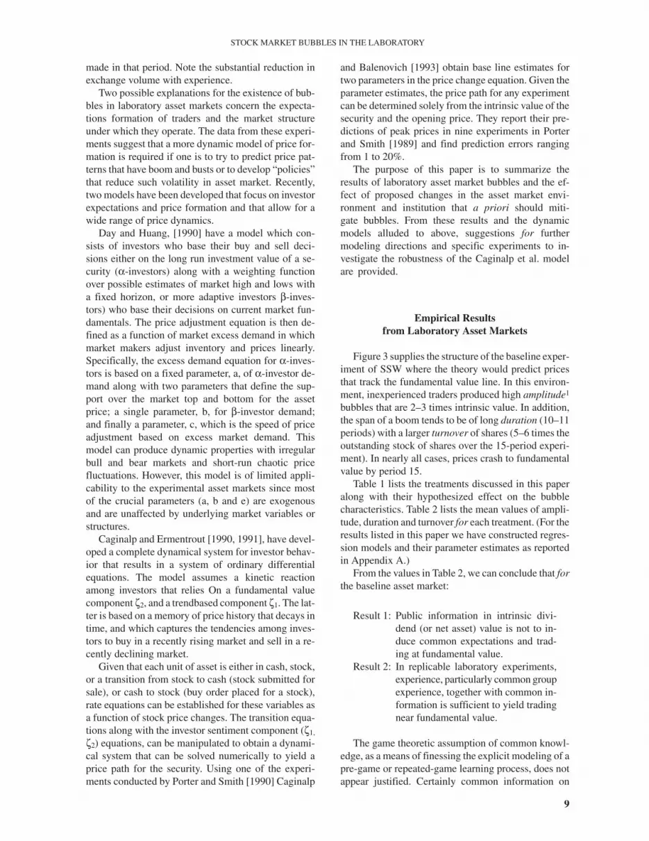
Table 1 lists the treatments discussed in this paperalong with their hypothesized effect on the bubblecharacteristics. Table 2 lists the mean values of ampli-tude, duration and turnover for each treatment. (For theresults listed in this paper we have constructed regres-sion models and their parameter estimates as reportedin Appendix A.)

From the values in Table 2, we can conclude that forthe baseline asset market:

Result 1: Public information in intrinsic divi-dend (or net asset) value is not to in-duce common expectations and trad-ing at fundamental value.

Result 2: In replicable laboratory experiments,experience, particularly common groupexperience, together with common in-formation is sufficient to yield tradingnear fundamental value.

The game theoretic assumption of common knowl-edge, as a means of finessing the explicit modeling of apre-game or repeated-game learning process, does notappear justified. Certainly common information on

9

STOCK MARKET BUBBLES IN THE LABORATORY

dividend value does not imply common knowledgeexpectations.

Given these results, a natural question to ask iswhether these bubbles can be related systematicallyto individual reported price expectations. Towards an-swering this question, SSW asked subjects to forecastthe mean price for the next period with a monetary

reward for the best forecaster across all periods. Theconsensus (mean) forecast results revealed that: (1)bullish capital gains expectations arise early in theseexperiments; (2) the mean forecast always fails topredict price jumps and turning points; (3) the meanforecasts are highly adaptive, i.e. jumps in the meanprice as well as turning points are only reflected in

10

PORTER AND SMITH

FIGURE 3Baseline Asset Market Experiment Parameters

Table 1. Treatments and Hypotheses

Treatment Description Hypothesis

Baseline Declining dividend value (see Figure 3) Rational expectations equilibrium has trading atfundamental values

Short-selling Traders are given the capacity to sell units to becovered by last period

Traders can leverage sales and counter ebullientexpectations

Margin Buying Traders are given interest-free loan to be paid backby last period

Purchases can be leveraged to raise prices that arebelow dividend value

Equal portfolio endowment Each trader is given the identical amounts of cashand shares

Traders do not need to use the market to balanceportfolios

Brokerage fees Buyer and seller in transaction pay 10 cents each forthe trade

Should reduce trading based on cost of transacting

Informed insiders Specially informed traders who are given bid askadjustment model

Expert traders aware of bubble characteristicseliminate bubble

Dividend certainty Security pays a fixed and known amount each period Trading based on dividend risk preferences iseliminated

Futures contracting Agents can trade a mid-horizon (period 8) security inadvance

Futures contracts should hasten the formation ofcommon expectations

Limit price change rule Asset price can only change a fixed limited amountfrom the previous period closing price

This rule has been recommended by expert advisorygroups to reduce price volatility and crashes.

forecasts after a one period lag. These observationsparallel the performance of professional forecasters(Zarnowitz, [1986]).

Result 3: Subjects have a strong early tendencyto develop home-grown expectationsof rising prices; their forecasts areadaptive and have a universal tendencyto misprice jumps and turning points.

The dynamics of these price adjustments can becharacterized empirically by a Walrasian price adjust-ment equation which stipulates that price responds inthe direction of the excess demand for the asset. Spe-cifically, dp/dt = F(D(p) – S(p)) where F(0) = 0 and F′> 0. The following ordinary least squares (OLS) Wal-rasian excess demand model has been estimated (SSWp. 1142).

where Pt is the mean price in period t, α is minus theone-period expected dividend value (adjusted for anyrisk aversion), β is adjustment speed, Bt–1 is the numberof bids to buy tendered in period t–1, and Ot–l is thenumber of offers to sell tendered in period t–1. Price

change in this model has three components: (1) therisk-adjusted per-period expected dividend payout; (2)an increase (decrease) due to excess demand arisingfrom home-grown capital gains (losses) expectations, aWalrasian measure of which is excess bids Bt –1 – Ot–I,and (3) unexplained noise, t. The R2 values for theasset markets experiments in our sample range from0.04 to 0.63. The variance in the estimates is large.

This model explains and predicts price changesbetter than subjects’forecasts in that it frequently antici-pates turning points. A rational expectations predictionfor this model is that α = – 24, the expected one perioddividend, and β = 0. The pooled results over all experi-ments with treatment effects can be found in AppendixB. The results in Appendix B show that we cannot rejectthe hypotheses that α = –24 and that β = 0. In addition,experience causes a significant decrease in the capitalgains expectations coefficient β. However, this modelprovides values of R2 that are much below unity, leavingmuch of the change in prices unexplained.

From the experimental results, which show a damp-ening of the bubble with experience, Renshaw [1988]hypothesizes that the severity of price bubbles andcrashes depends upon trader experience with extrememarket price changes. He examines the relationshipbetween major declines in the Standard and Poor indexand the length of time between major declines. The

11


1( ) (1)t t l t l t tP P B O Cα β ��

C�

Table 2. Mean Values by treatment

Treatment

Inexperienced Once-experienced Twice-experienced

Amplitude Duration Turnover Amplitude Duration Turnover Amplitude Duration Turnover

Baseline 1.21 9.23 5.79 0.75 5.51 3.00 0.10 3.00 1.60(0.10) (0.19) 0.00 0.00 0.00 0.00

n = 19 n=4 n=3Short-sell 1.61 9.50 6.67 0.76 5.80 4.19 0.40 3.67 1.74

(0.40) (0.30) (0.49) (0.48) (0.78) (0.03) (0.02) (0.69) (0.27)n=4 n=5 n=3

Margin buy 3.64 8.00 5.48 1.15 2.00 2.330.00 (0.66) (0.59) (0.09) (0.21) (0.58)n=2 n=1

Equal portfolios 1.87 10.00 6.29(0.12) (0.44) (0.84)n = 4

Brokerage fees 0.73 10.00 5.56 0.63 4.00 4.920.00 (0.44) (0.67) (0.62) (0.90) (0.10)n=2 n=3

Informed insiders 0.63 13.00 2.68 0.25 6.00 4.050.00 0.00 0.00 (0.04) (0.92) (0.40)n=2 n=3

Dividend certainty 1.10 11.00 8.84 0.52 9.67 2.71(0.98) (0.05) (0.13) (0.29) (0.24) (0.51)n=3 n=3

Futures contracting 10.00 6.85 0.60 5.50 2.63(0.11) (0.73) (0.81) (0.19) (0.60) (0.50)n=3 n=2

Limit price change 2.51 10.50 4.84 1.77 5.50 2.22 0.70 1.50 1.89(0.07) (0.46) (0.01) (0.05) (0.71) (0.15) (0.04) (0.17) (0.79)n=2 n=2 n=2

Note: p-values in parentheses.

time between crashes is his proxy for investor inexperi-ence. An OLS regression of the measured extent of theindex’s decline, Y, on the time since the previous de-cline, X, yields the estimate:

Y = 5.5 + 0.90X; R2 = 0.98.(t = 15.1)

The longer it has been since the previous crash inprices, the greater the magnitude of a new crash.

The baseline market developed by SSW omits manyinstitutional features that are present in the field. Sincesome of these factors may very well dampen bubbles,they have provided the impetus for several new experi-ments reported in two recent studies: (1) King et al.[1992] report experiments that introduce short selling,margin buying, brokerage fees, informed “insiders”,equal portfolio endowments and limit price changerules; (2) Porter and Smith [1994] (hereafter PS) reportnew experiments examining the effect of a futures mar-ket and the effect of dividend certainty. Table 1 liststhese structural changes, the associated data, and thepredictions of the effect of these treatments on the mar-ket. Such structural changes are a response to sug-gested explanations by others of the bubbles reportedin SSW.

Recall that in the baseline experiments individualtraders were endowed with different initial portfolios.A common characteristic of first-period trading is thatbuyers tend to be those with low share endowments,while sellers are those with relatively high share en-dowments. This suggests that risk averse traders mightbe using the market to acquire more balanced portfo-lios. If liquidity preference accounts for the low initialprices, which in turn lead to expectations of price in-creases, the making the initial trader endowmentsequal across subjects would tend to dampen bubbles:

Result 4: Observations from four experimentswith inexperienced traders show no sig-nificant effect of equal endowments onbubble characteristics.

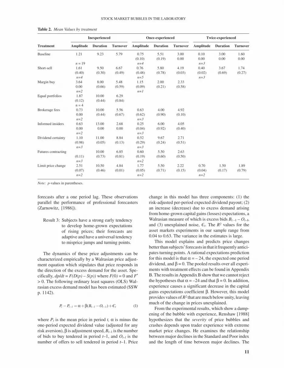
If risk aversion about price expectations due to divi-denduncertaintycausesadivergenceofcommonexpec-tations, then the elimination of such uncertainty shouldreduce the severity of bubbles. The PS experimentsdemonstrate otherwise (see Figure 4 for example).

Result 5: When the dividend draw each period isset equal to the one-period expecteddividend value, so that the asset divi-

12

PORTER AND SMITH

FIGURE 4Mean Contract Price and Total Volume: Certain Dividend

dend stream is certain, bubbles are notsignificantly reduced relative to divi-dend uncertainty.

In Table 2 we note that the duration of bubbles issignificantly increased with dividend certainty. The re-sults in Appendix B for the Walrasian adjustment equa-tion suggest, however, that dividend certainty does nothave a significant effect on the capital gains expecta-tions coefficient, β.

Results 4 and 5 are directed at changing the under-lying induced value parameters of the baseline exper-iments but not the basic structure of the market. Stockmarkets in the field allow traders to take a position oneither side of the market and leverage their sales bytaking a short position or leverage their purchases bybuying with borrowed funds. Consequently, a smallnumber of traders who have counter-cyclical expecta-tions would be able to offset the ebullient expecta-tions of others. These considerations led to an expla-nation of the hypothesis that allowing subjects theright to short sell or to buy on margin would dampenbubbles.

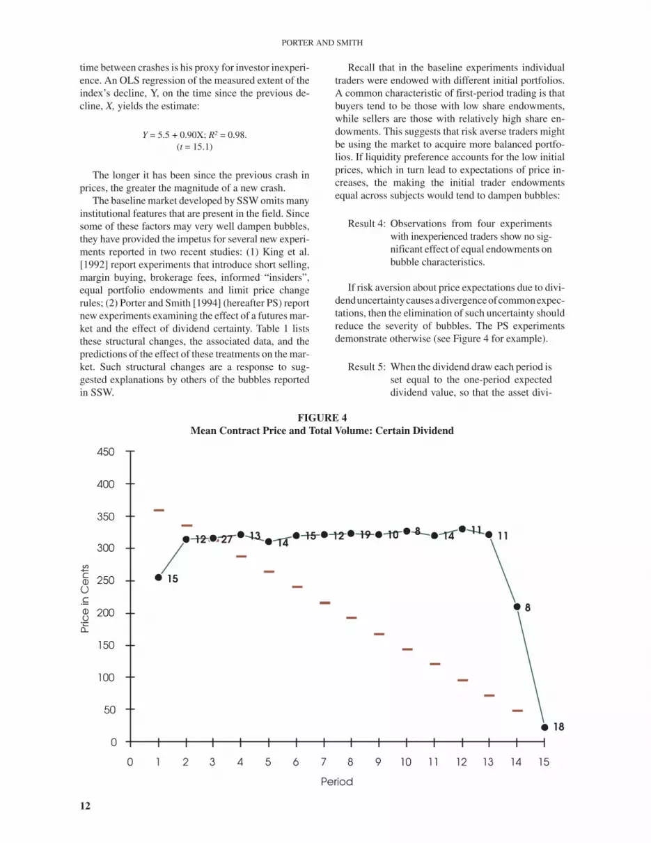
Result 6: Short-selling does not significantly di-minish the amplitude and duration ofbubbles, but the volume of trade is

increased significantly; Figure 5 pro-vides an example.

Result 7: Margin buying opportunities cause asignificant increase in the amplitude ofbubbles for inexperienced (p < 0.01),but not for experienced subjects.

Consequently, if anything, short selling and marginbuying tend to exacerbate some aspects of observedbubbles.

The laboratory double auction has low participationcosts of trading, since subjects only have to touch a but-ton to accept standing bids or asks. This, coupled withthe conjecture that laboratory subjects may believe thatthey are expected to trade may result in laboratory bub-bles. However, the claim that subjects trade becausethey believe they are expected to, merely predictstrade, not bubbles; nor is the claim consistent with thetendency for turnover’ to fall sharply with experience.One way to test the transactions cost hypothesis is toimpose a transactions fee on each trade.

Result 8: A brokerage fee of 20 cents on eachtrade (10 cents on the buyer and seller)significantly reduced the amplitude,but not the duration, or share turnovermeasures of bubbles.

13


FIGURE 5Mean Contract Price, Volume and Short Sales

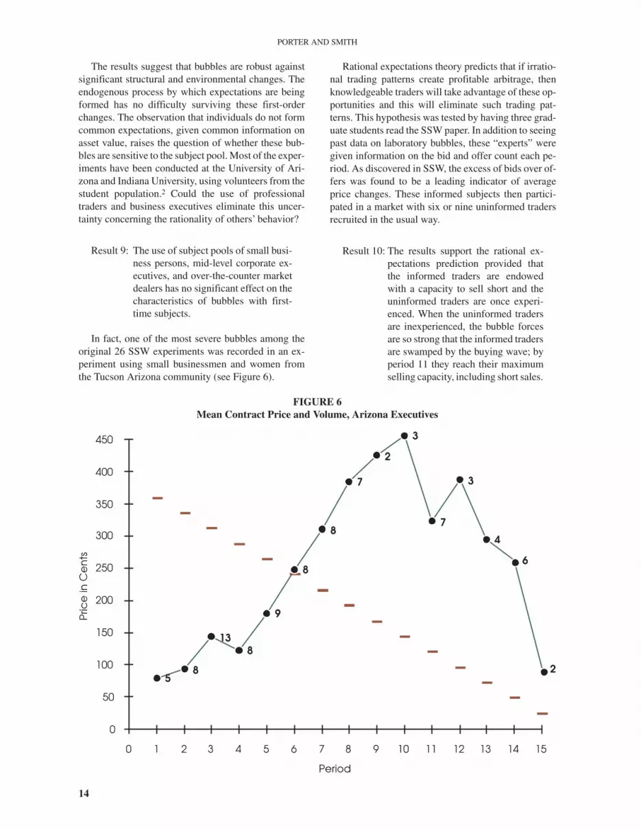
The results suggest that bubbles are robust againstsignificant structural and environmental changes. Theendogenous process by which expectations are beingformed has no difficulty surviving these first-orderchanges. The observation that individuals do not formcommon expectations, given common information onasset value, raises the question of whether these bub-bles are sensitive to the subject pool. Most of the exper-iments have been conducted at the University of Ari-zona and Indiana University, using volunteers from thestudent population.2 Could the use of professionaltraders and business executives eliminate this uncer-tainty concerning the rationality of others’ behavior?

Result 9: The use of subject pools of small busi-ness persons, mid-level corporate ex-ecutives, and over-the-counter marketdealers has no significant effect on thecharacteristics of bubbles with first-time subjects.

In fact, one of the most severe bubbles among theoriginal 26 SSW experiments was recorded in an ex-periment using small businessmen and women fromthe Tucson Arizona community (see Figure 6).

Rational expectations theory predicts that if irratio-nal trading patterns create profitable arbitrage, thenknowledgeable traders will take advantage of these op-portunities and this will eliminate such trading pat-terns. This hypothesis was tested by having three grad-uate students read the SSW paper. In addition to seeingpast data on laboratory bubbles, these “experts” weregiven information on the bid and offer count each pe-riod. As discovered in SSW, the excess of bids over of-fers was found to be a leading indicator of averageprice changes. These informed subjects then partici-pated in a market with six or nine uninformed tradersrecruited in the usual way.

Result 10: The results support the rational ex-pectations prediction provided thatthe informed traders are endowedwith a capacity to sell short and theuninformed traders are once experi-enced. When the uninformed tradersare inexperienced, the bubble forcesare so strong that the informed tradersare swamped by the buying wave; byperiod 11 they reach their maximumselling capacity, including short sales.

14

PORTER AND SMITH

FIGURE 6Mean Contract Price and Volume, Arizona Executives

The failure of the informed traders to eliminate thebubble when the uninformed traders are inexperiencedis illustrated by the experiment in Figure 7.

It should be noted in Figure 7 that since short saleshad to be covered by purchases to avoid penalties,when facing inexperienced traders short covering byinformed traders prevented the market from crashingto dividend value in period 15. Thus, short sellingagainst the bubble prevented convergence to the ratio-nal expectations value at the end.

A futures contract provides a mechanism by whicheach trader can get a reading on all traders’expectationsconcerning a future event. In effect, one runs a futurespot market in advance. If a price bubble arises becauseof the failureofcommoninformation to inducecommonexpectations, but the latter are achieved through repeatexperience, then a futures contract should have the ef-fect of speeding up this expectations homogenizing pro-cess. To test this hypothesis, PS ran two sequences oftwo experiments with the same subjects trained in themechanicsofa futuresmarket. In thenewexperiments, afutures contract due in period 8 was utilized, whereagents could trade both the spot and futures contracts inperiods 1–8; after period 8, only the spot market was ac-tive. This market mechanism may help traders focus ontheir expectations of share value at midhorizon, and pro-vide observations (futures’ contract prices) on thegroup’s period 8 expectations during the first seven peri-

ods of the market. Figure 8 shows the results of one ofthese futures market experiments.

Result 11: Futures markets dampen, but do noteliminate, bubbles by speeding up theprocess by which traders form com-mon expectations.

Appendix B supplies estimates of an ANOVAmodel on the Walrasian price adjustment equationstated in equation (1) with treatment effects for futuresmarket and certain dividend experiments. The resultsclearly demonstrate that the futures market has a sig-nificant dampening effect on capital gains expecta-tions. In addition, the combination of one time experi-ence and a futures market significantly reduces thecapital gains adjustment coefficient, β.

In the wake of the worldwide stock market crash of19 October, 1987, it was widely recommended by vari-ous investigatory groups that limit price change rulesbe implemented on US stock market exchanges. Kinget al. [1992] (KSW) report six experiments in whichceiling and floor limits were placed at plus (or minus)twice the expected one-period dividend value.

Result 12: Price limit change rules do not pre-vent bubbles; if anything they aremore pronounced.

15


FIGURE 7Mean Contract Price, Volume and Insider Purchases

KSW conjectures that bubbles are more severe withlimit price change rules because traders perceive a re-duced down-side risk inducing them to ride the bubblehigher and longer. But, of course, when the marketbreaks, it moves down by the limit and finds no buyers.Trading volume is zero in each period of the crash asthe market declines by the limit each period (see Figure9, for an example).

Summary

Laboratory stock markets in which shares have awell-defined expected fundamental (dividend) value,that is common information, exhibit strong price bub-bles relative to fundamental value. These bubbles di-minish with experience; trades fluctuate around funda-mental values when the same group returns for a thirdtrading session. Thus, common information is not suf-ficient to induce common rational expectations, buteventually through experience in a stationary environ-ment, the participants come to have common expecta-tions. If we suppose that investors are more “inexperi-enced” the longer it has been since the last stockmarket crash, the laboratory results are corroboratedby a study showing a 98% correlation between the se-verity of declines in the Standard and Poor index andthe length of time since the last crash.

More detailed analysis of the laboratory data showsthat expectations of a rising market, as measured bytrader price forecasts, occur early in a market. Traders’forecasts invariably miss price jumps and turningpoints. A more accurate predictor of mean pricechanges is lagged excess bids: a count of last period’sbids minus the offers submitted.

The baseline experiments have been criticized foromitting a number of factors that might account for thepropensity to bubble. A new generation of experimentsevaluated these factors. Briefly, short-selling does nothave a significant impact on bubble characteristics;margin buying fails to moderate, and even increasesthe amplitude of bubbles for inexperienced subjects;brokerage fees designed to raise transactions cost sig-nificantly reduced the amplitude of bubbles; the use ofsubjects from pools of small business persons, mid-level corporation executives and over-the-counterstock dealers had no significant effect on bubbles; theuse of subjects who had an opportunity to study SSW,and who were given information on excess bids at theclose of each period, support the rational expectationsequilibrium, but only when the informed traders couldleverage their sales with short selling, and when the un-informed subjects were experienced.

Finally, bubbles seem to be due to uncertainty aboutthe behavior of others, not to uncertainty about divi-dends, since making dividends certain does not signifi-

16

PORTER AND SMITH

FIGURE 8Mean Spot and Futures Contract Prices and Total Volumev

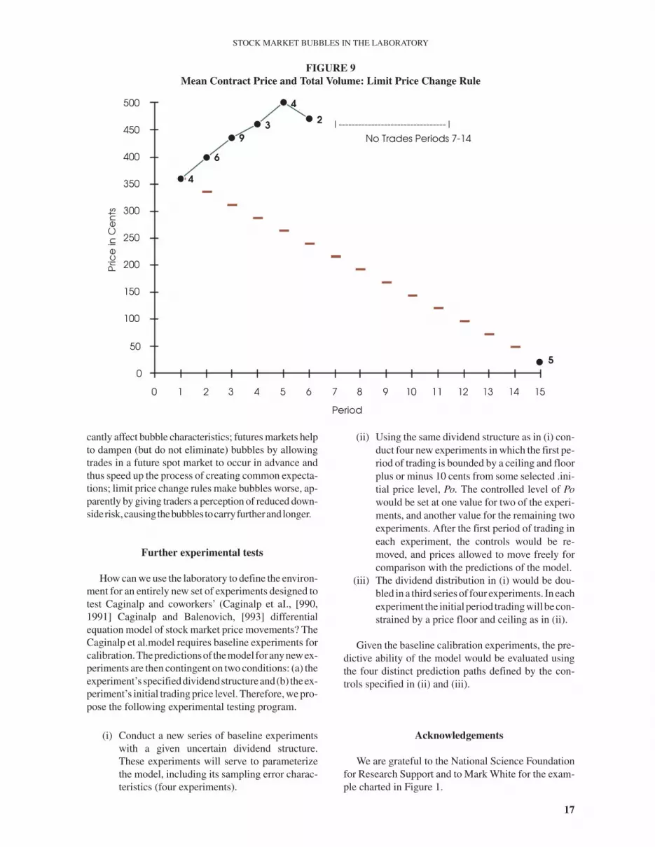
cantly affect bubble characteristics; futures markets helpto dampen (but do not eliminate) bubbles by allowingtrades in a future spot market to occur in advance andthus speed up the process of creating common expecta-tions; limit price change rules make bubbles worse, ap-parently by giving traders a perception of reduced down-siderisk,causingthebubbles tocarryfurtherandlonger.

Further experimental tests

How can we use the laboratory to define the environ-ment for an entirely new set of experiments designed totest Caginalp and coworkers’ (Caginalp et aI., [990,1991] Caginalp and Balenovich, [993] differentialequation model of stock market price movements? TheCaginalp et al.model requires baseline experiments forcalibration.Thepredictionsof themodel foranynewex-periments are then contingent on two conditions: (a) theexperiment’sspecifieddividendstructureand(b) theex-periment’s initial trading price level. Therefore, we pro-pose the following experimental testing program.

(i) Conduct a new series of baseline experimentswith a given uncertain dividend structure.These experiments will serve to parameterizethe model, including its sampling error charac-teristics (four experiments).

(ii) Using the same dividend structure as in (i) con-duct four new experiments in which the first pe-riod of trading is bounded by a ceiling and floorplus or minus 10 cents from some selected .ini-tial price level, Po. The controlled level of Powould be set at one value for two of the experi-ments, and another value for the remaining twoexperiments. After the first period of trading ineach experiment, the controls would be re-moved, and prices allowed to move freely forcomparison with the predictions of the model.

(iii) The dividend distribution in (i) would be dou-bled in a third series of four experiments. In eachexperiment the initial period trading will be con-strained by a price floor and ceiling as in (ii).

Given the baseline calibration experiments, the pre-dictive ability of the model would be evaluated usingthe four distinct prediction paths defined by the con-trols specified in (ii) and (iii).

Acknowledgements

We are grateful to the National Science Foundationfor Research Support and to Mark White for the exam-ple charted in Figure 1.

17


FIGURE 9Mean Contract Price and Total Volume: Limit Price Change Rule

Notes

1. We calculate amplitude as the difference between the highestdeviation of mean contract price from its fundamental valueand the lowest deviation of mean contract from its fundamentalvalue. This value is then normalized but the expected dividendvalue over 15 periods.

2. Bubbles have been observed with inexperienced student trad-ers in two experiments at the California Institute of Technologyand three experiments at the Wharton School.

References

Caginalp, G. and D. Ba1enovich. “Mathematical Models for the Psy-chology of Oscillations in Financial Markets.” Working paper,University of Pittsburgh, Pittsburgh, PA,1993.

Caginalp, G. and G.B. Ermentrout. “A Kinetic Thermodynamic Ap-proach to the Psychology of Fluctuations in Financial Markets.”Applied Mathematics, 4, (1990), pp. 17–19.

Caginalp, G. and G.B. Ermentrout. “Numerical Studies of Differen-tial Equations Related to Theoretical Financial Markets.” Ap-plied Mathematics, 4, (1991), pp. 35–38.

Day, R. and W. Huang. “Bulls, Bears and Market Sheep.” Journalof Economic Behavior and Organization, 14, (1990), pp.299–331.

King, R.R., V.L. Smith, A.W. Williams and M. Van Boening. TheRobustness of Bubbles and Crashes in Experimental StockMarkets, In, I. Prigogine, R.H. Day, and P. Chen (eds): “Nonlin-ear Dynamics and Evolutionary Economics”, Oxford Univer-sity Press, Oxford, UK, 1992.

Lee, C., A. Scheilfer and D. Thaler. “Investor Sentiment and theClosed-end Fund Puzzle.” Journal of Finance, March, (1991),pp. 75–109.

Porter, D. and V.L. Smith. “Futures Markets, Dividend Certainty andCommon Expectations in Asset Markets.” Working Paper, Uni-versity of Arizona, Tucson, 1989.

Porter, D. and V.L. Smith. “Futures Contracting and DividendUncertainty in Experimental Asset Markets.” Social ScienceWorking Paper, California Institute of Technology, 1994.

Renshaw, E. “The Crash of October 19 in Retrospect.” The MarketChronicle, 22, (1988), pp.1.

Smith, V.L., G.L. Suchanek and A.A. Williams. “Bubbles, Crashes,and Endogenous Expectations in Experimental Spot Asset Mar-kets.” Econometrica, 56, (1988), pp.1119–1151.

18

PORTER AND SMITH

APPENDIX A

The following results are based on seemingly unrelated regression estimates of amplitude, duration and turnoversimultaneous dummy variable equations.

19


ANOVA Estimates of Treatments on Amplitude, Duration and Turnover

Equation 1Dependent variable: AMPLITUDEValid cases: 72 Missing cases 0Total SS: 45.9484 Degrees of freedom: 61Residual SS: 17.8081 Standard error of estimates: 0.5156

Log likelihood –53.5848

Treatment Coefficient Standard Error t-Statistic p-Value

Short sales –0.0481 0.1708 –0.2816 0.7791Certain dividend 0.0626 0.2530 0.2472 0.8055Futures –0.6796 0.3800 –1.7884 0.0782Limit price rule 0.8843 0.2452 3.6072 0.0006Equal endowments 0.5073 0.2824 1.7960 0.0770Insiders –0.5646 0.2559 –2.2066 0.0308Transaction fee –0.3434 0.2628 –1.3066 0.1958Margin buying 0.8375 0.2505 3.3438 0.0013Inexperienced 1.3602 0.1154 11. 7849 0.0000Once experienced 0.7889 0.1624 4.8568 0.0000Twice experienced 0.1680 0.2267 0.7410 0.4613

Equation 2Dependent variable: DURATIONValid cases: 72 Missing cases 0Total SS: 1034 Degrees of freedom: 61Residual SS: 482.7757 Standard error of estimates: 2.6843



Short sales 0.9235 0.8895 1.0382 0.3029Certain dividend 2.7896 1.3175 2.1174 0.0379Futures –0.3107 1.9785 –0.1571 0.8757Limit price rule 0.1196 1.2764 0.0937 0.9256Equal endowments 0.7583 1.4706 0.5156 0.6078Insiders 1.2659 1.3321 0.9503 0.3454Transaction fee 0.6200 1.3685 0.4530 0.6520Margin buying 0.4967 1.3042 0.3808 0.7045Inexperienced 9.2417 0.6010 15.3779 0.0000Once experienced 5.4722 0.8457 6.4706 0.0000Twice experienced 2.4272 1.1802 2.0567

0.0436Equation 3Dependent variable: TURNOVERValid cases: 72 Missing cases 0Total SS: 568.1284 Degrees of freedom: 61Residual SS: 209.2946 Standard error of estimates: 1.7674



Short sales 1.5514 0.5857 2.6488 0.0101Certain dividend –0.7395 0.8675 –0.8525 0.3969Futures –2.7666 1.3027 –2.1237 0.0374Limit price rule –0.1561 0.8404 –0.1858 0.8532Equal endowments 1.0584 0.9683 1.0931 0.2783Insiders –1.0879 0.8771 –1.2403 0.2192Transaction fee –0.3911 0.9011 –0.4340 0.6656Margin buying –0.1470 0.8587 –0.1712 0.8646Inexperienced 5.2291 0.3957 13.2150 0.0000Once experienced 2.6124 0.5568 4.6916 0.0000Twice experienced 1.5769 0.7770 2.0293 0.0464

APPENDIX BANOVA Estimates of Treatmentsfor Walrasian Price Adjustment

The model that is estimated in this appendix is asfollows:

where:P = mean contract priceB = number of Bids tendereda = number of Offers tenderedX = experienced baselineC = Certain dividend treatment dummyCx = experienced Certain dividend treatment dummyF = Futures market treatment dummyFx = experienced Futures market treatment dummyS = Switch treatment dummyL = LAN market treatment dummy

20

PORTER AND SMITH

1

11 1 1

1 1 1 1

1 1 1 1

1 1

( )[ ( )] [ ( )][ ( )] [ ( )][ ( )] [ ( )][ ( )] C

t

t

t t l

t l

t t t

t t t t

t t t t

t t

P P X C Cx F FxS L B OX B O C B OCx B Q F B OFx B O S B OL B O

α ω Φ φ γη λ βρ µν θυ ζτ

�

�

�

�

�

� � �

� � � �

� � � �

� �

� � � � ��

� � � � � � �

� � � � � � � �

� � � � � � � �

� � � � � � � �

� � � � �

Dependent Variable: ∆Mean Contract Price

Certain DividendExperienced Coefficient Standard Error t-Statistic

α –0.1273 0.0697 –1.8249Baseline

experienced–0.0118 0.0942 –0.1249

Certain Dividend 0.0056 0.1185 0.0477Certain dividend

experienced–0.0082 0.1229 –0.0674

Futures Market –0.0512 0.1299 –0.3944Futures market

experienced–0.0188 0.1512 –0.1246

Switch 0.0065 0.1631 0.0399LAN 0.0041 0.0305 0.1357β 0.0329 0.0050 6.5923Baseline

experienced–0.0071 0.0036 –1.9722

Certain Dividend –0.0136 0.0091 –1.4981Certain dividend

experienced–0.0146 0.0093 –1.5577

Futures Market –0.0237 0.0062 –3.7882Futures market

experienced–0.0278 0.0095 –2.9072

Switch –0.0312 0.0135 –2.3012LAN –0.0021 0.0946 –0.0211

Number of observations: 364R2: 0.2571SSR: 0.0113SER: 0.5782D-W: 2.0679

stock market bubbles in the laboratory

Documents