Spectral and thermal sensing for nitrogen and waterstatus in rainfed and irrigated wheat environments

G. J. Fitzgerald Æ D. Rodriguez Æ L. K. Christensen ÆR. Belford Æ V. O. Sadras Æ T. R. Clarke

Published online: 1 July 2006� Springer Science+Business Media, LLC 2006

Abstract Variable-rate technologies and site-specific crop nutrient management require

real-time spatial information about the potential for response to in-season crop manage-

ment interventions. Thermal and spectral properties of canopies can provide relevant

information for non-destructive measurement of crop water and nitrogen stresses. In pre-

vious studies, foliage temperature was successfully estimated from canopy-scale (mixed

foliage and soil) temperatures and the multispectral Canopy Chlorophyll Content Index

(CCCI) was effective in measuring canopy-scale N status in rainfed wheat (Triticum

aestivum L.) systems in Horsham, Victoria, Australia. In the present study, results showed

that under irrigated wheat systems in Maricopa, Arizona, USA, the theoretical derivation of

foliage temperature unmixing produced relationships similar to those in Horsham. Deri-

vation of the CCCI led to an r2 relationship with chlorophyll a of 0.53 after Zadoks stage

43. This was later than the relationship (r2 = 0.68) developed for Horsham after Zadoks

stage 33 but early enough to be used for potential mid-season N fertilizer recommenda-

tions. Additionally, ground-based hyperspectral data estimated plant N (g kg)1) in Hor-

sham with an r2 = 0.86 but was confounded by water supply and N interactions. By

combining canopy thermal and spectral properties, varying water and N status can

potentially be identified eventually permitting targeted N applications to those parts of a

field where N can be used most efficiently by the crop.

G. J. Fitzgerald (&) Æ T. R. ClarkeUSDA-ARS, U.S. Water Conservation Laboratory, Phoenix, AZ, USAe-mail: glenn.fitzgerald@dpi.vic.gov.au

D. RodriguezDepartment of Primary Industries and Fisheries, Toowoomba, Queensland, Australia

L. K. ChristensenNordic Genebank, Alnarp, Sweden

R. BelfordPrimary Industries Research, Grains Innovation Park, Horsham, Victoria, Australia

V. O. SadrasSARDI, Waite Research Precinct, Adelaide, Australia

Precision Agric (2006) 7:233–248DOI 10.1007/s11119-006-9011-z

123

Keywords Remote sensing Æ Thermal sensing Æ Crop stress index Æ CCCI ÆChlorophyll Æ Nitrogen Æ Water stress Æ Wheat

Introduction

The ability to measure plant N and water status using reflected light has been well

documented (Blackmer, Schepers, & Varvel, 1994; Gao, 1996; Osborne, Schepers, Francis,

& Schlemmer, 2002; Penuelas, Filella, Biel, Serrano, & Save, 1993). It is also well

established that chemical and spectral characteristics of plants with nutrient deficiencies

change when water stress is present (Penuelas, Gamon, Fredeen, Merino, & Field, 1994;

Pettigrew, 2004) masking and perhaps eliminating the specific spectral response of the

deficiency. Hence, under field conditions with interacting water and N stresses, it is

necessary to develop indices capable of determining the physiological status of the canopy

to maximize the potential for response to management interventions. Response to applied

N will be greater in areas where the plants are less water stressed. Indices providing

simultaneous detection of N and water stress could prove useful for variable-rate man-

agement when applied to multi- or hyperspectral imagery, permitting spatial measures of

these stresses.

Estimation of crop water status using thermal indices has been shown to be very robust

(Clarke, 1997; Idso, Jackson, Pinter, Reginatio, & Hatfield, 1981; Jackson, Idso, Reginato,

& Pinter, 1981; Moran, Clarke, Inoue, & Vidal, 1994) and could provide a means to map

water status in a field. Since reflectance-based indices measure chemical and structural

responses by plants they may not be as sensitive as thermal measures to the onset of water

stress resulting from rapid stomatal closure and increased leaf temperature (Jackson, Pinter,

Reginato, & Idso, 1986; Maracchi, Zipoli, Pinter, & Reginato, 1988). Optical measures can

also be confounded by leaf angle changes due to wilting. By the time optical methods can

detect changes, yield may already be affected.

For site-specific farming, it is important that canopy-level indices are developed and

tested. Strong relationships have been shown between leaf chlorophyll concentrations and

various remotely sensed indices (Carter & Spiering, 2002; Penuelas et al., 1994). When

scaled up to the canopy, where shadows (Fitzgerald, Pinter, Hunsaker, & Clarke, 2005),

soil background (Huete, 1988) and structural differences (Moran, Pinter, Clothier, & Allen,

1989) are present, it may be more difficult to estimate leaf N status. The issue can be

illustrated in the ‘‘cover problem’’ where an index may calculate the same value for an

area of crop with low cover and high N concentration as in an area with high cover but low

N. The amount of ‘‘green’’ detected by the sensors and then estimated by the index can be

the same in both cases.

To estimate canopy-level N at varying amounts of canopy cover, different methods have

been recently proposed. Daughtry, Walthall, Kim, De Colstoun, and Mcmurtrey (2000)

used one multispectral index as a measure of cover and another as a measure of leaf

chlorophyll to model leaf N at varying canopy cover. Similarly, Barnes, Clarke, and

Richards (2000) developed the Canopy Chlorophyll Content Index (CCCI) based on planar

domain principles (Clarke, Moran, Barnes, Pinter, & Qi, 2001). The CCCI uses two other

indices derived from three spectral wavebands along the ‘‘red edge’’ part of a typical green

plant spectrum to estimate cover and leaf N. Other measures of N status, based on

234 Precision Agric (2006) 7:233–248

123

hyperspectral data, have also been developed (Filella & Penuelas, 1994; Fitzgerald et al.,

2005; Strachan, Pattey, & Boisvert, 2002) but hyperspectral data are typically expensive

and not widely available. The planar domain approach (Clarke et al., 2001) attempts to

isolate the plant signal from the background using remotely sensed indices as surrogates

for fractional cover and the property target (i.e., foliage temperature or plant N). The target

index could be derived from hyperspectral or multispectral data but, here, two indices

derived from multispectral and thermal data are presented for simultaneous measures of N

and water status.

We postulate that by combining remotely sensed indices of canopy spectral and thermal

properties that are cover independent, it is possible to target N inputs to areas with less water

stress where the potential for response to in-season N application is high. We elaborate on

the planar domain approach for measuring canopy N and water status with examples for

wheat in an Australian rainfed region and a US irrigated system. We also include a

hyperspectral measure of N status and discuss advantages and disadvantages between multi-

and hyperspectral approaches to N detection under water-limiting conditions.

Theory

Derivation of foliage temperature

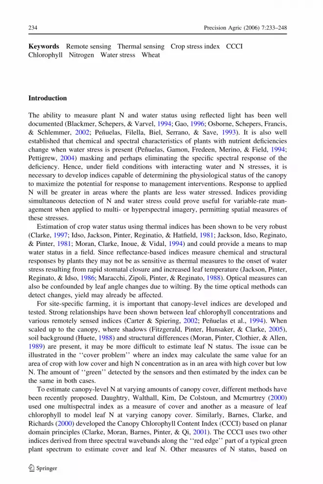
Based conceptually on work by Idso (1982) and described in Rodriguez, Sadras, Chris-

tensen, and Belford (2005b), the aggregate temperature of a given ground-acquired image

or pixel containing a mixture of soil and plants (‘‘mixed’’ pixel) (Tm) depends on the

fractional plant cover (fc) and fraction of soil (fs = 1 ) fc) and the temperature of each of

these components. Theoretically, Tm and Tf will converge as the canopy approaches full

cover (Fig. 1).

Hence, foliage temperature may be calculated as,

Tf ¼ Tm � DT ð�CÞ ð1Þ

where DT is the difference between Tm and Tf derived from direct foliage measurements or

pixels identified as foliage in an image. The Normalized Difference Vegetation Index

(NDVI), a remotely sensed index, can be used as a surrogate for canopy cover (Fitzgerald

Fig. 1 Theoretical relationshipbetween the mean temperature ofmixed-pixels (Tm), foliagetemperature (Tf), and fractionalground cover (fc) (redrawn fromRodriguez et al., 2005b)

Precision Agric (2006) 7:233–248 235

123

et al., 2005) and a relationship can be established between NDVI and DT. Once a rela-

tionship is developed between DT and NDVI (Rodriguez et al., 2005b), Tf can be solved

from NDVI and thermal data.

This approach is very similar to work presented by Maas, Fitzgerald, and DeTar (2000)

showing that Tm represents a mixed image or pixel such that,

Tm ¼ fc � Tf þ ð1� fcÞ � Tsi ð2Þ

where, Tf = foliage temperature; fc = fraction crop cover; (1 ) fc) = fs = fraction soil

within the canopy; Tsi = soil temperature inside the canopy.

Rearranging to solve for Tf:

Tf ¼ ½Tm � Tsi � ð1� fcÞ�=fc ð3Þ

The authors used a remote sensing technique to estimate crop cover (fc) (Maas, 1998,

2000) and developed a relationship between soil temperature within the canopy (Tsi) and

bare soil temperature from an area outside the canopy (Tso), allowing estimation of Tsi and

thus, Tf. The above is functionally equivalent to part of the ‘‘empirical’’ Vegetation Index

Temperature trapezoid derived by Clarke (1997), although it aggregates the wet and dry

soil terms and only requires that a pre-established relationship exist for Tsi and Tso.

It should be noted that thermal sensors measure radiance, which has a non-linear

relation to temperature described by the Stefan Boltzmann law where radiance is a function

of T4 (K). Thus, linear mixture analysis should be applied to radiance, not temperature. As

such, Eq. 2 could be written:

T 4m ¼ ½fc � T 4

f þð1� fcÞ � T 4si� ð4Þ

where, the temperature units are in K.

However, when leaf and soil temperature differences are small, such as shown here for

winter wheat, the error between linear and non-linear estimation of foliage temperature is

less then 0.5�C. As the temperatures of plant and soil components diverge, the error

increases so linear mixture modelling should proceed with caution in hot, well-irrigated

locations where soil and leaf temperature differences can be large.

Derivation of the canopy chlorophyll content index (CCCI)

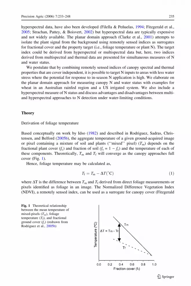
The Canopy Chlorophyll Content Index (CCCI) is derived from planar domain concepts

(Clarke et al., 2001) and has been shown to relate to canopy chlorophyll and plant N in

wheat and cotton (Barnes et al., 2000; Kostrzewski et al., 2002; Rodriguez, Fitzgerald, &

Belford, 2006). The methodology is based conceptually on the Crop Water Stress Index

(CWSI) discussed by Idso (1982) where boundary ranges in two-dimensions are set for two

measures of interest and the index for any given point is calculated as the proportional

distance between these boundaries (Fig. 2).

In the present study, the two measures of interest were canopy cover, represented by

NDVI and a measure of chlorophyll or N status represented by the Normalized Difference

Red Edge (NDRE). The NDRE takes the form of the NDVI but substitutes a band in the

so-called ‘‘red edge’’ of a green leaf for the band measuring red light in the NDVI:

NDRE ¼ ð790 nm� 720 nmÞ=ð790 nmþ 720 nmÞ ð5Þ

236 Precision Agric (2006) 7:233–248

123

where, 790 nm and 720 nm are narrow wavebands centred at these wavelengths.

The upper (maximum) and lower (minimum) boundaries encompassing the data (Fig. 2)

can be derived by Eqs. 6 and 7. In practice, the boundaries are hand-drawn to encompass

the range of data.

NDREmin ¼ NDRElowChl � fc þ NDREsoil � ð1� fcÞ ð6Þ

NDREmax ¼ NDREhighChl � fc þ NDREsoil � ð1� fcÞ ð7Þ

where, NDREmin = the lower Normalized Difference Red Edge (NDRE) bound-

ary; NDREmax = the upper Normalized Difference Red Edge (NDRE) boundary;

NDRElowChl = an idealized crop canopy with very low chlorophyll concentrations;

NDREhighChl = an idealized crop canopy with high chlorophyll concentrations;

NDREsoil = measured soil values of NDRE.

Thus, the CCCI (Eq. 8) should allow estimation of N status at any time during the

growing season, even with partial cover. Because of the maximum and minimum limits

imposed between points A and C in Fig. 2, the CCCI has a range of 0–1 (low to high

NRDE).

CCCI ¼ ðNDRE� NDREminÞ=ðNDREmax � NDREminÞ ð8Þ

where, NDRE = the data point of interest (point b in Fig. 2).

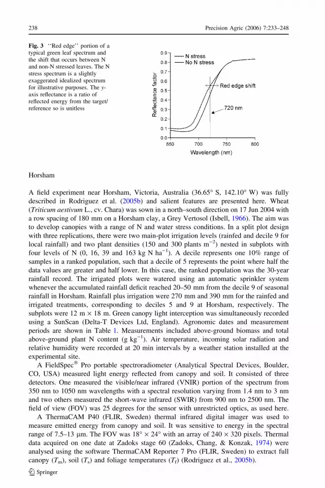
The NDRE responds to changes in chlorophyll a (Chl a) due to the effect of Chl a on the

shape of the spectral response curve along the red edge part of the spectrum (Fig. 3). For

example, as Chl a concentration decreases, the absorption band centred near 670 nm

increases in value, shifting the red edge to shorter wavelengths. Lower Chl a concentration

therefore has the effect of increasing the reflectance value at 720 nm and decreasing the

NDRE numerator while increasing the denominator. Thus, smaller values lie along the

minimum line in Fig. 2 while larger NDRE values lie along the maximum line (Barnes

et al., 2000).

Materials and methods

Data from two field sites are presented here for winter wheat: Horsham, Victoria, Australia

and Maricopa, Arizona, United States. Some of the data from Horsham have been

published previously (Rodriguez et al., 2006). These data are included here to allow direct

comparison between Horsham and Maricopa and expand on the original sources, including

the theoretical considerations above. Data from Maricopa have not appeared elsewhere.

Fig. 2 Derivation of an indexusing the using planar domainprinciples. The property signal inthis case (Canopy ChlorophyllContent Index [CCCI]) is derivedas: (B ) C)/(A ) C). (Modifiedfrom Clarke et al., 2001.)

Precision Agric (2006) 7:233–248 237

123

Horsham

A field experiment near Horsham, Victoria, Australia (36.65� S, 142.10� W) was fully

described in Rodriguez et al. (2005b) and salient features are presented here. Wheat

(Triticum aestivum L., cv. Chara) was sown in a north–south direction on 17 Jun 2004 with

a row spacing of 180 mm on a Horsham clay, a Grey Vertosol (Isbell, 1966). The aim was

to develop canopies with a range of N and water stress conditions. In a split plot design

with three replications, there were two main-plot irrigation levels (rainfed and decile 9 for

local rainfall) and two plant densities (150 and 300 plants m)2) nested in subplots with

four levels of N (0, 16, 39 and 163 kg N ha)1). A decile represents one 10% range of

samples in a ranked population, such that a decile of 5 represents the point where half the

data values are greater and half lower. In this case, the ranked population was the 30-year

rainfall record. The irrigated plots were watered using an automatic sprinkler system

whenever the accumulated rainfall deficit reached 20–50 mm from the decile 9 of seasonal

rainfall in Horsham. Rainfall plus irrigation were 270 mm and 390 mm for the rainfed and

irrigated treatments, corresponding to deciles 5 and 9 at Horsham, respectively. The

subplots were 12 m · 18 m. Green canopy light interception was simultaneously recorded

using a SunScan (Delta-T Devices Ltd, England). Agronomic dates and measurement

periods are shown in Table 1. Measurements included above-ground biomass and total

above-ground plant N content (g kg)1). Air temperature, incoming solar radiation and

relative humidity were recorded at 20 min intervals by a weather station installed at the

experimental site.

A FieldSpec� Pro portable spectroradiometer (Analytical Spectral Devices, Boulder,

CO, USA) measured light energy reflected from canopy and soil. It consisted of three

detectors. One measured the visible/near infrared (VNIR) portion of the spectrum from

350 nm to 1050 nm wavelengths with a spectral resolution varying from 1.4 nm to 3 nm

and two others measured the short-wave infrared (SWIR) from 900 nm to 2500 nm. The

field of view (FOV) was 25 degrees for the sensor with unrestricted optics, as used here.

A ThermaCAM P40 (FLIR, Sweden) thermal infrared digital imager was used to

measure emitted energy from canopy and soil. It was sensitive to energy in the spectral

range of 7.5–13 lm. The FOV was 18� · 24� with an array of 240 · 320 pixels. Thermal

data acquired on one date at Zadoks stage 60 (Zadoks, Chang, & Konzak, 1974) were

analysed using the software ThermaCAM Reporter 7 Pro (FLIR, Sweden) to extract full

canopy (Tm), soil (Ts) and foliage temperatures (Tf) (Rodriguez et al., 2005b).

Fig. 3 ‘‘Red edge’’ portion of atypical green leaf spectrum andthe shift that occurs between Nand non-N stressed leaves. The Nstress spectrum is a slightlyexaggerated idealized spectrumfor illustrative purposes. The y-axis reflectance is a ratio ofreflected energy from the target/reference so is unitless

238 Precision Agric (2006) 7:233–248

123

The spectroradiometer and thermal imager were mounted on a 4 wheel-drive (4WD)

motorbike (Fig. 4a). The sensor and imager were mounted on a steel boom 2.5 m above the

soil surface pointing downwards at a 90� angle (Fig. 4b) to measure up-welling radiance

and thermal emittance, respectively, from the wheat canopy. At the given height and FOV,

the spectroradiometer yielded a sampling area of 0.93 m2. The FOV of each was co-

located so they viewed the same area.

Spectral calibrations for changing light conditions were carried out frequently using a

99% Spectralon panel (Labsphere, Inc., North Sutton, NH, USA). The dark current was

automatically subtracted from the radiometric signal in each calibration session. Each

radiometric data point represented a mean of 25 scans. The radiometric data were stored as

relative reflectance in the range of 390–2500 nm. The spectral reflectance data were col-

lected under clear sky conditions between 11:00 and 14:00 local time, which minimized

the effect of changes in solar zenith angle. The 4WD motorbike was stopped for each

measurement, which took about 5 min. Destructive plant samples were taken within the

FOV of the FieldSpec� Pro after each measurement.

Maricopa

A hard red spring wheat (Triticum aestivum L., cv. Yecora Rojo) was sown into dry soil in

a north–south orientation in a 2.5 ha field at the Maricopa Agricultural Center (33.073� N;

111.979� W, 350 m above sea level) in Central Arizona, USA in mid-Dec., 2003. The first

post-plant irrigation was applied on 19 Dec 2003 (Day of Year [DOY] 353). Harvest

occurred on 26 May 2004 (DOY 147). The soil is classified as a Casa Grande series with

sandy loam to sandy clay loam textures (Post, Mack, Camp, & Sulliman, 1988).

The field was divided into 32 plots (each 11.2 by 20 m) separated from one another by

irrigation border dikes. There were three plant densities and two fertilizer treatments that

Table 1 Dates andagronomic events inHorsham, 2004. DAErefers to days afteremergence and DOY isDay of Year

Date DOY DAE Zadoks Activity

17 Jun 168 – – Planting22 Jun 173 0 – Emergence12 Aug 224 51 14 Sampling 127 Aug 239 66 30 Sampling 220 Sep 263 90 33 Sampling 36 Oct 279 106 47 Sampling 418 Oct 291 118 55 Sampling 515 Dec 349 176 – Harvest

Fig. 4 (a) Instrument setup at Horsham. FieldSpec� Pro and ThermaCAM P40 mounted on a 4-wheel drivemotorbike and (b) close-up image of the ThemaCAM P40 and the FieldSpec� Pro sensor in a pistol grip

Precision Agric (2006) 7:233–248 239

123

provided a wide range of canopy conditions in order to mimic those found in a producer’s

field. There were five rows m)1 and planting density treatments consisted of: Sparse (90

plants m)2, single-line planting); Typical (164 plants m)2, single-line planting); and Dense

(291 plants m)2, double-line planting). There were two fertilization levels, low N

(93 kg N ha)1) and high N (150 kg N ha)1). The split application dates varied depending

on irrigation scheduling since the fertilizer was applied in the irrigation water.

Canopy temperature was measured by walking transects across the central portion of

each plot using a handheld Everest model 100.3Z infrared sensor (Everest Interscience,

Tucson, AZ, USA). It was periodically calibrated to a blackbody of known temperature

(Everest Interscience, Tucson, AZ, USA). This resulted in canopy-level temperatures

representing mixed signals of soil and plant (Tm). Here, canopy is defined as the scale that

includes plants, shadows and soil background in the FOV of the sensors. Foliage is defined

as leaves only (with self-shadowing). Off-nadir measurements were also collected from the

east and west sides of each plot with the sensor held at an angle of about 25� so that only

foliage (Tf) was recorded by the sensor.

Spectral data were collected to calculate a normalized difference vegetation index

(NDVI) and Crop Canopy Chlorophyll Index (CCCI) with an Exotech 100-BX handheld

radiometer with a 15� field of view. The three bands had wavelength ranges of 650–

675 nm, 715–725 nm, and 780–900 nm. This was referenced to a 99% Spectralon panel

for calibration to reflectance. Only data collected on clear-sky days were analysed.

Transects across each plot were walked with the sensor held in a nadir position at least

twice weekly. Sensor data were collected at a constant 57� solar zenith. Meteorological

data that included wet and dry bulb temperatures for calculation of vapor pressure deficit

were collected with an on-site weather station. Cover was measured photographically with

a digital camera by taking pictures of the same plot locations of two rows on a weekly

basis. An area of approximately 2 m by 3 m was photographed from the camera held nadir

to and 3 m above the crop.

An empirical relationship using a non-linear power fit was developed between Chl a

concentration (lg cm)2) and SPAD (Minolta Corporation, Ramsey, NJ, USA) readings by

collecting leaf samples from all treatments for chlorophyll analysis on two dates (DOY 68

and 103). This relationship (r2 = .96) was developed to convert the more easily measured

field SPAD readings to Chl a concentration. The SPAD instrument is a hand-held meter

that measures differential attenuation of transmitted light by leaves in wavebands centred

at 650 nm and 940 nm. It has been found to be an excellent indicator of Chl a (Pinter et al.,

1994). The third fully expanded leaf on the main stem was sampled from 12 plants per plot,

one leaf per plant. One circular leaf punch of 6.85 mm diameter was removed from each

leaf and two SPAD readings were taken per leaf. There were three replications per sample

with 20 samples per date. The 12 leaves were divided into groups of six for Chl a and

SPAD measurements to provide replication. SPAD readings were calibrated by measuring

a ‘‘checker’’ of known SPAD value and normalizing all readings to this. Chl a concen-

tration was determined using the 80% acetone-BHT method according to Lichtenthaler and

Wellburn (1983). In the field, SPAD readings were acquired every 8–12 days from DOY

33–112 on the fully expanded upper leaf on 20 plants per plot in all plots.

Hyperspectral data analysis

In Horsham, hyperspectral data collected from five sampling dates (Table 1) from the

FieldSpec Pro were analysed using principal component (PC) analysis and partial least

square regression (PLS) with the multivariate analysis software, The Unscrambler�

240 Precision Agric (2006) 7:233–248

123

(CAMO ASA Oslo, Norway). Independent of the measurement sessions and plant density,

estimation of crop N content using the spectral response in the 450–1100 nm range was

tested. This spectral range of 750 nm with 2-nm band width resulted in 325 spectral input

variables. The output was reduced to nine PLS components, which were used to estimate

plant N. All data were centred and a cross validation (leave one out) technique was used to

validate the predictive model.

Results

Temperature

In Horsham, the theoretical relationship in Eq. (1) and Fig. 1 was tested using thermal

images from each plot at Zadoks stage 60 (anthesis) on one date. The Tm is the mixed

(mean) temperature for the whole image and Tf was measured in areas of the image

unequivocally identified as foliage and represent a mean foliage value for the plot. The

temperature of all pixels in these images decreased with increasing fraction of intercepted

radiation, representing cover (fc) (Fig. 5). Irrespective of N, irrigation or density treat-

ments, the value of DT decreased with increasing cover. At fc values greater than about 0.9

the mean image and foliage temperatures converged (Fig. 5).

In Maricopa, plot transects of ground-based temperature measurements were used as

input for Tm and off-nadir measurements of foliage temperatures were used for Tf (Fig. 6a).

The solid lines show line fits for DOY 57. These are extrapolated to indicate the expected

fit of data for DOY 42 in Fig. 6b. Data from DOY 57 showed substantially the same

relationship as that in Horsham (Fig. 5) with Tm and Tf converging at greater fc, although fconly ranged from about 0.65 to 0.90 (Fig. 6a). To test whether this was valid at lower

fractional covers, data from another date (DOY 42) were included (Fig. 6a). Since actual

temperatures varied on each date and the objective was to compare relative patterns

between the two dates, Tm and Tf points from DOY 42 were offset to lie along the line for

DOY 57 (Fig. 6b). This was done by adding a vertical (temperature) offset to the DOY 42,

Tf data equal to the temperature difference at the mean fc for DOY 42 and the projected line

for DOY 57, Tf. This allowed the data to be compared in a relative manner to test whether

they occupied the same data ranges (Fig. 6b).

The linear slopes (m) of Tf on DOY 42 (m = )4.0) and 57 (m = )5.5) (Fig. 6a) and the

combined slope of these (m = )5.0) (Fig. 6b) were very similar. The slope of DOY 42, Tm

Fig. 5 Observed relationshipbetween the mean temperature ofevery pixel in each plot canopyimage (Tm), foliage temperature(Tf) and fractional cover (fc) inHorsham. For each line therewere 48 points with significanceat a = .05 level (P < 0.001)(adapted from Rodriguez et al.,2005b)

Precision Agric (2006) 7:233–248 241

123

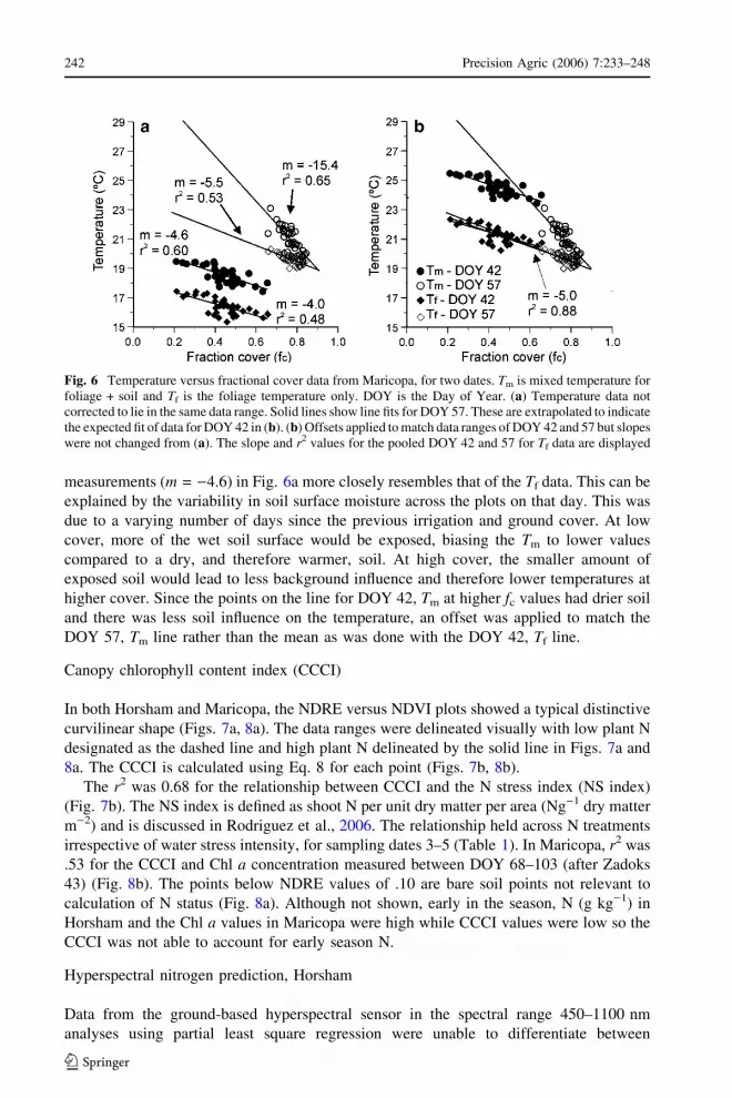
measurements (m = )4.6) in Fig. 6a more closely resembles that of the Tf data. This can be

explained by the variability in soil surface moisture across the plots on that day. This was

due to a varying number of days since the previous irrigation and ground cover. At low

cover, more of the wet soil surface would be exposed, biasing the Tm to lower values

compared to a dry, and therefore warmer, soil. At high cover, the smaller amount of

exposed soil would lead to less background influence and therefore lower temperatures at

higher cover. Since the points on the line for DOY 42, Tm at higher fc values had drier soil

and there was less soil influence on the temperature, an offset was applied to match the

DOY 57, Tm line rather than the mean as was done with the DOY 42, Tf line.

Canopy chlorophyll content index (CCCI)

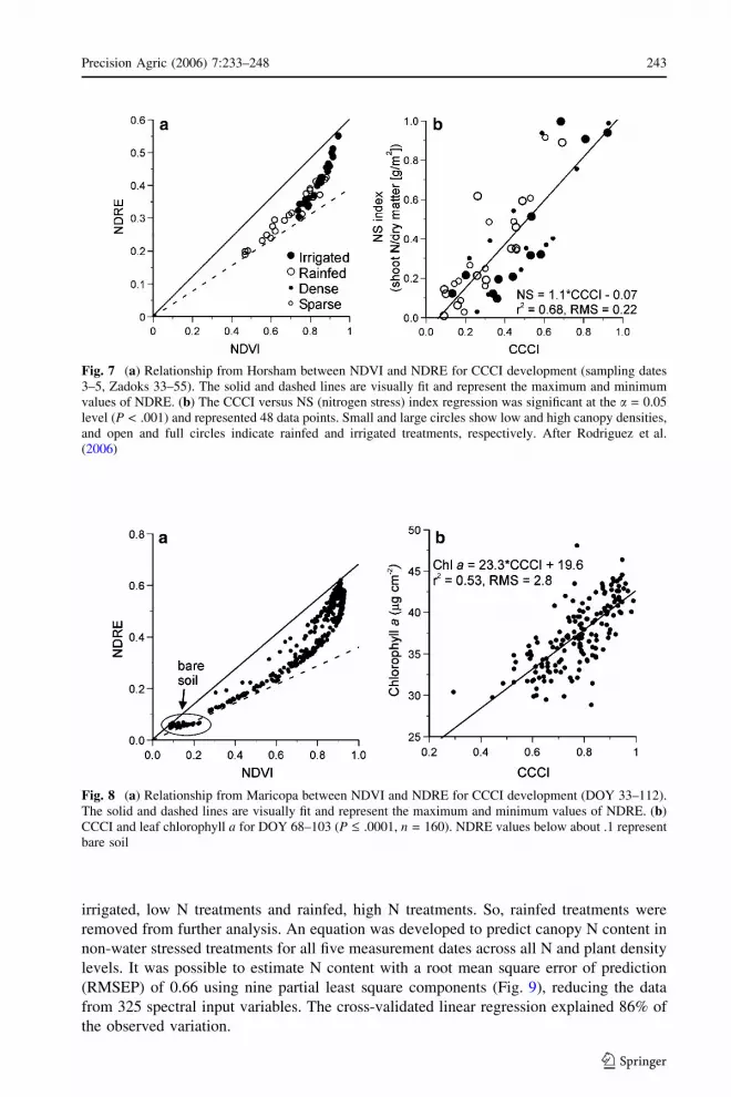
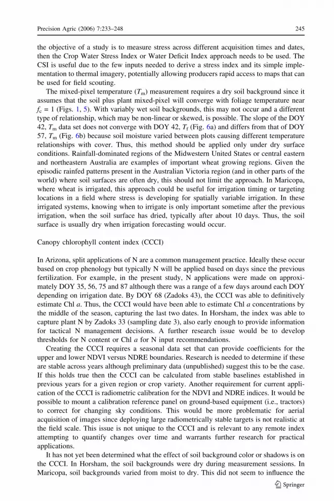
In both Horsham and Maricopa, the NDRE versus NDVI plots showed a typical distinctive

curvilinear shape (Figs. 7a, 8a). The data ranges were delineated visually with low plant N

designated as the dashed line and high plant N delineated by the solid line in Figs. 7a and

8a. The CCCI is calculated using Eq. 8 for each point (Figs. 7b, 8b).

The r2 was 0.68 for the relationship between CCCI and the N stress index (NS index)

(Fig. 7b). The NS index is defined as shoot N per unit dry matter per area (Ng)1 dry matter

m)2) and is discussed in Rodriguez et al., 2006. The relationship held across N treatments

irrespective of water stress intensity, for sampling dates 3–5 (Table 1). In Maricopa, r2 was

.53 for the CCCI and Chl a concentration measured between DOY 68–103 (after Zadoks

43) (Fig. 8b). The points below NDRE values of .10 are bare soil points not relevant to

calculation of N status (Fig. 8a). Although not shown, early in the season, N (g kg)1) in

Horsham and the Chl a values in Maricopa were high while CCCI values were low so the

CCCI was not able to account for early season N.

Hyperspectral nitrogen prediction, Horsham

Data from the ground-based hyperspectral sensor in the spectral range 450–1100 nm

analyses using partial least square regression were unable to differentiate between

Fig. 6 Temperature versus fractional cover data from Maricopa, for two dates. Tm is mixed temperature forfoliage + soil and Tf is the foliage temperature only. DOY is the Day of Year. (a) Temperature data notcorrected to lie in the same data range. Solid lines show line fits for DOY 57. These are extrapolated to indicatethe expected fit of data for DOY 42 in (b). (b) Offsets applied to match data ranges of DOY 42 and 57 but slopeswere not changed from (a). The slope and r2 values for the pooled DOY 42 and 57 for Tf data are displayed

242 Precision Agric (2006) 7:233–248

123

irrigated, low N treatments and rainfed, high N treatments. So, rainfed treatments were

removed from further analysis. An equation was developed to predict canopy N content in

non-water stressed treatments for all five measurement dates across all N and plant density

levels. It was possible to estimate N content with a root mean square error of prediction

(RMSEP) of 0.66 using nine partial least square components (Fig. 9), reducing the data

from 325 spectral input variables. The cross-validated linear regression explained 86% of

the observed variation.

Fig. 7 (a) Relationship from Horsham between NDVI and NDRE for CCCI development (sampling dates3–5, Zadoks 33–55). The solid and dashed lines are visually fit and represent the maximum and minimumvalues of NDRE. (b) The CCCI versus NS (nitrogen stress) index regression was significant at the a = 0.05level (P < .001) and represented 48 data points. Small and large circles show low and high canopy densities,and open and full circles indicate rainfed and irrigated treatments, respectively. After Rodriguez et al.(2006)

Fig. 8 (a) Relationship from Maricopa between NDVI and NDRE for CCCI development (DOY 33–112).The solid and dashed lines are visually fit and represent the maximum and minimum values of NDRE. (b)CCCI and leaf chlorophyll a for DOY 68–103 (P £ .0001, n = 160). NDRE values below about .1 representbare soil

Precision Agric (2006) 7:233–248 243

123

Discussion

Plant temperature has long been recognized as having potential to determine the water

status of crops (Idso, 1982; Jackson et al., 1981). For rainfed agroecosystems such as those

in Australia, seasonal rainfall is the main determinant of crop growth, response to in-crop

N applications and final grain yield. In addition, plant water availability can vary spatially

across the landscape by soil type, the presence of subsoil salinity (Rodriguez, Nuttall,

Sadras, Rees, & Armstrong, 2005a), soil strength (Sadras, O’Leary, & Roget, 2005) and

root diseases. In highly spatially variable environments, precision agriculture and variable

rate technologies are being considered as solutions to increase crop profitability, reduce

seasonal uncertainty and minimize unwanted losses of water and nutrients from the pro-

duction system.

For remote imagery to be useful, the fewest number of ground parameters must be

acquired and Tf cannot be practically measured during aerial overpasses of a sensor.

Because of meteorological variations (humidity, wind speed, etc.) and the mixed pixel

problem, Tf is the most difficult temperature parameter to measure remotely. The methods

presented in Rodriguez et al. (2005b) and extended here allow derivation of Tf based on

established relationships either between the DT (Tm ) Tf) and cover or soil temperature

outside the field (Tso) and soil temperature inside the crop (Tsi) (Maas et al., 2000).

Assuming one of these relationships is established, Tf can be determined and used as input

to water stress indices (Idso, 1982; Moran et al., 1994), which are fundamentally based on

foliage ) air temperature (Tf ) Ta). This relationship can then be applied to thermal

imagery to develop relative stress maps (Clarke, 1997) or a Crop Stress Index (CSI) as

presented by Rodriguez et al. (2005b).

The CSI is not a calibrated measure such as the Crop Water Stress Index (Idso et al.,

1981; Idso, 1982; Jackson et al., 1981) or the Water Deficit Index (Moran et al., 1994).

Calibrated measures of stress include maximum and minimum temperatures for Tf ) Ta

from derived stressed and unstressed baselines, allowing for temporal comparisons as the

stress develops. Therefore the CSI represents an instantaneous indication of the relative

spatial variation in ‘‘crop stress’’ or its physiological status, indicative of water stress or

any other stressors that cause the plants to close their stomata (Jackson et al., 1986) and

that most likely will limit the response of the crop to additional tactical N applications. If

Fig. 9 Measured versus predicted N using partial least square regression with hyperspectral data for theirrigated plots. The numbers 1–5 correspond to sampling dates 1–5, where 1 was the earliest growth stageand 5, the oldest

244 Precision Agric (2006) 7:233–248

123

the objective of a study is to measure stress across different acquisition times and dates,

then the Crop Water Stress Index or Water Deficit Index approach needs to be used. The

CSI is useful due to the few inputs needed to derive a stress index and its simple imple-

mentation to thermal imagery, potentially allowing producers rapid access to maps that can

be used for field scouting.

The mixed-pixel temperature (Tm) measurement requires a dry soil background since it

assumes that the soil plus plant mixed-pixel will converge with foliage temperature near

fc = 1 (Figs. 1, 5). With variably wet soil backgrounds, this may not occur and a different

type of relationship, which may be non-linear or skewed, is possible. The slope of the DOY

42, Tm data set does not converge with DOY 42, Tf (Fig. 6a) and differs from that of DOY

57, Tm (Fig. 6b) because soil moisture varied between plots causing different temperature

relationships with cover. Thus, this method should be applied only under dry surface

conditions. Rainfall-dominated regions of the Midwestern United States or central eastern

and northeastern Australia are examples of important wheat growing regions. Given the

episodic rainfed patterns present in the Australian Victoria region (and in other parts of the

world) where soil surfaces are often dry, this should not limit the approach. In Maricopa,

where wheat is irrigated, this approach could be useful for irrigation timing or targeting

locations in a field where stress is developing for spatially variable irrigation. In these

irrigated systems, knowing when to irrigate is only important sometime after the previous

irrigation, when the soil surface has dried, typically after about 10 days. Thus, the soil

surface is usually dry when irrigation forecasting would occur.

Canopy chlorophyll content index (CCCI)

In Arizona, split applications of N are a common management practice. Ideally these occur

based on crop phenology but typically N will be applied based on days since the previous

fertilization. For example, in the present study, N applications were made on approxi-

mately DOY 35, 56, 75 and 87 although there was a range of a few days around each DOY

depending on irrigation date. By DOY 68 (Zadoks 43), the CCCI was able to definitively

estimate Chl a. Thus, the CCCI would have been able to estimate Chl a concentrations by

the middle of the season, capturing the last two dates. In Horsham, the index was able to

capture plant N by Zadoks 33 (sampling date 3), also early enough to provide information

for tactical N management decisions. A further research issue would be to develop

thresholds for N content or Chl a for N input recommendations.

Creating the CCCI requires a seasonal data set that can provide coefficients for the

upper and lower NDVI versus NDRE boundaries. Research is needed to determine if these

are stable across years although preliminary data (unpublished) suggest this to be the case.

If this holds true then the CCCI can be calculated from stable baselines established in

previous years for a given region or crop variety. Another requirement for current appli-

cation of the CCCI is radiometric calibration for the NDVI and NDRE indices. It would be

possible to mount a calibration reference panel on ground-based equipment (i.e., tractors)

to correct for changing sky conditions. This would be more problematic for aerial

acquisition of images since deploying large radiometrically stable targets is not realistic at

the field scale. This issue is not unique to the CCCI and is relevant to any remote index

attempting to quantify changes over time and warrants further research for practical

applications.

It has not yet been determined what the effect of soil background color or shadows is on

the CCCI. In Horsham, the soil backgrounds were dry during measurement sessions. In

Maricopa, soil backgrounds varied from moist to dry. This did not seem to influence the

Precision Agric (2006) 7:233–248 245

123

CCCI but, by DOY 68, when the relationship with Chl a was significant, cover was nearly

complete. The spectral data were acquired at a constant solar zenith so sun angle differ-

ences, per se, did not affect the data. However, since the crop developed during the

measurement period, shadows became more complex during the season. Changes in soil

background, amount of shadows and canopy structure added to variability of the mea-

surements before canopy closure.

Combining information in the reflected light and emitted thermal regions of the spec-

trum could allow a new type of management option for producers—targeted application of

inputs based on the crop potential for utilization. Assuming that reliable indices can be

developed for crop N (or other factors) and water status, maps of regions within a field that

will be more responsive to a management input can be produced. These data could then be

input to variable rate equipment to target locations of optimal response for the input,

potentially reducing cost and impact to the environment due to off-site movement of

chemical, such as N into surface and ground waters.

Hyperspectral N estimation

In Horsham, hyperspectral measurements and the PLS data reduction technique successfully

estimated early season N (from Zadoks 14), whereas the CCCI could only estimate N after

Zadoks 33. However, the CCCI was able to estimate N under low water conditions in

Horsham whereas the hyperspectral approach was confounded. It is currently not known how

stable the hyperspectral relationship is and whether the regression coefficients can be gen-

eralized. More research is needed before it is can be determined whether a multispectral or

hyperspectral approach is superior for robust N status detection under low water conditions.

Conclusion

It is possible to identify areas of relative stress in producer’s fields due to water or other

factors that affect stomatal closure using thermal imaging technologies. In rainfed con-

ditions, this can be used to identify areas having potential for crop response to additional N

inputs. If combined with maps of crop N status, this technology could allow targeted

applications of N into those areas of higher potential response. Further research should

attempt to improve the relationships between N status and CCCI as well as test the

derivation of Tf more fully under various cropping systems and conditions. Under irrigated

systems, these methods could help target irrigation scheduling and N input timing. Full

implementation of a management scheme would additionally require quick image and

ancillary data processing and delivery to the producer as well as the ability to apply

variable rate N to the identified areas in a timely manner. Overall, the combination of

thermal and spectral information has the potential to improve in-season management under

spatially variable water and N stress conditions found in rainfed fields or just prior to an

irrigation cycle in irrigated crops.

Acknowledgments and Disclaimer The research in Horsham was funded by the Victoria Government,Our Rural Landscape Initiative, Australia. We fully acknowledge Russel Argall and Hemantha Rohitha fortheir technical assistance at running the field experiment and handling soil and plant samples in Horsham.We would also like to thank the personnel at the U.S. Water Conservation Laboratory for their advice, hardwork and dedication. Thanks also are extended to the reviewers who contributed to improving the manu-script. Mention of specific suppliers of hardware and software in this manuscript is for informative purposesonly and does not imply endorsement by the United States Department of Agriculture.

246 Precision Agric (2006) 7:233–248

123

References

Barnes, E. M., Clarke, T. R., & Richards, S. E. (2000). Coincident detection of crop water stress, nitrogenstatus and canopy density using ground based multispectral data. In P. C. Robert, R. H. Rust, & W. E.Larson (Eds.), Proceedings of the fifth international conference on precision agriculture. Madison, WI,USA: American Society of Agronomy, Unpaginated CD.

Blackmer, T. M., Schepers, J. S., & Varvel, G. E. (1994). Light reflectance compared with other N stressmeasurements in corn leaves. Agronomy Journal, 86, 934–938.

Carter, G. A., & Spiering, B. A. (2002). Optical properties of intact leaves for estimating chlorophyllconcentration. Journal of Environmental Quality, 31(5), 1424–1432.

Clarke, T. R. (1997). An empirical approach for detecting crop water stress using multispectral airbornesensors. Hortechnology, 7(1), 9–16.

Clarke, T. R., Moran, M. S., Barnes, E. M., Pinter P. J. Jr., & Qi, J. (2001). Planar domain indices: A methodfor measuring a quality of a single component in two-component pixels. In Proceedings IEEE inter-national geoscience and remote sensing symposium, 09–13 July, Sydney, Australia, unpaginated CD.

Daughtry, C. S. T., Walthall, C. L., Kim, M. S., De Colstoun, E. B., & Mcmurtrey, J. E. (2000). Estimatingcorn leaf chlorophyll concentration from leaf and canopy reflectance. Remote Sensing of Environment,74(2), 229–239.

Filella, I., & Penuelas, J. (1994). The red edge position and shape as indicators of plant chlorophyll content,biomass and hydric status. International Journal of Remote Sensing, 15(7), 1459–1470.

Fitzgerald, G. J., Pinter, P. J. Jr., Hunsaker, D. J., & Clarke, T. R. (2005). Multiple shadow fractions inspectral mixture analysis of a cotton canopy. Remote Sensing of Environment, 97, 526–539.

Gao, B.-C. (1996). NDWI – a normalized difference water index for remote sensing of vegetation liquidwater from space. Remote Sensing of Environment, 58, 257–266.

Huete, A. (1988). A soil-adjusted vegetation index (SAVI). Remote Sensing of Environment, 25(3), 295–309.

Idso, S. B., Jackson, R. D., Pinter, P. J., Reginatio, R. J., & Hatfield, J. L. (1981). Normalizing the stress-degree-day parameter for environmental variability. Agricultural Meteorology, 24(1), 45–55.

Idso, S. B. (1982). Non-water-stressed baselines: A key to measuring and interpreting plant water stress.Acricultural Meterorology, 27, 59–70.

Isbell, R. F. (1966). The Australian Soil Classification. Melbourne, Australia: CSIRO Publishing, 143 pp.Jackson, R. D., Idso, S. B., Reginato, R. J., & Pinter, P. J. (1981). Canopy temperature as a crop water stress

indicator. Water Resources Research, 17(4), 1133–1138.Jackson, R. D., Pinter, P. J., Reginato, R. J., & Idso, S. B. (1986). Detection and evaluation of plant stresses

for crop management decisions. IEEE Transactions on Geoscience and Remote Sensing, GE, 24(1), 99–106.

Kostrzewski, M., Waller, P., Guertin, P., Haberland, J., Colaizzi, P., Barnes, E., Thompson, T., Clarke, T.,Riley, E., & Choi, C. (2002). Ground-based remote sensing of water and nitrogen stress. Transactions ofthe ASAE, 46(1), 29–38.

Lichtenthaler, H. K., & Wellburn, A. R. (1983). Determination of total carotenoids and chlorophylls a and bof leaf extracts in different solvents. Biochemical Society Transactions, 11, 591–592.

Maas, S. J. (1998). Estimating cotton canopy ground cover from remotely sensed scene reflectance.Agronomy Journal, 90, 384–388.

Maas, S. J. (2000). Linear mixture modelling approach for estimating cotton canopy ground cover usingsatellite multispectral imagery. Remote Sensing Environment, 72, 304–308.

Maas, S., Fitzgerald, G., & DeTar, W. (2000). Determining cotton leaf canopy temperature using multi-spectral remote sensing. In Proceedings of the cotton beltwide conferences (pp. 623–626). NationalCotton Council, Memphis, TN, USA.

Maracchi, G., Zipoli, G., Pinter, P. J. Jr., & Reginato, R. J. (1988). Water stress effects on reflectance andemittance of winter wheat. In Proceedings of the eighth EARSEL symposium. Capri (Naples), Italy, 17–20 May.

Moran, M. S., Pinter, P. J., Clothier, B. E., & Allen, S. G. (1989). Effects of water stress on the canopyarchitecture and spectral indices of irrigated alfalfa. Remote Sensing of Environment, 29, 251–261.

Moran, M. S., Clarke, T. R., Inoue, Y., & Vidal, A. (1994). Estimating crop water deficit using the relationbetween surface-air temperature and spectral vegetation index. Remote Sensing of Environment, 49,246–263.

Osborne, S. L., Schepers, J. S., Francis, D. D., & Schlemmer, M. R. (2002). Detection of phosphorus andnitrogen deficiencies in corn using spectral radiance measurements. Agronomy Journal, 94, 1215–1221.

Penuelas, J., Filella, I., Biel, C., Serrano, L., & Save, R. (1993). The reflectance at the 950–970 nm region asan indicator of plant water status. International Journal Remote Sensing, 14(10), 1887–1905.

Precision Agric (2006) 7:233–248 247

123

Penuelas, J., Gamon, J. A., Fredeen, A. L., Merino, J., & Field, C. B. (1994). Reflectance indices associatedwith physiological changes in nitrogen – and water limited sunflower leaves. Remote Sensing ofEnvironment, 48, 135–146.

Pettigrew, W. T. (2004). Physiological consequences of moisture deficit stress in cotton. Crop Science, 44,1265–1272.

Pinter, P. J. Jr., Idso, S. B., Hendrix, D. L., Rokey, R. R., Rauschkolb, R. S., Mauney, J. R., Kimball, B. A.,Hendrey, G. R., Lewin, K. F., & Nagy, J. (1994). Effect of free-air CO2 enrichment on the chlorophyllcontent of cotton leaves. Agricultural and Forest Meteorology, 70, 163–169.

Post, D. F., Mack, C., Camp, P. D., & Sulliman, A. S. (1988). Mapping and characterization of the soils onthe University of Arizona, Maricopa Agricultural Center. In Proceedings of hydrology and waterresources in Arizona and the Southwest (pp. 49–60). The University of Arizona, Tucson, AZ, USA.

Rodriguez, D., Nuttall, J., Sadras, V., Rees, H. van, & Armstrong, R. (2005a). Impact of subsoil constraintson wheat yield and gross margin on fine-textured soils of the southern Victorian Mallee. AustralianJournal of Agricultural Research, 57(3), 335–365.

Rodriguez, D., Sadras, V. O., Christensen, L. K., & Belford, R. (2005b). Spatial assessment of the phy-siological status of wheat crops as affected by water and nitrogen supply using infrared thermalimagery. Australian Journal Agricultural Research, 56, 983–993.

Rodriguez, D., Fitzgerald, G. J., & Belford, R. (2006). Detection of nitrogen deficiency in wheat fromspectral reflectance indices and basic crop eco-physiological concepts. Australian Journal AgriculturalResearch, 57(7), (in press).

Sadras, V. O., O’Leary, G. J., & Roget, D. K. (2005). Crop responses to compacted soil: Capture andefficiency in the use of water and radiation. Field Crops Research, 91, 131–148.

Strachan, I. B., Pattey, E., & Boisvert, J. B. (2002). Impact of nitrogen and environmental conditions on cornas detected by hyperspectral reflectance. Remote Sensing Environment, 80, 213–224.

Zadoks, J. C., Chang, T. T., & Konzak, C. F. (1974). A decimal code for the growth stages of cereals. WeedResearch, 14, 415–421.

248 Precision Agric (2006) 7:233–248

123