speaker count application for smartphone platforms

Speaker Count Application for Smartphone

Platforms

Alessio Agneessens, Igor Bisio, Member, IEEE, Fabio Lavagetto, Mario Marchese, Senior Member, IEEE, Andrea Sciarrone

Department of Communications, Computer and Systems Science, University of Genoa, via dell’Opera Pia 13,

16145, Genoa, Italy

phone: +39-353-2983; fax: +39-353-2154; e-mail: for all authors : [email protected]

� Abstract��

�� !�� "� �� #�� #�� $�� "�� "�� #��

Index Terms��%�� &� �� " � $��$�� &� $�� &� '�� '��&�'��( � ��

I. INTRODUCTION

NTERDISCIPLINARY advances are required to innovate in

the field of pervasive computing and networking: new

communication and networking solutions, new and less

complex operating systems, miniaturized memorization

capacity, efficient signal processing and context aware

solutions. Context-aware applications are highly customizable

services tailored to the user’s preferences and needs and

relying on the real-time knowledge of the user’s surroundings,

without requiring complex configuration on the user’s part. In

this view, smartphones can be considered versatile devices

and offer a wide range of possible uses. Their technological

evolution, combined with their increasing diffusion, gives

mobile network providers the opportunity to come up with

more advanced and innovative services. In order to provide

context-aware services over smartphones, a description of

mobile device environment must be obtained by acquiring and

combining context data from different sources. Even if there

are not yet available applications on smartphones, the number

of active speakers in the surroundings can be useful context

information. Determining the number of speakers participating

in a conversation, which is the Speaker Count (SC) problem,

poses a greater challenge, on one hand, when no information

about the speakers is available [1] and, on the other hand, if

computational and energetic resources are limited as in the

smartphones’ case. Several speaker count algorithms have

been designed, both for closed- and open-set applications. In

the former case, speaker count implies the classification of

data belonging to speakers whose identity is known, while in

the open-set scenario there is no available a priori knowledge

on the speakers.

This work was supported in part by the Telecom Italia Laboratories

(TILab).

Although in many cases promising results have been

obtained for speaker count, available methods are not

specifically designed for mobile devices and their

computational requirements do not take into account the

limited smartphone processing power and the time

requirements of context-aware applications (e.g., [1]).

This paper presents a simple speaker count algorithm

designed to recognize single-speaker (1S) recordings from

two-speaker (2S) recordings operating in open-set scenarios.

The paper is organized as follows. A brief review of various

speaker count methods proposed in the literature is provided

in Section II. The proposed speaker count algorithm is

described in Section III. Experimental results also in terms of

recognition time, computational complexity, and battery

consumption are presented in Section IV, which also includes

audio recording database used for classifier training and

testing. The conclusions are contained in Section V.

II. RELATED WORK

Many of the existing speaker count methods are based on

the calculation of spectral features, e.g. linear predictive

cepstral coefficients [2], line spectral pairs, log-area ratio,

mel-frequency cepstral coefficients [3], area coefficients,

reflection coefficients [4]. The speaker count method

presented in [5] employs a feature derived from the time-

domain of the audio signal: the pitch estimation. Most

algorithms use the classification of individual speech signal

segments through classifiers such as Vector Quantizers [5],

GMMs and Neural Tree Networks [4].

The percentages of correct recognition of the number of

speakers obtained by the evaluated speaker count methods

taken from the literature are shown in Table I.

I

2010 5th International Symposium on Wireless Pervasive Computing (ISWPC)

978-1-4244-6857-7/10/$26.00 ©2010 IEEE 361

TABLE I

CLASSIFICATION ACCURACIES (PERCENT) OBTAINED BY THE EVALUATED

SPEAKER COUNT METHODS

Reference Classes Closed Set Open Set

1S vs. more than 1S - 92.5

1S vs. 2S vs. more than 2S - 77.5 [2] 1S vs. 2S vs. 3S vs. 4S - 63

1S vs. 2S - 79.6

1S vs. 2S vs. 3S - 72.3 [3] 1S vs. 2S vs. 3S vs. 4S - 62.5

[5] 1S vs. 2S 83.5 64.4

However, all the above-mentioned methods are hardly

applicable on smartphones. Their computational load is heavy.

Algorithms that consider the limited processing power of

smartphones and the time requirements of context-aware

applications are strongly necessary.

III. PROPOSED SPEAKER COUNT (SC) METHOD

A. Proposed Speaker Count Algorithm The proposed speaker count method is designed to distinguish

one-speaker audio recordings (1S) from two-speaker ones

(2S). It is designed to operate in an open-set scenario and is

based on audio recording pitch estimation.

The signal to be classified as one or two speaker is

identified as � � , 1,...,s n n N� . The SC method introduced in

this paper is composed of the following steps.

1) The signal � �s n is divided into frames.

2) The pitch frequency for each frame is estimated.

3) A number of frames of � �s n is grouped into blocks.

4) The pitch PDF (Probability Density Function) is

estimated for each block.

5) Features are extracted from each pitch PDF.

6) The decision about one or two speaker audio recording is

taken for each block by a Gaussian Mixture Model

(GMM) classifier on the base of the extracted pitch

features. Once all blocks are classified, the whole audio

recording is assigned to the class to which the majority of

blocks have been assigned.

The main novelty of this paper stands in points 2, 4, and 5, as

well as in the practical implementation of the designed SC

method on smartphones available off the shelf.

B. Pitch Frequency Estimation The fundamental frequency of a periodic signal is defined

as the reciprocal of its period. For audio signals such as

speech, which exhibit a relative periodicity, the fundamental

frequency is also referred to as pitch.

Given the real-value discrete-time signal of length , N� � � �0, 1s n n N� , its autocorrelation is defined as

(1) � � � � � � � �1

0

0,1,..., 1N

nR s n s n

�� N

Being in the case of audio speech signals, the set of possible

samples of the autocorrelation function can be reduced. [6]

reports that the pitch of a speech signal, due to physiological

reasons, is contained in a limited range � �1 2,P P with 1 50P �

Hz and 2P 500� Hz. It limits the range between the two

following values:

1 22 1

s sF F and

P P

� �

��

� � � � (2)

where sF is the sampling frequency applied to the original

analog signal to obtain the discrete-time signal � �s n . In

practice, the applied autocorrelation definition is:

� � � � � �1

0

2 2 2 1

ˆ

, 1, 2,...,

N

n

s s s s

R s n s n

F F F F

P P P P

��

� � � � � ��

� (3)

From the computational viewpoint, the physiological

limitation of the pitch range implies a first significant

reduction of the number of samples involved in the

computation and, as a consequence, of the overall complexity.

Pitch is linked to signal periodicity. The autocorrelation shows

how well the signal correlates with itself at a range of

different delays. So, given a “sufficiently periodical” speech

recording, its autocorrelation will present its highest value at

delays corresponding to multiples of pitch periods [6].

Being the pitch period defined as in (4),

� �ˆarg max

�pitch R (4)

the pitch is defined as

�

� spitch

pitch

F (5)

To further reduce the computational complexity of the pitch

estimation method, a downsampled version of the

autocorrelation function is introduced in this paper by using a

downsampling factor . Being the cardinality of the

original set of autocorrelation samples the downsampled

version uses

r N

K rN� samples. In practice the downsampled

autocorrelation is defined as:

� � � � � �1

0

2 2 2 1

1 2, , ,...,

N

n

s s s s

R x n x n

F F F F

P P r P r P

��

� � � � � ��

��

(6)

It means that � �R � considers just one sample of � �R̂ out

of 1

r in the interval

2 1

,...,s sF FP P

� � � � � � � ��

. In consequence,

� �Rarg maxpitch

�� and spitch

pitch

F �

��

�. In order to still

correctly determine the maximum of the full autocorrelation,

thus preventing errors in pitch estimation, a maximum “Fine

Search” method has been designed and implemented in this

362

paper to partially compensate the inaccuracies introduced by

downsampling . Starting from the delay corresponding to the

pitch obtained by the downsampled autocorrelation function

pitch� , the values of � �R̂ , in (3), are computed for values

adjacent to pitch� up to a depth of 1 1� r . Their maximum is

taken as new pitch period pitch �

� �

. Analytically:

1ˆ 11,..., 1h pitchr rR � � � � �arg max

, � �pitch� pitc � �� (7)

spitch

pitc

F � h

�� (8)

pit�� ch is the reference pitch value for the reminder of this

paper.

C. PDF Estimation

� � , 1,� ...,s n Nn is first divided into �

��

NFL

abutted

-sample frames. A pitch estimate is computed for each

frame by applying the described method. Sets of

consecutive frames are grouped together in blocks, in order to

allow the computation of a pitch PDF for each block.

LD

Consecutive blocks are overlapped by V frames (i.e., the

last V frames of a block are the first V of the following one)

in order to take into account the possibility of a signal portion

representing fully voiced speech falling across consecutive,

non-overlapping blocks, and therefore its contributions to the

classification process being divided between the two blocks.

This means there are a total of � � � �� B F V D V

blocks. The -th block is defined as . For each block

there are V pitch values computed as in (8) identified as

t tb tb

,tb vpitch�

,tb v

, . The PDF for block spans a frequency

interval ranging from the minimum to the maximum computed

pitch value. Such frequency interval is divided into H smaller

frequency bins of size Hz that is determined through

extensive tests. is the variable identifying the frequency.

1,...,v

p

V� tb

p�

The PDF for each block is estimated by a weighted

count of the number of occurrences of single

tb

pitch� , v within each frequency bin . 1� ,...,

� �

V 0,..., 1h H�

In short:

� �11

0hw re� � 2

H

h

p h pPD

p

�

� ��

�F p

hw

ct �

h

(9)

hw is the coefficient associated to the h t bin and

implements the mentioned weighted count, as explained in the

following. If is the number of

,tb vpitch� , , whose

values fall within the bin, then the PDF is simply

computed through the number of occurrences and is called

“histogram count”.

1,...,v � V

h t h

In order to have a more distinct PDF and, consequently,

more accurate features vectors, this paper links the coefficient

to the energy distribution of the signal hw ( )s n in the

frequency range where the PDF of a block is spanned. Given

the Discrete Time Fourier Transform (DTFT) of the signal

( )s n , 1

2

0

( ( )) ( ) ( )N

j nf

nDTFT s n S f s n e �

�

� � �� , � �1 2,f P P� ,

with 1 50P Hz� and 2 500P Hz� , as defined in the previous

subsection; given the definition of signal energy and the

Parseval relation,

121

2 2 df0

( )N

sn

E s n

�

� ��1

2

( )S f�

�

� �

, the energy

component at a given frequency is 2

S f . To evaluate the

energy component of each frequency bin h , we would need to

know the energy contribution carried by each pitch occurring

within bin . In practice, we would need h � � 2,tb v

pitchS � ,

1,...,v V � .

But � �S f is a continuous function. It must be substituted

by its sampled version, the Digital Fourier Transform (DFT)

to be practically computed and used. The DFT of signal � �s n

is defined as � �� 1 2

0

kN j nN

nDFT s n S k s n e

�

�

� � �� ,

0,...,k 1N � . The problem is that the DFT is a function of

an integer number k while . So, to allow the

computation,

,tb vpitch� ��

,tb vpitch� is approximated in this paper with the

closest integer number defined as follows: ,

,inttb v

pitch�

, , ,

,

,int

, , ,

1, if

2

1, if

2

t t t

t

t t t

b v b v b vpitch pitch pitch

b vpitch

b v b v b vpitch pitch pitch

� � ��

� � �

! � � "#� � � �#� $#� � � % � � �#&

(10)

The coefficient is defined as hw

� �

� �,

,

2,

,int

1 2,

,int

0

bt v bin hpitch

bt v bin hpitch

bt vpitch

h Hbt vpitch

h

Sv

wS

v

�

�

�

�

�

�

�

�

�

� � (11)

This assignment of is used in the reminder of the paper. hwThis idea leads to more distinct PDFs and more accurate

features vectors, thus significantly improving the SC method

performance compared to computing PDFs by simply

executing a “histogram count”.

D. Features Definition In order to determine the best feature vector that

maximizes the efficiency of the proposed SC method,

different feature vectors may be evaluated by combining

different individual features representing the block PDF

�

363

dispersion. The evaluated features are the PDF maximum

given by (12), the PDF mean computed according to (13),

where is the central frequency of the bin, the PDF

standard deviation defined in (14) and the absolute value,

reported in (15), of the difference between the PDF mean and

the central frequency of the bin containing the PDF maximum.

chp h th

0,..., H�

max max 1hh

PDF w h�

�

(12)

1

0

Hc

mean h hh

PDF p w

�� (13)

�1 2

meanF. .0

Hc

St Dev h hh

PDF p PD w

�� (14)

max

chp�

max arg max

disp mean

hh

PDF PDF

h w� (15)

� may be composed by using, for example, subsets of the

features mentioned above as tested in the performance

evaluation section.

E. Gaussian Mixture Model Classification Feature vector is employed to classify a block as either

1S or 2S, which are the considered speaker classes, through

the Gaussian Mixture Model (GMM) classifier known in the

literature. Once all individual blocks have been classified, the

whole audio recording is classified through a “majority vote”

decision: the chosen class is the one to which most blocks

have been assigned.

�

IV. PERFORMANCE INVESTIGATION

A. Audio Recording Database Training and testing of the classifiers are carried out using a

database of audio recordings acquired with a smartphone

audio-recording application. The overall dataset is composed

of audio recordings referred to five different situations: 1

Male speaker (1M), 1 Female speaker (1F), 2 Male speakers

(2M), 2 Female speakers (2F) and 2 mixed speakers (2MF).

The database is acquired using a 22 KHz sampling frequency

and 16 bits per sample, and all recordings are 4.5 s long. All

audio recordings refer to different speakers in order to

evaluate the classifier performances using data deriving from

speakers that have not influenced classifier training (open-set

application). A total of 50 recordings is acquired, 10 for each

situation. The starting section of each recording is deleted in

order to remove spurious signal peaks due to the turning-on

phase of the smartphone microphone. As a consequence, not

all recordings have the same amount of samples.

For the SC classifier, half of the recordings for each of the

five situations is used for GMM training, the other half for

testing.

B. Parameters Setting During the experiments, the frame size is set to 2048

samples. The block size is set to 20 frames. The number of

blocks for each recording varies between 3 and 4 due to the

different length in terms of amount of samples. The overall

dataset is composed of 194 blocks. The block overlap V is set

to 10 frames, a trade-off between having many, heavily-

overlapped blocks (which implies consecutive blocks bearing

redundant information and added computational load) and

few, slightly-overlapped blocks with the risk of having signal

sections representing fully voiced speech fall across

consecutive blocks.

LD

Pitch values in the range 50 Hz - 500 Hz are considered as

suggested in [6] and individual bins represent intervals of

approximately 10 Hz.

h

Starting from the computed PDF, feature vectors are

computed as detailed previously. PDFs and feature vectors

depend on the pitch estimation method and, as a consequence,

are influenced by its tuning. The downsampled autocorrelation

function in (6) is employed in this paper. The downsampling

may impact the precision of the overall method and therefore

its performance. To define the best trade-off between

precision and computational load, several tests have been

carried out by comparing the features obtained through the

full autocorrelation function and through the downsampled

one.

Downsampling factors 1 1 1 1 1 12 3 4 5 6 7

, , , , ,r � have been tested.

Related figures are not reported for the sake of synthesis; 15

r � represents the best compromise and it is the

downsampling factor used in the tests whose results are

discussed in the following.

C. Speaker Count Results Different feature vectors have been evaluated to select the

most discriminating one. The required classification is

between 1 Speaker (1S) or 2 Speakers (2S). After a deep

analysis, the feature vector ultimately used for GMM

classification is ' (max . .,�� St DevPDF PDF , which not only

leads to the best block classification performance but also

requires the computation of only two features, thus reducing

the computational load.

Table II reports the percentage of correct classification for

1S and 2S by using the whole dataset.

TABLE II

CORRECT CLASSIFICATION PERCENTAGE OF WHOLE TEST RECORDING FOR 1

AND 2 SPEAKERS ( ' (max . ., St DevPDF PDF�� )

)�� 1S 2S

1S 60% 40%

$� �

��

2S 40% 60%

Correct Classification (average): 60%

364

The obtained percentages are not so far from the results for

the same 1S vs 2S case through the other available open-set

algorithms reported in Table I, but the speaker count classifier

based on the feature vectors previously described leads to

results that do not live up to our expectations. Most of

classification errors happened in the cases 2M and 2F that can

be misclassified as 1M and 1F respectively. The motivation is

that same-gender speakers could have pitch estimates close

enough in value to lead to 2S PDFs similar to 1S PDFs of the

same gender. This observation has brought to the design of a

new GMM SC classifier, in order to distinguish not two

classes (1S and 2S) but three gender-based classes: 1M, 1F

and 2MF. The scheme is called SC classifier 1F-1M-2MF to

avoid confusion with the 1S-2S case. The case 2M and 2F,

which is still a problem, is not considered for now and its

investigation is left to further research. Again, different

feature vectors are evaluated. The best performance has been

provided by 2-dimensional feature vectors

and .

Anyway, independently of the feature vector, the only

classification errors involve exclusively class 2MF, i.e. test

recording blocks belonging to classes 1M and 1F have never

been mistaken one for another.

' (,mean dispPDF PDF�� ' max,�� meanPDF PDF (

(

(

The feature vector ultimately used for GMM classification is

, since it leads to the best test set

classification and, unlike ,

classifies 1F and 1M test recordings with comparable

accuracies. Table III contains the classification results by

using the test recordings of the whole dataset. Table IV

displays the classification results shown in Table III mapped

to the two-class (1S and 2S) SC, for a better comparison with

the results shown in Table II. As can be seen, the new 1F-1M-

2MF scheme does indeed lead to better performance.

' max,�� meanPDF PDF

' ,�� mean dispertionPDF PDF

This SC scheme performance is comparable (and, in one

case, better) with the other methods in the literature (Table I)

for similar sets of classes. It is important to remind that the

methods in Table I are hardly implementable on smartphones

because they imply a number of operations incompatible with

the computation capacity of a smartphone.

Concerning the use of the full autocorrelation instead of the

downsampled one, it does not provide clear performance

benefit, as better focused in the next sub-section.

TABLE III

CORRECT CLASSIFICATION PERCENTAGE OF WHOLE TEST RECORDING FOR

1F, 1M, AND 2MF ( ' (max,meanPDF PDF�� )

)��

1F 1M 2MF

1F 40% 0% 60%

1M 0% 80% 20%

$� �

��

2MF 20% 0% 80%


TABLE V

CORRECT CLASSIFICATION PERCENTAGE OF WHOLE TEST RECORDING FOR

1F, 1M, AND 2MF ( ' (max,meanPDF PDF�� ) MAPPED ON 1S -2S SC

)�� 1S 2S

1S 60% 40%

$� �

��

2S 20% 80%


D. Computational Time and Energy Consumption Analysis A Symbian OS application implementing the SC algorithm

has been designed as part of this study.

The smartphone used for all the experiments is a Nokia N95

with Symbian S60 3rd Edition, Feature Pack 1 operating

system. This kind of mobile phone is popular because of its

usability and its interesting features. Its most important

technical parameters are:

� Battery: Nokia (BL-5F) 950 mAH, 3.7 V;

� Dynamic Memory: 160 MB;

� Processor: RM-159 TI OMAP 2420 ARM-11 330

MHz.

Experiments have been carried out in order to evaluate the

performance of the proposed SC approach also in terms of

computational load and energy consumption. The chosen

metrics are the Recognition Time (RT) in s and the Residual

Battery Lifetime (RBL) in hours. The SC algorithm has been

compared to another version that does not implement

autocorrelation downsampling to emphasize the advantages of

the design choices proposed in this work. The two options are

identified as:

� Version 1, where the autocorrelation function is

downsampled and the pitch is computed through

equations (6) and (7) with 15

�r . It is the proposed SC

approach.

� Version 2, where the autocorrelation function is not

downsampled and is computed as in equation (3).

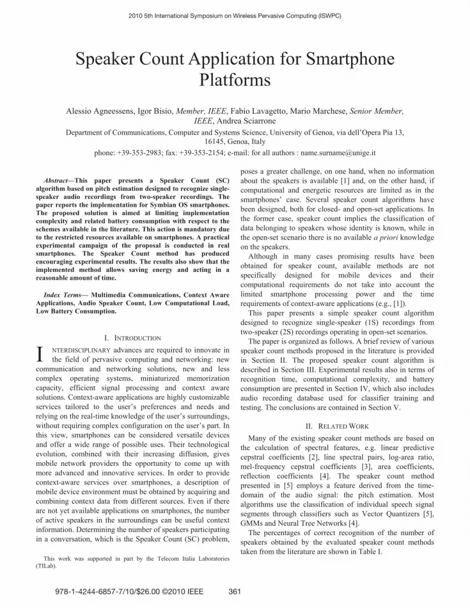
Figure 1 shows the overall Recognition Time RT (in

seconds) for the SC scheme as well as its main components:

the time required to compute the pitch, the DFT, and the other

operations to complete the algorithm. It has been separated

into the three contributions for the sake of clearness and to

allow a deeper investigation and possible further

improvements. The overall value is the average of the values

obtained from a set of 15 runs of the algorithm. It is worth

noting that an overall RT of 2.73 s, measured on real

smartphones, is compliant with most current context-aware

applications.

Computing a non-downsampled autocorrelation as in

Version 2 increases the pitch computation time to 5.79 s and

the overall RT to 7.28 s, 266.67% more of Version 1. On the

other hand, from the recognition percentage viewpoint

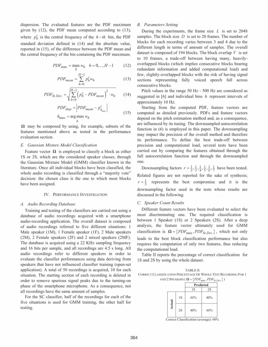
365

In the conditions previously introduced, the proposed SC

algorithm, running in a 30 s windows, allows a Residual

Battery Lifetime of 8.33 hours. This is a very satisfactory

result. Version 2 guarantees a RBL below 6 hours. In short:

the SC scheme guarantees a good recognition percentage,

performs the action in a reasonable amount of time (about 2.7

s), and saves a significant amount of RBL.

Version 2 does not give a meaningful advantage with respect

to Version 1. It is slightly above the 70% measured for

Version 1. Nevertheless, the significant advantage in terms of

both RT and RBL (detailed in the following) justifies a few

less correct recognition percentage points.

2.73

1.24

1.10

0.39

0.0

0.5

1.0

1.5

2.0

2.5

3.0

Pitch wh

coefficients

Other

Operations

RT

Tim

e [s

]

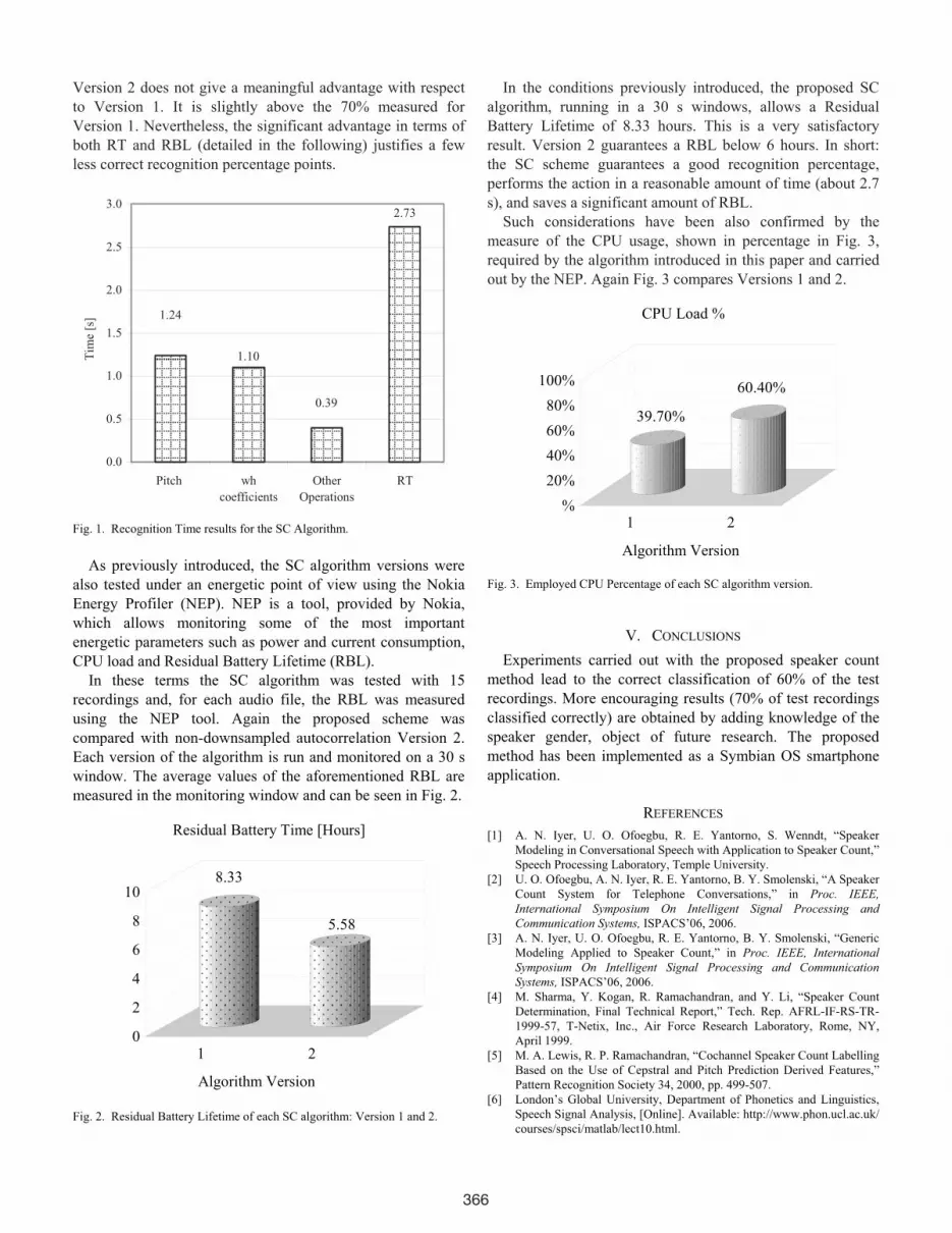
Such considerations have been also confirmed by the

measure of the CPU usage, shown in percentage in Fig. 3,

required by the algorithm introduced in this paper and carried

out by the NEP. Again Fig. 3 compares Versions 1 and 2.

39.70%

60.40%

%

20%

40%

60%

80%

100%

1 2

Algorithm Version

CPU Load %

Fig. 3. Employed CPU Percentage of each SC algorithm version.

Fig. 1. Recognition Time results for the SC Algorithm.

As previously introduced, the SC algorithm versions were

also tested under an energetic point of view using the Nokia

Energy Profiler (NEP). NEP is a tool, provided by Nokia,

which allows monitoring some of the most important

energetic parameters such as power and current consumption,

CPU load and Residual Battery Lifetime (RBL).

V. CONCLUSIONS

Experiments carried out with the proposed speaker count

method lead to the correct classification of 60% of the test

recordings. More encouraging results (70% of test recordings

classified correctly) are obtained by adding knowledge of the

speaker gender, object of future research. The proposed

method has been implemented as a Symbian OS smartphone

application.

In these terms the SC algorithm was tested with 15

recordings and, for each audio file, the RBL was measured

using the NEP tool. Again the proposed scheme was

compared with non-downsampled autocorrelation Version 2.

Each version of the algorithm is run and monitored on a 30 s

window. The average values of the aforementioned RBL are

measured in the monitoring window and can be seen in Fig. 2. REFERENCES

8.33

5.58

0

2

4

6

8

10

1 2

Algorithm Version

Residual Battery Time [Hours]

Fig. 2. Residual Battery Lifetime of each SC algorithm: Version 1 and 2.

[1] A. N. Iyer, U. O. Ofoegbu, R. E. Yantorno, S. Wenndt, “Speaker

Modeling in Conversational Speech with Application to Speaker Count,”

Speech Processing Laboratory, Temple University.

[2] U. O. Ofoegbu, A. N. Iyer, R. E. Yantorno, B. Y. Smolenski, “A Speaker

Count System for Telephone Conversations,” in Proc. IEEE, International Symposium On Intelligent Signal Processing and Communication Systems, ISPACS’06, 2006.

[3] A. N. Iyer, U. O. Ofoegbu, R. E. Yantorno, B. Y. Smolenski, “Generic

Modeling Applied to Speaker Count,” in Proc. IEEE, International Symposium On Intelligent Signal Processing and Communication Systems, ISPACS’06, 2006.

[4] M. Sharma, Y. Kogan, R. Ramachandran, and Y. Li, “Speaker Count

Determination, Final Technical Report,” Tech. Rep. AFRL-IF-RS-TR-

1999-57, T-Netix, Inc., Air Force Research Laboratory, Rome, NY,

April 1999.

[5] M. A. Lewis, R. P. Ramachandran, “Cochannel Speaker Count Labelling

Based on the Use of Cepstral and Pitch Prediction Derived Features,”

Pattern Recognition Society 34, 2000, pp. 499-507.

[6] London’s Global University, Department of Phonetics and Linguistics,

Speech Signal Analysis, [Online]. Available: http://www.phon.ucl.ac.uk/

courses/spsci/matlab/lect10.html.

366

speaker count application for smartphone platforms

Documents