spatial-contextual supervised classifiers explored: a challenging example of lithostratigraphy...

IEEE JOURNAL OF SELECTED TOPICS IN APPLIED EARTH OBSERVATIONS AND REMOTE SENSING, VOL. 8, NO. 3, MARCH 2015 1371

Spatial-Contextual Supervised Classifiers Explored:A Challenging Example of Lithostratigraphy

ClassificationMatthew J. Cracknell and Anya M. Reading

Abstract—Spatial-contextual classifiers exploit characteristicsof spatially referenced data and account for random noise thatcontributes to spatially inconsistent classifications. In contrast,standard global classifiers treat inputs as statistically independentand identically distributed. Spatial-contextual classifiers have thepotential to improve visualization, analysis, and interpretation:fundamental requirements for the subsequent use of classificationsrepresenting spatially varying phenomena. We evaluate randomforests (RF) and support vector machine (SVM) spatial-contextualclassifiers with respect to a challenging lithostratigraphy classifica-tion problem. Spatial-contextual classifiers are divided into threecategories aligned with the supervised classification work flow:1) data preprocessing—transformation of input variables usingfocal operators; 2) classifier training—using proximal trainingsamples to train multiple localized classifiers; and 3) postreg-ularization (PR)—reclassification of outputs. We introduce newvariants of spatial-contextual classifier that employ self-organizingmaps to segment the spatial domain. Segments are used to trainmultiple localized classifiers from k neighboring training instancesand to represent spatial structures that assist PR. Our exper-imental results, reported as mean (n = 10) overall accuracy±95% confidence intervals, indicate that focal operators (RF0.754 ±0.010, SVM 0.683 ±0.010) and PR majority filters (RF0.705 ±0.010, SVM 0.607 ±0.010 for 11 × 11 neighborhoods)generate significantly more accurate classifications than stan-dard global classifiers (RF 0.625 ±0.011, SVM 0.581 ±0.011).Thin and discontinuous lithostratigraphic units were best resolvedusing non-preprocessed variables, and segmentation coupled withpostregularized RF classifications (0.652 ±0.011). These methodsmay be used to improve the accuracy of classifications across awide variety of spatial modeling applications.

Index Terms—Decision trees, geology, geophysics, spatial filters,supervised learning, support vector machines (SVMs).

I. INTRODUCTION

S PATIAL-CONTEXTUAL supervised classifiers constitutean emerging field of research in geological remote sens-

ing applications [1]. Unlike standard global classifiers, which

Manuscript received May 05, 2014; revised October 27, 2014; acceptedDecember 05, 2014. Date of publication January 22, 2015; date of currentversion March 27, 2015. This work was conducted at the Australian ResearchCouncil (ARC) Centre of Excellence in Ore Deposits (CODES) and Schoolof Physical Sciences (Earth Sciences), University of Tasmania, under ProjectP3A3A. The work of M. J. Cracknell was supported by the University ofTasmania Elite Ph.D. Scholarship.

The authors are with the School of Physical Sciences (Earth Sciences) andARC Centre of Excellence in Ore Deposits (CODES), University of Tasmania,Hobart, Tasmania 7001, Australia (e-mail: [email protected]; [email protected]).

Color versions of one or more of the figures in this paper are available onlineat http://ieeexplore.ieee.org.

Digital Object Identifier 10.1109/JSTARS.2014.2382760

treat spatially distributed samples (pixels) as statistically inde-pendent and identically distributed [2], [3], spatial-contextualclassifiers exploit the spatial heterogeneity and spatial depen-dencies commonly encountered in spatial processes [4]–[7].Spatial heterogeneity refers to a nonstationary spatial processthat exhibits contrasting local statistical properties across agiven domain or region. This requires different parametersto characterize adequately nonstationary processes or mod-els at various locations [3], [8]–[11]. Spatial dependency, firstdescribed by Tobler [12], refers to the characteristic of spatiallydistributed variables to display autocorrelation, i.e., measure-ments that are close together in space are more likely to besimilar than those farther apart [3], [10], [11], [13].

Lithostratigraphic units share common lithological charac-teristics and are the fundamental classes for geological map-ping. Lithostratigraphic units also indicate specific intervalsof geologic time although the concept of time has little rele-vance in classifying these units and their boundaries [14]. Inthis study, the classification target represents generalized lithos-tratigraphic units with similar lithological attributes, i.e., sed-imentary materials, igneous mineralogy, metamorphic grade,and units with comparable stratigraphic positions. While usefulfor interpreting tectonic histories and prospecting for miner-alization, these classes encompass subtly different lithologieswhile also displaying significant lithological similarities toother classes.

The motivation for geological mapping using remote sensingdata is to compliment subjective geological interpretations usedto construct geological maps. This is especially true in envi-ronments where rugged terrain, dense vegetation, and a lackof exposed bedrock limit the number observations availableto constrain interpretations. The characteristics of lithostrati-graphic units, however, present a significant challenge to globalsupervised classifiers. In practice, global classifiers often gen-erate spatially distributed classifications that contain a largeamount of high frequency noise or “speckle.” This noise is aresult of a high degree of intra-class variability and low inter-class separability [15], [16], and the inclusion of irrelevant orerroneous data [17], [18]. This has a detrimental effect on super-vised classifier outputs and inhibits visualization, analysis, andinterpretation in the spatial domain.

The majority of recent research into remote sensing clas-sifications applications has investigated and tested spatial-contextual supervised classifiers for the prediction of land coverand geomorphic features, e.g., [5]–[7], [15], [19]–[25]. Thesemethods are reviewed and divided into three general categories

1939-1404 © 2015 IEEE. Personal use is permitted, but republication/redistribution requires IEEE permission.See http://www.ieee.org/publications_standards/publications/rights/index.html for more information.

1372 IEEE JOURNAL OF SELECTED TOPICS IN APPLIED EARTH OBSERVATIONS AND REMOTE SENSING, VOL. 8, NO. 3, MARCH 2015

that provide spatial context to supervised classifiers based onthe stages of the classification process: 1) data preprocessingusing focal operators; 2) the generation of multiple classifiersfrom subsets of training data; and 3) postprocessing [postreg-ularization (PR)] methods that reclassify outputs to representspatially homogeneous regions.

A. Preprocessing Methods

Preprocessing input variables prior to classification modeltraining approaches the problem of characterizing spatial-context using focal operators to derive new values representingsimilarity (or dissimilarity) within local neighborhoods [4], [6],[11], [24]. Focal operators generate first- or second-order spa-tial statistics which are a function of the values of pixels withina given neighborhood [11], [23], [26], [27]. First-order spa-tial statistics represent properties calculated from neighboringpixel intensity histograms, e.g., mean, variance, etc. Whereas,second-order spatial statistics assess the relationship betweenpairs of neighboring pixel values, e.g., textural properties esti-mated using [28] gray-level concurrence matrices (GLCM)[11], [23], [27].

Focal operator first-order statistics have been used to providesome notion of spatial context for the supervised classifica-tion of land cover, vegetation, and occasionally lithology fromremote sensing data, e.g., [5], [15]–[17], [20], [23], [26], [27],[29]. Ghimire et al. [15] incorporated measures of spatial auto-correlation via the Getis statistic [30], [31] as input data theprediction of vegetation classes using random forests (RF). Thelocal Getis statistic G* is essentially a standardized local con-volution filter that incorporates mean global values with a lowpass (mean) focal operator.

Image texture can be thought of as a measure of the variabil-ity or regularity within a local region [32]. There have beenseveral studies assessing the use of textural data for remotesensing classification. Zortea et al. [20] randomly selectedGLCM texture derivatives with different neighborhood sizesto train multiple support vector machine (SVM) classifiers.In this example, the contributions of trained SVM modelswere weighted to generate predictions. Grebby et al. [16]and Ricchetti [17] integrated multispectral reflectance imagerywith topographic derivatives to classify lithology. The inclusionof topographic derivatives increased classification accuracieswhen compared to those resulting solely from classifiers trainedon multispectral imagery. Shankar [27] employed first- andsecond-order spatial statistics to derive textural informationfrom airborne magnetics, whereas Li and Narayanan [5] derivedtextural derivatives using Gabor wavelet filters.

The separation of variable space into clusters with simi-lar characteristics is carried out during preprocessing but doesnot strictly exploit spatial-contextual information. However,in the context of image segmentation, the resulting segmentsoften represent spatially contiguous regions with homoge-neous spectral characteristics. Spatial-contextual informationcan be extracted from these segments indicating spatial struc-ture [4], [6]. The simplest method for segmenting an image isto divide the spatial domain up into quadrants of equal area[11]. Alternatively, multiple regions of arbitrary size and shape

can be derived using unsupervised clustering techniques [18],[21]. This is akin to the methods used in object-orientated clas-sification, although object-orientated methods often require theprovision of complex user defined rules to segment image space[32]–[34].

B. Local Training Data Selection

A local approach to supervised classification that utilizedthe k neighbors for a given test sample to train a linear learn-ing algorithm was first proposed by Bottou and Vapnik [36].This method did not change the architecture of the learningalgorithm just the training procedure. Nonetheless, significantgains in classifier accuracy for hand-written digit recognitionwere obtained when compared to a standard k-nearest neigh-bors (kNN) classifier. More recently, Refs. [21], [37], [38], and[21] proposed a kNN hybrid classifier using principles similarto those developed by Bottou and Vapnik [36]. The kNN hybridclassifier identifies k neighboring training samples in variablespace to the sample requiring classification. Instead of using amajority vote based on k class labels the decision is made by atrained SVM classifier (kNN-SVM) on the selected k trainingsamples [21], [25], [37].

The kNN hybrid method is computationally expensive as thenumber of models required to generate predictions is equal tothe number of test samples. A reduction in processing timecan be obtained using variations proposed by Refs. [39] and[40]. For each training sample, the k nearest training samplesin variable space are identified and used to train a localizedclassification model. Classifications are obtained using the localclassification model centered on the closest training sample invariable space to the sample requiring classification.

C. Postregularization

Spatial-contextual postprocessing involves the PR of classi-fications based on the labels of neighboring samples [6]. PRencompasses methods that result in relatively homogeneousregions containing a single class. These approaches are com-monly encountered in geological remote sensing classificationapplications, e.g., [16]–[18], [41]. This is because geologicalunits often represent contiguous regions that are larger thanthe scale of a single sample (pixel). Therefore, it is unlikelythat a classified sample will differ markedly to its imme-diate neighbors unless there is a boundary between classes.Isolated classifications representing different classes are usu-ally a response to high frequency noise present within inputvariables [17], [18]. The most commonly used PR method forremote sensing classification is the majority filter [6], [15], [24].Majority filters assign the most abundant class to the centerpixel of a local search neighborhood. Alternatively, Tarabalkaet al. [6] outline a PR method that combines image segmenta-tion with majority filters. This approach identifies the majorityclass within a given segment and assigns this class to the regioncovered by the segment in question.

D. Experiment Design

Machine learning algorithms, such as RF and SVM,offer practitioners the opportunity to integrate large disparate

CRACKNELL AND READING: SPATIAL-CONTEXTUAL SUPERVISED CLASSIFIERS EXPLORED 1373

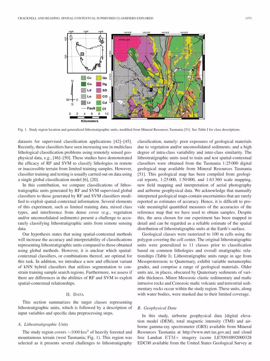
Fig. 1. Study region location and generalized lithostratigraphic units, modified from Mineral Resources Tasmania [51]. See Table I for class descriptions.

datasets for supervised classification applications [42]–[45].Recently, these classifiers have seen increasing use in multiclasslithological classification problems using remotely sensed geo-physical data, e.g., [46]–[50]. These studies have demonstratedthe efficacy of RF and SVM to classify lithologies in remoteor inaccessible terrain from limited training samples. However,classifier training and testing is usually carried out on data usinga single global classification model [6], [20].

In this contribution, we compare classifications of lithos-tratigraphic units generated by RF and SVM supervised globalclassifiers to those generated by RF and SVM classifiers modi-fied to exploit spatial-contextual information. Several elementsof this experiment, such as limited training data, mixed classtypes, and interference from dense cover (e.g., vegetationand/or unconsolidated sediments) present a challenge to accu-rately classifying lithostratigraphic units from remote sensingdata.

Our hypothesis states that using spatial-contextual methodswill increase the accuracy and interpretability of classificationsrepresenting lithostratigraphic units compared to those obtainedusing global methods. However, it is unclear which spatial-contextual classifiers, or combinations thereof, are optimal forthis task. In addition, we introduce a new and efficient variantof kNN hybrid classifiers that utilizes segmentation to con-strain training sample search regions. Furthermore, we assess ifthere are differences in the abilities of RF and SVM to exploitspatial-contextual relationships.

II. DATA

This section summarizes the target classes representinglithostratigraphic units, which is followed by a description ofinput variables and specific data preprocessing steps.

A. Lithostratigraphic Units

The study region covers ∼1000 km2 of heavily forested andmountainous terrain (west Tasmania; Fig. 1). This region wasselected as it presents several challenges to lithostratigraphy

classification, namely: poor exposures of geological materialsdue to vegetation and/or unconsolidated sediments; and a highdegree of intra-class variability and inter-class similarity. Thelithostratigraphic units used to train and test spatial-contextualclassifiers were obtained from the Tasmania 1:25 000 digitalgeological map available from Mineral Resources Tasmania[51]. This geological map has been compiled from geologi-cal reports, 1:25 000, 1:50 000, and 1:63 360 scale mapping,new field mapping and interpretation of aerial photographyand airborne geophysical data. We acknowledge that manuallyinterpreted geological maps contain uncertainties that are rarelyreported as estimates of accuracy. Hence, it is difficult to pro-vide meaningful quantified measures of the accuracies of thereference map that we have used to obtain samples. Despitethis, the area chosen for our experiment has been mapped indetail and can be regarded as a reliable estimate of the spatialdistribution of lithostratigraphic units at the Earth’s surface.

Geological classes were rasterized to 100 m cells using thepolygon covering the cell center. The original lithostratigraphicunits were generalized to 11 classes prior to classificationbased on common lithologies and overall stratigraphic rela-tionships (Table I). Lithostratigraphic units range in age fromMesoproterozoic to Quaternary, exhibit variable metamorphicgrades, and comprise a range of geological materials. Olderunits are, in places, obscured by Quaternary sediments of vari-able thickness. Minor Mesozoic clastic sedimentary and maficintrusive rocks and Cenozoic mafic volcanic and terrestrial sedi-mentary rocks occur within the study region. These units, alongwith water bodies, were masked due to their limited coverage.

B. Geophysical Data

In this study, airborne geophysical data [digital eleva-tion model (DEM), total magnetic intensity (TMI) and air-borne gamma-ray spectrometer (GRS) available from MineralResources Tasmania at http://www.mrt.tas.gov.au] and cloudfree Landsat ETM+ imagery (scene LE70910892000328EDC00 available from the United States Geological Survey at


TABLE ISUMMARY OF LITHOSTRATIGRAPHIC CLASSES

Classes are based on generalized lithostratigraphic units sourced from the 1:25 000 scale geological map of Tasmania [51]. Class abbreviations representgeochronological differences between lithostratigraphic units.

http://eros.usgs.gov) were used as input variables. These datawere transformed to a common coordinate system (GDA94zone 55) and resampled to 100 m resolution. TMI datawere downward continued to the ground surface to enhanceshallow magnetic anomalies [52]. Downward continued TMIdata were reduced-to-pole (RTP) using ERDAS ERMappper7.2 with dec. = 13.1 and inc. = −72.0 parameters basedon the Australian Geomagnetic Reference Field (GeoscienceAustralia: http://www.ga.gov.au/oracle/geomag/agrfform.jsp).RTP shifts the dipolar nature of the TMI anomalies as if thegeomagnetic field is vertically orientated [52]. The regional gra-dient observed in the RTP data was removed by subtracting alinear trend surface. GRS data (i.e., K, eTh, and eU) were cor-rected for negative values. In addition, the natural logarithm ofK/eTh was calculated and included as input. Landsat ETM+band ratios were calculated corresponding to those describedin Cracknell and Reading [50]. Landsat ETM+ variables withPearson’s correlation coefficients >0.85 associated with a largenumber of other Landsat ETM+ variables were removed. Thepreprocessing steps described above resulted in 11 variablesfor training and testing (i.e., DEM, RTP, K, eTh, eU, K/eTh,Landsat 1, Landsat 4, Landsat 6, Landsat 3/5, and Landsat5/7). These variables were standardized to zero mean and unitvariance.

III. METHODS

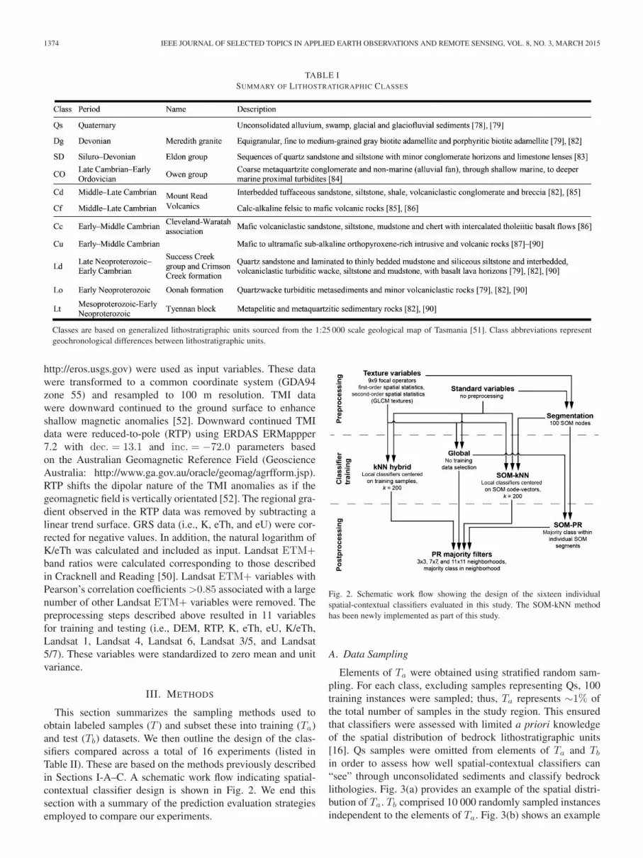
This section summarizes the sampling methods used toobtain labeled samples (T ) and subset these into training (Ta)and test (Tb) datasets. We then outline the design of the clas-sifiers compared across a total of 16 experiments (listed inTable II). These are based on the methods previously describedin Sections I-A–C. A schematic work flow indicating spatial-contextual classifier design is shown in Fig. 2. We end thissection with a summary of the prediction evaluation strategiesemployed to compare our experiments.

Fig. 2. Schematic work flow showing the design of the sixteen individualspatial-contextual classifiers evaluated in this study. The SOM-kNN methodhas been newly implemented as part of this study.

A. Data Sampling

Elements of Ta were obtained using stratified random sam-pling. For each class, excluding samples representing Qs, 100training instances were sampled; thus, Ta represents ∼1% ofthe total number of samples in the study region. This ensuredthat classifiers were assessed with limited a priori knowledgeof the spatial distribution of bedrock lithostratigraphic units[16]. Qs samples were omitted from elements of Ta and Tb

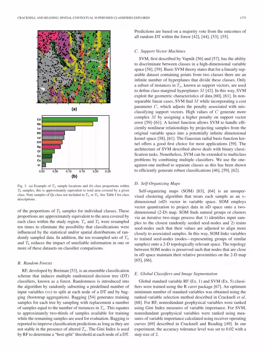
in order to assess how well spatial-contextual classifiers can“see” through unconsolidated sediments and classify bedrocklithologies. Fig. 3(a) provides an example of the spatial distri-bution of Ta. Tb comprised 10 000 randomly sampled instancesindependent to the elements of Ta. Fig. 3(b) shows an example


Fig. 3. (a) Example of Ta sample locations and (b) class proportions withinTb samples, this is approximately equivalent to total area covered by a givenclass. Note samples of Qs class not included in Ta or Tb. See Table I for classdescriptions.

of the proportions of Tb samples for individual classes. Theseproportions are approximately equivalent to the area covered byeach class within the study region. Ta and Tb were resampledten times to eliminate the possibility that classifications wereinfluenced by the statistical and/or spatial distributions of ran-domly sampled data. In addition, the ten resampled sets of Ta

and Tb reduces the impact of unreliable information in one ormore of these datasets on classifier comparisons.

B. Random Forests

RF, developed by Breiman [53], is an ensemble classificationscheme that induces multiple randomized decision tree (DT)classifiers, known as a forest. Randomness is introduced intothe algorithm by randomly subsetting a predefined number ofinput variables (m) to split at each node of a DT and by bag-ging (bootstrap aggregation). Bagging [54] generates trainingsamples for each tree by sampling with replacement a numberof samples equal to the number of instances in Ta. This equatesto approximately two-thirds of samples available for trainingwhile the remaining samples are used for evaluation. Bagging isreported to improve classification predictions as long as they arenot stable in the presence of altered Ta. The Gini Index is usedby RF to determine a “best split” threshold at each node of a DT.

Predictions are based on a majority vote from the outcomes ofall random DT within the forest [42], [44], [53], [55].

C. Support Vector Machines

SVM, first described by Vapnik [56] and [57], has the abilityto discriminate between classes in a high-dimensional variablespace [58], [59]. Basic SVM theory states that for a linearly sep-arable dataset containing points from two classes there are aninfinite number of hyperplanes that divide these classes. Onlya subset of instances in Ta, known as support vectors, are usedto define class marginal hyperplanes M [42]. In this way, SVMexploit the geometric characteristics of data [60], [61]. In non-separable linear cases, SVM find M while incorporating a costparameter C, which adjusts the penalty associated with mis-classifying support vectors. High values of C generate morecomplex M by assigning a higher penalty on support vectorerror [59]–[61]. A kernel function allows SVM to handle effi-ciently nonlinear relationships by projecting samples from theoriginal variable space into a potentially infinite dimensionalkernel space [58], [61]. The Gaussian radial basis function ker-nel offers a good first choice for most applications [59]. Thearchitecture of SVM described above deals with binary classi-fication tasks. Nonetheless, SVM can be extended to multiclassproblems by combining multiple classifiers. We use the one-against-one method to separate classes as this has been shownto efficiently generate robust classifications [46], [59], [62].

D. Self-Organizing Maps

Self-organizing maps (SOM) [63], [64] is an unsuper-vised clustering algorithm that treats each sample as an n-dimensional (nD) vector in variable space. SOM employsvector quantization to project data in nD space onto a two-dimensional (2-D) map. SOM finds natural groups or clustersvia an iterative two-stage process that 1) identifies input sam-ples to the closest randomly seeded seed-nodes and 2) trainsseed-nodes such that their values are adjusted to align moreclosely to associated samples. In this way, SOM links variablesto trained seed-nodes (nodes—representing groups of similarsamples) onto a 2-D topologically relevant space. The topologybetween SOM nodes is preserved such that nodes that are closein nD space maintain their relative proximities on the 2-D map[65], [66].

E. Global Classifiers and Image Segmentation

Global standard variable RF (Ex. 1) and SVM (Ex. 5) classi-fiers were trained using the R caret package [67]. An optimumminimum number of standard variables was obtained using theranked-variable selection method described in Cracknell et al.[68]. For RF, nonredundant geophysical variables were rankedusing Gini Index measures of variable importance. For SVM,nonredundant geophysical variables were ranked using mea-sures of variable importance calculated using receiver operatingcurves [69] described in Cracknell and Reading [49]. In ourexperiment, the accuracy tolerance level was set to 0.02 with astep size of 2.


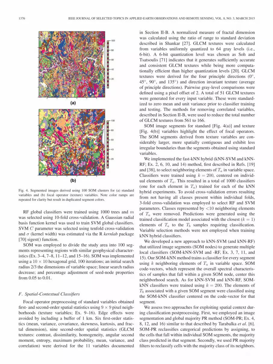
Fig. 4. Segmented images derived using 100 SOM clusters for (a) standardvariables and (b) focal operator (texture) variables. Note color ramps arerepeated for clarity but result in duplicated segment colors.

RF global classifiers were trained using 1000 trees and mwas selected using 10-fold cross-validation. A Gaussian radialbasis function kernel was used to train SVM global classifiers.SVM C parameter was selected using tenfold cross-validationand σ (kernel width) was estimated via the R kernlab package[70] sigest() function.

SOM was employed to divide the study area into 100 seg-ments representing regions with similar geophysical character-istics (Ex. 3–4, 7–8, 11–12, and 15–16). SOM was implementedusing a 10× 10 hexagonal grid, 100 iterations; an initial searchradius 2/3 the dimensions of variable space; linear search radiusdecrease; and percentage adjustment of seed-node propertiesfrom 0.05 to 0.01.

F. Spatial-Contextual Classifiers

Focal operator preprocessing of standard variables obtainedfirst- and second-order spatial statistics using 9× 9 pixel neigh-borhoods (texture variables; Ex. 9–16). Edge effects wereavoided by including a buffer of 1 km. Six first-order statis-tics (mean, variance, covariance, skewness, kurtosis, and frac-tal dimension), nine second-order spatial statistics (GLCMtextures: contrast, dissimilarity, homogeneity, angular secondmoment, entropy, maximum probability, mean, variance, andcorrelation) were derived for the 11 variables documented

in Section II-B. A normalized measure of fractal dimensionwas calculated using the ratio of range to standard deviationdescribed in Shankar [27]. GLCM textures were calculatedfrom variables uniformly quantized to 64 gray levels (i.e.,6-bit). A 6-bit quantization level was chosen as Soh andTsatsoulis [71] indicates that it generates sufficiently accurateand consistent GLCM textures while being more computa-tionally efficient than higher quantization levels [20]. GLCMtextures were derived for the four principle directions (0◦,45◦, 90◦, and 135◦) and direction invariant texture (averageof principle directions). Pairwise gray-level comparisons weredefined using a pixel offset of 2. A total of 51 GLCM textureswere generated for every input variable. These were standard-ized to zero mean and unit variance prior to classifier trainingand testing. The methods for removing correlated variables,described in Section II-B, were used to reduce the total numberof GLCM textures from 561 to 166.

SOM image segments for standard [Fig. 4(a)] and texture[Fig. 4(b)] variables highlight the effect of focal operators.The SOM segments derived from texture variables are con-siderably larger, more spatially contiguous and exhibit lessirregular boundaries than the segments obtained using standardvariables.

We implemented the fast-kNN hybrid (kNN-SVM and kNN-RF; Ex. 2, 6, 10, and 14) method, first described in Refs. [19]and [38], to select neighboring elements of Ta in variable space.Classifiers were trained using k = 200, centered on individ-ual elements of Ta. This resulted in a total of 1000 classifiers(one for each element in Ta) trained for each of the kNNhybrid experiments. To avoid cross-validation errors resultingfrom not having all classes present within individual folds,3-fold cross-validation was employed to select RF and SVMparameters. Classes represented by <10 neighboring elementsof Ta were removed. Predictions were generated using thetrained classification model associated with the closest (k = 1)elements of Ta to the Tb samples requiring classification.Variable selection methods were not employed when trainingkNN hybrid classifiers.

We developed a new approach to kNN-SVM (and kNN-RF)that utilized image segments (SOM nodes) to generate multiplelocal classifiers (SOM-kNN-SVM and -RF, Ex. 3, 7, 11, and15). Our SOM-kNN method trains a classifier for every segmentusing k neighboring elements of Ta in variable space. SOMcode-vectors, which represent the overall spectral characteris-tics of samples that fall within a given SOM node, center thisneighborhood search. As for kNN-SVM and kNN-RF, SOM-kNN classifiers were trained using k = 200. The elements ofTb associated with a given SOM segment were classified usingthe SOM-kNN classifier centered on the code-vector for thatsegment.

We assess two approaches for exploiting spatial context dur-ing classification postprocessing. First, we employed an imagesegmentation and global majority PR method (SOM-PR; Ex. 4,8, 12, and 16) similar to that described by Tarabalka et al. [6].SOM-PR reclassifies categorical predictions by assigning, tothe cells that fall within individual SOM segments, the majorityclass predicted in that segment. Secondly, we used PR majorityfilters to reclassify cells with the majority class of its neighbors.


If two or more classes were found to be equally representedwithin a local neighborhood the class associated with the targetcell was selected. PR majority filters with neighborhood dimen-sions of 3× 3, 7× 7, and 11× 11 cells were compared for allexperiments.

G. Prediction Evaluation

In this study, we randomly sampled Tb as a means of assess-ing supervised classifiers in regions close to and spatiallydisjoint from elements of Ta. We evaluate classifier successusing accuracy and associated 95% confidence limits, and thekappa statistic. The kappa statistic is based on a confusion(error) matrix and corrects accuracy estimates by accountingfor random chance [72]. We plot the spatial distributions oflithology classifications and mismatch between the interpretedgeological map and predicted classes as a means of evaluatingthe geological plausibility of classifier outputs.

IV. RESULTS

Table II provides Tb evaluation statistics for Ex. 1–16.All classifier mean kappa statistics are consistently ∼0.05less than mean accuracies. Furthermore, standard deviationsfrom kappa values are equal or negligibly higher (≤0.002)than those obtained for accuracy. Mean 95% confidence lim-its are approximately ±0.01 for all classifiers. Mean Tb

accuracies range from <0.60 for the global SVM classifiertrained on standard variables (Ex. 5) to >0.75 for RF globaland SOM-PR classifiers trained on texture variables (Ex. 9and 12).

Fig. 5 compares the distributions of Tb accuracies (n = 10)for global and spatial-contextual classifiers. The use of stan-dard variables results in ≤0.005 differences in mean accuraciesbetween global, kNN hybrid, and SOM-kNN RF classifiers(Ex. 1, 2, and 3). RF SOM-PR (Ex. 4) obtained a ∼0.03 increasein mean Tb accuracy compared to other standard variable RFclassifiers. There is a >0.10 increase in Tb accuracies whenusing the texture variable RF global classifier (Ex. 9) com-pared to accuracies obtained using the standard variable RFglobal classifier (Ex. 1). Texture variable global and SOM-PR RF classifiers (Ex. 9 and 12) achieve mean Tb accuracies>0.05 compared to texture variable kNN-RF (Ex. 10). Thebest performing texture variable RF classifiers (global andSOM-PR; Ex. 9 and 12) show considerable overlap betweenresampled sets of Tb.

Standard variable kNN hybrid and SOM-kNN SVM classi-fiers (Ex. 6 and 7) achieved significantly higher Tb accuraciesthan the standard variable SVM global (>0.04) and SOM-PR (>0.02) classifiers (Ex. 5 and 8). Considerable overlap inTb accuracies is observed using texture variable global, kNNhybrid, and SOM-kNN SVM classifiers (Ex. 13–15). The bestperforming SVM classifier was obtained using texture variablescoupled with the SOM-PR postprocessing method (Ex. 16).This method achieved a significant (>0.02) increase in meanTb accuracy compared to the other SVM classifiers utilizingtexture variables (Ex. 13–15).

TABLE IISPATIAL-CONTEXTUAL CLASSIFIER COMPARISON

Tb mean and standard deviations based on ten spatially and statistically inde-pendent resampled Ta and Tb. Standard deviation of 95% confidence intervals(CI) was, for all classifiers, �0.001. Ex. 1–16 refer to individual experimentsdescribed in the text.

Fig. 5. Comparison of spatial-contextual classifier Tb accuracies. Box plotsindicate the distribution (n = 10) of classifier Tb accuracy. Points (see leg-end) indicate mean Tb accuracy resulting from PR majority filter methods withdifferent neighborhood dimensions.

Substantial overlap between standard and texture variable RFand SVM, kNN hybrid, and SOM-kNN (Ex. 2–3, 6–7, 10–11,and 14–15) Tb accuracies is observed despite a considerableincrease in kNN hybrid training times compared to thoserequired for SOM-kNN. In our experiments, this increase incomputational cost is a function of the number of classi-fiers trained for kNN hybrid classifiers compared to thosetrained for SOM-kNN classifiers. kNN hybrid classifiers were


Fig. 6. Examples of the best performing spatial-contextual RF classifiers, standard variable SOM-PR (Ex. 4), and texture variable global (Ex. 9). Black squareindicates the location of Fig. 10. See Table I for class descriptions.

trained using 1000 classifiers and SOM-kNN was trainedusing 100 classifiers. Hence, computational cost is reducedby a factor of 10. When using texture variables, kNN hybrid,and SOM-kNN-SVM and -RF classifiers (Ex. 10–11 and14–15) obtain mean Tb accuracies that fall within the rangesof standard deviations from the mean.

Fig. 6 compares standard variable SOM-PR and texture vari-able RF global classifiers (Ex. 4 and 9). These classifiersare compared in terms of the spatial distributions of theirpredictions, the mismatch between these predictions and theinterpreted geological map used to sample Ta. There is ∼0.10difference in mean Tb accuracies between these two classifiers.The most striking difference in their predictions is observed inthe degree to which errors (or correct predictions) are increas-ingly spatially contiguous using texture variables. A similarpattern emerges in Fig. 7, which compares SVM classifiersutilizing standard and texture variables. In this case, the tex-ture variable SVM SOM-PR classifier (Ex. 16) achieves a0.075 increase in mean Tb accuracy over the standard variablekNN-SVM classifier (Ex. 7).

Table III provides a summary of the differences observed inmean Tb accuracies obtained using majority filter PR methodsand those not reclassified using these methods. As PR filter

dimensions increase there is a corresponding increase in thedifference in mean Tb accuracies. Classifiers trained using tex-ture variables exhibit lower increases in mean Tb accuraciesusing 7× 7 and 11× 11 majority filters than classifiers trainedon standard variables. The largest increase in mean Tb accu-racies (up to ∼0.09) using majority filters are obtained forstandard variable RF classifiers (Ex. 1–4) and texture variablekNN-SVM classifiers (Ex. 14 and 15). There is a small increasein mean Tb accuracies using the 3× 3 PR filters combined withtexture variable RF and SVM classifiers (Ex. 9–16). In con-trast, the greatest increase in mean Tb accuracies is observedusing majority filters with dimensions larger than 3× 3 cellsfor kNN hybrid and SOM-kNN predictions (Ex. 2–3, 6–7, 10–11, and 14–15). The results provided in Table III indicate usingPR filters of sizes much less than the size of focal operatorneighborhoods used to derive spatial statistics does not resultin a significant increase in prediction accuracy. Fig. 8 comparesstandard variable global RF and SVM classifier predictions(Ex. 1 and 5) and the effect on predictions resulting from PRfilters of different sizes. As the size of the PR filter neigh-borhood increases spatially contiguous classifications coveringlarger areas and increasingly rounded (convex) outer edgesare observed. The original predictions must be dominated by


Fig. 7. Examples of best performing spatial-contextual SVM classifiers, standard variable kNN-SVM (Ex. 6), and texture variable SOM-PR (Ex. 16). See Table Ifor class descriptions.

correct classifications in the first instance in order to reclassifypredictions correctly.

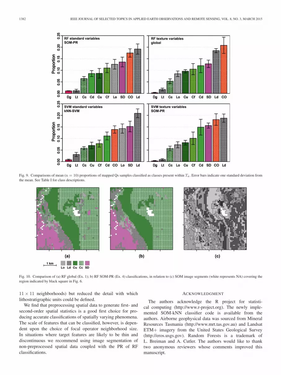
Fig. 9 shows the proportion of individual classes classi-fied as Qs for the best performing spatial-contextual RF andSVM classifiers. These plots show Ld, CO, SD classes makeup the majority of Qs classifications. The bulk of Ld and SDclassifications in areas of Qs occur on the southern limits ofthe Huskisson Syncline and east of Renison Bell. The major-ity of CO classifications cover spatially contiguous regions inthe southeast of the study area. The valley containing LakeRosebery, and the area mapped as Qs to the northeast, are likelyto be reflecting the presence of transported siliciclastic mate-rials and not generating plausible classifications of bedrocklithologies.

V. DISCUSSION

The best performing classifiers are those that employ texturevariable spatial-contextual preprocessing methods (Ex. 9–16).In contrast, standard variable global classifiers (Ex. 1 and5) generate the lowest or equal lowest Tb accuracies.Classifiers trained on texture variables were able to gener-ate spatially homogeneous classifications not affected by highfrequency noise. The inability of texture variable classifiers

to resolve lithologies expressed as narrow bodies suggeststhat the smoothing effect of focal operators is inhibiting theclassification of small scale features. This is because largeneighborhood dimensions can, in situations where the fea-tures of interest are relatively small, incorporate informationfrom neighboring features [26]. Focal operator neighborhooddimensions should, therefore, not be larger than the scale of thesmallest features of interest.

The use of the kNN-SVM method to train localized (in vari-able space) classifiers significantly increases the Tb accuraciesof standard variable SVM classifiers (Ex. 6). These resultsalign with the findings of Refs. [39] and [40]. The resultingTb accuracies of kNN-SVM classifiers are, however, equiva-lent to those obtained by standard variable RF global clas-sifiers (Ex. 1). In addition, there is no significant differencebetween RF global classifier (Ex. 1 and 9) Tb accuracies andthose observed for kNN-RF classifiers (Ex. 2 and 10). Theseresults reflect the adaptive nearest neighbor architecture ofRF classifiers, which adjusts the geometry of decision bound-aries based on the distribution of local training samples invariable space [44], [73]. By default, RF trains localized (invariable space) classifiers and does not require the use of meth-ods that explicitly select Ta samples representing local samplecharacteristics.


TABLE IIIPR MAJORITY FILTER COMPARISON

Difference between mean Tb accuracy obtained using 3× 3, 7× 7, and 11×11 neighborhood (cell) dimensions and mean Tb accuracy resulting from pre-dictions not utilizing majority filters (see Table II). Standard deviation of meanmajority filter Tb accuracies is �0.01 and mean 95% CI are ~0.01 ±0.001 forall classifiers.∗Denotes majority PR filter Tb accuracy increase greater than the sum of onestandard deviation and 95% CI of mean Tb accuracy not using majority PRfilters.

The kNN hybrid method (Ex. 2, 6, 10, and 14) induces mul-tiple localized classifiers and hence incurs significantly highercomputational cost compared to training a single global clas-sifier. This computational cost is related to the fact that thenumber of classifiers is equal to the number of Ta samples.The SOM-kNN method (Ex. 3, 7, 11, and 15), developed forthis study, reduced computational cost by a factor of 10 andgenerated equivalent Tb accuracies to kNN hybrid classifiers.SOM was implemented by selecting an arbitrary number ofseed-nodes from which to cluster samples. An optimal numberof SOM nodes and appropriate SOM 2-D map topology can beidentified by searching combinations of these SOM parametersand selecting those that result in minimum average quantizationand topological errors [74], [75].

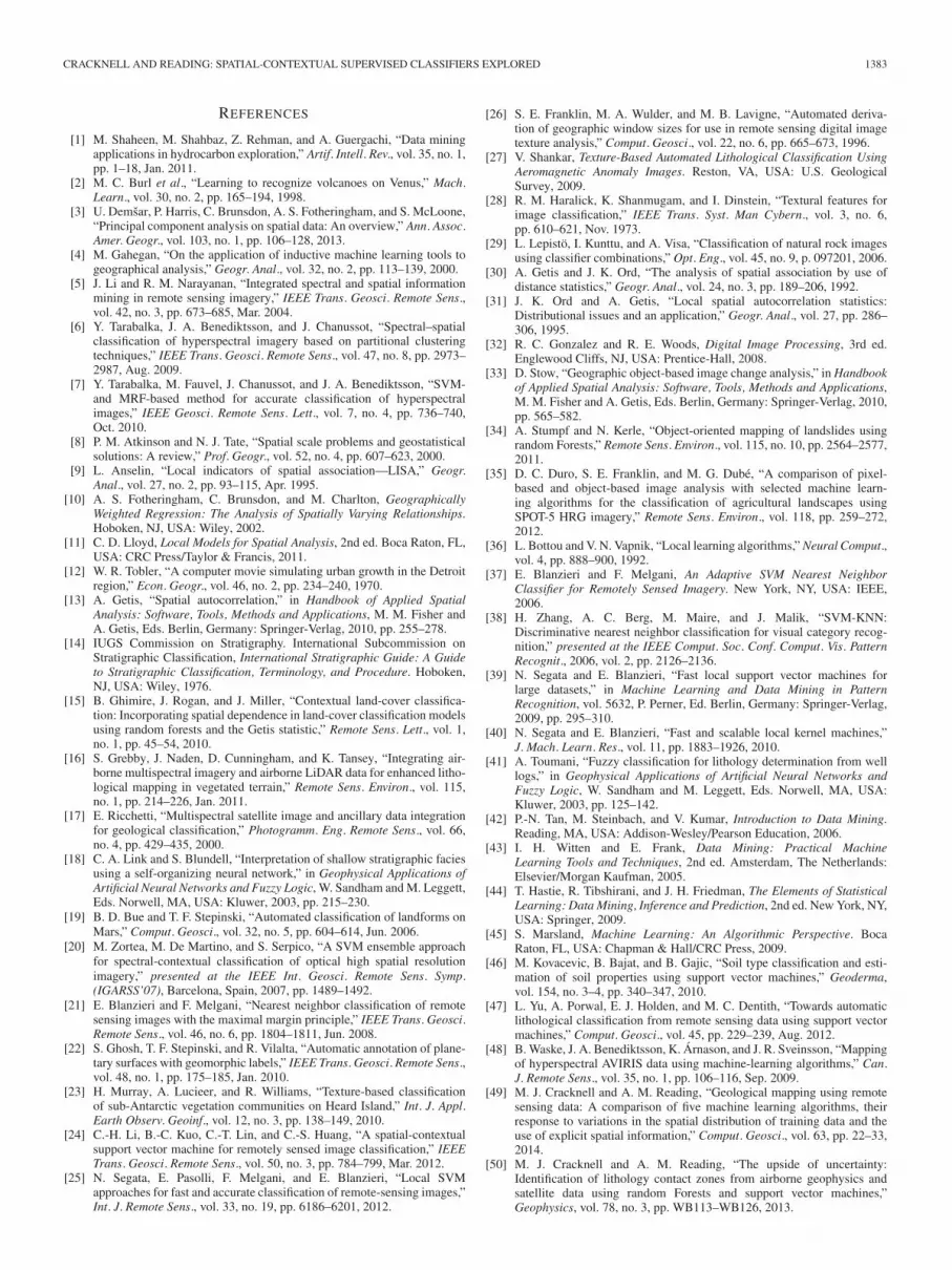
PR methods are useful for generating spatially contiguousregions of a given class by eliminating high frequency noisepresent in original classifications [6], [15], [17]. The SOM-PR method generated the highest Tb accuracies for standardvariable RF and texture variable SVM classifiers. SOM-PR pro-vided an efficient and effective means of limiting the effect ofhigh frequency noise on classifications. Unlike the classifiersthat used texture variables, standard variable SOM-PR classi-fiers (Ex. 4 and 8) were able to map thin and discontinuouslithostratigraphic units. A comparison of RF global [Fig. 10(a),Ex. 1] and RF SOM-PR [Fig. 10(b), Ex. 4] classifications high-lights the SOM-PR methods ability to eliminate the bulk ofisolated classifications and improve the definition of boundariesbetween classes. Fig. 10(c) shows numerous small SOM image

segments (derived from standard variables) are coincident withindividual classes. Small segments are desirable as they reducethe possibility of a large segment being misclassified; thus,mitigating against misclassifications impacting significantly onoverall accuracy [22].

Incorporating classifier uncertainty measures, derived fromclass membership probabilities as described in Cracknell andReading [50], may provide a means of weighting predictionsto reduce the effect of erroneous classifications on PR major-ity filters. Tarabalka et al. [7] demonstrate this concept using aprobabilistic SVM classifier coupled with a PR filter that com-bines edge detection filters and Markov random field (MRF)regularization. This approach aims to maintain the correct posi-tion of boundaries between spatially varying phenomena duringPR. Larger PR majority filter neighborhoods leads to higheroverall classification accuracies at the expense of identifyingnarrow and/or linear geological features. An ellipsoidal PRfilter that characterizes nonstationary spatial covariance param-eters representing local spatial scale [26] and anisotropic spatialstructure [76], [77] may result in improved representations oflinear geological features.

The results presented in Fig. 9 indicated regions mapped asQs were dominated by classifications representing Ld, CO, SD,and Lo units. The spectral characteristics of these classes arelikely to overlap with those of Qs. This is because large amountsof siliciclastic materials, specifically derived from CO (OwenGroup) lithologies, constitute the bulk of Quaternary sedimentsin the study area [78], [79]. For example, thick glacial outwashsands and gravels in the Boco Valley [78] obscure what islikely to be bedrock composed of lithologies associated with theMount Read Volcanics [80]. These Quaternary sediments weredominantly classified as either CO or Lo. In contrast, the valleyssurrounding Lake Rosebery are more likely to be classified asSD and (to the southeast) Ld.

During the preparation of Ta and Tb, units representing theWestern Volcano-Sedimentary Sequence and correlates of theTyndall Group, within the Huskisson Syncline south of LakePieman [51], were merged with the volcaniclastic sedimentsunit (Cd) of the Mount Read Volcanics. This unit comprisesfelsic to intermediate volcaniclastic sandstone, siltstone, andchert-rich granule-pebble conglomerate rocks [79]. The major-ity of spatial contextual classifiers are classifying this region asa combination of siliciclastic and volcaniclastic materials (Ld),rather than dominated solely by volcaniclastic sedimentarymaterials (Cd). A study conducted by Leaman and Richardson[81] interpreted the presence of granitoid bodies at shallowdepths (∼1 km) south of Renison Bell and Rosebery from grav-ity data. Many of the RF spatial-contextual classifiers trialed inthis study have predicted granite bodies in the area describedabove.

VI. CONCLUSION

We have evaluated new and preexisting methods for spatial-contextual RF and SVM supervised classification with respectto a challenging lithostratigraphy classification problem. Wedivide methods for including spatial-contextual informationinto the stages of the supervised classification work flow


Fig. 8. Example of global RF and SVM classifications trained on standard inputs (Ex. 1 and 5). Mismatch images represent correct and incorrect classificationas compared to the reference geological map used to train classifiers. PR mismatch images identify cells that were reclassified using majority filters of differentsizes. Colors indicate if the reclassification resulted in correct (green) or incorrect (red) reclassified predictions. See Table I for class descriptions.

1) data preprocessing using focal operators; 2) training mul-tiple classifiers from local neighborhoods of training samplesidentified using the k-nearest neighbor (kNN) hybrid method;and 3) postprocessing via PR. These spatial-contextual meth-ods, and combinations thereof, were compared to RF and SVMglobal classifiers.

Our experiments, reported as mean (n = 10) overall accu-racy ±95% confidence intervals, indicate spatial-contextualpreprocessing focal operators (texture variables) signifi-cantly increased (RF 0.754 ±0.010, SVM 0.683 ±0.010)classification accuracies over the use of standard variables (RF0.625 ±0.011, SVM 0.581 ±0.011). Combining image seg-mentation with PR methods was more advantageous for RF(0.652 ±0.011) than SVM (0.608 ±0.011) and was able to

resolve thin and discontinuous lithostratigraphic units usingstandard variables.

The kNN hybrid method only improves classification accu-racies for SVM (0.629 ±0.011). Combining textural data withthe kNN hybrid method decreased RF classifier accuracy (0.696±0.010) and did not result in any significant difference in theaccuracy of classifiers trained using SVM (0.671 ±0.010). Ournewly introduced kNN hybrid classifier (SOM-kNN), whichcombines image segmentation with local training sample selec-tion, significantly reduced processing times when comparedto standard kNN hybrid classifiers with no appreciable differ-ence in accuracy. Majority filter post regularization methodsresulted in a substantial increase in the accuracy of globalclassifiers using standard variables (RF 0.705, SVM 0.607 for


Fig. 9. Comparisons of mean (n = 10) proportions of mapped Qs samples classified as classes present within Ta. Error bars indicate one standard deviation fromthe mean. See Table I for class descriptions.

Fig. 10. Comparison of (a) RF global (Ex. 1); b) RF SOM-PR (Ex. 4) classifications, in relation to (c) SOM image segments (white represents NA) covering theregion indicated by black square in Fig. 6.

11× 11 neighborhoods) but reduced the detail with whichlithostratigraphic units could be defined.

We find that preprocessing spatial data to generate first- andsecond-order spatial statistics is a good first choice for pro-ducing accurate classifications of spatially varying phenomena.The scale of features that can be classified, however, is depen-dent upon the choice of focal operator neighborhood size.In situations where target features are likely to be thin anddiscontinuous we recommend using image segmentation ofnon-preprocessed spatial data coupled with the PR of RFclassifications.

ACKNOWLEDGMENT

The authors acknowledge the R project for statisti-cal computing (http://www.r-project.org). The newly imple-mented SOM-kNN classifier code is available from theauthors. Airborne geophysical data was sourced from MineralResources Tasmania (http://www.mrt.tas.gov.au) and LandsatETM+ imagery from the United States Geological Survey(http://eros.usgs.gov). Random Forests is a trademark ofL. Breiman and A. Cutler. The authors would like to thanktwo anonymous reviewers whose comments improved thismanuscript.


REFERENCES

[1] M. Shaheen, M. Shahbaz, Z. Rehman, and A. Guergachi, “Data miningapplications in hydrocarbon exploration,” Artif. Intell. Rev., vol. 35, no. 1,pp. 1–18, Jan. 2011.

[2] M. C. Burl et al., “Learning to recognize volcanoes on Venus,” Mach.Learn., vol. 30, no. 2, pp. 165–194, 1998.

[3] U. Demšar, P. Harris, C. Brunsdon, A. S. Fotheringham, and S. McLoone,“Principal component analysis on spatial data: An overview,” Ann. Assoc.Amer. Geogr., vol. 103, no. 1, pp. 106–128, 2013.

[4] M. Gahegan, “On the application of inductive machine learning tools togeographical analysis,” Geogr. Anal., vol. 32, no. 2, pp. 113–139, 2000.

[5] J. Li and R. M. Narayanan, “Integrated spectral and spatial informationmining in remote sensing imagery,” IEEE Trans. Geosci. Remote Sens.,vol. 42, no. 3, pp. 673–685, Mar. 2004.

[6] Y. Tarabalka, J. A. Benediktsson, and J. Chanussot, “Spectral–spatialclassification of hyperspectral imagery based on partitional clusteringtechniques,” IEEE Trans. Geosci. Remote Sens., vol. 47, no. 8, pp. 2973–2987, Aug. 2009.

[7] Y. Tarabalka, M. Fauvel, J. Chanussot, and J. A. Benediktsson, “SVM-and MRF-based method for accurate classification of hyperspectralimages,” IEEE Geosci. Remote Sens. Lett., vol. 7, no. 4, pp. 736–740,Oct. 2010.

[8] P. M. Atkinson and N. J. Tate, “Spatial scale problems and geostatisticalsolutions: A review,” Prof. Geogr., vol. 52, no. 4, pp. 607–623, 2000.

[9] L. Anselin, “Local indicators of spatial association—LISA,” Geogr.Anal., vol. 27, no. 2, pp. 93–115, Apr. 1995.

[10] A. S. Fotheringham, C. Brunsdon, and M. Charlton, GeographicallyWeighted Regression: The Analysis of Spatially Varying Relationships.Hoboken, NJ, USA: Wiley, 2002.

[11] C. D. Lloyd, Local Models for Spatial Analysis, 2nd ed. Boca Raton, FL,USA: CRC Press/Taylor & Francis, 2011.

[12] W. R. Tobler, “A computer movie simulating urban growth in the Detroitregion,” Econ. Geogr., vol. 46, no. 2, pp. 234–240, 1970.

[13] A. Getis, “Spatial autocorrelation,” in Handbook of Applied SpatialAnalysis: Software, Tools, Methods and Applications, M. M. Fisher andA. Getis, Eds. Berlin, Germany: Springer-Verlag, 2010, pp. 255–278.

[14] IUGS Commission on Stratigraphy. International Subcommission onStratigraphic Classification, International Stratigraphic Guide: A Guideto Stratigraphic Classification, Terminology, and Procedure. Hoboken,NJ, USA: Wiley, 1976.

[15] B. Ghimire, J. Rogan, and J. Miller, “Contextual land-cover classifica-tion: Incorporating spatial dependence in land-cover classification modelsusing random forests and the Getis statistic,” Remote Sens. Lett., vol. 1,no. 1, pp. 45–54, 2010.

[16] S. Grebby, J. Naden, D. Cunningham, and K. Tansey, “Integrating air-borne multispectral imagery and airborne LiDAR data for enhanced litho-logical mapping in vegetated terrain,” Remote Sens. Environ., vol. 115,no. 1, pp. 214–226, Jan. 2011.

[17] E. Ricchetti, “Multispectral satellite image and ancillary data integrationfor geological classification,” Photogramm. Eng. Remote Sens., vol. 66,no. 4, pp. 429–435, 2000.

[18] C. A. Link and S. Blundell, “Interpretation of shallow stratigraphic faciesusing a self-organizing neural network,” in Geophysical Applications ofArtificial Neural Networks and Fuzzy Logic, W. Sandham and M. Leggett,Eds. Norwell, MA, USA: Kluwer, 2003, pp. 215–230.

[19] B. D. Bue and T. F. Stepinski, “Automated classification of landforms onMars,” Comput. Geosci., vol. 32, no. 5, pp. 604–614, Jun. 2006.

[20] M. Zortea, M. De Martino, and S. Serpico, “A SVM ensemble approachfor spectral-contextual classification of optical high spatial resolutionimagery,” presented at the IEEE Int. Geosci. Remote Sens. Symp.(IGARSS’07), Barcelona, Spain, 2007, pp. 1489–1492.

[21] E. Blanzieri and F. Melgani, “Nearest neighbor classification of remotesensing images with the maximal margin principle,” IEEE Trans. Geosci.Remote Sens., vol. 46, no. 6, pp. 1804–1811, Jun. 2008.

[22] S. Ghosh, T. F. Stepinski, and R. Vilalta, “Automatic annotation of plane-tary surfaces with geomorphic labels,” IEEE Trans. Geosci. Remote Sens.,vol. 48, no. 1, pp. 175–185, Jan. 2010.

[23] H. Murray, A. Lucieer, and R. Williams, “Texture-based classificationof sub-Antarctic vegetation communities on Heard Island,” Int. J. Appl.Earth Observ. Geoinf., vol. 12, no. 3, pp. 138–149, 2010.

[24] C.-H. Li, B.-C. Kuo, C.-T. Lin, and C.-S. Huang, “A spatial-contextualsupport vector machine for remotely sensed image classification,” IEEETrans. Geosci. Remote Sens., vol. 50, no. 3, pp. 784–799, Mar. 2012.

[25] N. Segata, E. Pasolli, F. Melgani, and E. Blanzieri, “Local SVMapproaches for fast and accurate classification of remote-sensing images,”Int. J. Remote Sens., vol. 33, no. 19, pp. 6186–6201, 2012.

[26] S. E. Franklin, M. A. Wulder, and M. B. Lavigne, “Automated deriva-tion of geographic window sizes for use in remote sensing digital imagetexture analysis,” Comput. Geosci., vol. 22, no. 6, pp. 665–673, 1996.

[27] V. Shankar, Texture-Based Automated Lithological Classification UsingAeromagnetic Anomaly Images. Reston, VA, USA: U.S. GeologicalSurvey, 2009.

[28] R. M. Haralick, K. Shanmugam, and I. Dinstein, “Textural features forimage classification,” IEEE Trans. Syst. Man Cybern., vol. 3, no. 6,pp. 610–621, Nov. 1973.

[29] L. Lepistö, I. Kunttu, and A. Visa, “Classification of natural rock imagesusing classifier combinations,” Opt. Eng., vol. 45, no. 9, p. 097201, 2006.

[30] A. Getis and J. K. Ord, “The analysis of spatial association by use ofdistance statistics,” Geogr. Anal., vol. 24, no. 3, pp. 189–206, 1992.

[31] J. K. Ord and A. Getis, “Local spatial autocorrelation statistics:Distributional issues and an application,” Geogr. Anal., vol. 27, pp. 286–306, 1995.

[32] R. C. Gonzalez and R. E. Woods, Digital Image Processing, 3rd ed.Englewood Cliffs, NJ, USA: Prentice-Hall, 2008.

[33] D. Stow, “Geographic object-based image change analysis,” in Handbookof Applied Spatial Analysis: Software, Tools, Methods and Applications,M. M. Fisher and A. Getis, Eds. Berlin, Germany: Springer-Verlag, 2010,pp. 565–582.

[34] A. Stumpf and N. Kerle, “Object-oriented mapping of landslides usingrandom Forests,” Remote Sens. Environ., vol. 115, no. 10, pp. 2564–2577,2011.

[35] D. C. Duro, S. E. Franklin, and M. G. Dubé, “A comparison of pixel-based and object-based image analysis with selected machine learn-ing algorithms for the classification of agricultural landscapes usingSPOT-5 HRG imagery,” Remote Sens. Environ., vol. 118, pp. 259–272,2012.

[36] L. Bottou and V. N. Vapnik, “Local learning algorithms,” Neural Comput.,vol. 4, pp. 888–900, 1992.

[37] E. Blanzieri and F. Melgani, An Adaptive SVM Nearest NeighborClassifier for Remotely Sensed Imagery. New York, NY, USA: IEEE,2006.

[38] H. Zhang, A. C. Berg, M. Maire, and J. Malik, “SVM-KNN:Discriminative nearest neighbor classification for visual category recog-nition,” presented at the IEEE Comput. Soc. Conf. Comput. Vis. PatternRecognit., 2006, vol. 2, pp. 2126–2136.

[39] N. Segata and E. Blanzieri, “Fast local support vector machines forlarge datasets,” in Machine Learning and Data Mining in PatternRecognition, vol. 5632, P. Perner, Ed. Berlin, Germany: Springer-Verlag,2009, pp. 295–310.

[40] N. Segata and E. Blanzieri, “Fast and scalable local kernel machines,”J. Mach. Learn. Res., vol. 11, pp. 1883–1926, 2010.

[41] A. Toumani, “Fuzzy classification for lithology determination from welllogs,” in Geophysical Applications of Artificial Neural Networks andFuzzy Logic, W. Sandham and M. Leggett, Eds. Norwell, MA, USA:Kluwer, 2003, pp. 125–142.

[42] P.-N. Tan, M. Steinbach, and V. Kumar, Introduction to Data Mining.Reading, MA, USA: Addison-Wesley/Pearson Education, 2006.

[43] I. H. Witten and E. Frank, Data Mining: Practical MachineLearning Tools and Techniques, 2nd ed. Amsterdam, The Netherlands:Elsevier/Morgan Kaufman, 2005.

[44] T. Hastie, R. Tibshirani, and J. H. Friedman, The Elements of StatisticalLearning: Data Mining, Inference and Prediction, 2nd ed. New York, NY,USA: Springer, 2009.

[45] S. Marsland, Machine Learning: An Algorithmic Perspective. BocaRaton, FL, USA: Chapman & Hall/CRC Press, 2009.

[46] M. Kovacevic, B. Bajat, and B. Gajic, “Soil type classification and esti-mation of soil properties using support vector machines,” Geoderma,vol. 154, no. 3–4, pp. 340–347, 2010.

[47] L. Yu, A. Porwal, E. J. Holden, and M. C. Dentith, “Towards automaticlithological classification from remote sensing data using support vectormachines,” Comput. Geosci., vol. 45, pp. 229–239, Aug. 2012.

[48] B. Waske, J. A. Benediktsson, K. Árnason, and J. R. Sveinsson, “Mappingof hyperspectral AVIRIS data using machine-learning algorithms,” Can.J. Remote Sens., vol. 35, no. 1, pp. 106–116, Sep. 2009.

[49] M. J. Cracknell and A. M. Reading, “Geological mapping using remotesensing data: A comparison of five machine learning algorithms, theirresponse to variations in the spatial distribution of training data and theuse of explicit spatial information,” Comput. Geosci., vol. 63, pp. 22–33,2014.

[50] M. J. Cracknell and A. M. Reading, “The upside of uncertainty:Identification of lithology contact zones from airborne geophysics andsatellite data using random Forests and support vector machines,”Geophysics, vol. 78, no. 3, pp. WB113–WB126, 2013.


[51] Mineral Resources Tasmania, “1:25,000 Scale Digital Geology ofTasmania,” Mineral Resources Tasmania, Rosny Park, Australia,2011.

[52] W. M. Telford, L. P. Geldart, and R. E. Sheriff, Applied Geophysics, 2nded. Cambridge, U.K.: Cambridge Univ. Press, 1990.

[53] L. Breiman, “Random Forests,” Mach. Learn., vol. 45, no. 1, pp. 5–32,2001.

[54] L. Breiman, “Bagging predictors,” Mach. Learn., vol. 24, no. 2,pp. 123–140, 1996.

[55] B. Waske, J. A. Benediktsson, and J. R. Sveinsson, “Random Forests clas-sification of remote sensing data,” in Signal and Image Processing forRemote Sensing, 2nd ed., C. H. Chen, Ed. Boca Raton, FL, USA: CRCPress, 2012, pp. 365–374.

[56] V. N. Vapnik, The Nature of Statistical Learning Theory. Berlin,Germany: Springer-Verlag, 1995.

[57] V. N. Vapnik, Statistical Learning Theory. Hoboken, NJ, USA: Wiley,1998.

[58] C.-W. Hsu, C.-C. Chang, and C.-J. Lin, “A practical guide to supportvector classification,” Dept. Computer Science, National Taiwan Univ.,Taipei, Taiwan, Tech. Rep., 2010, p. 16 [Online]. Available: https://www.cs.sfu.ca/people/Faculty/teaching/726/spring11/svmguide.pdf

[59] A. Karatzoglou, D. Meyer, and K. Hornik, “Support vector machinesin R,” J. Stat. Softw., vol. 15, no. 9, p. 28, Apr. 2006.

[60] F. Melgani and L. Bruzzone, “Classification of hyperspectral remote sens-ing images with support vector machines,” IEEE Trans. Geosci. RemoteSens., vol. 42, no. 8, pp. 1778–1790, Aug. 2004.

[61] C. J. C. Burges, “A tutorial on support vector machines for pattern recog-nition,” Data Min. Knowl. Discovery, vol. 2, no. 2, pp. 121–167, Jun.1998.

[62] C.-W. Hsu and C.-J. Lin, “A comparison of methods for multiclasssupport vector machines,” IEEE Trans. Neural Netw., vol. 13, no. 2,pp. 415–425, Mar. 2002.

[63] T. Kohonen, “Self-organized formation of topologically correct featuremaps,” Biol. Cybern., vol. 43, no. 1, pp. 59–69, Jan. 1982.

[64] T. Kohonen, “The self-organizing map,” Neurocomputing, vol. 21,no. 1–3, pp. 1–6, 1998.

[65] F. P. Bierlein, S. J. Fraser, W. M. Brown, and T. Lees, “Advanced method-ologies for the analysis of databases of mineral deposits and major faults,”Aust. J. Earth Sci., vol. 55, no. 1, pp. 79–99, Feb. 2008.

[66] S. J. Fraser and B. L. Dickson, “A new method for data integrationand integrated data interpretation: Self-organising maps,” presented atthe 5th Decennial Int. Conf. Miner. Explor., Expanded Abstracts, 2007,pp. 907–910.

[67] M. Kuhn et al.. (2014). caret: Classification and Regression Training.R package version 5.15-023 [Online]. Available: http://CRAN.R-project.org/package=caret

[68] M. J. Cracknell, A. M. Reading, and A. W. McNeill, “Mapping geologyand volcanic-hosted massive sulfide alteration in the Hellyer–Mt Charterregion, Tasmania, using random ForestsTM and self-organising maps,”Aust. J. Earth Sci., vol. 61, pp. 287–304, 2014.

[69] F. Provost and T. Fawcett, “Analysis and visualization of classifier per-formance: Comparison under imprecise class and cost distributions,”presented at the Proc. 3rd Int. Conf. Knowl. Discovery Data Min.(KDD’97), 1997, pp. 43–48.

[70] A. Karatzoglou, A. Smola, K. Hornik, and A. Zeileis, “kernlab—An S4package for Kernel methods in R,” J. Stat. Softw., vol. 11, no. 9, pp. 1–20,2004.

[71] L.-K. Soh and C. Tsatsoulis, “Texture analysis of SAR sea ice imageryusing gray level co-occurrence matrices,” IEEE Trans. Geosci. RemoteSens., vol. 37, no. 2, pp. 780–795, Mar. 1999.

[72] R. G. Congalton and K. Green, Assessing the Accuracy of RemotelySensed Data: Principles and Practices, 1st ed. Boca Raton, FL, USA:Lewis, 1998.

[73] Y. Lin and Y. Jeon, “Random forest and adaptive nearest neighbors,”Dept. Statistics, Univ. Wisconsin, Madison, WI, USA, Tech. Rep. 1055,2002.

[74] K. Kiviluoto, “Topology preservation in self-organizing maps,” presentedat the IEEE Int. Conf. Neural Netw., 1996, vol. 1, pp. 294–299.

[75] E. A. Uriarte and F. D. Martín, “Topology preservation in SOM,” Int. J.Appl. Math. Comput. Sci., vol. 1, no. 1, pp. 19–22, 2005.

[76] J. Boisvert, J. Manchuk, and C. Deutsch, “Kriging in the presenceof locally varying anisotropy using non-Euclidean distances,” Math.Geosci., vol. 41, no. 5, pp. 585–601, 2009.

[77] J. B. Boisvert and C. V. Deutsch, “Programs for kriging and sequen-tial Gaussian simulation with locally varying anisotropy using non-Euclidean distances,” Comput. Geosci., vol. 37, no. 4, pp. 495–510,2011.

[78] P. Augustinus and E. A. Colhoun, “Glacial history of the upper Piemanand Boco valleys, western Tasmania,” Aust. J. Earth Sci., vol. 33, no. 2,pp. 181–191, Jun. 1986.

[79] A. V. Brown, Geology of the Dundas-Mt Lindsay-Mt Youngbuck Region.Rosny Park, Australia: Tasmanian Geological Survey Bulletin, 1986,GSB62.

[80] A. W. McNeill and K. D. Corbett, Geology of the Tullah–Mt Block Area.Rosny Park, Australia: Tasmanian Department of Mines, 1989.

[81] D. E. Leaman and R. G. Richardson, The Granites of West and North-WestTasmania—A Geophysical Interpretation. Rosny Park, Australia: Dept.Mines, 1989.

[82] D. B. Seymour and C. R. Calver, Explanatory Notes for the Time–SpaceDiagram and Stratotectonic Elements Map of Tasmania. Rosny Park,Australia: Tasmanian Geological Survey, 1995.

[83] M. R. Banks and P. W. Baillie, “Late Cambrian–Devonian,” in Geologyand Mineral Resources of Tasmania, vol. 15, C. F. Burrett andE. L. Martin, Eds. Brisbane, Australia: Special Publication GeologicalSociety of Australia, 1989, pp. 182–237.

[84] C. A. Noll and M. Hall, “Structural architecture of the OwenConglomerate, West Coast Range, western Tasmania: Field evidence forLate Cambrian extension,” Aust. J. Earth Sci., vol. 52, no. 3, pp. 411–426,Jun. 2005.

[85] K. D. Corbett and M. Solomon, “Cambrian Mt Read Volcanics and asso-ciated mineral deposits,” in Geology and Mineral Resources of Tasmania,vol. 15, C. F. Burrett and E. L. Martin, Eds. Brisbane, Australia: SpecialPublication Geological Society of Australia, 1989, pp. 84–153.

[86] D. B. Seymour, G. R. Green, and C. R. Calver, The Geology andMineral Deposits of Tasmania: A Summary. Rosny Park, Australia:Mineral Resources Tasmania, Department of Infrastructure, Energy andResources, 2013.

[87] M. J. Rubenach, “The origin and emplacement of the Serpentine HillComplex, Western Tasmania,” J. Geol. Soc. Aust., vol. 21, no. 1, pp. 91–106, Mar. 1974.

[88] R. F. Berry and A. J. Crawford, “The tectonic significance of Cambrianallochthonous mafic-ultramafic complexes in Tasmania,” Aust. J. EarthSci., vol. 35, no. 4, pp. 523–533, Dec. 1988.

[89] A. J. Crawford and R. F. Berry, “Tectonic implications of LateProterozoic-Early Palaeozoic igneous rock associations in westernTasmania,” Tectonophysics, vol. 214, no. 1–4, pp. 37–56, 1992.

[90] N. J. Turner, “Precambrian,” in Geology and Mineral Resources ofTasmania, vol. 15, C. F. Burrett and E. L. Martin, Eds. Brisbane,Australia: Special Publication Geological Society of Australia, 1989,pp. 5–46.

Matthew J. Cracknell received the B.Sc. degreein geology and geophysics (first class hons.) andthe Ph.D. degree in computational geophysicsfrom the School of Physical Sciences (EarthSciences)/CODES, Faculty of Science, Engineering,and Technology, University of Tasmania, Hobart,Tas., Australia, 2009 and 2014, respectively.

His research interests include the use of machinelearning for the classification of geological and geo-morphological features

Dr. Cracknell is a member of the GeologicalSociety of Australia, the Society of Exploration Geophysicists, and theInternational Association for Mathematical Geosciences.

Anya M. Reading received the B.Sc. degree (hons.)in geophysics with astrophysics from the Universityof Edinburgh, Edinburgh, U.K., and the Ph.D. degreein geophysics from the University of Leeds, Leeds,U.K., 1991 and 1997, respectively.

She has held technical research and academic posi-tions with British Antarctic Survey, The Universityof Edinburgh, and Australian National University.Currently, she leads the Computational Geophysicsand Earth Informatics Group, School of PhysicalSciences (UTas), University of Tasmania (UTas),

Hobart, Tas., Australia. Her research interests include computationalapproaches to global and regional geophysics.

Dr. Reading is a member of learned societies including the RoyalAstronomical Society, American Geophysical Union and Institute of Physics.She currently serves on the Australian Academy of Science, NationalCommittee for Earth Sciences.

spatial-contextual supervised classifiers explored: a challenging example of lithostratigraphy...

Documents