hydro-geochemical attributes based classifiers for

28

INTRODUCTION

The task of classification (Mishra and Dehuri, 2014) and prediction (Sarkar et al., 2020) in data mining (Sarkar, Salauddin, Hazra, et al., 2021) is a great challenge which appeals to many inves-tigators and researchers to develop a robust and

accurate model using the hidden data (Pati et al., 2020). However, the accuracy of the developed model is restricted to the use of quality data being used in the process of data mining. The research-ers who are working in the field of statistics, neural networks, and machine learning have de-veloped different types of classification methods

Hydro-Geochemical Attributes Based Classifiersfor Groundwater Analysis

Partha Sarathi Mishra1, Debabrata Nandi2*, Pramod Chandra Sahu3, Kamal Lochan Mohanta8 , Hisham Atan Edinur6, Tanmay Sarkar4, 5, Siddhartha Pati6, 9*

1 Department of Computer Science, MSCB University, Odisha, 757003, India2 Department of Remote Sensing and GIS, MSCB University, Odisha, 757003, India3 Department of Geology, MPC Autonomous College, 757003, Odisha, India4 Department of Food Technology and Bio-chemical Engineering, Jadavpur University, Jadavpur, Kolkata,

700032, India5 Malda Polyechnic, West Bengal State Council of Technical Education, Government of West Bengal, Malda,

732102, India6 School of Health Sciences, University Sains Malaysia, Kelantan, Malaysia7 SIAN Instytute, Association for Biodiversity Conservation and Research (ABC), Balasore, Odisha, 756020, India8 Department of Physics, ITER, Siksha ‘O’ Anusandhan Deemed to be University, Bhubaneswar, 751030, India9 Centre of Excellence, Khallikote University, Berhampur, India* Corresponding author’s e-mail: [email protected]; [email protected]

ABSTRACTFreshwater supply is critical for domestic, agricultural and industrial purposes. A good supply of clean water is nor-mally obtained from surface and groundwater water bodies. Nonetheless, many localities rely heavily on the latter as the main source of their water resource. Therefore, proper mapping, exploitation and conservation of groundwater resources should become a primary focus in the years to come. In this study, the groundwater samples collected from Bamanghati, Odisha were assigned into three classes (excellent, good and bad) based on the guidelines provided by World Health Organization in 1984. These water quality assignments were completed via a combined approach of hydro-geochemical information and artificial neural network for reconstructing a classifier for groundwater analysis. Here, the probabilistic approach and boosted instance selection method were used to remove inconsistencies in the dataset and to determine the classification accuracy, respectively. Finally, the transmuted dataset is used for kernel estimator-based Bayesian and Decision tree (J48) classification approaches. The findings from the present study confirm that the preprocessing task using statistical analysis along with the combined method of hydro-geochemical attributes-based classification approach is encouraging while the decision tree approach is better than the Bayesian neural network classifier in terms of precision, recall, F-measures, and Kappa statistics.

Keywords: data mining, classification, Bayesian artificial neural network, hydro-geochemical information, GIS.

Received: 2021.06.15Accepted: 2021.07.10Published: 2021.08.01

Ecological Engineering & Environmental Technology 2021, 22(5), 28–39https://doi.org/10.12912/27197050/139412ISSN 2719-7050, License CC-BY 4.0

ECOLOGICAL ENGINEERING & ENVIRONMENTAL TECHNOLOGY

29

Ecological Engineering & Environmental Technology 2021, 22(5), 28–39

(Dehuri and Cho, 2010b). Here, the concept of Bayesian neural network has been used for ac-curate classification impressed by probabilistic theory (Dehuri and Cho, 2010a).

Classification and prediction of ground-water quality is very crucial, because it is the major source of drinking water in many soci-eties. It is also used for agricultural, industri-al, and various other domestic purposes (Pati et al., 2021; Nandi et al., 2015, 2016, 2017). The chemical composition and concentration of groundwater are subjected to various dam-aging pollutants (Borowski and Ghazal, 2019; Kannan and Joseph, 2009; Mondal et al., 2011; Park et al., 2005). The method of groundwa-ter quality assessment could therefore help in deciding to manage the environment properly (Yan et al., 2010). In recent years, research-ers have used principal component analysis (PCA), discriminant function analysis, cluster analysis for groundwater quality assessment (Panda et al., 2006; Raghavachari, 2001). How-ever, groundwater records are nonlinear and the afore-mentioned linear and semi-automated techniques seem to be inappropriate for data analysis. Hence, the probabilistic approach of the Bayesian neural network as classifier has become a suitable approach for solving the above problem (Lahiri et al., 2021).

The objective of this paper was to develop a classifier to tackle the unpredictable data with a compromised architecture and simple learning methods to rebuild an ANN model which can evaluate, assess and classify the groundwater quality of the Bamanghati subdivision of May-urbhanj district, Odisha, India. The article is or-ganized into 5 sections. Section 1 gives an intro-duction to the proposed research. Section 2 dis-cusses the hydrogeologic framework through the Geographical Information System (GIS) along with hydro-geochemical information about the groundwater samples. It also discusses the boosting instance approach of attribute selection along with the descriptions of Bayesian Neural network architecture and learning process. Sec-tion 3 proposes a boosting instance selection based Bayesian classifier for the classification groundwater quality and in Section 4 experi-mental work is carried out followed by the result analysis. Finally, Section 5 gives the concluding remarks followed by references.

METHODS AND RELATED WORK

Geology and hydrogeology of the study area

The study area, Bamanghati, is one of the remote sub-division of the Mayurbhanj district of Odisha. It is one of the four subdivisions of Mayurbhanj also part of the Chhatonagpur pla-teau, which falls in the survey of India Toposheet (73J/2, 73J/3, 73J/4, 73J/7, 73J/8, 73F/14, 73F/15, 73F/16, 73K/1). The total area of the Bamanghati subdivision is 1917 Sq. Km. It is surrounded by the Singhbhum district in North and West, Pan-chpir Subdivision in South, and Baripada Sub-division in the East (Figure 1). The subdivision extends between 85°55ꞌE to 86°30ꞌE longitude and 22°.0ꞌN to 22°35ꞌN latitude. According to 2011 census, the Bamanghati subdivision has a population of 4, 95,005 with 2, 42,020 male and 2, 52,984 female. The study area represents con-spicuous physiographic variations marked by hills with intervening narrow intermountain valleys.

Hydro-geochemical information and model development

According to World Health Organization (WHO-1984), the groundwater quality index used in this paper is classified into three classes: (1) ex-cellent, (2) good, and (3) bad, as shown in Table 1.

According to World Health Organisation (WHO-1984), the model is based on the follow-ing parameters of hydro-geochemical information such as (1) hydrogen ion concentration (pH), (2) electrical conductivity (EC), (3) total dissolved solids (TDS), (4) bicarbonate (HCO3

-), (5) chlo-ride (Cl-), (6) sulfate (SO4

2-), (7) nitrate (NO3-), (8)

calcium (Ca2+), (9) magnesium (Mg2+), (10) sodi-

um (Na+), (11) potassium (K+), (12) fluoride (F-). The statistics of the hydro-geochemical attributes are given in Table 2.

The classification of the groundwater is made for the safe drinking purpose of the water. For example, the pH of the water is expressed on a scale ranging from 0–14, where 7 represents neu-tral alkalinity. A pH value below 7 indicates the acidic nature, whereas a pH value above 7 repre-sents the basic nature of the water. Accordingly, the pH value ranging within 7.5–8.5 represents the “excellent”, pH value ranging within 7.1–7.5 rep-resents the “good”, and a value within the range 0.01–7.0 and 8.51–14.00 is assigned for “bad”. According to WHO-1984, a value below 6.5 and

30


above 8.5 is considered to be appealing (Osmanaj et al., 2021). The groundwater is considered safe for drinking with the EC value below 1,500 μS/cm, but it is considered as saline as per WHO-1984 when the EC value is more than 1,500 μS/cm (Brown et al., 1970).

According to WHO-1948, the TDS value below 1,000 mg/l of the groundwater is safe for drinking. Similarly, it is safe for use with a limit to 300 mg/l of HCO3

- ions, below the 200 mg/l of Cl- ions, below the 200 mg/l of SO4

2- ions, less than 45 mg/l of NO3

- ions, 75 mg/l Ca2+ and 30 mg/l of Mg

2+ ions, respectively. In saline water,

Na+ K+ F- and ions also play a major role in the classification of groundwater to be considered for drinking. As per WHO-1948, the value of Na+ K+, and F- ions should have a value below 200 mg/l,

100 mg/l, and 1.1 mg/l, respectively. The hydro-geochemical attributes discussed above are taken as inputs to the model as shown in equation 1.

),,,,,,,,,,,( 22343

−++++−−−−= FKNaMgCaNOSOClHCOTDSECpHGQA

),,,,,,,,,,,( 22343

−++++−−−−= FKNaMgCaNOSOClHCOTDSECpHGQA

(1)

where: pH, EC, TDS, HCO3-, Cl-, SO4

-, NO3-,

Ca2+, Mg2+, Na+, K+, F- hydrogen ion con-

centration, electrical conductivity, total dissolved solids, bicarbonate, chloride, sulfate, nitrate, calcium, magnesium, so-dium, potassium, and fluoride of water samples, respectively. The mean, stan-dard deviation, and skew of the model at-tributes are shown in Figure 2.

Figure 1. Geological map

Table 1. The hydro-geochemical attributes/parameters for modelingHydro-geochemical

attributes Excellent (1.00) Good (0.50) Bad (0.00) Permissible limit (WHO 1984)

pH (-log10H+) 7.51–8.5 7.1–7.5 0.01–7.0 and 8.51–14.0 7.5–8.5

EC (mS/cm) 0.01–750 751–1500 1501–3000 750

TDS (mg/l) 0.01–500 501–1500 1501–3000 1000

HCO3– (mg/l) 0.01–200 201–300 301–500 300

Cl– (mg/l) 0.01–100 101–200 201–1000 200

SO42– (mg/l) 0.01–100 101–200 201–500 200

NO3– (mg/l) 0.01–25 25–45 45–100 45

Ca2+ (mg/l) 0.01–50 51–75 76–500 75

Mg2+ (mg/l) 0.01–20 21–30 31–200 30

Na+ (mg/l) 0.01–50 51–200 201–500 200

K+ (mg/l) 0.01–10 11–100 101–200 100

F– (mg/l) 0.01–0.5 0.6–0.9 0.9–1.1 1.1

31


Sources of Hydro-geochemical information

For the study of groundwater quality as-sessment, 89 water samples were systemati-cally collected from different tube wells (TW), dug wells (DW), and bore wells (BW) of the Bamanghati subdivision during pre and post-monsoon seasons (2017) in polyethylene bot-tles with the capacity of one liter. The water samples were collected from the wells which are used regularly for domestic and irrigational purposes covering the whole area.

The bottles were cleaned with distilled wa-ter, dried, and closed before their use for sample collection. Before collecting the respective wa-ter sample, each bottle was first rinsed with the water from the respective well and then filled with the well water, and method of collection

and analysis for the above-mentioned study was referred to the work of previous researchers (Brown et al., 1970; Rahman et al., 2021).

Boosting Instance Selection Approach

In data mining research, instance selection (Song and Shepperd, 2007) process plays a very important and relevant role. For managing the data in a proper way such as for efficiently process-ing, efficient storage, and data reduction purpose boosting instance selection method is needed. It is also essential for avoiding needless precision, re-moval of noise and outlier, smoothing of data, etc. (Benezzine et al., 2021; Loboichenko et al., 2021). Using these new developments and applications can be carried forward. Here, from the set of train-ing instances, the task was to find a meaning for

Table 2. Statistics of the hydro-geochemical attributesHydro-geochemical

attributes Minimum Maximum Mean STD Skew Kurtosis

pH (-log10H+) 7.04 8.51 7.75 0.41 0.23 –1.15

EC (mS/cm) 148.5 1225.19 437.62 224.89 1.43 2.51

TDS (mg/l) 95.08 784.12 280.08 143.93 1.43 2.51

HCO3– (mg/l) 44.8 390.4 156.58 76.11 0.93 0.64

Cl– (mg/l) 6.79 326.05 66.28 66.57 1.83 3.36

SO42– (mg/l) 2.8 60.55 18.66 12.96 1.43 2.16

NO3– (mg/l) 0.0 25.0 10.20 5.68 0.36 –0.52

Ca2+ (mg/l) 7.65 158.0 48.55 32.25 1.66 2.71

Mg2+ (mg/l) 2.21 107.5 19.41 18.37 2.18 6.17

Na+ (mg/l) 2.34 174.0 33.09 29.49 2.30 6.78

K+ (mg/l) 0.7 17.5 4.68 3.94 1.74 2.43

F– (mg/l) 0.0 8.8 0.73 1.09 5.91 39.23

TH (mg/l) 22.5 756 200.83 139.31 1.86 4.25

Figure 2. The Mean, Standard deviation, and Skew of the model attributes

32


the unidentified function f(x), where the mapping function is of a multi-class classifier mapping the instances to a component of Y (Dash et al., 2019; Vargas et al., 2018). Here, the authors used the sto-chastic gradient boosting technique to avoid over-fitting in the purpose of boosting instance selection.

Bayesian Neural Network

As per the approach, it is assumed all the features are equally valuable and independent of each other. In order to mode a feature, the Gauss-ian curve takes the role of the probability of membership. As per the work done by Moore and Zuev (Moore and Zuev, 2005), the above-men-tioned approach is refined to explain the impact of classification accuracy by the enhanced features. Algorithmically, naïve Bayesian kernel estima-tion and naïve Bayesian method are similar; the only difference is estimating the membership of an instance to a specific group

)|( jcf

)(1)|(ˆ)(:

=

−=

jiij cxCx

i

cj h

xtKhn

ctf

)).2/exp()2/1()(( 2ttK −=

)()()|()|(

sPwPwsPswP =

N

yyRMSE

N

iii

=−

= 1

2)ˆ(

Where iy is the observed value, iy is the predicted value. Similarly, cohen’s kappa (k) is represented by:

i

i

i

iiyy

yyyk

ˆ111

ˆ1ˆ

−−

−=−−

=

iy

, j = 1, …, k. In contrast, Gaussian distribution is consid-ered over data using naïve Bayesian (

)|( jcf

)(1)|(ˆ)(:

=

−=

jiij cxCx

i

cj h

xtKhn

ctf

)).2/exp()2/1()(( 2ttK −=

)()()|()|(

sPwPwsPswP =

N

yyRMSE

N

iii

=−

= 1

2)ˆ(


i

i

i

iiyy

yyyk

ˆ111

ˆ1ˆ

−−

−=−−

=

iy

, j = 1, …k) and the estimation by the use of kernel function

)|( jcf

)(1)|(ˆ)(:

=

−=

jiij cxCx

i

cj h

xtKhn

ctf

)).2/exp()2/1()(( 2ttK −=

)()()|()|(

sPwPwsPswP =

N

yyRMSE

N

iii

=−

= 1

2)ˆ(


i

i

i

iiyy

yyyk

ˆ111

ˆ1ˆ

−−

−=−−

=

iy

given below:

)|( jcf

)(1)|(ˆ)(:

=

−=

jiij cxCx

i

cj h

xtKhn

ctf

)).2/exp()2/1()(( 2ttK −=

)()()|()|(

sPwPwsPswP =

N

yyRMSE

N

iii

=−

= 1

2)ˆ(


i

i

i

iiyy

yyyk

ˆ111

ˆ1ˆ

−−

−=−−

=

iy

(2)

where: h is called the kernel parameter and K(t) is any kernel, where a kernel is defined as any non-negative function normal-

ized such that

−=1)( dttK . Exam-

ples include Gaussian distribution like

)|( jcf

)(1)|(ˆ)(:

=

−=

jiij cxCx

i

cj h

xtKhn

ctf

)).2/exp()2/1()(( 2ttK −=

)()()|()|(

sPwPwsPswP =

N

yyRMSE

N

iii

=−

= 1

2)ˆ(


i

i

i

iiyy

yyyk

ˆ111

ˆ1ˆ

−−

−=−−

=

iy

Due to the smoothness properties of Gaussian kernel, it is being used in the Bayesian Kernel estimation procedure (He et al., 2016; Specht, 1990).

The model is trained using the finite data set having input/target pairs 1}),({ == kN

kk zys by optimizing the misfit error as follows using equa-tion (3) as given below by adjusting the network parameters (weight and bias).

2)};({21

kkkN

kks wyozE −= (3)

The gradient of error Es is repeatedly evalu-ated by the back-propagation learning algo-rithm (Lauret et al., 2008; Sarkar, Salauddin,

Choudhury, et al., 2021). The tan sigmoid func-tion is also used as the cost function. The suitable prior probability distribution like P(w) of weights is considered in the Bayesian approach. The pos-terior probability distribution for the weights, say P(w|s), can be given as follows:

)|( jcf

)(1)|(ˆ)(:

=

−=

jiij cxCx

i

cj h

xtKhn

ctf

)).2/exp()2/1()(( 2ttK −=

)()()|()|(

sPwPwsPswP =

N

yyRMSE

N

iii

=−

= 1

2)ˆ(


i

i

i

iiyy

yyyk

ˆ111

ˆ1ˆ

−−

−=−−

=

iy

(4)

where: P(w|s) is the data set likelihood function and the P(s) is the normalizing factor. The distribution of outputs for a given input vector x can be written in the form as giv-en below (Maiti and Tiwari, 2010):

= dwswPwdxPsdxP )|(),|(),|( (5)

Boosting instance selection base Bayesian neural network classification modeling

The considered work involves such steps as preprocessing of data and classification, as shown in the proposed model (Figure 3). In the first step specific approaches for data preprocessing were considered. Then, for selecting the appropriate in-stances, the preprocessed dataset was given as an input to the boosted instance selection approach. The boosting instance selection approach was ap-plied to the classification process to remove the redundancy and insignificance in the instances. In the second step, the hydro-geochemical attributes and the Bayesian neural network were integrated for the construction of the classifier (Figure 3). In the proposed model, the input layer contains 12 different features as described in section 2, with a hidden layer and output layer. In the considered work, these relate to the three classes of member-ship. There can be more than one number of hidden layers comprising of the number of nodes within it. Each connection carries a weight wij.In the hidden layer, activation function gj(uj) is defined:

)( iii

ijj ugwu =

(6)

where: the sum is over all nodes i. The bias node is to be 1. The hyperbolic tangent function (Eq. 7) was used for sake of non-linearity found in the problem domain.

gi(uj) = tanh(uj) (7)

The proposed work is enumerated broadly in

the form of an Algorithm, as given below.

33


Algorithm

1. Collect the water samples for groundwater assessment.

2. Perform their hydro-geochemical analysis and set their parameters.

3. Then check the consistency of the dataset.4. Remove the irrelevant instances using the

Boost Instance selection method.5. Then, use the Bayesian Neural Network for

classification of dataset obtained after step 3.6. Then, built classifier is obtained.

EXPERIMENTAL STUDY

Description about the model setup and parameters

Here, a dataset was divided into reciprocally limited parts: a training set and a testing set. The model is built using a training and testing set. For obtaining the accuracy of the proposed model, 500 iterations were considered. Bayesian neural net-works and decision trees were used for comparing the classification exactness of the proposed work.

The WEKA 3 tool was used to gauge the perfor-mance of Naïve Bayes and decision tree classifiers (http://www.cs.waikato.ac.nz/ml/weka/).

According to the WHO-1984 standard limit, the training samples were produced tak-ing hydro-geochemical information, as given in Table 1. The neural network model used in this groundwater quality assessment is 12-7-3, i.e., there are twelve input nodes, seven hidden nodes, and three output nodes (Figure 4).

The input node takes the hydro-geochemical attributes. For the accuracy of the mode three-lay-er architecture of a Bayesian neural network was used. For the better optimization process, seven numbers hidden nodes were found to be suffi-cient. Three nodes at the output layer denote the groundwater quality assessment (GQA) index. Here, the cross-validation technique was used for keeping uniformity of the model development process. Throughout the model development pro-cess, the two-parameter of the Bayesian approach were fixed, such as used the kernel estimator and 10 fold cross-validation.

In the defined error model of the data like-lihood, the objective functions are defined as

Figure 3. Proposed model of classification

34


required for the Bayesian neural network (Dash et al., 2015). In this study, the root mean square error (RMSE), Kappa statistics, and Precision, Recall, F-measure, and confusion matrix were employed as the performance measurement for the groundwater quality assessment classification using Bayesian neural network. The equations for the parameters are as follows:

)|( jcf

)(1)|(ˆ)(:

=

−=

jiij cxCx

i

cj h

xtKhn

ctf

)).2/exp()2/1()(( 2ttK −=

)()()|()|(

sPwPwsPswP =

N

yyRMSE

N

iii

=−

= 1

2)ˆ(


i

i

i

iiyy

yyyk

ˆ111

ˆ1ˆ

−−

−=−−

=

iy

(8)

where: yi is the observed value,

)|( jcf

)(1)|(ˆ)(:

=

−=

jiij cxCx

i

cj h

xtKhn

ctf

)).2/exp()2/1()(( 2ttK −=

)()()|()|(

sPwPwsPswP =

N

yyRMSE

N

iii

=−

= 1

2)ˆ(


i

i

i

iiyy

yyyk

ˆ111

ˆ1ˆ

−−

−=−−

=

iy is the predict-ed value. Similarly, cohen’s kappa (k) is represented by:

)|( jcf

)(1)|(ˆ)(:

=

−=

jiij cxCx

i

cj h

xtKhn

ctf

)).2/exp()2/1()(( 2ttK −=

)()()|()|(

sPwPwsPswP =

N

yyRMSE

N

iii

=−

= 1

2)ˆ(


i

i

i

iiyy

yyyk

ˆ111

ˆ1ˆ

−−

−=−−

=

iy

(9)

where: yi is the observed agreement,

)|( jcf

)(1)|(ˆ)(:

=

−=

jiij cxCx

i

cj h

xtKhn

ctf

)).2/exp()2/1()(( 2ttK −=

)()()|()|(

sPwPwsPswP =

N

yyRMSE

N

iii

=−

= 1

2)ˆ(


i

i

i

iiyy

yyyk

ˆ111

ˆ1ˆ

−−

−=−−

=

iy is the ex-pected agreement. Similarly, precession is mathematically defined as follows:

FPTPTPprecision+

= (10)

where: TP represents the True Positives and FP represents the False Positive. Similar-ly, Recall is mathematically defined as follows:

FNTPTPrecall+

= (11)

where: TP represents the True Positive and FN represents the False Negative. Precision and recall play a tug of war in the classifi-cation process. Thus, precision and recall

play an important role in examining and evaluating the effectiveness of a model. Similarly, F-measure is mathematically defined as follows:

recallprecisionrecallprecisionMeasureF

+

=−2

(12)

In the classification evaluation process, pre-cision or recall alone can determine the effective-ness of the model. There may be situations where alternate importance of precision and recall can be found, for which F-Measure has been taken into consideration which leads to significant score value.

Further, the confusion matrix and its associ-ated metrics were taken as an alternative tool for the evaluation of the considered method. The per-formance of a classification model (or “classifi-er”) is determined by the confusion matrix which is a table represented in the form of a row and column applied on a set of test data for which the true values are known.

Result analysis

The groundwater quality governs the prac-ticality of water for drinking, irrigation, and in-dustrial uses. The chemical quality of the ground-water is affected to some level by the rock’s chemical arrangement and mass of the soil. The chemical arrangement of groundwater is modi-fied due to chemical reactions like oxidation and reduction (Schoeller, 1960). In the study, Table 2 describes different statistical behaviors of the col-lected groundwater samples (N=89). It was found that most of the parameters show wide ranges and high standard deviation (Table 2). Hence, it is very essential to study the performance of each

Figure 4. Bayesian neural network of 12-7-3 architecture

35


attribute in determining the quality of the ground-water usable for a different purpose.

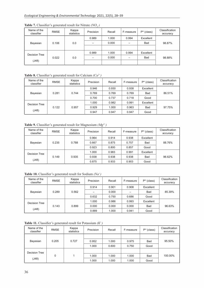
The performance of the classifiers obtained through the fifteen self-regulating runs of the con-ducted experiment for the groundwater quality as-sessment is illustrated through Tables 3 to 12. The Cohen’s Kappa (k) result and model classification accuracy obtained from the two classifiers named Bayesian and Decision tree used for groundwater quality assessment using the attributes taken for the classification is shown in Table 13.

Moreover, the confusion matrix was used as the performance measure for Bayesian and Deces-sion Tree (J48) classification algorithm. Here, the comparative analysis was performed using param-eters classification accuracy, classification error, sensitivity or recall, specificity, precision, and Mat-thew Correlation Coefficient (MCC) and the re-sults obtained are shown in Table 14 and Figure 5. From the above-mentioned analysis, it was found that with some exceptions, the groundwater from both the shallow and deeper aquifers comes under

Table 4. Classifier’s generated result for Electrical conductivityName of the

classifier RMSE Kappa statistics Precision Recall F-measure EC (class) Classification

accuracy

Bayesian 0.153 0.8451.000 0.976 0.988 Excellent

97.75%0.750 1.000 0.857 Good

Decision Tree

(J48)0.0 1.000

1.000 1.000 1.000 Excellent100.00%

1.000 1.000 1.000 Good

Table 5. Classifier’s generated result for Electrical conductivityName of the

classifier RMSE Kappa statistics Precision Recall F-measure PH (class) Classification

accuracy

Bayesian 0.240 0.729

0.957 0.971 0.964 Excellent

89.88%0.733 0.688 0.710 Bad

0.600 0.600 0.600 Good

Decision Tree

(J48)0.122 0.942

1.000 0.985 0.993 Excellent

97.75%0.833 1.000 0.909 Bad

0.938 0.938 0.938 Good

Table 6. Classifier’s generated result for Chloride (Cl-)Name of the


accuracy


1.000 0.929 0.963 Excellent

91.01%0.667 0.500 0.571 Bad

0.667 0.933 0.778 Good

Decision Tree

(J48)0.149 0.908

1.000 0.971 0.986 Excellent

96.62%0.800 1.000 0.889 Bad

0.875 0.933 0.903 Good

Table 3. Classifier’s generated result for Hydrogen ion concentration (PH)Name of the

classifier RMSE Kappa statistics Precision Recall F-Measure PH (class) Classification

accuracy


0.824 0.750 0.785 Excellent

58.43%0.037 0.250 0.065 Bad

0.818 0.310 0.450 Good

Decision Tree

(J48)0.208 0.862

0.964 0.964 0.964 Excellent

93.26%0.000 0.000 0.000 Bad

0.935 1.000 0.967 Good

36


Table 7. Classifier’s generated result for Nitrate (NO3_)

Name of the classifier RMSE Kappa

statistics Precision Recall F-measure PH (class) Classification accuracy

Bayesian 0.106 0.0

0.989 1.000 0.994 Excellent

98.87%– 0.000 – Bad

Decision Tree

(J48)0.022 0.0

0.989 1.000 0.994 Excellent

98.88%– 0.000 – Bad

Table 8. Classifier’s generated result for Calcium (Ca2+)Name of the


accuracy


0.946 0.930 0.938 Excellent

86.51%0.769 0.769 0.769 Bad

0.700 0.737 0.718 Good

Decision Tree

(J48)0.122 0.957

1.000 0.982 0.991 Excellent

97.75%0.929 1.000 0.963 Bad

0.947 0.947 0.947 Good

Table 9. Classifier’s generated result for Magnesium (Mg2+)Name of the


accuracy


0.964 0.914 0.938 Excellent

88.76%0.667 0.875 0.757 Bad

0.923 0.800 0.857 Good

Decision Tree

(J48)0.149 0.935

1.000 0.983 0.991 Excellent

96.62%0.938 0.938 0.938 Bad

0.875 0.933 0.903 Good

Table 10. Classifier’s generated result for Sodium (Na+)Name of the


accuracy


0.914 0.901 0.908 Excellent

85.39%– 0.000 – Bad

0.632 0.750 0.686 Good

Decision Tree

(J48)0.143 0.899

1.000 0.986 0.993 Excellent

96.63%0.000 0.000 0.000 Bad

0.889 1.000 0.941 Good

Table 11. Classifier’s generated result for Potassium (K+)Name of the


accuracy

Bayesian 0.205 0.727 95.50%0.952 1.000 0.975 Bad

1.000 0.600 0.750 Good

Decision Tree

(J48)0 1 100.00%1.000 1.000 1.000 Bad

1.000 1.000 1.000 Good

37


Table 12. Classifier’s generated result for Fluoride (F-)Name of the


accuracy


0.673 0.846 0.750 Excellent

61.79%0.750 0.400 0.522 Bad

0.417 0.500 0.455 Good

Decision Tree

(J48)0 1

1.000 1.000 1.000 Excellent

100.00%1.000 1.000 1.000 Bad

1.000 1.000 1.000 Good

Table 13. Result showing Kappa Statistics and Model AccuracyHydro–

geochemical attributes

Bayesian classifier Decision tree (J48)

Kappa statistics Model accuracy in (%) Kappa statistics Model accuracy in (%)

pH 0.290 58.43 0.862 93.26

EC 0.845 97.75 1.000 100.00

HCO3– 0.729 89.88 0.942 97.75

Cl– 0.766 91.01 0.908 96.62

NO3– 0.000 98.87 0.000 98.88

Ca2+ 0.744 86.51 0.957 97.75

Mg2+ 0.788 88.76 0.935 96.62

Na+ 0.562 85.39 0.899 96.63

K+ 0.767 95.50 1.000 100.00

F– 0.400 61.79 1.000 100.00

Table 14. Classification Result of groundwaterHydro-geochemical

attributesExcellent classification

(in numbers)Good classification

(in numbers)Bad classification

(in numbers)

pH 56 29 4

EC 83 6 0

HCO3– 68 16 5

Cl– 70 15 4

NO3– 88 0 1

Ca2+ 57 19 13

Mg2+ 58 15 16

Na+ 71 16 2

K+ 0 10 79

F– 39 20 30

Figure 5. Graph showing a different class of classification values of groundwater

38


the portable category with respect to the maximum permissible limit. It is also a general observation that the water from deeper aquifers has better qual-ity than that of the shallow aquifers. Therefore, from the quality point of view, the water from deep bore wells is most suitable for drinking purposes.

CONCLUSIONS

Groundwater has more greater importance as compared to surface water. Thus, proper planning of the groundwater becomes more essential now-adays. Hence, the efforts made by the authors for the classification of groundwater were carried out in two stages. In the first stage, the preprocessing task was carried out using the boosting instance ap-proach. In the second stage of the suggested work, a hydro-geochemical attributes-based Bayesian classifier model was developed for the groundwa-ter quality assessment using boosting approach and kernel estimator algorithm. Finally, the results ob-tained were compared with the Decision Tree (J48) classification algorithm and concluded that the clas-sification exactness of the Decision Tree (J48) clas-sification algorithm is better than the Bayesian neu-ral network classifier in terms of precision, recall, F-measures, and Kappa statistics. Furthermore, this effort may be prolonged to a natured inspired clas-sification by seeing precision and recall as the two important parameters. The future study suggests other bio-inspired metaheuristic approaches with more numbers data for the classification of ground-water of different geographical locations.

REFERENCES

1. Benezzine, G., Abdeljalil, Z., Yahya, K. 2021. Use of GIS for Digital Mapping and Spatial Analysis of Landfills: Case of the Settat Prov-ince in Morocco. Ecological Engineering & En-vironmental Technology, 22(3), 1–10. https://doi.org/10.12912/27197050/134868

2. Borowski, G., Ghazal, O.H. 2019. Use of Water In-jection Technique to Improve the Combustion Effi-ciency of the Spark-Ignition Engine: A Model Study. Journal of Ecological Engineering, 20(2), 226–233. https://doi.org/10.12911/22998993/99689

3. Brown, E., Skougstad, M., Fishman, M. 1970. Meth-ods for collection and analysis of water samples for dissolved minerals and gases. Techniques of Water-Resources Investigations.

4. Dash, C.S.K., Behera, A., Nayak, S.C., Dehuri,

S., Cho, S. 2019. An Integrated CRO and FLANN Based Classifier for a Non-Imputed and Incon-sistent Dataset. Int. J. Artif. Intell. Tools, 28, 1950013:1-1950013:32.

5. Dash, S.K., Dehuri, S., Cho, S.B., Wang, G.N. 2015. Towards Crafting a Smooth and Accurate Function-al Link Artificial Neural Networks Based on Dif-ferential Evolution and Feature Selection for Noisy Database. International Journal of Computational Intelligence Systems, 8(3), 539–552. https://doi.org/https://doi.org/10.1080/18756891.2015.1036221

6. Dehuri, S., Cho, S.-B. 2010a. A hybrid genetic based functional link artificial neural network with a statisti-cal comparison of classifiers over multiple datasets. Neural Computing and Applications, 19(2), 317–328. https://doi.org/10.1007/s00521-009-0310-y

7. Dehuri, S., Cho, S.-B. 2010b. Evolutionarily op-timized features in functional link neural network for classification. Expert Systems with Applica-tions, 37(6), 4379–4391. https://doi.org/https://doi.org/10.1016/j.eswa.2009.11.090

8. He, K., Zhang, X., Ren, S., Sun, J. 2016. Deep Re-sidual Learning for Image Recognition. 2016 IEEE Conference on Computer Vision and Pattern Rec-ognition (CVPR), 770–778. https://doi.org/10.1109/CVPR.2016.90

9. Kannan, N., Joseph, S. 2009. Quality of Groundwater in the Shallow Aquifers of a Paddy Dominated Agri-cultural River Basin, Kerala, India. World Academy of Science, Engineering and Technology, Internation-al Journal of Biological, Biomolecular, Agricultural, Food and Biotechnological Engineering, 3, 223–241.

10. Lahiri, D., Nag, M., Sarkar, T., Dutta, B., Ray, R.R. 2021. Antibiofilm Activity of α-Amylase from Ba-cillus subtilis and Prediction of the Optimized Con-ditions for Biofilm Removal by Response Surface Methodology (RSM) and Artificial Neural Network (ANN). Applied Biochemistry and Biotechnology. https://doi.org/10.1007/s12010-021-03509-9

11. Lauret, P., Fock, E., Randrianarivony, R.N., Manicom-Ramsamy, J.-F. 2008. Bayesian neural network ap-proach to short time load forecasting. Energy Conver-sion and Management, 49(5), 1156–1166. https://doi.org/https://doi.org/10.1016/j.enconman.2007.09.009

12. Loboichenko, V., Leonova, N., Shevchenko, R., Kapust-nik, A., Yeremenko, S., Pruskyi, A. 2021. Assessment of the Impact of Natural and Anthropogenic Factors on the State of Water Objects in Urbanized and Non-Urbanized Areas in Lozova District (Ukraine). Ecologi-cal Engineering & Environmental Technology, 22(2), 59–66. https://doi.org/10.12912/27197050/133333

13. Maiti, S., Tiwari, R.K. 2010. Neural network modeling and an uncertainty analysis in Bayesian framework: A case study from the KTB borehole site. Journal of Geophysical Research: Solid Earth, 115(B10). https://doi.org/https://doi.org/10.1029/2010JB000864

39


14. Mishra, P. S., Dehuri, S. 2014. Potential Indicators Based Neural Networks for Cash Forecasting of an ATM. Int. J. Inf. Syst. Soc. Chang., 5(4), 41–57. https://doi.org/10.4018/ijissc.2014100103

15. Mondal, N.C., Singh, V.S., Saxena, V.K., Singh, V.P. 2011. Assessment of seawater impact using major hydrochemical ions: a case study from Sa-dras, Tamilnadu, India. Environmental Monitoring and Assessment, 177(1–4), 315–335. https://doi.org/10.1007/s10661-010-1636-8

16. Moore, A., Zuev, D. 2005. Internet traffic classification using bayesian analysis techniques. SIGMETRICS ’05.

17. Nandi, D., Kant, J., Sahu., & C.K. (2015). Inte-grated Approach Using Remote Sensing and GIS for Hydrogeology of Moroda Block in Mayurbhanj District, Odisha, India. International Journal of con-servation Science. 06, (3), 383-390

18. Nandi, D., Nathjee, S., & Chatterjee, T. 2016. Mi-crowatershed Management using Remote Sensing and GIS. Advanced Science Letters, 22(2), 305-310. doi:10.1166/asl.2016.6866

19. Nandi, D., Sahu, P. C., & Goswami, S. 2017. Hydrogeomorphological study in Bamanghaty subdivision of Mayurbhanj district, Odisha an in-tegrated remote sensing and GIS approach. Interna-tional Journal of Geosciences, 08(11), 1361-1373. doi:10.4236/ijg.2017.811079

20. Osmanaj, L., Hajra, A., Berisha, A., de Beyer, T. 2021. The Journey of Establishing Groundwater Source Protection Zones in Kosovo on Example of Lipjan Municipality. Ecological Engineering & Environmental Technology, 22(3), 20–26. https://doi.org/10.12912/27197050/134753

21. Panda, U. C., Sundaray, S., Rath, P., Nayak, B. B., Bhatta, D. 2006. Application of factor and cluster analysis for characterization of river and estuarine water systems@_ A case study: Mahanadi River (India). Journal of Hydrology, 331, 434–445.

22. Park, S.-C., Yun, S.-T., Chae, G.-T., Yoo, I.-S., Shin, K.-S., Heo, C.-H., Lee, S.-K. 2005. Regional hydro-chemical study on salinization of coastal aquifers, western coastal area of South Korea. Journal of Hydrology, 313(3), 182–194. https://doi.org/https://doi.org/10.1016/j.jhydrol.2005.03.001

23. Pati, S., Sarkar, T., Sheikh, H.I., Bharadwaj, K.K., Mohapatra, P.K., Chatterji, A., Dash, B.P., Edinur, H.A., Nelson, B. R. 2021. γ-Irradiated Chitosan From Carcinoscorpius rotundicauda (Latreille, 1802) Improves the Shelf Life of Refrigerated Aquatic Products. Frontiers in Marine Science, 8, 498. https://doi.org/10.3389/fmars.2021.664961

24. Pati, S., Shahimi, S., Nandi, D., Sarkar, T., Acharya, S.N., Sheikh, H.I., Choudhury, T., John, A., Acha-rya, D.K., Nelson, B.R., Dash, B.P. 2020. Predict-ing Tachypleus gigas Spawning Distribution with

Climate Change in Northeast Coast of India. Journal of Ecological Engineering. http://www.jeeng.net/Pre-dicting-Tachypleus-gigas-Spawning-Distribution-with-Climate-Change-in-Northeast,131244,0,2.html

25. Raghavachari, M. 2001. Applied Multivariate Statistics in Geohydrology and Related Sciences. Technometrics, 43(1), 110. https://doi.org/10.1198/tech.2001.s566

26. Rahman, A., Mondal, N.C., Fauzia, F. 2021. Ar-senic enrichment and its natural background in groundwater at the proximity of active floodplains of Ganga River, northern India. Chemosphere, 265, 129096. https://doi.org/https://doi.org/10.1016/j.chemosphere.2020.129096

27. Sarkar, T., Salauddin, M., Choudhury, T., Um, J.S., Pati, S., Hazra, S.K., Chakraborty, R. 2021. Spatial optimisation of mango leather production and colour estimation through conventional and novel digital im-age analysis technique. Spatial Information Research, 29. https://doi.org/10.1007/s41324-020-00377-z

28. Sarkar, T., Salauddin, M., Hazra, S.., Chakraborty, R. 2020. Artificial neural network modelling ap-proach of drying kinetics evolution for hot air oven, microwave, microwave convective and freeze dried pineapple. SN Applied Sciences, 2(9), 1621. https://doi.org/10.1007/s42452-020-03455-x

29. Sarkar, T., Salauddin, M., Hazra, S. ., Choudhury, T., Chakraborty, R. 2021. Comparative approach of arti-ficial neural network and thin layer modelling for dry-ing kinetics and optimization of rehydration ratio for bael (Aegle marmelos (L) correa) powder production. Economic Computation and Economic Cybernetics Studies and Research, 55(1), 167–184. https://doi.org/http://dx.doi.org/10.24818/18423264/55.1.21.11

30. Schoeller, H. 1960. Arid Zone Hydrology – Recent Developments. Soil Science, 90(2). https://journals.lww.com/soilsci/Fulltext/1960/08000/Arid_Zone_Hydrology_Recent_Developments.33.aspx

31. Song, Q., Shepperd, M. 2007. A new imputation method for small software project data sets. Journal of Systems and Software, 80(1), 51–62. https://doi.org/https://doi.org/10.1016/j.jss.2006.05.003

32. Specht, D. F. 1990. Probabilistic neural networks. Neural Networks, 3(1), 109–118. https://doi.org/https://doi.org/10.1016/0893-6080(90)90049-Q

33. Vargas, G., Cypriano, J., Correa, T., Leão, P., Ba-zylinski, D.A., Abreu, F. 2018. Applications of magnetotactic bacteria, magnetosomes and magne-tosome crystals in biotechnology and nanotechnol-ogy: mini-review. Molecules, 23(10), 1–25. https://doi.org/10.3390/molecules23102438

34. Yan, H., Zou, Z., Wang, H. 2010. Adaptive neuro fuzzy inference system for classification of water quality status. Journal of Environmental Sciences, 22(12), 1891–1896. https://doi.org/https://doi.org/10.1016/S1001-0742(09)60335-1

hydro-geochemical attributes based classifiers for

Documents