i

U.S. Fish and Wildlife Service U.S. Department of the Interior National Wildlife Refuge System

South Atlantic-Gulf and Mississippi Basin Protocol Framework for Coastal Wetland Elevation Monitoring

Version 1.0 August 2020

ON THE COVER Description of image/photo used on front cover Supervisory Refuge biologist, Chuck Hayes, collecting surface elevation table data at Savannah National Wildlife Refuge. Photograph by: Nicole Rankin, U.S. Fish and Wildlife Service

iii

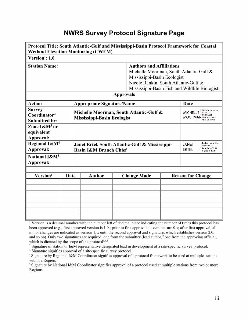
NWRS Survey Protocol Signature Page Protocol Title: South Atlantic-Gulf and Mississippi-Basin Protocol Framework for Coastal Wetland Elevation Monitoring (CWEM) Version1: 1.0 Station Name:

Authors and Affiliations Michelle Moorman, South Atlantic-Gulf & Mississippi-Basin Ecologist Nicole Rankin, South Atlantic-Gulf & Mississippi-Basin Fish and Wildlife Biologist

Approvals

Action Appropriate Signature/Name Date Survey Coordinator2 Submitted by:

Michelle Moorman, South Atlantic-Gulf & Mississippi-Basin Ecologist

Zone I&M3 or equivalent Approval:

Regional I&M4 Approval:

Janet Ertel, South Atlantic-Gulf & Mississippi-Basin I&M Branch Chief

National I&M5 Approval:

Version1 Date Author Change Made Reason for Change

1 Version is a decimal number with the number left of decimal place indicating the number of times this protocol has been approved (e.g., first approved version is 1.0.; prior to first approval all versions are 0.x; after first approval, all minor changes are indicated as version 1. x until the second approval and signature, which establishes version 2.0, and so on). Only two signatures are required: one from the submitter (lead author)2 one from the approving official, which is dictated by the scope of the protocol3,4,5. 2 Signature of station or I&M representative designated lead in development of a site-specific survey protocol. 3 Signature signifies approval of a site-specific survey protocol. 4 Signature by Regional I&M Coordinator signifies approval of a protocol framework to be used at multiple stations within a Region. 5 Signature by National I&M Coordinator signifies approval of a protocol used at multiple stations from two or more Regions.

iv

Survey Protocol Summary The regional protocol framework for Coastal Wetland Elevation Monitoring is based on the national protocol framework for The Surface Elevation Table and Marker Horizon Technique, A Protocol for Monitoring Wetland Elevation Dynamics (Lynch et al. 2015), which was approved for use in the National Wildlife Refuge System (Newman 2015). This regional protocol provides a framework for monitoring surface elevation, accretion, and porewater salinity in wetlands on coastal U.S. Fish and Wildlife Service (USFWS) Wildlife Refuges (hereafter NWR or Refuges) of the South Atlantic-Gulf and Mississippi-Basin. Specifically, this protocol outlines how the USFWS National Wildlife Refuge System (NWRS) monitors a series of rod surface elevation table (SET) benchmarks, marker horizon plots, and porewater salinity plots in the South Atlantic Landscape Conservation Cooperative (SALCC) geography to advance understanding of the impacts of sea-level rise, altered hydrology, and subsidence on coastal marshes, forested wetlands, and pocosins on coastal Refuges. These data will be combined with other data, tools, and models to better inform decisions on conservation plans and management actions within the coastal zone. The content and structure of this protocol framework follows standards set forth in the U.S. Fish and Wildlife Service’s, How to Develop Survey Protocols: A Handbook, Version 1.0 (USFWS 2016). To provide a mechanism for refuges to collect data to monitor the status and trends of wetland conditions, a series of 60 deep rod SET benchmarks (all “rod” SETs sensu Cahoon et al. 2002, but hereafter referred to as “SET”) were established on 18 coastal Refuges within the SALCC geography in 2012. Associated vegetation plots, porewater salinity plots and wells, and marker horizon plots were established at these locations. One water level station was established at Bell Island Pier, Swanquarter NWR in 2013. This protocol guides the continued monitoring of coastal wetland elevations at currently participating refuges and lends a framework for creating Site-specific Survey Protocols for refuges that decide to start the monitoring in the future. Participating Refuges include: Alligator River (NC), Blackbeard Island (GA), Cedar Island (NC), Currituck (NC), Ernest F. Hollings ACE Basin (SC), Harris Neck (GA), Lower Suwannee (FL), Mackay Island (NC), Pea Island (NC), Pinckney Island (SC), Pocosin Lakes (NC), Roanoke River (NC), Savannah (GA), St Marks (FL), Swanquarter (NC), Waccamaw (SC), Wassaw (GA), and Wolf Island (GA). Suggested citation: Moorman MC, Rankin NM. 2019. South Atlantic-Gulf and Mississippi Basin Protocol Framework for Coastal Wetland Elevation Monitoring (CWEM). Version 1.0. Atlanta, Georgia: US Fish and Wildlife Service, South Atlantic-Gulf and Mississippi-Basin. This protocol is available from ServCat [https://ecos.fws.gov/ServCat/Reference/Profile/114122https://ecos.fws.gov/ServCat/Reference/Profile/118377]

v

Acknowledgments This protocol was developed with the input and cooperation of Ken Krauss, Don Cahoon, and Nicole Cormier of the U.S. Geological Survey; Brian Boutin of The Nature Conservancy, Lisa Baron, Jim Lynch, Joe Devivo, Jenny Asper, and Tony Curtis of the National Park Service; Carolyn Currin, Anna Hilting, and Mike Green of the National Oceanic and Atmospheric Administration; Philippe Hensel from National Geodetic Survey; Tracy Buck of Baruch Marine Field Laboratory; Jacob Weiss who worked as a USFWS Director’s Fellow; Susan Adamowicz, Laura Mitchell, Jena Moon, and Roland Davis of USFWS. This protocol was reviewed by Jena Moon, Adam Smith, Zach Cravens and Janet Ertel of USFWS, Ken Krauss of U.S. Geological Survey, and Jim Lynch of the National Park Service. Mike Chouinard served as the review Coordinator. Pat Ward, National I&M for the Refuge System, reviewed the protocol for conformation to the NWRS standard and format. Much of this protocol framework follows the National Park Services Protocol, “The Surface Elevation Table and Marker Horizon Monitoring: A Protocol for Monitoring Wetland Elevation Dynamics, Version 1” (Lynch et al. 2015). This protocol is largely based on monitoring efforts that have been in use and development for more than two decades. We have borrowed heavily from several published and forthcoming reports. The following is a brief overview of some of the major efforts that we have relied on in the development of this protocol:

• Much of the discussion on sampling design and data analysis has been borrowed heavily from years of work by Don Cahoon, Philippe Hensel, Jim Lynch, and several others that have developed and refined the SET methods used to measure elevation changes in salt marshes. This document is intended to serve as a set of standards to facilitate data compatibility among programs moving forward, so we felt it important to base our sampling designs and methods on these standards to the greatest extent possible. Additionally, the authors’ feedback and technical support while developing this protocol—as well as their guidance document—were also invaluable.

• The Standard Operating Procedures developed by the National Park Service (Byrne 2012, Asper 2013, Asper and Curtis, 2012, Asper and Curtis 2013, Curtis 2012, Lynch et al. 2015) and the Louisiana Department of Natural Resources (Folse and West 2004, Theobald et al. 2007) were used heavily in development of the SOPs that accompany this protocol as they are designed for monitoring soft-bottomed marsh systems typical of those found in the Southeast Coast Network.

Contents NWRS Survey Protocol Signature Page ........................................................................................ iii

Survey Protocol Summary ............................................................................................................. iv

Acknowledgments........................................................................................................................... v

Contents ......................................................................................................................................... vi

List of Tables ................................................................................................................................. ix

List of Figures ................................................................................................................................ ix

Narrative ......................................................................................................................................... 1

Introduction ......................................................................................................... 1 Background .................................................................................................................. 4 Objectives .................................................................................................................... 4

Sampling ............................................................................................................. 5 Sample design .............................................................................................................. 5 Sampling units, sample frame, and target universe ..................................................... 6 Sample selection and size ............................................................................................ 8 Survey timing and schedule ....................................................................................... 12 Sources of error .......................................................................................................... 13

Field Methods and Processing of Collected Materials ..................................... 14 Establishment of sampling units ................................................................................ 14 Data collection procedures (field, lab) ....................................................................... 15 End-of-season procedures .......................................................................................... 18

Data Management and Analysis Metadata ....................................................... 18 Data entry, verification, and editing .......................................................................... 18 Metadata .................................................................................................................... 19 Data security and archiving ....................................................................................... 20 Analysis methods ....................................................................................................... 21 Software ..................................................................................................................... 23

Reporting .......................................................................................................... 24 Implications and application ...................................................................................... 24 Reporting schedule .................................................................................................... 26 Report distribution ..................................................................................................... 26

Personnel Requirements and Training .............................................................. 26 Roles and responsibilities .......................................................................................... 26 Qualifications ............................................................................................................. 26 Training ...................................................................................................................... 27

Continued

vii

Operational Requirements ................................................................................ 27 Budget ........................................................................................................................ 27 Staff time ................................................................................................................... 29 Schedule ..................................................................................................................... 29 Coordination .............................................................................................................. 29

References ......................................................................................................... 30

Standard Operating Procedures (SOP) .......................................................................................... 32

SOP 1: Rod Surface Elevation Table Benchmark Installation ............................................ 33 Summary .................................................................................................................... 33 Procedures .................................................................................................................. 33 Materials .................................................................................................................... 33 Tools .......................................................................................................................... 33 Procedure ................................................................................................................... 34 References .................................................................................................................. 35

SOP 2: Marker Horizon Plot Installation and Reestablishment .......................................... 36 Summary .................................................................................................................... 36 References .................................................................................................................. 37

SOP 3: Conducting Vertical Control Surveys ..................................................................... 38 Planning for Adequate Satellite and Tide Conditions ............................................... 38 Surveying with USGS RSET-GPS Adapter and Trimble R10 Receiver(s) .............. 40 Instructions for downloading, converting, and processing data ................................ 44 Reading an OPUS report ........................................................................................... 45 References .................................................................................................................. 45

SOP 4: Making Surface Elevation Table Measurements with the SET Arm ...................... 47 Monitoring Instructions ............................................................................................. 47 Equipment and Materials List .................................................................................... 49 References .................................................................................................................. 49

SOP 5: Reading Marker Horizons ....................................................................................... 50 Monitoring Instructions ............................................................................................. 50 Equipment and Materials List .................................................................................... 51 References .................................................................................................................. 51

SOP 6: Porewater Data Collection ...................................................................................... 52 Monitoring Instructions ............................................................................................. 52 Equipment and Materials List .................................................................................... 53 References .................................................................................................................. 53

SOP 7: Calibrating the YSI Pro 30 Unit ............................................................................. 54 Calibration Instructions ............................................................................................. 54 Equipment and Materials List .................................................................................... 55 References .................................................................................................................. 56

Continued

viii

SOP 8: Cleaning and storing the equipment ....................................................................... 57 Cleaning ..................................................................................................................... 57 Shipping ..................................................................................................................... 57 Storing ........................................................................................................................ 57

SM 1: ROD SET Installation Datasheets ............................................................................ 58

SM 2: Soil Porewater Sampling Datasheet ......................................................................... 59

SM 3: Rod Surface Elevation Table Sampling Datasheet ................................................... 61

SM 4: Marker horizon Plot Establishment Datasheet ......................................................... 63

SM 5: Marker horizon Plot Sampling Datasheet ................................................................ 65

ix

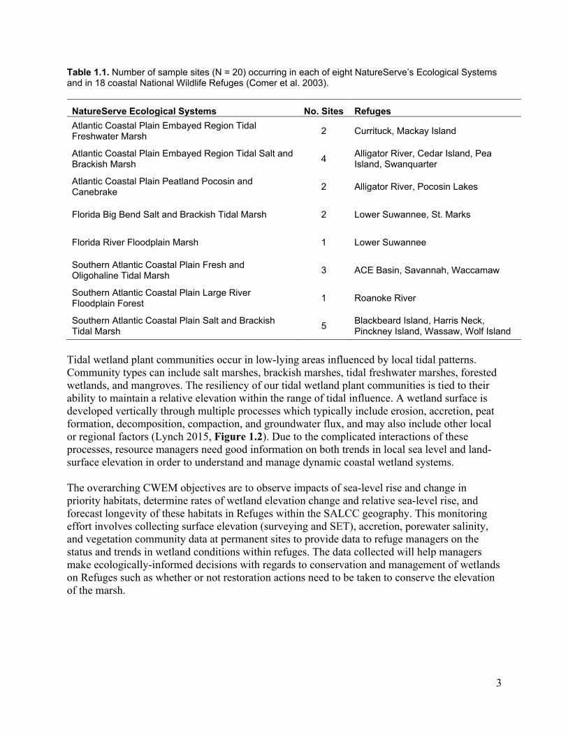
List of Tables Table 1.1. Number of sample sites (N = 20) occurring in each of eight NatureServe’s Ecological

Systems and in 18 coastal National Wildlife Refuges (Comer et al. 2003). ....................... 3

Table 2.1. Description of the sample design and spatial hierarchy of design elements. ................ 6

Table 2.2. Units of measure and number of stations, plots and measurements of each CWEM attribute. ............................................................................................................................ 11

Table 4.1. ServCat organization of documentation and products relevant to monitoring elevation in wetlands (CWEM) of the US South-Atlantic coast. ..................................................... 21

Table 6.1. Types of vehicles that one or more member of a field crew should be qualified to operate to assure visits to CWEM monitoring sites on each refuge. ................................ 27

Table 7.1. Costs in 2012 US Dollars and staff time (hours) to establish 3 benchmarks at one sample site in the first year of CWEM monitoring. .......................................................... 28

Table 7.2. Annual costs (2019 US Dollars) and staff time (hours) for collecting data at each CWEM sample site. .......................................................................................................... 28

Table 7.3. Local and Regional I&M Branch costs and time for project coordination, managing data, conducting analyses and reporting results. Also includes time and costs for periodic benchmark and vegetation surveys. .................................................................................. 28

Table SOP 3.1. Standardized antenna heights in meters (m) to be used in OPUS to calculate the elevation of the benchmark. Antenna heights are the sum of the adapter height, quick release, and height of the poles. ........................................................................................ 42

Table SOP 7.1. Calibration standards to be used at each CWEM site. ....................................... 55

Table 8.1. ...................................................................................................................................... 67

List of Figures Figure 1.1. Initial distribution of the South Atlantic coastal wetland elevation monitoring

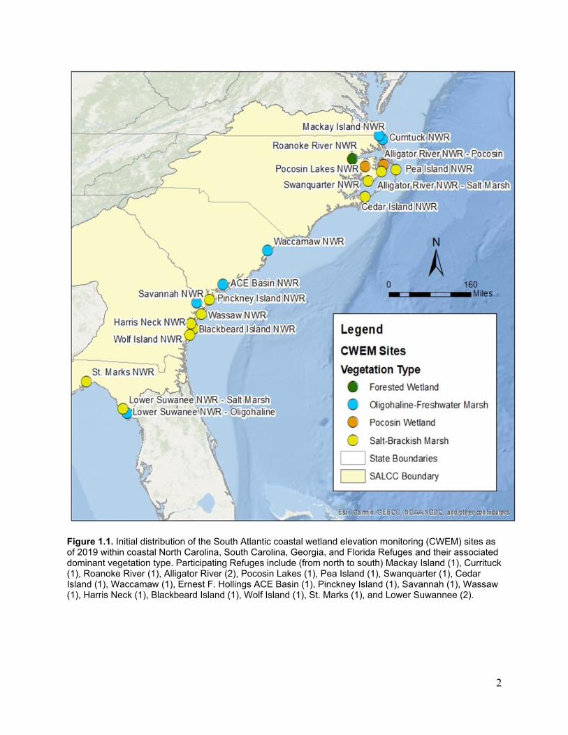
(CWEM) sites as of 2019 within coastal North Carolina, South Carolina, Georgia, and Florida Refuges and their associated dominant vegetation type. Participating Refuges include (from north to south) Mackay Island (1), Currituck (1), Roanoke River (1), Alligator River (2), Pocosin Lakes (1), Pea Island (1), Swanquarter (1), Cedar Island (1), Waccamaw (1), Ernest F. Hollings ACE Basin (1), Pinckney Island (1), Savannah (1), Wassaw (1), Harris Neck (1), Blackbeard Island (1), Wolf Island (1), St. Marks (1), and Lower Suwannee (2). .......................................................................................................... 2

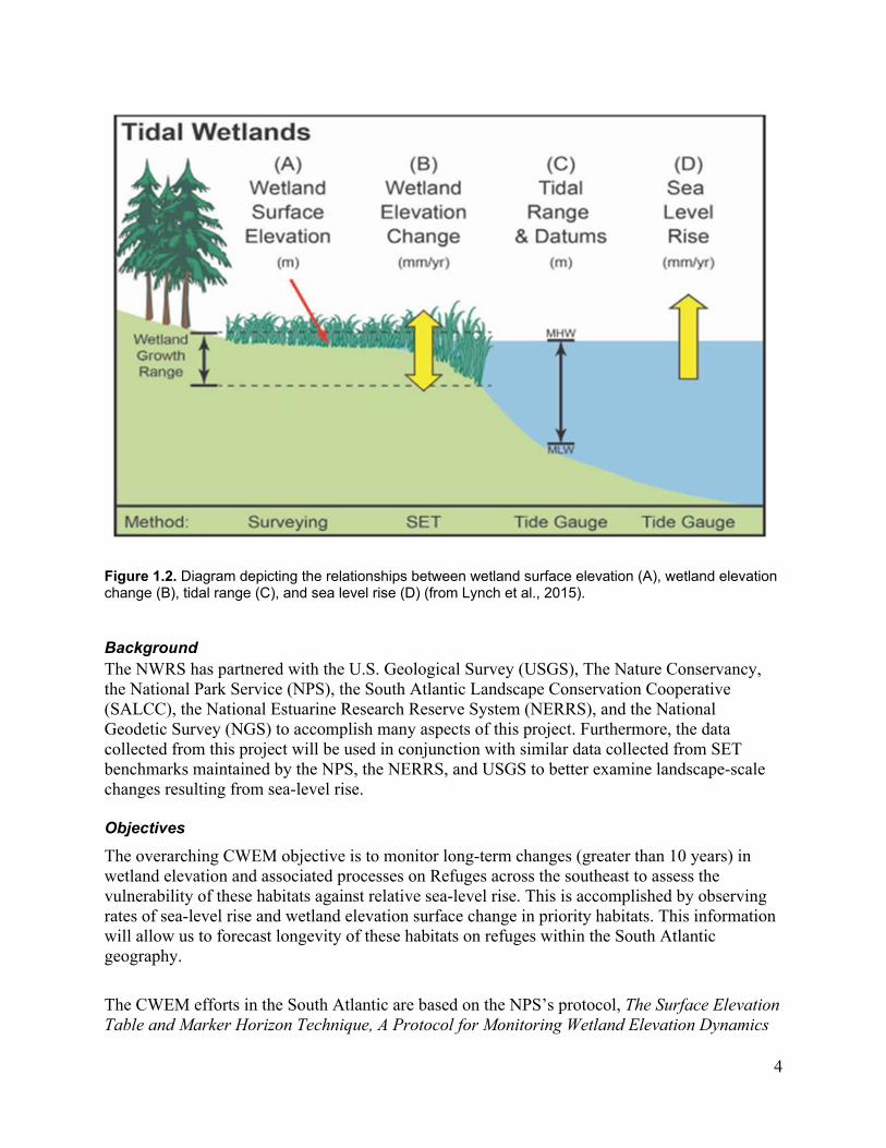
Figure 1.2. Diagram depicting the relationships between wetland surface elevation (A), wetland elevation change (B), tidal range (C), and sea level rise (D) (from Lynch et al., 2015). ... 4

x

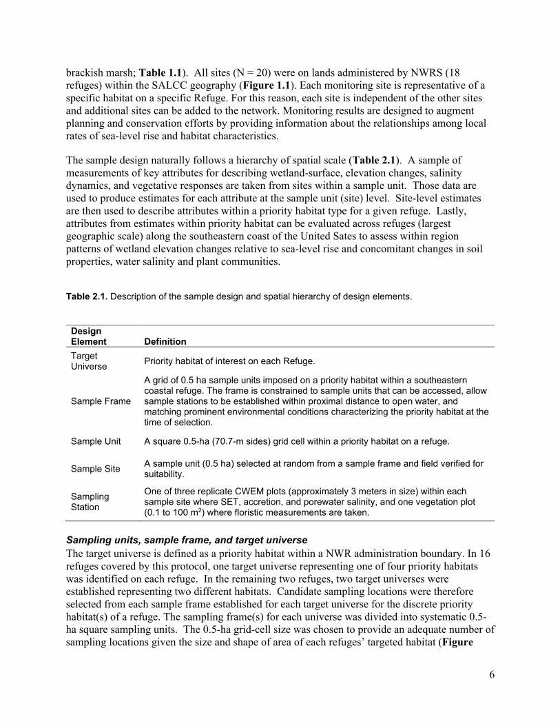
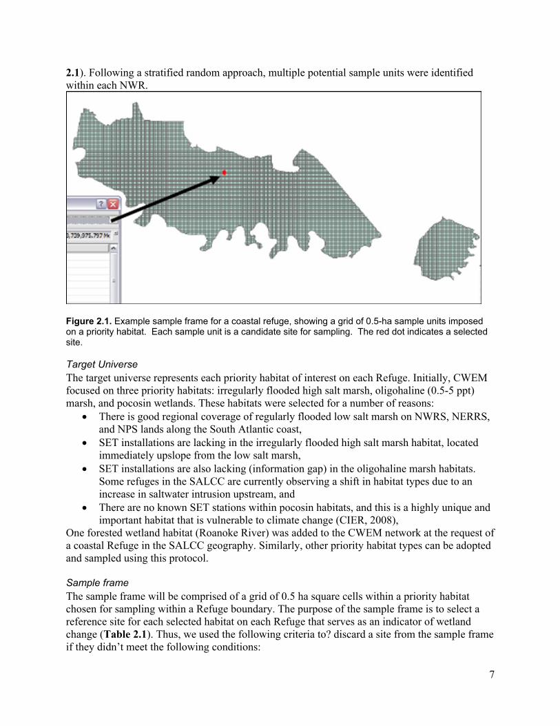
Figure 2.1. Example sample frame for a coastal refuge, showing a grid of 0.5-ha sample units imposed on a priority habitat. Each sample unit is a candidate site for sampling. The red dot indicates a selected site. ................................................................................................ 7

Figure 2.2. Example of the sample draw for marsh habitat on Alligator River NWR using the Reverse Randomized Quadrant-Recursive Raster methodology ........................................ 9

Figure 2.3. Example layout of at a site selected for monitoring and associated subsampling stations (n = 3) where a CWEM plot is placed (noted with an x). Vegetation plots (noted with a square) are associated with each station and are located within 20 m of the CWEM plot and open water. .......................................................................................................... 10

Figure 2.4. Example layout of a CWEM plot including the location of the SET benchmark (bullseye), SET arm directions in 4 cardinal directions, marker horizon plots (1, 2, 3), and porewater salinity plot (S). ................................................................................................ 10

Figure 3.1. Taking surface elevation table (SET) measurements in the field. ............................. 16

Figure 3.2. A photo of a soil core measurement. The core is taken with a McCauley corer and then the depth of soil to the recovered feldspar layer is measured in millimeters. ........... 16

Figure 3.3. Photo of field personnel taking soil porewater salinity measurements in the field. .. 17

Figure 4.1. Example plot of computed surface elevation and soil accretion trends through time from Lynch et al., (2015. Trends are reported in millimeters per a year. ......................... 22

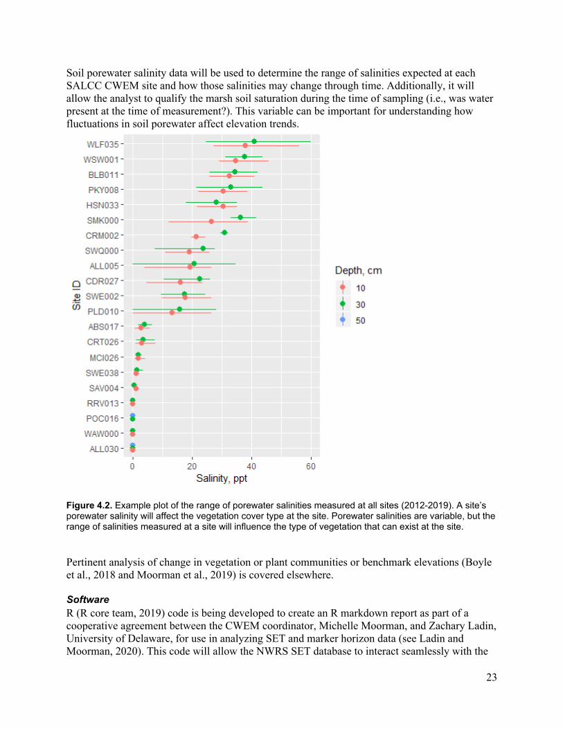
Figure 4.2. Example plot of the range of porewater salinities measured at all sites (2012-2019). A site’s porewater salinity will affect the vegetation cover type at the site. Porewater salinities are variable, but the range of salinities measured at a site will influence the type of vegetation that can exist at the site. .............................................................................. 23

Figure 5.1. Example plot comparing elevation trends among various sites being measured as part of the Coastal Wetland Elevation Monitoring network (Ladin and Moorman, 2020). ..... 25

Figure SOP 3.1. Settings window in on-line tool for planning use of GNSS Trimble receiver. . 38

Figure SOP 3.2. ........................................................................................................................... 39

Figure SOP 3.3. Online tool for NOAA tide predictions. ........................................................... 39

Figure SOP 3.4. Schematic of SET adapter. ................................................................................ 41

Figure SOP 3.5. ........................................................................................................................... 42

Figure SOP 3.6. Example of an OPUS report for static occupation (From Lynch et al. 2015). . 45

Figure SOP 7.1. Required level of coverage by solution when using the salinity meter. The porewater sample must cover the holes of the conductivity sensor, which are closest to the cable at the top of the probe. ....................................................................................... 54

xi

Figure SM 2.1. Porewater sample must cover the holes of the conductivity sensor which are closest to the cable at the top of the probe ........................................................................ 60

1

Narrative Excerpts below largely follow the national monitoring protocol framework, The surface elevation table and marker horizon technique: A protocol for monitoring wetland elevation dynamics. Natural Resource Report NPS/NCBN/NRR—2015/1078. National Park Service, Fort Collins, Colorado. (ServCat Reference: 56400, Lynch, Hensel, and Cahoon 2015).

Introduction

Sea-level rise and its potential impacts to habitats and species are a concern for the National Wildlife Refuges within the South Atlantic Landscape Conservation Cooperative (SALCC). Relative sea level has been rising along the Atlantic and Gulf of Mexico coasts, and recent climate models suggest an acceleration of sea-level rise on the Mid-Atlantic coast greater than the global average (Boon 2012; CCSP 2009). Existing National Oceanic and Atmospheric Administration water level gauges in the Atlantic region have measured relative sea-level rise rates ranging from 1.75 to 4.4 mm per year (CCSP 2009). Tidal salt and freshwater marshes are among the most susceptible ecosystems to accelerated sea-level rise, resulting in significant land loss and habitat conversion across coastal landscapes. The mean elevation of these wetland surfaces must increase to keep pace with the annual rise in sea level and subsidence of organic substrates. Understanding rates of wetland elevation change and relative sea-level rise will help managers at Refuges answer critical questions (e.g., are marshes going to keep pace with relative sea-level rise?) and adjust management techniques towards future conditions. Priority habitat types susceptible to damage and loss from sea-level rise in the SALCC geography include salt and brackish marshes, freshwater and oligohaline marshes, pocosins, and forested wetlands. In December 2011 and January 2012, southeast region (interagency regions 2 and 4) NWR biologists, ecologists, and managers in conjunction with partners determined where priority habitat types would occur for surface elevation table (SET) benchmarks and associated monitoring stations on 18 coastal Refuges within the South Atlantic Landscape Conservation Cooperative geography (Figure 1.1, Table 1.1). Salt marsh sites are located in secluded marsh platforms, embayments, back-barrier marshes, or open coast landforms. Freshwater marsh, oligohaline marsh, and forested wetland sites are located near the mouths of rivers. Coastal flooding is increasing as a result of global mean sea-level rise at rates ranging from 1.75 to 4.4 mm per year and is expected to continue to occur (CCSP 2009). Consistent with scientific understanding, sea levels have not been rising uniformly across the globe over the last century. Relative sea-level rise is the rate of sea-level rise in a particular area and is affected by two main factors, (1) vertical movement of the Earth’s surface, and (2) effects of water movement in the oceans. Vertical land movement can be a significant factor in relative sea-level rise, particularly if land subsidence due to non-climatic processes such as glacial isostatic adjustment, sediment compaction, and groundwater and oil and gas extraction are occurring (Cahoon 2014). Regardless of the cause of local subsidence it has the net result of increasing the rate of relative sea-level rise. Examples of regions experiencing high rates of subsidence include southern Louisiana and Cape Hatteras to New Jersey (NOAA 2017).

2

Figure 1.1. Initial distribution of the South Atlantic coastal wetland elevation monitoring (CWEM) sites as of 2019 within coastal North Carolina, South Carolina, Georgia, and Florida Refuges and their associated dominant vegetation type. Participating Refuges include (from north to south) Mackay Island (1), Currituck (1), Roanoke River (1), Alligator River (2), Pocosin Lakes (1), Pea Island (1), Swanquarter (1), Cedar Island (1), Waccamaw (1), Ernest F. Hollings ACE Basin (1), Pinckney Island (1), Savannah (1), Wassaw (1), Harris Neck (1), Blackbeard Island (1), Wolf Island (1), St. Marks (1), and Lower Suwannee (2).

3

Table 1.1. Number of sample sites (N = 20) occurring in each of eight NatureServe’s Ecological Systems and in 18 coastal National Wildlife Refuges (Comer et al. 2003).

NatureServe Ecological Systems No. Sites Refuges Atlantic Coastal Plain Embayed Region Tidal Freshwater Marsh 2 Currituck, Mackay Island

Atlantic Coastal Plain Embayed Region Tidal Salt and Brackish Marsh 4 Alligator River, Cedar Island, Pea

Island, Swanquarter

Atlantic Coastal Plain Peatland Pocosin and Canebrake 2 Alligator River, Pocosin Lakes

Florida Big Bend Salt and Brackish Tidal Marsh 2 Lower Suwannee, St. Marks

Florida River Floodplain Marsh 1 Lower Suwannee

Southern Atlantic Coastal Plain Fresh and Oligohaline Tidal Marsh 3 ACE Basin, Savannah, Waccamaw

Southern Atlantic Coastal Plain Large River Floodplain Forest 1 Roanoke River

Southern Atlantic Coastal Plain Salt and Brackish Tidal Marsh 5 Blackbeard Island, Harris Neck,

Pinckney Island, Wassaw, Wolf Island

Tidal wetland plant communities occur in low-lying areas influenced by local tidal patterns. Community types can include salt marshes, brackish marshes, tidal freshwater marshes, forested wetlands, and mangroves. The resiliency of our tidal wetland plant communities is tied to their ability to maintain a relative elevation within the range of tidal influence. A wetland surface is developed vertically through multiple processes which typically include erosion, accretion, peat formation, decomposition, compaction, and groundwater flux, and may also include other local or regional factors (Lynch 2015, Figure 1.2). Due to the complicated interactions of these processes, resource managers need good information on both trends in local sea level and land-surface elevation in order to understand and manage dynamic coastal wetland systems. The overarching CWEM objectives are to observe impacts of sea-level rise and change in priority habitats, determine rates of wetland elevation change and relative sea-level rise, and forecast longevity of these habitats in Refuges within the SALCC geography. This monitoring effort involves collecting surface elevation (surveying and SET), accretion, porewater salinity, and vegetation community data at permanent sites to provide data to refuge managers on the status and trends in wetland conditions within refuges. The data collected will help managers make ecologically-informed decisions with regards to conservation and management of wetlands on Refuges such as whether or not restoration actions need to be taken to conserve the elevation of the marsh.

4

Figure 1.2. Diagram depicting the relationships between wetland surface elevation (A), wetland elevation change (B), tidal range (C), and sea level rise (D) (from Lynch et al., 2015).

Background The NWRS has partnered with the U.S. Geological Survey (USGS), The Nature Conservancy, the National Park Service (NPS), the South Atlantic Landscape Conservation Cooperative (SALCC), the National Estuarine Research Reserve System (NERRS), and the National Geodetic Survey (NGS) to accomplish many aspects of this project. Furthermore, the data collected from this project will be used in conjunction with similar data collected from SET benchmarks maintained by the NPS, the NERRS, and USGS to better examine landscape-scale changes resulting from sea-level rise. Objectives

The overarching CWEM objective is to monitor long-term changes (greater than 10 years) in wetland elevation and associated processes on Refuges across the southeast to assess the vulnerability of these habitats against relative sea-level rise. This is accomplished by observing rates of sea-level rise and wetland elevation surface change in priority habitats. This information will allow us to forecast longevity of these habitats on refuges within the South Atlantic geography. The CWEM efforts in the South Atlantic are based on the NPS’s protocol, The Surface Elevation Table and Marker Horizon Technique, A Protocol for Monitoring Wetland Elevation Dynamics

5

(Lynch et al. 2015). The NPS outlines methods and techniques for monitoring long-term trends of a wetland elevation surface and decoupling the processes that influence elevation change, including the rate of vertical accretion. This regional protocol framework explicitly steps down the elements of design, field monitoring, and data management adopted and implemented at the network of sites within the South-Atlantic region and can serve as a site-specific protocol for all sites included in this network (Figure 1.1, Table 1.1). Additional Refuges in the region can adopt this protocol framework for their wetland monitoring but will need to step-down a site-specific protocol for their monitoring site. The objectives of the monitoring will enable an assessment of 1) the rate of wetland elevation change within specific habitats at all participating Refuges, 2) processes contributing to the measured changes (i.e. accretion rates), 3) wetland elevation rates to local sea-level rise rates to determine if the marsh is keeping up with sea level rise, 4) changes in marsh salinity dynamics, and 5) changes in vegetation composition through time as a response to changes in marsh elevation and marsh salinity. This is accomplished through the following activities:

• Establishing a network of CWEM sites from which to perform monitoring of surface elevation, accretion, pore water salinity, and vegetation community on coastal Refuges within the SALCC geography.

• Providing a data management, analysis, and reporting system for each participating site in the network.

• Calculating the magnitude, rate, and within-site variability of change in ground surface elevation, surface sediment accretion, pore water salinity at these sites.

• Developing a baseline inventory of vegetation species and vegetation community type and that is monitored every 3-5 years to determine the status, trends, and within-site variability in vegetation species composition, vegetation structure (strata height), vegetation cover, and abiotic site conditions (soil nutrients). This objective is not discussed further in this protocol framework as a regional protocol framework for this monitoring has been published elsewhere (Boyle et al. 2018).

• Monitoring the elevation of the rod surface elevation table benchmark to measure benchmark stability over time and tie elevation measurements to a common datum (currently NAVD88).

Sampling

Excerpts below are largely taken from The Surface Elevation Table and Marker Horizon Technique, A Protocol for Monitoring Wetland Elevation Dynamics, November 2015, Field Methods, pp 37-38 (Lynch et al., 2015). Sample design This protocol provides guidance for monitoring status and trends in wetland elevation, soil accretion, and porewater salinity over time in habitats of priority interest on National Wildlife Refuges. Since 2012, this protocol has been tested and implemented at 20 sites in four different habitat types (pocosin wetlands, forested wetlands, oligohaline-freshwater marsh and salt-

6

brackish marsh; Table 1.1). All sites (N = 20) were on lands administered by NWRS (18 refuges) within the SALCC geography (Figure 1.1). Each monitoring site is representative of a specific habitat on a specific Refuge. For this reason, each site is independent of the other sites and additional sites can be added to the network. Monitoring results are designed to augment planning and conservation efforts by providing information about the relationships among local rates of sea-level rise and habitat characteristics. The sample design naturally follows a hierarchy of spatial scale (Table 2.1). A sample of measurements of key attributes for describing wetland-surface, elevation changes, salinity dynamics, and vegetative responses are taken from sites within a sample unit. Those data are used to produce estimates for each attribute at the sample unit (site) level. Site-level estimates are then used to describe attributes within a priority habitat type for a given refuge. Lastly, attributes from estimates within priority habitat can be evaluated across refuges (largest geographic scale) along the southeastern coast of the United Sates to assess within region patterns of wetland elevation changes relative to sea-level rise and concomitant changes in soil properties, water salinity and plant communities.

Table 2.1. Description of the sample design and spatial hierarchy of design elements.

Design Element Definition Target Universe Priority habitat of interest on each Refuge.

Sample Frame

A grid of 0.5 ha sample units imposed on a priority habitat within a southeastern coastal refuge. The frame is constrained to sample units that can be accessed, allow sample stations to be established within proximal distance to open water, and matching prominent environmental conditions characterizing the priority habitat at the time of selection.

Sample Unit A square 0.5-ha (70.7-m sides) grid cell within a priority habitat on a refuge.

Sample Site A sample unit (0.5 ha) selected at random from a sample frame and field verified for suitability.

Sampling Station

One of three replicate CWEM plots (approximately 3 meters in size) within each sample site where SET, accretion, and porewater salinity, and one vegetation plot (0.1 to 100 m2) where floristic measurements are taken.

Sampling units, sample frame, and target universe The target universe is defined as a priority habitat within a NWR administration boundary. In 16 refuges covered by this protocol, one target universe representing one of four priority habitats was identified on each refuge. In the remaining two refuges, two target universes were established representing two different habitats. Candidate sampling locations were therefore selected from each sample frame established for each target universe for the discrete priority habitat(s) of a refuge. The sampling frame(s) for each universe was divided into systematic 0.5-ha square sampling units. The 0.5-ha grid-cell size was chosen to provide an adequate number of sampling locations given the size and shape of area of each refuges’ targeted habitat (Figure

7

2.1). Following a stratified random approach, multiple potential sample units were identified within each NWR.

Figure 2.1. Example sample frame for a coastal refuge, showing a grid of 0.5-ha sample units imposed on a priority habitat. Each sample unit is a candidate site for sampling. The red dot indicates a selected site.

Target Universe The target universe represents each priority habitat of interest on each Refuge. Initially, CWEM focused on three priority habitats: irregularly flooded high salt marsh, oligohaline (0.5-5 ppt) marsh, and pocosin wetlands. These habitats were selected for a number of reasons:

• There is good regional coverage of regularly flooded low salt marsh on NWRS, NERRS, and NPS lands along the South Atlantic coast,

• SET installations are lacking in the irregularly flooded high salt marsh habitat, located immediately upslope from the low salt marsh,

• SET installations are also lacking (information gap) in the oligohaline marsh habitats. Some refuges in the SALCC are currently observing a shift in habitat types due to an increase in saltwater intrusion upstream, and

• There are no known SET stations within pocosin habitats, and this is a highly unique and important habitat that is vulnerable to climate change (CIER, 2008),

One forested wetland habitat (Roanoke River) was added to the CWEM network at the request of a coastal Refuge in the SALCC geography. Similarly, other priority habitat types can be adopted and sampled using this protocol. Sample frame The sample frame will be comprised of a grid of 0.5 ha square cells within a priority habitat chosen for sampling within a Refuge boundary. The purpose of the sample frame is to select a reference site for each selected habitat on each Refuge that serves as an indicator of wetland change (Table 2.1). Thus, we used the following criteria to? discard a site from the sample frame if they didn’t meet the following conditions:

8

• Sites must have uniform vegetation community and cover. Vegetation community is defined by the Nature Serve Ecological Systems classification (Comer 2003).

• Sites must not be heavily stressed or disturbed habitat (i.e. poor health, wildlife corridor/trampling, etc.).

• Sites must be located at least 25 meters away from a creek, stream, ditch, estuary or other water body.

• Sites must be separated by at least 25 meters from and minimally influenced by spoil banks, levees, roads, or any other human induced alteration.

• Sites must be reasonably accessible via foot?, boat, road, fire break, etc. by field crews so that logistics don’t cause a barrier to sampling (i.e. site impossible to reach by airboat or site that is a 2-mile hike away).

Sample unit and stations The sampling frame(s) for each Refuge is divided into systematic 0.5-ha sampling units (Figure 2.1). The 0.5-ha grid-cell size is chosen to provide an adequate number of sampling locations given the size and shape of refuges. Each sample unit includes subsampling stations for replicate sampling of the attributes at the site-level (Table 2.1). Sample stations are comprised of a plot where individual SET benchmark, marker horizon, and porewater salinity measurements are taken and a plot where vegetation community dynamics are measured. Sample selection and size The sample site is the selected 0.5 ha grid-cell sampling unit (Figure 2.1). Three replicate SET sample stations are established at all sample sites. It was decided that a minimum of three RSET benchmarks would be installed within each priority habitat chosen on each Refuge. The design team discussed placing the three RSET benchmarks throughout the entire habitat or selecting one random site and clustering the three RSET benchmarks within a single sample unit. It was decided to place the three benchmarks as replicates within one sample unit in order to estimate the variance of measurements that might occur at the site. Following a stratified random approach, multiple potential sample units within each selected priority habitat for each NWR were identified (Figure 2.2). This is a monitoring design similar to Figure 11B in the NPS National Protocol, i.e. one site per a sample frame, but with replication within each sample site (Lynch et al. 2015, Table 2). Sampling sites The sample site is established within one 0.5 ha-grid sampling unit, which is chosen at random from the sample frame. A spatially balanced random sample is drawn from the sampling frame using the Reversed Randomized Quadrant-Recursive Raster (RRQRR) algorithm (Theobald and Norman 2006, Byrne 2012). It includes 35 to 60 potential sampling units that are sequentially numbered. Then, two levels of selection criteria are applied sequentially to all sampling locations whereby sites are excluded if (1) evaluation of relevant GIS data layers strongly suggests the potential sampling location doesn’t meet selection criteria, or (2) verification by field personnel determines the site does not meet all selection criteria (i.e. the site is accessible, is not disturbed,

9

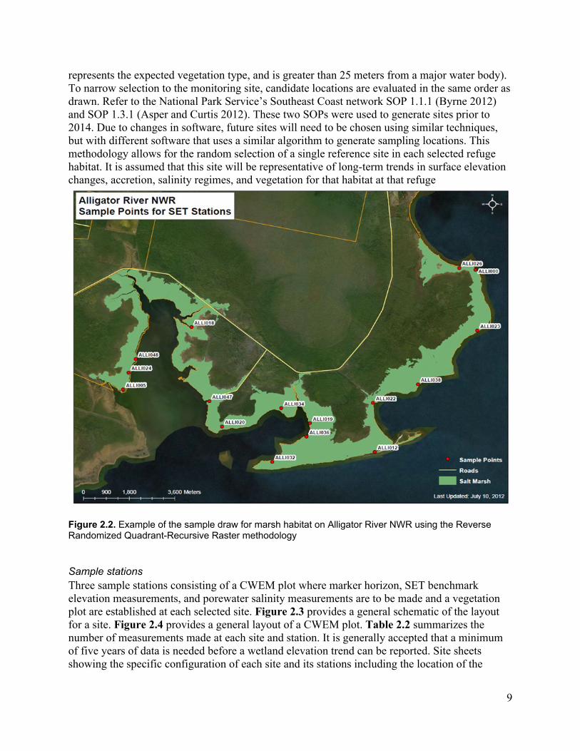
represents the expected vegetation type, and is greater than 25 meters from a major water body). To narrow selection to the monitoring site, candidate locations are evaluated in the same order as drawn. Refer to the National Park Service’s Southeast Coast network SOP 1.1.1 (Byrne 2012) and SOP 1.3.1 (Asper and Curtis 2012). These two SOPs were used to generate sites prior to 2014. Due to changes in software, future sites will need to be chosen using similar techniques, but with different software that uses a similar algorithm to generate sampling locations. This methodology allows for the random selection of a single reference site in each selected refuge habitat. It is assumed that this site will be representative of long-term trends in surface elevation changes, accretion, salinity regimes, and vegetation for that habitat at that refuge

Figure 2.2. Example of the sample draw for marsh habitat on Alligator River NWR using the Reverse Randomized Quadrant-Recursive Raster methodology

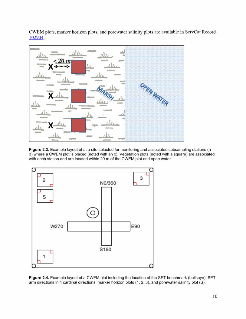
Sample stations Three sample stations consisting of a CWEM plot where marker horizon, SET benchmark elevation measurements, and porewater salinity measurements are to be made and a vegetation plot are established at each selected site. Figure 2.3 provides a general schematic of the layout for a site. Figure 2.4 provides a general layout of a CWEM plot. Table 2.2 summarizes the number of measurements made at each site and station. It is generally accepted that a minimum of five years of data is needed before a wetland elevation trend can be reported. Site sheets showing the specific configuration of each site and its stations including the location of the

10

CWEM plots, marker horizon plots, and porewater salinity plots are available in ServCat Record 102904.

Figure 2.3. Example layout of at a site selected for monitoring and associated subsampling stations (n = 3) where a CWEM plot is placed (noted with an x). Vegetation plots (noted with a square) are associated with each station and are located within 20 m of the CWEM plot and open water.

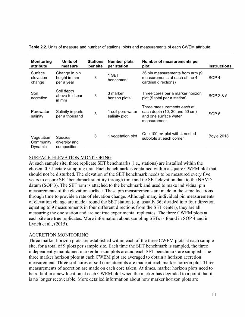
Figure 2.4. Example layout of a CWEM plot including the location of the SET benchmark (bullseye), SET arm directions in 4 cardinal directions, marker horizon plots (1, 2, 3), and porewater salinity plot (S).

11

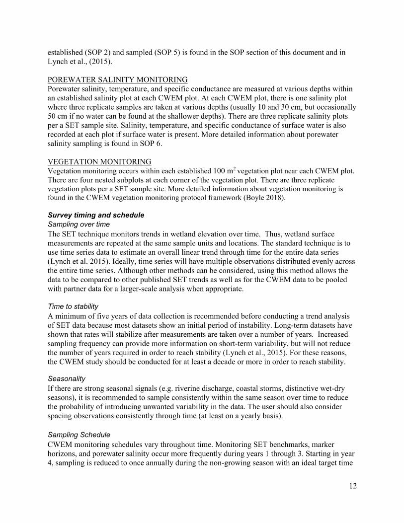
Table 2.2. Units of measure and number of stations, plots and measurements of each CWEM attribute.

Monitoring attribute

Units of measure

Stations per site

Number plots per station

Number of measurements per plot Instructions

Surface elevation change

Change in pin height in mm per a year

3 1 SET benchmark

36 pin measurements from arm (9 measurements at each of the 4 cardinal directions)

SOP 4

Soil accretion

Soil depth above feldspar in mm

3 3 marker horizon plots

Three cores per a marker horizon plot (9 total per a station) SOP 2 & 5

Porewater salinity

Salinity in parts per a thousand 3 1 soil pore water

salinity plot

Three measurements each at each depth (10, 30 and 50 cm) and one surface water measurement

SOP 6

Vegetation Community Dynamic

Species diversity and composition

3 1 vegetation plot One 100 m2-plot with 4 nested subplots at each corner Boyle 2018

SURFACE-ELEVATION MONITORING At each sample site, three replicate SET benchmarks (i.e., stations) are installed within the chosen, 0.5-hectare sampling unit. Each benchmark is contained within a square CWEM plot that should not be disturbed. The elevation of the SET benchmark needs to be measured every five years to ensure SET benchmark stability through time and tie SET elevation data to the NAVD datum (SOP 3). The SET arm is attached to the benchmark and used to make individual pin measurements of the elevation surface. These pin measurements are made in the same locations through time to provide a rate of elevation change. Although many individual pin measurements of elevation change are made around the SET station (e.g. usually 36; divided into four direction equating to 9 measurements in four different directions from the SET center), they are all measuring the one station and are not true experimental replicates. The three CWEM plots at each site are true replicates. More information about sampling SETs is found in SOP 4 and in Lynch et al., (2015). ACCRETION MONITORING Three marker horizon plots are established within each of the three CWEM plots at each sample site, for a total of 9 plots per sample site. Each time the SET benchmark is sampled, the three independently maintained marker horizon plots around each SET benchmark are sampled. The three marker horizon plots at each CWEM plot are averaged to obtain a horizon accretion measurement. Three soil cores or soil core attempts are made at each marker horizon plot. Three measurements of accretion are made on each core taken. At times, marker horizon plots need to be re-laid in a new location at each CWEM plot when the marker has degraded to a point that it is no longer recoverable. More detailed information about how marker horizon plots are

12

established (SOP 2) and sampled (SOP 5) is found in the SOP section of this document and in Lynch et al., (2015). POREWATER SALINITY MONITORING Porewater salinity, temperature, and specific conductance are measured at various depths within an established salinity plot at each CWEM plot. At each CWEM plot, there is one salinity plot where three replicate samples are taken at various depths (usually 10 and 30 cm, but occasionally 50 cm if no water can be found at the shallower depths). There are three replicate salinity plots per a SET sample site. Salinity, temperature, and specific conductance of surface water is also recorded at each plot if surface water is present. More detailed information about porewater salinity sampling is found in SOP 6. VEGETATION MONITORING Vegetation monitoring occurs within each established 100 m2 vegetation plot near each CWEM plot. There are four nested subplots at each corner of the vegetation plot. There are three replicate vegetation plots per a SET sample site. More detailed information about vegetation monitoring is found in the CWEM vegetation monitoring protocol framework (Boyle 2018). Survey timing and schedule Sampling over time The SET technique monitors trends in wetland elevation over time. Thus, wetland surface measurements are repeated at the same sample units and locations. The standard technique is to use time series data to estimate an overall linear trend through time for the entire data series (Lynch et al. 2015). Ideally, time series will have multiple observations distributed evenly across the entire time series. Although other methods can be considered, using this method allows the data to be compared to other published SET trends as well as for the CWEM data to be pooled with partner data for a larger-scale analysis when appropriate. Time to stability A minimum of five years of data collection is recommended before conducting a trend analysis of SET data because most datasets show an initial period of instability. Long-term datasets have shown that rates will stabilize after measurements are taken over a number of years. Increased sampling frequency can provide more information on short-term variability, but will not reduce the number of years required in order to reach stability (Lynch et al., 2015). For these reasons, the CWEM study should be conducted for at least a decade or more in order to reach stability. Seasonality If there are strong seasonal signals (e.g. riverine discharge, coastal storms, distinctive wet-dry seasons), it is recommended to sample consistently within the same season over time to reduce the probability of introducing unwanted variability in the data. The user should also consider spacing observations consistently through time (at least on a yearly basis). Sampling Schedule CWEM monitoring schedules vary throughout time. Monitoring SET benchmarks, marker horizons, and porewater salinity occur more frequently during years 1 through 3. Starting in year 4, sampling is reduced to once annually during the non-growing season with an ideal target time

13

of fall (October through December). Benchmark surveys occur once every 5 years. Vegetation sampling should occur once every 3 to 5 years. Funding, weather, tides, time, and other logistics are anticipated factors influencing the sampling schedule. Sources of error Two fundamental errors influence accuracy when measuring and? collecting samples and using those data to estimate a trend in a value over time. These are bias and precision. Both influence ‘accuracy’ of the estimator and both types of errors can influence estimates of any attribute, so general mention of these errors can be addressed up front, or with each attribute’s sources of error. Below we address biases that can occur as a result of the sampling process and suggestions for the field that can reduce the bias of an estimate. Sampling variances which provide a range of precision are reported in the CWEM trend analysis report (Ladin and Moorman, 2020). Surface-elevation monitoring There are several sources of error that can cause biases in the SET readings. The primary way to avoid bias is to make every effort to take measurements consistently with the same reader through time. Elevation monitoring often requires 20 to 30 years of consistent data collection to estimate a long-term elevation trend. There are subjective decisions made when determining the wetland surface. For this reason, SET readers need consistent rules for determining wetland surface. Operator bias is an important factor that affects the SET trend measured so it is preferable that the same person read the SET each time (Lynch et al. 2015). In the event that there is a change in readers, Lynch et al. (2015) recommends that a “double-read” be performed. A double-read involves the two operators taking readings of the same point, which allows an estimate of the bias between the two readers. The SET reader should always be recorded on the datasheet. Errors in SET measurements can also be due to environmental conditions and tidal changes that occur when readings are taken. Soil porewater conditions can cause the soil matrix to shrink or expand as can underground vegetation mass which can vary seasonally (i.e., greater during the growing season). The presence of water on the marsh surface can also influence the reader’s ability to accurately measure the soil surface. Thus, it is important to note factors such as the presence of water on the marsh surface, vegetation cover, time of year, and other environmental and site conditions to help explain any outliers that might be observed in the data. Additionally, all annual measurements are conducted during the non-growing season to reduce seasonal variability that can be caused by changes in underground vegetation mass. Accretion monitoring There are several sources of error that can cause biases in the marker horizon readings. If the marsh is super-saturated or surface water is present, it is often difficult to recover a measurable core. The core may fall apart once it is taken. Cryogenic coring may overcome this issue, but this method has not always proven successful or adopted by field personnel. In addition, missing marker horizon data through time can lead to a positive bias in accretion measurements if the data is missing due to an erosion event (Lynch et al. 2015). Field personnel have not always successfully recovered marker horizons at all CWEM plots and it is impossible to know if this is because there was no accretion or if it was because the feldspar has broken down and

14

disappeared through time. This has been overcome by establishing new feldspar plots when the original plots are no longer recoverable. Porewater salinity monitoring Salinity meters are calibrated with appropriate standards before each use. Proper calibration ensures that measurements are accurate. Occasionally, porewater salinity data are not collected because the field personnel are unable to extract water from the soil matrix. Vertical control surveys SET Benchmarks should be surveyed initially in order to tie the benchmark to a known datum. Benchmarks can move through time, so vertical control surveys are conducted once every five years to ensure that the benchmark has not moved. Moving benchmarks can introduce bias into SET measurements. Additionally, there are many sources of error that can be introduced during the vertical control surveys. Vertical control surveys can provide accuracy to the nearest centimeter but may not be able to provide sub-centimeter accuracy at these remote locations. These errors are discussed at length in another report (Moorman et al., 2019).

Field Methods and Processing of Collected Materials

Excerpts below are largely taken from The Surface Elevation Table and Marker Horizon Technique, A Protocol for Monitoring Wetland Elevation Dynamics, November 2015, Field Methods, pp 37-38 (Lynch et al., 2015). The CWEM project manager will coordinate with Refuge staff annually to ensure that Refuges have all the necessary equipment required to conduct the SET, accretion, and porewater salinity measurements. At Refuges where equipment is shared, the project manager will coordinate with Refuge staff to ensure equipment is available to all personnel during the sampling period. Refuge staff should check all equipment against the equipment list before going in the field. Prior to conducting fieldwork, all equipment should be calibrated. This includes using non-expired specific conductivity standards to calibrate or check the conductivity meter before use. In addition, SET pin length should be measured on an annual to biannual basis to confirm that the length of the fiberglass pins has not changed. All rulers used to measure pin lengths and marker horizon plots should be checked for wear and replaced when they become difficult to read; all rulers should include increments in millimeters and centimeters. Training required to conduct sampling or take measurements should be arranged and completed in advance of field work (see Element 6). The team should download and print a copy of the most recent site map (Record # 102904) and data sheets (Record # 102901)from ServCat prior to going in the field. These site maps provide coordinates for the site and a layout of all SET, marker horizon, and soil porewater salinity plots for that site. Establishment of sampling units Installation of SET Benchmarks One permanent SET benchmark is installed at each sample station. The SET benchmark is installed by driving 4’ sections of 9/16” diameter, stainless steel rods into the ground. Multiple rods thread together. The SET benchmarks can use as much of 30 m of rod before they reach a

15

point of refusal and cannot be driven further into the substrate. For existing CWEM sites, 10 to30 m of rod were commonly used in the installation. Once the rod reaches refusal, the rod is cut and encased in a 2’ long, 6” diameter PVC pipe. The SET receiver is bolted to the upper rod section and the entire PVC tube is filled with concrete. SET marks are allowed to settle for several weeks before the first measurements are taken. More detailed instructions on SET installation are available in Lynch et al. (2015). Our SOP 1 provides details on equipment and supplies used to install the SET marks. It also provides sample datasheets that can be used to record pertinent information for a new installation. SET benchmark installation is completed on a temporary platform placed above the sediment surface to minimize disturbance of the sediments. Refer to NPS SOP 2 (Lynch et al., 2015) for more information on installing SET benchmarks. Installation of Marker Horizons Marker horizons are artificial soil layers (e.g., feldspar) established on the surface of the wetland or shallow water bottoms to measure surface sediment accretion (Bauman et al. 1984, Cahoon and Turner 1989). Marker horizons are established at the time of the baseline SET readings (i.e., time zero). Three marker horizon plots are established in the immediate vicinity of the SET benchmark (Figure 2.4). Feldspar clay is being used as the material for marker horizon plots and is evenly scattered on the wetland surface within the plots. Refer to NPS SOP 2 (Lynch et al. 2015) for detailed instructions on installing marker horizons. Over time, marker horizons will need to be replaced as the feldspar deteriorates. This will likely happen on a 2- to 3-year interval. It is important to lay the new marker horizon plot in a unique location from all previously laid feldspar plots and accurately mark the location in the field with orange stakes and on the site information sheet. There are some existing CWEM sites where feldspar clay disappears within a short amount of time. At the time of this protocol writing, other options for obtaining accretion information are being explored. More information is provided in SOP 2, herein. Data collection procedures (field, lab) All measurements and descriptive data will be collected according to SOPs and recorded on paper data sheets. See ServCat record 102901 to download copies of the appropriate data sheets. SET Measurements The SET is a portable mechanical device which provides high-resolution measurements of relative elevation change in wetland sediments or shallow water bottoms relative to the depth of the reference mark to which it is attached. The SET instrument attaches to the SET benchmark. The SET arm is extended in the four cardinal directions specified on the site datasheet and leveled so it is horizontal to the marsh surface. Each of the nine pins is lowered to the wetland surface and secured with a badge clip. The reader uses a meter stick to determine the height, in millimeters, of each pin above the arm; this height is recorded on the datasheet (Figure 3.1). Measurements are repeatable, can be made over long periods of time, and are of sufficiently high resolution to compare trends in the elevation surface to long-term, relative sea-level trends measured by tide gauges (Cahoon 2014).

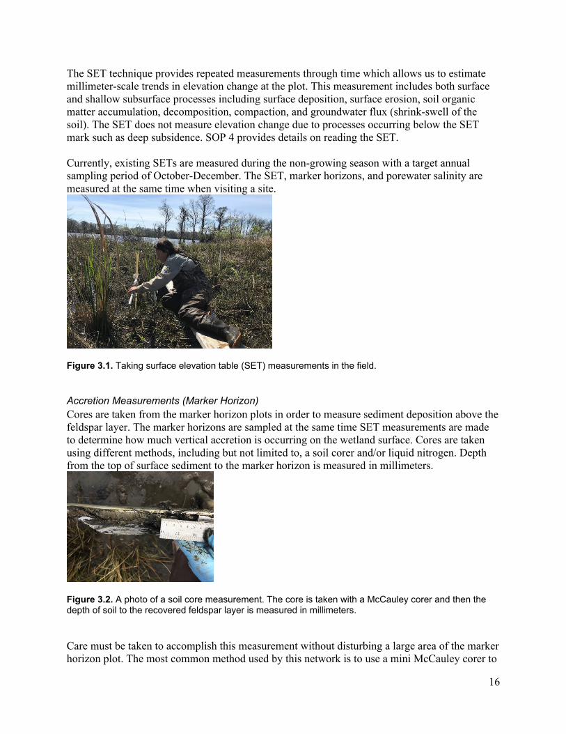
16

The SET technique provides repeated measurements through time which allows us to estimate millimeter-scale trends in elevation change at the plot. This measurement includes both surface and shallow subsurface processes including surface deposition, surface erosion, soil organic matter accumulation, decomposition, compaction, and groundwater flux (shrink-swell of the soil). The SET does not measure elevation change due to processes occurring below the SET mark such as deep subsidence. SOP 4 provides details on reading the SET. Currently, existing SETs are measured during the non-growing season with a target annual sampling period of October-December. The SET, marker horizons, and porewater salinity are measured at the same time when visiting a site.

Figure 3.1. Taking surface elevation table (SET) measurements in the field.

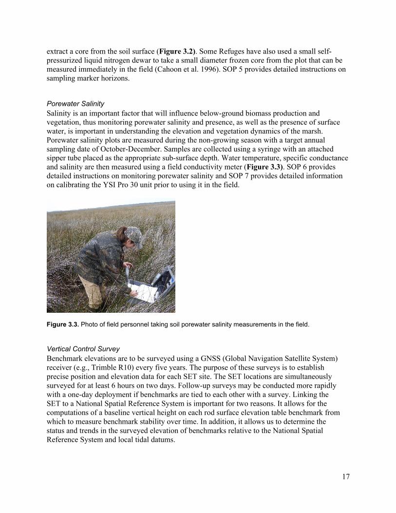
Accretion Measurements (Marker Horizon) Cores are taken from the marker horizon plots in order to measure sediment deposition above the feldspar layer. The marker horizons are sampled at the same time SET measurements are made to determine how much vertical accretion is occurring on the wetland surface. Cores are taken using different methods, including but not limited to, a soil corer and/or liquid nitrogen. Depth from the top of surface sediment to the marker horizon is measured in millimeters.

Figure 3.2. A photo of a soil core measurement. The core is taken with a McCauley corer and then the depth of soil to the recovered feldspar layer is measured in millimeters.

Care must be taken to accomplish this measurement without disturbing a large area of the marker horizon plot. The most common method used by this network is to use a mini McCauley corer to

17

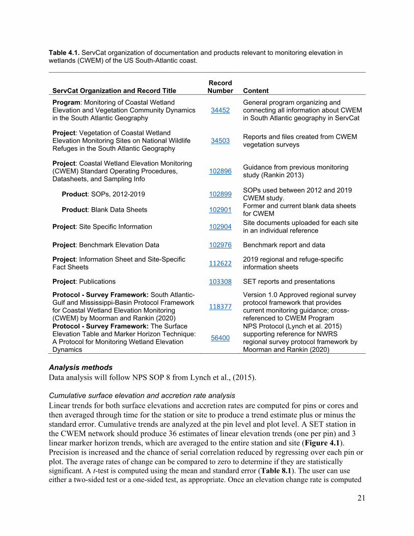
extract a core from the soil surface (Figure 3.2). Some Refuges have also used a small self-pressurized liquid nitrogen dewar to take a small diameter frozen core from the plot that can be measured immediately in the field (Cahoon et al. 1996). SOP 5 provides detailed instructions on sampling marker horizons. Porewater Salinity Salinity is an important factor that will influence below-ground biomass production and vegetation, thus monitoring porewater salinity and presence, as well as the presence of surface water, is important in understanding the elevation and vegetation dynamics of the marsh. Porewater salinity plots are measured during the non-growing season with a target annual sampling date of October-December. Samples are collected using a syringe with an attached sipper tube placed as the appropriate sub-surface depth. Water temperature, specific conductance and salinity are then measured using a field conductivity meter (Figure 3.3). SOP 6 provides detailed instructions on monitoring porewater salinity and SOP 7 provides detailed information on calibrating the YSI Pro 30 unit prior to using it in the field.

Figure 3.3. Photo of field personnel taking soil porewater salinity measurements in the field.

Vertical Control Survey Benchmark elevations are to be surveyed using a GNSS (Global Navigation Satellite System) receiver (e.g., Trimble R10) every five years. The purpose of these surveys is to establish precise position and elevation data for each SET site. The SET locations are simultaneously surveyed for at least 6 hours on two days. Follow-up surveys may be conducted more rapidly with a one-day deployment if benchmarks are tied to each other with a survey. Linking the SET to a National Spatial Reference System is important for two reasons. It allows for the computations of a baseline vertical height on each rod surface elevation table benchmark from which to measure benchmark stability over time. In addition, it allows us to determine the status and trends in the surveyed elevation of benchmarks relative to the National Spatial Reference System and local tidal datums.

18

SOP 3 provides specific instructions and guidance on conducting vertical control surveys. Additional information on the initial vertical control surveys conducted at each benchmark can be found in Moorman et al. 2019. End-of-season procedures All equipment should be cleaned and stored after each sampling event. SOP 8 provides detailed instructions on equipment cleaning and shipping procedures. Datasheets should be scanned and provided to I&M staff for entry into the SET database. Field personnel can either email completed data sheets to the CWEM coordinator or put them in the appropriate site folder on the CWEM sharepoint site. The program coordinator will inform field personnel about procedures for transferring the datasheets.

Data Management and Analysis Metadata

Excerpts below are largely taken from The Surface Elevation Table and Marker Horizon Technique, A Protocol for Monitoring Wetland Elevation Dynamics, November 2015, Data Handling Methods and Reporting, pp 42-50 (Lynch et al., 2015). Surface elevation table, accretion, porewater salinity, and vegetation measurement techniques differ in important ways such that the datasets are treated differently in collection, recording, and analyses. Measurements recorded using the SET method require specific, careful handling and manipulation since each pin theoretically returns to the same point on the wetland surface over the time period? of the study. This data structure results in serial correlation, which has implications for statistical analyses. Accretion data also come from distinct soil surfaces, but each sampling event results in the measurement of a different plug of sediment, so the same sediment surface is not repeatedly measured. Soil porewater salinity data come from distinct plots, but each sampling event generally results in the measurement of a different parcel of water, so the same water is not repeatedly measured. For these datasets, there are a number of factors which can result in a bias in the data, such as the observer, the nature of the sediment surface, and the phase of tide (exposed or flooded surface); these factors therefore need to be documented in metadata. Vegetation measurements are discussed further by Boyle et al. (2018). Data entry, verification, and editing As of 2018, the NWRS has developed a centralized database that can store all SET and accretion data as well as metadata on individual sites and stations. More information can be found at: https://ecos.fws.gov/ServCat/DownloadFile/138336. This SET application is a centralized database and user interface for entering, managing, and reporting data that was collected using the NPS Surface Elevation Table and Marker Horizon Technique protocol (Lynch 2015). The application currently supports the following functionality:

● Manage Stations - For each SET station, there is the ability to manage its characteristics (e.g., location, name, description, SET Arm directions, benchmark elevation) plus track new and deprecated marker horizons and add photos/station sketches.

● Add Station Data - The system supports the ability to add the pin heights, marker horizon soil cores, photographs, and scanned field sheets for each sampling event.

19

● Manage Users - FWS staff and external partners can be given permission to add data.

● Reporting - The SET application relies on a flexible reporting framework that provides staff with the ability to develop customized and shareable summaries/graphics for the purpose of both Quality Control (QC) and analysis.

A separate, standalone database has been developed by Interior Region 2/4 to house all porewater salinity data that consists of a data entry form and Excel spreadsheet. Data verification is used to ensure that data collected in the field is accurately entered into a spreadsheet or database. It is the job of the person entering the data to double check all database entries, correct discrepancies, and initial each datasheet prior to advancing to and transcribing the next datasheet. Errors or questions about the data content can be recorded in separate data entry notes; such notes are useful during data verification. The database has various verification reports that can be run to determine discrepancies and outliers in the database. A second person is required to check the data against the verified field sheets to make sure it was accurately entered before approving the data in the database. Data validation and quality control procedures follow NPS SOP 7 (Lynch et al. 2015). This includes running simple summary statistics on the data to look for discrepancies. These functionalities are currently being developed in conjunction with the northeast region and the University of Delaware and will be integrated with the SET database. Exploratory data analysis will be conducted annually to allow the project manager to review the data for range and logic error. Validation queries can identify generic errors such as missing, mismatched, or duplicate records. Interval calculations can be used to evaluate incremental change from one sampling event to the next (see Lynch et al. 2015, SOP 7:6 for more detail). This is a way to perform a quality control check on the dataset because it can detect large changes in pin readings (>25 mm) and see if pin readings are consistent with the other pins or with prior readings. Anything unusual may be explained by consulting the field notes or field personnel. Confirmation of why an unusual value was accepted or rejected should be noted so that future analysts will know the data has been verified. Metadata Metadata for SET, porewater salinity, and accretion datasets will include the following considerations:

● Types of data taken (SET and marker horizon)

● Location of the site

● Originator of the data (observer)

● Date site was established and sampling dates

Metadata specific to SET data:

● Type of SET mark (pipe mark or deep rod mark), including presumed depth and date installed

20

● Type of SET instrument (e.g. SET, Rod SET, NGS Rod SET)

● Type of SET measuring arm used (e.g., Nolan, Churchman)

● Benchmark to collar measurements

● Orientation of CWEM plot and direction of approach

● Orientation and numbers of positions read

● Photograph information (time, date, location, photo orientation)

● Pin length

Metadata specific to accretion data:

● Type of accretion marker and date established

● Location of marker horizon plots around (SET) station and identification (e.g. numbering)

● Accretion sampling method (e.g. coring tube, extraction with knife, cryo-coring)

Metadata specific to water monitoring:

● Model and serial number of salinity meter

● Calibration date and standard used (see SOP 7)

Metadata should be recorded on datasheets, so that the operators can cross-check original information. Metadata will also be stored and archived digitally in the national SET Database. Data security and archiving Access to reports and data in the USFWS SET database are limited to specific refuge staff actively collecting and managing data for their refuges. Ultimately, there is the intent to make the information more broadly available once the rules and expectations regarding data access have been defined. It is the intent that the Refuge staff collecting the SET and CWEM data will eventually be able to enter data and retrieve reports directly from the SET application. All datasheets are stored in the SET database. Back-up copies are available on the CWEM sharepoint site. In addition, all SET and accretion data is archived in the SET application which is backed-up by the NWRS. All porewater salinity data is archived in a database developed by the South Atlantic-Gulf and Mississippi Basin Region I&M Branch and backed-up on the regional server. All final CWEM data will be stored in ServCat under the ServCat Program, Coastal Wetland Elevation Monitoring (Record #: 34452, Table 4.1).

21

Table 4.1. ServCat organization of documentation and products relevant to monitoring elevation in wetlands (CWEM) of the US South-Atlantic coast.

ServCat Organization and Record Title Record Number Content

Program: Monitoring of Coastal Wetland Elevation and Vegetation Community Dynamics in the South Atlantic Geography

34452

General program organizing and connecting all information about CWEM in South Atlantic geography in ServCat

Project: Vegetation of Coastal Wetland Elevation Monitoring Sites on National Wildlife Refuges in the South Atlantic Geography

34503

Reports and files created from CWEM vegetation surveys

Project: Coastal Wetland Elevation Monitoring (CWEM) Standard Operating Procedures, Datasheets, and Sampling Info

102896

Guidance from previous monitoring study (Rankin 2013)

Product: SOPs, 2012-2019 102899

SOPs used between 2012 and 2019 CWEM study.

Product: Blank Data Sheets 102901

Former and current blank data sheets for CWEM

Project: Site Specific Information 102904

Site documents uploaded for each site in an individual reference

Project: Benchmark Elevation Data 102976 Benchmark report and data

Project: Information Sheet and Site-Specific Fact Sheets 112622

2019 regional and refuge-specific information sheets

Project: Publications 103308 SET reports and presentations

Protocol - Survey Framework: South Atlantic-Gulf and Mississippi-Basin Protocol Framework for Coastal Wetland Elevation Monitoring (CWEM) by Moorman and Rankin (2020)

118377

Version 1.0 Approved regional survey protocol framework that provides current monitoring guidance; cross-referenced to CWEM Program

Protocol - Survey Framework: The Surface Elevation Table and Marker Horizon Technique: A Protocol for Monitoring Wetland Elevation Dynamics

56400

NPS Protocol (Lynch et al. 2015) supporting reference for NWRS regional survey protocol framework by Moorman and Rankin (2020)

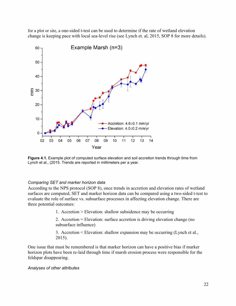
Analysis methods Data analysis will follow NPS SOP 8 from Lynch et al., (2015). Cumulative surface elevation and accretion rate analysis Linear trends for both surface elevations and accretion rates are computed for pins or cores and then averaged through time for the station or site to produce a trend estimate plus or minus the standard error. Cumulative trends are analyzed at the pin level and plot level. A SET station in the CWEM network should produce 36 estimates of linear elevation trends (one per pin) and 3 linear marker horizon trends, which are averaged to the entire station and site (Figure 4.1). Precision is increased and the chance of serial correlation reduced by regressing over each pin or plot. The average rates of change can be compared to zero to determine if they are statistically significant. A t-test is computed using the mean and standard error (Table 8.1). The user can use either a two-sided test or a one-sided test, as appropriate. Once an elevation change rate is computed

22

for a plot or site, a one-sided t-test can be used to determine if the rate of wetland elevation change is keeping pace with local sea-level rise (see Lynch et. al, 2015, SOP 8 for more details).

Figure 4.1. Example plot of computed surface elevation and soil accretion trends through time from Lynch et al., (2015. Trends are reported in millimeters per a year.

Comparing SET and marker horizon data According to the NPS protocol (SOP 8), once trends in accretion and elevation rates of wetland surfaces are computed, SET and marker horizon data can be compared using a two-sided t-test to evaluate the role of surface vs. subsurface processes in affecting elevation change. There are three potential outcomes:

1. Accretion > Elevation: shallow subsidence may be occurring 2. Accretion = Elevation: surface accretion is driving elevation change (no subsurface influence) 3. Accretion < Elevation: shallow expansion may be occurring (Lynch et al., 2015).

One issue that must be remembered is that marker horizon can have a positive bias if marker horizon plots have been re-laid through time if marsh erosion process were responsible for the feldspar disappearing. Analyses of other attributes

23

Soil porewater salinity data will be used to determine the range of salinities expected at each SALCC CWEM site and how those salinities may change through time. Additionally, it will allow the analyst to qualify the marsh soil saturation during the time of sampling (i.e., was water present at the time of measurement?). This variable can be important for understanding how fluctuations in soil porewater affect elevation trends.

Figure 4.2. Example plot of the range of porewater salinities measured at all sites (2012-2019). A site’s porewater salinity will affect the vegetation cover type at the site. Porewater salinities are variable, but the range of salinities measured at a site will influence the type of vegetation that can exist at the site.

Pertinent analysis of change in vegetation or plant communities or benchmark elevations (Boyle et al., 2018 and Moorman et al., 2019) is covered elsewhere. Software R (R core team, 2019) code is being developed to create an R markdown report as part of a cooperative agreement between the CWEM coordinator, Michelle Moorman, and Zachary Ladin, University of Delaware, for use in analyzing SET and marker horizon data (see Ladin and Moorman, 2020). This code will allow the NWRS SET database to interact seamlessly with the

24

code in order to generate results and reports for individual stations. The southeast region has developed R code (R core team, 2019) for analyzing porewater salinity data. All code will be stored with the companion trend analysis report in ServCat, Record 118378.

Reporting

Excerpts below are largely taken from The Surface Elevation Table and Marker Horizon Technique, A Protocol for Monitoring Wetland Elevation Dynamics, November 2015, Personnel Requirements and Training, pp 51. Citation Needed? Implications and application Objectives and methods This project will use established analytical methods described in SOP 8 of Lynch et al. (2015) to answer the following questions for each CWEM site? Sampling site?: 1. What is the overall rate of vertical accretion and elevation change?

2. Is the rate of elevation change less than or equal to local sea-level rise? • Are the coastal wetlands keeping pace with local sea-level rise? • Are the coastal wetlands at risk of becoming submerged and transitioning to open water? 3. Is the rate of elevation change the same as the rate of surface accretion (if sufficient marker horizon data exists)? • Is surface accretion alone responsible for elevation change? • Are below-ground processes involved in either elevation gain or elevation loss? In addition, we hope to answer the following question for all SALCC Refuges in the study: 4. Is the rate of accretion or elevation change the same across different Refuges? • Are different areas of the coast more or less sensitive to local sea-level rise? • Are different management options able to enhance wetland sustainability in the face of sea-level rise? 5. Is the relationship between elevation change and surface accretion the same across different refuges? Summary of results In 2019, a report was produced for each refuge that summarized data collection efforts to date and the NOAA sea level rise trends for each site. The report will serve as a Refuge-specific fact sheet that summarizes each project and all sampling efforts for the refuge to date. In addition, these refuge-specific reports will compliment a regional fact sheet that summarized the SALCC CWEM project. Finally, the report served as a check for the refuge that all data collection efforts are accurately stored in the database. These reports are archived in ServCat (Record 112622). In 2019, a report was produced summarizing the results of the benchmark elevation surveys. This report is archived in ServCat (Record 102976). In 2020, a trend analysis of CWEM data has been produced for the entire CWEM network using R markdown language(Ladin and Moorman, 2020) and can be found in ServCat (Record

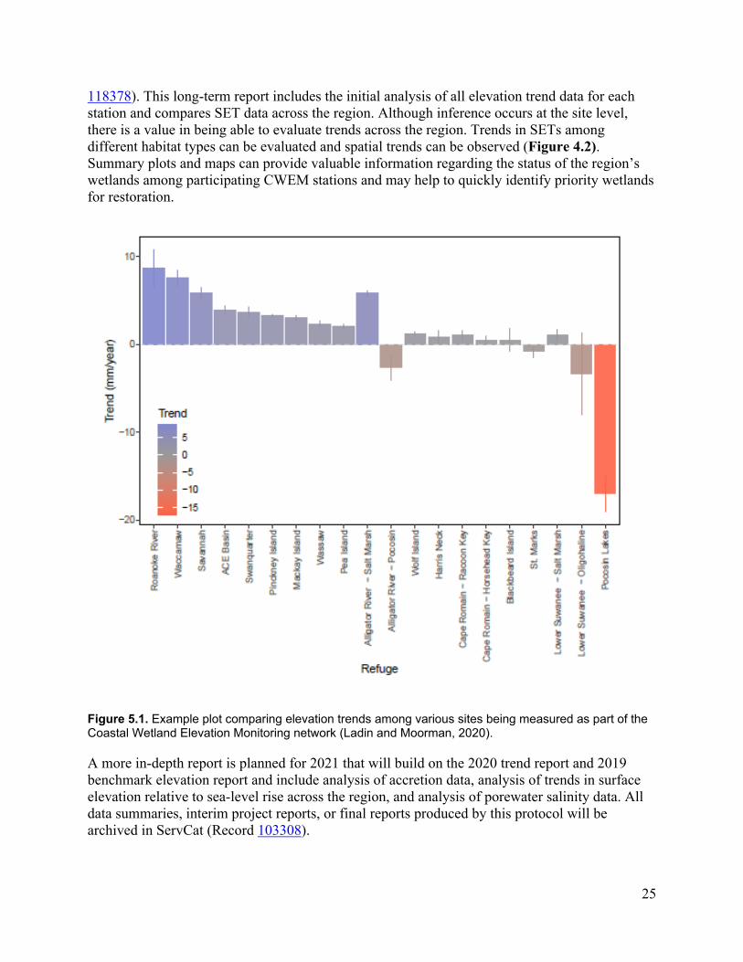
25

118378). This long-term report includes the initial analysis of all elevation trend data for each station and compares SET data across the region. Although inference occurs at the site level, there is a value in being able to evaluate trends across the region. Trends in SETs among different habitat types can be evaluated and spatial trends can be observed (Figure 4.2). Summary plots and maps can provide valuable information regarding the status of the region’s wetlands among participating CWEM stations and may help to quickly identify priority wetlands for restoration.

Figure 5.1. Example plot comparing elevation trends among various sites being measured as part of the Coastal Wetland Elevation Monitoring network (Ladin and Moorman, 2020).

A more in-depth report is planned for 2021 that will build on the 2020 trend report and 2019 benchmark elevation report and include analysis of accretion data, analysis of trends in surface elevation relative to sea-level rise across the region, and analysis of porewater salinity data. All data summaries, interim project reports, or final reports produced by this protocol will be archived in ServCat (Record 103308).

26

Important findings The long-term monitoring effort initiated by CWEM program in 2012 is to estimate the long-term elevation change rate for NWR marshes and determine if they are keeping pace with sea level rise. Additionally, if adequate data exists, the monitoring program was designed to identify the processes leading to the observed elevation change by comparing elevation change to surface accretion rates. Reporting schedule Refuge-specific fact sheets were produced in 2019 and will be updated as new information becomes available. Trend analysis will be completed each year once the R code and R markdown script being produced. A project report summarizing findings and putting them within the context of the efuge management will be produced every 10 years (Table 4.1). Report distribution Survey coordinators should ensure that field notes and reports are stored in compliance with Service Enterprise Architecture (270 FW 1), Data Resource Management (274 FW 1), and Electronic Records (282 FW 4) policies. The CWEM survey coordinator should also create accurate metadata and store data documents, metadata, reports, posters, graphs, maps, and any other documentation of results in ServCat and/or in the National SET Database.

Personnel Requirements and Training

Excerpts below are largely taken from The Surface Elevation Table and Marker Horizon Technique, A Protocol for Monitoring Wetland Elevation Dynamics, November 2015, Personnel Requirements and Training, pp 51. Roles and responsibilities As established in the CWEM network of cooperators, I&M survey coordinator is responsible for the development and implementation of SET and marker horizon protocols, field coordination, data documentation (metadata), data summary, and basic analysis and reporting. I&M survey coordinator is are also responsible for completing benchmark elevation surveys and vegetation surveys every 3-5 years. When available, localrefuge staff are responsible for the collection of data on Refuges as specified in the protocol, including field level data entry, quality assurance/quality control, and submission. In regard to field data collection, elevation monitoring using the SET requires 5+ years of data collection. It is best if the same person takes the measurements at a SET station through time. Currently, the I&M survey coordinator is responsible for ensuring that all data collected is entered and reviewed in the National SET database. The CWEM coordinator maintains a list of all POCs at each station. Additionally, the SET database documents and maintains the contact information of all participating field staff through time. Qualifications At least one member of the data collection crew will need proper DOI sanctioned certification to access sites if specialty equipment is required (Table 6.1). All personnel will also have completed a defensive driving course. The CWEM survey coordinator should have some familiarity with R code so they can continue to produce the R markdown report from the code

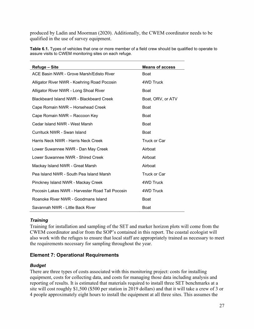
27

produced by Ladin and Moorman (2020). Additionally, the CWEM coordinator needs to be qualified in the use of survey equipment.

Table 6.1. Types of vehicles that one or more member of a field crew should be qualified to operate to assure visits to CWEM monitoring sites on each refuge.

Refuge – Site Means of access ACE Basin NWR - Grove Marsh/Edisto River Boat

Alligator River NWR - Koehring Road Pocosin 4WD Truck

Alligator River NWR - Long Shoal River Boat

Blackbeard Island NWR - Blackbeard Creek Boat, ORV, or ATV

Cape Romain NWR – Horsehead Creek Boat

Cape Romain NWR – Raccoon Key Boat

Cedar Island NWR - West Marsh Boat

Currituck NWR - Swan Island Boat

Harris Neck NWR - Harris Neck Creek Truck or Car

Lower Suwannee NWR - Dan May Creek Airboat

Lower Suwannee NWR - Shired Creek Airboat

Mackay Island NWR - Great Marsh Airboat

Pea Island NWR - South Pea Island Marsh Truck or Car

Pinckney Island NWR - Mackay Creek 4WD Truck

Pocosin Lakes NWR - Harvester Road Tall Pocosin 4WD Truck

Roanoke River NWR - Goodmans Island Boat

Savannah NWR - Little Back River Boat

Training Training for installation and sampling of the SET and marker horizon plots will come from the CWEM coordinator and/or from the SOP’s contained in this report. The coastal ecologist will also work with the refuges to ensure that local staff are appropriately trained as necessary to meet the requirements necessary for sampling throughout the year.

Operational Requirements

Budget There are three types of costs associated with this monitoring project: costs for installing equipment, costs for collecting data, and costs for managing those data including analysis and reporting of results. It is estimated that materials required to install three SET benchmarks at a site will cost roughly $1,500 ($500 per station in 2019 dollars) and that it will take a crew of 3 or 4 people approximately eight hours to install the equipment at all three sites. This assumes the

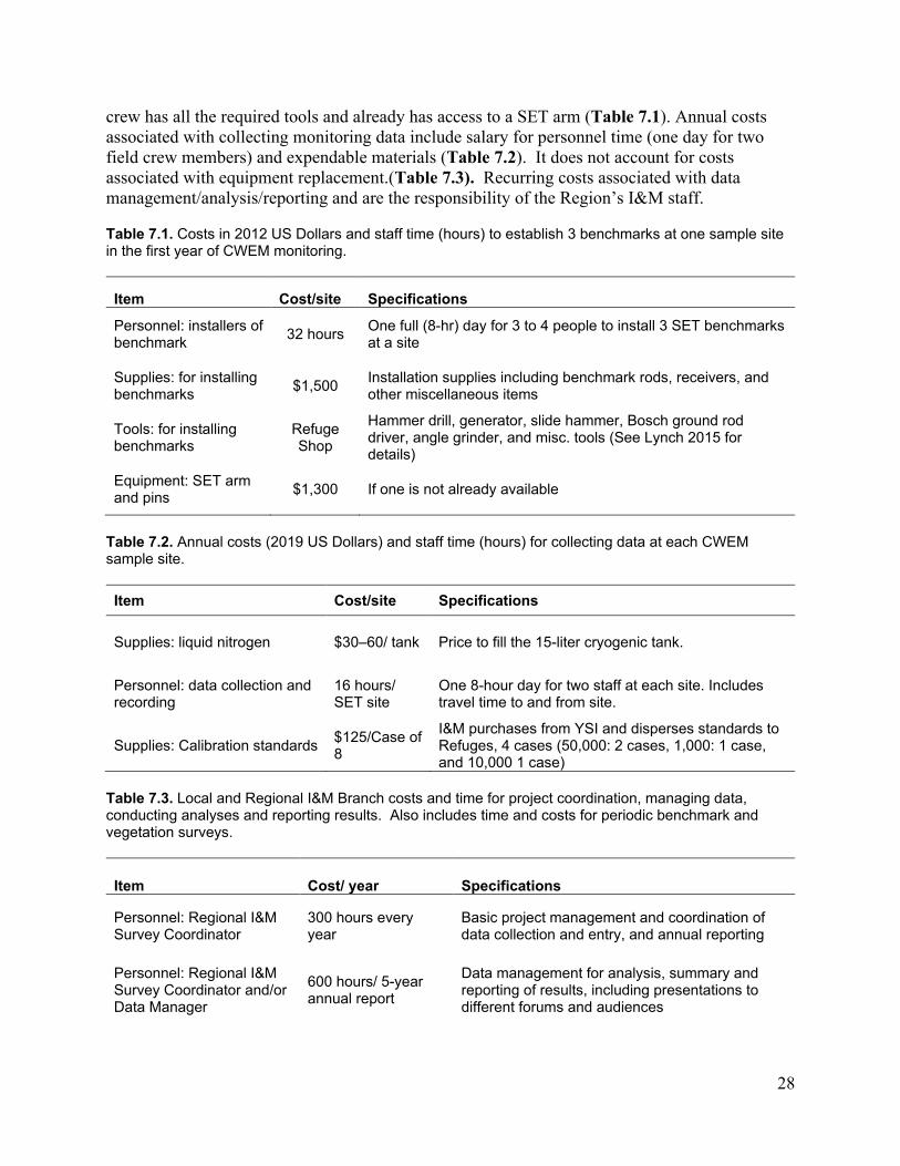
28

crew has all the required tools and already has access to a SET arm (Table 7.1). Annual costs associated with collecting monitoring data include salary for personnel time (one day for two field crew members) and expendable materials (Table 7.2). It does not account for costs associated with equipment replacement.(Table 7.3). Recurring costs associated with data management/analysis/reporting and are the responsibility of the Region’s I&M staff.

Table 7.1. Costs in 2012 US Dollars and staff time (hours) to establish 3 benchmarks at one sample site in the first year of CWEM monitoring.

Item Cost/site Specifications

Personnel: installers of benchmark 32 hours One full (8-hr) day for 3 to 4 people to install 3 SET benchmarks

at a site

Supplies: for installing benchmarks $1,500 Installation supplies including benchmark rods, receivers, and

other miscellaneous items

Tools: for installing benchmarks

Refuge Shop

Hammer drill, generator, slide hammer, Bosch ground rod driver, angle grinder, and misc. tools (See Lynch 2015 for details)

Equipment: SET arm and pins $1,300 If one is not already available

Table 7.2. Annual costs (2019 US Dollars) and staff time (hours) for collecting data at each CWEM sample site.

Item Cost/site Specifications

Supplies: liquid nitrogen $30–60/ tank Price to fill the 15-liter cryogenic tank.

Personnel: data collection and recording

16 hours/ SET site

One 8-hour day for two staff at each site. Includes travel time to and from site.

Supplies: Calibration standards $125/Case of 8

I&M purchases from YSI and disperses standards to Refuges, 4 cases (50,000: 2 cases, 1,000: 1 case, and 10,000 1 case)

Table 7.3. Local and Regional I&M Branch costs and time for project coordination, managing data, conducting analyses and reporting results. Also includes time and costs for periodic benchmark and vegetation surveys.

Item Cost/ year Specifications

Personnel: Regional I&M Survey Coordinator

300 hours every year

Basic project management and coordination of data collection and entry, and annual reporting

Personnel: Regional I&M Survey Coordinator and/or Data Manager

600 hours/ 5-year annual report

Data management for analysis, summary and reporting of results, including presentations to different forums and audiences

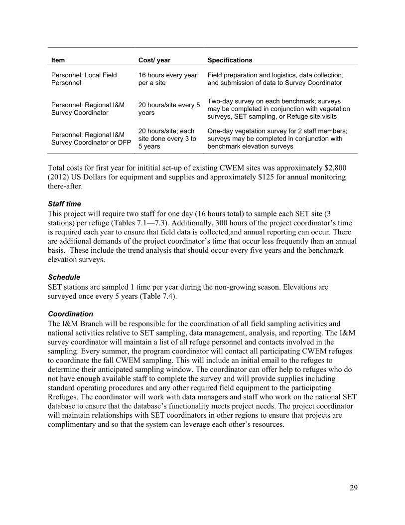
29

Item Cost/ year Specifications

Personnel: Local Field Personnel

16 hours every year per a site

Field preparation and logistics, data collection, and submission of data to Survey Coordinator

Personnel: Regional I&M Survey Coordinator

20 hours/site every 5 years

Two-day survey on each benchmark; surveys may be completed in conjunction with vegetation surveys, SET sampling, or Refuge site visits

Personnel: Regional I&M Survey Coordinator or DFP

20 hours/site; each site done every 3 to 5 years

One-day vegetation survey for 2 staff members; surveys may be completed in conjunction with benchmark elevation surveys

Total costs for first year for inititial set-up of existing CWEM sites was approximately $2,800 (2012) US Dollars for equipment and supplies and approximately $125 for annual monitoring there-after. Staff time This project will require two staff for one day (16 hours total) to sample each SET site (3 stations) per refuge (Tables 7.1—7.3). Additionally, 300 hours of the project coordinator’s time is required each year to ensure that field data is collected,and annual reporting can occur. There are additional demands of the project coordinator’s time that occur less frequently than an annual basis. These include the trend analysis that should occur every five years and the benchmark elevation surveys. Schedule SET stations are sampled 1 time per year during the non-growing season. Elevations are surveyed once every 5 years (Table 7.4). Coordination The I&M Branch will be responsible for the coordination of all field sampling activities and national activities relative to SET sampling, data management, analysis, and reporting. The I&M survey coordinator will maintain a list of all refuge personnel and contacts involved in the sampling. Every summer, the program coordinator will contact all participating CWEM refuges to coordinate the fall CWEM sampling. This will include an initial email to the refuges to determine their anticipated sampling window. The coordinator can offer help to refuges who do not have enough available staff to complete the survey and will provide supplies including standard operating procedures and any other required field equipment to the participating Rrefuges. The coordinator will work with data managers and staff who work on the national SET database to ensure that the database’s functionality meets project needs. The project coordinator will maintain relationships with SET coordinators in other regions to ensure that projects are complimentary and so that the system can leverage each other’s resources.

30

References

Asper JR. 2013. Generating Spatially-Balanced Sampling Locations for Coastal Assessments Using ArcGIS 10. Athens, Georgia: National Park Service, Southeast Coast Network Standard Operating Procedure NPS/SECN/SOP1.2.1. Asper JR, Curtis T. 2012. Salt marsh community monitoring: conducting field site suitability assessments. Athens, Georgia: National Park Service, Southeast Coast Network Standard Operating Procedure NPS/SECN/SOP-1.3.1. Asper JR, Curtis T. 2013. Measuring accretion with a feldspar marker horizon. Athens, Georgia: National Park Service, Southeast Coast Network Standard Operating Procedure NPS/SECN/SOP-1.3.7. Boon, J.D. 2012. Evidence of sea-level acceleration at U.S. and Canadian tide stations, Atlantic Coast, North America. Journal of Coastal Research 28(6):1437-1445. Boyle MF, Cook CE, Rankin NM. 2018. Regional Protocol Framework for Vegetation Monitoring on Coastal Wetland Elevation Monitoring (CWEM) Sites in the Southeastern U.S. (Region 4). Atlanta, Georgia: U.S. Department of Interior, Fish and Wildlife Service. Byrne MW. 2012. Generating a spatially-balanced random sample with the RRQRR tool in ArcGIS 9.1 and ArcGIS 9.3.1. Athens, Georgia: National Park Service, Standard Operating Procedure NPS/SECN/SOP-1.1.1 Baumann, RH, Day JW Jr., Miller CA. 1984. Mississippi deltaic wetland survival: Sedimentation versus coastal submergence. Science 224:1093-1095. Cahoon DR. 2015. Estimating relative sea-level rise and submergence potential at a coastal wetland. Estuaries and Coasts 38:1077-1084. DOI 10.1007/s12237-014-9872-8. Cahoon DR, Lynch JC, Perez BP, Segura B, Holland RD, Stelly C, Stephenson G, Hensel P. 2002. High-precision measurements of wetland sediment elevation: II. The rod surface elevation table. Journal of Sedimentary Research 72, 734-739. Cahoon DR,Turner RE. 1989. Accretion and canal impacts in a rapidly subsiding wetland. II. Feldspar marker horizon technique. Estuaries 12:260-268. Cahoon DR, Lynch JC,Knaus RM. 1996. Improved cryogenic coring device for sampling wetland soils. Journal of Sedimentary Research 66:1025-1027. [CCSP] Climate Change Science Program and. 2009. Coastal sensitivity to sea-level rise: a focus on the Mid-Atlantic Region. A report by the U.S. Climate Change Science Program and the Subcommittee on Global Climate Change Research [J.G. Titus (Coordinating Lead Author), K.E. Anderson, D.R. Cahoon, D.B. Gesch, S.K. Gill, B.T. Gutierrez, E.R. Thieler, and S.J. Williams (Lead Authors)]. U.S. Environmental Protection Agency, Washington, D.C. USA, 320 pp.

31

[CIER] Center for Integrative Environmental Research. 2008. Economic impacts of climate change on North Carolina. University of Maryland. 18p. <www.cier.umd.edu/climateadaptation>. Comer, P.J., D. Faber-Langendoen, R. Evans, S.C. Gawler, C. Josse, G. Kittel, S. Menard, M. Pyne, M. Reid, K. Schulz, K. Snow, and J. Teague. 2003. Ecological Systems of the United States: A Working Classification of U.S. Terrestrial Systems. NatureServe, Arlington, Virginia. Curtis AC. 2012. Soil porewater equipment construction and data collection. Athens, Georgia: National Park Service, Southeast Coast Network Standard Operating Procedure NPS/SECN/SOP-1.3.8. Folse, T. M., and J. L. West. 2004. A standard operating procedures manual for the Louisiana Department of Natural Resource's Coastal Restoration Division: methods for data collection, quality assurance / quality control, storage, and products. Louisiana Department of Natural Resources, Baton Rouge, LA. Ladin, Z. and Moorman, M.C. 2020. USFWS, Southeast Region SET Data Analysis. University of Delaware. XXX pp. Lynch JC, Hensel P, Cahoon DR. 2015. The surface elevation table and marker horizon technique: A protocol for monitoring wetland elevation dynamics. National Park Service, Fort Collins, Colorado, Natural Resource Report NPS/NCBN/NRR—2015/1078. National Park Service, Fort Collins, Colorado. Moorman MC, McDonald JM, Rankin NM, and Mulligan AS. 2019. Determining Elevation of Rod Surface Elevation Table Benchmarks at Coastal Wetland Elevation Monitoring Sites: Baseline Report. U.S. Fish and Wildlife Service, Southeast Region. Atlanta, GA. October 2019. 69 pp. [NOAA] National Oceanic and Atmospheric Administration. 2017. Global and regional sea-level rise scenarios for the United States. Technical Report NOS CO-OPS 083. R Core Team. 2019. R: A language and environment for statistical computing. Vienna, Austria: R Foundation for Statistical Computing. URL https://www.R-project.org/. Theobald DM, Norman JB. 2006. Spatially-balanced sampling using the Reversed Randomized Quadrant-Recursive Raster algorithm: a user’s guide for the RRQRR ArcGIS version 9.1 tool. Colorado State University, Fort Collins, CO. Theobald, D. M., D. Stevens, D. White, N. Urquhart, A. Olsen, J. Norman. 2007. Using GIS to generate spatially-balanced random survey designs for natural resource applications. Environmental Management 40(1):134-146.

32

Standard Operating Procedures (SOP)

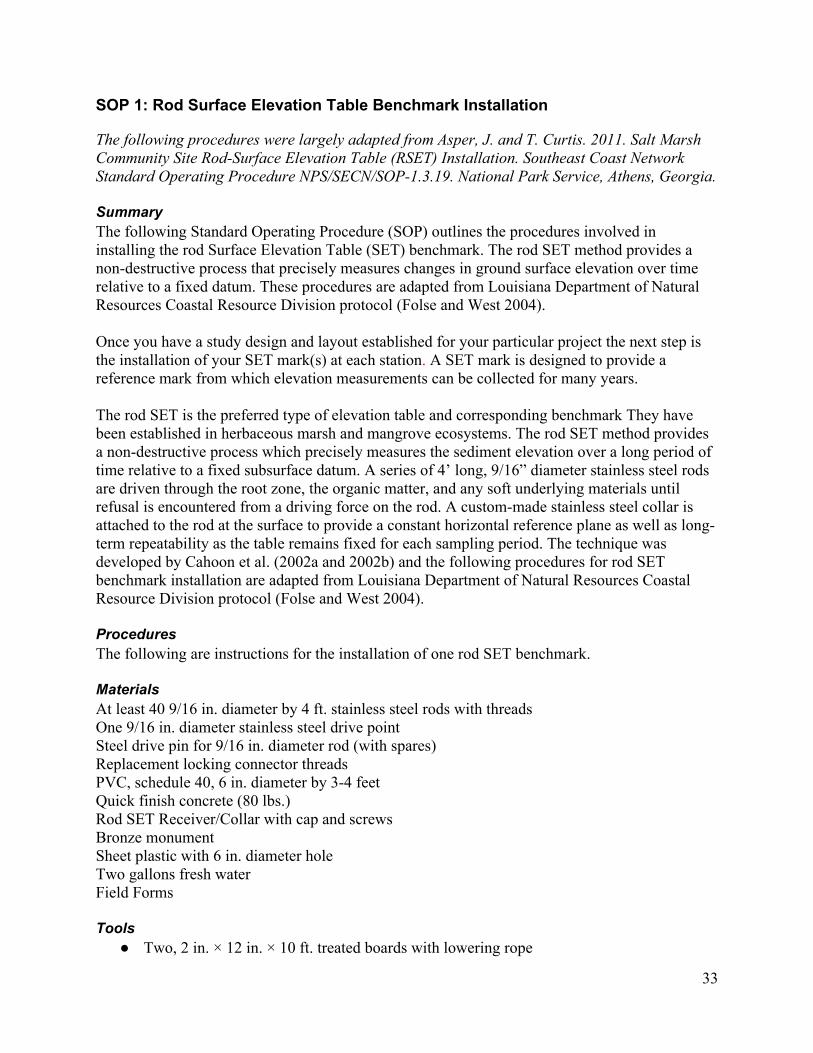
33

SOP 1: Rod Surface Elevation Table Benchmark Installation

The following procedures were largely adapted from Asper, J. and T. Curtis. 2011. Salt Marsh Community Site Rod-Surface Elevation Table (RSET) Installation. Southeast Coast Network Standard Operating Procedure NPS/SECN/SOP-1.3.19. National Park Service, Athens, Georgia. Summary The following Standard Operating Procedure (SOP) outlines the procedures involved in installing the rod Surface Elevation Table (SET) benchmark. The rod SET method provides a non-destructive process that precisely measures changes in ground surface elevation over time relative to a fixed datum. These procedures are adapted from Louisiana Department of Natural Resources Coastal Resource Division protocol (Folse and West 2004). Once you have a study design and layout established for your particular project the next step is the installation of your SET mark(s) at each station. A SET mark is designed to provide a reference mark from which elevation measurements can be collected for many years. The rod SET is the preferred type of elevation table and corresponding benchmark They have been established in herbaceous marsh and mangrove ecosystems. The rod SET method provides a non-destructive process which precisely measures the sediment elevation over a long period of time relative to a fixed subsurface datum. A series of 4’ long, 9/16” diameter stainless steel rods are driven through the root zone, the organic matter, and any soft underlying materials until refusal is encountered from a driving force on the rod. A custom-made stainless steel collar is attached to the rod at the surface to provide a constant horizontal reference plane as well as long-term repeatability as the table remains fixed for each sampling period. The technique was developed by Cahoon et al. (2002a and 2002b) and the following procedures for rod SET benchmark installation are adapted from Louisiana Department of Natural Resources Coastal Resource Division protocol (Folse and West 2004). Procedures The following are instructions for the installation of one rod SET benchmark. Materials At least 40 9/16 in. diameter by 4 ft. stainless steel rods with threads One 9/16 in. diameter stainless steel drive point Steel drive pin for 9/16 in. diameter rod (with spares) Replacement locking connector threads PVC, schedule 40, 6 in. diameter by 3-4 feet Quick finish concrete (80 lbs.) Rod SET Receiver/Collar with cap and screws Bronze monument Sheet plastic with 6 in. diameter hole Two gallons fresh water Field Forms Tools

● Two, 2 in. × 12 in. × 10 ft. treated boards with lowering rope

34

● Measuring tape (m of length?) ● Pruning Saw ● Post hole digger (metal handles preferred) ● 3- 5 Gallon Buckets (for mud, water, and mixing concrete) ● Personal protective equipment

○ Eye protection ○ Gloves ○ Ear protection ○ Dust masks

● Level ● 2 lb. sledge hammer ● Manual driving adapter ● Generator ● Fuel/oil (for generator) ● Extension cord ● Power driving device (35 lb. Bosch demolition hammer) ● Power driving adapter ● 2 pipe wrenches ● 2 vice grip wrenches ● Stopwatch ● Angle grinder (with extra discs) ● Bilge pump ● Cement mixing equipment

○ Trowel ○ Rubber gloves

● Socket wrench with 9/16 in. socket ● Metal scoop ● Stamp set ● Loctite ● Small Hammer (for stamp set) ● Camera ● Compass ● Platform and benches for accessing site

Procedure 1. Place one 2 in. × 12 in. × 10 ft. board across the long and short platforms on one side of where the rod for the rod SET benchmark will be installed. Use a rope to assist in lowering the board. 2. Lower the second board parallel to the first board. Spacing between the first and second board should be approximately 1-2’ based on comfort for the participating crew members. 3. Using a post-hole digger, dig a hole that is 1.5–2 feet deep with a maximum diameter of 6 inches. 4. Spread Loctite on the locking connector thread of one 4 ft stainless steel rods and attach a drive point to the end and tighten using vice grips. 5. Spread Loctite on the locking connector threads of the other end of the stainless steel rod and attach a second, 4 ft. stainless steel rod using a locking connector thread and tighten using vice grips or pipe wrenches.

35

6. Attach a drive pin to the other side of the second, 4-ft stainless steel rod and tighten with vice grips. The drive pin will be used as the impact point while driving the rods. Do not use Loctite between stainless steel rods and drive pin. 7. Insert the drive point into the center of the bottom of the hole. For a more detailed SOP on SET installation, please see Lynch et al., SOP 2 (2015). References Asper JR, Curtis T. 2012. Salt marsh community monitoring: conducting field site suitability assessments. Athens, Georgia: National Park Service, Southeast Coast Network Standard Operating Procedure NPS/SECN/SOP-1.3.1. Cahoon, D. R., J. C. Lynch, P. Hensel, R. Boumans, B. C. Perez, B. Segura, and J. W. Day, Jr. 2002a. High-precision measurements of wetland sediment elevation; I, Recent improvements to the sedimentation-erosion table. Journal of Sedimentary Research 72:730-733. Cahoon, D. R., J. C. Lynch, B. C. Perez, B. Segura, R. D. Holland, C. Stelly, G. Stephenson, and P. Hensel. 2002b. High-precision measurements of wetland sediment elevation; II, The rod surface elevation table. Journal of Sedimentary Research 72:734-739. Folse, T. M., and J. L. West. 2004. A standard operating procedures manual for the Louisiana Department of Natural Resource's Coastal Restoration Division: methods for data collection, quality assurance / quality control, storage, and products. Louisiana Department of Natural Resources, Baton Rouge, LA. Lynch JC, Hensel P, Cahoon DR. 2015. The surface elevation table and marker horizon technique: A protocol for monitoring wetland elevation dynamics. National Park Service, Fort Collins, Colorado, Natural Resource Report NPS/NCBN/NRR—2015/1078. National Park Service, Fort Collins, Colorado.

36

SOP 2: Marker Horizon Plot Installation and Reestablishment

The following procedures were largely adapted from Asper, J, and T. Curtis. 2013. Measuring accretion with a feldspar marker horizon. Southeast Coast Network Standard Operating Procedure NPS/SECN/SOP-1.3.7. National Park Service, Athens, Georgia. Summary Marker horizon plots are to be established on the same day that the initial rod-surface elevation table readings are recorded. This gives the best known baseline for both accretion and elevation change data sets to be interpreted when analysis occurs. Three marker horizon plots will be established within the benchmark site. The plots are numbered counter-clockwise starting with the north direction plot.

• When applying the feldspar, all necessary health precautions should be taken since the material is a fine powder and can be easily inhaled. NOTE: An appropriate respirator, gloves, and eye protection are required.

● Document water level with respect to marsh surface in the “Notes” section of the data. ● Place the 50 cm × 50 cm square on the marsh surface as close as possible to one of the

corner PVC poles that mark the CWEM plot. ● Mark the stations using two survey markers. Place one survey marker in the PVC corner

of the plot with the triangle pointing to the center of the plot and place the second survey marker in the opposite corner from the first one also with the triangle pointing to the center of the plot.

● Using a small cup, evenly sprinkle the feldspar on the marsh surface making sure not to leave any on the vegetation (vegetation can be gently shaken to knock any feldspar from the plant to the marsh surface). Each station is evenly coated until a minimum thickness of 1 cm is achieved.

● If the marsh is flooded on the day of the establishment, a large trashcan (~50 cm diameter) with the bottom cut out may be placed on the marsh and slightly inserted into the surface of the marsh to create a barrier.. Feldspar can then be applied within this can, though it may take 15 minutes or longer for all the feldspar to settle. The feldspar has a tendency to float when it is applied until it becomes completely saturated. Remove the barrier when all the feldspar has settled.

● Using a digital camera with the date and time stamp function enabled, take a picture of each marker horizon plot and one site photo to show orientation of the three stations. Record photo number, date, and time for each photo on datasheet. NOTE: Pictures will include one taken directly above each station with the PVC pipes in place and another picture taken of the entire site.

● Using a GPS, mark the center of the marker horizon plot. Record UTM zone, waypoint, and easting/northing for the point on the datasheet.

● Continue steps 1 – 7 for the remaining two marker horizon plots. ● Draw a sketch of the rod SET benchmark site with marker horizon plots, salinity plot,

and platform placement. Three plots may need to be re-established once the feldspar degrades to the point that it is no longer recoverable. As this point, follow the procedures outlined above to install the new plots. These plots SHOULD NOT be placed in the same area as the previously existing plots.

37

References Asper JR, Curtis T. 2012. Salt marsh community monitoring: conducting field site suitability assessments. Athens, Georgia: National Park Service, Southeast Coast Network Standard Operating Procedure NPS/SECN/SOP-1.3.1. Lynch JC, Hensel P, Cahoon DR. 2015. The surface elevation table and marker horizon technique: A protocol for monitoring wetland elevation dynamics. National Park Service, Fort Collins, Colorado, Natural Resource Report NPS/NCBN/NRR—2015/1078. National Park Service, Fort Collins, Colorado.

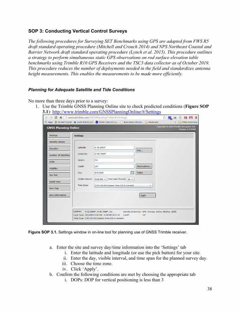
38

SOP 3: Conducting Vertical Control Surveys

The following procedures for Surveying SET Benchmarks using GPS are adapted from FWS R5 draft standard operating procedure (Mitchell and Crouch 2014) and NPS Northeast Coastal and Barrier Network draft standard operating procedure (Lynch et al. 2015). This procedure outlines a strategy to perform simultaneous static GPS observations on rod surface elevation table benchmarks using Trimble R10 GPS Receivers and the TSC3 data collector as of October 2019. This procedure reduces the number of deployments needed in the field and standardizes antenna height measurements. This enables the measurements to be made more efficiently. Planning for Adequate Satellite and Tide Conditions No more than three days prior to a survey:

1. Use the Trimble GNSS Planning Online site to check predicted conditions (Figure SOP 3.1): http://www.trimble.com/GNSSPlanningOnline/#/Settings

Figure SOP 3.1. Settings window in on-line tool for planning use of GNSS Trimble receiver.

a. Enter the site and survey day/time information into the ‘Settings’ tab

i. Enter the latitude and longitude (or use the pick button) for your site. ii. Enter the day, visible interval, and time span for the planned survey day.

iii. Choose the time zone. iv. Click ‘Apply’.

b. Confirm the following conditions are met by choosing the appropriate tab i. DOPs: DOP for vertical positioning is less than 3

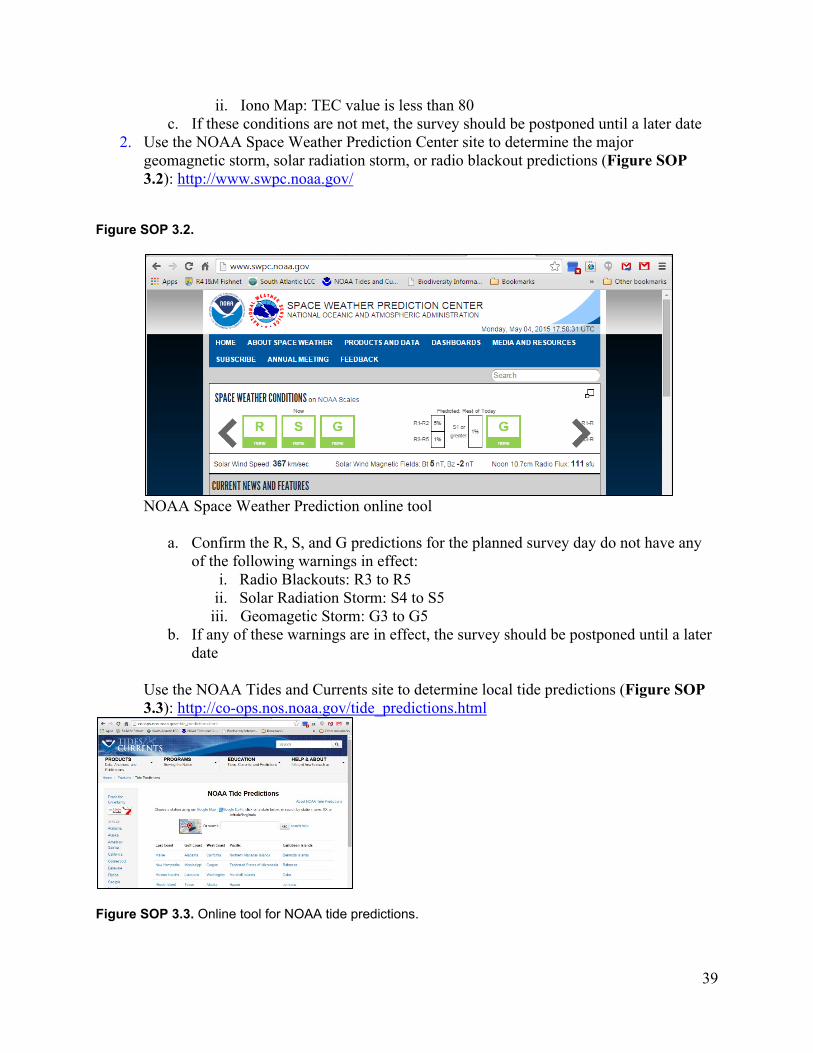
39

ii. Iono Map: TEC value is less than 80 c. If these conditions are not met, the survey should be postponed until a later date

2. Use the NOAA Space Weather Prediction Center site to determine the major geomagnetic storm, solar radiation storm, or radio blackout predictions (Figure SOP 3.2): http://www.swpc.noaa.gov/

Figure SOP 3.2.

NOAA Space Weather Prediction online tool

a. Confirm the R, S, and G predictions for the planned survey day do not have any of the following warnings in effect:

i. Radio Blackouts: R3 to R5 ii. Solar Radiation Storm: S4 to S5 iii. Geomagetic Storm: G3 to G5

b. If any of these warnings are in effect, the survey should be postponed until a later date

Use the NOAA Tides and Currents site to determine local tide predictions (Figure SOP 3.3): http://co-ops.nos.noaa.gov/tide_predictions.html

Figure SOP 3.3. Online tool for NOAA tide predictions.

40

c. Search for the published tide table for the survey site i. Select the state where the survey will be conducted

ii. Select the closest subordinate or harmonic station to the survey site iii. Download the published tide table in the annual PDF format

d. Check the time and height of high and low waters for the planned survey dates i. Avoid deploying the Trimble R10 receivers when tides significantly above

normal are predicted (e.g. extreme high tides) Surveying with USGS RSET-GPS Adapter and Trimble R10 Receiver(s) Equipment and Materials List

1. Site map of RSET locations 2. Yellow Pelican case(s):

a. Trimble R10 GPS receiver(s) (one for each benchmark to be surveyed) b. Lithium ion Trimble battery for each receiver (fully charged) c. Radio antenna for each receiver d. Quick release adapter for each receiver e. Digital tiltmeter(s)

3. Black Pelican gun case a. USGS RSET-GPS mounting adapter(s) and extension rod (one for each receiver)

4. Trimble TSC3 handheld (fully charged-light turns green on handheld when fully charged) 5. Aluminum plank (1 or more) 6. Stools (2 per plank) 7. Rite in the Rain data book 8. Digital camera/cell phone for photos 9. Handheld Garmin GPS/compass for navigating

Procedure for setting up the survey equipment

1. All work is performed from the platform (one plank plus two stools);no walking on the marsh surface within the benchmark site is permitted

2. Use compass/Garmin GPS and individual site sheet to determine platform placement at each benchmark

3. Set-up a single platform by using two step stools and one aluminum plank. Only set up platform in predetermined locations as shown on site sheet

4. Remove the RSET threaded receiver cap and place inside the black Pelican gun case 5. Mount the SET adapter to the RSET receiver

a. Insert the stainless steel coupler end of the SET adapter into the RSET receiver ensuring the alignment pin is nested completely against the bottom of the RSET receiver notch. Screw down the threaded cap

b. Attach together the remaining components of the SET adapter (Figure SOP 3.4) i. Attach the Manfrotto ball joint to the stainless steel coupler and hand-

tighten

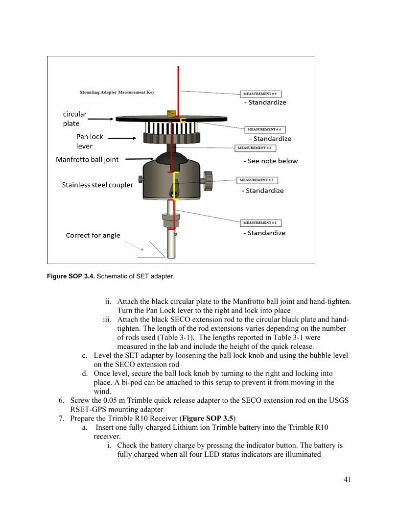
41

Figure SOP 3.4. Schematic of SET adapter.

ii. Attach the black circular plate to the Manfrotto ball joint and hand-tighten.

Turn the Pan Lock lever to the right and lock into place iii. Attach the black SECO extension rod to the circular black plate and hand-

tighten. The length of the rod extensions varies depending on the number of rods used (Table 3-1). The lengths reported in Table 3-1 were measured in the lab and include the height of the quick release.

c. Level the SET adapter by loosening the ball lock knob and using the bubble level on the SECO extension rod

d. Once level, secure the ball lock knob by turning to the right and locking into place. A bi-pod can be attached to this setup to prevent it from moving in the wind.

6. Screw the 0.05 m Trimble quick release adapter to the SECO extension rod on the USGS RSET-GPS mounting adapter

7. Prepare the Trimble R10 Receiver (Figure SOP 3.5) a. Insert one fully-charged Lithium ion Trimble battery into the Trimble R10

receiver. i. Check the battery charge by pressing the indicator button. The battery is

fully charged when all four LED status indicators are illuminated

42

ii. NOTE: The internal battery should run ~6 hours in the field. If significant time has passed since the last survey, it may be prudent to test internal battery life in the office prior to field deployment.

b. Screw the radio antenna into the SMA radio antenna connector

Figure SOP 3.5.

Schematic of Trimble GNSS R10 unit.

8. Attach the Trimble R10 receiver to the Trimble quick release adapter. Recheck to ensure the SET adapter remained level

9. Turn on the Trimble R10 receiver by pressing and releasing immediately the power button

a. All four LEDs will light up and remain lit for 3 seconds. Shortly after, the satellite and data logging LEDs will begin blinking

10. Record antenna height. The height of the antenna will be determined by the number of poles used to reach the appropriate height above the canopy (Table SOP 3.1).

Table SOP 3.1. Standardized antenna heights in meters (m) to be used in OPUS to calculate the elevation of the benchmark. Antenna heights are the sum of the adapter height, quick release, and height of the poles.

No. poles used in the

field Height of

adapter (m)

Height of

poles (m)

Height of quick release

(m)

Standard Antenna Height used in OPUS

(m) 1 pole 0.21 0.96 0.05 1.22 2 poles 0.21 1.92 0.05 2.18 3 poles 0.21 2.88 0.05 3.14

Instructions for first-time surveying of a location using Trimble TSC3 handheld controller 1. Turn on the Trimble TSC3 handheld controller

a. ‘Trimble Access’ will start automatically after turning on the Trimble TSC3 controller

2. Connect to intended Trimble R10 receiver

43

a. Select ‘Settings’>’Connect’>’Bluetooth’ b. Under ‘Connect to GNSS Base’ select the intended base receiver serial number c. Select ‘Accept’

3. Set up the Job File in ‘Trimble Access’ (each benchmark is a separate job). a. Select ‘Trimble Access’>’General Survey’>’Jobs’>’New Job’

i. Enter Job Name using the following format: RSETID###X 1. RSETID – refuge three letter code plus 3 digit site numerical code

plus one letter code for each benchmark; this information is found on the site sheet.

2. Use an existing template OR 3. Create one

a. Select the coordinate system b. Choose the Units (Dist) c. Make sure autoconnect is toggled ON on page 2

4. Start survey a. Select Trimble Access>General Survey>Jobs>Open job>Select the intended job b. Select Instrument>GNSS functions>Start survey

i. ‘Point name’>Key in 1. Enter job name (RSETID###X)

ii. Enter code as ‘BM’ for ‘benchmark’ iii. Select ‘Here’ at bottom of screen to fill in the ‘Northing’, ‘Easting’, and

‘Elevation’ sections iv. Select ‘Store’ v. Enter antenna height: Default is 1.22 m if one pole is used.

vi. ‘Measured to’ >‘Bottom of antenna mount’ vii. Select ‘Start’

c. Record receiver serial number, mounting adapter setup, antenna height used, and start time in data book

5. Repeat steps 2-4 for each benchmark to be surveyed 6. End Survey

a. After a 6-8 hour survey period, the survey may be ended b. Connect to intended R10 receiver (using step 2) c. Select ‘Trimble Access’>’General Survey’>’Jobs’>’Open job’>Select the

intended job d. Select ‘Instrument’>’GNSS functions’>’End survey’

i. When prompted with option to turn off receiver, select ‘No’ e. ‘GNSS functions’>’Import Files’

i. Select the TO2 file with appropriate survey date and time 1. Select ‘Import’>’Start’ 2. If transfer unsuccessful, attempt again. The file can also be

transferred at a later date using the same process. 3. If transfer successful, select ‘OK’

ii. Select ‘Esc’>’Esc’ f. Select Jobs>’Import/Export’>’Export fixed format’

i. Under ‘File format,’ select ‘ESRI Shapefiles’>’Accept’>’OK’ g. Select Jobs>’Import/Export’>’Export fixed format’

44

i. Under ‘File format,’ select ‘Comma Delimited’>’Accept’ 1. Select ‘All points’>’OK’

h. Select ‘Instrument’>’GNSS functions’>’Power down Receiver’ 7. Repeat step 6 for all other surveying receivers 8. Turn off Trimble TSC3

Instructions for downloading, converting, and processing data The following instructions require the prior installation of ‘Convert to RINEX’ and ‘Windows Mobile’ programs to computer of intended use. The following instructions should be completed at least 24 hours after completing the survey event.

1. Connect Trimble TSC3 handheld to a USB stick. 2. Turn on Trimble TSC3 handheld and plug in a USB stick 3. Hit the windows button and select the US Fish and Wildlife Folder by pressing down on

it with the pen 4. Select copy 5. Then navigate to Hard disk and paste the copied folder onto the USB Stick 6. Plug the USB stick into your computer and copy the files to an appropriate folder using

windows explorer a. Rename each TO2 file to include RSETID###X_mm_dd_yyyy b. Copy all TO2, Task Scheduler Task Object, CSV, SHP, DBF, and SHX files from

the RSET benchmarks surveyed to computer 7. Open the ‘Convert to RINEX’ program 8. Load files into RINEX

a. Select ‘File’>’Open’>Select TO2 files for the surveyed benchmarks>’Open’ 9. Convert files once scanning is complete

a. Select ‘File’>’Convert Files’ b. The converted files will be placed in computer folder than contains the original

TO2 files i. Converted files will include .15g, .15n, and .15o formats

10. Go to www.ngs.noaa.gov/OPUS/ a. Under ‘data file’, select ‘Choose File’>select .15o format TO2 file for each survey

to be uploaded into OPUS b. Under ‘antenna, select ‘TRMR10’ c. In ‘antenna height’, enter the recorded antenna height from the data book for the

intended survey (e.g. 1.2) d. In ‘email address’, enter the email address that the OPUS solution will be sent to

once processed e. Select ‘Upload to Static’ f. The rapid OPUS solution will be emailed once completed

11. Save the OPUS solution that was emailed as a text document 12. Upload the OPUS report and raw files to ServCat, record # 102976 and save in the

appropriate site file.

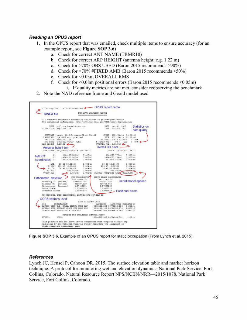
45

Reading an OPUS report

1. In the OPUS report that was emailed, check multiple items to ensure accuracy (for an example report, see Figure SOP 3.6)

a. Check for correct ANT NAME (TRMR10) b. Check for correct ARP HEIGHT (antenna height; e.g. 1.22 m) c. Check for >70% OBS USED (Baron 2015 recommends >90%) d. Check for >70% #FIXED AMB (Baron 2015 recommends >50%) e. Check for <0.03m OVERALL RMS f. Check for <0.08m positional errors (Baron 2015 recommends <0.05m)

i. If quality metrics are not met, consider reobserving the benchmark 2. Note the NAD reference frame and Geoid model used

Figure SOP 3.6. Example of an OPUS report for static occupation (From Lynch et al. 2015).

References Lynch JC, Hensel P, Cahoon DR. 2015. The surface elevation table and marker horizon technique: A protocol for monitoring wetland elevation dynamics. National Park Service, Fort Collins, Colorado, Natural Resource Report NPS/NCBN/NRR—2015/1078. National Park Service, Fort Collins, Colorado.

46

Mitchell, L. and Crouch, B. 2014. Standard Operating Procedure – Rod Surface Elevation Table Orthometric Height Data Collection and Online Data Processing Version 1.3. Unpublished SOP.

47

SOP 4: Making Surface Elevation Table Measurements with the SET Arm

The following procedures were largely taken from Lynch, J. C., P. Hensel, and D. R. Cahoon. 2015. The surface elevation table and marker horizon technique: A protocol for monitoring wetland elevation dynamics. Natural Resource Report NPS/NCBN/NRR—2015/1078. National Park Service, Fort Collins, Colorado. (ServCat Ref#: 56400) Monitoring Instructions REMEMBER: All work is performed from the boardwalk; no walking on the marsh surface is permitted. REMEMBER: Determine the magnetic declination and set compass before going into the field. 1. Use compass and site map to determine platform placement. 2. Prepare the SET arm by tightening bolts and inserting pins. Count visible threads before measurement to ensure same distance measured every time. Insert the numbered pins, through the bottom of the arm, into the appropriate hole and clamp with badge clips. 3. Remove the receiver cap and attach the insert collar. 4. Slide the SET arm onto the insert collar and clamp the SET arm to collar using two spring clamps. NOTE: Make sure the SET arm is attached flush with the collar without any vegetation between collar and arm. 5. Once the SET is secured to the collar, level the arm by using the turnbuckle and level bubble. The arm must be perfectly level in order to get precise measurements. Make sure that there are no plants or roots pushing on the pins or the arm when you level. 6. Using the compass, determine the direction (bearing) of the arm. Record the bearing and direction on the data sheet. Sampling will occur at four directions: north, south, east, and west. Be sure to measure the direction from the center of the benchmark out to the distance, NOT from the end of the pins in toward the center. All your directions will be off by 180 degrees (i.e., east will be confused with west, etc.). 7. One at a time, gently lower the pins onto the surface of the marsh making sure not to penetrate the surface of the marsh. In dense vegetation, leaves and non-attached debris may have to be carefully pushed aside in order for the pin to rest on the marsh surface. When lowering the pins, if a pin is going to contact some object other than marsh surface (crab burrow, hole, depression, etc.), move only those objects which are loose and not contributing to the soil surface. Do not move stems, mussels, or shells embedded in sediment. 8. Once the fiberglass pin is touching the marsh surface, use a badge clip to secure the pin from moving downward. When taking measurements, take great care not to push down the SET arm. Check that the SET arm is level before you take the measurements in case the arm was displaced during the pin setting.

48

9. All nine (9) measurements will be taken by measuring, in millimeters, the distance from the top of the aluminum arm to the top of the fiberglass pin. Read the nearest mm tick marker on the ruler visible in line with or above the top of the fiberglass pin. The measurer should make sure their eyes are level with the ruler. Use the same ruler every time and make sure the ruler used does not have any extra space before the first 1 mm marking. Record this distance on the data sheet, taking care to associate the measurement with the correct pin. 10. As measurements are being taken, the measurer must observe what the fiberglass pin is resting upon and make notes. See page 2 for note definitions and abbreviations. 11. Once the measurements have been recorded, raise the fiberglass pins and clamp them with the badge clips so that the pins do not interfere with rotating the SET arm. 12. Rotate the arm to the next direction, re-clamp the SET to the collar, and follow procedures 4 through 12. Continue these steps for the four cardinal directions. 13. Upon completion of measuring pins in the four cardinal directions, review the data sheet to verify that all the measurements have been obtained. If measurements have been altered by some type of obstruction, then make a note documenting the quality of the measurement on the data sheet. Surface Definition: The marsh surface is defined as the soil surface. It is very important to be careful when the surface is flooded, because it will be hard to read the soil surface. Always plan to read the SETs at low tide when there is no water on the surface of the soil. Note Definitions and Abbreviations: Please also note anything (shell, plants, obstructions, etc.) in the way of any pins. It is always better to make a note so we can decide to keep or discard the data. Also, if you step in the plot or drop the ruler in the plot, make a note of it in the book.

HU: Hummock - Transitional slope referring to a small knoll or mound above the rest of the marsh surface

H: Hole - Deep hole within the marsh surface and usually excluded from analysis. Should only be used when no apparent bottom can be reached or bottom is very deep.D: Depression – Area below the rest of the marsh surface (not a hole or crab burrow).

CB: Crab Burrow within the marsh surface CH: Chimney - Crab burrow chimney within the marsh surface. Pin lands on the

chimney of the crab burrow ST: Stem - Pile of vegetation or stem that cannot be moved without compromising

soil surface. S: Shell AP: Animal Print F: Footprint

49

For more detailed information on reading SETs, please see Lynch et al. 2015. Equipment and Materials List - Rod surface elevation table (RSET) o RSET instrument/arm, Insert collar, 9 fiberglass pins (numbered to correspond with respective numbered holes on arm), 9 badge clips, bull’s eye level - 2 spring clamps - Compass - Bungee cords - Aluminum meter stick - 18” metric ruler (ruler end being zero millimeters) - Allen wrenches - Metal files - Data Sheets - Digital Camera - GPS - Kneeling pads - Aluminum bleacher plank - 2 stools References Lynch JC, Hensel P, Cahoon DR. 2015. The surface elevation table and marker horizon technique: A protocol for monitoring wetland elevation dynamics. National Park Service, Fort Collins, Colorado, Natural Resource Report NPS/NCBN/NRR—2015/1078. National Park Service, Fort Collins, Colorado.

50

SOP 5: Reading Marker Horizons

The following procedures were largely taken from Lynch, J. C., P. Hensel, and D. R. Cahoon. 2015. The surface elevation table and marker horizon technique: A protocol for monitoring wetland elevation dynamics. Natural Resource Report NPS/NCBN/NRR—2015/1078. National Park Service, Fort Collins, Colorado. (ServCat Ref#: 56400) Monitoring Instructions For the first three years, sampling will occur every six months following establishment. Sampling will occur annually during years four and beyond. Marker horizon plots were established on the same day that the baseline SET measurements were recorded (see SOP 2). The same person performing the SET sampling will perform the marker horizon plot sampling. 1. Use compass and site sheet to determine marker horizon plot locations for each CWEM plot. 2. Use the necessary personal protective equipment to prevent any injuries from occurring. A minimum of gloves and eye glasses are required. 3. Thread together the T handle and the chambered bottom piece of the mini Macaulay corer. Hand-tighten the nut onto the chambered bottom piece. Turn the flange/blade piece on the bottom to screw-head side up, which is the open position of the corer. 4. Place the 50cm × 50cm PVC square over the survey markers on the marker horizon plot to sample. Remember, the survey markers will correspond with the PVC square corners. 5. Sediment cores will be collected clock-wise pattern around the plot. During the first sampling occasion, the sediment core will be collected from the northwest corner of the marker horizon plot. For the next sediment core, move clock-wise at least five centimeters (2”) from the previous sample. 6. Push the mini Macaulay corer straight down into the sediment. You want to capture the top layer of the surface - so leave at least ½ inch of the top of the flange/blade above the sediment surface. 7. Turn the T handle 180 degrees clockwise, which will enclose the sediment sample in the chamber and the blade/flange will close and cover the sample. 8. Slowly remove the mini Macaulay corer from the sediment. Notice the flange/blade is now in the closed position with screw-head side down. 9. Slowly open the flange/blade to the open position and inspect the sediment core. Examine the core quality and feldspar layer condition. Is the feldspar layer highly visible around the semi-

51

circle of the core (excellent), only visible on half of the semi-circle (good to poor depending on feldspar visibility), or not visible at all? (poor) 10. If the sediment core/feldspar layer is good quality and the three required measurements can be taken (see step 11), continue to the next step. If the sediment core/feldspar layer is poor quality or feldspar layer cannot be found, then repeat steps 5 - 8 to collect another sediment core. Remember, marker horizon plot sampling occurs in a clock-wise pattern, so move at least five centimeters (2”) from the previous sample. 11. Using the dial calipers, take three measurements in mm around the semi-circle of the sediment core. Measure the distance from the top of the feldspar layer to the top of the sediment surface. Take three measurements: one along the left-side edge of the semi-circle of visible core, one along the core center, and one along the right-side edge. 12. On the data sheet, document the CWEM plot ID, marker horizon plot number, collected core location, accretion measurements (mm), number of cores taken, and measured core quality for the marker horizon plot on the datasheet. Do not use a zero if the feldspar layer is not found, but instead note that the layer was not found and attempt to take another core. Zeroes mean the feldspar layer is visible on the surface with no measurable sediment on top of the feldspar layer. 13. The marker horizon plot has been sampled when three sediment cores have been taken and three measurements have been made on the sediment core or when three attempts for a sediment core are made and no feldspar is found in the sediment core. There are three marker horizon plots at each CWEM plot. 14. Repeat steps 4 – 11 for each marker horizon plot at each CWEM plot. Equipment and Materials List - Mini Macaulay corer - 50 cm × 50 cm PVC square (used during the station establishment) - Dial Calipers:

* Specifications: 0-150 mm, 0.1 mm increments - Data Sheets - Digital Camera - GPS - Personal Protection Equipment

* Gloves and eye protection References Lynch JC, Hensel P, Cahoon DR. 2015. The surface elevation table and marker horizon technique: A protocol for monitoring wetland elevation dynamics. National Park Service, Fort Collins, Colorado, Natural Resource Report NPS/NCBN/NRR—2015/1078. National Park Service, Fort Collins, Colorado.

52

SOP 6: Porewater Data Collection

The following procedures were largely taken from Curtis, A. C. 2012. Soil porewater equipment construction and data collection. Southeast Coast Network Standard Operating Procedure NPS/SECN/SOP-1.3.8. National Park Service, Athens, Georgia. Monitoring Instructions Soil porewater samples are extracted from the sediment matrix from the same salinity plot. Three (3) replicate samples will be taken from each depth with 10 and 30 cm being the primary sampling depths. However, the second and third replicate for each depth will be moved at least five centimeters (2”) to the right of the previous sample. Prior to sampling the 30-cm depth, the field personnel will move another five centimeters (2”) to the right of the third 10-cm sample and begin sampling at the second depth in the same manner (i.e., moving at least 2 inches to the right on each subsequent sample). Note: Before readings are taken in the field with a hand-held discrete salinity meter, the meter must be calibrated for quality assurance. Since the meter is capable of measuring a wide range of salinity concentrations, the instrument shall be calibrated with a solution that is relatively close to the conditions in the field (see SOP 7 for calibration). The meter shall be calibrated quarterly before each sample period.

1. Locate the porewater salinity plot using the site sheet.

2. Prior to insertion for each replication, inspect the sipper holes for blockage and unclog as necessary.

3. Insert the porewater sipper with the two marked graduations (10 and 30 cm) into the soil

to the desired depth (10 or 30 cm) graduation.

4. Before measuring porewater salinity, the tubing, syringe, centrifuge tube, and graduated cylinder must be rinsed with porewater from each sampling depth at least once. Fill about one-third to one-half the volume (~20-30 ml) of the syringe with porewater and rinse the interior of the syringe thoroughly. Turn the four-way valve to dispense water into the graduated cylinder and rinse the interior of the graduated cylinder. Discard the water. It is recommended to use the four-way valve to dispense water from the syringe to prevent losing suction on the sipper or the sipper hose.

5. Pull a second sample of porewater-enough to fill the syringe and cover the probe when it

is in the syringe (~30-45 ml). In highly organic wetland soils, porewater extraction may be blocked or severely inhibited by organic or small clay particles. If this condition occurs, securely fasten a piece of cheese cloth around the intake holes of the porewater sipper(s) to filter obstructing particles.

6. Turn the four-way valve to dispense water into the graduated cylinder and insert the

salinity probe into the graduated cylinder. The two holes at the top of the probe that must

53

be covered with the sample water (see Figure SM2-1 on soil porewater sampling data sheet). Gently move the probe up and down to remove any air bubbles from the sensor.

7. Record the date, time, depth (cm), temperature (°C), specific conductance (SPC-uS/cm),

and salinity (ppt) on the soil porewater field data sheet for the porewater sample. On the YSI instrument screen, temperature (°C) will be displayed on the bottom, salinity (ppt) will be above the temperature, and specific conductance (SPC-uS/cm) will be above the salinity. Rinse the salinity probe with distilled water after recording data.

8. Carefully remove the sipper probe and move ~5 cm (~2 in) to the right and reinsert the

sipper probe into the soil matrix. Repeat steps 2-7 for each of all replicates at each depth. At each salinity plot, 3 replicates will be taken at the 10 and 30-cm depths for a total of 6 measurements.

9. Record surface water temperature, specific conductance, and salinity, if there is surface

water on the marsh surface. Currently, all participating refuges use a YSI Pro 30 Unit. Instructions for calibrating and using this unit are in SOP 7

Equipment and Materials List - 2 sipper tubes o Rigid sipper probe (made from rigid plastic tubing and marked at 10 and 30 cm; NC marked at 50 cm as well)

o Tygon tubing (attached to open end of rigid sipper probe) o Four-way stop cock/valve (attached to Tygon tubing) o 60 mL syringe (attached to stop cock/valve)

- 250 mL plastic graduated cylinder - YSI Pro 30 salinity meter with 4-m cable - Cheesecloth - Calibration standards - Distilled water - Data Sheets

References Curtis AC. 2012. Soil porewater equipment construction and data collection. Athens, Georgia: National Park Service, Southeast Coast Network Standard Operating Procedure NPS/SECN/SOP-1.3.8. Nat

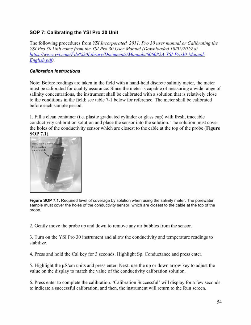
54

SOP 7: Calibrating the YSI Pro 30 Unit

The following procedures from YSI Incorporated. 2011. Pro 30 user manual.or Calibrating the YSI Pro 30 Unit came from the YSI Pro 30 User Manual (Downloaded 10/02/2019 at https://www.ysi.com/File%20Library/Documents/Manuals/606082A-YSI-Pro30-Manual-English.pdf). Calibration Instructions Note: Before readings are taken in the field with a hand-held discrete salinity meter, the meter must be calibrated for quality assurance. Since the meter is capable of measuring a wide range of salinity concentrations, the instrument shall be calibrated with a solution that is relatively close to the conditions in the field; see table 7-1 below for reference. The meter shall be calibrated before each sample period. 1. Fill a clean container (i.e. plastic graduated cylinder or glass cup) with fresh, traceable conductivity calibration solution and place the sensor into the solution. The solution must cover the holes of the conductivity sensor which are closest to the cable at the top of the probe (Figure SOP 7.1).

Figure SOP 7.1. Required level of coverage by solution when using the salinity meter. The porewater sample must cover the holes of the conductivity sensor, which are closest to the cable at the top of the probe.

2. Gently move the probe up and down to remove any air bubbles from the sensor. 3. Turn on the YSI Pro 30 instrument and allow the conductivity and temperature readings to stabilize. 4. Press and hold the Cal key for 3 seconds. Highlight Sp. Conductance and press enter. 5. Highlight the µS/cm units and press enter. Next, use the up or down arrow key to adjust the value on the display to match the value of the conductivity calibration solution. 6. Press enter to complete the calibration. ‘Calibration Successful’ will display for a few seconds to indicate a successful calibration, and then, the instrument will return to the Run screen.

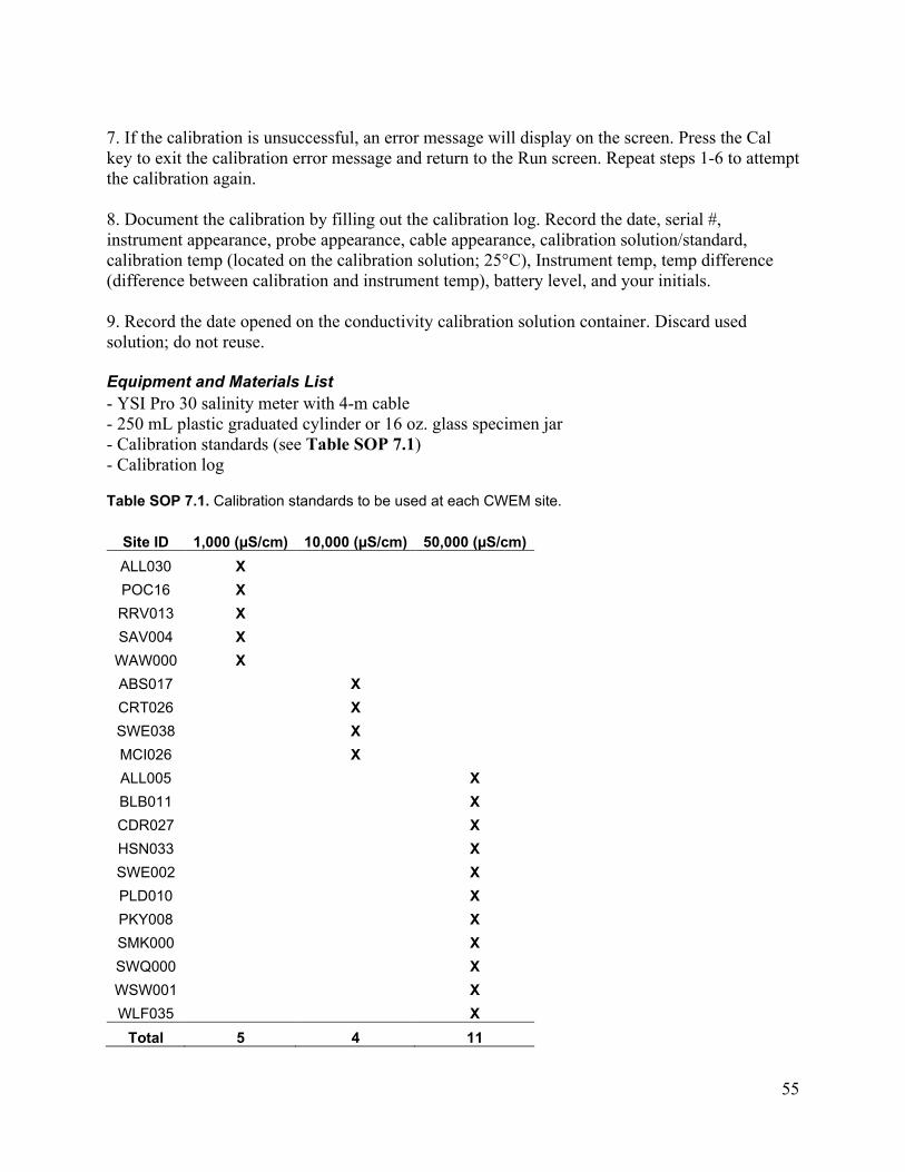
55

7. If the calibration is unsuccessful, an error message will display on the screen. Press the Cal key to exit the calibration error message and return to the Run screen. Repeat steps 1-6 to attempt the calibration again. 8. Document the calibration by filling out the calibration log. Record the date, serial #, instrument appearance, probe appearance, cable appearance, calibration solution/standard, calibration temp (located on the calibration solution; 25°C), Instrument temp, temp difference (difference between calibration and instrument temp), battery level, and your initials. 9. Record the date opened on the conductivity calibration solution container. Discard used solution; do not reuse. Equipment and Materials List - YSI Pro 30 salinity meter with 4-m cable - 250 mL plastic graduated cylinder or 16 oz. glass specimen jar - Calibration standards (see Table SOP 7.1) - Calibration log

Table SOP 7.1. Calibration standards to be used at each CWEM site.

Site ID 1,000 (µS/cm) 10,000 (µS/cm) 50,000 (µS/cm) ALL030 X POC16 X RRV013 X SAV004 X WAW000 X ABS017 X CRT026 X SWE038 X MCI026 X ALL005 X BLB011 X CDR027 X HSN033 X SWE002 X PLD010 X PKY008 X SMK000 X SWQ000 X WSW001 X WLF035 X

Total 5 4 11

56

References YSI Incorporated. 2011. Pro 30 user manual. Available https://www.ysi.com/File%20Library/Documents/Manuals/606082A-YSI-Pro30-Manual-English.pdf (10/02/2019).

57

SOP 8: Cleaning and storing the equipment

Cleaning Clean the SET unit and associated equipment after each sampling period and before shipping to another station.

To clean the SET instrument/arm, insert collar, fiberglass pins, and associated equipment:

o Rinse the entire unit with freshwater o If the SET unit is super dirty, soak the SET arm, insert collar, and pins in a bucket

of freshwater overnight o Use a soft brush or towel to wipe the unit free of dirt and debris o Use cotton swabs to remove dirt from pin holes on SET arm o Use WD-40 to lubricate the SET instrument and insert collar; do NOT lubricate

the fiberglass pins o Use freshwater to clean and rinse the meter stick, rulers, badge clips, bungee

cords, compass, levels, and spring clamps o Allow to dry before storing in pelican gun case

To clean the pelican gun case:

o Use mild soap, freshwater, and soft sponge to remove dirt and stains Shipping Ship the SET unit in the pelican gun case to the next refuge for sampling.

To ship the SET unit: o After cleaning the unit and associated equipment, place into the gun case o Contact next refuge to communicate shipping o Prepare a Fed-Ex shipment o Fill-out the Shipping Log with ship date, method, to/from and sign the log o Lock the gun case using zip ties and TSA Pelican Lock

After receiving shipment of SET unit:

o Inspect to insure all equipment arrived safely and is accounted for o Fill-out the Shipping Log with received date, by and sign the log o Scan the Shipping Log and upload the SALCC SET Monitoring Sharepoint site

(https://fishnet.fws.doi.net/regions/4/nwrs/IM/SASET/default.aspx)

Storing Store the SET unit and associated equipment in the pelican gun case until the next sample period.

o Allow SET unit and equipment to dry completely before storing in case o Store pelican gun case indoors to reduce weathering and humidity effects

58

SM 1: ROD SET Installation Datasheets

Site FID:_________________ Refuge Name:________________________________________

Benchmark ID:_____________ Date/Time (EST):_____________________________________

Field Personnel/Organization:_____________________________________________________

Vegetation Community

Dominant Species:__________________________ Quality: ____________________________

Depth of Refusal (m):____________________

Number of Rods Used: __________________ Length of Rods Used: ___________________

Top of Rod to Top of Collar Distance (mm): _________________________

Preliminary GPS Coordinates

UTM Zone (NAD83): ________

Easting_________________________________

Northing________________________________

Photos:

Number Direction Time Stamp

N

E

S

W

Site Description:

______________________________________________________________________________

______________________________________________________________________________

______________________________________________________________________________

______________________________________________________________________________

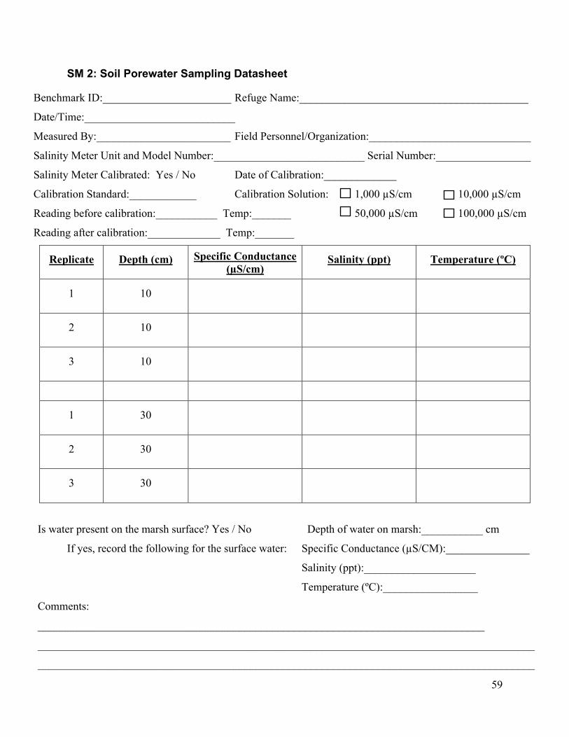
59

SM 2: Soil Porewater Sampling Datasheet

Benchmark ID:_______________________ Refuge Name:_________________________________________

Date/Time:___________________________

Measured By:________________________ Field Personnel/Organization:_____________________________

Salinity Meter Unit and Model Number:___________________________ Serial Number:_________________

Salinity Meter Calibrated: Yes / No Date of Calibration:_____________

Calibration Standard:____________ Calibration Solution: 1,000 µS/cm 10,000 µS/cm

Reading before calibration:___________ Temp:_______ 50,000 µS/cm 100,000 µS/cm

Reading after calibration:_____________ Temp:_______

Replicate Depth (cm) Specific Conductance (µS/cm)

Salinity (ppt) Temperature (ºC)

1 10

2 10

3 10

1 30

2 30

3 30

Is water present on the marsh surface? Yes / No Depth of water on marsh:___________ cm

If yes, record the following for the surface water: Specific Conductance (µS/CM):_______________

Salinity (ppt):____________________

Temperature (ºC):_________________

Comments:

________________________________________________________________________________

_________________________________________________________________________________________

_________________________________________________________________________________________

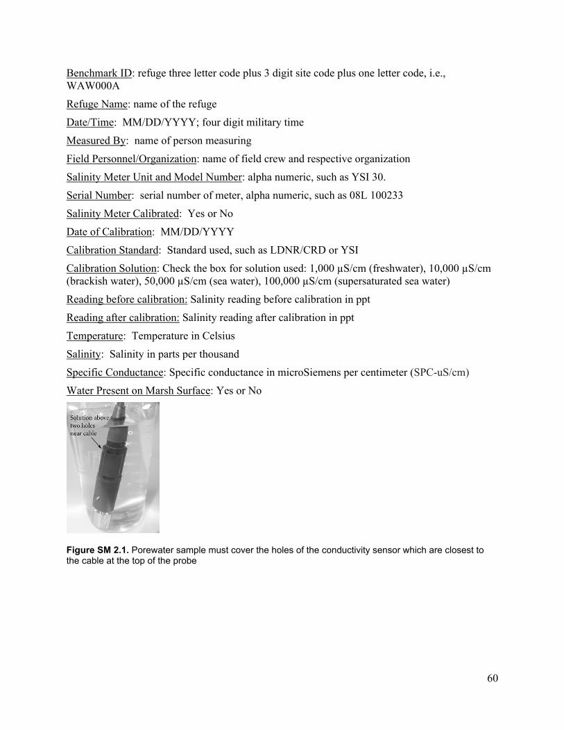
60

Benchmark ID: refuge three letter code plus 3 digit site code plus one letter code, i.e., WAW000A Refuge Name: name of the refuge Date/Time: MM/DD/YYYY; four digit military time Measured By: name of person measuring Field Personnel/Organization: name of field crew and respective organization Salinity Meter Unit and Model Number: alpha numeric, such as YSI 30. Serial Number: serial number of meter, alpha numeric, such as 08L 100233 Salinity Meter Calibrated: Yes or No Date of Calibration: MM/DD/YYYY Calibration Standard: Standard used, such as LDNR/CRD or YSI Calibration Solution: Check the box for solution used: 1,000 µS/cm (freshwater), 10,000 µS/cm (brackish water), 50,000 µS/cm (sea water), 100,000 µS/cm (supersaturated sea water) Reading before calibration: Salinity reading before calibration in ppt Reading after calibration: Salinity reading after calibration in ppt Temperature: Temperature in Celsius Salinity: Salinity in parts per thousand Specific Conductance: Specific conductance in microSiemens per centimeter (SPC-uS/cm) Water Present on Marsh Surface: Yes or No

Figure SM 2.1. Porewater sample must cover the holes of the conductivity sensor which are closest to the cable at the top of the probe

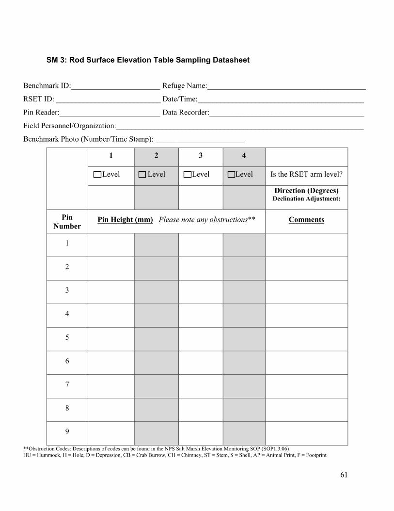
61

SM 3: Rod Surface Elevation Table Sampling Datasheet

Benchmark ID:_______________________ Refuge Name:_________________________________________

RSET ID: ___________________________ Date/Time:___________________________________________

Pin Reader:__________________________ Data Recorder:________________________________________

Field Personnel/Organization:________________________________________________________________

Benchmark Photo (Number/Time Stamp): _______________________

1 2 3 4

Level Level Level Level Is the RSET arm level?

Direction (Degrees)

Declination Adjustment: _____

Pin Number

Pin Height (mm) Please note any obstructions** Comments

1

2

3

4

5

6

7

8

9

**Obstruction Codes: Descriptions of codes can be found in the NPS Salt Marsh Elevation Monitoring SOP (SOP1.3.06) HU = Hummock, H = Hole, D = Depression, CB = Crab Burrow, CH = Chimney, ST = Stem, S = Shell, AP = Animal Print, F = Footprint

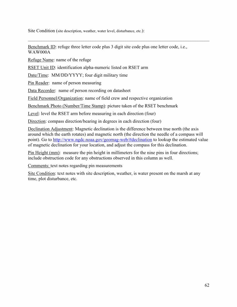
62

Site Condition (site description, weather, water level, disturbance, etc.):

______________________________________________________________________________

Benchmark ID: refuge three letter code plus 3 digit site code plus one letter code, i.e., WAW000A Refuge Name: name of the refuge RSET Unit ID: identification alpha-numeric listed on RSET arm Date/Time: MM/DD/YYYY; four digit military time Pin Reader: name of person measuring Data Recorder: name of person recording on datasheet Field Personnel/Organization: name of field crew and respective organization Benchmark Photo (Number/Time Stamp): picture taken of the RSET benchmark Level: level the RSET arm before measuring in each direction (four) Direction: compass direction/bearing in degrees in each direction (four) Declination Adjustment: Magnetic declination is the difference between true north (the axis around which the earth rotates) and magnetic north (the direction the needle of a compass will point). Go to http://www.ngdc.noaa.gov/geomag-web/#declination to lookup the estimated value of magnetic declination for your location, and adjust the compass for this declination. Pin Height (mm): measure the pin height in millimeters for the nine pins in four directions; include obstruction code for any obstructions observed in this column as well. Comments: text notes regarding pin measurements Site Condition: text notes with site description, weather, is water present on the marsh at any time, plot disturbance, etc.

63

SM 4: Marker horizon Plot Establishment Datasheet

Benchmark ID:_______________________ Refuge Name:_________________________________________

Established Date/Time:___________________________

Established By:_______________________ Field Personnel/Organization:_____________________________

Plot GPS Coordinates:

UTM Zone (NAD83): ________

Replicate Waypoint Easting Northing Photo (Number/Time Stamp)

1

2

3

Sketch of Site (includes measurements and dimensions)

Site Photo (Number/Time Stamp): ________________________

Comments: ________________________________________________________________________________

__________________________________________________________________________________________

__________________________________________________________________________________________

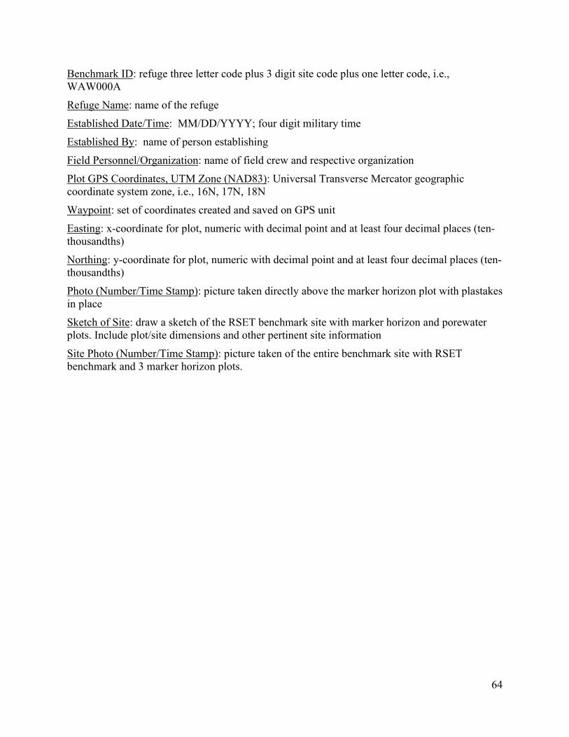
64

Benchmark ID: refuge three letter code plus 3 digit site code plus one letter code, i.e., WAW000A Refuge Name: name of the refuge Established Date/Time: MM/DD/YYYY; four digit military time Established By: name of person establishing Field Personnel/Organization: name of field crew and respective organization Plot GPS Coordinates, UTM Zone (NAD83): Universal Transverse Mercator geographic coordinate system zone, i.e., 16N, 17N, 18N Waypoint: set of coordinates created and saved on GPS unit Easting: x-coordinate for plot, numeric with decimal point and at least four decimal places (ten-thousandths) Northing: y-coordinate for plot, numeric with decimal point and at least four decimal places (ten-thousandths) Photo (Number/Time Stamp): picture taken directly above the marker horizon plot with plastakes in place Sketch of Site: draw a sketch of the RSET benchmark site with marker horizon and porewater plots. Include plot/site dimensions and other pertinent site information Site Photo (Number/Time Stamp): picture taken of the entire benchmark site with RSET benchmark and 3 marker horizon plots.

65

SM 5: Marker horizon Plot Sampling Datasheet

Site ID: Refuge Name: ________________________

Measurement Date/Time: EstablishedDate: ____________

Measured By: ______

Field Personnel/Organization:

Benchmark ID (A,B,C)

Marker horizon

Plot (1, 2, 3)

Collected Core

Location

Accretion Measurements (mm) Number

of Cores Taken

Core Quality (Excellent, Good, Fair, Poor, Layer

Not Found)

66

Notes/ Comments: Site ID: refuge three letter code plus 3 digit site code, i.e., WAW000

Refuge Name: name of the refuge

Measurement Date: date and time of measurement. MM/DD/YYYY; four digit military time

Established Date: date marker horizon plots were established. MM/DD/YYYY

Measured By: name of person collecting core and taken measurements Field Personnel/Organization: name of field crew and respective organization Benchmark ID: refuge three letter code plus 3 digit site code plus one letter code, i.e.,

WAW000A

Marker horizon Plot: number of the marker horizon plot (1, 2, 3)

Collected Core Location: mark with an X the location where the measured core was collected Accretion Measurements (mm): distant in millimeters of accretion above the feldspar layer to

the surface layer. Three measurements are taken. Number of Cores Taken: number of cores taken before measuring; numeric value Core Quality: condition/quality of core used for measuring: excellent, good, fair, poor, layer

not found

Notes/Comments: text field for additional notes or comments

67

U.S. Fish and Wildlife Service U.S. Department of the Interior National Wildlife Refuge System

Table 8.1.