Source Seeking by Dynamic Source Location Estimation

Tianpeng Zhang, Victor Qin, Yujie Tang, Na Li

Abstract— This paper focuses on the problem of multi-robotsource-seeking, where a group of mobile sensors localizes andmoves close to a single source using only local measurements.Drawing inspiration from the optimal sensor placement re-search, we develop an algorithm that estimates the sourcelocation while approaches the source following gradient descentsteps on a loss function defined on the Fisher information. Weshow that exploiting Fisher information gives a higher chanceof obtaining an accurate source location estimate and naturallyleads the sensors to the source. Our numerical experimentsdemonstrate the advantages of our algorithm, including fasterconvergence to the source than other algorithms, flexibility inthe choice of the loss function, and robustness to measurementmodeling errors. Moreover, the performance improves as thenumber of sensors increases, showing the advantage of usingmulti-robots in our source-seeking algorithm. We also imple-ment physical experiments to test the algorithm on small groundvehicles with light sensors, demonstrating success in seeking amoving light source.

I. INTRODUCTION

Multi-agent source seeking is to use autonomous vehicleswith measurement capabilities to locate a source of interestwhose position is unknown. The source of interest can be alight source, a radio signal transmitter, or a chemical leakagepoint. The source-seeking vehicles, or mobile sensors, canmeasure the source’s influence on the environment and usethis information to locate the source.

A large body of source seeking research investigatesfield climbing methods [1]–[4]. Assuming the source signalgets stronger as the sensor-source distance shortens, mobilesensors can “climb” the source signal field to physicallyapproach the source. These methods do not require explicitknowledge of the measurement model, making them easy toimplement and generalizable to different applications. How-ever, field climbing methods only exploit local informationof the source field, as the sensors must maintain a tightformation to make a reasonable ascent direction estimate,as is the case in [3], [4]. Furthermore, to achieve a stableincrease in measurement value, the sensors cannot move toofast as a group. Therefore field climbing methods are notnecessarily the most effective source-seeking methods.

An alternative approach is to perform source identifica-tion/localization using various estimation methods, such as(Extended) Kalman Filter (EKF) [5], [6], Particle Filter (PF)[7], [8], and so on, to keep a constantly updated estimate ofthe source location over time. Despite requiring an explicitmeasurement model, these methods enable the fusion ofmeasurements from multiple sensors to quickly identifya global view of the measurement field. To improve the

The authors are with the School of Engineering andApplied Sciences, Harvard University, Cambridge, MA02138, USA. Emails: tzhang@g.harvard.edu,victor l qin@college.harvard.edu,{yujietang,nali}@seas.harvard.edu.

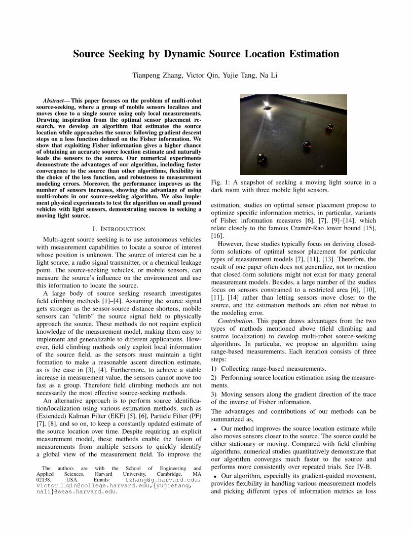
Fig. 1: A snapshot of seeking a moving light source in adark room with three mobile light sensors.

estimation, studies on optimal sensor placement propose tooptimize specific information metrics, in particular, variantsof Fisher information measures [6], [7], [9]–[14], whichrelate closely to the famous Cramer-Rao lower bound [15],[16].

However, these studies typically focus on deriving closed-form solutions of optimal sensor placement for particulartypes of measurement models [7], [11], [13]. Therefore, theresult of one paper often does not generalize, not to mentionthat closed-form solutions might not exist for many generalmeasurement models. Besides, a large number of the studiesfocus on sensors constrained to a restricted area [6], [10],[11], [14] rather than letting sensors move closer to thesource, and the estimation methods are often not robust tothe modeling error.

Contribution. This paper draws advantages from the twotypes of methods mentioned above (field climbing andsource localization) to develop multi-robot source-seekingalgorithms. In particular, we propose an algorithm usingrange-based measurements. Each iteration consists of threesteps:1) Collecting range-based measurements.2) Performing source location estimation using the measure-ments.3) Moving sensors along the gradient direction of the traceof the inverse of Fisher information.The advantages and contributions of our methods can besummarized as,• Our method improves the source location estimate while

also moves sensors closer to the source. The source could beeither stationary or moving. Compared with field climbingalgorithms, numerical studies quantitatively demonstrate thatour algorithm converges much faster to the source andperforms more consistently over repeated trials. See IV-B.• Our algorithm, especially its gradient-guided movement,

provides flexibility in handling various measurement modelsand picking different types of information metrics as loss

functions. Section IV-C confirms at least three applicablemetrics.• The algorithm takes advantage of multi-sensors in the

sense that the performance improves as the number ofsensors increases, see IV-B.• The algorithm is more robust to modeling error than the

source localization with stationary sensors, see IV-D.• We implement our algorithm on small ground vehicles

carrying light sensors to seek a moving light source in a darkroom, as shown in Figure 1. The hardware implementationfurther demonstrates the effectiveness of our algorithm. SeeIV-E.

A. Related Works

Field climbing methods. The field climbing problem stemsfrom scientific research that studies animal behavior in ex-ploring nutrition or chemical concentration fields [17], [18].Inspired by these studies, some methods propose using fieldvalue measurements to estimate the field gradient and applyformation control to climb along the gradient [2], [3]. Thereare also methods not reliant on gradient estimates: [4] keepsthe sensors in a circular formation and uses measured fieldvalues as directional weights to guide the overall movement;[19], [20] are based on Particle Swarm Optimization (PSO).

The main differences between field climbing and ouralgorithm are that i) field climbing maximizes the source fieldvalue, while ours exploits the Fisher information, an indicatorof both estimation accuracy and source-sensor distance, ii)field climbing does not require knowing the measurementfunction, but ours does, iii) field climbing algorithms oftendemand a tight sensor formation for a stable field ascent, onlyexploiting local information, while our algorithm uses thesensors to collect global information for source localization.We will show in Section IV that the sensors under ouralgorithm tend to spread out to estimate the source better.

Source localization and optimal sensor placement. If ameasurement model is available, various estimation methodscan be applied to estimate source location, including EKF[5], [6], PF [7], [8], or even a reconstruction of the entiresource field [9], [21]. To improve the estimation, peoplehave studied optimal sensor placement by optimizing variousinformation metrics including covariance [22], [23], mutualinformation [8], [24], and Fisher information measures [6],[7], [9]–[14] such as the determinant of Fisher information,the largest eigenvalue of its inverse, and the trace of itsinverse (D-, E-, and A-optimality criterion respectively).

Our method also employs Fisher information but is differ-ent from the previous ones in that:1) Most of the works focus on deriving closed-form so-lutions of optimal sensor placement for a particular typeof measurement model, for example, RSS [11], pollutantdiffusion [7], and gamma camera [13]. In contrast, ourfocus is not on providing closed-form solutions but insteadproviding a gradient-based method applicable to a largeclass of range-based measurement models. This method alsoprovides flexibility in choosing different information metricsas loss functions, see IV-C.2) Many previous works focus on finding the optimal angu-lar placement of the sensors at a fixed distance to the source

or on a restricted area [6], [10], [11], [14]. In contrast, weallow the sensors to move freely and eventually approach thesource.3) Some studies relax the restrictions on the sensor move-ment [12], [13]. However, these methods produce a spiralingsensor movement which is inefficient for source-seeking pur-poses, while our method does not produce such movement.Moreover, the way-point planning in these methods is basedon the closed-form optimal placement solutions, but ourmethod follows the gradient steps.Bayesian inference and optimization. The recent advances inBayesian learning inspire many studies to adopt the Bayesianmethods for source seeking [25]–[27]. These studies viewthe environment as a field characterized by an (unknown)density function related to measurement and use GaussianProcess or other likelihood models as a surrogate to guidethe sensor movements for new measurement collections. Thecomputation (for running the posterior update and Bayesianoptimization) and memory (for storing historical measure-ments as in non-parametric Bayesian methods) demands ofthese methods are often higher than our method. Overall,Bayesian-based methods and our method are designed fromdifferent principles. A detailed comparison is left for futurework.

Finally, we would like to highlight that our work issignificantly inspired by [6], which studies the optimal sensorplacement problem on a surveillance boundary. We leveragetheir ideas to introduce the Fisher information in our objec-tive, but we change the loss function from the determinantof Fisher information to the trace of its inverse. We alsogeneralize the measurement model, so it fits our experimentsand other real-world measurement settings. To handle suchmore general measurement models, the sensors only computethe gradient of the loss function rather than solving for itsoptimum at each time step.

II. PROBLEM SETUP

We consider the task of using a team of mobile sensors,with centralized coordination, to find a source whose locationis unknown. For concreteness, in our experiment setting, thesource is a lamp in a dark room, and the mobile sensorsare ground vehicles carrying light sensors measuring thelocal light intensity. The sensor positions are assumed to beavailable. The goal is to let sensors move to the proximityof the source based on field measurements.

Specifically, we use q ∈ Rk to denote the source po-sition, and use p1, p2, · · · , pm ∈ Rk to denote the sensorpositions, where m is the number of sensors and k is thespatial dimension. We use the vector (in bold font) p =[p>1 p>2 · · · p>m

]>to denote the joint location of all

mobile sensors.In this paper, we consider nonholomonic ground vehicles

with pi = [p1i , p

2i ]> ∈ R2. The states of mobile sensor i

are xi := [p1i , p

2i , θi]

> with θ being the robot orientation,and the control inputs ui are the linear and angular velocitiesof the robot ui := [vi, ωi]

>. The robot motion dynamics isgiven as

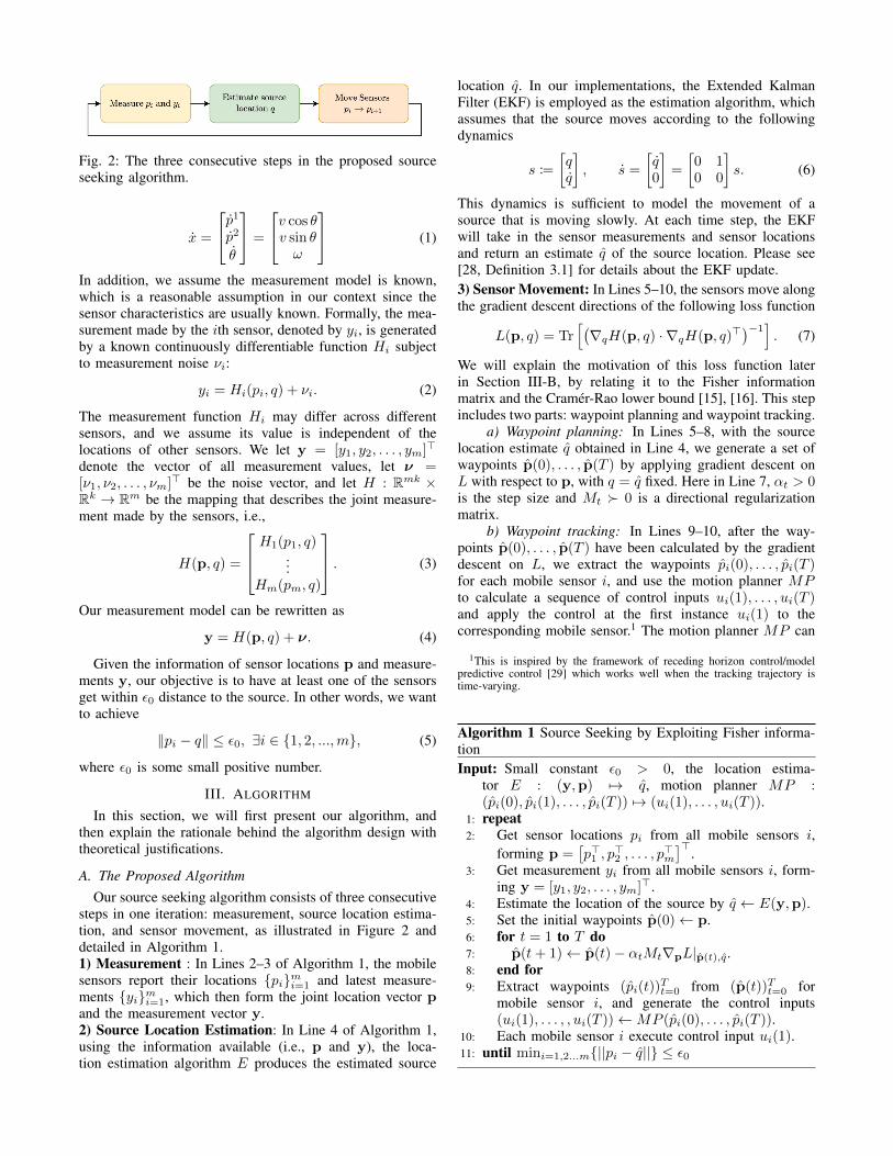
Fig. 2: The three consecutive steps in the proposed sourceseeking algorithm.

x =

p1

p2

θ

=

v cos θv sin θω

(1)

In addition, we assume the measurement model is known,which is a reasonable assumption in our context since thesensor characteristics are usually known. Formally, the mea-surement made by the ith sensor, denoted by yi, is generatedby a known continuously differentiable function Hi subjectto measurement noise νi:

yi = Hi(pi, q) + νi. (2)

The measurement function Hi may differ across differentsensors, and we assume its value is independent of thelocations of other sensors. We let y = [y1, y2, . . . , ym]>

denote the vector of all measurement values, let ν =[ν1, ν2, . . . , νm]> be the noise vector, and let H : Rmk ×Rk → Rm be the mapping that describes the joint measure-ment made by the sensors, i.e.,

H(p, q) =

H1(p1, q)...

Hm(pm, q)

. (3)

Our measurement model can be rewritten as

y = H(p, q) + ν. (4)

Given the information of sensor locations p and measure-ments y, our objective is to have at least one of the sensorsget within ε0 distance to the source. In other words, we wantto achieve

‖pi − q‖ ≤ ε0, ∃i ∈ {1, 2, ...,m}, (5)

where ε0 is some small positive number.

III. ALGORITHM

In this section, we will first present our algorithm, andthen explain the rationale behind the algorithm design withtheoretical justifications.

A. The Proposed AlgorithmOur source seeking algorithm consists of three consecutive

steps in one iteration: measurement, source location estima-tion, and sensor movement, as illustrated in Figure 2 anddetailed in Algorithm 1.1) Measurement : In Lines 2–3 of Algorithm 1, the mobilesensors report their locations {pi}mi=1 and latest measure-ments {yi}mi=1, which then form the joint location vector pand the measurement vector y.2) Source Location Estimation: In Line 4 of Algorithm 1,using the information available (i.e., p and y), the loca-tion estimation algorithm E produces the estimated source

location q. In our implementations, the Extended KalmanFilter (EKF) is employed as the estimation algorithm, whichassumes that the source moves according to the followingdynamics

s :=

[qq

], s =

[q0

]=

[0 10 0

]s. (6)

This dynamics is sufficient to model the movement of asource that is moving slowly. At each time step, the EKFwill take in the sensor measurements and sensor locationsand return an estimate q of the source location. Please see[28, Definition 3.1] for details about the EKF update.3) Sensor Movement: In Lines 5–10, the sensors move alongthe gradient descent directions of the following loss function

L(p, q) = Tr[(∇qH(p, q) · ∇qH(p, q)>

)−1]. (7)

We will explain the motivation of this loss function laterin Section III-B, by relating it to the Fisher informationmatrix and the Cramer-Rao lower bound [15], [16]. This stepincludes two parts: waypoint planning and waypoint tracking.

a) Waypoint planning: In Lines 5–8, with the sourcelocation estimate q obtained in Line 4, we generate a set ofwaypoints p(0), . . . , p(T ) by applying gradient descent onL with respect to p, with q = q fixed. Here in Line 7, αt > 0is the step size and Mt � 0 is a directional regularizationmatrix.

b) Waypoint tracking: In Lines 9–10, after the way-points p(0), . . . , p(T ) have been calculated by the gradientdescent on L, we extract the waypoints pi(0), . . . , pi(T )for each mobile sensor i, and use the motion planner MPto calculate a sequence of control inputs ui(1), . . . , ui(T )and apply the control at the first instance ui(1) to thecorresponding mobile sensor.1 The motion planner MP can

1This is inspired by the framework of receding horizon control/modelpredictive control [29] which works well when the tracking trajectory istime-varying.

Algorithm 1 Source Seeking by Exploiting Fisher informa-tionInput: Small constant ε0 > 0, the location estima-

tor E : (y,p) 7→ q, motion planner MP :(pi(0), pi(1), . . . , pi(T )) 7→ (ui(1), . . . , ui(T )).

1: repeat2: Get sensor locations pi from all mobile sensors i,

forming p =[p>1 , p

>2 , . . . , p

>m

]>.

3: Get measurement yi from all mobile sensors i, form-ing y = [y1, y2, . . . , ym]>.

4: Estimate the location of the source by q ← E(y,p).5: Set the initial waypoints p(0)← p.6: for t = 1 to T do7: p(t+ 1)← p(t)− αtMt∇pL|p(t),q .8: end for9: Extract waypoints (pi(t))

Tt=0 from (p(t))Tt=0 for

mobile sensor i, and generate the control inputs(ui(1), . . . , , ui(T ))←MP (pi(0), . . . , pi(T )).

10: Each mobile sensor i execute control input ui(1).11: until mini=1,2...m{||pi − q||} ≤ ε0

be viewed as a device that transforms the planned way-points into low-level actuation of a mobile sensor: by apply-ing (ui(1), . . . , ui(T )) = MP (pi(0), . . . , pi(T )) to sensori, the sensor will follow the trajectory of the waypointspi(0), . . . , pi(T ). The motion planner MP typically requiresthe knowledge of the sensors’ dynamics to compute thecontrol inputs, and any method that can fulfill this task canbe a motion planner in Algorithm 1. In our implementation,the motion planner is a combination of spline-based motiongeneration described in [30] and the Linear Quadratic Reg-ulator (LQR). Regarding the choice of the planning horizonT , in the Gazebo simulations and hardware implementation,we set T = 20 to ensure stability in sensor movement androbustness to disturbances. Meanwhile, in numerical studieswhere the robot dynamics is not simulated, it suffices to setT = 1.

Finally, the loop resets, and the sensors make a new set ofmeasurements. The loop repeats until one sensor is withinε0 distance to q.Remark 1. Note the algorithm aims to minimize L(p, q)rather than L(p, q), which raises the question of whetherimproving the former leads to a decrease in the value ofthe latter. Intuitively, it is expected that if q and q aresufficiently close to each other, i.e., the estimation error issmall, then improving L(p, q) will decrease L(p, q). Thesetwo components of the algorithm rely on each other tofunction as a whole.

B. The Design Rationale of the Loss FunctionIn location-estimation-based source seeking, one uses the

estimated location as a reference to move the sensors. Nat-urally, we want the location estimation to be as accurate aspossible. However, the Cramer–Rao Lower Bound (CRLB)shows an intrinsic limitation that prevents the location es-timation from being arbitrarily accurate. Formally, we havethe following definition and theorem:

Definition 1 (Fisher Information). Given the measurementfunction H(p, q), and assuming the measurement noise isGaussian white, the Fisher information matrix relative to thesource location q is

FIM = ∇qH(p, q) · ∇qH(p, q)>.

Here ∇qH(p, q) denotes the k×m matrix whose ith columnis equal to the (partial) gradient ∇qHi(pi, q).

Theorem 1 (Cramer–Rao Lower Bound (CRLB) [15], [16]).For any unbiased estimator q of q, the following matrixinequality holds2

E[(q − q)(q − q)>] � FIM−1. (8)

Martinez and Bullo [6] built on this result to maximizedet(FIM) in the hope of making FIM−1 small so that theestimation error is more likely to achieve low values. How-ever, a large value of det(FIM) does not necessarily meanthat the eigenvalues of FIM−1 will be uniformly small, and

2Strictly speaking, an additional constant factor should be multiplied tothe FIM as in Definition 1 for CRLB to hold. The constant is related tothe covariance of measurement noise but is independent of (q,p) and isinconsequential for our algorithm and results.

the lower bound provided by Theorem 1 might still be large.In Section IV-C, we show by simulation results that it isindeed not ideal for our application. Therefore, in this paper,we modify their idea and consider minimizing Tr(FIM−1)instead, which is also known as the A-optimality criterion[31] in literature.

The minimization of the loss function (7) will result intwo consequences: First, by taking the trace on both sides of(8), we get E

[‖q − q‖2

]≥ Tr

(FIM−1

)= L(p, q), i.e.,

the loss function is a lower bound on the mean squarederror, and so by minimizing (7), we increase the chance ofgetting accurate source location estimates. Second, as we willshow in the following subsection, a small value of the lossfunction implies the existence of at least one sensor that getssufficiently close to the source under certain assumptions onthe measurement model.Remark 2. While we choose Tr(FIM−1) as the loss func-tion in this paper, in principle one can also pick otherinformation metrics as the loss function L in Algorithm 1.In Section IV-C, we will numerically test the performanceusing different options of the loss function.

C. Reaching the SourceWe now provide analytical results showing that mini-

mizing Tr(FIM−1) will indeed enforce some sensor toapproach the source. For the sake of theoretical analysis, weneed some extra assumptions on the measurement model. Inparticular, we assume that Hi is a monotonic function of thedistance between sensors and the source.

Assumption 1. We make the following assumptions on themeasurement functions Hi:1) Isotropic measurement: The measurement values de-pend only on source-sensor distance, i.e.,

Hi(pi, q) = hi(‖pi − q‖) = hi(ri) (9)

for some function hi : (0,+∞)→ R, where ri := ‖pi − q‖.2) Monotonicity: Each function hi(r) is nonnegative andis monotonically decreasing in r. In addition, as r → 0, wehave hi(r)→ +∞ as well as |h′i(r)| → +∞.

Here the term isotropic means that the measurement doesnot depend on source-sensor bearings, a.k.a. relative angles.The isotropic and monotonic properties hold for a wide rangeof functions that model the decay of measurement signalsover distance, including, e.g., the function h(r) = − log rfor RSS sensors, and the functions h(r) = 1/rb, b > 0 forlight sensors. We can then prove the following proposition,showing that minimizing Tr(FIM−1) indeed results in atleast one sensor getting sufficiently close to the source.

Proposition 1 (Reaching the Source). Let ri denote the unitdirection vector from the source to the ith mobile sensor, i.e.,ri = (pi − q)/‖pi − q‖. Suppose the smallest eigenvalue of∑m

i=1 rir>i is not zero at all times. Then under Assumption 1,

we have mini ri → 0 whenever L(p, q)→ 0.

We remark that for the case k = 2, i.e., the source and themobile sensors move on a 2D plane, the smallest eigenvalueof∑m

i=1 rir>i is not zero as long as there is more than

one mobile sensor, and all mobile sensors together with

the source are not on the same straight line. The proof ofProposition 1 can be found in Appendix I.

IV. EXPERIMENTAL RESULTS

This section illustrates the performance of our proposedalgorithm through experiments. The algorithm performanceunder actual robot dynamics is studied in simulations in IV-A. In the other three numerical studies, we remove the robotdynamics in simulations to efficiently conduct repetitive trialsand assume the sensors follow the gradient steps exactly. Westudy the influence of the number of sensors in IV-B, thedifference of various information metrics in IV-C, and therobustness to modeling error in IV-D. Finally, we describeour real robot implementations in IV-E with a supplementaryvideo recording the experimental results available at [32].

A. Gazebo Numerical ExperimentsThe following numerical experiments are carried out using

the Gazebo simulation toolbox [33], with virtual mobilesensors simulating the same dynamics as the actual robots.We generate simulated measurement values of the sensorsby yi = 1/r2

i + νi, with νi drawn independently fromN (0, 0.01). The measurement function hi(r) = 1/r2

i isgiven to the EKF for estimation.

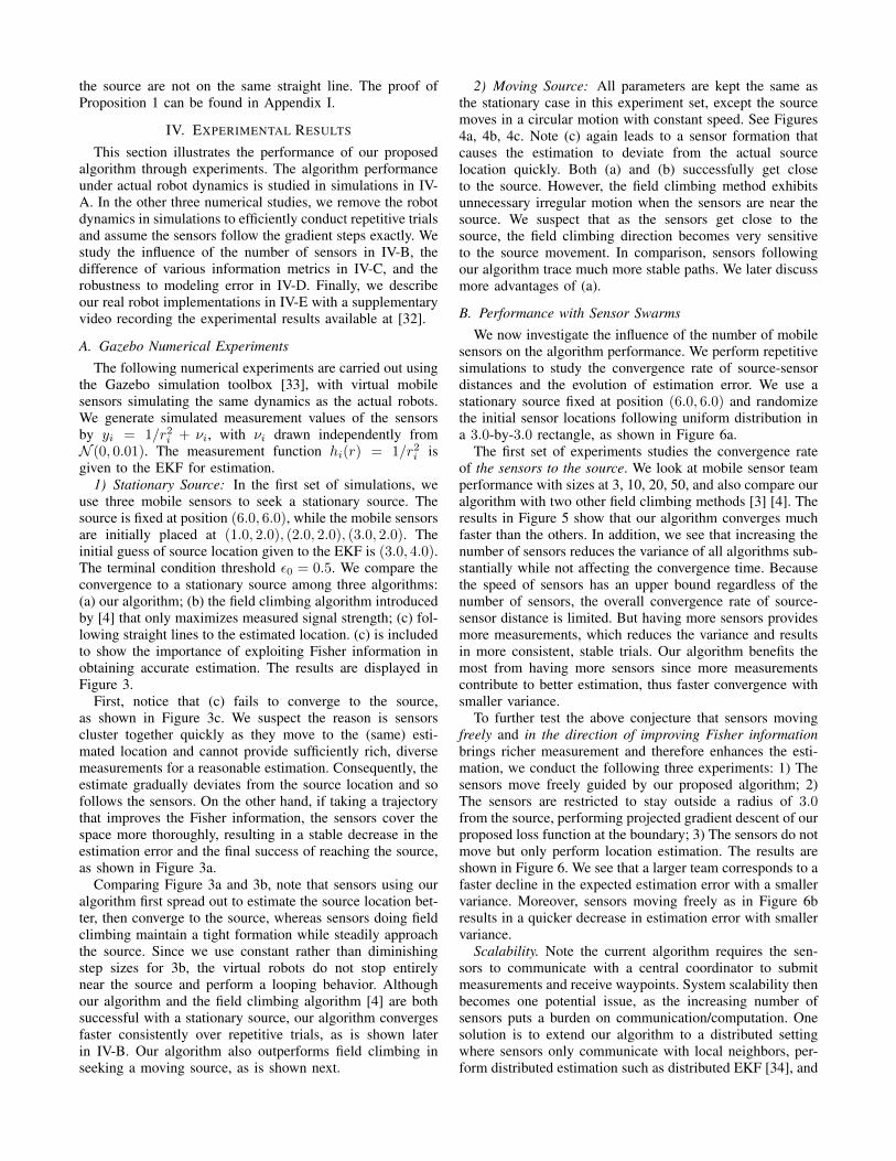
1) Stationary Source: In the first set of simulations, weuse three mobile sensors to seek a stationary source. Thesource is fixed at position (6.0, 6.0), while the mobile sensorsare initially placed at (1.0, 2.0), (2.0, 2.0), (3.0, 2.0). Theinitial guess of source location given to the EKF is (3.0, 4.0).The terminal condition threshold ε0 = 0.5. We compare theconvergence to a stationary source among three algorithms:(a) our algorithm; (b) the field climbing algorithm introducedby [4] that only maximizes measured signal strength; (c) fol-lowing straight lines to the estimated location. (c) is includedto show the importance of exploiting Fisher information inobtaining accurate estimation. The results are displayed inFigure 3.

First, notice that (c) fails to converge to the source,as shown in Figure 3c. We suspect the reason is sensorscluster together quickly as they move to the (same) esti-mated location and cannot provide sufficiently rich, diversemeasurements for a reasonable estimation. Consequently, theestimate gradually deviates from the source location and sofollows the sensors. On the other hand, if taking a trajectorythat improves the Fisher information, the sensors cover thespace more thoroughly, resulting in a stable decrease in theestimation error and the final success of reaching the source,as shown in Figure 3a.

Comparing Figure 3a and 3b, note that sensors using ouralgorithm first spread out to estimate the source location bet-ter, then converge to the source, whereas sensors doing fieldclimbing maintain a tight formation while steadily approachthe source. Since we use constant rather than diminishingstep sizes for 3b, the virtual robots do not stop entirelynear the source and perform a looping behavior. Althoughour algorithm and the field climbing algorithm [4] are bothsuccessful with a stationary source, our algorithm convergesfaster consistently over repetitive trials, as is shown laterin IV-B. Our algorithm also outperforms field climbing inseeking a moving source, as is shown next.

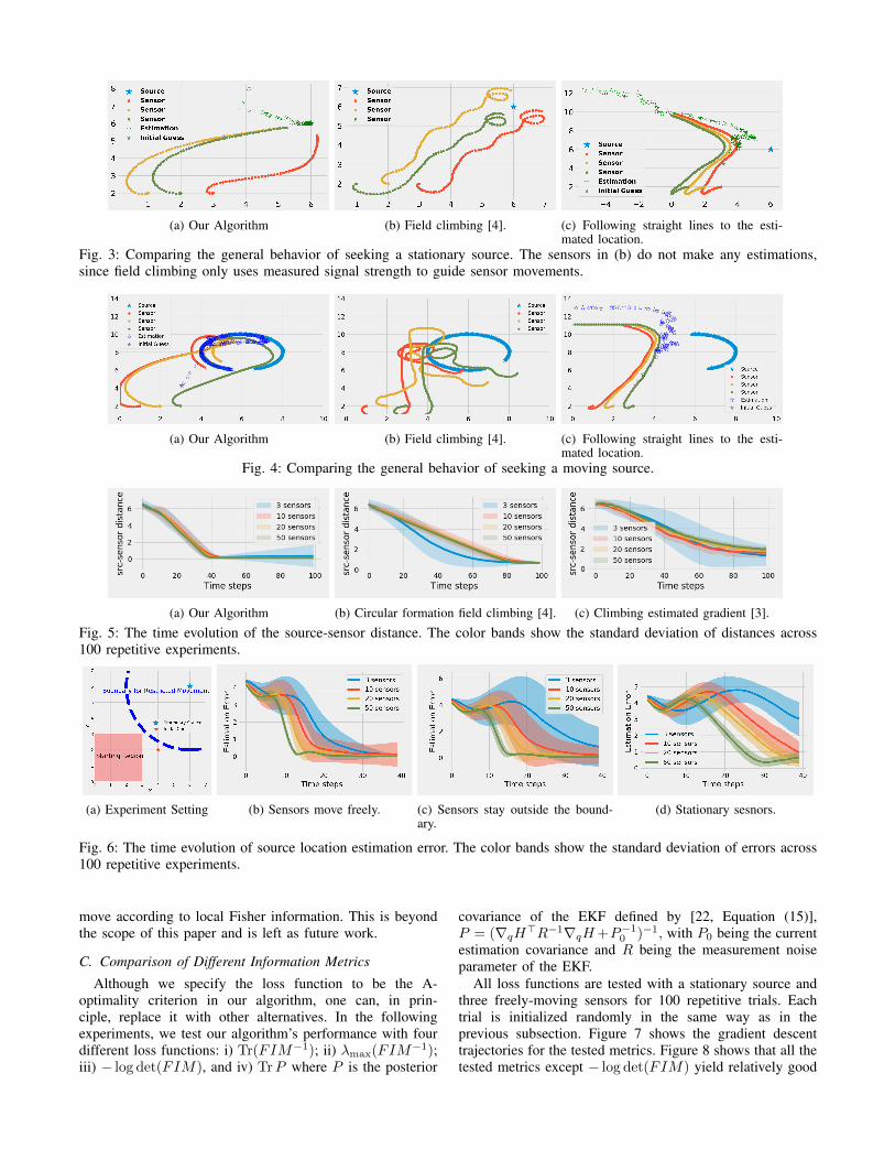
2) Moving Source: All parameters are kept the same asthe stationary case in this experiment set, except the sourcemoves in a circular motion with constant speed. See Figures4a, 4b, 4c. Note (c) again leads to a sensor formation thatcauses the estimation to deviate from the actual sourcelocation quickly. Both (a) and (b) successfully get closeto the source. However, the field climbing method exhibitsunnecessary irregular motion when the sensors are near thesource. We suspect that as the sensors get close to thesource, the field climbing direction becomes very sensitiveto the source movement. In comparison, sensors followingour algorithm trace much more stable paths. We later discussmore advantages of (a).

B. Performance with Sensor SwarmsWe now investigate the influence of the number of mobile

sensors on the algorithm performance. We perform repetitivesimulations to study the convergence rate of source-sensordistances and the evolution of estimation error. We use astationary source fixed at position (6.0, 6.0) and randomizethe initial sensor locations following uniform distribution ina 3.0-by-3.0 rectangle, as shown in Figure 6a.

The first set of experiments studies the convergence rateof the sensors to the source. We look at mobile sensor teamperformance with sizes at 3, 10, 20, 50, and also compare ouralgorithm with two other field climbing methods [3] [4]. Theresults in Figure 5 show that our algorithm converges muchfaster than the others. In addition, we see that increasing thenumber of sensors reduces the variance of all algorithms sub-stantially while not affecting the convergence time. Becausethe speed of sensors has an upper bound regardless of thenumber of sensors, the overall convergence rate of source-sensor distance is limited. But having more sensors providesmore measurements, which reduces the variance and resultsin more consistent, stable trials. Our algorithm benefits themost from having more sensors since more measurementscontribute to better estimation, thus faster convergence withsmaller variance.

To further test the above conjecture that sensors movingfreely and in the direction of improving Fisher informationbrings richer measurement and therefore enhances the esti-mation, we conduct the following three experiments: 1) Thesensors move freely guided by our proposed algorithm; 2)The sensors are restricted to stay outside a radius of 3.0from the source, performing projected gradient descent of ourproposed loss function at the boundary; 3) The sensors do notmove but only perform location estimation. The results areshown in Figure 6. We see that a larger team corresponds to afaster decline in the expected estimation error with a smallervariance. Moreover, sensors moving freely as in Figure 6bresults in a quicker decrease in estimation error with smallervariance.

Scalability. Note the current algorithm requires the sen-sors to communicate with a central coordinator to submitmeasurements and receive waypoints. System scalability thenbecomes one potential issue, as the increasing number ofsensors puts a burden on communication/computation. Onesolution is to extend our algorithm to a distributed settingwhere sensors only communicate with local neighbors, per-form distributed estimation such as distributed EKF [34], and

(a) Our Algorithm (b) Field climbing [4]. (c) Following straight lines to the esti-mated location.

Fig. 3: Comparing the general behavior of seeking a stationary source. The sensors in (b) do not make any estimations,since field climbing only uses measured signal strength to guide sensor movements.

(a) Our Algorithm (b) Field climbing [4]. (c) Following straight lines to the esti-mated location.

Fig. 4: Comparing the general behavior of seeking a moving source.

(a) Our Algorithm (b) Circular formation field climbing [4]. (c) Climbing estimated gradient [3].

Fig. 5: The time evolution of the source-sensor distance. The color bands show the standard deviation of distances across100 repetitive experiments.

(a) Experiment Setting (b) Sensors move freely. (c) Sensors stay outside the bound-ary.

(d) Stationary sesnors.

Fig. 6: The time evolution of source location estimation error. The color bands show the standard deviation of errors across100 repetitive experiments.

move according to local Fisher information. This is beyondthe scope of this paper and is left as future work.

C. Comparison of Different Information Metrics

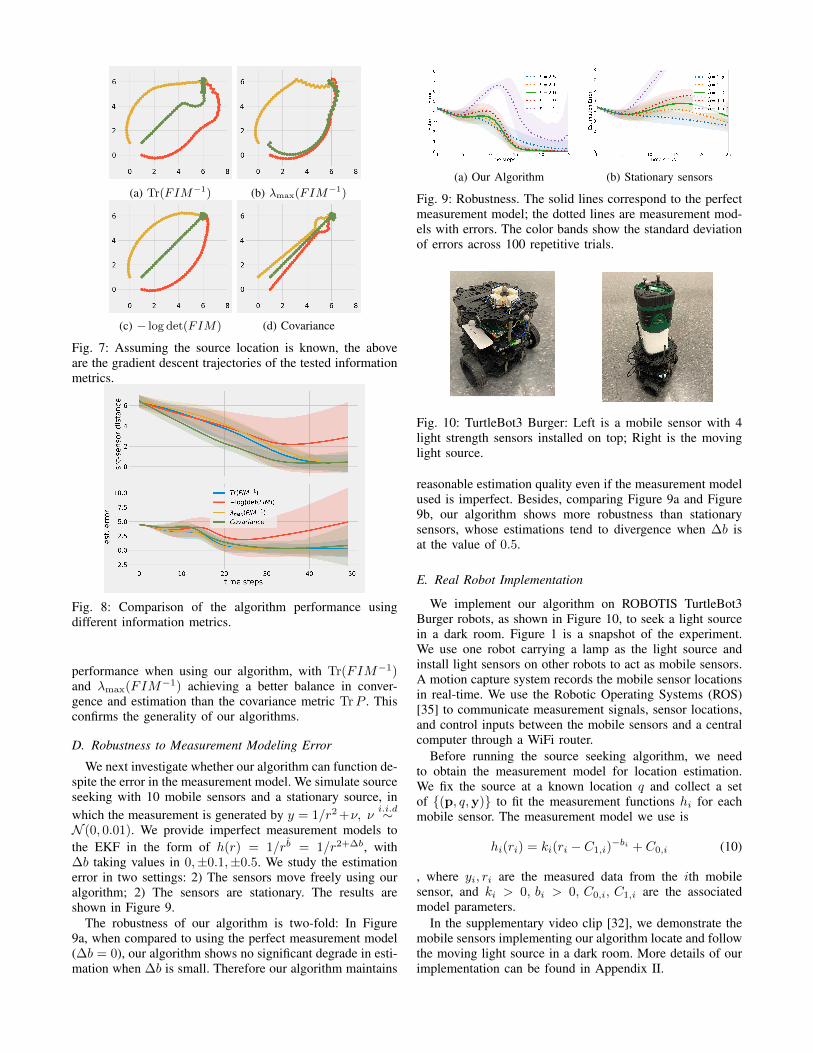
Although we specify the loss function to be the A-optimality criterion in our algorithm, one can, in prin-ciple, replace it with other alternatives. In the followingexperiments, we test our algorithm’s performance with fourdifferent loss functions: i) Tr(FIM−1); ii) λmax(FIM−1);iii) − log det(FIM), and iv) TrP where P is the posterior

covariance of the EKF defined by [22, Equation (15)],P = (∇qH

>R−1∇qH+P−10 )−1, with P0 being the current

estimation covariance and R being the measurement noiseparameter of the EKF.

All loss functions are tested with a stationary source andthree freely-moving sensors for 100 repetitive trials. Eachtrial is initialized randomly in the same way as in theprevious subsection. Figure 7 shows the gradient descenttrajectories for the tested metrics. Figure 8 shows that all thetested metrics except − log det(FIM) yield relatively good

(a) Tr(FIM−1) (b) λmax(FIM−1)

(c) − log det(FIM) (d) Covariance

Fig. 7: Assuming the source location is known, the aboveare the gradient descent trajectories of the tested informationmetrics.

Fig. 8: Comparison of the algorithm performance usingdifferent information metrics.

performance when using our algorithm, with Tr(FIM−1)and λmax(FIM−1) achieving a better balance in conver-gence and estimation than the covariance metric TrP . Thisconfirms the generality of our algorithms.

D. Robustness to Measurement Modeling Error

We next investigate whether our algorithm can function de-spite the error in the measurement model. We simulate sourceseeking with 10 mobile sensors and a stationary source, inwhich the measurement is generated by y = 1/r2 +ν, ν

i.i.d∼N (0, 0.01). We provide imperfect measurement models tothe EKF in the form of h(r) = 1/rb = 1/r2+∆b, with∆b taking values in 0,±0.1,±0.5. We study the estimationerror in two settings: 2) The sensors move freely using ouralgorithm; 2) The sensors are stationary. The results areshown in Figure 9.

The robustness of our algorithm is two-fold: In Figure9a, when compared to using the perfect measurement model(∆b = 0), our algorithm shows no significant degrade in esti-mation when ∆b is small. Therefore our algorithm maintains

(a) Our Algorithm (b) Stationary sensors

Fig. 9: Robustness. The solid lines correspond to the perfectmeasurement model; the dotted lines are measurement mod-els with errors. The color bands show the standard deviationof errors across 100 repetitive trials.

Fig. 10: TurtleBot3 Burger: Left is a mobile sensor with 4light strength sensors installed on top; Right is the movinglight source.

reasonable estimation quality even if the measurement modelused is imperfect. Besides, comparing Figure 9a and Figure9b, our algorithm shows more robustness than stationarysensors, whose estimations tend to divergence when ∆b isat the value of 0.5.

E. Real Robot Implementation

We implement our algorithm on ROBOTIS TurtleBot3Burger robots, as shown in Figure 10, to seek a light sourcein a dark room. Figure 1 is a snapshot of the experiment.We use one robot carrying a lamp as the light source andinstall light sensors on other robots to act as mobile sensors.A motion capture system records the mobile sensor locationsin real-time. We use the Robotic Operating Systems (ROS)[35] to communicate measurement signals, sensor locations,and control inputs between the mobile sensors and a centralcomputer through a WiFi router.

Before running the source seeking algorithm, we needto obtain the measurement model for location estimation.We fix the source at a known location q and collect a setof {(p, q,y)} to fit the measurement functions hi for eachmobile sensor. The measurement model we use is

hi(ri) = ki(ri − C1,i)−bi + C0,i (10)

, where yi, ri are the measured data from the ith mobilesensor, and ki > 0, bi > 0, C0,i, C1,i are the associatedmodel parameters.

In the supplementary video clip [32], we demonstrate themobile sensors implementing our algorithm locate and followthe moving light source in a dark room. More details of ourimplementation can be found in Appendix II.

V. CONCLUSION AND FUTURE DIRECTIONS

This paper develops a multi-robot source-seeking algo-rithm that exploits the Fisher information associated withthe source location estimation to guide the sensors’ move-ment. We show in theoretical analysis that improving thetrace of the inverse Fisher information benefits the sourcelocation estimation and naturally leads sensors to convergeto the source. The algorithm is verified both numerically andphysically on small ground vehicles.

There are several interesting future directions. For exam-ple, besides the scalability issue discussed in Section IV-B,another vital point to be addressed in future work is collisionavoidance, which can be incorporated into our algorithm by,for example, adding a collision penalty to the loss function oremploying a reactionary actuation control on top of waypointplanning. We expect that collision avoidance can improve therobustness of our algorithm without hindering either the con-vergence rate or estimation accuracy drastically. In addition,comparison to other types of source-seeking methods suchas Bayesian optimization needs more investigation. Somehybrid versions between these methods and our methodmight draw advantages from both sides.

REFERENCES

[1] B. A. Angelico, L. F. O. Chamon, S. Paternain, A. Ribeiro, andG. J. Pappas, “Source seeking in unknown environments with convexobstacles,” arXiv preprint arXiv:1909.07496, 2019.

[2] R. Bachmayer and N. E. Leonard, “Vehicle networks for gradientdescent in a sampled environment,” in Proceedings of the 41st IEEEConference on Decision and Control, vol. 1, 2002, pp. 112–117.

[3] P. Ogren, E. Fiorelli, and N. E. Leonard, “Cooperative control ofmobile sensor networks: Adaptive gradient climbing in a distributedenvironment,” IEEE Transactions on Automatic Control, vol. 49, no. 8,pp. 1292–1302, 2004.

[4] B. J. Moore and C. Canudas-de Wit, “Source seeking via collaborativemeasurements by a circular formation of agents,” in Proceedings ofthe 2010 American Control Conference, 2010, pp. 6417–6422.

[5] F. Morbidi and G. L. Mariottini, “Active target tracking and cooper-ative localization for teams of aerial vehicles,” IEEE Transactions onControl Systems Technology, vol. 21, no. 5, pp. 1694–1707, 2013.

[6] S. Martınez and F. Bullo, “Optimal sensor placement and motioncoordination for target tracking,” Automatica, vol. 42, no. 4, pp. 661–668, 2006.

[7] B. Bayat, N. Crasta, H. Li, and A. Ijspeert, “Optimal search strategiesfor pollutant source localization,” in 2016 IEEE/RSJ InternationalConference on Intelligent Robots and Systems (IROS), 2016, pp. 1801–1807.

[8] G. M. Hoffmann and C. J. Tomlin, “Mobile sensor network controlusing mutual information methods and particle filters,” IEEE Trans-actions on Automatic Control, vol. 55, no. 1, pp. 32–47, 2010.

[9] R. Khodayi-mehr, W. Aquino, and M. M. Zavlanos, “Model-basedactive source identification in complex environments,” IEEE Transac-tions on Robotics, vol. 35, no. 3, pp. 633–652, 2019.

[10] D. Moreno-Salinas, A. Pascoal, and J. Aranda, “Optimal sensor place-ment for multiple target positioning with range-only measurements intwo-dimensional scenarios,” Sensors, vol. 13, no. 8, pp. 10 674–10 710,2013.

[11] S. Xu, Y. Ou, and W. Zheng, “Optimal sensor-target geometries for3-D static target localization using received-signal-strength measure-ments,” IEEE Signal Processing Letters, vol. 26, no. 7, pp. 966–970,2019.

[12] A. N. Bishop and P. N. Pathirana, “Optimal trajectories for homingnavigation with bearing measurements,” IFAC Proceedings Volumes,vol. 41, no. 2, pp. 12 117–12 123, 2008.

[13] M. S. Lee, D. Shy, W. R. Whittaker, and N. Michael, “Active rangeand bearing-based radiation source localization,” in 2018 IEEE/RSJInternational Conference on Intelligent Robots and Systems (IROS),2018, pp. 1389–1394.

[14] S. Ponda, R. Kolacinski, and E. Frazzoli, “Trajectory optimizationfor target localization using small unmanned aerial vehicles,” inAIAA Guidance, Navigation, and Control Conference, 2009, doi:10.2514/6.2009-6015.

[15] H. Cramer, Mathematical Methods of Statistics. Princeton UniversityPress, 1946.

[16] C. R. Rao, “Information and the accuracy attainable in the estima-tion of statistical parameters,” Bulletin of the Calcutta MathematicalSociety, vol. 37, no. 3, pp. 81–91, 1945.

[17] V. Gazi and K. Passino, “Stability analysis of social foraging swarms:combined effects of attractant/repellent profiles,” in Proceedings ofthe 41st IEEE Conference on Decision and Control, vol. 3, 2002, pp.2848–2853.

[18] A. Okubo, “Dynamical aspects of animal grouping: Swarms, schools,flocks, and herds,” Advances in Biophysics, vol. 22, pp. 1–94, 1986.

[19] R. Zou, V. Kalivarapu, E. Winer, J. Oliver, and S. Bhattacharya, “Par-ticle swarm optimization-based source seeking,” IEEE Transactionson Automation Science and Engineering, vol. 12, no. 3, pp. 865–875,2015.

[20] Y. Cai and S. X. Yang, “An improved PSO-based approach withdynamic parameter tuning for cooperative target searching of multi-robots,” in 2014 World Automation Congress (WAC), 2014, pp. 616–621.

[21] R. Khodayi-mehr, W. Aquino, and M. M. Zavlanos, “Distributedreduced order source identification,” in 2018 Annual American ControlConference (ACC), 2018, pp. 1084–1089.

[22] C. Yang, L. Kaplan, and E. Blasch, “Performance measures of covari-ance and information matrices in resource management for target stateestimation,” IEEE Transactions on Aerospace and Electronic Systems,vol. 48, no. 3, pp. 2594–2613, 2012.

[23] K. Zhou and S. I. Roumeliotis, “Multirobot active target trackingwith combinations of relative observations,” IEEE Transactions onRobotics, vol. 27, no. 4, pp. 678–695, 2011.

[24] B. Charrow, G. Kahn, S. Patil, S. Liu, K. Goldberg, P. Abbeel,N. Michael, and V. Kumar, “Information-theoretic planning withtrajectory optimization for dense 3D mapping.” in Proceedings ofRobotics: Science and Systems, 2015, doi: 10.15607/RSS.2015.XI.003.

[25] Y. A. Prabowo, R. Ranasinghe, G. Dissanayake, B. Riyanto, andB. Yuliarto, “A bayesian approach for gas source localization in largeindoor environments,” in 2020 IEEE/RSJ International Conference onIntelligent Robots and Systems (IROS). IEEE, 2020, pp. 4432–4437.

[26] C. Sanchez-Garrido, J. G. Monroy, and J. G. Jimenez, “Probabilisticestimation of the gas source location in indoor environments bycombining gas and wind observations.” in APPIS, 2018, pp. 110–121.

[27] A. Benevento, M. Santos, G. Notarstefano, K. Paynabar, M. Bloch, andM. Egerstedt, “Multi-robot coordination for estimation and coverageof unknown spatial fields,” in 2020 IEEE International Conference onRobotics and Automation (ICRA). IEEE, 2020, pp. 7740–7746.

[28] K. Reif, S. Gunther, E. Yaz, and R. Unbehauen, “Stochastic stabilityof the discrete-time extended kalman filter,” IEEE Transactions onAutomatic control, vol. 44, no. 4, pp. 714–728, 1999.

[29] D. Q. Mayne, “Model predictive control: Recent developments andfuture promise,” Automatica, vol. 50, no. 12, pp. 2967–2986, 2014.

[30] R. Walambe, N. Agarwal, S. Kale, and V. Joshi, “Optimal trajectorygeneration for car-type mobile robot using spline interpolation,” IFAC–PapersOnLine, vol. 49, no. 1, pp. 601–606, 2016.

[31] D. Ucinski, Optimal measurement methods for distributed parametersystem identification. CRC press, 2004.

[32] T. Zhang, “Following a moving source(with description),”Mar. 2021. [Online]. Available: https://www.youtube.com/watch?v=mwrKunptnZQ

[33] N. Koenig and A. Howard, “Design and use paradigms for Gazebo,an open-source multi-robot simulator,” in 2004 IEEE/RSJ InternationalConference on Intelligent Robots and Systems (IROS), vol. 3, 2004,pp. 2149–2154.

[34] R. Olfati-Saber, “Distributed kalman filtering for sensor networks,” in2007 46th IEEE Conference on Decision and Control. IEEE, 2007,pp. 5492–5498.

[35] Stanford Artificial Intelligence Laboratory et al. Robotic operatingsystem. Version ROS Melodic Morenia, 2018-05-23. [Online].Available: https://www.ros.org

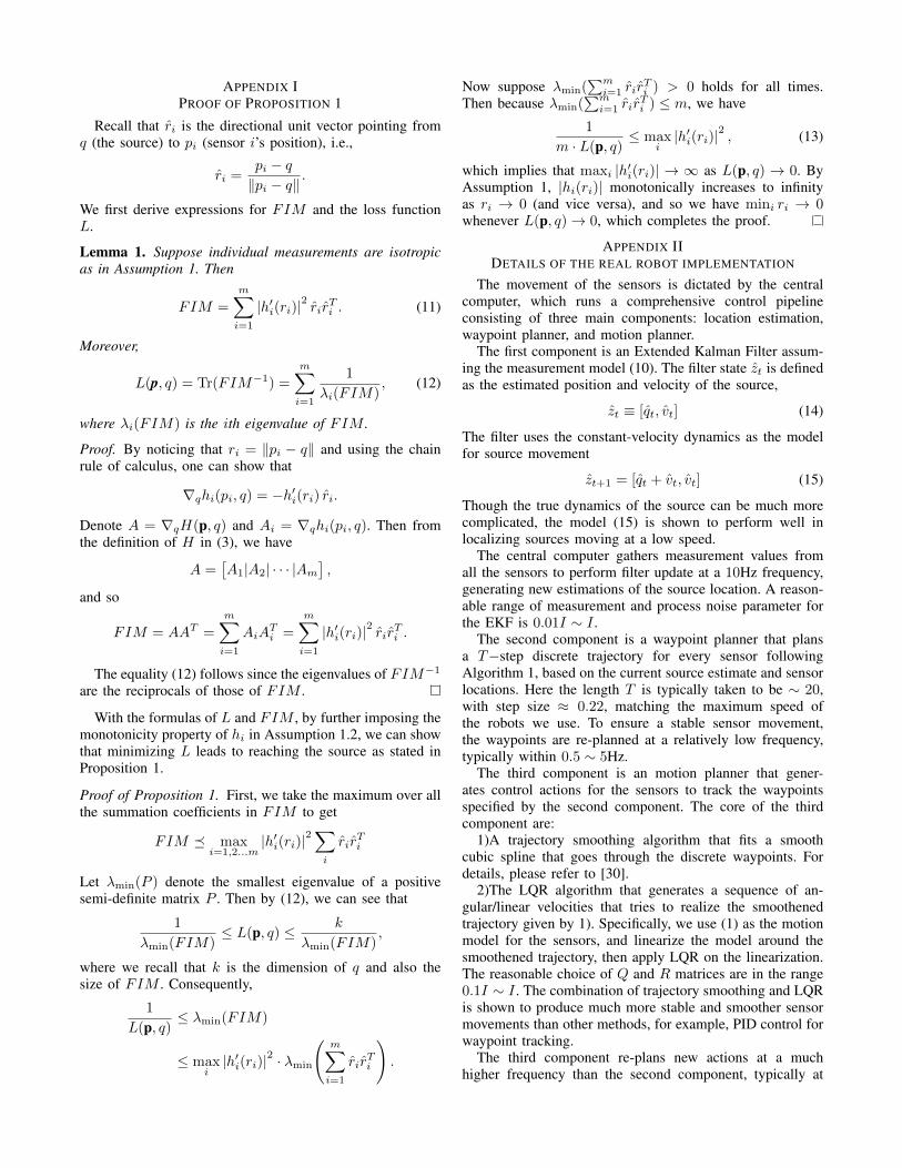
APPENDIX IPROOF OF PROPOSITION 1

Recall that ri is the directional unit vector pointing fromq (the source) to pi (sensor i’s position), i.e.,

ri =pi − q‖pi − q‖

.

We first derive expressions for FIM and the loss functionL.

Lemma 1. Suppose individual measurements are isotropicas in Assumption 1. Then

FIM =

m∑i=1

|h′i(ri)|2rir

Ti . (11)

Moreover,

L(p, q) = Tr(FIM−1) =

m∑i=1

1

λi(FIM), (12)

where λi(FIM) is the ith eigenvalue of FIM .

Proof. By noticing that ri = ‖pi − q‖ and using the chainrule of calculus, one can show that

∇qhi(pi, q) = −h′i(ri) ri.

Denote A = ∇qH(p, q) and Ai = ∇qhi(pi, q). Then fromthe definition of H in (3), we have

A =[A1|A2| · · · |Am

],

and so

FIM = AAT =

m∑i=1

AiATi =

m∑i=1

|h′i(ri)|2rir

Ti .

The equality (12) follows since the eigenvalues of FIM−1

are the reciprocals of those of FIM .

With the formulas of L and FIM , by further imposing themonotonicity property of hi in Assumption 1.2, we can showthat minimizing L leads to reaching the source as stated inProposition 1.

Proof of Proposition 1. First, we take the maximum over allthe summation coefficients in FIM to get

FIM � maxi=1,2...m

|h′i(ri)|2∑i

rirTi

Let λmin(P ) denote the smallest eigenvalue of a positivesemi-definite matrix P . Then by (12), we can see that

1

λmin(FIM)≤ L(p, q) ≤ k

λmin(FIM),

where we recall that k is the dimension of q and also thesize of FIM . Consequently,

1

L(p, q)≤ λmin(FIM)

≤ maxi|h′i(ri)|

2 · λmin

(m∑i=1

rirTi

).

Now suppose λmin(∑m

i=1 rirTi ) > 0 holds for all times.

Then because λmin(∑m

i=1 rirTi ) ≤ m, we have

1

m · L(p, q)≤ max

i|h′i(ri)|

2, (13)

which implies that maxi |h′i(ri)| → ∞ as L(p, q) → 0. ByAssumption 1, |hi(ri)| monotonically increases to infinityas ri → 0 (and vice versa), and so we have mini ri → 0whenever L(p, q)→ 0, which completes the proof.

APPENDIX IIDETAILS OF THE REAL ROBOT IMPLEMENTATION

The movement of the sensors is dictated by the centralcomputer, which runs a comprehensive control pipelineconsisting of three main components: location estimation,waypoint planner, and motion planner.

The first component is an Extended Kalman Filter assum-ing the measurement model (10). The filter state zt is definedas the estimated position and velocity of the source,

zt ≡ [qt, vt] (14)

The filter uses the constant-velocity dynamics as the modelfor source movement

zt+1 = [qt + vt, vt] (15)

Though the true dynamics of the source can be much morecomplicated, the model (15) is shown to perform well inlocalizing sources moving at a low speed.

The central computer gathers measurement values fromall the sensors to perform filter update at a 10Hz frequency,generating new estimations of the source location. A reason-able range of measurement and process noise parameter forthe EKF is 0.01I ∼ I .

The second component is a waypoint planner that plansa T−step discrete trajectory for every sensor followingAlgorithm 1, based on the current source estimate and sensorlocations. Here the length T is typically taken to be ∼ 20,with step size ≈ 0.22, matching the maximum speed ofthe robots we use. To ensure a stable sensor movement,the waypoints are re-planned at a relatively low frequency,typically within 0.5 ∼ 5Hz.

The third component is an motion planner that gener-ates control actions for the sensors to track the waypointsspecified by the second component. The core of the thirdcomponent are:

1)A trajectory smoothing algorithm that fits a smoothcubic spline that goes through the discrete waypoints. Fordetails, please refer to [30].

2)The LQR algorithm that generates a sequence of an-gular/linear velocities that tries to realize the smoothenedtrajectory given by 1). Specifically, we use (1) as the motionmodel for the sensors, and linearize the model around thesmoothened trajectory, then apply LQR on the linearization.The reasonable choice of Q and R matrices are in the range0.1I ∼ I . The combination of trajectory smoothing and LQRis shown to produce much more stable and smoother sensormovements than other methods, for example, PID control forwaypoint tracking.

The third component re-plans new actions at a muchhigher frequency than the second component, typically at

10 ∼ 20 Hz. It usually plans for action sequences with length∼ 20, with time interval between two consecutive actionsaround 0.05 ∼ 0.1s, matching the planning frequency. Inthis way, the sensors only execute their first planned actions,then the entire control sequences are re-planned to correct theeffect of disturbances or to accommodate updated waypoints.Note this is very different from our simulations, where thewaypoint planner only plans one-step ahead and the sensorsare assume to move exactly to the waypoints so motionplanning is unnecessary. The main reason of planning witha larger look-ahead length, and with different frequenciesbetween different components, is to ensure stability androbustness as real-world issues add complication to thesystem, such as robot dynamics, unforeseen disturbances,communication, and so on.