Measurement 46 (2013) 1922–1927

Contents lists available at SciVerse ScienceDirect

Measurement

journal homepage: www.elsevier .com/ locate /measurement

Some statistical aspects of binary measuring systems

0263-2241/$ - see front matter � 2013 Elsevier Ltd. All rights reserved.http://dx.doi.org/10.1016/j.measurement.2013.02.017

⇑ Corresponding author. Tel.: +972 4 990 1827; fax: +972 4 990 1852.E-mail addresses: ebashkan@braude.ac.il (B. Emil), tamarg@braude.

ac.il (G. Tamar).

Bashkansky Emil ⇑, Gadrich TamarORT Braude College, Industrial Engineering and Management Department, P.O.B. 78, 51 Snunit, Karmiel 21982, Israel

a r t i c l e i n f o

Article history:Received 26 October 2012Received in revised form 8 January 2013Accepted 18 February 2013Available online 5 March 2013

Keywords:Binary classificationQualitative analysisMetrological reliability

a b s t r a c t

Qualitative analysis is often used to determine whether or not a particular feature appears oris absent in tests, in quality control procedures, identification scans, go/no go measurementsand many other fields. Generally, such analysis uses simple measuring methods that classifythe analyzed property value into two comprehensive and exclusive classes/categories. Theperformance reliability of such binary measurement systems (BMSs) is usually assessedby false positive and false negative rates. The article presents some additional aspectsrelated to metrological properties of BMS: traceability – described in terms of sequentialhierarchical chain of consecutive BMSs calibrations – error accumulation, distribution of testresults, consistency and repeatability problems. It is shown that some intuitively plausible ata first glance concepts such as hypotheses about the binomial distribution of test results orconsistency testing by sequentially repeated sorting are wrong if the objective is to conduct adeep examination, and therefore, should be avoided.

� 2013 Elsevier Ltd. All rights reserved.

1. Introduction

Information quality, to a large extent, is determined bythe quality of the measuring system by which it is mined,and therefore, it is important to understand how it func-tions. Measurements performed on a binary scale haveonly two possible outcomes such as good/bad or exists/does not exist. Such measurements can be considered asthe simplest case of more general ones performed onordinal or nominal scale bases, consisting of more thantwo possible categories (the latter, however, unlike ordinalmeasurements, have not yet received official metrologicalrecognition). Despite the recent increased interest in themeasurement system analysis (MSA) of such measuringsystems, issues such as traceability (Section 2), statisticalproperties of results received in situations in which a ‘‘goldstandard’’ is absent and true values are unknown (Section3), and consistency checking (Section 4), as well as manyothers, have not yet been sufficiently investigated. In thispaper we attempt, at least partially, to fill the existing gaps.

2. Traceability and cumulative error

It is well known that the comparability of measurementresults obtained by different laboratories is the result of notonly mutual or inter-laboratory comparisons but mainly ofthe metrological traceability of such results. Only measuredvalues traceable to the same reference can be directlycompared with each other. Metrological traceability isdefined by BIPM–JCGM 200:2012 [1] as ‘‘property of ameasurement result whereby the result can be related toa reference through a documented unbroken chain ofcalibrations, each contributing to the measurement uncer-tainty’’. Metrological traceability requires an establishedcalibration hierarchy, i.e., the ‘‘sequence of calibrationsfrom a reference to the final measuring system (FMS),where the outcome of each calibration depends on theoutcome of the previous calibration’’ [1]. A comparisonbetween two measurement standards or systems may beviewed as a calibration if the comparison is used tocheck the quantity value and measurement uncertaintyattributed to one of them.

Metrological traceability problems and appropriatestatistical methods have been well-studied for the mostpopular quantitative properties [2], yet relatively little

B. Emil, G. Tamar / Measurement 46 (2013) 1922–1927 1923

investigation has been done into ordinal and nominalproperties. The main metrological aspects of ordinalmeasurement systems [3], their mutual [4] and inter-laboratory comparisons [5] were discussed in some previ-ous papers of the authors and other researchers [6–15].

In this paper section we focus on the traceability ofordinal measurement results received by a calibrationhierarchy chain and their associated uncertainty.Metaphorically speaking, if in our previous articles [4,5],we considered the comparison between laboratories in a‘‘horizontal’’ equipotential direction, here we study theissues related to hierarchical top-down or ‘‘vertical’’comparisons between measurement systems.

For the binary case, the nominal property/quantityunder study may take only two values (levels) betweenwhich there is no natural order such as: (1) non-existence(placebo) and (2) existence of some feature, for example.Although a binary scale is considered as if it were anominal one, all mathematics developed for ordinal scalesare also valid for binary data [3].

Binary measurement systems and their errors are fully

described using a ‘2 � 2’ stochastic classification matrix P̂[16]. Its components, Pj=i (where i, j = 1, 2), are theconditional probabilities that an object will be classifiedas level j, given that its actual/true level is i (clearly,P2

j¼1Pj=i ¼ 1; i ¼ 1;2). For the simplest binary case theclassification matrix has the form of:

P̂ ¼P1=1 P2=1

P1=2 P2=2

� �¼

1� a ab 1� b

� �ð1Þ

where error rate a is the risk probability of a Type I error(sometimes called ‘‘false positive’’ or ‘‘false alarm’’) anderror rate b is the risk probability of a Type II error (some-times called ‘‘false negative’’). Sometimes 1 � a is called‘‘specificity’’ of the test/measuring device and 1 � b its‘‘sensitivity’’ [17]. The matrix (1) has two eigenvalues:k1 ¼ 1 and k2 ¼ 1� ðaþ bÞ, its determinant equalsDet ¼ k1 � k2 ¼ 1� ðaþ bÞ and its trace: Trace ¼ k1 þ k2 ¼2� ðaþ bÞ.

The most exact, error-free measurement (primary refer-ence standard) means that bP is the unit matrix [3], i.e.:

bP0 ¼1 00 1

� �) a0 ¼ b0 ¼ 0: ð2Þ

Examples of such ‘‘gold’’ (usually expensive, sometimesdestructive or associated with undesirable and dangerousinterference/intervention) standards are:

1. Certified reference material for nominal property.2. Quantitative blood pregnancy test.3. Highest accuracy class plug gage.4. CVS (Chorionic Villus sampling) Down syndrome test.5. DNA personal identification. . .

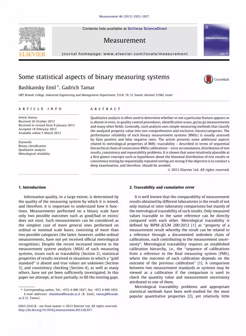
Fig. 1. The chain of n cons

The corresponding less accurate (but also cheaper andwith fewer if any adverse effects) measuring system (MS)may be:

1. Noncertified reference material.2. Urine pregnancy test.3. Low accuracy plug gage.4. Integrated Down syndrome test.5. Passport control photo identification. . .

Imagine now the chain of n consecutive measuring sys-tem calibrations starting from the primary reference stan-dard (Fig. 1):

where

� 1�ai – means the probability of agreement between MSi

and its predecessor MSi�1 in relation to the firstcategory.� ai – means the probability that MSi classifies the studied

property as belonging to the second category while itspredecessor MSi�1 classified as belonging to the firstcategory.� bi – means the probability that MSi classifies the studied

property as the first category while its predecessorMSi�1 classified as belonging to the second category.� 1�bi – means the probability of agreement between MSi

and its predecessor MSi�1 in relation to the secondcategory.

Each chain in Fig. 1 contributes to the measurement er-ror (in relation to the primary reference standard) of the fi-nal (n-th) measurement system expressed by (1). It is easyto prove that:

P̂n ¼1� a a

b 1� b

� �¼

1 00 1

� ��

1� a1 a1

b1 1� b1

� ��

1� a2 a2

b2 1� b2

� �� � � � �

1� ai ai

bi 1� bi

� �� � � � �

1� an an

bn 1� bn

� �ð4Þ

For example, for two calibration links only:

1� a ¼ ð1� a1Þ � ð1� a2Þ þ a1b2

1� b ¼ ð1� b1Þ � ð1� b2Þ þ b1a2 ð5Þ

reflects the fact that the proper classification has beenmade, if both MSs have made the proper classification, orif the first MS has made a mistake, and the second MSdisagrees with the classification. Note that the chain (3)may be considered as a Markov chain for a two-statesystem with transition matrices, as shown in the rectan-gles. The solution for particular case 8i : ai ¼ a; bi ¼ b isas follows [18]:

ecutive calibrations.

1924 B. Emil, G. Tamar / Measurement 46 (2013) 1922–1927

bPn ¼b

aþba

aþb

baþb

aaþb

!þ

a �a�b b

� �� ½1� ðaþ bÞ�n

aþ bð6Þ

when 8i : ai; bi � 1, leaving in (4) the first order termsonly, we are left with: a �

Pn0ai b �

Pn0bi, reflecting

the cumulative character of the error. Nevertheless, wedo not recommend using such a rough approximation forpractical needs. Nowadays matrix product (4) can easilybe calculated by many programs including Microsoft Exceland MathCad.

For qualitative estimations of bPn we may use the follow-ing idea. Since the determinant of the matrices’ productsequals the product of their determinants, the overall proba-bility of reaching the proper classification by the n-th MS is:

1� ðaþ bÞ ¼ ½1� ða1 þ b1Þ� � ½1� ða2 þ b2Þ� � � � ½1� ðan þ bnÞ� ð7Þ

when ai; bi are estimated on the basis of experimentalstudy, their lower/upper confidence limits must be substi-tuted in (7) in order to estimate the upper/lower limits ofthe overall probability of making a correct classification.

The important issue is: to what extent calibration pro-vides agreement between two different MS in relation tothe same items/samples, etc? This is not an idle question;authors have had to deal with conflict between providerand consumer resulting from the use of MSs calibratedby different calibration chains. Partly, the issue was con-sidered by the authors in their previous paper [4]. Thekey to solving the problem depends on degree of humaninvolvement in the measurement system. Errors resultingfrom instruments/devices may be treated as independent;human errors, however, cannot always be handled thesame way. Expanded analysis of the issue is beyond thescope of this article and should be considered separately.

3. How can an MS change the probability distribution oftest results?

Assume that in order to study some measurement sys-tem, n objects were submitted to this MS: n1 – belonging tothe first category and n2 – belonging to the second cate-gory. These items may be, for example, n1 objects possess-ing some property and n2 objects lacking such a property(placebo). Surely, n = n1 + n2. Let X1 be the number of ob-jects classified by the MS as belonging to the first categoryand X2 = n � X1 as belonging to the second category. As theMS and its errors are fully described by an ‘2 � 2’ stochasticclassification matrix (1), one can conclude that:

EðX1Þ ¼ n1ð1� aÞ þ n2b ¼ n½p1ð1� aÞ þ p2b� ¼ nq1

EðX2Þ ¼ n1aþ n2ð1� bÞ ¼ n½p1aþ p2ð1� bÞ� ¼ nq2ð8Þ

where E means expectation and

p1¼n1

n; p2 ¼

n2

n; q1¼ ½p1ð1�aÞþp2b�; q2¼ ½p1aþp2ð1�bÞ�

p1þp2¼ q1þq2¼1 EðX1ÞþEðX2Þ¼ n

ð9Þ

In this way, a and b can be estimated only if a largeamount of identical repetitions were provided so that

capabilities of two different MSs (for example, manualand automatic or two hypothetically equivalent MSs) canbe compared. In practice, usually only one trial can be or-ganized, so that a random value of X1 (and accordingly,X2 = n � X1) may significantly deviate from its expected va-lue (8). In order to perform any hypothesis testing concern-ing MS capabilities analysis—comparison betweendifferent MSs, for example—we need to know its distribu-tion—P(X1), variation—VAR(X1) and so on. In particular,the very important question is: does X1 follow binomialdistribution Binðn; q1Þ?

Historically, this problem is rooted in the debate aroundthe so-called ‘‘Maxwell’s demon’’ suspected to violate thesecond law of thermodynamics (see, for example, [19] fora later interpretation) and Ehrenfest’s famous work [20].

Consider X1 to be the sum of two independent randomvariables. The first reflects the number of objects classifiedas belonging to the first category in a sequence of n1 Ber-noulli trials, each of which yields success with probability1� a, and the second reflects the number of objects classi-fied as belonging to the first category in a sequence of n2

Bernoulli trials, each of which yields success with probabil-ity b. Then X1 is distributed according to convolution of thetwo above mentioned binomial distributions:

PðX1¼ x1Þ¼Xminf x1 ;n1g

k¼maxf0;x1�n2gBin½k;n1;ð1�aÞ� �Bin ½x1�k;n2;b�

¼Xminfx1 ;n1g

k¼maxf0;x1�n2g

n1

k

� �ð1�aÞkan1�k n2

x1�k

� �bx1�k

�ð1�bÞn 2�x1þk ðx1¼0;1; . . . ;nÞ ð10Þ

which variation is a sum of these two binomial variations:

VARðX1Þ ¼ VARðX2 ¼ n� X1Þ¼ n1ð1� aÞaþ n2bð1� bÞ¼ n½p1ð1� aÞaþ p2bð1� bÞ� ð11Þ

It is easy to see that the variation of binomial distribu-tion Binðn; q1Þ, having the same expected value (8), equals:

nq1ð1� q1Þ ¼ n½p1ð1� aÞ þ p2b�½p1aþ p2ð1� bÞ�¼ n½p1ð1� aÞaþ p2bð1� bÞ� þ np1ð1

� p1Þ½1� ðaþ bÞ�2

¼ VARðX1Þ þ np1ð1� p1Þ½1� ðaþ bÞ�2

P VARðX1Þ ð12Þ

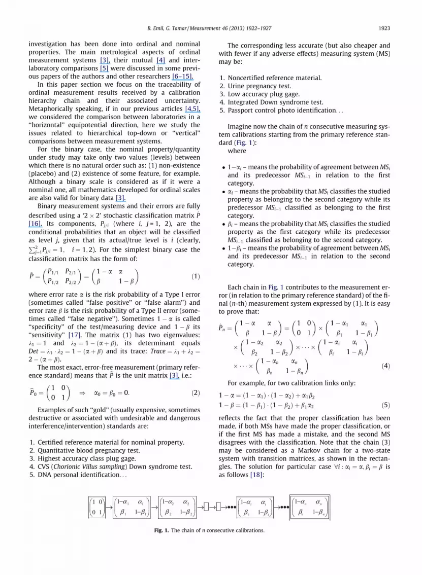
So the studied distribution PðX1Þ is under dispersed rel-ative to the corresponding binomial distribution. This factis demonstrated by the example built for n1 = 60, n2 = 40,a = 0.2, b = 0.1, so that EðX1Þ ¼ 52; q1 ¼ 0:52 (see Fig. 2).For this example, rðX1Þ � 3:6, while for the correspondingbinomial distribution Binðn; q1Þ, it is approximately 5. Thedifference is even more significant for small error rates;see Fig. 3 built for n1 = 60, n2 = 40, a = 0.02, b = 0.01.

In conclusion, since statistical tests for distributions oftype (10) are not developed well, we strongly recommendcarrying out binary MS calibrations using the usual contin-gency tables of MS results vs. standard values (Table 1).Every cell of Table 1 follows well-known binomial distribu-

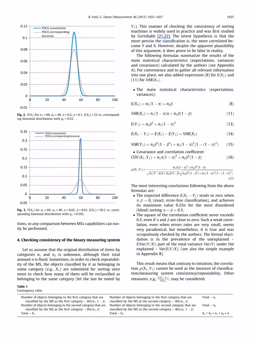
Fig. 2. P(X1) for n1 = 60, n2 = 40, a = 0.2, b = 0.1, E(X1) = 52 vs. correspond-ing binomial distribution with q1 = 0.52.

Fig. 3. P(X1) for n1 = 60, n2 = 40, a = 0.02, b = 0.01, E(X1) = 59.2 vs. corre-sponding binomial distribution with q1 = 0.592.

B. Emil, G. Tamar / Measurement 46 (2013) 1922–1927 1925

tions, so any comparison between MSs capabilities can eas-ily be performed.

4. Checking consistency of the binary measuring system

Let us assume that the original distribution of items bycategories n1 and n2 is unknown, although their totalamount n is fixed. Sometimes, in order to check repeatabil-ity of the MS, the objects classified by it as belonging tosome category (e.g., X1) are submitted for sorting oncemore to check how many of them will be reclassified asbelonging to the same category (let the last be noted by

Table 1Contingency table.

Number of objects belonging to the first category that areclassified by the MS as the first category Binðn1;1� aÞ

Number of objclassified by th

Number of objects belonging to the second category that areclassified by the MS as the first category Binðn2; bÞ

Number of objclassified by th

Total – X1 Total – X2

Y1). This manner of checking the consistency of sortingmachines is widely used in practice and was first studiedby Gertsbakh [21,22]. The latent hypothesis is that themore precise the classification is, the more correlated be-come Y and X. However, despite the apparent plausibilityof this argument, it does prove to be false in reality.

The following formulas summarize the results of themain statistical characteristics (expectations, variancesand covariance) calculated by the authors (see AppendixA). For convenience and to gather all relevant informationinto one place, we also added expression (8) for EðX1Þ and(11) for VARðX1Þ.

� The main statistical characteristics (expectations,variances):

EðX1Þ ¼ n1ð1� aÞ þ n2b ð8Þ

VARðX1Þ ¼ n1ð1� aÞaþ n2bð1� bÞ ð11Þ

EðY1Þ ¼ n2b2 þ n1ð1� aÞ2 ð13Þ

EðX1 � Y1Þ ¼ EðX1Þ � EðY1Þ ¼ VARðX1Þ ð14Þ

VARðY1Þ ¼ n2b2ð1� b2Þ þ n1ð1� aÞ2ð1� ð1� aÞ2Þ ð15Þ

� Covariance and correlation coefficient:COVðX1;Y1Þ ¼ n1að1� aÞ2 þ n2b

2ð1� bÞ ð16Þ

qðX1;Y1Þ¼n1að1�aÞ2þn2b2ð1�bÞffiffiffiffiffiffiffiffiffiffiffiffiffiffiffiffiffiffiffiffiffiffiffiffiffiffiffiffiffiffiffiffiffiffiffiffiffiffiffiffiffiffiffiffiffiffiffiffi

n1ð1�aÞaþn2bð1�bÞp ffiffiffiffiffiffiffiffiffiffiffiffiffiffiffiffiffiffiffiffiffiffiffiffiffiffiffiffiffiffiffiffiffiffiffiffiffiffiffiffiffiffiffiffiffiffiffiffiffiffiffiffiffiffiffiffiffiffiffiffiffiffiffiffiffiffiffiffiffiffiffiffiffiffiffiffiffiffiffi

n2b2ð1�b2Þþn1ð1�aÞ2ð1�ð1�aÞ2Þq

ð17Þ

The most interesting conclusions following from the aboveformulas are:� The expected difference EðX1 � Y1Þ tends to zero when

a; b! 0, (exact, error-free classification), and achievesits maximum value 0:25n for the most disordered(blind) sorting a ¼ b ¼ 0:5.� The square of the correlation coefficient never exceeds

0.5, even if a and b are close to zero. Such a weak corre-lation, even when errors rates are very small, seemsvery paradoxical, but nonetheless, it is true and wasscrupulously checked by the authors. The formal eluci-dation is in the prevalence of the unexplained –E½VarðY=XÞ� part of the total variance VarðYÞ under theexplained – Var½EðY=XÞ� (see also the simple examplein Appendix B).

This result means that contrary to intuition, the correla-tion qðX1;Y1Þ cannot be used as the measure of classifica-tion/measuring system consistency/repeatability. Othermeasures, e.g., EðX1�Y1Þ

EðX1Þ, may be considered.

ects belonging to the first category that aree MS at the second category Binðn1;aÞ

Total – n1

ects belonging to the second category that aree MS as the second category Binðn2;1� bÞ

Total – n2

X1 + X2 = n1 + n2 = n

1926 B. Emil, G. Tamar / Measurement 46 (2013) 1922–1927

5. Conclusions

The article analyzes some statistical properties of binaryclassification/measuring systems from the metrologicalpoint of view.

The traceability of test results received by BMS is ana-lyzed by presenting a traceability chain as a product ofconsecutive 2� 2 pairwise comparison matrices, each ofwhich reflects the result of calibration performed betweentwo adjacent levels of the traceability hierarchical ladder.This model allows the BMS’ error rates to be assessed bysimple matrix algebra methods.

We analyzed the distribution of the number of objectsclassified by BMS to one of the two categories and provedthat it is usually far from binomial. This phenomenonshould be taken into account when performing calibrationor any other comparison between performance capabilitiesof two different BMS or methods. Calibration based on acontingency table approach instead of a ‘‘scrambled’’method is proposed as the most effective and evidentiary.

The usual practice of checking the accuracy of BMS byrepeated sorting is shown in this paper to be faulty. In spiteof apparent plausibility, results of original and repeatedclassification are weakly correlated; therefore, other meth-ods of checking consistency must be considered.

The authors see as a future challenge generalization ofthe results presented in this paper to measuring systemswith more than two categories.

Acknowledgement

We would like to express our gratitude to Prof. I. Gerts-bakh, who inspired the authors to conduct this researchand to anonymous reviewers for their fruitful comments.

Appendix A

Let us consider classification described in Section 4 as aBernoulli process consisting of two finite trial sequences n1

and n2. Define random indicators Ið1Þi ði ¼ 1;2; . . . ;n1Þ and

Jð1Þj ðj ¼ 1;2; . . . ;n2Þ so that each indicator equals 1 if anitem is classified as belonging to the first category in thefirst step of the classification process and 0 otherwise.Accordingly, probabilities are 1� a for the first sequenceand b for the second.

In the same manner define indicators Ið2Þi ði ¼ 1;2; . . . ;n1Þand Jð2Þj ðj ¼ 1;2; . . . ;n2Þ so that the indicator equals 1 if anitem is classified as belonging to the first category in bothsteps of the classification process and 0 otherwise.

Accordingly, probabilities are ð1� aÞ2 for the first sequenceand b2 for the second. Below are the well known statisticalproperties of Bernoulli random indicators:

EðIð1Þi Þ ¼ ð1� aÞ VARðIð1Þi Þ ¼ a � ð1� aÞEðJð1Þj Þ ¼ b VARðJð1Þj Þ ¼ b � ð1� bÞ

EðIð2Þi Þ ¼ ð1� aÞ2 VARðIð2Þi Þ ¼ ð1� aÞ2 � ð1� ð1� aÞ2ÞEðJð2Þj Þ ¼ b2 VARðJð2Þj Þ ¼ b2 � ð1� b2Þ

Covariances:

COVðIð1Þi ; Ið2Þi Þ ¼ EðIð1Þi � Ið2Þi Þ � EðIð1Þi Þ � EðI

ð2Þi Þ

¼ ð1� aÞ2 � ð1� aÞð1� aÞ2 ¼ að1� aÞ2

COVðJð1Þi ; Jð2Þi Þ ¼ EðJð1Þi � Jð2Þi Þ � EðJð1Þi Þ � EðJ

ð2Þi Þ

¼ b2 � b � b2 ¼ b2ð1� bÞ

All the remaining covariances are zero, because Ber-noulli trials are independent.

Taking into account that:

X1 ¼Xn1

i¼1

Ið1Þi þXn2

j¼1

Jð1Þj

Y1 ¼Xn1

i¼1

Ið2Þi þXn2

j¼1

Jð2Þj

and considering independency between different indica-tors belonging to the same step, (8–16) is simply obtained.

Appendix B

Suppose n2 ¼ 0, so n1 ¼ n. For this caseX1 Binðn;1� aÞ and Y1=X1 BinðX1;1� aÞ, so:

EðX1Þ ¼ nð1� aÞ ðB1Þ

VARðX1Þ ¼ nð1� aÞa ðB2Þ

EðY1=X1Þ ¼ X1ð1� aÞ ðB3Þ

VARðY1=X1Þ ¼ X1ð1� aÞa ðB4Þ

Explained variance� Var½EðY1=X1Þ�

¼ ð1� aÞ2 � VarðX1Þ ¼ nað1� aÞ3 ðB5Þ

Unexplained variance� E½VARðY1=X1Þ�

¼ EðX1Þð1� aÞa ¼ nað1� aÞ2 ðB6Þ

As a result :unexplained variance

explained variance¼ 1

1� aP 1 ðB7Þ

References

[1] BIPM–JCGM 200:2012, International vocabulary of metrology—basicand general concepts and associated terms (VIM with minorcorrections): 2.41.

[2] BIPM–JCGM 100:2008, Evaluation of measurement data—Guide tothe expression of uncertainty in measurement (GUM 1995 withminor corrections).

[3] E. Bashkansky, T. Gadrich, Some metrological aspects of ordinalmeasurements, Accredit. Qual. Assur. 15 (2010) 331–336.

[4] E. Bashkansky, T. Gadrich, D. Knani, Some metrological aspects of thecomparison between two ordinal measuring systems, Accredit. Qual.Assur. 16 (2011) 63–72.

[5] E. Bashkansky, T. Gadrich, I. Kuselman, Interlaboratory comparisonof measurement or test results of an ordinal property: analysis ofvariation, Accredit. Qual. Assur. 17 (2012) 239–243.

[6] P.Th. Wilrich, The determination of precision of qualitativemeasurement methods by interlaboratory experiments, Accredit.Qual. Assur. 15 (2010) 439–444.

[7] I. Gertsbakh, Measurement Theory for Engineers, reprint ofhardcover, first ed., 2003, Springer-Verlag, Heidelberg, 2010.

[8] W.N. van Wieringen, J. de Mast, Measurement system analysis forbinary data, Technometrics 50 (2008) 468–478.

B. Emil, G. Tamar / Measurement 46 (2013) 1922–1927 1927

[9] J. de Mast, W.N. van Wieringen, Measurement system analysis forcategorical measurements: agreement and kappa type indices, J.Qual. Technol. 39 (2007) (2007) 191–202.

[10] J. de Mast, A. Trip, Gauge R&R studies for destructive measurements,J. Qual. Technol. 37 (2005) 40–49.

[11] J. de Mast, W.N. van Wieringen, Measurement system analysis forbounded ordinal data, Qual. Reliab. Eng. Int. 20 (2004) 383–395.

[12] J. de Mast, T. Erdmann, Assessment of binary inspection with ahybrid measurand, Qual. Reliab. Eng. Int. 28 (2012) 47–57.

[13] C.M. Borror, Measurement systems analysis, in: F. Ruggeri, R. Kenett,F.W. Faltin (Eds.), Encyclopedia of Statistics in Quality andReliability, Wiley, Chichester, 2007, pp. 1065–1070.

[14] P. Wehling, R.A. LaBudde, S.L. Brunelle, M.T. Nelson, Probability ofdetection (POD) as a statistical model for the validation ofqualitative methods, J. AOAC. Int. 94 (2011) 335–347.

[15] S. Uhlig, L. Niewohner, P. Gowik, Can the usual validation standardseries for quantitative methods, ISO 5725, be also applied forqualitative methods?, Accredit Qual. Assur. 16 (2011) 533–537.

[16] E. Bashkansky, S. Dror, R. Ravid, P. Grabov, Effectiveness of a productquality classifier, Qual. Eng. 19 (2007) 235–244.

[17] EURACHEM/CITAC Guide (2011, draft): Assessing Performance inQualitative Analysis.

[18] W. Feller, An Introduction to Probability Theory and Its Applications,third edition, vol. 2, John Willey & Sons, CITY, 1968.

[19] Harvey S. Leff, A.F. Rex (Eds.), Maxwell’s Demon 2: Entropy,Classical and Quantum Information, Computing, CRC Press, CITY,2002.

[20] P. Ehrenfest, T. Ehrenfest, Begriffliche Grundlagen der statistischenAuffassung in der Mechanik, in: F. Klein, C. Müller (Eds.),Enzyklopädie der mathematischen Wissenschaften mit Einschlußihrer Anwendungen. Band IV, 2. Teil, Teubner, Leipzig, 1911, pp. 3–90. Translated as The Conceptual Foundations of the StatisticalApproach in Mechanics. New York: Cornell University Press, 1959.ISBN 0-486-49504-3.

[21] I.B. Gertsbakh, Determining the error of an automatic measurement,testing and sorting machine, Meas. Tech. 5 (1962) 533–537.

[22] I. Gertsbakh, L. Friedman, Estimation of a standard measuring errorby repeated measurements and sortings, Stat. Plan. Infer. 11 (1985)1–14.