Journal of Quantitative Spectroscopy & Radiative Transfer 212 (2018) 10–23

Contents lists available at ScienceDirect

Journal of Quantitative Spectroscopy & Radiative Transfer

journal homepage: www.elsevier.com/locate/jqsrt

Skyglow changes over Tucson, Arizona, resulting from a municipal LED

street lighting conversion

John C. Barentine

a , b , ∗, Constance E. Walker c , a , Miroslav Kocifaj d , e , František Kundracik

e , Amy Juan

f , John Kanemoto

g , Christian K. Monrad

h

a International Dark-Sky Association, 3223 N. 1st Ave, Tucson, AZ 85719, USA b Consortium for Dark Sky Studies, University of Utah, Sterling Sill Center, 195 Central Campus Dr, Salt Lake City, UT 84112, USA c National Optical Astronomy Observatory, 950 N. Cherry Ave, Tucson, AZ 85719, USA d ICA, Slovak Academy of Sciences, Dúbravská Road 9, Bratislava 845 03, Slovakia e Faculty of Mathematics, Physics, and Informatics, Comenius University, Mlynská Dolina, Bratislava 842 48, Slovakia f University of Arizona, Tucson, AZ 85719, USA g Natomas Unified School District, 1901 Arena Blvd., Sacramento, CA 95834, USA h Monrad Engineering, Inc., 1926 E. Fort Lowell Road Suite 200, Tucson, AZ 85719, USA

a r t i c l e i n f o

Article history:

Received 28 October 2017

Revised 21 January 2018

Accepted 9 February 2018

Available online 16 March 2018

Keywords:

Light pollution

Skyglow

Sky brightness

Modeling

Site testing

a b s t r a c t

The transition from earlier lighting technologies to white light-emitting diodes (LEDs) is a significant

change in the use of artificial light at night. LEDs emit considerably more short-wavelength light into the

environment than earlier technologies on a per-lumen basis. Radiative transfer models predict increased

skyglow over cities transitioning to LED unless the total lumen output of new lighting systems is re-

duced. The City of Tucson, Arizona (U.S.), recently converted its municipal street lighting system from a

mixture of fully shielded high- and low-pressure sodium (HPS/LPS) luminaires to fully shielded 30 0 0 K

white LED luminaires. The lighting design intended to minimize increases to skyglow in order to protect

the sites of nearby astronomical observatories without compromising public safety. This involved the mi-

gration of over 445 million fully shielded HPS/LPS lumens to roughly 142 million fully shielded 30 0 0 K

white LED lumens and an expected concomitant reduction in the amount of visual skyglow over Tuc-

son. SkyGlow Simulator models predict skyglow decreases on the order of 10–20% depending on whether

fully shielded or partly shielded lights are in use. We tested this prediction using visual night sky bright-

ness estimates and luminance-calibrated, panchromatic all-sky imagery at 15 locations in and near the

city. Data were obtained in 2014, before the LED conversion began, and in mid-2017 after approximately

95% of ∼ 18,0 0 0 luminaires was converted. Skyglow differed marginally, and in all cases with valid data

changed by < ± 20%. Over the same period, the city’s upward-directed optical radiance detected from

Earth orbit decreased by approximately 7%. While these results are not conclusive, they suggest that LED

conversions paired with dimming can reduce skyglow over cities.

© 2018 Elsevier Ltd. All rights reserved.

t

i

S

i

t

s

1. Introduction

The conversion of the world’s lighting from conventional to

solid-state lighting (SSL) technologies is among the most signifi-

cant changes to the way we light our world at night since the

invention of electric light itself. Environmental pollution from ar-

∗ Corresponding author at: International Dark-Sky Association, 3223 N. 1st Ave,

Tucson, AZ 85719, USA.

E-mail addresses: john@darksky.org (J.C. Barentine), cwalker@noao.edu (C.E.

Walker), Miroslav.Kocifaj@savba.sk (M. Kocifaj), frantisek.kundracik@fmph.uniba.sk

(F. Kundracik), protecthimdag@gmail.com (A. Juan), kanemotojohn@hotmail.com (J.

Kanemoto), chrismonrad@monradengineeringinc.com (C.K. Monrad).

o

s

A

h

e

i

https://doi.org/10.1016/j.jqsrt.2018.02.038

0022-4073/© 2018 Elsevier Ltd. All rights reserved.

ificial light at night (ALAN) has already reached significant levels

n many parts of the world. [1] Improved luminous efficacy among

SL products is hypothesized to lead to a “rebound” effect, further-

ng global dependence on ALAN as cost savings are redirected into

he deployment of additional outdoor lighting. [2–5] The conver-

ion to SSL has also brought significant changes to the spectrum

f artificial light radiated into the global nighttime environment,

hifting a considerable amount of emission to shorter wavelengths.

number of known and suspected hazards to wildlife ecology and

uman health have been identified that are thought to result from

xposure to short-wavelength ALAN. [6–8] .

The spectrum shift in new SSL systems is also thought to yield

ncreases to skyglow, which is the diffuse luminescence of the

J.C. Barentine et al. / Journal of Quantitative Spectroscopy & Radiative Transfer 212 (2018) 10–23 11

n

t

a

l

s

s

t

f

l

o

s

s

u

i

s

s

e

p

n

i

“

f

1

t

t

c

t

w

t

o

a

r

t

c

n

t

t

t

2

g

1

t

b

1

l

p

n

t

a

t

p

b

r

i

i

a

t

c

m

c

r

i

o

t

l

v

g

s

o

t

n

t

o

s

b

t

a

c

T

c

t

h

s

f

t

p

n

c

w

c

c

t

w

c

l

o

e

r

a

i

h

u

s

r

“

u

s

s

c

N

m

2

a

S

c

s

2

2

l

o

ight sky attributable to light emitted from sources on the ground

hat is scattered back toward the ground from molecules and

erosols in the Earth’s atmosphere. Enhanced short-wavelength

ight emissions associated with blue-rich white LED are subject to

trong Rayleigh scattering in the atmosphere, resulting in higher

cattering probabilities, associated with the formation of skyglow,

han light of longer wavelengths. Radiative transfer models there-

ore predict that conversion from older technologies to solid-state

ighting should result in more skyglow, even when the system

utputs are matched lumen-for-lumen. [9] Clouds, fog, and other

ources of opacity at optical wavelengths in the lower atmo-

phere amplify skyglow [10] , leading to higher sky luminance val-

es and resulting increases in ambient light level at ground level

n cities. As the world increasingly adopts SSL, we expect the as-

ociated problems to be exacerbated unless the lighting conver-

ions involve corresponding reductions in the overall light levels

mployed. However, relatively few communities to date have ex-

erimented with reducing lighting levels as they convert their mu-

icipal lighting systems to solid state.

It is often held in media coverage of SSL conversions that mov-

ng from legacy lighting technologies to LED lighting will reduce

light pollution” because almost all new luminaire designs are

ully shielded and LEDs are highly directional light sources. [11–

4] However, a casual survey of the same media stories reveals

hat most municipalities are driven toward converting by lower

otal cost of ownership enabled by the improved luminous effi-

acy of LED luminaires. The rebound effect and impact of shifting

he spectrum of light emitted by street lighting systems to short

avelengths can displace the potential benefits of SSL to communi-

ies. Claims about the purported benefits of SSL may well be dubi-

us, and a lack of sound research can perpetuate unfounded myths

bout these benefits. [15–17] To the extent that conversion to SSL

esults in changes to skyglow over cities, there is a strong need

o measure conditions before and after the implementation of LED

onversions and identify strategies that successfully ensure they do

ot aggravate the problem.

Tucson, Arizona (U.S.), elected to reduce lighting levels during

he conversion of its municipal street lighting system from a mix-

ure of high-pressure sodium (HPS) and low-pressure sodium (LPS)

o 30 0 0 Kelvin correlated color temperature white LED in 2016–

017. The design of Tucson’s LED lighting system involved the mi-

ration of over 4.45 × 10 8 fully shielded HPS/LPS lumens to roughly

.42 × 10 8 fully shielded 30 0 0 K white LED lumens, resulting in a

otal lumen reduction of 62.8%. The maximum illuminance directly

eneath each street light at the road surface dropped from 60 lx to

7 lx ( −72%) as HPS lighting was removed and replaced with LED

uminaires. The program was undertaken by the City of Tucson in

art to help protect the assets of several major professional astro-

omical observatories located nearby, whose collective impact to

he local economy is significant. [18] .

We obtained an interesting and unique dataset in the Tucson

rea in 2014 that serves as a point of comparison for skyglow af-

er the 2016-17 LED conversion. The data were part of a student

roject to inter-compare different methods of characterizing the

rightness of the night sky through both direct detection of sky

adiance and indirect sensing of sky brightness using visual lim-

ting stellar magnitude estimates. While the project goal was to

nter-calibrate different measurement methods, the data set forms

record of sky brightness conditions in and around Tucson in

he years just prior to the LED conversion. Further, the data were

ollected in early summer, when weather conditions are typically

ost favorable for night sky brightness measurements. New data

ollected after the LED conversion is complete (or nearly so) may

eveal changes in skyglow attributable to the new lighting system,

f street lighting comprises a significant component of the city’s

verall light emission budget. [19] .

This dataset enables us to address a fundamental question: did

he skyglow over Tucson change as the result of reduced lighting

evels implemented during the municipal LED street lighting con-

ersion? Any net change would be attributable to a combination of

reater molecular scattering, as a consequence of fractionally more

hort-wavelength light emitted by the new LED system, and lower

verall light emission, resulting from the City of Tucson’s decision

o reduce the number of lumens emitted per City-owned lumi-

aire. Since the molecular content of the lower atmosphere fluc-

uates only by a few percent, we cannot attribute any net change

f skyglow to only molecular scatter.

Aerosols are the only atmospheric constituent that can vary

ignificantly, thus modulating skyglow. There is no doubt that

ackscatter of light is mostly due to molecular scatter, but this is

rue only if: (1) the particles are large compared to air molecules;

nd, concurrently, (2) the number concentration of aerosol parti-

les is several orders of magnitude smaller than that of molecules.

he size distribution of particles in urban air is conventionally

haracterized by three modes. The smallest nucleation mode con-

ains particles sized < 0.1 μm and is formed by condensation of

ot vapor from combustion sources and from chemical conver-

ion of gases to particles. These particles, or even the smallest

raction of accumulation-mode particles, can affect the backscat-

er significantly also, because the number concentration of these

articles is usually high. [20] We therefore endeavored to obtain

ight sky radiance measurements under comparable atmospheric

onditions in order to reduce the chance that differing turbidity

ould mask skyglow effects properly attributable to light source

hanges.

Assuming that (1) the reduction of lumens during the LED

onversion outweighed the increased upward light scattering con-

ribution resulting from shifting the spectrum of lighting to-

ard shorter wavelengths, and (2) municipal street lighting ac-

ounts for a significant fraction of the overall upward-directed

ight emissions from Tucson, we expected skyglow to decrease

ver Tucson as a consequence of the conversion. Further, the

xpected reduction in skyglow was simply proportional to the

eduction in the municipal street lighting emission, adjusted

ccording to the anticipated increase in light scattering. This

s because no other changes were made: luminaire mounting

eight, pole spacing, target albedo and other factors were left

nchanged during the conversion. In order to address the re-

earch question, we compared the observations with results of

adiative transfer model runs describing both the “before” and

after” conversion scenarios. We also measured change in the

pward-directed radiance from the city as seen by Earth-orbiting

atellites.

This paper is organized as follows. First, in Section 2 , we de-

cribe the radiative transfer model used to predict relative skyglow

hanges after the completion of the Tucson LED conversion project.

ext, in Section 3 , we review the site selection and measure-

ent methods for ground-based skyglow observation campaigns in

014 and 2017. The results are presented in Section 4 along with

n analysis in the context of our modeling outcomes. Finally, in

ection 5 , we summarize our work, point out its limitations, and

omment on the applicability of the results to other LED conver-

ion effort s.

. SkyGlow Simulator predictions

.1. Light clustering approach

The algorithm we have used to model the sky radiance and

uminance distributions for Tucson is based on the theory devel-

ped by Kocifaj [21] and improved in later releases. The software

12 J.C. Barentine et al. / Journal of Quantitative Spectroscopy & Radiative Transfer 212 (2018) 10–23

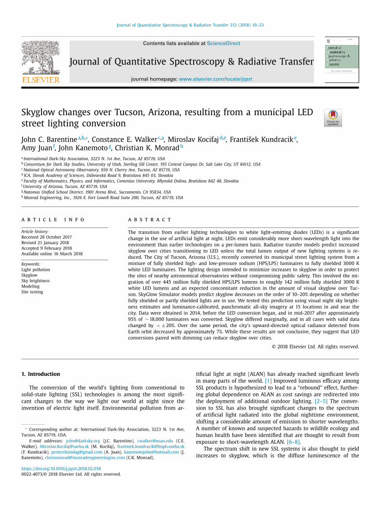
Fig. 1. Model of the Tucson city and suburban region illustrating the 18 polygonal modeling units referred to in the text. The inset image at right shows a 2017 NASA/NOAA

Suomi National Polar-orbiting Partnership Visible Infrared Imaging Radiometer Suite Day-Night Band (VIIRS-DNB) image of the area at night, at approximately the same spatial

scale and orientation.

s

9

t

w

a

w

i

1

3

r

s

l

t

u

5

r

2

i

t

l

c

d

I

solution “Skyglow v.5” is publicly available 1 and can be used to

simulate sky radiance or luminance patterns over any place in the

world. The SkyGlow tool allows for clustering of the light-emitting

areas that share similar properties such as spectral power distri-

bution (SPD), average number of lumens installed per unit land

area, angular emission pattern, and the spectral reflectance of the

ground.

The City of Tucson was divided into 18 light-emitting areas that

share common physical properties ( Fig. 1 ), meaning that, e.g., up-

light levels or built-up area densities fall within the same cate-

gories. Our analysis was based on Google Earth, Day-Night Band

(DNB) maps made using the Visible Infrared Imaging Radiometer

Suite (VIIRS) instrument aboard the NASA/NOAA Suomi National

Polar-orbiting Partnership satellite [22] , and NASA “City Lights” that

is part of Google Earth gallery. 2 A complete inventory of luminaires

in the central part of Tucson was available for City-owned lights,

and a partial inventory for other lights. However, the information

on lumens installed in suburban areas was completely missing; it

was thus determined numerically and normalized using the VIIRS

database.

The procedure was simple. First we analyzed a few areas in

central Tucson, where total emission spectra were computed as the

collective contribution of HPS, LPS and LED lamps, taking into ac-

count the information on initial lamp lumens and luminaire effi-

ciency. We found that the ratio of VIIRS-DNB uplight to lumens in-

stalled varies only slightly for these areas ( ± 4%); thus, the same

ratio was used to estimate lumens installed in other suburban

zones. Such calibration was possible also because the mean ground

albedo does not significantly change across the city territory.

Using the luminaire inventory and the above calibration we

found that, prior to the LED conversion, the central part of Tuc-

1 http://skyglow.sav.sk/#simulator . 2 https://www.gearthblog.com/blog/archives/2012/02/the _ city _ lights _ of _ earth.

html .

T

e

s

r

z

on emitted 8.52 × 10 8 photopic lumens, constituting a mixture of

3% HPS, 5.8% LPS, and 1.2% 30 0 0 K white LED. We determined

hat the legacy street lighting system comprised 4.81 × 10 8 lumens,

hich was 56.4% of lumens installed from all sources, both public

nd private. The City of Tucson chose to replace the legacy system

ith new LED luminaires whose output is 63% less than the exist-

ng lighting.

City planners estimated that the LED lamps would emit

.79 × 10 8 lumens if operated at maximum power, leaving

.71 × 10 8 lumens (43.6% of all light emissions) unchanged. This

esults in a total of 5.50 × 10 8 lumens from all sources, and repre-

ents a 35.4% reduction from the pre-retrofit condition if the new

uminaires were operated at full power. However, the City elected

o further dim the new LED lights to 90% of their maximum power

pon installation, so the total post-retrofit emission of the city was

.33 × 10 8 lumens, for a total reduction of 37.6% from the pre-

etrofit condition.

.2. Model lighting scenarios and inputs

The models in this study comprise two scenarios:

M1: Status quo ante (pre-retrofit condition): 8.52 × 10 8 lumens

nstalled prior the LED conversion

M2: Post-retrofit, dimming to 90% output: 5.33 × 10 8 lumens af-

er LED conversion (56.4% lumens undergo conversion, while the

ights are dimmed to 90% of maximum power). The total post-

onversion lumen output, I post , is obtained from the sum of (90%-

immed) street lighting and unchanged, non-street lighting:

post = (0 . 9 × 1 . 79 ×10

8 lm ) + (0 . 436 × 8 . 52 ×10

8 lm ) . (1)

he best we can do to get closer to at least a partially-controlled

xperiment is to make both the numerical modeling and field mea-

urements under similar sky conditions (clear sky, low dust, low

elative humidity, no moonlight, no twilight, no Milky Way in the

enith). The input parameters to the model were kept constant

J.C. Barentine et al. / Journal of Quantitative Spectroscopy & Radiative Transfer 212 (2018) 10–23 13

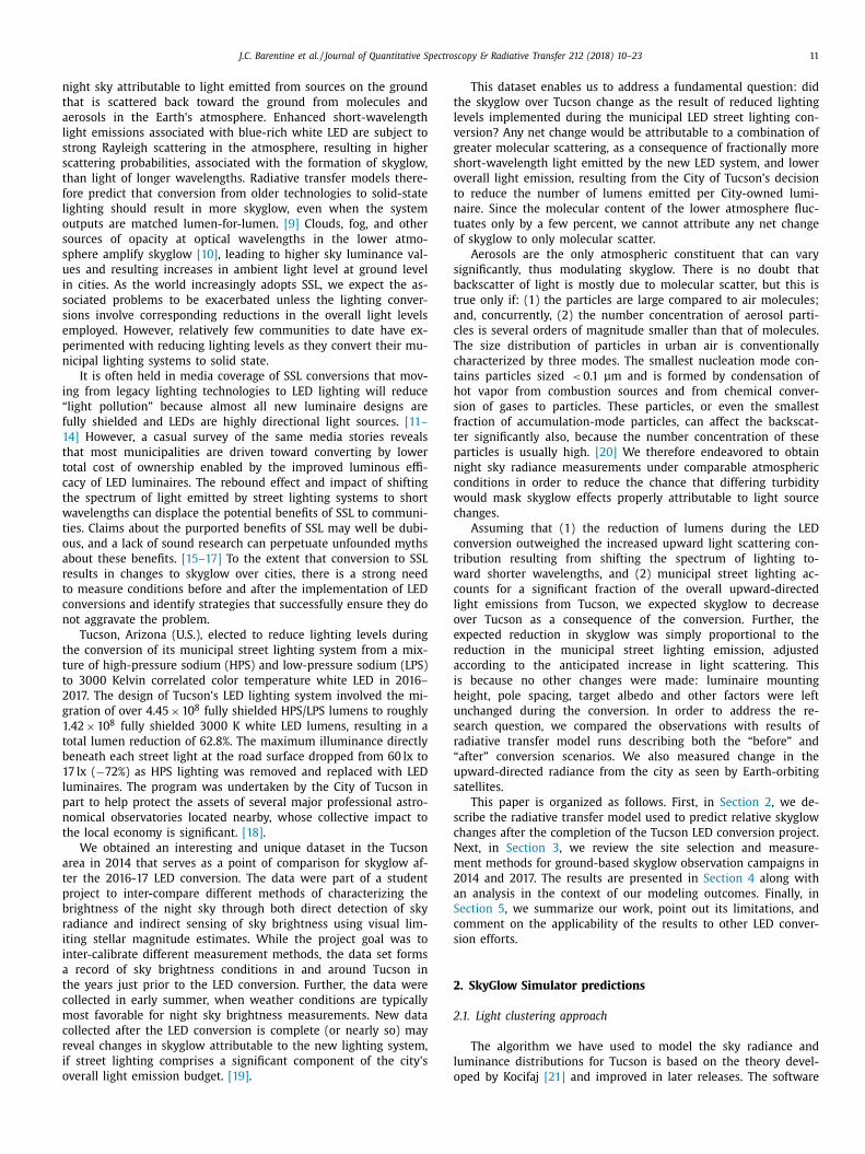
Fig. 2. A nighttime optical-light photograph of the Tucson, Arizona, vicinity from low Earth orbit shown superimposed on a background political map of the area; locations

of SkyGlow Simulator model runs are indicated with red symbols and 2014/2017 night sky brightness measurements with blue symbols. Light at night image: National

Aeronautics and Space Administration Astronaut Photo ISS030-E-61700, obtained on 31 January 2012. Background map: copyright 2017 Google, INEGI, used with permission.

(For interpretation of the references to colour in this figure legend, the reader is referred to the web version of this article.)

u

(

t

A

e

i

2

e

i

(

m

t

z

p

v

t

a

s

p

c

c

b

2

v

a

w

P

o

c

c

H

w

u

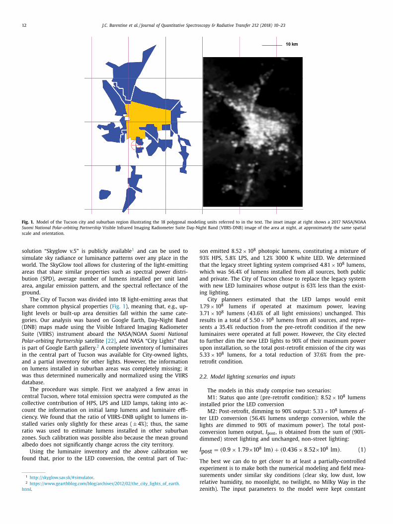
Fig. 3. A polygonal map of Tucson with a discrete observation site (Reid Park Brown

Conservation Learning Center) marked by the red cross in the red circle. This site

represents model predictions typical of the city core. (For interpretation of the ref-

erences to colour in this figure legend, the reader is referred to the web version of

this article.)

A

e

t

b

b

g

o

m

a

nless stated otherwise. For instance, the aerosol optical depth

AOD) at the reference wavelength ( λ = 500 nm) was 0.1, while

he Angström exponent was υ = 1 . 3 . The latter parameter models

OD as an exponential function of wavelength: AOD ∼ λ−υ . Mod-

ls were computed for five locations in and around Tucson, shown

n Fig. 2 .

.3. Results of model runs

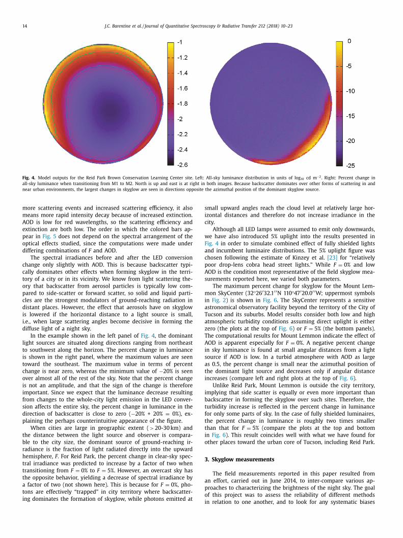
To illustrate results exemplifying the city core, skyglow mod-

ling and baseline/post conversion empirical measurements are

ndicated for the Reid Park Brown Conservation Learning Center

32 °12 ′ 29.7 ′ ′ N 110 °55 ′ 17.8 ′ ′ W; see the red cross in Fig. 3 ). The lu-

inance distribution as well as the percent change when transi-

ioning from M1 to M2 for Reid Park are shown in Fig. 4 . The

enith luminance and horizontal illuminance computed were ap-

roximately 3.5 mcd m

−2 and 25 mlux, respectively.

Bear in mind that the focus of the model is not on absolute

alues, but on the relative influence of lumen output change, given

he uncertainty of the normalization coefficient for the VIIRS data

nd the intent of this study to examine skyglow relative to the

ituation prior to the LED conversion. This is why the rightmost

lot in Fig. 4 and consequent graphical outputs show the percent

hange only. For example, a value of +20% for model M2 means a

onversion with LED lights dimmed to 90% increases the sky glow

y 20% or 1.2 times the M1 result, whereas a negative value of -

0% means the sky glow will decrease by 20% or 0.8 times the M1

alue.

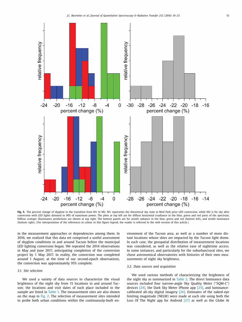
The percent change was computed for every radi-

nce/luminance or irradiance/illuminance. A change of -20%

as predicted for almost all computed luminance data for Reid

ark, while no change is only observed in the part of the sky

pposite to the azimuthal position of the dominant light source;

ompare the left and right plots in Fig. 5 , which shows the percent

hanges predicted by the models for the transition from M1 to M2.

ere we have assumed that fully shielded LED lights are mixed

ith lights that are not properly shielded, implying that the direct

plight ranges from 0% to 5%.

Computations were made for different combinations of F and

OD values in order to identify the statistical range of the optical

ffects we studied. There is therefore no reason a priori to expect

hat the red bars in Fig. 5 will be completely isolated from green

ars and blue bars. Instead, a partial overlap of blue, green and red

ars is seen in the figure. Additionally, the arrangement of blue,

reen and red bars in the figure is due to a non-trivial combination

f different optical effects; e.g., spectral power distribution and at-

ospheric optics, including an intensive scattering in the blue, but

lso an elevated value of AOD in blue. While a large AOD implies

14 J.C. Barentine et al. / Journal of Quantitative Spectroscopy & Radiative Transfer 212 (2018) 10–23

Fig. 4. Model outputs for the Reid Park Brown Conservation Learning Center site. Left: All-sky luminance distribution in units of log 10 cd m

−2 . Right: Percent change in

all-sky luminance when transitioning from M1 to M2. North is up and east is at right in both images. Because backscatter dominates over other forms of scattering in and

near urban environments, the largest changes in skyglow are seen in directions opposite the azimuthal position of the dominant skyglow source.

s

i

c

w

F

a

c

p

A

s

m

i

a

T

a

z

T

A

i

s

a

t

i

i

b

t

f

t

t

i

o

3

a

p

o

more scattering events and increased scattering efficiency, it also

means more rapid intensity decay because of increased extinction.

AOD is low for red wavelengths, so the scattering efficiency and

extinction are both low. The order in which the colored bars ap-

pear in Fig. 5 does not depend on the spectral arrangement of the

optical effects studied, since the computations were made under

differing combinations of F and AOD.

The spectral irradiances before and after the LED conversion

change only slightly with AOD. This is because backscatter typi-

cally dominates other effects when forming skyglow in the terri-

tory of a city or in its vicinity. We know from light scattering the-

ory that backscatter from aerosol particles is typically low com-

pared to side-scatter or forward scatter, so solid and liquid parti-

cles are the strongest modulators of ground-reaching radiation in

distant places. However, the effect that aerosols have on skyglow

is lowered if the horizontal distance to a light source is small,

i.e., when large scattering angles become decisive in forming the

diffuse light of a night sky.

In the example shown in the left panel of Fig. 4 , the dominant

light sources are situated along directions ranging from northeast

to southwest along the horizon. The percent change in luminance

is shown in the right panel, where the maximum values are seen

toward the southeast. The maximum value in terms of percent

change is near zero, whereas the minimum value of −20% is seen

over almost all of the rest of the sky. Note that the percent change

is not an amplitude, and that the sign of the change is therefore

important. Since we expect that the luminance decrease resulting

from changes to the whole-city light emission in the LED conver-

sion affects the entire sky, the percent change in luminance in the

direction of backscatter is close to zero ( −20% + 20% = 0%), ex-

plaining the perhaps counterintuitive appearance of the figure.

When cities are large in geographic extent ( > 20-30 km) and

the distance between the light source and observer is compara-

ble to the city size, the dominant source of ground-reaching ir-

radiance is the fraction of light radiated directly into the upward

hemisphere, F . For Reid Park, the percent change in clear-sky spec-

tral irradiance was predicted to increase by a factor of two when

transitioning from F = 0 % to F = 5 %. However, an overcast sky has

the opposite behavior, yielding a decrease of spectral irradiance by

a factor of two (not shown here). This is because for F = 0 %, pho-

tons are effectively “trapped” in city territory where backscatter-

ing dominates the formation of skyglow, while photons emitted at

i

mall upward angles reach the cloud level at relatively large hor-

zontal distances and therefore do not increase irradiance in the

ity.

Although all LED lamps were assumed to emit only downwards,

e have also introduced 5% uplight into the results presented in

ig. 4 in order to simulate combined effect of fully shielded lights

nd incumbent luminaire distributions. The 5% uplight figure was

hosen following the estimate of Kinzey et al. [23] for “relatively

oor drop-lens cobra head street lights.” While F = 0 % and low

OD is the condition most representative of the field skyglow mea-

urements reported here, we varied both parameters.

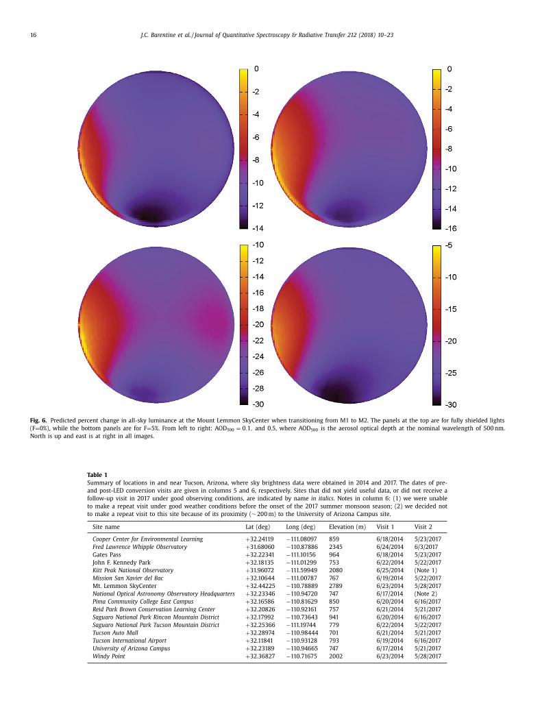
The maximum percent change for skyglow for the Mount Lem-

on SkyCenter (32 °26 ′ 32.1 ′ ′ N 110 °47 ′ 20.0 ′ ′ W; uppermost symbols

n Fig. 2 ) is shown in Fig. 6 . The SkyCenter represents a sensitive

stronomical observatory facility beyond the territory of the City of

ucson and its suburbs. Model results consider both low and high

tmospheric turbidity conditions assuming direct uplight is either

ero (the plots at the top of Fig. 6 ) or F = 5 % (the bottom panels).

he computational results for Mount Lemmon indicate the effect of

OD is apparent especially for F = 0 %. A negative percent change

n sky luminance is found at small angular distances from a light

ource if AOD is low. In a turbid atmosphere with AOD as large

s 0.5, the percent change is small near the azimuthal position of

he dominant light source and decreases only if angular distance

ncreases (compare left and right plots at the top of Fig. 6 ).

Unlike Reid Park, Mount Lemmon is outside the city territory,

mplying that side scatter is equally or even more important than

ackscatter in forming the skyglow over such sites. Therefore, the

urbidity increase is reflected in the percent change in luminance

or only some parts of sky. In the case of fully shielded luminaires,

he percent change in luminance is roughly two times smaller

han that for F = 5 % (compare the plots at the top and bottom

n Fig. 6 ). This result coincides well with what we have found for

ther places toward the urban core of Tucson, including Reid Park.

. Skyglow measurements

The field measurements reported in this paper resulted from

n effort, carried out in June 2014, to inter-compare various ap-

roaches to characterizing the brightness of the night sky. The goal

f this project was to assess the reliability of different methods

n relation to one another, and to look for any systematic biases

J.C. Barentine et al. / Journal of Quantitative Spectroscopy & Radiative Transfer 212 (2018) 10–23 15

Fig. 5. The percent change of skyglow in the transition from M1 to M2. M1 represents the theoretical sky state in Reid Park prior LED conversion, while M2 is for sky after

conversion with LED lights dimmed to 90% of maximum power. The plots at top left are for diffuse horizontal irradiance in the blue, green and red parts of the spectrum.

Diffuse scotopic illuminance predictions are shown at top right. The bottom panels are for zenith radiance in the blue, green and red (bottom left), and zenith luminance

(bottom right). (For interpretation of the references to colour in this figure legend, the reader is referred to the web version of this article.)

i

2

o

L

i

p

a

t

3

b

s

s

o

t

v

t

I

w

I

c

s

3

t

s

d

c

l

L

n the measurement approaches or dependencies among them. In

016, we realized that this data set comprised a useful assessment

f skyglow conditions in and around Tucson before the municipal

ED lighting conversion began. We repeated the 2014 observations

n May and June 2017, anticipating completion of the conversion

roject by 1 May 2017. In reality, the conversion was completed

round 1 August; at the time of our second-epoch observations,

he conversion was approximately 95% complete.

.1. Site selection

We used a variety of data sources to characterize the visual

rightness of the night sky from 15 locations in and around Tuc-

on; the locations and visit dates of each place included in the

ample are listed in Table 1 . The measurement sites are also shown

n the map in Fig. 2 . The selection of measurement sites intended

o probe both urban conditions within the continuously-built en-

ironment of the Tucson area, as well as a number of more dis-

ant locations whose skies are impacted by the Tucson light dome.

n each case, the geospatial distribution of measurement locations

as considered, as well as the relative ease of nighttime access.

n some instances, and particularly for the suburban/rural sites, we

hose astronomical observatories with histories of their own mea-

urements of night sky brightness.

.2. Data sources and acquisition

We used various methods of characterizing the brightness of

he night sky as summarized in Table 2 . The direct luminance data

ources included four narrow-angle Sky Quality Meter (“SQM-L”)

evices [24] , the Dark Sky Meter iPhone app [25] , and luminance-

alibrated all-sky digital imagery [26] . Estimates of the naked-eye

imiting magnitude (NELM) were made at each site using both the

oss Of The Night app for Android [27] as well as the Globe At

16 J.C. Barentine et al. / Journal of Quantitative Spectroscopy & Radiative Transfer 212 (2018) 10–23

Fig. 6. Predicted percent change in all-sky luminance at the Mount Lemmon SkyCenter when transitioning from M1 to M2. The panels at the top are for fully shielded lights

(F = 0%), while the bottom panels are for F = 5%. From left to right: AOD 500 = 0 . 1 , and 0.5, where AOD 500 is the aerosol optical depth at the nominal wavelength of 500 nm.

North is up and east is at right in all images.

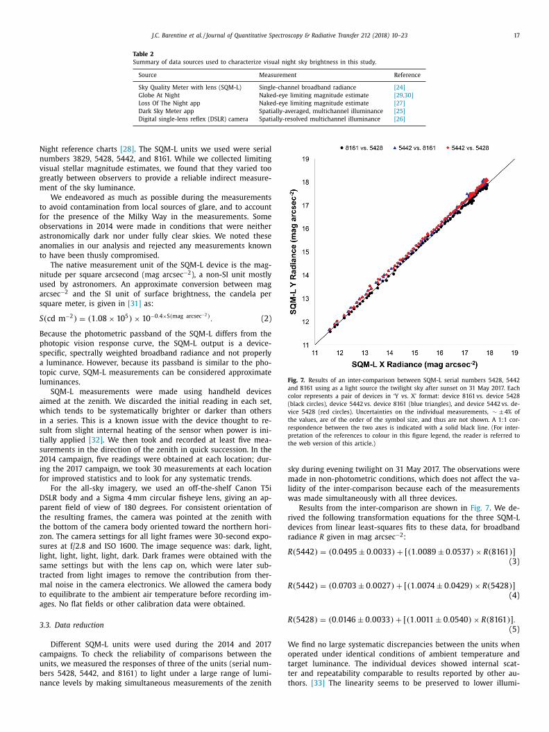
Table 1

Summary of locations in and near Tucson, Arizona, where sky brightness data were obtained in 2014 and 2017. The dates of pre-

and post-LED conversion visits are given in columns 5 and 6, respectively. Sites that did not yield useful data, or did not receive a

follow-up visit in 2017 under good observing conditions, are indicated by name in italics . Notes in column 6: (1) we were unable

to make a repeat visit under good weather conditions before the onset of the 2017 summer monsoon season; (2) we decided not

to make a repeat visit to this site because of its proximity ( ∼ 200 m) to the University of Arizona Campus site.

Site name Lat (deg) Long (deg) Elevation (m) Visit 1 Visit 2

Cooper Center for Environmental Learning + 32.24119 −111.08097 859 6/18/2014 5/23/2017

Fred Lawrence Whipple Observatory + 31.68060 −110.87886 2345 6/24/2014 6/3/2017

Gates Pass + 32.22341 −111.10156 964 6/18/2014 5/23/2017

John F. Kennedy Park + 32.18135 −111.01299 753 6/22/2014 5/22/2017

Kitt Peak National Observatory + 31.96072 −111.59949 2080 6/25/2014 (Note 1)

Mission San Xavier del Bac + 32.10644 −111.00787 767 6/19/2014 5/22/2017

Mt. Lemmon SkyCenter + 32.44225 −110.78889 2789 6/23/2014 5/28/2017

National Optical Astronomy Observatory Headquarters + 32.23346 −110.94720 747 6/17/2014 (Note 2)

Pima Community College East Campus + 32.16586 −110.81629 850 6/20/2014 6/16/2017

Reid Park Brown Conservation Learning Center + 32.20826 −110.92161 757 6/21/2014 5/21/2017

Saguaro National Park Rincon Mountain District + 32.17992 −110.73643 941 6/20/2014 6/16/2017

Saguaro National Park Tucson Mountain District + 32.25366 −111.19744 779 6/22/2014 5/22/2017

Tucson Auto Mall + 32.28974 −110.984 4 4 701 6/21/2014 5/21/2017

Tucson International Airport + 32.11841 −110.93128 793 6/19/2014 6/16/2017

University of Arizona Campus + 32.23189 −110.94665 747 6/17/2014 5/21/2017

Windy Point + 32.36827 −110.71675 2002 6/23/2014 5/28/2017

J.C. Barentine et al. / Journal of Quantitative Spectroscopy & Radiative Transfer 212 (2018) 10–23 17

Table 2

Summary of data sources used to characterize visual night sky brightness in this study.

Source Measurement Reference

Sky Quality Meter with lens (SQM-L) Single-channel broadband radiance [24]

Globe At Night Naked-eye limiting magnitude estimate [29,30]

Loss Of The Night app Naked-eye limiting magnitude estimate [27]

Dark Sky Meter app Spatially-averaged, multichannel illuminance [25]

Digital single-lens reflex (DSLR) camera Spatially-resolved multichannel illuminance [26]

N

n

v

g

m

t

f

o

a

a

t

n

u

a

s

S

B

p

s

a

t

l

a

w

i

s

t

s

2

i

f

D

p

t

t

z

s

l

s

t

m

t

a

3

c

u

b

n

Fig. 7. Results of an inter-comparison between SQM-L serial numbers 5428, 5442

and 8161 using as a light source the twilight sky after sunset on 31 May 2017. Each

color represents a pair of devices in ‘Y vs. X’ format: device 8161 vs. device 5428

(black circles), device 5442 vs. device 8161 (blue triangles), and device 5442 vs. de-

vice 5428 (red circles). Uncertainties on the individual measurements, ∼ ± 4% of

the values, are of the order of the symbol size, and thus are not shown. A 1:1 cor-

respondence between the two axes is indicated with a solid black line. (For inter-

pretation of the references to colour in this figure legend, the reader is referred to

the web version of this article.)

s

m

l

w

r

d

r

R

R

R

W

o

t

t

t

ight reference charts [28] . The SQM-L units we used were serial

umbers 3829, 5428, 5442, and 8161. While we collected limiting

isual stellar magnitude estimates, we found that they varied too

reatly between observers to provide a reliable indirect measure-

ent of the sky luminance.

We endeavored as much as possible during the measurements

o avoid contamination from local sources of glare, and to account

or the presence of the Milky Way in the measurements. Some

bservations in 2014 were made in conditions that were neither

stronomically dark nor under fully clear skies. We noted these

nomalies in our analysis and rejected any measurements known

o have been thusly compromised.

The native measurement unit of the SQM-L device is the mag-

itude per square arcsecond (mag arcsec −2 ), a non-SI unit mostly

sed by astronomers. An approximate conversion between mag

rcsec −2 and the SI unit of surface brightness, the candela per

quare meter, is given in [31] as:

( cd m

−2 ) = (1 . 08 × 10

5 ) × 10

−0 . 4 ×S ( mag arcsec −2 ) . (2)

ecause the photometric passband of the SQM-L differs from the

hotopic vision response curve, the SQM-L output is a device-

pecific, spectrally weighted broadband radiance and not properly

luminance. However, because its passband is similar to the pho-

opic curve, SQM-L measurements can be considered approximate

uminances.

SQM-L measurements were made using handheld devices

imed at the zenith. We discarded the initial reading in each set,

hich tends to be systematically brighter or darker than others

n a series. This is a known issue with the device thought to re-

ult from slight internal heating of the sensor when power is ini-

ially applied [32] . We then took and recorded at least five mea-

urements in the direction of the zenith in quick succession. In the

014 campaign, five readings were obtained at each location; dur-

ng the 2017 campaign, we took 30 measurements at each location

or improved statistics and to look for any systematic trends.

For the all-sky imagery, we used an off-the-shelf Canon T5i

SLR body and a Sigma 4 mm circular fisheye lens, giving an ap-

arent field of view of 180 degrees. For consistent orientation of

he resulting frames, the camera was pointed at the zenith with

he bottom of the camera body oriented toward the northern hori-

on. The camera settings for all light frames were 30-second expo-

ures at f/2.8 and ISO 1600. The image sequence was: dark, light,

ight, light, light, light, dark. Dark frames were obtained with the

ame settings but with the lens cap on, which were later sub-

racted from light images to remove the contribution from ther-

al noise in the camera electronics. We allowed the camera body

o equilibrate to the ambient air temperature before recording im-

ges. No flat fields or other calibration data were obtained.

.3. Data reduction

Different SQM-L units were used during the 2014 and 2017

ampaigns. To check the reliability of comparisons between the

nits, we measured the responses of three of the units (serial num-

ers 5428, 5442, and 8161) to light under a large range of lumi-

ance levels by making simultaneous measurements of the zenith

ky during evening twilight on 31 May 2017. The observations were

ade in non-photometric conditions, which does not affect the va-

idity of the inter-comparison because each of the measurements

as made simultaneously with all three devices.

Results from the inter-comparison are shown in Fig. 7 . We de-

ived the following transformation equations for the three SQM-L

evices from linear least-squares fits to these data, for broadband

adiance R given in mag arcsec −2 :

(5442) = (0 . 0495 ± 0 . 0033) + [(1 . 0089 ± 0 . 0537) × R (8161)] (3)

(5442) = (0 . 0703 ± 0 . 0027) + [(1 . 0074 ± 0 . 0429) × R (5428)] (4)

(5428) = (0 . 0146 ± 0 . 0033) + [(1 . 0011 ± 0 . 0540) × R (8161)] . (5)

e find no large systematic discrepancies between the units when

perated under identical conditions of ambient temperature and

arget luminance. The individual devices showed internal scat-

er and repeatability comparable to results reported by other au-

hors. [33] The linearity seems to be preserved to lower illumi-

18 J.C. Barentine et al. / Journal of Quantitative Spectroscopy & Radiative Transfer 212 (2018) 10–23

Table 3

Zenith luminance measurements from the 15 survey locations in 2014 and 2017. “Distance” means the radial distance from downtown Tucson

(32 °13 ′ 19.3 ′ ′ N 110 °58 ′ 07.0 ′ ′ W). For SQM-L data, “sSQM-L” refers to ‘synthetic’ SQM-L values derived from aperture photometry of luminance-

calibrated all-sky imagery; see the main text for details. Data are shown only where all of our quality criteria were met. Two sites are not

shown: No data were obtained at Kitt Peak National Observatory in 2017, and the 2014 Tucson Auto Mall data were not usable.

Location Name Distance (km) 2014 SQM-L

(mag arcsec −2 )

2017 SQM-L

(mag arcsec −2 )

2014 sSQM-L

(mag arcsec −2 )

2017 sSQM-L

(mag arcsec −2 )

Cooper Center for Environmental Learning 10.5 20.43 ± 0.02 20.46 ± 0.01 19.79 ± 0.01 20.20 ± 0.01

Fred Lawrence Whipple Observatory 61.2 21.52 ± 0.03 21.45 ± 0.02 21.54 ± 0.01 21.28 ± 0.01

Gates Pass 12.2 20.64 ± 0.10 20.51 ± 0.02 20.20 ± 0.01 20.43 ± 0.01

John F. Kennedy Park 6.1 19.61 ± 0.02 19.40 ± 0.02 19.08 ± 0.01 19.07 ± 0.01

Mission San Xavier del Bac 13.1 20.02 ± 0.02 20.01 ± 0.03 19.51 ± 0.04 19.82 ± 0.01

Mt. Lemmon SkyCenter 29.8 21.14 ± 0.08 21.38 ± 0.01 21.10 ± 0.01 21.31 ± 0.01

Pima Community College East Campus 16.1 19.77 ± 0.02 19.84 ± 0.04 18.99 ± 0.01 19.56 ± 0.01

Reid Park 4.8 18.69 ± 0.06 19.01 ± 0.02 18.37 ± 0.01 18.77 ± 0.01

Saguaro National Park Rincon Mountain District 26.9 20.93 ± 0.03 20.82 ± 0.03 18.99 ± 0.01 20.74 ± 0.01

Saguaro National Park Tucson Mountain District 21.6 20.79 ± 0.07 20.83 ± 0.02 20.50 ± 0.01 20.77 ± 0.01

Windy Point 29.0 21.60 ± 0.07 21.36 ± 0.01 18.38 ± 0.01 21.19 ± 0.01

Tucson International Airport 12.2 19.14 ± 0.05 19.19 ± 0.02 18.58 ± 0.02 18.74 ± 0.01

University of Arizona Campus 2.5 17.50 ± 0.21 18.39 ± 0.03 17.81 ± 0.01 18.38 ± 0.01

J

c

L

t

m

p

t

n

z

a

w

L

b

s

s

f

b

C

l

L

i

t

s

n

d

f

b

t

d

V

s

i

a

d

t

t

w

L

t

w

v

t

nances, although the fits are less reliable as the data become in-

creasingly noisy. Eqs. 2 –4 are simple linear fits, stated with fitting

uncertainties on the parameters.

The equations enabled us to put measurements from all of

the SQM devices we used onto a common photometric system

so that meaningful comparisons can be made. We transformed

all measurements made with SQM serial numbers 5428 and 8161

to the system defined by serial number 5442. We chose 5442 as

the reference since, among the four devices we used, it showed

the smallest internal scatter ( ± 0.03 mag arcsec −2 ) in repeatability

tests. Note that SQM-L serial number 3829 was unavailable for use

during the 2017 measurement campaign, so we did not include it

in the inter-comparison.

All-sky luminance images were calibrated using the method

and ‘dslrlum’ software described by Kolláth and Dömény [26] . The

routines read the camera RAW-formatted images, apply spatial dis-

tortion/vignetting and luminance corrections, and output several

data products. These include a luminance-calibrated version of the

input image in cd m

−2 ; a Mercator-projected version of this im-

age; and predicted SQM-L values in both mag arcsec −2 and cd m

−2 .

The predictions are based on photometry of the calibrated images

within software apertures of equivalent fields of view; we refer to

these values hereafter as “synthetic” luminances. The photometry

was tied to lab calibration of the camera and lens combination and

not to standard stars or other field calibrators. Comparison with ac-

tual SQM-L measurements at each site was made as a check, and

in most cases the results agreed to within their respective internal

uncertainties.

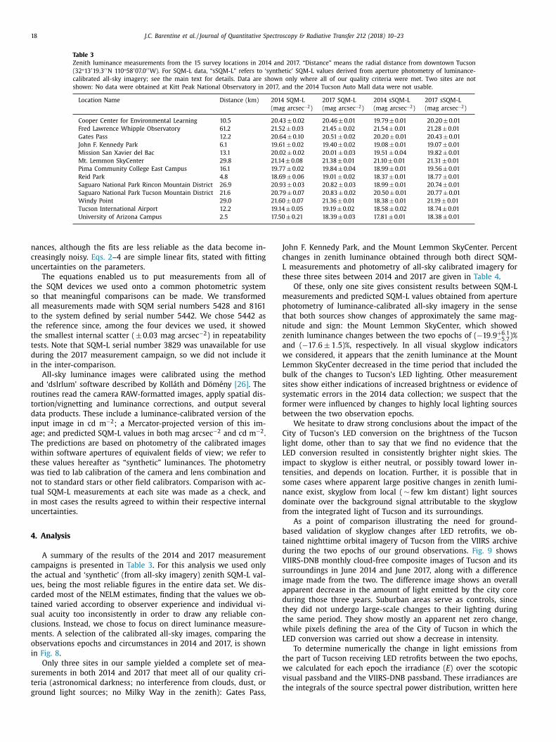
4. Analysis

A summary of the results of the 2014 and 2017 measurement

campaigns is presented in Table 3 . For this analysis we used only

the actual and ‘synthetic’ (from all-sky imagery) zenith SQM-L val-

ues, being the most reliable figures in the entire data set. We dis-

carded most of the NELM estimates, finding that the values we ob-

tained varied according to observer experience and individual vi-

sual acuity too inconsistently in order to draw any reliable con-

clusions. Instead, we chose to focus on direct luminance measure-

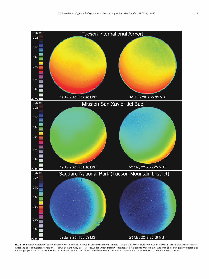
ments. A selection of the calibrated all-sky images, comparing the

observations epochs and circumstances in 2014 and 2017, is shown

in Fig. 8 .

Only three sites in our sample yielded a complete set of mea-

surements in both 2014 and 2017 that meet all of our quality cri-

teria (astronomical darkness; no interference from clouds, dust, or

ground light sources; no Milky Way in the zenith): Gates Pass,

ohn F. Kennedy Park, and the Mount Lemmon SkyCenter. Percent

hanges in zenith luminance obtained through both direct SQM-

measurements and photometry of all-sky calibrated imagery for

hese three sites between 2014 and 2017 are given in Table 4 .

Of these, only one site gives consistent results between SQM-L

easurements and predicted SQM-L values obtained from aperture

hotometry of luminance-calibrated all-sky imagery in the sense

hat both sources show changes of approximately the same mag-

itude and sign: the Mount Lemmon SkyCenter, which showed

enith luminance changes between the two epochs of ( −19 . 9 +6 . 1 −5 . 7

)%

nd ( −17 . 6 ± 1 . 5 )%, respectively. In all visual skyglow indicators

e considered, it appears that the zenith luminance at the Mount

emmon SkyCenter decreased in the time period that included the

ulk of the changes to Tucson’s LED lighting. Other measurement

ites show either indications of increased brightness or evidence of

ystematic errors in the 2014 data collection; we suspect that the

ormer were influenced by changes to highly local lighting sources

etween the two observation epochs.

We hesitate to draw strong conclusions about the impact of the

ity of Tucson’s LED conversion on the brightness of the Tucson

ight dome, other than to say that we find no evidence that the

ED conversion resulted in consistently brighter night skies. The

mpact to skyglow is either neutral, or possibly toward lower in-

ensities, and depends on location. Further, it is possible that in

ome cases where apparent large positive changes in zenith lumi-

ance exist, skyglow from local ( ∼ few km distant) light sources

ominate over the background signal attributable to the skyglow

rom the integrated light of Tucson and its surroundings.

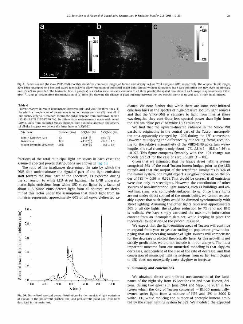
As a point of comparison illustrating the need for ground-

ased validation of skyglow changes after LED retrofits, we ob-

ained nighttime orbital imagery of Tucson from the VIIRS archive

uring the two epochs of our ground observations. Fig. 9 shows

IIRS-DNB monthly cloud-free composite images of Tucson and its

urroundings in June 2014 and June 2017, along with a difference

mage made from the two. The difference image shows an overall

pparent decrease in the amount of light emitted by the city core

uring those three years. Suburban areas serve as controls, since

hey did not undergo large-scale changes to their lighting during

he same period. They show mostly an apparent net zero change,

hile pixels defining the area of the City of Tucson in which the

ED conversion was carried out show a decrease in intensity.

To determine numerically the change in light emissions from

he part of Tucson receiving LED retrofits between the two epochs,

e calculated for each epoch the irradiance ( E ) over the scotopic

isual passband and the VIIRS-DNB passband. These irradiances are

he integrals of the source spectral power distribution, written here

J.C. Barentine et al. / Journal of Quantitative Spectroscopy & Radiative Transfer 212 (2018) 10–23 19

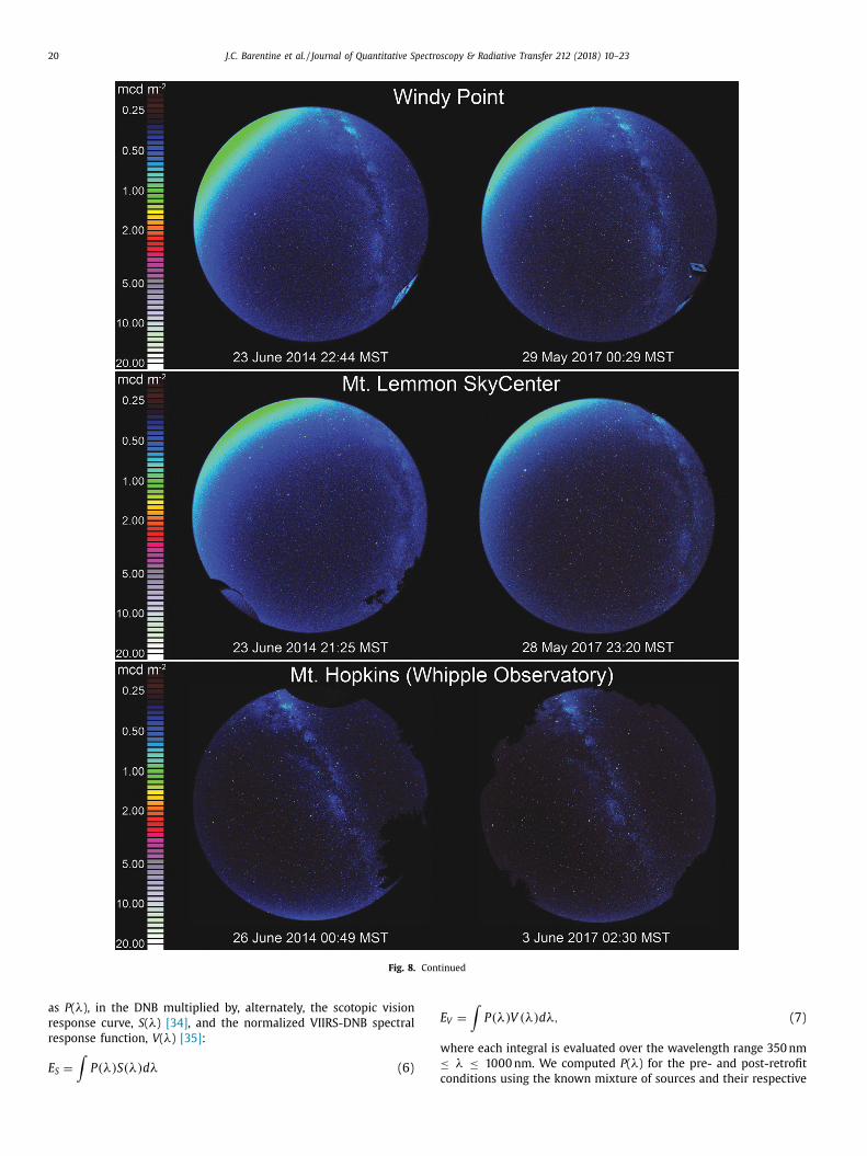
Fig. 8. Luminance-calibrated all-sky imagery for a selection of sites in our measurement sample. The pre-LED-conversion condition is shown at left in each pair of images,

while the post-conversion condition is shown at right. Only sites are shown for which imagery obtained at both epochs was available and met all of our quality criteria, and

the images pairs are arranged in order of increasing site distance from downtown Tucson. All images are oriented alike with north down and east at right.

20 J.C. Barentine et al. / Journal of Quantitative Spectroscopy & Radiative Transfer 212 (2018) 10–23

Fig. 8. Continued

E

w

≤

as P ( λ), in the DNB multiplied by, alternately, the scotopic vision

response curve, S ( λ) [34] , and the normalized VIIRS-DNB spectral

response function, V ( λ) [35] :

E S =

∫ P (λ) S(λ) dλ (6)

c

V =

∫ P (λ) V (λ) dλ, (7)

here each integral is evaluated over the wavelength range 350 nm

λ ≤ 10 0 0 nm. We computed P ( λ) for the pre- and post-retrofit

onditions using the known mixture of sources and their respective

J.C. Barentine et al. / Journal of Quantitative Spectroscopy & Radiative Transfer 212 (2018) 10–23 21

Fig. 9. Panels (a) and (b) show VIIRS-DNB monthly cloud-free composite images of Tucson and vicinity in June 2014 and June 2017, respectively. The original 32-bit images

have been resampled to 8 bits and scaled identically to allow resolution of individual bright light sources without saturation; scale bars indicating the gray levels in arbitrary

units (‘a.u.’) are provided. The horizontal line in panel (a) is a 25-km scale indicator common to all three panels; the spatial resolution of each image is approximately 750 m

pixel −1 . Panel (c) results from the subtraction of (a) from (b), showing the change in pixel intensity between the two epochs. North is up and east is right in all images.

Table 4

Percent changes in zenith illuminances between 2014 and 2017 for three sites (1)

for which a complete set of measurements in both exists and that (2) meet all of

our quality criteria. “Distance” means the radial distance from downtown Tucson

(32 °13 ′ 19.3 ′ ′ N 110 °58 ′ 07.0 ′ ′ W). To differentiate measurements made with actual

SQM-L units from predicted values obtained from synthetic aperture photometry

of all-sky imagery, we denote the latter here as “sSQM-L”.

Site name Distance (km) �SQM-L (%) �sSQM-L (%)

John F. Kennedy Park 6.1 + 21.1 +4 . 5 −4 . 4

+ 0.9 +1 . 9 −1 . 8

Gates Pass 12.2 + 13.2 +9 . 8 −9 . 0

−19 . 1 ± 1 . 5

Mount Lemmon SkyCenter 29.8 −19 . 9 +6 . 1 −5 . 7

−17 . 6 ± 1 . 5

f

a

D

s

t

m

a

m

m

F

o

d

d

e

a

w

t

p

t

H

i

l

−

m

c

r

t

d

w

s

v

a

ractions of the total municipal light emissions in each case; the

ssumed spectral power distributions are shown in Fig. 10 .

The ratio of the irradiances determines the rate by which the

NB data underestimate the signal if part of the light emissions

hift toward the blue part of the spectrum, as expected during

he conversion to white LED street lighting. The DNB underesti-

ates light emissions from white LED street lights by a factor of

bout 1.16. Since VIIRS detects light from all sources, we deter-

ined this factor under the assumption that direct light from lu-

inaires represents approximately 60% of all upward-directed ra-

ig. 10. Normalized spectral power distributions for the municipal light emissions

f Tucson in the pre-retrofit (dashed line) and post-retrofit (solid line) conditions

escribed in the main text.

a

s

5

i

c

t

t

p

f

s

i

d

c

t

5

n

z

t

o

w

t

iance. We note further that while there are some near-infrared

mission lines in the spectra of high-pressure sodium light sources

nd that the VIIRS-DNB is sensitive to light from lines at these

avelengths, they contribute less spectral power than light from

he 450 nm “blue peak” of white LED emissions.

We find that the upward-directed radiance in the VIIRS-DNB

assband originating in the central part of the Tucson metropoli-

an area apparently changed by −20% during the LED conversion.

owever, multiplying the difference by our scaling factor, account-

ng for the relative insensitivity of the VIIRS-DNB at certain wave-

engths, the real change is only about −7%: �L ∝ 1 − (0 . 8 × 1 . 16) =0 . 072 . This figure compares favorably with the -10% change our

odels predict for the case of zero uplight ( F = 0 %).

Given that we estimated that the legacy street lighting system

omprised 56% of the total Tucson lumen budget prior to the LED

etrofit and that the output of the retrofitted luminaires is 32% of

he earlier system, one might expect a skyglow decrease on the or-

er of 18% ( = 0.56 × 0.32). That would be correct if all emissions

ere due only to streetlights. However, the contribution of other

ources of non-inventoried light sources, such as buildings and ad-

ertising signs, was completely unknown to us. Since these lights

re not under direct control of the municipality, we cannot reason-

bly expect that such lights would be dimmed synchronously with

treet lighting. Assuming the other lights represent approximately

0% of all city lights, the skyglow reduction by 7% (and not 18%)

s realistic. We have simply extracted the maximum information

ontent from an incomplete data set, while keeping in place the

heoretical foundations of the procedures used.

We expect that the light-emitting areas of Tucson will continue

o expand from year to year according to population growth, im-

lying that an increasing number of light sources will compensate

or the decrease predicted theoretically here. As this growth is not

trictly predictable, we did not include it in our analysis. The most

mportant outcome from our numerical modeling is that skyglow

ecreases, independent of the size of the rate of decrease, and that

onversion of municipal lighting systems from earlier technologies

o LED does not necessarily cause skyglow to increase.

. Summary and conclusions

We obtained direct and indirect measurements of the lumi-

ance of the night sky from 15 locations in and near Tucson, Ari-

ona, during two epochs in June 2014 and May-June 2017, in be-

ween which the City of Tucson converted ∼ 18,0 0 0 municipally-

wned street lights from a mixture of HPS and LPS to 30 0 0 K

hite LED, while reducing the number of photopic lumens emit-

ed by the street lighting system by 63%. We modeled the expected

22 J.C. Barentine et al. / Journal of Quantitative Spectroscopy & Radiative Transfer 212 (2018) 10–23

5

t

a

d

H

f

t

l

n

o

s

Y

r

f

i

d

p

a

s

r

m

s

T

d

f

5

t

a

w

s

s

p

c

b

i

n

l

s

w

V

g

p

D

k

i

a

t

f

H

i

l

A

a

d

a

changes in skyglow using the SkyGlow Simulator software, which

predicted relative decreases in the brightness of skyglow over Tuc-

son of roughly −10% for F = 0 % (full shielding of all lights) and

−20% for F = 5 % (allowing a small amount of direct uplight).

The signal corresponding to the change resulting from the

street lighting conversion is not entirely clear in our data, but

there is some evidence of a decrease at certain measurement

sites of the order predicted by the models. Only one site of 15

yielded data of sufficient quality to conclude that the LED conver-

sion reduced skyglow in a manner consistent with our expecta-

tions: ( −19 . 9 +6 . 1 −5 . 7

)% and ( −17 . 6 ± 1 . 5 )%, using two different estima-

tion methods. Upward-directed radiance from the city detected in

the VIIRS-DNB shows an apparent decline of 7% during the same

period. To the extent that upward-directed radiance is a proxy

for skyglow intensity observed from the ground, the VIIRS-DNB

data may further support the conclusion that skyglow over Tuc-

son decreased after the municipal LED conversion. Therefore, there

is some evidence that the lumen reduction accompanying Tucson’s

conversion to SSL measurably decreased both the intensity of sky-

glow and upward-directed radiance.

5.1. Limitations of this work

There are a number of shortcomings in the approach to this

study that could be overcome in future efforts to characterize the

outcomes of LED conversions with regard to skyglow over cities.

These deficiencies result from the serendipitous nature of the 2014

field observations, which were not carried out with the intent of

making comparisons to a later epoch. We used different SQM de-

vices in the two campaigns, although we attempted to understand

any systematic differences in their responses after the fact through

mutual inter-comparison under controlled conditions. A number

of the 2014 measurements were carried out under circumstances

that were not ideal for the goals of this study; in particular, some

of the measurements were made at times during which we now

know the data were influenced by either moonlight or twilight

interference, or were taken in the presence of clouds. Conditions

were not precisely the same during the two epochs, such as the

time of night during which measurements were obtained, ambi-

ent air temperature, relative humidity, and atmospheric turbidity.

Furthermore, not all observations could be precisely replicated in

terms of geographic location, and we cannot rule out the possibil-

ity that observations from a given site in one epoch or the other

were contaminated by the presence of nearby, highly local outdoor

lighting sources. Lastly, observations in 2014 and 2017 were un-

dertaken by different observers with different levels of experience,

which may have further influenced certain measurements, in par-

ticular the naked-eye limiting magnitude estimates.

From these considerations, we conclude that such experiments

are difficult to conduct under real-world conditions when carried

out in campaign-style fashion. The variability of conditions from

one night to another, not to mention nights separated by several

years, is sufficiently unpredictable that perfect comparisons are not

possible. Rather, and in hindsight, a more effective approach would

be to install permanently-mounted sky brightness monitors prior

to the start of an LED conversion, and to collect data throughout.

Not only would such an approach allow for the suppression of vari-

able conditions from one night to the next, but it would also offer

temporal resolution that could be related back to the schedule of

luminaire replacements in a city.

The number and distribution of monitors should also be suffi-

cient to adequately sample the spatial distribution of light emitted

or reflected into the night sky over the geographic extent of a city

of arbitrary size. The recent work of Bará [36] suggests that opti-

mum spatial sampling to reconstruct the zenith sky luminance to a

precision of ∼ 10% rms is about one sample per square kilometer.

.2. Applicability to other cities

Tucson is unusual compared to many world cities due to its

ypically low relative humidity (and therefore often low AOD). On

verage, its frequently transparent night skies lead to darker con-

itions than experienced by other cities in more humid climates.

owever, it can at times be a dusty environment. We accounted

or turbidity effects in our models that can be likewise extended

o models of other cities, given local AOD inputs.

In policy terms, Tucson is also unusual in that the concern for

imiting light pollution is connected to the site protection of astro-

omical observatories that contribute significantly to its local econ-

my. Most world cities do not have such an influence on local deci-

ion making with respect to outdoor lighting practices and policies.

et the approach taken by Tucson of dimming its LED streetlights

elative to the light levels of its legacy HPS/LPS system could be ef-

ectively implemented by any city interested in limiting increases

n skyglow during a conversion to SSL. There are preliminary in-

ications in this study that that reducing lumens during munici-

al LED conversions may reduce skyglow over a city, even given

shift in the spectrum of lighting toward bluer wavelengths. Pre-

umably, full shielding of luminaires is especially effective in this

egard; we expect that cities moving from partially shielded lu-

inaires to fully shielded ones during their LED conversions will

ee even greater overall decreases in skyglow when coupled with

ucson-like dimming schemes. However, cities that elect not to

im may still see some benefit by simply converting to modern,

ully shielded luminaires.

.3. Future work

There is a distinct need for further studies like this one, given

hat policymakers planning LED conversions for their jurisdictions

re confronted with decisions that affect outcomes for skyglow,

hether positive or negative. We encourage more before/after

tudies, especially in cases where cities either (1) keep the inten-

ity of their new lighting systems equal to the intensity of their

revious systems, or (2) increase or decrease intensity during the

onversion. We expect skyglow will worsen in cases where the ‘re-

ound’ effect results in the installation of more lighting than ex-

sted prior to conversion. The installation of permanent sky bright-

ess monitoring equipment can obviate some of the practical prob-

ems identified in our single-epoch observations by allowing re-

earchers to more readily identify typical or average conditions, as

ell as to understand the range of parameters such as AOD.

We also encourage monitoring of upward-directed radiance in

IIRS-DNB before and after LED conversions as a check on the

round-based skyglow measurements. It is possible to use the ap-

roach of Falchi et al. [1] in predicting skyglow changes using

NB radiances as inputs and a model for skyglow formation, while

eeping in mind the relative insensitivity of the DNB to emissions

n the 450 nm “blue spike” of white LED products.

Lastly, it would be interesting to examine Tucson road safety

nd uniform crime statistics after 2017-18 data become available

o see whether changing the illuminance of roadways had any ef-

ect on either traffic accidents or the perpetration of certain crimes.

owever, given the criticism of poorly-constructed studies aim-

ng to find correlations between crime, public safety, and outdoor

ighting [15–17] , such effort s should be very carefully considered.

cknowledgments

The authors wish to recognize Jesse Sanders (LED Project Man-

ger, City of Tucson, Arizona) for providing streetlight inventory

ata, and Gilbert Esquerdo (Fred Lawrence Whipple Observatory

nd Planetary Science Institute) for assistance in obtaining some

J.C. Barentine et al. / Journal of Quantitative Spectroscopy & Radiative Transfer 212 (2018) 10–23 23

s

f

s

D

t

V

R

[

[

[

[

[

[

[

[

[

[

[

[

[

[

ky luminance data during the 2017 measurement campaign. They

urther thank the two anonymous reviewers whose comments and

uggestions improved the quality of this manuscript.

Funding: This work was supported by the Slovak Research and

evelopment Agency under contract No. APVV-14-0017. Computa-

ional work was supported by the Slovak National Grant Agency

EGA (grant No. 2/0016/16).

eferences

[1] Falchi F, Cinzano P, Duriscoe D, Kyba CCM, Elvidge CD, Baugh K, et al. The new

world atlas of artificial night sky brightness. Sci Adv 2016;2(6). doi: 10.1126/sciadv.1600377 .

[2] Tsao JY, Saunders HD, Creighton JR, Coltrin ME, Simmons JA. Solid-state light-ing: an energy-economics perspective. J Phys D Appl Phys 2010;43(35):354001.

doi: 10.1088/0022-3727/43/35/354001 .

[3] Saunders HD, Tsao JY. Rebound effects for lighting. Energy Policy 2012;49(Sup-plement C):477–8 . Special Section: Fuel Poverty Comes of Age: Commemorat-

ing 21 Years of Research and Policy, doi: 10.1016/j.enpol.2012.06.050 . [4] Tsao JY, Waide P. The world’s appetite for light: empirical data and trends

spanning three centuries and six continents. LEUKOS 2010;6(4):259–81. doi: 10.1582/LEUKOS.2010.06.04001 .

[5] Borenstein S. A microeconomic framework for evaluating energy efficiency re-

bound and some implications. Energy J 2014;36(1). doi: 10.5547/01956574.36.1.1 .

[6] Gaston KJ, Visser ME, Hölker F. The biological impacts of artificial lightat night: the research challenge. Philos Trans R Soc. Lond B Biol Sci

2015;370(1667). doi: 10.1098/rstb.2014.0133 . [7] Zubidat A, Haim A. Artificial light-at-night – a novel lifestyle risk factor

for metabolic disorder and cancer morbidity. J Basic Clin Physiol Pharmacol2017;28(4). doi: 10.1515/jbcpp- 2016- 0116 .

[8] Lunn RM, Blask DE, Coogan AN, Figueiro MG, Gorman MR, Hall JE, et al.

Health consequences of electric lighting practices in the modern world: a re-port on the national toxicology program’s workshop on shift work at night,

artificial light at night, and circadian disruption. Sci Total Environ 2017;607–608(Supplement C):1073–84. doi: 10.1016/j.scitotenv.2017.07.056 .

[9] Luginbuhl CB, Boley PA, Davis DR. The impact of light source spectral powerdistribution on sky glow. J Quant Spectrosc Radiat Transf 2014;139(Supplement

C):21–6. doi: 10.1016/j.jqsrt.2013.12.004 . Light pollution: Theory, modeling, and

measurements. [10] Kyba CCM, Ruhtz T, Fischer J, Hölker F. Cloud coverage acts as an amplifier

for ecological light pollution in urban ecosystems. PLoS ONE 2011;6(3):e17307.doi: 10.1371/journal.pone.0017307 .

[11] Thomson C., Anderson J. City converts streetlights to energy-savingLEDs. 2012. http://www.baltimoresun.com/news/maryland/baltimore-city/

bs- md- city- street- lights- 20120816- story.html .

[12] Bisknell E. Gloucestershire’s LED street light upgrade set to cost £22millionbut save £17million in 12 years. 2017. http://www.gazetteseries.co.uk/news/

15109951.Gloucestershire _ s _ LED _ street _ light _ upgrade _ set _ to _ cost _ 22million _ but _ save _ 17million _ in _ 12 _ years/ .

[13] Kelly W. New LED street lighting being eyed for far NorthEnd. 2017. http://www.palmbeachdailynews.com/news/local/

palm- beach- news- new- led- street- lighting- being- eyed- for- far- north- end/

iDRDdCgrOzgIprF0fteASM/ . [14] Fischenich M. Xcel street light conversion comes to

Mankato. 2017. http://www.mankatofreepress.com/news/ xcel- street- light- conversion- comes- to- mankato/article _

a1c1cfb4- 7640- 11e7- 9f1e- 7388877e2f10.html .

[15] Marchant PR. A demonstration that the claim that brighter lighting reducescrime is unfounded. Br J Criminol 2004;4 4(3):4 41–7. doi: 10.1093/bjc/azh009 .

[16] Marchant PR. What works? a critical note on the evaluation of crime reductioninitiatives. Crime Prev Commun. Saf 2005;7(2):7–13. doi: 10.1057/palgrave.cpcs.

8140214 . [17] Marchant PR. Why lighting claims might well be wrong. Int J Sustain Lighting

2017;19(1):69–74. doi: 10.26607/ijsl.v19i1.71 . [18] Pavlakovich-Kochi V., Charney A., Mwaniki-Lyman L. Astronomy, planetary

and space sciences research in arizona: an economic and tax revenue impact

study. 2007. https://ebr.eller.arizona.edu/sites/ebr/files/docs/research-studies/ economic- and- revenue- impact- of- astronomy-planetary-and-space-science-res

earch- in- Arizona- 2007.pdf . [19] Kuechly H, Kyba CCM, Ruhtz T, Lindemann C, Wolter C, Fischer J, et al. Aerial

survey and spatial analysis of sources of light pollution in Berlin, Germany. Re-mote Sens Environ 2012;126(Supplement C):39–50. doi: 10.1016/j.rse.2012.08.

0 08 . http://www.sciencedirect.com/science/article/pii/S0 0344257120 03203 .

20] Deirmendjian D . Electromagnetic scattering on spherical polydispersions. NewYork: Elsevier Scientific Publishing; 1969 .

[21] Kocifaj M. Light-pollution model for cloudy and cloudless night skies withground-based light sources. Appl Opt 2007;46(15):3013–22. doi: 10.1364/AO.46.

003013 . 22] Murphy RE, Ardanuy P, Deluccia FJ, Clement JE, Schueler CF. The visible in-

frared imaging radiometer suite. Earth Sci Satell Remote Sens 2006:199–223.

doi: 10.1007/978- 3- 540- 37293- 6 _ 11 . 23] Kinzey B., Perrin T.E., Miller N.J., Kocifaj M., Aubé M., Lamphar H.S. An inves-

tigation of LED street lighting’s impact on sky glow. 2017. https://energy.gov/sites/prod/files/2017/05/f34/2017 _ led- impact- sky- glow.pdf .

24] Cinzano P. Report on sky quality meter, version l. Technical Report. ISTIL Inter-nal Report; 2007 . http://unihedron.com/projects/sqm-l/sqmreport2.pdf .

25] Schmidt N. Dark Sky Meter website. 2017. http://www.darkskymeter.com/ .

26] Kolláth Z, Dömény A. Night sky quality monitoring in existing and planneddark sky parks by digital cameras. Int J Sustain Lighting 2017;19:61–8 . https:

//arxiv.org/abs/1705.09594 . [27] Kyba CCM. Brief introduction to the loss of the night app project. Technical

Report. Loss Of The Night Network; 2015 . http://lossofthenight.blogspot.co.at/2015/01/brief- introduction- to- loss- of- night- app.html .

28] Globe At Night. Globe At Night Reference Charts. http://www.globeatnight.org/

magcharts/ ; Accessed: 2017-10-01. 29] Kyba CCM, Wagner JM, Kuechly HU, Walker CE, Elvidge CD, Falchi F, et al. Citi-

zen science provides valuable data for monitoring global night sky luminance.Sci Rep 2013;3:1835. doi: 10.1038/srep01835 .

30] Birriel JJ , Walker CE , Thornsberry CR . Analysis of seven years of Globe At Nightdata. J Am Assoc Var Star Obs 2014;42:219–28 .

[31] Kubala M , Scie zor T , Dworak T , Kaszowski W . Artificial sky glow in Cracow

agglomeration. Pol J Environ Stud 2009;18(3A):194–9 . 32] Tekatch A. Private communication; 2017.

33] den Outer P, Lolkema D, Haaima M, van der Hoff R, Spoelstra H, Schmidt W.Stability of the nine sky quality meters in the Dutch night sky brightness mon-

itoring network. Sensors 2015;15(4):9466–80. doi: 10.3390/s150409466 . 34] Bureau Central de la Commission Internationale de l’Éclairage . Commission In-

ternationale de l’Éclairage. In: CIE Proceedings, 1; 1951. p. 37 . 35] National Oceanic and Atmospheric Administration. VIIRS Relative Spec-

tral Response Functions (RSR). 2013 https://ncc.nesdis.noaa.gov/VIIRS/

VIIRSSpectralResponseFunctions.php ; Accessed: 2018-01-04. 36] Bará S. Characterizing the zenithal night sky brightness in large territories:

how many samples per square kilometer are needed? Mon Not R Astron Soc2017;473(3):4164–73. doi: 10.1093/mnras/stx2571 .