single pass entrywise-transformed low rank approximation
TRANSCRIPT
Single Pass Entrywise-Transformed Low Rank Approximation
Yifei Jiang 1 Yi Li 2 Yiming Sun 2 Jiaxin Wang 3 David P. Woodruff 4
Abstract
In applications such as natural language process-ing or computer vision, one is given a large n×dmatrix A = (ai,j) and would like to compute amatrix decomposition, e.g., a low rank approxi-mation, of a function f(A) = (f(ai,j)) appliedentrywise to A. A very important special case isthe likelihood function f (A) = log (|aij |+ 1).A natural way to do this would be to simply applyf to each entry of A, and then compute the ma-trix decomposition, but this requires storing allof A as well as multiple passes over its entries.Recent work of Liang et al. shows how to find arank-k factorization to f(A) for an n× n matrixA using only n·poly(ε−1k log n) words of mem-ory, with overall error 10‖f(A) − [f(A)]k‖2F +poly(ε/k)‖f(A)‖21,2, where [f(A)]k is the bestrank-k approximation to f(A) and ‖f(A)‖21,2is the square of the sum of Euclidean lengthsof rows of f(A). Their algorithm uses threepasses over the entries of A. The authors posethe open question of obtaining an algorithm withn·poly(ε−1k log n) words of memory using onlya single pass over the entries of A. In this paperwe resolve this open question, obtaining the firstsingle-pass algorithm for this problem and for thesame class of functions f studied by Liang etal. Moreover, our error is ‖f(A)− [f(A)]k‖2F +poly(ε/k)‖f(A)‖2F , where ‖f(A)‖2F is the sumof squares of Euclidean lengths of rows of f(A).Thus our error is significantly smaller, as it re-moves the factor of 10 and also ‖f(A)‖2F ≤‖f(A)‖21,2. We also give an algorithm for regres-sion, pointing out an error in previous work, andempirically validate our results.
1Tianjin University, China 2School of Physical and Math-ematical Sciences, Nanyang Technological University, Singa-pore 3Wuhan University of Technology, China 4Department ofComputer Science, Carnegie Mellon University, USA. Corre-spondence to: Yi Li <[email protected]>, David P. Woodruff<[email protected]>.
Proceedings of the 38 th International Conference on MachineLearning, PMLR 139, 2021. Copyright 2021 by the author(s).
1. IntroductionThere are numerous applications with matrices that are toolarge to fit in main memory, such as matrices arising in ma-chine learning, image clustering, natural language process-ing, network analysis, and recommendation systems. Thismakes it difficult to process such matrices, and one com-mon way of doing so is to stream through the entries ofthe matrix one at a time and maintain a short summary orsketch that allows for further processing. In some of theseapplications, such as network analysis or distributed rec-ommendation systems, matters are further complicated be-cause one would like to take the difference or sum of twoor more matrices over time.
A common goal in such applications is to compute a lowrank approximation to a large matrix A ∈ Rn×d. If therank of the low rank approximation is k, then one can ap-proximate A as U · V , where U ∈ Rn×k and V ∈ Rk×d.This results in a parameter reduction, as U and V only have(n+d)k parameters in total, as compared to the nd param-eters required of A. Since k min(n, d), this parameterreduction is significant. Not only does it result in muchsmaller storage, when multiplying A by a vector x, it alsonow only takes O((n + d)k) time instead of O(nd) time,since one can first compute V · x and then U · (V · x).
A challenge in the above applications is that often wantsto compute a low rank approximation not to A, but to anentrywise transformation to A by a function f . Namely,if A = (ai,j), then we define f(A) = f(ai,j) where weapply the function f to each entry of A. Common func-tions f include f(x) = logc2(|x| + 1) or f(x) = |x|αfor 0 ≤ α ≤ 2. Indeed, for word embeddings in natu-ral language processing (NLP), an essential subroutine isto perform a low rank approximation of a matrix after ap-plying the log-likelihood function to each entry, which cor-responds to f(x) = log2(|x| + 1). Note that in NLP theinput matrices are often word co-occurrence count matri-ces, which can be created e.g., from the entire Wikipediadatabase. Thus, such matrices are huge, with millions ofrows and columns, and hard to store in memory. This ne-cessitates models such as the streaming model for process-ing such data.
We can indeed capture the above scenarios formally withthe streaming model of computation. In this model, there is
Single Pass Entrywise-Transformed Low Rank Approximation
a large underlying matrix A, and we see a long sequenceof updates to its coordinates in the form (i, j, δ) with δ∈ ±1, and representing the update Ai,j ← Ai,j + δ.Each pass over the data stream is very expensive, and thusone would like to minimize the number of such passes.Also, one would like to use as little memory as possibleto compute a low rank approximation of the transformedmatrix f(A) in this model. In this paper we will considerapproximately optimal low rank approximations, mean-ing factorizations U · V for which ‖U · V − f(A)‖2F ≤‖[f(A)]k − f(A)‖2F + poly(ε/k)‖f(A)‖2F , where [f(A)]kis the optimal rank-k matrix approximating f(A) in Frobe-nius norm. Recall the Frobenius norm ‖B‖F of a matrixB is defined to be (
∑i,j B
2i.j)
1/2, which is the entrywiseEuclidean norm of B.
Although there is a body of work in the streaming modelcomputing low rank approximations of matrices (Boutsidiset al., 2016; Clarkson & Woodruff, 2009; Drineas et al.,2012; Upadhyay, 2014; Woodruff, 2014), such methodsno longer apply in our setting due to the non-linearity ofthe function f . Indeed, a number of existing methods arebased on dimensionality reduction, or sketching, wherebyone stores S ·A for a random matrix S with a small numberof rows. If there were no entrywise transformation appliedto A, then given an update Ai,j ← Ai,j + δ, one could sim-ply update the sketch (S · A)j ← (S · A)j + Si · δ, where(S ·A)j denotes the j-th column of S ·A and Si denotes thei-th column of S. However, given an entrywise transforma-tion f , which may be non-linear, and given that we may seemultiple updates to an entry of A, e.g., in the difference oftwo datasets, it is not clear how to maintain S · f(A) in astream.
A natural question is: can we compute a low-rank approx-imation to f(A) in the streaming model with a small num-ber of passes, ideally one, and a small amount of memory,ideally n · poly(k/ε) memory?
Motivated by the applications above, this question wasasked by Liang et al. (2020); see also earlier work whichstudies entrywise low rank approximation in the distributedmodel (Woodruff & Zhong, 2016). The work of Lianget al. (2020) studies the function f(x) = log2(|x|+ 1) andgives a three-pass algorithm for n×nmatricesA achievingn · poly(ε−1k log n) memory and outputting factors U andV with the following error guarantee:
‖U · V − f(A)‖2F ≤ 10 ‖[f(A)]k − f(A)‖2F+ poly(ε/k) ‖f(A)‖21,2 ,
where for a matrix B, ‖B‖1,2 is the sum of the Euclideanlengths of its columns. We note that this error guaranteeis considerably weaker than what we would like, as thereis a multiplicative factor 10 and an additive error that de-pends on ‖f(A)‖1,2. Using the relationship between the
1-norm and the 2-norm, we have that ‖f(A)‖1,2 could beas large as
√n‖f(A)‖F , and so their additive error can be
a√n factor larger than what is desired. Also, although the
memory is of the desired order, the fact that the algorithmrequires 3 passes can significantly slow it down. Moreover,when data is crawled from the internet, e.g. in applicationsof network traffic, it may be impractical to store the entiredata set (Durme & Lall, 2009). Therefore, in these settingsit is impossible to make more than one pass over the data.Liang et al. (2020) say “Whether there exists a one-passalgorithm is still an open problem, and is left for futurework.”
1.1. Our Contributions
In this paper, we resolve this main open question of (Lianget al., 2020), obtaining a one-pass algorithm achieving (n+d) · poly(ε−1k log n) memory for outputting a low rankapproximation for the function f(x) = log2(|x| + 1), andachieving the stronger error guarantee:
‖U · V − f(A)‖2F ≤ ‖[f(A)]k − f(A)‖2F+ poly(ε/k) ‖f(A)‖2F .
We note that the poly(ε/k) factor in both the algorithmof (Liang et al., 2020) and our algorithm can be made ar-bitrarily small by increasing the memory by a poly(k/ε)factor, and thus it suffices to consider error of the form‖[f(A)]k − f(A)‖2F + ε‖f(A)‖2F . We also note that ouralgorithm can be trivially adapted to rectangular matrices,so for ease of notation, we focus on the case n = d.
At a conceptual level, the algorithm of (Liang et al., 2020)uses one pass to obtain so-called approximate leveragescores of f(A), then a second pass to sample columns off(A) according to these, and finally a third pass to do so-called adaptive sampling. In contrast, we observe that onecan just do squared column norm sampling of f(A) to ob-tain the above error guarantee, which is a common methodfor low rank approximation to A. However, in one pass itis not possible to sample actual columns of A or of f(A)according to these probabilities, so we build a data struc-ture to sample noisy columns by approximations to theirsquared norms in a single pass. This is related to block`2-sampling in a stream, see, e.g., (Mahabadi et al., 2020).However, the situation here is complicated by the fact thatwe must sample according to the sum of squares of f valuesof entries in a column of A, rather than the squared lengthof the column of A itself. The transformation function f ’snonlinearity makes many of the techniques considered in(Mahabadi et al., 2020) inapplicable. To this end we buildnew hashing and sub-sampling data structures, generaliz-ing data structures for length or squared length samplingfrom (Andoni et al., 2009; 2011; Levin et al., 2018), andwe give a novel analysis for sampling noisy columns of A
Single Pass Entrywise-Transformed Low Rank Approximation
proportional to the sum of squares of f values to their en-tries.
Additionally, we empirically validate our algorithm on areal-world data set, demonstrating significant advantagesover the algorithm of Liang et al. (2020) in practice.
Finally, we apply our new sampling techniques to the re-gression problem, showing that our techniques are morebroadly applicable. Although Liang et al. (2020) claim aresult for regression, we point out an error in their analy-sis1, showing that their algorithm obtains larger error thanclaimed, and the error of our regression algorithm is con-siderably smaller.
All omitted proofs can be found in the full version of thispaper, which is given in the supplementary material.
2. PreliminariesNotation. We use [n] to denote the set 1, 2, . . . , n. Fora vector x ∈ Rn, we denote by |x| the vector whose i-th entry is |xi|. For a matrix A ∈ RN×N , let Ai,∗ bethe i-th row of A and A∗,j be the j-th column of A. Wealso sometimes abbreviate Ai,∗ or A∗,i as Ai. We also de-fine the norms ‖A‖p,q = (
∑i ‖Ai,∗‖pq)1/p, of which the
Frobenius norm ‖A‖F = ‖A‖2,2 is a special case. Notethat ‖A‖p,q ≡ ‖A>‖q,p. We use σi(A) to denote the i-thsingular value of A and [A]k to denote the best rank-k ap-proximation to A. For a function f , let f(A) denote theentrywise-transformed matrix (f(A))ij = f(Aij).
Low-rank Approximation. Given a matrix M ∈ Rn×n,an integer k ≤ n and an accuracy parameter ε > 0, our goalis to output an n × k matrix L with orthonormal columnsfor which ‖M − LL>M‖2F ≤ ‖M − [M ]k‖2F + ε‖M‖2F ,where [M ]k = arg minrank(M ′)≤k ‖M − M ′‖2F . Thus,LL> provides a rank-k matrix to project the columns ofMonto. The rows of L>M can be thought of as the “latentfeatures” in applications, and the rank-k matrixLL>M canbe factored as L · (L>M), where L>M is a k × n matrixand L is an n× k matrix.
Best Low-rank Approximation. Consider the singularvalue decomposition G =
∑rt=1 σtutv
>t , where σ1 ≥
σ2 ≥ · · · ≥ σr > 0 are the nonzero singular values of G,and ut and vt are orthonormal sets of column vectorssuch that G>ut = σtvt and Gvt = σtut for each t ≤ r.The vectors ut and vt are called the left and the rightsingular values of G, respectively. By the Eckart-Youngtheorem, for any rotationally invariant norm ‖ · ‖, the ma-trix Dk that minimizes ‖G − Dk‖ among all matrices Dof rank at most k is given by Dk =
∑kt=1Gvtv
>t . This
implies that ‖G−Dk‖2F =∑rt=k+1 σ
2t .
1We have confirmed this with the authors.
For a matrix A, we denote by ‖A‖2 its operator norm,which is equal to its largest singular value.
Useful Inequalities. The first one is the matrix Bernsteininequality.
Lemma 1 (Matrix Bernstein). Let X1, . . . , Xs be s inde-pendent copies of a symmetric random matrix X ∈ Rd×dwith E(X) = 0, ‖X‖2 ≤ ρ and
∥∥E(X2)∥∥2≤ σ2. Let
W = 1s
∑si=1Xi. For any ε > 0, it holds that
Pr‖W‖2 > ε ≤ 2d · e−sε2/(σ2+ρε/3).
Below we list a few useful inequalities regarding the func-tion f(x) = log(1 + |x|).
Proposition 2. For x > 0, it holds that ln(1+x) > x/(1+2x).
Proposition 3. It holds for all x, y ∈ R and all a ≥ 0that f(x + y) ≤ f(x) + f(y) and f(ax) ≤ af(x). As aconsequence, for x, y ∈ Rn it holds that ‖f(x + y)‖22 ≤(‖f(x)‖2 + ‖f(y)‖2)2.
Proposition 4. It holds for all x, y ≥ 0 thatf(√x2 + y2)2 ≤ f(x)2 + f(y)2.
Lemma 5. Let a1, . . . , am be real numbers and ε1, . . . , εmbe 4-wise independent random variables on the set −1, 1(i.e., Rademacher random variables). It holds that
E f
(∑i
εiai
)2
≤ C∑i
f(ai)2.
where C > 0 is an absolute constant.
Lemma 6. For arbitrary vectors y, z ∈ Rn such that‖f(y)‖22 ≥ ξ−2‖f(z)‖22 for some ξ ∈ (0, 1), it holds that(1− 3ξ2/3)‖f(y)‖22 ≤ ‖f(y + z)‖22 ≤ (1 + 3ξ)‖f(y)‖22.
3. AlgorithmOur algorithm uses two important subroutines: a subsam-pling data structure called an H-Sketch, and a sketch forapproximating the inner product of a transformed vectorand a raw vector called LogSum. The former is inspiredfrom a subsampling algorithm of (Levin et al., 2018) and ismeant to sample a noisy approximation to a column froma distribution which is close to the desired distribution. Infact, one can show that it is impossible to sample the actualcolumns in a single pass, hence, we have to resort to noisyapproximations and show they suffice. The latter LogSumsketch is the same as in (Liang et al., 2020), which approx-imates the inner product 〈f(x), y〉 for vectors x, y. Exe-cuting these sketches in parallel is highly non-trivial sincethe subsampling algorithm of (Levin et al., 2018) samplescolumns ofA according to their `2 norms, but here we mustsample them according to the squares of their `2 norms af-ter applying f to each entry.
Single Pass Entrywise-Transformed Low Rank Approximation
Algorithm 1 Basic heavy hitter substructureInput: A ∈ Rn×n, ν, φOutput: a data structure H
1: w ← O(1/(φ2ν3))2: Prepare a pairwise independent hash function h :
[n]→ [w]3: Prepare 4-wise independent random signs εini=1
4: Prepare a hash table H with w buckets, where eachbucket stores a vector in Rn.
5: for each v ∈ [w] do6: Hv ←
∑i∈h−1(v) εiAi
7: end for8: return H
Roughly speaking, the above combination gives us a smallset of poly(k/ε) noisy columns of f(A), sampled approxi-mately from the squared `2 norm of each column of f(A),after which we can appeal to squared column-norm sam-pling results for low rank approximation in (Frieze et al.,2004), which argue that if you then compute the top-kleft singular vectors of f(A), forming the columns of then × k matrix L, then LL>f(A) is a good rank-k approxi-mation to f(A). The final output of the low-rank approxi-mation will be two factors, L and L>f(A). The algorithmin (Liang et al., 2020) first computes L by an involved al-gorithm in three passes, and then computes L>f(A) in an-other pass using LOGSUM sketches. Our algorithm fol-lows the same outline but we shall demonstrate how tocompute L in only one pass, which is our sole focus forlow-rank approximation in this paper. Note that our ul-timate goal, which we only achieve approximately, is tosample columns of f(A) proportional to their squared `2norms. This is a fundamentally different sampling schemefrom that of (Liang et al., 2020), which performs leveragescore sampling followed by adaptive sampling, which arenot amenable to a one-pass implementation.
3.1. H-Sketch
We first present a basic heavy hitter structure in Algo-rithm 1, and a complete heavy hitter structure in Algo-rithm 2 by repeating the basic structure R times. The com-plete heavy hitter structure supports a query function. Be-low we analyze the guarantee of this heavy hitter data struc-ture.
Let M = ‖f(A)‖2F . We define Iε = i ∈ [n] :‖f(Ai)‖22 ≥ εM, the set of the indices of the ε-heavycolumns. Let α be a small constant to be determined later.
Lemma 7. With probability at least 0.9, all columns in Iαφare isolated from each other under h.
Lemma 8. For each u ∈ [n], it holds with probability at
Algorithm 2 Complete heavy hitter structure DInput: A ∈ Rn×n, ν, φ, δOutput: a data structure H
1: R← O(log(n/δ))2: for each r ∈ [R] do3: Initialize a basic substructure H(r) (Algorithm 1)
with parameters ν and φ4: end for
5: function QUERY(i)6: for each r ∈ [R] do7: vr ← H
(r)hr(i)
. hr is the hash function in H(r)
8: end for9: r∗ ← index r of the median of ‖f(vr)‖2r∈[R]
10: return vr∗11: end function
least 2/3 that∥∥∥∥∥∥f ∑i 6∈(Iαφ∪u)
1h(i)=h(u)εiAi
∥∥∥∥∥∥2
2
≤ 3CM
w,
where C > 0 is an absolute constant.
Lemma 9. Suppose that ν ∈ (0, 0.05] and α = 0.3/C >β, where C is the absolute constant in Lemma 8. Withprobability at least 1 − δ, for all i ∈ [n], the output vr∗of Algorithm 2 satisfies that
(a) (1 − ν)‖f(Ai)‖22 ≤ ‖f(vr∗)‖22 ≤ (1 + ν)‖f(Ai)‖22for all i ∈ Iφ;
(b) ‖f(vr∗)‖22 ≤ 0.92φM for all i 6∈ Iαφ;
(c) ‖f(vr∗)‖22 ≤ (1 + ν3/2)2φM .
Proof. Fix u ∈ [n]. With probability at least 0.9 − 1/3 >0.5, the events in Lemmata 7 and 8 happen. Condition onthose events.
From the proof of Lemma 8, we know that i ∈ Iφ do notcollide with other elements in Iαφ. Hence, it follows fromLemma 6 (where ξ2 ≤ 3C/(φw) ≤ (ν/3)3) that
(1− ν) ‖f(Ai)‖22 ≤∥∥f(Hh(i))
∥∥22≤ (1 + ν) ‖f(Ai)‖22 ,
provided that w ≥ 34C/(φν3).
When i 6∈ Iαφ, we have
∥∥f(Hh(i))∥∥22≤ 3C
(αφ+
1
w
)M ≤ (0.9 + ν3/2)φM
≤ 0.92φM.
Single Pass Entrywise-Transformed Low Rank Approximation
Algorithm 3 Sampling using H-Sketch
Require: (i) An estimate M such that M ≤ M ≤ KM ;(ii) a complete heavy hitter structure D0 of parame-ters (O(1), O(ε3/(KL3)), 1/(L + 1)); (iii) L com-plete heavy hitter structures (see Algorithm 1), de-noted byD1, . . . ,DL, whereDj (j ∈ [L]) has parame-ters (O(1), O(ε3/L3), 1/(L+ 1)) and is applied to thecolumns of A downsampled at rate 2−j ;
1: L← log(Kn/ε), L← log n2: ζ ← a random variable uniformly distributed in
[1/2, 1]3: for j = 0, . . . , L do4: Λj ← top Θ(L3/ε3) heavy hitters from Dj5: end for6: j0 ← log(4Kε−3L3)7: ζ ← uniform variable in [1/2, 1]8: for j = 1, . . . , j0 do9: Let λ(j)1 , . . . , λ
(j)s be the elements in Λ0 contained
in [(1 + ε)ζ M2j , (2− ε)ζM2j ]
10: Mj ← |λ(j)1 |+ · · ·+ |λ(j)s |
11: end for12: for j = j0 + 1, . . . , L do13: Find the largest ` for which Λ` contains sj ele-
ments λ(j)1 , . . . , λ(j)sj in [(1 + ε)ζ M2j , (2 − ε)ζ M2j ] for
(1−√
20ε)L2/ε2 ≤ sj ≤ 2(1 +√
20ε)L2/ε2
14: if such an ` exists then15: Mj ← (|λ(j)1 |+ · · ·+ |λ
(j)sj |)2`
16: Wj ← Λ`17: else18: Mj ← 019: end if20: end for21: j∗ ← sample from [L] according to pdf Pr(j∗ =
j) = Mj/∑j Mj
22: i∗ ← sample from Wj∗ according to pdf Pr(i∗ =
i) = |λ(j)i |/Mj
23: vj∗,i∗ ← vector returned by QUERY(i∗) on Dj∗24: return vj∗,i∗
When i ∈ Iαφ \ Iφ, we have that Hi contains only i andcolumns from [n] \ Iαφ. Hence by Proposition 3,
∥∥f(Hh(i))∥∥22≤
(‖f(Ai)‖2 +
√3C
wM
)2
≤(√
φM +√ν3φM
)2≤ (1 + ν3/2)2φM,
provided that w ≥ 3C/(φν3).
Finally, repeating O(log(n/δ)) times and taking the me-dian and a union bound over all n columns gives the
claimed result.
Next we analyze the sampling algorithm, presented in Al-gorithm 3, which simulates sampling a column from A ac-cording to the column norms. The following theorem is ourguarantee.Theorem 10. Let ε > 0 be a constant small enough. Algo-rithm 3 outputs vj∗,i∗ which satisfies that, with probabilityat least 0.9, there exists u ∈ [n] such that
(1−O(ε)) ‖f(Au)‖22 ≤ ‖f(vj∗,i∗)‖22≤ (1 +O(ε)) ‖f(Au)‖22 .
Furthermore, there exists an absolute constant c ∈ (0, 1/2]such that
Pru = i ≥ c‖f(Ai)‖22‖f(A)‖2F
for all i belonging to some set I ⊆ [n] such that∑i∈I ‖f(Ai)‖22 ≥ (1− 6ε)M , provided that ε further sat-
isfies that ε ≤ c/C for some absolute constant C > 0.
Proof. The analysis of the algorithm is largely classical,for which we define the following notions:
(1) Tj = ζM/2j ;
(2) Sj =i ∈ [n] : ‖f(Ai)‖22 ∈ (Tj , 2Tj ]
is the j-th
level set of A;
(3) a level j ∈ [L] is important if |Sj | ≥ ε2j/L;
(4) J ⊆ [L] is the set of all important levels.
It follows from the argument in (Li et al., 2021), or an ar-gument similar to (Andoni et al., 2009) that the columnswe miss contribute to only an O(ε)-fraction of the norm,and for each level j ∈ 1, . . . , j0 ∪ J , each of the re-covered columns λi (i ∈ [sj ]) corresponds to some u =u(i) ∈ Sj and satisfies that (1 − O(ε))‖f(Aui)‖22 ≤ λi ≤(1 +O(ε))‖f(Aui)‖22.
Next we prove the second part. For a fixed i ∈ [n], defineevents
Ei = i falls in a level j ∈ [j0] ∪ J
and a set of “good” columns
I = i : PrEi ≥ β
for some constant β ≤ 1/2. Since all non-important levelsalways contribute to at most a 2ε-fraction of M , it followsthat the bad columns contribute to at most a 2ε/(1 − β)-fraction of M , that is,∑
i6∈I
‖f(Ai)‖22 ≤2ε
1− β·M.
Single Pass Entrywise-Transformed Low Rank Approximation
Next we define the event that
Fi = Ei and ‖f(Ai)‖22 ∈ [(1 + ε)Tj , 2(1− ε)Tj ],
then it holds for all i ∈ I that PrFi ≥ PrEi −O(ε) ≥0.9β for ε sufficiently small.
Let Gj denote the event that the magnitude level j is cho-sen, and j(i) is the index of the magnitude level containingcolumn i. Then for those i’s with j = j(i) ∈ [j0] ∪ J ,
PrGj |Fi =(1±O(ε))Mj
(1±O(ε))∑j Mj
=(1±O(ε))Mj
(1±O(ε))M
= (1±O(ε))Mj
M
and
Pru = i | Gj ∩ Fi =λ(j)t
Mj
=1±O(ε)‖f(Ai)‖22
(1±O(ε))Mj
= (1±O(ε))‖f(Ai)‖22Mj
Hence
Pru = i = Pru = i | Gj ∩ FiPrGj |FiPrFi
≥ 0.9β(1−O(ε))‖f(Ai)‖22
M≥ 0.8β
‖f(Ai)‖22M
,
provided that ε is sufficiently small.
Now we show how to obtain an overestimate M for M .We assume that all entries of A are integer multiples ofη = 1/poly(n) and are bounded by poly(n), which isa common and necessary assumption for streaming algo-rithms, otherwise storing a single number would take toomuch space. Let f(x) = log2(1 + |ηx|), then ‖f(A)‖2F =∑i,j f(η−1A), where η−1A has integer entries. Hence, we
can run the algorithm implied by Theorem 2 of (Braver-man et al., 2016) on η−1A in parallel in order to obtain aconstant-factor estimate to ‖f(A)‖2F . To justify this appli-cation of the theorem, we verify in Appendix B.3 that thefunction f(|x|) is slow-jumping, slow-dropping and pre-dictable on nonnegative integers as defined by (Bravermanet al., 2016).
Finally, we calculate the sketch length. The overallsketch length is dominated by that of Algorithm 3. InAlgorithm 3, there are L = O(ε−1 log n) heavy hit-ter structures D1, . . . ,DL, each of which has a sketchlength of O(1/(φ2ν3) log(nL)) = poly(L, 1/ε, log n) =poly(log n, 1/ε). There is an additional heavy hitter struc-ture D0 of sketch length O(poly(K,L, 1/ε, log n)) =poly(log n, 1/ε). Hence the overall sketch length ispoly(log n, 1/ε). Each cell of the sketch stores an n-dimensional vector. We summarize this in the followingtheorem.
Theorem 11. Suppose that A ∈ (ηZ)n×n with |Aij | ≤poly(n) is given in a turnstile stream, where η =1/ poly(n). There exists a randomized sketching algorithmwhich maintains a sketch of n poly(ε−1 log n) space andoutputs a vector vj∗,i∗ ∈ Rn which satisfies the same guar-antee as given in Theorem 10.
3.2. Low-Rank Approximation
Suppose that we have an approximate sampling of the rowsof f(A) so that we obtain a sample f(Ai) + Ei with prob-ability pi satisfying
pi ≥ c‖f(Ai)‖22‖f(A)‖2F
(1)
for some absolute constant c ≤ 1. The pi’s are known to us(if c = 1, then we do not need to know the pi).
The following is our main theorem in this section, which isanalogous to Theorem 2 of (Frieze et al., 2004).Theorem 12. Let V denote the subspace spanned by ssamples drawn independently according to the distribu-tion (1), where each sample has the form f(Ai) + Ei forsome i ∈ [n]. Suppose that ‖Ei‖2 ≤ γ‖f(Ai)‖2 for someγ > 0. Then with probability at least 9/10, there exists anorthonormal set of vectors y1, y2, . . . , yk in V such that∥∥∥∥∥∥f(A)− f(A)
k∑j=1
yjy>j
∥∥∥∥∥∥2
F
≤ minD:rank(D)≤k
‖f(A)−D‖2F +10k
sc(1+γ)2 ‖f(A)‖2F .
The theorem shows that the subspace spanned by a sampleof columns chosen according to (1) contains an approxima-tion to f(A) that is nearly the best possible. Note that if thetop k right singular vectors of S belong to this subspace,then f(A)
∑kt=1 vtv
>t would provide the required approx-
imation to f(A) and we would be done.
Now, the difference between Theorem 10 and the assump-tion (1) is that we do not have control over pi for an O(ε)-fraction of the rows (in squared row norm contribution) inTheorem 10. Let A′ be the submatrix of A after remov-ing those rows, then ‖f(A)‖F ≤ (1 + O(ε))‖f(A′)‖F .We can apply Theorem 12 to A′ and take more samplessuch that we obtain s rows from A′ (which holds with1 − exp(−Ω(s)) probability by a Chernoff bound). Wetherefore have the following corollary.Corollary 13. Let yi’s be as in Algorithm 4 and c and ε beas in Theorem 10. It holds with probability at least 0.7 that∥∥∥∥∥∥f(A)− f(A)
∑j
yjy>j
∥∥∥∥∥∥2
F
Single Pass Entrywise-Transformed Low Rank Approximation
Algorithm 4 Rank-k ApproximationInput: A ∈ Rn×n, rank parameter k, number of samples s
1: Initialize s parallel instances of (modified) Algorithm 32: Let (h1, p1), . . . , (hq, pq) be the returned vectors and
the sampling probability from the s instances of (mod-ified) Algorithm 3
3: F ← concatenated matrix(
h1√sp1
· · · hssps
)4: Compute the top k left singular vectors of F , formingL ∈ Rn×k
5: return L
≤ minD:rank(D)≤k
‖f(A)−D‖2F +
(30k
sc+ ε
)‖f(A)‖2F .
Note that Algorithm 3 can be easily modified to return thesampling probability of the sampled column, which is justλ(j)i /
∑j Mj . However, for each sample, we may lose con-
trol of it with a small constant probability. To overcomethis, inspecting the proof of H-Sketch, we see that forfixed stream downsampling and fixed ζ in Algorithm 3, re-peating each heavy hitter structure O(log(L/δ)) times andtaking the median of each Mj will lower the failure proba-bility of estimating the contribution of each important levelto δ/(L + 1), allowing for a union bound over all levels.Hence, with probability at least 1−δ, we can guarantee thatwe obtain a (1 ± O(ε))-approximation to ‖(f(A))u‖22 andthus a (1 ± O(ε))-approximation to ‖f(A)‖2F . Hence thereturned pu is a (1±O(ε))-approximation to the true row-sampling probability pu = ‖(f(A))u‖22/‖f(A)‖2F . Differ-ent runs of the sampling algorithm may produce differentvalues of pu for the same u but they are all (1 ± O(ε))-approximations to pu. We can guarantee this for all our ssamples by setting δ = O(1/s), which allows for a unionbound over all s samples.
Therefore, at the cost of an extra O(log s) factor in space,we can assume that pu = (1 ± O(ε))pu for all s samples.The overall algorithm is presented in Algorithm 4.
The following main theorem follows from Corollary 13 andthe argument in (Frieze et al., 2004).
Theorem 14. Let s = O(k/ε) be the number of samplesand y1, . . . , yk be the output of Algorithm 4. It holds withprobability at least 0.7 that
∥∥f(A)− LL>f(A)∥∥2F
≤ minD:rank(D)≤k
‖f(A)−D‖2F + ε ‖f(A)‖2F .
4. ExperimentsTo demonstrate the benefits of our algorithm empirically,we conducted experiments on low-rank approximation
with a real NLP data set and used the function f (x) =log (|x|+ 1).
The data we use is based on the Wikipedia data usedby Liang et al. (2020). The data matrix A′ ∈ Rn×n (n =104) contains information about the correlation among then words. Its entries areA′i,j = pj log(Ni,jN/(NiNj)+1),where Ni,j is the number of times words i and j co-occurin a window size of 10, Ni is the number of times word iappears and Ni’s are in a decreasing order, N =
∑iNi
and pj = max1, (Nj/N10)2 is a weighting factor whichadds larger weights to more frequent words. Since A′, andthus f(A′), have almost the same column norms, we in-stead consider A = A′ − 11>A′, where 1 is the vector ofall 1 entries.
We compare the accuracy and runtime with the previousthree-pass algorithm of Liang et al. (2020). The task is tofind L ∈ Rn×k with orthornormal columns to minimize theerror ratio
e(L) =
∥∥f(A)− LL>f(A)∥∥F
‖f(A)− UU>f(A)‖F,
where U ∈ Rn×k has the top k left singular vectors off(A) as columns. The numerator ‖f(A) − LL>f(A)‖Fis the approximation error and the denominator ‖f(A) −UU>f(A)‖F is the best approximation error, both inFrobenius norm.
4.1. Algorithm Implementation
We present our empirical results for the one-pass algorithmand a faster implementation of the two-pass algorithm inFigure 1 and Figure 2. Both algorithms run in 0.1% of theruntime of Liang et al. (2020)’s three-pass algorithm. Theone-pass algorithm is less accurate than the two-pass algo-rithm when the space usage is small, which is not unex-pected, because the second pass enables noiseless columnsamples. Still, as discussed below, one-pass algorithms areessential in certain internet NLP applications. Even ourtwo-pass algorithm has a considerable advantage over theprior three-pass algorithm, by matching its accuracy in sig-nificantly less time and one fewer pass.
For the two-pass algorithm, we sample the columns of Ausing Algorithm 3 in the first pass and only recover the po-sitions of the heavy columns in each magnitude level. Tak-ing s samples will incurO(spoly(ε−1 log n)) heavy hittersin total. In the second pass we obtain precise f(A) valuesfor our samples and thus noiseless column samples. Thenwe calculate the sampling probability pu according to theerror-free column norms.
To reduce the runtime, we do not run s independent copiesof Algorithm 3 for s samples; instead, we take m samplesfrom each single run of Algorithm 3 and run s/m indepen-
Single Pass Entrywise-Transformed Low Rank Approximation
0 0.05 0.1 0.15 0.2 0.25 0.3 0.35 0.4
1
1.1
1.2
1.3
space usage
erro
rrat
ioone-pass alg.two-pass alg.
three-pass alg.
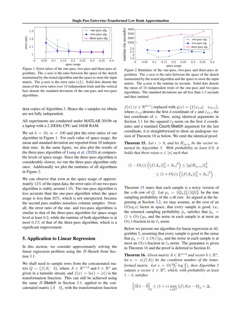
Figure 1. Error ratios of the one-pass, two-pass and three-pass al-gorithms. The x-axis is the ratio between the space of the sketchmaintained by the tested algorithm and the space to store the inputmatrix. The y-axis is the error ratio e(L). Solid dots denote themean of the error ratios over 10 independent trials and the verticalbars denote the standard deviation of the one-pass and two-passalgorithms.
dent copies of Algorithm 3. Hence the s samples we obtainare not fully independent.
All experiments are conducted under MATLAB 2019b ona laptop with a 2.20GHz CPU and 16GB RAM.
We set k = 10, m = 100 and plot the error ratios of ouralgorithm in Figure 1. For each value of space usage, themean and standard deviation are reported from 10 indepen-dent runs. In the same figure, we also plot the results ofthe three-pass algorithm of Liang et al. (2020) at compara-ble levels of space usage. Since the three-pass algorithm isconsiderably slower, we run the three-pass algorithm onlyonce. Additionally we plot the runtimes of all algorithmsin Figure 2.
We can observe that even at the space usage of approxi-mately 12% of the input data, the error ratio of our two-passalgorithm is stably around 1.05. The one-pass algorithm isless accurate than the one-pass algorithm when the spaceusage is less than 20%, which is not unexpected, becausethe second pass enables noiseless column samples. Over-all, the error ratio of the one- and two-pass algorithms issimilar to that of the three-pass algorithm for space usagelevel at least 0.2, while the runtime of both algorithms is atmost 0.1% of that of the three-pass algorithm, which is asignificant improvement.
5. Application to Linear RegressionIn this section, we consider approximately solving thelinear regression problem using the H-Sketch from Sec-tion 3.1.
We shall need to sample rows from the concatenated ma-trix Q =
(f(A) b
), where A ∈ Rn×d and b ∈ Rn are
given in a turnstile stream, and f(x) = ln(1 + |x|) is thetransformation function. This can still be achieved usingthe same H-Sketch in Section 3.1, applied to the con-catenated matrix
(A b
), with the transformation function
2500
3000
3500
4000
0 0.05 0.1 0.15 0.2 0.25 0.3 0.35 0.41.8
22.22.4
space usage
one-pass alg.two-pass alg.
three-pass alg.
runt
ime
(in
seco
nds)
Figure 2. Runtimes of the one-pass, two-pass and three-pass al-gorithms. The x-axis is the ratio between the space of the sketchmaintained by the tested algorithm and the space to store the inputmatrix. The y-axis is the runtime in seconds. Solid dots denotethe mean of 10 independent trials of the one-pass and two-passalgorithms. The standard deviations are all less than 1.5 secondsand thus omitted.
f(x) (x ∈ Rd+1) replaced with g(x) =(f(x1:d) xd+1
),
where x1:d denotes the first d coordinate of x and xd+1 thelast coordinate of x. Then, using identical arguments inSection 3.1 for the squared `2-norm on the first d coordi-nates and a standard Count-Sketch argument for the lastcoordinate, it is straightforward to show an analogous ver-sion of Theorem 10 as below. We omit the identical proof.
Theorem 15. Let ε > 0, and let Hj0,i0 be the vector re-turned by Algorithm 3. With probability at least 0.9, itholds that there exists u ∈ [n] such that
(1−O(ε))(‖f(Au)‖22 + |bu|2
)≤ ‖g(Hj0,i0)‖22
≤ (1 +O(ε))(‖f(Au)‖22 + |bu|2
).
Theorem 15 states that each sample is a noisy version ofthe u-th row of Q. Let pu = ‖Qu‖22/‖Q‖2F be the truesampling probability of the u-th row. As argued at the be-ginning at Section 3.2, we may assume, at the cost of anO(log s) factor in space, that every sample is good, i.e.,the returned sampling probability pu satisfies that pu =(1 ± O(ε))pu and the noise in each sample is at most anO(ε)-fraction in its `2 norm.
Below we present our algorithm for linear regression in Al-gorithm 5, assuming that every sample is good in the sensethat pu = (1 ± O(ε))pu and the noise in each sample is atmost an O(ε)-fraction in `2-norm. The guarantee is givenin Theorem 16 and the proof is deferred to Section D.
Theorem 16. Given matrix A ∈ Rn×d and vector b ∈ Rn,let κ = κ(f(A)) be the condition number of the trans-formed matrix. Let s = O(dκ
2
ε2 log dδ ), then Algorithm 5
outputs a vector x ∈ Rd, which, with probability at least1− δ, satisfies∥∥∥Mx− b
∥∥∥2≤ (1 + ε) min
x∈Rd‖f(A)x− b‖2 + ∆,
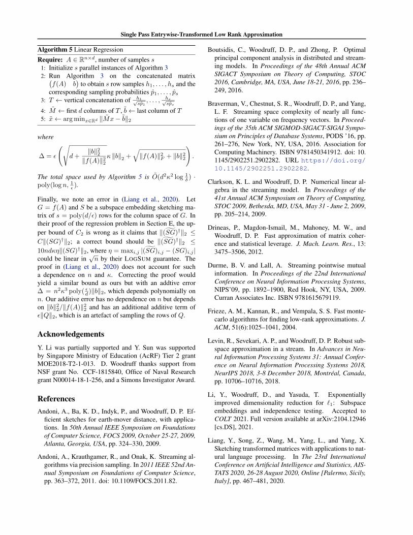
Single Pass Entrywise-Transformed Low Rank Approximation
Algorithm 5 Linear RegressionRequire: A ∈ Rn×d, number of samples s
1: Initialize s parallel instances of Algorithm 32: Run Algorithm 3 on the concatenated matrix(
f(A) b)
to obtain s row samples h1, . . . , hs and thecorresponding sampling probabilities p1, . . . , ps
3: T ← vertical concatenation of h1√sp1, . . . , hs√
sps
4: M ← first d columns of T , b← last column of T5: x← arg minx∈Rd ‖Mx− b‖2
where
∆ = ε
(√d+
‖b‖22‖f(A)‖22
κ ‖b‖2 +√‖f(A)‖2F + ‖b‖22
).
The total space used by Algorithm 5 is O(d2κ2 log 1δ ) ·
poly(log n, 1ε ).
Finally, we note an error in (Liang et al., 2020). LetG = f(A) and S be a subspace embedding sketching ma-trix of s = poly(d/ε) rows for the column space of G. Intheir proof of the regression problem in Section E, the up-per bound of C2 is wrong as it claims that ‖(SG)†‖2 ≤C‖(SG)†‖2; a correct bound should be ‖(SG)†‖2 ≤10ndκη‖(SG)†‖2, where η = maxi,j |(SG)i,j − (SG)i,j |could be linear in
√n by their LOGSUM guarantee. The
proof in (Liang et al., 2020) does not account for sucha dependence on n and κ. Correcting the proof wouldyield a similar bound as ours but with an addtive error∆ = n2κ3 poly( εd )‖b‖2, which depends polynomially onn. Our additive error has no dependence on n but dependson ‖b‖22/‖f(A)‖22 and has an additional additive term ofε‖Q‖2, which is an artefact of sampling the rows of Q.
AcknowledgementsY. Li was partially supported and Y. Sun was supportedby Singapore Ministry of Education (AcRF) Tier 2 grantMOE2018-T2-1-013. D. Woodruff thanks support fromNSF grant No. CCF-1815840, Office of Naval Researchgrant N00014-18-1-256, and a Simons Investigator Award.
ReferencesAndoni, A., Ba, K. D., Indyk, P., and Woodruff, D. P. Ef-
ficient sketches for earth-mover distance, with applica-tions. In 50th Annual IEEE Symposium on Foundationsof Computer Science, FOCS 2009, October 25-27, 2009,Atlanta, Georgia, USA, pp. 324–330, 2009.
Andoni, A., Krauthgamer, R., and Onak, K. Streaming al-gorithms via precision sampling. In 2011 IEEE 52nd An-nual Symposium on Foundations of Computer Science,pp. 363–372, 2011. doi: 10.1109/FOCS.2011.82.
Boutsidis, C., Woodruff, D. P., and Zhong, P. Optimalprincipal component analysis in distributed and stream-ing models. In Proceedings of the 48th Annual ACMSIGACT Symposium on Theory of Computing, STOC2016, Cambridge, MA, USA, June 18-21, 2016, pp. 236–249, 2016.
Braverman, V., Chestnut, S. R., Woodruff, D. P., and Yang,L. F. Streaming space complexity of nearly all func-tions of one variable on frequency vectors. In Proceed-ings of the 35th ACM SIGMOD-SIGACT-SIGAI Sympo-sium on Principles of Database Systems, PODS ’16, pp.261–276, New York, NY, USA, 2016. Association forComputing Machinery. ISBN 9781450341912. doi: 10.1145/2902251.2902282. URL https://doi.org/10.1145/2902251.2902282.
Clarkson, K. L. and Woodruff, D. P. Numerical linear al-gebra in the streaming model. In Proceedings of the41st Annual ACM Symposium on Theory of Computing,STOC 2009, Bethesda, MD, USA, May 31 - June 2, 2009,pp. 205–214, 2009.
Drineas, P., Magdon-Ismail, M., Mahoney, M. W., andWoodruff, D. P. Fast approximation of matrix coher-ence and statistical leverage. J. Mach. Learn. Res., 13:3475–3506, 2012.
Durme, B. V. and Lall, A. Streaming pointwise mutualinformation. In Proceedings of the 22nd InternationalConference on Neural Information Processing Systems,NIPS’09, pp. 1892–1900, Red Hook, NY, USA, 2009.Curran Associates Inc. ISBN 9781615679119.
Frieze, A. M., Kannan, R., and Vempala, S. S. Fast monte-carlo algorithms for finding low-rank approximations. J.ACM, 51(6):1025–1041, 2004.
Levin, R., Sevekari, A. P., and Woodruff, D. P. Robust sub-space approximation in a stream. In Advances in Neu-ral Information Processing Systems 31: Annual Confer-ence on Neural Information Processing Systems 2018,NeurIPS 2018, 3-8 December 2018, Montreal, Canada,pp. 10706–10716, 2018.
Li, Y., Woodruff, D., and Yasuda, T. Exponentiallyimproved dimensionality reduction for `1: Subspaceembeddings and independence testing. Accepted toCOLT 2021. Full version available at arXiv:2104.12946[cs.DS], 2021.
Liang, Y., Song, Z., Wang, M., Yang, L., and Yang, X.Sketching transformed matrices with applications to nat-ural language processing. In The 23rd InternationalConference on Artificial Intelligence and Statistics, AIS-TATS 2020, 26-28 August 2020, Online [Palermo, Sicily,Italy], pp. 467–481, 2020.
Single Pass Entrywise-Transformed Low Rank Approximation
Mahabadi, S., Razenshteyn, I. P., Woodruff, D. P., andZhou, S. Non-adaptive adaptive sampling on turnstilestreams. In Proccedings of the 52nd Annual ACMSIGACT Symposium on Theory of Computing, STOC2020, Chicago, IL, USA, June 22-26, 2020, pp. 1251–1264, 2020.
Upadhyay, J. Differentially private linear algebra in thestreaming model. arXiv preprint arXiv:1409.5414, 2014.
Woodruff, D. P. Low rank approximation lower bounds inrow-update streams. In Advances in Neural InformationProcessing Systems 27: Annual Conference on NeuralInformation Processing Systems 2014, December 8-132014, Montreal, Quebec, Canada, pp. 1781–1789, 2014.
Woodruff, D. P. and Zhong, P. Distributed low rank ap-proximation of implicit functions of a matrix. In 2016IEEE 32nd International Conference on Data Engineer-ing (ICDE), pp. 847–858. IEEE, 2016.