simultaneous estimation of both soil moisture and model parameters using particle filtering method...

Simultaneous estimation of both soil moisture and model

parameters using particle filtering method through

the assimilation of microwave signal

Jun Qin,1 Shunlin Liang,2 Kun Yang,1 Ichiro Kaihotsu,3 Ronggao Liu,4 and Toshio Koike5

Received 25 October 2008; revised 10 March 2009; accepted 3 June 2009; published 5 August 2009.

[1] Soil moisture is a very important variable in land surface processes. Both fieldmoisture measurements and estimates from modeling have their limitations when beingused to estimate soil moisture on a large spatial scale. Remote sensing is becoming apractical method to estimate soil moisture globally; however, the quality of current soilsurface moisture products needs to be improved in order to meet practical requirements.Data assimilation (DA) is a promising approach to merge model dynamics and remotesensing observations, thus having the potential to estimate soil moisture more accurately.In this study, a data assimilation algorithm, which couples the particle filter and the kernelsmoothing technique, is presented to estimate soil moisture and soil parameters frommicrowave signals. A simple hydrological model with a daily time step is utilized toreduce the computational burden in the process of data assimilation. An observationoperator based on the ratio of two microwave brightness temperatures at differentfrequencies is designed to link surface soil moisture with remote sensing measurements,and a sensitivity analysis of this operator is also conducted. Additionally, a variant ofparticle filtering method is developed for the joint estimation of soil moisture and soilparameters such as texture and porosity. This assimilation scheme is validated against fieldmoisture measurements at the CEOP/Mongolia experiment site and is found to estimatenear-surface soil moisture very well. The retrieved soil texture still contains largeuncertainties as the retrieved values cannot converge to fixed points or narrow rangeswhen using different initial soil texture values, but the retrieved soil porosity has relativelysmall uncertainties.

Citation: Qin, J., S. Liang, K. Yang, I. Kaihotsu, R. Liu, and T. Koike (2009), Simultaneous estimation of both soil moisture and

model parameters using particle filtering method through the assimilation of microwave signal, J. Geophys. Res., 114, D15103,

doi:10.1029/2008JD011358.

1. Introduction

[2] Soil moisture plays a significant role in the terrestrialwater cycle [Daly and Porporato, 2005; Hirabayashi et al.,2005; Reichle et al., 2007; Sheffield and Wood, 2007]. It isvery important to obtain information about soil moisturedue to its profound impacts on practical water resourceapplications such as flood forecasting, weather and climateprediction, crop growth monitoring, and water resource

management [Claussen, 1998; Davies and Allen, 1973;Drusch, 2007; Drusch and Viterbo, 2007; Foley, 1994;Schmugge et al., 2002; Texier et al., 1997]. There aretwo common methods to obtain the soil moisture status[Moradkhani, 2008]. One is to measure it in the field withinstruments. These measurements are merely representativeover a small spatial scale since the soil moisture has largespatial heterogeneity. It is not practical to densely installmany instruments on a large scale. The other is to simulatesoil moisture by running land surface models (LSMs) withmeteorological data and other parameters as inputs. Thesimulated soil moisture performs well when both the modelparameters and meteorological forcing are known with ahigh degree of precision and accuracy. This can be realizedat only a very limited number of sites, where a variety ofmeasurement instruments are installed. When running themodel on a large scale, it is very difficult to accuratelyobtain model inputs and parameter values.[3] Microwave remote sensing data has offered another

means to map land surface soil moisture on a large scale[Kerr et al., 2001; Njoku et al., 2003; Wagner et al., 2003].However, it also has many limitations and thus mapping

JOURNAL OF GEOPHYSICAL RESEARCH, VOL. 114, D15103, doi:10.1029/2008JD011358, 2009ClickHere

for

FullArticle

1Key Laboratory of Tibetan Environment Changes and Land SurfaceProcesses, Institute of Tibetan Plateau Research, Chinese Academy ofSciences, Beijing, China.

2Department of Geography, University of Maryland, College Park,Maryland, USA.

3Department of Natural and Environmental Sciences, Faculty ofIntegrated Arts and Sciences, Hiroshima University, Hiroshima, Japan.

4Institute of Geographic Sciences and Natural Resources Research,Chinese Academy of Sciences, Beijing, China.

5Department of Civil Engineering, School of Engineering, University ofTokyo, Tokyo, Japan.

Copyright 2009 by the American Geophysical Union.0148-0227/09/2008JD011358$09.00

D15103 1 of 13

http://dx.doi.org/10.1029/2008JD011358

results cannot satisfy the practical requirements. Dataassimilation (DA) methods can consistently couple bothmodeling and observations and thus yield superior soilmoisture retrievals [Entekhabi et al., 1994; Galantowicz etal., 1999; Houser et al., 1998; Margulis et al., 2002;McLaughlin, 2002; Reichle et al., 2001;Walker and Houser,2001]. Thus it has attracted much attention from researchersin many fields.[4] Data assimilation techniques can generally be divided

into two categories: sequential-based and cost-function-based methods. Sequentially based methods [Bertino et al.,2003], especially those based on a Monte Carlo approachsuch as Ensemble Kalman Filtering (EnKF [Evensen, 2003]),are currently popular in land data assimilation research andapplications since they can be applied to nonlinear anddiscontinuous models and be realized easily [Huang et al.,2008a, 2008b]. This is especially important in land surfacedata assimilation because there are many land surface param-eterizations which are not continuous or not differentiableand this makes it difficult or inefficient to use cost-function-based methods as assimilation algorithms. In addition, thecost-function-based method cannot directly consider uncer-tainties in atmospheric inputs which are used to drive a LSM.It just treats uncertainties included in inputs as one part ofmodel noise. These uncertainties can, however, be handledreadily in the sequential methods [Liang and Qin, 2008].[5] Reichle et al. [2002] used EnKF to assimilate L-band

(1.4 GHz) microwave brightness temperature observationsinto a LSM. Their research indicated that the EnKF is aflexible and robust DA option that gives satisfactory esti-mates even for moderate ensemble sizes although theupdating process is suboptimal. Crow [2003] and Crowand Wood [2003] applied EnKF to assimilate L-bandmicrowave data to correct for the impact of poorly sampledrainfall on land surface modeling of root-zone soil moistureand surface energy fluxes. The results suggested that theEnKF-based assimilation system is capable of correcting asubstantial fraction of model errors in root-zone soil mois-ture and latent heat flux predictions associated with the useof temporally sparse rainfall measurements as the forcingdata. Ni-Meister et al. [2006] assimilated retrieved soilsurface moisture from Scanning Multichannel MicrowaveRadiometer (SMMR) data using EnKF. Reichle et al. [2007]applied EnKF to assimilate retrieved soil surface moisturefrom the Advanced Microwave Sounding Radiometer-Earth Observing System (EOS) (AMSR-E) as observationsinto a LSM. Comparisons were also performed betweenEnKF and other Monte Carlo-based filtering methods [Zhouet al., 2006].[6] Most of the studies mentioned above assimilated

microwave brightness into a LSM with an hourly or sub-hourly time step rather than with a daily time step. It isbecause the microwave radiative transfer equation (RTE) asthe observation operator requires instantaneous soil surfaceand canopy temperatures as inputs, which have the apparentdiurnal variations, but the daily-based model lacks such atemporal resolution. It is obvious that significant computa-tional cost could be saved if a daily-basedmodel is used in theprocess of assimilation. Furthermore, most of previous landsurface assimilation studies focus on either retrieving statevariables such as soil moisture or estimating some model

parameters independently. Moreover, some aforementionedstudies assimilated L-band brightness temperature, which hasnot been available for large spatial regions. Other studiesassimilated retrieved soil surface moisture from AMSR-Eand/or SMMR data at a continental scale. In addition, allthese studies assumed that soil texture data or hydraulicproperties are available, although it is rather difficult toobtain their accurate values at a large scale. Few inves-tigations [Moradkhani et al., 2005a; Yang et al., 2007] putforward the idea of jointly retrieving state variables andmodel parameters, and perform assimilation experimentsusing a conceptual rainfall-runoff model and a complexLSM, respectively.[7] In this study, a simple model is used to characterize

the water movement in soils with a daily-based time step, anobservation operator is designed to link the AMSR-Emicrowave signal and soil surface moisture, and a variantof particle filtering method is used to simultaneouslyestimate soil surface moisture and soil parameters such astexture, and porosity, and surface parameters. Then, thewhole DA scheme is validated against the field measure-ments. In this paper, the DA scheme is first described.Validation results are then presented and finally followed bydiscussions and conclusions.

2. Data Assimilation Scheme

[8] A DA system consists of four parts: model dynamics,observation operator, assimilation algorithm, and errormodels [Lermusiaux and Robinson, 2001]. In the followingsubsections, details of these four parts are presented.

2.1. Land Surface Water Balance Model

[9] A land surface scheme to model the water balance ona daily basis is simplified from the Simple Biosphere Model2 (SiB2 [Sellers et al., 1996]). We aim to develop the dataassimilation system mainly for arid or semiarid areas; thusthe interception storage of the canopy can be ignored, sincethe leaf area index (LAI) normally peaks around 1.5. Thesoil column is vertically divided into three layers: surfacelayer, root zone layer, and recharge zone. The governingequations characterizing the water movement in the soil areas follows:

@q1@t¼ 1

D1

Pt � Q1;2 �1

rwEg

� �; ð1Þ

@q2@t¼ 1

D2

Q1;2 � Q2;3 �1

rwEtr

� �; ð2Þ

@q3@t¼ 1

D3

Q2;3 � Q3

� �; ð3Þ

where qi is volumetric soil moisture content of each layer,Di the soil thickness of each layer, Pt is the precipitation,Q1,2, Q2,3, and Q3 are soil water fluxes between layers andout of the bottom layer, Eg and Etr are evaporation from thesoil surface and transpiration from the vegetation canopy,respectively, and rw is the water density. Equations (1)–(3)

D15103 QIN ET AL.: SOIL MOISTURE BY DATA ASSIMILATION

2 of 13

D15103

are discretized on a daily basis using an implicit differencescheme. The formulas for soil water flux are as follows:

Qi;iþ1 ¼y i � y iþ1

0:5 Di þ Diþ1ð Þ þ 1

� �Kiy i � Kiþ1y iþ1

y iþ1 � y i

� �B

Bþ 3

� �;

ð4Þ

y i ¼ ysat

qiqsat

� ��B; ð5Þ

Ki ¼ Ksat

qiqsat

� �2Bþ3; ð6Þ

Ksat ¼ 7:0556 � 10�6:884þ0:0153�%sand ð7Þ

B ¼ 2:91þ 0:159 �%clay ð8Þ

where Ki is the hydraulic conductivity of each layer, y i thematrix potential of each layer, qsat the soil porosity, Ksat thehydraulic conductivity at saturation, and B the empiricalparameter related to soil texture, %sand the sand content,and %clay the clay content. The drainage out of the bottomlayer is assumed to be K3 and the surface runoff occurswhen surface soil water content q1 exceeds the porosity qsat.[10] Both the evaporation Eg from the soil surface and

transpiration Etr from the vegetation canopy are the impor-tant components in equations (1)–(3). There exist manymethods to compute the potential evapotranspiration on adaily basis, including Penman-Monteith, Priestley-Taylor,and so on. The actual evapotranspiration and its partitioninto evaporation and transpiration are needed in the calcu-lation of the water balance. In this study, a variant of thePriestley-Taylor equation [Davies and Allen, 1973] is takento estimate the daily actual evapotranspiration and thevegetation coverage is used to separate it. The daily evapo-transpiration process is parameterized as follows [Sau et al.,2004]:

ETa ¼ aD

Dþ gRn � 1� exp b

q1qsat

� �3" #( )

; ð9Þ

Eg ¼ ETa � 1� fvð Þ; ð10Þ

Etr ¼ ETa � fv; ð11Þ

fv ¼ 1� exp �0:5LAIð Þ; ð12Þ

where ETa denotes the actual evapotranspiration, a = 1.26the Priestly-Taylor constant, b the constraint coefficient,D the slope of the saturated vapor pressure with respectto the air temperature, g the psychometric constant, and fvthe vegetation coverage. The power 3 does not exist in its

original form of equation (9) and it is found that equation (9)performs better after adding an exponent of 3 [Nakayama etal., 1993].[11] An implicit scheme is used for the computation with

daily time step and is stable, but big errors may occurimmediately after a rainfall event. Nevertheless, such errorsmay be compensated to some degree by information fromsatellite signals.

2.2. Observation Operator and Microwave Data

[12] In this study, a microwave RTE is implemented tolink the surface soil moisture to satellite measurements. It isa Q-h model with minor revisions to include vegetationeffect. The concrete form of this RTE is as follows:

Tbp ¼ Tg 1� Gp

� �exp �tcð Þ þ Tc 1� wð Þ

� 1� exp �tcð Þ½ � 1þ Gp exp �tcð Þ� �

; ð13Þ

where the subscript p represents the vertical or horizontalpolarization, Gp the soil reflectivity, tc the vegetation opticaldepth, and w the vegetation single scattering albedo. A Q-hmodel is used to calculate the soil reflectivity as follows:

Gp ¼ 1� Qð ÞRp þ QRq

� �exp �hð Þ; ð14Þ

where the subscripts p denotes the vertical or horizontalpolarization, respectively, Q and h are empirical surfaceroughness parameters, and R the Fresnel power reflectivitywith a smooth soil surface. The R is determined using thefollowing equations:

Rp ¼cos g �

ffiffiffiffiffiffiffiffiffiffiffiffiffiffiffiffiffiffiffiffiffier � sin2 g

pcos g þ


p��

��2

; ð15Þ

Rq ¼er cos g �


per cos g þ


p��

��2

; ð16Þ

where p and q denote the horizontal and vertical polariza-tion, g the incident angle, and er the soil dielectric constant.The soil dielectric constant is computed as follows:

er ¼ 1þ 1� qsatð Þ eas � 1� �

þ qb1eafw � q1

h i1=a; ð17Þ

where es = 4.7 + 0.0j denotes the dielectric constant formineral soil, efw the dielectric constant of free water, a =0.65, and b the coefficient dependent upon the soil texture.The parameters in equations (13) and (14) are dependent onwave frequency and can be parameterized as follows:

h ¼ k � sð Þffiffiffiffiffiffiffiffiffiffiffiffi0:1 cos gp

; ð18Þ

Q ¼ Q0 k � sð Þ0:795; ð19Þ


3 of 13

D15103

tc ¼b0 100lð Þcwc

cos q; ð20Þ

wc ¼ exp LAI=3:3ð Þ � 1 ð21Þ

w ¼ 0:00083

l; ð22Þ

where l[m] is the wavelength, k the wave number definedas 2p/l, s the standard deviation of surface roughness,wc [kg m�2] the vegetation water content, andQ0, b

0, and cthe empirical coefficients. Equations (19) and (22) areempirical formulas fitted from limited microwave experi-mental data [Fujii, 2005] and were firstly used by Yang et al.[2007] to reduce the parameter number of the radiativetransfer equation.[13] As shown in equation (13), both the soil surface

temperature and the canopy temperature are importantfactors to determine the value of the simulated microwavebrightness temperature. Since the time step is one day in thismodel, the brightness temperature cannot be simulated atthe satellite overpassing times. So it is challenging todirectly assimilate the satellite-observed brightness temper-ature into the dynamics. However, this dilemma can beremoved by defining a ratio of two brightness temperaturesat different frequencies, which can reflect the soil wetness,based on the assumption that the soil surface temperatureand the canopy temperature have equal values. WhenAMSR-E data are used as the information source to beassimilated, a new index called the soil water ratio (SWR) isdefined in this study in accordance with equation (13) bycanceling out temperatures as follows:

SWR ¼T18:7bq

T6:9bq

¼1� Gq

� �exp �tcð Þ þ 1� wð Þ 1� exp �tcð Þ½ � 1þ Gq exp �tcð Þ

� �� 18:7

1� Gq

� �exp �tcð Þ þ 1� wð Þ 1� exp �tcð Þ½ � 1þ Gq exp �tcð Þ

� �� 6:9

where the superscript denotes the frequency and Tbq18.7 and

Tbq6.9 the vertical polarization brightness temperatures at

18.7 GHz and 6.9 GHz. The reason for choosing thevertical polarization temperatures in (23) is that they areless sensitive to vegetation heterogeneity than thehorizontal polarization temperatures. Up to now, thereare still two problems not to be resolved. One is that SWRdoes not completely eliminate the influence of temperaturesince Gq in equation (23) is a function of the dielectricconstant of free water which is in turn dependent on thesoil temperature. It is, however, found that SWR is notsensitive to the soil surface temperature and thus thistemperature can be replaced with the daily averaged airtemperature. The other is the issue of whether the definedSWR really has the capacity to reflect the soil wetness.The solutions to these two problems will be shown insection 4.

2.3. Assimilation Algorithm

[14] Mainstream sequential-based methods includeKalman Filtering (KF) and Particle Filtering (PF), and theirvariants. PF is also called sequential Monte Carlo filtering.

It has been applied in many engineering fields and attractedsome data assimilation practitioners since the posteriordistribution of the state vector can be represented withMonte Carlo samples and the Gaussian assumption can beavoided. KF and its variants, however, just evaluate themean and covariance of the posterior distribution. Thus PFcan better grasp the filtering density evolution of thenonlinear system in time than KF and its variants do. PFitself also has many variants such as the sampling impor-tance resampling filter (SIR). Han and Li [2008] make adetailed evaluation of PF, KF, and their variants andconclude that PF is suited to applications in land surfacedata assimilation according to both effectiveness and effi-ciency. Before moving on, some notations are introduced tofacilitate the following discussions.

xtþ1 ¼ f ðxt; ut; xÞ þ vt ð24Þ

where x denotes the model state vector, u the externalforcing data, x the model parameter vector, v the modelnoise, t the subscript for time step, and f(�) the modeloperator mapping the previous state xt to the next state xt + 1.

yt ¼ �hðxt ; xÞ þ et ð25Þ

where y denotes the observation vector, e the observationnoise, and �h(�) the observation operator. In this study, thestate vector x = [q1, q2, q3]

T, external forcing u = [Pt, Rn, Ta,LAI]T, x = [%sand, %clay, qsat, b, s, Q0, b

0, c]T, f (�) is thediscrete form from equations (1)–(3), and �h(�) is theequation (23).[15] In the framework of sequential filtering techniques,

the joint estimation of state variables and model parameterscan be performed through the state augmentation method

[Chen et al., 2005]. This approach regards model parame-ters to be estimated as part of the state vector. The newaugmented state vector becomes [xT, xT]T. Conventionally,the random walk model is assumed for the time evolution ofx [Moradkhani et al., 2005b]. However, this model resultsin much larger variances of x than actual ones in theestimation process. The kernel smoothing technique iscurrently introduced to remove this feature.[16] In this study, both the SIR method and kernel

smoothing technique are combined [Chen et al., 2005] tomerge the dynamics and the observations for simultaneousestimation of the model states and parameters. Main stepsfor the entire assimilation algorithm [Thomas, 2006] are asfollows:

Step 1: for t = 0, sample {~x0(i)}i = 1

N : p(x0) and {~x0(i)}i=1

N :p(x0);

Step 2: draw {xt+1(i) }i=1

N : N(xt+1|mt(i), h2 � Vt), where mt

(i) =

(ffiffiffiffiffiffiffiffiffiffiffiffi1� l2p

)~xt(i) � (1 �

ffiffiffiffiffiffiffiffiffiffiffiffi1� l2p

)~x ið Þt , Vt denotes the covari-

ance matrix of ~xt, and s an adjustable parameter;

ð23Þ


4 of 13

D15103

Step 3: draw {xt+1(i) }i=1

N : p(xt+1|~xt(i), xt+1

(i) ), where xt+1(i) = f (~xt

(i),

ut(i), xt+1

(i) ) + vt(i), vt

(i) : p(vt);

Step 4: compute weights wt+1(i) =

p ytþ1jx ið Þtþ1;x

ið Þtþ1ð ÞPN

i¼1p ytþ1jx ið Þ

tþ1;xið Þtþ1ð Þ

, where

p(yt+1 |xt+1(i) , xt+1

(i) ) denotes the value of p(yt+1 j (xt+1(i) , xt+1(i) ));

Step 5: resample {xt + 1(i) , xt + 1

(i) }i = 1N with replacement according

to weightswt+1(i) }i=1

N in order to get {~xt+1(i) , ~xt+1

(i) }i=1N with weights

{1/N}i=1N ;

Step 6: set t = t + 1 and go to step 2.

[17] The parameter l is an adjustable constant for consid-ering that the model parameters to be estimated are tochange quickly or slowly. l is set to 0 < l < 0.2 for slowlyvarying parameters and 0.8 < l < 1.0 for rapidly varyingparameters. In this work, only variances of each modelparameter are computed and nondiagonal elements are set tozero for the covariance matrix Vt in Step 2 above. Thusdifferent values of l can be easily set independently fordetermination of different parameters.

2.4. Error Models

[18] One significant advantage of sequential-based dataassimilation methods is that uncertainties, which are frommodel structure, model parameters, and inputs, etc., can behandled explicitly in their own framework. As shown inabove subsections, there are four error sources, includingerrors in the model dynamics, observations, input forcing,and model parameters, respectively. All of these errors canbe divided into biased and unbiased noises. Only theunbiased part in these errors is taken into account in thisstudy. The error model must be specified for each errorsource.[19] As summarized by Hamill [2006], four methods can

be applied to parameterize uncertainties in model dynamics.The so-called covariance inflation approach is used andcoupled with the assimilation algorithm. Before assimilatingobservation information into dynamics, deviations of par-ticles around their mean are inflated by a factor r, which is alittle bit greater than 1.0, as follows:

xið Þt r x

ið Þt � x

ið Þt

� �þ x

ið Þt ð26Þ

where the operation denotes the replacement of theprevious value of xt

(i). It is found that a moderate inflationimproves the assimilation accuracy. More details can beobtained in the work of Hamill [2006]. One advantage ofsequential data assimilation methods over variational ones isthat errors in input forcing can be explicitly considered byadding perturbations to them according to some errorparameterizations. In this work, error models for inputs aretaken as the following uniform probability distributionfunction (PDF):

uið Þt ¼ ut 1:0þ zð Þ z : U �d;þd½ � ð27Þ

where z obeys the uniform distribution and d reflects theknowledge of inputs. Different values of d can be assignedto each component in u = [Pt, Rn, Ta, LAI]T. Similarly,uniform distributions are also assumed for the parametererror models. The observation error model is assumed to beGaussian.

3. Sensitivity Study of Soil Water Ratio

[20] As mentioned in section 2.2, two issues with SWRneed to be addressed. As for the first problem, thevariance-based sensitivity analysis method is applied todetermine the global sensitivity of SWR to each inputparameter in equation (23). The variance-based sensitivitymethod is briefly introduced below [Helton et al., 2006].[21] The entire SWR formula can be denoted by Y = �h(X)

where Y means SWR, X the input parameters, and �h(�) theequation (23), as given in the previous section. If eachcomponent of vector X = [x1, x2, � , xnX]T is considered to bean independent random variable, then the variance VY of Ycan be decomposed and expressed as:

VY ¼Xi

Vi þXi<j

VijþXi<j<k

Vijkþ � � � þ V12...nX ð28Þ

where Vi is the contribution of xi to VY, Vij thecontribution of the interaction of xi and xj to VY, and soon up to V12 . . . nX, which is the contribution of theinteraction of x1, x2, � � �, xnX to VY. Two types ofsensitivity indices can be defined as:

Si ¼Vi

VY

and ð29Þ

STi ¼VY � V i

VY

where V~i is the sum of all variance terms which do notinclude the index i. Si is the first-order sensitivity indexfor the ith parameter. This index characterizes the maininfluence of parameter xi on the output variable Y andmeasures the variance reduction that would be achievedby fixing that parameter. STi is the total sensitivity indexfor the ith parameter and measures the sum of all effectsrelated to this parameter, considering the interactionbetween the ith parameter and other ones.[22] The Monte Carlo based method can be used to

evaluate these indices. The computation steps are as follows:

Step 1: generate two sets of random samples according togiven distributions to inputs X

Xað Þ

i ¼ x að Þi1; x að Þ

i2; � � � ; x að Þ

i;nX

h i; i ¼ 1; 2; . . . ; nS

and ð30Þ

Xbð Þ

i ¼ x bð Þi1; x bð Þ

i2; � � � ; x bð Þ

i;nX

h i; i ¼ 1; 2; . . . ; nS


5 of 13

D15103

in which nS is the number of samples.

Step 2: estimate the sample mean and variance of Y as

EY ¼XnSi¼1

�h Xað Þ

i

� �nS

and ð31Þ

V Y ¼XnSi¼1

�h2 Xað Þ

i

� �nS

� E2

Y

Step 3: calculate some intermediate parameters as

V i ¼1

nS

XnSp¼1

�h xað Þp ið Þ; x

að Þpi

� ��h x

bð Þp ið Þ; x

að Þpi

� �� E

2

Y

and ð32Þ

V i ¼1

nS

XnSp¼1

�h xað Þp ið Þ; x

að Þpi

� ��h x

að Þp ið Þ; x

bð Þpi

� �� E

2

Y

Step 4: evaluate sensitivity indices as follows:

Si ¼ V i=V Y

and ð33ÞSTi ¼ 1� V i=V Y

� �V Y

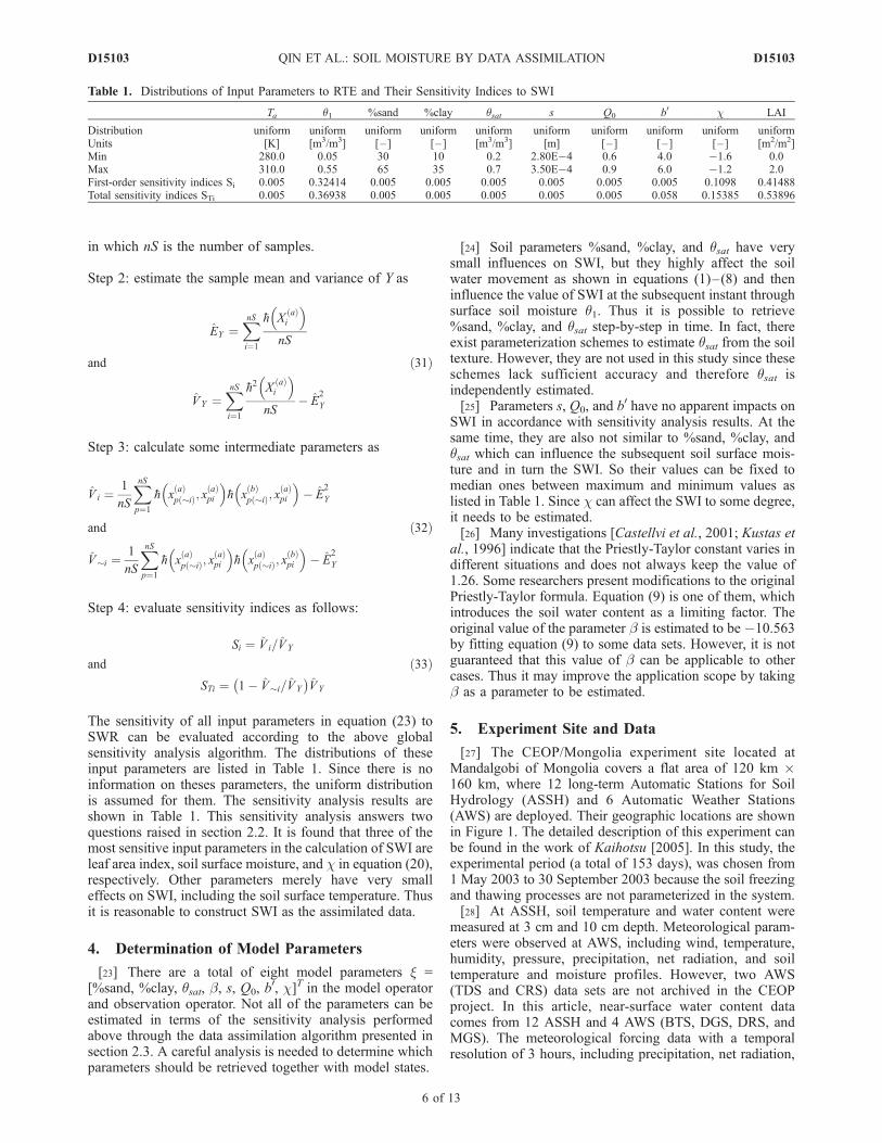
The sensitivity of all input parameters in equation (23) toSWR can be evaluated according to the above globalsensitivity analysis algorithm. The distributions of theseinput parameters are listed in Table 1. Since there is noinformation on theses parameters, the uniform distributionis assumed for them. The sensitivity analysis results areshown in Table 1. This sensitivity analysis answers twoquestions raised in section 2.2. It is found that three of themost sensitive input parameters in the calculation of SWI areleaf area index, soil surface moisture, and c in equation (20),respectively. Other parameters merely have very smalleffects on SWI, including the soil surface temperature. Thusit is reasonable to construct SWI as the assimilated data.

4. Determination of Model Parameters

[23] There are a total of eight model parameters x =[%sand, %clay, qsat, b, s, Q0, b

0, c]T in the model operatorand observation operator. Not all of the parameters can beestimated in terms of the sensitivity analysis performedabove through the data assimilation algorithm presented insection 2.3. A careful analysis is needed to determine whichparameters should be retrieved together with model states.

[24] Soil parameters %sand, %clay, and qsat have verysmall influences on SWI, but they highly affect the soilwater movement as shown in equations (1)–(8) and theninfluence the value of SWI at the subsequent instant throughsurface soil moisture q1. Thus it is possible to retrieve%sand, %clay, and qsat step-by-step in time. In fact, thereexist parameterization schemes to estimate qsat from the soiltexture. However, they are not used in this study since theseschemes lack sufficient accuracy and therefore qsat isindependently estimated.[25] Parameters s, Q0, and b0 have no apparent impacts on

SWI in accordance with sensitivity analysis results. At thesame time, they are also not similar to %sand, %clay, andqsat which can influence the subsequent soil surface mois-ture and in turn the SWI. So their values can be fixed tomedian ones between maximum and minimum values aslisted in Table 1. Since c can affect the SWI to some degree,it needs to be estimated.[26] Many investigations [Castellvi et al., 2001; Kustas et

al., 1996] indicate that the Priestly-Taylor constant varies indifferent situations and does not always keep the value of1.26. Some researchers present modifications to the originalPriestly-Taylor formula. Equation (9) is one of them, whichintroduces the soil water content as a limiting factor. Theoriginal value of the parameter b is estimated to be �10.563by fitting equation (9) to some data sets. However, it is notguaranteed that this value of b can be applicable to othercases. Thus it may improve the application scope by takingb as a parameter to be estimated.

5. Experiment Site and Data

[27] The CEOP/Mongolia experiment site located atMandalgobi of Mongolia covers a flat area of 120 km �160 km, where 12 long-term Automatic Stations for SoilHydrology (ASSH) and 6 Automatic Weather Stations(AWS) are deployed. Their geographic locations are shownin Figure 1. The detailed description of this experiment canbe found in the work of Kaihotsu [2005]. In this study, theexperimental period (a total of 153 days), was chosen from1 May 2003 to 30 September 2003 because the soil freezingand thawing processes are not parameterized in the system.[28] At ASSH, soil temperature and water content were

measured at 3 cm and 10 cm depth. Meteorological param-eters were observed at AWS, including wind, temperature,humidity, pressure, precipitation, net radiation, and soiltemperature and moisture profiles. However, two AWS(TDS and CRS) data sets are not archived in the CEOPproject. In this article, near-surface water content datacomes from 12 ASSH and 4 AWS (BTS, DGS, DRS, andMGS). The meteorological forcing data with a temporalresolution of 3 hours, including precipitation, net radiation,

Table 1. Distributions of Input Parameters to RTE and Their Sensitivity Indices to SWI

Ta q1 %sand %clay qsat s Q0 b0 c LAI

Distribution uniform uniform uniform uniform uniform uniform uniform uniform uniform uniformUnits [K] [m3/m3] [– ] [– ] [m3/m3] [m] [– ] [– ] [– ] [m2/m2]Min 280.0 0.05 30 10 0.2 2.80E�4 0.6 4.0 �1.6 0.0Max 310.0 0.55 65 35 0.7 3.50E�4 0.9 6.0 �1.2 2.0First-order sensitivity indices Si 0.005 0.32414 0.005 0.005 0.005 0.005 0.005 0.005 0.1098 0.41488Total sensitivity indices STi 0.005 0.36938 0.005 0.005 0.005 0.005 0.005 0.058 0.15385 0.53896


6 of 13

D15103

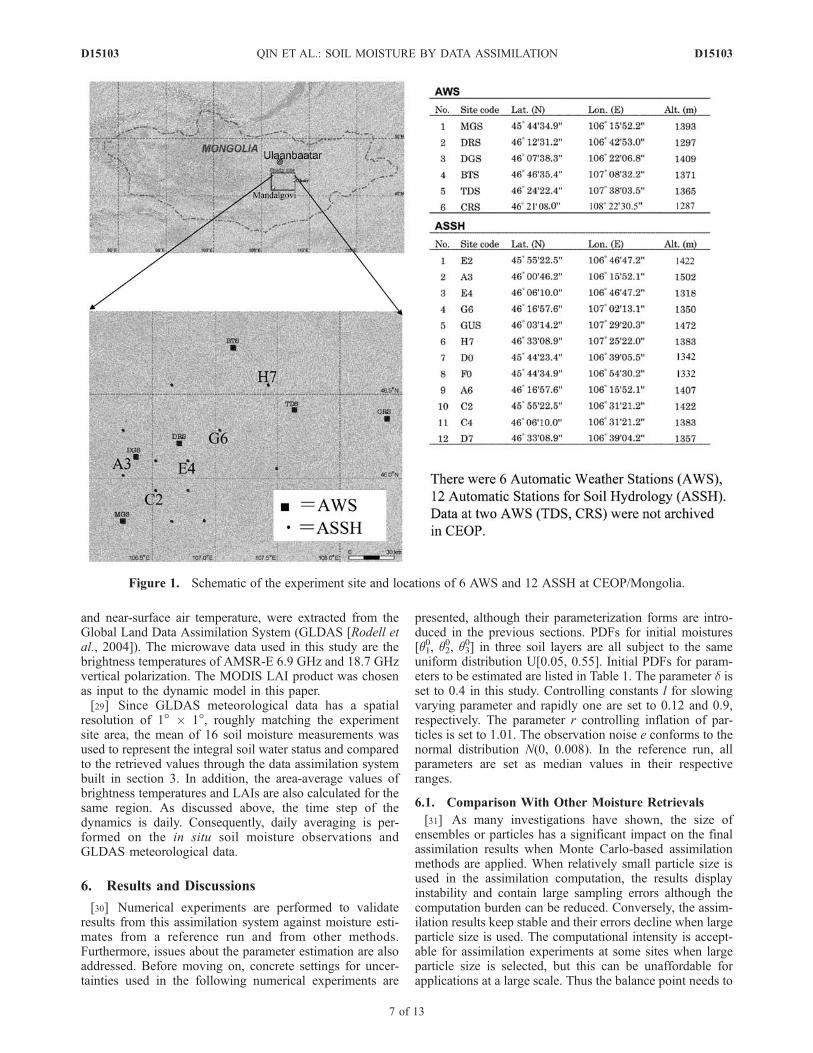
and near-surface air temperature, were extracted from theGlobal Land Data Assimilation System (GLDAS [Rodell etal., 2004]). The microwave data used in this study are thebrightness temperatures of AMSR-E 6.9 GHz and 18.7 GHzvertical polarization. The MODIS LAI product was chosenas input to the dynamic model in this paper.[29] Since GLDAS meteorological data has a spatial

resolution of 1� � 1�, roughly matching the experimentsite area, the mean of 16 soil moisture measurements wasused to represent the integral soil water status and comparedto the retrieved values through the data assimilation systembuilt in section 3. In addition, the area-average values ofbrightness temperatures and LAIs are also calculated for thesame region. As discussed above, the time step of thedynamics is daily. Consequently, daily averaging is per-formed on the in situ soil moisture observations andGLDAS meteorological data.

6. Results and Discussions

[30] Numerical experiments are performed to validateresults from this assimilation system against moisture esti-mates from a reference run and from other methods.Furthermore, issues about the parameter estimation are alsoaddressed. Before moving on, concrete settings for uncer-tainties used in the following numerical experiments are

presented, although their parameterization forms are intro-duced in the previous sections. PDFs for initial moistures[q1

0, q20, q3

0] in three soil layers are all subject to the sameuniform distribution U[0.05, 0.55]. Initial PDFs for param-eters to be estimated are listed in Table 1. The parameter d isset to 0.4 in this study. Controlling constants l for slowingvarying parameter and rapidly one are set to 0.12 and 0.9,respectively. The parameter r controlling inflation of par-ticles is set to 1.01. The observation noise e conforms to thenormal distribution N(0, 0.008). In the reference run, allparameters are set as median values in their respectiveranges.

6.1. Comparison With Other Moisture Retrievals

[31] As many investigations have shown, the size ofensembles or particles has a significant impact on the finalassimilation results when Monte Carlo-based assimilationmethods are applied. When relatively small particle size isused in the assimilation computation, the results displayinstability and contain large sampling errors although thecomputation burden can be reduced. Conversely, the assim-ilation results keep stable and their errors decline when largeparticle size is used. The computational intensity is accept-able for assimilation experiments at some sites when largeparticle size is selected, but this can be unaffordable forapplications at a large scale. Thus the balance point needs to

Figure 1. Schematic of the experiment site and locations of 6 AWS and 12 ASSH at CEOP/Mongolia.


7 of 13

D15103

be found for the particle size in the assimilation practice,around which both the computational cost and assimilationprecision are all acceptable. For this purpose, a series oftrials are performed using different particle sizes in accor-dance with assimilation settings in preceding sections. Theanalysis indicates that a particle size of 500 is large enoughto achieve stable results. In the following, all experimentsand analyses are conducted based upon a 500-particle size.[32] In order to verify the effectiveness of the data

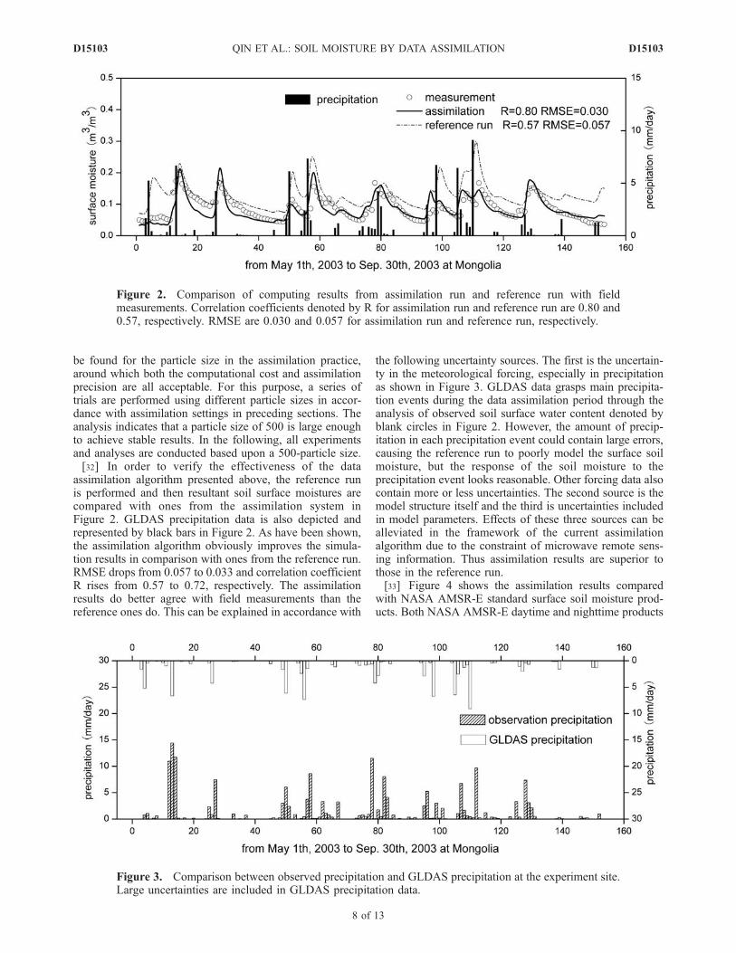
assimilation algorithm presented above, the reference runis performed and then resultant soil surface moistures arecompared with ones from the assimilation system inFigure 2. GLDAS precipitation data is also depicted andrepresented by black bars in Figure 2. As have been shown,the assimilation algorithm obviously improves the simula-tion results in comparison with ones from the reference run.RMSE drops from 0.057 to 0.033 and correlation coefficientR rises from 0.57 to 0.72, respectively. The assimilationresults do better agree with field measurements than thereference ones do. This can be explained in accordance with

the following uncertainty sources. The first is the uncertain-ty in the meteorological forcing, especially in precipitationas shown in Figure 3. GLDAS data grasps main precipita-tion events during the data assimilation period through theanalysis of observed soil surface water content denoted byblank circles in Figure 2. However, the amount of precip-itation in each precipitation event could contain large errors,causing the reference run to poorly model the surface soilmoisture, but the response of the soil moisture to theprecipitation event looks reasonable. Other forcing data alsocontain more or less uncertainties. The second source is themodel structure itself and the third is uncertainties includedin model parameters. Effects of these three sources can bealleviated in the framework of the current assimilationalgorithm due to the constraint of microwave remote sens-ing information. Thus assimilation results are superior tothose in the reference run.[33] Figure 4 shows the assimilation results compared

with NASA AMSR-E standard surface soil moisture prod-ucts. Both NASA AMSR-E daytime and nighttime products

Figure 2. Comparison of computing results from assimilation run and reference run with fieldmeasurements. Correlation coefficients denoted by R for assimilation run and reference run are 0.80 and0.57, respectively. RMSE are 0.030 and 0.057 for assimilation run and reference run, respectively.

Figure 3. Comparison between observed precipitation and GLDAS precipitation at the experiment site.Large uncertainties are included in GLDAS precipitation data.


8 of 13

D15103

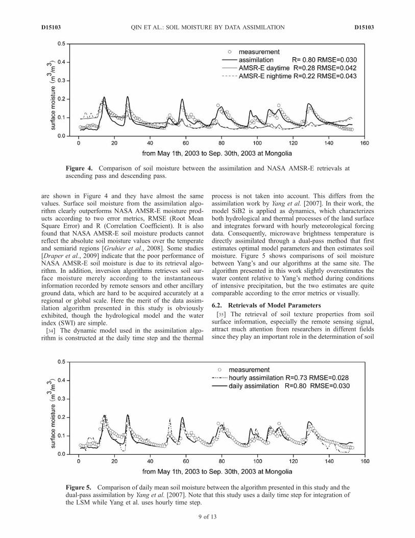
are shown in Figure 4 and they have almost the samevalues. Surface soil moisture from the assimilation algo-rithm clearly outperforms NASA AMSR-E moisture prod-ucts according to two error metrics, RMSE (Root MeanSquare Error) and R (Correlation Coefficient). It is alsofound that NASA AMSR-E soil moisture products cannotreflect the absolute soil moisture values over the temperateand semiarid regions [Gruhier et al., 2008]. Some studies[Draper et al., 2009] indicate that the poor performance ofNASA AMSR-E soil moisture is due to its retrieval algo-rithm. In addition, inversion algorithms retrieves soil sur-face moisture merely according to the instantaneousinformation recorded by remote sensors and other ancillaryground data, which are hard to be acquired accurately at aregional or global scale. Here the merit of the data assim-ilation algorithm presented in this study is obviouslyexhibited, though the hydrological model and the waterindex (SWI) are simple.[34] The dynamic model used in the assimilation algo-

rithm is constructed at the daily time step and the thermal

process is not taken into account. This differs from theassimilation work by Yang et al. [2007]. In their work, themodel SiB2 is applied as dynamics, which characterizesboth hydrological and thermal processes of the land surfaceand integrates forward with hourly meteorological forcingdata. Consequently, microwave brightness temperature isdirectly assimilated through a dual-pass method that firstestimates optimal model parameters and then estimates soilmoisture. Figure 5 shows comparisons of soil moisturebetween Yang’s and our algorithms at the same site. Thealgorithm presented in this work slightly overestimates thewater content relative to Yang’s method during conditionsof intensive precipitation, but the two estimates are quitecomparable according to the error metrics or visually.

6.2. Retrievals of Model Parameters

[35] The retrieval of soil texture properties from soilsurface information, especially the remote sensing signal,attract much attention from researchers in different fieldssince they play an important role in the determination of soil

Figure 4. Comparison of soil moisture between the assimilation and NASA AMSR-E retrievals atascending pass and descending pass.

Figure 5. Comparison of daily mean soil moisture between the algorithm presented in this study and thedual-pass assimilation by Yang et al. [2007]. Note that this study uses a daily time step for integration ofthe LSM while Yang et al. uses hourly time step.


9 of 13

D15103

hydraulic and thermal properties, which greatly affect thesoil water and heat movement. However, barely effectivevalues could be retrieved for each pixel with remote sensinginformation as constraints, because the variability of soilproperties in both horizontal and vertical directions is ratherlarge and there is not enough information to retrieve theseheterogeneous properties.[36] In this work, model parameters are also estimated

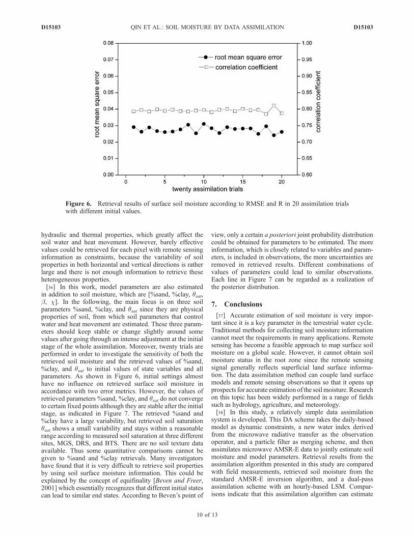
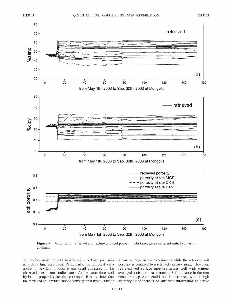
in addition to soil moisture, which are [%sand, %clay, qsat,b, c]. In the following, the main focus is on three soilparameters %sand, %clay, and qsat since they are physicalproperties of soil, from which soil parameters that controlwater and heat movement are estimated. These three param-eters should keep stable or change slightly around somevalues after going through an intense adjustment at the initialstage of the whole assimilation. Moreover, twenty trials areperformed in order to investigate the sensitivity of both theretrieved soil moisture and the retrieved values of %sand,%clay, and qsat to initial values of state variables and allparameters. As shown in Figure 6, initial settings almosthave no influence on retrieved surface soil moisture inaccordance with two error metrics. However, the values ofretrieved parameters %sand, %clay, and qsat do not convergeto certain fixed points although they are stable after the initialstage, as indicated in Figure 7. The retrieved %sand and%clay have a large variability, but retrieved soil saturationqsat shows a small variability and stays within a reasonablerange according to measured soil saturation at three differentsites, MGS, DRS, and BTS. There are no soil texture dataavailable. Thus some quantitative comparisons cannot begiven to %sand and %clay retrievals. Many investigatorshave found that it is very difficult to retrieve soil propertiesby using soil surface moisture information. This could beexplained by the concept of equifinality [Beven and Freer,2001] which essentially recognizes that different initial statescan lead to similar end states. According to Beven’s point of

view, only a certain a posteriori joint probability distributioncould be obtained for parameters to be estimated. The moreinformation, which is closely related to variables and param-eters, is included in observations, the more uncertainties areremoved in retrieved results. Different combinations ofvalues of parameters could lead to similar observations.Each line in Figure 7 can be regarded as a realization ofthe posterior distribution.

7. Conclusions

[37] Accurate estimation of soil moisture is very impor-tant since it is a key parameter in the terrestrial water cycle.Traditional methods for collecting soil moisture informationcannot meet the requirements in many applications. Remotesensing has become a feasible approach to map surface soilmoisture on a global scale. However, it cannot obtain soilmoisture status in the root zone since the remote sensingsignal generally reflects superficial land surface informa-tion. The data assimilation method can couple land surfacemodels and remote sensing observations so that it opens upprospects for accurate estimation of the soilmoisture. Researchon this topic has been widely performed in a range of fieldssuch as hydrology, agriculture, and meteorology.[38] In this study, a relatively simple data assimilation

system is developed. This DA scheme takes the daily-basedmodel as dynamic constraints, a new water index derivedfrom the microwave radiative transfer as the observationoperator, and a particle filter as merging scheme, and thenassimilates microwave AMSR-E data to jointly estimate soilmoisture and model parameters. Retrieval results from theassimilation algorithm presented in this study are comparedwith field measurements, retrieved soil moisture from thestandard AMSR-E inversion algorithm, and a dual-passassimilation scheme with an hourly-based LSM. Compar-isons indicate that this assimilation algorithm can estimate

Figure 6. Retrieval results of surface soil moisture according to RMSE and R in 20 assimilation trialswith different initial values.


10 of 13

D15103

soil surface moisture with satisfactory speed and precisionat a daily time resolution. Particularly, the temporal vari-ability of AMR-E product is too small compared to theobserved one in our studied area. At the same time, soilhydraulic properties are also estimated. Results show thatthe retrieved soil texture cannot converge to a fixed value or

a narrow range in our experiments while the retrieved soilporosity is confined to a relatively narrow range. However,retrieved soil surface moisture agrees well with station-averaged moisture measurements. Soil moisture in the rootzone or deep zone could not be retrieved with a highaccuracy since there is no sufficient information to derive

Figure 7. Variation of retrieved soil texture and soil porosity with time, given different initial values in20 trials.


11 of 13

D15103

relevant soil parameters, which possibly change with thesoil depth. Some researchers also find this problem that thewater content in the root zone cannot be easily retrieved,just relying on the soil surface moisture information withoutaccurate soil hydraulic properties.

[39] Acknowledgments. This work was supported by the ChineseNatural Science Foundation under contract 40701129, the ‘‘100-Talent’’Project of the Chinese Academy of Sciences, Chinese 863 project undercontract 2006AA01A120, and Data Sharing Network of Earth SystemScience under contract 2005DKA32300. We thank Dr. Carol Russell forEnglish editing. AMPEX was implemented in the framework of NASDA-JRA ‘‘Ground Truth for Evaluation of Soil Moisture and Geophysical/Vegetation parameters Related to Ground Surface Conditions with AMSRand GLI in the Mongolian Plateau’’ (PI: Prof. Ichirow Kaihotsu, Universityof Hiroshima). The Mongolian partnership is among the Institute ofMeteorology and Hydrology, the National Agency for Meteorology,Hydrology, and Environment Monitoring of Mongolia.

ReferencesBertino, L., et al. (2003), Sequential data assimilation techniques in ocea-nography, Int. Stat. Rev., 71, 223–241.

Beven, K., and J. Freer (2001), Equifinality, data assimilation, and uncer-tainty estimation in mechanistic modelling of complex environmentalsystems using the GLUE methodology, J. Hydrol., 249, 11–29.

Castellvi, F., et al. (2001), Comparison of methods for applying the Priestley-Taylor equation at a regional scale, Hydrol. Processes, 15, 1609–1620.

Chen, T., et al. (2005), Particle filters for state and parameter estimation inbatch processes, J. Process Control, 15, 665–673.

Claussen, M. (1998), On multiple solutions of the atmosphere-vegetationsystem in present-day climate, Global Change Biol., 4, 549–559.

Crow, W. T. (2003), Correcting land surface model predictions for theimpact of temporally sparse rainfall rate measurements using an ensembleKalman filter and surface brightness temperature observations, J. Hydro-meteorol., 4, 960–973.

Crow, W. T., and E. F. Wood (2003), The assimilation of remotely sensedsoil brightness temperature imagery into a land surface model usingEnsemble Kalman filtering: A case study based on ESTAR measurementsduring SGP97, Adv. Water Resour., 26, 137–149.

Daly, E., and A. Porporato (2005), A review of soil moisture dynamics:From rainfall infiltration to ecosystem response, Environ. Eng. Sci., 22,9–24.

Davies, J. A., and C. D. Allen (1973), Equilibrium, potential and actualevaporation from cropped surfaces in southern Ontario, J. Appl. Meteorol.,12, 649–657.

Draper, C. S., et al. (2009), An evaluation of AMSR-E derived soil moistureover Australia, Remote Sens. Environ., 113, 703–710.

Drusch, M. (2007), Initializing numerical weather prediction models withsatellite derived surface soil moisture: Data assimilation experiments withECMWF’s Integrated Forecast System and the TMI soil moisture dataset, J. Geophys. Res., 112, D03102, doi:10.1029/2006JD007478.

Drusch, M., and P. Viterbo (2007), Assimilation of screen-level variables inECMWF’s integrated forecast system: A study on the impact on theforecast quality and analyzed soil moisture, Mon. Weather Rev., 135,300–314.

Entekhabi, D., et al. (1994), Solving the inverse problem for soil moistureand temperature profiles by sequential assimilation of multifrequencyremotely sensed observations, Geosci. Remote Sens., IEEE Trans., 32,438–448.

Evensen, G. (2003), The ensemble Kalman filter: Theoretical formulationand practical implementation, Ocean Dyn., 53, 343–367.

Foley, J. A. (1994), The sensitivity of the terrestrial biosphere to climaticchange: A simulation of themiddle Holocene,Global Biogeochem. Cycles,8, 505–525.

Fujii, H. (2005), Development of a microwave radiative transfer model forvegetated land surface based on comprehensive in-situ observations,Ph.D. thesis, Univ. of Tokyo, Japan.

Galantowicz, J. F., et al. (1999), Tests of sequential data assimilation forretrieving profile soil moisture and temperature from observed L-bandradiobrightness, Geosci. Remote Sens., IEEE Trans., 37, 1860–1870.

Gruhier, C., et al. (2008), Evaluation of AMSR-E soil moisture productbased on ground measurements over temperate and semi-arid regions,Geophys. Res. Lett., 35, L10405, doi:10.1029/2008GL033330.

Hamill, T. M. (2006), Ensemble-based atmospheric data assimilation,in Predictability of Weather and Climate, edited by T. Palmer andR. Hagedorn, pp. 124–156, Cambridge Univ. Press., New York.

Han, X., and X. Li (2008), An evaluation of the nonlinear/non-Gaussianfilters for the sequential data assimilation, Remote Sens. Environ., 112,1434–1449.

Helton, J. C., et al. (2006), Survey of sampling-based methods for uncer-tainty and sensitivity analysis, Reliab. Eng. Syst. Saf., 91, 1175–1209.

Hirabayashi, Y., et al. (2005), A 100-year (1901–2000) global retrospectiveestimation of the terrestrial water cycle, J. Geophys. Res., 110, D19101,doi:10.1029/2004JD005492.

Houser, P. R., et al. (1998), Integration of soil moisture remote sensing andhydrologic modeling using data assimilation, Water Resour. Res., 34,3405–3420.

Huang, C., et al. (2008a), Retrieving soil temperature profile by assimilat-ing MODIS LST products with ensemble Kalman filter, Remote Sens.Environ., 112, 1320–1336.

Huang, C., et al. (2008b), Experiments of one-dimensional soil moistureassimilation system based on ensemble Kalman filter, Remote Sens.Environ., 112, 888–900.

Kaihotsu, I., T. Yamanaka, T. Koike, D. Oyunbaatar, and G. Davaa (Eds.)(2005), Ground truth for evaluation of soil moisture and geophysical/vegetation parameters related to ground surface conditions with AMSRand GLI in the Mongolian Plateau, in Ground-based Observations for theADEOS II/AQUA Validation in the Mongolian Plateau, pp. 5–21, JapanAerosp. Explor. Agency.

Kerr, Y. H., et al. (2001), Soil moisture retrieval from space: The SoilMoisture and Ocean Salinity (SMOS) mission, Geosci. Remote Sens.,IEEE Trans., 39, 1729–1735.

Kustas, W. P., et al. (1996), Variability in surface energy flux partitioningduring Washita’92: Resulting effects on Penman-Monteith and Priestley-Taylor parameters, Agric. For. Meteorol., 82, 171–193.

Lermusiaux, P. F. J., and A. R. Robinson (2001), Data assimilation inmodels, in Encyclopedia of Ocean Sciences, edited by J. Steel et al.,pp. 623–634, Academic, London.

Liang, S., and J. Qin (2008), Data assimilation methods for land surfacevariable estimation, in Advances in Land Remote Sensing, edited byS. Liang, pp. 313–339, Springer, Netherlands.

Margulis, S. A., D. McLaughlin, D. Entekhabi, and S. Dunne (2002), Landdata assimilation and estimation of soil moisture using measurementsfrom the Southern Great Plains 1997 Field Experiment, Water Resour.Res., 38(12), 1299, doi:10.1029/2001WR001114.

McLaughlin, D. (2002), An integrated approach to hydrologic data assim-ilation: Interpolation, smoothing, and filtering, Adv. Water Resour., 25,1275–1286.

Moradkhani, H. (2008), Hydrologic remote sensing and land surface dataassimilation, Sensors, 8, 2986–3004.

Moradkhani, H., et al. (2005a), Uncertainty assessment of hydrologic modelstates and parameters: Sequential data assimilation using the particle filter,Water Resour. Res., 41, W05012, doi:10.1029/2004WR003604.

Moradkhani, H., et al. (2005b), Dual state-parameter estimation of hydro-logical models using ensemble Kalman filter, Adv. Water Resour., 28,135–147.

Nakayama, K., et al. (1993), Estimation of soil moisture in the shallow rootzone region, J. Agric. Meteorol., 48, 851–854.

Ni-Meister, W., et al. (2006), Soil moisture initialization for climate predic-tion: Assimilation of scanning multifrequency microwave radiometer soilmoisture data into a land surface model, J. Geophys. Res., 111, D20102,doi:10.1029/2006JD007190.

Njoku, E. G., et al. (2003), Soil moisture retrieval from AMSR-E, Geosci.Remote Sens., IEEE Trans., 41, 215–229.

Reichle, R. H., et al. (2001), Downscaling of radio brightness measure-ments for soil moisture estimation: A four-dimensional variational dataassimilation approach, Water Resour. Res., 37, 2353–2364.

Reichle, R. H., et al. (2002), Hydrologic data assimilation with the ensem-ble Kalman filter, Mon. Weather Rev., 130, 103–114.

Reichle, R. H., et al. (2007), Comparison and assimilation of global soilmoisture retrievals from the Advanced Microwave Scanning Radiometerfor the Earth Observing System (AMSR-E) and the Scanning Multichan-nel Microwave Radiometer (SMMR), J. Geophys. Res., 112, D09108,doi:10.1029/2006JD008033.

Rodell, M., et al. (2004), The global land data assimilation system, Bull.Am. Meteorol. Soc., 85, 381–394.

Sau, F., et al. (2004), Testing and improving evapotranspiration and soilwater balance of the DSSAT crop models, Agron. J., 96, 1243–1257.

Schmugge, T. J., et al. (2002), Remote sensing in hydrology, Adv. WaterResour., 25, 1367–1385.

Sellers, P. J., et al. (1996), A revised land surface parameterization (SiB2)for atmospheric GCMS: Part I. Model formulation, J. Clim., 9, 676–705.

Sheffield, J., and E. F. Wood (2007), Characteristics of global and regionaldrought, 1950–2000: Analysis of soil moisture data from off-line simu-lation of the terrestrial hydrologic cycle, J. Geophys. Res., 112, D17115,doi:10.1029/2006JD008288.


12 of 13

D15103

Texier, D., et al. (1997), Quantifying the role of biosphere-atmospherefeedbacks in climate change: Coupled model simulations for 6000 yearsBP and comparison with palaeodata for northern Eurasia and northernAfrica, Clim. Dyn., 13, 865–881.

Thomas, B. S. (2006), Estimation of nonlinear dynamic systems - theoryand applications, Ph.D. thesis, Linkopings Univ., Linkopings, Sweden.

Wagner, W., K. Scipal, C. Pathe, D. Gerten, W. Lucht, and B. Rudolf (2003),Evaluation of the agreement between the first global remotely sensed soilmoisture data with model and precipitation data, J. Geophys. Res.,108(D19), 4611, doi:10.1029/2003JD003663.

Walker, J. P., and P. R. Houser (2001), A methodology for initializing soilmoisture in a global climate model: Assimilation of near-surface soilmoisture observations, J. Geophys. Res., 106, 11,761–11,774.

Yang, K., et al. (2007), Auto-calibration system developed to assimilateAMSR-E data into a land surface model for estimating soil moistureand the surface energy budget, J. Meteorol. Soc. Jpn., 85, 229–242.

Zhou, Y., et al. (2006), Assessing the performance of the ensembleKalman filter for land surface data assimilation, Mon. Weather Rev.,134, 2128–2142.

��I. Kaihotsu, Department of Natural and Environmental Sciences, Faculty

of Integrated Arts and Sciences, Hiroshima University, Kagamiyama 1-7-1,Higashi-Hiroshima 739-8521, Japan.T. Koike, Department of Civil Engineering, School of Engineering,

University of Tokyo, 7-3-1, Hongo, Bunkyo-ku, Tokyo 113-8656, Japan.S. Liang, Department of Geography, University of Maryland, 2181

LeFrak Hall, College Park, MD 20742, USA.R. Liu, Institute of Geographic Sciences and Natural Resources Research,

Chinese Academy of Sciences, No. 11A, Datun Road, Chaoyang District,Beijing 100101, China.J. Qin and K. Yang, Key Laboratory of Tibetan Environment Changes

and Land Surface Processes, Institute of Tibetan Plateau Research,Chinese Academy of Sciences, P.O. Box 2871, Beijing 100085, China.([email protected])


13 of 13

D15103

simultaneous estimation of both soil moisture and model parameters using particle filtering method...

Documents