exponential stability for nonlinear filtering

ANNALES DE L’I. H. P., SECTIONB

RAMI ATAR

OFERZEITOUNI

Exponential stability for nonlinear filtering

Annales de l’I. H. P., section B, tome 33, no 6 (1997), p. 697-725.

<http://www.numdam.org/item?id=AIHPB_1997__33_6_697_0>

© Gauthier-Villars, 1997, tous droits réservés.

L’accès aux archives de la revue « Annales de l’I. H. P., section B »(http://www.elsevier.com/locate/anihpb), implique l’accord avec les condi-tions générales d’utilisation (http://www.numdam.org/legal.php). Toute uti-lisation commerciale ou impression systématique est constitutive d’uneinfraction pénale. Toute copie ou impression de ce fichier doit conte-nir la présente mention de copyright.

Article numérisé dans le cadre du programmeNumérisation de documents anciens mathématiques

http://www.numdam.org/

http://www.numdam.org/item?id=AIHPB_1997__33_6_697_0

http://www.elsevier.com/locate/anihpb

http://www.numdam.org/legal.php



697

Exponential stability for nonlinear filtering

Rami ATAR and Ofer ZEITOUNI *

Department of Electrical Engineering, Technion,Israel Institute of Technology, Haifa 32000, Israel.

Ann. Inst. Henri Poincaré,

Vol. 33, n° 6, 1997, p. .725 Probabilités et Statistiques

ABSTRACT. - We study the a.s. exponential stability of the optimal filterw.r.t. its initial conditions. A bound is provided on the exponential rate(equivalently, on the memory length of the filter) for a general settingboth in discrete and in continuous time, in terms of Birkhoff’s contractioncoefficient. Criteria for exponential stability and explicit bounds on therate are given in the specific cases of a diffusion process on a compactmanifold, and discrete time Markov chains on both continuous and discrete-countable state spaces. A similar question regarding the optimal smootheris investigated and a stability criterion is provided.

Key words: Nonlinear filtering, nonlinear smoothing, exponential stability, Birkhoffcontraction coefficient.

RÉSUMÉ. - Nous étudions la stabilité du filtre optimal par rapport ases conditions initiales. Le taux de décroissance exponentielle est calculédans un cadre general, pour temps discret et temps continu, en terme ducoefficient de contraction de Birkhoff. Des critères de stabilité exponentielleet des bornes explicites sur le taux sont calculés pour les cas particuliersd’une diffusion sur une variété compacte, ainsi que pour des chaines deMarkov sur un espace discret ou continu.

* This work was partially supported by the Israel Science Foundation, administered by theIsraeli Academy of Sciences and Humanities.A.M.S. Subject classification : 93 E 11, 60 J 57.

Annales de l’lnstitut Henri Poincaré - Probabilités et Statistiques - 0246-0203Vol. 33/97/06/© Elsevier, Paris

698 R. ATAR AND O. ZEITOUNI

1. INTRODUCTION

To a Markov process xt on a state space S, we attach an observationa-field generated by an observation corrupted by Gaussian white noise(precise definitions are postponed to Section 2). The optimal filteringproblem consists then of computing the conditional law of xt given This work is concerned with the asymptotic dependence of the optimalfilter on its initial conditions, and the relation between this dependence andthe corrupting noise intensity.

It is known since the work of Kunita [12] that under mild conditions, theconditional law, viewed as a random process taking values in the space ofprobability measures, is stationary when appropriately initialized. Stettner[18] shows that whenever the state process is a Feller Markov process

converging in law to its unique invariant measure, so is its conditional

law. Actually, cf. [19], the joint law of the state and its filtering processis Markovian even if the filter is wrongly initialized. It thus seems naturalto investigate the rate of convergence and to study the sensitivity of theoptimal filter to its initialization with the wrong initial measure. This issue isalso highly relevant for numerical and practical computation of the optimalfilter or its approximations, for almost never does one have access to thetrue initial distribution.

Several approaches exist to analyze this sensitivity. In a recent article[ 14], Ocone and Pardoux have studied LP type of convergence, and showedthat actually, the nonlinear filter initialized at the wrong initial conditionconverges (in an LP sense) to the nonlinear filter initialized at the correctinitial condition. In particular cases (most notably, the Kalman filter), thisconvergence is exponential. In general, however, no rates of convergenceare given by this approach.

Another approach, first suggested in [7], is to use Lyapunov exponenttechniques. Building on Bougerol [4], it is shown in [7] that under suitablealgebraic conditions, the dependence on initial conditions of the optimalfilter of finite state Markov processes observed in white noise decaysexponentially. This approach was recently extended in [ 1 ], and the questionis essentially resolved in the case where the state process is Markovian withfinite state space. In particular, the decay rate is shown to be related to theLyapunov exponents of the Zakai equation, and, with good observation, toincrease as the perturbing noise becomes weaker.Below we provide bounds on the convergence rate .of the filter to its

ergodic behaviour in a more general setting. The technique is based onconsidering the unnormalized filtering process as a positive flow in the

Annales de l’Institut Henri Poincaré - Probabilités et Statistiques

699EXPONENTIAL STABILITY FOR NONLINEAR FILTERING

space of measures, acting on the initial measure, and then bounding theamount of contraction generated by the flow, at a discrete skeleton of

time instances. To this purpose, we have found the Hilbert metric and

the related Birkhoff contraction coefficient, most appropriate. The idea touse this approach originated from a result of Peres [16, Prop. 5], where arelated question is treated, concerning the contraction of finite dimensionalrandom operators. Next, we treat specific filtering models, for which we

prove exponential convergence rate, and, when possible, provide explicitbounds on the rate. The question of sensitivity of the optimal smoother toits initial conditions is then addressed and a stability criterion is providedfor a diffusion processes setting.The rest of the paper is organized as follows. In Section 2, we define

the setting of the optimal filtering problem we deal with, quote a generalresult of Birkhoff concerning positive operators, and use it to formulate abound on the decay rate referred to above. This bound is used to deducemore specific results in the special cases, treated in the succeeding sections3 and 4. In Section 3, the discrete time filtering problem is treated. First, a

general uniform bound on the decay rate is obtained, depending only on thelaw of the state process itself. Then, in the case of a bounded domain one-dimensional state process, observed via a one-to-one observation function, it

is proved that the decay rate converges to oo as the perturbing noise intensitybecomes smaller. In Section 4, bounds are derived for the filtering of adiffusion on a compact manifold, observed in white noise. In Section 5, adiscrete time, countable state space process is treated, with an approach thatis independent of the general results of Section 2. We provide a bound onthe decay rate in the weak observation noise limit, which, in special cases,including the filtering of a nearest-neighbour process, is shown to providethe exact asymptotic behaviour. Finally, the smoothing stability questionis treated in Section 6, a relation between the filtering and the smoothingquestions is observed, and a bound on the decay rate is obtained.

2. GENERAL SETTING AND A BASIC ESTIMATE

Let T denote either R+ or Z+ (cases which we refer to as continuous ordiscrete time, respectively), and consider a homogeneous Markov process{xt}t~T on the probability space Bx, Px) defined as

follows. Let the state space S be a Polish space and let S be the a-

field of Borel subsets of S. In continuous time we set Ox to be the set ofall mappings from R+ to S which are RCLL and equip it with Skorohod’s

Vol. 33, n° 6-1997.


metric relative to the metric defined on S. Let Bx be the Borel a-fieldon 03A9x w.r.t. this metric. For t > 0 and 03C9 E nx, let denote the

value of cv at time t. For t > 0, let be the restriction of x to [0, t] .Let Bx(t) be the smallest sub a-field of Bx for which all

are measurable. We assume that the semigroup Gt, t > 0 associatedwith the transition probabilities Pt(x, .) is a Feller semigroup i. e. , if f isany continuous function on S then so is Gt f , and limt~o Gtf(x) = f (x)uniformly on S. The infinitesimal generator of Gt is denoted by discrete time we set SZ and Bx == SZwhere (,5’i, SZ ) are all identical copies of (S, S), and denote the transition’kernel by G(., .) . A Markovian family of measures a E S is defined

on ( SZx , Bx) in continuous time by

where 0 ti ... tn and Ei,..., En E S. In discrete time is

induced by G ( ~ , ~ ) on ( SZx , Bx) in a similar manner. With any probabilitymeasure q on (S, S) there will be associated a Markovian measure Pidefined as

Further, let be a process on (SZv, Bv, Pv) defined asfollows. In continuous time, Ov is the set of continuous mappings from R+to Bv is the Borel a-field w.r.t. the sup-norm, and Bv(t) == where is defined similarly to the above. Let Pv be the d-dimensionalstandard Wiener measure on In discrete is a

standard normal random walk in 7~d starting at the origin. Now let

H x Ov, B = Bx x Bv and Pq = Pi x Pv. We fix a specificmeasure po on (S, S) that will be called the "exact" initial distribution of

and denote Px = P = Expectation w.r.t. Pq (P, will be denoted by Eq (E, E~~>, respectively). Let g : S -~ I~d be ameasurable function, and let the observation process on (~d be defined by

Annales de l’lnstitut Henri Poincaré - Probabilités et Statistiques


where by convention ~° = 0. We shall denote the observation filtrationof sub a-fields by .

We shall sometimes also use the notation

The filtering of xt based on is defined as the conditional distribution of

xt conditioned on Ft i. e., for all measurable bounded f,

We denote the "exact" filtering process by pt ( f ) = In the continuous time case, under further assumptions of compactness

of S and continuity of g, it follows from Kunita [12], Theorem 1.1 that

{pt}~ ~ 0 satisfies the Kushner equation namely,

Zakai’s approach of the reference measure provides another expressionfor pt, in terms of a bilinear SPDE [20]. Motivated by this approach, wedefine the reference measure Po on (0., 8(t), ,~3) as follows:

for all A E and B E ,t3’, where ,L~’ is the smallest suba-field of 8 for which all yt, 0 t oo are measurable. P’ is a standardWiener measure in the continuous case, and a standard normal randomwalk in the discrete case. This defines the joint law of x and y, and sincev is determined by x and y, also the joint law of x and v. Define similarlyP3 and Po, and denote by Eo°~ ~ , Eo and Eo expectations under Poand Po, respectively.

Define now on (0., B(t) , B, Po ) the process

Vol. 33, n° 6-1997.


where = ~ 2014~-i. Assume that E fo oo for any t E R+.Then At of (2) is a martingale. It follows from Girsanov’s theorem [13],chapter 6.3, [10], chapter 3.5, in the continuous case, and from Bayes’rule in the discrete case, that for every t E T B ~0~, the restriction pq, tof Pq to B(t) is absolutely continuous w.r.t. the restriction of PJto Z3(t), and that

It follows that for any measurable bounded function f, pq-a.s.,

The unnormalized conditional measure E T, defined by

therefore has the property that = ~(/)/~(1). Since S is assumedto be a Polish space, S2 with Skorohod’s metric is itself a Polish space.The xt is measurable, and thus there exists a regular conditionalprobability distribution [15], pp. 146-7

satisfying for B E B(t) and A E S

We thus obtain from (5) by conditioning first on the followingrepresentation for the unnormalized conditional distribution

where we define

We shall also use the following notation for any finite measures /~ A anda measurable function f on (8, S) :

Annales de l ’lnstitut Henri Poincaré - Probabilités et Statistiques


In order to be able to compare different filtering processes (namely, for different values of q), we use (4) and (5) to define p~(’) and ~(’),respectively, as stochastic processes on the common probability space

(S2, B, P), as follows. We first regard, for each q, equation (4) as the

definition of a mapping pi. Then, the law of pi on is

induced from that of Yt on the same probability space by this mapping.The definition of pi is similar.

Our goal is to study the behaviour under P of the asymptotic rate

We shall establish exponential stability of the filtering process by providingconditions for q’ ) to be negatively bounded, uniformly in q and q’. Notethat whenever either the Kushner or the Zakai equations apply, this providesexponential stability of these equations w.r.t. their initial conditions (see[8] for a study of the related topic of Lyapunov exponents for a generalbilinear SPDE).We now deviate to some classical definitions and results regarding

Hilbert’s metric and contraction of positive operators, which we adaptto our setting. Thus we focus on positive operators on finite measures. LetV be the vector space of finite signed measures on (9, S). Define on it thepartial order relation by a ~c for iff À(A) for everyA E S. Let C C V be the resulting positive cone. Then À E C iff À is a finitenon-zero measure on (S, S). Moreover, V is an integrally closed, directedvector space (see [3], pp. 289, 290 for definitions). Two elements À, M E Care called comparable if c~~ ~ M ,~a for suitable positive scalars 0152, ~3.The Hilbert metric, also called the projective distance, on C is defined as

and h(03BB, ) = oo otherwise. The function h defined above is a pseudo-metric on C (see e.g., [3], chapter 16 or, in a discrete setup [17]) and henceis a metric on the space of all probability measures on (S, S) that are

comparable to any fixed measure Ao E C.Let now K be a linear positive operator on V i.e., which maps C into

itself. Then K is a contraction under the Hilbert metric and as has beenshown by Birkhoff [2] and Hopf [9] (see also [3] chapter 16, [17])

Vol. 33, n° 6-1997.


where H(K) is the h-diameter of the transform KC of C under K i.e.,

The function T defined in (10) is called Birkhoff’s contraction coefficient.We shall denote by P the subset of C of probability measures on (8,5).

Note that if for a specific À E C, the operator K has the kernel

representation

where K(a, (3) is non-negative, then

with the convention § = 1 The supremum above is strict over

0152, 0152’ E S, and is essential over ,C3, ,C3’ E S w.r.t. ~.Back to the filtering problem, let now q E V be any signed measure, and

for t E T let J0,t : 03BD ~ 03BD denote the (Ft-measurable) mapping q - p#defined by equation (6). Hence, for q E P, pi = Jo,tq. Next, for s, t E Twith s t define Js,t = where 8S is the shift operator on H. Thus

Js,t is a positive linear operator on V. Moreover, the smoothing propertyfor the conditional expectation implies that for q E P and 0 s t

We assume that there exists a unique invariant measure, ps, of the

Markovian family (associated with the state process), and let the

stationary measure be. denoted by Ps = S (and Es = We assume

the following ergodicity assumptions of the state process.

ASSUMPTION Al. - Ps is ergodic.

ASSUMPTION A2. - The measures Px and Ps are mutually absolutelycontinuous on the tail a-field.

’

Our basic estimate will be the following

THEOREM 1. - Let the assumptions of section 2 hold for either T = 7~+or T = R+. Let 8 E T B ~0~. Then the following hold.



(a) For any comparable q, q’ E P, P-a.s.,

(b) If for every a E S, Gs ( c~, ~ ) is absolutely continuous w. r. t. a specificmeasure À E C, then for any comparable q, q’ E P, P-a. s. ,

(c) Iffor every a E S, G ð ( 0152, .) is comparable to a specific measure À E C,and Is (a, ,C3; ~o ) can be bounded above and below by positive bounds thatdo not depend on a and ,C3, then ( 14) and (15) hold P-a. s. for any q, q’ E P.To prove Theorem 1, we need the

LEMMA 1. - Let ~, M E ~. Then

Proof of Lemma 1. - In case that À and p are not comparable (16)holds trivially. Otherwise set A = {A E S : ~(A) > > 0~ andA’ _ {A E S : > À(A) > OJ. Note that A cannot be empty.Moreover, since if A’ is empty it follows that A = ~, with which (16) againholds trivially, we shall assume the contrary. Thus we have

which implies

and (16) follows. D

Proof of Theorem 1. - For either t E Z+ or t E IR+ let n = s ~ . UseLemma 1, the insensitivity of h to multiplication by a positive scalar, the

Vol. 33, n° 6-1997.


property (13), the definition (10) of T and the fact that r(-) 1 to get

Since depends only on v2s), theresult (14) follows from Assumption Al and Birkhoff’s ergodic theorem,for Px = Since (14) is a tail event, Assumption A2 implies part (a)of the theorem.

Next, under the absolute continuity assumption, let ==

G~ (a, ,C~) ~(d,C~) and define ~Io,s (c~, ,~) = Gs (a, ,~)Is (cx, ,(3; ~o ) . Then by(6) we’ get

Thus has the kernel representation ( 11 ), and ( 12) can be used. We have

Now (15) is deduced from (14) using (10). As for part (c), note that

Therefore, since by assumption both G and Is are bounded, the R.N.derivative above is bounded above and below (by bounds that do notdepend on ,~), and ps and ps must be comparable. Thus the argumentexpressed in (17) holds where h(q, q’) is replaced by D

Remark. - Note that ergodicity of the process would suffice insteadof that of Xt. In that case Ps is to be understood as the measure Pq withthe appropriate q to make g(xt) a stationary process.



3. THE DISCRETE TIME CASE

In this section we are concerned with the case where the state processis a discrete time Markov chain. The filtering of a continuous time

process observed in discrete time is a special case of this setting, if

we understand the transition kernel G(’,’) as that of the propagator ofthe continuous process, at time equal one observation-period. We keep allthe assumptions and definitions of section 2 in the case T = Z+. Wedenote by G the unconditional discrete time propagator at time 1 i.e.,Gjj(A) = fs G(x, for any A E S. Note that in this case Iidefined in (7) is given by

The latter is independent of 0152 and hence if g is bounded, H(Il(~ ; y) ) ) = 0.Moreover, if the unconditional kernel satisfies the condition

for positive constants cl, c2 and a po E C, then by definition (9), h(GÀ , G~c)is uniformly bounded for À, p E P. Hence by the right hand side of( 10), r( G) 1. In the latter case, note also that for every q, q’ E ~(not necessarily comparable) pi and pq are comparable. Therefore as acorollary of Theorem 1 we get

COROLLARY 1. - Assume that the state process is ergodic, thetransition kernel G( ~, ~ ) satisfies (19) and that g is bounded. Then for anyq, q’ E P, P-a. s.,

Next we treat a specific example in which the state space is the unit

interval and the observation function is real-valued and one-to-one. We

assume that the observation process is given by

The positive scalar a is used to parameterize the observation- (orequivalently, the noise- ) intensity. Below we use the notion ~(’,’) for~( ., .) defined in (8), to denote the dependence on a. In what follows

Vol. 33, n° 6-1997.


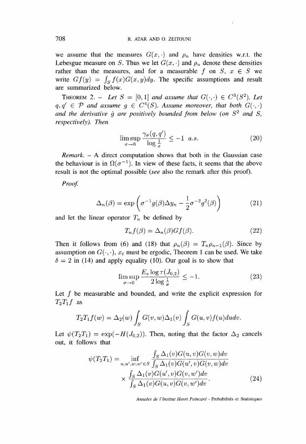
we assume that the measures G(x, ~) and pn have densities w.r.t. the

Lebesgue measure on S. Thus we let G(x, .) and pn denote these densitiesrather than the measures, and for a measurable f on S, xES wewrite ~S f(x)G(x, The specific assumptions and resultare summarized below.

THEOREM 2. - Let S = [0, 1] and assume that G(~, ~) E C3(~S‘2). Letq, q’ E P and assume g E C4 (,5’). Assume moreover, that both G( ~, ~ )and the derivative g are positively bounded from below (on 82 and S,respectively). Then

Remark. - A direct computation shows that both in the Gaussian casethe behaviour is in ~(7’~). In view of these facts, it seems that the aboveresult is not the optimal possible (see also the remark after this proof).

Proof

and let the linear operator Tn be defined by

Then it follows from (6) and (18) that p.r,, (,~) = Since byassumption on G( . , . ) , xt must be ergodic, Theorem 1 can be used. We take8 = 2 in (14) and apply equality (10). Our goal is to show that .

Let f be measurable and bounded, and write the explicit expression forT2T1f as

Let = exp(-H(Jo,2)). Then, noting that the factor A2 cancelsout, it follows that



We show below that the integrands in (24) are controlled by the behaviourof Ai, which tends to concentrate on one point as a - 0, causing the cross-ratio to converge to 1. Substituting v = g(v), using the differentiability andmonotonicity of g and the definition of On (21), the first integral in thenumerator of (24) reads

where by assumptions on g we have y(S) - E 8} == ~g(0), g(1)~.Dividing I(u, 5, w) by exp(y21 /2), which does not depend on u, w,it follows that

where

For E > 0 define now A = ~g(0) + 6~(1) - e]}, and recall thatayi = + Then

for some constant c independent of E and cr, provided that a is sufficientlysmall. Since T is always 1 it follows that

We thus assume Y1 E A from now on. For M > 0 let us divide the

integration region in (25) according to > aM and its complement.Note that

Vol. 33, n° 6-1997.


for some constant ci > 0, and that if we keep Ma E then

g(S) n {v : |v - 03C3y1] {v : |v - 03C3y1] Thus it follows

from (25) and (27) that .

Expand now the function

with respect to v around (note that ?/i E A) to get

Here ] the derivatives with respect to the second variableindeed exist and are continuous due to the differentiability assumptions onG(. , .) and g(.). The integrals in (28) may thus be estimated by

where

for some c2, c3 > 0, independent of E, a and M, provided that M issufficiently large. Setting M = a-1/8 so that a3 M4 = a2.5, and combining(28), (29) and (30), it follows that for Y1 E A

where



Noting that 1, and

moreover that p and cp22 are bounded while cp is bounded away from

zero (all bounds .are uniform), it follows from (31 ) that for ~/i E A,

for some 0 provided that a is sufficiently small. Thus by (10) it

holds that for ~/i E A,

and

By (26), (33) and Fatou’s lemma, one gets

and taking E - 0 one obtains (23). The result now follows from Theorem1. D

Remark. - One checks that the coefficient corresponding to a2 that resultsfrom expanding the cross ratio in (31 ) with respect to a is not identicallyzero, and especially does assume negative values for some u, u’, w, w’ E Sso the term a2 in (32) cannot be replaced by a higher power of a, andtherefore it seems that the above bound is the asymptotically best boundone can get by the technique used.

4. THE CASE OF A DIFFUSION ON A COMPACT MANIFOLD

In this section we treat the filtering of a diffusion process xt, on a

compact Riemannian manifold M of dimension m. All assumptions and

Vol. 33, n° 6-1997.


definitions of section 2 are kept with T = !R~. Embedding the manifold inIRd, some large enough d, one may write the Ito equation

with a one dimensional observation process:

Here W and v are independent standard Brownian motions on f~d andR, respectively, b = (b(?) )izd, % = (%(?3) ) ixxd and g are Lipschitz-continuous on M. The function g is also twice continuously differentiable,and we denote by gi and gij its partial derivatives of first and second order,respectively, in the directions of the coordinate vectors in (~d. Furthermore,we assume that the coefficients band ( lead to a strictly elliptic generatoron M, with heat kernel Gt(x, y) . By comparing to standard bounds on heatkernels of strictly elliptic operators on ~d (e.g., [6], chapter 3), the ellipticityassumption implies that there exist positive constants co, ci and c2, such that

As in section 3, a is used to parameterize the intensity of observation, andwe use the notion q« ( . , .) instead of -y( ~, ~ ) to denote the dependence on a.

THEOREM 3. - Let the state and observation processes be as in (34)and (35), and assume that the ellipticity condition holds. Then there exista non-random function > 0 and constants c’ > 0, c" > 0 s. t. for anyq, q’ E ~, the following hold P-a. s.

Remarks. - 1 ) (c) above provides an upper bound which convergeto 0 as a - 0. This bound is certainly not believed to be tight (comparewith Theorems 2 and 4 in the discrete time setting). The significance ofthis bound is in those cases for which 1a indeed seems to converges to 0as a - 0 (see [7] for such an example). -



2) Under additional assumptions, with ,~* denoting the forward operatorof xt on M, the Zakai equation for the filtering of xt given is written

where Uo equals the density of q. Though below we do not make useof the representation (37), Theorem 3 yields exponential stability for its

normalized solution.

Proof. - Throughout the proof c denotes a deterministic constant whosevalue may change from line to line. The proof is based on (15). Byellipticity, xt is ergodic, and in view of (12), H(G8) oo. Next, we fix

8 > 0, and let A be the Riemannian measure on M. Note that in view of (15)and part (c) of Theorem 1, to prove (a), it suffices to bound R(7~(- ;~))by a finite, possibly random, bound. We do so by bounding defined in (7) by bounds that do not depend on cx and (3, and using the

representation (12). To this end, note that (see (2), (7) and (35)),

We begin with the upper bound. Integrating by parts in (38), we have that

where

Note that b~i~, g, gi and gij are all bounded, hence

where ym = and

Vol. 33,n° 6-1997.


Denote

We bound the conditional expectation = ,~, .~’s) in (39). First,by Fatou’s lemma and continuity of Ft with respect to t,

where 8n is a sequence increasing to 8. By the Markov property and theboundedness from below of Gs ( ~, ~ ),

where we have defined bn as the conditional expectation in (41). Notethat since is measurable w.r.t. it follows by the sameargument that

In view of (39) and (40), in order to show the existence of a uniform upperbound on J(a, (3), it suffices to bound bn uniformly in 0152, {3 and n. Now,

where we have used Holder’s inequality and denoted



To bound Qi we first use the inequality lex -11 + and the

Cauchy-Schwartz inequality. Denoting m’ = 2m + 1 one has

Next, using Minkowski’s inequality, and the Burkholder-Davis-Gundy

inequality [10], p. 166 for the martingales t one obtains

While

where

Vol. 33, n° 6-1997.


B.y time change for the stochastic integral, one has that, conditioned on ;::8,where Bt, conditioned on ;::8, is a standard BM and

and hence

One therefore concludes that

On the other hand, using (36) one obtains

Now, if we chose 8n = b ( 1 - 2 -n ) and combine (42), (43) and (44), itfollows that

Since bo = G 8 ( 0152, {3) it follows that

which is bounded uniformly in n, a, /?. Thus from (39) and (41 ) and using(36), we obtain the upper bound

The lower bound follows easily from the upper bound, since by Cauchy-Schwartz Eex > 1 /Ee-X . Hence

Actually, the above suffices for parts (a) and (b) in view of (12) and (15),since the bounds (45) and (46) are both positive and finite for fixed a aswell as in the limit 03C3 ~ oo.



As for part (c), we shall need the concrete dependence on 03C3 and

8 of the bound derived from (15) using (45) and (46). Since

cba-1 + for c large enough, it follows that (~m + 4 ~) > 1 / 2 . Denote a~ = + 4B/~. Thus, combining (15),

(45), (46) and the inequality tanh(~ log z ) 1 - > 0 we get

Substituting 8 = a, we conclude that there exist positive constants c andao s.t. for every a ao,

5. THE COUNTABLE STATE SPACE CASE

In [1] bounds are derived for 1 in the finite state space case both in discreteand in continuous time. The technique there is based on the connection

between 1 and the gap between the two top Lyapunov exponents of theZakai equation, and Oseledec’s multiplicative ergodic theorem is intensivelyused. Theorem 2 above may be directly applied to provide an extensionof Theorem 2 in [ 1 ] to the case of countable state space discrete time.

However, as we show below, in the low observation noise limit, a sharperresult is possible by a direct computation that relies neither on the estimatesof sections 2 and 3, nor on Oseledec’s theorem (and provides an extensionof Theorem 3 of [1]).We let S = Z and T = Z+, and denote the transition matrix by

G = (G(z~)). Information on its state is given through the observationprocess

The unnormalized conditional law is then given (as in (21), (22)) by thevectors

where G* is the transpose of G and Dn is a diagonal matrix with

i) = O’ 2~’2(2)~2). The following resultshows that in the limit 03C3 ~ 0, the behaviour of 03B303C3 is at least in SZ (o--2 ) .Vol. 33, n° 6-1997.


THEOREM 4. - Assume that the state process satisfiesthe following conditions. (a) is ergodic. (b) Eg2(xn) oo.

(c) ES log G(xo, x1) > -oo. (d) = supj 03A3i G(i, j) oo. Let q and

q’ be any two probability distributions on S. Then P-a.s.,

In particular, if there exists a state io such that = io ) > 0 andinfj~i0 |g ( Zo ) - g(j)| ~ 0 then the lim sup in (49) is a. s. negative.

In order to prove the theorem, we introduce some notations. For a, b E £1,let the exterior product be defined by a /B b = ab* - ba* (compare withthe usual definition [5], p. 61 ). Note that W = a /B b is an antisymmetricmatrix. We define for it the pth norm by

Let denote the space {a A b G and note that oo if

a A b G For p E [1, oo] and a linear operator A on we denote

by its operator norm w.r.t. the pth norm defined by (50). We do notdistinguish between the measure q E P and the vector q E R1 for which

= 1. Moreover, we define the set of positive probability measures on(S, S) by 7~ - {q E Plq(i) > o, z E Z}.We first prove the followingLEMMA 2. - Let p, 17 E R1 be non-negative and non-zero, and denote

p == = Then

Proof. - On one hand, it is easy to see that for any a > 1 and a, b E 12,if = = 1 then ~ 2014 b~~2 - Thus, assuming w.l.o.g.that ~p)~2 ~ and denoting the angle between p and q by p q we get



The last equality is well known (see e.g., [5], p. 61). On the other hand,

Proof of Theorem 4. - Given q and q’ we denote pn = pn and r~n = In order to use the lemma, we first provide lower bounds on and

and an upper bound on A r~n ~~~ 1. First,

Using the ergodic theorem, we get that P-a. s.

Secondly, using (48), we obtain the following recursion

Write the above elementwise as

and get the relation

where G is the operator on defined by u A v - By (53),

We thus obtain, using again the ergodic theorem, that P-a. s.

Vol. 33, n° 6-1997.


Next, since

for any constant E > 0 and sufficiently small a. Now the right hand side of. (51 ) together with (52), (54) and the above imply the theorem. D

We next show that in a specific class of problems, (49) is also a lowerbound in a sense to be explained below. We concentrate on the class Uof processes for which the transition matrix G has all its 2 x 2 minors

non-negative. An important subclass of U is that of the nearest neighbourprocesses i.e., those that possess a transition matrix G = exp(sA) wheres > 0 and A is an intensity matrix for which Ii - jl > 1 impliesA( i, j) = 0. Indeed, the latter condition on G implies that it is totallypositive as an operator on which by definition implies that the processit generates belongs to U. For the above results and further discussion see[ 11 ], pp. 38-45]. Let us denote for 7L

For i j, k l the latter are the 2 x 2 minors of G. We further assumethat the infimum in (49) is always achieved namely, there exists a function7r : Z - 7L such that

For a probability measure m on P, we shall require the following.



ASSUMPTION A3. - For every proper linear subspace Q of £1,m( Q n P) = 0.

EXAMPLE 1. - Let ai , i E lL be i.i.d. real-valued non-negative boundedrandom variables, with a common law that is absolutely continuous w. r. t.the Lebesgue measure, and let ci, i E 7~ be positive constants s.t. ~i ci oo.

Let z2 = ci ai / ¿j cjaj, i E 7~ and define m to be the measure on P inducedby the random vector ~zi Then m satisfies Assumption A3.

Proof. - Define p to be the measure on induced Let

Q be a proper subspace of Then there exists a non-zero w E £CX)s.t. if q E Q then ~ wiqi = O. Let k be such that 0. Then

E PI 03A3iwizi == 0}) == E wiciai}) whichvanishes, since ak is -independent of ai, i ~ k, and its law is absolutelycontinuous w.r.t. the Lebesgue measure. D

We have the following result.

THEOREM 5. - Let belong to U and let it satisfy (a)-(d) oftheorem 4. Assume moreover that there exists a ~r : ~ -~ 7~ satisfying (56),such that Es log ] > -00. Let q and q’ be random, distributed ’according to two given probability measures m and m’, respectively, on Psatisfying Assumption A3. Then m x m’ x P-a. s.,

In particular, rrz x rrz’ x P-a. s., (49) holds with equality.

Proof. - We shall use the left hand side of (51) and develop boundsanalogous to (52) and (54) but in opposite direction. The first boundfollows easily from (48) namely,

The lower bound on A is more complicated. Assume first thatq and q’ are such that all the entries above the diagonal of the matrixq are positive. By (53), positivity of the 2 x 2 minors and the positivityassumption on the initial condition, it follows that for i j and k l

Vol. 33, n° 6-1997.


Note however, that for z > j we have ( pn A = -(pn A and

moreover, It thus follows from (59) that for anyz,~, ~ we have

~

Substituting i = xn, j = k = xn-1 and I = passing tothe limit, we get that P-a. s. ,

Observe that in the derivation of the bounds (54), (55) and (61), onlybounds on the operators Dn and G are involved, not on q or q’. Hence thenull sets of P on which these bounds fail to hold are independent of q andq’. We thus summarize (54), (55) and (61) as follows. There exists a set

of full P-measure, such that for all q and q’ with q A q’ positiveabove the diagonal, and (;J E Ho.

Hence, for q, q’ as assumed, (57) holds by the l.h.s. of (51 ), (58) and (62).We extend the -above result to general q and q’ in a few steps.LEMMA 3. - For any q E ~° there exists a qo E ~° s. t. all entries above

the diagonal of q /B qo are positive.

LEMMA 4. - There exists a set 03A91 E B of full P-measure s. t. the followingholds. If q E ~° and Q’ (cv, q) is the subset of P of all q’ for which (62) doesnot hold, then for every w E 03A91, Q’(c.v, q) is the intersection of a properlinear subs pace of .~1 and ~.

°

In view of Lemma 4 and Assumption A3, for every w E SZ1 and

q E ~°, (57) fails to hold only when q’ belongs to a null set of m’

(possibly depending on q and w). Since from Assumption A3, ~°) _



E P : q(7i,) == O}) ::; ~n E P : q( n) == O}) == 0, the proofis complete. D

Proof of Lemma 3. - Define the sequence a(n), n E lL as follows. Let

a(0) = 1; for n > 1 and k -1 let

Then for any n ~ Z, a(n) cq( n) / q(O) so that a(n) is summable. Let

now qo(n) = a(n)/ ~i a(i). Then for j = i + 1 we have from (63) thatq(i)qo(j) > By induction, the latter holds for any i j, andthe Lemma follows. D .

Proof of Lemma 4. - Denote the matrix pn Â qn for which po = qand 7~0 = q’ by Wn(q, q’). Since (54) and (55) hold, there exists a fullP-measure set such that for all cv E SZ~ and q, q’ E P,

where C is as in (62). Fix q E If Q’(w, q) is empty, the lemmaholds trivially. Otherwise, let Q’(w, q). Then (62) does not holdfor i = 1, 2 (i.e., when pn = p~ and r~n = Hence, forall w E H~

Let A e R be such that q’ = q’(A) = 03BBp1 + (1 - 03BB)p2 ~ P. ThenWn (q, q’ ) = it follows that for w E O~,

Thus for every q E ~° and w E Q’(w, q) is the intersection of alinear subspace of li and P. Let now qo be as in Lemma 3. Thus by (62),whenever úJ E 03A90, one has that qo fj. Q’(03C9, q). This implies that wheneverw E 03A91 = 00 n 03A9’0, the subspace must be proper. D

EXAMPLE 2. - If G is the transition matrix of a finite state Markov chainsuch that all its entries and 2 x 2 minors are positive, then all assumptionsof Theorems 4, 5 hold.

Vol. 33, n° 6-1997.


6. STABILITY OF THE OPTIMAL SMOOTHER

The above analysis has implications to the problem of sensitivity of theoptimal smoother to its initial conditions. We focus on the following model,studied in [21].

Here, Wt and vt are independent standard Brownian motions, b =

{b(i)}1~i~n, 03C3 = {03C3(ij)} and g = are globally Lipschitz-continuous, b and g are continuously differentiable and 03C3 is twice

continuously differentiable and its second derivatives are all bounded. Theinitial condition x is distributed according to po, independently of Wt and vt .

For 0 r s t, let and denote the joint filtering-smoothing conditional law and the smoothing conditional law, respectively,defined by = and =

and the corresponding unnormalized conditional laws by and = Let now pt(~) be

the density of the unconditional law of xt under P. Under the assumptionsstated above, it is shown in [21] that the density of the joint filtering-smoothing law, where the variable zi E Rn corresponds to xt and z2 E Rnto xs, satisfies

Letting z2 ) == (z2 ) one can show that for 0 s t,= and it follows that

THEOREM 6. - Under the assumptions of this section and those ofTheorem 1, for any comparable q and q’, and any 8 > 0, P-a. s.,

ACKNOWLEDGEMENTS

We thank P. Bougerol and F. Ledrappier for referring us to [9]. We wouldalso like to thank Z. Schuss for suggesting to investigate the smoothingstability question. Finally, we are grateful to the anonymous referee forseveral important comments.



REFERENCES

[1] R. ATAR and O. ZEITOUNI, Lyapunov Exponents for Finite State Nonlinear Filtering, SiamJ. Contr. Optim., Vol. 35, No 1, 1997, pp. 36-55.

[2] G. BIRKHOFF, Extensions of Jentzsch’s Theorem, Trans. Am. Math. Soc., Vol. 85, 1957,pp. 219-227.

[3] G. BIRKHOFF, Lattice Theory, Am. Math. Soc. Publ. 25, 3rd ed., 1967.[4] P. BOUGEROL, Théorèmes limites pour les systèmes linéaires à coefficients markoviens,

Prob. Theory Rel. Fields, Vol. 78, 1988, pp. 192-221.[5] P. BOUGEROL and J. LACROIX, Products of Random Matrices with Applications to

Schrödinger Operators, Birkhäuser, 1985.

[6] E. B. DAVIES, Heat Kernels and Spectral Theory, Cambridge University Press, 1989.[7] B. DELYON and O. ZEITOUNI, Lyapunov exponents for filtering problems, Applied Stochastic

Analysis, edited by Davis, M. H. A. and Elliot, R. J., Gordon and Breach SciencePublishers, London, pp. 511-521, 1991.

[8] F. FLANDOLI and K. SCHAUMLÖFFEL, Stochastic Parabolic Equations in Bounded Domains:Random Evolution Operator and Lyapunov Exponents, Stochastics and Stochastic

Reports, Vol. 29, 1990, pp. 461-485.[9] E. HOPF, An Inequality for Positive Linear Integral Operators, Journal of Mathematics and

Mechanics, Vol. 12, No. 5, 1963, pp. 683-692.[10] I. KARATZAS and S. E. SHREVE, Brownian Motion and Stochastic Calculus, Springer-Verlag,

1991.

[11] S. KARLIN, Total Positivity, Stanford University Press, Stanford, California, 1968.[12] H. KUNITA, Asymptotic Behavior of the Nonlinear Filtering Errors of Markov Processes,

J. Multivariate Anal., Vol. 1, 1971, pp. 365-393.[13] R. S. LIPTSER and A. N. SHIRYAYEV, A. N. Statistics of Random Processes, Nauka, Moscow,

1974, English ed., Springer-Verlag, New-york, 1977.[14] D. OCONE and E. PARDOUX, Asymptotic Stability of the Optimal Filter with respect to its

Initial Condition, Siam J. Contr. Optim., Vol. 34, No. 1, 1996, pp. 226-243.[15] K. R. PARTHASARATHY, Probability Measures on Metric Spaces, Academic Press, New York

and London, 1967.

[16] Y. PERES, Domains of Analytic Continuation for the Top Lyapunov Exponent, Ann. Inst.Henri Poincaré, Vol. 28, 1992, No. 1, pp. 131-148.

[17] E. SENETA, Non-negative Matrices and Markov Chains, Springer-Verlag, 1981.[18] L. STETTNER, On Invariant Measures of Filtering Processes, Stochastic Differential Systems,

Proc. 4th Bad Honnef Conf., 1988, Lecture Notes in Control and Inform. Sci. 126, editedby Christopeit, N., Helmes, K. and Kohlmann, M., Springer, 1989, pp. 279-292.

[19] L. STETTNER, Invariant Measures of the Pair: State, Approximate Filtering Process, Colloq.Math., LXII, 1991, pp. 347-351.

[20] M. ZAKAI, On the Optimal Filtering of Diffusion Processes, Z. Wahr. Verw. Geb., Vol. 11,1969, pp. 230-243.

[21] O. ZEITOUNI and B. Z. BOBROVSKY, On the Joint Nonlinear Filtering-Smoothing of DiffusionProcesses, Systems & Control Letters, Vol. 7, 1986, pp. 317-321.

(Manuscript received May 13, 1996;Revised November 13, 1996. )

Vol. 33, n° 6-1997.

exponential stability for nonlinear filtering

Documents