simulation environment for an ofdm transmitter using uvm
TRANSCRIPT
Equation Chapter 1 Section 1
Final Project
Degree in Telecommunications Engineering with a
specialization in electronics
Simulation environment for an OFDM transmitter
using UVM methodology
Author: Antonio Martínez Zambrana
Tutor: Hipólito Guzmán Miranda
Electronic Engineering Department
Escuela Técnica Superior de Ingeniería
Universidad de Sevilla
Sevilla, 2016

iii
Final Project
Degree in Telecommunications Engineering
Simulation environment for an OFDM transmitter
using UVM methodology
Author:
Antonio Martínez Zambrana
Tutor:
Hipólito Guzmán Miranda
Associate Professor
Electronic Engineering Department
Escuela Técnica Superior de Ingeniería
Universidad de Sevilla
Sevilla, 2016

v
Final Project: Simulation environment for an OFDM transmitter using UVM methodology
Author: Antonio Martínez Zambrana
Tutor: Hipólito Guzmán Miranda
The comittee judging the Project indicated above is comprised of the following members:
President:
Chair:
Secretary:
They agree to grant this project a grade of:
Sevilla, 2016
Tribunal Secretary.

vii
Acknowledgments
I would like to express my thanks firstly to Hipólito Guzmán Miranda, my tutor. He gave me the chance of
learning these new skills which were totally unknown to me. I have had the opportunity to use tools that would
have otherwise been imposible to use. He supported me and motivated me, thank you.
I am incredibly grateful to my parents and family. They made me the person I am now and they have always
been supporting and motivating me. Everything I have done is thanks to them.
Thank you Christoph Suehnel, you solved so many doubts and helped me when I needed it. I felt highly
motivated with your help.
Thank you Steve Ingham, you listened to me when I needed and encouraged me in a way that no one did
before.
Sarah Parkinson, thank you for all your patience and help.
Thank you Adrián Jiménez, for all those moments we were motivating and helping each other.
To my friends and colleagues, thank you for listening, offering me advice and supporting me all this time.

ix
Abstract
The aim of this Project was to design a verification testbench using the Universal Verification Methodology
standardized by Accellera. The HDL design I chose to verify was an OFDM transceiver written in VHDL
according to the PRIME alliance specifications. The tools used were EDA proprietary software for hardware
verification working in conjunction with Matlab.
The strategy to develop the final testbench was based on a series of UVM testbenches, focusing on adding
more UVM and verification functionality than the previous version. The final testbench was fully integrated
with Matlab, which worked as a Golden model.
The results of the project successfully prove that the UVM is a very scalable verification methodology, has the
possibility to implement the most advanced verification measures and is simple to integrate with most modern
technologies.

xi
Index
Acknowledgments ....................................................................................................................................... vii
Abstract ........................................................................................................................................................ ix
Index ............................................................................................................................................................. xi
Tables index ................................................................................................................................................ xiii
Figures index ................................................................................................................................................ xv
Notation ..................................................................................................................................................... xvii
1 Introduction ......................................................................................................................................... 10 1.1 Verification necessities .............................................................................................................................. 10 1.2 PRIME alliance based transceiver ............................................................................................................. 12
2 Design Under Verification .................................................................................................................... 13 2.1 Functional requirements of the Convolutional Encoder .......................................................................... 13 2.2 Functional requirements of the Scrambler .............................................................................................. 14 2.3 Functional requirements of the Interleaver ............................................................................................. 14 2.4 Functional requirements of the Mapper .................................................................................................. 16 2.5 Functional requirements of the IFFT and CRC .......................................................................................... 17
3 The Universal Verification Methodology (UVM) .................................................................................. 19 3.1 Introduction ................................................................................................................................................ 19 3.2 UVM components ...................................................................................................................................... 20 3.3 UVM Transactions ..................................................................................................................................... 21 3.4 The BFM...................................................................................................................................................... 21 3.5 Container Components .............................................................................................................................. 22 3.5.1 The Env Component .......................................................................................................................... 22 3.5.2 The Agent Component ...................................................................................................................... 22
3.6 Components of the Stimulus layer ............................................................................................................ 23 3.6.1 UVM Sequencer ................................................................................................................................. 23 3.6.2 UVM Driver ........................................................................................................................................ 24 3.6.3 UVM Sequences ................................................................................................................................. 24
3.7 Components of the Analysis layer ............................................................................................................ 24 3.7.1 The Monitor ....................................................................................................................................... 25 3.7.2 The Scoreboard .................................................................................................................................. 25 3.7.3 Predictor ............................................................................................................................................. 26 3.7.4 Coverage objects ............................................................................................................................... 27
3.8 The UVM Factory ....................................................................................................................................... 27 3.9 Configuration of a UVM testbench environment .................................................................................... 27 3.10 The Standard UVM phases ........................................................................................................................ 28 3.11 Testbench Construction ............................................................................................................................. 31
4 Workflow ............................................................................................................................................. 33 4.1 Introduction ............................................................................................................................................... 33 4.2 Tools ........................................................................................................................................................... 33 4.3 Process to learn the UVM ......................................................................................................................... 33
5 Matlab Integrated in the Scrambler testbench .................................................................................... 39 5.1 Matlab integration into Questasim ......................................................................................................... 39 5.2 Necessities to adapt the Matlab Script .................................................................................................... 40 5.3 Topology of the Scrambler testbench. ..................................................................................................... 40 5.3.1 Merging I/O Monitors ....................................................................................................................... 40 5.3.2 Scoreboard topology ......................................................................................................................... 42 5.3.3 Predictor Factory override ................................................................................................................ 42
6 Matlab integrated in the final testbench ............................................................................................. 45 6.1 Compiling Xilinx IP Cores ........................................................................................................................... 45 6.2 VHDL modification ..................................................................................................................................... 45 6.3 Binding internal signals ............................................................................................................................. 45 6.4 Matlab Predictor modifications ................................................................................................................ 46 6.5 Final Testbench Architecture .................................................................................................................... 47 6.5.1 The Sequencer and the Sequence ................................................................................................... 48 6.5.2 The Driver ........................................................................................................................................... 48 6.5.3 Coverage Monitor and Coverage Component ................................................................................ 48 6.5.4 Symbol to Symbol Monitors ............................................................................................................. 48 6.5.5 Scoreboard Implementation ............................................................................................................ 49 6.5.6 Top module and BFM ........................................................................................................................ 49
6.6 Inheritance and relations between classes .............................................................................................. 49
7 Results and conclusions ....................................................................................................................... 51 7.1 Results ........................................................................................................................................................ 51 7.2 Conclusions ................................................................................................................................................ 51
8 Future work ......................................................................................................................................... 53
References .................................................................................................................................................. 55
xiii
TABLES INDEX
Table 1 - DBPSK Interleaving matrix (Source: [9]) 15
Table 2 - DQPSK Interleaving matrix (Source: [9]) 15
Table 3 - D8PSK Interleaving matrix (Source: [9]) 16
Table 4 – UVM components (Source: [15]) 21

xv
FIGURES INDEX
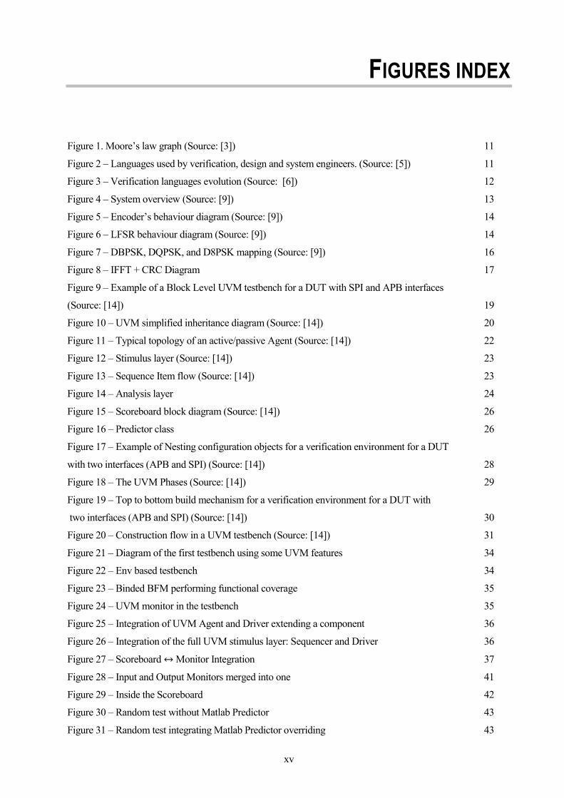
Figure 1. Moore’s law graph (Source: [3]) 11
Figure 2 – Languages used by verification, design and system engineers. (Source: [5]) 11
Figure 3 – Verification languages evolution (Source: [6]) 12
Figure 4 – System overview (Source: [9]) 13
Figure 5 – Encoder’s behaviour diagram (Source: [9]) 14
Figure 6 – LFSR behaviour diagram (Source: [9]) 14
Figure 7 – DBPSK, DQPSK, and D8PSK mapping (Source: [9]) 16
Figure 8 – IFFT + CRC Diagram 17
Figure 9 – Example of a Block Level UVM testbench for a DUT with SPI and APB interfaces
(Source: [14]) 19
Figure 10 – UVM simplified inheritance diagram (Source: [14]) 20
Figure 11 – Typical topology of an active/passive Agent (Source: [14]) 22
Figure 12 – Stimulus layer (Source: [14]) 23
Figure 13 – Sequence Item flow (Source: [14]) 23
Figure 14 – Analysis layer 24
Figure 15 – Scoreboard block diagram (Source: [14]) 26
Figure 16 – Predictor class 26
Figure 17 – Example of Nesting configuration objects for a verification environment for a DUT
with two interfaces (APB and SPI) (Source: [14]) 28
Figure 18 – The UVM Phases (Source: [14]) 29
Figure 19 – Top to bottom build mechanism for a verification environment for a DUT with
two interfaces (APB and SPI) (Source: [14]) 30
Figure 20 – Construction flow in a UVM testbench (Source: [14]) 31
Figure 21 – Diagram of the first testbench using some UVM features 34
Figure 22 – Env based testbench 34
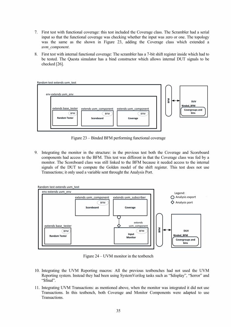
Figure 23 – Binded BFM performing functional coverage 35
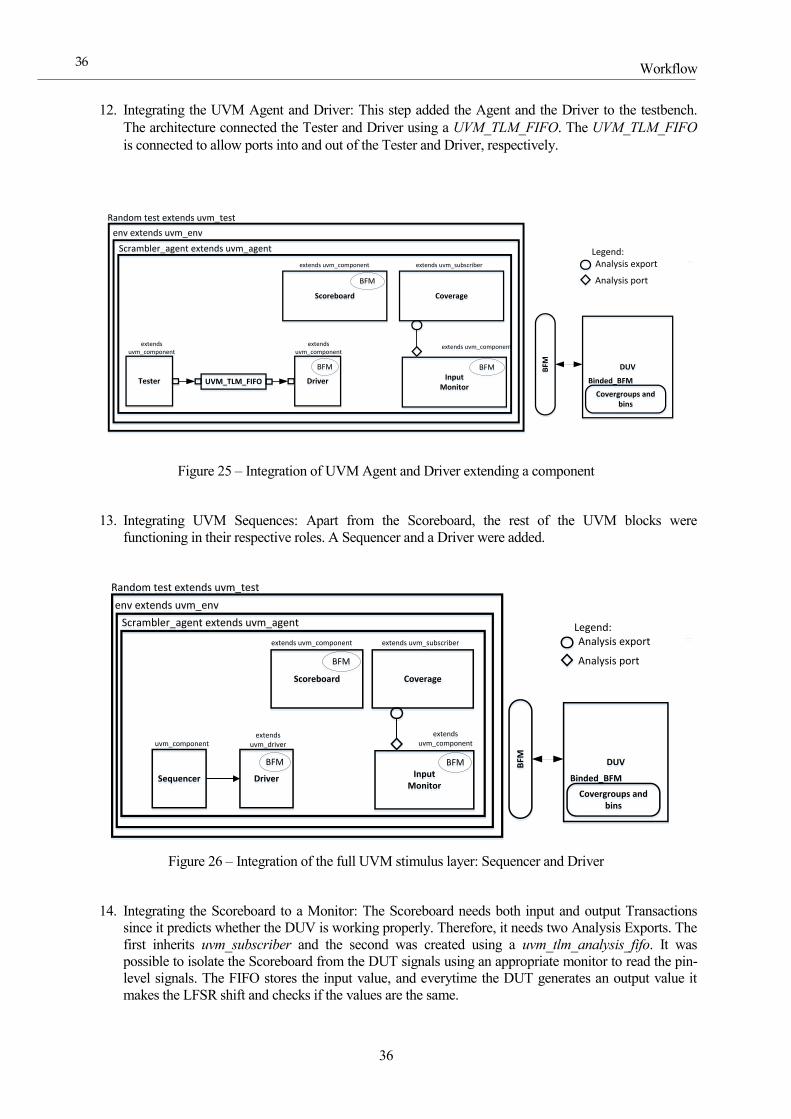
Figure 24 – UVM monitor in the testbench 35
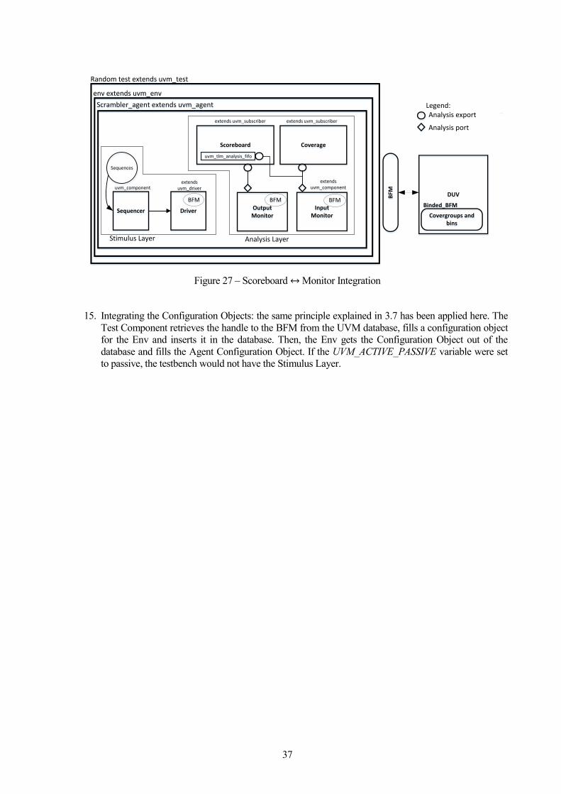
Figure 25 – Integration of UVM Agent and Driver extending a component 36
Figure 26 – Integration of the full UVM stimulus layer: Sequencer and Driver 36
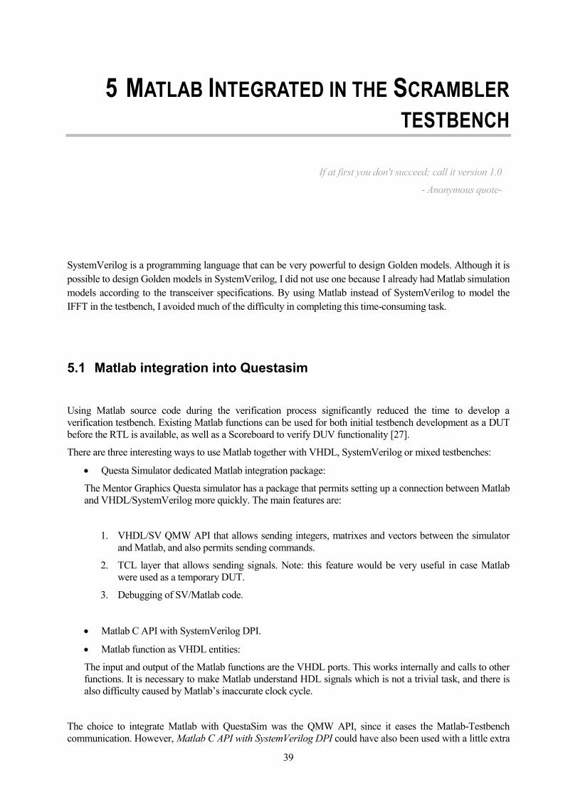
Figure 27 – Scoreboard ↔ Monitor Integration 37
Figure 28 – Input and Output Monitors merged into one 41
Figure 29 – Inside the Scoreboard 42
Figure 30 – Random test without Matlab Predictor 43
Figure 31 – Random test integrating Matlab Predictor overriding 43
Figure 32 – Matlab ↔ SystemVerilog communication 47
Figure 33 – Final testbench topology 48
Figure 34 – Collaboration and inheritance diagram 50
xvii
Notation
AE Analysis Export
AP Analysis Port
API Application Programming Interface
ASCII American Standard Code for Information Interchange
ASIC Aplication-Specific Integrated Circuit
BFM Bus Functional Model
CENELEC Comité Européen de Normalisation ELECtrotechnique
CRC Cyclic Redundance Check
CPLD Complex Programmable Logic Device
DBPSK Binary Phase Shift Keying
DPI Direct Programming Interface
DQPSK Quadrature Phase Shift Keying
DUT Device Under Test
DUV Design Under Verification
D8PSK Eight Phase Shift Keying
EDA Electronic Design Automation
FIFO First In First Out
FPGA Field Programming Gate Array
FSM Finite State Machine
HDL Hardware Description Language
HVL Hardware Verification Languages
IC Integrated circuit
IFFT Inverse Fast Fourier Transform
IP Intellectual Property
KHz KiloHertz
Kbps Kilo bits per second
NBPC Number of bits per carrier
NBPS Number of Bits Per OFDM Symbol
LFSR Linear Feedback shift Register
OFDM Orthogonal Frequency Division Multiplexing
OVM Open Verification Methodology
PPDU PHY Protocol Data Unit
PRIME PoweRline Intelligent Metering Evolution
RAM Random Access Memory
ROM Read Only Memory
RTL Register-transfer Level
SV SystemVerilog
TCL Tool Command Language
URL Uniform Resource Locator
UVM Universal Verification Methodology
VHDL VHSIC Hardware Description Language
VMM Verification Methodology Manual
XOR Exclusive OR
3D Three Dimensional

1 INTRODUCTION
This chapter contains a brief summary of the whole document. The principal aspects of the thesis are covered.
For a deeper understanding the reader will need to go chapter by chapter where everything will be explained in
detail.
1.1 Verification necessities
Unfortunately, verification is not a topic well covered in the university background. This makes the study of
verification challenging, but also very rewarding. Engineering schools teach briefly how to test either analog
or digital electronic designs. After graduating, an electronic engineer is only able to accomplish simple tests,
which are not enough in an industrial environment where everything has to be tested before being sold.
Directed testing is not enough to test a design and should only be used as a strategy to reach those “countable”
corners which are harder to verify using constrained random verification.
Verification has evolved rapidly in ASIC designs, however it took longer for engineers to realize how
important verification also is in FPGAs. In general, it could be said the electronic engineer community did not
care about verification in programmable devices. This was due to the fact of being able to program the device
again if it did not work the first time. However, semiconductor professionals working with ASICs were much
more aware of the importance of verification, considering that errors in a chip mask are irreversible and can
cause huge economic losses for a company. Verification is a process that saves two of the most important
aspects in an engineering project: time and money. It is a common practice in companies that need to rent
electronic equipment to test the designs. When bugs are not detected before reaching the lab, they prolong the
use of electronic equipment. This causes problems for other engineers who also need access to the equipment,
as well as the company that needs to pay more for the rental. Most of these problems could be solved using a
good verification strategy.
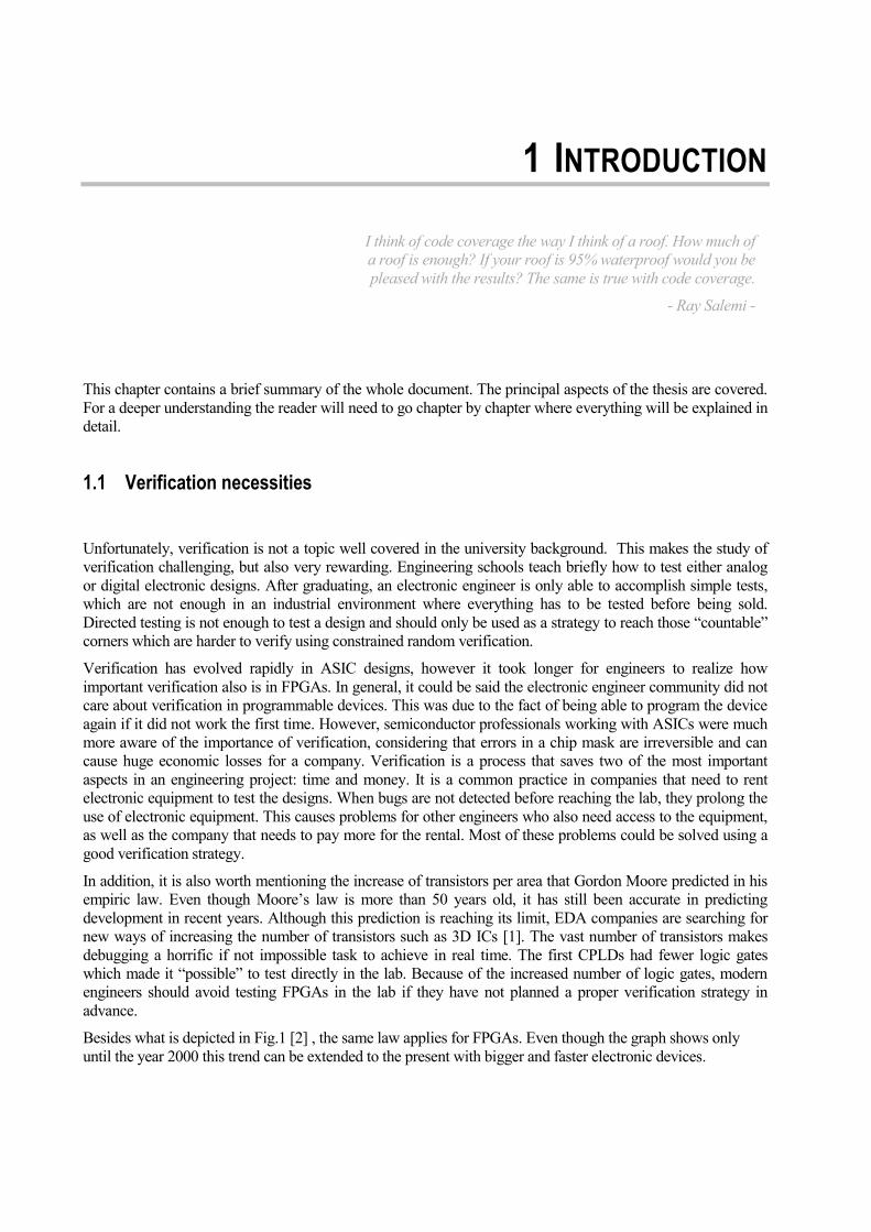
In addition, it is also worth mentioning the increase of transistors per area that Gordon Moore predicted in his
empiric law. Even though Moore’s law is more than 50 years old, it has still been accurate in predicting
development in recent years. Although this prediction is reaching its limit, EDA companies are searching for
new ways of increasing the number of transistors such as 3D ICs [1]. The vast number of transistors makes
debugging a horrific if not impossible task to achieve in real time. The first CPLDs had fewer logic gates
which made it “possible” to test directly in the lab. Because of the increased number of logic gates, modern
engineers should avoid testing FPGAs in the lab if they have not planned a proper verification strategy in
advance.
Besides what is depicted in Fig.1 [2] , the same law applies for FPGAs. Even though the graph shows only
until the year 2000 this trend can be extended to the present with bigger and faster electronic devices.
I think of code coverage the way I think of a roof. How much of
a roof is enough? If your roof is 95% waterproof would you be
pleased with the results? The same is true with code coverage.
- Ray Salemi -
11
Figure 1. Moore’s law graph (Source: [3])
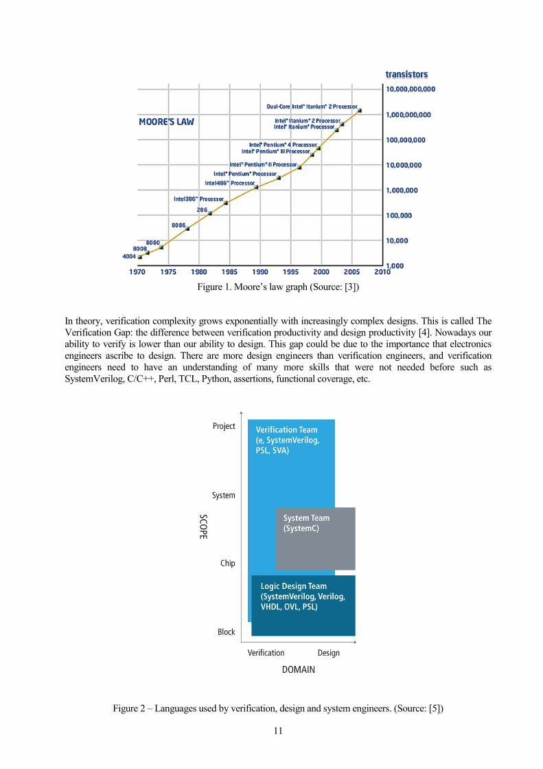
In theory, verification complexity grows exponentially with increasingly complex designs. This is called The
Verification Gap: the difference between verification productivity and design productivity [4]. Nowadays our
ability to verify is lower than our ability to design. This gap could be due to the importance that electronics
engineers ascribe to design. There are more design engineers than verification engineers, and verification
engineers need to have an understanding of many more skills that were not needed before such as
SystemVerilog, C/C++, Perl, TCL, Python, assertions, functional coverage, etc.
Figure 2 – Languages used by verification, design and system engineers. (Source: [5])
Introduction
12
12
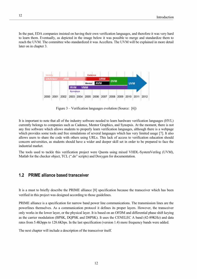
In the past, EDA companies insisted on having their own verification languages, and therefore it was very hard
to learn them. Eventually, as depicted in the image below it was possible to merge and standardize them to
reach the UVM. The committee who standardized it was Accellera. The UVM will be explained in more detail
later on in chapter 3.
Figure 3 – Verification languages evolution (Source: [6])
It is important to note that all of the industry software needed to learn hardware verification languages (HVL)
currently belongs to companies such as Cadence, Mentor Graphics, and Synopsis. At the moment, there is not
any free software which allows students to properly learn verification languages, although there is a webpage
which provides some tools and free simulations of several languages which has very limited usage [7]. It also
allows users to share the code with others using URLs. This lack of access to verification education should
concern universities, as students should have a wider and deeper skill set in order to be prepared to face the
industrial market.
The tools used to tackle this verification project were Questa using mixed VHDL-SystemVerilog (UVM),
Matlab for the checker object, TCL (“.do” scripts) and Doxygen for documentation.
1.2 PRIME alliance based transceiver
It is a must to briefly describe the PRIME alliance [8] specification because the transceiver which has been
verified in this project was designed according to those guidelines.
PRIME alliance is a specification for narrow band power line communications. The transmission lines are the
powerlines themselves. As a communication protocol it defines its proper layers. However, the transceiver
only works in the lower layer, or the physical layer. It is based on an OFDM and differential phase shift keying
as the carrier modulation (BPSK, DQPSK and D8PSK). It uses the CENELEC A band (42-89KHz) and data
rates from 5.4Kbpps to 128.6Kbps. In the last specification (version 1.4) more frequency bands were added.
The next chapter will include a description of the transceiver itself.
13
2 DESIGN UNDER VERIFICATION
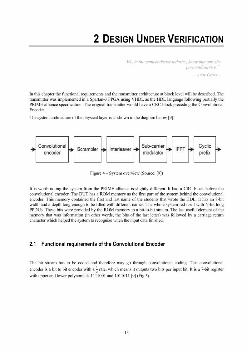
In this chapter the functional requirements and the transmitter architecture at block level will be described. The
transmitter was implemented in a Spartan-3 FPGA using VHDL as the HDL language following partially the
PRIME alliance specification. The original transmitter would have a CRC block preceding the Convolutional
Encoder.
The system architecture of the physical layer is as shown in the diagram below [9]:
Figure 4 – System overview (Source: [9])
It is worth noting the system from the PRIME alliance is slightly different. It had a CRC block before the
convolutional encoder. The DUT has a ROM memory as the first part of the system behind the convolutional
encoder. This memory contained the first and last name of the students that wrote the HDL. It has an 8-bit
width and a depth long enough to be filled with different names. The whole system fed itself with N-bit long
PPDUs. These bits were provided by the ROM memory in a bit-to-bit stream. The last useful element of the
memory that was information (in other words; the bits of the last letter) was followed by a carriage return
character which helped the system to recognize when the input data finished.
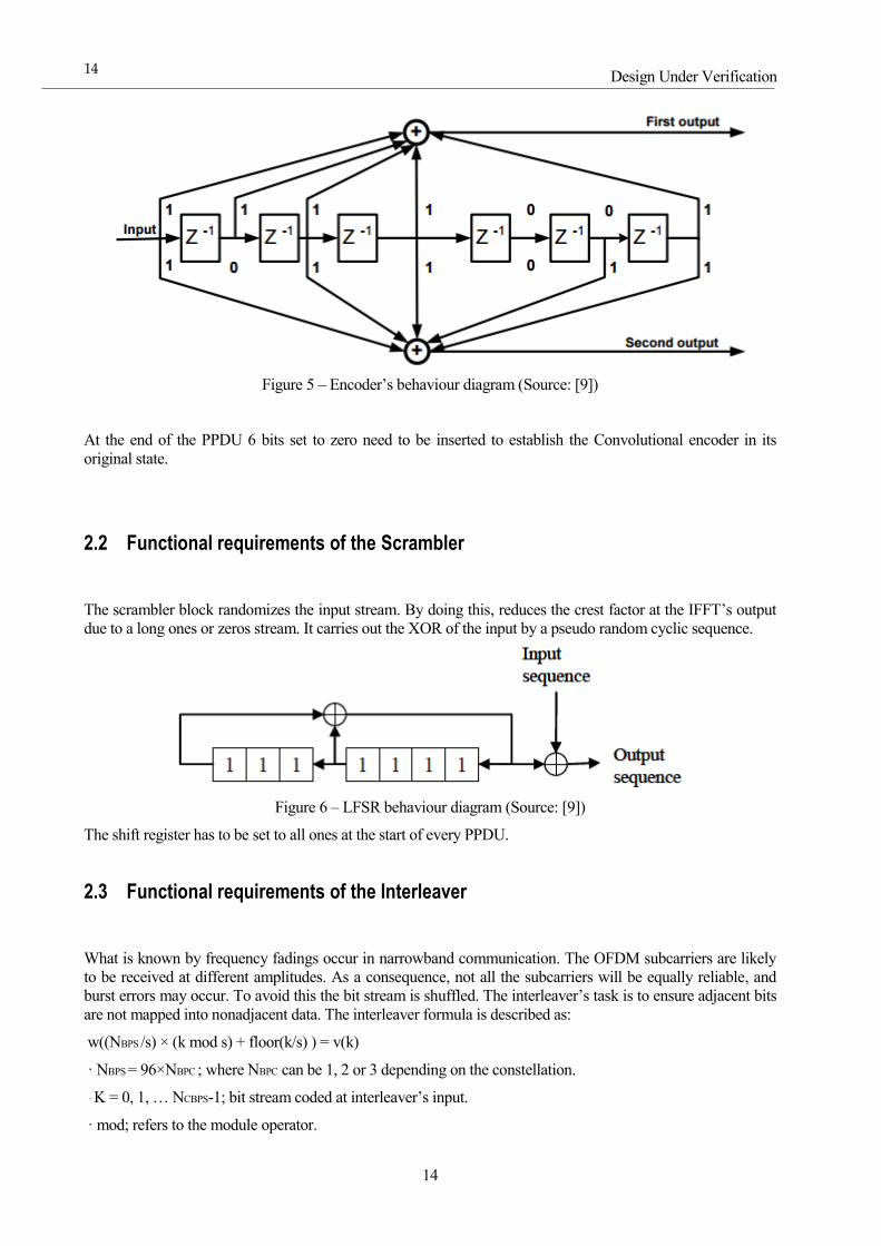
2.1 Functional requirements of the Convolutional Encoder
The bit stream has to be coded and therefore may go through convolutional coding. This convolutional
encoder is a bit to bit encoder with a 1
2 rate, which means it outputs two bits per input bit. It is a 7-bit register
with upper and lower polynomials 1111001 and 1011011 [9] (Fig.5).
“We, in the semiconductor industry, know that only the
paranoid survive.”
- Andy Grove -
Design Under Verification
14
14
Figure 5 – Encoder’s behaviour diagram (Source: [9])
At the end of the PPDU 6 bits set to zero need to be inserted to establish the Convolutional encoder in its
original state.
2.2 Functional requirements of the Scrambler
The scrambler block randomizes the input stream. By doing this, reduces the crest factor at the IFFT’s output
due to a long ones or zeros stream. It carries out the XOR of the input by a pseudo random cyclic sequence.
Figure 6 – LFSR behaviour diagram (Source: [9])
The shift register has to be set to all ones at the start of every PPDU.
2.3 Functional requirements of the Interleaver
What is known by frequency fadings occur in narrowband communication. The OFDM subcarriers are likely
to be received at different amplitudes. As a consequence, not all the subcarriers will be equally reliable, and
burst errors may occur. To avoid this the bit stream is shuffled. The interleaver’s task is to ensure adjacent bits
are not mapped into nonadjacent data. The interleaver formula is described as:
w((NBPS /s) × (k mod s) + floor(k/s) ) = v(k)
· NBPS = 96×NBPC ; where NBPC can be 1, 2 or 3 depending on the constellation.
· K = 0, 1, … NCBPS-1; bit stream coded at interleaver’s input.
· mod; refers to the module operator.
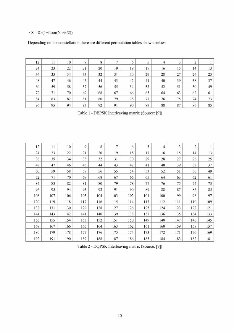
15
· S = 8×(1+floor(NBPC /2)).
Depending on the constellation there are different permutation tables shown below:
12 11 10 9 8 7 6 5 4 3 2 1
24 23 22 21 20 19 18 17 16 15 14 13
36 35 34 33 32 31 30 29 28 27 26 25
48 47 46 45 44 43 42 41 40 39 38 37
60 59 58 57 56 55 54 53 52 51 50 49
72 71 70 69 68 67 66 65 64 63 62 61
84 83 82 81 80 79 78 77 76 75 74 73
96 95 94 93 92 91 90 89 88 87 86 85
Table 1 - DBPSK Interleaving matrix (Source: [9])
12 11 10 9 8 7 6 5 4 3 2 1
24 23 22 21 20 19 18 17 16 15 14 13
36 35 34 33 32 31 30 29 28 27 26 25
48 47 46 45 44 43 42 41 40 39 38 37
60 59 58 57 56 55 54 53 52 51 50 49
72 71 70 69 68 67 66 65 64 63 62 61
84 83 82 81 80 79 78 77 76 75 74 73
96 95 94 93 92 91 90 89 88 87 86 85
108 107 106 105 104 103 102 101 100 99 98 97
120 119 118 117 116 115 114 113 112 111 110 109
132 131 130 129 128 127 126 125 124 123 122 121
144 143 142 141 140 139 138 137 136 135 134 133
156 155 154 153 152 151 150 149 148 147 146 145
168 167 166 165 164 163 162 161 160 159 158 157
180 179 178 177 176 175 174 173 172 171 170 169
192 191 190 189 188 187 186 185 184 183 182 181
Table 2 - DQPSK Interleaving matrix (Source: [9])
Design Under Verification
16
16
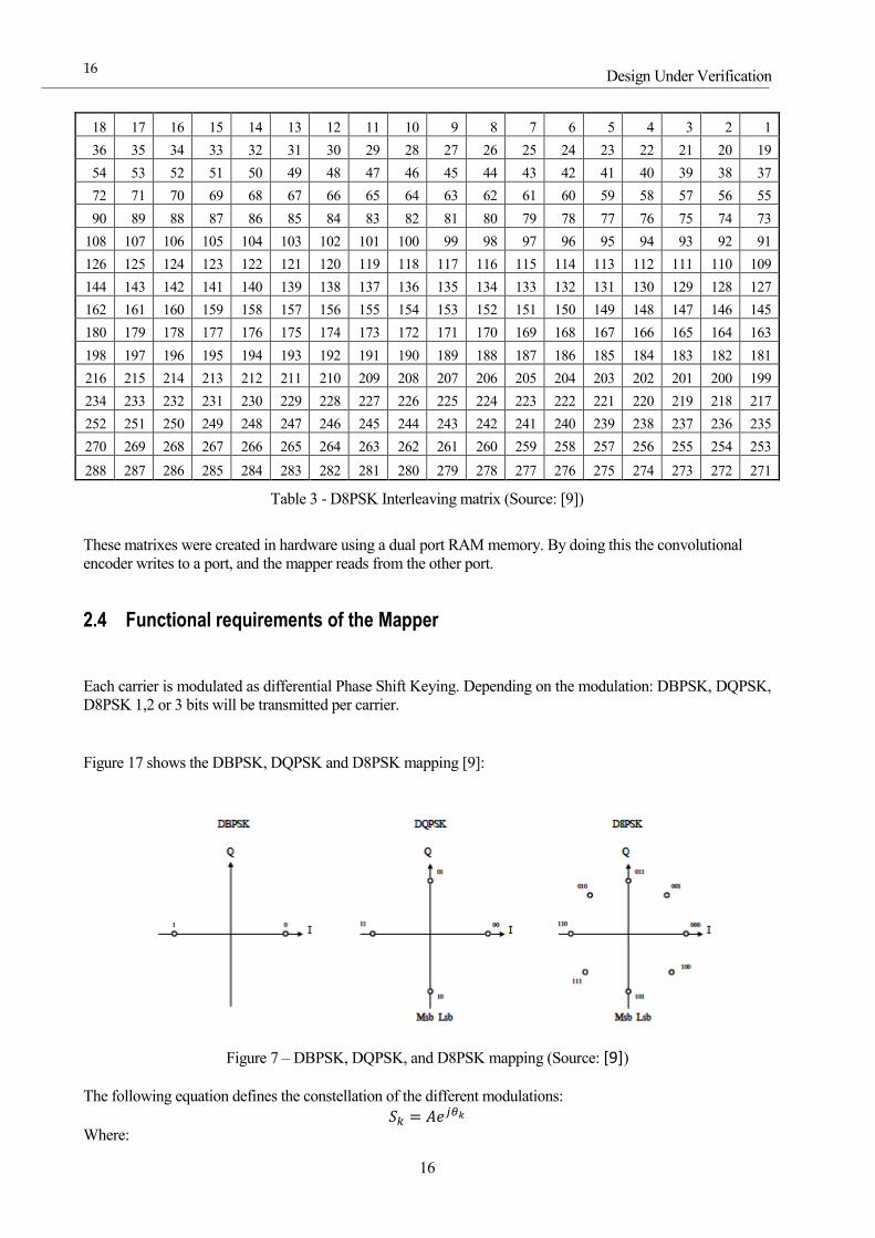
18 17 16 15 14 13 12 11 10 9 8 7 6 5 4 3 2 1
36 35 34 33 32 31 30 29 28 27 26 25 24 23 22 21 20 19
54 53 52 51 50 49 48 47 46 45 44 43 42 41 40 39 38 37
72 71 70 69 68 67 66 65 64 63 62 61 60 59 58 57 56 55
90 89 88 87 86 85 84 83 82 81 80 79 78 77 76 75 74 73
108 107 106 105 104 103 102 101 100 99 98 97 96 95 94 93 92 91
126 125 124 123 122 121 120 119 118 117 116 115 114 113 112 111 110 109
144 143 142 141 140 139 138 137 136 135 134 133 132 131 130 129 128 127
162 161 160 159 158 157 156 155 154 153 152 151 150 149 148 147 146 145
180 179 178 177 176 175 174 173 172 171 170 169 168 167 166 165 164 163
198 197 196 195 194 193 192 191 190 189 188 187 186 185 184 183 182 181
216 215 214 213 212 211 210 209 208 207 206 205 204 203 202 201 200 199
234 233 232 231 230 229 228 227 226 225 224 223 222 221 220 219 218 217
252 251 250 249 248 247 246 245 244 243 242 241 240 239 238 237 236 235
270 269 268 267 266 265 264 263 262 261 260 259 258 257 256 255 254 253
288 287 286 285 284 283 282 281 280 279 278 277 276 275 274 273 272 271
Table 3 - D8PSK Interleaving matrix (Source: [9])
These matrixes were created in hardware using a dual port RAM memory. By doing this the convolutional
encoder writes to a port, and the mapper reads from the other port.
2.4 Functional requirements of the Mapper
Each carrier is modulated as differential Phase Shift Keying. Depending on the modulation: DBPSK, DQPSK,
D8PSK 1,2 or 3 bits will be transmitted per carrier.
Figure 17 shows the DBPSK, DQPSK and D8PSK mapping [9]:
Figure 7 – DBPSK, DQPSK, and D8PSK mapping (Source: [9])
The following equation defines the constellation of the different modulations:
𝑆𝑘 = 𝐴𝑒𝑗𝜃𝑘 Where:
17
k is the frequency index that represents each subcarrier within an OFDM symbol. k =1 corresponds to the
phase reference (0º).
𝑆𝑘 is the mapper output for each subcarrier.
𝜃𝑘 is the carrier phase, defined by: 𝜃𝑘 = (𝜃𝑘−1 + (2𝜋
𝑀) ∆𝑏𝑘) mod 2𝜋 .
o ∆𝑏𝑘 represent the data coded in each modulation. ∆𝑏𝑘 ∈ {0,1, … , 𝑀 − 1}
o M = 2,4 or 8 for DBPSK, DQPSK, D8PSK respectively.
o A represents the power in each carrier and also the ring radius from the center of the
constellation.
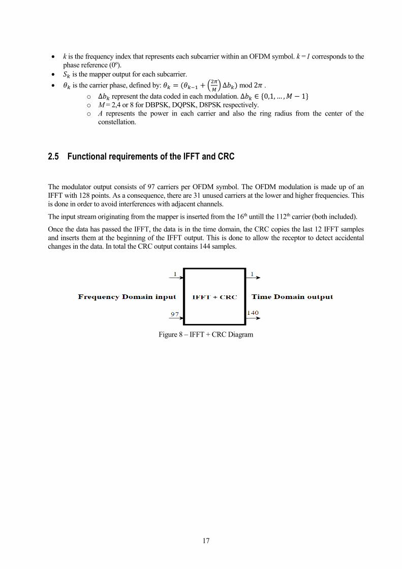
2.5 Functional requirements of the IFFT and CRC
The modulator output consists of 97 carriers per OFDM symbol. The OFDM modulation is made up of an
IFFT with 128 points. As a consequence, there are 31 unused carriers at the lower and higher frequencies. This
is done in order to avoid interferences with adjacent channels.
The input stream originating from the mapper is inserted from the 16th untill the 112th carrier (both included).
Once the data has passed the IFFT, the data is in the time domain, the CRC copies the last 12 IFFT samples
and inserts them at the beginning of the IFFT output. This is done to allow the receptor to detect accidental
changes in the data. In total the CRC output contains 144 samples.
Figure 8 – IFFT + CRC Diagram

Design Under Verification
18
18
19
3 THE UNIVERSAL VERIFICATION
METHODOLOGY (UVM)
3.1 Introduction
The UVM is very comprehensive, and this chapter does not go into extensive detail into it. Instead this chapter
will cover briefly the main features of a UVM testbench. The interested reader can find the official
documentation in [10]. There are also free online courses and very good cookbook in the Verification
Academy website [11].
The Universal Verification Methodology was standardized in 2009 by Accellera, a standards organization in
the EDA and IC areas. The UVM is a methodology for verifying integrated circuit designs. It is the combined
effort of designers and tool vendors based on the VMM and the OVM (which is based in e). The UVM is not a
verification language, but rather an open source SystemVerilog class library. It is designed to enable the
creation of robust, reusable, interoperable verification IP and testbench components [12].
The main caracteristics of the UVM are the powerful testbenches that use constrained random stimulus
generation and functional coverage methodologies. Unfortunately, (or fortunately) the UVM is not yet a total
methodology of how to approach every step in verification. However, even though there are discrepancies on
how to follow certain aspects of it, it is a great guide to the main paths in verification. Furthermore, it is in its
popularity and most knowledgable engineers agree that is the future verification methodology. At the moment
the UVM is endorsed by all the major simulator vendors.
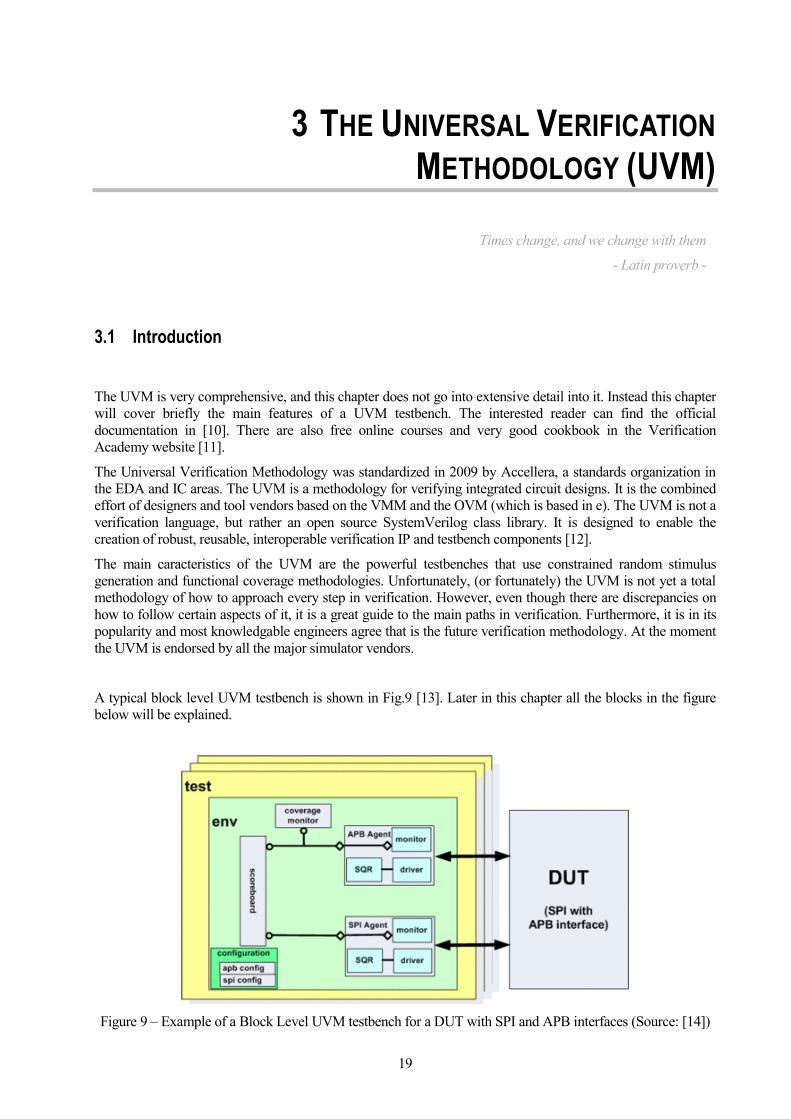
A typical block level UVM testbench is shown in Fig.9 [13]. Later in this chapter all the blocks in the figure
below will be explained.
Figure 9 – Example of a Block Level UVM testbench for a DUT with SPI and APB interfaces (Source: [14])
Times change, and we change with them
- Latin proverb -
The Universal Verification Methodology (UVM)
20
20
3.2 UVM components
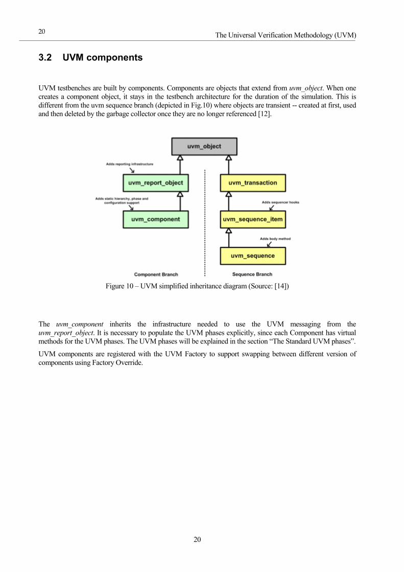
UVM testbenches are built by components. Components are objects that extend from uvm_object. When one
creates a component object, it stays in the testbench architecture for the duration of the simulation. This is
different from the uvm sequence branch (depicted in Fig.10) where objects are transient -- created at first, used
and then deleted by the garbage collector once they are no longer referenced [12].
Figure 10 – UVM simplified inheritance diagram (Source: [14])
The uvm_component inherits the infrastructure needed to use the UVM messaging from the
uvm_report_object. It is necessary to populate the UVM phases explicitly, since each Component has virtual
methods for the UVM phases. The UVM phases will be explained in the section “The Standard UVM phases”.
UVM components are registered with the UVM Factory to support swapping between different version of
components using Factory Override.
21
Class Description Contains sub-
components?
uvm_driver Adds sequence communication sub-components, used with the uvm_sequencer Yes
uvm_sequencer Adds sequence communication sub-components, used with the uvm_driver Yes
uvm_subscriber A wrapper around a uvm_analysis_export Yes
uvm_env Container for the verification components surrounding a DUT, or other envs surrounding a
(sub)system No
uvm_test Used for the top level test class No
uvm_monitor Used for monitors No
uvm_scoreboard Used for scoreboards No
uvm_agent Used as the agent container class No
Table 4 – UVM components (Source: [15])
In the UVM the components could be separated in three groups:
Container components.
Stimulus layer.
Analysis layer.
3.3 UVM Transactions
In verification of digital designs, Transactions could be described as a class which groups data and the
necessary operations that can be done to that data. UVM Transactions are used to separate relevant data from
pin activity. For a VHDL user a transaction could be seen as a record data type, only that transactions are
relative to the class-based objects world. Transactions are used to share data between different components.
The life of a Transaction is generally related to its use; when the testbench no longer references it, it is
collected by the garbage collector.
Because the type uvm_transaction is deprecated, verification engineers use its subtype: uvm_sequence_item.
The Sequencer and Monitor Components send Transactions, while the Driver, Scoreboard and Coverage
Components receive them.
3.4 The BFM
BFM stands for Bus Functional Model and consists of an abstraction to interact with the DUV. It encapsulates
all the signals of the DUV so the rest of the testbench can be separated from the static module-based world.
How complex a BFM is will vary from design to design depending on the bus protocol. BFMs are usually
implemented within a SystemVerilog interface and perform the BFM model by using tasks and functions.
The Universal Verification Methodology (UVM)
22
22
3.5 Container Components
The two container Components in a testbench are the Environment and the Agent.
3.5.1 The Env Component
In general, the Env could be defined as the component that groups the rest of the testbench. This may change
from design to design, and sometimes there is a top level Env with other Envs inside. In order to use the UVM
Env methods, a class may need to extend the UVM component uvm_env.
3.5.2 The Agent Component
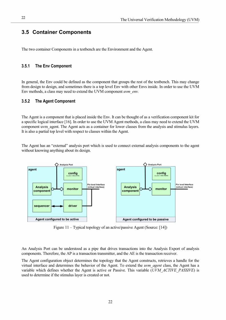
The Agent is a component that is placed inside the Env. It can be thought of as a verification component kit for
a specific logical interface [16]. In order to use the UVM Agent methods, a class may need to extend the UVM
component uvm_agent. The Agent acts as a container for lower classes from the analysis and stimulus layers.
It is also a partial top level with respect to classes within the Agent.
The Agent has an “external” analysis port which is used to connect external analysis components to the agent
without knowing anything about its design.
Figure 11 – Typical topology of an active/passive Agent (Source: [14])
An Analysis Port can be understood as a pipe that drives transactions into the Analysis Export of analysis
components. Therefore, the AP is a transaction transmitter, and the AE is the transaction receiver.
The Agent configuration object determines the topology that the Agent constructs, retrieves a handle for the
virtual interface and determines the behavior of the Agent. To extend the uvm_agent class, the Agent has a
variable which defines whether the Agent is active or Passive. This variable (UVM_ACTIVE_PASSIVE) is
used to determine if the stimulus layer is created or not.
23
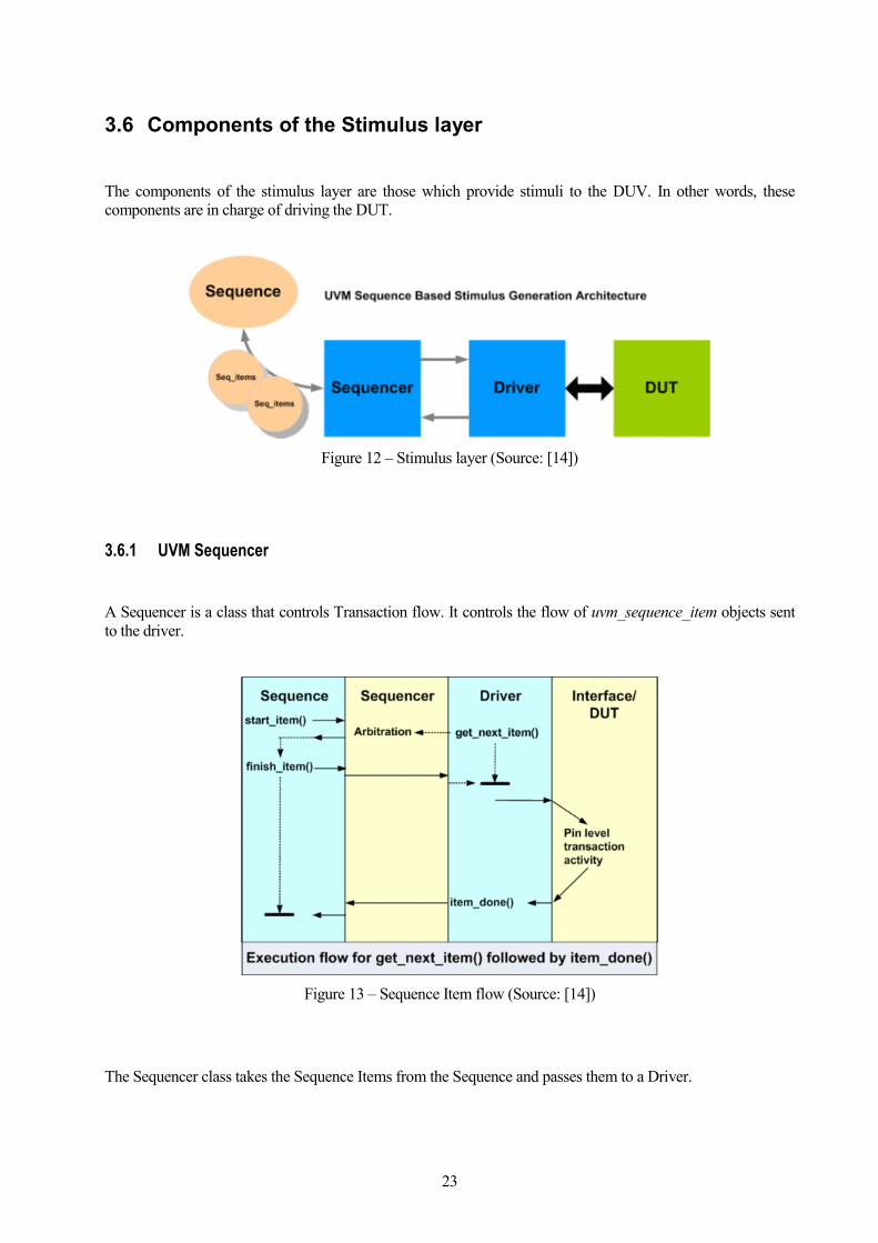
3.6 Components of the Stimulus layer
The components of the stimulus layer are those which provide stimuli to the DUV. In other words, these
components are in charge of driving the DUT.
Figure 12 – Stimulus layer (Source: [14])
3.6.1 UVM Sequencer
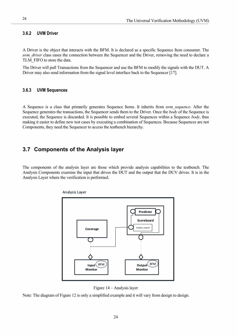
A Sequencer is a class that controls Transaction flow. It controls the flow of uvm_sequence_item objects sent
to the driver.
Figure 13 – Sequence Item flow (Source: [14])
The Sequencer class takes the Sequence Items from the Sequence and passes them to a Driver.
The Universal Verification Methodology (UVM)
24
24
3.6.2 UVM Driver
A Driver is the object that interacts with the BFM. It is declared as a specific Sequence Item consumer. The
uvm_driver class eases the connection between the Sequencer and the Driver, removing the need to declare a
TLM_FIFO to store the data.
The Driver will pull Transactions from the Sequencer and use the BFM to modify the signals with the DUT. A
Driver may also send information from the signal level interface back to the Sequencer [17].
3.6.3 UVM Sequences
A Sequence is a class that primarily generates Sequence Items. It inherits from uvm_sequence. After the
Sequence generates the transactions, the Sequencer sends them to the Driver. Once the body of the Sequence is
executed, the Sequence is discarded. It is possible to embed several Sequences within a Sequence body, thus
making it easier to define new test cases by executing a combination of Sequences. Because Sequences are not
Components, they need the Sequencer to access the testbench hierarchy.
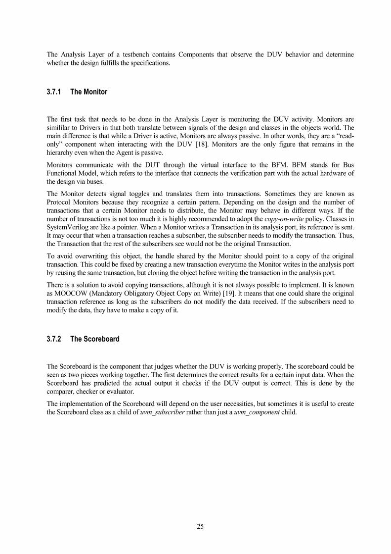
3.7 Components of the Analysis layer
The components of the analysis layer are those which provide analysis capabilities to the testbench. The
Analysis Components examine the input that drives the DUT and the output that the DUV drives. It is in the
Analysis Layer where the verification is performed.
Analysis Layer
Coverage
Scoreboard
Input Monitor
Output Monitor
Analysis_export
BFM BFM
Predictor
Figure 14 – Analysis layer
Note: The diagram of Figure 12 is only a simplified example and it will vary from design to design.
25
The Analysis Layer of a testbench contains Components that observe the DUV behavior and determine
whether the design fulfills the specifications.
3.7.1 The Monitor
The first task that needs to be done in the Analysis Layer is monitoring the DUV activity. Monitors are
simililar to Drivers in that both translate between signals of the design and classes in the objects world. The
main difference is that while a Driver is active, Monitors are always passive. In other words, they are a “read-
only” component when interacting with the DUV [18]. Monitors are the only figure that remains in the
hierarchy even when the Agent is passive.
Monitors communicate with the DUT through the virtual interface to the BFM. BFM stands for Bus
Functional Model, which refers to the interface that connects the verification part with the actual hardware of
the design via buses.
The Monitor detects signal toggles and translates them into transactions. Sometimes they are known as
Protocol Monitors because they recognize a certain pattern. Depending on the design and the number of
transactions that a certain Monitor needs to distribute, the Monitor may behave in different ways. If the
number of transactions is not too much it is highly recommended to adopt the copy-on-write policy. Classes in
SystemVerilog are like a pointer. When a Monitor writes a Transaction in its analysis port, its reference is sent.
It may occur that when a transaction reaches a subscriber, the subscriber needs to modify the transaction. Thus,
the Transaction that the rest of the subscribers see would not be the original Transaction.
To avoid overwriting this object, the handle shared by the Monitor should point to a copy of the original
transaction. This could be fixed by creating a new transaction everytime the Monitor writes in the analysis port
by reusing the same transaction, but cloning the object before writing the transaction in the analysis port.
There is a solution to avoid copying transactions, although it is not always possible to implement. It is known
as MOOCOW (Mandatory Obligatory Object Copy on Write) [19]. It means that one could share the original
transaction reference as long as the subscribers do not modify the data received. If the subscribers need to
modify the data, they have to make a copy of it.
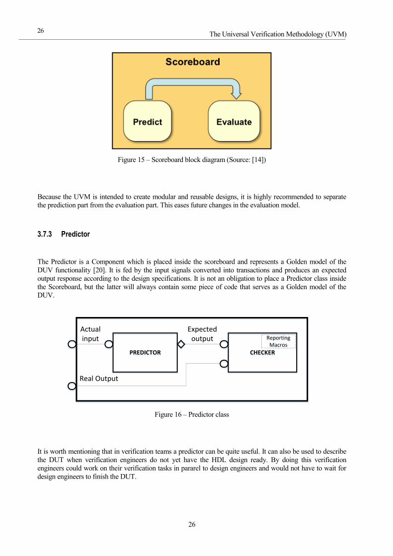
3.7.2 The Scoreboard
The Scoreboard is the component that judges whether the DUV is working properly. The scoreboard could be
seen as two pieces working together. The first determines the correct results for a certain input data. When the
Scoreboard has predicted the actual output it checks if the DUV output is correct. This is done by the
comparer, checker or evaluator.
The implementation of the Scoreboard will depend on the user necessities, but sometimes it is useful to create
the Scoreboard class as a child of uvm_subscriber rather than just a uvm_component child.
The Universal Verification Methodology (UVM)
26
26
Figure 15 – Scoreboard block diagram (Source: [14])
Because the UVM is intended to create modular and reusable designs, it is highly recommended to separate
the prediction part from the evaluation part. This eases future changes in the evaluation model.
3.7.3 Predictor
The Predictor is a Component which is placed inside the scoreboard and represents a Golden model of the
DUV functionality [20]. It is fed by the input signals converted into transactions and produces an expected
output response according to the design specifications. It is not an obligation to place a Predictor class inside
the Scoreboard, but the latter will always contain some piece of code that serves as a Golden model of the
DUV.
CHECKERCHECKERPREDICTORPREDICTOR
Actual input
Expected output
Real Output
Reporting Macros
Reporting Macros
Figure 16 – Predictor class
It is worth mentioning that in verification teams a predictor can be quite useful. It can also be used to describe
the DUT when verification engineers do not yet have the HDL design ready. By doing this verification
engineers could work on their verification tasks in pararel to design engineers and would not have to wait for
design engineers to finish the DUT.
27
3.7.4 Coverage objects
Coverage objects perform functional coverage, and their design and distribution around the testbench will vary
from design to design. The Coverage objects’ task is to determine whether all the possible stimuli has been
applied to the system. A design is not considered fully tested until all functional coverage has been done, even
if the design has 100% code coverage.
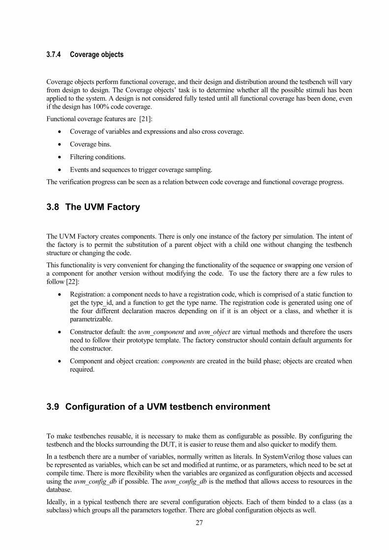
Functional coverage features are [21]:
Coverage of variables and expressions and also cross coverage.
Coverage bins.
Filtering conditions.
Events and sequences to trigger coverage sampling.
The verification progress can be seen as a relation between code coverage and functional coverage progress.
3.8 The UVM Factory
The UVM Factory creates components. There is only one instance of the factory per simulation. The intent of
the factory is to permit the substitution of a parent object with a child one without changing the testbench
structure or changing the code.
This functionality is very convenient for changing the functionality of the sequence or swapping one version of
a component for another version without modifying the code. To use the factory there are a few rules to
follow [22]:
Registration: a component needs to have a registration code, which is comprised of a static function to
get the type_id, and a function to get the type name. The registration code is generated using one of
the four different declaration macros depending on if it is an object or a class, and whether it is
parametrizable.
Constructor default: the uvm_component and uvm_object are virtual methods and therefore the users
need to follow their prototype template. The factory constructor should contain default arguments for
the constructor.
Component and object creation: components are created in the build phase; objects are created when
required.
3.9 Configuration of a UVM testbench environment
To make testbenches reusable, it is necessary to make them as configurable as possible. By configuring the
testbench and the blocks surrounding the DUT, it is easier to reuse them and also quicker to modify them.
In a testbench there are a number of variables, normally written as literals. In SystemVerilog those values can
be represented as variables, which can be set and modified at runtime, or as parameters, which need to be set at
compile time. There is more flexibility when the variables are organized as configuration objects and accessed
using the uvm_config_db if possible. The uvm_config_db is the method that allows access to resources in the
database.
Ideally, in a typical testbench there are several configuration objects. Each of them binded to a class (as a
subclass) which groups all the parameters together. There are global configuration objects as well.
The Universal Verification Methodology (UVM)
28
28
Basically, all Components that require configuration follow the same flow. Immediately after being
configured, the internal structure and behavior is created based on that configuration. Finally, they configure
all children at lower levels. Configuration objects can be retrieved and inserted from/into the database using
the uvm_config_db API through the methods uvm_config_db #(…)::get(…) and uvm_config_db #(…)::set
respectively. The uvm_config_db method is parametrizable to be able to retrieve and insert different
configuration objects.
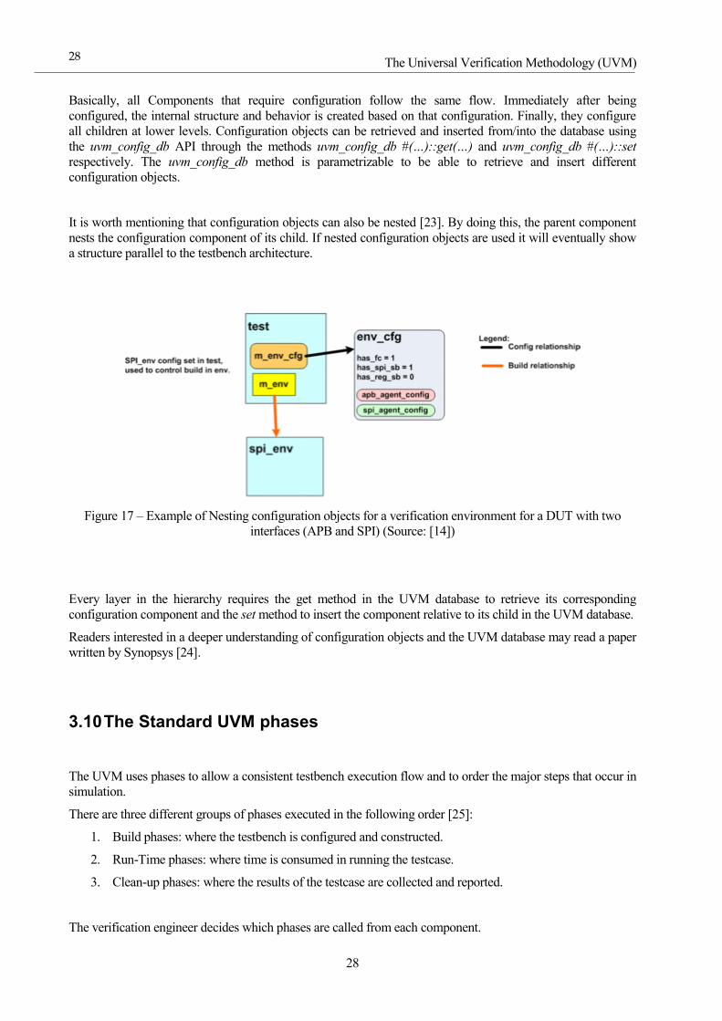
It is worth mentioning that configuration objects can also be nested [23]. By doing this, the parent component
nests the configuration component of its child. If nested configuration objects are used it will eventually show
a structure parallel to the testbench architecture.
Figure 17 – Example of Nesting configuration objects for a verification environment for a DUT with two
interfaces (APB and SPI) (Source: [14])
Every layer in the hierarchy requires the get method in the UVM database to retrieve its corresponding
configuration component and the set method to insert the component relative to its child in the UVM database.
Readers interested in a deeper understanding of configuration objects and the UVM database may read a paper
written by Synopsys [24].
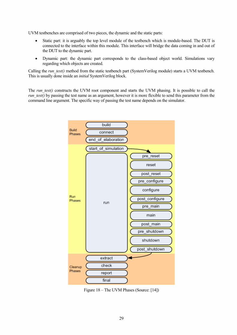
3.10 The Standard UVM phases
The UVM uses phases to allow a consistent testbench execution flow and to order the major steps that occur in
simulation.
There are three different groups of phases executed in the following order [25]:
1. Build phases: where the testbench is configured and constructed.
2. Run-Time phases: where time is consumed in running the testcase.
3. Clean-up phases: where the results of the testcase are collected and reported.
The verification engineer decides which phases are called from each component.
29
UVM testbenches are comprised of two pieces, the dynamic and the static parts:
Static part: it is arguably the top level module of the testbench which is module-based. The DUT is
connected to the interface within this module. This interface will bridge the data coming in and out of
the DUT to the dynamic part.
Dynamic part: the dynamic part corresponds to the class-based object world. Simulations vary
regarding which objects are created.
Calling the run_test() method from the static testbench part (SystemVerilog module) starts a UVM testbench.
This is usually done inside an initial SystemVerilog block.
The run_test() constructs the UVM root component and starts the UVM phasing. It is possible to call the
run_test() by passing the test name as an argument, however it is more flexible to send this parameter from the
command line argument. The specific way of passing the test name depends on the simulator.
Figure 18 – The UVM Phases (Source: [14])
The Universal Verification Methodology (UVM)
30
30
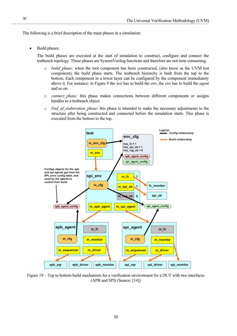
The following is a brief description of the main phases in a simulation:
Build phases:
The build phases are executed at the start of simulation to construct, configure and connect the
testbench topology. These phases are SystemVerilog functions and therefore are not time consuming.
o build_phase: when the root component has been constructed, (also know as the UVM test
component), the build phase starts. The testbench hierarchy is built from the top to the
bottom. Each component in a lower layer can be configured by the component immediately
above it. For instance: in Figure 9 the test has to build the env, the env has to build the agent
and so on.
o connect_phase: this phase makes connections between different components or assigns
handles to a testbench object.
o End_of_elaboration_phase: this phase is intended to make the necessary adjustments to the
structure after being constructed and connected before the simulation starts. This phase is
executed from the bottom to the top.
.
Figure 19 – Top to bottom build mechanism for a verification environment for a DUT with two interfaces
(APB and SPI) (Source: [14])
31
Run phases:
The testbench stimulus is generated and executed during the time consuming phases or tasks. This
phase goes right after the build phase has finished. Everything within the run_phase() goes in parallel.
The run phase generates and checks the stimuli.
Clean-up phases:
These phases are used to extract the information of the scoreboard and functional coverage of the
monitors, thus determining whether the test passed and the coverage goals were reached. Clean-up
phases do not consume time and therefore are implemented as functions. These phases have a bottom
to top approach.
o extract_phase(): is used to retrieve and process information from analysis objects.
o report_phase():is used to print the results of simulation.
o final_phase(): is used to do any other task that was not done before.
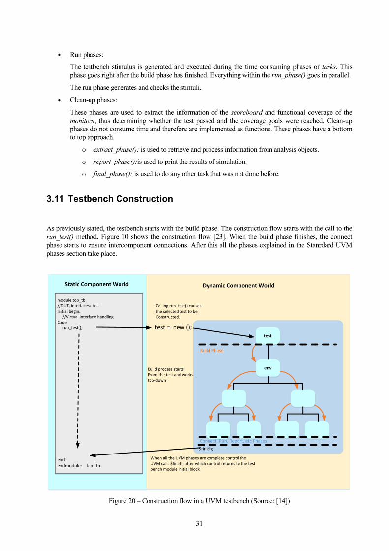
3.11 Testbench Construction
As previously stated, the testbench starts with the build phase. The construction flow starts with the call to the
run_test() method. Figure 10 shows the construction flow [23]. When the build phase finishes, the connect
phase starts to ensure intercomponent connections. After this all the phases explained in the Stanrdard UVM
phases section take place.
env
test
$finish;
Connect, Run, Report, etc Phases
Build Phase
Dynamic Component WorldStatic Component World
Calling run_test() causesthe selected test to be Constructed.
Build process startsFrom the test and works top-down
test = new ();
When all the UVM phases are complete control the UVM calls $finish, after which control returns to the testbench module initial block
module top_tb;//DUT, interfaces etc Initial begin. //Virtual Interface handlingCode run_test();
endendmodule: top_tb
Figure 20 – Construction flow in a UVM testbench (Source: [14])
The Universal Verification Methodology (UVM)
32
32
The call to build method in the build phase triggers the construction of the test class, which is the first object
constructed. Thus the test class will determine the testbench architecture. The test class [23] :
Sets up factory overrides, thus creating the components or configuration objects as derived types.
Factory overrides allow classes to be substituted by child classes. By using the factory override
mechanism, it is possible to write more reusable testbenches, avoiding the need to change the
component declaration for every case.
Creates and configures the configuration objects required by the subcomponents.
Assigns virtual interfaces. The recommended way of sharing the virtual interface handlers is by
configuring the objects and the database. Before calling the run_test() method, it is necessary to
connect the DUT with the interfaces. A handle to each interface should have been assigned to virtual
interface handles and then passed to the UVM database. These virtual interface references will then be
assigned to the BFM inside the relevant configuration object handles. They are used to drive or
monitor DUT signals. Drivers and Monitors should not get the virtual interface handlers from the
database and should use configuration objects to keep the testbench structure clean, reusable and
modular. In the test class, virtual interfaces should be assigned to the corresponding components as
part of their configuration objects.
Builds a level below in the testbench hierarchy as shown in Figure 13.
The UVM is very flexible. More than one env can be built if required by the DUV complexity. The creation of
additional Envs is conditional and depends on each testing situation.
It is very common to have a similar test classes if they are not the same for each test. Due to this, it is highly
recommended to create a virtual “base test” class which the rest of the test cases will extend from.
33
4 WORKFLOW
4.1 Introduction
This chapter explains my approach to learning how to create a UVM verification testbench for the OFDM
transceiver, the tools I used and the verification capabilities I sought to add to the testbench.
4.2 Tools
The tools I had for this Project were:
QuestaSim: an HDL and VHDL simulator of Mentor Graphics. It was used to carry the mixed VHDL
and SystemVerilog + UVM simulations.
Matlab: because of the compatibility with the Questa simulator, Matlab was the software used to
accomplish the Golden Model.
Doxygen: a tool for generating documentation. It does not integrate SystemVerilog, but a Perl patch
design by Christoph Suehnel allows it to integrate SystemVerilog.
Emacs: At the moment there are several text editors which are SystemVerilog compatible. I used
Emacs because the HDL part of the project was written in VHDL, it has a great VHDL mode
integrated in it, and it is SystemVerilog compatible.
4.3 Process to learn the UVM
Before starting this project, I did not know anything about the UVM. Therefore, I needed to decide on the best
strategy to face the task. SystemVerilog has the same syntax as Verilog, but with Extended functions.
SystemVerilog is both an HDL and HVL language. However, this project only used its HVL capabilities
because the HDL was already written in VHDL. SystemVerilog is an Object Oriented Programming
Language, of which I had no previous knowledge.
I took several steps to adapt and improve my testbench. The first approach was to test only one block of the
whole transceiver. I chose to test the scrambler because it is one of the simplest blocks. The steps I followed
were the following:
1. Conventional testbench: I coded a SystemVerilog testbench without using any OOP. All the code was
If you don’t know where you are going, you might wind up
someplace else.
- Yogi Berra -
Workflow
34
34
in the same file under the same SystemVerilog module.
2. Interfaces and BFM: the files were separated in different SystemVerilog modules. There was a top
SystemVerilog module where the rest of modules were instatiated. All the modules had access to the
BFM. This test did not have functional coverage yet.
3. First OOP testbench: This test had first two parts: the static and dynamic object worlds. It did not have
any functional coverage at that time.
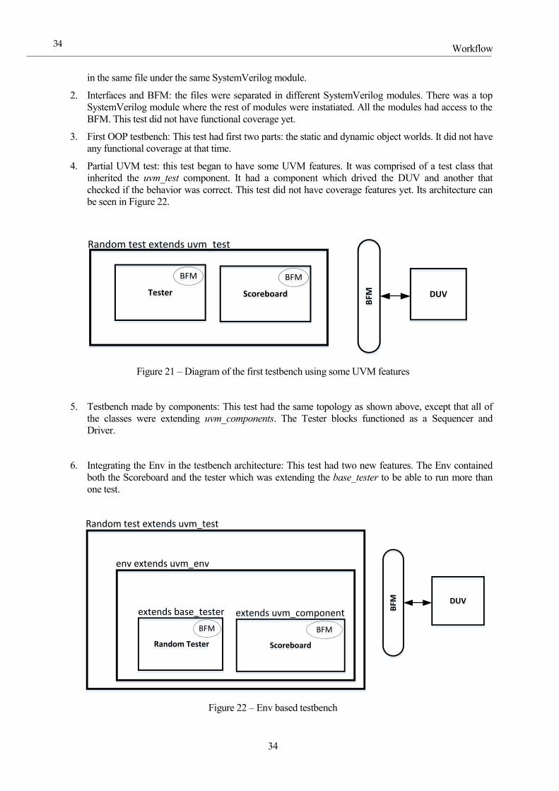
4. Partial UVM test: this test began to have some UVM features. It was comprised of a test class that
inherited the uvm_test component. It had a component which drived the DUV and another that
checked if the behavior was correct. This test did not have coverage features yet. Its architecture can
be seen in Figure 22.
Random test extends uvm_testRandom test extends uvm_test
ScoreboardScoreboard
BFMBFM
TesterTester
BFMBFM
BFMBFM DUVDUV
Figure 21 – Diagram of the first testbench using some UVM features
5. Testbench made by components: This test had the same topology as shown above, except that all of
the classes were extending uvm_components. The Tester blocks functioned as a Sequencer and
Driver.
6. Integrating the Env in the testbench architecture: This test had two new features. The Env contained
both the Scoreboard and the tester which was extending the base_tester to be able to run more than
one test.
extends base_testerextends base_tester
Random test extends uvm_testRandom test extends uvm_test
ScoreboardScoreboard
BFMBFM
Random Tester Random Tester
BFMBFM
BFMBFM DUVDUV
extends uvm_componentextends uvm_component
env extends uvm_envenv extends uvm_env
Figure 22 – Env based testbench
35
7. First test with functional coverage: this test included the Coverage class. The Scrambler had a serial
input so that the functional coverage was checking whether the input was zero or one. The topology
was the same as the shown in Figure 23, adding the Coverage class which extended a
uvm_component.
8. First test with internal functional coverage: The scrambler has a 7-bit shift register inside which had to
be tested. The Questa simulator has a bind constructor which allows internal DUT signals to be
checked [26].
extends base_testerextends base_tester
Random test extends uvm_testRandom test extends uvm_test
Random Tester Random Tester
BFMBFM
BFMBFM DUVDUV
env extends uvm_envenv extends uvm_env
CoverageCoverage
BFMBFM
extends uvm_componentextends uvm_component
ScoreboardScoreboard
BFMBFM
extends uvm_componentextends uvm_componentCovergroups and
bins
Covergroups and bins
Binded_BFMBinded_BFM
Figure 23 – Binded BFM performing functional coverage
9. Integrating the monitor in the structure: in the previous test both the Coverage and Scoreboard
components had access to the BFM. This test was different in that the Coverage class was fed by a
monitor. The Scoreboard class was still linked to the BFM because it needed access to the internal
signals of the DUT to compute the Golden model of the shift register. This test does not use
Transactions; it only used a variable sent throught the Analysis Port.
extends base_testerextends base_tester
Random test extends uvm_testRandom test extends uvm_test
Random Tester Random Tester
BFMBFM BFMBFM DUVDUV
env extends uvm_envenv extends uvm_env
CoverageCoverage
extends uvm_subscriberextends uvm_subscriber
ScoreboardScoreboard
BFMBFM
extends uvm_componentextends uvm_component
Covergroups and bins
Covergroups and bins
Binded_BFMBinded_BFMInput Monitor
Input Monitor
BFMBFM
extends uvm_component
extends uvm_component
Legend:Analysis export
Analysis port
Figure 24 – UVM monitor in the testbench
10. Integrating the UVM Reporting macros: All the previous testbenches had not used the UVM
Reporting system. Instead they had been using SystemVerilog tasks such as “$display”, “$error” and
“$final”.
11. Integrating UVM Transactions: as mentioned above, when the monitor was integrated it did not use
Transactions. In this testbench, both Coverage and Monitor Components were adapted to use
Transactions.
Workflow
36
36
12. Integrating the UVM Agent and Driver: This step added the Agent and the Driver to the testbench.
The architecture connected the Tester and Driver using a UVM_TLM_FIFO. The UVM_TLM_FIFO is connected to allow ports into and out of the Tester and Driver, respectively.
extends uvm_component
extends uvm_component
Scrambler_agent extends uvm_agentScrambler_agent extends uvm_agent
BFMBFM DUVDUV
env extends uvm_envenv extends uvm_env
CoverageCoverage
extends uvm_subscriberextends uvm_subscriber
ScoreboardScoreboard
BFMBFM
extends uvm_componentextends uvm_component
Covergroups and bins
Covergroups and bins
Binded_BFMBinded_BFMInput Monitor
Input Monitor
BFMBFM
extends uvm_componentextends uvm_component
Legend:Analysis export
Analysis port
Random test extends uvm_testRandom test extends uvm_test
TesterTester UVM_TLM_FIFOUVM_TLM_FIFO DriverDriver
BFMBFM
extends uvm_component
extends uvm_component
Figure 25 – Integration of UVM Agent and Driver extending a component
13. Integrating UVM Sequences: Apart from the Scoreboard, the rest of the UVM blocks were
functioning in their respective roles. A Sequencer and a Driver were added.
Random test extends uvm_testRandom test extends uvm_test
env extends uvm_envenv extends uvm_env
uvm_componentuvm_component
Scrambler_agent extends uvm_agentScrambler_agent extends uvm_agent
BFMBFM DUVDUV
CoverageCoverage
extends uvm_subscriberextends uvm_subscriber
ScoreboardScoreboard
BFMBFM
extends uvm_componentextends uvm_component
Covergroups and bins
Covergroups and bins
Binded_BFMBinded_BFMInput Monitor
Input Monitor
BFMBFM
extends uvm_component
extends uvm_component
Legend:Analysis export
Analysis port
SequencerSequencer DriverDriver
BFMBFM
extends uvm_driver
extends uvm_driver
Figure 26 – Integration of the full UVM stimulus layer: Sequencer and Driver
14. Integrating the Scoreboard to a Monitor: The Scoreboard needs both input and output Transactions
since it predicts whether the DUV is working properly. Therefore, it needs two Analysis Exports. The
first inherits uvm_subscriber and the second was created using a uvm_tlm_analysis_fifo. It was
possible to isolate the Scoreboard from the DUT signals using an appropriate monitor to read the pin-
level signals. The FIFO stores the input value, and everytime the DUT generates an output value it
makes the LFSR shift and checks if the values are the same.
37
Random test extends uvm_testRandom test extends uvm_test
uvm_componentuvm_component
Scrambler_agent extends uvm_agentScrambler_agent extends uvm_agent
BFMBFM DUVDUV
env extends uvm_envenv extends uvm_env
CoverageCoverage
extends uvm_subscriberextends uvm_subscriber
ScoreboardScoreboard
extends uvm_subscriberextends uvm_subscriber
Covergroups and bins
Covergroups and bins
Binded_BFMBinded_BFMInput
Monitor
Input Monitor
BFMBFM
extends uvm_component
extends uvm_component
Legend:Analysis export
Analysis port
SequencerSequencer DriverDriver
BFMBFM
extends uvm_driver
extends uvm_driver
Output Monitor
Output Monitor
uvm_tlm_analysis_fifouvm_tlm_analysis_fifo
SequencesSequences
Stimulus Layer Analysis Layer
BFMBFM
Figure 27 – Scoreboard ↔ Monitor Integration
15. Integrating the Configuration Objects: the same principle explained in 3.7 has been applied here. The
Test Component retrieves the handle to the BFM from the UVM database, fills a configuration object
for the Env and inserts it in the database. Then, the Env gets the Configuration Object out of the
database and fills the Agent Configuration Object. If the UVM_ACTIVE_PASSIVE variable were set
to passive, the testbench would not have the Stimulus Layer.

Workflow
38
38
39
5 MATLAB INTEGRATED IN THE SCRAMBLER
TESTBENCH
SystemVerilog is a programming language that can be very powerful to design Golden models. Although it is
possible to design Golden models in SystemVerilog, I did not use one because I already had Matlab simulation
models according to the transceiver specifications. By using Matlab instead of SystemVerilog to model the
IFFT in the testbench, I avoided much of the difficulty in completing this time-consuming task.
5.1 Matlab integration into Questasim
Using Matlab source code during the verification process significantly reduced the time to develop a
verification testbench. Existing Matlab functions can be used for both initial testbench development as a DUT
before the RTL is available, as well as a Scoreboard to verify DUV functionality [27].
There are three interesting ways to use Matlab together with VHDL, SystemVerilog or mixed testbenches:
Questa Simulator dedicated Matlab integration package:
The Mentor Graphics Questa simulator has a package that permits setting up a connection between Matlab
and VHDL/SystemVerilog more quickly. The main features are:
1. VHDL/SV QMW API that allows sending integers, matrixes and vectors between the simulator
and Matlab, and also permits sending commands.
2. TCL layer that allows sending signals. Note: this feature would be very useful in case Matlab
were used as a temporary DUT.
3. Debugging of SV/Matlab code.
Matlab C API with SystemVerilog DPI.
Matlab function as VHDL entities:
The input and output of the Matlab functions are the VHDL ports. This works internally and calls to other
functions. It is necessary to make Matlab understand HDL signals which is not a trivial task, and there is
also difficulty caused by Matlab’s inaccurate clock cycle.
The choice to integrate Matlab with QuestaSim was the QMW API, since it eases the Matlab-Testbench
communication. However, Matlab C API with SystemVerilog DPI could have also been used with a little extra
If at first you don't succeed; call it version 1.0
- Anonymous quote-
Matlab Integrated in the Scrambler testbench
40
40
effort.
5.2 Necessities to adapt the Matlab Script
According to the PRIME alliance specifications, the scrambler can be modeled as a 7-bit LFSR, which is
equivalent to XORing the input of the scrambler and a pseudo sequence given as:
Pref0..126= {0,0,0,0,1,1,1,0,1,1,1,1,0,0,1,0,1,1,0,0,1,0,0,1,0,0,0,0,0,0,1,0,0,0,1,0,0,1,1,0,0,0,1,0,1,1,1,0,1,0,1,1,0,1,1,0,0,0,0
,0,1,1,0,0,1,1,0,1,0,1,0,0,1,1,1,0,0,1,1,1,1,0,1,1,0,1,0,0,0,0,1,0,1,0,1,0,1,1,1,1,1,0,1,0,0,1,0,1,0,0,0,1,1,0,1,1,1,0,
0,0,1,1,1,1,1,1,1}
The Matlab script was designed originally to work with complete blocks of bits, and the original script would
not work with the HDL scrambler because the RTL code had an FSM that Matlab could not follow.
In order to adapt the Matlab script it was necessary to implement a variable that was not erased every time the
SV predictor sent a new input bit. Most programming languages have a static variable type. Static variables are
used in functions. When the function is called for the first time, the variable is declared and is stored in the
memory. Matlab has a static type called persistent. By using static variables, it was possible to adapt the
internal state of the FSM to the Matlab function.
5.3 Topology of the Scrambler testbench.
The testbench had the architecture shown in Fig. 28 with a few modifications to the Components.
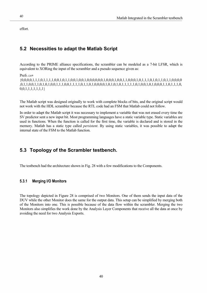
5.3.1 Merging I/O Monitors
The topology depicted in Figure 28 is comprised of two Monitors. One of them sends the input data of the
DUV while the other Monitor does the same for the output data. This setup can be simplified by merging both
of the Monitors into one. This is possible because of the data flow within the scrambler. Merging the two
Monitors also simplifies the work done by the Analysis Layer Components that receive all the data at once by
avoiding the need for two Analysis Exports.
41
Analysis LayerAnalysis Layer
CoverageCoverage
extends uvm_subscriberextends uvm_subscriber
ScoreboardScoreboard
extends uvm_subscriberextends uvm_subscriber
I / O Monitor
I / O Monitor
BFMBFM
extends uvm_monitor
extends uvm_monitor
Legend:Analysis export
Analysis port
Figure 28 – Input and Output Monitors merged into one
It is worth mentioning that in order to being able to modify the Monitor as explained above it is also necessary
to modify the Transaction class. The Transactions previously were working as two separate transactions. There
was an input and an output Transaction, which were combined into one Transaction class that contains all of
the compacted data.
Note: In all the testbench topologies the Monitor extended the uvm_component, but it was modified to extend
uvm_monitor. In fact, this change was not necessary because the features of uvm_monitor are the same as
uvm_component. However, the UVM guidelines suggest extending the proper component when possible. By
doing so, if in the future such Components have any additional features, the migration would be easier, faster
and less prone to error.
Matlab Integrated in the Scrambler testbench
42
42
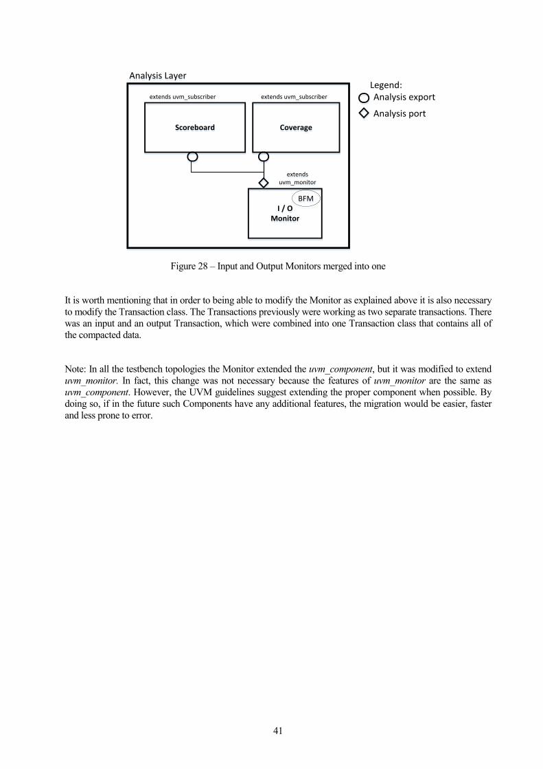
5.3.2 Scoreboard topology
The Scoreboard functionality has been split between two additional Components: The Predictor and the
Checker. The Predictor is the class which will work as the golden model while the Checker will test whether
the DUV is working according to the specifications.
Analysis LayerAnalysis Layer
CoverageCoverage
extends uvm_subscriberextends uvm_subscriberScoreboard extends uvm_componentScoreboard extends uvm_component
I / O Monitor
I / O Monitor
BFMBFM
extends uvm_monitor
extends uvm_monitor
Legend:Analysis export
Analysis port
Predictor extends uvm_subcriberPredictor extends uvm_subcriber
analysis_portanalysis_port
analysis_exportanalysis_exportanalysis_FIFOanalysis_FIFO
analysis_exportanalysis_exportanalysis_FIFOanalysis_FIFO
Expected valueExpected value
Actual valueActual value
Comparer extends uvm_componentComparer extends uvm_component
Figure 29 – Inside the Scoreboard
In order to make the configuration shown in Figure 30 it was necessary to design two Components:
Predictor: the predictor task was to work as a golden model, and also was to send the predicted output
to the comparer Component after calculating it. To accomplish that, it was necessary to implement an
Analysis Port which could send the expected output.
Comparer: The Comparer Component works as a checker. It receives both the real RTL output and
the ideal output and compares them. If the two values are unidentical it stops the simulation by using
the uvm_fatal reporting macro. I chose to have two Analysis Ports which were connected to an
Analysis FIFO. The purpose of adding an Analysis FIFO was that in case the Transactions were
arriving faster than what the Checker could run, the extra Transactions would be stored.
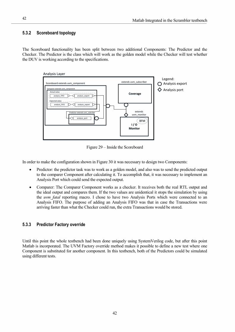
5.3.3 Predictor Factory override
Until this point the whole testbench had been done uniquely using SystemVerilog code, but after this point
Matlab is incorporated. The UVM Factory override method makes it possible to define a new test where one
Component is substituted for another component. In this testbench, both of the Predictors could be simulated
using different tests.
43
CoverageCoverage
extends uvm_subscriberextends uvm_subscriber
I / O Monitor
I / O Monitor
BFMBFM
extends uvm_monitor
extends uvm_monitor
Random test extends base_testRandom test extends base_test
uvm_componentuvm_component
Scrambler_agent extends uvm_agentScrambler_agent extends uvm_agent
BFMBFM
DUVDUV
env extends uvm_envenv extends uvm_env
Covergroups and binsCovergroups and bins
Binded_BFMBinded_BFM
Legend:
Analysis export
Analysis port
SequencerSequencer DriverDriver
BFMBFM
extends uvm_driver
extends uvm_driver
SequencesSequences
Stimulus Layer Analysis Layer
Scoreboard extends uvm_componentScoreboard extends uvm_component
Predictor extends uvm_subcriberPredictor extends uvm_subcriber
analysis_portanalysis_port
analysis_exportanalysis_exportanalysis_FIFOanalysis_FIFO
analysis_exportanalysis_exportanalysis_FIFOanalysis_FIFO
Expected valueExpected value
Actual valueActual value
Comparer extends uvm_componentComparer extends uvm_component
Figure 30 – Random test without Matlab Predictor
CoverageCoverage
extends uvm_subscriberextends uvm_subscriber
I / O Monitor
I / O Monitor
BFMBFM
extends uvm_monitor
extends uvm_monitor
Random_test_matlab extends random_testRandom_test_matlab extends random_test
uvm_componentuvm_component
Scrambler_agent extends uvm_agentScrambler_agent extends uvm_agent
BFMBFM
DUVDUV
env extends uvm_envenv extends uvm_env
Covergroups and binsCovergroups and bins
Binded_BFMBinded_BFM
Legend:
Analysis export
Analysis port
SequencerSequencer DriverDriver
BFMBFM
extends uvm_driver
extends uvm_driver
SequencesSequences
Stimulus Layer Analysis Layer
Scoreboard extends uvm_componentScoreboard extends uvm_component
Predictor_matlab extends predictorPredictor_matlab extends predictor
analysis_portanalysis_port
analysis_exportanalysis_exportanalysis_FIFOanalysis_FIFO
analysis_exportanalysis_exportanalysis_FIFOanalysis_FIFO
Expected valueExpected value
Actual valueActual value
Comparer extends uvm_componentComparer extends uvm_component
UVM Factory OverridesUVM Factory Overrides
Figure 31 – Random test integrating Matlab Predictor overriding
Because of the override method, we can extend a previously written test and modify only the necessary
components by overriding.
Matlab Integrated in the Scrambler testbench
44
44
To automatize the test execution a Makefile [28] was created. The Makefile had two targets, to compile and
simulate the random test with the SV predictor, and to compile and simulate the random test using the Matlab
predictor.
45
6 MATLAB INTEGRATED IN THE FINAL
TESTBENCH
This chapter will describe all the necessary steps to create the testbench for the complete transceiver.
6.1 Compiling Xilinx IP Cores
The transceiver originally had two Xilinx IPCores, a dual port RAM memory and an IFFT. To simulate those
IPCores in the Questa simulator, it is necessary to compile them and link the compiled files to the Questa
simulator so it can instantiate them into the RTL design.
Xilinx provides a tool for compiling IPCores called Compxlib [29]. After compiling the IPs with Compxlib it
is possible to link them.
6.2 VHDL modification
The original VHDL design had a ROM memory which inserted the 8-bit to 8-bit stream into the system. In
order to provide verification, it was necessary to modify the input of the System, removing the ROM. In the
RTL there was a small FSM that controlled the flow of the bit stream into the Convolutional Encoder.
To accomplish this, I adapted the way the Driver inserted the data into the DUV. The easiest and least
error-prone solution was to change the input Transaction that the Driver receives from the Sequencer into a
Transaction with 8-bit data fields. Because the FSM that controlled the ROM stopped the transmission when it
detected a carriage return character, in order to not modify the VHDL, the Sequence plan needed to have the
carriage return as the last 8-bit data Transaction that the Driver toggled in the DUT interface. The VHDL top
entity has a signal used by the driver called ask4byte, and when that signal goes high the Driver sends the 8-bit
input.
6.3 Binding internal signals
In theory, verification engineers should not modify the design, but they sometimes need to access internal
signals [30]. This is called white box, grey box or black box testing, depending on the degree to which a
verification engineer has to go inside the RTL.
All internal signals that interconnect RTL components have been binded using an interface per signal, making
Success is nothing more than a few simple disciplines, practiced
every day.
- Jim Rohn-
Matlab integrated in the final testbench
46
46
them accessible at the top module, and connecting them to the BFM to ease future work. The binded signals
are:
Convolutional Encoder input.
Scrambler input.
Interleaver input.
Mapper input.
It is not necessary to bind the IFFT output because it is a top level output.
As explained in the Workflow chapter, the functional coverage of internal registers has been maintained so
that binded interfaces perform functional coverage:
Shift register of the scrambler.
Shift Register of the Convolutional Encoder.
6.4 Matlab Predictor modifications
As explained in section 4.2, the original Matlab script was originally intended to work with bit vectors. By
doing this it was possible to detect an error in an exact clock cycle. The goal of the predictor is to work at the
lowest number of bits possible in order to identify any HDL error with the maximum timing accuracy possible.
However, the actual Predictor was not designed with the same intended purpose. Since errors are now detected
at OFDM symbol level.
The design of this predictor was changed such that the SystemVerilog code does not call a function, but rather
a Matlab script. Before the simulation starts, SystemVerilog sends a variable to Matlab in the build phase
which indicates what modulation the transceiver is going to run. After that there are three main Matlab scripts:
A Configuration file.
The predictor script.
IFFT that checks the IFFT
After sending the modulation, the Predictor sends a command to run a configuration script which will set all
the variables to their initial values. The IFFT block works at OFDM symbol level, which means that if one
wants to verify the complete system it has to work with those block of bits.
Before running the Predictor Matlab script, SystemVerilog has to send all the variables that the script needs to
work: the input, the output, and end of simulation. Once Matlab has all that information it is possible to run the
Predictor script, as depicted in Figure 33.
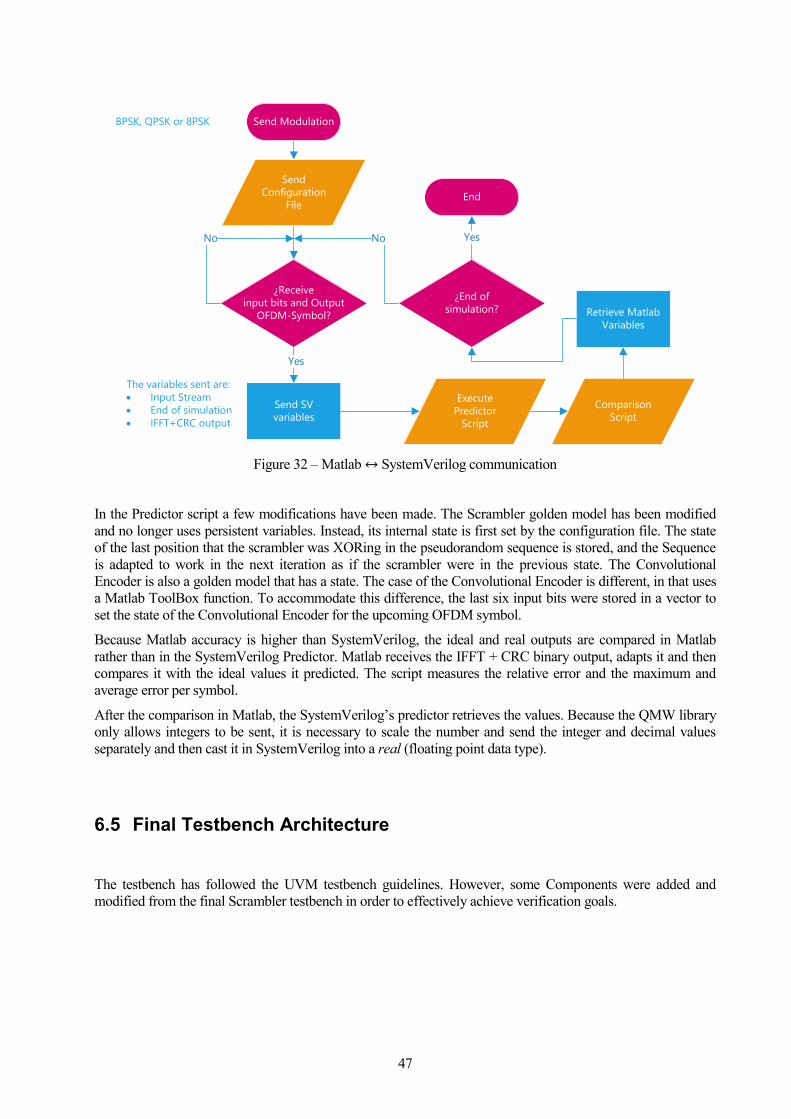
47
BPSK, QPSK or 8PSK Send Modulation
Send
Configuration
File
¿Receive
input bits and Output
OFDM-Symbol?
Send SV
variables
End
Yes
The variables sent are:
Input Stream
End of simulation
IFFT+CRC output
¿End of
simulation?
No
Execute
Predictor
Script
Comparison
Script
Retrieve Matlab
Variables
No Yes
Figure 32 – Matlab ↔ SystemVerilog communication
In the Predictor script a few modifications have been made. The Scrambler golden model has been modified
and no longer uses persistent variables. Instead, its internal state is first set by the configuration file. The state
of the last position that the scrambler was XORing in the pseudorandom sequence is stored, and the Sequence
is adapted to work in the next iteration as if the scrambler were in the previous state. The Convolutional
Encoder is also a golden model that has a state. The case of the Convolutional Encoder is different, in that uses
a Matlab ToolBox function. To accommodate this difference, the last six input bits were stored in a vector to
set the state of the Convolutional Encoder for the upcoming OFDM symbol.
Because Matlab accuracy is higher than SystemVerilog, the ideal and real outputs are compared in Matlab
rather than in the SystemVerilog Predictor. Matlab receives the IFFT + CRC binary output, adapts it and then
compares it with the ideal values it predicted. The script measures the relative error and the maximum and
average error per symbol.
After the comparison in Matlab, the SystemVerilog’s predictor retrieves the values. Because the QMW library
only allows integers to be sent, it is necessary to scale the number and send the integer and decimal values
separately and then cast it in SystemVerilog into a real (floating point data type).
6.5 Final Testbench Architecture
The testbench has followed the UVM testbench guidelines. However, some Components were added and
modified from the final Scrambler testbench in order to effectively achieve verification goals.
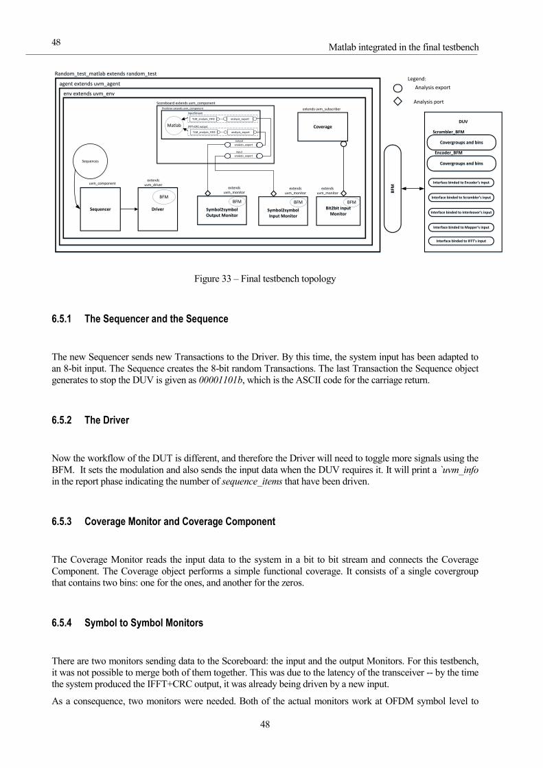
Matlab integrated in the final testbench
48
48
CoverageCoverage
extends uvm_subscriberextends uvm_subscriber
Bit2bit inputMonitor
Bit2bit inputMonitor
BFMBFM
extends uvm_monitor
extends uvm_monitor
Random_test_matlab extends random_testRandom_test_matlab extends random_test
uvm_componentuvm_component
agent extends uvm_agentagent extends uvm_agent
BFMBFM
DUVDUV
env extends uvm_envenv extends uvm_env
Covergroups and binsCovergroups and bins
Scrambler_BFMScrambler_BFM
Legend:
Analysis export
Analysis port
SequencerSequencer DriverDriver
BFMBFM
extends uvm_driver
extends uvm_driver
SequencesSequences
Scoreboard extends uvm_componentScoreboard extends uvm_component
analysis_exportanalysis_exportTLM_analysis_FIFOTLM_analysis_FIFO
analysis_exportanalysis_exportTLM_analysis_FIFOTLM_analysis_FIFO
IFFT+CRC outputIFFT+CRC output
InputStreamInputStream
Predictor extends uvm_componentPredictor extends uvm_component
Symbol2symbol Input Monitor
Symbol2symbol Input Monitor
BFMBFM
extends uvm_monitor
extends uvm_monitor
Symbol2symbol Output Monitor
Symbol2symbol Output Monitor
BFMBFM
extends uvm_monitor
extends uvm_monitor
analysis_exportanalysis_export
analysis_exportanalysis_export
input
output
MatlabMatlab
Covergroups and binsCovergroups and bins
Encoder_BFMEncoder_BFM
Interface binded to Encoder s inputInterface binded to Encoder s input
Interface binded to Scrambler s inputInterface binded to Scrambler s input
Interface binded to Interleaver s inputInterface binded to Interleaver s input
Interface binded to Mapper s inputInterface binded to Mapper s input
Interface binded to IFFT s inputInterface binded to IFFT s input
Figure 33 – Final testbench topology
6.5.1 The Sequencer and the Sequence
The new Sequencer sends new Transactions to the Driver. By this time, the system input has been adapted to
an 8-bit input. The Sequence creates the 8-bit random Transactions. The last Transaction the Sequence object
generates to stop the DUV is given as 00001101b, which is the ASCII code for the carriage return.
6.5.2 The Driver
Now the workflow of the DUT is different, and therefore the Driver will need to toggle more signals using the
BFM. It sets the modulation and also sends the input data when the DUV requires it. It will print a `uvm_info
in the report phase indicating the number of sequence_items that have been driven.
6.5.3 Coverage Monitor and Coverage Component
The Coverage Monitor reads the input data to the system in a bit to bit stream and connects the Coverage
Component. The Coverage object performs a simple functional coverage. It consists of a single covergroup
that contains two bins: one for the ones, and another for the zeros.
6.5.4 Symbol to Symbol Monitors
There are two monitors sending data to the Scoreboard: the input and the output Monitors. For this testbench,
it was not possible to merge both of them together. This was due to the latency of the transceiver -- by the time
the system produced the IFFT+CRC output, it was already being driven by a new input.
As a consequence, two monitors were needed. Both of the actual monitors work at OFDM symbol level to
49
facilitate the Predictor task.
6.5.5 Scoreboard Implementation
The Scoreboard design in the final testbench is different compared to the Scrambler test. In the final testbench
there is no Checker implementation. This task is performed by Matlab as explained in section 5.4. The reason
for this was the difficulty of the synchronization job necessary between the Checker and the Predictor. In
addition, sending variables to Matlab from two different Components imply modifying the Matlab workspace
from two different angles, which is more complex to debug.
Inside the Scoreboard there is the Predictor class, which actually works as both a Predictor and a checker.
Even though it was not necessary to design the Scoreboard with subcomponents, it was implemented in that
way because it allows changes to the Scoreboard content and future reuse.
The Predictor needs to implement two TLM_FIFOs to avoid losing incoming Transactions. When retrieveing
the FIFO data, the first position in both FIFOs will correspond to the same OFDM symbol.
In the run phase, the Predictor prints the average relative error per real and imaginary parts using a `uvm_info
message. Additionally, in the report phase it prints the maximum real and imaginary relative error in the whole
simulation using another `uvm_info.
At the moment the Predictor is purely informative. It does not stop the simulation since the computation it
performs is just the relative error. Nevertheless, it would be very easy to add a `uvm_error or `uvm_fatal
message according to a maximum tolerable error.
6.5.6 Top module and BFM
The top module contains the DUV and BFM instantiations and connections. In addition, all the intermediate
signals between components have been linked to the BFM interface. Thus if in the future more functionality
needs to be added to the testbench, it can easily be done.
The internal signals have been accessed from the interfaces binded within the DUT using the SystemVerilog
assign key word.
6.6 Inheritance and relations between classes
The Doxygen documentation generation tool generates online documentation as well as diagrams that show all
of the relations between classes once all of the SystemVerilog code is commented according to its marking
syntax. It gives very useful information because it is possible to see the position of every class and where
classes extend from a simple picture. This is shown in Figure 35.
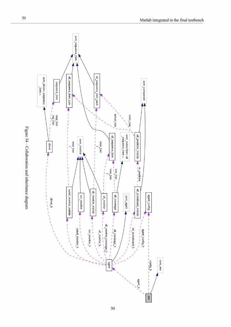
Matlab integrated in the final testbench
50
50
Fig
ure 3
4 –
Collab
oratio
n an
d in
heritan
ce diag
ram
51
7 RESULTS AND CONCLUSIONS
7.1 Results
This project was accomplished creating a complete UVM testbench for an OFDM transceiver written in
VHDL. In order to adopt the Universal Verification Methodology many testbenches have been set up until
reaching the final version. The testbench now is comprised of the fundamentals of verification:
Code coverage.
Functional coverage.
Random Testing.
7.2 Conclusions
The UVM is a methodology used by electronic engineers in the semiconductor industry and therefore is very
comprehensive. It is usually used in conjunction with other verification technologies. For an engineering
student it can be frustrating at first, especially because there are not many resources available and most of the
resources are for engineers that work in the verification field. However, although it can seem impossible to
learn at times, after finishing this project I have realized how powerful this methodology is. Once one starts
coding the first testbenches, the rest only depends on being patient and continuing to learn.
I strongly encourage other engineering students to learn the UVM. I believe verification helps to open minds
with respect to the way you design. Even if your goals are to work as a design engineer, going through the
process of learning the UVM will help you to communicate effectively with your colleagues.
However beautiful the strategy, you should occasionally look at
the results.
-Winston Churchill-

Results and conclusions
52
52
53
8 FUTURE WORK
It is difficult to point to how this work could be expanded because testbenches can be so diverse and there can
be so many variations. One possible improvement in the future may be to mix a series of random and directed
testing until reaching 100% code coverage in the design. In addition, UVM testbenches are very modular, and
it would be very interesting to study the efficiency of a testbench that, instead of using a single OFDM-Symbol
level Scoreboard, also included Scoreboards (with their own Predictor and Checker) for each system module
with Predictors less Matlab-based. In this more scalable testbench, there would exist several Agents in which
each Agent performs the verification of one of the DUT blocks.
Outside of the verification world, the OFDM transceiver was originally done as part of coursework. It would
be extremely useful to integrate the testbench in a server where students could upload their HDL code, and the
testbench would check whether the RTL of those students is working under the specifications. This would
improve verification in student designs because the UVM can deliver messages using the reporting macros,
that are very clock cycle accurate, which would help students to fix their RTL more rapidly.
I never think of the future - it comes soon enough.
-Albert Einstein-

Future work
54
54
55
REFERENCES
[1] M. Demler, "Signal processing design," [Online]. Available: http://signal-processing.mil-
embedded.com/articles/designing-the-beyond-moores-law/.
[2] . J. Perry and T. Kupper, "The decline of scarcity," [Online]. Available:
http://declineofscarcity.com/?cat=14.
[3] P. Rosenzweig, "Heritage," [Online]. Available: http://www.heritage.org/research/testimony/2012/08/the-
state-of-privacy-and-security-our-antique-privacy-rules.
[4] R. Narayan and T. Symons, I created the Verification Gap.
[5] Cadence, "Cadence," [Online]. Available: https://www.cadence.com/content/cadence-
www/global/en_US/home/alliances/standards-and-languages.html.
[6] T. L. Anderson, "Chip Design," [Online]. Available:
http://chipdesignmag.com/display.php?articleId=5153.
[7] [Online]. Available: https://www.edaplayground.com/.
[8] P. alliance. [Online]. Available: http://www.prime-alliance.org/?page_id=769.
[9] P. alliance, "Specification for PoweRline Intelligen Metering Evolution," [Online]. Available:
http://www.prime-alliance.org/wp-content/uploads/2014/10/PRIME-Spec_v1.4-20141031.pdf.
[10] Accellera, "Standard Universal Verification Methodology".
[11] Verification Academy, "Verification Academy," [Online].
[12] Verification Academy, "Verification Academy," [Online]. Available:
https://verificationacademy.com/cookbook/component.
[13] Verification Academy, [Online]. Available: https://verificationacademy.com/cookbook/testbench.
[14] Verification Academy, "Verification Academy," [Online]. Available:
https://verificationacademy.com/cookbook/uvm.
[15] Verification Academy, "Verification Academy," [Online]. Available:
https://verificationacademy.com/cookbook/component.
[16] Verification Academy, "Verification Academy," [Online]. Available:
References
56
56
https://verificationacademy.com/cookbook/agent.
[17] Doulos , "Doulos," [Online]. Available:
https://www.doulos.com/knowhow/sysverilog/uvm/easier_uvm_guidelines/.
[18] Verification Academy, "Verification Academy," [Online]. Available:
https://verificationacademy.com/cookbook/monitorcomponent.
[19] R. Salemi, The UVM primer.
[20] Verification Academy, "Verification Academy," [Online]. Available:
https://verificationacademy.com/cookbook/predictors.
[21] D. K. Tala, "Asic World," [Online]. Available: http://www.asic-
world.com/systemverilog/coverage1.html#Introduction.
[22] Verification Academy, [Online]. Available: https://verificationacademy.com/cookbook/factory.
[23] Verification Academy, [Online]. Available: https://verificationacademy.com/cookbook/testbench/build.
[24] H. Nurminen and S. Durga Ravi, "Synopsys - Hierarchal Testbench Configuration Using
uvm_config_db".
[25] Verification Academy, [Online]. Available: https://verificationacademy.com/cookbook/phasing.
[26] Mentor Graphics, [Online]. Available: https://www.mentor.com/products/fv/resources/overview/binding-
systemverilog-to-vhdl-components-using-questa-f43cc1c4-6607-44e3-8dc0-515bf2c08abc.
[27] Verification Academy, "Verification Academy," [Online]. Available:
https://verificationacademy.com/cookbook/matlab/integration.
[28] GNU, [Online]. Available: https://www.gnu.org/software/make/manual/html_node/Makefiles.html.
[29] Xilinx, "Xilinx," [Online]. Available:
http://www.xilinx.com/support/documentation/sw_manuals/xilinx11/cgn_c_df_compile_lib.htm.
[30] D. Rich, "The Missing Link: The Testbench to DUT".
[31] O. Autor, "Otra cita distinta," revista, p. 12, 2001.
[32] Ray Kurzweil, "Syngularity Simposium," [Online]. Available:
http://www.singularitysymposium.com/moores-law.html.
[33] verificationacademy, [Online]. Available: https://verificationacademy.com/cookbook/testbench.
[34] Mentor Graphics, [Online]. Available: https://www.mentor.com/products/fv/methodologies/uvm-ovm/.
[35] R. Salemi, FPGA Simulation A complete Step-by-Step Guide.

57