Simulated Field Maps: Toward ImprovedSusceptibility Artefact Correction in

Interventional MRI

Martin Kochan?1, Pankaj Daga1, Ninon Burgos1, Mark White2,M. Jorge Cardoso1,3, Laura Mancini2, Gavin P. Winston4,

Andrew W. McEvoy2, John Thornton2, Tarek Yousry2, John S. Duncan4,Danail Stoyanov1 and Sebastien Ourselin1,3

1Centre for Medical Image Computing,University College London, London, UK

2National Hospital for Neurology and Neurosurgery,UCLH NHS Foundation Trust, London, UK

3Dementia Research Centre, Institute of Neurology,University College London, London, UK

4Department of Clinical and Experimental Epilepsy, Institute of Neurology,University College London, London, UK

Abstract. Intraoperative MRI is a powerful modality for acquiringstructural and functional images of the brain to enable precise image-guided neurosurgery. In this paper, we propose a novel method for sim-ulating main magnetic field inhomogeneity maps during intraoperativeMRI-guided neurosurgery. Our method relies on an air-tissue segmenta-tion of intraoperative patient specific data, which is used as an input toa subsequent field simulation step. The generated simulation can thenbe used to enhance the precision of image-guidance. We report resultsof our method on 12 patient datasets acquired during image-guided neu-rosurgery for anterior lobe resection for surgical management of focaltemporal lobe epilepsy. We find a close agreement between the field in-homogeneity maps acquired as part of the imaging protocol and thesimulated field inhomogeneity maps generated by the proposed method.

Keywords: image-guided neurosurgery, interventional MRI, inhomo-geneity field map simulation

1 Introduction

Anterior temporal lobe resection (ATLR) is an effective treatment for refractorytemporal lobe epilepsy. However, resective surgery may result in severe compli-cations such as contralateral superior visual field deficit (VFD) that restricts theseizure-free patient from returning to regular activity. Magnetic resonance imag-ing (MRI) is the preferred modality for imaging soft-tissue brain morphology and

? m.kochan.12@ucl.ac.uk

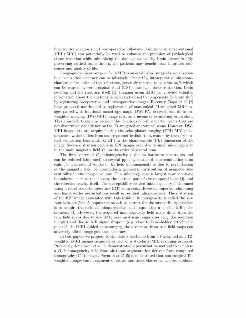
function for diagnosis and postoperative follow-up. Additionally, interventionalMRI (iMRI) can potentially be used to enhance the precision of pathologicaltissue resection while minimizing the damage to healthy brain structures. Bypreserving critical brain tissues, the patients may benefit from improved out-comes and quality of life.

Image-guided neurosurgery for ATLR is an established surgical specialisationbut localization accuracy can be adversely affected by intraoperative physiome-chanical deformation of the soft tissue, generally referred to as brain shift, whichcan be caused by cerebrospinal fluid (CSF) drainage, tissue retraction, brainswelling and the resection itself [1]. Imaging using iMRI can provide valuableinformation about the anatomy, which can be used to compensate for brain shiftby registering preoperative and intraoperative images. Recently, Daga et al. [2]have proposed multimodal co-registration of anatomical T1-weighted MRI im-ages paired with fractional anisotropy maps (DWI-FA) derived from diffusion-weighted imaging (DW-MRI) image sets, as a means of estimating brain shift.This approach takes into account the locations of white matter tracts that arenot discernible visually nor on the T1-weighted anatomical scans. However, DW-MRI image sets are acquired using the echo planar imaging (EPI) MRI pulsesequence, which suffers from severe geometric distortion, caused by the very lim-ited acquisition bandwidth of EPI in the phase-encode (PE) dimension of theimage. Severe distortion occurs in EPI images even due to small inhomogeneityin the main magnetic field B0 on the order of several ppm.

The first source of B0 inhomogeneity is due to hardware constraints andcan be reduced (shimmed) to several ppm by means of superconducting shimcoils [3]. The second source of B0 field inhomogeneity is due to perturbationof the magnetic field by non-uniform geometric distribution of magnetic sus-ceptibility in the imaged volume. This inhomogeneity is largest near air-tissueboundaries, such as the sinuses, the petrous part of the temporal bone [4], andthe resection cavity itself. The susceptibility-related inhomogeneity is shimmedusing a set of room-temperature (RT) shim coils. However, imperfect shimmingand higher-order perturbations result in residual inhomogeneity. The distortionof the EPI image associated with this residual inhomogeneity is called the sus-ceptiblity artefact. A popular approach to correct for the susceptibility artefactis to acquire the residual inhomogeneity field maps using a specific MR pulsesequence [4]. However, the acquired inhomogeneity field maps differ from thetrue field maps due to low SNR near air-tissue boundaries (e.g. the resectionmargin) and due to MR signal dropout (e.g. close to head-holder attachmentpins) [5]. In iMRI guided neurosurgery, the diversions from true field maps canadversely affect image guidance accuracy.

In this paper, we propose to simulate a field map from T1-weighted and T2-weighted iMRI images acquired as part of a standard iMRI scanning protocol.Previously, Jenkinson et al. [6] demonstrated a perturbation method to calculatea B0 inhomogeneity field from air-tissue segmentation derived from computedtomography (CT) images. Poynton et al. [5] demonstrated that non-surgical T1-weighted images can be segmented into air and tissue classes using a probabilistic

CT atlas, and reported that a subsequent application of the method [6] resultsin close overall agreement between the acquired and simulated field maps. How-ever, we observe that a probabilistic atlas is not suited to the segmentation ofintraoperative iMR images that contain air-filled craniotomy and resection areasof variable shape that depend on the surgery and patient morphology. Instead,we employ an expectation-maximization (EM) based segmentation method in-formed by priors derived from a synthetic CT image. We compute the syntheticCT from the intraoperative T1-weighted image and a database of MR/CT pairtemplates. We subsequently feed the air-tissue segmentation into the method [6].The field map simulation is evaluated by comparison with field maps acquiredduring iMRI guided ATLR neurosurgery for 12 cases. The proposed methodgenerates field maps in close agreement with the acquired field maps.

This result has the potential to lead to improvements in EPI image correctionand image guidance for neurosurgery. Additionally, the proposed method can alsobe used to correct distortion in historical intraoperative EPI datasets, which didnot include field map acquisition as part of the acquisition protocol.

2 Methods

2.1 Field map in terms of voxel displacement

Let the magnetic field at point x be B0 + ∆B0(x) [T] where B0 is the homoge-neous field and ∆B0(x) is the inhomogeneity field map, which can be equivalently

expressed as γ∆B0(x) [rad/s] or γ∆B0(x)2π [Hz]. For the purposes of image cor-

rection, one is interested in the millimetre displacement along the phase encodedirection that the inhomogeneity causes to an EPI image. The displacement canbe calculated based on theory in [4, 7]. Consider the acquisition of a single EPIslice with matrix size N ×N and voxel dimensions rFE in the frequency encode(FE) direction and rPE in the phase encode (PE) direction, respectively. TheEPI slice is reconstructed by the inverse Fourier transform of the MR signal.In the PE direction, the MR signal sampling rate is N

Tacq[Hz], where Tacq is

the signal acquisition time. The reconstructed image resolution in the PE di-rection is N

NTacq= 1

Tacq[Hz/pixel] or Tacq [pixel/Hz]. Since the PE gradient is

used to encode position along the PE direction, the above offset corresponds toa distortion along the PE direction of size:

dPE(x) =γ∆B0(x)

2πTacqrPE . (1)

In this study, the EPI image correction itself was only performed for visualconfirmation (Figure 2), by converting the field map into a vector displace-ment/deformation vector field and subsequently resampling the image using cu-bic spline interpolation [8].

2.2 Field map acquisition

Field map acquisition was based on the method introduced in [4], whereby thefield map is dependent on phase difference map between the phase components of

MR images acquired during two MR signal echoes, separated by echo differencetime TED. The phase difference corresponds to spin phase evolution during TED

but is modulo-2π phase-wrapped due to unknown number of elapsed revolutions.Additionally, the phase difference signal is noisy in low spin-density areas (airand bone) and has low SNR near air-tissue boundaries. Therefore, to recover theinhomogeneity γ∆B0(x), we used a novel phase-unwrapping algorithm basedon a probabilistic model spatially constrained by means of a Markov randomfield (MRF) formulation, as presented in [8]. We de-meaned the recovered phasedifference map, since the recovered phase difference necessarily has an arbitraryconstant component.

2.3 Air-tissue segmentation

The magnetic susceptibility values for soft tissue (≈ −9.1 × 10−6) and bone(≈ −11.4×10−6) are similar, but both are significantly different from that of air(≈ 0.4 × 10−6) [5]. Therefore, we need a binary labelling of the head into tissueand air. For each subject, a segmentation was performed on the sum of the T1-and T2-weighted iMRI image (a pseudo spin density image). In this image, thesoft tissues (grey and white matter, the eyes) were grey, CSF and fat tissue werebright, and air and bone were black.

For the air-tissue segmentation, we used a segmentation algorithm based onan expectation-maximization (EM) intensity model spatially regularized usingan MRF [9]. Tissue was segmented into three partial volume classes: air, boneand soft tissue (Figure 1, centre right) and later the bone and soft tissue classeswere combined into the tissue class. Each class had its associated spatial priormap. The spatial prior maps were calculated from a closed skull synthetic CT.In CT, each of the 3 classes has a unique intensity range and therefore, the CTwas intensity-transformed using 2 sigmoid functions that acted as separators toselect tissue based on intensity. During the EM segmentation, full MRF strengthwas chosen to enforce the presence of air in the resection area (as opposed tosoft tissue) and of air in the craniotomy area (as opposed to bone).

The closed skull synthetic CT image was constructed from the T1-weightediMRI image following the method described by Burgos et al. [10]. The methodrelies on a database consisting of 6 pairs of co-registered T1-weighted MR / CTimages from healthy subjects. Each MR image from the database was non-rigidlyregistered to the intraoperative iMRI image so that each CT could be propagatedinto the iMRI space. The resampled CT images were fused together using avoxel-wise rank-based weighting scheme (Figure 1, centre left).

The intraoperative field of view contains the cranial part of the head, butdoes not include the head below the nose level. The later field map simulationstep (as described in Section 2.4) assumes that no tissue is present outside of theair-tissue segmentation volume that has a significant contribution to the fielddistribution inside the volume. Therefore, an approximated lower head tissuevolume was constructed in a volume inferior to the iMRI (Figure 1, right). Toconstruct the lower head tissue volume, the affine registration from the CTsynthesis step was reused to resample the MR templates into the target volume,

and the resampled volumes intensity transformed using a sigmoid function andaveraged.

Fig. 1. Air-tissue segmentation. Left: a T1-weighted intraoperative image. The sectionruns through a plane close to the anatomical coronal plane (head at angle due tointraoperative orientation). Middle left: an accompanying synthetic CT. Middle right:the result of the segmentation (red for air, green for soft-tissue, blue for bone). Right:the final air-tissue segmentation (black for air, white for tissue) with the fitted lowerhead volume.

2.4 Field map estimation

The field map estimation follows from [6] and models the first order perturbationsof the main magnetic field. The susceptibility χ can be expanded as χ = χ0+δχ1,where χ0 is the magnetic susceptibility of air, δ is the susceptibility differencebetween air and brain tissue and χ1 is a binary variable describing the tissuetype. The first order perturbations of the z-component of the main magneticfield (B1

z ) can be written in terms of the main magnetic field (B0z ):

B1z =

χ1

3 + χ0B0z −

1

1 + χ0

((∂2G

∂z2

)∗ (χ1B

0z )

)(2)

where G is the Green’s function G(x) = (4πr)−1 and r =√x2 + y2 + z2. Note

that the expression is simplified considerably due to the fact that we only have anon-zero component in the longitudinal axis (z-direction) of the main magneticfield.

The convolution H(x) for a single voxel with the resolution (a, b, c) for aconstant field along the z-axis is given by:

H(x) =(∂2G

∂z2

)∗ (χ1B

0z ) =

∑i,j,k∈(−1,1)

(ijk)F

(x+

ia

2, y +

jb

2, z +

kc

2

)(3)

where F (x) = 14π arctan(xyzr ).

Due to the linearity of Equation (2), the single voxel solutions can be addedtogether to compute the total field:

B1z (x) =

∑x′

χ1x′H(x− x′) (4)

where x′ are the voxel locations and x is the point where the field is evaluated.This can be implemented using the 3D Fast Fourier Transform.

Although this approach simulates the field distribution due to the main coil,MRI scanners also contain room-temperature (RT) shim coils, whose purposeis to decrease the inhomogeneity in the imaged volume. The RT shim coils arewound to form magnetic fields that follow first- and second-order spherical har-monics, S(x) = [x, y, z, z2 − (x2 + y2)/2, xz, yz, x2 − y2, 2xy](x), where x = 0 atthe magnet isocentre [11]. The field in the scanner becomes B1

z (x) − Sθ, wherethe coefficients θ = [θ1, θ2, . . . , θ8]T are proportional to the currents in the shimcoils, which are dynamically optimized by the scanner during image acquisitionbased on the field in the imaged volume [11]. In this simulation, we approximatethe shim currents as a linear combination that minimizes the inhomogeneityfield across the field of view, as used in [5]. We perform a least-squares fit of the

spherical harmonics to determine θ̂ = argminθ(B1z (x) − Sθ).

3 Results

The proposed algorithm was validated on 12 datasets that were acquired usinginterventional MRI during ATLR procedures. Validation was done as part of anaudit to assess the usability of simulated field maps in a clinical scenario. Theimages were acquired using a 1.5T Espree MRI scanner (Siemens, Erlangen,Germany) designed for interventional procedures. The intraoperative protocolincluded a T1-weighted FLASH image (TR = 5.25 ms, TE = 2.5 ms, flip angle= 15◦, 0.547 × 0.547 × 1.25 mm grid of 512 × 512 × 176 voxels) and a T2-weighted turbo spin echo image (TR = 3200 ms, TE = 510 ms, flip angle =120◦, 1.0 × 1.0 × 1.0 mm grid of 256 × 256 × 176 voxels), a DW-MRI datasetof 65 diffusion-weighted images acquired using a single shot EPI sequence withGRAPPA-based parallel imaging (acceleration factor of 2, 2.5 × 2.5 × 2.5 mmgrid of 84 × 84 × 49 voxels, readout time 35.52 ms) and a field map acquiredusing a gradient-recalled echo pulse sequence (2.91667 × 2.91667 × 2.9 mm gridof 72 × 72 × 43 voxels, echo time difference of 4.76 ms).

The DW-MRI dataset for each subject was corrected as per Section 2.1 usingthe acquired field map and the proposed simulated field map, respectively. Anexample for a subject is shown in Figure 2.

The most direct validation of the simulated field map would be to compareDWI images corrected using acquired and simulated field maps, respectively,against anatomical landmarks identified on the intraoperative T1-weighted im-ages, which are not affected by the susceptibility artefact (Figure 2). However,due to the low resolution and low signal-to-noise ratio of DW-MRI, the land-marks are challenging to identify reliably and repeatably. Since there is no way

Fig. 2. Detail of correction for the susceptibility artefact. Left: an intraoperative T1-weighted image unaffected by the distortion. The section runs through a plane close tothe anatomical axial plane (head at angle due to intraoperative orientation). A brainsurface outlined using a surface extractor2 is shown for reference (red outline). Middleleft: an uncorrected “b0” DW-MRI image (an image for which no diffusion gradientsare applied). Arrows point at an area of severe susceptibility distortion. Middle right:the “b0” image corrected using the acquired field map. Right: the “b0” image correctedusing the simulated field map.

of measuring the true field maps in vivo, we compared the simulated field mapsto the acquired field maps (Figure 3). The field maps were expressed in mm ofdisplacement along the PE direction, as these are the units significant to the cor-rection. Next, we calculated statistics for the difference between the simulatedand acquired field maps. The results for the 12 subjects are reported in Table 1.For most of the brain, there is a close agreement. However, the differences followa long-tailed distribution, so that in some areas, there are larger disagreements.

Mean ( std ) Median P90 P95 P99

0.86 ( 1.13 ) 0.57 1.83 2.64 5.341.16 ( 1.50 ) 0.68 2.68 3.78 7.150.98 ( 1.37 ) 0.55 2.30 3.36 6.290.89 ( 1.29 ) 0.48 2.08 3.03 5.971.00 ( 1.37 ) 0.63 2.16 3.19 6.240.77 ( 1.03 ) 0.50 1.60 2.25 4.740.93 ( 1.17 ) 0.60 1.98 2.80 5.670.94 ( 1.41 ) 0.49 2.12 3.21 7.061.35 ( 1.84 ) 0.80 2.94 4.22 9.031.06 ( 1.47 ) 0.65 2.36 3.33 6.831.23 ( 1.84 ) 0.60 2.99 4.33 9.500.95 ( 1.39 ) 0.56 2.10 3.13 6.44

1.01 ( 1.40 ) 0.59 2.26 3.27 6.690

1

2

3

4

5

6

7

8

9

10

Mean Std. dev. Median P90 P95 P99

Absolute field map difference [mm]

Table 1. Quantification of absolute difference (in mm) between the correction dis-placement in the phase encode direction as predicted by the proposed simulated fieldmap and the acquired field map, respectively, for the 12 subjects. Only voxels withinbrain mask are considered. The mean, standard deviation, median, and 90th, 95th and99th percentile values are reported. The bottom row contains column averages.

2 As included in NiftyView (http://cmic.cs.ucl.ac.uk/home/software).

Fig. 3. Field maps expressed as mm of displacement along the phase-encode direction.The view is centered at the resection area of surgery. First row: A phase-wrapped ac-quired field map for a representative subject, showing a step change in phase value closeto the resection margin. Second row: The acquired field map after phase-unwrapping.Only the volume inside the brain mask, as employed by the phase-unwrapping algo-rithm, is shown. Third row: A corresponding simulated field map (considered onlyinside the brain mask for fair comparison). Last row: The voxel-wise absolute differ-ence between the simulated and the phase-unwrapped acquired field maps. Left toright: coronal, sagittal and axial sections, not coincident with anatomical planes dueto intraoperative orientation of the head.

4 Discussion

Across the subjects, the simulated and acquired field maps on average differby 1.01 ± 1.40 mm in the brain volume. This is within the voxel size of theDWI dataset (2.5 mm, which is typical for DW-MRI datasets). This numberalso has to be evaluated with respect to a desired resection accuracy, whichis patient and surgeon specific and difficult to define. We believe that 1 mmresection accuracy in areas of low difference is clinically useful. However, sincethe difference between field maps follows a long-tailed distribution, we attemptto interpret the values of the field maps in areas of more significant difference todeduce where the simulated field maps are more correct, and vice versa.

We observe that the simulated field map is more positive in the vicinity ofthe resection area. We hypothesize that this could be due to an accumulatederror in phase-unwrapping caused by the low SNR in this area and hence due toan underestimated acquired field map.

We observe that near the regions of signal dropout, as visible near the head-holder attachment pins, the simulated field map is more positive than the ac-quired field map. This is in line with the expectation to see a reduced phaseevolution in regions of signal dropout and hence due to an underestimated ac-quired field map.

We also observe that, conversely, near the petrous part of the temporal bonein both hemispheres and anteriorly in the frontal lobe, the simulated field mapsare 2–3 mm above the acquired field maps. This likely occurs because the pro-posed segmentation method overestimates the size of the air-filled cavities. Thisoverestimation is caused by the high penalty imposed on the bone class in theEM/MRF segmentation step, which had been empirically found to be necessary,to robustly segment the craniotomy area as completely air-filled, when relyingon the EM/MRF algorithm alone. Therefore, if it was possible to introduce amethod to segment the resection cavity and the craniotomy area robustly, thepenalty on bone in the the EM/MRF algorithm could be relaxed and the over-estimation of the simulated field map could be reduced.

5 Conclusion

In summary, field map simulation is important for iMRI guided neurosurgeryand in this study we have proposed a method that can achieve a close agree-ment between the simulated and acquired field maps for 12 patients. We suggestthat in the future, simulated field maps could be used to regularize the phase-unwrapping of intraoperatively acquired field maps.

While our results are promising, a significant obstacle for intraoperative useof the proposed method is the computational time required to simulate thefield map, currently above 20 minutes (Intel Core i5 @ 3.30 GHz). Therefore, apossible future work would be to explore methods to speed up the CT synthesisand field map calculation, for instance using GPU hardware.

Acknowledgements. This work was supported by the UCL DoctoralTraining Programme in Medical and Biomedical Imaging studentship funded bythe EPSRC. Danail Stoyanov would like to thank for the support of The RoyalAcademy of Engineering/EPSRC Research Fellowship. Sebastien Ourselin re-ceives funding from the EPSRC (EP/H046410/1, EP/J020990/1, EP/K005278),the MRC (MR/J01107X/1), the EU-FP7 project VPH-DARE@IT (FP7-ICT-2011-9-601055), the NIHR Biomedical Research Unit (Dementia) at UCL andthe National Institute for Health Research University College London HospitalsBiomedical Research Centre (NIHR BRC UCLH/UCL High Impact Initiative).

References

1. Nimsky, C., Ganslandt, O., Cerny, S., Hastreiter, P., Greiner, G., Fahlbusch, R.:Quantification of, visualization of, and compensation for brain shift using intraop-erative magnetic resonance imaging. Neurosurgery 47.5, 1070–1080 (2000)

2. Daga, P., Winston, G., Modat, M., White, M., Mancini, L., Cardoso, M.J., Symms,M., Stretton, J., McEvoy, A.W., Thornton, J., Micallef, C., Yousry, T., Hawkes,D.J., Duncan, J.S., Ourselin, S.: Accurate Localization of Optic Radiation Dur-ing Neurosurgery in an Interventional MRI Suite. IEEE Transactions on MedicalImaging 31.4, 882–891 (2012)

3. Clare, S., Evans, J., Jezzard, P.: Requirements for room temperature shimming ofthe human brain. Magn. Reson. Med. 55, 210–214 (2006)

4. Jezzard, P., Balaban, R.S.: Correction for geometric distortion in echo planar im-ages from b0 field variations. Magn. Reson. Med. 34, 65–73 (1995)

5. Poynton, C., Jenkinson, M., Wells, W.: Atlas-Based Improved Prediction of Mag-netic Field Inhomogeneity for Distortion Correction of EPI Data. In: G.-Z. Yanget al. (Eds.): MICCAI 2009, Part II, LNCS vol. 5762, pp. 951-959. Springer, Hei-delberg (2009)

6. Jenkinson, M., Wilson J. L., Jezzard, P.: Perturbation method for magnetic fieldcalculations of nonconductive objects. Magnetic Resonance in Medicine 52.3, 471–477 (2004)

7. Hutton, C., Bork, A., Josephs, O., Deichmann, R., Ashburner, J., Turner, R.: Imagedistortion correction in fMRI: a quantitative evaluation. Neuroimage 16.1, 217–240(2002)

8. Daga, P, Modat, M., Winston, G, White, M., Mancini, L., McEvoy, A. W., Thorn-ton, J., Yousry, T., Duncan, J. S., Ourselin, S.: Susceptibility artefact correction bycombining B0 field maps and non-rigid registration using graph cuts. SPIE MedicalImaging, International Society for Optics and Photonics, 86690B–86690B (2013)

9. Cardoso, M. J.: Improved Maximum a Posteriori Cortical Segmentation by Itera-tive Relaxation of Priors G.-Z. Yang et al. (Eds.): MICCAI 2009, Part II, LNCS5762, 441–449 (2009)

10. Burgos, N., Cardoso, M. J., Modat, M., Pedemonte, S., Dickson, J., Barnes, A.,Duncan, J. S., Atkinson, D., Arridge, S. R., Hutton, B. F., Ourselin, S.: AttenuationCorrection Synthesis for Hybrid PET-MR Scanners. K. Mori et al. (Eds.): MICCAI2013, Part II, LNCS 8150, 147–154 (2013)

11. Gruetter, R., Boesch, C.: Fast, noniterative shimming of spatially localized signals.In vivo analysis of the magnetic field along axes. Journal of Magnetic Resonance,96.2, 323–334 (1992)