ARTICLE IN PRESS

Thin-Walled Structures 47 (2009) 919–930

Contents lists available at ScienceDirect

Thin-Walled Structures

0263-82

doi:10.1

� Corr

E-m

landolfo

journal homepage: www.elsevier.com/locate/tws

Sheathed cold-formed steel housing: A seismic design procedure

Luigi Fiorino a, Ornella Iuorio b, Raffaele Landolfo b,�

a Department of Structural Engineering, University of Naples ‘‘Federico II’’, Naples, Italyb Department of Constructions and Mathematical Methods in Architecture, University of Naples ‘‘Federico II’’, Naples, Italy

a r t i c l e i n f o

Article history:

Received 21 January 2008

Received in revised form

19 November 2008

Accepted 16 February 2009Available online 31 March 2009

Keywords:

Design nomographs

Cold-formed steel

Linear dynamic analysis

Nonlinear static analysis

Seismic design

Sheathing panels

Housing

31/$ - see front matter & 2009 Elsevier Ltd. A

016/j.tws.2009.02.004

esponding author.

ail addresses: lfiorino@unina.it (L. Fiorino),

@unina.it (R. Landolfo).

a b s t r a c t

Nowadays, different research teams are engaged on experimental and theoretical studies having as

main aim the evaluation of seismic performance of sheathed cold-formed steel frame structures.

Although a relatively large number of experimental and theoretical studies are available, the

development of useful tools for the seismic design should be improved. As an attempt to overcome

this lack, this paper aims to present a structural design procedure that allows, through the definition of

three design nomographs, the screw spacing and all the shear walls components to be obtained on the

basis of linear dynamic or nonlinear static seismic analysis. In addition, a procedure for the prediction of

the whole pushover response curve of sheathed cold-formed steel shear walls, which can be

advantageously used for developing the design nomographs, is presented.

& 2009 Elsevier Ltd. All rights reserved.

1. Introduction

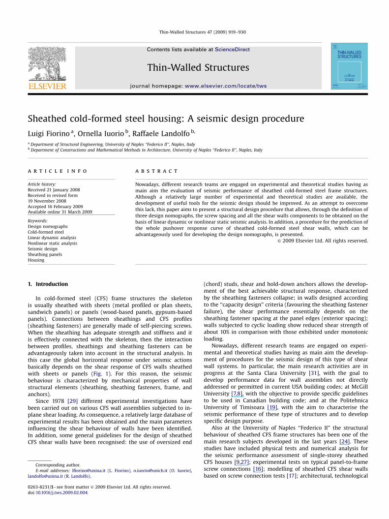
In cold-formed steel (CFS) frame structures the skeletonis usually sheathed with sheets (metal profiled or plan sheets,sandwich panels) or panels (wood-based panels, gypsum-basedpanels). Connections between sheathings and CFS profiles(sheathing fasteners) are generally made of self-piercing screws.When the sheathing has adequate strength and stiffness and itis effectively connected with the skeleton, then the interactionbetween profiles, sheathings and sheathing fasteners can beadvantageously taken into account in the structural analysis. Inthis case the global horizontal response under seismic actionsbasically depends on the shear response of CFS walls sheathedwith sheets or panels (Fig. 1). For this reason, the seismicbehaviour is characterized by mechanical properties of wallstructural elements (sheathing, sheathing fasteners, frame, andanchors).

Since 1978 [29] different experimental investigations havebeen carried out on various CFS wall assemblies subjected to in-plane shear loading. As consequence, a relatively large database ofexperimental results has been obtained and the main parametersinfluencing the shear behaviour of walls have been identified.In addition, some general guidelines for the design of sheathedCFS shear walls have been recognised: the use of oversized end

ll rights reserved.

o.iuorio@unich.it (O. Iuorio),

(chord) studs, shear and hold-down anchors allows the develop-ment of the best achievable structural response, characterizedby the sheathing fasteners collapse; in walls designed accordingto the ‘‘capacity design’’ criteria (favouring the sheathing fastenerfailure), the shear performance essentially depends on thesheathing fastener spacing at the panel edges (exterior spacing);walls subjected to cyclic loading show reduced shear strength ofabout 10% in comparison with those exhibited under monotonicloading.

Nowadays, different research teams are engaged on experi-mental and theoretical studies having as main aim the develop-ment of procedures for the seismic design of this type of shearwall systems. In particular, the main research activities are inprogress at the Santa Clara University [31], with the goal todevelop performance data for wall assemblies not directlyaddressed or permitted in current USA building codes; at McGillUniversity [7,8], with the objective to provide specific guidelinesto be used in Canadian building code; and at the PolitehnicaUniversity of Timisoara [19], with the aim to characterise theseismic performance of these type of structures and to developspecific design purpose.

Also at the University of Naples ‘‘Federico II’’ the structuralbehaviour of sheathed CFS frame structures has been one of themain research subjects developed in the last years [24]. Thesestudies have included physical tests and numerical analysis forthe seismic performance assessment of single-storey sheathedCFS houses [9,27]; experimental tests on typical panel-to-framescrew connections [16]; modelling of sheathed CFS shear wallsbased on screw connection tests [17]; architectural, technological

ARTICLE IN PRESS

bottomtrack

N

H

h

N

l

end studs

hold-down anchorshear

anchor

internal studs

sheathing panel

external sheathing fasteners

internal sheathing fasteners

top track

s

p

c

≠≠ t

V

a

≠≠ �

internal studs size

end studs size

tracks size be

hold-down device

foundation

N: axial force acting on the end stud / hold-down anchor V: shear force acting on a shear anchor

Fig. 1. Geometry and component of typical sheathed CFS shear wall.

L. Fiorino et al. / Thin-Walled Structures 47 (2009) 919–930920

and structural design of sustainable house prototypes forcontemporary living needs [23].

However, even if a relatively large number of experimental andtheoretical studies on the seismic performance of CFS shear wallsare available, the development of useful tools for the seismicdesign should be improved. As an attempt to overcome this lack,three design nomographs for the seismic design of single-storeysheathed CFS frame structures are presented in this paper. Inparticular, the proposed design approach is shown in Section 2,while a procedure for the prediction of the pushover responsecurve of sheathed CFS shear walls, which can be used fordeveloping the design nomographs, is illustrated in Section 3.Finally, the application of the proposed design approach to a casestudy is given in Section 4.

2. The proposed design approach

2.1. General

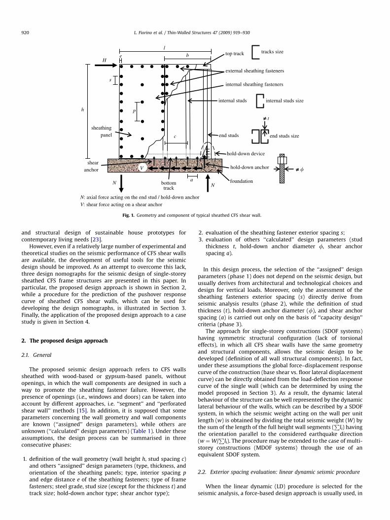
The proposed seismic design approach refers to CFS wallssheathed with wood-based or gypsum-based panels, withoutopenings, in which the wall components are designed in such away to promote the sheathing fastener failure. However, thepresence of openings (i.e., windows and doors) can be taken intoaccount by different approaches, i.e. ‘‘segment’’ and ‘‘perforatedshear wall’’ methods [15]. In addition, it is supposed that someparameters concerning the wall geometry and wall componentsare known (‘‘assigned’’ design parameters), while others areunknown (‘‘calculated’’ design parameters) (Table 1). Under theseassumptions, the design process can be summarised in threeconsecutive phases:

1.

definition of the wall geometry (wall height h, stud spacing c)and others ‘‘assigned’’ design parameters (type, thickness, andorientation of the sheathing panels; type, interior spacing p

and edge distance e of the sheathing fasteners; type of framefasteners; steel grade, stud size (except for the thickness t) andtrack size; hold-down anchor type; shear anchor type);

2.

evaluation of the sheathing fastener exterior spacing s; 3. evaluation of others ‘‘calculated’’ design parameters (stud

thickness t, hold-down anchor diameter f, shear anchorspacing a).

In this design process, the selection of the ‘‘assigned’’ designparameters (phase 1) does not depend on the seismic design, butusually derives from architectural and technological choices anddesign for vertical loads. Moreover, only the assessment of thesheathing fasteners exterior spacing (s) directly derive fromseismic analysis results (phase 2), while the definition of studthickness (t), hold-down anchor diameter (f), and shear anchorspacing (a) is carried out only on the basis of ‘‘capacity design’’criteria (phase 3).

The approach for single-storey constructions (SDOF systems)having symmetric structural configuration (lack of torsionaleffects), in which all CFS shear walls have the same geometryand structural components, allows the seismic design to bedeveloped (definition of all wall structural components). In fact,under these assumptions the global force–displacement responsecurve of the construction (base shear vs. floor lateral displacementcurve) can be directly obtained from the load-deflection responsecurve of the single wall (which can be determined by using themodel proposed in Section 3). As a result, the dynamic lateralbehaviour of the structure can be well represented by the dynamiclateral behaviour of the walls, which can be described by a SDOFsystem, in which the seismic weight acting on the wall per unitlength (w) is obtained by dividing the total seismic weight (W) bythe sum of the length of the full height wall segments (

Pli) having

the orientation parallel to the considered earthquake direction(w ¼W/

Pli). The procedure may be extended to the case of multi-

storey constructions (MDOF systems) through the use of anequivalent SDOF system.

2.2. Exterior spacing evaluation: linear dynamic seismic procedure

When the linear dynamic (LD) procedure is selected for theseismic analysis, a force-based design approach is usually used, in

ARTICLE IN PRESS

Table 1Wall design parameters.

‘‘Assigned’’ design parameters Limiting conditions ‘‘Calculated’’ design

parameters

Limiting conditions

Wall geometry Wall height (h) h/lp2 (l: wall length) –

Stud spacing (c) c ¼ 600 mm –

Wall components

Sheathing Type PLYa with tsX10 mm

Thickness (tp) OSBa with tsX9 mm

GWBa with tsX12 mm –

Orientation Orientation: vertical

Sheathing fasteners Type Flat head or bugle head self drilling

screws with: diameter X4.2 mm

(for PLYa and OSBa)

diameter X3.5 mm (for GWBa)

head diameter X7.4 mm

lengthXtp+2t+10 mm

Interior spacing (p) p ¼ 300 mm Exterior spacing (s) s ¼ 50–750 mm

Edge distance (e) eX10 mm

Frame Steel grade Yielding strength X230 Mpa

Stud sizec Studs size:minimum

90� 40�10 mmb

Stud thickness (t) tX1.0 mm

Track size Tracks size:minimum 90�30 mmc

Frame fasteners Type Wafer head or modified truss head

self drilling screws with diameter

X4.2 mm

length X2t+10 mm

–

Hold-down anchors Type (with the exception of

the anchor diameter)

S/HDd with HIT-RE 500 with

HIS-N 8.8eAnchor diameter (f) fX16 mm

Shear anchors Type (with the exception of

the anchor spacing)

HST M8f Anchor spacing (a) ap300 mm

a PLY: plywood; OSB: oriented strand board; GWB: gypsum wallboard.b Outside-to-outside web depth�outside-to-outside flange size�outside-to-outside lip size.c Outside-to-outside web depth�outside-to-outside flange size.d S/HD: metal-to-metal connectors by Simpson Strong-Tie Company [40] or equivalent hold-down devices.e HIT-RE 500 with HIS-N 8.8: adhesive-bonded anchors by HILTI [4] or equivalent tension anchors.f HST M8: mechanical shear anchors by HILTI [4] or equivalent shear anchors.

L. Fiorino et al. / Thin-Walled Structures 47 (2009) 919–930 921

which the inelastic behaviour and the structural overstrength aretaken into account by the seismic force modification factors. Inthis case, the comparison between seismic capacity and demand,in terms of forces, shall satisfy the following equation:

HCXHD (1)

where HC and HD are the seismic strength capacity and seismicaction demand, respectively.

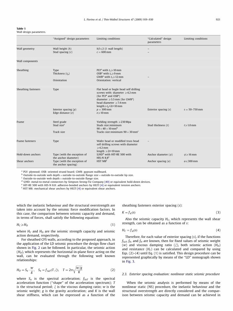
For sheathed CFS walls, according to the proposed approach, inthe application of the LD seismic procedure the design flow chartshown in Fig. 2 can be followed. In particular, the seismic action(HD), which represents the horizontal in-plane force acting on thewall, can be evaluated through the following well knownrelationships:

HD ¼ Sa �w

g; Sa ¼ f SaT ðT; xÞ; T ¼ 2p

ffiffiffiffiffiffiffiffiffiw=g

K

r(2)

where Sa is the spectral acceleration; fSaT is the spectralacceleration function (‘‘shape’’ of the acceleration spectrum); T

is the structural period; x is the viscous damping ratio; w is theseismic weight; g is the gravity acceleration; and K is the wallshear stiffness, which can be expressed as a function of the

sheathing fasteners exterior spacing (s):

K ¼ f K ðsÞ (3)

Also the seismic capacity HC, which represents the wall shearstrength, can be obtained as a function of s:

HC ¼ f HðsÞ (4)

Therefore, for each value of exterior spacing (s), if the functionsfSaT, fK, and fH are known, then for fixed values of seismic weight(w) and viscous damping ratio (x), both seismic action (HD)and resistance (HC) can be calculated and compared by usingEqs. (2)–(4) until Eq. (1) is satisfied. This design procedure can berepresented graphically by means of the ‘‘LD’’ nomograph shownin Fig. 3.

2.3. Exterior spacing evaluation: nonlinear static seismic procedure

When the seismic analysis is performed by means of thenonlinear static (NS) procedure, the inelastic behaviour and thestructural overstrength are directly considered and the compar-ison between seismic capacity and demand can be achieved in

ARTICLE IN PRESS

Exterior

spacing (si)

Seismic

weight (w)

Viscous

damping

ratio (�)

Spectral

acceleration

spectrum (fSaT)

Seismic strength

capacity (HC,i)

Seismic action

demand (HD,i)

Stiffness (Ki)Structural

period (Ti)

HC,i ≥ HD,i

End

Yes

NoDesign review (si+1 < si)

Fig. 2. Design flow chart for LD seismic procedure.

s

K

T

HD = Saw/g HC

HC = fH (s)

K

w/gT = 2�

HD = fSaT (T,�) w/g

K = fK (s)

Fig. 3. Nomograph for LD seismic procedure.

Exterior

spacing (si)Seismic

weight (w)

Viscousdampingratio (�)

Spectral

acceleration

spectrum (fSaT)

Capacity

spectrum (dC,i)

Demand spectrum

(dD,i)

Yield

strength

(HC,i)

Yield

displacement

(dy,i)

dC,i ≥ dD,i

End

Yes

No

Ultimate

displacement

(du,i)

Design review(si+1<si)

Fig. 4. Design flow chart for NS seismic procedure.

s d

S aHC g/w

T

U

Y

HC g/w = fH (s) g/w

dy = fy (s) du = fu (s)

Demand spectrum

dD dC

Capacity spectrum

Sa = fSad (d,�)

s

Fig. 5. Nomograph for NS seismic procedure.

L. Fiorino et al. / Thin-Walled Structures 47 (2009) 919–930922

terms of displacements (displacement-based approach):

dCXdD (5)

where dC and dD are the seismic displacement capacity andseismic displacement demand, respectively (Fig. 4).

This comparison can be easily performed by means of the wellknown acceleration–displacement spectrum, in which the de-mand and capacity spectra are represented together. In particular,the demand spectrum can be obtained as follows:

Sa ¼ f Sadðd; xÞ (6)

where fSad is the spectral acceleration function (‘‘shape’’ of thespectrum in the acceleration–displacement format), and d is thegeneric wall lateral displacement.

The capacity spectrum, instead, can be represented by anelastic–plastic curve, which is drawn by defining the yield (Y) andultimate (U) limit points:

Y dy;HC

wg

� �; U du;

HC

wg

� �(7)

where the yield displacement (dy) and ultimate displacement (du)can be obtained as function of the exterior spacing (s):

dy ¼ f yðsÞ; du ¼ f uðsÞ (8)

Therefore, for each value of exterior spacing (s), if the functionsfSad, fH, fy, and fu are known, then for fixed values of seismic weight

(w) and viscous damping ratio (x), both seismic demand (dD) andcapacity (dC) can be calculated and compared by using Eqs. (6)–(8)until Eq. (5) is satisfied. This design procedure can be representedgraphically by means of the ‘‘NS’’ nomograph shown in Fig. 5.

2.4. Evaluation of the others ‘‘calculated’’ design parameters

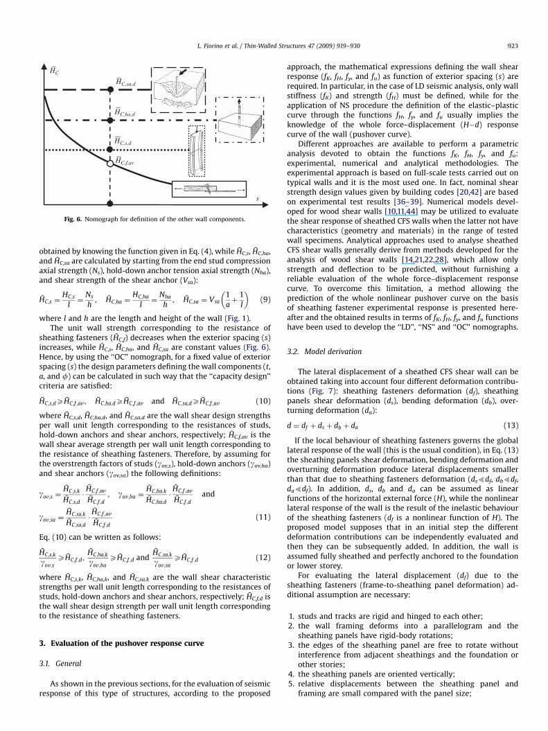
Defined the sheathing fastener exterior spacing (s), theevaluation of stud thickness (t), hold-down anchor diameter (f),and shear anchor spacing (a) need to complete the wall design.Also in this case the design procedure for the definition of theother structural wall components can be represented graphicallyby means of the ‘‘OC’’ nomograph (Fig. 6), in which the wall shearstrengths per wall unit length (HC) corresponding to the resistanceof sheathing fasteners (HC,f), studs (HC,s), hold-down anchors(HC,ha) and shear anchors (HC,sa) are represented together asfunction of the exterior spacing (s). In particular, HC,f can be

ARTICLE IN PRESS

s

HC

HC,f,av

HC,ha,d

HC,s,d

HC,sa,d

Fig. 6. Nomograph for definition of the other wall components.

L. Fiorino et al. / Thin-Walled Structures 47 (2009) 919–930 923

obtained by knowing the function given in Eq. (4), while HC,s, HC,ha,and HC,sa are calculated by starting from the end stud compressionaxial strength (Ns), hold-down anchor tension axial strength (Nha),and shear strength of the shear anchor (Vsa):

HC;s ¼HC;s

l¼

Ns

h; HC;ha ¼

HC;ha

l¼

Nha

h; HC;sa ¼ Vsa

1

aþ

1

l

� �(9)

where l and h are the length and height of the wall (Fig. 1).The unit wall strength corresponding to the resistance of

sheathing fasteners (HC,f) decreases when the exterior spacing (s)increases, while HC,s, HC,ha, and HC,sa are constant values (Fig. 6).Hence, by using the ‘‘OC’’ nomograph, for a fixed value of exteriorspacing (s) the design parameters defining the wall components (t,a, and f) can be calculated in such way that the ‘‘capacity design’’criteria are satisfied:

HC;s;dXHC;f ;av; HC;ha;dXHC;f ;av and HC;sa;dXHC;f ;av (10)

where HC,s,d, HC,ha,d, and HC,sa,d are the wall shear design strengthsper wall unit length corresponding to the resistances of studs,hold-down anchors and shear anchors, respectively; HC,f,av is thewall shear average strength per wall unit length corresponding tothe resistance of sheathing fasteners. Therefore, by assuming forthe overstrength factors of studs (gov,s), hold-down anchors (gov,ha)and shear anchors (gov,sa) the following definitions:

gov;s ¼HC;s;k

HC;s;d

�HC;f ;av

HC;f ;d

; gov;ha ¼HC;ha;k

HC;ha;d

�HC;f ;av

HC;f ;d

and

gov;sa ¼HC;sa;k

HC;sa;d

�HC;f ;av

HC;f ;d

(11)

Eq. (10) can be written as follows:

HC;s;k

gov;s

XHC;f ;d;HC;ha;k

gov;ha

XHC;f ;d andHC;sa;k

gov;sa

XHC;f ;d (12)

where HC,s,k, HC,ha,k, and HC,sa,k are the wall shear characteristicstrengths per wall unit length corresponding to the resistances ofstuds, hold-down anchors and shear anchors, respectively; HC,f,d isthe wall shear design strength per wall unit length correspondingto the resistance of sheathing fasteners.

3. Evaluation of the pushover response curve

3.1. General

As shown in the previous sections, for the evaluation of seismicresponse of this type of structures, according to the proposed

approach, the mathematical expressions defining the wall shearresponse (fK, fH, fy, and fu) as function of exterior spacing (s) arerequired. In particular, in the case of LD seismic analysis, only wallstiffness (fK) and strength (fH) must be defined, while for theapplication of NS procedure the definition of the elastic–plasticcurve through the functions fH, fy, and fu usually implies theknowledge of the whole force–displacement (H�d) responsecurve of the wall (pushover curve).

Different approaches are available to perform a parametricanalysis devoted to obtain the functions fK, fH, fy, and fu:experimental, numerical and analytical methodologies. Theexperimental approach is based on full-scale tests carried out ontypical walls and it is the most used one. In fact, nominal shearstrength design values given by building codes [20,42] are basedon experimental test results [36–39]. Numerical models devel-oped for wood shear walls [10,11,44] may be utilized to evaluatethe shear response of sheathed CFS walls when the latter not havecharacteristics (geometry and materials) in the range of testedwall specimens. Analytical approaches used to analyse sheathedCFS shear walls generally derive from methods developed for theanalysis of wood shear walls [14,21,22,28], which allow onlystrength and deflection to be predicted, without furnishing areliable evaluation of the whole force–displacement responsecurve. To overcome this limitation, a method allowing theprediction of the whole nonlinear pushover curve on the basisof sheathing fastener experimental response is presented here-after and the obtained results in terms of fK, fH, fy, and fu functionshave been used to develop the ‘‘LD’’, ‘‘NS’’ and ‘‘OC’’ nomographs.

3.2. Model derivation

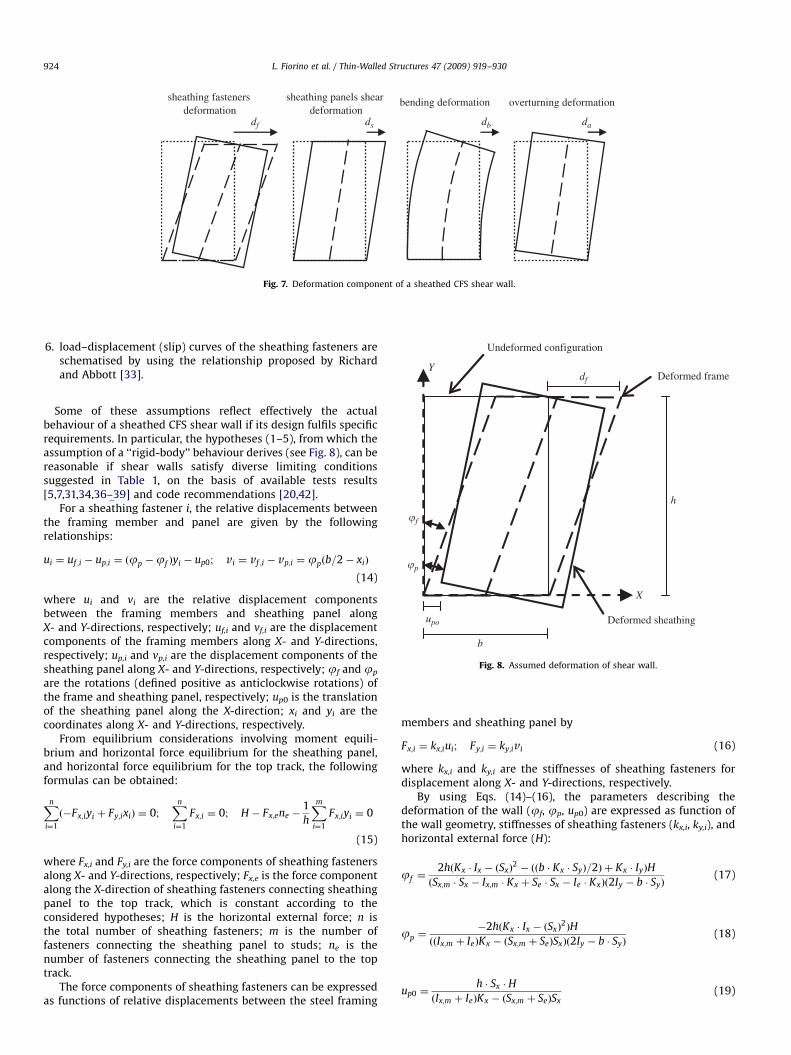
The lateral displacement of a sheathed CFS shear wall can beobtained taking into account four different deformation contribu-tions (Fig. 7): sheathing fasteners deformation (df), sheathingpanels shear deformation (ds), bending deformation (db), over-turning deformation (da):

d ¼ df þ ds þ db þ da (13)

If the local behaviour of sheathing fasteners governs the globallateral response of the wall (this is the usual condition), in Eq. (13)the sheathing panels shear deformation, bending deformation andoverturning deformation produce lateral displacements smallerthan that due to sheathing fasteners deformation (ds5df, db5df,da5df). In addition, ds, db and da can be assumed as linearfunctions of the horizontal external force (H), while the nonlinearlateral response of the wall is the result of the inelastic behaviourof the sheathing fasteners (df is a nonlinear function of H). Theproposed model supposes that in an initial step the differentdeformation contributions can be independently evaluated andthen they can be subsequently added. In addition, the wall isassumed fully sheathed and perfectly anchored to the foundationor lower storey.

For evaluating the lateral displacement (df) due to thesheathing fasteners (frame-to-sheathing panel deformation) ad-ditional assumption are necessary:

1.

studs and tracks are rigid and hinged to each other; 2. the wall framing deforms into a parallelogram and the

sheathing panels have rigid-body rotations;

3. the edges of the sheathing panel are free to rotate without

interference from adjacent sheathings and the foundation orother stories;

4.

the sheathing panels are oriented vertically; 5. relative displacements between the sheathing panel and

framing are small compared with the panel size;

ARTICLE IN PRESS

sheathing fasteners deformation

sheathing panels shear deformation

bending deformation overturning deformation

df ds db da

Fig. 7. Deformation component of a sheathed CFS shear wall.

Undeformed configuration

L. Fiorino et al. / Thin-Walled Structures 47 (2009) 919–930924

6.

YDeformed framedf

load–displacement (slip) curves of the sheathing fasteners areschematised by using the relationship proposed by Richardand Abbott [33].

X

upo Deformed sheathing

b

h

�f

�p

Fig. 8. Assumed deformation of shear wall.

Some of these assumptions reflect effectively the actualbehaviour of a sheathed CFS shear wall if its design fulfils specificrequirements. In particular, the hypotheses (1–5), from which theassumption of a ‘‘rigid-body’’ behaviour derives (see Fig. 8), can bereasonable if shear walls satisfy diverse limiting conditionssuggested in Table 1, on the basis of available tests results[5,7,31,34,36–39] and code recommendations [20,42].

For a sheathing fastener i, the relative displacements betweenthe framing member and panel are given by the followingrelationships:

ui ¼ uf ;i � up;i ¼ ðjp �jf Þyi � up0; vi ¼ vf ;i � vp;i ¼ jpðb=2� xiÞ

(14)

where ui and vi are the relative displacement componentsbetween the framing members and sheathing panel alongX- and Y-directions, respectively; uf,i and vf,i are the displacementcomponents of the framing members along X- and Y-directions,respectively; up,i and vp,i are the displacement components of thesheathing panel along X- and Y-directions, respectively; jf and jp

are the rotations (defined positive as anticlockwise rotations) ofthe frame and sheathing panel, respectively; up0 is the translationof the sheathing panel along the X-direction; xi and yi are thecoordinates along X- and Y-directions, respectively.

From equilibrium considerations involving moment equili-brium and horizontal force equilibrium for the sheathing panel,and horizontal force equilibrium for the top track, the followingformulas can be obtained:

Xn

i¼1

ð�Fx;iyi þ Fy;ixiÞ ¼ 0;Xn

i¼1

Fx;i ¼ 0; H � Fx;ene �1

h

Xm

i¼1

Fx;iyi ¼ 0

(15)

where Fx,i and Fy,i are the force components of sheathing fastenersalong X- and Y-directions, respectively; Fx,e is the force componentalong the X-direction of sheathing fasteners connecting sheathingpanel to the top track, which is constant according to theconsidered hypotheses; H is the horizontal external force; n isthe total number of sheathing fasteners; m is the number offasteners connecting the sheathing panel to studs; ne is thenumber of fasteners connecting the sheathing panel to the toptrack.

The force components of sheathing fasteners can be expressedas functions of relative displacements between the steel framing

members and sheathing panel by

Fx;i ¼ kx;iui; Fy;i ¼ ky;ivi (16)

where kx,i and ky,i are the stiffnesses of sheathing fasteners fordisplacement along X- and Y-directions, respectively.

By using Eqs. (14)–(16), the parameters describing thedeformation of the wall (jf, jp, up0) are expressed as function ofthe wall geometry, stiffnesses of sheathing fasteners (kx,i, ky,i), andhorizontal external force (H):

jf ¼2hðKx � Ix � ðSxÞ

2� ððb � Kx � SyÞ=2Þ þ Kx � IyÞH

ðSx;m � Sx � Ix;m � Kx þ Se � Sx � Ie � KxÞð2Iy � b � SyÞ(17)

jp ¼�2hðKx � Ix � ðSxÞ

2ÞH

ððIx;m þ IeÞKx � ðSx;m þ SeÞSxÞð2Iy � b � SyÞ(18)

up0 ¼h � Sx � H

ðIx;m þ IeÞKx � ðSx;m þ SeÞSx(19)

ARTICLE IN PRESS

L. Fiorino et al. / Thin-Walled Structures 47 (2009) 919–930 925

in which

Kx ¼Xn

i¼1

kx;i; Sx ¼Xn

i¼1

kx;i � yi; Sy ¼Xn

i¼1

ky;i � xi; Sx;m ¼Xm

i¼1

kx;i � yi;

Se ¼ kxe � ne � h; Ix ¼Xn

i¼1

kx;iðyiÞ2; Iy ¼

Xn

i¼1

ky;iðxiÞ2;

Ix;m ¼Xm

i¼1

kx;iðyiÞ2; Ie ¼ kxe � ne � h

2 (20)

where kxe is the stiffness of sheathing fasteners connecting thesheathing panel to the top track for displacement along theX-direction.

When for sheathing fasteners a linear load–displacementresponse is assumed (kx,i, ky,i, and kxe are constant values),Eq. (17) gives a closed-form solution and the top wall displace-ment (df) can be evaluated as follows:

df ¼ jf h (21)

where jf is calculated from Eq. (17). When a nonlinearload–displacement curve is adopted for sheathing fasteners, Eqs.(12)–(19) can be written in differential format and can be used ina numerical step-by-step procedure which allows to obtain theload (H) vs. deflection (df) response curve of the wall. More detailson the numerical procedure are given in Fiorino et al. [17].

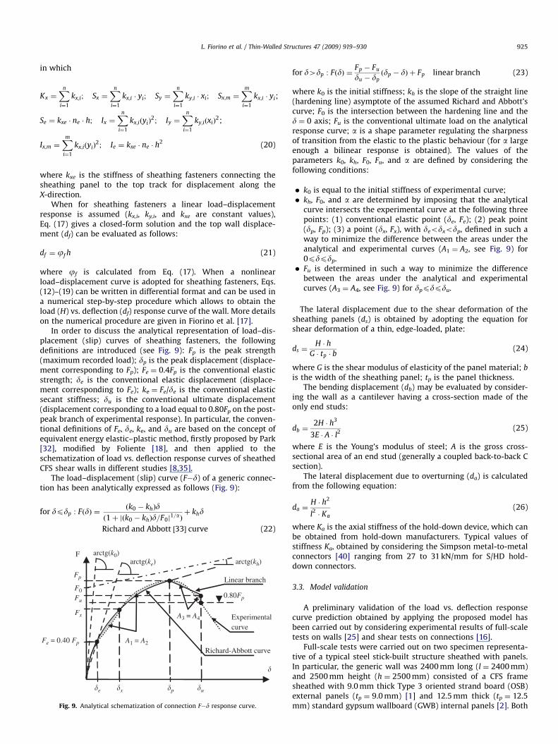
In order to discuss the analytical representation of load–dis-placement (slip) curves of sheathing fasteners, the followingdefinitions are introduced (see Fig. 9): Fp is the peak strength(maximum recorded load); dp is the peak displacement (displace-ment corresponding to Fp); Fe ¼ 0.4Fp is the conventional elasticstrength; de is the conventional elastic displacement (displace-ment corresponding to Fe); ke ¼ Fe/de is the conventional elasticsecant stiffness; du is the conventional ultimate displacement(displacement corresponding to a load equal to 0.80Fp on the post-peak branch of experimental response). In particular, the conven-tional definitions of Fe, de, ke, and du are based on the concept ofequivalent energy elastic–plastic method, firstly proposed by Park[32], modified by Foliente [18], and then applied to theschematization of load vs. deflection response curves of sheathedCFS shear walls in different studies [8,35].

The load–displacement (slip) curve (F�d) of a generic connec-tion has been analytically expressed as follows (Fig. 9):

for dpdp : FðdÞ ¼ðk0 � khÞd

ð1þ jðk0 � khÞd=F0j1=aÞþ khd

Richard and Abbott ½33� curve (22)

F

Fp

Fe = 0.40 Fp

Richard-Abbott curve

Experimental curve

arctg(k0)arctg(kh)

F00.80Fp

Fx

Linear branch

Fu

arctg(ke)

A1 = A2

A3 = A4

�x�e �p �u

�

Fig. 9. Analytical schematization of connection F�d response curve.

for d4dp : FðdÞ ¼Fp � Fu

du � dpðdp � dÞ þ Fp linear branch (23)

where k0 is the initial stiffness; kh is the slope of the straight line(hardening line) asymptote of the assumed Richard and Abbott’scurve; F0 is the intersection between the hardening line and thed ¼ 0 axis; Fu is the conventional ultimate load on the analyticalresponse curve; a is a shape parameter regulating the sharpnessof transition from the elastic to the plastic behaviour (for a largeenough a bilinear response is obtained). The values of theparameters k0, kh, F0, Fu, and a are defined by considering thefollowing conditions:

�

k0 is equal to the initial stiffness of experimental curve; � kh, F0, and a are determined by imposing that the analytical

curve intersects the experimental curve at the following threepoints: (1) conventional elastic point (de, Fe); (2) peak point(dp, Fp); (3) a point (dx, Fx), with deodxodp, defined in such away to minimize the difference between the areas under theanalytical and experimental curves (A1 ¼ A2, see Fig. 9) for0pdpdp.

� Fu is determined in such a way to minimize the difference

between the areas under the analytical and experimentalcurves (A3 ¼ A4, see Fig. 9) for dppdpdu.

The lateral displacement due to the shear deformation of thesheathing panels (ds) is obtained by adopting the equation forshear deformation of a thin, edge-loaded, plate:

ds ¼H � h

G � tp � b(24)

where G is the shear modulus of elasticity of the panel material; b

is the width of the sheathing panel; tp is the panel thickness.The bending displacement (db) may be evaluated by consider-

ing the wall as a cantilever having a cross-section made of theonly end studs:

db ¼2H � h3

3E � A � l2(25)

where E is the Young’s modulus of steel; A is the gross cross-sectional area of an end stud (generally a coupled back-to-back Csection).

The lateral displacement due to overturning (da) is calculatedfrom the following equation:

da ¼H � h2

l2 � Ka

(26)

where Ka is the axial stiffness of the hold-down device, which canbe obtained from hold-down manufacturers. Typical values ofstiffness Ka, obtained by considering the Simpson metal-to-metalconnectors [40] ranging from 27 to 31 kN/mm for S/HD hold-down connectors.

3.3. Model validation

A preliminary validation of the load vs. deflection responsecurve prediction obtained by applying the proposed model hasbeen carried out by considering experimental results of full-scaletests on walls [25] and shear tests on connections [16].

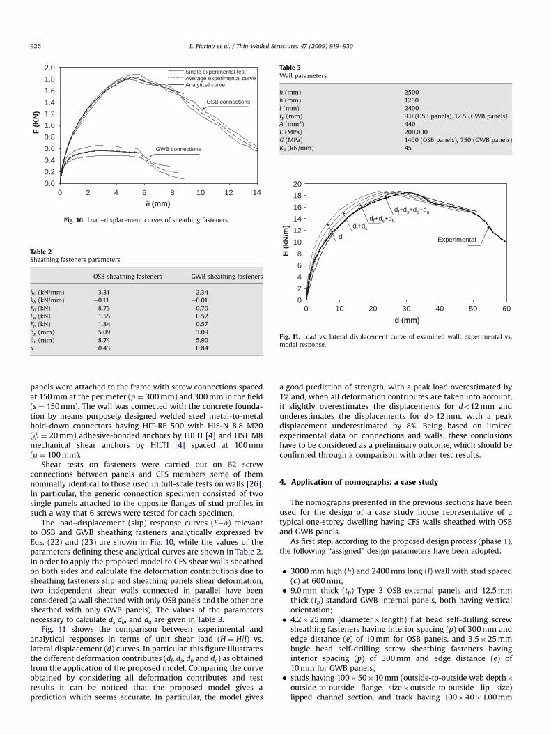
Full-scale tests were carried out on two specimen representa-tive of a typical steel stick-built structure sheathed with panels.In particular, the generic wall was 2400 mm long (l ¼ 2400 mm)and 2500 mm height (h ¼ 2500 mm) consisted of a CFS framesheathed with 9.0 mm thick Type 3 oriented strand board (OSB)external panels (tp ¼ 9.0 mm) [1] and 12.5 mm thick (tp ¼ 12.5mm) standard gypsum wallboard (GWB) internal panels [2]. Both

ARTICLE IN PRESS

0.00.20.40.60.81.01.21.41.61.82.0

0δ (mm)

Single experimental testAverage experimental curveAnalytical curve

GWB connections

OSB connections

F (K

N)

2 4 6 8 10 12 14

Fig. 10. Load–displacement curves of sheathing fasteners.

Table 2Sheathing fasteners parameters.

OSB sheathing fasteners GWB sheathing fasteners

k0 (kN/mm) 3.31 2.34

kh (kN/mm) �0.11 �0.01

F0 (kN) 8.73 0.70

Fu (kN) 1.55 0.52

Fp (kN) 1.84 0.57

dp (mm) 5.09 3.09

du (mm) 8.74 5.90

a 0.43 0.84

Table 3Wall parameters.

h (mm) 2500

b (mm) 1200

l (mm) 2400

tp (mm) 9.0 (OSB panels), 12.5 (GWB panels)

A (mm2) 440

E (MPa) 200,000

G (MPa) 1400 (OSB panels), 750 (GWB panels)

Ka (kN/mm) 45

02468

101214161820

0d (mm)

H (k

N/m

)

df

df+ds

df+ds+db

df+ds+db+da

Experimental

10 20 30 40 50 60

Fig. 11. Load vs. lateral displacement curve of examined wall: experimental vs.

model response.

L. Fiorino et al. / Thin-Walled Structures 47 (2009) 919–930926

panels were attached to the frame with screw connections spacedat 150 mm at the perimeter (p ¼ 300 mm) and 300 mm in the field(s ¼ 150 mm). The wall was connected with the concrete founda-tion by means purposely designed welded steel metal-to-metalhold-down connectors having HIT-RE 500 with HIS-N 8.8 M20(f ¼ 20 mm) adhesive-bonded anchors by HILTI [4] and HST M8mechanical shear anchors by HILTI [4] spaced at 100 mm(a ¼ 100 mm).

Shear tests on fasteners were carried out on 62 screwconnections between panels and CFS members some of themnominally identical to those used in full-scale tests on walls [26].In particular, the generic connection specimen consisted of twosingle panels attached to the opposite flanges of stud profiles insuch a way that 6 screws were tested for each specimen.

The load–displacement (slip) response curves (F�d) relevantto OSB and GWB sheathing fasteners analytically expressed byEqs. (22) and (23) are shown in Fig. 10, while the values of theparameters defining these analytical curves are shown in Table 2.In order to apply the proposed model to CFS shear walls sheathedon both sides and calculate the deformation contributions due tosheathing fasteners slip and sheathing panels shear deformation,two independent shear walls connected in parallel have beenconsidered (a wall sheathed with only OSB panels and the other onesheathed with only GWB panels). The values of the parametersnecessary to calculate ds db, and da are given in Table 3.

Fig. 11 shows the comparison between experimental andanalytical responses in terms of unit shear load (H ¼ H/l) vs.lateral displacement (d) curves. In particular, this figure illustratesthe different deformation contributes (df, ds, db and da) as obtainedfrom the application of the proposed model. Comparing the curveobtained by considering all deformation contributes and testresults it can be noticed that the proposed model gives aprediction which seems accurate. In particular, the model gives

a good prediction of strength, with a peak load overestimated by1% and, when all deformation contributes are taken into account,it slightly overestimates the displacements for do12 mm andunderestimates the displacements for d412 mm, with a peakdisplacement underestimated by 8%. Being based on limitedexperimental data on connections and walls, these conclusionshave to be considered as a preliminary outcome, which should beconfirmed through a comparison with other test results.

4. Application of nomographs: a case study

The nomographs presented in the previous sections have beenused for the design of a case study house representative of atypical one-storey dwelling having CFS walls sheathed with OSBand GWB panels.

As first step, according to the proposed design process (phase 1),the following ‘‘assigned’’ design parameters have been adopted:

�

3000 mm high (h) and 2400 mm long (l) wall with stud spaced(c) at 600 mm; � 9.0 mm thick (tp) Type 3 OSB external panels and 12.5 mm

thick (tp) standard GWB internal panels, both having verticalorientation;

� 4.2�25 mm (diameter� length) flat head self-drilling screw

sheathing fasteners having interior spacing (p) of 300 mm andedge distance (e) of 10 mm for OSB panels, and 3.5�25 mmbugle head self-drilling screw sheathing fasteners havinginterior spacing (p) of 300 mm and edge distance (e) of10 mm for GWB panels;

� studs having 100�50�10 mm (outside-to-outside web depth�

outside-to-outside flange size�outside-to-outside lip size)lipped channel section, and track having 100� 40�1.00 mm

ARTICLE IN PRESS

5075150

0

0.2

0.4

0.6

0.8

0.18

0

0.2

0.4

0.6

0.8

5075100125150

2.4

1.2

0.18

2.4

1.2

HC

/w

T (s)

3025201510 35w (kN/m)

10152025303540

w (kN/m)

ag/g0.350.250.15

Soil typeD

BCEA

T (s)s (mm)

k (k

N/m

m m

)

s (mm)

40

0.005

0.020.02

0.005

0.040.04

A

B

C

D

k (k

N/m

m m

)

0.28 0.38

HD

/w

0.28 0.38100125

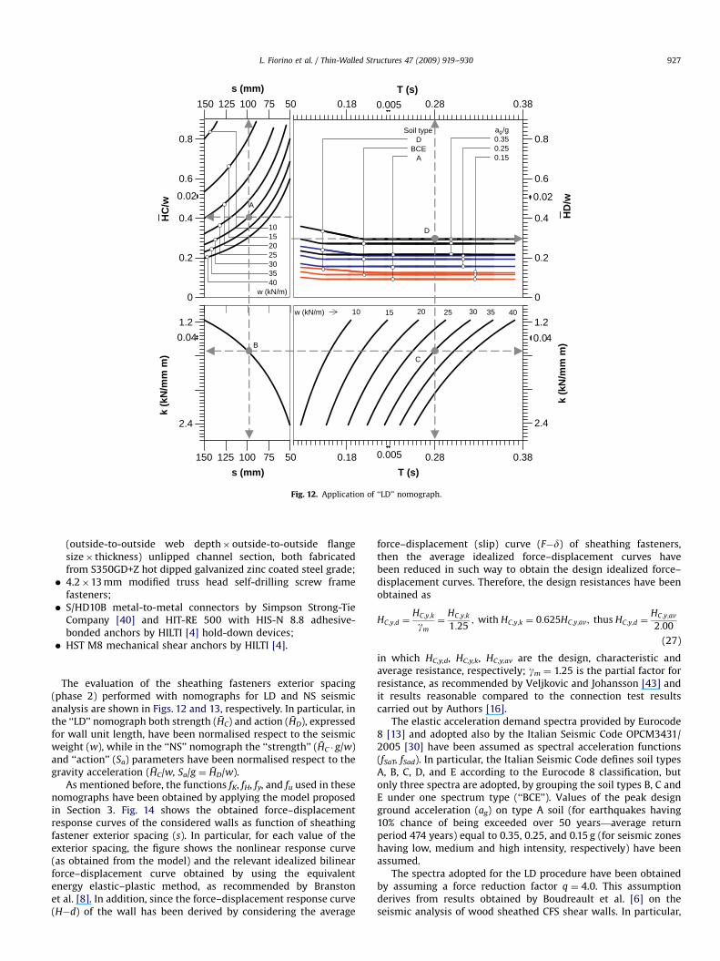
Fig. 12. Application of ‘‘LD’’ nomograph.

L. Fiorino et al. / Thin-Walled Structures 47 (2009) 919–930 927

(outside-to-outside web depth� outside-to-outside flangesize� thickness) unlipped channel section, both fabricatedfrom S350GD+Z hot dipped galvanized zinc coated steel grade;

� 4.2�13 mm modified truss head self-drilling screw frame

fasteners;

� S/HD10B metal-to-metal connectors by Simpson Strong-Tie

Company [40] and HIT-RE 500 with HIS-N 8.8 adhesive-bonded anchors by HILTI [4] hold-down devices;

� HST M8 mechanical shear anchors by HILTI [4].

The evaluation of the sheathing fasteners exterior spacing(phase 2) performed with nomographs for LD and NS seismicanalysis are shown in Figs. 12 and 13, respectively. In particular, inthe ‘‘LD’’ nomograph both strength (HC) and action (HD), expressedfor wall unit length, have been normalised respect to the seismicweight (w), while in the ‘‘NS’’ nomograph the ‘‘strength’’ (HC � g/w)and ‘‘action’’ (Sa) parameters have been normalised respect to thegravity acceleration (HC/w, Sa/g ¼ HD/w).

As mentioned before, the functions fK, fH, fy, and fu used in thesenomographs have been obtained by applying the model proposedin Section 3. Fig. 14 shows the obtained force–displacementresponse curves of the considered walls as function of sheathingfastener exterior spacing (s). In particular, for each value of theexterior spacing, the figure shows the nonlinear response curve(as obtained from the model) and the relevant idealized bilinearforce–displacement curve obtained by using the equivalentenergy elastic–plastic method, as recommended by Branstonet al. [8]. In addition, since the force–displacement response curve(H�d) of the wall has been derived by considering the average

force–displacement (slip) curve (F�d) of sheathing fasteners,then the average idealized force–displacement curves havebeen reduced in such way to obtain the design idealized force–displacement curves. Therefore, the design resistances have beenobtained as

HC;y;d ¼HC;y;k

gm

¼HC;y;k

1:25; with HC;y;k ¼ 0:625HC;y;av; thus HC;y;d ¼

HC;y;av

2:00

(27)

in which HC,y,d, HC,y,k, HC,y,av are the design, characteristic andaverage resistance, respectively; gm ¼ 1.25 is the partial factor forresistance, as recommended by Veljkovic and Johansson [43] andit results reasonable compared to the connection test resultscarried out by Authors [16].

The elastic acceleration demand spectra provided by Eurocode8 [13] and adopted also by the Italian Seismic Code OPCM3431/2005 [30] have been assumed as spectral acceleration functions(fSaT, fSad). In particular, the Italian Seismic Code defines soil typesA, B, C, D, and E according to the Eurocode 8 classification, butonly three spectra are adopted, by grouping the soil types B, C andE under one spectrum type (‘‘BCE’’). Values of the peak designground acceleration (ag) on type A soil (for earthquakes having10% chance of being exceeded over 50 years—average returnperiod 474 years) equal to 0.35, 0.25, and 0.15 g (for seismic zoneshaving low, medium and high intensity, respectively) have beenassumed.

The spectra adopted for the LD procedure have been obtainedby assuming a force reduction factor q ¼ 4.0. This assumptionderives from results obtained by Boudreault et al. [6] on theseismic analysis of wood sheathed CFS shear walls. In particular,

ARTICLE IN PRESS

0.4

0.8

1.2

1.6

5075100125150

0

0.4

0.8

1.2

1.6

0

50

75

100

125

150

dy du

T (s)

s (mm)

s (m

m)

40

101520253035

w(kN/m)

soil type DBCE A

1

d (mm)

1

d (mm)

0.05

0.05

0.38

0.35

0.32

0.30

0.27

0.24

0.21

0.18

0.15

0.11

0.410.450.500.550.620.730.89

HC/w

HD/w

A

Y

B C

O

U D

10 20 30 40 50 60 70

0 10 20 30 40 50 60 70

ag/g=0.35ag/g=0.25ag/g=0.15

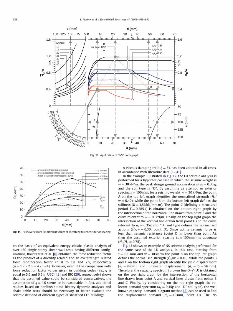
Fig. 13. Application of ‘‘NS’’ nomograph.

0

10

20

30

40

50

60

70

0

H [k

N/m

]

s = 50mms = 75mms = 100mms = 150mm

average non linear response curveaverage idealised bilinear response curve design idealized bilinear response curve

Hy,d

Hy,av

Hp,av

d [mm]10 20 30 40 50 60 70 80

Fig. 14. Pushover curves for different values of sheathing fastener exterior spacing.

L. Fiorino et al. / Thin-Walled Structures 47 (2009) 919–930928

on the basis of an equivalent energy elastic–plastic analysis ofover 180 single-storey shear wall tests having different config-urations, Boudreault et al. [6] obtained the force reduction factoras the product of a ductility related and an overstrength relatedforce modification factor equal to 1.8 and 2.5, respectively(q ¼ 1.8�2.5 ¼ 4.25E4). However, even if the comparison withforce reduction factor values given in building codes (i.e., q isequal to 5.5 and 6.5 in UBC [42] and IBC [20], respectively) showsthat the assumed value could be considered conservatives, theassumption of q ¼ 4.0 seems to be reasonable. In fact, additionalstudies based on nonlinear time history dynamic analyses andshake table tests should be necessary to better evaluate theseismic demand of different types of sheathed CFS buildings.

A viscous damping ratio x ¼ 5% has been adopted in all cases,in accordance with literature data [12,41].

In the example illustrated in Fig. 12, the LD seismic analysis isperformed for a hypothetical case in which the seismic weight isw ¼ 30 kN/m, the peak design ground acceleration is ag ¼ 0.35 g,and the soil type is ‘‘D’’. By assuming as attempt an exteriorspacing s ¼ 100 mm, for a seismic weight w ¼ 30 kN/m, the pointA on the top left graph identifies the normalised strength (HC/w ¼ 0.40), while the point B on the bottom left graph defines thestiffness (K ¼ 1.56 kN/mm m). The point C (defining a structuralperiod T ¼ 0.285 s) is obtained on the bottom right graph bythe intersection of the horizontal line drawn from point B and thecurve relevant to w ¼ 30 kN/m. Finally, on the top right graph theintersection of the vertical line drawn from point C and the curverelevant to ag ¼ 0.35g and ‘‘D’’ soil type defines the normalisedactions (HD/w ¼ 0.30, point D). Since acting seismic force isless than seismic resistance (point D is lower than point A),then the assumed exterior spacing (s ¼ 100 mm) is adequate(HD/HC ¼ 0.75).

Fig. 13 shows an example of NS seismic analysis performed forthe same case of the LD analysis. In this case, starting froms ¼ 100 mm and w ¼ 30 kN/m the point A on the top left graphdefines the normalised strength (HC/w ¼ 0.40), while the points Band C on the bottom right graph identify the yield displacement(dy ¼ 8 mm) and ultimate displacement (du ¼ dC ¼ 56 mm).Therefore, the capacity spectrum (broken line O–Y–U) is obtainedon the top right graph by the intersection of the horizontalline drawn from point A and vertical lines drawn from points Band C. Finally, by considering on the top right graph the re-levant demand spectrum (ag ¼ 0.35g and ‘‘D’’ soil type), the wellknown capacity–demand–diagram method [3] can be used to findthe displacement demand (dD ¼ 49 mm, point D). The NS

ARTICLE IN PRESS

0

5

10

15

20

25

30

50

HC (k

N/m

)

s (mm)

150200300

a (mm)HC,sa,k / γov,sa

1.51.0

t (mm)HC,s,k / γov,s

M24M20M16

φ (mm)HC,ha,k / γov,ha

HC,f,d

A B

C ≡ D

75 100 125 150

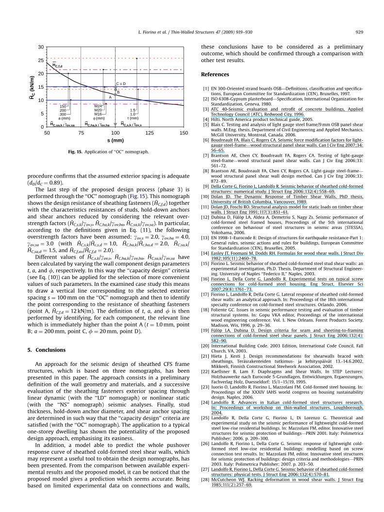
Fig. 15. Application of ‘‘OC’’ nomograph.

L. Fiorino et al. / Thin-Walled Structures 47 (2009) 919–930 929

procedure confirms that the assumed exterior spacing is adequate(dD/dC ¼ 0.89).

The last step of the proposed design process (phase 3) isperformed through the ‘‘OC’’ nomograph (Fig. 15). This nomographshows the design resistance of sheathing fasteners (HC,f,d) togetherwith the characteristics resistances of studs, hold-down anchorsand shear anchors reduced by considering the relevant over-strength factors (HC,s,k/gov,s, HC,ha,k/gov,ha, HC,sa,k/gov,sa). In particular,according to the definitions given in Eq. (11), the followingoverstrength factors have been assumed: gov,s ¼ 2.0, gov,ha ¼ 4.0,gov,sa ¼ 3.0 (with HC,s,k/Hc,s,d ¼ 1.0, HC,ha,k/Hc,ha,d ¼ 2.0, HC,sa,k/HC,sa,d ¼ 1.5, and HC,f,av/HC,f,d ¼ 2.0).

Different values of HC,s,k/gov,s, HC,ha,k/gov,ha, HC,sa,k/gov,sa havebeen calculated by varying the wall component design parameterst, a, and f, respectively. In this way the ‘‘capacity design’’ criteria(see Eq. (10)) can be applied for the selection of more convenientvalues of such parameters. In the examined case study this meansto draw a vertical line corresponding to the selected exteriorspacing s ¼ 100 mm on the ‘‘OC’’ nomograph and then to identifythe point corresponding to the resistance of sheathing fasteners(point A, HC,f,d ¼ 12 kN/m). The definition of t, a, and f is thenperformed by identifying, for each component, the relevant linewhich is immediately higher than the point A (t ¼ 1.0 mm, pointB; a ¼ 200 mm, point C, f ¼ 20 mm, point D).

5. Conclusions

An approach for the seismic design of sheathed CFS framestructures, which is based on three nomographs, has beenpresented in this paper. The approach consists in a preliminarydefinition of the wall geometry and materials, and a successiveevaluation of the sheathing fasteners exterior spacing throughlinear dynamic (with the ‘‘LD’’ nomograph) or nonlinear static(with the ‘‘NS’’ nomograph) seismic analyses. Finally, studthickness, hold-down anchor diameter, and shear anchor spacingare determined in such way that the ‘‘capacity design’’ criteria aresatisfied (with the ‘‘OC’’ nomograph). The application to a typicalone-storey dwelling has shown the potentiality of the proposeddesign approach, emphasising its easiness.

In addition, a model able to predict the whole pushoverresponse curve of sheathed cold-formed steel shear walls, whichmay represent a useful tool to obtain the design nomographs, hasbeen presented. From the comparison between available experi-mental results and the proposed model, it can be noticed that theproposed model gives a prediction which seems accurate. Beingbased on limited experimental data on connections and walls,

these conclusions have to be considered as a preliminaryoutcome, which should be confirmed through a comparison withother test results.

References

[1] EN 300-Oriented strand boards OSB—Definitions, classification and specifica-tions, European Committee for Standardization (CEN), Bruxelles, 1997.

[2] ISO 6308-Gypsum plasterboard—Specification, International Organization forStandardization, Geneva, 1980.

[3] ATC 40-Seismic evaluation and retrofit of concrete buildings, AppliedTechnology Council (ATC), Redwood City, 1996.

[4] Hilti. North America product technical guide, 2005.[5] Blais C. Testing and analysis of light gauge steel frame/9 mm OSB panel shear

walls. M.Eng. thesis, Department of Civil Engineering and Applied Mechanics.McGill University, Montreal, Canada. 2006.

[6] Boudreault FA, Blais C, Rogers CA. Seismic force modification factors for light-gauge steel-frame—wood structural panel shear walls. Can J Civ Eng 2007;34:56–65.

[7] Brantson AE, Chen CY, Boudreault FA, Rogers CA. Testing of light-gaugesteel-frame—wood structural panel shear walls. Can J Civ Eng 2006;33:561–72.

[8] Brantson AE, Boudreault FA, Chen CY, Rogers CA. Light-gauge steel-frame—

wood structural panel shear wall design method. Can J Civ Eng 2006;33:872–89.

[9] Della Corte G, Fiorino L, Landolfo R. Seismic behavior of sheathed cold-formedstructures: numerical study. J Struct Eng 2006;132(4):558–69.

[10] Dolan JD. The Dynamic Response of Timber Shear Walls, PhD thesis,University of British Columbia, Vancouver, 1989.

[11] Dolan JD, Foschi RO. Structural analysis model for static loads on timber shearwalls. J Struct Eng 1991;117(3):851–61.

[12] Dubina D, Fulop LA, Aldea A, Demetriu S, Nagy Zs. Seismic performance ofcold-formed steel framed houses, Proceedings of the 5th internationalconference on behaviour of steel structures in seismic areas (STESSA),Yokohama, 2006.

[13] EN 1998-1-Eurocode 8: Design of structures for earthquake resistance-Part 1:General rules, seismic actions and rules for buildings, European Committeefor Standardization (CEN), Bruxelles, 2005.

[14] Easley JT, Foomani M, Dodds RH. Formulas for wood shear walls. J Struct Div1982;105(11):2460–78.

[15] Fiorino L. Seismic behavior of sheathed cold-formed steel stud shear walls: anexperimental investigation, Ph.D. Thesis, Department of Structural Engineer-ing. University of Naples ‘‘Federico II,’’ Naples, 2003.

[16] Fiorino L, Della Corte G, Landolfo R. Experimental tests on typical screwconnections for cold-formed steel housing. Eng Struct, Elsevier Sci2007;29(8):1761–73.

[17] Fiorino L, Landolfo R, Della Corte G. Lateral response of sheathed cold-formedshear walls: an analytical approach. In: Proceedings of the 18th internationalspecialty conference on cold-formed steel structures. Orlando. 2006.

[18] Foliente GC. Issues in seismic performance testing and evaluation of timberstructural systems. In: Gopu VKA editor, Proceedings of the internationalwood engineering conference. Vol. 1. New Orleans. Forest Products Society,Madison, Wis, 1996, p. 29–36.

[19] Fulop LA, Dubina D. Design criteria for seam and sheeting-to-framingconnections of cold-formed steel shear panels. J Struct Eng 2006;132(4):582–90.

[20] International Building Code. 2003 Edition, International Code Council, FallChurch, VA, 2003.

[21] Hieta J, Kesti J. Design recommendations for shearwalls braced withsheathings, Terasrakenteiden tutkimus- ja kehityspaivat 13.-14.6.2002,Mikkeeli, Finnish Constructional Steelwork Association, 2002.

[22] Kaellsner B, Lam F. Diaphragms and Shear Walls, In STEP Lectures:Holzbauwerke nach Eurocode 5-Grundlagen, Entwicklungen, Ergaenzungen,Fachverlag Holz, Duesseldorf: 15/1–15/19, 1995.

[23] Iuorio O, Landolfo R, Fiorino L, Mazzolani FM. Cold-formed steel housing. In:Proceedings of the XXXIV IAHS world congress on housing sustainabilitydesign. Naples, 2006.

[24] Landolfo R. Advances in Italian cold-formed steel structures research.In: Proceedings of workshop on thin-walled structures. Loughborough,2004.

[25] Landolfo R, Della Corte G, Fiorino L, Di Lorenzo G. Theoretical andexperimental study on the seismic performance of lightweight cold-formedsteel low-rise residential buildings. In: Mazzolani FM, editor. Innovative steelstructures for seismic protection of buildings—PRIN 2001. Italy: PolimetricaPublisher; 2006. p. 209–300.

[26] Landolfo R, Fiorino L, Della Corte G. Seismic response of lightweight cold-formed steel low-rise residential buildings: modelling based on screwconnection test results. In: Mazzolani FM, editor. Innovative steel structuresfor seismic protection of buildings: design criteria and methodologies—PRIN2003. Italy: Polimetrica Publisher; 2007. p. 203–50.

[27] Landolfo R, Fiorino L, Della Corte G. Seismic behavior of sheathed cold-formedstructures: physical tests. J Struct Eng 2006;132(4):570–81.

[28] McCutcheon WJ. Racking deformation in wood shear walls. J Struct Eng1985;111(2):257–69.

ARTICLE IN PRESS

L. Fiorino et al. / Thin-Walled Structures 47 (2009) 919–930930

[29] McCreless S, Tarpy TS. Experimental investigation of steel stud shear walldiaphragms. In: Proceedings of the 4th international specialty conference oncold-formed steel structures. St. Louis, 1978.

[30] OPCM 3431/2005. Primi elementi in materia di criteri generali per laclassificazione sismica del territorio nazionale e di normative tecniche perle costruzioni in zona sismica. Ordinanza della Presidenza del Consiglio deiMinistri No. 3431/2005, Rome, 2005.

[31] Morgan KA, Sorhouet MA, Serrette RL. Performance of cold-formed steel-framedshear walls: alternative configurations. Research Rep. No. LGSRG-06-02 (finalrevision 9 September 2002), Light Gauge Steel Research Group, Santa Clara, 2002.

[32] Park R. Evaluation of ductility of structures and structural assemblages fromlaboratory testing. Bull N Z Nat Soc Earthquake Eng 1989;22(3):155–66.

[33] Richard RM, Abbott BJ. Versatile elastic–plastic stress–strain formula. J EngMech Div, Am 1975;101(4):511–5.

[34] Rokas, R. Testing of light gauge steel panel shear walls. M.Eng. Project,Department of Civil Engineering and Applied Mechanics, McGill University,Montreal, Canada. 2006.

[35] Salenikovich AJ, Dolan JD. Monotonic and cyclic tests of long steel-frameshear walls with openings. Report TE-1999-001. Department of Wood Scienceand Forest Product. Virginia Polytechnic Institute and State University,Blacksburg, VA, USA. 1999.

[36] Serrette R, Nguyen H, Hall G. Shear wall values for light weight steel framing,Report no. LGSRG-3-96, Light Gauge Steel Research Group, Department ofCivil Engineering, Santa Clara University, Santa Clara, 1996a.

[37] Serrette R, Hall G, Nguyen H. Dynamic performance of light gauge steelframed shear walls. In: Proceedings of the 13th international specialtyconference on cold-formed steel structures. St. Louis, 1996b, p. 487–98.

[38] Serrette RL, Encalada J, Juadines M, Nguyen H. Static racking behavior ofplywood, OSB, gypsum, and fiberboard walls with metal framing. J Struct Eng1997;123(8):1079–86.

[39] Serrette R, Encalada J, Matchen B, Nguyen H, Williams A. Additional shearwall values for light weight steel framing, Report no. LGSRG-1-97, Light GaugeSteel Research Group, Department of Civil Engineering, Santa ClaraUniversity. Santa Clara, 1997b.

[40] Simpson Strong-Tie Company, /http://www.strongtie.comS, 2007.[41] The Committee on Light-gauge Steel Structures. The Japan Iron and Steel

Federation, Steel-Framed House Association. Steel-framed Houses—HighStructural Performances and Habitability. Vol. 10. Steel Construction Today& Tomorrow. 2004, p. 1–9.

[42] Uniform Building Code, 1997 Edition, International Conference of BuildingOfficials. Whittier, CA, 1997.

[43] Veljkovic M, Johansson B. Light steel framing for residential buildings. Thin-Walled Struct 2006;44:1272–9.

[44] White MW, Dolan JD. Nonlinear shear-wall analysis. J Struct Eng 1995;121(11):1629–35.