shallow foundations: discussions and problem solving
TRANSCRIPT

worksaccounts.com

worksaccounts.com

Shallow Foundations
worksaccounts.com

worksaccounts.com

Shallow FoundationsDiscussions and Problem Solving
Tharwat M. BabanB.Sc. (Hons.); M.S. (Berkeley, Calif.)
University Professor andGeotechnical Consultant
(Retired)
worksaccounts.com

This edition first published 2016© 2016 by John Wiley & Sons, Ltd
Registered OfficeJohn Wiley & Sons, Ltd, The Atrium, Southern Gate, Chichester, West Sussex, PO19 8SQ, United Kingdom
Editorial Offices9600 Garsington Road, Oxford, OX4 2DQ, United KingdomThe Atrium, Southern Gate, Chichester, West Sussex, PO19 8SQ, United Kingdom
For details of our global editorial offices, for customer services and for information about how to apply forpermission to reuse the copyright material in this book please see our website at www.wiley.com
The right of the author to be identified as the author of this work has been asserted in accordance with the UKCopyright, Designs and Patents Act 1988.
All rights reserved. No part of this publication may be reproduced, stored in a retrieval system, or transmitted,in any form or by any means, electronic, mechanical, photocopying, recording or otherwise, except aspermitted by the UK Copyright, Designs and Patents Act 1988, without the prior permission of the publisher.
Designations used by companies to distinguish their products are often claimed as trademarks. All brandnames and product names used in this book are trade names, service marks, trademarks or registeredtrademarks of their respective owners. The publisher is not associated with any product or vendor mentionedin this book.
Limit of Liability/Disclaimer of Warranty: While the publisher and author(s) have used their best efforts inpreparing this book, they make no representations or warranties with respect to the accuracy or completenessof the contents of this book and specifically disclaim any implied warranties of merchantability or fitness for aparticular purpose. It is sold on the understanding that the publisher is not engaged in rendering professionalservices and neither the publisher nor the author shall be liable for damages arising herefrom. If professional adviceor other expert assistance is required, the services of a competent professional should be sought.
Library of Congress Cataloging-in-Publication Data applied for.
Hardback ISBN: 9781119056119
A catalogue record for this book is available from the British Library.
Wiley also publishes its books in a variety of electronic formats. Some content that appears in print may not beavailable in electronic books.
Cover image: Courtesy of the Author
Set in 9.5/11.5pt Minion by SPi Global, Pondicherry, India
1 2016
worksaccounts.com

To The Baban Family
worksaccounts.com

worksaccounts.com

Contents
Preface xAcknowledgements xiii
1 Site Investigation in Relation to Analysis and Design of Foundations 11.1 General 11.2 Site Investigation 2
1.2.1 Reconnaissance 21.2.2 Subsurface Exploration 31.2.3 Laboratory Tests 41.2.4 Compiling Information 61.2.5 Final Geotechnical Report 7
Problem Solving 8References 73
2 Shallow Foundations – Introductory Chapter 762.1 General 762.2 Types of Shallow Foundations 772.3 Depth of Foundations 822.4 Foundation Performance Requirements 84
2.4.1 General 842.4.2 Strength Requirements 852.4.3 Serviceability Requirements 862.4.4 Constructibility Requirements 862.4.5 Economy Requirements 87
2.5 Sulfate and Organic Acid Attack on Concrete 872.5.1 Sulfate Attack 872.5.2 Organic Acid Attack 88
2.6 Pressures under Foundations 892.6.1 Contact Pressure and Contact Settlement 892.6.2 Contact Pressure under Eccentrically Loaded Spread Footings 92
2.7 Vertical Stresses in a Soil Mass due to Foundation Loads 952.7.1 General 952.7.2 Vertical Stress Due to a Concentrated Load 952.7.3 Vertical Stress Due to a Line Load 962.7.4 Vertical Stress Due to a Uniformly Loaded Strip Area 97
worksaccounts.com
2.7.5 Vertical Stress Due to a Uniformly Loaded Circular Area 972.7.6 Vertical Stress Due to a Uniformly Loaded Rectangular Footing 992.7.7 Newmark’s Chart Method of Determining Vertical Stresses 1042.7.8 Pressure Bulbs Method of Determining Vertical Stresses 1052.7.9 Average Vertical Stress Due to a Loaded Rectangular Area 1072.7.10 Westergaard’s Equations 109
Problem Solving 111References 143
3 Shallow Foundations – Settlement 1443.1 General 1443.2 Immediate Settlement 1493.3 Settlement of Foundations on Coarse-grained Soils 155
3.3.1 General 1553.3.2 Estimation of Settlements from SPT 1573.3.3 Estimation of Settlements from CPT 161
3.4 Settlement of Foundations on Fine-grained Soils 1643.4.1 General 1643.4.2 Immediate Settlement of Fine-grained Soils 1663.4.3 Consolidation Settlement 1683.4.4 Estimation of the Rate of Consolidation Settlement 1743.4.5 Method of Accelerating the Rate of Consolidation Settlement 1753.4.6 Estimation of Settlements over the Construction Period 1803.4.7 Secondary Compression 181
3.5 Settlement of Foundations on Rock 183Problem Solving 187References 262
4 Shallow Foundations – Bearing Capacity 2654.1 General 2654.2 Basic Definitions 2664.3 Gross and Net Foundation Pressures 2684.4 Bearing Capacity Failure Mechanism for Long (Strip or Continuous) Footings 2724.5 Bearing Capacity Equations 2734.6 Some Considerations Concerning the Use of Bearing Capacity Equations 2784.7 Bearing Capacity of Footings with Inclined Loads 2804.8 Bearing Capacity of Footings with Eccentric Loads 2814.9 Effect of Water Table on Bearing Capacity 2864.10 Influence of Soil Compressibility on Bearing Capacity 2904.11 Effect of Adjacent Footings on Bearing Capacity 2914.12 Bearing Capacity of Foundations on Slopes 292
4.12.1 General 2924.12.2 Solutions 292
4.13 Bearing Capacity of Footings on Layered Soils 2964.13.1 General 2964.13.2 Ultimate Bearing Capacity: Stronger Soil Underlain by Weaker Soil 2984.13.3 Ultimate Bearing Capacity: Weaker Soil Underlain by Stronger Soil 302
4.14 Safety Factor 3044.15 Bearing Capacity from Results of In Situ Tests 3054.16 Uplift Capacity of Shallow Foundations 3064.17 Some Comments and Considerations Concerning the Geotechnical Design of
Shallow Foundations 3104.18 Bearing Capacity of Rock 312
viii Contents
worksaccounts.com

Problem Solving 316References 378
5 Shallow Foundations – Structural Design 3815.1 General 3815.2 Design Loads 3825.3 Selection of Materials 3825.4 Structural Action of Vertically and Centrically Loaded Isolated and Continuous
(Strip) Footings 3835.4.1 General 3835.4.2 Flexure 3835.4.3 Shear 3885.4.4 Development of Reinforcement 3905.4.5 Transfer of Force at Base of Column, Wall or Pedestal 390
5.5 Eccentrically Loaded Spread Footings 3965.6 Pedestals 3985.7 Pile Caps 3995.8 Plain Concrete Spread Footings 4005.9 Combined Footings 402
5.9.1 General 4025.9.2 Rectangular Combined Footings 4035.9.3 Trapezoidal Combined Footings 4045.9.4 Strap (or Cantilever) Footings 405
5.10 Modulus of Subgrade Reaction 4065.11 Beams on Elastic Foundations 4095.12 Mat Foundations 413
5.12.1 General 4135.12.2 Design Procedure for the Conventional (Rigid) Method 4145.12.3 Design Procedure for the Approximate Flexible Method 4175.12.4 Finite Difference Method for the Design of Mat Foundations 4195.12.5 Modulus of Subgrade Reaction and Node Coupling of Soil Effects for Mats 4215.12.6 Finite Element Method for the Design of Mat Foundations 4245.12.7 Finite Grid Method for the Design of Mat Foundations 426
Problem Solving 427References 647
6 Eurocode Standards and the Design of Spread Foundations 6496.1 General 6496.2 Basis of Design Irrespective of the Material of Construction 651
6.2.1 Introduction 6516.2.2 Terms and Definitions 6526.2.3 Requirements 6556.2.4 Quality Management 6576.2.5 Principles of Limit States Design 657
6.3 Design of Spread Foundations 6646.3.1 Introduction 6646.3.2 Geotechnical Categories 6656.3.3 Limit States 6666.3.4 Geotechnical Design 6676.3.5 Structural Design 677
Problem Solving 688References 729
Index 730
Contents ix
worksaccounts.com
Preface
This book is intended primarily to introduce civil engineers, especially geotechnical engineers and allcivil engineering students reading the specialist subjects of soil mechanics and geotechnical engineer-ing, to the fundamental concepts and application of shallow foundation analysis and design. Also, thefurnished material can be considered as an essential reference work for practising civil engineers, con-sulting engineers and government authorities. The primary focus of this book is on interfacing struc-tural elements with the underlying soil, which is, in the author’s opinion, where the major focus ofshallow foundation engineering lies.
The book is not intended to be a specific text book on soil mechanics or geotechnical engineering.Therefore, there is no part of the text alone that could be used as a core syllabus for a certain course.However, it is the author’s opinion that more than 70% of the book is core material at the advancedundergraduate levels. It is expected that civil engineering students will find the text helpful in betterunderstanding the fundamental concepts and their implications for the analysis and design of shallowfoundations. The author tried to present the material such that separable topics and subtopics arecovered in separate sections, with clear and unambiguous titles and subtitles. Thus, it would not bedifficult for a university lecturer to draw up a personalised reading schedule, appropriate to his orher own course. It is hoped that the book can establish itself as an effective reference and a useful textin most of the engineering colleges and technical institutions.
Generally, the given material is of an advanced level and, therefore, it is assumed that the reader has agood understanding of basic statics and the mechanics of materials and has studied the basic principlesof soil mechanics, lateral earth pressures and reinforced concrete. SI units are used throughout all thechapters and, therefore, the reader also needs to have sufficient background knowledge regarding theuse of these units.
The book would be very beneficial to the reader, since it provides essential data for the design ofshallow foundations under ordinary circumstances. The necessary background concepts and theoriesare generally presented clearly in concise forms of formulas or charts, and their applications are high-lighted through solving a relatively large number of realistic problems. Moreover, the worked problemsare of the types usually faced by civil engineers in practice and, therefore, the obtained information willbe most valuable.
Generally, the subject matter is introduced here by first discussing the particular topic and then solv-ing a number of pertinent objective problems that highlight the relevant theories, concepts and analysismethods. A list of crucial references is given at the end of each chapter. Thus, each chapter consists ofthree parts: discussions, problem solving and references.
The “discussion” part is presented in a clear and concise but precise manner, keeping in view theavoidance of unnecessary details. In some chapters, where the topics are of special difficulty, full guid-ing explanations are given; where the subject of study is simpler, less detailed treatment is provided.
worksaccounts.com
The “problem solving” part gives a relatively comprehensive range of worked out problems toconsolidate an understanding of the principles and illustrate their applications in simple practical situ-ations. A total of 180 worked problems have been provided. The author’s academic and professionalcareer has proved to him that geotechnical engineers and civil engineering students need to be wellacquainted with the correct and effective use of the theoretical and empirical principles and formulasthey have learned. An effective way to lessen the deficiency may be through solving, as much as pos-sible, a variety of problems of the type or nearly similar to those engineers face in practice. For thesereasons the author considers the “problem solving” part, on which the book is partially based, as a vitalportion of the text.The “references” part that comes directly at the end of each chapter enriches the discussions part
with valuable sources of information and increases its reliability. Moreover, the furnished referenceswill be very beneficial to any ambitious fresh civil engineer or undergraduate student who may wishlater to undertake higher studies in the subject.The text comprises six chapters. The chapters are devoted mostly to the geotechnical and structural
aspects of shallow foundation design. A brief overview of each chapter follows:
• Chapter 1 deals with site investigation in relation to the analysis and design of shallow foundations.Unlike the other chapters, this chapter requires various topics, field tests in particular, to be dis-cussed separately. Therefore, only a general and relatively brief overview of the overall subject mat-ter, consistent with the chapter title, is given in the main “discussion” part. Discussion individualtopics is given in the “problem solving” part directly below the relevant problem statement. Solu-tions of 27 problems have been provided. These solutions and those of the other five chapters havefully worked out calculations.
• Chapter 2 presents introductory discussions and explanations of various topics pertaining to shal-low foundations, their analysis and design. It discusses type and depth of shallow foundations, per-formance requirements, sulfate and organic acid attack on concrete, distribution of contactpressures and settlements and vertical stress increase in soils due to foundation loads. Solutionsof 21 problems are presented.
• Chapter 3 concerns settlements due to foundation loads. The chapter discusses various types ofsettlements of foundations on both coarse- and fine-grained soils, methods of settlement estima-tion, methods of estimating and accelerating consolidation settlement, settlement due to secondarycompression (creep), estimation of settlements over the construction period and settlement of foun-dations on rock. Solutions of 56 problems are introduced.
• Chapter 4 deals with the bearing capacity of shallow foundations. The chapter discusses most of thesignificant aspects of the subject matter, among them: bearing capacity failure mechanism, bearingcapacity equations, bearing capacity of footings with concentric and eccentric vertical loads, bearingcapacity of footings with inclined loads, effects of water table and other factors on bearing capacity,uplift capacity of shallow foundations, bearing capacity of foundations on layered soils and onslopes, and bearing capacity of rock. Solutions of 40 problems are provided.
• Chapter 5 deals with the structural design of different types of shallow foundations. Structuraldesign of plain concrete spread footings, pedestals, pile caps and the foundations of earth-retainingconcrete walls are also included. The discussion part of the chapter covers most of the major aspectsof the subject matter such as: selection of materials, design loads, structural action of isolated andcontinuous footings, eccentrically loaded footings, modulus of subgrade reaction and beams onelastic foundations, rigid and flexible design methods and so on. Design calculations of 28 typicalproblems are presented in a step by step order. All the structural designs conform to the BuildingCode Requirements for Structural Concrete (ACI 318) and Commentary, USA.
• Chapter 6 deals with Eurocode Standards in relation to the design of spread foundations. The dis-cussion part of the chapter covers certain important topics such as: Eurocode background andapplications, basis of design and requirements, principles of limit states design, design approaches,partial factors and load combinations, geotechnical and structural designs of spread foundationsand so on. The problem solving part of the chapter provides design calculations of eight typical
Preface xi
worksaccounts.com

problems, as an attempt to introduce the concerned engineer to application of the design rulesstipulated by Eurocodes 2 and 7 (or EN 1992 and 1997) rather than the geotechnical and structuralrelated issues.It is well known that not all civil engineers are acquainted with all internationally recognised
codes, such as the ACI Code and Eurocodes, at the same time. Therefore, this chapter is especiallywritten for those civil engineers, specially geotechnical engineers, who are unfamiliar with the tech-nical rules and requirements of the Eurocode Standards (Structural Eurocode). The implementationof the Eurocode is extended to all the European Union countries and there are firm steps towardtheir international adoption.
It must be clear that, despite every care taken to ensure correctness or accuracy, some errors mighthave crept in. The author will be grateful to the readers for bringing such errors, if any, to his notice.Also, suggestions for the improvement of the text will be gratefully acknowledged.
Tharwat M. Baban
xii Preface
worksaccounts.com

Acknowledgements
The author wishes to express his gratitude to those writers and researchers whose findings are quotedand to acknowledge his dependence on those authors whose works provided sources of material;among them are:
Giuseppe Scarpelli, Technical University of Marche Region, Ancona, ItalyTrevor L.L. Orr, Trinity College, Dublin, IrelandAndrew J. Bond, Geocentrix Ltd, Banstead, UKAndrew Harris, Kingston University, London, UKJenny Burridge, The Concrete Center, London, UK
The author is truly grateful to Dr. Paul Sayer, who was kind enough to suggest the inclusion ofChapter 6.The author wishes to thank all the members of his family, especially his wife Mrs. Sawsan Baban, for
their encouragement, assistance and patience in preparing the manuscript of this book.Finally, the author likes to thank John Wiley and Sons, Ltd and their production staff for their
cooperation and assistance in the final development and production of this book.
worksaccounts.com

worksaccounts.com
CHAPTER 1
Site Investigation in Relation to Analysisand Design of Foundations
1.1 General
The stability and safety of a structure depend upon the proper performance of its foundation.Hence, the first step in the successful design of any structure is that of achieving a proper foundationdesign.Soil mechanics is the basis of foundation design since all engineered constructions rest on the earth.
Before the established principles of soil mechanics can be properly applied, it is necessary to have aknowledge of the distribution, types and engineering properties of subsurface materials. Therefore,an adequate site investigation is an essential preliminary to enable a safe and economic design andto avoid any difficulties during construction. A careful site investigation can minimise the need foroverdesign and reduce the risks of underdesign. A designer who is well equipped with the necessaryreliable information can use a lower factor of safety, thereby achieving a more economical design. Withenough information available, construction troubles can be decreased and, therefore, constructioncosts are decreased too.A site investigation usually costs a small percentage of total construction costs. According to Bowles
(2001), elimination of the site exploration, which usually ranges from about 0.5 to 1.0% of totalconstruction costs, only to find after construction has started that the foundation must be redesignedis certainly a false economy. However, a geotechnical engineer planning a subsurface explorationprogram for a specific job must keep in mind the relative costs of the exploration versus the total con-struction costs. It is understood that there is no hard and fast procedure for an economical planning asite investigation programme. Each condition must be weighed with good judgment and relativeeconomy.Nowadays, it is doubtful that any major structures are designed without site exploration being
undertaken. Sometimes, for small jobs, it may be more economical to make the foundation designon conservative values rather than making elaborate borings and tests, especially, when the conditionof the adjacent structures is an indication that the site is satisfactory. However, generally, design ofstructures without site investigation is not recommended by civil engineers.The cheapest and most common method of subsurface exploration is by drilling boreholes. Test pits
are too expensive for general exploration, but they may be used for more careful examination if foundto be needed.
Shallow Foundations: Discussions and Problem Solving, First Edition. Tharwat M. Baban.© 2016 John Wiley & Sons, Ltd. Published 2016 by John Wiley & Sons, Ltd.
worksaccounts.com

1.2 Site Investigation
A successful investigation of a site for an important structure will generally falls under the following fiveheadings:
(1) Reconnaissance(2) Subsurface exploration(3) Laboratory tests(4) Compiling information(5) Geotechnical report.
1.2.1 Reconnaissance
Office Reconnaissance: This phase of reconnaissance comprises the following duties:
• Review of plans, boring logs and construction records of existing structures in the area.
• Study of the preliminary plans and designs of the proposed structure, including the approximatemagnitude of the loads to be transmitted to the supporting material.
• Review of other backlogs of information already compiled on the same general area and similarstructures.
• Review of other information pertaining to the site area obtained from such sources as different typesof maps (i.e., topographic, geologic and agricultural maps), photographs, records of adjacent bridgeif exists, underground utility constructions and well drilling logs.
• Formulation of a boring plan should be made during the latter phases of the office reconnaissance.This prepared boring plan should be reviewed during the field reconnaissance. The objective shouldbe the development of a maximum of subsurface information through the use of a minimum num-ber of boreholes. Spacing, number and depth of boreholes will be discussed later in conjunction withthe Solution of Problem 1.4.
Field Reconnaissance: This phase of reconnaissance should commence with a visit to the site of the pro-posed structure. It should always be made by a Soils or Foundation Engineer who will complete theGeotechnical Report. Whenever possible, it is desirable that this engineer be accompanied by the drilleror the driller foreman. Notes on items to be observed are as follows:
• Surface Soils: Surface soils are easily revealed through the use of a shovel or post-hole diggers. Thesesoils may sometimes be identified as belonging to some particular formation, and usually they indi-cate the underlying material.
• Gullies, Excavations and Slopes: Any cut or hole near the proposed structure site is a subsurfacewindow, and for its depth it will provide more information than borehole since it may be examinedin detail.
• Surface and Subsurface Water: The presence of either surface or subsurface water is an importantfactor in both preparation of boring plans and foundation design. All surface flows should be noted,and all opportunities should be taken to observe the groundwater level.
• Study of Existing Structures: The existing structures within an area are valuable sources of infor-mation. A very close examination of them with regard to their performance, type of foundation,apparent settlement, load, location and age will yield a wealth of data.
• Topography: To some extent, topography is indicative of subsurface conditions. In narrow, steepstream beds, rock is likely to be near the surface with little overlying stream-deposited soil. On theother hand, wide, flat valleys indicate deep soil deposits.
2 Shallow Foundations
worksaccounts.com
• Information required by the Drill Crew. The drill crew needs to know how to get to the site,where to drill, what equipment to take, and what difficulties to expect. Generally, the followingtypes of information are usually needed:
• Information regarding verification of the boring plan which was already prepared during theoffice reconnaissance phase. The proposed locations of boreholes should be checked for acces-sibility. Desirable deletions, additions, and relocations should be made as are necessary to bettersuit the crew’s capabilities and to add completeness to the subsurface information.
• Type of drilling and equipment needed. Notes should be made as to which type of drilling is bestsuited to the site (i.e., rotary, auger, etc.).
• Reference points and benchmarks. The reconnaissance should determine if reference points andbench marks are in place adjacent to the site and properly referenced on the plans.
• Utilities. Underground and overhead utilities located at the site should be accurately shown onthe plans or their locations should be staked on the ground.
• Geophysical Survey: The field reconnaissance may require a geophysical survey of the site. The useof geophysical methods provides information on the depths to the soil and rock layers, the homo-geneity of the layer and the type of soil or rock present. This information can be used to supplementthe boring plan.
• Field Reconnaissance Report: A concise and informative field reconnaissance report, in which alldecisions concerning the boring plan and the drill crew are delineated, should be prepared. It can befacilitated by the use of a special check list or form.
1.2.2 Subsurface Exploration
General:After the reconnaissance has been completed, the results should be given to the foreman of thedrill crew in order to carry out the foundation investigation at the site. Briefly, the subsurface or foun-dation exploration consists of making the borings and collecting the pertinent samples (i.e., drilling andsampling), performing the required field tests in conjunction with the drilling, coring, and identifica-tion of materials. Each job site must be studied and explored according to its subsurface conditions andthe size and type of the proposed structure. The civil engineer or the experienced geologist in charge ofthe exploration task should endeavour to furnish complete data such that a reliable study of practicalfoundation types can be made.Before the arrival of the drill crew at the exploration site, enough survey control should have been
previously carried out with reference to at least one bench mark already established at the site. Theborehole locations should be staked in conformity with the boring plan. The stakes could indicatethe borehole number and the existing ground surface elevation.Drilling: It is defined as that process which advances the borehole. There are various methods of
drilling or boring, namely: auger drilling, rotary drilling, wash boring, drilling by continuous sampling,percussion drilling and rock coring. Most of these methods are best suited for some particular problemor type of information sought. It is doubtful if an organisation (authority responsible for site investi-gation) would adopt any one method for all of its work unless the work was limited to one particulararea. The same argument is true with respect to the various types of equipment used in drilling andcoring.Sampling: It is defined as that process wherein samples of the subsurface materials are obtained. As
there are various methods of drilling and various equipment types, also there are different types ofsampling, namely: split-barrel or spoon sampling, push barrel or thin-walled Shelby tube and station-ary piston type sampling, wet barrel or double wall and dry barrel or single wall sampling, retractableplug sampling and rock coring.Samples: The samples obtained during subsurface exploration should always represent the material
encountered, that is, representative samples. These samples are disturbed, semi-disturbed or
Site Investigation in Relation to Analysis and Design of Foundations 3
worksaccounts.com

undisturbed. Usually, disturbed and semi-disturbed samples are used for identification and classifica-tion of the material. Undisturbed samples are used for determining the engineering properties such asstrength, compressibility, permeability and so on, density and natural moisture content of the material.Disturbed samples are those in which the material (soil or rock) structure has not been maintained, andthey are used in those tests in which structure is not important. On the other hand, relatively undis-turbed samples have structures maintained enough that they could be used in engineering propertiesdetermination of the material. The degree of disturbance depends upon several factors such as type ofmaterials being sampled, sampler or core barrel used, the drilling equipment, methods of transportingand preserving samples and driller skill. Extended exposure of the sample material to the atmospherewill change relatively undisturbed sample into an unusable state; therefore, the methods of obtainingand maintaining samples cannot be overemphasised.
Field Tests: there are various types of tests performed in the field, in conjunction with the drillings, inorder to determine soil properties in situ. These tests are: dynamic penetration tests, such as standard(SPT) cone penetration and driven probe and driven casing; static cone penetration (CPT); in-place vaneshear; plate-load (may not be in conjunction with the drillings); pressuremeter; flat-plate dilatometer; andother tests made in field laboratories, such as classification tests and unconfined strength test. Rock qual-ity designation (RQD) test is performed on rock core samples. Note: Discussion of a particular field testwill be given in the “Problem Solving” part of this chapter directly below the relevant problem statement.
Field Boring Log and Borehole Logging: The log is a record which should contain all of the informa-tion obtained from a boring whether or not it may seem important at the time of drilling. The process ofrecording the information in a special field log form is “logging”. It is important to record the max-imum amount of accurate information. This record is the “field” boring log. The importance of goodlogging and field notes cannot be overemphasised, and it is most necessary for the logger (whomay be asoil engineer, a geologist, a trained technician or a trained drill crew foreman) to realise that a good fielddescription must be recorded. The field boring log is the major portion of the factual data used in theanalysis of foundation conditions.
Groundwater Table: The location of the groundwater level is an important factor in foundation ana-lysis and design, and emphasis should be placed upon proper determination and reporting of this data.
In order to determine the elevation of groundwater it is suggested that at least two boreholes be leftopen for the duration of the subsurface exploration and periodically checked as to water level. Thesetwo boreholes should have their final check made no earlier than 24 h after the completion of explor-ation. The depth to the water level should be recorded on the boring log each time a reading is made,along with the time lapse since completion of the boring. When there is significant difference betweenthe two borings checked, or when the logger deems it otherwise necessary, the water level in other bore-holes should be checked.
Note: It is obvious that details of all the various methods and descriptions of the above mentioneddrilling, samples and sampling, field tests, field boring log and borehole logging are too large in bulk forinclusion in the discussions. However, those interested in further information and details, should seevarious standards, practice codes and manuals, such as AASHTOManual on Subsurface Investigations(1988), ASTM, BSI and Eurocode standards.
1.2.3 Laboratory Tests
Economical foundation design requires the use of the physical properties of the foundation material(soil or rock). The physical properties may be determined by in situ tests, load tests and laboratory tests.Results of laboratory tests, in addition to their use in foundations design, are used to predict the foun-dation behavior based on the experience of similar tested materials and their performance in the field.The two main reasons for making these laboratory tests are first to verify classification and second todetermine engineering properties. An adequate amount of laboratory testing should be conducted tosimulate the most sever design criteria. Generally, the amount of testing performed will depend on thesubsurface conditions, laboratory facilities and type of the proposed structure.
4 Shallow Foundations
worksaccounts.com
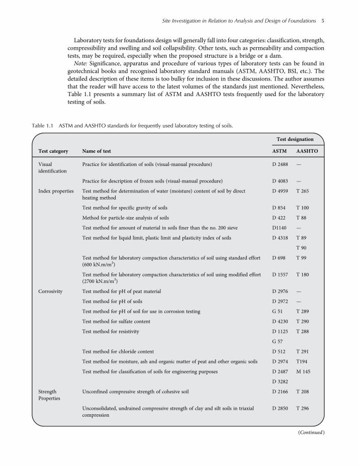
Laboratory tests for foundations design will generally fall into four categories: classification, strength,compressibility and swelling and soil collapsibility. Other tests, such as permeability and compactiontests, may be required, especially when the proposed structure is a bridge or a dam.Note: Significance, apparatus and procedure of various types of laboratory tests can be found in
geotechnical books and recognised laboratory standard manuals (ASTM, AASHTO, BSI, etc.). Thedetailed description of these items is too bulky for inclusion in these discussions. The author assumesthat the reader will have access to the latest volumes of the standards just mentioned. Nevertheless,Table 1.1 presents a summary list of ASTM and AASHTO tests frequently used for the laboratorytesting of soils.
Table 1.1 ASTM and AASHTO standards for frequently used laboratory testing of soils.
Test category Name of test
Test designation
ASTM AASHTO
Visualidentification
Practice for identification of soils (visual-manual procedure) D 2488 —
Practice for description of frozen soils (visual-manual procedure) D 4083 —
Index properties Test method for determination of water (moisture) content of soil by directheating method
D 4959 T 265
Test method for specific gravity of soils D 854 T 100
Method for particle-size analysis of soils D 422 T 88
Test method for amount of material in soils finer than the no. 200 sieve D1140 —
Test method for liquid limit, plastic limit and plasticity index of soils D 4318 T 89
T 90
Test method for laboratory compaction characteristics of soil using standard effort(600 kN.m/m3)
D 698 T 99
Test method for laboratory compaction characteristics of soil using modified effort(2700 kN.m/m3)
D 1557 T 180
Corrosivity Test method for pH of peat material D 2976 —
Test method for pH of soils D 2972 —
Test method for pH of soil for use in corrosion testing G 51 T 289
Test method for sulfate content D 4230 T 290
Test method for resistivity D 1125 T 288
G 57
Test method for chloride content D 512 T 291
Test method for moisture, ash and organic matter of peat and other organic soils D 2974 T194
Test method for classification of soils for engineering purposes D 2487 M 145
D 3282
StrengthProperties
Unconfined compressive strength of cohesive soil D 2166 T 208
Unconsolidated, undrained compressive strength of clay and silt soils in triaxialcompression
D 2850 T 296
(Continued )
Site Investigation in Relation to Analysis and Design of Foundations 5
worksaccounts.com

1.2.4 Compiling Information
General: Having carried the investigation through the steps of reconnaissance, subsurface explorationand laboratory testing, the next step is obviously the compilation of all the information.
Prior to preparing finished (final) logs, all samples should be checked by the Engineer in charge. Thisshould ideally be performed immediately after the borings are completed and even while the boringprogram is still in progress. Significant soil characteristics that may have been omitted from the fieldlogs may be identified, and the Engineer thus alerted to a potential foundation problem that mightotherwise have gone undetected.
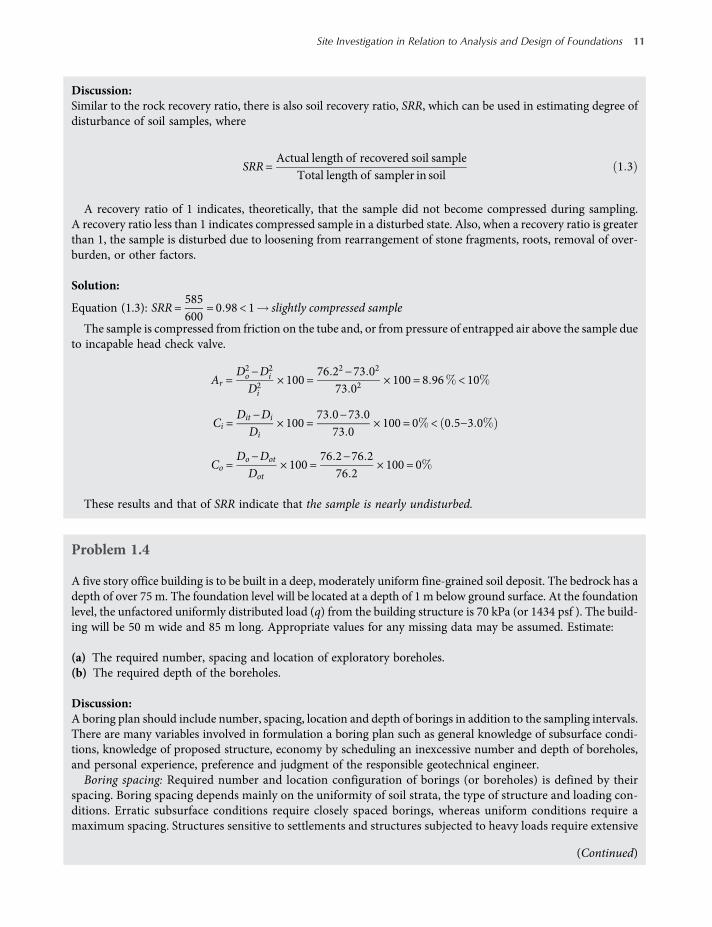
Finished Boring Log: It is important to differentiate clearly between the “field” boring log and the“finished” boring log. The field log is a factual record of events during boring operation, whereasthe finished log is a graphical representation. The field log gives a wide range of information in notesor tabular form. The finished log is drawn from the data given in the field log as well as from results ofvisual inspection of samples; it represents a graphical picture of subsurface conditions. Informationobtained from laboratory test results along with other necessary information are also utilised in itspreparation. Also, various data such as results of field tests, depth location of different samples andgroundwater level are superimposed upon it. It is important that the soil or rock in each stratum beclearly described and classified. A typical finished boring log is shown in Figure 1.1.
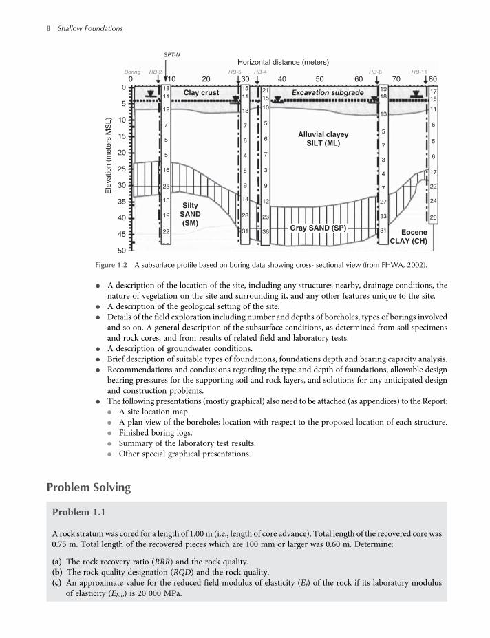
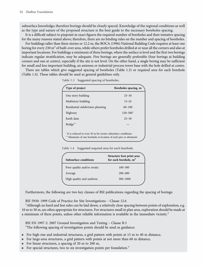
Soil Profile: In many cases it may be advantageous to plot a soil profile along various longitudinal ortransverse lines. This should be done by plotting the boreholes in their true location, but with verticalscale exaggerated, connecting the similar strata by lines and shading similar areas by means of an iden-tifying cross-section mark. The groundwater level should also be shown on the plot. Thus a probablerepresentation of the subsurface conditions between the boreholes can be given, although a pocket ormore of different formation may exist between any two adjacent boreholes. A representative exampleof an interpreted subsurface profile is shown in Figure 1.2.
Table 1.1 (Continued)
Test category Name of test
Test designation
ASTM AASHTO
Consolidated undrained triaxial compression test on cohesive soils D 4767 T 297
Direct shear test of soils for unconsolidated drained conditions D 3080 T 236
Modulus and damping of soils by the resonant-columnmethod (small-strain properties) D 4015 —
Test method for laboratory miniature vane shear test for saturated fine-grainedclayey soil
D 4648 —
Test method for bearing ratio of soils in place D 4429 —
StrengthProperties
California bearing ratio (CBR) of laboratory-compacted soils D 1883 —
Test method for resilient modulus of soils — T 294
Method for resistance R-value and expansion pressure of compacted soils D 2844 T 190
Permeability Test method for permeability of granular soils (constant head) D 2434 T 215
Test method for measurement of hydraulic conductivity of saturated porous materialsusing flexible wall perameters
D 5084 —
CompressionProperties
Method for one-dimensional consolidation characteristics of soils (oedometer test) D 2435 T 216
Test method for one-dimensional swell or settlement potential of cohesive soils D 4546 T 258
Test method for measurement of collapse potential of soils D 5333 —
6 Shallow Foundations
worksaccounts.com

1.2.5 Final Geotechnical Report
After information compiling has been successfully completed, a final written Geotechnical Reportshould be prepared and presented to the designer for use in the foundations design. Additionally, thisreport will furnish the Resident Engineer with data regarding anticipated construction problems, aswell as serving to establish a firm basis for the contractor to estimate costs, unless the organisation’spolicies or regulations restrict the release of such information. A good policy may be of releasing suchinformation, which should be as accurate as possible, provided that it is expressly and formally under-stood that the organisation will not be liable for any damages or losses incurred as a result of relianceupon it in the bidding or in the construction operations.The Geotechnical Engineer who writes the Report should avoid including extraneous data which are
of no use to the Designer or Resident Engineer. Also, his recommendations should be brief, conciseand, where possible, definite. The Report should include:
• Authorisation of the site investigation and the job contract number and date.
• A description of the investigation scope.
• A description of the proposed structure for which the subsurface exploration has been conducted.
Boring Log
Name of the ProjectTwo-story apartment building
Location Johnson & Olive St. March 2, 2005Date of Boring
Boring No. 3 Type of Hollow-stem auger Ground 60.8 m
Boring
Soil
description
Elevation
Depth
(m)
Soil
sample
type and
number
Comments
Light brown clay (fill)
Silty sand (SM)
1
2SS-1 9 8.2
17.6 LL = 38
LL = 36
PI = 11
20.4
20.6
9
Groundwater table
observed after one
week of drilling
12
11
27
SS-2
ST-1
SS-3
SS-4
3
4
5
6
7
8
°G.W.T.
3.5 m
Light gray clayey
silt (ML)
Sand with some
gravel (SP)
End of boring @ 8 m
N60wn
(%)
N60= standard penetration number
wn= natural moisture content
qu= 112 kN/m2
LL = liquid limit; PI = plasticity index
SS = split-spoon sample; ST = Shel by tube sample
qu= unconfined compression strength
Figure 1.1 A typical finished boring log (from Das, 2011).
Site Investigation in Relation to Analysis and Design of Foundations 7
worksaccounts.com
• A description of the location of the site, including any structures nearby, drainage conditions, thenature of vegetation on the site and surrounding it, and any other features unique to the site.
• A description of the geological setting of the site.
• Details of the field exploration including number and depths of boreholes, types of borings involvedand so on. A general description of the subsurface conditions, as determined from soil specimensand rock cores, and from results of related field and laboratory tests.
• A description of groundwater conditions.
• Brief description of suitable types of foundations, foundations depth and bearing capacity analysis.
• Recommendations and conclusions regarding the type and depth of foundations, allowable designbearing pressures for the supporting soil and rock layers, and solutions for any anticipated designand construction problems.
• The following presentations (mostly graphical) also need to be attached (as appendices) to the Report:
• A site location map.
• A plan view of the boreholes location with respect to the proposed location of each structure.
• Finished boring logs.
• Summary of the laboratory test results.
• Other special graphical presentations.
Problem Solving
Problem 1.1
A rock stratumwas cored for a length of 1.00m (i.e., length of core advance). Total length of the recovered core was0.75 m. Total length of the recovered pieces which are 100 mm or larger was 0.60 m. Determine:
(a) The rock recovery ratio (RRR) and the rock quality.(b) The rock quality designation (RQD) and the rock quality.(c) An approximate value for the reduced field modulus of elasticity (Ef) of the rock if its laboratory modulus
of elasticity (Elab) is 20 000 MPa.
Horizontal distance (meters)
0
5
18
11
12
7
5
5
16
25
15
19
22
SiltySAND(SM)
Clay crust Excavation subgrade
Alluvial clayeySILT (ML)
15
HB-5HB-2Boring
SPT-N
HB-4 HB-8 HB-11
1121
15
19
0 10 20 30 40 50 60 70 80
18
13
17
15
11
6
5
6
17
22
24
28
EoceneCLAY (CH)
5
7
3
4
7
27
33
31
10
5
6
7
3
9
12
23
36
13
7
6
4
5
9
14
28
31
10
15
20
25
30
Ele
vation (
mete
rs M
SL)
35
40
45
50
Gray SAND (SP)
Figure 1.2 A subsurface profile based on boring data showing cross- sectional view (from FHWA, 2002).
8 Shallow Foundations
worksaccounts.com
Discussion:General evaluation or classification of rock quality may be determined by calculating rock recovery ratio (RRR)and rock quality designation (RQD), where
RRR =Total length of core recovered
Length of core advance1 1
RQD =ΣLengths of intact pieces of core > 10mm
Length of core advance1 2
Value of RRR near to 1.0 usually indicates good-quality rock, while in badly fractured or soft rock the RRR valuemay be 0.5 or less. Table 1.2 presents a general relationship between RQD and in situ rock quality (Deere, 1963).An approximate relationship between RQD and ratio of field and laboratory modulus of elasticity (Ef /Elab) wasadded to Table 1.2 (Bowles, 2001). This relationship can be used as a guide only.
Solution:
(a) Equation (1.1): RRR=0 751 00
= 0 75 Fair rock quality
(b) Equation (1.2): RQD=0 601 00
= 0 60 Fair rock quality (see Table 1.2)
(c) RQD = 0 6EfElab
= 0 25 (see Table 1.2)
Ef = 20000 × 0 25 = 5000MPa
Problem 1.2
(a) What are the factors on which disturbance of a soil sample depends?(b) The cutting edge of a sampling tube has outside diameter Do = 50.8 mm and inside diameter Di = 47.6 mm,
while the sampling tube has Dot = 50.03 mm and Dit = 48.50 mm. Is the tube sampler well designed?
(Continued)
Table 1.2 Correlation for RQD and in situ rock quality.
RQD Rock quality Ef /Elab�
<0.25 Very poor 0.15
0.25–0.5 Poor 0.2
0.50–0.75 Fair 0.25
0.75–0.9 Good 0.3–0.7
>0.9 Excellent 0.7–1.0
∗Approximately for field/laboratory ratio of compression strengths also.
Site Investigation in Relation to Analysis and Design of Foundations 9
worksaccounts.com
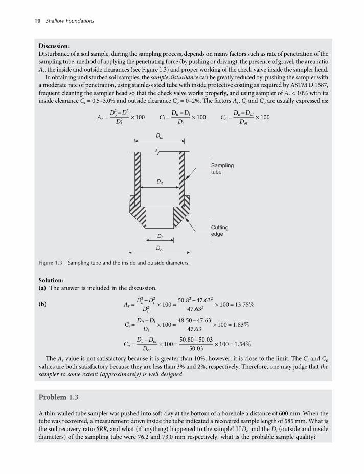
Discussion:Disturbance of a soil sample, during the sampling process, depends onmany factors such as rate of penetration of thesampling tube, method of applying the penetrating force (by pushing or driving), the presence of gravel, the area ratioAr, the inside and outside clearances (see Figure 1.3) and proper working of the check valve inside the sampler head.In obtaining undisturbed soil samples, the sample disturbance can be greatly reduced by: pushing the sampler with
a moderate rate of penetration, using stainless steel tube with inside protective coating as required by ASTMD 1587,frequent cleaning the sampler head so that the check valve works properly, and using sampler of Ar < 10% with itsinside clearance Ci = 0.5–3.0% and outside clearance Co = 0–2%. The factors Ar, Ci and Co are usually expressed as:
Ar =D2o−D
2i
D2i
× 100 Ci =Dit −Di
Di× 100 Co =
Do−Dot
Dot× 100
Solution:(a) The answer is included in the discussion.
(b) Ar =D2o−D
2i
D2i
× 100 =50 82−47 632
47 632× 100 = 13 75
Ci =Dit −Di
Di× 100 =
48 50−47 6347 63
× 100 = 1 83
Co =Do−Dot
Dot× 100 =
50 80−50 0350 03
× 100 = 1 54
The Ar value is not satisfactory because it is greater than 10%; however, it is close to the limit. The Ci and Co
values are both satisfactory because they are less than 3% and 2%, respectively. Therefore, one may judge that thesampler to some extent (approximately) is well designed.
Problem 1.3
A thin-walled tube sampler was pushed into soft clay at the bottom of a borehole a distance of 600 mm. When thetube was recovered, a measurement down inside the tube indicated a recovered sample length of 585 mm. What isthe soil recovery ratio SRR, and what (if anything) happened to the sample? If Do and the Di (outside and insidediameters) of the sampling tube were 76.2 and 73.0 mm respectively, what is the probable sample quality?
Dot
Dit
Di
Do
Sampling
tube
Cutting
edge
Figure 1.3 Sampling tube and the inside and outside diameters.
10 Shallow Foundations
worksaccounts.com
Discussion:Similar to the rock recovery ratio, there is also soil recovery ratio, SRR, which can be used in estimating degree ofdisturbance of soil samples, where
SRR=Actual length of recovered soil sample
Total length of sampler in soil1 3
A recovery ratio of 1 indicates, theoretically, that the sample did not become compressed during sampling.A recovery ratio less than 1 indicates compressed sample in a disturbed state. Also, when a recovery ratio is greaterthan 1, the sample is disturbed due to loosening from rearrangement of stone fragments, roots, removal of over-burden, or other factors.
Solution:
Equation (1.3): SRR=585600
= 0 98 < 1 slightly compressed sample
The sample is compressed from friction on the tube and, or from pressure of entrapped air above the sample dueto incapable head check valve.
Ar =D2o−D
2i
D2i
× 100 =76 22−73 02
73 02× 100 = 8 96 < 10
Ci =Dit −Di
Di× 100 =
73 0−73 073 0
× 100 = 0 < 0 5−3 0
Co =Do−Dot
Dot× 100 =
76 2−76 276 2
× 100 = 0
These results and that of SRR indicate that the sample is nearly undisturbed.
Problem 1.4
A five story office building is to be built in a deep, moderately uniform fine-grained soil deposit. The bedrock has adepth of over 75 m. The foundation level will be located at a depth of 1 m below ground surface. At the foundationlevel, the unfactored uniformly distributed load (q) from the building structure is 70 kPa (or 1434 psf ). The build-ing will be 50 m wide and 85 m long. Appropriate values for any missing data may be assumed. Estimate:
(a) The required number, spacing and location of exploratory boreholes.(b) The required depth of the boreholes.
Discussion:A boring plan should include number, spacing, location and depth of borings in addition to the sampling intervals.There are many variables involved in formulation a boring plan such as general knowledge of subsurface condi-tions, knowledge of proposed structure, economy by scheduling an inexcessive number and depth of boreholes,and personal experience, preference and judgment of the responsible geotechnical engineer.Boring spacing: Required number and location configuration of borings (or boreholes) is defined by their
spacing. Boring spacing depends mainly on the uniformity of soil strata, the type of structure and loading con-ditions. Erratic subsurface conditions require closely spaced borings, whereas uniform conditions require amaximum spacing. Structures sensitive to settlements and structures subjected to heavy loads require extensive
(Continued)
Site Investigation in Relation to Analysis and Design of Foundations 11
worksaccounts.com
subsurface knowledge; therefore borings should be closely spaced. Knowledge of the regional conditions as wellas the type and nature of the proposed structure is the best guide to the necessary boreholes spacing.It is a difficult subject to pinpoint in exact figures the required number of boreholes and their tentative spacing
for the many reasons stated above; therefore, there are no binding rules on the number and spacing of boreholes.For buildings taller than three stories or 12.2 m, the BOCA (1996) National Building Code requires at least one
boring for every 230m2 of built-over area, while others prefer boreholes drilled at or near all the corners and also atimportant locations. For buildings a minimum of three borings, where the surface is level and the first two boringsindicate regular stratification, may be adequate. Five borings are generally preferable (four borings at buildingcorners and one at centre), especially if the site is not level. On the other hand, a single boring may be sufficientfor small and less important building, an antenna or industrial process tower base with the hole drilled at centre.There are tables which give suggested spacing of boreholes (Table 1.3) or required area for each borehole
(Table 1.4). These tables should be used as general guidelines only.
Furthermore, the following are two key clauses of BSI publications regarding the spacing of borings:
BSI 5930: 1999 Code of Practice for Site Investigations – Clause 12.6“Although no hard and fast rules can be laid down, a relatively close spacing between points of exploration, e.g.
10 m to 30 m, are often appropriate for structures. For structures small in plan area, exploration should be made ata minimum of three points, unless other reliable information is available in the immediate vicinity.”
BSI EN 1997-2: 2007 Ground Investigation and Testing – Clause B.3“The following spacing of investigation points should be used as guidance:
• For high-rise and industrial structures, a grid pattern with points at 15 m to 40 m distance,
• For large-area structures, a grid pattern with points at not more than 60 m distance,
• For linear structures, a spacing of 20 m to 200 m,
• For special structures, two to six investigation points per foundation.”
Table 1.4 Suggested required area for each borehole.
Subsurface conditionsStructure foot print areafor each borehole, m2
Poor quality and/or erratic 100–300
Average 200–400
High quality and uniform 300–1000
Table 1.3 Suggested spacing of boreholes.
Type of project Boreholes spacing, m
One story building 25–30
Multistory building 15–25
Residential subdivision planning 60–100
Highway 150–300∗
Earth dam 25–50
Bridge∗∗ —
∗ It is reduced to even 30 m for erratic subsurface conditions.∗∗Minimum of one borehole at location of each pier or abutment.
12 Shallow Foundations
worksaccounts.com

Depth of Borings: As it was the case with the required spacing and number of borings and due to nearly thesamemain reasons, here also, there is no absolute and unique rule to determine the required depth of exploratoryborings. Borings should reach depths adequate to explore the nature of the subsurface soils, mainly encounteredin the influence stress zones, including all strata likely to contribute significantly to settlement. There are manyempirical and semi-empirical criteria, rules and equations established by individual researchers, engineeringagencies and societies, to estimate the required minimum depth of borings. Some of these are as follows:
ASCE Criteria (1972): “Unless bedrock is encountered first, borings should be carried to such depth that the netincrease in soil stress σz under the weight of the structure is less than 10 percent of the average load of thestructure q, or less than 5 percent of the effective overburden stress σO in the soil at that depth, whicheveris the lesser depth.” These two criteria are shown in the scheme below.
Criterion 1: σz = 0.10 q find z1Criterion 2: σz = 0.05 σO find z2Use z1 or z2, whichever is smaller.Boring depth = zb = (z1 or z2) + DD = the anticipative foundation depth
Smith (1970) used Criterion 2 in the form: σz = M σO;in which M is the compressibility criterion equals 10% forfine-grained soils and 20% for course-grained soils. Heused the Boussinesq principles of stress distribution todetermine the influence depth z, and established a set ofcurves relating the influence depth to the equivalent squaredimension of a uniformly loaded rectangular or circulararea. Also, he derived equations for estimating minimumdepth of borings for embedded footing systems, mats orrafts and pile groups.Baban (1992) established the same relationships using the ASCE criteria andWestergaard principles of stress
distribution; with an assumed average value for Poisson’s ratio of the base soil equals 0.3. He found thatfor embedded footing systems, mats or rafts and pile groups of width B larger than 20 m, Criterion 2 alwayscontrols the minimum boring depth. The equations derived by Baban are as follows:According to the ASCE Criterion 1,
Z = 0 5 0 9B2 + 0 9L22+ 122B2L2
1 ∕ 2−0 4 B2 + L2
1 ∕ 2
1 4
According to the ASCE Criterion 2,
tan0 025 π γAz
q=
BL
1 144B2Z2 + 1 144L2Z2 + 1 309Z4 1 ∕ 2 1 5
Zb =Z +D
γA = average effective unit weight of soil within depth Z in lb/ft3, q is in lb/ft2, and Z, B and L are in feet.Sowers and Sowers (1970) suggested a rough estimate of minimum boring depth (unless bedrock is encoun-
tered) required for building structures according to number of stories S, as follows:
For light steel or narrow concrete buildings, zb = 3 S0 7 + D 1 6
For heavy steel or wide concrete buildings, zb = 6 S0 7 + D 1 7
(Continued)
Base soil
•
Base level
z
B
q
σ o
σz
Scheme 1.1
Site Investigation in Relation to Analysis and Design of Foundations 13
worksaccounts.com
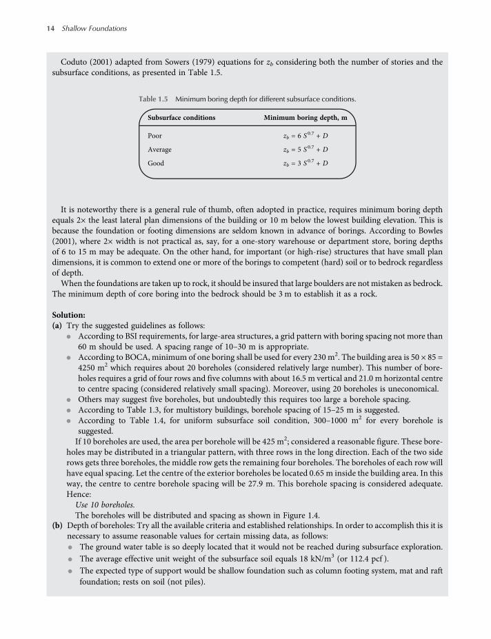
Coduto (2001) adapted from Sowers (1979) equations for zb considering both the number of stories and thesubsurface conditions, as presented in Table 1.5.
It is noteworthy there is a general rule of thumb, often adopted in practice, requires minimum boring depthequals 2× the least lateral plan dimensions of the building or 10 m below the lowest building elevation. This isbecause the foundation or footing dimensions are seldom known in advance of borings. According to Bowles(2001), where 2× width is not practical as, say, for a one-story warehouse or department store, boring depthsof 6 to 15 m may be adequate. On the other hand, for important (or high-rise) structures that have small plandimensions, it is common to extend one or more of the borings to competent (hard) soil or to bedrock regardlessof depth.When the foundations are taken up to rock, it should be insured that large boulders are not mistaken as bedrock.
The minimum depth of core boring into the bedrock should be 3 m to establish it as a rock.
Solution:(a) Try the suggested guidelines as follows:
• According to BSI requirements, for large-area structures, a grid pattern with boring spacing not more than60 m should be used. A spacing range of 10–30 m is appropriate.
• According to BOCA, minimum of one boring shall be used for every 230 m2. The building area is 50 × 85 =4250 m2 which requires about 20 boreholes (considered relatively large number). This number of bore-holes requires a grid of four rows and five columns with about 16.5 m vertical and 21.0 m horizontal centreto centre spacing (considered relatively small spacing). Moreover, using 20 boreholes is uneconomical.
• Others may suggest five boreholes, but undoubtedly this requires too large a borehole spacing.
• According to Table 1.3, for multistory buildings, borehole spacing of 15–25 m is suggested.
• According to Table 1.4, for uniform subsurface soil condition, 300–1000 m2 for every borehole issuggested.If 10 boreholes are used, the area per borehole will be 425 m2; considered a reasonable figure. These bore-
holes may be distributed in a triangular pattern, with three rows in the long direction. Each of the two siderows gets three boreholes, the middle row gets the remaining four boreholes. The boreholes of each row willhave equal spacing. Let the centre of the exterior boreholes be located 0.65 m inside the building area. In thisway, the centre to centre borehole spacing will be 27.9 m. This borehole spacing is considered adequate.Hence:
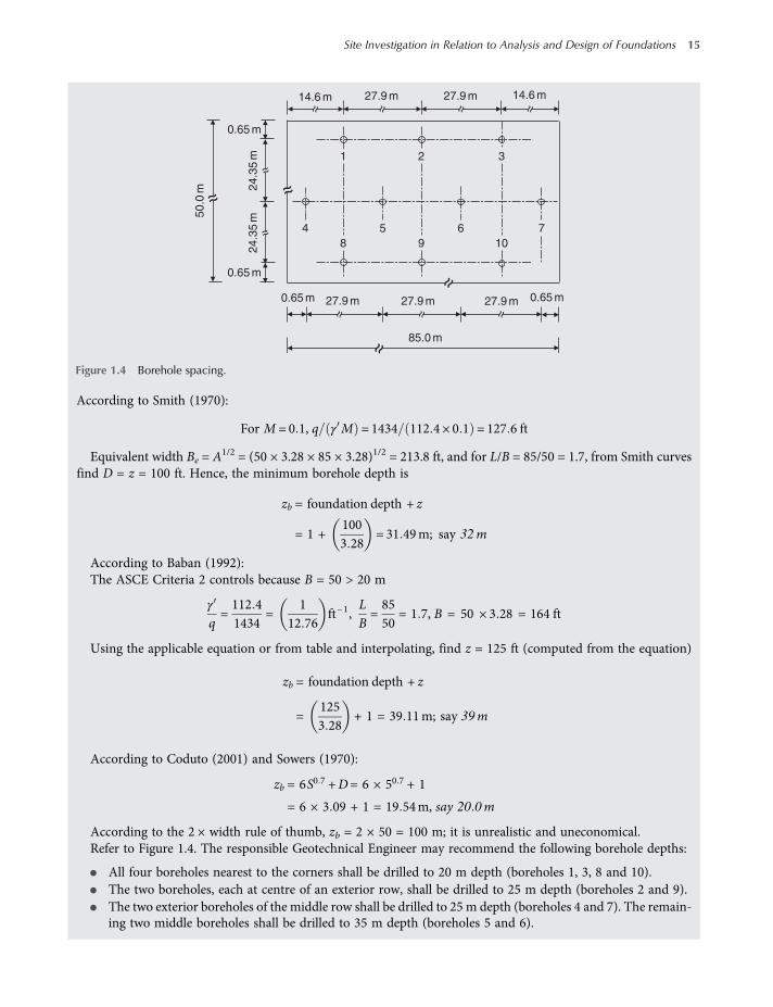
Use 10 boreholes.The boreholes will be distributed and spacing as shown in Figure 1.4.
(b) Depth of boreholes: Try all the available criteria and established relationships. In order to accomplish this it isnecessary to assume reasonable values for certain missing data, as follows:
• The ground water table is so deeply located that it would not be reached during subsurface exploration.
• The average effective unit weight of the subsurface soil equals 18 kN/m3 (or 112.4 pcf ).
• The expected type of support would be shallow foundation such as column footing system, mat and raftfoundation; rests on soil (not piles).
Table 1.5 Minimum boring depth for different subsurface conditions.
Subsurface conditions Minimum boring depth, m
Poor zb = 6 S 0.7 + D
Average zb = 5 S 0.7 + D
Good zb = 3 S 0.7 + D
14 Shallow Foundations
worksaccounts.com
According to Smith (1970):
For M = 0 1, q γ M = 1434 112 4 × 0 1 = 127 6 ft
Equivalent width Be = A1/2 = (50 × 3.28 × 85 × 3.28)1/2 = 213.8 ft, and for L/B = 85/50 = 1.7, from Smith curvesfind D = z = 100 ft. Hence, the minimum borehole depth is
zb = foundation depth + z
= 1 +1003 28
= 31 49m; say 32m
According to Baban (1992):The ASCE Criteria 2 controls because B = 50 > 20 m
γ
q=112 41434
=1
12 76ft−1,
LB=8550
= 1 7, B = 50 × 3 28 = 164 ft
Using the applicable equation or from table and interpolating, find z = 125 ft (computed from the equation)
zb = foundation depth + z
=1253 28
+ 1 = 39 11m; say 39m
According to Coduto (2001) and Sowers (1970):
zb = 6S0 7 +D= 6 × 50 7 + 1
= 6 × 3 09 + 1 = 19 54m, say 20 0m
According to the 2 × width rule of thumb, zb = 2 × 50 = 100 m; it is unrealistic and uneconomical.Refer to Figure 1.4. The responsible Geotechnical Engineer may recommend the following borehole depths:
• All four boreholes nearest to the corners shall be drilled to 20 m depth (boreholes 1, 3, 8 and 10).
• The two boreholes, each at centre of an exterior row, shall be drilled to 25 m depth (boreholes 2 and 9).
• The two exterior boreholes of the middle row shall be drilled to 25 m depth (boreholes 4 and 7). The remain-ing two middle boreholes shall be drilled to 35 m depth (boreholes 5 and 6).
27.9 m27.9 m 14.6 m14.6 m
0.65 m
0.65 m
24.3
5m
0.65 m 0.65 m27.9 m
24.3
5m
27.9 m 27.9 m
50.0
m
85.0 m
4 5 6 7
1 2 3
8 9 10
Figure 1.4 Borehole spacing.
Site Investigation in Relation to Analysis and Design of Foundations 15
worksaccounts.com

Problem 1.5
Field vane shear tests (FVST) were conducted in a layer of organic clay (not peat). The rectangular vane dimen-sions were 63.5 mm width × 127 mm height. At the 2 m depth, the torque T required to cause failure was 51 N.m.The liquid limit LL and plastic limit PL of the clay were 50 and 20, respectively. The effective unit weight γ of theclay is 18 kN/m3. Estimate the design undrained vane shear strength su, the preconsolidation pressure σc and theratio OCR of the clay.
Discussion:The in situ or field vane shear test (FVST – ASTM D-2573) is used to estimate the in situ undrained shearstrength su (or undrained cohesion cu) of very soft to soft clay, silty clay (muck) and clayey silt soils. It ispractically used when sensitive fine-grained soils are encountered. However, these materials must be freeof gravel, large shell particles, and roots in order to avoid inaccurate results and probable damage to thevane.Briefly, the test apparatus consists of a small diameter shaft with four tapered or rectangular thin blades or fins
(Figure 1.5), and suitable extension rods and fasteners used to connect the shear vane with a torque measuringdevice at the ground surface, as shown in Figure 1.6a. There are various forms of the equipment; the device shownin the figure is somewhat an antique version, belongs to The Bureau of Reclamation, USA; (Gibbs andHoltz, 1960).Also, there are different vane sizes (the diameter D and height H dimensions) used for soils of different consist-encies; the softer the soil, the larger the vane diameter should be. A standard vane has theH/D ratio equals 2, whereDis the overall vane width. Typical vane dimensions being 150 mm by 75 mm and 100 mm by 50 mm.
(a)
45°
H=
2D
L=
10D
H=
2D
(b)
D
D
D
Figure 1.5 Field vane shapes: (a) tapered vane, (b) rectangular vane.
16 Shallow Foundations
worksaccounts.com
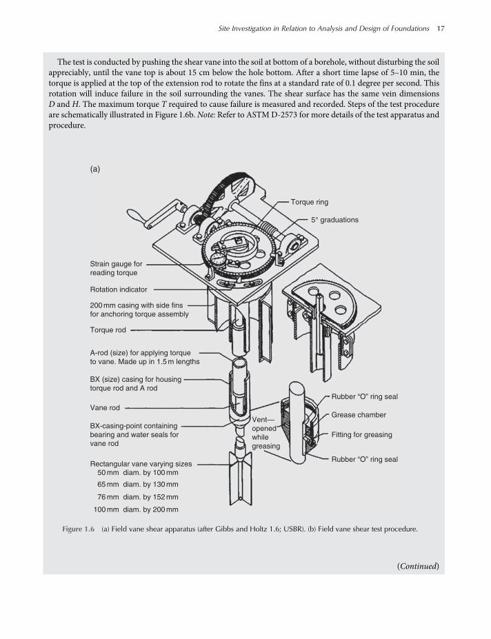
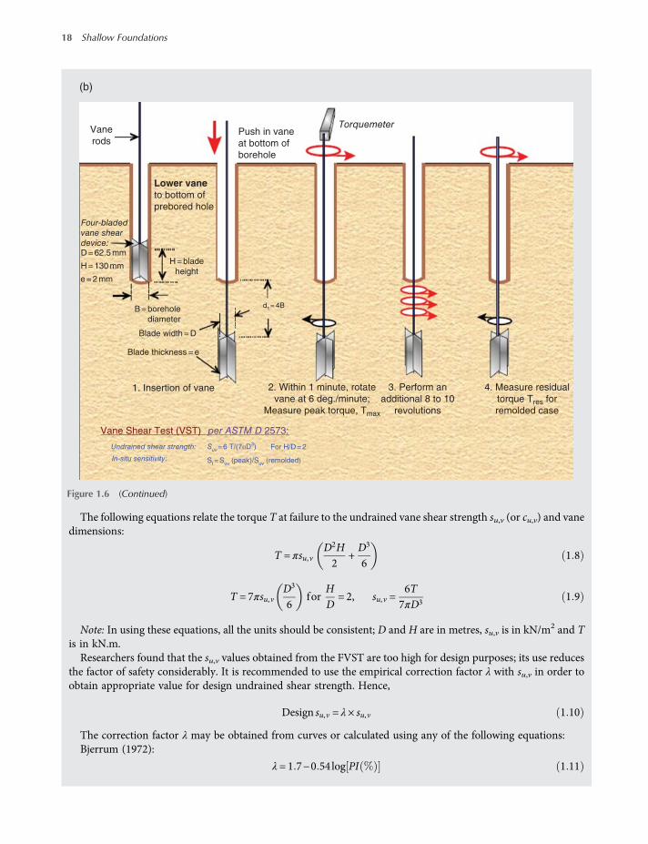
The test is conducted by pushing the shear vane into the soil at bottom of a borehole, without disturbing the soilappreciably, until the vane top is about 15 cm below the hole bottom. After a short time lapse of 5–10 min, thetorque is applied at the top of the extension rod to rotate the fins at a standard rate of 0.1 degree per second. Thisrotation will induce failure in the soil surrounding the vanes. The shear surface has the same vein dimensionsD and H. The maximum torque T required to cause failure is measured and recorded. Steps of the test procedureare schematically illustrated in Figure 1.6b. Note: Refer to ASTMD-2573 for more details of the test apparatus andprocedure.
(Continued)
Torque ring
5° graduations
Rotation indicator
Strain gauge for
reading torque
(a)
200 mm casing with side fins
for anchoring torque assembly
Torque rod
A-rod (size) for applying torque
to vane. Made up in 1.5 m lengths
Rubber “O” ring seal
Grease chamber
Fitting for greasing
Rubber “O” ring seal
BX (size) casing for housing
torque rod and A rod
Vane rod
65 mm diam. by 130 mm
76 mm diam. by 152 mm
100 mm diam. by 200 mm
BX-casing-point containing
bearing and water seals for
vane rod
Vent—
opened
while
greasing
50 mm diam. by 100 mmRectangular vane varying sizes
Figure 1.6 (a) Field vane shear apparatus (after Gibbs and Holtz 1.6; USBR). (b) Field vane shear test procedure.
Site Investigation in Relation to Analysis and Design of Foundations 17
worksaccounts.com
The following equations relate the torque T at failure to the undrained vane shear strength su,v (or cu,v) and vanedimensions:
T = πsu,vD2H2
+D3
61 8
T = 7πsu,vD3
6for
HD
= 2, su,v =6T7πD3
1 9
Note: In using these equations, all the units should be consistent; D and H are in metres, su,v is in kN/m2 and Tis in kN.m.Researchers found that the su,v values obtained from the FVST are too high for design purposes; its use reduces
the factor of safety considerably. It is recommended to use the empirical correction factor λ with su,v in order toobtain appropriate value for design undrained shear strength. Hence,
Design su,v = λ× su,v 1 10
The correction factor λ may be obtained from curves or calculated using any of the following equations:Bjerrum (1972):
λ = 1 7−0 54log PI 1 11
Vane
rods
B = borehole
diameter
H = blade
height
Blade width = D
Blade thickness = e
1. Insertion of vane
d1= 4B
Vane Shear Test (VST) per ASTM D 2573:
Undrained shear strength:
In-situ sensitivity:
Suv
= 6 T/(7пD3)
St= S
uv (peak)/S
uv (remolded)
For H/D = 2
2. Within 1 minute, rotate
vane at 6 deg./minute;
Measure peak torque, Tmax
3. Perform an
additional 8 to 10
revolutions
4. Measure residual
torque Tres for
remolded case
D = 62.5 mm
H = 130 mm
e = 2 mm
Lower vaneto bottom of
prebored hole
Push in vane
at bottom of
borehole
Four-bladed
vane shear
device:
Torquemeter
(b)
Figure 1.6 (Continued)
18 Shallow Foundations
worksaccounts.com
PI = plasticity indexMorris and Williams (1994):
λ= 7 01 e−0 08 LL + 0 57 1 12
λ= 1 18 e−0 08 PI + 0 57 for PI > 5 1 13
For organic soils other than peat, an additional correction factor of 0.85 is recommended be used with the cor-rected su,v (Terzaghi, Peck, and Mesri, 1996). However, this correction may not be necessary when the Morris andWilliams correction factors are used.Researchers derived empirical equations for estimating the effective preconsolidation pressure σc and the over-
consolidation ratio OCR (or σc σO) of natural clays using results of the field vane shear test. Mayne and Mitchell(1988) found the following correlations:
σc = 7 04 cu,v field0 83
, cu,v field and σc are in kN m2 1 14
OCR= βcu,v field
σO, cu,v field and σO are in kN m2 1 15
β = 22 PI −0 48
β =222ω
, ω = moisture content Hansbo, 1957 1 16
β =1
0 08 + 0 0055 PILarsson, 1980 1 17
Solution:
T = 51N m = 51 × 10−3 kN m;D= 63 5mm = 63 5 × 10⁻³ mH = 127mm = 127 × 10−3 m;H D= 2
Equation (1.9): su,v =6T7πD3
=6 × 51 × 10−3
7 × π 63 5 × 10⁻³ 3 = 54 32 kN m2
Equation (1.11): λ= 1 7−0 54 log PI
= 1 7−0 54 log 50−20 = 0 902
As the soil is organic (not peat), an additional correction factor of 0.85 is recommended.
Designsu ,v = 0 85 × λ× su ,v = 0 85 × 0 902 × 54 32 = 41 65 kN m2
Equation (1.14): σc = 7 04 cu,v field0 83
= 7 04 54 32 0 83 = 193 9 kN m2
Equation (1.15): OCR= βcu,v field
σO
β = 22 PI −0 48 = 22 50−20 −0 48 = 4 3
OCR= βcu,v field
σO= 4 3 ×
54 322 × 18
= 6 5 >193 92 × 18
= 5 4
(Continued)
Site Investigation in Relation to Analysis and Design of Foundations 19
worksaccounts.com
Equation (1.17): β =1
0 08 + 0 0055 PI=
10 08 + 0 0055 50−20
= 4 08
OCR= βcu,v field
σO= 4 08 ×
54 322 × 18
= 6 2 >193 92 × 18
= 5 4
Problem 1.6
At the site of a proposed structure the variation of the SPT number (N60) with depth in a deposit of normallyconsolidated sand is as given below:
Depth, m: 1.5 3.0 4.5 6.0 7.5 9.0
N60: 6 8 9 8 13 14
The ground water table (W.T) is located at a depth of 6.5 m. The dry unit weight γdry of the sand above W.T is18 kN/m3, and its saturated unit weight γsat below W.T is 20.2 kN/m3.
(a) Correct the SPT numbers.(b) Select an appropriate SPT corrected number N60 for use in designs. Assume the given depths are located
within the influence zone (zone of major stressing).
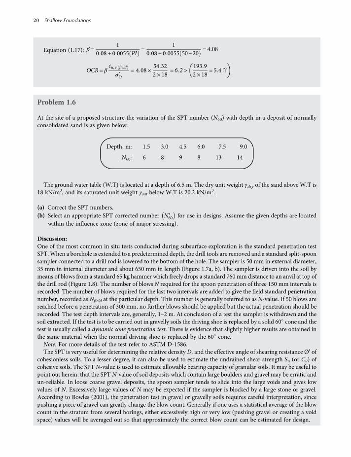
Discussion:One of the most common in situ tests conducted during subsurface exploration is the standard penetration testSPT.When a borehole is extended to a predetermined depth, the drill tools are removed and a standard split-spoonsampler connected to a drill rod is lowered to the bottom of the hole. The sampler is 50 mm in external diameter,35 mm in internal diameter and about 650 mm in length (Figure 1.7a, b). The sampler is driven into the soil bymeans of blows from a standard 65 kg hammer which freely drops a standard 760 mm distance to an anvil at top ofthe drill rod (Figure 1.8). The number of blows N required for the spoon penetration of three 150 mm intervals isrecorded. The number of blows required for the last two intervals are added to give the field standard penetrationnumber, recorded as Nfield at the particular depth. This number is generally referred to as N-value. If 50 blows arereached before a penetration of 300 mm, no further blows should be applied but the actual penetration should berecorded. The test depth intervals are, generally, 1–2 m. At conclusion of a test the sampler is withdrawn and thesoil extracted. If the test is to be carried out in gravelly soils the driving shoe is replaced by a solid 60 cone and thetest is usually called a dynamic cone penetration test. There is evidence that slightly higher results are obtained inthe same material when the normal driving shoe is replaced by the 60 cone.Note: For more details of the test refer to ASTM D-1586.The SPT is very useful for determining the relative density Dr and the effective angle of shearing resistance Ø of
cohesionless soils. To a lesser degree, it can also be used to estimate the undrained shear strength Su (or Cu) ofcohesive soils. The SPT N-value is used to estimate allowable bearing capacity of granular soils. It may be useful topoint out herein, that the SPT N-value of soil deposits which contain large boulders and gravel may be erratic andun-reliable. In loose coarse gravel deposits, the spoon sampler tends to slide into the large voids and gives lowvalues of N. Excessively large values of N may be expected if the sampler is blocked by a large stone or gravel.According to Bowles (2001), the penetration test in gravel or gravelly soils requires careful interpretation, sincepushing a piece of gravel can greatly change the blow count. Generally if one uses a statistical average of the blowcount in the stratum from several borings, either excessively high or very low (pushing gravel or creating a voidspace) values will be averaged out so that approximately the correct blow count can be estimated for design.
20 Shallow Foundations
worksaccounts.com
Corrections of SPT number:The recorded Nfield should be adjusted and corrected for the effects of some factors such as effective overburdenpressure (CN), hammer efficiency (ηh), borehole size (ηb), sampler (ηs) and rod length (ηr).
Due to various types of driving hammers with different efficiencies, the hammer energy ratio Er is referencedto a standard or basic energy ratio, Erb, such that ηh be equal to ratio of the particular hammer energy to the stand-ard Erb, which is equal to either 60 or 70%.WhenNfield is adjusted to ηh, ηb, ηs and ηr corrections, it is generally referred to asN60 orN70 according to the Erb
value, as follows:
N60 =Er ηb ηs ηr Nfield
601 18
N70 =Er ηb ηs ηr Nfield
701 19
Table 1.6 gives values of Er for different types of SPT hammers. Table 1.7 gives values for borehole, sampler androd correction factors.When N60 and N70 are corrected for the effective overburden pressure, they are written as N60 and N70, where
N60 =CN N60
N70 =CN N70(Continued)
Basket shoe, the
flexible fingers
open to admit the
sand then close
when the tube is
withdrawn
Trap value sample
retainer used to
recover muds and
watery samples
Spring sample
retainer
4 events with minimum diameter ofDriving
shoe
in.in.
in.
2 in
.
1 in
.
Split barrelCoupling
6 in., (minimum)
14 in., (minimum)
3 in., (min)
24 in., (minimum. open)
(b)
(c)
(d)
(a)
Sand L ≥ 5 – 10 Do
Cloy L ≥ 10 – 15 Do
CR = ≤ 0.03
Do D′i
D′i –Di
Di
Di
1
10
3
4
1
2
1 2
Basket shoe, the
flexible fingers
open to admit the
sand then close
when the tube is
withdrawn
Trap value sample
retainer used to
Spring sample
retainer
4 events with minimum diameter ofDriving
shoe
n.in.
in.
2 in
.
111111 in
.
Split barrelCoupling
6 in., (minimum)
14 in., (minimum)
3 in., (min)
24 in., (minimum. open)
(b)
(c)
( )
(a)
Sand L ≥ 5 – 10 Do
Cloy L ≥ 10 – 15 Do
D′i
D′ D
Di
3
4
1
2
1 2
Figure 1.7 (a) Standard split-spoon sampler; (b, d) dimensions and inserts of the standard split-spoon sampler, respectively;(c) Shelby tube (from Bowles, 2001).
Site Investigation in Relation to Analysis and Design of Foundations 21
worksaccounts.com

Guid
e r
od
Guid
e r
od
Lim
iters
Guid
e r
od
Dri
ll ro
d
Dri
ll ro
d
Drill rod
Anvil
or drive
head
XX
63.5 kg
63.5 kg
W
X
(a) (b) (c)
Coupling
Donut or center-hole
hammer.
Safety hammer.
Early style “pinweight”
hammer.
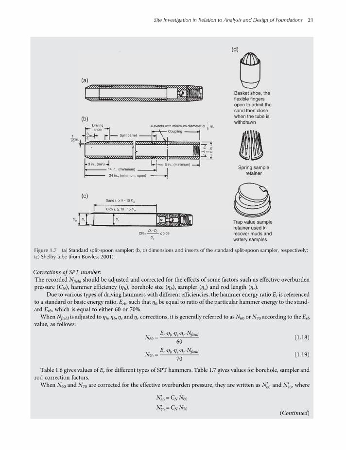
Figure 1.8 Schematic diagrams of the three commonly used hammers (from Bowles, 2001).
Table 1.6 SPT hammer efficiencies (adapted from Clayton, 1990).
Country Hammer type Hammer release mechanism Efficiency, Er
Argentina Donut Cathead 45
Brazil Pin weight Hand dropped 72
China Automatic Trip 60
Donut Hand dropped 55
Donut Cathead 50
Colombia Donut Cathead 50
Japan Donut Tombi triggers 78–85
Donut Cathead, two turns + special release 65–67
UK Automatic Trip 73
US Safety Cathead, two turns 55–60
Donut Cathead, two turns 45
Venezuela Donut Cathead 43
22 Shallow Foundations
worksaccounts.com
CN = effective overburden pressure factor
CN ≤ 2
Terzaghi and Peck (1967) have recommended the following additional correction where the soil is fine sand orsilty sand below the water table:
Nfield = 15 + 0 5 Nfield −15 , for Nfield > 15 1 20
Note: This correction is applied first and then the overburden and other corrections are applied.
The effective overburden pressure factor CN, may be determined from different empirical relationships, such as:Liao and Whitman (1986):
CN =paσO
, where σO = effective overburden pressure, kPa 1 21
Skempton (1986):
CN =2
1 +σOPa
, for normally consolidated fine sand 1 22
CN =3
2 +σOPa
, for normally consolidated coarse sand 1 23
CN =1 7
0 7 +σOPa
, for overconsolidated sand 1 24
(Continued)
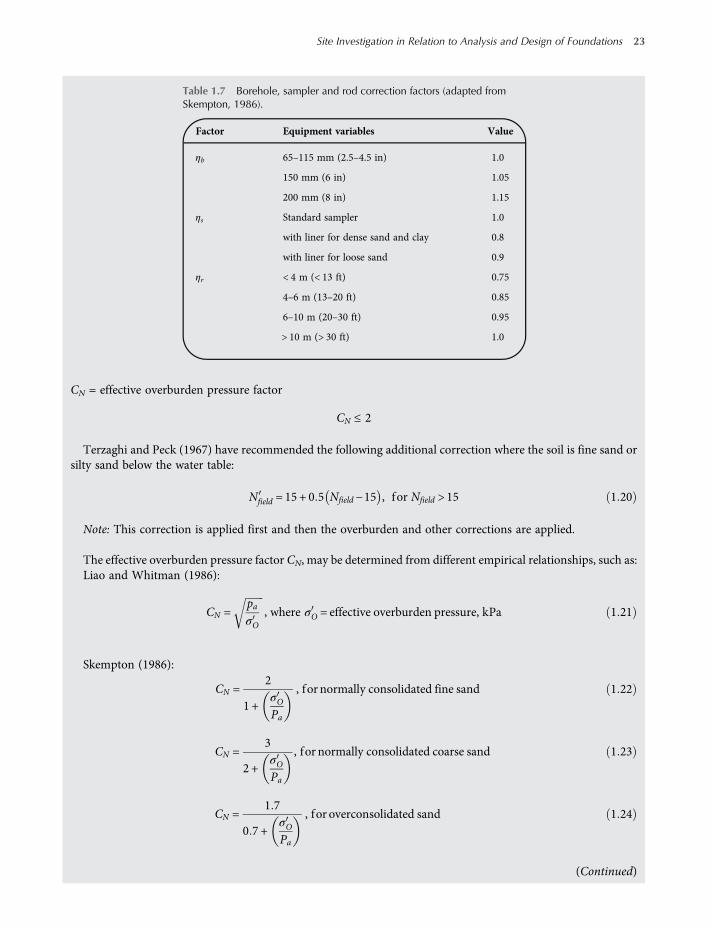
Table 1.7 Borehole, sampler and rod correction factors (adapted fromSkempton, 1986).
Factor Equipment variables Value
ηb 65–115 mm (2.5–4.5 in) 1.0
150 mm (6 in) 1.05
200 mm (8 in) 1.15
ηs Standard sampler 1.0
with liner for dense sand and clay 0.8
with liner for loose sand 0.9
ηr < 4 m (< 13 ft) 0.75
4–6 m (13–20 ft) 0.85
6–10 m (20–30 ft) 0.95
> 10 m (> 30 ft) 1.0
Site Investigation in Relation to Analysis and Design of Foundations 23
worksaccounts.com
Seed et al (1975):
CN = 1−1 25logσOPa
1 25
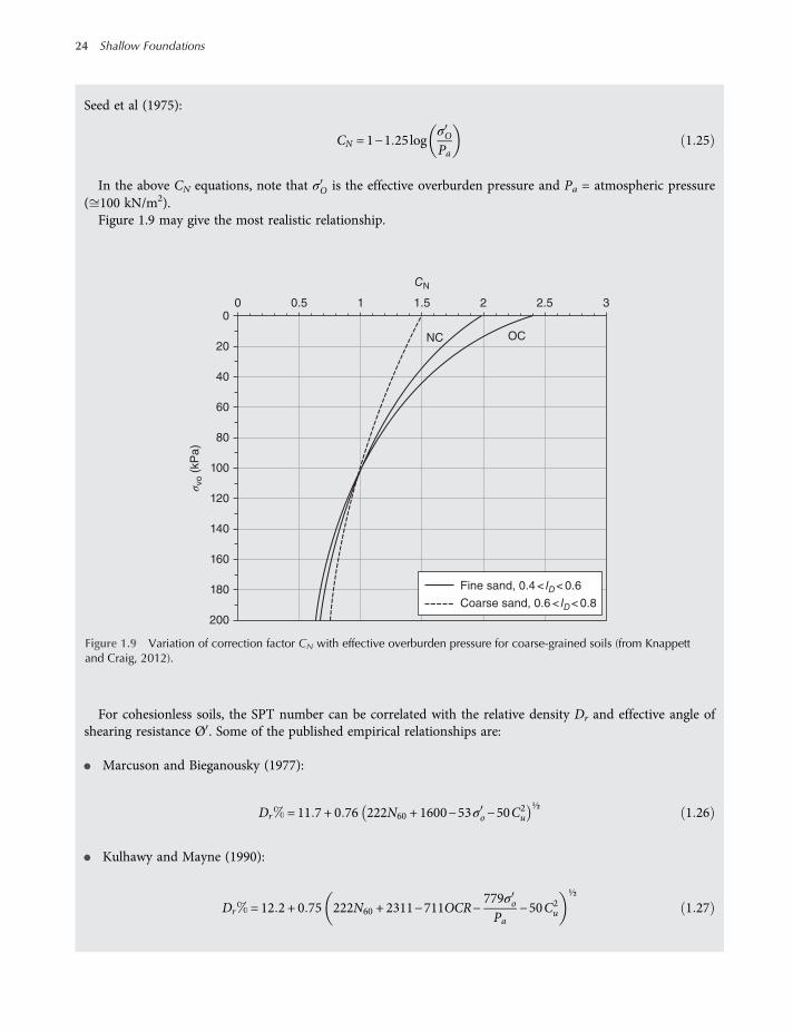
In the above CN equations, note that σO is the effective overburden pressure and Pa = atmospheric pressure( 100 kN/m2).Figure 1.9 may give the most realistic relationship.
For cohesionless soils, the SPT number can be correlated with the relative density Dr and effective angle ofshearing resistance Ø . Some of the published empirical relationships are:
• Marcuson and Bieganousky (1977):
Dr = 11 7 + 0 76 222N60 + 1600−53σo−50C2u
½1 26
• Kulhawy and Mayne (1990):
Dr = 12 2 + 0 75 222N60 + 2311−711OCR−779σoPa
−50C2u
½
1 27
00 0.5 1 1.5
CN
NC OC
σ vo (
kP
a)
2 2.5
Fine sand, 0.4 < lD< 0.6
Coarse sand, 0.6 < lD< 0.8
3
20
40
60
80
100
120
140
160
180
200
Figure 1.9 Variation of correction factor CN with effective overburden pressure for coarse-grained soils (from Knappettand Craig, 2012).
24 Shallow Foundations
worksaccounts.com
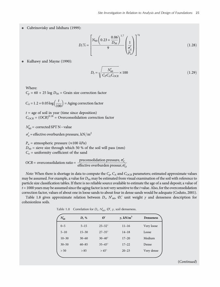
• Cubrinovisky and Ishihara (1999):
Dr =N60 0 23 +
0 06D50
1 7
91σoPa
½
1 28
• Kulhawy and Mayne (1990):
Dr =N60
CPCACOCR× 100 1 29
Where:Cp = 60 + 25 log D50 = Grain size correction factor
CA = 1 2 + 0 05logt
100=Aging correction factor
t = age of soil in year (time since deposition)COCR = (OCR)0.18 = Overconsolidation correction factor
N60 = corrected SPTN−value
σo = effective overburden pressure, kN m2
Pa = atmospheric pressure (≈100 kPa)D50 = sieve size through which 50 % of the soil will pass (mm)Cu = uniformity coefficient of the sand
OCR = overconsolidation ratio =preconsolidation pressure, σCeffective overburden pressur,σO
Note:When there is shortage in data to compute the Cp, CA and COCR parameters; estimated approximate valuesmay be assumed. For example, a value forD50 may be estimated from visual examination of the soil with reference toparticle size classification tables. If there is no reliable source available to estimate the age of a sand deposit; a value oft= 1000 yearsmay be assumed since the aging factor is not very sensitive to the t value. Also, for the overconsolidationcorrection factor, values of about one in loose sands to about four in dense sands would be adequate (Coduto, 2001).Table 1.8 gives approximate relation between Dr, N 60, Ø, unit weight γ and denseness description for
cohesionless soils.
(Continued)
Table 1.8 Correlation for Dr, N60, Ø , γ, soil denseness.
N60 Dr % Ø γ, kN/m3 Denseness
0–5 5–15 25–32 11–16 Very loose
5–10 15–30 27–35 14–18 Loose
10–30 30–60 30–40 17–20 Medium
30–50 60–85 35–45 17–22 Dense
> 50 > 85 > 45 20–23 Very dense
Site Investigation in Relation to Analysis and Design of Foundations 25
worksaccounts.com
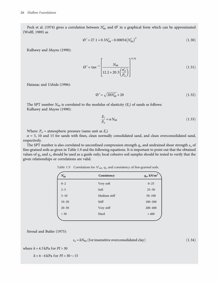
Peck et al. (1974) gives a correlation between N60 and Ø in a graphical form which can be approximated(Wolff, 1989) as
Ø = 27 1 + 0 3N60−0 00054 N602
1 30
Kulhawy and Mayne (1990):
Ø = tan−1 N60
12 2 + 20 3σOPa
0 34
1 31
Hatanac and Ushida (1996):
Ø = 20N60 + 20 1 32
The SPT number N60 is correlated to the modulus of elasticity (Es) of sands as follows:Kulhawy and Mayne (1990):
EsPa
= αN60 1 33
Where: Pa = atmospheric pressure (same unit as Es)α = 5, 10 and 15 for sands with fines, clean normally consolidated sand, and clean overconsolidated sand,
respectively.The SPT number is also correlated to unconfined compression strength qu and undrained shear strength su of
fine-grained soils as given in Table 1.9 and the following equations. It is important to point out that the obtainedvalues of qu and su should be used as a guide only; local cohesive soil samples should be tested to verify that thegiven relationships or correlations are valid.
Stroud and Butler (1975):
su = kN60 for insensitive overconsolidated clay 1 34
where k= 4 5 kPa for PI > 30
k= 4 – 6 kPa for PI = 30 15
Table 1.9 Correlations for N 60, qu and consistency of fine-grained soils.
N60 Consistency qu, kN/m2
0–2 Very soft 0–25
2–5 Soft 25–50
5–10 Medium stiff 50–100
10–20 Stiff 100–200
20–30 Very stiff 200–400
> 30 Hard > 400
26 Shallow Foundations
worksaccounts.com
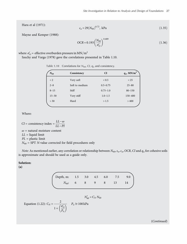
Hara et al (1971):cu = 29 N60
0 72, kPa 1 35
Mayne and Kemper (1988):
OCR = 0 193N60
σO
0 689
1 36
where σO = effective overburden pressure inMN m2
Szechy and Varga (1978) gave the correlations presented in Table 1.10.
Where:
CI = consistency index =LL−ωLL−PI
ω = natural moisture contentLL = liquid limitPL = plastic limitN60 = SPT N-value corrected for field procedures only
Note:As mentioned earlier, any correlation or relationship between N60, su, cu,OCR, CI and qu for cohesive soilsis approximate and should be used as a guide only.
Solution:(a)
Depth, m: 1.5 3.0 4.5 6.0 7.5 9.0
N60: 6 8 9 8 13 14
N60 =CN N60
Equation (1.22): CN =2
1 +σOPa
Pa 100 kPa
(Continued)
Table 1.10 Correlations for N60, CI, qu and consistency.
N60 Consistency CI qu, MN/m2
< 2 Very soft < 0.5 < 25
2–8 Soft to medium 0.5–0.75 25–80
8–15 Stiff 0.75–1.0 80–150
15–30 Very stiff 1.0–1.5 150–400
> 30 Hard > 1.5 > 400
Site Investigation in Relation to Analysis and Design of Foundations 27
worksaccounts.com
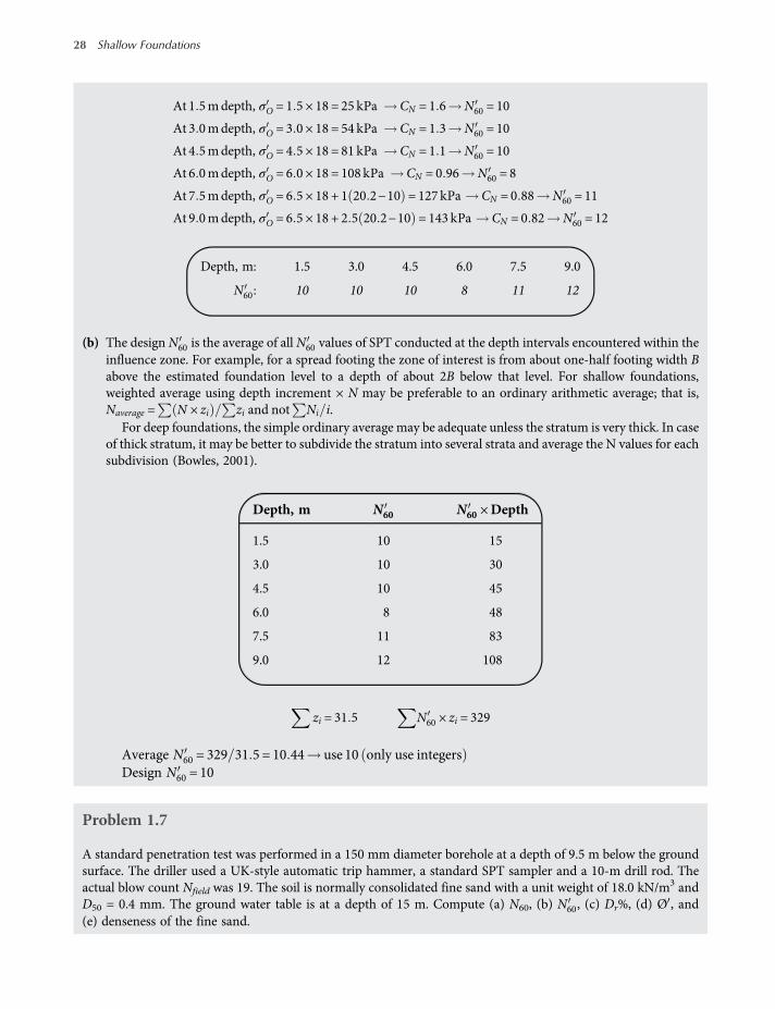
At 1 5mdepth, σO = 1 5 × 18 = 25 kPa CN = 1 6 N60 = 10
At 3 0mdepth, σO = 3 0 × 18 = 54 kPa CN = 1 3 N60 = 10
At 4 5mdepth, σO = 4 5 × 18 = 81 kPa CN = 1 1 N60 = 10
At 6 0mdepth, σO = 6 0 × 18 = 108 kPa CN = 0 96 N60 = 8
At 7 5mdepth, σO = 6 5 × 18 + 1 20 2−10 = 127 kPa CN = 0 88 N60 = 11
At 9 0mdepth, σO = 6 5 × 18 + 2 5 20 2−10 = 143 kPa CN = 0 82 N60 = 12
Depth, m: 1.5 3.0 4.5 6.0 7.5 9.0
N60: 10 10 10 8 11 12
(b) The design N60 is the average of all N60 values of SPT conducted at the depth intervals encountered within theinfluence zone. For example, for a spread footing the zone of interest is from about one-half footing width Babove the estimated foundation level to a depth of about 2B below that level. For shallow foundations,weighted average using depth increment × N may be preferable to an ordinary arithmetic average; that is,Naverage = N × zi zi and not Ni i.
For deep foundations, the simple ordinary average may be adequate unless the stratum is very thick. In caseof thick stratum, it may be better to subdivide the stratum into several strata and average the N values for eachsubdivision (Bowles, 2001).
Depth, m N60 N60 ×Depth
1.5 10 15
3.0 10 30
4.5 10 45
6.0 8 48
7.5 11 83
9.0 12 108
zi = 31 5 N60 × zi = 329
Average N60 = 329 31 5 = 10 44 use 10 only use integersDesign N60 = 10
Problem 1.7
A standard penetration test was performed in a 150 mm diameter borehole at a depth of 9.5 m below the groundsurface. The driller used a UK-style automatic trip hammer, a standard SPT sampler and a 10-m drill rod. Theactual blow count Nfield was 19. The soil is normally consolidated fine sand with a unit weight of 18.0 kN/m3 andD50 = 0.4 mm. The ground water table is at a depth of 15 m. Compute (a) N60, (b) N60, (c) Dr%, (d) Ø , and(e) denseness of the fine sand.
28 Shallow Foundations
worksaccounts.com

Solution:(a) From Table 1.6, for the UK automatic trip hammer, Er = 73%
From Table 1.7, for 150 mm diameter borehole, ηb = 1.05From Table 1.7, for a standard sampler, ηs = 1.0From Table 1.7, for a 10-m drill rod, ηr = 0.95
Equation (1.18): N60 =Er ηb ηs ηr Nfield
60=73 × 1 05 × 1 × 0 95 × 19
60= 23
(b)N60 =CN N60
Assume using Equation (1.18): CN =paσO
=100
9 5 × 18= 0 76
N60 = 0 76 × 23 = 17
(c) Equation (1.28):
Dr =N60 0 23 +
0 06D50
1 7
91σOPa
½
=23 0 23 +
0 060 4
1 7
91
9 5 × 18100
½
100 = 54
(d) Equation (1.31):
Ø = tan−1 N60
12 2 + 20 3σOPa
0 34
= tan−1 23
12 2 + 20 39 5 × 18100
0 34
= tan−1 0 785 Ø = 38
(e) Table 1.8: forN60 = 17,Dr = 54%, Ø = 38% and γ = 18 kN/m3, the soil may be classified asmedium dense sand.
Problem 1.8
A 15 cm diameter borehole has been drilled through a fine sand deposit to a depth of 7 m. At this depth, the SPT,using a US safety hammer and a standard SPT sampler, gave Nfield = 23. Boring then continued to greater depths,encountering water table at a depth of 11 m. Compute N60, Ø , and Dr at the test location, and use the data toestimate the denseness of the sand.
Solution:ThemeasuredNfield of 23, with an estimated allowance of about ± 20% for the correction factors, suggests medium-dense sand (Table 1.8). Knowing that fine sand may be considered poorly graded, a value for γ equals 18 kN/m3
may be assumed appropriate (Table 1.8).(Continued)
Site Investigation in Relation to Analysis and Design of Foundations 29
worksaccounts.com
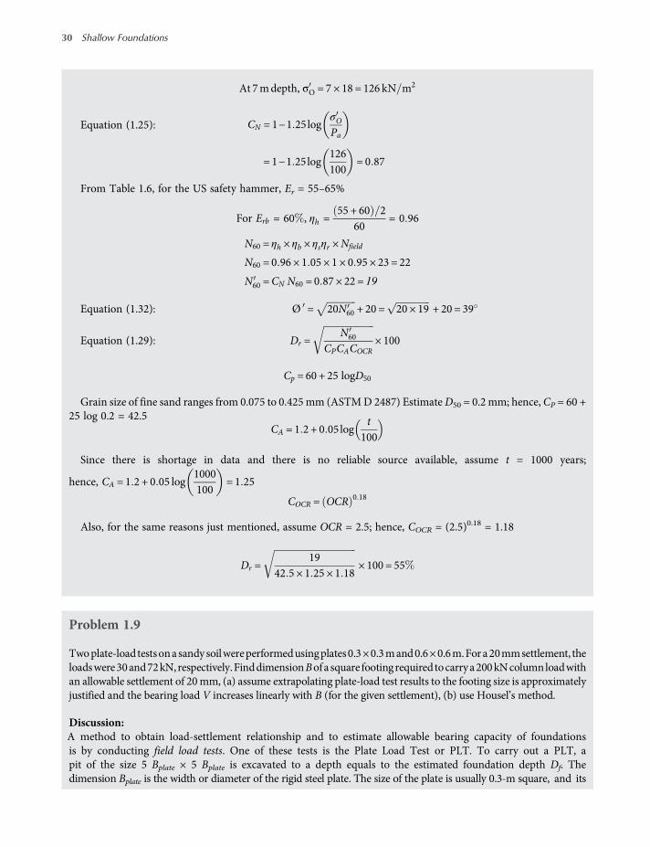
At 7mdepth, σO = 7 × 18 = 126 kN m2
Equation (1.25): CN = 1−1 25logσOPa
= 1−1 25log126100
= 0 87
From Table 1.6, for the US safety hammer, Er = 55–65%
For Erb = 60 , ηh =55 + 60 2
60= 0 96
N60 = ηh × ηb × ηsηr ×Nfield
N60 = 0 96 × 1 05 × 1 × 0 95 × 23 = 22
N60 =CN N60 = 0 87 × 22 = 19
Equation (1.32): Ø = 20N60 + 20 = 20 × 19 + 20 = 39
Equation (1.29): Dr =N60
CPCACOCR× 100
Cp = 60 + 25 logD50
Grain size of fine sand ranges from 0.075 to 0.425 mm (ASTMD 2487) EstimateD50 = 0.2 mm; hence, CP = 60 +25 log 0.2 = 42.5
CA = 1 2 + 0 05logt
100
Since there is shortage in data and there is no reliable source available, assume t = 1000 years;
hence, CA = 1 2 + 0 05 log1000100
= 1 25
COCR = OCR 0 18
Also, for the same reasons just mentioned, assume OCR = 2.5; hence, COCR = (2.5)0.18 = 1.18
Dr =19
42 5 × 1 25 × 1 18× 100 = 55
Problem 1.9
Twoplate-load testsonasandysoilwereperformedusingplates0.3×0.3mand0.6×0.6m.Fora20mmsettlement, theloadswere30and72kN, respectively.FinddimensionBofa square footingrequired tocarrya200kNcolumnloadwithan allowable settlement of 20mm, (a) assume extrapolating plate-load test results to the footing size is approximatelyjustified and the bearing load V increases linearly with B (for the given settlement), (b) use Housel’s method.
Discussion:A method to obtain load-settlement relationship and to estimate allowable bearing capacity of foundationsis by conducting field load tests. One of these tests is the Plate Load Test or PLT. To carry out a PLT, apit of the size 5 Bplate × 5 Bplate is excavated to a depth equals to the estimated foundation depth Df. Thedimension Bplate is the width or diameter of the rigid steel plate. The size of the plate is usually 0.3-m square, and its
30 Shallow Foundations
worksaccounts.com
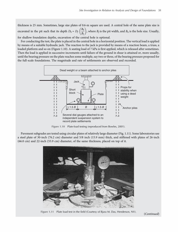
thickness is 25 mm. Sometimes, large size plates of 0.6-m square are used. A central hole of the same plate size is
excavated in the pit such that its depth Dh = DfBh
Bf, where Bf is the pit width, and Bh is the hole size. Usually,
for shallow foundation depths, excavation of the central hole is optional.For conducting the test, the plate is placed in the central hole in a horizontal position. The vertical load is applied
by means of a suitable hydraulic jack. The reaction to the jack is provided by means of a reaction beam, a truss, aloaded platform and so on (Figure 1.10). A seating load of 7 kPa is first applied, which is released after sometimes.Then the load is applied in successive increments until failure of the ground in shear is attained or, more usually,until the bearing pressure on the plate reaches somemultiple, say two or three, of the bearing pressure proposed forthe full-scale foundations. The magnitude and rate of settlements are observed and recorded.
Pavement subgrades are tested using circular plates of relatively large diameter (Fig. 1.11). Some laboratories usea steel plate of 30-inch (76.2 cm) diameter and 5/8 inch (15.9 mm) thick, and stiffened with plates of 26-inch(66.0 cm) and 22-inch (55.9 cm) diameter, of the same thickness, placed on top of it.
(Continued)
Props for
stability when
using a dead
weight
Several dial gauges attached to an
independent suspension system to
record plate settlements
Plate
Jack
Short
block
+
≥ 1.5 B B ≥ 1.5 B Anchor piles
Dead weight or a beam attached to anchor piles
Figure 1.10 Plate-load testing (reproduced from Bowles, 2001).
Figure 1.11 Plate load test in the field (Courtesy of Bjara M. Das, Henderson, NV).
Site Investigation in Relation to Analysis and Design of Foundations 31
worksaccounts.com
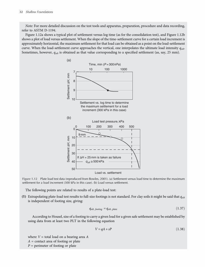
Note: For more detailed discussion on the test tools and apparatus, preparation, procedure and data recording,refer to ASTM D-1194.Figure 1.12a shows a typical plot of settlement versus log time (as for the consolidation test), and Figure 1.12b
shows a plot of load versus settlement. When the slope of the time-settlement curve for a certain load increment isapproximately horizontal, the maximum settlement for that load can be obtained as a point on the load-settlementcurve. When the load-settlement curve approaches the vertical, one interpolates the ultimate load intensity qult.Sometimes, however, qult is obtained as that value corresponding to a specified settlement (as, say, 25 mm).
The following points are related to results of a plate-load test:
(1) Extrapolating plate-load test results to full-size footings is not standard. For clay soils it might be said that qultis independent of footing size, giving:
qult, footing = qult, plate 1 37
According to Housel, size of a footing to carry a given load for a given safe settlement may be established byusing data from at least two PLT in the following equation
V = qA+ sP 1 38
where V = total load on a bearing area AA = contact area of footing or plateP = perimeter of footing or plate
0 100 200 300 400 500
Settle
ment Δ
H, m
mS
ettle
ment Δ
H, m
m
Load vs. settlement
9 mm
If ΔH = 25 mm is taken as failure
Time, min (P = 300 kPa)
10 100 1000
50
40
30
20
10
0
10
9
8
7
Settlement vs. log time to determine
the maximum settlement for a load
increment (300 kPa in this case)
Load test pressure, kPa
qult ≅ 500 kPa
(b)
(a)
Figure 1.12 Plate load test data (reproduced from Bowles, 2001). (a) Settlement versus load time to determine the maximumsettlement for a load increment (300 kPa in this case). (b) Load versus settlement.
32 Shallow Foundations
worksaccounts.com

q = bearing pressure beneath AP = perimeter shear
For sand soils, practically, extrapolation may be justified using
qult, footing = qult, plateBfooting
Bplate1 39
However, the use of this equation is not recommended unless the ratio Bfooting/Bplate is not much more thanabout three. When the ratio is 6 to 15 or more, the extrapolation from a plate-load test is little more than aguess that could be obtained at least as reliably using SPT or cone penetration test (CPT) correlations(Bowles, 2001).
(2) For clayey soils (cohesive soils) and for the same qult of the footing and plate, the following empirical approxi-mate relationship regarding footing settlement may be used:
Sfooting = SplateBfooting
Bplate1 40
However, since a plate-load test is of short duration, consolidation settlements usually cannot be predicted.If the test is performed on a material overlying a saturated compressible stratum, the test may give highlymisleading information. As a precautionary measure against this event, it is good practice to have boringsperformed at the plate-load test site. Note: For clayey soils, settlement is normally determined from laboratoryconsolidation test results and not from results of plate-load test.
For sandy soils (cohesionless soils) and for the same qult of the footing and plate, the following empiricalrelationship regarding footing settlement may be used:
Sfooting = SplateBfooting Bplate + 0 3
Bplate Bfooting + 0 3
2
1 41
In this equation, both Bfooting and Bplate are in meters.(3) In designing a shallow foundation for an allowable settlement, a trial and error procedure is usually adopted.
First, a value for Bfooting is assumed and qo is calculated using qo =Q/Afooting, whereQ is the structure load (suchas a column load). Then, for the computed value of qo, from the load-settlement curve a value for Splate isestimated. The value of Sfooting is computed from the above equations and compared with the allowable settle-ment value. The procedure is repeated till the computed settlement value is equal to the allowable settlement.
(4) The plate load test can also be used for determination of the stress-strain modulus (or deformation modulus)Es of the supporting soil, used in the known immediate settlement equation
ΔH = qB1−μ2
EsI 1 42
Where: ΔH = settlementq = uniform load per unit areaB = least lateral dimension of the loaded areaI = influence factorμ = Poisson’s ratio of the soil obtained from tables
(Continued)
Site Investigation in Relation to Analysis and Design of Foundations 33
worksaccounts.com
The expression1−μ2
EsI equals to
ΔHqB
which is the slope of an assumed straight line plotted with coord-
inatesΔH and q B. It is determined from results of two or more plate-load tests, using plates of the same shape.The main features of Equation (1.42) and its applications will be outlined in Chapter 3.
(5) The influence depth of the plate (about 2 Bplate) is much smaller than that of the real footing, so the test reflectsonly the load carrying capacity of the near surface soils, whereas, usually, soils type and property vary withdepth. This can introduce large errors. Several complete foundation failures occurred in spite of the use ofplate-load tests (Terzaghi and Peck, 1967; Mesri, 1996). Obviously, for the reasons just mentioned, plate-loadtest is not used for design of deep foundations. Because of the development of better methods of testing andanalysis, current engineering practice rarely uses plate-load tests for design of foundations. However, thesetests are still useful for other design problems, such as those involving wheel loads on pavement subgrades,where the service loads act over smaller area.
Solution:
(a) The linear proportionality requires
V = aB + b
From the first PLT 30 = a 0 3 + bFrom the second PLT 72 = a 0 6 + b
Therefore, a =420 3
= 140 and b= 30−140 0 3 = −12
For full-size footing:
V = 140 B−12V = column load = 200 kN200 = 140 B−12
Therefore, B=212140
= 1 514m
Try 1 5m× 1 5msquare footing
(b) Equation 1 38 V = qA+ sP
From the first PLT 30 = q 0 3 2 + s 4 × 0 3 = 0 09q+ 1 2 s
From the secondPLT 72 = q 0 6 2 + s 4 × 0 6 = 0 36q+ 2 4 s or 36 = 0 18q+ 1 2 s
Therefore, q=36−300 09
= 66 67 and s=30−66 67 0 09
1 2= 20
For full-size footing:
200 = 66 67B2 + 20 × 4B or B2 + 1 2B−3 = 0
B=−1 2 ± 1 22−4 × 1 −3
2 × 1=−1 2 + 3 67
2= 1 23 m
Try 1.3 m × 1.3 m square footing.Obviously, the assumed linear proportionality used in solution (a) is in error, whereas the Housel’s equa-
tion used in solution (b) is based on research results; expected to be more correct. Therefore, one may decideon using 1.3 m × 1.3 m square footing.
34 Shallow Foundations
worksaccounts.com
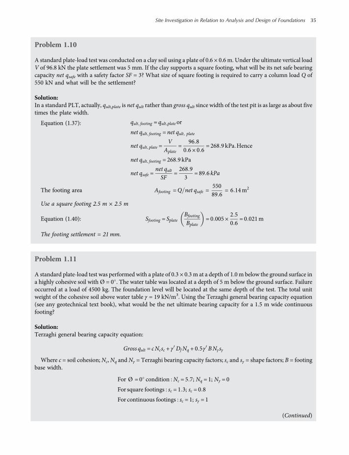
Problem 1.10
A standard plate-load test was conducted on a clay soil using a plate of 0.6 × 0.6 m. Under the ultimate vertical loadV of 96.8 kN the plate settlement was 5 mm. If the clay supports a square footing, what will be its net safe bearingcapacity net qsafe with a safety factor SF = 3? What size of square footing is required to carry a column load Q of550 kN and what will be the settlement?
Solution:In a standard PLT, actually, qult,plate is net qult rather than gross qult since width of the test pit is as large as about fivetimes the plate width.
Equation (1.37): qult, footing = qult,plateor
net qult, footing = net qult, plate
net qult, plate =V
Aplate=
96 80 6 × 0 6
= 268 9 kPa Hence
net qult, footing = 268 9 kPa
net qsafe =net qultSF
=268 93
= 89 6 kPa
The footing area Afooting =Q net qsafe =55089 6
= 6 14m2
Use a square footing 2.5 m × 2.5 m
Equation (1.40): Sfooting = SplateBfooting
Bplate= 0 005 ×
2 50 6
= 0 021m
The footing settlement = 21 mm.
Problem 1.11
A standard plate-load test was performed with a plate of 0.3 × 0.3 m at a depth of 1.0 m below the ground surface ina highly cohesive soil with Ø = 0 . The water table was located at a depth of 5 m below the ground surface. Failureoccurred at a load of 4500 kg. The foundation level will be located at the same depth of the test. The total unitweight of the cohesive soil above water table γ = 19 kN/m3. Using the Terzaghi general bearing capacity equation(see any geotechnical text book), what would be the net ultimate bearing capacity for a 1.5 m wide continuousfooting?
Solution:Terzaghi general bearing capacity equation:
Gross qult = cNcsc + γ DfNq + 0 5γ BNγsγ
Where c = soil cohesion;Nc,Nq andNγ = Terzaghi bearing capacity factors; sc and sγ = shape factors; B = footingbase width.
For Ø = 0 condition Nc = 5 7; Nq = 1; Nγ = 0
For square footings sc = 1 3; sc = 0 8
For continuous footings sc = 1; sγ = 1
(Continued)
Site Investigation in Relation to Analysis and Design of Foundations 35
worksaccounts.com

Water table is located at 4 m depth below the foundation level which is deeper than B, hence, γ = γ = 19 kN/m3
net qult = gross qult −γ Df
= c× 5 7 × 1 3 + 19 × 1 × 1 + 0 – 19 × 1
= 7 41c
Equation (1.37): qult, footing = qult,plate or
net qult, footing = net qult,plate
net qult, plate =4500
0 3 × 0 3= 50 000 kg m2
7 41c= 50 000 kg m2 c= 6748 kg m2
For continuous footings, net qult = c× 5 7 × 1
= 6748 × 5 7 = 38 462 kg m2
= 384 62 kN m2
Usenet qult = 385 kN m2
Problem 1.12
Two plate load tests on a cohesionless soil yielded the following data:
Plate size, m Load V, kN splate, mm
0.6 × 0.6 40 10
0.9 × 0.9 40 3
(a) Determine the stress-strain modulus Es of the supporting soil. Assume the soil Poisson’s ratio μ = 0.3.(b) What will be the differential settlement of two footings; one of the size 2.5 × 2.5 m, supporting a column load
of 700 kN; the other of the size 3.0 × 3.0 m, supporting a column load of 1000 kN? Assume the footings are soapart that there will be no overlap of stresses take place in the supporting soil.
Solution:
(a) Equation (1.42): ΔH = qB1−μ2
EsI
From the first PLT, let q1 = qult :
q1 =40
0 6 × 0 6= 111 1 kN m2, and q1B1 = 111 1 × 0 6 = 66 7 kN m
From the second PLT, let q2 = qult :
q2 =40
0 9 × 0 9= 49 4 kN m2, and q2B2 = 49 4 × 0 9 = 44 5 kN m
36 Shallow Foundations
worksaccounts.com
From a plot of ΔH versus q B or by calculation:
1−μ2
EsI =
ΔHqB
=ΔH1 – ΔH2q1B1− q2B2
=0 010−0 00366 7−44 5
=0 00722 2
= 3 15 × 10−4
From tables (available in any geotechnical or foundation engineering text book), for a point at centre of a rigidsquare plate or footing, obtain I = 0.82 (approximately),
1−μ2
EsI =
1−0 32
Es× 0 82 =
0 75Es
0 75Es
= 3 15 × 10−4
Es =0 75
3 15 × 10−4= 2381 kPa
(b) Equation (1.41): Sfooting = SplateBfooting Bplate + 0 3
Bplate Bfooting + 0 3
2
First footing : load intensity = 700 2 5 × 2 5 = 112 0 kN m2
Second footing : load intensity = 1000 3 × 3 = 111 1 kN m2
The load intensity of the first PLT = 111 1 kN m2
The load intensity of the secondPLT = 49 4 kN m2
Use the results of the first PLT, since its load intensity is equal or very close to that of the footings.
Settlement of the first footing = 0 012 5 0 6 + 0 30 6 2 5 + 0 3
2
= 0 018 m
Settlement of the second footing = 0 013 0 6 + 0 30 6 3 + 0 3
2
= 0 019 m
The differential settlement of the footings is 0 019−0 018 = 0 001m
The differential settlement = 1 mm.
Problem 1.13
A static cone penetration test was conducted in a deposit of normally consolidated and moderately compressibledry sand. The test results were as given below:
Depth (m): 1.50 3.00 4.50 6.00 7.50 9.00
Point resistance qc (MN/m2): 2.05 4.23 6.01 8.18 9.97 12.42
(Continued)
Site Investigation in Relation to Analysis and Design of Foundations 37
worksaccounts.com

Assume the dry unit weight of the sand deposit = 16 kN/m3. Estimate its average peak friction angle Ø andrelative density Dr.
Discussion:The static cone penetration test or cone penetrometer test, CPT, also known as the Dutch cone penetration test, hasfound wide application in lieu of the SPT, especially in European countries.The test is particularly used for soft clays, soft silts and fine to medium sand deposits. It is not well adapted to
gravel deposits or to stiff and hard cohesive soil deposits. Briefly, in its original version, the test consists in pushingdown a standard steel cone, usually a 60 cone of a 1000mm2 base area, into ground at a steady rate of 10–20mm/sfor a depth of 40mm each time (each stroke) over stages (intervals) of 200mm; the resistance in units of pressure isrecorded for each stroke. The cone is pushed by applying thrust and not by driving. Data usually recorded as pointor tip bearing resistance qc, side friction resistance qs and total penetration resistance qT. Pore pressures, verticalalignment, and temperature may also be taken if allowed by the equipment configuration. A CPT allows nearlycontinuous testing at many sites, which is often valuable. If the soil is stratified, the test may be performed inparallel with a drilling machine. In this case the hole is drilled to a soft material, a CPT is done, boring recom-mences and so on. This test is rather popular for sites where there are deep deposits of transported soil such as inflood plains, river deltas and along coastlines.Although many different penetrometer styles and configurations have been used, however, the most widely used
are the mechanical Dutch cone (Figure 1.13), and the electric friction cone (Figure 1.14). The operation of the two
15 mm
35.7 mm
47 mm
387 mm
69 mm
60°
133.5
mm
30 mm dia
20 mm dia
35.7 mm
23 mm dia
32.5 mm dia
35.7 mm dia
187 mm
15 mm
52.5 mm
11.5 mm
25 mm
33.5 mm
266 mm
146 mm
30 mm 35 mm
ExtendedCollapsed
12.5 mm
45 mm
Figure 1.13 A mechanical friction cone penetrometer (from ASTM, 2001).
38 Shallow Foundations
worksaccounts.com

types differs in that the mechanical cone is advanced in stages and measures qc and qs at intervals of 20 cm, whereasthe electric cone is able to measure qc and qs continuously with depth. In either case, the CPT defines the soil profilewith much greater resolution than does the SPT. Another advantage of the CPT is that the disturbance to the soil isminimal.In conducting a CPT, using a developedmechanical cone, initially the inner rod is pushed downwards a distance
of 40mm, causing the cone only to penetrate the soil, and the cone point resistance qc is recorded. The outer shaft isnow advanced to the cone base, and the side (or skin) friction resistance qs is recorded. Now the cone and theengaged friction sleeve are advanced in combination to obtain the total penetration resistance qT, which shouldbe approximately the sum of the point and side resistances just measured.In using the electric friction cone, the cone penetration resistance is measured by means of a load cell inside the
body of the instrument and can thus be recorded continuously as the penetrometer is pushed into the soil. Theresults are normally plotted automatically, against depth, by means of a chart recorder. The friction sleeve is mech-anically separate from the conical point; side resistance is measured bymeans of a second load cell. Cone resistanceand side resistance can thus be measured independently. A full description of the test apparatus, procedure andresults interpretation is given by Meigh (1987). Note: This test has been standardised by ASTM as D-3441.The CPT data are used to classify a soil, to establish the allowable bearing capacity of shallow foundation
elements, or to design piles. The CPT data processing and evaluating should always be handled by a specialised
(Continued)
Friction
sleeve
435.6 mm
1
2
3
4
To surface
1. Load c
ell
2.
Friction s
leeve
3.
Wate
rpro
of
bushin
g
4. C
able
5.
Str
ain
gages
6. C
onnection w
ith r
ods
7.
Inclin
om
ete
r
8.
O-r
ing w
ate
r seal (o
ne o
r m
ore
)
9. S
oil
seal if r
equired
5
6
7
8
9
qc
qT
AT = 10 cm2
ucD
πD2
uc
=
d1
Figure 1.14 An electric friction cone penetrometer (from Bowles, 2001).
Site Investigation in Relation to Analysis and Design of Foundations 39
worksaccounts.com
geotechnical engineer with enough experience because the data can be so erratic that may need good engineeringjudgment.The measured point resistance qc and side friction qs are used to compute the friction ratio fr as
fr =qsqc
× 100 1 43
The friction ratio fr may also be estimated using D50 as in the following empirical equations:Anagnostopoulos et al (2003),
fr = 1 45−1 36logD50 using electric cone 1 44
fr = 0 781−1 611logD50 using mechanical cone 1 45
Note: In developing these equations, the D50 of soils ranged from 0.01 mm to about 10 mm.The friction ratio fr is primarily used for soil classification as illustrated in the charts of Figures 1.15 and 1.16.
The friction ratio may be used to give an estimate for soil sensitivity St as follows (Robertson andCampanella, 1983):
St≈10fr
fr is in 1 46
CPT correlations for cohesive soils:The cone bearing resistance qc (tip bearing resistance) and the undrained shear strength su (or cu) are correlatedthrough the following empirical equation (Mayne and Kemper, 1988):
su =qc−σoNk
1 47
σo = γZ = overburden pressure where the qc is measured. It is in the same units of qc and same type of pressure(i.e., if qc is an effective pressure, σO shall be used).
400
200
10080
60
40
20
108
6
4
2
11 2 3 4 5 60
Sand
(SW, SP)
Silty
sand
(SM,
SC)
Sandy
silts and
siltsSilty clay
clayey
siltClay
Cone tip
resis
tance q
c, kP
a (
×100)
Peat
Friction ratio fr, (%)
Figure 1.15 Soil classification chart for standard electric friction or mechanical cone (from Bowles, 2001, after Robertson andCampanella, 1983).
40 Shallow Foundations
worksaccounts.com

Nk = Cone factor or bearing capacity factor, constant for a certain soil; depends mainly on soil plasticity index(PI) and sensitivity (St), and on the cone penetrometer type. Its range is 5–30. The recommended values for mech-anical and electric cones are 20 and 15, respectively. Anagnostopoulos et al. (2003) determined these two valuesequal 18.9 and 17.2, respectively. They also showed that cu equals 0.79 qs and qs for mechanical and electric cones,respectively. For normally consolidated clays of St < 4 and PI < 30, a value of Nk = 18 may be satisfactory.The preconsolidation pressure σc and overconsolidation ratio OCR are correlated as follows (Mayne and
Kemper, 1988):
σc = 0 243 qc0 96 qc and σc are inMN m2 1 48
OCR= 0 37qc−σoσo
1 01
1 49
CPT correlations for cohesionless soils:Lancellotta (1983) and Jamiolkowsk et al (1985) showed that for the normally consolidated sand, the relative dens-ity Dr and the cone resistance qc can be correlated as:
Dr = 66 × logqcσo
−98 1 50
where the qc and σO are in t/m2
According to Kulhawy and Mayne (1990), the above equation can be rewritten as
Dr = 68 logqcpa σo
−1 1 51
Pa = atmospheric pressure ≈100 kPa
Figure 1.17 represents the empirical relationship recommended by Baldi et al. (1982), and Robertson andCampanella (1983), for normally consolidated quartz sand.
(Continued)
Friction ratio fr, (%)C
one
tip
resis
tance q
c,
MP
a
Zone Soil behaviour type
1 Sensitive fine gained
2 Organic material
3 Clay
4 Silty clay to clay
5 Clayey silt to silty clay
6 Sandy silt to clayey silt
7 Silty sand to sandy silt
8 Sand to silt
9 Sand
10 Gravelly sand to sand
11 Very stiff fine grained*
12 Sand to clayey sand*
*Overconsolidated or
cemented
100
10
1
0.10 1
1
2
2
3
3
θ
4
4
5
5
6
6
7
7
8
8
9
10 1112
OCR
S 1
Dr.
Figure 1.16 Soil behaviour type chart based on qc and fr (reproduced from paper by P.K. Robertson, 2010; it is the originalRobertson and Campanella chart, 1986).
Site Investigation in Relation to Analysis and Design of Foundations 41
worksaccounts.com
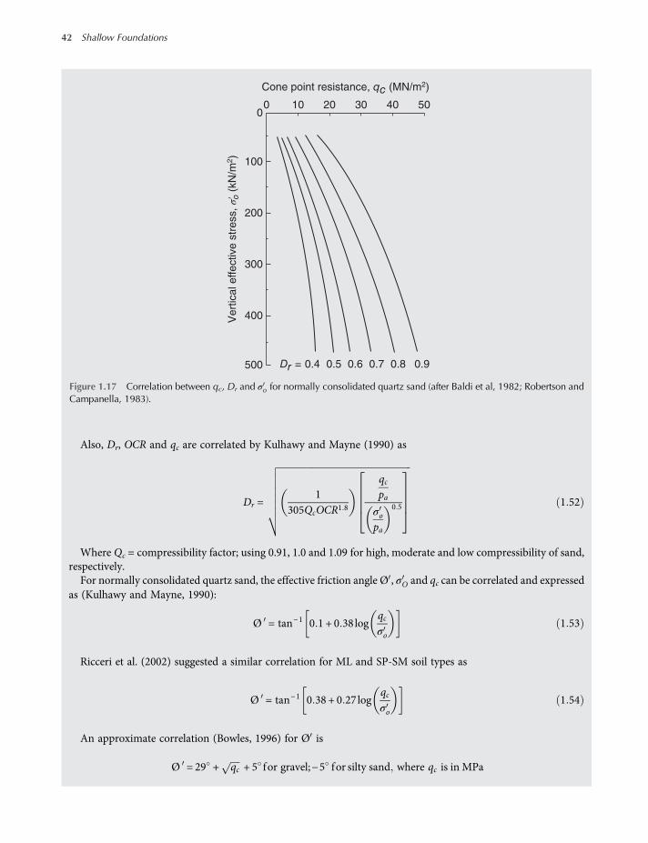
Also, Dr, OCR and qc are correlated by Kulhawy and Mayne (1990) as
Dr =1
305QcOCR1 8
qcpaσopa
0 5 1 52
Where Qc = compressibility factor; using 0.91, 1.0 and 1.09 for high, moderate and low compressibility of sand,respectively.For normally consolidated quartz sand, the effective friction angle Ø , σO and qc can be correlated and expressed
as (Kulhawy and Mayne, 1990):
Ø = tan−1 0 1 + 0 38logqcσo
1 53
Ricceri et al. (2002) suggested a similar correlation for ML and SP-SM soil types as
Ø = tan−1 0 38 + 0 27logqcσo
1 54
An approximate correlation (Bowles, 1996) for Ø is
Ø = 29 + qc + 5 for gravel;−5 for silty sand where qc is in MPa
Vert
ical effe
ctive s
tress,
σ′ o (k
N/m
2)
Cone point resistance, qc (MN/m2)
0 10 20 30 40 50
400
500
200
100
0
300
= 0.4 0.5 0.6 0.7 0.8 0.9Dr
Figure 1.17 Correlation between qc, Dr and σo for normally consolidated quartz sand (after Baldi et al, 1982; Robertson andCampanella, 1983).
42 Shallow Foundations
worksaccounts.com
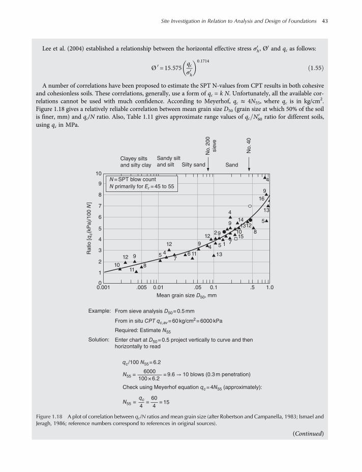
Lee et al. (2004) established a relationship between the horizontal effective stress σh, Ø and qc as follows:
Ø = 15 575qcσh
0 1714
1 55
A number of correlations have been proposed to estimate the SPT N-values from CPT results in both cohesiveand cohesionless soils. These correlations, generally, use a form of qc = k N. Unfortunately, all the available cor-relations cannot be used with much confidence. According to Meyerhof, qc ≈ 4N55, where qc is in kg/cm2.Figure 1.18 gives a relatively reliable correlation between mean grain size D50 (grain size at which 50% of the soilis finer, mm) and qc/N ratio. Also, Table 1.11 gives approximate range values of qc N60 ratio for different soils,using qc in MPa.
(Continued)
1
2
13
13
5
4
4
44
5
5
6
7
7
8
8
9
9
9
9
9
10
10
10
9
8
7
6
5
4
3
2
1
00.001 .005 0.01 .05 0.1 .5 1.0
11
11
12
12
12
12
1314
15
16
Clayey silts
and silty clay
Sandy silt
and silt Silty sand Sand
N = SPT blow count
N primarily for Er = 45 to 55
Mean grain size D50, mm
Required: Estimate N55
Enter chart at D50= 0.5 project vertically to curve and then
horizontally to read
Example:
Solution:
From sieve analysis D50= 0.5 mm
From in situ CPT qc,av= 60 kg/cm2= 6000 kPa
Ratio [
qc(k
Pa)/
100 N
]
No. 40
No. 200
sie
ve
qc/100 N55= 6.2
N55 = 9.6 → 10 blows (0.3 m penetration)
Check using Meyerhof equation qc= 4N55 (approximately):
N55
6000
100 × 6.2
4 415
60= = =
qc
=
Figure 1.18 A plot of correlation between qc/N ratios and mean grain size (after Robertson and Campanella, 1983; Ismael andJeragh, 1986; reference numbers correspond to references in original sources).
Site Investigation in Relation to Analysis and Design of Foundations 43
worksaccounts.com
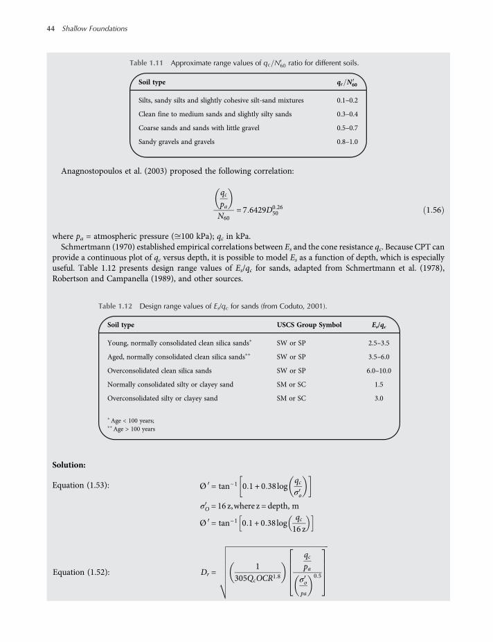
Anagnostopoulos et al. (2003) proposed the following correlation:
qcpaN60
= 7 6429D0 2650 1 56
where pa = atmospheric pressure ( 100 kPa); qc in kPa.Schmertmann (1970) established empirical correlations between Es and the cone resistance qc. Because CPT can
provide a continuous plot of qc versus depth, it is possible to model Es as a function of depth, which is especiallyuseful. Table 1.12 presents design range values of Es/qc for sands, adapted from Schmertmann et al. (1978),Robertson and Campanella (1989), and other sources.
Solution:
Equation (1.53): Ø = tan−1 0 1 + 0 38logqcσo
σO = 16 z,where z = depth, m
Ø = tan−1 0 1 + 0 38logqc16 z
Equation (1.52): Dr =1
305QcOCR1 8
qcpaσopa
0 5
Table 1.12 Design range values of Es/qc for sands (from Coduto, 2001).
Soil type USCS Group Symbol Es/qc
Young, normally consolidated clean silica sands∗ SW or SP 2.5–3.5
Aged, normally consolidated clean silica sands∗∗ SW or SP 3.5–6.0
Overconsolidated clean silica sands SW or SP 6.0–10.0
Normally consolidated silty or clayey sand SM or SC 1.5
Overconsolidated silty or clayey sand SM or SC 3.0
∗Age < 100 years;∗∗Age > 100 years
Table 1.11 Approximate range values of qc N60 ratio for different soils.
Soil type qc N60
Silts, sandy silts and slightly cohesive silt-sand mixtures 0.1–0.2
Clean fine to medium sands and slightly silty sands 0.3–0.4
Coarse sands and sands with little gravel 0.5–0.7
Sandy gravels and gravels 0.8–1.0
44 Shallow Foundations
worksaccounts.com

pa = 100 kN m2; σO = 16 z
For normally consolidated sand OCR= 1
For moderately compressible sand Qc = 1
Dr =1305
qc100
16 z100
0 5 =qc
12200 z0 5
Obtain Ø and Dr values for different values of qc at the given depths, as shown in the table below:
Z, m qc, kN/m2 σO, kN/m
3 Ø , degree Dr, %
1.5 2050 24 39.8 37.0
3.0 4230 48 40.0 44.7
4.5 6010 72 39.7 48.2
6.0 8180 96 39.8 52.3
7.5 9970 120 39.7 54.6
9.0 12420 144 39.9 58.3
Average Ø = Ø 6= 238 9 6 = 39 8
Average Dr = Dr 6 = 295 1 6 = 49 2
Note: To obtain the average values for Ø and Dr, one may prefer to use the same procedure as that followed forN60 in Solution (b) of Problem 1.6. If that procedure is used, the average values will be 39.8 and 52.5%.
Problem 1.14
A cone penetration test was conducted, using an electric-friction cone, in a clay deposit. The cone penetrationresistance, at 6 m depth, was 0.8 MN/m2. Sensitivity of the clay St < 4, and its PI < 30. Ground water table waslocated at 2 m depth. The unit weight γ of the clay above and below water table was 18 and 20 kN/m3, respectively.Find the over consolidation ratio OCR, and the undrained cohesion cu.
Solution:
Equation (1.49): OCR= 0 37qc−σoσo
1 01
qc = 0 8MN m2 = 800 kN m2
σo = 2 × 18 + 4 × 20 = 116 kN m2
σo = 2 × 18 + 4 20−10 = 76 kN m2
(Continued)
Site Investigation in Relation to Analysis and Design of Foundations 45
worksaccounts.com
OCR= 0 37800−116
76
1 01
= 3 4
Equation (1.49): su =qc−σoNk
= cu
For electric friction penetrometers a value of Nk = 15 may be used. However, because the clay has St < 4 andPI < 30, and in order to be more on the safe side, assume using Nk = 18.
cu =800−116
18= 38 kN m2
Problem 1.15
Figure 1.19 shows an electric cone penetration record at site of a proposed structure. The average soil unit weightγ = 19 kN/m3. Classify the soil encountered at the depth interval of 10–12 m. Also estimate the internal frictionangle Ø , the relative density Dr and the undrained shear strength Su of the classified soil, as applicable (accordingto the soil type). Assume the soil is normally consolidated and of low compressibility.
Solution:Estimate the average value for qc = 10 MPa = 10 000 kN/m2
Estimate the average value for fr = 4Use Figure 1.15 and classify the soil as sandy siltConsider the soil as cohesionless (approximately); estimate Ø and Dr:
Depth
z, m
Depth
z, m
00
1
2
2
3
4
4
5
6
6
7
8
9
10
8 10
11
12
13
14
00 0200
qs, kPa qc, MPa fr, %
400 600 4 8 10 16
1
2
3
4
5
6
7
8
9
10
11
12
13
14
Figure 1.19 Cone penetration record.
46 Shallow Foundations
worksaccounts.com
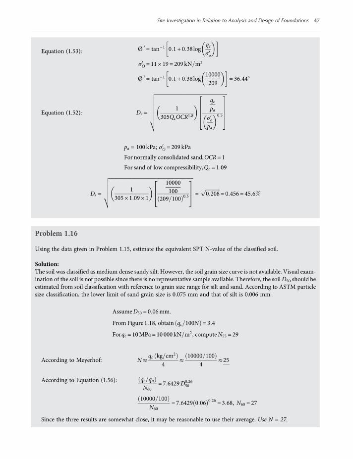
Equation (1.53): Ø = tan−1 0 1 + 0 38logqcσo
σO = 11 × 19 = 209 kN m2
Ø = tan−1 0 1 + 0 38log10000209
= 36 44
Equation (1.52): Dr =1
305QcOCR1 8
qcpaσopa
0 5
pa = 100 kPa; σO = 209 kPa
For normally consolidated sand,OCR= 1
For sand of low compressibility,Qc = 1 09
Dr =1
305 × 1 09 × 1
10000100
209 100 0 5 = 0 208 = 0 456 = 45 6
Problem 1.16
Using the data given in Problem 1.15, estimate the equivalent SPT N-value of the classified soil.
Solution:The soil was classified as medium dense sandy silt. However, the soil grain size curve is not available. Visual exam-ination of the soil is not possible since there is no representative sample available. Therefore, the soilD50 should beestimated from soil classification with reference to grain size range for silt and sand. According to ASTM particlesize classification, the lower limit of sand grain size is 0.075 mm and that of silt is 0.006 mm.
AssumeD50 = 0 06mm
From Figure 1 18, obtain qc 100N = 3 4
Forqc = 10MPa = 10 000 kN m2, computeN55 = 29
According to Meyerhof: N≈qc kg cm2
4≈
10000 1004
≈25
According to Equation (1.56): qc qaN60
= 7 6429D0 2650
10000 100N60
= 7 6429 0 06 0 26 = 3 68, N60 = 27
Since the three results are somewhat close, it may be reasonable to use their average. Use N = 27.
Site Investigation in Relation to Analysis and Design of Foundations 47
worksaccounts.com
Problem 1.17
A pressuremeter test (PMT) was conducted in a soft saturated clay.Given: corrected Vo = 535 cm3, vo = 46 cm3, po = 42 4 kN m2, pf = 326 5 kN m2, and vf = 180 cm3.Assuming Poisson’s ratio μs = 0.5 and using Figure 1.22, calculate the pressuremeter modulus Esp.
Discussion:A PMT is a cylindrical device designed to apply a uniform radial pressure to the sides of a borehole at the requireddepth below ground surface. Although it can be used in different types of soil, however, its best applications are inrelatively fine-grained sedimentary soil deposits. The original PMT was developed in the year 1956 by LouisMenard in an attempt to overcome the problem of sampling disturbance and to insure that the in-place soil struc-ture is adequately represented. There are two different basic types: (1) The Menard PMT, which is lowered into apre-formed borehole (Figure 1.20a); (2) The self-boring PMT, which forms its own borehole and thus causes muchless disturbance to the soil prior to testing (Figure 1.20b).
The device basically consists of a cylindrical rubber cell, usually of 58 mm in diameter and 535 cm3 in volume,and two guard cells of the same diameter arranged coaxially. The probe length is usually 420 mm. The deviceis lowered into a carefully prepared (slightly oversize) borehole to the required depth. As recommendedby ASTM, for diameters of 44, 58 and 74 mm, the required borehole diameter ranges are 45–53 mm, 60–70 mm
Pressure
Water
Feeler
Hollow shaft
Membrane
Pore pressure
transducer
Cutters
(a) (b)
Guard cell
Guard cell
[Sheath]
Soil
under
test
Borehole
Measuring
cell
Gas
Volume
indicator
Figure 1.20 Basic features of (a) Menard pressuremeter and (b) self-boring pressuremeter (from Knappett and Craig, 2012).
48 Shallow Foundations
worksaccounts.com

and 76–89 mm, respectively. The central measuring cell is expanded against the borehole wall by means of waterpressure, measurements of the applied pressure and the corresponding increase in volume being recorded.Pressure is applied to the water by compressed gas (usually nitrogen) in a controlled gas cylinder at the surface.The increase in volume of the pressure cell is determined from the movement of the water-gas interface in theother control cylinder (Figure 1.20a). Readings being normally taken at 15, 30, 60 and 120 s after a pressure incre-ment has been applied. The process is continued until the total volume of the expanded cavity becomes as large astwice the volume of the original cavity, or, the pressure limit of the device is reached. A new test begins after theprobe has been deflated and advanced to another depth. A version of Menard pressuremeter test is schematicallyshown in Figure 1.21. Note: Refer to ASTM D 4719 for more details of the test.
Generally, a pressuremeter is designed for maximum pressures in the ranges 2.5–10.0 MPa in soils and 10–20MPa in very stiff soils and weak rocks. Corrections must be made to the measured pressure, volume change andcavity deformation in order to account for: (a) the head difference between the water level in the cylinder and thetest level in the borehole (or between the pressure transducer and the element), (b) the pressure required to stretchthe rubber cell (i.e. for stiffness of the membrane) and (c) the expansion of the control cylinder and tubingunder pressure. The two other guard cells are expanded under the same pressure as in the measuring cell but usingcompressed gas. The increase in volume of the guard cells is not measured. The function of the guard cells is toeliminate end effects, insuring a state of plane strain.
(Continued)
Pressuremeter
test (PMT)
ASTM D 4719
Prebored hole
d = 73 mm
L = 440 mm
Temporary
casing
Gage
Tubing
Rubber membrane of probe
expands as a right cylinder,
evaluated per cylindrical
cavity expansion theory.
Screw pump:
1. Each full rotation of
piston cylinder forces
an incremental volume of
water (or gas or oil)
into the PMT probe.
2. Measure corresponding
pressure at each increment.
Lower probe
into pre-bored hole
and expand with
pressurized water
Pressuremeter
probe:
Plot pressure ψ versus
volume change ΔV (or
alternatively, volumetric
strain or cavity strain) to
find pressuremeter parameters:
P0= Lift-off pressure
PL= Limit pressure
E = Elastic modules
Tmax= Shear strength
Drill rod
(“N” or
“A” type)
Figure 1.21 A version of the Menard pressuremeter test schematic (from FHWA, 2002).
Site Investigation in Relation to Analysis and Design of Foundations 49
worksaccounts.com
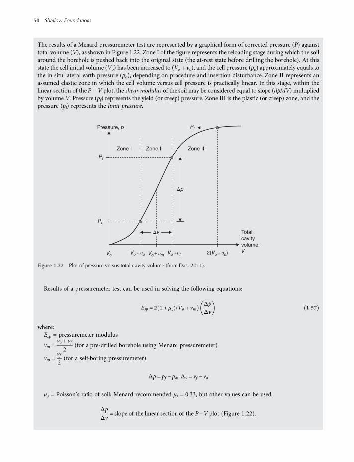
The results of a Menard pressuremeter test are represented by a graphical form of corrected pressure (P) againsttotal volume (V), as shown in Figure 1.22. Zone I of the figure represents the reloading stage during which the soilaround the borehole is pushed back into the original state (the at-rest state before drilling the borehole). At thisstate the cell initial volume (Vo) has been increased to (Vo + vo), and the cell pressure (po) approximately equals tothe in situ lateral earth pressure (ph), depending on procedure and insertion disturbance. Zone II represents anassumed elastic zone in which the cell volume versus cell pressure is practically linear. In this stage, within thelinear section of the P − V plot, the shear modulus of the soil may be considered equal to slope (dp/dV) multipliedby volume V. Pressure (pf) represents the yield (or creep) pressure. Zone III is the plastic (or creep) zone, and thepressure (pl) represents the limit pressure.
Results of a pressuremeter test can be used in solving the following equations:
Esp = 2 1 + μs Vo + vmΔpΔv
1 57
where:Esp = pressuremeter modulus
vm =vo + vf
2(for a pre-drilled borehole using Menard pressuremeter)
vm =vf2(for a self-boring pressuremeter)
Δp= pf −po, Δv = vf −vo
μs = Poisson’s ratio of soil; Menard recommended μs = 0.33, but other values can be used.
ΔpΔv
= slope of the linear section of the P−V plot Figure 1 22
Pressure, p
Zone I Zone II Zone III
Total
cavity
volume,
V
Δp
Δv
Pf
Pl
Po
Vo Vo+ υfVo+ υo 2(Vo+ υo)Vo+ υm
Figure 1.22 Plot of pressure versus total cavity volume (from Das, 2011).
50 Shallow Foundations
worksaccounts.com

According to Ohya et al. (1982):
Esp kN m2 = 1930N0 6360 for clays 1 58
Esp kN m2 = 908N0 6660 for sands 1 59
Esp = 2 1 + μs Gsp 1 60
Gsp = Vo + vmΔpΔv
1 61
where:
Gsp = pressuremeter shear modulus
ΔVV
= 1− 1 + εc−2
1 62
where
ΔVV
= volumetric strain of soil
εc = circumferential strain
= increase in cavity radiusΔr radius ro
Ko =phσo
≈poσo
1 63
where Ko = at-rest earth-pressure coefficient.σo = total vertical stress
According to Kulhawy and Mayne (1990):
σc = 0 45 pl 1 64
where σc =Preconsolidation pressurepl = limit pressure (Figure 1.22)
According to Baguelin et al. (1978):
cu =pl−poNp
1 65
where Np = 1 + lnEsp3cu
; cu = the undrained shear strength of soil. Typical values of Np vary between 5 and 12.
In the case of saturated clays, it is possible to obtain the value of cu by iteration from the following expression:
pl−po = cu lnGsp
cu+ 1 1 66
Note: Experience indicates that cu values obtained from pressuremeter tests are probably higher by about 50%than the values obtained from other tests.A comprehensive review of the use of pressuremeter, including examples of test results and their applications
in design, has been given by Mair and Wood (1987) and Clarke (1995). Also, an analysis for the interpretation
(Continued)
Site Investigation in Relation to Analysis and Design of Foundations 51
worksaccounts.com

of pressuremeter tests in sands has been given by Hughes, Wroth and Windle (1977). Those who are interestedin the pressuremeter test should refer to E. Winter (1982) for the test and calibration details and to Briaud andGambin (1984), and Briaud (1989) for borehole preparation (which is extremely critical).
Solution:
Equation (1.57): Esp = 2 1 + μs Vo + vmΔpΔv
vm =vo + vf
2= 46 + 180 2 = 113 cm3
Δp= pf −po = 326 5−42 4 = 284 1 kPa
ΔV = vf −vo = 180−46 = 134 cm3
Esp = 2 1 + 0 5 535 × 10−6 + 113 × 10−6284 1
134 × 10−6= 4122 kPa
Problem 1.18
Refer to Problem 1.17. The test was conducted at a depth of 4 m below the existing ground surface. Saturated γ ofthe clay was 20 kN/m3. The test results gave the limit pressure pl = 400 kN/m2. Determine: σc, Gsp, Ko and a designvalue for cu. Also, find an approximate value for N60.
Solution:Equation (1.64): σc = 0 45 pl = 0 45 × 400 = 180 kN m2
Equation (1.61): Gsp = Vo + vmΔpΔv
= 535 × 10−6 + 113 × 10−6284 1
134 × 10−6
= 648 × 2 12 = 1374 kN m2
Equation (1.63): Ko =phσo
≈poσo
=42 420 × 4
= 0 53
Equation (1.65): cu =pl−poNp
Typical values for Np vary in the range 5 to 12; assume Np = 8.5.
cu =400−42 4
8 5= 42 1 kN m2
Equation (1.66): pl−p = cu lnGsp
cu+ 1
400−42 4 = cu ln1374cu
+ 1 . Using iteration, find cu = 98.4 kN/m2
However, it is recommended to reduce this value by 50%; hence, cu = 49.2 kN/m2.Average of the two results is 45.7 kN/m2. Hence,
Use cu = 45 kN m2
52 Shallow Foundations
worksaccounts.com
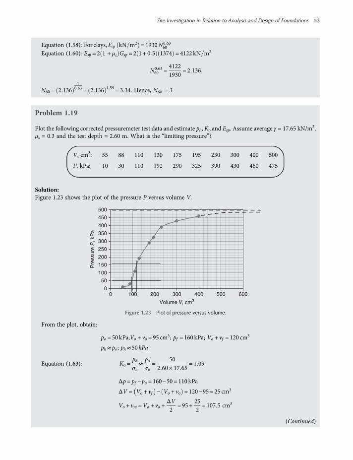
Equation (1.58): For clays, Esp kN m2 = 1930N0 6360
Equation (1.60): Esp = 2 1 + μs Gsp = 2 1 + 0 5 1374 = 4122 kN m2
N0 6360 =
41221930
= 2 136
N60 = 2 1361
0 63 = 2 136 1 59 = 3 34. Hence, N60 = 3
Problem 1.19
Plot the following corrected pressuremeter test data and estimate ph, Ko and Esp. Assume average γ = 17.65 kN/m3,μs = 0.3 and the test depth = 2.60 m. What is the “limiting pressure”?
V, cm3: 55 88 110 130 175 195 230 300 400 500
P, kPa: 10 30 110 192 290 325 390 430 460 475
Solution:Figure 1.23 shows the plot of the pressure P versus volume V.
From the plot, obtain:
po = 50 kPa;Vo + vo = 95 cm3; pf = 160 kPa; Vo + vf = 120 cm3
ph≈po; ph≈50 kPa
Equation (1.63): Ko =phσo
≈poσo
=50
2 60 × 17 65= 1 09
Δp= pf −po = 160−50 = 110 kPa
ΔV = Vo + vf − Vo + vo = 120−95 = 25 cm3
Vo + vm =Vo + vo +ΔV2
= 95 +252= 107 5 cm3
(Continued)
0
50
Pre
ssure
P, kP
a
Volume V, cm3
100
150
200
250
300
350
400
450
500
0 200 300 400 500 600100
Figure 1.23 Plot of pressure versus volume.
Site Investigation in Relation to Analysis and Design of Foundations 53
worksaccounts.com
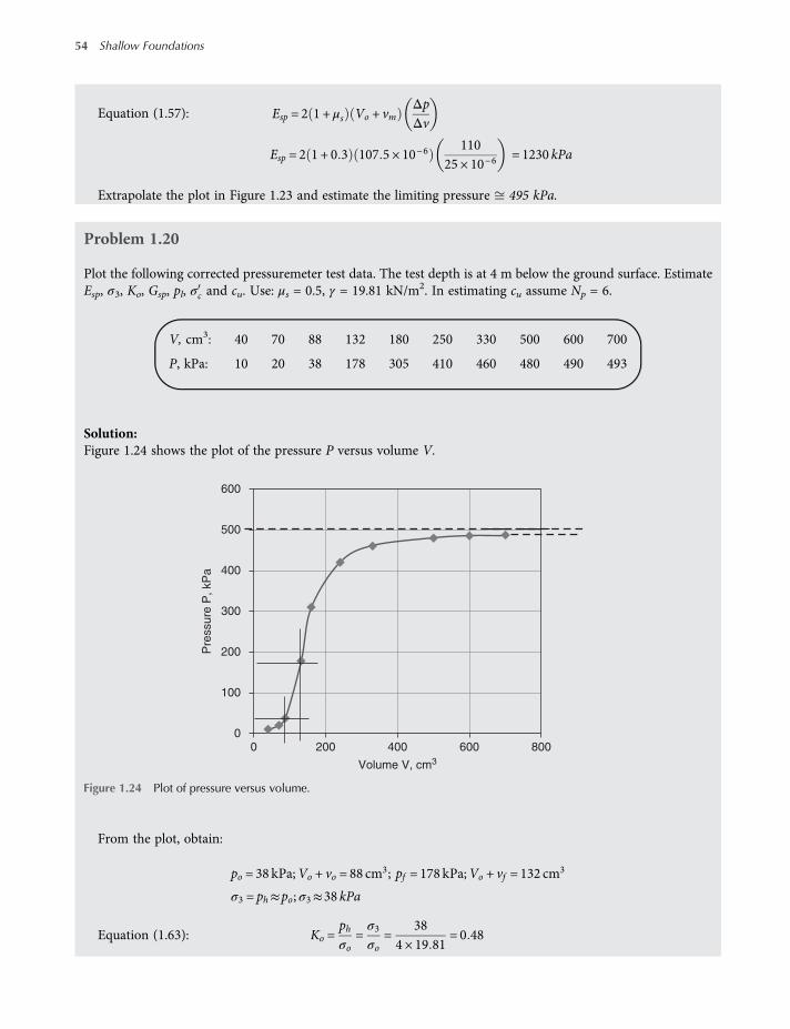
Equation (1.57): Esp = 2 1 + μs Vo + vmΔpΔv
Esp = 2 1 + 0 3 107 5 × 10−6110
25 × 10−6= 1230 kPa
Extrapolate the plot in Figure 1.23 and estimate the limiting pressure 495 kPa.
Problem 1.20
Plot the following corrected pressuremeter test data. The test depth is at 4 m below the ground surface. EstimateEsp, σ3, Ko, Gsp, pl, σc and cu. Use: μs = 0.5, γ = 19.81 kN/m2. In estimating cu assume Np = 6.
V, cm3: 40 70 88 132 180 250 330 500 600 700
P, kPa: 10 20 38 178 305 410 460 480 490 493
Solution:Figure 1.24 shows the plot of the pressure P versus volume V.
From the plot, obtain:
po = 38 kPa;Vo + vo = 88 cm3; pf = 178 kPa;Vo + vf = 132 cm3
σ3 = ph≈po; σ3≈38 kPa
Equation (1.63): Ko =phσo
=σ3σo
=38
4 × 19 81= 0 48
0
100
200
300
400
500
600
0 200 400 600 800
Pre
ssure
P, kP
a
Volume V, cm3
Figure 1.24 Plot of pressure versus volume.
54 Shallow Foundations
worksaccounts.com

Δp= pf −po = 178−38 = 140 kPaΔV = Vo + vf − Vo + vo = 132−88 = 44 cm3
Vo + vm =Vo + vo +Δv2
= 88 +442= 110 cm3
Equation (1.57): Esp = 2 1 + μs Vo + vmΔpΔv
Esp = 2 1 + 0 5 110 × 10−6140
44 × 10−6= 1050 kPa
Equation (1.61): Gsp = Vo + vmΔpΔv
= 110 × 10−6140
44 × 10−6= 350 kPa
Extrapolate the plot in Figure 1.24 and estimate the limiting pressure 500 kPa
Equation (1.64): σc = 0 45 pl = 0 45 × 500 = 225 kN m2
Equation (1.65): cu =pl −poNp
=500−38
6= 77 kPa
Problem 1.21
A dilatometer test (DMT) was conducted in a clay deposit. The water table was located at a depth of 3 m below theground surface. At 8 m depth the contact pressure (p1) was 280 kPa and the expansion stress (p2) was 350 kPa.Assume σo = 95 kPa at the 8 m depth and μ = 0.35. Determine (a) Coefficient of at-rest earth pressure Ko,(b) Overconsolidation ratio OCR and (c) Modulus of elasticity Es.
Discussion:ADMT is an in situ test carried out in order to assess the in place stresses and compressibility of soils. The test usesa device called dilatometer developed during the late 1970s in Italy by Silvano Marchetti. It is also known as a flatdilatometer or aMarchetti dilatometer. The device consists of a spade-shaped flat plate (tapered blade) measuring240 mm (length) × 95 mm (width) × 15 mm (thickness) with an expandable steel-faced membrane (pressure cell)60 mm in diameter on one face of the probe (Figure 1.25a). Figure 1.26 shows theMarchetti dilatometer along withits control panel and accessories. The dilatometer probe is inserted down by pushing or driving (if necessary). TheCPT pushing equipment (or some other suitable device) can be used for pressing the dilatometer (Figure 1.25b).In soils where the expected SPT-N value is greater than 35–40, it can be driven or pushed from the bottom of a
predrilled borehole using the SPT drilling and testing equipment. After insertion of the probe to the depth of inter-est z, the DMT is conducted as in the following steps:
(1) Apply nitrogen gas pressure to the expandable membrane so as to move it 0.05 mm into the soil and record therequired pressure (termed “liftoff” pressure) as p1. The operator gets a signal at liftoff.
(2) Increase the probe pressure until the membrane expands Δd = 1.1 mm into the adjacent soil and record thispressure as p2. This pressure is recorded after the operator receives a signal again.
(3) Decrease the pressure and take a reading when the membrane has returned to the liftoff position. Record thispressure as p3.
(4) The probe is then pushed to the next depth position, which is normally from 150 to 300 mm further down intothe ground, and the test is repeated. The probing is continued until the desired depth is reached.According to Schmertmann (1988), the CPT and DMT are complementary tests. The CPT is a good way to
evaluate soil strength, whereas the DMT assess the compressibility and in situ stresses. These three kinds ofinformation form the basis for most foundation engineering analysis. In addition, the dilatometer taperedblade is most easily pressed into the ground using a conventional CPT rig, so it is a simple matter to conductboth CPT and DMT while mobilising only a minimum of equipment.
(Continued)
Site Investigation in Relation to Analysis and Design of Foundations 55
worksaccounts.com

According to bothMarchetti (1980) and Schmertmann (1986) the DMT can be used to obtain the full range ofsoil ED, Ko, OCR, su, Ø and mv parameters for both strength and compressibility analyses.A given test data are reduced to obtain the following parameters:
(1) Dilatometer modulus ED. According to Marchetti (1980),
Δd =2D P2−P1
π
1−μ2
Es1 67
(a)
Wire to data acquisition equipment
14 mm
1.1 mm
lift off
95mm
D=
60
mm
Pu
sh
ro
d
z60mm
Flexible
membrane
Flexible
membrane
of diameter D
P2P1
Pneumatic
tubing
(b)
Figure 1.25 Schematic diagrams of a flat-plate dilatometer and the equipment inserter. (a) Marchetti dilatometer(after Marchetti, 1980). (b) The dilatometer pushed to depth z for test.
Figure 1.26 Dilatometer along with control panel and accessories (Courtesy of N.Sivakugan, James Kook University, Australia).
56 Shallow Foundations
worksaccounts.com
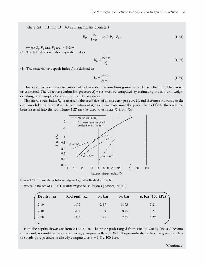
where Δd = 1.1 mm, D = 60 mm (membrane diameter)
ED =Es
1−μ2= 34 7 P2−P1 1 68
where Es, P1 and P2 are in kN/m2
(2) The lateral stress index KD is defined as
KD =p1−uσo
1 69
(3) The material or deposit index ID is defined as
ID =p2−p1p2−u
1 70
The pore pressure u may be computed as the static pressure from groundwater table, which must be knownor estimated. The effective overburden pressure σo = γ z must be computed by estimating the soil unit weightor taking tube samples for a more direct determination.The lateral stress index KD is related to the coefficient of at-rest earth pressure Ko and therefore indirectly to the
overconsolidation ratio OCR. Determination of Ko is approximate since the probe blade of finite thickness hasbeen inserted into the soil. Figure 1.27 may be used to estimate Ko from KD.
A typical data set of a DMT results might be as follows (Bowles, 2001):
Depth z, m Rod push, kg p1, bar p2, bar u, bar (100 kPa)
2.10 1400 2.97 14.53 0.21
2.40 1250 1.69 8.75 0.24
2.70 980 1.25 7.65 0.27
Here the depths shown are from 2.1 to 2.7 m. The probe push ranged from 1400 to 980 kg (the soil becamesofter) and, as should be obvious, values of p2 are greater than p1. With the groundwater table at the ground surfacethe static pore pressure is directly computed as u = 9.81z/100 bars.
(Continued)
2
1.5
1
0.8
0.6
0.5
0.4
0.31 1.5
ϕ′ = 25°
ϕ′ = 35°
2 3
In s
itu K
o
Lateral stress index KD
Marchetti (1980)
Schmertmann as cited
by Baldi et al. (1986)
4 5 6 7 8 910 15 20 30
ϕ′ = 40°
Figure 1.27 Correlations between KD and Ko (after Baldi et al. 1986).
Site Investigation in Relation to Analysis and Design of Foundations 57
worksaccounts.com
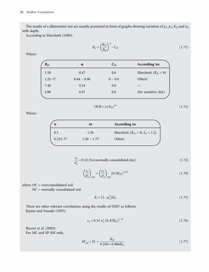
The results of a dilatometer test are usually presented in form of graphs showing variation of p1, p2, KD and IDwith depth.According to Marchetti (1980):
Ko =KD
BD
α
−CD 1 71
Where:
BD α CD According to:
1.50 0.47 0.6 Marchetti (KD < 8)
1.25–?? 0.44 – 0.46 0 – 0.6 Others
7.40 0.54 0.0 —
2.00 0.47 0.6 (for sensitive clay)
OCR= nKDm 1 72
Where:
n m According to
0.5 1.56 Marchetti (KD < 8; ID < 1.2)
0.225–?? 1.30 – 1.75 Others
cuσo
= 0 22 for normally consolidated clay 1 73
cuσo OC
=cuσo NC
0 5KD1,25 1 74
where OC = overconsolidated soilNC = normally consolidated soil.
Es = 1−μ2s ED 1 75
There are other relevant correlations using the results of DMT as follows:Kamei and Iwasaki (1995):
cu = 0 35 σo 0 47KD1 14 1 76
Ricceri et al. (2002):For ML and SP-SM soils,
Ø ult = 31 +KD
0 236 + 0 066KD1 77
58 Shallow Foundations
worksaccounts.com

Ø ult = 28 + 14 6 logKD−2 1 logKD2
1 78
The material index ID and the stress index KD together are related to the soil type and to the soil consistency ordensity, as illustrated in Figure 1.28.
Solution:
(a) Equation (1.71): Ko =KD
BD
α
−CD
Equation (1.69): KD =p1−uσo
=280−5 × 10
95= 2 42
According to Marchetti (1980):BD = 1 5, α= 0 47, CD = 0 6, for KD < 8
Ko =2 421 5
0 47
−0 6 = 0 65
(Continued)
Clay
ClayeySilty Silty
Silt
Sandy
Sand
Very rig
id
(2.15)
Medium rigidity
(1.90)
Low rigidity
(1.80)
Low density
(1.70)
Medium density
(1.80)
Loose
(1.70)
Rigid
(2.00)
Dense
(1.95)
Very dense
(2.10)
Hard
(2.05)
High consis
tency
(1.90)
Medium consis
tency
(1.80)
Low consistency
(1.70)*
Soft
(1.60)*
Compressible
(1.60)
100
200
50
20
10
5
Dila
tom
ete
r m
odulu
s, E
D(M
N/m
2)
2
1.2
1.0
0.510 0.2
0.35 0.6 0.9 1.2 1.8 3.3
0.5 1 2 5 10
Material index, ID
Mud/peat
(1.50)
(y) – Approximate soil unit weight in
t/m3 shown in parentheses
* – If PI > 50, then y in these regions is
overestimated by about 0.10 t/m3
Figure 1.28 Chart for determining soil type and estimating soil unit weight (After Schmertmann, 1986).
Site Investigation in Relation to Analysis and Design of Foundations 59
worksaccounts.com
(b) Equation (1.72): OCR = nKDm
According to Marchetti (1980):
n= 0 5, m= 1 56 for KD < 8; ID < 1 2
OCR= 0 5 × 2 42 1 56 = 1 35
(c) Equation (1.68): ED =Es
1−μ2= 34 7 P2−P1
Es1−μ2
= 34 7 350−280 = 2429 kPa
Es = 1−μ2 ED = 1−0 352 2429 = 2131 kPa
Problem 1.22
A dilatometer test was conducted in a sand deposit at a depth of 6 m. The water table was located at a depth of 2 mbelow the ground surface. Given: sand γd = 14.5 kN/m3, γsat = 19.8 kN/m3 and contact stress p1 = 260 kN/m2.Estimate the soil friction angles Ø and Ø ult .
Solution:
Equation (1.69): KD =p1−uσo
=260−4 × 10
2 × 14 5 + 4 19 8−10= 3 23
Equation (1.77): Ø = 31 +KD
0 236 + 0 066KD= 31 +
3 230 236 + 0 066 × 3 23
= 38 2
Equation (1.78): Ø ult = 28 + 14 6 logKD−2 1 logKD2
= 28 + 14 6 log3 23 – 2 1 log3 23 2
= 28 + 7 434−0 545 Ø ult = 34 9
Problem 1.23
Below is a corrected DMT data set. For the individually assigned depth value, estimate ED, KD, ID, Ko, and soildescription. In case the soil classification suggests fine-grained soil, an estimate of cu is required.
Depth z, m Rod push, kg p1, bar p2, bar u, bar*
2.10 1400 2.97 14.53 0.21
2.40 1250 1.69 8.75 0.24
2.70 980 1.25 7.65 0.27
∗1 bar ≈ 100 kPa.
60 Shallow Foundations
worksaccounts.com
Solution:DMTat 2.1mdepth: Both γ and μ are not known; they must be assumed. Therefore, Assume γsat = 19 kN/m3 andμ = 0.35. From the u values it is clear that the groundwater table is located at the ground surface. Use 1 bar = 100kN/m2.Equation (1.68): ED =
ES1−μ2
= 34 7 P2−P1
= 34 7 1453−297 = 40 113 kPa
Equation (1.69): KD =p1−uσo
=297−21
2 1 19−10= 14 6
Equation (1.70): ID =p2−p1p2−u
=1453−2971453−21
= 0 81
In the Marchetti equation of Ko [i.e. Equation (1.71)] the assigned values for BD, α and CD factors may not beapplicable because KD is greater than 8. In such a case we may assign other’s values for the factors and useEquation (1.71), or estimate Ko from the Schmertmann curves of Figure 1.27. Let us try both possibilities:
(1) Using other values for BD, α and CD factors [refer to the table of the factors which belong to Equation (1.71)].Assume average values as follows:
BD =1 25 + 7 4 + 2 0
3= 3 55; α=
0 45 + 0 54 + 0 473
= 0 49; CD =0 3 + 0 + 0 6
3= 0 3
Equation (1.71): Ko =KD
BD
α
− CD =14 63 55
0 49
− 0 3 = 1 7
(2) Using Figure 1.27. ForKD = 14.60 and a Ø value between 35 and 40 , the Schmertmann curves give a value forKo 1.5.
Using the average of the estimated two values, obtain Ko = 1.6.The soil is considered overconsolidated since the upper limit for Ko in normally consolidated soils is 1.
Using the Schmertmann chart of Figure 1.28, for the estimated ED and ID values, the soil is very dense clayeysilt. Therefore, the soil may be described as very dense overconsolidated clayey silt.DMT at 2.4 m depth:
Equation (1.68): ED =ES
1−μ2= 34 7 P2−P1 = 34 7 875−169
= 24 498 kPa
Equation (1.69): KD =p1−uσo
=169−24
2 4 19−10= 6 71
Equation (1.70): ID =p2−p1p2−u
=875−169875−24
= 0 83
Equation (1.71):
Ko =KD
BD
α
−CD; KD = 6 71 < 8
=6 711 5
0 47
−0 6 = 1 42 > 1 overconsolidated soil
Using the Schmertmann chart of Figure 1.28, for the estimated ED and ID values, the soil is dense clayey silt.Therefore, the soil may be described as dense overconsolidated clayey silt.DMT at 2.7 m depth:
Equation (1.68): ED =ES
1−μ2= 34 7 = P2−P1 = 34 7 765−125
= 22 208 kPa(Continued)
Site Investigation in Relation to Analysis and Design of Foundations 61
worksaccounts.com
Equation (1.69): KD =p1−uσo
=125−27
2 7 19−10= 4 03
Equation (1.70): ID =p2−p1p2−u
=765−125765−27
= 0 87
Equation (1.71): Ko =KD
BD
α
−CD; KD = 4 03 < 8
=4 031 5
0 47
−0 6 = 1 0 slightly overconsolidated soil
Using the Schmertmann chart of Figure 1.23, for the estimated ED and ID values, the soil is dense clayey silt.Therefore, the soil may be described as dense slightly overconsolidated clayey silt.Summary of results:
z, m ED KD ID Ko Soil description
2.10 40113 14.60 0.81 1.80 very dense overconsolidated clayey silt
2.40 24498 6.71 0.83 1.42 dense overconsolidated clayey silt
2.70 22208 4.03 0.87 1.00 dense slightly overconsolidated clayey silt
Problem 1.24
The results of a refraction survey at a site are given in Table 1.13. Determine the thickness and the P-wave velocityof the materials encountered.
Discussion:In the last five decades, even earlier, the trend for increased knowledge of subsurface conditions has placedemphasis upon methods which save time and money in obtaining this information. This is why geophysicalmethods have been developed. Among the several developed and used, the seismic refraction and electrical resist-ivity methods have received the widest use. The basic philosophy of geophysical methods of exploration is thatchanges in subsurface conditions near the surface of the earth can be detected by the nature of the physical
Table 1.13 Refraction survey site results.
Distance from the sourceof disturbance (m)
Time of first arrival ofP-waves (s × 10−3)
10.0 50.0
20.0 100.0
24.0 118.0
30.49 148.2
45.73 174.2
60.98 202.8
76.22 228.6
91.46 256.7
62 Shallow Foundations
worksaccounts.com
characteristics of the material. Generally speaking, these methods are particularly suited for large sites and forareas inaccessible to other forms of equipment when the geology of these areas is well known, that is, when thematerials to be encountered are known but the depths at which they lie are to be determined. The main uses ofseismic refraction and resistivity methods in foundation exploration are:
(1) To determine the depths and homogeneity of the soil and rock layers. The methods are accurate enough; how-ever, classification and identification of the soil and rock type cannot always be accurately accomplished. Theengineering properties of soils, to some extent, can be detected; however, the results would not be accurateenough for direct use in the foundations design.
(2) To detect subsurface anomalies such as faults, caves, cavities and sinkholes. Caves and sinkholes, however, canbest be located by resistivity methods.
(3) To aid in planning the initial boring plan. The boring plan will require less change and a better estimate ofthe cost and time required for detailed exploration can bemade if a geophysical investigation is conducted first.
(4) To complement borings, so a more complete soil profile can be drawn. Closely spaced borings are costly andmay not find trouble areas that may often be easily detected by a geophysical investigation. Complementaryuse of geophysical data and boring can save time and money during all phases of design and construction.Seismic Refraction Method (ASTM D 5777): In this method impact or shock waves are generated either by
the detonation of explosives or by striking a metal plate with a large hammer at a certain location on theground surface, such as point A in Figure 1.29. The equipment consists of one or more sensitive vibrationtransducers, called geophones, installed at a number of points in a straight line with increasing distances fromthe source of wave generation, and an extremely accurate time-measuring device called seismograph. Thelength of the line of points should be three to five times the required depth of investigation. A circuit betweenthe detonator or hammer and the seismograph starts the timing mechanism at the instant of detonation orimpact. The geophone is also connected electrically to the seismograph. When the first wave reaches the geo-phone the timing mechanism stops and the time interval is recorded in milliseconds.Seismic waves bend (refract) with different velocities when crossing different strata interface. Using this wave
property and the principles of wave propagation in layered systems, different strata thickness can be determined.An impact on the ground surface creates different types of stress wave, such as the compression or P-wave
and shear or S-wave. The P-waves travel faster than the S-waves; hence the first arrival of disturbance waveswill be related to P-waves in various layers. P-wave and S-wave velocities range in common geotechnicalmaterials are given in Tables 1.14 and 1.15, respectively.The velocity of P-waves in a medium is
vP =λ+ 2Gs
ρ=
Es 1−μsγ
g1−2μs 1 + μs
1 79
Where λ = Lame s constant = 2μsGs 1−2μsρ = mass density of medium = γ/gGs = dynamic shear modulus of medium= Es 2 1 + μsg = acceleration due to gravity (9.81 m/s2)Es = modulus of elasticity of mediumγ = unit weight of mediumμs = Poisson’s ratio of mediumThe velocity vp and thickness Z of various layers are determined as follows:
• Times of first wave arrival t1, t2, t3 … for distances x1, x2, x3 … from impact source are recorded.
• A plot of time t versus distance x is prepared (Figure 1.30).
• Slope of the lines l1, l2, l3 … are determined using slope of l1 =1v1, slope of l2 =
1v2, slope of l3 =
1v3, …; vel-
ocities v1, v2, v3, …, are the P-wave velocities in layers I, II, III; …, respectively (Figure 1.29).
(Continued)
Site Investigation in Relation to Analysis and Design of Foundations 63
worksaccounts.com
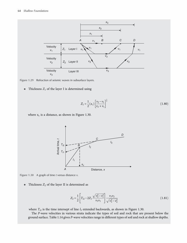
• Thickness Z1 of the layer I is determined using
Z1 =12xc
v2−v1v2 + v1
12
1 80
where xc is a distance, as shown in Figure 1.30.
• Thickness Z2 of the layer II is determined as
Z2 =12
Ti2−2Z1v23 −v
21
v3v1
v3v2v23 −v
22
1 81
where Ti2 is the time intersept of line l3 extended backwards, as shown in Figure 1.30.The P-wave velocities in various strata indicate the types of soil and rock that are present below the
ground surface. Table 1.14 gives P-wave velocities range in different types of soil and rock at shallow depths.
•• • •
Layer I
Layer III
Layer II
Velocity
v3
Velocity
v2
Velocity
v1
x3
x2
x1
A B C Dv1
v1 v1 v1v1
v2
v2
v2
v3
Z2
Z1
Figure 1.29 Refraction of seismic waves in subsurface layers.
Arr
ival tim
e, t
Distance, x
Ti2
Ti1
l2
l3
l1
A
C
B
D
xc
Figure 1.30 A graph of time t versus distance x.
64 Shallow Foundations
worksaccounts.com
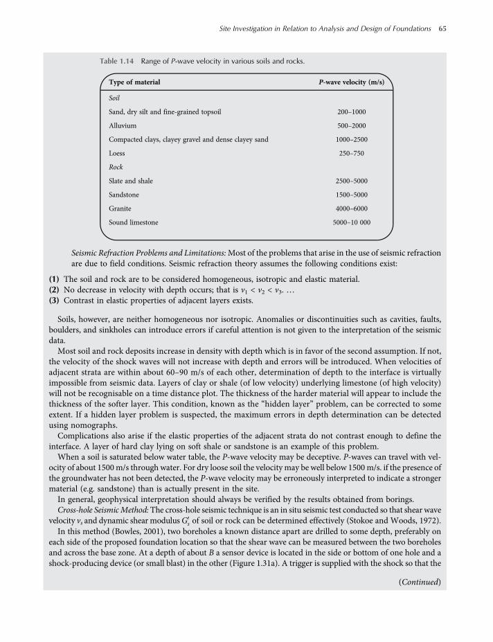
Seismic Refraction Problems and Limitations:Most of the problems that arise in the use of seismic refractionare due to field conditions. Seismic refraction theory assumes the following conditions exist:
(1) The soil and rock are to be considered homogeneous, isotropic and elastic material.(2) No decrease in velocity with depth occurs; that is v1 < v2 < v3. …(3) Contrast in elastic properties of adjacent layers exists.
Soils, however, are neither homogeneous nor isotropic. Anomalies or discontinuities such as cavities, faults,boulders, and sinkholes can introduce errors if careful attention is not given to the interpretation of the seismicdata.Most soil and rock deposits increase in density with depth which is in favor of the second assumption. If not,
the velocity of the shock waves will not increase with depth and errors will be introduced. When velocities ofadjacent strata are within about 60–90 m/s of each other, determination of depth to the interface is virtuallyimpossible from seismic data. Layers of clay or shale (of low velocity) underlying limestone (of high velocity)will not be recognisable on a time distance plot. The thickness of the harder material will appear to include thethickness of the softer layer. This condition, known as the “hidden layer” problem, can be corrected to someextent. If a hidden layer problem is suspected, the maximum errors in depth determination can be detectedusing nomographs.Complications also arise if the elastic properties of the adjacent strata do not contrast enough to define the
interface. A layer of hard clay lying on soft shale or sandstone is an example of this problem.When a soil is saturated below water table, the P-wave velocity may be deceptive. P-waves can travel with vel-
ocity of about 1500m/s through water. For dry loose soil the velocity may be well below 1500m/s. if the presence ofthe groundwater has not been detected, the P-wave velocity may be erroneously interpreted to indicate a strongermaterial (e.g. sandstone) than is actually present in the site.In general, geophysical interpretation should always be verified by the results obtained from borings.Cross-hole SeismicMethod:The cross-hole seismic technique is an in situ seismic test conducted so that shear wave
velocity vs and dynamic shear modulusGs of soil or rock can be determined effectively (Stokoe and Woods, 1972).In this method (Bowles, 2001), two boreholes a known distance apart are drilled to some depth, preferably on
each side of the proposed foundation location so that the shear wave can be measured between the two boreholesand across the base zone. At a depth of about B a sensor device is located in the side or bottom of one hole and ashock-producing device (or small blast) in the other (Figure 1.31a). A trigger is supplied with the shock so that the
(Continued)
Table 1.14 Range of P-wave velocity in various soils and rocks.
Type of material P-wave velocity (m/s)
Soil
Sand, dry silt and fine-grained topsoil 200–1000
Alluvium 500–2000
Compacted clays, clayey gravel and dense clayey sand 1000–2500
Loess 250–750
Rock
Slate and shale 2500–5000
Sandstone 1500–5000
Granite 4000–6000
Sound limestone 5000–10 000
Site Investigation in Relation to Analysis and Design of Foundations 65
worksaccounts.com
time for the induced shear wave can be observed at the pickup unit. The time of travel Th of the known distanceDh
between the two holes gives the shear wave velocity vs as
vs =Dh
Th1 82
The dynamic shear modulus of the material at the depth at which the test is taken can be determined from therelation
Gs =v2s γg
or vs =Gs
γ g1 83
Borehole
Borehole
Borehole
Energy source
(a)
(b)
Energy source
Detector unit
Detector unit
Pickup
Pickup
Pickup unit
Pickup unit
Trace
Trigger
Trigger
Distance
Figure 1.31 Two seismic methods for obtaining dynamic shear modulus Gs. (a) Cross-hole method, (b) Down-hole method(from Bowles, 2001).
66 Shallow Foundations
worksaccounts.com

Down-hole Seismic Method: The down-hole method is similar to the cross-hole but has the advantage of onlyrequiring one boring, as shown in Figure 1.31b. In this method, the hole is drilled, and a shock device is located aknown distance away. A shock detector is located at some known depth in the hole and a shock applied. As withthe cross-hole method, we can measure the time Th for arrival of the shear wave and, by computing the diagonalside of the triangle, obtain the travel distance Dh. The detector device is then placed at a greater depth and the testrepeated until a reasonably average value of vs is obtained.
Hoar and Stokoe (1978) discuss in some detail precautionary measures to take in making either of the abovementioned two tests so that the results can justify the test effort (Bowles, 2001).Electrical Resistivity Method: There are two types of the electrical resistivity methods:
(1) The electrical resistivity sounding method. It is used when the variation of resistivity of the subsurface mater-ials with depth is required at a predetermined location; resulting in rough estimates of types and depths ofstrata. In other words, the method can indicate subsurface variation when a hard layer overlies a soft layer orvice versa. It can also be used to locate the groundwater table.
(2) The electrical resistivity mapping (profiling) method. Here, the resistivity soundings are conducted alongdifferent profile lines across the area such that contours of resistivity variation with depth can be plotted.Themethods depend ondifferences in the electrical resistance of different types of soil and rock. Resistivity of a
material depends upon type of material, its water content and the concentration of dissolved salts in the porewater. Themineral particles of a soil are poor conductors of electric current; they are of high resistivity. Resistivityof a soil decreases (conductivity increases) as both the water content and pore water salts concentration increase.Approximate ranges of resistivity value for different types of soil and rock are given in Table 1.16.
(Continued)
Table 1.15 S-wave velocities range in common geotechnical materials at shallow depths.
Type of material S-wave velocity (m/s)
Hard rocks (e.g. metamorphic) 1400+
Firm to hard rocks (e.g. igneous, conglomerates, competent sedimentary) 700–1400
Gravelly soils and soft rocks (e.g. sandstone, shale, soils with > 20% gravel) 375–700
Stiff clays and sandy soils 200–375
Soft soils (e.g. loose submerged fills and soft clays) 100–200
Very soft soils (e.g. marshland, reclaimed soil) 50–100
Table 1.16 Representative values of resistivity.
Material Resistivity (ohm.m)
Sand 500–1500
Clays, saturated silt 0–100
Clayey sand 200–500
Gravel 1500–40 000
Weathered rock 1500–2500
Sound rock > 1500
Site Investigation in Relation to Analysis and Design of Foundations 67
worksaccounts.com
Resistivity of any conducting material having a length l and cross section area A is given by the equation:
ρ=RAl
1 84
where ρ = electrical resistivity (ohm.m)
R= electrical resistance ohm =voltage dropE
current I(Ohm’s law)
The in situ common electrical sounding procedure involves driving four electrodes, which are usually in theform of metal spikes, into the ground at equal distances L apart in a straight line (Figure 1.32a). The two outerelectrodes are known as current electrodes, and the inner electrodes are called potential electrodes. The current I,usually 50–100 mA, from a battery, flows through the soil between the two current electrodes producing an elec-trical field within the soil. The potential (voltage) drop E is then measured between the two potential electrodes.The mean (apparent) resistivity ρ is given by the equation:
ρ=2πLEI
1 85
Battery
Layer 1
Layer 2
(a)
(b)
Electrode spacing
Appa
rent re
sis
tivity
Milliammeter
Potentiometer
Nonpolarizing
electrodes
Steel pin
electrodes
Steel pin
electrodes
ρ2
ρ1
ρ1
ρ2
I
E
L
A B
L L
Figure 1.32 (a) Electrical resistivity method schematically illustrated; (b) apparent resistivity versus electrode spacing(redrawn from Knappett and Craig, 2012).
68 Shallow Foundations
worksaccounts.com
Equation (1.85) gives the mean resistivity up to a depth equals the distance L below the ground surface, as thedepth of current penetration below the ground surface is approximately equal to the spacing L of the two potentialelectrodes.A series of readings are taken, the (equal) spacingof the electrodes being increased for each successive reading; how-
ever the central position of the four electrodes remains unchanged. As L is increased, the resistivity ρ is influenced by agreater depth of soil. The distance L is thus gradually increases to a distance equal to the required depth of exploration.Themaximumdepth is usually about 30mor so. Ifρ decreaseswith increasingL a stratumof lower resistivity, suchas asaturated clay layer, is beginning to influence the readings. If ρ increases with increasing L it can be concluded that anunderlying stratum of higher resistivity, such as a gravel layer, is beginning to influence the readings.The mean resistivity ρ is plotted against the electrode spacing L, preferably on log-log paper. Characteristic
curves for a two-layer structure are illustrated in Figure 1.32b. For curve A the resistivity of layer 1 is lower thanthat of layer 2; for curve B the resistivity of layer 1 is higher than that of layer 2. The curves become asymptotic tolines representing the true resistivity ρ1 and ρ2 of the respective layers. Approximate layer thickness can beobtained by comparing the observed curve of ρ versus L with a set of standard curves, or, by using other methodsof interpretation, such as the method illustrated by the graph of Figure 1.33, which relates the sum of the apparentresistivity Σρ to the electrode spacing. In this figure, the slopes ρ1 and ρ2 are actual resistivity of layers 1 and 2,respectively.
Resistivity Problems and Limitations: The theoretical basis for electrical resistivity assumes:
(1) The soil or rock is homogeneous and isotropic.(2) Uniform resistivity exists.(3) The soil layers are parallel to each other and to ground surface.
Unfortunately, the assumed soil conditions seldom exist in the field because soil and rock are not homoge-neous and isotropic. Therefore the user must be aware of the effects on data caused by anomalies, such as faults,folded layers, caves, sinkholes or intermixing of soil and rock in the layers. Also, buried pipelines, undergroundcables, tunnels or any buried metallic materials will cause anomalous readings.Nonparallel layers cause bending or warping of the current flow lines causing erroneous resistivity readings. If
the ground surface and the interfaces are not parallel the exact depth below centre of the fixed location (centre ofthe spread) may not be found due to varying layer thickness.Materials differ in their electrical resistivity. The resistivity of materials does not change due to texture only,
but also because of the changes in the moisture and electrolytic content. As a result, considerable overlapping ofthe resistivity of various materials will exist. Overlapping makes interpretation of resistivity data very difficult insome cases.
(Continued)
Slope = ρ1
Electrode spacing, L
Σρ
Z1= thickness of
layer 1 Slope = ρ2
Figure 1.33 An approximate method for determining resistivity and thickness of subsurface layers.
Site Investigation in Relation to Analysis and Design of Foundations 69
worksaccounts.com

It is noteworthy: (1) there is no masked layer problem with electrical resistivity methods as there is with seis-mic methods, (2) an increase in material density is not necessary, as is the case with seismic refraction, (3) as theresistivity measures change in texture rather than change in strength and consolidation; it is generally used forlocating coarse-grained soil deposits within fine-grained soil deposits, (4) the resistivity methods are not con-sidered as reliable as the seismic methods, (5) as it is the case with seismic methods, the resistivity data shouldalso be supplemented by few borings, (6) since seismic and resistivity methods measure different properties, theycan be used effectively to complement each other.
Solution:Plot the times of first arrival of P waves against the distance of geophone from the source of disturbance, as shownin the scheme below.From the plot:
Slope of segment ab =1v1
=148 2 – 50 0 × 10−3
30 49 −10=0 09820 49
; hence,
v1 = 209m s
Slope of segment bc =1v2
=228 6 – 174 2 × 10⁻³
76 22 −45 73=0 05430 49
; hence
v2 = 565m s
From the plot: xc = 30.5 m
Equation (1.80): Z1 =12xc
v2−v1v2 + v1
12 =
12× 30 5
565−209565 + 209
12 = 10 34m
Thickness of the top layer = 10.34 m
0
50
100
150
200
250
300
0 20 40 60 80 100
c
Distance x, m
Tim
e o
f firs
t arr
ival t, s
ec
×10
–3
xc
a
b
Scheme 1.2
70 Shallow Foundations
worksaccounts.com
Problem 1.25
The plot in the scheme below represents the results of a seismic refraction survey.
Determine the P-wave velocities and the thickness of the material encountered in the third stratum.
Solution:From the plot:
Slope of segment ab =1v1
=47 × 10−3
10 5, v1 = 223 4m s first layer
Slope of segment ab =1v2
=25 × 10−3
19 5, v2 = 780 0m s second layer
Slope of segment cd =1v3
=4 5 × 10⁻³
20, v3 = 4444 4m s third layer
Comparing these velocity values with those given in Table 1.14, we find that the third layer is rock.From the plot: xc = 10.5 m
Equation (1.80): Z1 =12xc
v2−v1v2 + v1
12
Thickness of the first layer =Z1 =12xc
v2−v1v2 + v1
12
=12× 10 5
780 0 −223 4780 0 + 223 4
12 = 3 91m
Equation (1.81): Z2 =12
Ti2−2Z1v23 −v
21
v3v1
v3v2v23 −v
22
From the plot Ti2 = 66 × 10−3
(Continued)
80
60
40
20
00 10 20 30 40 50
c d
Distance x, m
Tim
e o
f firs
t arr
ival t, S
×10
–3
xc
Ti2
Ti1
a
b
Scheme 1.3
Site Investigation in Relation to Analysis and Design of Foundations 71
worksaccounts.com

Thickness of the second layer is
Z2 =12
66 × 10−3−2 3 914444 42−223 42
4444 4 × 223 44444 4 × 780
4444 42−7802= 12 29m
Surface of the rock layer is located at the depth D = Z1 + Z2 = 16.2 m
Problem 1.26
Using the data of Problem 1.25 determine the dynamic shear modulusGs and Es of the material encountered in thetop layer. Assume the unit weight γ of the material equals 16 kN/m3, and the Poisson’s ratio μs = 0.35.
Solution:
Equation (1.79): vP =λ+ 2Gs
ρ
λ= Lame s constant =Gs
1−2μs; ρ=
γ
g=
γ
9 81
vp =Gs
γ
9 811−2μs
+2Gsγ
9 81
=Gs
169 81
1−2 × 0 35+2Gs169 81
= 3 27Gs
vp = 223 4m s from Solution of Problem1 25
223 4 = 3 27Gs
Gs =223 42
3, 27= 15 262 kN m2
Gs =Es
2 1 + μsEs = 2Gs 1 + μs = 2 × 15262 1 + 0 35 = 41 207 kN m2
Problem 1.27
A seismic refraction test yielded the following data:v1 = 610 m/s; v2 = 4268 m/s; xc = 91.5 mThe profile was a two-layer system and no v3 was detected.Determine the thickness of the top layer.
Solution:
Equation (1.80): Z1 =12xc
v2−v1v2 + v1
12
Thickness of the top layer Z1 =12xc
v2−v1v2 + v1
12
=12× 91 5
4268−6104268 + 610
12
= 40m
72 Shallow Foundations
worksaccounts.com

References
AASHTO (1988), Manual on Subsurface Investigations, American Association of State Highway and transportation offi-cials, Developed by the Subcommittee on Materials, Washington, D.C.
ASCE (1972), “Subsurface Investigation for Design and Construction of Foundations of Buildings,” ASCE Journal of theSoil Mechanics and Foundations Division, Vol. 98 Nos SM5, SM6, SM7 and SM8.
ASTM (2009), Annual Book of ASTM Standards, Vol. 04.08, American Society for Testing and Materials, West Consho-hocken, PA.
Anagnostopoulos, A., Koukis, G., Sabtakakis, N. and Tsiambaos, G. (2003), “Empirical Correlations of Soil ParametersBased on Cone Penetration Tests (CPT) for Greek Soils,” Geotechnical and Geological Engineering, Vol. 21, No. 4,pp. 377–387.
Baban, Tharwat M. (1992), “The Required Depth of Soil Exploration for a Building Foundation.” The Scientific Journal ofSalahaddin University, Vol. 5, No. 3, pp. 77–87.
Baguelin, F., Jezequel, J. F. and Shields, D. H. (1978), The Pressuremeter and Foundation Engineering, Trans Tech Publi-cations, Clousthal, Germany.
Baldi, G., Bellotti, R., Gionna, V. and Jamiolkowski, M. (1982), “Design Parameters for Sands from CPT,” Proceedings,Second European Symposium on Penetration Testing, Amsterdam, Vol. 2, pp. 425–438.
Baldi, G., et al. (1986), “Flat Dilatometer Tests in Calibration Chambers,” 14th PSC, ASCE, pp. 431–446.Bjerrum, L. (1972), “Embankments on Soft Ground,” Proceedings of the Specialty Conference, ASCE, Vol. 2, pp. 1–54.BOCA (1996), National Building Code, Building Officials and Code Administrators International, Inc., Country Club
Hills, IL.Bowles, J. E. (2001), Foundation Analysis and Design, 5th edn, McGraw-Hill, New York.Briaud, J. L. (1989), “The Pressuremeter Test for Highway Applications,” Report FDHWA-IP-008, Federal Highway
Administration, Washington, D.C., 148.Briaud, J. L. and M. Gambin (1984), “Suggested Practice for Drilling Boreholes for Pressuremeter Testing,” GTJ, ASTM,
Vol. 7, No. 1, March, pp. 36–40.BSI (1999), BS 5930: 1999 Code of Practice for Site Investigations – Clause 12.6, British Standards Institution, London.BSI (2007), BS EN 1997-2: 2007 Ground Investigation and Testing – Clause B.3, British Standards Institution, London.BSI (2006), Geotechnical Investigation and Testing – Sampling Methods and Groundwater Measurements. Technical Prin-
ciples for Execution BS EN ISO 22475-1:2006, British Standards Institution, London.Chandler, R. J. (1988), “The In situ Measurement of the Undrained Shear Strength of Clays Using the Field Vane,” ASTM
STP No. 1014, pp. 13–44.Clarke, B. G. (1995), Pressuremeters in Geotechnical Design, International Thomson Publishing/BiTech Publishers,
Vancouver.Clayton, C. R. I. (1990), “SPT Energy Transmission: Theory, Measurement and Significance,”Ground Engineering,Vol. 23,
No. 10, pp. 35–43.Coduto, Donald P. (2001), Foundation Design: Principles and Practices, 2nd edn, Prentice-Hall, Inc., New Jersey.Craig, R. F. (2004), Soil Mechanics, 7th edn, Chapman and Hall, London.Cubrinovski, M. and Ishihara, K. (1999), “Empirical Correlations between SPT N-Values and Relative Density for Sandy
Soils,” Soils and Foundations, Vol. 39, No. 5, pp. 61–92.Das, Braja M. (2011), Principles of Foundation Engineering, 7th edn, CENGAGE Learning, United States.Deere, D. U. (1963), “Technical Description of Rock Cores for Engineering Purposes,” Felsmechanik und Ingenieurgeologie,
Vol. 1, No. 1, pp. 16–22.FHWA (2002), Subsurface Investigations-Geotechnical Site Characterization, Publication No. FHWANHI-01-031, Federal
Highway Administration, Washington, D.C.Gibbs, H. J. and Holtz, W. G. (1960), “Shear Strength of Cohesive Soils,” First PSC ASCE, pp. 33–162.Hansbo, S. (1957), A New Approach to the Determination of the Shear Strength of Clay by the Fall Cone Test, Swedish
Geotechnical Institute, Report No. 114.Hara, A., Ohata, T. and Niwa, M. (1971), “Shear Modulus and Shear Strength of Cohesive Soils,” Soils and Foundations,
Vol. 14, No. 3, pp. 1–12.Hatanaka, M. andUshida, A. (1996), “Empirical Correlation between Penetration Resistance and Internal Friction Angle of
Sandy Soils,” Soils and Foundations, Vol. 36, No. 4, pp. 1–10.Hoar, R. J. and K. H. Stokoe II (1978), “Generation and Measurement of Shear Waves In situ,” ASTM STP No. 645, pp.
3–29.Housel, W. S. (1929), “a Practical Method for the Selection of Foundations Based on Fundamental Research in Soil
Mechanics,” University of Michigan Engineering Research Bull. 13, Ann Arbour, Mich., October.Hughes, J. M. O., Worth, C. P. and Windle, D. (1977), “Pressuremeter Tests in Sands,” Geotechnique, 27, pp. 455–477.Ismael, N. F. and A. M. Jeragh (1986) “Static Cone Tests and Settlement of Calcareous Desert Sands,” CGJ, Vol. 23, No. 3,
Aug, pp. 297–303.
Site Investigation in Relation to Analysis and Design of Foundations 73
worksaccounts.com

Jamiolkowski, M., Ladd, C. C., Germaine, J. T. et al. (1985), “New Developments in Field and Laboratory Testing of Soils,”11th ICSMFE, Vol. 1, pp. 57–153.
Kamie, T. and Iwasaki, K. (1995), “Evaluation of Undrained Shear Strength of Cohesive Soils Using a Flat Dilatometer,”Soils and Foundations, Vol. 35, No. 2, pp. 111–116.
Knappett, J. A. and Craig, R. F. (2012), Soil Mechanics, 8th edn, Spon Press, Abingdon, United Kingdom.Kulhawy, F. H. and Mayne, P. W. (1990), Manual on Engineering Soil Properties for Foundation Design, Electric Power
Research Institute, Palo Alto, California.Lancellotta, R. (1983), Analisi di Affidabilita in Ingegneria Geotecnica, Atti Instituto Scienza Construzioni, No. 625, Poli-
tecnico di Torino.Larson, R. (1980), “Undrained Shear Strength in Stability Calculation of Embankments and Foundations on Clay,” Can-
adian Geotechnical Journal, Vol. 17, pp. 591–602.Lee, L., Salgado R. and Carraro, A. H. (2004), “Stiffness Degradation and Shear Strength of Silty Sand,” Canadian Geo-
technical Journal, Vol. 41, No. 5, pp. 831–843.Liao, S. S. C. andWhitman, R. V. (1986), “Overburden Correction Factors for SPT in Sand,” Journal of Geotechnical Engin-
eering Division, ASCE, Vol. 112, No. 3, March, pp. 373–377.Mair, R. J. and Wood, D. M. (1987), Pressuremeter Testing: Methods and Interpretation, Construction Industry Research
and Information Association/Butterworths, London.Marchetti, S. (1980), “In Situ Test by Flat Dilatometer,” Journal of Geotechnical Engineering Division, ASCE, Vol. 106, GT.
3, March, pp. 299–321.Marcuson, W. F., III and Bieganousky, W. A. (1980), “SPT and Relative Density in Coarse Sands,” Journal of Geotechnical
Engineering Division, ASCE, Vol. 103, No. 11, pp. 1295–1309.Mayne, P. W. and Mitchell, J. K. (1988), “Profiling of Over consolidation Ratio in Clays by Field Vane,” Canadian Geo-
technical Journal, Vol. 25, No. 1, pp. 150–158.Mayne, P. W. and Kemper, J. B. (1988), “Profiling OCR in Stiff Clays by CPT and SPT,” Geotechnical Testing Journal,
ASTM, Vol. 11, No. 2, pp. 139–147.Meigh, A. C. (1987), Cone Penetrometer Testing, Construction Industry Research and Information Association/Butter-
worths, London.Menard, L. (1956), “An Apparatus for Measuring the Strength of Soils in Place,”MSc Thesis, University of Illinois, Illinois.Morris, P. M. andWilliams, D. T. (1994), “Effective Stress Vane Shear Strength Correction Factor Correlations,” Canadian
Geotechnical Journal, Vol. 31, No. 3, pp. 335–342.Ohya, S., Imai, T. and Matsubara, M. (1982), “Relationships between N Value by SPT and LLT Pressuremeter Results,”
Proceedings, Second European Symposium on Penetration Testing, Vol. 1, Amsterdam, pp. 125–130.Peck, R. B., Hanson, W. E. and Thornburn T. H. (1974), Foundation Engineering, 2nd edn, John Wiley & Sons, Inc.,
New York.Ramaswamy, S. D., Daulah, I. U. and Hasan, Z. (1982), “Pressuremeter Correlations with Standard Penetration and Cone
Penetration Tests,” 2nd ESOPT, Vol. 1, pp. 137–142.Ricceri, G., Simonini, P. and Cola, S. (2002), “Applicability of Piezocone and Dilatometer to Characterize the Soils of the
Venice Lagoon,” Geotechnical and Geological Engineering, Vol. 20, No. 2, pp. 89–121.Robertson, P. K. (2010), “Soil Behaviour Type from the CPT: an update,” Second International Symposium on Cone Pene-
tration Testing, CPT10, Technical Paper No. 2-56, Huntington Beach, CA, USA, www.cpt10.com. Or, Soil behaviourtype from the CPT: an update. P.K. Robertson Gregg Drilling and Testing Inc., Signal Hill, California, USA.
Robertson, P. K. and Campanella, R G. (1986), “Interpretation of Cone Penetration Tests. Part I: Sand and Part II: Clay,”Canadian Geotechnical Journal, Vol. 20, No. 4, pp. 718–745.
Robertson, P. K. and Campanella, R. G. (1983), “SPT-CPT Correlations,” Journal of Geotechnical Engineering Division,ASCE, Vol. 109, No. 11, pp. 1449–1459.
Robertson, P. K. and Campanella, R. G. (1989), Guidelines for Geotechnical Design Using the Cone Penetrometer Test andCPT with Pore Pressure Measurement, 4th edn, Hogentogler and Co., Columbia, MD.
Schmertmann, J. H. (1970), “Static Cone to Compute Static Settlement over Sand,” Journal of Soil Mechanics and Foun-dations Division, ASCE, Vol. 96, SM 3, pp. 1011–1043.
Schmertmann, J. H. (1978), Guidelines for Cone Penetration Test: Performance and Design, Report FHWA-TS-78-209,Federal Highway Administration, Washington, D.C.
Schmertmann, J. H. (1986), “Suggested Method for Performing the Flat Dilatometer Test,” Geotechnical Testing Journal,ASTM, Vol. 9, No. 2, pp. 93–101.
Seed, H. B., Arango, I. and Chan, C. K. (1975), Evaluation of Soil Liquefaction Potential during Earthquakes, Report No.EERC 75-28, Earthquake Engineering Research Centre, University of California, Berkeley.
Skempton, A.W. (1986), “Standard Penetration Test Procedures and the Effects in Sands of Overburden Pressure, RelativeDensity, Particle Size, Aging and Over consolidation,” Geotechnique, Vol. 36, No. 3, pp. 425–447.
Smith, R. E. (1970), “Guide for Depth of Foundation Exploration,” Journal of Soil Mechanics and Foundations Division,ASCE, Vol. 96, SM 2, March, pp. 377–384.
74 Shallow Foundations
worksaccounts.com
Sowers, G. B. and Sowers, G. F. (1970), Introductory Soil Mechanics and Foundations, 3rd edn, Macmillan, New York.Sowers, G. F. (1979), Introductory Soil Mechanics and Foundations, 4th edn, Macmillan, New York.Stokoe, K. H. and Woods, R. D. (1972), “In Situ Shear Wave Velocity by Cross-Hole Method,” Journal of Soil Mechanics
and Foundations Division, ASCE, Vol. 98, SM 5, pp. 443–460.Stroud, M. A. and Butler, F. G. (1975), “The Standard Penetration Test and the Engineering Properties of Glacial
Materials,” Proceedings of a Symposium on the Engineering Behaviour of Glacial Materials, pp. 124–135, Midland Geo-technical Society, Birmingham.
Szechy, K. and Varga, L. (1978), Foundation Engineering – Soil Exploration and Spread Foundation, Akademial Klado,Budapest, Hungary.
Terzaghi, K., Peck, R. B. and Mesri, G. (1996), Soil Mechanics in Engineering Practice, 3rd edn, John Wiley & Sons, Inc.,New York.
Terzaghi, K., Peck, R. B. (1967), Soil Mechanics in Engineering Practice, 2nd edn, John Wiley & Sons, Inc., New York.Winter, E. (1982), “Suggested Practice for Pressuremeter Testing in Soils,”Geotechnical Testing Journal, ASTM, Vol. 5, No.
3/4, Sept, pp. 85–88.Wolff, T. F. (1989), “Pile Capacity Prediction Using Parameter Functions,” in Predicted and Observed Axial Behaviour of
Piles, Results of a Pile Prediction Symposium, ASCE Geotechnical Special Publication No. 23, pp. 96–106.
Site Investigation in Relation to Analysis and Design of Foundations 75
worksaccounts.com
CHAPTER 2
Shallow Foundations – IntroductoryChapter
2.1 General
In civil engineering, the foundation may be defined as that part of a structure which transmits loadsdirectly to the underlying soil and/or rock safely. This is also sometimes called the substructure, sincethe superstructure brings load onto the foundation, or substructure. The term foundation soil is com-monly used to describe the underlying material within the adjacent zone which will be affected by thesubstructure and its loads. This is also sometimes called the supporting soil, or base material, since thetotal structure will rest on it.
Generally, foundations may be broadly classified into two categories: (1) Shallow foundations, (2)Deep foundations.
A shallow foundation transmits loads to the near-surface strata; it is positioned at a shallow depth.According to Terzaghi and Peck (1967), a foundation is shallow if the least dimension (usually thewidth B) of the structural base is equal to or greater than the foundation depth Df . This criterion isreasonable for normal shallow foundations, but it is unsatisfactory for narrow or very wide founda-tions. Some investigators have suggested that Df can be as great as 3–4B (Das, 2011). Here, Df isthe vertical distance from the ground surface down to a level at which the bottom of the structuralbase is located. The level at this depth is usually known as the foundation level.
In practice, all the spread footing foundations are usually shallow foundations. Also, the mat and raftfoundations are mostly shallow foundations. Here, “spread” is a generic word can be applied to anystructural base that spreads its structure load on a large area. It is function of the base to spreadthe load laterally to the underlying strata so that the stress intensity is reduced to a value that the foun-dation soil or rock can safely carry. In practice, however, a spread footing is particularly used to meanan individual column footing.
Before the early twentieth century, almost all the spread footings were made of steel grillage ormasonry. The steel grillage footings included several layers of railroad tracks or I-beams placed in bothdirections. The masonry footings were dimension-stone footings built of stones cut and dressed to spe-cific sizes fit together with joints of very small gap, or, they were rubble-stone footings built of randomsize material joined with mortar. These footings prevailed until the advent of reinforced concrete in theearly twentieth century. Compared to steel grillage or masonry footings, reinforced concrete footingsare very strong, economical, durable and easy to build. Also, they are thinner and smaller in plan
Shallow Foundations: Discussions and Problem Solving, First Edition. Tharwat M. Baban.© 2016 John Wiley & Sons, Ltd. Published 2016 by John Wiley & Sons, Ltd.
worksaccounts.com
dimensions than the old masonry footings, so they do not require large excavations and do notintrude into basements. Therefore, nearly all shallow foundations are nowmade of reinforced concrete.
2.2 Types of Shallow Foundations
There are different types of shallow foundations. They are different due to the differences in theirgeometrical shape, design and construction. They are of the following types:
(1) Strip or continuous footing. Load bearing walls are supported by continuous-strip footings (alsoknown as wall footings) as shown in Figure 2.1. Transverse reinforcing steel bars are providedat the footing bottom to satisfy the bending requirements of the footing projection. Longitudinalsteel bars are required to satisfy shrinkage requirements. Longitudinal steel will, in general, bemoreeffective in the top of the footing than in the bottom.
A strip footing is also used to support a row of columns which are so closely spaced that theirindividual footings overlap or nearly touch each other. In this case it is more economical to exca-vate and concrete a strip foundation than to work in a large number of individual pits. In fact it isoften thought to be more economical to provide a strip footing whenever the distance between theadjacent individual footings is less than their dimensions. The individual footings are formed byinserting vertical joints in a continuous strip of concrete. Also, footings of this type, if the foun-dation soil conditions permit, are more economical in reinforcing steel than continuous combined(beam) footings.
(2) Spread footing (also, individual, single, isolated or independent column footing). This is an inde-pendent footing provided to support an individual column. The footing may be circular, squareor rectangular slab of uniform thickness or may be stepped or sloped, used to spread the load overa large area (Figure 2.2). An advantage of this type of footing foundation is that the footing size canbe adjusted to the same or different contact soil pressures. Also, the footings can be located at dif-ferent foundation levels so as to distribute the structure’s load advantageously over the site, holdingthe differential settlement within certain limits. It is often thought that this type of foundationbecomes more economical than the continuous-strip foundation when the required foundationdepth is greater than 1.5 m.
(3) Combined footing. When a reinforced concrete slab supports a line of two or more columns, it iscalled combined footing. An ordinary combined footing which supports two columns may be rect-angular or trapezoidal in plan (Figure 2.3). When the slab supports more than two columns it iscalled continuous combined footing. In this case, more often the slab has a longitudinal pedestalbeam (rib), and the footing is designed as a continuous inverted T-beam (Figure 2.4b). Combinedfootings are used when the columns are so close to each other that their individual footings wouldtouch each other or overlap. They are also used when the foundation soil is erratic and of relativelylow bearing capacity. A combined footing may be used when a column is located near or right nextto a property limit; it often supports the edge column and an interior column to avoid using anundesirable eccentrically loaded spread footing adjacent to the property line (Figure 2.4a).
R.C. wall footing
Transverse steel
Longitudinal steel
Masonry wall
Figure 2.1 Strip or continuous wall footing.
Shallow Foundations – Introductory Chapter 77
worksaccounts.com
Column
(round or
square)Footing
Shoulder for
column forms
Plan
Column
Elevation
(a) (b) (c)
PP P
Metal column Bearing base plate
Floor
Pedestal
FootingSection
(d)P
Figure 2.2 Typical spread column footings: (a) sloped footing, (b) footing of uniform thickness, (c) stepped footingand (d) footing with pedestal.
Columns Columns
Footing Footing B2B1B
L
(a) (b)
Elevation
Plan
S SP2P1 P1 P2
L
Figure 2.3 Typical ordinary combined footings: (a) rectangular footing; (b) trapezoid footing.
Combined
footings
ElevationPedestal
Combined
footings
Pedestal
Pedestal
(a) (b)
Footing
P3P1 P2
Beam
Side view
Plan
Figure 2.4 (a) Typical combined footings, (b) Combined footing with a pedestal beam designed as an invertedT-beam to reduce footing mass.
worksaccounts.com

(4) Strap footing. A strap footing (also known as a cantilever footing) consists of two individual foot-ings connected to each other with a structural rigid beam called strap; so it may be considered as aspecial form of the ordinary combined footing. Figure 2.5 shows the common arrangements ofstrap footings. The strap should be out of contact with soil so that there are no soil reactionand the srap could act as a rigid beam. Strap footings may be used in place of the combined footingsto achieve the same purposes. However, this type of foundation would be economical than rect-angular or trapezoidal combined footing foundations only when the allowable soil bearing capacityis high and the distance between the columns are relatively large. Similar to the continuous com-bined footing, strap footing can be continuous supporting more than two columns in one row;designed as continuous strap footing.
(5) Ring spread footing. This is a continuous-strip footing that has been wrapped into a circle(Figure 2.6). This type of footing is commonly used to support above-ground and elevated storagetanks, transmission towers, TV antennas and various process tower structures. Regarding the
Elevation
Elevation
Elevation
Plan
Plan
Plan
Strap Strap
Strap
P2P1
P1
P1P1
P2
P2P2
Strap Footing
Wall
(a) (b)
(c)
(d)
Column
Figure 2.5 Common configurations of strap footing.
Shallow Foundations – Introductory Chapter 79
worksaccounts.com
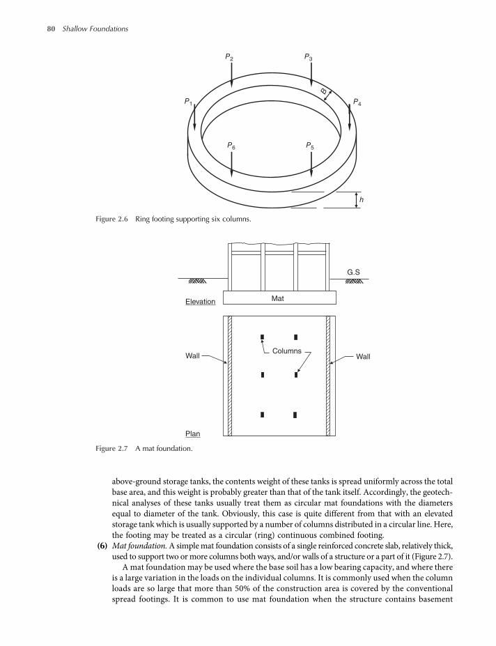
above-ground storage tanks, the contents weight of these tanks is spread uniformly across the totalbase area, and this weight is probably greater than that of the tank itself. Accordingly, the geotech-nical analyses of these tanks usually treat them as circular mat foundations with the diametersequal to diameter of the tank. Obviously, this case is quite different from that with an elevatedstorage tank which is usually supported by a number of columns distributed in a circular line. Here,the footing may be treated as a circular (ring) continuous combined footing.
(6) Mat foundation.A simplemat foundation consists of a single reinforced concrete slab, relatively thick,used to support two ormore columns both ways, and/or walls of a structure or a part of it (Figure 2.7).
A mat foundation may be used where the base soil has a low bearing capacity, and where thereis a large variation in the loads on the individual columns. It is commonly used when the columnloads are so large that more than 50% of the construction area is covered by the conventionalspread footings. It is common to use mat foundation when the structure contains basement
P2 P3
P4
h
B
P5P6
P1
Figure 2.6 Ring footing supporting six columns.
Mat
Plan
G.S
Elevation
WallColumns
Wall
Figure 2.7 A mat foundation.
80 Shallow Foundations
worksaccounts.com
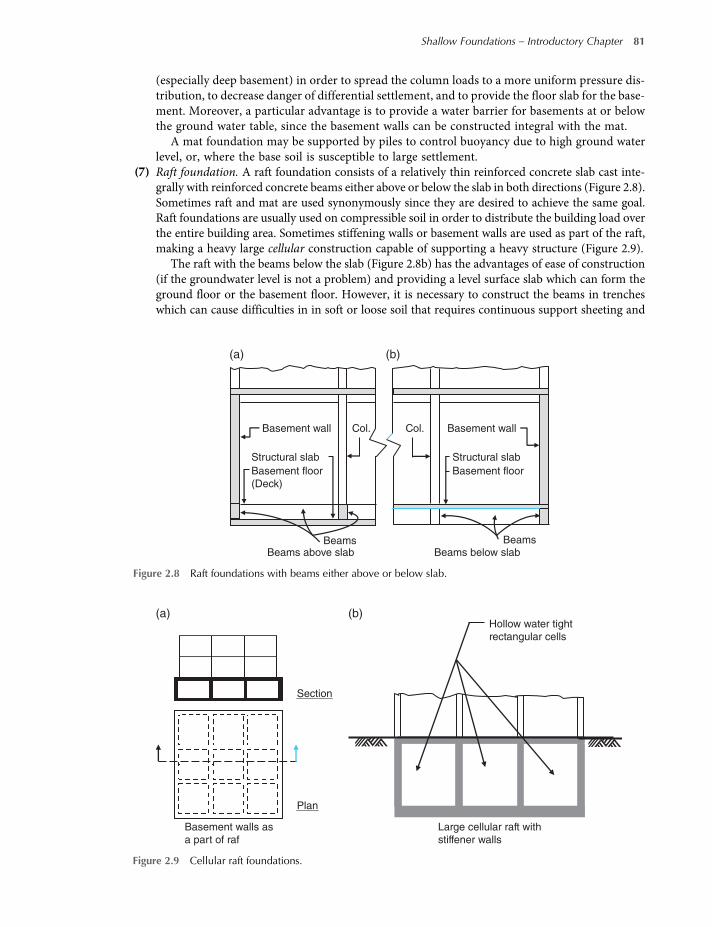
(especially deep basement) in order to spread the column loads to a more uniform pressure dis-tribution, to decrease danger of differential settlement, and to provide the floor slab for the base-ment. Moreover, a particular advantage is to provide a water barrier for basements at or belowthe ground water table, since the basement walls can be constructed integral with the mat.
A mat foundation may be supported by piles to control buoyancy due to high ground waterlevel, or, where the base soil is susceptible to large settlement.
(7) Raft foundation. A raft foundation consists of a relatively thin reinforced concrete slab cast inte-grally with reinforced concrete beams either above or below the slab in both directions (Figure 2.8).Sometimes raft and mat are used synonymously since they are desired to achieve the same goal.Raft foundations are usually used on compressible soil in order to distribute the building load overthe entire building area. Sometimes stiffening walls or basement walls are used as part of the raft,making a heavy large cellular construction capable of supporting a heavy structure (Figure 2.9).
The raft with the beams below the slab (Figure 2.8b) has the advantages of ease of construction(if the groundwater level is not a problem) and providing a level surface slab which can form theground floor or the basement floor. However, it is necessary to construct the beams in trencheswhich can cause difficulties in in soft or loose soil that requires continuous support sheeting and
Basement wall Basement wall
Structural slab Structural slab
Beams
(b)(a)
BeamsBeams above slab Beams below slab
Col.Col.
Basement floorBasement floor
(Deck)
Figure 2.8 Raft foundations with beams either above or below slab.
Plan
Section
(a) (b)Hollow water tight
rectangular cells
Large cellular raft with
stiffener walls
Basement walls as
a part of raf
Figure 2.9 Cellular raft foundations.
Shallow Foundations – Introductory Chapter 81
worksaccounts.com
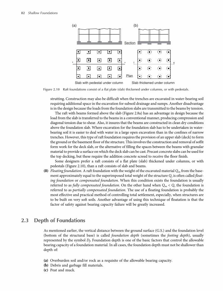
strutting. Construction may also be difficult when the trenches are excavated in water-bearing soilrequiring additional space in the excavation for subsoil drainage and sumps. Another disadvantageis in the design because the loads from the foundation slabs are transmitted to the beams by tension.
The raft with beams formed above the slab (Figure 2.8a) has an advantage in design because theload from the slab is transferred to the beams in a conventional manner, producing compression anddiagonal tension due to shear. Also, it insures that the beams are constructed in clean dry conditionsabove the foundation slab. Where excavation for the foundation slab has to be undertaken in water-bearing soil it is easier to deal with water in a large open excavation than in the confines of narrowtrenches. However, this type of raft foundation requires the provision of an upper slab (deck) to formthe ground or the basement floor of the structure. This involves the construction and removal of soffitform work for the deck slab, or the alternative of filling the spaces between the beams with granularmaterial to provide a surface onwhich the deck slab can be cast. Precast concrete slabs can be used forthe top decking, but these require the addition concrete screed to receive the floor finish.
Some designers prefer a raft consists of a flat plate (slab) thickened under columns, or withpedestals (Figure 2.10), than a raft consists of slab and beams.
(8) Floating foundation.A raft foundation with the weight of the excavated materialQm from the base-ment approximately equal to the superimposed total weight of the structureQs is often called float-ing foundation or compensated foundation. When this condition exists the foundation is usuallyreferred to as fully compensated foundation. On the other hand when Qm < Qs the foundation isreferred to as partially compensated foundation. The use of a floating foundation is probably themost effective and practical method of controlling total settlement, especially, when structures areto be built on very soft soils. Another advantage of using this technique of floatation is that thefactor of safety against bearing capacity failure will be greatly increased.
2.3 Depth of Foundations
As mentioned earlier, the vertical distance between the ground surface (G.S.) and the foundation level(bottom of the structural base) is called foundation depth (sometimes the footing depth), usuallyrepresented by the symbol Df. Foundation depth is one of the basic factors that control the allowablebearing capacity of a foundation material. In all cases, the foundation depth must not be shallower thandepth of:
(a) Overburden soil and/or rock as a requisite of the allowable bearing capacity.(b) Debris and garbage fill materials.(c) Peat and muck.
Section
Plan
(a) (b)
Slab thickened under columnSlab with pedestal under column
Figure 2.10 Raft foundations consist of a flat plate (slab) thickened under columns, or with pedestals.
82 Shallow Foundations
worksaccounts.com
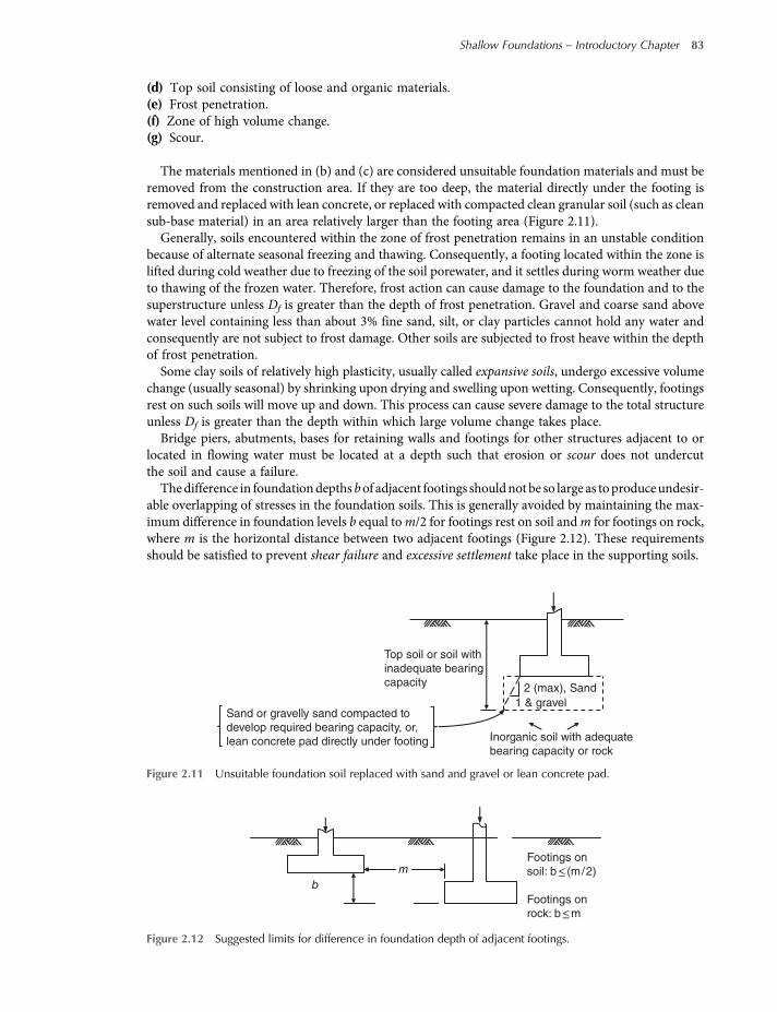
(d) Top soil consisting of loose and organic materials.(e) Frost penetration.(f) Zone of high volume change.(g) Scour.
The materials mentioned in (b) and (c) are considered unsuitable foundation materials and must beremoved from the construction area. If they are too deep, the material directly under the footing isremoved and replaced with lean concrete, or replaced with compacted clean granular soil (such as cleansub-base material) in an area relatively larger than the footing area (Figure 2.11).Generally, soils encountered within the zone of frost penetration remains in an unstable condition
because of alternate seasonal freezing and thawing. Consequently, a footing located within the zone islifted during cold weather due to freezing of the soil porewater, and it settles during worm weather dueto thawing of the frozen water. Therefore, frost action can cause damage to the foundation and to thesuperstructure unless Df is greater than the depth of frost penetration. Gravel and coarse sand abovewater level containing less than about 3% fine sand, silt, or clay particles cannot hold any water andconsequently are not subject to frost damage. Other soils are subjected to frost heave within the depthof frost penetration.Some clay soils of relatively high plasticity, usually called expansive soils, undergo excessive volume
change (usually seasonal) by shrinking upon drying and swelling upon wetting. Consequently, footingsrest on such soils will move up and down. This process can cause severe damage to the total structureunless Df is greater than the depth within which large volume change takes place.Bridge piers, abutments, bases for retaining walls and footings for other structures adjacent to or
located in flowing water must be located at a depth such that erosion or scour does not undercutthe soil and cause a failure.Thedifference in foundationdepthsbof adjacent footings shouldnot be so large as toproduceundesir-
able overlapping of stresses in the foundation soils. This is generally avoided by maintaining the max-imum difference in foundation levels b equal tom/2 for footings rest on soil andm for footings on rock,where m is the horizontal distance between two adjacent footings (Figure 2.12). These requirementsshould be satisfied to prevent shear failure and excessive settlement take place in the supporting soils.
Top soil or soil with
inadequate bearing
capacity
Sand or gravelly sand compacted to
develop required bearing capacity, or,
lean concrete pad directly under footing Inorganic soil with adequate
bearing capacity or rock
2 (max), Sand
1 & gravel
Figure 2.11 Unsuitable foundation soil replaced with sand and gravel or lean concrete pad.
m
b
Footings on
soil: b≤(m/2)
Footings on
rock: b≤m
Figure 2.12 Suggested limits for difference in foundation depth of adjacent footings.
Shallow Foundations – Introductory Chapter 83
worksaccounts.com
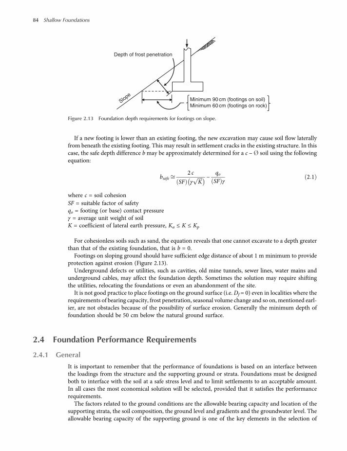
If a new footing is lower than an existing footing, the new excavation may cause soil flow laterallyfrom beneath the existing footing. This may result in settlement cracks in the existing structure. In thiscase, the safe depth difference bmay be approximately determined for a c – soil using the followingequation:
bsafe2 c
SF γ K−
qoSF γ
2 1
where c = soil cohesionSF = suitable factor of safetyqo = footing (or base) contact pressureγ = average unit weight of soilK = coefficient of lateral earth pressure, Ka ≤ K ≤ Kp
For cohesionless soils such as sand, the equation reveals that one cannot excavate to a depth greaterthan that of the existing foundation, that is b = 0.
Footings on sloping ground should have sufficient edge distance of about 1 m minimum to provideprotection against erosion (Figure 2.13).
Underground defects or utilities, such as cavities, old mine tunnels, sewer lines, water mains andunderground cables, may affect the foundation depth. Sometimes the solution may require shiftingthe utilities, relocating the foundations or even an abandonment of the site.
It is not good practice to place footings on the ground surface (i.e.Df = 0) even in localities where therequirements of bearing capacity, frost penetration, seasonal volume change and so on, mentioned earl-ier, are not obstacles because of the possibility of surface erosion. Generally the minimum depth offoundation should be 50 cm below the natural ground surface.
2.4 Foundation Performance Requirements
2.4.1 General
It is important to remember that the performance of foundations is based on an interface betweenthe loadings from the structure and the supporting ground or strata. Foundations must be designedboth to interface with the soil at a safe stress level and to limit settlements to an acceptable amount.In all cases the most economical solution will be selected, provided that it satisfies the performancerequirements.
The factors related to the ground conditions are the allowable bearing capacity and location of thesupporting strata, the soil composition, the ground level and gradients and the groundwater level. Theallowable bearing capacity of the supporting ground is one of the key elements in the selection of
Depth of frost penetration
Slope
Minimum 90 cm (footings on soil)
Minimum 60 cm (footings on rock)
Figure 2.13 Foundation depth requirements for footings on slope.
84 Shallow Foundations
worksaccounts.com

appropriate foundations for all types of structures. The ground of a satisfactory bearing strength maybe located at a considerable depth below the surface that may require using a deep foundation ratherthan a shallow foundation form which is unlikely to be efficient or cost effective. It is not uncommon tofind buildings being constructed on sites made up of filled ground which is of greater variability incomposition than the natural ground strata even they are ununiformed or heterogeneous deposits.With respect to ground surface; it is quite rare for building sites to be truly flat and level. Wherethe groundwater is present, it is common to lower its level below the construction zone either perman-ently or for the duration of the construction work. If the groundwater rises above the foundation level,the foundation will be subject to uplift or flotation, which would have to be taken into account. Also,there is a potential problem of ground subsidence in the area surrounding the construction site if thereis significant lowering of groundwater level. Obviously, solutions to such problems increase theconstruction cost.The factors related to the structure loads are the type and application, source and duration of the
loads. There are different types of loads such as axial compressive or tensile, shear, moment and tor-sional loads. Knowing nature of these design loads can in turn help in selecting the type of foundationto be used. The nature of framed buildings is such that the loads are likely to be concentrated at thepoint of application, that is the column bases. Hence the use of pads (spread bases) and piles tends to bemost common. However, there may be situations where there are also uniformly distributed loads, suchas frommasonry cladding for example. These must also be dealt with and a combination of foundationsolutions may applied in a given situation.In design of foundations for a structure the designer should already have appropriate answers to
questions such as what functions the proposed structure will accomplish?What are the required designcriteria? What would be the acceptable performance? As long as failure is an unacceptable differencebetween expected and observed performance, the foundations like the other engineering products willhave varying degrees of performance which are not the same for all structures.In view of the above discussions, the performance requirements of foundations concern the
followings:
(1) Strength(2) Serviceability(3) Constructibility(4) Economy
2.4.2 Strength Requirements
Foundations are required to be strong enough that catastrophic failures not be allowed to take place.There are two types of strength requirements: the geotechnical and the structural strengthrequirements.Geotechnical strength requirements are those that directly related to the supporting soil or rock strata.
In footing foundations geotechnical strength is expressed as bearing capacity considering shear in thesupporting material; the failure due to shear is usually referred to as bearing capacity failure(Figure 2.14). In the design of foundations there must be a sufficient factor of safety against such failures.Geotechnical strength analysis is usually performed using working (unfactored) loads, that is usingallowable stress design (ASD) methods. However, using the load and resistance factor design(LRFD) methods are not uncommon.Structural strength requirements are those that directly related to the structural foundation compo-
nents. The foundation elements are designed to avoid structural failures, similar to the other structuralanalyses. The strength analyses are made using either LRFD or ASDmethods, depending on the type ofstructure and its foundation, the structural material, and the governing design code. It is important torealise that foundations which are loaded beyond there structural capacity will, in principle, failcatastrophically.
Shallow Foundations – Introductory Chapter 85
worksaccounts.com

2.4.3 Serviceability Requirements
The second performance requirement is serviceability. A foundation should have adequate service-ability performance when subjected to the service loads during its design life time. That is it shouldnot excessively: (a) settle under vertical downward loads, move laterally due to lateral loads, (b) moveupward due to heave of the supporting soil or uplift pressure or (c) tilt because of uneven settlementor heave occurring under a part of the structure. Also, it should not excessively move due to otherfactors such as changes in groundwater level, seasonal changes (dry and wet periods), internal erosion(piping), soil creep, adjacent excavations and buildings and vibrations. Moreover, the foundationconcrete must be durable; resistant to the various physical and chemical processes, such as sulfateand acid attacks, that cause deterioration. In practice, all foundations are subjected to one or moreof these undesirable events or processes; however, there are tolerable limits laid down in variousbuilding codes and specifications in order to control their effects and to achieve acceptableperformance.
The most important seviceability requirement is the one that concerns settlement. The variability ofsoil in combination with unanticipated loads can result in settlement problems over which the designermay have little control. However, a relatively low number of modern buildings collapse from excessivesettlements, but it is not uncommon for a partial collapse or a localised failure in a structural member tooccur. More common occurrences are unsightly wall and floor cracks, uneven floors (sags and slopes),sticking doors and windows and the like.
2.4.4 Constructibility Requirements
The third performance requirement is constructibility. According to the Construction Industry Insti-tute (CII) at the University of Texas in Austin, USA, constructibility may be defined as “the optimumuse of construction knowledge and experience in planning, design, procurement and field operations toachieve the overall project objectives”. In some universities research has been developed for new man-agement methods and techniques to improve the construction industry. In addition, local and regionalgroups of construction users have been formed, resulting in increased awareness of the benefits to begained through improved constructibility programs. These benefits include improvements in qualityand reliability, as well as savings in time and money.
The foundation should be buildable with available construction personnel and, as much as possible,without having to use extraordinary methods or equipment. A proper design requires insuring that astructural member can be constructed without degrading the specified material quality of the product.For example, problems of constructibility of concrete structures occur most often because of theattempt to design slimmer columns or beams of smaller cross-section area. These designs, althoughsatisfying the governing design codes, reduce space for placing concrete, and can create problems
Ground surface
after failure
Ground surface
before failure
Failure surface
P
Figure 2.14 A bearing capacity failure beneath a spread footing foundation. The soil has failed in shear, causingthe foundation to collapse.
86 Shallow Foundations
worksaccounts.com
in obtaining good vibration and proper compaction. In case there is no enough previous experiencerequired for construction of a certain kind of projects, it may be necessary that all concerned partiescarefully work together to achieve the desired result.
2.4.5 Economy Requirements
The last performance requirement is economy. In general, it is common practice to be conservative indesign of foundations. This is because of the uncertainties in soil properties, loads and the uncertaintyin the nature and distribution of the load transfer between foundations and the ground (soil–structureinteraction).Due to the fact that foundations being the most important part of the total structure but the most
difficult to access if problems later develop, a conservative design or even an overdesign has a betterreturn on investment here than in other parts of the structure or the project. However, gross over-conservatism is not warranted. An overly conservative design can be very expensive to build, especiallywith large projects where the foundation is a greater portion of the total project cost. Being excessivelyconservative is an ethics problem, unless the client is made aware of the several alternatives and acceptsthe more conservative recommendation as being in his or her interests. It is necessary that a designeralways try to produce designs that are both safe and cost-effective. Achieving the optimum balancebetween safety and cost is a part of good engineering. It is important to remember, designs that min-imise the required quantity of construction materials do not necessarily minimise the cost. In somecases, designs that use more mterials may be easier to build, and thus have a lower overall cost.As a summary, foundation design tends to be more conservative than other structural designs
because the unknowns are not as well quantified; consequences of catastrophic foundation failureare much greater, as the entire structure fails with the foundation; reduction in weight may not be bene-ficial in foundation design, depending upon the circumstance.
2.5 Sulfate and Organic Acid Attack on Concrete
2.5.1 Sulfate Attack
Concrete in foundations may have to withstand attack by water soluble sulfate salts existing in theground or in chemical wastes. Calcium sulfate occurs naturally in soils, usually clays, as crystalline gyp-sum. Sodium and magnesium sulfates are usually occur to a lesser degree, but as they are more solublethan the calcium sulfate they are potentially more dangerous. The severity of attack on concrete foun-dations depends mainly on the type and quality of the concrete, the concentration of sulfates (SO4), thelevel of and fluctuations in the groundwater table and the climatic conditions.Sulfates in solution can react with cement to form insoluble calcium sulfate and calcium sulfoalu-
minate crystals. The latter compound is highly hydrated and contains 31 molecules of water of hydra-tion. The internal stresses in the concrete, created by the expansion accompanying the formation ofcalcium sulfoaluminate, are sufficient to cause disruption of the concrete at the surface. This disruptionexposes fresh areas to attack again and if there is flow of groundwater bringing fresh sulfates to theaffected area, the rate of disruption can be very rapid causing mechanical failure of the concreteas whole.In areas that were formerly used for agricultural purposes, some fertilisers contain a high concen-
tration of sulfates that may cause problems to concrete foundations of structures built in such areas.The same is true for some industrial wastes.Attack takes place when there is groundwater; and for the disruption of concrete to continue there
must be replenishment of the sulfates. If the groundwater is always static the attack does not penetratebeyond the outer skin of concrete. Thus there is little risk of serious attack on structures buried in claysoils provided that there is no flow of groundwater such as might occur along a loosely backfilledtrench. There is risk of attack in clayey soils in certain climatic conditions, for example when hot,
Shallow Foundations – Introductory Chapter 87
worksaccounts.com

dry conditions cause an upward flow of water by capillarity from sulfate-bearing waters below foun-dation level. Similar conditions can occur when water is drawn up to the ground floor of a building dueto the drying action of domestic heating or furnaces.
In case the laboratory tests indicate that the soil or groundwater has high sulfate content, for examplemore than 0.1% by weight in soil or more than 150 ppm in water, the foundation concrete may beprotected against sulfate attack by using one or more of the following methods:
(1) Reduce the water:cement ratio. This reduces the permeability of concrete; thus retarding the chem-ical reactions and disruption. This is one of the most effective methods of resisting sulfate attack.Table 2.1 presents suggested maximum water:cement ratio with sulfate concentration and cementtype. The table is adapted from Kosmatka and Panarese, 1988, and Portland Cement Association(PCA), 1991.
(2) Increase the cement content. The permeability of concrete is also reduced when the cement contentis increased. A minimum cement content of 335 kg/m3 is recommended.
(3) Use sulfate resisting cement. In American practice, type I cement (ASTM C 150-71) is similar inchemical and physical properties to British ordinary Portland cement. The American type IIcement has a moderate sulfate resistance, and type V has a high sulfate resistance equivalent tothat of British sulfate resisting cement (BS 4027). Pozzolan additives to the type V cement also help.
(4) Coat the concrete with an asphalt emulsion. This alternative method is usually used for retainingwalls or buried concrete pipes, but not practical for foundations.
(5) Use well-compacted dense impermeable concrete made with sulfate resisting cement or in severeconditions use a protective membrane formed from a heavy coat of hot bitumen or from polythenesheeting. This method provides the best form of protection for high sulfate concentrations inordinary foundation work.
2.5.2 Organic Acid Attack
The acidic nature of organic matter constituents tends to give an acid reaction to the water in soil whichin turn may have a corrosive effect on materials buried in the soil. In certain marsh peats, oxidation ofpyrite or marcasite can produce free sulfuric acid which is highly aggressive to concrete. The presenceof free sulfuric acid is indicated by pH values lower than 4.3 and high sulfate content. However, the pHvalue of the groundwater provides a rather crude measure of the potential aggressiveness to concrete ofnaturally occurring organic acids. In European countries reliance is generally placed on obtaining adense impermeable concrete as a means of resisting attack by organic acids rather than the use of spe-cial cements. Researchers found that ordinary Portland or rapid-hardening Portland cement combinedwith ground-granulated slag or of ash provides better resistance to acid attack than concrete made onlywith ordinary Portland cement.
Where the acids are organic and derived from natural sources the reader may find Table 2.2 moreconvenient to use; it gives precautions for foundations against attack by organic acids in peaty or
Table 2.1 Suggested maximum water–cement ratio, sulfate concentration and cement type.
Water-soluble sulfatein soil (% by weight)
Sulfates inwater (ppm)
Sulfate attackhazard Cement type
Maximumwater–cement ratio
0.0–0.1 0–150 Negligible – –
0.1–0.2 150–1500 Moderate II 0.5
0.2–2.0 1500–10000 Severe V 0.45
>2.0 >10000 Very severe V plus pozzolan 0.45
88 Shallow Foundations
worksaccounts.com
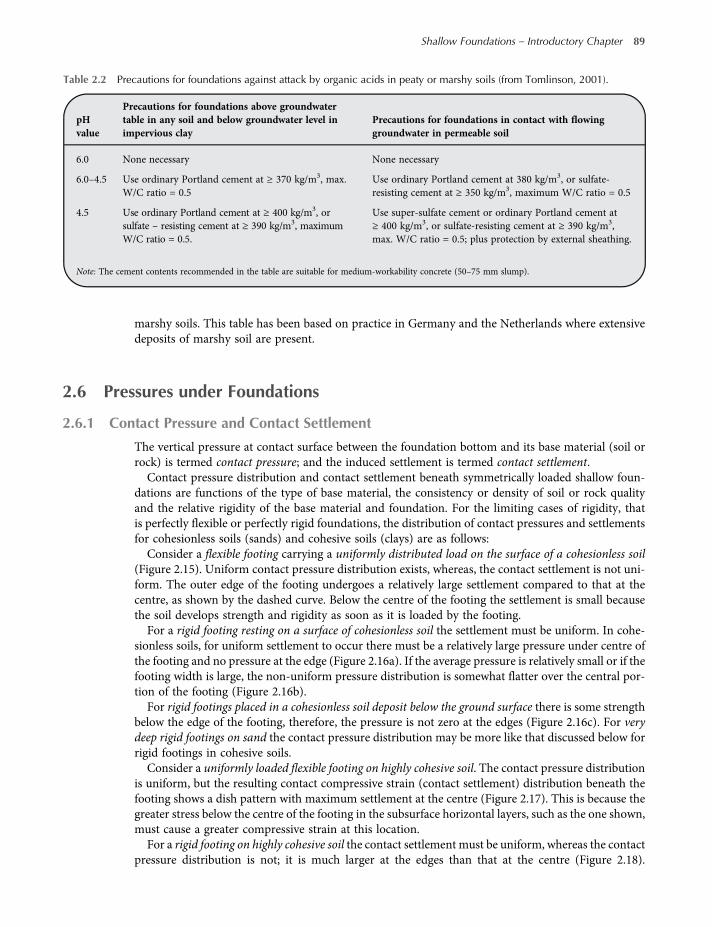
marshy soils. This table has been based on practice in Germany and the Netherlands where extensivedeposits of marshy soil are present.
2.6 Pressures under Foundations
2.6.1 Contact Pressure and Contact Settlement
The vertical pressure at contact surface between the foundation bottom and its base material (soil orrock) is termed contact pressure; and the induced settlement is termed contact settlement.Contact pressure distribution and contact settlement beneath symmetrically loaded shallow foun-
dations are functions of the type of base material, the consistency or density of soil or rock qualityand the relative rigidity of the base material and foundation. For the limiting cases of rigidity, thatis perfectly flexible or perfectly rigid foundations, the distribution of contact pressures and settlementsfor cohesionless soils (sands) and cohesive soils (clays) are as follows:Consider a flexible footing carrying a uniformly distributed load on the surface of a cohesionless soil
(Figure 2.15). Uniform contact pressure distribution exists, whereas, the contact settlement is not uni-form. The outer edge of the footing undergoes a relatively large settlement compared to that at thecentre, as shown by the dashed curve. Below the centre of the footing the settlement is small becausethe soil develops strength and rigidity as soon as it is loaded by the footing.For a rigid footing resting on a surface of cohesionless soil the settlement must be uniform. In cohe-
sionless soils, for uniform settlement to occur there must be a relatively large pressure under centre ofthe footing and no pressure at the edge (Figure 2.16a). If the average pressure is relatively small or if thefooting width is large, the non-uniform pressure distribution is somewhat flatter over the central por-tion of the footing (Figure 2.16b).For rigid footings placed in a cohesionless soil deposit below the ground surface there is some strength
below the edge of the footing, therefore, the pressure is not zero at the edges (Figure 2.16c). For verydeep rigid footings on sand the contact pressure distribution may be more like that discussed below forrigid footings in cohesive soils.Consider a uniformly loaded flexible footing on highly cohesive soil. The contact pressure distribution
is uniform, but the resulting contact compressive strain (contact settlement) distribution beneath thefooting shows a dish pattern with maximum settlement at the centre (Figure 2.17). This is because thegreater stress below the centre of the footing in the subsurface horizontal layers, such as the one shown,must cause a greater compressive strain at this location.For a rigid footing on highly cohesive soil the contact settlement must be uniform, whereas the contact
pressure distribution is not; it is much larger at the edges than that at the centre (Figure 2.18).
Table 2.2 Precautions for foundations against attack by organic acids in peaty or marshy soils (from Tomlinson, 2001).
pHvalue
Precautions for foundations above groundwatertable in any soil and below groundwater level inimpervious clay
Precautions for foundations in contact with flowinggroundwater in permeable soil
6.0 None necessary None necessary
6.0–4.5 Use ordinary Portland cement at ≥ 370 kg/m3, max.W/C ratio = 0.5
Use ordinary Portland cement at 380 kg/m3, or sulfate-resisting cement at ≥ 350 kg/m3, maximum W/C ratio = 0.5
4.5 Use ordinary Portland cement at ≥ 400 kg/m3, orsulfate – resisting cement at ≥ 390 kg/m3, maximumW/C ratio = 0.5.
Use super-sulfate cement or ordinary Portland cement at≥ 400 kg/m3, or sulfate-resisting cement at ≥ 390 kg/m3,max. W/C ratio = 0.5; plus protection by external sheathing.
Note: The cement contents recommended in the table are suitable for medium-workability concrete (50–75 mm slump).
Shallow Foundations – Introductory Chapter 89
worksaccounts.com
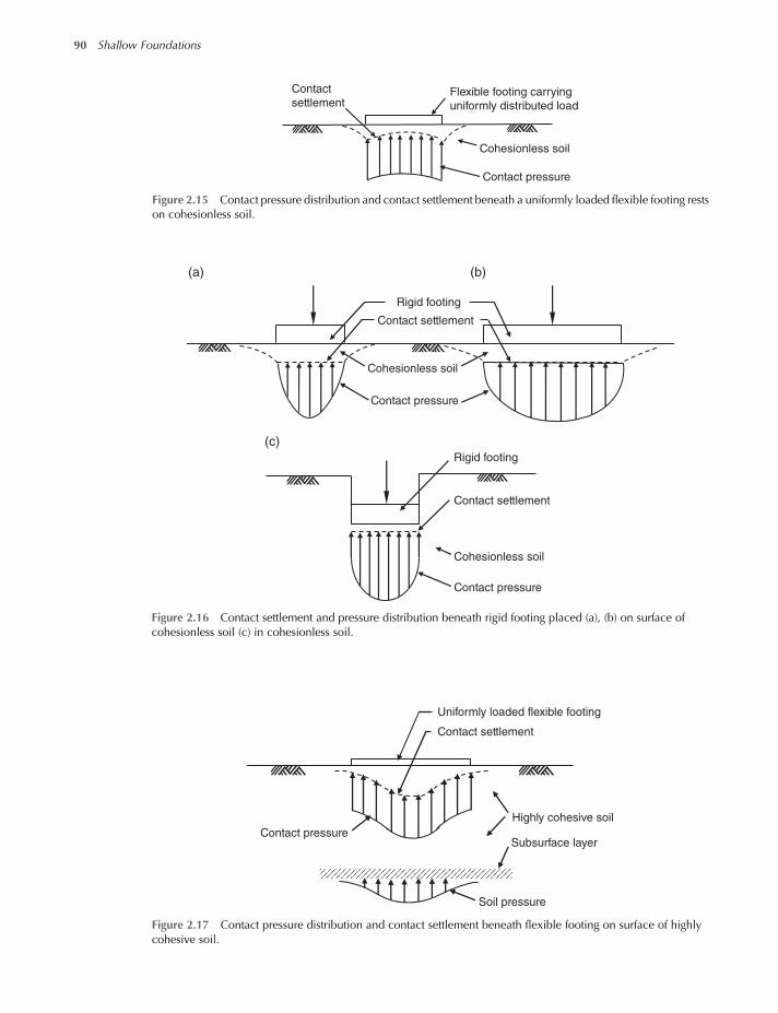
Contact pressure
Contact pressure
Cohesionless soil
Cohesionless soil
Contact settlement
Contact settlement
Rigid footing
Rigid footing
(a) (b)
(c)
Figure 2.16 Contact settlement and pressure distribution beneath rigid footing placed (a), (b) on surface ofcohesionless soil (c) in cohesionless soil.
Contact pressure
Uniformly loaded flexible footing
Contact settlement
Highly cohesive soil
Subsurface layer
Soil pressure
Figure 2.17 Contact pressure distribution and contact settlement beneath flexible footing on surface of highlycohesive soil.
Contact
settlement
Cohesionless soil
Contact pressure
Flexible footing carrying
uniformly distributed load
Figure 2.15 Contact pressure distribution and contact settlement beneath a uniformly loaded flexible footing restson cohesionless soil.
90 Shallow Foundations
worksaccounts.com

According to the theory of elasticity, for an elastic material of infinite strength the contact pressuredistribution is as indicated in the Figure by the long dash-dot curve which shows an infinite stressat the edge of the footing. Actually an infinite stress cannot occur, but the stress at the edges maybe much larger than that at the centre.In practice, spread footings are usually of intermediate to very high rigidity, so the actual contact
pressure distribution is not uniform. Bearing capacity and settlement analyses as well as structuraldesign of footings based on such a distribution would be very complex. Therefore, it is common prac-tice to use the uniformly distributed contact pressure beneath centrally loaded spread footings, asshown in Figure 2.19. Results of some field measurements indicate this simplification in design ofspread footings does not cause serious error and the assumption can be considered adequate. However,after a design has been prepared on this basis, it is suggested that the designer review it and strength it atlocations where the actual distribution gives greater stresses than are given by the assumed distribution.In Figure 2.18, for example, the bending moment in the footing is much larger for the distributionshown than it is for a case of uniform pressure; additional reinforcing steel is needed to carry thisgreater moment.With mat or raft foundations the problems of contact pressure distribution and deformation are
quite different from those with spread footings. Usually, mat foundations have a much smaller thick-ness to width ratio, and thus are more flexible than spread footings. Therefore, the assumption of rigid-ity is no longer valid. Also, the assumption of linear contact pressure distribution would be erroneousunless the supporting material is mud or peat or soft soil. At locations of heavy loads, such as those ofcolumns and bearing walls, a mat settles more than at locations with relatively light loads because thepressure beneath the heavily loaded zones are greater. Figure 2.20a shows contact pressure distributionbeneath a mat rests on strong bedrock; the column loads are transmitted to the rock on a relatively
Highly cohesive soil
Rigid footing
Contact settlement
Contact pressure
Figure 2.18 Contact pressure distribution and contact settlement beneath a rigid footing on surface of highlycohesive soil.
Centrally loaded rigid
spread footing
Supporting soil
Assumed uniform
contact pressure
Figure 2.19 Assumed uniform contact pressure distribution beneath a spread footing.
Shallow Foundations – Introductory Chapter 91
worksaccounts.com
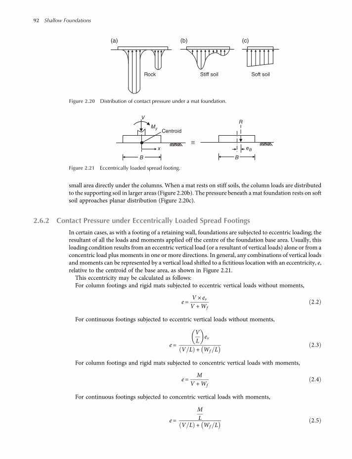
small area directly under the columns. When a mat rests on stiff soils, the column loads are distributedto the supporting soil in larger areas (Figure 2.20b). The pressure beneath amat foundation rests on softsoil approaches planar distribution (Figure 2.20c).
2.6.2 Contact Pressure under Eccentrically Loaded Spread Footings
In certain cases, as with a footing of a retaining wall, foundations are subjected to eccentric loading; theresultant of all the loads and moments applied off the centre of the foundation base area. Usually, thisloading condition results from an eccentric vertical load (or a resultant of vertical loads) alone or from aconcentric load plus moments in one or more directions. In general, any combinations of vertical loadsand moments can be represented by a vertical load shifted to a fictitious location with an eccentricity, e,relative to the centroid of the base area, as shown in Figure 2.21.
This eccentricity may be calculated as follows:For column footings and rigid mats subjected to eccentric vertical loads without moments,
e =V × evV +Wf
2 2
For continuous footings subjected to eccentric vertical loads without moments,
e=
VL
ev
V L + Wf L2 3
For column footings and rigid mats subjected to concentric vertical loads with moments,
e =M
V +Wf2 4
For continuous footings subjected to concentric vertical loads with moments,
e=
ML
V L + Wf L2 5
(a) (b) (c)
Rock Stiff soil Soft soil
Figure 2.20 Distribution of contact pressure under a mat foundation.
Centroid
V
x
B B
R
eB
My
Figure 2.21 Eccentrically loaded spread footing.
92 Shallow Foundations
worksaccounts.com
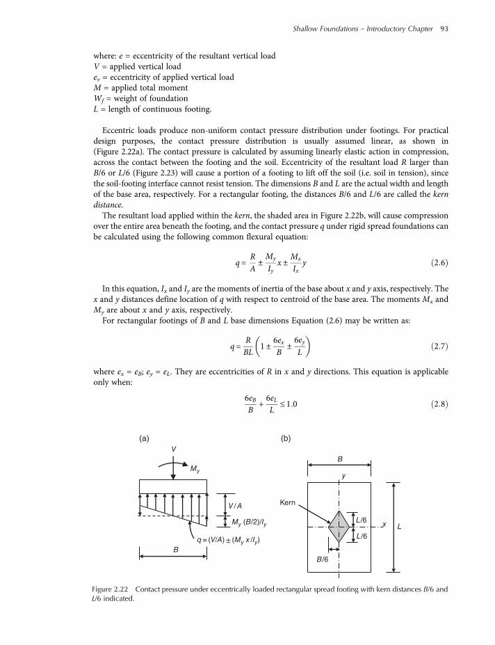
where: e = eccentricity of the resultant vertical loadV = applied vertical loadev = eccentricity of applied vertical loadM = applied total momentWf = weight of foundationL = length of continuous footing.
Eccentric loads produce non-uniform contact pressure distribution under footings. For practicaldesign purposes, the contact pressure distribution is usually assumed linear, as shown in(Figure 2.22a). The contact pressure is calculated by assuming linearly elastic action in compression,across the contact between the footing and the soil. Eccentricity of the resultant load R larger thanB/6 or L/6 (Figure 2.23) will cause a portion of a footing to lift off the soil (i.e. soil in tension), sincethe soil-footing interface cannot resist tension. The dimensions B and L are the actual width and lengthof the base area, respectively. For a rectangular footing, the distances B/6 and L/6 are called the kerndistance.The resultant load applied within the kern, the shaded area in Figure 2.22b, will cause compression
over the entire area beneath the footing, and the contact pressure q under rigid spread foundations canbe calculated using the following common flexural equation:
q=RA±My
Iyx ±
Mx
Ixy 2 6
In this equation, Ix and Iy are the moments of inertia of the base about x and y axis, respectively. Thex and y distances define location of q with respect to centroid of the base area. The moments Mx andMy are about x and y axis, respectively.For rectangular footings of B and L base dimensions Equation (2.6) may be written as:
q=RBL
1 ±6exB
±6eyL
2 7
where ex = eB; ey = eL. They are eccentricities of R in x and y directions. This equation is applicableonly when:
6eBB
+6eLL
≤ 1 0 2 8
V
V / A
My (B/2)/Iy
q = (V/A) ± (My x /Iy)
Kern
(a) (b)
y
B
x L
L/6
B/6
B
L/6
My
Figure 2.22 Contact pressure under eccentrically loaded rectangular spread footing with kern distances B/6 andL/6 indicated.
Shallow Foundations – Introductory Chapter 93
worksaccounts.com

If the applied resultant load falls outside the kern area, Equation (2.6) will not be satisfied. However,the soil reaction resultant remains equal and opposite in direction to the resultant R, as shown inFigure 2.23. Generally, such a pressure distribution would not be acceptable because it makes insuffi-cient use of the footing concrete and tends to overload the supporting soil. Therefore, foundations witheccentric loads and/or moments must have R always fall within the kern. This criterion maintains com-pressive stresses along the entire base area.
The kern distance for circular footings is r/4 where r is radius of the circular base area, as shown inFigure 2.24.
Resultant of
applied loads
> (2qav= 2R/A)
Resultant
of contact
pressure
B
B/6
3[(B/2)–e]
Re
qmax= 4R/3L (B–2e)
Figure 2.23 Contact pressure under eccentrically loaded spread footing where the resultant load falls outsidethe kern.
Location of
resultant R
Kern
qmax
e
rr/4
2r
For e ≤ r/4: q = (R/A) [1± (4e/r)], A = πr2
0.25 0.30 0.35 0.40 0.45 0.50 0.55 0.60 0.65 0.70 0.75 0.80 0.90
80.013.09.207.205.904.924.223.553.102.702.432.202.00
Values of k are tabulated below:
e/r:
k:
For e > )r4
R
A: qmax= k (
Figure 2.24 Contact pressure under eccentrically loaded circular spread footings.
94 Shallow Foundations
worksaccounts.com
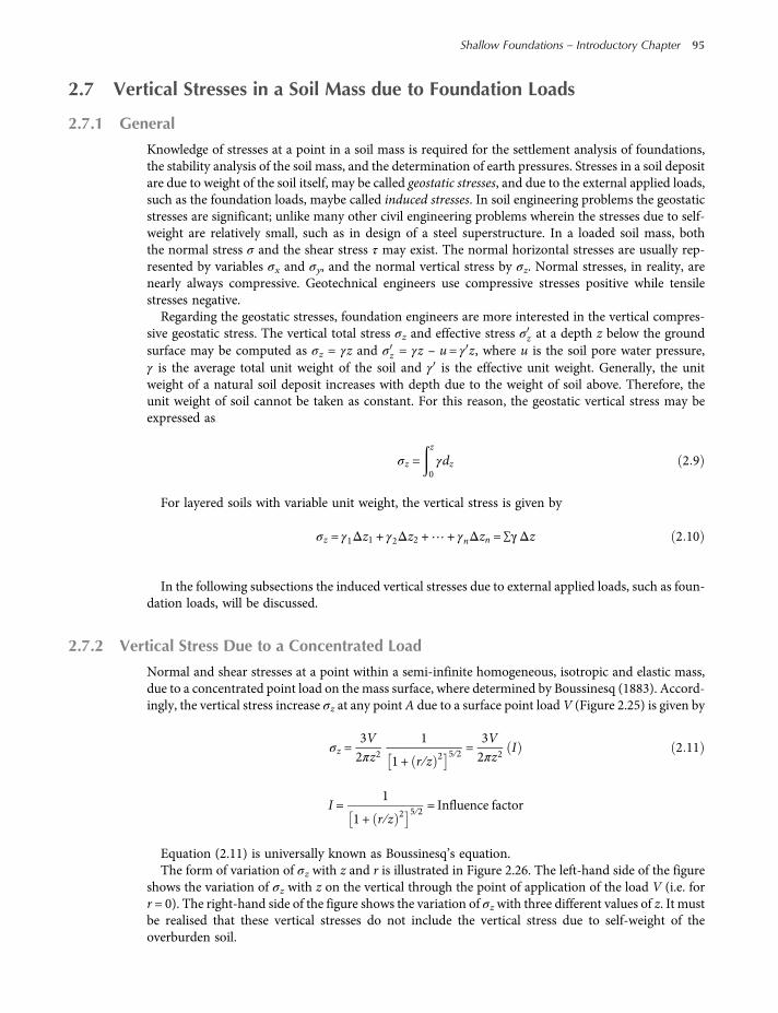
2.7 Vertical Stresses in a Soil Mass due to Foundation Loads
2.7.1 General
Knowledge of stresses at a point in a soil mass is required for the settlement analysis of foundations,the stability analysis of the soil mass, and the determination of earth pressures. Stresses in a soil depositare due to weight of the soil itself, may be called geostatic stresses, and due to the external applied loads,such as the foundation loads, maybe called induced stresses. In soil engineering problems the geostaticstresses are significant; unlike many other civil engineering problems wherein the stresses due to self-weight are relatively small, such as in design of a steel superstructure. In a loaded soil mass, boththe normal stress σ and the shear stress τ may exist. The normal horizontal stresses are usually rep-resented by variables σx and σy, and the normal vertical stress by σz. Normal stresses, in reality, arenearly always compressive. Geotechnical engineers use compressive stresses positive while tensilestresses negative.Regarding the geostatic stresses, foundation engineers are more interested in the vertical compres-
sive geostatic stress. The vertical total stress σz and effective stress σz at a depth z below the groundsurface may be computed as σz = γz and σz = γz – u= γ z, where u is the soil pore water pressure,γ is the average total unit weight of the soil and γ is the effective unit weight. Generally, the unitweight of a natural soil deposit increases with depth due to the weight of soil above. Therefore, theunit weight of soil cannot be taken as constant. For this reason, the geostatic vertical stress may beexpressed as
σz =z
0γdz 2 9
For layered soils with variable unit weight, the vertical stress is given by
σz = γ1Δz1 + γ2Δz2 +… + γnΔzn = ∑γΔz 2 10
In the following subsections the induced vertical stresses due to external applied loads, such as foun-dation loads, will be discussed.
2.7.2 Vertical Stress Due to a Concentrated Load
Normal and shear stresses at a point within a semi-infinite homogeneous, isotropic and elastic mass,due to a concentrated point load on the mass surface, where determined by Boussinesq (1883). Accord-ingly, the vertical stress increase σz at any point A due to a surface point load V (Figure 2.25) is given by
σz =3V2πz2
1
1 + r ∕z 2 5 ∕2 =3V2πz2
I 2 11
I =1
1 + r ∕z 2 5 ∕2 = Influence factor
Equation (2.11) is universally known as Boussinesq’s equation.The form of variation of σz with z and r is illustrated in Figure 2.26. The left-hand side of the figure
shows the variation of σz with z on the vertical through the point of application of the load V (i.e. forr = 0). The right-hand side of the figure shows the variation of σzwith three different values of z. It mustbe realised that these vertical stresses do not include the vertical stress due to self-weight of theoverburden soil.
Shallow Foundations – Introductory Chapter 95
worksaccounts.com

2.7.3 Vertical Stress Due to a Line Load
The Boussinesq’s solution described in Section 2.7.2 can be used to obtain the vertical stresses in a soilmass due to a vertical line load. Figure 2.27 shows a line load of infinite length having intensity V perunit length on the surface of a semi-infinite soil mass. The vertical stress increase at point A inside thesoil mass is
σz =2Vπ
z3
x2 + z2 2 2 12
z
σr
σz
σθrA
V
Figure 2.25 Stresses at point A of depth z below ground surface acted on by a point load.
z1
z2
z3
V
r
r
r
(r = 0)
(σz plotted vertically)(σz plotted horizontally)
Variation of σz with
variable r at depths
z1, z2, and z3
z
rVariation of σz with
depth z below the
point load (r = 0)
Figure 2.26 Variation of vertical stress σz due to a point load.
96 Shallow Foundations
worksaccounts.com
2.7.4 Vertical Stress Due to a Uniformly Loaded Strip Area
Referring to Figure 2.28a, the vertical stress at point A due to a uniform load per unit area q on a flexiblestrip area of width B and infinite length are given in terms of the angles α and β, as follows:
σz =qπα+ sinα cos α+ 2β 2 13
The vertical stress at points below the centre of the strip, such as point A of Figure 2.28b, is given as
σz =qπ
α+ sinα 2 14
The vertical stress at point A of Figure 2.28c due to pressure increasing linearly from zero to q on astrip area of width B and infinite length is given in terms of the angles α and β as follows:
σz =qπ
xBθ−
12sin2β 2 15
When the point is located within B under the loaded area, β is negative.
2.7.5 Vertical Stress Due to a Uniformly Loaded Circular Area
Referring to Figure 2.29, the stresses at a point due to a uniformly loaded circular area with intensity qcan be obtained by dividing the loaded area into many small elements, each with an area of dA and asmall concentrated load at its centre equal to
dV = q dA
From the Boussinesq’s equation of vertical stress due to a concentrated point load, the vertical stressat point A due to dV is
dσZ =3 dV2πz2
1
1 + r ∕z 2 5 ∕2 =3q2πz2
1
1 + r ∕z 2 5 ∕2 dA
The stress increase σz can be found by integrating this equation over the loaded area. If we considerthe vertical stress at any depth z underneath the centre of the loaded area of radius R, we will have
σZ =3q2π
2π
0
R
0
1
z2 1 + r ∕z 2 5 ∕2 r dθ dr
where r.dθ.dr = dA
V / unit length
x A
xσz
+ ∞– ∞y
z
z
Figure 2.27 Vertical stress due to a line load of infinite length.
Shallow Foundations – Introductory Chapter 97
worksaccounts.com

B B
(b)(a)
q q
Z
A
Z
A
α σz
σz
β
α
x
B
(c)
q
Z
A
β
θ σz
Figure 2.28 (a, b) Vertical stresses due to a uniformly loaded strip area of infinite length. (c) Vertical stresses due to a triangularlyloaded trip area of infinite length.
dV
dA
A
drr
R
z
dθ
σz
Figure 2.29 Vertical stresses below center of a uniformly loaded circular area.
worksaccounts.com
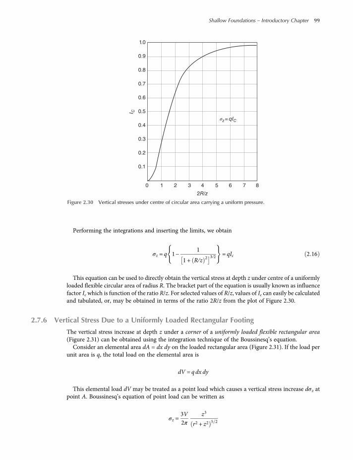
Performing the integrations and inserting the limits, we obtain
σz = q 1−1
1 + R ∕z 2 3 ∕2 = qIc 2 16
This equation can be used to directly obtain the vertical stress at depth z under centre of a uniformlyloaded flexible circular area of radius R. The bracket part of the equation is usually known as influencefactor Icwhich is function of the ratio R/z. For selected values of R/z, values of Ic can easily be calculatedand tabulated, or, may be obtained in terms of the ratio 2R/z from the plot of Figure 2.30.
2.7.6 Vertical Stress Due to a Uniformly Loaded Rectangular Footing
The vertical stress increase at depth z under a corner of a uniformly loaded flexible rectangular area(Figure 2.31) can be obtained using the integration technique of the Boussinesq’s equation.Consider an elemental area dA = dx dy on the loaded rectangular area (Figure 2.31). If the load per
unit area is q, the total load on the elemental area is
dV = q dx dy
This elemental load dV may be treated as a point load which causes a vertical stress increase dσz atpoint A. Boussinesq’s equation of point load can be written as
σz =3V2π
z3
r2 + z2 5 2
1.0
0.9
0.8
0.7
0.6
0.5
0.4
0.3
0.2
0 1 2 3 4
2R/z
I C
5 6 7 8
0.1
σz= qIC
Figure 2.30 Vertical stresses under centre of circular area carrying a uniform pressure.
Shallow Foundations – Introductory Chapter 99
worksaccounts.com
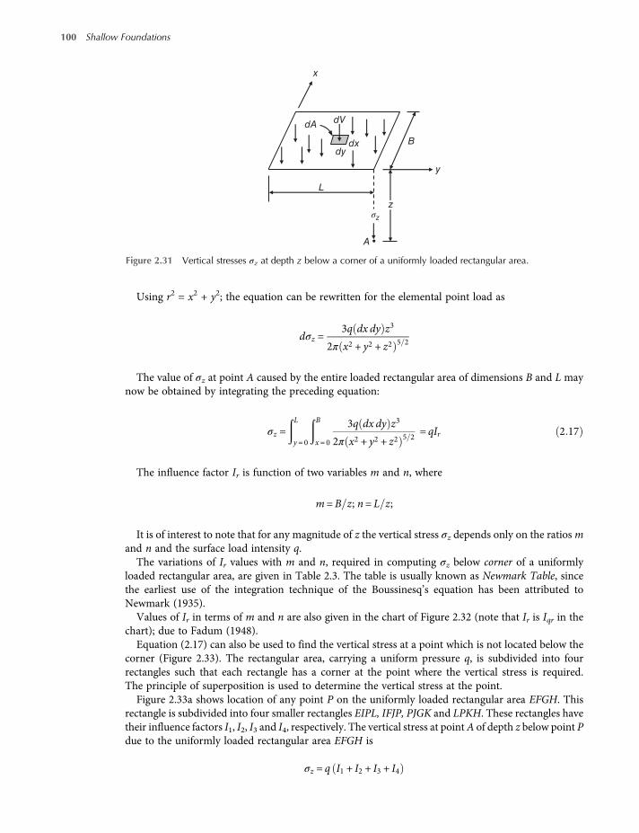
Using r2 = x2 + y2; the equation can be rewritten for the elemental point load as
dσz =3q dx dy z3
2π x2 + y2 + z2 5 2
The value of σz at point A caused by the entire loaded rectangular area of dimensions B and L maynow be obtained by integrating the preceding equation:
σz =L
y = 0
B
x = 0
3q dx dy z3
2π x2 + y2 + z2 5 2= qIr 2 17
The influence factor Ir is function of two variables m and n, where
m=B z; n= L z;
It is of interest to note that for any magnitude of z the vertical stress σz depends only on the ratiosmand n and the surface load intensity q.
The variations of Ir values with m and n, required in computing σz below corner of a uniformlyloaded rectangular area, are given in Table 2.3. The table is usually known as Newmark Table, sincethe earliest use of the integration technique of the Boussinesq’s equation has been attributed toNewmark (1935).
Values of Ir in terms of m and n are also given in the chart of Figure 2.32 (note that Ir is Iqr in thechart); due to Fadum (1948).
Equation (2.17) can also be used to find the vertical stress at a point which is not located below thecorner (Figure 2.33). The rectangular area, carrying a uniform pressure q, is subdivided into fourrectangles such that each rectangle has a corner at the point where the vertical stress is required.The principle of superposition is used to determine the vertical stress at the point.
Figure 2.33a shows location of any point P on the uniformly loaded rectangular area EFGH. Thisrectangle is subdivided into four smaller rectangles EIPL, IFJP, PJGK and LPKH. These rectangles havetheir influence factors I1, I2, I3 and I4, respectively. The vertical stress at pointA of depth z below point Pdue to the uniformly loaded rectangular area EFGH is
σz = q I1 + I2 + I3 + I4
x
B
L
dxdy
dAdV
A
y
zσz
Figure 2.31 Vertical stresses σz at depth z below a corner of a uniformly loaded rectangular area.
100 Shallow Foundations
worksaccounts.com
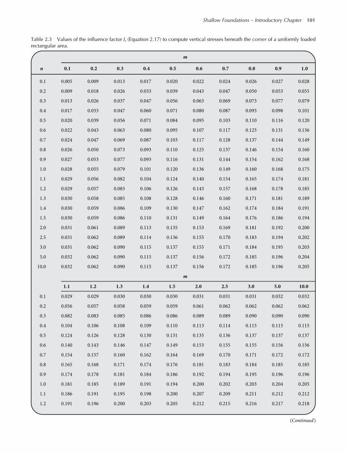
Table 2.3 Values of the influence factor Ir (Equation 2.17) to compute vertical stresses beneath the corner of a uniformly loadedrectangular area.
n
m
0.1 0.2 0.3 0.4 0.5 0.6 0.7 0.8 0.9 1.0
0.1 0.005 0.009 0.013 0.017 0.020 0.022 0.024 0.026 0.027 0.028
0.2 0.009 0.018 0.026 0.033 0.039 0.043 0.047 0.050 0.053 0.055
0.3 0.013 0.026 0.037 0.047 0.056 0.063 0.069 0.073 0.077 0.079
0.4 0.017 0.033 0.047 0.060 0.071 0.080 0.087 0.093 0.098 0.101
0.5 0.020 0.039 0.056 0.071 0.084 0.095 0.103 0.110 0.116 0.120
0.6 0.022 0.043 0.063 0.080 0.095 0.107 0.117 0.125 0.131 0.136
0.7 0.024 0.047 0.069 0.087 0.103 0.117 0.128 0.137 0.144 0.149
0.8 0.026 0.050 0.073 0.093 0.110 0.125 0.137 0.146 0.154 0.160
0.9 0.027 0.053 0.077 0.093 0.116 0.131 0.144 0.154 0.162 0.168
1.0 0.028 0.055 0.079 0.101 0.120 0.136 0.149 0.160 0.168 0.175
1.1 0.029 0.056 0.082 0.104 0.124 0.140 0.154 0.165 0.174 0.181
1.2 0.029 0.057 0.083 0.106 0.126 0.143 0.157 0.168 0.178 0.185
1.3 0.030 0.058 0.085 0.108 0.128 0.146 0.160 0.171 0.181 0.189
1.4 0.030 0.059 0.086 0.109 0.130 0.147 0.162 0.174 0.184 0.191
1.5 0.030 0.059 0.086 0.110 0.131 0.149 0.164 0.176 0.186 0.194
2.0 0.031 0.061 0.089 0.113 0.135 0.153 0.169 0.181 0.192 0.200
2.5 0.031 0.062 0.089 0.114 0.136 0.155 0.170 0.183 0.194 0.202
3.0 0.031 0.062 0.090 0.115 0.137 0.155 0.171 0.184 0.195 0.203
5.0 0.032 0.062 0.090 0.115 0.137 0.156 0.172 0.185 0.196 0.204
10.0 0.032 0.062 0.090 0.115 0.137 0.156 0.172 0.185 0.196 0.205
m
1.1 1.2 1.3 1.4 1.5 2.0 2.5 3.0 5.0 10.0
0.1 0.029 0.029 0.030 0.030 0.030 0.031 0.031 0.031 0.032 0.032
0.2 0.056 0.057 0.058 0.059 0.059 0.061 0.062 0.062 0.062 0.062
0.3 0.082 0.083 0.085 0.086 0.086 0.089 0.089 0.090 0.090 0.090
0.4 0.104 0.106 0.108 0.109 0.110 0.113 0.114 0.115 0.115 0.115
0.5 0.124 0.126 0.128 0.130 0.131 0.135 0.136 0.137 0.137 0.137
0.6 0.140 0.143 0.146 0.147 0.149 0.153 0.155 0.155 0.156 0.156
0.7 0.154 0.157 0.160 0.162 0.164 0.169 0.170 0.171 0.172 0.172
0.8 0.165 0.168 0.171 0.174 0.176 0.181 0.183 0.184 0.185 0.185
0.9 0.174 0.178 0.181 0.184 0.186 0.192 0.194 0.195 0.196 0.196
1.0 0.181 0.185 0.189 0.191 0.194 0.200 0.202 0.203 0.204 0.205
1.1 0.186 0.191 0.195 0.198 0.200 0.207 0.209 0.211 0.212 0.212
1.2 0.191 0.196 0.200 0.203 0.205 0.212 0.215 0.216 0.217 0.218
(Continued )
Shallow Foundations – Introductory Chapter 101
worksaccounts.com

Table 2.3 (Continued)
n
m
1.1 1.2 1.3 1.4 1.5 2.0 2.5 3.0 5.0 10.0
1.3 0.195 0.200 0.204 0.207 0.209 0.217 0.220 0.221 0.222 0.223
1.4 0.198 0.203 0.207 0.210 0.213 0.221 0.224 0.225 0.226 0.227
1.5 0.200 0.205 0.209 0.213 0.216 0.224 0.227 0.228 0.230 0.230
2.0 0.207 0.212 0.217 0.221 0.224 0.232 0.236 0.238 0.240 0.240
2.5 0.209 0.215 0.220 0.224 0.227 0.236 0.240 0.242 0.244 0.244
3.0 0.211 0.216 0.221 0.225 0.228 0.238 0.242 0.244 0.246 0.247
5.0 0.212 0.217 0.222 0.226 0.230 0.240 0.244 0.246 0.249 0.249
10.0 0.212 0.218 0.223 0.227 0.230 0.240 0.244 0.247 0.249 0.250
Note: The factors m and n are interchangeable.
0.28
0.26
0.24
0.22
0.20
0.18
0.16
I qr 0.14
0.12
0.10
0.08
0.06
0.04
0.02
0
0.1 1 10
2.0
∞nmz
nz
z
q
1.4
1.0
0.8
0.6
0.4
0.5
0.2
0.3
0.1
0
m
σz
Δσz= qIqr
Figure 2.32 Values of the influence factor for computing vertical stress under corner of rectangular area carrying a uniform pressure(reproduced from Knappett and Craig, 2012; after R.E. Fadum, 1948).
102 Shallow Foundations
worksaccounts.com
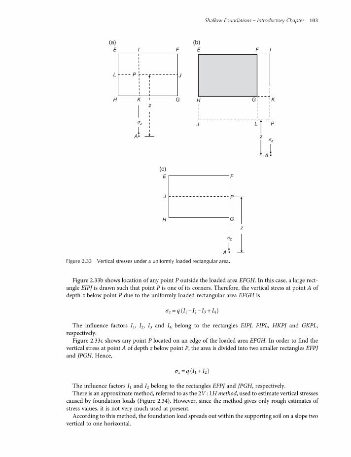
Figure 2.33b shows location of any point P outside the loaded area EFGH. In this case, a large rect-angle EIPJ is drawn such that point P is one of its corners. Therefore, the vertical stress at point A ofdepth z below point P due to the uniformly loaded rectangular area EFGH is
σz = q I1− I2− I3 + I4
The influence factors I1, I2, I3 and I4 belong to the rectangles EIPJ, FIPL, HKPJ and GKPL,respectively.Figure 2.33c shows any point P located on an edge of the loaded area EFGH. In order to find the
vertical stress at point A of depth z below point P, the area is divided into two smaller rectangles EFPJand JPGH. Hence,
σz = q I1 + I2
The influence factors I1 and I2 belong to the rectangles EFPJ and JPGH, respectively.There is an approximate method, referred to as the 2V : 1Hmethod, used to estimate vertical stresses
caused by foundation loads (Figure 2.34). However, since the method gives only rough estimates ofstress values, it is not very much used at present.According to this method, the foundation load spreads out within the supporting soil on a slope two
vertical to one horizontal.
I IF FE
L
E
J
J L
K
P
G GK
P
z
z
H H
σz
A
A σz
(a) (b)
FE
J P
G
z
A
H
σz
(c)
Figure 2.33 Vertical stresses under a uniformly loaded rectangular area.
Shallow Foundations – Introductory Chapter 103
worksaccounts.com
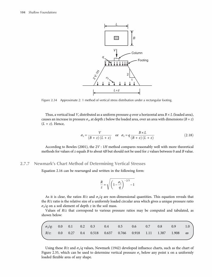
Thus, a vertical loadV, distributed as a uniform pressure q over a horizontal area B × L (loaded area),causes an increase in pressure σz, at depth z below the loaded area, over an area with dimensions (B + z)(L + z). Hence,
σz =V
B + z L + zor σz = q
B× LB + z L + z
2 18
According to Bowles (2001), the 2V : 1H method compares reasonably well with more theoreticalmethods for values of z equals B to about 4B but should not be used for z values between 0 and B value.
2.7.7 Newmark’s Chart Method of Determining Vertical Stresses
Equation 2.16 can be rearranged and written in the following form:
Rz= 1−
σzq
−2 ∕3
−1
As it is clear, the ratios R/z and σz/q are non-dimensional quantities. This equation reveals thatthe R/z ratio is the relative size of a uniformly loaded circular area which gives a unique pressure ratioσz/q on a soil element of depth z in the soil mass.
Values of R/z that correspond to various pressure ratios may be computed and tabulated, asshown below:
σz/q: 0.0 0.1 0.2 0.3 0.4 0.5 0.6 0.7 0.8 0.9 1.0
R/z: 0.0 0.27 0.4 0.518 0.637 0.766 0.918 1.11 1.387 1.908 ∞
Using these R/z and σz/q values, Newmark (1942) developed influence charts, such as the chart ofFigure 2.35, which can be used to determine vertical pressure σz below any point x on a uniformlyloaded flexible area of any shape.
B
Column
Footing
2
2 V
:1H
V
L
L+z
q
1σz
Figure 2.34 Approximate 2: 1 method of vertical stress distribution under a rectangular footing.
104 Shallow Foundations
worksaccounts.com

The influence chart is useful in cases where access to a computer is not practical and there are severalfootings with different contact pressures or where the footing is irregular-shaped and σz is desired for anumber of points.An influence chart consists of concentric circles and radial lines (Figure 2.35). The radii of the circles
are equal to the R/z values corresponding to σz/q = 0, 0.1, 0.2… 1.0 (note that for σz/q = 0, R/z = 0, andfor σz/q = 1, R/z =∞, so nine circles are shown). The unit length for plotting the circles is the length ofthe scale line AB. The circles are divided by several equally spaced radial lines. The influence value I ofthe chart is given by 1/N, whereN equals to number of elements in the chart. In the chart of Figure 2.35,there are 200 elements; hence, the influence value I = 0.005.Steps of the procedure for obtaining vertical stress σz at a point of depth z below a uniformly loaded
area of any shape are as follows:
• Determine the depth z below the uniformly loaded area at which the vertical stress is required.
• Plot the plan of the loaded area on a transparent paper to a scale such that the length of the scale lineAB represents the depth z at which the vertical stress σz is required. On the drawn plan locate thepoint, say point x, below which σz is required.
• Place the plan on top of the influence chart with point x located at the origin of the chart.
• Count the number of elements M occupied by the plan of the loaded area.
• The vertical stress at the point under consideration is given by
σz = I Mq 2 19
where I and M are dimensionless quantities.
2.7.8 Pressure Bulbs Method of Determining Vertical Stresses
Based on Boussinesq’s equation, the vertical stresses under continuous (strip), rectangular, square andcircular footings have been computed. For example, the results due to uniformly loaded square andcontinuous areas are shown in Figures 2.36 and 2.37. The magnitudes of vertical stresses at variouspoints in a soil mass are given in terms of the uniform contact pressures qo in Figure 2.36 and q inFigure 2.37. The vertical stress is designated q in Figure 2.36. The pressure bulbs are isobars (lines
A
B
1 unit
Influence value: I=0.005
O
Figure 2.35 Influence chart for computing vertical stresses based on Boussinesq’s theory (after Newmark, 1942).
Shallow Foundations – Introductory Chapter 105
worksaccounts.com

1.5B
1B
1B 1B
B/2 B/2
1B
Continuous
0.9
0.8
0.8
0.7
0.6
0.7
0.6
0.5 0.4
0.40.3
0.2
0.05
q /q o= 0.1
q / qo = 0.05
q / qo = 0.9
0.2
0.1
Square
2B
2B
3B
3B
4B
5B
6B
B/2
CL
B/2B
L/2
L
Ba
a
b
b
7B
2B
3B
0.5
0.3
Figure 2.36 Pressure isobars (also called pressure bulbs) based on the Boussinesq’s equation for square and longfootings. Applicable only along line ab from centre to edge of base (From Bowles, 2001).
z
q
B
2B
3B
BB
aa
a
bb
b
c
c
cd
d
d
Stress
isobar
0.8 q
0.6 q
0.4 q
0.2 q
0
(a) (b)q
σz
Figure 2.37 Contours of equal vertical stress: (a) under strip area, (b) under square area (redrawn from Knappettand Craig, 2012).
106 Shallow Foundations
worksaccounts.com
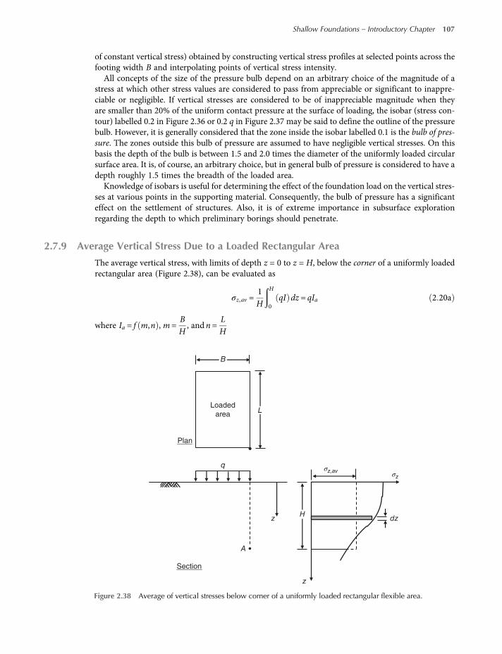
of constant vertical stress) obtained by constructing vertical stress profiles at selected points across thefooting width B and interpolating points of vertical stress intensity.All concepts of the size of the pressure bulb depend on an arbitrary choice of the magnitude of a
stress at which other stress values are considered to pass from appreciable or significant to inappre-ciable or negligible. If vertical stresses are considered to be of inappreciable magnitude when theyare smaller than 20% of the uniform contact pressure at the surface of loading, the isobar (stress con-tour) labelled 0.2 in Figure 2.36 or 0.2 q in Figure 2.37 may be said to define the outline of the pressurebulb. However, it is generally considered that the zone inside the isobar labelled 0.1 is the bulb of pres-sure. The zones outside this bulb of pressure are assumed to have negligible vertical stresses. On thisbasis the depth of the bulb is between 1.5 and 2.0 times the diameter of the uniformly loaded circularsurface area. It is, of course, an arbitrary choice, but in general bulb of pressure is considered to have adepth roughly 1.5 times the breadth of the loaded area.Knowledge of isobars is useful for determining the effect of the foundation load on the vertical stres-
ses at various points in the supporting material. Consequently, the bulb of pressure has a significanteffect on the settlement of structures. Also, it is of extreme importance in subsurface explorationregarding the depth to which preliminary borings should penetrate.
2.7.9 Average Vertical Stress Due to a Loaded Rectangular Area
The average vertical stress, with limits of depth z = 0 to z = H, below the corner of a uniformly loadedrectangular area (Figure 2.38), can be evaluated as
σz,av =1H
H
0qI dz = qIa 2 20a
where Ia = f m,n , m=BH, andn=
LH
Loaded
area
Plan
Section
L
B
q
Hz
A
dz
z
σz,av σz
Figure 2.38 Average of vertical stresses below corner of a uniformly loaded rectangular flexible area.
Shallow Foundations – Introductory Chapter 107
worksaccounts.com
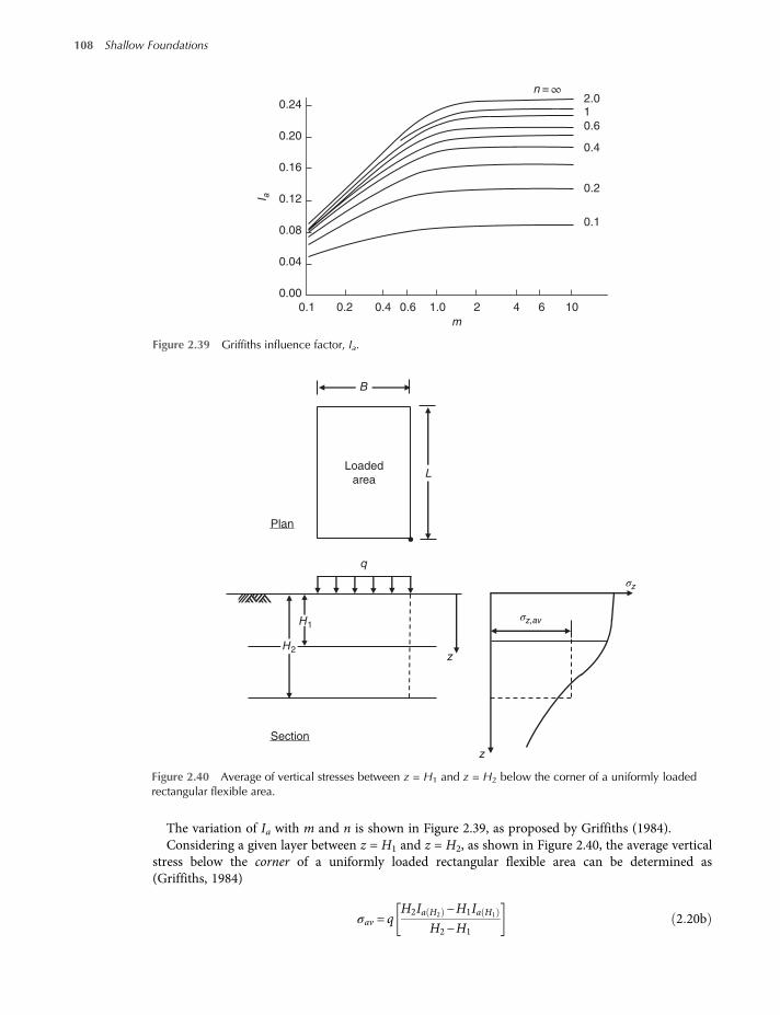
The variation of Ia with m and n is shown in Figure 2.39, as proposed by Griffiths (1984).Considering a given layer between z = H1 and z = H2, as shown in Figure 2.40, the average vertical
stress below the corner of a uniformly loaded rectangular flexible area can be determined as(Griffiths, 1984)
σav = qH2Ia H2
−H1Ia H1
H2−H12 20b
0.24
0.20
0.16
0.12
0.08
0.04
0.00
0.1 0.2 0.4 0.6 1.0 2 4 6 10
2.0n = ∞
m
I a
0.6
0.4
0.2
0.1
1
Figure 2.39 Griffiths influence factor, Ia.
Loaded
area
Plan
L
σz,av
σz
q
B
Section
H2
H1
z
z
Figure 2.40 Average of vertical stresses between z = H1 and z = H2 below the corner of a uniformly loadedrectangular flexible area.
108 Shallow Foundations
worksaccounts.com

Where Ia H2= Ia = f m=
BH2
, n=LH2
for z = 0 to z = H2, and
Ia H1= Ia = f m=
BH1
, n=LH1
for z = 0 to z =H1
Another simple and nearly accurate method for determination of an average vertical stress σav in alayer is by the use of the following Simpson’s rule, provided that the vertical stress values at top, middleand bottom of the layer are known:
σav =16σzt + 4σzm + σzb
Where σzt, σzm and σzb are vertical stresses at top, middle and bottom of the layer.
2.7.10 Westergaard’s Equations
An actual soil mass may not be as homogeneous and isotropic as Boussinesq’s solution assumes.Sedimentary soil deposits are generally anisotropic.Typical clay strata usually have partings or thin lenses of coarser and more rigid materials sandwiched
within them. These lenses or thin sheets are the cause of a greatly increased resistance to lateral strain.Westergaard (1938) derived equations, for computing vertical stress σz, based on conditions which
are nearly analogous to extreme conditions exist in reality. Therefore, Westergaard’s elastic solutioncan give a better estimate of vertical stress in actual sedimentary soil deposits and in a soil mass consistsof layered strata of fine and coarse materials.Westergaard’s equation for the vertical stress caused by a surface point load Q is
σz =Q
12π
1−2μ2−2μ
z21−2μ2−2μ
+rz
2 3 22 21
As it is seen, the Westergaard’s equation, unlike that of the Boussinesq’s, includes Poisson’s ratio μ;the other terms are the same as defined in the Boussinesq equation. Also, as done for the Boussinesqequation we can write this equation as
σz =Qz2
Iw 2 22
Where, Iw represents Westergaard influence coefficient. For μ = 0.30 we obtain the following values:
r/z 0.0 0.1 0.2 0.3 0.4 0.5 0.75 1.0 1.5 2.0
Iw 0.557 0.529 0.458 0.369 0.286 0.217 0.109 0.058 0.021 0.01
Shallow Foundations – Introductory Chapter 109
worksaccounts.com
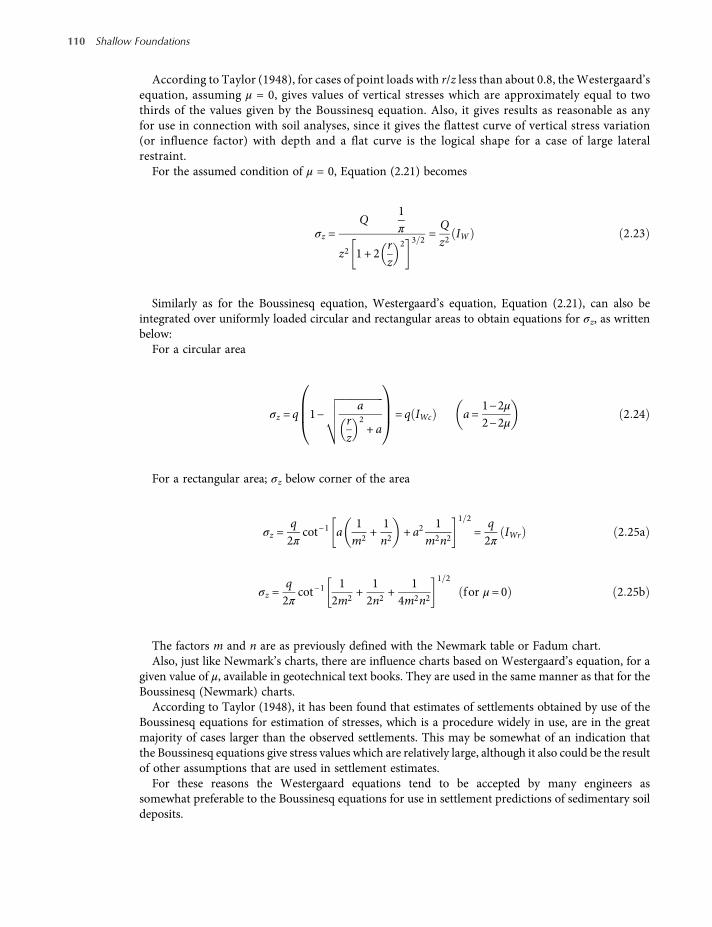
According to Taylor (1948), for cases of point loads with r/z less than about 0.8, theWestergaard’sequation, assuming μ = 0, gives values of vertical stresses which are approximately equal to twothirds of the values given by the Boussinesq equation. Also, it gives results as reasonable as anyfor use in connection with soil analyses, since it gives the flattest curve of vertical stress variation(or influence factor) with depth and a flat curve is the logical shape for a case of large lateralrestraint.
For the assumed condition of μ = 0, Equation (2.21) becomes
σz =Q
1π
z2 1 + 2rz
2 3 2=Qz2
IW 2 23
Similarly as for the Boussinesq equation, Westergaard’s equation, Equation (2.21), can also beintegrated over uniformly loaded circular and rectangular areas to obtain equations for σz, as writtenbelow:
For a circular area
σz = q 1−a
rz
2+ a
= q IWc a=1−2μ2−2μ
2 24
For a rectangular area; σz below corner of the area
σz =q2π
cot−1 a1m2
+1n2
+ a21
m2n2
1 2
=q2π
IWr 2 25a
σz =q2π
cot−11
2m2+
12n2
+1
4m2n2
1 2
for μ= 0 2 25b
The factors m and n are as previously defined with the Newmark table or Fadum chart.Also, just like Newmark’s charts, there are influence charts based on Westergaard’s equation, for a
given value of μ, available in geotechnical text books. They are used in the same manner as that for theBoussinesq (Newmark) charts.
According to Taylor (1948), it has been found that estimates of settlements obtained by use of theBoussinesq equations for estimation of stresses, which is a procedure widely in use, are in the greatmajority of cases larger than the observed settlements. This may be somewhat of an indication thatthe Boussinesq equations give stress values which are relatively large, although it also could be the resultof other assumptions that are used in settlement estimates.
For these reasons the Westergaard equations tend to be accepted by many engineers assomewhat preferable to the Boussinesq equations for use in settlement predictions of sedimentary soildeposits.
110 Shallow Foundations
worksaccounts.com

Problem Solving
Problem 2.1
Compute the effective contact pressure q beneath the following foundations:
(a) An individual column footing is 0.5 m × 2.0 m × 2.0 m. The column load is 500 kN. Unit weights of concreteand the overburden soil are 24 and 18 kN/m3, respectively. The foundation depth is 2.5 m, and the water tableis located at a depth of 2.2 m below the ground surface.
(b) A continuous concrete footing is 0.75 m wide and 0.50 m thick, supports a wall load of 100 kN/m. The foun-dation level is at a depth of 0.5 m below the ground surface. The soil has a unit weight of 17 kN/m3. The groundwater table is at a depth of 8 m below the ground surface.
(c) A mat foundation of a building structure is 1.2 m × 40 m × 80 m. The sum of the column and wall loads is800 MN. The foundation depth is 10 m, and the water table exists at 5 m depth below the ground surface. Theunit weight γ of the soil above and below water table are 17 and 20 kN/m3 respectively.
Also, compute the net increase in the vertical effective stress immediately below the mat centre.
Solution:(a)
Wf = 2 × 2 × 0 5 × 24 = 48 kN
Weight of overburden (backfill) soil
= 2 × 2 × 2 × 18 = 144 kN
The upward pore water pressure
= 10 2 5−2 2 = 3 kN m2
The effective contact pressure is
q=500 + 48 + 144
2 × 2– 3 = 170 kPa
(b)
Wf = 1 × 0 75 × 0 5 × 24 = 9 kN
Here, since the foundation depth equals the footing thickness there will be no backfill soil.Also, since the water table exists below the foundation level, there will be no uplift pressure. Hence, the
effective contact pressure is
q=100 + 91 × 0 75
= 145 3 kPa
(Continued)
2.2 m 2.0 m
500 kN
2.0 m
0.5 m
Scheme 2.1
Shallow Foundations – Introductory Chapter 111
worksaccounts.com

(c)Wf = 1 2 × 40 × 80 × 24 = 92160 kN
The effective contact pressure is
q= 800000 + 92160 40 × 80 −5 × 10 = 228 8kPa
The vertical effective stress (i.e.the effective overburden pressure)at the foundation level due to theeffective weight of the overburdensoil is
σo = 5 × 17 + 5 20 – 10 = 135 kPa
Hence, the net increase in the vertical effective stress immediately below the mat centre due to the foundationload is
228 8−135 0 = 93 8 kPa
Problem 2.2
A continuous footing is 1.5 m wide, subjected to aconcentric vertical load V = 200 kN/m and momentMy = 40 m.kN/m acting laterally across the footing,as shown in the scheme. The ground water table isat a great depth. Unit weight of concrete = 24 kN/m3. Determine whether the resultant force on thefooting base acts within the middle third andcompute the maximum and minimum contactpressures.
Solution:
Wf = 0 5 × 1 5 × 1 0 × 24 = 18 kN m
Equation 2 5 ex =
My
LVL+Wf
L
=40
200 + 18= 0 183m
800 MN
5 m
1.2 m
10 m
Mat: 40 m × 80 m
Scheme 2.2
V
My
1.5 m
0.5 m
Scheme 2.3
112 Shallow Foundations
worksaccounts.com

B6=1 56
= 0 25m> e. Therefore, the resultant force acts within the middle third.
The ground water table has no effect on the contact pressure, since it exists at a great depth below thefoundation level.
Equation 2 7 q=RBL
1 ±6exB
±6eyL
=200 + 181 5 × 1
1 ±6 × 0 183
1 5± 0
qmax = 145 33 + 106 56 = 251 89 kPa
qmin = 145 33−106 56 = 38 77 kPa
Problem 2.3
Six cylindrical grain silos are to be supported by a mat foundation, as shown in the scheme below. Weight of themat is 90 MN, and empty weight of each silo is 29 MN. Each silo can hold up 110 MN. Each silo will be filledindependently. For the various critical loading conditions find whether the resultant force falls within the kern.In case the resultant falls within the kern compute the maximum and minimum contact pressures and show thecontact pressure diagram, and if it does not, revise the plan dimensions of the mat so that Equation (2.8) issatisfied.
(Continued)
12 m
24 m
24 m
B = 50 m
Silo
Elevation
Plan
Silo
Mat
y
x
24 m
L = 75 m
Scheme 2.4
Shallow Foundations – Introductory Chapter 113
worksaccounts.com
Solution:(1) Check one-way eccentricity
(a) One-way eccentricity in L or y direction occurs when two adjacent (in B or x direction) corner silos are fullof grains and the other four silos are empty.
Weight of grains in the two silos cause a moment about x axis equals
Mx = 2 × 110 × 24 = 5280MN m
R= 6 × 29 + 2 × 110 + 90 = 484MN
eL = ey =Mx
R=5280484
= 10 91m; eB = ex = 0
L6=756= 12 5 > eL the resultant R falls within the kern
or,
Equation 2 86eBB
+6eLL
≤ 1
6eBB
+6eLL
= 0 +6 × 10 91
75= 0 87 < 1 the resultant R falls within the kern.
Equation 2 7 q=RBL
1 ±6exB
±6eyL
=484
50 × 751 ± 0 ±
6 × 10 9175
Use the plus sign (+) for soil in compression, and the minus sign (−) for soil in tension.
qmax =484
50 × 751 +
6 × 10 9175
= 0 24175 MN m2 =241 75 kPa
qmin =484
50 × 751−
6 × 10 9175
= 0 01642 MN m2 = 16 42 kPa
(b) One-way eccentricity in B or x direction occurs when three silos in one row are full, and the other threesilos are empty.
Weight of grains in the three silos cause a moment about y axis equals
My = 3 × 110 × 12 = 3960MN m
R= 6 × 29 + 3 × 110 + 90 = 594MN
eB = ex =My
R=3960594
= 6 67m; eL = ey = 0
6eBB
+6eLL
=6 × 6 67
50+ 0 = 0 80 < 1 the resultant R falls within the kern.
qmax
= 241.75 kPa
qmin
= 16.42 kPa
L = 75 m
Scheme 2.5
114 Shallow Foundations
worksaccounts.com

qmax =RA
1 +6eBB
=594
50 × 751 +
6 × 6 6750
= 0 28518 MN m2 = 285 18 kPa
qmin =RA
1 –6eBB
=594
50 × 751 –
6 × 6 6750
= 0 03168 MN m2 = 31 68 kPa
(c) One-way eccentricity in B or x direction occurs when one of the two silos, located on x axis, is full and theother five silos are empty.
Weight of grains in the silo cause a moment about y axis equals
My = 1 × 110 × 12 = 1320MN m
R= 6 × 29 + 1 × 110 + 90 = 374MN
eB = ex =My
R=1320374
= 3 53m; eL = ey = 0
6eBB
+6eLL
=6 × 3 53
50+ 0 = 0 42 < 1 the resultant R falls within the kern.
qmax =RA
1 +6eBB
=374
50 × 751 +
6 × 3 5350
= 0 1416 MN m2 = 141 62 kPa
qmin =RA
1 –6eBB
=374
50 × 751 –
6 × 3 5350
= 0 05749 MN m2 = 57 49 kPa
(d) One-way eccentricity in B or x direction occurs when the two corner silos, located on a line parallel toy axis, are full and the other four silos are empty. Since computing eccentricity and pressures are similar tothose presented in (b), this will be left to the reader.
(Continued)
B = 50 m
qmax
= 285.18 kPa
qmin
= 31.68 kPa
Scheme 2.6
Shallow Foundations – Introductory Chapter 115
worksaccounts.com
(2) Check two-way eccentricity(a) Eccentricities ex and ey occur simultaneously when one corner silo is full, and the other five silos
are empty.
Mx = 1 × 110 × 24 = 2640MN m
My = 1 × 110 × 12 = 1320MN m
R= 6 × 29 + 1 × 110 + 90 = 374MN
eB = ex =My
R=1320374
= 3 53m; eL = ey =Mx
R=2640374
= 7 06m
6eBB
+6eLL
=6 × 3 53
50+6 × 7 06
75= 0 424 + 0 565 = 0 989m< 1 the resultant R falls within the kern but
very close to the limit.It may not be necessary now to compute the contact pressures for this case because in the remaining
critical cases the resultant may not be located within the kern and a revise of mat dimensions may berequired.
(b) Eccentricities ex and ey occur simultaneously when two adjacent silos, located on a line parallel to y axis,are full and the other four silos are empty.
Mx = 1 × 110 × 24 = 2640MN m
My = 2 × 110 × 12 = 2640MN m
R= 6 × 29 + 2 × 110 + 90 = 484MN
eB = ex =My
R=2640484
= 5 45m; eL = ey =Mx
R=2640484
= 5 45m
6eBB
+6eLL
=6 × 5 45
50+6 × 5 45
75= 0 654 + 0 436 = 1 09m> 1 the resultant R does not fall within the
kern but very close to limit.Therefore, the mat dimensions should be revised.
However, it would be better to examine the following case too before doing any change in dimensions.(c) Eccentricities ex and ey occur simultaneously when two adjacent corner silos and another adjacent silo are
full and the other three silos are empty.
Mx = 2 × 110 × 24 = 5280MN m
My = 1 × 110 × 12 = 1320MN m
R= 6 × 29 + 3 × 110 + 90 = 594MN
B = 50 m
qmax
= 141.62 kPa
qmin
= 57.49 kPa
Scheme 2.7 (belongs to (c) in previous page)
116 Shallow Foundations
worksaccounts.com
eB = ex =My
R=1320594
= 2 22 m, eL = ey =Mx
R=5280594
= 8 89 m
6eBB
+6eLL
=6 × 2 22
50+6 × 8 89
75= 0 266 + 0 711 = 0 977m < 1 the resultant R falls within the kern but
very close to the limit.The above results reveal that the mat dimensions need to be revised, as indicated in case (2b).
Try a mat area 56 m × 80 m provided that centre to centre of the silos and their distances from the x and y axisremain unchanged (i.e. the mat projections are increased only). Weight of the mat becomes 107.52 MN.
Consider case (2b) again:
Mx = 1 × 110 × 24 = 2640MN m
My = 2 × 110 × 12 = 2640MN m
R= 6 × 29 + 2 × 110 + 107 52 = 501 52MN
eB = ex =My
R=
2640501 52
= 5 26m; eL = ey =Mx
R=
2640501 52
= 5 26m
6eBB
+6eLL
=6 × 5 26
56+6 × 5 26
80= 0 564 + 0 395 = 0 96m; hence, the resultant R falls within the kern.
Equation 2 7 q=RBL
1 ±6exB
±6eyL
qA =RBL
1−6exB
−6eyL
=501 5256 × 80
1−6 × 5 26
56−6 × 5 26
80
qA = 0 112 1−0 564−0 395 = 0 0046MN m2 = 4 6 kPa
qB = 0 112 1 + 0 564−0 395 = 0 1309MN m2 = 130 9 kPa
qC = 0 112 1−0 564 + 0 395 = 0 0046MN m2 = 93 1 kPa
qD = 0 112 1 + 0 564 + 0 395 = 0 0046MN m2 = 219 4 kPa
12 m 12 m
Full silo
yq
B
qA
qC
qD
BA
C D
Plan
Contact pressure
diagram for case 2-(b)
B = 56 m
L =
80 m
24 m
24 m
Empty silo
Scheme 2.8
Shallow Foundations – Introductory Chapter 117
worksaccounts.com

Problem 2.4
The square footing shown in the scheme below is subjected to a concentric column load V = 300 kN and momentM = 50 kN.m acting clockwise about the diagonal axisAD. The footing is 0.6 m thick. The foundation depth equals0.6 m and the ground water table is encountered at a great depth. Determine whether the resultant force fallswithin the kern of the footing base area, and compute contact pressure at corner points A, B, C and D.
Solution:The resultant force is
R= 300 + 0 6 × 1 7 × 1 7 × 24 = 341 62 kN
e =50
341 62= 0 15m. The components of this eccentricity are
ex = e cos 45o = 0 15 × 0 707 = 0 11m< 1 7 6
ey = e sin 45o = 0 15 × 0 707 = 0 11m< 1 7 6
6eBB
+6eLL
=6 × 0 111 7
+6 × 0 111 7
= 0 39 + 0 39 = 0 78 < 1. Hence, the resultant R falls within the kern.
y
BA
M
M
0.6 m
V
x1.7 m
1.7 m
1.7 m
DC
Scheme 2.9
Ry
B
D
x
ex
1.7 m45°
1.7 m
A
C
ey
Scheme 2.10
118 Shallow Foundations
worksaccounts.com
q=RBL
1 ±6exB
±6eyL
qA =RBL
1−6exB
+6eyL
=341 621 7 × 1 7
1−6 × 0 111 7
+6 × 0 111 7
= 118 21 1−0 39 + 0 39 = 118 21 kPa
qB = 118 21 1 + 0 39 + 0 39 = 210 41 kPa
qC = 118 21 1−0 39−0 39 = 26 01 kPa
qD = 118 21 1 + 0 39−0 39 = 118 21 kPa
Problem 2.5
(a) Two columns A and B are to be supported on a trapezoidal combined footing, as shown in the schemebelow. The footing is 0.7 m thick. The top of the footing is flush with the ground surface, and the groundwater table is located at a great depth. The vertical dead load on columns A and B is 500 and 1400 kN,respectively. Determine dimension B2 so that the resultant of the column loads acts through the centroidof the footing.
(b) In addition to the dead loads, columns A and B also can carry vertical live loads of up to 800 and 1200 kN,respectively. The live load on each column is independent of that on the other column; that is, one could becarrying the full live load while the other does not. Using the dimensions obtained in (a), find the worstpossible combination of the columns live load.
Solution:(a) Centroid of the trapezoid is located at distance m from B2, as shown. The trapezoid rule gives
m=L3
2B1 +B2
B1 +B2=4 53
2 × 1 5 +B2
B1 +B2=4 5 + 1 5B2
B2 + 1 51
Wf = 24 × 0 7 × 4 51 5 +B2
2= 56 7 + 37 8B2
R=Wf + 500 + 1400 = 56 7 + 37 8B2 + 1900 = 1956 7 + 37 8B2
(Continued)
y
xBA
Centroid
3.0 m 1.0 m0.5 m
B1= 1.5 m B2
m
Scheme 2.11
Shallow Foundations – Introductory Chapter 119
worksaccounts.com
Moment of R about B2 equals to moment of components:
m 1956 7 + 37 8B2 =m 56 7 + 37 8B2 + 4 × 500 + 1 × 1400
m=34001900
= 1 79m 2
Hence,
1 79 =4 5 + 1 5B2
B2 + 1 51 79B2 + 2 69 = 4 5 + 1 5B2 0 29B2 = 1 81
B2 =1 810 29
= 6 241m UseB2 = 6 3m
m=4 5 + 1 5B2
B2 + 1 5=4 5 + 1 5 × 6 3
6 3 + 1 5= 1 79m unchanged
(b) In order to find the worst possible combination of the columns live load, it is necessary to find whichcombination produces the greatest maximum contact pressure qmax. Therefore the following possible loadingconditions may be examined:(1) The two column live loads are present at the same time.
A= 4 51 5 + 6 3
2= 17 55 m2,Wf = 0 7 × 17 55 × 24 = 294 84 kN
R= 294 84 + 500 + 800 + 1400 + 1200 = 4194 84 kN
Moment of R about B2 equals to moment of components:
4194 84x = 294 84 × 1 79 + 1300 × 4 + 2600 × 1 = 8327 76
x =8327 764194 84
= 1 99m>m; ex = x −m= 1 99−1 79 = 0 2
Equation 2 6 q=RA±My
Iyx ±
Mx
Ixy
Mx = 0; xmax = L−m= 4 5−1 79 = 2 71m
For a trapezoid area
Iy =B21 + 4B1B2 +B2
2
36 B1 +B2L3
Iy =1 52 + 4 × 1 5 × 6 3 + 6 32
36 1 5 + 6 34 53 = 25 88m4
My =Rex = 4194 84 × 0 2 = 838 97 kN m
qmax =4194 8417 55
+838 97 × 2 71
25 88= 239 02 + 87 85 = 326 87 kPa
It may be noticed that qmin is also positive. Therefore, the supporting soil is totally in compression.
120 Shallow Foundations
worksaccounts.com

(2) Live load of column A is present only.
R= 294 84 + 500 + 800 + 1400 = 2994 84Kn
Moment of R about B2 equals to moment of components:
2994 84x = 294 84 × 1 79 + 1300 × 4 + 1400 × 1 = 7127 76
x =7127 762994 84
= 2 38m>m; ex = x −m= 2 38−1 79 = 0 59m
qmax =RA+Myxmax
Iy, xmax = L−m= 4 5−1 79 = 2 71m
My =Rex = 2994 84 × 0 59 = 1766 96 kN m
qmax =2994 8417 55
+1766 96 × 2 71
25 88= 170 65 + 185 03 = 355 68 kPa
However, in this case, qmin is negative which indicates tension between the soil and a part of the footingbottom. Because soil cannot take any tension, separation between the footing and the soil underlying it willtake place. This condition tends to overload the base soil, that is to increase qmax. Therefore, the maximumcontact pressure needs to be recomputed, using the same concept as outlined for rectangular footings (seeFigure 2.23).The soil reaction resultant Rs remains equal and opposite in direction to the resultant R, as shown below.
Let L represent length of the base area under which the soil is in compression, andm equals the distance ofits centroid from side B, as shown in the scheme below.
(Continued)
L′
L′
2.12 m
Centroid
RB B2= 6.3 mB1= 1.5 m
L = 4.5 m
R
Rs
qmax
ex m
x
m′
m′
Scheme 2.12
Shallow Foundations – Introductory Chapter 121
worksaccounts.com
L − L−x =m =L3
2B1 +BB1 +B
L − 4 5−2 38 =L3
2 × 1 5 +B1 5 +B
L −2 12 =L3
2 × 1 5 +B1 5 +B
………… 1
B=B1 + 2 LB2−B1
2L = 1 5 + L
6 3−1 54 5
B= 1 5 + 1 07L ………… 2Hence,
L −2 12 =L3
2 × 1 5 + 1 5 + 1 07L1 5 + 1 5 + 1 07L
=L3
4 5 + 1 07L3 + 1 07L
3L + 1 07 L 2−6 36−2 27L = 1 5L + 0 36 L 2
L 2−1 08 L −8 96 = 0
L =− −1 08 ± −1 08 2 −4 1 −8 96
2 1=1 08 ± 6 08
2= 3 58m
Rs =R= 2994 84 kN
Rs =qmax L
2B1 +B2
=qmax 3 58
21 5 + 1 5 + 1 07 × 3 58
2= 6 11 qmax
qmax =2994 846 11
= 490 15 kPa > 355 68 kPa
(3) Live load of column B is present only.
R= 294 84 + 500 + 1400 + 1200 = 3394 84 kN
Moment of R about B2 equals to moment of components:
3394 84 x = 294 84 × 1 79 + 500 × 4 + 2600 × 1 = 5127 76
x =5127 763394 84
= 1 51m<m; ex =m−x = 1 79−1 51 = 0 28
qmax =RA+Myxmax
Iy, xmax =m= 1 79m
My =Rex = 3394 84 × 0 28 = 950 56 kN m
qmax =3394 8417 55
+950 56 × 1 79
25 88= 193 44 + 65 75 = 259 19 kPa
Therefore, the worst possible combination of the columns live load occurs when the live load of columnA ispresent only.
122 Shallow Foundations
worksaccounts.com

Problem 2.6
Awater tower has a circular foundation of 10m diameter. If the total weight of the tower, including the foundation,is 20 MN, calculate the vertical stress increase at a depth of 2.5 m below the foundation level.
Solution:The base area A= 22 7 102 4 = 78 57m2
The uniformly distributed load q= 20 78 57 = 0 255MN m2
Equation 2 16 σz = q 1−1
1 + R z 2 3 2
= 0 255 1−1
1 + 5 2 5 2 3 2
= 0 255 × 0 911 = 0 2319MN m2 = 231 9 kPa
Problem 2.7
Amonument weighing 15MN is erected on the ground surface. Considering the load as a concentrated one, deter-mine the vertical pressure directly under the monument at a depth of 8 m below the ground surface.
Solution:
Equation 2 11 σz =3V2πz2
1
1 + r ∕z 2 5 ∕2 =3 × 15
2π 8 2
1
1 + 0 ∕z 2 5 ∕2
σz =3 × 15
2π 8 2 = 0 1119MN m2 = 111 9 kPa
Problem 2.8
A square foundation 5 × 5m is to carry a load of 4MN. Calculate the vertical stress increase at a depth of 5 m belowthe centre of the foundation, using (a) The Newmark table, (b) The approximate 2 V: 1 H ratio method
Solution:(a) The area is divided into four squares, each of B = L = 5/2 = 2.5 m.
B z = L z = 2 5 5 = 0 5
From Table 2.3 find I = 0.084
σz = q 4I =4
5 × 5× 4 × 0 084 = 0 05376MN m2 = 53 76 kPa
(Continued)
Shallow Foundations – Introductory Chapter 123
worksaccounts.com
(b) Using the approximate 2 V: 1 H ratio method
σz =V
B + z L + z=
45 + 5 5 + 5
= 0 040MN m2 = 40 kPa
Problem 2.9
Two columns A and B situated 6 m apart. Column A transfers a load of 500 kN, and column B transfers a load of250 kN. Determine the resultant vertical stress increase at points vertically below the columns on a horizontalplane 2 m below the ground surface.
Solution:Consider the point below column A:
Equation 2 11 σz =3V2πz2
1
1 + r z 2 5 2
Vertical stress increase due to load of column A
σz =3 × 5002π22
1
1 + 0 ∕2 2 5 ∕2 = 59 67 kPa
Vertical stress increase due to load of column B
σz =3V2πz2
1
1 + r ∕z 2 5 ∕2 =3 × 2502π22
1
1 + 6 ∕2 2 5 ∕2 = 29 83 ×1
105 2= 0 09 kPa
The resultant vertical stress increase = 59.67 + 0.09 = 59.76 kPaConsider the point below column B:
Equation 2 11 σz =3V2πz2
1
1 + r z 2 5 2
Vertical stress increase due to load of column B
σz =3 × 2502π22
1
1 + 0 ∕2 2 5 ∕2 = 29 83 kPa
Vertical stress increase due to load of column A
σz =3 × 5002π22
1
1 + 6 ∕2 2 5 ∕2 = 59 67 ×1
105 2= 0 19 kPa
The resultant vertical stress increase = 29.83 + 0.19 = 30.02 kPa
124 Shallow Foundations
worksaccounts.com

Problem 2.10
An excavation 3 × 6 m for a foundation is to be made to a depth of 2.5 m below ground level in a soil of bulkunit weight = 20 kN/m3. What effect this excavation will have on the vertical pressure at a depth of 6 m measuredfrom the ground surface vertically below the centre of foundation? The influence factor form = 0.43 and n = 0.86is 0.10.
Solution:The area is divided into four rectangles, each of B = 1.5 m and L = 3 m.
m = B z = 1 5 6−2 5 = 0 43
n = L z = 3 6−2 5 = 0 86
From Table 2.3 find I = 0.1
The decrease in vertical stress isσz = q(4I) = (20 × 2.5)(4 × 0.1) = 20 kPa. Therefore, the vertical stress at 6 m depth will be decreased by 20 kPa.
Problem 2.11
The contact pressure due to a mat foundation 10 × 20 m is 250 kPa. Determine the vertical stress increase at adepth of 5 m below P at the foundation level, as shown in the scheme below. Use the Fadum chart of Figure 2.32.
Solution:A large rectangle EIPJ is drawn such that point p is one of its corners.
σz = q I1− I2− I3 + I4
I1 = influence factor for rectangle EIPJ;m=185= 3 6, n =
285= 5 6
I2 = influence factor for rectangle FIPL;m=85= 1 6, n=
185= 3 6
I3 = influence factor for rectangle HKPJ;m=85= 1 6, n=
285= 5 6
I4 = influence factor for rectangle GKPL; m=85= 1 6, n=
85= 1 6
(Continued)
E
H
JL
G
F I
K
P20 m 8 m
8 m
10 m
Scheme 2.13
Shallow Foundations – Introductory Chapter 125
worksaccounts.com
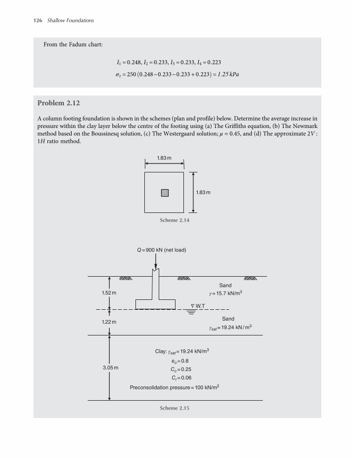
From the Fadum chart:
I1 = 0 248, I2 = 0 233, I3 = 0 233, I4 = 0 223
σz = 250 0 248−0 233−0 233 + 0 223 = 1 25 kPa
Problem 2.12
A column footing foundation is shown in the schemes (plan and profile) below. Determine the average increase inpressure within the clay layer below the centre of the footing using (a) The Griffiths equation, (b) The Newmarkmethod based on the Boussinesq solution, (c) The Westergaard solution; μ = 0.45, and (d) The approximate 2V :1H ratio method.
Sand
Sand
W.T
eo= 0.8
1.22 m
1.52 m
Q = 900 kN (net load)
3.05 m Cc= 0.25
Cr= 0.06
Preconsolidation pressure = 100 kN/m2
γ = 15.7 kN/m3
γsat= 19.24 kN / m3
Clay: γsat= 19.24 kN/m3
Δ
Scheme 2.15
1.83 m
1.83 m
Scheme 2.14
126 Shallow Foundations
worksaccounts.com
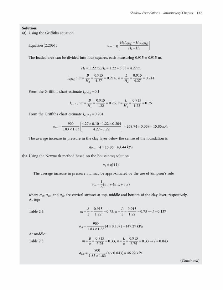
Solution:(a) Using the Griffiths equation
Equation 2 20b σav = qH2Ia H2
−H1Ia H1
H2−H1
The loaded area can be divided into four squares, each measuring 0.915 × 0.915 m.
H1 = 1 22m;H2 = 1 22 + 3 05 = 4 27m
Ia H2m=
BH2
=0 9154 27
= 0 214, n=LH2
=0 9154 27
= 0 214
From the Griffiths chart estimate Ia H2= 0 1
Ia H1m =
BH1
=0 9151 22
= 0 75, n=LH1
=0 9151 22
= 0 75
From the Griffiths chart estimate Ia H1= 0 204
σav =900
1 83 × 1 834 27 × 0 10−1 22 × 0 204
4 27−1 22= 268 74 × 0 059 = 15 86 kPa
The average increase in pressure in the clay layer below the centre of the foundation is
4σav = 4 × 15 86 = 63 44 kPa
(b) Using the Newmark method based on the Boussinesq solution
σz = q 4 I
The average increase in pressure σav may be approximated by the use of Simpson’s rule
σav =16σzt + 4σzm + σzb
where σzt, σzm and σzb are vertical stresses at top, middle and bottom of the clay layer, respectively.At top:
Table 2.3: m=Bz=0 9151 22
= 0 75, n=Lz=0 9151 22
= 0 75 I = 0 137
σzt =900
1 83 × 1 834 × 0 137 = 147 27 kPa
At middle:
Table 2.3: m=Bz=0 9152 75
= 0 33, n=Lz=0 9152 75
= 0 33 I = 0 043
σzm =900
1 83 × 1 834 × 0 043 = 46 22 kPa
(Continued)
Shallow Foundations – Introductory Chapter 127
worksaccounts.com
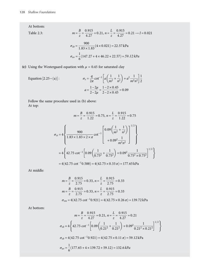
At bottom:
Table 2.3: m=Bz=0 9154 27
= 0 21, n=Lz=0 9154 27
= 0 21 I = 0 021
σzb =900
1 83 × 1 834 × 0 021 = 22 57 kPa
σav =16147 27 + 4 × 46 22 + 22 57 = 59 12 kPa
(c) Using the Westergaard equation with μ = 0.45 for saturated clay
Equation 2 25− a σz =q2π
cot−1 a1m2
+1n2
+ a21
m2n212
a=1−2μ2−2μ
=1−2 × 0 452−2 × 0 45
= 0 09
Follow the same procedure used in (b) above:At top:
m=Bz=0 9151 22
= 0 75, n=Lz=0 9151 22
= 0 75
σzt = 4900
1 83 × 1 83 × 2 × πcot−1
0 091m2
+1n2
+ 0 0921
m2n2
1 2
= 4 42 75 cot−1 0 091
0 752+
10 752
+ 0 0921
0 752 × 0 752
1 2
= 4 42 75 cot−10 588 = 4 42 75 × 0 33 π = 177 65 kPa
At middle:
m=Bz=0 9152 75
= 0 33, n=Lz=0 9152 75
= 0 33
m=Bz=0 9152 75
= 0 33, n=Lz=0 9152 75
= 0 33
σzm = 4 42 75 cot−10 921 = 4 42 75 × 0 26 π = 139 72 kPa
At bottom:
m=Bz=0 9154 27
= 0 21, n=Lz=0 9154 27
= 0 21
σzb = 4 42 75 cot−1 0 091
0 212+
10 212
+ 0 0921
0 212 × 0 212
1 2
σzb = 4 42 75 cot−10 921 = 4 42 75 × 0 11 π = 59 12kPa
σav =16177 65 + 4 × 139 72 + 59 12 = 132 6 kPa
128 Shallow Foundations
worksaccounts.com

(d) Using the approximate 2V : 1H ratio method
Equation 2 18 σz =V
B + z L + z
V =Q= 900 kPa
At top:
σzt =900
1 83 + 1 22 1 83 + 1 22= 96 75 kPa
At middle:
σzm =900
1 83 + 2 75 1 83 + 2 75= 42 91 kPa
At bottom:
σzb =900
1 83 + 4 27 1 83 + 4 27= 24 19 kPa
σav =16σzt + 4σzm + σzb
σav =1696 75 + 4 × 42 91 + 24 19 = 48 76 kPa
Problem 2.13
An embankment is shown in the scheme below. Determine the vertical stress increase under the embankment atpoints A1 and A2.
Solution:The embankment section may be divided into a rectangle at the middle and two triangles on sides of the embank-ment, as shown below. Superposition enables the vertical stress increase to be obtained at points A1 and A2 usingEquations (2.13), (2.14) and (2.15) as applicable.
Vertical stress increase at point A1:
tanα
2=2 55
= 0 5α
2= 26 6 α= 53 2 ; β =
α
2= 26 6
tan θ + β =14 + 2 5
5= 3 3 θ + β = 73 1 θ = 46 5
Equation 2 14 σz =qπ
α+ sinα
Equation 2 15 σz =qπ
xBθ−
12sin2β
Σσz =7 × 17 5
π
53 2180
π + sin53 2 + 27 × 17 5
π
16 514
×46 5180
π−12sin53 2
= 67 42 + 43 42 = 110 84 kPa
(Continued)
Shallow Foundations – Introductory Chapter 129
worksaccounts.com
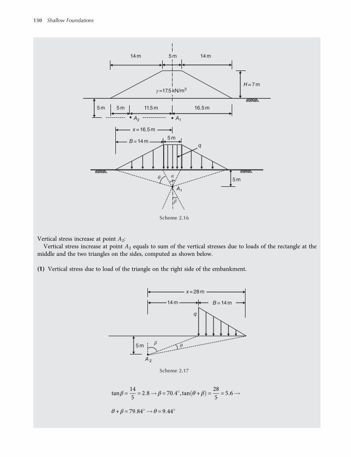
Vertical stress increase at point A2:Vertical stress increase at point A2 equals to sum of the vertical stresses due to loads of the rectangle at the
middle and the two triangles on the sides, computed as shown below.
(1) Vertical stress due to load of the triangle on the right side of the embankment.
tanβ =145= 2 8 β = 70 4 , tan θ + β =
285= 5 6
θ + β = 79 84 θ = 9 44
14 m
5 m
A 2
q
β
x = 28 m
B = 14 m
θ
Scheme 2.17
14 m 14 m
16.5 m11.5 m
A2 A1
5 m5 m
H = 7 m
5 m
γ =17.5 kN/m3
5 m
5 m
x = 16.5 m
B = 14 m
A1
q
αθ
β
Scheme 2.16
130 Shallow Foundations
worksaccounts.com
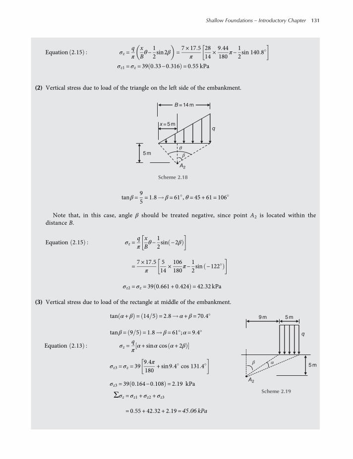
Equation 2 15 σz =qπ
xBθ−
12sin2β =
7 × 17 5π
2814
×9 44180
π−12sin 140 8
σz1 = σz = 39 0 33−0 316 = 0 55 kPa
(2) Vertical stress due to load of the triangle on the left side of the embankment.
tanβ =95= 1 8 β = 61 , θ = 45 + 61 = 106
Note that, in this case, angle β should be treated negative, since point A2 is located within thedistance B.
Equation 2 15 σz =qπ
xBθ−
12sin −2β
=7 × 17 5
π
514
×106180
π−12sin −122
σz2 = σz = 39 0 661 + 0 424 = 42 32 kPa
(3) Vertical stress due to load of the rectangle at middle of the embankment.
tan α+ β = 14 5 = 2 8 α+ β = 70 4
tanβ = 9 5 = 1 8 β = 61 ;α= 9 4
Equation 2 13 σz =qπα+ sinα cos α+ 2β
σz3 = σz = 399 4π180
+ sin9 4 cos 131 4
σz3 = 39 0 164−0 108 = 2 19 kPa
Σσz = σz1 + σz2 + σz3
= 0 55 + 42 32 + 2 19 = 45 06 kPa
5 m
5 m
A2
9 m
q
αβ
Scheme 2.19
B = 14 m
x = 5 mq
A2
θβ5 m
Scheme 2.18
Shallow Foundations – Introductory Chapter 131
worksaccounts.com
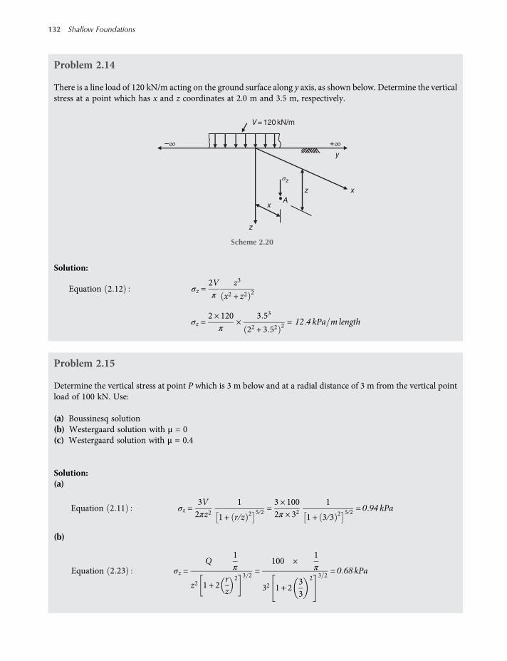
Problem 2.14
There is a line load of 120 kN/m acting on the ground surface along y axis, as shown below. Determine the verticalstress at a point which has x and z coordinates at 2.0 m and 3.5 m, respectively.
Solution:
Equation 2 12 σz =2Vπ
z3
x2 + z2 2
σz =2 × 120
π×
3 53
22 + 3 52 2 = 12 4 kPa m length
Problem 2.15
Determine the vertical stress at point P which is 3 m below and at a radial distance of 3 m from the vertical pointload of 100 kN. Use:
(a) Boussinesq solution(b) Westergaard solution with μ = 0(c) Westergaard solution with μ = 0.4
Solution:(a)
Equation 2 11 σz =3V2πz2
1
1 + r ∕z 2 5 ∕2 =3 × 1002π × 32
1
1 + 3 ∕3 2 5 ∕2 = 0 94 kPa
(b)
Equation 2 23 σz =Q
1π
z2 1 + 2rz
2 3 2=
100 ×1π
32 1 + 233
2 3 2= 0 68 kPa
V = 120 kN/m
+∞–∞
σz
z
z
x
x
y
A
Scheme 2.20
132 Shallow Foundations
worksaccounts.com

(c)
σz =Q
12π
1−2μ2−2μ
z2 1−2μ 2−2μ + r z 2 3 2=
100 ×12π
1−2 × 0 42−2 × 0 4
32 1−2 × 0 4 2−2 × 0 4 + 3 3 2 3 2= 0 573 kPa
Problem 2.16
The scheme below shows an embankment load on a silty clay layer of soil. Determine the vertical stress increase atpoints A, B and C, located at a depth of 5 m below the ground surface.
Solution:The embankment section may be divided into a rectangle at the middle and two triangles on sides of the embank-ment, as shown below. Superposition enables the vertical stress increase to be obtained at points A, B and C usingEquations (2.13), (2.14) and (2.15) as applicable.
Vertical stress increase at point A:
tanα
2=35= 0 6
α
2= 31 α= 62 ; β =
α
2= 31
tan θ + β =235= 4 6 θ + β = 77 75 θ = 46 75
(Continued)
6 m
5 m
ABC
10 m
1V :2H1V :2HSilty clay
γ = 17 kN/m3
Scheme 2.21
Silty clay
10 m
6 m
5 m
γ = 17 kN/m3
α θ
q
x
A
1V:2H 1V:2H
B
β
Scheme 2.22
Shallow Foundations – Introductory Chapter 133
worksaccounts.com
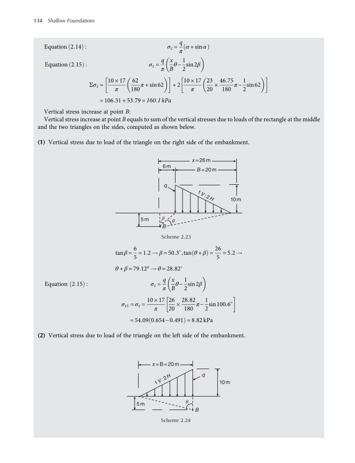
Equation 2 14 σz =qπ
α+ sinα
Equation 2 15 σz =qπ
xBθ−
12sin2β
Σσz =10 × 17
π
62180
π + sin62 + 210 × 17
π
2320
×46 75180
π−12sin62
= 106 31 + 53 79 = 160 1 kPa
Vertical stress increase at point B:Vertical stress increase at point B equals to sum of the vertical stresses due to loads of the rectangle at the middle
and the two triangles on the sides, computed as shown below.
(1) Vertical stress due to load of the triangle on the right side of the embankment.
tanβ =65= 1 2 β = 50 3 , tan θ + β =
265= 5 2
θ + β = 79 12o θ = 28 82
Equation 2 15 σz =qπ
xBθ−
12sin2β
σz1 = σz =10 × 17
π
2620
×28 82180
π−12sin100 6
= 54 09 0 654−0 491 = 8 82kPa
(2) Vertical stress due to load of the triangle on the left side of the embankment.
x = 26 m
q
B
β
6 m
5 m
1V : 2H 10 m
B = 20 m
θ
Scheme 2.23
10 m
x = B = 20 m
1V : 2H
5 mB
q
θ
Scheme 2.24
134 Shallow Foundations
worksaccounts.com

β = 0 , tanθ =205= 4 θ = 76
Equation 2 15 σz =qπ
xBθ−
12sin2β
σz2 = σz =qπ
xBθ = 54 09
2020
×76180
π = 71 78 kPa
(3) Vertical stress due to load of the rectangle at middle of the embankment.
β = 0 , tan α+ β = tanα=65= 1 2 α= 50 3
Equation 2 13 σz =qπα+ sinα cos α+ 2β
σz3 = σz = 54 0950 3 × π180
+ sin50 3 cos 50 3
= 54 09 0 878 + 0 491 = 74 05 kPa
Σσz = σz1 + σz2 + σz3= 8 82 + 71 78 + 74 05 = 154 65 kPa
Vertical stress increase at point C:The determination of vertical stress at point C proceeds in the same manner as that for vertical stress at point A2
in Problem 2.14. The necessary computations are left for the reader.
Problem 2.17
Three point loads 10, 7.5 and 9 MN, act in line 5 m apart near the surface of a soil mass, as shown below. Calculatethe vertical stress at a depth of 4 m vertically below the centre load.
Solution:Vertical stress due to a point load is
Equation 2 11 σz =3V2πz2
1
1 + r ∕z 2 5 ∕2
(Continued)
5 m
6 m
q
B
α
Scheme 2.25
Shallow Foundations – Introductory Chapter 135
worksaccounts.com

Vertical stress due to the 10 MN load plus the 9 MN load is
σz =3
2π × 421
1 + 5 ∕4 2 5 ∕2 10 + 9 = 0 00284 19 = 0 054MN m2
Vertical stress due to the 7.5 MN load is
σz =3 × 7 52π × 42
1
1 + 0 ∕4 2 5 ∕2 = 0 224MN m2
Totalσz = 0 054 + 0 224 = 0 278MN m2 = 278 kPa
Problem 2.18
A strip footing 2.5 m wide carries a uniform pressure of 300 kPa on the surface of a deposit of sand, as shown in thescheme below. The water table is at the surface. The sand has a saturated unit weight = 20 kN/m3. Determine theeffective vertical stress at a point 3m below the centre of the footing before and after the application of the pressure.
Solution:Before loading:
Effective unit weight of soil = γ = γsat −γw
The effective unit weight of the sand = γ = 20−10 = 10 kN m3
The effective vertical stress = σz = 3 × γ = 3 × 10 = 30 kPa
10 MN 7.5 MN 9 MN
4 m
5 m5 m
Scheme 2.26
2.5 m
Sand:
γ = 20 kN/m3
W.T
3 m
q = 300 kPa
α
Scheme 2.27
136 Shallow Foundations
worksaccounts.com

After loading:
tanα
2=2 5 23
= 0 417α
2= 22 65 α= 45 3
Equation 2 14 σz =qπ
α+ sinα =300π
45 3180
π + sin45 3
= 143 35 kPa
The effective vertical stress = σz + σz = 143 35 + 30 00 = 173 35 kPa
Problem 2.19
Loads P and 2P of two columns are to be applied to the surface of a 6 m thick layer of dense sand which overlies alayer of clay. Determine the maximum spacing of the columns if the settlement of the heavier column is not to begreater than 1.5 times that of the other column. Assume the settlement is due to the clay alone and that its com-pressibility characteristics are the same for each load.
Solution:Settlement of a clay layer may be assumed proportional to the effective vertical stress causing it provided thatcompressibility characteristics of the clay as well as the layer thickness remain unchanged. This is readily noticedin the known equation of consolidation settlement: sc =mvσzH; in whichmv is the coefficient of volume compress-ibility of the clay and H is the layer thickness.
Equation 2 11 σz =3V2πz2
1
1 + r ∕z 2 5 ∕2
Let V = P, and assume x = [1 + (r/z)2]5/2. Also, let the vertical effective stress increase below centre of loadP equals σz1 and that below centre of load 2P equals σz2, as shown in the scheme above.
σz1 =3P2πz2
+6P2πz2
1x=
3P2πz2
1 +2x
σz2 =6P2πz2
+3P2πz2
1x=
3P2πz2
2 +1x
sc =mvσzH;sc2sc1
≤1 51
mvσz2Hmvσz1H
≤1 51
σz2σz1
≤1 51
(Continued)
P 2P
Dense sand σ′z2σ′z1
Clay
z = 6 m
r
Scheme 2.28
Shallow Foundations – Introductory Chapter 137
worksaccounts.com

Useσz2σz1
=1 51
σz2σz1
=
3P2πz2
2 +1x
3P2πz2
1 +2x
=2 +
1x
1 +2x
=2x + 1x + 2
= 1 5
1 5x + 3 = 2x + 1 x = 4 = 1 + r z 2 5 2
4 = 1 + r z 2 5 2= 1 + r 6 2 5 2
1 74 = 1 + r 6 2 0 74 = r 6 2
r2 = 26 64 r = 5 16m
Therefore, the maximum spacing of the columns = 5.16 m
Problem 2.20
Centres of two columns A and B are 3 m apart. Column A is supported by a footing 1.2 × 1.2 m and column B by afooting 1 × 1 m. Column A is founded at a depth of 2.5 m below ground level and column B at 1.5 m. The contactpressure on the soil under each footing is 425 kPa. Find the increase in vertical stress at a depth of 9 m verticallybelow the centres of A and B and the point midway between them. Use the Newmark method.
Solution:Vertical stress increase below centre of column A:
(1) Vertical stress increase due to load of column A is
σA1 = q 4Iq = 425 kPa
BA
3 m
2.5 m
1 m
9 m
1.5 m
1.2 m
Scheme 2.29
138 Shallow Foundations
worksaccounts.com

B z = L z = 0 6 6 5 ≈ 0 1 I = 0 0047
σA1 = q 4I = 425 × 4 × 0 0047 = 7 99 kPa
(2) Vertical stress increase due to load of column B is obtained using thescheme shown below.
For the two long rectangles:BZ=0 57 5
= 0 067 andLZ=3 57 5
= 0 467
Ilong = 0 012
For the two short rectangles:BZ=0 57 5
= 0 067 andLZ=2 57 5
= 0 333
Ishort = 0 01
σA2 = q 2Ilong −2Ishort = 425 2 × 0 012−2 × 0 01 = 1 7 kPa
Vertical stress increase below centre of column A is
σA = σA1 + σA2 = 7 99 + 1 7 = 9 67 kPa
Vertical stress increase below centre of column B :
(1) Vertical stress increase due to load of column B is
σB1 = q 4I
q = 425 kPa
B z = L z = 0 5 7 5 = 0 067 I = 0 003
σA1 = q 4I = 425 × 4 × 0 003 = 5 1 kPa
(2) Vertical stress increase due to load of column A is obtained using the scheme shown below.
(Continued)
I I
II
A
1.2 m
1.2 m
Scheme 2.30
2.5 m 1 m
1 mBA
Scheme 2.31
I I
I
B
I
1 m
1 m
Scheme 2.32
A B
2.4 m1.2 m
1.2 m
Scheme 2.33
Shallow Foundations – Introductory Chapter 139
worksaccounts.com

For the two long rectangles:BZ=0 66 5
= 0 092 andLZ=3 66 5
= 0 467
Ilong = 0 016
For the two short rectangles:BZ=0 66 5
= 0 092 andLZ=2 46 5
= 0 369
Ishort = 0 0125
σB2 = q 2Ilong −2Ishort = 425 2 × 0 016−2 × 0 0125 = 2 98 kPa
Vertical stress increase below centre of column B is
σB = σB1 + σB2 = 5 1 + 2 98 = 8 08 kPa
Vertical stress increase below the point midway between centres of A and B:
(1) Vertical stress increase due to load of column A is obtained using the scheme shown below.
For the two long rectangles:BZ=0 66 5
= 0 092 andLZ=2 16 5
= 0 323
Ilong = 0 013
For the two short rectangles:BZ=0 66 5
= 0 092 andLZ=0 96 5
= 0 138
Ishort = 0 006
σA = q 2Ilong −2Ishort = 425 2 × 0 013−2 × 0 006 = 5 95 kPa
(2) Vertical stress increase due to load of column B is obtained using the scheme shown below.
A
0.9 m1.2 m
1.2 m
Scheme 2.34
B 1 m
1 m1 m
Scheme 2.35
140 Shallow Foundations
worksaccounts.com
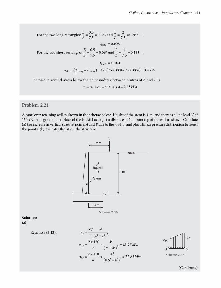
For the two long rectangles:BZ=0 57 5
= 0 067 andLZ=
27 5
= 0 267
Ilong = 0 008
For the two short rectangles:BZ=0 57 5
= 0 067 andLZ=
17 5
= 0 133
Ishort = 0 004
σB = q 2Ilong −2Ishort = 425 2 × 0 008−2 × 0 004 = 3 4 kPa
Increase in vertical stress below the point midway between centres of A and B is
σz = σA + σB = 5 95 + 3 4 = 9 35 kPa
Problem 2.21
A cantilever retaining wall is shown in the scheme below. Height of the stem is 4 m, and there is a line load V of150 kN/m length on the surface of the backfill acting at a distance of 2 m from top of the wall as shown. Calculate(a) the increase in vertical stress at points A and B due to the loadV, and plot a linear pressure distribution betweenthe points, (b) the total thrust on the structure.
Solution:(a)
Equation 2 12 σz =2Vπ
z3
x2 + z2 2
σzA =2 × 150
π×
43
22 + 42 2 = 15 27 kPa
σzB =2 × 150
π×
43
0 62 + 42 2 = 22 82 kPa
(Continued)
2 m
Backfill
Stem
1.4 m
4 m
V
BA
Scheme 2.36
B
σzBσzA
A
Scheme 2.37
Shallow Foundations – Introductory Chapter 141
worksaccounts.com
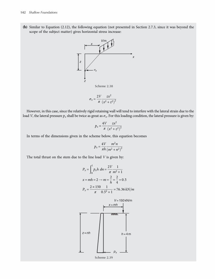
(b) Similar to Equation (2.12), the following equation (not presented in Section 2.7.3, since it was beyond thescope of the subject matter) gives horizontal stress increase:
σx =2Vπ
zx2
x2 + z2 2
However, in this case, since the relatively rigid retaining wall will tend to interfere with the lateral strain due to theload V, the lateral pressure px shall be twice as great as σx. For this loading condition, the lateral pressure is given by:
px =4Vπ
zx2
x2 + z2 2
In terms of the dimensions given in the scheme below, this equation becomes
px =4Vπh
m2n
m2 + n2 2
The total thrust on the stem due to the line load V is given by:
Px =1
0pxh dn=
2Vπ
1m2 + 1
x =mh= 2 m=2h=24= 0 5
Px =2 × 150
π
10 52 + 1
= 76 36 kN m
x
x
z
z
σx
V/m
Scheme 2.38
V = 150 kN/m
z = nh
px
x = mh
h = 4 m
Scheme 2.39
142 Shallow Foundations
worksaccounts.com
References
Bowles, J. E. (2001), Foundation Analysis and Design, 5th edn, McGraw-Hill, New York.Boussinesq, M. J. (1883), Application Des Potentials à l’Étude de l’Équilibre et du Movvement Des Solides Elastiques,
Gauthier-Villars, Paris (in French).Coduto, Donald P. (2001), Foundation Design: Principles and Practices, 2nd edn, Prentice-Hall, Inc., New Jersey.Das, Braja M. (2011), Principles of Foundation Engineering, 7th edn, CENGAGE Learning, United States.Fadum, R. E. (1948), “Influence Values for Estimating Stresses in Elastic Foundations”, Proceedings of 2nd International
Conference SFME, Rotterdam, Vol. 3, pp. 77–84.Griffiths, D. V. (1984), “A Chart for Estimating the Average Vertical Stress Increase in an Elastic Foundation below a Uni-
formly Rectangular Loaded Area”, Canadian Geotechnical Journal, Vol. 21, No. 4, pp. 710–713.Knappett, J. A., and Craig, R. F. (2012), Soil Mechanics, 8th edn, Spon, Abingdon, United Kingdom.Kosmatca, S. H., and Panarese, W. C. (1988), Design and Control of Concrete Mixtures, 13th edn, Portland-Cement Asso-
ciation, Skokie, Illinois.Newmark, N. M. (1935), Simplified Computation of Vertical Pressures in Elastic Foundations, Engineering Experiment Sta-
tion Circular No. 24, University of Illinois, Urbana, Illinois.Newmark, N. M. (1942), Influence Charts for Computation of Stresses in Elastic Foundations, University of Illinois Bulletin
No. 338, University of Illinois, Urbana, Illinois.PCA (1991), “Durability of Concrete in Sulfate-Rich Soils”, Concrete Technology Today, Vol. 12, No. 3, pp. 6–8, Portland
Cement Association, New York.Taylor, D. W. (1948), Fundamentals of Soil Mechanics, 1st edn, John Wiley and Sons, Inc., New York.Terzaghi, K., and Peck, R. B. (1967), Soil Mechanics in Engineering Practice, 2nd edn, JohnWiley and Sons, Inc., New York.Tomlinson, M. J. (2001), Foundation Design and Construction, 7th edn, Pearson Education, Harlow, United Kingdom.Westegaard, H. M. (1938), “A Problem of Elasticity Suggested by a Problem in Soil Mechanics: Soft Material Reinforced by
a Numerous Strong Horizontal Sheets”, Contributions to Mechanics of Solids, Stephen Timoshenko 60th AnniversaryVolume, The Macmillan Company, New York.
Shallow Foundations – Introductory Chapter 143
worksaccounts.com
CHAPTER 3
Shallow Foundations – Settlement
3.1 General
The vertical downward displacements at the ground surface or the vertical downward displacement of astructure are often called settlement. It is usually caused by direct application of structural loads on thefoundation which in turn cause compression of the supporting material (soil or rock). However, inaddition to the settlement under loads, foundation settlement may also occur due to some or combin-ation of other causes, as follows:
(1) Seasonal swelling and shrinking of expansive soils.(2) Ground water lowering or a falling ground water table. Prolonged lowering of water level in fine-
grained soils may introduce settlement due to consolidation. Repeated lowering and rising of waterlevel in loose granular soils tends to compact the soil and cause settlement. Pumping water ordraining water by pipes or tiles from granular soils without adequate filter material as protectionmay in a period of time wash and carry a sufficient amount of fine particles away from the soil andcause settlement.
(3) Underground erosion. It may cause formation of cavities in the subsoil which when collapse settle-ment occurs.
(4) Changes in the vicinity. If there are changes adjacent to the property such as recently placed fill,excavation, construction of a new structure, underground tunnelling or mining and so on, settle-ment may occur due to increase in the stresses.
(5) Vibrations and shocks. Vibrations due to pile driving or oscillating machineries as well as shocksdue to blasting or earthquake cause settlements, especially in granular soils.
(6) Ground movement on earth slopes. If surface erosion, slow creep or landslides occur, there may besettlement problems.
Theoretically, no damage is done to the superstructure if the foundations settle uniformly. How-ever, settlement exceeding a certain limit may cause trouble in utilities such as water pipe lines,sewers, telephone lines; also trouble in the surface drainage configuration and in access fromstreets. Sometimes buildings must join existing structures, and it is required that floors of thetwo buildings be at the same level. If the new building settles excessively, the floors will nolonger remain at the same level, causing serious serviceability problems. In addition to all these
Shallow Foundations: Discussions and Problem Solving, First Edition. Tharwat M. Baban.© 2016 John Wiley & Sons, Ltd. Published 2016 by John Wiley & Sons, Ltd.
worksaccounts.com
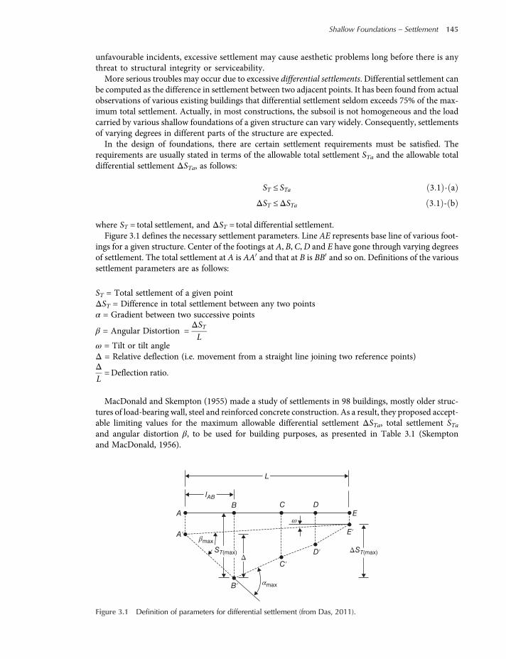
unfavourable incidents, excessive settlement may cause aesthetic problems long before there is anythreat to structural integrity or serviceability.More serious troubles may occur due to excessive differential settlements. Differential settlement can
be computed as the difference in settlement between two adjacent points. It has been found from actualobservations of various existing buildings that differential settlement seldom exceeds 75% of the max-imum total settlement. Actually, in most constructions, the subsoil is not homogeneous and the loadcarried by various shallow foundations of a given structure can vary widely. Consequently, settlementsof varying degrees in different parts of the structure are expected.In the design of foundations, there are certain settlement requirements must be satisfied. The
requirements are usually stated in terms of the allowable total settlement STa and the allowable totaldifferential settlement ΔSTa, as follows:
ST ≤ STa 3 1 - a
ΔST ≤ΔSTa 3 1 - b
where ST = total settlement, and ΔST = total differential settlement.Figure 3.1 defines the necessary settlement parameters. Line AE represents base line of various foot-
ings for a given structure. Center of the footings at A, B, C,D and E have gone through varying degreesof settlement. The total settlement at A is AA and that at B is BB and so on. Definitions of the varioussettlement parameters are as follows:
ST = Total settlement of a given pointΔST = Difference in total settlement between any two pointsα = Gradient between two successive points
β = Angular Distortion =ΔSTL
ω = Tilt or tilt angleΔ = Relative deflection (i.e. movement from a straight line joining two reference points)ΔL=Deflection ratio.
MacDonald and Skempton (1955) made a study of settlements in 98 buildings, mostly older struc-tures of load-bearing wall, steel and reinforced concrete construction. As a result, they proposed accept-able limiting values for the maximum allowable differential settlement ΔSTa, total settlement STaand angular distortion β, to be used for building purposes, as presented in Table 3.1 (Skemptonand MacDonald, 1956).
C DB
βmax
αmax
ωA
A′
B′
C′D′
E′
E
L
lAB
ST(max) ΔΔST(max)
Figure 3.1 Definition of parameters for differential settlement (from Das, 2011).
Shallow Foundations – Settlement 145
worksaccounts.com
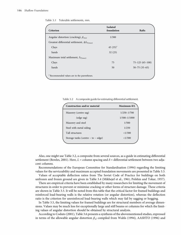
Also, one might use Table 3.2, a composite from several sources, as a guide in estimating differentialsettlement (Bowles, 2001). Here, L = column spacing and δ = differential settlement between two adja-cent columns.
Recommendations of the European Committee for Standardisation (1994) regarding the limitingvalues for the serviceability and maximum accepted foundation movements are presented in Table 3.3.
Values of acceptable deflection ratios from The Soviet Code of Practice for buildings on bothunfrozen and frozen ground are given in Table 3.4 (Mikhejef et al., 1961; Polshin and Tokar, 1957).
There are empirical criteria have been established by many researchers for limiting the movement ofstructures in order to prevent or minimise cracking or other forms of structure damage. These criteriaare shown in Table 3.5. It will be noted from this table that the critical factor for framed buildings andreinforced load-bearing walls is the relative rotation (or angular distortion), whereas the deflectionratio is the criterion for unreinforced load-bearing walls which may fail by sagging or hogging.
In Table 3.5, the limiting values for framed buildings are for structural members of average dimen-sions. Values may be much less for exceptionally large and stiff beams or columns for which the limit-ing values of angular distortion should be obtained by structural analysis.
According to Coduto (2001), Table 3.6 presents a synthesis of the abovementioned studies, expressedin terms of the allowable angular distortion βa; compiled from Wahls (1994), AASHTO (1996) and
Table 3.1 Tolerable settlements, mm.
CriterionIsolatedfoundation Rafts
Angular distortion (cracking), βmax 1/300
Greatest differential settlement, ΔST(max)
Clays 45 (35)∗
Sands 32 (25)
Maximum total settlement, ST(max)
Clays 75 75–125 (65–100)
Sands 50 50–75 (35–65)
a Recommended values are in the parentheses.
Table 3.2 A composite guide for estimating differential settlement.
Construction and/or material Maximum δ/L
Masonry (centre sag) 1/250–1/700
(edge sag) 1/500–1/1000
Masonry and steel 1/500
Steel with metal siding 1/250
Tall structures <1/300
Storage tanks (centre – to – edge) <1/300
146 Shallow Foundations
worksaccounts.com

other sources. These values already include a factor of safety of at least 1.5. They may be used to com-pute the allowable differential settlement as follows:
ΔSTa = βaL 3 2
Where:ΔSTa = allowable differential settlementβa = allowable angular distortion (from the following table)L = column spacing (horizontal distance between columns)
Note: Be sure to consider local practice and precedent when developing design values of ΔSTa.
Table 3.4 Allowable deflection ratios for structures (from Bowles, 2001).
Structure on:
Average maximumsettlement, mmStructure
Sand orhard clay Plastic clay
Crane runway 0.003 0.003
Steel and concrete frames 0.002 0.002 100
End rows of brick-clad frame 0.0007 0.001 150
Where strain does not occur 0.005 0.005
Multistory brick wall 25 L/H ≥ 2.5
L/H to 3a 0.0003 0.0004 100 L/H ≤ 1.5
Multistory brick wall
L/H over 5 0.0005 0.0007
One-story mill buildings 0.001 0.001
Smokestacks, water towers, ring foundations 0.004 0.004 300
a L/H = ratio of the length to the height of a building.
Table 3.3 Recommendations of the European Committee for Standardisation of Differential Settlement Parameters(from Das, 2011).
Item Parameter Magnitude Comments
Limiting values for serviceability(European Committee for Standardization, 1994a)
ST 25 mm Isolated shallow foundation
50 mm Raft foundation
ΔST 5 mm Frames with rigid cladding
10 mm Frames with flexible cladding
20 mm Open frames
β 1/500 —
Maximum acceptable foundation movement(European Committee for Standardization, 1994b)
ST 50 Isolated shallow foundation
ΔST 20 Isolated shallow foundation
β ≈1/500 —
Shallow Foundations – Settlement 147
worksaccounts.com

Total settlement (ST) under loads of a structural foundation is generally made up of three compo-nents. The immediate settlement (Si) takes place immediately after application of the loading or within ashort period of time (not more than several days) as a result of elastic deformation of the soil without
Table 3.5 Limiting values of distortion and deflection ratio of buildings (from Tomlinson, 2001).
Type of structure Type of damage
Limiting values
Values of relative rotation (angular distortion)
Skempton andMacDonald Mayerhof Polshin and Tokar Bjerrum
Framed buildingsand reinforced loadbearing walls
Structuraldamage
1/15 1/250 1/200 1/150
Cracking in wallsand partitions
1/300 (but 1/500recommended)
1/500 1/500 (0.7/1000 to1/1000 for end bays)
1/500
Values of deflection ratio Δ/L
Mayerhof Polshin and Tokar Burland and Wroth
Unreinforcedload-bearing walls
Cracking bysagging
0.4/1000 L/H = 3: 0.3 to0.4 × 10−3
At L/H = 1: 0.4 × 10⁻³
At L/H = 5: 0.8 × 10⁻³
Cracking byhogging
– – At L/H = 1: 0.2 × 10⁻³
At L/H = 5: 0.4 × 10⁻³
Table 3.6 Allowable angular distortions βa (compiled from Wahls, 1994; AASHTO, 1996; and other sources).
Tyle of structure βa
Steel tanks 1/25
Bridges with simply-supported spans 1/125
Bridges with continuous spans 1/250
Buildings which are very tolerant of differential settlement, such as industrial buildingswith corrugated steel siding and no sensitive interior finish
1/250
Typical commercial and residential buildings 1/500
Overhead traveling crane rails 1/500
Buildings which are especially intolerant of differential settlements, such as that withsensitive wall or floor finishes
1/1000
Machinerya 1/1500
Buildings with unreinforced masonry load bearing wallsLength/height≤ 3
1/2500
Length/height≥ 5 1/1250
a Large machines, such as turbines or large punch presses, often have their own foundation, separate from that of the building thathouses them. It often is appropriate to discuss allowable differential settlement issues with the machine manufacturer.
148 Shallow Foundations
worksaccounts.com

change in water content. It may predominate in all coarse-grained soils with a large coefficient of per-meability (not less than 0.001 m/s) and in unsaturated (degree of saturation less than 90%) fine-grainedsoils. The consolidation settlement (Sc) takes place as a result of volume reduction of the soil caused byextrusion of some of the porewater from the soil. It predominates in saturated or nearly saturated fine-grained soils unless the soil is very organic. Analysis of consolidation settlement requires estimate ofboth the settlement and how long a time it will take for most of the settlement to occur. Secondarycompression or creep (Ss) caused by the viscous resistance of the soil to continuing readjustmentof the soil particles into a closer (or denser) state under the compressive load. This phenomenon isassociated with both immediate and consolidation-type settlements, although it is usually not of muchsignificance with immediate settlements. Secondary compression may be the larger component of totalsettlement in some soils, particularly in soils with a large organic content.Thus, the total settlement (ST) is given by
ST = Si + Sc + Ss 3 3
3.2 Immediate Settlement
Immediate settlement or elastic settlement of a shallow foundation can be estimated by using the theoryof elasticity.The settlement under the corner of a uniformly loaded flexible rectangular base of dimensions B× L,
or a round base converted to an equivalent square, on the surface of an elastic half-space can becomputed as
Si = q×B×1−μ2
Es×m× IS 3 4
According to Fox (1948), the settlement is reduced when the loaded area (the foundation base) isplaced at some depth in the ground. He suggested a factor IF be used with the above equation as follows:
Si = q×B×1−μ2
Es×m × IS × IF 3 5
Where:
q = Contact pressure intensity (uniformly distributed load), in units of EsB = Least lateral dimension of the contributing base area, in units of SiL = Length of the contributing base area in units of SiEs = Average modulus of elasticity of soil for a depth equals to HH = Thickness of the soil layer or 4B whichever is smaller
IF = Influence factor (Fox, 1948) depends on Poisson’s ratio of soil μ,BLor
LBand
DB; it can be obtained
from Figure 3.2 or from Table 3.7 (approximately).m = Number of corners contributing to Si
IS = Influence factor (Steinbrenner) = I1 +1−2μ1−μ
I2
I1 and I2 = Factors obtained from equations by Steinbrenner or from Table 3.8, depend on M and N
M =LB, N =
HB, H = Thickness of the soil layer, in units of B
For Si at centre useB2instead of B,
L2instead of L, and m = 4.
For Si at corner use B = B, L = L, and m = 1.
Shallow Foundations – Settlement 149
worksaccounts.com
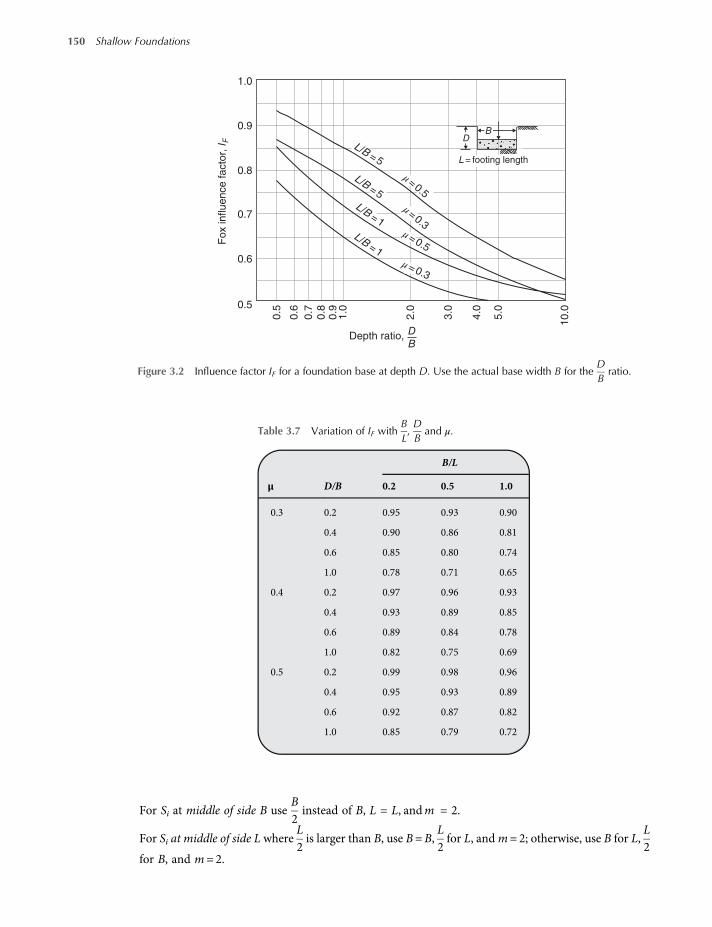
For Si at middle of side B useB2instead of B, L = L, andm = 2.
For Si at middle of side L whereL2is larger than B, use B=B,
L2for L, andm= 2; otherwise, use B for L,
L2
for B, and m= 2.
Table 3.7 Variation of IF withBL,DBand μ.
B/L
μ D/B 0.2 0.5 1.0
0.3 0.2 0.95 0.93 0.90
0.4 0.90 0.86 0.81
0.6 0.85 0.80 0.74
1.0 0.78 0.71 0.65
0.4 0.2 0.97 0.96 0.93
0.4 0.93 0.89 0.85
0.6 0.89 0.84 0.78
1.0 0.82 0.75 0.69
0.5 0.2 0.99 0.98 0.96
0.4 0.95 0.93 0.89
0.6 0.92 0.87 0.82
1.0 0.85 0.79 0.72
Depth ratio, D
B
1.0
L/B=5
L/B=5
L/B=1
L/B=1
μ =0.3
μ=0.5
μ=0.3
μ=0.5
0.9
0.8
0.7F
ox influence facto
r, I
F
0.6
0.5
0.5
0.6
0.7
0.8
0.9
1.0
2.0
3.0
4.0
5.0
10.0
L = footing length
DB
Figure 3.2 Influence factor IF for a foundation base at depth D. Use the actual base width B for theDBratio.
150 Shallow Foundations
worksaccounts.com
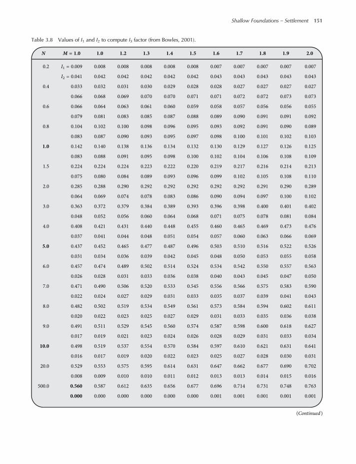
Table 3.8 Values of I1 and I2 to compute IS factor (from Bowles, 2001).
N M = 1.0 1.0 1.2 1.3 1.4 1.5 1.6 1.7 1.8 1.9 2.0
0.2 I1 = 0.009 0.008 0.008 0.008 0.008 0.008 0.007 0.007 0.007 0.007 0.007
I2 = 0.041 0.042 0.042 0.042 0.042 0.042 0.043 0.043 0.043 0.043 0.043
0.4 0.033 0.032 0.031 0.030 0.029 0.028 0.028 0.027 0.027 0.027 0.027
0.066 0.068 0.069 0.070 0.070 0.071 0.071 0.072 0.072 0.073 0.073
0.6 0.066 0.064 0.063 0.061 0.060 0.059 0.058 0.057 0.056 0.056 0.055
0.079 0.081 0.083 0.085 0.087 0.088 0.089 0.090 0.091 0.091 0.092
0.8 0.104 0.102 0.100 0.098 0.096 0.095 0.093 0.092 0.091 0.090 0.089
0.083 0.087 0.090 0.093 0.095 0.097 0.098 0.100 0.101 0.102 0.103
1.0 0.142 0.140 0.138 0.136 0.134 0.132 0.130 0.129 0.127 0.126 0.125
0.083 0.088 0.091 0.095 0.098 0.100 0.102 0.104 0.106 0.108 0.109
1.5 0.224 0.224 0.224 0.223 0.222 0.220 0.219 0.217 0.216 0.214 0.213
0.075 0.080 0.084 0.089 0.093 0.096 0.099 0.102 0.105 0.108 0.110
2.0 0.285 0.288 0.290 0.292 0.292 0.292 0.292 0.292 0.291 0.290 0.289
0.064 0.069 0.074 0.078 0.083 0.086 0.090 0.094 0.097 0.100 0.102
3.0 0.363 0.372 0.379 0.384 0.389 0.393 0.396 0.398 0.400 0.401 0.402
0.048 0.052 0.056 0.060 0.064 0.068 0.071 0.075 0.078 0.081 0.084
4.0 0.408 0.421 0.431 0.440 0.448 0.455 0.460 0.465 0.469 0.473 0.476
0.037 0.041 0.044 0.048 0.051 0.054 0.057 0.060 0.063 0.066 0.069
5.0 0.437 0.452 0.465 0.477 0.487 0.496 0.503 0.510 0.516 0.522 0.526
0.031 0.034 0.036 0.039 0.042 0.045 0.048 0.050 0.053 0.055 0.058
6.0 0.457 0.474 0.489 0.502 0.514 0.524 0.534 0.542 0.550 0.557 0.563
0.026 0.028 0.031 0.033 0.036 0.038 0.040 0.043 0.045 0.047 0.050
7.0 0.471 0.490 0.506 0.520 0.533 0.545 0.556 0.566 0.575 0.583 0.590
0.022 0.024 0.027 0.029 0.031 0.033 0.035 0.037 0.039 0.041 0.043
8.0 0.482 0.502 0.519 0.534 0.549 0.561 0.573 0.584 0.594 0.602 0.611
0.020 0.022 0.023 0.025 0.027 0.029 0.031 0.033 0.035 0.036 0.038
9.0 0.491 0.511 0.529 0.545 0.560 0.574 0.587 0.598 0.600 0.618 0.627
0.017 0.019 0.021 0.023 0.024 0.026 0.028 0.029 0.031 0.033 0.034
10.0 0.498 0.519 0.537 0.554 0.570 0.584 0.597 0.610 0.621 0.631 0.641
0.016 0.017 0.019 0.020 0.022 0.023 0.025 0.027 0.028 0.030 0.031
20.0 0.529 0.553 0.575 0.595 0.614 0.631 0.647 0.662 0.677 0.690 0.702
0.008 0.009 0.010 0.010 0.011 0.012 0.013 0.013 0.014 0.015 0.016
500.0 0.560 0.587 0.612 0.635 0.656 0.677 0.696 0.714 0.731 0.748 0.763
0.000 0.000 0.000 0.000 0.000 0.000 0.001 0.001 0.001 0.001 0.001
(Continued )
Shallow Foundations – Settlement 151
worksaccounts.com

Table 3.8 (Continued)
N M = 2.5 4.0 5.0 6.0 7.0 8.0 9.0 10.0 25.0 50.0 100.0
0.2 I1 = 0.007 0.006 0.006 0.006 0.006 0.006 0.006 0.006 0.006 0.006 0.006
I2 = 0.043 0.044 0.044 0.044 0.044 0.044 0.044 0.044 0.044 0.044 0.044
0.4 0.026 0.024 0.024 0.024 0.024 0.024 0.024 0.024 0.024 0.024 0.024
0.074 0.075 0.075 0.075 0.076 0.076 0.076 0.076 0.076 0.076 0.076
0.6 0.053 0.051 0.050 0.050 0.050 0.049 0.049 0.049 0.049 0.049 0.049
0.094 0.097 0.097 0.098 0.098 0.098 0.098 0.098 0.098 0.098 0.098
0.8 0.086 0.082 0.081 0.080 0.080 0.080 0.079 0.079 0.079 0.079 0.079
0.107 0.111 0.112 0.113 0.113 0.113 0.113 0.114 0.114 0.114 0.114
1.0 0.121 0.115 0.113 0.112 0.112 0.112 0.111 0.111 0.110 0.110 0.110
0.114 0.120 0.122 0.123 0.123 0.124 0.124 0.124 0.125 0.125 0.125
1.5 0.207 0.197 0.194 0.192 0.191 0.190 0.190 0.189 0.188 0.188 0.188
0.118 0.130 0.134 0.136 0.137 0.138 0.138 0.139 0.140 0.140 0.140
2.0 0.284 0.271 0.267 0.264 0.262 0.261 0.260 0.259 0.257 0.256 0.256
0.114 0.131 0.136 0.139 0.141 0.143 0.144 0.145 0.147 0.147 0.148
3.0 0.402 0.392 0.386 0.382 0.378 0.376 0.374 0.373 0.368 0.367 0.367
0.097 0.122 0.131 0.137 0.141 0.144 0.145 0.147 0.152 0.153 0.154
4.0 0.484 0.484 0.479 0.474 0.470 0.466 0.464 0.462 0.453 0.451 0.451
0.082 0.110 0.121 0.129 0.135 0.139 0.142 0.145 0.154 0.155 0.156
5.0 0.553 0.554 0.552 0.548 0.543 0.540 0.536 0.534 0.522 0.519 0.519
0.070 0.098 0.111 0.120 0.128 0.133 0.137 0.140 0.154 0.156 0.157
6.0 0.585 0.609 0.610 0.608 0.604 0.601 0.598 0.595 0.579 0.576 0.575
0.060 0.087 0.101 0.111 0.120 0.126 0.131 0.135 0.153 0.157 0.157
7.0 0.618 0.653 0.658 0.658 0.656 0.653 0.650 0.647 0.628 0.624 0.623
0.053 0.078 0.092 0.103 0.112 0.119 0.125 0.129 0.152 0.157 0.158
8.0 0.643 0.688 0.697 0.700 0.700 0.698 0.695 0.692 0.672 0.666 0.665
0.047 0.071 0.084 0.095 0.104 0.112 0.118 0.124 0.151 0.156 0.158
9.0 0.663 0.716 0.730 0.736 0.737 0.736 0.735 0.732 0.710 0.704 0.702
0.042 0.064 0.077 0.088 0.097 0.105 0.112 0.118 0.149 0.156 0.158
10.0 0.679 0.740 0.758 0.766 0.770 0.770 0.770 0.768 0.745 0.738 0.735
0.038 0.059 0.071 0.082 0.091 0.099 0.106 0.112 0.147 0.156 0.158
20.0 0.756 0.856 0.896 0.925 0.945 0.959 0.969 0.977 0.982 0.965 0.957
0.020 0.031 0.039 0.046 0.053 0.059 0.065 0.071 0.124 0.148 0.156
500.0 0.832 0.977 1.046 1.102 1.150 1.191 1.227 1.259 1.532 1.721 1.879
0.001 0.001 0.002 0.002 0.002 0.003 0.003 0.003 0.008 0.016 0.031
152 Shallow Foundations
worksaccounts.com

Equation (3.5) is strictly applicable to flexible bases on the half-space. Here, the half-space may con-sist of either cohesionless materials of any water content or unsaturated cohesive soils, with no or verysmall organic content.In practice most foundations are not perfectly rigid. Even thick footings deflect under the superstruc-
ture loads.It was found that if the footing is rigid the settlement will be uniform and the IS factor will be reduced
by about 7%. Hence, Si of a rigid base can be estimated as
Si rigid = 0 93Si flexible 3 6
It may be more correct to use the weighted average of Es than the simple ordinary average. Theweighted average Es in the depth z =H can be computed (where for n layers, H = n
i Hi as
Es, av =H1Es1 +H2Es2 +…+HnEsn
H3 7
Another equation may be considered as an improved equation compared to Equation (3.5) for cal-culation of the elastic settlement was presented by Mayne and Poulos (1999). The equation takes intoaccount the increase in the modulus of elasticity of the soil with depth, the rigidity of the base, the depthof embedment of the foundation and the location of rigid layers at a limited depth. The equation givesthe elastic settlement below centre of a uniformly loaded rectangular base of the equivalent diameterBe, as
Si =qoBeIGIFIE
Eo1−μ2s 3 8
Where:
qo = Contact pressure intensity in units of EoEo = Soil modulus of elasticity considered at the foundation level
IG = Influence factor for the variation of Es with depth, = f β =EokBe
,HBe
, obtained from Figure 3.4
IF = Foundation rigidity correction factor, obtained from Figure 3.5IE = Foundation embedment correction factor, obtained from Figure 3.6μs = Poisson’s ratio of soilEs = Eo + kz , as shown in Figure 3.3Ef = Modulus of elasticity of the foundation material
0
Compressible
soil layer
Base;Be
Df
H
Ef
Es
Es= (Eo+ kz)
Eo
z
Es; μs
t
Rigid layer
Figure 3.3 Defined general parameters for use in the improved elastic settlement equation.
Shallow Foundations – Settlement 153
worksaccounts.com
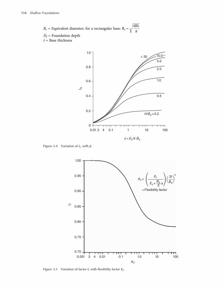
Be = Equivalent diameter; for a rectangular base: Be =4BLπ
Df = Foundation deptht = Base thickness
1.00
0.95
= Flexibility factor0.90
0.85
0.80
0.75
0.70
0.001 2 4 0.01 0.1 1.0
KF
I F
10 100
2
2t3
KF=Ef
Be BekEo+
Figure 3.5 Variation of factor IF with flexibility factor KF.
0.01 2 4 0.1 1 10 100
β = E0 /k Be
1.0> 30
0.8
0.6I G
0.4
0.2
0
10.0
5.0
2.0
1.0
0.5
H/Be= 0.2
Figure 3.4 Variation of IG with β.
154 Shallow Foundations
worksaccounts.com

The foundation rigidity correction factor can be expressed as
IF =π
4+
1
4 6 + 10 Ef Eo + Bek 2 2t Be3 3 9
The foundation embedment correction factor can be expressed as
IE = 1−1
3 5 exp 1 22μs−0 4 Be Df + 1 63 10
Figure 3.3 shows a foundation with an equivalent diameter Be, located at a depthDf below the groundsurface. A rigid layer is located at a depth H below the bottom of the foundation. Variation of Es withdepth is also shown.
3.3 Settlement of Foundations on Coarse-grained Soils
3.3.1 General
Settlements of foundations on sands, gravel deposits and granular fill materials take place almostimmediately as the foundation loading is imposed on them. Therefore, Equation (3.5) or (3.8) canbe used with enough confidence provided that the elastic parameters Es and μ are computed to a rea-sonable degree of accuracy. This is because these parameters especially the Es, are mainly responsiblefor magnitude of the soil strain ε occurs under the imposed load. Since the elastic settlement is simply
Si =H0 εdh= n
i = 1εiHi, anymethod that accurately gives the strains in the identified influence depthHwould give an accurate evaluation of the settlement Si. However, because of difficulty of obtainingundisturbed samples of sand and gravel soils, there is no practicable laboratory test procedure for
1.00
μs= 0.5
0.4
0.3
0.2
0.1
0
0.95
0.90
0.85
0.80
0.75
0.70
0 5 10
Df /Be
I E
15 20
Figure 3.6 Variation of factor IE with Df /Be.
Shallow Foundations – Settlement 155
worksaccounts.com

determining their elastic parameters or consolidation characteristics. For these reasons geotechnicalengineers resort to empirical or semi-empirical methods for estimation of foundation settlements,based on the results of in situ PLT, SPT, CPT, pressuremeter test and dilatometer test.
Due to the many limitations the PLT suffers from (as indicated in the discussion of Problem 1.9),the test has little real value. Sutherland (1974) concluded that there is no reliable method for extrapo-lating the settlement of a standard plate to the settlement of an actual foundation at the samelocation.
The pressuremeter and the dilatometer tests tend to obtainmore direct measurement of Es. However,the value of Es obtained from these tests is generally the horizontal value, whereas the vertical value isusually needed for settlement. According to Bowles (2001), most soils are anisotropic, so the horizontalEs value may considerably different from the vertical Es value. Overconsolidation may also alter thevertical and horizontal values of a stress–strain modulus. Therefore, in computing Si the geotechnicalengineer should use results of these tests with caution.
As already noted, because the laboratory values of Es are difficult and expensive to obtain and aregenerally not very good anyway owing to sampling disturbance and due to the limitations of the otherin situ tests just mentioned above, the standard penetration test (SPT) and cone penetration test (CPT)have been widely used to obtain the stress–strainmodulus Es. For this purpose there aremany empiricalequations and/or correlations have been developed by researchers [see Equations (1.33), (1.57) and(3.32), Tables 1.12 and 3.10]. Also, a comprehensive study of the subject has been done by Bowles(2001); the outcome was a table, such as Table 3.9, which gives empirical equations for stress-strainmodulus Es by several test methods. However, Bowles suggested that the value to use should be basedon local experience with that equation giving the best fit for that locality. Bowles, in his table, indicatedthat the SPT-N values should be estimated asN55 and notN70. As suggested by Bowles, the value ranges
Table 3.9 Equations for stress-strain modulus Es by several test methods (reproduced from Bowles, 2001). Note: The N -valuesshould be estimated as N55; and Es should be used in kPa for SPT and units of qc for CPT.
Soil SPT CPT
Sand (normally consolidated) Es = 500 N + 15
= 7000 N
= 6000N
— — —
Es = 2 to 4 qe
= 800 qc
— — —
Sand (saturated)
‡Es = 15000 to 22000 lnN
Es = 250 N + 15
Es = 1 2 3D2e + 2 qe
∗Es = 1 +D2e qe
Es = Fqe
e= 1 0 F = 3 5
e= 0 6 F = 7 0
Sandt, all (norm. concol.) ¶Es = (2600 to 2900)N
Sand (overconsolidated) †Es = 40 000 + 1050N Es = (6 to 30)qc
Ep OCR =Es, nc OCR
Gravelly sand Es = 1200(N + 6)
= 600(N + 6) N ≤ 15
= 600(N + 6) + 2000 N > 15
Clayey sand Es = 320(N + 15) Es = (3 to 6)qc
Silts, sandy silt, or clayey silt Es = 300(N + 6) Es = (1 to 2)qc
156 Shallow Foundations
worksaccounts.com

for static stress-strain modulus Es presented in Table 3.10 and the values or value ranges of Poisson’sratio μ presented in Tables 3.11 and 3.12 should also be used as references or guides.
3.3.2 Estimation of Settlements from SPT
(1) Using bearing capacity equations.Mayerhof (1956, 1974) published equations for computing the net allowable bearing capacity (net qa)for 25 mm settlement. Considering the accumulation of field observations and the stated opinions ofthe author and others, Bowles (1977) adjusted the Mayerhof equations for an approximate 50%increase in net qa to obtain the following:
net qa =N55
F1KdWr for footings; B≤ F4 3 11
Table 3.9 (Continued)
Soil SPT CPT
If qc < 2500 kPa use 2500 < qc < 5000 use $Es = 2 5qe
Es = 4qc + 5000
where
Es = constrained modulus =Es 1−μ
1 + μ 1−2μ=
1me
Soft clay or clayey silt Es = (3 to 8)qc
Clay and silt Ip > 30 or organic Es = (100 to 500)su
Silty or sandy clay Ir < 30 or stiff Es = (500 to 1500)su
Again,Ei,OCR =Es,nc OCR
Use smaller su − coefficient for highlyplastic clay
Of general application in clays is
Es = Ksw (units of su) (a)
where K is defined as
K = 4200−142 54IP + 1 73I2P −0 0071IP3 (b)
and Ip = plasticity index in percent. Use 20% ≤ Ip ≤ 100% and round K to the nearest multiple of 10.
Another equation of general application is
Es = 9400 − 8900Ip + 11600Ic − 8800S (kPa)
(c)
IP, Ic, S = previously defined above and/or in chapter 2
* Vesic (1970); †based on plot of D’Appolonia et al. (1970); ‡USSR (may not be standard blow count N); ¶Japanese Design Standards (lower value forstructures); $Senneset et al. (1988).
Shallow Foundations – Settlement 157
worksaccounts.com

Table 3.10 Value ranges∗ for static stress–strain modulus Esfor selected soils.
Soil Es, MPa
Clay
Very soft 2–15
Soft 5–25
Medium 15–50
Hard 50–100
Sandy 25–250
Glacial till
Loose 10–150
Dense 150–720
Very dense 500–1440
Loess 15–60
Sand
Silty 5–20
Loose 10–25
Dense 50–81
Sand and gravel
Loose 50–150
Dense 100–200
Shale 150–5000
Silt 2–20
∗The value ranges are too large to use an “average” value for design.
Table 3.11 Values or value ranges for Poisson’s ratio μ.
Type of soil μ
Clay, saturated 0.4–0.5
Clay, unsaturated 0.1–0.3
Sandy clay 0.2–0.3
Silt 0.3–0.35
Sand, gravelly sand −0.1–1.00
commonly used 0.3–0.4
Rock 0.1–0.4 a
Loess 0.1–0.3
Ice 0.36
Concrete 0.15
Steel 0.33
aDepends somewhat on type of rock
worksaccounts.com
net qa =N55
F2
B+ F3B
2
KdWr for footings; B > F4 3 12
net qa =N55
F2KdWr formats 3 13
where:
Kd = depth factor = 1 + 0 33DB
≤ 1 33
Wr = water reduction factor due to ground water table (W.T)
0 5 +0 5 zwB
; zw = depth of W.T below foundation level ≤B
D = depth of foundationB = width of footingF1, F2, F3 and F4 = factors depend on the SPT hammer energy ratio Er, as given below:
N F1 F2 F3 F4
N55 0.05 0.08 0.3 1.2
N70 0.04 0.06 0.3 1.2
Note that, for complete saturation (submergence) conditions, that is when W.T is above thefoundation level or when zw = 0, Wr 0 5; and Wr 1 0 for zw ≥B.
In these equations N55 is the statistical average corrected value (refer to Solution (b) ofProblem 1.6) for the footing influence zone of about 0.5 B above the foundation level to atleast 2 B below.
In the above three equations the allowable soil pressure is for an assumed 25-mm settlement. Ingeneral, for cohesionless soils, it is possible to assume that settlement S is proportional to net soilpressure net q. Based on this assumption, the settlement Si caused by any given net soil pressurenetq Si is
Si = So ×netq Si
netqa, So
3 14
where So = 25 mm, Si = required settlement in mm.(2) Using Burland and Burbidge empirical relationship
Burland and Burbidge (1985) established the following empirical relationship, based on SPTresults, for estimating settlement Si of foundations on sands and/or gravels:
Table 3.12 Commonly used values ranges for μ.
μ Soil type
0.4–0.5 Most clay soils
0.45–0.50 Saturated clay soils
0.3–0.4 Cohesionless—medium and dense
0.2–0.35 Cohesionless—loose to medium
Shallow Foundations – Settlement 159
worksaccounts.com
SiBR
= α1α2α31 25
LB
0 25 + L B
2
BBR
0 7 qpa
3 15
where:α1 = a constantα2 = compressibility indexα3 = correction for depth of influenceBR = reference width = 0.3 mB = width of actual foundationL = length of actual foundationpa = atmospheric pressure = 100 kN/m2
q = contact pressure in kN/m2
Values of q , α1, α2 and α3 are given in Table 3.13.Equation (3.15) may be applied as follows:
(a) Obtain the field penetration number N60 with depth at the foundation location. The followingadjustments of each N60 -value may be necessary, depending on field conditions:For gravel or sandy gravel, the adjusted N60 is
N60 a = 1 25N60 3 16
For fine sand or silty sand below the ground water table and N60 > 15, the adjusted N60 is
N60 a = 15 + 0 5 N60−15 3 17
(b) Determine the influence depth z as follows:Case I. If N60 or [N60(a)] is nearly constant with depth, calculate z from:
zBR
= 1 4BBR
0 75
3 18
Case II. If N60 or [N60(a)] is increasing with depth, use Equation (3.18) to calculate zCase III. If N60 or [N60(a)] is decreasing with depth, calculate z = 2B or to the bottom of soft soil
layer measured from the bottom of the foundation, whichever is smaller.
Table 3.13 Values of q , α1, α2 and α3.
Soil type q α1 α2 α3
Normally consolidated sand net q 0.141 71
N60 orN60 a1 4 α3 =
HZ
2−HZ
for H ≤ z
Overconsolidated sand for net q≤ σc net q 0.0470 57
N60 orN60 a1 4 α3 = 1 for H > z
where σc = preconsolidation pressure where H = depth of compressible layer
Overconsolidated sand for net q > σc net q − 0.67 σc 0.140 57
N60 orN60 a1 4 z = influence depth
160 Shallow Foundations
worksaccounts.com

Note: N60 or N60 a = the statistical average of N60 or [N60(a)] values within the depth of stressinfluence.
3.3.3 Estimation of Settlements from CPT
(1) The Buisman–DeBeer methodAccording to this method, the constant of compressibility (C) of the sand is proportional to staticcone penetration resistance (qc), as in the following empirical equation:
C = 1 5qcσo
3 19
where:σo is the effective overburden pressure at the depth of measurement.
Settlement of a sand layer of thickness H can be estimated using the equation:
Si =HClnσo + σzσo
3 20
where:σz is the increase in vertical stress at the centre of the layer.
Considering an elemental layer of small thicknesses (dz) with C assumed constant; the settlement iscomputed by means of the equation:
Si =z =H
z = 0
1C
lnσo + σzσo
dz 3 21
or approximately:
Si =H
0
2 3σ01 5qc
Δz logσo + σzσo
Si =H
01 53
σoqcΔz log
σo + σzσo
3 22
In practice the thickness H is divided into suitable layers (thickness Δz) provided that withineach of which the value of qc is assumed constant. In deep deposits the summation may be ter-minated at the depth at which the stress increment σz becomes less than 10% of the effective over-burden pressure σo. According to Craig (2004), the Buisman–DeBeer method is strictly applicableonly to normally consolidated sands. In the case of overconsolidated sands the method will givesettlements which are too high. Based on a study of case records, Mayerhof (1965) recommendedthat the foundation pressure producing the allowable settlement by the Buisman–DeBeer methodshould be increased by 50%. This is approximately equivalent to using the following equation forthe constant of compressibility:
C = 1 9qcσo
3 23
(2) The Schmertmann methodA semi-empirical equation to compute settlement of granular soils was proposed by Schmertmann(1978). The equation is based on a simplified distribution of vertical strain εz under the centre of a
Shallow Foundations – Settlement 161
worksaccounts.com
shallow foundation, expressed in the form of a strain influence factor Iz. According to this method,the settlement is
Si =C1C2C3qnetz = z2
z = 0
IzEsΔz 3 24
where:C1 = depth factor = 1−0 5σo qnet
C2 = correction factor for creep in soil = 1 + 0 2logt0 1
C3 = shape factor = 1 03−0 03LB
≥ 0 73
= 1 for square and circular foundationsqnet = net contact pressure = qtotal−σo in kN m2
σo = effective overburden pressure at foundation level in kN/m2
qtotal = total contact pressure in kN/m2
Es = equivalent modulus of elasticity (linear function), in kN/m2
Δz = thickness of a soil layer in mt = time in yearsz2 = final depth below foundation where Iz is insignificant or zero.
The assumed distribution of Iz with depth is shown in Figure 3.7; depth is expressed in terms of thewidth B of the footing. This is a simplified distribution, based on both theoretical and experimentalresults, in which it is assumed that strains become insignificant at a depth of 2B below square or circularfootings and at a depth of 4B below continuous L B ≥ 10 footings. It should be noted that the max-imum vertical strain does not occur immediately below the footing as is the case with vertical stress.
As already noted in Section 3.3.1, there are several direct correlations between Es and qc, such as thosepresented in Table 1.11 or given by Equation 1.57, which may be used to obtain a suitable value for Es.Schmertmann et al. (1978) recommended Es = 2 5 qc for square or circular foundations and Es = 3 5 qcfor long strip foundations with L B ≥ 10.
The measured qc/depth profile, to a depth z2 below the footing, is divided into suitable layers (thick-ness Δz) within each of which the value of qc is assumed constant. The value of Iz at the centre of each
0
1
2
3
4
z = depth below bottom of footing
B = width of footing
L = length of footing
Es= 2.5 qc
L/B = 1
Es= 3.5 qc
L/B ≥ 10
z/B = 0.5; z = z1
z/B
z2= 2B
0 0.1 0.2
Strain influence factor. Iz
z/B = 1.0; z = z1
z2= 4B
Izp
Figure 3.7 Distribution of Iz with depth under shallow foundations.
162 Shallow Foundations
worksaccounts.com
layer is determined by superimposing the distribution of Iz in Figure 3.7. It being assumed that thisdistribution of Iz is independent of the sand heterogeneity. The sum of the settlement of the layersequals Si.Figure 3.7 is drawn such that: for square or circular foundations value of Iz at depth z = 0 (i.e. foun-
dation level), z = 0 5B and z = 2B are respectively equal to 0.1, peak value of Iz and 0; for continuousfoundations with L B ≥ 10 value of Iz at depth z = 0, z = B and z = 4B are respectively equal to 0.2,peak value of Iz and 0; for rectangular foundations with 1 < L B < 10 interpolation can be made.The peak strain influence factor Izp is calculated as
Izp = 0 5 + 0 1qnetσzp
3 25
where σzp initial vertical effective stress at depth of Izp.
The exact value of Iz at any given depth z below the foundation level may be most easily computedusing equations of the straight lines in Figure 3.7, as follows:
Considering square and circular foundations:
For z = 0 toB2
Iz = 0 1 +zB
2Izp−0 2 3 26
For z =B2to 2B Iz = 0 667Izp 2−
zB
3 27
Considering continuous foundations L B ≥ 10 :
For z = 0 toB Iz = 0 2 +zB
Izp−0 2 3 28
For z =B to 4B Iz = 0 333Izp 4−zB
3 29
Considering rectangular foundations 1 < L B < 10 :
Iz = Izs + 0 111 Izc− IzsLB−1 3 30
where:
z = depth below foundation to centre of layerIzc = Iz for a continuous foundationIzs = Iz for a square foundation
When only minimal subsurface data is available, as it is often the case with SPT and the soil appearsto be fairly homogeneous, it may be possible to consider Es constant with depth between the bottomof foundation and the depth of influence Δz = 2B=H for square and circular footings andΔz = 4B = H for continuous footings. Consequently, it may be possible to use Iz, av instead of theIz in Equation 3.24; considered constant within the influence depth.For square and circular foundations Δz = 2B=H :
Iz, av = 0 0125 + 0 5 Izp
Si =C1C2C3qnetB Izp + 0 025
Es
3 31 - a
Shallow Foundations – Settlement 163
worksaccounts.com

For continuous footings Δz = 4B=H :
Iz, av = 0 025 + 0 5 Izp
Si =C1C2C3qnetB 2 Izp + 0 1
Es
3 31 - b
It is useful to understand clearly that Schmertmann’s method was developed primarily for ordinaryspread footings, so the various empirical data used to calibrate the method have been developed withthis type of foundations in mind. However, in principle, the method also may be used with mat foun-dations. In using the Schmertmann’s method with mats, an overestimated settlement is obtainedbecause their depth of influence is much greater and the equivalent modulus values at these depthsis larger than predicted from correlations based on results of tests which are usually performed at rela-tively shallow depths.
According to Coduto (2001); when applying Schmertmann’s method to mat foundations, it is best toprogressively increase the Es values with depth, such that Es at 30 m is about three times that predicted,as just mentioned above.
It is noteworthy that the Schmertmann’s method also may be used with Es values based on the stand-ard penetration test. However, generally, these values may not be as precise as those obtained from thecone penetration test. For those projects in which the soil conditions are satisfactory and the loads arerelatively small, the SPT data is considered adequate for use with the Schmertmann’s method.
There are several direct correlations between Es and SPTN-values have been developed; see Table 3.9and Equation (1.33). The correlations between qc and N given in Tables 1.11, 1.12 and Figure 1.16 maybe used, indirectly, to obtain Es values.
Also, the following relationship gives approximate values of Es:
Es = βo OCR+ β1N60 3 32
where:
Es = equivalent modulus of elasticity in kPaN60 = SPT N−value corrected for field procedures onlyOCR = overconsolidation ratio. Use OCR = 1 unless there is clear evidence of overconsolidationβo, β1 = correlation factors, as given below:
Soil type βo β1
Clean sands (SW and SP) 5000 1200
Silty sands and clayey sands (SM and SC) 2500 600
3.4 Settlement of Foundations on Fine-grained Soils
3.4.1 General
Before starting any settlement analysis it is necessary to study carefully the particular soil report,especially, those items concerning description and engineering properties of soils encountered in eachstratum. In the case of thick clay strata, it must not be assumed that the compressibility is constantthroughout the depth of the strata. Clays usually show progressively decreasing compressibility and
164 Shallow Foundations
worksaccounts.com

increase in modulus of elasticity (deformation modulus) with increasing depth. For large and import-ant structures it is worthwhile to make settlement analyses for the highest compressibility and max-imum depth of compressible strata and the lowest compressibility with the minimum depth of strataand then to compare the two analyses to obtain an idea of the differential settlement if these twoextremes of conditions occur over the area of the structure. Since strain varies non-linearly with depth,analyses that use a large number of thin layers produce a more precise results than those that use a fewthick layers. However, unless computer is used in settlement computations of a large number of thinlayers, it would be too tedious to do the computations by hand, so manual computations normally useless number of layers. According to Coduto (2001), for most soils, the guidelines in Table 3.14 shouldproduce reasonable results.When considering long-term consolidation settlement, it is essential that the foundation loading
used in the analysis should be realistic and representative of the sustained loading over the time periodunder consideration. This is a different procedure from that used when calculating safe bearing cap-acity. In the latter case the most severe loading conditions are allowed for, with full provision for max-imum imposed loading. The imposed loading used in a settlement analysis is an average valuerepresenting the continuous load over the time period being considered.Wind loading is only considered in settlement analyses for high structures where it represents a
considerable proportion of the total loads. If so, the wind loads, expressed as equivalent static loads,representing the average of continuous wind over the full period are allowed for. However, many well-known building codes, such as ICBO, BOCA and ICC, allow 33% greater allowable bearing capacity forshort term loads (such as wind and seismic loads) which are included in the design total load combin-ations. Usually, geotechnical engineers do not use this increase in the allowable bearing capacity forfoundations supported on soft clayey soils.In the case of deep compressible soils the lowest level considered in the settlement analysis is the
point where the increase in vertical stress σz resulting from the net foundation pressure qn is equalor less than 20% of the effective overburden pressure σo, as shown in Figure 3.8. However, some author-ities prefer 10% instead of the 20%. In the case of soil layers of limited thicknesses, the lowest levelconsidered is the bottom of the layer or the depth z = 4B below the foundation level, whichever isgiving a shallower depth.As already noted in Section 2.6.1, the distribution of contact pressure and settlement beneath a shal-
low foundation are functions of the type of the supporting soil and the relative rigidity of the founda-tion and soil. In a ground steel storage tank the weight of the stored liquid is supported directly on theplate steel floor. Usually this type of floor is so thin that could be considered to be perfectly flexible. Thesettlement beneath the floor centre and edge would not be the same and their difference (i.e. differentialsettlement) could be computed. On the other hand, a spread footing is much more rigid than the platesteel floor. This increase in rigidity causes the settlement to be nearly uniform or uniform beneath the
Table 3.14 Approximate thicknesses of soil layers for manual computation of consolidation settlement of shallowfoundations.
Layer Number
Approximate Layer Thickness
Layer 1
B
Layer 3
Layer 2
Square Footing Continuous Footing
1 B/2 B
2 B 2B
3 2B 4B
Shallow Foundations – Settlement 165
worksaccounts.com

footing. Another possibility is associated with mat foundations. A mat is more rigid than a plate steelfloor and less rigid than a spread footing. Obviously, there will be differential settlement between centreand the edge, but not as much as that of a plate steel floor.
For these reasons, in order to account for the degree of rigidity of foundations, results of settlementcomputations may be multiplied by a rigidity factor r. Table 3.15 presents values of r for various con-ditions. When r is used as1, which is preferred by many geotechnical engineers, the design will be con-servative. This practice may not have serious impact on construction costs of small or moderate-sizestructures and can be considered acceptable. The use of r < 1 is justified when the subsurface condi-tions have been well defined and the provided data are complete and reliable to make a more preciseanalysis.
3.4.2 Immediate Settlement of Fine-grained Soils
The immediate settlement, that is the elastic settlement, beneath the corner or centre of a flexibleuniformly loaded rectangular area, can be calculated from Equations (3.5) and (3.8), respectively, asdiscussed in Section 3.2.
In saturated clays or clayey silts the immediate settlement occurs under undrained conditions; hence,the undrained modulus Eu is required. It is the general practice to obtain drained and undrainedE-values of fine-grained soils from laboratory tests on undisturbed samples taken from boreholes.The undrained modulus Eu of clays can be determined from relationships with the undrained shearstrength, as presented in Table 3.9. Also, the value of Eu can be determined from results of pressure-meter tests or other in situ tests.
In the case of an extensive, homogeneous deposit of saturated clay, it is a reasonable approximationto assume that Eu is constant throughout the deposit.
Researchers demonstrated that for certain soils, such as normally consolidated clays, there is a sig-nificant departure from linear stress- strain behaviour within the range of working stress, that is local
Table 3.15 Values of rigidity factor r for computation of total settlement St at thecentre of a shallow foundation (adapted from Coduto, 2001).
Foundation rigidity r – Values for St at center of foundation
Perfectly flexible (i.e. steel tanks) 1.00
Intermediate (i.e. mat foundations) 0.85–1.00, typically about 0.90
Perfectly rigid (i.e. spread footings) 0.85
Lowest level considered
in settlement analysis,
σz≤ 0.2 σo′
σzσo′
Overburden pressure
qn
Combined σo′ and σz
Figure 3.8 Vertical pressure and stress distribution for deep clay layer (redrawn from Tomlinson, 2001).
166 Shallow Foundations
worksaccounts.com

yielding will occur within this range and the immediate settlement will be underestimated; hence,geotechnical engineers should be aware of that.In principle the settlement under fully drained conditions could be estimated using the settlement
elastic equations if the value of drainedmodulus Ed and the value of Poisson’s ratio μ for the soil skel-eton could be determined. If the results of drained triaxial tests are not available, Ed for overconsoli-dated clays can be obtained approximately from the relationship Ed = 0 6 Eu. Alternatively if values ofthe coefficient of volume compressibility mv from oedometer tests are available, the relationshipEd = 1 mv may be used.In practice, in most of cases, the soil deposit will be of limited thickness and will be underlain by a
hard stratum. Christian and Carrier (1978) proposed the following equation for determining averagevertical displacement Si (in mm) under a uniformly loaded flexible area carrying a uniform pressure q:
Si = μoμ1qBE
3 33
where μo depends on the depth of foundation and μ1 depends on the layer thickness and the shape ofthe loaded area. The width B is in metres; q is in kN/m2 and E is in MN/m2.Values of the coefficients μo and μ1 for Poisson’s ratio μ equal to 0.5 are given in Figure 3.9. It may be
noted that the rigidity factor is not included in the equation. The principle of superposition can be usedin cases of a number of soil layers each having a different value of E. The equation is used mainly toestimate the immediate settlement of foundations on saturated clays; such settlement occurs underundrained conditions, the suitable value of μ being 0.5 and therefore the value of undrained modulusEu should be used in the equation.According to Tomlinson (2001), due to the difficulty of obtaining representative values of the
deformation modulus of clay, either by correlation with the undrained shear strength or directly from
1.0
0.9
0.80 5 10 15 20
10
53
2
1.5
1
Circle
1000100502010
H/B
D/B
5210.50.20.10.0
0.5
1.0
1.5
2.0
μ0
μ1
L /BB = width
L = lengthμ = 0.5
∞
Si= μ0 μ1qB
E
q
HB
D
Figure 3.9 Factors for average immediate settlement in saturated clay or silty clay soils (from Knappett andCraig, 2012; after Christian and Carrier, 1978).
Shallow Foundations – Settlement 167
worksaccounts.com

field or laboratory tests, it may be preferable to determine the immediate settlement from relationshipsestablished by Burland et al. (1977), as follows:
For stiff over-consolidated clays:Immediate settlement = Si = 0 5 to 0.6 SoedConsolidation settlement = Sc = 0 5 to 0.4 Soed
Final settlement = Soed = settlement calculated from results of an oedometer test (i.e. one-dimensionalconsolidation test).
For soft normally-consolidated clays:Immediate settlement = Si = 0 1 SoedConsolidation settlement = Sc = SoedFinal settlement = 1.1 Soed
3.4.3 Consolidation Settlement
(1) Lateral strain is neglected – Terzaghi methodLaboratory one-dimensional consolidation tests (ASTM Test Designation D-2435) on represen-tative undisturbed saturated fine-grained soil specimens can be conducted to determine the con-solidation settlement caused by various incremental loadings.
In order to estimate consolidation settlement, the value of coefficient of volume compressibilitymv or the values of compression index Cc, expansion (swelling) index Ce, recompression index Cr
and effective preconsolidation pressure σc are required.Consider a layer of saturated clay of thickness H: due to construction the total vertical stress in
an elemental layer of thickness dz at depth z is increased by σz , as shown in Figure 3.10. It isassumed that the condition of zero lateral strain applies within the clay layer; which is the samecondition with the specimen under the oedometer test due to the confining ring. After the com-pletion of consolidation an equal increase in effective vertical stress σz = σ1−σo will have takenplace corresponding to a stress increase σo to σ1 and a reduction in void ratio from eo to e1 onthe e−σ curve. The reduction in volume ΔV per unit initial volume Vo of clay can be writtenin terms of void ratio as
ΔVVo
=eo−e11 + eo
The lateral strain is assumed equal to zero; hence, the reduction in volume per unit volumeis equal to the reduction in thickness per unit thickness, that is the settlement per unit depth.
Sc
eo
e1
z
Hdz
σ′z
σ′z
σ′o σ′1
Figure 3.10 Consolidation settlements.
168 Shallow Foundations
worksaccounts.com
Therefore, by proportion, the consolidation settlement dSc of the elemental layer of thickness dzwill be given by:
dSc =eo−e11 + eo
dz =eo−e1σ1−σo
σ1−σo1 + eo
dz
The coefficient of volume compressibility mv is defined as the volume change ΔV per unitvolume Vo per unit increase in effective stress σz , written as
mv =eo−e11 + eo
×1
σ1−σo=
1Ho
Ho−H1
σ1−σo
Therefore, dSc =mv σz dz and the settlement of the layer of thickness H is given by
Sc =z =H
z = 0mv σz dz
If mv and σz are assumed constant with depth, then
Sc =mv σzH 3 34
or
Sc =Δe
1 + eoH 3 35
It is noteworthy that Equation (3.34) or (3.35) is general and can be used for normally consoli-dated, overconsolidated and underconsolidated clays.
According to the Terzaghi theory of consolidation, the void ratio versus log of pressure rela-tionship for normally consolidated clays is a straight line. The slope of this straight line is the
compression index Cc =Δe
logσ1− logσo, as shown in Figure 3.11. Therefore, Δe=Cc log σ1 σo .
Hence, Equation (3.35) can be written as
Sc =Cc log σ1 σo
1 + eoH
Virgin compression curve
Slope = Cc=eo
e1
eo– e1
log σ′o
log σ′1– log σ′o
log σ′1
Figure 3.11 Relationship of pressure-versus-void ratio for normally consolidated clay, according to the Terzaghitheory of consolidation.
Shallow Foundations – Settlement 169
worksaccounts.com

or
Sc =CcH1 + eo
logσo + σzσo
for σo≈σc; OCR≈1 3 36 - a
According to Terzaghi and Peck (1967), for normally consolidated undisturbed clays with lowor moderate sensitivity
Cc 0 009 LL−10 3 36 - b
Figure 3.12 shows the virgin compression curves for both normally-consolidated and over-consolidated clays. It also shows the expansion and recompression curves. The slope of the expan-sion curve KI is the expansion (or swelling) indexCe, while, the slope of the recompression curve KJor that of the curve GB is the recompression index Cr. The dotted line HF is the virgin compressioncurve for normally consolidated clays, that is when σo≈σc. Lines GB and BF are respectively thevirgin recompression and compression curves for overconsolidated clays.
Derivation of the consolidation settlement equations for overconsolidated clays proceeds in thesame manner as that for the normally consolidated clays, as follows:
Case I: σo < σ1 = σo + σz ≤ σc ;OCR > 1
Sc =CrH1 + eo
logσo + σzσo
3 37
Case II: σo < σc < σ1 = σo + σz ;OCR > 1
Sc =CrH1 + eo
logσcσo
+CcH1 + eo
logσo + σzσc
3 38
Normally consolidated
clay
Overconsolidated clay
Virgin recompression curve,
slope = Cr
Virgin compression curve,
slope = Cc
H
B
G
F
IJ
K
e
eo
0.42eo
Lab expansion curve
Case I
σ′o σ′cσ′o+ σ′z σ′o+ σ′z
Case II
log σ′
Slope ≈ Ce≈ Cr
Lab recompression curve
Lab compression curve
Figure 3.12 In situ and laboratory consolidation curves for normally and overconsolidated clays.
170 Shallow Foundations
worksaccounts.com
If a clay deposit has not reached equilibrium under the overburden loads, i.e. still consolidating,it is said to be underconsolidated clay. Based on the definition of normally consolidated clays, theOCR of underconsolidated clays must be less than 1. This condition normally occurs in areas ofrecent land fill and newly transported clay deposits, particularly via water, which tend initially toproduce somewhat loose deposits with large void ratios. Following the same technique used indefining the virgin compression curves for normally and overconsolidated clays; the same typeof curves may be obtained for underconsolidated clays too, as shown in Figure 3.13.
The settlement equation for underconsolidated clays can be written as
Sc =CcH1 + eo
logσo + σzσc
σ1 > σo > σc;OCR < 1 3 39
Figure 3.14 shows the Casagrande (1936) empirical construction to obtain from the e− logσcurve the maximum effective vertical stress that has acted on an overconsolidated clay depositin the past; referred to as the preconsolidation pressure, σc. Steps of the construction are as follows:
• Extend back the straight part BC of the curve to a point E.
• Determine the point D of maximum curvature on the recompression part AB of the curve.
• Draw the tangent to the curve at D and bisect the angle between the tangent and the horizontalthrough D.
• The vertical through the point of intersection of the bisector and EC gives the approximatevalue of the preconsolidation pressure.
An indication that a clay deposit is overconsolidated is when the natural moisture content ofthe clay is nearer to its plastic limit PL than to the liquid limit LL. Whenever possible the precon-solidation pressure for overconsolidated clays should not be exceeded in construction. Settlementwill not usually be great if the effective vertical stress remains below σc; only if σc is exceeded willsettlement be large.
The laboratory σc represents the preconsolidation stress only at the sample depth. To estimateσc at a desired depth shallower than the sample depth in the same strata (i.e. in soil strata with thesame geologic origin), the difference in effective overburden pressure Δσo at the two depths (thesample depth and the desired depth) is subtracted from the laboratory σc and, for a deeper depth inthe same strata, the difference is added.
Any of the two expressions OCR=σcσo
and σm = σc−σo may be used to classify clay soils with
Lab compression
curve
Virgin compression curve; slope = Cce
Δe1
eo
0.42 eo
Lab expansion curve
σ′c σ′o σ′o+ σ′zlog σ′
Δe2
Δe
Figure 3.13 In situ and laboratory consolidation curves for underconsolidated clays.
Shallow Foundations – Settlement 171
worksaccounts.com

respect to their degree of overconsolidation as indicated in Table 3.16, where OCR = the overcon-solidation ratio and σm = the overconsolidation margin.
(2) Lateral strain is considered – Skempton–Bjerrum methodIn reality the condition of zero lateral strain is satisfied approximately in the cases of thin clay layersand of layers under loaded areas which are large compared with the layer thickness. In practice,however, there are many situations where significant lateral strain will occur and the initial excesspore water pressure will depend on the in-situ stress conditions. In these cases, there will be animmediate settlement, under undrained conditions, in addition to the consolidation settlement.Immediate settlement is zero if the lateral strain is zero, as assumed in the one-dimensional methodof calculating settlement. In the Skempton–Bjerrum method the final settlement S (excludingsettlement due to creep or secondary compression) of a foundation on clay equals to the immediatesettlement Si plus the consolidation settlement Sc. However, Skempton and Bjerrum (1957)accounted for differences in the way excess pore water pressures are generated when the soilexperiences lateral strain. This is reflected in the three-dimensional adjustment coefficient K (alsoknown as settlement coefficient or settlement ratio), using
Sc =K Soed 3 40
An equation for the coefficient K can be derived as follows:From soil mechanics, if there is no change in static pore water pressure, the initial value of excess
pore water pressure ui at a point in a fully saturated clay layer is given as
Table 3.16 Types of overconsolidated clay soils.
OCR σm(kPa) Classification
1–3 0–100 Lightly overconsolidated
3–6 100–400 Moderately overconsolidated
>6 >400 Heavily overconsolidated
EA
e
σ ′c log σ′
B
C
D
Figure 3.14 Determination of preconsolidation pressure.
172 Shallow Foundations
worksaccounts.com

ui =Δσ3 +A Δσ1−Δσ3
=Δσ1 A+Δσ3Δσ1
1−A3 41
where A is a pore pressure coefficient. Value of A for a fully saturated soil can be determined frommeasurements of pore water pressure during the application of principal stress difference Δσ1under undrained conditions in a triaxial compression test (see ASTM D2850).
By the Skempton–Bjerrum method, consolidation settlement is expressed as
Sc =H
0mvuidz,
=H
0mvΔσ1 A+
Δσ3Δσ1
1−A dz,
where H is the thickness of the clay layer. By the one-dimensional consolidation method, settle-ment calculated from results of an oedometer test is
Soed =H
0mvΔσ1dz whereΔσ1 = σz
A settlement coefficient K is introduced, such that Sc =K Soed , where
K =
H
0mv Δσ1 A+
Δσ3Δσ1
1−A dz
H
0mvΔσ1dz
3 42
Values of the settlement coefficient K, for circular footing of diameter B and strip footingof width B, in terms of A and the ratio H/B are given in Figure 3.15. For square and rectangularfoundations B will be the diameter of the equivalent circle.
1.2
1.0
4
41
1
0.50.5
0.25
0.25
0.8
H/B
K
A
0.6
0.4
0.2
00
0.2 0.4 0.6 0.8 1.0 1.2
Strip footing
Circular footing
Figure 3.15 Settlement coefficients K for circular and strip foundations.
Shallow Foundations – Settlement 173
worksaccounts.com
According to Leonards (1976), the settlement ratio KOC for circular foundation on overcon-solidated clay is a function of overconsolidation ratio OCR and the ratio B/H and the consoli-dation settlement is:
Sc =KOC Soed 3 43
According to Das (2011), the interpolated values ofKOC from the work of Leonards (1976) are asgiven in Table 3.17.
According to Craig (2004), values of K are typically within the following ranges:
Soft, sensitive clays 1.0 to 1.2Normally consolidated clays 0.7 to 1.0Lightly overconsolidated clays 0.5 to 0.7Heavily overconsolidated clays 0.2 to 0.5
3.4.4 Estimation of the Rate of Consolidation Settlement
Sometimes it is necessary to know the rate at which the foundations will settle during the long processof consolidation of a clay layer. In practical problems it is the average degree of consolidationU over thedepth of the layer as a whole that is of interest; the consolidation settlement at time t being given by theproduct of U and the final settlement.
In one-dimensional consolidation, the dimensionless time factor
Tv =cvtd2
3 44
Table 3.17 Values of KOC for round footings.
OCR
KOC
B/H = 4.0 B/H = 1.0 B/H = 0.2
1 1 1 1
2 0.986 0.957 0.929
3 0.972 0.914 0.842
4 0.964 0.871 0.771
5 0.950 0.829 0.707
6 0.943 0.800 0.643
7 0.929 0.757 0.586
8 0.914 0.729 0.529
9 0.900 0.700 0.493
10 0.886 0.671 0.457
11 0.871 0.643 0.429
12 0.864 0.629 0.414
13 0.857 0.614 0.400
14 0.850 0.607 0.386
15 0.843 0.600 0.371
16 0.843 0.600 0.357
174 Shallow Foundations
worksaccounts.com

Hence,
t =Tvd2
cvor t =
10−7 ×Tv × d2
3 154 × cv3 45
where
t = time in yearscv = average coefficient of consolidation over the range of pressure involved, obtained from oedometer
test, in m2/secd =H (thickness of compressible layer in metres) for drainage at top
or at bottom only, whereas, d =H2for drainage at top and bottom.
The following empirical equations, for the condition of constant initial porewater pressure, givealmost exact relationships between the average degrees of consolidation U and time factor Tv:
Tv =π
4U2 forU < 60 3 46
Tv = 1 781−0 933log 100−U forU > 60 3 47
Sivaram and Swamee (1977) also developed an empirical relationship between Tv and U, for thecondition of constant initial porewater pressure, which is valid forU varying from 0 to 100%. The equa-tion is of the form
Tv =
π
4U100
2
1−U100
5 6 0 357 3 48
The total settlement at any time t is given by
St = Si +USc 3 49
3.4.5 Method of Accelerating the Rate of Consolidation Settlement
The use of preload fills and other means to precompress soils in advance of construction of permanentfacilities is a relatively inexpensive but effective method for improving poor foundation soils. The bene-fits of precompression are to increase shear strength and to decrease post construction settlements totolerable values. Temporary surcharge loading makes it possible to practically eliminate, in advance ofconstruction of structures or paving of roadways or runways, subsoil settlement that would otherwiseoccur subsequent to completion of construction. However, many compressible subsoil deposits are suf-ficiently thick or impermeable so that consolidation occurs slowly and preload fills required to precom-press the soil within the time available may become so high that they become uneconomical or, becauseof possible foundation instability, require large and costly berms. When this happens, it may be wise toinstall artificial internal drainage channels in the poor subsoil to accelerate the rate of consolidation.One method of doing this consists of installing vertical drains.The slow rate of consolidation in saturated clays of low permeability is accelerated by means of
vertical drains which shorten the drainage path within the clay. Consolidation is then due mainlyto horizontal radial drainage, resulting in the faster dissipation of excess pore water pressure; verticaldrainage becomes of minor importance. In theory the final magnitude of consolidation settlement is
Shallow Foundations – Settlement 175
worksaccounts.com
the same, only the rate of settlement being affected. The traditional vertical drains are sand drains(Figure 3.16). These drains are constructed by drilling holes through the clay layer (or layers) inthe field at regular intervals. The holes are then backfilled with suitably graded sand. This can beachieved by several means, such as: (a) rotary drilling and then backfilling with sand, (b) drillingby continuous-flight auger with a hollow stem and backfilling with sand (through the hollow stem)and (c) driving hollow steel piles. The soil inside the pile is then jetted out, after which backfilling withsand is done. Typical diameters of sand drains are 200–400 mm and drains have been installed todepths of over 30 m. The sand should be capable of allowing the efficient drainage of water withoutpermitting fine soil particles to be washed in.
In the case of an embankment constructed over a highly compressible clay layer (Figure 3.17),vertical drains installed in the clay would enable the embankment to be brought into service muchsooner and there would be a quicker increase in the shear strength of the clay. A degree of consolidationof the order of 80% would be desirable at the end of construction. Any advantages, of course, must beset against the additional cost of the installation.
Prefabricated drains (PVDs) are also used and are generally cheaper than backfilled drains for agiven area of treatment. One such type consists of a filter stocking, generally of woven polypropylene,filled with sand, a typical diameter being 65 mm; compressed air is used to ensure that the stockingis completely filled with sand. This type of drain is very flexible and is usually unaffected by lateral
Embankment
Vertical
drains
G.S
Horizontal
drainage layer
Soft
clay
Impervious stratum
H
Figure 3.17 Vertical drains (redrawn from Knappett and Craig, 2012).
Surcharge
∇ W.T Sand
Sand
Radial
drainage
Vertical
drainage
Clay
layer H
Figure 3.16 Sand drains.
176 Shallow Foundations
worksaccounts.com
groundmovements. Another type of PVDs is the band drain, consisting of a flat plastic core with drain-age channels, enclosed by a thin layer of geotextile filter fabric (Figure 3.18); the fabric must have suf-ficient strength to prevent it from being squeezed into the channels. The main function of the fabric isto prevent the passage of fine soil particles which might clog the channels in the core. Typical dimen-sions of a band drain are 100 × 4mm and the equivalent diameter is generally assumed to be the per-imeter divided by π. The PVDs are installed either by insertion into pre-bored holes or by placing theminside a mandrel or casing which is then driven or vibrated into the ground (Figure 3.19); thus, drilling
Figure 3.19 Installation of PVDs in the field (from Das, 2011).
Polypropylene core
Geotextile fabric
b
a
Figure 3.18 Prefabricated vertical drain.
Shallow Foundations – Settlement 177
worksaccounts.com
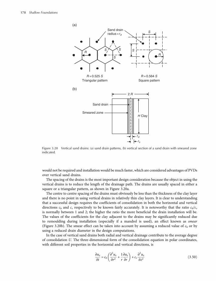
would not be required and installation would bemuch faster, which are considered advantages of PVDsover vertical sand drains.
The spacing of the drains is the most important design consideration because the object in using thevertical drains is to reduce the length of the drainage path. The drains are usually spaced in either asquare or a triangular pattern, as shown in Figure 3.20a.
The centre to centre spacing of the drains must obviously be less than the thickness of the clay layerand there is no point in using vertical drains in relatively thin clay layers. It is clear to understandingthat a successful design requires the coefficients of consolidation in both the horizontal and verticaldirections ch and cv respectively to be known fairly accurately. It is noteworthy that the ratio ch/cvis normally between 1 and 2; the higher the ratio the more beneficial the drain installation will be.The values of the coefficients for the clay adjacent to the drains may be significantly reduced dueto remoulding during installation (especially if a mandrel is used), an effect known as smear(Figure 3.20b). The smear effect can be taken into account by assuming a reduced value of ch or byusing a reduced drain diameter in the design computations.
In the case of vertical sand drains both radial and vertical drainage contribute to the average degreeof consolidation U. The three-dimensional form of the consolidation equation in polar coordinates,with different soil properties in the horizontal and vertical directions, is
∂ue∂t
= ch∂2ue∂r2
+1r∂ue∂r
+ cv∂2ue∂z2
3 50
Sand drain
Smeared zone
rd
rs
Sand drain
radius = rd
R = 0.525 S R = 0.564 S
Triangular pattern Square pattern
RR
S
SSS
S
2 R
H Clay
(a)
(b)
Figure 3.20 Vertical sand drains: (a) sand drain patterns, (b) vertical section of a sand drain with smeared zoneindicated.
178 Shallow Foundations
worksaccounts.com
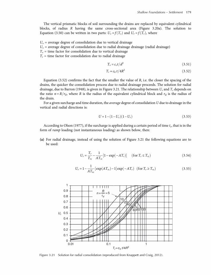
The vertical prismatic blocks of soil surrounding the drains are replaced by equivalent cylindricalblocks, of radius R having the same cross-sectional area (Figure 3.20a). The solution toEquation (3.50) can be written in two parts: Uv = f Tv and Ur = f Tr , where
Uv = average degree of consolidation due to vertical drainageUv = average degree of consolidation due to radial drainage drainage (radial drainage)Tv = time factor for consolidation due to vertical drainageTr = time factor for consolidation due to radial drainage
Tv = cvt d2 3 51
Tr = ch t 4R2 3 52
Equation (3.52) confirms the fact that the smaller the value of R, i.e. the closer the spacing of thedrains, the quicker the consolidation process due to radial drainage proceeds. The solution for radialdrainage, due to Barron (1948), is given in Figure 3.21. The relationship between Ur and Tr depends onthe ratio n=R rd, where R is the radius of the equivalent cylindrical block and rd is the radius ofthe drain.For a given surcharge and time duration, the average degree of consolidationU due to drainage in the
vertical and radial directions is:
U = 1− 1−Uv 1−Ur 3 53
According to Olson (1977), if the surcharge is applied during a certain period of time tc, that is in theform of ramp loading (not instantaneous loading) as shown below, then:
(a) For radial drainage, instead of using the solution of Figure 3.21 the following equations are tobe used:
Ur =Tr
Trc−
1ATrc
1− exp −ATr forTr ≤Trc 3 54
Ur = 1−1
ATrcexp ATrc −1 exp −ATr forTr ≥Trc 3 55
1
0.9
0.8
0.7
0.6
0.5
0.4
0.3
0.2
0.1
00.01 0.1
Tr= ch t/4R21
Ur
1008060
4020
10
1008060
4020
10
= 5n =rd
R
Figure 3.21 Solution for radial consolidation (reproduced from Knappett and Craig, 2012).
Shallow Foundations – Settlement 179
worksaccounts.com
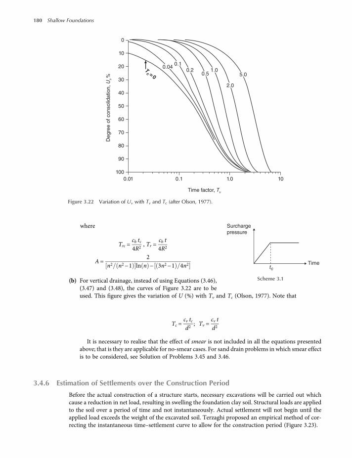
where
Trc =ch tc4R2
, Tr =ch t4R2
A=2
n2 n2−1 ln n − 3n2−1 4n2
(b) For vertical drainage, instead of using Equations (3.46),(3.47) and (3.48), the curves of Figure 3.22 are to beused. This figure gives the variation of U (%) with Tv and Tc (Olson, 1977). Note that
Tc =cv tcd2
; Tv =cv td2
It is necessary to realise that the effect of smear is not included in all the equations presentedabove; that is they are applicable for no-smear cases. For sand drain problems in which smear effectis to be considered, see Solution of Problems 3.45 and 3.46.
3.4.6 Estimation of Settlements over the Construction Period
Before the actual construction of a structure starts, necessary excavations will be carried out whichcause a reduction in net load, resulting in swelling the foundation clay soil. Structural loads are appliedto the soil over a period of time and not instantaneously. Actual settlement will not begin until theapplied load exceeds the weight of the excavated soil. Terzaghi proposed an empirical method of cor-recting the instantaneous time–settlement curve to allow for the construction period (Figure 3.23).
0
10
20
30
40
50
60
70
80
90
100
0.01
5.0Tc =0
2.0
0.51.00.2
0.040.1
0.1 1.0 10
Degre
e o
f consolid
ation, U
ν%
Time factor, Tν
Figure 3.22 Variation of Uv with Tv and Tc (after Olson, 1977).
Surcharge
pressure
tcTime
Scheme 3.1
180 Shallow Foundations
worksaccounts.com
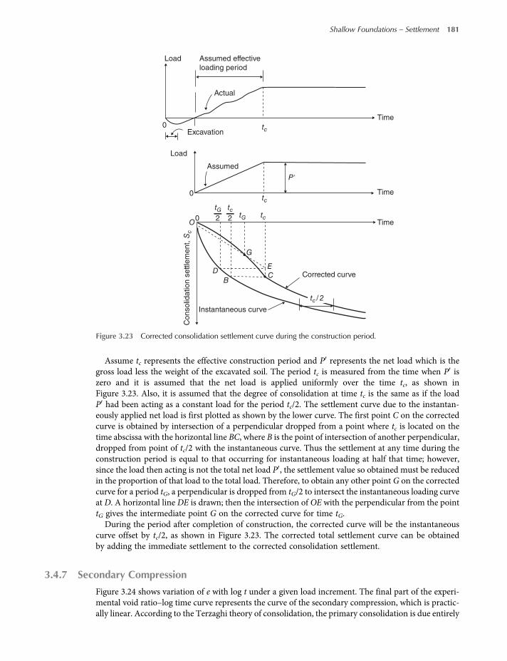
Assume tc represents the effective construction period and P represents the net load which is thegross load less the weight of the excavated soil. The period tc is measured from the time when P iszero and it is assumed that the net load is applied uniformly over the time tc, as shown inFigure 3.23. Also, it is assumed that the degree of consolidation at time tc is the same as if the loadP had been acting as a constant load for the period tc/2. The settlement curve due to the instantan-eously applied net load is first plotted as shown by the lower curve. The first point C on the correctedcurve is obtained by intersection of a perpendicular dropped from a point where tc is located on thetime abscissa with the horizontal line BC, where B is the point of intersection of another perpendicular,dropped from point of tc/2 with the instantaneous curve. Thus the settlement at any time during theconstruction period is equal to that occurring for instantaneous loading at half that time; however,since the load then acting is not the total net load P , the settlement value so obtained must be reducedin the proportion of that load to the total load. Therefore, to obtain any other point G on the correctedcurve for a period tG, a perpendicular is dropped from tG/2 to intersect the instantaneous loading curveat D. A horizontal line DE is drawn; then the intersection of OE with the perpendicular from the pointtG gives the intermediate point G on the corrected curve for time tG.During the period after completion of construction, the corrected curve will be the instantaneous
curve offset by tc/2, as shown in Figure 3.23. The corrected total settlement curve can be obtainedby adding the immediate settlement to the corrected consolidation settlement.
3.4.7 Secondary Compression
Figure 3.24 shows variation of e with log t under a given load increment. The final part of the experi-mental void ratio–log time curve represents the curve of the secondary compression, which is practic-ally linear. According to the Terzaghi theory of consolidation, the primary consolidation is due entirely
Assumed effective
loading period
Actual
Load
Excavation0
Assumed
tc
tc
tc
tctG
tG
Time
Time
Time
G
D
B
EC
P′
Corrected curve
Instantaneous curve
Consolid
ation s
ettle
ment, S
c
Load
0
0O
2 2
tc / 2
Figure 3.23 Corrected consolidation settlement curve during the construction period.
Shallow Foundations – Settlement 181
worksaccounts.com
to the dissipation of the excess porewater pressure, with permeability alone governing the time depend-ency of the consolidation process. However, practice observations as well as experimental results showthat compression does not cease when the excess porewater pressure has dissipated to zero but con-tinues at a gradually decreasing rate under constant effective stress.
Secondary compression (or creep) is thought to be due to the gradual readjustment of the clay par-ticles into a more stable configuration following the structural disturbance caused by the decrease invoid ratio, especially if the clay is laterally confined. Another factor is the gradual lateral displacementswhich take place in thick clay layers. Some authorities relate secondary compression to the clayadsorbed water (the water molecules that are held to the clay particles). Researchers measured the sec-ondary compression in a clay soil after the water was replaced by a non-polar liquid, such as CCl4 andfound its value was considerably less than that in the undisturbed clay. Hence, the adsorbed water mayexert an important influence on the viscoelastic behaviour of the clay–particle contacts. The rate ofsecondary compression is thought to be controlled by the highly viscous film of adsorbed water sur-rounding the clay mineral particles in the soil. A very low viscous flow of adsorbed water takes placefrom the zones of film contact, allowing the soil particles to move closer together. The viscosity of thefilm increases as the particles move closer, resulting in a decrease in the rate of compression of the soil.According to Knappett and Craig (2012), it is presumed that primary consolidation and secondarycompression proceed simultaneously from the time of loading.
The secondary compression index Cα can be defined by the slope of the final part of the curve ofFigure 3.24; written as
Cα =Δe
log t2− log t1=
Δelog t2 t1
3 56
where
Δe = change in void ratiot1, t2 = time
From the results of laboratory tests and field observations, Simons (1974) derived the followingequation for clays:
Cα = 0 00018 × natural moisture content in percent 3 57
The magnitude of the secondary compression can be calculated as
Ss =CαH log t2 t1 3 58
log tlog
Ca=
Time, t
ΔeΔe
Void
ratio,
e
End of primary
consolidation
t2
t2
t1
t1
Secondary
compression
Figure 3.24 Variation of ewith log t under a given load increment and definition of secondary compression index.
182 Shallow Foundations
worksaccounts.com
where Cα =Cα
1 + epep = void ratio at the end of primary consolidationH = thickness of clay layerThe magnitude of secondary compression in a given time is generally greater in normally consoli-
dated clays than in overconsolidated clays.Mesri (1973) correlated Cα with the natural moisture content w of several soils, from which it
appears that
Cα = 0 0001w 3 59
where w = natural moisture content, in percent.For most overconsolidated clays, the range of Cα values are 0.0005 to 0.001. Also, Mesri and
Godlewski (1977) compiled the magnitude of Cα/Cc for a number of soils (Cc = compression index).Accordingly, the following relationships can be given:
For inorganic clays and silts Cα Cc = 0 04 +− 0 01 3 60
For organic clays and silts Cα Cc = 0 05 +− 0 01 3 61
For peats Cα Cc = 0 075 +− 0 01 3 62
For a particular soil under oedometer test, the magnitude of secondary compression over a giventime, as a percentage of the total compression, increases as the ratio of pressure increment to initialeffective pressure decreases; the magnitude of secondary compression also increases as the thicknessof the oedometer specimen decreases and as temperature increases. The secondary compression char-acteristics of an oedometer specimen cannot normally be extrapolated to the case of a full-scalefoundation (Knappett and Craig, 2012).
3.5 Settlement of Foundations on Rock
Closely jointed rock formations and weak to moderately weak weathered rocks possess a degree ofcompressibility such that it is necessary to make estimates of settlement wherever heavily loaded struc-tures are founded on these formations.Settlement of a rock mass may be estimated using equations from elastic theory similar to
Equation (3.4). Meigh (1976) proposed the following settlement equation:
ρi = qBEf
IpFBFD 3 63
where ρi = immediate settlement beneath corner of a uniformly loaded areaq = net foundation pressurerB = width of foundationEf = deformation modulus of rock at the foundation levelIP = influence factor (Figure 3.25)FB = correction factor for roughness of the base (Figure 3.26a)FD = correction factor for depth of embedment in rock (Figure 3.26b)
In the case of a flexible rectangular foundation, the loaded area is divided into four equal rectanglesand the settlement computed at the corner of each rectangle. The settlement at the centre of the foun-dation is then four times the corner settlement. In the case of relatively rigid foundation, the settlements
Shallow Foundations – Settlement 183
worksaccounts.com

H
B
H
B
H
B
H
B
H
B
0.70.60.50.40.30.20.1
1/8
1/8
1/8
1/4
1/4
1/4
1/2
1/2
1/2
1
1
1
2
8
6
4
2
2
2
5
5
5
1010
10
10
L/B = 5
L/B = 3
L/B = 2
L/B = 1
0.7
0.7
0.6
0.6
0.5
0.5
0.4
0.4
0.3
0.3
0.2
0.2
0.1
0.1
Assumed incompressible
0.1 0.2 0.3 0.4 0.5 0.6 0.7 0.8
1/61/41/2125
2
4
6
8
k =
k =
k =
k =
k =
= ρ1= q Ef
I′pFBFD
Hk =
B
B
Diagrams applicable for H/B ≯10
Settlement of corner of loaded area
Ef
(Ed– Ef)
Poisson’s ratio μ = 0.2
01/81/41/212
L/B ≥10
Use for L/B > 10
51010
0 0.2 0.3 0.4 0.5 0.6 0.7 0.8 0.90.1
10 0
0.90
2
4
6
8
10
0
D
H
B
B
1+( )kH
L
q
E0
Ef
Ed= Ef
0
0
0
0
0
2
2
4
4
6
6
8
8
10
10
Influence factor, I′P
Figure 3.25 Values of influence factor IP for deformation modulus increasing linearly with depth and Poisson’sratio of 0.2 (from Tomlinson, 2001).
184 Shallow Foundations
worksaccounts.com

at centre, at the midpoint of a longer side and at a corner of the loaded area are calculated. Then theaverage settlement of the rigid foundation is given by (Tomlinson, 2001),
ρi, ave = 1 3 ρi, center + ρi, midpoint long side + ρi, corner 3 64
Meigh obtained curves for influence factors for various values of the constant k using a value forPoisson’s ratio equals to 0.2, as shown in Figure 3.25. The value of k is computed from the followingequation:
k=Ed −EfEf
Bz
3 65
For a rock mass of thickness H below the foundation level
k=Ed −EfEf
BH
Measured values of E against depth z are plotted and a straight line through the plotted points isdrawn (Figure 3.25). Thus values of deformation modulus such as Ed and Ef are obtained, whichare used in Equation (3.65) to obtain value of k.
Correction factorFB =Settlement for rough baseSettlement for smooth base
The most important of the procedure is to obtain reliable variation of E values with depth. Accordingto Tomlinson (2001), where the results of unconfined compression test on core samples are in sufficientnumbers to be representative of the variation in strength of the rock over the depth stressed bythe foundation loading, the deformation modulus Em of the rock mass can be obtained from therelationship
Em = j Mr quc 3 66
1.0
1.0(b)(a)
0.9
0.8
0.70 1 2 3 4 5 6 7 8 9 10
0.9
0.8
0.7
0.6
0.50 0.5 1.0 1.5 2.0 2.5
H/B D/B
B
D
G.L. Rock surface
FD
FB
Figure 3.26 Correction factors: (a) for roughness of base of foundation; (b) for depth of embedment of foundationbelow surface of rock (from Tomlinson, 2001).
Shallow Foundations – Settlement 185
worksaccounts.com
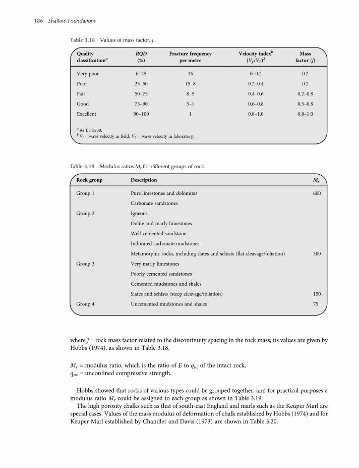
where j = rock mass factor related to the discontinuity spacing in the rock mass; its values are given byHobbs (1974), as shown in Table 3.18,
Mr = modulus ratio, which is the ratio of E to quc of the intact rock,quc = unconfined compressive strength.
Hobbs showed that rocks of various types could be grouped together, and for practical purposes amodulus ratio Mr could be assigned to each group as shown in Table 3.19.
The high porosity chalks such as that of south-east England and marls such as the Keuper Marl arespecial cases. Values of the mass modulus of deformation of chalk established by Hobbs (1974) and forKeuper Marl established by Chandler and Davis (1973) are shown in Table 3.20.
Table 3.19 Modulus ratios Mr for different groups of rock.
Rock group Description Mr
Group 1 Pure limestones and dolomites
Carbonate sandstones
600
Group 2 Igneous
Oolite and marly limestones
Well-cemented sandstone
Indurated carbonate mudstones
Metamorphic rocks, including slates and schists (flat cleavage/foliation) 300
Group 3 Very marly limestones
Poorly cemented sandstones
Cemented mudstones and shales
Slates and schists (steep cleavage/foliation) 150
Group 4 Uncemented mudstones and shales 75
Table 3.18 Values of mass factor, j.
Qualityclassificationa
RQD(%)
Fracture frequencyper metre
Velocity indexb
(Vf /VL)2
Massfactor (j)
Very poor 0–25 15 0–0.2 0.2
Poor 25–50 15–8 0.2–0.4 0.2
Fair 50–75 8–5 0.4–0.6 0.2–0.8
Good 75–90 5–1 0.6–0.8 0.5–0.8
Excellent 90–100 1 0.8–1.0 0.8–1.0
aAs BS 5930.b Vf = wave velocity in field, VL = wave velocity in laboratory.
186 Shallow Foundations
worksaccounts.com
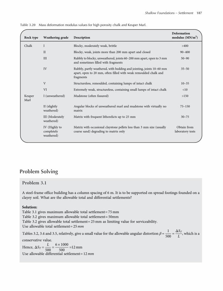
Problem Solving
Problem 3.1
A steel-frame office building has a column spacing of 6 m. It is to be supported on spread footings founded on aclayey soil. What are the allowable total and differential settlements?
Solution:Table 3.1 gives maximum allowable total settlement= 75mmTable 3.2 gives maximum allowable total settlement= 50mmTable 3.2 gives allowable total settlement= 25mm as limiting value for serviceability.Use allowable total settlement= 25mm
Tables 3.2, 3.4 and 3.5, relatively, give a small value for the allowable angular distortion β =1500
=ΔSTL
, which is a
conservative value.
Hence, ΔST =L500
=6 × 1000500
=12mm
Use allowable differential settlement= 12mm
Table 3.20 Mass deformation modulus values for high porosity chalk and Keuper Marl.
Rock type Weathering grade DescriptionDeformationmodulus (MN/m2)
Chalk I Blocky, moderately weak, brittle >400
II Blocky, weak, joints more than 200 mm apart and closed 90–400
III Rubbly to blocky, unweathered, joints 60–200 mm apart, open to 3 mmand sometimes filled with fragments
50–90
IV Rubbly, partly weathered, with bedding and jointing, joints 10–60 mmapart, open to 20 mm, often filled with weak remoulded chalk andfragments
35–50
V Structureless, remoulded, containing lumps of intact chalk 10–35
VI Extremely weak, structureless, containing small lumps of intact chalk <10
KeuperMarl
I (unweathered) Mudstone (often fissured) >150
II (slightlyweathered)
Angular blocks of unweathered marl and mudstone with virtually nomatrix
75–150
III (Moderatelyweathered)
Matrix with frequent lithorelicts up to 25 mm 30–75
IV (Highly tocompletelyweathered)
Matrix with occasional claystone pellets less than 3 mm size (usuallycoarse sand) degrading to matrix only
Obtain fromlaboratory tests
Shallow Foundations – Settlement 187
worksaccounts.com
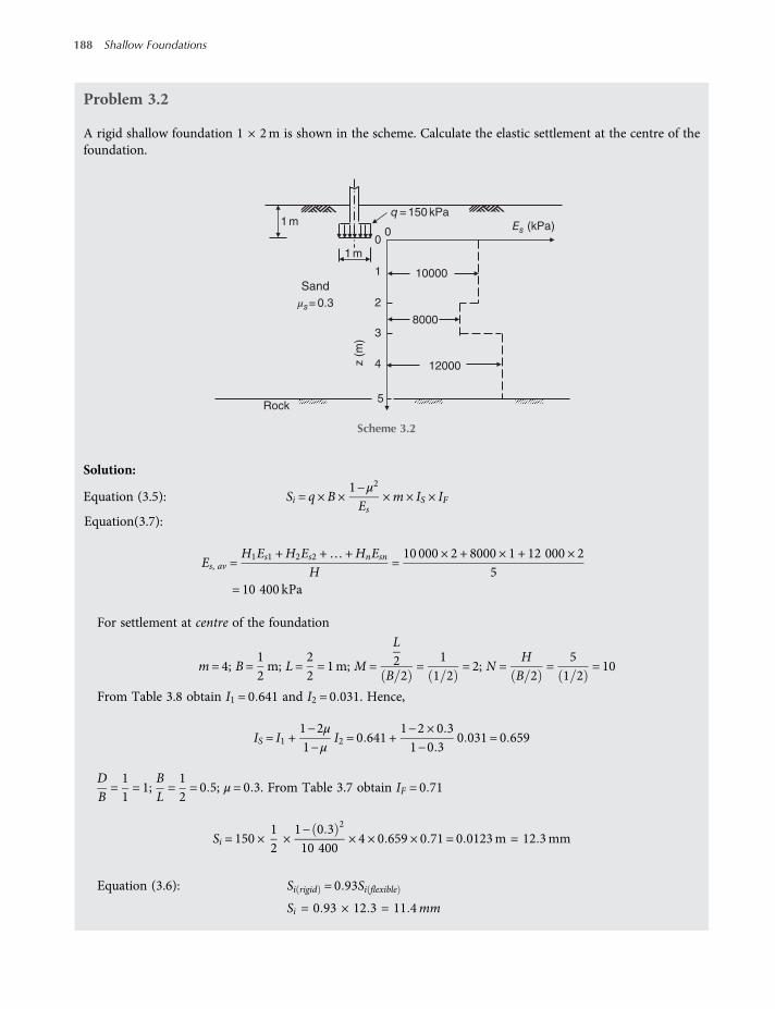
Problem 3.2
A rigid shallow foundation 1 × 2m is shown in the scheme. Calculate the elastic settlement at the centre of thefoundation.
Solution:
Equation (3.5): Si = q×B×1−μ2
Es×m× IS × IF
Equation(3.7):
Es, av =H1Es1 +H2Es2 +…+HnEsn
H=10 000 × 2 + 8000 × 1 + 12 000 × 2
5= 10 400 kPa
For settlement at centre of the foundation
m= 4; B=12m; L=
22= 1m; M =
L2
B 2=
11 2
= 2; N =HB 2
=51 2
= 10
From Table 3.8 obtain I1 = 0 641 and I2 = 0 031. Hence,
IS = I1 +1−2μ1−μ
I2 = 0 641 +1−2 × 0 31−0 3
0 031 = 0 659
DB=11= 1;
BL=12= 0 5; μ= 0 3. From Table 3.7 obtain IF = 0 71
Si = 150 ×12×1− 0 3 2
10 400× 4 × 0 659 × 0 71 = 0 0123m = 12 3mm
Equation (3.6): Si rigid = 0 93Si flexible
Si = 0 93 × 12 3 = 11 4mm
Sand
μs= 0.3 2
3
1
8000
10000
Es (kPa)1 m
1 m
4 12000
5
00
Rock
z (
m)
q = 150 kPa
Scheme 3.2
188 Shallow Foundations
worksaccounts.com
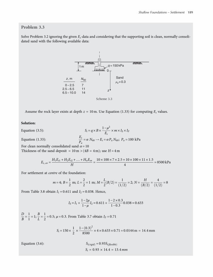
Problem 3.3
Solve Problem 3.2 ignoring the given Es-data and considering that the supporting soil is clean, normally consoli-dated sand with the following available data:
Assume the rock layer exists at depth z = 10m. Use Equation (1.33) for computing Es values.
Solution:
Equation (3.5): Si = q×B×1−μ2
Es×m× IS × IF
Equation (1.33):EsPa
= α N60 Es = αPa N60; Pa = 100 kPa
For clean normally consolidated sand α= 10Thickness of the sand deposit = 10m > 4B = 4m ; use H = 4m
Es, av =H1Es1 +H2Es2 +… +HnEsn
H=10 × 100 × 7 × 2 5 + 10 × 100 × 11 × 1 5
4= 8500 kPa
For settlement at centre of the foundation:
m= 4; B=12m; L=
22= 1 m; M =
L2B 2 =
11 2
= 2; N =HB 2
=41 2
= 8
From Table 3.8 obtain I1 = 0 611 and I2 = 0 038. Hence,
IS = I1 +1−2μ1−μ
I2 = 0 611 +1−2 × 0 31−0 3
0 038 = 0 633
DB=11= 1;
BL=12= 0 5; μ= 0 3. From Table 3.7 obtain IF = 0 71
Si = 150 ×12×1− 0 3 2
8500× 4 × 0 633 × 0 71 = 0 0144m = 14 4mm
Equation (3.6): Si rigid = 0 93Si flexible
Si = 0 93 × 14 4 = 13 4mm
z, m N60Sand
μs= 0.3711
0 − 2.52.5 − 6.56.5 − 10.0 14
1 m q = 150 kPa
0
z
Scheme 3.3
Shallow Foundations – Settlement 189
worksaccounts.com
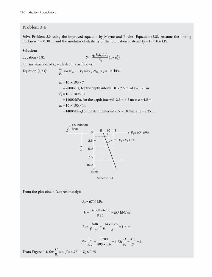
Problem 3.4
Solve Problem 3.3 using the improved equation by Mayne and Poulos: Equation (3.8). Assume the footingthickness t = 0 30m, and the modulus of elasticity of the foundation material Ef = 15 × 106 kPa.
Solution:
Equation (3.8): Si =qoBeIGIFIE
Eo1−μ2s
Obtain variation of Es with depth z as follows:
Equation (1.33):EsPa
= αN60 Es = αPa N60; Pa = 100 kPa
Es = 10 × 100 × 7
= 7000 kPa, for the depth interval 0 2 5 m; at z = 1 25m
Es = 10 × 100 × 11
= 11000 kPa, for the depth interval 2 5 6 5m; at z = 4 5m
Es = 10 × 100 × 14
= 14000 kPa, for the depth interval 6 5 10 0m; at z = 8 25m
From the plot obtain (approximately):
Eo = 6700 kPa
k =14 000−6700
8 25= 885 kN m
Be =4BLπ
=4 × 1 × 2
π= 1 6 m
β =EokBe
=6700
885 × 1 6= 4 73;
HBe
=4Be
Be= 4
From Figure 3.4, forHBe
= 4; β = 4 73 IG≈0 75
0 Es× 103, kPa
Es= Eo+ k z2.5
5.0
7.5
z
10.0
5 10 15
Foundation
level
z (m)
Scheme 3.4
190 Shallow Foundations
worksaccounts.com
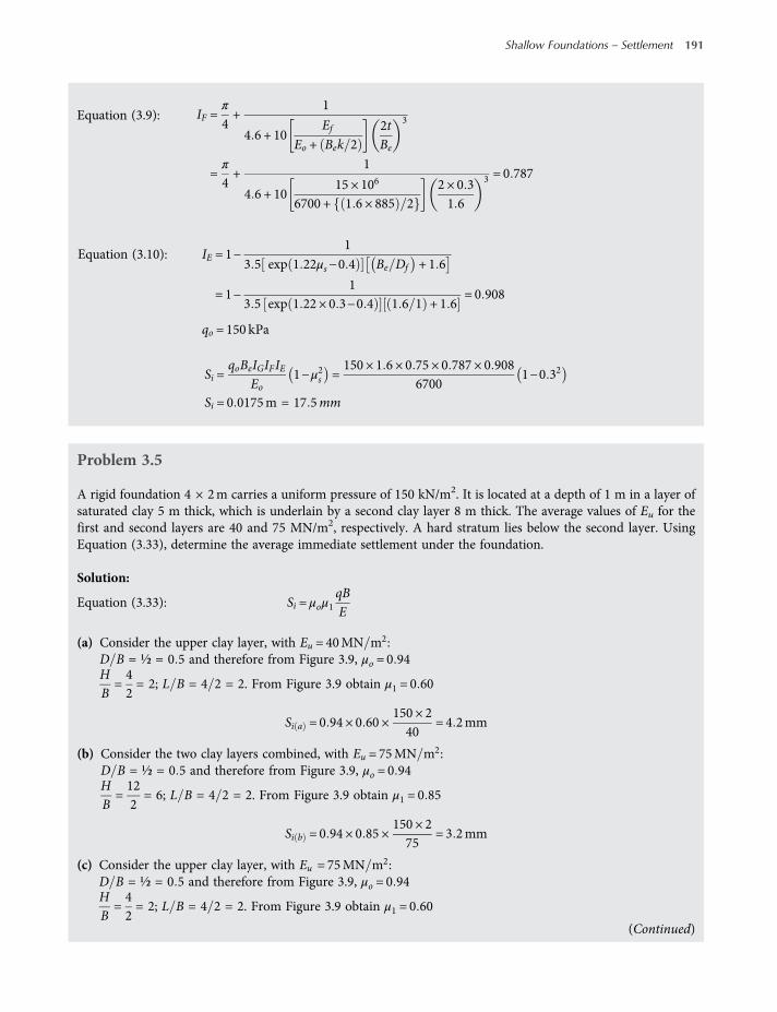
Equation (3.9): IF =π
4+
1
4 6 + 10Ef
Eo + Bek 22tBe
3
=π
4+
1
4 6 + 1015 × 106
6700 + 1 6 × 885 22 × 0 31 6
3 = 0 787
Equation (3.10): IE = 1−1
3 5 exp 1 22μs−0 4 Be Df + 1 6
= 1−1
3 5 exp 1 22 × 0 3−0 4 1 6 1 + 1 6= 0 908
qo = 150 kPa
Si =qoBeIGIFIE
Eo1−μ2s =
150 × 1 6 × 0 75 × 0 787 × 0 9086700
1−0 32
Si = 0 0175m = 17 5mm
Problem 3.5
A rigid foundation 4 × 2m carries a uniform pressure of 150 kN/m2. It is located at a depth of 1 m in a layer ofsaturated clay 5 m thick, which is underlain by a second clay layer 8 m thick. The average values of Eu for thefirst and second layers are 40 and 75 MN/m2, respectively. A hard stratum lies below the second layer. UsingEquation (3.33), determine the average immediate settlement under the foundation.
Solution:
Equation (3.33): Si = μoμ1qBE
(a) Consider the upper clay layer, with Eu = 40MN m2:D B = ½ = 0 5 and therefore from Figure 3.9, μo = 0 94HB=42= 2; L B = 4 2 = 2. From Figure 3.9 obtain μ1 = 0 60
Si a = 0 94 × 0 60 ×150 × 240
= 4 2mm
(b) Consider the two clay layers combined, with Eu = 75MN m2:D B = ½ = 0 5 and therefore from Figure 3.9, μo = 0 94HB=122= 6; L B = 4 2 = 2. From Figure 3.9 obtain μ1 = 0 85
Si b = 0 94 × 0 85 ×150 × 275
= 3 2mm
(c) Consider the upper clay layer, with Eu = 75MN m2:D B = ½ = 0 5 and therefore from Figure 3.9, μo = 0 94HB=42= 2; L B = 4 2 = 2. From Figure 3.9 obtain μ1 = 0 60
(Continued)
Shallow Foundations – Settlement 191
worksaccounts.com

Si c = 0 94 × 0 60 ×150 × 275
= 2 3mm
Hence, using the principle of superposition, the average settlement of the foundation, considering flexibleloading area, is given by:
Si = Si a + Si b −Si c = 4 2 + 3 2 − 2 3 = 5 1mm
Equation (3.6): Si rigid = 0 93Si flexible
Si = 0 93 × 5 1 = 4 7; say 5mm
Problem 3.6
Solve Problem 3.5 using equation Equation (3.5). Use μ= 0 5 for saturated clays. Consider settlement at centre ofthe foundation only.
Solution:
Equation (3.5): Si = q×B×1−μ2
Es×m× IS × IF
(a) Consider the upper clay layer, with Eu = 40MN m2:For settlement at centre of the foundation:
m= 4; B =22= 1 m; L=
42= 2 m; M =
L2
B 2=
422 2
= 2; N =HB 2
=42 2
= 4
From Table 3.8 obtain I1 = 0 476 and I2 = 0 069. Hence,
IS = I1 +1−2μ1−μ
I2 = 0 476 +1−2 × 0 51−0 5
0 069 = 0 476
DB=12= 0 5;
BL=24= 0 5; μ = 0 5. From Table 3.7 obtain IF = 0 90
Si a = 150 ×22×1− 0 5 2
40 000× 4 × 0 476 × 0 9 = 0 0048 m = 4 8mm
(b) Consider the two clay layers combined, with Eu = 75MN m2:For settlement at centre of the foundation:
m= 4;B =22= 1 m;L=
42= 2 m;M =
L2
B 2=
422 2
= 2;N =HB 2
=122 2
= 12
From Table 3.8 obtain I1 = 0 653 and I2 = 0 028. Hence,
IS = I1 +1−2μ1−μ
I2 = 0 653 +1−2 × 0 51−0 5
0 069 = 0 0 653
192 Shallow Foundations
worksaccounts.com
DB=12= 0 5;
BL=24= 0 5; μ = 0 5. From Table 3.7 obtain IF = 0 90
Si b = 150 ×22×1− 0 5 2
75 000× 4 × 0 653 × 0 9 = 0 0035 m= 3 5 mm
(c) Consider the upper clay layer, with Eu = 75MN m2:For settlement at centre of the foundation:
m= 4;B =22= 1 m;L=
42= 2 m;M =
L2
B 2=
422 2
= 2;N =HB 2
=42 2
= 4
From Table 3.8 obtain I1 = 0 476 and I2 = 0 069. Hence,
IS = I1 +1−2μ1−μ
I2 = 0 476 +1−2 × 0 51−0 5
0 069 = 0 476
DB=12= 0 5;
BL=24= 0 5; μ = 0 5. From Table 3.7 obtain IF = 0 90
Si c = 150 ×22×1− 0 5 2
75 000× 4 × 0 476 × 0 9 = 0 0026m = 2 6mm
Hence, using the principle of superposition, settlement at centre of the foundation, considering flexible loadingarea, is given by:
Si = Si a + Si b −Si c = 4 8 + 3 5 − 2 6 = 5 7mm
Equation (3.6): Si rigid = 0 93Si flexible
Si = 0 93 × 5 7 = 5 3mm
Another procedure is to calculate settlement of each layer alone and then adding them to obtain the total settle-ment, as follows:
(a) Settlement of the upper clay layer was calculated = 4 8mm.(b) Settlement of the lower clay layer:
Assume using the simple 2V : 1H ratio method of stress distributionAt top of the layer: q = 150 2 × 4 2 + 4 4 + 4 = 25 kN m2
For settlement at the centre of the foundation:
m= 4;B =62= 3 m;L=
82= 4 m;M =
L2
B 2=43= 1 33
N =HB 2
=83= 2 67
From Table 3.8 obtain I1 = 0 36 and I2 = 0 074. Hence,
IS = I1 +1−2μ1−μ
I2 = 0 36 +1−2 × 0 51−0 5
0 074 = 0 36
(Continued)
Shallow Foundations – Settlement 193
worksaccounts.com

DB=56= 0 83;
BL=68= 0 75; μ = 0 5. From Table 3.7 obtain IF = 0 79
Si b = 25 ×62×1− 0 5 2
75 000× 4 × 0 36 × 0 79 = 0 0009m = 0 9mm
Hence, using the principle of superposition, settlement at centre of the foundation, considering flexible loadingarea, is given by
Si = Si a + Si b = 4 8 + 0 9 = 5 7mm
Equation (3.6): Si rigid = 0 93Si flexible
Si = 0 93 × 5 7 = 5 3mm
Problem 3.7
A bridge pier has a base 8.5 m long by 7.5 m wide, founded at a depth of 3.0 m. The base of the pier imposes netfoundation contact pressure equals 220 kN/m2 due to dead loading and 360 kN/m2 due to combined dead and liveloading. Borings showed dense sand and gravel with cobbles and boulders to a depth of 9 m, followed by very stiffoverconsolidated clay tomore than 25m below ground level. Standard penetration tests gave an averageN-value of40 blows per 300 mm in the sand and gravel stratum. A number of oedometer tests were made on samples of thestiff clay; the following values for the coefficient of compressibilitymv corresponding to the respective incrementsof pressure (due to the two types of loading) were obtained as follows:
Net contact pressure qn, kN/m2 Depth of layer, m mv m
2/kN
220 9−12 0.000 11
12−18 0.000 03
360 9−12 0.000 20
12−18 0.000 04
Triaxial tests on undisturbed samples of the clay (nearly saturated) gave minimum shear strength of 120 kN/m2
and undrained modulus of deformation Eu of 40MN/m2. Calculate the immediate and long-term settlement of thebridge pier.
Solution:(1) Calculating immediate settlements in sand and gravel stratum.
It is not known whether this stratum is overconsolidated; the preconsolidation pressure is not given, henceassume it is normally consolidated.
Assume using the Burland and Burbidge empirical relationship:
Equation (3.15):SiBR
= α1α2α31 25
LB
0 25 + L B
2
BBR
0 7 qpa
Use Equation (3.16) to adjust the N-value for the gravel content; and therefore,
N a = 1 25 ×N = 1 25 × 40 = 50
194 Shallow Foundations
worksaccounts.com

Equation 3.18:zBR
= 1 4BBR
0 75
z0 3
= 1 47 50 3
0 75
; z = 4 7m< H = 6m ; hence use α3 = 1
For normally consolidated sand and gravel, α1 = 0 14 and
α2 = 1 71 N1 4a = 1 71 501 4 = 0 007
For dead loading only:
Si = 0 3 × 0 14 × 0 007 × 11 25
8 57 5
0 25 + 8 5 7 5
2
7 50 3
0 7 220100
= 0 0065m
Si = 6 5mm
For combined dead and live loading:
Si = 6 5 ×360220
= 10 6mm
(2) Calculating immediate settlements in clay stratumDetermine the net average vertical stress at top of the clay layer using Fadum chart of Figure 2.32:Below centre of the pier base at depth z = 6m;
m=B2
z=
7 52
6= 0 63; n=
L2
z=
8 52
6= 0 71; I = 0 12
σz = q 4I = 220 × 4 × 0 12 = 105 6 kN m2
Below middle of the long side at depth z = 6m;
m=Bz=7 56
= 1 25; n=L2
z=
8 52
6= 0 71; I = 0 158
σz = q 2I = 220 × 2 × 0 158 = 69 5 kN m2
Below middle of the short side at depth z = 6m;
m=B2
z=7 5 26
= 0 63; n=Lz=8 56
= 1 42; I = 0 156
σz = q 2I = 220 × 2 × 0 156 = 68 6 kN m2
Below corner of the pier base at depth z = 6m;
m=Bz=7 56
= 1 25; n=Lz=8 56
= 1 42; I = 0 203
σz = q I = 220 × 0 203 = 44 7 kN m2
(Continued)
Shallow Foundations – Settlement 195
worksaccounts.com
The average stress below middle of the long side is greater than that below middle of the short side; hencethe average stress on top of the clay layer, for the dead loading only, may be calculated, approximately, as
qave = σz,ave =105 6 +
69 5 + 44 72
2= 81 4 kN m2
This pressure is distributed over an area B × L =22081 4
× 7 5 × 8 5
B × L = 172 3m2;BL
=7 58 5
B =7 58 5
L ; hence,
L =8 5 × 172 3
7 5= 14 0m, and B = 12 3m
For combined dead and live loading,
qave = 81 4 ×360220
= 133 2 kN m2. It is distributed over the area B × L
The pier base is nearly square. According to the pressure bulb of Figure 2.36 for a square area loaded with q,the pressure at a depth of 2B below the loaded area is about 0.1q. Therefore, practically, we need not considersettlements below that depth. Hence, thickness of the clay layer to be used in computations is
H = 2 × 7 5−6 = 9m
Si = q×B×1−μ2
Es×m× IS × IF
For settlement below the centre of the loaded area B L :
m= 4;B =B2=12 32
= 6 15m;L=L2=142= 7m;M =
L2
B 2= 1 14
N =H
B 2=
96 15
= 1 46. Assume μ= 0 5
From Table 3.8 obtain I1 = 0 217; I2 = 0 083
IS = I1 +1−2μ1−μ
I2 = 0 217 +1−2 × 0 51−0 5
0 083 = 0 217
DB
=9
12 3= 0 73;
BL
=12 314
= 0 88. From Table 3.7 obtain IF = 0 8
For dead loading only:
Si clay = 81 4 ×12 32
×1− 0 5 2
40 000× 4 × 0 217 × 0 8 = 0 0065m
= 6 5 mm
196 Shallow Foundations
worksaccounts.com
For combined dead and live loading:
Si clay = 6 5 ×133 281 4
= 10 6 mm
(3) Calculating consolidation settlements Sc =KSoedConsider the first 3 m clay layer:
Equation (2.20)-(a): σav = qIa (Below corner of the loaded area)
m=B 2H
=12 3 2
3= 2 05; and n=
L 2H
=14 23
= 2 33
From Figure 2.38: Ia = 0 248For dead loading only, below centre of the loaded area:
σav = 4qIa = 4 × 81 4 × 0 248 = 80 7 kN m2
For combined dead and live loading, below centre of the loaded area:
σav = 4qIa = 4 × 133 2 × 0 248 = 132 1 kN m2
Consider the remaining 6 m clay layer:
Equation (2.20)-(b): σav = qH2Ia H2
−H1Ia H1
H2−H1(Below corner of the loaded area)
m=B2
H2=
12 32
9= 0 68 and n=
L2
H2=
142
9= 0 78; from Figure 2.38
Ia H2= 0 2
m=B2
H1=
12 32
3= 2 05; and n=
L2
H1=
142
3= 2 33. From Figure 2.38:
Ia H1= 0 248
For dead loading only, below centre of the loaded area:
σav = 4 × 81 49 × 0 2−3 × 0 248
9−3= 57 3 kN m2
For combined dead and live loading, below centre of the loaded area:
σav = 4 × 133 29 × 0 2−3 × 0 248
9−3= 93 8 kN m2
Soed =H ×mv × σav
Sc =K × Soed
(Continued)
Shallow Foundations – Settlement 197
worksaccounts.com
Since the clay is overconsolidated, we can take K = 0 5.
Net contactpressure, kN/m2
Depth oflayer, m
Layerthickness, m
mv
m2/kNσav
kN/m2Soedmm K
Scmm
220 9–12 3 0.000 11 80.7 26.6 0.5 13.3
12–18 6 0.000 03 57.3 10.3 0.5 5.2
360 9−12 3 0.000 20 132.1 79.3 0.5 39.7
12–18 6 0.000 04 93.8 22.5 0.5 11.3
The total final settlement of the bridge pier is given byS = immediate settlement in sand and gravel
+ Immediate settlement in clay+ Consolidation settlement in clay
For the dead loading net q = 220 kN m2 :
S = 6 5 + 6 5 + 13 3 + 5 2 = 31 5 mm
For the combined dead and live loadings net q = 360 kN m2 :
S= 10 6 + 10 6 + 39 7 + 11 3 = 72 2 mm
The results may be interpreted such that a settlement of 13 mmwill take place as the pier is constructed andthis will increase to about 22 mm if and when the bridge sustains its maximum live load. The remaining settle-ment due to long-term consolidation of the clay under the dead load and sustained live load will take a longperiod of time to attain its final value of about 50 mm.
Problem 3.8
A compacted fill of 8.5 m height is to be placed over a large area. The soil profile under the filled area is shown inthe scheme below. Oedometer tests on samples from points A and B produced the following results:
Cc Cr eo σc kPa
Sample A 0.25 0.08 0.66 101
Sample B 0.2 0.06 0.45 510
Compute Soed and make an estimate of Si and Sc.
Solution:The loaded area is large and, therefore, B/z and L/z values will be large too (say three or above). Assume the samevertical pressure q will be transmitted to any point located in the concerned subsurface layers below centre of thefilled area. Accordingly,
σz = q= 20 3 × 8 5 = 172 6 kPa
198 Shallow Foundations
worksaccounts.com
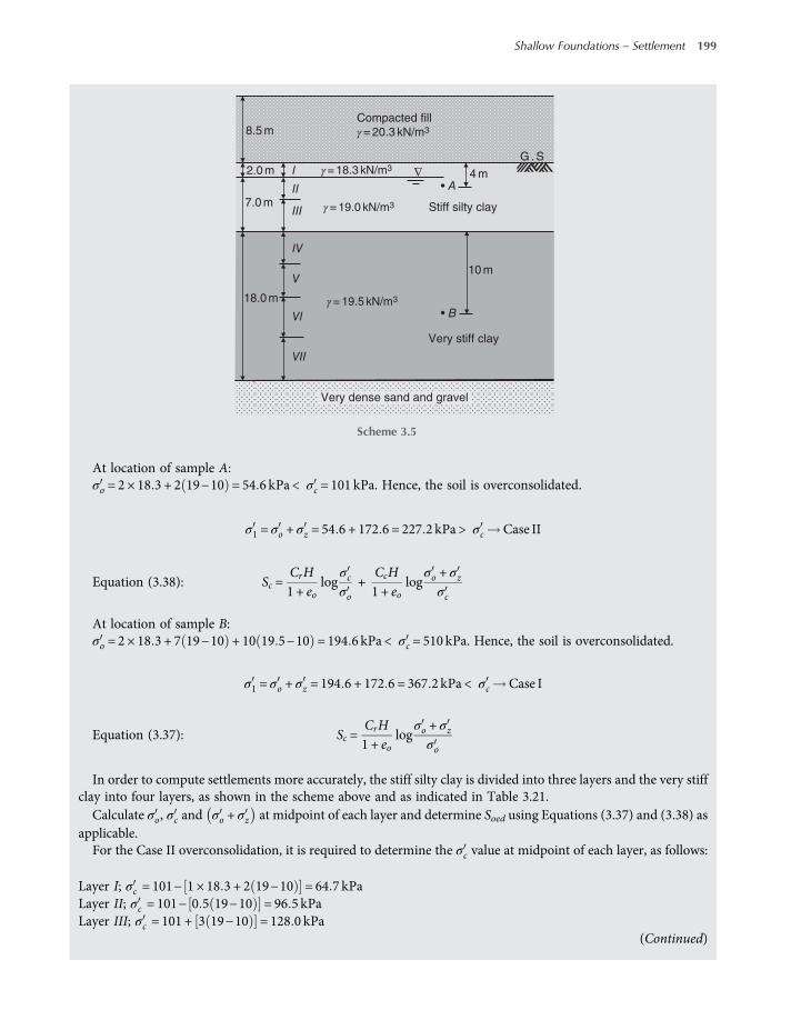
At location of sample A:σo = 2 × 18 3 + 2 19−10 = 54 6 kPa < σc = 101 kPa. Hence, the soil is overconsolidated.
σ1 = σo + σz = 54 6 + 172 6 = 227 2 kPa > σc Case II
Equation (3.38): Sc =CrH1 + eo
logσcσo
+CcH1 + eo
logσo + σzσc
At location of sample B:σo = 2 × 18 3 + 7 19−10 + 10 19 5−10 = 194 6 kPa < σc = 510 kPa. Hence, the soil is overconsolidated.
σ1 = σo + σz = 194 6 + 172 6 = 367 2 kPa < σc Case I
Equation (3.37): Sc =CrH1 + eo
logσo + σzσo
In order to compute settlements more accurately, the stiff silty clay is divided into three layers and the very stiffclay into four layers, as shown in the scheme above and as indicated in Table 3.21.Calculate σo, σc and σo + σz at midpoint of each layer and determine Soed using Equations (3.37) and (3.38) as
applicable.For the Case II overconsolidation, it is required to determine the σc value at midpoint of each layer, as follows:
Layer I; σc = 101− 1 × 18 3 + 2 19−10 = 64 7 kPaLayer II; σc = 101− 0 5 19−10 = 96 5 kPaLayer III; σc = 101 + 3 19−10 = 128 0 kPa
(Continued)
10
γ = 18.3 kN/m3
γ = 19.0 kN/m3
Very stiff clay
Stiff silty clay
∇• A
• B
4 m
G . S
10 m
8.5 m
2.0 m
7.0 m
18.0 m
Very dense sand and gravel
Compacted fill
γ = 20.3 kN/m3
II
III
IV
V
VI
VII
I
γ = 19.5 kN/m3
Scheme 3.5
Shallow Foundations – Settlement 199
worksaccounts.com
Total Soed = 834mm
The clays are stiff and overconsolidated; hence, according to Burland et al. (1977), the immediate settlement Siand the consolidation settlement Sc may be estimated, approximately, as
Si = 0 5 Soed = 0 5 × 834 = 417mm
Sc = 0 5 Soed = 0 5 × 834 = 417mm
Also, the Sc may be estimated, approximately, using Equation (3.42) as follows:
According to Craig (1995), value the settlement ratio K for lightly over-consolidated clays is typically between 0.5and 0.7. Values of σc and σo indicate that the clays are lightly overconsolidated OCR < 3 . Hence, an averagevalue of K = 0 6 may be used to estimate, approximately,
Sc = 0 6 Soed = 0 6 × 834 = 500mm
Si = 0 4 × 834 = 334mm
Problem 3.9
A compacted fill of 3.0 m height is to be placed over a large area. The soil profile under the area is shown in thescheme below.An oedometer test on a sample from point A produced the following results:
Cc Cr eo σc kPa
Sample A: 0.40 0.08 1.10 70.0
These results can be used in settlement calculations for the soft clay stratum as a whole.Compute the total settlement below centre of the area due to the weight of the fill.
Table 3.21 Division of stiff silty clay and very stiff clay into layers.
Layer H (m) σo (kPa) σc (kPa) σo + σz (kPa)Cr
1+ eo
Cc
1+ eo Eq. Soed mm
I 2.0 18.3 64.7 190.9 0.05 0.15 (3.38) 196
II 3.0 50.1 96.5 222.7 0.05 0.15 (3.38) 206
III 4.0 81.6 128.0 254.2 0.05 0.15 (3.38) 218
IV 4.0 118.6 – – 291.2 0.04 0.14 (3.37) 62
V 4.0 156.6 – – 329.2 0.04 0.14 (3.37) 52
VI 5.0 199.4 – – 372.0 0.04 0.14 (3.37) 54
VII 5.0 246.9 – – 419.5 0.04 0.14 (3.37) 46
200 Shallow Foundations
worksaccounts.com
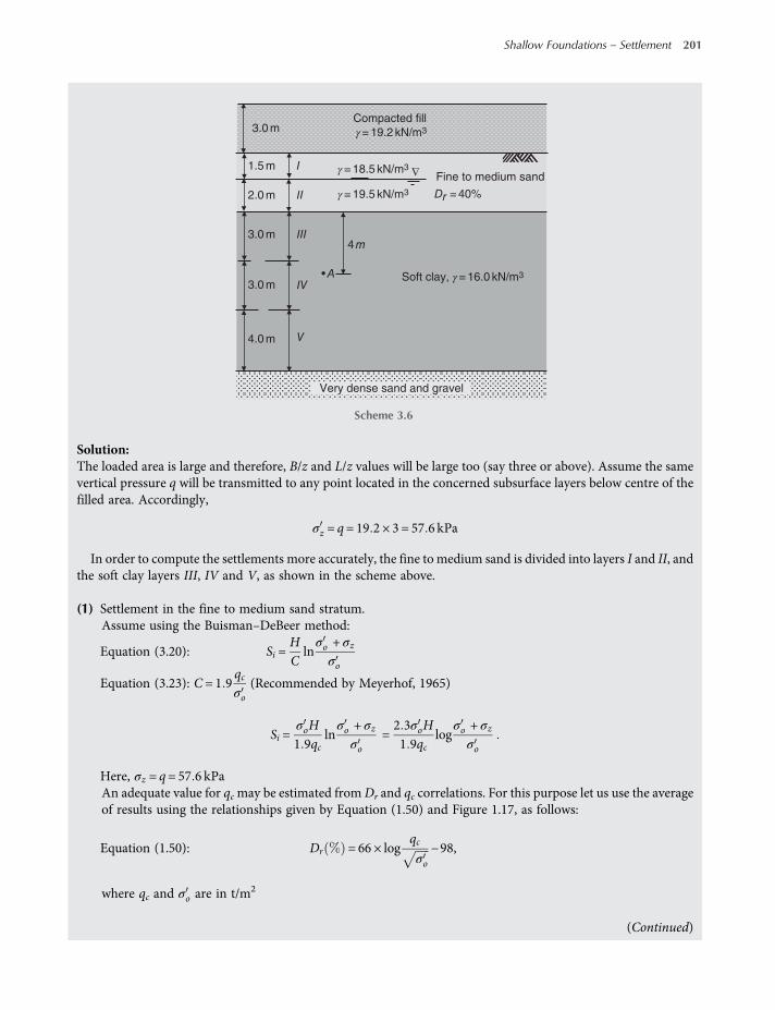
Solution:The loaded area is large and therefore, B/z and L/z values will be large too (say three or above). Assume the samevertical pressure q will be transmitted to any point located in the concerned subsurface layers below centre of thefilled area. Accordingly,
σz = q= 19 2 × 3 = 57 6 kPa
In order to compute the settlements more accurately, the fine to medium sand is divided into layers I and II, andthe soft clay layers III, IV and V, as shown in the scheme above.
(1) Settlement in the fine to medium sand stratum.Assume using the Buisman–DeBeer method:
Equation (3.20): Si =HClnσo + σzσo
Equation (3.23): C = 1 9qcσo
(Recommended by Meyerhof, 1965)
Si =σoH1 9qc
lnσo + σzσo
=2 3σoH1 9qc
logσo + σzσo
Here, σz = q= 57 6 kPaAn adequate value for qcmay be estimated from Dr and qc correlations. For this purpose let us use the averageof results using the relationships given by Equation (1.50) and Figure 1.17, as follows:
Equation (1.50): Dr = 66 × logqcσo
−98,
where qc and σo are in t/m2
(Continued)
Compacted fill
Fine to medium sand∇
• A
3.0 m
3.0 m
4.0 m
3.0 m
1.5 m
2.0 m
Very dense sand and gravel
4 m
γ = 19.2 kN/m3
I
II
III
IV
V
γ = 19.5 kN/m3
γ = 18.5 kN/m3
Dr = 40%
Soft clay, γ = 16.0 kN/m3
Scheme 3.6
Shallow Foundations – Settlement 201
worksaccounts.com

At midpoint of Layer I:
σO = 0 75 × 18 5 = 13 9 kPa = 1 39 t m2
40 = 66 × logqc1 39
−98 log 0 85qc = 2 09
qc = 143 53 t m2 = 1435 kPa
From Figure 1.17; qc = 1 333MNm2
= 1333 kPa
Use qc =1435 + 1333
2= 1384 kPa
Si I =2 3 × 1 5 × 13 9
1 9 × 1384log
13 9 + 57 613 9
= 0 013m
At mid-point of Layer II:
σO = 1 5 × 18 5 + 1 19 5−10 = 37 25 kPa = 3 73 t m2
40 = 66 × logqc3 73
−98 log 0 52qc = 2 09
qc = 234 6 t m2 = 2346 kPa
From Figure 1.17, qc = 2 667MNm2
= 2667 kPa
Use qc =2346 + 2667
2= 2507 kPa
Si II =2 3 × 2 × 37 251 9 × 2507
log37 25 + 57 6
37 25= 0 015m
Settlement in the fine to medium sand stratum
Ssand = Si I + Si II = 0 013 + 0 15 = 0 028m= 28 mm
(2) Settlement in the soft clay stratum:At sample A: σo = 1 5 × 18 5 + 2 19 5−10 + 4 16−10 = 70 75 kPa≈pc = 70 0 kPa. Hence, the clay is con-sidered normally consolidated.
Calculate σo and σo + σz at midpoint of layers and determine Soed using Equation (3.36)-(a)
Equation (3.36)-(a): Sc =CcH1 + eo
logσo + σzσo
The total settlement below centre of the area due to the weight of the fill = Stotal = Ssand +Soed = 28 + 476 = 504 mm
Layer (σ o+ σ z)
(kPa) Eq.
H
(m)
3III
IV
V
55.8 113.4 0.19 176
3 73.8 131.4 0.19 143
4 94.8 152.4 0.19 157
Σ Soed = 476 mm
σ o
(kPa) 1+eo
cc Soed
(mm)
(3.36)
(3.36)
(3.36)
Scheme 3.7
202 Shallow Foundations
worksaccounts.com
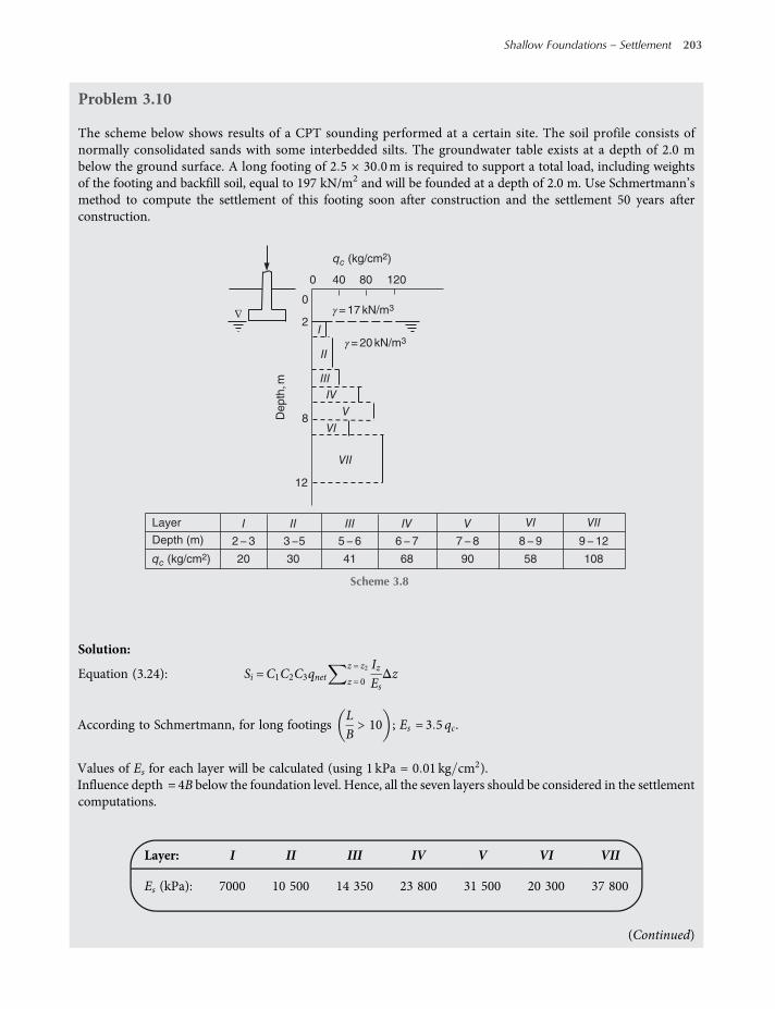
Problem 3.10
The scheme below shows results of a CPT sounding performed at a certain site. The soil profile consists ofnormally consolidated sands with some interbedded silts. The groundwater table exists at a depth of 2.0 mbelow the ground surface. A long footing of 2 5 × 30 0m is required to support a total load, including weightsof the footing and backfill soil, equal to 197 kN/m2 and will be founded at a depth of 2.0 m. Use Schmertmann’smethod to compute the settlement of this footing soon after construction and the settlement 50 years afterconstruction.
Solution:
Equation (3.24): Si =C1C2C3qnetz = z2
z = 0
IzEsΔz
According to Schmertmann, for long footingsLB> 10 ; Es = 3 5 qc.
Values of Es for each layer will be calculated (using 1 kPa = 0 01 kg cm2).Influence depth = 4B below the foundation level. Hence, all the seven layers should be considered in the settlementcomputations.
Layer: I II III IV V VI VII
Es (kPa): 7000 10 500 14 350 23 800 31 500 20 300 37 800
(Continued)
Layer
Depth (m) 2 − 3 3 −5 5 − 6 6 − 7 7 − 8 8 − 9 9 − 12
qc (kg/cm2) 20 30 41 68 90 58 108
VIIVI
8
0 40 80 120
0
12
VII
VI
IV
III
II
I
V
2∇
Depth
,m
qc (kg/cm2)
γ = 17 kN/m3
γ = 20 kN/m3
I II III IV V
Scheme 3.8
Shallow Foundations – Settlement 203
worksaccounts.com

Equation (3.25): Izp = 0 5 + 0 1qnetσzp
qnet = q−σo = 197−2 × 17 = 163 kPa
For long footings, σzp is calculated at depth B below foundation level; hence, σzp = 2 × 17 + 2 5 20−10 = 59 kPa
Izp = 0 5 + 0 116359
= 0 666
Considering continuous foundations L B ≥ 10 :
For z = 0 to B Iz = 0 2 +zB
Izp−0 2
For z =B to 4B Iz = 0 333Izp 4−zB
Determine value ofIzEsΔz at midpoint of each layer, as shown in Table 3.22
C1 = 1−0 5σoqnet
= 1−0 5 2 × 17
163= 0 896
C2 = 1 + 0 2logt0 1
At t = 0 1 year C2 = 1
C3 = 1 03−0 03LB
= 1 03−0 03 × 30
2 5= 0 67 < 0 73 useC3 = 0 73
0.1 0.666
4B
0
B Izp
Iz
z
0.2
Scheme 3.9
204 Shallow Foundations
worksaccounts.com
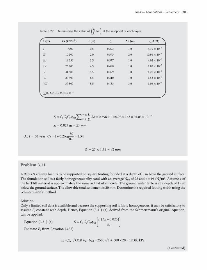
Si =C1C2C3qnetz = z2
z = 0
IzEsΔz = 0 896 × 1 × 0 73 × 163 × 25 03 × 10−5
Si = 0 027m = 27mm
At t = 50 year: C2 = 1 + 0 2log500 1
= 1 54
Si = 27 × 1 54 = 42mm
Problem 3.11
A 900-kN column load is to be supported on square footing founded at a depth of 1 m blow the ground surface.The foundation soil is a fairly homogeneous silty sand with an average N60 of 28 and γ = 19 kN m3. Assume γ ofthe backfill material is approximately the same as that of concrete. The ground water table is at a depth of 15 mbelow the ground surface. The allowable total settlement is 20mm. Determine the required footing width using theSchmertmann’s method.
Solution:Only a limited soil data is available and because the supporting soil is fairly homogeneous, it may be satisfactory toassume Es constant with depth. Hence, Equation (3.31)-(a), derived from the Schmertmann’s original equation,can be applied.
Equation (3.31)-(a): Si =C1C2C3qnetB Izp + 0 025
EsEstimate Es from Equation (3.32):
Es = βo OCR+ β1N60 = 2500 1 + 600 × 28 = 19 300 kPa
(Continued)
Table 3.22 Determining the value ofIzEsΔz at the midpoint of each layer.
Layer Es (kN/m2) z (m) Iz Δz (m) Iz Δz/Es
I 7000 0.5 0.293 1.0 4.19 × 10⁻⁵
II 10 500 2.0 0.573 2.0 10.91 × 10⁻⁵
III 14 350 3.5 0.577 1.0 4.02 × 10⁻⁵
IV 23 800 4.5 0.488 1.0 2.05 × 10⁻⁵
V 31 500 5.5 0.399 1.0 1.27 × 10⁻⁵
VI 20 300 6.5 0.310 1.0 1.53 × 10⁻⁵
VII 37 800 8.5 0.133 3.0 1.06 × 10⁻⁵
(Iz Δz/Es) = 25.03 × 10⁻⁵
Shallow Foundations – Settlement 205
worksaccounts.com

As a first trial, assume B = 2 0m
qnet = q−σo =900 + 2 0 × 2 0 × 1 × 24
2 0 × 2 0−1 × 19 = 230 kPa
C1 = 1−0 5σoqnet
= 1−0 5 × 1 × 19
230= 0 959
Assume the total settlement will be completed after 50 years;
C2 = 1 + 0 2logt0 1
= 1 + 0 2log500 1
= 1 54
C3 = 1 03−0 03LB
= 1 03−0 03 × 2 5
2 5= 1
Equation (3.25): Izp = 0 5 + 0 1qnetσzp
For square footings, σzp is calculated at depth 0.5B below foundation level; hence σzp = 1 × 19 + 0 5 × 2 × 19 =
38 kPa
Izp = 0 5 + 0 1qnetσzp
= 0 5 + 0 123038
= 0 746
Si = 0 02 = 0 959 × 1 54 × 1 × 230B 0 746 + 0 025
19300= 0 0136B
B= 1 47m< 2 0 m increase B
As a second trial, assume B = 2 5m
qnet = q−σo =900 + 2 5 × 2 5 × 1 × 24
2 5 × 2 5−1 × 19 = 149 kPa
C1 = 1−0 5σoqnet
C1 = 1−0 5 × 1 × 19
149= 0 936
Assume the total settlement will be completed after 50 years;
C2 = 1 + 0 2logt0 1
= 1 + 0 2log500 1
= 1 54
C3 = 1 03−0 03LB
=C3 = 1 03−0 03 × 2 5
2 5= 1
Izp = 0 5 + 0 1qnetσzp
= 0 5 + 0 1149
19 1 +2 52
= 0 69
Si = 0 02 = 0 936 × 1 54 × 1 × 149B 0 69 + 0 025
19 300= 0 008B
B= 2 5m= the assumed value
Use the footing width B = 2 5m
206 Shallow Foundations
worksaccounts.com

Problem 3.12
Solve Problem 3.10 using the Buisman–DeBeer method.
Solution:
Equation (3.20): Si =HClnσo + σzσo
Equation (3.23): C = 1 9qcσo
(Recommended by Meyerhof, 1965)
Si =H
0
2 3σo1 9qc
Δzlogσo + σzσo
Refer to Table 3.23. The depth z (below ground level) to the centre of each layer is obtained from the figure ofProblem 10. The effective overburden pressure σo and the stress increment σz at the centre of each layer arecalculated. The σz-values are obtained using either Figure 2.32 or Table 2.3. Values of qc in kg/cm2 are convertedto their corresponding values in kPa using 1 kPa = 0 01 kg cm2. The above settlement equations are applied toobtain the total settlement.
The total settlement = 56mmThis result, compared with that obtained by Schmertmann’s method (see Solution of Problem 3.10), is
considered too conservative.
Problem 3.13
A column load of 500 kN is supported on a 1 5 × 2 0m spread footing. The foundation depth equals 0.5m. Assumeγ of the backfill material is approximately the same as γ of concrete. The soil profile consists of clean, well graded,normally consolidated sand with γ = 17 kN m3 and the following SPT results:
Depth (m): 1.0 2.0 3.0 4.0 5.0
N60, (blow): 12 13 13 18 22
(Continued)
Table 3.23 Data for solving Problem 3.12.
Layer z (m) Δz (m) σo (kPa) σz (kPa) logσo + σzσo
qc (kPa)2 3σo1 9qc
Δz (mm) Si (mm)
I 2.5 1.0 39 158.0 0.703 2000 23.6 16.6
II 4.0 2.0 54 104.3 0.467 3000 43.6 20.4
III 5.5 1.0 69 68.5 0.300 4100 20.4 6.1
IV 6.5 1.0 79 57.4 0.237 6800 14.1 3.3
V 7.5 1.0 89 45.6 0.180 9000 12.0 2.2
VI 8.5 1.0 99 38.5 0.143 5800 20.7 3.0
VII 10.5 3.0 119 31.3 0.101 10800 40.0 4.0
Si = 55.6
Shallow Foundations – Settlement 207
worksaccounts.com
The ground water table is at a depth of 25 m. Using Schmertmann’s method, compute the total settlement att = 30 years.
Solution:
Equation (1.33):EsPa
= αN60 Es = αPa N60;Pa = 100 kPa
α= 10 for normally consolidated sands Es = 1000N60
Equation (3.32): Es = βo OCR+ β1N60
βo = 5000 and β1 = 1200 (for clean normally consolidated sands)
Es = 5000 1 + 1200N60 = 5000 + 1200N60
It may be a reasonable judgment to use the average of Es values computed from these two equations, aspresented below:
Depth (m): 1.0 2.0 3.0 4.0 5.0
Es, (kPa): 15 700 16 800 16 800 22 300 26 700
L B = 2 1 5 = 1 33
1 < L B < 10
Hence,
Iz = Izs + 0 111 Izc− IzsLB−1
Considering square and circular foundations:
For z = 0 toB2
Izs = 0 1 +zB
2Izp−0 2
For z =B2
to 2B Izs = 0 667Izp 2−zB
Considering continuous foundations L B ≥ 10 :
For z = 0 toB Izc = 0 2 +zB
Izp−0 2
For z =B to 4B Izc = 0 333Izp 4−zB
Izp = 0 5 + 0 1qnetσzp
qnet = q−σo = 500 1 5 × 2 + 0 5 × 24−0 5 × 17 = 170 2 kPa
208 Shallow Foundations
worksaccounts.com

For square footings: σzp is calculated at depth 0.5B below foundation level; hence, σzp = 0 5 × 17 + 1 5 2 17 =
21 25 kPa
Izp = 0 5 + 0 1170 221 25
= 0 783
For long footings: σzp is calculated at depth B below foundation level; hence, σzp = 0 5 × 17 + 1 5 × 17 = 34 kPa
Izp = 0 5 + 0 1170 234
= 0 724
Si =C1C2C3qnetz = z2
z = 0
IzEsΔz
C1 = 1−0 5σoqnet
= 1−0 5 0 5 × 17
170 2= 0 975
C2 = 1 + 0 2logt0 1
= 1 + 0 2log300 1
= 1 495
C3 = 1 03−0 03LB
= 1 03−0 03 × 22 5
= 1 006 > 0 73
Si = 0 975 × 1 495 × 1 006 × 170 2 × 7 86 × 10−5
Si = 0 02m= 20mm
Total settlement at t = 30 years is 20 mmValues of (Iz Δz/ Es) indicate that the influence depth is, practically, equals to 2B (or 3 m) because the footing is
too close to a square footing than to a long or continuous footing.
Problem 3.14
A raft 30 × 40m supports a building. The net contact pressure equals 120 kPa; assumed uniformly distributedover the building area. The soil profile is shown in the scheme below. The laboratory test results gave an averagevalue of mv for the clay equals 0.32 m2/MN. Determine the final settlement under the centre of the raft due toconsolidation of the clay.
(Continued)
Es(kPa)
Layer
No.
z
(m)Δz
(m)
1 15700 0.5 0.555
Izs Iz Δz/EsIzc Iz
0.375 0.548 1 3.49 × 10⁻⁵
2 16800 1.5 0.522 0.724 0.529 1 3.15 × 10⁻⁵
3 16800 2.5 0.174 0.562 0.188 1 1.12 × 10⁻⁵
4 22300 3.5 0 0.402 0.015 1 0.07 × 10⁻⁵
5 26700 4.5 0 0.241 0.009 1 0.03 × 10⁻⁵
Σ (Iz Δz/Es) = 7.86 × 10⁻⁵
Scheme 3.10
Shallow Foundations – Settlement 209
worksaccounts.com
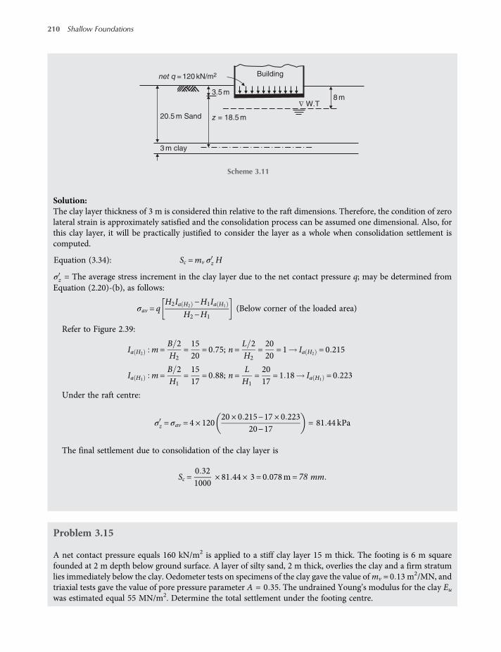
Solution:The clay layer thickness of 3 m is considered thin relative to the raft dimensions. Therefore, the condition of zerolateral strain is approximately satisfied and the consolidation process can be assumed one dimensional. Also, forthis clay layer, it will be practically justified to consider the layer as a whole when consolidation settlement iscomputed.
Equation (3.34): Sc =mv σz H
σz = The average stress increment in the clay layer due to the net contact pressure q; may be determined fromEquation (2.20)-(b), as follows:
σav = qH2Ia H2
−H1Ia H1
H2−H1(Below corner of the loaded area)
Refer to Figure 2.39:
Ia H2m=
B 2H2
=1520
= 0 75; n=L 2H2
=2020
= 1 Ia H2= 0 215
Ia H1m=
B 2H1
=1517
= 0 88; n=LH1
=2017
= 1 18 Ia H1= 0 223
Under the raft centre:
σz = σav = 4 × 12020 × 0 215−17 × 0 223
20−17= 81 44 kPa
The final settlement due to consolidation of the clay layer is
Sc =0 321000
× 81 44 × 3 = 0 078m= 78 mm
Problem 3.15
A net contact pressure equals 160 kN/m2 is applied to a stiff clay layer 15 m thick. The footing is 6 m squarefounded at 2 m depth below ground surface. A layer of silty sand, 2 m thick, overlies the clay and a firm stratumlies immediately below the clay. Oedometer tests on specimens of the clay gave the value ofmv = 0 13 m2/MN, andtriaxial tests gave the value of pore pressure parameter A = 0 35. The undrained Young’s modulus for the clay Euwas estimated equal 55 MN/m2. Determine the total settlement under the footing centre.
3.5 m8 m
20.5 m Sand z = 18.5 m
3 m clay
Buildingnet q = 120 kN/m2
∇ W.T
Scheme 3.11
210 Shallow Foundations
worksaccounts.com
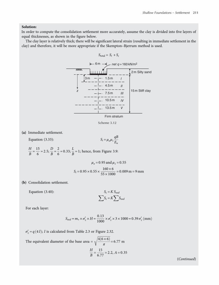
Solution:In order to compute the consolidation settlement more accurately, assume the clay is divided into five layers ofequal thicknesses, as shown in the figure below.The clay layer is relatively thick; there will be significant lateral strain (resulting in immediate settlement in the
clay) and therefore, it will be more appropriate if the Skempton–Bjerrum method is used.
Stotal = Si + Sc
(a) Immediate settlement.
Equation (3.33): Si = μoμ1qBEu
HB=156= 2 5;
DB=26= 0 33;
LB= 1; hence, from Figure 3.9:
μo = 0 95 and μ1 = 0 55
Si = 0 95 × 0 55 ×160 × 655 × 1000
= 0 009m= 9mm
(b) Consolidation settlement.
Equation (3.40): Sc =K Soed
Sc =K Soed
For each layer:
Soed =mv × σz ×H =0 131000
× σz × 3 × 1000 = 0 39 σz mm
σz = q 4 I ; I is calculated from Table 2.3 or Figure 2.32.
The equivalent diameter of the base area =4 6 × 6
π= 6 77 m
HB=
156 77
= 2 2, A= 0 35
(Continued)
6 m
Firm stratum
2 m Silty sand
3 m
z
1.5 m I
II
III
IV
V
4.5 m
7.5 m
10.5 m
13.5 m
15 m Stiff clay
net q = 160 kN/m2
Scheme 3.12
Shallow Foundations – Settlement 211
worksaccounts.com

Figure 3.15 forHB= 2 2 and A= 0 35, obtain K = 0 55
Sc = 0 55 × 116 6 = 64mm
Stotal = Si + Sc = 9 + 64 = 73 mm
Problem 3.16
A general soil profile at a certain site is shown in the scheme below. The lower sand layer is under artesian pressure,the piezometric level being 6 m above ground level. For the clay, mv = 0 94m2 MN and cv = 1 4m2 year.As a result of pumping from the artesian layer the piezometric level falls by 3 m over a period of 2 years. Draw
the time-settlement curve due to consolidation of the clay for a period of 5 years from the start of pumping.
Solution:Consolidation of the clay layer occurs due to decrease in porewater pressure at the lower boundary of the clay asa consequence of pumping operation. As there is no change in total vertical stress; the effective vertical stress inthe clay layer will increase with depth. The 3 m drop in piezometric level is equivalent to the decrease in theporewater pressure and increase in the effective vertical stress, which is 3γw at bottom of the clay layer, as shownbelow.
Sand
Artesian sand layer
4 m2 m
8 m
Clay
G.S
mν= 0.94 m2/MN
Cν= 1.4 m2/year
∇ W.T
Scheme 3.14
Layer
1.5 0.233
0.121
0.060
0.033
0.021
149
78
38
21
13
58.1
30.4
14.8
8.2
5.1
Σ Soed= 116.6
4.5
7.5
10.5
13.5
z
(m)
σ'z (kPa)
I Soed
(mm)
I
II
III
IV
V
Scheme 3.13
212 Shallow Foundations
worksaccounts.com
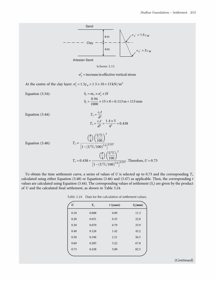
σz = increase in effective vertical stress
At the centre of the clay layer: σz = 1 5γw = 1 5 × 10 = 15 kN m2
Equation (3.34): Sc =mv × σz ×H
Sc =0 941000
× 15 × 8 = 0 113m= 113mm
Equation (3.44): Tv =cvtd2
Tv =cvtd2
=1 4 × 542
= 0 438
Equation (3.48): Tv =
π
4U100
2
1− U 100 5 6 0 357
Tv = 0 438 =
π
4U100
2
1− U 100 5 6 0 357 Therefore,U = 0 73
To obtain the time settlement curve, a series of values of U is selected up to 0.73 and the corresponding Tv
calculated using either Equation (3.48) or Equations (3.46) and (3.47) as applicable. Then, the corresponding tvalues are calculated using Equation (3.44). The corresponding values of settlement (Sc) are given by the productof U and the calculated final settlement, as shown in Table 3.24.
(Continued)
Table 3.24 Data for the calculation of settlement values.
U Tv t (years) Sc(mm)
0.10 0.008 0.09 11.3
0.20 0.031 0.35 22.8
0.30 0.070 0.79 33.9
0.40 0.126 1.42 45.2
0.50 0.196 2.21 56.5
0.60 0.285 3.22 67.8
0.73 0.438 5.00 82.5
Sand
Artesian Sand
4 m
4 m
Clay
𝜎 zʹ = 1.5 𝛾 w
𝜎 zʹ = 3 𝛾 w
Scheme 3.15
Shallow Foundations – Settlement 213
worksaccounts.com

Problem 3.17
At a certain site the soil profile consists of 8 m sand layer overlying a 6 m layer of normally consolidated clay,below which is an impermeable stratum. The water table exists at 2 m depth below the surface of the sand (groundsurface), as shown in the scheme below.
Sand8 m
2 m
6 m
Clay
cν = 1.26 m2/year
4.5 m
1.5 m
d = 2.25 m
d = 1.5 md = 6 m
Impermeable stratum
q
∇ W.T
Fill, γ = 20 kN/m3
γ = 17 kN/m3
γ = 19 kN/m3
γ = 20 kN/m3
Scheme 3.17
0 1 2 3 4 5
20
40
60
80
Corrected curve
0
Instantaneous curve
t (years)
Sc (
mm
)
Scheme 3.16
214 Shallow Foundations
worksaccounts.com
The saturated unit weight of the sand = 19 kN m3 and that of the clay = 20 kN m3. The sand above water tablehas unit weight = 17 kN m3. For the clay, the relationship between void ratio and effective stress (in kN/m2) canbe represented by the equation e = 0 88−0 32log σ 100 ; and the coefficient of consolidation cv = 1 26m2 year.Over a period of 1 year a fill of 3 m depth is to be dumped on the surface over an extensive area. The fill has unit
weight γ = 20 kN m3.
(a) Calculate the final settlement of the area due to consolidation of the clay and the settlement after a period of3 years from the start of dumping.
(b) If a very thin layer of sand, freely draining, exists 1.5 m above the bottom of the clay layer, what will be the finaland 3 year settlements?
Solution:(a) The fill covers a wide area; hence, the same fill pressure q is transmitted (approximately) to the concerned
subsurface layers and the problem can be considered one-dimensional. Consider one-dimensional consolida-tion, taking the clay layer as a whole.
At the middle of the clay layer:
σo = 17 × 2 + 6 19−10 + 3 20−10 = 118 kN m2
eo = 0 88−0 32log118100
= 0 857
From the given relationship it is clear that Cc = 0 32
Equation (3.36)-(a): Sc =CcH1 + eo
logσo + σzσo
Final consolidation settlement is
Sc =0 32 × 60001 + 0 857
log118 + 3 × 20
118= 185mm
The corrected value of time to allow for 1 year dumping period is
t = 3−121 = 2 5 years
The clay layer is half closed; hence, d = 6m
Equation (3.44):Tv =
cvtd2
Tv =1 26 × 2 5
62= 0 0875
Equation (3.48):
Tv =
π
4U100
2
1− U 100 5 6 0 357
0 0875 =
π
4U100
2
1− U 100 5 6 0 357 U = 0 334
Settlement after 3 years =U × final consolidation settlementSettlement after 3 years = 0 334 × 185 = 62mm
(Continued)
Shallow Foundations – Settlement 215
worksaccounts.com

(b) Thickness of the drainage layer (i.e. the very thin layer of sand) can be ignored and from the point of view ofdrainage there is an open upper clay layer of thickness 4.5m d = 2 25m above a half closed lower clay layer of1.5 m d = 1 5m , as shown in the scheme above.
Now, by proportion:
Tv1 =0 0875 × 62
2 252= 0 622. Equation (3.48) gives U1 = 0 825 upper layer; U
Tv2 =0 0875 × 62
1 52= 1 4. Equation (3.48) gives U2 = 0 968 lower layer
For each layer, Sc is proportional to HU. Therefore, if Ū is the overall degree of consolidation for thetwo layers combined:
4 5U1 + 1 5U2 = 6 ×U4 5 × 0 825 + 1 5 × 0 968 = 6 ×U . Hence U = 0 86 and the 3 year settlement isSc = 0 86 × 185 = 159 1mm; say 160 mm
Problem 3.18
A 2 0 × 3 2m flexible loaded area carries a uniformly distributed load = 210 kN m2, as shown in the schemebelow. Estimate the elastic settlement below the centre of the loaded area. Assume that the foundation depthDf = 1 6m and H = ∞ . Use Equation (3.5).
Solution:Elastic settlement Si below the centre of the loaded area:
Equation (3.5): Si = q×B×1−μ2
Es×m × IS × IF
m= 4;B2=22= 1 m;
L2=3 22
= 1 6 m; M =
L2
B 2=1 61
= 1 6; B=22= 1
N =HB 2
=∞1
= ∞
From Table 3.8 obtain I1 = 0 697 and I2 = 0 0; hence,
IS = I1 +1−2μ1−μ
I2 = 0 697
DB=1 62
= 0 8;BL=
23 2
= 0 625, μ= 0 3. From Table 3.7: IF = 0 728
Si = 210 ×22×1− 0 3 2
8500× 4 × 0 697 × 0 728 = 0 046m = 46 mm
Df
H
Silty sand
Es= 8500 kN/m2
μs = 0.3
2.0 m × 3.2 m
210 kN/m2
Rock
≈
Scheme 3.18
216 Shallow Foundations
worksaccounts.com
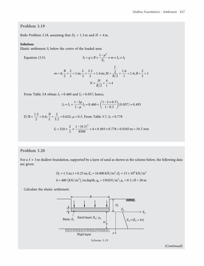
Problem 3.19
Redo Problem 3.18, assuming that Df = 1 2m and H = 4m.
Solution:Elastic settlement Si below the centre of the loaded area:
Equation (3.5): Si = q× B×1−μ2
Es×m× IS × IF
m= 4;B2=22= 1m;
L2=3 22
= 1 6m;M =
L2
B 2=1 61
= 1 6;B=22= 1
N =HB 2
=41= 4
From Table 3.8 obtain I1 = 0 460 and I2 = 0 057; hence,
IS = I1 +1−2μ1−μ
I2 = 0 460 +1−2 × 0 31−0 3
0 057 = 0 493
D B=1 22
= 0 6;BL=
23 2
= 0 625; μ = 0 3. From Table 3.7: IF = 0 778
Si = 210 ×22×1− 0 3 2
8500× 4 × 0 493 × 0 778 = 0 0345m= 34 5mm
Problem 3.20
For a 3 × 3m shallow foundation, supported by a layer of sand as shown in the scheme below, the following dataare given:
Df = 1 5m; t = 0 25m;Eo = 16 000 kN m2;Ef = 15 × 106 kN m2
k= 400 kN m2 mdepth; qo = 150 kN m2; μs = 0 3 ;H = 20m
Calculate the elastic settlement.
(Continued)
Rigid layer
Sand layer; Es; μsBase; Ef
≈
Df
EoEs
Es= (Eo + kz)H
z
t
B
Scheme 3.19
Shallow Foundations – Settlement 217
worksaccounts.com
Solution:
Equation (3.8): Si =qoBeIGIFIE
Eo1−μ2s
Be =4BLπ
=4 × 3 × 3
π= 3 384m
β =EokBe
=16 000
400 × 3 384= 11 82;
HBe
=20
3 384= 5 91
Figure 3.4 obtain IG = 0 85
Equation (3.9):
IF =π
4+
1
4 6 + 10 Ef Eo + Bek 2 2t Be3
=π
4+
1
4 6 + 10 15 × 106 16 000 + 3 384 × 400 2 2 × 0 25 3 384 3
= 0 816
Equation (3.10):
IE = 1−1
3 5 exp 1 22μs−0 4 Be Df + 1 6
IE = 1−1
3 5 exp 1 22 × 0 3−0 4 3 384 1 5 + 1 6= 0 926
Si =150 × 3 384 × 0 85 × 0 816 × 0 926
16 0001−0 32 = 0 0183m= 18 3 mm
Problem 3.21
Estimate the consolidation settlement of the clay layer shown in the scheme in Problem 2.13, using the results ofpart (a) of the same problem.
Solution:At the middle of the clay layer:
σo = 1 52 × 15 7 + 1 22 19 24−10 +3 052
19 24−10
= 49 23kNm2
< σc = 100 kN m2 the clay is overconsolidated
Solution of Problem 2.13, part (a), gave σz = 63 44 kN m2
63 44 + 49 23 = 112 67 kN m2 > σc. Hence, Equation (3.38) is applied.
Equation (3.38): Sc =CrH1 + eo
logσcσo
+CcH1 + eo
logσo + σzσc
Sc =0 06 × 3 051 + 0 8
log10049 23
+0 25 × 3 051 + 0 8
log49 23 + 63 44
100= 0 053 m= 53 mm
218 Shallow Foundations
worksaccounts.com
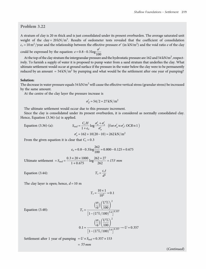
Problem 3.22
A stratum of clay is 20 m thick and is just consolidated under its present overburden. The average saturated unitweight of the clay = 20 kN m3. Results of oedometer tests revealed that the coefficient of consolidationcv = 10m2 year and the relationship between the effective pressure σ (in kN/m2) and the void ratio e of the clay
could be expressed by the equation: e= 0 8−0 3logσ
100At the top of the clay stratum the intergranular pressure and the hydrostatic pressure are 162 and 54 kN/m2, respect-
ively. To furnish a supply of water it is proposed to pump water from a sand stratum that underlies the clay. Whatultimate settlement would occur at ground surface if the pressure in the water below the clay were to be permanentlyreduced by an amount = 54 kN m2 by pumping and what would be the settlement after one year of pumping?
Solution:The decrease in water pressure equals 54 kN/m2 will cause the effective vertical stress (granular stress) be increasedby the same amount.At the centre of the clay layer the pressure increase is
σZ = 54 2 = 27 kN m2
The ultimate settlement would occur due to this pressure increment.Since the clay is consolidated under its present overburden, it is considered as normally consolidated clay.
Hence, Equation (3.36)-(a) is applied.
Equation (3.36)-(a): Soed =CcH1 + eo
logσo + σzσo
for σo≈σc; OCR≈1
σo = 162 + 10 20−10 = 262 kN m2
From the given equation it is clear that Cc = 0 3
eo = 0 8−0 3log262100
= 0 800−0 125 = 0 675
Ultimate settlement = Soed =0 3 × 20 × 1000
1 + 0 675log
262 + 27262
= 153 mm
Equation (3.44): Tv =cvtd2
The clay layer is open; hence, d = 10 m
Tv =10 × 1102
= 0 1
Equation (3.48): Tv =
π
4U100
2
1− U 100 5 6 0 357
0 1 =
π
4U100
2
1− U 100 5 6 0 357 U = 0 357
Settlement after 1 year of pumping =U × Soed = 0 357 × 153
= 55mm(Continued)
Shallow Foundations – Settlement 219
worksaccounts.com
Problem 3.23
The following results were obtained from an oedometer test on a specimen of saturated clay:
Pressure (kPa): 27 54 107 214 429 214 107 54
Void ratio: 1.243 1.217 1.144 1.068 0.994 1.001 1.012 1.024
A layer of this clay 8 m thick lies below a 4 m depth of sand, the water table being at the surface. The saturatedunit weight for both soils = 19 kN m3. A 4 m depth of fill, unit weight = 21 kN m3, is placed on the sand over anextensive area. Determine the final settlement due to consolidation of the clay. If the fill were to be removed sometime after the completion of consolidation, what heave would eventually take place due to swelling of the clay?
Solution:A plot of e–log σ , using the given pressure–void ratio data, was drawn on a separate semi-logarithmic graph paper.From the plot the preconsolidation pressure σc was approximately determined = 73 kN m2.At the centre of the clay layer, the effective overburden pressure is
σo = 4 19−10 + 4 19−10 = 72 kN m2≈σc
Therefore, the clay is considered normally consolidated.After the virgin compression curve and the expansion curve were found, approximately, the following e – log σ
relationships and indices could be obtained:
Compression: e= 1 74−0 27logσ ;Cc = 0 27Expansion: e = 1 075−0 031logσ ;Ce = 0 031Compression: eo = 1 74−0 27log72 = 1 24
The fill covers a wide area; hence, the same fill pressure q is transmitted to the concerned subsurface layers andthe problem can be considered one-dimensional. Consider one-dimensional consolidation, taking the clay layer asa whole:
The increase in the vertical effective stress at centre of the clay layer is
σz = q= 4 × 21 = 84 kN m2
Equation (3.36)-(a): Soed =CcH1 + eo
logσo + σzσo
for σo≈σc; OCR≈1
Soed =0 27 × 8 × 1000
1 + 1 24log
72 + 8472
= 324 mm
Expansion (heave):
σo = 4 × 21 + 4 19−10 + 4 19−10 = 156 kN m2
eo = 1 075−0 031log156 = 1 01
Removed pressure σz = q= 4 × 21 = 84 kN m2 will be used as a negative pressure in the settlement equa-tion. Hence,
220 Shallow Foundations
worksaccounts.com
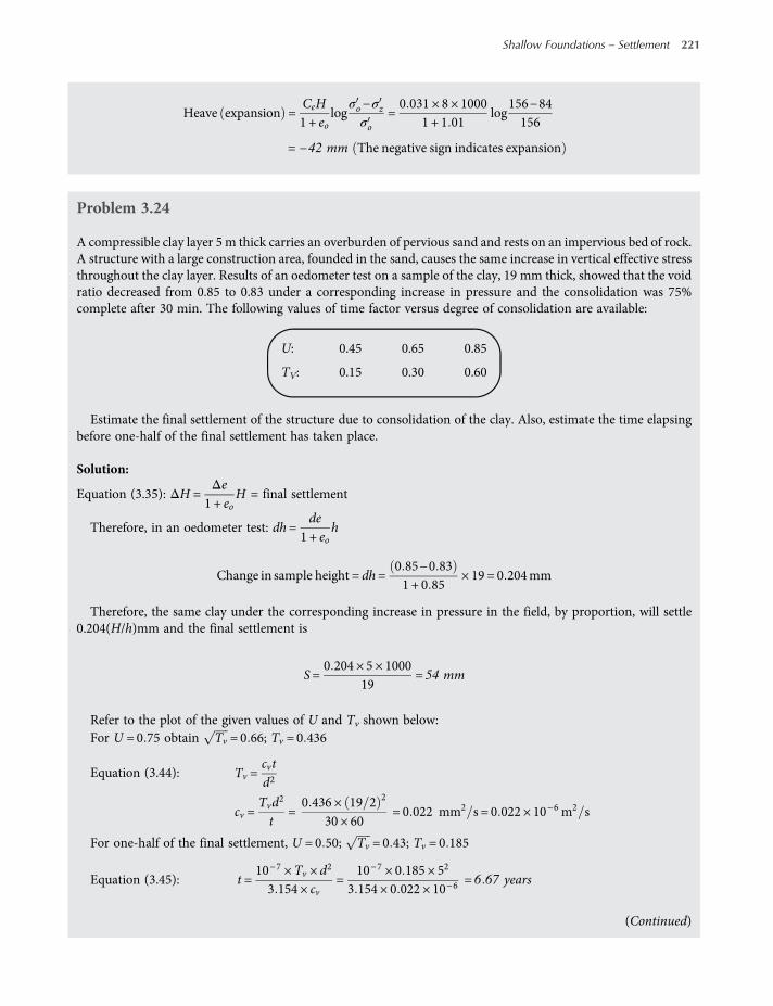
Heave expansion =CeH1 + eo
logσo−σzσo
=0 031 × 8 × 1000
1 + 1 01log
156−84156
= −42 mm The negative sign indicates expansion
Problem 3.24
A compressible clay layer 5 m thick carries an overburden of pervious sand and rests on an impervious bed of rock.A structure with a large construction area, founded in the sand, causes the same increase in vertical effective stressthroughout the clay layer. Results of an oedometer test on a sample of the clay, 19 mm thick, showed that the voidratio decreased from 0.85 to 0.83 under a corresponding increase in pressure and the consolidation was 75%complete after 30 min. The following values of time factor versus degree of consolidation are available:
U: 0.45 0.65 0.85
TV: 0.15 0.30 0.60
Estimate the final settlement of the structure due to consolidation of the clay. Also, estimate the time elapsingbefore one-half of the final settlement has taken place.
Solution:
Equation (3.35): ΔH =Δe
1 + eoH = final settlement
Therefore, in an oedometer test: dh=de
1 + eoh
Change in sample height = dh=0 85−0 831 + 0 85
× 19 = 0 204mm
Therefore, the same clay under the corresponding increase in pressure in the field, by proportion, will settle0.204(H/h)mm and the final settlement is
S=0 204 × 5 × 1000
19= 54 mm
Refer to the plot of the given values of U and Tv shown below:For U = 0 75 obtain Tv = 0 66; Tv = 0 436
Equation (3.44): Tv =cvtd2
cv =Tvd2
t=0 436 × 19 2 2
30 × 60= 0 022 mm2 s = 0 022 × 10−6 m2 s
For one-half of the final settlement, U = 0 50; Tv = 0 43; Tv = 0 185
Equation (3.45): t =10−7 ×Tv × d2
3 154 × cv=
10−7 × 0 185 × 52
3 154 × 0 022 × 10−6= 6 67 years
(Continued)
Shallow Foundations – Settlement 221
worksaccounts.com
Problem 3.25
In an oedometer test, with half-closed drainage condition, a specimen of saturated clay 19 mm thick reaches 50%consolidation in 20 min. How long would it take a layer of this clay 5 m thick to reach the same degree ofconsolidation under the same stress and drainage conditions? How long would it take the layer to reach 30%consolidation?
Solution:For the same degree of consolidation U under the same stress and drainage conditions the time factor Tv is thesame too.
Equation (3.44): Tv =cvtd2
Sample: Tv =cvtd2
=cv × 20
19 2
Layer:
Tv =cvtd2
=cv × t
5 × 1000 2
cv × 20
19 2 =cv × t
5 × 1000 2
t =20 5 × 1000 2
19 2 min
t =20 5 × 1000 2
19 2 ×1
365 × 24 × 60= 2 63 years
Equation (3.46): Tv =π
4U2 forU < 60
0
0.1
0.2
0.3
0.4
0.5
0.6
0.7
0.8
0.9
0 0.2 0.4
Tν
U
0.6 0.8
Scheme 3.20
222 Shallow Foundations
worksaccounts.com
For U = 50 , Tv =π
4× 0 52 =
cv × 2 63
5 2
cv = 1 867m2 year
For 30% consolidation: Tv =π
4× 0 32 =
cv × t
5 2
t =
π
4× 0 32 × 52
cv=
π
4× 0 32 × 52
1 867= 0 95 year
Problem 3.26
Assuming the fill in Problem 3.23 is dumped very rapidly, what would be the value of excess porewater pressure atthe centre of the clay layer after a period of three years? The layer is open and the value of cv = 2 4m2 year.
Solution:The total stress increment, applied very rapidly t 0 , equals to the pressure applied by the fill and will becarried initially entirely by the pore water, that is the initial value of excess pore water pressureui =Δσ = 4 × 21 = 84 kN m2. In particular, if ui is constant throughout the clay layer, the excess porewaterpressure ue at any time t > 0 may be determined from the following equation based on the Terzaghi theory ofone-dimensional consolidation:
ue =n= ∞
n= 1
2uinπ
1− cos nπ sinnπz2H
exp −n2π2Tv
4
where:
n = an odd integer; hence, 1−cosnπ = 2
z =H
2 H = thickness of the clay layer
Equation (3.44): Tv =cvtd2
=2 4 × 3
4 2 = 0 45
Using ui = 84 kN m2, n = 1 and Tv = 0 45:
ue =2 × 84π
2 sinπ
2exp −
π2 × 0 454
ue = 106 91 × 1 × 0 329 = 35 2 kN m2
Problem 3.27
A 10 m depth of sand overlies a clay layer 8 m thick, below which is a further depth of sand. For the clay,mv = 0 83m2 MN and cv = 4 4m2 year. Water table is at the surface level but is to be lowered permanently by4 m, the initial lowering taking place over a period of 40 weeks. Calculate the final settlement due to consolidationof the clay, assuming no change in the weight of sand and the settlement 2 years after the start of lowering.
(Continued)
Shallow Foundations – Settlement 223
worksaccounts.com

Solution:Total increase in vertical effective stress equals to total decrease in the porewater pressure due to lowering of thewater table, which is
4γw = 4 × 10 = 40 kN m2
Assume taking the clay layer as a whole:At the centre of the layer the increase in effective stress is
σz =12× 40 = 20 kN m2
Equation (3.34): Sc =mv σzH
Sc = 8 ×0 831000
× 20 = 0 133m= 133 mm
For calculation of settlement two years after the start of lowering, the time t would be equal to two years minusone-half of the total lowering period.
Equation (3.44): Tv =cvtd2
=4 4
4 2 2−20 × 7365
= 0 444
Equation (3.48): Tv =
π
4U100
2
1−U100
5 6 0 357
0 444 =
π
4U100
2
1−U100
5 6 0 357 U = 0 73
Settlement two years after the start of lowering the water table is
S=U × Sc = 0 73 × 133 = 97mm
Problem 3.28
A raft foundation 60 × 40m carrying a net pressure of 145 kN/m2 is located at a depth of 4.5 m below the surface ina deposit of dense sandy gravel 22 m deep. The water table is at a depth of 7 m and below the sandy gravel is a layerof clay 5 m thick which, in turn, is underlain by dense sand. The average value of mv for the clay is 0.22 m
2/MN.Determine the settlement below the centre of the raft, the corner of the raft and the centre of each edge of the raft,due to consolidation of the clay.
Solution:Final settlement due to consolidation of the clay is given by
Equation (3.34): Sc =mv σzH
224 Shallow Foundations
worksaccounts.com
Calculation of σz at depth z = 20m (i.e. at middle of the clay layer), using Table 2.3 or Figure 2.32:
(a) Below the centre of the raft
Bz=2020
= 1;L z = 30 20 = 1 5 Ir = 0 194
σz = q 4Ir = 145 × 4 × 0 194 = 112 52 kN m2
(b) Below the corner of the raft
B z = 40 20 = 2, L z = 60 20 = 3 Ir = 0 238
σz = q Ir = 145 × 0 238 = 34 51 kN m2
(c) Below the centre of a long edge of the raft
B z = 30 20 = 1 5, L z = 40 20 = 2 Ir = 0 224
σz = q 2Ir = 145 × 2 × 0 224 = 64 96 kN m2
(d) Below centre of a short edge of the raft
B z = 20 20 = 1, L z = 60 20 = 3 Ir = 0 203
σz = q 2Ir = 145 × 2 × 0 203 = 58 87 kN m2
Calculation of consolidation settlement:
(a) Below the raft centre
Sc = 5 ×0 221000
× 112 52 = 0 124m= 124 mm
(b) Below the raft corner
Sc = 5 ×0 221000
× 34 51 = 0 038m= 38 mm
(c) Below centre of a long edge
Sc = 5 ×0 221000
× 64 96 = 0 072m= 72 mm
(d) Below centre of a short edge
Sc = 5 ×0 221000
× 58 87 = 0 065m= 65 mm
Problem 3.29
An oil storage tank 35 m in diameter is located 2 m below the surface of a deposit of clay 32 m thick, which overliesa firm stratum, as shown in the scheme below. The net foundation pressures at the foundation level equal105 kN/m2. The average values of mv and pore pressure coefficient A for the clay are 0.14 m2/MN and 0.65,respectively. The undrained value of Young’s modulus is estimated to be 40 MN/m2. Determine the total settle-ment (excluding settlement due to secondary compression or creep) under the centre of the tank.
(Continued)
Shallow Foundations – Settlement 225
worksaccounts.com
Solution:The clay deposit is considered a thick layer; there will be significant lateral strain (resulting in immediate settle-ment in the clay) and therefore it would be appropriate if the Skempton–Bjerrummethod is used in the settlementcomputations. Accordingly, the total settlement (excluding settlement due to secondary compression or creep) isgiven by
Equation (3.3): ST = Si + Sc
Immediate settlement Si may be calculated using Equation (3.33) and Figure 3.9, whereas the consolidationsettlement Sc is calculated using Equation (3.40) and Figure 3.15.In order to compute the consolidation settlement more accurately, assume the clay below the foundation level is
divided into six layers of equal thicknesses, as shown in the scheme above:
(a) Immediate settlement
Equation (3.33): Si = μoμ1qBEu
HB=3035
= 0 857;DB=
235
= 0 057
Figure 3.9: obtain μo = 0 99 and μ1 = 0 35
Si = 0 99 × 0 35 ×105 × 3540 × 1000
= 0 032m= 32mm
(b) Consolidation settlement.
Equation (3.40): Sc =K SoedFor each layer:
Soed =mv × σz ×H =0 141000
× σz × 5 × 1000 = 0 7 σz mm
Figure 2.30: σz = σz = q Ic
35 m Oil tank
32 m clay
2.5 m I
zII
III
7.5 m
12.5 m
17.5 m
22.5 m
27.5 m
Firm stratum
2 m
5 m
∇ W.T Net q = 105 kN/m2
IV
V
VI
Scheme 3.21
226 Shallow Foundations
worksaccounts.com

A= 0 65 ;HB= 0 857
Figure 3.15: obtain K = 0 775
Sc = 0 775 × 320 6 = 248mm
Total settlement ST = Si + Sc = 32 + 248 = 280 mm
Problem 3.30
The foundation of a large building is at 3m below ground level. The building contains one-story basement. The soilprofile consists of topsoil and sand 7.5 m thick, overlies a clay layer 3 m thick. The water table is 6.25 m deep. Unitweights of the sand above and below water table are 20 and 22 kN/m3, respectively. Saturated unit weight of theclay is 19.2 kN/m3. The average value ofmv for the clay is 177 × 10−6 m2 kN and the coefficient of consolidation cvis 0.025 mm2/s. Additional pressure on the clay due to weight of the building = 200 kN m2 at the top of thestratum, decreasing uniformly with depth to 150 kN/m2 at the bottom. Find:
(a) The original effective pressures at top and bottom of the clay stratum before excavation commences.(b) The effective pressures at the top and bottom of the clay stratum after completion of the building.(c) The magnitude of settlement of the building expected due to consolidation of the clay.(d) The probable time in which 90 % of the settlement will occur. Assume half-closed drainage condition.
Solution:(a) At top of the clay: σo = 6 25 × 20 + 1 25 22−10 = 140 kPa
At bottom of the clay: σo = 140 + 3 19 2−10 = 167 6 kPa(b) At top of the clay: σ = 140 + 200 −3 × 20 = 280 kPa
At bottom of the clay: σ = 167 6 + 150 −3 × 20 = 257 6 kPa
(c) The net increase in effective pressure at the centre of the clay layer σz =280 + 257 6
2−140 + 167 6
2=
268 8−153 8 = 115 kPaor,
σz =200 + 150
2−3 × 20 = 115 kPa
Equation (3.34): Sc =mv × σz ×H
= 177 × 10−6 × 115 × 3 = 0 061 m= 61 mm(Continued)
Layer
2.5 1.00
0.94
0.82
0.65
0.55
0.40
105.0
98.7
86.1
68.3
57.8
42.0
73.5
69.1
60.3
47.8
40.5
29.4
Σ Soed = 320.6 mm
7.5
12.5
17.5
22.5
27.5
z, (m) σ′z, (mPa)Ic Soed, (mm)
I
II
III
IV
V
VI
Scheme 3.22
Shallow Foundations – Settlement 227
worksaccounts.com

(d) For 90 % of the settlement, the degree of consolidation U = 0 90 > 0 60; hence the time factor may becomputed from
Equation (3.47): Tv = 1 781−0 933log 100−U
Tv = 1 781−0 933log 100−90 = 0 85
Equation (3.45): t =10−7 ×Tv × d2
3 154 × cv
t =10−7 × 0 85 × 32
3 154 ×0 02510002
=0 85 × 9
3 154 × 0 25= 9 7 years
Problem 3.31
Below the foundation of a structure there is a stratum of compressible clay 6 m thick with incompressible porousstrata above and below. The average overburden pressure on the stratum before construction was 115 kPa andafter completion of the structure the pressure increased to 210 kPa. Oedometer tests were carried out on a sampleof clay initially 20 mm thick. Each pressure was allowed to act for 24 h and the decrease in thickness measured, theresults being as follows:
Pressure, (kPa): 0 50 100 200 400
Thickness, mm: 20.0 19.8 19.4 19.0 18.6
Under a pressure of 100 kPa, 90 % of the total consolidation took place in 21 min.Find (a) value ofmv for the increased stress range after completion of the structure, (b) the probable settlement
of the structure and (c) the time in which 90% of this settlement may be expected to occur.
Solution:
(a)
mv =eo−e11 + eo
×1
σ1−σo=
1Ho
Ho−H1
σ1−σo
A plot of the given pressure versus thickness was drawn on a separate graph paper. From the plot, thicknessof the oedometer sample under a pressure of 115 kPa was estimated at 19.34 mm and that under a pressure of210 kPa was 18.97 mm. Hence,
mv =1
19 3419 34−18 98210−115
= 1 97 × 10−4m2 kN
(b)σz = 210−115 = 95 kPa
Equation (3.34): Sc =mv × σz ×H
= 1 96 × 10−4 × 95 × 6 × 1000 = 112 mm
(c) Equation (3.44): Tv =cvtd2
228 Shallow Foundations
worksaccounts.com

For the same 90 % of the total consolidation and pressure increment, the time factor of the clay stratum equalsthat of the test sample. Therefore, under a pressure of 100 kPa, we can write
cv × t32
=cv × 21
10 1000 2
t = 9 × 21 × 10 000 = 189 × 104min
Under a pressure of 95 kPa:
t = 189 × 104 ×10095
= 198 95 × 104min
The time in which 90% of the 112 mm settlement may be expected to occur is
t =198 95 × 104
365 × 24 × 60= 3 8 years
Problem 3.32
On a flat site boreholes reveal that a 4 m layer of dense sand overlies a layer of compressible clay 8 m thick, belowwhich stiffer clay extends to a considerable depth. The appropriate values of the coefficient of compressibility ofthe 8 m clay layer are:
Upper 4 m, mv = 0 746 × 10−3m2 kNLower 4 m, mv = 0 559 × 10−3m2 kN
It is proposed to store material on two adjacent paved areas as indicated in the scheme below. The pavement andthe stored material together can be assumed to provide a uniform contact pressure q on the surface of the ground.Estimate the value of q in kPa if the differential settlement between points A and B is to be limited to 0.05 m. Usethe pressure influence chart of Figure 2.32.
(Continued)
12 m 4 m 12 m
6 m
6 m
12 m A B
Scheme 3.23
Shallow Foundations – Settlement 229
worksaccounts.com
Solution:(A) Settlement at point A
Equation (3.34): Sc =mv × σz ×H
(1) Settlement of the upper 4 m clay; z = 6mLeft area:Bz=Lz=66= 1; Figure 2.31 gives I = 0 175 and 4I = 0 7
σz = q 4I = 0 7 q kPa
Right area:
Bz=66= 1;
Lz=226= 3 67 I = 0 204 2I = 0 408
Bz=66= 1; L z = 10 6 = 1 67 I = − 0 195 2I = − 0 390
σz = q 0 408 −0 390 = 0 018 q kPa
Sc = 0 746 × 10−3 0 7q+ 0 018 q 4 = 2 143 × 10−3 q m
(2) Settlement of the lower 4 m clay, z = 10 mLeft area:Bz=Lz=
610
= 0 6. Figure 2.31 gives I = 0 107 and 4I = 0 428.
σz = q 4I = 0 428 q kPa
Right area:
Bz=
610
= 0 6;L z = 22 10 = 2 2 I = 0 153 2I = 0 306
Bz=
610
= 0 6;L z = 10 10 = 1 I = − 0 136 2I = − 0 272
σz = 0 306−0 272 q= 0 034 q kPa
Sc = 0 559 × 10−3 0 428 q+ 0 034 q 4 = 1 033 × 10−3 q
Settlement at A = 2 143 × 10−3 q+ 1 033 × 10−3 q= 3 176 × 10−3 q(B) Settlement at point B
Equation (3.34): Sc =mv × σz ×H
(1) Settlement of the upper 4 m clay; z = 6m:Left area:
Bz=66= 1;
Lz=126= 2 I = 0 2,and 2I = 0 4
σz = 0 4 q kPa
Right area:
Bz=66= 1;
Lz=166= 2 67 I = 0 202; and 2I = 0 404
230 Shallow Foundations
worksaccounts.com

Bz=46= 0 667;
Lz=66= 1 I = − 0 145; and 2I = −0 29
σz = 0 404−0 290 q= 0 114 q kPa
Sc = 0 746 × 10−3 0 404 q+ 0 114 q 4 = 1 546 × 10−3 q
(2) Settlement of the lower 4 m clay, z = 10 mLeft area:
Bz=
610
= 0 6; L z = 12 10 = 1 2 I = 0 143 and 2I = 0 286
σz = 0 286 q kPa
Right area:
Bz=
610
= 0 6;Lz=1610
= 1 6 I = 0 15, and 2I = 0 3
Bz=
410
= 0 4;L z = 6 10 = 0 60 I = − 0 08, and 2I = − 0 16
σz = 0 3−0 16 q= 0 14 q kPa
Sc = 0 559 × 10−3 0 286 q+ 0 14 q 4 = 0 953 × 10−3 q
Settlement at B= 1 546 × 10−3 q + 0 953 × 10−3 q= 2 499 × 10−3 qThe differential settlement between points A and B = 0 05m. Therefore, 0 05 = 3 176 × 10−3 q
−2 499 × 10−3 q
q=0 05
0 677 × 10−3= 73 86 kPa
Problem 3.33
Solve Problem 3.32 taking the 8 m clay layer as a whole.
Solution:(A) Settlement at point A
Equation (3.34): Sc =mv × σz ×H
Use average mv =0 746 + 0 559
2× 10−3 = 0 653 × 10−3 m2 kN
z = 8m
Left area:Bz=Lz=68= 0 75; Figure 2.31 gives I = 0 14 and 4I = 0 56
σz = q 4I = 0 56 q kPa
(Continued)
Shallow Foundations – Settlement 231
worksaccounts.com

Right area:
Bz=68= 0 75;
Lz=228= 2 75 I = 0 18; and 2I = 0 36
Bz=68= 0 75;
Lz=108= 1 1 25 I = − 0 165 2I = − 0 33
σz = q 0 36−0 33 = 0 03 q kPa
Sc = 0 653 × 10−3 0 56q+ 0 03 q 8 = 3 082 × 10−3q m
(B) Settlement at point BEquation (3.34): Sc =mv × σz ×H
Use average mv =0 746 + 0 559
2× 10−3 = 0 653 × 10−3 m2 kN
z = 8m
Left area:
Bz=68= 0 75;
Lz=128= 1 5 I = 0 17; and 2I = 0 34
σz = 0 34 q kPa
Right area:
Bz=68= 0 75;
Lz=168= 2 I = 0 175; and 2I = 0 35
Bz=48= 0 5;
Lz=68= 0 75 I = − 0 108; and 2I = −0 216
σz = 0 35 −0 216 q= 0 134 q kPa
Sc = 0 653 × 10−3 0 34 q+ 0 134 q 8 = 2 476 × 10−3 q
The differential settlement between points A and B= 0 05m. Therefore,
0 05 = 3 082 × 10−3 q−2 476 × 10−3 q
q=0 05
0 606 × 10−3= 82 51 kPa
Problem 3.34
A building has a foundation base slab supported on a bed of compact sand. Under the sand there is a stratum ofclay 4.5 m thick which in turn rests on impermeable shale. The ground water level is situated within the sand. Theinitial effective overburden pressure at the top of the clay is 85 kPa. Additional pressures due to the foundationloads are as follows:
232 Shallow Foundations
worksaccounts.com

Location Additional pressure, kPa
Under centre of slab Under corner of slab
Top of clay layer 85.0 45.0
Bottom of clay layer 25.0 10.5
The clay has an average unit weight = 19 2 kN m3 and oedometer tests gave the following void ratio/effectivepressure data:
e 0.93 0.91 0.88 0.85
σ , kPa 50 100 200 400
Estimate the final settlement under the centre and under a corner of the foundation base slab due to consoli-dation of the clay stratum.
Solution:(A) Final settlement under centre of the base slab:
The initial effective overburden pressure at bottom of the clay layer is
85 + 4 5 19 2 − 10 = 126 4 kPa
The average initial effective overburden pressure at centre of the clay layer is
85 + 126 42
= 105 7 kPa
The average increase in pressure at centre of the clay layer is
85 + 252
= 55 kPa
The total effective pressure at centre of the clay layer is
105 7 + 55 = 160 7 kPa
The graph of e versus σ is shown in the scheme below.From this graph the initial void ratio eo = 0 908 at the initial effective pressure σ = 105 7 kPa,
anddedσ
= 3 5 × 10⁻⁴
mv =1
1 + eo
dedσ
=1
1 + 0 908× 3 5 × 10−4 = 18 34 × 10−5m2 kN
Sc =mv × σz ×H = 18 34 × 10−5 × 55 × 4 5 = 0 045 m= 45 mm
It is noteworthy that mv may also be calculated approximately by assuming a straight line relationshipbetween e and σ over the current range of pressures, as follows:
(Continued)
Shallow Foundations – Settlement 233
worksaccounts.com
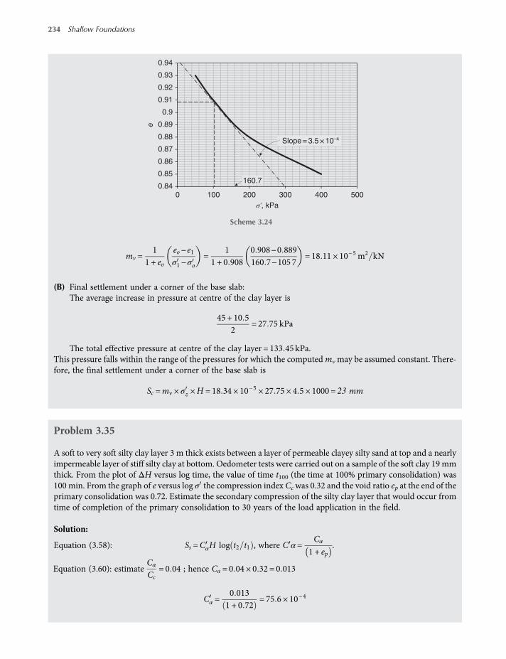
mv =1
1 + eo
eo−e1σ1−σo
=1
1 + 0 9080 908−0 889160 7−105 7
= 18 11 × 10−5 m2 kN
(B) Final settlement under a corner of the base slab:The average increase in pressure at centre of the clay layer is
45 + 10 52
= 27 75 kPa
The total effective pressure at centre of the clay layer = 133 45 kPa.This pressure falls within the range of the pressures for which the computedmv may be assumed constant. There-fore, the final settlement under a corner of the base slab is
Sc =mv × σz ×H = 18 34 × 10−5 × 27 75 × 4 5 × 1000 = 23 mm
Problem 3.35
A soft to very soft silty clay layer 3 m thick exists between a layer of permeable clayey silty sand at top and a nearlyimpermeable layer of stiff silty clay at bottom. Oedometer tests were carried out on a sample of the soft clay 19 mmthick. From the plot of ΔH versus log time, the value of time t100 (the time at 100% primary consolidation) was100 min. From the graph of e versus log σ the compression index Ccwas 0.32 and the void ratio ep at the end of theprimary consolidation was 0.72. Estimate the secondary compression of the silty clay layer that would occur fromtime of completion of the primary consolidation to 30 years of the load application in the field.
Solution:
Equation (3.58): Ss =CαH log t2 t1 , where C α=Cα
1 + ep.
Equation (3.60): estimateCα
Cc= 0 04 ; hence Ca = 0 04 × 0 32 = 0 013
Cα =0 0131 + 0 72
= 75 6 × 10⁻⁴
0.84
0.85
0.86
0.87
0.88
0.89
0.9
0.91
0.92
0.93
0.94
0 100 200 300
σʹ, kPa
400 500
160.7
e
Slope = 3.5 × 10⁻⁴
Scheme 3.24
234 Shallow Foundations
worksaccounts.com

For the same clay soil:
Tv =cv × tfielddfield
2 =cv × tlabdlab
2 ; hence tfield =dfield
2 × tlabdlab
2 =30002 × 100
192
2
tfield = 99 723 × 105 min =99 723 × 105
365 × 24 × 60= 19 years
t1 = tfield = 19 years; t2 = 30 years
Ss = 75 6 × 10−4 × 3000 × log 30 19 = 4 5 mm
However, it is very likely that the secondary compression will be larger than this small value, as some will occurduring primary consolidation. Theoretically, at the end of the 19 years there is no excess pore pressure anywhere inthe 3-m clay layer; however during this time period dissipation occurs from the top down, with secondary com-pression beginning before 19 years have elapsed in the upper regions.
Problem 3.36
A soil profile is shown in the scheme below. A uniformly distributed load q = 100 kPa is applied at the groundsurface covering an extensive area. The clay is normally consolidated. Assume that the primary consolidation willbe complete in 3.5 years. The secondary compression index Ca = 0 011. Estimate the total settlement 10 years afterthe load application due to consolidation and secondary compression of the clay layer.
Solution:
Equation (3.36)-(b): Sc =CcH1 + eo
logσo + σzσo
The average effective overburden stress at the middle of the clay layer is
σo = 2 × 14 + 4 18−10 + 2 19−10 = 78 kN m2
Equation (3.36)-(b): Cc = 0 009 LL−10 = 0 009 40−10 = 0 27The loaded area is a large area; hence, practically, σz = q= 100 kPa
Sc =0 27 × 41 + 0 8
log78 + 100
78= 0 215 m= 215mm
(Continued)
γdry= 14 kN/m3
γsat= 18 kN/m3
γsat= 19 kN/m3
e = 0.8
LL = 40
Sand
Clay
Sand
2 m
4 m
4 m
G. S
q = 100 kPa
∇ W.T
Scheme 3.25
Shallow Foundations – Settlement 235
worksaccounts.com
Equation (3.58):
Ss =CαH log t2 t1 , where Cα =Cα
1 + ep
Cc =Δe
logσo + σzσo
; Δe= eo− ep =Cc logσo + σzσo
; hence,
ep = e0−Cc logσo + σzσo
= 0 8−0 27log78 + 100
78= 0 703; hence,
Cα =0 011
1 + 0 703= 0 0065; t1 = 3 5 years; t2 = 10 years
Ss = 0 0065 × 4log 10 3 5 = 0 0118m= 12mm
Therefore, the total settlement 10 years after the load application due to consolidation and secondary compres-sion of the clay layer is
215 + 12 = 227mm
Problem 3.37
A soil profile consists of two strata of normally consolidated homogeneous clay above an impervious layer andwith a drainage layer of incompressible sand, γsat = 19 6 kN m3, separating the strata, as shown in the schemebelow. Undisturbed samples were taken from nearly middle of the clay layers, consolidation tests were carriedout, e− logσ curves were plotted and values of Cc were determined. Also, for one point on each curve (the straightpart of the curve), the value of σ and its corresponding e value were found. These data and values of specific gravityGs are as tabulatedin the scheme:
q = 74 kPa
Upper clay layer
Lower clay layer
G.S
∇ W.T
Soft clay
Silty clay
1.2 m
3 m
0.6 m
4 m
Impervious bed
Layer Gs Cc e σʹ, kPa
2.74
2.70
0.36
0.24
1.02
0.73
100
160
Sand
Scheme 3.26
236 Shallow Foundations
worksaccounts.com

A very large area is to be loaded on the surface with a uniform load of 74 kPa. Determine:
(a) The settlement due to consolidation of the clay strata under the added surface uniform load.(b) The data required for drawing a time settlement curve using the following additional data:
Layer Height of specimen, cm t50, min
Upper 2.54 4.6
Lower 1.62 3.1
Solution:(a) The upper and lower clay strata are divided into convenient layers for the desired degree of accuracy. In the
upper layer the water table is a convenient plane for division. The lower 4 m stratum is arbitrarily divided intotwo equal layers. The necessary calculations are carried out on the tabulated form in Table 3.25, in accordancewith the following procedure:(1) Number the layers and record them in column 1 of the table.(2) Write the layers thickness H in column 2.(3) Determine the effective overburden pressure σo at mid-depth of each layer and record them in column 3.
Practically, the first soft clay layer may be considered nearly saturated.
For layers I and II: γsat =Gs + e1 + e
γw =2 74 + 1 021 + 1 02
10 = 18 6 kN m3
For layers III and IV: γsat =2 7 + 0 731 + 0 73
10 = 19 8 kN m3
For example, the effective overburden pressure σo at the mid-depth of layer III is
σo = 1 2 × 18 6 + 1 8 18 6−10 + 0 6 19 6−10 + 1 19 8−10
= 53 36 kPa
(4) Record Cc values in column 4.
(5) Compute eo values using the relationship eo = e +Cc logσ
σoand record them in column 5. For example, at
the mid-depth of layer III
eo = 0 73 + 0 24 log16053 36
= 0 844
(6) Record values ofCc H1 + e0
in column 6. BecauseCc
1 + e0is dimensionless, thicknessH can be in any unit and the
consolidation settlement Sc will be in the same unit.(7) Determine and record in column 7 the effective pressure increase σz produced at the mid-depth of each
layer by the added load. In this problem, because the loaded area is large compared to the depth of thecompressible layers, σz may be considered as constant for the full depth and equals to the added uniformload q which is 74 kPa.
(Continued)
Shallow Foundations – Settlement 237
worksaccounts.com
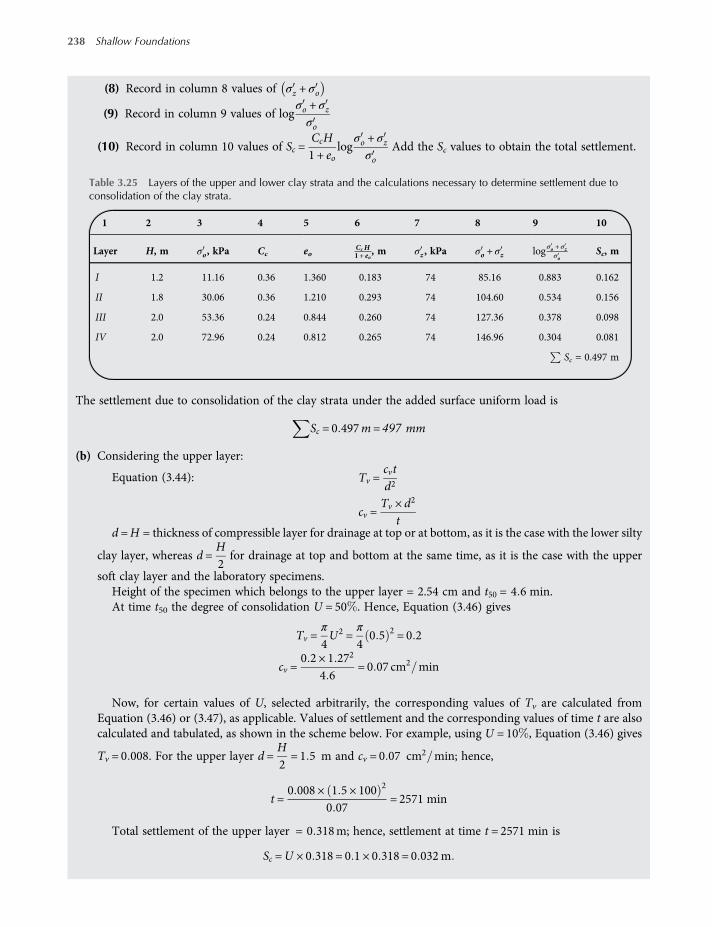
(8) Record in column 8 values of σz + σo
(9) Record in column 9 values of logσo + σzσo
(10) Record in column 10 values of Sc =CcH1 + eo
logσo + σzσo
Add the Sc values to obtain the total settlement.
The settlement due to consolidation of the clay strata under the added surface uniform load is
Sc = 0 497m= 497 mm
(b) Considering the upper layer:
Equation (3.44): Tv =cvtd2
cv =Tv × d2
td =H = thickness of compressible layer for drainage at top or at bottom, as it is the case with the lower silty
clay layer, whereas d =H2for drainage at top and bottom at the same time, as it is the case with the upper
soft clay layer and the laboratory specimens.Height of the specimen which belongs to the upper layer = 2.54 cm and t50 = 4 6 min.At time t50 the degree of consolidation U = 50 . Hence, Equation (3.46) gives
Tv =π
4U2 =
π
40 5 2 = 0 2
cv =0 2 × 1 272
4 6= 0 07 cm2 min
Now, for certain values of U, selected arbitrarily, the corresponding values of Tv are calculated fromEquation (3.46) or (3.47), as applicable. Values of settlement and the corresponding values of time t are alsocalculated and tabulated, as shown in the scheme below. For example, using U = 10 , Equation (3.46) gives
Tv = 0 008. For the upper layer d =H2= 1 5 m and cv = 0 07 cm2 min; hence,
t =0 008 × 1 5 × 100 2
0 07= 2571 min
Total settlement of the upper layer = 0 318m; hence, settlement at time t = 2571 min is
Sc =U × 0 318 = 0 1 × 0 318 = 0 032m
Table 3.25 Layers of the upper and lower clay strata and the calculations necessary to determine settlement due toconsolidation of the clay strata.
1 2 3 4 5 6 7 8 9 10
Layer H, m σo, kPa Cc eoCc H1+ eo
, m σz , kPa σo + σz logσo + σzσoSc, m
I 1.2 11.16 0.36 1.360 0.183 74 85.16 0.883 0.162
II 1.8 30.06 0.36 1.210 0.293 74 104.60 0.534 0.156
III 2.0 53.36 0.24 0.844 0.260 74 127.36 0.378 0.098
IV 2.0 72.96 0.24 0.812 0.265 74 146.96 0.304 0.081
Sc = 0.497 m
238 Shallow Foundations
worksaccounts.com
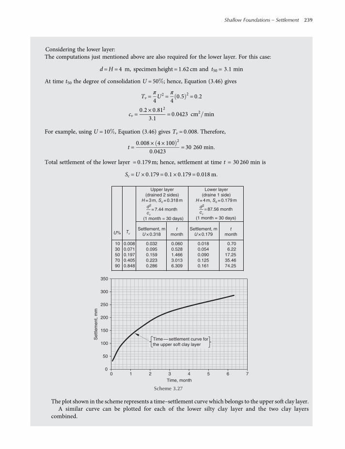
Considering the lower layer:The computations just mentioned above are also required for the lower layer. For this case:
d =H = 4 m, specimen height = 1 62 cm and t50 = 3 1 min
At time t50 the degree of consolidation U = 50 ; hence, Equation (3.46) gives
Tv =π
4U2 =
π
40 5 2 = 0 2
cv =0 2 × 0 812
3 1= 0 0423 cm2 min
For example, using U = 10 , Equation (3.46) gives Tv = 0 008. Therefore,
t =0 008 × 4 × 100 2
0 0423= 30 260 min
Total settlement of the lower layer = 0 179m; hence, settlement at time t = 30 260 min is
Sc =U × 0 179 = 0 1 × 0 179 = 0 018m
The plot shown in the scheme represents a time–settlement curve which belongs to the upper soft clay layer.A similar curve can be plotted for each of the lower silty clay layer and the two clay layers
combined.
0
50
100
150
200
250
300
350
0 1 2 3 4 5 6 7
Settle
men
t, m
m
Time, month
Time — settlement curve for
the upper soft clay layer
Upper layer
(drained 2 sides)
H = 3 m, Sc= 0.318 m
Lower layer
(draine 1 side)
H = 4 m, Sc= 0.179 m
(1 month = 30 days) (1 month = 30 days)
Settlement, m
U × 0.318
Settlement, m
U × 0.179U%t
month
t
month
10 0.008 0.032 0.060 0.018 0.70
30 0.071 0.095 0.528 0.054 6.22
50 0.197 0.159 1.466 0.090 17.25
70 0.405 0.223 3.013 0.125 35.46
90 0.848 0.286 6.309 0.161 74.25
= 7.44 monthd2
cν
Tν
= 87.56 monthd2
cν
Scheme 3.27
Shallow Foundations – Settlement 239
worksaccounts.com
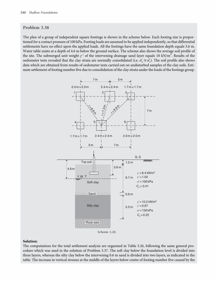
Problem 3.38
The plan of a group of independent square footings is shown in the scheme below. Each footing size is propor-tioned for a contact pressure of 100 kPa. Footing loads are assumed to be applied independently, so that differentialsettlements have no effect upon the applied loads. All the footings have the same foundation depth equals 3.6 m.Water table exists at a depth of 4.6 m below the ground surface. The scheme also shows the average soil profile ofthe site. The submerged unit weight γ of the intervening drainage sand layer equals 10 kN/m3. Results of theoedometer tests revealed that the clay strata are normally consolidated (i.e. σo σc). The soil profile also showsdata which are obtained from results of oedometer tests carried out on undisturbed samples of the clay soils. Esti-mate settlement of footing number five due to consolidation of the clay strata under the loads of the footings group.
Solution:The computations for the total settlement analysis are organised in Table 3.26, following the same general pro-cedure which was used in the solution of Problem 3.37. The soft clay below the foundation level is divided intothree layers, whereas the silty clay below the intervening 0.6 m sand is divided into two layers, as indicated in thetable. The increase in vertical stresses at the middle of the layers below centre of footing number five caused by the
γʹ = 8.4 kN/m3
eʹ = 1.02
σʹ = 100 kPa
Cc= 0.41
γʹ = 10.2 kN/m3
eʹ = 0.67
σʹ = 150 kPa
Cc= 0.22
5 m 7 m
1
2.0 m × 2.0 m
2.0 m × 2.0 m
2.4 m × 2.4 m
2.4 m × 2.4 m
r=8.6
m
r=7.3
m
r=9.
9m
1.7 m × 1.7 m
1.7 m × 1.7 m
2
7 m 5 m
3
4 5 6
Soft clay
Silty clay
Top soil 1.2 m
4.6 m
∇ W. T
5.5 m
Sand
Rock bed
6.7 m
0.6 m
3.6 m
G. S
7 m
Scheme 3.28
240 Shallow Foundations
worksaccounts.com
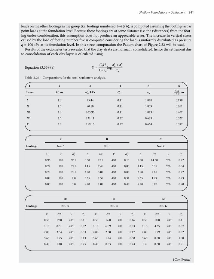
loads on the other footings in the group (i.e. footings numbered 1–4 & 6), is computed assuming the footings act aspoint loads at the foundation level. Because these footings are at some distance (i.e. the r distances) from the foot-ing under consideration, this assumption does not produce an appreciable error. The increase in vertical stresscaused by the load of footing number five is computed considering the load is uniformly distributed as pressureq = 100 kPa at its foundation level. In this stress computation the Fadum chart of Figure 2.32 will be used.Results of the oedometer tests revealed that the clay strata are normally consolidated; hence the settlement due
to consolidation of each clay layer is calculated using
Equation (3.36)-(a): Sc =CcH1 + eo
logσo + σzσo
(Continued)
Table 3.26 Computations for the total settlement analysis.
1 2 3 4 5 6
Layer H, m σo, kPa Cc eoCc H1+ eo
, m
I 1.0 75.44 0.41 1.070 0.198
II 1.3 90.10 0.41 1.039 0.261
III 2.0 103.96 0.41 1.013 0.407
IV 2.5 131.11 0.22 0.683 0.327
V 3.0 159.16 0.22 0.664 0.397
7 8 9
Footing: No. 5 No. 1 No. 2
4 I q σz z r/z V σz z r/z V σz
0.96 100 96.0 0.50 17.2 400 0.15 0.50 14.60 576 0.22
0.72 100 72.0 1.15 7.48 400 0.03 1.15 6.35 576 0.04
0.28 100 28.0 2.80 3.07 400 0.08 2.80 2.61 576 0.22
0.08 100 8.0 5.65 1.52 400 0.31 5.65 1.29 576 0.73
0.03 100 3.0 8.40 1.02 400 0.48 8.40 0.87 576 0.90
10 11 12
Footing: No. 3 No. 4 No. 6
z r/z V σz z r/z V σz z r/z V σz
0.50 19.8 289 0.11 0.50 14.0 400 0.16 0.50 10.0 289 0.11
1.15 8.61 289 0.02 1.15 6.09 400 0.03 1.15 4.35 289 0.07
2.80 3.54 289 0.33 2.80 2.50 400 0.17 2.80 1.79 289 0.02
5.65 1.75 289 0.13 5.65 1.24 400 0.58 5.65 0.88 289 1.00
8.40 1.18 289 0.25 8.40 0.83 400 0.74 8.4 0.60 289 0.91
Shallow Foundations – Settlement 241
worksaccounts.com

Total settlement = 199 mm
Problem 3.39
Assume the soft clay layer of Figure 3.17 is 12 m thick and construction of the embankment will increase theaverage total vertical stress in the clay by 70 kPa. Design requirement is that all except the last 20 mm of the settle-ment due to consolidation of the clay layer will have taken place after 6 months. For the clay:
cv = 5m2 year; ch = 8m
2 year;mv = 0 2m2 MN
Determine the spacing, in a square pattern, of 450 mm diameter sand drains to achieve the above requirement.
Solution:Final settlement is calculated from
Equation (3.34): Sc =mvσzH
=0 21000
× 70 × 12 = 0 168m= 168mm
For t = 6 months, U =168−20168
= 0 88
Diameter of each sand drain is 0.45 m. Therefore, rd = 0 225mRadius of equivalent cylindrical block = R= n rd = 0 225nThe layer is half-closed and therefore d = H = 12m
Equation (3.44): Tv =cvtd2
=5 ×
612
122= 0 0174
Equation (3.48): Tv =
π
4Uv
100
2
1− Uv 100 5 6 0 357 = 0 0174
Uv = 14 9 = 0 149
Equation (3.53): U = 1− 1−Uv 1−Ur
0 88 = 1− 1−0 149 1−Ur Hence,Ur = 0 86
13 14 15 16 17
Layer σz , kPa σo + σz , kPa logσo + σz
σoSc, m
I 96.75 172.19 0.358 0.071
II 72.19 162.29 0.256 0.067
III 28.82 132.78 0.106 0.043
IV 10.75 141.86 0.034 0.011
V 6.28 165.44 0.017 0.007
Sc = 0.199 m
242 Shallow Foundations
worksaccounts.com
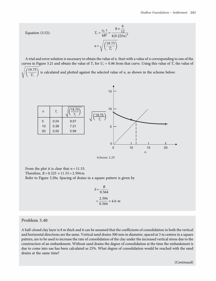
Equation (3.52): Tr =ch t4R2
=8 ×
612
4 0 225n 2
n=19 75Tr
A trial and error solution is necessary to obtain the value of n. Start with a value of n corresponding to one of thecurves in Figure 3.21 and obtain the value of Tr for Ur = 0 86 from that curve. Using this value of Tr the value of
19 75Tr
is calculated and plotted against the selected value of n, as shown in the scheme below:
From the plot it is clear that n= 11 53.Therefore, R= 0 225 × 11 53 = 2 594mRefer to Figure 3.20a. Spacing of drains in a square pattern is given by
S=R
0 564
=2 5940 564
= 4 6 m
Problem 3.40
A half-closed clay layer is 8 m thick and it can be assumed that the coefficients of consolidation in both the verticaland horizontal directions are the same. Vertical sand drains 300 mm in diameter, spaced at 3 m centres in a squarepattern, are to be used to increase the rate of consolidation of the clay under the increased vertical stress due to theconstruction of an embankment. Without sand drains the degree of consolidation at the time the embankment isdue to come into use has been calculated as 25%. What degree of consolidation would be reached with the sanddrains at the same time?
(Continued)
Tr
Trn19.75
15
10
Tr
n
5
5
5
10
20
0.24
0.38
0.55
9.07
7.21
5.99
10 15 20
0
19.75
Scheme 3.29
Shallow Foundations – Settlement 243
worksaccounts.com
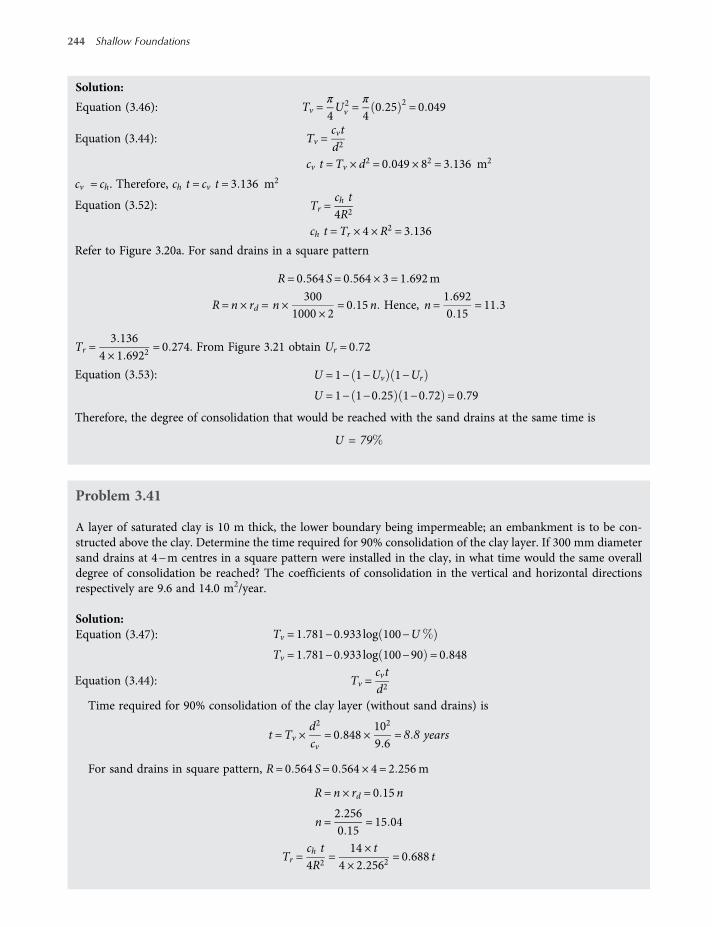
Solution:
Equation (3.46): Tv =π
4U2v =
π
40 25 2 = 0 049
Equation (3.44): Tv =cvtd2
cv t =Tv × d2 = 0 049 × 82 = 3 136 m2
cv = ch. Therefore, ch t = cv t = 3 136 m2
Equation (3.52): Tr =ch t4R2
ch t =Tr × 4 ×R2 = 3 136
Refer to Figure 3.20a. For sand drains in a square pattern
R= 0 564 S= 0 564 × 3 = 1 692m
R= n × rd = n×300
1000 × 2= 0 15n Hence, n=
1 6920 15
= 11 3
Tr =3 136
4 × 1 6922= 0 274. From Figure 3.21 obtain Ur = 0 72
Equation (3.53): U = 1− 1−Uv 1−Ur
U = 1− 1−0 25 1−0 72 = 0 79
Therefore, the degree of consolidation that would be reached with the sand drains at the same time is
U = 79
Problem 3.41
A layer of saturated clay is 10 m thick, the lower boundary being impermeable; an embankment is to be con-structed above the clay. Determine the time required for 90% consolidation of the clay layer. If 300 mm diametersand drains at 4−m centres in a square pattern were installed in the clay, in what time would the same overalldegree of consolidation be reached? The coefficients of consolidation in the vertical and horizontal directionsrespectively are 9.6 and 14.0 m2/year.
Solution:Equation (3.47): Tv = 1 781−0 933log 100−U
Tv = 1 781−0 933log 100−90 = 0 848
Equation (3.44): Tv =cvtd2
Time required for 90% consolidation of the clay layer (without sand drains) is
t =Tv ×d2
cv= 0 848 ×
102
9 6= 8 8 years
For sand drains in square pattern, R= 0 564 S= 0 564 × 4 = 2 256m
R= n× rd = 0 15n
n =2 2560 15
= 15 04
Tr =ch t4R2
=14 × t
4 × 2 2562= 0 688 t
244 Shallow Foundations
worksaccounts.com

For selected values of t determine the corresponding values of Tr and then from Figure 3.21 obtain the corres-ponding values of Ur.
Tv =cv td2
=9 6 × t102
= 0 096 t
For selected values of t determine the corresponding values of Tv and then from Equation (3.48) obtain thecorresponding values of Uv.For the obtained values of Uv and Ur, compute values of U usingEquation (3.53): U = 1− 1−Uv 1−Ur
All the computed values of Tr, Ur, Tv, Uv and U are shown in Table 3.27.
Draw a plot of t against U, as shown in the scheme below. Thus, from the plot, the time required for 90% con-solidation of the clay layer, with sand drains, is
t = 0 67 years
Problem 3.42
During the construction of a highway bridge, the average permanent load on a normally consolidated clay layer,6 m thick with open drainage at top and bottom, is expected to increase by about 115 kPa. The average effectiveoverburden pressure at mid-depth of the layer is 210 kPa. The average values of Cc and eo are 0.28 and 0.9, respect-ively. The consolidation coefficient is 0.36 m2/month. Determine:
(a) The final consolidation settlement without precompression(b) The added pressureΔσ f , due to weight of a temporary surcharge fill as a part of the total surcharge load, at the
middle of the clay layer, needed to eliminate the consolidation settlement in nine months by precompression.
(Continued)
0
0.2
0.4
0.6
0.8
1
1.2
U= 90%
0 0.5 1 1.5 2
U
t= 0.67 year
t , year
Scheme 3.30
Table 3.27 All the computed values of Tr, Ur, Tv, Uv and U.
t,year Tv Uv (1 − Uv) Tr Ur (1 − Ur) U
0.5 0.050 0.245 0.755 0.344 0.760 0.240 0.819
1.0 0.096 0.350 0.650 0.688 0.933 0.067 0.956
2.0 0.192 0.495 0.505 1.376 0.990 0.010 0.995
Shallow Foundations – Settlement 245
worksaccounts.com

Solution:
(a) Equation (3.36)-(a):Sc =
CcH1 + eo
logσo + σzσo
=0 28 × 61 + 0 9
log210 + 115
210= 0 168 m= 168 mm
(b) This technique of precompression is sometimes used to control or eliminate, as desired, consolidation settle-ment due to a structure load. Assume the permanent load of the structure causes increase in pressure, at themiddle of the clay layer, equals Δσ p . Settlement Sc will take place if a total surcharge load, which causes
increase in pressure =Δσ p +Δσ f , is acting for a sufficient period of time t. At that time, if the entire sur-
charge is removed and a permanent load of a structure is applied which causes increase in pressure equalsΔσ p no appreciable settlement will occur.
Equation (3.44): Tv =cvtd2
=0 36 × 9
6 2 2 = 0 36
Equation (3.48): Tv =
π
4U100
2
1− U 100 5 6 0 357 = 0 36 Compute U = 66 5
According to this process of consolidation, the entire settlement due to U = 100 is computed as
Sc =10066 5
× 0 168 = 0 253m
Therefore, it is necessary σz be increased so that the entire consolidation settlement is eliminated in ninemonths.Equation (3.36)-(a):
Sc =CcH1 + eo
logσo + σzσo
0 253 =0 28 × 61 + 0 9
log210 + σz210
log210 + σz210
=0 2530 884
= 0 286
210 + σz210
= 1 93 Hence,
σz = 195 3 kPa
σz =Δσ p +Δσ f
195 3 = 115 +Δσ f
Δσ f = 195 3−115 = 80 3 kPa
Another method for determining (approximately) the surcharge pressure Δσ f is by using the scheme below
(Das, 2011), as follows:Values of Tv and U% are computed as before.
246 Shallow Foundations
worksaccounts.com

Δσ p
Δσo=115210
= 0 548
From the scheme, for U = 66 5 andΔσ p
Δσo= 0 548, estimate
Δσ f
Δσ p
= 0 7
Therefore, Δσ f = 0 7 × 115 = 80 5 kPa
Problem 3.43
Solve Problem 3.42 with the addition of some sand drains. Assume that rd = 0 1 m, R= 1 5 m, cv = ch. Also,assume that this is a no-smear case. Consider that the surcharge is applied instantaneously.
Solution:(a) Settlement due to consolidation of the normally consolidated clay will be 168 mm as computed before.(b) Values of Tv and Uv remain unchanged, that is Tv = 0 36 and Uv = 66 5 .
n=Rrd
=1 50 1
= 15 and Tr =ch t4R2
=0 36 × 94 × 1 52
= 0 36
From Figure 3.21, obtain Ur = 0 77
Equation (3.53): U = 1− 1−Uv 1−Ur
= 1− 1−0 67 1−0 77 = 0 924 = 92 4(Continued)
100
90
80
70
60U (
%)
50
40
300 0.2 0.4 0.6 0.8 1.0 1.2 1.4 1.6 1.8 2.0
Δσʹ(p)
Δσ o
Δσʹ( f)
Δσʹ( p)
10.08.05.0
3.0
2.01.41.0
0.5
0.30.1
4.06.0
Scheme 3.31
Shallow Foundations – Settlement 247
worksaccounts.com
The entire settlement due to U = 100 is
10092 4
× 0 168 = 0 182 m
Therefore, σz should have an increased value so that the entire consolidation settlement is eliminated in ninemonths.
Equation (3.36)-(a): Sc =CcH1 + eo
logσo + σzσo
0 182 =CcH1 + eo
logσo + σzσo
=0 28 × 61 + 0 9
log210 + σz210
log210 + σz210
=0 1820 884
= 0 206
Hence,210 + σZ
210= 1 61 and σZ = 128 1 kPa.
σZ =Δσ p +Δσ f . Therefore,
Δσ f = 128 1−115 = 13 1 kPa
or,
from the scheme in Problem 3.42: for U = 92 4 andΔσ p
Δσo= 0 548, estimate
Δσ f
Δσ p
= 0 115. Therefore,
Δσ f = 0 115 × 115 = 13 2 kPa
Problem 3.44
For a sand drain project the clay is normally consolidated and the entire surcharge is applied, as shown in thescheme below:
The following data are given:
For the sand drains:rd = 0 1m, R= 1 0 m, cv = ch. Assume no-smear case.
For the clay: thickness H = 4 6m (two-way drainage), Cc = 0 31, eo = 1 1, σo = 50 kPa at middle of claylayer, cv = 0 011 m2 day
Calculate the degree of consolidation 30 days after the surcharge is first applied. Also, determine the consoli-dation settlement at that time due to the surcharge.
Total surcharge
pressure, kPa
Time, days
60 days = tc
tc
100 = Δσʹ(p)+ Δσʹ( f )
Scheme 3.32
248 Shallow Foundations
worksaccounts.com

Solution:
Equation (3.44): Tv =cv td2
=0 011 × 30
4 6 2 2 = 0 062
Tc =cv tcd2
=0 011 × 60
4 6 2 2 = 0 125
Using Figure 3.22, for Tc = 0 125 and Tv = 0 062, we obtain Uv≈9Equation (3.54):
n=Rrd
=10 1
= 10
Trc =ch tc4R2
=0 011 × 604 × 12
= 0 165
Tr =ch t4R2
=0 011 × 304 × 12
= 0 082 <Trc; hence use
Ur =Tr
Trc−
1ATrc
1− exp −ATr ; A=2
n2 n2−1 ln n − 3n2−1 4n2
A=2
102 102−1 ln 10 − 3 × 10²−1 4 × 102=
21 576
= 1 269
Ur =0 0820 165
−1
1 269 × 0 1651− exp −1 269 × 0 082 = 0 024 = 2 4
Equation (3.53): U = 1− 1−Uv 1−Ur
U = 1− 1−0 090 1−0 024 = 0 112 = 11 2
The final consolidation settlement Sc =CcH1 + eo
logσo + Δσ p +Δσ f
σo
Sc =0 31 × 4 61 + 1 1
log50 + 100
50= 0 324m
The consolidation settlement after 30 days =U × Sc
= 0 112 × 0 324 = 0 036m
= 36 mm
Problem 3.45
For a sand drain project, the following are given:Clay: Normally consolidated (one-way drainage)
H = 5 5m
Cc = 0 3;eo = 0 76;cv = 0 015m2 day
σo = 80 kPa,atmiddle of clay layer
Sand drains: rd = 0 07m, R= 1 25m, rs = rd , cr = cv.(Continued)
Shallow Foundations – Settlement 249
worksaccounts.com
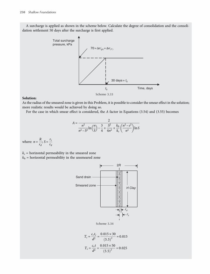
A surcharge is applied as shown in the scheme below. Calculate the degree of consolidation and the consoli-dation settlement 50 days after the surcharge is first applied.
Solution:As the radius of the smeared zone is given in this Problem, it is possible to consider the smear effect in the solution;more realistic results would be achieved by doing so.For the case in which smear effect is considered, the A factor in Equations (3.54) and (3.55) becomes
A=2
n2
n2−S2ln
nS
−34+
S2
4n2+khks
n2− s2
n2lnS
where: n=Rrd; S=
rsrd
ks = horizontal permeability in the smeared zonekh = horizontal permeability in the unsmeared zone
Tc =cvtcd2
=0 015 × 30
5 5 2 = 0 015
Tv =cvtd2
=0 015 × 50
5 5 2 = 0 025
Total surcharge
pressure, kPa
30 days = tc
70 = Δσ(p)+ Δσ( f )
tc Time, days
Scheme 3.33
rd
rs
H ClaySmeared zone
Sand drain
2R
Scheme 3.34
250 Shallow Foundations
worksaccounts.com
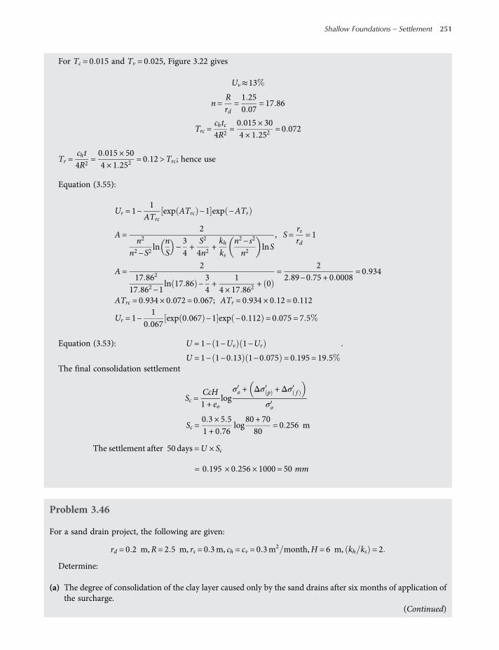
For Tc = 0 015 and Tv = 0 025, Figure 3.22 gives
Uv≈13
n=Rrd
=1 250 07
= 17 86
Trc =chtc4R2
=0 015 × 304 × 1 252
= 0 072
Tr =cht4R2
=0 015 × 504 × 1 252
= 0 12 >Trc; hence use
Equation (3.55):
Ur = 1−1
ATrcexp ATrc −1 exp −ATr
A=2
n2
n2−S2ln
nS
−34+
S2
4n2+khks
n2− s2
n2lnS
, S=rsrd
= 1
A=2
17 862
17 862−1ln 17 86 −
34+
14 × 17 862
+ 0=
22 89−0 75 + 0 0008
= 0 934
ATrc = 0 934 × 0 072 = 0 067; ATr = 0 934 × 0 12 = 0 112
Ur = 1−1
0 067exp 0 067 −1 exp −0 112 = 0 075 = 7 5
Equation (3.53): U = 1− 1−Uv 1−Ur
U = 1− 1−0 13 1−0 075 = 0 195 = 19 5
.
The final consolidation settlement
Sc =CcH1 + eo
logσo + Δσ p +Δσ f
σo
Sc =0 3 × 5 51 + 0 76
log80 + 7080
= 0 256 m
The settlement after 50 days =U × Sc
= 0 195 × 0 256 × 1000 = 50 mm
Problem 3.46
For a sand drain project, the following are given:
rd = 0 2 m,R= 2 5 m, rs = 0 3m, ch = cv = 0 3m2 month,H = 6 m, kh ks = 2
Determine:
(a) The degree of consolidation of the clay layer caused only by the sand drains after six months of application ofthe surcharge.
(Continued)
Shallow Foundations – Settlement 251
worksaccounts.com
(b) The degree of consolidation of the clay layer caused by the combination of vertical drainage (drained at topand bottom) and radial drainage after six months of application of the surcharge.
Assume that the surcharge is applied instantaneously.
Solution:(a) For the case in which smear effect is considered and the surcharge assumed instantaneously applied, according
to Barron (1948),
Ur = 1−exp−8Tr
m
m =n2
n2−S2ln
nS
−34+
S2
4n2+khks
n2− s2
n2lnS; n=
Rrd; S=
rsrd
n =2 50 2
= 12 5; S=0 30 2
= 1 5; Tr =cht4R2
=0 3 × 64 × 2 52
= 0 072
m =12 52
12 52−1 52ln
12 51 5
−34+
1 52
4 × 12 52+ 2
12 52−1 52
12 52ln1 5
m = 2 151−0 75 + 0 004 + 0 799 = 2 204
Ur = 1−exp−8 × 0 0722 204
= 1−0 77 = 0 23 = 23
(b) Equation (3.44): Tv =cv td2
=0 3 × 6
6 2 2 = 0 2
Equation (3.48): Tv =
π
4U100
2
1− U 100 5 6 0 357
0 2 =
π
4U100
2
1− U 100 5 6 0 357 ; hence U≈50 =Uv
Equation (3.53): U = 1− 1−Uv 1−Ur
U = 1− 1−0 5 1−0 23 = 615−61 5
Problem 3.47
Redo part (a) of Problem 3.46 considering no-smear case.
Solution:
Tr =ch t4R2
=0 3 × 64 × 2 52
= 0 072; n=2 50 2
= 12 5
From Figure 3.21 obtain the corresponding value of Ur = 0 28 = 28or,
Ur = 1−exp−8Tr
m. For no-smear case:
252 Shallow Foundations
worksaccounts.com
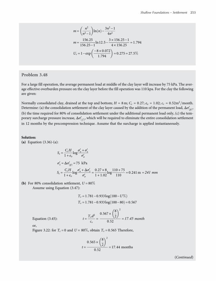
m=n2
n2−1ln n −
3n2−14n2
m=156 25
156 25−1ln12 5−
3 × 156 25−14 × 156 25
= 1 794
Ur = 1−exp−8 × 0 0721 794
= 0 275 = 27 5
Problem 3.48
For a large fill operation, the average permanent load at middle of the clay layer will increase by 75 kPa. The aver-age effective overburden pressure on the clay layer before the fill operation was 110 kpa. For the clay the followingare given:
Normally consolidated clay, drained at the top and bottom; H = 8m; Cc = 0 27; eo = 1 02; cv = 0 52m2 month.Determine: (a) the consolidation settlement of the clay layer caused by the addition of the permanent load, Δσ p ,
(b) the time required for 80% of consolidation settlement under the additional permanent load only, (c) the tem-porary surcharge pressure increase, Δσ f , which will be required to eliminate the entire consolidation settlement
in 12 months by the precompression technique. Assume that the surcharge is applied instantaneously.
Solution:(a) Equation (3.36)-(a):
Sc =CcH1 + eo
logσo + σzσo
σz =Δσ p = 75 kPa
Sc =CcH1 + eo
logσo +Δσz
σo=0 27 × 81 + 1 02
log110 + 75110
= 0 241m = 241 mm
(b) For 80% consolidation settlement, U = 80Assume using Equation (3.47):
Tv = 1 781−0 933log 100−U
Tv = 1 781−0 933log 100−80 = 0 567
Equation (3.45): t =Tvd2
cv=0 567 ×
82
2
0 52= 17 45 month
or,Figure 3.22: for Tc = 0 and U = 80 , obtain Tv = 0 565 Therefore,
t =0 565 ×
82
2
0 52= 17 44 months
(Continued)
Shallow Foundations – Settlement 253
worksaccounts.com
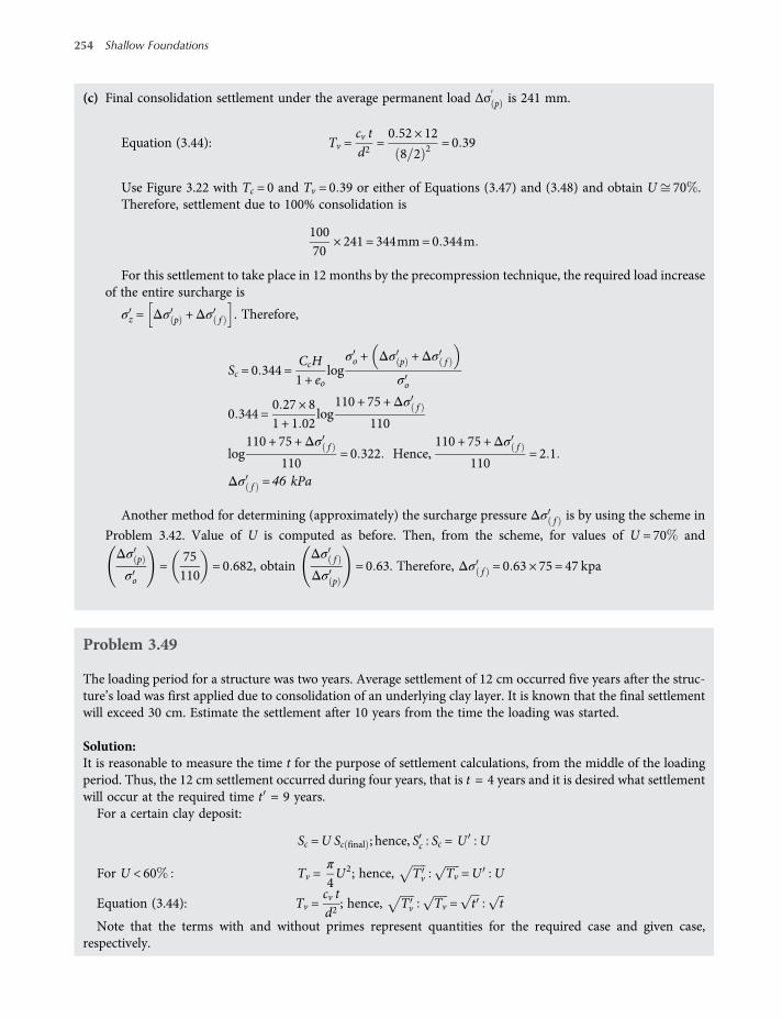
(c) Final consolidation settlement under the average permanent load Δσ p is 241 mm.
Equation (3.44): Tv =cv td2
=0 52 × 12
8 2 2 = 0 39
Use Figure 3.22 with Tc = 0 and Tv = 0 39 or either of Equations (3.47) and (3.48) and obtain U 70 .Therefore, settlement due to 100% consolidation is
10070
× 241 = 344mm=0 344m
For this settlement to take place in 12 months by the precompression technique, the required load increaseof the entire surcharge is
σz = Δσ p +Δσ f . Therefore,
Sc = 0 344 =CcH1 + eo
logσo + Δσ p +Δσ f
σo
0 344 =0 27 × 81 + 1 02
log110 + 75 +Δσ f
110
log110 + 75 +Δσ f
110= 0 322 Hence,
110 + 75 +Δσ f
110= 2 1
Δσ f = 46 kPa
Another method for determining (approximately) the surcharge pressure Δσ f is by using the scheme in
Problem 3.42. Value of U is computed as before. Then, from the scheme, for values of U = 70 andΔσ p
σo=
75110
= 0 682, obtainΔσ f
Δσ p
= 0 63. Therefore, Δσ f = 0 63 × 75 = 47 kpa
Problem 3.49
The loading period for a structure was two years. Average settlement of 12 cm occurred five years after the struc-ture’s load was first applied due to consolidation of an underlying clay layer. It is known that the final settlementwill exceed 30 cm. Estimate the settlement after 10 years from the time the loading was started.
Solution:It is reasonable to measure the time t for the purpose of settlement calculations, from the middle of the loadingperiod. Thus, the 12 cm settlement occurred during four years, that is t = 4 years and it is desired what settlementwill occur at the required time t = 9 years.For a certain clay deposit:
Sc =U Sc final ; hence, Sc Sc = U U
For U < 60 Tv =π
4U2; hence, Tv Tv =U U
Equation (3.44): Tv =cv td2
; hence, Tv Tv = t t
Note that the terms with and without primes represent quantities for the required case and given case,respectively.
254 Shallow Foundations
worksaccounts.com

Now, we can write Sc Sc = t t or Sc = 12 = 9 4
Therefore, the settlement after 10 years from the time the loading was started, Sc = 12 ×32= 18 cm.
Since the final settlement was given as greater than 30 cm the obtained 18 cm settlement probably correspondsto less than 60%, that is U < 60 and cannot be above 60% by a sufficient amount to invalidate the expres-
sion Tv =π
4U2.
Problem 3.50
Building (A) settled 10 cm in three years due to consolidation of the underlying clay layer and it is known that thefinal settlement will be about 30 cm Building (B) and its underlying clay layer are, as far as the available data con-firm, very similar to (A) except that the underlying clay layer is 20% thicker than the clay layer below (A). Theavailable data also confirm that the increase in the average pressure at the middle of the two clay layers can beconsidered approximately alike. Estimate the final settlement of building (B) and also the settlement in three years.
Solution:For a certain clay deposit:Sc =mvσzH; hence, Sc Sc =H HH = 1 2H. Therefore, Sc 30 = 1 2H H.The final settlement of building B = Sc = 30 × 1 2 = 36 cmEquation (3.44):
Tv =cvtd2
Tv = cvtH2
;
Tv = cvtH2
; hence,
Tv Tv =t
H 2
t
H 2
Tv Tv =3
1 2H 2
3
H 2 =1
1 2 2
In this case the expression Tv =π
4U2 is valid, that is U < 60 ; hence
Tv Tv = U 2 U 2; hence, U U =11 2
Sc =USc final ; U =Sc
Sc final; hence, U U =
ScSc final
ScSc final
=11 2
ScSc
Sc final
Sc final
=11 2
Sc final =mv σz H and Sc final =mv σz 1 2H ; hence,Sc final
Sc final
=11 2
Therefore, Sc = Sc. Thus at any time the settlement of buildings (A) and (B) are alike, as long as U < 60 .Therefore, settlement in three years = 10 cm.
Shallow Foundations – Settlement 255
worksaccounts.com
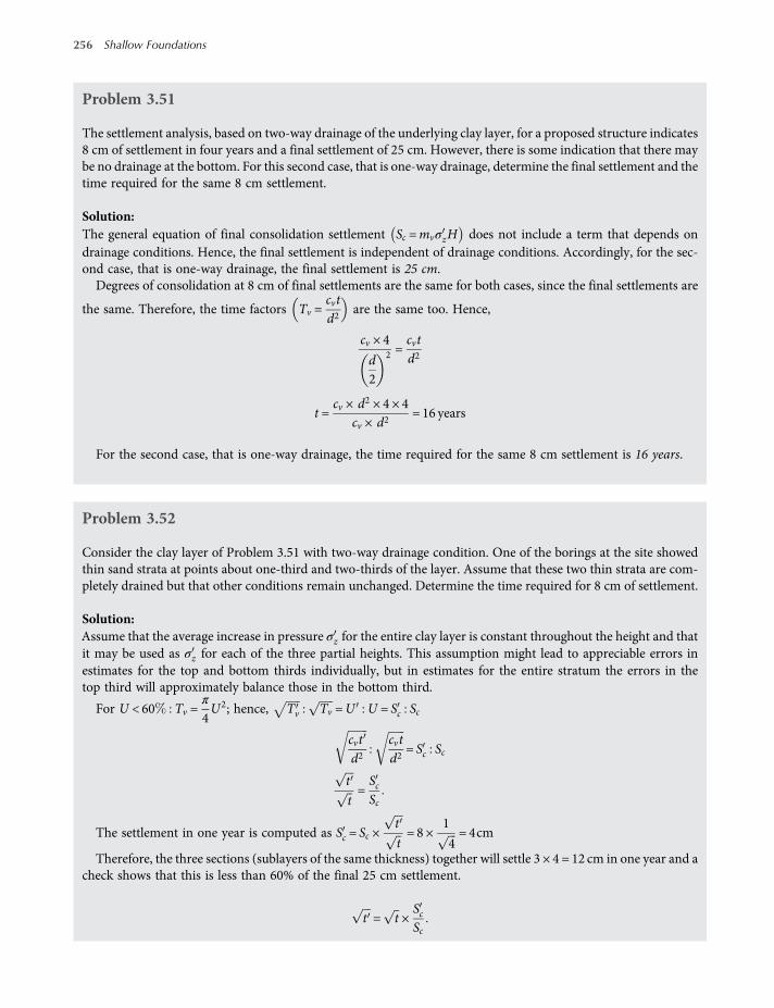
Problem 3.51
The settlement analysis, based on two-way drainage of the underlying clay layer, for a proposed structure indicates8 cm of settlement in four years and a final settlement of 25 cm. However, there is some indication that there maybe no drainage at the bottom. For this second case, that is one-way drainage, determine the final settlement and thetime required for the same 8 cm settlement.
Solution:The general equation of final consolidation settlement Sc =mvσzH does not include a term that depends ondrainage conditions. Hence, the final settlement is independent of drainage conditions. Accordingly, for the sec-ond case, that is one-way drainage, the final settlement is 25 cm.Degrees of consolidation at 8 cm of final settlements are the same for both cases, since the final settlements are
the same. Therefore, the time factors Tv =cvtd2
are the same too. Hence,
cv × 4
d2
2 =cvtd2
t =cv × d2 × 4 × 4
cv × d2= 16 years
For the second case, that is one-way drainage, the time required for the same 8 cm settlement is 16 years.
Problem 3.52
Consider the clay layer of Problem 3.51 with two-way drainage condition. One of the borings at the site showedthin sand strata at points about one-third and two-thirds of the layer. Assume that these two thin strata are com-pletely drained but that other conditions remain unchanged. Determine the time required for 8 cm of settlement.
Solution:Assume that the average increase in pressure σz for the entire clay layer is constant throughout the height and thatit may be used as σz for each of the three partial heights. This assumption might lead to appreciable errors inestimates for the top and bottom thirds individually, but in estimates for the entire stratum the errors in thetop third will approximately balance those in the bottom third.
For U < 60 Tv =π
4U2; hence, Tv Tv =U U = Sc Sc
cvtd2
cvtd2
= Sc Sc
t
t=ScSc
The settlement in one year is computed as Sc = Sc ×t
t= 8 ×
1
4= 4cm
Therefore, the three sections (sublayers of the same thickness) together will settle 3 × 4 = 12 cm in one year and acheck shows that this is less than 60% of the final 25 cm settlement.
t = t ×ScSc
256 Shallow Foundations
worksaccounts.com
t = 1 ×812
t = 1 ×812
2
=49year
Therefore, the time required for 8 cm settlement = 0.444 years.
Problem 3.53
The laboratory data for the clay layer of Problem 3.51, with two-way drainage condition, were from tests on a fewsamples. Subsequent tests on additional samples give what are believed to be more accurate determinations of thesoil coefficients and show that the coefficient of volume compressibility mv is 20% smaller and the coefficient ofconsolidation cv is 30% smaller than originally obtained. Considering these changes into account, but otherwiseusing the same available data of the original two-way drainage condition, determine the final settlement and thetime required for 8 cm settlement.
Solution:Equation (3.44): Sc =mvσzH
Sc final =mvσz H
after change
Sc final =mv σz H before change
mv = 0 8mv
mv mv = Sc final Sc final
Sc final = Sc final ×mv
mv= 25 ×
0 8mv
mv= 20 cm
Taking the changes into account, the final settlement = 20 cm.Considering 8 cm settlement:
For U < 60 Tv =π
4U2 =
cvt
d 2 2
For U =825
π
4825
2
=cv × 4
d 2 2 ; hence,cv
d 2 2 =π
16825
2
For U =820:
π
4820
2
=cv × t
d 2 2 ; cv = 0 7cv ; hence,
(Continued)
Shallow Foundations – Settlement 257
worksaccounts.com

π
4820
2
=0 7 × cv × t
d 2 2 = 0 7tcv
d 2 2 ;
t =
π
4820
2
0 7cvd 2 2
=
π
4820
2
0 7 ×π
16825
2 =4
820
2
0 7825
2 =4 × 6250 7 × 400
= 8 93 years
Taking the changes into account, the time required for 8 cm of settlement = 8.93 years.
Problem 3.54
The settlement analysis for a proposed building structure indicates 8 cm of settlement in four years and a finalsettlement of 25 cm. The underlying clay layer is drained at both its top and bottom surfaces. An alternate designof the structure uses a taller building (i.e. the same proposed building structure with increased number of storiesonly) which would increase the net building load by 25% On the basis of this heavier load, determine the finalsettlement, the settlement in four years and the time required for 8 cm settlement.
Solution:Equation (3.44): Sc =mvσzH
Sc final =mv σzH before change
Sc final =mv 1 25 σz H after change
Sc final =1 25σz × 25
σz= 31 25 cm
The final settlement under the heavier building = 31.25 cmEquation (3.44):
Tv =cvtd2
Since the quantitycvd2
remains unchanged, for the same time t (i.e. t = t = 4 years) the time factor Tv remains
unchanged too (i.e. Tv =Tv).Equation (3.46):
Tv =π
4U2 forU < 60
Tv =π
4U2 before change
Tv =π
4U2 after change
Therefore, U =U
Sc =USc final
258 Shallow Foundations
worksaccounts.com

U =Sc
Sc final
; hence, U =Sc
Sc final=
825
=U
825
=Sc
32 25; hence, Sc =
31 25 × 825
= 10cm
Under the heavier building, the settlement in four years = 10 cm.
For U =10
31 25and t = 4 years:
Tv =π
410
31 25
2
= 4cvd2
; hencecvd2
=π
4 × 410
31 25
2
For U =8
31 25and t = t :
Tv =π
48
31 25
2
= tcvd2
= tπ
4 × 410
31 25
2
t =
π
48
31 25
2
π
4 × 410
31 25
2=4 × 82
102= 2 56 years
The time required for 8 cm settlement, under the heavier building, is 2.56 years.
Problem 3.55
A building consisting of 20 storeys is founded on a stiff raft 20 mwide by 40 m long at a depth of 2 m below groundlevel. The raft rests on a weathered rock becoming less weathered with increasing depth, until a relatively incom-pressible stratum is met at a depth of 45 m Deformation modulus, Ed, values obtained from plate-load tests madein a large-diameter borehole are shown in the scheme below. Estimate the settlement of the building for a netbearing pressure (net uniform contact pressure) of 250 kPa (a) considering the raft as a flexible base, (b) consid-ering the raft as a rigid base.
(Continued)
net q = 250 kPaEd × 1000 (MPa)
Weathered rock
2 m
Incompressible stratum
0 1 2 3 4
10
20
30
45
Depth
,m
•
••
•
•
200 MPa
3600 MPa
Values from
load test
z
H
20 m × 40 m
Scheme 3.35
Shallow Foundations – Settlement 259
worksaccounts.com
Solution:Variation of Ed with depth is obtained by plotting a straight line through the given points, shown in the figure. Atfoundation level Ef = 200MPa and at a depth of 30 m below ground level, where z = 28m, Ed = 3600MPa.Equation (3.65):
K =Ed−EfEf
Bz
=3600−200
2002028
= 12 14
(a) Considering the raft as a flexible base.The raft area is divided into four equal rectangles, each 10 × 20m.
H = 45−2 = 43 m;HB=4310
= 4 3;LB=2010
= 2; k= 12 14. Therefore, from Figure 3.25: IP≈0 05
From Figure 3.26a, forHB=4320
= 2 15, the factor FB = 0 96
From Figure 3.26b, forDB=
220
= 0 1, the factor FD = 1 0
From Equation (3.63), immediate settlement at corner of each flexible rectangle is given by
ρi = qBEf
IpFBFD = 25010
200 × 10000 05 0 96 1 = 6 × 1−4m
The immediate settlement at the centre of the flexible raft is
ρi = 4 6 × 1 – 4 = 2 4 × 10 – 3 m = 2 4mm
(b) Considering the raft as a rigid base.The average settlement of the rigid foundation is given by
Equation (3.64): ρi, ave = 1 3 ρi, centre + ρi,midpoint long side + ρi, cornerρi,comer:
H = 45−2 = 43m;HB=4320
= 2 15;LB=4020
= 2; k= 12 14 Therefore, from Figure 3.25: IP≈0 05
From Figure 3.26a, forHB=4320
= 2 15, the factor FB = 0 96
From Figure 3.26b, forDB=
220
= 0 1, the factor FD = 1 0
From Equation (3.63), immediate settlement at corner of the flexible raft is given by
ρi = qBEf
IpFBFD = 25020
200 × 10000 05 0 96 1 = 1 2 × 1−3m
260 Shallow Foundations
worksaccounts.com

ρi, mid point long side:
H = 45−2 = 43m;HB=4320
= 2 15;LB=2020
= 1; k= 12 14
Therefore, from Figure 3.25: IP≈0 05
From Figure 3.26a, forHB=4320
= 2 15, the factor FB = 0 96
From Figure 3.26b, forDB=
220
= 0 1, the factor FD = 1 0
From Equation (3.63), immediate settlement at the corner of each flexible rectangle is given by
ρi = qBEf
IpFBFD = 25020
200 × 10000 05 0 96 1 = 1 2 × 1−3m
Immediate settlement at the midpoint of a long side of the flexible raft is
ρi = 2 1 2 × 1−3 = 2 4 × 10⁻³m
ρi, centre
From (a), ρi, centre = 2 4 × 10⁻³ m
The average settlement of the rigid foundation is
ρi, ave =13
2 4 × 10⁻³ + 2 4 × 10⁻³ + 1 2 × 10−3 = 2 × 10⁻³ m
= 2 mm
There could, in addition, be some creep settlement in the weathered rock which might double the immediatesettlement.
Problem 3.56
A column footing 1.8 m square is to be founded at a depth of 0.6 m on weak medium-bedded poorly cementedsandstone. The net foundation pressure (net contact pressure) is 1.55 MPa Examination of rock cores showed anaverage joint spacing of 250 mm Tests on the cores showed representative uniaxial compression strength of1.75 MPa Make an estimation of the foundation settlement. Consider the footing as a rigid base.
Solution:For the 250 cm joint spacing, the fracture frequency per metre (or joint spacing per metre) is 1000 250 = 4From Table 3.18, for a fracture frequency of four per metre; a suitable value for the mass factor (j) is 0.6, Also,from Table 3.19, for poorly cemented sandstone the modulus ratio (Mr) is 150. Let quc of the intact rockequals the uniaxial compression strength, which is 1.75 MPa. The mass deformation modulus is given byEquation (3.66):
Em= jMrquc = 0 6 × 150 × 1 75 = 157 5MPa
(Continued)
Shallow Foundations – Settlement 261
worksaccounts.com

Assume the influence depth H of the rock below the foundation level is 4B= 4 × 1 8 = 7 2mDivide the footing area into four equal squares each of 0.9 m width.
From Figure 3.25 forLB=0 90 9
= 1;HB=7 20 9
= 8 and k= 0 (using Em = Ed = Ef ), obtain IP≈0 48
From Figure 3.26a, forHB=7 21 8
= 4, the factor FB≈ 1
From Figure 3.26b, forDB=0 61 8
= 0 33, the factor FD = 0 93
From Equation (3.63), immediate settlement at corner of each flexible square is given by
ρi = qBEf
IpFBFD = 1 550 9157 5
0 48 1 0 93 = 3 954 × 1−3m
The immediate settlement at centre of the flexible raft is
4 3 954 × 1−3 = 15 82 × 10−3m
According to Equation (3.6) the rigidity factor is 0.93 and according to Table 3.15 the rigidity factor is 0.85.Assume the rigidity factor is 0.90. Accordingly, the average settlement of the foundation is
0 90 × 15 82 × 10−3 = 14 24 × 10−3m= 14 24 mm; say15mm
(Creep might increase this settlement to about 30 m in the long term.)
References
AASHTO (1996), Standard Specifications for Highway Bridges, 16th edn, American Association of State Highway andtransportation officials, Washington, D.C.
Barron, R. A. (1948), “Consolidation of Fine-Grained Soils by Drain Wells”, Transactions ASCE, 113, pp. 718–742.Bjerrum, L. (1963), “Discussion on Compressibility of soils”, Proceedings of the European Conference on Soil Mechanics and
Foundation Engineering, Wiesbaden, Vol. 2, pp. 16–17.Bjerrum, L. (1967), “Engineering Geology of Norwegian Normally Consolidated Marine Clays as Related to Settlement of
Buildings”, Geotechnique, 17, pp. 83–118.Bowles, J. E. (2001), Foundation Analysis and Design, 5th edn, McGraw-Hill, New York.Bowles, J. E. (1977), Foundation Analysis and Design, 2nd edn, McGraw-Hill, New York.Buisman, A. K. (1943), Grondmechanica (Soil Mechanics), 2nd edn, 281 pp., Waltman, Delft, Netherlands.Burland, J. B. andWroth, C. P. (1974), “Review Paper: Settlement of Buildings and Associated Damage”, Proceedings of the
Conference on Settlement of Structures, Pentech Press, Cambridge, pp. 611–654.Burland, J, B. and Burbidge, M. C. (1985), “Settlement of Foundations on Sand and Gravel”, Proceedings, Institute of Civil
Engineers, Part I, Vol. 7, pp. 1325–1381.Burland, J, B., Broms, B. B. and DeMello, V. F. B. (1977), “Behaviour of Foundations and Structures”, Proceedings of the 9th
ICSMFE, Tokyo, Vol. 2, Japanese Society SFME, pp. 495–538.Casagrande, A. (1936), “The Determination of the Preconsolidation Load and Its Practical Significance”, Proceedings of the
1st ICSMFE, Vol. 3, pp. 60–64.Chandler, R. J. andDavis, A. G. (1973), “FurtherWork on the Engineering Properties of KeuperMarl”,Construction Indus-
try Research and Information Association Report No. 47, England.
262 Shallow Foundations
worksaccounts.com

Christian, J. T. and Carrier, W. D. (1978), “Janbu, Bjerrum and Kjaernsli’s chart reinterpreted”, Canadian GeotechnicalJournal, 15, pp. 123–128, and discussion, 15, pp. 436–437.
Coduto, Donald P. (2001), Foundation Design: Principles and Practices, 2nd edn, Prentice-Hall, Inc., New Jersey.Craig, R. F. (2004), Soil Mechanics, 7th edn, Chapman and Hall, London.D’Appolonia, D. J., D’Appolonia, E. D. and Brissetta, R. F. (1970), “Closure Settlement of Spread Footings on Sand”,
Journal of Soil Mechanics and Foundations Division, ASCE, Vol. 96, SM 2, March, pp. 561–584.Das, Braja M. (2011), Principles of Foundation Engineering, 7th edn, CENGAGE Learning, United States.DeBeer, E. E. and Martens, A. (1957), “Method of Computation of an Upper Limit for the Influence of Heterogeneity of
Sand Layers on the Settlement of Bridges”, Proceedings 4th International Conference on Soil Mechanics and FoundationEngineering, London, Vol. 1, pp. 275–281, Butterworths, London.
DeBeer, E. E. (1963), “The Scale Effect in the Transposition of the Results of Deep Sounding Tests on the Ultimate BearingCapacity of Piles and Caisson Foundations”, Geotechnique, 13, pp. 39–75.
European Committee for Standardisation (1994a), Basis of Design and Actions on Structures, Eurocode 1, Brussels,Belgium.
European Committee for Standardisation (1994b), Geotechnical Design, General Rules-Part 1, Eurocode 7, Brussels,Belgium.
Fox, E. N. (1957), “The Mean Elastic Settlement of a Uniformly Loaded Area at a Depth below the Ground Surface”, Pro-ceedings 2nd International Conference on Soil Mechanics and Foundation Engineering, London, Vol. 1, pp. 129–132,Rotterdam.
Hobbs, N, B. (1974), “General Report and State-of-the-Art Review”, Proceedings of the Conference on Settlement of Struc-tures, Pentech Press, Cambridge, pp. 579–609.
Knappett, J. A. and Craig, R. F. (2012), Soil Mechanics, 8th edn, Spon Press, Abingdon, Oxon, United Kingdom.Leonards, G. A. (1976), Estimating Consolidation Settlement of Shallow Foundations on Overconsolidated Clay, Special
Report No. 163, Transportation Research Board, Washington, D.C., pp. 13–16.MacDonald, D. H. and Skempton, A. W. (1955), “A Survey of Comparisons between Calculated and Observed Settlements
of Structures on Clay”, Conference on Correlation of Calculated and Observed Stresses and Displacements, ICE, London,pp. 318–337.
Mayne, P. W. and Poulos, H. G. (1999), “Approximate Displacement Influence Factors for Elastic Shallow Foundations”,Journal of Geotechnical and Geoenvironmental Engineering, ASCE, Vol. 125, No. 6, pp. 453–460.
Meigh, A. C. (1976), “The Triassic Rocks, with Particular Reference to Predicted and Observed Performance of someMajorStructures”, Geotechnique, 26, pp. 393–451, London.
Mesri, G. (1973), “Coefficient of Secondary Compression”, Journal of the Soil Mechanics and Foundations Division, ASCE,Vol. 99, No. SM1, pp. 122–137.
Mesri, G. and P. M. Godlewski (1977), “Time- and Stress-Compatibility Interrelationship”, Journal of Geotechnical Engin-eering Division, ASCE, Vol. 103, GT5, May, pp. 417–430.
Meyerhof, G. G. (1956), “Penetration Tests and Bearing Capacity of Cohesionless Soils”, Journal of Soil Mechanics andFoundations Division, ASCE, Vol. 82, SM1, pp. 1–19.
Meyerhof, G. G. (1965), “Shallow Foundations”, Proceedings ASCE, 91, No. SM2, pp. 21–31.Meyerhof, G. G. (1974), “Ultimate Bearing Capacity of Footings on Sand layer Overlying Clay”, Canadian Geotechnical
Journal, Ottawa, Vol. 11, No. 2, May, pp. 223–229.Meyerhof, G. G. (1982), The Bearing Capacity and Settlement of Foundations, Tech-Press, Technical University of Nova
Scotia, Halifax.Mikhejef, V. V., Ushkalor, V. P., Tokar, R. A. et al. (1961), “Foundation Design in the USSR”, Fifth ICSMFE, Vol. 1,
pp. 753–757.Olson, R. E. (1977), “Consolidation under Time-Dependent Loading”, Journal of Geotechnical Engineering Division, ASCE,
Vol. 102, No. GT1, pp. 55–60.Polshin, D. E. and Tokar, R. A. (1957), “Maximum Allowable Non-Uniform Settlement of Structures”, Proceedings of the
4th ICSMFE, London, Vol. 1, pp. 402–405.Schmertmann, J. H. and Hartman, J. P. (1978), “Improved Strain Influence Factor Diagrams”, Journal of the Soil Mechanics
and Foundations Division, ASCE, Vol. 104, No. GT8, pp. 1131–1135.Senneset, K., Sandven, R., Lunne, T. et al. (1988), “Piezocone Tests in Silty Soils”, Proceedings 1st ISOPT, Vol. 2,
pp. 955–966.Simons, N. A. (1974), “Review Paper: Normally Consolidated and lightly Overconsolidated Cohesive Materials”, Proceed-
ings of the Conference on Settlements of Structures, Pentech Press, Cambridge, pp. 500–530.Sivaram, B. and Swamee, P. (1977), “A Computational Method for Consolidation Coefficient”, Soils and Foundations,
Tokyo, Vol. 17, No. 2 pp. 48–52.Skempton, A. W. and Bjerrum, L. (1957), “A Contribution to the Settlement Analysis of Foundations on Clay”, Geotech-
nique, 7, pp. 168–178.
Shallow Foundations – Settlement 263
worksaccounts.com

Skempton, A. W. and MacDonald, D. H. (1956), “The Allowable Settlement of Buildings”, Proceedings of the Institute ofCivil Engineering, Part 3, 5, pp. 727–784.
Sutherland, H. B. (1974), “Review paper: Granular Materials”, Proceedings of the Conference on Settlement of Structures,Pentech Press, Cambridge, pp. 473–499.
Terzaghi, K., Peck, R. B. (1967), Soil Mechanics in Engineering Practice, 2nd edn, John Wiley, New York.Tomlinson, M. J. (2001), Foundation Design and Construction, 7th edn, Pearson Education Ltd., Harlow, Essex.Tomlinson, M. J. (1995), Foundation Design and Construction, 6th edn, Longman Scientific and Technical, Harlow, Essex.Vesic, A. S. (1970), “Tests on Instrumented Piles, Ogeechee River Site”, Journal of Soil Mechanics and Foundations Division,
ASCE, Vol. 96, SM 2, March, pp. 561–584.Wahls, Harvey E. (1994), “Tolerable Deformations”, Vertical and Horizontal Deformations of Foundations and Embank-
ments, A. T. Yeung and G. Y, Felio, Eds., Vol. 2, pp. 1611–1628, ASCE.
264 Shallow Foundations
worksaccounts.com
CHAPTER 4
Shallow Foundations – Bearing Capacity
4.1 General
As discussed in Section 2.4, the geotechnical strength, expressed as bearing capacity, is considered oneof the most important performance aspects of shallow foundations. Therefore, the subject of bearingcapacity is perhaps the most important of all subjects in soil engineering. Geotechnical strengthrequirements of a shallow foundation comprise two fundamental criteria which must be alwayssatisfied:
(1) The shearing stresses transmitted to the supporting material must be smaller than the shearingstrength by an amount sufficient to give an ample factor of safety, a value between 2.5 and 3.0 nor-mally being specified.
(2) The settlement of the foundation should be tolerable and, in particular, differential settlementshould not cause any unacceptable damage nor interfere with the function of the structure. Thissettlement criterion was discussed in Chapter 3.
This chapter will concern criterion (1), that is the bearing capacity requirements. In conjunction withthis subject, sometimes the shear failure of the supporting soil is called bearing capacity failure, maybebecause the observation of the behaviour of shallow foundations revealed that bearing capacity failureusually occurs due to shear failure of the supporting material.Three principal modes of shear failure, shown in Figure 4.1, have been identified and described in
literature: general shear failure, local shear failure and punching shear failure.The mode of the general shear failure is characterised by the existence of a well-defined failure pat-
tern, which consists of continuous slip surfaces from the edges of the footing to ground surface. Underthe increased pressure towards the ultimate failure load, the state of plastic equilibrium is reached ini-tially in the soil around the edges of the footing then gradually spreads downwards and outwards.Finally the state of plastic equilibrium is fully developed throughout the soil above the failure surfaces(Figure 4.1a). Bulging or heaving of the adjacent ground surface occurs on both sides of the footing,although the final slip movement (or soil collapse) occurs only on one side and it is often accompaniedby tilting of the footing. The general shear failure is typical of soils of low compressibility such as denseor stiff soils. In this mode of failure, the pressure settlement curve comes to a vertical ultimate conditionat a relatively small settlement, as illustrated by curve (a) in Figure 4.1.
Shallow Foundations: Discussions and Problem Solving, First Edition. Tharwat M. Baban.© 2016 John Wiley & Sons, Ltd. Published 2016 by John Wiley & Sons, Ltd.
worksaccounts.com
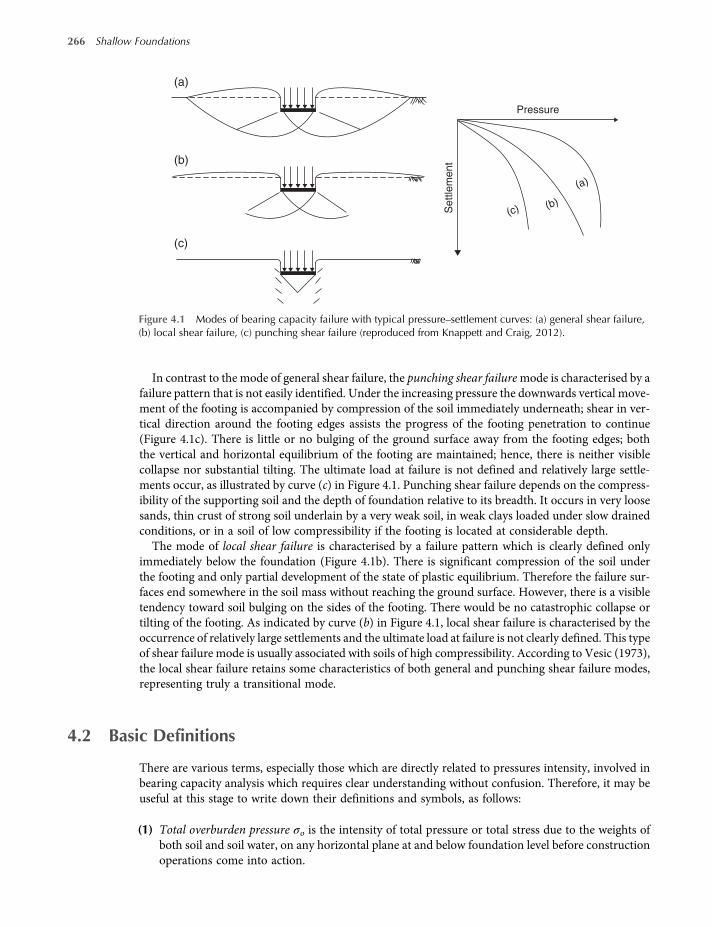
In contrast to the mode of general shear failure, the punching shear failuremode is characterised by afailure pattern that is not easily identified. Under the increasing pressure the downwards vertical move-ment of the footing is accompanied by compression of the soil immediately underneath; shear in ver-tical direction around the footing edges assists the progress of the footing penetration to continue(Figure 4.1c). There is little or no bulging of the ground surface away from the footing edges; boththe vertical and horizontal equilibrium of the footing are maintained; hence, there is neither visiblecollapse nor substantial tilting. The ultimate load at failure is not defined and relatively large settle-ments occur, as illustrated by curve (c) in Figure 4.1. Punching shear failure depends on the compress-ibility of the supporting soil and the depth of foundation relative to its breadth. It occurs in very loosesands, thin crust of strong soil underlain by a very weak soil, in weak clays loaded under slow drainedconditions, or in a soil of low compressibility if the footing is located at considerable depth.
The mode of local shear failure is characterised by a failure pattern which is clearly defined onlyimmediately below the foundation (Figure 4.1b). There is significant compression of the soil underthe footing and only partial development of the state of plastic equilibrium. Therefore the failure sur-faces end somewhere in the soil mass without reaching the ground surface. However, there is a visibletendency toward soil bulging on the sides of the footing. There would be no catastrophic collapse ortilting of the footing. As indicated by curve (b) in Figure 4.1, local shear failure is characterised by theoccurrence of relatively large settlements and the ultimate load at failure is not clearly defined. This typeof shear failure mode is usually associated with soils of high compressibility. According to Vesic (1973),the local shear failure retains some characteristics of both general and punching shear failure modes,representing truly a transitional mode.
4.2 Basic Definitions
There are various terms, especially those which are directly related to pressures intensity, involved inbearing capacity analysis which requires clear understanding without confusion. Therefore, it may beuseful at this stage to write down their definitions and symbols, as follows:
(1) Total overburden pressure σo is the intensity of total pressure or total stress due to the weights ofboth soil and soil water, on any horizontal plane at and below foundation level before constructionoperations come into action.
Pressure
(b)(c)
(a)
(b)
(c)
(a)
Settle
ment
Figure 4.1 Modes of bearing capacity failure with typical pressure–settlement curves: (a) general shear failure,(b) local shear failure, (c) punching shear failure (reproduced from Knappett and Craig, 2012).
266 Shallow Foundations
worksaccounts.com

(2) Effective overburden pressure σo is the intensity of the intergranular pressure, or effective normalstress, on any horizontal plane at and below foundation level before construction operations comeinto action. It is the total overburden pressure σo less the pore-water pressure u. Therefore,
σo = σo−u
(3) Gross foundation pressure (or gross contact pressure, or, gross loading intensity), gross q, is theintensity of total pressure directly beneath the foundation (at the foundation level) after the struc-ture has been erected and fully loaded. It is inclusive of the load of the foundation substructure,the loading from the superstructure and the total loading from any backfilled soil.
(4) Gross effective foundation pressure, gross q is the gross foundation pressure less the uplift pres-sure due to height h of ground water table (W.T) above the foundation level, expressed as
gross q = gross q−hγw
(5) Net foundation pressure (or net contact pressure, or, net loading intensity), net q, is the excesspressure or the difference between the gross foundation pressure gross q and the total overburdenpressure σo directly beneath the foundation, expressed as
net q= gross q−σo 4 1
(6) Net effective foundation pressure, net q , is the effective excess pressure or the difference betweenthe gross effective foundation pressure gross q and the effective overburden pressure σo directlybeneath the foundation, expressed as
net q = gross q −σo 4 2
The term net q is used for calculating the net increase in effective stresses at any depth below thefoundation level.
(7) Gross ultimate bearing capacity (or gross ultimate soil pressure), gross qult, is the minimum valueof the gross effective contact pressure at which the supporting material fails in shear. It is oftenwritten as qult only.
(8) Net ultimate bearing capacity (or net ultimate soil pressure), net qult, is the minimum value of theexcess effective contact pressure at which the supporting material fails in shear, expressed as
net qult = gross qult−σo 4 3
(9) Net safe bearing capacity, net qs is the net ultimate bearing capacity divided by a suitable safetyfactor SF, expressed as
net qs =net qultSF
4 4
(10) Gross safe bearing capacity, net qs is the net safe bearing capacity plus the effective overburdenpressure, expressed as
gross qs =net qultSF
+ σo 4 5
Note that the σo term is not divided by the safety factor and may not be logical to do so because itsvalue is usually available in full. However, some authors define the gross qs as the gross ultimatebearing capacity divided by a suitable safety factor, expressed as
gross qs =gross qult
SF=net qult + σo
SF=net qultSF
+σoSF
4 6
Shallow Foundations – Bearing Capacity 267
worksaccounts.com
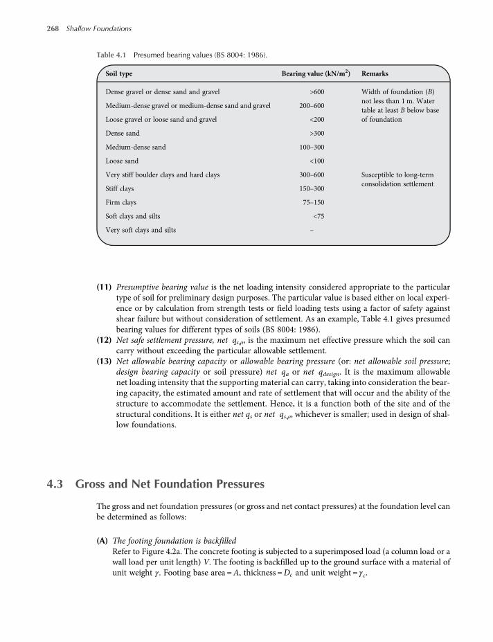
(11) Presumptive bearing value is the net loading intensity considered appropriate to the particulartype of soil for preliminary design purposes. The particular value is based either on local experi-ence or by calculation from strength tests or field loading tests using a factor of safety againstshear failure but without consideration of settlement. As an example, Table 4.1 gives presumedbearing values for different types of soils (BS 8004: 1986).
(12) Net safe settlement pressure, net qs,ρ, is the maximum net effective pressure which the soil cancarry without exceeding the particular allowable settlement.
(13) Net allowable bearing capacity or allowable bearing pressure (or: net allowable soil pressure;design bearing capacity or soil pressure) net qa or net qdesign. It is the maximum allowablenet loading intensity that the supporting material can carry, taking into consideration the bear-ing capacity, the estimated amount and rate of settlement that will occur and the ability of thestructure to accommodate the settlement. Hence, it is a function both of the site and of thestructural conditions. It is either net qs or net qs,ρ, whichever is smaller; used in design of shal-low foundations.
4.3 Gross and Net Foundation Pressures
The gross and net foundation pressures (or gross and net contact pressures) at the foundation level canbe determined as follows:
(A) The footing foundation is backfilledRefer to Figure 4.2a. The concrete footing is subjected to a superimposed load (a column load or awall load per unit length) V. The footing is backfilled up to the ground surface with a material ofunit weight γ. Footing base area =A, thickness =Dc and unit weight = γc.
Table 4.1 Presumed bearing values (BS 8004: 1986).
Soil type Bearing value (kN/m2) Remarks
Dense gravel or dense sand and gravel >600 Width of foundation (B)not less than 1m. Watertable at least B below baseof foundation
Medium-dense gravel or medium-dense sand and gravel 200–600
Loose gravel or loose sand and gravel <200
Dense sand >300
Medium-dense sand 100–300
Loose sand <100
Very stiff boulder clays and hard clays 300–600 Susceptible to long-termconsolidation settlement
Stiff clays 150–300
Firm clays 75–150
Soft clays and silts <75
Very soft clays and silts –
268 Shallow Foundations
worksaccounts.com

The gross foundation pressure is given by
gross q=V +Wf
A4 7 - a
or
gross q=VA+Dcγc + γ Df −Dc 4 7 - b
where Wf = total weights of the footing and the backfill material.Assuming unit weight γ of the overburden soil above W.T is the same as that of the backfill
material and the saturated unit weight of the overburden soil (below W.T) is γsat, then fromEquation (4.1), the net foundation pressure is given by
net q=V +Wf
A−σo 4 8 - a
or
net q=VA+Dcγc + γ Df −Dc − γ Df −h + γsath
=VA−h γsat−γ +Dc γc−γ
h γsat −γ = γwhHence,
net q=VA−γwh+Dc γc−γ ≤ net qa 4 8 - b
Column or wall
Backfill material
Basement
Floor
Footing
(a)
∇
∇ WT
VWf
Wf
Dc
Dc
Df
h
h
Df
V
tc
(b)
Figure 4.2 Footings subjected to superimposed loads.
Shallow Foundations – Bearing Capacity 269
worksaccounts.com

where: γwh= uplift water pressureFrom Equation (4.2), the net effective foundation pressure is given by
net q =V +Wf
A−γwh −σo
net q =VA+ γDf −γDc + γcDc−γwh− γ Df −h + h γsat−γw
=VA+ γDf −γDc + γcDc−γwh−γDf + γh−γsath+ γwh
=VA−h γsat−γ +Dc γc−γ
h γsat−γ = γwh
4 9 - a
Hence,
net q =VA−γwh+Dc γc−γ ≤ net qa 4 9 - b
It is noteworthy that both Equations (4.8)-(b) and (4.9)-(b) give the same result, indicating that itmakes no difference whether the net foundation pressure is computed on the basis of total stress oreffective stress approach.Equation (4.9)-(b) indicates that if γ γc and W.T is located at a depthgreater than Df, the net effective foundation pressure can be written as
net q =VA
4 10
For a safe design, the net effective foundation pressure net q should be less than or equal to thenet allowable bearing capacity net qa. Therefore,
net q ≤ net qa 4 11
(B) The footing foundation is not backfilled.Refer to Figure 4.2b. In this case the interior footings are directly below the basement floor, notbackfilled and with no overburden soil above. Also, one side of the exterior footings are under thesame loading conditions. Therefore, the overburden pressure should not be deducted from q whennet q or net q is calculated.
The gross foundation pressure is given by
gross q=V +Wf
A=VA+Dcγc + tcγc
net q= gross q=VA+Dcγc + tcγc
gross q =VA−γwh +Dcγc + tcγc
4 12
net q = gross q =VA−γwh +Dcγc + tcγc ≤ net qa 4 13
where tc = thickness of the floor slab
Comparing Equation (4.13) with Equation (4.9)-(b), it is observed that the load carrying cap-acity of a foundation is increased if it is not backfilled.
270 Shallow Foundations
worksaccounts.com

(C) Mat or raft foundation under a basement.Assume the basement footings and the floor slabs in Figure 4.2b are replaced by a mat withthickness Dc and the building load is Q.
Equation (4.7)-(a):
gross q=Q+Wf
A
gross q=QA+A Dcγc
A=QA+Dcγc
Equation (4.1): net q= gross q−σo
net q=QA+Dcγc−σo
Assume γ represents unit weight of the overburden soil aboveW.T, that is the effective unit weight.
net q=QA+Dcγc− γ Df −h + γsath 4 14
Equation (4.2): net q = gross q −σo
net q =QA−γwh +Dcγc−σo
=QA−γwh +Dcγc− γ Df −h + h γsat−γw
=QA− γwh+Dcγc−γ Df + γ h−γsath+ γwh
=QA−h γsat−γ +Dcγc−γ Df
h γsat−γ = γwh; hence,
net q =QA−γwh +Dcγc −γ Df ≤ net qa
4 15
or
Net effectivefoundationpressure
=
Total applied effectivepressure due to the totalbuilding loads includingweight of foundation
−Effectiveoverburdenpressure
≤ net qa 4 16
Here, also, it makes no difference whether the net foundation pressure is computed on the basis oftotal stress or effective stress approach, as it is clear from Equations (4.14) and (4.15)Equation (4.16) indicates that the net effective foundation pressure would reduce to zero if the
total applied effective pressureQA−γwh +Dcγc equals the effective overburden pressure
(γ Df). This is the same principle of floating foundations (or compensated foundations) whichhas been discussed in Section 2.2.
Shallow Foundations – Bearing Capacity 271
worksaccounts.com
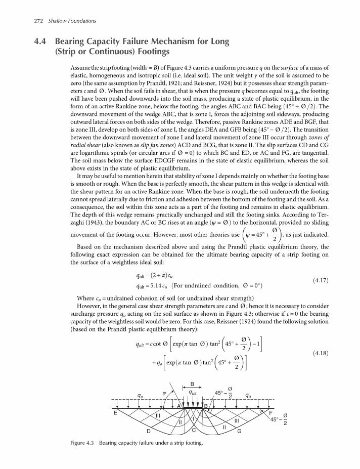
4.4 Bearing Capacity Failure Mechanism for Long(Strip or Continuous) Footings
Assumethestrip footing (width =B) of Figure 4.3 carries a uniform pressure q on the surface of amass ofelastic, homogeneous and isotropic soil (i.e. ideal soil). The unit weight γ of the soil is assumed to bezero (the same assumption by Prandtl, 1921; and Reissner, 1924) but it possesses shear strength param-eters c and Ø .When the soil fails in shear, that is when the pressure q becomes equal to qult, the footingwill have been pushed downwards into the soil mass, producing a state of plastic equilibrium, in theform of an active Rankine zone, below the footing, the angles ABC and BAC being 45 + Ø 2 . Thedownward movement of the wedge ABC, that is zone I, forces the adjoining soil sideways, producingoutward lateral forces on both sides of the wedge. Therefore, passive Rankine zones ADE and BGF, thatis zone III, develop on both sides of zone I, the angles DEA and GFB being 45 − Ø 2 . The transitionbetween the downward movement of zone I and lateral movement of zone III occur through zones ofradial shear (also known as slip fan zones) ACD and BCG, that is zone II. The slip surfaces CD and CGare logarithmic spirals (or circular arcs if Ø = 0) to which BC and ED, or AC and FG, are tangential.The soil mass below the surface EDCGF remains in the state of elastic equilibrium, whereas the soilabove exists in the state of plastic equilibrium.
It may be useful tomention herein that stability of zone I dependsmainly on whether the footing baseis smooth or rough. When the base is perfectly smooth, the shear pattern in this wedge is identical withthe shear pattern for an active Rankine zone. When the base is rough, the soil underneath the footingcannot spread laterally due to friction and adhesion between the bottom of the footing and the soil. As aconsequence, the soil within this zone acts as a part of the footing and remains in elastic equilibrium.The depth of this wedge remains practically unchanged and still the footing sinks. According to Ter-zaghi (1943), the boundary AC or BC rises at an angle ψ = Ø to the horizontal, provided no sliding
movement of the footing occur. However, most other theories use ψ = 45 +Ø2
, as just indicated.
Based on the mechanism described above and using the Prandtl plastic equilibrium theory, thefollowing exact expression can be obtained for the ultimate bearing capacity of a strip footing onthe surface of a weightless ideal soil:
qult = 2 + π cu
qult = 5 14 cu For undrained condition, Ø = 04 17
Where cu =undrained cohesion of soil (or undrained shear strength)However, in the general case shear strength parameters are c and Ø ; hence it is necessary to consider
surcharge pressure qo acting on the soil surface as shown in Figure 4.3; otherwise if c= 0 the bearingcapacity of the weightless soil would be zero. For this case, Reissner (1924) found the following solution(based on the Prandtl plastic equilibrium theory):
qult = ccot Ø exp π tan Ø tan2 45 +Ø2
−1
+ qo exp π tan Ø tan2 45 +Ø2
4 18
45°–Ø2
45° −Ø2
IIIIII
IIII
IE
D C G
F
A B
B
qo qoqultψ
Figure 4.3 Bearing capacity failure under a strip footing.
272 Shallow Foundations
worksaccounts.com

We should not forget that Equation (4.18) was derived assuming weightless soil. Therefore, an add-itional termmust be added to this equation to take into account the component of bearing capacity dueto the self-weight of the soil. This third term cannot theoretically (or exactly) be determined mainlybecause of the inclination angle ψ which is unknown; hence the term can only be determined usingapproximate procedures (e.g. Terzaghi, 1943; Meyerhof, 1951, 1955; Terzaghi and Peck, 1966; Hansen,1969; Vesic, 1973). According to Terzaghi, the ultimate bearing capacity (gross qult) of the soil under ashallow strip footing can be expressed by the following general equation (known as the Terzaghi gen-eral bearing capacity equation):
gross qult = cNc + γ DfNq +12γ BNγ 4 19
where Nc, Nq and Nγ are bearing capacity factors depending only on the value of Ø .Contributions of the first, second and third terms in Equation (4.19) are due to the constant com-
ponent of shear strength, the surcharge pressure and the self-weight of the soil, respectively. It is neces-sary to realise, however, that the superposition of the components of bearing capacity is not strictlycorrect for a plastic material; it leads to errors which are on the safe side, not exceeding 17–20%for Ø = 30 to 40 and zero for Ø = 0 .It may be useful to mention herein that there exists in literature a great variety of proposed solutions
to the problem of ultimate bearing capacity, especially, those related to the bearing capacity factors.While variations in the proposed Nc and Nq values remain relatively insignificant, the differences inNγ values, coming primarily from the sharp variation of this factor with the angle ψ , are substantial.
4.5 Bearing Capacity Equations
Various analytical methods have been established so that the problem of a two-dimensional solutionfor a strip footing is extended to a solution of three-dimensional problem for square, rectangular andcircular footings. Accordingly, semi-empirical shape, depth and various inclination factors are appliedto the ultimate bearing capacity solution for a strip footing.Table 4.2 shows four general equations for estimating gross ultimate bearing capacity, currently in
use, proposed by the four authors Terzaghi (1943), Meyerhof (1963), Hansen (1970) and Vesic (1973,1975). The table also shows equations for computing the bearing capacity factors included in eachequation. Table 4.3 gives values of bearing capacity factors for the Terzaghi bearing capacity equations.Table 4.4 gives values of bearing capacity factors for the Hansen, Meyerhof and Vesic equations.Table 4.5 shows equations for computing shape, depth and load inclination factors for use in theMeyerhof bearing capacity equations. Table 4.6 shows equations for computing shape and depth fac-tors for use in either the Hansen or Vesic bearing capacity equations. Table 4.7 shows equations forcomputing load inclination, ground and base factors for use in the Hansen bearing capacity equations.Table 4.8 shows equations for computing load inclination, ground and base factors for use in the Vesicbearing capacity equations. According to Bowles (2001), as a result of his observations regarding theuse of the various bearing capacity equations, one may suggest the following equation use:
• Terzaghi – best for very cohesive soils where D B≤ 1 or for a quick estimate of qult to compare withother methods. Do not use for footings with moments and/or horizontal forces or for tilted basesand/or sloping ground.
• Hansen, Meyerhof, Vesic – best for any situatin that applies, depending on user preference or famil-iarity with a particular method.
• Hansen, Vesic – best when base is tilted, when footing is on a slope or when D B > 1.
Notes for Table 4.2–4.8:
(1) Note use of “effective” base dimensions B , L in shape factors by Hansen but not by Vesic.B =B−2 eB, L = L−2 eL and Af =B L .
Shallow Foundations – Bearing Capacity 273
worksaccounts.com
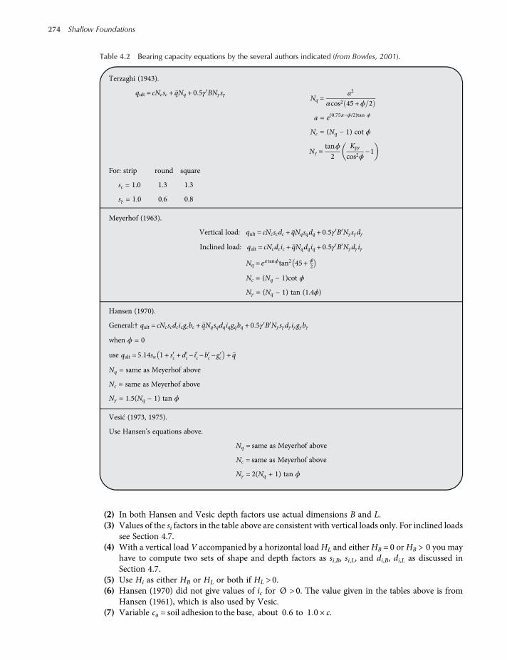
(2) In both Hansen and Vesic depth factors use actual dimensions B and L.(3) Values of the si factors in the table above are consistent with vertical loads only. For inclined loads
see Section 4.7.(4) With a vertical load V accompanied by a horizontal loadHL and eitherHB = 0 orHB > 0 you may
have to compute two sets of shape and depth factors as si,B, si,L, and di,B, di,L as discussed inSection 4.7.
(5) Use Hi as either HB or HL or both if HL > 0.(6) Hansen (1970) did not give values of ic for Ø > 0. The value given in the tables above is from
Hansen (1961), which is also used by Vesic.(7) Variable ca = soil adhesion to the base, about 0 6 to 1 0 × c.
Table 4.2 Bearing capacity equations by the several authors indicated (from Bowles, 2001).
Terzaghi (1943).
qult = cNcsc + qNq + 0 5γ BNγsγNq =
a2
αcos2 45 +ϕ 2
a = e(0.75π−ϕ/2)tan ϕ
Nc = (Nq − 1) cot ϕ
Nγ =tanϕ2
Kpγ
cos2ϕ−1
For: strip round square
sc = 1.0 1.3 1.3
sγ = 1.0 0.6 0.8
Meyerhof (1963).
Vertical load: qult = cNcscdc + qNqsqdq + 0 5γ B Nγsγdγ
Inclined load: qult = cNcdcic + qNqdqiq + 0 5γ B Nγdγ iγ
Nq = eπ tanϕtan2 45 + ϕ2
Nc = (Nq − 1)cot ϕ
Nγ = (Nq − 1) tan (1.4ϕ)
Hansen (1970).
General:† qult = cNcscdcicgcbc + qNqsqdqiqgqbq + 0 5γ B Nγsγdγ iγgγbγ
when ϕ = 0
use qult = 5 14su 1 + sc + dc− ic−bc−gc + q
Nq = same as Meyerhof above
Nc = same as Meyerhof above
Nγ = 1.5(Nq − 1) tan ϕ
Vesić (1973, 1975).
Use Hansen’s equations above.
Nq = same as Meyerhof above
Nc = same as Meyerhof above
Nγ = 2(Nq + 1) tan ϕ
274 Shallow Foundations
worksaccounts.com
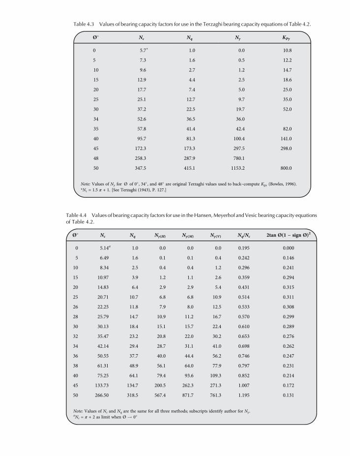
Table 4.3 Values of bearing capacity factors for use in the Terzaghi bearing capacity equations of Table 4.2.
Ø Nc Nq Nγ KPγ
0 5.7∗ 1.0 0.0 10.8
5 7.3 1.6 0.5 12.2
10 9.6 2.7 1.2 14.7
15 12.9 4.4 2.5 18.6
20 17.7 7.4 5.0 25.0
25 25.1 12.7 9.7 35.0
30 37.2 22.5 19.7 52.0
34 52.6 36.5 36.0
35 57.8 41.4 42.4 82.0
40 95.7 81.3 100.4 141.0
45 172.3 173.3 297.5 298.0
48 258.3 287.9 780.1
50 347.5 415.1 1153.2 800.0
Note: Values of Nγ for Ø of 0 , 34 , and 48 are original Terzaghi values used to back–compute Kpγ (Bowles, 1996).*Nc = 1.5 π + 1. [See Terzaghi (1943), P. 127.]
Table 4.4 Values of bearing capacity factors for use in theHansen,Meyerhof andVesic bearing capacity equationsof Table 4.2.
Ø Nc Nq Nγ(H) Nγ(M) Nγ(V) Nq/Nc 2tan Ø(1 − sign Ø)2
0 5.14a 1.0 0.0 0.0 0.0 0.195 0.000
5 6.49 1.6 0.1 0.1 0.4 0.242 0.146
10 8.34 2.5 0.4 0.4 1.2 0.296 0.241
15 10.97 3.9 1.2 1.1 2.6 0.359 0.294
20 14.83 6.4 2.9 2.9 5.4 0.431 0.315
25 20.71 10.7 6.8 6.8 10.9 0.514 0.311
26 22.25 11.8 7.9 8.0 12.5 0.533 0.308
28 25.79 14.7 10.9 11.2 16.7 0.570 0.299
30 30.13 18.4 15.1 15.7 22.4 0.610 0.289
32 35.47 23.2 20.8 22.0 30.2 0.653 0.276
34 42.14 29.4 28.7 31.1 41.0 0.698 0.262
36 50.55 37.7 40.0 44.4 56.2 0.746 0.247
38 61.31 48.9 56.1 64.0 77.9 0.797 0.231
40 75.25 64.1 79.4 93.6 109.3 0.852 0.214
45 133.73 134.7 200.5 262.3 271.3 1.007 0.172
50 266.50 318.5 567.4 871.7 761.3 1.195 0.131
Note: Values of Nc and Nq are the same for all three methods; subscripts identify author for Nγ.aNc = π + 2 as limit when Ø 0
worksaccounts.com

Table 4.5 Shape, depth, and load inclination factors, for use in the Meyerhofbearing capacity equations of Table 4.2.
Factor Value For
Shapesc = 1 + 0 2Kp
BL
Any ϕ
sq = sγ = 1+ 0 1KpBL
ϕ > 10
sq = sγ = 1 ϕ = 0
Depthdc = 1 + 0 2 Kp
DB
Any ϕ
dq = dγ = 1 + 0 1 KpDB
ϕ > 10
dq = dγ = 1 ϕ = 0
Load-inclinationic = iq = 1−
θ∘
90∘
2 Any ϕ
H
VR
θ <iγ = 1−
θ∘
ϕ∘
2 ϕ > 0
iγ = 0 for θ > 0 ϕ = 0
Where: KP = tan2 (45 + Ø/2)θ = angle of resultant R measured from vertical without a sign; if θ = 0 all ii = 1.0D = depth of foundationB = width of footingL = length of footingsi, di, ii = shape, depth, and load – inclination factors, respectively
Table 4.6 Shape and depth factors for use in the Hansen and Vesic bearingcapacity equations of Table 4.2. Use sc and dc when Ø =0 only for Hansenequations. Subscripts H, V used for Hansen, Vesic, respectively.
Shape factors Depth factors
sc H = 0 2BL
ϕ= 0∘ dc = 0 4k ϕ= 0∘
dc = 1.0 + 0.4 k
Sc H = 1 0 +Nq
Nc
BL
k = D/B for D/B ≤ 1
Sc V = 1 0 +Nq
Nc
BL
k = tan−1(D/B) for D/B >1
k in radians
sc = 1.0 for strip
Sq H = 1 0 +BLsinϕ
dq = 1 + 2 tan ϕ(1 − sin ϕ)2 k
Sq V = 1 0 +BLtanϕ
k defined above
for all ϕ
sγ H = 1 0−0 4BL
≥ 0 6dγ = 1.00 for all ϕ
sγ V = 1 0−0 4BL
≥ 0 6
worksaccounts.com
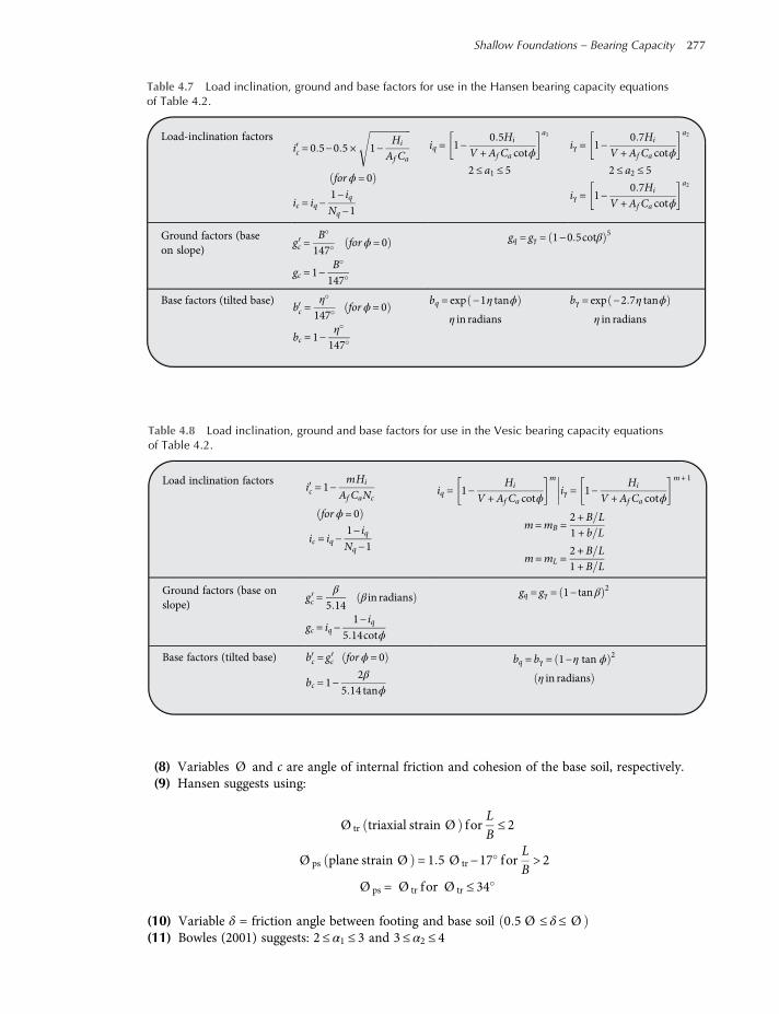
(8) Variables Ø and c are angle of internal friction and cohesion of the base soil, respectively.(9) Hansen suggests using:
Ø tr triaxial strain Ø forLB≤ 2
Ø ps plane strain Ø = 1 5 Ø tr−17 forLB> 2
Ø ps = Ø tr for Ø tr ≤ 34
(10) Variable δ = friction angle between footing and base soil 0 5 Ø ≤ δ≤ Ø(11) Bowles (2001) suggests: 2≤ α1 ≤ 3 and 3≤ α2 ≤ 4
Table 4.7 Load inclination, ground and base factors for use in the Hansen bearing capacity equationsof Table 4.2.
Load-inclination factorsic = 0 5−0 5 × 1−
Hi
Af Ca
forϕ= 0
ic = iq−1− iqNq−1
iq = 1−0 5Hi
V +Af Ca cotϕ
a1
2≤ a1 ≤ 5
iγ = 1−0 7Hi
V +Af Ca cotϕ
a2
2≤ a2 ≤ 5
iγ = 1−0 7Hi
V +Af Ca cotϕ
a2
Ground factors (baseon slope)
gc =B147
forϕ= 0
gc = 1−B147
gq = gγ = 1−0 5cotβ 5
Base factors (tilted base)bc =
η
147forϕ= 0
bc = 1−η
147
bq = exp −1η tanϕ
η in radians
bγ = exp −2 7η tanϕ
η in radians
Table 4.8 Load inclination, ground and base factors for use in the Vesic bearing capacity equationsof Table 4.2.
Load inclination factorsic = 1−
mHi
Af CaNc
forϕ= 0
ic = iq−1− iqNq−1
iq = 1−Hi
V +Af Ca cotϕ
m
iγ = 1−Hi
V +Af Ca cotϕ
m+ 1
m=mB =2 +B L1 + b L
m=mL =2 +B L1 +B L
Ground factors (base onslope)
gc =β
5 14β in radians
gc = iq−1− iq
5 14cotϕ
gq = gγ = 1− tanβ 2
Base factors (tilted base) bc = gc forϕ= 0
bc = 1−2β
5 14 tanϕ
bq = bγ = 1−η tan ϕ 2
η in radians
Shallow Foundations – Bearing Capacity 277
worksaccounts.com
(12) According to Vesic:with Ø = 0 (and β 0), use Nγ = −2sin ± β .m=mB when Hi =HB (H parallel to B) and m=mL when Hi =HL (H parallel to L)
Use m= m2B +m
2L if you have both HB and HL.
Note use of B and L, not B and LThe Hi term ≤ 1 0 for computing iq, iγ (always).
(13) Vesic uses B in the Nγ term even when Hi =HL.(14) Refer to the scheme 4.1 for identification of angles η and β, foundation depthD and location ofHi
(parallel and at top of the base slab; usually also produces eccentricity). Especially note that V =force normal to the base and is not the resultant R from combining V and Hi.
4.6 Some Considerations Concerning the Use of BearingCapacity Equations
(1) The requirement of moment equilibrium M = 0 is not satisfied in the methods used in devel-
oping the bearing capacity equations; only the requirements FH = FY = 0 are satisfied.
However this error would not be serious since statics is obviously satisfied at ultimate loading.(2) The common practice is, usually, to use conservative estimates for the soil parameters; hence, the
bearing capacity equations tend to be conservative most of the time. Moreover, after obtaining aconservative qult this is reduced to the safe soil pressure qs using a safety factor. Therefore, theprobability is very high that the allowable soil pressure qa is safe.
(3) Terzaghi developed his bearing capacity equations considering the mode of general shear failurein a dense or stiff soil and the mode of local shear failure in a loose or soft soil. According toTerzaghi, the same general bearing capacity equation of Table 4.2 is used for the mode of localshear failure provided that reduced values of the parameters c and Ø are used, as follows:
clocal =23cgeneral
tan Ø local =23tan Ø general; or Ø local = tan
−1 23tan Ø general
Therefore, according to Terzaghi, for the mode of local shear failure clocal instead of c should beused in the Nc term and Ø local instead of Ø should be used in computing the bearing capacityfactors (using equations or Table 4.3).
Hmax = V tan δ + ca Af
Limitations:V
HB
D
iq, iγ > 0
H < Hmax
η + β ≤ 90°+β
β
+η
β ≤ ϕ
Scheme 4.1
278 Shallow Foundations
worksaccounts.com

(4) The researchers Vesic (1969) and De Beer (1965) found that, for very large values of B of the Nγ
term, the limiting value of qult approaches that of deep foundations and suggest a reduction factorsuch as rγ may be used with the Nγ term of all the bearing capacity equations. Bowles (1996)suggests:
rγ = 1−0 25 logBK
forB > 2m 4 20
where B = width or diameter of footing or mat foundation, in m, and K = 2(5) It is not recommended using tables of N factors (Tables 4.3 and 4.4) that require interpolation
over about 2 . For angles larger than 35 the factors change rapidly and by large amounts;interpolation can have a considerable error, so someone checking the work may not be ableto verify qult.
(6) The Nc term (the shear strength term) predominates in cohesive soils.(7) The Nq term (the surcharge term) predominates in cohesionless soils.(8) The Nγ term (the weight term) provides some increase in bearing capacity for both c- Ø and
cohesionless soils.(9) One should avoid placing a footing on the surface of a cohesionless soil mass.(10) It is recommended to compact loose cohesionless soils of relative density less than 50% to a higher
density prior to placing footings in it.(11) In case the soil beneath a footing is not homogeneous or is stratified, some judgment must be
applied to determine the bearing capacity. Bearing capacity for footings on layered soils willbe considered in Section 4.13.
(12) It is obvious that the Terzaghi bearing capacity equation is much easier to use than the othersequation so that it has great appeal for many practitioners, particularly for bases with only vertical
loads andDB≤ 1. The shape factors proposed by Terzaghi and Peck (1967) are still widely used in
practice although they are considered to give conservative values of qult. The shape factors for strip,square and circular footings are as shown in Table 4.2. For a rectangular footing of breadth B andlength L, the shape factors are obtained by linear interpolation between the values for a strip
footingBL= 0 and a square footing
BL= 1 . Hence,
sc = 1 + 0 3BL, and sγ = 1−0 2
BL
(13) According to Vesic (1973), it is recommended that the depth factors di are not be used forshallow foundations D B≤ 1 because of uncertainties in quality of the overburden. How-ever, he did give the di values as shown in Table 4.6 despite this recommendation. Also, Vesicalways used the actual B as B in the Nγ term of the general bearing capacity equation ofTable 4.2.
(14) In a study of bearing capacity theories, Skempton (1951) concluded that the bearing capacity fac-tor Nc for saturated clays under undrained conditions Ø u = 0 is a function of the shape of thefooting and the depth to breadth ratio, as shown in Figure 4.4. This figure also includes relation-ships suggested by Salgado et al. (2004), which are described by Nc = 2 + π 1 + 0 27 d B 0 5 .Nc for circular footings may be obtained by taking the square values. The factor for a rectangularfooting of dimensions B× L whereB < L is the value for a square footing multiplied by0 84 + 0 16B L . In practice, Nc is normally limited at a value equals 9.0 for very deeply embed-ded square or circular foundations.
Shallow Foundations – Bearing Capacity 279
worksaccounts.com
4.7 Bearing Capacity of Footings with Inclined Loads
A footing may be subjected to inclined loading and such condition leads to a reduction in bearing cap-acity. This type of loading is common for footing of retaining walls loaded with both horizontal (lateralearth pressure) and vertical loading, for footings of many industrial process structures where horizontalwind loads are acting in combination with the gravity loads and for a number of other types of foun-dations which are subjected to horizontal and vertical loads simultaneously. The effect of inclined load-ing on bearing capacity can be taken into account by means of inclination factors, as shown inTables 4.5, 4.7 and 4.8.
The Terzaghi equations have no direct provision for a reduction in cases where the load is inclined.TheMeyerhof inclination factors of Table 4.5 do not need explanation. However, he did not take into
account the direction of the load horizontal component (HB,HL).The Vesic inclination factors take into account the load direction (HB,HL) in computing the m
exponents, as shown in Table 4.8. According to Vesic, the shape s factors are computed regardless ofi factors.
The Hansen inclination and shape factors take into account the load direction (HB,HL) asfollows:
(1) Compute the inclination factors using the equations given in Table 4.7 and using either the expo-nents given in that table or those suggested by Bowles mentioned before (see note 11 belowTable 4.8). Accordingly, for:
HB = 0; ic,B = 0 and ic,B, iq,B, iγ,B are all 1 0
HL = 0; ic,L = 0 and ic,L, iq,L, iγ,L are all 1 0
10
9
8
7
6
5
4
0 1 2 3
d/B
B/L = 0 (strip)
B/L = 1 (square)
Nc
4 5
Salgado (2004)
Skempton (1951)
Note: Values of Nc for stratified
deposits provided the value of
Cu for a particular stratum is
not greater than or less than
the average value for all strata
within the significant depth by
more than 50% of the average
value.
Figure 4.4 Bearing capacity factors Nc for embedded foundations in undrained soil (reproduced from Knappettand Craig, 2012).
280 Shallow Foundations
worksaccounts.com
(2) Use the computed inclination factors to compute Hansen shape factors, as follows:
sc,B = 0 2B ic,B L sc,L = 0 2L ic,L B ϕ= 0 case
sc,B = 1 0 +Nq
Nc
B ic,BL
sc,L = 1 0 +Nq
Nc
L ic,LB
sq,B = 1 + sinϕ B iq,B L sq,L = 1 + sinϕ L iq,L B
sγ,B = 1−0 4B iγ,B L iγ,L sγ,L = 1−0 4L iγ,LB iγ,B
Limitation sγ, i ≥ 0 6 if less than 0 6 use 0 60
These factors are used in the following modifications of the Hansen general bearing capacityequation of Table 4.2:
qult = cNcsc,Bdc,Bic,Bgc,Bbc,B + qNqsq,Bdq,Biq,Bgq,Bbq,B
+ 0 5γB Nγsγ,Bdγ,Biγ,Bgγ,Bbγ,B4 21
or
qult = cNcsc,Ldc,Lic,Lgc,Lbc,L + qNqsq,Ldq,Liq,Lgq,Lbq,L
+ 0 5γL Nγsγ,Ldγ,Liγ,Lgγ,Lbγ,L4 22
4.8 Bearing Capacity of Footings with Eccentric Loads
A footing may be subjected to eccentric loading and such condition leads to a reduction in bearingcapacity.The estimate of ultimate bearing capacity for footings with eccentricity, using the general bearing
capacity equations of Table 4.2, may be obtained by the following methods:
(1) The effective area method (Meyerhof, 1953, 1963; Hansen, 1970).Refer to Figure 4.5. The procedure is as explained below:(a) Determine the effective footing dimensions B and L using
B =B−2 eB; where eB is the eccentricity parallel toB
L = L−2 eL; where eL is the eccentricity parallel toL
The smaller of the two dimensions (i.e. B and L ) is the effective width of the footing used in theNγ term of the bearing capacity equations. Effective area of the footing A = B L .The equivalent effective areaA and the effective width B for eccentrically loaded circular foot-ings is given in a nondimensional form (Highter and Anders, 1985), as shown in the table ofFigure 4.5b. Hence, the effective length L =A B . It may be noted that in the case of circularfoundations under eccentric loading, the eccentricity is always one-way.
(b) Use the effective footing dimensions B and L in computing the shape factors.(c) Use actual B and L dimensions in computing the depth factors.(d) Use a general bearing capacity equation to obtain qult.
The ultimate load that the foundation can support is
Qult = qult ×A = qult B L 4 23
Shallow Foundations – Bearing Capacity 281
worksaccounts.com

≡
(a)
(b)
0.1 0.2 0.3 0.4 0.5 0.6 0.7 0.8 0.9 0.1
2.80 2.40 2.00 1.61 1.23 0.93 0.62 0.35 0.12 0.00
1.85 1.32 1.20 0.80 0.67 0.50 0.37 0.23 0.12 0.00
Centroid
Location of
resultant RLocation
of load V
≡
Location of
resultant R
Effective
area Aʹ
Effective
area A′
Lʹ / 2
Lʹ / 2
Bʹ / 2 Bʹ / 2
Bʹ
Aʹ / r2
Bʹ / r
B
B2eB
er
r
er / r
eL
eB
x Lʹ
V
My
My
Mx
Mx
y
x
x L
B
eB = ex
eL = ey
R
B
2eL
Figure 4.5 Eccentrically loaded footings and method of computing effective footing dimensions.
282 Shallow Foundations
worksaccounts.com

The safety factor against bearing capacity failure is
SF =Qult
R4 24
(2) The Meyerhof reduction factor method.In this procedure the ultimate bearing capacity is computed for concentric loading condition usingtheMeyerhof bearing capacity equations of Table 4.2. This computed ultimate soil pressure, qult(c),is then reduced with a reduction factor Re to obtain the ultimate soil pressure for eccentric loadingcondition which is
qult e = qult c ×Re 4 25
The original Meyerhof method gave reduction curves for obtaining Re; however, Bowles (1982)converted the curves to the following suitable equations:
Re = 1−2eB
cohesive soil 4 26 - a
Re = 1−eB
12
cohesionless soil and for 0 < e B < 0 3 4 26 - b
It should be evident that, for two-way eccentricity (ex, ey), two reduction factors are usedfor each type of soil. According to this method, the ultimate load that the foundation cansupport is
Qult = qult e ×A= qult e BL 4 27
(3) Purkaystha and Char reduction factor method (for granular soils).Purkaystha and Char (1977) performed stability analysis of strip foundations under eccentric ver-tical loads supported by sand, using the method of slices. Their analysis resulted in the followingeccentricity reduction factor,
Rk = 1−qult eqult c
4 28
Rk = aeB
k4 29
Where Rk = eccentricity reduction factor
qult e = ultimate bearing capacity of strip foundations under eccenteric vertical loads
qult c = ultimate bearing capacity of strip foundations under centeric vertical loads
a and k= functions of the embedment ratio Df B Table 4 9
By combining Equations (4.28) and (4.29),
qult e = qult c 1−Rk = qult c 1−aeB
k
qult e = qult c 1−aeB
k4 30
Shallow Foundations – Bearing Capacity 283
worksaccounts.com
Where
qult c = qNqFqd +12γBNγFγd 4 31
The relationships for the depth factors Fqd and Fγd are given in Table 4.6.The ultimate load per unit length of the strip foundation can be given as
Qult =Bqult eccentric 4 32
(4) Prakash and Saran methodAccording to Prakash and Saran (1971), the ultimate load per unit length of an eccentrically andvertically loaded strip (continuous) foundation can be estimated as
Qult =B c Nc e + qNq e +12γBNγ e 4 33
where Nγ(e), Nq(e) and Nc(e) are bearing capacity factors depend on Ø , given in Figures 4.6, 4.7 and4.8, respectively.
400.4 0.3 0.2 0.1
e/B = 0.0
30
20
10
00 10 20 30 40 50 60 70 80 90 100
Angle
of in
tern
al fr
iction Ø
Weight factor Nγ
Ø = 40°
0.0 115.80
0.1 71.80
0.2 41.60
0.3 18.50
0.4 4.62
e/B Nγ
Figure 4.6 Nγ versus Ø.
Table 4.9 Variations of a and k, Equation (4.30).
Df / B a k
0.00 1.862 0.730
0.25 1.811 0.785
0.50 1.754 0.800
1.00 1.820 0.888
284 Shallow Foundations
worksaccounts.com

For an eccentrically and vertically loaded rectangular foundation, the ultimate load can begiven as
Qult = BL c Nc e Fcs e + qNq e Fqs e +12γBNγ e Fγs e 4 34
where Fcs (e), Fqs(e) and Fγs(e) are shape factors can be determined as
Fcs e = 1 2−0 025LB
≥ 1
Fqs e = 1
Fγs e = 1 0 +2eB−0 68
BL+ 0 43−
32
eB
BL
2
For dense sands
Fγs e = 1 For loose sands
400.4 0.3
0.1
e/B = 0.030
20
10
00 10 20 30 40 50 60 70 80 90 100
Angle
of in
tern
al fr
iction Ø
Cohesion factor Nc
Ø = 40°
0.0 94.83
0.1 66.60
0.2 54.45
0.3 36.30
0.4 18.15
e/B Nc
0.2
Figure 4.8 Nc versus Ø.
400.4 0.3 0.2 0.1
e/B = 0.0
30
20
10
00 10 20 30 40 50 60 70 80 90
Angle
of in
tern
al fr
iction Ø
Surcharge factor Nq
Ø = 40°
0.0 81.27
0.1 56.09
0.2 45.18
0.3 30.18
0.4 13.06
e/B Nq
Figure 4.7 Nq versus Ø.
Shallow Foundations – Bearing Capacity 285
worksaccounts.com
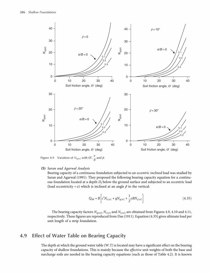
(5) Saran and Agarwal AnalysisBearing capacity of a continuous foundation subjected to an eccentric inclined load was studied bySaran and Agarwal (1991). They proposed the following bearing capacity equation for a continu-ous foundation located at a depth Df below the ground surface and subjected to an eccentric load(load eccentricity = e) which is inclined at an angle β to the vertical:
Qult =B c Nc ei + qNq ei +12γBNγ ei 4 35
The bearing capacity factors Nq(ei), Nc(ei) and Nγ(ei) are obtained from Figures 4.9, 4.10 and 4.11,respectively. These figures are reproduced fromDas (1911). Equation (4.35) gives ultimate load perunit length of a strip foundation.
4.9 Effect of Water Table on Bearing Capacity
The depth at which the ground water table (W.T) is located may have a significant effect on the bearingcapacity of shallow foundations. This is mainly because the effective unit weights of both the base andsurcharge soils are needed in the bearing capacity equations (such as those of Table 4.2). It is known
40 40
30
20
10
0.1
0.2
0.3
0
30
20
10
0
30
20
10
0
40
30
30
20
2010
β = 0
β = 10°
β = 20° β = 30°
e/B = 0
e/B = 0
e/B = 0
e/B = 0
10
Nq
(ei)
Nq
(ei)
Nq
(ei)
Nq
(ei)
0
0
403020100
403020100
403020100
Soil friction angle, Ø′ (deg) Soil friction angle, Ø′ (deg)
Soil friction angle, Ø′ (deg) Soil friction angle, Ø′ (deg)
0.3
0.3
0.3
0.2
0.2
0.2
0.1
0.1
0.1
Figure 4.9 Variation of Nq(ei) with Ø ,eBand β.
286 Shallow Foundations
worksaccounts.com

that the effective unit weight of a submerged soil will be reduced to about half of its unit weight abovewater table. Moreover, generally, the submergence of soils will cause the loss of all apparent cohesions,coming from capillary stresses or from weak cementation bonds. Thus, through submergence, all thethree terms (cohesion, surcharge and weight) of the bearing capacity equation become considerablysmaller. Therefore, it is essential that the bearing capacity analyses be made assuming the highest pos-sible W.T at the particular location for the expected lifetime of the structure in question. It is necessarythat the assessment of this highest possible level is made taking into consideration the probability oftemporary high levels that could be expected in some locations during heavy rainstorms or floods,
100
80
40
30
20
10
0.1
0.2
0.3
0
40
60
30
40
2010
β = 0
β = 10°
β = 20°
β = 30°
e/B = 0
e/B = 0
e/B = 0e/B = 0
20
Nc(
ei)
Nc(
ei)
Nc(
ei)
30
20
10
0
Nc(
ei)
0
0
403020100
0
60
50
40
30
20
10
Soil friction angle, Ø′ (deg)
Soil friction angle, Ø′ (deg)
403020100
Soil friction angle, Ø′ (deg)403020100
Soil friction angle, Ø′ (deg)
0.3
0.3 0.3
0.2
0.20.2
0.1
0.1
0.1
Figure 4.10 Variation of Nc(ei) with Ø ,eBand β.
Shallow Foundations – Bearing Capacity 287
worksaccounts.com
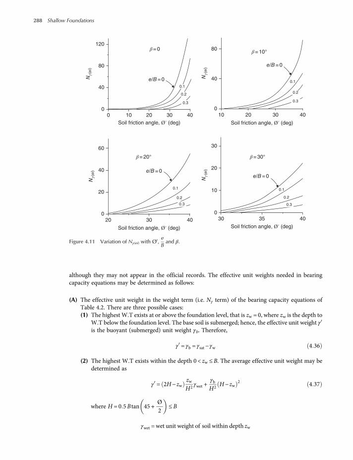
although they may not appear in the official records. The effective unit weights needed in bearingcapacity equations may be determined as follows:
(A) The effective unit weight in the weight term (i.e. Nγ term) of the bearing capacity equations ofTable 4.2. There are three possible cases:(1) The highest W.T exists at or above the foundation level, that is zw = 0, where zw is the depth to
W.T below the foundation level. The base soil is submerged; hence, the effective unit weight γis the buoyant (submerged) unit weight γb. Therefore,
γ = γb = γsat−γw 4 36
(2) The highest W.T exists within the depth 0 < zw ≤B. The average effective unit weight may bedetermined as
γ = 2H−zwzwH2
γwet +γbH2
H−zw2 4 37
where H = 0 5B tan 45 +Ø2
≤B
γwet = wet unit weight of soil within depth zw
120
80
80
40
40
40
302010
β = 0 β = 10°
β = 20° β = 30°
Nγ(
ei)
Nγ(
ei)
Nγ(
ei)
Nγ(
ei)
0 0
60 30
20
10
0
40
20
0
0
Soil friction angle, Ø′ (deg)
40302010
Soil friction angle, Ø′ (deg)
403020
Soil friction angle, Ø′ (deg)
4030 35
Soil friction angle, Ø′ (deg)
e/B = 0e/B = 0
e/B = 0
e/B = 0
0.1
0.2
0.3
0.1
0.1
0.1
0.2 0.2
0.2
0.3
0.30.3
Figure 4.11 Variation of Nγ(ei) with Ø ,eBand β.
288 Shallow Foundations
worksaccounts.com

Also, it may be determined as
γ = γb +zwB
γwet−γb 4 38
(3) The highest W.T exists permanently at a depth well below the foundation level, that is zw >B.The average effective unit weight is determined as
γ = γwet 4 39
(B) The effective unit weight needed for computing the effective surcharge (overburden) pressure q inthe surcharge term (i.e. Nq term) of the bearing capacity equations of Table 4.2. There are threepossible cases:(1) The highest W.T exists at or below the foundation level, that is dw ≥Df , where dw is the depth
toW.T below the ground surface. Hence, the average effective unit weight of the surcharge soilis determined as
γ = γwet 4 40 - a
and
q = γwetDf 4 40 - b
(2) The highest W.T exists within the depth 0 < dw <Df . In this case, γ = γwet is used for the soil
within the depth dw, and γb = γsat−γw is used for the soil within the depth Df −dw . Hence,
q = γwet dw + γb Df −dw 4 41
G.S
(Df – dw)
Df
∇ W.T
B
zw
dw
dw
Scheme 4.3
G.S
∇ W.T
B
zw
zwdw
Scheme 4.2
Shallow Foundations – Bearing Capacity 289
worksaccounts.com
(3) The highest W.T exists at or above the ground surface, i.e. dw = 0. The surcharge soil issubmerged; hence, the effective unit weight γ is the buoyant (submerged) unit weight γb.Therefore,
γ = γb = γsat−γw 4 42 - a
q = γbDf 4 42 - b
It may be useful to mention herein that all preceding considerations are based on the assump-tion that the seepage forces acting on the soil skeleton are negligible. In case there is significantground-water seepage in any direction, it may have an effect on the bearing capacity. In additionto possible internal erosion of the soil (undermining, piping and similar phenomena), the seepageforce adds a component to the body forces caused by gravity. When it is believed wise to considerseepage effects, a particular bearing capacity analysis would be necessary.
4.10 Influence of Soil Compressibility on Bearing Capacity
The bearing capacity equations of Table 4.2 are based on the assumption of incompressibility of soiland that they should be applied, strictly speaking, only to cases where the mode of general shear failureprevails. The other two failure modes are characteristic for compressible soils as previously explained inSection 4.1. Terzaghi (1943) accounted for the effect of soil compressibility, considering the mode oflocal shear failure, through using reduced values of cohesion c and friction angle Ø , as explained inSection 4.6. However, according to Vesič (1973), such an approach is not always satisfactory; andinstead, he proposed using the following compressibility factors (ζic), always smaller than 1, withthe three terms of bearing capacity equations of Table 4.2:
For Ir < Ir cr :
ζcc = 0 32 + 0 12BL+ 0 60 logIr for Ø = 0 4 43
ζcc = ζqc−1−ζqc
Nc tan Øfor Ø > 0 4 44
ζqc = ζγc = exp −4 4 + 0 6BL
tan Ø +3 07sin Ø log2Ir
1 + sin Ø4 45
For Ir ≥ Ir cr :
ζcc = ζqc = ζγc = 1 4 46
Where:
Ir = Rigidity index of soil at a depth approximately B/2 below the foundation level
Ir =Gs
c+ q tan Ø4 47
Gs = shear modulus of the soilq = effective overburden pressure at a depth of Df + B 2Ir(cr) = Critical rigidity index of soil
290 Shallow Foundations
worksaccounts.com

Ir cr =12
exp 3 30−0 45BL
cot 45−Ø2
4 48
The variations of Ir(cr) with (B/L) for different values of Ø are given in Table 4.10.
4.11 Effect of Adjacent Footings on Bearing Capacity
Approximations for the spacing of footings to avoid interference between old and new footings werediscussed in Section 2.3.The analyses used in the derivation of the bearing capacity equations (Table 4.2) were concerned
with the bearing capacity of isolated footings. All analyses based on the assumption that that the sup-porting soil is under the action of gravity forces alone and is not under the influence of any other foot-ing. However, in engineering practice, there are conditions where footings are placed so close to eachother that the influence zones of their supporting soils overlap.This problem of stress overlap due to closely spaced, simultaneously loaded, footings has been
investigated and studied by many researchers. For example, the results of experimental studiesby Stuart (1962) and West and Stuart (1965) indicate that the effects of adjacent parallelstrip footings in sand on bearing capacity may vary considerably with the angle of shearing resist-ance, Ø . With decreased Ø values the effects become small or negligible; however, for high Ø valuesthey appear to be significant, especially if a footing is surrounded by others on both sides. According toVesic (1973), these effects are considerably reduced as the value of (L/B) ratio approaches unity.Similarly, the compressibility of soils reduces and may eliminate completely the interference effects.There are practically no such effects in the case of punching shear failure. For these and other reasons,as Vesic suggested, it is not recommended to consider interference effects in bearing capacity compu-tations. A designer should be aware, however, of the possibility of their existence in some specialcircumstances.
Table 4.10 Values of critical rigidity index of soil.
Critical rigidity index, Ir(cr)
Ø (deg) B/L = 0 B/L = 0.2 B/L = 0.4 B/L = 0.6 B/L = 0.8 B/L = 1.0
0 13.56 12.39 11.32 10.35 9.46 8.64
5 18.30 16.59 15.04 13.63 12.36 11.20
10 25.53 22.93 20.60 18.50 16.62 14.93
15 36.85 32.77 29.14 25.92 23.05 20.49
20 55.66 48.95 43.04 37.85 33.29 29.27
25 88.93 77.21 67.04 58.20 50.53 43.88
30 151.78 129.88 111.13 95.09 81.36 69.62
35 283.20 238.24 200.41 168.59 141.82 119.31
40 593.09 488.97 403.13 332.35 274.01 225.90
45 1440.94 1159.56 933.19 750.90 604.26 486.26
Shallow Foundations – Bearing Capacity 291
worksaccounts.com
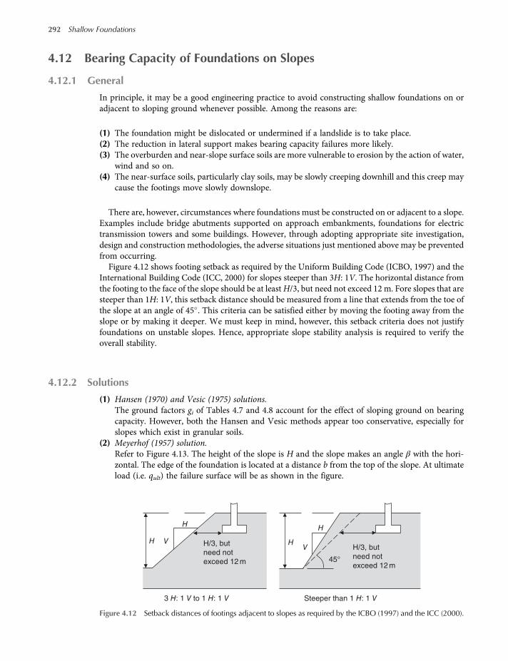
4.12 Bearing Capacity of Foundations on Slopes
4.12.1 General
In principle, it may be a good engineering practice to avoid constructing shallow foundations on oradjacent to sloping ground whenever possible. Among the reasons are:
(1) The foundation might be dislocated or undermined if a landslide is to take place.(2) The reduction in lateral support makes bearing capacity failures more likely.(3) The overburden and near-slope surface soils are more vulnerable to erosion by the action of water,
wind and so on.(4) The near-surface soils, particularly clay soils, may be slowly creeping downhill and this creep may
cause the footings move slowly downslope.
There are, however, circumstances where foundations must be constructed on or adjacent to a slope.Examples include bridge abutments supported on approach embankments, foundations for electrictransmission towers and some buildings. However, through adopting appropriate site investigation,design and construction methodologies, the adverse situations just mentioned above may be preventedfrom occurring.
Figure 4.12 shows footing setback as required by the Uniform Building Code (ICBO, 1997) and theInternational Building Code (ICC, 2000) for slopes steeper than 3H: 1V. The horizontal distance fromthe footing to the face of the slope should be at leastH/3, but need not exceed 12 m. Fore slopes that aresteeper than 1H: 1V, this setback distance should be measured from a line that extends from the toe ofthe slope at an angle of 45 . This criteria can be satisfied either by moving the footing away from theslope or by making it deeper. We must keep in mind, however, this setback criteria does not justifyfoundations on unstable slopes. Hence, appropriate slope stability analysis is required to verify theoverall stability.
4.12.2 Solutions
(1) Hansen (1970) and Vesic (1975) solutions.The ground factors gi of Tables 4.7 and 4.8 account for the effect of sloping ground on bearingcapacity. However, both the Hansen and Vesic methods appear too conservative, especially forslopes which exist in granular soils.
(2) Meyerhof (1957) solution.Refer to Figure 4.13. The height of the slope is H and the slope makes an angle β with the hori-zontal. The edge of the foundation is located at a distance b from the top of the slope. At ultimateload (i.e. qult) the failure surface will be as shown in the figure.
Steeper than 1 H: 1 V
H/3, but
need not
exceed 12 m
3 H: 1 V to 1 H: 1 V
45°
H/3, but
need not
exceed 12 m
H
H
V H
H
V
Figure 4.12 Setback distances of footings adjacent to slopes as required by the ICBO (1997) and the ICC (2000).
292 Shallow Foundations
worksaccounts.com
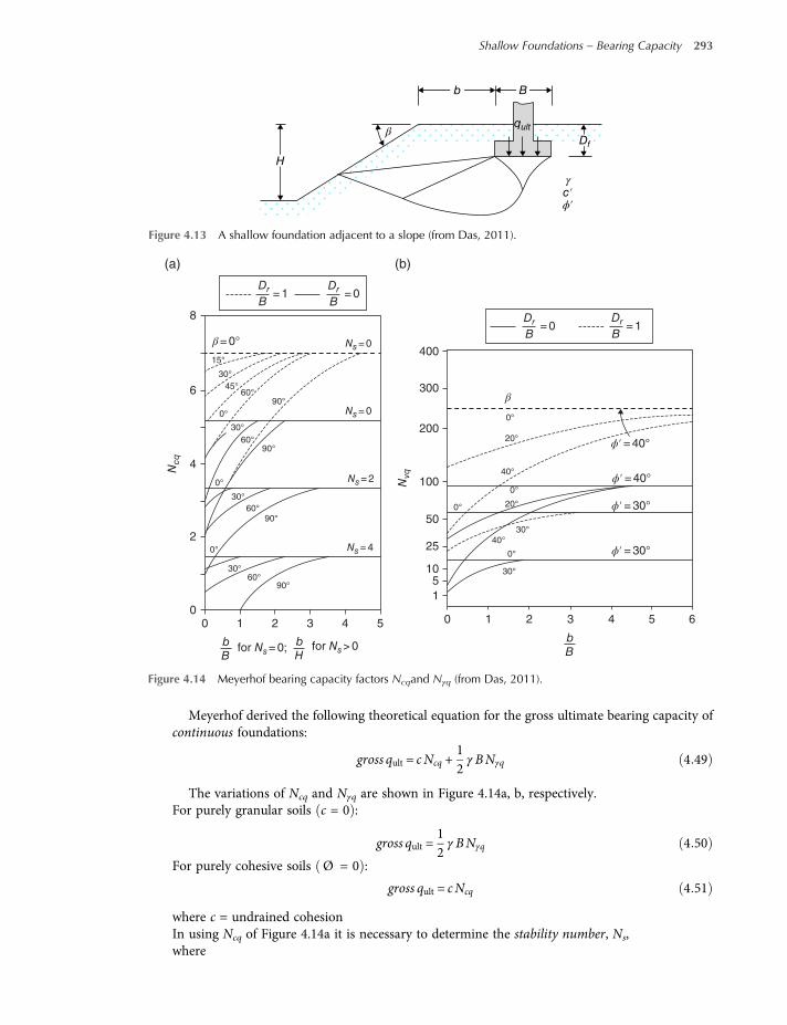
Meyerhof derived the following theoretical equation for the gross ultimate bearing capacity ofcontinuous foundations:
gross qult = cNcq +12γ BNγq 4 49
The variations of Ncq and Nγq are shown in Figure 4.14a, b, respectively.For purely granular soils c = 0 :
gross qult =12γ BNγq 4 50
For purely cohesive soils Ø = 0 :
gross qult = cNcq 4 51
where c = undrained cohesionIn using Ncq of Figure 4.14a it is necessary to determine the stability number, Ns,where
H
β
γ
b B
qult
Df
c′ϕ′
Figure 4.13 A shallow foundation adjacent to a slope (from Das, 2011).
8
6
400
(a) (b)
300
200
Ns= 0
Ns= 0
Ns= 2
Ns= 4
100
50
25
105
1
0 1 2 3 4 50 1
for Ns= 0; for Ns> 0
2 3 4 5 6
4
2
0
β
β = 0°
0°
0°
0°
Ncq
Nvq
0°
15°
30°
30°
30°
30°
45°60°
60°
60°
60°
90°
90°
90°
90°
0°
0°
20°
30°
40°
0°
30°
20°
40°
ϕ′ = 40°
ϕ′ = 40°
ϕ′ = 30°
ϕ′ = 30°
Bb
Dr
B= 0
Dr
B= 1
Hb
Bb
Dr
B= 0
Dr
B= 1
Figure 4.14 Meyerhof bearing capacity factors Ncqand Nγq (from Das, 2011).
Shallow Foundations – Bearing Capacity 293
worksaccounts.com
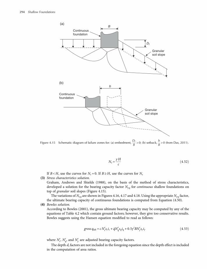
Ns =γHc
4 52
If B <H, use the curves for Ns = 0. If B≥H, use the curves for Ns
(3) Stress characteristics solution.Graham, Andrews and Shields (1988), on the basis of the method of stress characteristics,developed a solution for the bearing capacity factor Nγq for continuous shallow foundations ontop of granular soil slopes (Figure 4.15).
The variations ofNγq are shown in Figures 4.16, 4.17 and 4.18. Using the appropriate Nγq factor,the ultimate bearing capacity of continuous foundations is computed from Equation (4.50).
(4) Bowles solution.According to Bowles (2001), the gross ultimate bearing capacity may be computed by any of theequations of Table 4.2 which contain ground factors; however, they give too conservative results.Bowles suggests using the Hansen equation modified to read as follows:
gross qult = cNcscic + qNqsqiq + 0 5γ BNγsγiγ 4 53
where Nc, Nq, and Nγ are adjusted bearing capacity factors.
The depth di factors are not included in the foregoing equation since the depth effect is includedin the computation of area ratios.
Continuous
foundation
Continuous
foundation
Granular
soil slope
Granular
soil slope
(a)
b
B
Df
(b)
Figure 4.15 Schematic diagram of failure zones for: (a) embedment,Df
B>0; (b) setback,
bB>0 (from Das, 2011).
294 Shallow Foundations
worksaccounts.com
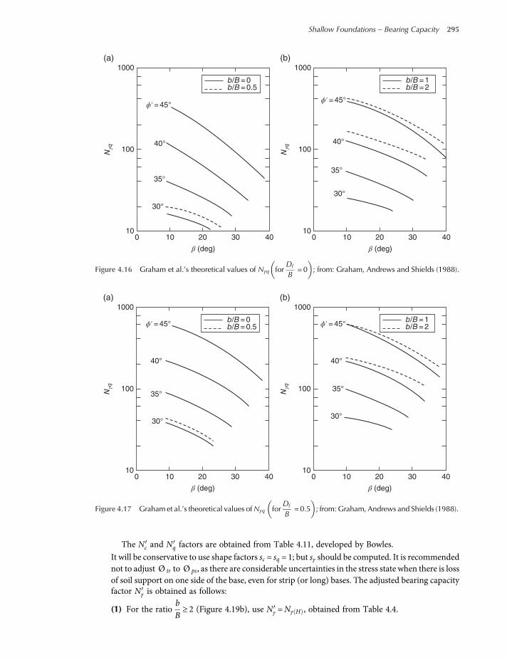
The Nc and Nq factors are obtained from Table 4.11, developed by Bowles.
It will be conservative to use shape factors sc = sq = 1; but sγ should be computed. It is recommendednot to adjust Ø tr to Ø ps, as there are considerable uncertainties in the stress state when there is lossof soil support on one side of the base, even for strip (or long) bases. The adjusted bearing capacityfactor Nγ is obtained as follows:
(1) For the ratiobB≥ 2 (Figure 4.19b), use Nγ =Nγ H , obtained from Table 4.4.
1000
100
10
1000
b/B = 0b/B = 0.5
100
100 10 20
β (deg) β (deg)
(a) (b)
ϕ′ = 45°ϕ′ = 45°
40° 40°
35°35°
30°
30°
Nγq
Nγq
30 40 0 10 20 30 40
b/B = 1b/B = 2
Figure 4.16 Graham et al.’s theoretical values of Nγq forDf
B=0 ; from: Graham, Andrews and Shields (1988).
1000
100
10
1000
b/B = 0b/B = 0.5
100
100 10 20
β (deg) β (deg)
(a) (b)
ϕ′ = 45° ϕ′ = 45°
40° 40°
35°35°
30°30°
Nγq
Nγq
30 40 0 10 20 30 40
b/B = 1b/B = 2
Figure 4.17 Graham et al.’s theoretical values ofNγq forDf
B=0 5 ; from: Graham, Andrews and Shields (1988).
Shallow Foundations – Bearing Capacity 295
worksaccounts.com

(2) For the ratiobB< 2, use Nγ = adjustedNγ H , as follows:
(a) Compute the Coulomb passive pressure coefficients for the slope angle β using β = − forone computation and + for the other. Use the friction angle δ= Ø and α= 90 for bothcomputations. The Coulomb passive pressure coefficient Kp can be computed from equa-tions or obtained from tables or curves, usually given in geotechnical text books. Whenβ = + or 0 is used, the computed Kp =Kmax on the base side away from the slopeand when β = − is used, the computed Kp =Kmin (see Figure 4.19).
(b) Compute a reduction factor R=Kmin Kmax
(c) Compute Nγ =Nγ H
2+Nγ H
2R+
b2B
1−R . This equation is easily checked:
At b= 0 and foundation on slope; Nγ =Nγ H
2+Nγ H
2R
At b= 2B and foundation on top of slope and out of slope influence; Nγ =Nγ H
4.13 Bearing Capacity of Footings on Layered Soils
4.13.1 General
All the preceding bearing capacity equations presented in Section 4.5 or referred to in the other sectionshave considered only the cases in which the supporting soil is homogeneous, with constant strengthparameters and unit weight with depth and extends to a depth sufficient to fully enclose the rupturezone. However, in practice, many soil profiles exist which are not uniform; consist of different soil typesin layers of variable thicknesses. In these cases, if the failure zone extends into the lower layer (or layersif they are very thin) the ultimate bearing capacity, undoubtedly, will be modified to some extent.
1000
100
10
1000
b/B = 0b/B = 0.5
100
100 10 20
β (deg) β (deg)
(a) (b)
ϕ′ = 45°ϕ′ = 45°
40°
40°
35°
35°
30°
30°
Nγq
Nγq
30 40 0 10 20 30 40
b/B = 1b/B = 2
Figure 4.18 Graham et al.’s theoretical values of Nγq forDf
B=1 ; from: Graham, Andrews and Shields (1988).
296 Shallow Foundations
worksaccounts.com
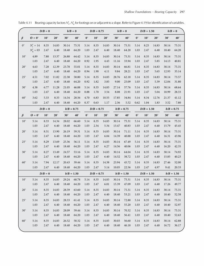
Table 4.11 Bearing capacity factorsNc,Nq for footings on or adjacent to a slope. Refer to Figure 4.19 for identification of variables.
D/B = 0 b/B = 0 D/B = 0.75 b/B = 0 D/B = 1.50 b/B = 0
β Ø = 0 10 20 30 40 0 10 20 30 40 0 10 20 30 40
0 Nc = 14 8.35 14.83 30.14 75.31 5.14 8.35 14.83 30.14 75.31 5.14 8.25 14.83 30.14 75.31
Nq = 03 2.47 6.40 18.40 64.20 1.03 2.47 6.40 18.40 64.20 1.03 2.47 6.40 18.40 64.20
10 4.89 7.80 13.37 26.80 64.42 5.14 8.35 14.83 30.14 75.31 5.14 8.35 14.83 30.14 75.31
1.03 2.47 6.40 18.40 64.20 0.92 1.95 4.43 11.16 33.94 1.03 2.47 5.85 14.13 40.81
20 4.63 7.28 12.39 23.78 55.01 5.14 8.35 14.83 30.14 66.81 5.14 8.35 14.83 30.14 75.31
1.03 2.47 6.40 18.40 64.20 0.94 1.90 4.11 9.84 28.21 1.03 2.47 5.65 12.93 35.14
25 4.51 7.02 11.82 22.38 50.80 5.14 8.35 14.83 28.76 62.18 5.14 8.35 14.83 30.14 73.57
1.03 2.47 6.40 18.40 64.20 0.92 1.82 3.85 9.00 25.09 1.03 2.47 5.39 12.04 31.80
30 4.38 6.77 11.28 21.05 46.88 5.14 8.35 14.83 27.14 57.76 5.14 8.35 14.83 30.14 68.64
1.03 2.47 6.40 18.40 64.20 0.88 1.70 3.54 8.08 21.91 1.03 2.47 5.04 10.99 28.33
60 3.62 5.33 8.33 14.34 28.56 4.70 6.83 10.55 17.85 34.84 5.14 8.34 12.76 21.37 41.12
1.03 2.47 6.40 18.40 64.20 0.37 0.63 1.17 2.36 5.52 0.62 1.04 1.83 3.52 7.80
D/B = 0 b/B = 0.75 D/B = 0.75 b/B = 0.75 D/B = 1.50 b/B = 0.75
β Ø = 0 10 20 30 40 0 10 20 30 40 0 10 20 30 40
10 5.14 8.33 14.34 28.02 66.60 5.14 8.35 14.83 30.14 75.31 5.14 8.35 14.83 30.14 75.31
1.03 2.47 6.40 18.40 64.20 1.03 2.34 5.34 13.47 40.83 1.03 2.47 6.40 15.79 45.45
20 5.14 8.31 13.90 26.19 59.31 5.14 8.35 14.83 30.14 71.11 5.14 8.35 14.83 30.14 75.31
1.03 2.47 6.40 18.40 64.20 1.03 2.47 6.04 14.39 40.88 1.03 2.47 6.40 16.31 43.96
25 5.14 8.29 13.69 25.36 56.11 5.14 8.35 14.83 30.14 67.49 5.14 8.35 14.83 30.14 75.31
1.03 2.47 6.40 18.40 64.20 1.03 2.47 6.27 14.56 40.06 1.03 2.47 6.40 16.20 42.35
30 5.14 8.27 13.49 24.57 53.16 5.14 8.35 14.83 30.14 64.04 5.14 8.35 14.83 30.14 74.92
1.03 2.47 6.40 18.40 64.20 1.03 2.47 6.40 14.52 38.72 1.03 2.47 6.40 15.85 40.23
60 5.14 7.94 12.17 20.43 39.44 5.14 8.35 14.38 23.94 45.72 5.14 8.35 14.83 27.46 52.00
1.03 2.47 6.40 18.40 64.20 1.03 2.47 5.14 10.05 22.56 1.03 2.47 4.97 9.41 20.33
D/B = 0 b/B = 1.50 D/B = 0.75 b/B = 1.50 D/B = 1.50 b/B = 1.50
10 5.14 8.35 14.83 29.24 68.78 5.14 8.35 14.83 30.14 75.31 5.14 8.35 14.83 30.14 75.31
1.03 2.47 6.40 18.40 64.20 1.03 2.47 6.01 15.39 47.09 1.03 2.47 6.40 17.26 49.77
20 5.14 8.35 14.83 28.59 63.60 5.14 8.35 14.83 30.14 75.31 5.14 8.35 14.83 30.14 75.31
1.03 2.47 6.40 18.40 64.20 1.03 2.47 6.40 18.40 53.21 1.03 2.47 6.40 18.40 52.58
25 5.14 8.35 14.83 28.33 61.41 5.14 8.35 14.83 30.14 72.80 5.14 8.35 14.83 30.14 75.31
1.03 2.47 6.40 18.40 64.20 1.03 2.47 6.40 18.40 55.20 1.03 2.47 6.40 18.40 52.97
30 5.14 8.35 14.83 28.09 59.44 5.14 8.35 14.83 30.14 70.32 5.14 8.35 14.83 30.14 75.31
1.03 2.47 6.40 18.40 64.20 1.03 2.47 6.40 18.40 56.41 1.03 2.47 6.40 18.40 52.63
60 5.14 8.35 14.83 26.52 50.32 5.14 8.35 14.83 30.03 56.60 5.14 8.35 14.83 30.14 62.88
1.03 2.47 6.40 18.40 64.20 1.03 2.47 6.40 18.40 46.18 1.03 2.47 6.40 16.72 36.17
Shallow Foundations – Bearing Capacity 297
worksaccounts.com
The easiest way to tackle this problem is estimating the bearing capacity using the lowest values ofstrength parameters (c, Ø) and unit weight (γ) in the zone between the foundation level and a depth Bbelow that level (i.e. the zone in which bearing capacity failures occur), where B equals to the founda-tion width. This procedure may be too conservative, since the rupture zone comprises the strongerlayers also. Therefore, this methodmay be adopted only when it is clear that the bearing capacity failurecriterion does not control the geotechnical design even with a conservative analysis (i.e. the settlementcriterion controls); thus, there would be no need to conduct a more detailed analysis. Another way tohandle the problem of layered soils is using weighted average values of strength parameters and unitweight based on the relative thicknesses of each stratum in the zone in which bearing capacity failuresoccur. This method could be conservative or unconservative, but should provide acceptable results solong as the differences in the strength parameters are not too great (Coduto, 2001). A more detailedmethod, in which a series of trial slip surfaces under the foundation are considered, requires more effortto implement and would be appropriate only for critical projects on complex soil profiles. For thesereasons, numerous solutions have been proposed to enable one to make an estimate of the ultimatebearing capacity. Some of these solutions will be presented in the following sections.
4.13.2 Ultimate Bearing Capacity: Stronger Soil Underlain by Weaker Soil
(A) General caseMeyerhof and Hanna (1978) and Meyerhof (1974) proposed semi-theoretical methods for esti-mating ultimate bearing capacity of a shallow continuous foundation supported by two-layeredsoils. The stronger soil layer which exists immediately beneath the foundation, underlain by a
45 − (ϕ/2)
β
β
45 + (ϕ/2)
(a)
Slope
Slope
(b)
FootingDf
Df
B
V
B
V
b
Footing
Figure 4.19 Foundation: (a) on a slope; (b) adjacent to a slope.
298 Shallow Foundations
worksaccounts.com

weaker soil layer, extends to a great depth, as shown in Figure 4.20. The physical parametersγ1, Ø 1,c1 and γ2, Ø 2,c2 belong to the stronger and weaker soil layers (top and bottom layers),respectively. In case the depth H is small compared with the foundation width B, the punchingshear failure will take place in the top soil layer, followed by a general shear failure in the bottomsoil layer, as shown in Figure 4.20a. In case, however, the depth H is large, then the general shearfailure completely occurs in the top soil layer, as shown in Figure 4.20b. This condition is con-sidered the upper limit of the ultimate bearing capacity.
Considering these two cases, the following equation for ultimate bearing capacity of a continu-ous footing could be derived (Das, 2011):
qult = qult,b +2caHB
+ γ1H2 1 +
2Df
HKs tan Ø 1
B−γ1H ≤ qult, t 4 54
Where
qult, t = c1Nc 1 + γ1Df Nq 1 +12γ1BNγ 1
= ultimate bearing capacity of the top stronger soil layer
4 55
Pp
=passiv
e forc
e p
er
unit length
of th
e faces a
a′ a
nd b
b′
Weaker soil
(a)
(b)
Stronger soil
Df
Df
II
II
B
B
Ca
δ′ δ′
Ca
qu
qu
a
a′ b′
c′1
bγ′1
Pp Pp
ϕ′1
c′1
γ′1ϕ′1Stronger soil
c′2
γ′2ϕ′2
c′2
γ′2ϕ′2Weaker soil
Figure 4.20 Bearing capacity of continuous foundation on layered soil(adapted from Das, 2011).
Shallow Foundations – Bearing Capacity 299
worksaccounts.com

qult,b = c2Nc 2 + γ1 Df +H Nq 2 +12γ2BNγ 2 4 56
q1 = c1Nc 1 +12γ1BNγ 1 4 57
q2 = c2Nc 2 +12γ2BNγ 2 4 58
Ks = punching shear coefficient; its variation withq2q1
and Ø 1 is shown in Figure 4 21 -
ca = unit adhesion of stronger soil. The variation ofcac1
withq2q1
is shown in Figure 4.22.
Ca = adhesive force = caH
40
40 50
30
30
20
20
10
0
Ks
q2
q1= 1
0.4
0.2
0
ϕ′1(des)
Figure 4.21 Meyerhof and Hanna’s punching shear coefficient Ks.
1.0
0.9
0.8
0.7
0.60 0.2 0.4 0.6 0.8 1.0
C′aC′1
q2
q1
Figure 4.22 Variation ofcac1
withq2
q1based on the theory of Meyerhof and Hanna (1978).
300 Shallow Foundations
worksaccounts.com

For rectangular foundations, Equation 4.54 can be extended to the form
qult = qult,b + 1 +BL
2caHB
+ γ1H2 1 +
BL
1 +2Df
HKs tan Ø 1
B−γ1H ≤ qult, t 4 59
Where
qult, t = c1Nc 1 Fcs 1 + γ1Df Nq 1 Fqs 1 +12γ1BNγ 1 Fγs 1 4 60
qult,b = c2Nc 2 Fcs 2 + γ1 Df +H Nq 2 Fqs 2 +12γ2BNγ 2 Fγs 2 4 61
Fcs 1 , Fqs 1 , Fγs 1 = Shape factors with respect to the stronger soil layer
Fcs 2 , Fqs 2 , Fγs 2 = Shape factors with respect to the weaker soil layer
(B) Special cases(1) Strong sand (top layer) overlying saturated soft clay Ø 2 = 0
From Equation (4.61):
qult,b = 1 + 0 2BL
5 14c2 + γ1 Df +H 4 62
From Equation (4.60):
qult, t = γ1Df Nq 1 Fqs 1 +12γ1BNγ 1 Fγs 1 4 63
Hence, from Equation (4.59):
qult = 1 + 0 2BL
5 14c2 + γ1H2 1 +
BL
1 +2Df
HKs tan Ø 1
B+ γ1Df ≤ γ1Df Nq 1 Fqs 1
+12γ1BNγ 1 Fγs 1
4 64
wherec2 = undrained cohesion of the soft clayKs is determined from Figure 4.21, using
q2q1
=c2Nc 2
12γ1BNγ 1
=5 14c2
0 5γ1BNγ 14 65
(2) Stronger sand (top layer) overlying weaker sand c1 = 0,c2 = 0From Equation (4.61):
qult,b = γ1 Df +H Nq 2 Fqs 2 +12γ2BNγ 2 Fγs 2 4 66 - a
From Equation (4.60):
qult, t = γ1Df Nq 1 Fqs 1 +12γ1BNγ 1 Fγs 1 4 66 - b
Shallow Foundations – Bearing Capacity 301
worksaccounts.com

Hence, from Equation (4.59):
qult = γ1 Df +H Nq 2 Fqs 2 +12γ2BNγ 2 Fγs 2 + γ1H
2 1 +BL
1 +2Df
HKs tanØ 1
B−γ1H
≤ γ1Df Nq 1 Fqs 1 +12γ1BNγ 1 Fγs 1
4 67
Ks is determined from Figure 4.21, using
q2q1
=
12γ2BNγ 2
12γ1BNγ 1
=γ2BNγ 2
γ1BNγ 14 68
(3) Stronger saturated clay Ø 1 = 0 overlying weaker saturated clay Ø 2 = 0From Equation (4.61):
qult,b = 1 + 0 2BL
5 14c2 + γ1 Df +H
From Equation (4.60):
qult, t = 1 + 0 2BL
5 14c1 + γ1Df 4 69
Hence, from Equation (4.59):
qult = 1 + 0 2BL
5 14c2 + 1 +BL
2caHB
+ γ1Df
≤ 1 + 0 2BL
5 14c1 + γ1Df
4 70
wherec1 and c2 = undrained cohesion of the top and bottom clays,ca is determined from Fig. 4.22, using
q2q1
=5 14c25 14c1
=c2c1
4 71
4.13.3 Ultimate Bearing Capacity: Weaker Soil Underlain by Stronger Soil
Refer to Figure 4.23a. If the ratioHBis relatively small, the slip surface at ultimate load will pass through
both soil layers, as shown in the left half of the figure. For largeHBratio, however, the failure surface will
be completely located in the weaker soil layer which overlies the stronger soil, as shown in the right halfof the figure. The ultimate bearing capacities q1 and q2 are the same as defined by Equations (4.57)
and (4.58); however, the ratioq2q1
should be greater than unity.
302 Shallow Foundations
worksaccounts.com
For this case, the ultimate bearing capacity can be given by the following semi-theoretical generalequation (Meyerhof, 1974; Meyerhof and Hanna, 1978):
qult = qult, t + qult,b−qult, tHD
2
≥ qult, t 4 72
Where:
qult, t = c1Nc 1 Fcs 1 + γ1Df Nq 1 Fqs 1 +12γ1BNγ 1 Fγs 1
= ultimate bearing capacity of the top weaker soil layer
4 73
Weaker soil Weaker soil
Stronger soil
Stronger soil
qult
Df
H
H
B
D
qult, b
qult, t
H/B
D/B
c′1
γ′1ϕ′1
c′2
γ′2ϕ′2
c′2
γ′2ϕ′2
(a)
(b)
Figure 4.23 (a) Foundation on weaker soil layer underlain by stronger soil layer. (b) Nature of variation of qultwith (H/B). From Das (2011).
Shallow Foundations – Bearing Capacity 303
worksaccounts.com

qult,b = c2Nc 2 Fcs 2 + γ2Df Nq 2 Fqs 2 +12γ2BNγ 2 Fγs 2
= ultimate bearing capacity of the bottom stronger soil layer
4 74
D = maximum depth of failure surface beneath the foundation in the thick bed of the upper (weaker)soil layer.
Meyerhof and Hanna (1978) suggested that:
D≈B for loose sand and clayD≈2B for dense sand
Equations (4.72) to (4.74) indicate that qult,b ≥ qult ≥ qult, t , as shown in Figure 4.23b.Equation (4.72) is general; can be applied to special cases as needed following the same procedure
delineated in Section 4.13.2
4.14 Safety Factor
One of the main performance requirements of any structure is strength.With respect to foundations, asexplained in Section 2.4, this performance requirement comprises both the geotechnical strength andthe structural strength. In general, structures are designed on the basis of determining the service loadsand obtaining a suitable ratio of material strength to these loads, termed either a safety factor (SF; ingeotechnical design) or load factor (in structural design). These factors are used to compensate for themany uncertainties usually associated with analysis and design of structures, particularly, foundations.Thus, reliable designs could be developed. In design, the selected safety factor defines the designer’sestimate of the best compromise between cost and reliability. Therefore, in selection of an appropriatesafety factor the designer should consider many factors or parameters, including: importance of struc-ture, probability of failure and its consequences; uncertainties in materials properties, applied loads andanalytical methods; cost–benefit ratio of additional conservatism in the design.
In the analysis and design of foundations, especially the geotechnical part, there are more uncertain-ties than those associated with analysis and design of superstructure elements. For this reason, safetyfactors in foundations are typically greater than those in the superstructure. These uncertainties andtheir causes may be stated as follows:
Insufficient knowledge of subsurface conditionsDeficient in accurate determination of the soil propertiesComplexity of soil behavior and soil–structure interactionDeficient in methods of analysesLack of control over environmental changes after construction
Coduto (2001) presents the necessary parameters and the typical values of safety factor which areusually considered in selecting an adequate design safety factor, as shown in Figure 4.24. Geotechnicalengineers usually use SF between 2.5 and 3.5 for bearing capacity analyses of shallow foundations.Occasionally, however, they might use values as low as 2.0 or as high as 4.0.
It may be useful to mention herein that the true safety factor is probably greater than the designsafety factor, for one or combination of the following reasons:
(1) Where settlement controls the final design, the safe bearing capacity will be reduced, which in turnincreases the real safety factor.
(2) The shear strength data are usually interpreted conservatively, so the design strength parameters cand Ø implicitly contain another safety factor.
304 Shallow Foundations
worksaccounts.com

(3) The service loads are probably less than the design loads.(4) Spread footings are commonly built somewhat larger than the plan dimensions.(5) Where the same design safety factor for a spread footing 2 5−3 5 is also used for a mat foun-
dation, the real safety factor of the mat will be higher because, normally, mats require a lowerdesign safety factor 2 0−2 5 .
4.15 Bearing Capacity from Results of In Situ Tests
(1) From results of standard penetration test.The standard penetration test, SPT, has been described and explained in some detail in the dis-cussion of solution of Problem 1.6. Also, the use of SPT results, that is N-values, in estimatingsettlement of granular soils was discussed in Section 3.3.2. In that discussion a set of allowablebearing capacity equations [Equations (3.11) to (3.13)], based on SPT results, have been presented.These equations give net allowable bearing capacity for a specified 25 mm settlement. It has beenstated also that for cohesionless soils, it is possible to assume that settlement is proportional tonet allowable soil pressure. Based on this assumption, a net allowable soil pressure, netq Si , foran allowable settlement other than 25 mm can be estimated using Equation (3.14).
(2) From results of plate-load test.The plate-load test, PLT, was described and explained in some detail in the discussion of the Solu-tion of Problem 1.9. Also, the use of PLT results, that is the time settlement curves (Figure 1.12a)for different load increments and the load settlement curve (Figure 1.12b), was explained in thediscussion of the Solution of the same Problem. In that discussion a set of equations[Equations (1.37) to (1.39)], based on PLT results, were presented. These equations give ultimatebearing capacities, qult, for different types of soils. However, due to several factors which areexplained in the same discussion and also in Section 3.3.1, the extrapolation of the PLT resultsto full-size footings is questionable except in very limited cases.
(3) From results of cone penetration test.The static cone penetration test, CPT, was described and explained in some detail in the discussionof the Solution of Problem 1.13. Also, the CPT correlations for both cohesive and cohesionless soils(i.e. qc with cu or su and Ø correlations) have been provided. It is obvious that we can use theseCPT correlations to obtain the necessary parameters so that the bearing capacity equations ofTable 4.2 can be applied. Furthermore, correlations for the SPT-N values have been presented,as shown in Figure 1.18, Table 1.11 and Equation (1.56). The net allowable bearing capacity ofsand can be estimated directly using Equations (3.11) to (3.13) in which the N55 is replaced
(approximately) byqc4(Meyerhof, 1956), where qc is in units of kg/cm2.
Soil Type Sand Clay
Site characterisation data Extensive Minimal
Soil variability Uniform Erratic
Importance of structure
and consequences of failure
Low High
Likelihood of design load
occurringLow High
Design SF extreme values 2.0 4.0
Typical range 25 3.5
Figure 4.24 Factors considered in selecting design safety factor and typical values of SF (adapted fromCoduto, 2001).
Shallow Foundations – Bearing Capacity 305
worksaccounts.com

According to Schmertmann (1978), the bearing capacity factors for use in the Terzaghi bearingcapacity equation of Table 4.2 can be estimated as
0 8Nq 0 8Nγ qc forDB
≤ 1 5 4 75
The qc (kg/cm2) is averaged over the depth interval from about B/2 above to 1.1 B below the
footing base.For cohesionless soils one may use
qult = 28−0 0052 300−qc1 5 kg cm2 Strip footings 4 76
qult = 48−0 009 300−qc1 5 kg cm2 Square footings 4 77
For clays one may useqult = 2 + 0 28 qc kg cm2 Strip footings 4 78
qult = 5 + 0 34 qc kg cm2 Square footings 4 79
According to Bowles (2001), Equations (4.76) through (4.79) are based on charts given bySchmertmann (1978) credited to an unpublished reference by Awakti.
4.16 Uplift Capacity of Shallow Foundations
Foundations under special circumstances, particularly in industrial applications, are subjected to exter-nal uplift or tension forces. Examples are: footings for the columns (legs) of an elevated water tank,bases for legs of power transmission towers, anchorages for the anchor cables of transmission towersand many other industrial equipment installations.
Balla (1961) considered the problem of round footings which develop tension resistance. Heassumed circular failure surfaces and developed mathematical expressions. Later, Meyerhof andAdams (1968) studied the problem and proposed two conditions; one for shallow and the other fordeep footings, as shown in Figure 4.25. They provided relationships to estimate the ultimate upliftingload for shallow circular and rectangular footings.
Refer to Figure 4.26. The ultimate load Qu (or the ultimate tension Tu) can be expressed in the formof a nondimensional breakout factor Fq as follows:
Fq =Qu
A γDf4 80
where A = area of footing
Probable
pull-out
zone
Probable
pull-out
zone
Shallow (D ≤ H) Deep (D > H)
WD
D
L1q = γ L1
aB
H
b′b
Tu
Figure 4.25 Footing under uplift load.
306 Shallow Foundations
worksaccounts.com

The factor Fq is a function of the soil friction angle Ø and the embedment ratioDf/B. For a given soilfriction angle, the breakout factor increases with increase in Df/B and reaches its maximum value atDf/B equals to the critical embedment ratio, (Df/B)cr. For shallow foundations the embedment ratioDf B≤ Df B cr, whereas for deep foundations Df B > Df B cr. Using Equation (4.80) and therelationships developed by Meyerhof and Adams (1968), Das and Seely (1975) developed relationshipsfor foundations subjected to uplift load as follows:
(A) Uplift capacity of footings in granular soils c = 0For shallow circular and square foundations:
Fq = 1 + 2 1 +mDf
B
Df
BKu tan Ø 4 81
For shallow rectangular foundations:
Fq = 1 + 1 + 2mDf
BBL
+ 1Df
BKu tan Ø 4 82
wherem = a coefficient which is a function of ØKu = nominal uplift coefficient
The variations of Ku,m and (Df/B)cr for square and circular foundations are given in Table 4.12(Meyerhof and Adams, 1968).Das and Jones (1982) recommended the following critical embedment ratio for rectangularfoundations:
Df
B cr, rec
=Df
B cr, sq
0 133LB
+ 0 867 ≤ 1 4Df
B cr, sq
4 83
Figure 4.27 shows variations of Fq with Df/B and Ø for square and circular foundations. Thevariations have been calculated from Equation (4.81).
Assumed approximation for
surface of shear resistance
Probable actual
pull-out zone
Sand
Pp
Df
B
Pp
Qu
α
Unit weight = γFriction angle = ϕ′
δ′ δ′
Figure 4.26 Shallow continuous foundation subjected to uplift load (reproduced from Das, 2011).
Shallow Foundations – Bearing Capacity 307
worksaccounts.com
According to Das (2011), the steps of the procedure to estimate the uplift capacity of founda-tions in granular soils are as below:(1) Determine Df, B, L and Ø .(2) Calculate Df/B.(3) Using Table 4.12 and Equation (4.83), calculate (Df/B)cr.(4) If Df/B is less than or equal to (Df/B)cr, it is a shallow foundation.(5) If Df/B is greater than (Df/B)cr, it is a deep foundation.(6) For shallow foundations, use Df/B calculated in Step 2 in Equation (4.81) or (4.82) to estimate
Fq. Thus, Qu = FqAγDf .(7) For deep foundations, substitute (Df/B)cr for Df/B in Equation (4.81) or (4.82) to obtain Fq
from which the ultimate load Qu may be obtained.(B) Uplift capacity of footings in cohesive soils Ø =0
The ultimate load Qu of a foundation in a cohesive soil, considering Ø = 0, may be expressed as
Qu =A γDf + cuFc 4 84
Table 4.12 Variations of Ku, m and (Df/B)cr for circular and square foundations.
Ø (deg) Ku m (Df/B)cr
20 0.856 0.05 2.5
25 0.888 0.10 3
30 0.920 0.15 4
35 0.936 0.25 5
40 0.960 0.35 7
45 0.960 0.50 9
100
10Fq
11 2 3 4 5 6 7 8 9 10
Df /B
ϕ′ = 45°
40°
35°
30°
Figure 4.27 Variations of Fq with Df/B and Ø for circular and square foundations.
308 Shallow Foundations
worksaccounts.com
whereA = area of foundationcu = undrained shear strength of soilFc = breakout factor
The breakout factor increases with increase inDf/B and reaches its maximum value of Fc = F∗c at
Df/B equals to the critical embedment ratio, (Df/B)cr. Das (1978, 1980) proposed
Df
B cr
= 0 107 cu + 2 5 ≤ 7 for square and circular footings 4 85
where
cu = undrained shear strength of soil, in kN m2
Df
B cr
=Df
B cr, sq
0 73 + 0 27LB
≤ 1 55Df
B cr, sq
for rectangular footings
4 86
whereL = length of footing
According to Das (2011), steps of the procedure to estimate the uplift capacity of foundations incohesive soils are as below:
(1) Determine the undrained cohesion, cu.(2) Determine the (Df /B)cr using Equations (4.85) and (4.86).
(3) Determine theDf
Bratio of the foundation. If Df B≤ Df B cr, it is a shallow foundation.
However, if Df/B is greater than (Df /B)cr, it is a deep foundation.(4) For Df B > Df B cr (i.e. deep foundations)
Fc = F∗c = 7 56 + 1 44
BL
Qu =A 7 56 + 1 44BL
cu + γDf
4 87
(5) For Df B≤ Df B cr (i.e. shallow foundations)
Qu =A B F∗c cu + γDf =A B 7 56 + 1 44
BL
cu + γDf 4 88
where:
B =FcF∗c
, obtained from the average curve of Figure 4.28 which shows a plot of B versus a non-
dimensional factor α .
α =Df B
Df B cr
According to Das, the procedures outlined above give fairly good results for estimating the netultimate uplift capacity of foundations and agree reasonably well with the theoretical solution ofMerifield et al. (2003).
Shallow Foundations – Bearing Capacity 309
worksaccounts.com

4.17 Some Comments and Considerations Concerning theGeotechnical Design of Shallow Foundations
(1) The geotechnical design of a shallow foundation comprises determination of the depth of foun-dation and the dimensions of the foundation base area through assessment of the results of bearingcapacity and settlement analyses, as well as other considerations, so that the applied loads are trans-ferred from the foundation to the ground safely.
The foundation depth was discussed in some detail in Section 2.3. Dimensions of the base areaare determined such that the net effective foundation pressure net q , is always less or equal to thenet allowable bearing capacity (or design soil pressure) net qa; see Equation (4.11). Therefore, as itis obvious, the main and most important task in geotechnical design is how to determine net qareasonably so that the performance requirements of Section 2.4 are satisfied. However, the basedimensions are usually required in executing the bearing capacity and settlement computations.For example, the width B and length L dimensions are needed to compute shape, depth and loadinclination factors which are contained in the ultimate bearing capacity equations of Table 4.2.Therefore, the analysis methods require trial process to obtain the design base dimensions.
(2) In selecting a design soil pressure, it is important to consider the following:
• If the supporting soil is very loose and saturated, it should be compacted and retested. Based onthe available new data, an allowable bearing capacity can be selected.
• Usually, the allowable bearing capacity values for sand, except for narrow footings on loose sat-urated sand, are governed only by settlement considerations, because it can be taken for grantedthat the safety factor with respect to bearing capacity failure (base failure) is adequate (Terzaghiand Peck, 1967). On routine jobs the net allowable soil pressure on dry and moist sand can bedetermined from Equations (3.11) to (3.13) on the basis of the results of SPT or CPT. TheseEquations satisfy the condition that the maximum total and differential settlements are unlikelyto exceed 25 and 20 mm, respectively. Obviously, results of computations using these equationsmay be verified, if desired, using other appropriate bearing capacity and settlement equations.
• The net ultimate bearing capacity for clay can be calculated on the basis of the equations givenin Table 4.2 and the results of unconfined compression tests or undrained shear tests. The net
1.2
1.0
0.8
0.6
0.4
0.2
0
0 0.2
Upp
er lim
it
Avera
ge
Lower lim
it
0.4 0.6 0.8 1.0
B′
α′
Figure 4.28 Plot of β versus α .
310 Shallow Foundations
worksaccounts.com
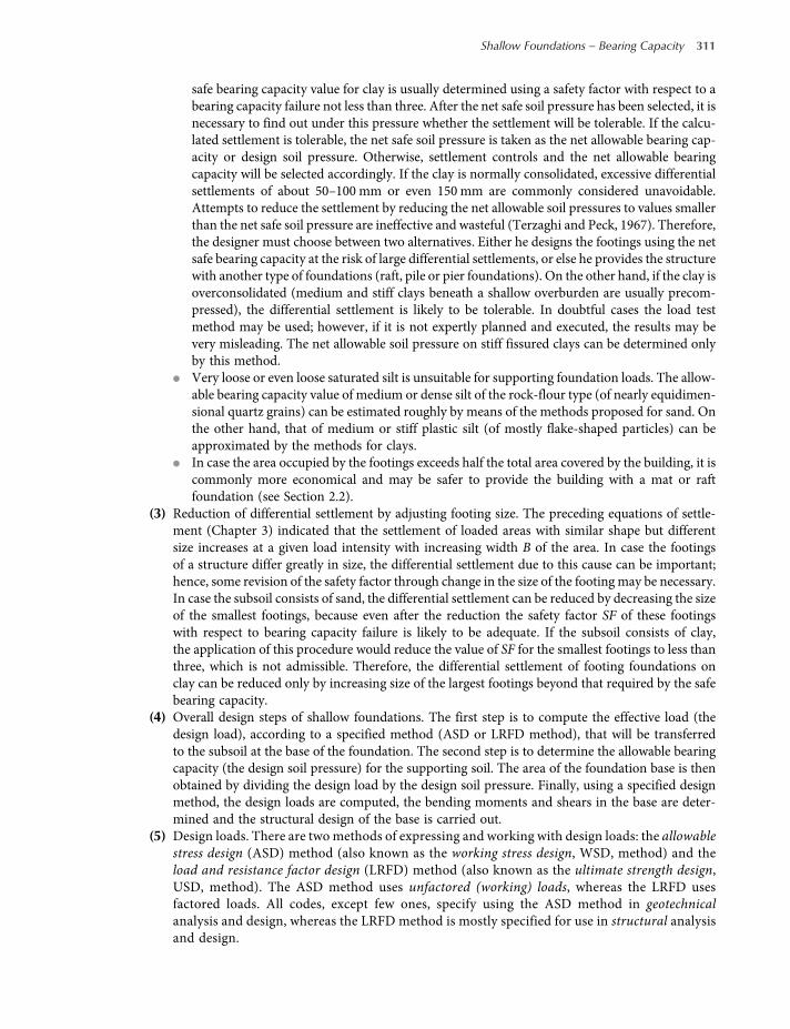
safe bearing capacity value for clay is usually determined using a safety factor with respect to abearing capacity failure not less than three. After the net safe soil pressure has been selected, it isnecessary to find out under this pressure whether the settlement will be tolerable. If the calcu-lated settlement is tolerable, the net safe soil pressure is taken as the net allowable bearing cap-acity or design soil pressure. Otherwise, settlement controls and the net allowable bearingcapacity will be selected accordingly. If the clay is normally consolidated, excessive differentialsettlements of about 50–100 mm or even 150 mm are commonly considered unavoidable.Attempts to reduce the settlement by reducing the net allowable soil pressures to values smallerthan the net safe soil pressure are ineffective and wasteful (Terzaghi and Peck, 1967). Therefore,the designer must choose between two alternatives. Either he designs the footings using the netsafe bearing capacity at the risk of large differential settlements, or else he provides the structurewith another type of foundations (raft, pile or pier foundations). On the other hand, if the clay isoverconsolidated (medium and stiff clays beneath a shallow overburden are usually precom-pressed), the differential settlement is likely to be tolerable. In doubtful cases the load testmethod may be used; however, if it is not expertly planned and executed, the results may bevery misleading. The net allowable soil pressure on stiff fissured clays can be determined onlyby this method.
• Very loose or even loose saturated silt is unsuitable for supporting foundation loads. The allow-able bearing capacity value of medium or dense silt of the rock-flour type (of nearly equidimen-sional quartz grains) can be estimated roughly by means of the methods proposed for sand. Onthe other hand, that of medium or stiff plastic silt (of mostly flake-shaped particles) can beapproximated by the methods for clays.
• In case the area occupied by the footings exceeds half the total area covered by the building, it iscommonly more economical and may be safer to provide the building with a mat or raftfoundation (see Section 2.2).
(3) Reduction of differential settlement by adjusting footing size. The preceding equations of settle-ment (Chapter 3) indicated that the settlement of loaded areas with similar shape but differentsize increases at a given load intensity with increasing width B of the area. In case the footingsof a structure differ greatly in size, the differential settlement due to this cause can be important;hence, some revision of the safety factor through change in the size of the footing may be necessary.In case the subsoil consists of sand, the differential settlement can be reduced by decreasing the sizeof the smallest footings, because even after the reduction the safety factor SF of these footingswith respect to bearing capacity failure is likely to be adequate. If the subsoil consists of clay,the application of this procedure would reduce the value of SF for the smallest footings to less thanthree, which is not admissible. Therefore, the differential settlement of footing foundations onclay can be reduced only by increasing size of the largest footings beyond that required by the safebearing capacity.
(4) Overall design steps of shallow foundations. The first step is to compute the effective load (thedesign load), according to a specified method (ASD or LRFD method), that will be transferredto the subsoil at the base of the foundation. The second step is to determine the allowable bearingcapacity (the design soil pressure) for the supporting soil. The area of the foundation base is thenobtained by dividing the design load by the design soil pressure. Finally, using a specified designmethod, the design loads are computed, the bending moments and shears in the base are deter-mined and the structural design of the base is carried out.
(5) Design loads. There are two methods of expressing and working with design loads: the allowablestress design (ASD) method (also known as the working stress design, WSD, method) and theload and resistance factor design (LRFD) method (also known as the ultimate strength design,USD, method). The ASD method uses unfactored (working) loads, whereas the LRFD usesfactored loads. All codes, except few ones, specify using the ASD method in geotechnicalanalysis and design, whereas the LRFD method is mostly specified for use in structural analysisand design.
Shallow Foundations – Bearing Capacity 311
worksaccounts.com
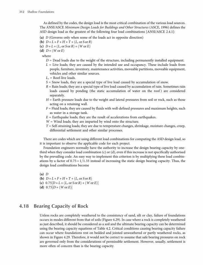
As defined by the codes, the design load is the most critical combination of the various load sources.The ANSI/ASCEMinimum Design Loads for Buildings and Other Structures (ASCE, 1996) defines theASD design load as the greatest of the following four load combinations [ANSI/ASCE 2.4.1]:
(a) D (Governs only when some of the loads act in opposite direction)(b) D+ L+ F +H +T + Lr or S orR(c) D+ L+ Lr or S orR + W orE(d) D+ W orE
whereD = Dead loads due to the weight of the structure, including permanently installed equipment.L = Live loads; they are caused by the intended use and occupancy. These include loads from
people, furniture, inventory, maintenance activities, moveable partitions, moveable equipment,vehicles and other similar sources.
Lr = Roof-live loads.S = Snow loads, they are a special type of live load caused by accumulation of snow.R = Rain loads; they are a special type of live load caused by accumulation of rain. Sometimes rain
loads caused by ponding (the static accumulation of water on the roof ) are consideredseparately.
H = Earth pressure loads due to the weight and lateral pressures from soil or rock, such as thoseacting on a retaining wall.
F = Fluid loads; they are caused by fluids with well-defined pressures and maximum heights, suchas water in a storage tank.
E = Earthquake loads; they are the result of accelerations from earthquakes.W = Wind loads; they are imparted by wind onto the structure.T = Self-straining loads; they are due to temperature changes, shrinkage, moisture changes, creep,
differential settlement and other similar processes.
There are codes which are using different load combinations for computing the ASD design load, soit is important to observe the applicable code for each project.
Foundation engineers normally have the authority to increase the design bearing capacity by one-third when they consider load combination (c) or (d), even if this increase is not specifically authorisedby the prevailing code. An easy way to implement this criterion is by multiplying these load combin-ations by a factor of 0 75 = 1 1 33 instead of increasing the static design bearing capacity. Thus, thedesign load combinations become
(a) D(b) D+ L+ F +H +T + Lr or S orR(c) 0 75 D+ L+ Lr or S orR + W orE(d) 0 75 D+ W orE
4.18 Bearing Capacity of Rock
Unless rocks are completely weathered to the consistency of sand, silt or clay, failure of foundationsoccurs in modes different from that of soils (Figure 4.29). In case where a rock is completely weatheredas just described, it should be considered as a soil and the ultimate bearing capacity can be determinedusing the bearing capacity equations of Table 4.2. Critical conditions causing bearing capacity failurecan occur where foundations rest on bedded and jointed unweathered or partly weathered rocks, asshown in Figure 4.29. Therefore, it would not be correct to assume that safe bearing pressures on rockare governed only from the considerations of permissible settlement. However, usually, settlement ismore often of concern than is the bearing capacity.
312 Shallow Foundations
worksaccounts.com
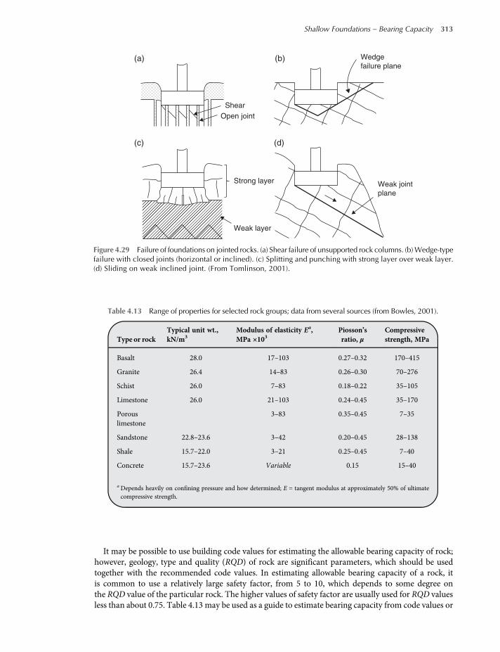
It may be possible to use building code values for estimating the allowable bearing capacity of rock;however, geology, type and quality (RQD) of rock are significant parameters, which should be usedtogether with the recommended code values. In estimating allowable bearing capacity of a rock, itis common to use a relatively large safety factor, from 5 to 10, which depends to some degree onthe RQD value of the particular rock. The higher values of safety factor are usually used for RQD valuesless than about 0.75. Table 4.13 may be used as a guide to estimate bearing capacity from code values or
Shear
Wedge
failure plane
Weak joint
plane
Strong layer
Weak layer
Open joint
(a) (b)
(c) (d)
Figure 4.29 Failure of foundations on jointed rocks. (a) Shear failure of unsupported rock columns. (b)Wedge-typefailure with closed joints (horizontal or inclined). (c) Splitting and punching with strong layer over weak layer.(d) Sliding on weak inclined joint. (From Tomlinson, 2001).
Table 4.13 Range of properties for selected rock groups; data from several sources (from Bowles, 2001).
Type or rockTypical unit wt.,kN/m3
Modulus of elasticity Ea,MPa ×103
Piosson’sratio, μ
Compressivestrength, MPa
Basalt 28.0 17–103 0.27–0.32 170–415
Granite 26.4 14–83 0.26–0.30 70–276
Schist 26.0 7–83 0.18–0.22 35–105
Limestone 26.0 21–103 0.24–0.45 35–170
Porouslimestone
3–83 0.35–0.45 7–35
Sandstone 22.8–23.6 3–42 0.20–0.45 28–138
Shale 15.7–22.0 3–21 0.25–0.45 7–40
Concrete 15.7–23.6 Variable 0.15 15–40
aDepends heavily on confining pressure and how determined; E = tangent modulus at approximately 50% of ultimatecompressive strength.
Shallow Foundations – Bearing Capacity 313
worksaccounts.com
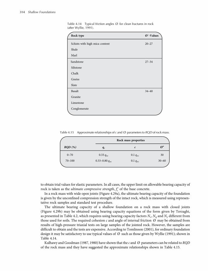
to obtain trial values for elastic parameters. In all cases, the upper limit on allowable bearing capacity ofrock is taken as the ultimate compressive strength, fc of the base concrete.
In a rock mass with wide open joints (Figure 4.29a), the ultimate bearing capacity of the foundationis given by the unconfined compression strength of the intact rock, which is measured using represen-tative rock samples and standard test procedure.
The ultimate bearing capacity of a shallow foundation on a rock mass with closed joints(Figure 4.29b) may be obtained using bearing capacity equations of the form given by Terzaghi,as presented in Table 4.2, which requires using bearing capacity factors Nc, Nq and Nγ different fromthose used for soils. The required cohesion c and angle of internal friction Ø may be obtained fromresults of high-pressure triaxial tests on large samples of the jointed rock. However, the samples aredifficult to obtain and the tests are expensive. According to Tomlinson (2001), for ordinary foundationdesign it may be satisfactory to use typical values of Ø such as those given by Wyllie (1991); shown inTable 4.14.
Kulhawy and Goodman (1987, 1980) have shown that the c and Ø parameters can be related to RQDof the rock mass and they have suggested the approximate relationships shown in Table 4.15.
Table 4.14 Typical friction angles Ø for clean fractures in rock(after Wyllie, 1991).
Rock type Ø -Values
Schists with high mica content
Shale
Marl
20–27
Sandstone
Siltstone
Chalk
Gneiss
Slate
27–34
Basalt
Granite
Limestone
Conglomerate
34–40
Table 4.15 Approximate relationships of c and Ø parameters to RQD of rockmass.
Rock mass properties
RQD (%) qc c Øo
0–70 0.33 quc 0.1 quc 30
70–100 0.33–0.80 quc 0.1 quc 30–60
314 Shallow Foundations
worksaccounts.com
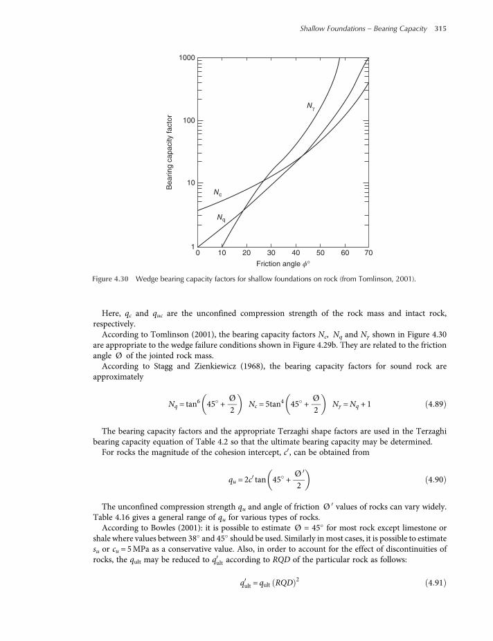
Here, qc and quc are the unconfined compression strength of the rock mass and intact rock,respectively.According to Tomlinson (2001), the bearing capacity factors Nc, Nq and Nγ shown in Figure 4.30
are appropriate to the wedge failure conditions shown in Figure 4.29b. They are related to the frictionangle Ø of the jointed rock mass.According to Stagg and Zienkiewicz (1968), the bearing capacity factors for sound rock are
approximately
Nq = tan6 45 +
Ø2
Nc = 5tan4 45 +
Ø2
Nγ =Nq + 1 4 89
The bearing capacity factors and the appropriate Terzaghi shape factors are used in the Terzaghibearing capacity equation of Table 4.2 so that the ultimate bearing capacity may be determined.For rocks the magnitude of the cohesion intercept, c , can be obtained from
qu = 2c tan 45 +Ø2
4 90
The unconfined compression strength qu and angle of friction Ø values of rocks can vary widely.Table 4.16 gives a general range of qu for various types of rocks.According to Bowles (2001): it is possible to estimate Ø = 45 for most rock except limestone or
shale where values between 38 and 45 should be used. Similarly inmost cases, it is possible to estimatesu or cu = 5MPa as a conservative value. Also, in order to account for the effect of discontinuities ofrocks, the qult may be reduced to qult according to RQD of the particular rock as follows:
qult = qult RQD 2 4 91
1000
Nγ
Nc
Nq
100
10
10 10 20 30 40 50
Friction angle ϕ°
60 70
Bearin
g c
apacity facto
r
Figure 4.30 Wedge bearing capacity factors for shallow foundations on rock (from Tomlinson, 2001).
Shallow Foundations – Bearing Capacity 315
worksaccounts.com
Problem Solving
Problem 4.1
A mat foundation 22.5 × 60.0 m supports a silo which completely covers the mat area. The dead weightW of thecomplete structure, unloaded, is assumed to be 200 MN. The foundation level is located at 3 m below groundsurface. The soil profile consists of a uniform saturated clay deposit with average undrained shear strength of75 kPa and unit weight of 17.5 kN/m3. The water table is located at the ground surface. If the safety factor SFagainst bearing capacity failure is to be not less than three and neglecting soil adhesion on the walls of the silo:
(a) Determine the maximum vertical load V which the silo may carry, considering bearing capacity failure onlyand using Terzaghi bearing capacity equation.
(b) What will be the effect on the SF if the water level rises to 1.5 m above the ground surface in times of flooding?
Solution:(a) Gross effective foundation pressure is
Gross q = gross q−uplift pressure
Gross q =V +W
A−hγw =
V + 200 × 103
22 5 × 60−3 × 10 kPa
Equation 4 2 net q = gross q −σo
net q =V + 200 × 103
22 5 × 60−3 × 10⁻³ 17 5−10
= 7 41 × 10−4 V + 95 7 kPa
Table 4.2: gross qult = cNcsc + γ DfNq +12γ BNγsγ
For saturated clay, Ø = 0 undrained condition ; hence, from Table 4.3, Nc = 5 7, Nq = 1, Nγ = 0 and from
Section 4.6: sc = 1 + 0 3BL
Gross qult = 75 × 5 7 1 + 0 3 ×22 560
+ γ Df kPa
Equation (4.3): net qult = gross qult−σo
net qult = 75 × 5 7 1 + 0 3 ×22 560
+ γ Df −γ Df = 476 kPa
Table 4.16 Ranges of unconfined compression strength of varioustypes of rocks.
Rock type qu, MN/m2 Ø , degree
Granite 65–250 45–55
Limestone 30–150 35–45
Sandstone 25–130 30–40
Shale 5–40 15–30
316 Shallow Foundations
worksaccounts.com
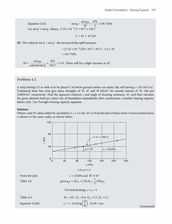
Equation (4.4): net qs =net qultSF
=4763
= 158 7 kPa
Let net q = net qs. Hence, 7 41 × 10−4 V + 95 7 = 158 7
V = 85 × 103 kN
(b) The reduced net q = net q − the increase in the uplift pressure
= 7 41 × 10−4 85 × 103 + 95 7 −1 5 × 10
= 143 7 kPa
SF =net qult
reduced net q=
476143 7
= 3 31. There will be a slight increase in SF.
Problem 4.2
A strip footing 3.5 m wide is to be placed 3 m below ground surface on sandy clay soil having γ = 20 5 kN m3.Undrained shear box tests give shear strengths of 35, 47 and 59 kN/m2 for normal stresses of 70, 140 and210kN/m2, respectively. Find the apparent cohesion c and angle of shearing resistance Ø , and then calculatethe gross ultimate load per metre run of foundation immediately after construction. Consider bearing capacityfailure only. Use Terzaghi bearing capacity equation.
Solution:Obtain c and Ø values either by calculation τ = c+ σ tan Ø or from the plot of shear stress τ versus normal stressσ (drawn to the same scale), as shown below.
From the plot: c = 23 kPa and Ø 10
Table 4.2: gross qult = cNcsc + γ DfNq +12γ BNγsγ
For strip footings sc = sγ = 1
Table 4.3: Ø = 10 ; Nc = 9 6; Nq = 2 7; Nγ = 1 2
Equation (4.20): rγ = 1−0 25 logBK
forB > 2m
120
80
40
00 40 80 120 160
σ, kPa
τ, k
Pa τ = c + σ tan ϕ
ϕ ≅ 10°
200 240
c = 23 kPa
Scheme 4.4
(Continued)
Shallow Foundations – Bearing Capacity 317
worksaccounts.com

rγ = 1−0 25log3 52
= 0 94
gross qult = 23 × 9 6 × 1 + 20 5 × 3 × 2 7
+12× 20 5 × 3 5 × 1 2 × 1 × 0 94
= 220 80 + 166 05 + 40 47 = 427 32 kPa
Gross ultimate load = 427 32 × B = 427 32 × 3 5 = 1496 kN mrun.
Problem 4.3
A square footing is required to carry a gross load of1500 kN. The base of the footing is to be 4.5 m below the groundlevel. The ground water table will rise to the ground surface. The soil is saturated clay having the following prop-erties: apparent cohesion c = 57 5 kPa, Ø = 0 and γ = 19 2 kN m3. Using the Terzaghi bearing capacity equa-tion with a safety factor SF = 3 0, find a suitable size for the footing.The clay extends to a depth of 8.1 m below the ground surface and below this level there is a stratum of relatively
incompressible material. Assume that the mean vertical pressure in the 3.6 m clay layer under the footing is 0.56 ofthe net contact pressure. Consolidation tests on the clay under similar conditions of pressure distribution anddrainage show that an increment of pressure equals 10 kP a causes a settlement of 1.5 % of the sample thickness.Find the probable settlement of the footing.
Solution:
Table 4.2: gross qult = cNcsc + γ DfNq +12γ BNγsγ
Table 4.3: Ø = 0 ; Nc = 5 7; Nq = 1; Nγ = 0;
For square footings, the Terzaghi sc = 1 3
gross qult = cNcsc + γ Df
Equation (4.3): net qult = gross qult−σo = cNcsc + γ Df −γ Df = cNcsc
Equation (4.5): gross qs =net qultSF
+ σo =57 5 × 5 7 × 1 3
3+ 19 2−10 4 5
= 142 03 + 41 4 = 183 43 kPa
Equation (4.4): net qs =net qultSF
=57 5 × 5 7 × 1 3
3= 142 03 kPa
Gross effective foundation pressure is
Gross q = gross q−uplift pressure
Gross q =1500A
−hγw =1500A
−4 5 × 10 =1500A
−45 kPa
Equation (4.2): net q = gross q −σo
=1500A
−45−4 5 19 2−10
=1500A
−45−41 4 kPa
318 Shallow Foundations
worksaccounts.com
On the basis of gross pressures:Gross q = gross qs
1500A
−45 = 183 43 A=1500228 43
= 6 57m2
On the basis of net pressures:
net q = net qs
1500A
−45−41 4 = 142 03 A=1500228 43
= 6 57m2
The footing size = 2 6 × 2 6mSettlement of the clay stratum under the footing= Sc =mv × σz ×H
σz = 0 561500
2 6 × 2 6−45−41 4 = 75 88 kPa
Settlement of the clay sample = 0 015h=mv × 10 × h, where h = thickness of the sample. Hence,
Sc0 015h
=mv × 75 88 × 3 6mv × 10 × h
The probable settlement of the footing = Sc =0 015 × 75 88 × 3 6
10= 0 41 m
Problem 4.4
A strip footing is to be designed to carry a gross foundation load equals 800 kN/m run at a depth of 0.7m in a gravellysand stratum. Appropriate shear strength parameters are c = 0 and Ø = 40 . Assume that the water table exists atthe foundation level. The sand unit weights above and below the water table are 17 and 20 kN/m3, respectively. UsingTerzaghi bearing capacity equation with a safety factor of three, considering shear failure only, determine the width ofthe footing.
Solution:Equation (4.3): net qult = gross qult−σo
= cNcsc + γ DfNq +12γ BNγsγ −γ Df
= γ Df Nq−1 +12γ BNγsγ
Table 4.3: Ø = 40 ; Nq = 81 3; Nγ = 100 4For strip footings all shape factors areone. Hence,
net qult = 17 × 0 7 81 3−1 + 0 5 × 20−10 B 100 4
= 955 6 + 502B kPa
Equation(4.4): net qs =net qultSF
=955 6 + 502B
3kPa
Equation (4.1): net q= gross q−σo =800B
−17 × 0 7 kPa(Continued)
Shallow Foundations – Bearing Capacity 319
worksaccounts.com
Let net q = net qs. Hence,
800B
−11 9 =955 6 + 502B
3
2400−35 7B= 955 6B+ 502B2
B2 + 1 97B−4 78 = 0
B=−1 97 ± 1 972−4 × 1 −4 78
2 × 1=−1 97 + 4 8
2=2 832
= 1 415m
Use width of the footing = 1.45m
Problem 4.5
A footing 2 m square is located at a depth of 4 m in stiff clay of unit weight 21 kN/m3. The undrained strength ofclay at a depth of 4 m is given by the parameters cu = 120 kPa and Ø u = 0 . For SF = 3 with respect to bearingcapacity failure, determine the gross foundation vertical load that the footing can carry using: (a) the Vesic method,(b) the Skempton method.
Solution:(a) The Vesic method. For saturated clay with Ø u = 0 :
Table 4.4: Nc = 5 14, Nq = 1, Nγ = 0
Table 4.2: gross qult = cNcscdcicgcbc + qNqsqdqiqgqbq
Table 4.8: for the conditions of this problem all i, g and b factors are one.
Table 4.6: sc = 1 +Nq
Nc
BL
= 1 +1
5 1422
= 1 2
dc = 1 + 0 4 tan−1DB= 1 + 0 4 tan−1 4
2= 1 44
sq = dq = 1
gross qult = 120 × 5 14 × 1 2 × 1 44 + 4 × 21 = 1065 8 kPa
Equation (4.3): net qult = gross qult−σo = 1065 8− 4 × 21 = 982 kPa
Equation (4.4): net qs =net qultSF
=9823
= 327 kPa
Equation (4.5): gross qs =net qultSF
+ σo = 327 + 4 × 21 = 411 kPa
Let gross q = gross qs. Hence,The gross load the footing can carry (gross safe foundation load) is 411 × A = 411 × 22 = 1644 kN
(b) The Skempton method.
Figure 4.4:DB= 2;Nc = 8 35
gross qult = cNc + q
net qult = cNc = 120 × 8 35 = 1002 kPa
320 Shallow Foundations
worksaccounts.com
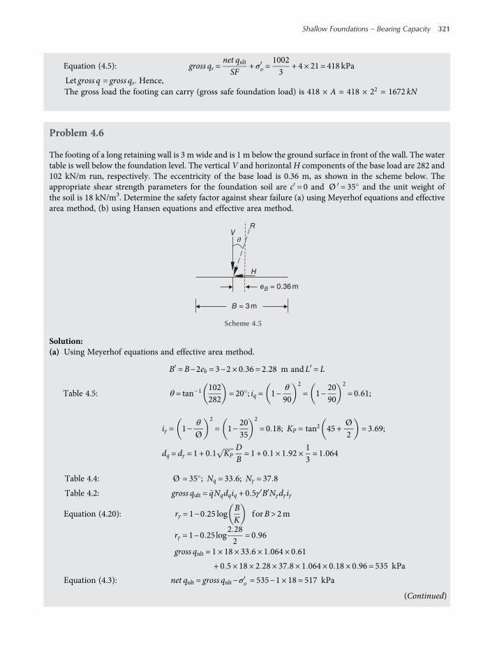
Equation (4.5): gross qs =net qultSF
+ σo =10023
+ 4 × 21 = 418 kPa
Let gross q = gross qs. Hence,The gross load the footing can carry (gross safe foundation load) is 418 × A = 418 × 22 = 1672 kN
Problem 4.6
The footing of a long retaining wall is 3 m wide and is 1 m below the ground surface in front of the wall. The watertable is well below the foundation level. The vertical V and horizontal H components of the base load are 282 and102 kN/m run, respectively. The eccentricity of the base load is 0.36 m, as shown in the scheme below. Theappropriate shear strength parameters for the foundation soil are c = 0 and Ø = 35 and the unit weight ofthe soil is 18 kN/m3. Determine the safety factor against shear failure (a) using Meyerhof equations and effectivearea method, (b) using Hansen equations and effective area method.
Solution:(a) Using Meyerhof equations and effective area method.
B =B−2eb = 3−2 × 0 36 = 2 28 m andL = L
Table 4.5: θ = tan−1 102282
= 20 ; iq = 1−θ
90
2
= 1−2090
2
= 0 61;
iγ = 1−θ
Ø
2
= 1−2035
2
= 0 18; KP = tan2 45 +Ø2
= 3 69;
dq = dγ = 1 + 0 1 KPDB= 1 + 0 1 × 1 92 ×
13= 1 064
Table 4.4: Ø = 35 ; Nq = 33 6; Nγ = 37 8
Table 4.2: gross qult = qNqdqiq + 0 5γ B Nγdγiγ
Equation (4.20): rγ = 1−0 25 logBK
forB > 2m
rγ = 1−0 25log2 282
= 0 96
gross qult = 1 × 18 × 33 6 × 1 064 × 0 61
+ 0 5 × 18 × 2 28 × 37 8 × 1 064 × 0 18 × 0 96 = 535 kPa
Equation (4.3): net qult = gross qult−σo = 535−1 × 18 = 517 kPa
VR
H
θ
B = 3 m
eB = 0.36 m
Scheme 4.5
(Continued)
Shallow Foundations – Bearing Capacity 321
worksaccounts.com
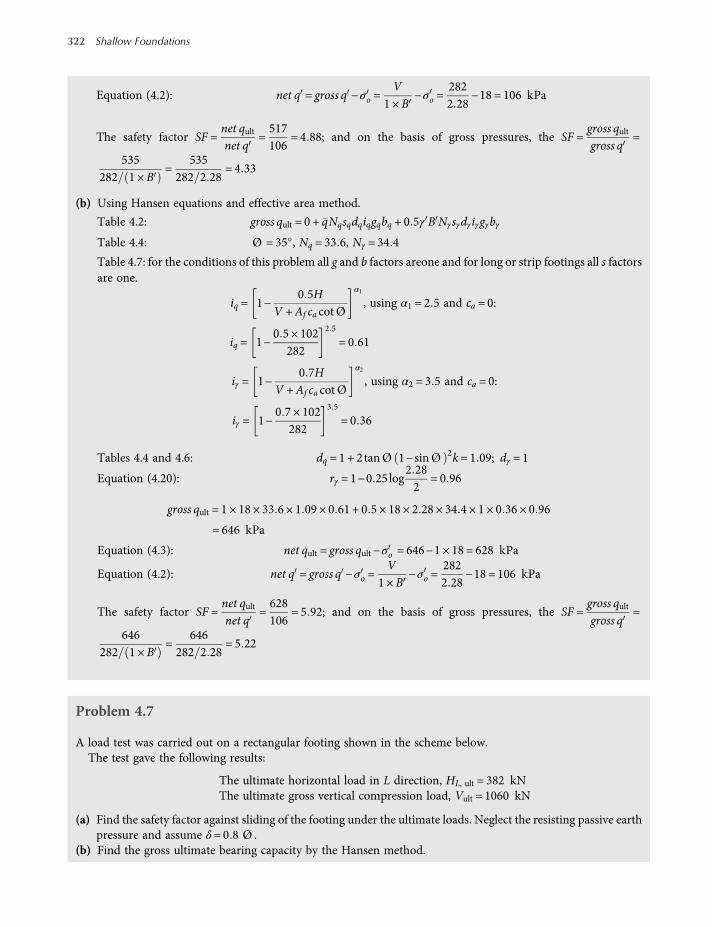
Equation (4.2): net q = gross q −σo =V
1 ×B−σo =
2822 28
−18 = 106 kPa
The safety factor SF =net qultnet q
=517106
= 4 88; and on the basis of gross pressures, the SF =gross qultgross q
=
535282 1 ×B
=535
282 2 28= 4 33
(b) Using Hansen equations and effective area method.
Table 4.2: gross qult = 0 + qNqsqdqiqgqbq + 0 5γ B Nγsγdγiγgγbγ
Table 4.4: Ø = 35 , Nq = 33 6, Nγ = 34 4
Table 4.7: for the conditions of this problem all g and b factors areone and for long or strip footings all s factorsare one.
iq = 1−0 5H
V +Af ca cotØ
α1
, using α1 = 2 5 and ca = 0:
iq = 1−0 5 × 10²
282
2 5
= 0 61
iγ = 1−0 7H
V +Af ca cotØ
α2
, using α2 = 3 5 and ca = 0:
iγ = 1−0 7 × 10²
282
3 5
= 0 36
Tables 4.4 and 4.6: dq = 1 + 2tanØ 1−sinØ 2k= 1 09; dγ = 1
Equation (4.20): rγ = 1−0 25log2 282
= 0 96
gross qult = 1 × 18 × 33 6 × 1 09 × 0 61 + 0 5 × 18 × 2 28 × 34 4 × 1 × 0 36 × 0 96
= 646 kPa
Equation (4.3): net qult = gross qult−σo = 646−1 × 18 = 628 kPa
Equation (4.2): net q = gross q −σo =V
1 ×B−σo =
2822 28
−18 = 106 kPa
The safety factor SF =net qultnet q
=628106
= 5 92; and on the basis of gross pressures, the SF =gross qultgross q
=
646282 1 ×B
=646
282 2 28= 5 22
Problem 4.7
A load test was carried out on a rectangular footing shown in the scheme below.The test gave the following results:
The ultimate horizontal load in L direction, HL, ult = 382 kNThe ultimate gross vertical compression load, Vult = 1060 kN
(a) Find the safety factor against sliding of the footing under the ultimate loads. Neglect the resisting passive earthpressure and assume δ= 0 8 Ø .
(b) Find the gross ultimate bearing capacity by the Hansen method.
322 Shallow Foundations
worksaccounts.com
(c) Find the gross ultimate bearing capacity by the Vesic method.(d) Find the gross ultimate bearing capacity by the Meyerhof method.
Solution:(a) Maximum resisting force =Hmax =V tanδ+ caAf
ca = 0, since c= 0. Hence,
Hmax =Vult tanδ = 1060 × tan 0 8 × 43 = 726kN
The sliding force =HL,ult = 382 kN
Safety factor against sliding of the footing = SF =Hmax
HL,ult=726382
= 1 9
(b) Hansen method.LB
=LB=
20 5
= 4 > 2, and Ø tr = 43 > 34 . Hence according to Hansen
Ø ps = 1 5Ø tr−17 = 1 5 × 43−17 = 47 5
According to Meyerhof: Ø ps = 1 1Ø tr = 1 1 × 43 = 47 3Use Ø ps = 47
Table 4.2: Nq = eπ tanØ tan2 45 +
Ø2
= eπ tan47 tan2 45 +472
= 187 21
Nγ = 1 5 Nq−1 tanØ
= 1 5 187 21−1 tan47 = 299 53
Table 4.4: 2 tanØ 1−sinØ 2 = 2tan47 1−sin47 2 = 0 155
HB = 0
HL = 382 kN
HL = 382 kN
B = 0.5 m
0.5 m
Dense sand: γ ′ = 9.43 kN/m3
ϕtr = 43°; c = 0
L = 2 m
L = 2 m
V = 1060 kN
∇ W.T
PLAN
SECTION
Scheme 4.6
(Continued)
Shallow Foundations – Bearing Capacity 323
worksaccounts.com
Because the horizontal component is in L direction, both Equations (4.21) and (4.22) should be used in orderto find the smaller gross q
ult.Refer to Tables 4.6 and 4.7 and Section 4.7:
dq,B = 1 + 2tanØ 1−sinØ 2D B= 1 + 0 1550 50 5
= 1 16
dq,L = 1 + 2tanØ 1−sinØ 2D L= 1 + 0 1550 52
= 1 04
dγ,B = dγ,L = 1
iq, B = 1−0 5HB
V +Af ca cotØ
α1 = 2 5
= 1 using α1 = 2 5 and HB = 0
iγ,B = 1−0 7HB
V +Af ca cotØ
α2 = 3 5
= 1 using α2 = 3 5, HB = 0 and η = 0
ca = 0 since c= 0
iq, L = 1−0 5HL
V +Af ca cotØ
2 5
= 1−0 5 × 3821060 + 0
2 5
= 0 608
iγ,L = 1−0 7HL
V +Af ca cotØ
α2 = 3 5
= 1−0 7 × 3821060 + 0
α2 = 3 5
= 0 361
sq, B = 1 + sinØ Biq, B L = 1 + sin47 0 5 × 1 2 = 1 18
sq, L = 1 + sinØ Liq,L B = 1 + sin47 2 × 0 608 0 5 = 2 78
sγ ≥ 0 6
sγ, B = 1−0 4Biγ, BLiγ, L
= 1−0 40 5 × 12 × 0 361
= 0 723 > 0 6
sγ, L = 1−0 4Liγ, LBiγ, B
= 1−0 42 × 0 3610 5 × 1
= 0 422 < 0 6
Use sγ, L = 0 6All ground g factors and base b factors are one, since both the ground and base are horizontal.
Equation (4.21):
qult = qNqsq,Bdq,Biq,Bgq,Bbq,B
= 0 5 × 9 43 × 187 × 1 18 × 1 16 × 1
+ 0 5 × 9 43 × 0 5 × 300 × 0 732 × 1 × 1 = 1718 kPa
Equation (4.22):
qult = qNqsq,Ldq,Liq,Lgq,Lbq,L + 0 5γL Nγsγ,Ldγ,Liγ,Lgγ,Lbγ,L
= 0 5 × 9 43 × 187 × 2 78 × 1 04 × 0 608
+ 0 5 × 9 43 × 2 × 300 × 0 6 × 1 × 0 361 = 2163 kPa
Use the smaller value of qult = 1718 kPa
This result is much greater than the 1060 kPa of the load test.
324 Shallow Foundations
worksaccounts.com
(c) Vesic method.Table 4.2:
Nq = eπ tanØ tan2 45 +Ø2
= eπ tan47 tan2 45 +472
= 187 21
Nγ = 2 Nq + 1 tanØ = 2 187 21 + 1 tan47 = 403 66
Table 4.4: 2tanØ 1−sinØ 2 = 2tan47 1−sin47 2 = 0 155Refer to Tables 4.6 and 4.8:
BL=BL
=0 52
= 0 25;DB
=DB=0 50 5
= 1; k=DB=0 50 5
= 1;LB=
20 5
= 4
sq = 1 +BLtanØ = 1+
0 52tan47 = 1 27
sγ = 1−0 4BL
= 1−0 4 0 25 = 0 9 > 0 6
dq = 1 +2tanØ 1−sinØ 2D
B= 1 + 0 155 1 = 1 16; dγ = 1
m=mL =2 +
LB
1 +LB
=2 + 41 + 4
= 1 2
iq, L = 1−HL
V +Af ca cot Ø
m
= 1−382
1060 + 0
1 2
= 0 585
iγ,L = 1−HL
V +Af ca cot Ø
m + 1
= 1−382
1060 + 0
1 2 + 1
= 0 374
All ground g factors and base b factors are one, since both the ground and base are horizontal.
gross qult = qNqsqdqiq + 0 5γ B Nγsγdγ iγ
= 0 5 × 9 43 × 187 × 1 27 × 1 16 × 0 585
+ 0 5 × 9 43 × 0 5 × 404 × 0 9 × 1 × 0 374 = 1081 kPa
This result is practically very close to the 1060 kPa of the load test.(d) Meyerhof method.
Table 4.5:
θ = tan−1 3821060
≈20o; iq = 1−θ
90
2
= 1−2090
2
= 0 61
iγ = 1−θ
Ø
2
= 1−2047
2
= 0 33; KP = tan2 45 +Ø2
= 6 44
dq = dγ = 1 + 0 1 KPDB= 1 + 0 1 × 2 54 ×
0 50 5
= 1 254
Table 4.2: Nq = 187 21 (the same as that of Hansen)
Nγ = Nq−1 tan 1 4Ø = 187 21−1 tan 1 4 × 47
= 414 34(Continued)
Shallow Foundations – Bearing Capacity 325
worksaccounts.com
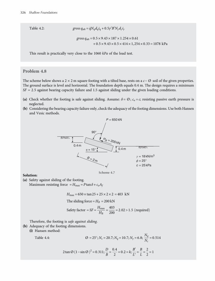
Table 4.2: gross qult = qNqdqiq + 0 5γ B Nγdγiγ
gross qult = 0 5 × 9 43 × 187 × 1 254 × 0 61
+ 0 5 × 9 43 × 0 5 × 414 × 1,254 × 0 33 = 1078 kPa
This result is practically very close to the 1060 kPa of the load test.
Problem 4.8
The scheme below shows a 2 × 2 m square footing with a tilted base, rests on a c− Ø soil of the given properties.The ground surface is level and horizontal. The foundation depth equals 0.4 m. The design requires a minimumSF = 2 5 against bearing capacity failure and 1.5 against sliding under the given loading conditions.
(a) Check whether the footing is safe against sliding. Assume: δ= Ø ; ca = c; resisting passive earth pressure isneglected.
(b) Considering the bearing capacity failure only, check the adequacy of the footing dimensions. Use both Hansenand Vesic methods.
Solution:(a) Safety against sliding of the footing.
Maximum resisting force =Hmax = P tanδ+ caAf
Hmax = 650 × tan25 + 25 × 2 × 2 = 403 kN
The sliding force =HB = 200 kN
Safety factor = SF =Hmax
HB=403200
= 2 02 > 1 5 required
Therefore, the footing is safe against sliding.(b) Adequacy of the footing dimensions.
(i) Hansen method:
Table 4.4: Ø = 25 ;Nc = 20 7;Nq = 10 7;Nγ = 6 8;Nq
Nc= 0 514
2tanØ 1−sinØ 2 = 0 311;DB=0 42
= 0 2 = k;BL
=BL=22= 1
0.4 m0.4 m
90°
η = 15°
P = 650 kN
c = 25 kPa
HB = 200 kN
B = 2 m
γ = 18 kN/m3
ϕ = 25°
Scheme 4.7
326 Shallow Foundations
worksaccounts.com
Table 4.7: β = 0 ; hence, all g factors are one.Equation 4 21 gross qult = cNcsc,Bdc,Bic,Bbc,B + qNqsq,Bdq,Biq,Bbq,B
+ 0 5γ B Nγsγ,Bdγ,Biγ,Bbγ,B
Refer to Tables 4.6 and 4.7 and Section 4.7:
η= 15 = 0 262 radians
bc,B = 1−η
147= 1−
15147
= 0 9
bq,B = exp −2η tanØ = exp −2 0 262 tan25 = 0 783
bγ,B = exp −2 7η tanØ = exp −2 7 0 262 tan25 = 0 719
dc,B = 1 + 0 4k= 1 + 0 4 × 0 2 = 1 08
dq,B = 1 + 2tanØ 1−sinØ 2k= 1 + 0 311 × 0 2 = 1 062
dγ,B = 1
V = P = 650 kN. HB = 200 kN. Assume α1 = 3 and α2 = 4
V +Af ca cotØ = 650 + 2 × 2 × 25 × cot25 = 864 5
iq,B = 1−0 5HB
V +Af ca cotØ
α1
= 1−0 5 × 200864 5
3
= 0 692
iγ,B = 1−0 7 −η 450 HB
V +Af ca cot Ø
α2
= 1−0 678 × 200
864 5
4
= 0 506
ic,B = iq−1− iqNq−1
= 0 692−1−0 69210 7−1
= 0 66
sc,B = 1 +Nq
Nc×Bic,BL
= 1 + 0 514 ×2 × 0 66
2= 1 34
sq,B = 1 + sinØ Biq,B L = 1 + sin25 2 × 0 692 2 = 1 29
sγ,B = 1−0 4Biγ,BLiγ,L
. The value of iγ,L = 1, since HL = 0; hence,
sγ,B = 1−0 42 × 0 5062 × 1
= 0 798 > 0 6
gross qult = 25 × 20 7 × 1 34 × 1 08 × 0 66 × 0 9
+ 0 4 × 18 × 10 7 × 1 29 × 1 062 × 0 692 × 0 783
+ 0 5 × 18 × 2 × 6 8 × 0 798 × 1 × 0 506 × 0 719
= 444 9 + 57 2 + 35 5 = 537 6 kPa
gross contact pressure gross q=PA=
6502 × 2
= 162 5 kPa(Continued)
Shallow Foundations – Bearing Capacity 327
worksaccounts.com

Safety factor SF =gross qultgross q
=537 6162 5
= 3 3 > 2 5 (required); hence,
The footing dimensions are adequate according to the Hansen method.(ii) Vesic method:
Table 4.4: Ø = 25 ; Nc = 20 7; Nq = 10 7; Nγ = 10 9;Nq
Nc= 0 514
2tanØ 1−sinØ 2 = 0 311;BL=22= 1
Refer to Tables 4.6 and 4.8:
η= 15 = 0 262 radians; β = 0
bc = 1−2β
5 14tanØ= 1 since ground slope β = 0
bq = bγ = 1−ηtanØ 2 = 1− 0 262 tan25 2 = 0 771
dc = 1 080; dq = 1 062; dγ = 1 (The same as Hansen depth factors)
sc = 1 +Nq
Nc×BL= 1 + 0 514 ×
22= 1 514
sq = 1 + tanØBL
= 1 + tan2522
= 1 466
sγ = 1−0 4BL
= 1−0 4 ×22= 0 6
m=2 +
LB
1 +LB
=2 + 11 + 1
= 1 5
V = P = 650 kN H = 200 kN
V +Af ca cot Ø = 650 + 2 × 2 × 25 × cot25 = 864 5
iq = 1−H
V +Af ca cot Ø
m
= 1−200864 5
1 5
= 0 674
iγ = 1−H
V +Af ca cot Ø
m+1
= 1−200864 5
2 5
= 0 518
ic = iq−1− iqNq−1
= ic,B = 0 674−1−0 67410 7−1
= 0 64
gc = iq−1− iq
5 14 tanØ= 0 674−
1−0 6745 14 tan25
= 0 538
gq = gγ = 1− tanβ 2 = 1
gross qult = cNcscdcicbcgc + qNqsqdqiqbqgq
+ 0 5γ B Nγsγdγiγbγgγ
328 Shallow Foundations
worksaccounts.com
gross qult = 25 × 20 7 × 1 514 × 1 08 × 0 64 × 1 × 0 538
+ 0 4 × 18 × 10 7 × 1 466 × 1 062 × 0 674 × 0 771 × 1
+ 0 5 × 18 × 2 × 10 9 × 0 6 × 1 × 0 518 × 0 771 × 1
= 291 4 + 62 3 + 47 0 = 400 7 kPa
gross contact pressure gross q=PA=
6502 × 2
= 162 5 kPa
Safety factor = SF =gross qultgross q
=400 7162 5
= 2 5 = 2 5 (required); hence:
The footing dimensions are probably adequate according to the Vesic method.The large difference between the two results is mainly due to the g
cfactor of the predominating cohesion term;
it is considered as unity in the Hansen equation, whereas in the Vesic equation it is about half (0.538) of thisvalue, which reduces the cohesion term by about 50%.
Problem 4.9
Solve Problem 4.6 (a) using the Saran and Agarwal analysis and (b) find whether the Purkaystha and Charreduction factor method, which is originally used for eccentric vertical loads, gives reasonable results for eccentricinclined loads. Use the Hansen bearing capacity, depth and inclination factors.
Solution:(a) Saran and Agarwal analysis
Equation 4 35 Qult =B c Nc ei + qNq ei +12γBNγ ei
β = tan−1 102282
= 20 ; Ø = 35 ; B= 3m; e= 0 36m; Df = 1m
eB=0 363
= 0 12; γ = 18 kN m3; q= γDf ; c = 0
Figure 4.9: Nq ei = 11 5Figure 4.11: Nγ ei = 14
Qult = 3 0 + 18 × 1 × 11 5 +12× 18 × 3 × 14 = 1755 kN
The vertical load V = 282 kN
Safety factor SF =Qult
V=1755282
= 6 2
(b) Purkaystha and Char reduction factor method.
Equation (4.30): qult e = qult c 1−aeB
k
Equation (4.31): qult c = qNqFqd +12γBNγFγd
Table 4.9: forDf
B=13obtain a= 1 793, k= 0 79 (by interpolation)
Table 4.4: for Ø = 35 Nq = 33 6 and Nγ = 34 4 (by interpolation)
Table 4.6:Fqd = 1 + 2tanØ 1−sinØ 2k
= 1 + 2tan35 1−sin35 2 13
= 1 085Fγd = 1
(Continued)
Shallow Foundations – Bearing Capacity 329
worksaccounts.com

Use Hansen iq and iγ factors to account for the effect of inclined loading condition. These factors are alreadycomputed before (see Solution of Problem 4.6):iq = 0 61; iγ = 0 36
qult e =1 × 18 × 33 6 × 1 085 × 0 61
+12× 18 × 3 × 34 4 × 1 × 0 36
1−1 7930 363
0 79
= 400 3 + 334 4 0 664 = 487 8 kPa
Qult =Bqult e = 3 × 487 8 = 1463 4 kN
Safety factor SF =Qult
V=1463 4282
= 5 2
This result represents the average of the three results obtained before. Therefore, one may consider that thePurkaystha and Char reduction factor method gives reasonable results for eccentric inclined loading condi-tions provided that the Hansen bearing capacity, depth and inclination factors are used in Equation (4.30).
Problem 4.10
A mat foundation 9 × 27 m is to be placed at a depth of 3 m in a deep stratum of soft, saturated clay ofγ = 16 5 kN m3. The water table is at 2.5 m below the ground surface. The strength parameters of the soil, obtainedfrom unconsolidated, undrained tests are cu = 25 kPa, Ø u = 0, whereas consolidated, drained tests givecd = 5 kPa, Ø d = 23 . The modulus of deformation of the soil in the undrained condition obtained equals toEu = 2593 kPa. The modulus of confined compression (in drained conditions) increases with pressure q (or σz)according to Mv = 12 6 q . Taking the effect of compressibility of the soil into consideration and using the Vesicequations, find the ultimate bearing capacity in the following conditions:
(a) Assume the rate of application of dead and live loads (vertical loads) is fast in comparison with rateof dissipation of excess pore-water pressures caused by loads, so that undrained conditions prevail atfailure.
(b) Assume, as the other extreme, that the rate of vertical loading is slow enough so that no excess pore-waterpressures are introduced in the foundation soil.
Solution:(a) Undrained condition.
Assume incompressibility soil condition; hence,
gross qult = cNcscdcicbcgc + qNqsqdqiqbqgq
+ 0 5γ B Nγsγdγiγbγgγ
There is no horizontal load component, the base is not tilted and the foundation is not on slope, therefore allii, bi and gi factors are 1. Hence,
gross qult = cu Ncscdc + qNqsqdq + 0 5γ B Nγsγdγ
For saturated clay, under undrained conditions, Ø = 0; hence, from Table 4.4: Nc = 5 14; Nq = 1 and Nγ = 0.According to Vesic, from
Table 4.6: sc = 1 +Nq
Nc×BL= 1 +
15 14
×927
= 1 065
330 Shallow Foundations
worksaccounts.com
sq = 1 +BLtanØ = 1
dc = 1 + 0 4k;DB=39= 0 33 < 1; dc = 1 + 0 4 ×
39= 1 133
dq = 1 + 2tanØ 1−sinØ 2k= 1
q= 2 5 × 16 5 + 0 5 16 5−10 = 44 5 kPa
gross qult = 25 × 5 14 × 1 065 × 1 133 + 44 5 × 1 × 1 × 1 + 0
= 200 kPa
Equation 4 48 Ir cr =12
exp 3 30−0 45BL
cot 45−Ø2
=12
exp 3 30−0 45 ×927
1 = 11 7
Equation (4.47): Ir =Gs
c+ q tanØ
Equation (1.61): shear modulus of the clay =Gs =Eu
2 1 + μTable 3.10: assume Poisson’s ratio of the saturated clay μ= 0 5
Gs =2593
2 1 + 0 5= 864 33 kPa
c= cu = 25 kPa; and Ø = 0 undrained condition
Ir =864 3325 + 0
= 35 > 11 7
Therefore, the assumption of soil incompressibility is justified. The computed value of ultimate bearingcapacity can be used without reduction. Use gross qult = 200 kPa
(b) Drained condition.Assume incompressibility soil condition; hence,
gross qult = cd Ncscdc + qNqsqdq + 0 5γ B Nγsγdγ
For Ø = 23 , Nc = 18 05; Nq = 8 66; Nγ = 8 20 (these values are computed from equations of Table 4.2).Table 4.6:
sc = 1 +8 6618 05
×927
= 1 16
sq = 1 +927
tan23 = 1 14
sγ = 1−0 4 ×BL= 1−0 4 ×
927
= 0 87 > 0 6, use 0 87
dc = 1 + 0 4k= 1 + 0 4 ×39= 1 133
dq = 1 + 2tanØ 1−sinØ 2k
= 1 + 2tan23 1−sin23 2 3 9 = 1 105
dγ = 1
(Continued)
Shallow Foundations – Bearing Capacity 331
worksaccounts.com
Equation 4 20 rγ = 1−0 25 logBK
for B≥ 2 m
= 1−0 25 log92
= 0 84
gross qult = 5 × 18 05 × 1 16 × 1 133 + 44 5 × 8 66 × 1 14 × 1 105
+ 0 5 16 5−10 9 8 2 × 0 87 × 1 0 84
gross qult = 118 61 + 485 45 + 175 28 = 779 kPa
The average effective overburden pressure in the influence zone, which is taken as pressure at the depthB/2 below the foundation level, is
q = 2 5 × 16 5 + 0 5 + 4 5 16 5−10 = 73 75 kPa
The modulus of confined compression Mv = 12 6 q = 12 6 × 73 75 = 929 25 kPaFor drained condition, Poisson’s ratio may be calculated from the following equation (Vesic, 1973):
μ=1−sin1 2Ø d
2−sin1 2Ø d=1−sin 1 2 × 232−sin 1 2 × 23
= 0 35
Drained modulus of deformation Ed may be calculated from the following equation (Vesic, 1973):
Ed =Mv1 + μ 1−2μ
1−μ= 929 25
1 + 0 35 1−2 × 0 351−0 35
= 579 kPa
The actual rigidity index is
Equation 4 47 Ir =Gs
c+ q tanØ
=Ed
2 1 + μ×
1cd + q tan Ø d
=579
2 1 + 0 35 5 + 73 75tan23= 5 9
Equation 4 48 Ir cr =12
exp 3 30−0 45BL
cot 45−Ø2
=12
exp 3 30−0 45 ×927
cot 45−232
= 59
Ir < Ir cr . Thus, the assumption of soil incompressibility is not justified. The compressibility factorsof Equations (4.44) and (4.45) need to be used in the bearing capacity equation.
Equation 4 45 ζqc = exp −4 4 + 0 6BL
tanØ +3 07sinØ log2Ir
1 + sinØ
= exp −4 4 + 0 6 ×927
tan23 +3 07sin23 log11 8
1 + sin23
= 0 424
ζγc = ζqc = 0 424
332 Shallow Foundations
worksaccounts.com
Equation 4 44 ζcc = ζqc−1−ζqc
Nc tan Øfor Ø > 0
= 0 424−1−0 424
18 05 × tan 23= 0 35
gross qult = 118 61 0 35 + 485 45 0 424 + 175 28 0 424
= 322 kPa
Problem 4.11
Solve Problem 4.10 if the soil consists of a deep stratum of medium-dense sand. Assume the followingadditional data:
For the sand, the saturated unit weight = 19 kN m3 and an average moist unit weight above the watertable = 16 kN m3.
Drained triaxial tests on sand samples show that the angle of shearing resistance of sand Ø varies with meannormal stress σ according to
Ø = Ø 1− 5 5 logσ
σ1, in which Ø 1 = 38 = the angle of shearing resistance of the sand at mean normal stress
σ1 = 100 kPa. According to De Beer (1965), the average mean normal stress along the slip surface is
σ =14qult + 3q 1−sinØ ,
in which q is the effective overburden pressure at the fundation level. In the low and elevated pressure range, the
modulus of deformation E of sand increases with the mean normal stress according to the relationship E = E1σ
σ1in which E1 is the modulus at the mean normal stress σ1.
Also, the following equations may be needed in solving the Problem:
Ko = 1−sin 1 2Ø = coefficient of earth pressure at rest
μ=Ko
1 +Ko=Poisson’sratio
σ =1 + 2Ko
3q = initial mean normal stress at depth z
Solution:In sands, the drained condition prevails. Assume incompressibility soil condition.A preliminary estimate of qult is required so that the mean normal stress along the slip surface can be found. For
this preliminary analysis, assume that Ø = 34 , and Table 4.4 gives Nq = 29 4; Nγ = 41.Table 4.6:
sq = 1 +927
tan34 = 1 22
sγ = 1−0 4 ×BL= 1−0 4 ×
927
= 0 87
dq = 1 + 2tanØ 1−sinØ 2k
= 1 + 2tan34 1−sin34 2 39
= 1 09
dγ = 1 (Continued)
Shallow Foundations – Bearing Capacity 333
worksaccounts.com
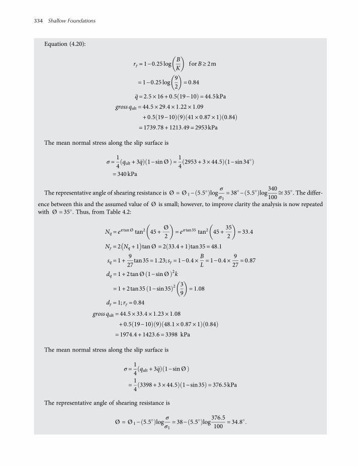
Equation (4.20):
rγ = 1−0 25 logBK
forB ≥ 2m
= 1−0 25 log92
= 0 84
q= 2 5 × 16 + 0 5 19−10 = 44 5kPa
gross qult = 44 5 × 29 4 × 1 22 × 1 09
+ 0 5 19−10 9 41 × 0 87 × 1 0 84
= 1739 78 + 1213 49 = 2953kPa
The mean normal stress along the slip surface is
σ =14qult + 3q 1−sinØ =
142953 + 3 × 44 5 1−sin34
= 340 kPa
The representative angle of shearing resistance is Ø = Ø 1− 5 5 logσ
σ1= 38 − 5 5 log
340100
35 . The differ-
ence between this and the assumed value of Ø is small; however, to improve clarity the analysis is now repeatedwith Ø = 35 . Thus, from Table 4.2:
Nq = eπ tanØ tan2 45 +Ø2
= eπ tan35 tan2 45 +352
= 33 4
Nγ = 2 Nq + 1 tanØ = 2 33 4 + 1 tan35 = 48 1
sq = 1 +927
tan35 = 1 23; sγ = 1−0 4 ×BL= 1−0 4 ×
927
= 0 87
dq = 1 + 2tanØ 1−sinØ 2k
= 1 + 2tan35 1−sin35 2 39
= 1 08
dγ = 1; rγ = 0 84
gross qult = 44 5 × 33 4 × 1 23 × 1 08
+ 0 5 19−10 9 48 1 × 0 87 × 1 0 84
= 1974 4 + 1423 6 = 3398 kPa
The mean normal stress along the slip surface is
σ =14qult + 3q 1−sinØ
=143398 + 3 × 44 5 1−sin35 = 376 5kPa
The representative angle of shearing resistance is
Ø = Ø 1− 5 5 logσ
σ1= 38− 5 5 log
376 5100
= 34 8
334 Shallow Foundations
worksaccounts.com

The analysis can be repeated again for more accuracy; however, in view of small change in mean normal stressfrom the previously found value, a value for gross qult using Ø = 34 8 would be retained for incompressible soil.For this value of Ø , the equations of Tables 4.2 and 4.6 give
Nq = 32 8;Nγ = 47; sq = 1 +927
tan34 7 = 1 23; dγ = 1;
sγ = 1−0 4 ×927
= 0 87; dq = 1 + 2tan34 8 1−sin34 8 2 39
= 1 09
gross qult = 44 5 × 32 8 × 1 23 × 1 09
+ 0 5 19−10 9 47 × 0 87 × 1 0 84
= 1956 9 + 1391 1 = 3348 kPa
To check whether the assumption of incompressibility is justified, the following computations may benecessary.The mean normal stress in the expansion zone, needed in estimating the elastic parameters E and μ of the sand
soil, is taken as the initial mean normal stress at a depth =B 2 below the foundation level. With Ø = 38 for thesand in elastic zone the coefficient of earth pressure at rest is
Ko = 1− sin 1 2 Ø = 1−sin 1 2 × 38 = 0 29
The mean normal stress at a depth of 7.5 m, below ground surface, is
σ =1 + 2Ko
3q =
1 + 2 × 0 293
2 5 × 16 + 5 × 9 = 44 77 kPa
the modulus of deformation is
E = E1σ
σ1= 36 400
44 77100
= 24 355kPa
Poison’s ratio is μ=Ko
1 +Ko=
0 291 + 0 29
= 0 225
The representative angle of shearing resistance for the plastic zone is taken again to be 34.8 .The critical rigidity index is
Equation (4.48):
Ir cr =12
exp 3 30−0 45BL
cot 45−Ø2
=12
exp 3 30−0 45 ×927
cot 45−34 82
= 208
Ir =Gs
c + q tanØ=
Ed2 1 + μ
×1
q tan Ø d=
243552 1 + 0 225 2 5 × 16 + 5 × 9 tan34 8
= 168
Ir < Ir cr Thus, the assumption of soil incompressibility is not justified. The compressibility factors of Equation (4.45)need to be used in the bearing capacity equation.
(Continued)
Shallow Foundations – Bearing Capacity 335
worksaccounts.com

Equation (4.45):
ζqc = exp −4 4 + 0 6BL
tanØ +3 07sinØ log2Ir
1 + sinØ
= exp
−4 4 + 0 6 ×927
tan34 8
+3 07sin34 8 log338
1 + sin34 8
= 0 9
ζγc = ζqc = 0 9
gross qult = 44 5 × 32 8 × 1 23 × 1 09 0 9
+ 0 5 19−10 9 47 × 0 87 × 1 0 84 0 9
= 3013 kPa
(This value is considered too high; however, the allowable soil pressure may be controlled by maximum tolerablesettlement for the structure in question).
Problem 4.12
For the design of a shallow foundation, the following data are given:Foundation: L = 1 5m, B = 1 0m, Df = 1 0mSoil: Ø = 25
c= 50kPa
γ = 17kN m3
Modulus of deformation Es = 1020 kPaPoisson’s ratio μs = 0 35Calculate the gross qult of the soil. Take the soil compressibility into consideration.
Solution:Assume incompressibility soil condition; hence,
gross qult = cd Ncscdc + qNqsqdq + 0 5γ B Nγsγdγ
For Ø = 25 , Nc = 20 72; Nq = 10 66; Nγ = 10 88 (these values are computed from the Vesic equations ofTable 4.2).Table 4.6:
sc = 1 +10 6620 72
×11 5
= 1 343
sq = 1 +11 5
tan25 = 1 311
sγ = 1−0 4 ×11 5
= 0 733 > 0 6, use 0 733
336 Shallow Foundations
worksaccounts.com

DB=11= 1 k=
DB= 1
dc = 1 + 0 4k= 1 + 0 4 × 1 = 1 4
dq = 1 + 2tanØ 1−sinØ 2k
= 1 + 2tan25 1−sin25 2 1 1 = 1 311
dγ = 1
gross qult = 50 × 20 72 × 1 343 × 1 4
+ 1 × 17 × 10 66 × 1 311 × 1 311
+ 0 5 × 17 × 1 × 10 88 × 0 733 × 1
= 1947 89 + 311 47 + 67 79 = 2327 kPa
The average overburden pressure in the influence zone, which is taken as pressure at the depth B/2 below thefoundation level, is
q= 1 5 × 17 = 25 5 kPa
Equation (4.47):
Ir =Gs
c+ q tanØ=
Es2 1 + μ
×1
c+ q tanØ
=1020
2 1 + 0 35 50 + 25 5tan25= 6 1
Equation (4.48):
Ir cr =12
exp 3 30−0 45BL
cot 45−Ø2
=12
exp 3 30−0 45 ×11 5
cot 45−252
= 55 53
Ir < Ir cr . Thus, the assumption of soil incompressibility is not justified. The compressibility factors ofEquations (4.44) and (4.45) need to be used in the bearing capacity equation.
Equation (4.45):
ζqc = exp −4 4 + 0 6BL
tanØ +3 07sinØ log2Ir
1 + sinØ
= exp
−4 4 +0 6 × 11 5
tan25
+3 07sin25 log12 2
1 + sin25
= 0 417
Equation (4.44):
ζcc = ζqc−1−ζqc
Nc tan Øfor Ø > 0
ζcc = 0 417−1−0 417
20 72 × tan 25= 0 357
ζγc = ζqc = 0 417
gross qult = 1947 89 0 357 + 311 47 0 417 + 67 79 0 417
= 854 kPa
Shallow Foundations – Bearing Capacity 337
worksaccounts.com

Problem 4.13
The column footing shown in the scheme below measures 1.2 × 1.8 m and is subjected to a centric vertical loadQ and two momentsMB andML. If eB = 0 12 m, eL = 0 26 m and the depth of foundation Df = 1 m, determine theallowable load the foundation can carry using: (a) Terzaghi equations and effective area method, (b) the Meyerhofequations and effective area method, (c) thePrakash and Saran method. Use the safety factor against bearingcapacity failure equals three.
Solution:(a) Terzaghi equations and effective area method
Table 4.2: gross qult = cNcsc + γ DfNq +12γ BNγsγ
The Nc term is 0, since the cohesion c = 0. B=B
Table 4.3: Ø = 35 ; Nq = 41 4; Nγ = 42 4
For rectangular footings, the Terzaghi sγ = 1−0 2BL(see Section 4.6)
B =B−2eB = 1 2−2 × 0 12 = 0 96 m
L = L−2eL = 1 8−2 × 0 26 = 1 28 m
gross qult =Df γ Nq +12γ B Nγsγ
= 1 × 17 41 4 + 0 5 × 17 0 96 42 4 1−0 2 ×0 961 08
= 703 8 + 284 4 = 988 2 kPa
Gross ultimate load = gross qult ×B L = 988 2 × 0 96 × 1 28
= 1214 3 kN
The allowable load (safe load) the footing can carry =1214 3SF = 3
= 405 kN
(b) Meyerhof equations and effective area method
Table 4.2: gross qult = cNcscdc + γ DfNqsqdq +12γ B Nγsγdγ
Df = 1 m
B
QMB
ML
c ′ = 0
γ = 17 kN/m3
Ø′ = 35°
Scheme 4.8
338 Shallow Foundations
worksaccounts.com
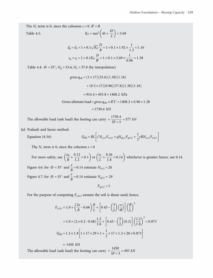
The Nc term is 0, since the cohesion c= 0. B =B
Table 4.5: KP = tan2 45 +Ø2
= 3 69
dq = dγ = 1 + 0 1 KPDB= 1 + 0 1 × 1 92 ×
11 2
= 1 16
sq = sγ = 1 + 0 1KPDB
= 1 + 0 1 × 3 69 ×1
0 96= 1 38
Table 4.4: Ø = 35 ; Nq = 33 6; Nγ = 37 8 (by interpolation)
gross qult = 1 × 17 33 6 1 38 1 16
+ 0 5 × 17 0 96 37 8 1 38 1 16
= 914 4 + 493 8 = 1408 2 kPa
Gross ultimate load = gross qult ×B L = 1408 2 × 0 96 × 1 28
= 1730 4 kN
The allowable load (safe load) the footing can carry =1730 4SF = 3
= 577 kN
(c) Prakash and Saran method.
Equation (4.34): Qult =BL c Nc e Fcs e + qNq e Fqs e +12γBNγ e Fγs e
The Nc term is 0, since the cohesion c= 0
For more safety, useeBB=0 121 2
= 0 1 oreLL=0 261 8
= 0 14 whichever is greater; hence, use 0.14.
Figure 4.6: for Ø = 35 andeB= 0 14 estimate Nγ e = 20
Figure 4.7: for Ø = 35 andeB= 0 14 estimate Nq e = 29
Fqs e = 1
For the purpose of computing Fγs(e) assume the soil is dense sand; hence,
Fγs e = 1 0 +2eB−0 68
BL+ 0 43−
32
eB
BL
2
= 1 0 + 2 × 0 2−0 681 21 8
+ 0 43−32
0 21 21 8
2
= 0 873
Qult = 1 2 × 1 8 1 × 17 × 29 × 1 +12× 17 × 1 2 × 20 × 0 873
= 1450 kN
The allowable load (safe load) the footing can carry =1450SF = 3
= 483 kN
Shallow Foundations – Bearing Capacity 339
worksaccounts.com
Problem 4.14
A footing 2.5 m square carries a gross foundation pressure of 400 kPa at a depth of 1 m in a sand soil. The saturatedand moist unit weights of the sand are 20 and 17 kN/m3, respectively. The shear strength parameters are c = 0 andØ = 40 . Determine the factor of safety with respect to shear failure for the following cases:
(a) The water table is 5 m below ground level.(b) The water table is 1 m below ground level.(c) The water table is 2 m below ground level.(d) The water table is at ground level and there is seepage vertically upwards under hydraulic gradient i= 0 2.
Use the Terzaghi bearing capacity equation and assume the bearing capacity factors Nq and Nγ equal 65 and 95,respectively.
Solution:
(a) Table 4.2: gross qult = cNcsc + qNq +12γ BNγsγ
Equation (4.40): γ = γwet and q = γwetDf = q (Nq term)
Equation (4.39): γ = γwet (Nγ term)The cohesion term is zero, since c = 0.For square footings, sγ = 0 8
Equation (4.20): rγ = 1−0 25 logBK
for B > 2 m
rγ = 1−0 25log2 52
= 0 98
gross qult = 1 × 17 × 65 + 0 5 × 17 × 2 5 × 95 × 0 8 × 0 98
= 2688 kPaEquation (4.3): net qult = gross qult−σo = 2688−1 × 17 = 2671 kPa
gross q = gross q−hγw = 400− 0 γw = 400 kPa
Equation (4.2): net q = gross q −σo = 400−1 × 17 = 383 kPa
Safety factor SF =net qultnet q
=2671383
= 6 97
(b) Table 4.2: gross qult = cNcsc + qNq +12γ BNγsγ
Equation (4.40): γ = γwet and q = γwetDf = q (Nq term)
Equation (4.36): γ = γb = γsat−γw (Nγ term)
The cohesion term is zero, since c = 0.
For square footings, sγ = 0 8
Equation (4.20): rγ = 1−0 25 logBK
for B > 2 m
rγ = 1−0 25log2 52
= 0 98
340 Shallow Foundations
worksaccounts.com

gross qult = 1 × 17 × 65 + 0 5 × 20−10 × 2 5 × 95 × 0 8 × 0 98
= 2036 kPa
Equation (4.3): net qult = gross qult−σo = 2036−1 × 17 = 2019 kPa
gross q = gross q−hγw = 400− 0 γw = 400kPa
Equation (4.2): net q = gross q −σo = 400−1 × 17 = 383kPa
Safety factor SF =net qultnet q
=2019383
= 5 27
(c) Table 4.2: gross qult = cNcsc + qNq +12γ BNγsγ
Equation (4.40): γ = γwet and q = γwetDf = q (Nq term)
Equation (4.37): γ = 2H−zwzwH2
γwet +γbH2
H−zw2 (Nγ term)
H = 0 5B tan 45 +Ø2
= 0 5 × 2 5 × tan 45 +402
= 2 68m
γ = 2 × 2 68−11
2 68 2 17 +10
2 68 2 2 68−1 2 = 14 25kN m3
or
Equation (4.38):
γ = γb +zwB
γwet−γb
= 10 +12 5
17−10 = 12 8 kN m3
Equation (4.37) gives a more exact result than Equation (4.38) does. However, it would be moreconservative to use Equation (4.38). Use γ = 13kN m3.
The cohesion term is zero, since c = 0.For square footings, sγ = 0 8
Equation (4.20):rγ = 1−0 25 log
BK
forB > 2m
rγ = 1−0 25log2 52
= 0 98
gross qult = 1 × 17 × 65 + 0 5 × 13 × 2 5 × 95 × 0 8 × 0 98
= 2315kPa
Equation (4.3): net qult = gross qult−σo = 2315−1 × 17 = 2298kPa
gross q = gross q−hγw = 400− 0 γw = 400kPa
Equation (4.2): net q = gross q −σo = 400−1 × 17 = 383kPa
Safety factor SF =net qultnet q
=2298383
= 6
(d) Table 4.2: gross qult = cNcsc + qNq +12γ BNγsγ
The cohesion term is zero, since c = 0(Continued)
Shallow Foundations – Bearing Capacity 341
worksaccounts.com
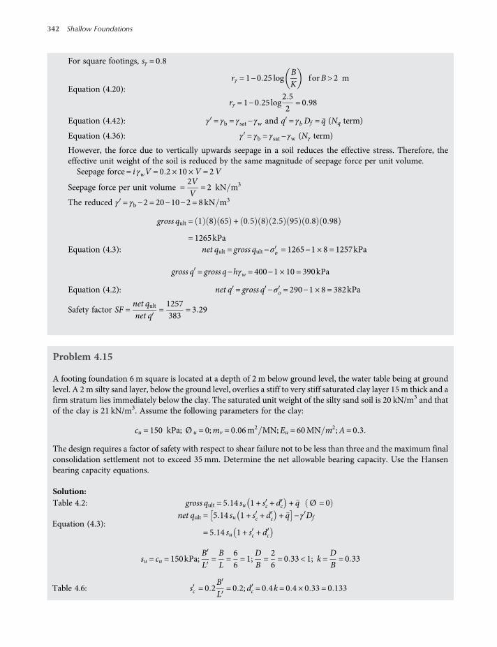
For square footings, sγ = 0 8
Equation (4.20):rγ = 1−0 25 log
BK
forB > 2 m
rγ = 1−0 25log2 52
= 0 98
Equation (4.42): γ = γb = γsat−γw and q = γb Df = q (Nq term)
Equation (4.36): γ = γb = γsat−γw (Nγ term)
However, the force due to vertically upwards seepage in a soil reduces the effective stress. Therefore, theeffective unit weight of the soil is reduced by the same magnitude of seepage force per unit volume.
Seepage force = i γwV = 0 2 × 10 ×V = 2V
Seepage force per unit volume =2VV
= 2 kN m3
The reduced γ = γb−2 = 20−10−2 = 8kN m3
gross qult = 1 8 65 + 0 5 8 2 5 95 0 8 0 98
= 1265kPaEquation (4.3): net qult = gross qult−σo = 1265−1 × 8 = 1257kPa
gross q = gross q−hγw = 400−1 × 10 = 390kPa
Equation (4.2): net q = gross q −σo = 290−1 × 8 = 382kPa
Safety factor SF =net qultnet q
=1257383
= 3 29
Problem 4.15
A footing foundation 6 m square is located at a depth of 2 m below ground level, the water table being at groundlevel. A 2 m silty sand layer, below the ground level, overlies a stiff to very stiff saturated clay layer 15 m thick and afirm stratum lies immediately below the clay. The saturated unit weight of the silty sand soil is 20 kN/m3 and thatof the clay is 21 kN/m3. Assume the following parameters for the clay:
cu = 150 kPa; Ø u = 0;mv = 0 06m2 MN; Eu = 60MN m2;A= 0 3
The design requires a factor of safety with respect to shear failure not to be less than three and the maximum finalconsolidation settlement not to exceed 35 mm. Determine the net allowable bearing capacity. Use the Hansenbearing capacity equations.
Solution:Table 4.2: gross qult = 5 14 su 1 + sc + dc + q Ø =0
Equation (4.3):net qult = 5 14 su 1 + sc + dc + q −γ Df
= 5 14 su 1 + sc + dc
su = cu = 150kPa;BL
=BL=66= 1;
DB=26= 0 33 < 1; k=
DB= 0 33
Table 4.6: sc = 0 2BL
= 0 2; dc = 0 4k= 0 4 × 0 33 = 0 133
342 Shallow Foundations
worksaccounts.com

net qult = 5 14 150 1 + 0 2 + 0 133 = 1027 7 kPa
Equation (4.4): net qs =net qultSF
=1027 7
3= 343 kPa
Calculation of final consolidation settlement may be carried out considering the net effective foundationpressure of 343 kPa. However; experience indicates that this pressure is likely to cause settlement larger thanthe specified allowable settlement of 35 mm. Therefore, as the first trial use a net design soil pressure of150 kPa.The clay layer is relatively thick; there will be significant lateral strain (resulting in immediate settlement in the
clay) and it is appropriate to use the Skempton–Bjerrum method. Accordingly, the final settlement S = Si + Sc,may be calculated as follows.In order to compute the consolidation settlement more accurately, assume the clay is divided into five layers of
equal thicknesses, as shown in the scheme below.
Calculation of the immediate settlement Si:
Equation (3.33): Si = μoμ1qBEu
HB=156= 2 5;
DB=26= 0 33;
LB= 1; hence, from figure 3.9:
μo = 0 95 and μ1 = 0 55
Si = 0 95 × 0 55 ×150 × 660 × 1000
= 0 008m= 8mm
Calculation of consolidation settlement Sc:
Sc =K Soed
For each layer:
Soed =mv × σz ×H =0 061000
× σz × 3 × 1000 = 0 18 σz mm
σz = q 4 I ; I is calculated from Table 2.3 or Figure 2.32.
2 m Silty sand
15 m Stiff clay
Firm stratum
1.5 m3 m
∇ W.T6 m net q = 150 kN/m2
4.5 m
I
II
III
IV
V
7.5 m
10.5 m
13.5 m
z
Scheme 4.9
(Continued)
Shallow Foundations – Bearing Capacity 343
worksaccounts.com
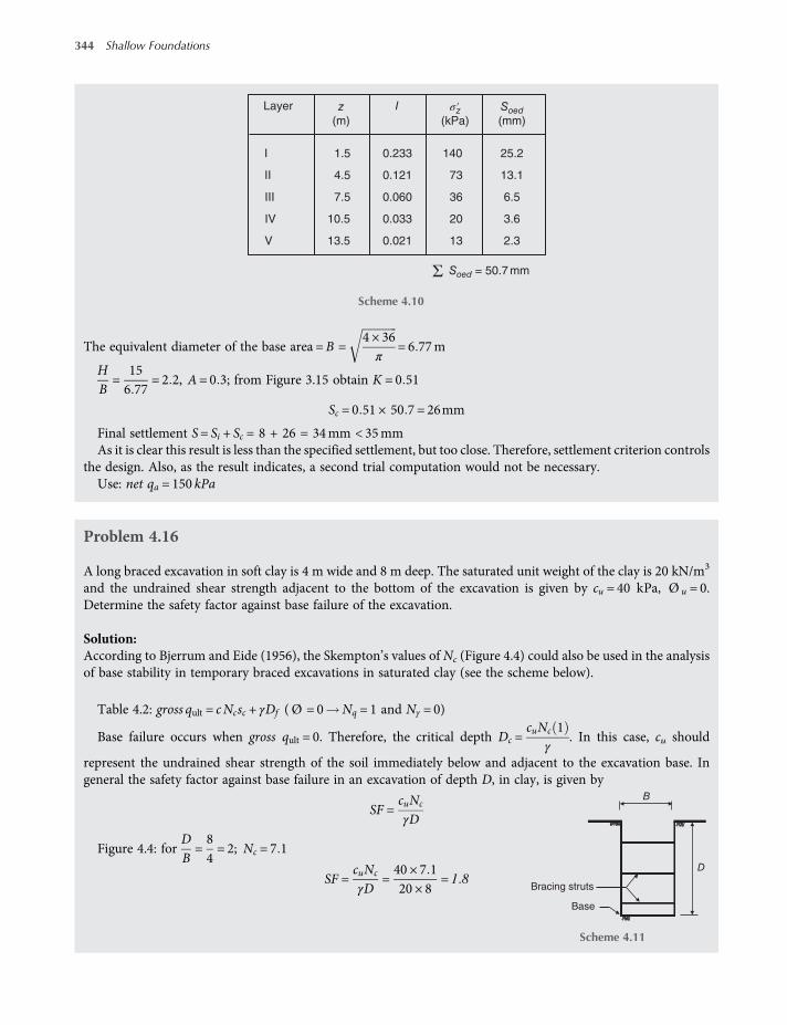
The equivalent diameter of the base area =B =4 × 36π
= 6 77m
HB=
156 77
= 2 2, A= 0 3; from Figure 3.15 obtain K = 0 51
Sc = 0 51 × 50 7 = 26mm
Final settlement S= Si + Sc = 8 + 26 = 34mm < 35mmAs it is clear this result is less than the specified settlement, but too close. Therefore, settlement criterion controls
the design. Also, as the result indicates, a second trial computation would not be necessary.Use: net qa = 150 kPa
Problem 4.16
A long braced excavation in soft clay is 4 m wide and 8 m deep. The saturated unit weight of the clay is 20 kN/m3
and the undrained shear strength adjacent to the bottom of the excavation is given by cu = 40 kPa, Ø u = 0.Determine the safety factor against base failure of the excavation.
Solution:According to Bjerrum and Eide (1956), the Skempton’s values of Nc (Figure 4.4) could also be used in the analysisof base stability in temporary braced excavations in saturated clay (see the scheme below).
Table 4.2: gross qult = cNcsc + γDf ( Ø = 0 Nq = 1 and Nγ = 0)
Base failure occurs when gross qult = 0. Therefore, the critical depth Dc =cuNc 1
γ. In this case, cu should
represent the undrained shear strength of the soil immediately below and adjacent to the excavation base. Ingeneral the safety factor against base failure in an excavation of depth D, in clay, is given by
SF =cuNc
γD
Figure 4.4: forDB=84= 2; Nc = 7 1
SF =cuNc
γD=40 × 7 120 × 8
= 1 8
z(m)
σ′z(kPa)
Soed(mm)
Soed = 50.7 mm
Layer
I
II
1.5
4.5
7.5
10.5
13.5
0.233 140 25.2
13.1
6.5
3.6
2.3
73
36
20
13
0.121
0.060
0.033
0.021
III
IV
V
I
ΣScheme 4.10
Base
Bracing struts
D
B
Scheme 4.11
344 Shallow Foundations
worksaccounts.com

Problem 4.17
A footing foundation 3.5 m square is to be constructed at a depth of 2 m in the deep sand deposit of Problem 1.6.All the data given in that problem are also to be used in solution of this problemwithout change. If the settlement isnot to exceed 30 mm, determine the net allowable bearing capacity using (a) the bearing capacity Equation (3.12),(b) the Meyerhof bearing capacity equation with a safety factor against shear failure SF = 3.
Solution:(a) Refer to the solution of Problem 1.6. In general, in design of shallow foundations, the zone of interest startsfrom a depth of about one-half footing width (B) above the estimated foundation level to a depth of about (2B)below. Therefore, this zone is located between depths 0.25 m and 9 m below the ground surface. All the given SPTN-values should be considered in selecting a design N-value, which is the weighted average of the correctedN-values. In the solution of Problem 1.6, the average N60 selected equalled 10, that is the design N60 = 10.
Net allowable bearing capacity for 25 mm settlement:
Equation (3.12):
net qa =N55
F2
B+ F3B
2
KdWr B > F4
where F2 = 0 08;F3 = 0 3; F4 = 1 2
N55 =N606055
= 10 ×6055
= 11
The water table is located at 6.5 m depth; hence,
zw = 6 5−2 = 4 5m>B= 3 5m
For zw ≥B Wr 1 (see Section 3.3.2)
Kd = 1 + 0 33DB
= 1 + 0 3323 5
= 1 19 < 1 33
net qa =110 08
3 5 + 0 33 5
2
1 19 1 = 193 kPa
Equation (3.14): Si = So ×netq Si
netqa So
. Hence,
netqa = Si ×netq So
So= 30 ×
210 425
= 232 kPa
γ = 18 kN/m3
γ = 20.2 kN/m3
6.5 m
G.S
2 m
B = 3.5 m
∇ W.T
Scheme 4.12
(Continued)
Shallow Foundations – Bearing Capacity 345
worksaccounts.com
Table 4.2: gross qult = cNcscdc + γ DfNqsqdq +12γ BNγsγdγ
For the sand soil the Nc term is 0, since c is zero. Hence,
gross qult = γ DfNqsqdq +12γ BNγsγdγ
Because there is no value for Ø given in the Problem data, it is necessary to select a suitable value using the variousapproximate correlations between Ø , Dr and N given in the discussion of Problem 1.6.
Equation (1.30):Ø = 27 1 + 0 3N60−0 00054 N60
2
= 27 1 + 0 3 10 – 0 00054 10 2 = 30
Equation (1.32): Ø = 20N60 + 20 = 20 × 11 + 20 = 34
The average denseness of the sand may be classified as loose. For loose sands Table 1.7 gives an average value forØ = 31 . It would be appropriate use the average of these three values and select Ø = 32 .
Table 4.5: KP = tan2 45 +Ø2
= 3 25
dq = dγ = 1 + 0 1 KPDB= 1 + 0 1 × 1 8 ×
23 5
= 1 1
sq = sγ = 1 + 0 1KPDB= 1 + 0 1 × 3 25 ×
23 5
= 1 19
rγ = 1−0 25logBk
= 1−0 25log3 52
= 0 94
Table 4.4: Ø = 32 ; Nq = 23 2; Nγ = 22 0
gross qult = 2 × 18 23 2 1 19 1 1
+ 0 5 × 18 3 5 22 1 19 1 1 0 94
= 1093 3 + 852 7 = 1946kPa
Equation (4.3): net qult = gross qult−σo = 1946−18 × 2 = 1910kPa
net qs =net qultSF
=19103
= 637 kPa
Check settlement:
Equation (3.5): Si = q×B×1−μ2
Es×m× IS × IF
Because there are no given values for the elastic parameters Es and μ, it is necessary to select suitable values for theseparameters using the tables and various approximate correlations between Es and N given in Section 3.3.1 and inthe discussion of Problem 1.6.Es value:
Equation (1.33):EsPa
= αN60
346 Shallow Foundations
worksaccounts.com
Pa = atmospheric pressure = 100 kPa
Assume α= 10 (for clean normally consolidated sand) and N60 N60
Es = 100 × 10 × 10 = 11 000 kPa
Table 3.8: for normally consolidated sand the following values are suggested:
Es = 7000 N55 = 7000 11 = 23 216 kPa
Es = 500 N55 + 15 = 500 11 + 15 = 13 000 kPa
Es = 2600N55 = 2600 × 11 = 28 600 kPa
Table 3.9: for loose sand Es ranges 10–25MPa, with average Es = 17 5 MPa = 17 500 kPaUse the average of these values, which gives Es = 20 579 kPa.μ value:Table 3.10a: commonly used value for μ ranges 0 3−0 4Table 3.10b: for loose to medium dense sand μ ranges 0 2−0 35Assume μ= 0 31
Is value
IS = I1 +1−2μ1−μ
I2
M =L 2B 2
= 1; N =HB 2
=4BB 2
=4 × 3 53 5 2
= 8
Table 3.7: I1 = 0 482; I2 = 0 02. Hence,
IS = 0 482 +1−2 × 0 311−0 31
× 0 02 = 0 493
IF value
Table 3.6:DB=
23 5
= 0 57;BL=3 53 5
= 1 IF = 0 75
For settlement under centre of the loaded area, m = 4
q= net qs = 637 kPa
Si = 637 ×3 52
×1− 0 31 2
20579× 4 × 0 493 × 0 75 = 0 0724m
Equation (3.6): Si rigid = 0 93Si flexible
Si = 0 93 × 0 0724 = 0 067m
Si = 67 mm> 30mm. Hence, settlement criterion controls the design.
Equation (3.14): Si = So ×netq Si
netqa So
. Hence,
netqa = Si ×netq So
So= 30 ×
63767
= 285 kPa
Shallow Foundations – Bearing Capacity 347
worksaccounts.com

Problem 4.18
A footing 3 m square carries a net foundation pressure of 130 kPa at a depth of 1.2 m in a deep deposit of sand. Thewater table is at a depth of 3 m and the unit weights of the sand above and below the water table are 16 and19 kN/m3, respectively. The variation of cone penetration resistance (qc) with depth (z) is as follows:
The allowable settlement is specified not to exceed 25 mm and the safety factor against bearing capacity failureshould not be less than three. Check whether these two requirements are satisfied. Use the Vesic, Buisman–DeBeerand Schmertmann methods as applicable.
Solution:The CPT results show that the sand deposit below the foundation level may be divided into four layers as shown inTable 4.17.
Check safety factor against bearing capacity failure.For each layer, select a suitable value for Ø using the various approximate correlations between Ø and qc given
in the discussion of Problem 1.13. If more than one correlation is considered, the average of the results will be takenas a design value for Ø ; in this solution the following two correlations are considered:
Equation (1.53): Ø 1 = tan−1 0 1 + 0 38logqcσo
An approximate correlation (Bowles, 2001) for Ø isØ = 29 + qc + 5 for gravel; − 5 for silty sand, where qc is in MPa. As a second correlation, assume
Ø 2 = 29 + qc (Table 4.18).
z (m) 1.2 1.6 2.0 2.4 2.6 3.0 3.4 3.8 4.2
qc (MN/m2)
z (m)
qc (MN/m2)
3.2 2.1 2.8 2.3 6.1 5.0 6.6 4.5 5.5
4.6 5.0 5.5 5.8 6.2 6.6 7.0 7.4 8.0
4.5 5.4 10.4 8.9 9.9 9.0 15.1 12.9 14.8
Scheme 4.13
Table 4.18 Values of Ø 1 and Ø 2 obtained using correlations.
LayerAve. qc(MN/m2)
Depth to centerof layer (m) σO (kN/m2)
Ø 1
(degree)Ø 2
(degree)Ave. Ø(degree)
I 2.60 1.85 29.60 40.0 30.6 35
II 5.37 3.85 55.65 40.5 31.3 36
III 9.55 6.00 75.00 42.0 32.1 37
IV 14.27 7.40 87.60 43.2 32.8 38
Table 4.17 Layers of the sand deposit below the foundation level.
Layer Depth (m) Thickness (m) Average qc (MN/m2)
I 1.2–2.5 1.3 2.60
II 2.5–5.2 2.7 5.37
III 5.2–6.8 1.6 9.55
IV 6.8–8.0 1.2 14.27
348 Shallow Foundations
worksaccounts.com

In bearing capacity analysis, the influence depth for square footings is about 2B below the foundation level andtherefore, the Ø values of the first three layers need to be taken into consideration only. Accordingly, the designØ is
Ø =35 + 36 + 37
3= 36
Table 4.2:gross qult = cNcscdcicgcbc + qNqsqdqiqgqbq
+12γ BNγsγdγiγgγbγ
The Nc term is 0, since the cohesion c= 0Table 4.8: for the conditions of this problem all icgcbc and iqgqbq are 1.
gross qult = qNqsqdq +12γ BNγsγdγ
Table 4.4: for Ø = 36 Nq = 37 7, Nγ = 56 2
Table 4.6:
sq = 1 +BLtanØ = 1 73; sγ = 1−0 4
BL= 0 6
dq = 1 + 2tanØ 1−sinØ 2 DB
= 1 + 2tan36 1−sin36 2 0 4 = 1 1
= 1 + 2tan36 1−sin36 2 0 4 = 1 1
dγ = 1
Equation (4.38):γ = γb +
zwB
γwet−γb = 19−10 +1 83
16−9
= 13 2 kN m3
gross qult = 16 × 1 2 × 37 7 × 1 73 × 1 1
+ 0 5 × 13 2 × 3 × 56 2 × 0 6 × 1
gross qult = 1252 + 668 = 1920 kPa
Equation (4.3): net qult = gross qult−σo = 1920− 1 2 × 16 = 1901 PaThe safety factor against bearing capacity failure is
SF =net qult
net foundation pressure=1901130
= 14 6 3
The required safety against bearing capacity failure is satisfied.Check allowable settlement using the Buisman–DeBeer method:
C = 1 9qcσo
(Recommended by Meyerhof, 1965)
Si =HClnσo + σzσo
=2 3H σo1 9qc
logσo + σzσo
or ΣSi =H
0
2 3σ01 9qc
Δzlogσo + σzσo
The stress increment σz at the centre of each layer will be calculated using either Figure 2.32 or Table 2.3. Theabove settlement equations are applied to obtain the total settlement, as in Table 4.19.
ΣSi = 24 5 mm 25 mm(Continued)
Shallow Foundations – Bearing Capacity 349
worksaccounts.com
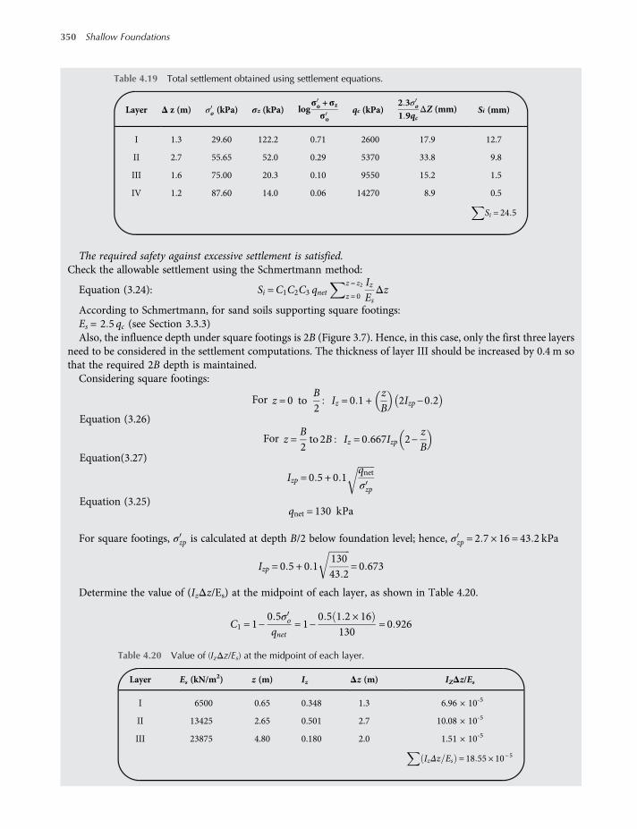
The required safety against excessive settlement is satisfied.Check the allowable settlement using the Schmertmann method:
Equation (3.24): Si =C1C2C3 qnetz = z2
z = 0
IzEsΔz
According to Schmertmann, for sand soils supporting square footings:Es = 2 5 qc (see Section 3.3.3)Also, the influence depth under square footings is 2B (Figure 3.7). Hence, in this case, only the first three layers
need to be considered in the settlement computations. The thickness of layer III should be increased by 0.4 m sothat the required 2B depth is maintained.Considering square footings:
For z = 0 toB2
Iz = 0 1 +zB
2Izp−0 2
Equation (3.26)
For z =B2to 2B Iz = 0 667Izp 2−
zB
Equation(3.27)
Izp = 0 5 + 0 1qnetσzp
Equation (3.25)qnet = 130 kPa
For square footings, σzp is calculated at depth B/2 below foundation level; hence, σzp = 2 7 × 16 = 43 2 kPa
Izp = 0 5 + 0 113043 2
= 0 673
Determine the value of (IzΔz/Es) at the midpoint of each layer, as shown in Table 4.20.
C1 = 1−0 5σoqnet
= 1−0 5 1 2 × 16
130= 0 926
Table 4.19 Total settlement obtained using settlement equations.
Layer Δ z (m) σo (kPa) σz (kPa) logσo +σzσo
qc (kPa)2 3σo1 9qc
ΔZ (mm) Si (mm)
I 1.3 29.60 122.2 0.71 2600 17.9 12.7
II 2.7 55.65 52.0 0.29 5370 33.8 9.8
III 1.6 75.00 20.3 0.10 9550 15.2 1.5
IV 1.2 87.60 14.0 0.06 14270 8.9 0.5
Si = 24 5
Table 4.20 Value of (IzΔz/Es) at the midpoint of each layer.
Layer Es (kN/m2) z (m) Iz Δz (m) IZΔz/Es
I 6500 0.65 0.348 1.3 6.96 × 10⁻⁵
II 13425 2.65 0.501 2.7 10.08 × 10⁻⁵
III 23875 4.80 0.180 2.0 1.51 × 10⁻⁵
IzΔz Es = 18 55 × 10−5
350 Shallow Foundations
worksaccounts.com
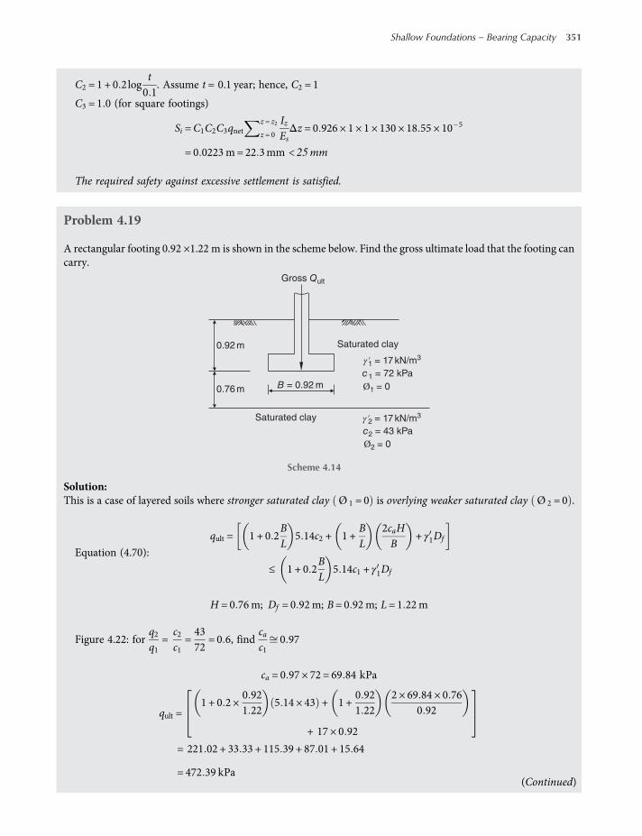
C2 = 1 + 0 2logt0 1
. Assume t = 0.1 year; hence, C2 = 1
C3 = 1 0 (for square footings)
Si =C1C2C3qnetz = z2
z = 0
IzEsΔz = 0 926 × 1 × 1 × 130 × 18 55 × 10−5
= 0 0223m= 22 3mm < 25mm
The required safety against excessive settlement is satisfied.
Problem 4.19
A rectangular footing 0.92 ×1.22 m is shown in the scheme below. Find the gross ultimate load that the footing cancarry.
Solution:This is a case of layered soils where stronger saturated clay Ø 1 = 0 is overlying weaker saturated clay Ø 2 = 0 .
Equation (4.70):
qult = 1 + 0 2BL
5 14c2 + 1 +BL
2caHB
+ γ1Df
≤ 1 + 0 2BL
5 14c1 + γ1Df
H = 0 76m; Df = 0 92m; B= 0 92m; L= 1 22m
Figure 4.22: forq2q1
=c2c1
=4372
= 0 6, findcac1
0 97
ca = 0 97 × 72 = 69 84 kPa
qult =1 + 0 2 ×
0 921 22
5 14 × 43 + 1 +0 921 22
2 × 69 84 × 0 760 92
+ 17 × 0 92
= 221 02 + 33 33 + 115 39 + 87 01 + 15 64
= 472 39 kPa
Gross Qult
0.92 m
0.76 m B = 0.92 m
Saturated clay
Saturated clay
c1 = 72 kPa
γ ′1 = 17 kN/m3
Ø1 = 0
c2 = 43 kPa
γ ′2 = 17 kN/m3
Ø2 = 0
Scheme 4.14
(Continued)
Shallow Foundations – Bearing Capacity 351
worksaccounts.com

As a check, we have:
Equation (4.69):
qult, t = 1 + 0 2BL
5 14c1 + γ1Df
= 1 + 0 2 ×0 921 22
5 14 × 72 + 17 × 0 92
= 441 54 kPa < qultTherefore, qult = qult, tThe gross ultimate load is
Qult = 441 54 0 92 × 1 22 = 496 kN
Problem 4.20
A square footing on layered sand is shown in the scheme below. Determine the net allowable load that the foun-dation can support, considering shear failure only. Use theMeyerhof bearing capacity and shape factors. The safetyfactor against bearing capacity failure should not be less than four.
Solution:This is a case of layered soils where Stronger sand c1 = 0 is overlying weaker sand c2 = 0 .Equation (4.67):
qult = γ1 Df +H Nq 2 Fqs 2 +12γ2BNγ 2 Fγs 2 + γ1H
2 1 +BL
1 +2Df
HKs tanØ 1
B−γ1H
≤ γ1Df Nq 1 Fqs 1 +12γ1BNγ 1 Fγs 1
H = 1 0 m; Df = 1 5m; B= L= 1 5m
Table 4.4:Ø 1 = 40 ; Nq 1 = 64 1; Nγ 1 = 93 69
Ø 2 = 32 ; Nq 2 = 23 2; Nγ 2 = 22 02
Fqs 1 = Fγs 1 = 1 + 0 1BLtan2 45 +
Ø 1
2= 1 + 0 1 ×
1 51 5
× 4 6 = 1 5
Fqs 2 = Fγs 2 = 1 + 0 1BLtan2 45 +
Ø 2
2= 1 + 0 1 ×
1 51 5
× 3 3 = 1 3
Net Qa
1.5 m
1.0 m B = 1.5 m
Sand
Sand
c′1 = 0 kPa
γ′1 = 18 kN/m3
Ø′1 = 40°
c′2 = 0 kPa
γ′2 = 16.7 kN/m3
Ø′2 = 32°
Scheme 4.15
352 Shallow Foundations
worksaccounts.com
Figure 4.21: forq2q1
=γ2BNγ 2
γ1BNγ 1=16 7 × 22 0218 × 93 69
= 0 22 and Ø 1 = 40 ,
find Ks 4 5
qult =
18 1 5 + 1 23 2 1 3 + 0 5 16 7 1 5 22 02 1 3
+ 18 1 2 1 + 1 1 +2 × 1 5
14 5 × 0 84
1 5−18 × 1
= 1357 2 + 358 5 + 362 9−18 = 2060 6 kPa
As a check, we have: Equation (4.66)-(b)
Equation(4.66)-(b):
qult, t = γ1Df Nq 1 Fqs 1 +12γ1BNγ 1 Fγs 1
= 18 × 1 5 64 1 × 1 5
+ 0 5 × 18 × 1 5 × 93 69 × 1 5
= 2596 1 + 1897 2 = 4493 3 kPa qult
Use gross qult = 2060 6 kPaEquation (4.3): net qult = gross qult−σo
net qult = 2060 6 −18 × 1 5 = 2033 6 kPa
Considering shear failure only, net qa =net qultSF
=2033 6
4= 508 4 kPa
The net allowable load is
NetQa = 508 4 1 5 2 = 1144 kN
Problem 4.21
Find the gross qult that the 1.22 × 1.83 m footing, shown in the scheme, can carry. The soil profile consists of twolayers of saturated clay.
Solution:This is a case of layered soils where weaker saturated clay Ø 1 = 0 is overlying stronger saturated clay Ø 2 = 0 .
Equation (4.72): qult = qult, t + qult,b−qult, tHD
2
≥ qult, t
0.91m
0.61m B = 122 m
Saturated clay
Saturated clay
gross qult
c1 = 57.5 kPa
γ ′1 = 17.29 kN/m3
Ø1 = 0
c2 = 119.79 kPa
γ ′2 = 19.65 kN/m3
Ø2 = 0
Scheme 4.16
(Continued)
Shallow Foundations – Bearing Capacity 353
worksaccounts.com
Equation (4.73):qult, t = c1Nc 1 Fcs 1 + γ1Df Nq 1 Fqs 1 +
12γ1BNγ 1 Fγs 1
= c1Nc 1 Fcs 1 + γ1Df Fqs 1
Fqs 1 = 1 + 0 1BLtan2 45 +
Ø 1
2= 1 + 0 1 ×
1 221 83
× 1 = 1 067
Fcs 1 = 1 + 0 2BLtan2 45 +
Ø 1
2= 1 + 0 2 ×
1 221 83
× 1 = 1 133
For Ø = 0 Nc 1 =Nc 2 = 5 14
gross qult, t = 57 5 × 5 14 × 1 133
+ 17 29 × 0 91 × 1 067 = 351 74 kPa
Equation (4.74):
gross qult,b = c2Nc 2 Fcs 2 + γ2Df Nq 2 Fqs 2 +12γ2BNγ 2 Fγs 2
= c2Nc 2 Fcs 2 + γ2Df Fqs 2
Fqs 2 = Fqs 1 = 1 067; Fcs 2 = Fcs 1 = 1 133
gross qult,b = 119 79 × 5 14 × 1 133
+ 19 65 × 0 91 × 1 067 = 716 9 kPa
Equation (4.72): gross qult = qult, t + qult,b−qult, tHD
2
≥ qult, t
= 351 74 + 716 9−351 740 611 22
2
gross qult = 351 74 + 91 29 = 443 kPa > gross qult, t
< gross qult,b
Use gross qult = 443 kPa
Problem 4.22
Assume locations of the two sand layers of Problem 4.20 are reversed, that is the weaker layer at top and the stron-ger layer at bottom. Determine the net allowable load that the foundation can support, considering shear failureonly. Use theMeyerhof bearing capacity and shape factors. The safety factor against bearing capacity failure shouldnot be less than four.
Solution:This is a case of layered soils where weaker sand c1 = 0 is overlying stronger sand c2 = 0 .
354 Shallow Foundations
worksaccounts.com
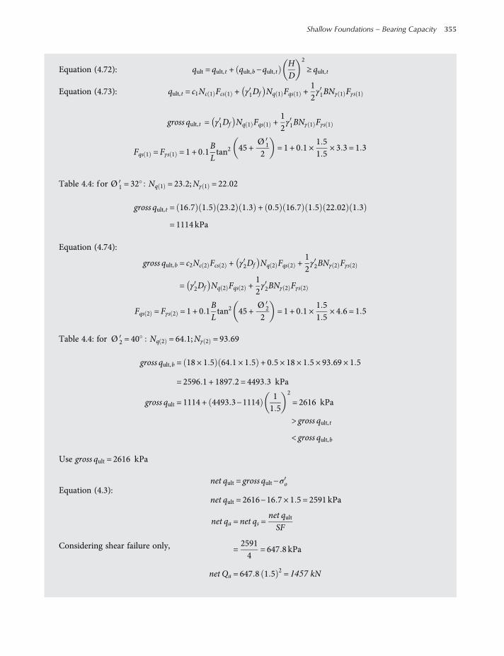
Equation (4.72): qult = qult, t + qult,b−qult, tHD
2
≥ qult, t
Equation (4.73): qult, t = c1Nc 1 Fcs 1 + γ1Df Nq 1 Fqs 1 +12γ1BNγ 1 Fγs 1
gross qult, t = γ1Df Nq 1 Fqs 1 +12γ1BNγ 1 Fγs 1
Fqs 1 = Fγs 1 = 1 + 0 1BLtan2 45 +
Ø 1
2= 1 + 0 1 ×
1 51 5
× 3 3 = 1 3
Table 4.4: for Ø 1 = 32 Nq 1 = 23 2;Nγ 1 = 22 02
gross qult, t = 16 7 1 5 23 2 1 3 + 0 5 16 7 1 5 22 02 1 3
= 1114 kPa
Equation (4.74):
gross qult,b = c2Nc 2 Fcs 2 + γ2Df Nq 2 Fqs 2 +12γ2BNγ 2 Fγs 2
= γ2Df Nq 2 Fqs 2 +12γ2BNγ 2 Fγs 2
Fqs 2 = Fγs 2 = 1 + 0 1BLtan2 45 +
Ø 2
2= 1 + 0 1 ×
1 51 5
× 4 6 = 1 5
Table 4.4: for Ø 2 = 40 Nq 2 = 64 1;Nγ 2 = 93 69
gross qult,b = 18 × 1 5 64 1 × 1 5 + 0 5 × 18 × 1 5 × 93 69 × 1 5
= 2596 1 + 1897 2 = 4493 3 kPa
gross qult = 1114 + 4493 3−111411 5
2
= 2616 kPa
> gross qult, t
< gross qult,b
Use gross qult = 2616 kPa
Equation (4.3):net qult = gross qult−σo
net qult = 2616−16 7 × 1 5 = 2591 kPa
Considering shear failure only,
net qa = net qs =net qultSF
=25914
= 647 8 kPa
net Qa = 647 8 1 5 2 = 1457 kN
Shallow Foundations – Bearing Capacity 355
worksaccounts.com
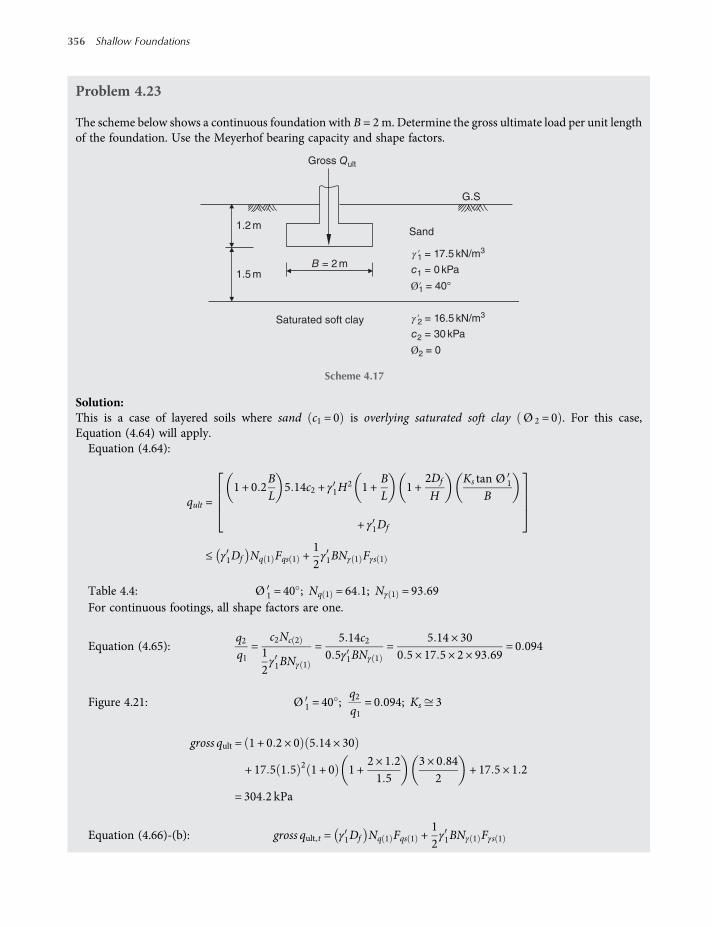
Problem 4.23
The scheme below shows a continuous foundation with B = 2m. Determine the gross ultimate load per unit lengthof the foundation. Use the Meyerhof bearing capacity and shape factors.
Solution:This is a case of layered soils where sand c1 = 0 is overlying saturated soft clay Ø 2 = 0 . For this case,Equation (4.64) will apply.Equation (4.64):
qult =1 + 0 2
BL
5 14c2 + γ1H2 1 +
BL
1 +2Df
HKs tan Ø 1
B
+ γ1Df
≤ γ1Df Nq 1 Fqs 1 +12γ1BNγ 1 Fγs 1
Table 4.4: Ø 1 = 40 ; Nq 1 = 64 1; Nγ 1 = 93 69For continuous footings, all shape factors are one.
Equation (4.65):q2q1
=c2Nc 2
12γ1BNγ 1
=5 14c2
0 5γ1BNγ 1=
5 14 × 300 5 × 17 5 × 2 × 93 69
= 0 094
Figure 4.21: Ø 1 = 40 ;q2q1
= 0 094; Ks 3
gross qult = 1 + 0 2 × 0 5 14 × 30
+ 17 5 1 5 2 1 + 0 1 +2 × 1 21 5
3 × 0 842
+ 17 5 × 1 2
= 304 2 kPa
Equation (4.66)-(b): gross qult, t = γ1Df Nq 1 Fqs 1 +12γ1BNγ 1 Fγs 1
c1 = 0 kPa
γ ′1 = 17.5 kN/m3
Ø′1 = 40°
c2 = 30 kPa
γ ′2 = 16.5 kN/m3
Ø2 = 0
Gross Qult
1.2 m
1.5 m
Saturated soft clay
Sand
G.S
B = 2 m
Scheme 4.17
356 Shallow Foundations
worksaccounts.com
gross qult, t = 17 5 × 1 2 64 1 1 + 0 5 17 5 2 93 69 1
= 2986 kPa > gross qult
Use gross qult = 304 2 kP
Gross ultimate load per meter length of the foundation = 304 2 B
= 304 2 2
= 608 kN
Problem 4.24
Assume locations of the sand and clay layers of Problem 4.23 are reversed, that is the saturated soft clay layer at topand the stronger sand layer at bottom. Determine the net allowable bearing capacity, considering shear failureonly. Use the Meyerhof bearing capacity and shape factors. Use a safety factor SF = 3.
Solution:This is a case of layered soils where weaker saturated clay Ø 1 = 0 overlying stronger sand layer c2 = 0 .
Equation (4.72): qult = qult, t + qult,b−qult, tHD
2
≥ qult, t
Equation (4.73): qult, t = c1Nc 1 Fcs 1 + γ1Df Nq 1 Fqs 1 +12γ1BNγ 1 Fγs 1
= c1Nc 1 Fcs 1 + γ1Df Fqs 1
Table 4.4:Ø 2 = 40 ;Nq 2 = 64 1;Nγ 2 = 93 69
Ø = 0;Nc 1 = 5 14; Nq 1 = 1;Nγ 1 = 0
For continuous footings, all shape factors are one.
gross qult, t = 30 × 5 14 × 1 + 16 5 × 1 2 × 1 = 174 kPa
Equation (4.74):
gross qult,b = c2Nc 2 Fcs 2 + γ2Df Nq 2 Fqs 2 +12γ2BNγ 2 Fγs 2
= γ2Df Nq 2 Fqs 2 +12γ2BNγ 2 Fγs 2
= 17 5 × 1 2 × 64 1 + 0 5 × 17 5 × 2 × 93 69
= 2986 kPa
H = 1 5m; D≈B= 2m
gross qult = 174 + 2986−1741 52
2
= 1756 kPa > gross qult, t
net qult = gross qult−γ1Df = 1756−16 5 × 1 2 = 1736 2 kPa
(Continued)
Shallow Foundations – Bearing Capacity 357
worksaccounts.com
Considering shear failure only:
net qa = net qs =net qultSF
=1736 2
3= 575 kPa
(This result is considered too high!)
In the author’s opinion, this method overestimates net qult of soft clays which overly strong sands. However, inmany of such circumstances the allowable soil pressure is based on allowable settlement rather than net qs.
Problem 4.25
A rectangular footing of 3 × 6m is to be placed on a two-layer clay deposit, as shown in the scheme below. Estimatethe gross ultimate bearing capacity. Use the Meyerhof bearing capacity and shape factors.
Solution:This is a case of layered soils where weaker saturated clay Ø 1 = 0 is overlying stronger saturated clay Ø 2 = 0 .
Equation (4.72): qult = qult, t + qult,b−qult, tHD
2
≥ qult, t
Equation (4.73): qult, t = c1Nc 1 Fcs 1 + γ1Df Nq 1 Fqs 1 +12γ1BNγ 1 Fγs 1
= c1Nc 1 Fcs 1 + γ1Df Fqs 1
Fqs 1 = 1 + 0 1BLtan2 45 +
Ø 1
2= 1 + 0 1 ×
36× 1 = 1 05
Fcs 1 = 1 + 0 2BLtan2 45 +
Ø 1
2= 1 + 0 2 ×
36× 1 = 1 1
Table 4.4: Ø = 0; Nc 1 =Nc 2 = 5 14gross qult, t = 77 × 5 14 × 1 1
+ 17 26 × 1 83 × 1 05 = 468 52 kPa
Equation (4.74):
gross qult,b = c2Nc 2 Fcs 2 + γ2Df Nq 2 Fqs 2 +12γ2BNγ 2 Fγs 2
= c2Nc 2 Fcs 2 + γ2Df Fqs 2
Fqs 2 = Fqs 1 = 1 05; Fcs 2 = Fcs 1 = 1 1
1.83 m
1.22 m B = 3 m
Saturated clay
Saturated clay
gross qult
c1 = 77 kPa
γ ′1 = 17.26 kN/m3
Ø1 = 0
c2 = 115 kPa
γ ′2 = 19.65 kN/m3
Ø2 = 0
Scheme 4.18
358 Shallow Foundations
worksaccounts.com

gross qult,b = 115 × 5 14 × 1 1
+ 17 26 × 1 83 × 1 05 = 683 38 kPa
Equation (4.72): qult = qult, t + qult,b−qult, tHD
2
≥ qult, t
D≈B= 3m
Equation (4.72): gross qult = 468 52 + 683 38−468 521 223
2
gross qult = 504 kPa > gross qult, t
< gross qult,bgross qult = 504 kPa
Problem 4.26
A 2 × 2 m square footing is to be placed on a sand layer overlying a clay layer, as shown in the scheme below.Determine the net qa, considering shear failure only. Use the Meyerhof bearing capacity and shape factors.The safety factor against bearing capacity failure should not be less than three.
Solution:In this case it may not be very clear which soil is stronger or weaker than the other. In such a case, it may bereasonable to try the two possibilities then choosing the smaller result.
(a) Assume the sand is stronger than the clay:Equation (4.64):
qult =1 + 0 2
BL
5 14c2 + γ1H2 1 +
BL
1 +2Df
HKs tan Ø 1
B
+ γ1Df
≤ γ1Df Nq 1 Fqs 1 +12γ1BNγ 1 Fγs 1
Table 4.4: for Ø 1 = 34 Nq 1 = 29 4; Nγ 1 = 31 1
net qa1.5 m
0.6 m B = 2 m
Sand
Clay
c1 = 0 kPa
γ′1 = 17.25 kN/m3
Ø′1 = 34°
c2 = 75 kPa
γ′2 = 17.25 kN/m3
Ø2 = 0
Scheme 4.19
(Continued)
Shallow Foundations – Bearing Capacity 359
worksaccounts.com
Table 4.5:
Fqs 1 = Fγs 1
= 1 + 0 1BLtan2 45 +
Ø 1
2= 1 + 0 1 ×
22× 3 5 = 1 35
Equation (4.65):q2q1
=c2Nc 2
12γ1BNγ 1
=5 14c2
0 5γ1BNγ 1=
5 14 × 750 5 × 17 25 × 2 × 31 1
= 0 72
Figure 4.21: Ø 1 = 34 ;q2q1
= 0 72; Ks 6
gross qult = 1 + 0 2 × 1 5 14 × 75
+ 17 25 0 6 2 1 + 1 1 +2 × 1 50 6
6 × 0 672
+ 17 25 × 1 5 = 638 3 kPa
γ1Df Nq 1 Fqs 1 +12γ1BNγ 1 Fγs 1 = 17 25 × 1 5 29 4 1 35
+ 0 5 17 25 2 31 1 1 35
= 1751 2 kPa > gross qult
gross qult = 638 3kPa
(b) Assume the sand is weaker than the clay:
gross qult = qult, t + qult,b−qult, tHD
2
≥ qult, t
Equation (4.73):qult, t = c1Nc 1 Fcs 1 + γ1Df Nq 1 Fqs 1 +
12γ1BNγ 1 Fγs 1
= γ1Df Nq 1 Fqs 1 +12γ1BNγ 1 Fγs 1
Fqs 1 = Fγs 1 = 1 + 0 1BLtan2 45 +
Ø 1
2= 1 + 0 1 ×
22× 3 5 = 1 35
Table 4.4: for Ø 1 = 34 Nq 1 = 29 4; Nγ 1 = 31 1
gross qult, t = 17 25 1 5 29 4 1 35
+ 0 5 17 25 2 31 1 1 35 = 1751 2 kPa
Equation (4.74):
gross qult,b = c2Nc 2 Fcs 2 + γ2Df Nq 2 Fqs 2 +12γ2BNγ 2 Fγs 2
= c2Nc 2 Fcs 2 + γ2Df Nq 2 Fqs 2
Fqs 2 = 1 + 0 1BLtan2 45 +
Ø 2
2= 1 + 0 1 ×
22× 1 = 1 1
Fcs 2 = 1 + 0 2BLtan2 45 +
Ø 2
2= 1 + 0 2 ×
22× 1 = 1 2
360 Shallow Foundations
worksaccounts.com

Table 4.4: for Ø 2 = 0 Nc 2 = 5 14; Nq 2 = 1; Nγ 2 = 0
gross qult,b = 75 × 5 14 × 1 2 + 17 25 × 1 5 × 1 × 1 1
= 2596 1 + 1897 2 = 488 5 kPa
H = 0 6m; D≈B = 2m
gross qult = 1751 2 + 488 5−1751 20 62
2
= 1637 6 kPa < gross qult, tHence, gross qult = 1751 2 kPa
Now, the result of (a) is smaller than that of (b); therefore use:
gross qult = 638 3 kPa
net qult = gross qult−γ1Df = 638 3−17 25 × 1 5 = 612 42 kPa
Considering shear failure only, net allowable bearing capacity is
net qa = net qs =net qultSF
=612 42
3= 204 kPa
Problem 4.27
A 1mwide strip footing is located on the top of a compacted (not very dense) cohesionless sand slope, as shown inthe scheme below. The other available data are: β = 26 5 ; Ø tr = 36 ; γ = 14 85 kN m3.Determine the gross ultimate bearing capacity using the Bowles method and the Hansen bearing capacity equa-
tion and shape factors.
Solution:Equation (4.53): gross qult = cNcscic + qNqsqiq + 0 5γ BNγsγ iγThe cohesion term is zero, since c= 0. Hence,
gross qult = qNqsqiq + 0 5γBNγsγiγ
For footings on slopes, it is recommended not to adjust Ø tr to Ø ps, as there are considerable uncertainties in the
stress state when there is loss of soil support on one side of the base, even for strip (or long) bases. Therefore, useØ ps = Ø tr = 36 .
Slope
B = 1.0 m
b = 0.75 m
gross qult
c = 0
γ ′ = 14.85 kN/m3
Ø′tr = 36°
β = 26.5°
D = 1.5 m
Scheme 4.20
(Continued)
Shallow Foundations – Bearing Capacity 361
worksaccounts.com

For strip footings, all shape (s) factors are one and in this case, since the foundation load is vertical Hi = 0 , allload inclination (i) factors are also one.
bB=0 751
= 0 75 < 2
Hence, the Nγ factor should be adjusted as follows:
Determine the Coulomb passive pressure coefficients using + β for KP,max and −β for KP,min, using
KP =sin2 α− Ø
sin2αsin α+ δ 1−sin Ø + δ sin Ø + βsin α+ δ sin α+ β
2
This method uses α= 90 and δ= Ø .For Ø = 36 ; δ= 36 ; α= 90 ; β = + 26 5 KP,max = 128 2For Ø = 36 ; δ= 36 ; α= 90 ; β = −26 5 KP,min = 2 8
R=KP,min
KP,max=
2 8128 2
= 0 022
Table 4.4: Ø = 36 ; Nγ = 40
Nγ =Nγ
2+Nγ
2R+
b2B
1−R =402+402
0 022 +0 752 × 1
1−0 022
Nγ = 28
Table 4.11:bB= 0 75;
DB=1 51
= 1 5; β = 26 5 ; Ø = δ= 36 ; obtain (by interpolation) Nq≈27.
gross qult = 14 85 × 1 5 × 27 + 0 5 × 14 85 × 1 × 28 = 809 kPa
Problem 4.28
Solve Problem 4.27 using (a) D= 0 and b= 1 5, (b) D= b= 0.
Solution:(a) gross qult = qNqsqiq + 0 5γBNγsγ iγ
bB=1 51
= 1 5 < 2. Hence, the Nγ factor should be adjusted.
The KP,max, KP,min, Nγ and R values remain unchanged.
Nγ =Nγ
2+Nγ
2R+
b2B
1−R =402+402
0 022 +1 52 × 1
1−0 022
Nγ = 35 11
362 Shallow Foundations
worksaccounts.com

q= 0, since D= 0. Hence, the Nq term will be 0. All shape (s) and load inclination (i) factors are one for thesame reasons stated earlier.
gross qult = 0 5γBNγsγ iγ = 0 5 × 14 85 × 1 × 35 11 = 261 kPa
(b)bB=01= 0 < 2. Hence, the Nγ factor should be adjusted.
Nγ =Nγ
2+Nγ
2R+
b2B
1−R =402+402
0 022 +0
2 × 11−0 022
Nγ = 20 44
q= 0, since D = 0. Hence, the Nq term will be 0.All shape (s) and load inclination (i) factorsare one for thesame reasons stated earlier.
gross qult = 0 5γBNγsγ iγ = 0 5 × 14 85 × 1 × 20 44 = 152 kPa
Problem 4.29
A shallow continuous foundation in a clay soil is shown in the scheme below. Determine the gross ultimate bearingcapacity using: (a) the Meyerhof method, (b) the Bowles method.
Solution:(a) Meyerhof method
Equation (4.51): gross qult = cNcq
Assume the stability number Ns = 0, since B < H.
Figure 4.14a:bB=0 81 2
=34;Df
B=1 21 2
= 1; β = 30 ;Ns = 0;Ncq≈6 3
gross qult = 50 × 6 3 = 315 kN m2
B = 1.2 m
b = 0.8 m
H = 6.2 m Gross qult
c = 50 kN/m2
γ ′ = 17.5 kN/m3
Ø = 0
β = 30°
D = 1.2 m
Scheme 4.21
(Continued)
Shallow Foundations – Bearing Capacity 363
worksaccounts.com
(b) Bowles methodEquation (4.53): gross qult = cNcscic + qNqsqiq + 0 5γ BNγsγ iγ
Since Ø = 0, the Nγ term is zero. For strip footings, all shape (s) factors are one and in this case, since thefoundation load is vertical Hi = 0 , all load inclination (i) factors are also one.
gross qult = cNc + qNq
Table 4.11:bB=34;Df
B=1 21 2
= 1; β = 30 ; Ø = δ= 0 ; obtain
Nc = 5 14; Nq = 1 03 (by interpolation)
gross qult = 50 × 5 14 + 1 2 × 1 03 = 258 2 kPa
Problem 4.30
Refer to Problem 4.29. Assume the soil is cohesionless compacted sand which has Ø = 40 and γ = 20 kN m3.Determine the gross ultimate bearing capacity using (a) the Bowles method, (b) the Meyerhof method, (c) thestress characteristic solution method.
Solution:(a) Bowles method.
Equation (4.53): gross qult = cNcscic + qNqsqiq + 0 5γ BNγsγiγThe cohesion term is zero, since c= 0. Hence,
gross qult = qNqsqiq + 0 5γ BNγsγ iγ
For strip footings, all shape (s) factors are one and in this case, since the foundation load is vertical Hi = 0 ,all load inclination (i) factors are also one.
Table 4.11:bB=0 81 2
= 0 75;DB=1 21 2
= 1; β = 30 ; Ø = δ= 40 ; Nq = 39 2 (by interpolation).
bB= 0 75 < 2. Hence, the Nγ factor should be adjusted as follows.
Determine the Coulomb passive pressure coefficients using + β for KP,max and −β for KP,min
KP =sin2 α− Ø
sin2αsin α+ δ 1−sin Ø + δ sin Ø + βsin α+ δ sin α+ β
2
This method uses α= 90 and δ= Ø .
For Ø = 40 ; δ= 40 ; α= 90 ; β = + 30 KP,max = 23 38
For Ø = 40 ; δ= 40 ; α= 90 ; β = −30 KP,min = 3 16
R=Kmin
Kmax=
3 1623 38
= 0 135
364 Shallow Foundations
worksaccounts.com

Table 4.4: Ø = 40 ; Nγ = 93 6 (according to Meyerhof )
Nγ =Nγ
2+Nγ
2R+
b2B
1−R =93 62
+93 62
0 135 +0 8
2 × 1 21−0 135
Nγ = 66 61
gross qult = 20 × 1 2 × 39 2 + 0 5 × 20 × 1 2 × 66 61 = 1740 kPa
(b) Meyerhof method.
Equation (4.50): gross qult =12γ BNγq
Figure 4.14b:bB=0 81 2
= 0 75;DB=1 21 2
= 1; β = 30 ; Ø = 40 ; Nγq = 113.
gross qult =12γ BNγq = 0 5 × 20 × 1 2 × 113 = 1356 kPa
(c) Stress characteristic solution method.
Equation (4.50): gross qult =12γ BNγq
Figure 4.18a, b:bB=0 81 2
= 0 75;DB=1 21 2
= 1; β = 30 ; Ø = 40 :
Nγq = 170 (by interpolation).
gross qult =12γ BNγq = 0 5 × 20 × 1 2 × 170 = 2040 kPa
It may be useful to note that the Bowels solution gave a result which is nearly equal to the average of theother two results.
Problem 4.31
Refer to Problem 4.29. Assume a c− Ø soil with c= 25 kPa, Ø = 30 and δ= 20 for computing KP. Use 1.2 × 1.2 msquare footing; other data remain unchanged. Determine the gross ultimate bearing capacity using the Bowlesmethod. Use the Hansen bearing capacity and shape factors.
Solution:Equation (4.53): gross qult = cNcscic + qNqsqiq + 0 5γ BNγsγ iγAll load-inclination (i) factors are one, since the foundation load is vertical Hi = 0 . Hence,
gross qult = cNcsc + qNqsq + 0 5γ BNγsγ
Table 4.4: Ø = 30 ; Nc = 30 13; Nq = 18 4; Nγ = 15 1
Table 4.6:
sc = 1 +Nq
Nc
BL
= 1 +18 430 13
1 21 2
= 1 61
sq = 1 +BL
sinØ = 1 +1 21 2
sin30 = 1 5
sγ = 1−0 4BL
= 1−0 41 21 2
= 0 6(Continued)
Shallow Foundations – Bearing Capacity 365
worksaccounts.com

Table 4.11:bB=0 81 2
= 0 75;DB=1 21 2
= 1; β = 30 ; Ø = 30 ; δ= 20 ;
Nc = 30 14; Nq = 15 03 (by interpolation).
bB= 0 75 < 2. Hence, the Nγ factor should be adjusted as follows:
Determine the passive earth pressure coefficients using + β for KP,max and –β for KP,min.
KP =sin2 α− Ø
sin2αsin α+ δ 1−sin Ø + δ sin Ø + βsin α+ δ sin α+ β
2
α= 90 ; δ= 20
For Ø = 30 ; δ= 20 ; α= 90 ; β = + 30 KP,max = 84 65For Ø = 30 ; δ= 20 ; α= 90 ; β = −30 KP,min = 0 8
R=Kmin
Kmax=
0 884 65
= 0 0095
Nγ =Nγ
2+Nγ
2R+
b2B
1−R =15 12
+15 12
0 0095 +0 8
2 × 1 21−0 0095 = 10 11
gross qult = 25 × 30 14 × 1 61 + 17 5 × 1 2 × 15 03 × 1 5
+ 0 5 × 17 5 × 1 2 × 10 11 × 0 6 = 1750 kPa
Problem 4.32
A strip footing is located on the slope shown in the scheme below. What is the net safe bearing capacity using theBowles method with a safety factor SF = 3 5? Use the Hansen bearing capacity and shape factors. Assume δ = 20for computing KP.
Solution:Equation (4.53): gross qult = cNcscic + qNqsqiq + 0 5γ BNγsγiγFor strip footings, all shape (s) factors are one and in this case since the foundation load is vertical Hi = 0 , all
load inclination (i) factors are also one.
gross qult = cNc + qNq + 0 5γ BNγ
B = 2 m
Q
1 m
c = 25 kN/m2
γ ′ = 18 kN/m3
Ø = 30°β = 25°
Scheme 4.22
366 Shallow Foundations
worksaccounts.com
Table 4.11:bB=02= 0;
DB=12= 0 5; β = 25 ; Ø = 30 ;
Nc = 26 63; Nq = 12 13. (by interpolation)bB= 0 < 2. Hence, the Nγ factor should be adjusted as follows.
Determine the Coulomb passive earth pressure coefficients using + β for KP,max and −β for KP,min.
KP =sin2 α− Ø
sin2αsin α+ δ 1−sin Ø + δ sin Ø + βsin α+ δ sin α+ β
2
α= 90 and δ= 20 (assumed).For Ø = 30 ; δ= 20 ; α= 90 ; β = + 25 KP,max = 39 79For Ø = 30 ; δ= 20 ; α= 90 ; β = −25 KP,min = 1 54
R=Kmin
Kmax=
1 5439 79
= 0 039
Table 4.4: Ø = 30 ; Nγ = 15 1
Nγ =Nγ
2+Nγ
2R+
b2B
1−R
=15 12
+15 12
0 039 +1
2 × 21−0 039 = 9 66
gross qult = 25 × 26 63 + 18 × 1 × 12 13 + 0 5 × 18 × 2 × 9 66
gross qult = 1058 kPa
net qult = gross qult−γ Df = 1058−18 × 1 = 1040 kPa
net qs =net qultSF
=10403 5
= 297 kPa
Problem 4.33
A square foundation in a sand deposit measures 1.22 × 1.22 m in plan. Given: Df = 1 52m, soil friction angleØ = 35 and soil unit weight γ = 17 6 kN m3. Estimate the ultimate uplift capacity of the foundation.
Solution:
Table 4.12: Ø = 35 ;Df
B cr
= 5, m= 0 25, Ku = 0 936
Df
B=1 521 22
= 1 25 <Df
B cr
. Hence, it is a shallow foundation.
Equation (4.81):Fq = 1 + 2 1 +m
Df
B
Df
BKu tan Ø
= 1 + 2 1 + 0 25 1 25 1 25 0 936 × tan35 = 3 15
(Continued)
Shallow Foundations – Bearing Capacity 367
worksaccounts.com
Equation (4.80): Fq =Qu
A γDf
The ultimate uplift capacity of the foundation is
Qu = Fq A γDf = 3 15 1 22 × 1 22 × 17 6 × 1 52 = 125 4 kN
Problem 4.34
A circular foundation of 1.5 m diameter is constructed in a sand deposit. Given: Df = 1 5m, soil friction angleØ = 35 and soil unit weight γ = 17 4 kN m3. Estimate the ultimate uplift capacity of the foundation.
Solution:
Table 4.12: Ø = 35 ;Df
B cr
= 5, m= 0 25, Ku = 0 936
Df
B=1 51 5
= 1 <Df
B cr
. Hence, it is a shallow foundation
Equation (4.81):Fq = 1 + 2 1 +m
Df
B
Df
BKu tan Ø
= 1 + 2 1 + 0 25 1 1 0 936 × tan35 = 2 64
Equation (4.80): Fq =Qu
A γDf
The ultimate uplift capacity of the foundation is
Qu = Fq A γDf = 2 64π
4× 1 52 × 17 4 × 1 5 = 121 8 kN
Problem 4.35
A rectangular foundation in a saturated clay deposit measures 1.5m × 3.0 m in plan. The data given: Df = 1 8m,cu = 52 kPa and soil unit weight γ = 18 9 kN m3. Estimate the ultimate uplift capacity of the foundation.
Solution:
Equation (4.85):
Df
Bcr = 0 107 cu + 2 5≤ 7 for square footings
= 0 107 × 52 + 2 5 = 8 1 > 7 Hence use 7
Equation (4.86):
Df
B cr
=Df
B cr, sq
0 73 + 0 27LB
≤ 1 55Df
B cr, sq
for rectangular footings
= 7 0 73 + 0 2731 5
= 8 89
368 Shallow Foundations
worksaccounts.com

Check:
1 55Df
B cr, sq
= 1 55 × 7 = 10 85 >Df
B cr
. Hence,Df
B cr
= 8 89
Df
B=1 81 5
= 1 2 <Df
B cr
= 8 89 . Hence, it is a shallow foundation.
α =Df B
Df B cr
=1 28 89
= 0 135
From the average curve of Figure 4.28, for α = 0 135 obtain β = 0 2Equation (4.88):
Qu =A B 7 56 + 1 44BL
cu + γDf
= 1 5 × 3 0 2 7 56 + 1 441 53
52 + 18 9 × 1 8
= 540 6 kN
The ultimate uplift capacity of the foundation =Qu = 540 6 kN
Problem 4.36
A foundation measuring 1.2 × 2.4 m in plan is constructed in a saturated clay deposit. The data given: Df = 2 m,cu = 74 kPa and soil unit weight γ = 18 kN m3. Estimate the ultimate uplift capacity of the foundation.
Solution:
Equation (4.85):
Df
B cr
= 0 107 cu + 2 5≤ 7 for square footings
= 0 107 × 74 + 2 5 = 10 4 > 7 Hence use 7
For rectangular footings, Equation (4.86) gives
Df
B cr
=Df
B cr, sq
0 73 + 0 27LB
≤ 1 55Df
B cr, sq
= 7 0 73 + 0 272 41 2
= 8 89
Check:
1 55Df
B cr, sq
= 1 55 × 7 = 10 85 >Df
B cr
. Hence, useDf
B cr
= 8 89
Df
B=
21 2
= 1 67 <Df
B cr
= 8 89 . Hence, it is a shallow foundation.
α =Df B
Df B cr
=1 678 89
= 0 188
(Continued)
Shallow Foundations – Bearing Capacity 369
worksaccounts.com
From the average curve of Figure 4.28, for α = 0 188 obtain β ≈0 28Equation (4.88):
Q18u =A B 7 56 + 1 44BL
cu + γDf
= 1 2 × 2 4 0 28 7 56 + 1 441 22 4
74 + 18 × 2 = 598 kN
The ultimate uplift capacity of the foundation =Qu = 598 kN
Problem 4.37
A composite of the several site borings gave the average soil profile shown below. A square mat, estimated to be inthe order of 15 m in plan dimensions, is to be located at Df 1 5 m. Estimate the net allowable bearing capacitywhich will be recommended for design of the mat foundation.
Solution:It is noteworthy that the very limited data given in this problem are basically the type a geotechnical consultantwould have on which to make a design soil pressure recommendation.Usually, in the analysis of such design problems, a net safe bearing capacity (net qs) is found first and then the
final settlement due to a net effective foundation pressure, using net q = net qs, is computed and compared to the
Very stiff silty clay (nearly saturated)
qu(av) = 300 kPa
Medium dense sand
N70(av) = 18
Medium dense gravelly sand
N70(av) = 22
Very dense sand with gravel
N70(av) = 40
Rock
Base−1.5
−4.9
−8.2
−15.2
−29.0
3.4 m
3.3 m
7.0 m
13.8 m
0.0
∇ W.T
G.S
γ = 18.7 kN/m3
Scheme 4.23
370 Shallow Foundations
worksaccounts.com
desired maximum allowable settlement (not specified in this problem). If the computed settlement is consideredacceptable, the net allowable bearing capacity (net qa) will be recommended equal to net qs; otherwise, a lowervalue for net qa should be selected so that excessive settlement will not occur.
(A) Bearing capacity analysis:Find net qs with a safety factor = 3 for the supporting saturated silty clay soil. Assume undrained condition,Ø = 0 and use the Hansen bearing capacity equations.
Table 4.2: gross qult = 5 14 su 1 + sc + dc− ic−bc−gc + q
Table 4.7: for the conditions of this problem all i, g and b factors arezero.
Equation (4.3):net qult = gross qult−γ Df
= 5 14 su 1 + sc + dc
Table 4.6:sc = 0 2
BL
= 0 2 ×1515
= 0 2
dc = 0 4k; k=DBfor
DB≤ 1;
DB=1 515
= 0 1; hence, dc = 0 04
su =qu2=3002
= 150 kPa Ø = 0
net qult = 5 14 150 1 + 0 2 + 0 04 = 956 04 kPa
net qs =net qultSF
=956 04
3= 319 kPa
(B) Settlement analysis:Find the final settlement due to a net effective foundation pressure net q = net qs = 319 kPa.(a) The very stiff saturated silty clay layer:
Assume the secondary compression settlement is neglected (which is common to do so).Equation (3.3): ST = Si + Sc
In this Problem, consolidation data for the clay is not given. Therefore, some assumptions and approxi-mations may be necessary to be made.
Assume, for the very stiff saturated clay, Sc = Si = 0 5 ST , approximately (see Section 3.4.2) and Poisson’sμ= 0 5 (see Table 3.10). Also, from Table 3.8, select Es = 500−1500 su and assume Es = 500 su. Hence,Es = 500 su = 500 × 150 1000 = 75 MPa (it is the same average value given in Table 3.9).
Equation (3.5): Si = q×B×1−μ2
Es×m× IS × IF
For settlement below the centre of the mat:
m= 4; B = 0 5 width =152= 7 5m; L= 0 5 length =
152= 7 5 m;
M =0 5 width0 5 length
=7 57 5
= 1;N =H
0 5 width=3 47 5
= 0 453
Table 3.7: M = 1; N = 0 453; I1 = 0 042; I2 = 0 066
IS = I1 +1−2μ1−μ
I2 = 0 042 +1−2 × 0 51−0 5
× 0 066 = 0 042
Figure 3.2:DB=1 515
= 0 1;BL=1515
= 1; μ= 0 5; IF = 0 89(Continued)
Shallow Foundations – Bearing Capacity 371
worksaccounts.com

Use the average q at middle of the clay layer below the base = net qs, since the ratiosBzand
Lzare so large
that the value of (4I) is nearly one (see Figure 2.32 or Table 2.3).
Si = 319 × 7 5 ×1− 0 5 2
75000× 4 × 0 042 × 0 89 = 0 0036 m= 3 6mm
ST , clay = 2 × 3 6 = 7 2mm
(b) The sand layers:The depth to the rock is less than 2B; therefore, all the three sand layers should be included in the settle-ment computations. It may be sufficient if the weighted average of the estimated Es values is obtained andused in Equation (3.5) only once. For each sand layer, assume Es = 500 N55 + 15 . This equation is themost conservative equation given in Table 3.8.
Determine N55 and compute the weighted average value of Es, as shown in Table 4.21.
Es, av =EsH
H=668 60024 1
= 27 743kPa
Determine q(av) at the middle of the three sand layers together due to the 319 kPa pressure acting at top ofthe first sand layer (the same net contact pressure is, conservatively, used here also because thickness of theclay layer is small compared to the base dimensions).
Figure 2.32: z =24 12
= 12 05m;B 2z
=L 2z
=15 212 05
= 0 622; I = 0 115
Therefore, q av = 319 4I = 319 × 4 × 0 115 = 147kPaFor settlement below the centre of the mat:
m= 4; B = 0 5 width =152= 7 5m; L= 0 5 length =
152= 7 5m;
M =0 5 width0 5 length
=7 57 5
= 1; N =H
0 5 width=24 17 5
= 3 213
Table 3.7: M = 1; N = 3 213; I1 = 0 373; I2 = 0 046Estimate μ= 0 3 for all sand layers (see Table 3.10). Hence,
IS = I1 +1−2μ1−μ
I2 = 0 373 +1−2 × 0 31−0 3
× 0 046 = 0 399
Figure 3.2:DB=4 915
= 0 33;BL=1515
= 1; μ= 0 3; IF = 0 78
Si = 147 × 7 5 ×1− 0 3 2
27743× 4 × 0 399 × 0 78 = 0 045m= 45mm
Table 4.21 Values of N55 and Es.
Layer N70 N55 = N70 (70/55) Es, kPa H, m EsH
I 18 23 19 000 3.3 62 700
II 22 28 21 500 7.0 150 500
III 40 51 33 000 13.8 455 400
Σ = 24.1 668 600
372 Shallow Foundations
worksaccounts.com
The common value of the allowable total settlement for mat or raft foundations on clay is on the order ofabout 50 mm (Tables 3.1 and 3.2). The final settlement = 7 2 + 45 = 52 2mm> 50 0mm. However, the dif-ference is so small that it can be neglected and therefore the geotechnical engineer may recommend adesign net soil pressure (net allowable bearing capacity) = 300 kPa < net qs = 319 kPa . Other geotechnicalengineers may be in favour of recommending an even smaller value, such as 250 kPa for example, on thebasis that the available data are very limited and the selected values for Es and μ are not sufficientlyaccurate.
Problem 4.38
The retaining wall shown in the scheme below provides lateral support for an existing car park adjacent to a newpavement in a road-widening project. The soil beneath the footing is 3 m clay with average su = 120 kPaand mv = 12 × 10−4 m2 kN, underlain by a very dense silty sand deposit. It is required that the safety factor againstshear failure not to be less than SF = 3 and the maximum settlement not to exceed 50 mm. Check the safety of thefoundation with respect to these two geotechnical design criteria.
Solution:(1) Safety against bearing capacity failure.
(a) Determine the horizontal force Pa and its overturning moment Mo due to the active lateral earthpressures.
qz = qs + γz Ka = 12 + 17 3z 0 4
Pavement
Concrete footing
Concrete wall;
0.25 m thick
Compacted
granular backfill
0.45m
0.8m
2 m
1.2 m0.55 m
0.25 m
γ = 18 kN/m3
Soil:
Excavation line
(approx.)2.45m
Car park
su = cu = 120 kPa
Ka = 0.4
qs = 12 kPa (Surcharge)
mv = 12 × 10−4m2/kN
γ = 19 kN/m3; Ø = 0
ϕ = 36°
γ = 17.3 kN/m3
Scheme 4.24
(Continued)
Shallow Foundations – Bearing Capacity 373
worksaccounts.com
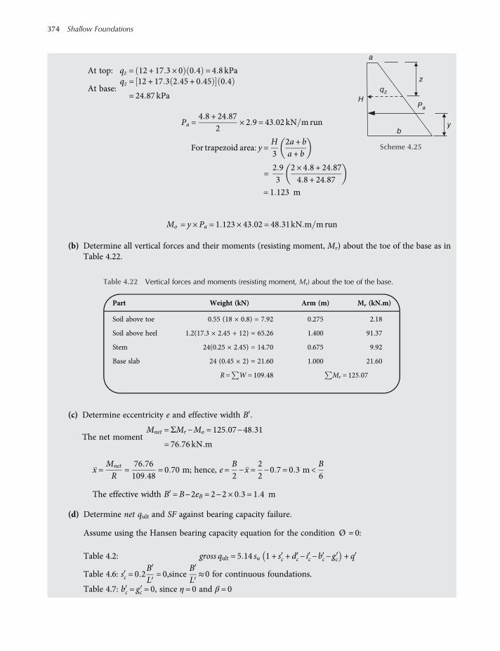
At top: qz = 12 + 17 3 × 0 0 4 = 4 8 kPa
At base:qz = 12 + 17 3 2 45 + 0 45 0 4
= 24 87 kPa
Pa =4 8 + 24 87
2× 2 9 = 43 02 kN mrun
For trapezoid area y =H3
2a+ ba + b
=2 93
2 × 4 8 + 24 874 8 + 24 87
= 1 123 m
Mo = y × Pa = 1 123 × 43 02 = 48 31kN m mrun
(b) Determine all vertical forces and their moments (resisting moment, Mr) about the toe of the base as inTable 4.22.
(c) Determine eccentricity e and effective width B .
The net momentMnet =ΣMr −Mo = 125 07−48 31
= 76 76 kN m
x =Mnet
R=
76 76109 48
= 0 70 m; hence, e=B2−x =
22−0 7 = 0 3 m<
B6
The effective width B = B−2eB = 2−2 × 0 3 = 1 4 m
(d) Determine net qult and SF against bearing capacity failure.
Assume using the Hansen bearing capacity equation for the condition Ø = 0:
Table 4.2: gross qult = 5 14 su 1 + sc + dc− ic−bc−gc + q
Table 4.6: sc = 0 2BL
= 0,sinceBL≈0 for continuous foundations.
Table 4.7: bc = gc = 0, since η= 0 and β = 0
H
b
qz
Pa
y
a
z
Scheme 4.25
Table 4.22 Vertical forces and moments (resisting moment, Mr) about the toe of the base.
Part Weight (kN) Arm (m) Mr (kN.m)
Soil above toe 0.55 (18 × 0.8) = 7.92 0.275 2.18
Soil above heel 1.2(17.3 × 2.45 + 12) = 65.26 1.400 91.37
Stem 24(0.25 × 2.45) = 14.70 0.675 9.92
Base slab 24 (0.45 × 2) = 21.60 1.000 21.60
R= W = 109 48 Mr = 125 07
374 Shallow Foundations
worksaccounts.com
dc = 0 4k; k=DBfor
DB≤ 1;
DB=1 252
= 0 625; hence, dc = 0 25
ic = 0 5−0 5 1−HAf ca
Af =B × 1;H = Pa. Assume ca = 0 7cu = 0 7 × 120 = 84 kPa
ic = 0 5−0 5 1−43 02
1 4 × 1 × 84= 0 102
gross qult = 5 14 su 1 + dc− ic + q
= 5 14 120 1 + 0 25−0 102 + 18 × 1 25
= 730 59 kPa
Equation (4.3):net qult = gross qult−γ Df
= 730 59−18 × 1 25 = 708 09 kPa
Net uniform foundation pressure,net q=R
B × 1−q=
109 481 4 × 1
−18 × 1 25
= 55 7 kPa
SF =net qultnet q
=708 955 7
= 12 7 3
Check the maximum foundation pressure, qmax:
qmax =RA+
R× eB2
1 B 3 1 12=109 481 × 2
+109 48 × 0 3
22
1 2 3 1 12= 104 01 kPa
gross qsafe =gross qult
SF=730 59
3= 243 53 kPa 104 01 kPa
The foundation is very safe against bearing capacity failure.(2) Safety against excessive settlement:
Assume average uniformnet contact pressure =RA−q
=109 481 × 2
−18 × 1 25
= 32 24 kPa
B 2z
=1 21 5
= 0 33,L 2z
=2 21 5
= 0 67. From Figure 2.32 obtain I≈0 075
At centre of the clay layerσz = 32 24 4I
= 32 24 × 4 × 0 07 = 10kPa
Equation (3.34):S= h mv σz = 3 12 × 10−4 10
= 0 036m= 36mm< 50mmThe foundation is safe against excessive settlement.
Shallow Foundations – Bearing Capacity 375
worksaccounts.com
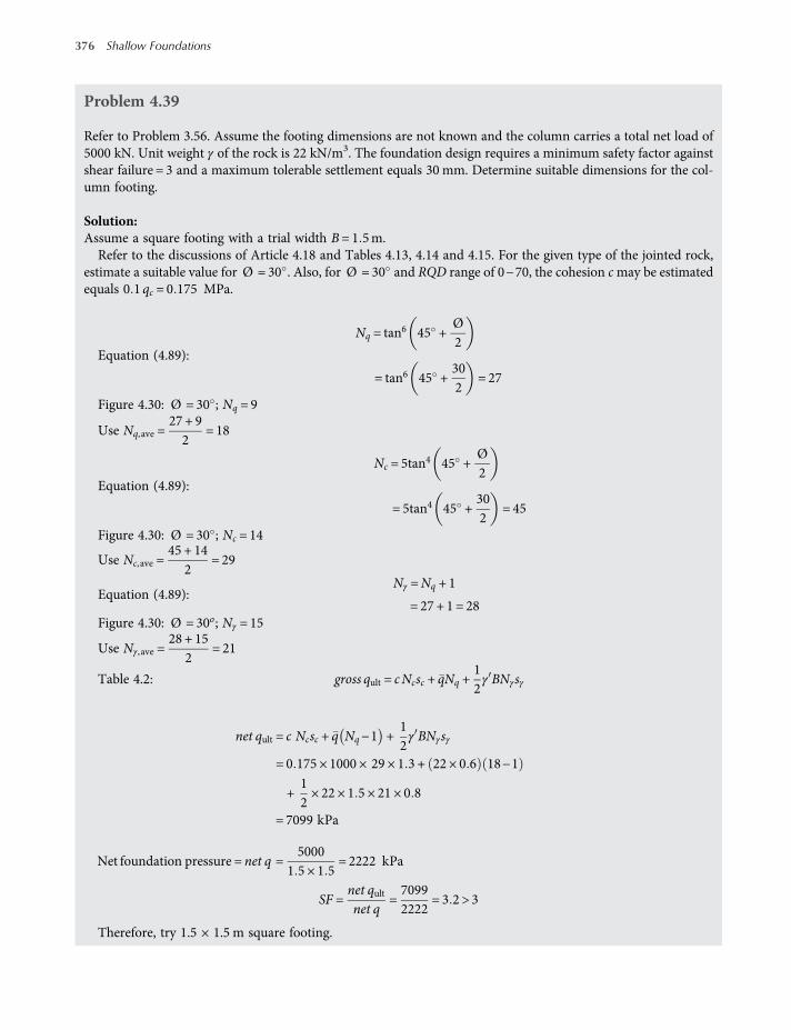
Problem 4.39
Refer to Problem 3.56. Assume the footing dimensions are not known and the column carries a total net load of5000 kN. Unit weight γ of the rock is 22 kN/m3. The foundation design requires a minimum safety factor againstshear failure = 3 and a maximum tolerable settlement equals 30 mm. Determine suitable dimensions for the col-umn footing.
Solution:Assume a square footing with a trial width B= 1 5m.Refer to the discussions of Article 4.18 and Tables 4.13, 4.14 and 4.15. For the given type of the jointed rock,
estimate a suitable value for Ø = 30 . Also, for Ø = 30 and RQD range of 0−70, the cohesion cmay be estimatedequals 0 1 qc = 0 175 MPa.
Equation (4.89):
Nq = tan6 45 +Ø2
= tan6 45 +302
= 27
Figure 4.30: Ø = 30 ; Nq = 9
Use Nq,ave =27 + 92
= 18
Equation (4.89):
Nc = 5tan4 45 +Ø2
= 5tan4 45 +302
= 45
Figure 4.30: Ø = 30 ; Nc = 14
Use Nc, ave =45 + 14
2= 29
Equation (4.89):Nγ =Nq + 1
= 27 + 1 = 28Figure 4.30: Ø = 30o; Nγ = 15
Use Nγ,ave =28 + 15
2= 21
Table 4.2: gross qult = cNcsc + qNq +12γ BNγsγ
net qult = c Ncsc + q Nq−1 +12γ BNγsγ
= 0 175 × 1000 × 29 × 1 3 + 22 × 0 6 18−1
+12× 22 × 1 5 × 21 × 0 8
= 7099 kPa
Net foundation pressure = net q =5000
1 5 × 1 5= 2222 kPa
SF =net qultnet q
=70992222
= 3 2 > 3
Therefore, try 1.5 × 1.5 m square footing.
376 Shallow Foundations
worksaccounts.com

Check settlement as follows:
Net foundation pressure = 2222 kPa = 2 222 MPa
For the 250 mm joint spacing, the fracture frequency per metre (or joint spacing per metre) is 1000 250 = 4.From Table 3.15, for a fracture frequency of four per metre, a suitable value for the mass factor ( j) is 0.6. Also, fromTable 3.16, for poorly cemented sandstone the modulus ratio (Mr) is 150. Let quc of the intact rock equals theuniaxial compression strength which is 1.75 MPa. The mass deformation modulus is given by Equation (3.66):
Em = jMr quc = 0 6 × 150 × 1 75 = 157 5 MPa
Assume the influence depth of the rock below the foundation level is H = 4B= 4 × 1 5 = 6 m.Divide the footing area into four equal 0.75 × 0.75 m squares.
Figure 3.25:LB=0 750 75
= 1;HB=
60 75
= 8; k= 0 (using Em = Ed = Ef ), obtain IP≈0 46
Figure 3.26a:HB=
61 5
= 4; FB≈1
Figure 3.26b:DB=0 61 5
= 0 4; FD = 0 925
Immediate settlement at the corner of each flexible square is given by
Equation (3.63):
ρi = qBEf
IpFBFD
= 2 2220 75157 5
0 46 1 0 925 = 4 5 × 10⁻³ m
Immediate settlement at the centre of the flexible raft is
4 4 5 × 10−3 = 0 018m
Equation (3.6):Si rigid = 0 93Si flexible
= 0 93 × 0 018 = 0 017 m= 17mmTable 3.12: gives rigidity factor = 0 85. Hence,
Si rigid = 0 85 × 0 018 = 0 015 m= 15mm
Average of the two settlement values = 16mm< 30mm; O KHowever, creep might increase the settlement to about the maximum tolerable settlement of 30 mm in thelong term.Use 1.5 m × 1.5 m square footing.
Problem 4.40
A column footing 1.6 × 1.6 m is required to be founded in a moderately strong rock mass of limestone. An embed-ment depth of 1.5 m is required to get through the top soil and weathered rock zone. Tests on rock cores takenbelow the foundation level showed representative unconfined compression strength quc = 24 MPa; other tests gaveaverage RQD= 0 5; friction angle Ø = 38 and rock unit weight γ = 24 5 kN m3. Neglect the relatively thin topsoil layer which overlies the rock. For the footing concrete use fc = 28 MPa. Assume a safety factor against bearingcapacity failure = 4. Estimate the gross safe bearing capacity for the foundation, taking into consideration the effectof discontinuities of the rock.
Solution:
Table 4.2: gross qult = cNcsc + qNq +12γ BNγsγ
(Continued)
Shallow Foundations – Bearing Capacity 377
worksaccounts.com
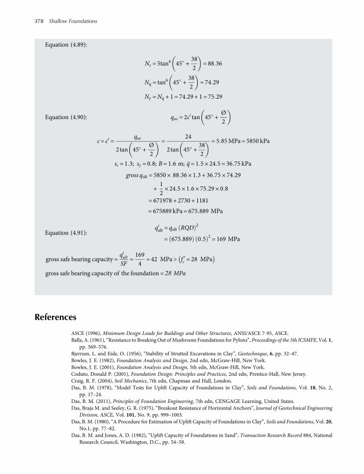
Equation (4.89):
Nc = 5tan4 45 +
382
= 88 36
Nq = tan6 45 +
382
= 74 29
Nγ =Nq + 1 = 74 29 + 1 = 75 29
Equation (4.90): quc = 2c tan 45 +Ø2
c= c =quc
2tan 45 +Ø2
=24
2tan 45 +382
= 5 85MPa = 5850 kPa
sc = 1 3; sγ = 0 8; B= 1 6 m; q= 1 5 × 24 5 = 36 75 kPa
gross qult = 5850 × 88 36 × 1 3 + 36 75 × 74 29
+12× 24 5 × 1 6 × 75 29 × 0 8
= 671978 + 2730 + 1181
= 675889 kPa = 675 889 MPa
Equation (4.91):qult = qult RQD 2
= 675 889 0 5 2 = 169 MPa
gross safe bearing capacity =qultSF
=1694
= 42 MPa > fc = 28 MPa
gross safe bearing capacity of the foundation = 28 MPa
References
ASCE (1996), Minimum Design Loads for Buildings and Other Structures, ANSI/ASCE 7-95, ASCE.Balla, A. (1961), “Resistance to BreakingOut ofMushroom Foundations for Pylons”, Proceedings of the 5th ICSMFE, Vol. 1,
pp. 569–576.Bjerrum, L. and Eide, O. (1956), “Stability of Strutted Excavations in Clay”, Geotechnique, 6, pp. 32–47.Bowles, J. E. (1982), Foundation Analysis and Design, 2nd edn, McGraw-Hill, New York.Bowles, J. E. (2001), Foundation Analysis and Design, 5th edn, McGraw-Hill, New York.Coduto, Donald P. (2001), Foundation Design: Principles and Practices, 2nd edn, Prentice-Hall, New Jersey.Craig, R. F. (2004), Soil Mechanics, 7th edn, Chapman and Hall, London.Das, B. M. (1978), “Model Tests for Uplift Capacity of Foundations in Clay”, Soils and Foundations, Vol. 18, No. 2,
pp. 17–24.Das, B. M. (2011), Principles of Foundation Engineering, 7th edn, CENGAGE Learning, United States.Das, Braja M. and Seeley, G. R. (1975), “Breakout Resistance of Horizontal Anchors”, Journal of Geotechnical Engineering
Division, ASCE, Vol. 101, No. 9, pp. 999–1003.Das, B. M. (1980), “A Procedure for Estimation of Uplift Capacity of Foundations in Clay”, Soils and Foundations, Vol. 20,
No.1, pp. 77–82.Das, B. M. and Jones, A. D. (1982), “Uplift Capacity of Foundations in Sand”, Transaction Research Record 884, National
Research Council, Washington, D.C., pp. 54–58.
378 Shallow Foundations
worksaccounts.com

DeBeer, E. E. (1965), “The Scale Effect on the Phenomenon of Progressive Rupture in Cohesionless Soils”, Proceedings ofthe 6th ICSMFE, Vol. 2, pp. 13–17.
Graham, J., Andrews, M. and Shields, D. H. (1988), “Stress Characteristics for Shallow Footing on Cohesionless Slopes”,Canadian Geotechnical Journal, Ottawa, Vol. 25, No. 2, pp. 238–249.
Hansen, J. B. (1970), “A Revised and Extended Formula for Bearing Capacity”,Danish Geotechnical Institute, Copenhagen,Bull. No. 28, 21, pp. (successor to Bull. No. 11) and Code of Practice for Foundation Engineering, Danish GeotechnicalInstitute Bull. No. 32(1978).
Hansen, J. B. (1961), “A General Formula for Bearing Capacity”, Danish Geotechnical Institute, Copenhagen, Bull. No. 11,pp. 38–46.
Highter, W. H. and Anders, J. C. (1985), “Dimensioning Footings Subjected to Eccentric Loads”, Journal of GeotechnicalEngineering Division, ASCE, Vol. 111, No. GT5, pp. 659–665.
ICBO (1997), Uniform Building Code, International Conference of Building Officials, Whittier, CA.ICC (2000), International Building Code, International Code Council.Knappett, J. A. and Craig, R. F. (2012), Soil Mechanics, 8th edn, Spon Press, Abingdon, Oxon, United Kingdom.Kulhawy, F. H. and Goodman, R. E. (1987), “Foundations in Rock”, Chapter 5 of Ground Engineering Reference Book, ed.
F. G. Bell, Butterworths, London.Kulhawy, F. H. and Goodman, R. E. (1980), “Design of Foundations on Discontinuous Rock”, Structural Foundations on
Rock, Balkema, Rotterdam, pp. 209–220.Merifield, R. S., Lyamin, A. and Sloan, S. W. (2003), “Three Dimensional Lower Bound Solution for the Stability
of Plate Anchors in Clay”, Journal of Geotechnical and Geoenvironmental Engineering, ASCE, Vol. 129, No. 3,pp. 243–253.
Meyerhof, G. G. (1951), “The Ultimate Bearing Capacity of Foundations”, Geotechnique, Vol. 2, No. 4, pp. 301–331.Meyerhof, G. G. (1953), “The Bearing Capacity of Foundations under Eccentric and Inclined Loads”, Third ICSMFE, Vol.
1, pp. 440–445.Meyerhof, G. G. (1955), “Influence of Roughness of Base and Ground-Water Conditions on the Ultimate Bearing Capacity
of Foundations”, Geotechnique, Vol. 5, pp. 227–242 (reprinted in Meyerhof, 1982).Meyerhof, G. G. (1956), “Penetration Tests and Bearing Capacity of Cohesionless Soils”, JSMFD, ASCE, Vol. 82, SM 1,
pp. 1–19.Meyerhof, G. G. (1957), “The Ultimate Bearing Capacity of Foundations on Slopes”, Fourth ICSMFE, Vol. 1, pp. 384–387.Meyerhof, G. G. (1963), “Some Recent Research on the Bearing Capacity of Foundations”, Canadian Geotechnical Journal,
Ottawa, Vol. 1, No. 1, Sept, pp. 16–26.Meyerhof, G. G. (1965), “Shallow Foundations”, Proceedings ASCE, 91, No. SM2, pp. 21–31.Meyerhof, G. G. and Adams, J. I. (1968), “The Ultimate Uplift Capacity of Foundations”, Canadian Geotechnical Journal,
Ottawa, Vol. 5, No. 4, Nov, pp. 225–244.Meyerhof, G. G. (1974), “Ultimate Bearing Capacity of Footings on Sand layer Overlying Clay”, Canadian Geotechnical
Journal, Ottawa, Vol. 11, No. 2, May, pp. 223–229.Meyerhof, G. G. and Hanna, A. M. (1978), “Ultimate Bearing Capacity of Foundations on Layered Soil under Inclined
Load”, Canadian Geotechnical Journal, Ottawa, Vol. 15, No. 4, pp. 565–572.Meyerhof, G. G. (1982), Bearing Capacity and Settlement of Foundations, Tech-Press, Technical University of Nova Scotia,
Halifax.Prakash, S. and Saran, S. (1971), “Bearing Capacity of Eccentrically Loaded Footings”, Journal of the Soil Mechanics and
Foundations Division, ASCE, Vol. 97, No. SM1, pp. 95–117.Prandtl, M. (1921), “Űber die Eindringungsfestigkeit (H arte) plastischer Baustoffe und die Festigkeit von Schneiden”, [On
the penetrating strengths (Hardness) of plastic construction materials and the strength of cutting edges], Zeitchrift fürangewandte Mathematik und Mechanik, Vol. 1, No.1, pp. 15–20.
Purkayastha, R. D. and Char, R. A. N. (1977), “Stability Analysis of Eccentrically Loaded Footings”, Journal of GeotechnicalEngineering Division, ASCE, Vol. 103, No. GT6, pp. 647–651.
Reissner, H., (1924), Zum Erddruckproblem”, (Concerning the earth-pressure problem), Proceedings of the 1st Inter-national Congress of Applied Mechanics, Delft, Netherlands, pp. 295–311.
Saran, S. and Agarwal, R. B. (1991), “Bearing Capacity of Eccentrically Obliquely Loaded Footing”, Journal of GeotechnicalEngineering Division, ASCE, Vol. 117, No. 11, pp. 1669–1690.
Schmertmann, J. H. (1978), Guidelines for Cone Penetration Test: Performance and Design, Report FHWA-TS-78-209,Federal Highway Administration, Washington, D.C.
Skempton, A. W. (1951), “The Bearing Capacity of Clays”, Proceedings Building Research Congress, 1, pp. 180–189.London.
Stuart, J. G. (1962), “Interference between Foundations with Special Reference to Surface Footings in Sand”, Geotechnique,London, England, Vol. 12, No. 1, pp.15–22.
Stagg, K. G. and O. C. Zienkiewicz (1968), Rock Mechanics in Engineering Practice (with 12 contributing authors), JohnWiley & Sons, Inc., New York, 442 pp.
Terzaghi, K. (1943), Theoretical Soil Mechanics, John Wiley & Sons, Inc., New York, 510 pp.
Shallow Foundations – Bearing Capacity 379
worksaccounts.com
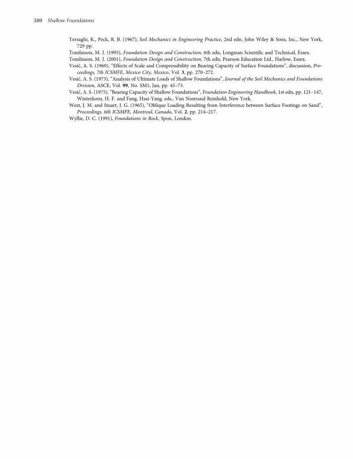
Terzaghi, K., Peck, R. B. (1967), Soil Mechanics in Engineering Practice, 2nd edn, John Wiley & Sons, Inc., New York,729 pp.
Tomlinson, M. J. (1995), Foundation Design and Construction, 6th edn, Longman Scientific and Technical, Essex.Tomlinson, M. J. (2001), Foundation Design and Construction, 7th edn, Pearson Education Ltd., Harlow, Essex.Vesič, A. S. (1969), “Effects of Scale and Compressibility on Bearing Capacity of Surface Foundations”, discussion, Pro-
ceedings, 7th ICSMFE, Mexico City, Mexico, Vol. 3, pp. 270–272.Vesič, A. S. (1973), “Analysis of Ultimate Loads of Shallow Foundations”, Journal of the Soil Mechanics and Foundations
Division, ASCE, Vol. 99, No. SM1, Jan, pp. 45–73.Vesič, A. S. (1975), “Bearing Capacity of Shallow Foundations”, Foundation Engineering Handbook, 1st edn, pp. 121–147,
Winterkorn, H. F. and Fang, Hsai-Yang, eds., Van Nostrand Reinhold, New York.West, J. M. and Stuart, J. G. (1965), “Oblique Loading Resulting from Interference between Surface Footings on Sand”,
Proceedings, 6th ICSMFE, Montreal, Canada, Vol. 2, pp. 214–217.Wyllie, D. C. (1991), Foundations in Rock, Spon, London.
380 Shallow Foundations
worksaccounts.com

CHAPTER 5
Shallow Foundations – Structural Design
5.1 General
One of the most important matters the foundation performance requirements concern is the strengthof the foundation. As discussed in Section 2.4, one type of this strength is the structural strength. It isimportant to realise that foundations which are loaded beyond their structural strength capacity will, inprinciple, fail catastrophically. Therefore, foundations are designed to avoid structural failures, similarto the other structural analyses.Foundation units such as footings transfer the loads from the structure to the soil or rock supporting
the structure. As the soil is generally much weaker than the concrete columns and walls that must besupported, the contact area between the soil and the foundation base is much larger than that betweenthe supported member and the base. The plan dimensions of the base contact area and the embedmentdepth (foundation depth) are primarily geotechnical concerns, as discussed in Section 4.17. Soon afterthese design requirements have been set, the next step is to develop a structural design that gives thefoundation enough strength and integrity to safely transmit the design loads from the structure to theground.In general, the structural design of a reinforced concrete base includes:
• Selecting the more significant combination of loads that the particular foundation must support,and computing the design factored loads.
• Selecting an appropriate value for the compressive strength, fc , of concrete.
• Selecting an appropriate grade of the reinforcing steel which specifies the yield strength, fy, ofreinforcement.
• Determining the required thickness of the concrete base.
• Determining the size, number, spacing and location of the flexural and temperature reinfor-cing bars.
• Designing the connection between the supported member (column, pedestal or wall) and the struc-tural base.
Virtually all foundations support a compressive vertical load and, unlike the geotechnical design, it iscomputed without including the weight of the structural base because this weight is evenly distributedand thus does not produce shear or moment in the base. Sometimes foundations are required to
Shallow Foundations: Discussions and Problem Solving, First Edition. Tharwat M. Baban.© 2016 John Wiley & Sons, Ltd. Published 2016 by John Wiley & Sons, Ltd.
worksaccounts.com
support shear and moment loads also. Again, unlike the geotechnical design, in structural design all theloads supported by the foundation must be factored loads.
In structural design of shallow foundations there are two modes of failure considered: shear andflexure. A structural base may fail in shear as a wide beam, referred to as one-way shear or beam shear,or as a result of punching, referred to as two-way shear or punching shear. Punching shear failure occurswhen part of the base is just about to come out of the bottom, which is actually a combination of tensionand shear on inclined failure surfaces. These shear stresses are resisted by providing an adequate basethickness; without using shear reinforcement. The flexural (bending) stresses are resisted by providingsteel reinforcement similar to any other reinforced concrete structural member.
The design and construction of buildings is regulated by municipal bylaws called building codes(MacGregor et al., 2005). Unlike the geotechnical design, the structural design aspects are more strictlycodified. Any structural design must satisfy requirements of a specified building code. The most not-able, widely used, code is the Building Code Requirements for Structural Concrete, generally referred toas theACI 318 orACI Code, published by the American Concrete Institute (ACI). The code is explainedin a Commentary; they are bound together in one volume. Chapter 5 of this book refers extensively tothe ACI 318M-08 code. Chapter 15 of the code concerns the structural design of footings. It is recom-mended that the reader have a copy available.
5.2 Design Loads
Section 9.2 of ACI 318M-08 defines the design factored load, for use in the LRFDmethod, as the largestof those computed from the following equations:
ACI Equation 9-1 U = 1 4 D+ F 5 1
ACIEquation 9-2 U = 1 2 D+ F +T + 1 6 L+H + 0 5 Lr or S orR 5 2
ACI Equation 9-3 U = 1 2D+ 1 6 Lr or S orR + 1 0L or 0 8W 5 3
ACIEquation 9-4 U = 1 2D+ 1 6W + 1 0L+ 0 5 Lr or S orR 5 4
ACI Equation 9-5 U = 1 2D+ 1 0E + 1 0L+ 0 2S 5 5
ACI Equation 9-6 U = 0 9D+ 1 6W + 1 6H 5 6
ACI Equation 9-7 U = 0 9D+ 1 0E + 1 6H 5 7
Each load designation such as D, F, T and so on is defined in Section 2.1 of the ACI Code and inSection 4.17 of this book.
The reader should be aware of the exceptions and limitations regarding some of the factored loads inthe above equations, as stated in ACI Section 9.2.1. Also, it is important to remember that the above-mentioned design factored load combinations must only be used in conjunction with strength-reduction factors of ACI Section 9.3.2.
As an alternative to the requirements of ACI Sections 9.2.1 and 9.3.2, ACI 318M-08, Appendix C,Section C.9.1 permits the design of reinforced structural concrete members using the load combin-ations defined in Section C.9.2 and the strength-reduction factors of Section C.9.3.
5.3 Selection of Materials
In the design of shallow foundations the structural engineer (the designer) must select appropriatevalues for concrete compressive strength, fc , and reinforcing steel yield strength, fy. It is easy for a struc-tural engineer to do so, whereas a geotechnical engineer has little or no control over the engineer prop-erties of the supporting natural soil deposits.
382 Shallow Foundations
worksaccounts.com

In design of spread footings, selection of high strength concrete may not be justified unless the foot-ings carry relatively large loads. The plan dimensions of footings are governed by bearing capacity andsettlement requirements; it is the footing thickness only which is governed by the concrete strength.Moreover, high strength concrete requires additional materials and inspection costs. Spread footingsare usually designed using fc of only 20–25 MPa. For footings that carry relatively large loads, highstrength concrete might be justified to keep the footing thickness within reasonable limits, perhapsusing fc as high as 35 MPa.Usually, the flexural stresses in footings are small compared to those in the other structural members
of the superstructure. Grade-300 steel is usually adequate to resist flexural stresses in spread footings,whereas, Grade-420 steel is, most probably, required on the remaining reinforced concrete members.However, due to practical and economic reasons, usually, designers like to use one grade of steel asmuch as possible. Therefore, for foundations built of reinforced concrete, designers often useGrade-420 steel, the same as for the other structural members of the structure.
5.4 Structural Action of Vertically and Centrically Loaded Isolatedand Continuous (Strip) Footings
5.4.1 General
The structural analysis and design methodology of reinforced concrete footings that engineers now usehave been developed, standardised and codified as a result of full-scale tests conducted by manyresearchers at various times (Talbot, 1913; Richart, 1948; Whitney, 1957; Moe, 1961). Scientific soci-eties, associations and organisations made important contributions (ACI-ASCE, 1962). The structuraldesign of a footing must essentially consider flexure (bending), shear, development of reinforcement,and the transfer of load from the column or wall to the footing. Each of these design aspects will beconsidered separately in the following Sections.
5.4.2 Flexure
An individual column footing is shown in Figure 5.1. Contact soil pressures cause bending of the footingabout axes A−A and B−B, as shown in Figure 5.1a. Soil pressures acting under the cross-hatched portionof the footing in Figure 5.1b cause moments,Mu, about axis A−A at the face of the column. The footingbehaves as if it is an inverted cantilever beam. The same argument is true with respect to a continuous(strip) wall footing, in which soil pressures cause bending of the footing about axis A−A along the walllength only. Tensile stresses due to these bending moments must be resisted by tensile reinforcementplaced near the footing bottom, in both directions for column footing (Figure 5.1c), and in transversedirection for wall footing. The total factored moment at the critical section (Figure 5.1b) is:
Mu = lbqfactored l 2 5 8
The critical sections for maximum factored moment, Mu, in the footing are located as follows (ACISection 15.4.2):
• At face of column, pedestal, or wall, for footings supporting a concrete column, pedestal, or wall;
• Halfway between middle and edge of wall, for footings supporting a masonry wall;
• Halfway between face of column and edge of steel base plate, for footings supporting a column withsteel base plate.
According to ACI Section 15.3, for location of critical sections for moment, shear, and developmentof reinforcement in footings, it shall be permitted to treat circular or regular polygon-shaped concretecolumns or pedestals as square members with the same area.
Shallow Foundations – Structural Design 383
worksaccounts.com
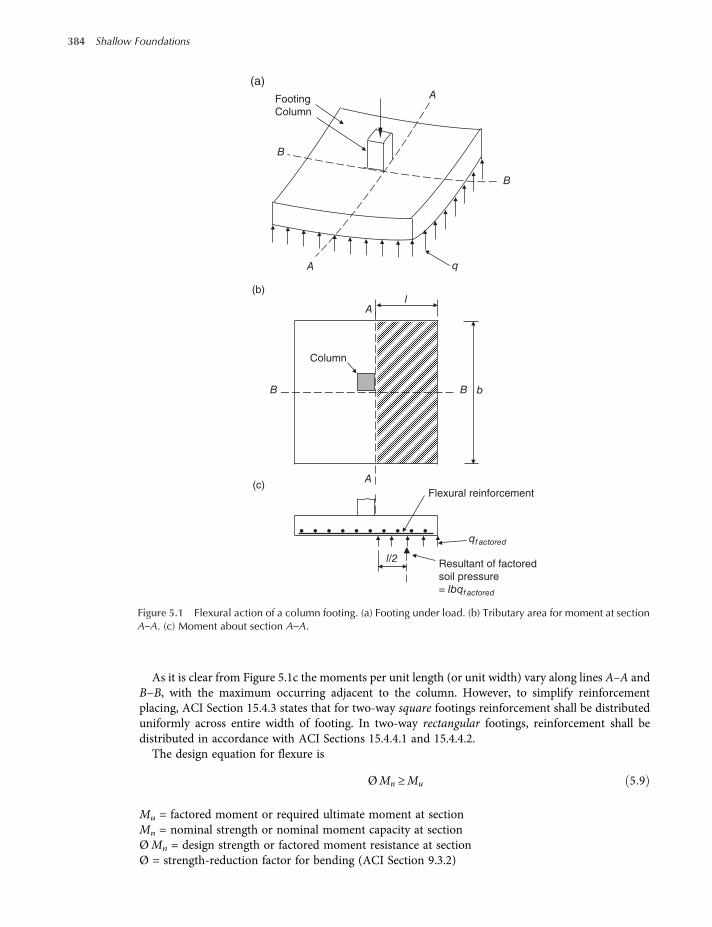
As it is clear from Figure 5.1c the moments per unit length (or unit width) vary along lines A–A andB−B, with the maximum occurring adjacent to the column. However, to simplify reinforcementplacing, ACI Section 15.4.3 states that for two-way square footings reinforcement shall be distributeduniformly across entire width of footing. In two-way rectangular footings, reinforcement shall bedistributed in accordance with ACI Sections 15.4.4.1 and 15.4.4.2.
The design equation for flexure is
ØMn ≥Mu 5 9
Mu = factored moment or required ultimate moment at sectionMn = nominal strength or nominal moment capacity at sectionØMn = design strength or factored moment resistance at sectionØ = strength-reduction factor for bending (ACI Section 9.3.2)
Footing
Column
B
A
A
A
B
A
B b
l
B
q
(c)
Column
(a)
(b)
Resultant of factored
soil pressure
= lbqf actored
Flexural reinforcement
qf actored
l/2
Figure 5.1 Flexural action of a column footing. (a) Footing under load. (b) Tributary area for moment at sectionA–A. (c) Moment about section A–A.
384 Shallow Foundations
worksaccounts.com

Two requirements are satisfied throughout the analysis and design of a reinforced concrete member,(1) stress and strain compatibility, which requires stress at any point in the beam must correspond tothe strain at that point, (2) equilibrium, which requires the internal forces must balance the externalload effects.
Equations forMn – Tension steel yielding:ACI Section 10.2.7 permits the use of the equivalent rectangular compressive stress distribution, asshown below:
α1fc = 0 85fc ACI Section 10 2 7 1
β1 = factor relating depth a of the equivalent rectangularcompressive stress block to the neutral axis depth c.
For fc between 17 and 28 MPa, β1 shall be taken as 0.85. For fc above 28 MPa, β1 shall be reducedlinearly at a rate of 0.05 for each 7 MPa of strength in excess of 28 MPa, but β1 shall not be taken lessthan 0.65 (ACI Section 10.2.7.3).The compressive force in the concrete is
C = volume of the compressive stress block = 0 85fc ba
The tension force in the steel is
T =Asfs
For equilibrium, C = T, and therefore, the depth of the equivalent stress block is
a=Asfs
0 85fc b
If it is assumed that fs = fy, then
a=Asfy
0 85fc b5 10
Neutral axis
(axis of zero
strain) Cross section
of a beam
b
c
d = dt
a = β1ca/2
C
α1f'c
Equivalent rectangular
stress distribution
jd = d – a/2
T
Scheme 5.1
Shallow Foundations – Structural Design 385
worksaccounts.com
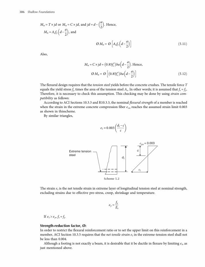
Mn = T × jd or Mn = C × jd, and jd = d−a2
. Hence,
Mn =Asfy d−a2
, and
ØMn = Ø Asfy d−a2
5 11
Also,
Mn =C × jd = 0 85fc ba d−a2
Hence,
ØMn = Ø 0 85fc ba d−a2
5 12
The flexural design requires that the tension steel yields before the concrete crushes. The tensile force Tequals the yield stress fy times the area of the tension steel As. In other words; it is assumed that fs = fy.Therefore, it is necessary to check this assumption. This checking may be done by using strain com-patibility as follows:
According to ACI Sections 10.3.3 and R10.3.3, the nominal flexural strength of a member is reachedwhen the strain in the extreme concrete compression fiber εcu reaches the assumed strain limit 0.003as shown in thisscheme.
By similar triangles,
εt = 0 003dt −cc
The strain εt is the net tensile strain in extreme layer of longitudinal tension steel at nominal strength,excluding strains due to effective pre-stress, creep, shrinkage and temperature.
εy =fyEs
If εt > εy, fs = fy
Strength-reduction factor, Ø:In order to restrict the flexural reinforcement ratio or to set the upper limit on this reinforcement in amember, ACI Section 10.3.5 requires that the net tensile strain εt in the extreme-tension steel shall notbe less than 0.004.
Although a footing is not exactly a beam, it is desirable that it be ductile in flexure by limiting εt, asjust mentioned above.
Extreme tension
steeldt
εt
c
εcu = 0.003
Scheme 5.2
386 Shallow Foundations
worksaccounts.com
ACI Section 10.3.3 states that, sections are compression-controlled if the net tensile strain in theextreme tension steel εt is equal to or less than the compression-controlled strain limit when the con-crete in compression reaches its assumed strain limit of 0.003. The compression-controlled strain limitis the net tensile strain in the reinforcement at balanced strain conditions. For Grade-420 reinforce-ment, and for all pre-stressed reinforcement, it shall be permitted to set the compression-controlledstrain limit equal to 0.002.ACI Section 10.3.4 states that, sections are tension-controlled if the net tensile strain in the extreme
tension steel εt is equal or greater than 0.005 when the concrete in compression reaches its assumedstrain limit of 0.003. Sections with εt between the compression-controlled strains limit and 0.005 con-stitute a transition region between compression-controlled and tension-controlled sections.For tension-controlled sections: Ø = 0.9 (ACI Section 9.3.2.1):
For compression-controlled sections (flexural members other than spiral columns): Ø = 0.65 [ACISection 9.3.2.2(b)]
For sections in the transition region: 0.90 > Ø > 0.65
According to ACI Section 9.3.2.2, for sections in the transition region, Ø shall be permitted to be lin-early increased from that for compression-controlled sections to 0.9 as εt increases from the compres-sion-controlled strain limit to 0.005.For Grade-420 steel, for which the compression-controlled strain limit is 0.002, the variation of Ø
with net tensile strain in extreme tension steel εt is shown in ACI Figure R9.3.2. Accordingly, Ø is deter-mined by linear proportionality as follows:
Ø = 0 65 +εt −0 002
0 005−0 0020 9−0 65
Ø = 0 65 + εt −0 002 250 3
5 13
As indicated in ACI Figure R9.3.2, the factor Ø is also determined from the following equation:
Ø = 0 65 + 0 251
c dt−53
5 14
Equations (5.13) and (5.14) give
εt =dt −cc
× 0 003 5 15
where
c = distance from extreme compression fiber to neutral axisdt = the distance from the extreme compression fiber to the extreme tension steel
Similarly, for Grade-280 steel, for which the compression-controlled strain limit isfyEs
= 0 0014 , the
factor Ø is determined from the following equations:
Ø = 0 55 + 69 4εt 5 16
or
Ø = 0 34 +0 21c dt
5 17
Shallow Foundations – Structural Design 387
worksaccounts.com

According to ACI Section 10.5.4, for footings of uniform thickness, the minimum area of flexural ten-sile reinforcement As, min shall be the same as that required for shrinkage and temperature reinforce-ment in accordance with ACI Section 7.12.2.1. Therefore, for deformed bars of Grade-280 or 530 steel,As, min = 0.002 bh; for deformed bars or welded wire reinforcement of Grade-420 steel, As,min =0.0018 bh. Also, ACI Section 10.5.4 requires that, the maximum spacing of this minimum reinforce-ment shall not exceed three times the footing thickness, or 450 mm whichever is smaller.
In case the required flexural reinforcement exceeds the minimum flexural reinforcement, it shall beadequate to use the same maximum spacing of reinforcement for slabs which is two times the slabthickness or 450 mm, whichever is smaller, as specified by ACI Section 13.3.2.
According to ACI Section 7.12.2.2, shrinkage and temperature reinforcement shall be spaced notfarther apart than five times the slab thickness, nor farther apart than 450 mm.
ACI Section 7.7.1-(a) states that, cover for reinforcement in concrete cast against and permanentlyexposed to earth, shall not be less than 75 mm.
ACI Section 15.7 states that, depth of footing above bottom reinforcement shall not be less than150 mm for footings on soil, or less than 300 mm for footings on piles.
5.4.3 Shear
As mentioned in Section 5.1, a footing may fail in shear as a wide beam, referred to as one-way shear orbeam shear (Figure 5.2a), or as a result of punching, referred to as two-way shear or punching shear(Figure 5.2b).
Shear reinforcement is very seldom used in spread footings or in mats, due to difficulty in placing it,and due to the fact that it is usually cheaper and easier to deepen the footings than to provide stirrups.ACI Section 11.4.6.1 excludes footings from the minimum shear reinforcement requirements. For thesereasons the factored shear force, Vu, at any critical section shall be resisted only by the concrete shearstrength alone.
Inclined crack
d f
Critical section
for one-way
shear
qf actored
Column
Tributary area for
one-way shear
k
Critical section for
two-way shear
m +
d
m
n
n + d
Tributary area for
two-way shear
Inclined
crack d/2
d/2
d/2
(a)
d
b
(b)
Figure 5.2 Critical sections and tributary areas for shear in a column footing (see text for details).
388 Shallow Foundations
worksaccounts.com

One-way shear:According to ACI Sections 15.5.1, 15.5.2, 11.11.1.1 and 11.1.3.1, critical section for one-way shearextends in a plane across the entire width of the footing, located at distance d from face of the column,pedestal, or wall, as shown in Figure 5.2a. For footings supporting a column or pedestal with steel baseplates, the critical section shall be located at distance d from a line halfway between the face of thecolumn and the edge of the base plate.From Figure 5.2a, the factored shear force
Vu = bfqfactored 5 18
ACI Section 11.1.1 requires that
ØVc ≥Vu taking reinforcement shear strength, Vs = 0 5 19
where
Ø = strength-reduction factor= 0.75 for shear (ACI Section 9.3.2.3)
Vc = nominal shear strength provided by concret
According to ACI Sections 11.11.1.1 and 11.2.1.1, Vc shall be computed as
Vc = 0 17λ fc bwd 5 20
where
λ = modification factor (ACI Section 8.6.1)fc = square root of specified compressive strength of concrete in MPA.
bw = footing width or length of critical sectiond = distance from extreme compression fiber to centroid of longitudinal tension reinforcement
Two-way shear:In footings subject to two-way action, failure may occur by punching along a truncated cone or pyramidaround a column. For square or rectangular columns, ACI Sections 11.11.1.2 and 11.11.1.3 allows theuse of a critical section with four straight sides drawn parallel to and at a distance d/2 from the faces ofthe column (or the edges of the loaded area), as shown by the dashed lines in Figure 5.2b. The tributaryarea, assumed critical for design purposes, is shown cross-hatched. For footings supporting a column orpedestal with steel base plates, the critical section shall be located at distance d/2 from a line halfwaybetween the face of the column and the edge of the base plate ACI Section 15.5.2.The applied net factored shear force is:
Vu = factored column loads – factored soil reaction on the shear block
Vu =Af qfactored − m+ d n+ d qfactored 5 21
where Af is the footing areaSince shear reinforcement is not used in a footing, Ø Vc ≥Vu. According to ACI Section 11.11.2.1, Vc
shall be the smallest of (a), (b), and (c):
Shallow Foundations – Structural Design 389
worksaccounts.com
(a) Vc = 0 17 1 +2β
λ fc bod 5 22
(b) Vc = 0 083αsdbo
+ 2 λ fc bod 5 23
(c) Vc = 0 33 λ fc bod 5 24
where:
β = the ratio of long side to short side of the column, concentrated load or reaction area.bo = the perimeter of the critical section for two-way shear.αs = a constant equals 40 for interior columns, 30 for edge columns and 20 for corner columns.
ACI Section 15.5.3 requires that, footing supported on piles (i.e. piles cap) shall satisfy ACI Sections11.11 and 15.5.4.
ACI Section 15.5.4 states that, computations of shear on any section through a footing supported onpiles shall be in accordance with 15.5.4.1, 15.5.4.2, and 15.5.4.3.
5.4.4 Development of Reinforcement
The calculated reinforcing bar stresses at any section must be developed by extending each bar on eachside of that section a sufficient distance ld (embedment length), or by hook (for bars in tension only) atthe outer ends.
ACI Section 15.6.2 states that calculated tension or compression in reinforcement at eachsection shall be developed on each side of that section by embedment length, hook (tension only)or mechanical device or a combination thereof. ACI Section 15.6.1 requires this development ofreinforcement in footings be accomplished in accordance with Chapter 12 of the Code. Accordingto ACI Section 15.6.3, critical sections for development of reinforcement shall be assumed at the samelocations as defined in ACI Section 15.4.2 for maximum factored moment and at all other verticalplanes where changes of section or reinforcement occur.
5.4.5 Transfer of Force at Base of Column, Wall or Pedestal
Connections through which forces and moments are transferred must be designed carefully, sincethey are often the weak links in structures. There are different types of connections available; eachis intended for particular loading conditions, and construction materials of both the supported andsupporting members. For example; the methods of connecting concrete, steel and wood columns toconcrete footings are different. This Section will discuss concrete column, wall or pedestal con-nected to concrete footing, and steel column with base plate connected to concrete footing orpedestal.
Concrete column, wall or pedestal connected to concrete footing:ACI Section 15.8.1 states that, forces and moments at base of column, wall, or pedestal shall be trans-ferred to supporting pedestal or footing by bearing on concrete and by reinforcement, dowels andmechanical connectors.
According to ACI Section 15.8.1.1, bearing stress on concrete at contact surface between concretecolumn or wall (supported member) and concrete footing or pedestal (supporting member) must notexceed concrete bearing strength for either surface as given by ACI Section 10.14.
According to ACI Section 10.14.1, the maximum design bearing strength of concrete isØ 0 85fc A1 except when the supporting surface is wider on all sides than the loaded area; then
390 Shallow Foundations
worksaccounts.com

the design bearing strength of the loaded area shall be permitted to be multiplied by A2 A1 but not
more than two (i.e. the design bearing strength = Ø 0 85fc A1 A2 A1, and A2 A1 ≤ 2). For theload combinations of ACI Section 9.2.1, ACI Section 9.3.2.4 gives the strength-reduction factor Ø =0.65 for bearing.Area A1 is the loaded area (area of the contact surface) but not greater than the bearing cross-
sectional area or the bearing plate area. Area A2 is area of the lower base of larger frustum of apyramid, cone, or tapered wedge contained wholly within the support and having for its upperbase the loaded area (A1), and having side slopes of 1 vertical to 2 horizontal, as shown inFigure 5.3.ACI Section 15.8.2 states that, for a castinplace construction, the reinforcement required to satisfying
15.8.1 shall be provided either by extending longitudinal bars (reinforcement) into supporting pedestalor footing, or by dowels. For cast-in-place columns and pedestals, area of these bars across interfaceshall be not less than 0.005 Ag, where Ag is the gross area of the supported member (ACISection 15.8.2.1). For cast-in-place walls, ACI Section 15.8.2.2 requires area of reinforcement acrossinterface shall be not less than minimum vertical reinforcement given in ACI Section 14.3.2.In practice, generally, the column bars stop at the top of the footing or pedestal, and dowels are used
to transfer loads across the interface. This is because it is unwieldy to embed the column steel in thefooting or pedestal, due to its unsupported height above the supporting member and the difficulty inlocating it properly.For castinplace columns and pedestals, normally, the number of dowels is equal to the number of
longitudinal bars in the column or pedestal. However, at least four dowels should be provided acrossinterface.According to ACI Section 15.8.2.3:
• Dowels shall not be larger than No. 36 bar.
• At footings, it is permitted to lap splice longitudinal bars of sizes as large as No. 43 and No. 57, incompression only, with dowels.
Column
45° 45°
2
1
2
1
Side view
Plan
Frustum
A1= Loaded area
A2= Lower base area
of frustum
Footing or pedestal
A2 is measured
on this plane
Footing or
pedestal
Column
A2
A1
Figure 5.3 Application of frustum to find A2 in footing or pedestal.
Shallow Foundations – Structural Design 391
worksaccounts.com

• Dowels shall extend into supported member a distance not less than the compression developmentlength ldc of the longitudinal bars (larger than dowels) and compression lap splice length of thedowels, whichever is greater (ACI Sections 12.3.2, 12.3.3, 12.16.1, 12.16.2).
• Dowels shall extend into the footing a distance not less than ldc of the dowels (ACI Sections 12.3.2and 12.3.3).
Usually, dowels have a 90 hook at the bottom used to facilitate fastening them tightly in place with thefooting bottom bars. Figure 5.4a shows a column-footing joint with dowel bars extending through theinterface, and Figure 5.4b shows a wall-footing joint.
The preceding discussions concern the condition in which the full section at the interface is undercompressive stresses. In other words, no moments are transferred or the eccentricity falls within thekern of the section. The total force transferred by bearing is then calculated as (Ag − Asd) timesthe smaller of the bearing stresses allowed on the supported member (column, pedestal or wall) orthe supporting member (footing), where Asd is area of the longitudinal bars or dowels crossing theinterface. Any additional load must be transferred by dowels [ACI Section 15.8.1.2-(a)].
For the condition in which moments are transferred to the supporting footing or pedestal, usually,compressive stresses will exist over part, but not all, of the cross-section. The number of dowelsrequired can be obtained by considering the cross-sectional area as an eccentrically loaded column witha maximum compressive concrete stress equal to the smaller of the bearing stresses allowed on thesupported member (column, pedestal or wall) or the supporting member (footing). Sufficientreinforcement must cross the interface to provide the necessary axial load and moment capacity. Ingeneral, this requires that all the column bars or dowels of the same steel area must cross the interface.According to ACI Section 15.8.1.3, these longitudinal bars or dowels should satisfy ACI Section 12.17.Also, the minimum embedment length of these bars in the footing should not be smaller than the com-pression development length ldc or tension development length ldh, whichever is greater.
Since the footing and column are poured separately, there is a weak shear plane along the cold joint.For the condition in which lateral forces are imparted to the supporting footing or pedestal, ACISection 15.8.1.4 requires that, these forces shall be transferred in accordance with shear-friction pro-visions of ACI Section 11.6, or by other appropriate means.
Dowel
length
in wall
Dowel
length in
column
Column longitudinal
steel bars Wall vertical
steel bars
Dowel
≥ ldc≥ ldc
Dowel
Footing
reinforcement
Footing
reinforcement
Concrete
footing
Concrete
footing
Concrete
column
Concrete
wall
(a) (b)
Figure 5.4 (a) Column-footing joint. (b) Wall-footing joint.
392 Shallow Foundations
worksaccounts.com

Steel column with base plate connected to concrete footing or pedestal:A steel column requires a base plate either shop-welded or field-bolted to its bottom, to spread the veryhigh stresses in the small column contact area to a value that the supporting footing or pedestal can safelycarry. Steel columns are connected to their foundations using anchor bolts or rods of specified type, gradeand ultimate tensile strength (Table 5.1). Slightly oversized holes, 2 to 5 mm larger in diameter than thebolts, are shop punched in the base plate for later attachment to the supportingmember. The anchor boltsare usually set in nearly exact position in the wet concrete and become fixed in place. The slightly over-sized holes allow a small amount of bolt misalignment when placing the base plate into position; thus,erection of the column onto the foundation is simplified. Figure 5.5 shows a base plate and anchor boltsused to connect ametal column to its foundation.More often, four anchor bolts are used for each column.If possible, it is best to place the bolts in a square pattern to simplify construction and leave less oppor-tunity for mistakes. Of course, more bolts and other patterns also may be used, if necessary.It is necessary the base plate is carefully aligned horizontally and to elevation, since top surface of the
concrete footing or pedestal is usually rough and not necessarily level. Therefore, the contractor mustuse special construction methods to provide adequate support for the plate and to make the columnplumb. One method is to use shims (small and thin steel wedges), which are driven between the baseplate and the supportingmember. The remaining space is grouted, using non-shrink grout which swellsslightly when it cures (as compared to normal grout, which shrinks).
Table 5.1 Ultimate tensile strength, Tu, of selected A307 bolts*.
Bolt diameter and pitch, mm Net tensile stress area, At, mm2
Tensile force Tu, kN
Grade A Grade B
16P2 ** 157 63 108
20P2.5 245 98 169
24P3 353 141 244
30P3.5 561 224 387
36P4 817 327 564
42P4.5 1120 448 773
48P5 1470 588 1014
56P5.5 2030 812 1401
64P6 2680 1072 1849
72P6 3460 1384 2387
80P6 4340 1736 2995
90P6 5590 2236 3857
100P6 6990 2796 4823
* From American National Standards Institute (ANSI) SR 17 (also, ASTM STP 587 dated 1975).** 16P2 is a nominal bolt diameter of 16 mm with a thread pitchP = 2 mm.Grade A, fult = 400 MPa; fy = 250 MPaGrade B, fult = 690 MPa; fy = 400 MPaAt = 0.7854 (Diam. −0.9382P)2
For 16P2: At = 0.7854 (16 − 0.9382 × 2)2 = 157 mm2
Tu =400 × 100010002
× 157 = 63 kN
P = thread pitch = distance between corresponding points on adjacent thread forms in mm. A pitch of 2 means there are 2 mmbetween points.
P
Shallow Foundations – Structural Design 393
worksaccounts.com

The AISC (1989) manual provides general guidance in the design of base plates. The design of baseplates is beyond the scope of this book, but it is covered in most steel design texts and scientific docu-ments such as “Column Base Plates,” AISC, by DeWolf and Ricker (1990).
Anchor bolts may be cast-in or post-installed in the supporting member. Cast-in anchor is a headedbolt, headed stud, or hooked bolt installed before placing concrete. Post-installed anchor, such asexpansion anchor and undercut anchor, is an anchor installed in hardened concrete. These types ofanchor bolts are shown in Figure RD.1– Appendix D of ACI 318M-08.
In general, the modes of failure associated with anchor bolts are (i) rupture or fracture of the boltitself, due to the structural tension and shear loads transmitted from the column to the supportingmember, (ii) loss of anchorage in the concrete, such as bolt pullout, concrete breakout, concrete split-ting and concrete side-face blowout, due to tension loads; or, such as concrete spall, concrete pryout andconcrete breakout, due to shear loads. All these modes of failure are illustrated in Figure RD.4.1–Appendix D of ACI 318M-08.
Steel, of which anchor bolts are made, is more ductile than concrete. For this reason, it is preferredthat anchors are designed so the critical mode of failure is tension or shear of the bolt itself rather thanfailure of the anchorage.
Compression load transfer:If the structural design loads between the column and the supporting member consist solely of com-pression, then theoretically no anchorage will be required. However, anchor bolts are still required toresist erection loads, accidental collisions during erection, and unanticipated shear or tensile loads. Theengineer might attempt to estimate these loads and design accordingly, or simply select the bolts usingengineering judgment. For example, an engineer might arbitrarily select enough bolts of specified typeand diameter to carry 10% of the total compressive load (unfactored) in shear.
Tensile load transfer:For the design of anchors (except when anchor design includes earthquake forces), each anchor boltmust satisfy the following design criterion (ACI Appendix D Section D.4.1.1):
ØNn ≥Nua 5 25
Metal
column
Base plate
Nut
Anchor bolts
embedded
in concrete
Figure 5.5 Base plate and anchor bolts to connect a metal column to its foundation.
394 Shallow Foundations
worksaccounts.com

where
ØNn = the lowest design strength in tension determined from all appropriate failure modes (ACISection D. 4.1.2).
Ø = strength-reduction factor for anchors in concrete (ACI Section D. 4.4).Nn = factored tensile force applied to anchor or group of anchors.
Shear load transfer:For the design of anchors (except when anchor design includes earthquake forces), each anchor boltmust satisfy the following design criterion (ACI Appendix D Section D.4.1.1):
ØVn ≥Vua 5 26
where
Ø Vn = the lowest design strength in shear determined from all appropriate failure modes (ACISection D. 4.1.2).
Ø = strength-reduction factor for anchors in concrete (ACI Section D. 4.4).Vn = nominal shear strength for any mode of failure (ACI Sections D. 6.1, D.6.2, and D.6.3).Vua = factored shear force applied to a single anchor or group of anchors.
Combined tensile and shear load transfer:When both tensile force Nua and shear force Vua are present, interaction effects shall be considered indesign (ACI Section D. 4.1.3). According to ACI Section D.4.3, this requirement shall be consideredsatisfied by ACI Section D.7 which specifies that, anchors or groups of anchors shall be designed tosatisfy the requirements of ACI Sections D.7.1–D.7.3, as follows:
• If Vua ≤ 0.2 Ø Vn, then full strength in tension shall be permitted:
ØNn ≥Nua ACI SectionsD 7 1
• If Nua ≤ 0.2 ØNn, then full strength in shear shall be permitted:
ØVn ≥Vua ACI SectionsD 7 2
• If Vua > 0.2 ØVn and Nua > 0.2 ØNn, then
Nua
ØNn+
Vua
ØVn≤ 1 2 ACI SectionD 7 2 5 27
where values of ØNn and Ø Vn shall be as given in Equations (5.25) and (5.26), respectively.
Anchorage:The designer must determine the required depth of embedment of the anchor bolts into the concrete toprovide the necessary anchorage. This required embedment depth is not specifically indicated in most(including ACI) building codes. For an expansion or undercut post-installed anchors only, the ACISection D.8.5 requires the value of hef (effective embedment depth of anchor) shall not exceed the greaterof two-thirds of the member (footing or pedestal) thickness and the member thickness minus 100 mm.However, it is understood that the hefmust be so determined that the requirements of concrete breakoutstrength (ACI Section D.5.2) and pullout strength (ACI Section D.5.3) of the anchor in tension are
Shallow Foundations – Structural Design 395
worksaccounts.com

satisfied. In addition, the anchorage design must satisfy the requirements of ACI Section D.9 regardingminimum spacing and edge distances for anchors and minimum thickness of members.
According to Coduto (2001), Table 5.2 presents conservative design values for embedment depthand edge distance.
5.5 Eccentrically Loaded Spread Footings
Onoccasions, footings have overturningmoments as well as axial loads (eccentric loading condition), asshown in Figures 2.22 and 4.5. Structural design of eccentrically loaded footings can proceed in the samemanner as that for centrically loaded footings. However, the contact soil pressure will not be uniform, asdiscussed in Section 2.6.2 and shown in Figure 2.22. Therefore, for square footings as well as rectangularfootings, it will be necessary to consider both the one-way shear and two-way shear in determining thefooting thickness, and to determine the amount of steel required in each direction separately.
A footing is also considered eccentrically loaded when the column, with or without moment, is offsetfrom the footing centroid. If space permits, it will be possible to place the column away from the centreso that the resulting soil pressure is uniform, i.e. the structural load resultant coincides with the soilpressure resultant at centre of the footing, as shown in Figure 5.6. This solution is obviously valid onlyfor moments which always act in the direction shown for that footing configuration. This is not a validsolution for wind moments, since reversals can occur.
In conventional analysis of rigid footings the soil pressure can be computed using Equation (2.7),repeated here for convenience:
q=RBL
1 ±6exB
±6eyL
Equation 2 7
where B and L are in x and y directions. respectively.
Table 5.2 Anchorage requirements for bolts and threaded rods (Shipp and Haninger, 1983; © AISC).
Steel grade Minimum embedment depth Minimum edge distance
A307, A36 12d 5d or 100 mm, whichever is greater
A325, A449 17d 7d or 100 mm, whichever is greater
d = Nominal bolt diameter
Centroid
R
M
V
e =e
R = V
q ≤ qa
M
V
L
Figure 5.6 Eccentrically loaded spread footing with uniform soil pressure.
396 Shallow Foundations
worksaccounts.com
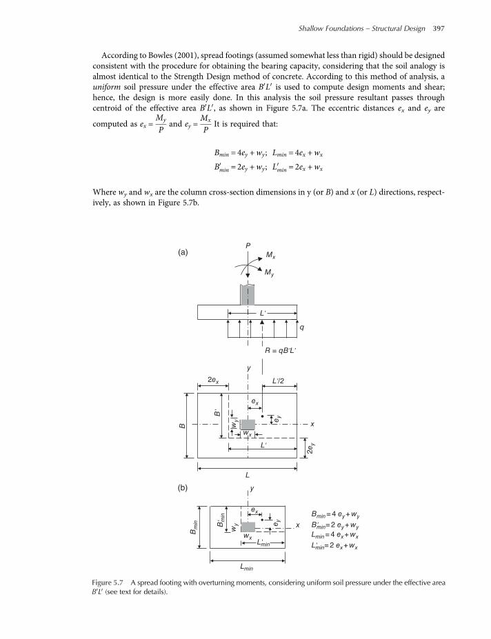
According to Bowles (2001), spread footings (assumed somewhat less than rigid) should be designedconsistent with the procedure for obtaining the bearing capacity, considering that the soil analogy isalmost identical to the Strength Design method of concrete. According to this method of analysis, auniform soil pressure under the effective area B L is used to compute design moments and shear;hence, the design is more easily done. In this analysis the soil pressure resultant passes throughcentroid of the effective area B L , as shown in Figure 5.7a. The eccentric distances ex and ey are
computed as ex =My
Pand ey =
Mx
PIt is required that:
Bmin = 4ey +wy; Lmin = 4ex +wx
Bmin = 2ey +wy; Lmin = 2ex +wx
Where wy and wx are the column cross-section dimensions in y (or B) and x (or L) directions, respect-ively, as shown in Figure 5.7b.
PMx
My
q
R = qB'L'
L'/2
B'
L'
L
xB
y
2ex
2e
y
ex
ey
wy
wx
L'
(a)
(b)
x
y
Bm
in
Bmin= 4 ey+ wy
Lmin= 4 ex+ wx
L'min= 2 ex+ wx
B'min= 2 ey+ wy
Lmin
B' mi
n
L'min
ex
ey
wy
wx
Figure 5.7 A spread footing with overturning moments, considering uniform soil pressure under the effective areaB L (see text for details).
Shallow Foundations – Structural Design 397
worksaccounts.com
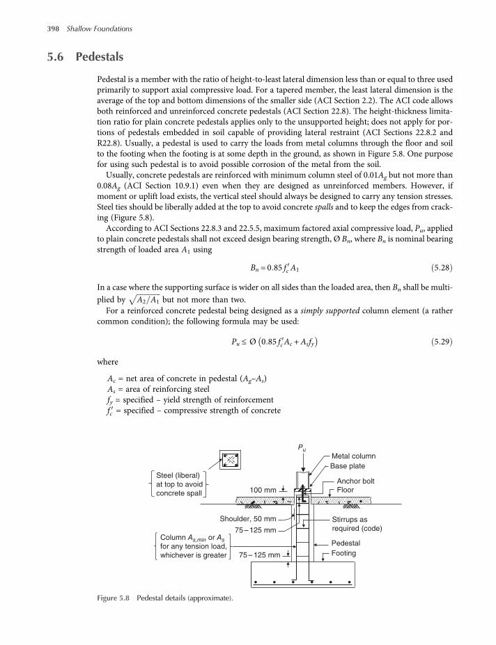
5.6 Pedestals
Pedestal is a member with the ratio of height-to-least lateral dimension less than or equal to three usedprimarily to support axial compressive load. For a tapered member, the least lateral dimension is theaverage of the top and bottom dimensions of the smaller side (ACI Section 2.2). The ACI code allowsboth reinforced and unreinforced concrete pedestals (ACI Section 22.8). The height-thickness limita-tion ratio for plain concrete pedestals applies only to the unsupported height; does not apply for por-tions of pedestals embedded in soil capable of providing lateral restraint (ACI Sections 22.8.2 andR22.8). Usually, a pedestal is used to carry the loads from metal columns through the floor and soilto the footing when the footing is at some depth in the ground, as shown in Figure 5.8. One purposefor using such pedestal is to avoid possible corrosion of the metal from the soil.
Usually, concrete pedestals are reinforced with minimum column steel of 0.01Ag but not more than0.08Ag (ACI Section 10.9.1) even when they are designed as unreinforced members. However, ifmoment or uplift load exists, the vertical steel should always be designed to carry any tension stresses.Steel ties should be liberally added at the top to avoid concrete spalls and to keep the edges from crack-ing (Figure 5.8).
According to ACI Sections 22.8.3 and 22.5.5, maximum factored axial compressive load, Pu, appliedto plain concrete pedestals shall not exceed design bearing strength, Ø Bn, where Bn is nominal bearingstrength of loaded area A1 using
Bn = 0 85 fc A1 5 28
In a case where the supporting surface is wider on all sides than the loaded area, then Bn shall be multi-
plied by A2 A1 but not more than two.For a reinforced concrete pedestal being designed as a simply supported column element (a rather
common condition); the following formula may be used:
Pu ≤ Ø 0 85 fc Ac +Asfy 5 29
where
Ac = net area of concrete in pedestal (Ag–As)As = area of reinforcing steelfy = specified – yield strength of reinforcementfc = specified – compressive strength of concrete
Metal columnPu
Base plate
Anchor boltFloor
Pedestal
Footing75 – 125 mm
Column As,min or As
for any tension load,
whichever is greater
75 – 125 mm
100 mm
Shoulder, 50 mm Stirrups as
required (code)
Steel (liberal)
at top to avoid
concrete spall
Figure 5.8 Pedestal details (approximate).
398 Shallow Foundations
worksaccounts.com
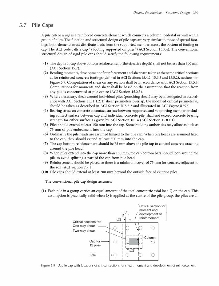
5.7 Pile Caps
A pile cap or a cap is a reinforced concrete element which connects a column, pedestal or wall with agroup of piles. The function and structural design of pile caps are very similar to those of spread foot-ings; both elements must distribute loads from the supported member across the bottom of footing orcap. The ACI code calls a cap “a footing supported on piles” (ACI Section 15.5.4). The conventionalstructural design of rigid pile caps should satisfy the following requirements:
(1) The depth of cap above bottom reinforcement (the effective depth) shall not be less than 300 mm(ACI Section 15.7).
(2) Bendingmoments, development of reinforcement and shear are taken at the same critical sectionsas for reinforced-concrete footings (defined in ACI Sections 15.4.2, 15.6.3 and 15.5.2), as shown inFigure 5.9. Computation of shear on any section shall be in accordance with ACI Section 15.5.4.Computations for moments and shear shall be based on the assumption that the reaction fromany pile is concentrated at pile centre (ACI Section 15.2.3).
(3) Where necessary, shear around individual piles (punching shear) may be investigated in accord-ance with ACI Section 11.11.1.2. If shear perimeters overlap, the modified critical perimeter boshould be taken as described in ACI Section R15.5.2 and illustrated in ACI Figure R15.5.
(4) Bearing stress on concrete at contact surface between supported and supporting member, includ-ing contact surface between cap and individual concrete pile, shall not exceed concrete bearingstrength for either surface as given by ACI Section 10.14 (ACI Section 15.8.1.1).
(5) Piles should extend at least 150 mm into the cap. Some building authorities may allow as little as75 mm of pile embedment into the cap.
(6) Ordinarily the pile heads are assumed hinged to the pile cap. When pile heads are assumed fixedto the cap, they should extend at least 300 mm into the cap.
(7) The cap bottom reinforcement should be 75 mm above the pile top to control concrete crackingaround the pile head.
(8) When piles extend into the cap more than 150 mm, the cap bottom bars should loop around thepile to avoid splitting a part of the cap from pile head.
(9) Reinforcement should be placed so there is a minimum cover of 75 mm for concrete adjacent tothe soil (ACI Section 7.7.1).
(10) Pile caps should extend at least 200 mm beyond the outside face of exterior piles.
The conventional pile cap design assumes:
(1) Each pile in a group carries an equal amount of the total concentric axial load Q on the cap. Thisassumption is practically valid when Q is applied at the centre of the pile group, the piles are all
d/2
d/2
d
Critical sections for:
One-way shear
Two-way shear
Critical section for
moment and
development of
reinforcement
Pile
Column Cap for
12 piles
Figure 5.9 A pile cap with locations of critical sections for shear, moment and development of reinforcement.
Shallow Foundations – Structural Design 399
worksaccounts.com
vertical, the pile group is symmetrical, the cap is rigid and in contact with the ground. The designconsiders structural axial loads of the supported member, weight of the cap and weight of any soiloverlying the cap (if it is below the ground surface). For a group of n piles, the load Pp per pile is
Pp =Qn
5 30
(2) For a pile cap eccentrically loaded with Q or loaded with Q at centre and moments, the combinedstress equation [Equation (2.6)] is assumed valid (assuming planar stress distribution). The equa-tion is repeated here for convenience:
q=RA±My
Iyx ±
Mx
Ixy Equation 2 6
Where
q=Pp
pile cross section area=PpAp
; A= nAp; R=Q
My = Moment about y axisMx = Moment about x axisy = Distance from x axis at pile centrex = Distance from y axis at pile centreIy = Moment of inertia of the pile group about y axis= Σ Moment of inertia of Ap about y axis=Σ Io +Apx2
= ApΣx2 (Considering ΣIo has a negligible value)Ix = Moment of inertia of the pile group about x axis= Σ Moment of inertia of Ap about x axis=Σ Io +Apy2
= ApΣy2 (Considering ΣIo has a negligible value)
Therefore, the combined stress equation can be written in the form
PpAp
=QnAp
±My
ApΣx2x ±
Mx
ApΣy2y; hence,
Pp =Qn±My
Σx2x ±
Mx
Σy2y 5 31
5.8 Plain Concrete Spread Footings
Structural plain concrete is concrete with no reinforcement or with less reinforcement than the min-imum amount specified for reinforced concrete (ACI Section 2.2). Chapter 22 of ACI 318M-08 build-ing code concerns design requirements of structural plain concrete members. However, according toACI Section 22.1.2, unless in conflict with the provisions of Chapter 22, the provisions of ACI Sections1.1–7.5, 7.6.1, 7.6.2, 7.6.4, 7.7, 9.1.3, 9.2 and 9.3.5 shall also apply to structural plain concrete. Also,provisions of ACI Chapter 20, ACI Section 21.12.2.5, Sections C.9.2 and C.9.3.5 of ACI Appendix C,and ACI Appendix D are applied.
400 Shallow Foundations
worksaccounts.com

According to ACI Section 22.2.1, use of structural plain concrete shall be limited to: (a) members thatare continuously supported by soil or supported by other structural members capable of providing con-tinuous vertical support; (b) members for which arch action provides compression under all conditionsof loading; (c) walls and pedestals. Therefore, it is clear that structural plain concrete can be used forconstruction of spread footings. However, plain concrete shall not be used for footings on piles (ACISection 22.7.3). Generally, plain concrete footings are only practical and economical for small columnor wall loads.The structural design of plain concrete spread footings should satisfy the following
requirements:
(1) Thickness of structural plain concrete footingsh shall not be less than 200 mm (ACISection 22.7.4).
(2) When computing strength in flexure, combined flexure and axial load, and shear, the thicknesshshall be taken as 50 mm less than actual thickness (ACI Section 22.4.7).
(3) When load factor combinations of ACI Section 9.2.1 are used, the strength-reduction factor Øshall be 0.6 for flexure, compression, shear, and bearing (ACI Section 9.3.5). When load factorcombinations of ACI Section C.9.2.1 are used, the strength-reduction factor Ø shall be 0.65 forflexure, compression, shear, and bearing (ACI Section C.9.3.5).
(4) According to ACI Section 22.5.1, design of cross-sections subject to flexure shall be based on
ØMn ≥Mu the same as Equation 5 9 5 32
If tension controls
Mn = 0 42λ fc Sm 5 33
If compression controls
Mn = 0 85fc Sm 5 34
Sm = The corresponding elastic section modulus.(5) Maximum factored moment shall be taken at the critical sections defined in ACI Section 22.7.5
(taken at the same critical sections as for reinforced-concrete footings).(6) According to ACI Section 22.5.4, design of rectangular cross-sections subject to shear shall be
based on
ØVn ≥Vu 5 35
where Vn is computed by
Vn = 0 11λ fc bwh 5 36
for one-way shear, and by
Vn = 0 11 1 +2β
λ fc boh 5 37
for two-way shear, but not greater than0 22λ fc bohwhere β corresponds to ratio of long side to short side of concentrated load or reaction area.
Shallow Foundations – Structural Design 401
worksaccounts.com
(7) Location of critical section for shear shall be measured from face of column, pedestal, or wall forfooting supporting a column, pedestal, or wall. For footing supporting a column with steel baseplates, the critical section shall be measured from location of critical section for moment (ACISection 22.7.6.1).
(8) Critical section across the entire footing width for one-way shear is located at a distance h fromface of concentrated load or reaction area (ACI Section 22.7.6.2). For this condition, the footingshall be designed in accordance with Equation (5.36).
(9) Critical section for two-way shear is located so that the perimeter bo is a minimum, but need notapproach closer than h/2 to perimeter of concentrated load or reaction area (ACI Section 22.7.6.2).For this condition, the footing shall be designed in accordance with Equation (5.37).
(10) Circular or regular polygon-shaped concrete columns or pedestals shall be permitted to be treatedas square members with the same area for location of critical sections for moment and shear (ACISection 22.7.7).
(11) According to ACI Sections 22.7.8 and 22.5.5, factored bearing load, Bu, on concrete at contactsurface between supporting and supported member shall not exceed design bearing strength,Ø Bn, for either surface as given in Equation (5.28). In case where the supporting surface is wider
on all sides than the loaded area, then Bn shall be multiplied by A2 A1 but not more than 2.(12) Plain concrete shall not be used for footings on piles (ACI Section 22.7.3).
5.9 Combined Footings
5.9.1 General
Generally, a combined footing is a rectangular or trapezoidal reinforced concrete slab supporting morethan one column in a line. A combined footing supporting two columns only is usually known as ordin-ary combined footing (Figure 2.3). A combined footing supporting more than two columns is usuallycalled continuous combined footing or strip footing. Another form of combined footing is strap (or can-tilever) footing which consists of two or more spread footings connected by a rigid beam called strap.All these footings are more complicated foundation members than isolated footings due to complexityof their loading and geometry. Therefore, it is appropriate to conduct a more rigorous structural ana-lysis. The available methods of analysis are the rigid method (also known as the conventional method)and the flexible method (also known as the beam on elastic foundation method), as reported by ACICommittee 336 (1993).
The rigid method assumes that the footing is much more rigid than the underlying soils, whichmeans any distortions in the footing are too small to significantly impact the distribution of soil bearingpressure. Consequently, the magnitude and distribution of bearing pressure depends only on theapplied loads and footing geometry, which is assumed either uniform across the bottom of the footing(if the normal resultant load acts through the centroid) or varies linearly (if the loading is eccentric);thus simplifying the design computations. This method of design, in spite of its substantial approxi-mations and inaccuracies, can be considered appropriate for most combined footings.
For large or heavily loaded combined footings such as continuous strip footings or grid foundations,it may bemore appropriate to conduct structural design based on a beam on elastic foundation analysis,as described in Section 5.11. This analysis produces more reliable estimates of the shears, momentsand deformations in the footing. However, unfortunately, it is more difficult to implement as itrequires consideration of soil-structure interaction which is not as simple. The analysis requires a com-puter program for maximum design efficiency, such as the program B-5 (FADBEMLP) given inBowles (2001).
Structural designs will be based on the Load and Resistance Factor Design (LRFD) method. Provi-sions of Chapter 15 of the ACI code, where applicable, shall apply for design of combined footings and
402 Shallow Foundations
worksaccounts.com
mats also (ACI Section 15.1.1). The direct design method of Chapter 13 of the ACI code shall not beused for design of combined footings and mats (ACI Section 15.10.2).The following Sections will describe a design procedure, based on the rigid method of analysis, for
each of the ordinary rectangular combined footing, trapezoidal combined footing and strap footing.
5.9.2 Rectangular Combined Footings
According to the conventional method of analysis, the design is conducted on the assumption that thefooting acts as a rigid body, and the contact pressure is assumed to follow a linear distribution, as dis-cussed earlier. Also, the footing base area and its B and L dimensions should be established such thatthe maximum contact pressure (unfactored) at no place exceeds the given allowable soil pressure. Thestructural design steps may be summarised as follows:
(1) Determine the appropriate load factor combination, as discussed in Section 5.2. Then, determinethe resultant (R) of all column service (working) loads and moments and the factored resultant(Rfact) of all column factored loads and moments.
(2) Determine the factored net contact pressure (net qfact) using
A=R
net qa=
Rfact
net qfactHence,
net qfact = net qaRfact
R
(3) Find footing dimensions B and L. First find the location of Rfact by taking moments about thecentre of column 1 (exterior column). Let this location represent the centre of the footing basearea A and the centre of contact pressure instantaneously; hence, L/2 equals the distance betweenthe centre and the given property line (exterior edge of the footing). Find B = R/L(net qa).
(4) Draw factored load, shear and moment diagrams considering the footing as a reinforced concretebeam. The diagrams should give shear and moment values at the critical sections and other neces-sary locations. For convenience, take each column load as a concentrated load acting at the col-umn centre.
(5) Find the thickness of the footing by calculating d based on analysis for both wide-beam andtwo-way shear at the most critical sections.
(6) Find steel for bending in long direction required by the maximum (+) and (−) bending moments.Steel bars for (+) bending shall be placed in the bottom of the footing near the columns, and thosefor (−) bending in the top near or in the centre portion between columns. When it is found thattrying to cut the (−) bars in accordance with ACI code requirements is not worth the extra engin-eering and bar placing effort, it would be preferable to extend the bars full length of the footing.Also, enough number of the (+) bottom bars are needed full length of the footing so that the trans-verse bottom bars (bars in short direction) can be supported. The design should provide number,size, spacing and length of steel bars for each type of reinforcement, in accordance with ACI coderequirements.
(7) Check the development of the top and bottom steel bars in long direction in accordance with therequirements of ACI Section 12.2.
(8) Find steel for bending in short direction required at bottom of the footing. For this purpose(Bowles, 2001), the footing is divided into three zones or strips of the defined widths shownin Figure 5.10. Zones I and II, usually known as effective zones, should be analysed as beams;the provided steel should not be less than that required for bending or As(min), whichever isgreater. For zone III (the remaining portions), the provided steel should satisfy As(min) require-ment only.
Shallow Foundations – Structural Design 403
worksaccounts.com

(9) Check the development of the bottom steel bars in the short direction in accordance with therequirements of ACI Section 12.2.
(10) Check column bearing on the footing at the location of each column, and design the column-to-footing dowels. Follow the same procedure used for isolated spread footings, as discussed inSection 5.4.4.
5.9.3 Trapezoidal Combined Footings
A trapezoidal combined footing may be necessary if a rectangular combined footing cannot provide theassumed uniform contact pressure. This condition will exist if the column which has too limited spacefor a spread footing carries much larger load. In this case the resultant of all column loads (includingmoments) will be much closer to the heavier column, and doubling the centroid distance as done forthe rectangular combined footing will not provide sufficient footing length to reach the other column.In order to obtain uniform contact pressure, the location of centroid can be adjusted to agree withlocation of the resultant load by using a trapezoid-shaped base area with dimensions L, B1 and B2,where B2 is the larger width near or adjacent to the heavier column, as shown in Figure 5.11. Usingthe known values of the base area A, footing length L and centroid distance x , the unique values ofwidths B1 and B2 are computed by solving the following two equations simultaneously:
A=B1 +B2
2L 5 38
x =L3
2B1 +B2
B1 +B25 39
Equation (5.39) reveals that the solution for B1 = 0 is a triangle and for B1 = B2 is a rectangle. Therefore,a trapezoid solution exists only for (L/3) < x < (L/2) with the minimum value of L as out-to-out of thecolumn faces.
When the values of B1 and B2 are computed, the footing is treated similarly to the rectangular com-bined footing (as a reinforced concrete beam); following the same design steps mentioned in
Zone I Zone III Zone II Zone III
B
c + w1+
0.75d
c ≤ 0.75d
w2+ 1.5d
w2w1cCol. 1 Col. 2
L
Figure 5.10 Zones (transverse strips) for steel bars at bottom of a rectangular combined footing in short direction.
Col. 2
x–
x'Col. 1
B1 B2
L
S
Rectangular combined footing
is too short to reach Col. 1 due
to limited space at Col. 2
Figure 5.11 A trapezoidal combined footing supporting two columns.
404 Shallow Foundations
worksaccounts.com
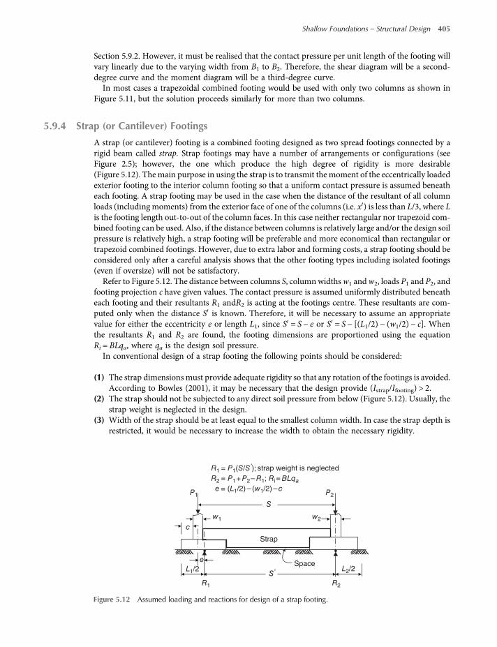
Section 5.9.2. However, it must be realised that the contact pressure per unit length of the footing willvary linearly due to the varying width from B1 to B2. Therefore, the shear diagram will be a second-degree curve and the moment diagram will be a third-degree curve.In most cases a trapezoidal combined footing would be used with only two columns as shown in
Figure 5.11, but the solution proceeds similarly for more than two columns.
5.9.4 Strap (or Cantilever) Footings
A strap (or cantilever) footing is a combined footing designed as two spread footings connected by arigid beam called strap. Strap footings may have a number of arrangements or configurations (seeFigure 2.5); however, the one which produce the high degree of rigidity is more desirable(Figure 5.12). Themain purpose in using the strap is to transmit the moment of the eccentrically loadedexterior footing to the interior column footing so that a uniform contact pressure is assumed beneatheach footing. A strap footing may be used in the case when the distance of the resultant of all columnloads (including moments) from the exterior face of one of the columns (i.e. x ) is less than L/3, where Lis the footing length out-to-out of the column faces. In this case neither rectangular nor trapezoid com-bined footing can be used. Also, if the distance between columns is relatively large and/or the design soilpressure is relatively high, a strap footing will be preferable and more economical than rectangular ortrapezoid combined footings. However, due to extra labor and forming costs, a strap footing should beconsidered only after a careful analysis shows that the other footing types including isolated footings(even if oversize) will not be satisfactory.Refer to Figure 5.12. The distance between columns S, columnwidthsw1 andw2, loads P1 and P2, and
footing projection c have given values. The contact pressure is assumed uniformly distributed beneatheach footing and their resultants R1 andR2 is acting at the footings centre. These resultants are com-puted only when the distance S is known. Therefore, it will be necessary to assume an appropriatevalue for either the eccentricity e or length L1, since S = S − e or S = S − [(L1/2) − (w1/2) − c]. Whenthe resultants R1 and R2 are found, the footing dimensions are proportioned using the equationRi = BLqa, where qa is the design soil pressure.In conventional design of a strap footing the following points should be considered:
(1) The strap dimensionsmust provide adequate rigidity so that any rotation of the footings is avoided.According to Bowles (2001), it may be necessary that the design provide (Istrap/Ifooting) > 2.
(2) The strap should not be subjected to any direct soil pressure from below (Figure 5.12). Usually, thestrap weight is neglected in the design.
(3) Width of the strap should be at least equal to the smallest column width. In case the strap depth isrestricted, it would be necessary to increase the width to obtain the necessary rigidity.
Strap
Space
P1
R1 = P1(S/S'); strap weight is neglected
R2 = P1+ P2– R1; Ri= BLqa
e = (L1/2) – (w1/2) – cP2
L1/2 L2/2
R1 R2
S'
w1 w2
S
c
e
Figure 5.12 Assumed loading and reactions for design of a strap footing.
Shallow Foundations – Structural Design 405
worksaccounts.com
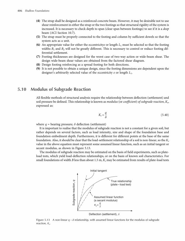
(4) The strap shall be designed as a reinforced concrete beam. However, it may be desirable not to useshear reinforcement in either the strap or the two footings so that structural rigidity of the system isincreased. It is necessary to check depth to span (clear span between footings) to see if it is a deepbeam (ACI Section 10.7).
(5) The strap must be properly connected to the footing and column by sufficient dowels so that thesystem acts as a unit.
(6) An appropriate value for either the eccentricitye or length L1 must be selected so that the footingwidths B1 and B2 will not be greatly different. This is necessary to control or reduce footing dif-ferential settlement.
(7) Footing thicknesses are designed for the worst case of two-way action or wide-beam shear. Thedesign wide-beam shear values are obtained from the factored shear diagram.
(8) Design footing reinforcing as a spread footing for both directions.(9) It is not possible to obtain a unique design, since the footing dimensions are dependent upon the
designer’s arbitrarily selected value of the eccentricity e or length L1.
5.10 Modulus of Subgrade Reaction
All flexible methods of structural analysis require the relationship between deflection (settlement) andsoil pressure be defined. This relationship is known asmodulus (or coefficient) of subgrade reaction, Ks,expressed as:
Ks =qδ
5 40
where q = bearing pressure; δ deflection (settlement)It is important to realise that the modulus of subgrade reaction is not a constant for a given soil, but
rather depends on several factors, such as load intensity, size and shape of the foundation base andfoundation embedment depth. Furthermore, it is different for different points at the base of the samefoundation. Also, it should be clear that the load-settlement relationship of a soil is non-linear, so the Ks
value in the above equation must represent some assumed linear function, such as an initial tangent orsecant modulus, as shown in Figure 5.13.
The modulus of subgrade reaction may be estimated on the basis of field experiments, such as plate-load tests, which yield load-deflection relationships, or on the basis of known soil characteristics. Forsmall foundations of width B less than about 1.5 m, Ksmay be estimated from results of plate-load tests
Subgra
de r
eaction, q
Deflection (settlement), δ
Assumed linear function
(a secant modulus)
Ks=
Initial tangent
True relationship
(plate – load test)
δq
Figure 5.13 A non-linear q − δ relationship, with assumed linear functions for the modulus of subgradereaction, Ks.
406 Shallow Foundations
worksaccounts.com
as suggested by Terzaghi (1955). He proposed certain equations for estimating Ks for full-sized footingson clay and sand soils (see Das, 2011; Bowles, 2001). However, even for small-sized footings, the evalu-ation of Ks involves many uncertainties, and the customary procedure for determining Ks on the basisof small-scale load tests is subject to all limitations of the plate-load test described in the discussion ofProblem 1.9. For mat foundations, Ks cannot be reliably estimated on the basis of field plate-load testsbecause the scale effects are too severe.According to Vesic (1961), the modulus of subgrade reaction could be computed as
Ks =Ks
B=1B
0 65EsB4
Ef If
12 Es1−μ2s
5 41
where
Ks = modulus of subgrade reaction, in units of EsKs = modulus of subgrade reaction, in units of unit weightEs = deformation modulus of soilEf = modulus of elasticity of foundation materialμs = Poisson’s ratio of soilIf = moment of inertia of the cross-section of the foundationB = foundation width
For all practical purposes, value of 0 65EsB4
Ef If
12can be approximated as one; hence, the above Vesic
equation reduces to
Ks =Es
B 1−μ2s5 42
Equation (5.42) shows a direct relationship between Ks and Es. According to Bowles (2001), one mayrearrange the general equation of immediate settlement, Equation (3.5), using Es = 1−μ2s Es, andobtain
Si = δ= q×B× Es ×m× IS × IF
Hence,
Ks =qδ=
1B× Es ×m× IS × IF
5 43
Carefully note in using Equation (5.43) that its basis is in the settlement equation of Chapter 3,Equation (3.5), and use B, m, IS and IF as defined there.Also, Bowles has suggested the following equation for approximating KS from the allowable bearing
capacity qa provided by the geotechnical engineer:
Ks = 40 SF qa 5 44
where
KS = modulus of subgrade reaction in kN/m3.SF = safety factorqa = allowable bearing capacity in kPa
Shallow Foundations – Structural Design 407
worksaccounts.com

Tables 5.3 and 5.4 provide approximate ranges of KS values for sandy and clayey soils which may beused as a guide and for comparison when using the approximate equations.
The KS values of Table 5.4 were obtained from results of load tests using square plates of size0.3 × 0.3 m.
Equation (5.44) is based on relationships: qa =qultSF
; Ks =qultδ; and qult is at a settlement δ =
0.0254 m (or 25 mm). According to Bowles, for δ = 6, 12, 20 mm and so on, the factor 40 can beadjusted to 165, 83, 50 and so on. Factor 40 is reasonably conservative but smaller assumed displace-ments can always be used.
Table 5.3 Values of modulus of subgrade reaction, Ks (fromBowles, 2001).
Soil Ks, kN/m3
Loose sand 4800–16 000
Medium dense sand 9600–80 000
Dense sand 64 000–128 000
Clayey medium dense sand 32 000–80 000
Silty medium dense sand 24 000–48 000
Clayey soil:
qa ≤ 200 kPa 12 000–24 000
200 < qa ≤ 800 kPa 24 000–48 000
qa > 800 kPa >48 000
Table 5.4 Typical values of modulus of subgrade reaction,Ks (from Das, 2001).
Soil Ks, MN/m3
Dry or moist sand:
Loose 8–25
Medium 25–125
Dense 125–375
Saturated sand:
Loose 10–15
Medium 35–40
Dense 130–150
Clay:
Stiff 10–25
Very stiff 25–50
Hard >50
408 Shallow Foundations
worksaccounts.com

5.11 Beams on Elastic Foundations
When flexural rigidity of a continuous strip footing (either isolated or taken from a mat) is taken intoaccount, the foundation is considered as an elastic (or flexible) member interacting with an elastic soil;analysed on the basis of some form of a beam on elastic foundation. The analysis may be based on:(1) classical solutions, (2) discrete-element formulations.
(1) Classical solutions.A classical solution (also known as classical Winkler solution) is an approximate flexible method ofanalysis in which the soil is considered to be equivalent to a bed of infinite number of coil springs(Figure 5.14) used to compute the shears, moments, and deformations in the supported structuralbase. This equivalent foundation is sometimes referred to as the Winkler foundation because theearliest use of these “springs” to represent the interaction between soil and foundations has beenattributed toWinkler (1867). The elastic stiffness of these assumed springs represents the modulusof subgrade reaction, KS.
Refer to Figure 5.15. The beam has an infinite length and a width B; rests on an elastic soilequivalent to an infinite number of elastic springs. Using deflection δ = y, soil reaction per unitlength of the beam = q, and Ks =Ks B, then from Equation (5.40)
q= −y Ks 5 45
From the mechanic of materials
M = Ef Ifd2ydx2
; V =dMdx
; q=dVdx
Spring with a
stiffness = Ks
Flexible beam
or strip footing
P1 P2P3 P4
Figure 5.14 A flexible foundation on a “bed of springs” (Winkler concept).
P PA
A
x
y
t
Sec. A – A
q = y K'sB
Figure 5.15 Beam of infinite length on elastic foundation.
Shallow Foundations – Structural Design 409
worksaccounts.com
hence, q= Ef Ifd4ydx4
, and from Equation (5.45)
Ef Ifd4ydx4
= −y Ks 5 46
where
M = moment at any sectionV = shear force at any sectionEf = modulus of elasticity of the material of the beamIf = moment of inertia of the cross-section of the beam
The solution of Equation (5.46) is
y = eλx C1 cosλx +C2 sinλx + e−λx C3 cosλx +C4 sinλx 5 47
where factor λ=Ks
4Ef If4 =
KsB4Ef If
4
The factor λ is impotant in determining whether a foundation should be analysed on the basis ofthe conventional rigid procedure or as a beam on an elastic foundation (Section 5.12.1). It has beensuggested that rigid members of length L should have λL < (π/4), flexible members have λL > π, andmembers of intermediate flexibility have (π/4) < λL < π. However, these criteria are of limitedapplication because of the number of loads and their locations along the member.
The closed-form solution of the basic differential equations concerning the deflections, slopes,moments and shears in the beam of Figure 5.15, for several loadings, is given in Table 5.5.
Deflections, moments and shears in a beam of finite length L, rests on an elastic foundation andcarries a concentrated load P at any point (Figure 5.16), are given in Table 5.6. The equations weredeveloped by Hetenyi (1946) using the Winkler concept. The distance x to use in the equations ismeasured from the end of the beam to the point for which the deflection, moment, or shear isdesired. For x < a, use the equations as given, and measurex from E (Figure 5.16). For x > a, replacea with b in the equations, and measure x from F. Applying the boundary conditions, as illustratedin Figure 5.16, the equations of Table 5.6 can be expressed as
y =PλKs
A M =P2λ
B V = PC
where the coefficients A , B and C are the values for the hyperbolic and trigonometric remainderof the equations. These coefficients are so complicated that a computer program will be required tocarry out the design computations.
The classical Winkler solutions, being of closed form, suffer from many problems and difficul-ties. According to the classical approach each spring is linear and acts independently from theothers, and that all of the springs have the same KS. In other words, it is difficult to allow for changein subgrade reaction along footing. In reality, the load-deformation behavior of soil is nonlinear,and a load at one point on a footing induces deflection both at that point and in the adjacent partsof the footing. Another problem with the classical solution it is difficult to account for boundaryconditions of known rotation or deflection at desired points. Also, it is difficult to apply multipletypes of loads to a footing. The classical solution assumes weightless footing, but weight will be afactor when footing tends to separate from the soil. Due to all these shortcomings, the classicalapproach is rarely a better model than a discrete-element analysis.
410 Shallow Foundations
worksaccounts.com
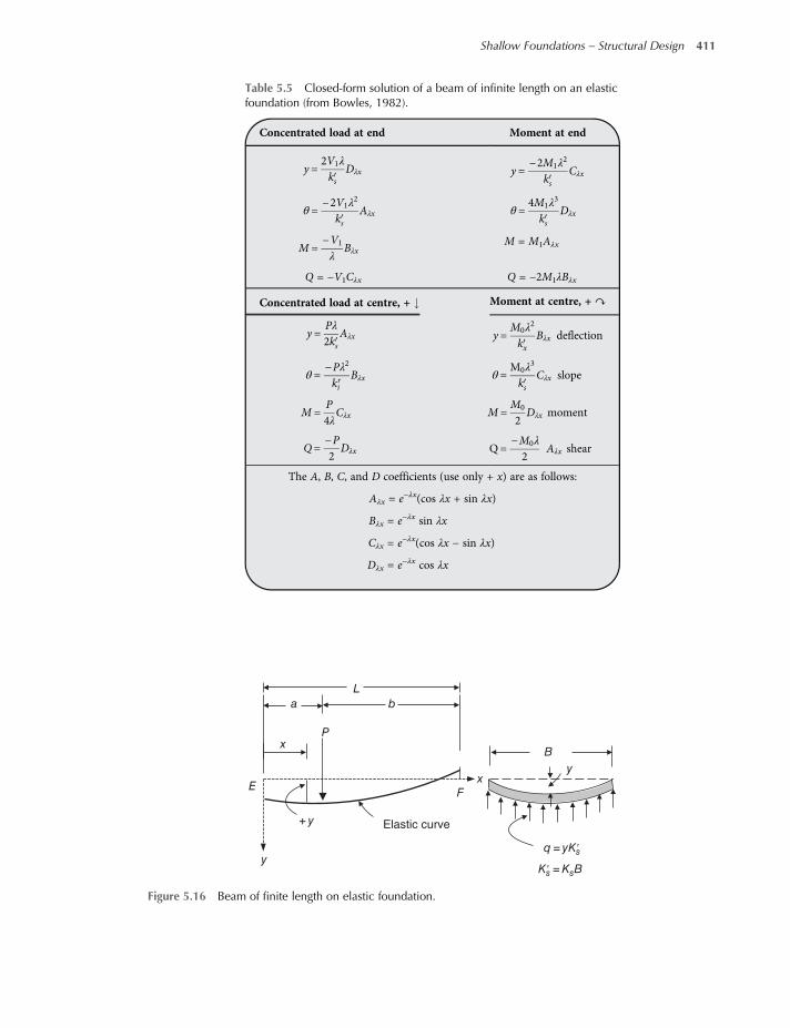
Table 5.5 Closed-form solution of a beam of infinite length on an elasticfoundation (from Bowles, 1982).
Concentrated load at end Moment at end
y =2V1λ
ksDλx y =
−2M1λ2
ksCλx
θ =−2V1λ
2
ksAλx θ =
4M1λ3
ksDλx
M =−V1
λBλx
M = M1Aλx
Q = −V1Cλx Q = −2M1λBλx
Concentrated load at centre, + Moment at centre, + ↷
y =Pλ2ks
Aλx y =M0λ
2
kxBλx deflection
θ =−Pλ2
kriBλx θ =
M0λ3
ksCλx slope
M =P4λ
Cλx M =M0
2Dλx moment
Q=−P2
Dλx Q=−M0λ
2Aλx shear
The A, B, C, and D coefficients (use only + x) are as follows:
Aλx = e−λx(cos λx + sin λx)
Bλx = e−λx sin λx
Cλx = e−λx(cos λx − sin λx)
Dλx = e−λx cos λx
Elastic curve
L
a b
xP
F
B
yx
E
y
+ y
K's = KsB
q = yK's
Figure 5.16 Beam of finite length on elastic foundation.
Shallow Foundations – Structural Design 411
worksaccounts.com
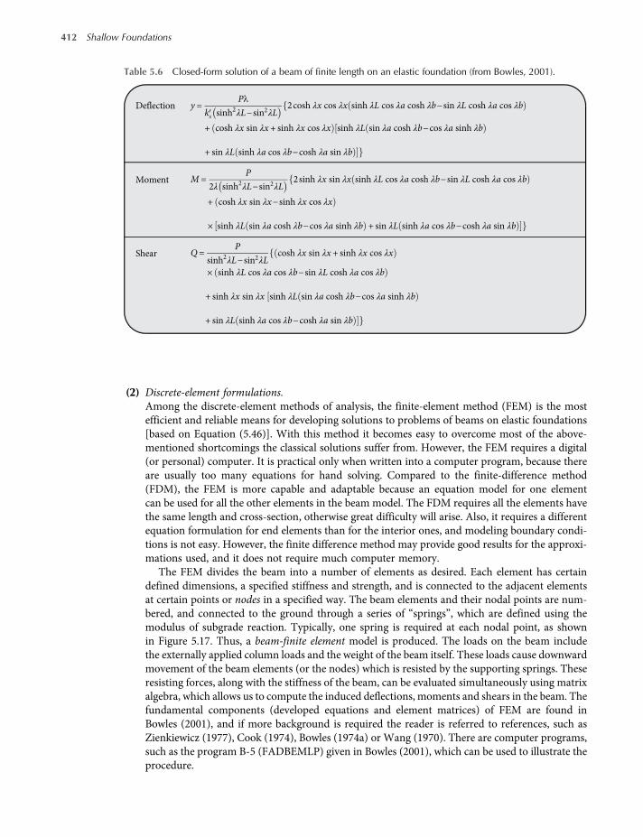
(2) Discrete-element formulations.Among the discrete-element methods of analysis, the finite-element method (FEM) is the mostefficient and reliable means for developing solutions to problems of beams on elastic foundations[based on Equation (5.46)]. With this method it becomes easy to overcome most of the above-mentioned shortcomings the classical solutions suffer from. However, the FEM requires a digital(or personal) computer. It is practical only when written into a computer program, because thereare usually too many equations for hand solving. Compared to the finite-difference method(FDM), the FEM is more capable and adaptable because an equation model for one elementcan be used for all the other elements in the beam model. The FDM requires all the elements havethe same length and cross-section, otherwise great difficulty will arise. Also, it requires a differentequation formulation for end elements than for the interior ones, and modeling boundary condi-tions is not easy. However, the finite difference method may provide good results for the approxi-mations used, and it does not require much computer memory.
The FEM divides the beam into a number of elements as desired. Each element has certaindefined dimensions, a specified stiffness and strength, and is connected to the adjacent elementsat certain points or nodes in a specified way. The beam elements and their nodal points are num-bered, and connected to the ground through a series of “springs”, which are defined using themodulus of subgrade reaction. Typically, one spring is required at each nodal point, as shownin Figure 5.17. Thus, a beam-finite element model is produced. The loads on the beam includethe externally applied column loads and the weight of the beam itself. These loads cause downwardmovement of the beam elements (or the nodes) which is resisted by the supporting springs. Theseresisting forces, along with the stiffness of the beam, can be evaluated simultaneously using matrixalgebra, which allows us to compute the induced deflections, moments and shears in the beam. Thefundamental components (developed equations and element matrices) of FEM are found inBowles (2001), and if more background is required the reader is referred to references, such asZienkiewicz (1977), Cook (1974), Bowles (1974a) or Wang (1970). There are computer programs,such as the program B-5 (FADBEMLP) given in Bowles (2001), which can be used to illustrate theprocedure.
Table 5.6 Closed-form solution of a beam of finite length on an elastic foundation (from Bowles, 2001).
Deflection y =Pλ
ks sinh2λL−sin2λL2cosh λx cos λx sinh λL cos λa cosh λb−sin λL cosh λa cos λb
+ cosh λx sin λx + sinh λx cos λx sinh λL sin λa cosh λb−cos λa sinh λb
+ sin λL sinh λa cos λb−cosh λa sin λb
Moment M =P
2λ sinh2λL−sin2λL2sinh λx sin λx sinh λL cos λa cosh λb−sin λL cosh λa cos λb
+ cosh λx sin λx−sinh λx cos λx
× sinh λL sin λa cosh λb−cos λa sinh λb + sin λL sinh λa cos λb−cosh λa sin λb
Shear Q=P
sinh2λL−sin2λLcosh λx sin λx + sinh λx cos λx
× sinh λL cos λa cos λb−sin λL cosh λa cos λb
+ sinh λx sin λx sinh λL sin λa cosh λb−cos λa sinh λb
+ sin λL sinh λa cos λb−cosh λa sin λb
412 Shallow Foundations
worksaccounts.com

5.12 Mat Foundations
5.12.1 General
Mat, raft and floating foundations were described in some detail in Section 2.2. Usually, a mat foun-dation is a reinforced concrete slab, relatively thick and with or without depressions or openings, sup-porting an array of columns in several lines both ways. Most mat foundations are supported directly onthe underlying soils. However, mats may be supported on piles, or, partially on the underlying soil, anduse piles to carry the balance of the load. These foundation options may be necessary when the contactpressure is too high or the underlying supporting soil is too compressible; that a soil-supported matmay experience large excessive settlement. This Section concerns structural design of mat foundationssupported on soils. Depending upon the flexural rigidity of foundation, the methods of design of matfoundations can be classified into the following two categories:
(1) Rigid (or conventional) methods.As mentioned earlier (Section 5.9.1), the conventional method assumes that the base (mat) is per-fectly rigid and that the contact pressure follows a planar distribution; its centroid coincides withthe line of action of the resultant force of all loads acting on the base. This method does not con-sider redistribution of contact pressure beneath the mat, and it assumes that the individual col-umns will not settle differentially. These simplifying assumptions make it easy to compute theshears, moments, and deflections using the principles of structural mechanics. However, althoughthe conventional analysis is appropriate for isolated and most of combined footings, it does notreliably model mat foundations because the rigidity assumption, inmost of cases, is no longer valid.A continuous strip footing (or a mat which consists of continuous strip footings in both directions)having adjacent column loads and column spacing vary by not more than 20% of the greater value,and the average of two adjacent spans is less than 1.75/λ, can be considered rigid and the variationof soil pressure determined on the basis of simple statics (ACI Committee 336). The conventionaldesign method may be adequate where these rigidity requirements are satisfied. The factor λ is
λ=KsB4EcI
4 5 48
where
KS = coefficient (or modulus) of vertical subgrade reactionEC = modulus of elasticity of concreteI = moment of inertia of the beam (strip) section
The geotechnical engineer should furnish the designer KS values even when a simplified designmethod is used. The design procedure will be described in Section 5.12.2.
2 3 4
Node numbers Element numbers
1 (1)
Ks1 Ks2 Ks3 Ks4
L1 L2 L3
(2) (3)
Figure 5.17 A continuous beam or strip footing on elastic foundation (bed of springs) divided into a number ofbeam finite elements.
Shallow Foundations – Structural Design 413
worksaccounts.com

(2) Flexible methods.For general cases falling outside the rigidity limitations given in method (1), it is recommended todesign the mat as a flexible plate supported by an elastic foundation (the soil). Flexible methodsinclude the following:(A) Approximate flexible method. It is primarily based on the theory of plates on elastic foun-
dation, using the Winkler’s concept (i.e., the plate or mat rests on a bed of “springs” whichhave the same KS). This method was proposed by ACI Committee 336 (1993) to calculatemoments, shears, and deflections at all points in a mat foundation with the help of charts.The design procedure will be briefly described in Section 5.12.3.
(B) Discrete (finite) element methods. In these methods the mat is divided into a number of dis-crete elements using grid lines. These methods use modulus of subgrade reaction KS as the soilcontribution to the structural model. There are three general discrete element formulationswhich may be used:
• Finite difference method (FDM)
• Finite element method (FEM)
• Finite grid method (FGM).
5.12.2 Design Procedure for the Conventional (Rigid) Method
The procedure for design a mat foundation, using the conventional method, consists of the follow-ing steps:
(1) All the columns and walls are numbered and their total unfactored (working) axialloads, moments and any overturning moment due to wind or other causes, are calculated sep-arately. The mat self-weight, however, may not be considered because it is taken directly bythe supporting soil. It may be useful if a suitable table is used for this purpose. The table shouldalso contain summations of all the vertical loads and moments, that is Σ (column loads), ΣMx
and ΣMy.(2) The line of action of the resultant R of all the axial loads and moments is determined using statics;
summing moments about two of the adjacent mat edges, and computing the x and y momentarms of the resultant force. Then, the eccentricities ex and ey are computed (Figure 5.18a).
(3) Determine the maximum contact pressure (unfactored), qmax, below one of the mat corners usingEquation (2.7), repeated here for convenience.
q=RBL
1 ±6exB
±6eyL
Equation 2 7
In this equation, the B and L dimensions are in x and y directions, respectively.(4) Compare the computed qmax with the allowable soil pressure qa furnished by the geotechnical
engineer to check if qmax ≤ qa.(5) Compute the contact pressure (unfactored) at selected points beneath the mat. These selected
points are corners of continuous beam strips (or combined footings with multiple columns)to which the mat is divided in both x and y directions, as shown in Figure 5.18b. The contactpressure q at any point below the mat is computed using Equation (2.6), repeated here:
q x, y =RA±My
Iyx ±
Mx
Ixy Equation 2 6
(6) Check static equilibrium of each individual beam strip, and modify the column loads and contactpressures accordingly. Since a mat transfers load horizontally, any given strip may not satisfy avertical load summation (vertical equilibrium) unless consideration is given to the shear transfer
414 Shallow Foundations
worksaccounts.com
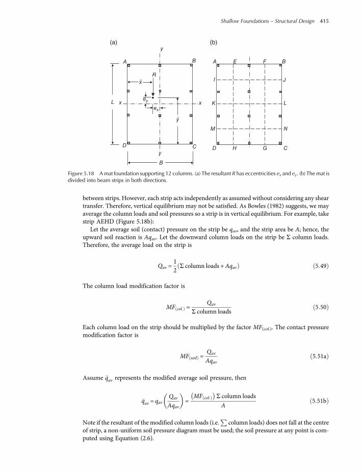
between strips. However, each strip acts independently as assumed without considering any sheartransfer. Therefore, vertical equilibrium may not be satisfied. As Bowles (1982) suggests, we mayaverage the column loads and soil pressures so a strip is in vertical equilibrium. For example, takestrip AEHD (Figure 5.18b):
Let the average soil (contact) pressure on the strip be qav, and the strip area be A; hence, theupward soil reaction is Aqav. Let the downward column loads on the strip be Σ column loads.Therefore, the average load on the strip is
Qav =12Σ column loads +Aqav 5 49
The column load modification factor is
MF col =Qav
Σ column loads5 50
Each column load on the strip should be multiplied by the factor MF(col.). The contact pressuremodification factor is
MF soil =Qav
Aqav5 51a
Assume qav represents the modified average soil pressure, then
qav = qavQav
Aqav=
MF col Σ column loads
A5 51b
Note if the resultant of the modified column loads (i.e. column loads) does not fall at the centreof strip, a non-uniform soil pressure diagram must be used; the soil pressure at any point is com-puted using Equation (2.6).
(a) (b)
A E F B
J
L
N
CGHD
A
y
B
Rx–
y–
L x
Dy
B
C
x
M
K
I
ex
ey
Figure 5.18 Amat foundation supporting 12 columns. (a) The resultant R has eccentricities ex and ey. (b) The mat isdivided into beam strips in both directions.
Shallow Foundations – Structural Design 415
worksaccounts.com

(7) Change each modified column load (dead load D + live load L) to factored load. For example, afactored modified column load may be computed as
1 2 MF col D + 1 6 MF col L
However, in order to avoid repetition, this computation can be done directly as soon as the factorMF(col.) is determined; using the factored modified load as
MF col 1 2D+ 1 6L
Compute modified factored contact pressure, modified qfactored, as follows:If the resultant of the factored modified loads (modified Rfactored) passes through the centre of
strip, the modified qfactored is simply given by
modified qfactored =modifiedRfactored
A5 52
If the modified Rfactored has an eccentricity eL (in x or y direction), modified qfactored at any pointbelow the strip is given by
modified qfactored =modifiedRfactored
A±
eL modifiedRfactored
IBl 5 53
where
l = distance of point from the strip centre in L directionIB =moment of inertia of the strip area about an axis passes through the strip centre in B direction
(8) Draw factored load, shear and moment diagrams for the continuous beam strips in bothdirections.
(9) Determine the minimum mat thickness considering punching shear (two-way or diagonal ten-sion shear) at critical columns, based on factored column load and shear perimeter, similarly asfor a spread footing. Note that the factored actual column load should be used and not the fac-tored modified column load. Columns adjacent to a mat edge often control the mat depth d, andmay require investigation of a two-sided (corner column) and three-sided (side column) diagonaltension shear perimeter. Also, the condition of unbalanced moment transfer should be investi-gated, and the design must satisfy the requirements of ACI Sections 11.11.7.1.
It is common practice not to use shear reinforcement so that depth is a maximum. Thisincreases the flexural stiffness (rigidity) and increases the reliability of using Equation (2.6) orEquation (2.7).
(10) Check the computed mat depth d considering beam shear (one-way shear) at the most criticalsection.For this purpose, the maximum factored shear value may be obtained from the factoredshear diagram of the most critical strip. Furthermore, some designers also perform this checkingcomputations at most critical section in a given direction taking the mat as a whole.
(11) Obtain the maximum factored positive and negative moments per unit width using the factoredmoment diagrams of the strips in each direction.
(12) Determine the positive and negative reinforcement required in each direction in accordance withthe requirements of ACI 318M-08.
(13) Check development of the reinforcement in both directions in accordance with the requirementsof ACI code-Chapter 12.
(14) Check column bearing on the mat at critical column locations and design the column-to-matdowels. Follow the same procedure used for isolated spread footings, as discussed in Section 5.4.4.
416 Shallow Foundations
worksaccounts.com
5.12.3 Design Procedure for the Approximate Flexible Method
The procedure for design a mat foundation, using the approximate flexible method, consists of thefollowing major steps:
(1) Find the required total thickness t of the mat. The computations proceed exactly in the samemanner as that described in step 9 for the conventional rigid method.
(2) Determine the flexural rigidity D of the mat as
D=Ef t3
12 1−μ2f5 54
where
Ef = modulus of elasticity of foundation materialμf = Poisson’s ratio of foundation material.
(3) Determine the radius of effective stiffness L as
L =DKs
4 5 55
where KS = coefficient of subgrade reaction.
The radius of influence of any column load is on the order of 3L to 4L .(4) Determine the radial moment Mr and tangential moment Mt at any point (in polar coordinates)
caused by a column load P using the following equations:
Mr = −P4
Z4−1− μfx
Z3 5 56
Mt = −P4
μf Z4−1− μfx
Z3 5 57
Where
Zi = factors depend on x, obtained from Figure 5.19
x = distance rationrL
shown in Figure 5.19
In rectangular coordinates the above moment equations can be written as
Mx =Mrcos2θ +Mtsin
2θ 5 58
My =Mrsin2θ +Mtcos
2θ 5 59
where θ is the angle which the radius r makes with x – axis (Figure 5.19).(5) Determine the shear force V per unit width of the mat caused by a column load as
V = −P4L
Z4 5 60
(6) Determine the deflection δ caused by a column load as
δ=P L 2
8Dat location of a column load 5 61
Shallow Foundations – Structural Design 417
worksaccounts.com

δ=P L 2
4DZ3 at any point a distance r from a column load 5 62
(7) When the zones of influence of two or more columns overlap, the method of superposition can beused to obtain the net values of responses (moment, shear and deflection) at any desired point.
(8) If the free edge of the mat is at a distance less than the radius of influence from an individual col-umn load, a correction should be applied to the calculated response net values, as follows:(a) Responses at the edge points of the mat due to column loads within the radius of influence
should be calculated by Equations (5.56–5.62).(b) Assuming strips of 1 m width as semi-infinite beams, shear and moments equal and opposite
to those obtained in (a) should be applied as edge loads and their effects at various pointssuperimposed on the net value of the respective response.
(c) Moment, shear, and deflection in a semi-infinite beam are
M =M1 Aλx−P1λBλx V = −2M1 λBλx−P1Cλx
δ= −2M1 λ
2
KsCλx +
2P1 λKs
Dλx
0
0.5
0.4
0.3
0.2
0.1
0
–0.1
–0.2
–0.3
–0.4
–0.50 1 2 3
x = r/L'
x = r/L'L' = (D/Ks)¼
Et3
12(I – μ2)=D
Zi f
acto
r
Z4
Z'4
y
r
xθ
Mr
Mx = Mrcos2 θ + Mrsin2 θ
My = Mrsin2 θ + Mrcos θ
Mr
Z'3
Z3
4 5 6
Load pointL'
Figure 5.19 Zi factors for computing moments, shears, and deflections in a flexible mat (reproduced from Bowles,2001; after Hetenyi, 1946).
418 Shallow Foundations
worksaccounts.com
Where M1, P1 = moment and shear, respectively, from (a)
λ=Ksb4EcIb
0 25
b = strip width (1 m)Ib = moment of inertia of the stripAλx; Bλx; Cλx; Dλx = coefficients obtained from tables or figures (see Hetenyi, 1946).
5.12.4 Finite Difference Method for the Design of Mat Foundations
The following fourth-order differential equation, which corresponds to Equation (5.46), concernsdeflection of a mat foundation, considered as a flexible plate:
∂4w∂x4
+ 2∂4w
∂x2∂y2+∂4w∂y4
=qD+
PD ∂x ∂y
5 63
where
w = deflection (contact settlement)q = subgrade reaction per unit area of mat (contact pressure)D = flexural rigidity of matP = concentrated load at a given point
The mat rests on an assumed bed of uniformly distributed coil springs representing the supporting soil.The modulus of subgrade reaction KS at a point is represented by the elastic stiffness of a spring at thatpoint. It is common to use the concept of modulus of subgrade reaction in the solution of this type ofproblem. Because the subgrade reaction becomes converted to an equivalent spring applied at the nodeof interest, the analytical methods for mat foundations using this concept are considerably simplifiedover other methods of computations.When a mat is divided into a grid of elements of (rh × h) dimension (Figure 5.20), Equation (5.63)
can be reproduced in a finite- difference equation for deflection at an interior point O, as follows:
6r4
+8r2
+ 6 wO + −4r4−4r2
wL +wR + −4r2−4 wT +wB
+2r2
wTL +wTR +wBL +wBR +wTT +wBB +1r4
wLL +wRR
=qh4
D+Ph2
rD
5 64
when r = 1, that is using a grid of square elements, Equation (5.64) becomes
20wO−8 wL +wR +wT +wB + 2 wTL +wTR +wBL +wBR
+ wTT +wBB +wLL +wRR =qh4
D+Ph2
D
5 65
Since q = − KswO, Equation (5.65) becomes
20 +Ksh4
DwO−8 wL +wR +wT +wB
+ 2 wTL +wTR +wBL +wBR + wTT +wBB +wLL +wRR =Ph2
D
5 66
Shallow Foundations – Structural Design 419
worksaccounts.com
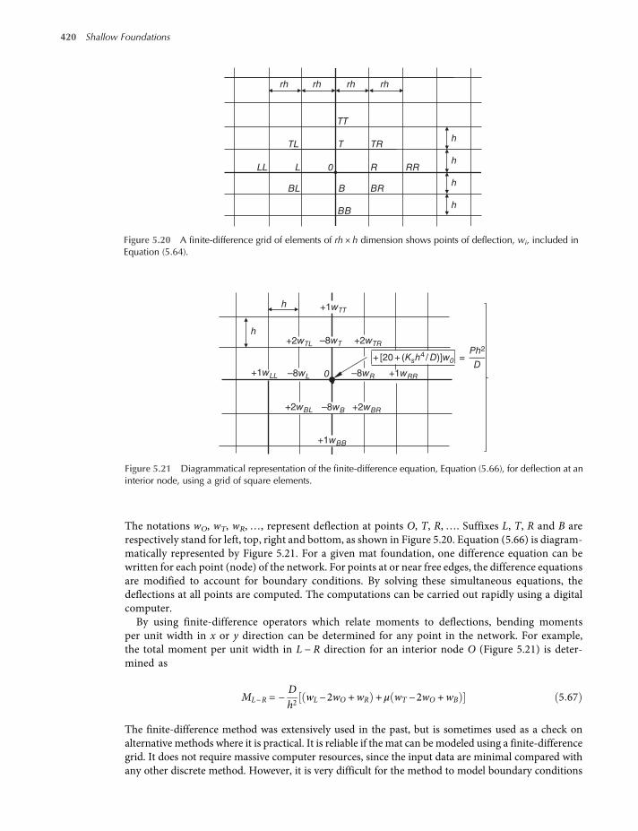
The notations wO, wT, wR,…, represent deflection at points O, T, R,…. Suffixes L, T, R and B arerespectively stand for left, top, right and bottom, as shown in Figure 5.20. Equation (5.66) is diagram-matically represented by Figure 5.21. For a given mat foundation, one difference equation can bewritten for each point (node) of the network. For points at or near free edges, the difference equationsare modified to account for boundary conditions. By solving these simultaneous equations, thedeflections at all points are computed. The computations can be carried out rapidly using a digitalcomputer.
By using finite-difference operators which relate moments to deflections, bending momentsper unit width in x or y direction can be determined for any point in the network. For example,the total moment per unit width in L − R direction for an interior node O (Figure 5.21) is deter-mined as
ML−R = −Dh2
wL−2wO +wR + μ wT −2wO +wB 5 67
The finite-difference method was extensively used in the past, but is sometimes used as a check onalternative methods where it is practical. It is reliable if the mat can be modeled using a finite-differencegrid. It does not require massive computer resources, since the input data are minimal compared withany other discrete method. However, it is very difficult for the method to model boundary conditions
rh rh rh rh
TT
TL T TR
LL L 0 R RR
BL B BR
BB
h
h
h
h
Figure 5.20 A finite-difference grid of elements of rh × h dimension shows points of deflection, wi, included inEquation (5.64).
–8wL –8wR0
+2wTL
+1wTTh
h+2wTR–8wT
+1wLL +1wRR
Ph2
D
+2wBR+2wBL
+1wBB
–8wB
=+ [20 + (Ksh4 / D)]w0
Figure 5.21 Diagrammatical representation of the finite-difference equation, Equation (5.66), for deflection at aninterior node, using a grid of square elements.
420 Shallow Foundations
worksaccounts.com
for column fixity, to allow for holes, notches, or re-entrant corners. Also, it is difficult to account formoments applied at nodes (such as columnmoments) since the difference model uses moment per unitof width.There are FDM computer programs, such as program FADMATFD, B19, which can be used to illus-
trate the procedure. Bowles (2001) has given an example problem (Example 10-4) which illustratestypical input and output from this FDM program. All the necessary equations for various nodesand a FDM program for their solutions are given in Bowles 1974a.
5.12.5 Modulus of Subgrade Reaction and Node Coupling of Soil Effects for Mats
It is very common to use the concept of modulus of subgrade reaction in the discrete element analysesfor mat foundations. As it has already been mentioned in Section 5.10.4, the use of KS in analysing matsis rather widespread because of the greater convenience of this parameter. These analyses use KS tocompute the node springs. At any node, a node spring (or spring constant) K is simply equals tothe product of the node KS and the contributory area from any element, expressed as
Ki = Ks ×Contributory area in units of kN m 5 68
Since the result of this product has units of a “spring” it is commonly called a node spring.Figure 5.22 shows grid lines dividing an irregular-shaped mat into discrete elements. The spring
constant K at various nodal points is computed as follows:Assume the area of any element such asA; B; C; and so on equals AA;AB;AC; and so on. Also, assume
the modulus of subgrade reaction within any element A; B; C; and so on equals KA; KB; KC; and soon. Then:
K1 =KAAA
3+KBAB
4, K2 =
KBAB
4+KCAC
4, K3 =
KCAC
4+KDAD
4, K4 =
KDAD
4,
K5 =KAAA
3+KEAE
3+KFAF
4, K6 =
KAAA
3+KBAB
4+KFAF
4+KGAG
4,
K7 =KBAB
4+KCAC
4+KGAG
4+KHAH
4, K8 =
KCAC
4+KDAD
4+KHAH
4+KIAI
4,
K9 =KDAD
4+KIAI
4
When the coil springs with constant KS are acting independent of each other, the bed of springs sup-porting the mat is termed a “Winkler” foundation (see Section 5.11). Springs of this foundation are
5
4
3
2
1
9
8
7
6
14
15
13
12
10
E
F
G
H
I
A
B
C
D
11
J
~
~~
~~
Figure 5.22 Grid lines dividing an irregular shaped mat into discrete elements.
Shallow Foundations – Structural Design 421
worksaccounts.com

uncoupled; hence, the deflection of any spring is not influenced by adjacent springs. If we computenode springs based on contributing node area, as just outlined above, analysis of a uniformly loadedmat (base of an oil tank) will produce a constant settlement profile across the slab with uncoupledsprings and a dishing settlement profile with coupled springs, as shown in Figure 5.23. Boussinesq the-ory indicates the dishing profile is correct. Because of this major shortcoming associated withuncoupled springs, some designers do not like to use the concept of KS, preferring instead to use adiscrete element method of the elastic foundation bed with ES and μS as elastic parameters. This choicedoes somewhat couple the effects; however, the computations are extensive and only as good as one’sestimate of ES and μS. It was already shown in Section 5.10 that there is a direct relationship betweenthese elastic parameters and KS. Since the elastic parameters ES and KS usually increase with depth fromoverburden and preconsolidation it appears this may be lessen the effect of ignoring coupling(Christian, 1976).
More accurate analysis will be achieved when the node springs are coupled, as shown in Figure 5.24.Accordingly, the vertical springs no longer act independently, and the uniformly loaded mat ofFigure 5.23 exhibits the desired dish shape. In principle, this approach is more realistic than the Wink-ler analysis, but it is difficult to select appropriate KS values for the coupling springs, and the equationsto be programmed become much more complicated. Additionally, fractions of the springs Ki appear inoff-diagonal terms of the stiffness matrix, making it difficult to perform any kind of nonlinear analysis(soil-base separation or excessive deformation).
In order to avoid the difficulties of true coupling and at the same time overcome the lack ofcoupling in the Winkler method, several ways have been proposed (Bowles, 1986; Liao, 1991; Hor-vath, 1993; ACI Committee 336) which indirectly allow for coupling (approximately). These proposedways are known as the pseudo-coupled method. This method uses “springs” that act independently, buthave different KS values depending on their location on the mat. In order to produce the actual dish-shaped deformation (settlement) in a uniformly loaded mat resting on a uniform soil, the methodrequires the mat area be concentrically zoned using softer springs in the innermost (central) zoneand transitioning to the outer (exterior) zone. Some authorities recommend using KS values alongthe mat perimeter be about twice those in the centre. In case concentrated loads, such as column loads,also are present, the resulting deformations are automatically superimposed on the dishing deform-ation profile.
There are different methods to assign a KS value to each zone so that approximate coupling can bedone. The following two methods may be used:
(1) Compute values of KS at 1/4 or 1/8 points, depending on the mat size and L/B value, along centreline of the mat area in L or B direction as applicable. Subsequently, the mat plan is zoned with
(a) (b)
Figure 5.23 Settlement of a uniformly loaded flexible mat on a uniform soil: (a) constant settlement, Winklerconcept; (b) dishing settlement, actual.
Mat
Vertical spring
Coupling spring
Figure 5.24 Soil–structure interaction using coupled springs.
422 Shallow Foundations
worksaccounts.com
different values of KS, as shown in Figure 5.25. Value of KS at any point may be computed fromEquation (5.43), repeated here for convenience, as follows:
Ks =qδ=
1B× Es ×m× IS × IF
Es =1−μ2sEs
; δ= Si
Carefully note in using Equation (5.43) that its basis is Equation (3.5) of Chapter 3, and use B,m, IS,and IF as defined there.
Consolidation settlement Sc, which is a time-dependent effect, can be incorporated into the matanalyses in an approximate manner using a revised modulus of subgrade reaction Ks . This param-eter can be computed from the basic definition of KS as follows:
Ks =base contact pressure remains constant
total settlement=
qST
=q
Si + Sc5 69
Ks =qSi, as indicated above. Hence,
Ks =Ks SiSi + Sc
5 70
As before, the mat plan is zoned with different values of Ks (Figure 5.25). If the computer outputshows that the contact pressure in the zone of interest is much different from the consolidationpressure q (which may change as computations progress), a new value of Sc would have to beestimated and the problem recycled.
(2) This method also requires that the mat plan be divided into three or more concentric zones. Theinnermost (central) zone should be about half as wide and half as long as the mat, as shown inFigure 5.26. Then, a KS value shall be assigned to each zone using softer springs in the innermostzone and transitioning to the outermost (exterior) zone. Usually, the outermost zone will have aKS about twice as large as that of the innermost zone. For example, assume the central zone(Figure 5.26) has KS equals to Ks, A. Exterior and interior zones may have modulus of subgrade
Exterior zone
L
A B C D E B
Interior zone
Central zone
Ks and K' s values
of the edge points
A and E are used
for the nodes of
the exterior zone
Ks and K' s values
of the points
B and D are used
for the nodes of
the interior zone
14
Ks and K' s values
of the center point
C are used for the
nodes of the
central zone
Figure 5.25 A rectangular mat foundation divided into three zones for the pseudo-coupled analysis.The coefficients of subgrade reaction Ks andKs are assigned for the nodes of each zone.
Shallow Foundations – Structural Design 423
worksaccounts.com

reaction equals to 2Ks,A and 1.5 Ks,A, respectively. Summation of product of each zone area andits KS should equal to the product of the mat area and Ks,av. Average modulus of subgradereaction Ks,av is usually furnished by the geotechnical consultant. Thus, KS for each zone willbe computed.
According to ACI Committee 336 (1993), the pseudo-coupled method produced computedmoments 18 to 25 percent higher than those determined from the Winkler method, which is anindication of how unconservative Winkler method can be.
5.12.6 Finite Element Method for the Design of Mat Foundations
Finite element method (FEM) is a computer-based technique which can model soil–mat interactionwith good realism over a wide range of practical conditions. Use of finite element method is a necessityfor the detailed analysis of those cases where it is unrealistic to assume a mat as being either infinitelyrigid or infinitely flexible. The usual manner of carrying out an analysis using FEM involves use of platebending finite elements to model the mat. These elements, rectangular and/or triangular in shape, aredefined by a two-dimensional mesh with specific node points. The surface of the soil under the mat isdefined by an equivalent mesh and node points. In order to include soil contribution to the structuralmodel, the mat elements are connected to the ground through a series of “springs,” which are definedusing the modulus of subgrade reaction KS (Section 5.10.5). Typically, one spring is located at eachcorner of each element. The finite element method is the most efficient means for analysing mats withcurved boundaries or notches with re-entrant corners as shown in Figure 5.27a. Generally, finite elem-ent models require gridding that produces large number of elements, nodes, and equations. For thisreason, the FEM is computationally intensive. The simple gridding of Figure 5.27b produces 70 elem-ents, 82 nodes and 246 equations.
Finite element programs use displacement functions to produce conforming inter-elementcompatibility at nodes and along element boundaries. The displacement function for a plate finiteelement is
u = a1 + a2X + a3Y + a4X2 + a5XY + a6Y2 + a7X3 + a8X2Y +
a9XY2 + a10Y3 + a11X4 + a12X3Y + a13X2Y2 + a14XY3 + a15Y45 71
Exterior zone
L
B
Interior zone
Central zone
Central zone has Ks= Ks,A
Interior zone has Ks = 1.5 Ks,A
Exterior zone has Ks= 2.0 Ks,A
Figure 5.26 A rectangular mat foundation divided into three zones for the pseudo-coupled analysis. Modulus ofsubgrade reaction, KS, progressively increases from the central zone to the exterior zone.
424 Shallow Foundations
worksaccounts.com
This general displacement equation consists of 15 unknown terms. For bending, the vertical displace-ment and slopes (rotations) in the X- and Y-directions are required at each node. Therefore, with arectangular plate element and these three general displacements (three degrees of freedom) at eachcorner node only 12 unknowns (four translations and eight rotations) are required, as shown inFigure 5.28. For this reason one must reduce Equation (5.71) to one with 12 terms instead of 15 oradd a node and use the 15-term displacement function. There are computer programs which deleteterms, combined terms and add nodes. These programs will give about the same computed outputso the preferred program is that one most familiar to the user.
+ +
+
37
25
17
9
1 2 3 4 5 6 7 8
12
28
20
29
21
13 15 16
23 24
31 36
40 42 47
48 57
58 66
74 78
79 81
82
67 73
Columns
+ + + + +
+ + + + +
+ + + + +
+ +
+ + + + +
+ + ++
Notch
(a) (b)
Nodes
Wall
Number of elements = 70
Number of nodes = 82
Number of equations = 246
Figure 5.27 Mat gridding for finite element or finite grid method. (a) Mat with wall, notch with re-entrant cornersand irregular shape, including a curved area. (b) Finite element model for themat shown in (a); the curved boundaryhas been replaced with straight segments and triangles are utilised.
θ6
θ5
θ2
θ3
θ4
θ1
θ8 θ7
w4
w3
w1
w2
K
K
K
Figure 5.28 Displacements at the corner nodes of a rectangular plate finite element.
Shallow Foundations – Structural Design 425
worksaccounts.com

An important advance in FEM is using an iso-parametric element approach. An element is of thistype if the same function can be used to describe both shape and displacement. Iso-parametric formu-lation can allow a given element have more nodes than an adjacent one, which produces some meshrefinement without the large increase in grid lines of the other methods. It was found that adequate matanalysis can be carried out through implementing computer programs based on this methodology.However, the method is heavily computation-intensive.
The FEM technique is mathematically efficient, canmodel boundary condition displacements effect-ively and utilise an iso-parametric approach. All these are considered as major advantages of themethod. However, the followings may be considered as disadvantages of FEM:
• Identification of the incorrect output is not easy since the methodology uses advanced mathematicalconcepts which are not commonly known to many geotechnical and structural engineers.
• The formulation of the stiffness matrix is computationally intensive
• The methodology gives output node moments per unit width, whereas the input moments are con-centrated at the nodes. This unit incompatibility makes direct moment summation and nodal staticscheck difficult. Similarly a vertical force summation is not easy since element node shears are dif-ficult to compute with the element moments obtained on a unit width basis
• FEM is particularly sensitive to aspect ratios of rectangular elements and intersection angles oftriangles. To control these factors, the designer needs to increase the grid lines and number ofnodes. This solution increases user input and causes rapid increase in the size of the stiffnessmatrix
In addition to the references mentioned in Section 5.11, the finite element necessary equations andmatrix formulations can be found inmany other publications and textbooks (for example Bowles, 1976;Ghali and Neville, 1972). Also, a variety of FEM programs have been implemented into readily-available software packages. Commercial computerised finite element programs, such as SAP, SAFE,NASTRAN, ANSYS and so on, may be used to run a mat analysis and design.
5.12.7 Finite Grid Method for the Design of Mat Foundations
The finite grid method (FGM) is similar to the beam-finite element described in Section 5.11 butextended to a beam-column finite element, used for a plate with bending and torsional resistance,as shown in Figure 5.29. The torsional resistance is used to incorporate the plate twist using the shearmodulusG. The FGMproduces nonconforming elements, that is inter-element compatibility is insuredonly at the nodes.
Node spring
Typical beam element
with torsion included
M2= F2
Bt
L
M1= F1
T=F 3
P5– X5
P6– X6 (or Δz)
P1, P2, P4, P5= moment (Xi = 0i)
P3, P6= P (Xi = Δzi)
P2– X2
P3– X3
K
P1–X1
P4–X4
T=F 3
Node P – X
Figure 5.29 Element coding for nodes and element forces for the finite grid method.
426 Shallow Foundations
worksaccounts.com
The analysis is begun by drawing the mat plan to a suitable scale with all column and walllocations. Then, a grid is laid on this plan such that the grid nodes occur at any points of zero rotationsor displacements, i.e. at column faces, wall edges, fixed edges and similar (Figure 5.27). If no nodeshave unknown rotations or displacements, any convenient gridding will be used. It is not necessarythe grid elements have the same size, but best results are obtained if very small members are not adja-cent to large ones. For pinned columns between nodes the grid can be at convenient divisions. Suitableorientation of node numbers helps in reducing size of stiffness matrix. It is recommended the orien-tation be such that the origin of node numbers located at the upper left corner of the grid, a minimumnumber of nodes are horizontal and coding starts first across and then down. Since the elements inputdata are enormous, a data generator (e.g. program B-18; Bowles, 2001) to produce all element data is anecessity.A comprehensive theoretical development of FGM specifically for mats is found in Bowles (2001).
This reference also presents several examples which are used to illustrate mat analyses using the FGM.Computer program FADMAT (B-6) with necessary example data sets (EXAM? DATA), given in thesame reference, are used to obtain the particular example output.The FGM is particularly well-suited for use for the analysis of mats and plates. Usually, this method
of analysis requires large number of data entries and large matrices (even using band-matrix solutionmethods) to solve. Some designers consider these problems as disadvantages of the method. However,the FGM has the following distinct advantages (Bowles, 2001):
• It is easy to input concentrated column moments directly.
• The output is easy to interpret since beam-column type elements that have only bending and torsionare used. The moment per unit width is simply the node moment (from a node summation) dividedby the element width.
• It is easy to model notches or slots, holes, or re-entrant corners as with the FEM.
• Boundary conditions are as easily modeled as with the FEM.
• It is easy to obtain design shears at the ends of the elements. The shear is simply the sum of theelement end moments divided by element length. Then one divides the total element shear bythe element width to get the shear per unit width.
• It is relatively simple to extend the three degrees of freedom (d.o.f.) nodes of this method to use six d.o.f. nodes that are required for pile-cap analysis (Bowles, 1983).
• The method can be fixed (reprogrammed) to solve circular mats or plates.
Problem Solving
Problem 5.1
A reinforced concrete circular column is supported by a square isolated footing (spread footing). The footing isof plain concrete, and concentrically loaded. Design the footing in accordance with the requirements of ACI318M-08 and using the following available data:
Net allowable soil pressure: net qa = 150 kPa.3Column loads (unfactored): D= 150 kN L= 100 kNColumn diameter = 300 mmColumn steel: six No. 25 bars; fy = 420 MPa, Esteel = 200 000 MPaColumn concrete: fc = 28MPaFooting concrete: fc = 21MPa
(Continued)
Shallow Foundations – Structural Design 427
worksaccounts.com
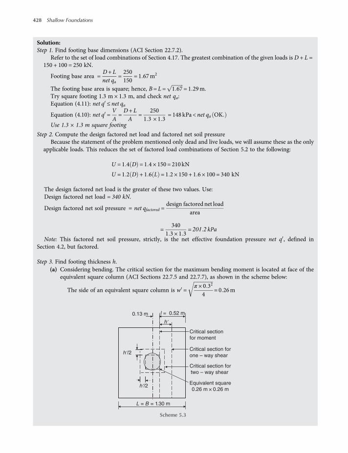
Solution:Step 1. Find footing base dimensions (ACI Section 22.7.2).
Refer to the set of load combinations of Section 4.17. The greatest combination of the given loads is D + L =150 + 100 = 250 kN.
Footing base area =D+ Lnet qa
=250150
= 1 67m2
The footing base area is square; hence, B= L= 1 67 = 1 29m.Try square footing 1.3 m × 1.3 m, and check net qa:Equation (4.11): net q ≤ net qa
Equation (4.10): net q =VA=D+ LA
=250
1 3 × 1 3= 148 kPa < net qa OK
Use 1.3 × 1.3 m square footing
Step 2. Compute the design factored net load and factored net soil pressureBecause the statement of the problem mentioned only dead and live loads, we will assume these as the only
applicable loads. This reduces the set of factored load combinations of Section 5.2 to the following:
U = 1 4 D = 1 4 × 150 = 210 kN
U = 1 2 D + 1 6 L = 1 2 × 150 + 1 6 × 100 = 340 kN
The design factored net load is the greater of these two values. Use:Design factored net load = 340 kN.
Design factored net soil pressure = net qfactored =design factored net load
area
=340
1 3 × 1 3= 201 2 kPa
Note: This factored net soil pressure, strictly, is the net effective foundation pressure net q , defined inSection 4.2, but factored.
Step 3. Find footing thickness h.(a) Considering bending. The critical section for the maximum bending moment is located at face of the
equivalent square column (ACI Sections 22.7.5 and 22.7.7), as shown in the scheme below:
The side of an equivalent square column is w =π × 0 32
4= 0 26m
h'/2
h'/2
Critical section
for moment
Critical section for
one – way shear
Critical section for
two – way shear
Equivalent square
0.26 m × 0.26 m
0.13 m l = 0.52 m
h'
L = B = 1.30 m
Scheme 5.3
428 Shallow Foundations
worksaccounts.com

Use effective footing thickness = h = h − 0.05 m (ACI Section 22.4.7)The applied factored bending moment per meter of the critical section is
Mu =net qfactored l 2
2=201 2 × 0 522
2= 27 20 kN m
Equation (5.32): ØMn ≥Mu
When load factor combinations of ACI Section 9.2.1 are used, the strength-reduction factor Ø shall be 0.6 forflexure, compression, shear, and bearing (ACI Section 9.3.5).Equation (5.33): Mn = 0 42λ fc Smwhere
λ = modification factor (ACI Section 8.6.1)= 1.0 for normal-weight concrete
Sm = the corresponding elastic section modulus
=b h 2
6(for rectangular section)
Let ØMn =Mu; hence,
0 6 0 42 1 21 10001 h 2
6= 27 2
h = 0 376m= 376mm; hence,
h= 376 + 50 = 426mm
> hmin = 200mm; ACI Section 22 7 4 OK
(b) Considering two-way shear. The critical section for two-way shear is located a distance h /2 from faces of theequivalent square column (ACI Sections 22.7.6.2 and 22.7.7), as shown in the scheme above.
Equation (5.35): ØVn ≥Vu
Vu =Af net qfactored −soil reaction on the shear block
For columns of small cross-section, such as the column of this problem, the soil reaction on the shear block issmall; it is usually neglected. Hence, use
Vu =Af net qfactored = 1 3 × 1 3 × 201 2 = 340 kN
Equation (5.37): Vn = 0 11 1 +2β
λ fc bo h
Vn ≤ 0 22λ fc bo h ACI Section 22 5 4
where β corresponds to ratio of long side to short side of concentrated load or reaction area.
Use Vn = 0 22λ fc bo h , since β =0 260 26
= 1
Let ØVn = Vu(Continued)
Shallow Foundations – Structural Design 429
worksaccounts.com
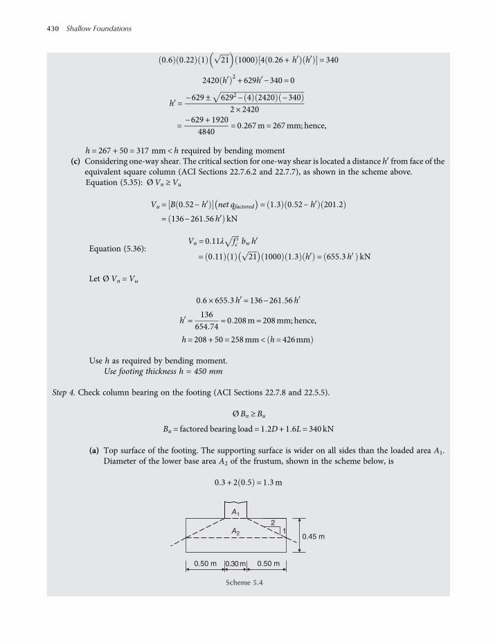
0 6 0 22 1 21 1000 4 0 26 + h h = 340
2420 h 2 + 629h −340 = 0
h =−629 ± 6292− 4 2420 −340
2 × 2420
=−629 + 1920
4840= 0 267m= 267mm; hence,
h = 267 + 50 = 317 mm < h required by bending moment(c) Considering one-way shear. The critical section for one-way shear is located a distance h from face of the
equivalent square column (ACI Sections 22.7.6.2 and 22.7.7), as shown in the scheme above.Equation (5.35): ØVn ≥Vu
Vu = B 0 52− h net qfactored = 1 3 0 52− h 201 2
= 136−261 56h kN
Equation (5.36):Vn = 0 11λ fc bw h
= 0 11 1 21 1000 1 3 h = 655 3 h kN
Let Ø Vn =Vu
0 6 × 655 3h = 136−261 56h
h =136
654 74= 0 208m= 208mm; hence,
h= 208 + 50 = 258mm< h= 426mm
Use h as required by bending moment.Use footing thickness h = 450 mm
Step 4. Check column bearing on the footing (ACI Sections 22.7.8 and 22.5.5).
ØBn ≥Bu
Bu = factored bearing load = 1 2D+ 1 6L= 340 kN
(a) Top surface of the footing. The supporting surface is wider on all sides than the loaded area A1.Diameter of the lower base area A2 of the frustum, shown in the scheme below, is
0 3 + 2 0 5 = 1 3m
2 1
0.50 m 0.50 m
A2
A1
0.30 m
0.45 m
Scheme 5.4
430 Shallow Foundations
worksaccounts.com

A2 =π 1 3 2
4= 1 33m2; A1 =
π 0 3 2
4= 0 071m2;
A2
A1= 4 3 > 2; hence, use
A2
A1= 2.
ØBn = Ø 0 85fc A1A2
A1ACI Section 22 5 5
ØBn = 0 6 0 85 × 21 × 0 071 2
= 1 521MN=1521 kN Bu OK
Therefore, vertical compression reinforcement or dowels through the supporting surface at the interface istheoretically not required.
(b) Base of the column. The allowable bearing strength of the column base at the interface is
ØBn = Ø 0 85fc A1
= 0 6 0 85 × 28 × 0 071 = 1 014MN=1014 kN Bu OK
Therefore, dowels through the column base at the interface are theoretically not required.Step 5. Design dowels to satisfy the minimum area of reinforcement across interface (ACI Section 15.8.2.1).
As,min = 0 005Ag
where Ag is the gross area of the supported member
As,min = 0 005π 0 3 2
4= 0 005 0 071 = 0 355 × 10−3 m2
Assume using (arbitrarily) six No. 20 dowel bars:
As,provided = 6π 0 020 2
4= 1 88 × 10−3 m2 As,min OK
Usesix No. 20 dowels (fy = 420 MPa).
Step 6. Find the embedment length of dowels in both the footing and the column.As mentioned in Section 5.4.4, dowels shall not be larger than a No. 36 bar and shall extend into supportedmember a distance not less than the larger of ldc, of the longitudinal bars (No. 57 and smaller but larger thandowels) and compression lap splice length of the dowels, whichever is greater, and into the footing a distancenot less than ldc of the dowels. Also, according to ACI Section 12.16.2, when bars of different size are lapspliced in compression, splice length shall be the larger of ldc of larger bar and compression lap splice lengthof smaller bar.
(a) Embedment length of dowels in the footing:According to ACI Section 12.3.2,
ldc =0 24fydbλ fc
or ldc = 0 043fy db, whichever is the larger
ldc =0 24 420 20
1 21= 440mm,
(Continued)
Shallow Foundations – Structural Design 431
worksaccounts.com
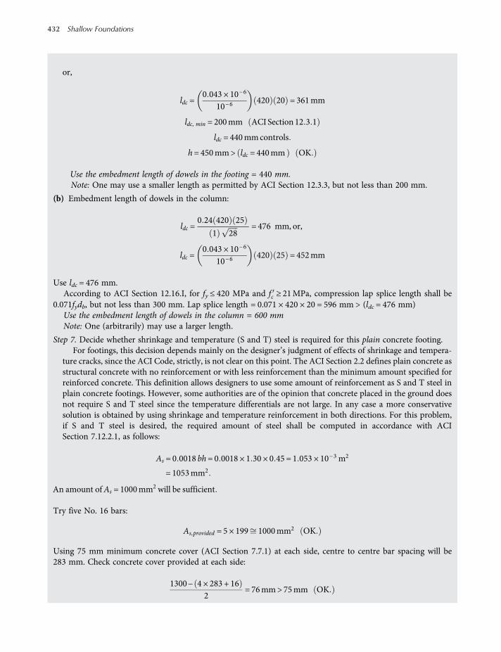
or,
ldc =0 043 × 10−6
10−6420 20 = 361mm
ldc, min = 200mm ACI Section 12 3 1
ldc = 440mmcontrols
h= 450mm> ldc = 440mm OK
Use the embedment length of dowels in the footing = 440 mm.Note: One may use a smaller length as permitted by ACI Section 12.3.3, but not less than 200 mm.
(b) Embedment length of dowels in the column:
ldc =0 24 420 25
1 28= 476 mm, or,
ldc =0 043 × 10−6
10−6420 25 = 452mm
Use ldc = 476 mm.According to ACI Section 12.16.I, for fy ≤ 420 MPa and fc ≥ 21MPa, compression lap splice length shall be
0.071fydb, but not less than 300 mm. Lap splice length = 0.071 × 420 × 20 = 596 mm > (ldc = 476 mm)Use the embedment length of dowels in the column = 600 mmNote: One (arbitrarily) may use a larger length.
Step 7. Decide whether shrinkage and temperature (S and T) steel is required for this plain concrete footing.For footings, this decision depends mainly on the designer’s judgment of effects of shrinkage and tempera-
ture cracks, since the ACI Code, strictly, is not clear on this point. The ACI Section 2.2 defines plain concrete asstructural concrete with no reinforcement or with less reinforcement than the minimum amount specified forreinforced concrete. This definition allows designers to use some amount of reinforcement as S and T steel inplain concrete footings. However, some authorities are of the opinion that concrete placed in the ground doesnot require S and T steel since the temperature differentials are not large. In any case a more conservativesolution is obtained by using shrinkage and temperature reinforcement in both directions. For this problem,if S and T steel is desired, the required amount of steel shall be computed in accordance with ACISection 7.12.2.1, as follows:
As = 0 0018 bh= 0 0018 × 1 30 × 0 45 = 1 053 × 10−3 m2
= 1053mm2
An amount ofAs = 1000mm2 will be sufficient
Try five No. 16 bars:
As,provided = 5 × 199 1000mm2 OK
Using 75 mm minimum concrete cover (ACI Section 7.7.1) at each side, centre to centre bar spacing will be283 mm. Check concrete cover provided at each side:
1300− 4 × 283 + 162
= 76mm> 75mm OK
432 Shallow Foundations
worksaccounts.com
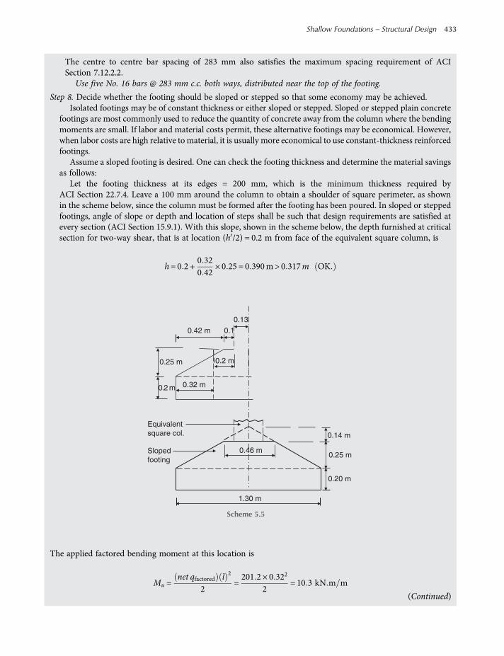
The centre to centre bar spacing of 283 mm also satisfies the maximum spacing requirement of ACISection 7.12.2.2.
Use five No. 16 bars @ 283 mm c.c. both ways, distributed near the top of the footing.
Step 8. Decide whether the footing should be sloped or stepped so that some economy may be achieved.Isolated footings may be of constant thickness or either sloped or stepped. Sloped or stepped plain concrete
footings are most commonly used to reduce the quantity of concrete away from the column where the bendingmoments are small. If labor and material costs permit, these alternative footings may be economical. However,when labor costs are high relative to material, it is usually more economical to use constant-thickness reinforcedfootings.
Assume a sloped footing is desired. One can check the footing thickness and determine the material savingsas follows:
Let the footing thickness at its edges = 200 mm, which is the minimum thickness required byACI Section 22.7.4. Leave a 100 mm around the column to obtain a shoulder of square perimeter, as shownin the scheme below, since the column must be formed after the footing has been poured. In sloped or steppedfootings, angle of slope or depth and location of steps shall be such that design requirements are satisfied atevery section (ACI Section 15.9.1). With this slope, shown in the scheme below, the depth furnished at criticalsection for two-way shear, that is at location (h /2) = 0.2 m from face of the equivalent square column, is
h= 0 2 +0 320 42
× 0 25 = 0 390m> 0 317m OK
The applied factored bending moment at this location is
Mu =net qfactored l 2
2=201 2 × 0 322
2= 10 3 kN m m
0.13
0.1
0.32 m
0.2 m
0.2 m
0.25 m
0.42 m
0.14 m
0.25 m
1.30 m
Equivalent
square col.
Sloped
footing
0.20 m
0.46 m
Scheme 5.5
(Continued)
Shallow Foundations – Structural Design 433
worksaccounts.com
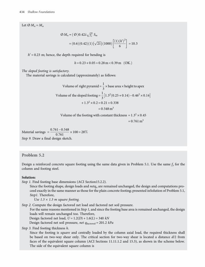
Let ØMn =Mu
ØMn = Ø 0 42λ fc Sm
= 0 6 0 42 1 21 10001 h 2
6= 10 3
h = 0.23 m; hence, the depth required for bending is
h= 0 23 + 0 05 = 0 28m< 0 39m OK
The sloped footing is satisfactory.The material savings is calculated (approximately) as follows:
Volume of right pyramid =13× base area × height to apex
Volume of the sloped footing =131 32 0 25 + 0 14 −0 462 × 0 14
+ 1 32 × 0 2 = 0 21 + 0 338
= 0 548m3
Volume of the footing with constant thickness = 1 32 × 0 45
= 0 761m3
Material savings =0 761−0 548
0 761× 100 = 28
Step 9. Draw a final design sketch.
Problem 5.2
Design a reinforced concrete square footing using the same data given in Problem 5.1. Use the same fy for thecolumn and footing steel.
Solution:Step 1. Find footing base dimensions (ACI Section15.2.2).
Since the footing shape, design loads and netqa are remained unchanged, the design and computations pro-ceed exactly in the same manner as those for the plain concrete footing; presented inSolution of Problem 5.1,Step1. Therefore,
Use 1.3 × 1.3 m square footing.
Step 2. Compute the design factored net load and factored net soil pressure.For the same reasons mentioned in Step 1, and since the footing base area is remained unchanged, the designloads will remain unchanged too. Therefore,Design factored net load, U = 1.2(D) + 1.6(L) = 340 kNDesign factored net soil pressure, net qfactored = 201.2 kPa
Step 3. Find footing thickness h.Since the footing is square and centrally loaded by the column axial load, the required thickness shallbe based on two-way shear only. The critical section for two-way shear is located a distance d/2 fromfaces of the equivalent square column (ACI Sections 11.11.1.2 and 15.3), as shown in the scheme below.The side of the equivalent square column is
434 Shallow Foundations
worksaccounts.com
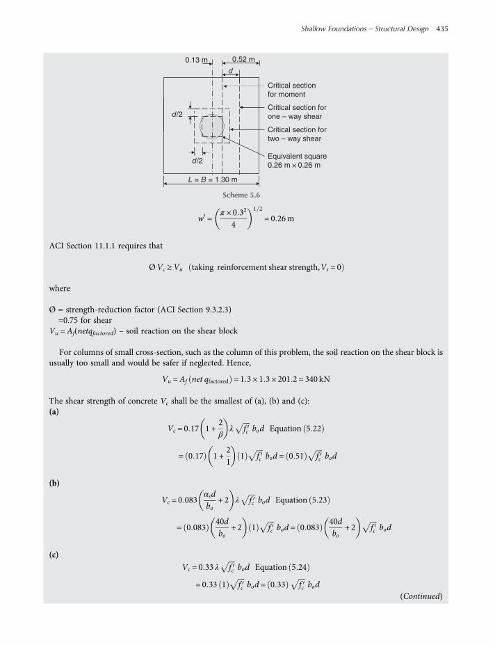
w =π × 0 32
4
1 2
= 0 26m
ACI Section 11.1.1 requires that
ØVc ≥Vu taking reinforcement shear strength,Vs = 0
where
Ø = strength-reduction factor (ACI Section 9.3.2.3)=0.75 for shear
Vu = Af(netqfactored) – soil reaction on the shear block
For columns of small cross-section, such as the column of this problem, the soil reaction on the shear block isusually too small and would be safer if neglected. Hence,
Vu =Af net qfactored = 1 3 × 1 3 × 201 2 = 340 kN
The shear strength of concrete Vc shall be the smallest of (a), (b) and (c):(a)
Vc = 0 17 1 +2β
λ fc bod Equation 5 22
= 0 17 1 +21
1 fc bod = 0 51 fc bod
(b)
Vc = 0 083αsdbo
+ 2 λ fc bod Equation 5 23
= 0 08340dbo
+ 2 1 fc bod = 0 08340dbo
+ 2 fc bod
(c)
Vc = 0 33 λ fc bod Equation 5 24
= 0 33 1 fc bod = 0 33 fc bod
0.52 m
Critical section
for moment
Critical section for
one – way shear
Critical section for
two – way shear
Equivalent square
0.26 m × 0.26 m
0.13 m
d
d/2
d/2
L = B = 1.30 m
Scheme 5.6
(Continued)
Shallow Foundations – Structural Design 435
worksaccounts.com
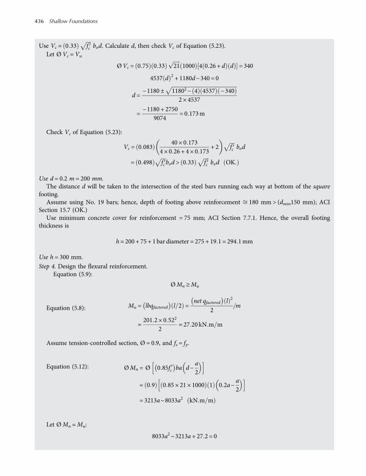
Use Vc = 0 33 fc bod. Calculate d, then check Vc of Equation (5.23).Let ØVc = Vu
ØVc = 0 75 0 33 21 1000 4 0 26 + d d = 340
4537 d 2 + 1180d−340 = 0
d =−1180 ± 11802− 4 4537 −340
2 × 4537
=−1180 + 2750
9074= 0 173m
Check Vc of Equation (5.23):
Vc = 0 08340 × 0 173
4 × 0 26 + 4 × 0 173+ 2 fc bod
= 0 498 fc bod > 0 33 fc bod OK
Use d = 0.2 m = 200 mm.The distance d will be taken to the intersection of the steel bars running each way at bottom of the square
footing.Assume using No. 19 bars; hence, depth of footing above reinforcement 180 mm > (dmin150 mm); ACI
Section 15.7 (OK.)Use minimum concrete cover for reinforcement = 75 mm; ACI Section 7.7.1. Hence, the overall footing
thickness is
h= 200 + 75 + 1 bar diameter = 275 + 19 1 = 294 1mm
Use h = 300 mm.
Step 4. Design the flexural reinforcement.Equation (5.9):
ØMn ≥Mu
Equation (5.8): Mu = lbqfactored l 2 =net qfactored l 2
2m
=201 2 × 0 522
2= 27 20 kN m m
Assume tension-controlled section, Ø = 0.9, and fs = fy.
Equation (5.12): ØMn = Ø 0 85fc ba d−a2
= 0 9 0 85 × 21 × 1000 1 0 2a−a2
= 3213a−8033a2 kN m m
Let ØMn =Mu:
8033a2−3213a+ 27 2 = 0
436 Shallow Foundations
worksaccounts.com

a=− −3213 ± 32132− 4 8033 27 2
2 × 8033=
13916 066
= 8 65 × 10−3 m
Equation (5.10): a=Asfy
0 85fc b
As =0 85fc b a
fy=0 85 × 21 × 1000 × 1 × 8 65 × 10−3
420 × 1000
= 3 7 × 10⁻⁴ m2 = 368mm2 m
As,min = 0.0018 bh (ACI Sections 10.5.4 and 7.12.2.1)
= 0 0018 × 1 × 0 3 = 5 4 × 10⁻⁴ m2
= 540 mm2/m > As required by analysisHence, use As = As,min.Use three No. 16; As,provided = 3 × 199 = 597 mm2/mCompute a for As = 597mm2/m, and check if fs = fy and whether the section is tension-controlled:
a=Asfy
0 85fc b=5 97 × 10−4 × 4200 85 × 21 × 1
= 0 014m= 14mm
c=aβ1
For fc between 17 and 28 MPa, β1 shall be taken as 0.85. Hence,
c=140 85
= 16 47
dt = d + 16 2 = 200 + 8 = 208mm
εt = 0 003dt −cc
= 0 003208−16 47
16 47= 0 035 > 0 005Equation 5 15
Hence, the section is tension-controlled, and Ø = 0.9 (ACI Sections 10.3.4 and 9.3.2.1).
εy =fyEs
=420
200 000= 0 0021
Therefore, εt > εy, and fs = fyThe assumptions made are satisfied. Note that this checking may not be necessary when As,min governs.
Total number of bars required each way =1 31
× 3 = 3 9; use four bars.
Note: The reinforcement and thickness results indicate clearly that it may be more economical and effective touse reinforced concrete footing than plain concrete footing with S and T steel provided.
Using 75 mm concrete cover at each side, centre to centre bars spacing will be 378 mm. ACI Section 10.5.4requires maximum spacing shall not exceed three times the slab or footing thickness, or 450 mm, whichever issmaller. Therefore, the 378 mm spacing is adequate.
Try four No. 16 bars @ 378 mm c.c. each way.
Step 5. Check the development of reinforcement.In this case, the bars are in tension, the provided bar size is smaller than No. 19, the clear spacing of the barsexceeds 2db, and the clear cover exceeds db. Therefore, the development length ld of bars at each side of the
(Continued)
Shallow Foundations – Structural Design 437
worksaccounts.com
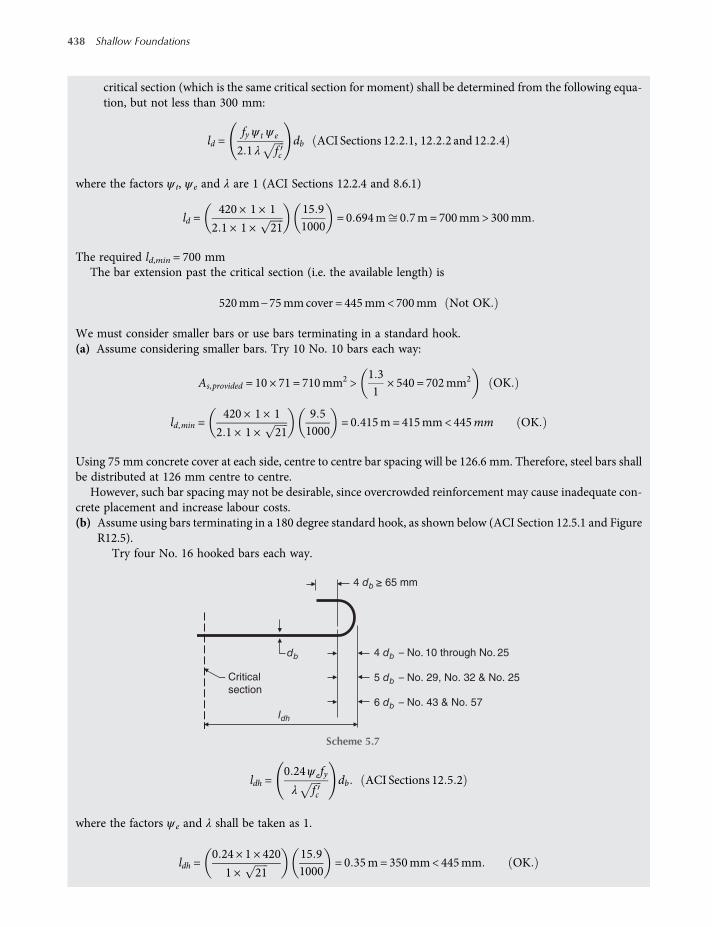
critical section (which is the same critical section for moment) shall be determined from the following equa-tion, but not less than 300 mm:
ld =fy ψ t ψ e
2 1 λ fcdb ACI Sections 12 2 1, 12 2 2 and 12 2 4
where the factors ψ t, ψ e and λ are 1 (ACI Sections 12.2.4 and 8.6.1)
ld =420 × 1 × 1
2 1 × 1 × 21
15 91000
= 0 694m 0 7m= 700mm> 300mm
The required ld,min = 700 mmThe bar extension past the critical section (i.e. the available length) is
520mm−75mmcover = 445mm<700mm Not OK
We must consider smaller bars or use bars terminating in a standard hook.(a) Assume considering smaller bars. Try 10 No. 10 bars each way:
As,provided = 10 × 71 = 710mm2 >1 31
× 540 = 702mm2 OK
ld,min =420 × 1 × 1
2 1 × 1 × 21
9 51000
= 0 415m= 415mm<445mm OK
Using 75 mm concrete cover at each side, centre to centre bar spacing will be 126.6 mm. Therefore, steel bars shallbe distributed at 126 mm centre to centre.
However, such bar spacing may not be desirable, since overcrowded reinforcement may cause inadequate con-crete placement and increase labour costs.(b) Assume using bars terminating in a 180 degree standard hook, as shown below (ACI Section 12.5.1 and Figure
R12.5).Try four No. 16 hooked bars each way.
ldh =0 24ψ efyλ fc
db ACI Sections 12 5 2
where the factors ψ e and λ shall be taken as 1.
ldh =0 24 × 1 × 420
1 × 21
15 91000
= 0 35m= 350mm< 445mm OK
5 db – No. 29, No. 32 & No. 25
6 db – No. 43 & No. 57
– Critical
section
db
4 db ≥ 65 mm
ldh
4 db – No. 10 through No. 25
Scheme 5.7
438 Shallow Foundations
worksaccounts.com
Assume the designer prefers using the specified hooked bars.Use four No. 16 bars @ 378 mm c.c. each way at bottom of the footing. The bars must have 180 degree standard
hooks at each end.
Step 6. Check column bearing on the footing (ACI Section 10.14).The factored load at the base of the column = 1.2D + 1.6L = 340 kN
(a) Top surface of the footing. From Step 4 – (a) of the solution of Problem 5.1, the maximum bearing load on thetop of the footing may be taken equal to Ø 0 85fc A1 2 . (ACI Section 10.14.1)
ACI Section 9.3.2.4 gives Ø = 0.65 for bearing. Hence,The maximum bearing factored load = 0.65(0.85)(21)(0.071)(2)
= 1 648MN=1648 kN 340 kN
Therefore, vertical compression reinforcements or dowels through the supporting surface at the interface are,theoretically, not required.
(b) Base of the column. The allowable bearing strength of the column base at the interface is Ø 0 85fc A1 . Hence,The allowable bearing factored load = (0.65)(0.85 × 28 × 0.071)
= 1 098MN=1098 kN 340 kN
Therefore, dowels through the column base at the interface are, theoretically, not required.Step 7. Design dowels to satisfy the minimum area of reinforcement across interface required by ACI
Section 15.8.2.1.From Step 5 of the Solution of Problem 5.1, As,min = 0.36 × 10− 3 m2
Assume, arbitrarily, usingsix No 20 dowel bars:
As,provided = 6π 0 020 2
4= 1 88 × 10−3 m2 As,min
Try six No. 20 dowels (fy = 420 MPa).
Step 8. Find the embedment length of dowels in both the footing and the column.(a) Embedment length of dowels in the footing:
Refer to ACI Section 12.3.
ACI Section 12.3.2: ldc =0 24fydbλ fc
or ldc = (0.043fy)db, whichever is larger, but shall not be less than 200 mm.
ldc =0 24 420 20
1 21= 440mm, or
ldc =0 043 × 10−6
10−6420 20 = 361mm
ldc,min = 200mm ACI Section 12 3 1
ldc = 440mm> h= 300mm NotOK
According to ACI Section 12.3.3, for reinforcement in excess of that required by analysis, ldc is permitted to bereduced as follows:
Required ldc = ldc (As required/As provided)
= 440 0 36 ×10−3
1 88× 10−3 = 84mm< ldc,min OK
(Continued)
Shallow Foundations – Structural Design 439
worksaccounts.com

Use the embedment length of dowels in the footing = 200 mm.(b) Embedment length of dowels in the column:
The necessary computations are exactly the same as those presented in Step 6(b) of the Solution of Problem5.1. Therefore,
Use the embedment length of dowels in the column = 600 mm.Note: One, arbitrarily, may use a larger length.
Step 9. Draw a final design sketch as shown in the scheme below.
Problem 5.3
A rectangular reinforced concrete footing is required to support an interior concrete column carrying a service(working) dead load of 2000 kN and a service live load of 1350 kN, at centre of the footing. The column cross-section is 450 × 450 mm. The column is built of 35-MPa concrete and has eight No. 29 longitudinal steel bars withfy = 420 MPa and Esteel = 2 × 10⁵ MPa. The gross allowable soil pressure (gross qa) at an expected foundation levelof 1.0–1.5 m depth has been recommended by the geotechnical consultant equals 250 kPa. The maximum width ofthe footing is limited to 3 m. The top of the footing will be covered with 0.15 m fill with a unit weight of 20 kN/m3
and a 0.15-m concrete basement floor (γc = 24 kN/m3) with a uniform live loadof 3.75 kPa. Using fc = 21MPa andfy = 420 MPa, design the footing in accordance with the requirements of ACI 318M-08.
Solution:Step 1. Find footing base dimensions (ACI Section15.2.2).
Assume the foundation depth Df = 1.2 m.Hence, footing thickness (assumed) h = 1.2 − (0.15 + 0.15) = 0.9 m
The greatest combination of the given loads is
D+ L= 2000 +A 0 15 × 24 + 0 15 × 20 + 0 9 × 24
+ 1350 + 3 75A
= 3350 + 31 95A kN
The gross effective foundation pressure = gross q =D + L
= 3350 + 31 95A
6 No. 25
6 No. 20 dowels
4 No. 16 bars @ 378
mm c. c. each way with
180 – degree standard
hook
Square footing
200 mm 300 mm
600 mm
300 mm – diameter
round column
84 mm
B = L = 1300 mm
Scheme 5.8
440 Shallow Foundations
worksaccounts.com

Footing base area =A=gross qgross qa
=3350 + 31 95A
250; hence,
A=3350218 05
= 15 36m2
Use the maximum footing width B = 3 m. Therefore, the footing length is
L=AB=15 363
= 5 12m
Use:3.0 × 5.2 mrectangular footing [gross q < gross qa, OK.]
Step 2. Compute the design factored net load and factored net soil pressure.Because the statement of the problem mentioned only dead and live loads, we will assume these as the only
applicable loads. This reduces the set of foundation net factored load combinations of Section 5.2 to thefollowing:
U = 1 4 D
U = 1 2 D + 1 6 L
The factored soil pressure is usually computed without including the weights of footing, backfill material, floor andthe floor uniform live load because these loads are evenly distributed and supported; thus they do not produceshear or moment in the footing.
U = 1 4 D = 1 4 × 2000 = 2800 kN; or,
U = 1 2 D + 1 6 L = 1 2 2000 + 1 6 1350 = 4560 kN
Use design factored net load = 4560 kN.
Design factored net soil pressure = net qfactored =45603 × 5 2
= 292 31 kPa
Step 3. Find footing thickness h.Since the footing is rectangular in shape, determine the required thickness based on both one-way shear and
two-way shear analyses.(a) Considering one-way shear:
The critical section for one-way shear is located at a distanced from face of the column across the entirefooting width (ACI Sections 11.11.1.1 and 11.1.3.1), as shown in the scheme below.
Critical section
for moment;
(steel bars in
long direction)
Critical section
for moment;
(steel bars in
short direction)
Critical section for
two – way shear
B=
3.0
m
2.38 m
1.28 m
d/2
d
d/2
L = 5.2 m
450–mm square
concrete column
Criticial section for
one – way shear
Scheme 5.9(Continued)
Shallow Foundations – Structural Design 441
worksaccounts.com

Equation (5.19): ØVc ≥Vu taking reinforcement shear strength,VS = 0
whereØ = strength-reduction factor (ACI Section 9.3.2.3)= 0.75 for shear
Vu = B 2 38−d net qfactored = 3 2 38−d 292 31
= 2087 09−876 93 d kN
Equation (5.20): Vc = 0 17λ fc bwd
Let ØVc = Vu:
0 75 × 0 17 × 1 21 1000 3 d = 2087 09−876 93 d
d =2087 092629 77
= 0 794m= 794mm
(b) Considering two-way shear:
Vu =Af net qfactored −soil reaction on the shear block
= 3 × 5 20 292 31 − 0 45 + d 2 292 31
= 4560−59 19−263 08 d−292 31 d2
= 4500 81−263 08 d−292 31 d2
The shear strength of concrete Vc shall be the smallest of (i), (ii) and (iii):(i)
Vc = 0 17 1 +2β
λ fc bod Equation 5 22
= 0 17 1 +21
1 fc bod = 0 51 fc bod
(ii)
Vc = 0 083αsdbo
+ 2 λ fc bod Equation 5 23
= 0 08340dbo
+ 2 1 fc bod = 0 08340dbo
+ 2 fc bod
(iii)
Vc = 0 33 λ fc bod Equation 5 24
= 0 33 1 fc bod = 0 33 fc bod
442 Shallow Foundations
worksaccounts.com

Use Vc = 0 33 fc bod. Calculate d, then check Vc of Equation (5.23).
ØVc = 0 75 0 33 21 1000 4 0 45 + d d = 4537 d 2 + 2042d
Let ØVn =Vu:
4537 d 2 + 2042 d = 4500 81−263 08 d−292 31 d2
4829d2 + 2305d−4501 = 0
d =−2305 ± 23052− 4 4829 −4501
2 × 4829=−2305 + 9605
9658= 0 756m= 756mm
Check Vc of Equation (5.23):
Vc = 0 08340 × 0 756
4 0 45 + 0 756+ 2 fc bod
= 0 686 fc bod >Vc = 0 33 fc bod OK
d = 756 mm < (d = 794 mm, required by one way shear)Therefore, the one-way shear controls:Use d = 0.8 m = 800 mm.The distance d will be taken to the centre of the steel bars in long direction.Assume using No. 25 bars, and 75 mmminimum concrete cover (ACI Section 7.7.1). Hence, the overall footing
thickness is
h= 800 + 75 + 1 2bar diameter = 875 + 12 7 = 887 7mm
Use h = 900 mm.Step 4. Design the flexural reinforcement.(a) Reinforcement in long direction. The critical section is shown in the figure of Step 3.
Equation (5.9): ØMn ≥Mu
Equation (5.8): Mu = lbqfactored l 2 =net qfactored l 2
2m
=net qfactored l 2
2=292 31 × 2 382
2= 828 kN m m
Assume tension-controlled section, Ø = 0.9, and fs = fy.
a=Asfy
0 85fc b=
As × 4200 85 × 21 × 1
= 23 53As
ØMn = Ø Asfy d−a2
Equation 5 11
= 0 9 As × 420 × 1000 0 8−23 53As
2
= 302 400As−4 447 170A2s kN m m
(Continued)
Shallow Foundations – Structural Design 443
worksaccounts.com

Let ØMn =Mu:
302 400As−4 447 170A2s = 828
4 447 170A2s −302 400As + 828 = 0
As =− −302 400 ± −302 400 2− 4 4 447 170 828
2 × 4 447 170=302 400−276 978
8 894 340
= 2858 × 10−6 m2 m= 2858mm2 m
As,min = 0 0018 bh (ACI Sections 10.5.4 and 7.12.2.1)
= 0 0018 × 1 × 0 9 = 1 62 × 10−3 m2 m
= 1620mm2 m<As required by analysis
Try six No. 25; As,provided = 6 × 510 = 3060 mm2/m > As (OK.)Compute a for As = 3060 mm2/m, and check if fs = fy and whether the section is tension-controlled:
a= 23 53As = 23 53 × 3060 × 10−6 = 0 072m= 72mm
c=aβ1; For fc between 17 and 28 MPa, β1 shall be taken as 0.85.
c=720 85
= 84 71mm
dt = d = 800mm
εt = 0 003dt −cc
Equation 5 23
= 0 003800−84 71
84 71= 0 025 > 0 005.
Hence, the section is tension-controlled, and Ø = 0.9 (ACI Sections 10.3.4 and 9.3.2.1).
εy =fyEs
=420
200 000= 0 0021
Hence, εt > εy ,
and fs = fy
Therefore the assumptions made are satisfied.Total number of bars required in long direction = 3 × 6 = 18Using 75 mm minimum concrete cover at each side, centre to centre bar spacing will be 166 mm. Check con-
crete cover provided at each side:
3000− 17 × 166 + 25 42
= 76 3mm> 75 mm OK
444 Shallow Foundations
worksaccounts.com

In case the required flexural reinforcement exceeds the minimum flexural reinforcement, it shall be adequate touse the samemaximum spacing of reinforcement for slabs which is two times the slab thickness, or 450mmwhich-ever is smaller, as specified by ACI Section 13.3.2. Therefore, the 166 mm spacing is adequate.
Try 18 No. 25 @ 166 mm c.c. across the footing width.Check the development of reinforcement:In this case, the bars are in tension, the provided bar size is larger than No. 19, the clear spacing of the bars
exceeds 2db, and the clear cover exceeds db. Therefore, the development length ld of bars at each side of the criticalsection (which is the same critical section for moment) shall be determined from the following equation, but notless than 300 mm:
ld =fy ψ t ψ e
1 7 λ fcdb ACI Sections 12 2 1, 12 2 2 and 12 2 4
where the factors ψ t, ψ e and λ are 1. (ACI Sections 12.2.4 and 8.6.1)
ld =420 × 1 × 1
1 7 × 1 × 21
25 41000
= 1 37m= 1370mm> 300mm
Therefore, the required ld = 1370 mm.The bar extension past the critical section (i.e. the available length) is
2380mm−75mmcover = 2305mm> 1370mm OK
Use 18 No. 25 @ 166 mm c.c. across the footing width, at bottom in long direction.(b) Reinforcement in short direction. The critical section is shown in the scheme in Step 3.
Bars in short direction are placed on bars in long direction. Therefore,
d = 0 8−
12diameter of bar in long direction +
12diameter of bar in short direction
Assume using No. 19 bars in short direction. Hence,
d = 0 8−12× 0 0254 +
12× 0 0191 = 0 778m
Equation (5.9):
ØMn ≥Mu
0.9 m
Bar inshort direction
Bar in long direction
d
Scheme 5.10
(Continued)
Shallow Foundations – Structural Design 445
worksaccounts.com
Mu =net qfactored l 2
2=292 31 × 1 282
2= 239 5 kN m m
Assume tension-controlled section, Ø = 0.9, and fs = fy.
a=Asfy
0 85fc b=
As × 4200 85 × 21 × 1
= 23 53As
ØMn = Ø Asfy d−a2
Equation 5 11
= 0 9 As × 420 × 1000 0 778−23 53As
2
= 294084As−4447170A2s kN m m
Let ØMn =Mu:
294 084As−4 447 170A2s = 239 5
4 447 170A2s −294 084As + 239 5 = 0
As =− −294 084 ± −294 084 2− 4 4 447 170 239 5
2 × 4 447 170=294 084−286 749
8 894 340
= 824 7 × 10⁻⁶ m2 m= 825mm2 m
As,min = 0.0018 bh (ACI Sections 10.5.4 and 7.12.2.1)
= 0 0018 × 1 × 0 9 = 1 62 × 10−3 m2 m
= 1620mm2 m>As required by analysis
Therefore, use As required = As,min = 1620 mm2/mThe assumptions made are satisfied, since As required = As,min.Total As required = 1620 × 5.2 = 8424 mm2
Try 30 No. 19:
As,provided = 30 × 284 = 8520mm2 > 8424mm2 OK
Check the development of reinforcement:In this case, the bars are in tension, the provided bar size is No. 19, the clear spacing of the bars exceeds 2db,
and the clear cover exceeds db. Therefore, the development length ld of bars at each side of the criticalsection (which is the same critical section for moment) shall be determined from the following equation, butnot less than 300 mm:
ld =fy ψ t ψ e
2 1 λ fcdb ACI Sections 12 2 1, 12 2 2 and 12 2 4
where the factors ψ t, ψ e and λ are 1. (ACI Sections 12.2.4 and 8.6.1)
ld =420 × 1 × 1
2 1 × 1 × 21
19 11000
= 0 833m= 833mm>300 mm
446 Shallow Foundations
worksaccounts.com
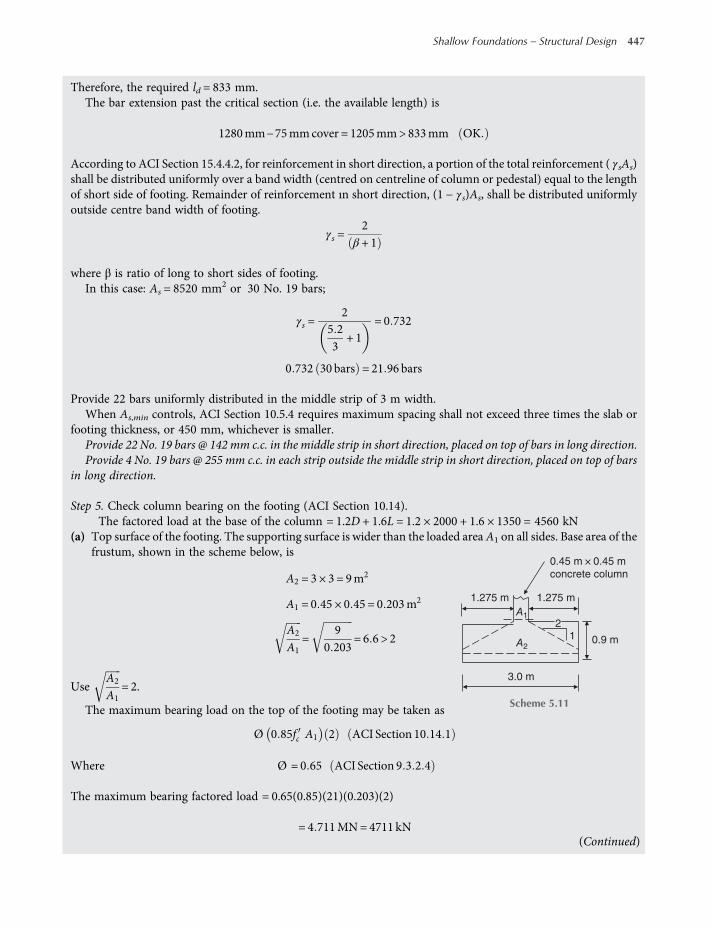
Therefore, the required ld = 833 mm.The bar extension past the critical section (i.e. the available length) is
1280mm−75mmcover = 1205mm> 833mm OK
According to ACI Section 15.4.4.2, for reinforcement in short direction, a portion of the total reinforcement ( γsAs)shall be distributed uniformly over a band width (centred on centreline of column or pedestal) equal to the lengthof short side of footing. Remainder of reinforcement ın short direction, (1 − γs)As, shall be distributed uniformlyoutside centre band width of footing.
γs =2
β + 1
where β is ratio of long to short sides of footing.In this case: As = 8520 mm2 or 30 No. 19 bars;
γs =2
5 23
+ 1= 0 732
0 732 30 bars = 21 96 bars
Provide 22 bars uniformly distributed in the middle strip of 3 m width.When As,min controls, ACI Section 10.5.4 requires maximum spacing shall not exceed three times the slab or
footing thickness, or 450 mm, whichever is smaller.Provide 22 No. 19 bars @ 142 mm c.c. in the middle strip in short direction, placed on top of bars in long direction.Provide 4 No. 19 bars @ 255 mm c.c. in each strip outside the middle strip in short direction, placed on top of bars
in long direction.
Step 5. Check column bearing on the footing (ACI Section 10.14).The factored load at the base of the column = 1.2D + 1.6L = 1.2 × 2000 + 1.6 × 1350 = 4560 kN
(a) Top surface of the footing. The supporting surface is wider than the loaded areaA1 on all sides. Base area of thefrustum, shown in the scheme below, is
A2 = 3 × 3 = 9m2
A1 = 0 45 × 0 45 = 0 203m2
A2
A1=
90 203
= 6 6 > 2
UseA2
A1= 2.
The maximum bearing load on the top of the footing may be taken as
Ø 0 85fc A1 2 ACI Section 10 14 1
Where Ø = 0 65 ACI Section 9 3 2 4
The maximum bearing factored load = 0.65(0.85)(21)(0.203)(2)
= 4 711MN=4711 kN
2
A2
A1
1
1.275 m 1.275 m
3.0 m
0.9 m
0.45 m × 0.45 m
concrete column
Scheme 5.11
(Continued)
Shallow Foundations – Structural Design 447
worksaccounts.com

The factored load at the base of the column is less than the maximum bearing factored load. Therefore, verticalcompression reinforcement or dowels through the supporting surface at the interface is theoretically not required.(b) Base of the column. The allowable bearing strength of the column base at the interface is Ø 0 85fc A1 .
The allowable bearing factored load = 0 65 0 85 × 35 × 0 203
= 3 925MN=3925 kN
< 4560 kN
Therefore, dowels through the column base at the interface are needed to transfer the excess load.
Area of dowels required =Ad =4560−3925
Ø fy
Ø =0 65 ACI Sections 9 3 2 4 and 9 3 2 2 b
Ad =4560−3925
0 65 × 420 × 1000= 2 326 × 10−3 m2 = 2326mm2
The area of dowels must also satisfy ACI Section 15.8.2.1, which requires
Ad ≥ 0 005Ag
Ad = 0 005 × 0 452 = 1 013 × 10−3 m2 = 1013mm2 < 2326mm2
Trysix No. 22 dowels. As,provided = 6 × 387 = 2322 mm2 (acceptable).Provide six No. 22 dowels (fy = 420 MPa); dowel each corner bar and two other (opposite) bars.
Step 6. Find the embedment length of dowels in both the footing and the column.(a) Embedment length of dowels in the footing:
According to ACI Sections 15.8.2.3 and 12.3.2:
ldc =0 24fydbλ fc
, or, ldc = 0 043fy db, whichever is the larger
ldc =0 24 420 22 2
1 21= 488mm, or, ldc = 0 043 420 22 2
= 401mm
ldc, min = 200mm ACI Section 12 3 1
Therefore, the required ldc = 488 mm < dThe dowel bars will be extended down to the level of the main footing steel and hooked 90 (ACI standard 90
hook). The hooks will be tied (wired) to the main steel to hold the dowels in place.Use the embedment length of dowels in the footing 768 mm.
(b) Embedment length of dowels in the column:According to ACI Sections 15.8.2.3, 12.3.2 and 12.16.1:
ldc =0 24 420 28 7
1 35= 489mm, or, ldc = 0 043 420 28 7
= 518mm
ldc =0 043 × 10−6
10−6420 28 7 = 518mm
448 Shallow Foundations
worksaccounts.com

Therefore, the required ldc = 518 mmFor fy ≤ 420MPa and fc ≥ 21MPa: compression lap splice length shall be 0.071 fydb, but not less than 300 mm.Lap splice length = 0.071 × 420 × 22.2 = 662 mm > (ldc = 518 mm)Therefore, the minimum embedment length = lap splice length = 662 mmUse the embedment length of dowels in the column = 700 mm.Note: One, arbitrarily, may use a larger length.
Step 7. Develop the final design sketch as shown in the scheme below.
Problem 5.4
A single column footing is loaded with an axial column load at centre, a moment and a horizontal load, as shown inthe scheme below. Design the footing for the following given design data:
Loads:
P =D+ L D= 420 kN L= 535 kN
My =My,D +My,L My,D = 228 kN m My,L = 250 kN m
H =HD +HL HD = 42 kN HL = 53 kN
Column:Reinforced concrete 500mm×500mm 8No 19 bars
fy = 420MPa Esteel = 2 × 10⁵ MPa fc = 28MPa
Footıng:Reinforced concrete footing
fy = 420MPa Esteel = 2 × 10⁵ MPa fc = 21MPa
Foundation soil:Net allowable soil pressure = net qa = 150 kPa
– 4 No. 19
@ 255
mm c.c.
– 22 No. 19
@142
mm c.c.
– 4 No. 19
@255
mm c.c.
1020 mm 1020 mm3000 mm
80 mm 80 mm L = 5200 mm
150 mm
3.0 m × 5.2 m Footing900 mm
Basement floor
–18 No. 25 @166 mm c.c.
6 No. 22 dowels
700 mm
8 No. 29
450 mm-square column
85
mm
Fill 150 mm
Scheme 5.12
(Continued)
Shallow Foundations – Structural Design 449
worksaccounts.com
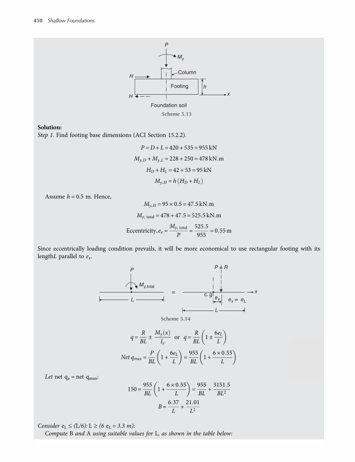
Solution:Step 1. Find footing base dimensions (ACI Section 15.2.2).
P =D+ L= 420 + 535 = 955 kN
My,D +My,L = 228 + 250 = 478 kN m
HD +HL = 42 + 53 = 95 kN
My,H = h HD +HL
Assume h = 0.5 m. Hence,My,H = 95 × 0 5 = 47 5 kN m
My, total = 478 + 47 5 = 525 5 kN m
Eccentricity,ex =My, total
P=525 5955
= 0 55m
Since eccentrically loading condition prevails, it will be more economical to use rectangular footing with itslengthL parallel to ex.
q=RBL
±My x
Iyor q=
RBL
1 ±6eLL
Net qmax =PBL
1 +6eLL
=955BL
1 +6 × 0 55
L
Let net qa = net qmax:
150 =955BL
1 +6 × 0 55
L=955BL
+3151 5BL2
B=6 37L
+21 01L2
Consider eL≤ (L/6): L≥ (6 eL = 3.3 m):Compute B and A using suitable values for L, as shown in the table below:
Foundation soil
H
H
P
hx
My
Footing
Column
Scheme 5.13
= c. g
P
ex = eL
My,total
L
L
xex
P = R
Scheme 5.14
450 Shallow Foundations
worksaccounts.com
L, m B, m A, m2
3.5 3.54 > L? 12.394.0 2.91 11.644.5 2.45 11.035.0 2.11 10.55
These results indicate that when L increases, area decreases providing more economical design. However, it is alsorequired not to use a large value for L in order to avoid the appearance of the column on a beam. Therefore, it isnecessary to take these requirements into consideration when L and B dimensions are selected.
Use rectangular footing 2.5 × 4.5 m.
Check net qa: net qmax =PBL
1 +6eLL
=955
2 5 × 4 51 +
6 × 0 554 5
= 84 89 + 62 25
= 147 14 kPa < net qa OK
Step 2. Compute the design factored net loads, moments and soil pressures.Factored P = Pult = 1.2 × 420 + 1.6 × 535 = 1360 kNFactored My =My, ult = 1.2(228 + 42 × 0.5) + 1.6(250 + 53 × 0.5)
= 298 8 + 442 4 = 741 2 kN m
eL =My,ult
Pult=741 21360
= 0 55m<L6= 0 75m OK
Factorednet qmax =PultBL
1 +6eLL
=1360
2 5 × 4 51 +
6 × 0 554 5
= 120 89 + 88 65 = 209 54 kPa
Factorednet qmin =PultBL
1−6eLL
= 120 89−88 65 = 32 24 kPa
Step 3. Draw the factored soil pressure diagram and locate the necessary critical sections.
209.54 kPa
Critical section for moment
(steel bars in long direction)
Critical section for moment
(steel bars in short direction
Critical section for one way shear
Critical section for two way shear
Slope = (39.4/1)
209.54 kPa
32.24 kPa
L = 4.5 m
2 m2 – d
0.5 + d
B =
2.5
m1 m
d
Scheme 5.15 (Continued)
Shallow Foundations – Structural Design 451
worksaccounts.com
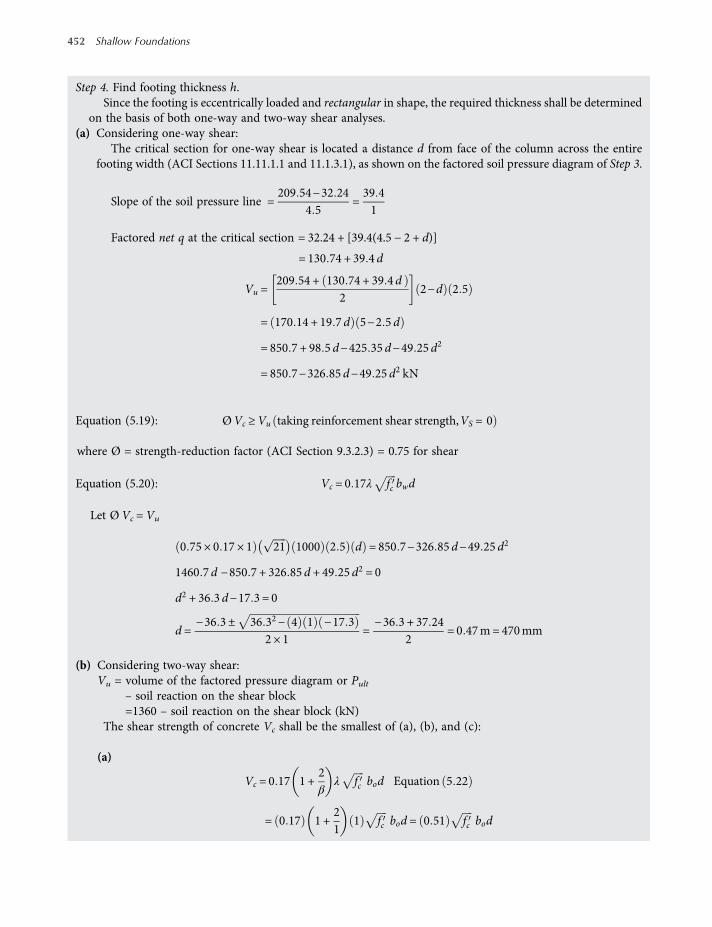
Step 4. Find footing thickness h.Since the footing is eccentrically loaded and rectangular in shape, the required thickness shall be determined
on the basis of both one-way and two-way shear analyses.(a) Considering one-way shear:
The critical section for one-way shear is located a distance d from face of the column across the entirefooting width (ACI Sections 11.11.1.1 and 11.1.3.1), as shown on the factored soil pressure diagram of Step 3.
Slope of the soil pressure line =209 54−32 24
4 5=39 41
Factored net q at the critical section = 32.24 + [39.4(4.5 − 2 + d)]
= 130 74 + 39 4 d
Vu =209 54 + 130 74 + 39 4 d
22−d 2 5
= 170 14 + 19 7 d 5−2 5 d
= 850 7 + 98 5 d−425 35 d−49 25 d2
= 850 7−326 85 d−49 25 d2 kN
Equation (5.19): ØVc ≥Vu taking reinforcement shear strength,VS = 0
where Ø = strength-reduction factor (ACI Section 9.3.2.3) = 0.75 for shear
Equation (5.20): Vc = 0 17λ fc bwd
Let ØVc = Vu
0 75 × 0 17 × 1 21 1000 2 5 d = 850 7−326 85 d−49 25 d2
1460 7 d −850 7 + 326 85 d + 49 25 d2 = 0
d2 + 36 3 d−17 3 = 0
d =−36 3 ± 36 32− 4 1 −17 3
2 × 1=−36 3 + 37 24
2= 0 47m= 470mm
(b) Considering two-way shear:Vu = volume of the factored pressure diagram or Pult
– soil reaction on the shear block=1360 – soil reaction on the shear block (kN)
The shear strength of concrete Vc shall be the smallest of (a), (b), and (c):
(a)
Vc = 0 17 1 +2β
λ fc bod Equation 5 22
= 0 17 1 +21
1 fc bod = 0 51 fc bod
452 Shallow Foundations
worksaccounts.com
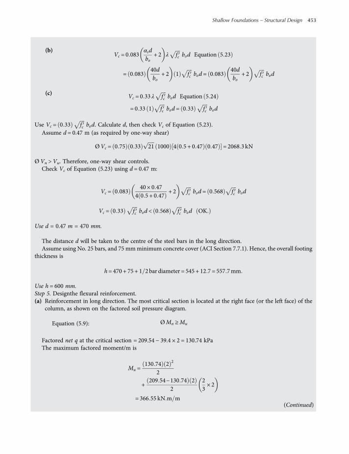
(b)Vc = 0 083
αsdbo
+ 2 λ fc bod Equation 5 23
= 0 08340dbo
+ 2 1 fc bod = 0 08340dbo
+ 2 fc bod
(c) Vc = 0 33 λ fc bod Equation 5 24
= 0 33 1 fc bod = 0 33 fc bod
Use Vc = 0 33 fc bod. Calculate d, then check Vc of Equation (5.23).Assume d = 0.47 m (as required by one-way shear)
ØVc = 0 75 0 33 21 1000 4 0 5 + 0 47 0 47 = 2068 3 kN
ØVn >Vu. Therefore, one-way shear controls.Check Vc of Equation (5.23) using d = 0.47 m:
Vc = 0 08340 × 0 47
4 0 5 + 0 47+ 2 fc bod = 0 568 fc bod
Vc = 0 33 fc bod < 0 568 fc bod OK
Use d = 0.47 m = 470 mm.
The distance d will be taken to the centre of the steel bars in the long direction.Assume using No. 25 bars, and 75 mmminimum concrete cover (ACI Section 7.7.1). Hence, the overall footing
thickness is
h= 470 + 75 + 1 2bar diameter = 545 + 12 7 = 557 7mm
Use h = 600 mm.Step 5. Designthe flexural reinforcement.(a) Reinforcement in long direction. The most critical section is located at the right face (or the left face) of the
column, as shown on the factored soil pressure diagram.
Equation (5.9): ØMn ≥Mu
Factored net q at the critical section = 209.54 − 39.4 × 2 = 130.74 kPaThe maximum factored moment/m is
Mu =130 74 2 2
2
+209 54−130 74 2
223× 2
= 366 55 kN m m(Continued)
Shallow Foundations – Structural Design 453
worksaccounts.com
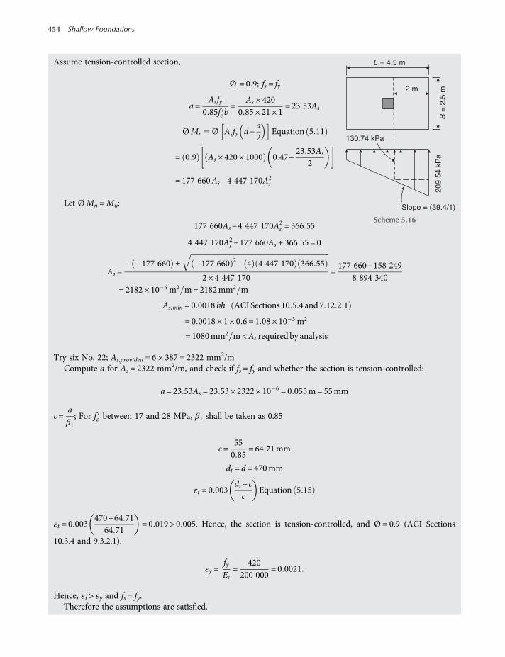
Assume tension-controlled section,
Ø = 0 9; fs = fy
a=Asfy
0 85fc b=
As × 4200 85 × 21 × 1
= 23 53As
ØMn = Ø Asfy d−a2
Equation 5 11
= 0 9 As × 420 × 1000 0 47−23 53As
2
= 177 660As−4 447 170A2s
Let ØMn =Mu:
177 660As−4 447 170A2s = 366 55
4 447 170A2s −177 660As + 366 55 = 0
As =− −177 660 ± −177 660 2− 4 4 447 170 366 55
2 × 4 447 170=177 660−158 249
8 894 340= 2182 × 10−6 m2 m= 2182mm2 m
As,min = 0 0018 bh ACI Sections 10 5 4 and 7 12 2 1
= 0 0018 × 1 × 0 6 = 1 08 × 10−3 m2
= 1080mm2 m<As required by analysis
Try six No. 22; As,provided = 6 × 387 = 2322 mm2/mCompute a for As = 2322 mm2/m, and check if fs = fy and whether the section is tension-controlled:
a= 23 53As = 23 53 × 2322 × 10−6 = 0 055m= 55mm
c=aβ1; For fc between 17 and 28 MPa, β1 shall be taken as 0.85
c=550 85
= 64 71mm
dt = d = 470mm
εt = 0 003dt −cc
Equation 5 15
εt = 0 003470−64 71
64 71= 0 019 > 0 005. Hence, the section is tension-controlled, and Ø = 0.9 (ACI Sections
10.3.4 and 9.3.2.1).
εy =fyEs
=420
200 000= 0 0021
Hence, εt > εy and fs = fy.Therefore the assumptions are satisfied.
130.74 kPa
Slope = (39.4/1)
2 m
L = 4.5 m
B =
2.5
m2
09
.54
kP
a
Scheme 5.16
454 Shallow Foundations
worksaccounts.com
Total number of bars required in long direction = 2.5 × 6 = 15Using 75 mm minimum concrete cover at each side, centre to centre bar spacing will be 166 mm. Check con-
crete cover provided at each side:
2500− 14 × 166 + 22 22
= 76 9mm> 75mm OK
In case the required flexural reinforcement exceeds the minimum flexural reinforcement, it shall be adequate touse the samemaximum spacing of reinforcement for slabs which is two times the slab thickness, or 450mmwhich-ever is smaller, as specified by ACI Section 13.3.2.
Try 15 No. 22 @ 166 mm c.c. in long direction at bottom of the footing.Check the development of reinforcement:In this case, the bars are in tension, the provided bar size is larger than No. 19, the clear spacing of the bars
exceeds 2db, and the clear cover exceeds db. Therefore, the development length ld of bars at each side of the criticalsection (which is the same critical section for moment) shall be determined from the following equation, but notless than 300 mm:
ld =fy ψ t ψ e
1 7 λ fcdb ACI Sections 12 2 1, 12 2 2 and 12 2 4
where the factors ψ t, ψ e and λ are 1. (ACI Sections 12.2.4 and 8.6.1)
ld =420 × 1 × 1
1 7 × 1 × 21
22 21000
= 1 20m= 1200mm> 300 mm
Therefore, the required ld = 1200 mmThe bar extension past the critical section (i.e. the available length) is
2000mm−75mmcover = 1925mm>1200mm OK
Use 15 No. 22 @ 166 mm c.c. across the footing width, at bottom in long direction.(b) Reinforcement in short direction. The critical section is located at the face of the column, as shown on the
factored soil pressure diagram.Bars in short direction are placed on bars in long direction. Therefore,
d = 0 47−
12diameter of bar in long direction +
12diameter of bar in short direction
Assume using No. 19 bars in short direction. Hence,
d = 0 47−12× 0 0222 +
12× 0 0191 = 0 449m
0.47 m
Bar inshort direction
Bar in long direction
d
Scheme 5.17
(Continued)
Shallow Foundations – Structural Design 455
worksaccounts.com

ØMn ≥Mu
Mu =32 24 + 209 54 4 5
21
12
4 5
= 60 45 kN m m
Assume tension-controlled section, Ø = 0.9, and fs = fy.
a=Asfy
0 85fc b=
As × 4200 85 × 21 × 1
= 23 53As
ØMn = Ø Asfy d−a2
Equation 5 11
= 0 9 As × 420 × 1000 0 449−23 53As
2
= 1 697 224As−4 447 170A2s
Let ØMn =Mu
169 722As−4 447 170A2s = 60 45
4 447 170A2s −169 722As + 60 45 = 0
As =− −169 722 ± −169 722 2− 4 4 447 170 60 45
2 × 4 447 170=169 722−166 524
8 894 340= 360 × 10−6 m2 m= 360mm2 m
As,min = 0 0018 bh= 0 0018 × 1 × 0 6 = 1 08 × 10−3 m2 m
= 1080mm2 m>As required by analysis
Use As required = As,min = 1080 mm2/mThe assumptions made are satisfied, since As required = As,min.Total As required = 1080 × 4.5 = 4860 mm2
Try 18 No. 19: As,provided = 18 × 284 = 5112 mm2 > 4860 mm2 (OK.)Check the development of reinforcement:In this case, the bars are in tension, the provided bar size is No. 19, the clear spacing of the bars exceeds 2db, and
the clear cover exceeds db. Therefore, the development length ld of bars at each side of the critical section (which isthe same critical section for moment) shall be determined from the following equation, but not less than 300 mm:
ld =fy ψ t ψ e
2 1 λ fcdb ACI Sections 12 2 1, 12 2 2 and 12 2 4
Where the factors ψ t, ψ e and λ are 1. (ACI Sections 12.2.4 and 8.6.1)
ld =420 × 1 × 1
2 1 × 1 × 21
19 11000
= 0 833m= 833mm> 300mm
Therefore, the required ld = 833 mmThe bar extension past the critical section (i.e. the available length) is
1000mm−75mmcover = 925mm> 833mm OK
456 Shallow Foundations
worksaccounts.com
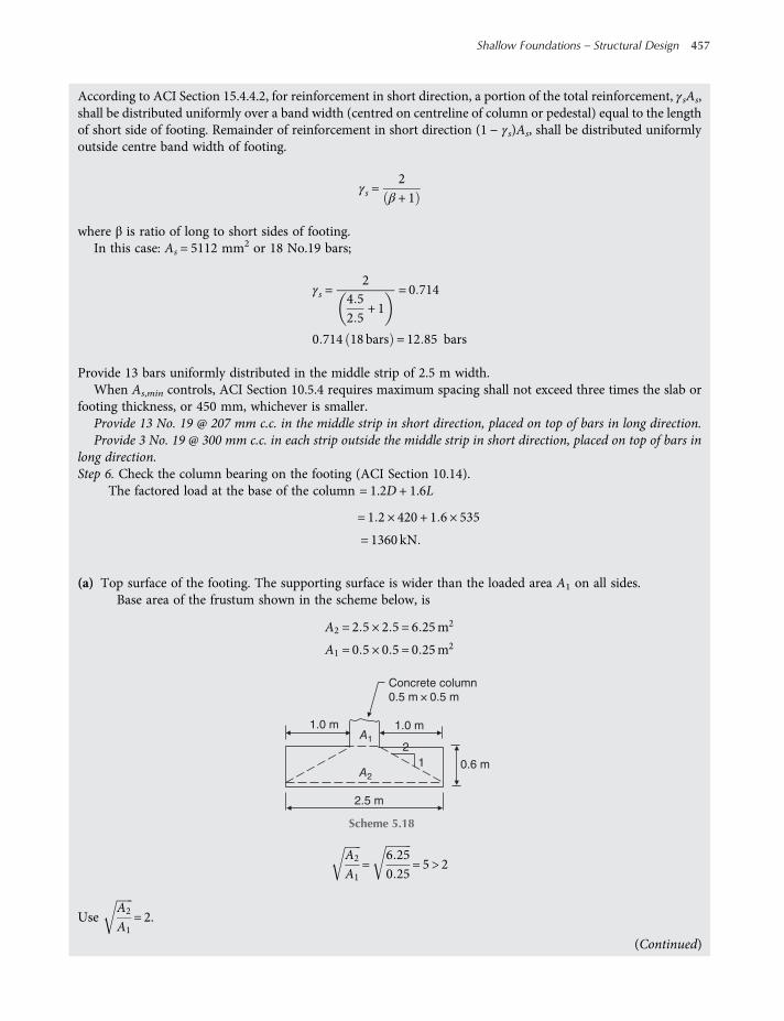
According to ACI Section 15.4.4.2, for reinforcement in short direction, a portion of the total reinforcement, γsAs,shall be distributed uniformly over a band width (centred on centreline of column or pedestal) equal to the lengthof short side of footing. Remainder of reinforcement in short direction (1 − γs)As, shall be distributed uniformlyoutside centre band width of footing.
γs =2
β + 1
where β is ratio of long to short sides of footing.In this case: As = 5112 mm2 or 18 No.19 bars;
γs =2
4 52 5
+ 1= 0 714
0 714 18 bars = 12 85 bars
Provide 13 bars uniformly distributed in the middle strip of 2.5 m width.When As,min controls, ACI Section 10.5.4 requires maximum spacing shall not exceed three times the slab or
footing thickness, or 450 mm, whichever is smaller.Provide 13 No. 19 @ 207 mm c.c. in the middle strip in short direction, placed on top of bars in long direction.Provide 3 No. 19 @ 300 mm c.c. in each strip outside the middle strip in short direction, placed on top of bars in
long direction.Step 6. Check the column bearing on the footing (ACI Section 10.14).
The factored load at the base of the column = 1.2D + 1.6L
= 1 2 × 420 + 1 6 × 535
= 1360 kN
(a) Top surface of the footing. The supporting surface is wider than the loaded area A1 on all sides.Base area of the frustum shown in the scheme below, is
A2 = 2 5 × 2 5 = 6 25m2
A1 = 0 5 × 0 5 = 0 25m2
A2
A1=
6 250 25
= 5 > 2
UseA2
A1= 2.
2A1
A2
1
1.0 m 1.0 m
2.5 m
0.6 m
Concrete column
0.5 m × 0.5 m
Scheme 5.18
(Continued)
Shallow Foundations – Structural Design 457
worksaccounts.com
The maximum bearing load on the top of the footing may be taken as
Ø 0 85fc A1 2 ACI Section 10 14 1
ACI Section 9.3.2.4 gives Ø = 0.65 for bearing. Hence,The maximum bearing factored load = 0.65(0.85)(21)(0.25)(2)
= 5 801MN
= 5801 kN 1360 kN
Therefore, vertical compression reinforcement or dowels through the supporting surface at the interface are the-oretically not required.(b) Base of the column. The allowable bearing strength of the column base at the interface is Ø 0 85fc A1 . Hence,
The allowable bearing factored load = 0 65 0 85 × 28 × 0 25
= 3868MN=3868 kN 1360 kN
Therefore, dowels through the column base at the interface are theoretically not required.It should be realised that the preceding analysis concerns the condition in which the full section at the interface
is under compressive stresses. In other words, no moments are transferred to the section or the eccentricity fallswithin the kern of the section. For the condition in which moments are transferred to the supporting footing orpedestal, usually, compressive stresses will exist over part, but not all, of the section at the interface, which is thesame condition of this Problem. The number of dowels required can be obtained by considering the cross-sectionalarea as an eccentrically loaded column with a maximum compressive concrete stress equal to the smaller of thebearing stresses allowed on the supported member (column, pedestal or wall) or the supporting member (footing).Sufficient reinforcement must cross the interface to provide the necessary axial load and moment capacity.
In general, this requires that all the column bars or dowels of the same steel area must cross the interface. Theselongitudinal bars or dowels should satisfy ACI Sections 15.8.1.3, 12.17 and 15.8.2.3. Also, the minimum embed-ment length of these bars in the footing should not be smaller than the compression development length ldc ortension development length ldh, whichever is greater.Step 7.Design dowels to satisfy the requirements of moment transfer and the minimum reinforcement area across
interface (ACI Section 15.8.2.1).Assume using dowels of the same number and size of the column bars. Hence, use eight No. 19 dowels.
As,min = 0 005Ag = 0 005 × 0 52 = 1 25−3m2 = 1250mm2
As,provided = 8 × 284 = 2272mm2 >As,min OK
Provide eight No.19 dowels (fy = 420 MPa).
Step 8. Find the embedment length of dowels in both the footing and the column.(a) Embedment length of dowels in the footing.
According to ACI Sections 15.8.2.3 and 12.3.2:
ldc =0 24fydbλ fc
or ldc = 0 043fy db,
whichever is the larger
458 Shallow Foundations
worksaccounts.com
ldc =0 24 420 19 1
1 21= 420mmor
ldc =0 043 × 10−6
10−6420 19 1 = 345mm
ldc,min = 200mm ACI Section 12 3 1
Therefore, the required ldc = 420 mm < d = 470 mmAccording to ACI Sections 12.5.1 and 12.5.2:
ldh =0 24fydbλ fc
or 8db or 150mm ,
which ever is the larger.Therefore, it is clear that the minimum embedment length of dowels in the footing is 420 mm.The dowel bars will be extended down to the level of the main footing steel and hooked 90 (ACI standard 90
hook). The hooks will be tied (wired) to the main steel to hold the dowels in place.Use the embedment length of dowels in the footing 450 mm.
(b) Embedment length of dowels in the column.According to ACI Sections 15.8.2.3, 12.3.2 and 12.16.1:
ldc =0 24fydbλ fc
or ldc = 0 043fy db,
whichever is the larger
ldc =0 24 420 19 1
1 28= 364mm or
ldc = 0 043 × 420 × 19 1 = 345mm
ldc,min = 200mm ACI Section 12 3 1
Therefore, the required ldc = 364 mmFor fy ≤ 420 MPa and fc ≥ 21MPa: compression lap splice length shall be 0.071 fydb, but not less than 300 mm.
Lap splice length = 0.071 × 420 × 19.1 = 570 mm > 364 mm.According to ACI Sections 12.17.2.2 and 12.15:Minimum length of lap for tension lap splices shall be for class B splice, but not less than 300 mm.
Class B-splice length = 1 3 ld = 1 3fy ψ t ψ e
2 1 λ fcdb
where the factors ψ t, ψ e and λ are 1. (ACI Sections 12.2.4 and 8.6.1)
1 3 ld = 1 3420 × 1 × 1
2 1 × 1 28
19 11000
= 0 94m= 940mm> 570 mm
Use the embedment length of dowels in the column = 1000 mm.
(Continued)
Shallow Foundations – Structural Design 459
worksaccounts.com

Step 9. Develop the final design sketch as shown in the scheme below.
Problem 5.5
Given: Same data as that of Problem 5.4 except we have the same moment about both axes, the load H = 0, andinstead the given net qa the following geotechnical data is available:
• Angle of internal friction Ø = 0
• Undrained shear strength su = 100 kPa
• Depth of foundation Df = 1m
• Unit weight of soil γ = 17.5 kN/m3
Required: Design the footing using uniform soil pressure distribution as suggested by Bowles (2001). Assume bear-ing capacity failure controls the design soil pressure. Use Hansen’s bearing capacity equation with SF = 3.
Solution:Step 1. Determine the design net qa using the Hansen’s bearing capacity equation.
We realise that with equal moments about both axes the optimum footing shape will be square with ex = ey,L = B and L = B .
Table 4.2 gross qult = 5 14 su 1 + sc + dc + q Ø =0
Equation (4.3): net qult = gross qult −σoσo = q= γ Df
net qult = 5 14 su 1 + sc + dc
3 No. 19
@ 300
mm c. c.
3 No. 19
@ 300
mm c. c.
13 No. 19
@ 207
mm c. c.
910 mm 910 mm 90
mm
90
mm L = 4500 mm
1000 mm
600
mm
15 No. 22 @ 166 mm c. c.
8 No. 19 dowels
500 mm – square column
8 No. 19
119 mm
2.5 m × 4.5 m footing
2500 mm
PM
Scheme 5.19
Foundation soil
Footing
Column
P My
Mx
Df
xh
Scheme 5.20
460 Shallow Foundations
worksaccounts.com
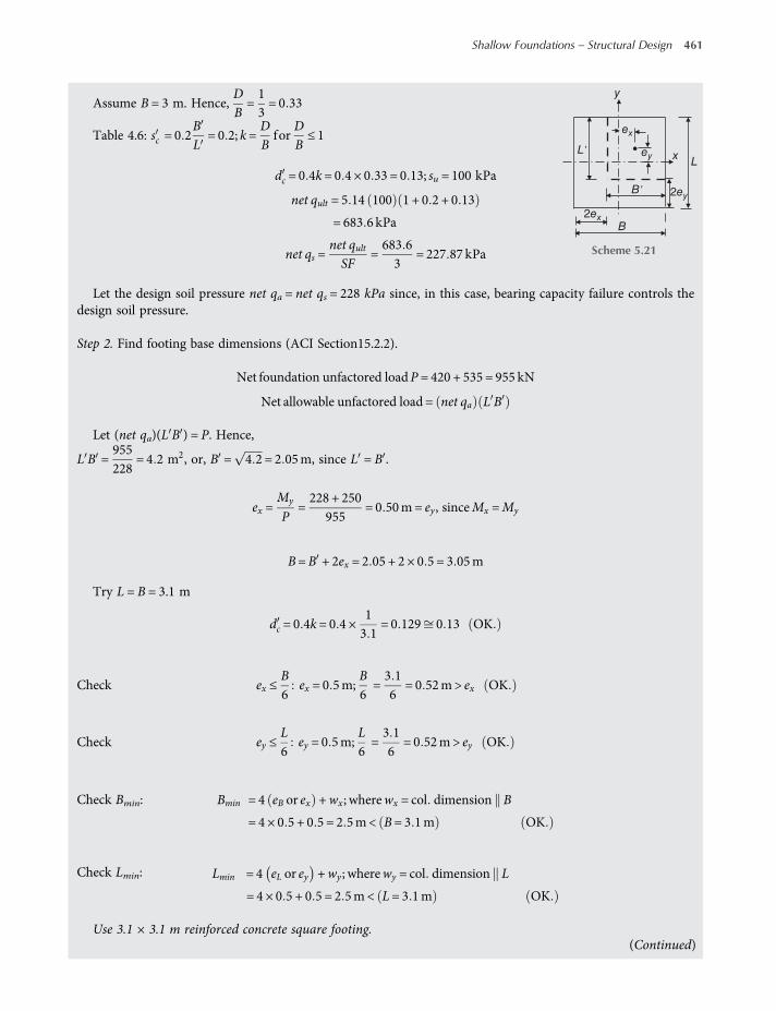
Assume B = 3 m. Hence,DB=13= 0 33
Table 4.6: sc = 0 2BL
= 0 2; k=DBfor
DB≤ 1
dc = 0 4k= 0 4 × 0 33 = 0 13; su = 100 kPa
net qult = 5 14 100 1 + 0 2 + 0 13
= 683 6 kPa
net qs =net qultSF
=683 63
= 227 87 kPa
Let the design soil pressure net qa = net qs = 228 kPa since, in this case, bearing capacity failure controls thedesign soil pressure.
Step 2. Find footing base dimensions (ACI Section15.2.2).
Net foundation unfactored loadP = 420 + 535 = 955 kN
Net allowable unfactored load = net qa L B
Let (net qa)(L B ) = P. Hence,
L B =955228
= 4 2 m2, or, B = 4 2 = 2 05m, since L = B .
ex =My
P=228 + 250
955= 0 50m= ey , sinceMx =My
B=B + 2ex = 2 05 + 2 × 0 5 = 3 05m
Try L = B = 3.1 m
dc = 0 4k= 0 4 ×13 1
= 0 129 0 13 OK
Check ex ≤B6
ex = 0 5m;B6=3 16
= 0 52m> ex OK
Check ey ≤L6
ey = 0 5m;L6=3 16
= 0 52m> ey OK
Check Bmin: Bmin = 4 eB or ex +wx ; wherewx = col dimension B
= 4 × 0 5 + 0 5 = 2 5m< B= 3 1m OK
Check Lmin: Lmin = 4 eL or ey +wy ; wherewy = col dimension L
= 4 × 0 5 + 0 5 = 2 5m< L= 3 1m OK
Use 3.1 × 3.1 m reinforced concrete square footing.
2ey
2exB
B'
L'
y
Lxey
ex
Scheme 5.21
(Continued)
Shallow Foundations – Structural Design 461
worksaccounts.com

Step 3. Compute the design factored net loads, moments and soil pressures.
FactoredP = Pult = 1 2 × 420 + 1 6 × 535 = 1360 kN
FactoredMx =Mx,ult = 1 2 228 + 1 6 250 = 673 6 kN m
Factored My =My, ult = 1 2 228 + 1 6 250 = 673 6 kN m
ex = ey =673 61360
0 50m<3 16
= 0 52m OK
B = L = 3 1−2 × 0 5 = 2 1m
Factorednet q=PultB L
=1360
2 1 × 2 1= 308 4 kPa
Step 4. Draw the factored soil pressure diagram and locate the necessary critical sections.
Step 5. Find footing thickness h.Since the footing is eccentrically loaded, the required thickness shall be based on both one-way shear and
two-way shear analyses. The critical sections for shear are shown on the scheme of Step 4.(a) Consider one-way shear: The critical section for one-way shear is located at distance d from face of the column.
Vu = B 1 3−d net qfactored = 1 1 3−d 308 4
= 400 92−308 4 d kN m
Equation (5.19):
ØVc ≥Vu taking reinforcement shear strength,Vs = 0
whereØ = strength reduction factor ACI Section 9 3 2 3
= 0 75for shear
Critical section
for two-way shear
Critical section
for moment
Critical section
for one-way shear
308.4 kPa
308.4 kPa 308.4 kPa
y
B = L
= 3
.1 m
1.3–d
d
d/2
d/2
B' = L
' = 2
.1 m
x
Scheme 5.22
462 Shallow Foundations
worksaccounts.com

Equation (5.20): Vc = 0 17λ fc bwd
Let ØVc =Vu
0 75 × 0 17 × 1 21 1000 1 d = 400 92−308 4 d
d =400 92892 7
= 0 45m= 450mm
(b) Consider two-way shear:
Vu = Pult −soil reaction on the shear block
= 1360−soil reaction on the shear block kN
The shear strength of concrete Vc shall be the smallest of (a), (b) and (c):
(a) Vc = 0 17 1 +2β
λ fc bod
= 0 17 1 +21
1 fc bod = 0 51 fc bod
Equation 5 22
(b) Vc = 0 083αsdbo
+ 2 λ fc bod
= 0 08340dbo
+ 2 1 fc bod = 0 08340dbo
+ 2 fc bod
Equation 5 23
(c) Vc = 0 33 λ fc bod
= 0 33 1 fc bod = 0 33 fc bodEquation 5 24
Use Vc = 0 33 fc bod. Calculate d, then check Vc of Equation (5.23).Assume d = 0.45 m
ØVc = 0 75 0 33 21 1000 4 0 5 + 0 45 0 45 = 1939 5 kN
ØVc >Vu. Therefore, one-way shear controls.Check Vc of Equation (5.23):
Vc = 0 08340 × 0 45
4 0 5 + 0 45+ 2 fc bod = 0 56 fc bod
Vc = 0 33 fc bod < 0 568 fc bod OK
Use d = 0.45 m = 450 mm.
The distance d will be taken to the intersection of the steel bars running each way at bottom of the footing.Assume using No. 22 bars; hence, depth of footing above reinforcement = (450 − 22.2) mm > 150 mm min-
imum required (ACI Section 15.7).Minimum concrete cover for reinforcement (ACI Section 7.7.1) = 75mmHence, the overall footing thickness is
h= 450 + 75 + 22 2 = 275 + 19 1 = 547 2mm(Continued)
Shallow Foundations – Structural Design 463
worksaccounts.com
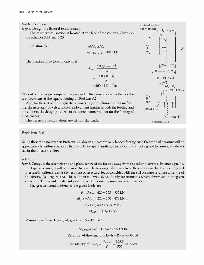
Use h = 550 mm.Step 6. Design the flexural reinforcement.
The most critical section is located at the face of the column, shown inthe schemes 5.22 and 5.23.
Equation (5.9): ØMn ≥Mu
net qfactored = 308 4 kN
The maximum factored moment is
Mu =net qfactored × l2
2
=308 4 1 3 2
2= 260 6 kN m m
The rest of the design computations proceed in the samemanner as that for thereinforcement of the square footing of Problem 5.2.
Also, for the rest of the design steps concerning the column bearing on foot-ing, the necessary dowels and their embedment lengths in both the footing andthe column, the design proceeds in the same manner as that for the footing ofProblem 5.4.
The necessary computations are left for the reader.
Problem 5.6
Using thesame data given in Problem 5.4, design an eccentrically loaded footing such that the soil pressure will beapproximately uniform. Assume there will be no space limitation in layout of the footing and the moments alwaysact in the directions shown.
Solution:Step 1. Compute theeccentricity e and place centre of the footing away from the column centre a distance equals e.
If space permits, it will be possible to place the footing centre away from the column so that the resulting soilpressure is uniform, that is the resultant of structural loads coincides with the soil pressure resultant at centre ofthe footing (see Figure 5.6). This solution is obviously valid only for moments which always act in the givendirection. This is not a valid solution for wind moments, since reversals can occur.
The greatest combinations of the given loads are
P =D+ L= 420 + 535 = 955 kN
My,D +My,L = 228 + 250 = 478 kN m
HD +HL = 42 + 53 = 95 kN
My,H = h HD +HL
Assume h = 0.5 m. Hence, My,H = 95 × 0.5 = 47.5 kN. m
My, total = 478 + 47 5 = 525 5 kN m
Resultant of the structural loads =R= P = 955 kN
Eccentricity of P = ex =My, total
P=525 5955
= 0 55m
B = L = 3.1 m
1.3 m
308.4 kPa
L' =
2.1
m
B' = 2.1 m
= 673.6 kN. m
P = 1360 kN
R = 1360 kN
0.5
5 m
Critical section
for moment y
x
Mx= My
Scheme 5.23
464 Shallow Foundations
worksaccounts.com

Place the column centre at 0.55 m to the left of the footing centre; thus, the resultant of structural loads coincideswith the soil pressure resultant at centre of the footing, as shown below:
Step 2. Find footing base dimensions (ACI Section 15.2.2).Since the soil pressure is uniformly distributed, a square footing may be used.
Let net q= net qa
A=R
net qa=955150
= 6 4m2. Hence, B = L= 6 4 = 2 53m
Use 2.6 × 2.6 m square footing.
Step 3. Compute the design factored net load, moment and soil pressure.
Factored P = Pult = 1 2 × 420 + 1 6 × 535 = 1360 kN
Factored My =My,ult = 1 2 228 + 42 × 0 5 + 1 6 250 + 53 × 0 5
= 298 8 + 442 4 = 741 2 kN m
Factorednet q=PultBL
=1360
2 6 × 2 6= 201 2 kPa
Check the eccentricity of the factored P:
ex =Factored My
Factored P=741 21360
= 0 545m 0 55m OK
Step 4. Find footing thickness h.
Centroid
P = 955 kN
My,total = 525.5 kN. m
ex = 0.55 m
R = P
R = P
x
net q =AR
=
Scheme 5.24
Pult= 1360 kN
My,ult = 741.2 kN.m
Footing
Column
h
1.30 m
Long sideShort side
1.6
Critical section
for moment
(steel in x direction)
y
d
x
R = P = 1360 kN
Critical section for moment
(steel in y direction)R = P = 1360 kN
201.2 kPa
0.55
0.50
0.5
0
0.50
1.0
5 m
2.60 m
2.6
0 m 0.3
1.60 m
1.30 m
Critical section
for one way shear
ex= 0.55 m
Scheme 5.25 (Continued)
Shallow Foundations – Structural Design 465
worksaccounts.com
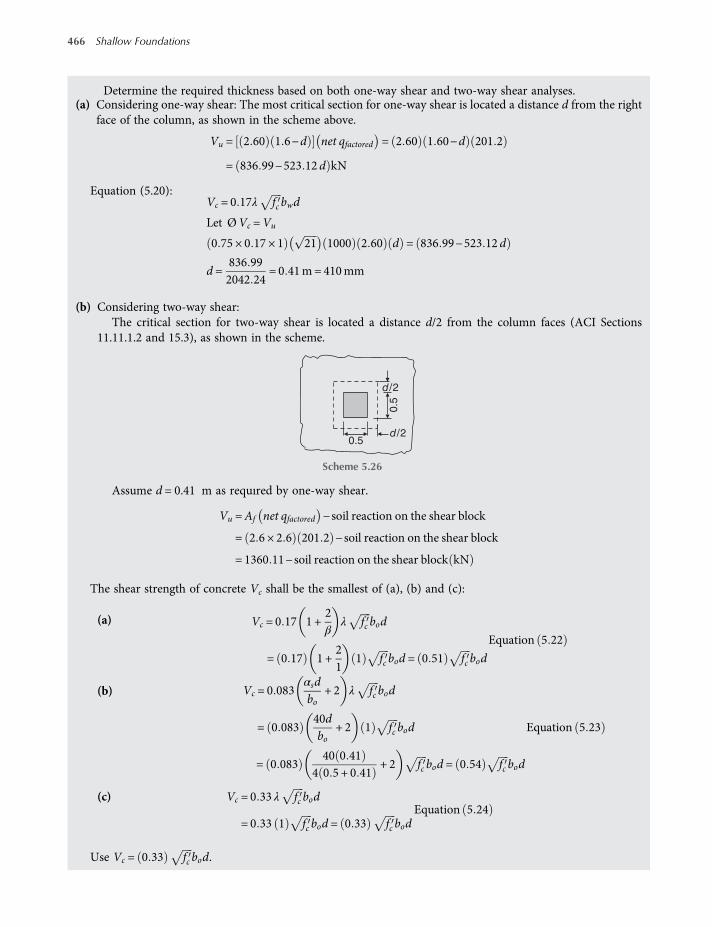
Determine the required thickness based on both one-way shear and two-way shear analyses.(a) Considering one-way shear: The most critical section for one-way shear is located a distance d from the right
face of the column, as shown in the scheme above.
Vu = 2 60 1 6−d net qfactored = 2 60 1 60−d 201 2
= 836 99−523 12 d kN
Equation (5.20):Vc = 0 17λ fc bwd
Let ØVc =Vu
0 75 × 0 17 × 1 21 1000 2 60 d = 836 99−523 12 d
d =836 992042 24
= 0 41m= 410mm
(b) Considering two-way shear:The critical section for two-way shear is located a distance d/2 from the column faces (ACI Sections
11.11.1.2 and 15.3), as shown in the scheme.
Assume d = 0.41 m as requıred by one-way shear.
Vu =Af net qfactored −soil reaction on the shear block
= 2 6 × 2 6 201 2 −soil reaction on the shear block
= 1360 11−soil reaction on the shear block kN
The shear strength of concrete Vc shall be the smallest of (a), (b) and (c):
(a) Vc = 0 17 1 +2β
λ fc bod
= 0 17 1 +21
1 fc bod = 0 51 fc bod
Equation 5 22
(b) Vc = 0 083αsdbo
+ 2 λ fc bod
= 0 08340dbo
+ 2 1 fc bod
= 0 08340 0 41
4 0 5 + 0 41+ 2 fc bod = 0 54 fc bod
Equation 5 23
(c) Vc = 0 33 λ fc bod
= 0 33 1 fc bod = 0 33 fc bodEquation 5 24
Use Vc = 0 33 fc bod.
d/2
d/20.5
0.5
Scheme 5.26
466 Shallow Foundations
worksaccounts.com
ØVc = 0 75 0 33 21 1000 4 0 5 + 0 41 0 41
= 1692 7 kN>Vu
Therefore one-way shear controls.Use d = 0.41 m = 410 mm.This depth d will be taken to the centre of the steel bars in the x-direction.Using No. 22 bars with 75 mm concrete cover (ACI Section 7.7.1), the overall footing thickness is
h= 410 + 75 + 11 1 = 875 + 12 7 = 496 1mm
Use h = 500 mm.
Step 5. Design the flexural reinforcement.(a) Reinforcement in the x-direction. The critical section is shown in the scheme 5.25.
Equation (5.9):
ØMn ≥Mu
The maximum factored moment is
Mu =net qfactored l 2
2=201 2 × 1 62
2= 258 kN m m
Assume tension-controlled section, Ø = 0.9, and fs = fy.
a=Asfy
0 85 fc b=
As × 4200 85 × 21 × 1
= 23 53As
ØMn = Ø Asfy d−a2
= 0 9 As × 420 × 1000 0 41−23 53As
2
= 154980As−4447170As2
Equation 5 11
Let ØMn =Mu
154980As−4447170As2 = 258
4447170As2−154980As + 258 = 0
As =− −154 980 ± −154 980 2− 4 4 447 170 258
2 × 4 447 170=154980−139389
8894340= 1753 × 10−6 m2 m= 1753mm2 m
As,min = 0 0018 bh= 0 0018 × 1 × 0 5 = 0 9 × 10⁻³ m2 m
= 900mm2 m<As required by analysis
Try five No.22 bars: As,provided = 5 × 387 = 1935 mm2/m > As (OK.)Compute a for As = 1935 mm2/m and check if fs = fy and whether the section is tension-controlled:
a= 23 53As = 23 53 × 1935 × 10−6 = 0 0455m= 45 5mm(Continued)
Shallow Foundations – Structural Design 467
worksaccounts.com

c=aβ1; For fc between 17 and 28 MPa, β1 shall be taken as 0.85
c=45 50 85
= 53 53mm
dt = d = 410mm
εt = 0 003dt −cc
= 0 003410−53 53
53 53= 0 020 > 0 005
Equation 5 15
Hence, the section is tension-controlled, and Ø = 0.9 (ACI Sections 10.3.4 and 9.3.2.1).
εy =fyEs
=420
200000= 0 0021
Hence, εt > εy and fs = fy.Therefore the assumptions made are satisfied.Total number of bars required in the x-direction = 2.6 × 5 = 13Using 75 mm minimum concrete cover at each side, centre to centre bar spacing will be 202 mm. Check con-
crete cover provided at each side:
2600− 12 × 202 + 22 22
= 76 9mm> 75 mm OK
In case the required flexural reinforcement exceeds the minimum flexural reinforcement, it shall be adequate touse the same maximum spacing of reinforcement for slabs which is two times the slab thickness, or 450 mm,whichever is smaller, as specified by ACI Section 13.3.2.
Try 13 No.22 bars @ 202 mm c.c. in the x -direction at bottom of the footing.Check the development of reinforcement:In this case, the bars are in tension, the provided bar size is larger than No.19, the clear spacing of the bars
exceeds 2db, and the clear cover exceeds db. Therefore, the development length ld of bars at each side of the criticalsection (which is the same critical section for moment) shall be determined from the following equation, but notless than 300 mm:
ld =fy ψ t ψ e
1 7 λ fcdb ACI Sections 12 2 1, 12 2 2 and 12 2 4
where the factors ψ t, ψ e and λ are 1. (ACI Sections 12.2.4 and 8.6.1)
ld =420 × 1 × 1
1 7 × 1 × 21
22 21000
= 1 2m= 1200mm> ld,min = 300mm
Therefore, the required ld = 1200 mmThe smaller bar extension past the critical section (i.e. the available length) is
1000mm−75mmcover = 925mm< 1200mm NotOK
468 Shallow Foundations
worksaccounts.com
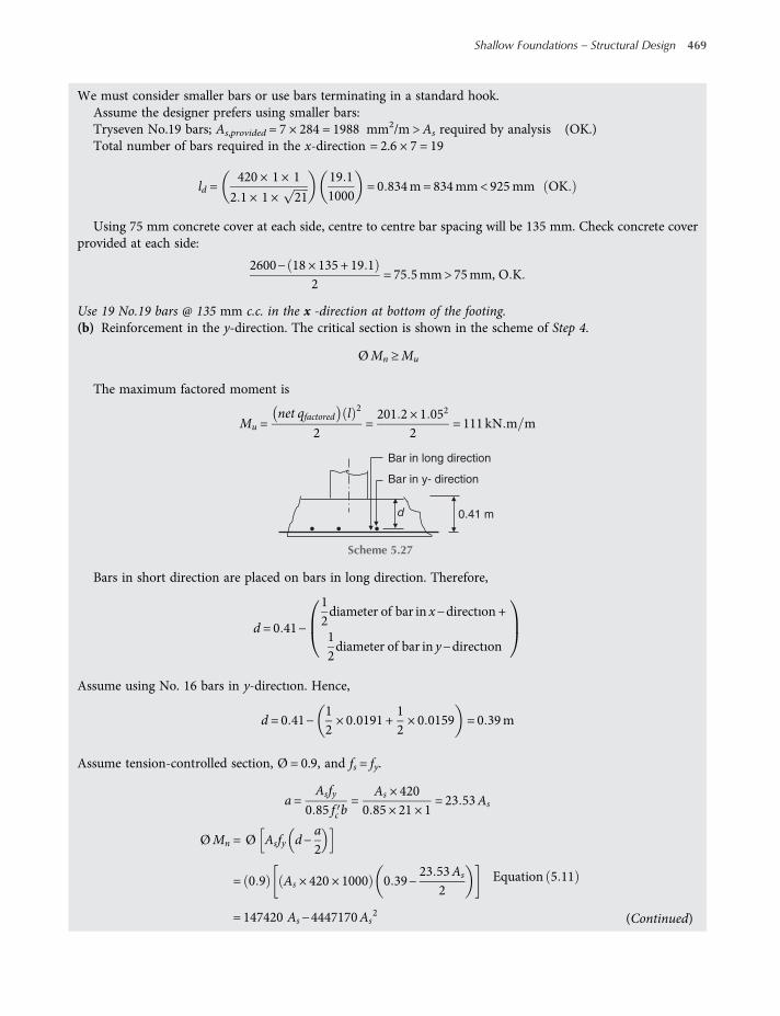
We must consider smaller bars or use bars terminating in a standard hook.Assume the designer prefers using smaller bars:Tryseven No.19 bars; As,provided = 7 × 284 = 1988 mm2/m > As required by analysis (OK.)Total number of bars required in the x-direction = 2.6 × 7 = 19
ld =420 × 1 × 1
2 1 × 1 × 21
19 11000
= 0 834m= 834mm< 925mm OK
Using 75 mm concrete cover at each side, centre to centre bar spacing will be 135 mm. Check concrete coverprovided at each side:
2600− 18 × 135 + 19 12
= 75 5mm> 75mm, O K
Use 19 No.19 bars @ 135 mm c.c. in the x -direction at bottom of the footing.(b) Reinforcement in the y-direction. The critical section is shown in the scheme of Step 4.
ØMn ≥Mu
The maximum factored moment is
Mu =net qfactored l 2
2=201 2 × 1 052
2= 111 kN m m
Bars in short direction are placed on bars in long direction. Therefore,
d = 0 41−
12diameter of bar in x−directıon +
12diameter of bar in y−directıon
Assume using No. 16 bars in y-directıon. Hence,
d = 0 41−12× 0 0191 +
12× 0 0159 = 0 39m
Assume tension-controlled section, Ø = 0.9, and fs = fy.
a=Asfy
0 85 fc b=
As × 4200 85 × 21 × 1
= 23 53As
ØMn = Ø Asfy d−a2
= 0 9 As × 420 × 1000 0 39−23 53As
2
= 147420 As−4447170As2
Equation 5 11
0.41 m
Bar in y- direction
d
Bar in long direction
Scheme 5.27
(Continued)
Shallow Foundations – Structural Design 469
worksaccounts.com

Let ØMn =Mu
147420As−4447170As2 = 111
4447170As2−147420 + 111 = 0
As =− −147 420 ± −147 420 2− 4 4 447 170 111
2 × 4447170=147420−140563
8 894 340
= 771 × 10−6 m2 m= 771mm2 m
As,min = 0 0018 bh= 0 0018 × 1 × 0 5 = 0 9 × 10⁻³ m2
= 900mm2 m>As required by analysis
Therefore, use As = As,min = 900 mm2/mTry five No.16 bars; As,provided = 5 × 199 = 995 mm2/m > As (OK.)The assumptions made are satisfied, since As required = As,min.Total number of bars required in the y -direction = 2.6 × 5 = 13.It may be more appropriate to place eight bars (about 60% of the total bars) within the half of the footing area
that contains the column and the other five bars in the other half, uniformly distributed.Check the development of reinforcement:In this case, the bars are in tension, the provided bar size is smaller than No. 19, the clear spacing of the bars
exceeds 2db, and the clear cover exceeds db. Therefore, the development length ld of bars at each side of the criticalsection (which is the same critical section for moment) shall be determined from the following equation, but notless than 300 mm:
ld =fy ψ t ψ e
2 1 λ fcdb ACI Sections 12 2 1, 12 2 2 and 12 2 4
where the factors ψ t, ψ e and λ are 1. (ACI Sections 12.2.4 and 8.6.1)
ld =420 × 1 × 1
2 1 × 1 × 21
15 91000
= 0 694m= 694mm> ld,min = 300mm
Therefore, the required ld = 694 mmThe bar extension past the critical section (i.e. the available length) is
1050mm−75mmcover = 975mm>694 mm OK
When As,min controls, ACI Section 10.5.4 requires maximum spacing shall not exceed three times the slab orfooting thickness, or 450 mm, whichever is smaller.
Using 75 mm minimum concrete cover at each side, the reinforcement distribution and centre to centre barspacing shall be as follow:
Provide eight No.16 bars @ 173mm c.c.in the half of the footing area that contains the column, placed on top ofbars in x-direction.
Provide five No.13 bars @ 243 mm c.c. in the other half of the footing area, placed on top of bars in x-direction.Step 6. Check the column bearing on the footing (ACI Section 10.14).
For this step and the other design steps concerning the necessary dowels and their embedment lengths inboth the footing and the column, the design proceeds in the same manner as that for the footing of Problem 5.4.The necessary computations are left for the reader.
470 Shallow Foundations
worksaccounts.com

Problem 5.7
The bearing walls of a one-story industrial building will be built of concrete block 200 × 300 × 400 mm. Design awall footing for the following data:
Wall loads including wall floor and roof contribution D= 70 kN m
L= 30 kN m
D+ L= 100 kN m
Wall thickness = 300mm
Footing fc = 21MPa fy = 420 MPa Esteel = 2 × 10⁵ MPa
Foundation soil net qa = 150 kPa
Solution:Step 1. Find the footıng width and the factored net soil pressure.
Neglect any weight increase from displacing the lighter soil with heavier concrete, since it is usually too smallfor lightly loaded footings.
Footing width =B= area per meter length of wall =wall loadnet qa
B=100150
= 0 67m
Let the footing projects 200 mm on each side of the wall to facilitate placing the foundation wall.Use B = 0.7 m = 700 mm.
Factored net soil pressure = net qfactored =factored net load
area=1 2D+ 1 6L
area
=1 2 × 70 + 1 6 × 30
0 7 × 1= 188 6 kPa
Step 2. Find footing thickness h.One-way shear only is significant in wall footings. Critical section for one-way shear is located a distance d
from face of the wall (ACI Sections 11.11.1.1 and 11.1.3.1). However, in this case, the critical section may fall outthe footing projection, and to account for the most severe condition, we consider the section located at face ofthe wall, as shown in the scheme below.
Vu = 1 × 0 2 net qfactored = 1 × 0 2 188 6 = 37 72 kN m
Equation (5.19): ØVc ≥Vu taking reinforcement shear strength,Vs = 0
where Ø = strength reduction factor ACI Section 9 3 2 3
= 0 75 for shear
(Continued)
Shallow Foundations – Structural Design 471
worksaccounts.com

Equation(5.20): Vc = 0 17λ fc bwd
Let ØVc =Vu
0 75 × 0 17 × 1 21 1000 1 d = 37 72
d =37 72584 28
= 0 065m= 65mm
dmin = 150mm
ACI Section 15 7
Choose arbitrarily d = 250 mm.The depth d will be taken to the centre of the transverse steel bars.
Minimum concrete cover = 75mm ACI Section 7 7 1
Assume using No.13 bars. Hence, the overall footing thickness is
h= 250 + 75 + 6 4 = 331 4mm
Use h = 350 mm.
Step 3. Design the flexural reinforcement.The critical section for transverse bending is shown in the scheme of Step 2.Equation (5.9): ØMn ≥Mu
The maximum factored moment is
Mu =net qfactored l 2
2=188 6 × 0 282
2= 7 4 kN m m
Assume tension-controlled section, Ø = 0.9, and fs = fy
a=Asfy
0 85fc b=
As × 4200 85 × 21 × 1
= 23 53As
ØMn = Ø Asfy d−a2
= 0 9 As × 420 × 1000 0 25−23 53As
2
= 94 500 As−4 447170 As2
Equation 5 11
0.2 m0.2 m 0.3 m
B = 0.7 m
0.28 m
Critical section
for moment
(ACI Section 15.4.2)
Critical section for
one way shear
(arbirarily located)Wall
Footing
Scheme 5.28
472 Shallow Foundations
worksaccounts.com
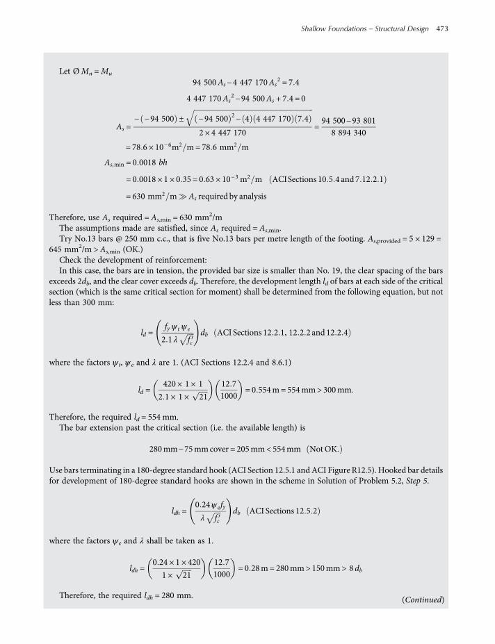
Let ØMn =Mu
94 500As−4 447 170As2 = 7 4
4 447 170As2−94 500As + 7 4 = 0
As =− −94 500 ± −94 500 2− 4 4 447 170 7 4
2 × 4 447 170=94 500−93 801
8 894 340
= 78 6 × 10⁻⁶m2 m= 78 6 mm2 m
As,min = 0 0018 bh
= 0 0018 × 1 × 0 35 = 0 63 × 10−3 m2 m
= 630 mm2 m As required by analysis
ACISections 10 5 4 and 7 12 2 1
Therefore, use As required = As,min = 630 mm2/mThe assumptions made are satisfied, since As required = As,min.Try No.13 bars @ 250 mm c.c., that is five No.13 bars per metre length of the footing. As,provided = 5 × 129 =
645 mm2/m > As,min (OK.)Check the development of reinforcement:In this case, the bars are in tension, the provided bar size is smaller than No. 19, the clear spacing of the bars
exceeds 2db, and the clear cover exceeds db. Therefore, the development length ld of bars at each side of the criticalsection (which is the same critical section for moment) shall be determined from the following equation, but notless than 300 mm:
ld =fy ψ t ψ e
2 1 λ fcdb ACI Sections 12 2 1, 12 2 2 and 12 2 4
where the factors ψ t, ψ e and λ are 1. (ACI Sections 12.2.4 and 8.6.1)
ld =420 × 1 × 1
2 1 × 1 × 21
12 71000
= 0 554m= 554mm> 300mm
Therefore, the required ld = 554 mm.The bar extension past the critical section (i.e. the available length) is
280mm−75mmcover = 205mm< 554mm NotOK
Use bars terminating in a 180-degree standard hook (ACI Section 12.5.1 andACI Figure R12.5). Hooked bar detailsfor development of 180-degree standard hooks are shown in the scheme in Solution of Problem 5.2, Step 5.
ldh =0 24ψ efyλ fc
db ACI Sections 12 5 2
where the factors ψ e and λ shall be taken as 1.
ldh =0 24 × 1 × 420
1 × 21
12 71000
= 0 28m= 280mm> 150mm> 8db
Therefore, the required ldh = 280 mm. (Continued)
Shallow Foundations – Structural Design 473
worksaccounts.com

ldh = 280mm> 205mmavailable NotOK
However, ldh can be reduced by the applicable modification factor of ACI Section 12.5.3(a), as follows:
Reduced ldh = 0 7 × ldh = 0 7 × 280 = 196mm<205mm
> 150mm OK
Therefore, the bars shall be terminating in a 180-degree standard hook.Use No.13 bars @ 250 mm c.c. placed transversely at bottom of the footing. The bars must have 180-degree standardhook at each end.
Step 4. Select longitudınal steel based on the minimum shrinkage and temperature reinforcement (ACI Sectıons7.12.1 and 7.12.2.1).
As = 0 0018 bh= 0 0018 × 0 7 × 0 35 = 4 41 × 10−4 m2 = 441mm2
Try seven No. 10 bars: As,provided = 7 × 71 = 497mm2 > 441mm2 OKLongitudinal steel will, in general, be more effective in the top of the footing than in the bottom; it could controlcracks when the foundation settles. According to ACI Section 7.12.2.2, shrinkage and temperature reinforcementshall be spaced not farther apart than five times the slab thickness, nor farther apart than 450 mm. Provide fourNo. 10 bars at top and three No. 10 bars at bottom, which will also provide support for the transverse flexuralreinforcement.
Provide four No.10 bars @ 180 mm c.c. at top of the footing in long direction.Provide three No.10 bars @ 250 mm c.c. at bottom of the footing in long direction as support for the transverse bars.
Step 5. Draw a final design sketch as shown in the scheme below.
Problem 5.8
A 300 mm thick reinforced concrete wall carries a service dead load of 150 kN/m and live load of 185 kN/m. Thewall is reinforced with No. 13 vertical steel bars in two layers parallel with faces of the wall at 350 mm centre tocentre. The supporting soil has gross qa = 240 kPa at the foundation level, which is 1.5 m below the final ground
3 No. 10 bars
@ 250 mm c. c.
180 – degree
standard hook
350 mm
No. 13 bars @
250 mm c. c.
700 mm
80 mm
Footing
4 No. 10 bars @
180 mm c. c.
Concrete block wall
300 mm
Scheme 5.29
474 Shallow Foundations
worksaccounts.com

surface. The soil unit weight is 19 kN/m3. Design the wall footing using fc = 21MPa, fy = 420MPa and Esteel = 2 ×10⁵ MPa.
Solution:Step 1. Find footing width B and the factored net soil pressure.
Equation 4.8b: net q=VA−γwh+Dc γc−γ ≤ net qa
where γwh= uplift water pressure = 0 in this case Hence
net q=VA+Dc γc−γ
Guess a trial value for Dc between 1 and 1.5 times the wall thickness.Assume Dc = 0.4 m
net q=150 + 185
A+ 0 4 24−19 =
335A
+ 2 kPa
net qa = gross qa−σo = 240−19 × 1 5 = 211 5 kPa
Let net q = net qa335A
+ 2 = 211 5
A=335209 5
= 1 6m2
A = B × 1. Hence, B = 1.6 m.Another method to find B is as follows:
Gross foundation load = 150 + 185 + B × 1 24 × 0 4 + 19 × 1 1
= 335 + 30 5 B kN
A=B× 1 =gross foundation load
gross qa=335 + 30 5 B
240
B=335209 5
= 1 6m2
The factored soil pressure is computed without including the weights of footing and backfill material becausethese loads are evenly distributed and thus do not produce shear or moment in the footing.
Foundation factored net load = 1 2 150 + 1 6 × 185 = 476 kN
Factorednet soil pressure = net qfactored =476A
=476
1 6 × 1300 kPa
Step 2. Find footing thickness h. One-way shear only is significant in strip footings.Critical section for one-way shear is located a distance d from face of the wall (ACI Sections 11.11.1.1 and
11.1.3.1), as shown in the scheme below.
(Continued)
Shallow Foundations – Structural Design 475
worksaccounts.com
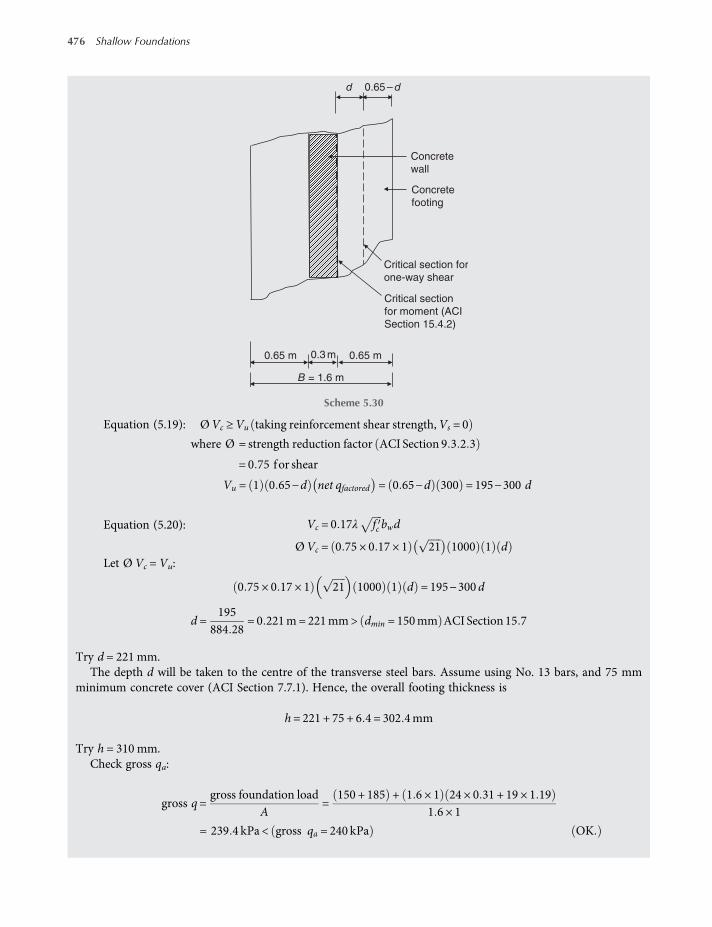
Equation (5.19): ØVc ≥Vu taking reinforcement shear strength,Vs = 0
where Ø = strength reduction factor ACI Section 9 3 2 3
= 0 75 for shear
Vu = 1 0 65−d net qfactored = 0 65−d 300 = 195−300 d
Equation (5.20): Vc = 0 17λ fc bwd
ØVc = 0 75 × 0 17 × 1 21 1000 1 dLet Ø Vc =Vu:
0 75 × 0 17 × 1 21 1000 1 d = 195−300 d
d =195
884 28= 0 221m= 221mm> dmin = 150mm ACI Section 15 7
Try d = 221 mm.The depth d will be taken to the centre of the transverse steel bars. Assume using No. 13 bars, and 75 mm
minimum concrete cover (ACI Section 7.7.1). Hence, the overall footing thickness is
h= 221 + 75 + 6 4 = 302 4mm
Try h = 310 mm.Check gross qa:
gross q=gross foundation load
A=
150 + 185 + 1 6 × 1 24 × 0 31 + 19 × 1 191 6 × 1
= 239 4 kPa < gross qa = 240 kPa OK
0.65 m0.65 m 0.3 m
B = 1.6 m
Critical section
for moment (ACI
Section 15.4.2)
Critical section for
one-way shear
Concrete
wall
Concrete
footing
0.65 – dd
Scheme 5.30
476 Shallow Foundations
worksaccounts.com

Use: d = 221 mmh = 310mm
Step 3. Design the flexural reinforcement.The critical section for transverse bending is shown in the scheme of Step 2.
Equation (5.9): ØMn ≥Mu
Mu =net qfactored l 2
2=300 × 0 652
2= 63 4 kN m m
Equation (5.11): ØMn = Ø Asfy d−a2
Assume tension-controlled section, Ø = 0.9, and fs = fy.
a=Asfy
0 85fc b=
As × 4200 85 × 21 × 1
= 23 53As
ØMn = 0 9 As × 420 × 1000 0 221−23 53As
2
= 83 538As−4 447 170As2
Let ØMn =Mu
83 538As−4 447 170As2 = 63 4
4 447 170As2−83 538As + 63 4 = 0
As =− −83 538 ± −83 538 2− 4 4 447 170 63 4
2 × 4 447 170=83 538−76 490
8 894 340
= 792 × 10−6 m2 m= 792 mm2 m
As,min = 0 0018 bh= 0 0018 × 1 × 0 31 = 5 58 × 10−4 m2
= 558 mm2 m<As required by analysis
In case the required flexural reinforcement exceeds the minimum flexural reinforcement, it shall be adequate touse the samemaximum spacing of reinforcement for slabs which is two times the slab thickness, or 450mmwhich-ever is smaller, as specified by ACI Section 13.3.2.
Try No. 13 @ 160 mm c.c.
As,provided =1000160
× 129 = 806mm2 m >As OK
Compute a for As = 806 mm2/m, and check if fs = fy and whether the section is tension-controlled:
a= 23 53As = 23 53 × 806 × 10−6 = 0 019m= 19mm
(Continued)
Shallow Foundations – Structural Design 477
worksaccounts.com
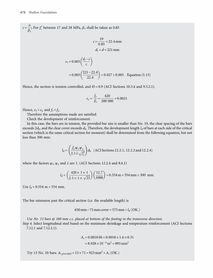
c=aβ1; For fc between 17 and 28 MPa, β1 shall be taken as 0.85
c=190 85
= 22 4mm
dt = d = 221mm
εt = 0 003dt −cc
= 0 003221−22 4
22 4= 0 027 > 0 005 Equation 5 15
Hence, the section is tension-controlled, and Ø = 0.9 (ACI Sections 10.3.4 and 9.3.2.1).
εy =fyEs
=420
200 000= 0 0021
Hence, εt > εy and fs = fy.Therefore the assumptions made are satisfied.Check the development of reinforcement:In this case, the bars are in tension, the provided bar size is smaller than No. 19, the clear spacing of the bars
exceeds 2db, and the clear cover exceeds db. Therefore, the development length ld of bars at each side of the criticalsection (which is the same critical section for moment) shall be determined from the following equation, but notless than 300 mm:
ld =fy ψ t ψ e
2 1 λ fcdb ACI Sections 12 2 1, 12 2 2 and 12 2 4
where the factors ψ t, ψ e and λ are 1. (ACI Sections 12.2.4 and 8.6.1)
ld =420 × 1 × 1
2 1 × 1 × 21
12 71000
= 0 554m= 554mm> 300 mm
Use ld = 0.554 m = 554 mm.
The bar extension past the critical section (i.e. the available length) is
650mm−75mmcover = 575mm> ld OK
Use No. 13 bars @ 160 mm c.c. placed at bottom of the footing in the transverse direction.Step 4. Select longitudinal steel based on the minimum shrinkage and temperature reinforcement (ACI Sectıons
7.12.1 and 7.12.2.1).
As = 0 0018 bh= 0 0018 × 1 6 × 0 31
= 8 928 × 10−4 m2 = 893mm2
Try 13 No. 10 bars: As,provided = 13 × 71 = 923mm2 >As OK
478 Shallow Foundations
worksaccounts.com
Longitudinal steel will, in general, be more effective in the top of the footing than in the bottom; it could controlcracks when the foundatıon settles.
According to ACI Section 7.12.2.2, shrinkage and temperature reinforcement shall be spaced not farther apartthan five times the slab thickness, nor farther apart than 450 mm.
Provide eight No. 10 @ 205 mm c.c. at top of the footing in long direction.Provide five No. 10 @ 360 mm c.c. at bottom of the footing in long direction as support for the transverse bars.
Step 5. Check wall bearing on the footing (ACI Section 10.14).
The factored load at the base of the wall = 1 2D+ 1 6L
= 1 2 × 150 + 1 6 × 185
= 476 kN
(a) Base of the wall. The allowable bearing strength of concrete at the wall base is
Ø 0 85fc A1 = 0 65 0 85 × 21 0 3 × 1
= 3 48MN=3480 kN 1 2D+ 1 6L OK
(b) Top surface of the footing. The design bearing strength on the top surface of the footing shall not exceedØ 0 85fc A1 , except when the supporting surface is wider on all sides than the loaded area; then the design
bearing strength of the loaded area shall be permitted to be multiplied by A2 A1 but not more than 2, (ACISection 10.14.1).
Since both the footing and wall concrete have the same fc , it is clear that the design bearing strength on thetop surface of the footing is also much greater than (1.2D + 1.6L).
Therefore, vertical compression reinforcement or dowels through the supporting surface at the interfaceare theoretically not required. However, ACI Section 15.8.2.2 requires area of reinforcement across interfaceshall be not less than the minimum vertical reinforcement given in ACI Section 14.3.2.
Step 6. Design dowels to satisfy the minimum area of reinforcement across interface required by ACI Sections15.8.2.2 and14.3.2.
ACI Section 14.3.2 states that minimum ratio of vertical reinforcement area to gross concrete area, ρℓ,shall be:
(a) 0.0012 for deformed bars not larger than No. 13 with fy not less than 420 MPa; or(b) 0.0015 for other deformed bars; or(c) 0.0012 for welded wire reinforcement not larger than MW200 or MD200.
Assume using No. 10 dowels with fy = 420MPa. Hence, ρℓ = 0.0012.
As,min = 0 0012 × 1 × 0 3 = 3 6 × 10⁻⁴ m2 m= 360mm2 m
Try No. 10 @ 350 mm c.c. (the same spacing of the wall vertical bars) in two layers parallel with faces of the wall:
As,provided = 21000350
× 71 = 406mm2 m >As,min OK
Provide No. 10 @ 350 mm c.c. in two layers parallel with faces of the wall.
Step 7. Find the embedment length of dowels in both the footing and the wall.For this step, the design proceeds in the same manner as that of Solution of Problem 5.3, Step 6.
Step 8. Develop the final design sketch.
Shallow Foundations – Structural Design 479
worksaccounts.com

Problem 5.9
A metal column with steel base bearing plate is supported by a concrete pedestal rests on a reinforced concretefooting. The pedestal should have shoulder to provide bearing for the floor slab which will be placed 1.5 m abovethe footing, as shown in the scheme below. Design the pedestal and bearing plate for the following given data:
Loads P =D+ L D= 600 kN L= 450 kN
Column: W 310×107 metal (A-36 steel) column; fy = 250 MPaBearing plate: metal (A-36 steel) plate; fy = 250 MPaAnchor bolts: A307-grade A (A-36 steel); fult = 400 MPa; fy = 250 MPaConcrete pedestal: fc = 24MPaSteel bars: fy = 420 MPa; Esteel = 2 × 10⁵ MPa
Solution:Step 1. Find area of the base plate and the cross-section dimensions of the pedestal.
Usually, the cross-sectional area of the pedestal is set for the base plate but increased by at least 50 mm toprovide bearing for the floor slab.
(a) Area of the base plate, A1. Design according to the AISC specifications.
A1 =1A2
P0 35 fc
2
, or, A1 =P
0 7 fc, whichever is greater.
A2 = Surface area of the supporting member
A2 =P
0 175 fc
A2 =P
0 175 fc=
600 + 4500 175 × 24 × 1000
= 0 25m2
A1 =1
0 251050
0 35 × 24 × 1000
2
= 0 0625m2, or,
Metal column
P
Base bearing plate
Anchor bolt100 mm
150 mm-Concrete floor
Concrete pedestal
Reinforced concrete
footing
1.5 m
Foundation soil
Scheme 5.31
480 Shallow Foundations
worksaccounts.com
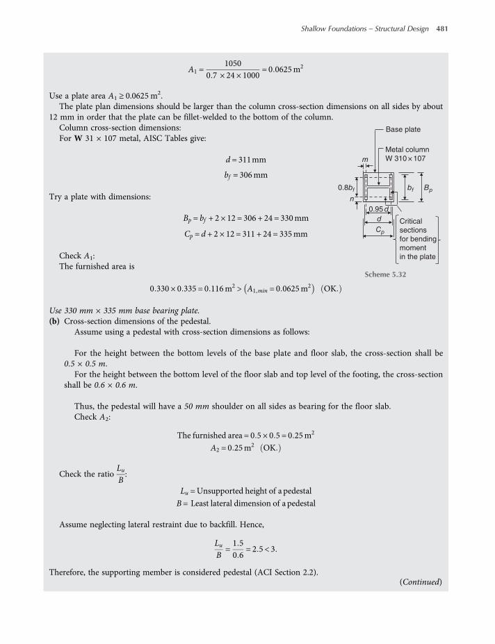
A1 =1050
0 7 × 24 × 1000= 0 0625m2
Use a plate area A1 ≥ 0.0625 m2.The plate plan dimensions should be larger than the column cross-section dimensions on all sides by about
12 mm in order that the plate can be fillet-welded to the bottom of the column.Column cross-section dimensions:For W 31 × 107 metal, AISC Tables give:
d = 311mm
bf = 306mm
Try a plate with dimensions:
Bp = bf + 2 × 12 = 306 + 24 = 330mm
Cp = d + 2 × 12 = 311 + 24 = 335mm
Check A1:The furnished area is
0 330 × 0 335 = 0 116m2 > A1,min = 0 0625m2 OK
Use 330 mm × 335 mm base bearing plate.(b) Cross-section dimensions of the pedestal.
Assume using a pedestal with cross-section dimensions as follows:
For the height between the bottom levels of the base plate and floor slab, the cross-section shall be0.5 × 0.5 m.
For the height between the bottom level of the floor slab and top level of the footing, the cross-sectionshall be 0.6 × 0.6 m.
Thus, the pedestal will have a 50 mm shoulder on all sides as bearing for the floor slab.Check A2:
The furnished area = 0 5 × 0 5 = 0 25m2
A2 = 0 25m2 OK
Check the ratioLuB:
Lu =Unsupported height of a pedestal
B= Least lateral dimension of a pedestal
Assume neglecting lateral restraint due to backfill. Hence,
LuB
=1 50 6
= 2 5 < 3
Therefore, the supporting member is considered pedestal (ACI Section 2.2).
Critical
sections
for bending
moment
in the plate
Base plate
Metal column
W 310 × 107
0.95 d
0.8bf
d
Cp
bf Bp
n
m
Scheme 5.32
(Continued)
Shallow Foundations – Structural Design 481
worksaccounts.com
Step 2. Check plate bearing on pedestal.
Maximum allowable bearing load should be ≤ 0 7 fc A1
≥ D+ L
0 7 fc A1 = 0 7 × 24 × 0 33 × 0 36 = 1 996MN
D+ L= 600 + 450 = 1050 kN
According to AISC, for the case A2 > A1, the maximum allowable bearing load on the top of the pedestal is
0 35 fc A1 A2 A1, on the condition A2 A1 ≤ 2.
A2 A1 = 0 25 0 33 × 0 36 = 1 45 < 2
Maximum allowable bearing load = 0 35 24 0 33 × 0 36 1 45
= 1 447MN=1447 kN
< 0 7 fc A1
> D+ L OK
Step 3. Find the plate thickness tp.Actually, computation of tp is beyond the scope of this text. However, for completeness, we may compute tp
using the AISC specifications.Refer to the scheme of Step 1:
tp = 2 νfpfy
where fy = tensile yield stress of the plate steel
fp = service loadP Bp ×Cp
ν= m or n or λn , whichever is the greatest, mm
m= Cp−0 95 d 2
n= Bp−0 80 bf 2
n = 0 25 d × bf
λ =2 X
1 + 1−Xor 1 0whichever is smaller If X > 1, use λ= 1
X =4PoL2 Fb
UsePo = P andFb = 0 35 fc A2 A1
L= d + bf
L= 311 + 306 = 617mm=0 617m
m=335−0 95 × 311
2= 19 8mm; n=
330−0 80 × 3062
= 42 6mm>m
n = 0 25 311 × 306 = 77 1mm;Fb = 0 35 24 1 45 = 12 18MPa
X =4 × 1050
0 6172 12 18 × 1000= 0 906
482 Shallow Foundations
worksaccounts.com
λ=2 × 0 906
1 + 1−0 906= 1 457 > 1 Hence, use λ = 1
λn = 1 × 77 1 = 77 1mm> n Hence, ν = 77.1 mm
fp =1050
0 330 × 0 335= 9498 kPa = 9 498MPa; fy = 250MPa
tp = 2 77 19 498250
= 30 06mm
Use plate thickness tp = 30 mm.
Step 4. Design pedestal reinforcement.Longitudinal reinforcement:As mentioned in Section 5.6, usually, concrete pedestals are reinforced with minimum column steel of 0.01
Ag but not more than 0.08 Ag (ACI Section 10.9.1) even when they are designed as unreinforced members.The top surface area of the pedestal A2 = 0 25m2 = 250 000mm2
As, min = 0 01Ag = 0 01 × 250 000 = 2500mm2
Try 8 No. 22 bars. As,provided = 8 × 387 = 3096mm2
> As, min
< 0 08Ag OK
Provide eight No. 22 bars.The bars should terminate at about 100 mm below the top surface of the pedestal in order to minimise point
loading on the base plate. The bars should be extended through the pedestal-footing interface into the footing,hooked (90-degree standard hook) and fastened tightly with the footing bottom bars.
Ties:Lateral ties should be at least No. 10 in size (ACI Section 7.10.5.1).Provide No. 10 square-shaped ties.
The longitudinal bar clear spacing =500− 2 × 40 + 2 × 9 5 + 3 × 22 2
2= 167 2mm> 150 mm
Therefore, diamond-shaped ties should be provided also (ACI Section 7.10.5.3). (See the final design sketches ofStep 7).
Vertical spacing of ties shall not exceed 16 longitudinal bar diameters, 48 tie bar or wire diameters, or leastdimension of the compression member (ACI Section 7.10.5.2):
16 longitudinal bar diameters = 16 × 22 2 = 355 2mm
48 tie bar diameters = 48 × 9 5 = 456mm
Least dimension of the compression member = 0 5m= 500mm
Use maximum tie spacing = 355mm(Continued)
Shallow Foundations – Structural Design 483
worksaccounts.com

Place a tie not more than one-half tie spacing above the top of the footing (ACI Section 7.10.5.4). The ties shall belocated vertically as follows:
Locate the first tie at 100 mm below the top of the pedestal (at top end of the longitudinal bars). Locate thesecond tie at 100 mm below the first one. Use 355 mm tie spacing for the rest of the required ties. The lowesttie will be placed at 130 mm above the footing, which is less than one-half tie spacing. With this arrangementthe required number of ties will be 6 square-shaped and 6 diamond-shaped ties.
Step 5. Design anchor bolts.If the structural design loads between the column and the supporting member consist solely of compres-
sion (as in thıs Problem), then theoretically no anchorage will be required. However, anchor bolts are stillrequired to resist erection loads, accidental collisions during erection, and unanticipated shear or tensileloads. The engineer might attempt to estimate these loads and design accordingly, or simply select the boltsusing engineering judgment. For example, an engineer might arbitrarily select enough bolts of specified typeand diameter to carry 10 % of the total compressive load in shear. Assume we consider the latter option asfollows:
Equation (5.26): ØVn ≥Vua
Vua = total factored shear force = 0 1 × factoredP
= 0 1 1 2 × 600 + 1 6 × 450 = 144 kN
ØVn = the lowest of ØVsa, ØVcb and ØVcp ACI SectionD 4 1 2
Ø = strength reduction factor for anchors in concrete
= 0 65 for anchors of ductile steel in shear ACI SectionD 4 4
Since this analysis is based on an arbitrary choice or option and the anchor bolts will be installed in a deep member(the pedestal) relatively far from the edges, the concrete breakout and pryout effects may be neglected.
Assume using A307 bolt material grade A (A-36 steel of fult = 400MPa and fy = 250MPa). From Table 5.1 selecta bolt diameter and pitch equal to 20P2.5. For threaded bolts, ANSI/ASME B1.1 uses the same effective cross-sectional area of a bolt in tension or in shear (see ACI Sections RD.5.1.2 and RD.6.1.2). For the 20P2.5 bolt,Table 5.1 gives At = 245 mm2.
For cast-in headed bolt and hooked bolt anchors (ACI Section D.6.1.2):
ØVsa = Ø n 0 6Ase, V futa
where n is the number of anchors in the group, and futa shall not be taken greater than the smaller of 1.9 fya and860 Mpa.
fya = fy of bolt steel
ØVsa = 0 65 0 6 × 245 × 1 9 × 250 106 n = 0 0454 n
Let ØVsa = ØVn =Vua
0 0454 n = 144 1000
n=14445 4
= 3 17
Provide four 20P2.5 A307 Grade A cast-in headed bolt or hooked bolt anchors.
484 Shallow Foundations
worksaccounts.com

Step 6. Determine the effective embedment depth hef, spacing and edge distances of the anchor bolts.Effective embedment depth hef :The required anchor bolt embedment depth hef is not directly and specifically indicated in most (including
ACI) building codes. We may, however, use the minimum depth of Table 5.2, compression developmentlength ldc (ACI Section 12.3.2) and tension development length ldh (ACI Section 12.5.2), whichever is thegreatest.
Table 5 2 gives minimum effective embedment depth = 12 da
= 12 × 20
= 240 mm
ldc =0 24fydbλ fc
or ldc = 0 043fy db,whichever is the larger
ldc =0 24 250 20
1 21= 262mm, or
ldc =0 043 × 10−6
10−6250 20 = 215mm
ldc,min = 200mm ACI Section 12 3 1
Required ldc = 262mm
ldh =0 24fydbλ fc
or 8 db or 150mm, whichever is the larger.
ldh =0 24 250 20
1 21= 262mm> 8db > 150mm
Required ldh = 262 mmTherefore, use hef = 262 mmAlso, additional lengths due to the plate and nut thicknesses, grout bed, bend and so on are to be specified.
Anchor bolt spacing:
ACI Section D.8.1 requires minimum centre-to-centre spacing of anchors shall be 4da for untorqued cast-inanchors and 6da for torqued cast-in anchors and post-installed anchors.
In this case, it is not exactly clear whether the anchors will be torqued or untorqued. Therefore, it may be betterto use anchor spacing not less than 6da.
Use minimum anchor spacing = 6da = 6 × 20 = 120 mm.Edge distances for anchor bolts:Table 5.2 gives minimum edge distances for A307 (A-36 steel) anchor bolts = 5da or 100 mm, whichever is
greater.ACI Section D.8.2 requires minimum edge distances for cast-in headed anchors that will not be torqued shall be
based on concrete cover for reinforcement specified in ACI Section 7.7. For cast-in headed anchors that will betorqued, the minimum edge distances shall be 6da.
(Continued)
Base plate
hef
Nut
Anchor bolt
Scheme 5.33
Shallow Foundations – Structural Design 485
worksaccounts.com

As mentioned above, here also it may be better to use minimum edge distance not less than 6da, which is largerthan 5da or 100 mm.
Use minimum edge distance = 6da = 6 × 20 = 120 mmIn order to satisfy the above anchor spacing and edge distance requirements, the anchor bolts may be placed in
the pattern shown in the scheme below.
Step 7. Develop the final design sketch.
4-20P2.5 A307 (A36 steel)
cast-in anchor bolt
Concrete pedestal
Base baring plate (A36 steel)
335 × 330 × 30 mm
W 310 × 107 column (A-36 steel)
d = 311 mm; bf = 306 mm
a = 99.5 mm
b = 65.0 mm
500 mm
600 mm
600 m
m
50
a
b
CL
CL
182 136 182 50
50
15
02
00
150
50
Scheme 5.34
W 310 × 107 column
(A-36 steel)
d = 311 mm
bf = 306 mm
Base plate (A36 steel)
335 × 330 × 30 mm
4 - 20P2.5 A307
(A36 steel) cast-
in anchor bolts
100 mm
P
150-mm Concrete floor
Concrete pedestal
500 × 500 mm
R. C. Footing
1.5 m
Foundation soil
130 mm
5 No. 10 square-shaped and
5 No. 10 diamond-shaped
ties @ 355 mm c.c.
+
1 No. 10 square-shaped and
1 No. 10 diamond-shaped
ties @ 100 mm below top of
8 No. 22
6 No. 10
6 No. 10
8 No. 22
500 mm
500 mm
Pedestal
Scheme 5.35
486 Shallow Foundations
worksaccounts.com

Problem 5.10
A rigid pile cap is required to support at its centre an interior metal column of type HP 360 × 174 with660 × 660 mm base plate. The column will carry a service dead load of 1000 kN and live load of 1400 kN. Eachpile working load and diameter should not exceed 300 kN and 400mm, respectively. Top of the cap will be coveredwith 0.15 m compacted fill with a unit weight of 20 kN/m3 and a 0.15 m concrete floor (γc = 24 kN/m3) with auniform live load of 3.75 kPa. Design the pile cap using fc = 28MPa for concrete, fy = 420MPa for reinforcing steeland minimum centre-to-centre pile spacing = two pile diameters but not less than 760 mm.
Solution:Step 1. Determine number of piles required, pile-group pattern, pile spacing and plan dimensions of the pile cap.
Equation (5.30): Pp =Qn
n=QPp
A trial estimate of the cap dimensions may be necessary in order to compute the total load Q. Since the cap will beconcentrically loaded (the column is at centre without moments), it may be appropriate to use a square cap andpile-group pattern.
Try a square cap with dimensions 2.8 × 28 × 0.85 m.
Q= 1000 + 1400 + 2 8 × 2 8 0 85 × 24 + 0 15 × 20 + 0 15 × 24 + 3 75
= 2641 08 kN
n=2641 08300
= 8 8 piles
Use nine piles distributed uniformly in a square pattern.Assume pile diameter = 400 mmMinimum centre to centre pile spacing
= 2 × 400= 800 mm
Use centre-to-centre pile spacing = 1000 mm.Plan dimensions of the pile cap shall be larger than that of its pile-group pattern by at least 200 mm on all sides
(see Section 5.7).Use the cap plan dimensions = 2.8 × 2.8 m.
Step 2. Locate the necessary critical sections according to ACI Sections 15.4, 15.5 and 15.6.AISC Tables give the dimensions for the HP 360 174 as shown in Scheme 5.37.
Step 3. Find cap thickness h.Determine the required thickness based on both two-way shear and one-way shear analyses.
ACI Section 15.5.3 states that where the distance between the axis of any pile and the axis of the column ismore than two times the distance between the top of the pile cap and the top of the pile, the pile cap shall satisfy11.11 and 15.5.4. Other pile caps shall satisfy either Appendix A or 11.11 and 15.5.4.
In this case, we design the cap so that the requirements of ACI Sections 11.11 and 15.5.4 are satisfied and,therefore, Appendix A will not be considered.
(a) Two-way shear.Two-way shear at location of the column:The critical section is located at distance d/2 from a line halfway between the face of the column and the
edge of the base plate (ACI Section 15.5.2), as shown in the scheme 5.37.
1 m
2.8 m
1 m
2.8
m
Cap
0.4 m
0.4
m
Group
perimeter
Scheme 5.36
(Continued)
Shallow Foundations – Structural Design 487
worksaccounts.com
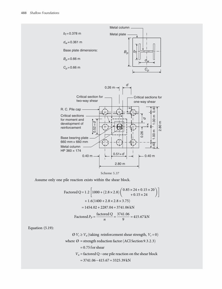
Assume only one pile reaction exists within the shear block.
FactoredQ= 1 2 1000 + 2 8 × 2 80 85 × 24 + 0 15 × 20
+ 0 15 × 24
+ 1 6 1400 + 2 8 × 2 8 × 3 75
= 1454 02 + 2287 04 = 3741 06 kN
FactoredPP =factoredQ
n=3741 06
9= 415 67 kN
Equation (5.19):
ØVc ≥Vu taking reinforcement shear strength, Vs = 0
where Ø = strength reduction factor ACI Section 9 3 2 3
= 0 75 for shear
Vu = factoredQ−one pile reaction on the shear block
= 3741 06−415 67 = 3325 39 kN
bf = 0.378 m
dw= 0.361 m
Base plate dimensions:
Bp= 0.66 m
Cp= 0.66 m
0.2
6
0.51+ d
0.5
2+
dCritical sections for
one-way shear
Critical section for
two-way shear
Critical sections
for moment and
development of
reinforcement
0.4
0
0.4
0 1
.00 m
2.8
0 m
1.0
0 m
2.80 m
Metal column
HP 360 × 174
Base bearing plate
660 mm × 660 mm
0.26 m
0.40 m0.40 m
Metal plate
Metal column
R. C. Pile cap
bfBp
Cp
dw
d
x
d
Scheme 5.37
488 Shallow Foundations
worksaccounts.com

The shear strength of concrete Vc shall be the smallest of (i), (ii) and (iii):
(i)
Vc = 0 17 1 +2β
λ fc bod
= 0 17 1 +21
1 fc bod = 0 51 fc bod
Equation 5 22
(ii)
Vc = 0 083αsdbo
+ 2 λ fc bod
= 0 08340dbo
+ 2 1 fc bod = 0 08340dbo
+ 2 fc bod
Equation 5 23
(iii)Vc = 0 33 λ fc bod
= 0 33 1 fc bod = 0 33 fc bodEquation 5 24
Use Vc = 0 33 fc bod. Calculate d, then check Vc of Equation (5.23).Perimeter of the critical section is 2(0.51 + d + 0.52 + d) m
ØVc = 0 75 0 33 28 1000 2 0 51 + d + 0 52 + d d
= 5239 d 2 + 2698 d kN
Let ØVc = Vu
5239 d 2 + 2698d = 3325 39
5239 d 2 + 2698 d −3325 39 = 0
d =−2698 ± 26982− 4 5239 −3325 39
2 × 5239=−2698 + 8773
10478= 0 58m= 580mm
Check Vc of Equation (5.23):
Vc = 0 08340 × 0 580
2 0 51 + 0 580 + 0 52 + 0 580+ 2 fc bod = 0 606 fc bod
Vc = 0 33 fc bod < 0 606 fc bod OK
Try d = 0.6 m = 600 mm and h = 850 mm.Check whether only one pile reaction exists within the shear block:Face of the nearest pile is located at 0.8 m from the cap centre, whereas, the critical section is at 0.56 m Hence,
there is only one pile reaction located within the shear block area, as assumed. (OK.)Two-way shear around individual piles:Where necessary, shear around individual piles may be investigated in accordance with ACI Sections 11.11.1.2.
In this case, by inspection, it is clear that shear around individual piles is not critical. However, for completeness, itmay be performed as follows:
Check first whether there is any overlapping of critical shear perimeters from the adjacent piles.Since the centre-to-centre pile spacing (i.e. 1000 mm) is not less than two times the radius of shear perimeter
[i.e. 2(300 + 200) = 1000 mm)], there is no overlapping of critical shear perimeters. Therefore, the modified criticalperimeter for shear defined in ACI Section R 15.5.2 and Figure R 15.5 is not applicable.
It will be sufficient to investigate two-way shears around one of the piles only, since the pile cap has a constant dand the piles have the same Pp and diameter.
(Continued)
Shallow Foundations – Structural Design 489
worksaccounts.com
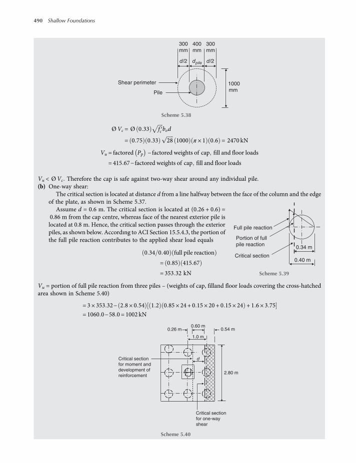
ØVc = Ø 0 33 fc bod
= 0 75 0 33 28 1000 π × 1 0 6 = 2470 kN
Vu = factored Pp − factored weights of cap fill and floor loads
= 415 67− factored weights of cap fill and floor loads
Vu < ØVc Therefore the cap is safe against two-way shear around any individual pile.(b) One-way shear:
The critical section is located at distance d from a line halfway between the face of the column and the edgeof the plate, as shown in Scheme 5.37.
Assume d = 0.6 m. The critical section is located at (0.26 + 0.6) =0.86 m from the cap centre, whereas face of the nearest exterior pile islocated at 0.8 m. Hence, the critical section passes through the exteriorpiles, as shown below. Accordıng to ACI Section 15.5.4.3, the portion ofthe full pile reaction contributes to the applied shear load equals
0 34 0 40 full pile reaction
= 0 85 415 67
= 353 32 kN
Vu = portion of full pile reaction from three piles – (weights of cap, filland floor loads covering the cross-hatchedarea shown in Scheme 5.40)
= 3 × 353 32− 2 8 × 0 54 1 2 0 85 × 24 + 0 15 × 20 + 0 15 × 24 + 1 6 × 3 75
= 1060 0−58 0 = 1002 kN
d/2 d/2dpile
400
mm
300
mm
300
mm
1000
mm
Shear perimeter
Pile
Scheme 5.38
0.40 m
0.34 m
Full pile reaction
Portion of full
pile reaction
Critical section
Scheme 5.39
0.54 m
1.0 m
0.60 m
Critical section
for one-way
shear
2.80 m
d
0.26 m
Critical section
for moment and
development of
reinforcement
Scheme 5.40
490 Shallow Foundations
worksaccounts.com

Equation (5.20):
ØVc = Ø 0 17λ fc bwd
= 0 75 0 17 × 1 28 1000 2 80 0 6
= 1133 kN>Vu
Therefore, the two-way shear controls.Use d = 0.60 m = 600 mm.The depth d will be taken to the intersection of the steel bars running each way at bottom of the cap.Check the cap thickness h:
h= d + one bar diameter say 25mm
+75mmspace between steel bars and top of piles
+ 150mm pile embedment into the cap
= 600 + 25 + 75 + 150 = 850mm OK
Use the cap thickness h = 850 mm.
Step 4. Design the flexural reinforcement.The cap is square and centrically loaded, the pile pattern is symmetrical about both x and y axes and the critical
sections formoment in both directions are approximately located at the same distance (0.260mor 0.255m) fromthe cap centre. Therefore, practically, the same bottom reinforcement will be required for both directions.
Equation (5.9): ØMn ≥Mu
The maximum factored moment is
Mu = 0 74 3 × factoredPP − 0 57 factored W + floor load
= 0 74 3 × 415 67 −
0 571 2 2 8 × 1 14 0 15 × 24 + 0 15 × 20 + 0 85 × 24
+ 1 6 2 8 × 1 14 3 75
= 923− 70 = 853 kN m
Mu Per metre width =8532 8
= 305 kN m m
(Continued)
2.8 m
1.14 m
0.74 m
2.80 m
0.26 m
Critical section
for moment and
development of
reinforcement
0.40 m
Scheme 5.41
Shallow Foundations – Structural Design 491
worksaccounts.com

Assume tension-controlled section, Ø = 0.9, and fs = fy.
a=Asfy
0 85fc b=
As × 4200 85 × 28 × 1
= 17 65As
d = 0 6m
Equation (5.11): ØMn = Ø Asfy d−a2
= 0 9 As × 420 × 1000 0 6−17 65As
2
= 226 800As−3 335 850As2
Let ØMn =Mu 226 800As−3 335 850As2 = 305
3 335 850As2−226 800As + 305 = 0
As =− −226 800 ± −226 800 2− 4 3 335 850 305
2 × 3 335 850=226 800−217 643
6 671 700
= 1 373 × 10−3 m2 m= 1373mm2 m,
required by analysis.In order to provide a more strong and rigid pile cap it may be more appropriate to use As,min as required for
flexural members (ACI Section 10.5.1) rather than As,min based on shrinkage and temperature reinforcement (ACISections 10.5.1 and 7.12.2.1). Accordingly, ACI Section 10.5.1 requires
As,min =0 25 fc
fybwd
=0 25 28
420× 1 × 0 6
= 1 89 × 10−3 m2 m= 1890mm2 m
0.15 m concrete
floor
0.15 m fill
0.6
0m
0.8
5 m
0.2
5
3.75 kPa
0.57 m
W = weights of cap + floor + fill
Pp
MnVc
1.14 m
W
Scheme 5.42
492 Shallow Foundations
worksaccounts.com

and not less than 1.4
bw dfy
=1 4 × 1 × 0 6
420
= 2 × 10⁻³ m2 m= 2000mm2 m
Therefore,As,min = 2000mm2/m controls. However, according to ACI Section 10.5.3, thisAs,min need not be used ifAs,provided is at least one-third greater than that required by analysis.
1.33As = 1 33 × 1373 = 1826mm2 m
As, total = 2 8 × 1826 = 5113mm2
Try 18 No. 19 bars:
As,provided = 18 × 284
= 5112mm2 > 1 33As OK
The assumptions made will be satisfied, since As,min controls.
Provide 18 No. 19 bars each way
Check the development of reinforcement:In this case, the bars are in tension, the provided bar size is No. 19, the clear spacing of the bars exceeds 2db,
and the clear cover exceeds db. Therefore, the development length ld of bars at each side of the criticalsection (which is the same critical section for moment) shall be determined from the following equation,but not less than 300 mm:
ld =fy ψ t ψ e
2 1 λ fcdb ACI Sections 12 2 1, 12 2 2 and 12 2 4
where the factors ψ t, ψ e and λ are 1. (ACI Sections 12.2.4 and 8.6.1)
ld =420 × 1 × 1
2 1 × 1 × 28
19 11000
= 0 722m= 722mm> 300mm
Therefore, the required ld = 0.722.The bar extension past the critical section (i.e. the available length) is
1140mm−75mmcover = 1065mm> 722mm OK
However, we shall hook the bars (90-degree standard hook) at both ends to insure better anchorage and keep thepile cap safe against bursting of the side cover where the pile transfers its load to the cap.
ACI Sections 7.6.5 and 10.5.4 requires maximum spacing shall not exceed three times the slab or footing thick-ness, or 450 mm, whichever is smaller.
(Continued)
Shallow Foundations – Structural Design 493
worksaccounts.com
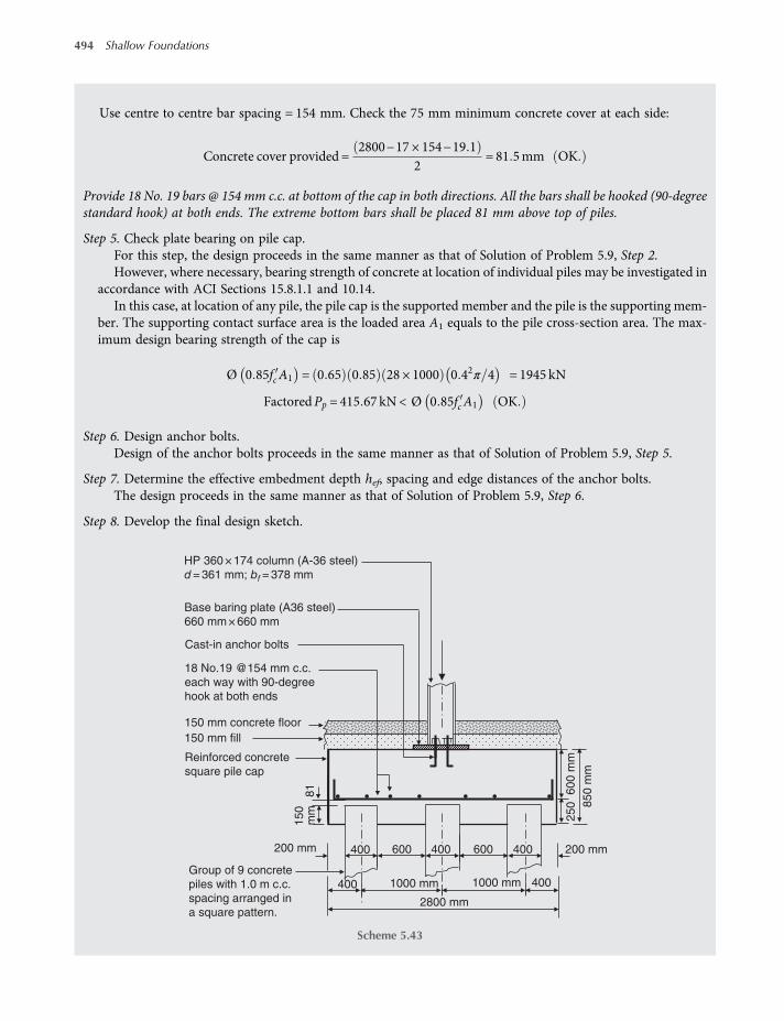
Use centre to centre bar spacing = 154 mm. Check the 75 mm minimum concrete cover at each side:
Concrete cover provided =2800−17 × 154−19 1
2= 81 5mm OK
Provide 18 No. 19 bars @ 154 mm c.c. at bottom of the cap in both directions. All the bars shall be hooked (90-degreestandard hook) at both ends. The extreme bottom bars shall be placed 81 mm above top of piles.
Step 5. Check plate bearing on pile cap.For this step, the design proceeds in the same manner as that of Solution of Problem 5.9, Step 2.However, where necessary, bearing strength of concrete at location of individual piles may be investigated in
accordance with ACI Sections 15.8.1.1 and 10.14.In this case, at location of any pile, the pile cap is the supported member and the pile is the supporting mem-
ber. The supporting contact surface area is the loaded area A1 equals to the pile cross-section area. The max-imum design bearing strength of the cap is
Ø 0 85fc A1 = 0 65 0 85 28 × 1000 0 42π 4 = 1945 kN
FactoredPp = 415 67 kN< Ø 0 85fc A1 OK
Step 6. Design anchor bolts.Design of the anchor bolts proceeds in the same manner as that of Solution of Problem 5.9, Step 5.
Step 7. Determine the effective embedment depth hef, spacing and edge distances of the anchor bolts.The design proceeds in the same manner as that of Solution of Problem 5.9, Step 6.
Step 8. Develop the final design sketch.
200 mm 400 600 400 600 400 200 mm
400400
2800 mm
600 m
m
250
850 m
m
150
mm
81
HP 360 × 174 column (A-36 steel)
d = 361 mm; bf = 378 mm
Cast-in anchor bolts
Base baring plate (A36 steel)
660 mm × 660 mm
18 No.19 @154 mm c.c.
each way with 90-degree
hook at both ends
Reinforced concrete
square pile cap
150 mm concrete floor
150 mm fill
Group of 9 concrete
piles with 1.0 m c.c.
spacing arranged in
a square pattern.
1000 mm1000 mm
Scheme 5.43
494 Shallow Foundations
worksaccounts.com

Problem 5.11
Given: same data as that of Problem 5.10 except the column, in addition to its axial loads, carries the same momentM about both x and y axes, and each pile working load should not exceed 435kN.
M =MD +ML MD = 55 kN m ML = 65 kN m
Required: Design the pile cap.
Solution:Step 1. Determine number of piles required, pile-group pattern, pile spacing and plan dimensions of the pile cap.
The greatest combinations of the given loads are
Q= P =D+ L
My =Mx =M =MD +ML = 55 + 65 = 120 kN m
Since the column is at centre of the pile cap and carries the same moment M about both x and y axes, it may beappropriate to use a square cap.
Try a square cap with trial dimensions: 3.0 m × 3.0 m × 0.85 mFor the purpose of estimating a trial number of piles let:
n=Q
allowable pile working load
Q= 1000 + 1400 + 3 × 3 0 85 × 24 + 0 15 × 20 + 0 15 × 24 + 3 75
= 2677 kN
n=2677435
= 6 2piles
Try seven pilesPile diameter = 0.4 mA square pile cap can accommodate seven piles distributed in a stable hexagonal pattern as shown. The pile
group pattern will be symmetrical about both x and y axes.
O O O
O O
s
s sO O
Scheme 5.44
(Continued)
E
0.55 0.55 1.100.4 m 0.4 m
B
F
Pile cap
Metal column
HP 360 × 174
Base bearing plate
660 mm × 660 mm
A
C
0.5
50.5
50.9
5 m
0.9
5 m 3
.00 m
3.00 m
My
Mx
x
y
s = 1
.1 m
Scheme 5.45
Shallow Foundations – Structural Design 495
worksaccounts.com

Pile caps should extend at least 200 mm beyond the outside face of exterior piles (see Section 5.7).Centre-to-centre spacing of adjacent piles is
s= 3−2 cap projection at each side −2 half pile diameter 2
= 3−2 × 0 2−2 × 0 2 2 = 1 1 m
Equation (5.31): Pp =Qn±My
Σx2x ±
Mx
Σy2y
It is clear that Pp, max is located at centre of pile B. Compute Pp, max and check the 435 kN pile working load.
Pp, max =Qn+My
Σx2x +
Mx
Σy2y =
26777
+120
4 × 0 552 + 2 × 1 12× 0 55 +
1204 × 0 952
× 0 95
= 382 4 + 18 2 + 31 6 = 432 kN< 435 kN OK
Also, it is clear that Pp,min is located at pile C.
Pp,min =Qn−My
Σx2x−
Mx
Σy2y =
26997
−120
4 × 0 552 + 2 × 1 12× 1 1−
1204 × 0 952
× 0 95
= 382 4−18 2−31 6 = 333 kN
Use seven piles arranged in a hexagonal pattern.Use centretocentre pile spacing = 1100 mm.Use the cap plan dimensions = 3000 × 3000 mm.
Step 2. Locate the necessary critical sections according to ACI Sections 15.4, 15.5 and 15.6.AISC Tables give the dimensions for the HP 360 174 as shown in Scheme 5.46.
Step 3. Find cap thickness h.Determine the required thickness based on both two-way shear and one-way shear analyses.
ACI Section 15.5.3 states that where the distance between the axis of any pile and the axis of the column ismore than two times the distance between the top of the pile cap and the top of the pile, the pile cap shall satisfySections 11.11 and 15.5.4. Other pile caps shall satisfy either Appendix A or Sections 11.11 and 15.5.4.
Metal platedw
Cp
bf Bp
Metal column
bf = 0.378 m
dw= 0.361 m
Base plate dimensions:
Bp= 0.66 m
Cp= 0.66 m
Scheme 5.46
496 Shallow Foundations
worksaccounts.com

In this case, we design the cap so that the requirements of ACI Sections 11.11 and 15.5.4 are satisfied, andtherefore, Appendix A will not be considered.
(a) Two-way shear:Two-way shear at location of the column:The critical section is located at distance d/2 from a line halfway between face of the column and edge of the
base plate, as shown in the scheme below.
Assume only one pile (centre pile) reaction exists within the shear block.
FactoredQ= 1 2 1000 + 3 × 30 85 × 24 + 0 15 × 20
+ 0 15 × 24
+ 1 6 1400 + 3 × 3 × 3 75
= 1491 6 + 2294 0 = 3785 6 kN
FactoredPP center pile = Pp =Qn±My
Σx2x ±
Mx
Σy2y
=factoredQ
n+ 0 + 0 =
3785 67
= 540 8 kN
Equation (5.19): ØVc ≥Vu taking reinforcement shear strength,Vs = 0
where Ø = strength reduction factor ACI Section 9 3 2 3
= 0 75 for shear
Vu = factoredQ−one pile reaction on the shear block
= 3785 6−540 8 = 3245 kN
E
0.2
6
0.51 + d
0.5
2+
d
Critical sections
for one-way shearCritical section for
two-way shear
Critical sections
for moment and
development of
reinforcement
0.5
5
0.5
5
0.9
5 m
0.9
5 m
B
F Metal column
HP 360 × 174
Base bearing plate
660 mm × 660 mm
A
C
0.26 m
3.0
0m
yd
d
3.00 m
Scheme 5.47
(Continued)
Shallow Foundations – Structural Design 497
worksaccounts.com

The shear strength of concrete Vc shall be the smallest of (i), (ii) and (iii):
(i) Vc = 0 17 1 +2β
λ fc bod
= 0 17 1 +21
1 fc bod = 0 51 fc bod
Equation 5 22
(ii) Vc = 0 083αsdbo
+ 2 λ fc bod
= 0 08340dbo
+ 2 1 fc bod = 0 08340dbo
+ 2 fc bod
Equation 5 23
(iii) Vc = 0 33 λ fc bod
= 0 33 1 fc bod = 0 33 fc bodEquation 5 24
Use Vc = 0 33 fc bod. Calculate d, then check Vc of Equation (5.23).
ØVc = 0 75 0 33 28 1000 2 0 51 + d + 0 52 + d d
= 5239 d 2 + 2698 d
Let ØVn =Vu:
5239 d 2 + 2698 d = 3245
5239 d 2 + 2698 d −3245 = 0
d =−2698 ± 26982− 4 5239 −3245
2 × 5239=−2698 + 8246
10 478= 0 53m= 530mm
Check Vc of Equation (5.23):
Vc = 0 08340 × 0 53
2 0 51 + 0 53 + 0 52 + 0 53+ 2 fc bod = 0 60 fc bod
Vc = 0 33 fc bod < 0 60 fc bod OK
Try d = 0.6 m = 600 mm and h = 850 mmCheck whether only one pile reaction exists within the shear block:Face of the nearest pile to the critical section is located (0.95 − half pile diameter = 0.95 − 0.2 = 0.75 m) from the
cap centre.
0 52 + d2
=0 52 + 0 6
2= 0 56m< 0 75m
Hence, there is only one pile (centre pile) reaction located within the shear block area. (OK.)
498 Shallow Foundations
worksaccounts.com
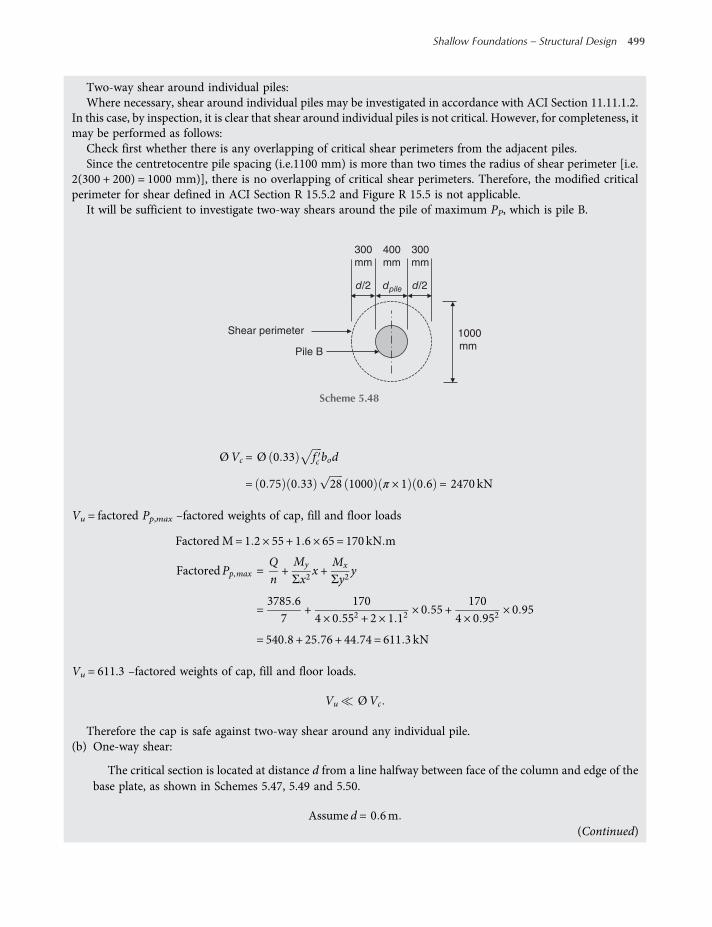
Two-way shear around individual piles:Where necessary, shear around individual piles may be investigated in accordance with ACI Section 11.11.1.2.
In this case, by inspection, it is clear that shear around individual piles is not critical. However, for completeness, itmay be performed as follows:
Check first whether there is any overlapping of critical shear perimeters from the adjacent piles.Since the centretocentre pile spacing (i.e.1100 mm) is more than two times the radius of shear perimeter [i.e.
2(300 + 200) = 1000 mm)], there is no overlapping of critical shear perimeters. Therefore, the modified criticalperimeter for shear defined in ACI Section R 15.5.2 and Figure R 15.5 is not applicable.
It will be sufficient to investigate two-way shears around the pile of maximum PP, which is pile B.
ØVc = Ø 0 33 fc bod
= 0 75 0 33 28 1000 π × 1 0 6 = 2470 kN
Vu = factored Pp,max –factored weights of cap, fill and floor loads
Factored M= 1 2 × 55 + 1 6 × 65 = 170 kN m
FactoredPp,max =Qn+My
Σx2x +
Mx
Σy2y
=3785 6
7+
1704 × 0 552 + 2 × 1 12
× 0 55 +170
4 × 0 952× 0 95
= 540 8 + 25 76 + 44 74 = 611 3 kN
Vu = 611.3 –factored weights of cap, fill and floor loads.
Vu ØVc
Therefore the cap is safe against two-way shear around any individual pile.(b) One-way shear:
The critical section is located at distance d from a line halfway between face of the column and edge of thebase plate, as shown in Schemes 5.47, 5.49 and 5.50.
Assume d = 0 6m
d/2 d/2dpile
400
mm
300
mm
300
mm
1000
mm
Shear perimeter
Pile B
Scheme 5.48
(Continued)
Shallow Foundations – Structural Design 499
worksaccounts.com
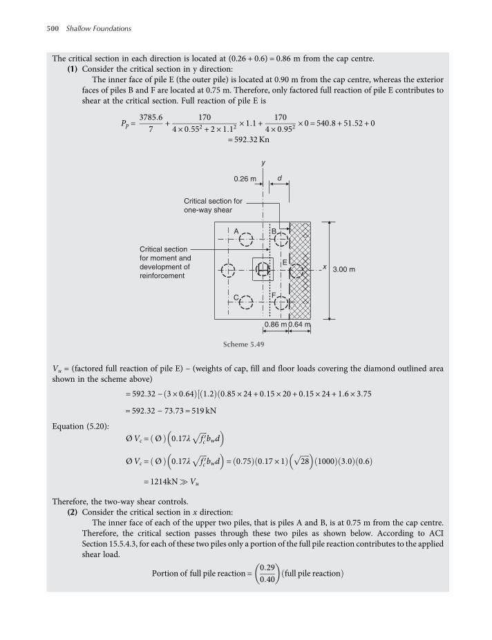
The critical section in each direction is located at (0.26 + 0.6) = 0.86 m from the cap centre.(1) Consider the critical section in y direction:
The inner face of pile E (the outer pile) is located at 0.90 m from the cap centre, whereas the exteriorfaces of piles B and F are located at 0.75 m. Therefore, only factored full reaction of pile E contributes toshear at the critical section. Full reaction of pile E is
Pp =3785 6
7+
1704 × 0 552 + 2 × 1 12
× 1 1 +170
4 × 0 952× 0 = 540 8 + 51 52 + 0
= 592 32Kn
Vu = (factored full reaction of pile E) – (weights of cap, fill and floor loads covering the diamond outlined areashown in the scheme above)
= 592 32 − 3 × 0 64 1 2 0 85 × 24 + 0 15 × 20 + 0 15 × 24 + 1 6 × 3 75
= 592 32 − 73 73 = 519 kN
Equation (5.20):
ØVc = Ø 0 17λ fc bwd
ØVc = Ø 0 17λ fc bwd = 0 75 0 17 × 1 28 1000 3 0 0 6
= 1214kN Vu
Therefore, the two-way shear controls.(2) Consider the critical section in x direction:
The inner face of each of the upper two piles, that is piles A and B, is at 0.75 m from the cap centre.Therefore, the critical section passes through these two piles as shown below. According to ACISection 15.5.4.3, for each of these two piles only a portion of the full pile reaction contributes to the appliedshear load.
Portion of full pile reaction =0 290 40
full pile reaction
E
C
0.86 m 0.64 m
x
y
d
Critical section for
one-way shear
Critical section
for moment and
development of
reinforcement3.00 m
B
F
A
0.26 m
Scheme 5.49
500 Shallow Foundations
worksaccounts.com
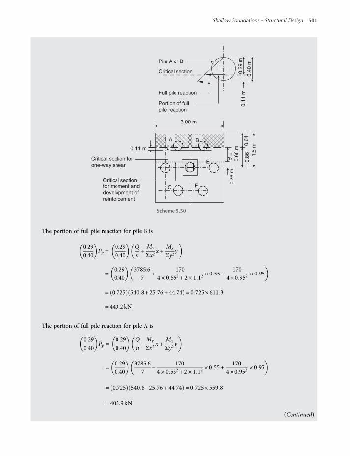
The portion of full pile reaction for pile B is
0 290 40
Pp =0 290 40
Qn+My
Σx2x +
Mx
Σy2y
=0 290 40
3785 67
+170
4 × 0 552 + 2 × 1 12× 0 55 +
1704 × 0 952
× 0 95
= 0 725 540 8 + 25 76 + 44 74 = 0 725 × 611 3
= 443 2 kN
The portion of full pile reaction for pile A is
0 290 40
Pp =0 290 40
Qn−My
Σx2x +
Mx
Σy2y
=0 290 40
3785 67
−170
4 × 0 552 + 2 × 1 12× 0 55 +
1704 × 0 952
× 0 95
= 0 725 540 8−25 76 + 44 74 = 0 725 × 559 8
= 405 9 kN
(Continued)
E
C
0.6
0 m
d =
0.2
6 m
0.8
6
0.6
4
0.11 m
Critical section for
one-way shear
Critical section
for moment and
development of
reinforcement
3.00 m
B
F
A
0.4
0 m
0.2
9 m
Full pile reaction
Portion of full
pile reaction
Critical section
0.1
1 m
Pile A or B
1.5
m
Scheme 5.50
Shallow Foundations – Structural Design 501
worksaccounts.com
Vu = pile reactions – (weights of cap, fill and floor loads covering the cross-hatched area shown in the scheme)
= 443 2 + 405 9 −
3 × 0 64 1 2 0 9 × 24 + 0 15 × 20 + 0 15 × 24 + 1 6 × 3 75
= 849 1−76 49 = 772 61 kN
ØVc = Ø 0 17λ fc bwd = 0 75 0 17 × 1 28 1000 3 0 0 6
= 1214 kN>Vu
Therefore, the two-way shear controls.Use d = 0.60 m = 600 mm.The depth d will be taken to the centre of the steel bars placed at bottom of the cap.Check the assumed cap thickness h:
h= d + one bar diameter say 25mm
+75mmspace between steel bars and top of piles
+ 150mm pile embedment into the cap
= 600 + 25 + 75 + 150 = 850mm OK
Use the cap thickness h = 850 mmCheck the pile working load or the number of piles required, using the designed cap dimensions:Actually, this checking is unnecessary, since the provided cap dimensions are exactly the same assumed dimen-
sions which were used in the design computations.
Q= 1000 + 1400 + 3 × 3 0 85 × 24 + 0 15 × 20 + 0 15 × 24 + 3 75
= 2677 kN
Pp,max =Qn+My
Σx2x +
Mx
Σy2y
=26777
+120
4 × 0 552 + 2 × 1 12× 0 55 +
1204 × 0 952
× 0 95
= 382 43 + 18 2 + 31 6 = 432 2 kN< 435 kN OK
Step 4. Design the flexural reinforcement.(a) Reinforcement in x direction. The critical section is located at 0.26 m to the right of y axis, as shown in the
scheme below. Use d = 0.60 m.From Step 3:
FactoredPp, E = 592 32 kNand Pp, B = 611 3 kN
FactoredPp, F =Qn+My
Σx2x−
Mx
Σy2y
=3785 6
7+
1704 × 0 552 + 2 × 1 12
× 0 55−170
4 × 0 952× 0 95
= 540 8 + 25 76−44 74 = 521 82 kN
502 Shallow Foundations
worksaccounts.com
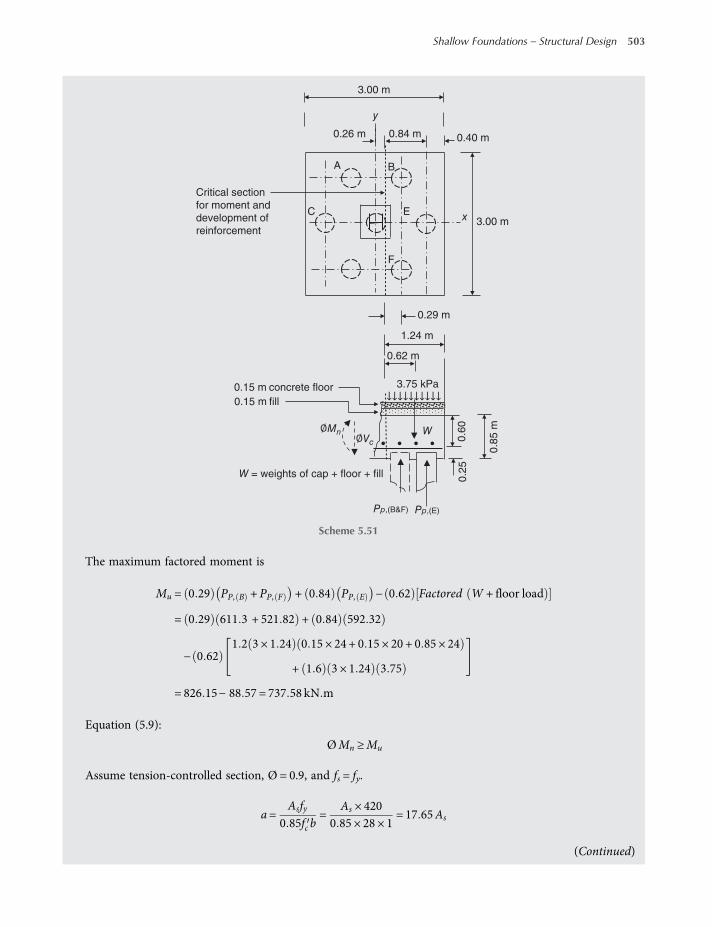
The maximum factored moment is
Mu = 0 29 PP, B + PP, F + 0 84 PP, E − 0 62 Factored W + floor load
= 0 29 611 3 + 521 82 + 0 84 592 32
− 0 621 2 3 × 1 24 0 15 × 24 + 0 15 × 20 + 0 85 × 24
+ 1 6 3 × 1 24 3 75
= 826 15− 88 57 = 737 58 kN m
Equation (5.9):
ØMn ≥Mu
Assume tension-controlled section, Ø = 0.9, and fs = fy.
a=Asfy
0 85fc b=
As × 4200 85 × 28 × 1
= 17 65As
C E
0.84 m 0.40 m
3.00 m
0.15 m concrete floor
0.15 m fill
0.6
0
0.8
5 m
0.2
5
3.75 kPa
0.62 m
W = weights of cap + floor + fill
MnVc
Pp,(B&F) Pp,(E)
1.24 m
0.29 m
y
Critical section
for moment and
development of
reinforcement 3.00 m x
B
F
A
0.26 m
W
Scheme 5.51
(Continued)
Shallow Foundations – Structural Design 503
worksaccounts.com
ØMn = Ø Asfy d−a2
= 0 9 As × 420 × 1000 0 6−17 65As
2
= 226 800As−3335 850As2
Equation 5 11
Let ØMn =Mu
226 800As−3 335 850As2 = 246
3 335 850As2−226 800As + 246 = 0
As =− −226 800 ± −226 800 2− 4 3 335 850 246
2 × 3 335 850=226 800−219 444
6 671 700
= 1 108 × 10−3 m2 m= 1108mm2 m
In order to provide amore strong and rigid pile cap it may bemore appropriate to useAs,min as required for flexuralmembers (ACI Section 10.5.1) rather than As,min based on shrinkage and temperature reinforcement (ACISections 10.5.1 and 7.12.2.1). Accordingly, ACI Section 10.5.1 requires
As,min =0 25 fc
fybwd =
0 25 28420
× 1 × 0 6
= 1 89 × 10−3 m2 m= 1890mm2 m
and not less than 1.4bw dfy
=1 4 × 1 × 0 6
420
= 2 × 10⁻³ m2 m= 2000mm2 m
Therefore, As,min = 2000 mm2/m controls. However, according to ACI Section 10.5.3, this As,min need not beused if As,provided is at least one-third greater than that required by analysis.
1.33 As required by analysis = 1.33 × 1108 = 1474 mm2/m
As, total = 3 × 1474 = 4422mm2
Try 16 No. 19 bars:
As,provided = 16 × 284 = 4544mm2 > 1 33As OK
The assumptions made are satisfied, since As,min controls.Provide 16 No. 19 bars.Check the development of reinforcement:In this case, the bars are in tension, the provided bar size is No. 19, the clear spacing of the bars exceeds 2db, and
the clear cover exceeds db. Therefore, the development length ld of bars at each side of the critical section (which isthe same critical section for moment) shall be determined from the following equation, but not less than 300 mm:
ld =fy ψ t ψ e
2 1 λ fcdb ACI Sections 12 2 1, 12 2 2 and 12 2 4
504 Shallow Foundations
worksaccounts.com
where the factors ψ t, ψ e and λ are 1 (ACI Sections 12.2.4 and 8.6.1) ld =420 × 1 × 1
2 1 × 1 × 28
19 11000
= 0 722 m=
722mm> 300 mm. Therefore, the required ld = 722 mm.The bar extension past the critical section (i.e. the available length) is
1240mm−75mmcover = 1165mm> 722mm OK
However, we shall hook the bars (90-degree standard hook) at both ends to insure better anchorage and keep thepile cap safe against bursting of the side cover where the pile transfers its load to the cap.
ACI Sections 7.6.5 and 10.5.4 require maximum spacing shall not exceed three times the slab or footing thick-ness, or 450 mm, whichever is smaller.
Use centre to centre bar spacing = 188 mm.Check the 75 mm minimum concrete cover at each side:
Concrete cover =3000−15 × 188−19 1
2= 80 5mm> 75mm, O K
Provide 16 No.19 bars @ 188 mm c.c. at bottom of the pile cap in x direction, placed 90 mm above top of piles andhooked (90-degree standard hook) at both ends.(b) Reinforcement in y direction. The critical section is located at 0.26 m above the x axis, as shown in the scheme
below.
From Step 3:Factored Pp,(A) = 559.8 kN and Pp,(B) = 611.3 kNThe maximum factored moment is
Mu = 0 69 PP, A + PP, B − 0 62 factored W + floor load
= 0 69 559 8 + 611 3
− 0 621 2 3 × 1 24 0 15 × 24 + 0 15 × 20 + 0 85 × 24
+ 1 6 3 × 1 24 3 75
= 808 06−88 57 = 719 5 kN m
Mu =719 53
= 240 kN m m
This moment is very close to the Mu just calculated in (a) above. Therefore, it is very clear here again As,min con-trols. Consequently, it is appropriate to use reinforcement in y direction equals to that in x direction. Also, the same
E
C
0.5
5
1.2
4 m
x
0.6
90
.26
Critical section
for moment and
development of
reinforcement
B
F
A
3.0
0 m
3.00 m
Scheme 5.52
(Continued)
Shallow Foundations – Structural Design 505
worksaccounts.com

size, number and spacing of the steel bars will be used for both directions, since the cap is square, h is constant andthe critical sections are located at the same distance from the cap centre.
Provide 16 No.19 bars @ 188 mm c.c. at bottom of the pile cap in y direction, placed on top of bars in x direction,and hooked (90-degree standard hook) at both ends.
Step 5. Check plate bearing on pile cap.For this step, the design proceeds in the same manner as that of Solution of Problem 5.9, Step 2 and Solution
of Problem 5.10, Step 5.
Step 6. Design the anchor bolts and determine their effective embedment depth hef, spacing and edge distances.The design computations proceed in the same manner as those presented in Solution of Problem 5.9, Steps 5
and 6.
Step 7. Develop the final design sketch.
Problem 5.12
The following design data belong to a rectangular ordinary combined footing which supports two columns. Thedistance between the columns is 6 m, centre to centre. The exterior face of the exterior column (Col. 1) is locatedright on the property line. The gross allowable soil pressure (gross qa) is 250 kPa at a depth of 1.3 m below thefinished basement floor. The basement concrete floor is 0.15 m thick and supports a live load of 5 kPa. The densityof the fill above the footing is γs = 20 kN m3. Design the footing using the conventional method.Footing: concretestrength fc = 21MPa; reinforcing steel fy = 420 MPa.
200 400 700 700 400 200
400 1100 mm 1100 mm 400
3000 mm
600
250
150
90
HP 360 × 174 column (A-36 steel)
d = 361 mm; bf= 378 mm
Cast-in anchor bolts
Base baring plate (A36 steel)
660 mm × 660 mm
16 No.19 @ 188
mm c.c. each way
with 90-degree
hook at both ends
Concrete pile cap
3000 × 3000 × 850
mm
150 mm concrete floor
150 mm fill
Group of 7 concrete
piles with 1.1 m c.c.
spacing arranged in
a hexagonal pattern.
O O O
O O
s s O O
s
850 m
m
400
PMx
My
Scheme 5.53
506 Shallow Foundations
worksaccounts.com
Solution:Step 1. Estimate the net factored soil pressure and footing dimensions.
Let resultant of all moments and axial loads passes through the centroid of the footing base area to achieve uni-form soil pressure. The gross load of this resultant equals to the dead and live loads of the two columns plus the floorload and the weights of footing, backfill material and floor. For a first trial guess the footing thickness h equals 1 m.
Df = foundation depth = thicknesses of footing + fill + floor = 1 3m
Therefore thickness of the fill above the footing = 1 3−1−0 15
= 0 15 m
The net resultant load is
net R= gross R−Af Df γs
net q=net RAf
=gross R−Af Df γs
Af=gross RAf
−Df γs
=900 + 675 + 1350 + 1000 +Af 1 × 24 + 0 15 × 24 + 0 15 × 20 + 5
Af−1 3 × 20
=3925Af
+ 35 6−26 0 =3925Af
+ 9 6 kPa
net qa = gross qa−Df γs = 250−1 3 × 20 = 224 kPa
Let net q = net qa:
3925Af
+ 9 6 = 224
Af =3925
224−9 6=3925214 4
= 18 31m2
As for the concentrically loaded spread footings, the net factored soil pressure (net qfactored) is computed withoutincluding the uniform floor load and the weights of footing, backfill material and floor because these loads areevenly distributed and directly transferred to the soil below and, thus, do not affect the footing shear forcesand moments. Therefore, the factored net soil pressure is
net qfactored =factored column loads
Af=1 2 900 + 1350 + 1 6 675 + 1000
18 31
=538018 31
= 293 83 kPa
Compute factored moments, factored column loads and factored resultant.Column No. 1: factored moment M1 = 1.2 × 90 + 1.6 × 70 = 220 kN. m
D,kN L,kN MD,kN.m ML,kN.m M,kN.m
1 0.6 × 0.4
Size, m
Working loads
Column
No.
900 675 90 70 160
1350 1000 130 100 2300.6 × 0.62
Scheme 5.54
(Continued)
Shallow Foundations – Structural Design 507
worksaccounts.com

Column No. 2: factored momentM2 = 1 2 × 130 + 1 6 × 100
= 316 kN mFactored ΣM = 536 kN. mColumn No. 1: factored load P1 = 1.2 × 900 + 1.6 × 675 = 2160 kNColumn No. 2: factored loadP2 = 1 2 × 1350 + 1 6 × 1000
= 3220 kN
Factored resultantR= FactoredΣP = 5380 kN
X =0 2 × P1 + 0 2 + 6 0 P2 +M
R=0 2 × 2160 + 0 2 + 6 0 3220 + 536
5380= 3 891m
LetL2=X:
L= 2 × 3 891 = 7 782m
B=AL=18 317 782
= 2 353m
Use rectangular combined footing 2.4 m × 7.8 mCheck eccentricity of unfactored R:
X =0 2 900 + 675 + 0 2 + 6 0 1350 + 1000 + 160 + 230
900 + 675 + 1350 + 1000=152753925
= 3 892m
eccentricity e=X−L 2 = 3 892−3 891 = 0 001m 0 OK
Step 2. Obtain data for shear-force and bending-moment diagrams considering the combined footing as a rein-forced concrete beam.
Any convenient method, for example integral calculus, may be used for calculating the shear and momentvalues at different locations necessary to obtain informable diagrams. Usually, the design calculations involvetedious busywork; therefore, it may be preferable to use any available computer program concerns the conven-tional design of ordinary combined footings.
In the design computations it may be necessary to use the exact B and L values (i.e. B = 2.353 m andL = 7.782 m) so that the shear and moment diagrams will close.
L/2
6.0 m0.2 m
Property line CentroidM1 M2
P1 P2R
L
x–
Scheme 5.55
508 Shallow Foundations
worksaccounts.com

It is preferable to draw the complete load diagram first, and then the shear and moment diagrams, as shownabove. The factored distributed loads on the footing, shear forces and bending moments are computed for thefull 2.4-m width of the footing.
Step 3. Find footing thickness h.Determine the required thickness based on both one-way shear and two-way shear analyses.
(a) One-way shear. It is critical at distance d from the interior face of the interior column (Col. No. 2), as indicatedon the shear-force diagram.
Equation (5.19): ØVc ≥Vu taking reinforcement shear strength,Vs = 0
where Ø = strength reduction factor ACI Section 9 3 2 3
= 0 75 for shear
Vu = 2126−691 38 d + 0 3 = 1919−691 38 d kN
Equation (5.20): Vc = 0 17λ fc bwd
= 0 75 × 0 17 × 1 21 1000 2 353 dLet ØVc =Vu:
0 75 × 0 17 × 1 21 1000 2 353 d = 1919−691 38 d
d =1919
2066 19= 0 929m= 929mm
Try d = 0.93 m.
(b) Two-way shear. This shear action is most critical at one of the two columns. Therefore, both locations shouldbe considered. The critical sections are shown in the scheme below.
= 293.83 × 2.353
= 691.38 kN/m
Combined footing
L = 7.8 m (= 7.782 m, in computations)
Shear-force diagram
Factored load diagram
2022 kN
234 kN.m
138 kN
1094 kN
2126 kN
Bending-moment diagram
3.12 m
567 kN.m
864 kN.m
Location of inflection point
0.6 m0.4 m 1.3 m 5.5 m
–59 kN. m–157 kN.m
Critical sec.
beam shear
0.27 m
–Mmax = 2722 kN. m
q = net qf actored × B
P1 = 2160 kN P2 = 3220 kN
M1 = 220 kN. m M2 = 316 kN. m
x
d
Scheme 5.56
(Continued)
Shallow Foundations – Structural Design 509
worksaccounts.com
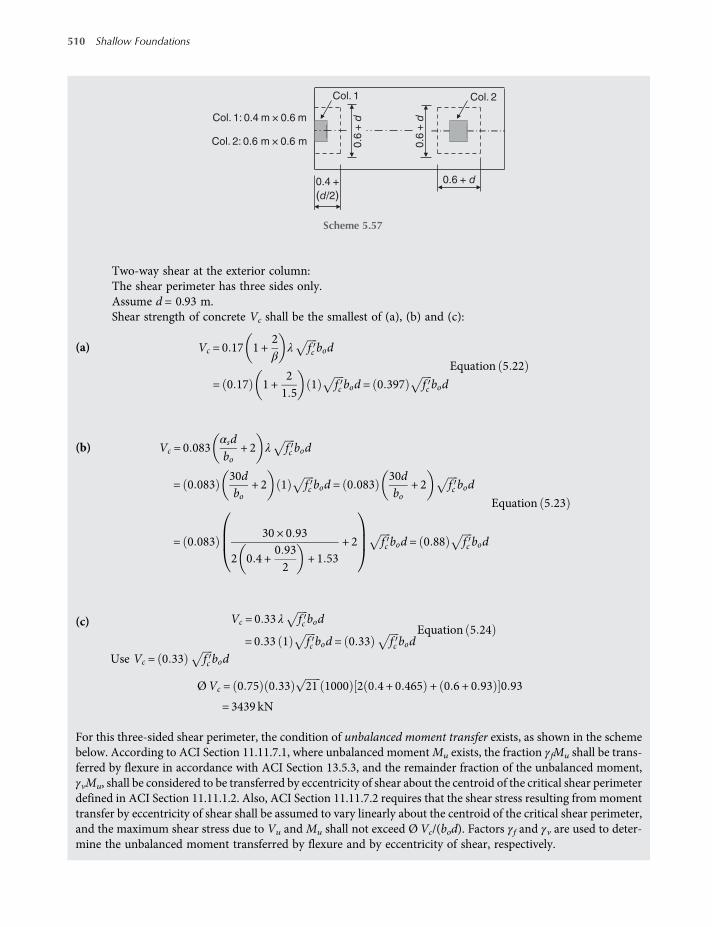
Two-way shear at the exterior column:The shear perimeter has three sides only.Assume d = 0.93 m.Shear strength of concrete Vc shall be the smallest of (a), (b) and (c):
(a) Vc = 0 17 1 +2β
λ fc bod
= 0 17 1 +21 5
1 fc bod = 0 397 fc bod
Equation 5 22
(b) Vc = 0 083αsdbo
+ 2 λ fc bod
= 0 08330dbo
+ 2 1 fc bod = 0 08330dbo
+ 2 fc bod
= 0 08330 × 0 93
2 0 4 +0 932
+ 1 53+ 2 fc bod = 0 88 fc bod
Equation 5 23
(c) Vc = 0 33 λ fc bod
= 0 33 1 fc bod = 0 33 fc bodEquation 5 24
Use Vc = 0 33 fc bod
ØVc = 0 75 0 33 21 1000 2 0 4 + 0 465 + 0 6 + 0 93 0 93
= 3439 kN
For this three-sided shear perimeter, the condition of unbalanced moment transfer exists, as shown in the schemebelow. According to ACI Section 11.11.7.1, where unbalanced momentMu exists, the fraction γfMu shall be trans-ferred by flexure in accordance with ACI Section 13.5.3, and the remainder fraction of the unbalanced moment,γvMu, shall be considered to be transferred by eccentricity of shear about the centroid of the critical shear perimeterdefined in ACI Section 11.11.1.2. Also, ACI Section 11.11.7.2 requires that the shear stress resulting from momenttransfer by eccentricity of shear shall be assumed to vary linearly about the centroid of the critical shear perimeter,and the maximum shear stress due to Vu and Mu shall not exceed ØVc/(bod). Factors γf and γv are used to deter-mine the unbalanced moment transferred by flexure and by eccentricity of shear, respectively.
Col. 2
0.4 +
(d/2)
0.6
+ d
0.6
+ d
0.6 + d
Col. 1
Col. 1: 0.4 m × 0.6 m
Col. 2: 0.6 m × 0.6 m
Scheme 5.57
510 Shallow Foundations
worksaccounts.com
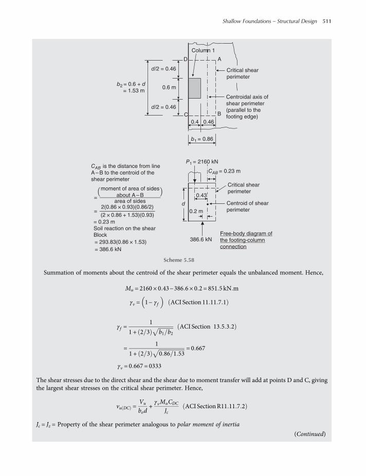
Summation of moments about the centroid of the shear perimeter equals the unbalanced moment. Hence,
Mu = 2160 × 0 43−386 6 × 0 2 = 851 5 kN m
γv = 1− γf ACI Section 11 11 7 1
γf =1
1 + 2 3 b1 b2ACI Section 13 5 3 2
=1
1 + 2 3 0 86 1 53= 0 667
γv = 0 667 = 0333
The shear stresses due to the direct shear and the shear due to moment transfer will add at points D and C, givingthe largest shear stresses on the critical shear perimeter. Hence,
vu DC =Vu
bod+γvMuCDC
JcACI SectionR11 11 7 2
Jc = Jz = Property of the shear perimeter analogous to polar moment of inertia
d/2 = 0.46
d/2 = 0.46
0.2 m
0.43
0.6 m
0.4
A
B C
D
Column 1
Centroid of shear
perimeter
Critical shear
perimeter
P1 = 2160 kN
CAB = 0.23 m
b2 = 0.6 + d
= 1.53 m
0.46
Critical shear
perimeter
Centroidal axis of
shear perimeter
(parallel to the
footing edge)
b1 = 0.86
=
moment of area of sides
about A – Barea of sides
=2(0.86 × 0.93)(0.86/2)
(2 × 0.86 + 1.53)(0.93)
CAB is the distance from line
A – B to the centroid of the
shear perimeter
= 0.23 m
Soil reaction on the shear
Block
= 293.83(0.86 × 1.53)
= 386.6 kN
386.6 kNFree-body diagram of
the footing-column
connection
d
Scheme 5.58
(Continued)
Shallow Foundations – Structural Design 511
worksaccounts.com

Jc = 2b1d3
12+ 2
db3112
+ 2 b1db12−CAB
2
+ b2d CAB2
= 20 86 × 0 933
12+ 2
0 93 × 0 863
12+ 2 0 86 × 0 93
0 862
−0 232
+
1 53 × 0 93 0 232
= 0 115 + 0 099 + 0 064 + 0 075 = 0 353m4
vu DC =2160−386 6
2 × 0 86 + 1 53 0 93+0 333 × 851 5 0 86−0 23
0 353= 586 73 + 506 05
= 1093 kN m2
Ø vc =ØVc
bod=
34392 0 4 + 0 465 + 0 6 + 0 93 0 93
= 1134 kN m2 > vu DC OK
Therefore, the one-way shear controls.Two-way shear at the interior column:
ØVc ≥Vu
The shear perimeter has four sides.Assumed = 0.93 m.The shear strength of concrete Vc shall be the smallest of (a), (b) and (c):
(a) Vc = 0 17 1 +2β
λ fc bod
= 0 17 1 +21
1 fc bod = 0 51 fc bod
Equation 5 22
D
Z
ZB
A
C
d = 0.93 m
Centroidal axis
CAB = 0.23 m
b1 = 0.86 m
CDC
b2 =1.53 m
Scheme 5.59
512 Shallow Foundations
worksaccounts.com

(b)Vc = 0 083
αsdbo
+ 2 λ fc bod
= 0 08340dbo
+ 2 1 fc bod
= 0 08340 × 0 93
4 0 6 + 0 93+ 2 fc bod = 0 67 fc bod
Equation 5 23
(c) Vc = 0 33 λ fc bod
= 0 33 1 fc bod = 0 33 fc bodEquation 5 24
Use Vc = 0 33 fc bod.
ØVc = 0 75 0 33 21 1000 4 0 6 + 0 93 0 93 = 6455 kN
Vu = P2 –soil reaction on the shear blockVu = 3220 –soil reaction on the shear block (kN)Vu < ØVc. Hence, the one-way shear controls.
Use d = 0.93 m = 930 mm.
The depth d will be taken to the centre of the steel bars at top or at bottom of the footing in long direction.Assume using No. 25 bars, and 75 mmminimum concrete cover (ACI Section 7.7.1). Hence, the overall footing
thickness is
h= 930 + 75 + 1 2 bar diameter = 1005 + 12 7 = 1017 7mm
This value of h is considered very close to the assumed 1000mm. For more safety, one may use a slightly larger value.Use h = 1050 mm.
Step 4. Design the flexural reinforcement in the long direction.(a) Midspan negative reinforcement at top of the footing.
Refer to the factored bending moment diagram of Step 2.
−Mmax = 2722 kN m
Equation (5.9):ØMn ≥Mu
Mu =2722B
=27222 4
= 1134 2 kN m m
Assume tension-controlled section, Ø = 0.9, and fs = fy.Equation (5.11):
ØMn = Ø Asfy d−a2
a=Asfy
0 85fc b=
As × 4200 85 × 21 × 1
= 23 53As
(Continued)
Shallow Foundations – Structural Design 513
worksaccounts.com
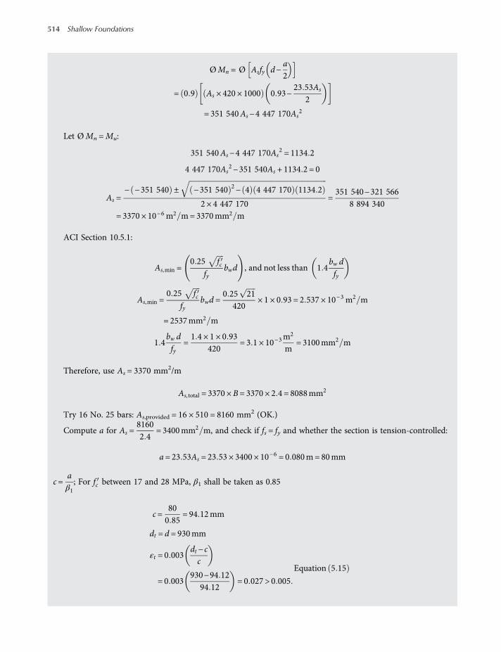
ØMn = Ø Asfy d−a2
= 0 9 As × 420 × 1000 0 93−23 53As
2
= 351 540As−4 447 170As2
Let ØMn =Mu:
351 540As−4 447 170As2 = 1134 2
4 447 170As2−351 540As + 1134 2 = 0
As =− −351 540 ± −351 540 2− 4 4 447 170 1134 2
2 × 4 447 170=351 540−321 566
8 894 340= 3370 × 10−6 m2 m= 3370mm2 m
ACI Section 10.5.1:
As,min =0 25 fc
fybwd , and not less than 1 4
bw dfy
As,min =0 25 fc
fybwd =
0 25 21420
× 1 × 0 93 = 2 537 × 10−3 m2 m
= 2537mm2 m
1 4bw dfy
=1 4 × 1 × 0 93
420= 3 1 × 10⁻³
m2
m= 3100mm2 m
Therefore, use As = 3370 mm2/m
As, total = 3370 ×B= 3370 × 2 4 = 8088mm2
Try 16 No. 25 bars: As,provided = 16 × 510 = 8160 mm2 (OK.)
Compute a for As =81602 4
= 3400mm2 m, and check if fs = fy and whether the section is tension-controlled:
a= 23 53As = 23 53 × 3400 × 10−6 = 0 080m= 80mm
c=aβ1; For fc between 17 and 28 MPa, β1 shall be taken as 0.85
c=800 85
= 94 12mm
dt = d = 930mm
εt = 0 003dt −cc
= 0 003930−94 12
94 12= 0 027 > 0 005
Equation 5 15
514 Shallow Foundations
worksaccounts.com

Hence, the section is tension-controlled, and Ø = 0.9 (ACI Sections 10.3.4 and 9.3.2.1).
εy =fyEs
=420
200 000= 0 0021 Hence, εt > εy and fs = fy.
Therefore, the assumptions made are satisfied.In case the required flexural reinforcement exceeds the minimum flexural reinforcement, it shall be adequate to
use the samemaximum spacing of reinforcement for slabs which is two times the slab thickness or 450mm, which-ever is smaller, as specified by ACI Section 13.3.2.
Use centre to centre bar spacing = 148 mm. Check the 75 mm minimum concrete cover at each side:
2400− 15 × 148 + 25 42
= 77 3mm> 75mm OK
Try 16 No. 25 bars @ 148 mm c. c. at top, across the footing width.Check the development of reinforcement:In this case, the bars are in tension, the provided bar size is No. 25, the clear spacing of the bars exceeds 2db and
the clear cover exceeds db. Therefore, the development length ld of bars at each side of the critical section (which islocated where the maximum factored negative moment exists) shall be determined from the following equation,but not less than 300 mm:
ld =fy ψ t ψ e
1 7 λ fcdb ACI Sections 12 2 1, 12 2 2 and 12 2 4
where the factors ψ e and λ are 1 (ACI Sections 12.2.4 and 8.6.1) .The factor ψ t = 1.3 because the reinforcement is placed such that more than 300 mm of fresh concrete exists
below the top bars (ACI Section 12.2.4).
ld =420 × 1 3 × 1
1 7 × 1 × 21
25 41000
= 1 78m= 1780mm> 300 mm
Therefore, the required ld = 1780 mm.The bar extension past the critical section (i.e. the available length) is
3120mm−75mmcover = 3045mm>1780mm OK
According to MacGregor and Wight (2005), since the loading, the supports and the shape of the moment diagramare all inverted from those found in a normally loaded beam, the necessary check of the ACI Section 12.11.3 require-ment which concerns positive moment reinforcement shall be made for the negative moment reinforcement.
It may be appropriate to extend all the bars into the column regions at both ends. At the point of inflection, 0.27 mfrom the centre of the interior column, Vu = 1940 kN and by ACI Section 12.11.3,
ld ≤Mn
Vu+ la
Mn = nominal flexural strength of the cross section =Asfy d−a2
a=Asfy
0 85fc b=
8160 106 4200 85 × 21 × 2 4
= 0 08
Mn = 8160 106 420 × 1000 0 93−0 082
= 3050 kN m
(Continued)
Shallow Foundations – Structural Design 515
worksaccounts.com

Let ld =Mn
Vu+ la. Hence, la, min = ld −
Mn
Vu= 1 78−
30501940
= 0 21m. The distance la at a support shall be the embed-
ment length beyond centre of support.Accordingly, extend the bars to the exterior face of the interior column. This will give
la = 0 30m> la,min
However, in order to satisfy the requirements of ACI Sections 12.12.3 and 12.10.3, the negative moment reinforce-ment shall have an embedment length beyond the point of inflection not less than d, 12db or ℓn/16, whichever isgreater. In this case, d controls. Therefore, the top bars should be extended not less than 0.93 m beyond the point ofinflection at x = 5.93 m. However, since the remaining distance to the footing edge is only 0.94 m, it may be morepractical to extend the top bars to the right edge of the footing (less 75 mm minimum concrete cover).
At centre of the exterior column, Vu = 2022 kN; hence,
la,min = ld −Mn
Vu= 1 78−
30502022
= 0 27m
The available space beyond the column centre is 0.2 m less concrete cover, which is less than la,min. Therefore, thetop bars will all have to be hooked at the exterior end. This is also necessary to anchor the bars transferring theunbalanced moment from the column to the footing.
Provide 16 No.25 bars @ 148 mm c.c. at top, full length of the footing (less concrete cover at the ends). All the barsshould be hooked at the exterior end (at the exterior face of the exterior column).(b) Positive reinforcement at bottom of the footing.
Let us design, conservatively, for +Mmax = 864 kN. m instead the 567 kN.m positive moment. However, inmost of cases As,min controls and it makes no difference which moment is used.
Equation (5.9): ØMn ≥Mu
Mu =864B
=8642 4
= 360 kN m m
Assume tension-controlled section, Ø = 0.9, and fs = fy.
a=Asfy
0 85fc b=
As × 4200 85 × 21 × 1
= 23 53As
ØMn = Ø Asfy d−a2
= 0 9 As × 420 × 1000 0 93−23 53As
2
= 351 540As−4 447 170As2
Equation 5 11
Let ØMn =Mu:
351 540As−4 447 170As2 = 360
4 447 170As2−351 540As + 360 = 0
As =− −351 540 ± −351 540 2− 4 4 447 170 360
2 × 4 447 170=351 540−342 310
8 894 340
= 1038 ×10−6 m2
m= 1038mm2 m< As,min = 3100mm2 m
516 Shallow Foundations
worksaccounts.com

Therefore, As,min controls.
As, total = 3100 ×B= 3100 × 2 4 = 7440mm2
Try 15 No. 25 bars: As,provided = 15 × 510 = 7650mm2 mACI Sections 7.6.5 and 10.5.4 requires maximum spacing shall not exceed three times the slab or footing thicknessor 450 mm, whichever is smaller.
Use centretocentre bar spacing = 158 mm. Check the 75 mm minimum concrete cover at each side:
Concrete cover =2400− 14 × 158 + 25 4
2= 81 3mm> 75mm OK
Try 15 No. 25 bars @ 158 mm c.c. at bottom, across the footing width.Check the development of reinforcement:In this case, the bars are in tension, the provided bar size is No. 25, the clear spacing of the bars exceeds 2db, and
the clear cover exceeds db. Therefore, the development length ld of bars at each side of the critical section (which islocated where the maximum factored positive moment exists) shall be determined from the following equation,but not less than 300 mm:
ld =fy ψ t ψ e
1 7 λ fcdb ACI Sections 12 2 1, 12 2 2 and 12 2 4
where the factors ψ t, ψ e and λ are 1 (ACI Sections 12.2.4 and 8.6.1).
ld =420 × 1 × 1
1 7 × 1 × 21
25 41000
= 1 37m= 1370mm> 300mm
Therefore, the required ld = 1370 mm.The bar extension past the critical section (i.e. the available length) is
1600mm−75mmcover = 1525mm> 1370mm OK
In order to satisfy the requirements of ACI Sections 12.10.3 and even 12.12.3 when we consider the footing as aninverted normally loaded beam (the same as we did for the top bars), it is necessary to extend the bottom bars aminimum distance d (greater than 12db) past the point of inflection. Therefore, cut off eight bottom bars (alter-nately spaced) at 1.4 m from centre of the interior column toward the exterior column. The other seven bars shallbe extended full length (less 75 mm cover at each end) of the footing and hooked at the exterior end (at the exteriorcolumn). These seven bars will resist the tensile stresses due to the relatively small positive moment at the exteriorcolumn, and provide supports to the transverse bottom bars.
Provide 15 No.25 bars @ 158 mm c.c. at bottom of the footing. Cut off eight bars (alternately spaced) at 1.40 mfrom the centre of the interior column. The other seven bars shall be extended full length of the footing and hooked atthe exterior end (at the exterior column).
Step 5. Design the transverse reinforcement at bottom of the footing.The footing is divided into three zones or strips of the defined widths shown in the scheme below.
Zones I and II, usually known as effective zones, should be analyzed as beams; the provided steel shouldnot be less than that required for bending or As,min, whichever is greater. For zone III (the remaining portions),the provided steel should satisfy As,min requirement only. All the transverse steel bars should be placed on top ofbars in long direction at the bottom of the footing.
(Continued)
Shallow Foundations – Structural Design 517
worksaccounts.com
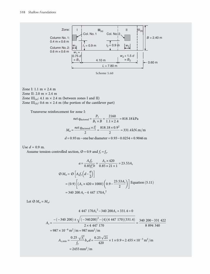
Zone I: 1.1 m × 2.4 mZone II: 2.0 m × 2.4 mZone III(a): 4.1 m × 2.4 m (between zones I and II)Zone III(b): 0.6 m × 2.4 m (the portion of the cantilever part)
Transverse reinforcement for zone I:
net qfactored =P1
B1 ×B=
21601 1 × 2 4
= 818 18 kPa
Mu =net qfactored × l21
2=818 18 × 0 92
2= 331 4 kN m m
d = 0 93m−one bar diameter = 0 93−0 0254 = 0 9046m
Use d = 0.9 m.Assume tension-controlled section, Ø = 0.9 and fs = fy.
a=Asfy
0 85fc b=
As × 4200 85 × 21 × 1
= 23 53As
ØMn = Ø Asfy d−a2
= 0 9 As × 420 × 1000 0 9−23 53As
2
= 340 200As−4 447 170As2
Equation 5 11
Let ØMn =Mu:
4 447 170As2−340 200As + 331 4 = 0
As =− −340 200 ± −340200 2− 4 4 447 170 331 4
2 × 4 447 170=340 200−331 422
8 894 340= 987 × 10−6 m2 m= 987mm2 m
As,min =0 25 fc
fybwd =
0 25 21420
× 1 × 0 9 = 2 455 × 10−3 m2 m
= 2455mm2 m
B = 2.40 m
L = 7.80 m
Col. No. 1
I
4.10 m
Column No. 1:
0.4 m × 0.6 m
Column No. 2:
0.6 m × 0.6 m
l1 = 0.9 m l2 = 0.9 m
Zone:
Col. No. 2
III II
0.60 m
III(a)
w2 + 1.5 d = B2
w1 +
0.75 d= B1
w1 w2
III(b)
Scheme 5.60
518 Shallow Foundations
worksaccounts.com
and not less than 1.4
bw dfy
=1 4 × 1 × 0 9
420= 3 0 ×
10−3m2
m
= 3000mm2 m
As,min > As required by analysis. Use As = As,min = 3000 mm2/mTransverse reinforcement for zone II:
net qfactored =P2
B2 ×B=
32202 × 2 4
= 670 83 kPa
Mu =net qfactored × l21
2=670 83 × 0 92
2= 271 7 kN m m <Mu of zone I
Therefore, As,min controls. Use As = 3000 mm2/mTransverse reinforcement for zone III:
Use As =As,min = 3000mm2 mThus, in this case, for all the three zones the same amount of reinforcement will be required.
As, total = 3000 × L= 3000 × 7 8 = 23 400mm2
Try 46 No. 25 bars: As,provided = 46 × 510 = 23 460 mm2.ACI Sections 7.6.5 and 10.5.4 require maximum spacing shall not exceed three times the slab or footing thick-
ness or 450 mm, whichever is smaller.Use centre to centre bar spacing = 169 mm. Check the 75 mm minimum concrete cover at each side:
Concrete cover =7800− 45 × 169 + 25 4
2= 84 8mm> 75mm OK
Thus, theoretically, the bars will be uniformly distributed with 169 mm centretocentre.However, it may be more realistic if the amount of steel in the effective zones I and II are somewhat increased
and that in zone III decreased. We shall do this by arbitrarily decreasing and increasing the bar spacing in the threezones but without decreasing the required total steel amount, as follows:
Zone I: Eight No.25 bars; seven spacings @ 142 mm c.c.Zone II: 15 No.25 bars;14 spacings @ 141 mm c.c.Zone III(a): 19 No.25 bars;18 spacings @ 226 mm c.c.Zone III(b): Four No.25 bars; three spacings @ 166 mm c.c.
Check the development of reinforcement:In this case, the bars are in tension, the provided bar size is No. 25, the clear spacing of the bars exceeds 2db,
and the clear cover exceeds db. Therefore, the development length ld of bars at each side of the criticalsection (which is located where the maximum factored positive moment exists) shall be determined fromthe following equation, but not less than 300 mm:
ld =fy ψ t ψ e
1 7 λ fcdb ACI Sections 12 2 1, 12 2 2 and 12 2 4
(Continued)
Shallow Foundations – Structural Design 519
worksaccounts.com
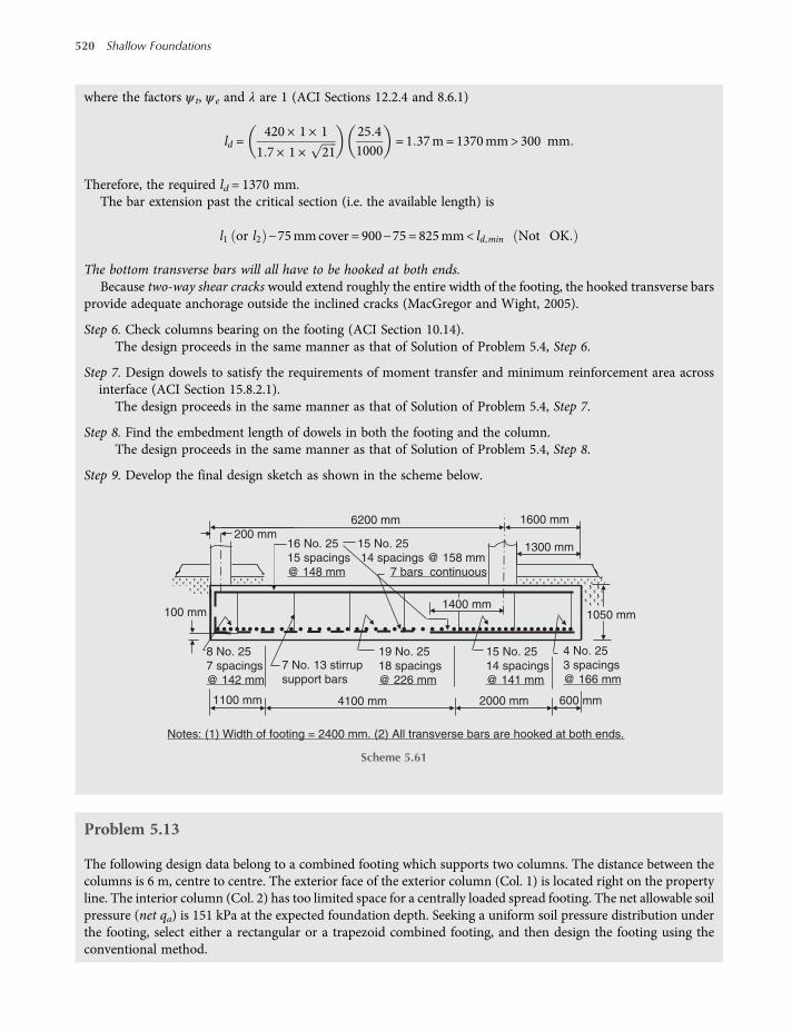
where the factors ψ t, ψ e and λ are 1 (ACI Sections 12.2.4 and 8.6.1)
ld =420 × 1 × 1
1 7 × 1 × 21
25 41000
= 1 37m= 1370mm> 300 mm
Therefore, the required ld = 1370 mm.The bar extension past the critical section (i.e. the available length) is
l1 or l2 −75mmcover = 900−75 = 825mm< ld,min Not OK
The bottom transverse bars will all have to be hooked at both ends.Because two-way shear cracks would extend roughly the entire width of the footing, the hooked transverse bars
provide adequate anchorage outside the inclined cracks (MacGregor and Wight, 2005).
Step 6. Check columns bearing on the footing (ACI Section 10.14).The design proceeds in the same manner as that of Solution of Problem 5.4, Step 6.
Step 7. Design dowels to satisfy the requirements of moment transfer and minimum reinforcement area acrossinterface (ACI Section 15.8.2.1).
The design proceeds in the same manner as that of Solution of Problem 5.4, Step 7.
Step 8. Find the embedment length of dowels in both the footing and the column.The design proceeds in the same manner as that of Solution of Problem 5.4, Step 8.
Step 9. Develop the final design sketch as shown in the scheme below.
Problem 5.13
The following design data belong to a combined footing which supports two columns. The distance between thecolumns is 6 m, centre to centre. The exterior face of the exterior column (Col. 1) is located right on the propertyline. The interior column (Col. 2) has too limited space for a centrally loaded spread footing. The net allowable soilpressure (net qa) is 151 kPa at the expected foundation depth. Seeking a uniform soil pressure distribution underthe footing, select either a rectangular or a trapezoid combined footing, and then design the footing using theconventional method.
1050 mm
1600 mm6200 mm
8 No. 25
7 spacings
@ 142 mm
19 No. 25
18 spacings
@ 226 mm
2000 mm
1400 mm
15 No. 25
14 spacings @ 158 mm
7 bars continuous
15 No. 25
14 spacings
@ 141 mm
600 mm
16 No. 25
15 spacings
@ 148 mm
4 No. 25
3 spacings
@ 166 mm
1100 mm
Notes: (1) Width of footing = 2400 mm. (2) All transverse bars are hooked at both ends.
4100 mm
1300 mm200 mm
100 mm
7 No. 13 stirrup
support bars
Scheme 5.61
520 Shallow Foundations
worksaccounts.com
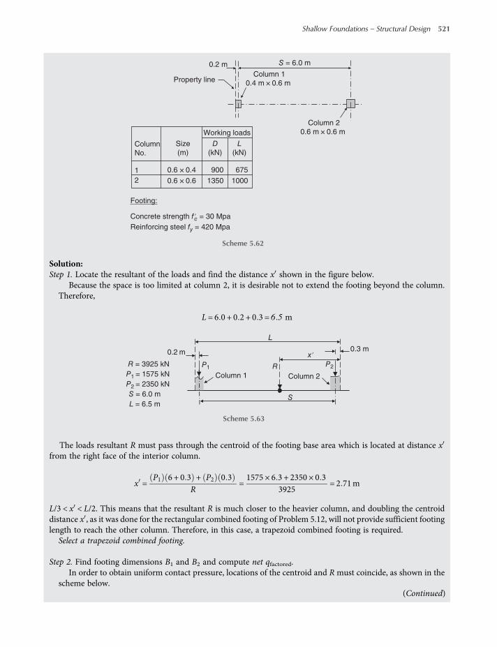
Solution:Step 1. Locate the resultant of the loads and find the distance x shown in the figure below.
Because the space is too limited at column 2, it is desirable not to extend the footing beyond the column.Therefore,
L = 6 0 + 0 2 + 0 3 = 6 5 m
The loads resultant R must pass through the centroid of the footing base area which is located at distance xfrom the right face of the interior column.
x =P1 6 + 0 3 + P2 0 3
R=1575 × 6 3 + 2350 × 0 3
3925= 2 71m
L/3 < x < L/2. This means that the resultant R is much closer to the heavier column, and doubling the centroiddistance x , as it was done for the rectangular combined footing of Problem 5.12, will not provide sufficient footinglength to reach the other column. Therefore, in this case, a trapezoid combined footing is required.
Select a trapezoid combined footing.
Step 2. Find footing dimensions B1 and B2 and compute net qfactored.In order to obtain uniform contact pressure, locations of the centroid and R must coincide, as shown in the
scheme below.
Column 2
0.6 m × 0.6 m
Column 1
0.4 m × 0.6 m Property line
0.2 m S = 6.0 m
Column
No.
Size
(m)
Working loads
D
(kN)
L
(kN)
1
2
Concrete strength f′c = 30 Mpa
Reinforcing steel fy = 420 Mpa
Footing:
0.6 × 0.4 900 675
1350 10000.6 × 0.6
Scheme 5.62
R = 3925 kN
P1 = 1575 kN
P2 = 2350 kN
S = 6.0 m
L = 6.5 m
0.3 m
0.2 m
Column 1 Column 2
P1 P2
S
R
L
x′
Scheme 5.63
(Continued)
Shallow Foundations – Structural Design 521
worksaccounts.com
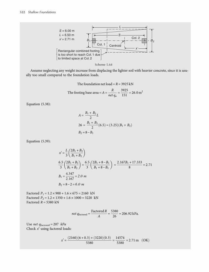
Assume neglecting any weight increase from displacing the lighter soil with heavier concrete, since it is usu-ally too small compared to the foundation loads.
The foundationnet load =R= 3925 kN
The footing base area =A =R
net qa=3925151
= 26 0m2
Equation (5.38):
A =B1 + B2
2L
26 =B1 + B2
26 5 = 3 25 B1 + B2
B2 = 8−B1
Equation (5.39):
x =L3
2B1 +B2
B1 +B2
6 53
2B1 +B2
B1 + B2=6 53
2B1 + 8−B1
B1 + 8−B1=2 167B1 + 17 333
8= 2 71
B1 =4 3472 167
= 2 0 m
B2 = 8−2 = 6 0 m
Factored P1 = 1.2 × 900 + 1.6 × 675 = 2160 kNFactored P2 = 1.2 × 1350 + 1.6 × 1000 = 3220 kNFactored R = 5380 kN
net qfactored =FactoredR
A=538026
= 206 92 kPa
Use net qfactored = 207 kPaCheck x using factored loads:
x =2160 6 + 0 3 + 3220 0 3
5380=145745380
= 2 71m OK
Col. 2
Col. 1
Rectangular combined footing
is too short to reach Col. 1 due
to limited space at Col. 2
Centroid
S = 6.00 m
L = 6.50 m
x′= 2.71 m
x′
B1 B2
L
S
Scheme 5.64
522 Shallow Foundations
worksaccounts.com
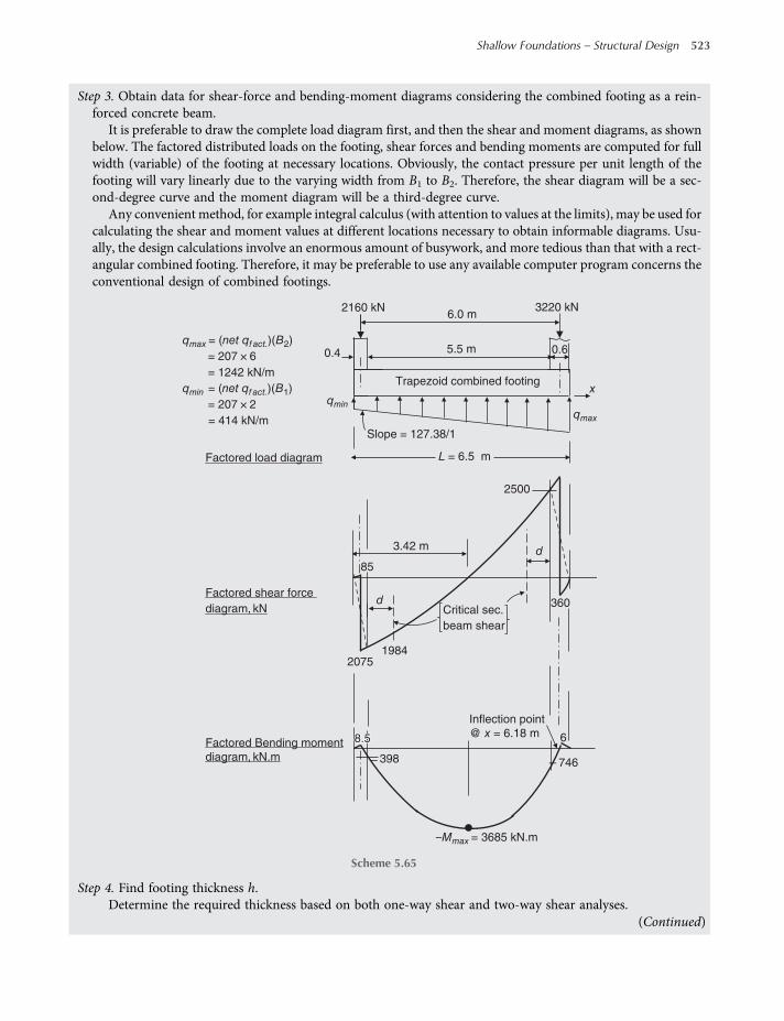
Step 3. Obtain data for shear-force and bending-moment diagrams considering the combined footing as a rein-forced concrete beam.
It is preferable to draw the complete load diagram first, and then the shear and moment diagrams, as shownbelow. The factored distributed loads on the footing, shear forces and bending moments are computed for fullwidth (variable) of the footing at necessary locations. Obviously, the contact pressure per unit length of thefooting will vary linearly due to the varying width from B1 to B2. Therefore, the shear diagram will be a sec-ond-degree curve and the moment diagram will be a third-degree curve.
Any convenient method, for example integral calculus (with attention to values at the limits), may be used forcalculating the shear and moment values at different locations necessary to obtain informable diagrams. Usu-ally, the design calculations involve an enormous amount of busywork, and more tedious than that with a rect-angular combined footing. Therefore, it may be preferable to use any available computer program concerns theconventional design of combined footings.
Step 4. Find footing thickness h.Determine the required thickness based on both one-way shear and two-way shear analyses.
0.6 0.4
Trapezoid combined footing
5.5 m
Factored shear force
diagram, kN
Factored load diagram
2075
85
360
Factored Bending moment
diagram, kN.m
3.42 m
1984
746
6
–Mmax = 3685 kN.m
qmax
qmin
x
d
398
Critical sec.
beam shear
Inflection point
@ x = 6.18 m
qmin = (net qf act.)(B1)
= 207 × 2
= 414 kN/m
qmax = (net qf act.)(B2)
= 207 × 6
= 1242 kN/m
Slope = 127.38/1
3220 kN 6.0 m
2500
2160 kN
L = 6.5 m
d
8.58.58.5
Scheme 5.65
(Continued)
Shallow Foundations – Structural Design 523
worksaccounts.com

(a) One-way shear. Since the footing width varies, we should consider shear at two critical sections; one at distanced from the right face of the exterior column, and the other at distance d from the left face of the interior col-umn, as indicated on the shear-force diagram. However, in this case, one may detect location of the mostcritical shear by comparing the B ratio with the ratio of shear forces at the column faces, as follows:
The width B ratio (approximately) =62= 3
The shear-force ratio =25001984
= 1 26
Since the width ratio is much larger than the shear-force ratio, the footing depth dwill probably be based onshear at distance d from the interior face of the exterior column. Based on this reasoning, d is calculated asfollows:
Vu = 414 0 4 + d + 127 38 0 4 + d 2 0 5 −2160
= 165 6 + 414d + 10 19 + 50 95d + 63 69d2−2160
= 464 95d + 63 69d2−1984 21 kN
It may be noticed from the shear diagram that at this critical section Vu is negative. Therefore, it would benecessary to use it positive when equated to the shear strength.
Equation (5.19):
ØVc ≥Vu taking reinforcement shear strength,Vs = 0
where Ø = strength reduction factor ACI Section 9 3 2 3
= 0 75 for shear
Equation (5.20):
Vc = 0 17λ fc bwd
bw = 2 +0 4 + d6 5
× 4 = 2 + 0 25 + 0 62d = 2 25 + 0 62d
ØVc = 0 75 × 0 17 × 1 30 1000 2 25 + 0 62d d
= 1571d + 433 d2
Let ØVc =Vu:
1571d + 433 d2 = − 464 95d + 63 69d2−1984 21
497 d2 + 2036 d−1984 21 = 0
d2 + 4d−4 = 0
d =−4 ± 42−4 × 1 −4
2 × 1=−4 + 5 66
2= 0 83m
Since there will be moment transfer at the column regions, the two-way shear may require d larger than0.83 m.Try d = 1.0 m = 1000 mm
(b) Two-way shear at location of each column. If it is not very clear at which column this shear is most critical,both locations should be considered. The shear perimeter at each column has three sides only, as shown in thescheme below. One may detect location of the most critical shear by comparing the shear- perimeter ratio withthe shear-force ratio.
524 Shallow Foundations
worksaccounts.com
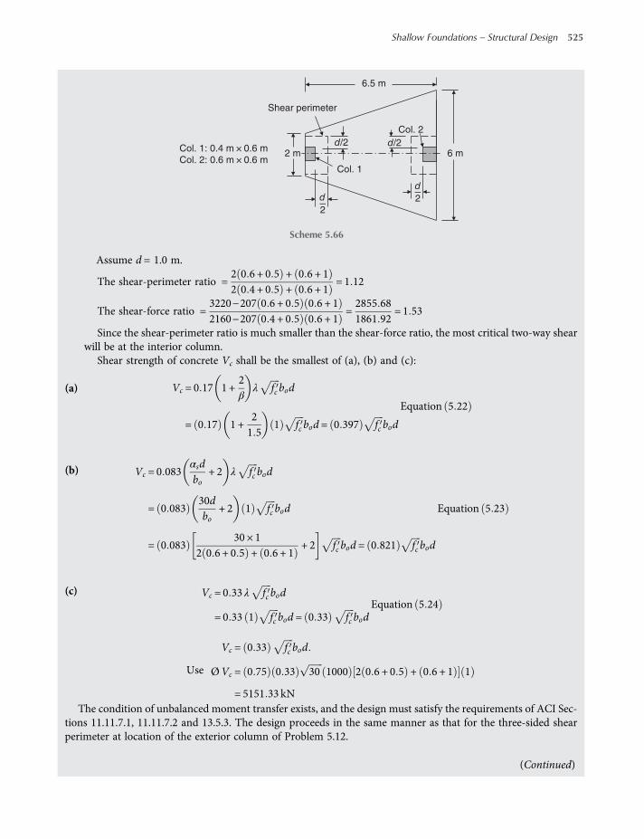
Assume d = 1.0 m.
The shear-perimeter ratio =2 0 6 + 0 5 + 0 6 + 12 0 4 + 0 5 + 0 6 + 1
= 1 12
The shear-force ratio =3220−207 0 6 + 0 5 0 6 + 12160−207 0 4 + 0 5 0 6 + 1
=2855 681861 92
= 1 53
Since the shear-perimeter ratio is much smaller than the shear-force ratio, the most critical two-way shearwill be at the interior column.
Shear strength of concrete Vc shall be the smallest of (a), (b) and (c):
(a) Vc = 0 17 1 +2β
λ fc bod
= 0 17 1 +21 5
1 fc bod = 0 397 fc bod
Equation 5 22
(b) Vc = 0 083αsdbo
+ 2 λ fc bod
= 0 08330dbo
+ 2 1 fc bod
= 0 08330 × 1
2 0 6 + 0 5 + 0 6 + 1+ 2 fc bod = 0 821 fc bod
Equation 5 23
(c) Vc = 0 33 λ fc bod
= 0 33 1 fc bod = 0 33 fc bodEquation 5 24
Use
Vc = 0 33 fc bod
ØVc = 0 75 0 33 30 1000 2 0 6 + 0 5 + 0 6 + 1 1
= 5151 33 kNThe condition of unbalanced moment transfer exists, and the design must satisfy the requirements of ACI Sec-
tions 11.11.7.1, 11.11.7.2 and 13.5.3. The design proceeds in the same manner as that for the three-sided shearperimeter at location of the exterior column of Problem 5.12.
6 m 2 m
Col. 2
Col. 1
6.5 m
22
d/2 d/2
dd
Shear perimeter
Col. 1: 0.4 m × 0.6 m
Col. 2: 0.6 m × 0.6 m
Scheme 5.66
(Continued)
Shallow Foundations – Structural Design 525
worksaccounts.com
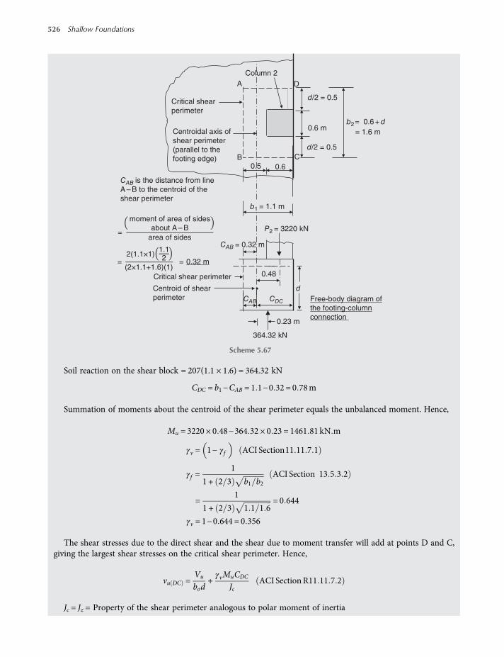
Soil reaction on the shear block = 207(1.1 × 1.6) = 364.32 kN
CDC = b1−CAB = 1 1−0 32 = 0 78m
Summation of moments about the centroid of the shear perimeter equals the unbalanced moment. Hence,
Mu = 3220 × 0 48−364 32 × 0 23 = 1461 81 kN m
γv = 1− γf ACI Section11 11 7 1
γf =1
1 + 2 3 b1 b2ACI Section 13 5 3 2
=1
1 + 2 3 1 1 1 6= 0 644
γv = 1−0 644 = 0 356
The shear stresses due to the direct shear and the shear due to moment transfer will add at points D and C,giving the largest shear stresses on the critical shear perimeter. Hence,
vu DC =Vu
bod+γvMuCDC
JcACI SectionR11 11 7 2
Jc = Jz = Property of the shear perimeter analogous to polar moment of inertia
d/2 = 0.5
d/2 = 0.5
0.23 m
0.48
0.6 m
0.6
A
B C
D
Column 2
Centroid of shear
perimeter
Critical shear perimeter
P2 = 3220 kN
CAB = 0.32 m
= 1.6 m
0.5
Critical shear
perimeter
Centroidal axis of
shear perimeter
(parallel to the
footing edge)
=
moment of area of sides
about A – B
area of sides
CAB is the distance from line
A – B to the centroid of the
shear perimeter
=(2×1.1+1.6)(1)
= 0.32 m
364.32 kN
Free-body diagram of
the footing-column
connection
d
CAB CDC
b1 = 1.1 m
2(1.1×1)1.12
b2= 0.6 + d
Scheme 5.67
526 Shallow Foundations
worksaccounts.com

Jc = 2b1d3
12+ 2
db3112
+ 2 b1db12−CAB
2
+ b2d CAB2
= 21 1 × 13
12+ 2
1 × 1 13
12+ 2 1 1 × 1
1 12
−0 322
+ 1 6 × 1 0 322
= 0 183 + 0 222 + 0 116 + 0 164 = 0 685m4
vu DC =3220−364 322 × 1 1 + 1 6 1
+0 356 × 1461 81 0 78
0 685
= 751 49 + 592 58 = 1344 07 kN m2
Ø vc =ØVc
bod=
5151 332 0 6 + 0 5 + 0 6 + 1 1
= 1355 61 kN m2 > vu DC OK
The factored shear stress vu(DC) is too close to Ø vc (the choice of using d = 1 m was successful), which meansthat two-way shear requires d 1 m, whereas, one-way shear requires d = 0.83 m and, therefore, the two-wayshear controls the footing depth.
Use d = 1.0 m = 1000 mm.The depth d will be taken to the centre of the steel bars in long direction.Assume using No. 29 bars, and 75 mmminimum concrete cover (ACI Section 7.7.1). Hence, the overall footing
thickness is
h= 1000 + 75 + 1 2bar diameter = 1075 + 14 4 = 1089 4mm
Use h = 1010 mm.Step 5. Design the flexural reinforcement in the long direction.
The bending-moment diagram requires that the flexural reinforcement in long direction must be placed attop of the footing. The maximum factored negative moment of 3685 kN.m is located at x = 3.42 m (from the leftface of the exterior column). At this location the footing width is
B = 2 +3 426 5
× 4 = 4 1m
Equation (5.9):ØMn ≥Mu
Mu =3685B
=36854 1
= 899 kN m m
Assume tension-controlled section, Ø = 0.9, and fs = fy.
D
Z
B
A
C d = 0.93 m
b1 = 1.1 m
CAB C
DC
Centroidal
axis
Z b2 =
1.6 m
Scheme 5.68
(Continued)
Shallow Foundations – Structural Design 527
worksaccounts.com
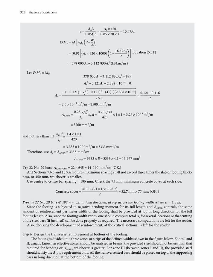
a=Asfy
0 85fc b=
As × 4200 85 × 30 × 1
= 16 47As
ØMn = Ø Asfy d−a2
= 0 9 As × 420 × 1000 1−16 47As
2
= 378 000As−3 112 830As2 kN m m
Equation 5 11
Let ØMn =Mu:378 000As−3 112 830As
2 = 899
As2−0 121As + 2 888 × 10−4 = 0
As =− −0 121 ± −0 121 2− 4 1 2 888 × 10−4
2 × 1=0 121−0 116
2
= 2 5 × 10⁻³ m2 m= 2500mm2 m
As,min =0 25 fc
fybwd =
0 25 30420
× 1 × 1 = 3 26 × 10−3 m2 m
= 3260mm2 m
and not less than 1.4bw dfy
=1 4 × 1 × 1
420
= 3 333 × 10−3 m2 m= 3333mm2 mTherefore, use As = As,min = 3333 mm2/m
As, total = 3333 ×B= 3333 × 4 1 = 13 667mm2
Try 22 No. 29 bars: As,provided = 22 × 645 = 14 190 mm2/m (OK.)ACI Sections 7.6.5 and 10.5.4 requires maximum spacing shall not exceed three times the slab or footing thick-
ness, or 450 mm, whichever is smaller.Use centre to centre bar spacing = 186 mm. Check the 75 mm minimum concrete cover at each side:
Concrete cover =4100− 21 × 186 + 28 7
2= 82 7mm> 75 mm OK
Provide 22 No. 29 bars @ 188 mm c.c. in long direction, at top across the footing width where B = 4.1 m.Since the footing is subjected to negative bending moment for its full length and As,min controls, the same
amount of reinforcement per meter width of the footing shall be provided at top in long direction for the fullfooting length. Also, since the footing width varies, one should compute totalAs for several locations so that cuttingof the steel bars (if justified) can be done properly as required. The necessary computations are left for the reader.
Also, checking the development of reinforcement, at the critical sections, is left for the reader.
Step 6. Design the transverse reinforcement at bottom of the footing.The footing is divided into three zones or strips of the defined widths shown in the figure below. Zones I and
II, usually known as effective zones, should be analysed as beams; the provided steel should not be less than thatrequired for bending or As,min, whichever is greater. For zone III (between zones I and II), the provided steelshould satisfy theAs,min requirement only. All the transverse steel bars should be placed on top of the supportingbars in long direction at the bottom of the footing.
528 Shallow Foundations
worksaccounts.com
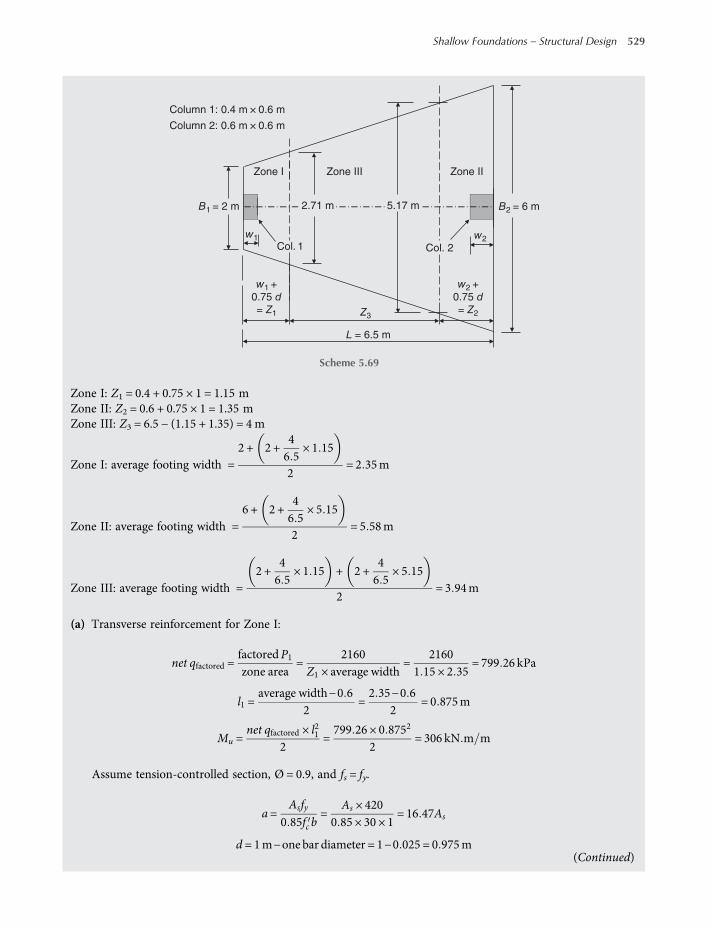
Zone I: Z1 = 0.4 + 0.75 × 1 = 1.15 mZone II: Z2 = 0.6 + 0.75 × 1 = 1.35 mZone III: Z3 = 6.5 − (1.15 + 1.35) = 4 m
Zone I: average footing width =2 + 2 +
46 5
× 1 15
2= 2 35m
Zone II: average footing width =6 + 2 +
46 5
× 5 15
2= 5 58m
Zone III: average footing width =2 +
46 5
× 1 15 + 2 +46 5
× 5 15
2= 3 94m
(a) Transverse reinforcement for Zone I:
net qfactored =factoredP1zone area
=2160
Z1 × average width=
21601 15 × 2 35
= 799 26 kPa
l1 =average width−0 6
2=2 35−0 6
2= 0 875m
Mu =net qfactored × l21
2=799 26 × 0 8752
2= 306 kN m m
Assume tension-controlled section, Ø = 0.9, and fs = fy.
a=Asfy
0 85fc b=
As × 4200 85 × 30 × 1
= 16 47As
d = 1m−one bar diameter = 1−0 025 = 0 975m
B1 = 2 m
L = 6.5 m
Zone I Zone II
Column 1: 0.4 m × 0.6 m
Column 2: 0.6 m × 0.6 m
B2 = 6 m
Zone III
2.71 m 5.17 m
w1
w1 +
0.75 d
= Z1
w2 +
0.75 d
= Z2
w2
Col. 2Col. 1
Z3
Scheme 5.69
(Continued)
Shallow Foundations – Structural Design 529
worksaccounts.com
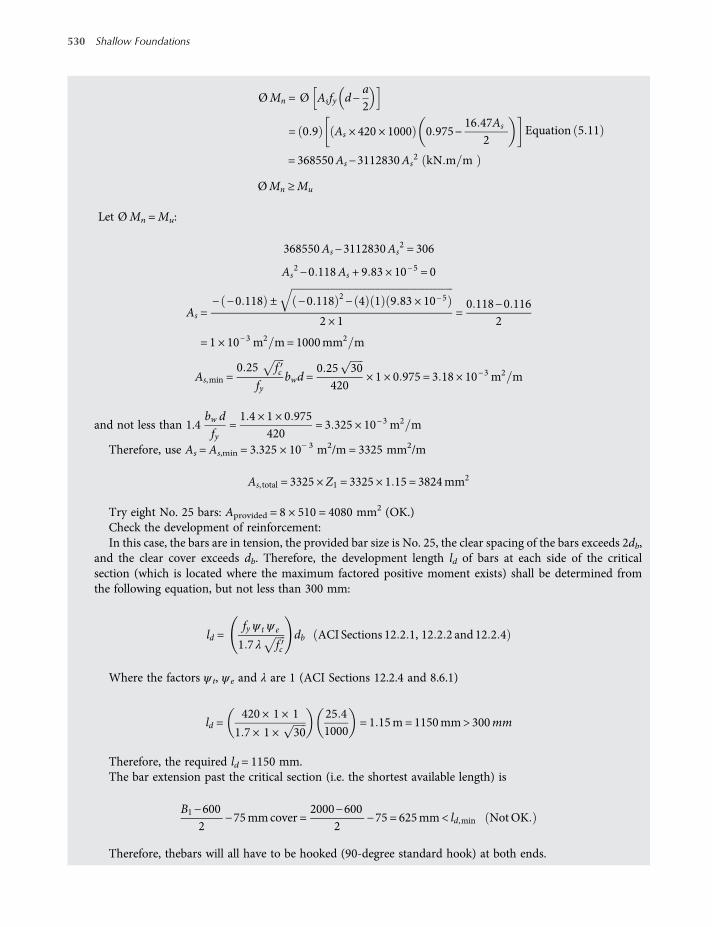
ØMn = Ø Asfy d−a2
= 0 9 As × 420 × 1000 0 975−16 47As
2
= 368550As−3112830As2 kN m m
Equation 5 11
ØMn ≥Mu
Let ØMn =Mu:
368550As−3112830As2 = 306
As2−0 118As + 9 83 × 10
−5 = 0
As =− −0 118 ± −0 118 2− 4 1 9 83 × 10−5
2 × 1=0 118−0 116
2
= 1 × 10⁻³ m2 m= 1000mm2 m
As,min =0 25 fc
fybwd =
0 25 30420
× 1 × 0 975 = 3 18 × 10−3 m2 m
and not less than 1.4bw dfy
=1 4 × 1 × 0 975
420= 3 325 × 10−3 m2 m
Therefore, use As = As,min = 3.325 × 10− 3 m2/m = 3325 mm2/m
As, total = 3325 ×Z1 = 3325 × 1 15 = 3824mm2
Try eight No. 25 bars: Aprovided = 8 × 510 = 4080 mm2 (OK.)Check the development of reinforcement:In this case, the bars are in tension, the provided bar size is No. 25, the clear spacing of the bars exceeds 2db,
and the clear cover exceeds db. Therefore, the development length ld of bars at each side of the criticalsection (which is located where the maximum factored positive moment exists) shall be determined fromthe following equation, but not less than 300 mm:
ld =fy ψ t ψ e
1 7 λ fcdb ACI Sections 12 2 1, 12 2 2 and 12 2 4
Where the factors ψ t, ψ e and λ are 1 (ACI Sections 12.2.4 and 8.6.1)
ld =420 × 1 × 1
1 7 × 1 × 30
25 41000
= 1 15m= 1150mm> 300mm
Therefore, the required ld = 1150 mm.The bar extension past the critical section (i.e. the shortest available length) is
B1−6002
−75mmcover =2000−600
2−75 = 625mm< ld,min NotOK
Therefore, thebars will all have to be hooked (90-degree standard hook) at both ends.
530 Shallow Foundations
worksaccounts.com

Check ldh (ACI Section 12.5.2):
ldh =0 24ψ efyλ fc
db
where the factors ψ e and λ shall be taken as 1.
ldh =0 24 × 1 × 420
1 × 30
25 41000
= 0 47m= 470mm> 8db > 150mm
Therefore, the required ldh = 470 mm.
ldh < 625mm OK
ACI Sections 7.6.5 and 10.5.4 require maximum spacing shall not exceed three times the slab or footingthickness or 450 mm, whichever is smaller.
Use centre-to-centre bar spacing = 150mm. Check the 75 mmminimum concrete cover at the small end ofthe footing:
Concrete cover = 1150−7 × 150−25 42
= 87 3mm> 75mm OK
Provide eight No. 25 bars @ 150 mm c.c. in Zone I, placed at bottom of the footing in the transverse direction.The bars will all have to be hooked (90-degree standard hook) at both ends.
(b) Transverse reinforcement for zone II:
net qfactored =factoredP2zone area
=3220
Z2 × average width=
32201 35 × 5 58
= 427 45 kPa
l2 =average width−0 6
2=5 58−0 6
2= 2 49 m
Mu =net qfactored × l22
2=427 45 × 2 492
2= 1325 12 kN m m
d = 1m−one bar diameter = 1−0 025 = 0 975m
Assume tension-controlled section, Ø = 0.9, and fs = fy.
a=Asfy
0 85fc b=
As × 4200 85 × 30 × 1
= 16 47As
ØMn = Ø Asfy d−a2
= 0 9 As × 420 × 1000 0 975−16 47As
2
= 368 550As−3 112 830As2 kN m m
Equation 5 11
ØMn ≥Mu
Let ØMn =Mu:368 550As−3 112 830As
2 = 1325 12(Continued)
Shallow Foundations – Structural Design 531
worksaccounts.com

As2−0 118As + 4 26 × 10−4 = 0
As =− −0 118 ± −0 118 2− 4 1 4 26 × 10−4
2 × 1=0 118−0 111
2
= 3 5 × 10⁻³ m2 m= 3500mm2 m
As,min =0 25 fc
fybwd =
0 25 30420
× 1 × 0 975 = 3 18 × 10−3 m2 m
and not less than 1.4bw dfy
=1 4 × 1 × 0 975
420= 3 325 × 10−3 m2 m<As
Therefore, use As = 3.5 × 10− 3 m2/m = 3500 mm2/m
As, total = 3500 ×Z2 = 3500 × 1 35 = 4725mm2
Try 10 No. 25 bars: As,provided = 10 × 510 = 5100 mm2 (OK.)
Compute a for As =51001 35
= 3778mm2 m, and check if fs = fy and whether the section is tension-controlled:
a= 16 47As = 16 47 × 3778 × 10−6 = 0 062m= 62mm
c=aβ1. For fc between 17 and 28MPa, β1 shall be taken as 0.85. For fc above 28MPa, β1 shall be reduced linearly at a
rate of 0.05 for each 7 MPa of strength in excess of 28 MPa, but β1 shall not be taken less than 0.65 (ACISection 10.2.7.3).
β1 = 0 85−27× 0 05 = 0 836
c=62
0 836= 74 16mm
dt = d = 975mm
εt = 0 003dt −cc
= 0 003975−74 16
74 16= 0 036 > 0 005
Equation 5 15
Hence, the section is tension-controlled, and Ø = 0.9 (ACI Sections 10.3.4 and 9.3.2.1).
εy =fyEs
=420
200 000= 0 0021
Hence, εt > εy and fs = fy.Therefore, the assumptions made are satisfied.Check the development of reinforcement:
ld =fy ψ t ψ e
1 7 λ fcdb ACI Sections 12 2 1, 12 2 2 and 12 2 4
where the factors ψ t, ψ e and λ are 1 (ACI Sections 12.2.4 and 8.6.1)
ld =420 × 1 × 1
1 7 × 1 × 30
25 41000
= 1 15m= 1150mm> 300mm
532 Shallow Foundations
worksaccounts.com
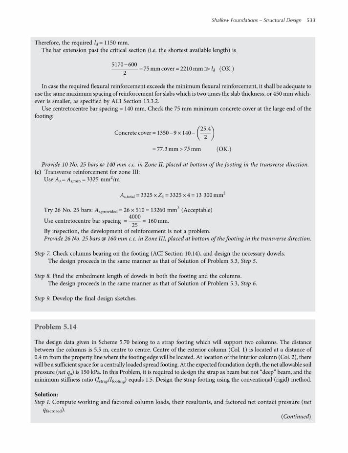
Therefore, the required ld = 1150 mm.The bar extension past the critical section (i.e. the shortest available length) is
5170−6002
−75mmcover = 2210mm ld OK
In case the required flexural reinforcement exceeds the minimum flexural reinforcement, it shall be adequate touse the samemaximum spacing of reinforcement for slabs which is two times the slab thickness, or 450mmwhich-ever is smaller, as specified by ACI Section 13.3.2.
Use centretocentre bar spacing = 140 mm. Check the 75 mm minimum concrete cover at the large end of thefooting:
Concrete cover = 1350−9 × 140−25 42
= 77 3mm> 75mm OK
Provide 10 No. 25 bars @ 140 mm c.c. in Zone II, placed at bottom of the footing in the transverse direction.(c) Transverse reinforcement for zone III:
Use As = As,min = 3325 mm2/m
As, total = 3325 ×Z3 = 3325 × 4 = 13 300mm2
Try 26 No. 25 bars: As,provided = 26 × 510 = 13260 mm2 (Acceptable)
Use centretocentre bar spacing =400025
= 160mm.
By inspection, the development of reinforcement is not a problem.Provide 26 No. 25 bars @ 160 mm c.c. in Zone III, placed at bottom of the footing in the transverse direction.
Step 7. Check columns bearing on the footing (ACI Section 10.14), and design the necessary dowels.The design proceeds in the same manner as that of Solution of Problem 5.3, Step 5.
Step 8. Find the embedment length of dowels in both the footing and the columns.The design proceeds in the same manner as that of Solution of Problem 5.3, Step 6.
Step 9. Develop the final design sketches.
Problem 5.14
The design data given in Scheme 5.70 belong to a strap footing which will support two columns. The distancebetween the columns is 5.5 m, centre to centre. Centre of the exterior column (Col. 1) is located at a distance of0.4 m from the property line where the footing edge will be located. At location of the interior column (Col. 2), therewill be a sufficient space for a centrally loaded spread footing. At the expected foundation depth, the net allowable soilpressure (net qa) is 150 kPa. In this Problem, it is required to design the strap as beam but not “deep” beam, and theminimum stiffness ratio (Istrap/Ifooting) equals 1.5. Design the strap footing using the conventional (rigid) method.
Solution:Step 1. Compute working and factored column loads, their resultants, and factored net contact pressure (net
qfactored).(Continued)
Shallow Foundations – Structural Design 533
worksaccounts.com
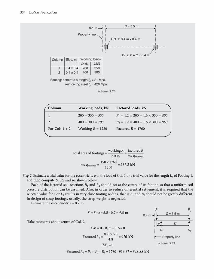
Total area of footings =workingRnet qa
=factoredRnet qfactored
net qfactored =150 × 1760
1250= 211 2 kN
Step 2. Estimate a trial value for the eccentricity e of the load of Col. 1 or a trial value for the length L1 of Footing 1,and then compute S , R1 and R2 shown below.
Each of the factored soil reactions R1 and R2 should act at the centre of its footing so that a uniform soilpressure distribution can be assumed. Also, in order to reduce differential settlement, it is required that theselected value for e or L1 results in very close footing widths, that is B1 and B2 should not be greatly different.In design of strap footings, usually, the strap weight is neglected.
Estimate the eccentricity e = 0.7 m
S = S−e= 5 5−0 7 = 4 8 m
Take moments about centre of Col. 2:
ΣM = 0−R1S −P1S = 0
FactoredR1 =800 × 5 5
4 8= 916 kN
ΣFv = 0
FactoredR2 = P1 + P2−R1 = 1760−916 67 = 843 33 kN
Col. 2: 0.4 m × 0.4 m
Col. 1: 0.4 m × 0.4 m
Property line
0.4 m S = 5.5 m
Column
1
2
Footing: concrete strength f′c = 21 Mpa.
Size, m Working loads
D,kN L,kN
0.4 × 0.4 200 350
3004000.4 × 0.4
reinforcing steel fy = 420 Mpa.
Scheme 5.70
S = 5.5 m0.4 m
P1 P2
R2
e S′
R1
Property line
Scheme 5.71
Column Working loads, kN Factored loads, kN
1 200 + 350 = 550 P1 = 1.2 × 200 + 1.6 × 350 = 800
2 400 + 300 = 700 P2 = 1.2 × 400 + 1.6 × 300 = 960
For Cols 1 + 2 Working R = 1250 Factored R = 1760
534 Shallow Foundations
worksaccounts.com
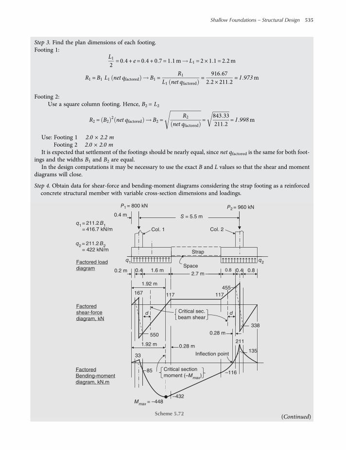
Step 3. Find the plan dimensions of each footing.Footing 1:
L12= 0 4 + e= 0 4 + 0 7 = 1 1m L1 = 2 × 1 1 = 2 2m
R1 = B1 L1 net qfactored B1 =R1
L1 net qfactored=
916 672 2 × 211 2
= 1 973m
Footing 2:Use a square column footing. Hence, B2 = L2
R2 = B22 net qfactored B2 =
R2
net qfactored=
843 33211 2
= 1 998m
Use: Footing 1 2.0 × 2.2 mFooting 2 2.0 × 2.0 m
It is expected that settlement of the footings should be nearly equal, since net qfactored is the same for both foot-ings and the widths B1 and B2 are equal.
In the design computations it may be necessary to use the exact B and L values so that the shear and momentdiagrams will close.
Step 4. Obtain data for shear-force and bending-moment diagrams considering the strap footing as a reinforcedconcrete structural member with variable cross-section dimensions and loadings.
Strap
0.8 0.4
0.4 m
0.4 0.81.6 m
P2 = 960 kN
S = 5.5 m
P1 = 800 kN
Space
2.7 m
q1
= 211.2 B1
= 416.7 kN/m
q1
d d
q2
q2
= 211.2 B2
= 422 kN/m
0.2 m
Col. 1 Col. 2
Factored load
diagram
Factored
shear-force
diagram, kN
167
211
Factored
Bending-moment
diagram, kN.m
0.28 m
–116
135
Mmax
= –448
85
33 Inflection point
117
550
338
4551.92 m
Critical sec.
beam shear
Critical section
moment (–Mmax
)
1.92 m 0.28 m
117
–432
Scheme 5.72 (Continued)
Shallow Foundations – Structural Design 535
worksaccounts.com
It is preferable to draw the complete load diagram first, and then the shear and moment diagrams, as shownabove.
The factored distributed loads on the footings (uniform contact pressure), shear forces and bendingmoments at any location shall be computed for the full width of the member.
Any convenient method, for example integral calculus (with attention to values at the limits), may be used forcalculating the shear and moment values at necessary locations so that informable diagrams are obtained.
If the necessary computations involve tedious busywork, it will be preferable to use an appropriate computerprogram.
Step 5. Find footing thickness h. Determine the required thickness for each footing based on both one-way shearand two-way shear analyses.
(a) One-way shear.Footing 1 (the exterior footing):
The critical section is located at distance d from the interior face of the exterior column, as indicated on theshear-force diagram.
Equation (5.19):ØVc ≥Vu taking reinforcement shear strength,Vs = 0
where Ø = strength reduction factor ACI Section 9 3 2 3
= 0 75 for shear
Vu = 550−416 7d kN
Equation (5.20):Vc = 0 17λ fc bwd
Let ØVc =Vu
0 75 × 0 17 × 1 21 1000 2 d = 550−416 7d
d =5501585
= 0 35m= 350mm
Try d = 0.36 m = 360 mm.Footing 2 (the interior footing):The critical section is located at distance d from the interior face of the interior column, as indicated on the
shear-force diagram.
Vu = 454−422d kN
Let ØVc = Vu:0 75 × 0 17 × 1 21 1000 2 d = 454−422d
d =4541591
= 0 29m= 290mm
This depth is close to that of Footing 1 (only 0.06 m difference); it may be more practical, in this case, to use thesame d for both footings.
Try d = 0.36 m = 360 mm.(b) Two-way shear.
Footing 1 (the exterior footing):Consider the shear perimeter has three sides only.In this case, the condition of unbalanced moment transfer exists, and the design must satisfy the require-
ments of ACI Sections 11.11.7.1, 11.11.7.2 and 13.5.3. The design proceeds in the same manner as that for thethree-sided shear perimeter at location of column1 of Problem 5.12.
536 Shallow Foundations
worksaccounts.com

Assume d = 0.36 m = 360 mm.
CAB is the distance from line A–B to the centroid of the shear perimeter
=
moment of area of sides
aboutA-B
area of sides=2 0 78 × 0 36 0 78 22 × 0 78 + 0 76 0 36
= 0 26m
Soil reaction on the shear block = 211.2(0.78 × 0.76) = 125.2 kNSummation of moments about the centroid of the shear perimeter equals the unbalanced momentMu. Hence,Mu = 800 × 0.12 − 125.2 × 0.13 = 80 kN. m
γv = 1− γf ACI Section 11 11 7 1
γf =1
1 + 2 3 b1 b2
=1
1 + 2 3 0 78 0 76= 0 60
γv = 1−0 6 = 0 4
The shear stresses due to the direct shear and the shear due to moment transfer will add at points D and C,giving the largest shear stresses on the critical shear perimeter. Hence,
vu DC =Vu
bod+γvMuCDC
JcACI SectionR11 11 7 2
d/2 = 0.18
d/2 = 0.18
0.4 m
0.4
A
B C
D
Column 1
b2 = 0.4 + d
= 0.76 m
Critical shear perimeter
Centroidal axis of shear
perimeter (parallel to
the footing edge)
b1 = 0.78
0.2 m 0.18 m
Scheme 5.73
0.39
0.40
Centroid of shear
perimeter
Critical shear perimeter
CAB = 0.26 m
0.12
125.2 kN
Free-body diagram of the
footing-column connection0.13 m
800 kN
d
Scheme 5.74
(Continued)
Shallow Foundations – Structural Design 537
worksaccounts.com
Jc = Jz = Property of the shear perimeter analogous to polar moment of inertia
Jc = 2b1d3
12+ 2
db3112
+ 2 b1db12−CAB
2
+ b2d CAB2
= 20 78 × 0 363
12+ 2
0 36 × 0 783
12+ 2 0 78 × 0 36
0 782
−0 262
+
0 76 × 0 36 0 262 = 0 0061 + 0 0285 + 0 0095 + 0 0185 = 0 063m4
Vu = 800−125 2 = 674 8 kN
CDC = b1−CAB = 0 78−0 26 = 0 52m
vu DC =674 8
2 × 0 78 + 0 76 0 36+0 4 × 80 × 0 52
0 063= 807 95 + 264 13
= 1072 1 kN m2
Ø vc ≥ vu DC
Ø vc =ØVc
bod
Shear strength of concrete Vc shall be the smallest of (i), (ii) and (iii):
(i) Vc = 0 17 1 +2β
λ fc bod
= 0 17 1 +21
1 fc bod = 0 51 fc bod
Equation 5 22
(ii) Vc = 0 083αsdbo
+ 2 λ fc bod
= 0 08330 × 0 36
2 0 78 + 0 76+ 2 fc bod = 0 46 fc bod
Equation 5 23
(iii) Vc = 0 33 λ fc bod
= 0 33 1 fc bod = 0 33 fc bodEquation 5 24
Use Vc = 0 33 fc bod
ØVc = 0 75 0 33 21 1000 bod = 1134 2 bod kN
Ø vc =1134 2 bod
bod= 1134 2 kN m2 > vu DC OK
Footing 2 (the interior footing):The footing is concentrically loaded, and the shear perimeter has four sides, as shown below.
538 Shallow Foundations
worksaccounts.com
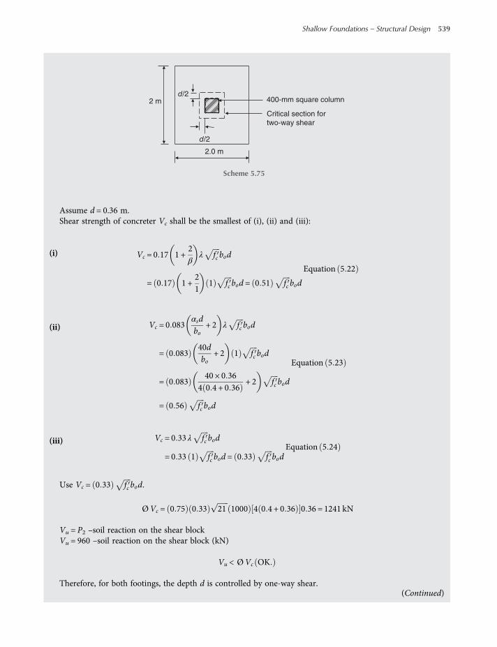
Assume d = 0.36 m.Shear strength of concreter Vc shall be the smallest of (i), (ii) and (iii):
(i) Vc = 0 17 1 +2β
λ fc bod
= 0 17 1 +21
1 fc bod = 0 51 fc bod
Equation 5 22
(ii) Vc = 0 083αsdbo
+ 2 λ fc bod
= 0 08340dbo
+ 2 1 fc bod
= 0 08340 × 0 36
4 0 4 + 0 36+ 2 fc bod
= 0 56 fc bod
Equation 5 23
(iii) Vc = 0 33 λ fc bod
= 0 33 1 fc bod = 0 33 fc bodEquation 5 24
Use Vc = 0 33 fc bod.
ØVc = 0 75 0 33 21 1000 4 0 4 + 0 36 0 36 = 1241 kN
Vu = P2 –soil reaction on the shear blockVu = 960 –soil reaction on the shear block (kN)
Vu < ØVc OK
Therefore, for both footings, the depth d is controlled by one-way shear.
d/2
Critical section for
two-way shear
d/2
2.0 m
400-mm square column 2 m
Scheme 5.75
(Continued)
Shallow Foundations – Structural Design 539
worksaccounts.com
Assume using No. 19 bars, with 75mmminimum concrete cover (ACI Section 7.7.1). Hence, the overall footingthickness is
h= 360 + 75 +12bar diameter = 435 +
19 12
= 444 6mm
Therefore, for both footings, use:d = 0 36m = 360mm
h = 450 mm.
Step 6. Design theflexural reinforcement for each footing.(a) Footing 1 (the exterior footing).
It is expected that the strap depth will be larger than that of the footings, since the design requires the strap-footing stiffness ratio not be less than 1.5. In such a case, it is usual practice to extend the strap beam over thefootings to the columns. Thus, Footing 1, actually, acts as a wall footing, cantilevering out on the two sides ofthe strap. Therefore, the main flexural reinforcement at the footing bottom shall be the transverse reinforce-ment only (i.e. one-way footing). Obviously, shrinkage and temperature reinforcement shall be provided nor-mal to the flexural reinforcement (ACI Sections 7.12.1 and 7.12.2.1). As indicated by the bending-momentdiagram, the footing is subjected to negative moments in long direction. This moment will be resisted bythe strap top bars, since the strap extends over the footing to Column 1.
Transverse flexural positive reinforcement:Design the footing reinforcement as a spread footing. Consider the critical section located at the face of
Column 1 (not the strap face so that conservative design is achieved), as shown below.
ØMn ≥Mu
The maximum factored moment is
Mu =net qfactored ℓ
2
2=211 2 × 0 82
2= 68 kN m m
Assume tension-controlled section, Ø = 0.9 and fs = fy.
a=Asfy
0 85fc b=
As × 4200 85 × 21 × 1
= 23 53As
d = 0 36m
ØMn = Ø Asfy d−a2
= 0 9 As × 420 × 1000 0 36−23 53As
2
= 136 080As−4 447 170As2 kN m m
Equation 5 11
= 0.8 m
Critical section
for moment
Strap
2.2 m
400-mm square
column 2 m
Scheme 5.76
540 Shallow Foundations
worksaccounts.com
Let ØMn =Mu:
136 080As−4 447 170As2 = 68
4 447 170As2−136 080As + 68 = 0
As2−0 031As + 1 529 × 10−5 = 0
As =− −0 031 ± −0 031 2− 4 1 1 529 × 10−5
2 × 1=0 0310−0 0299
2
= 550 × 10−6 m2 m= 550mm2 m
As,min = 0 0018 bh= 0 0018 × 1 × 0 45 = 810 × 10−6 m2 m
= 810mm2 m>As
Use As = As,min = 810 mm2/mThe assumptions made are satisfied, since As required = As,min.
As, total =As × L1 = 810 × 2 2 = 1782mm2
Try nine No.16 bars: As,provided = 9 × 199 = 1791 mm2 (OK.)Check the development of reinforcement:In this case, the bars are in tension, the provided bar size is smaller than No. 19, the clear spacing of the bars
exceeds 2db, and the clear cover exceeds db. Therefore, the development length ld of bars at each side of the criticalsection (which is the same critical section for moment) shall be determined from the following equation, but notless than 300 mm:
ld =fy ψ t ψ e
2 1 λ fcdb ACI Sections 12 2 1, 12 2 2 and 12 2 4
where the factors ψ t, ψ e and λ are 1. (ACI Sections 12.2.4 and 8.6.1)
ld =420 × 1 × 1
2 1 × 1 × 21
15 91000
= 0 694m= 694mm> 300mm
Therefore, the required ld = 694 mm.The bar extension past the critical section (i.e. the available length) is
800mm−75mmcover = 725mm> 694mm OK
ACI Sections 7.6.5 and 10.5.4 requires maximum spacing shall not exceed three times the slab or footing thick-ness or 450 mm, whichever is smaller.
Use centretocentre bar spacing = 253 mm. Check the 75 mm minimum concrete cover at each side:
Concrete cover =2200−8 × 253−15 9
2= 80mm> 75mm OK
Provide nine No. 16 bars @ 253 mm c.c., placed at bottom of the footing in the transverse direction.(Continued)
Shallow Foundations – Structural Design 541
worksaccounts.com
Shrinkage and temperature reinforcement:This reinforcement shall be provided, in long direction, normal to the flexural reinforcement (ACI Sections
7.12.1 and 7.12.2.1).Total
As = 0 0018 bh= 0 0018 × 2 × 0 45 = 1620 × 10−6 m2
= 1620mm2
Try nine No.16 bars: As,provided = 9 × 199 = 1791 mm2 (OK.)According to ACI Section 7.12.2.2, shrinkage and temperature reinforcement shall be spaced not farther apart
than five times the slab thickness, nor farther apart than 450 mm.Use centre-to-centre bar spacing = 229 mm. Check the 75 mm minimum concrete cover at each side:
Concrete cover =2000−8 × 229−15 9
2= 76mm> 75mm OK
Provide nine No. 16 @ 229mm c.c. in the long direction, placed on top of the transverse reinforcement at bottom ofthe footing.
Longitudinal flexural negative reinforcement:As mentioned earlier, this reinforcement will be provided by the strap top bars (see design of the strap later).
(b) Footing 2 (the interior footing).Dimension of Footing 2 in both directions is the same as the transverse dimension of Footing 1(i.e.
B = 2 m); the design contact pressure for both footings is the same (i.e. net qfactored = 211.2 kPa); the columnshave the same cross-section dimensions (i.e. 0.4 m × 0.4 m); the same d, fc and fy are used in design of bothfootings. For these reasons, the same amount of flexural positive reinforcement which was computed for Foot-ing 1 shall also be used for Footing 2 and in both directions.
Use centre-to-centre bar spacing = 229 mm. Check the 75 mm minimum concrete cover at each side:
Concrete cover =2000−8 × 229−15 9
2= 76mm> 75mm OK
As indicated by the bending-moment diagram, a small portion of the footing is subjected to a smallnegative moment. This moment will be resisted by the strap top bars, since the strap extends over the footingto Column 2.
Provide nine No. 16 @ 229 mm c.c.,placed at bottom of the footing in both directions.Step 7. Check column bearing on each footing (ACI Section 10.14), and design the necessary dowels.
Proceed in the same manner as that of Solution of Problem 5.3, Step 5.
Step 8. Find the embedment length of dowels in both the footing and the column for each column-footing joint.Proceed in the same manner as that of Solution of Problem 5.3, Step 6.
Step 9. Design the strap as a reinforced concrete structural beam.This design step involves findingb, d and As. Bending-moment and shear-force diagrams indicate that the
strap must be designed for a negative moment of 432 kN.m and a shear force of 117 kN. However, this designmoment is too close to the maximum negative moment (448 kN.m) and it would be conservative if the latter isused for design. In order to compute the cross-section dimensions b and d, it may be necessary to select a trialsteel ratio ρ. For Grade-420 reinforcement and fc values between 21 and 35MPa, it may be appropriate to start abeam design by assuming that ρ 0.01. This choice or assumption of ρ value, generally, is economical, givesdesirable level of structural ductility and assures easy placement of reinforcement.
The required strap-footing minimum stiffness ratio of 1.5 will be a factor in selecting a minimum value forthe strap height h. Also, if the designer wants to avoid deflection calculations, ACI Section 9.5.2.1 and ACITable 9.5(a) require h≥ ℓ
16. Furthermore, it is required the strap shall be designed as beam but not “deep” beam,
542 Shallow Foundations
worksaccounts.com
which requires h < ℓn4 (ACI Section 10.7).Taking all these factors into consideration, the strap may be designed
as follows:Assume tension-controlled section, Ø = 0.9, and fs = fy.Equation (5.10):
a=Asfy
0 85fc b
If we substitute As = ρbd into Equation (5.10), we get
a =ρfyfc
d0 85
Equation (5.12):
ØMn = Ø 0 85fc ba d−a2
If we substitute a=ρfyfc
d0 85
into Equation (5.12), we get
ØMn = Ø 0 85fc bρfyfc
d0 85
d−ρfy2fc
d0 85
Hence, for fc = 21MPa, fy = 420 MPa, ρ = 0.01
ØMn = Ø 0 85 × 21 b0 01 × 420d21 × 0 85
d−0 01 × 420d2 × 21 × 0 85
= Ø bd2 4 2 1−4 235 7
= 3 706Ø bd2 MN m
=3706Ø bd2 kN m
Mu = 448 kN m
ØMn ≥Mu
Let ØMn =Mu:
3706Ø bd2 = 448
bd2 =448
3706 × 0 9= 0 134m3; b=
0 134d2
m
The strap width b should be at least equal to the smaller width of the columns. Therefore, use b ≥ 0.4 m, or,bmin = 0.40 m.
Assume b = 0.40 m. Hence, d =0 1340 4
= 0 52 m.
According to ACI Section10.7, deep beams have ℓn ≤ 4 h.The strap clear span ℓn = 2.7 m.Let ℓn = 4 h:
h=2 74
= 0 675m(Continued)
Shallow Foundations – Structural Design 543
worksaccounts.com

It is required to design the strap as beam but not “deep” beam. Therefore, the overall strap depth or height hmust be smaller than 0.675 m.
Assume: h = 0.67 m; concrete cover = 0.08 m. Hence,
d = 0 67−0 08 = 0 59m> d = 0 52m
Try: h= 0 67m d = 0 59m b= 0 40mCheck the minimum stiffness ratio:
IstrapIfooting
=
bh3
12 strap
bh3 12 footing
=0 4 ×
0 673
122 × 0 453 12
= 0 66 1 5 Not OK
Increase the strap width and check the stiffness ratioagain.Try b = 0.9 m:
bd3
12 strap
bd3 12 footing
=0 9 ×
0 673
122 × 0 453 12
= 1 49 1 5 Acceptable
Check deflection of the strap beam:According to ACI Section 9.5.2.1 and ACI Table 9.5(a), for a simple beam constructed with structural normal-
weight concrete and Grade 420 reinforcement, not supporting or attached to partitions or other construction likely
to be damaged by large deflections, theminimum overall depth or h to avoid deflection calculations isℓ
16, where ℓ is
the span length of the beam. In this case, the individual footings are supporting the strap, and it may be appropriateto let ℓ represent the distance between the footings, centre to centre, which is 4.8 m.Therefore,
ℓ
16=4 816
= 0 3m< h= 0 67m . Therefore, deflections should not be a problem.
Use a strap beam with b = 0.90 m, d = 0.59 m and h = 0.67 m.Flexural reinforcement at the top of the strap:
ØMn ≥Mu
Mu = 448 kN m
Assume tension-controlled section, Ø = 0.9, and fs = fy.
a=Asfy
0 85fc b=
As × 4200 85 × 21 × 0 9
= 26 14As m
ØMn = Ø 0 85fc ba d−a2
= 0 9 0 85 × 21 × 1000 0 9 × 26 14As 0 59−26 14As
2
= 222 988As−4 939 744A2s kN m
Let ØMn =Mu:222 988As−4939 744A
2s = 448
A2s −45 14 × 10−3As + 9 07 × 10−5 = 0
544 Shallow Foundations
worksaccounts.com

As =− −45 14 × 10−3 ± −45 14 × 10−3 2−4 × 1 × 9 07 × 10−5
2 × 1= =
0 04514−0 040922
= 2 11 × 10−3 m2 = 2110mm2
As,min =0 25 fc
fybwd =
0 25 21420
× 0 9 × 0 59 = 1 448 × 10−3 m2
= 1448mm2
and not less than 1.4bw dfy
=1 4 × 0 9 × 0 59
420= 1 77 × 10−3 m2 = 1770mm2
Use As = 2110 mm2
Try six No. 22 bars: As,provided = 6 × 387 = 2322 mm2 (OK.)Compute a for As = 2322 mm2 and check if fs = fy and whether the section is tension-controlled:
a= 26 14As = 26 14 × 2322 × 10−6 = 0 061m= 61mm
c=aβ1; For fc between 17 and 28 MPa, β1 shall be taken as 0.85
c=610 85
= 71 8mm
dt = d = 590mm
εt = 0 003dt −cc
= 0 003590−71 8
71 8= 0 022 > 0 005 Equation 5 15
Hence, the section is tension-controlled, and Ø = 0.9 (ACI Sections 10.3.4 and 9.3.2.1).
εy =fyEs
=420
200000= 0 0021. Hence, εt > εy and fs = fy.
Therefore the assumptions made are satisfied.Because εt = 0.022 exceeds 0.004, the strap section satisfies the definition of beam in ACI Section 10.3.5.It may be a good practice to compute ØMn to check whether the provided As is adequate. This checking guards
against errors in computations. Thus,
ØMn = Ø 0 85fc ba d−a2
= 0 9 × 0 85 × 21 × 1000 × 0 9 × 0 061 0 59−0 0612
= 493 kN m> Mu = 448 kN m OK
Provide six No. 22 bars at the top of the strap in one layer.Check the development of reinforcement:In this case, the bars are in tension, the provided bar size is No. 22, the clear spacing of the bars exceeds 2db, and
the clear cover exceeds db. Therefore, the development length ld of bars at each side of the critical section (which islocated where the maximum factored negative moment exists) shall be determined from the following equation,but not less than
ld =fy ψ t ψ e
1 7 λ fcdb (ACI Sections 12.2.1, 12.2.2 and 12.2.4)
where the factors ψ e and λ are 1 (ACI Sections 12.2.4 and 8.6.1). (Continued)
Shallow Foundations – Structural Design 545
worksaccounts.com
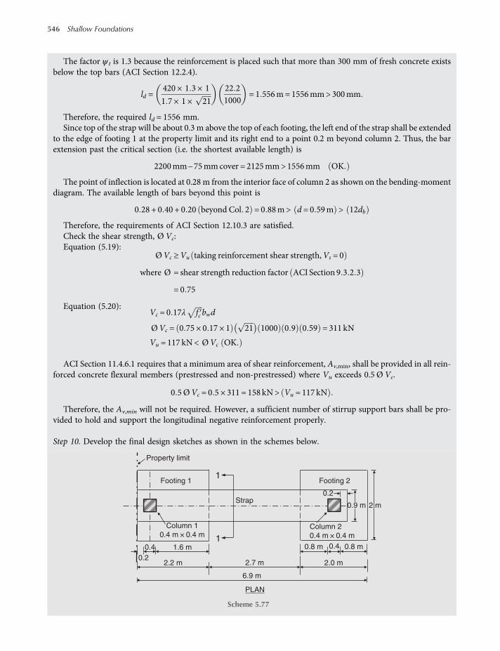
The factor ψ t is 1.3 because the reinforcement is placed such that more than 300 mm of fresh concrete existsbelow the top bars (ACI Section 12.2.4).
ld =420 × 1 3 × 1
1 7 × 1 × 21
22 21000
= 1 556m= 1556mm> 300mm
Therefore, the required ld = 1556 mm.Since top of the strap will be about 0.3 m above the top of each footing, the left end of the strap shall be extended
to the edge of footing 1 at the property limit and its right end to a point 0.2 m beyond column 2. Thus, the barextension past the critical section (i.e. the shortest available length) is
2200mm−75mmcover = 2125mm>1556mm OK
The point of inflection is located at 0.28 m from the interior face of column 2 as shown on the bending-momentdiagram. The available length of bars beyond this point is
0 28 + 0 40 + 0 20 beyond Col 2 = 0 88m> d = 0 59m > 12db
Therefore, the requirements of ACI Section 12.10.3 are satisfied.Check the shear strength, Ø Vc:Equation (5.19):
ØVc ≥Vu taking reinforcement shear strength,Vs = 0
where Ø = shear strength reduction factor ACI Section 9 3 2 3
= 0 75
Equation (5.20):Vc = 0 17λ fc bwd
ØVc = 0 75 × 0 17 × 1 21 1000 0 9 0 59 = 311 kN
Vu = 117 kN< ØVc OK
ACI Section 11.4.6.1 requires that a minimum area of shear reinforcement, Av,min, shall be provided in all rein-forced concrete flexural members (prestressed and non-prestressed) where Vu exceeds 0.5 Ø Vc.
0 5ØVc = 0 5 × 311 = 158 kN> Vu = 117 kN
Therefore, the Av,min will not be required. However, a sufficient number of stirrup support bars shall be pro-vided to hold and support the longitudinal negative reinforcement properly.
Step 10. Develop the final design sketches as shown in the schemes below.
2.7 m
Property limit
1.6 m
2.0 m2.2 m
Strap
6.9 m
PLAN
0.4 0.8 m0.8 m
0.2
0.41
1
2 m
Footing 1 Footing 2
Column 1
0.4 m × 0.4 mColumn 2
0.4 m × 0.4 m
0.9 m
0.2
Scheme 5.77
546 Shallow Foundations
worksaccounts.com
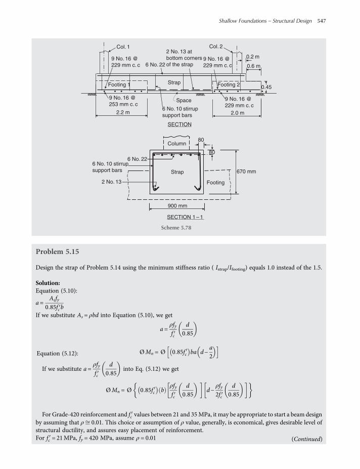
Problem 5.15
Design the strap of Problem 5.14 using the minimum stiffness ratio ( Istrap/Ifooting) equals 1.0 instead of the 1.5.
Solution:Equation (5.10):
a=Asfy
0 85fc bIf we substitute As = ρbd into Equation (5.10), we get
a =ρfyfc
d0 85
Equation (5.12): ØMn = Ø 0 85fc ba d−a2
If we substitute a=ρfyfc
d0 85
into Eq. (5.12) we get
ØMn = Ø 0 85fc bρfyfc
d0 85
d−ρfy2fc
d0 85
For Grade-420 reinforcement and fc values between 21 and 35MPa, it may be appropriate to start a beam designby assuming that ρ 0.01. This choice or assumption of ρ value, generally, is economical, gives desirable level ofstructural ductility, and assures easy placement of reinforcement.For fc = 21MPa, fy = 420 MPa, assume ρ = 0.01 (Continued)
0.6 m
0.2 m
Strap
2.0 m
9 No. 16 @
253 mm c. c
2.2 m
9 No. 16 @
229 mm c. c6 No. 10 stirrup
support bars
SECTION
SECTION 1 – 1
Space
Col. 1 Col. 2
9 No. 16 @
229 mm c. c9 No. 16 @
229 mm c. c6 No. 22
Footing 2Footing 1
2 No. 13 at
bottom corners
of the strap
0.45
80
80
670 mm
Footing
900 mm
2 No. 13
6 No. 10 stirrup
support bars
6 No. 22
Column
Strap
Scheme 5.78
Shallow Foundations – Structural Design 547
worksaccounts.com

ØMn = Ø 0 85 × 21 b0 01 × 420d21 × 0 85
d−0 01 × 420d2 × 21 × 0 85
= Ø bd2 4 2 1−4 235 7
= 3 706Ø bd2 MN m
=3706Ø bd2 kN m
Mu = 448 kN.m (see the B.M.D. of Solution of Problem 5.14, Step 4)
ØMn ≥Mu
Let ØMn =Mu:
3706Ø bd2 = 448
Assume tension-controlled section, Ø = 0.9.
bd2 =448
3706 × 0 9= 0 134m3
The strap width b should be at least equal to the smaller width of the columns. Therefore, use b ≥ 0.4 m orbmin = 0.40 m. Assume b = 0.40 m. Hence,
d =0 1340 4
= 0 52m
According to ACI Section10.7, deep beams have ℓn ≤ 4 h.Strap clear span ℓn = 2.7 m, and the overall strap depth or height h = d + 0.080 (assumed).
Let ℓn = 4 h. Hence, h=2 74
= 0 675m If a deep strap is not required, the strap height h should be decreased.
Assume hmax = 0.67 m. Hence,
dmax = 0 67−0 08 = 0 59m> d = 0 52m
Try h = 0.67 m, d = 0.59 m and b = 0.40 m. Check the required strap-footing stiffness ratio, (Istrap/Ifooting) ≥ 1.
IstrapIfooting
=
bh3
12strap
bh3 12footing
=0 4 ×
0 673
122 × 0 453 12
= 0 66 < 1 (Not OK.)
Increase the strap width and check the stiffness ratioagain.Try b = 0.6 m:
bd3
12 strap
bd3 12 footing
=0 6 ×
0 673
122 × 0 453 12
= 0 99 1 0 Acceptable
Check deflection of the strap beam:According to ACI Section 9.5.2.1 and ACI Table 9.5(a), for a simple beam constructed with structural normal-weight concrete and Grade 420 reinforcement, not supporting or attached to partitions or other construction likely
to be damaged by large deflections, theminimum overall depth or h to avoid deflection calculations isℓ
16, where ℓ is
the span length of the beam. In this case, the individual footings are supporting the strap, and it may be appropriateto let ℓ represent the distance between the footings, centre to centre, which is 4.8 m,ℓ
16=4 816
= 0 3m< h= 0 67m . Therefore, deflections should not be a problem.
548 Shallow Foundations
worksaccounts.com
Use h = 0.67 m, d = 0.59 m and b = 0.6 m.Compute the area of reinforcement, As:Assume tension-controlled section, Ø = 0.9 and fs = fy.
a=As fy
0 85fc b=
As × 4200 85 × 21 × 0 6
= 39 22As m
ØMn = Ø 0 85fc ba d−a2
= 0 9 0 85 × 21 × 1000 0 6 × 39 22As 0 59−39 22As
2
= 223 045As−7 413 395A2s kN m
Mu = 448 kN m
ØMn ≥Mu
Let ØMn =Mu:223 045As−7 413 395A2
s = 448
A2s −0 03As + 6 04 × 10−5 = 0
As =− −0 03 ± −0 03 2−4 × 1 × 6 04 × 10−5
2 × 1=0 03−0 02857
2
= 2 17 × 10−3 m2 = 2170mm2
As,min =0 25 fc
fybwd =
0 25 21420
× 0 6 × 0 59 = 9 66 × 10−4 m2
= 966mm2
and not less than: 1 4bw dfy
=1 4 × 0 6 × 0 59
420= 1 18 × 10−3 m2
= 1180mm2
Use As = 2170 mm2
Try six No. 22 bars: As,provided = 6 × 387 = 2322 mm2 (OK.)Compute a for As = 2322 mm2 and check if fs = fy and whether the section is tension-controlled:
a= 39 22As = 39 22 × 2322 × 10−6 = 0 091m= 91mm
c=aβ1; For fc between 17 and 28 MPa, β1 shall be taken as 0.85
c=910 85
= 107 06mm; dt = d = 590mm
εt = 0 003dt −cc
= 0 003590−107 06
107 06= 0 014 > 0 005
Equation 5 15
Hence, the section is tension-controlled, and Ø = 0.9 (ACI Sections 10.3.4 and 9.3.2.1).
εy =fyEs
=420
200000= 0 0021. Hence, εt > εy and fs = fy. (Continued)
Shallow Foundations – Structural Design 549
worksaccounts.com

Therefore the assumptions made are satisfied.Because εt = 0.014 exceeds 0.004, the strap section satisfies the definition of beam in ACI Section 10.3.5.
It may be a good practice to compute ØMn to check whether the provided As is adequate. This checking guardsagainst errors in computations. Thus,
ØMn = Ø 0 85fc ba d−a2
= 0 9 × 0 85 × 21 × 1000 × 0 6 × 0 091 0 59−0 0912
= 478 kN m> Mu = 448 kN m
OK
Provide six No. 22 bars at the top of the strap in one layer.
Check the development of reinforcement:The check proceeds exactly in the same manner as that for the strap of Problem 5.14; its repetition isunnecessary.Check the shear strength, Ø Vc:Equation (5.19):
ØVc ≥Vu taking reinforcement shear strength, Vs = 0
where Ø = shear strength reduction factor ACI Section 9 3 2 3
= 0 75Equation (5.20):
Vc = 0 17λ fc bwd
ØVc = 0 75 × 0 17 × 1 21 1000 0 6 0 59 = 206 8 kN
Vu = 117 kN< ØVc OK
However, ACI Section 11.4.6.1 requires that a minimum area of shear reinforcement,Av,min, shall be provided inall reinforced concrete flexural members (prestressed and non-prestressed) where Vu exceeds0.5 ØVc.0.5 ØVc = 0.5 × 206.8 = 103.4 kN < (Vu = 117 kN).
Therefore, Av,min is required.Try No.10 double-leg stirrups (fyt = 300 MPa) with standard 135 stirrup hooks.
Av = 2 × 71 = 142mm2
Anchorage of stirrups:
ACI Sections 7.1.3 and 12.13.2.1 allow No. 25 and smaller stirrups to be anchored by standard90 or 135 stirruphooks. The stirrup legs should be hooked around longitudinal bars.
Provide two No. 13 bars in the lower corners of the strap cross-section to anchor the stirrups properly.Stirrups spacing, s.
(a) Based on the strap depth d:According to ACI Section 11.4.5.1, spacing of shear reinforcement perpendicular to axis of member shall not
exceed the smaller of d/2 of the member and 600 mm.
550 Shallow Foundations
worksaccounts.com
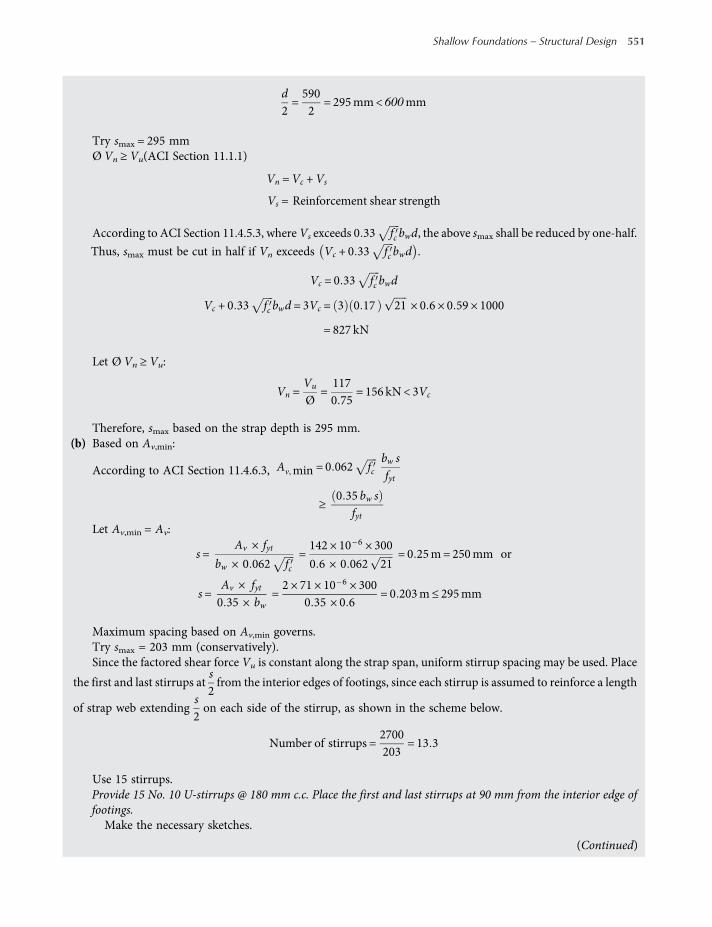
d2=5902
= 295mm< 600mm
Try smax = 295 mmØ Vn ≥ Vu(ACI Section 11.1.1)
Vn =Vc +Vs
Vs = Reinforcement shear strength
According to ACI Section 11.4.5.3, whereVs exceeds 0 33 fc bwd, the above smax shall be reduced by one-half.
Thus, smax must be cut in half if Vn exceeds Vc + 0 33 fc bwd .
Vc = 0 33 fc bwd
Vc + 0 33 fc bwd = 3Vc = 3 0 17 21 × 0 6 × 0 59 × 1000
= 827 kN
Let Ø Vn ≥Vu:
Vn =Vu
Ø=1170 75
= 156 kN< 3Vc
Therefore, smax based on the strap depth is 295 mm.(b) Based on Av,min:
According to ACI Section 11.4.6.3, Av, min = 0 062 fcbw sfyt
≥0 35 bw s
fytLet Av,min = Av:
s=Av × fyt
bw × 0 062 fc=142 × 10−6 × 300
0 6 × 0 062 21= 0 25m= 250mm or
s=Av × fyt0 35 × bw
=2 × 71 × 10−6 × 300
0 35 × 0 6= 0 203m ≤ 295mm
Maximum spacing based on Av,min governs.Try smax = 203 mm (conservatively).Since the factored shear force Vu is constant along the strap span, uniform stirrup spacing may be used. Place
the first and last stirrups ats2from the interior edges of footings, since each stirrup is assumed to reinforce a length
of strap web extendings2on each side of the stirrup, as shown in the scheme below.
Number of stirrups =2700203
= 13 3
Use 15 stirrups.Provide 15 No. 10 U-stirrups @ 180 mm c.c. Place the first and last stirrups at 90 mm from the interior edge offootings.
Make the necessary sketches.
(Continued)
Shallow Foundations – Structural Design 551
worksaccounts.com
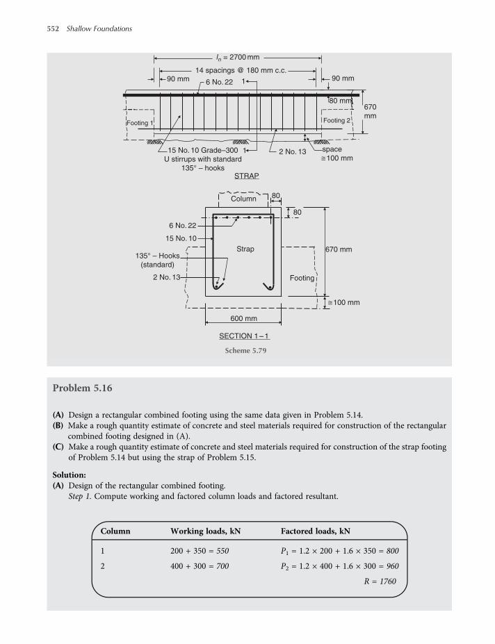
Problem 5.16
(A) Design a rectangular combined footing using the same data given in Problem 5.14.(B) Make a rough quantity estimate of concrete and steel materials required for construction of the rectangular
combined footing designed in (A).(C) Make a rough quantity estimate of concrete and steel materials required for construction of the strap footing
of Problem 5.14 but using the strap of Problem 5.15.
Solution:(A) Design of the rectangular combined footing.
Step 1. Compute working and factored column loads and factored resultant.
Column Working loads, kN Factored loads, kN
1 200 + 350 = 550 P1 = 1.2 × 200 + 1.6 × 350 = 800
2 400 + 300 = 700 P2 = 1.2 × 400 + 1.6 × 300 = 960
R = 1760
Footing 2
90 mm
Footing 1
90 mm14 spacings @ 180 mm c.c.
ln = 2700 mm
space
100 mm
6 No. 22 1
1
2 No. 13 15 No. 10 Grade–300
U stirrups with standard
135° – hooks
670
mm
80 mm
Strap 670 mm
Footing
15 No. 10
6 No. 22
600 mm
STRAP
SECTION 1 – 1
Column
100 mm
80
80
2 No. 13
135° – Hooks
(standard)
Scheme 5.79
552 Shallow Foundations
worksaccounts.com

Step 2. Estimate the footing dimensions and net qfactored.
The factored resultant R is located at
X =0 4 × P1 + 0 4 + 5 5 P2
R=0 4 × 800 + 5 9 960
1760= 3 4m
LetL2=X
L= 2 × 3 4 = 6 8m
Area of footingAf =working Rnet qa
=550 + 700
150= 8 33m2
B=Af
L=8 336 8
= 1 225m
With these B and L dimensions the footing appears like a beam supporting columns, which is, usually,undesirable. Therefore, it may be more adequate if a wider footing is provided.
Let us, arbitrarily, use B = 2.0 m:
Af = 2 × 6 8 = 13 6m2 > 8 33m2
net q=workingR
Af=125013 6
= 92 kPa net qa OK
Check eccentricity of unfactored R:
X =0 4 550 + 5 9 700
1250=43501250
= 3 48m
eccentricity e=X−L2
= 3 48−3 40 = 0 08m Acceptable
Average net qfactored =factoredR
Af=176013 6
= 129 41 kPa
Use 2.0 × 6.8 m rectangular combined footing.Step 3. Obtain data for shear-force and bending-moment diagrams considering the combined footing as a rein-
forced concrete beam.
Property line
0.4 m5.5 m
R
L/2
P1P2
X
Centroid
L
Scheme 5.80
(Continued)
Shallow Foundations – Structural Design 553
worksaccounts.com

It is preferable to draw the complete load diagram first, and then the shear and moment diagrams, asshown below. The factored distributed loads on the footing, shear forces and bending moments shall becomputed for the full 2.0-m width of the footing.
q= net qfactored ×B
= 129 41 × 2 = 258 82 kN m
L = 6.8 m
x = 3.09 m
x = 3.09 m
104
644
675727
233
105
63
–35
696
21
–113
Factored
shear-force
diagram.kN
Factored
Bending-moment
diagram,kN.m
Factored load
diagram
Inflection point
@ x = 5.75 m
5.5 m0.4 m
5.1 m0.40.2 m 0.4 0.7
Col.1 Col.2
Rectangular combined footing
0.9 m
Critical sec.
beam shear
Critical section for
moment (Mmax)
Mmax = – 1076 kN. m
q = 258.85
kN/m
q
x
P1 = 800 kN
y
P2 = 960 kN
d
Scheme 5.81
554 Shallow Foundations
worksaccounts.com

Step 4. Find footing thickness h.Determine the required thickness based on both one-way shear and two-way shear analyses.
(a) One-way shear. It is critical at distance d from the interior face of the interior column (Col. No. 2), asindicated on the shear-force diagram.
Vu = 675−258 82 d kN
Equation (5.19):
ØVc ≥Vu taking reinforcement shear strength,Vs = 0
where Ø = strength reduction factor ACI Section 9 3 2 3
= 0 75 for shear
Equation (5.20): Vc = 0 17λ fc bwd
Let ØVc =Vu
0 75 × 0 17 × 1 21 1000 2 d = 675−258 82 d
d =675
1427 38= 0 473m= 473mm
Try d = 0.5 m = 500 mm
(b) Two-way shear at location of each column. If it is not very clear at which column this shear is most critical,both locations should be considered. One may detect location of the most critical shear by comparing theshear-perimeter ratio with the shear-force ratio.
The shear perimeter at Column 1 (the exterior column) has three sides only, whereas at Column 2 (theinterior column) it has four sides, as shown in the scheme below.
Assume using d = 0.5 m, as required by one-way shear.
The shear-perimeter ratio =2 0 2 + 0 4 + 0 25 + 0 4 + 0 5
4 0 4 + 0 5= 0 72
The shear-force ratio =800−129 41 0 2 + 0 4 + 0 25 0 4 + 0 5
960−129 41 0 4 + 0 5 0 4 + 0 5=
701855 18
= 0 82
Since the shear-perimeter ratio is smaller than the shear-force ratio, themost critical shear will probably beat column 1. Furthermore, there will be an increase in applied shear stress at Column 1 due to transfer ofunbalanced moment. However, for completeness, we will check two-way shear at location of each column.
0.2 m
/
Column No.1:
0.4 m × 0.4 m
Column No.2:
0.4 m × 0.4 m
L = 6.8 m
B = 2.0 m
Col.1
d/2d/2
d/2d/2
Col.2
Scheme 5.82
(Continued)
Shallow Foundations – Structural Design 555
worksaccounts.com
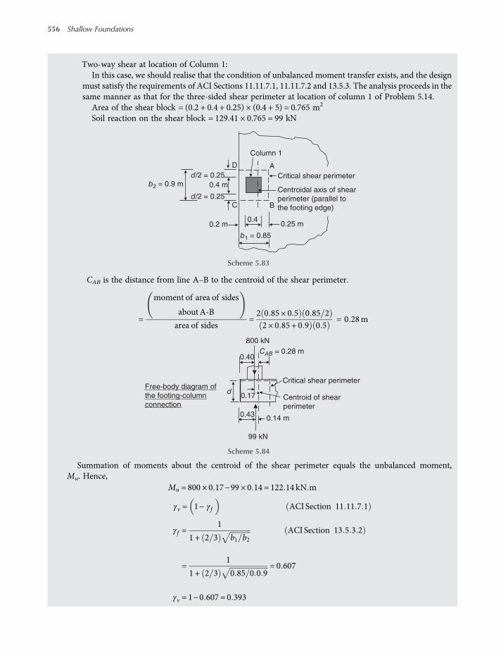
Two-way shear at location of Column 1:In this case, we should realise that the condition of unbalanced moment transfer exists, and the design
must satisfy the requirements of ACI Sections 11.11.7.1, 11.11.7.2 and 13.5.3. The analysis proceeds in thesame manner as that for the three-sided shear perimeter at location of column 1 of Problem 5.14.
Area of the shear block = (0.2 + 0.4 + 0.25) × (0.4 + 5) = 0.765 m2
Soil reaction on the shear block = 129.41 × 0.765 = 99 kN
CAB is the distance from line A–B to the centroid of the shear perimeter.
=
moment of area of sides
aboutA-B
area of sides=2 0 85 × 0 5 0 85 22 × 0 85 + 0 9 0 5
= 0 28m
Summation of moments about the centroid of the shear perimeter equals the unbalanced moment,Mu. Hence,
Mu = 800 × 0 17−99 × 0 14 = 122 14 kN m
γv = 1− γf ACI Section 11 11 7 1
γf =1
1 + 2 3 b1 b2ACI Section 13 5 3 2
=1
1 + 2 3 0 85 0 0 9= 0 607
γv = 1−0 607 = 0 393
d/2 = 0.25
d/2 = 0.25
0.4 m
0.4
A
BC
D
Column 1
b2 = 0.9 m
b1 = 0.85
Critical shear perimeter
Centroidal axis of shear
perimeter (parallel to
the footing edge)
0.2 m 0.25 m
Scheme 5.83
0.43
0.40
dCentroid of shear
perimeter
Critical shear perimeter
0.17
99 kN
Free-body diagram of
the footing-column
connection
0.14 m
800 kN
CAB = 0.28 m
Scheme 5.84
556 Shallow Foundations
worksaccounts.com
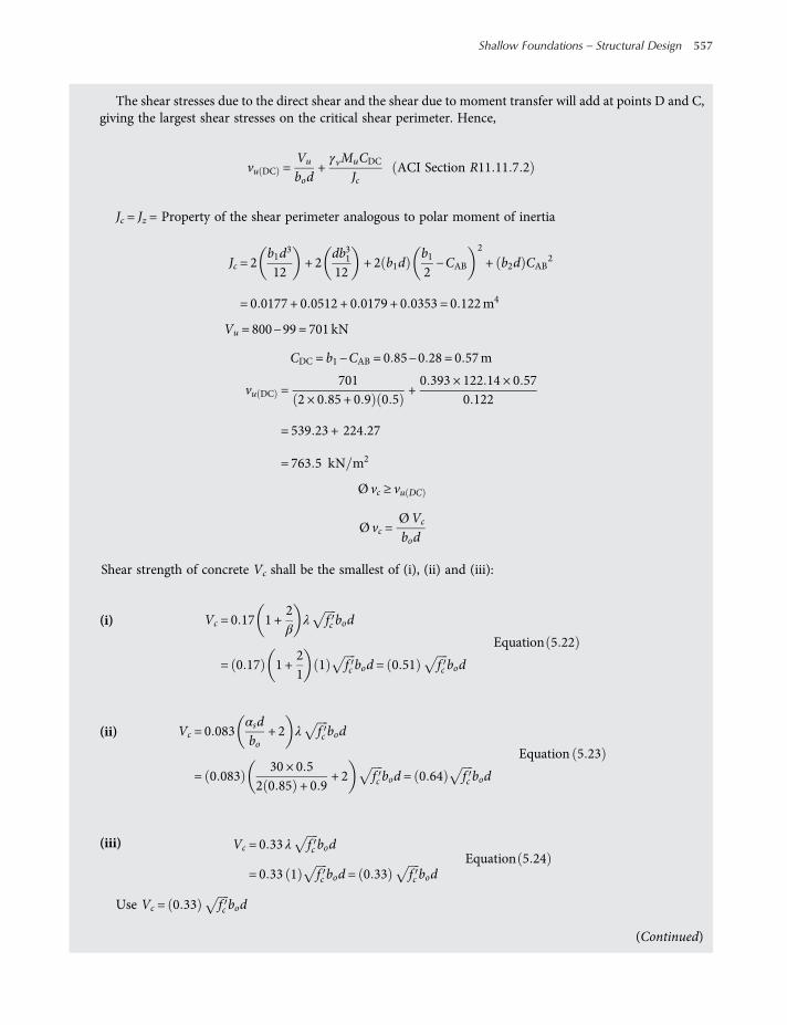
The shear stresses due to the direct shear and the shear due to moment transfer will add at points D and C,giving the largest shear stresses on the critical shear perimeter. Hence,
vu DC =Vu
bod+γvMuCDC
JcACI Section R11 11 7 2
Jc = Jz = Property of the shear perimeter analogous to polar moment of inertia
Jc = 2b1d3
12+ 2
db3112
+ 2 b1db12−CAB
2
+ b2d CAB2
= 0 0177 + 0 0512 + 0 0179 + 0 0353 = 0 122m4
Vu = 800−99 = 701 kN
CDC = b1−CAB = 0 85−0 28 = 0 57m
vu DC =701
2 × 0 85 + 0 9 0 5+0 393 × 122 14 × 0 57
0 122
= 539 23 + 224 27
= 763 5 kN m2
Ø vc ≥ vu DC
Ø vc =ØVc
bod
Shear strength of concrete Vc shall be the smallest of (i), (ii) and (iii):
(i) Vc = 0 17 1 +2β
λ fc bod
= 0 17 1 +21
1 fc bod = 0 51 fc bod
Equation 5 22
(ii) Vc = 0 083αsdbo
+ 2 λ fc bod
= 0 08330 × 0 5
2 0 85 + 0 9+ 2 fc bod = 0 64 fc bod
Equation 5 23
(iii) Vc = 0 33 λ fc bod
= 0 33 1 fc bod = 0 33 fc bodEquation 5 24
Use Vc = 0 33 fc bod
(Continued)
Shallow Foundations – Structural Design 557
worksaccounts.com
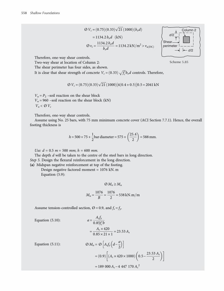
ØVc = 0 75 0 33 21 1000 bod
= 1134 2 bod kN
Ø vc =1134 2 bod
bod= 1134 2 kN m2 > vu DC
Therefore, one-way shear controls.Two-way shear at location of Column 2:The shear perimeter has four sides, as shown.It is clear that shear strength of concrete Vc = 0 33 fc bod controls. Therefore,
ØVc = 0 75 0 33 21 1000 4 0 4 + 0 5 0 5 = 2041 kN
Vu = P2 –soil reaction on the shear blockVu = 960 –soil reaction on the shear block (kN)
Vu < ØVc
Therefore, one-way shear controls.Assume using No. 25 bars, with 75 mm minimum concrete cover (ACI Section 7.7.1). Hence, the overall
footing thickness is
h= 500 + 75 +12bar diameter = 575 +
25 42
= 588mm
Use: d = 0.5 m = 500 mm; h = 600 mm.The depth d will be taken to the centre of the steel bars in long direction.
Step 5. Design the flexural reinforcement in the long direction.(a) Midspan negative reinforcement at top of the footing.
Design negative factored moment = 1076 kN. mEquation (5.9):
ØMn ≥Mu
Mu =1076B
=10762
= 538 kN m m
Assume tension-controlled section, Ø = 0.9, and fs = fy.
Equation (5.10): a=Asfy
0 85fc b
=As × 420
0 85 × 21 × 1= 23 53As
Equation (5.11): ØMn = Ø Asfy d−a2
= 0 9 As × 420 × 1000 0 5−23 53 As
2
= 189 000As−4 447 170 As2
Shear
perimeter
Column 2
d/2
d/2
Scheme 5.85
558 Shallow Foundations
worksaccounts.com
Let ØMn =Mu:189 000As−4 447 170As
2 = 538
As2−42 5 × 10⁻³As + 1 21 × 10−4 = 0
As =− −42 5 × 10⁻³ ± −42 5 × 10⁻³ 2− 4 1 1 21 × 10−4
2 × 1=0 0425−0 0364
2
= 3 05 × 10−3 m2 m= 3050mm2 m
ACI Section 10.5.1:
As,min =0 25 fc
fybwd =
0 25 21420
× 1 × 0 5 = 1 364 × 10−3 m2 m
= 1364mm2 m
and not less than 1.4bw dfy
=1 4 × 1 × 0 5
420= 1 667 × 10−3
m2
m= 1667mm2 m
Therefore, use As = 3050 mm2/m
TotalAs = 3050 ×B= 3050 × 2 = 6100mm2
Try 12 No. 25 bars. As,provided = 12 × 510 = 6120 mm2 (OK.)
Compute a for As =61202
= 3060mm2 m, and check if fs = fy and
whether the section is tension-controlled:
a= 23 53As = 23 53 × 3060 × 10−6 = 0 072m= 72mm
c=aβ1. For fc between 17 and 28 MPa, β1 shall be taken as 0.85. For fc above 28 MPa, β1 shall be reduced
linearly at a rate of 0.05 for each 7 MPa of strength in excess of 28 MPa, but β1 shall not be taken less than 0.65(ACI Section 10.2.7.3).
c=720 85
= 84 71mm
dt = d = 500mm
εt = 0 003dt −cc
= 0 003500−84 71
84 71= 0 015 > 0 005
Equation 5 15
Hence, the section is tension-controlled, and Ø = 0.9 (ACI Sections 10.3.4 and 9.3.2.1).
εy =fyEs
=420
200 000= 0 0021. Hence, εt > εy and fs = fy
Therefore the assumptions made are satisfied.In case the required flexural reinforcement exceeds the minimum flexural reinforcement, it shall be
adequate to use the same maximum spacing of reinforcement for slabs which is two times the slab thicknessor 450 mm, whichever is smaller, as specified by ACI Section 13.3.2.
(Continued)
Shallow Foundations – Structural Design 559
worksaccounts.com
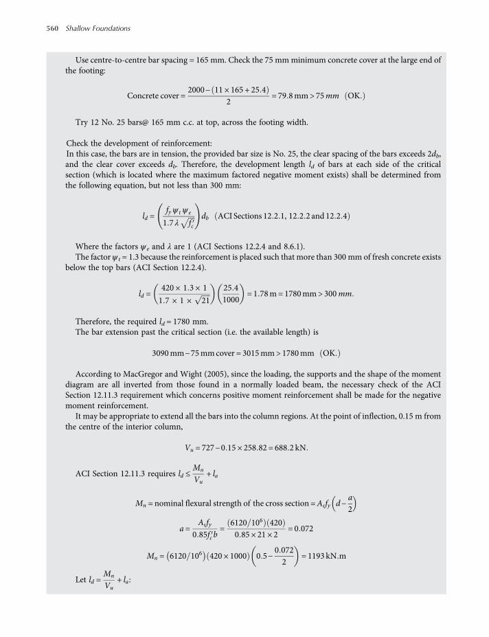
Use centre-to-centre bar spacing = 165 mm. Check the 75 mmminimum concrete cover at the large end ofthe footing:
Concrete cover =2000− 11 × 165 + 25 4
2= 79 8mm> 75mm OK
Try 12 No. 25 bars@ 165 mm c.c. at top, across the footing width.
Check the development of reinforcement:In this case, the bars are in tension, the provided bar size is No. 25, the clear spacing of the bars exceeds 2db,and the clear cover exceeds db. Therefore, the development length ld of bars at each side of the criticalsection (which is located where the maximum factored negative moment exists) shall be determined fromthe following equation, but not less than 300 mm:
ld =fy ψ t ψ e
1 7 λ fcdb ACI Sections 12 2 1, 12 2 2 and 12 2 4
Where the factors ψ e and λ are 1 (ACI Sections 12.2.4 and 8.6.1).The factor ψ t = 1.3 because the reinforcement is placed such that more than 300 mm of fresh concrete exists
below the top bars (ACI Section 12.2.4).
ld =420 × 1 3 × 1
1 7 × 1 × 21
25 41000
= 1 78m= 1780mm> 300mm
Therefore, the required ld = 1780 mm.The bar extension past the critical section (i.e. the available length) is
3090mm−75mmcover = 3015mm> 1780mm OK
According to MacGregor and Wight (2005), since the loading, the supports and the shape of the momentdiagram are all inverted from those found in a normally loaded beam, the necessary check of the ACISection 12.11.3 requirement which concerns positive moment reinforcement shall be made for the negativemoment reinforcement.
It may be appropriate to extend all the bars into the column regions. At the point of inflection, 0.15 m fromthe centre of the interior column,
Vu = 727−0 15 × 258 82 = 688 2 kN
ACI Section 12.11.3 requires ld ≤Mn
Vu+ la
Mn = nominal flexural strength of the cross section =Asfy d−a2
a=Asfy
0 85fc b=
6120 106 4200 85 × 21 × 2
= 0 072
Mn = 6120 106 420 × 1000 0 5−0 0722
= 1193 kN m
Let ld =Mn
Vu+ la:
560 Shallow Foundations
worksaccounts.com
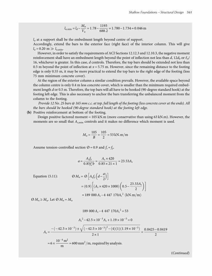
la,min = ld −Mn
Vu= 1 78−
1193688 2
= 1 780−1 734 = 0 046m
la at a support shall be the embedment length beyond centre of support.Accordingly, extend the bars to the exterior face (right face) of the interior column. This will givela = 0.20 m la,min.
However, in order to satisfy the requirements of ACI Sections 12.12.3 and 12.10.3, the negative momentreinforcement shall have an embedment length beyond the point of inflection not less than d, 12db or ℓn/16, whichever is greater. In this case, d controls. Therefore, the top bars should be extended not less than0.5 m beyond the point of inflection at x = 5.75 m. However, since the remaining distance to the footingedge is only 0.55 m, it may be more practical to extend the top bars to the right edge of the footing (less75 mm minimum concrete cover).
At the region of the exterior column a similar condition prevails. However, the available space beyondthe column centre is only 0.4 m less concrete cover, which is smaller than the minimum required embed-ment length d or 0.5 m. Therefore, the top bars will all have to be hooked (90-degree standard hook) at thefooting left edge. This is also necessary to anchor the bars transferring the unbalanced moment from thecolumn to the footing.
Provide 12 No. 25 bars @ 165 mm c.c. at top, full length of the footing (less concrete cover at the ends). Allthe bars should be hooked (90-degree standard hook) at the footing left edge.
(b) Positive reinforcement at bottom of the footing.Design positive factored moment = 105 kN.m (more conservative than using 63 kN.m). However, the
moments are so small that As,min controls and it makes no difference which moment is used.
Mu =105B
=1052
= 53 kN m m
Assume tension-controlled section Ø = 0.9 and fs = fy.
a=Asfy
0 85fc b=
As × 4200 85 × 21 × 1
= 23 53As
Equation (5.11): ØMn = Ø Asfy d−a2
= 0 9 As × 420 × 1000 0 5−23 53As
2
= 189 000As−4 447 170As2 kN m m
ØMn ≥Mu. Let ØMn =Mu
189 000As−4 447 170As2 = 53
As2−42 5 × 10⁻³As + 1 19 × 10−5 = 0
As =− −42 5 × 10⁻³ ± −42 5 × 10⁻³ 2− 4 1 1 19 × 10−5
2 × 1=0 0425−0 0419
2
= 6 ×10⁻⁴ m2
m= 600mm2 m, required by analysis
(Continued)
Shallow Foundations – Structural Design 561
worksaccounts.com

ACI Section 10.5.1:
As,min =0 25 fc
fybwd =
0 25 21420
× 1 × 0 5 = 1 364 × 10−3 m2 m
= 1364mm2 m
and not less than:
1 4bw dfy
=1 4 × 1 × 0 5
420= 1 667 × 10−3 m2 m= 1667mm2 m
Therefore, As,min controls. However, ACI Section 10.5.3 states that the requirements of ACI Section 10.5.1need not be applied if, at every section, As provided is at least one-third greater than that required by analysis.
Accordingly, total As,min = (1.33 × 600)(B) = 800 × 2 = 1600 mm2.Try 6 No. 19 bars: As,provided = 6 × 284 = 1704 mm2 (OK.)ACI Sections 7.6.5 and 10.5.4 requires maximum spacing shall not exceed three times the slab or footing
thickness, or 450 mm, whichever is smaller.Use centre to centre bar spacing = 365 mm. Check the 75 mm minimum concrete cover at each side:
Concrete cover =2000− 5 × 365 + 19 1
2= 78mm> 75mm OK
Try six No. 19 bars @ 364 mm c.c. at bottom, across the footing width.
Check the development of reinforcement:In this case, the bars are in tension, the provided bar size is No. 19, the clear spacing of the bars exceeds 2db,
and the clear cover exceeds db. Therefore, the development length ld of bars at each side of the criticalsection (which is located where the maximum factored positive moment exists) shall be determined fromthe following equation, but not less than 300 mm:
ld =fy ψ t ψ e
2 1 λ fcdb ACI Sections 12 2 1, 12 2 2 and 12 2 4
Where the factors ψ t ψ e, λ and are 1 (ACI Sections 12.2.4 and 8.6.1).
ld =420 × 1 × 1
2 1 × 1 × 21
19 11000
= 0 83m= 830mm> 300mm
Therefore, the required ld = 830 mm.The bar extension past the critical section (i.e. the available length) is
900mm−75mmcover = 825mm<830mm NotOK
Therefore, all the bottom bars in long direction have to be hooked (90-degree standard hook) at the footingright edge.
In order to satisfy the requirements of ACI Sections 12.10.3 and 12.11.3, it is necessary to extend the bottombars a minimum distance d past the point of inflection. Therefore, cut off two bottom bars at 1.0 m from thecenter of the interior column toward the exterior column. The otherfour bars shall be extended full length ofthe footing (less75 mm cover at each end). These four bars will resist the tensile stresses due to the relativelysmall positive moment at the exterior column and provide support to the transverse bottom bars.
562 Shallow Foundations
worksaccounts.com
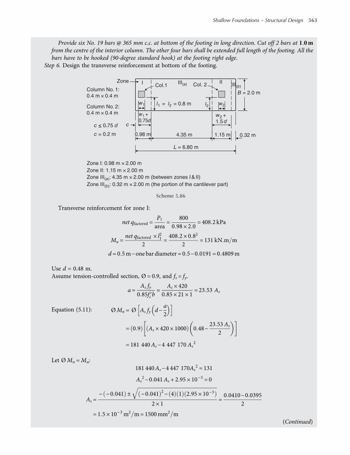
Provide six No. 19 bars @ 365 mm c.c. at bottom of the footing in long direction. Cut off 2 bars at 1 0mfrom the centre of the interior column. The other four bars shall be extended full length of the footing. All thebars have to be hooked (90-degree standard hook) at the footing right edge.
Step 6. Design the transverse reinforcement at bottom of the footing.
Transverse reinforcement for zone I:
net qfactored =P1area
=800
0 98 × 2 0= 408 2 kPa
Mu =net qfactored × l21
2=408 2 × 0 82
2= 131 kN m m
d = 0 5m−one bar diameter = 0 5−0 0191 = 0 4809m
Use d = 0.48 m.Assume tension-controlled section, Ø = 0.9, and fs = fy.
a=As fy
0 85fc b=
As × 4200 85 × 21 × 1
= 23 53 As
Equation (5.11): ØMn = Ø As fy d−a2
= 0 9 As × 420 × 1000 0 48−23 53As
2
= 181 440As−4 447 170 As2
Let ØMn =Mu:181 440As−4 447 170As
2 = 131
As2−0 041As + 2 95 × 10
−5 = 0
As =− −0 041 ± −0 041 2− 4 1 2 95 × 10−5
2 × 1=0 0410−0 0395
2
= 1 5 × 10⁻³ m2 m= 1500mm2 m
1.15 m
Col.1
c = 0.2 m
c ≤ 0.75 d.
l1 = l2 = 0.8 m
I II
0.32 m4.35 m0.98 m
Zone
Zone I: 0.98 m × 2.00 m
Zone II: 1.15 m × 2.00 m
Zone III(a): 4.35 m × 2.00 m (between zones I & II)
Zone III(b): 0.32 m × 2.00 m (the portion of the cantilever part)
III(a)
Column No. 1:
0.4 m × 0.4 m
Column No. 2:
0.4 m × 0.4 m
c
Col. 2
l2 w2w1
w2 +
1.5 d
w1 +
0.75d
L = 6.80 m
B = 2.0 m
III(b)
Scheme 5.86
(Continued)
Shallow Foundations – Structural Design 563
worksaccounts.com
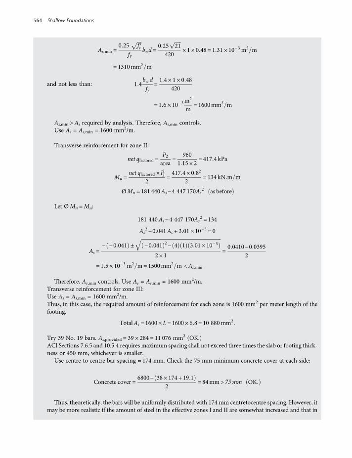
As,min =0 25 fc
fybwd =
0 25 21420
× 1 × 0 48 = 1 31 × 10−3 m2 m
= 1310mm2 m
and not less than: 1 4bw dfy
=1 4 × 1 × 0 48
420
= 1 6 × 10⁻³m2
m= 1600mm2 m
As,min > As required by analysis. Therefore, As,min controls.Use As = As,min = 1600 mm2/m.
Transverse reinforcement for zone II:
net qfactored =P2area
=960
1 15 × 2= 417 4 kPa
Mu =net qfactored × l22
2=417 4 × 0 82
2= 134 kN m m
ØMn = 181 440As−4 447 170As2 as before
Let ØMn =Mu:
181 440As−4 447 170As2 = 134
As2−0 041As + 3 01 × 10
−5 = 0
As =− −0 041 ± −0 041 2− 4 1 3 01 × 10−5
2 × 1=0 0410−0 0395
2
= 1 5 × 10⁻³ m2 m= 1500mm2 m <As,min
Therefore, As,min controls. Use As = As,min = 1600 mm2/m.Transverse reinforcement for zone III:Use As = As,min = 1600 mm2/m.Thus, in this case, the required amount of reinforcement for each zone is 1600 mm2 per meter length of thefooting.
TotalAs = 1600 × L = 1600 × 6 8 = 10 880mm2
Try 39 No. 19 bars. As,provided = 39 × 284 = 11 076 mm2 (OK.)ACI Sections 7.6.5 and 10.5.4 requires maximum spacing shall not exceed three times the slab or footing thick-ness or 450 mm, whichever is smaller.
Use centre to centre bar spacing = 174 mm. Check the 75 mm minimum concrete cover at each side:
Concrete cover =6800− 38 × 174 + 19 1
2= 84mm> 75mm OK
Thus, theoretically, the bars will be uniformly distributed with 174 mm centretocentre spacing. However, itmay be more realistic if the amount of steel in the effective zones I and II are somewhat increased and that in
564 Shallow Foundations
worksaccounts.com
zone III decreased. We shall do this by arbitrarily decreasing and increasing the bar spacing in the three zonesbut without decreasing the required total steel amount, as follows:
Zone I: seven No.19 bars; six spacings @ 147 mm c.c.Zones II+ Zone III(b): 11 No.19 bars;10 spacings @ 137 mm c.c.Zone III(a): 21 No.19 bars;20 spacings @ 216 mm c.c.
Check the development of reinforcement:In this case, the bars are in tension, the provided bar size is No. 19, the clear spacing of the bars exceeds 2db, andthe clear cover exceeds db. Therefore, the development length ld of bars at each side of the criticalsection (which is located where the maximum factored positive moment exists) shall be determined fromthe following equation, but not less than 300 mm.
ld =fy ψ t ψ e
2 1 λ fcdb ACI Sections 12 2 1, 12 2 2 and 12 2 4
where the factors ψ t, ψ e and λ are 1 (ACI Sections 12.2.4 and 8.6.1)
ld =420 × 1 × 1
2 1 × 1 × 21
19 11000
= 0 83m= 830mm> 300mm
Therefore, the required ld = 830 mm.The bar extension past the critical section (i.e. the available length) is
800mm−75mmcover = 725mm< 830mm NotOK
Therefore, all the bottom transverse bars have to be hooked at both ends.The bottom transverse bars will all have to be hooked (90-degree standard hook) at both ends.Because two-way shear cracks would extend roughly the entire width of the footing, the hooked transverse bars
provide adequate anchorage outside the inclined cracks (MacGregor and Wight, 2005).Step7. Check columns bearing on the footing (ACI Section 10.14), and design the necessary dowels.
The design proceeds in the same manner as that of Solution of Problem 5.3, Step 5.Step8. Find the embedment length of dowels in both the footing and the columns.
The design proceeds in the same manner as that ofSolution of Problem 5.3, Step 6.Step 9. Develop the final design sketches.
(B) and (C) Rough quantity estimate of concrete and steel materials.
Table 5.7 Quantity estimates of concrete and steel materials.
Material Rectangular combined footing
Strap footing
Footing 1 andFooting 2 Strap Total
Concrete, m3
(fc = 21 MPa)0.6 × 2.0 × 6.8 = 8.16 0.45(2 × 2.2 + 2 × 2) =
3.780.67 × 0.6 × 2.7 + 0.32 ×0.6 × 3.6 = 1.7
5.48
Steel, kg (fy =420 MPa)
(12)(6.8 – 0.15 + 12 × 0.0254)(4) = 339(2)(1.9 – 0.075 + 12 × 0.0191)(2.24) = 9(4)(6.8 – 0.15 + 12 × 0.0191)(2.24) = 62(39)(2 – 0.15 + 24 × 0.0191)(2.24) = 202
Total (339 + 9 + 62 + 202) = 612
(3 × 9)(2.0 – 0.15)(1.55) = 77
(9)(2.2 – 0.15)(1.55) =29
Total (77 + 29) = 106
(6)(6.2 – 0.15)(3.04) = 110
(20)(0.56)(2 × 0.57 + 1 ×0.5 + 24 × 0.01) = 21
(2)(6.2 – 0.15)(0.994) = 12
Total (110 + 21 + 12) = 143
249
Shallow Foundations – Structural Design 565
worksaccounts.com

Problem 5.17
Design the reinforced concrete cantilever retaining wall in the scheme shown below to provide lateral support for arecreational park. In the required length of the wall, the largest wall height above the ground level (in front thewall) is 2 m. Factors such as soil bearing capacity, depth of frost penetration and seasonal volume change requirethe base (footing) be placed at a foundation depth D = 1.2 m, as shown in the scheme. It is required the wall shallhave a front batter not less than 1H : 48V and thickness at top = 0.3 m. Other given data are:Surcharge: qs = 10 kPa.
Backfill material: compacted granular backfill in the limited zone over the heel, which will be compacted toγ = 17 kN/m3 and an estimated Ø = 35 .
Supporting soil: clay of γ = 18 kN/m3, qu = 200 kPa, cu = 100 kPa and Ø = 0 .Wall stability : SF against overturning should not be less than 2.0.
SF against sliding should not be less than 1.5.Concrete: fc = 21 MPaReinforcing steel: fy = 420MPa
Solution:Step 1. Select tentative values for the base dimensions, stem thickness and toe distance. For this purpose, it is common
to use the following approximate relationships as a guide (based on experience accumulated with stable walls):Base widthB = (0.4 to 0.7)H, whereH is the total height of the retaining wall including the footing. In this case,
H = 2.0 + 1.2 = 3.2m
Base thickness h=112
to110
H
Stem bottom thickness b hToe distance l B/3Assume the following dimensions:
B = 2 2m
h = 0 45m
b = 0 4m
l = 0 6m
g = 1 2m
D = 1.2 m
2.0 m
Excavation line
(approximately)
q1 = 10 kPa
Guard railing
Compacted
granular
backfill
γ = 17 kN
m3
= 35°
Clay: γ = 18 kN/m3
cu = 2=
200
2= 100 kPa
ϕ = 0°
Stem
Base
Front face
batter≥ (1H: 48V)
qu
Scheme 5.87
qs = 10 kPa
0.3 m
f
bh
g
e
lH
B
Scheme 5.88
566 Shallow Foundations
worksaccounts.com
Check the front batter:
Slope of the front face =b−0 3H−h
=0 4−0 33 20−0 45
=0 102 75
=1
27 5>
148
OK
Step 2. Using earth pressure principles, obtain the profiles of the active lateral pressure on both the stem andvertical line ef at the heel (the “virtual” back, shown in the scheme of Step 1).
Lateral earth pressure due to the vertical surcharge pressure qs and the vertical soil pressure γz, at anydepth z, is
qhz = qs + γz Ka
where Ka = Rankine active earth pressure coefficient.The coefficient Ka depends on the backfill slope angle β and friction angle Ø can be obtained from tables or may
be calculated from the equation:
Ka = cosβcosβ− cos2β−cos2 Ø
cosβ + cos2β−cos2 Ø
For β = 0o andØ = 35o Ka = 11 − 1 −cos235
1 + 1 −cos235=1−sin351 + sin35
= 0 271
However, there will be a relatively large lateral pressure induced by compaction of the backfill, which may beaccounted for by using a larger value for Ka. Also, the probability that a Rankine active wedge will not formin the limited backfill zone should be realised. Moreover, in this case, the guard rail would occasionally have alateral load from persons leaning against it, which increases lateral pressure on the wall. In order to accountfor all these effects, it may be advisable (Bowles, 2001) to use Ka equals to the at rest lateral earth pressure coef-ficient Ko. This gives
Ka =Ko = 1−sinØ = 1−sin35 = 0 426
qhz = 10 + 17z 0 426
At top:qhz = 10 + 17 × 0 0 0 426
= 4 26 kPa
At bottom of stem:qhz = 10 + 17 3 20−0 45 0 426
= 24 18 kPa
At bottom of base: qhz = [(10) + 17(3.20)](0.426) = 27.43 kPa
(Continued)
Shallow Foundations – Structural Design 567
worksaccounts.com
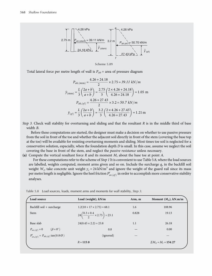
Total lateral force per metre length of wall is Pah = area of pressure diagram
Pah, stem =4 26 + 24 18
2× 2 75 = 39 11 kN m
y stem =L3
2a+ ba+ b
=2 753
2 × 4 26 + 24 184 26 + 24 18
= 1 05 m
Pah, ef =4 26 + 27 43
2× 3 2 = 50 7 kN m
y ef =L3
2a+ ba + b
=3 23
2 × 4 26 + 27 434 26 + 27 43
= 1 21m
Step 3. Check wall stability for overturning and sliding and that the resultant R is in the middle third of basewidth B.
Before these computations are started, the designer must make a decision on whether to use passive pressurefrom the soil in front of the toe and whether the adjacent soil directly in front of the stem (covering the base topat the toe) will be available for resisting overturning moments and sliding. Most times toe soil is neglected for aconservative solution, espacially, when the foundation depth D is small. In this case, assume we neglect the soilcovering the base in front of the stem, and neglect the passive resistance unless necessary.
(a) Compute the vertical resultant force R and its moment Mr about the base toe at point A.For these computations refer to the scheme of Step 1 It is convenient to use Table 5.8, where the load sources
are labelled, weights computed, moment arms given and so on. Include the surcharge qs in the backfill soilweight Ws, take concrete unit weight γc = 24 kN/m3 and ignore the weight of the guard rail since its massper metre length is negligible. Ignore the heel friction Pav ef in order to accomplishmore conservative stability
analyses.
4.26 kPa
27.43 kPa 24.18 kPa
4.26 kPa
Pah,(stem) = 39.11 kN/mPah,(ef ) = 50.70 kN/m
3.2 m
f
e
y (stem) –
y (ef) –
2.75 m
Scheme 5.89
Table 5.8 Load sources, loads, moment arms and moments for wall stability, Step 3.
Load source Load (weight), kN/m Arm, m Moment (MA), kN.m/m
Backfill soil + surcharge 1.2(10 + 17 × 2.75) = 68.1 1.6 108.96
Stem24
0 3 + 0 42
× 2 75 = 23 10.828 19.13
Base slab 24(0.45 × 2.2) = 23.8 1.1 26.18
Pav, ef = 0 β = 0 0.0 — 0.00
Pav, ef = Pah, ef tan 0 8Ø ignored — —
R= 115 0 ΣMA =Mr = 154 27
568 Shallow Foundations
worksaccounts.com
(b) Check the overturning stability.
Overturning moment Mo = Pah, ef × y ef
= 50 7 × 1 21 = 61 35 kN m m
Resisting moment (ignoring the resisting moment due to the heel friction Pav, ef , as shown in Table 5.8) =
Mr = 154.27 kN.m/m
Safety factor against overturning SF =Mr
Mo=154 2761 35
= 2 5 > 2 0 OK
(c) Check that the location of the resultant R is inside the middle third of the base width B.
The net overturning momentMo,net =Mr −Mo = 154 27−61 35
= 92 92 kN m m
x =Mo,net
R=92 92115
= 0 81 m from the toe
Eccentricity = e=B2−x =
2 22
−0 81 = 0 29 m
B6=2 26
= 0 37 m> e OK
The resultant R is inside the middle third of the base width B.(d) Check the sliding stability.
Resistance against sliding is
Fr =R tanδ+ caAf + PP
whereAf = base effective area =B × 1 = B−2e 1
= 2 2−2 × 0 29 = 1 62m2 m
ca = base adhesion 0 6 to 1 0c Assume ca = 0 6cu
= 0 6 100 = 60 kPa
δ= friction angle between base and soil 0 5 to 1 0 Ø
= 0 for Ø = 0
PP = passive resistance
In this case, assume PP is neglected.
Fr = 0 + 60 × 1 62 + 0 = 97 2 kN m
Safety factor against sliding SF =Fr
Pah, ef=97 250 7
= 1 9 > 1 5 OK
Step 4. Compute safe bearing capacity of the supporting soil. Assume using Hansen bearing capacity equation forthe Ø = 0 condition.
(Continued)
Shallow Foundations – Structural Design 569
worksaccounts.com
Table 4.2 gross qult = 5 14 su 1 + sc + dc− ic−bc−gc + qSince the toe soil is neglected, the overburden pressure q= 0. Hence, the safe bearing capacity is
gross qsafe = 5 14 su 1 + dc− ic SF
su = cu = 100 kPa
Table 4.6: sc = 0 2BL = 0, since B
L ≈0 for continuous foundations.Table 4.7: bc = gc = 0, since η = 0 and β = 0
dc = 0 4k; k=DB
forDB≤ 1;
DB=1 22 2
= 0 545; hence, dc = 0 218
ic = 0 5−0 5 1−HAf ca
. Use ca = 60 kPa; Af = 1 62 m2 as in Step 3 (d).
ic = 0 5−0 5 1−50 7
1 62 × 60= 0 154
gross qsafe = 5 14 100 1 + 0 218−0 154 3
= 182 3 kPa
Gross foundation pressure gross q=R
B × 1=1151 62
= 71 0 kPa gross qsafe OK
Check the maximum gross foundation pressure, gross qmax:
gross qmax =RA+
R× eB2
1 B 3 112
Check
=115
1 × 2 2+
115 × 0 292 22
1 2 2 3 1 12= 93 62 kPa < gross qsafe OK
Step 5. Apply the appropriate load factors (ACI Section 9.2) to all the horizontal and vertical forces, computeeccentricity e of the factored resultant force and calculate the base factored contact pressures.
In this case, the only applicable loads areD (dead loads, or related internal moments and forces) andH (loadsdue to weight and pressure of soil, or related internal moments and forces). The applicable load combinations ofthe ACI Section 9.2.1 are reduced to:
U = 1 2D+ 1 6 H
where H represents loads due to soil and surcharge (Table 5.9).
Factored overturning momentMo = 1 6 Pah, ef × y ef
= 1 6 × 61 35 = 98 16 kN m m
570 Shallow Foundations
worksaccounts.com
Factored net overturning momentMo,net =Mr −Mo = 223 3−98 16
= 125 14 kN m m
x =Mo,net
R=125 14160 2
= 0 78 m from the toe
Eccentricity e=B2−x =
2 22
−0 78 = 0 32 m
B6=2 26
= 0 37 m> e OK
Factored qA, max =RA+
MB2
1 B 3 112
=160 22 2 × 1
+51 3
2 22
1 2 2 3 112
= 72 82 + 63 60 = 136 42 kPa
Factored qf , min =RA−
MB2
1 B 3 112
= 72 82−63 60 = 9 22 kPa
Step 6. Check the assumed footing thickness h using (a) uniform soil pressure distribution as suggested by Bowles(2001), (b) linear non-uniform soil pressure distribution.
(a) Using uniform soil pressure distribution. Uniform soil pressure is
q=R
B × 1=
160 22 2−2 × 0 32 1
=160 21 56
= 103 0 kPa
Table 5.9 Factored loads and moments required for calculating factored contact pressures, Step 5.
Load source Factored load (weight), kN/m Arm, m Factored moment (MA), Kn.m/m
Backfill soil + surcharge 1.6[1.2(10 + 17 × 2.75)] = 109.0 1.6 174.4
Stem1 2 24
0 3 + 0 42
× 2 75 = 27 70.83 23.0
Base slab 1.2[24(0.45 × 2.2)] = 23.5 1.1 25.9
Pav, ef = 0 β = 0 0.0 — 0.0
Pav, ef = 1 6 Pah, ef tan 0 8Ø ignored — —
R = 160.2 kN/m ΣMA =Mr = 223.3 kN.m/m
M = 51.3 kN. m/m
0.78 m
R = 160.2 kN/m
A Af f
B = 2.2 m
e = 0.32 m
R = 160.2 kN/m
B = 2.2 m
Scheme 5.90
(Continued)
Shallow Foundations – Structural Design 571
worksaccounts.com
One-way shear is only significant in a continuous-strip footing supporting a wall. To consider the mostsevere condition we use, conservatively, the critical sections located at the faces of the wall as shown.
Shear at the stem front face:Neglect backfill soil over the toe as being conservative.
qnet = q−qc = 103−13 = 90 kPa
Vu = qnet ×A= 90 1 × 0 6 = 54 kN
Shear at the stem back face:
Vu = 91 + 13 1 × 0 64 + 91 + 13−103 1 × 0 56 = 67 12 kN
Use Vu = 67.12 kN/mEquation (5.19): ØVc ≥ Vu (taking reinforcement shear strength, Vs = 0)
where Ø = strength reduction factor ACI Section 9 3 2 3
= 0 75 for shear
Equation (5.20): Vc = 0 17λ fc bwd
Estimate d = h−concrete cover−0 5 bar diameter assume No 25
= 0 450−0 075−0 013 = 0 362 m
ØVc = 0 75 × 0 17 × 1 21 1000 1 0 362
= 212 kN m Vu OK
(b) Using linear non-uniform soil pressure distribution.Shear at the stem front face:
Vu =qmax + q1
20 6 1 −qc 0 6 1
=136 42 + 101 73
20 6 1 − 13 0 6 1 = 64 kN m
ØVc = 212 kN m Vu OK
0.6 m
= 91 kPa
Footing
Critical section (back face)
Critical section (front face)
0.56 m
B = 2.2 m
q = 103 kPa
2e
h = 0.45 m
0.64 m0.4 m
Stem
q(s+soil) = 1.6 (10 + 17 × 2.75)
qc = 1.2(24 × 0.45) = 13 kPa
Scheme 5.91
572 Shallow Foundations
worksaccounts.com

Shear at the stem back face:
q2 = 9 22 +136 42−9 22
2 21 2 = 78 6 kPa
Vu = 91 + 13 1 2 1 −78 6 + 9 22
21 2 1 = 72 11 kN m
ØVc = 212 kN m Vu OK
Use footing thickness h = 0.45 m.Step 7. Find the flexural reinforcement needed for the toe and heel.
(a) Toe flexural reinforcement. The shear computations of Step 6 indicate that the ultimate momentMu based onuniform soil pressure (Bowles method) will be smaller than that based on non-uniform pressure. The lattermethod, furnish more conservative design but not as economical as the Bowles method. Since the providedbase thickness h is more than adequate, it may be appropriate to use the more economical or Bowles method.
The critical section for bending is at the front face of the stem where the maximum factored positivemoment is
Mu =qnet l 2
2=90 × 0 62
2= 16 2 kN m m
Equation (5.9): ØMn ≥Mu
Assume tension-controlled section, Ø = 0.9, and fs = fy.
Equation (5.11): ØMn = Ø Asfy d−a2
q1 = 9.22 +132.42–9.22
2.2(1.6 )
= 101.73 kPa
Stem
0.6 m
B = 2.2m
1.6 m
q(s+soil) = 1.6 (10 + 17 × 2.75) = 91 kPa
Footing
qmax= 136.4
kPa
qmin = 9.22 kPa
qc = 1.2(24 × 0.45) = 13 kPa
q2
h = 0.45 m
Scheme 5.92
(Continued)
Shallow Foundations – Structural Design 573
worksaccounts.com
Equation (5.10): a=Asfy
0 85fc b
=As × 420
0 85 × 21 × 1= 23 53 As
ØMn = 0 9 As × 420 × 1000 0 362−23 53 As
2
= 136 836As−4 447 170 As2 kN m m
Let ØMn =Mu:
136 836As−4 447 170 As2 = 16 2
As2−0 031As + 3 64 × 10
−6 = 0
As =− −0 031 ± −0 031 2− 4 1 3 64 × 10−6
2 × 1=0 031−0 03076
2= 1 2 × 10⁻⁴m2 m= 120mm2 m, required by analysis
As,min = 0 0018 bh ACI Sections 10 5 4 and 7 12 2 1
= 0 0018 × 1 × 0 45 = 8 1 × 10⁻⁴ m2 = 810mm2 m
As,min > As. Therefore, use As = As,min = 810 mm2/mThe assumptions made are satisfied, since As,min controls.
Try four No. 16 bars. As,provided = 4 × 199 = 796 mm2/m. It is less than As,min but much greater than 1.33 As
allowed by ACI Section 10.5.3. Because the difference is too small and the base thickness h is somewhat overde-signed, the provided As is considered adequate.
ACI Sections 10.5.4 and 7.6.5 requires maximum spacing shall not exceed three times the slab or footing thick-ness, or 450 mm, whichever is smaller.
Try No. 16 bars @ 250 mm c.c.
Check the development of reinforcement:In this case, the bars are in tension, the provided bar size is No. 16, the clear spacing of the bars exceeds 2db, andthe clear cover exceeds db. Therefore, the development length ld of bars at each side of the critical section (which islocated where the maximum factored positive moment exists) shall be determined from the following equation,but not less than 300 mm:
ld =fy ψ t ψ e
2 1 λ fcdb ACI Sections 12 2 1, 12 2 2 and 12 2 4
where the factors ψ t, ψ e and λ are 1 (ACI Sections 12.2.4 and 8.6.1).
ld =420 × 1 × 1
2 1 × 1 × 21
15 91000
= 0 694m= 694mm> 300 mm
Therefore, the required ld = 694 mm.The bar extension past the critical section (i.e. the available length) is
600mm−75mmcover = 525mm< ld Not OK
574 Shallow Foundations
worksaccounts.com

Therefore, the bottom bars in the transverse direction will all have to be hooked (90-degree standard hook) atthe toe end.
Check ldh (ACI Section 12.5.2):
ldh =0 24ψ efyλ fc
db
where the factors ψ e and λ shall be taken as 1.
ldh =0 24 × 1 × 420
1 × 21
15 91000
= 0 35m= 350mm>8db > 150 mm
Therefore, the required ldh = 350 mm.The available length = 525 mm > (ldh = 350 mm)These bars may be cut at a minimum distance = 0.6 + 0.694 = 1.3 m from the toe end. However, since full-
width bar length is only 2.05 m, it may not worth the effort to cut the bars. In this case, assume we prefer to cutsome of the bars as indicated below.
Provide No. 16 bars @ 250 mm c.c. placed at bottom of the footing in the transverse direction. All the barshave to be hooked (90-degree standard hook) at the toe end. Two out of each four bars shall be extended fullwidth of the footing and the other two bars cut at 1.3 m from the toe end.
(b) Heel flexural reinforcement. The critical section for bending is at the back face of the stem.The maximum factored negative moment is
Mu =103 × 0 562
2−
91 + 13 1 2 2
2= −59 kN m m
ØMn ≥Mu
Assume tension-controlled section, Ø = 0.9, and fs = fy.
ØMn = Ø Asfy d−a2
a=Asfy
0 85fc b=
As × 4200 85 × 21 × 1
= 23 53 As Equation 5 11
ØMn = 0 9 As × 420 × 1000 0 362−23 53As
2
= 136 836As−4447170 As2 kN m m
Let ØMn =Mu:
136 836As−4447170As2 = 59
As2−0 031As + 1 33 × 10
−5 = 0
As =− −0 031 ± −0 031 2− 4 1 1 33 × 10−5
2 × 1=0 031−0 0301
2= 4 5 × 10−4 = 450mm2 m, required by analysis
As,min = 0 0018 bh ACI Sections 10 5 4 and 7 12 2 1
= 0 0018 × 1 × 0 45 = 8 1 × 10⁻⁴ m2 = 810 mm2 m(Continued)
Shallow Foundations – Structural Design 575
worksaccounts.com

As,min > As. Therefore, use As = As,min = 810 mm2/mThe assumptions made are satisfied, since As,min controls.
Try four No. 16 bars. As,provided = 4 × 199 = 796 mm2/m. It is considered adequate for the same reasons justmentioned in (a).
ACI Sections 10.5.4 and 7.6.5 requires maximum spacing shall not exceed three times the slab or footing thick-ness, or 450 mm, whichever is smaller.
Try No. 16 bars @ 250 mm c.c.
Check the development of reinforcement:In this case, the bars are in tension, the provided bar size is smaller than No. 19, the clear spacing of the barsexceeds 2db, and the clear cover exceeds db. Therefore, the development length ld of bars at each side of the criticalsection (which is located where the maximum factored positive moment exists) shall be determined from the fol-lowing equation, but not less than 300 mm:
ld =fy ψ t ψ e
2 1 λ fcdb ACI Sections 12 2 1, 12 2 2 and 12 2 4
where the factors ψ e and λ are 1 (ACI Sections 12.2.4 and 8.6.1).The factor ψ t = 1.3 because the reinforcement is placed such that more than 300 mm of fresh concrete exists
below the top bars (ACI Section 12.2.4).
ld =420 × 1 3 × 1
2 1 × 1 × 21
15 91000
= 0 902m= 902mm> 300 mm
Therefore, the required ld = 902 mm.The bar extension past the critical section (i.e. the available length) is
1000mm−75mmcover = 925mm> 902mm OK
Provide No. 16 bars @ 250 mm c.c. placed at top of the footing, full width, in the transverse direction.Step 8. Provide longitudinal shrinkage and temperature reinforcement.
ACI Chapter 15 (Footings) does not give any provision or requirement concerning shrinkage and tempera-ture reinforcement. The provisions of ACI Section 7.12 are intended for structural slabs only; they are notintended for slabs on ground (ACI R7.12.1). Some authorities (e.g. Bowles, 1996) do not use this reinforcementin one-way footings, whereas others (MacGregor and Wight) use it to satisfy ACI Section 7.12.2.1. In this case,assume we also prefer to provide minimum shrinkage and temperature reinforcement perpendicular to the toeand heel transverse reinforcement.
Select longitudınal steel based on the minimum shrinkage and temperature reinforcement (ACI Sectıons7.12.1 and 7.12.2.1).
As = 0 0018 bh= 0 0018 × 2 2 × 0 45 = 1 782 × 10−3 m2
= 1782 mm2
Try 14 No. 13 bars: As,provided = 14 × 129 = 1806 mm2 > As (OK.)Longitudinal steel will, in general, be more effective in the top of the footing than in the bottom; it could
control cracks when the foundation settles.According to ACI Section 7.12.2.2, shrinkage and temperature reinforcement shall be spaced not farther
apart than five times the slab thickness, nor farther apart than 450 mm.Use eight No. 13 bars at top and six No. 13 bars at bottom, which will also provide support for the transverse
flexural reinforcement.Provide eight No. 13 @ 288 mm c.c. at top of the footing in long direction, as support for the transverse bars.Provide six No. 13 @ 405 mm c.c. at bottom of the footing in long direction.
576 Shallow Foundations
worksaccounts.com
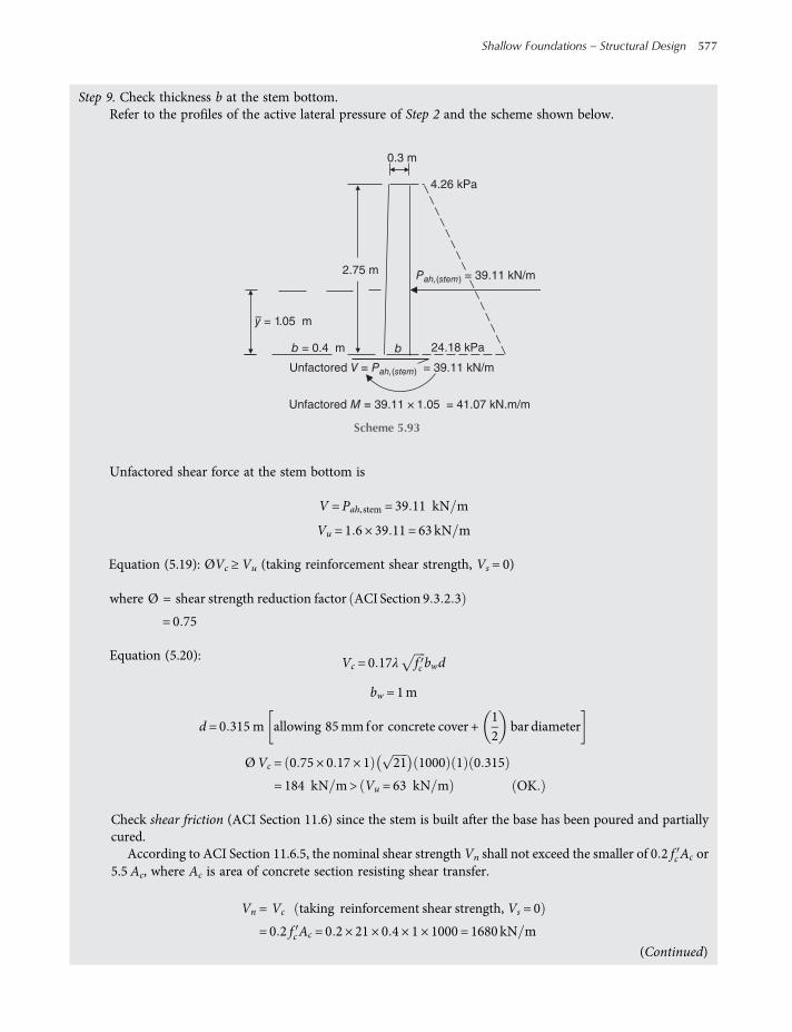
Step 9. Check thickness b at the stem bottom.Refer to the profiles of the active lateral pressure of Step 2 and the scheme shown below.
Unfactored shear force at the stem bottom is
V = Pah, stem = 39 11 kN m
Vu = 1 6 × 39 11 = 63 kN m
Equation (5.19): ØVc ≥ Vu (taking reinforcement shear strength, Vs = 0)
where Ø = shear strength reduction factor ACI Section 9 3 2 3
= 0 75
Equation (5.20): Vc = 0 17λ fc bwd
bw = 1m
d = 0 315m allowing 85mm for concrete cover +12
bar diameter
ØVc = 0 75 × 0 17 × 1 21 1000 1 0 315
= 184 kN m> Vu = 63 kN m OK
Check shear friction (ACI Section 11.6) since the stem is built after the base has been poured and partiallycured.
According to ACI Section 11.6.5, the nominal shear strength Vn shall not exceed the smaller of 0 2 fc Ac or5.5 Ac, where Ac is area of concrete section resisting shear transfer.
Vn = Vc taking reinforcement shear strength, Vs = 0
= 0 2 fc Ac = 0 2 × 21 × 0 4 × 1 × 1000 = 1680 kN m
0.3 m
24.18 kPa
4.26 kPa
2.75 m
bb = 0.4 m
Unfactored V = Pah,(stem) = 39.11 kN/m
Unfactored M = 39.11 × 1.05 = 41.07 kN.m/m
y = 1.05 m–
Pah,(stem) = 39.11 kN/m
Scheme 5.93
(Continued)
Shallow Foundations – Structural Design 577
worksaccounts.com
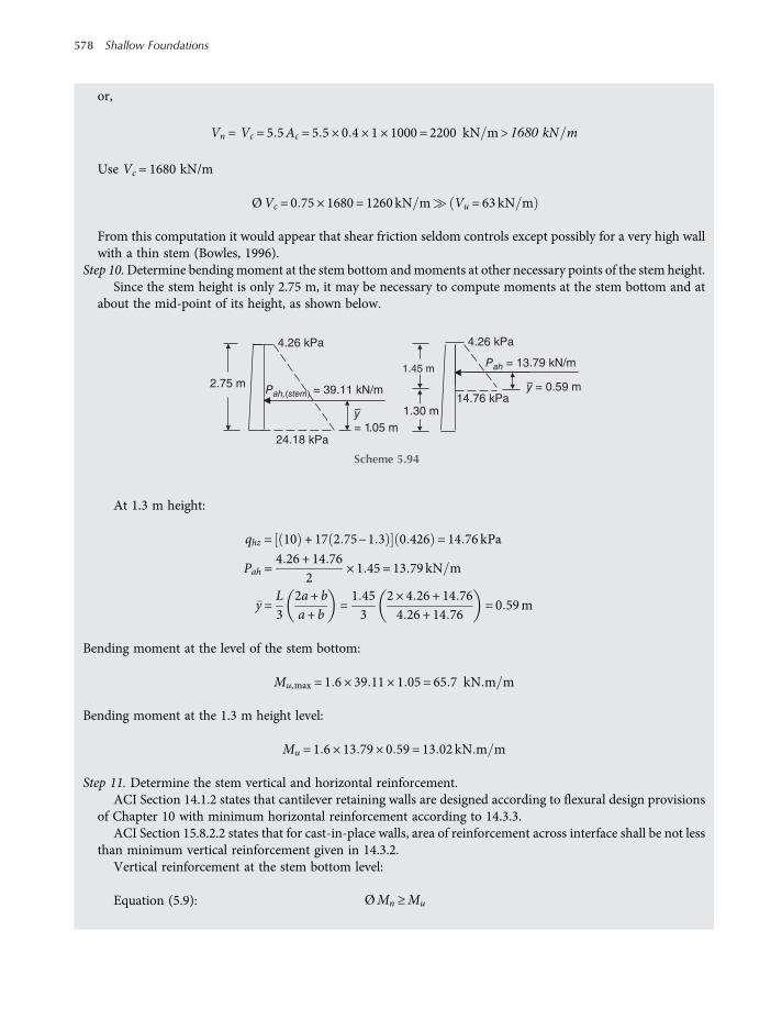
or,
Vn = Vc = 5 5Ac = 5 5 × 0 4 × 1 × 1000 = 2200 kN m> 1680 kN m
Use Vc = 1680 kN/m
ØVc = 0 75 × 1680 = 1260 kN m Vu = 63 kN m
From this computation it would appear that shear friction seldom controls except possibly for a very high wallwith a thin stem (Bowles, 1996).
Step 10.Determine bendingmoment at the stem bottom andmoments at other necessary points of the stem height.Since the stem height is only 2.75 m, it may be necessary to compute moments at the stem bottom and at
about the mid-point of its height, as shown below.
At 1.3 m height:
qhz = 10 + 17 2 75−1 3 0 426 = 14 76 kPa
Pah =4 26 + 14 76
2× 1 45 = 13 79 kN m
y =L3
2a+ ba+ b
=1 453
2 × 4 26 + 14 764 26 + 14 76
= 0 59m
Bending moment at the level of the stem bottom:
Mu,max = 1 6 × 39 11 × 1 05 = 65 7 kN m m
Bending moment at the 1.3 m height level:
Mu = 1 6 × 13 79 × 0 59 = 13 02 kN m m
Step 11. Determine the stem vertical and horizontal reinforcement.ACI Section 14.1.2 states that cantilever retaining walls are designed according to flexural design provisions
of Chapter 10 with minimum horizontal reinforcement according to 14.3.3.ACI Section 15.8.2.2 states that for cast-in-place walls, area of reinforcement across interface shall be not less
than minimum vertical reinforcement given in 14.3.2.Vertical reinforcement at the stem bottom level:
Equation (5.9): ØMn ≥Mu
14.76 kPa
24.18 kPa
4.26 kPa4.26 kPa
1.30 m
1.45 m
2.75 mPah,(stem) = 39.11 kN/m
Pah = 13.79 kN/m
y = 0.59 m–
y
= 1.05 m
–
Scheme 5.94
578 Shallow Foundations
worksaccounts.com
Assume tension-controlled section, Ø = 0.9, and fs = fy.
Equation (5.11): ØMn = Ø Asfy d−a2
Equation (5.10): a=Asfy
0 85 fc b
=As × 420
0 85 × 21 × 1= 23 53As
ØMn = 0 9 As × 420 × 1000 0 315−23 53As
2
= 119 070As−4 447 170As2 kN m m
Let ØMn =Mu:
119 070As−4 447 170As2 = 65 7
As2−0 027As + 1 48 × 10
−5 = 0
As =− −0 027 ± −0 027 2− 4 1 1 48 × 10−5
2 × 1=0 0270−0 0259
2= 5 6 × 10−4 = 560mm2 m
Try three No. 16 bars:
As,provided = 3 × 199 = 597mm2 m OK
Minimum ratio of vertical reinforcement area to gross concrete area perpendicular to that reinforcement, ρℓ,shall be 0.0012 for deformed bars not larger than No. 16 with fy not less than 420 MPa (ACI Section 14.3.2).
As,min = 0 0012 bℓ = 0 0012 × 0 4 × 1 = 4 8 × 10⁻⁴ m2 = 480mm2 m
As,min <As OK
Compute a for As = 597 mm2/m, and check if fs = fy and whether the section is tension-controlled:
a= 23 53As = 23 53 × 597 × 10−6 = 0 014m= 14mm
c=aβ1; For fc between 17 and 28 MPa, β1 shall be taken as 0.85.
c=140 85
= 16 47mm;
dt = d = 315mm
εt = 0 003dt −cc
Equation 5 15
(Continued)
Shallow Foundations – Structural Design 579
worksaccounts.com
εt = 0 003315−16 47
16 47= 0 054 > 0 005. Hence, the section is tension-controlled, and Ø = 0.9 (ACI Sections
10.3.4 and 9.3.2.1).
εy =fyEs
=420
200 000= 0 0021
Hence, εt > εy and fs = fy.The assumptions made are satisfied.Vertical and horizontal reinforcement shall not be spaced farther apart than three times the wall thickness or
farther apart than 450 mm, whichever is smaller (ACI Section 14.3.5).Provide No. 16 bars @ 333 mm c.c. at bottom level of the stem.Vertical reinforcement at the 1.3 m stem height level:
Stem thickness b= 0 3 +0 4−0 32 75
× 1 45 = 0 305m
d = 0 305−0 085 = 0 22m
ØMn = Ø Asfy d−a2
= 0 9 As × 420 × 1000 0 22−23 53As
2
= 83160 As−4447170As2 kN m m
Let ØMn =Mu:
83160As−4447170As2 = 13 02
As2−0 0187As + 2 928 × 10
−6 = 0
As =− −0 0187 ± −0 0187 2− 4 1 2 928 × 10−6
2 × 1=0 0187−0 0184
2= 1 5 × 10−4 = 150mm2 m
As,min = 0 0012 bℓ = 0 0012 × 0 305 × 1
= 3 66 × 10−4 m2 = 366mm2 m>As
Therefore, As,min controls.This reinforcement will be provided by extending two out of each three bars of the stem reinforcement, at the
bottom level, full height of the stem. The third bar shall be cut at d or 12db, whichever is greater, above the 1.3 mheight level (ACI Section 12.10.3). Accordingly, the cut point will be located at 1.52 m height level.
All the vertical bars shall be extended through the interface into the footing, hooked (90-degree standard hook)and wired to the bars at the toe bottom.Thus, the requirement of ACI Section 15.8.2.2 will be satisfied.
Provide No. 16 bars @ 333 mm c.c. placed vertically and extended through the interface into the footing. All thebars shall be hooked (90-degree standard hook) at the lower end only and wired to the bars at the toe bottom. Twoout of each three bars shall be extended full height of the stem and the third bar shall be cut at 1.52 m stem height.
Horizontal reinforcement (ACI Section 14.3.3):Minimum ratio of horizontal reinforcement area to gross concrete area perpendicular to that reinforcement ρt,shall be 0.0020 for deformed bars not larger than No. 16 with fy not less than 420 MPa.
As,min = 0 0020 baveh = 0 002 ×0 4 + 0 3
2× 1
= 7 × 10⁻⁴m2 = 700mm2 per metre height of the stem
580 Shallow Foundations
worksaccounts.com

Try four No. 16 bars: As,provided = 4 × 199 = 796mm2 m OK
Provide No. 16 bars @ 250 mm c.c. placed horizontally for the full stem height and wired to the verticalreinforcement.
Step 12. Develop the final design sketches.
Problem 5.18
Refer to Problem 5.17. Find the flexural reinforcement needed for the toe and heel based on linear non-uniformsoil pressure distribution.
0.45 m
0.40 m
0.30 m
No. 16 @
250 mm c.c.
8 No. 10 @
288 mm c.c.
6 No. 10 @
405 mm c.c.
No. 16 @
333 mm c.c.
Two out of each
three bars shall
be extended full
height of the
stem
No. 16 @250 mm c.c.
Two out of each four
bar extended full
width of the footing
qs = 10 kPa
Compacted
granular
backfill
γ = 17 kN/m3
ϕ = 35°
Excavation line
(approximately)
O
O Guard railing
1.30 m
2.20 m
0.60 m 1.20 m
No. 16 @
250 mm c.c.
2.75 m
0.75 m
1.52 m
Scheme 5.95
(Continued)
Shallow Foundations – Structural Design 581
worksaccounts.com
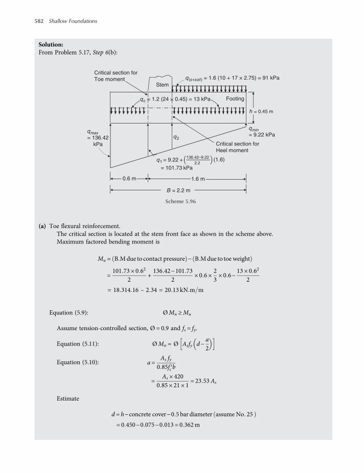
Solution:From Problem 5.17, Step 6(b):
(a) Toe flexural reinforcement.The critical section is located at the stem front face as shown in the scheme above.Maximum factored bending moment is
Mu = B Mdue to contact pressure − B Mdue to toe weight
=101 73 × 0 62
2+136 42−101 73
2× 0 6 ×
23× 0 6−
13 × 0 62
2
= 18 314 16 – 2 34 = 20 13 kN m m
Equation (5.9): ØMn ≥Mu
Assume tension-controlled section, Ø = 0.9 and fs = fy.
Equation (5.11): ØMn = Ø Asfy d−a2
Equation (5.10): a=As fy
0 85fc b
=As × 420
0 85 × 21 × 1= 23 53As
Estimate
d = h−concrete cover−0 5 bar diameter assume No 25
= 0 450−0 075−0 013 = 0 362m
Critical section for
Toe moment
Critical section for
Heel moment
q1 = 9.22 +136.42–9.22
2.2(1.6)
= 101.73 kPa
Stem
0.6 m 1.6 m
B = 2.2 m
q(s+soil) = 1.6 (10 + 17 × 2.75) = 91 kPa
qc = 1.2 (24 × 0.45) = 13 kPa Footing
qmin= 9.22 kPa
qmax= 136.42
kPa
q2
h = 0.45 m
Scheme 5.96
582 Shallow Foundations
worksaccounts.com

ØMn = 0 9 As × 420 × 1000 0 362−23 53 As
2
= 136 836As−4 447 170 As2 kN m m
Let ØMn =Mu:
136 836As−4 447 170As2 = 20 13
As2−0 031As + 4 53 × 10
−6 = 0
As =− −0 031 ± −0 031 2− 4 1 4 53 × 10−6
2 × 1=0 031−0 03071
2= 1 45 × 10−4m2 m= 145mm2 m, required by analysis
As,min = 0 0018 bh ACI Sections 10 5 4 and 7 12 2 1
= 0 0018 × 1 × 0 45 = 8 1 × 10⁻⁴ m2 = 810mm2 m
As,min > As by analysis. Therefore, use As = As,min = 810 mm2/mThe assumptions made are satisfied, since As,min controls.Try four No.16 bars: As,provided = 4 × 199 = 796 mm2/m. It is less than As,min but much greater than 1.33 As
required by analysis. Since the difference is too small and the base thickness h is somewhat overdesigned, it isconsidered acceptable.
ACI Sections 10.5.4 and 7.6.5 requires maximum spacing shall not exceed three times the slab or footingthickness, or 450 mm, whichever is smaller.
Try No. 16 bars @ 250 mm c.c.
Check the development of reinforcement:The necessary computations is exactly the same as that carried out in Problem 5.17, Step 7(a). Since thereinforcement, concrete and footing dimensions are all remained unchanged, the same results will beobtained.
Provide No. 16 bars @ 250 mm c.c. placed at bottom of the footing in the transverse direction. All the barshave to be hooked (90-degree standard hook) at the toe end. Two out of each four bars shall be extended fullwidth of the footing and the other two bars cut at 1.3 m from the toe end.
(b) Heel flexural reinforcement.The critical section for bending is located at the back face of the stem, as shown in the scheme above.
q2 = 9 22 +136 42−9 22
2 21 0 = 67 04 kPa
Mu = (B.M due to weight of backfill soil and load) + (B.M due to heel weight) – (B.M due to contact pressure)
Mu =91 × 1 02
2+
13 × 1 02
2−
9 22 × 1 02
2+67 04−9 22
2× 1 0 ×
13× 1 0
= 45 5 + 6 5 – 4 61 – 9 64 = 37 75 kN m m
Equation (5.9): ØMn ≥Mu
Assume tension-controlled section, Ø = 0.9 and fs = fy.
Equation (5.11): ØMn = Ø As fy d−a2
(Continued)
Shallow Foundations – Structural Design 583
worksaccounts.com

Equation (5.10):
a=Asfy
0 85 fc b
=As × 420
0 85 × 21 × 1= 23 53As
ØMn = 0 9 As × 420 × 1000 0 362−23 53 As
2
= 136836As−4447170A2s kN m m
Let ØMn =Mu:
136836As−4447170A2s = 37 75
A2s −0 031As + 8 49 × 10
−6 = 0
As =− −0 031 ± −0 031 2− 4 1 8 49 × 10−6
2 × 1=0 031−0 0304
2
= 3 × 10⁻⁴m2 m= 300mm2 m, required by analysis
As,min = 0 0018 bh ACI Sections 10 5 4 and 7 12 2 1
= 0 0018 × 1 × 0 45 = 8 1 × 10⁻⁴ m2 = 810mm2 m
As,min > As required by analysis.Therefore, use As = As,min = 810 mm2/m.The assumptions made are satisfied, since As,min controls.Try four No.16 bars: As,provided = 4 × 199 = 796 mm2/m. It is acceptable for the same reasons mentioned in
(a) above.ACI Sections 10.5.4 and 7.6.5 requires maximum spacing shall not exceed three times the slab or footing
thickness, or 450 mm, whichever is smaller.Try No. 16 bars @ 250 mm c.c.
Check the development of reinforcement:The necessary computations is exactly the same as that carried out in Problem 5.17, Step 7(a). Since thereinforcement, concrete and footing dimensions are all remained unchanged, the same results will beobtained.
Provide No. 16 bars @ 250 mm c.c. placed at top, extended full width of the footing in the transverse direction.Thus, in this case, we find that the required transverse flexural reinforcement based on the linear non-
uniform soil pressure distribution is the same as that based on the uniform soil pressure distribution sinceAs,min governs in both cases.
Problem 5.19
Refer to Problem 5.17. Assume the base soil and that in front the wall is gravelly sand of Ø = 33 and γ = 18 kN/m3,overlying a soft-clay deposit at 1.0mdepth below the base level, as shown in the scheme below.The groundwater tableis also located at the same depth. The soft clay has an average c = 20 kPa, Ø = 0 and γ = 17.5 kN/m3. Determine thesafety factor (SF) against a deep-seated shear failure (or rotational instability) for a trial cylindrical slip surface throughthe heel shown in Scheme 5.97. Assume radius of the cylindrical slip surface is 4.33 m, and its centre O located at2.87 m above the foundation level. Use the conventional method of slices (the Fellenius or Swedish solution).
584 Shallow Foundations
worksaccounts.com
SolutionNormally, the safety factor (SF) against a deep-seated shear failure (or rotational instability) should be at least two.For this analysis, several trial failure surfaces (circles) should be drawn, the safety factor computed, and the min-imum value taken. It may be useful to mention that the trial failure circles passing through the heel apply forground or backfill slope angles of β = 0 to perhaps β = 10 ; for larger values of β, irregular surfaces or surcharges,the assumed failure circles may not pass through the heel, and other failure locations should be investigated.In this case, we try to compute the safety factor for the circle indicated in the given scheme of the Problem as an
example. Due to the repetitive nature of the calculations and the need to select an adequate number of trial sur-faces, the method of slices is particularly suitable for solution by computer, especially, where more complex slopegeometry and different soil strata are required to be introduced.
Step 1. Draw the wall-soil system to a convenient scale, as shown below.
γ = 18 kN/m3
c = 0
Soft clay: γ = 17.5 kN/m3
c = 20 kPa
ϕ = 0°
W. T
Δ
0.3 m
0
ϕ = 33°1.21 m
H = 3.20 m
Gravelly sand:
D = 1.20 mB = 2.20 mg = 1.20 mh = 0.45 mb = 0.40 ml = 0.60 mz = 1.00 m
R = 4.33 m
D
Bf
g
e
qs = 10 kPa
z
h
lb
Pa =
50.7 kN/mH
Scheme 5.97
Scale:7 mm = 600 mm
0.3 m
1.21 m
Soft clay: γ = 17.5 kN/m3
c = 20 kPa
ϕ = 0°
W. T
Δ
0
H = 3.20 mD = 1.20 mB = 2.20 mg = 1.20 mh = 0.45 mb = 0.40 ml = 0.60 mz = 1.00 m
R = 4.33 m
qs = 10 kPa
ϕ = 33°c = 0
Gravelly sand: γ = 18 kN/m3
H
D
z
h
Bf
g
e
bl
Pa =
50.7 kN/m
Scheme 5.98 (Continued)
Shallow Foundations – Structural Design 585
worksaccounts.com
Step 2.Divide the circular segment amnf and the material above by vertical planes into a series of slices, as shown inthe scheme below. The base b of each slice is assumed to be a straight line. For any slice the inclination of thebase to the horizontal is α and the height, measured on the centre line, is h. WeightW (including surcharge) ofeach slice is resolved into its normal component N =W cos α and tangential component T =W sin α, which aredetermined graphically, as shown. Alternatively, the value of α can be measured or calculated.
Note: Since the centre of rotation O is centered with respect to the circular arcmn (located in the soft clay), it isnot necessary to divide this arc and the material above into slices and findN and T; their resultant effects will bezero (neglecting the difference in weights of a portion of the concrete footing and displaced soil). However, somecorrection was applied to include the weight of a portion of the concrete stem in slice 5, as shown in the scheme.
Step 3.Determine values ofN and T per metre length of the retaining wall for each slice, as indicated in Table 5.10.
1 m
3.86 m
53°3.87 m
ϕ = 33°c = 0
γ = 18 kN/m3
c = 20 kPaϕ = 0°
γ = 17.5 kN/m3
R = 4.33 m
0
qs = 10 kPa
e
W. T
Δ
α
5 45 4 3 3 2 2 1 1 5 4 3 2 1
Scale: 1 mm = 0.64 kN
7 mm = 600 mm
9 9 8 7 6 8 7 6 9 8 7 6
Scheme 5.99
Table 5.10 Values of N and T per metre length for each slice of the retaining wall.
Slice number Weight of slice, W (kN) N (kN) T (kN)
1 0.4 (10 + 2.92 × 18) + 0.4 × 0.45 × 24 = 29.3 21.2 20.3
2 0.4 (10 + 3.26 × 18) + 0.4 × 0.45 × 24 = 31.8 25.0 19.7
3 0.4 (10 + 3.56 × 18) + 0.4 × 0.45 × 24 = 34.0 28.8 18.1
4 0.2 (10 + 1.00 × 18) + 0.2 × 3.20 × 24 = 21.0 18.6 9.7
5 0.15 × 2.75 × 24 = 9.9 9.0 4.5
6 0.43 × 2.06 × 18 = 15.9 14.1 –7.5
7 0.43 × 1.84 × 18 = 13.8 10.2 –9.3
8 0.43 × 1.37 × 18 = 10.6 7.2 –7.7
9 0.5 × 0.63 × 1.11 × 18 = 6.3 3.8 –5.0
Σ N = 137.8. Σ T = 42.8
586 Shallow Foundations
worksaccounts.com

Step 4. Determine the driving and resisting moments about centre of rotation at point O, then compute thesafety factor SF.
(a) Driving moment Md.This moment consists of moment of the total active thrust Pa plus moment of Σ T, computed as
Md = y Pa +R T
The thrust Pa is located at 1.21 m above the foundation level, whereas, pointO is located at 2.87 m above thesame level. Therefore,
y = 2 87−1 21 = 1 66m
Md = 1 66 × 50 7 + 4 33 × 42 8 = 269 5 kN m m
(b) Resisting moment Mr.This moment equals to moment of the total shear strength Tf along the circular arc amnf,
computed as
Mr =R Tf
Tf = cohesion force + friction force = arc length × c + N tanØ
Gravelly sand:The base of slice 5 is located in soft clay. Therefore, N for this slice should not be considered.
Tf = 0 + N −N of slice 5 tan Ø o = 137 8−9 tan33
= 83 6 kN m
Soft clay:
Tf = length of arcmn× c + 0 =53360
2πR c
=53360
× 2 ×227× 4 33 × 20 = 80 1 kN m
Mr = 4 33 83 6 + 80 1 = 708 8 kN m m
Safety factor is
SF =Mr
Md=708 8269 5
= 2 63 > 2 OK
Problem 5.20
A gravity concrete retaining wall is shown in the scheme below. Determine the maximum andminimum pressuresunder the base of the wall, and the safety factors against overturning and sliding (ignore any material which mayexist in front the wall). Use Coulomb’s active earth pressure theory and wall friction angle δ = (2/3)Ø.
(Continued)
Shallow Foundations – Structural Design 587
worksaccounts.com
Solution:Step 1. Determine the total active earth pressure thrust Pa and its components Pah and Pav.
Pa =γH2
2Ka
Where Ka = Coulomb’s coefficient of lateral active earth pressure.For cohesionless soils, Ka may be obtained from tables or calculated as
Ka =sin2 α+ Ø
sin2αsin α−δ 1 +sin Ø + δ sin Ø −β
sin α−δ sin α+ β
2
Angles:
Ø = 36
β = 15
α= 80
δ=2Ø3
=23× 36 = 24
Ka =sin2116
sin280sin56 1 +sin60sin21sin56sin95
2
Ka =0 808
0 804 1 +0 3100 826
2 =0 808
0 84 1 + 0 613 2
β = 15°
0.60 m0.74 m
Concrete wall
γ = 23.5 kN/m3
γ = 18 kN/m3
ϕ = 36°c = 0
0.60 m
0.75 m
B = 3.00 m
α = 80°
H = 6.00 m
Scheme 5.100
588 Shallow Foundations
worksaccounts.com

=0 808
0 84 × 2 6= 0 37
Pa =18 × 62
2× 0 37 = 120 kN m
The active thrust Pa acts on the wall back face at a height of13H and at δ above the normal, or at 34 above the
horizontal as shown.
Pah = Pa cos34 = 120 × 0 83 = 99 6 kN m
Pav = Pa sin34 = 120 × 0 56 = 67 2 kN m
Step 2.Compute the vertical resultant force R, net momentMnet, eccentricity e, overturningmomentMo about basetoe at point A and the resisting moment Mr.
For these computations refer to the scheme in Step 1. It is convenient to tabulate the load sources, loads,moment arms and moments, as in Table 5.11.
γ =18 kN/m3
β
2.0 m(I)
(II)
B = 3.0 m
(III)
(IV)
1.34
0.75 m
1.060.6A
H = 6.0 m
ϕ = 36°
δ 34°
c = 0
Pav
Pah
P a
α
Scheme 5.101
Table 5.11 Load sources, loads, moment arms and moments.
Load source Load (weight) kN/m Arm m Moment MA kN.m/m+ ↷
(I) 0.5 × 6 × 1.06 × 23.5 = 74.73 2.29 171.13
(II) 0.6 × 6 × 23.5 = 84.60 1.64 138.74
(III) 0.5 × 5.25 × 0.74 × 23.5 = 45.65 1.09 49.76
(IV) 0.75 × 1.34 × 23.5 = 23.62 0.67 15.83
Pav = 67.20 2.65 178.08
Pah = 99.6 kN/m 2.00 −199.20
R = 295.80 Mnet = 354.34
(Continued)
Shallow Foundations – Structural Design 589
worksaccounts.com
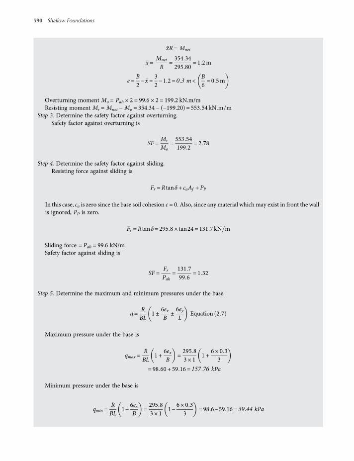
xR= Mnet
x =Mnet
R=354 34295 80
= 1 2m
e=B2−x =
32−1 2 = 0 3 m <
B6= 0 5m
Overturning moment Mo = Pah × 2 = 99.6 × 2 = 199.2 kN.m/mResisting moment Mr = Mnet − Mo = 354.34 − (−199.20) = 553 54 kN m m
Step 3. Determine the safety factor against overturning.Safety factor against overturning is
SF =Mr
Mo=553 54199 2
= 2 78
Step 4. Determine the safety factor against sliding.Resisting force against sliding is
Fr =R tanδ+ caAf + PP
In this case, ca is zero since the base soil cohesion c = 0. Also, since anymaterial which may exist in front the wallis ignored, PP is zero.
Fr =R tanδ= 295 8 × tan24 = 131 7 kN m
Sliding force = Pah = 99.6 kN/mSafety factor against sliding is
SF =FrPah
=131 799 6
= 1 32
Step 5. Determine the maximum and minimum pressures under the base.
q=RBL
1 ±6exB
±6eyL
Equation 2 7
Maximum pressure under the base is
qmax =RBL
1 +6exB
=295 83 × 1
1 +6 × 0 3
3
= 98 60 + 59 16 = 157 76 kPa
Minimum pressure under the base is
qmin =RBL
1−6exB
=295 83 × 1
1−6 × 0 3
3= 98 6−59 16 = 39 44 kPa
590 Shallow Foundations
worksaccounts.com
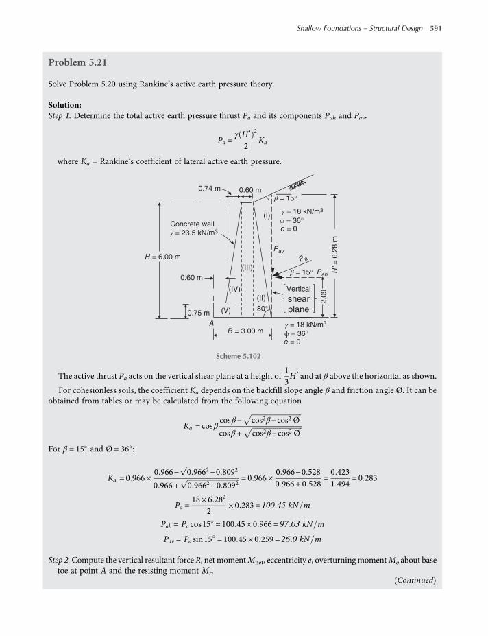
Problem 5.21
Solve Problem 5.20 using Rankine’s active earth pressure theory.
Solution:Step 1. Determine the total active earth pressure thrust Pa and its components Pah and Pav.
Pa =γ H 2
2Ka
where Ka = Rankine’s coefficient of lateral active earth pressure.
The active thrust Pa acts on the vertical shear plane at a height of13H and at β above the horizontal as shown.
For cohesionless soils, the coefficient Ka depends on the backfill slope angle β and friction angle Ø. It can beobtained from tables or may be calculated from the following equation
Ka = cosβcosβ− cos2β−cos2 Ø
cosβ + cos2β−cos2 Ø
For β = 15 and Ø = 36 :
Ka = 0 966 ×0 966− 0 9662−0 8092
0 966 + 0 9662−0 8092= 0 966 ×
0 966−0 5280 966 + 0 528
=0 4231 494
= 0 283
Pa =18 × 6 282
2× 0 283 = 100 45 kN m
Pah = Pa cos15 = 100 45 × 0 966 = 97 03 kN m
Pav = Pa sin15 = 100 45 × 0 259 = 26 0 kN m
Step 2.Compute the vertical resultant force R, net momentMnet, eccentricity e, overturningmomentMo about basetoe at point A and the resisting moment Mr.
80°
β = 15°
β = 15°
0.60 m0.74 m
Concrete wall
γ = 23.5 kN/m3
0.60 m
0.75 m
B = 3.00 m
(IV)
(III)
Vertical
shear
plane
(II)
(V)
(I)
2.0
9 γ = 18 kN/m3
ϕ = 36°c = 0
γ = 18 kN/m3
ϕ = 36°c = 0
A
P a
Pah
PavH = 6.00 m
H' =
6.2
8 m
Scheme 5.102
(Continued)
Shallow Foundations – Structural Design 591
worksaccounts.com

For these computations refer to the scheme of Step 1. It is convenient to tabulate the load sources, loads,moment arms and moments in a table such as Table 5.12.
xR= Mnet
x =MR
R=409 23314 51
= 1 3m
e=B2−x =
32−1 3 = 0 2 m <
B6= 0 5m
Overturning momentMo = Pah × 2 09 = 97 03 × 2 09
= 202 79 kN m m
Resisting momentMr = Mnet− Mo = 409 23− −202 79
= 612 02 kN m m
Step 3. Determine the maximum and minimum pressures under the base.
q=RBL
1 ±6exB
±6eyL
Equation 2 7
Maximum pressure under the base is
qmax =RBL
1 +6exB
=314 513 × 1
1 +6 × 0 2
3
= 104 84 + 41 93 = 146 77 kPa
Minimum pressure under the base is
qmin =RBL
1−6exB
=314 513 × 1
1−6 × 0 2
3
= 104 84−41 93 = 62 91 kPa
Table 5.12 Load sources, loads, moment arms and moments.
Load source Load (weight) kN/m Arm m Moment MA kN. m/m + ↷
(I) 0.5 × 6.28 × 1.06 × 18.0 = 59.91 2.65 158.56
(II) 0.5 × 6.0 × 1.06 × 23.5 = 74.73 2.29 171.13
(III) 0.6 × 6 × 23.5 = 84.60 1.64 138.74
(IV) 0.5 × 5.25 × 0.74 × 23.5 = 45.65 1.09 49.76
(V) 0.75 × 1.34 × 23.5 = 23.62 0.67 15.83
Pav = 26.00 3.00 78.00
Pah = 97.03 kN/m 2.09 −202.79
R = 314.51 Mnet = 409.23
592 Shallow Foundations
worksaccounts.com
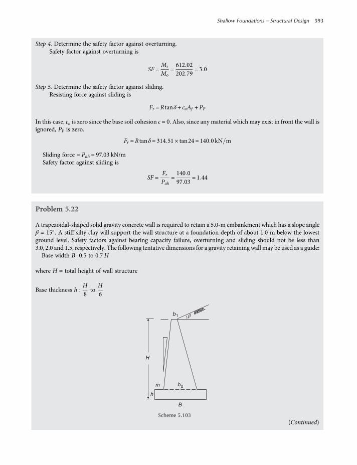
Step 4. Determine the safety factor against overturning.Safety factor against overturning is
SF =Mr
Mo=612 02202 79
= 3 0
Step 5. Determine the safety factor against sliding.Resisting force against sliding is
Fr =R tanδ+ caAf + PP
In this case, ca is zero since the base soil cohesion c = 0. Also, since any material which may exist in front the wall isignored, PP is zero.
Fr =R tanδ= 314 51 × tan24 = 140 0 kN m
Sliding force = Pah = 97.03 kN/mSafety factor against sliding is
SF =FrPah
=140 097 03
= 1 44
Problem 5.22
A trapezoidal-shaped solid gravity concrete wall is required to retain a 5.0-m embankment which has a slope angleβ = 15 . A stiff silty clay will support the wall structure at a foundation depth of about 1.0 m below the lowestground level. Safety factors against bearing capacity failure, overturning and sliding should not be less than3.0, 2.0 and 1.5, respectively. The following tentative dimensions for a gravity retaining wall may be used as a guide:Base width B : 0.5 to 0.7H
where H = total height of wall structure
Base thickness hH8
toH6
H
m
h
B
βb1
b2
Scheme 5.103(Continued)
Shallow Foundations – Structural Design 593
worksaccounts.com
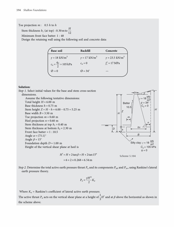
Toe projection m : 0.5 h to h
Stem thickness b1 (at top) 0 30m toH12
Minimum front face batter: 1 : 48Design the retaining wall using the following soil and concrete data:
Base soil Backfill Concrete
γ = 18 kN/m3 γ = 17 kN/m3 γ = 23.5 kN/m3
cu =qu2= 105 kPa cu = 0 fc = 17MPa
Ø = 0 Ø = 34 —
Solution:Step 1. Select initial values for the base and stem cross-section
dimensions.Assume the following tentative dimensions:Total height H = 6.00 mBase thickness h = 0.75 mStem height Z =H − h = 6.00 − 0.75 = 5.25 mBase width B = 3.50 mToe projection m = 0.60 mHeel projection n = 0.60 mStem thickness at top b1 = 0.40 mStem thickness at bottom b2 = 2.30 mFront face batter = 1 : 10.5Angle α = (75.1)Angle β = 15Foundation depth D = 1.00 mHeight of the vertical shear plane at heel is
H =H + 2tanβ =H + 2tan15o
= 6 + 2 × 0 268 = 6 54m
Step 2. Determine the total active earth pressure thrust Pa and its components Pah and Pav, using Rankine’s lateralearth pressure theory.
Pa =γH 2
2Ka
Where Ka = Rankine’s coefficient of lateral active earth pressure.
The active thrust Pa acts on the vertical shear plane at a height of13H and at β above the horizontal as shown in
the scheme above.
Silty clay: γ = 18 kN
Cu = 105 kPa
ϕ = 0
Batter
10.5
1
kN
m3
ϕ = 34°Cu = 0
H′
n
b2
b1
B
m3
m
hD
HZ
γ = 18
β
Scheme 5.104
594 Shallow Foundations
worksaccounts.com

For cohesionless soils, the coefficient Ka depends on the backfill slope angle β and friction angle Ø, can beobtained from tables or may be calculated from the equation
Ka = cosβcosβ− cos2β−cos2 Ø
cosβ + cos2β−cos2 Ø
For β = 15 and Ø = 34 :
Ka = 0 966 ×0 966− 0 9662−0 8292
0 966 + 0 9662−0 8292= 0 966 ×
0 966−0 4960 966 + 0 496
=0 4541 462
= 0 311
Pa =18 × 6 542
2× 0 311 = 119 72 kN m
Pah = Pa cos15 = 119 72 × 0 966 = 115 65 kN m
Pav = Pa sin15 = 119 72 × 0 259 = 31 01 kN m
Step 3.Compute the vertical resultant force R, net momentMnet, eccentricity e, overturningmomentMo about basetoe at point A, and the resisting moment Mr.
For these computations refer to the scheme in Step 2. It is convenient to tabulate the load sources, loads,moment arms and moments, as in Table 5.13. Assume, conservatively, we neglect the toe soil and that coveringthe base in front of the wall stem.
β = 15°
β = 15°
0.6
II I
0.6
IV
0.5 Silty clay: γ = 18 kN/m3
cu = 105 kPa
ϕ = 0°0.4
5.25 m
1.40
III
VI
V Vertical
shear
plane
Pav
Pah
Pa
B = 3.50 m
0.75 m
A
2.18 m
γ = 18
kN/m3
ϕ = 34°cu = 0
H′ = 6.54 mH = 6.00 m
Scheme 5.105
(Continued)
Shallow Foundations – Structural Design 595
worksaccounts.com
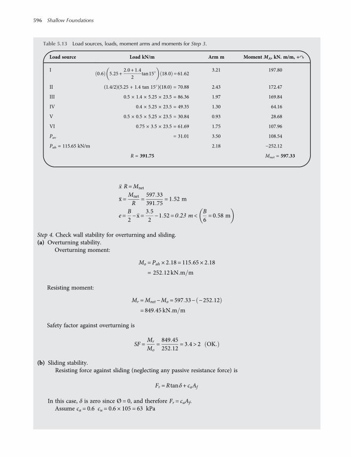
x R=Mnet
x =Mnet
R=597 33391 75
= 1 52 m
e =B2−x =
3 52
−1 52 = 0 23 m <B6= 0 58 m
Step 4. Check wall stability for overturning and sliding.(a) Overturning stability.
Overturning moment:
Mo = Pah × 2 18 = 115 65 × 2 18
= 252 12 kN m m
Resisting moment:
Mr =Mnet −Mo = 597 33− −252 12
= 849 45 kN m m
Safety factor against overturning is
SF =Mr
Mo=849 45252 12
= 3 4 > 2 OK
(b) Sliding stability.Resisting force against sliding (neglecting any passive resistance force) is
Fr =R tanδ+ caAf
In this case, δ is zero since Ø = 0, and therefore Fr = caAf.Assume ca = 0.6 cu = 0.6 × 105 = 63 kPa
Table 5.13 Load sources, loads, moment arms and moments for Step 3.
Load source Load kN/m Arm m Moment MA, kN. m/m, +↷
I0 6 5 25 +
2 0 + 1 42
tan15 18 0 = 61 623.21 197.80
II (1.4/2)(5.25 + 1.4 tan 15 )(18.0) = 70.88 2.43 172.47
III 0.5 × 1.4 × 5.25 × 23.5 = 86.36 1.97 169.84
IV 0.4 × 5.25 × 23.5 = 49.35 1.30 64.16
V 0.5 × 0.5 × 5.25 × 23.5 = 30.84 0.93 28.68
VI 0.75 × 3.5 × 23.5 = 61.69 1.75 107.96
Pav = 31.01 3.50 108.54
Pah = 115.65 kN/m 2.18 −252.12
R = 391.75 Mnet = 597.33
596 Shallow Foundations
worksaccounts.com
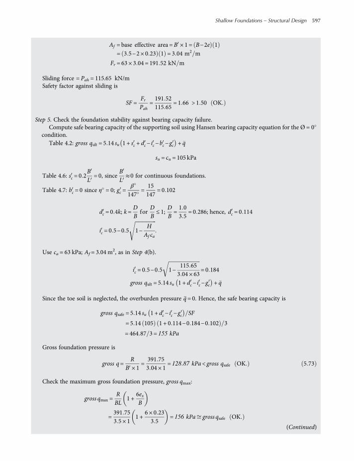
Af = base effective area =B × 1 = B−2e 1
= 3 5−2 × 0 23 1 = 3 04 m2 m
Fr = 63 × 3 04 = 191 52 kN m
Sliding force = Pah = 115.65 kN/mSafety factor against sliding is
SF =FrPah
=191 52115 65
= 1 66 > 1 50 OK
Step 5. Check the foundation stability against bearing capacity failure.Compute safe bearing capacity of the supporting soil using Hansen bearing capacity equation for the Ø = 0
condition.Table 4.2: gross qult = 5 14 su 1 + sc + dc− ic−bc−gc + q
su = cu = 105 kPa
Table 4.6: sc = 0 2BL
= 0, sinceBL≈0 for continuous foundations.
Table 4.7: bc = 0 since η = 0; gc =β
147=
15147
= 0 102
dc = 0 4k; k=DB
forDB≤ 1;
DB=1 03 5
= 0 286; hence, dc = 0 114
ic = 0 5−0 5 1−HAf ca
Use ca = 63 kPa; Af = 3.04 m2, as in Step 4(b).
ic = 0 5−0 5 1−115 653 04 × 63
= 0 184
gross qult = 5 14 su 1 + dc− ic−gc + q
Since the toe soil is neglected, the overburden pressure q= 0. Hence, the safe bearing capacity is
gross qsafe = 5 14 su 1 + dc− ic−gc SF
= 5 14 105 1 + 0 114−0 184−0 102 3
= 464 87 3 = 155 kPa
Gross foundation pressure is
gross q=R
B × 1=
391 753 04 × 1
= 128 87 kPa < gross qsafe OK 5 73
Check the maximum gross foundation pressure, gross qmax:
gross qmax =RBL
1 +6exB
=391 753 5 × 1
1 +6 × 0 233 5
= 156 kPa gross qsafe OK
(Continued)
Shallow Foundations – Structural Design 597
worksaccounts.com
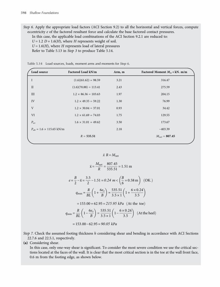
Step 6. Apply the appropriate load factors (ACI Section 9.2) to all the horizontal and vertical forces, computeeccentricity e of the factored resultant force and calculate the base factored contact pressures.
In this case, the applicable load combinations of the ACI Section 9.2.1 are reduced to:U = 1.2 D + 1.6(H), where H represents weight of soil.U = 1.6(H), where H represents load of lateral pressuresRefer to Table 5.13 in Step 3 to produce Table 5.14.
x R=Mnet
x =Mnet
R=807 45535 51
= 1 51 m
e =B2−x =
3 52
−1 51 = 0 24 m <B6= 0 58m OK
qmax =RBL
1 +6exB
=535 513 5 × 1
1 +6 × 0 243 5
= 153 00 + 62 95 = 215 95 kPa At the toe
qmin =RBL
1−6exB
=535 513 5 × 1
1−6 × 0 243 5
At the heel
= 153 00−62 95 = 90 05 kPa
Step 7. Check the assumed footing thickness h considering shear and bending in accordance with ACI Sections22.7.6 and 22.5.1, respectively.
(a) Considering shear.In this case, only one-way shear is significant. To consider the most severe condition we use the critical sec-tions located at the faces of the wall. It is clear that the most critical section is in the toe at the wall front face,0.6 m from the footing edge, as shown below.
Table 5.14 Load sources, loads, moment arms and moments for Step 6.
Load source Factored Load kN/m Arm, m Factored Moment MA + kN. m/m
I (1.6)(61.62) = 98.59 3.21 316.47
II (1.6)(70.88) = 113.41 2.43 275.59
III 1.2 × 86.36 = 103.63 1.97 204.15
IV 1.2 × 49.35 = 59.22 1.30 76.99
V 1.2 × 30.84 = 37.01 0.93 34.42
VI 1.2 × 61.69 = 74.03 1.75 129.55
Pav 1.6 × 31.01 = 49.62 3.50 173.67
Pah = 1.6 × 115.65 kN/m 2.18 −403.39
R = 535.51 Mnet = 807.45
598 Shallow Foundations
worksaccounts.com
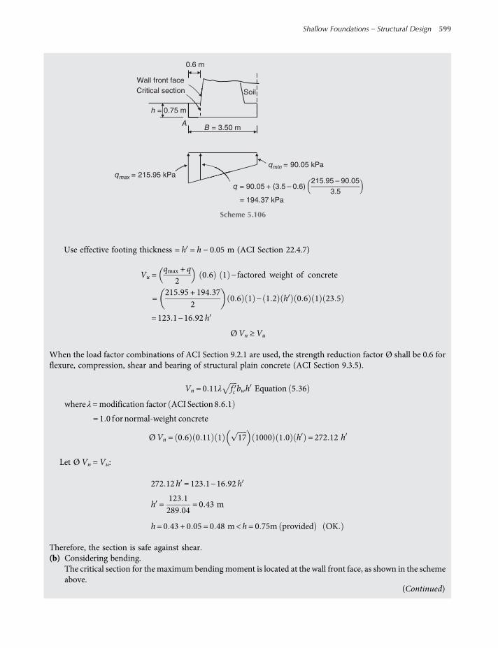
Use effective footing thickness = h = h − 0.05 m (ACI Section 22.4.7)
Vu =qmax + q
20 6 1 − factored weight of concrete
=215 95 + 194 37
20 6 1 − 1 2 h 0 6 1 23 5
= 123 1−16 92 h
ØVn ≥Vu
When the load factor combinations of ACI Section 9.2.1 are used, the strength reduction factor Ø shall be 0.6 forflexure, compression, shear and bearing of structural plain concrete (ACI Section 9.3.5).
Vn = 0 11λ fc bwh Equation 5 36
where λ=modification factor ACI Section 8 6 1
= 1 0 for normal-weight concrete
ØVn = 0 6 0 11 1 17 1000 1 0 h = 272 12 h
Let ØVn =Vu:
272 12h = 123 1−16 92h
h =123 1289 04
= 0 43 m
h= 0 43 + 0 05 = 0 48 m< h= 0 75m provided OK
Therefore, the section is safe against shear.(b) Considering bending.
The critical section for the maximum bending moment is located at the wall front face, as shown in the schemeabove.
B = 3.50 mA
Critical section
h = 0.75 m
Wall front face
0.6 m
Soil
qmin = 90.05 kPa
qmax = 215.95 kPa
q = 90.05 + (3.5 – 0.6)215.95 – 90.05
3.5= 194.37 kPa
Scheme 5.106
(Continued)
Shallow Foundations – Structural Design 599
worksaccounts.com
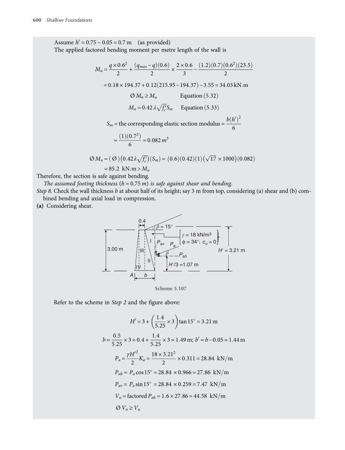
Assume h = 0.75 − 0.05 = 0.7 m (as provided)The applied factored bending moment per metre length of the wall is
Mu =q× 0 62
2+
qmax−q 0 62
×2 × 0 6
3−
1 2 0 7 0 62 23 52
= 0 18 × 194 37 + 0 12 215 95−194 37 −3 55 = 34 03 kN m
ØMn ≥Mu Equation 5 32
Mn = 0 42 λ fc Sm Equation 5 33
Sm = the corresponding elastic section modulus =b h 2
6
=1 0 72
6= 0 082m3
ØMn = Ø 0 42λ fc Sm = 0 6 0 42 1 17 × 1000 0 082
= 85 2 kN m>Mu
Therefore, the section is safe against bending.The assumed footing thickness (h = 0.75m) is safe against shear and bending.
Step 8. Check the wall thickness b at about half of its height; say 3 m from top, considering (a) shear and (b) com-bined bending and axial load in compression.
(a) Considering shear.
Refer to the scheme in Step 2 and the figure above:
H = 3 +1 45 25
× 3 tan15 = 3 21m
b=0 55 25
× 3 + 0 4 +1 45 25
× 3 = 1 49m; b = b−0 05 = 1 44m
Pa =γH 2
2Ka =
18 × 3 212
2× 0 311 = 28 84 kN m
Pah = Pa cos15 = 28 84 × 0 966 = 27 86 kN m
Pav = Pa sin15 = 28 84 × 0 259 = 7 47 kN m
Vu = factoredPah = 1 6 × 27 86 = 44 58 kN m
ØVn ≥Vu
I
III
0.4
3.00 m
II
IVV
γ = 18 kN/m3
ϕ = 34°;
β = 15°
β
cu = 0Pav Pa
Pah
bA
H′ = 3.21 m
H′/3 =1.07 m
Scheme 5.107
600 Shallow Foundations
worksaccounts.com
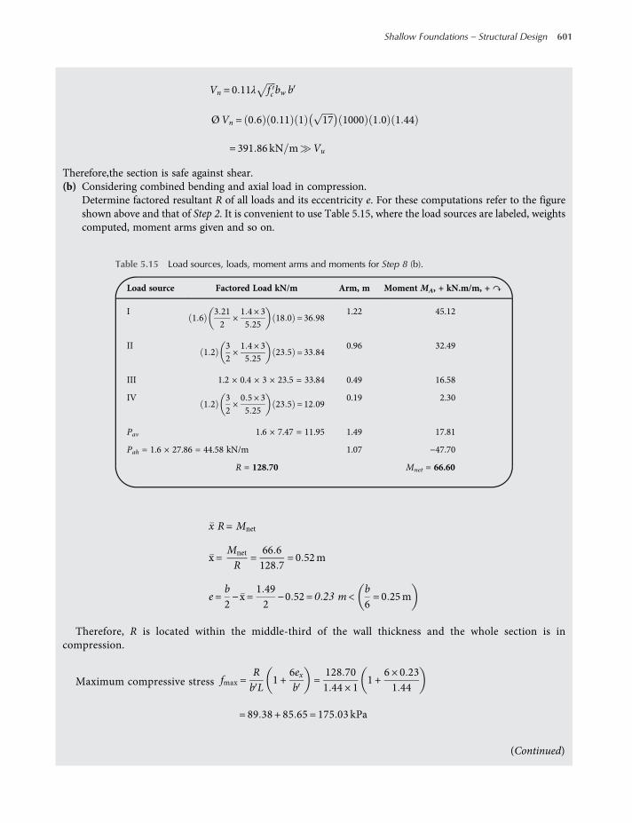
Vn = 0 11λ fc bw b
ØVn = 0 6 0 11 1 17 1000 1 0 1 44
= 391 86 kN m Vu
Therefore,the section is safe against shear.(b) Considering combined bending and axial load in compression.
Determine factored resultant R of all loads and its eccentricity e. For these computations refer to the figureshown above and that of Step 2. It is convenient to use Table 5.15, where the load sources are labeled, weightscomputed, moment arms given and so on.
x R= Mnet
x =Mnet
R=
66 6128 7
= 0 52m
e=b2−x =
1 492
−0 52 = 0 23 m <b6= 0 25m
Therefore, R is located within the middle-third of the wall thickness and the whole section is incompression.
Maximum compressive stress fmax =Rb L
1 +6exb
=128 701 44 × 1
1 +6 × 0 231 44
= 89 38 + 85 65 = 175 03 kPa
Table 5.15 Load sources, loads, moment arms and moments for Step 8 (b).
Load source Factored Load kN/m Arm, m Moment MA, + kN.m/m, + ↷
I1 6
3 212
×1 4 × 35 25
18 0 = 36 981.22 45.12
II1 2
32×1 4 × 35 25
23 5 = 33 840.96 32.49
III 1.2 × 0.4 × 3 × 23.5 = 33.84 0.49 16.58
IV1 2
32×0 5 × 35 25
23 5 = 12 090.19 2.30
Pav 1.6 × 7.47 = 11.95 1.49 17.81
Pah = 1.6 × 27.86 = 44.58 kN/m 1.07 −47.70
R = 128.70 Mnet = 66.60
(Continued)
Shallow Foundations – Structural Design 601
worksaccounts.com
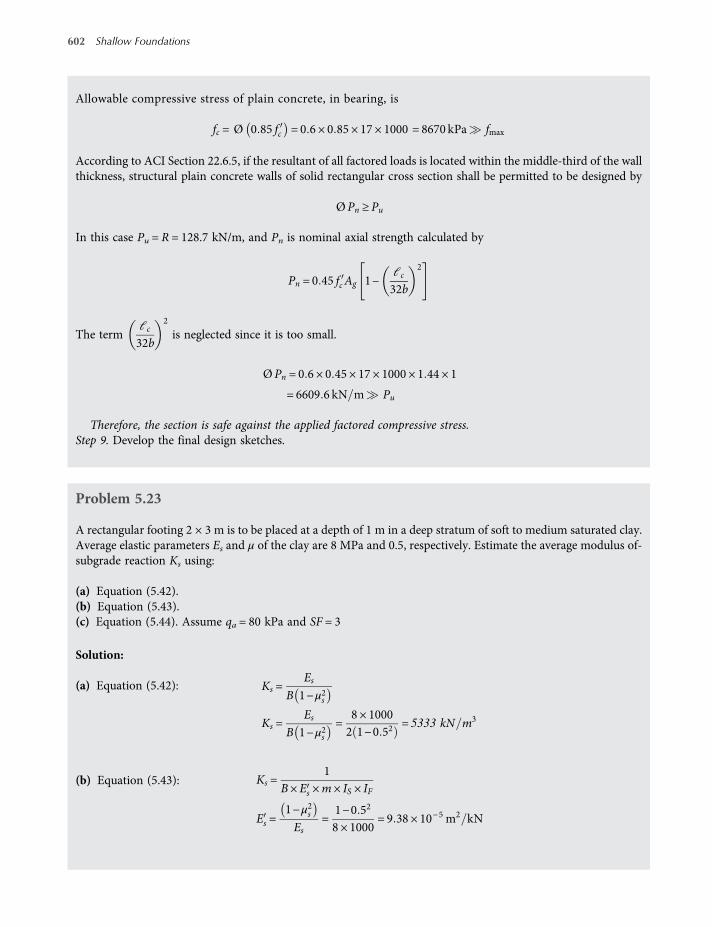
Allowable compressive stress of plain concrete, in bearing, is
fc = Ø 0 85 fc = 0 6 × 0 85 × 17 × 1000 = 8670 kPa fmax
According to ACI Section 22.6.5, if the resultant of all factored loads is located within the middle-third of the wallthickness, structural plain concrete walls of solid rectangular cross section shall be permitted to be designed by
Ø Pn ≥ Pu
In this case Pu = R = 128.7 kN/m, and Pn is nominal axial strength calculated by
Pn = 0 45 fc Ag 1−ℓc
32b
2
The termℓc
32b
2
is neglected since it is too small.
Ø Pn = 0 6 × 0 45 × 17 × 1000 × 1 44 × 1
= 6609 6 kN m Pu
Therefore, the section is safe against the applied factored compressive stress.Step 9. Develop the final design sketches.
Problem 5.23
A rectangular footing 2 × 3 m is to be placed at a depth of 1 m in a deep stratum of soft to medium saturated clay.Average elastic parameters Es and μ of the clay are 8 MPa and 0.5, respectively. Estimate the average modulus of-subgrade reaction Ks using:
(a) Equation (5.42).(b) Equation (5.43).(c) Equation (5.44). Assume qa = 80 kPa and SF = 3
Solution:
(a) Equation (5.42): Ks =Es
B 1−μ2s
Ks =Es
B 1−μ2s=
8 × 10002 1−0 52
= 5333 kN m3
(b) Equation (5.43): Ks =1
B× Es ×m× IS × IF
Es =1−μ2sEs
=1−0 52
8 × 1000= 9 38 × 10−5 m2 kN
602 Shallow Foundations
worksaccounts.com
For the centre of the loaded area:
Use:B2instead of B,
L2instead of L, m = 4 and H = 4B
M = L/B, N =H/B, H = Thickness of the soil layer, in units of B
M =1 51
= 1 5,N = 4 ×21= 8
From Table 3.7 obtain I1 = 0.561 and I2 = 0.029
IS = I1 +1−2μ1−μ
I2 = 0 561 +1−2 × 0 51−0 5
× 0 029 = 0 561
For actual values ofBL= 0 667;
DB= 0 5; μ = 0.5, from Table 3.6, obtain IF = 0.88.
Ks =1
1 × 9 38 × 10−5 × 4 × 0 561 × 0 88= 5399 kN m3
For a corner of the loaded area:Use: actual B and L dimensions; m = 1; H = 4B;
M =32= 1 5; N = 4 ×
22= 4
From Table 3.7 obtain I1 = 0.455 and I2 = 0.054
IS = I1 +1−2μ1−μ
I2 = 0 455 +1−2 × 0 51−0 5
× 0 054 = 0 455
For actual values ofBL= 0 667,
DB= 0 5, μ = 0.5 Table 3.6 gives
IF = 0 88 as before
Ks =1
2 × 9 38 × 10−5 × 1 × 0 455 × 0 88= 13313 kN m3
Compute weighted average Ks using four centre Ks values and one corner value, as follows:
Average Ks =4 × 5399 + 13313
5= 6982 kN m3
(c) Equation (5.44):Ks = 40 SF qa
Ks = 40 SF qa = 40 × 3 × 80 = 9600 kN m3
Problem 5.24
For the 15 × 15 m mat foundation and soil data of Problem 4.37 recommend a single value of Ks that may beconsidered as an average value for the base.
(Continued)
Shallow Foundations – Structural Design 603
worksaccounts.com
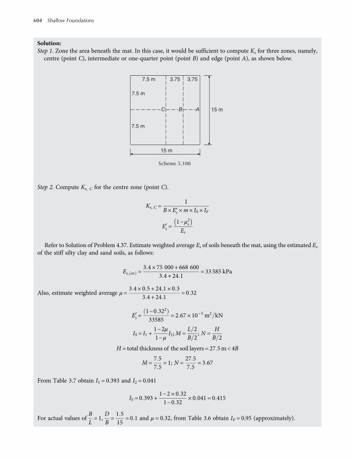
Solution:Step 1. Zone the area beneath the mat. In this case, it would be sufficient to compute Ks for three zones, namely,
centre (point C), intermediate or one-quarter point (point B) and edge (point A), as shown below.
Step 2. Compute Ks, C for the centre zone (point C).
Ks, C =1
B× Es ×m× IS × IF
Es =1−μ2sEs
Refer to Solution of Problem 4.37. Estimate weighted average Es of soils beneath the mat, using the estimated Esof the stiff silty clay and sand soils, as follows:
Es, av =3 4 × 75 000 + 668 600
3 4 + 24 1= 33 585 kPa
Also, estimate weighted average μ=3 4 × 0 5 + 24 1 × 0 3
3 4 + 24 1= 0 32
Es =1−0 322
33585= 2 67 × 10−5 m2 kN
IS = I1 +1−2μ1−μ
I2;M =L 2B 2
; N =HB 2
H = total thickness of the soil layers = 27 5m< 4B
M =7 57 5
= 1; N =27 57 5
= 3 67
From Table 3.7 obtain I1 = 0.393 and I2 = 0.041
IS = 0 393 +1−2 × 0 321−0 32
× 0 041 = 0 415
For actual values ofBL= 1,
DB=1 515
= 0 1 and μ = 0.32, from Table 3.6 obtain IF = 0.95 (approximately).
3.75 3.75
7.5 m
7.5 m
7.5 m
15 m
15 m ABC
Scheme 5.108
604 Shallow Foundations
worksaccounts.com

Ks,C =1
B× Es ×m× IS × IF=
17 5 × 2 67 × 10−5 × 4 × 0 415 × 0 95
= 3167 kN m3
Step 3. Compute Ks,B for the intermediate zone at the one-quarter point (point B).There are two sets of rectangles contribute at point B, as shown below:
Set 1: two rectangles of B = 7.5 m and L = 11.25 m
M =LB= 1 5; N =
HB= 3 67
I1 = 0 41; I2 = 0 065; IS = 0 444
BL= 0 67;
DB=1 57 5
= 0 2; IF = 0 926
Si = q×B×1−μ2sEs
×m× IS × IF
Si = q×B× Es ×m × IS × IF
Siq= 7 5 × 2 67 × 10−5 × 2 × 0 444 × 0 926 = 1 647 × 10−4 m3 kN
Set 2: two rectangles of B = 3.75 m and L = 7.5 m
M =LB= 2;N =
HB= 7 33; I1 = 0 597; I2 = 0 041; IS = 0 619
BL= 0 5;
DB=
1 53 75
= 0 4; IF = 0 866
Si = q×B× Es ×m × IS × IF
Siq= 3 75 × 2 67 × 10−5 × 2 × 0 619 × 0 86 = 1 073 × 10−4 m3 kN
1Ks,B
=Siq= 1 647 × 10−4 + 1 073 × 10−4 = 2 72 × 10−4 m3 kN
Ks,B =1
2 72 × 10−4= 3676 kN m3
3.75 m
3.75 m
11.25 m
11.25 m
7.5 m
7.5 m
B
Scheme 5.109
(Continued)
Shallow Foundations – Structural Design 605
worksaccounts.com

Step 4. Compute Ks,A for the edge zone (point A).There is one set of two rectangles contributing at point A, as shown below:
B = 7.5 m and L = 15.0 m
M =LB= 2;N =
HB=27 57 5
= 3 67
I1 = 0 452; I2 = 0 074; IS = 0 491
BL= 0 5;
DB=1 57 5
= 0 2; IF = 0 936
Si = q×B× Es ×m × IS × IF
1Ks, A
=Siq=B× Es ×m× IS × IF
Ks, A =1
7 5 × 2 67 × 10−5 × 2 × 0 491 × 0 936= 5433 kN m3
Step 5. Recommend a single value of KS that may be considered as an average value for the base.If a single value of KS is to be provided, one might simply use
Ks =Ks,C +Ks,B +Ks,A
3=3167 + 3676 + 5433
3= 4092 kN m3
or (weighting Ks,C),
Ks =4Ks,C +Ks,A
5=4 × 3167 + 5433
5= 3620 kN m3
or (weighting Ks,B and using Simpson’s rule),
Ks =Ks,C + 4Ks,B +Ks,A
6=3167 + 4 × 3676 + 5433
6= 3884 kN m3
Another method may be by equating summation of product of each zone area and its Ks to the product of the matarea and Ks,av, as follows:
Divide the mat area into three zones, as shown in the scheme below, and compute the area of each zone.
15.00 m
11.25 m
3.75 m
15.0
0 m
3.7
5 m
11.2
5 m Zone C
Zone A
Zone B
BC A
Scheme 5.111
7.5 m
15.0 m
A
7.5 m
15.0 m
Scheme 5.110
606 Shallow Foundations
worksaccounts.com

Area of zoneC central AC = 3 75 × 3 75 = 14 063m2
Area of zoneB interior AB = 11 25 × 11 25−14 063 = 112 5m2
Area of zoneA exterior AA = 15 × 15−112 5 = 98 437m2
AA Ks,A +AB Ks,B +AC Ks,C = AA +AB +AC Ks,av
98 437 5433 + 112 5 3676 + 14 063 3167 = 152 Ks,av
Ks,av =992896225
= 4413 kN m3
It may be appropriate to recommend the average of all the computed values as a single value for the requiredmodulus of subgrade reaction, which is
Ks =4092 + 3620 + 3884 + 4413
4= 4002 25 kN m3
Recommend Ks = 4000 kN/m3
Problem 5.25
A structure is to be supported on a 15-m square mat foundation. The average contact pressure is 100 kPa.A settlement analysis conducted by the geotechnical engineer gave an average settlement S = 25 mm.Recommend design values for the modulus of subgrade reaction KS which may be used in a pseudo-coupled
analysis.
Solution:
Step 1. Estimate Ks,av.Equation (5.40): Ks =
qδ
Where
q= bearing pressure
δ= deflection settlement
Average modulus of subgrade reaction = Ks,av =1000 025
= 4000 kN m3
Step 2. Divide the mat area into three zones and compute the area of each zone. Note that the innermost (central)zone shall be half as wide and half as long as the mat.
Area of zoneA central AA = 7 5 × 7 5 = 56 25m2
Area of zoneB interior AB = 11 25 × 11 25−7 5 × 7 5 = 70 313m2
Area of zoneC exterior AC = 15 × 15−11 25 × 11 25 = 98 438m2
Step 3.Assign a KS value to each zone.The KS values should progressively increase from the centre such that the outermost zone (exterior zone) has
a KS about twice as large as the innermost zone (central zone). In this case, let us use:
(Continued)
Shallow Foundations – Structural Design 607
worksaccounts.com
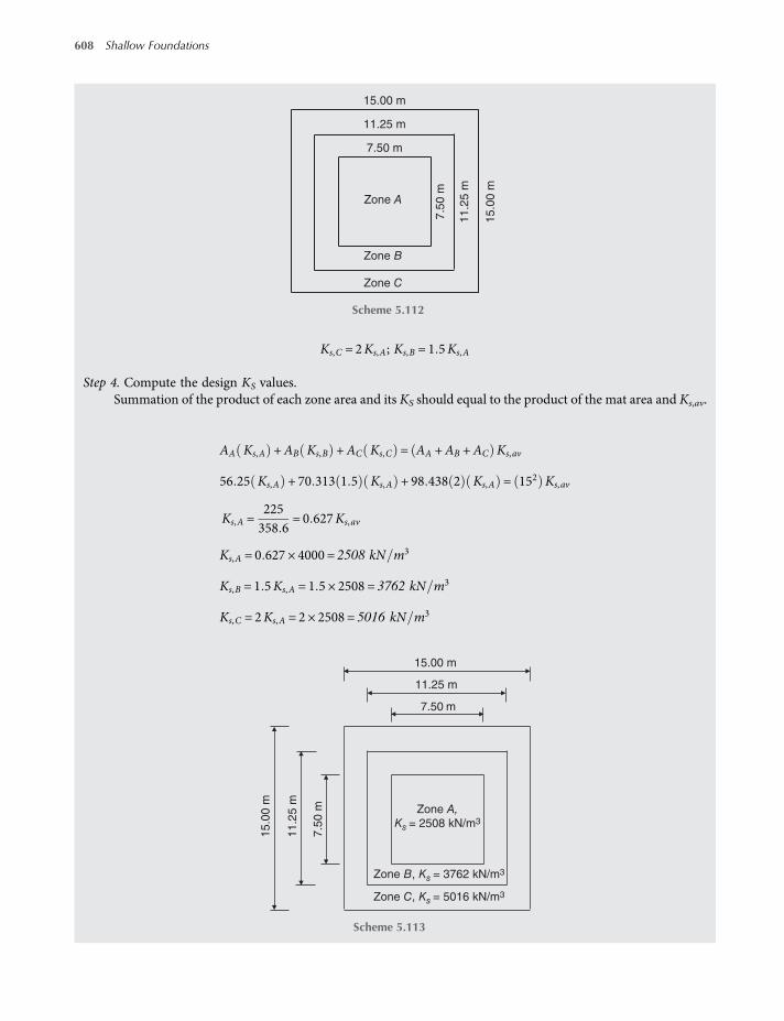
Ks,C = 2Ks,A; Ks,B = 1 5Ks,A
Step 4. Compute the design KS values.Summation of the product of each zone area and its KS should equal to the product of the mat area and Ks,av.
AA Ks,A +AB Ks,B +AC Ks,C = AA +AB +AC Ks,av
56 25 Ks,A + 70 313 1 5 Ks,A + 98 438 2 Ks,A = 152 Ks,av
Ks,A =225358 6
= 0 627Ks,av
Ks,A = 0 627 × 4000 = 2508 kN m3
Ks,B = 1 5Ks,A = 1 5 × 2508 = 3762 kN m3
Ks,C = 2Ks,A = 2 × 2508 = 5016 kN m3
Zone A
15.00 m
11.25 m
7.50 m
Zone B
Zone C
15.0
0 m
7.5
0 m
11.2
5 m
Scheme 5.112
Zone B, Ks = 3762 kN/m3
Zone C, Ks = 5016 kN/m3
Zone A,Ks = 2508 kN/m3
7.50 m
11.25 m
11.2
5 m
15.00 m
7.5
0 m
15.0
0 m
Scheme 5.113
608 Shallow Foundations
worksaccounts.com

Problem 5.26
The plan of a simple mat foundation and the tabulated column working loads are shown in the scheme below. Allthe columns are 0.4 × 0.4 m and carry no moment of significant value.The design soil pressure or net qa and average modulus of subgrade reaction Ks,av, recommended by the
geotechnical engineer, are 60 kPa and 7200 kN/m3, respectively.Design the mat by the conventional rigid method, and then check if this design method could be considered
appropriate. Use:
fc = 24 MPa
fy = 420 MPa
Solution:Step 1. Compute resultant R of all working (unfactored) loads, as shown in Table 5.16.Step 2. Find location of R and determine the eccentricities ex and ey.(a) Take moments about the left edge of the mat and compute x as follows:
Rx =Σmoment of column D+ L ±ΣMy
x =
2 0 2 240 + 2 0 2 960 + 2 6 0 360 + 2 6 0 960
+ 11 8 300 + 810 + 810 + 270 ± 07230
= 5 83 m
ex =122−5 83 = 0 17 m <
B6
7.2
m
7.2
m
0.2 m
0.2 m
B = 12 m
L=
22 m
7.2
m5.8m5.8 m 0.2 m
0.2 m
10
1
64
7 8 9
32
5
11 12
y
y
x x
D,kN L,kNCol.No.
Axial col.loads
1 80 160
2 120 240
3 100 200
4 320 640
5 320 640
6 270 540
7 320 640
8 320 640
9 270 540
10 80 160
11 120 240
12 90 180
Scheme 5.114
(Continued)
Shallow Foundations – Structural Design 609
worksaccounts.com
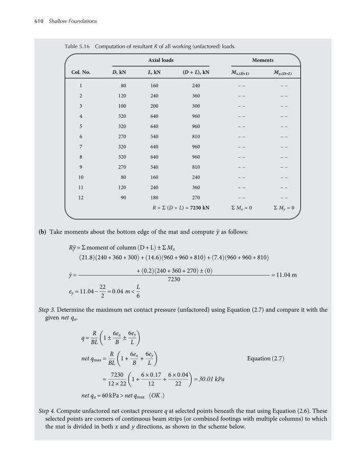
(b) Take moments about the bottom edge of the mat and compute y as follows:
Ry =Σmoment of column D+L ±ΣMx
y =
21 8 240 + 360 + 300 + 14 6 960 + 960 + 810 + 7 4 960 + 960 + 810
+ 0 2 240 + 360 + 270 ± 07230
= 11 04 m
ey = 11 04−222= 0 04 m <
L6
Step 3. Determine the maximum net contact pressure (unfactored) using Equation (2.7) and compare it with thegiven net qa.
q=RBL
1 ±6exB
±6eyL
net qmax =RBL
1 +6exB
+6eyL
Equation 2 7
=723012 × 22
1 +6 × 0 17
12+6 × 0 04
22= 30 01 kPa
net qa = 60 kPa > net qmax OK
Step 4. Compute unfactored net contact pressure q at selected points beneath the mat using Equation (2.6). Theseselected points are corners of continuous beam strips (or combined footings with multiple columns) to whichthe mat is divided in both x and y directions, as shown in the scheme below.
Table 5.16 Computation of resultant R of all working (unfactored) loads.
Col. No.
Axial loads Moments
D, kN L, kN (D + L), kN Mx,(D+L) My,(D+L)
1 80 160 240 – – – –
2 120 240 360 – – – –
3 100 200 300 – – – –
4 320 640 960 – – – –
5 320 640 960 – – – –
6 270 540 810 – – – –
7 320 640 960 – – – –
8 320 640 960 – – – –
9 270 540 810 – – – –
10 80 160 240 – – – –
11 120 240 360 – – – –
12 90 180 270 – – – –
R = Σ (D + L) = 7230 kN Σ Mx = 0 Σ My = 0
610 Shallow Foundations
worksaccounts.com
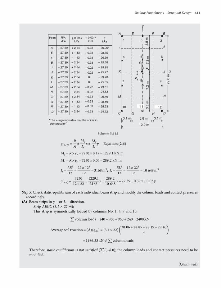
q x, y =RA±My
Iyx ±
Mx
Ixy Equation 2 6
My =R× ex = 7230 × 0 17 = 1229 1 kN m
Mx =R× ey = 7230 × 0 04 = 289 2 kN m
Iy =LB3
12=22 × 123
12= 3168m3; Ix =
BL3
12=12 × 223
12= 10 648m3
q x,y =723012 × 22
±1229 13168
x ±289 210 648
y = 27 39 ± 0 39 x ± 0 03 y
Step 5. Check static equilibrium of each individual beam strip and modify the column loads and contact pressuresaccordingly.
(A) Beam strips in y − or L − direction.Strip AEGC (3.1 × 22 m):This strip is symmetrically loaded by columns No. 1, 4, 7 and 10.
column loads = 240 + 960 + 960 + 240 = 2400 kN
Average soil reaction = A qav = 3 1 × 2230 06 + 28 85 + 28 19 + 29 40
4
= 1986 33 kN column loads
Therefore, static equilibrium is not satisfied ( Fv 0); the column loads and contact pressures need to bemodified.
1
7.2
m7.2
m
3.1 m
12.0 m
5.8 m
3.8
m
3.1 m
3.8
m
22.0
m
10
6
ex
ey
4
R
K
M
C G H D
8 9
32
7
5
11 12
y
A
I
E F B
J
J X
N
Point
+ 27.39A
R/A
kPaq
kPa
E
F
B
I
J
K
L
M
N
C
G
H
D
+ 2.34
+– 0.39 x
kPa
+– 0.03 y
kPa
+ 0.33 + 30.06*
+ 28.85
+ 26.59
+ 25.38
+ 29.95
+ 29.73
+ 29.51
+ 25.27
+ 25.05
+ 24.83
+ 29.40
+ 28.19
+ 25.93
+ 24.72
+ 0.33
+ 0.33
+ 0.33
+ 0.22
+ 0.22
– 0.22
– 0.22
– 0.33
– 0.33
– 0.33
– 0.33
0
0
+ 2.34
+ 2.34
+ 2.34
– 2.34
+ 2.34
– 2.34
– 2.34
– 2.34
– 2.34
+ 1.13
+ 1.13
– 1.13
– 1.13
+ 27.39
+ 27.39
+ 27.39
+ 27.39
+ 27.39
+ 27.39
+ 27.39
+ 27.39
+ 27.39
+ 27.39
+ 27.39
+ 27.39
+ 27.39
*The + sign indicates that the soil is in
“compression”
Scheme 5.115
(Continued)
Shallow Foundations – Structural Design 611
worksaccounts.com
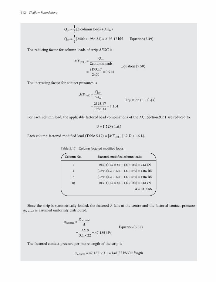
Qav =12Σ column loads +Aqav
Qav =122400 + 1986 33 = 2193 17 kN Equation 5 49
The reducing factor for column loads of strip AEGC is
MF col =Qav
Σcolumn loads
=2193 172400
= 0 914
Equation 5 50
The increasing factor for contact pressures is
MF soil =Qav
Aqav
=2193 171986 33
= 1 104
Equation 5 51 - a
For each column load, the applicable factored load combinations of the ACI Section 9.2.1 are reduced to:
U = 1 2D+ 1 6L
Each column factored modified load (Table 5.17) = [MF(col.)](1.2 D + 1.6 L).
Since the strip is symmetrically loaded, the factored R falls at the centre and the factored contact pressureqfactored is assumed uniformly distributed.
qfactored =Rfactored
A
=3218
3 1 × 22= 47 185 kPa
Equation 5 52
The factored contact pressure per metre length of the strip is
qfactored = 47 185 × 3 1 = 146 27 kN m length
Table 5.17 Column factored modified loads.
Column No. Factored modified column loads
1 (0.914)(1.2 × 80 + 1.6 × 160) = 322 kN
4 (0.914)(1.2 × 320 + 1.6 × 640) = 1287 kN
7 (0.914)(1.2 × 320 + 1.6 × 640) = 1287 kN
10 (0.914)(1.2 × 80 + 1.6 × 160) = 322 kN
R = 3218 kN
612 Shallow Foundations
worksaccounts.com
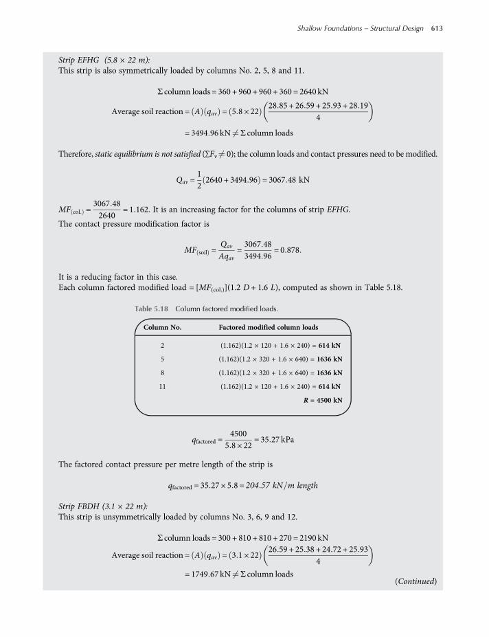
Strip EFHG (5.8 × 22 m):This strip is also symmetrically loaded by columns No. 2, 5, 8 and 11.
Σ column loads = 360 + 960 + 960 + 360 = 2640 kN
Average soil reaction = A qav = 5 8 × 2228 85 + 26 59 + 25 93 + 28 19
4
= 3494 96 kN Σ column loads
Therefore, static equilibrium is not satisfied (∑Fv 0); the column loads and contact pressures need to be modified.
Qav =122640 + 3494 96 = 3067 48 kN
MF col =3067 482640
= 1 162. It is an increasing factor for the columns of strip EFHG.
The contact pressure modification factor is
MF soil =Qav
Aqav=3067 483494 96
= 0 878
It is a reducing factor in this case.Each column factored modified load = [MF(col.)](1.2 D + 1.6 L), computed as shown in Table 5.18.
qfactored =4500
5 8 × 22= 35 27 kPa
The factored contact pressure per metre length of the strip is
qfactored = 35 27 × 5 8 = 204 57 kN m length
Strip FBDH (3.1 × 22 m):This strip is unsymmetrically loaded by columns No. 3, 6, 9 and 12.
Σ column loads = 300 + 810 + 810 + 270 = 2190 kN
Average soil reaction = A qav = 3 1 × 2226 59 + 25 38 + 24 72 + 25 93
4
= 1749 67 kN Σ column loads
Table 5.18 Column factored modified loads.
Column No. Factored modified column loads
2 (1.162)(1.2 × 120 + 1.6 × 240) = 614 kN
5 (1.162)(1.2 × 320 + 1.6 × 640) = 1636 kN
8 (1.162)(1.2 × 320 + 1.6 × 640) = 1636 kN
11 (1.162)(1.2 × 120 + 1.6 × 240) = 614 kN
R = 4500 kN
(Continued)
Shallow Foundations – Structural Design 613
worksaccounts.com

Therefore, static equilibrium is not satisfied (ΣFv 0); the column loads and contact pressures need to bemodified.
Qav =122190 + 1749 67 = 1969 84 kN
MF col =1969 842190
= 0 899. This is a reducing factor for columns of strip FBDH.
Each column factored modified load = [MF(col.)](1.2 D + 1.6 L), computed as shown in Table 5.19.
Since the strip is unsymmetrically loaded, the factored R does not fall at the centre; it has an eccentricity eL or ey,calculated as follows:
Ry = moment of factored column loads
y =396 × 21 8 + 1068 × 14 6 + 1068 × 7 4 + 356 × 0 2
2888= 11 15m
eL = 11 15−222= 0 15m<
L6
The factored contact pressures are calculated, using Equation (5.53), as follows:
qfactored =Rfactored
A±eLRfactored
IBl
qmax =2888
3 1 × 22+
0 15 × 28883 1 × 223 12
× 11 = 42 346 + 1 732 = 44 078 kPa
qmin = 42 346−1 732 = 40 614 kPa
qmax = 44 078 × 3 1 = 136 64 kN m length
qmin = 40 614 × 3 1 = 125 9 kN m length
(B) Beam strips in x − or B − direction.Strip ABJI (3.8 × 12 m):This strip is unsymmetrically loaded by columns No. 1, 2 and 3.
column loads = 240 + 360 + 300 = 900 kN
Average soil reaction = A qav = 3 8 × 1230 06 + 25 38 + 25 27 + 29 95
4
= 1261 52 kN ∑ column loads
Table 5.19 Column factored modified loads.
Column No. Factored modified column loads
3 (0.899)(1.2 × 100 + 1.6 × 200) = 396 kN
6 (0.899)(1.2 × 270 + 1.6 × 540) = 1068 kN
9 (0.899)(1.2 × 270 + 1.6 × 540) = 1068 kN
12 (0.899)(1.2 × 90 + 1.6 × 180) = 356 kN
R = 2888 kN
614 Shallow Foundations
worksaccounts.com
Therefore, static equilibrium is not satisfied (ΣFv 0); the column loads and contact pressures need to bemodified.
Qav =12900 + 1261 52 = 1080 76 kN
MF col =1080 76900
= 1 2 It is an increasing factor for columns of stripABJI
Each column factored modified load = [MF(col.)](1.2 D + 1.6 L), computed as shown in Table 5.20.
Since the strip is unsymmetrically loaded, the factored R does not fall at the centre; it has an eccentricity excalculated as follows:
Rx =Σmoment of factored column loads
x =422 × 0 2 + 634 × 6 0 + 528 × 11 8
1584= 6 388 m
ex = 6 388−122= 0 388 m<
126
The factored contact pressures are calculated, using Equation (5.53), as follows:
qfactored =Rfactored
A±exRfactored
Iyl
qmax =1584
3 8 × 12+0 388 × 15843 8 × 123 12
× 6 = 34 737 + 6 739 = 41 476 kPa
qmin = 34 737−6 739 = 27 998 kPa
qmax = 41 476 × 3 8 = 157 61 kN m length
qmin = 27 998 × 3 8 = 106 39 kN m length
Strip IJLK (7.2 × 12 m):This strip is unsymmetrically loaded by columns No. 4, 5 and 6.
column loads = 960 + 960 + 810 = 2730 kN
Average soil reaction = A qav = 7 2 × 1229 95 + 25 27 + 25 05 + 29 73
4
= 2376 kN column loads
Table 5.20 Column factored modified loads.
Column No. Factored modified column loads
1 (1.2)(1.2 × 80 + 1.6 × 160) = 422 kN
2 (1.2)(1.2 × 120 + 1.6 × 240) = 634 kN
3 (1.2)(1.2 × 100 + 1.6 × 200) = 528 kN
R = 1584 kN
(Continued)
Shallow Foundations – Structural Design 615
worksaccounts.com

Therefore, static equilibrium is not satisfied (ΣFv 0); the column loads and contact pressures need to bemodified.
Qav =122730 + 2376 = 2553 kN
MF col =25532730
= 0 935. This is a reducing factor for columns of strip IJLK.
Each column factored modified load = [MF(col.)](1.2 D + 1.6 L), computed as shown in Table 5.21.
Since the strip is unsymmetrically loaded, the factored R does not fall at the centre; it has an eccentricity excalculated as follows:
Rx =Σmoment of factored column loads
x =1316 × 0 2 + 1316 × 6 0 + 1111 × 11 8
3743= 5 682 m
ex =122−5 682 = 0 318 m<
126
The factored contact pressures are calculated, using Equation (5.53), as follows:
qfactored =Rfactored
A±exRfactored
Iyl
qmax =3743
7 2 × 12+0 318 × 37437 2 × 123 12
× 6 = 43 322 + 6 888 = 50 210 kPa
qmin = 43 322−6 888 = 36 434 kPa
qmax = 50 210 × 7 2 = 361 51 kN m length
qmin = 36 434 × 7 2 = 262 32 kN m length
Strip KLNM (7.2 × 12 m):This strip is the same as strip IJLK. However, there is a very small difference in their average soil reactions; com-puted equals 0.8% only, which may be considered negligible. For design purposes, assume both strips identical.Strip MNDC (3.8 × 12 m):This strip is unsymmetrically loaded by columns No. 10, 11 and 12.
Table 5.21 Column factored modified loads.
Column No. Factored modified column loads
4 (0.935)(1.2 × 320 + 1.6 × 640) = 1316 kN
5 (0.935)(1.2 × 320 + 1.6 × 640) = 1316 kN
6 (0.935)(1.2 × 270 + 1.6 × 540) = 1111 kN
R = 3743 kN
616 Shallow Foundations
worksaccounts.com
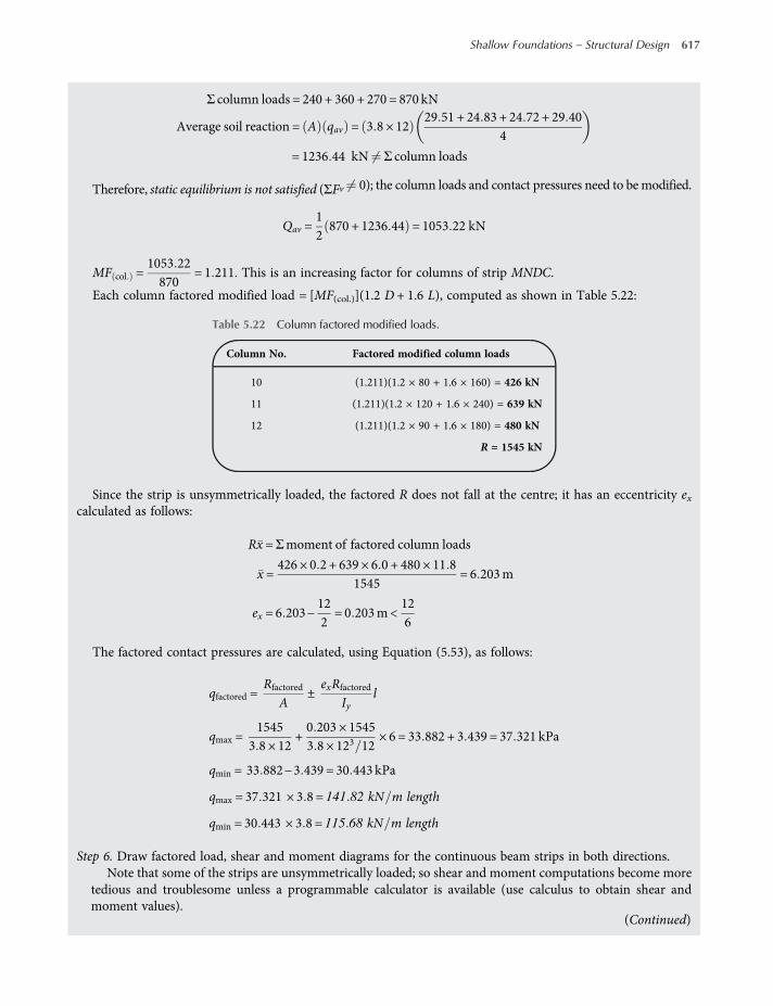
Σ column loads = 240 + 360 + 270 = 870 kN
Average soil reaction = A qav = 3 8 × 1229 51 + 24 83 + 24 72 + 29 40
4
= 1236 44 kN Σ column loads
Therefore, static equilibrium is not satisfied (ΣFv 0); the column loads and contact pressures need to be modified.
Qav =12870 + 1236 44 = 1053 22 kN
MF col =1053 22870
= 1 211. This is an increasing factor for columns of strip MNDC.
Each column factored modified load = [MF(col.)](1.2 D + 1.6 L), computed as shown in Table 5.22:
Since the strip is unsymmetrically loaded, the factored R does not fall at the centre; it has an eccentricity excalculated as follows:
Rx =Σmoment of factored column loads
x =426 × 0 2 + 639 × 6 0 + 480 × 11 8
1545= 6 203m
ex = 6 203−122= 0 203m<
126
The factored contact pressures are calculated, using Equation (5.53), as follows:
qfactored =Rfactored
A±exRfactored
Iyl
qmax =1545
3 8 × 12+0 203 × 15453 8 × 123 12
× 6 = 33 882 + 3 439 = 37 321 kPa
qmin = 33 882−3 439 = 30 443 kPa
qmax = 37 321 × 3 8 = 141 82 kN m length
qmin = 30 443 × 3 8 = 115 68 kN m length
Step 6. Draw factored load, shear and moment diagrams for the continuous beam strips in both directions.Note that some of the strips are unsymmetrically loaded; so shear and moment computations become more
tedious and troublesome unless a programmable calculator is available (use calculus to obtain shear andmoment values).
Table 5.22 Column factored modified loads.
Column No. Factored modified column loads
10 (1.211)(1.2 × 80 + 1.6 × 160) = 426 kN
11 (1.211)(1.2 × 120 + 1.6 × 240) = 639 kN
12 (1.211)(1.2 × 90 + 1.6 × 180) = 480 kN
R = 1545 kN
(Continued)
Shallow Foundations – Structural Design 617
worksaccounts.com
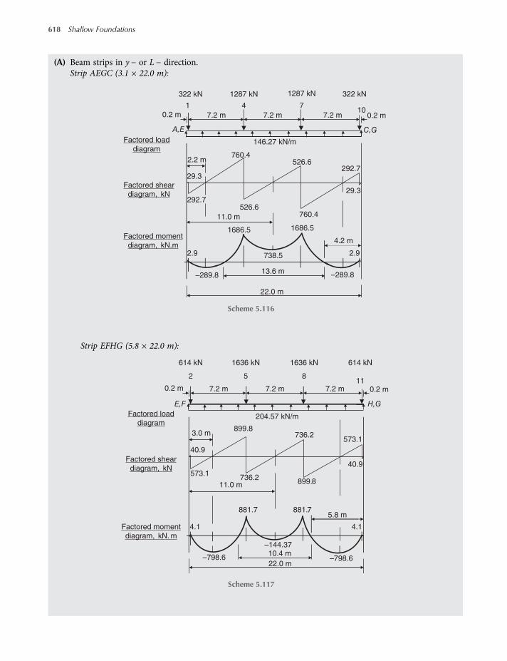
(A) Beam strips in y − or L − direction.Strip AEGC (3.1 × 22.0 m):
Strip EFHG (5.8 × 22.0 m):
–289.8 –289.8
22.0 m
4.2 m
Factored shear
diagram, kN
Factored moment
diagram, kN.m2.9
13.6 m
738.5
11.0 m
2.2 m
1686.5
292.7
292.7
146.27 kN/m
526.6760.4
1686.5
29.3
Factored load
diagram
29.3
526.6760.4
2.9
0.2 m0.2 m
A,E C,G
1 4 710
322 kN 322 kN1287 kN
7.2 m7.2 m 7.2 m
1287 kN
Scheme 5.116
881.7
–798.622.0 m
5.8 m
Factored shear
diagram, kN
–798.610.4 m
–144.37
11.0 m
3.0 m
881.7
573.1
573.1
204.57 kN/m
899.8736.2
40.9
Factored load
diagram899.8
40.9
736.2
0.2 m0.2 m
E,F H,G
614 kN 614 kN
11
1636 kN
7.2 m7.2 m 7.2 m
1636 kN
Factored moment
diagram, kN. m
5 82
4.1 4.1
Scheme 5.117
618 Shallow Foundations
worksaccounts.com
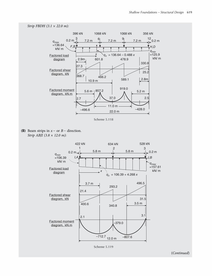
Strip FBDH (3.1 × 22.0 m):
(B) Beam strips in x − or B − direction.Strip ABJI (3.8 × 12.0 m):
919.0
2.52.7 37.0
11.0 m
10.9 m
5.6 m 857.2
368.7
330.8
589.1466.2
25.2
5.2 m
2.8m
601.8
27.3
478.9
0.2 m
qx = 136.64 – 0.488 x
0.2 m
2.9m
x
3 9 126
396 kN
qmax
=136.64
kN/ mqmin
=125.9
kN/ m
356 kN1068 kN
7.2 m7.2 m 7.2 m
1068 kN
22.0 m
H,DF,B
Factored load
diagram
Factored shear
diagram, kN
Factored moment
diagram, kN.m
–496.6 –428.0
Scheme 5.118
12.0 m
2.1
400.6
3.1
293.2
21.4
340.8
0.2 m 0.2 m
1
31.5
2 3
422 kN
496.5
634 kN
5.8 m5.8 m
528 kN
qmin
=106.39
kN/ mqmax
=157.61
kN/ m
I,A J,B
Factored load
diagram
Factored shear
diagram, kN
Factored moment
diagram, kN.m
xqx = 106.39 + 4.268 x
3.7 m
3.5 m
–379.0
–807.6–712.7
Scheme 5.119
(Continued)
Shallow Foundations – Structural Design 619
worksaccounts.com

Strip IJLK (7.2 × 12.0 m):
Strip KLNM (7.2 × 12.0 m):The same load, shear and moment diagrams which belong to strip IJLK are also used for strip KLNM, sincethese two strips are assumed identical, as mentioned earlier.
Strip MNDC (3.8 × 12.0 m):
12.0 m
1243.9
5.3
704.3
72.1
611.7
0.2 m 0.2 m1
52.7
1316 kN
1058.3
1316 kN
5.8 m5.8 m
1111 kN
7.2
2 3
qmin
= 262.32
kN/ mqx = 361.51 – 8.266 x
3.8m
4.0 m
–1423.3
–2034.0–2203.1
qmax
=361.51
kN/ m
Factored load
diagram
Factored shear
diagram, kN
Factored moment
diagram, kN.m
K ,I L, J
x
Scheme 5.120
3.5 m
Factored shear
diagram, kN
Factored moment
diagram, kN. m
2.3
3.6 m
–681.9 –731.7
2.8
Factored load
diagram
307.3
331.7
23.2
0.2 m
D,NC,M
qmax
= 141.82
kN/m
qmin
= 115.68
kN/m
xqx = 115.68 + 2.178 x
28.3
426 kN
10
451.7
639 kN
11
5.8 m5.8 m0.2 m
480 kN
12
402.8
–310.2
12.0 m
Scheme 5.121
620 Shallow Foundations
worksaccounts.com
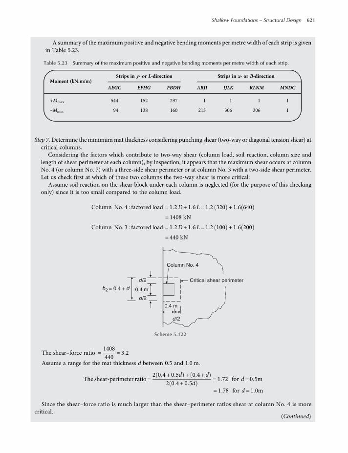
A summary of the maximum positive and negative bending moments per metre width of each strip is givenin Table 5.23.
Step 7.Determine the minimummat thickness considering punching shear (two-way or diagonal tension shear) atcritical columns.
Considering the factors which contribute to two-way shear (column load, soil reaction, column size andlength of shear perimeter at each column), by inspection, it appears that the maximum shear occurs at columnNo. 4 (or column No. 7) with a three-side shear perimeter or at column No. 3 with a two-side shear perimeter.Let us check first at which of these two columns the two-way shear is more critical:
Assume soil reaction on the shear block under each column is neglected (for the purpose of this checkingonly) since it is too small compared to the column load.
Column No 4 factored load = 1 2D+ 1 6L= 1 2 320 + 1 6 640
= 1408 kN
Column No 3 factored load = 1 2D+ 1 6L= 1 2 100 + 1 6 200
= 440 kN
The shear–force ratio =1408440
= 3 2
Assume a range for the mat thickness d between 0.5 and 1.0 m.
The shear-perimeter ratio =2 0 4 + 0 5d + 0 4 + d
2 0 4 + 0 5d= 1 72 for d = 0 5m
= 1 78 for d = 1 0m
Since the shear–force ratio is much larger than the shear–perimeter ratios shear at column No. 4 is morecritical.
Table 5.23 Summary of the maximum positive and negative bending moments per metre width of each strip.
Moment (kN.m/m)Strips in y- or L-direction Strips in x- or B-direction
AEGC EFHG FBDH ABJI IJLK KLNM MNDC
+Mmax 544 152 297 1 1 1 1
–Mmin 94 138 160 213 306 306 1
d/2
d/2
d/2
0.4 m
0.4 m
Column No. 4
b2 = 0.4 + d
Critical shear perimeter
Scheme 5.122
(Continued)
Shallow Foundations – Structural Design 621
worksaccounts.com
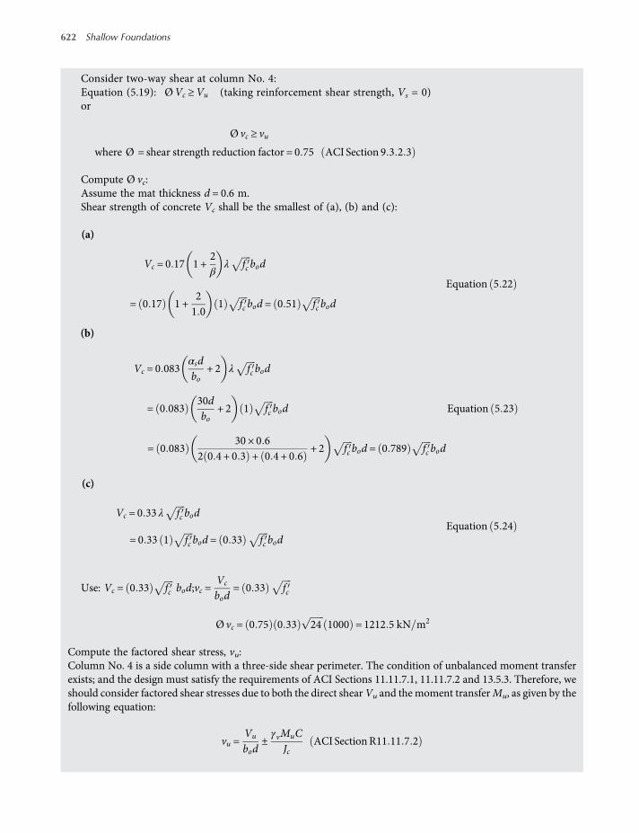
Consider two-way shear at column No. 4:Equation (5.19): ØVc ≥Vu (taking reinforcement shear strength, Vs = 0)or
Ø vc ≥ vu
where Ø = shear strength reduction factor = 0 75 ACI Section 9 3 2 3
Compute Ø vc:Assume the mat thickness d = 0.6 m.Shear strength of concrete Vc shall be the smallest of (a), (b) and (c):
(a)
Vc = 0 17 1 +2β
λ fc bod
= 0 17 1 +21 0
1 fc bod = 0 51 fc bod
Equation 5 22
(b)
Vc = 0 083αsdbo
+ 2 λ fc bod
= 0 08330dbo
+ 2 1 fc bod
= 0 08330 × 0 6
2 0 4 + 0 3 + 0 4 + 0 6+ 2 fc bod = 0 789 fc bod
Equation 5 23
(c)
Vc = 0 33 λ fc bod
= 0 33 1 fc bod = 0 33 fc bodEquation 5 24
Use: Vc = 0 33 fc bod;vc =Vc
bod= 0 33 fc
Ø vc = 0 75 0 33 24 1000 = 1212 5 kN m2
Compute the factored shear stress, vu:Column No. 4 is a side column with a three-side shear perimeter. The condition of unbalanced moment transferexists; and the design must satisfy the requirements of ACI Sections 11.11.7.1, 11.11.7.2 and 13.5.3. Therefore, weshould consider factored shear stresses due to both the direct shearVu and the moment transferMu, as given by thefollowing equation:
vu =Vu
bod±γvMuC
JcACI SectionR11 11 7 2
622 Shallow Foundations
worksaccounts.com
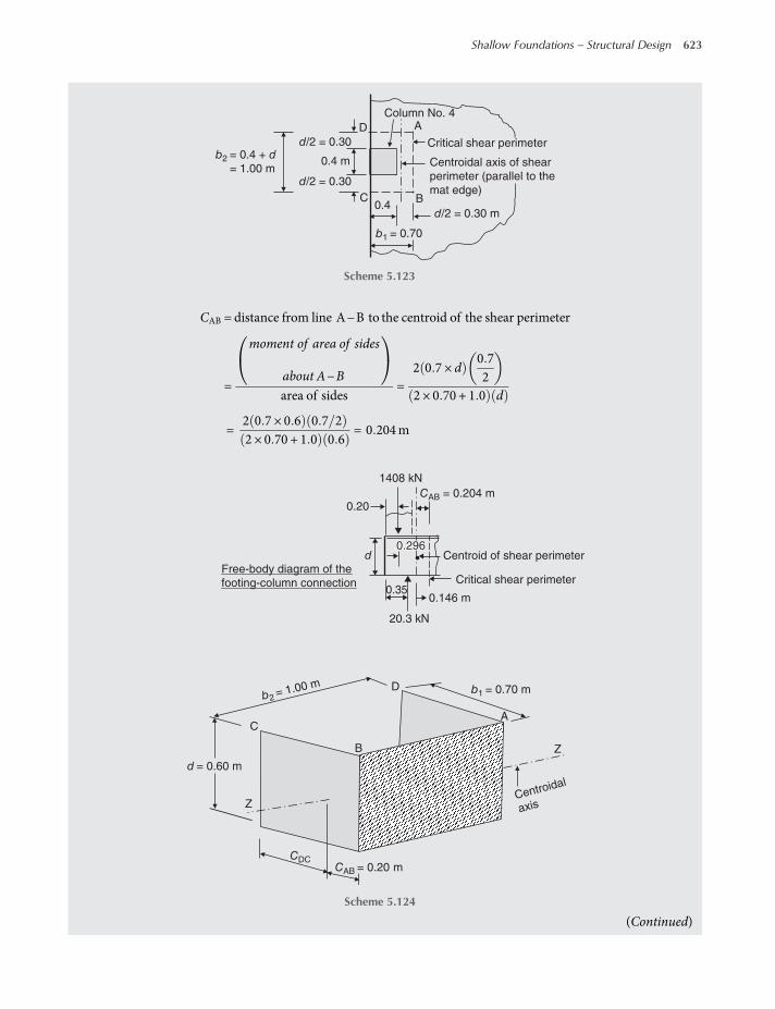
CAB = distance from line A−B to the centroid of the shear perimeter
=
moment of area of sides
about A−B
area of sides=
2 0 7 × d0 72
2 × 0 70 + 1 0 d
=2 0 7 × 0 6 0 7 22 × 0 70 + 1 0 0 6
= 0 204m
d/2 = 0.30
d/2 = 0.30
0.4 m
0.4
A
BC
D
Column No. 4
b2 = 0.4 + d
= 1.00 m
Critical shear perimeter
Centroidal axis of shear
perimeter (parallel to the
mat edge)
b1 = 0.70
d/2 = 0.30 m
Scheme 5.123
D
Z B
A C
b1 = 0.70 m
d = 0.60 m
Centroidal
axis
CDCCAB = 0.20 m
Z
b2 =1.00 m
Free-body diagram of the
footing-column connection
0.20
1408 kN
Centroid of shear perimeter
Critical shear perimeter
0.146 m
20.3 kN
0.35
d
CAB = 0.204 m
0.2960.2960.296
Scheme 5.124
(Continued)
Shallow Foundations – Structural Design 623
worksaccounts.com
Estimate the average soil pressure on the shear block = 29 kPa. (Note: it would be more correct if the factoredvalue is used. However, since its effect is nearly negligible and in order to obtain a more conservative design theun-factored value is considered.)
Soil reaction on the shear block = 29 × 1 × 0.7 = 20.3 kNSummation of moments about the centroid of the shear perimeter equals the unbalanced moment,Mu. Hence,
Mu = 1408 × 0 296−20 3 × 0 146 = 413 8 kN m
Vu = 1408−20 3 = 1387 7 kN
γv = 1− γf
γf =1
1 + 2 3 b1 b2ACI Section 11 11 7 1
=1
1 + 2 3 0 7 1 0= 0 642 ACI Section 13 5 3 2
γv = 1−0 642 = 0 358
Jc = Jz = Property of the shear perimeter analogous to polar moment of inertia
Jc = 2b1d3
12+ 2
db3112
+ 2 b1db12−CAB
2
+ b2d CAB2
= 20 7 × 0 63
12+ 2
0 6 × 0 73
12+ 2 0 7 × 0 6
0 72
−0 2042
+ 1 × 0 6 0 2042
= 0 0252 + 0 0343 + 0 0179 + 0 0250 = 0 1024m4
C =CDC = b1−CAB = 0 70−0 204 = 0 496m
İn this case, the shear stresses due to direct shear and shear due to moment transfer will add at points D and C,giving the largest shear stresses on the critical shear perimeter. Hence,
vu DC =Vu
bod+γvMuCDC
JcACI SectionR11 11 7 2
vu DC =1387 7
2 × 0 7 + 1 0 6+0 358 × 413 8 × 0 496
0 1024= 963 68 + 717 56
= 1681 24 kPa > Ø vc = 1212 5 kPa Not OK
Assume another value for d and check Ø vc again.Try d = 0.76 m:
b1 = 0 4 + d 2 = 0 78m; b2 = 0 4 + d = 1 16m
CAB =
moment of area of sidesabout A−B
area of sides=2 0 78 × d 0 78 22 × 0 78 + 1 16 d
2 0 78 × 0 76 0 392 × 0 78 + 1 16 0 76
= 0 224 m
C =CDC = b1−CAB = 0 78−0 224 = 0 56 m
624 Shallow Foundations
worksaccounts.com
Soil reaction on the shear block = 29 × 1 16 × 0 78 = 26 24 kN
Moment arm of soil reaction =b12
−CAB
=0 782
−0 224 = 0 17m
Moment arm of column load = b1−0 2 −CAB
= 0 58−0 22 = 0 36m
Mu = 1408 × 0 36−26 24 × 0 17 = 502 42 kN m
Vu = 1408−26 24 = 1381 76 kN
γf =1
1 + 2 3 b1 b2
=1
1 + 2 3 0 78 1 16= 0 646; γv = 1−0 646 = 0 354
Jc = 2b1d3
12+ 2
db3112
+ 2 b1db12−CAB
2
+ b2d CAB2
= 20 78 × 0 763
12+ 2
0 76 × 0 783
12+ 2 0 78 × 0 76
0 782
−0 2242
+ 1 16 × 0 76 0 2242
= 0 0571 + 0 0601 + 0 0327 + 0 0442 = 0 194m4
vu DC =1381 76
2 × 0 78 + 1 16 0 76+0 354 × 502 42 × 0 56
0 194= 668 42 + 513 40
= 1181 82 kPa < Ø vc = 1212 5 kPa OK
Use d = 0.76 m; h = 0.85 mStep 8. Check the computed mat depth d considering beam shear (one-way shear) at the most critical section.
Refer to the shear diagrams in Step 6. It is clear that the most critical section for shear per metre width islocated in strip AEGC at distance d from either the left face of column No. 4 or the right face of column No. 7.The applied beam shear at any of these two locations is
Vu =760 4−q d + 0 2
3 1=760 4−146 27 0 76 + 0 2
3 1= 200 kN mwidth
Equation (5.19):ØVc ≥Vu taking reinforcement shear strength, Vs = 0
Equation (5.20):
Vc = 0 17λ fc bwdØVc = 0 75 × 0 17 × 1 24 1000 1 0 76
= 474 7 kN m Vu = 200 kN m OK
Step 9. Obtain the design factored positive and negative moments per metre width using the factored momentdiagrams in Step 6.
Refer to Table 5.23 at the end of Step 6. Obtain the following factored maximum moments per metre width:(A) Moments required for design of reinforcement in y − or L − direction.
(Continued)
Shallow Foundations – Structural Design 625
worksaccounts.com
+Mmax = 544 kN m m for steel inmidspans, at bottom of the mat
−Mmax = 160 kN m m for steel in exterior spans, at top
(B) Moments required for design of reinforcement in x − or B − direction.+ Mmax 1 kN. m/m. For all practical purposes, it is considered negligible.− Mmax = 306 kN. m/m (for steel in both spans, at top of the mat)
Step 10. Determine the positive and negative flexural reinforcement required in each direction.
(A) Flexural reinforcement required in y − or L − direction.(a) Negative reinforcement at top of the mat:
Equation (5.9): ØMn ≥Mu
Mu = 160 kN m m
Assume tension-controlled section, Ø = 0.9 and fs = fy.Equation (5.10):
a=Asfy
0 85fc b
=As × 420
0 85 × 24 × 1= 20 59As m
Equation (5.11):
ØMn = Ø Asfy d−a2
= 0 9 As × 420 × 1000 0 76−20 59As
2
= 287 280As−3 891 510As2
Let ØMn =Mu:287 280As−3 891 510As
2 = 160
As2−0 074As + 4 11 × 10−5 = 0
As =− −0 074 ± −0 074 2− 4 1 4 11 × 10−5
2 × 1=0 074−0 073
2
= 0 5 ×10⁻³ m2
m= 500mm2 m required by analysis
ACI Section 10.5.1:
As,min =0 25 fc
fybwd and not less than 1 4
bw dfy
As,min =0 25 24
420× 1 × 0 76 = 2 216 × 10−3 m2 m= 2216mm2 m
1 4bw dfy
=1 4 × 1 × 0 76
420= 2 533 × 10−3 m2 m= 2533mm2 m
As,min > As by analysis. However, the requirements of ACI Section 10.5.1 need not be applied if, at every section,As provided is at least one-third greater than that required by analysis (According to ACI Section 10.5.3).
626 Shallow Foundations
worksaccounts.com
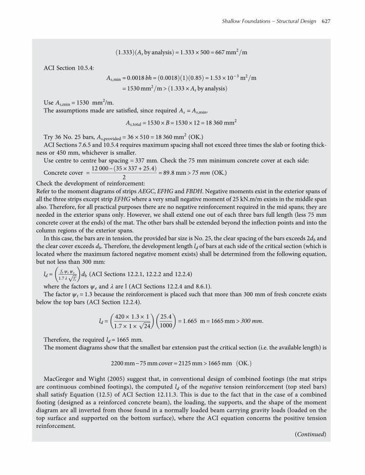
1 333 As by analysis = 1 333 × 500 = 667mm2 m
ACI Section 10.5.4:
As,min = 0 0018 bh= 0 0018 1 0 85 = 1 53 × 10−3 m2 m
= 1530mm2 m> 1 333 ×As by analysis
Use As,min = 1530 mm2/m.The assumptions made are satisfied, since required As = As,min.
As, total = 1530 ×B= 1530 × 12 = 18 360 mm2
Try 36 No. 25 bars, As,provided = 36 × 510 = 18 360 mm2 (OK.)ACI Sections 7.6.5 and 10.5.4 requires maximum spacing shall not exceed three times the slab or footing thick-
ness or 450 mm, whichever is smaller.Use centre to centre bar spacing = 337 mm. Check the 75 mm minimum concrete cover at each side:
Concrete cover =12 000− 35 × 337 + 25 4
2= 89 8 mm> 75mm (OK.)
Check the development of reinforcement:Refer to the moment diagrams of strips AEGC, EFHG and FBDH. Negative moments exist in the exterior spans ofall the three strips except strip EFHG where a very small negative moment of 25 kN.m/m exists in the middle spanalso. Therefore, for all practical purposes there are no negative reinforcement required in the mid spans; they areneeded in the exterior spans only. However, we shall extend one out of each three bars full length (less 75 mmconcrete cover at the ends) of the mat. The other bars shall be extended beyond the inflection points and into thecolumn regions of the exterior spans.
In this case, the bars are in tension, the provided bar size is No. 25, the clear spacing of the bars exceeds 2db andthe clear cover exceeds db. Therefore, the development length ld of bars at each side of the critical section (which islocated where the maximum factored negative moment exists) shall be determined from the following equation,but not less than 300 mm:
ld =fy ψ t ψ e
1 7 λ fcdb (ACI Sections 12.2.1, 12.2.2 and 12.2.4)
where the factors ψ e and λ are l (ACI Sections 12.2.4 and 8.6.1).The factor ψ t = 1.3 because the reinforcement is placed such that more than 300 mm of fresh concrete exists
below the top bars (ACI Section 12.2.4).
ld =420 × 1 3 × 1
1 7 × 1 × 24
25 41000
= 1 665 m= 1665mm> 300mm
Therefore, the required ld = 1665 mm.The moment diagrams show that the smallest bar extension past the critical section (i.e. the available length) is
2200mm−75mmcover = 2125mm> 1665mm OK
MacGregor and Wight (2005) suggest that, in conventional design of combined footings (the mat stripsare continuous combined footings), the computed ld of the negative tension reinforcement (top steel bars)shall satisfy Equation (12.5) of ACI Section 12.11.3. This is due to the fact that in the case of a combinedfooting (designed as a reinforced concrete beam), the loading, the supports, and the shape of the momentdiagram are all inverted from those found in a normally loaded beam carrying gravity loads (loaded on thetop surface and supported on the bottom surface), where the ACI equation concerns the positive tensionreinforcement.
(Continued)
Shallow Foundations – Structural Design 627
worksaccounts.com
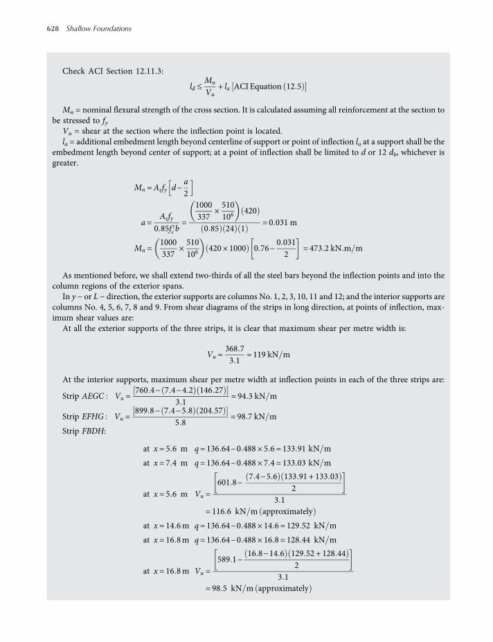
Check ACI Section 12.11.3:
ld ≤Mn
Vu+ la ACIEquation 12 5
Mn = nominal flexural strength of the cross section. It is calculated assuming all reinforcement at the section tobe stressed to fy
Vu = shear at the section where the inflection point is located.la = additional embedment length beyond centerline of support or point of inflection la at a support shall be the
embedment length beyond center of support; at a point of inflection shall be limited to d or 12 db, whichever isgreater.
Mn =Asfy d−a2
a=Asfy
0 85fc b=
1000337
×510106
420
0 85 24 1= 0 031 m
Mn =1000337
×510106
420 × 1000 0 76−0 0312
= 473 2 kN m m
As mentioned before, we shall extend two-thirds of all the steel bars beyond the inflection points and into thecolumn regions of the exterior spans.
In y − or L − direction, the exterior supports are columns No. 1, 2, 3, 10, 11 and 12; and the interior supports arecolumns No. 4, 5, 6, 7, 8 and 9. From shear diagrams of the strips in long direction, at points of inflection, max-imum shear values are:
At all the exterior supports of the three strips, it is clear that maximum shear per metre width is:
Vu =368 73 1
= 119 kN m
At the interior supports, maximum shear per metre width at inflection points in each of the three strips are:
Strip AEGC Vu =760 4− 7 4−4 2 146 27
3 1= 94 3 kN m
Strip EFHG Vu =899 8− 7 4−5 8 204 57
5 8= 98 7 kN m
Strip FBDH:
at x = 5 6 m q= 136 64−0 488 × 5 6 = 133 91 kN m
at x = 7 4 m q= 136 64−0 488 × 7 4 = 133 03 kN m
at x = 5 6 m Vu =601 8−
7 4−5 6 133 91 + 133 032
3 1= 116 6 kN m approximately
at x = 14 6m q= 136 64−0 488 × 14 6 = 129 52 kN m
at x = 16 8m q= 136 64−0 488 × 16 8 = 128 44 kN m
at x = 16 8m Vu =589 1−
16 8−14 6 129 52 + 128 442
3 1= 98 5 kN m approximately
628 Shallow Foundations
worksaccounts.com
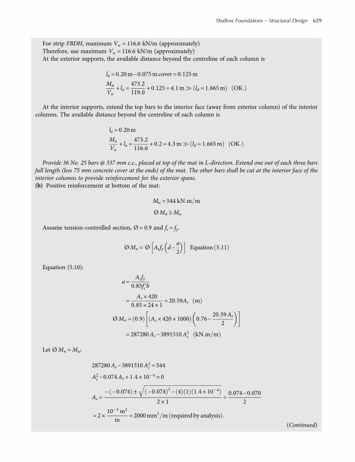
For strip FBDH, maximum Vu = 116.6 kN/m (approximately)Therefore, use maximum Vu = 116.6 kN/m (approximately)At the exterior supports, the available distance beyond the centreline of each column is
la = 0 20m−0 075mcover = 0 125m
Mn
Vu+ la =
473 2119 0
+ 0 125 = 4 1m ld = 1 665m OK
At the interior supports, extend the top bars to the interior face (away from exterior column) of the interiorcolumns. The available distance beyond the centreline of each column is
la = 0 20m
Mn
Vu+ la =
473 2116 6
+ 0 2 = 4 3m ld = 1 665m OK
Provide 36 No. 25 bars @ 337 mm c.c., placed at top of the mat in L-direction. Extend one out of each three barsfull length (less 75 mm concrete cover at the ends) of the mat. The other bars shall be cut at the interior face of theinterior columns to provide reinforcement for the exterior spans.(b) Positive reinforcement at bottom of the mat:
Mu = 544 kN m m
ØMn ≥Mu
Assume tension-controlled section, Ø = 0.9 and fs = fy.
ØMn = Ø Asfy d−a2
Equation 5 11
Equation (5.10):
a=Asfy
0 85fc b
=As × 420
0 85 × 24 × 1= 20 59As m
ØMn = 0 9 As × 420 × 1000 0 76−20 59As
2
= 287280As−3891510A2s kN m m
Let ØMn =Mu:
287280As−3891510A2s = 544
A2s −0 074As + 1 4 × 10−4 = 0
As =− −0 074 ± −0 074 2− 4 1 1 4 × 10⁻⁴
2 × 1=0 074−0 070
2
= 2 ×10⁻³ m2
m= 2000mm2 m required by analysis
(Continued)
Shallow Foundations – Structural Design 629
worksaccounts.com

ACI Section 10.5.1:
As,min =0 25 fc
fybwd and not less than 1 4
bw dfy
As,min =0 25 24
420× 1 × 0 76 = 2 216 × 10−3 m2 m= 2216mm2 m
1 4bw dfy
=1 4 × 1 × 0 76
420= 2 533 × 10−3 m2 m= 2533mm2 m
As,min > As by analysis Therefore, use As = As,min = 2533 mm2/mThe assumptions made are satisfied, since As required = As,min.
As, total = 2533 ×B= 2533 × 12 = 30 396mm2
Try 60 No. 25 bars, As,provided = 60 × 510 = 30 600 mm2 (OK.)ACI Sections 7.6.5 and 10.5.4 requires maximum spacing shall not exceed three times the slab or footing thick-
ness, or 450 mm, whichever is smaller.Use centre to centre bar spacing = 200 mm. Check the 75 mm minimum concrete cover at each side:
Concrete cover =12 000− 59 × 200 + 25 4
2= 87 3 mm> 75mm OK
Check the development of reinforcement:We shall extend one out of each four bars full length (less 75 mm concrete cover at the ends) of the mat. The
other bars shall be extended beyond the inflection points a distance equal to d or 12db, whichever is greater (ACISections 12.10.3). In this case, it is clear that d controls. Maximum distance between any two inflection points in allthe three strips is 13.6 m (strip AEGH). Therefore, each cut off point shall be located beyond the column centre at adistance equal to
13 6−7 22
+ 0 76 = 3 96 m; say, 4m
In this case, the bars are in tension, the provided bar size is No. 25, the clear spacing of the bars exceeds 2db andthe clear cover exceeds db. Therefore, the development length ld of bars at each side of the critical section (which islocated where the maximum factored positive moment exists) shall be determined from the following equation,but not less than 300 mm:
ld =fy ψ t ψ e
1 7 λ fcdb (ACI Sections 12.2.1, 12.2.2 and 12.2.4)
Where the factors ψ t, ψ e and λ are 1 (ACI Sections 12.2.4 and 8.6.1).
ld =420 × 1 × 1
1 7 × 1 × 24
25 41000
= 1 28 m= 1280mm> 300mm
Therefore, the required ld = 1280 mm.The bar extension past the critical section (at column centre) is
4m= 4000mm 1280mm OK
630 Shallow Foundations
worksaccounts.com
Provide 60 No. 25 bars @ 200 mm c.c., placed at bottom of the mat in L-direction. Extend one out of each four barsfull length (less 75 mm concrete cover at the ends) of the mat. The other bars (short bars of 15.2 m length) shall beextended 4 m beyond the centre line of each interior column toward the exterior column.(B) Flexural reinforcement required in x − or B − direction.
(a) Negative reinforcement at top of the mat:
Mu = 306 kN m m
ØMn ≥Mu
Assume tension-controlled section, Ø = 0.9 and fs = fy.
ØMn = Ø Asfy d−a2
Equation 5 11
Equation (5.10):
a =Asfy
0 85fc b
=As × 420
0 85 × 24 × 1= 20 59As m
d = 0 7600−0 0254 = 0 735m
ØMn = 0 9 As × 420 × 1000 0 735−20 59As
2
= 277 830As−3 891 510A2s kN m m
Let ØMn =Mu:
277 830As−3 891 510A2s = 306
A2s −0 0714As + 4 11 × 10−5 = 0
As =− −0 0714 ± −0 0714 2− 4 1 7 86 × 10−5
2 × 1=0 0714−0 0692
2= 1 1 × 10⁻³ m2 m= 1100mm2 m required by analysis
ACI Section 10.5.1:
As,min =0 25 fc
fybwd and not less than 1 4
bw dfy
As,min =0 25 24
420× 1 × 0 735 = 2 143 × 10−3 m2 m= 2143mm2 m
1 4bw dfy
=1 4 × 1 × 0 735
420= 2 450 × 10−3 m2 m= 2450mm2 m
(Continued)
Shallow Foundations – Structural Design 631
worksaccounts.com
As,min > As by analysis. However, the requirements of ACI Section 10.5.1 need not be applied if, at every section,As provided is at least one-third greater than that required by analysis (According to ACI Section 10.5.3).
1 333 As by analysis = 1 333 × 1100 = 1463mm2 m
ACI Section 10.5.4:
As,min = 0 0018 bh= 0 0018 1 0 85 = 1 53 × 10−3 m2 m
= 1530mm2 m> 1 333 ×As by analysis
Use As = As,min = 1530 mm2/mThe assumptions made are satisfied, since required As = As,min.
As, total = 1530 × L= 1530 × 22 = 33 660mm2
Try 66 No. 25 bars, As,provided = 66 × 510 = 33 660 (OK.)ACI Sections 7.6.5 and 10.5.4 requires maximum spacing shall not exceed three times the slab or footing thick-
ness, or 450 mm, whichever is smaller.Use centre to centre bar spacing = 335 mm. Check the 75 mm minimum concrete cover at each side:
Concrete cover =22 000− 65 × 335 + 25 4
2= 99 8 mm> 75mm OK
Check the development of reinforcement:We shall extend all the bars full width (less 75 mm concrete cover at the ends) of the mat.In this case, the bars are in tension, the provided bar size is No. 25, the clear spacing of the bars exceeds 2db, and
the clear cover exceeds db Therefore, the development length ld of bars at each side of the critical section (which islocated where the maximum factored negative moment exists) shall be determined from the following equation,but not less than 300 mm:
ld =fy ψ t ψ e
1 7 λ fcdb (ACI Sections 12.2.1, 12.2.2 and 12.2.4)
where the factors ψ e and λ are l (ACI Sections 12.2.4 and 8.6.1).The factor ψ t = 1.3 because the reinforcement is placed such that more than 300 mm of fresh concrete exists
below the top bars (ACI Section 12.2.4).
ld =420 × 1 3 × 1
1 7 × 1 × 24
25 41000
= 1 665m= 1665mm> 300mm
Therefore, the required ld = 1665 mm.The moment diagrams show that the smallest bar extension past the critical section (i.e. the available length) is
3500mm−75mmcover = 3425mm> 1665mm OK
Check ACI Section 12.11.3:In this case, it is required to check ACI Equation (12.5) at the exterior supports only, since all the bars are
extended full width of the mat.
ld ≤Mn
Vu+ la ACIEquation 12 5
632 Shallow Foundations
worksaccounts.com
Mn =Asfy d−a2
a =Asfy
0 85fc b=
1000335
×510106
420
0 85 24 1= 0 0313 m
Mn =1000335
×510106
420 × 1000 0 735−0 0313
2
Vu =1243 97 2
= 172 8 kN m
At all the exterior supports of the three strips, it is clear that maximum shear per metre length is
Vu =1243 97 2
= 172 8 kN m
At the exterior supports, the available distance beyond the centreline of each column is
la = 0 20m−0 075 mcover = 0 125m
Mn
Vu+ la =
460 0172 8
+ 0 125 = 2 8m> ld = 1 665m OK
Provide 66 No. 25 bars @ 335 mm c.c., placed at top of the mat in B − direction and directly below the bars inL-direction. Extend all the bars full width (less 75 mm concrete cover at the ends) of the mat.(b) Positive reinforcement at bottom of the mat:
As mentioned in Step 9, for all practical purposes there are no (+) moments in any span; so (+) momentsteel in x − or B − direction is not required by analysis. However, enough supportive steel bars shall be pro-vided and wired to the bottom bars in L − direction so that the latter bars can be positioned and held properly.
Provide 50-No. 13 bars @ 450 mm c.c., at bottom of the mat in B − direction, wired to the bars in L −direction. Extend all the bars full width (less 75 mm concrete cover at the ends) of the mat.
Step 11. Check column bearing on the mat at critical column locations and design the column to mat dowels.The design computations proceed in the same manner as that presented in the design Steps 5 and 6 for the
column footing of Problem 5.3. The necessary computations are left for the reader.Step 12. Check if the conventional rigid design method could be considered appropriate.
The rigid design method is considered appropriate if the mat strips, both ways, can be considered or treatedas a rigid body. As mentioned in Section 5.10.1, strips (continuous footings or combined footings with multiplecolumns) can be considered rigid if the following requirements or criteria are met:
(a) Variation in adjacent column loads and spacing is not over 20% of the greater value.(b) Average of two adjacent spans is < (1.75/ λ).
Equation (5.48):
λ=KsB4EcI
4
WhereKs = coefficient (or modulus) of vertical subgrade reactionEc = modulus of elasticity of concreteI = moment of inertia of the beam (strip) sectionB = width of the strip
(Continued)
Shallow Foundations – Structural Design 633
worksaccounts.com

Criterion (a):All strips (both ways) have no variation in the adjacent column spacing. The problem is with the column
loads. All strips except strips IJLK and KLNM have adjacent column loads varying by more than 20%.Therefore criterion (a) is not fully satisfied. One may estimate that this requirement of rigidity is only
50–60% met.Criterion (b):
Ec = 4700 fc (ACI Section 8.5.1)
Ec = 4700 × 24 = 23025 2 MPa = 5 2 × 10⁷ kPa
Ks, av = 7200 kN m3 given
I =bh3
12=
B 0 853
12= 0 051 B m4
λ=KsB4EcI
4
=7200 B
4 5 2 × 10⁷ 0 051 B4
= 0 161
1 75λ
=1 750 161
= 10 87m
Maximum span length in all the strips (both ways) is 7.2 m < (1.75/ λ)Therefore, the rigidity requirement of criterion (b) is fully satisfied.However, since both rigidity criteria were not met simultaneously, one may consider the conventional rigid
method is unsuitable or not appropriate for design of the given mat.
Step 13. Draw the final design sketches showing top and bottom steel bars, as shown below.
Steel bars @ top of matSteel bars @ bottom of mat
Mat thickness h = 0.85 m
12.0 m
22.0
m
6.8
m
Extend each fourth
bar full length of mat
60 No. 25 @
200 mm c. c.
across mat width
7.2
m4.0
m
12.0 m
7.6
m
3.4
m4.0
m3.4
m
7.6
m
66
–N
o. 25 @
335 m
m c
. c.
full
wid
th o
f m
at
acro
ss m
at le
ngth
50 N
o. 13 @
450 m
m c
. c.
fu
ll w
idth
of m
at
a
cro
ss m
at le
ngth
36 – No. 25 @
337 mm c. c.
across mat width
Extend each third bar
full length of mat
Scheme 5.125
634 Shallow Foundations
worksaccounts.com
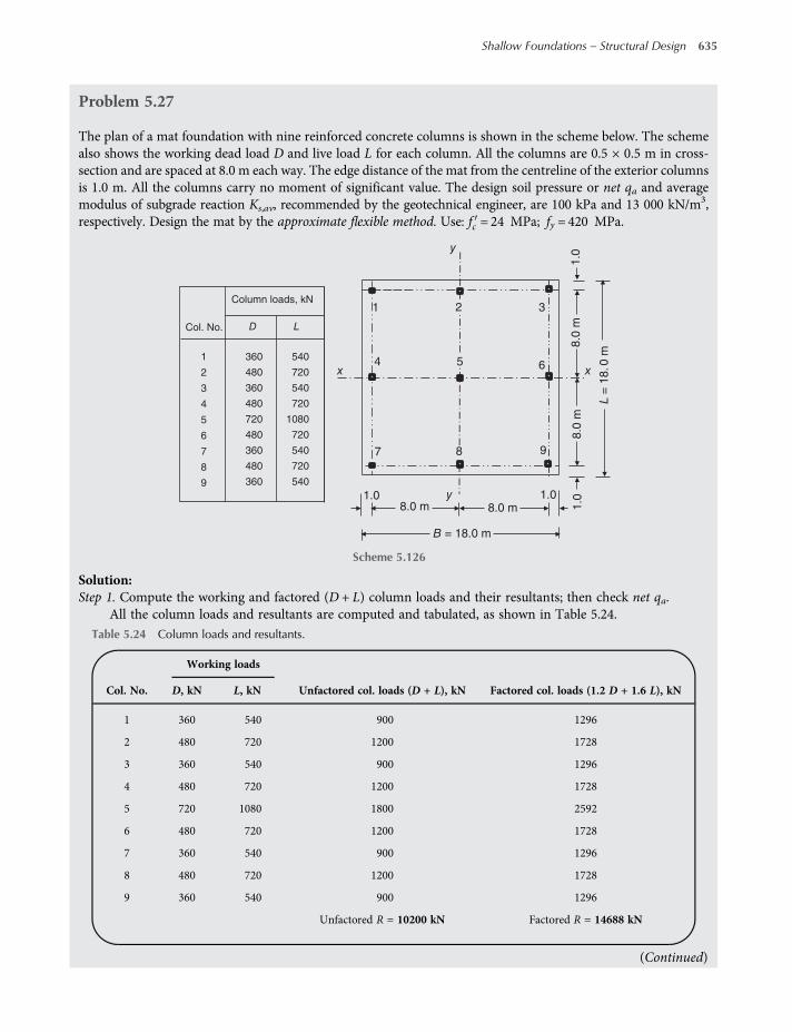
Problem 5.27
The plan of a mat foundation with nine reinforced concrete columns is shown in the scheme below. The schemealso shows the working dead load D and live load L for each column. All the columns are 0.5 × 0.5 m in cross-section and are spaced at 8.0 m each way. The edge distance of the mat from the centreline of the exterior columnsis 1.0 m. All the columns carry no moment of significant value. The design soil pressure or net qa and averagemodulus of subgrade reaction Ks,av, recommended by the geotechnical engineer, are 100 kPa and 13 000 kN/m3,respectively. Design the mat by the approximate flexible method. Use: fc = 24 MPa; fy = 420 MPa.
Solution:Step 1. Compute the working and factored (D + L) column loads and their resultants; then check net qa.
All the column loads and resultants are computed and tabulated, as shown in Table 5.24.
1.0
8.0
m8.0
m
8.0 m1.0
B = 18.0 m
y
y
x x
L=
18.0
m
8.0 m 1.0
1.0
1
64
9
3
7
2
5
8
Column loads, kN
Col. No.
1 360 540
720
540
720
1080
720
540
720
540
480
360
480
720
480
360
480
360
2
3
4
5
6
7
8
9
D L
Scheme 5.126
Table 5.24 Column loads and resultants.
Col. No.
Working loads
Unfactored col. loads (D + L), kN Factored col. loads (1.2 D + 1.6 L), kND, kN L, kN
1 360 540 900 1296
2 480 720 1200 1728
3 360 540 900 1296
4 480 720 1200 1728
5 720 1080 1800 2592
6 480 720 1200 1728
7 360 540 900 1296
8 480 720 1200 1728
9 360 540 900 1296
Unfactored R = 10200 kN Factored R = 14688 kN
(Continued)
Shallow Foundations – Structural Design 635
worksaccounts.com

Unfactorednet q=unfactoredR
A=10 20018 × 18
= 31 5 kPa net qa = 100 kPa OK
Step 2. Determine the minimum mat thickness t considering punching shear.In this problem, all the columns are of the same size with the same four-side shear perimeter. Therefore,
punching shear is most critical at the heaviest column which is the interior column (Col. No. 5). Since it iscommon practice not to use shear reinforcement, we conservatively neglect the resisting factored soil reaction(which is too small compared to the factored column load) on the shear block. Thus, the factored applied shearforce on the shear perimeter is
Vu = 2592 kN
Equation (5.19):
ØVc ≥Vu (taking reinforcement shear strength, Vs = 0)
where Ø = strength reduction factor ACI Section 9 3 2 3
= 0 75 for shear
Shear strength of concrete Vc shall be the smallest of (a), (b) and (c):
(a) Vc = 0 17 1 +2β
λ fc bod
= 0 17 1 +21 0
1 fc bod = 0 51 fc bod
Equation 5 22
(b) Vc = 0 083αsdbo
+ 2 λ fc bod
= 0 08340dbo
+ 2 1 fc bod
Equation 5 23
(c) Vc = 0 33 λ fc bod
= 0 33 1 fc bod = 0 33 fc bodEquation 5 24
d/2Critical section for
two-way shear
d/2
500-mm square column
Column No. 5
Scheme 5.127
636 Shallow Foundations
worksaccounts.com
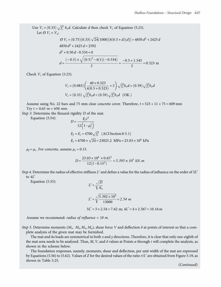
Use Vc = 0 33 fc bod. Calculate d then check Vc of Equation (5.23).Let ØVc = Vu:
ØVc = 0 75 0 33 24 1000 4 0 5 + d d = 4850 d2 + 2425d
4850d2 + 2425d = 2592
d2 + 0 50 d−0 534 = 0
d =−0 5 ± 0 5 2−4 1 −0 534
2=−0 5 + 1 545
2= 0 523 m
Check Vc of Equation (5.23):
Vc = 0 08340 × 0 523
4 0 5 + 0 523+ 2 fc bod = 0 59 fc bod
Vc = 0 33 fc bod < 0 59 fc bod OK
Assume using No. 22 bars and 75 mm clear concrete cover. Therefore, t = 523 + 11 + 75 = 609 mmTry t = 0.65 m = 650 mm.
Step 3. Determine the flexural rigidity D of the mat.Equation (5.54):
D=Ef t3
12 1−μ2f
Ef = Ec = 4700 fc ACI Section 8 5 1
Ec = 4700 × 24 = 23025 2 MPa = 23 03 × 106 kPa
μf = μc. For concrete, assume μc = 0.15.
D=23 03 × 106 × 0 653
12 1−0 152= 5 395× 105 kN m
Step 4.Determine the radius of effective stiffness L and define a value for the radius of influence on the order of 3Lto 4L
Equation (5.55):L =
DKs
4
L =5 392 × 105
13000
4
= 2 54 m
3L = 3 × 2 54 = 7 62 m; 4L = 4 × 2 567 = 10 16m
Assume we recommend: radius of influence < 10 m.
Step 5. Determine moments (Mr, Mt,Mx,My), shear force V and deflection δ at points of interest so that a com-plete analysis of the given mat may be furnished.
The mat and its loads are symmetrical in both x and y directions. Therefore, it is clear that only one-eighth ofthe mat area needs to be analysed. Thus,M,V, and δ values at Points α through i will complete the analysis, asshown in the scheme below.
The foundation responses, namely, moments, shear and deflection, per unit width of the mat are expressedby Equations (5.56) to (5.62). Values of Z for the desired values of the ratio r/L are obtained from Figure 5.19, asshown in Table 5.25.
(Continued)
Shallow Foundations – Structural Design 637
worksaccounts.com

Table 5.26 gives the calculated factored moments, shear and deflection at the points of interest. It is note-worthy that, theoretically, as observed from Figure 5.19 (Z4 and Z4 are∞ for zero r/L ), the moments and sheardue to a point load at the load itself will be infinite. Therefore, it will be necessary to determine these responses atthe column faces and, for design purpose, assume their maximum values uniform under the column. In thepresent Problem with square columns, Mx and My (moments in x and y directions) at the column faces willhave the same maximum values. Also, Mx and My, calculated from Equations (5.58) and (5.59), are momentsabout the y − and x − axis, respectively.
8.0
m8.0
m
8.0 m
1.0
B = 18.0 m
y
y
e f
h i
a b c d
xx
L=
18.0
m
8.0 m 1.0
1.0
1.0
1
64
8 9
3 2
7
5 4 m
4 m
4 m 4 m
Notes:
(1) Points a, c and h are located
at center of columns No. 5, 6 and
3, respectively.
(2) Each point is located within
the radius of influence of a
number of column loads, as
follows:
Point a: Cols. No. 5, 4, 2,
6 and 8.
Point b: Cols. No. 5, 2, 3,
6, 9 and 8.
Point c and d: Cols. No. 5,
3, 6 and 9.
Point e, f and g:
Cols. No. 5, 2, 3 and 6.
Point h and i: Cols. No. 2
3 and 6.
g
Scheme 5.128
Table 5.25 Values of Z for the desired values of the ratio r/L .
r, m r/L Z3 Z3 Z4 Z4
0.25 0.10 0.490 −0.100 −0.850 1.550
1.00 0.39 0.440 −0.210 −0.575 1.200
4.00 1.57 0.190 −0.180 −0.025 0.170
4.12 1.62 0.180 −0.170 −0.020 0.165
5.66 2.23 0.100 −0.125 0.040 0.040
8.00 3.15 0.025 −0.060 0.040 −0.020
8.06 3.17 0.024 −0.058 0.038 −0.022
8.94 3.52 0.015 −0.040 0.035 −0.025
9.00 3.54 0.013 −0.035 0.034 −0.023
9.85 3.88 0.002 −0.020 0.025 −0.020
638 Shallow Foundations
worksaccounts.com

Table 5.26 Calculated factored moments, shear and deflection.
(1) Point a:
P(kN)
r(m)
Mr
(kN, m)Mt
(kN, m)θ
(deg)sin2 θ cos2 θ Mx
(kN, m)My
(kN, m)V
(kN)δ
mm
2592 0.25 0 633.4 0, 90 0,1 1,0 633.4 633.4 −395.4 3.9
1728 8.00 −24.3 4.4 0 0 1 −24.3 4.4 3.4 0.1
1728 8.00 −24.3 4.4 −90 1 0 4.4 −24.3 3.4 0.1
1728 8.00 −24.3 4.4 180 0 1 −24.3 4.4 3.4 0.1
1728 8.00 −24.3 4.4 90 1 0 4.4 −24.3 3.4 0.1
Σ = 593.6 593.6 −381.8 4.3
(2) Point b:
P(kN)
r(m)
Mr
(kN, m)Mt
(kN, m)θ
(deg)sin2 θ cos2 θ Mx
(kN, m)My
(kN, m)V
(kN)δ
mm
2592 4.00 −46.9 65.6 0 0 1 −46.9 65.6 −43.4 1.5
1728 8.94 −19.3 1.9 −63.5 0.8 0.2 −2.3 −15.1 4.3 0.1
1296 8.94 −14.5 1.4 243.5 0.8 0.2 −1.8 −11.3 3.2 0.1
1728 4.00 −31.3 43.7 180 0 1 −31.3 43.7 −28.9 1.0
1296 8.94 −14.5 1.4 116.5 0.8 0.2 −1.8 −11.3 3.2 0.1
1728 8.94 −19.3 1.9 63.5 0.8 0.2 −2.3 −15.1 4.3 0.1
Σ = −86.4 56.5 −57.3 2.9
(3) Point c:
P(kN)
r(m)
Mr
(kN, m)Mt
(kN, m)θ
(deg)sin2 θ cos2 θ Mx
(kN, m)My
(kN, m)V
(kN)δ
mm
2592 8.00 −36.4 6.6 0 0 1 −36.4 6.6 5.1 0.2
1296 8.00 −18.2 3.3 −90 1 0 3.3 −18.2 2.6 0.1
1728 0.25 0 422.3 0, 90 0, 1 1, 0 422.3 422.3 −263.6 2.6
1296 8.00 −18.2 3.3 90 1 0 3.3 −18.2 2.6 0.1
Σ = 392.5 392.5 −253.3 3.0
(4) Point d:
P(kN)
r(m)
Mr
(kN, m)Mt
(kN, m)θ
(deg)sin2 θ cos2 θ Mx
(kN, m)My
(kN, m)V
(kN)δ
mm
2592 9.00 −27.5 2.1 0 0 1 −27.5 2.1 5.9 0.1
1296 8.06 −17.4 3.2 −82.9 0.98 0.02 2.8 −17.0 2.8 0.1
1728 1.00 50.7 235.0 0 0 1 50.7 235.0 −204.1 2.3
1296 8.06 −17.4 3.2 82.9 0.98 0.02 2.8 −17.0 2.8 0.1
Σ = 28.8 203.1 −192.6 2.6
(Continued )
Shallow Foundations – Structural Design 639
worksaccounts.com

Table 5.26 (Continued)
(5) Point e:
P(kN)
r(m)
Mr
(kN, m)Mt
(kN, m)θ
(deg)sin2 θ cos2 θ Mx
(kN, m)My
(kN, m)V
(kN)δ
mm
2592 5.66 −56.8 27.0 45 0.5 0.5 −14.9 −14.9 −10.2 0.8
1728 5.66 −37.9 18.0 −45 0.5 0.5 −10.0 −10.0 −6.8 0.5
1296 5.66 −28.4 13.5 225 0.5 0.5 −7.5 −7.5 −5.1 0.4
1728 5.66 −37.9 18.0 135 0.5 0.5 −10.0 −10.0 −6.8 0.5
Σ = −42.4 −42.4 −28.9 2.2
(5) Point f:
P(kN)
r(m)
Mr
(kN, m)Mt
(kN, m)θ
(deg)sin2 θ cos2 θ Mx
(kN, m)My
(kN, m)V
(kN)δ
mm
2592 9.85 −28.9 2.9 26.6 0.2 0.8 −22.5 −3.5 6.4 0.1
1728 9.85 −19.3 1.9 −26.6 0.2 0.8 −15.1 −2.3 4.3 0.1
1296 4.00 −23.5 32.8 −90 1 0 32.8 −23.5 −21.7 0.7
1728 4.00 −31.3 43.7 90 1 0 43.7 −31.3 −28.9 1.0
Σ = 38.9 −60.6 −39.9 1.9
(6) Point g:
P(kN)
r(m)
Mr
(kN, m)Mt
(kN, m)θ
(deg)sin2 θ cos2 θ Mx
(kN, m)My
(kN, m)V
(kN)δ
mm
2592 9.85 −19.0 0.4 24 0.17 0.83 −15.7 −2.9 5.1 0.1
1728 9.85 −12.7 0.3 −24 0.17 0.83 −10.5 −1.9 3.4 0
1296 4.12 −22.4 29.9 −76 0.94 0.06 26.8 −19.3 −21.0 0.7
1728 4.12 −29.9 39.8 76 0.94 0.06 35.6 −25.7 −28.1 0.9
Σ = 36.2 −49.8 −40.6 1.7
(7) Point h:
P(kN)
r(m)
Mr
(kN, m)Mt
(kN, m)θ
(deg)sin2 θ cos2 θ Mx
(kN, m)My
(kN, m)V
(kN)δ
mm
1728 8.00 −24.3 4.4 0 0 1 −24.3 4.4 3.4 0.1
1296 0.25 0 316.7 0,90 0,1 1,0 316.7 316.7 −197.7 2.0
1728 8.00 −24.3 4.4 90 1 0 4.4 −24.3 3.4 0.1
Σ = 296.8 296.8 −190.9 2.2
(8) Point i:
P(kN)
r(m)
Mr
(kN, m)Mt
(kN, m)θ
(deg)sin2 θ cos2 θ Mx
(kN, m)My
(kN, m)V
(kN)δ
mm
1728 9.00 −18.3 1.4 0 0 1 −18.3 1.4 3.9 0.1
1296 1.00 38.0 176.3 0 0 1 38.0 176.3 −153.1 1.7
1728 8.06 −23.2 4.3 82.9 0.98 0.02 3.8 −22.7 3.7 0.1
Σ = 23.5 155.0 −145.5 1.9
640 Shallow Foundations
worksaccounts.com
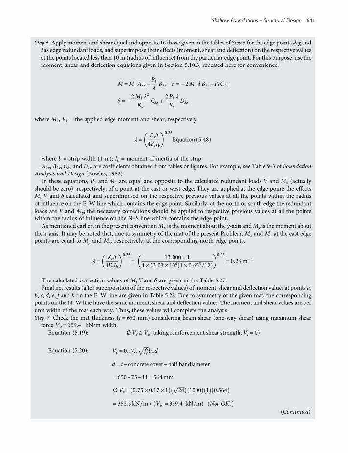
Step 6.Applymoment and shear equal and opposite to those given in the tables of Step 5 for the edge points d, g andi as edge redundant loads, and superimpose their effects (moment, shear and deflection) on the respective valuesat the points located less than 10m (radius of influence) from the particular edge point. For this purpose, use themoment, shear and deflection equations given in Section 5.10.3, repeated here for convenience:
M =M1 Aλx−P1λBλx V = −2M1 λBλx−P1Cλx
δ= −2M1 λ
2
KsCλx +
2P1 λKs
Dλx
where M1, P1 = the applied edge moment and shear, respectively.
λ=Ksb4EcIb
0 25
Equation 5 48
where b = strip width (1 m); Ib = moment of inertia of the strip.Aλx, Bλx, Cλx and Dλx are coefficients obtained from tables or figures. For example, see Table 9-3 of Foundation
Analysis and Design (Bowles, 1982).In these equations, P1 and M1 are equal and opposite to the calculated redundant loads V and Mx (actually
should be zero), respectively, of a point at the east or west edge. They are applied at the edge point; the effectsM, V and δ calculated and superimposed on the respective previous values at all the points within the radiusof influence on the E–W line which contains the edge point. Similarly, at the north or south edge the redundantloads are V and My; the necessary corrections should be applied to respective previous values at all the pointswithin the radius of influence on the N–S line which contains the edge point.
As mentioned earlier, in the present conventionMx is the moment about the y-axis andMy is themoment aboutthe x-axis. It may be noted that, due to symmetry of the mat of the present Problem, Mx and My at the east edgepoints are equal to My and Mx, respectively, at the corresponding north edge points.
λ=Ksb4EcIb
0 25
=13 000 × 1
4 × 23 03 × 106 1 × 0 653 12
0 25
= 0 28 m−1
The calculated correction values of M,V and δ are given in the Table 5.27.Final net results (after superposition of the respective values) of moment, shear and deflection values at points a,
b, c, d, e, f and h on the E–W line are given in Table 5.28. Due to symmetry of the given mat, the correspondingpoints on the N–W line have the same moment, shear and deflection values. The moment and shear values are perunit width of the mat each way. Thus, these values will complete the analysis.Step 7. Check the mat thickness (t = 650 mm) considering beam shear (one-way shear) using maximum shear
force Vu = 359.4 kN/m width.Equation (5.19): ØVc ≥Vu taking reinforcement shear strength,Vs = 0
Equation (5.20): Vc = 0 17λ fc bwd
d = t−concrete cover−half bar diameter
= 650−75−11 = 564mm
ØVc = 0 75 × 0 17 × 1 24 1000 1 0 564
= 352 3 kN m< Vu = 359 4 kN m Not OK(Continued)
Shallow Foundations – Structural Design 641
worksaccounts.com

However, the difference (1.7%) is so small that the 0.65-m thickness may be considered acceptable or increasedby 15 mm (i.e t = 665 mm). This slight increase in the mat thickness would not require any analysis revision.
Use mat thickness t = 665 mm.
Step 8. Determine the positive and negative flexural reinforcement required in E–W and N–S directions, that is xand y directions, respectively.
Due to the symmetry of the given mat and its loads, the same positive and negative flexural reinforcementshall be required in both x and y directions. The design maximum positive and negative moments per metrewidth of the mat are: +M = 561.4 kN.m; −M = 261.8 kN. m. The design of flexural reinforcement proceeds inthe same manner as that for the mat of the Solution of Problem 5.26, Step 10, with attention to the momentlocations. The remainder of the solution is left for the reader.
Step 9. Check column bearing on the mat at critical column locations and design the column to mat dowels.The design computations proceed in the same manner as that presented in the design Steps 5 and 6 for the
column footing of Problem 5.3. The necessary computations are left for the reader.
Step 10. Develop the final design sketches.
Table 5.27 Calculated correction values of M, V and δ.
(1) Edge point d, (E − W line): M1 = −28.8 kN.m; P1 = 192.6 kN
Point x (m) λx Aλx Bλx Cλx Dλx M (kN.m) V (kN) δ (mm)
a 9 2.52 −0.0175 0.0475 −0.1124 −0.0649 −32.2 22.4 0.0
b 5 1.40 0.2849 0.2430 −0.2011 0.0419 −175.4 42.7 0.0
c 1 0.28 0.9416 0.2078 0.5190 0.7266 −170.1 −96.6 0.0
(2) Edge point g, (E − W line): M1 = −36.2 kN.m; P1 = 40.6 kN
Point x (m) λx Aλx Bλx Cλx Dλx M (kN.m) V (kN) δ (mm)
e 5 1.40 0.2849 0.2430 −0.2011 0.0419 −45.5 13.1 0.0
f 1 0.28 0.9416 0.2078 0.5190 0.7266 −64.2 −16.9 0.0
(3) Edge point i, (E − W line): M1 = −23.5 kN.m; P1 = 145.5 kN
Point x (m) λx Aλx Bλx Cλx Dλx M (kN.m) V (kN) δ (mm)
h 1 0.28 0.9416 0.2078 0.5190 0.7266 −130.1 −72.8 0.0
Table 5.28 Moment, shear and deflection values.
Point M (kN. m) V (kN) δ (mm)
a 561.4 −359.4 4.3
b −261.8 −14.6 2.9
c 222.4 −349.9 3.0
e −87.9 −15.8 2.2
f −25.3 −56.8 1.9
h 166.7 −263.7 2.2
642 Shallow Foundations
worksaccounts.com

Problem 5.28
Consider the mat foundation of Problem 5.27.
(a) Check the rigidity of the mat. Use t = 665 mm, Ec = 23.03 × 10⁶ kPa and Ks = 13000 kN/m3.(b) Using the conventional (rigid) design method, determine the minimum mat thickness t and the design
maximum positive and negative moments. Compare the results with those obtained in the Solution ofProblem 5.27.
Solution:(a) A strip taken from a mat may be considered rigid if the following criteria are met:
(1) Variation in adjacent column loads and spacing is not over 20% of the greater value.(2) Average of two adjacent spans is < (1.75/ λ). The factor λ is
λ=KsB4EcI
4 Equation 5 48
Criterion (1) is not fully satisfied since variation in the adjacent column loads is over 20% of the greatervalue (25 and 33%).
=KsB4EcI
4 =KsB
4EcBt3
12
4 =13 000 × 12
4 × 23 03 × 106 × 0 66534
= 0 275m−1;1 75λ
=1 750 275
= 6 36m
The given span length = 8 m. Therefore, criterion (2) is also not satisfied.The given mat cannot be considered rigid.
(b) Refer to Solution of Problem 5.27, Step 7. The provided mat thickness t considering two-way shear is665 mm. However, this thickness should be checked for one-way shear soon after shear diagrams areobtained.
8.0
m5.0
m
1.0
L =
18.0
m
B = 18.0 m
y
g
e
x
c
a b
d
f
x
h
5.0
m
1
4
8 9
3 2
7
5
9 m9 m1.0
1.0 1.0
6
Strips in x direction have the
following dimensions:
Note: Due to symmetry, only
two strips, namely, strips
abcd and cdef, need to be
analyzed.
Strips abcd 5 m × 18 m
8 m × 18 m
5 m × 18 mStrips cdef
Strips efgh
Scheme 5.129
(Continued)
Shallow Foundations – Structural Design 643
worksaccounts.com

Divide themat into three continuous beam strips (or combined footingswithmultiple columns), as shownabove. Due to symmetry of themat and its loads, it makes no difference in which direction themat is divided.
The net contact pressure, net q, is assumed uniformly distributed since the mat and its loads are symmet-rical about both the x and y axes (ex = ey = 0).
Unfactored net q=unfactoredR
A=10 20018 × 18
= 31 48 kPa.
Check the static equilibrium of strips abcd and efgh and modify the column loads and contact pressuresaccordingly.
Strip abcd:
Σ column unfactored loads = 900 + 1200 + 900 = 3000 kN
Average soil reaction = A Unfactorednet q = 5 × 18 31 48
= 2833 2 kN Σ column loads
Therefore, static equilibrium is not satisfied (ΣFv 0); the column loads and contact pressures need to bemodified.
Qav =12∑ column loads + average soil reaction
=123000 + 2833 2 = 2916 6 kN
Equation 5 49
MF col =Qav
Σ column loads
=2916 63000
= 0 972
Equation 5 50
This is a reducing factor for columns of strip abcd.Each column load on the strip should be multiplied by the factor MF(col.).Each column factored modified load = (MF(col.))(1.2 D + 1.6 L). The computed load values are as shown in
Table 5.29 (for the column factored loads refer to Table 5.24 in Solution of Problem 5.27, Step 1).
Since the strip is symmetrically loaded, the factored R falls at the centre and the factored contact pressureqfactored is assumed uniformly distributed.
qfactored =Rfactored
A
=41965 × 18
= 46 622 kPaEquation 5 52
Table 5.29 Computed load values.
Column No. Factored modified column loads
1 (0.972)(1296) = 1258 kN
2 (0.972)(1728) = 1680 kN
3 (0.972)(1296) = 1258 kN
R = 4196 kN
644 Shallow Foundations
worksaccounts.com

The factored contact pressure per metre length of the strip isqfactored = 46.622 × 5 = 233.11 kN/m lengthStrip cdef:
Σ column unfactored loads = 1200 + 1800 + 1200 = 4200 kN
Average soil reaction = A unfactored net q = 8 × 18 31 48
= 4533 12 kN Σ column loads
Therefore, static equilibrium is not satisfied (ΣFv 0); the column loads and contact pressures need to bemodified.
Qav =12Σ column loads + average soil reaction
=124200 + 4533 12 = 4366 56 kN
MF col =Qav
Σ column loads=4366 564200
= 1 04
It is an increasing factor for columns of strip cdef.Each column load on the strip should be multiplied by the factor MF(col.).Each column factored modified load = [MF(col.)](1.2 D + 1.6 L). The computed load values are as shown in
Table 5.30 (for the column factored loads refer to Table 5.24 in Solution of Problem 5.27, Step 1).
Since the strip is symmetrically loaded, the factored R falls at the centre and the factored contact pressureqfactored is assumed uniformly distributed.
qfactored =Rfactored
A
=62908 × 18
= 43 681 kPa
Table 5.30 Computed load values.
Column No. Factored modified column loads
4 (1.04)(1728) = 1797 kN
5 (1.04)(2592) = 2696 kN
6 (1.04)(1728) = 1797 kN
R = 6290 kN
(Continued)
Shallow Foundations – Structural Design 645
worksaccounts.com
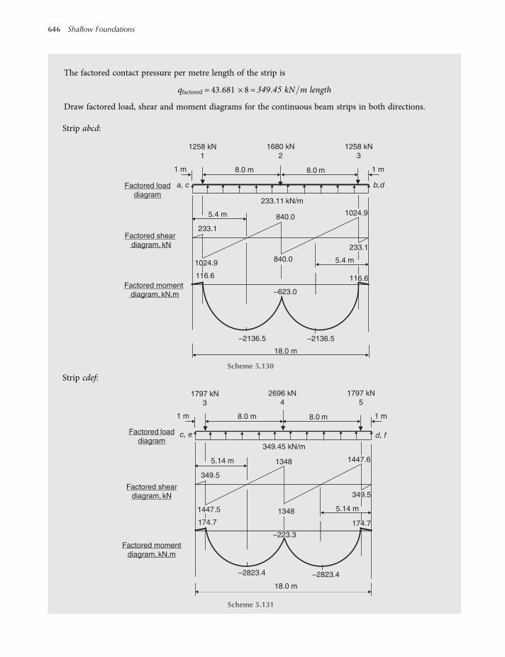
The factored contact pressure per metre length of the strip is
qfactored = 43 681 × 8 = 349 45 kN m length
Draw factored load, shear and moment diagrams for the continuous beam strips in both directions.
Strip abcd:
Strip cdef:
18.0 m
Factored shear
diagram, kN
Factored moment
diagram, kN.m
Factored load
diagram
–2136.5 –2136.5
116.6
5.4 m
1024.9
1024.9
233.11 kN/m
840.0
116.6
233.1
233.1
840.0
1 m1 m
a, c b,d
1258 kN
31258 kN
1
8.0 m
5.4 m
8.0 m
1680 kN
2
–623.0
Scheme 5.130
Factored shear
diagram, kN
Factored moment
diagram, kN.m
Factored load
diagram
–2823.4
–223.3
18.0 m
–2823.4
174.7
5.14 m
1447.5
1447.6
1348
174.7
349.5
349.5
1348
1 m1 m
c, e d, f
1797 kN
51797 kN
3
8.0 m
5.14 m
8.0 m
2696 kN
4
349.45 kN/m
Scheme 5.131
646 Shallow Foundations
worksaccounts.com

The provided mat thickness t = 665 mm
d = t−concrete cover−half bar diameter
= 665−75−11 = 579mm
Check the designed mat depth d considering beam shear (one-way shear) at the most critical section:Refer to the shear diagrams. It is clear that the most critical section for shear per metre width is located in stripabcd, at distance d from either the left face of column No. 3 or the right face of column No. 1. The applied beamshear at any of these two locations is
Vu =1024 9−q d + 0 2
5=1024 9−233 11 0 579 + 0 200
5= 168 7 kN mwidth
Equation (5.19): ØVc ≥Vu taking reinforcement shear strength,Vs = 0
Equation (5.20): Vc = 0 17λ fc bwd
ØVc = 0 75 × 0 17 × 1 24 1000 1 0 579
= 352 3kNm
Vu = 168 7 kN mwidth OK
Table 5.31 elucidates comparison of results obtained using the approximate flexible and rigid methods ofanalysis:
Note: For a flexible mat such as the one given in Problems 5.27 and 5.28, one may conclude that the approximateflexible method gives more realistic results than the conventional (rigid) method.
References
ACI 318 (2008), Building Code Requirements for Structural Concrete (ACI 318M-08) and Commentary, reported by ACICommittee 318, an ACI Standard, American Concrete Institute, Farmington Hills, MI, U.S.A., 473 pp.
ACI-ASCE (1962), “Shear and Diagonal Tension”, Part 3, “Slabs and Footings”, reported by ACI-ASCE Committee 326,Proceedings, ACI Journal, March, Vol. 59, No. 3, pp. 353–396.
Table 5.31 A comparison of results obtained using the approximate flexible and rigid methods of analysis.
Item
Design method
Approximate flexible method Conventional (rigid) method
Thickness 665 mm 665 mm
Maximum one–way shear 359.4 kN/m width 1024 95
= 205 0kN mwidth
Maximum two–way shear 2592 kN 2592 kN
Maximum positive moment 561.4 kN.m/m width 23.3 kN.m/m width
Maximum Negative moment 261.8 kN.m/m width 427.3 kN.m/m width
Shallow Foundations – Structural Design 647
worksaccounts.com

ACI Committee 336 (1993), “Suggested Analysis and Design Procedures for Combined Footings andMats, ACI 336.2R-88(Reapproved 1993)”, ACI Manual of Concrete Practice, American Concrete Institute, Farmington Hills, MI,pp. 336.2R-1 to 336.2R-21 plus discussion.
AISC (1989), Manual of Steel Construction, Allowable Stress Design, 9th edn, American Institute of Steel Construction,Chicago.
Bowles, J. E. (2001), Foundation Analysis and Design, 5th edn, McGraw-Hill, New York.Bowles, J. E. (1982), Foundation Analysis and Design, 3rd edn, McGraw-Hill, New York.Bowles, J. E. (1974a), Analytical and Computer Methods in Foundation Engineering, McGraw-Hill, New York, 519 pp.Bowles, J. E. (1976), “Mat Foundations” and “ComputerAnalysis ofMat Foundations”, Proceedings, Short Course-Seminar on
Analysis and Design of Building Foundations (Lehigh University), Envo Press, Lehigh Valley, pp. 209–232 and 233–256.Bowles, J. E. (1983), “Pile Cap Analysis,” Proceedings 8th Conference on Electronic Computation, ASCE, pp. 102–113.Bowles, J. E. (1986), “Mat Design”, Journal of American Concrete Institute, Vol. 83, No. 6, Nov/Dec, pp. 1010–1017.Christian, J. T. (1976), “Soil–Foundation–Structure Interaction”, Proceedings, Short Course-Seminar on Analysis and
Design of Building Foundations (Lehigh University), Envo Press, Lehigh Valley, pp. 149–179.Coduto, Donald P. (2001), Foundation Design: Principles and Practices, 2nd edn, Prentice-Hall, Inc., New Jersey.Cook, R. D. (1974), Concepts and Applications of Finite Element Analysis, John Wiley & Sons, Inc., New York, 402 pp.Das, Braja M. (2011), Principles of Foundation Engineering, 7th edn, CENGAGE Learning, United States.DeWolf, J. T., and Ricker, D. T. (1990), Column Base Plates, American Institute of Steel Construction, Chicago, IL.Ghali, A. and Neville, A. M. (1972), Structural Analysis: A Unified Classical and Matrix Approach, Intext Educational Pub-
lishers (Now Harper and Row), Chapters 17–20.Hetenyi, M. (1946), Beams on Elastic Foundations, The University of Michigan Press, Ann Arbor, MI, 255 pp.Horvath, J. S. (1993), Subgrade Modeling for Soil–Structure Interaction Analysis of Horizontal Foundation Elements, Man-
hattan College Research Report No. CE/GE-93-1, Manhattan College, New York.Liao, S. S. C. (1991), Estimating the Coefficient of Subgrade Reaction for Tunnel Design, Internal Research Report, Parsons
Brinkerhoff, Inc., New York.MacGregor, J. G., and Wight J. K. (2005), Reinforced Concrete: Mechanics and Design, 4th edn, Pearson Prentice Hall,
Upper Saddle River, New Jersey, 1132 pp.Moe, J. (1961), Shearing Strength of Reinforced Concrete Slabs and Footings under Concentrated Loads, Portland cement
Association Bulletin D47, Skokie, Illinois.Richart, F. E. (1948), “Reinforced Concrete Wall and Column Footings”, Journal of the American Concrete Institute,
Vol. 20, No. 2, pp. 97–127, and Vol. 20, No. 3, pp. 237–260.Shipp, J. G., and Haninger, E. R. (1983), “Design of Headed Anchor Bolts”, Engineering Journal, Vol. 20, No. 2, pp. 58–69,
American Institute of Steel Construction, Chicago, IL.Talbot, A. N. (1913), Reinforced Concrete Wall Footings and Column Footings, Bulletin No. 67, University of Illinois Engin-
eering Experiment Station, Urbana.Terzaghi, K. (1955), “Evaluation of Coefficients of Subgrade Reaction”, Geotechnique, Vol. 5, No. 4, pp. 297–326.Vesič, A. S. (1973), “Bending of Beams Resting on Isotropic Elastic Solid”, Journal of Engineering Mechanics Division,
ASCE, Vol. 87, No. EM2, pp. 35–53.Wang, C. K. (1970),Matrix Methods of Structural Analysis, 2nd edn, Intext Educational Publishers, Scranton, PA, 406 pp.Whitney, Charles S. (1957), “Ultimate Shear Strength of Reinforced Concrete Flat Slabs, Footings, Beams, and Frame
Members without Shear Reinforcement”, Journal of the American Concrete Institute, Vol. 29, No. 4, pp. 265–298.Winkler, E. (1867), Die Lehre von Elastizität und Festigkeit (On Elasticity and Fixity), H. Dominicus, Prague.
648 Shallow Foundations
worksaccounts.com

CHAPTER 6
Eurocode Standards and the Designof Spread Foundations
6.1 General
In line with the European Union’s (EU’s) strategy of smart, sustainable and inclusive growth, Stand-ardisation plays an important part in supporting the industrial policy for the globalisation era. All33 national members of the European Committee for Standardisation (CEN; French: Comité Européende Normalisation, founded in 1961) work together to develop European Standards (ENs) in varioussectors in order to build a European market for goods and services and to position Europe in the globaleconomy. CEN is officially recognised as a European standards body by the EU.The construction sector is of strategic importance to the EU as it delivers the buildings and infra-
structure needed. It is the largest single economic activity and it is the biggest industrial employer inEurope. These facts urged CEN to produce what is known as Eurocode Standards, also called StructuralEurocodes or Eurocodes.They are a set of harmonised technical rules and requirements developed bythe CEN for the structural design of construction works in the European Union. The development ofthe Eurocodes started in 1975; since then they have evolved significantly and are now claimed to beamong the most technically advanced structural codes in the world. With the publication of all the58 Eurocodes Parts in 2007, the implementation of the Eurocode Standards has been extended toall the European Union countries and there are firm steps toward their adoption internationally.The purposes of the Eurocodes may be summarised as follows:
• A means to prove compliance with the requirements for mechanical strength and stability andsafety in case of fire established by European Union law.
• A basis for construction and engineering contract specifications.
• A framework for creating harmonised technical specifications for building products.
There are 10 Structural Eurocodes,each published as a separate European Standard and each havinga number of parts (so far 58 parts have been produced), covering all the main structural materials(Figure 6.1).It has been a legal requirement from March 2010 that all European public-sector clients base their
planning and building control applications on structural designs that meet the requirements of theEurocode. To comply with this, changes have been necessary to the building regulations. The Euro-codes therefore replace the existing national building codes published by national standard bodies(e.g. BS 5950), although many countries had a period of co-existence. Each country is required to
Shallow Foundations: Discussions and Problem Solving, First Edition. Tharwat M. Baban.© 2016 John Wiley & Sons, Ltd. Published 2016 by John Wiley & Sons, Ltd.
worksaccounts.com
publish a Eurocode with a national title page and forward but the original text of the Eurocode (includ-ing any annexes) must appear as produced by CEN as the main body of the document. A NationalAnnex can be included at the back of the document (Figure 6.2). Throughout Chapter 6 the relevantUK National Annexes will be used along with the Eurocodes.
There are two categories of Annexes to the Structural Eurocodes. One type is labelled “I” and isInformative (i.e. for information and not as a mandatory part of the code). The second type is labelled“N” and is Normative (i.e. a mandatory part of the code). In their National Annex a country can chooseto make an Informative annex Normative if they so whish. In other words, a National annex may onlycontain information on those parameters which are left open in the Eurocode for national choice,known as Nationally Determined Parameters (NDP), to be used for the design of buildings and civilengineering works in the country concerned, that is:
• Values and/or classes where alternatives are given in the Eurocode,
• Values to be used where a symbol only is given in the Eurocode,
• Country-specific data (geographical, climatic, etc.), for example a snow map,
• A procedure to be used where an alternative procedure is given in the Eurocode,
• Decisions on the application of informative annexes,
• References to non-contradictory complementary information so that the Eurocode may easily beused without complications.
BS EN 1992, Eurocode 2: Concrete
BS EN 1993, Eurocode 3: Steel
BS EN 1994, Eurocode 4: Composite
BS EN 1995, Eurocode 5: Timber
BS EN 1996, Eurocode 6: Masonry
BS EN 1999, Eurocode 9: Aluminium
EN 1990, Eurocode: Basis of structural design
EN 1991, Eurocode 1: Actions on structures
EN 1992, Eurocode 2: Design of concrete structures
EN 1993, Eurocode 3: Design of steel structures
EN 1994, Eurocode 4: Design of composite steel and concrete structures
EN 1995, Eurocode 5: Design of timber structures
EN 1996, Eurocode 6: Design of masonry structures
EN 1997, Eurocode 7: Geotechnical design
EN 1998, Eurocode 8: Design of structures for earthquake resistance
EN 1999, Eurocode 9: Design of aluminium structures
BS EN 1991, Eurocode 1:Actions on structures
BS EN 1990, Eurocode:Basis of structural design
BS EN 1998, Eurocode 8:Seismic design
BS EN 1997, Eurocode 7:Geotechnical design
Structural
safety,
serviceability
Actions on
structures
Design and
detailing
Geotechnical and
seismic design
Figure 6.1 The Eurocodes and their relationships.
650 Shallow Foundations
worksaccounts.com
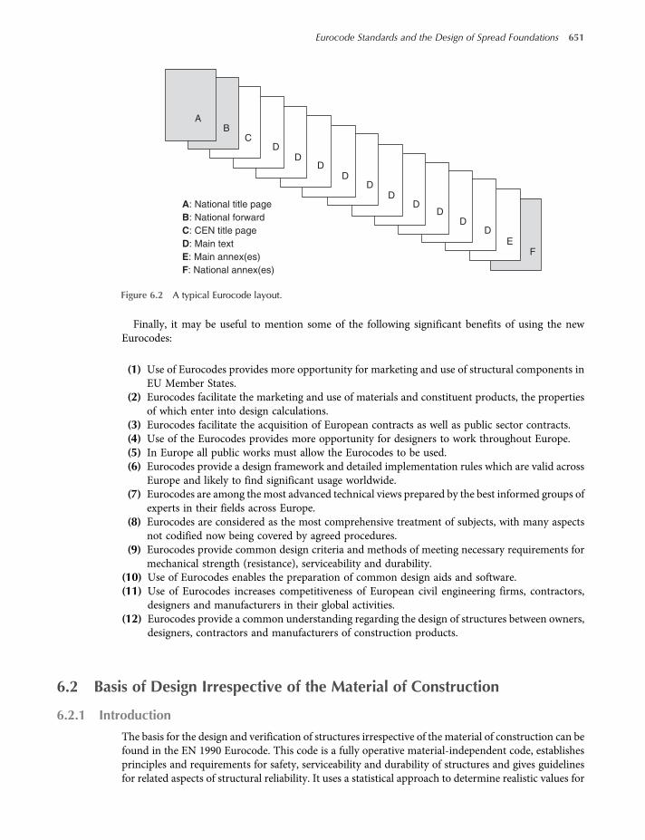
Finally, it may be useful to mention some of the following significant benefits of using the newEurocodes:
(1) Use of Eurocodes provides more opportunity for marketing and use of structural components inEU Member States.
(2) Eurocodes facilitate the marketing and use of materials and constituent products, the propertiesof which enter into design calculations.
(3) Eurocodes facilitate the acquisition of European contracts as well as public sector contracts.(4) Use of the Eurocodes provides more opportunity for designers to work throughout Europe.(5) In Europe all public works must allow the Eurocodes to be used.(6) Eurocodes provide a design framework and detailed implementation rules which are valid across
Europe and likely to find significant usage worldwide.(7) Eurocodes are among the most advanced technical views prepared by the best informed groups of
experts in their fields across Europe.(8) Eurocodes are considered as the most comprehensive treatment of subjects, with many aspects
not codified now being covered by agreed procedures.(9) Eurocodes provide common design criteria and methods of meeting necessary requirements for
mechanical strength (resistance), serviceability and durability.(10) Use of Eurocodes enables the preparation of common design aids and software.(11) Use of Eurocodes increases competitiveness of European civil engineering firms, contractors,
designers and manufacturers in their global activities.(12) Eurocodes provide a common understanding regarding the design of structures between owners,
designers, contractors and manufacturers of construction products.
6.2 Basis of Design Irrespective of the Material of Construction
6.2.1 Introduction
The basis for the design and verification of structures irrespective of the material of construction can befound in the EN 1990 Eurocode. This code is a fully operative material-independent code, establishesprinciples and requirements for safety, serviceability and durability of structures and gives guidelinesfor related aspects of structural reliability. It uses a statistical approach to determine realistic values for
A: National title page
B: National forward
C: CEN title page
D: Main text
E: Main annex(es)
F: National annex(es)
B
D
C
DD
DD
DD
DD
D
FE
BA
Figure 6.2 A typical Eurocode layout.
Eurocode Standards and the Design of Spread Foundations 651
worksaccounts.com
actions that occur in combination with each other. It is based on the limit state concept and used inconjunction with the partial factor method.
The EN 1990 Eurocode is intended to be used in conjunction with the other Eurocodes for the struc-tural design of buildings and civil engineering works, including geotechnical aspects, structural firedesign and situations involving earthquakes, execution and temporary structures. Also, it is applicablefor: design of structures where other materials or actions outside the scope of the EN 1991 to EN 1999Eurocodes are involved, structural appraisal of existing construction, developing the design of repairsand alterations or in assessing changes of use.
As a fully operative material-independent key code, EN 1990 is new to the European design engineer.It needs to be fully understood as it is a key code to designing structures that have an acceptable level ofsafety and economy, with opportunities for innovation.
As mentioned above and shown in Figure 6.1, for the design of new structures, EN 1990 will be usedtogether with:
• EN 1991 (Eurocode 1: Actions on structures);
• EN 1992 to EN 1999 (design Eurocodes 2–9).
Gulvanessian et al. (2012) provide a comprehensive description, background and commentary to EN1990 Eurocode.
6.2.2 Terms and Definitions
To assist familiarity, the followings are definitions of some important Eurocode terminology, symbolsand subscripts, which will be used throughout Chapter 6.
Common terms and special terms relating to design in general:
(1) Structure: organised combination of connected parts designed to carry loads and provideadequate rigidity.
(2) Structural member: physically distinguishable part of a structure, for example a column, a beam, afoundation pile.
(3) Structural system: load-bearing members of a building or civil engineering works and the way inwhich these members function together.
(4) Structural model: idealisation of the structural system used for the purposes of analysis, designand verification.
(5) Design criteria: quantitative formulations that describe for each limit state the conditions to befulfilled.
(6) Design situations: sets of physical conditions representing the real conditions occurring during acertain time interval for which the design will demonstrate that relevant limit states are notexceeded.
(7) Persistent design situation: design situation that is relevant during a period of the same order asthe design working life of the structure.
(8) Transient design situation: design situation that is relevant during a period much shorter than thedesign working life of the structure and which has a high probability of occurrence.
(9) Seismic design situation: design situation involving exceptional conditions of the structure whensubjected to a seismic event.
(10) Accidental design situation: design situation involving exceptional conditions of the structure orits exposure, including fire, explosion, impact or local failure.
(11) Fire design: design of a structure to fulfill the required performance in case of fire.(12) Hazard: for the purpose of EN 1991 to EN 1999, an unusual and severe event, for example an
abnormal action or environmental influence, insufficient strength or resistance, or excessive devi-ation from intended dimensions.
652 Shallow Foundations
worksaccounts.com

(13) Design working life: assumed period for which a structure or part of it is to be used for its intendedpurpose with anticipated maintenance but without major repair being necessary.
(14) Limit states: states beyond which the structure no longer fulfills the relevant design criteria.(15) Ultimate limit states: states associated with collapse or with other similar forms of structural
failure.(16) Serviceability limit states: states that correspond to conditions beyond which specified service
requirements for a structure or structural member are no longer met.(17) Reversible serviceability limit states: serviceability limit states where no consequences of actions
exceeding the specified service requirements will remain when the actions are removed.(18) Irreversible serviceability limit states: serviceability limit states where some consequences of
actions exceeding the specified service requirements will remain when the actions are removed.(19) Serviceability criterion: design criterion for a serviceability limit state.(20) Resistance (R): capacity of a member or component, or a cross-section of a member or compo-
nent of a structure, to withstand actions without mechanical failure, for example bending resist-ance, buckling resistance, tension resistance
(21) Strength: mechanical property of a material indicating its ability to resist actions, usually given inunits of stress.
(22) Basic variable: part of a specified set of variables representing physical quantities which charac-terise actions and environmental influences, geometrical quantities and material propertiesincluding soil properties.
(23) Nominal value: value fixed on non-statistical bases, for instance on acquired experience or onphysical conditions.
(24) Characteristic value: a value that may be derived statistically with a probability of not beingexceeded during a reference period. The value corresponds to a specified fractile (that point belowwhich a stated fraction of the values lie) for a particular property of material or product. Thecharacteristic values are denoted by subscript “k” (e.g. Qk etc.). It is the principal representativevalue from which other representative values may be derived.
(25) Representative value: value used for verification of a limit state. It may be the characteristic valueor an accompanying value, for example combination, frequent or quasi-permanent.
(26) Reference period: chosen period of time that is used as a basis for assessing statistically variableactions, and possibly for accidental actions.
(27) Combination of actions: set of design values used for the verification of the structural stability for alimit state under the simultaneous influence of different and statistically independent actions.
Terms relating to actions:(28) Action (F): (a) set of forces (loads) applied to the structure (direct action), (b) set of imposed
deformations or accelerations caused for example, by temperature changes, moisture variation,uneven settlement or earthquakes (indirect actions).
(29) Effect of action (E): effect of actions (or action effect) on structural members, (e.g. internal force,moment, stress, strain) or on the whole structure (e.g. deflection, rotation).
(30) Permanent action (G): action that is likely to act throughout a given reference period and forwhich the variation in magnitude with time is negligible, or for which the variation is alwaysin the same direction (monotonic) until the action attains a certain limit value.
(31) Variable action (Q): action for which the variation in magnitude with time is neither negligiblenor monotonic.
(32) Accidental action (A): action, usually of short duration but of significant magnitude; that isunlikely to occur on a given structure during the design working life.
(33) Seismic action (AE): action that arises due to earthquake ground motion.(34) Fixed action: action that have a fixed distribution and position over the structure or structural
member such that the magnitude and direction of the action are determined unambiguouslyfor the whole structure or structural member if this magnitude and direction are determinedat one point on the structure or structural member.
Eurocode Standards and the Design of Spread Foundations 653
worksaccounts.com
(35) Free action: action that may have various spatial distributions over the structure.(36) Single action: action that can be assumed to be statically independent in time and space of any
other action.(37) Static action: action that does not cause significant acceleration of the structure or structural
members.(38) Dynamic action: action that cause significant acceleration of the structure or structural members.(39) Quasi-static action: dynamic action represented by an equivalent static action in a static model.(40) Characteristic value of an action (Fk): principal representative value of an action (see defin-
ition 24.).(41) Combination value of a variable action (Ψ0Qk): value chosen – in so far as it can be fixed on stat-
istical bases – so that the probability of the effects caused by the combination is approximately thesame as by the characteristic value of an individual action. It may be expressed as a determinedpart of the characteristic value by using a factor Ψ0 ≤ 1.
(42) Frequent value of a variable action (Ψ1Qk): value determined– in so far as it can be fixed on statisticalbases – so that either the total time, within the reference period, during which it is exceeded is only asmall given part of the reference period, or the frequency of it being exceeded is limited to a givenvalue. It may be expressed as a determined part of the characteristic value by using a factorΨ1 ≤ 1.
(43) Quasi-permanent value of a variable action (Ψ2Qk): value determined so that the total period oftime for which it will be exceeded is a large fraction of the reference period. It may be expressed asa determined part of the characteristic value by using a factor Ψ2 ≤ 1.
(44) Accompanying value of a variable action (ΨQk): value of a variable action that accompanies theleading action in a combination. It may be the combination value, the frequent value or the quasi-permanent value.
(45) Representative value of an action (Frep): value used for the verification of a limit state.A representative value may be the characteristic value (Fk) or an accompanying value ΨFk).
(46) Design value of an action (Fd): value obtained by multiplying the representative value by the par-tial factor γf.
(47) Load arrangement: identification of the position, magnitude and direction of a free action.
Terms relating to material and product properties:(48) Characteristic value (Xk or Rk): value of a material or product property having a prescribed
probability of not being attained in a hypothetical unlimited test series. This value generallycorresponds to a specified fractile of the assumed statistical distribution of the particular prop-erty of the material or product. A nominal value is used as the characteristic value in somecircumstances.
(49) Design value of a material or product property (Xd or Rd): value obtained by dividing the char-acteristic value by a partial factor γm, or γM or, in special circumstances, by direct determination.
(50) Nominal value of a material or product property (Xnom or Rnom): value normally used as a charac-teristic value and established from an appropriate document such as a European Standard orPrestandard.
Terms relating to geometrical data:(51) Characteristic value of a geometrical property (αk): value usually corresponding to the dimensions
specified in the design. Where relevant, values of geometrical quantities may correspond to someprescribed fractile of the statistical distribution.
(52) Design value of a geometrical property (αd): generally a nominal value. Where relevant, values ofgeometrical quantities may correspond to some prescribed fractile of the statistical distribution.
Note: The design value of a geometrical property is generally equal to the characteristic value.However, it may be treated differently in cases where the limit state under consideration is verysensitive to the value of the geometrical property, for example when considering the effect of geo-metrical imperfections on buckling. In such cases, the design value will normally be established asa value specified directly, for example in an appropriate European Standard or Prestandard.
654 Shallow Foundations
worksaccounts.com
Alternatively, it can be established from a statistical basis, with a value corresponding to a moreappropriate fractile (e.g. a rarer value) than applies to the characteristic value.
Symbols and subscriptsSo far as we may notice, most of the significant symbols and subscripts have been presented. The fol-lowing are some others:
AEd – Design value of seismic action AEd = γI AEd.AEk – Characteristic value of seismic action.Cd – Nominal value or a function of certain properties of materials.Ed,dst – Design value of effect of destabilising section.Ed,stb – Design value of effect of stabilising section.Fw – Wind force (general symbol).Fwk – Characteristic value of the Wind force.P – Relevant representative value of a prestressing action.QSn – Characteristic value of snow load.T – Thermal climatic action (general symbol).X – Material property.ad – Design values of geometrical data.ad – Characteristic values of geometrical data.anom –Nominal value of geometrical data.dset – Difference in settlement of an individual foundation or part of a foundation compared to a
reference level.u – Horizontal displacement of a structure or structural member.w – Vertical deflection of a structural member.γ – Partial factor (safety or serviceability).γG – Partial factor for permanent action.γQ – Partial factor for variable action.γM – Partial factor for a material property, also accounting for model uncertainties and dimensional
variations.γF – Partial factor for actions, also accounting for model uncertainties and dimensional variations.γG,set – Partial factor for permanent actions due to settlements, also accounting for model uncertainties.ψ – Factor for converting a characteristic value to a representative value.ψ0 – Factor for combination value of a variable action.ψ1 – Factor for frequent value of a variable action.ψ2 – Factor for quasi-permanent value of a variable action.ξ – Reduction factor for permanent action.
Note: Other symbols will be defined when they appear for the first time.
6.2.3 Requirements
The followings are the requirements that must be adhered to by all the Eurocode suite and constructionproduct standards so that safety, serviceability anddurability of structures are achieved inapropermanner:
• Basic requirements,
• Reliability management and differentiation,
• Design working life,
• Durability.
These requirements are thoroughly covered by EN 1990 Section 2, and may be summarised as in thefollowing paragraphs.
Eurocode Standards and the Design of Spread Foundations 655
worksaccounts.com
Basic requirementsAccording to EN 1990 Section 2, Clause 2.1, the basic requirements stipulate that:
A structure and structural members should be designed and executed in such a way that it will, dur-ing its intended life, with appropriate degrees of reliability and in an economic way:
• Sustain all actions and influences likely to occur during execution and use (safety requirement relat-ing to the ultimate limit state); and remain fit for use under all expected conditions (serviceabilityrequirement relating to the serviceability limit state).
• Have satisfactory structural resistance, serviceability and durability.
• In the case of fire, provide satisfactory structural resistance for the required period of time.
• Not be damaged by events such as explosions, impact or consequences of human errors, to an extentdisproportionate to the original cause (robustness requirement).
EN 1990 Section 2, Clause 2.1 provides methods of avoiding or limiting potential damage. Also, itprovides methods of achieving basic requirements satisfied.
Reliability management and differentiationEN 1990 Section 2, Clause 2.2 provides: methods of achieving and adopting reliability, factors to beconsidered in selecting reliability levels, methods of specifying reliability levels that apply to a particularstructure, measures of achieving reliability levels relating to structural resistance and serviceability.
Reliability is ability of a structure or a structural member to fulfill the specified requirements, includ-ing the design working life, for which it has been designed. It covers safety, serviceability and durabilityof a structure or a structural member. Reliability is usually expressed in probabilistic terms. Design andexecution according to the suite of the Eurocodes, together with appropriative quality control meas-ures, will ensure an appropriate degree of reliability for the majority of structures.
Reliability differentiation means measures intended for the socio-economic optimisation of theresources to be used to build construction works, taking into account all the expected consequencesof failures and the cost of construction works. It is a concept which is not covered by BSI codes.EN 1990 provides guidance for adopting reliability differentiation. It gives further guidance in anInformative Annex “Management of Structural Reliability for Construction Works” (2005). Calgaroet al. (2001) describe the management of structural reliability in EN 1990, where the concept of therisk background of the Eurocodes is described more comprehensively.
Design working lifeThe design working life should be specified. Table 6.1, taken from the UK National Annex for EN 1990,gives indicative designworking life classifications. BSI codes do not have a designworking life requirementfor buildings. The given values may also be used for time-dependent performance (e.g. fatigue-related cal-culations).Buildings subject to Building Regulations, hospitals, schools and so on will be in Category 4 (Table 6.1).
The design working life requirement is useful for:
• The selection of design actions,
• Consideration of material property deterioration,
• Life cycle costing,
• Evolving maintenance strategies.
DurabilityThe durability of a structure is its ability to remain fit for use during the design working life givenappropriate maintenance. EN 1990 stipulates that the structure needs to be designed so that deteri-oration over its design working life does not impair the performance of the structure. The Factorsthat should be considered to ensure adequately durable structures are listed in EN 1990 Section 2,Clause 2.4.
656 Shallow Foundations
worksaccounts.com
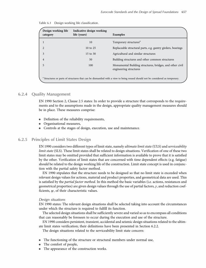
6.2.4 Quality Management
EN 1990 Section 2, Clause 2.5 states: In order to provide a structure that corresponds to the require-ments and to the assumptions made in the design, appropriate quality management measures shouldbe in place. These measures comprise:
• Definition of the reliability requirements,
• Organisational measures,
• Controls at the stages of design, execution, use and maintenance.
6.2.5 Principles of Limit States Design
EN 1990 considers two different types of limit state, namely ultimate limit state (ULS) and serviceabilitylimit state (SLS). These limit states shall be related to design situations. Verification of one of these twolimit states may be omitted provided that sufficient information is available to prove that it is satisfiedby the other. Verification of limit states that are concerned with time dependent effects (e.g. fatigue)should be related to the design working life of the construction. Limit state concept is used in conjunc-tion with the partial safety factor method.EN 1990 stipulates that the structure needs to be designed so that no limit state is exceeded when
relevant design values for actions, material and product properties, and geometrical data are used. Thisis satisfied by the partial factor method. In this method the basic variables (i.e. actions, resistances andgeometrical properties) are given design values through the use of partial factors, γ, and reduction coef-ficients, ψ , of their characteristic values.
Design situationsEN 1990 states: The relevant design situations shall be selected taking into account the circumstancesunder which the structure is required to fulfill its function.The selected design situations shall be sufficiently severe and varied so as to encompass all conditions
that can reasonably be foreseen to occur during the execution and use of the structure.EN 1990 considers persistent, transient, accidental and seismic design situations related to the ultim-
ate limit states verification; their definitions have been presented in Section 6.2.2.The design situations related to the serviceability limit state concern:
• The functioning of the structure or structural members under normal use,
• The comfort of people,
• The appearance of the construction works.
Table 6.1 Design working life classification.
Design working lifecategory
Indicative design workinglife (years) Examples
1 10 Temporary structuresa
2 10 to 25 Replaceable structural parts, e.g. gantry girders, bearings
3 15 to 30 Agricultural and similar structures
4 50 Building structures and other common structures
5 100 Monumental Building structures, bridges, and other civilengineering structures
a Structures or parts of structures that can be dismantled with a view to being reused should not be considered as temporary.
Eurocode Standards and the Design of Spread Foundations 657
worksaccounts.com
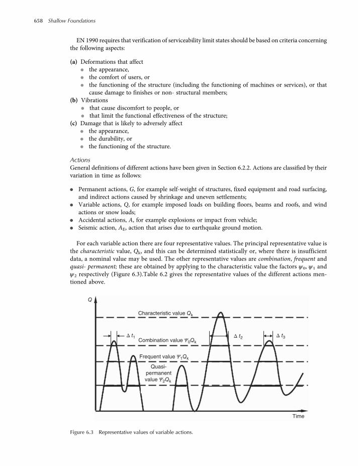
EN 1990 requires that verification of serviceability limit states should be based on criteria concerningthe following aspects:
(a) Deformations that affect
• the appearance,
• the comfort of users, or
• the functioning of the structure (including the functioning of machines or services), or thatcause damage to finishes or non- structural members;
(b) Vibrations
• that cause discomfort to people, or
• that limit the functional effectiveness of the structure;(c) Damage that is likely to adversely affect
• the appearance,
• the durability, or
• the functioning of the structure.
ActionsGeneral definitions of different actions have been given in Section 6.2.2. Actions are classified by theirvariation in time as follows:
• Permanent actions, G, for example self-weight of structures, fixed equipment and road surfacing,and indirect actions caused by shrinkage and uneven settlements;
• Variable actions, Q, for example imposed loads on building floors, beams and roofs, and windactions or snow loads;
• Accidental actions, A, for example explosions or impact from vehicle;
• Seismic action, AE, action that arises due to earthquake ground motion.
For each variable action there are four representative values. The principal representative value isthe characteristic value, Qk, and this can be determined statistically or, where there is insufficientdata, a nominal value may be used. The other representative values are combination, frequent andquasi- permanent; these are obtained by applying to the characteristic value the factors ψ0, ψ1 andψ2 respectively (Figure 6.3).Table 6.2 gives the representative values of the different actions men-tioned above.
Time
Characteristic value Qk
Q
Combination value Ψ0Qk
Δ t1 Δ t2 Δ t3
Quasi-
permanent
value Ψ2Qk
Frequent value Ψ1Qk
Figure 6.3 Representative values of variable actions.
658 Shallow Foundations
worksaccounts.com
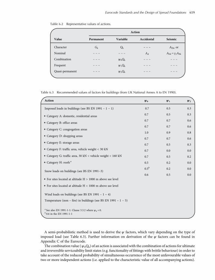
A semi-probabilistic method is used to derive the ψ factors, which vary depending on the type ofimposed load (see Table 6.3). Further information on derivation of the ψ factors can be found inAppendix C of the Eurocode.The combination value ( ψ0Qk) of an action is associated with the combination of actions for ultimate
and irreversible serviceability limit states (e.g. functionality of fittings with brittle behaviour) in order totake account of the reduced probability of simultaneous occurrence of the most unfavourable values oftwo or more independent actions (i.e. applied to the characteristic value of all accompanying actions).
Table 6.3 Recommended values of factors for buildings (from UK National Annex A to EN 1990).
Action ψ0 ψ1 ψ2
Imposed loads in buildings (see BS EN 1991 – 1 − 1)
•Category A: domestic, residential areas
•Category B: office areas
•Category C: congregation areas
•Category D: shopping areas
•Category E: storage areas
•Category F: traffic area, vehicle weight < 30 kN
•Category G: traffic area, 30 kN < vehicle weight < 160 kN
•Category H: roofs a
Snow loads on buildings (see BS EN 1991−3)
•For sites located at altitude H > 1000 m above see level
•For sites located at altitude H < 1000 m above see level
Wind loads on buildings (see BS EN 1991 – 1 − 4)
Temperature (non – fire) in buildings (see BS EN 1991 – 1 − 5)
0.7
0.7
0.7
0.7
1.0
0.7
0.7
0.7
0.7
0.5
0.5b
0.6
0.5
0.5
0.7
0.7
0.9
0.7
0.5
0.0
0.5
0.2
0.2
0.5
0.3
0.3
0.6
0.6
0.8
0.6
0.3
0.0
0.2
0.0
0.0
0.0
a See also EN 1991-1-1: Clause 3.3.2 where ψ0 = 0.b 0.6 in the EN 1991-1-1
Table 6.2 Representative values of actions.
Value
Action
Permanent Variable Accidental Seismic
Character Gk Qk – – – AEk, or
Nominal – – – – – – Ad AEd = γIAEk
Combination – – – ψ0Qk – – – – – –
Frequent – – – ψ1Qk – – – – – –
Quasi-permanent – – – ψ2Qk – – – – – –
Eurocode Standards and the Design of Spread Foundations 659
worksaccounts.com

The frequent value (ψ1Qk) is primarily associated with the frequent combination in the service-ability limit states, but it is also used for verification of the accidental design situation of theultimate limit states (e.g. every day office use). In both cases, the factor ψ1 is applied as a multiplierof the leading variable action. In accordance with EN 1990, the frequent value ψ1Qk of a variableaction Q is determined so that the total time, within a chosen period of time, during whichQ > ψ1Qk is only a specified (small) part of the period, or the frequency of the event Q > ψ1Qk islimited to a given value. The total time for which ψ1Qk is exceeded is equal to sum of time periods,shown in Figure 6.3 by continuous sections of the horizontal line that belongs to the frequentvalue ψ1Qk.
The quasi-permanent values (ψ2Qk) are mainly used in the assessment of long-term effects, (e.g.cosmetic cracking of a slab). They are also used for the representation of variable actions in accidentaland seismic combinations of actions (ultimate limit states) and for verification of frequent and quasi-permanent combinations (long-term effects) of serviceability limit states. In accordance with EN 1990,the quasi-permanent values (ψ2Qk) is defined so that the total time, within a chosen period duringwhich it is exceeded, that is when Q > ψ2Qk is a considerable part (0.5) of the chosen period of time.The value may also be determined as the value averaged over the chosen period of time. The total timeof ψ2Qk being exceeded is equal to the sum of periods, shown in Figure 6.3 by continuous sections of thehorizontal line that belongs to the frequent value ψ2Qk.
The representative values ψ0Qk, ψ1Qk and ψ2Qk and the characteristic values are used to define thedesign values of the actions and the combinations of the actions as explained in the followingparagraphs.
Combinations of actionsThe term “combinations of actions”, as defined in Section 6.2.2, should not be confused with “loadcases”, which are concerned with the arrangement of the variable actions to give the most unfavourableconditions.
The following process can be used to determine the value of actions used for analysis:
(1) Identify the design situation (e.g. persistent, transient, etc.).(2) Identify all realistic actions.(3) Determine the partial factors for each applicable combination of actions.(4) Arrange the actions to produce the most critical conditions.
Where there is only one variable action (e.g. imposed load) in a combination, the magnitude of theactions can be obtained by multiplying them by the appropriate partial factors. Where there is morethan one variable action in a combination, it is necessary to identify the leading action (Qk,1) and otheraccompanying actions (Qk,i).
For the persistent and transient design situations for ultimate limit states and for the characteristic(rare) combinations of serviceability limit states, only the non-leading variable actions may be reducedusing the ψ0 factors. In other cases (for accidental design situation and combinations of serviceabilitylimit states), the leading as well as accompanying actions may be reduced using the appropriate ψfactors (see Table 6.4).
Verification by the partial factor method
(A) Ultimate limit states(a) Ultimate limit state categories and verifications.EN 1990 stipulates that the effects of design actions do not exceed the design resistance of thestructure at the ultimate limit state (ULS); and the following four categories to which ULS aredivided needs to be verified, where relevant:
660 Shallow Foundations
worksaccounts.com

(1) EQU. Loss of static equilibrium of the structure or any part of it considered as a rigidbody, where:
• Minor variations in the value or the spatial distribution of actions from a single source aresignificant;
• The strengths of construction materials or ground are generally not governing.
The verification shall be based on:
Ed,dst ≤ Ed,stb 6 1
where:Ed,dst = design value of the effect of destabilizing action,Ed,stb = design value of the effect of stabilizing actions.
(2) STR. Internal failure or excessive deformation of the structure or structural members, includ-ing footings, piles and basement walls and so on, where the strength of construction materialsof the structure governs.The verification shall be based on:
Ed ≤Rd 6 2
where:Ed = design value of the effect of actionsRd = design value of the corresponding resistance.
(3) GEO. Failure or excessive deformation of the ground where the strengths of soil or rock aresignificant in providing resistant.The verification shall be based on Equation (6.2).
(4) FAT. Fatigue failure of the structure or structural members. The combinations apply:
• Persistent or transient design situation (fundamental combination);
• Accidental design situation;
• Seismic design situation.Specific rules for FAT limit states are given in the design Eurocodes EN 1992 to EN 1999.
(B) (b) Load combination expressions in EN 1990 for the verification of ULS for the persistent and tran-sient design situations.EN 1990 Clause 6.4.3.2 defines three alternative sets of expressions for the verification of ultimatelimit states for the persistent and transient design situations as follows:(1) EN 1990 Expression (6.10)
j≥ 1γG, jGk, j + γPP + γQ,1Qk, 1 +
i > 1γQ, iψ0, iQk, i
Table 6.4 Applicationof factorsψ0, ψ1 andψ2 for leadingandnon-leadingvariableactionsatultimateandserviceability limit states.
Limit stateDesign situation orCombination
Combinationvalue ψ0
Frequentvalue ψ1
Qusi-permanentvalue ψ2
Ultimate Persistent and transient non-leading × ×
Accidental × leading leading and non-leading
Seismic × × all variable actions
Serviceability Characteristic non-leading × ×
Frequent × leading non-leading
× means not applied Quasi-permanent × × all variable actions
Eurocode Standards and the Design of Spread Foundations 661
worksaccounts.com
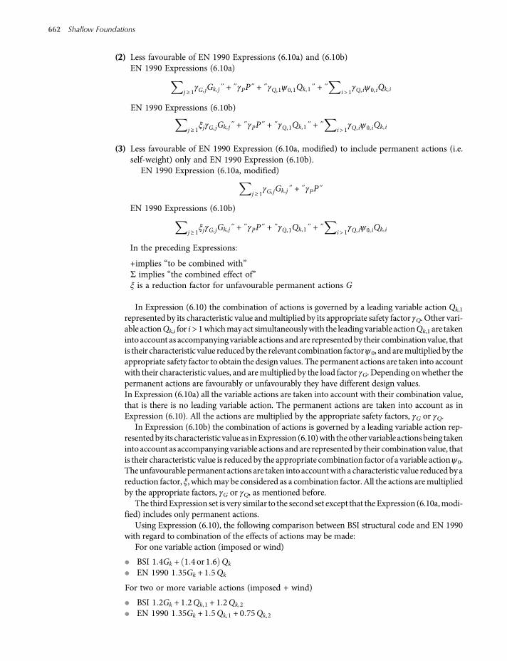
(2) Less favourable of EN 1990 Expressions (6.10a) and (6.10b)EN 1990 Expressions (6.10a)
j≥ 1γG, jGk, j + γPP + γQ,1ψ0,1Qk, 1 +
i > 1γQ, iψ0, iQk, i
EN 1990 Expressions (6.10b)
j≥ 1ξjγG, jGk, j + γPP + γQ, 1Qk,1 +
i > 1γQ, iψ0, iQk, i
(3) Less favourable of EN 1990 Expression (6.10a, modified) to include permanent actions (i.e.self-weight) only and EN 1990 Expression (6.10b).
EN 1990 Expression (6.10a, modified)
j≥ 1γG, jGk, j + γPP
EN 1990 Expressions (6.10b)
j≥ 1ξjγG, jGk, j + γPP + γQ, 1Qk,1 +
i > 1γQ, iψ0, iQk, i
In the preceding Expressions:
+implies “to be combined with”Σ implies “the combined effect of”ξ is a reduction factor for unfavourable permanent actions G
In Expression (6.10) the combination of actions is governed by a leading variable action Qk,1
represented by its characteristic value andmultiplied by its appropriate safety factor γQ. Other vari-able actionQk,i for i > 1whichmayact simultaneouslywith the leadingvariable actionQk,1 are takenintoaccount as accompanying variable actions and are representedby their combinationvalue, thatis their characteristic value reducedby the relevant combination factorψ0, and aremultipliedby theappropriate safety factor to obtain the design values. The permanent actions are taken into accountwith their characteristic values, and aremultiplied by the load factor γG. Depending onwhether thepermanent actions are favourably or unfavourably they have different design values.In Expression (6.10a) all the variable actions are taken into account with their combination value,that is there is no leading variable action. The permanent actions are taken into account as inExpression (6.10). All the actions are multiplied by the appropriate safety factors, γG or γQ.
In Expression (6.10b) the combination of actions is governed by a leading variable action rep-resentedby its characteristic valueas inExpression (6.10)with theother variable actionsbeing takenintoaccount as accompanying variable actions and are representedby their combinationvalue, thatis their characteristic value is reduced by the appropriate combination factor of a variable actionψ0.Theunfavourable permanent actions are taken intoaccountwith a characteristic value reducedbyareduction factor, ξ, whichmay be considered as a combination factor. All the actions aremultipliedby the appropriate factors, γG or γQ, as mentioned before.
The thirdExpression set is very similar to the second set except that theExpression (6.10a,modi-fied) includes only permanent actions.
Using Expression (6.10), the following comparison between BSI structural code and EN 1990with regard to combination of the effects of actions may be made:
For one variable action (imposed or wind)
• BSI 1 4Gk + 1 4 or 1 6 Qk
• EN 1990 1 35Gk + 1 5Qk
For two or more variable actions (imposed + wind)
• BSI 1 2Gk + 1 2Qk,1 + 1 2Qk,2
• EN 1990 1 35Gk + 1 5Qk, 1 + 0 75Qk,2
662 Shallow Foundations
worksaccounts.com
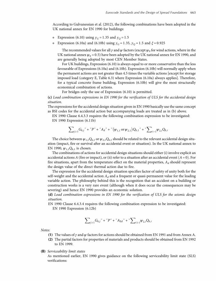
According to Gulvanessian et al. (2012), the following combinations have been adopted in theUK national annex for EN 1990 for buildings:
• Expression (6.10) using γG = 1 35 and γQ = 1 5
• Expression (6.10a) and (6.10b) using γG = 1 35, γQ = 1 5 and ξ= 0 925
The recommended values for all γ and ψ factors (except ψ0 for wind actions, where in theUK national annex ψ0 = 0 5) have been adopted by the UK national annex for EN 1990, andare generally being adopted by most CEN Member States.
For UK buildings, Expression (6.10) is always equal to or more conservative than the lessfavourable of Expressions (6.10a) and (6.10b). Expression (6.10b) will normally apply whenthe permanent actions are not greater than 4.5 times the variable actions [except for storageimposed load (category E, Table 6.3) where Expression (6.10a) always applies]. Therefore,for a typical concrete frame building, Expression (6.10b) will give the most structurallyeconomical combination of actions.
For bridges only the use of Expression (6.10) is permitted.
(C) (c) Load combination expressions in EN 1990 for the verification of ULS for the accidental designsituation.The expressions for the accidental design situation given in EN 1990 basically use the same conceptas BSI codes for the accidental action but accompanying loads are treated as in (b) above.
EN 1990 Clause 6.4.3.3 requires the following combination expression to be investigated:EN 1990 Expression (6.11b)
j≥ 1Gk, j + P + Ad + ψ1,1 orψ2,1 Qk,1 +
i > 1ψ2, iQk, i
The choice between ψ1,1Qk,1 or ψ2,1Qk,1 should be related to the relevant accidental design situ-ation (impact, fire or survival after an accidental event or situation). In the UK national annex toEN 1990, ψ1,1Qk,1 is chosen.
The combinations of actions for accidental design situations should either (i) involve explicit anaccidental actionsA (fire or impact), or (ii) refer to a situation after an accidental event A= 0 . Forfire situations, apart from the temperature effect on the material properties, Ad should representthe design value of the direct thermal action due to fire.
The expression for the accidental design situation specifies factor of safety of unity both for theself-weight and the accidental action Ad and a frequent or quasi-permanent value for the leadingvariable action. The philosophy behind this is the recognition that an accident on a building orconstruction works is a very rare event (although when it does occur the consequences may besevering) and hence EN 1990 provides an economic solution.
(D) (d) Load combination expressions in EN 1990 for the verification of ULS for the seismic designsituation.EN 1990 Clause 6.4.3.4 requires the following combination expression to be investigated:
EN 1990 Expression (6.12b)
j≥ 1Gk, j + P + AEd +
i≥ 1ψ2, iQk, i
Notes:(1) The values of γ and ψ factors for actions should be obtained from EN 1991 and fromAnnex A.(2) The partial factors for properties of materials and products should be obtained from EN 1992
to EN 1999.
(B) Serviceability limit statesAs mentioned earlier, EN 1990 gives guidance on the following serviceability limit state (SLS)verifications:
Eurocode Standards and the Design of Spread Foundations 663
worksaccounts.com
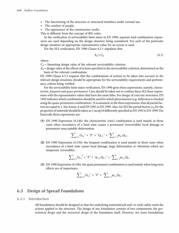
• The functioning of the structure or structural members under normal use,
• The comfort of people,
• The appearance of the construction works.This is different from the concept of BSI codes.
In the verification of serviceability limit states in EN 1990, separate load combination expres-sions are used depending on the design situation being considered. For each of the particulardesign situation an appropriate representative value for an action is used.
For the SLS verification, EN 1990 Clause 6.5.1 stipulates that
Ed ≤Cd 6 3
where:Cd = limmiting design value of the relevant serviceability criterionEd = design value of the effects of actions specified in the serviceability criterion, determined on the
basis of the relevant combination.EN 1990 Clause 6.5.3 requires that the combinations of actions to be taken into account in therelevant design situations should be appropriate for the serviceability requirements and perform-ance criteria being verified.
For the serviceability limit states verification, EN 1990 gives three expressions, namely, charac-teristic, frequent and quasi-permanent. Care should be taken not to confuse these SLS three expres-sions with the representative values that have the same titles. For design of concrete structures, EN1992 indicateswhich combination should be used for which phenomenon (e.g. deflection is checkedusing the quasi-permanent combination). It is assumed, in the three expressions, that all partial fac-tors are equal to 1. See Annex A and EN 1991 to EN 1999. Also, for SLS the partial factors γM for theproperties ofmaterials should be taken as 1 except if differently specified in EN1992 to EN1999.TheEurocode three expressions are:
(1) EN 1990 Expression (6.14b): the characteristic (rare) combination is used mainly in thosecases when exceedance of a limit state causes a permanent (irreversible) local damage orpermanent unacceptable deformation.
j≥ 1Gk, j + P + Qk, 1 +
i > 1ψ0, iQk, i
(2) EN 1990 Expression (6.15b): the frequent combination is used mainly in those cases whenexceedance of a limit state causes local damage, large deformation or vibrations which aretemporary (reversible).
j≥ 1Gk, j + P + ψ1,1Qk, 1 +
i > 1ψ2, iQk, i
(3) EN 1990 Expression (6.16b): the quasi permanent combination is usedmainly when long termeffects are of importance.
j≥ 1Gk, j + P +
i > 1ψ2, iQk, i
6.3 Design of Spread Foundations
6.3.1 Introduction
All foundations should be designed so that the underlying materials(soil and/ or rock) safely resist theactions applied to the structure. The design of any foundation consists of two components; the geo-technical design and the structural design of the foundation itself. However, for some foundations
664 Shallow Foundations
worksaccounts.com
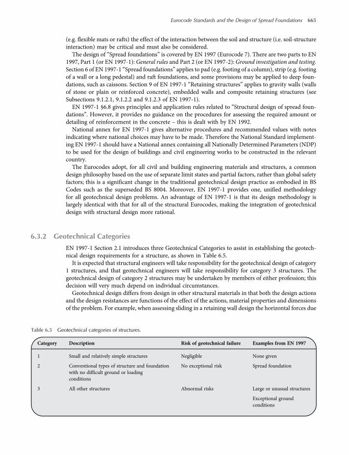
(e.g. flexible mats or rafts) the effect of the interaction between the soil and structure (i.e. soil-structureinteraction) may be critical and must also be considered.The design of “Spread foundations” is covered by EN 1997 (Eurocode 7). There are two parts to EN
1997, Part 1 (or EN 1997-1): General rules and Part 2 (or EN 1997-2):Ground investigation and testing.Section 6 of EN 1997-1 “Spread foundations” applies to pad (e.g. footing of a column), strip (e.g. footingof a wall or a long pedestal) and raft foundations, and some provisions may be applied to deep foun-dations, such as caissons. Section 9 of EN 1997-1 “Retaining structures” applies to gravity walls (wallsof stone or plain or reinforced concrete), embedded walls and composite retaining structures (seeSubsections 9.1.2.1, 9.1.2.2 and 9.1.2.3 of EN 1997-1).EN 1997-1 §6.8 gives principles and application rules related to “Structural design of spread foun-
dations”. However, it provides no guidance on the procedures for assessing the required amount ordetailing of reinforcement in the concrete – this is dealt with by EN 1992.National annex for EN 1997-1 gives alternative procedures and recommended values with notes
indicating where national choices may have to be made. Therefore the National Standard implement-ing EN 1997-1 should have a National annex containing all Nationally Determined Parameters (NDP)to be used for the design of buildings and civil engineering works to be constructed in the relevantcountry.The Eurocodes adopt, for all civil and building engineering materials and structures, a common
design philosophy based on the use of separate limit states and partial factors, rather than global safetyfactors; this is a significant change in the traditional geotechnical design practice as embodied in BSCodes such as the superseded BS 8004. Moreover, EN 1997-1 provides one, unified methodologyfor all geotechnical design problems. An advantage of EN 1997-1 is that its design methodology islargely identical with that for all of the structural Eurocodes, making the integration of geotechnicaldesign with structural design more rational.
6.3.2 Geotechnical Categories
EN 1997-1 Section 2.1 introduces three Geotechnical Categories to assist in establishing the geotech-nical design requirements for a structure, as shown in Table 6.5.It is expected that structural engineers will take responsibility for the geotechnical design of category
1 structures, and that geotechnical engineers will take responsibility for category 3 structures. Thegeotechnical design of category 2 structures may be undertaken by members of either profession; thisdecision will very much depend on individual circumstances.Geotechnical design differs from design in other structural materials in that both the design actions
and the design resistances are functions of the effect of the actions, material properties and dimensionsof the problem. For example, when assessing sliding in a retaining wall design the horizontal forces due
Table 6.5 Geotechnical categories of structures.
Category Description Risk of geotechnical failure Examples from EN 1997
1 Small and relatively simple structures Negligible None given
2 Conventional types of structure and foundationwith no difficult ground or loadingconditions
No exceptional risk Spread foundation
3 All other structures Abnormal risks Large or unusual structures
Exceptional groundconditions
Eurocode Standards and the Design of Spread Foundations 665
worksaccounts.com
to the earth (design effect of the actions) are derived from the material properties of the soil and thedimensions of the problem; similarly, the resistance to sliding is also derived from the actions, materialproperties and the dimensions. Therefore, geotechnical calculations have a greater level of complexitythan design in other structural materials where actions are not normally a function of the materialproperties and resistances not a function of the actions.
6.3.3 Limit States
The following limit states should be satisfied for geotechnical design:
(a) Ultimate limit statesUltimate limit states (ULS) are those that will lead to failure of the ground and/or the associatedstructure.
EN 1997-1 identifies the following five ultimate limit states. They should be satisfied for geo-technical design; each has its combination of actions (For an explanation of Eurocode terminology,please refer to the Section 6.2.2 of this chapter):EQU – Loss of static equilibrium of the structure.STR – Internal failure or excessive deformation of the structure.GEO – Failure or excessive deformation in the ground.UPL – Loss of equilibrium or excessive deformation due to uplift.HYD – Failure due to hydraulic heave, piping and erosion.
(b) Serviceability limit statesServiceability limit states (SLS) are those that result in unacceptable levels of deformation (e.g.excessive settlement or heave), vibration and noise. They should be satisfied for geotechnicaldesign.
The designer of a geotechnical structure tries first to identify the possible ultimate and service-ability limit states that are likely to affect the structure. Usually, it will be clear that one of the limitstates will govern the design and therefore it will not be necessary to carry out verifications for all ofthem, although it is good practice to record that they have all been considered. Verifications ofserviceability limit states is a key requirement of a EN 1997 design, which does not explicitly featurein more traditional approaches. In traditional design it is assumed in many calculation proceduresthat the lumped safety factor provides not only safety against failure but also will limit deform-ations to tolerable levels. For example, it is common to adopt safety factors against bearing capacityfailure in the foundation soil in excess of 3.0. This is far greater than needed to ensure sufficientreserve against failure. EN 1997 generally requires a specific verification that serviceability limitsare met and thus serviceability requirements are more likely to be the governing factor for manysettlement sensitive projects.
Traditional geotechnical design methods, adopting lumped safety factors, have proved sat-isfactory over many decades and much experience has been built on such methods. However,the use of a single factor to account for all uncertainties in the analysis does not provide anadequate control of different levels of doubt in various parts of the design process. The limitstate approach forces designers to think more rigorously about possible modes of failure andthose parts of the calculation process where there is most uncertainty. The partial factors in EN1997 have been chosen to give similar designs to those obtained using lumped factors; thus,ensuring that the wealth of previous experience is not lost by the introduction of a radicallydifferent design methodology. The Eurocodes present a unified approach to all structuralmaterials and should lead to less confusion and fewer errors when considering soil–structureinteraction.
666 Shallow Foundations
worksaccounts.com
EN 1997-1 §6.2 lists eight different types of limit states (repeated below for convenience)that should be considered in geotechnical design of spread foundations including pads, stripsand rafts. The limit states are:
• Loss of overall stability;
• Bearing resistance failure, punching failure, squeezing;
• Failure by sliding;
• Combined failure in the ground and in the structure;
• Structural failure due to foundation movement;
• Excessive settlements;
• Excessive heave due to swelling, frost and other causes;
• Unacceptable vibrations.
We may notice that the first five limit states are related to ultimate limit state design; their detailsare covered in EN 1997-1 §6.5. The remaining three limit states are related to serviceability limitstate design; their details are covered in EN 1997-1 §6.6.
6.3.4 Geotechnical Design
(A) Design situationsEN1997-1 Section 6.3 requires that design situations shall be selected in accordancewith EN1997-1Section 2.2 which states: both short-term and long-term design situations shall be considered. Thisconsideration is to reflect the sometimes vastly different resistances obtained from drained andundrained soils. Examples of these situations may be given as follows:
• For persistent design situation: long-term is considered where structures are founded on coursesoils and fully-drained fine soils; and short-term is considered where there is partially-drainedfine soils (with design working life less than 25 years).
• For transient design situation: long-term is considered where there are temporary works incoarse soils; and short-term is considered where there are temporary works in fine soils
• For accidental design situation: long-term is considered where structures are founded oncourse soils and quick-draining fine soils; and short-term is considered where structures arefounded on slow-draining fine soils.
• For seismic design situation: short-term is considered where structures are founded on slow-draining fine soils.
EN 1997-1 Section 2.2 provides a list of nine different items that the detailed specifications ofdesign situations should include.
(B) ActionsEN 1997-1 Section 6.3 requires that the actions listed in EN 1997-1 Section 2.4.2(4) should be con-sidered when selecting the limit states for calculation. This section provides a list of 20 types ofactions that should be included in geotechnical design.
In geotechnical design it is necessary to identify which action is favourable and which action isunfavourable. The Eurocodes make an important distinction between favourable (or stabilising) andunfavourable(or destabilising) actions, which is reflected in the values of the partial factors γF appliedto each type of action. Unfavourable actions are typically increased by the partial factor (i.e. γF > 1)and favourable actions are decreased or left unchanged (i.e. γF ≤ 1). For example, to provide sufficientreliability against bearing capacity failure, the self-weight of a wall and its strip footing should beconsidered as unfavourable actions, since they increase the effective stress beneath the footing. How-ever, the same actions should be considered as favourable for sliding, since they increase resistance.
The designer should be aware of not treating an action as both favourable and unfavourable inthe same calculation since it is illogical to do so. EN 1997 deals with this issue in what has been
Eurocode Standards and the Design of Spread Foundations 667
worksaccounts.com
known as the Single-Source Principle: “unfavourable (or destabilising) and favourable (or stabilising)permanent actions may in some situations be considered as coming from a single source. If they areconsidered so, a single partial factor may be applied to the some of these actions or to the some oftheir effects”. [EN 1997-1 Section 2.4.2(9) P Note]. In the example just given if the water table islocated above the foundation level, the upward thrust on the footing bottom owing to water pressurewill be considered as favourable and the horizontal thrust on the wall as unfavourable for bearing(both thrusts coming from a single source). The Note allows these thrusts to be treated in the sameway; either both unfavourable or both favourable, whichever represents the more critical designcondition.
(C) Basic requirementsConsidering the ULS, the design effect of destabilising actions Ed,dst and design effect of actions Edmust be less than or equal to the design effect of stabilising actions Ed,st and design resistance Rd,respectively, as indicated in Equations (6.1) and (6.2). Considering the SLS, the design effect of theactions Ed must be less than or equal to the limiting design value of the relevant serviceability cri-terion Cd, as indicated in Equation (6.3).
(D) Geometrical dataAccording to EN 1997-1 Section 2.4.4, the level and slope of ground surface, water levels, levels ofinterfaces between strata, excavation levels and the dimensions of the geotechnical structure shallbe treated as geometrical data.
(E) Design approaches and combinationsThere has not been a consensus amongst geotechnical engineers over the application of limit stateprinciples to geotechnical design. EN 1997-1, to allow for these differences of opinion, presentsthree different Design Approaches (DAs) for carrying out ultimate limit state analysis for theGEO and STR limit states. The decision on which approach to use for a particular country is givenin its National Annex. The design approaches are:
• DA1 – Combination 1: A1 “+” M1 “+” R1 (EN 1997-1§2.4.7.3.4.2)– Combination 2: A2 “+” M2 “+” R1
• DA2: A1 “+” M1 “+” R2 (EN 1997-1§2.4.7.3.4.3)
• DA3: (A1 or A2) “+” M2 “+” R3 (EN 1997-1§2.4.7.3.4.4)“+”implies “to be combined with” (EN 1997-1§2.4.7.3.4.2)
These approaches apply the partial factor sets in different combinations in order to provide reliabil-ity in the design. Themethod of applying the partial factors reflects the differing opinions regardinggeotechnical design held across theEuropeanUnion.Actually,DesignApproach 1provides reliabil-ity by applying different partial factor sets to two variables (actions and ground strength parametersor ground resistance) in two separate calculations (Combinations 1 and 2), whereas DesignApproaches 2 and 3 apply factor sets to two variables simultaneously, in a single calculation. Furtherclarification of the Design approaches is provided in Annex B of EN 1997-1.
InAnnexAofEN1997-1 thepartial factors are grouped in sets denotedbyA (for actions or effectsof actions), M (for soil parameters) and R (for resistances).
In the UK, Design Approach 1 is specified in the National Annex. For this Design Approach(excluding design of axially loaded piles and anchors) there are two sets of combinations to usefor the STR and GEO ultimate limit states, as indicated above. The values for the partial factorsto be applied to the actions for these combinations are given in Table 6.6 and the partial factorsfor the geotechnical material properties are given in Table 6.7. Combination 1 will generally governthe structural resistance, and Combination 2 will generally govern the size of the foundations.
The partial factors to be applied to the geotechnical material properties and actions at the EQUlimit state are given in Table 6.7 and Table 6.8, respectively.
For the SLS, EN 1997-1 does not give any advice onwhether the characteristic, frequent or quasi-permanent combination should be used. Where the prescriptive design method is used for spreadfoundations (will be discussed in the following paragraphs) then the characteristic combination
668 Shallow Foundations
worksaccounts.com

Table 6.7 Partial factors for geotechnical material properties.
Symbol
Angle of shearingresistance(apply to tan φ)
Effectivecohesion
Undrainedshearstrength
Unconfinedstrength
Bulkdensity
γφ γc γcu γqu γγ
Combination 1
Combination 2
EQU
1.0
1.25
1.1
1.0
1.25
1.1
1.0
1.4
1.2
1.0
1.4
1.2
1.0
1.0
1.0
Table 6.6 Design valuesof actionsderived forUKdesign, STRandGEOultimate limit states–persistent and transient design situations.
Combination Exp. referenceBS EN 1990
Permanent actions
Leading variableaction
Accompanying variableactions
Unfavorable FavorableMain(if any) Others
Combination 1{Application of combination 1(BS EN 1997) to set B (BS EN 1990)}
Exp. (6.10)
Exp. (6.10a)
Exp. (6.10b)
1 35Gak
1 35Gak
0 925d × 1 35Gak
1 0Gak
1 0Gak
1 0Gak
1.5bQk
–
1.5bQk
–
1 5ψ c0,1Qk
–
1 5bψ c0, iQk, i
1 5bψ c0, iQk, i
1 5bψ c0, iQk, i
Combination 2{Application of combination 2(BS EN 1997) to set C (BS EN 1990)}
Exp. (6.10) 1 0Gak 1 0Ga
k 1.3bQk,1 – 1 3bψ c0, iQk, i
Key:a Where the variation in permanent action is not considered significant Gk,jsup and Gk,jinf may be taken as Gk; Gk,jsup & Gk,jinf are upper & lower
characteristic values of permanent action j.b Where the action is favorable, γQ,i = 0 and the variable actions should be ignored.c The value of ψ0 can be obtained from NA A1.1 of the UK NA to BS EN 1990 or from Table 6.3.d The value of ξ in the UK NA to BS EN 1990 is 0.925
Table 6.8 Design values of actions derived for UK design, EQU ultimate limit states– persistent and transient design situations.
Combination Exp.referenceBS EN 1990
Permanent actionsLeading variableaction
Accompanying variableactions
Unfavorable Favorable Main (if any) Others
Exp.(6.10) 1 1Gak 0 90Ga
k 1.5bQk – 1 5bψ c0, iQk, i
Key:a Where the variation in permanent action is not considered significant Gk,jsup and Gk,jinfmay be taken as Gk; Gk,jsup& Gk,jinf are upper & lower
characteristic values of permanent action j.b Where the action is favorable, γQ,i = 0 and the variable actions should be ignored.c The value of ψ0 can be obtained from NA A1.1 of the UK NA to BS EN 1990 or from Table 6.3.
Eurocode Standards and the Design of Spread Foundations 669
worksaccounts.com
should be adopted. For direct design method the frequent combination can be used for sizing offoundations and the quasi-permanent combination can be used for settlement calculations.
(F) Design methodsSection 6 of EN 1997-1 requires spread foundations (e.g. pad and strip) to be designed using thefollowing methods:(1) Direct method – calculation is carried out for each limit state. At the ULS, the bearing resistance
of the soil should be checked using partial factors on the soil properties as well as on theactions. At the SLS, the settlement of the foundations should be calculated and checked againstpermissible limits. As mentioned earlier, the frequent combination can be used for sizing offoundations and the quasi-permanent combination can be used for settlement calculations.
(2) Indirect method – experience and testing used to determine serviceability limit state parametersthat also satisfy all relevant limit states. Thismethod is used predominantly for Geotechnical Cat-egory 1 structures (see Table 6.5), where there is negligible risk in terms of overall stability orground movements, which are known from comparable local experience to be sufficientlystraightforward. In these cases the procedures may consist of routine methods for foundationdesign and construction. The procedures should be used only if there is no excavation belowthe water table or if comparable local experience indicates that a proposed excavation belowthewater tablewillbe straightforward. Indirectmethodsmayalsobeused forhigher risk structureswhere it is difficult to predict the structural performance with sufficient accuracy from analyticalsolutions. In these cases, reliance is placed on the observational method, and identification ofpotential behaviour. Then the final, suitably conservative, designof the foundation canbedecided.
(3) Prescriptive method – a presumed bearing resistance is used. This method may be used wherecalculation of the soil properties is not possible or necessary and can be used provided that con-servative rules of design are used. Tables (for example Tables in the Building Regulations) ofpresumed bearing values may be used to determine presumed (allowable) bearing pressuresforGeotechnical Category 1 structures where ground conditions arewell known, and in prelim-inary calculations for Geotechnical Category 2 structures. Alternatively, the presumed bearingpressure to allow for settlement can be calculated by the geotechnical designer and included inthe geotechnical design report. Unlike British standard BS 8004 – which was giving allowablebearing pressures for rocks, non-cohesive soils, cohesive soils, peat and organic soils, madeground, fill, high porosity chalk and theMerciaMudstone –Annex G of EN 1997-1-1 only pro-vides values of presumed bearing resistance for rock (which was also appeared in BS 8004).This chapter does not attempt to provide complete guidance on the design of spread founda-tions, for which the reader should refer to any well-established text on the subject.
(G) Footings subject to vertical actions(a) Eccentricity e= 0
EN 1997-1 requires the design vertical action Vd acting on the foundation to be less than orequal to the design bearing resistance Rd of the ground beneath it:
Vd ≤Rd 6 4
The action Vd should include the self-weight of the foundation and any backfill on it.Equation (6.4) is simply a re-statement of Equation (6.2). Designers more commonly considerpressures and stresses rather thanwork in terms of forces, so we will re-write Equation (6.4) as:
qEd ≤ qRd 6 5
The pressure qEd is the design bearing pressure on the ground (an action effect); qRd is thecorresponding design resistance.
Design baring pressure:Figure 6.4 shows a footing carrying characteristic vertical actions VGk (permanent) and
VQk (variable) imposed on it by the super-structure. The characteristic self-weights of thefooting and of the backfill upon it are both permanent actions (WGk)
670 Shallow Foundations
worksaccounts.com
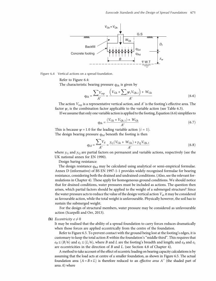
Refer to Figure 6.4:The characteristic bearing pressure qEk is given by
qEk =Vrep
A=
VGk + iψ iVQk,i + WGk
A6 6
The action Vrep is a representative vertical action, and A is the footing’s effective area. Thefactor ψ i is the combination factor applicable to the variable action (see Table 6.3).
Ifwe assume that only one variable action is applied to the footing, Equation (6.6) simplifies to
qEk =VGk +VQk,1 + WGk
A6 7
This is because ψ = 1 0 for the leading variable action i = 1 .The design bearing pressure qEd beneath the footing is then
qEd =Vd
A=γG VGk + WGk + γQVQk,1
A6 8
where γG and γQ are partial factors on permanent and variable actions, respectively (see theUK national annex for EN 1990).
Design baring resistance:The design resistance qRd may be calculated using analytical or semi-empirical formulae.
Annex D (informative) of BS EN 1997-1-1 provides widely-recognised formulae for bearingresistance, considering both the drained and undrained conditions. (Also, see the relevant for-mulations in Chapter 4). These apply for homogeneous ground conditions. We should noticethat for drained conditions, water pressures must be included as actions. The question thenarises, which partial factors should be applied to the weight of a submerged structure? Sincethe water pressure acts to reduce the value of the design vertical actionVd, it may be consideredas favourable action, while the total weight is unfavourable. Physically however, the soil has tosustain the submerged weight.
For the design of structural members, water pressure may be considered as unfavourableaction (Scarpelli and Orr, 2013).
(b) Eccentricity e 0It may be realised that the ability of a spread foundation to carry forces reduces dramaticallywhen those forces are applied eccentrically from the centre of the foundation.
Refer to Figure 6.5. To prevent contact with the ground being lost at the footing’s edges, it iscustomary to keep the total action Rwithin the foundation’s “middle third”. This requires thateB ≤ B 6 and eL ≤ L 6 , where B and L are the footing’s breadth and length; and eB and eLare eccentricities in the direction of B and L. (see Section 4.8 of Chapter 4).
Amethod to take account of the effect of eccentric loading on bearing capacity calculations is byassuming that the load acts at centre of a smaller foundation, as shown in Figure 6.5. The actualfoundation area A=B× L is therefore reduced to an effective area A (the shaded part ofarea A) where
Backfill
Concrete footing
G.S
W.T
Δ
qEd
qRd
Df
zw
VGk+ VQk
WGk
B
Figure 6.4 Vertical actions on a spread foundation.
Eurocode Standards and the Design of Spread Foundations 671
worksaccounts.com
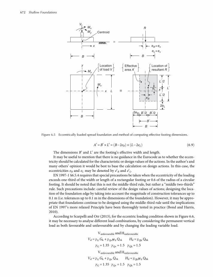
A =B × L = B−2eB × L−2eL 6 9
The dimensions B and L are the footing’s effective width and length.It may be useful to mention that there is no guidance in the Eurocode as to whether the eccen-
tricity should be calculated for the characteristic or design values of the actions. In the author’s andmany others’ opinion it would be best to base the calculation on design actions. In this case, theeccentricities eB and eL may be denoted by e B and e L.
EN 1997-1 §6.5.4 requires that special precautions be taken when the eccentricity of the loadingexceeds one-third of the width or length of a rectangular footing or 0.6 of the radius of a circularfooting. It should be noted that this is not the middle-third rule, but rather a “middle two-thirds”rule. Such precautions include: careful review of the design values of actions; designing the loca-tion of the foundation edge by taking into account the magnitude of construction tolerances up to0.1 m (i.e. tolerances up to 0.1 m in the dimensions of the foundation). However, it may be appro-priate that foundations continue to be designed using the middle-third rule until the implicationsof EN 1997’s more relaxed Principle have been thoroughly tested in practice (Bond and Harris,2010).
According to Scarpelli and Orr (2013), for the eccentric loading condition shown in Figure 6.6,it may be necessary to analyse different load combinations, by considering the permanent verticalload as both favourable and unfavourable and by changing the leading variable load.
Vunfavourable andHunfavourable
Vd = γGGk + γQvψ0Qvk Hd = γQhQhk
γG = 1 35 γQv = 1 5 γQh = 1 5
Vunfavourable andHunfavourable
Vd = γGGk + γQv Qvk Hd = γQhψ0Qhk
γG = 1 35 γQv = 1 5 γQh = 1 5
Centroid
VMx
x
My
My
Mx
x
Location of
resultant R
Location
of load VEffective
area A′
B
y
L
B
L′/2
L′/2
2eL
2eB B′/2 B′/2
B′
B
B
R
eB
xeL
eB= ex
eL= ev
L′
Figure 6.5 Eccentrically loaded spread foundation and method of computing effective footing dimensions.
672 Shallow Foundations
worksaccounts.com
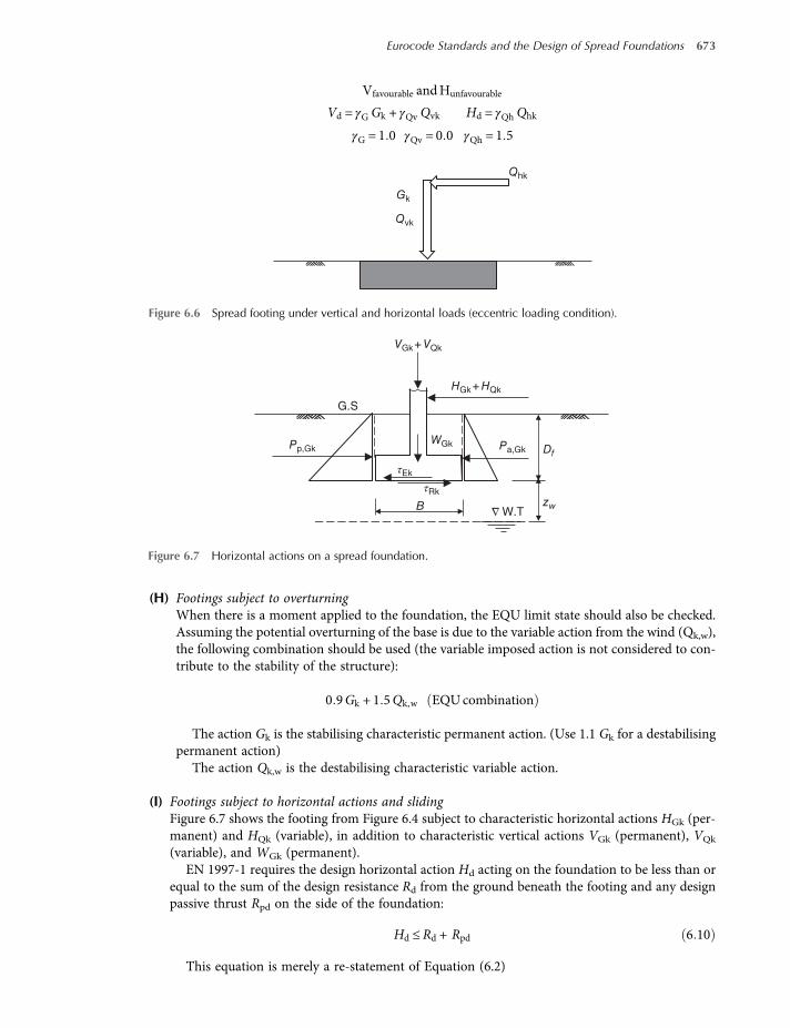
Vfavourable andHunfavourable
Vd = γGGk + γQv Qvk Hd = γQhQhk
γG = 1 0 γQv = 0 0 γQh = 1 5
(H) Footings subject to overturningWhen there is a moment applied to the foundation, the EQU limit state should also be checked.Assuming the potential overturning of the base is due to the variable action from the wind (Qk,w),the following combination should be used (the variable imposed action is not considered to con-tribute to the stability of the structure):
0 9Gk + 1 5Qk,w EQUcombination
The action Gk is the stabilising characteristic permanent action. (Use 1.1 Gk for a destabilisingpermanent action)
The action Qk,w is the destabilising characteristic variable action.
(I) Footings subject to horizontal actions and slidingFigure 6.7 shows the footing from Figure 6.4 subject to characteristic horizontal actions HGk (per-manent) and HQk (variable), in addition to characteristic vertical actions VGk (permanent), VQk
(variable), and WGk (permanent).EN 1997-1 requires the design horizontal action Hd acting on the foundation to be less than or
equal to the sum of the design resistance Rd from the ground beneath the footing and any designpassive thrust Rpd on the side of the foundation:
Hd ≤Rd + Rpd 6 10
This equation is merely a re-statement of Equation (6.2)
Gk
Qvk
Qhk
Figure 6.6 Spread footing under vertical and horizontal loads (eccentric loading condition).
W.T Δ
G.S
Pp,Gk Pa,Gk Df
zw
HGk+ HQk
VGk+ VQk
WGk
τEk
τRk
B
Figure 6.7 Horizontal actions on a spread foundation.
Eurocode Standards and the Design of Spread Foundations 673
worksaccounts.com
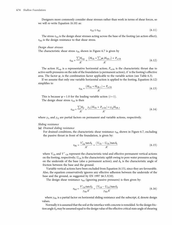
Designers more commonly consider shear stresses rather than work in terms of shear forces, sowe will re-write Equation (6.10) as:
τEd ≤ τRd 6 11
The stress τEd is the design shear stresses acting across the base of the footing (an action effect);τRd is the design resistance to that shear stress.
Design shear stressesThe characteristic shear stress τEk shown in Figure 6.7 is given by
τEk =Hrep
A=
HGk + iψ iHQk,i + Pa,GkA
6 12
The action Hrep is a representative horizontal action; Pa,Gk is the characteristic thrust due toactive earth pressures on the side of the foundation (a permanent action);A is the footing’s effectivearea. The factor ψ i is the combination factor applicable to the variable action (see Table 6.3).
If we assume that only one variable horizontal action is applied to the footing, Equation (6.12)simplifies to
τEk =HGk +HQk,1 + Pa,Gk
A6 13
This is because ψ = 1 0 for the leading variable action i= 1 .The design shear stress τEd is then
τEd =Hd
A=γG HGk + Pa,Gk + γQHQk,1
A6 14
where γG and γQ are partial factors on permanent and variable actions, respectively.
Sliding resistance(a) Drained sliding resistance
For drained conditions, the characteristic shear resistance τRk shown in Figure 6.7, excludingthe passive thrust in front of the foundation, is given by:
τRk =VGk tanδk
A=
VGk − UGk tanδkA
6 15
where VGk and V Gk represent the characteristic total and effective permanent vertical actionson the footing, respectively; UGk is the characteristic uplift owing to pore water pressures actingon the underside of the base (also a permanent action); and δk is the characteristic angle offriction between the base and the ground.
Variable vertical actions have been excluded from Equation (6.15), since they are favourable.Also, the equation conservatively ignores any effective adhesion between the underside of thebase and the ground, as suggested by EN 1997 §6.5.3(10).
The design shear resistance τRd (ignoring passive pressures) is then given by:
τRd =V 'Gd tanδdγRhA
=VGd− UGd tanδd
γRhA6 16
where γRh is a partial factor on horizontal sliding resistance and the subscript, d, denote designvalues.
Normally it is assumed that the soil at the interfacewith concrete is remolded. So the design fric-tion angle δdmaybe assumed equal to the design value of the effective critical state angle of shearing
674 Shallow Foundations
worksaccounts.com
resistance φ cv,d for cast in situ concrete foundations and equal to 2/3 φ cv,d for smooth precastfoundations [EN 1997 §6.5.3(10)]. The design effective critical state angle is
φ'cv,d = tan−1 tanφcv,k
γφ6 17
where γφ is the partial factor on shearing resistance.The vertical action VGk is favourable, since an increase in its value increases the shear resistance;
whereas UGd is unfavourable action, since an increase in its value decreases the resistance. Intro-ducing into Equation (6.15) partial factors on favourable and unfavourable permanent actions(γG,fav and γG) results in:
τRd =γG,favVGk − γGUGk tanδk
γRhγφA
=γG,fav
γRh × γφVGk −
γGγRh × γφ
UGk ×tanδkA
6 18
If, however, partial factors are applied to the net effects of actions rather than to the actionsthemselves, then Equation (6.18) will become
τRd =γG,fav VGk − UGk tanδk
γRhγφA=
γG,favγRh × γφ
VGk − UGk ×tanδkA
6 19
Table 6.9 summarises the values of these partial factors for each of the EN 1997’s three DesignApproaches.
As far as an ultimate limit state of sliding is concerned, the horizontal component of an inclinedload on the footing is considered unfavourable, whereas the vertical component is favourable,although they have the same source. Except in Combination 2 of Design Approach 1, a favourablepermanent action attracts a partial factor γG,fav = 1 and an unfavourable permanent action a partial
Table 6.9 Partial factors for each of the EN 1997’s three Design Approaches.
Individual Partial Factor orPartial Factor “Grouping”
Design Approach
1
2 3Combination 1 Combination 2
γG
γG,fav
γφ
γcu
γRh
1.35
1.0
1.0
1.0
1.0
1.0
1.0
1.25
1.4
1.0
1.35
1.0
1.0
1.0
1.1
1.35/1
1.0
1.0
1.4
1.0
γG,fav γRh × γφ
γG γRh × γφ
1 γRh × γcu
1.0
1.35
1.0
0.8
0.8
0.71
0.91
1.23
0.91
0.8
1.08/0.8
0.71
Eurocode Standards and the Design of Spread Foundations 675
worksaccounts.com

factor γG = 1 35. In case the components of the inclined action are treated differently, then theinclination of that action will change. This is a prime example of where the Single Source Principle[discussed in Section 6.3.4 (B)] should be invoked and the whole action should be treated either asunfavourable or as favourable, whichever represents the more critical design condition.(b) Undrained sliding resistance
For undrained conditions, the characteristic shear resistance τRk shown in Figure 6.7,excluding the passive thrust in front of the foundation, is given by:
τRk =Cuk 6 20
where Cuk represents the characteristic undrained shear strength of the soil.The design shear resistance τRd (ignoring passive pressures) is then given by:
τRd =Cud
γRh=
Cuk
γcu × γRh6 21
where γcu is the partial factor on undrained shear strength (see Table 6.9).
(J) SLS verificationWhen design is carried out by direct methods, settlement calculations are required to check SLS.For soft clays, irrespective of Geotechnical categories, settlement calculations shall be carried out.For spread foundations on stiff and firm clays in Geotechnical categories 2 and 3, vertical displace-ment should usually be calculated [EN 1997 §6.6.1(3, 4)].
As mentioned in Sections 6.2.5(B) and 6.3.3(b), EN 1997 requires the design movements Ed of afoundation to be less than or equal to the limiting movement Cd specified for the project; seeEquation (6.3).
The following three components of settlement should be considered for partially or fully satur-ated soils [EN 1997-1 §6.6.2(2)]:
• s0: immediate settlement; for fully-saturated soil due to shear deformation at constant volume,and for partially-saturated soil due to both shear deformation and volume reduction;
• s1: settlement caused by consolidation;
• s2: settlement caused by creep.
So, Equation (6.3) can be re-written for settlement of foundations as follows:
sEd = s0 + s1 + s2 ≤ sCd 6 22
where sEd is the total settlement (an action effect), and sCd is the limiting value of that settlement.The components of foundation movement, which should be considered include: settlement, rela-
tive (or differential) settlement, rotation, tilt, relative deflection, relative rotation, horizontal displace-ment and vibration amplitude. Definitions and limiting values of some terms for foundationmovement and deformation are given in Annex H to EN1997-1. For example, for normal structureswith isolated foundations, total settlements up to 50mm are often acceptable. Larger settlements maybe acceptable provided the relative rotations remain within acceptable limits and provided the totalsettlements do not cause problems with the services entering the structure, or cause tilting and so on.
In verifications of SLS, partial factors are normally set to 1. The combination factors ψ applied toaccompanying variable actions are those specified for the characteristic, frequent, or quasi-permanentcombinations, which are the ψ2 values from EN 1990.
Annex F of EN 1997-1 presents two methods to evaluate settlement. Other methods (from the insitu tests) are given in the Annexes to EN 1997-2.
EN 1997 emphasises the fact that settlement calculations should not be regarded as accurate. Theymerely provide an approximate indication [EN 1997-1 §6.6.1(6)].
676 Shallow Foundations
worksaccounts.com
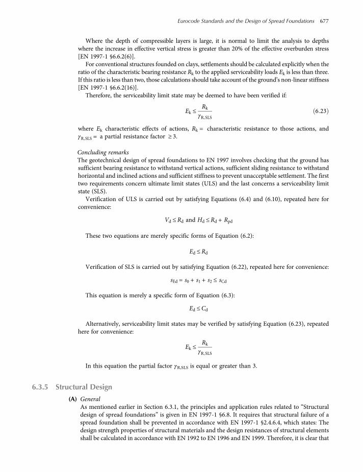
Where the depth of compressible layers is large, it is normal to limit the analysis to depthswhere the increase in effective vertical stress is greater than 20% of the effective overburden stress[EN 1997-1 §6.6.2(6)].
For conventional structures founded on clays, settlements should be calculated explicitly when theratio of the characteristic bearing resistance Rk to the applied serviceability loads Ek is less than three.If this ratio is less than two, those calculations should take account of the ground’s non-linear stiffness[EN 1997-1 §6.6.2(16)].
Therefore, the serviceability limit state may be deemed to have been verified if:
Ek ≤Rk
γR,SLS6 23
where Ek characteristic effects of actions, Rk = characteristic resistance to those actions, andγR,SLS = a partial resistance factor ≥ 3.
Concluding remarksThe geotechnical design of spread foundations to EN 1997 involves checking that the ground hassufficient bearing resistance to withstand vertical actions, sufficient sliding resistance to withstandhorizontal and inclined actions and sufficient stiffness to prevent unacceptable settlement. The firsttwo requirements concern ultimate limit states (ULS) and the last concerns a serviceability limitstate (SLS).
Verification of ULS is carried out by satisfying Equations (6.4) and (6.10), repeated here forconvenience:
Vd ≤Rd and Hd ≤Rd + Rpd
These two equations are merely specific forms of Equation (6.2):
Ed ≤Rd
Verification of SLS is carried out by satisfying Equation (6.22), repeated here for convenience:
sEd = s0 + s1 + s2 ≤ sCd
This equation is merely a specific form of Equation (6.3):
Ed ≤Cd
Alternatively, serviceability limit states may be verified by satisfying Equation (6.23), repeatedhere for convenience:
Ek ≤Rk
γR,SLS
In this equation the partial factor γR,SLS is equal or greater than 3.
6.3.5 Structural Design
(A) GeneralAs mentioned earlier in Section 6.3.1, the principles and application rules related to “Structuraldesign of spread foundations” is given in EN 1997-1 §6.8. It requires that structural failure of aspread foundation shall be prevented in accordance with EN 1997-1 §2.4.6.4, which states: Thedesign strength properties of structural materials and the design resistances of structural elementsshall be calculated in accordance with EN 1992 to EN 1996 and EN 1999. Therefore, it is clear that
Eurocode Standards and the Design of Spread Foundations 677
worksaccounts.com

all the structural reinforced concrete elements of a spread foundation shall be designed in accord-ance with EN 1992.
For stiff footings, EN 1997-1 §6.8 recommends a linear distribution of bearing pressures may beused to calculate bending moments and shear stresses in the structural elements. A more detailedanalysis of soil-structure interaction may be used to justify a more economic design.
The distribution of bearing pressures beneath flexible foundations may be derived by modelingthe foundation as a beam or raft resting on a deforming continuum or series of springs, withappropriate stiffness and strength.
(B) Selected symbols and their definitionsAc Cross-sectional area of concrete= bhAs Area of tension steelAs,prov Area of tension steel providedAs,req ’ d Area of tension steel requiredd Effective depthdeff Average effective depth = dy + dz 2fcd Design value of concrete compressive strength= accfck γcfck Characteristic cylinder strength of concrete
fctm Mean of axial tensile strength= 0 3fck2 3 for fck ≤C50 60 (From Table 3.1, EN 1992)
Gk Characteristic value of a permanent actionh Overall depth of the sectionleff Effective span of memberM Design moment at the ULSQk Characteristic value of a variable actionQkw Characteristic value of a variable wind actionVEd Design value of applied shear forcevEd Design value of applied shear stressVRd,c Design value of the punching shear resistance without punching shear reinforcementvRd,c Design value of the punching shear stress resistance without punching shear
reinforcementvRd,max Design value of the maximum punching shear stress resistance along the control
section consideredx Depth to neutral axis = d−z 0 4xmax Limiting value for depth to neutral axis = δ−0 4 d, where δ≤ 1z Lever armacc Coefficient taking account of long term effects on compressive strength and of unfavour-
able effects resulting from the way load is applied (from UK National Annex) = 0 85 forflexure and axial loads, 1.0 for other phenomena
β Factor for determining punching shear stressδ Ratio of the redistributed moment to the elastic bending momentγm Partial factor for material propertiesρ0 Reference reinforcement ratio = fck 1000ρl Required tension on reinforcement at mid-span to resist the moment due to the design
loads (or at support for cantilevers) =As bdψ0 Factor for combination value of a variable actionψ1 Factor for frequent value of a variable actionψ2 Factor for quasi-permanent value of a variable action
(C) Material properties(a) Concrete
The concrete compressive strength classes are based on the characteristic cylinder strength fckdetermined at 28 days with a maximum value of Cmax. The value of Cmax for use in a Countrymay be found in its National Annex. EN 1992-1-1 §3.1.2(2) recommends C90/105. Details of
678 Shallow Foundations
worksaccounts.com

the required concrete properties such as strength, elastic deformation and creep and shrink-age, are given in EN 1992-1-1 §3.1.
Typical concrete properties are given in Table 6.10.In EN 1992 the design of reinforced concrete is based on the characteristic cylinder strength
fck rather than cube strength and should be specified to BS 8500: Concrete-complementaryBritish Standard to BS EN 206-1.
A key change in BS 8500 was the introduction of dual classification system where the con-crete cylinder strength is given alongside the equivalent concrete cube strength (e.g. for classC28/35 concrete the cylinder strength is 28 MPa, whereas the cube strength is 35 MPa).
As mentioned above, EN 1992 allows the designer to use high strength concrete, up to a classC90/105 (or class C70/85 for bridges). Above a class C50/60, the engineer will find that there arerestrictions placed in EN 1992. For example, there are lower strain limits, additional require-ments for fire resistance and in the UK the resistance to shear should be limited to that of aclass C50/60 concrete.
(b) Reinforcing steelAccording to EN 1992-1-1 §3.2.2(1), the behaviour of reinforcing steel is specified by the fol-lowing properties:
• Yield strength (fyk or f0,2k)
• Maximum actual yield strength (fy,max),
• Tensile strength (ft),
• Ductility (εuk and ft /fyk)
• Bond characteristics (fR: See Annex C),
• Section sizes and tolerances,
• Fatigue strength,
• Weldability,
• Shear and weld strength for welded fabric and lattice girders.Details of all these required reinforcing steel properties are given in EN 1992-1-1 §3.2.The application rules for design and detailing in EN 1992-1-1 are valid for a specified yield
strength range fyk = 400 – 600MPa. The upper limit of fyk within this range for use within aCountry may be found in its National Annex. The recommended value for partial factor γs is1.15 for ULS, persistent and transient design situations [EN 1992-1-1 §2.4.2.4(1)].
The characteristic strength of reinforcing steel supplied in the UK is 500MPa; previously theminimum strength was 460 MPa. In order to ensure that there was no confusion with oldersteel grades the 500 grade steel is designated with an “H”. The properties of reinforcing steel
Table 6.10 Selected concrete properties based on Table 3.1 of EN 1992, Part1-1.
Symbol Properties
fck (MPa) 12 16 20 25 30 35 40 45 50 28a 32a
fck,cube (MPa) 15 20 25 30 37 45 50 55 60 35a 40a
fctm (MPa) 1.6 1.9 2.2 2.6 2.9 3.2 3.5 3.8 4.1 2.8a 3.0a
Ecmb(GPa) 27 29 30 31 33 34 35 36 37 32a 34a
Key
fck = Characteristic cylinder strength
fck, cube = Characteristic cube strength
fctm = Mean tensile strength
Ecm = Mean secant modulus of elasticitya Concrete properties not cited in Table 3.1 of EN 1992, Part1-1.bMean secant modulus of elasticity at 28 days for concrete with quartzite aggregates. For concrete with other aggregates refer to CI 3.1.3 (2)
Eurocode Standards and the Design of Spread Foundations 679
worksaccounts.com
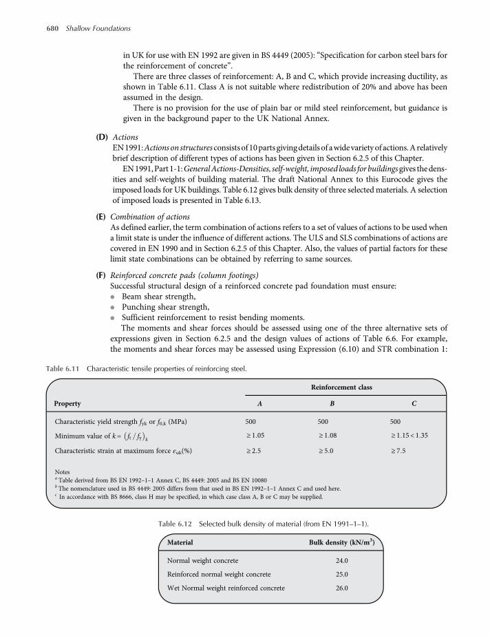
in UK for use with EN 1992 are given in BS 4449 (2005): “Specification for carbon steel bars forthe reinforcement of concrete”.
There are three classes of reinforcement: A, B and C, which provide increasing ductility, asshown in Table 6.11. Class A is not suitable where redistribution of 20% and above has beenassumed in the design.
There is no provision for the use of plain bar or mild steel reinforcement, but guidance isgiven in the background paper to the UK National Annex.
(D) ActionsEN1991:Actionsonstructuresconsistsof10partsgivingdetailsofawidevarietyofactions.Arelativelybrief description of different types of actions has been given in Section 6.2.5 of this Chapter.
EN1991,Part1-1:GeneralActions-Densities, self-weight, imposed loads forbuildingsgives thedens-ities and self-weights of building material. The draft National Annex to this Eurocode gives theimposed loads for UK buildings. Table 6.12 gives bulk density of three selectedmaterials. A selectionof imposed loads is presented in Table 6.13.
(E) Combination of actionsAs defined earlier, the term combination of actions refers to a set of values of actions to be used whena limit state is under the influence of different actions. The ULS and SLS combinations of actions arecovered in EN 1990 and in Section 6.2.5 of this Chapter. Also, the values of partial factors for theselimit state combinations can be obtained by referring to same sources.
(F) Reinforced concrete pads (column footings)Successful structural design of a reinforced concrete pad foundation must ensure:
• Beam shear strength,
• Punching shear strength,
• Sufficient reinforcement to resist bending moments.The moments and shear forces should be assessed using one of the three alternative sets of
expressions given in Section 6.2.5 and the design values of actions of Table 6.6. For example,the moments and shear forces may be assessed using Expression (6.10) and STR combination 1:
Table 6.11 Characteristic tensile properties of reinforcing steel.
Reinforcement class
Property A B C
Characteristic yield strength fyk or f0,k (MPa) 500 500 500
Minimum value of k= ft fy k≥ 1 05 ≥ 1 08 ≥ 1 15 < 1 35
Characteristic strain at maximum force εuk(%) ≥ 2 5 ≥ 5 0 ≥ 7 5
Notesa Table derived from BS EN 1992–1–1 Annex C, BS 4449: 2005 and BS EN 10080b The nomenclature used in BS 4449: 2005 differs from that used in BS EN 1992–1–1 Annex C and used here.c In accordance with BS 8666, class H may be specified, in which case class A, B or C may be supplied.
Table 6.12 Selected bulk density of material (from EN 1991–1–1).
Material Bulk density (kN/m3)
Normal weight concrete 24.0
Reinforced normal weight concrete 25.0
Wet Normal weight reinforced concrete 26.0
680 Shallow Foundations
worksaccounts.com
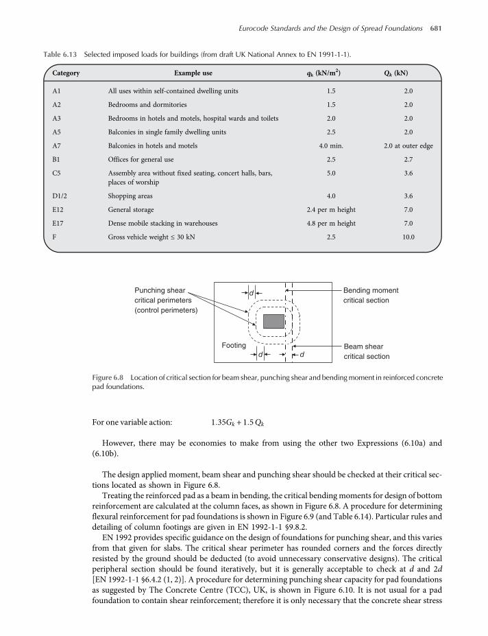
For one variable action 1 35Gk + 1 5Qk
However, there may be economies to make from using the other two Expressions (6.10a) and(6.10b).
The design applied moment, beam shear and punching shear should be checked at their critical sec-tions located as shown in Figure 6.8.
Treating the reinforced pad as a beam in bending, the critical bending moments for design of bottomreinforcement are calculated at the column faces, as shown in Figure 6.8. A procedure for determiningflexural reinforcement for pad foundations is shown in Figure 6.9 (and Table 6.14). Particular rules anddetailing of column footings are given in EN 1992-1-1 §9.8.2.
EN 1992 provides specific guidance on the design of foundations for punching shear, and this variesfrom that given for slabs. The critical shear perimeter has rounded corners and the forces directlyresisted by the ground should be deducted (to avoid unnecessary conservative designs). The criticalperipheral section should be found iteratively, but it is generally acceptable to check at d and 2d[EN 1992-1-1 §6.4.2 (1, 2)]. A procedure for determining punching shear capacity for pad foundationsas suggested by The Concrete Centre (TCC), UK, is shown in Figure 6.10. It is not usual for a padfoundation to contain shear reinforcement; therefore it is only necessary that the concrete shear stress
Punching shear
critical perimeters
(control perimeters)
Beam shear
critical section
Bending moment
critical section
Footing
d
d d
Figure 6.8 Location of critical section for beam shear, punching shear and bendingmoment in reinforced concretepad foundations.
Table 6.13 Selected imposed loads for buildings (from draft UK National Annex to EN 1991-1-1).
Category Example use qk (kN/m2) Qk (kN)
A1 All uses within self-contained dwelling units 1.5 2.0
A2 Bedrooms and dormitories 1.5 2.0
A3 Bedrooms in hotels and motels, hospital wards and toilets 2.0 2.0
A5 Balconies in single family dwelling units 2.5 2.0
A7 Balconies in hotels and motels 4.0 min. 2.0 at outer edge
B1 Offices for general use 2.5 2.7
C5 Assembly area without fixed seating, concert halls, bars,places of worship
5.0 3.6
D1/2 Shopping areas 4.0 3.6
E12 General storage 2.4 per m height 7.0
E17 Dense mobile stacking in warehouses 4.8 per m height 7.0
F Gross vehicle weight ≤ 30 kN 2.5 10.0
Eurocode Standards and the Design of Spread Foundations 681
worksaccounts.com

capacity without shear reinforcement (vRd,c; see Table 6.17) is greater than the applied shear stressvEd = VEd bd . If the basic shear stress is exceeded, the designer may increase the thickness ofthe pad. Alternatively, the amount of main reinforcement could be increased or, less desirably, shearlinks could be provided. EN 1992-1-1 §6.4.4(2) gives equations for calculation of applied and resistingshear stresses.
Determine the applied design moment MEd at face of column or wall
Is concrete class
≤ C50/60?
Yes
No Outside scope of
this publication
Determine K from: K = M
b d2
eff f
ck
No compression reinforcement required
Determine K' from Table 6.14 or
K′ = 0.60 δ – 0.18 δ 2 – 0.21 where δ ≤ 1.0
Yes
No
Compression
reinforcement
required - (Not
recommended;
usually, not
needed in pad
foundations
START
Obtain lever arm z from Table 6.15 or: z = (deff/2) 1 + 1 K3.53 0.95 deff
Check maximum reinforcement requirements: As,max= 0.04 Ac
Is K ≤ K′?
Check minimum reinforcement requirements (see Table 6.16)
As,min = (0.26 fctmbtdeff) / fyk
Calculate tension reinforcement required from: As= M /(z × fyd)
Figure 6.9 Procedure for determining flexural reinforcement for pad foundations.
682 Shallow Foundations
worksaccounts.com
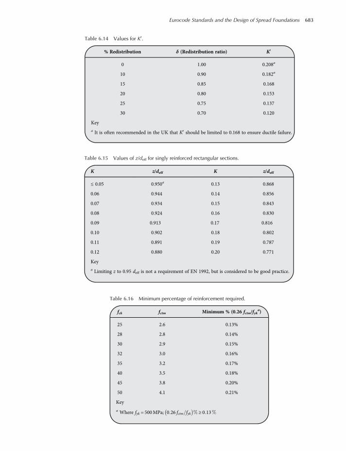
Table 6.16 Minimum percentage of reinforcement required.
fck fctm Minimum % (0.26 fctm/fyka)
25 2.6 0.13%
28 2.8 0.14%
30 2.9 0.15%
32 3.0 0.16%
35 3.2 0.17%
40 3.5 0.18%
45 3.8 0.20%
50 4.1 0.21%
Key
a Where fyk = 500MPa; 0 26 fctm fyk ≥ 0 13
Table 6.14 Values for K .
% Redistribution δ (Redistribution ratio) K
0 1.00 0.208a
10 0.90 0.182a
15 0.85 0.168
20 0.80 0.153
25 0.75 0.137
30 0.70 0.120
Key
a It is often recommended in the UK that K should be limited to 0.168 to ensure ductile failure.
Table 6.15 Values of z/deff for singly reinforced rectangular sections.
K z/deff K z/deff
≤ 0.05 0.950a 0.13 0.868
0.06 0.944 0.14 0.856
0.07 0.934 0.15 0.843
0.08
0.09
0.924
0.913
0.16
0.17
0.830
0.816
0.10 0.902 0.18 0.802
0.11 0.891 0.19 0.787
0.12 0.880 0.20 0.771
Key
a Limiting z to 0.95 deff is not a requirement of EN 1992, but is considered to be good practice.
Eurocode Standards and the Design of Spread Foundations 683
worksaccounts.com
(G) Reinforced concrete strip foundationsWhere the supporting soil is weak and the wall load is heavy a wide strip footing may be required.For this case, a reinforced concrete strip foundation, at a comparatively shallow depth, is likely toshow an advantage in safety and cost over unreinforced concrete. In addition to the main trans-verse reinforcement, longitudinal bars is also desirable in strip foundations on highly variable soilswhen the foundation is enabled to bridge over local weak or hard spots in the soil at the foundationlevel, or when there is an abrupt change in loading.
START
Determine value of νRd,max (refer to Table 6.18)
Determine value of factor β . [ β = 1.0 when applied moment is zero; refer
to Expressions (6.38) to (6.42) from BS EN 1992-1-1 for other cases]
Yes
No Redesign
foundation
No shear reinforcement required. Check complete
Determine concrete punching shear capacity νRd (without shear
reinforcement) from 2d νRd/a (refer to Table 6.17 for νRd,c)
Yes
No
Either increase main
steel, or provide
punching shear
reinforcement. (Not
recommended for
foundations)
Is νEd,max< νRd,max ?
Is νEd < νRd? at
critical perimeter
Determine value of νEd (design shear stress) from: vEd =
where u1 is length of control perimeter (refer to Fig. 6.8). For eccentrically
loaded bases, refer to Expression (6.51). The control perimeter will have to
be found though iteration; it will usually be between d and 2d
(VEd– ΔVEd)
(u1 deff)
Determine value of νEd,max (design shear stress at face of column) from:
=β (VEd– ΔVEd)
(u0 deff)[from Expression (6.38)] where u0 is
perimeter of column (see Clause 6.4.5 for columns at base edges)
vEd,max
deff = (dy + dz)/2 where dy and dz are the effective depths in orthogonal
directions
Figure 6.10 Procedure for determining punching shear capacity for pad foundations.
684 Shallow Foundations
worksaccounts.com

The critical bending moments for design of bottom transverse reinforcement are calculated atthe wall faces on the assumption that the footing projections behave as cantilevers. The slab mustalso be designed to withstand shear and bond stresses. It is necessary to consider only the beamshear stress, which is usually checked at the critical sections, in long direction, located a distance dfrom the wall face. Particular rules and detailing of wall footings are given in EN 1992-1-1 §9.8.2.
(H) Pile capsThe function and structural design of pile caps are very similar to those of reinforced concretepads; both elements must distribute loads from the supported member across their bottoms.
Here also, a pile cap may be treated as a beam in bending, where the critical bending momentsfor the design of the bottom reinforcement are located at the column faces. Alternatively, a trussanalogy may be used; this is covered in EN 1992-1-1 §5.6.4 and 6.5.
Both beam shear and punching shear should be checked as shown in Figure 6.11a. For calcu-lating the design values of shear resistances, Table 6.17 may be used. Again here also, if the basicshear stress is exceeded, the designer may increase the thickness of the cap. Alternatively, theamount of main reinforcement could be increased or, less desirably, shear links could be provided.Care should be taken that main reinforcing bars are fully anchored. The compression caused bythe support reaction from the pile may be assumed to spread at 45 degree angles from the edge ofthe pile (Figure 6.11b).This compression may be taken into account when calculating the anchor-age length. Also, when assessing the shear capacity in a pile cap, only the tension steel placedwithin the stress zone should be considered as contributing to the shear capacity.
Table 6.17 Resistance vRd,c of members without shear reinforcement, MPa.
ρl
Effective depth, d (mm)
300 400 500 600 700 800 900 1000a
0.25% 0.47 0.43 0.40 0.38 0.36 0.35 0.35 0.34
0.50% 0.54 0.51 0.48 0.47 0.45 0.44 0.44 0.43
0.75% 0.62 0.58 0.55 0.53 0.52 0.51 0.50 0.49
1.00% 0.68 0.64 0.61 0.59 0.57 0.56 0.55 0.54
1.25% 0.73 0.69 0.66 0.63 0.62 0.60 0.59 0.58
1.50% 0.78 0.73 0.70 0.67 0.65 0.64 0.63 0.62
1.75% 0.82 0.77 0.73 0.71 0.69 0.67 0.66 0.65
≥ 2.00% 0.85 0.80 0.77 0.74 0.72 0.70 0.69 0.68
K 1.816 1.707 1.632 1.577 1.535 1.500 1.471 1.447
fck 25 28 32 35 40 45 50
Factor 0.94 0.98 1.02 1.05 1.10 1.14 1.19
Key
a For depths greater than 1000 mm calculate vRd,c directly.
Notes
(1) Table derived from: vRd,c = 0 12k 100ρl fck1 3 ≥ 0 035k1 5 fck
0 5 where k= 1 + 200 d ≤ 2 and ρl = ρly × ρlz ≤ 0 02,
ρly =Asy bd and ρlz =Asz bd
(2) This Table has been prepared for fck = 30; where ρl exceed 0.40 % the following factors may be used:
fck 25 28 32 35 40 45 50
Factor 0.94 0.98 1.02 1.05 1.10 1.14 1.19
Eurocode Standards and the Design of Spread Foundations 685
worksaccounts.com

Particular rules and detailing of column footings on piles are given in EN 1992-1-1 §9.8.1.
(I) Raft foundationsThe basic design processes for rafts are similar to those for isolated pad foundations or pile caps.The only difference in approach lies in the selection of an appropriate method for analysing theinteraction between the raft and he ground so as to achieve a reasonable representation of theirbehaviour (TCC, 2006).
For stiffer rafts (i.e. span to thickness smaller than 10) with a fairly regular layout, simplifiedapproaches such as yield line or the flat slab equivalent framemethodmay be employed, once an esti-mationof the variations inbearingpressurehasbeenobtained fromageotechnical specialist.Whateversimplifications are made, individual elastic raft reactions should equate to the applied column loads.
For thinner,more flexible rafts or for thosewith a complex layout, the application of a finite elementor grillage analysis may be required. For rafts bearing on cohesionless subgrades or when contiguouswalls ordiaphragmperimeterwalls are present, the groundmaybemodeled as abedofWinkler springs(see Section 5.11 of Chapter 5).For rafts bearing on cohesive subgrades, this approach is unlikely to bevalid, and specialist software will be required (TCC, 2006).
(J) Spacing and quantity of reinforcementThe minimum clear spacing of reinforcing bars should be the greatest of (see EN 1992-1-1 § 8.2):
• Bar diameter
• Aggregate size plus 5 mm
• 20 mm
The minimum area of principal reinforcement is As,min = 0 26 fctmbtdfyk
, but not less than 0.0013 btd
(see Table 6.19; EN 1992-1-1 §9.2.1.1).
(a) (b)
45°Cap
Pile
Stress zone
As contributing to shear capacity
Pile diameter ϕ
Beam shear ≤ d from column face
Punching shear ≤ 2d from column
ϕ/5
ϕ/5
Figure 6.11 A pile cap: (a) critical shear perimeters, (b) compressed zone.
Table 6.18 Values for vRd,max, MPa.
fck 20 25 28 30 32 35 40 45 50
vRd,max 3.68 4.50 4.97 5.28 5.58 6.02 6.72 7.38 8.00
Table 6.19 Minimum percentage of reinforcement required.
fck 25 28 30 32 35 40 45 50
fctm 2.6 2.8 2.9 3.0 3.2 3.5 3.8 4.1
Minimum% (0.26 fctm/fyk); fyk = 500MPa 0.13 0.14 0.15 0.16 0.17 0.18 0.20 0.21
686 Shallow Foundations
worksaccounts.com
Except at lap locations, the maximum area of tension or compression reinforcement, shouldnot exceed As,max = 0 04Ac (EN 1992-1-1 §9.2.1.1).
(K) Bar bend and anchorage lengthThe minimum diameter to which a bar is bent shall be such as to avoid bending cracks in the bar,and to avoid failure of the concrete inside the bend of the bar. In order to avoid these damages, EN1992-1-1 §8.3(2) specifies minimum mandrel diameter m,min (diameter to which the bar is bent)to be 4 and 7 for bar diameters ≤ 16mm and > 16mm, respectively. EN 1992-1-1 §8.3(3)give further guidance and provisions regarding the mandrel diameter.
Reinforcing bars shall be so anchored that the bond forces are safely transmitted to the concreteavoiding longitudinal cracking or spalling. Transverse reinforcement shall be provided if neces-sary. The calculation of the required anchorage length shall take into consideration the type ofsteel and bond properties of the bar. EN 1992-1-1 §8.4.3give guidance and an equation for calcu-lation of the basic required anchorage length lb,rqd. Also, EN 1992-1-1 §8.4.4 give guidance and anequation for calculation of the design anchorage length lbd. For bent bars the lengths lb,rqd and lbdshould be measured along the centre line of the bar [EN 1992-1-1 §8.4.3(3)]. Bends and hooks donot contribute to compression anchorages [EN 1992-1-1 §8.4.1(3)].
Table 6.20 gives anchorage length lbd for reinforcing straight bars, and length lb,rqd for standardbends, hooks and loops, in footings, based on the simplified procedure suggested in EN 1992-1-1§8.4.4(2). The given length values account for good or poor bond conditions (related to concreting)as well as reinforcement function (i.e. tension or compression reinforcement). Also, for standardbends or hooks, the table data are based on the assumption that minimum bar spacing smin ≥ 2cnom,using the nominal concrete cover to reinforcement cnom = 40mm.
(L) Plain concrete foundationsEN 1992-1-1 §12.9.3(1) states: In the absence of more detailed data, axially loaded strip and padfootings may be designed and constructed as plain concrete provided that:
0 85 × hFa
≥ 3σgd fctd,pl
Where:hF = The foundation depth (footing thickness; see Figure 6.12)a = The projection from the column faceσgd = The design value of the ground bearing pressure
Table 6.20 Anchorage lengths for reinforcing bars in footings (C25/30).
Diameter(mm)
Straight bar lbd (mm) Bend, hook and loop (mm)
Tension Compression Tension
Good Poor Good Poor Good Poor
8 226 323 323 461 226 323
10 283 404 404 577 283 404
12 339 484 484 692 339 484
14 408 582 565 807 565 807
16 500 715 646 922 646 922
20 686 980 807 1153 807 1153
25 918 1312 1009 1441 1009 1441
Eurocode Standards and the Design of Spread Foundations 687
worksaccounts.com
fctd,pl = The design concrete tensile strength from Expression (3.16).As a simplification the relation hF a ≥ 2 may be used.For plain concrete in compression: the value of acc should be taken as 0.6 instead of the 0.85
usually used for reinforced concrete. The coefficient acc is applied to the design compressivestrength to take account of long-term effects.
The possibility of splitting forces, especially, for footings on rock, as advised in EN 1992-1-1§9.8.4, may need to be considered.
EN 1992-1-1 §12.1(4) allows plain concrete to contain reinforcement needed to satisfy ser-viceability and/or durability requirements, for example, to control cracking.
Problem Solving
Problem 6.1
A building consists of n= 3 stories with plan dimensions L= 48 m and B= 15 m; divided into NL = 8 bays in the Ldirection and NB = 2 bays in the B direction, as shown in the scheme below. The height of each story is h= 3 2 m.The floors of the building are dfloor = 250 mm thick.Shear walls, intended to resist overturning, are located at both ends of the building and are t = 300 mm thick by
bw = 4 m wide on plan.A water tank, dtank = 2 m deep by ltank = 5 m long by btank = 5 m wide, sits over the shear wall at one end of the
building.The shear walls are supported by strip foundations of length lfdn = 6 5 m, width bfdn = 2 m and dfdn = 1 5 m. The
following characteristic imposed/wind actions act on the building:
• roof loading qrf ,k = 0 6 kPa
• office floor loading qoff ,k = 2 5 kPa
• partition loading qpar,k = 0 8kPa
• wind (horizontal) qw,k = 1 15 kPa
The characteristic unit weight of reinforced concrete is γc,k = 25 kN m3 and of water γw,k = 10 kN m3.Required: the way in which actions should be combined according to Eurocode (EN 1990), in a way that is
suitable for geotechnical design of foundations.
Solution:GeometryThe total plan area of building is
Atotal = L×B= 48 × 15 = 720m2
bF
hF
a a
Figure 6.12 Unreinforced strip and pad footings; notations.
688 Shallow Foundations
worksaccounts.com
The tributary area above the stability wall is
A=B+ bw
2×12
LNL
=15 + 42
×12
488
= 28 5m2
Characteristic permanent actionsSelf-weight of slabs:
• Floor gfl,Gk = γc, k × dfloor = 25 × 0 25 = 6 25 kPa
• Screed on roof gscr,Gk = 1 5 kPa
• Raised floor gr, − fl,Gk = 0 5 kPa (removable)
Self-weight of water tank on roof-only half total weight is carried by the core wall:
Wtank,Gk =12γw, k × dtank × ltank × btank =
12× 10 × 2 × 5 × 5
= 250 kN removable
Self-weight of core wall:
Wwall,Gk = γc, ktwbw nh = 25 × 0 3 × 4 × 3 × 3 2 = 288 kN
Self-weight of strip foundation:
Wfdn,Gk = γc, kdfdnbfdnlfdn = 25 × 1 5 × 2 × 6 5 = 488 kN
(Continued)
6m
L=
48
m
7.5 m
Strip
footing
7.5 m
B = 15 m
Water
tank
h
h
h
df dn
Scheme 6.1
Eurocode Standards and the Design of Spread Foundations 689
worksaccounts.com
Total self-weight of non-removable members (normal to ground):
NGk1 =A ngfl,Gk + gscr,Gk +Wwall,Gk +Wfdn,Gk
= 28 5 3 × 6 25 + 1 5 + 288 + 488 = 1353 kN
Total self-weight of removable members (normal to ground):
NGk2 =A n−1 gr, − fl,Gk +Wtank, Gk
= 28 5 3−1 × 0 5 + 250 = 279 kN
Characteristic variable actionsImposed actions (normal to ground):
• On roof N rf ,Qk = qrf ,kA= 0 6 × 28 5 = 171 kN
• On floor Nfl,Qk = n−1 qoff ,k + qpar,k A
= 3−1 2 5 + 0 8 × 28 5 = 188 1 kN
Wind actions (horizontal direction):
• On roof Qw,rf , Qk = qw, kh2
L2
= 1 153 22
482
= 44 2 kN
• On each floor Qw, fl, Qk = qw, k hL2
= 1 15 3 2482
= 88 3 kN
Total wind action (normal to ground):
Nw, Qk = 0 kN
Moment effect of wind action (on ground):
• First floorMw, Qk1 =Qw, fl, Qk n−2 h+ dfdn
= 88 3 3−2 3 2 + 1 5 = 415 kN m
• Second floorMw, Qk2 =Qw, fl, Qk n−1 h+ dfdn
= 88 3 3−1 3 2 + 1 5 = 698 kN m
• RoofMw, Qk3 =Qw,rf , Qk n−0 h+ dfdn
= 44 2 3−0 3 2 + 1 5 = 490 kN m
• totalMw, Qk = Moment effect of wind action
= 415 + 698 + 490 = 1603 kN m
Combinations of actions for persistent and transient design situations – ULS verificationCombination 1 – wind as leading variable action, vertical actions unfavourable, partial factors from Set B inTable 6.6 or Section 6.3.4(G).
690 Shallow Foundations
worksaccounts.com
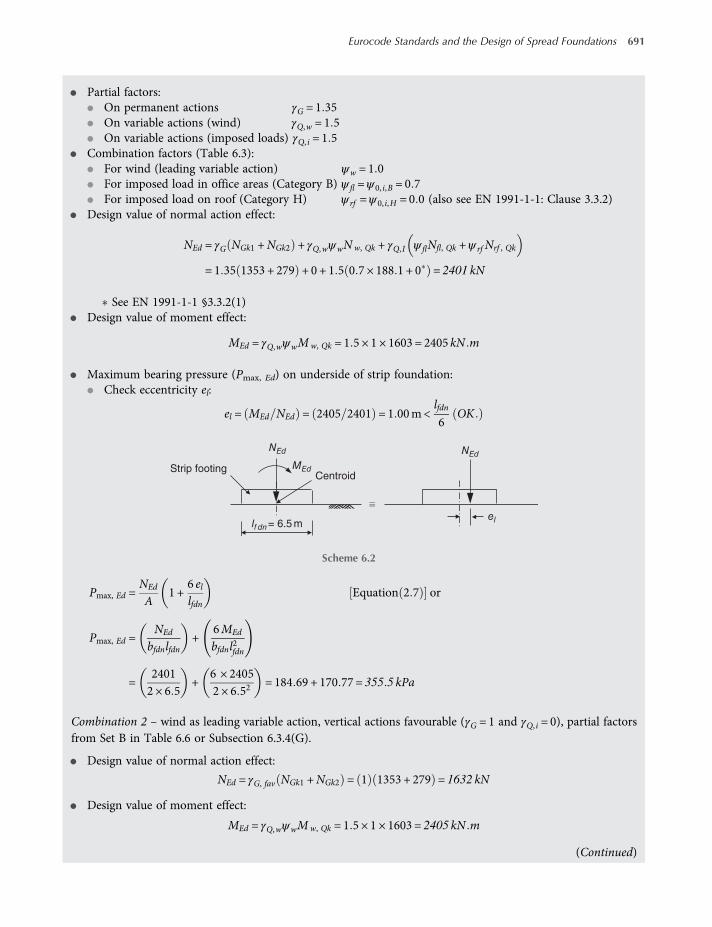
• Partial factors:
• On permanent actions γG = 1 35
• On variable actions (wind) γQ,w = 1 5
• On variable actions (imposed loads) γQ, i = 1 5
• Combination factors (Table 6.3):
• For wind (leading variable action) ψw = 1 0
• For imposed load in office areas (Category B) ψ fl =ψ0, i,B = 0 7
• For imposed load on roof (Category H) ψ rf =ψ0, i,H = 0 0 (also see EN 1991-1-1: Clause 3.3.2)
• Design value of normal action effect:
NEd = γG NGk1 +NGk2 + γQ,wψwNw, Qk + γQ,I ψ flNfl, Qk +ψ rf Nrf , Qk
= 1 35 1353 + 279 + 0 + 1 5 0 7 × 188 1 + 0∗ = 2401 kN
∗ See EN 1991-1-1 §3.3.2(1)
• Design value of moment effect:
MEd = γQ,wψwMw, Qk = 1 5 × 1 × 1603 = 2405 kN m
• Maximum bearing pressure (Pmax, Ed) on underside of strip foundation:
• Check eccentricity el:
el = MEd NEd = 2405 2401 = 1 00m<lfdn6
OK
Pmax, Ed =NEd
A1 +
6 ellfdn
Equation 2 7 or
Pmax, Ed =NEd
bfdnlfdn+
6MEd
bfdnl2fdn
=24012 × 6 5
+6 × 24052 × 6 52
= 184 69 + 170 77 = 355 5 kPa
Combination 2 – wind as leading variable action, vertical actions favourable (γG = 1 and γQ, i = 0), partial factorsfrom Set B in Table 6.6 or Subsection 6.3.4(G).
• Design value of normal action effect:
NEd = γG, fav NGk1 +NGk2 = 1 1353 + 279 = 1632 kN
• Design value of moment effect:
MEd = γQ,wψwMw, Qk = 1 5 × 1 × 1603 = 2405 kN m
(Continued)
Centroid
lf dn= 6.5 m
Strip footing
NEd NEd
el
MEd
Scheme 6.2
Eurocode Standards and the Design of Spread Foundations 691
worksaccounts.com

• Maximum bearing pressure (Pmax,Ed) on underside of strip foundation:
• Check eccentricity el:
el = MEd NEd = 2405 1632 = 1 47m>lfdn6
(Not OK.)
Therefore, Equation (2.7) is not applicable.Since tension cannot occur between ground and the underside of the footing, the triangular bearing pres-
sure distribution shown below may be considered (see Section 2.6.2 of Chapter 2).
a=lfdn2
− el =12
lfdn−2el
NEd =Pmax, Ed × 3a
2bfdn = Pmax, Ed
34
bfdn lfdn−2el
Pmax, Ed =4NEd
3bfdn lfdn−2el=
4 × 16323 × 2 6 5−2 × 1 47
= 306 kPa
However, TCC (2006) recommends a rectangular ULS pressure distribution diagram to be considered andnot triangular, as shown below.
Accordingly, the maximum bearing pressure (Pmax, Ed) on the underside of the strip foundation is
Pmax, Ed =NEd
bfdn × 2a=
1632
2 × 212
lfdn−2el
=1632
2 6 5−2 × 1 47= 229 kPa
NEd
Pmax,Ed
a2a
lf dn /2 el
lf dn= 6.5 m
Scheme 6.3
NEd
Pmax,Ed
aa
lf dn /2 el
lf dn= 6.5 m
Scheme 6.4
692 Shallow Foundations
worksaccounts.com
Combination 3 – imposed loads as leading variable action, vertical actions unfavourable, partial factors from SetB in Table 6.6 or Section 6.3.4(G).
• Partial factors:
• On permanent actions γG = 1 35
• On variable actions (imposed loads) γQ, i = 1 5
• On variable actions (imposed loads) (wind) γQ,w = 1 5
• Combination factors (Table 6.3):
• For imposed load in office areas (Category B) ψ fl = 1 0
• For imposed load on roof (Category H) ψ rf = 1 0
• For wind ψw =ψ0, w = 0 6
• Design value of normal action effect:
NEd = γG NGk1 +NGk2 + γQ, i ψ flNfl, Qk + ψ rf Nrf , Qk + γQ,wψ0,wNw, Qk
= 1 35 1353 + 279 + 1 5 1 × 188 1 + 1 × 17 1 + 0
= 2511 kN
• Design value of moment effect:
MEd = γQ,wψ0,wMw, Qk = 1 5 × 0 6 × 1603 = 1443 kN m
• Maximum bearing pressure (Pmax, Ed) on underside of strip foundation:
• Check eccentricity el:
el = MEd NEd = 1443 2511 = 0 57m<lfdn6
OK
Pmax, Ed =NEd
bfdnlfdn+
6MEd
bfdnl2fdn
=25112 × 6 5
+6 × 14432 × 6 52
= 193 15 + 102 46 = 296 kPa
Combination 4 – wind as leading variable action, vertical actions unfavourable, partial factors from Set C inTable 6.6 or Section 6.3.4(G).
• Partial factors:
• On permanent actions γG = 1 0
• On variable actions (wind) γQ,w = 1 3
• On variable actions (imposed loads) γQ, i = 1 3
• Combination factors (Table 6.3):
• For wind (leading variable action) ψw = 1 0
• For imposed load in office areas (Category B) ψ fl =ψ0, i,B = 0 7
• For imposed load on roof (Category H) ψ rf =ψ0, i,H = 0 0 (also see EN 1991-1-1: Clause 3.3.2)
• Design value of normal action effect:
NEd = γG NGk1 +NGk2 + γQ,wψwNw, Qk + γQ,I ψ flNfl, Qk +ψ rf Nrf , Qk
= 1 0 1353 + 279 + 0 + 1 3 0 7 × 188 1 + 0∗ = 1803 kN
(Continued)
Eurocode Standards and the Design of Spread Foundations 693
worksaccounts.com

∗ See EN 1991-1-1 §3.3.2(1)
• Design value of moment effect:
MEd = γQ,wψwMw, Qk = 1 3 × 1 × 1603= 2084 kN m
• Maximum bearing pressure (Pmax, Ed) on underside of strip foundation.The calculations proceed in the same manner as those for the preceding combinations; left for the reader.
Combination 5– wind as leading variable action, vertical actions favourable γG = 1 and γQ, i = 0 , partial factorsfrom Set C in Table 6.6 or Section 6.3.4(G).
• Design value of normal action effect:
NEd = γG, fav NGk1 +NGk2 = 1 1353 + 279 = 1632 kN
• Design value of moment effect:
MEd = γQ,wψwMw, Qk = 1 3 × 1 × 1603 = 2084 kN m
• Maximum bearing pressure (Pmax, Ed) on underside of strip foundation:The calculations proceed in the same manner as those for the preceding combinations; left for the reader.Combination 6 – imposed loads as leading variable action, vertical actions unfavourable, partial factors from SetC in Table 6.6 or Section 6.3.4(G).
• Partial factors:
• On permanent actions γG = 1 0
• On variable actions (imposed loads) γQ, i = 1 3
• On variable actions (imposed loads) (wind) γQ,w = 1 3
• Combination factors (Table 6.3):
• For imposed load in office areas (Category B) ψ fl = 1 0
• For imposed load on roof (Category H) ψ rf = 1 0
• For wind ψw =ψ0, w = 0 6
• Design value of normal action effect:
NEd = γG NGk1 +NGk2 + γQ, i ψ flNfl, Qk + ψ rf Nrf , Qk + γQ,wψ0,wNw, Qk
= 1 0 1353 + 279 + 1 3 1 × 188 1 + 1 × 17 1 + 0
= 1899 kN
• Design value of moment effect:
MEd = γQ,wψ0,wMw, Qk = 1 3 × 0 6 × 1603 = 1250 kN m
• Maximum bearing pressure (Pmax, Ed) on underside of strip foundation.The calculations proceed in the same manner as those for the preceding combinations; left for the reader.Combinations of actions for quasi-persistent design situations – SLS verificationsCombination 1 – wind as leading variable action, vertical actions unfavourable, partial factors for SLS.
• Partial factors [see Section 6.3.4(J)]:
• On permanent actions γG = γG, SLS = 1 0
• On variable actions (wind) γQ,w = γQ,w, SLS = 1 0
• On variable actions (imposed loads) γQ, i = γQ, i, SLS = 1 0
• Combination factors [see Section 6.3.4(J) and Table 6.3]:
• For wind ψw =ψ2, w = 0 0
• For imposed load in office areas (Category B) ψ fl =ψ2, i = 0 3
• For imposed load on roof (Category H) ψ rf =ψ2, i = 0 0
694 Shallow Foundations
worksaccounts.com

• Design value of normal action effect:
NEd = γG NGk1 +NGk2 + γQ,wψwNw, Qk + γQ, i ψ flNfl, Qk +ψ rf Nrf , Qk
= 1 0 1353 + 279 + 0 + 1 0 0 3 × 188 1 + 0 = 1688 kN
• Design value of moment effect:
MEd = γQ,wψwMw, Qk = 1 0 × 0 × 1603 = 0 0 kN m
Combination 2 – wind as leading variable action, vertical actions favourable, partial factors for SLS.
• Design value of normal action effect:
NEd = γG, fav NGk1 +NGk2 = 1 0 1353 + 279 = 1632 kN
• Design value of moment effect:
MEd = γQ,wψwMw, Qk = 1 0 × 0 × 1603 = 0 0 kN m
Combination 3 – imposed loads as leading variable action, vertical actions unfavourable, partial factors for SLS.
• Combination factors [see Section 6.3.4(J) and Table 6.3]:
• For wind ψw =ψ2, w = 0 0
• For imposed load in office areas (Category B) ψ fl =ψ2, i = 0 3
• For imposed load on roof (Category H) ψ rf =ψ2, i = 0 0
• Design value of normal action effect:
NEd = γG NGk1 +NGk2 + γQ, i ψ flNfl, Qk + ψ rf Nrf , Qk + γQ,wψwNw, Qk
= 1 0 1353 + 279 + 1 0 0 3 × 188 1 + 0 + 0
= 1688 kN
• Design value of moment effect:
MEd = γQ,wψwMw, Qk = 1 0 × 0 × 1603 = 0 0 kN m
Problem 6.2
A centrally loaded column footing (pad) of length L= 2 5m, width B= 1 5m and depth (thickness) d = 0 5m isrequired to carry a vertical imposed permanent action VGk = 800 kN and a vertical imposed variable actionVQk = 450 kN. The footing base is horizontal (i.e. α= 0 ) and located at a depth of 0.5 m below ground surface(i.e. D= 0 5m). The weight density (unit weight) of the reinforced concrete is γc, k = 25 kN m3 (seeTable 6.12). The footing is founded on dry sand which has the following characteristic parameters:
• Angle of shearing resistance ϕk = 35
• Effective cohesion ck = 0 0 kPa
• weight density γk = 18 kN m3
It is required to perform verification of strength (GEO ultimate limit state), that is verification of bearing resist-ance, using all the three Design Approaches. Note: In order to concentrate on the EN 1997 rather than the geo-technical related issues a relatively simple problem has been selected which excludes the effects of groundwater.
(Continued)
Eurocode Standards and the Design of Spread Foundations 695
worksaccounts.com
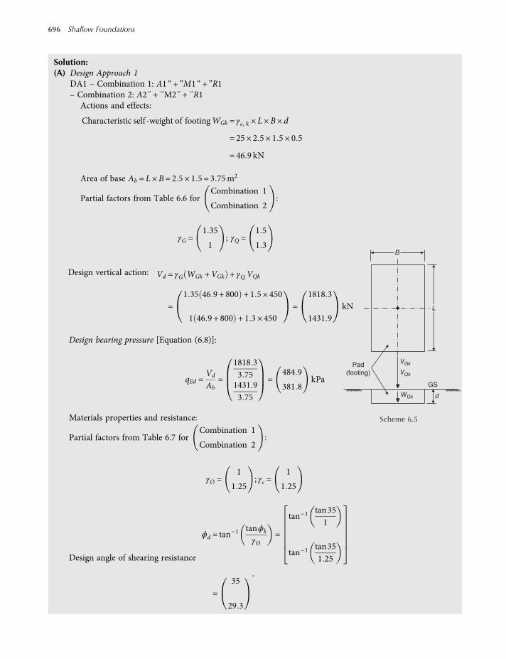
Solution:(A) Design Approach 1
DA1 – Combination 1: A1 “ + ”M1 “ + ”R1– Combination 2: A2 + M2 + R1
Actions and effects:
Characteristic self -weight of footingWGk = γc, k × L×B× d
= 25 × 2 5 × 1 5 × 0 5
= 46 9 kN
Area of base Ab = L×B = 2 5 × 1 5 = 3 75m2
Partial factors from Table 6.6 forCombination 1
Combination 2:
γG =1 35
1; γQ =
1 5
1 3
Design vertical action: Vd = γG WGk +VGk + γQ VQk
=1 35 46 9 + 800 + 1 5 × 450
1 46 9 + 800 + 1 3 × 450=
1818 3
1431 9kN
Design bearing pressure [Equation (6.8)]:
qEd =Vd
Ab=
1818 33 751431 93 75
=484 9
381 8kPa
Materials properties and resistance:
Partial factors from Table 6.7 forCombination 1
Combination 2:
γ =1
1 25; γc =
1
1 25
Design angle of shearing resistance
ϕd = tan−1 tanϕk
γ=
tan−1 tan351
tan−1 tan351 25
=35
29 3
GS
dWGk
VQk
VGkPad
(footing)
L
B
Scheme 6.5
696 Shallow Foundations
worksaccounts.com

Design effective cohesion cd =ckγc
=0
0kPa
Bearing capacity factors from Annex D of EN 1997-1:
For effect of overburden, Nq = eπ tan d tan2 45o + d
2=
33 3
17 0
For effect of cohesion, Nc = Nq−1 cotϕd =46 1
28 4
For effect of self-weight, Nγ = 2 Nq−1 tanϕd =45 2
17 8
Shape factors:
For effect of overburden, sq = 1 +BLsinϕd =
1 34
1 29
For effect of cohesion, sc =sqNq−1
Nq−1=
1 35
1 31
For effect of self-weight, sγ = 1−0 3BL=
0 82
0 82
Depth factors:The suggested method in Annex D does not include depth factors which are present in other formulations
of the extended bearing capacity formula (see Section 4.5 of Chapter 4). There has been concern in using thesedepth factors as their influence can be significant and the reliance on the additional capacity provided by itsinclusion is not conservative.
Load-inclination factors, caused by a horizontal load H:Since H = 0, each of the load-inclination factors ic, iq and iγ is 1.0.Base-inclination factors:Since the foundation base is horizontal, that is α= 0, each of the base-inclination factors bc, bq and bγ is 1.0.Ground-inclination factors:The suggested method in Annex D omits the ground-inclination factors which are present in other
formulations of the extended bearing capacity formula. However, neglecting these factors is unsafe.Effective overburden pressure q (or σvk,b):
q = γk ×D= 18 × 0 5 = 9kN m2
Gross ultimate bearing capacity (Gross qult) or gross bearing resistance (R/A ):
Annex D of EN 1997-1 suggests that bearing resistance may be calculated from
R A = c Nc bc sc icCohesion
+ q Nq bq sq iq
Overburden
+ 0 5γ B Nγ bγsγ iγ
Self -weight
• From cohesion: Gross qult 1 =0
0
46 1
28 4
1 35
1 31=
0
0kPa
(Continued)
Eurocode Standards and the Design of Spread Foundations 697
worksaccounts.com
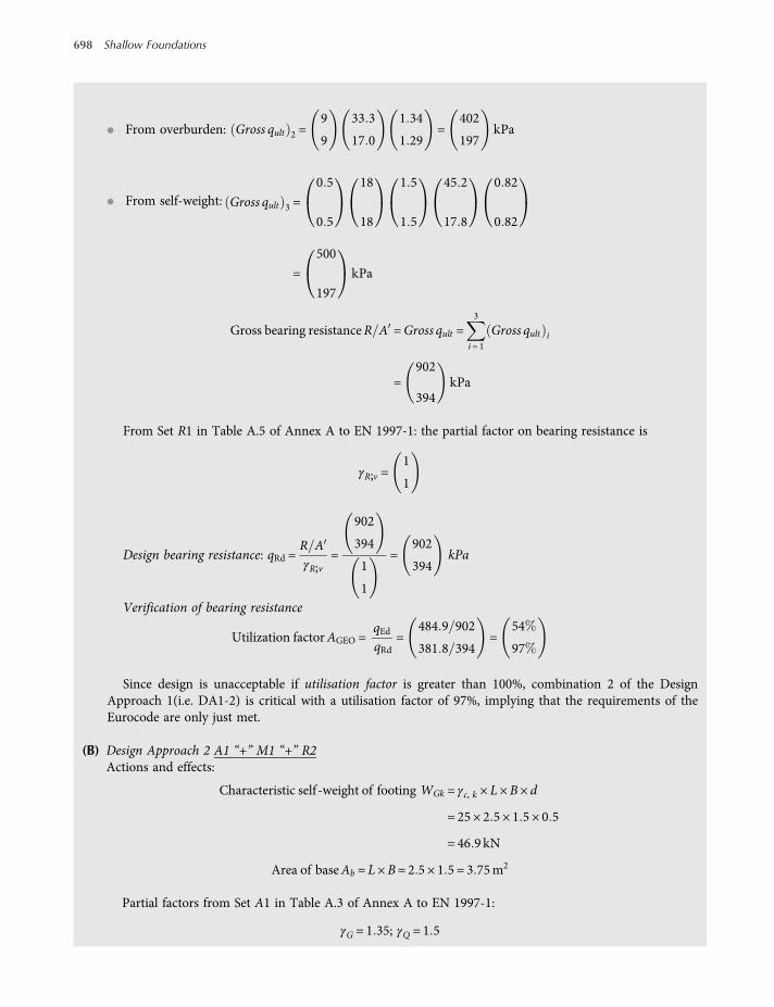
• From overburden: Gross qult 2 =9
9
33 3
17 0
1 34
1 29=
402
197kPa
• From self-weight: Gross qult 3 =
0 5
0 5
18
18
1 5
1 5
45 2
17 8
0 82
0 82
=
500
197
kPa
Gross bearing resistanceR A =Gross qult =3
i= 1
Gross qult i
=902
394kPa
From Set R1 in Table A.5 of Annex A to EN 1997-1: the partial factor on bearing resistance is
γR;v =1
1
Design bearing resistance: qRd =R AγR;v
=
902
394
1
1
=902
394kPa
Verification of bearing resistance
Utilization factorAGEO =qEdqRd
=484 9 902
381 8 394=
54
97
Since design is unacceptable if utilisation factor is greater than 100%, combination 2 of the DesignApproach 1(i.e. DA1-2) is critical with a utilisation factor of 97%, implying that the requirements of theEurocode are only just met.
(B) Design Approach 2 A1 “+” M1 “+” R2Actions and effects:
Characteristic self -weight of footing WGk = γc, k × L×B× d
= 25 × 2 5 × 1 5 × 0 5
= 46 9 kN
Area of baseAb = L×B = 2 5 × 1 5 = 3 75m2
Partial factors from Set A1 in Table A.3 of Annex A to EN 1997-1:
γG = 1 35; γQ = 1 5
698 Shallow Foundations
worksaccounts.com
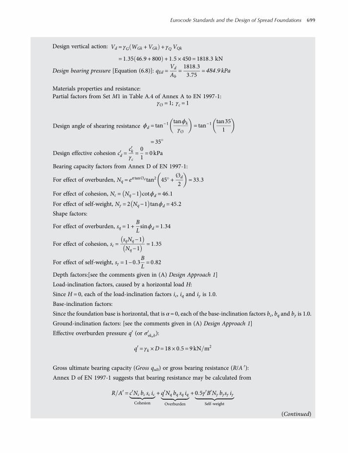
Design vertical action: Vd = γG WGk +VGk + γQ VQk
= 1 35 46 9 + 800 + 1 5 × 450 = 1818 3 kN
Design bearing pressure [Equation (6.8)]: qEd =Vd
Ab=1818 33 75
= 484 9 kPa
Materials properties and resistance:Partial factors from Set M1 in Table A.4 of Annex A to EN 1997-1:
γ = 1; γc = 1
Design angle of shearing resistance ϕd = tan−1 tanϕk
γ= tan−1 tan35
1
= 35
Design effective cohesion cd =ckγc
=01= 0kPa
Bearing capacity factors from Annex D of EN 1997-1:
For effect of overburden, Nq = eπ tan d tan2 45 + d
2= 33 3
For effect of cohesion, Nc = Nq−1 cotϕd = 46 1
For effect of self-weight, Nγ = 2 Nq−1 tanϕd = 45 2
Shape factors:
For effect of overburden, sq = 1 +BLsinϕd = 1 34
For effect of cohesion, sc =sqNq−1
Nq−1= 1 35
For effect of self-weight, sγ = 1−0 3BL= 0 82
Depth factors:[see the comments given in (A) Design Approach 1]
Load-inclination factors, caused by a horizontal load H:
Since H = 0, each of the load-inclination factors ic, iq and iγ is 1.0.
Base-inclination factors:
Since the foundation base is horizontal, that is α= 0, each of the base-inclination factors bc, bq and bγ is 1.0.
Ground-inclination factors: [see the comments given in (A) Design Approach 1]
Effective overburden pressure q (or σvk,b):
q = γk ×D= 18 × 0 5 = 9kN m2
Gross ultimate bearing capacity (Gross qult) or gross bearing resistance (R/A ):
Annex D of EN 1997-1 suggests that bearing resistance may be calculated from
R A = c Nc bc sc icCohesion
+ q Nq bq sq iq
Overburden
+ 0 5γ B Nγ bγsγ iγ
Self -weight
(Continued)
Eurocode Standards and the Design of Spread Foundations 699
worksaccounts.com
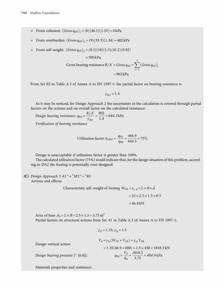
• From cohesion: Gross qult 1 = 0 46 1 1 35 = 0 kPa
• From overburden: Gross qult 2 = 9 33 3 1 34 = 402 kPa
• From self-weight: Gross qult 3 = 0 5 18 1 5 45 2 0 82
= 500 kPa
Gross bearing resistanceR A =Gross qult =3
i= 1
Gross qult i
= 902 kPa
From Set R2 in Table A.5 of Annex A to EN 1997-1: the partial factor on bearing resistance is
γR;v = 1 4
As it may be noticed, for Design Approach 2 the uncertainty in the calculation is covered through partialfactors on the actions and on overall factor on the calculated resistance.
Design bearing resistance: qRd =R AγR;v
=9021 4
= 644 3 kPa
Verification of bearing resistance
Utilization factorAGEO =qEdqRd
=484 9644 3
= 75
Design is unacceptable if utilisation factor is greater than 100%.The calculated utilisation factor (75%) would indicate that, for the design situation of this problem, accord-
ing to DA2 the footing is potentially over-designed.
(C) Design Approach 3 A1 “+ ”M2 “+ ”R3Actions and effects:
Characteristic self -weight of footing WGk = γc, k × L×B× d
= 25 × 2 5 × 1 5 × 0 5
= 46 9 kN
Area of base Ab = L×B = 2 5 × 1 5 = 3 75m2
Partial factors on structural actions from Set A1 in Table A.3 of Annex A to EN 1997-1:
γG = 1 35; γQ = 1 5
Design vertical action:Vd = γG WGk +VGk + γQ VQk
= 1 35 46 9 + 800 + 1 5 × 450 = 1818 3 kN
Design bearing pressure [ (6.8)]: qEd =Vd
Ab=1818 33 75
= 484 9 kPa
Materials properties and resistance:
700 Shallow Foundations
worksaccounts.com
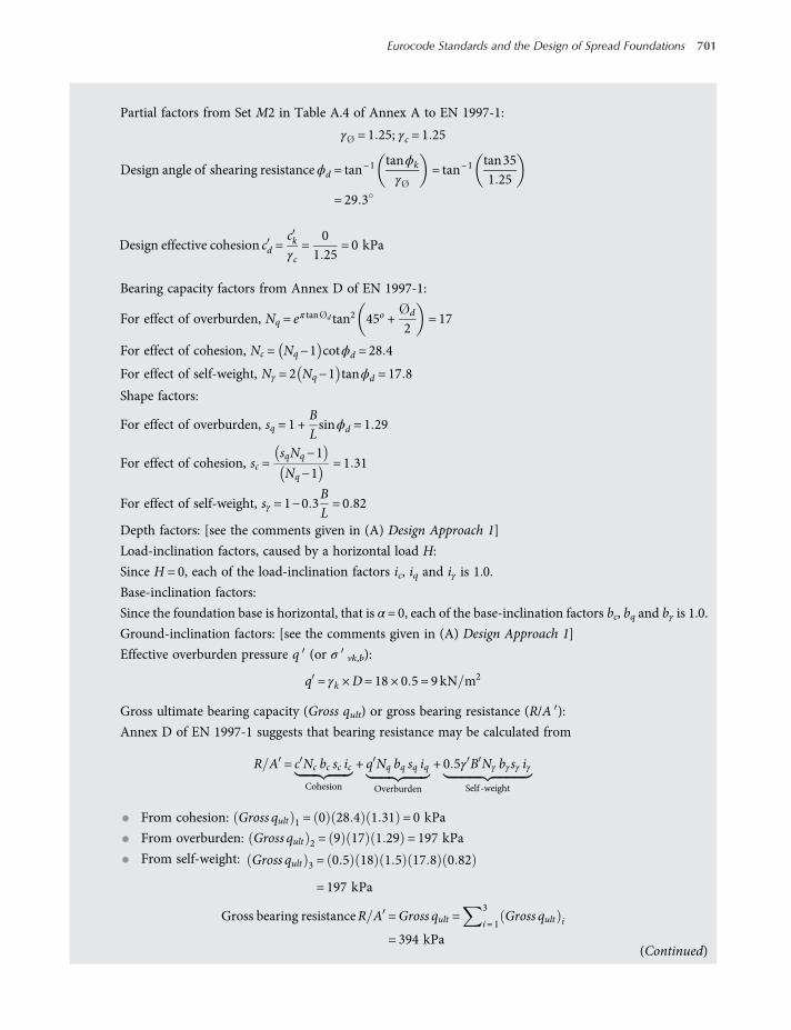
Partial factors from Set M2 in Table A.4 of Annex A to EN 1997-1:
γ = 1 25; γc = 1 25
Design angle of shearing resistanceϕd = tan−1 tanϕk
γ= tan−1 tan35
1 25
= 29 3
Design effective cohesion cd =ckγc
=0
1 25= 0 kPa
Bearing capacity factors from Annex D of EN 1997-1:
For effect of overburden, Nq = eπ tan d tan2 45o + d
2= 17
For effect of cohesion, Nc = Nq−1 cotϕd = 28 4
For effect of self-weight, Nγ = 2 Nq−1 tanϕd = 17 8
Shape factors:
For effect of overburden, sq = 1 +BLsinϕd = 1 29
For effect of cohesion, sc =sqNq−1
Nq−1= 1 31
For effect of self-weight, sγ = 1−0 3BL= 0 82
Depth factors: [see the comments given in (A) Design Approach 1]
Load-inclination factors, caused by a horizontal load H:
Since H = 0, each of the load-inclination factors ic, iq and iγ is 1.0.
Base-inclination factors:
Since the foundation base is horizontal, that is α= 0, each of the base-inclination factors bc, bq and bγ is 1.0.
Ground-inclination factors: [see the comments given in (A) Design Approach 1]
Effective overburden pressure q (or σ vk,b):
q = γk ×D= 18 × 0 5 = 9kN m2
Gross ultimate bearing capacity (Gross qult) or gross bearing resistance (R/A ):
Annex D of EN 1997-1 suggests that bearing resistance may be calculated from
R A = c Nc bc sc icCohesion
+ q Nq bq sq iq
Overburden
+ 0 5γ B Nγ bγsγ iγ
Self -weight
• From cohesion: Gross qult 1 = 0 28 4 1 31 = 0 kPa
• From overburden: Gross qult 2 = 9 17 1 29 = 197 kPa
• From self-weight: Gross qult 3 = 0 5 18 1 5 17 8 0 82
= 197 kPa
Gross bearing resistanceR A =Gross qult =3
i= 1Gross qult i
= 394 kPa(Continued)
Eurocode Standards and the Design of Spread Foundations 701
worksaccounts.com
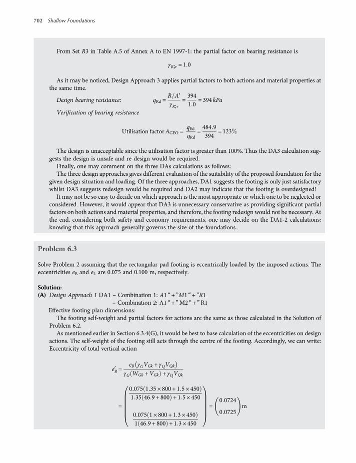
From Set R3 in Table A.5 of Annex A to EN 1997-1: the partial factor on bearing resistance is
γR;v = 1 0
As it may be noticed, Design Approach 3 applies partial factors to both actions and material properties atthe same time.
Design bearing resistance: qRd =R AγR;v
=3941 0
= 394 kPa
Verification of bearing resistance
Utilisation factorAGEO =qEdqRd
=484 9394
= 123
The design is unacceptable since the utilisation factor is greater than 100%. Thus the DA3 calculation sug-gests the design is unsafe and re-design would be required.
Finally, one may comment on the three DAs calculations as follows:The three design approaches gives different evaluation of the suitability of the proposed foundation for the
given design situation and loading. Of the three approaches, DA1 suggests the footing is only just satisfactorywhilst DA3 suggests redesign would be required and DA2 may indicate that the footing is overdesigned!
It may not be so easy to decide on which approach is the most appropriate or which one to be neglected orconsidered. However, it would appear that DA3 is unnecessary conservative as providing significant partialfactors on both actions andmaterial properties, and therefore, the footing redesign would not be necessary. Atthe end, considering both safety and economy requirements, one may decide on the DA1-2 calculations;knowing that this approach generally governs the size of the foundations.
Problem 6.3
Solve Problem 2 assuming that the rectangular pad footing is eccentrically loaded by the imposed actions. Theeccentricities eB and eL are 0.075 and 0.100 m, respectively.
Solution:(A) Design Approach 1 DA1 – Combination 1: A1 “ + ”M1 “ + ”R1
– Combination 2: A1 “+ ”M2 “+ ”R1Effective footing plan dimensions:
The footing self-weight and partial factors for actions are the same as those calculated in the Solution ofProblem 6.2.
As mentioned earlier in Section 6.3.4(G), it would be best to base calculation of the eccentricities on designactions. The self-weight of the footing still acts through the centre of the footing. Accordingly, we can write:Eccentricity of total vertical action
eB =eB γGVGk + γQVQk
γG WGk +VGk + γQVQk
=
0 075 1 35 × 800 + 1 5 × 4501 35 46 9 + 800 + 1 5 × 450
0 075 1 × 800 + 1 3 × 4501 46 9 + 800 + 1 3 × 450
=0 0724
0 0725m
702 Shallow Foundations
worksaccounts.com
Eccentricity of total vertical action
eL =eL γGVGk + γQVQk
γG WGk +VGk + γQVQk
=
0 100 1 35 × 800 + 1 5 × 4501 35 46 9 + 800 + 1 5 × 450
0 100 1 × 800 + 1 3 × 4501 46 9 + 800 + 1 3 × 450
=0 0965
0 0967m
Load is within the middle third since eB <B6= 0 25m and
eL <L6= 0 42m
Effective width B =B−2eB = 1 5−20 0724
0 0725=
1 36
1 35m
Effective length L = L−2eL = 2 5−20 0965
0 0967=
2 31
2 31m
Effective area A = L × B =2 31 × 1 36
2 31 × 1 35=
3 13
3 13m2
Actions and effects:
From previous calculation (Solution of Problem 6.2.), Vd =1818 3
1431 9kN
Design bearing pressure [Equation (6.8)]: qEd =Vd
Ab
=
1818 33 131431 93 13
=581 6
458 2kPa
Materials properties and resistance:
From previous calculation (Solution of Problem 6.2.), ϕd =35
29 3and
cd =0
0kPa
Also, bearing capacity factors Nq =33 3
17 0, Nc =
46 1
28 4and Nγ =
45 2
17 8
(Continued)
Effective
area A′ Centroid of A′
L′L
e'L
e'B
L′/2
L′/2
B′/2 B′/2
B
B′
2e′L
2e′B
Scheme 6.6
Eurocode Standards and the Design of Spread Foundations 703
worksaccounts.com
Shape factors:
For effect of overburden, sq = 1 +BLsinϕd =
1 34
1 29
For effect of cohesion, sc =sqNq−1
Nq−1=
1 35
1 31
For effect of self-weight, sγ = 1−0 3BL
=0 82
0 82
Depth factors: [see the comments given in Solution of Problem 6.2- (A) Design Approach 1]
Load-inclination factors, caused by a horizontal load H:
Since H = 0, each of the load-inclination factors ic, iq and iγ is 1.0.
Base-inclination factors:
Since the foundation base is horizontal, that is α= 0, each of the base-inclination factors bc, bq and
bγ is 1.0.
Ground-inclination factors: [see the comments given in Solution of Problem 6.2- (A)Design Approach 1]
Effective overburden pressure q (or σ vk,b):
q = γk ×D= 18 × 0 5 = 9kN m2
Gross ultimate bearing capacity (Gross qult) or gross bearing resistance (R/A ):
Annex D of EN 1997-1 suggests that bearing resistance may be calculated from
R A = c Nc bc sc icCohesion
+ q Nq bq sq iq
Overburden
+ 0 5γ B Nγ bγsγ iγ
Self -weight
• From cohesion: Gross qult 1 =0
0
46 1
28 4
1 35
1 31=
0
0kPa
• From overburden: Gross qult 2 =9
9
33 3
17 0
1 34
1 29=
402
197kPa
• From self-weight: Gross qult 3 =0 50 5
1818
1 361 35
45 217 8
0 820 82
=454177
kPa
Gross bearing resistance R A =Gross qult =3
i = 1Gross qult i
=856374
kPa
704 Shallow Foundations
worksaccounts.com

From Set R1 in Table A.5 of Annex A to EN 1997-1: the partial factor on bearing resistance is
γR;v =1
1
Design bearing resistance: qRd =R AγR;v
=
856
374
1
1
=856
374kPa
Verification of bearing resistance
Utilization factorAGEO =qEdqRd
=581 6 856
458 2 374=
68%
122%
Design is unacceptable if utilisation factor is greater than 100%.
(B) Design Approach 2A1“+ ”M1“ + ”R2Effective footing plan dimensions:
The footing self-weight and partial factors for actions are the same as those calculated in the Solution ofProblem 6.2.
eB =eB γGVGk + γQVQk
γG WGk +VGk + γQVQk= 0 0724m as before
Load is within middle-third since eB <B6= 0 25m
eL =eL γGVGk + γQVQk
γG WGk +VGk + γQVQk= 0 0965m
Load is within middle-third since eL <L6= 0 42m
Effective width B =B−2eB = 1 5−2 × 0 0724 = 1 36mEffective length L = L−2eL = 2 5−2 × 0 0965 = 2 31mEffective area A = L × B = 2 31 × 1 36 = 3 14m2
Actions and effects:From previous calculation (Solution of Problem 6.2.), Vd = 1818 3 kN
Design bearing pressure [Equation (6.8)]: qEd =Vd
Ab
=1818 33 14
= 579 1 kPa
Materials properties and resistance:From previous calculation (Solution of Problem 6.2.), ϕd = 35
o and cd = 0 kPaAlso, bearing capacity factors Nq = 33 3, Nc = 46 1 and Nγ = 45 2Shape factors:
For effect of overburden, sq = 1 +BLsinϕd = 1 34
For effect of cohesion, sc =sqNq−1
Nq−1= 1 35
(Continued)
Eurocode Standards and the Design of Spread Foundations 705
worksaccounts.com

For effect of self-weight, sγ = 1−0 3BL
= 0 82
Depth factors: [see the comments given in Solution of Problem 6.2]Load-inclination factors, caused by a horizontal load H:Since H = 0, each of the load-inclination factors ic, iq and iγ is 1.0.Base-inclination factors:Since the foundation base is horizontal, that is α= 0, each of the base-inclination factors bc, bq and bγ is 1.0.Ground-inclination factors: [see the comments given in Solution of Problem 6.2]Effective overburden pressure q (or σvk,b):
q = γk ×D= 18 × 0 5 = 9kN m2
Gross ultimate bearing capacity (Gross qult) or gross bearing resistance (R/A ):Annex D of EN 1997-1 suggests that bearing resistance may be calculated from
R A = c Nc bc sc icCohesion
+ q Nq bq sq iq
Overburden
+ 0 5γ B Nγ bγsγ iγ
Self -weight
• From cohesion: Gross qult 1 = 0 46 1 1 35 = 0 kPa
• From overburden: Gross qult 2 = 9 33 3 1 34 = 402 kPa
• From self-weight: Gross qult 3 = 0 5 18 1 36 45 2 0 82
= 454 kPaGross bearing resistanceR A =Gross qult =
3
i= 1Gross qult i
= 856 kPa
From Set R2 in Table A.5 of Annex A to EN 1997-1: the partial factor on bearing resistance is
γR;v = 1 4
Design bearing resistance: qRd =R AγR;v
=8561 4
= 611 kPa
Verification of bearing resistance
Utilization factorAGEO =qEdqRd
=597 1611
= 98
Design is unacceptable if utilisation factor is greater than 100%.
(C) Design Approach 3 A1“+ ”M2 “+ ”R3Effective footing plan dimensions:
The footing self-weight and partial factors for actions are the same as those calculated in the Solution ofProblem 6.2.
eB =eB γGVGk + γQVQk
γG WGk +VGk + γQVQk= 0 0724m as before
Load is within middle-third since eB <B6= 0 25m
706 Shallow Foundations
worksaccounts.com

eL =eL γGVGk + γQVQk
γG WGk +VGk + γQVQk= 0 0965m
Load is within middle-third since eL <L6= 0 42m
Effective width B =B−2eB = 1 5−2 × 0 0724 = 1 36m
Effective length L = L−2eL = 2 5−2 × 0 0965 = 2 31m
Effective area A = L × B = 2 31 × 1 36 = 3 14m2
Actions and effects:
From previous calculation (Solution of Problem 6.2.), Vd = 1818 3 kN
Design bearing pressure [Equation (6.8)]: qEd =Vd
Ab
=1818 33 14
= 579 1 kPa
Materials properties and resistance:
From previous calculation (Solution of Problem 6.2.), ϕd = 29 3 and cd = 0 kPa
Also, bearing capacity factors Nq = 16 9, Nc = 28 4 and Nγ = 17 8
Shape factors:
For effect of overburden, sq = 1 +BLsinϕd = 1 29
For effect of cohesion, sc =sqNq−1
Nq−1= 1 31
For effect of self-weight, sγ = 1−0 3BL
= 0 82
Depth factors (see the comments given in Solution of Problem 6.2):
Load-inclination factors, caused by a horizontal load H:
Since H = 0, each of the load-inclination factors ic, iq and iγ is 1.0.
Base-inclination factors:
Since the foundation base is horizontal, that is α= 0, each of the base-inclination factors bc, bq and bγ is 1.0.
Ground-inclination factors: [see the comments given in Solution of Problem 6.2]
Effective overburden pressure q (or σvk,b):
q = γk ×D= 18 × 0 5 = 9kN m2
Gross ultimate bearing capacity (Gross qult) or gross bearing resistance (R/A ):
Annex D of EN 1997-1 suggests that bearing resistance may be calculated from
R A = c Nc bc sc icCohesion
+ q Nq bq sq iq
Overburden
+ 0 5γ B Nγ bγsγ iγ
Self -weight
• From cohesion: Gross qult 1 = 0 28 4 1 31 = 0 kPa
• From overburden: Gross qult 2 = 9 16 9 1 29 = 196 2 kPa
• From self-weight: Gross qult 3 = 0 5 18 1 36 17 8 0 82
= 178 7 kPa(Continued)
Eurocode Standards and the Design of Spread Foundations 707
worksaccounts.com
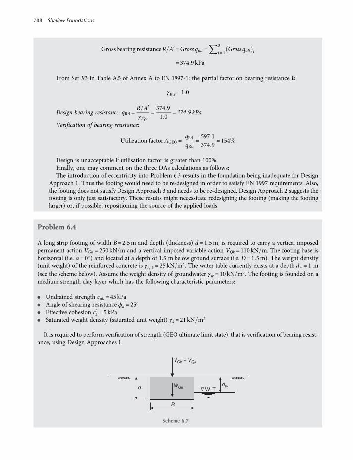
Gross bearing resistanceR A =Gross qult =3
i= 1Gross qult i
= 374 9 kPa
From Set R3 in Table A.5 of Annex A to EN 1997-1: the partial factor on bearing resistance is
γR;v = 1 0
Design bearing resistance: qRd =R AγR;v
=374 91 0
= 374 9 kPa
Verification of bearing resistance:
Utilization factorAGEO =qEdqRd
=597 1374 9
= 154
Design is unacceptable if utilisation factor is greater than 100%.Finally, one may comment on the three DAs calculations as follows:The introduction of eccentricity into Problem 6.3 results in the foundation being inadequate for Design
Approach 1. Thus the footing would need to be re-designed in order to satisfy EN 1997 requirements. Also,the footing does not satisfy Design Approach 3 and needs to be re-designed. Design Approach 2 suggests thefooting is only just satisfactory. These results might necessitate redesigning the footing (making the footinglarger) or, if possible, repositioning the source of the applied loads.
Problem 6.4
A long strip footing of width B= 2 5m and depth (thickness) d = 1 5m, is required to carry a vertical imposedpermanent action VGk = 250 kN m and a vertical imposed variable action VQk = 110 kN m. The footing base ishorizontal (i.e. α= 0 ) and located at a depth of 1.5 m below ground surface (i.e. D= 1 5m). The weight density(unit weight) of the reinforced concrete is γc, k = 25 kN m3. The water table currently exists at a depth dw = 1 m(see the scheme below). Assume the weight density of groundwater γw = 10 kN m3. The footing is founded on amedium strength clay layer which has the following characteristic parameters:
• Undrained strength cuk = 45kPa
• Angle of shearing resistance ϕk = 25o
• Effective cohesion ck = 5 kPa
• Saturated weight density (saturated unit weight) γk = 21 kN m3
It is required to perform verification of strength (GEO ultimate limit state), that is verification of bearing resist-ance, using Design Approaches 1.
VGk + VQk
WGk
B
d W. T
Δ dw
Scheme 6.7
708 Shallow Foundations
worksaccounts.com

Solution:DA1 – Combination 1: A1 “ + ”M1 “+ ”R1
– Combination 2: A2 “+ ”M2 “+ ”R1
Geometrical parametersIn an ultimate limit state, the design water level should represent the most onerous that could occur during thedesign working life of the structure. Therefore, it would be appropriate to take the ground water level at theground surface.Use the design depth of water table dw = 0 0 m
Actions and effectsCharacteristic self -weight of footing WGk = γc, k ×B× d
= 25 × 2 5 × 1 5
= 93 8 kN m
Area of base Ab = L×B= 1 × 2 5 = 2 5 m2 m
Partial factors from Table 6.6 forCombination 1
Combination 2:
γG =1 35
1; γG, fav =
1
1; γQ =
1 5
1 3
Design vertical action:Vd = γG WGk +VGk + γQ VQk
=1 35 93 8 + 250 + 1 5 × 110
1 93 8 + 250 + 1 3 × 110=
629 1
486 8kN m
Design bearing pressure (total stress) qEd =Vd
B=
251 6
194 7kPa
Characteristic pore pressure (uplift pressure) underneath footing is
uk,base = γw d− dw = 10 1 5−0 = 15 kPa
Design uplift pressure (favourable) is
ud = γG, fav × uk,base =1 × 15
1 × 15=
15
15kPa
(Continued)
Strip footing VGk + VQk
WGk
B
d
W. T (dw= 0)
Δ
Scheme 6.8
Eurocode Standards and the Design of Spread Foundations 709
worksaccounts.com

Design bearing pressure (effective stress) qEd = qEd −ud =236 6
179 7kPa
Materials properties and resistance:
Partial factors from Table 6.7 forCombination 1
Combination 2:
γ =1
1 25; γc =
1
1 25; γcu =
1
1 4
Design angle of shearing resistance ϕd = tan−1 tanϕk
γ=
tan−1 tan251
tan−1 tan251 25
=25
20 5
Design effective cohesion cd =ckγc
=5 1
5 1 25=
5
4kPa
Design undrained strength cu, d =cu,kγcu
=45 1
45 1 4=
45
32 1kPa
Drained bearing capacity factors from Annex D of EN 1997-1:
For effect of overburden, Nq = eπ tan d tan2 45o + d
2=
10 7
6 7
For effect of cohesion, Nc = Nq−1 cotϕd =20 7
15 3
For effect of self-weight, Nγ = 2 Nq−1 tanϕd =9
4 3
Shape factors:Drained and undrained shape factors for strip footing are taken as 1.0.Depth factors:The suggested method in Annex D does not include depth factors whatsoever, which are present in other for-
mulations of the extended bearing capacity formula (see Section 4.5 of Chapter 4). There has been concern in usingthese depth factors as their influence can be significant and the reliance on the additional capacity provided by itsinclusion is not conservative.
Load-inclination factors, caused by a horizontal load H:Since H = 0, all the load-inclination factors, for both drained and undrained conditions, ic, iq and iγ are 1.0.Base-inclination factors:Since the foundation base is horizontal, that is α= 0, all the base-inclination factors, for both drained and
undrained conditions, bc, bq and bγ are 1.0.
710 Shallow Foundations
worksaccounts.com
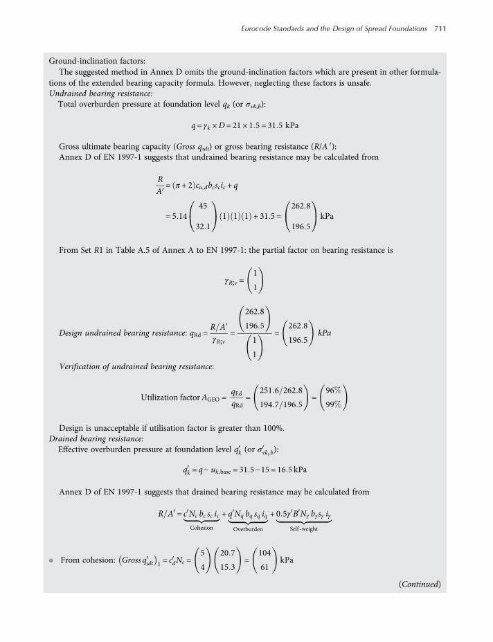
Ground-inclination factors:The suggested method in Annex D omits the ground-inclination factors which are present in other formula-
tions of the extended bearing capacity formula. However, neglecting these factors is unsafe.Undrained bearing resistance:
Total overburden pressure at foundation level qk (or σvk,b):
q= γk ×D= 21 × 1 5 = 31 5 kPa
Gross ultimate bearing capacity (Gross qult) or gross bearing resistance (R/A ):Annex D of EN 1997-1 suggests that undrained bearing resistance may be calculated from
RA
= π + 2 cu,dbcscic + q
= 5 1445
32 11 1 1 + 31 5 =
262 8
196 5kPa
From Set R1 in Table A.5 of Annex A to EN 1997-1: the partial factor on bearing resistance is
γR;v =1
1
Design undrained bearing resistance: qRd =R AγR;v
=
262 8
196 5
1
1
=262 8
196 5kPa
Verification of undrained bearing resistance:
Utilization factorAGEO =qEdqRd
=251 6 262 8
194 7 196 5=
96
99
Design is unacceptable if utilisation factor is greater than 100%.Drained bearing resistance:
Effective overburden pressure at foundation level qk (or σvk,b):
qk = q− uk,base = 31 5−15 = 16 5 kPa
Annex D of EN 1997-1 suggests that drained bearing resistance may be calculated from
R A = c Nc bc sc icCohesion
+ q Nq bq sq iq
Overburden
+ 0 5γ B Nγ bγsγ iγ
Self -weight
• From cohesion: Gross qult 1 = cdNc =5
4
20 7
15 3=
104
61kPa
(Continued)
Eurocode Standards and the Design of Spread Foundations 711
worksaccounts.com

• From overburden: Gross qult 2 = q Nq = 16 510 7
6 7
=177
111kPa
• From self-weight: Gross qult 3 = 0 5γ B Nγ
=0 5
0 5
11
11
2 5
2 5
9
4 3=
124
59kPa
Gross drained bearing resistance R A =Gross qult
=405
231kPa
From Set R1 in Table A.5 of Annex A to EN 1997-1: the partial factor on bearing resistance is
γR;v =1
1
Design drained bearing resistance: qRd =R AγR;v
=
405
231
1
1
=405
231kPa
Verification of drained bearing resistance
Utilization factorAGEO =qEdqRd
=236 6 405
179 7 231=
58
78
Design is unacceptable if utilisation factor is greater than 100%.Finally, one may comment on the Design Approach 1 calculation as follows:The calculation indicates that the undrained (short-term) situation is more critical than the drained (long-
term). The main reason for this may be due to the favourable depth and shape factors which are ignored in bothsituations. However, finite element studies indicate that these factors could be more significant when undrainedcondition prevails, and therefore, it may not be realistic to assume that short-term situation is always critical.
Combination 2 governs in both cases and is verified, since the utilisation factors in each case is less than 100%,although it is too close in the undrained condition.
Problem 6.5
Consider the same long strip footing of Problem 6.4 with the following available additional data:
• The clay layer overlies a rigid layer at a depth dR = 4 5mbelow the ground surface, as shown in the scheme below.
• The clay’s characteristic coefficient of compressibilitymv,k = 0 12m2 MN and its undrained Young’s modulusis assumed to be Eu,k = 600 cu,k.
• The limiting value of total settlement sCd = 50mm.
712 Shallow Foundations
worksaccounts.com
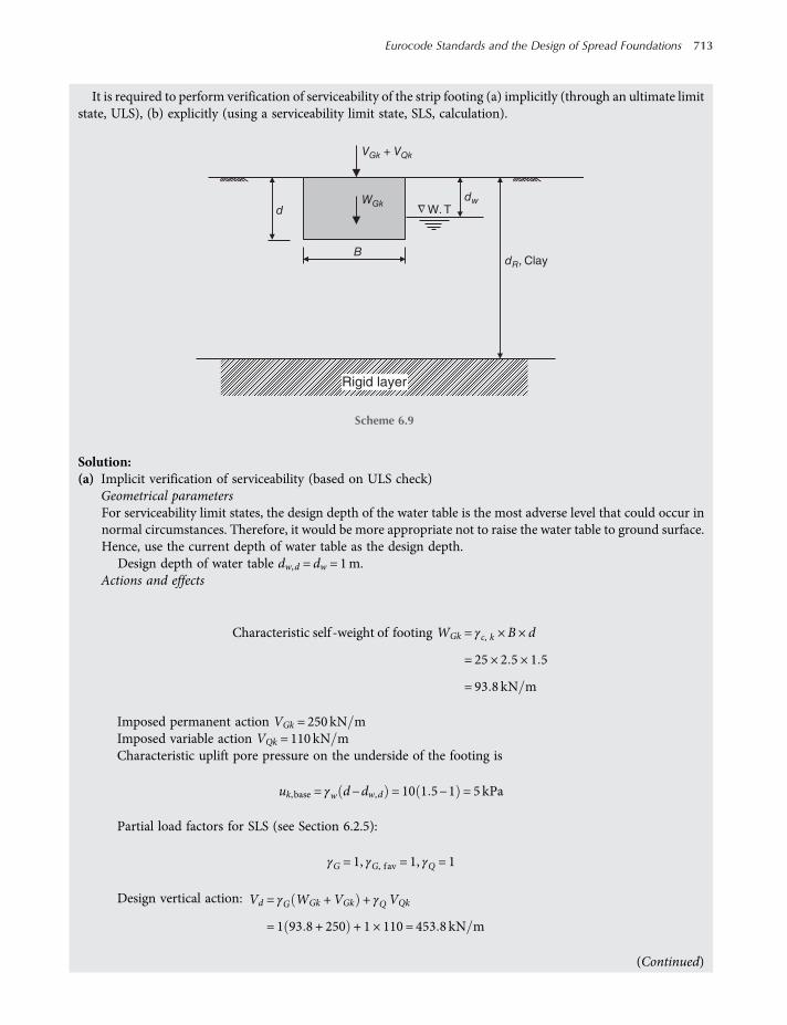
It is required to perform verification of serviceability of the strip footing (a) implicitly (through an ultimate limitstate, ULS), (b) explicitly (using a serviceability limit state, SLS, calculation).
Solution:(a) Implicit verification of serviceability (based on ULS check)
Geometrical parametersFor serviceability limit states, the design depth of the water table is the most adverse level that could occur innormal circumstances. Therefore, it would be more appropriate not to raise the water table to ground surface.Hence, use the current depth of water table as the design depth.
Design depth of water table dw,d = dw = 1m.Actions and effects
Characteristic self -weight of footing WGk = γc, k ×B× d
= 25 × 2 5 × 1 5
= 93 8 kN m
Imposed permanent action VGk = 250 kN mImposed variable action VQk = 110 kN mCharacteristic uplift pore pressure on the underside of the footing is
uk,base = γw d−dw,d = 10 1 5−1 = 5kPa
Partial load factors for SLS (see Section 6.2.5):
γG = 1, γG, fav = 1, γQ = 1
Design vertical action: Vd = γG WGk +VGk + γQ VQk
= 1 93 8 + 250 + 1 × 110 = 453 8 kN m
(Continued)
Rigid layer
VGk + VQk
WGk
B
d
dR, Clay
W. T
Δ dw
Scheme 6.9
Eurocode Standards and the Design of Spread Foundations 713
worksaccounts.com
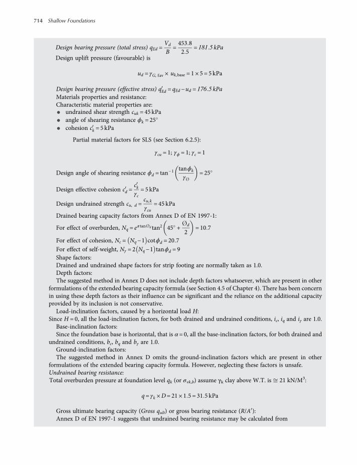
Design bearing pressure (total stress) qEd =Vd
B=453 82 5
= 181 5 kPa
Design uplift pressure (favourable) is
ud = γG, fav × uk,base = 1 × 5 = 5kPa
Design bearing pressure (effective stress) qEd = qEd −ud = 176 5 kPaMaterials properties and resistance:Characteristic material properties are:
• undrained shear strength cuk = 45 kPa
• angle of shearing resistance ϕk = 25
• cohesion ck = 5kPa
Partial material factors for SLS (see Section 6.2.5):
γcu = 1; γϕ = 1; γc = 1
Design angle of shearing resistance ϕd = tan−1 tanϕk
γ= 25
Design effective cohesion cd =ckγc
= 5 kPa
Design undrained strength cu, d =cu,kγcu
= 45 kPa
Drained bearing capacity factors from Annex D of EN 1997-1:
For effect of overburden, Nq = eπ tan d tan2 45 + d
2= 10 7
For effect of cohesion, Nc = Nq−1 cotϕd = 20 7
For effect of self-weight, Nγ = 2 Nq−1 tanϕd = 9Shape factors:Drained and undrained shape factors for strip footing are normally taken as 1.0.Depth factors:The suggested method in Annex D does not include depth factors whatsoever, which are present in other
formulations of the extended bearing capacity formula (see Section 4.5 of Chapter 4). There has been concernin using these depth factors as their influence can be significant and the reliance on the additional capacityprovided by its inclusion is not conservative.
Load-inclination factors, caused by a horizontal load H:Since H = 0, all the load-inclination factors, for both drained and undrained conditions, ic, iq and iγ are 1.0.
Base-inclination factors:Since the foundation base is horizontal, that is α= 0, all the base-inclination factors, for both drained and
undrained conditions, bc, bq and bγ are 1.0.Ground-inclination factors:The suggested method in Annex D omits the ground-inclination factors which are present in other
formulations of the extended bearing capacity formula. However, neglecting these factors is unsafe.Undrained bearing resistance:Total overburden pressure at foundation level qk (or σvk,b) assume γk clay above W.T. is 21 kN/M3:
q= γk ×D= 21 × 1 5 = 31 5 kPa
Gross ultimate bearing capacity (Gross qult) or gross bearing resistance (R/A ):Annex D of EN 1997-1 suggests that undrained bearing resistance may be calculated from
714 Shallow Foundations
worksaccounts.com
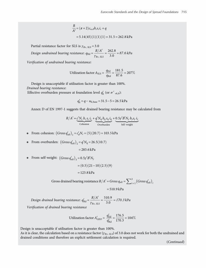
RA
= π + 2 cu,dbcscic + q
= 5 14 45 1 1 1 + 31 5 = 262 8 kPa
Partial resistance factor for SLS is γRv, SLS = 3 0
Design undrained bearing resistance: qRd =R AγRv, SLS
=262 83 0
= 87 6 kPa
Verification of undrained bearing resistance:
Utilization factorASLS =qEdqRd
=181 587 6
= 207
Design is unacceptable if utilisation factor is greater than 100%.Drained bearing resistance:Effective overburden pressure at foundation level qk (or σ vk,b):
qk = q− uk,base = 31 5−5 = 26 5 kPa
Annex D of EN 1997-1 suggests that drained bearing resistance may be calculated from
R A = c Nc bc sc icCohesion
+ q Nq bq sq iq
Overburden
+ 0 5γ B Nγ bγsγ iγ
Self -weight
• From cohesion: Gross qult 1 = cdNc = 5 20 7 = 103 5 kPa
• From overburden: Gross qult 2 = q Nq = 26 5 10 7
= 283 6 kPa
• From self-weight: Gross qult 3 = 0 5γ B Nγ
= 0 5 21−10 2 5 9
= 123 8 kPa
Gross drained bearing resistanceR A =Gross qult =3
i = 1Gross qult i
= 510 9 kPa
Design drained bearing resistance: qRd =R AγRv, SLS
=510 93 0
= 170 3 kPa
Verification of drained bearing resistance
Utilization factorAGEO =qEdqRd
=176 5170 3
= 104
Design is unacceptable if utilisation factor is greater than 100%.As it is clear, the calculation based on a resistance factor (γRv, SLS) of 3.0 does not work for both the undrained anddrained conditions and therefore an explicit settlement calculation is required.
(Continued)
Eurocode Standards and the Design of Spread Foundations 715
worksaccounts.com
(b) Explicit verification of serviceabilityActions and effectsThe net bearing pressure at the foundation level z = 0m is
qnet, d = qEd−σvk,b = 181 5−31 5 = 150 kPa
Immediate settlement so (or si)For evaluation of settlement Annex F to EN 1997-1 suggests using an equation of the form:
s= p×B× f Em
The symbols are defined in the Annex F.The following settlement equation [Equation (3.33)] is one of many that are available and follows the guid-
ance given in the Annex F, as indicated above.
so = μoμ1qBEm
where the coefficient μo depends on the depth of foundation and μ1 depends on the layer thickness and theshape of the loaded area (see Figure 3.9). The width B is in m, q in kPa and Em in MPa.
The immediate settlement is considered to be the short-term component of the total settlement, whichoccurs without drainage.
The values adopted for the stiffness parameters (such as Em and Poisson’s ratio) should in this caserepresent the undrained behaviour.
Refer to Figure 3.9:
DB=dB=1 52 5
= 0 6. For this value ofdBobtain μo 0 93
HB=dR−dB
=4 5−1 5
2 5= 1 2. For this value of
dR−dB
obtain μ1 0 4
q= qnet, d = 150 kPa
Em = Eu,k = 600 cu,k = 600 × 45 = 27 000 kPa = 27MPa
so = μoμ1qnet, d BEu,k
= 0 93 × 0 4 ×150 × 2 5
27= 5 2mm
This settlement equation gives average vertical displacement under a flexible uniformly loaded area. It doesnot include a factor to account for rigidity. It was found that if the footing is rigid the settlement will be uni-form and reduced by about 7%, as Equation (3.6) indicates. If we assume that the given strip footing isrigid, then
so 0 93 × 5 2 = 4 8mm
Consolidation settlement s1 (or sc)In order to compute the consolidation settlement more accurately, assume the 3 m clay layer below the foun-dation level is divided into five sub-layers, each 0.6 m thick, as shown in the scheme below.
Consolidation settlement in each sub-layer is
sc, i =mvk × σz, i × h
mv,k = 0 12m2 MN
716 Shallow Foundations
worksaccounts.com
h= 0 6m= thickness of sublayer iσz, i = net increase in pressure atmiddle of sublayer i = qnet, d 4II = stress influence factor obtained from Table 2.3 or Figure 2.32
Results of the necessary calculations are presented in the table below:
Layer (m) z I (kPa) qnet, d (kPa) σz, i (m2/Mpa) mv,k (m) h (mm) sc
I 0.3 0.24 150 144 0.12 0.6 10.4
II 0.3 0.22 150 132 0.12 0.6 9.5
III 0.3 0.18 150 108 0.12 0.6 7.8
IV 0.3 0.15 150 90 0.12 0.6 6.5
V 0.3 0.12 150 72 0.12 0.6 5.2
s1 = sc = 39 4
The total consolidation settlement s1 = 39 4 mmTotal settlementIn this solution only immediate and consolidation settlements have been considered. The creep component s2(secondary compression) is considered negligible.
Sum of settlements is s= so + s1 = 5 2 + 39 4 = 44 6mmDesign effect of actions is sEd = s= 45mm
Verification of settlement (SLS)Equation (6.22): sEd = s0 + s1 + s2 ≤ sCd
sCd = 50mm given
Utilisation factor ASLS =sEdsCd
=4550
= 90
Design is unacceptable if utilisation factor is greater than 100%.Serviceability is satisfied by the explicit calculation since ASLS = 90
h = 0.6 m
0.9 m II
1.5 m III
2.1 m IV
2.7 m V
z = 0
Rigid layer
VGk + VQk
WGk
z
d
dR, Clay
dwW. T
Δ
0.3 m I
Scheme 6.10
Eurocode Standards and the Design of Spread Foundations 717
worksaccounts.com
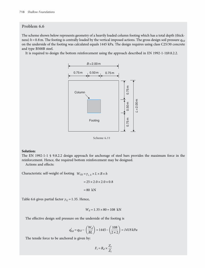
Problem 6.6
The scheme shown below represents geometry of a heavily loaded column footing which has a total depth (thick-ness) h= 0 8m. The footing is centrally loaded by the vertical imposed actions. The gross design soil pressure qEdon the underside of the footing was calculated equals 1445 kPa. The design requires using class C25/30 concreteand type B500B steel.It is required to design the bottom reinforcement using the approach described in EN 1992-1-1§9.8.2.2.
Solution:The EN 1992-1-1 § 9.8.2.2 design approach for anchorage of steel bars provides the maximum force in thereinforcement. Hence, the required bottom reinforcement may be designed.
Actions and effects:
Characteristic self-weight of footing WGk = γc, k × L×B× h
= 25 × 2 0 × 2 0 × 0 8
= 80 kN
Table 6.6 gives partial factor γG = 1 35. Hence,
Wd = 1 35 × 80 = 108 kN
The effective design soil pressure on the underside of the footing is
qEd = qEd −Wd
BL= 1445−
1082 × 2
= 1418 kPa
The tensile force to be anchored is given by:
Fs =Rd ×Ze
Zi
0.75 m0.75 m 0.50 m
B = 2.00 m
0.7
5m
L=
2.0
0m
0.5
0m
0.7
5mFooting
Column
Scheme 6.11
718 Shallow Foundations
worksaccounts.com
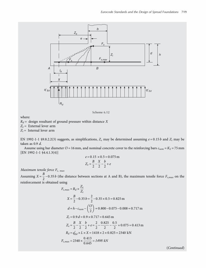
where:Rd = design resultant of ground pressure within distance XZe = External lever armZi = Internal lever arm
EN 1992-1-1 §9.8.2.2(3) suggests, as simplifications, Ze may be determined assuming e= 0 15 b and Zi may betaken as 0.9 d.
Assume using bar diameter = 16mm, and nominal concrete cover to the reinforcing bars cnom =K2 = 75mm[EN 1992-1-1 §4.4.1.3(4)]
e = 0 15 × 0 5 = 0 075m
Ze =B2−X2−b2+ e
Maximum tensile force Fs, max
Assuming X =B2−0 35 b (the distance between sections at A and B), the maximum tensile force Fs,max on the
reinforcement is obtained using
Fs,max =Rd ×Ze
Zi
X =B2−0 35 b=
22−0 35 × 0 5 = 0 825m
d = h−cnom− 2= 0 800−0 075−0 008 = 0 717m
Zi = 0 9d = 0 9 × 0 717 = 0 645m
Ze =B2−X2−b2+ e=
22−0 8252
−0 52
+ 0 075 = 0 413m
Rd = qEd × L×X = 1418 × 2 × 0 825 = 2340 kN
Fs,max = 2340 ×0 4130 645
= 1498 kN
(Continued)
b
e
Ze
Zi
B
d h
Alb
Rd
X
q′Ed q′Ed
Fs,maxFs
Fc
Scheme 6.12
Eurocode Standards and the Design of Spread Foundations 719
worksaccounts.com

Required reinforcement area As
Partial factor for reinforcing steel γs = 1 15
Required reinforcement areaAs =
Fs, max
fyk γs=1498 1000500 1 15
= 3 445 × 10−3 m2 = 3445mm2
Provide 18 16 both ways with 91 mm clear bar spacing.Verifications and reinforcement arrangement
• The recommended minimum bar diameter is 8 mm [EN 1992-1-1 §9.8.2.1(1)]. The provided bar diameter is16mm> min (OK.)
As, provided = 18 × 200 = 3600mm2 > As,required OK
• The minimum clear spacing of reinforcing bars smin = 25mm (EN 1992-1-1 §8.2). The provided clear bar spa-cing is 91mm> smin (OK.)
As, max = 0 04Ac (EN 1992-1-1 §9.2.1.1)
= 0 04 × 800 × 2000 = 64000mm2 As,provided OK
• From Table 6.16: minimum percentage of reinforcement is
As,min = 0 13 = 0 0013 × 717 × 2000
= 1864mm2 < As, provided OK
• The provided concrete cover to the external reinforcing bars is
cprovided =2000−18 × 16−17 × 91
2= 82 5mm> 75mm OK
• Verification of straight bar anchorage:For straight bars without end anchorage the minimum value of X is the most critical. As a simplification,
Xmin = h 2 may be assumed [EN 1992-1-1 §9.8.2.2(5)]
Xmin =h2=0 82
= 0 4m
Ze =B2−Xmin
2−b2+ e =
22−0 42
−0 52
+ 0 075 = 0 625m
Rd = qEd × L× Xmin = 1418 × 2 × 0 4 = 1134 4 kN
Fs = 1134 4 ×0 6250 645
= 1099 2 kN
for the purpose of this verification assume cnom = 0 040m.From Table 6.20: the design anchorage length in case of tensile force and good bond conditions
is lbd = 500mm=0 5m.
lb =Fs
Asfyd× lbd =
1099 23600106
×500 × 1000
1 15
× 0 5 = 0 351m
720 Shallow Foundations
worksaccounts.com
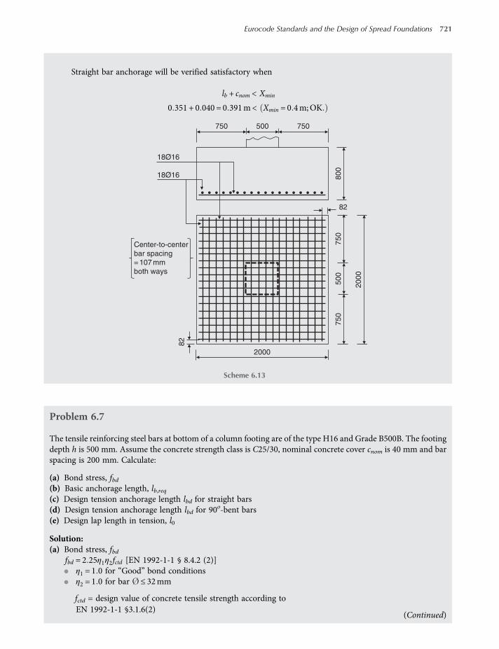
Straight bar anchorage will be verified satisfactory when
lb + cnom < Xmin
0 351 + 0 040 = 0 391m< Xmin = 0 4m;OK
Problem 6.7
The tensile reinforcing steel bars at bottom of a column footing are of the type H16 and Grade B500B. The footingdepth h is 500 mm. Assume the concrete strength class is C25/30, nominal concrete cover cnom is 40 mm and barspacing is 200 mm. Calculate:
(a) Bond stress, fbd(b) Basic anchorage length, lb,req(c) Design tension anchorage length lbd for straight bars(d) Design tension anchorage length lbd for 90
o-bent bars(e) Design lap length in tension, l0
Solution:(a) Bond stress, fbd
fbd = 2 25η1η2fctd [EN 1992-1-1 § 8.4.2 (2)]
• η1 = 1 0 for “Good” bond conditions
• η2 = 1 0 for bar ≤ 32mm
fctd = design value of concrete tensile strength according toEN 1992-1-1 §3.1.6(2)
(Continued)
750 750500
80
0750
750
18Ø16
18Ø16
500
20002000
82
82
Center-to-center
bar spacing
= 107 mm
both ways
Scheme 6.13
Eurocode Standards and the Design of Spread Foundations 721
worksaccounts.com
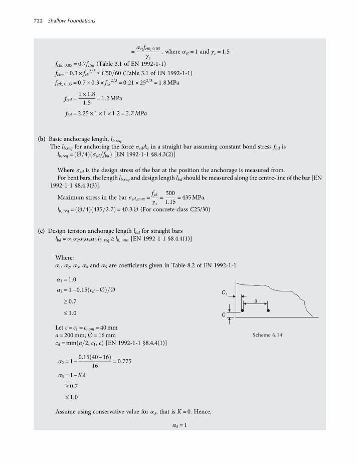
=αct fctk, 0 05
γc, where αct = 1 and γc = 1 5
fctk, 0 05 = 0 7fctm (Table 3.1 of EN 1992-1-1)
fctm = 0 3 × fck2 3 ≤C50 60 (Table 3.1 of EN 1992-1-1)
fctk, 0 05 = 0 7 × 0 3 × fck2 3 = 0 21 × 252 3 = 1 8MPa
fctd =1 × 1 81 5
= 1 2MPa
fbd = 2 25 × 1 × 1 × 1 2 = 2 7MPa
(b) Basic anchorage length, lb,reqThe lb,req for anchoring the force σsdAs in a straight bar assuming constant bond stress fbd is
lb,req = 4 σsd fbd [EN 1992-1-1 §8.4.3(2)]
Where σsd is the design stress of the bar at the position the anchorage is measured from.For bent bars, the length lb,req and design length lbd should bemeasured along the centre-line of the bar [EN
1992-1-1 §8.4.3(3)].
Maximum stress in the bar σsd,max =fykγs
=5001 15
= 435MPa.
lb, req = 4 435 2 7 = 40 3 (For concrete class C25/30)
(c) Design tension anchorage length lbd for straight barslbd = α1α2α3α4α5 lb, req ≥ lb, min [EN 1992-1-1 §8.4.4(1)]
Where:α1, α2, α3, α4 and α5 are coefficients given in Table 8.2 of EN 1992-1-1
α1 = 1 0
α2 = 1−0 15 cd −
≥ 0 7
≤ 1 0
Let c= c1 = cnom = 40mma= 200mm; = 16mmcd =min a 2, c1, c [EN 1992-1-1 §8.4.4(1)]
α2 = 1−0 15 40−16
16= 0 775
α3 = 1−Kλ
≥ 0 7
≤ 1 0
Assume using conservative value for α3, that is K = 0. Hence,
α3 = 1
C1
a
C
Scheme 6.14
722 Shallow Foundations
worksaccounts.com
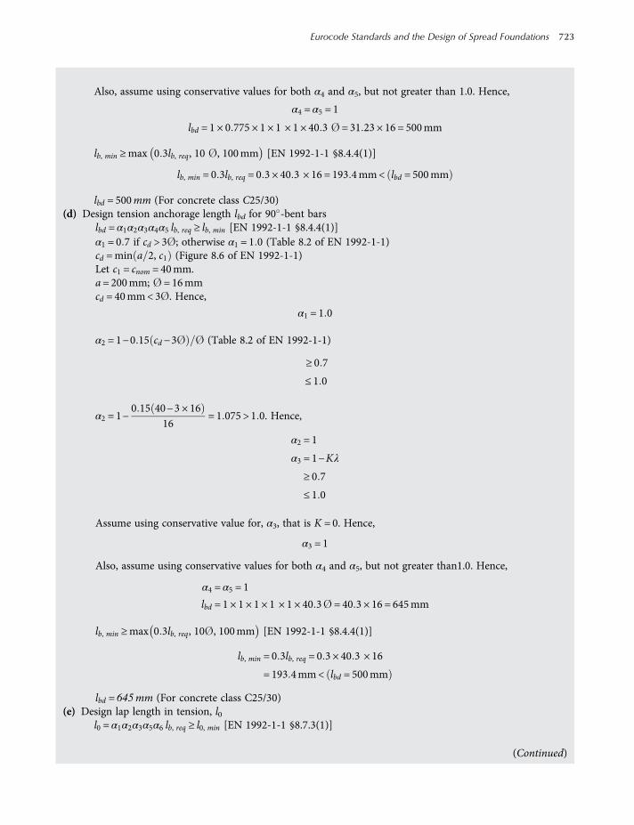
Also, assume using conservative values for both α4 and α5, but not greater than 1.0. Hence,
α4 = α5 = 1
lbd = 1 × 0 775 × 1 × 1 × 1 × 40 3 = 31 23 × 16 = 500mm
lb, min ≥max 0 3lb, req, 10 , 100mm [EN 1992-1-1 §8.4.4(1)]
lb, min = 0 3lb, req = 0 3 × 40 3 × 16 = 193 4mm< lbd = 500mm
lbd = 500mm (For concrete class C25/30)(d) Design tension anchorage length lbd for 90 -bent bars
lbd = α1α2α3α4α5 lb, req ≥ lb, min [EN 1992-1-1 §8.4.4(1)]α1 = 0 7 if cd > 3 ; otherwise α1 = 1 0 (Table 8.2 of EN 1992-1-1)cd =min a 2, c1 (Figure 8.6 of EN 1992-1-1)Let c1 = cnom = 40mm.a= 200mm; = 16mmcd = 40mm< 3 . Hence,
α1 = 1 0
α2 = 1−0 15 cd −3 (Table 8.2 of EN 1992-1-1)
≥ 0 7
≤ 1 0
α2 = 1−0 15 40−3 × 16
16= 1 075 > 1 0. Hence,
α2 = 1
α3 = 1−Kλ
≥ 0 7
≤ 1 0
Assume using conservative value for, α3, that is K = 0. Hence,
α3 = 1
Also, assume using conservative values for both α4 and α5, but not greater than1.0. Hence,
α4 = α5 = 1
lbd = 1 × 1 × 1 × 1 × 1 × 40 3 = 40 3 × 16 = 645mm
lb, min ≥max 0 3lb, req, 10 , 100mm [EN 1992-1-1 §8.4.4(1)]
lb, min = 0 3lb, req = 0 3 × 40 3 × 16
= 193 4mm< lbd = 500mm
lbd = 645mm (For concrete class C25/30)(e) Design lap length in tension, l0
l0 = α1α2α3α5α6 lb, req ≥ l0, min [EN 1992-1-1 §8.7.3(1)]
(Continued)
Eurocode Standards and the Design of Spread Foundations 723
worksaccounts.com

Values of α1, α2, α3 and α5 may be taken from Table 8.2 of EN 1992-1-1; however, for the calculation of α3,
ΣAst, min should be taken as 1 0Asσsdfyd
, with As = area of one lapped bar.
From Table 8.2 of EN 1992-1-1:
α1 = 1 0
α2 = 0 775 [As calculated in (c)]α3 = 1 0 [Conservative value as calculated in (c)]α5 = 1 0 [Conservative value]
α6 =ρ125
0 5with 1 5≥ a6 ≥ 1 0. The ratio ρ1 is the percentage of reinforcement lapped within 0.65 l0 from
centre of the lap length considered (see Figure 8.8 of EN 1992-1-1). Values of α6 are given in Table 8.3 of EN1992-1-1.
Percentage of reinforcement lapped within a bar spacing of 200 mm is conservatively calculated as
ρ1 =Ast
Ac=2 π 2 4
Ac=2 π × 162 4200 × 500
= 0 004 = 0 4 < 25 . Hence,
Table 8.3 of EN 1992-1-1 gives α6 = 1 0l0, min ≥ max 0 3α6lb, req;15 ;200mm [EN 1992-1-1 §8.7.3(1)]
≥ max 0 3 × 1 × 40 3 × 16;15 × 16;200mm
≥ max 193 4mm;240mm;200mm
≥ 240mm
l0 = 1 × 0 775 × 1 × 1 × 1 × 40 3 × 16 = 500mm> l0, min. Hence,l0 = 500mm (For concrete class C25/30)
Problem 6.8
Fairly loose becomingmedium-dense medium sand will support the widely spaced individual column footings of astructure. One of the centrally loaded interior column footings is required to carry a vertical imposed permanentaction VGk = 1100 kN and a vertical imposed variable action VQk = 700 kN. The column is 600 mm square. Thegeotechnical designer recommended using an isolated footing 4 m square, and a foundation depth = 1 2m. Also,he reported that the differential settlement between columns founded on loosest and densest soils will be about2 mm, which is negligible.The structural design requires using class C25/30 concrete fck = 25MPa and type B500B steel fyk = 500MPa .
Using DA1-Combination 1, perform the necessary design calculations for flexure and shear (i.e. determine thefooting depth (thickness) h and design the reinforcement).
Solution:Actions and effects:
Partial factors from Annex A to EN 1990, or from Table 6.6 of this chapter:
γG = 1 35; γQ = 1 5
Design vertical action:Vd = γGVGk + γQ VQk
= 1 35 × 1100 + 1 5 × 700 = 2535 kN
Design bearing pressure [Equation (6.8)]: qEd =Vd
Ab=25354 × 4
= 158 4 kPa
724 Shallow Foundations
worksaccounts.com
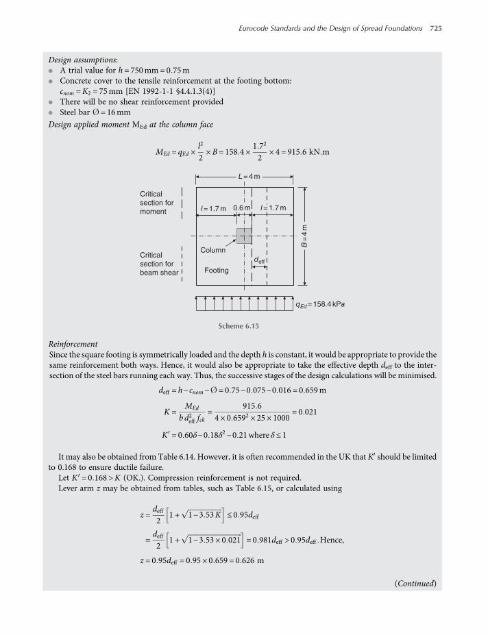
Design assumptions:
• A trial value for h= 750mm=0 75m
• Concrete cover to the tensile reinforcement at the footing bottom:cnom =K2 = 75mm [EN 1992-1-1 §4.4.1.3(4)]
• There will be no shear reinforcement provided
• Steel bar = 16mm
Design applied moment MEd at the column face
MEd = qEd ×l2
2×B= 158 4 ×
1 72
2× 4 = 915 6 kN m
ReinforcementSince the square footing is symmetrically loaded and the depth h is constant, it would be appropriate to provide thesame reinforcement both ways. Hence, it would also be appropriate to take the effective depth deff to the inter-section of the steel bars running each way. Thus, the successive stages of the design calculations will be minimised.
deff = h−cnom− = 0 75−0 075−0 016 = 0 659m
K =MEd
bd2eff fck=
915 64 × 0 6592 × 25 × 1000
= 0 021
K = 0 60δ−0 18δ2−0 21where δ≤ 1
It may also be obtained from Table 6.14. However, it is often recommended in the UK that K should be limitedto 0.168 to ensure ductile failure.
Let K = 0 168 >K (OK.). Compression reinforcement is not required.Lever arm z may be obtained from tables, such as Table 6.15, or calculated using
z =deff2
1 + 1−3 53K ≤ 0 95deff
=deff2
1 + 1−3 53 × 0 021 = 0 981deff > 0 95deff Hence,
z = 0 95deff = 0 95 × 0 659 = 0 626 m
(Continued)
l = 1.7 m
Column
L = 4 m
B=
4m
Footing
deff
qEd= 158.4 kPa
Critical
section for
moment
Critical
section for
beam shear
l = 1.7 m0.6 m
Scheme 6.15
Eurocode Standards and the Design of Spread Foundations 725
worksaccounts.com

The required tension steel area As may be calculated from
As =MEd
fykγs
× z
γs = 1 15 [EN 1992-1-1 §2.4.2.4(1)]
As =915 6
500 × 10001 15
× 0 626= 3 364 × 10−3 m2 = 3364mm2
Try 18 16 As, provided = 3618mm2
Check minimum reinforcement requirements using Table 6.16 or by calculating As, min from:
As, min = 0 26fctmbtdeff
fyk,but not less than 0 0013 btdeff
where fck ≥ 25MPa
As, min = 0 26 ×2 6btdeff500
= 0 0013 btdeff
Minimum percentage of reinforcement required = 0 13
Percentage of reinforcement provided =3618
4000 × 659× 100 = 0 14 (OK.)
Check maximum reinforcement requirements:
As, max = 0 04Ac = 0 04 × 4000 × 659 = 105440mm2 As, provided OK
Provide 18 16 steel bars both ways at the bottom of the footingBar clear spacing and concrete cover:For footings on soil, minimum concrete cover iscnom =K2 = 75mm [EN 1992-1-1 §4.4.1.3(4)]
Bar clear spacing s=4000−2 × 75−18 × 16
17= 209 5mm. Use:
sprovided = 209mm. Hence,
cprovided =4000−17 × 209−18 × 16
2= 79 5mm > cnom (OK).
Centre to centre bar spacing = 209 + 16 = 225mm
Beam Shear (one-way shear)Design beam shear at critical section is
VEd = qEd l−deff B = 158 4 1 7−0 659 4 = 660 kN
Design shear stress at critical section is
vEd =VEd
Bdeff=
6604 × 0 659
= 250 4 kPa
Design concrete resisting shear stress, vRd, c:
vRd, c =CRd, ck 100ρl fck1 3 ≥ 0 035k1 5fck
0 5 [EN 1992-1-1 §6.2.2]
726 Shallow Foundations
worksaccounts.com
k= 1 +200deff
≤ 2;fck = 25MPa; ρl =As
Bdeff= 0 0014;CRd, c =
0 18γc
k= 1 +200659
= 1 55;CRd, c =0 181 5
= 0 12; 0 035k1 5fck0 5 = 0 338MPa
vRd, c = 0 12 × 1 55 100 × 0 0014 × 25 1 3 = 0 282MPa
vRd, c < 0 035k1 5fck0 5. Hence,
vRd, c = 0 338MPa = 338 kPa > vEd (OK.); no shear reinforcement is required by beam shear in both directions.
Punching shear [EN 1992-1-1 § 6.4.1(4), 6.4.3(2) and 6.4.4]Refer to the flow chart of Figure 6.10.
(a) Considering punching shear perimeter u0 at the column face:The factor β = 1 0 since there is no external applied moment.Design maximum shear stress at the face of the column is
vEd,max =VEd −ΔVEd
u0deff
u0 = perimeter of the column= 4 × 0 6 = 2 4m
ΔVEd =ΔVd = the net upward force within the control perimeter u0
= 158 4 × 0 6 × 0 6−0 75 × 0 62 × 25 = 50 3 kPa
VEd =Vd = the applied design shear force = 2535 kN
deff = the average of the effective depths in orthogonal directions
vEd,max =2535−50 32 4 × 0 659
= 1567 kPa = 1 571MPa
Refer to Table 6.18: for fck = 25MPa, the maximum resisting shear is
vEd,max = 4 5MPa > vEd, max (OK)
(Continued)
Column
B=
4m
Footing
2deff
2deff
L = 4 m
Punching shear
critical perimeter u1
(control perimeters)
Scheme 6.16
Eurocode Standards and the Design of Spread Foundations 727
worksaccounts.com

No shear reinforcement is required by punching shear [EN 1992-1-1 §6.4.3(2)].(b) Considering punching shear perimeter u1 at distance 2deff from the column face:
Design punching shear stress at distance 2deff from the column face is
vEd =VEd −ΔVEd
u1deff
ΔVEd =ΔVd = the net upward force within the control perimeter u1
= qEdπ 2 × 2deff
2
4+ 4 0 6 × 2deff + 0 6 × 0 6
−0 75π 2 × 2deff
2
4+ 4 0 6 × 2deff + 0 6 × 0 6 × 25
= 158 4π 2 × 2 × 0 659 2
4+ 4 0 6 × 2 × 0 659 + 0 36
−0 75π 2 × 2 × 0 659 2
4+ 4 0 6 × 2 × 0 659 + 0 36 × 25
= 1423− 168 = 1255 kN
u1 = 4 × 0 6 + 2 × 2 × 0 659π = 10 68m
vEd =2535−125510 68 × 0 659
= 189 kPa = 0 189MPa
1700 1700600
750
1700
1700
600
4000
4000
79
79
Center-to-center
bar spacing
= 225 mm
both ways
(spacing is not
to scale)
18Ø16
18Ø16
Scheme 6.17
728 Shallow Foundations
worksaccounts.com

Design punching resisting shear stress, vRd, c:
vRd, c =CRd, ck 100ρlfck1 3 ≥ 0 035k1 5fck
0 5 [EN 1992-1-1 §6.4.4]
k= 1 +200deff
≤ 2;fck = 25MPa;ρl =As
Bdeff= 0 0014;CRd, c =
0 18γc
k= 1 +200659
= 1 55;CRd, c =0 181 5
= 0 12; 0 035k1 5f 0 5ck = 0 338MPa
vRd, c = 0 12 × 1 55 100 × 0 0014 × 25 1 3 = 0 282MPa
vRd, c < 0 035k1 5f 0 5ck . Hence,
vRd, c = 0 338MPa = 338 kPa = 0 338MPa > vEd (OK).No shear reinforcement is required by punching shear [EN 1992-1-1 § 6.4.3(2)].
Summary of design calculation results
• Footing depth h= 750mm
• No shear reinforcement is required
• No compression reinforcement is required
• Tension reinforcement is required at the footing bottom: 18 16 straight bars, both ways
• Centre-to-centre bar spacing = 225mm
• Concrete cover to the bottom steel bars = 79mm
• Concrete: fck = 25MPa; Steel: fyk = 500 MPa
References
BCA (2006), How to Design Concrete Structures using Eurocode 2, British Cement Association and The Concrete Centre,Blackwater, Camberley.
Bond, A., and Harris, A. (2010), Decoding Eurocode 7, 1st edn, Taylor and Francis, 270 Madison Avenue, New York, NY10016, USA.
BS NA EN 1997-1 (2004), UK National Annex to Eurocode 7: Geotechnical Design: General Rules, British Standards Insti-tution, London.
BS NA EN 1990 (2005) UK National Annex to Eurocode: Basis of Structural Design, British Standards Institution, LondonBurridge, J. (2010), “RC Detailing to Eurocode 2”, The Concrete Centre, Riverside House, 4 Meadows Business Park,
Station Approach, Blackwater, Camberley, Surrey GU17 9AB, UK.Calgaro J-A., Tchumi M., and M. Gulvanessian, H. (2009), Designers’ Guide to Eurocode 1: Actions on Buildings, Thomas
Telford Publishing, London.EN 1990:2002+A1 (2005) Eurocode –Basis of Structural Design, European Committee for Standardisation, BrusselsEN 1991-1-1 (2002), Eurocode 1 –Actions on Structures – Part 1-1: General Actions – Densities, Self-weight, Imposed Loads
for Buildings: Committee for Standardisation, Brussels.EN 1992-1-1 (2004), Eurocode 2 –Design of Concrete Structures – Part 1-1: General Rules and Rules for Buildings: Com-
mittee for Standardisation, Brussels.EN 1997-1 (2004b), Eurocode 7 –Geotechnical Design – Part 1: General Rules: Committee for Standardisation, Brussels.EN 1997-1: Annex F (2004c), EN Annex F to Eurocode 7 – Geotechnical Design – Part 1:General Rules: Sample Methods for
Settlement Evaluation: Committee for Standardisation, Brussels.Gulvanessian, H., Calgaro J-A., and Holicky, M. (2002), Designers’ Guide to EN 1990 Eurocode: Basis of Structural Design,
Thomas Telford Publishing, London.Scarpelli, G., and Orr, Trevor L.L (2013), “Eurocode 7: Geotechnical Design –Worked Examples”, JRC Scientific and Policy
Re ports, Publications Office of the European Union, Brussels.(TCC) (2006), How to Design Concrete Structures using Eurocode 2: The Concrete Centre and British Cement Association,
Blackwater, Camberley, UK.
Eurocode Standards and the Design of Spread Foundations 729
worksaccounts.com
Index
AASHTO manual, 4, 5accidental design situation, 652accompanying values, 654ACI 318M-08 code, 382actions, 653, 658, 667, 680active earth pressure, 373, 567, 588, 591active Rankine zone, 272AISC (1989), 394allowable bearing capacity see bearing capacityallowable bearing pressure, 268allowable settlement see settlementallowable stress design, 311anchorage & anchorage length, 395, 687anchor bolt, 393
design criteria, 394–395tensile strength, 393
angle of internal friction,CPT, based on, 42DMT, based on, 58–59SPT, based on, 25–26
A-pore pressure coefficient, 173approximate flexible method, 414, 417–419approximate 2V : 1H method see vertical stress in a
soil massarea ratio, 10ASD see allowable stress designat-rest earth pressure-coefficient, Ko
DMT, based on, 57–58PMT, based on, 51
auger drilling, 3average degree of consolidation, 178–179average vertical stress, 107–109
basic requirements, 656, 668beam-finite element model, 412beam shear, 388
beams on elastic foundations, 409–412bearing capacity, 265eccentric inclined loading, 286eccentric loading, 281–286effect of adjacent footings, 291effect of water table, 286–290equations, 273–278factors, 273–277failure mechanism, 272–273from results of in-situ tests, 305–306for rock, 312–316gross safe, 267gross ultimate, 267influence of soil compressibility, 290–291layered soils, 296–304net allowable, 268net safe, 267net ultimate, 267safety factor (SF), 304–305on slopes, 292–296
bearing strength of concrete, 390–391, 398, 402bending see flexureboreholedepth, 13–14drilling, 3finished log, 6–7logging, 4spacing and number, 11–12
Boussinesq’s equations, 95Bowles method, 397, 573–574Bowles solution, 294–296braced excavation in soft claySF against base failure, 344
building codes, 165Buisman–DeBeer method, 161Burland and Burbidge method, 159–161
Shallow Foundations: Discussions and Problem Solving, First Edition. Tharwat M. Baban.© 2016 John Wiley & Sons, Ltd. Published 2016 by John Wiley & Sons, Ltd.
worksaccounts.com
cantilever footing, 79, 405–406design, 533–547
cantilever gravity retaining walldesign, 593–602stability analysis, 587–593
cantilever reinforced concrete retaining wallSF against rotational instability 584–587stability analysis & design, 566–581
Casagrande empirical method, 171CEN, 649characteristic value, 653, 658coefficientconsolidation, 175Coulomb active earth pressure, 587lateral earth pressure, 84, 683Rankine active earth pressure, 567, 594–595settlement or settlement ratio K, 172–173subgrade reaction, 406volume compressibility, 167, 169
column-base plate, 393–394combination of actions, 660combination values, 654, 658combined footing, 77, 402rectangular, 403–404design, 506–520, 552–565
trapezoid, 404design, 520–533
compensated foundation, 82compressibility factor, 42, 290compressibility index, 160compression-controlled section, 387compression index, 169empirical equation, 170secondary, 182
compression load transfer, 394compression reinforcement, 431, 682compressive stress block, 385concrete compressive strength, 314cone penetration test, 4, 38, 156–157, 161–164,
305–306correlation for cohesionless soils, 41–43correlation for cohesive soils, 40–41CPT-qc and SPT-N correlations, 43–44discussion, 38–40Es/qc ratio, 44friction ratio, 40penetrometers, 38–39soil classification charts, 40–41solved problems, 44–47
consistency index, 26, 27consolidation settlement, 149, 168–174constant k, 184–185constant of compressibility, 161constructibility requirements, 86–87contact pressure, 89–94contact settlement, 89–91continuous footing, 77, 383design (wall footing), 471–479
Coulomb’s active earth pressure, coefficient, 588
creep, 149, 182, 676critical sections forbending moment, 383–385development of reinforcement, 390one-way shear, 389two-way shear, 389
cross-hole seismic method, 65–66
deep beam, 406, 542, 544deep foundation, 76degree of consolidation, 175, 178, 179depth factorsbearing capacity, 276settlement (FD ; rock), 183–185settlement (IF ; soil), 149–150
depth of foundations, 74, 82–84design approaches & combinations, 668design bearing capacity, 268design loads, 311–312, 382design situations, 652, 667development of reinforcement, 390differential settlement, 145–148, 311dilatometer test, 4discussion, equations and correlations, 55–59solved problems, 59–62
Donut hammer, 22dowels, 391–392down-hole seismic method, 67dynamic cone penetration test, 20 see also standard
penetration test
eccentrically loaded footingsbearing capacity of, 281effective area method, 281–283Meyerhof method, 283Prakash et al. method, 284–285Purkaystha et al. method, 283–284Saran et al. analysis, 286
contact pressure under, 92non-uniform linear, 93–94uniform, 396–397
economy requirements, 87edge distance for anchor bolts, 396effective embedment depth of anchor, 395effective overburden pressure, 267effective stress approach, 270–271effective zones, 403elastic parameters, 155–158elastic settlement, 149electrical resistivity method see geophysical methodselectric cone penetrometer, 38–39ENs see European Standardsequilibrium, 385equivalent compressive stress block, 385equivalent modulus of elasticity, 162EU see European UnionEuropean Standards, 649European Union, 649expansive soils, 83
Index 731
worksaccounts.com

factored load combinations, 382factor of safety, 304, 344, 584Fadum’s chart, 102FDM see finite difference methodFEM see finite element methodFGM see finite grid methodfield boring log, 4field load tests, 30field penetration number (N60), 160Field Reconnaissance Report, 2–3field tests, 4final geotechnical report, 7–8finished boring log, 6–7finite difference method, 419–421finite element method, 424–426finite grid method, 426–427fire design, 652flexible footing (base), 89–91, 153flexural strength, 386flexure, 383–386, 680–682floating foundation, 82foundation performance requirements
constructibility, 86–87economy, 87general, 84–85serviceability, 86strength, 85–86
foundation pressuregross effective, 267–271net effective, 267–271
frequent values, 654, 658frost penetration, 83
general shear failure, 265–266, 278geophysical methods, 62
electrical resistivity method, 67–69problems and limitations, 69–70
seismic refraction method, 63–65cross-hole method, 65–66down-hole method, 67
problems and limitations, 65solved problems, 70–72
geophysical survey, 3geotechnical categories, 665geotechnical design, 664, 667geotechnical design of shallow foundations
comments and considerations, 310–312design loads, 311–312reduction of differential settlement, 311selection of design soil pressure,
310–311geotechnical strength requirement, 85, 265groundwater table, 4
hammer efficiency, 21hammer energy ratio, 21hammer, SPT, 20Hetenyi chart, 418high strength concrete, 383
horizontal effective stress, 43Housel’s method, 32, 34
immediate settlement, 149–155, 676coarse-grained soils, 155–157fine-grained soils, 166–168
improved equation, 153inclination factors, 276–277influence chart, Newmark’s, 105influence depth, 34, 160influence factors forEs variation with depth, 153–154settlement (IF &IS), 149–150vertical stress due to loaded circular areaBoussinesq, 99Westergaard, 110
vertical stress due to loaded rectangular areaBoussinesq, 100–102Westergaard, 110
vertical stress due to point loadBoussinesq, 95Westergaard (coefficient), 109
influence of soil compressibility on bearing capacity,290–291
influence value (Newmark’s chart), 105initial excess pore water pressure, 172International Code Council, ICC, 165International Conference of Building Officials,
ICBO, 165isolated concrete footing, 77, 383designrectangle, reinforced, 440–449eccentrically loaded, 449–460
square, plain, 427–434square, reinforced, 434–440eccentrically loaded, 460–470
iso-parametric element approach, 426
Kern, 93–94Kern distance, 93
laboratory tests, 4Lame’s constant, 63lap-splice length, 392lateral strain, 168, 172lateral stress index, 57limit pressure, 50–51load and resistance factor design, 85, 311, 382load transfercombined tensile and shear, 395compression, 394shear, 395tensile, 394unbalanced moment, 510
local shear failure, 265, 278, 290longitudinal bars (reinforcement), 391
material index, 57Mat foundation, 80, 91
732 Index
worksaccounts.com

general, 413–414Ks for, 421–424structural design byapproximate flexible method, 635–642rigid method, 609–634, 643–648
structural design methodsflexibleapproximate, 414, 417–419finite difference, 414, 419–421finite element, 414, 424–426finite grid, 414, 426–427
rigid (conventional), 413–416method of accelerating the rate of consolidation, 175–176method of slices, 584modes of shear failure (soil), 265–266modulus of elasticity of concrete, 413, 633modulus of elasticity of soil, 155–157, 166average and weighted average, 153, 372drained & undrained, 167effect of OCR on, 156, 164empirical equations for, 26, 156, 164equivalent, 162in situ tests used for, 155–156pressuremeter modulus, 50–51tables for, 44, 156–158
modulus of subgrade reaction, 406for analysis and design ofbeams on elastic foundations, 409–412Mat foundations, 421–424
as an assumed linear function, 406based on qa (approximate), 407coupling and pseudocoupled methods, 421–422empirical equation, 407solved problems, 602–608as spring elastic stiffness, 409–410table of typical values, 408
net allowable bearing capacity, 268net effective foundation pressure, 267net foundation pressure, 267–271net safe bearing capacity, 267net ultimate bearing capacity, 267Newmark’s influence chart, 105Nfield, 20node, 412node spring, 421normally consolidated clay, 168–169
Oedometer settlement Soed, 168, 173Oedometer test, 168office reconnaissance, 2one-dimensional consolidation, 174one-way shear, 388–389organic-acid attack, 88–89overburden correction factor, 23–24overconsolidated clay, 169–170overconsolidation correction factor, 25overconsolidation margin, 172overconsolidation ratio, 19, 25, 174
equations for OCR, 19, 27, 41, 58overturning stability, 569
partial factor method, 657passive resistance, 568–569, 596peat, 82pedestals, 398design, 480–486
percussion drilling, 3permanent actions, 653permeability, 5, 1149persistent design situation, 652pile caps, 399–400design, 487–506
plain concrete spread footings, 400, 687design see isolated concrete footing
plane strain , 277, 295Plate load test, 4discussion, equations and correlations, 30–34solved problems, 34–37
Poisson’s ratio, 13, 109, 153, 155, 167, 185table of typical values, 158–159
polar moment of inertia, 511pore-water pressure, 267Pozzolan additives, 88precompression, 175solved problems, 245–254
preconsolidation pressure, 19, 171prescriptive method, 670pressure bulbs, 105–107pressuremeter test, 4discussion, equations and correlations, 48–52solved problems, 52–55
presumptive bearing values, 268Pryout, concrete, 394pseudo-coupled method, 422punching shear, 265, 382concrete footings & mats, 388supporting soils, 266
P-wave velocity, 63–64
quasi-permanent values, 654, 658
raft foundation, 81–82cellular, 81
ramp loading, 179Rankine’s active earth pressure coefficient, 567, 591rate of consolidation settlementaccelerating method, 175–180estimation, 174–175
recovery ratiorock (RRR), 8–9soil (SRR), 10–11
rectangular combined footing see combined footingrefraction survey see geophysical methodsrelative density, 24correlation withN60, σo, Cu: 24N60, σo, Cu, OCR: 24
Index 733
worksaccounts.com

relative density (cont’d)N60, σo, D50 : 25N60, CP , CA, COCR: 25qc, σo: 41–42qc, σo, OCR, Qc: 42
representative values, 653retaining walls see cantilever wallsretractable plug sampling, 3rigid footing (base), 89–91, 153rigidity factor, 166rigidity index, 290–291
critical, 290ring spread footing, 79–80rock, 6, 65, 76
bearing capacity, 312–316factors, 315
coring, 3layers, 3, 63quality, 8–9quality designation (RQD), 4, 9correlation for, 9as a reduction factor, 315
recovery ratio (RRR), 8–9settlement, 183–187equation, 183
modulus ratio (Mr), 185–186mass factor (j), 185–186
rotary drilling, 3
safety factor (SF) see factor of safetysafety hammer see SPT hammer efficienciessample disturbance, 9–10samples, 3sampling, 3sand drains, 176
average degree of consolidation, 179patterns and spacing, 178radius of the equivalent cylindrical block, 179smeared zone, 178solved problems, 242–253
Schmertmann’s method, 161–164Scour depth, 83secondary compression, 181–183, 676
Cα/Cc, 183index (Cα), 182
seismic design situation, 652seismic refraction method see geophysical methodssensitivity, 40serviceability limit state, 653, 666serviceability requirements, 86settlement, 33, 84, 86, 89, 144, 265, 304, 676
allowable angular distortion (βa), 148allowable deflection ratios, 147differential settlement, 145–148estimation from CPT, 161estimation from consolidation test see consolidation
settlementestimation from SPT, 157estimation over the construction period, 180
general, 144–149immediate see immediate settlementlimiting values for angular distortion, 148limiting values for deflection ratios, 148settlement, 146tolerable total and differential settlements, 146
shape factor see bearing capacityshear, 85, 265, 382, 388one-way (concrete), 388–389, 680–681punching, 388, 680–681, 684shear failure (soil), 83, 265–266general, 265–266local, 266, 278, 290punching, 265–266
two-way, 388–390shear friction, 577shear modulus, 51, 290dynamic, 63, 66
shear reinforcement, 382, 388, 681–682shear strength, 265, 388anchor bolt (nominal), 395concrete see shearsoil, undrained, fromCPT, 40DMT, 58FVST, 18–19PMT, 51SPT, 26–27
Shelby tube sampling, 3shrinkage & temperature reinforcement, 388sieve size (D50), 25, 43simplified soil classification chart, 40–41Simpson’s rule, 109, 606single-source principle, 668site investigation, 1compiling information, 6Final Geotechnical Report, 2, 7–8laboratory tests, 4–5reconnaissance, 2–3subsurface exploration, 3–4
Skempton–Bjerrum method, 172slices method, 584retaining wall analysis, 584–587
slip fan zones, 272SLS see serviceability limit statesmear zone see sand drainssoil classification charts, CPT, 40–41spall, concrete, 394, 398splice length see lap-splice lengthsplit-barrel/spoon sampling, 3spread footing see isolated footingspring constant, 421springs, soil, 409, 412stability (retaining wall), 566overturning, 568–569rotation, 584–587sliding, 569
stability number, 293standard penetration test, 4, 20, 156–158, 305
734 Index
worksaccounts.com
correlation of SPT-number withcu: 27Dr , σo, Cu: 24Dr , σo, Cu, OCR: 24Dr , σo, D50: 25Dr, CP, CA, COCR: 25Dr , , γ: 25Es: 26, 156–157
: 25–26, σo: 26
OCR, σo: 27qu: 26qu, CI: 27su: 26
corrections of SPT-number, 21, 23–24CPT-qc and SPT-N correlations, 43–44design N60, 28discussion, 20–21solved problems, 27–30
static penetration test see cone penetration teststrain, 385compatibility, 385, 386lateral, 168, 172limit, 386, 387net tensile, 386, 387strain influence factor, 162
strength, 85, 381flexural, 386geotechnical, 85, 265high (concrete), 383shear see shear strengthstructural, 381ultimate compressive (concrete), 314, 381ultimate tensile, anchor bolt, 393yield, steel, 381, 382
strength-reduction factors, 382plain concrete, 401reinforced concrete, 384, 386, 389, 391
strength requirements, 85stress, 385compressive, concrete, 385tensile, 383vertical (soil), 95due toconcentrated load, 95–96line load, 96–97loaded circular area, 97–98loaded rectangular area, 99–103loaded strip area, 97–98
general, 95stress and strain compatibility, 385stress–strain modulus, (soil), 156strip footing, 77, 383design, wall footing, 471–479
structural action, 383structural analysis and design (methods), 402, 413–414,
664, 677structural Eurocodes, 649, 650subsurface exploration see site investigation
sulfate attack, 87–88sulfate resisting cement, 88S-wave velocity, 63, 65–67Swedish solution see slices methodswelling (expansion) index, 168, 170
tangent modulus (rock), 313temperature reinforcement see shrinkage & temperature
reinforcementtensile reinforcement, 383tensile strain see straintensile stress see stresstension-controlled section, 387tension steel, 386Terzaghi method, 168thin-walled tube sampler, 3, 10time factor, 179tolerable settlement see settlementtotal stress approach, 270–271transient design situation, 652trapezoidal combined footing see combined
footingtwo-way shear see sheartwo-way shear cracks, 520types of shallow foundations, 77–82
ULS see ultimate limit statesultimate bearing capacity see bearing capacityultimate compressive strength (rock), 314ultimate limit states, 653, 657, 666ultimate strength design, 311unbalanced moment transfer, 510unconfined compression strength, 26correlation with N60, 26correlation with N60, 27for rock, 313–314
undrained cohesion, 16 see also shear strengthundrained shear strength, 16 see also shear strengthuniformity coefficient, 25uplift capacity of shallow foundations, 306–310breakout factor, 309nominal uplift coefficient, 307non-dimensional factor, 309
utilization factor, 698
vane shear test (field), 16apparatus, 16–17correction factor, 18discussion, 16–19procedure steps (schematically), 18solved problem, 19–20vane shear strength correlations, 19
variable actions, 653vertical drains, 175–177band, 177prefabricated (PVDs), 176sand see sand drains
vertical stresses in soils see stressVesič’s compressibility factors, 290
Index 735
worksaccounts.com

virgin compression curve, 169–171virtual back (retaining wall), 567
wall footings see strip footingswash boring, 3water table, effect on bearing capacity, 286–290Westergaard’s equations, 109–110wide-beam shear, 388–389, 680–681wind load, 312, 382Winkler foundation, 409, 421
concept, 409–410
working loads, 85, 311working stress design, 311
yield strength, steel see strengthYoung’s modulus see modulus of elasticity
zone (pull-out), 306zone of high volume change, 83zones of radial shear, 272zones (effective) see effective zones
736 Index
worksaccounts.com

wiley end user license agreementGo to www.wiley.com/go/eula to access Wiley’s ebook EULA.
worksaccounts.com