setup for dynamic solvent vapor annealing (dsva)
TRANSCRIPT
Setup for dynamic Solvent Vapor Annealing (dSVA) – design, operation and performance evaluation Björn Landeke-Wilsmark, Division of Solar Cell Technology, Uppsala University
1
Technical Report
Setup for dynamic Solvent Vapor Annealing (dSVA)
- design, operation and performance evaluation
2022.05.18
Björn Landeke-Wilsmark Division of Solar Cell Technology (SCT)
Department of Materials Science and Engineering Uppsala University
Main supervisor: Carl Hägglund1 Co-supervisor: Marika Edoff1 1Division of Solar Cell Technology, Department of Materials Science and Engineering, Uppsala University
Setup for dynamic Solvent Vapor Annealing (dSVA) – design, operation and performance evaluation Björn Landeke-Wilsmark, Division of Solar Cell Technology, Uppsala University
2
Contents Table of Abbreviations and Symbols ............................................................................................... 3
Part I – Introduction 1.1 Nanolithography .................................................................................................................... 5
1.2 Self-Assembly of Block Copolymers ....................................................................................... 5 1.2.1 Static Solvent Vapor Annealing ........................................................................................ 6 1.2.2 Dynamic Solvent Vapor Annealing ................................................................................... 6
Part II - Design of dSVA Setup 2.1 Design Specifications .............................................................................................................. 9 2.2.1 Practical Concerns ............................................................................................................ 9 2.2.2 Process Requirements.................................................................................................... 10 2.3 Implemented Design ............................................................................................................ 10 2.3.1 Structural Framework of Module 1 ................................................................................ 13 2.3.2 N2 Supply Network ......................................................................................................... 13 2.3.3 Mass Flow Controllers and Digital Control Unit ............................................................. 13 2.3.4 N2 Distribution Network ................................................................................................. 14 2.3.5 Bubblers and Bypasses ................................................................................................... 14 2.3.6 Mixing Network .............................................................................................................. 15 2.3.7 Water Bath and Temperature Control ........................................................................... 16 2.3.8 Structural Framework of Module 2 ................................................................................ 16 2.3.9 Routing Hub ................................................................................................................... 17 2.3.10 Annealing Chamber ...................................................................................................... 17 2.3.11 Vacuum Pump and Exhaust.......................................................................................... 18 2.3.12 Spectroscopic Reflectometer ....................................................................................... 19 2.3.13 Protective Hood ........................................................................................................... 20
Part III - Operation of the dSVA Setup 3.1 Operating Principles ............................................................................................................. 22 3.1.1 Solvent Vapor Pressure .................................................................................................. 22 3.1.2 Control of Solvent Activity Level .................................................................................... 22 3.2 In-situ Spectroscopic Reflectometry .................................................................................... 24 3.3 Operational States ............................................................................................................... 25 3.3 Operation of the dSVA Setup ............................................................................................... 26 3.3.1 Phase 1: Initialization ..................................................................................................... 27 3.3.2 Phase 2: dSVA Process ................................................................................................... 28 3.3.3 Phase 3: Standby Procedure .......................................................................................... 28 3.4 Procedure for Filling/Emptying Bubblers ............................................................................. 29 3.4 Performance Evaluation of the dSVA Setup ......................................................................... 29 3.5 Examples of dSVA of a Block Copolymer Films ..................................................................... 35
Part IV – Potential Improvements 4. Potential Improvements .................................................................................................. 37
5. Acknowledgments .............................................................................................................. 39 6. References .......................................................................................................................... 39
Appendix Part I – Photo Documentation of Implemented Setup(s) Part II – Technical Drawings of Chamber Assembly Components Part III – List of Components Part IV – Operational States of the dSVA Setup Part V – Scripts
Setup for dynamic Solvent Vapor Annealing (dSVA) – design, operation and performance evaluation Björn Landeke-Wilsmark, Division of Solar Cell Technology, Uppsala University
3
Table of Abbreviations and Symbols 𝑎𝑖 Solvent Activity Level of Species 𝑖 BCP Block copolymer 𝜒 Flory-Huggins Interaction Parameter 𝐷𝑂𝑆 Degree of Swelling (𝐷𝑂𝑆 ≡ ℎ/ℎ0) dSVA dynamic Solvent Vapor Annealing GISAXS Grazing Incidence Small Angle X-ray Scattering ℎ (Swollen) Polymer Film Thickness ℎ0 Initial (Unswollen) Polymer Film Thickness 𝑀𝑖 Molar Flow Rate of Species 𝑖 𝑀𝑖
𝑤 Molecular Weight of Species 𝑖 MFC Mass Flow Controller 𝑃𝑎𝑡𝑚 Atmospheric Pressure 𝑝𝑖
∗ Vapor Pressure of Species 𝑖 𝑝𝑖 Partial Pressure of Species 𝑖 𝑃𝑠𝑦𝑠 Pressure in dSVA System
PFA Perfluoroalkoxy Alkanes PS Polystyrene PS-b-P2VP Poly(styrene-block-2-vinyl pyridine) 𝑄𝑖 Volumetric Flow Rate of Species 𝑖 QCM Quartz Crystal Microbalance RT Room Temperature sccm Standard Cubic Centimeters per Minute SE Spectroscopic Ellipsometry SS Stainless Steel sSVA static Solvent Vapor Annealing SR Spectroscopic Reflectometry 𝑇𝑐ℎ SVA Chamber Temperature 𝑇𝑔 Glass Transition Temperature
𝑇𝑊𝐵 Water Bath Temperature TA Thermal Annealing
Setup for dynamic Solvent Vapor Annealing (dSVA) – design, operation and performance evaluation Björn Landeke-Wilsmark, Division of Solar Cell Technology, Uppsala University
4
Part I - Introduction 1.1 Nanolithography Although nanostructured surfaces and interfaces are of interest in a range of scientific and technological fields, developing lithography techniques able to rapidly, reliably and cost-effectively pattern large-area substrates at the deep nanoscale is key to enable their wider application. Block copolymer (BCP) lithography has been identified as a potential next-generation technique as pattern generation is achieved through bottom-up self-assembly which enables rapid implementation of periodic patterns with high feature resolution and density over arbitrarily large surfaces. An application particularly suited to BCP lithography is thus fabrication of dense, large-area arrays of surface-supported metal nanoparticles and multiple strategies, involving various BCP material systems, have been demonstrated to this end.1-6 All rely, however, on the ability of certain BCPs, given the right conditions, to collectively and spontaneously adopt morphologies that minimize the free energy of the system. This report details the design, operation and performance evaluation of a setup dedicated to provide such conditions. To contextualize the work, a cursory introduction to the field of BCPs is provided below prior to discussing the various aspects of the manufactured piece of equipment.
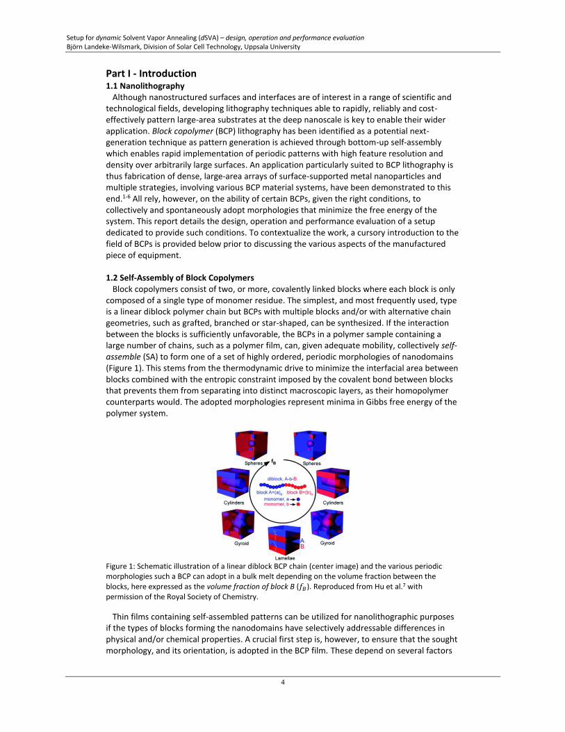
1.2 Self-Assembly of Block Copolymers Block copolymers consist of two, or more, covalently linked blocks where each block is only composed of a single type of monomer residue. The simplest, and most frequently used, type is a linear diblock polymer chain but BCPs with multiple blocks and/or with alternative chain geometries, such as grafted, branched or star-shaped, can be synthesized. If the interaction between the blocks is sufficiently unfavorable, the BCPs in a polymer sample containing a large number of chains, such as a polymer film, can, given adequate mobility, collectively self-assemble (SA) to form one of a set of highly ordered, periodic morphologies of nanodomains (Figure 1). This stems from the thermodynamic drive to minimize the interfacial area between blocks combined with the entropic constraint imposed by the covalent bond between blocks that prevents them from separating into distinct macroscopic layers, as their homopolymer counterparts would. The adopted morphologies represent minima in Gibbs free energy of the polymer system.
Figure 1: Schematic illustration of a linear diblock BCP chain (center image) and the various periodic morphologies such a BCP can adopt in a bulk melt depending on the volume fraction between the blocks, here expressed as the volume fraction of block B (𝑓𝐵). Reproduced from Hu et al.7 with permission of the Royal Society of Chemistry.
Thin films containing self-assembled patterns can be utilized for nanolithographic purposes if the types of blocks forming the nanodomains have selectively addressable differences in physical and/or chemical properties. A crucial first step is, however, to ensure that the sought morphology, and its orientation, is adopted in the BCP film. These depend on several factors
Setup for dynamic Solvent Vapor Annealing (dSVA) – design, operation and performance evaluation Björn Landeke-Wilsmark, Division of Solar Cell Technology, Uppsala University
5
including (i) the volume ratio between the blocks, (ii) differential wetting at the top and bottom interfaces, (iii) lateral and vertical confinement, and (iv) the conditions used during the annealing process. As most BCPs of any practical lithographic use are in a glassy state – a state characterized by very limited chain mobility – at room temperature (RT), an annealing process is required to temporarily increase the chain mobility and allow the BCPs to move relative to each other and fold themselves into the lowest free energy conformation. The two principal approaches to accomplish this are thermal annealing (TA) and solvent vapor annealing (SVA) although hybrid techniques such as solvothermal annealing that incorporate both concepts can also be found in the literature.
Thermal annealing simply entails heating the sample to well over the glass transition temperatures (𝑇𝑔) for the BCP blocks but below the order-disorder transition temperature
(𝑇𝑂𝐷𝑇) above which phase-separation does not occur. TA can be performed using a vacuum oven, rapid thermal processing equipment, hotplate, heated filament (zone annealing) or microwave equipment.
SVA is usually performed at, or close to, RT and entails subjecting the sample to an atmosphere rich in appropriate solvent vapors. Solvent molecules will be absorbed into the BCP film causing swelling and in turn greater mobility of the BCP chains, essentially lowering the effective 𝑇𝑔s of the blocks below RT. A SVA process involves more complex molecular
interactions as compared to TA due to the presence of additional species, which not seldom are toxic solvents, and can practically be more difficult to achieve in a controlled way. It has, nonetheless, become prevalent in academic research for a number of reasons. First, TA is not applicable to many BCPs of interest for aggressive dimensional scaling of the pattern features as the temperature needed to achieve sufficient chain mobility exceeds the thermal decomposition temperature of these polymers. Second, SVA can achieve high mobility at RT which enables short processing times and is of particular interest for samples requiring a low thermal budget. Third, SVA offers a more dynamic process as, for example, different solvents can be used to achieve block-differential swelling and the solvent partial pressure above the sample can often be changed more rapidly than the temperature. 1.3 Static Solvent Vapor Annealing (sSVA) Static SVA (sSVA), or ‘bell jar annealing’, is the simplest form of SVA as it merely entails sealing the BCP-clad sample in a hermetically sealed vessel with a set amount of solvent (or solvent mixture) (Figure S1 in Appendix). The partial pressure (𝑝) of the solvent will then increase until the its vapor pressure (𝑝∗) is reached i.e., the equilibrium between evaporation and condensation. The sSVA is typically terminated by simply removing the lid, thereby dissipating 𝑝 above the sample which in turn leads to rapid evaporation of the absorbed solvent in the BCP film. Among the virtues of this approach are (i) its simplicity, (ii) no continual solvent consumption during steady-state operation and (iii) that excess solvent readily can be retrieved. Nonetheless, this approach suffers from reproducibility concerns and a limited control of 𝑝 which makes it less suited for SVA processes requiring 𝑝 < 𝑝∗. 1.4 Dynamic Solvent Vapor Annealing (dSVA) Dynamic solvent vapor annealing (dSVA) is a more sophisticated approach to SVA than sSVA as it entails being able to dynamically change the processing conditions in a controlled way during the procedure. This includes operating at 𝑝 < 𝑝∗ for potentially more than one solvent simultaneously, seamlessly switching between solvents in a single SVA procedure and tailor swelling and de-swelling transients by ramping 𝑝 up or down in a controlled way. Advanced SVA procedures, containing multiple steps, can thus be enacted which allows for a systematic exploration of the SVA parameter space. Moreover, dSVA can be used in conjunction with in-situ monitoring of the polymer film for characterization, added process control (potentially via a feedback loop) and reproducibility. The monitoring options include spectroscopic
Setup for dynamic Solvent Vapor Annealing (dSVA) – design, operation and performance evaluation Björn Landeke-Wilsmark, Division of Solar Cell Technology, Uppsala University
6
reflectometry (SR)8, spectroscopic ellipsometry (SE)9, use of a quartz crystal micro-balance10 (QCM) and grazing incidence X-ray scattering (GISAXS).11 SR and SE yield optical properties and information on swelling-induced changes in the thickness (ℎ) of the polymer film. In addition to ℎ, viscoelastic properties of the swollen polymer film can be obtained via the QCM.10 In-situ GISAXS, on the other hand, can be used to study the self-assembly dynamics and map the morphology of a BCP film as a function of the SVA conditions used. For the nanodomain sizes and periodicities of BCPs, a source of synchrotron radiation is, however, required to perform GISAXS which is generally not feasible on a routine basis. SR, SE and GISAXS all require an optically transparent window in the SVA chamber and measurements can be acquired on the sample being processed rather than on a proxy. The opposite generally holds true when using a QCM which also can be prone to signal noise due to pressure variations and require an electrical feed-through in the vessel wall.
A number of instances of using dedicated dSVA setups, which predominantly are open-ended, flow-based systems, can be found in the literature.8-10, 12-28 Essentially, the operating principle involves controlled continual flows of a carrier gas through separate solvent bubblers which are then combined with a dedicated dilution flow of the carrier gas before the new mixed flow passes through the annealing chamber containing the sample. Low to moderate flows of carrier gas through a well-designed bubbler will become saturated with solvent (𝑝 = 𝑝∗) and 𝑝 control is achieved through dilution. An additional degree of freedom is obtained through control of the temperature of the bubblers as 𝑝∗ is strongly temperature dependent. The descriptions of the dSVA setups in the literature tend, however, to be highly schematic, indicating function rather than actual implementation, with a few notable exceptions.8-10, 12-14, 16, 17, 29 The main purpose of this technical report is therefore to describe the design, operation, validation of intended function and suggested user protocols for an implemented dSVA setup. As research and equipment design tend to be iterative pursuits, the described setup here not being our first version (Figure S2), hopefully this report can provide inspiration for future improvements.
Setup for dynamic Solvent Vapor Annealing (dSVA) – design, operation and performance evaluation Björn Landeke-Wilsmark, Division of Solar Cell Technology, Uppsala University
7
PART II
Design of dSVA Setup
Setup for dynamic Solvent Vapor Annealing (dSVA) – design, operation and performance evaluation Björn Landeke-Wilsmark, Division of Solar Cell Technology, Uppsala University
8
Part II - Design of dSVA Setup 2.1 Design Specifications The design specifications applicable to our dSVA setup can be categorized as either practical concerns or process requirements. 2.1.1 Practical Concerns Optical in-situ Process Monitoring. Real-time process monitoring is highly desired when exploring the dSVA parameter space and in designing new SVA protocols, hence, the setup will be built around a K-MAC ST4000-DLX spectroscopic reflectometer (Figure S3). The SVA chamber thus has to be designed to fit on the movable stage and under the objective lens of this instrument, which imposes several constraints. First, as the gap between the stage and the objective is ≤ 5 cm, the SVA chamber assembly cannot exceed a height of ~3 cm since it must be possible to readily mount/unmount the assembly on the stage (the reflectometer being a shared resource) without risking damage to the optical column. This criterion is further reinforced as opening the chamber, while in place, to load/unload samples is also considered a requirement. Second, the chamber has to be sufficiently light-weight to use the movable stage as intended and also not to shift the center of mass of the instrument sufficiently to make it unstable. Equally important is that once mounted, the chamber must be immobilized i.e., it cannot be allowed to tilt or slide along the stage during operation as this would affect the SR measurements. Third, the chamber has to be able to accommodate large samples, at least 100 mm wafers, and the option to perform SR in any part of the chamber is desired. This necessitates a large inspection window with high transparency in the near infrared to near ultraviolet spectral band. For accurate calibration and hence measurements, the window must furthermore be distortion free and exhibit a low thickness variation. Several of these design requirements would have been far less stringent if a reflectometer with a freely movable probe head, connected via fiberoptic cables to the light source and detector, was used.
Material Compatibility. The nature of the setup means that all internal wetted parts, including seals, must be compatible with a range of organic solvents. Moreover, as a water bath is a straightforward way of creating a uniform, temperature-controlled environment for setting and maintaining a desired vapor pressure inside solvent bubblers, galvanic corrosion considerations of immersed parts are also prudent. Galvanic corrosion is an electrochemical redox-reaction in which one metal is preferentially consumed when in conductive contact with another more noble metal and both in the presence of an electrolyte. A difference in electrode potential between the metals is the root cause and the two metals will form a galvanic pair where one acts as anode and the other as cathode. This problem is most effectively addressed by judicious material selection and electrical isolation of components.
Air-tight. The entire system, with exception of the exhaust, must be hermetically sealed for safe operation in a general cleanroom environment where a large fraction of the air is recirculated throughout the facility. Many organic solvents are harmful, toxic, mutagenic, affect reproduction or fetal development etc., meaning that the risk of exposure, to the operator and others, to solvents in liquid or vapor form must be absolutely minimal. Leaks could, furthermore, affect the performance and reliability of the setup.
Mechanical Robustness. As the dSVA setup will not be a fixed installation, it needs be sufficiently robust for safe room-to-room transport within the cleanroom facility. A modular design approach with flexible interconnections would allow transport by a single person. Moreover, to ensure a hermetically sealed SVA chamber, compressed elastomeric o-ring seals in-between parts are necessary. The compressive force on an o-ring should be fairly evenly distributed to achieve a reliable seal which means that the parts cannot be allowed to noticeably warp or flex in response to the mechanical forces involved. Dimensions and materials must be chosen accordingly.
Setup for dynamic Solvent Vapor Annealing (dSVA) – design, operation and performance evaluation Björn Landeke-Wilsmark, Division of Solar Cell Technology, Uppsala University
9
Budget. As a research project conducted in an academic setting with limited resources in terms of time, manpower, budget and access to manufacturing equipment and facilities, some engineering compromises are to be expected.
Constituent Components. There is a veritable jungle of systems for connecting pipes and tubes but the components of the chosen system must have the required chemical resistance, be sufficiently leak-proof, be capable of handle high and low pressures, be mechanically robust and be available with all the desired configurations and dimensions. 2.1.2 Process Requirements Process Control, Stability and Reproducibility. Achieving a stable, reproducible, and highly granular control of the solvent activity level in the annealing chamber supersedes all other process requirements.
Wide Process Window. As the main purpose of this setup is research, access to a large dSVA parameter space is desired. Consequently, ability to combine and independently control the partial pressures of more than one solvent in the process chamber is sought.
Dynamic Process. Having a low latency i.e., a short response time between a change in setpoint and new steady-state solvent activity level in the process chamber, would enable short transients during the initiation and termination of the dSVA procedure. Low latency is achievable by using high flows and/or minimizing the internal volume of the annealing chamber and the ‘dead space’ in the pipes leading up to it. Fast ramp rates open for shorter process times, ability to readily quench the process and/or more complex processes where the activity level varies over time within a single run.
Uniform Annealing Conditions. As large-area substates will be processed, the chamber must not just be able to accommodate these but also provide uniform conditions throughout. Effectively, the solvent-containing incoming flow should be distributed laterally upon entering the chamber and prior to reaching the sample. Essentially, a distribution nozzle ought to be integrated at the chamber inlet, and if this is customizable then it might also be possible to tailor the flow profile inside the chamber.
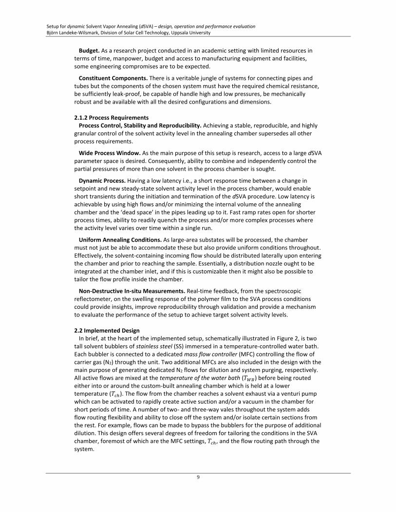
Non-Destructive In-situ Measurements. Real-time feedback, from the spectroscopic reflectometer, on the swelling response of the polymer film to the SVA process conditions could provide insights, improve reproducibility through validation and provide a mechanism to evaluate the performance of the setup to achieve target solvent activity levels. 2.2 Implemented Design In brief, at the heart of the implemented setup, schematically illustrated in Figure 2, is two tall solvent bubblers of stainless steel (SS) immersed in a temperature-controlled water bath. Each bubbler is connected to a dedicated mass flow controller (MFC) controlling the flow of carrier gas (N2) through the unit. Two additional MFCs are also included in the design with the main purpose of generating dedicated N2 flows for dilution and system purging, respectively. All active flows are mixed at the temperature of the water bath (𝑇𝑊𝐵) before being routed either into or around the custom-built annealing chamber which is held at a lower temperature (𝑇𝑐ℎ). The flow from the chamber reaches a solvent exhaust via a venturi pump which can be activated to rapidly create active suction and/or a vacuum in the chamber for short periods of time. A number of two- and three-way vales throughout the system adds flow routing flexibility and ability to close off the system and/or isolate certain sections from the rest. For example, flows can be made to bypass the bubblers for the purpose of additional dilution. This design offers several degrees of freedom for tailoring the conditions in the SVA chamber, foremost of which are the MFC settings, 𝑇𝑐ℎ, and the flow routing path through the system.
Setup for dynamic Solvent Vapor Annealing (dSVA) – design, operation and performance evaluation Björn Landeke-Wilsmark, Division of Solar Cell Technology, Uppsala University
10
Figure 2: Schematic, not-to-scale illustration of the dSVA setup with mass flow controllers (MFCs), valves (V0-V10), solvent bubblers (B1 and B2) and other components indicated.
The setup can be broken down into function-based sections and structurally coherent modules. The sections are: (a) the N2 supply network, (b) the MFCs, (c) the N2 distribution network, (d) the bubblers and associated bypasses, (e) the mixing network, (f) the routing hub, (g) the process chamber and (h) the vacuum extraction pump assembly, (i) the MFC control unit, and (j) the water bath and its temperature control unit. A highly accurate Pt-100 RTD temperature probe is also necessary for precision operation but the spectroscopic reflectometer is technically optional. Sections (a)-(e) and (f)-(g) are mounted on separate structural frameworks and form Module 1 and Module 2, respectively. Module 3 consists of the vacuum pump assembly (h). The MFC control unit (i) and the temperature-controlled water bath (j) are separate entities. The modules are connected in sequence by clear, flexible PFA tubes and all flow paths go from Module 1, via Module 2, to Module 3. Here we will go deeper into the design considerations and the actual implementation of each section, following in the direction of flow.
Setup for dynamic Solvent Vapor Annealing (dSVA) – design, operation and performance evaluation Björn Landeke-Wilsmark, Division of Solar Cell Technology, Uppsala University
11
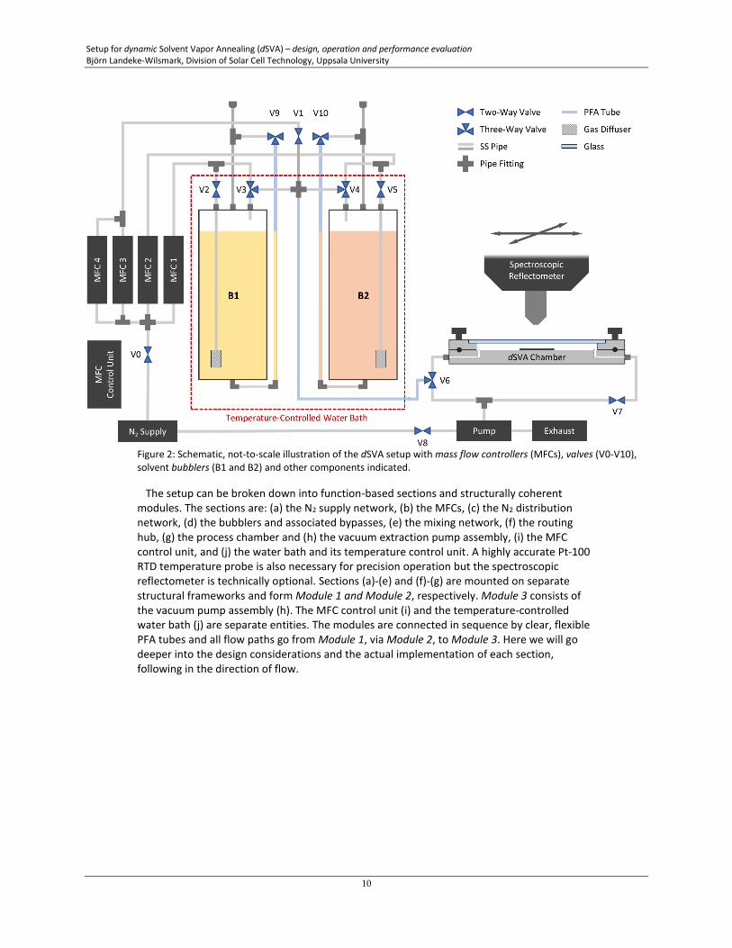
Figure 3: Module 1 rotated clockwise in increments of ~45 ° (a-g), starting with the front view (a). Panel (h) depicts Module 1 as seen from above.
a) b) c) d)
e) f) h) g)
Setup for dynamic Solvent Vapor Annealing (dSVA) – design, operation and performance evaluation Björn Landeke-Wilsmark, Division of Solar Cell Technology, Uppsala University
12
2.2.1 Structural Framework of Module 1 For reasons of mechanical stability, portability and space-saving the N2 supply network, the N2 distribution network, the MFCs, the bubbler assemblies and the mixing network are all mounted on a structural framework principally constructed of sheets of acrylic plastic and L-profiles (20x20x2 mm cross-section) of anodized aluminum or stainless steel (Figure 3 and S4). The upside-down U-shape of the framework allows the flow path from the N2 source to the mixing network output to be folded in on itself, enabling the required workspace area to be substantially reduced and furthermore the front part of the framework to be ‘draped’ over the edge of the water bath vessel. The height of the framework, as well as included splash guards, ensures that the MFCs are not exposed to any water. Acrylic sheeting (4 mm) was chosen due to its light weight, ease of machinability, low cost, availability, non-conductive nature (c. f. galvanic corrosion) and that it has a high optical transparency – the latter of which makes it easy to inspect different parts of the module and verify that all relevant components are sufficiently submerged during operation. Using sheets of polypropylene or polyethylene would, however, have been preferable considering their high chemical resistance to solvents and the nature of the setup. All fasteners, the plate carrying the brunt of the weight of the bubblers and the L-profiles in the vicinity of the water bath are all of stainless steel. 2.2.2 N2 Supply Network This section distributes the lab supply of pressurized nitrogen gas (N2, 99.99%) to the inlet of the MFCs and contains a valve (V0) and quick-release connectors to enable system isolation and the ability to readily disconnect Module 1 (Figure 3e and S4f). The pipe diameter is 6 mm in this part of the system which conforms to the in-house standard. Brass pipe fittings are used here and in all other sections not exposed to water. A full list of the components for all sections can be found in Figure S22 and Table S1 in the Appendix. 2.2.3 Mass Flow Controllers and Digital Control Unit All MFCs in this build are older analog units with 0-5 V setpoint and readout signals, with a linear flow to voltage relationship, and requiring a ±15 VDC power supply (Figure 3). Power, flow control and readout are all handled by a repurposed control box, containing 10-bit analog-to-digital and digital-to-analog converters, from Research Electronics Inc. All internal wetted surfaces of the MFCs are either stainless steel or fluoroelastomer (FKM/FPM seals), providing good resistance to many commonly used solvents. As at least one of our MFCs (MKS 1159B) utilizes the principle of convective heat transport to monitor the gas flow rate they require a ≥ 30 min warmup before accurate values can be obtained. In constructing a setup, note that the orientation of the flow path inside the MFC in the vertical plane can affect its accuracy and that an unproven MFC and be calibrated by connecting it in series with a reliable unit and comparing readouts and setpoints. Details and the intended purpose of the separate MFCs are outlined below.
MFCs 1 and 2 (Tylan FC-2901MEP, 0-100 sccm N2) supply controlled flows of N2 into, or around (via bypasses), bubbler 1 and 2 (B1 and B2), respectively. Choosing an appropriate flow range for MFC 1 and 2 was one of the main considerations in the construction of this setup. A high range reduces the latency of the system but can also entail a reduced probability of fully saturating the flow during its passage through the bubbler. The range 0-100 sccm was deemed a suitable compromise. When only one bubbler is active, the bypass around the other can be opened and its MFC be used for dilution, potentially in conjunction with MFC 3 (and/or MFC 4).
MFC 3 (MKS 1479A, 0-100 sccm N2) is dedicated for dilution of the bubbler outputs and is critical for accessing the entire parameter space of solvent partial pressures when both bubblers are active and held at an elevated temperature. Again, the choice of range is non-trivial and depends on the values used for MFC 1 and 2, the difference between 𝑇𝑊𝐵 and 𝑇𝑐ℎ
Setup for dynamic Solvent Vapor Annealing (dSVA) – design, operation and performance evaluation Björn Landeke-Wilsmark, Division of Solar Cell Technology, Uppsala University
13
and the level of dilution desired. Furthermore, operating in the lowest 10-20% of the stated MFC range should, generally, be avoided due to a relatively high rate of inaccuracy here.
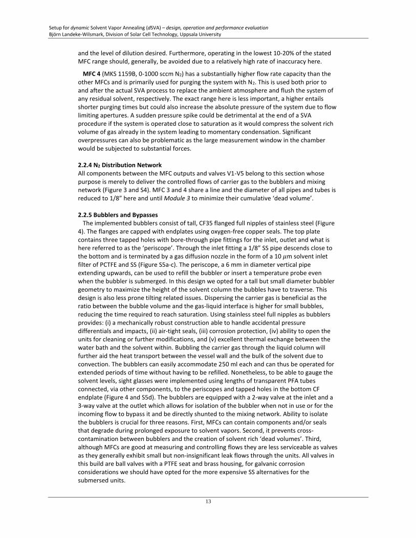
MFC 4 (MKS 1159B, 0-1000 sccm N2) has a substantially higher flow rate capacity than the other MFCs and is primarily used for purging the system with N2. This is used both prior to and after the actual SVA process to replace the ambient atmosphere and flush the system of any residual solvent, respectively. The exact range here is less important, a higher entails shorter purging times but could also increase the absolute pressure of the system due to flow limiting apertures. A sudden pressure spike could be detrimental at the end of a SVA procedure if the system is operated close to saturation as it would compress the solvent rich volume of gas already in the system leading to momentary condensation. Significant overpressures can also be problematic as the large measurement window in the chamber would be subjected to substantial forces. 2.2.4 N2 Distribution Network All components between the MFC outputs and valves V1-V5 belong to this section whose purpose is merely to deliver the controlled flows of carrier gas to the bubblers and mixing network (Figure 3 and S4). MFC 3 and 4 share a line and the diameter of all pipes and tubes is reduced to 1/8” here and until Module 3 to minimize their cumulative ‘dead volume’. 2.2.5 Bubblers and Bypasses The implemented bubblers consist of tall, CF35 flanged full nipples of stainless steel (Figure 4). The flanges are capped with endplates using oxygen-free copper seals. The top plate contains three tapped holes with bore-through pipe fittings for the inlet, outlet and what is here referred to as the ‘periscope’. Through the inlet fitting a 1/8” SS pipe descends close to the bottom and is terminated by a gas diffusion nozzle in the form of a 10 𝜇m solvent inlet filter of PCTFE and SS (Figure S5a-c). The periscope, a 6 mm in diameter vertical pipe extending upwards, can be used to refill the bubbler or insert a temperature probe even when the bubbler is submerged. In this design we opted for a tall but small diameter bubbler geometry to maximize the height of the solvent column the bubbles have to traverse. This design is also less prone tilting related issues. Dispersing the carrier gas is beneficial as the ratio between the bubble volume and the gas-liquid interface is higher for small bubbles, reducing the time required to reach saturation. Using stainless steel full nipples as bubblers provides: (i) a mechanically robust construction able to handle accidental pressure differentials and impacts, (ii) air-tight seals, (iii) corrosion protection, (iv) ability to open the units for cleaning or further modifications, and (v) excellent thermal exchange between the water bath and the solvent within. Bubbling the carrier gas through the liquid column will further aid the heat transport between the vessel wall and the bulk of the solvent due to convection. The bubblers can easily accommodate 250 ml each and can thus be operated for extended periods of time without having to be refilled. Nonetheless, to be able to gauge the solvent levels, sight glasses were implemented using lengths of transparent PFA tubes connected, via other components, to the periscopes and tapped holes in the bottom CF endplate (Figure 4 and S5d). The bubblers are equipped with a 2-way valve at the inlet and a 3-way valve at the outlet which allows for isolation of the bubbler when not in use or for the incoming flow to bypass it and be directly shunted to the mixing network. Ability to isolate the bubblers is crucial for three reasons. First, MFCs can contain components and/or seals that degrade during prolonged exposure to solvent vapors. Second, it prevents cross-contamination between bubblers and the creation of solvent rich ‘dead volumes’. Third, although MFCs are good at measuring and controlling flows they are less serviceable as valves as they generally exhibit small but non-insignificant leak flows through the units. All valves in this build are ball valves with a PTFE seat and brass housing, for galvanic corrosion considerations we should have opted for the more expensive SS alternatives for the submersed units.
Setup for dynamic Solvent Vapor Annealing (dSVA) – design, operation and performance evaluation Björn Landeke-Wilsmark, Division of Solar Cell Technology, Uppsala University
14
Figure 4: One of the bubbler assemblies (B2), rotated clockwise 90°, as seen from the front (a) and the side (b).
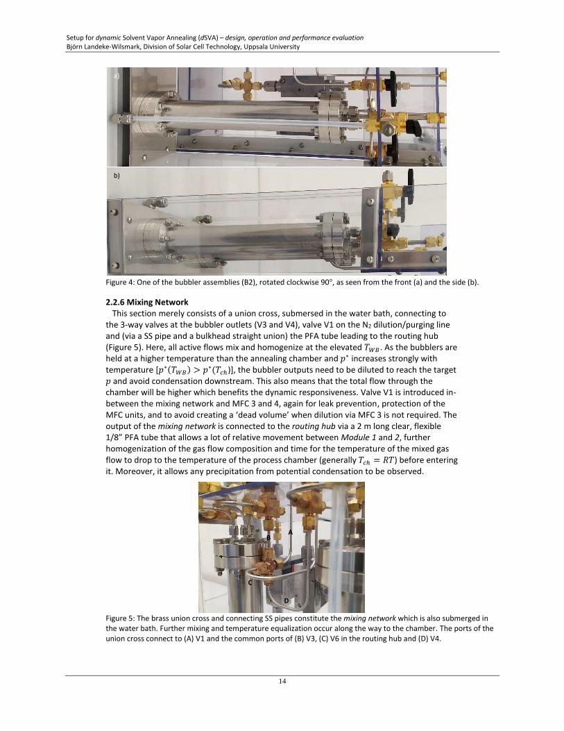
2.2.6 Mixing Network This section merely consists of a union cross, submersed in the water bath, connecting to the 3-way valves at the bubbler outlets (V3 and V4), valve V1 on the N2 dilution/purging line and (via a SS pipe and a bulkhead straight union) the PFA tube leading to the routing hub (Figure 5). Here, all active flows mix and homogenize at the elevated 𝑇𝑊𝐵. As the bubblers are held at a higher temperature than the annealing chamber and 𝑝∗ increases strongly with temperature [𝑝∗(𝑇𝑊𝐵) > 𝑝∗(𝑇𝑐ℎ)], the bubbler outputs need to be diluted to reach the target 𝑝 and avoid condensation downstream. This also means that the total flow through the chamber will be higher which benefits the dynamic responsiveness. Valve V1 is introduced in-between the mixing network and MFC 3 and 4, again for leak prevention, protection of the MFC units, and to avoid creating a ‘dead volume’ when dilution via MFC 3 is not required. The output of the mixing network is connected to the routing hub via a 2 m long clear, flexible 1/8” PFA tube that allows a lot of relative movement between Module 1 and 2, further homogenization of the gas flow composition and time for the temperature of the mixed gas flow to drop to the temperature of the process chamber (generally 𝑇𝑐ℎ = 𝑅𝑇) before entering it. Moreover, it allows any precipitation from potential condensation to be observed.
Figure 5: The brass union cross and connecting SS pipes constitute the mixing network which is also submerged in the water bath. Further mixing and temperature equalization occur along the way to the chamber. The ports of the union cross connect to (A) V1 and the common ports of (B) V3, (C) V6 in the routing hub and (D) V4.
a)
b)
A B
C
D
Setup for dynamic Solvent Vapor Annealing (dSVA) – design, operation and performance evaluation Björn Landeke-Wilsmark, Division of Solar Cell Technology, Uppsala University
15
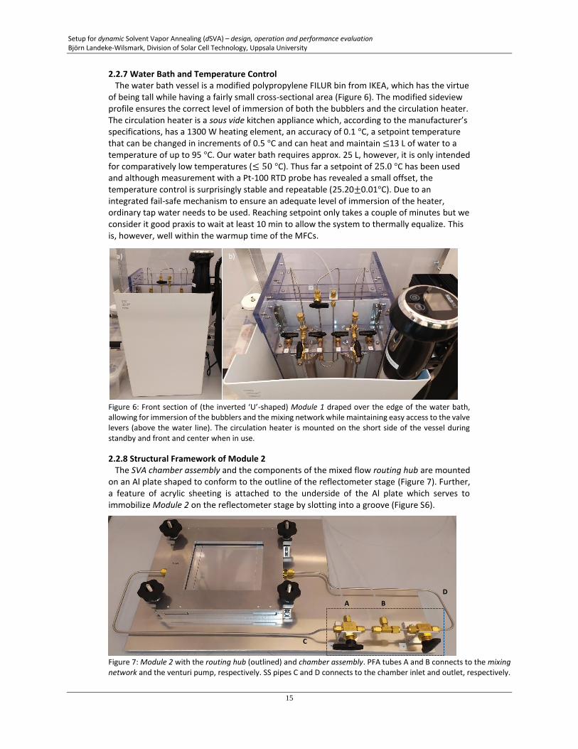
2.2.7 Water Bath and Temperature Control The water bath vessel is a modified polypropylene FILUR bin from IKEA, which has the virtue of being tall while having a fairly small cross-sectional area (Figure 6). The modified sideview profile ensures the correct level of immersion of both the bubblers and the circulation heater. The circulation heater is a sous vide kitchen appliance which, according to the manufacturer’s specifications, has a 1300 W heating element, an accuracy of 0.1 °C, a setpoint temperature that can be changed in increments of 0.5 °C and can heat and maintain ≤13 L of water to a temperature of up to 95 °C. Our water bath requires approx. 25 L, however, it is only intended for comparatively low temperatures (≤ 50 °C). Thus far a setpoint of 25.0 °C has been used and although measurement with a Pt-100 RTD probe has revealed a small offset, the temperature control is surprisingly stable and repeatable (25.20±0.01°C). Due to an integrated fail-safe mechanism to ensure an adequate level of immersion of the heater, ordinary tap water needs to be used. Reaching setpoint only takes a couple of minutes but we consider it good praxis to wait at least 10 min to allow the system to thermally equalize. This is, however, well within the warmup time of the MFCs.
Figure 6: Front section of (the inverted ‘U’-shaped) Module 1 draped over the edge of the water bath, allowing for immersion of the bubblers and the mixing network while maintaining easy access to the valve levers (above the water line). The circulation heater is mounted on the short side of the vessel during standby and front and center when in use.
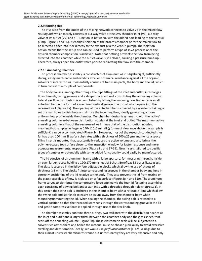
2.2.8 Structural Framework of Module 2 The SVA chamber assembly and the components of the mixed flow routing hub are mounted on an Al plate shaped to conform to the outline of the reflectometer stage (Figure 7). Further, a feature of acrylic sheeting is attached to the underside of the Al plate which serves to immobilize Module 2 on the reflectometer stage by slotting into a groove (Figure S6).
Figure 7: Module 2 with the routing hub (outlined) and chamber assembly. PFA tubes A and B connects to the mixing network and the venturi pump, respectively. SS pipes C and D connects to the chamber inlet and outlet, respectively.
a) b)
A B
C
D
Setup for dynamic Solvent Vapor Annealing (dSVA) – design, operation and performance evaluation Björn Landeke-Wilsmark, Division of Solar Cell Technology, Uppsala University
16
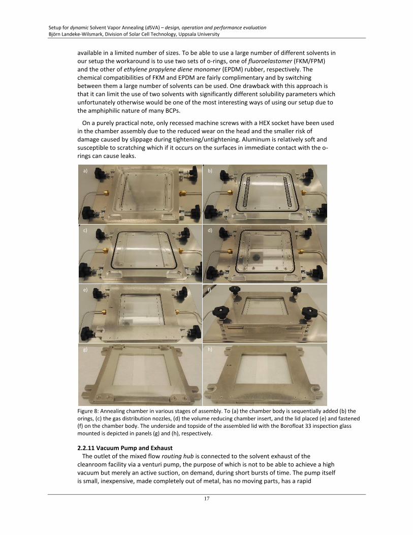
2.2.9 Routing Hub The PFA tube from the outlet of the mixing network connects to valve V6 in the mixed flow routing hub which merely consists of a 3-way valve at the SVA chamber inlet (V6), a 2-way valve at its outlet (V7) and a T-junction in-between, with the added port leading to the venturi pump (Figure 7 and S6). It enables isolation of the process chamber or for the mixed flow to be directed either into it or directly to the exhaust (via the venturi pump). The isolation option means that the setup also can be used to perform a type of sSVA process once the desired chamber composition is achieved. Note that nothing prevents the flow from being directed into the chamber while the outlet valve is still closed, causing a pressure build-up. Therefore, always open the outlet valve prior to redirecting the flow into the chamber. 2.2.10 Annealing Chamber The process chamber assembly is constructed of aluminum as it is lightweight, sufficiently strong, easily machinable and exhibits excellent chemical resistance against all the organic solvents of interest to us. It essentially consists of two main parts, the body and the lid, which in turn consist of a couple of components.
The body houses, among other things, the pipe fittings at the inlet and outlet, internal gas flow channels, o-ring grooves and a deeper recessed well constituting the annealing volume. Lateral gas flow distribution is accomplished by letting the incoming flow first enter a small antechamber, in the form of a machined vertical groove, the top of which opens into the recessed well (Figure 8a). The opening of the antechamber is covered by a nozzle containing a set of small holes to distribute and diffuse the incoming flow, ideally generating a more uniform flow profile inside the chamber. Our chamber design is symmetric with the ‘active’ annealing volume in-between distribution nozzles at the inlet and outlet. The maximum active annealing volume is that of the reassessed well minus that of the distribution nozzles, meaning that samples as large as 140x110x5 mm (if ≥ 1 mm of clearance above the sample is sufficient) can be accommodated (Figure 8c). However, most of the research conducted thus far has used 100 mm Si wafer substrates with a thickness of 500±25 𝜇m and hence a space filling insert is mounted that substantially reduces the active volume and also brings the polymer-coated top surface closer to the inspection window for faster response and more accurate measurements, respectively (Figure 8d and S7-S9). New inserts tailored to specific types of samples or potentially with some added functionality could easily be manufactured.
The lid consists of an aluminum frame with a large aperture, for measuring through, inside an even larger recess holding a 190x170 mm sheet of Schott Borofloat 33 borosilicate glass. The glass is secured in the lid by four adjustable blocks which allow the use of sheets of thickness ≥3 mm. The blocks fit into corresponding grooves in the chamber body and help in correctly positioning of the lid relative to the body. They also prevent the lid from resting on the glass regardless of how it is placed on a flat surface (Figure 8g-h and S10). The aluminum frame serves to distribute the compressive force applied via the four lid fastening assemblies, each consisting of a swing bolt and a star knob with a threaded through hole (Figure S11). In this design the swing bolt is anchored in the chamber body with a rotatable joint which allow the swing bolt and star knob to easily be swung away from the chamber body when mounting/unmounting the lid. When sealing the chamber, the swing bolt is rotated to a vertical position so that the threaded stem runs through the corresponding groove in the lid and gentle compressive force is applied through use of the star knob.
The chamber assembly contains three o-rings, two affiliated with the distribution nozzles at the inlet and outlet and a larger third, between the chamber body and the glass sheet, that seals off the annealing volume (Figure 8b). These elastomeric seals will be subjected to a solvent rich atmosphere and hence the material must be chosen judiciously to avoid excessive swelling and deterioration. Ideally, we would use perfluoroelastomer (FFKM) o-rings due to their almost universal chemical resistance but unfortunately they are very expensive and only
Setup for dynamic Solvent Vapor Annealing (dSVA) – design, operation and performance evaluation Björn Landeke-Wilsmark, Division of Solar Cell Technology, Uppsala University
17
available in a limited number of sizes. To be able to use a large number of different solvents in our setup the workaround is to use two sets of o-rings, one of fluoroelastomer (FKM/FPM) and the other of ethylene propylene diene monomer (EPDM) rubber, respectively. The chemical compatibilities of FKM and EPDM are fairly complimentary and by switching between them a large number of solvents can be used. One drawback with this approach is that it can limit the use of two solvents with significantly different solubility parameters which unfortunately otherwise would be one of the most interesting ways of using our setup due to the amphiphilic nature of many BCPs.
On a purely practical note, only recessed machine screws with a HEX socket have been used in the chamber assembly due to the reduced wear on the head and the smaller risk of damage caused by slippage during tightening/untightening. Aluminum is relatively soft and susceptible to scratching which if it occurs on the surfaces in immediate contact with the o-rings can cause leaks.
Figure 8: Annealing chamber in various stages of assembly. To (a) the chamber body is sequentially added (b) the orings, (c) the gas distribution nozzles, (d) the volume reducing chamber insert, and the lid placed (e) and fastened (f) on the chamber body. The underside and topside of the assembled lid with the Borofloat 33 inspection glass mounted is depicted in panels (g) and (h), respectively.
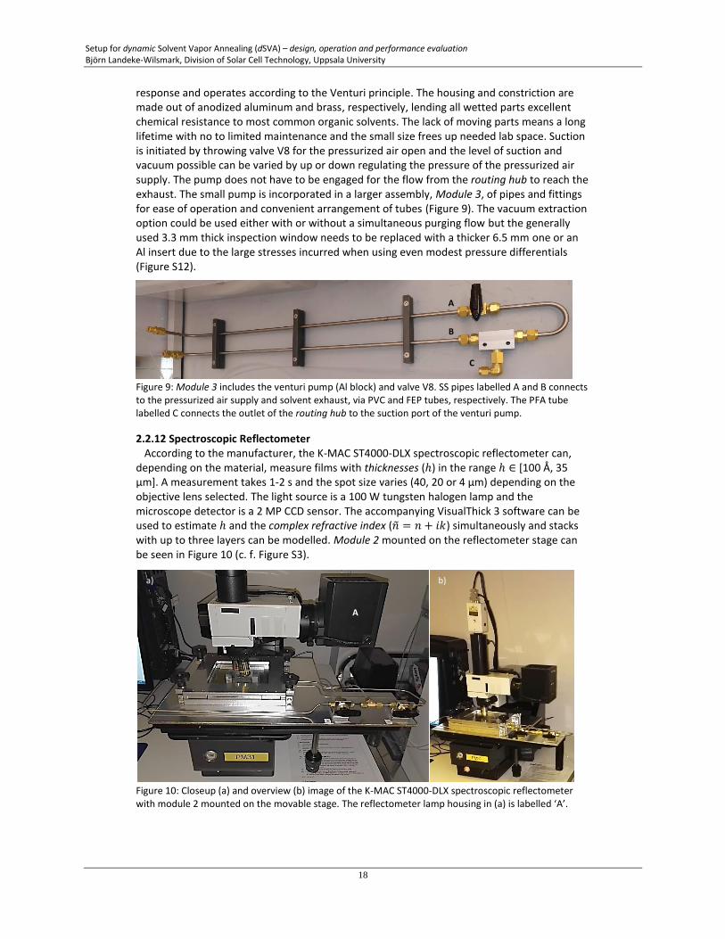
2.2.11 Vacuum Pump and Exhaust The outlet of the mixed flow routing hub is connected to the solvent exhaust of the cleanroom facility via a venturi pump, the purpose of which is not to be able to achieve a high vacuum but merely an active suction, on demand, during short bursts of time. The pump itself is small, inexpensive, made completely out of metal, has no moving parts, has a rapid
f)
b)
c) d)
e)
g) h)
a)
Setup for dynamic Solvent Vapor Annealing (dSVA) – design, operation and performance evaluation Björn Landeke-Wilsmark, Division of Solar Cell Technology, Uppsala University
18
response and operates according to the Venturi principle. The housing and constriction are made out of anodized aluminum and brass, respectively, lending all wetted parts excellent chemical resistance to most common organic solvents. The lack of moving parts means a long lifetime with no to limited maintenance and the small size frees up needed lab space. Suction is initiated by throwing valve V8 for the pressurized air open and the level of suction and vacuum possible can be varied by up or down regulating the pressure of the pressurized air supply. The pump does not have to be engaged for the flow from the routing hub to reach the exhaust. The small pump is incorporated in a larger assembly, Module 3, of pipes and fittings for ease of operation and convenient arrangement of tubes (Figure 9). The vacuum extraction option could be used either with or without a simultaneous purging flow but the generally used 3.3 mm thick inspection window needs to be replaced with a thicker 6.5 mm one or an Al insert due to the large stresses incurred when using even modest pressure differentials (Figure S12).
Figure 9: Module 3 includes the venturi pump (Al block) and valve V8. SS pipes labelled A and B connects to the pressurized air supply and solvent exhaust, via PVC and FEP tubes, respectively. The PFA tube labelled C connects the outlet of the routing hub to the suction port of the venturi pump.
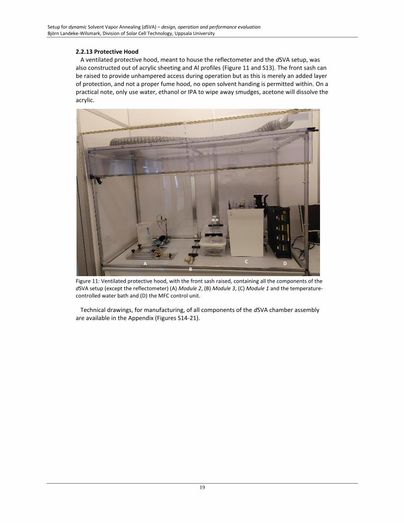
2.2.12 Spectroscopic Reflectometer According to the manufacturer, the K-MAC ST4000-DLX spectroscopic reflectometer can, depending on the material, measure films with thicknesses (ℎ) in the range ℎ ∈ [100 Å, 35 μm]. A measurement takes 1-2 s and the spot size varies (40, 20 or 4 μm) depending on the objective lens selected. The light source is a 100 W tungsten halogen lamp and the microscope detector is a 2 MP CCD sensor. The accompanying VisualThick 3 software can be used to estimate ℎ and the complex refractive index (�̃� = 𝑛 + 𝑖𝑘) simultaneously and stacks with up to three layers can be modelled. Module 2 mounted on the reflectometer stage can be seen in Figure 10 (c. f. Figure S3).
Figure 10: Closeup (a) and overview (b) image of the K-MAC ST4000-DLX spectroscopic reflectometer with module 2 mounted on the movable stage. The reflectometer lamp housing in (a) is labelled ‘A’.
A
B
C
a) b)
A
Setup for dynamic Solvent Vapor Annealing (dSVA) – design, operation and performance evaluation Björn Landeke-Wilsmark, Division of Solar Cell Technology, Uppsala University
19
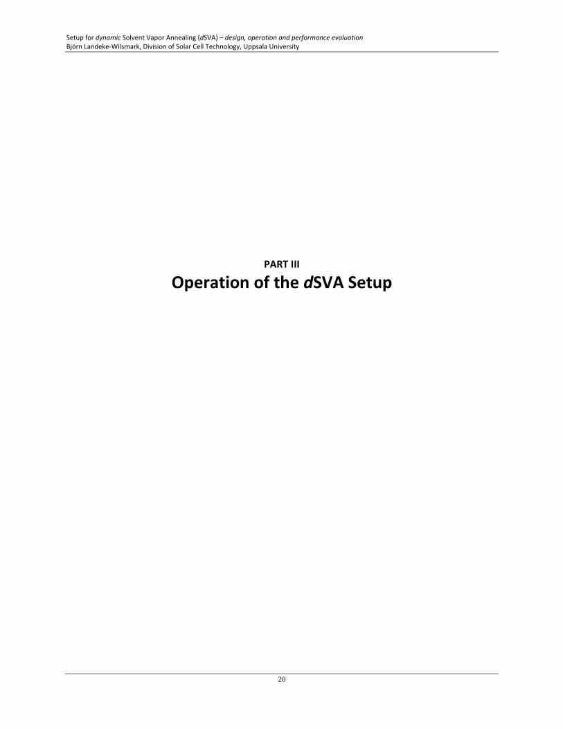
2.2.13 Protective Hood A ventilated protective hood, meant to house the reflectometer and the dSVA setup, was also constructed out of acrylic sheeting and Al profiles (Figure 11 and S13). The front sash can be raised to provide unhampered access during operation but as this is merely an added layer of protection, and not a proper fume hood, no open solvent handing is permitted within. On a practical note, only use water, ethanol or IPA to wipe away smudges, acetone will dissolve the acrylic.
Figure 11: Ventilated protective hood, with the front sash raised, containing all the components of the dSVA setup (except the reflectometer) (A) Module 2, (B) Module 3, (C) Module 1 and the temperature-controlled water bath and (D) the MFC control unit.
Technical drawings, for manufacturing, of all components of the dSVA chamber assembly are available in the Appendix (Figures S14-21).
D A B
C
Setup for dynamic Solvent Vapor Annealing (dSVA) – design, operation and performance evaluation Björn Landeke-Wilsmark, Division of Solar Cell Technology, Uppsala University
20
PART III
Operation of the dSVA Setup
Setup for dynamic Solvent Vapor Annealing (dSVA) – design, operation and performance evaluation Björn Landeke-Wilsmark, Division of Solar Cell Technology, Uppsala University
21
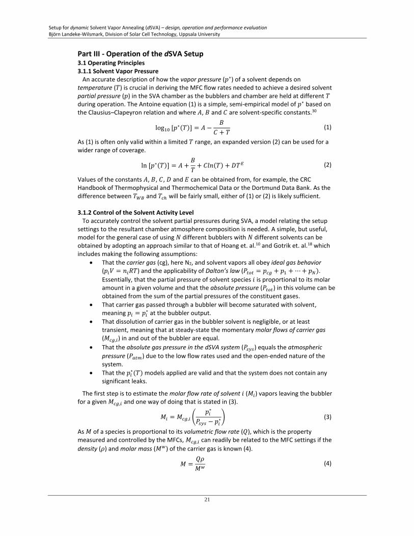
Part III - Operation of the dSVA Setup 3.1 Operating Principles 3.1.1 Solvent Vapor Pressure An accurate description of how the vapor pressure (𝑝∗) of a solvent depends on temperature (𝑇) is crucial in deriving the MFC flow rates needed to achieve a desired solvent partial pressure (𝑝) in the SVA chamber as the bubblers and chamber are held at different 𝑇 during operation. The Antoine equation (1) is a simple, semi-empirical model of 𝑝∗ based on the Clausius–Clapeyron relation and where 𝐴, 𝐵 and 𝐶 are solvent-specific constants.30
log10 [𝑝∗(𝑇)] = 𝐴 −
𝐵
𝐶 + 𝑇 (1)
As (1) is often only valid within a limited 𝑇 range, an expanded version (2) can be used for a wider range of coverage.
ln [𝑝∗(𝑇)] = 𝐴 +
𝐵
𝑇+ 𝐶𝑙𝑛(𝑇) + 𝐷𝑇𝐸 (2)
Values of the constants 𝐴, 𝐵, 𝐶, 𝐷 and 𝐸 can be obtained from, for example, the CRC Handbook of Thermophysical and Thermochemical Data or the Dortmund Data Bank. As the difference between 𝑇𝑊𝐵 and 𝑇𝑐ℎ will be fairly small, either of (1) or (2) is likely sufficient. 3.1.2 Control of the Solvent Activity Level To accurately control the solvent partial pressures during SVA, a model relating the setup settings to the resultant chamber atmosphere composition is needed. A simple, but useful, model for the general case of using 𝑁 different bubblers with 𝑁 different solvents can be obtained by adopting an approach similar to that of Hoang et. al.10 and Gotrik et. al.18 which includes making the following assumptions:
• That the carrier gas (cg), here N2, and solvent vapors all obey ideal gas behavior (𝑝𝑖𝑉 = 𝑛𝑖𝑅𝑇) and the applicability of Dalton’s law (𝑃𝑡𝑜𝑡 = 𝑝𝑐𝑔 + 𝑝1 + ⋯ + 𝑝𝑁).
Essentially, that the partial pressure of solvent species 𝑖 is proportional to its molar amount in a given volume and that the absolute pressure (𝑃𝑡𝑜𝑡) in this volume can be obtained from the sum of the partial pressures of the constituent gases.
• That carrier gas passed through a bubbler will become saturated with solvent, meaning 𝑝𝑖 = 𝑝𝑖
∗ at the bubbler output.
• That dissolution of carrier gas in the bubbler solvent is negligible, or at least transient, meaning that at steady-state the momentary molar flows of carrier gas (𝑀𝑐𝑔,𝑖) in and out of the bubbler are equal.
• That the absolute gas pressure in the dSVA system (𝑃𝑠𝑦𝑠) equals the atmospheric
pressure (𝑃𝑎𝑡𝑚) due to the low flow rates used and the open-ended nature of the system.
• That the 𝑝𝑖∗(𝑇) models applied are valid and that the system does not contain any
significant leaks.
The first step is to estimate the molar flow rate of solvent 𝑖 (𝑀𝑖) vapors leaving the bubbler for a given 𝑀𝑐𝑔,𝑖 and one way of doing that is stated in (3).
𝑀𝑖 = 𝑀𝑐𝑔,𝑖 (
𝑝𝑖∗
𝑃𝑠𝑦𝑠 − 𝑝𝑖∗) (3)
As 𝑀 of a species is proportional to its volumetric flow rate (𝑄), which is the property measured and controlled by the MFCs, 𝑀𝑐𝑔,𝑖 can readily be related to the MFC settings if the
density (𝜌) and molar mass (𝑀𝑤) of the carrier gas is known (4).
𝑀 =𝑄𝜌
𝑀𝑤 (4)
Setup for dynamic Solvent Vapor Annealing (dSVA) – design, operation and performance evaluation Björn Landeke-Wilsmark, Division of Solar Cell Technology, Uppsala University
22
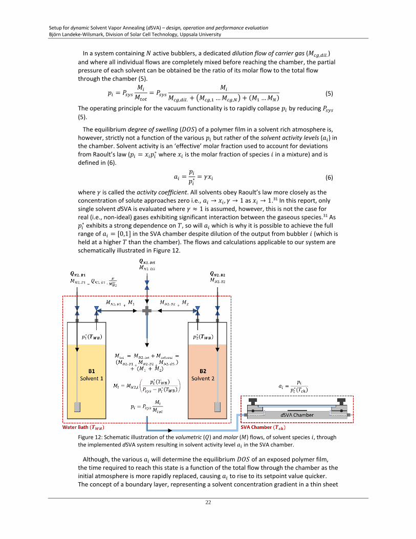
In a system containing 𝑁 active bubblers, a dedicated dilution flow of carrier gas (𝑀𝑐𝑔,𝑑𝑖𝑙.)
and where all individual flows are completely mixed before reaching the chamber, the partial pressure of each solvent can be obtained be the ratio of its molar flow to the total flow through the chamber (5).
𝑝𝑖 = 𝑃𝑠𝑦𝑠
𝑀𝑖
𝑀𝑡𝑜𝑡
= 𝑃𝑠𝑦𝑠
𝑀𝑖
𝑀𝑐𝑔,𝑑𝑖𝑙. + (𝑀𝑐𝑔,1 … 𝑀𝑐𝑔,𝑁) + (𝑀1 … 𝑀𝑁) (5)
The operating principle for the vacuum functionality is to rapidly collapse 𝑝𝑖 by reducing 𝑃𝑠𝑦𝑠
(5).
The equilibrium degree of swelling (𝐷𝑂𝑆) of a polymer film in a solvent rich atmosphere is, however, strictly not a function of the various 𝑝𝑖 but rather of the solvent activity levels (𝑎𝑖) in the chamber. Solvent activity is an ‘effective’ molar fraction used to account for deviations from Raoult’s law (𝑝𝑖 = 𝑥𝑖𝑝𝑖
∗ where 𝑥𝑖 is the molar fraction of species 𝑖 in a mixture) and is defined in (6).
𝑎𝑖 =
𝑝𝑖
𝑝𝑖∗ = 𝛾𝑥𝑖 (6)
where 𝛾 is called the activity coefficient. All solvents obey Raoult’s law more closely as the concentration of solute approaches zero i.e., 𝑎𝑖 → 𝑥𝑖 , 𝛾 → 1 as 𝑥𝑖 → 1.31 In this report, only single solvent dSVA is evaluated where 𝛾 ≈ 1 is assumed, however, this is not the case for real (i.e., non-ideal) gases exhibiting significant interaction between the gaseous species.31 As 𝑝𝑖
∗ exhibits a strong dependence on 𝑇, so will 𝑎𝑖 which is why it is possible to achieve the full range of 𝑎𝑖 = [0,1] in the SVA chamber despite dilution of the output from bubbler 𝑖 (which is held at a higher 𝑇 than the chamber). The flows and calculations applicable to our system are schematically illustrated in Figure 12.
Figure 12: Schematic illustration of the volumetric (𝑄) and molar (𝑀) flows, of solvent species 𝑖, through the implemented dSVA system resulting in solvent activity level 𝑎𝑖 in the SVA chamber.
Although, the various 𝑎𝑖 will determine the equilibrium 𝐷𝑂𝑆 of an exposed polymer film, the time required to reach this state is a function of the total flow through the chamber as the initial atmosphere is more rapidly replaced, causing 𝑎𝑖 to rise to its setpoint value quicker. The concept of a boundary layer, representing a solvent concentration gradient in a thin sheet
Setup for dynamic Solvent Vapor Annealing (dSVA) – design, operation and performance evaluation Björn Landeke-Wilsmark, Division of Solar Cell Technology, Uppsala University
23
above the sample surface, here due to a net absorption of solvent molecules into the polymer film, might also be applicable. A higher flow through the chamber equates to a higher gas flow velocity in the bulk of the chamber and the thickness of a boundary layer decreases with increasing bulk flow velocity.32 A thinner boundary layer means improved mass transport kinetics, a higher impingent flux of solvent molecules at the top surface and conceivably a more rapid solvent incorporation into the polymer film.
This setup thus enables independent, linear control of 𝑎𝑖 of two different solvents at different rates of total flow and to tailor startup and termination transients, all of which can be combined to create advanced SVA procedures. 3.2 In-situ Spectroscopic Reflectometry As the size and pitch of the nanodomains in self-assembled BCP films are far smaller than the wavelength of light in the visual part of the EM spectrum, optical microscopy cannot be used to study the self-assembly dynamics. Spectroscopic reflectometry (SR) can, however, measure the evolution of the instantaneous polymer film thickness [ℎ(𝑡)] at time 𝑡 during SVA and by extension 𝐷𝑂𝑆 ≡ ℎ(𝑡)/ℎ0, where ℎ0 is the initial thickness of the unswollen film. As 𝐷𝑂𝑆 is directly related to the amount of solvent in the film, which in turn affects polymer chain mobility, interactions between polymer blocks, interfacial conditions etc. the hope is that certain combinations of ℎ0 and 𝐷𝑂𝑆 can be associated with favorable annealing conditions leading to the sought self-assembled structures. In-situ optical process monitoring could then be used to ensure a high degree of reproducibility. Monitoring can be done either on the BCP sample itself or on a homopolymer indicator sample included in the chamber during the run.
In-situ SR involves the introduction of the inspection window in the optical path, fortunately the effects of this are compensated for during calibration of the equipment. During calibration two reference spectra are acquired by measuring the reflected light from the polished frontside and the rough backside of a Si(100) substrate, respectively. The first represent an identical sample except for the polymer film and also allow for adjustment of the power fed to the lamp to maximize the intensity without saturating the CCD detector. The second, ‘dark’ measurement is taken on a strongly scattering surface to account for the background illumination. The large area of the annealing volume allows reference pieces to be included even when annealing a full 100 mm wafer.
The thickness, ℎ is obtained through an iterative procedure in which a model, containing the complex refractive index (�̃� = 𝑛 + 𝑖𝑘) of the layer material, is fitted to the measurement data. Although ℎ and �̃� can be fitted simultaneously in the SR software (VisualThick 3), we have thus far obtained �̃� using spectroscopic ellipsometry (J. A. Woollam, M2000VI) and then exported the optical material properties to the reflectometer beforehand.
The reflectometer software unfortunately lacks a native recording function which is important to be able to study the dynamic swelling behavior over time. Recording can, however, be achieved without modifying the source code by using additional software to simulate keyboard inputs to initiate measurements at a stated time interval. The results are saved in a temporary list, containing maximum 200 entries, in the reflectometer software and then (by yet other simulated inputs) periodically exported to a sequence of files. AutoHotkey which is a free, open-source scripting language is used to simulate keyboard inputs here. In AutoHotkey it should be possible to send commands to a specific window but our script requires that the reflectometer program is the active window on the desktop during recording (see Appendix). Note, the recorded time stamps of the measurements are believed to refer to when the iterative calculations are done rather than the time of the data acquisition.
Setup for dynamic Solvent Vapor Annealing (dSVA) – design, operation and performance evaluation Björn Landeke-Wilsmark, Division of Solar Cell Technology, Uppsala University
24
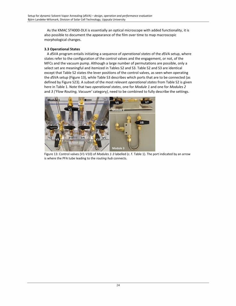
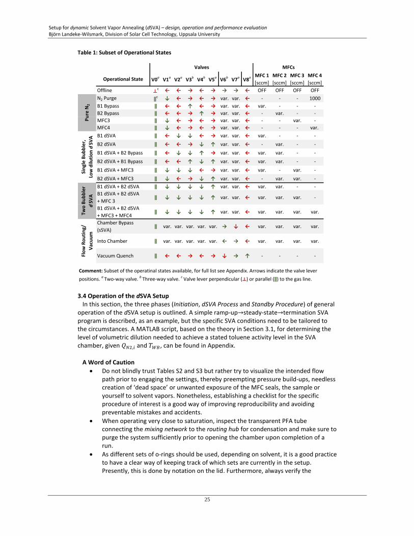
As the KMAC ST4000-DLX is essentially an optical microscope with added functionality, it is also possible to document the appearance of the film over time to map macroscopic morphological changes. 3.3 Operational States A dSVA program entails initiating a sequence of operational states of the dSVA setup, where states refer to the configuration of the control valves and the engagement, or not, of the MFCs and the vacuum pump. Although a large number of permutations are possible, only a select set are meaningful and itemized in Tables S2 and S3. Table S2 and S3 are identical except that Table S2 states the lever positions of the control valves, as seen when operating the dSVA setup (Figure 13), while Table S3 describes which ports that are to be connected (as defined by Figure S23). A subset of the most relevant operational states from Table S2 is given here in Table 1. Note that two operational states, one for Module 1 and one for Modules 2 and 3 (‘Flow Routing, Vacuum’ category), need to be combined to fully describe the settings.
Figure 13: Control valves (V1-V10) of Modules 1-3 labelled (c. f. Table 1). The port indicated by an arrow is where the PFA tube leading to the routing hub connects.
Module 1
Module 2
Module 3
V1
V2 V3 V4 V5 V9 V10
V6 V7
V8
Setup for dynamic Solvent Vapor Annealing (dSVA) – design, operation and performance evaluation Björn Landeke-Wilsmark, Division of Solar Cell Technology, Uppsala University
25
Table 1: Subset of Operational States
3.4 Operation of the dSVA Setup In this section, the three phases (Initiation, dSVA Process and Standby Procedure) of general operation of the dSVA setup is outlined. A simple ramp-up→steady-state→termination SVA program is described, as an example, but the specific SVA conditions need to be tailored to the circumstances. A MATLAB script, based on the theory in Section 3.1, for determining the level of volumetric dilution needed to achieve a stated toluene activity level in the SVA chamber, given 𝑄𝑁2,𝑖 and 𝑇𝑊𝐵, can be found in Appendix.
A Word of Caution
• Do not blindly trust Tables S2 and S3 but rather try to visualize the intended flow path prior to engaging the settings, thereby preempting pressure build-ups, needless creation of ‘dead space’ or unwanted exposure of the MFC seals, the sample or yourself to solvent vapors. Nonetheless, establishing a checklist for the specific procedure of interest is a good way of improving reproducibility and avoiding preventable mistakes and accidents.
• When operating very close to saturation, inspect the transparent PFA tube connecting the mixing network to the routing hub for condensation and make sure to purge the system sufficiently prior to opening the chamber upon completion of a run.
• As different sets of o-rings should be used, depending on solvent, it is a good practice to have a clear way of keeping track of which sets are currently in the setup. Presently, this is done by notation on the lid. Furthermore, always verify the
Operational State V0a V1a V2a V3b V4b V5a V6b V7a V8a MFC 1
[sccm]
MFC 2
[sccm]
MFC 3
[sccm]
MFC 4
[sccm]
Offline ⟂c ← ← → ← → → → ← OFF OFF OFF OFF
N2 Purge ‖c ↓ ← → ← → var. var. ← - - - 1000
B1 Bypass ‖ ← ← ↑ ← → var. var. ← var. - - -
B2 Bypass ‖ ← ← → ↑ → var. var. ← - var. - -
MFC3 ‖ ↓ ← → ← → var. var. ← - - var. -
MFC4 ‖ ↓ ← → ← → var. var. ← - - - var.
B1 dSVA ‖ ← ↓ ↓ ← → var. var. ← var. - - -
B2 dSVA ‖ ← ← → ↓ ↑ var. var. ← - var. - -
B1 dSVA + B2 Bypass ‖ ← ↓ ↓ ↑ → var. var. ← var. var. - -
B2 dSVA + B1 Bypass ‖ ← ← ↑ ↓ ↑ var. var. ← var. var. - -
B1 dSVA + MFC3 ‖ ↓ ↓ ↓ ← → var. var. ← var. - var. -
B2 dSVA + MFC3 ‖ ↓ ← → ↓ ↑ var. var. ← - var. var. -
B1 dSVA + B2 dSVA ‖ ↓ ↓ ↓ ↓ ↑ var. var. ← var. var. - -
B1 dSVA + B2 dSVA
+ MFC 3‖ ↓ ↓ ↓ ↓ ↑ var. var. ← var. var. var. -
B1 dSVA + B2 dSVA
+ MFC3 + MFC4‖ ↓ ↓ ↓ ↓ ↑ var. var. ← var. var. var. var.
Chamber Bypass
(sSVA)‖ var. var. var. var. var. → ↓ ← var. var. var. var.
Into Chamber ‖ var. var. var. var. var. ← → ← var. var. var. var.
Vacuum Quench ‖ ← ← → ← → ↓ → ↑ - - - -
Valves MFCs
Pu
re N
2Si
ngl
e B
ub
ble
r,
Low
dilu
tio
n d
SVA
Two
Bu
bb
ler
dSV
A
Flo
w R
ou
tin
g/
Vac
uu
m
Comment: Subset of the operatinal states available, for full list see Appendix. Arrows indicate the valve lever
positions. a Two-way valve. b Three-way valve. c Valve lever perpendicular (⟂) or parallel (‖) to the gas line.
Setup for dynamic Solvent Vapor Annealing (dSVA) – design, operation and performance evaluation Björn Landeke-Wilsmark, Division of Solar Cell Technology, Uppsala University
26
chemical compatibility of the o-rings (and other wetted components/surfaces) when introducing a new solvent. Damaged seals can entail leakage and solvent exposure.
• If the intention is to use the vacuum functionality, mount the 6.5 mm thick glass inspection window or the Al window insert in the lid prior to the run.
• Adhere to common sense safety guidelines in all aspects of solvent handling e.g., adequate ventilation, personal protection equipment (PPE) etc. The ventilated protective hood around the setup is not a fume hood, just an added (unverified) layer of protection.
3.4.1 Phase 1: Initialization STEP Action I1 Turn on the MFC control unit, some MFCs require a 30 min warmup time during which
steps I2-I15 can be performed. I2 Open valve V0 to access the N2 supply. I3 Fill the water bath, with tap water, up to the underside of the acrylic sheet on which
valves V2-V5 are mounted, thus ensuring that the mixing network and the relevant valve housings are completely immersed.
I4 Place the circulation heater font and center on the water bath vessel wall facing you. Turn on the circulation heater and set the desired setpoint for 𝑇𝑊𝐵. Once the correct temperature is reached, let it stabilize for at least 10 min before starting the dSVA process.
I5 Remove the chamber lid and, if necessary, clean the inspection window with absolute ethanol or IPA. Place the lid off to the side.
I6 Raise the K-MAC ST4000-DLX microscope objective as far as possible and remove the stage inserts, see Figure S3b.
I7 Carefully place Module 2 (without chamber lid) on the reflectometer stage. Let it rest on the acrylic glass plate on the bottom and gently slide the unit in under the objective lens until the plate locks into the corresponding hole in the stage, thereby immobilizing the module.
I8 Load the samples, including those for calibration of reflectometer. I9 Mount and fasten the chamber lid. Note that not much force is needed and be careful
not to collide with one of the objective lenses. I10 Start the VisualThick software, lower the objective lens, position the measurement
spot by moving the stage, find focus, choose Sample Model and perform the calibration. Position the measurement spot on the desired location on your sample or an indicator sample clad with a suitable homopolymer.
I11 Purge the entire system, including the chamber, with 1000 sccm N2 for at least 2 min (operational states ‘N2 Purge’ + ‘Into Chamber’).
I12 Use a calibrated thermometer with high resolution, accuracy and precision, in our case a Pt-100 RTD temperature probe, to ascertain 𝑇𝑐ℎ and 𝑇𝑊𝐵 (in that order). Note, 𝑇𝑐ℎ is estimated by placing the probe along the outside wall of the dSVA chamber, the high thermal conductivity of Al ought to make this a decent proxy. Be aware of the response time of your instrument.
I13 Input the recorded temperatures in a MATLAB script or use the printed Look-Up Tables (LUTs) to obtain the dilution flow required to obtain the desired solvent activity level.
I14 Modify the relevant lines (e.g. ‘SampleName’, ‘Nbr_F’, ‘Nbr_M,M_Interval’) in the AutoHotkey script. Run the script.
I15 Open the VisualThick software window and, if desired, clear the list and change Sample Name and Number. The sequence of automated, repeated measurements is initiated by the keyboard command ctrl + alt + b and is ended by ctrl + alt + s or after a set number of measurements. Note, to record, the VisualThick window needs to be the ‘active’ window. Do not begin recording until after step P2.
Setup for dynamic Solvent Vapor Annealing (dSVA) – design, operation and performance evaluation Björn Landeke-Wilsmark, Division of Solar Cell Technology, Uppsala University
27
3.4.2 Phase 2: dSVA Process STEP Action P1 End the N2 purge, in step I11, after ≥2 min. Engage ‘Chamber Bypass’ and the desired
operational state e.g., ‘B1 dSVA + B2 Bypass’, with the specific MFC settings for your dSVA process. Always adjust the valves before initiating the MFC flows. The mixed flow is now diverted around the chamber which is a good way of making sure a steady-state output from the mixing network is achieved and that this new gas mixture has replaced the purging N2 in the gas delivery system. The duration of this step depends on the total volumetric gas flow but for total flow rates of ≥100 sccm, 2 min is typically used.
P2 Start the SVA process by switching the routing hub from ‘Chamber Bypass’ to ‘Into Chamber’ and make sure to adjust valve V7 before V6 to avoid a pressure build-up. Use the AutoHotkey command (ctrl + alt + b) to start the sequence of measurements and let the process run for the desired amount of time. Note the change in sample appearance as the polymer film swells.
P3 Terminate the SVA process either by quenching (e.g., ‘N2 Purge’ or ‘Vacuum Quench’) or a slower, more controlled solvent activity ramp-down (e.g., ‘MFC3’, ‘B1 Bypass’ or ‘B2 Bypass’). The duration depends on termination method and examining the polymer film appearance or 𝐷𝑂𝑆 is indicative. Thus far ‘B1 Bypass’ is the most frequently used option.
P4 Switch to operational mode ‘N2 Purge’ (+ ‘Into Chamber’) and purge the system with N2 for ≥2 min. This is a safety precaution to minimize the risk of operator exposure to residual solvent vapors. The duration depends on the toxicity of the solvent, the ventilation in the surrounding environment, the used 𝑎𝑖 etc.
P5 As 𝑎𝑖 is a function of 𝑇𝑊𝐵 and 𝑇𝑐ℎ, it is a good practice to re-measure and note, at least, 𝑇𝑐ℎ while purging the system.
P6 Terminate the recording of measurements with the keyboard command ctrl + alt + s or by right-clicking on the AutoHotkey icon in the Windows taskbar (lower right corner).
P7 To unload your sample(s), raise the objective lens, slide the stage towards you until it reaches its end position, release the lid fastening assemblies and gently remove the lid. Note that the o-ring can loosely stick to the glass.
P8 Always log the details of each dSVA run, including 𝑇𝑊𝐵, 𝑇𝑐ℎ, active MFC flows and termination procedure settings.
P9 To initiate a new run start at step I8. To avoid accidentally overwriting data files, modify the AutoHotkey script to state a new sample name (or dSVA run identifier).
3.4.3 Phase 3: Standby Procedure After completion of the last dSVA run, the standby procedure should be initiated. STEP Action S1 Set the system to operational state ‘Offline’. S2 Turn off the circulation heater and relocate it to one of the short edges of the water
bath vessel. S3 Turn off the MFC control unit. S4 Empty the water bath using, for example, plastic beakers or a siphon. The water can
be disposed of in the fume hood sink. S5 Make sure the objective is raised as far as possible and that the chamber lid is
removed. Move the stage to the end position towards you and lift the edge (closest to the operator) of the Module 2 Al base plate and gently pull forward until the edge of the acrylic glass plate pops out of the hole in the stage. The entire module can then be slid, along the plane of the stage, out from under the objective lens. Restore the initial state of the reflectometer by reinserting the stage inserts and lower the objective lens to an appropriate location. Re-mount the lid on the chamber.
Setup for dynamic Solvent Vapor Annealing (dSVA) – design, operation and performance evaluation Björn Landeke-Wilsmark, Division of Solar Cell Technology, Uppsala University
28
S6 The pressurized air supply and the power to the circulator and MFC control unit can be disconnected as an added precaution.
Note: If in-situ film thickness monitoring is not necessary, then obviously skip steps I5-7, I10, I14, I15, P6 and S6. 3.5 Procedure for Filling/Emptying Bubblers When emptying or filling the bubblers of solvent, move Module 1 into a solvent fume hood. This involves closing valve V0 and disconnecting (i) the MFC electrical connectors, (ii) the N2 supply using the quick-release connector on the backside and (iii) the PFA tube (close to V1) leading to the routing hub. Once in the fume hood, studiously wrap all exposed acrylic surfaces with ‘cling film’ – it exhibits excellent chemical resistance against many solvents, unlike the acrylic sheeting in the structural framework (Figure S24a).
There are two ways of accessing the solvent in the bubblers, through the ‘periscopes’ or via the capped port on the sight glass valves (valves V9 and V10). Periscope access is obtained by removing the Swagelok brass cap at the top end, which is done with two wrenches.
To empty a bubbler via the periscope, a siphon, consisting of a length of 1/8” SS pipe attached in one end to a PFA tube, is used (Figure S25). The 1/8” pipe is threaded through the 6 mm (in diameter) periscope into the bubbler and a large syringe or micropipette is used to draw solvent up into the pipe and tube until a self-sustaining, gravity driven flow is obtained (see Table S2 for the relevant operational state). The other, arguably safer option, involves attaching a PFA (or FEP) tube to the unused port of valve V9 or V10, adjusting the valve position and again use siphoning or suction to empty the bubbler (Table S2). In either case, before removing the solvent make sure to establish a free path between the bubbler output and the surrounding atmosphere to allow incoming air to replace the solvent volume. If possible, run some N2 through the bubbler input to displace any solvent in the descending pipe. Remove all residual solvent in the bubbler by flushing it with N2 or leaving the periscope port open in the fume hood for a sufficiently long time. Flushing can be performed using the MFCs (once Module 1 is reconnected) or by connecting either the open end of the PFA tube of the siphoning tool or the sight glass valve to the N2 supply. By connecting directly to the N2 supply we can have flows measured in standard liters per minute (slm) rather than sccm and hence the drying process is substantially faster. When drying, it is better to be excessive as you do not want residual solvent to mix with the new one.
Filling a bubbler via the periscope opening is done using either a syringe or a small funnel (a micropipette tip for a 10 ml device works well, see Figure S24b). The capacity of the bubblers is approx. 250 ml. Again, make sure the outlet is open to allow the air inside to be replaced.
After emptying/filling the bubblers, reseal the periscope or the sight glass valve port and make sure to counteract the torque with a stationary wrench. Lastly, isolate the bubblers using the appropriate valves, return V9 and V10 to their previous positions, remove the protective plastic film and reconnect Module 1 with the rest of the dSVA setup. 3.6 Performance Evaluation of the dSVA Setup As mentioned in Section 3.1, we can target an arbitrary 𝑎𝑖 in the dSVA chamber by having a good approximation of 𝑝𝑖
∗(𝑇), knowing 𝑇𝑐ℎ, and judiciously choosing 𝑇𝑊𝐵 and the MFC flow rates. However, the predictions involved several assumptions and hence it is important to evaluate the performance of the system and determine how the setpoint solvent activity level (𝑎𝑠𝑒𝑡𝑢𝑝) compares to the actual 𝑎𝑖 in the chamber. For some solvents this could be done by
means of IR spectroscopy but it requires equipment we do not have at hand. Instead, excerpts from the Flory-Huggins theory of polymer solutions can be used to relate 𝑎𝑖 above the sample to the volume fraction of polymer (𝜙𝑝) in a solvent-swollen film at equilibrium
conditions (7).33
Setup for dynamic Solvent Vapor Annealing (dSVA) – design, operation and performance evaluation Björn Landeke-Wilsmark, Division of Solar Cell Technology, Uppsala University
29
ln(𝑎𝑖) = ln(1 − 𝜙𝑝) + (1 −
1
𝑟) 𝜙𝑝 + 𝜒𝑖,𝑝𝜙𝑝
2 (7)
Here indices ‘𝑖’ and ‘𝑝’ are used for solvent and polymer, respectively, and 𝑟 is the number of solvent equivalent segments in the polymer chain. The Flory-Huggins interaction parameter (𝜒𝑖,𝑝) is a unitless quantity that represents the interaction energy per solvent molecule
divided by 𝑘𝑇 (𝑘 being the Boltzmann constant).33 For a real polymer sample, 𝑟 can be taken to be the number average degree of polymerization, �̅� = 𝑀𝑛/𝑀0 where 𝑀𝑛 is the number average molecular weight and 𝑀0 is the molecular weight of the repeating unit. As 𝑟 is large for most polymers, (7) can be reduced to (8).
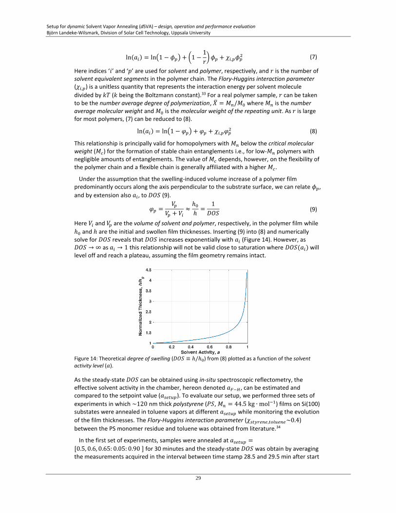
ln(𝑎𝑖) = ln(1 − 𝜑𝑝) + 𝜑𝑝 + 𝜒𝑖,𝑝𝜑𝑝
2 (8)
This relationship is principally valid for homopolymers with 𝑀𝑛 below the critical molecular weight (𝑀𝑐) for the formation of stable chain entanglements i.e., for low-𝑀𝑛 polymers with negligible amounts of entanglements. The value of 𝑀𝑐 depends, however, on the flexibility of the polymer chain and a flexible chain is generally affiliated with a higher 𝑀𝑐.
Under the assumption that the swelling-induced volume increase of a polymer film predominantly occurs along the axis perpendicular to the substrate surface, we can relate 𝜙𝑝,
and by extension also 𝑎𝑖, to 𝐷𝑂𝑆 (9).
𝜑𝑝 =𝑉𝑝
𝑉𝑝 + 𝑉𝑖
≈ℎ0
ℎ=
1
𝐷𝑂𝑆 (9)
Here 𝑉𝑖 and 𝑉𝑝 are the volume of solvent and polymer, respectively, in the polymer film while
ℎ0 and ℎ are the initial and swollen film thicknesses. Inserting (9) into (8) and numerically solve for 𝐷𝑂𝑆 reveals that 𝐷𝑂𝑆 increases exponentially with 𝑎𝑖 (Figure 14). However, as 𝐷𝑂𝑆 → ∞ as 𝑎𝑖 → 1 this relationship will not be valid close to saturation where 𝐷𝑂𝑆(𝑎𝑖) will level off and reach a plateau, assuming the film geometry remains intact.
Figure 14: Theoretical degree of swelling (𝐷𝑂𝑆 ≡ ℎ/ℎ0) from (8) plotted as a function of the solvent activity level (𝑎).
As the steady-state 𝐷𝑂𝑆 can be obtained using in-situ spectroscopic reflectometry, the effective solvent activity in the chamber, hereon denoted 𝑎𝐹−𝐻, can be estimated and compared to the setpoint value (𝑎𝑠𝑒𝑡𝑢𝑝). To evaluate our setup, we performed three sets of
experiments in which ~120 nm thick polystyrene (𝑃𝑆, 𝑀𝑛 = 44.5 kg ∙ mol−1) films on Si(100) substates were annealed in toluene vapors at different 𝑎𝑠𝑒𝑡𝑢𝑝 while monitoring the evolution
of the film thicknesses. The Flory-Huggins interaction parameter (𝜒𝑠𝑡𝑦𝑟𝑒𝑛𝑒,𝑡𝑜𝑙𝑢𝑒𝑛𝑒~0.4)
between the PS monomer residue and toluene was obtained from literature.34
In the first set of experiments, samples were annealed at 𝑎𝑠𝑒𝑡𝑢𝑝 =
[0.5, 0.6, 0.65: 0.05: 0.90 ] for 30 minutes and the steady-state 𝐷𝑂𝑆 was obtain by averaging the measurements acquired in the interval between time stamp 28.5 and 29.5 min after start
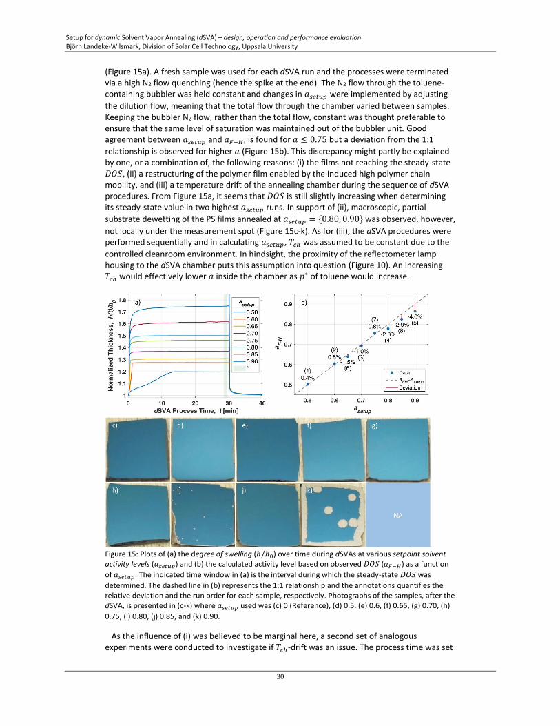
Setup for dynamic Solvent Vapor Annealing (dSVA) – design, operation and performance evaluation Björn Landeke-Wilsmark, Division of Solar Cell Technology, Uppsala University
30
(Figure 15a). A fresh sample was used for each dSVA run and the processes were terminated via a high N2 flow quenching (hence the spike at the end). The N2 flow through the toluene-containing bubbler was held constant and changes in 𝑎𝑠𝑒𝑡𝑢𝑝 were implemented by adjusting
the dilution flow, meaning that the total flow through the chamber varied between samples. Keeping the bubbler N2 flow, rather than the total flow, constant was thought preferable to ensure that the same level of saturation was maintained out of the bubbler unit. Good agreement between 𝑎𝑠𝑒𝑡𝑢𝑝 and 𝑎𝐹−𝐻, is found for 𝑎 ≤ 0.75 but a deviation from the 1:1
relationship is observed for higher 𝑎 (Figure 15b). This discrepancy might partly be explained by one, or a combination of, the following reasons: (i) the films not reaching the steady-state 𝐷𝑂𝑆, (ii) a restructuring of the polymer film enabled by the induced high polymer chain mobility, and (iii) a temperature drift of the annealing chamber during the sequence of dSVA procedures. From Figure 15a, it seems that 𝐷𝑂𝑆 is still slightly increasing when determining its steady-state value in two highest 𝑎𝑠𝑒𝑡𝑢𝑝 runs. In support of (ii), macroscopic, partial
substrate dewetting of the PS films annealed at 𝑎𝑠𝑒𝑡𝑢𝑝 = {0.80, 0.90} was observed, however,
not locally under the measurement spot (Figure 15c-k). As for (iii), the dSVA procedures were performed sequentially and in calculating 𝑎𝑠𝑒𝑡𝑢𝑝, 𝑇𝑐ℎ was assumed to be constant due to the
controlled cleanroom environment. In hindsight, the proximity of the reflectometer lamp housing to the dSVA chamber puts this assumption into question (Figure 10). An increasing 𝑇𝑐ℎ would effectively lower 𝑎 inside the chamber as 𝑝∗ of toluene would increase.
Figure 15: Plots of (a) the degree of swelling (ℎ/ℎ0) over time during dSVAs at various setpoint solvent activity levels (𝑎𝑠𝑒𝑡𝑢𝑝) and (b) the calculated activity level based on observed 𝐷𝑂𝑆 (𝑎𝐹−𝐻) as a function
of 𝑎𝑠𝑒𝑡𝑢𝑝. The indicated time window in (a) is the interval during which the steady-state 𝐷𝑂𝑆 was
determined. The dashed line in (b) represents the 1:1 relationship and the annotations quantifies the relative deviation and the run order for each sample, respectively. Photographs of the samples, after the dSVA, is presented in (c-k) where 𝑎𝑠𝑒𝑡𝑢𝑝 used was (c) 0 (Reference), (d) 0.5, (e) 0.6, (f) 0.65, (g) 0.70, (h)
0.75, (i) 0.80, (j) 0.85, and (k) 0.90.
As the influence of (i) was believed to be marginal here, a second set of analogous experiments were conducted to investigate if 𝑇𝑐ℎ-drift was an issue. The process time was set
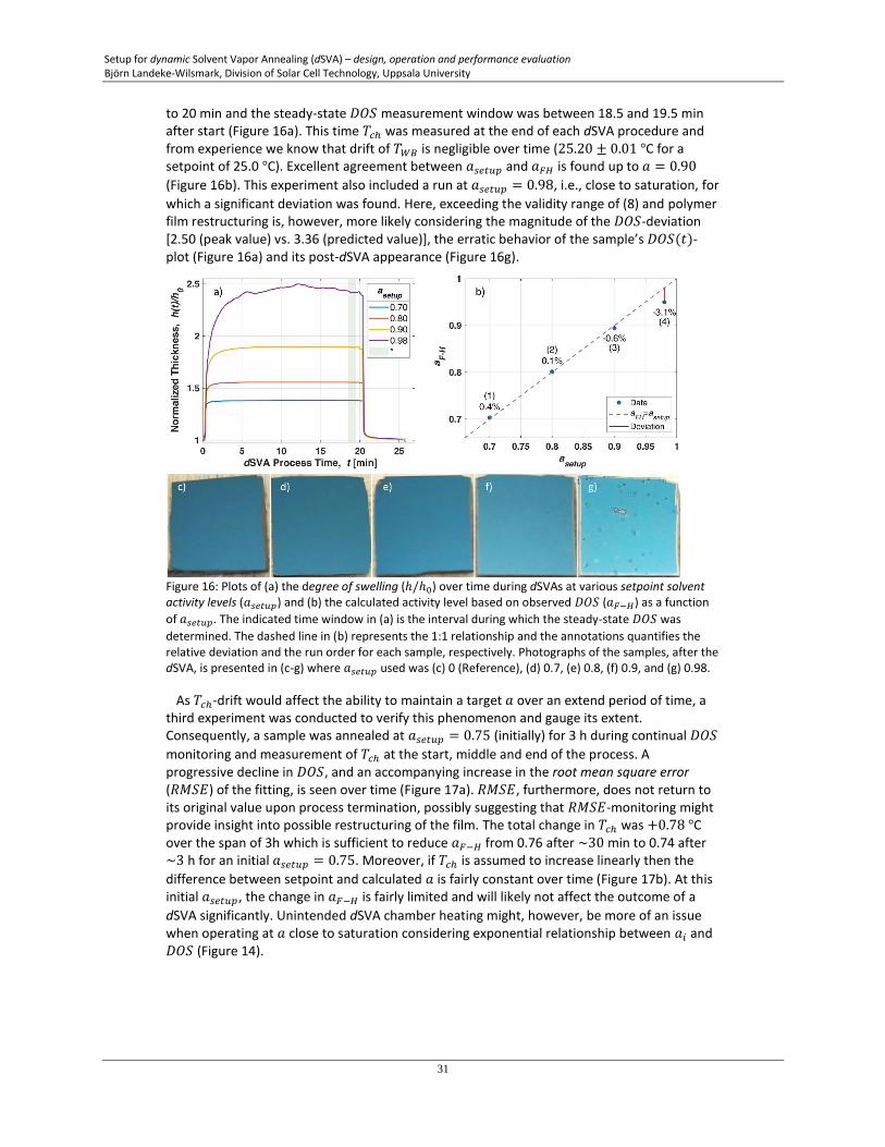
Setup for dynamic Solvent Vapor Annealing (dSVA) – design, operation and performance evaluation Björn Landeke-Wilsmark, Division of Solar Cell Technology, Uppsala University
31
to 20 min and the steady-state 𝐷𝑂𝑆 measurement window was between 18.5 and 19.5 min after start (Figure 16a). This time 𝑇𝑐ℎ was measured at the end of each dSVA procedure and from experience we know that drift of 𝑇𝑊𝐵 is negligible over time (25.20 ± 0.01 °C for a setpoint of 25.0 °C). Excellent agreement between 𝑎𝑠𝑒𝑡𝑢𝑝 and 𝑎𝐹𝐻 is found up to 𝑎 = 0.90
(Figure 16b). This experiment also included a run at 𝑎𝑠𝑒𝑡𝑢𝑝 = 0.98, i.e., close to saturation, for
which a significant deviation was found. Here, exceeding the validity range of (8) and polymer film restructuring is, however, more likely considering the magnitude of the 𝐷𝑂𝑆-deviation [2.50 (peak value) vs. 3.36 (predicted value)], the erratic behavior of the sample’s 𝐷𝑂𝑆(𝑡)-plot (Figure 16a) and its post-dSVA appearance (Figure 16g).
Figure 16: Plots of (a) the degree of swelling (ℎ/ℎ0) over time during dSVAs at various setpoint solvent activity levels (𝑎𝑠𝑒𝑡𝑢𝑝) and (b) the calculated activity level based on observed 𝐷𝑂𝑆 (𝑎𝐹−𝐻) as a function
of 𝑎𝑠𝑒𝑡𝑢𝑝. The indicated time window in (a) is the interval during which the steady-state 𝐷𝑂𝑆 was
determined. The dashed line in (b) represents the 1:1 relationship and the annotations quantifies the relative deviation and the run order for each sample, respectively. Photographs of the samples, after the dSVA, is presented in (c-g) where 𝑎𝑠𝑒𝑡𝑢𝑝 used was (c) 0 (Reference), (d) 0.7, (e) 0.8, (f) 0.9, and (g) 0.98.
As 𝑇𝑐ℎ-drift would affect the ability to maintain a target 𝑎 over an extend period of time, a third experiment was conducted to verify this phenomenon and gauge its extent. Consequently, a sample was annealed at 𝑎𝑠𝑒𝑡𝑢𝑝 = 0.75 (initially) for 3 h during continual 𝐷𝑂𝑆
monitoring and measurement of 𝑇𝑐ℎ at the start, middle and end of the process. A progressive decline in 𝐷𝑂𝑆, and an accompanying increase in the root mean square error (𝑅𝑀𝑆𝐸) of the fitting, is seen over time (Figure 17a). 𝑅𝑀𝑆𝐸, furthermore, does not return to its original value upon process termination, possibly suggesting that 𝑅𝑀𝑆𝐸-monitoring might provide insight into possible restructuring of the film. The total change in 𝑇𝑐ℎ was +0.78 °C over the span of 3h which is sufficient to reduce 𝑎𝐹−𝐻 from 0.76 after ~30 min to 0.74 after ~3 h for an initial 𝑎𝑠𝑒𝑡𝑢𝑝 = 0.75. Moreover, if 𝑇𝑐ℎ is assumed to increase linearly then the
difference between setpoint and calculated 𝑎 is fairly constant over time (Figure 17b). At this initial 𝑎𝑠𝑒𝑡𝑢𝑝, the change in 𝑎𝐹−𝐻 is fairly limited and will likely not affect the outcome of a
dSVA significantly. Unintended dSVA chamber heating might, however, be more of an issue when operating at 𝑎 close to saturation considering exponential relationship between 𝑎𝑖 and 𝐷𝑂𝑆 (Figure 14).
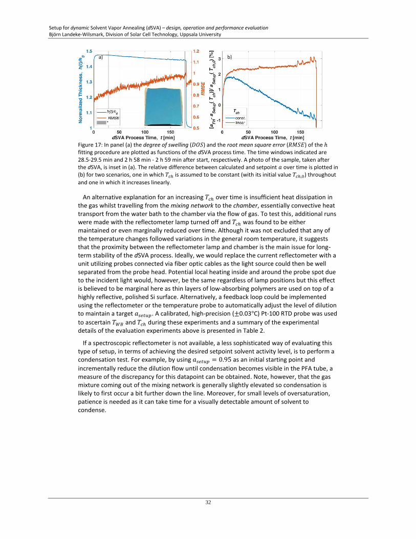
Setup for dynamic Solvent Vapor Annealing (dSVA) – design, operation and performance evaluation Björn Landeke-Wilsmark, Division of Solar Cell Technology, Uppsala University
32
Figure 17: In panel (a) the degree of swelling (𝐷𝑂𝑆) and the root mean square error (𝑅𝑀𝑆𝐸) of the ℎ fitting procedure are plotted as functions of the dSVA process time. The time windows indicated are 28.5-29.5 min and 2 h 58 min - 2 h 59 min after start, respectively. A photo of the sample, taken after the dSVA, is inset in (a). The relative difference between calculated and setpoint 𝑎 over time is plotted in (b) for two scenarios, one in which 𝑇𝑐ℎ is assumed to be constant (with its initial value 𝑇𝑐ℎ,0) throughout
and one in which it increases linearly.
An alternative explanation for an increasing 𝑇𝑐ℎ over time is insufficient heat dissipation in the gas whilst travelling from the mixing network to the chamber, essentially convective heat transport from the water bath to the chamber via the flow of gas. To test this, additional runs were made with the reflectometer lamp turned off and 𝑇𝑐ℎ was found to be either maintained or even marginally reduced over time. Although it was not excluded that any of the temperature changes followed variations in the general room temperature, it suggests that the proximity between the reflectometer lamp and chamber is the main issue for long-term stability of the dSVA process. Ideally, we would replace the current reflectometer with a unit utilizing probes connected via fiber optic cables as the light source could then be well separated from the probe head. Potential local heating inside and around the probe spot due to the incident light would, however, be the same regardless of lamp positions but this effect is believed to be marginal here as thin layers of low-absorbing polymers are used on top of a highly reflective, polished Si surface. Alternatively, a feedback loop could be implemented using the reflectometer or the temperature probe to automatically adjust the level of dilution to maintain a target 𝑎𝑠𝑒𝑡𝑢𝑝. A calibrated, high-precision (±0.03°C) Pt-100 RTD probe was used
to ascertain 𝑇𝑊𝐵 and 𝑇𝑐ℎ during these experiments and a summary of the experimental details of the evaluation experiments above is presented in Table 2.
If a spectroscopic reflectometer is not available, a less sophisticated way of evaluating this type of setup, in terms of achieving the desired setpoint solvent activity level, is to perform a condensation test. For example, by using 𝑎𝑠𝑒𝑡𝑢𝑝 = 0.95 as an initial starting point and
incrementally reduce the dilution flow until condensation becomes visible in the PFA tube, a measure of the discrepancy for this datapoint can be obtained. Note, however, that the gas mixture coming out of the mixing network is generally slightly elevated so condensation is likely to first occur a bit further down the line. Moreover, for small levels of oversaturation, patience is needed as it can take time for a visually detectable amount of solvent to condense.
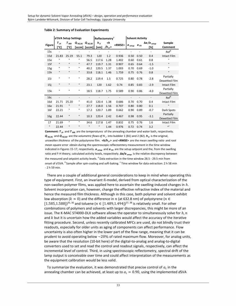
Setup for dynamic Solvent Vapor Annealing (dSVA) – design, operation and performance evaluation Björn Landeke-Wilsmark, Division of Solar Cell Technology, Uppsala University
33
Table 2: Summary of Evaluation Experiments
There are a couple of additional general considerations to keep in mind when operating this type of equipment. First, an invariant �̃�-model, derived from optical characterization of the non-swollen polymer films, was applied here to ascertain the swelling-induced changes in ℎ. Solvent incorporation can, however, change the effective refractive index of the material and hence the measured film thickness. Although in this case, both polymer and solvent exhibit low absorption (𝑘 ≈ 0) and the difference in 𝑛 (at 632.8 nm) of polystyrene (𝑛 ∈[1.585,1.588])35, 36 and toluene (𝑛 ∈ [1.489,1.494])37, 38 is relatively small. For other combinations of polymers and solvents with larger discrepancies, this might be more of an issue. The K-MAC ST4000-DLX software allows the operator to simultaneously solve for ℎ, 𝑛 and 𝑘 but it is uncertain how the added variables would affect the accuracy of the iterative fitting procedure. Second, unless recently calibrated MFCs are used, do not blindly trust their readouts, especially for older units as aging of components can affect performance. Flow uncertainty is also often higher in the lower part of the flow range, meaning that it can be prudent to avoid operating below ~20% of rated maximum flow. Moreover, for analog units, be aware that the resolution (10-bit here) of the digital-to-analog and analog-to-digital converters used to set and read the control and readout signals, respectively, can affect the incremental level of control. Third, in using spectroscopic reflectometry, spectral drift of the lamp output is conceivable over time and could affect interpretation of the measurements as the equipment calibration would be less valid.
To summarize the evaluation, it was demonstrated that precise control of 𝑎𝑖 in the annealing chamber can be achieved, at least up to 𝑎𝑖 = 0.90, using the implemented dSVA
FigureT ch
[°C]
T WB
[°C]
Q N2,B1
[sccm]
Q N2,B2
[sccm]
h 0
[nm]
<h
/h 0 ><RMSE> a setup a FH
Δa /a setup
[%]
Sample
Comment
15c - - - - - - - - - - Refb
15d 21.83 25.19 55.1 79.3 120 1.2 0.936 0.50 0.50 0.4 Intact Film
15e " " " 56.5 117.6 1.28 1.402 0.60 0.61 0.8 "
15f " " " 47.7 119.7 1.31 0.907 0.65 0.64 -1.5 "
15g " " " 40.2 120.5 1.37 1.003 0.70 0.69 -1.0 "
15h " " " 33.8 118.1 1.46 1.759 0.75 0.76 0.8 "
15i " " " 28.2 119.4 1.5 0.725 0.80 0.78 -2.8Partially
Dewetted Film
15j " " " 23.1 120 1.62 0.74 0.85 0.83 -2.9 Intact Film
15k " " " 18.5 118.7 1.75 0.589 0.90 0.86 -4.0Partially
Dewetted Film
16c - - - - - - - - - - Refb
16d 21.71 25.20 " 41.0 120.4 1.38 0.686 0.70 0.70 0.4 Intact Film
16e 21.91 " " 27.7 118.0 1.56 0.707 0.80 0.80 0.1 "
16f 22.21 " " 17.2 120.7 1.89 0.662 0.90 0.89 -0.7 Dark Spots
16g 22.44 " " 10.3 120.4 2.42 0.467 0.98 0.95 -3.1Partially
Dewetted Film
17 21.69 " " 34.6 117.8 1.47 0.832 0.75 0.76 1.6 Intact Film
" 22.44 " " " " 1.44 0.976 0.72 0.74 3.2 "c
Comment: T ch and T WB are the temperatures of the annealing chamber and water bath, respectively.
Q N2,B1 and Q N2,B2 are the volumetric flows of N 2 into bubbler 1 (B1) and 2 (B2). h 0 is the original,
unswollen thickness of the polystyrene film. <h/h 0 > and <RMSE> are the mean swelling ratio and root
mean square error obtain during the spectroscopic reflectomtery measurement in the time window
indicated in Figures 15-17, respectively. a setup and a FH are the setup setpoint and the, from the swelling
ratio and F-H theory, calculated activity levels, respectively. Δa/a setup is the relative discrepency between
the measured and setpoint activity levels. a Data extraction in the time window 28.5 - 29.5 min from
onset of d SVA. b Sample after spin-coating and soft-baking. c Time window for data extraction: 2 h 58 min
- 2 h 59 min.
d SVA Setup Settings Reflectometrya Solvent Activity
Setup for dynamic Solvent Vapor Annealing (dSVA) – design, operation and performance evaluation Björn Landeke-Wilsmark, Division of Solar Cell Technology, Uppsala University
34
setup if 𝑇𝑐ℎ is tracked. Low-level heat exchange between the reflectometer lamp housing and the chamber can otherwise likely reduce the effective 𝑎𝑖 by a few percent for extended dSVA procedures with continuously running in-situ measurements. In this evaluation, a low-𝑀𝑛 homopolymer and a single solvent was used. The solvent-induced swelling behavior of BCPs when using one or more solvents will, however, be more complex as multiple interaction parameters etc. come into play. 3.7 Examples of dSVA of a Block Copolymer Films Although systematic exploration of the dSVA parameter space of thin BCP films falls outside the scope of this technical report, the utility of the setup to reliably and repeatably achieve target morphologies in BCP films have previously been demonstrated in the course of conducting published scientific research.39-41 To illustrate this, two examples (experiment I and II, respectively) are provided here. In the first experiment the uniformity of the annealing conditions within the annealing volume was investigated by placing small samples clad with a ~22 nm film of neat poly(styrene-block-2-vinyl pyridine) (PS-b-P2VP, 𝑀𝑛 = 44-b-18.5 kg ∙mol−1, 𝑃𝐷𝐼 = 1.07) at different positions within the chamber (Figure 18a). As all samples are virtually identical, as evidenced by scanning electron microscopy (SEM) inspection, after having performed a simultaneous 60 min toluene dSVA, it can be surmised that any variations in conditions within the chamber are sufficiently small so as to not affect the resultant BCP morphology, at least in this case (Figure 18c-f). All samples exhibit highly ordered, hexagonally non-close-packed arrays of P2VP minority domains within a PS matrix. Moreover, the effect of the dSVA in improving the ordering in the BCP films is clearly observed by comparing the BCP film morphology prior to the SVA (Figure 18b) with that after the procedure (Figure 18c-f). The samples were here subjected to a solvent-induced surface reconstruction (SISR) in the form of an ethanol – a P2VP-selctive solvent, but a PS non-solvent – immersion to reversibly redistribute the location/orientation of the P2VP-blocks anchored in the glassy PS matrix. A surface topography with depressions in the P2VP-domains is thus obtained which provides topological contrast in the SEM images. The experimental details are provided in Table 3.
Table 3: Experimental Details
Settings I II
Substrate Si(100) Si(100)
Substrate Surface Functionalization HMDS HMDS
Polymers PS44k-b -P2VP18.5k
PS44k-b -P2VP18.5k +
10 wt% h PS12.5k
Polymer Film Thickness, h BCP [nm] 21-22 22.4
Steady-State Toluene Activity, a toluene, setup 0.99 0.99
MFC1 Volumetic Flow, Q N2,B1 (Toluene) [sccm] 95.0 95.0
MFC2 Volumetic Flow, Q N2,B2 (Bypass) [sccm] 19.7 20.3
Water Bath Temperature, T WB [°C] 25.19 25.19
Annealing Chamber Temperature, T ch [°C] 21.90 21.80
SVA Duration, t SVA [min] 60 30
Volumetric N 2 Termination Flow, Q N2,End [sccm] 95.0 95.0
Solvent Ethanol Ethanol
Solvent Temperature [°C] RT (~21) RT (~21)
Duration of Immersion, t SISR [min] 30 20
Drying Method N2-Gun N2-Gun
Experiment
SISR
SVA
Sam
ple
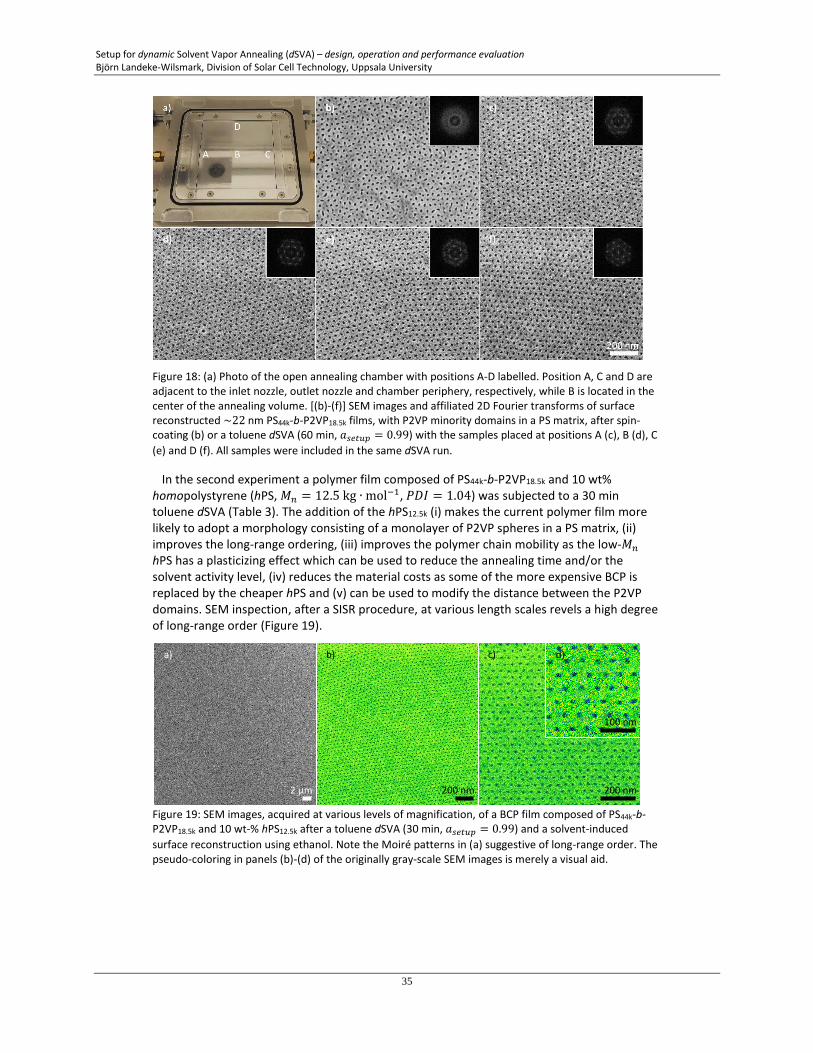
Setup for dynamic Solvent Vapor Annealing (dSVA) – design, operation and performance evaluation Björn Landeke-Wilsmark, Division of Solar Cell Technology, Uppsala University
35
Figure 18: (a) Photo of the open annealing chamber with positions A-D labelled. Position A, C and D are adjacent to the inlet nozzle, outlet nozzle and chamber periphery, respectively, while B is located in the center of the annealing volume. [(b)-(f)] SEM images and affiliated 2D Fourier transforms of surface reconstructed ~22 nm PS44k-b-P2VP18.5k films, with P2VP minority domains in a PS matrix, after spin-coating (b) or a toluene dSVA (60 min, 𝑎𝑠𝑒𝑡𝑢𝑝 = 0.99) with the samples placed at positions A (c), B (d), C
(e) and D (f). All samples were included in the same dSVA run.
In the second experiment a polymer film composed of PS44k-b-P2VP18.5k and 10 wt% homopolystyrene (hPS, 𝑀𝑛 = 12.5 kg ∙ mol−1, 𝑃𝐷𝐼 = 1.04) was subjected to a 30 min toluene dSVA (Table 3). The addition of the hPS12.5k (i) makes the current polymer film more likely to adopt a morphology consisting of a monolayer of P2VP spheres in a PS matrix, (ii) improves the long-range ordering, (iii) improves the polymer chain mobility as the low-𝑀𝑛 hPS has a plasticizing effect which can be used to reduce the annealing time and/or the solvent activity level, (iv) reduces the material costs as some of the more expensive BCP is replaced by the cheaper hPS and (v) can be used to modify the distance between the P2VP domains. SEM inspection, after a SISR procedure, at various length scales revels a high degree of long-range order (Figure 19).
Figure 19: SEM images, acquired at various levels of magnification, of a BCP film composed of PS44k-b-P2VP18.5k and 10 wt-% hPS12.5k after a toluene dSVA (30 min, 𝑎𝑠𝑒𝑡𝑢𝑝 = 0.99) and a solvent-induced
surface reconstruction using ethanol. Note the Moiré patterns in (a) suggestive of long-range order. The pseudo-coloring in panels (b)-(d) of the originally gray-scale SEM images is merely a visual aid.
2 μm 200 nm
a) b) c)
200 nm
100 nm
d)
Setup for dynamic Solvent Vapor Annealing (dSVA) – design, operation and performance evaluation Björn Landeke-Wilsmark, Division of Solar Cell Technology, Uppsala University
36
PART IV
Potential Improvements
Setup for dynamic Solvent Vapor Annealing (dSVA) – design, operation and performance evaluation Björn Landeke-Wilsmark, Division of Solar Cell Technology, Uppsala University
37
Part IV - Potential Improvements As with most builds, lessons have been learned along the way that advocate alternative solutions and/or design approaches. In this section some of these are presented and discussed.
4.1 Thermal Management As indicated by the evaluation of our setup, accurate monitoring of the temperature of the chamber is necessary to control the effective solvent activity. Currently, we use a handheld Pt-100 RTD probe but permanently affixed sensors would be a welcome addition since it would allow for continuous monitoring. This sensor input could then be combined with control of the MFCs to instigate a feedback loop to maintain a setpoint solvent activity even during drifts in temperature.
For added flexibility, individual electrical heating jackets around the bubblers and the mixing network are conceivable as it would allow the bubblers to be operated at different temperatures and thus add an additional degree of freedom. The temperature of the mixing network would then have to be equal to, or higher, than that of the hottest bubbler unit. An additional benefit of using heating jackets would be the elimination of the cumbersome water bath and related galvanic corrosion considerations. However, it is questionable if this approach is preferable as the temperature profiles would likely be less precis and uniform. A water bath, furthermore, has a larger thermal mass which lends stability to the temperature. The use of heating jackets or heating bands could also be affiliated with greater risk as they can achieve higher temperatures and the implementation of a fail-safe might be required to prevent accidentally turning the bubblers into high pressure vessels. The circulation heater used is limited to 95°C and it would be fairly evident if the water bath reached that temperature. The temperature of a heating jacket/band is harder to gauge visually.
4.2 Interchangeable Bubbler Units and MFCs Readily interchangeable, modular bubbler units could be of interest to rapidly being able to switch in-between solvents without first having to empty, dry and refill the currently permanently mounted bubblers. The same concept could be applied to the MFCs to enable access to different flow ranges. Alternatively, MFCs could be connected in parallel to allow selection of the MFC with the most appropriate range or even to combine the output from different units. To some extent the current setup already has this functionality as the flow from four different MFCs can be combined in various ways, allowing a high degree of flexibility.
4.3 Computer Control One of the most desirable functionalities is to exercise computer control over all MFCs and valves. This would allow for automation of most of the process and minimize operator intervention which in turn could also improve reproducibility and reduce the training time for new operators.
4.4 Heated Stage Introduction of a thin aluminum nitride (AlN) heating element, capable of high ramp rates and with an integrated RTD element to monitor the temperature, inside the dSVA chamber could also be an interesting option to add functionality to the setup. Such elements are commercially available and could be used to perform solvothermal annealing or as an alternative way of rapidly tailor the effective solvent activity above the sample and by extension the solvent content of the polymer film. The element could be used as an optional chamber insert if the electrical feedthrough, needed to drive the AlN element and integrated temperature probe, could be solved without compromising the integrity of the chamber.
Setup for dynamic Solvent Vapor Annealing (dSVA) – design, operation and performance evaluation Björn Landeke-Wilsmark, Division of Solar Cell Technology, Uppsala University
38
4.5 Cold trap The exhaust of our setup could be fitted with a cold trap for recovery of the solvent. This might be warranted, for environmental and/or economic reasons, for an industrial scale setup consuming more solvent. However, in our case the solvents used are fairly inexpensive, not excessively toxic and the cost and inconvenience of operating the cold trap would likely shadow potential gains of solvent recovery.
4.6 Additional Safety Precautions Pressure transducers could be inserted in various parts of the system and be rigged to act as fail-safe mechanisms to prevent a pressure build-up in susceptible parts of the system. A simple version would simply be that power is cut to the MFC control unit if the pressure transducer output exceeds a threshold value. In the same vein, back-flow valves could be introduced to prevent the flow from being forced the wrong way due to erroneous operation of valves. Technically, a particle filter should also be added between the quick-release connector and the MFC inlets in the N2 supply network to prevent particles from entering and potentially damaging the MFCs.
Setup for dynamic Solvent Vapor Annealing (dSVA) – design, operation and performance evaluation Björn Landeke-Wilsmark, Division of Solar Cell Technology, Uppsala University
39
5. Acknowledgements The author likes to thank and acknowledge Alireza Hosseini Shabestari, at the company Dione Kullager AB, for fruitful discussion regarding manufacturing and for converting the author’s CAD-files into technical drawings fit for manufacture, see Appendix.
The author acknowledges Myfab Uppsala for providing experimental facilities. Myfab is funded by the Swedish Research Council (2019-00207) as a national research infrastructure.
This work was funded by the Swedish Research Council, reg. number 621-2014-5599, and the Swedish Energy Agency, project number 45409-1. 6. References 1. Tu, K.-H.; Bai, W.; Liontos, G.; Ntetsikas, K.; Avgeropoulos, A.; Ross, C. A., Universal pattern
transfer methods for metal nanostructures by block copolymer lithography. Nanotechnology 2015, 26 (37), 375301.
2. Baruth, A.; Rodwogin, M. D.; Shankar, A.; Erickson, M. J.; Hillmyer, M. A.; Leighton, C., Non-lift-off Block Copolymer Lithography of 25 nm Magnetic Nanodot Arrays. ACS Appl. Mater. Interfaces 2011, 3 (9), 3472-3481.
3. Hong, A. J.; Liu, C.-C.; Wang, Y.; Kim, J.; Xiu, F.; Ji, S.; Zou, J.; Nealey, P. F.; Wang, K. L., Metal Nanodot Memory by Self-Assembled Block Copolymer Lift-Off. Nano Lett. 2010, 10 (1), 224-229.
4. Cho, H.; Park, H.; Russell, T. P.; Park, S., Precise placements of metal nanoparticles from reversible block copolymer nanostructures. J. Mater. Chem. 2010, 20 (24), 5047-5051.
5. Chang, C.-C.; Botez, D.; Wan, L.; Nealey, P. F.; Ruder, S.; Kuech, T. F., Fabrication of large-area, high-density Ni nanopillar arrays on GaAs substrates using diblock copolymer lithography and electrodeposition. J. Vac. Sci. Technol. B 2013, 31 (3), 031801.
6. Son, J. G.; Bae, W. K.; Kang, H.; Nealey, P. F.; Char, K., Placement Control of Nanomaterial Arrays on the Surface-Reconstructed Block Copolymer Thin Films. ACS Nano 2009, 3 (12), 3927-3934.
7. Hu, H. Q.; Gopinadhan, M.; Osuji, C. O., Directed self-assembly of block copolymers: a tutorial review of strategies for enabling nanotechnology with soft matter. Soft Matter 2014, 10 (22), 3867-3889.
8. Selkirk, A.; Prochukhan, N.; Lundy, R.; Cummins, C.; Gatensby, R.; Kilbride, R.; Parnell, A.; Baez Vasquez, J.; Morris, M.; Mokarian-Tabari, P., Optimization and Control of Large Block Copolymer Self-Assembly via Precision Solvent Vapor Annealing. Macromolecules 2021, 54 (3), 1203-1215.
9. Cheng, X.; Böker, A.; Tsarkova, L., Temperature-Controlled Solvent Vapor Annealing of Thin Block Copolymer Films. Polymers 2019, 11 (8), 1312.
10. Hoang, D. T.; Yang, J.; Paeng, K.; Kwon, Y.; Kweon, O. S.; Kaufman, L. J., In situ multi-modal monitoring of solvent vapor swelling in polymer thin films. Rev. Sci. Instrum. 2016, 87 (1), 8.
11. Müller-Buschbaum, P., GISAXS and GISANS as metrology technique for understanding the 3D morphology of block copolymer thin films. Eur. Polym. J. 2016, 81, 470-493.
12. Nelson, G.; Drapes, C. S.; Grant, M. A.; Gnabasik, R.; Wong, J.; Baruth, A., High-Precision Solvent Vapor Annealing for Block Copolymer Thin Films. Micromachines 2018, 9 (6), 21.
13. Jin, C.; Olsen, B. C.; Luber, E. J.; Buriak, J. M., Nanopatterning via Solvent Vapor Annealing of Block Copolymer Thin Films. Chem. Mat. 2017, 29 (1), 176-188.
14. Baruth, A.; Seo, M.; Lin, C. H.; Walster, K.; Shankar, A.; Hillmyer, M. A.; Leighton, C., Optimization of Long-Range Order in Solvent Vapor Annealed Poly(styrene)-block-poly(lactide) Thin Films for Nano lithography. ACS Appl. Mater. Interfaces 2014, 6 (16), 13770-13781.
15. Lundy, R.; Flynn, S. P.; Cummins, C.; Kelleher, S. M.; Collins, M. N.; Dalton, E.; Daniels, S.; Morris, M. A.; Enright, R., Controlled solvent vapor annealing of a high chi block copolymer thin film. Phys. Chem. Chem. Phys. 2017, 19 (4), 2805-2815.
16. Stenbock-Fermor, A.; Knoll, A. W.; Boker, A.; Tsarkova, L., Enhancing Ordering Dynamics in Solvent-Annealed Block Copolymer Films by Lithographic Hard Mask Supports. Macromolecules 2014, 47 (9), 3059-3067.
17. Lundy, R.; Cummins, C.; Morris, M. A.; Enright, R. In Automated nanolithography process control for rapid & well ordered molecular self-assembly, 2018 IEEE 18th International Conference on Nanotechnology (IEEE-NANO), 23-26 July 2018; 2018; pp 1-2.
18. Gotrik, K. W.; Hannon, A. F.; Son, J. G.; Keller, B.; Alexander-Katz, A.; Ross, C. A., Morphology Control in Block Copolymer Films Using Mixed Solvent Vapors. ACS Nano 2012, 6 (9), 8052-8059.
Setup for dynamic Solvent Vapor Annealing (dSVA) – design, operation and performance evaluation Björn Landeke-Wilsmark, Division of Solar Cell Technology, Uppsala University
40
19. Gotrik, K. W.; Ross, C. A., Solvothermal Annealing of Block Copolymer Thin Films. Nano Lett. 2013, 13 (11), 5117-5122.
20. Xiong, S. S.; Wan, L.; Ishida, Y.; Chapuis, Y. A.; Craig, G. S. W.; Ruiz, R.; Nealey, P. F., Directed Self-Assembly of Triblock Copolymer on Chemical Patterns for Sub-10-nm Nanofabrication via Solvent Annealing. ACS Nano 2016, 10 (8), 7855-7865.
21. Gu, X.; Gunkel, I.; Hexemer, A.; Gu, W.; Russell, T. P., An In Situ Grazing Incidence X-Ray Scattering Study of Block Copolymer Thin Films During Solvent Vapor Annealing. Adv. Mater. 2014, 26 (2), 273-281.
22. Cushen, J. D.; Wan, L.; Pandav, G.; Mitra, I.; Stein, G. E.; Ganesan, V.; Ruiz, R.; Willson, C. G.; Ellison, C. J., Ordering Poly(trimethylsilyl styrene-block-(D),(L)-lactide) Block Copolymers in Thin Films by Solvent Annealing Using a Mixture of Domain-Selective Solvents. J. Polym. Sci. Pt. B-Polym. Phys. 2014, 52 (1), 36-45.
23. Park, S.; Kim, B.; Xu, J.; Hofmann, T.; Ocko, B. M.; Russell, T. P., Lateral Ordering of Cylindrical Microdomains Under Solvent Vapor. Macromolecules 2009, 42 (4), 1278-1284.
24. Cavicchi, K. A.; Russell, T. P., Solvent Annealed Thin Films of Asymmetric Polyisoprene−Polylactide Diblock Copolymers. Macromolecules 2007, 40 (4), 1181-1186.
25. Gu, X.; Gunkel, I.; Hexemer, A.; Russell, T. P., Controlling Domain Spacing and Grain Size in Cylindrical Block Copolymer Thin Films by Means of Thermal and Solvent Vapor Annealing. Macromolecules 2016, 49 (9), 3373-3381.
26. Gu, X.; Gunkel, I.; Hexemer, A.; Russell, T. P., Solvent vapor annealing of block copolymer thin films: removal of processing history. Colloid Polym. Sci. 2014, 292 (8), 1795-1802.
27. Lee, S.; Cheng, L.-C.; Yager, K. G.; Mumtaz, M.; Aissou, K.; Ross, C. A., In Situ Study of ABC Triblock Terpolymer Self-Assembly under Solvent Vapor Annealing. Macromolecules 2019, 52 (4), 1853-1863.
28. Albert, J. N. L.; Young, W.-S.; Lewis, R. L.; Bogart, T. D.; Smith, J. R.; Epps, T. H., Systematic Study on the Effect of Solvent Removal Rate on the Morphology of Solvent Vapor Annealed ABA Triblock Copolymer Thin Films. ACS Nano 2012, 6 (1), 459-466.
29. Lundy, R.; Flynn, S. P.; Cummins, C.; Kelleher, S. M.; Collins, M. N.; Dalton, E.; Daniels, S.; Morris, M. A.; Enright, R., Controlled solvent vapor annealing of a high χ block copolymer thin film. Phys. Chem. Chem. Phys. 2017, 19 (4), 2805-2815.
30. Rodgers, R. C.; Hill, G. E., EQUATIONS FOR VAPOUR PRESSURE VERSUS TEMPERATURE: DERIVATION AND USE OF THE ANTOINE EQUATION ON A HAND-HELD PROGRAMMABLE CALCULATOR. British Journal of Anaesthesia 1978, 50 (5), 415-424.
31. Atkins, P. d. P., J, Atkin's Physical Chemistry. 9th ed.; Oxford University Press: New York, 2010. 32. Krumdieck, S. P., Chapter 2 CVD Reactors and Delivery System Technology. In Chemical Vapour
Deposition: Precursors, Processes and Applications, The Royal Society of Chemistry: 2009; pp 37-92. 33. Fried, J. R., Polymer Science & Technology. 2nd ed.; Prentice Hall: New Jersey, 2003; p 1-582. 34. Park, S.; Wang, J.-Y.; Kim, B.; Chen, W.; Russell, T. P., Solvent-Induced Transition from Micelles in
Solution to Cylindrical Microdomains in Diblock Copolymer Thin Films. Macromolecules 2007, 40 (25), 9059-9063.
35. Zhang, X.; Qiu, J.; Li, X.; Zhao, J.; Liu, L., Complex refractive indices measurements of polymers in visible and near-infrared bands. Appl. Optics 2020, 59 (8), 2337-2344.
36. Sultanova, N. G.; Kasarova, S. N.; Nikolov, I. D., Dispersion Properties of Optical Polymers. Acta Physica Polonica A 2009, 116, 585-587.
37. Moutzouris, K.; Papamichael, M.; Betsis, S. C.; Stavrakas, I.; Hloupis, G.; Triantis, D., Refractive, dispersive and thermo-optic properties of twelve organic solvents in the visible and near-infrared. Applied Physics B 2014, 116 (3), 617-622.
38. Kedenburg, S.; Vieweg, M.; Gissibl, T.; Giessen, H., Linear refractive index and absorption measurements of nonlinear optical liquids in the visible and near-infrared spectral region. Opt. Mater. Express 2012, 2 (11), 1588-1611.
39. Landeke-Wilsmark, B.; Nyholm, L.; Hägglund, C., Seeded Growth of Large-Area Arrays of Substrate Supported Au Nanoparticles Using Citrate and Hydrogen Peroxide. Langmuir 2020, 36 (24), 6848-6858.
40. Landeke-Wilsmark, B.; Nyholm, L.; Hägglund, C., Process Window for Seeded Growth of Arrays of Quasi-Spherical Substrate-Supported Au Nanoparticles. Langmuir 2021, 37 (19), 6032-6041.
41. Landeke-Wilsmark, B.; Hägglund, C., Metal nanoparticle arrays via a water-based lift-off scheme using a block copolymer template. Nanotechnology 2022, 33 (32), 325302.