experimental evaluation of fatigue test setup
TRANSCRIPT
University of New Hampshire University of New Hampshire
University of New Hampshire Scholars' Repository University of New Hampshire Scholars' Repository
Master's Theses and Capstones Student Scholarship
Winter 2018
EXPERIMENTAL EVALUATION OF FATIGUE TEST SETUP FOR A EXPERIMENTAL EVALUATION OF FATIGUE TEST SETUP FOR A
GUSSET-LESS TRUSS CONNECTION GUSSET-LESS TRUSS CONNECTION
Duncan William McGeehan University of New Hampshire, Durham
Follow this and additional works at: https://scholars.unh.edu/thesis
Recommended Citation Recommended Citation McGeehan, Duncan William, "EXPERIMENTAL EVALUATION OF FATIGUE TEST SETUP FOR A GUSSET-LESS TRUSS CONNECTION" (2018). Master's Theses and Capstones. 1259. https://scholars.unh.edu/thesis/1259
This Thesis is brought to you for free and open access by the Student Scholarship at University of New Hampshire Scholars' Repository. It has been accepted for inclusion in Master's Theses and Capstones by an authorized administrator of University of New Hampshire Scholars' Repository. For more information, please contact [email protected].
i
EXPERIMENTAL EVALUATION OF FATIGUE TEST SETUP FOR A GUSSET-LESS
TRUSS CONNECTION
BY
Duncan W. McGeehan
BS, University of New Hampshire, 2017
THESIS
Submitted to the University of New Hampshire in Partial Fulfillment of the
Requirements for the Degree of
Master of Science in Civil Engineering
December, 2018

ii
This thesis/dissertation has been examined and approved in partial fulfillment of the
requirements for the degree of Master of Science in Civil Engineering by:
Thesis Director, Erin Santini Bell, Ph.D., P.E. Civil and Environmental Engineering
Ricardo A. Medina, Ph.D., P.E. Civil and Environmental Engineering
Eshan V. Dave, Ph.D. Civil and Environmental Engineering
On December 6th 2018
Original approval signatures are on file with the University of New Hampshire
Graduate School.

iii
ACKNOWLEDGEMENTS
I would like to acknowledge the NHDOT (New Hampshire Department of
Transportation) for their technical and financial support throughout this project. This
work was partially supported by National Science Foundation Grant #1430260. Any
opinions, findings, and conclusions or recommendations expressed in this material are
those of the author and do not necessarily reflect the views of the National Science
Foundation.
I would like to sincerely thank my advisor, Dr. Erin Santini Bell, who was the PI
of this project, for her continued support, guidance, and patience throughout this work.
I would like to sincerely thank Dr. Ricardo A. Medina, the Co-PI of this project, for his
tireless efforts towards this work. Both Dr. Bell and Dr. Medina were incremental in
maintaining forward progress and focus on the goals of this research despite the many
setbacks that we have faced. I would also like to thank Dr. Eshan V. Dave for his support
throughout my time at UNH, and his willingness to lend his time and knowledge when
needed.
I would like to thank Fernanda Fischer for her efforts in the start of this project and
laying the groundwork for this study. Thank you to Shokoufeh Zargar, for her input and
expertise along the way. Thank you to all the people who helped move this project
forward along the way; John Ahern, Scott Campbell, Dr. Gary Schajer, Andrew Lanza,
Christian Harris. I would also like to thank my friends and officemates for all the fun
along the way, and my family for all the support. Last but certainly not least, I would like

iv
to extend a special thank you to Ashley Blum for her continued support and
encouragement in all my pursuits.

v
TABLE OF CONTENTS
ACKNOWLEDGEMENTS ......................................................................................................................................... III
TABLE OF CONTENTS .............................................................................................................................................. V
LIST OF FIGURES .................................................................................................................................................. VIII
LIST OF TABLES ................................................................................................................................................... XIV
ABSTRACT ............................................................................................................................................................ XV
1. INTRODUCTION ............................................................................................................................................ 1
1.1 PROJECT OVERVIEW .............................................................................................................................................. 1
1.2 THESIS OBJECTIVES AND CONTRIBUTIONS .................................................................................................................. 3
1.3 BACKGROUND INFORMATION AND LITERATURE REVIEW ............................................................................................... 5
INSTRUMENTATION ............................................................................................................................................. 5
TEST MONITORING ............................................................................................................................................... 8
FINITE ELEMENT MODEL ...................................................................................................................................... 8
FATIGUE ............................................................................................................................................................... 9
RESIDUAL STRESS ............................................................................................................................................... 15
2 LABORATORY TEST SETUP........................................................................................................................... 17
2.1 SPECIMEN DESIGN .............................................................................................................................................. 17
2.2 FATIGUE TEST SETUP........................................................................................................................................... 21
2.3 INSTRUMENTATION ............................................................................................................................................. 34
3 FATIGUE TEST MONITORING....................................................................................................................... 43
3.1 FATIGUE TEST MONITORING PROTOCOL ................................................................................................................. 43
3.2 SYSTEM IDENTIFICATION ...................................................................................................................................... 50
3.3 REPRESENTATIVE MEASUREMENT .......................................................................................................................... 57

vi
3.4 SUMMARY ........................................................................................................................................................ 65
4 FINITE ELEMENT MODELING ....................................................................................................................... 67
4.1 FINITE ELEMENT MODELING ................................................................................................................................. 67
4.2 FATIGUE TEST MODEL ......................................................................................................................................... 68
4.3 RESULTS – FEM ................................................................................................................................................. 74
4.4 SUMMARY ........................................................................................................................................................ 81
5 FATIGUE TESTING RESULTS ......................................................................................................................... 82
5.1 INTRODUCTION .................................................................................................................................................. 82
5.2 STRAIN GAUGE RESULTS ...................................................................................................................................... 84
5.3 DIC RESULTS ..................................................................................................................................................... 92
5.4 MEASUREMENT COMPARISON .............................................................................................................................. 97
5.5 SUMMARY AND DISCUSSION ............................................................................................................................... 100
6 RESIDUAL STRESSES .................................................................................................................................. 102
6.1 IMPORTANCE OF RESIDUAL STRESSES ................................................................................................................... 102
6.2 HOLE-DRILLING METHOD .................................................................................................................................. 104
6.3 BLIND-HOLE RESIDUAL STRESS CALCULATIONS ....................................................................................................... 110
6.4 RESULTS – RESIDUAL STRESSES ........................................................................................................................... 117
7 SUMMARY, CONCLUSIONS, AND FUTURE WORK ...................................................................................... 128
7.1 SUMMARY ...................................................................................................................................................... 128
7.2 CONCLUSIONS ................................................................................................................................................. 130
7.3 FUTURE WORK ................................................................................................................................................ 132
REFERENCES ....................................................................................................................................................... 134
APPENDICIES.......................................................................................................................................................A-1

vii
APPENDIX A – INSTRUMENTATION .....................................................................................................................A-2
APPENDIX B – TEST TRACKING ............................................................................................................................A-6
APPENDIX C – SYSTEM ID .................................................................................................................................. A-12
APPENDIX D – FATIGUE RESULTS ...................................................................................................................... A-19
APPENDIX E – RESIDUAL STRESS CODE.............................................................................................................. A-27
APPENDIX F – RESIDUAL STRESS RESULTS ......................................................................................................... A-31
viii
LIST OF FIGURES
Figure 1 - Gusset-less Connections ............................................................................................ 2
Figure 2 - Welded Steel S-N Curves [16] ................................................................................ 11
Figure 3 - Sample Fatigue Categories [19] .............................................................................. 12
Figure 4 - Mean-Stress Effect [26] ............................................................................................ 13
Figure 5 - Goodman Line [27] .................................................................................................. 14
Figure 6 - Memorial Bridge, Top-Chord Gusset-less Connection ....................................... 17
Figure 7 - HNTB Design Stress Contour [1] ........................................................................... 18
Figure 8 - Geometric Reductions of Scaled Connection [30] ............................................... 20
Figure 9 - Specimen Dimensions and Material Properties ................................................... 21
Figure 10 - (1) Reaction Block (top), (2) Support Bracket (bottom) ..................................... 23
Figure 11 - Location of Shim Support at Specimen Tip ........................................................ 26
Figure 12 - Reaction Block Reinforcement (a), Reaction Block with Concrete .................. 27
Figure 13 - System Components - Overall Test Setup, Reaction Block (a), Bracket Support
(b), Specimen (c), and Shim Support (d) ................................................................................. 29
Figure 14 - Cyclic Loading Sample .......................................................................................... 31
Figure 15 - Sample Loading Protocol ...................................................................................... 32
Figure 16 - Loading Schematic ................................................................................................. 32
Figure 17 - Instrumentation of Gusset-less Fatigue Specimen ............................................ 40
Figure 18 - DIC Schematic and Setup ...................................................................................... 41
Figure 19 - Sample Speckle Pattern ......................................................................................... 42
ix
Figure 20 - Monitoring Protocol Flowchart ............................................................................ 44
Figure 21 - Shim Support Movement ...................................................................................... 47
Figure 22 - System Identification - DIC Measurement Locations ....................................... 52
Figure 23 - Force Time-History - 07/24 .................................................................................. 53
Figure 24 - Force Time-History - 10/23 ................................................................................. 53
Figure 25 - DIC and LVDT Verification .................................................................................. 54
Figure 26 - Reaction Block (Right) - Horizontal Displacement ........................................... 55
Figure 27 - Hysteresis 06/20-07/10 ......................................................................................... 59
Figure 28 - Hysteresis 07/11-07/18 ......................................................................................... 59
Figure 29 - Hysteresis 07/19-08/16 ......................................................................................... 60
Figure 30 - Hysteresis 08/17-10/01 ......................................................................................... 60
Figure 31 - Hysteresis 10/11-10/30 ......................................................................................... 61
Figure 32 - Hysteresis 06/20 and 06/27.................................................................................. 62
Figure 33 - Hysteresis 06/27 and 07/03.................................................................................. 63
Figure 34 - Hysteresis 07/03 and 07/10.................................................................................. 64
Figure 35 - Hysteresis 07/03 and 07/10 - Zoomed ............................................................... 65
Figure 36 - Finite Element Model of Experimental Test Setup ............................................ 69
Figure 37 - Meshing of Entire Model ...................................................................................... 73
Figure 38 - FEM Deflected Shape ............................................................................................. 75
Figure 39 - FEM Specimen Deflected Shape .......................................................................... 75
Figure 40 - HNTB Design Stress Contour ............................................................................... 76
x
Figure 41 - FEM Web Max Principal Stress (Absolute) ........................................................ 76
Figure 42 - FEM - Specimen Max Principal Stress (Absolute) ............................................. 77
Figure 43 - FEM - AOI Max Principal Stress (Absolute) ...................................................... 78
Figure 44 - FEM Specimen Horizontal Strain ........................................................................ 79
Figure 45 - FEM AOI Horizontal Strain .................................................................................. 79
Figure 46 - FEM Specimen Vertical Strain .............................................................................. 80
Figure 47 - FEM AOI Vertical Strain ....................................................................................... 81
Figure 48 - Horizontal Strain Pattern Along Weld Toe ........................................................ 85
Figure 49 - Horizontal Strain Pattern Away from Weld Toe ............................................... 86
Figure 50 - North and South Comparison .............................................................................. 87
Figure 51 - Horizontal Strain, Test Interval Comparison ..................................................... 88
Figure 52 - Vertical Strain, Test Interval Comparison .......................................................... 89
Figure 53 - Analysis Area of Interest - DIC ............................................................................ 94
Figure 54 - Horizontal Displacement DIC Contour .............................................................. 95
Figure 55 - DIC Comparison Locations .................................................................................. 96
Figure 56 - DIC Response Along Weld ................................................................................... 96
Figure 57 - Drilling Assembly ................................................................................................ 105
Figure 58 - Strain Rosette Information [36] .......................................................................... 106
Figure 59 - Residual Stress Strain Rosette - (a) Layout Diagram [30], (b) Example Rosette
..................................................................................................................................................... 111
Figure 60 - Representation of Calibration Matrix [30] ........................................................ 113
xi
Figure 61 - Annealed Steel - Plunging .................................................................................. 118
Figure 62 - Annealed Steel - Orbital ...................................................................................... 119
Figure 63 - Calculation Verification....................................................................................... 121
Figure 64 - Residual Hole Location 1 - Elevation (left), Plan View (right) ...................... 122
Figure 65 - Residual Stress Profile - Location 1 ................................................................... 122
Figure 66 - Residual Hole Location 2 - Elevation (left), Plan View (right) ...................... 123
Figure 67 - Residual Stress Profile - Location 2 ................................................................... 124
Figure 68 - Residual Hole Location 3 - Elevation (left), Plan View (right) ...................... 125
Figure 69 - Residual Stress Profile - Location 3 ................................................................... 126
Figure 70 - Strain Rosette Data Sheet .................................................................................... A-2
Figure 71 - Uniaxial Strain Gauge Data Sheet [40] .............................................................. A-3
Figure 72 - DIC Correlation [41] ............................................................................................ A-4
Figure 73 - Lagrange Strain Equations [42] .......................................................................... A-5
Figure 74 - Test Tracking Data Sheet - Front ...................................................................... A-10
Figure 75 - Test Tracking Data Sheet - Back ....................................................................... A-11
Figure 76 - Horizontal Displacements - All Locations ...................................................... A-12
Figure 77 - Reaction Block Right - Vertical Displacement ............................................... A-12
Figure 78 - Reaction Block Right - Horizontal Displacement .......................................... A-13
Figure 79 - Reaction Block Left - Horizontal Displacement ............................................. A-13
Figure 80 - Reaction Block Left - Vertical Displacement .................................................. A-14
Figure 81 - Actuator - Horizontal Displacement ............................................................... A-14
xii
Figure 82 - Actuator Tip - Horizontal Displacement. ....................................................... A-15
Figure 83 - Actuator - Vertical Displacement ..................................................................... A-15
Figure 84 - Specimen Tip - Horizontal Displacement ....................................................... A-16
Figure 85 - Actuator Tip - Vertical Displacement.............................................................. A-16
Figure 86 - Bracket - Vertical Displacement ....................................................................... A-17
Figure 87 - Specimen Tip - Vertical Displacement ............................................................ A-17
Figure 88 - Bracket - Horizontal Displacement.................................................................. A-18
Figure 89 - NRW1 - Vertical.................................................................................................. A-19
Figure 90 - NRW1 - Horizontal ............................................................................................ A-19
Figure 91 - NRW1 - Diagonal ............................................................................................... A-20
Figure 92 - NRW2 - Horizontal ............................................................................................ A-20
Figure 93 - NRW2 - Vertical.................................................................................................. A-21
Figure 94 - NRW2 - Diagonal ............................................................................................... A-21
Figure 95 - NRW3 - Horizontal ............................................................................................ A-22
Figure 96 - NRW3 - Vertical.................................................................................................. A-22
Figure 97 - NRW3 - Diagonal ............................................................................................... A-23
Figure 98 - NRW4 - Horizontal ............................................................................................ A-23
Figure 99 - NRW4 - Vertical.................................................................................................. A-24
Figure 100 - NRW4 - Diagonal ............................................................................................. A-24
Figure 101 - NRW5 - Horizontal .......................................................................................... A-25
Figure 102 - NRW5 - Vertical................................................................................................ A-25
xiii
Figure 103 - NRW5 - Diagonal ............................................................................................. A-26
Figure 104 - MATLAB Code 1 .............................................................................................. A-27
Figure 105 - MATLAB Code 2 .............................................................................................. A-28
Figure 106 - MATLAB Code 3 .............................................................................................. A-29
Figure 107 - MATLAB Code 4 .............................................................................................. A-30
Figure 108 - Residual Stress Measurement #1 - Strain (top) and Stress (bottom) ........ A-32
Figure 109 - Residual Stress Measurement #2 - Strain (top) and Stress (bottom) ....... A-33
Figure 110 - Residual Stress Measurement #3 - Strain (top) and Stress (bottom) ....... A-34
Figure 111 - Residual Stress Measurement #4 - Strain (top) and Stress (bottom) ....... A-35
Figure 112 - Residual Stress Measurement #5 - Strain (top) and Stress (bottom) ....... A-36
Figure 113 - Residual Stress Measurement #6 - Strain (top) and Stress (bottom) ....... A-37
Figure 114 - Residual Stress Measurement #7 - Strain (top) and Stress (bottom) ....... A-38
Figure 115 - Residual Stress Measurement #8 - Strain (top) and Stress (bottom) ....... A-39
Figure 116 - Residual Stress Measurement #9 - Strain (top) and Stress (bottom) ....... A-40
Figure 117 - Residual Stress Measurement #10 - Strain (top) and Stress (bottom) ...... A-41
Figure 118 - Residual Stress Measurement #11 - Strain (top) and Stress (bottom) ...... A-42

xiv
LIST OF TABLES
Table 1 - System ID Comparison ............................................................................................. 56
Table 2 - NRW1 – Test Interval Comparison ......................................................................... 90
Table 3 - NRW2 - Test Interval Comparison .......................................................................... 90
Table 4 - NRW3 - Test Interval Comparison .......................................................................... 91
Table 5 - NRW4 - Test Interval Comparison .......................................................................... 91
Table 6 - NRW5 - Test Interval Comparison .......................................................................... 92
Table 7 - DIC and Strain Gauge ............................................................................................... 97
Table 8 - Strain Gauges and FEA ............................................................................................. 98
Table 9 - DIC and FEA Comparison ........................................................................................ 99
Table 10 - Test Tracking History ............................................................................................ A-6
Table 11 - Residual Stress Table of Measurements ........................................................... A-31

xv
ABSTRACT
EXPERIMENTAL EVALUATION OF FATIGUE TEST SETUP FOR A GUSSET-LESS
TRUSS CONNECTION
by
Duncan W. McGeehan
University of New Hampshire, December 2018
In 2013, the newly designed Memorial bridge, located between Portsmouth, NH,
and Kittery, ME, was opened to traffic. The structural system of the bridge is composed
of truss elements with a unique “Gusset-less” connection which utilizes curved steel to
transition from the chords to the diagonals where splice plates join the members. With
such a unique connection, it is important to verify the design assumptions and assess the
performance. In this study, the fatigue performance of the Gusset-less connection is
investigated through an experimental fatigue test of a scale model of the connection.
In a high-cycle fatigue test, it is critical to ensure that consistency is maintained
across all testing periods. This is especially challenging when the test setup is not
standardized, and the laboratory infrastructure is limited. In this work a monitoring
protocol was developed to systematically monitor the structural response of the test
setup. Using this protocol, across a total of 1,600,000 fatigue load cycles the average
difference in structural response was found to be 5% across the test setup. Using the most
conservative assumptions, using a hot-spot stress of 14 Ksi at the toe of the weld, the

xvi
AASHTO S-N curve, and a category C fatigue detail, the connection has been tested and
the results show that the design expectations are exceeded.
The residual stresses were investigated in the top-flange of the fatigue specimen.
The stresses indicate a compressive stress at the surface of the specimen, which is
consistent with the residual stress profile of a sand blasted metal. The magnitude of the
stresses was higher than the theoretical limits of the calculation method and therefore
must be used qualitatively, not quantitatively.

1
1. INTRODUCTION
This chapter will provide background information on the project. Following the
background, an overview of the objectives of this work will be outlined. Finally,
background information on fatigue testing, measurement methods used, fatigue test
monitoring, Finite Element Modeling (FEM), and residual stresses will be outlined, and
a literature review provided.
1.1 Project Overview
The Memorial Bridge spans the Piscataquis river between Portsmouth, NH, and
Kittery, ME. The original Memorial Bridge had been in operation since 1923, when it was
opened to traffic originally, making it over 89 years old when it was officially closed in
2012 due to structural deficiencies. The original design was a vertical lift bridge utilizing
a traditional steel truss structural system, where the center span of the three-span bridge
was the vertical lift span. In 2013 the new Memorial Bridge, designed by HNTB corp.,
was opened to traffic. The new bridge utilized a similar design with a lift-span in the
center and a steel truss structural system. One of the major changes was the innovate
connection designed for the members of the truss system.
In most bridges that use a steel truss structural system, the connections between
the members are made using gusset plates. When using gusseted connections, there are
multiple structural members framing into one joint, where the gusset plates are bolted
2
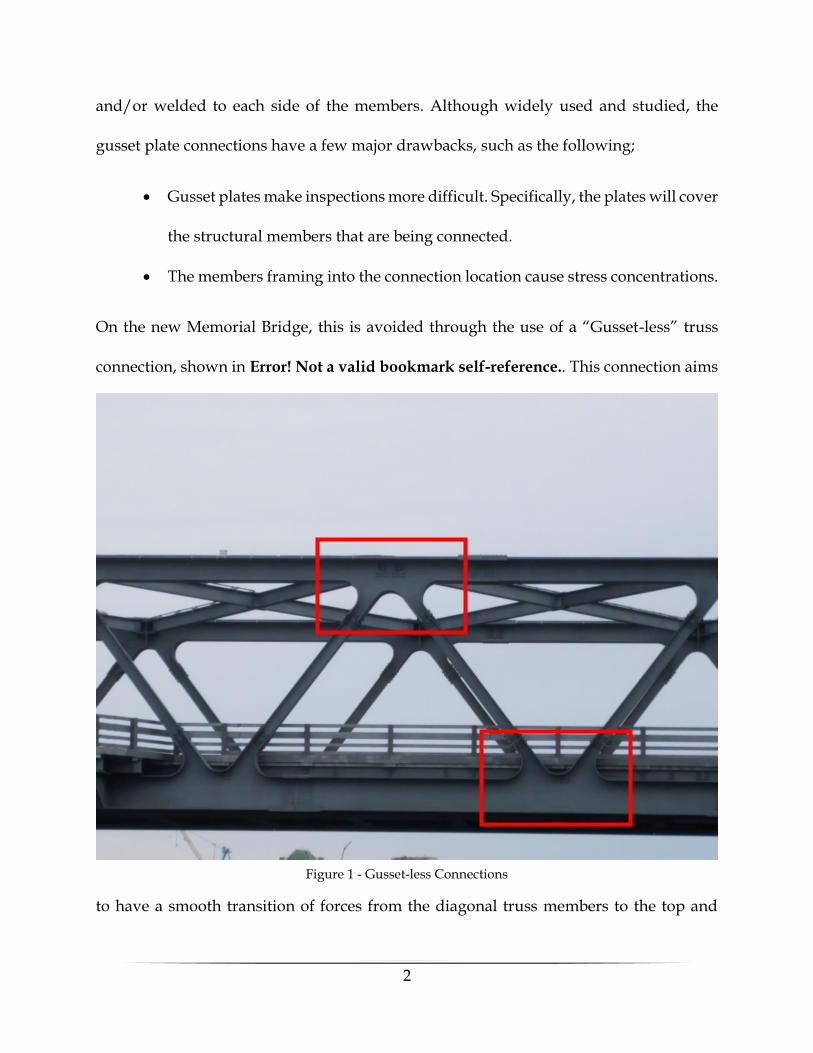
and/or welded to each side of the members. Although widely used and studied, the
gusset plate connections have a few major drawbacks, such as the following;
• Gusset plates make inspections more difficult. Specifically, the plates will cover
the structural members that are being connected.
• The members framing into the connection location cause stress concentrations.
On the new Memorial Bridge, this is avoided through the use of a “Gusset-less” truss
connection, shown in Error! Not a valid bookmark self-reference.. This connection aims
to have a smooth transition of forces from the diagonal truss members to the top and
Figure 1 - Gusset-less Connections

3
bottom chords of the truss system. This is accomplished using cold-bent steel flanges and
a unique geometric approach. Since connections are incorporated into the chords of the
bridge, the diagonals members are connected individually using bolted splice plates.
Some of the main benefits of using this connection are as follows [1];
• Reduction in number of bolts needed on the bridge, compared to a traditional
gusseted connection.
• The connections are much easier to inspect than a gusseted connection since
nothing is shrouded behind a large plate.
• The spliced connections can be partially replaced while the bridge is under load.
Although this connection has many benefits, it has not been as widely used or studied as
a traditional gusseted connection. One aim of this research is to investigate the structural
performance of this connection through laboratory testing. More specifically, the aim of
the overall study is to evaluate the fatigue performance of the Gusset-less truss
connection. In addition to the structural performance, it is important to understand the
connection and the critical locations for inspections. The overall project also intends to
use the laboratory data to aid in the development of an inspection protocol for the
Memorial Bridge.
1.2 Thesis Objectives and Contributions
As previously discussed, the overall objective of this research is to evaluate the
fatigue performance of the Gusset-less truss connection. In this thesis, work towards the
evaluation will be presented. The contribution of this thesis to the overall project is in the

4
form of experimental fatigue testing, which is used to evaluate the fatigue life prediction
of the Gusset-less connection. Additionally, a test monitoring protocol was developed to
ensure consistency across testing periods. Lastly, a work towards measuring and
calculating the residual stresses in the Gusset-less test specimen was done. The layout of
this thesis is presented below;
Chapter 1 – Introduction; This chapter will provide background information on the
project, an overview of the objectives of this work, and a summary of relevant literature.
Chapter 2 – Laboratory Test Setup; This chapter will introduce the experimental fatigue
testing, specifically the physical test setup, the loading protocol and the instrumentation
plan for the fatigue test.
Chapter 3 – Fatigue Test Monitoring; This chapter will discuss the importance, and the
development, of a monitoring protocol for high-cycle fatigue testing performed across
multiple testing intervals.
Chapter 4 – Finite Element Monitoring; This chapter will discuss the use of finite
element modeling as a tool for understanding and evaluating the fatigue test specimen
and setup.
Chapter 5 – Fatigue Testing Results; This chapter will introduce the results of the fatigue
testing and the implications of those results
Chapter 6 – Residual Stresses; This chapter will discuss the importance, and the
measurements, of residual stresses in the fatigue test specimen.

5
Chapter 7 – Summary, Conclusions, and Future Work; This chapter will present an
overall summary of the work, including conclusions, and future work for this project.
In addition to these chapters, this thesis includes six appendices;
• Instrumentation – Strain gauge data sheets, DIC background and additional info
• Fatigue Test Tracking – Data sheets from testing
• System ID – Additional plots from system IDs
• Additional Fatigue test results
• Residual Stress Calculations – MATLAB Code of integral method
• Residual Stress Measurements – Additional residual stress measurements
1.3 Background Information and Literature Review
In order to achieve the goals of this thesis, a literature review was needed to
provide a background information on the work to be performed. In this literature review,
there are five main topics investigated; instrumentation, test monitoring, finite element
modeling, fatigue, and residual stress. The background information needed for this study
is provided in the following section.
INSTRUMENTATION
Structural performance prediction of innovative connection details requires both
advanced design tools and analysis models that are verified through experimental data.
For most civil structures field or full-scale tests to failure are not feasible, therefore scale-
model laboratory experiments are critical to advancing the state-of-the-art for structural

6
design. Scale-model laboratory experiments must be carefully designed to provide
information on specific structural behaviors. In order to isolate the target behavior, all of
behaviors, including influences of boundary conditions and members interactions, must
be controlled and accurately accounted for in the associated structural models.
Characterization of the structural response of a laboratory experiment can be
challenging depending on multiple factors including the experimental objectives,
specimen geometry, available laboratory resources and infrastructure, experimental
setup, and loading conditions. These factors will have a large influence on the selection
of what type of measurements can be made and the method used to obtain those
measurements. The typical types of measurements used to characterize a structure are
the displacement, the strain, the acceleration, or any combination thereof, in the
directions of interest. Obtaining these measurements is not always a trivial task
depending on the experiment and the level of characterization desired. Therefore, it is
important to choose the appropriate measurement method that will provide the best
characterization of the system to achieve the goals of the experiments.
The measurement methods used in this study include: 2-Dimensional Digital
Image Correlation (DIC), strain gauges (uniaxial and rosettes), and Linear Variable
Differential Transformers (LVDTs). Each of these measurement methods are used to
characterize a specific behavior in the system and create redundancy in the measurement
collection.

7
Resistance based strain gauges have been used extensively to measure the strain
response of civil engineering structures. The gauges work by forming a circuit in which
there is a known electrical resistance, and as the specimen is deformed, the gauge is also
deformed, and a change is resistance is measured. Based on the gauge geometry and the
circuit, this change in resistance is converted to a strain measurement [2]. In a fatigue test,
it is important to ensure that the gauge is not susceptible to failure due to repeated
loadings [3].
LVDTs have also been used extensively [4] to measure the displacement response
of civil engineering structures. The LVDTs work by associating the position of the LVDT
core with a signal value. As the position of the core changes, the magnitude and sign of
the signal changes, allowing the LVDT to measure the magnitude and direction of the
displaced core [5].
Finally, 2-D DIC has also been used frequently and has been gaining popularity as
imaging technology has advanced. Generally, in a civil engineering application, DIC is
used to measure full-field surface displacements and strains. This is accomplished by
identifying and tracking the movement of groups of pixels, through a series of digital
images, captured via a speckle pattern on the area of interest. Using a correlation
algorithm, as the specimen is deformed, the translation vectors for each pixel grouping
are calculated and the movement is computed relative to the location of the pixel
groupings of an undeformed reference image [6].
8
TEST MONITORING
The instrumentation generally serves the purpose of measuring the structural
response of the test specimen, but in specialized testing fixtures, it is important to
understand the behavior and influence of the different components of the entire test
setup. Since the consistency, reliability, and performance of the experiment are vital, it is
important to monitor the response to ensure the behavior is as expected using a
systematic approach. Research has been performed on characterization of structural
systems and the interaction between experimental and numerical models considering
field conditions and errors [7-9].
FINITE ELEMENT MODEL
In civil engineering applications, finite element models (FEMs) are often used as
an analytical tool to aid in design as well as the analysis of local and global behavior of
engineering structures. The key to using a FEM as a tool in engineering is understanding
the assumptions that go into the analysis being performed and being able to distinguish
between a good estimation and a bad estimation of reality in terms of results. This
requires experience and engineering judgement when creating the FEM as well as
interpreting the results.
Often finite element modeling is an iterative process in which models are created
and refined until reasonable results are obtained. Within these iterations adjustments are
made in the form of element type, element geometry, load applications and boundary
conditions, to name a few. One of the most common sources of variation in FEM results

9
is the mesh used, in terms of geometry and type [10]. In most software, there are a wide
variety of element types to choose from depending on the model geometry. Some of the
common elements used are beam elements (1-D), quadrilateral or triangular (2-D), and
tetrahedral or hexahedral (3-D) [11]. In addition to the element-type, the size of the
elements is of great importance. Many previous research studies [10, 12, 13] have shown
that the size of the elements have a large impact on the accuracy and resolution of the
analysis. Unfortunately, as the element size decreases, more elements are required for a
model of the same size, and with more elements the computations become much more
time consuming. For this reason, it is important to refine a mesh, typically through a
sensitivity analysis, until any further changes in mesh size do not greatly influence the
results. The ideal mesh will minimize computation time while maximizing the accuracy
in the model. As previously mentioned, the acceptance of the model is dependent on
experience and engineering judgement, so great care must be taken to ensure that the
model is representative of reality.
FATIGUE
Fatigue, in terms of engineering materials, is the degradation of material due to
repeated loading and unloading. The cyclic loading causes cumulative damage in the
material which causes microscopic cracks to form and propagate. Fatigue failures occur
when these microscopic cracks reach a critical size and then they propagate very quickly
[14]. The fatigue life of a structural component is defined as the number of cycles, with
an applied stress range, before the crack reaches this critical size.

10
In most cases fatigue can be categorized as high-cycle or low-cycle fatigue. High-
cycle fatigue is characterized by a low applied stress range and results in a high number
of load cycles to failure, typically greater than 105 cycles [15]. Low-cycle fatigue is the
opposite, with a high applied stress range which results in a low number of load cycles
to failure [14]. This relationship between cycles to failure and the applied stress range is
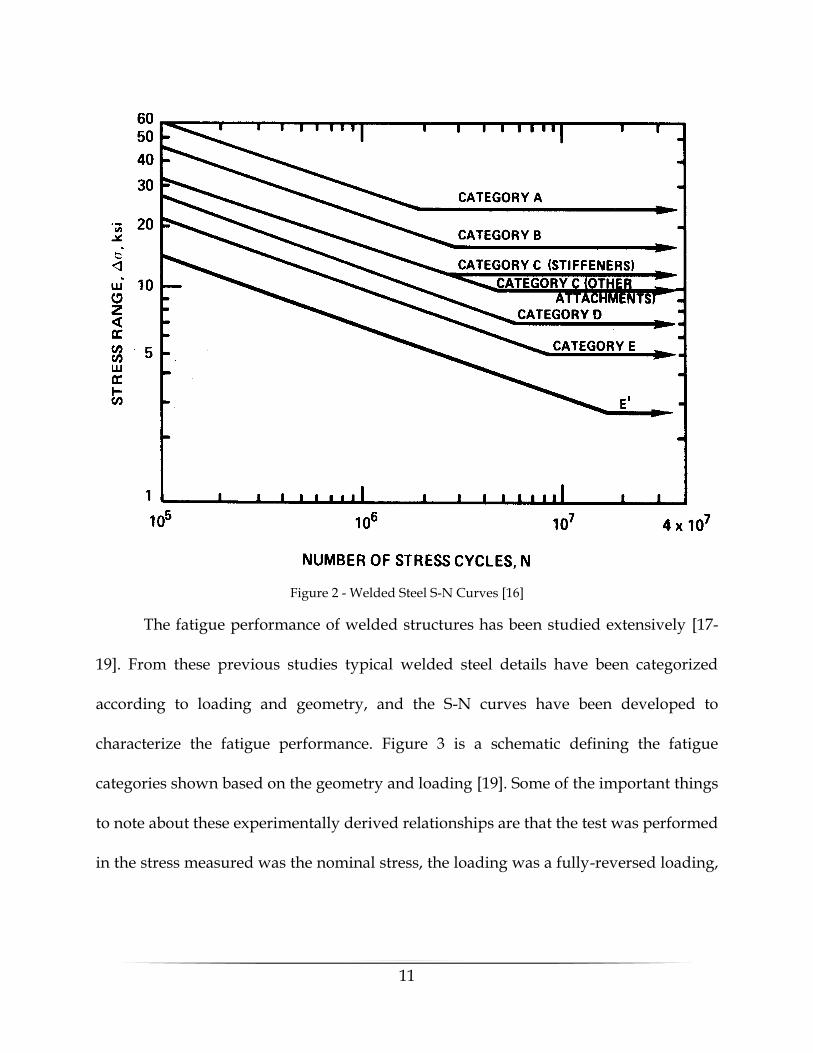
typically documented in terms of an S-N curve [14]. The S-N curves use a log-log scale
with the y-axis showing the applied stress range and the x-axis showing the expected
cycles to failure. A sample S-N curve for welded steel fatigue details is shown in Figure
2 [16]. As the figure shows, there are two distinct portions of an S-N curve. The first
portion shows the relationship between the applied stress and the expected cycles to
failure, but at a certain threshold the slope flattens, and the cycles to failure increase
indefinitely. This threshold is commonly referred to as the endurance limit and it signifies
the maximum applied stress range at which fatigue failure would not occur. This means
that any applied stress equal to or lower than the endurance limit will not result in any
fatigue damage [14]. These relationships are derived experimentally with many inputs
such as material, geometry, and loading conditions. These inputs are the most influential
factors in terms of fatigue performance and for this reason, S-N curves exist for many
different materials and geometries.
11
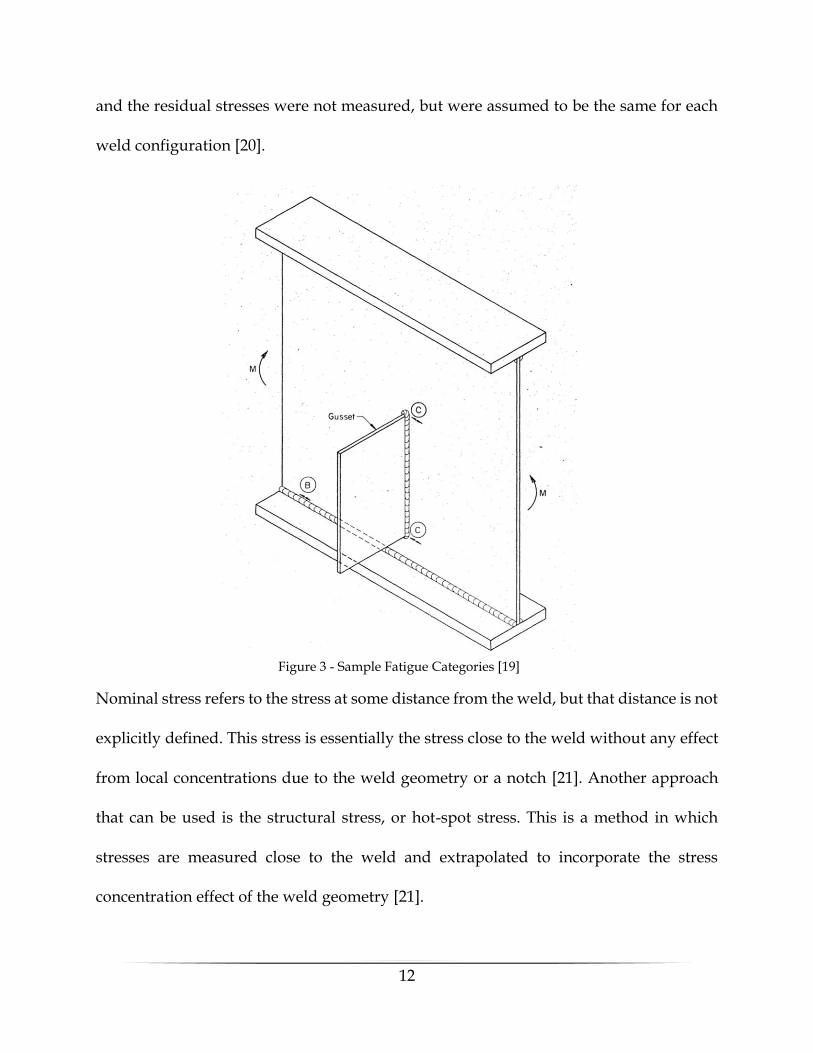
The fatigue performance of welded structures has been studied extensively [17-
19]. From these previous studies typical welded steel details have been categorized
according to loading and geometry, and the S-N curves have been developed to
characterize the fatigue performance. Figure 3 is a schematic defining the fatigue
categories shown based on the geometry and loading [19]. Some of the important things
to note about these experimentally derived relationships are that the test was performed
in the stress measured was the nominal stress, the loading was a fully-reversed loading,
Figure 2 - Welded Steel S-N Curves [16]
12
and the residual stresses were not measured, but were assumed to be the same for each
weld configuration [20].
Nominal stress refers to the stress at some distance from the weld, but that distance is not
explicitly defined. This stress is essentially the stress close to the weld without any effect
from local concentrations due to the weld geometry or a notch [21]. Another approach
that can be used is the structural stress, or hot-spot stress. This is a method in which
stresses are measured close to the weld and extrapolated to incorporate the stress
concentration effect of the weld geometry [21].
Figure 3 - Sample Fatigue Categories [19]
13
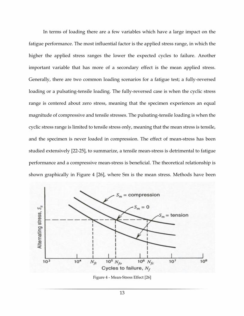
In terms of loading there are a few variables which have a large impact on the
fatigue performance. The most influential factor is the applied stress range, in which the
higher the applied stress ranges the lower the expected cycles to failure. Another
important variable that has more of a secondary effect is the mean applied stress.
Generally, there are two common loading scenarios for a fatigue test; a fully-reversed
loading or a pulsating-tensile loading. The fully-reversed case is when the cyclic stress
range is centered about zero stress, meaning that the specimen experiences an equal
magnitude of compressive and tensile stresses. The pulsating-tensile loading is when the
cyclic stress range is limited to tensile stress only, meaning that the mean stress is tensile,
and the specimen is never loaded in compression. The effect of mean-stress has been
studied extensively [22-25], to summarize, a tensile mean-stress is detrimental to fatigue
performance and a compressive mean-stress is beneficial. The theoretical relationship is
shown graphically in Figure 4 [26], where Sm is the mean stress. Methods have been
Figure 4 - Mean-Stress Effect [26]

14
developed to convert the different types of tests to the fully reversed case in order to
compare the results to the standardized S-N curves. The most commonly used
relationship is the Goodman line shown in Figure 5 [27]. This line uses a combination of
alternating stress (sa), along the y-axis, and mean-stress (sm,) along the x-axis to identify
an equivalent alternating stress (s’e) that would provide the same fatigue life, in terms of
cycles, when the mean stress is zero.
In addition to the mean-stress effect, the residual stress state of the specimen will
have a secondary effect on the fatigue performance. The behavior is similar to the mean-
stress effect where tensile stresses are detrimental and compressive stresses are beneficial
to fatigue performance [28]. Often times the residual stresses are not accounted for in civil
engineering applications.
Figure 5 - Goodman Line [27]

15
RESIDUAL STRESS
Residual stresses are stresses that are created from manufacturing or fabrication
processes and remain in the material even after any external loads are removed [29].
Some examples of the most common sources of residual stresses are welding, cold-
bending, and hot-rolling. These stresses are often overlooked due to their complexity and
the difficulties in measuring them reliably, but the effect of this initial stress state can be
critical in terms of structural performance, in terms of material strength, fatigue
performance, or even stability [29].
In terms of measurement methods, there are a variety of different methods, each
with their own limitations and applications. Generally, the methods are categorized into
relaxation measurement methods and diffraction methods. Relaxation methods rely on
the relationship of the deformations caused from releasing the residual stresses present
in a specimen through cutting, drilling, or other material removal methods [29]. Since
material is being removed, relaxation methods are categorized into destructive methods,
and semi-destructive methods. Destructive methods, as the name suggests, are methods
in which the specimen to be evaluated must be significantly damaged, often to a point
where the specimen no longer be used, while semi-destructive methods are methods in
which the damage is tolerable or is insignificant to the performance of the specimen.
Diffraction methods are often also referred to as non-destructive methods because no
damage is induced through the measurement method.
16
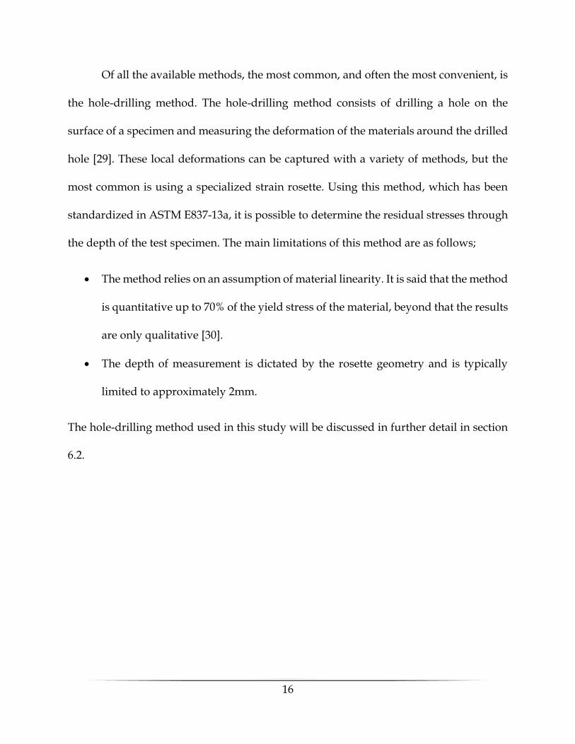
Of all the available methods, the most common, and often the most convenient, is
the hole-drilling method. The hole-drilling method consists of drilling a hole on the
surface of a specimen and measuring the deformation of the materials around the drilled
hole [29]. These local deformations can be captured with a variety of methods, but the
most common is using a specialized strain rosette. Using this method, which has been
standardized in ASTM E837-13a, it is possible to determine the residual stresses through
the depth of the test specimen. The main limitations of this method are as follows;
• The method relies on an assumption of material linearity. It is said that the method
is quantitative up to 70% of the yield stress of the material, beyond that the results
are only qualitative [30].
• The depth of measurement is dictated by the rosette geometry and is typically
limited to approximately 2mm.
The hole-drilling method used in this study will be discussed in further detail in section
6.2.

17
2 LABORATORY TEST SETUP
This chapter will briefly discuss the design of the scale gusset-less truss connection
fatigue specimen, with the limitation of the structural laboratory as a main design
constraint, which was part of a previous thesis [31]. Additionally, the laboratory fatigue
test setup will be described in detail in its original state, which was part of a previous
thesis [31]. The test setup in its current state will be presented with a discussion of the
adjustments made to the setup. The laboratory setup will also introduce and explain the
fatigue loading protocol. Lastly, the instrumentation of the specimen and test setup will
be discussed.
2.1 Specimen Design
The gusset-less truss connection, Figure 6, used in place of typical gusseted
connection on the previously mentioned Memorial Bridge, has a unique geometry which
incorporates prominent bends in the steel to create a transition from the chord to the
Figure 6 - Memorial Bridge, Top-Chord Gusset-less Connection
18
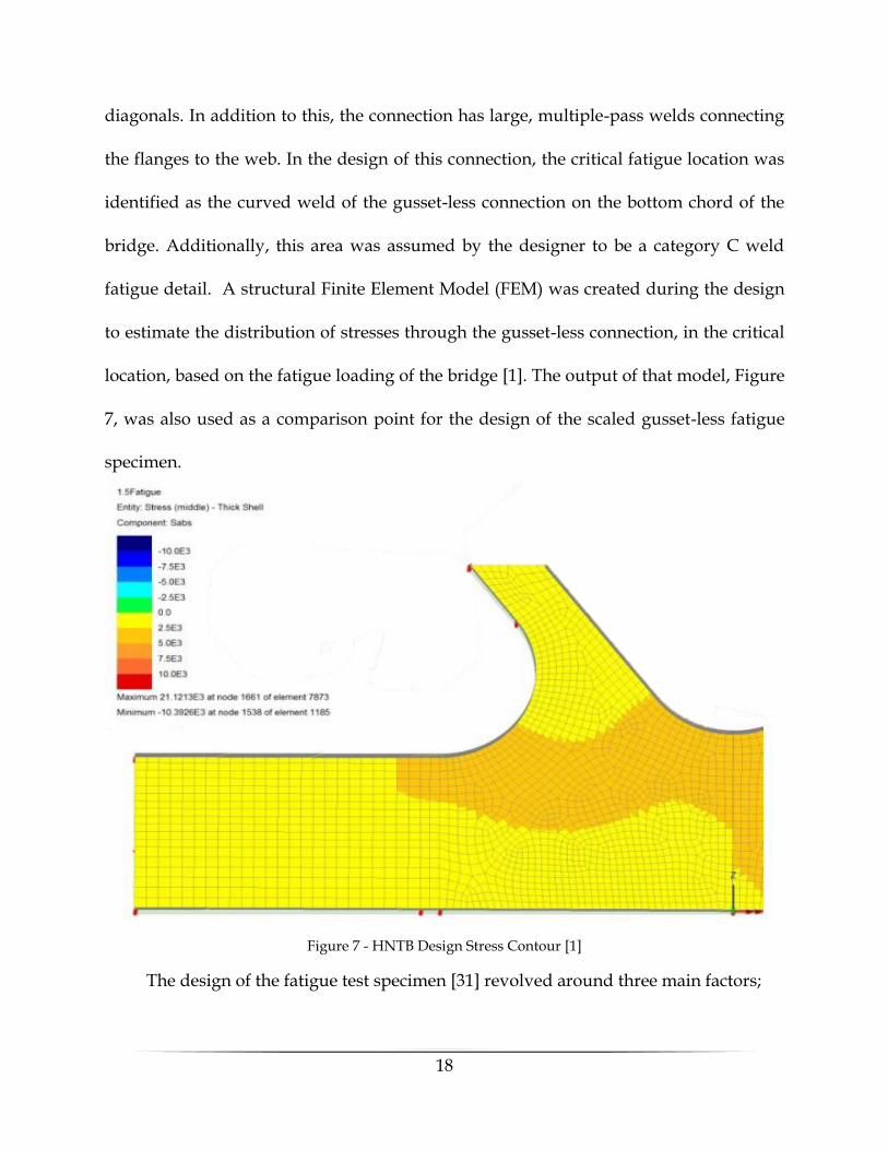
diagonals. In addition to this, the connection has large, multiple-pass welds connecting
the flanges to the web. In the design of this connection, the critical fatigue location was
identified as the curved weld of the gusset-less connection on the bottom chord of the
bridge. Additionally, this area was assumed by the designer to be a category C weld
fatigue detail. A structural Finite Element Model (FEM) was created during the design
to estimate the distribution of stresses through the gusset-less connection, in the critical
location, based on the fatigue loading of the bridge [1]. The output of that model, Figure
7, was also used as a comparison point for the design of the scaled gusset-less fatigue
specimen.
The design of the fatigue test specimen [31] revolved around three main factors;
Figure 7 - HNTB Design Stress Contour [1]

19
1. Capturing and replicating the structural behavior of the in-place connection,
present at the bridge.
2. Replicating the same fabrication process, specifically regarding the weld size
and number of passes, as well as the cold-bending of the top flanges.
3. Scaling the connection in a way that would allow for a representative test to be
conducted with the equipment limitation of the UNH Structural Engineering
Laboratory.
Based on these design goals, the limitations of the structural laboratory were identified
as the primary constraint for this scaled connection. The main limitation was the lack of
infrastructure designed to carry lateral forces, which will be discussed when the fatigue
test setup is introduced. The supports required for the fatigue test played a large role in
the geometric constraints of the specimen. For this specimen design, similitude scaling
was used to determine the geometry and loading. The primary design check was a
comparison to the design stress contours from HNTB. For this check, several numerical
models of different geometries and loading configurations were used to check the stress
contours and general behavior of the specimen. The progression of the geometric
cutbacks is shown in Figure 8 [31].

20
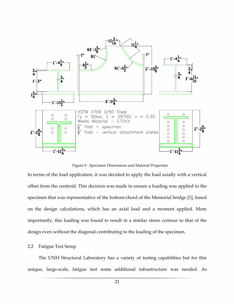
The final scale factor used was 1:1.62 in terms of geometric scaling signifying that the
geometry of the specimen is approximately 62% of the actual connection [31]. The final
geometry and relevant material properties used are shown in Figure 9. Note that two
vertical plates are bounding either side of the test specimen in order to mount it to the
actuator and support respectively. Lastly, the specimen was fabricated by Canam-
Bridges, the steel fabricator for the Memorial Bridge. This ensured that the fabrication
procedures used to produce this specimen were the same as those used in the actual
fabrication of the Memorial Bridge.
Figure 8 - Geometric Reductions of Scaled Connection [30]
21
In terms of the load application, it was decided to apply the load axially with a vertical
offset from the centroid. This decision was made to ensure a loading was applied to the
specimen that was representative of the bottom-chord of the Memorial bridge [1], based
on the design calculations, which has an axial load and a moment applied. More
importantly, this loading was found to result in a similar stress contour to that of the
design even without the diagonal contributing to the loading of the specimen.
2.2 Fatigue Test Setup
The UNH Structural Laboratory has a variety of testing capabilities but for this
unique, large-scale, fatigue test some additional infrastructure was needed. As
Figure 9 - Specimen Dimensions and Material Properties

22
previously mentioned, the main constraint of the laboratory is the lack of infrastructure
capable of handling lateral forces. The main system for mounting equipment in the
structural laboratory is the “Strong-floor” system, which was designed for pull-out
forces. Therefore, in addition to the specimen design, an initial design for the fatigue test
setup was produced [31]. The design goals for the test setup were the following;
• The ability to mount and support the fatigue rated hydraulic actuator, at
multiple heights.
• The ability to support the gusset-less fatigue specimen.
• Provide a transfer of the reactionary forces from the fatigue loading into the
“Strong-floor” system.
The support system design consisted of two parts; (1) the “Reaction Block”, and (2) the
support “Bracket”. The original reaction block was made up of a horizontal steel base
plate with 8 bolt holes for floor anchors, two vertical steel plates with 16 bolt holes for the
actuator attachment rods, four steel kickers, and 16 steel tubes. All the individual
components were welded together as seen in Figure 10.
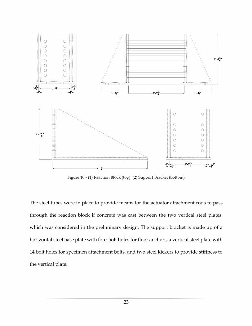
23
The steel tubes were in place to provide means for the actuator attachment rods to pass
through the reaction block if concrete was cast between the two vertical steel plates,
which was considered in the preliminary design. The support bracket is made up of a
horizontal steel base plate with four bolt holes for floor anchors, a vertical steel plate with
14 bolt holes for specimen attachment bolts, and two steel kickers to provide stiffness to
the vertical plate.
Figure 10 - (1) Reaction Block (top), (2) Support Bracket (bottom)
24
Once the test setup was fabricated, the supports were positioned in their
appropriate locations based on the Strong-Floor anchor pattern and bolted in place. With
the supports in position the actuator was lifted into position and attached to the reaction
block using high-strength threaded steel rods with nuts torqued to 1400 ft-lb. Finally, the
specimen was bolted, to a specified 800 ft-lb of torque, into the test setup. After
installation of the supports and test specimen, some initial static load tests were
performed to identify the behavior of the system. Specifically, the strain in the area of
interest and at the boundary conditions, as well as the displacements in key locations
along the test setup were investigated, which will be discussed in detail in section 3.2.
These measurements led to four key observations made about the test setup in its initial
state;
1. There was significant support motion in both the reaction block and the
support bracket, causing undesirable actuator motion.
2. The vertical plate connecting the specimen and the actuator, also referred to as
the specimen tip, was displacing significantly in the vertical direction.
3. The specimen tip was rotating significantly out of plane about the horizontal
loading axis.
4. There was a high strain reading (2000 μϵ) in the vertical direction on the
vertical plate connecting the specimen and the actuator.
Based on these observations, some modifications to the test setup were needed in order
to further control the behavior of the test setup. Specifically, the modifications are
25
intended to ensure the desired loading was applied to the fatigue specimen while
protecting the hydraulic actuator from undesirable side loading [32].
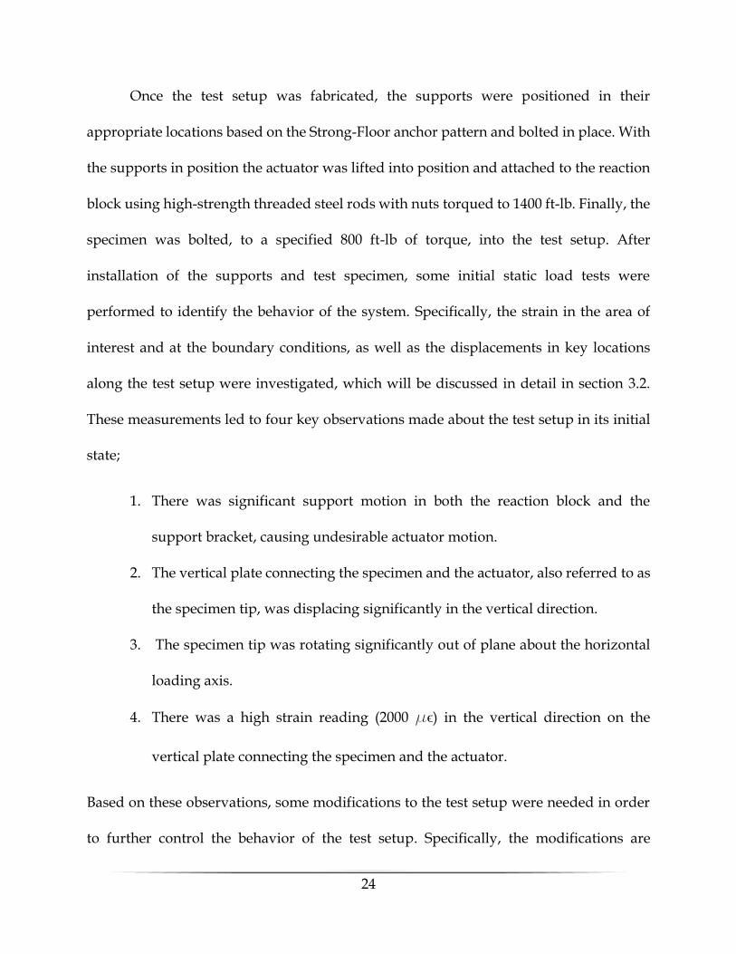
The first modification was creating a new boundary condition at the specimen tip,
hereby referred to as the “shim support”, in order to restrain the vertical displacement as
well as the rotation of the test specimen. This was accomplished using multiple steel
shims, shown in Figure 11, wedged under the tip of the specimen at two locations, on
either side of the specimen tip. This support acts as a roller in the plane of loading because
the steel shims can slide against each other while restricting motion in the vertical
direction. It should be noted that this only restrains the vertical motion while applying a
tensile load, which causes the specimen to displace downward. Due to the discretization
of the shims, at either ends of the specimen tip, the rotation about the plane of loading is
also restrained. In addition to the shims at the tip of the specimen, shims were added
under the reaction block and bracket to increase the contact with the floor and decrease
rotations at the supports.
26
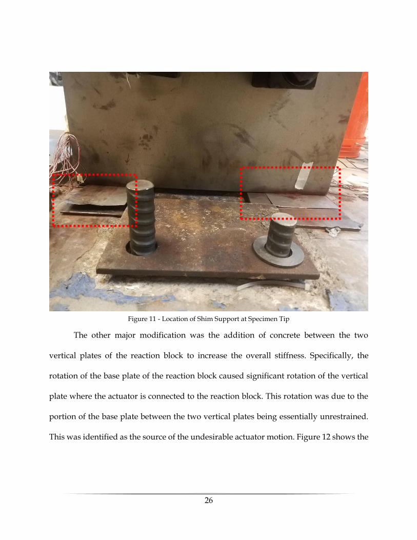
The other major modification was the addition of concrete between the two
vertical plates of the reaction block to increase the overall stiffness. Specifically, the
rotation of the base plate of the reaction block caused significant rotation of the vertical
plate where the actuator is connected to the reaction block. This rotation was due to the
portion of the base plate between the two vertical plates being essentially unrestrained.
This was identified as the source of the undesirable actuator motion. Figure 12 shows the
Figure 11 - Location of Shim Support at Specimen Tip
27
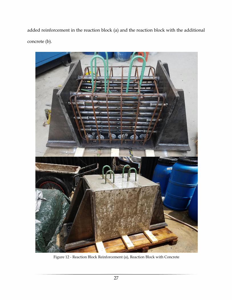
added reinforcement in the reaction block (a) and the reaction block with the additional
concrete (b).
Figure 12 - Reaction Block Reinforcement (a), Reaction Block with Concrete

28
The final modification was the change in actuator position to prevent a stress
concentration on the vertical plate attaching the specimen to the actuator. During
installation, it was noted that the vertical plate had a significant bend, most likely due to
the welding process. When the actuator was in it’s original, highest, position and the bolts
were tightened, this bend was removed due to the force from the bolts. The straightening
of this plate caused the strain in the plate close to the weld to exceed the yield strain of
the material, creating a point in the test setup that would be prone to fatigue damage to
the magnitude of the strain applied. Since this location was not the area of interest, it was
decided to lower the actuator to the next position, which resulted in a significant
reduction in the strain at the location.
With the modifications to the test setup made, additional tests were performed,
and the structural response was measured and found to be acceptable. The test setup in
its final state is shown in Figure 13. This configuration consists of the reaction block, the
actuator, the fatigue specimen, the shim support, and the bracket.
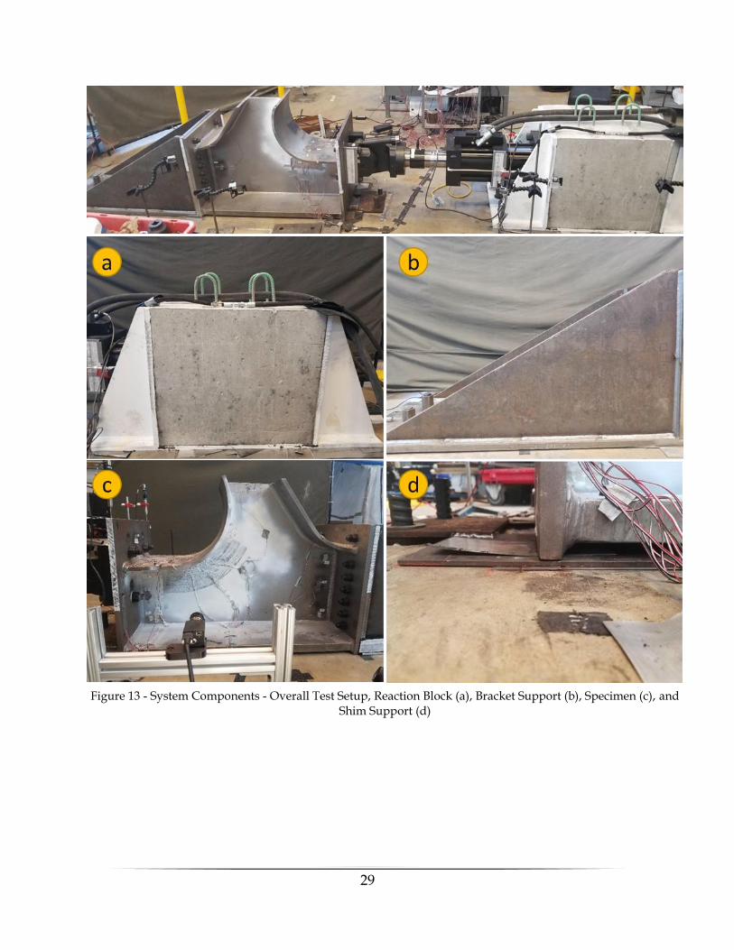
29
Figure 13 - System Components - Overall Test Setup, Reaction Block (a), Bracket Support (b), Specimen (c), and Shim Support (d)

30
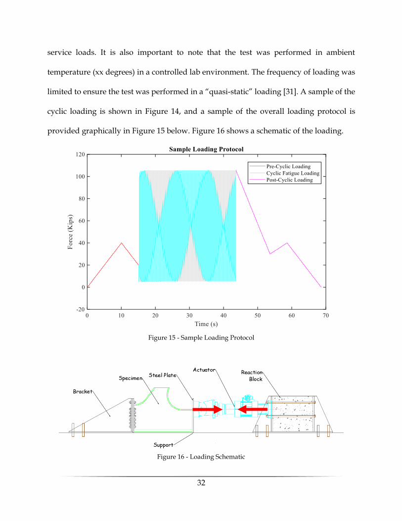
In addition to the physical test setup, a loading protocol was also developed for
this test. The loading protocol can be divided into three main sections;
1. The pre-cyclic loading
2. The cyclic fatigue loading
3. The post-cyclic loading
The loading protocol is applied using MTS Multi-Purpose Testware software to
apply either loads or displacements to the MTS 244.41 hydraulic actuator. In this specific
loading protocol, the commands are given in terms of force measured on the load cell, a
device to measure the force applied, of the actuator. The loading procedures were coded
in the MPT Procedure Editor in the form of force commands.
The pre-cyclic loading consists of two ramp functions in which the load is brought
from 0 Kip to 40 Kip in 10 seconds, then from 40 Kip to 20 Kip in 5 seconds and occurs
before the cyclic fatigue loading. The purpose of this ramp loading is to create some
unique peaks in the measured response that will be used to synchronize the data sets
from different measurement methods. The post-cyclic loading consists of three ramp
functions in which the load is brought to 40 Kip in 7.5 seconds, then 60 Kip in 5 seconds,
and finally 0 Kip in 7.5 seconds. The post-cyclic loading occurs after the cyclic fatigue
loading and serves as a second point of synchronization for the post-processing.
The cyclic fatigue loading, which is implemented after the pre-cyclic loading and
before the post-cyclic loading, that is being used in this test is a pulsating tensile loading,
31
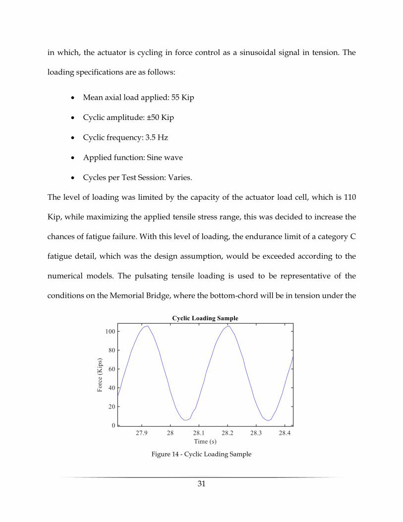
in which, the actuator is cycling in force control as a sinusoidal signal in tension. The
loading specifications are as follows:
• Mean axial load applied: 55 Kip
• Cyclic amplitude: ±50 Kip
• Cyclic frequency: 3.5 Hz
• Applied function: Sine wave
• Cycles per Test Session: Varies.
The level of loading was limited by the capacity of the actuator load cell, which is 110
Kip, while maximizing the applied tensile stress range, this was decided to increase the
chances of fatigue failure. With this level of loading, the endurance limit of a category C
fatigue detail, which was the design assumption, would be exceeded according to the
numerical models. The pulsating tensile loading is used to be representative of the
conditions on the Memorial Bridge, where the bottom-chord will be in tension under the
Figure 14 - Cyclic Loading Sample
32
service loads. It is also important to note that the test was performed in ambient
temperature (xx degrees) in a controlled lab environment. The frequency of loading was
limited to ensure the test was performed in a “quasi-static” loading [31]. A sample of the
cyclic loading is shown in Figure 14, and a sample of the overall loading protocol is
provided graphically in Figure 15 below. Figure 16 shows a schematic of the loading.
Figure 15 - Sample Loading Protocol
Figure 16 - Loading Schematic
33
In addition to the development of the loading procedures, the tuning parameters
as well as the limits for the actuator were selected. The tuning of the actuator refers to
adjusting the inputs, in terms of a proportional-integral-derivative (PID) control loop.
The specific methods for tuning this control loop were obtained from the MTS user
manual [33]. The goal of tuning the actuator controls was to ensure that the command
being input, in terms of force and frequency, matched the actual measured output of the
actuator. Additionally, with a poorly tuned actuator, especially when using force-
controlled testing, the system is susceptible to instability in which the measured force can
rapidly deviate from the command in terms of magnitude and frequency. This is one of
the main reasons for the limits being implemented. The limits refer to an upper and lower
force limit that, if the actuator load cell reading exceeds, will interlock the hydraulics and
stop pressure from reaching the actuator. The upper limit, set to approximately 107 Kip,
is in place to prevent the actuator load cell from reaching the 110 Kip limit, while the
lower limit, set to approximately -2 Kip (compression), is in place to prevent the specimen
from being loaded in compression. Therefore, in the case of instability, the limits will be
exceeded, and the hydraulics will quickly cease pressure to the actuator.

34
2.3 Instrumentation
The objectives of the experiment must be considered prior to determining the
location and type of sensors. Each sensor should provide a needed piece of information
to fulfill these objectives. For this experiment, the bridge owner was interested in (1)
investigating the design assumption of fatigue category C [20] for the gusset-less truss
connection, which implies infinite-fatigue life under service conditions, and (2) collecting
data useful for providing guidance for fatigue-focused visual inspection procedures of
the gusset-less connection through the service life of the bridge. An additional interest of
the research was verifying the structural model of the gusset-less connection and
evaluating the dissipation of strain with distance from the weld toe. In order to
accomplish these goals, the experimental set up, including boundary condition and
component interface, must be categorized and fully understood for both fatigue
assessment and structural model verification.
The measurements techniques and sensors that are utilized for the scale model
laboratory fatigue experiment are Digital Image Correlation (DIC), Linear Variable
Differential Transformers (LVDTs), and strain gauges (uniaxial and rosettes), which are
used to measure displacements, rotations and strains. The instrumentation used can
broadly be categorized as contact (LVDTs and strain gauges) and non-contact (DIC)
measurements.
Strain gauges and LVDTs are two of the most traditional contact tools for obtaining
structural response measurements. These sensors function by maintaining contact with
35
the specimen, through contact in the case of the LVDT, or bonding (epoxy or spot-weld),
in the case of the strain gauge. These tools tend to be the most commonly used due to
their cost, availability, reliability, and accuracy of structural response measurements.
Although strain gauges are the most frequently used sensors, there are some significant
drawbacks and limitations to their use and applicability. One of the most significant
drawbacks for the strain gauges is the installation procedure, which generally consists of
the following:
1. Surface preparation consisting of abrasion (sanding or grinding) followed by a
thorough cleaning of the surface to remove particles and oils which could
weaken the adhesive bond.
2. Positioning of the gauge to define the measurement direction(s).
3. Application of accelerant to prepare the gauge for adhesion.
4. Application of adhesive and bonding of the gauge.
5. Positioning of the lead wires and soldering if necessary.
6. Connection to strain measuring device and data recording.
Strain gauges are limited to relatively smooth and preferably flat surfaces that allow
complete bonding of the gauge to the specimen. Additionally, the locations that the strain
gauges and LVDTs can be installed is limited to locations that can be physically accessible
with sufficient space to perform all the steps necessary for installation.
Another major drawback to these contact measurements is the amount of surface
preparation required for adequate installation. Not only is surface preparation a

36
significant amount of work but it also has the potential to interact and affect the specimen
behavior. Specifically, if there is any coating or outer layer of environmental protection
on a specimen, the surface preparation requires coating removal, while this is not an issue
for laboratory specimens exposed to indoor environmental conditions, it can adversely
impact field application. Further, strain gauges and LVDTs only provide discrete
measurements at the point of installation. Often times, the amount of measurements
needed to fully characterize the response of a specimen is significant. To capture all the
required measurements, many sensors are necessary, which is costly in terms of number
of sensors and installation time. To a lesser extent, the size of these sensors may also
provide important limitations, especially when localized strain measurements are
needed very close to one another.
The DIC measurements fall under the non-contact measurements category since
contact is not present between the cameras and the specimen. DIC identifies and tracks
the movement of groups of pixels captured via a speckle pattern on the area of interest.
Using a correlation algorithm, the translation vectors for each pixel grouping are
calculated and the movement is computed relative to the location of the pixel groupings
of an undeformed reference image. A mathematical background of the DIC analysis
method is provided in Appendix A. Although DIC is not as widely used as the traditional
measurement methods, it is becoming more popular as digital image technology
advances become more cost-effective and the post-processing technology improves. DIC
measurements, while not being as consistently accurate as traditional methods, given the

37
impact of image collection conditions and camera capability, excels in many other
aspects. One of the largest benefits of DIC compared to other forms of instrumentation is
its ease of installation. DIC requires very little installation time depending on the type of
equipment used and the environment where the measurements are collected. The general
installation procedure is as follows:
1. Application of a suitable tracking pattern to the measurement area of intertest.
Typically, this is done with a black on white speckle pattern or the inverse.
2. Placement of camera(s) to focus on the measurement area. If 2-D DIC is being
used, the cameras need to be perpendicular to the area of interest. When 3-D
DIC is being used, a minimum of two cameras will be in a stereo configuration,
typically at an angle of 30 degrees with respect to each other.
3. Adjustment of camera(s) settings to optimize focus, lighting, and resolution.
These parameters should be optimized uniquely for the test setup and the
hardware used.
4. Image capturing. Typically, a commercial program is used to control the capture
settings/timings, especially in the case of 3-D DIC in order to synchronize the
multiple cameras.
An experienced user can record measurements with DIC in a relatively short time
without difficulty. The other major benefit is that the DIC measurements can be used to
characterize a large area where applying multiple gauges would not be feasible. With the
correct setup and equipment, it is possible to obtain a full-field characterization of the

38
area of interest. One major drawback for the DIC is the computational effort is much more
significant compared to the strain gauges and LVDTs. This is due to the differences in
data, with the strain gauges and LVDTs it is a direct measurement and there is no post-
processing needed, but with DIC it is indirect in that it is converting pixel movements
into displacements and strains mathematically. Lastly, the initial cost of the DIC
equipment can be high, but it is a tool that can be reused and applied to a variety of
situations, which has the potential to mitigate long-term costs.
The strain gauge instrumentation plan for the specimen is shown in Figure 17. The
naming convention for the gauges are as follows;
• Specimen side; N = on the North face of the specimen, S = on the South face of
the specimen, VP = on the vertical plate of the specimen.
• Type; R = Rosette type strain gauge, U = Uniaxial type strain gauge.
• Location; W = web of specimen. FB = Flange (bottom-side). FT = Flange (top-
side).
• Number; the number corresponding to specific gauge of a specific type.
• Example; NRW1 = Rosette number one on the North face of the specimen web
In this study, a total of 12 strain rosettes and 10 uniaxial strain gauges are being
used to characterize the strains throughout the specimen. The uniaxial strain gauges used
were CEA-06-125UW-120 gauges while the rosettes used were EA-XX-125BZ-350, all of
which were wired in a quarter bridge configuration [2]. The device used to connect the
strain gauges to a data acquisition computer was the NI cDAQ™-9178 chassis with NI

39
9219 Universal Analog Input Modules, and the data acquisition software was LabVIEW
2017. The capture frequency chosen for all strain gauges was 60Hz, which was sufficient
enough to characterize the response given the input frequency, while maintaining a
reasonable sized data set from each testing period. The strains were chosen to be recorded
continuously throughout the entire loading protocol, as opposed to incrementally, to
ensure that if there was a change in behavior, it would be captured through the strain
measurements. Lastly, it is important to note that the strain gauges were calibrated, or
zeroed, while the specimen was not attached to the test setup, meaning that the strains
from the installation, mainly the bolt loading and gravity loads, are present in the
measured strains. Since the main factor is strain range, the range for each of the gauges
during the fatigue loading is of interest, but the mean strain is also important for
characterizing the fatigue performance.
40
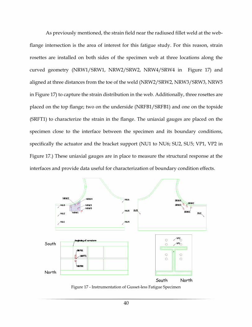
As previously mentioned, the strain field near the radiused fillet weld at the web-
flange intersection is the area of interest for this fatigue study. For this reason, strain
rosettes are installed on both sides of the specimen web at three locations along the
curved geometry (NRW1/SRW1, NRW2/SRW2, NRW4/SRW4 in Figure 17) and
aligned at three distances from the toe of the weld (NRW2/SRW2, NRW3/SRW3, NRW5
in Figure 17) to capture the strain distribution in the web. Additionally, three rosettes are
placed on the top flange; two on the underside (NRFB1/SRFB1) and one on the topside
(SRFT1) to characterize the strain in the flange. The uniaxial gauges are placed on the
specimen close to the interface between the specimen and its boundary conditions,
specifically the actuator and the bracket support (NU1 to NU6; SU2, SU5; VP1, VP2 in
Figure 17.) These uniaxial gauges are in place to measure the structural response at the
interfaces and provide data useful for characterization of boundary condition effects.
Figure 17 - Instrumentation of Gusset-less Fatigue Specimen
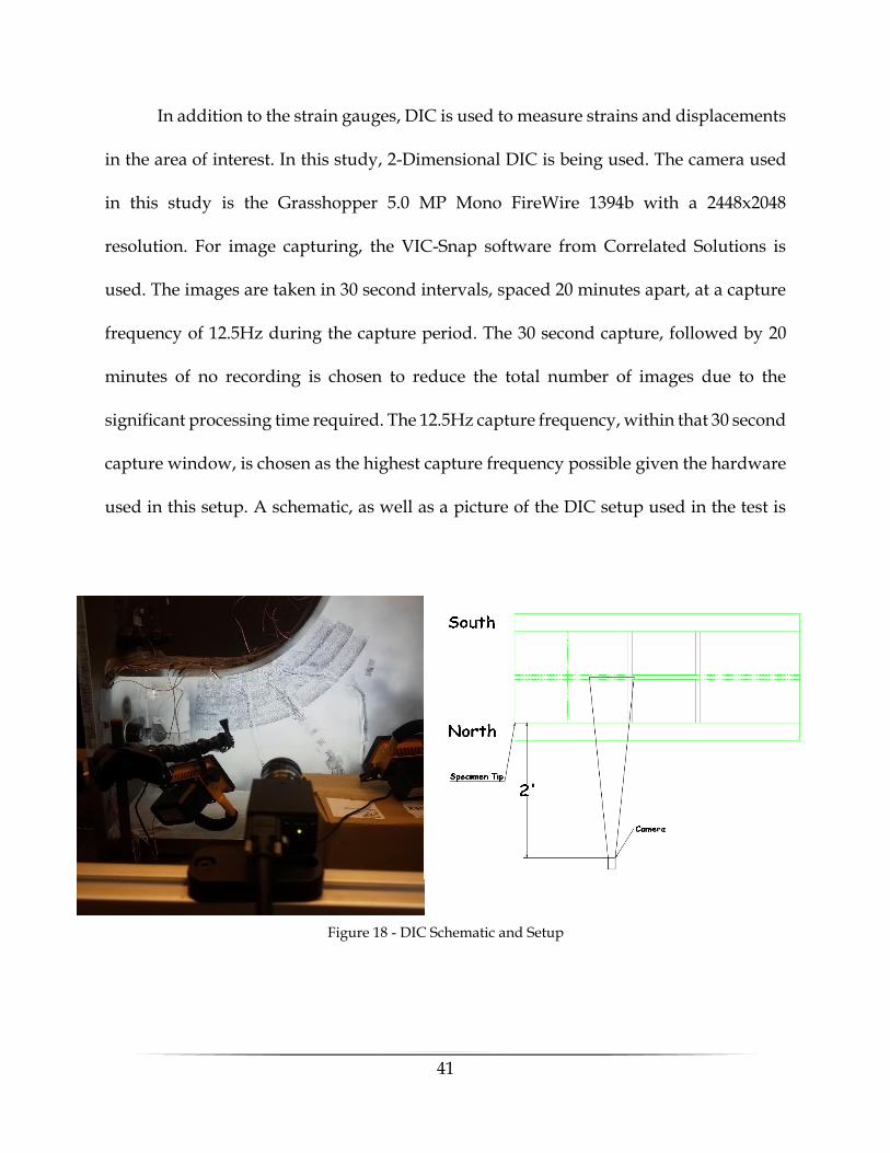
41
In addition to the strain gauges, DIC is used to measure strains and displacements
in the area of interest. In this study, 2-Dimensional DIC is being used. The camera used
in this study is the Grasshopper 5.0 MP Mono FireWire 1394b with a 2448x2048
resolution. For image capturing, the VIC-Snap software from Correlated Solutions is
used. The images are taken in 30 second intervals, spaced 20 minutes apart, at a capture
frequency of 12.5Hz during the capture period. The 30 second capture, followed by 20
minutes of no recording is chosen to reduce the total number of images due to the
significant processing time required. The 12.5Hz capture frequency, within that 30 second
capture window, is chosen as the highest capture frequency possible given the hardware
used in this setup. A schematic, as well as a picture of the DIC setup used in the test is
Figure 18 - DIC Schematic and Setup
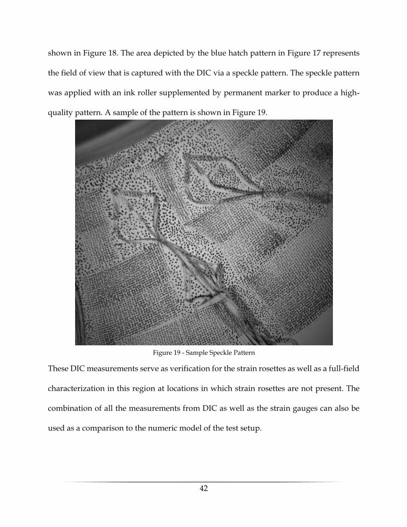
42
shown in Figure 18. The area depicted by the blue hatch pattern in Figure 17 represents
the field of view that is captured with the DIC via a speckle pattern. The speckle pattern
was applied with an ink roller supplemented by permanent marker to produce a high-
quality pattern. A sample of the pattern is shown in Figure 19.
These DIC measurements serve as verification for the strain rosettes as well as a full-field
characterization in this region at locations in which strain rosettes are not present. The
combination of all the measurements from DIC as well as the strain gauges can also be
used as a comparison to the numeric model of the test setup.
Figure 19 - Sample Speckle Pattern

43
3 FATIGUE TEST MONITORING
This chapter will introduce the developed fatigue test monitoring protocol specific to
this test. After this introduction, the System Identification (System ID) that has been
performed will be explained in detail and the results of the System IDs performed will be
presented. Finally, the force-displacement relationship of the actuator will be discussed,
specifically regarding how it is a representative measurement for the behavior of the
system.
3.1 Fatigue Test Monitoring Protocol
Ensuring consistent behavior in a high-cycle fatigue test is important, especially
when the test must be performed in multiple smaller testing intervals in which the
loading is paused and later resumed. There is an added complication in this study in the
potential for changes in the test setup due to the fatigue loading of the test setup.
Specifically, the shims under the specimen tip as well as all the bolted connections in the
test setup have the potential for degradation, in the case of the shims, or loosening in the
case of the bolted connections. In this scenario, it is critical to develop a protocol to
systematically monitor the structural response of the system and use this data to identify
any changes in behavior throughout the high-cycle fatigue test. Additionally, a
monitoring protocol aids in identifying potential fatigue damage or failure in the
specimen. For these reasons, a test monitoring protocol was developed for this study in
order to maintain a consistent structural behavior throughout this test. A graphical
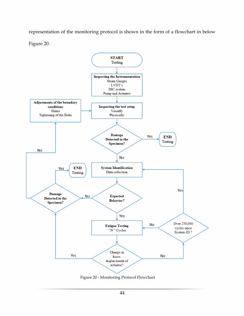
44
representation of the monitoring protocol is shown in the form of a flowchart in below
Figure 20.
Figure 20 - Monitoring Protocol Flowchart

45
The flowchart developed for monitoring the high-cycle fatigue test is specific to this
research, but the general concept can be applied while the specific monitoring details can
be altered to be used in another test.
The start point of this monitoring protocol is equivalent to day zero of testing,
meaning that the specimen is mounted in the test setup and is properly instrumented for
the fatigue test, but no fatigue testing has been performed on the specimen. Advancing
from the start position in this protocol, the next step is to inspect the instrumentation used
in the test. This is one of the most critical steps, specifically because the monitoring
protocol revolves around making data driven decisions using the measured structural
response from the instrumentation. Therefore, it is extremely important to ensure that the
measurements that are being used are not compromised. There are a few things that are
checked in this instrumentation inspection;
1. Strain gauges, both rosettes and uniaxial gauges, are checked for debonding
from the specimen surface. Additionally, the wiring is inspected for any
damage. This check is in place to ensure that there has not been any physical
change to the gauges. Specifically, due to the location and length of the wires
connecting the strain gauges to the measurement system, there is a significant
risk that the wires become damaged due to foot traffic in the laboratory.
46
2. A gauge test, in the form of recording strains for ~10 seconds, is performed to
check the strain values being recorded by the gauges. This test will
quantitatively indicate any erroneous strain measurements as well as allow the
user to quickly identify which, if any, strain gauges need to be inspected
further. One example of this is if a strain gauge wire is damaged due to foot-
traffic, an abnormally high strain will be shown in the gauge test.
3. The LVDT’s are tested in a similar fashion to the gauges. They are visually
inspected to ensure that the required contact to the specimen is made and the
direction of the LVDT is still consistent with the measurement in the direction
of interest. Additionally, the displacements are recorded for ~10 seconds to
check for any measurement errors.
4. Lastly the DIC system is assessed. First the camera is turned on and the lens
cap removed. The two LED lights are turned on and positioned to illuminate
the area of interest. Next the camera is inspected for perpendicularity to the
surface in which the area of interest is located on. The saturation of the light is
checked in the VIC-Snap software and adjusted to the optimal level through
adjustments to the exposure timing. Lastly, images are recorded for ~10
seconds to check for any errors in the recording software. One specific example
of an error in this study was that the cameras would sometimes not record at
the specified frequency, so adjustments had to be made before testing.
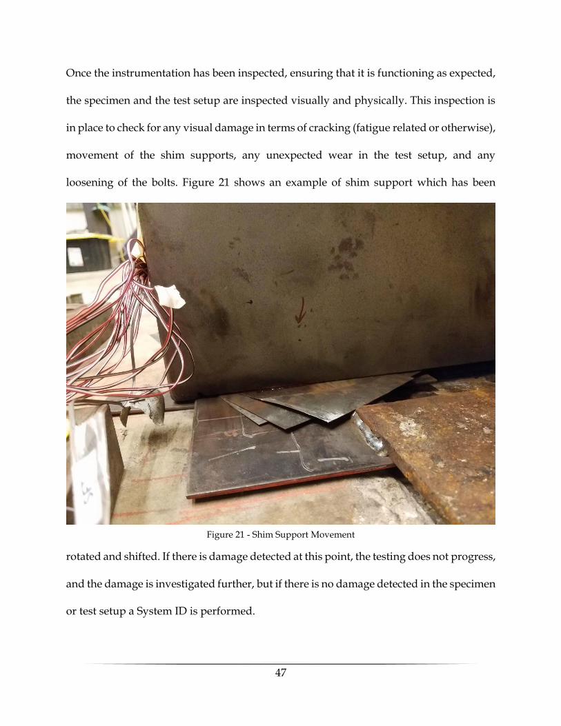
47
Once the instrumentation has been inspected, ensuring that it is functioning as expected,
the specimen and the test setup are inspected visually and physically. This inspection is
in place to check for any visual damage in terms of cracking (fatigue related or otherwise),
movement of the shim supports, any unexpected wear in the test setup, and any
loosening of the bolts. Figure 21 shows an example of shim support which has been
rotated and shifted. If there is damage detected at this point, the testing does not progress,
and the damage is investigated further, but if there is no damage detected in the specimen
or test setup a System ID is performed.
Figure 21 - Shim Support Movement

48
The System ID is a full characterization of the structural response of the test setup
through measurements at key points in the test setup while it is being subjected to a short
version of a testing interval using the fatigue loading protocol. A detailed explanation of
the System ID and the measurements taken will be provided in section 3.2. The response
captured with the System ID is used as a baseline behavior to compare future system IDs
to. Once the System ID is performed and the data is processed, the research team
compares the observed structural behavior to the previous System ID or a theoretical
behavior in the case of the first system ID. Specifically in this study, the first
measurements were compared to a numerical model of the test setup. At this point, the
behavior is evaluated, and a decision is made on whether the behavior is as expected or
if there is a significant difference between the expected and the measured response.
If the response is significantly different than expected, adjustments must be made
to the system to modify and correct the behavior. Some examples of how this is
accomplished are; adjusting the shim supports, re-torqueing the anchor bolts, and re-
torqueing the bolts connecting the different parts of the test setup. Once the modifications
have been made another inspection is performed followed by the System IDif there is no
damage detected during the inspection. This process forms an iterative loop until the
behavior is acceptable, at which point the fatigue testing can begin.
The fatigue testing is performed in testing intervals with a set number of cycles
per interval. The intervals used in this research ranged from 2-hours (~26000 load cycles)
up to 12-hours (~155000 load cycles), but due to the likelihood of data acquisition errors
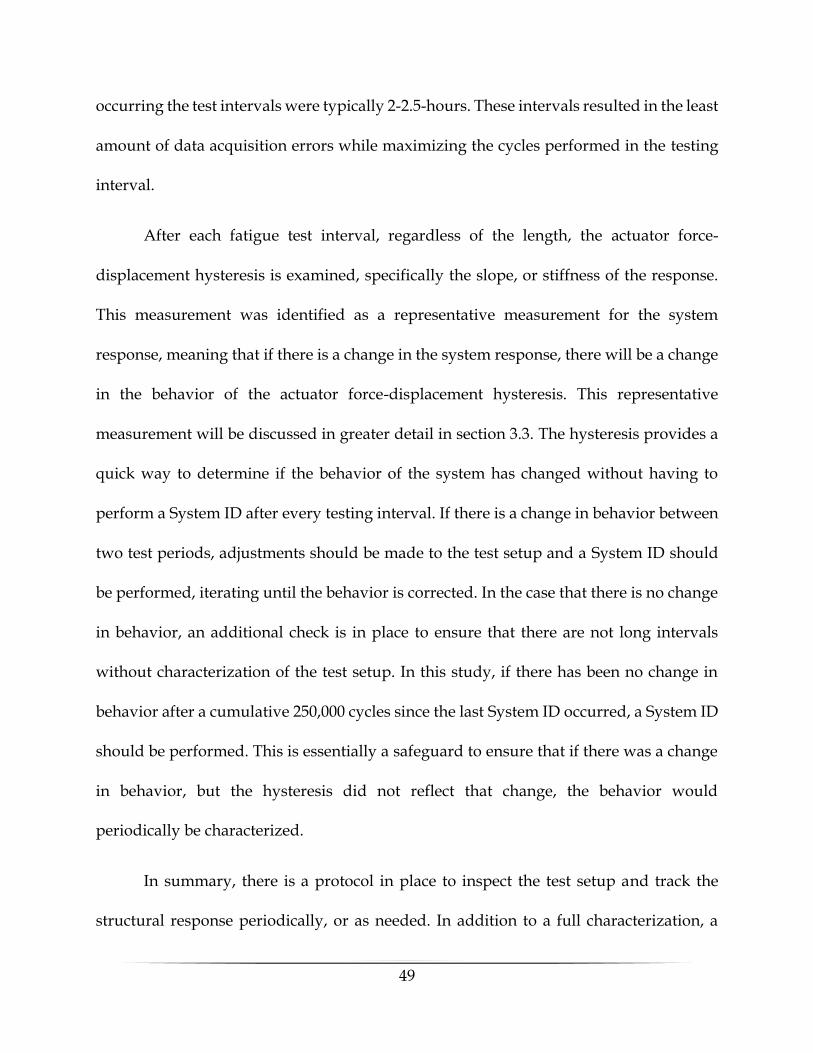
49
occurring the test intervals were typically 2-2.5-hours. These intervals resulted in the least
amount of data acquisition errors while maximizing the cycles performed in the testing
interval.
After each fatigue test interval, regardless of the length, the actuator force-
displacement hysteresis is examined, specifically the slope, or stiffness of the response.
This measurement was identified as a representative measurement for the system
response, meaning that if there is a change in the system response, there will be a change
in the behavior of the actuator force-displacement hysteresis. This representative
measurement will be discussed in greater detail in section 3.3. The hysteresis provides a
quick way to determine if the behavior of the system has changed without having to
perform a System ID after every testing interval. If there is a change in behavior between
two test periods, adjustments should be made to the test setup and a System ID should
be performed, iterating until the behavior is corrected. In the case that there is no change
in behavior, an additional check is in place to ensure that there are not long intervals
without characterization of the test setup. In this study, if there has been no change in
behavior after a cumulative 250,000 cycles since the last System ID occurred, a System ID
should be performed. This is essentially a safeguard to ensure that if there was a change
in behavior, but the hysteresis did not reflect that change, the behavior would
periodically be characterized.
In summary, there is a protocol in place to inspect the test setup and track the
structural response periodically, or as needed. In addition to a full characterization, a

50
representative measurement has been identified and used to quickly see if there is a
change in behavior. Using a systematic approach as described above and shown
graphically in Error! Reference source not found., ensures that consistent conditions are
kept throughout the duration of a high-cycle fatigue test performed across multiple
testing intervals.
3.2 System Identification
As previously mentioned the system identification (system ID) refers to a full
characterization of the structural response of the test setup while it is being subjected to
a short version of a testing interval using the fatigue loading protocol. The System ID
serves two purposes: (1) ensuring the test is producing measurements in the expected
range, and (2) monitoring and verifying the consistency of the structural behavior
throughout the fatigue test prior to specimen damage.
In the current high-cycle fatigue experiment, due to the estimated cycles to failure,
the test is completed over multiple testing periods. The test is performed under constant
loading (force) amplitude and it is expected that the specimen will experience a consistent
range of stress, which can be verified, for example, by evaluating the strain history
measurements collected during the test. The stability and consistency of the testing
environment and boundary conditions is critical during the test. Consequently, it is
critical to characterize the behavior prior to the test. Any changes in the test setup during
the test could result in system responses that are inconsistent. Using the System ID, a
reference set of measurements is generated to serve as benchmark for future

51
characterizations of the system. Using this benchmark as a reference, the test setup is
periodically checked against previous characterizations to ensure that the behavior is
consistent between fatigue testing intervals.
One of the key features of the System ID used in this study is the ability to identify
behavior at key locations. This is achieved using many sensors and data acquisition
devices, namely;
• 2-Dimensional Digital Image Correlation (2-D DIC)
• Linear Variable Differential Transformers (LVDTs)
• Strain Gauges
The background on the measurement devices has been provided in section 2.3. There are
two significant change between the instrumentation plan for the fatigue test and the
instrumentation used in the System ID. The first is the use of GoPro cameras to capture
2-D DIC measurements at additional locations along the test setup. The second is the use
of LVDTs as verification points for the DIC measurements.
The locations of the additional measurements using the GoPro cameras are shown
as the red hatched areas in Figure 22. Each location was chosen to characterize the
boundaries between different portions of the test setup as well as the relative behavior of
each component of the test setup. The LVDTs used in this study is an LVDT-01-030 from
BDI, the data acquisition software used is STS-LIVE, and the capture frequency is 100Hz.
The locations of the LVDTs are not shown in Figure 22, but are always present in the
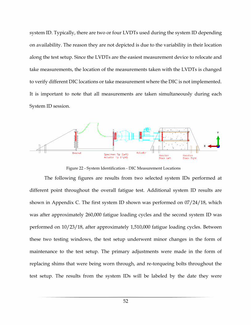
52
system ID. Typically, there are two or four LVDTs used during the system ID depending
on availability. The reason they are not depicted is due to the variability in their location
along the test setup. Since the LVDTs are the easiest measurement device to relocate and
take measurements, the location of the measurements taken with the LVDTs is changed
to verify different DIC locations or take measurement where the DIC is not implemented.
It is important to note that all measurements are taken simultaneously during each
System ID session.
The following figures are results from two selected system IDs performed at
different point throughout the overall fatigue test. Additional system ID results are
shown in Appendix C. The first system ID shown was performed on 07/24/18, which
was after approximately 260,000 fatigue loading cycles and the second system ID was
performed on 10/23/18, after approximately 1,510,000 fatigue loading cycles. Between
these two testing windows, the test setup underwent minor changes in the form of
maintenance to the test setup. The primary adjustments were made in the form of
replacing shims that were being worn through, and re-torqueing bolts throughout the
test setup. The results from the system IDs will be labeled by the date they were
Figure 22 - System Identification - DIC Measurement Locations
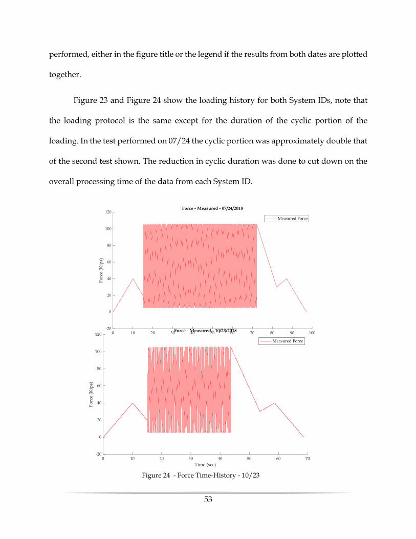
53
performed, either in the figure title or the legend if the results from both dates are plotted
together.
Figure 23 and Figure 24 show the loading history for both System IDs, note that
the loading protocol is the same except for the duration of the cyclic portion of the
loading. In the test performed on 07/24 the cyclic portion was approximately double that
of the second test shown. The reduction in cyclic duration was done to cut down on the
overall processing time of the data from each System ID.
Figure 23 - Force Time-History - 07/24
Figure 24 - Force Time-History - 10/23
54
Figure 25 shows an example of the cross-verification between the measurements with the
2-D DIC and an LVDT, in this case the location is the tip of the actuator and the
measurement taken is the horizontal displacement. As the graph shows, the
measurements match closely, it should be noted that this is raw data with no post-
processing or adjustments.
Figure 25 - DIC and LVDT Verification
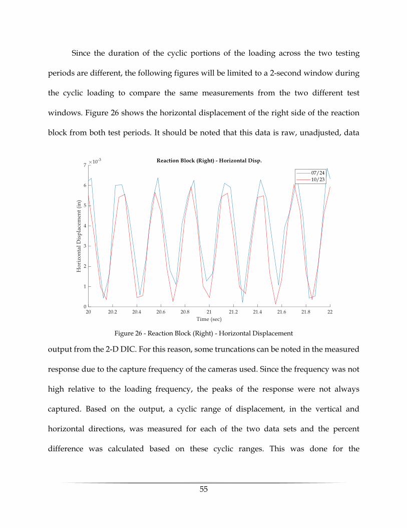
55
Since the duration of the cyclic portions of the loading across the two testing
periods are different, the following figures will be limited to a 2-second window during
the cyclic loading to compare the same measurements from the two different test
windows. Figure 26 shows the horizontal displacement of the right side of the reaction
block from both test periods. It should be noted that this data is raw, unadjusted, data
output from the 2-D DIC. For this reason, some truncations can be noted in the measured
response due to the capture frequency of the cameras used. Since the frequency was not
high relative to the loading frequency, the peaks of the response were not always
captured. Based on the output, a cyclic range of displacement, in the vertical and
horizontal directions, was measured for each of the two data sets and the percent
difference was calculated based on these cyclic ranges. This was done for the
Figure 26 - Reaction Block (Right) - Horizontal Displacement
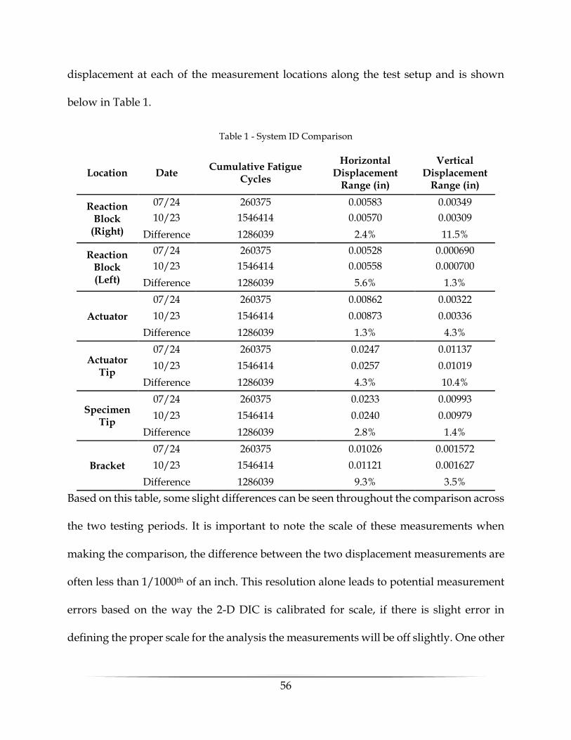
56
displacement at each of the measurement locations along the test setup and is shown
below in Table 1.
Table 1 - System ID Comparison
Location Date Cumulative Fatigue
Cycles
Horizontal Displacement
Range (in)
Vertical Displacement
Range (in)
Reaction Block
(Right)
07/24 260375 0.00583 0.00349
10/23 1546414 0.00570 0.00309
Difference 1286039 2.4% 11.5%
Reaction Block (Left)
07/24 260375 0.00528 0.000690
10/23 1546414 0.00558 0.000700
Difference 1286039 5.6% 1.3%
Actuator
07/24 260375 0.00862 0.00322
10/23 1546414 0.00873 0.00336
Difference 1286039 1.3% 4.3%
Actuator Tip
07/24 260375 0.0247 0.01137
10/23 1546414 0.0257 0.01019
Difference 1286039 4.3% 10.4%
Specimen Tip
07/24 260375 0.0233 0.00993
10/23 1546414 0.0240 0.00979
Difference 1286039 2.8% 1.4%
Bracket
07/24 260375 0.01026 0.001572
10/23 1546414 0.01121 0.001627
Difference 1286039 9.3% 3.5%
Based on this table, some slight differences can be seen throughout the comparison across
the two testing periods. It is important to note the scale of these measurements when
making the comparison, the difference between the two displacement measurements are
often less than 1/1000th of an inch. This resolution alone leads to potential measurement
errors based on the way the 2-D DIC is calibrated for scale, if there is slight error in
defining the proper scale for the analysis the measurements will be off slightly. One other
57
potential cause of error, as previously mentioned, is the minor adjustments between the
shim supports, as well as the torqueing of the bolts. Overall, the differences ranged from
1%-11% with an average difference of 4.84% between the two measurement dates.
3.3 Representative Measurement
Ensuring consistent behavior in a prolonged test is important but performing a
System ID before every testing period would be cumbersome and would add a significant
delay between testing due to the processing time required to analyze the System ID
measurements. Hence, it is important to have the availability of benchmark
measurements during the fatigue test that could be used as reference measurements to
identify potential undesirable changes in the structural response of the system. Having
such measurements allows the test to be monitored between System ID intervals and can
be used as a tool to decide when an additional (unscheduled) System ID needs to be
performed.
In this study, the measurement that is being used as a representative
characterization of the system is the force-displacement relationship of the actuator. This
is measured through the actuator LVDT, with respect to the displacement, and the
actuator load-cell for the force. The force-displacement relationship is an indicative
measurement because if a consistent force is applied (force-controlled test), any change
in a stable system, for example boundary conditions, will be reflected in this
measurement. For example, if the attachment bolts are not tightened at the specimen-
bracket interaction the actuator will end up displacing a further distance to reach the

58
same level of force compared to if the bolts were completely tightened. Therefore, if there
is a noticeable change in the force-displacement hysteresis of the actuator, the test setup
ought to be evaluated for changes in the supports, any loosening of bolts, or any
noticeable damage. If the source of the change is not visible, a full characterization is
required in the form of the SI process. This creates a systematic approach for maintaining
a consistent structural response throughout the fatigue test.
Throughout this study, a history of the force-displacement relationship has been
monitored to create a benchmark measurement and use this benchmark to assess the
presence of changes in the system. Figure 27 through Figure 31 show an overall history
of the force-displacement relationship of the actuator throughout the setup and testing
phases of this project. Each of the data sets shown, labeled by the date in which the test
was performed, are approximately 50 seconds of the cyclic loading protocol close to the
end of the respective testing interval. Taking a data window close to the end of the testing
period ensures that the maximum number of cycles occurs between the comparisons of
the data sets. This is desirable to ensure that the changes that occurred during that testing
period are reflected on the measurement before the next testing period occurs.
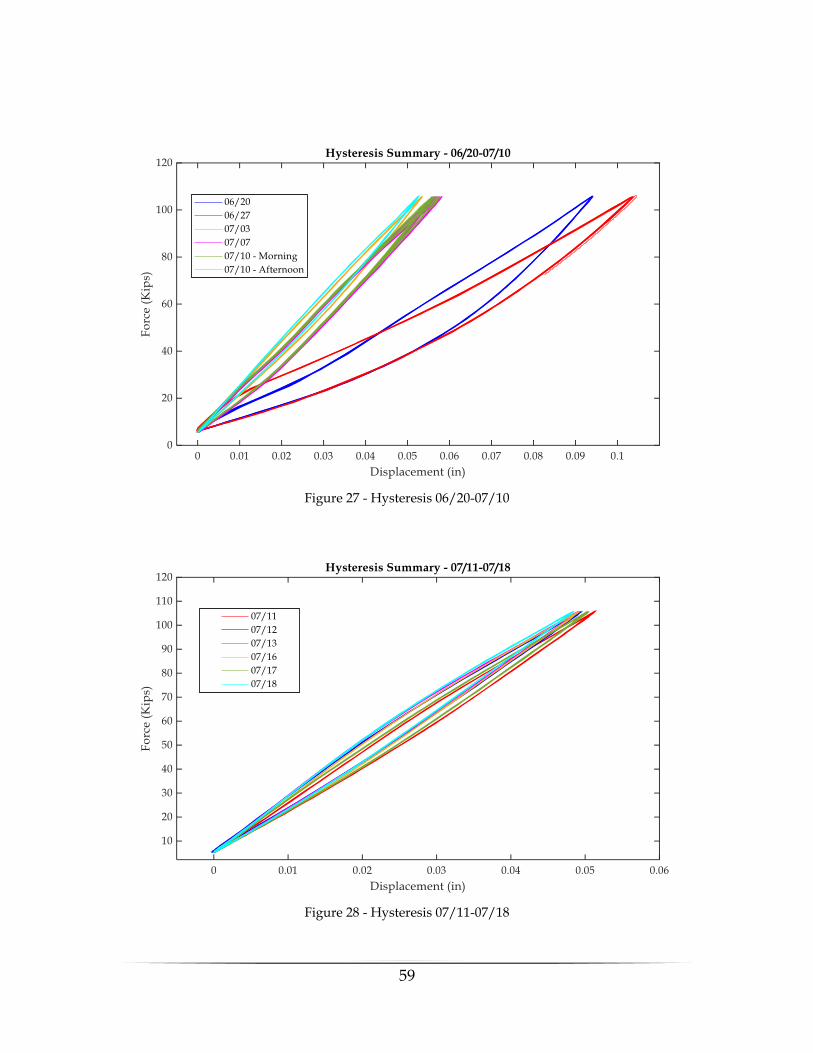
59
Figure 27 - Hysteresis 06/20-07/10
Figure 28 - Hysteresis 07/11-07/18
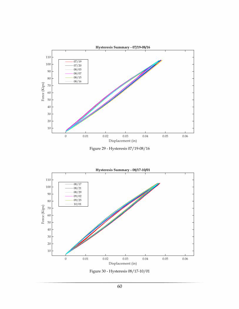
60
Figure 29 - Hysteresis 07/19-08/16
Figure 30 - Hysteresis 08/17-10/01
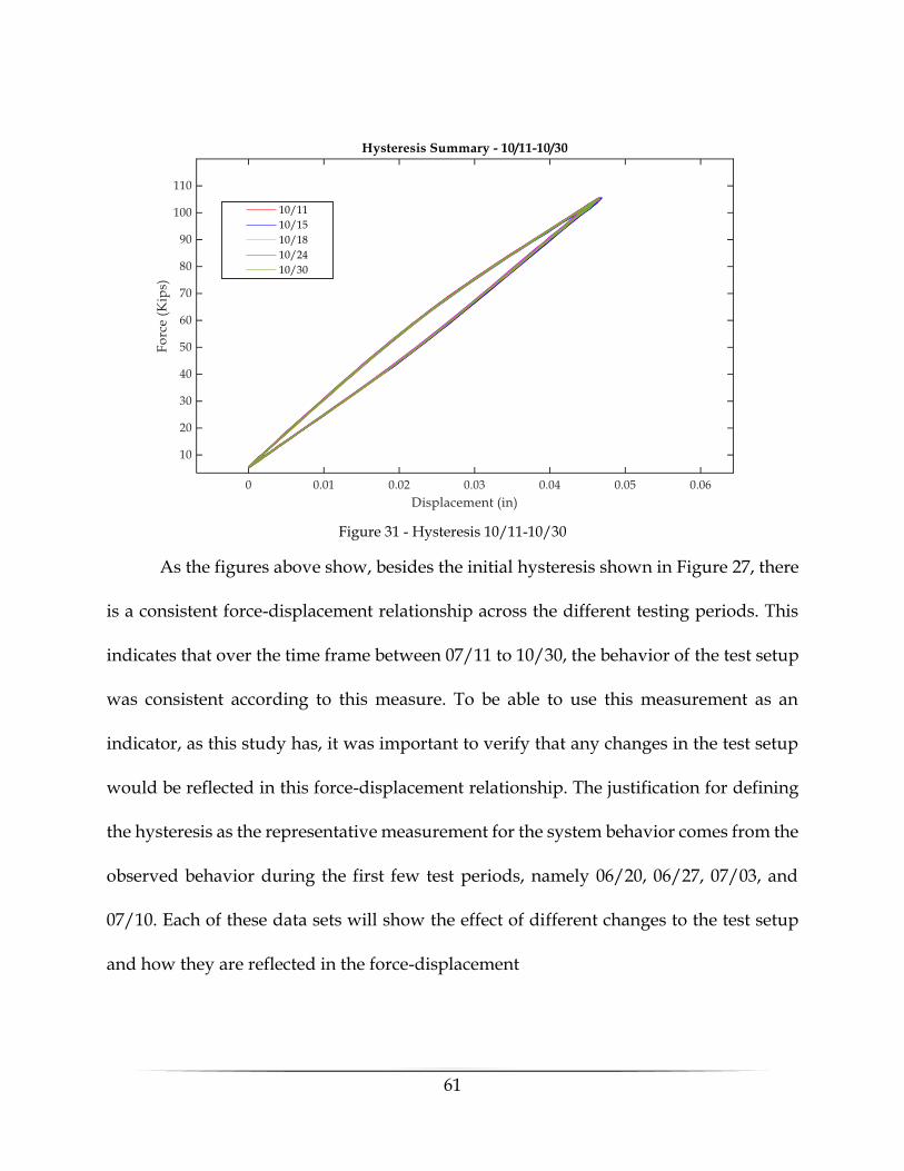
61
As the figures above show, besides the initial hysteresis shown in Figure 27, there
is a consistent force-displacement relationship across the different testing periods. This
indicates that over the time frame between 07/11 to 10/30, the behavior of the test setup
was consistent according to this measure. To be able to use this measurement as an
indicator, as this study has, it was important to verify that any changes in the test setup
would be reflected in this force-displacement relationship. The justification for defining
the hysteresis as the representative measurement for the system behavior comes from the
observed behavior during the first few test periods, namely 06/20, 06/27, 07/03, and
07/10. Each of these data sets will show the effect of different changes to the test setup
and how they are reflected in the force-displacement
Figure 31 - Hysteresis 10/11-10/30
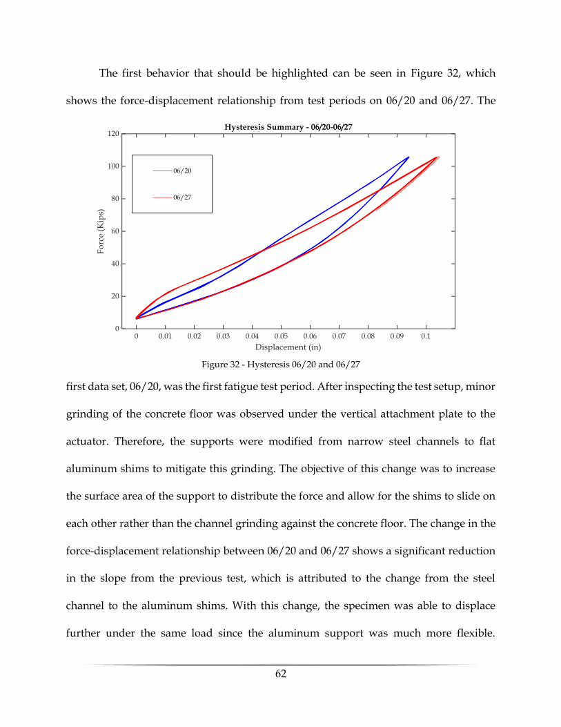
62
The first behavior that should be highlighted can be seen in Figure 32, which
shows the force-displacement relationship from test periods on 06/20 and 06/27. The
first data set, 06/20, was the first fatigue test period. After inspecting the test setup, minor
grinding of the concrete floor was observed under the vertical attachment plate to the
actuator. Therefore, the supports were modified from narrow steel channels to flat
aluminum shims to mitigate this grinding. The objective of this change was to increase
the surface area of the support to distribute the force and allow for the shims to slide on
each other rather than the channel grinding against the concrete floor. The change in the
force-displacement relationship between 06/20 and 06/27 shows a significant reduction
in the slope from the previous test, which is attributed to the change from the steel
channel to the aluminum shims. With this change, the specimen was able to displace
further under the same load since the aluminum support was much more flexible.
Figure 32 - Hysteresis 06/20 and 06/27
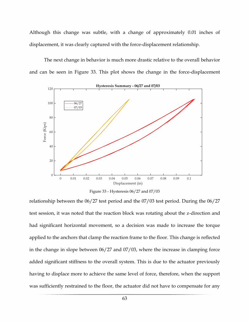
63
Although this change was subtle, with a change of approximately 0.01 inches of
displacement, it was clearly captured with the force-displacement relationship.
The next change in behavior is much more drastic relative to the overall behavior
and can be seen in Figure 33. This plot shows the change in the force-displacement
relationship between the 06/27 test period and the 07/03 test period. During the 06/27
test session, it was noted that the reaction block was rotating about the z-direction and
had significant horizontal movement, so a decision was made to increase the torque
applied to the anchors that clamp the reaction frame to the floor. This change is reflected
in the change in slope between 06/27 and 07/03, where the increase in clamping force
added significant stiffness to the overall system. This is due to the actuator previously
having to displace more to achieve the same level of force, therefore, when the support
was sufficiently restrained to the floor, the actuator did not have to compensate for any
Figure 33 - Hysteresis 06/27 and 07/03
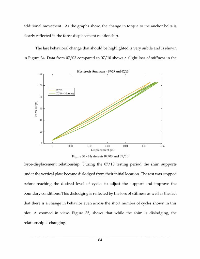
64
additional movement. As the graphs show, the change in torque to the anchor bolts is
clearly reflected in the force-displacement relationship.
The last behavioral change that should be highlighted is very subtle and is shown
in Figure 34. Data from 07/03 compared to 07/10 shows a slight loss of stiffness in the
force-displacement relationship. During the 07/10 testing period the shim supports
under the vertical plate became dislodged from their initial location. The test was stopped
before reaching the desired level of cycles to adjust the support and improve the
boundary conditions. This dislodging is reflected by the loss of stiffness as well as the fact
that there is a change in behavior even across the short number of cycles shown in this
plot. A zoomed in view, Figure 35, shows that while the shim is dislodging, the
relationship is changing.
Figure 34 - Hysteresis 07/03 and 07/10
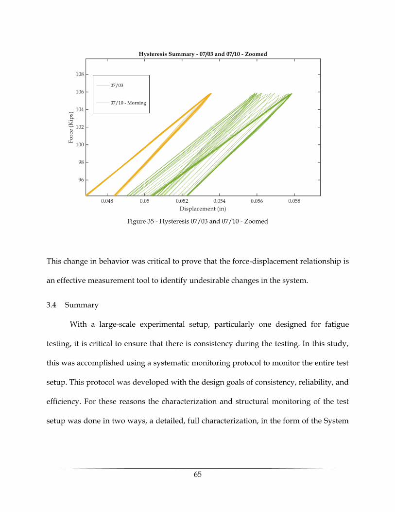
65
This change in behavior was critical to prove that the force-displacement relationship is
an effective measurement tool to identify undesirable changes in the system.
3.4 Summary
With a large-scale experimental setup, particularly one designed for fatigue
testing, it is critical to ensure that there is consistency during the testing. In this study,
this was accomplished using a systematic monitoring protocol to monitor the entire test
setup. This protocol was developed with the design goals of consistency, reliability, and
efficiency. For these reasons the characterization and structural monitoring of the test
setup was done in two ways, a detailed, full characterization, in the form of the System
Figure 35 - Hysteresis 07/03 and 07/10 - Zoomed

66
ID, and a representative measurement, in the form of the actuator force-displacement
hysteresis.
The results from the System ID characterized the structural response of the entire
test setup at critical locations. From this characterization, the behavior of the test setup
was monitored and periodically checked for changes. Although there were slight
differences between each characterization, the overall behavior was consistent
throughout the test.
The force-displacement relationship was used as a fast way to detect changes in
the behavior of the test setup. It was found that the physical changes to the test setup had
a clear effect on the force-displacement relationship. These changes justify the use of this
measure as a representative, quantitative, measurement of the overall system. After some
initial changes near the beginning of the overall fatigue test, the force-displacement
relationship reflected the consistency of the test setup over the time frame between 07/11
to 10/30.

67
4 FINITE ELEMENT MODELING
This chapter will discuss the need for finite element modeling of the fatigue test
and setup. The chapter will then introduce the developed model of the test setup and
discuss the modeling technique and assumptions made. Lastly, the results from the
numerical analysis will be introduced and briefly discussed.
4.1 Finite Element Modeling
The use of finite element modeling was a powerful tool to estimate behaviors and
structural responses of various components such as the specimen and test setup used in
this study. A numerical model might not be a perfect representation of an actual test due
to the idealistic conditions assumed in modeling, but it can still be used as a way to
estimate structural behavior. With such a geometrically complex test specimen, it is
important to be able to have a theoretical comparison point for the measurements being
recorded. Additionally, understanding the stress distribution in this complex specimen
is critical in order to maximize the efficiency of the instrumentation of the test setup.
Lastly, numerical models can be used to investigate the effect of different changes to
boundary conditions in the test setup and aid in decision making in terms of potential
modifications to the test setup.
Although there are many benefits to having a numerical model, the results must
be examined with caution. It is important to be able to distinguish whether the numerical
results are true, or a close representation of reality. Often times, a complex numerical
model contains sharp geometries and transitions which can result in spurious results in

68
the form of stress concentrations. For this reason, engineering judgement must be used
when using numerical models for analysis.
4.2 Fatigue Test Model
In this study, multiple finite element models (FEM) of the specimen as well as
portions of the test setup were developed and refined using ABAQUS® CAE/2017 [34].
The models were created in order to estimate stresses and strains in the specimen as well
as the overall structural response of the test setup. As noted in section 2.3, the original
model of the specimen [31] was used to estimate the overall stress contours to determine
the locations of interest for the instrumentation. Although this model provided a good
approximation to the areas of interest, an error in the modeling of the attachment plate
which connects the specimen and actuator was discovered. The error resulted in a false
approximation of stresses in the vertical plate which attaches the actuator to the
specimen. This error was localized and did not influence the area of interest, but the
decision was made to remodel the specimen to ensure that the behavior throughout was
accurate. Additionally, the model was expanded to include a more detailed model of the
welds in the specimen, the actuator swivel, the support bracket, the rigid floor, and the
bolts throughout the test setup. The goal of this more detailed model was to create a
numerical model of the test setup and understand the true behavior of the boundary
conditions not just the specimen. The results of the finite element analysis (FEA) are
compared to the actual measurements from the test in section 5.2 to verify the structural
response of the model.
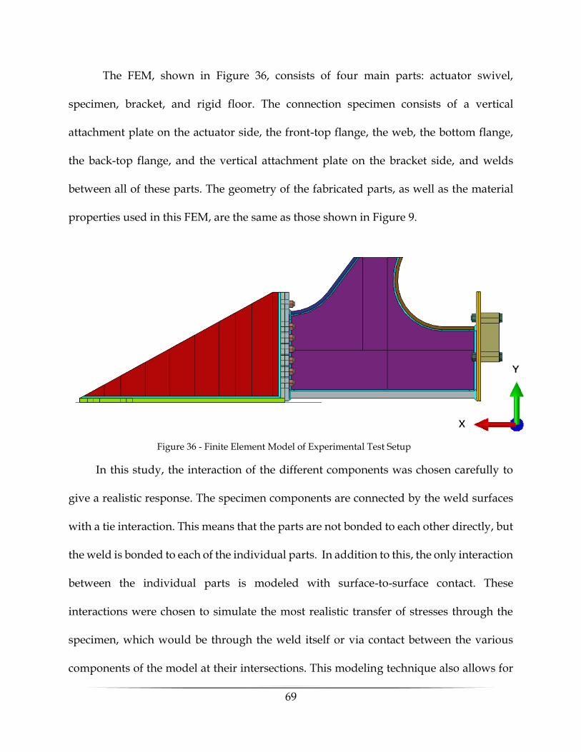
69
The FEM, shown in Figure 36, consists of four main parts: actuator swivel,
specimen, bracket, and rigid floor. The connection specimen consists of a vertical
attachment plate on the actuator side, the front-top flange, the web, the bottom flange,
the back-top flange, and the vertical attachment plate on the bracket side, and welds
between all of these parts. The geometry of the fabricated parts, as well as the material
properties used in this FEM, are the same as those shown in Figure 9.
In this study, the interaction of the different components was chosen carefully to
give a realistic response. The specimen components are connected by the weld surfaces
with a tie interaction. This means that the parts are not bonded to each other directly, but
the weld is bonded to each of the individual parts. In addition to this, the only interaction
between the individual parts is modeled with surface-to-surface contact. These
interactions were chosen to simulate the most realistic transfer of stresses through the
specimen, which would be through the weld itself or via contact between the various
components of the model at their intersections. This modeling technique also allows for
Figure 36 - Finite Element Model of Experimental Test Setup
70
a better estimate of the stress distribution through the weld geometry. The same approach
was taken when modeling the support bracket, all forces are transferred through the
welds or through part to part contact.
Further, the bolted connection of the specimen to the actuator swivel, as well of the
specimen to the bracket, are simulated in the numerical model. Each bolt is modeled as a
single solid part consisting of the bolt (shaft and hex-head), one washer on either end,
and the hex-nut. The bolt’s interactions with each individual component are modeled as
surface-to-surface contact using the washer surfaces as the contact surface to the
individual parts. This interaction was chosen to simulate the interaction between parts
including their potential separation or loss of contact, whereas the tie constraint would
simulate the components working as a unit. The last modeled interaction is between the
bottom of the support bracket and the rigid floor. This interaction is modeled as a
frictionless “hard” contact between the bottom surface of the support bracket and the top
surface of the rigid floor. The frictionless “hard” contact interaction allows the bracket to
press against the rigid floor without penetrating it or having any frictional force
generated between the two surfaces.
The boundary conditions of the FEM were chosen to be representative of those
present in the experimental test setup. Boundary conditions are applied at four locations
in this FEM; the swivel’s center of rotation, the bottom surface of the vertical attachment
plate on the actuator side, the surface of the rigid floor, and the locations of the anchor
holes in the bracket.

71
The actuator swivel is restrained from rotation about the X, Y, and Z directions
and allowed to translate in the X, Y, and Z directions. These restraints were selected to
simulate the swivel, which has its orientation locked in place, preventing any rotations
during loading. This boundary was applied by coupling a reference point, located at the
center of rotation of the swivel geometry, with the swivel, and restraining the rotations
of this reference point, but allowing it to translate freely.
The bottom surface of the vertical attachment plate on the actuator side is
restrained from rotation about the Z direction and restrained from translations in the Y
direction. These restraints are representative of the metal shim supports that are under
this vertical plate, these shims slide on top of each other while restraining any vertical (Y
direction) movement and preventing rotation. This boundary was applied by coupling a
reference point to the bottom surface of the vertical attachment plate and restricting the
rotation about the Z direction and the translations in the Y direction of the reference point.
The bracket is restrained from translations and rotations at the location of the
anchors. This is meant to simulate the near fixed-end condition created by the four
anchors at the end of the bracket. This was accomplished by coupling the inner surfaces
of the anchor holes to reference points located in the center of the circular holes and
restraining all translations and rotations.
Lastly, the rigid floor is restrained in all directions against translations and
rotations to simulate the actual floor under the test setup. This was applied by coupling

72
a reference point to the entire bottom surface of the rigid floor and restraining all
translations and rotations.
The loading protocol is implemented in the numerical model in two steps; the pre-
tensioning step, and the static loading step. The pre-tensioning step is created to simulate
the application of the bolt loads generated from tightening the bolts that connect the
various components together as discussed previously while the static loading step is
meant to simulate the fatigue loading. These two steps were created to give a better
approximation of the behavior of the test setup, including the behavior during
installation (pre-tensioning step), and not just the specimen under idealized fatigue
loading. Additionally, since the instrumentation, namely the strain gauges, are calibrated
when the specimen is uninstalled, this will be a more representative comparison to the
measured data.
As mentioned, the pre-tension step occurs first. In this step a pre-tension load is
applied to the bolts, creating a clamping force on the two components that the bolt is
connecting. This is meant to be consistent with the actual axial force applied to these bolts.
This force was estimated by converting an applied torque of 800 ft-lb to an axial force
which was then applied to each bolt in the FEM through the bolt-load option in Abaqus.
The way that the bolt-load applies a force is by pulling the bolt-head and nut towards the
center of the bolts, simulating a tension force on the bolt which causes it to clamp the
parts that it is in contact with. Once the pre-tensioning of the bolts is completed the static
loading step is performed.
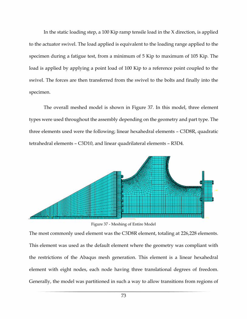
73
In the static loading step, a 100 Kip ramp tensile load in the X direction, is applied
to the actuator swivel. The load applied is equivalent to the loading range applied to the
specimen during a fatigue test, from a minimum of 5 Kip to maximum of 105 Kip. The
load is applied by applying a point load of 100 Kip to a reference point coupled to the
swivel. The forces are then transferred from the swivel to the bolts and finally into the
specimen.
The overall meshed model is shown in Figure 37. In this model, three element
types were used throughout the assembly depending on the geometry and part type. The
three elements used were the following; linear hexahedral elements – C3D8R, quadratic
tetrahedral elements – C3D10, and linear quadrilateral elements – R3D4.
The most commonly used element was the C3D8R element, totaling at 226,228 elements.
This element was used as the default element where the geometry was compliant with
the restrictions of the Abaqus mesh generation. This element is a linear hexahedral
element with eight nodes, each node having three translational degrees of freedom.
Generally, the model was partitioned in such a way to allow transitions from regions of
Figure 37 - Meshing of Entire Model
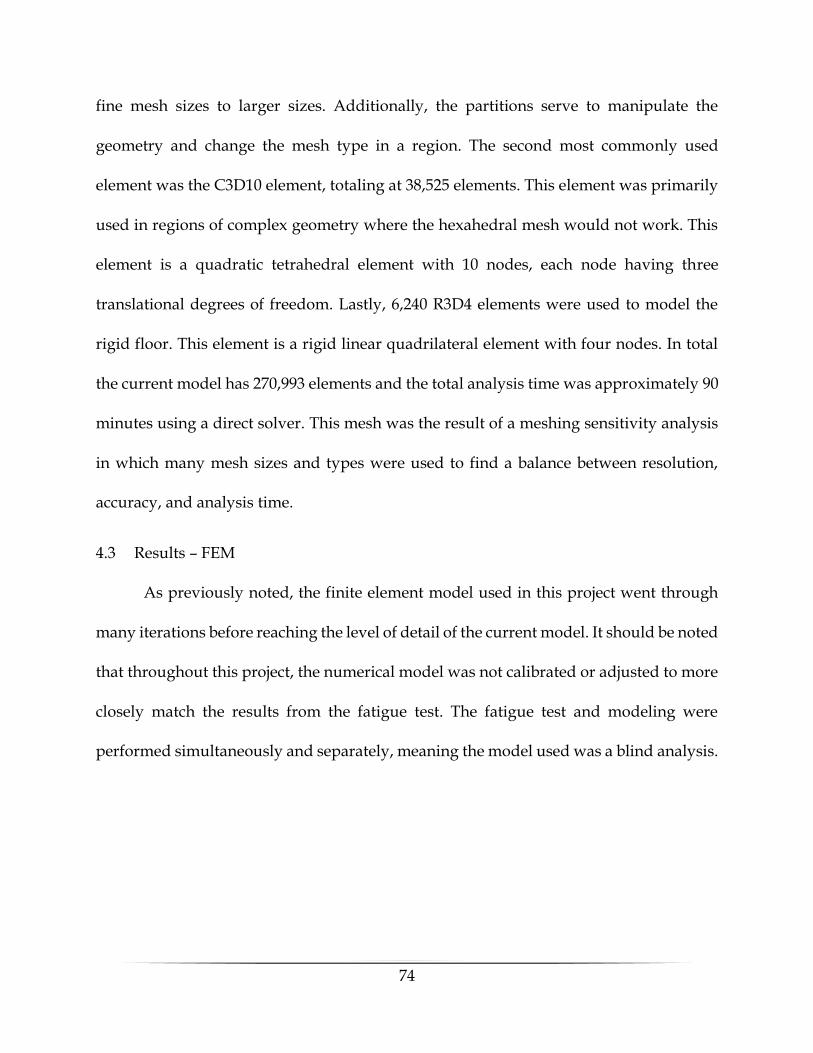
74
fine mesh sizes to larger sizes. Additionally, the partitions serve to manipulate the
geometry and change the mesh type in a region. The second most commonly used
element was the C3D10 element, totaling at 38,525 elements. This element was primarily
used in regions of complex geometry where the hexahedral mesh would not work. This
element is a quadratic tetrahedral element with 10 nodes, each node having three
translational degrees of freedom. Lastly, 6,240 R3D4 elements were used to model the
rigid floor. This element is a rigid linear quadrilateral element with four nodes. In total
the current model has 270,993 elements and the total analysis time was approximately 90
minutes using a direct solver. This mesh was the result of a meshing sensitivity analysis
in which many mesh sizes and types were used to find a balance between resolution,
accuracy, and analysis time.
4.3 Results – FEM
As previously noted, the finite element model used in this project went through
many iterations before reaching the level of detail of the current model. It should be noted
that throughout this project, the numerical model was not calibrated or adjusted to more
closely match the results from the fatigue test. The fatigue test and modeling were
performed simultaneously and separately, meaning the model used was a blind analysis.
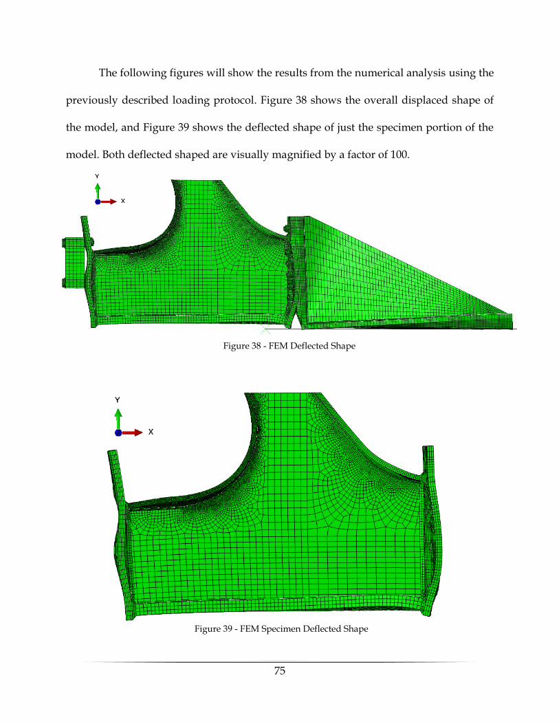
75
The following figures will show the results from the numerical analysis using the
previously described loading protocol. Figure 38 shows the overall displaced shape of
the model, and Figure 39 shows the deflected shape of just the specimen portion of the
model. Both deflected shaped are visually magnified by a factor of 100.
Figure 38 - FEM Deflected Shape
Figure 39 - FEM Specimen Deflected Shape
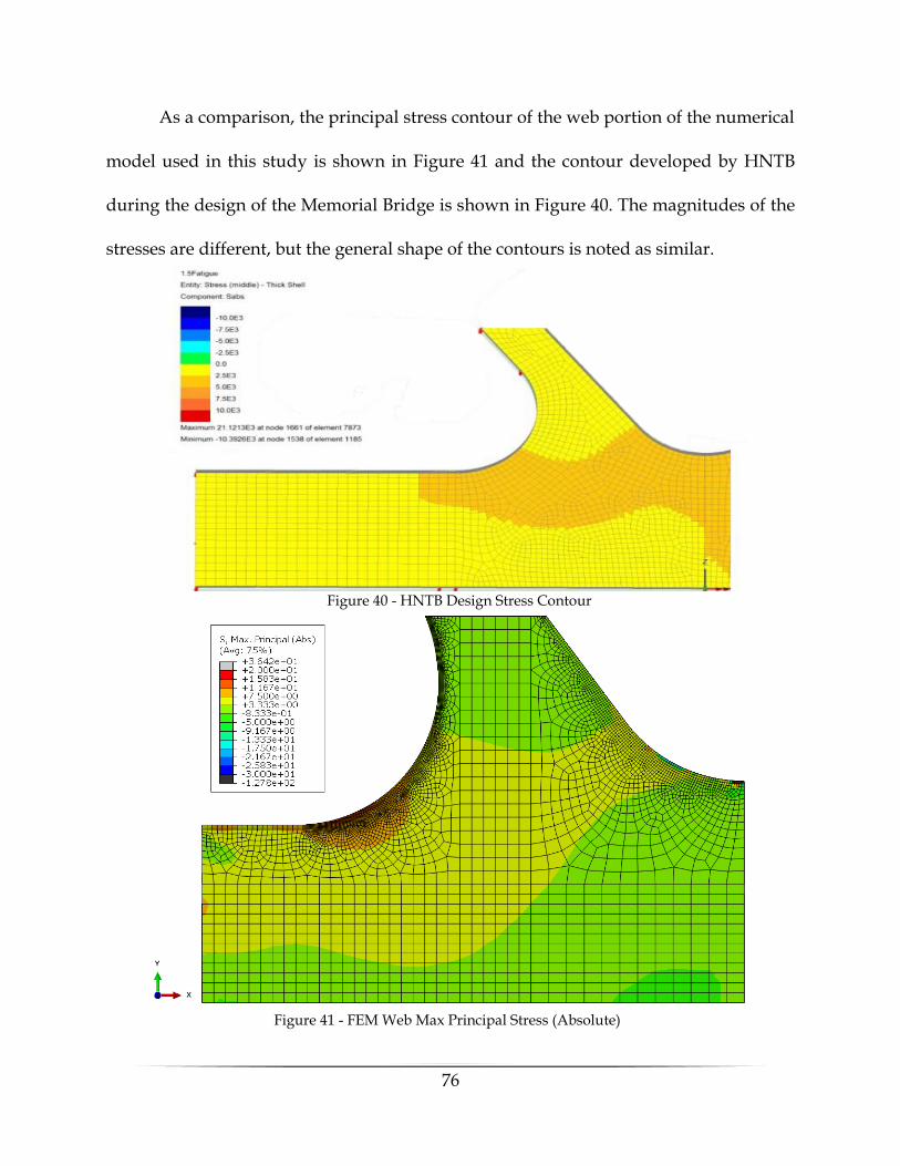
76
As a comparison, the principal stress contour of the web portion of the numerical
model used in this study is shown in Figure 41 and the contour developed by HNTB
during the design of the Memorial Bridge is shown in Figure 40. The magnitudes of the
stresses are different, but the general shape of the contours is noted as similar.
Figure 40 - HNTB Design Stress Contour
Figure 41 - FEM Web Max Principal Stress (Absolute)
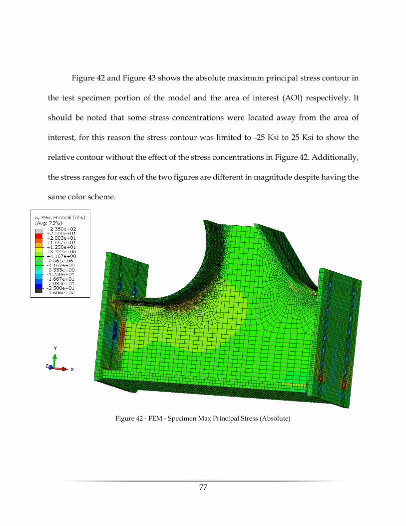
77
Figure 42 and Figure 43 shows the absolute maximum principal stress contour in
the test specimen portion of the model and the area of interest (AOI) respectively. It
should be noted that some stress concentrations were located away from the area of
interest, for this reason the stress contour was limited to -25 Ksi to 25 Ksi to show the
relative contour without the effect of the stress concentrations in Figure 42. Additionally,
the stress ranges for each of the two figures are different in magnitude despite having the
same color scheme.
Figure 42 - FEM - Specimen Max Principal Stress (Absolute)
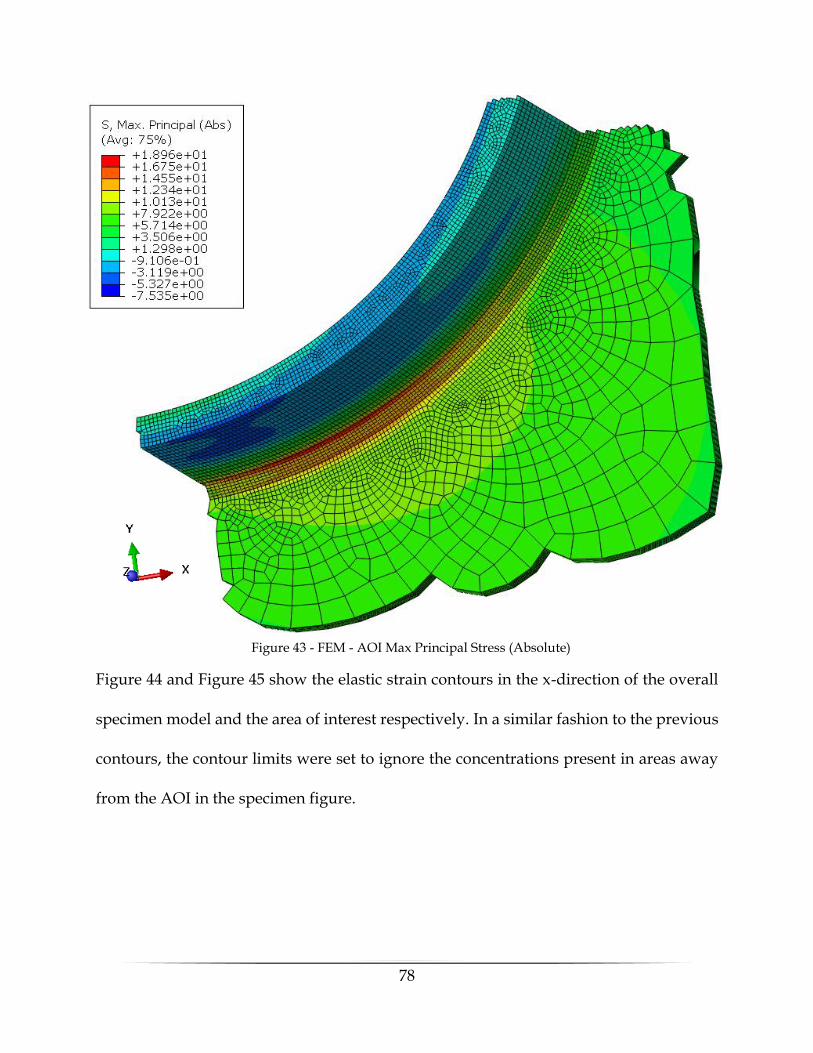
78
Figure 44 and Figure 45 show the elastic strain contours in the x-direction of the overall
specimen model and the area of interest respectively. In a similar fashion to the previous
contours, the contour limits were set to ignore the concentrations present in areas away
from the AOI in the specimen figure.
Figure 43 - FEM - AOI Max Principal Stress (Absolute)
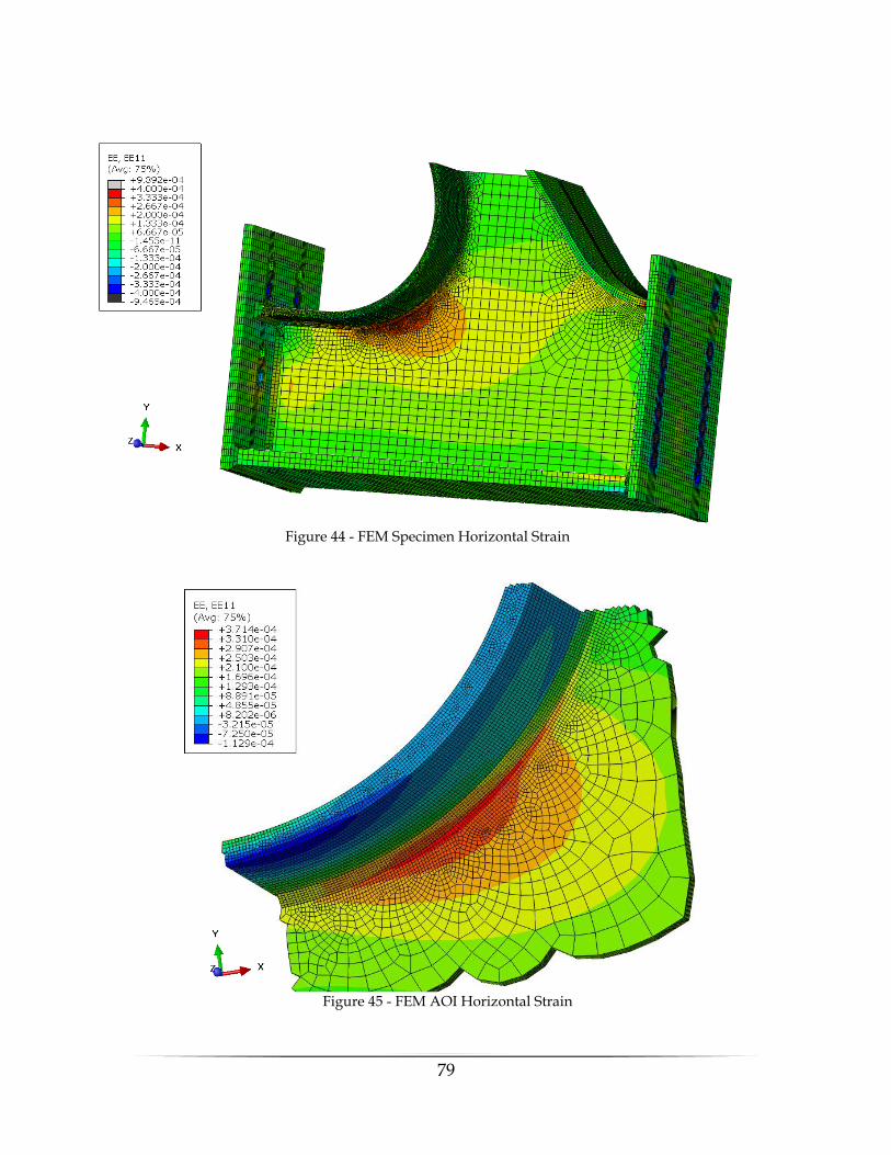
79
Figure 44 - FEM Specimen Horizontal Strain
Figure 45 - FEM AOI Horizontal Strain
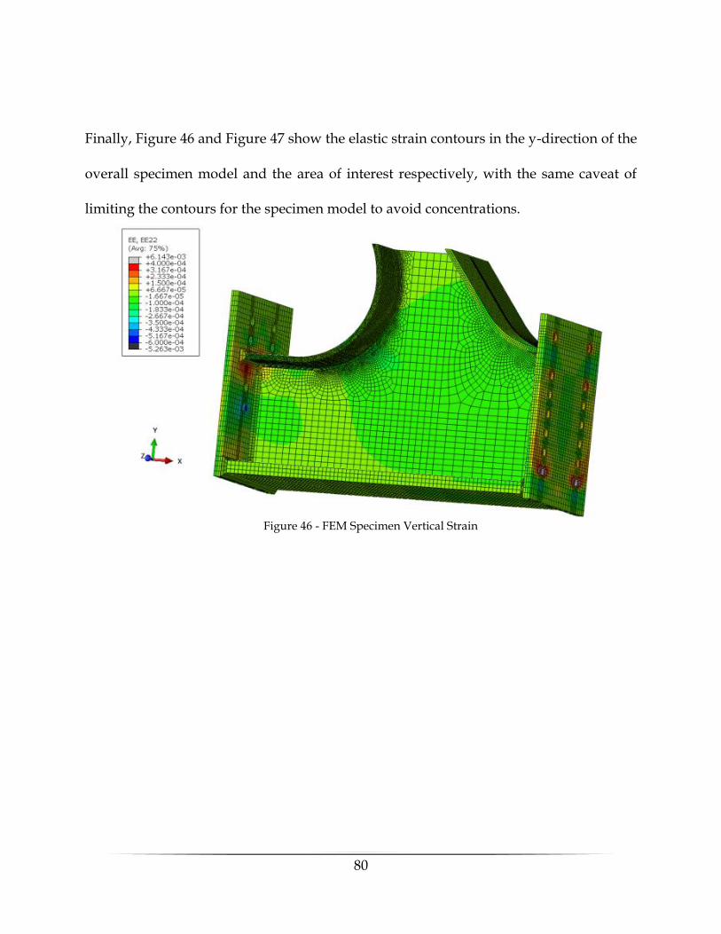
80
Finally, Figure 46 and Figure 47 show the elastic strain contours in the y-direction of the
overall specimen model and the area of interest respectively, with the same caveat of
limiting the contours for the specimen model to avoid concentrations.
Figure 46 - FEM Specimen Vertical Strain
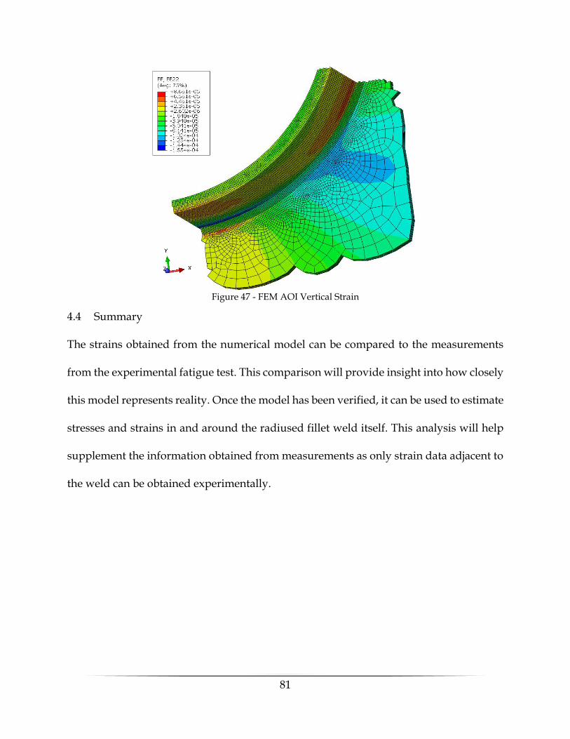
81
4.4 Summary
The strains obtained from the numerical model can be compared to the measurements
from the experimental fatigue test. This comparison will provide insight into how closely
this model represents reality. Once the model has been verified, it can be used to estimate
stresses and strains in and around the radiused fillet weld itself. This analysis will help
supplement the information obtained from measurements as only strain data adjacent to
the weld can be obtained experimentally.
Figure 47 - FEM AOI Vertical Strain

82
5 FATIGUE TESTING RESULTS
This chapter will briefly reintroduce the fatigue loading protocol and reiterate the
design criteria for the connection. The performance expectation will also be discussed.
Next, the results from the fatigue test, in terms of measured strains from the strain gauges
and the 2-D DIC in the area of interest, will be introduced and discussed. Lastly, a
comparison between the measured response and the theoretical response from the
numerical model will be discussed.
5.1 Introduction
The objective of the fatigue testing was to investigate the fatigue performance of
the gusset-less truss connection used in place at the Memorial Bridge. Since the
connection has such a unique geometry, there was no specific category for the critical
fatigue location, which was the radiused weld connecting the curved top flange to the
web. For this reason, the assumption was made to conservatively categorize the region
of interest as fatigue category C. With this assumption, and the calculated stresses in the
fatigue load case for the Memorial Bridge, the gusset-less connection is expected to have
infinite life because the design stresses, approximately 4 Ksi, are well below the
endurance limit of 10 Ksi for fatigue category C [1]. Therefore, to investigate the
assumption, it was critical to increase the stress applied to the fatigue specimen compared
to the Memorial Bridge.
The cyclic loading protocol used in this fatigue test was previously described in
section 2.2, but is repeated here;

83
• Mean axial load applied: 55 Kip
• Cyclic amplitude: ±50 Kip
• Cyclic frequency: 3.5 Hz
• Applied function: Sine wave
With the applied loading, the numerical model predicts principal stresses of
approximately 14 Ksi close to the toe of the weld. Although this stress is higher than the
endurance limit for the fatigue category C, the stress predicted is better described as a
hot-spot stress due to its proximity to the weld toe. Therefore, the comparison of a hot-
spot stress to the S-N curves derived using nominal stresses, is considered conservative.
Using this “hot-spot” stress at the weld toe and applying it to the S-N curve for the design
category, the expected cycles to failure would be 1,600,000 fatigue cycles. At the time of
this thesis, the specimen has undergone a total of 1,602,300 fatigue cycles.

84
5.2 Strain Gauge Results
The following section will present the results from the fatigue testing in terms of
strain gauges in the area of interest. The strain gauge results presented will be
measurements from three testing sessions spaced over the course of the overall fatigue
test. The goal of showing the results in this manner is to make a comparison of the cyclic
strain range applied to the specimen throughout the fatigue test. The testing periods will
be labeled by the date on which they were performed;
• Test period 1: 07/17/2018, Cumulative fatigue cycles; 178,831
• Test period 2: 08/29/2018, Cumulative fatigue cycles; 880,014
• Test period 3: 10/30/2018, Cumulative fatigue cycles; 1,602,287
In terms of fatigue testing, the strain of interest is the maximum principal strain. For this
reason, all comparisons to the S-N curve were using the principal strains calculated from
the rosettes or obtained from the DIC. Just for the sake of comparisons, with respect to
each other, the strain gauge results are shown in terms of the horizontal, diagonal, and
vertical strain components.

85
Before the comparison between different test periods takes place, the overall
structural response of the specimen in the area of interest will be presented. Figure 48
shows the horizontal strain measurements of the gauges NRW1, NRW2, and NRW4.
These rosettes are the gauges that are placed along the curved weld, close to the toe of
the weld. As the figure shows, the horizontal strain range increases as the measurement
is taken along the weld. In other words, NRW1 had the smallest strain range while NRW4
had the largest, with 35% increase in the measured horizontal strain range between the
two rosettes. Similarly, Figure 49 shows the horizontal strain components of the gauges
NRW2, NRW3, and NRW5. These gauges are placed on the same path, in terms of the
Figure 48 - Horizontal Strain Pattern Along Weld Toe
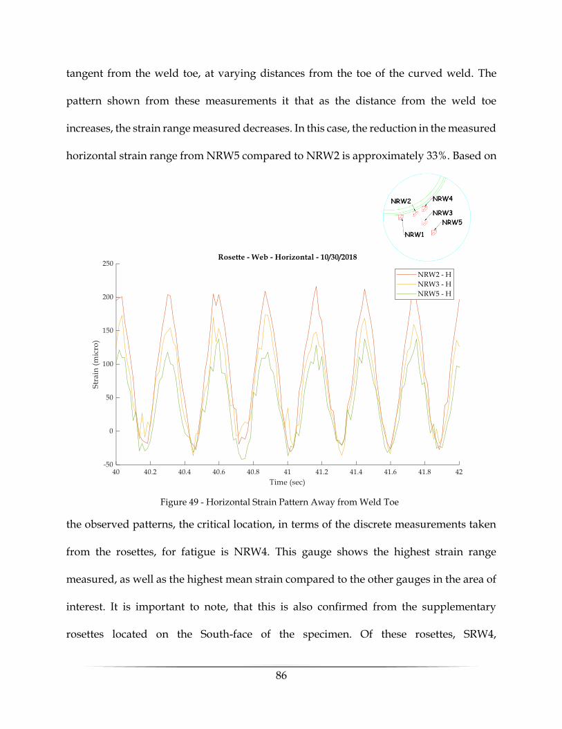
86
tangent from the weld toe, at varying distances from the toe of the curved weld. The
pattern shown from these measurements it that as the distance from the weld toe
increases, the strain range measured decreases. In this case, the reduction in the measured
horizontal strain range from NRW5 compared to NRW2 is approximately 33%. Based on
the observed patterns, the critical location, in terms of the discrete measurements taken
from the rosettes, for fatigue is NRW4. This gauge shows the highest strain range
measured, as well as the highest mean strain compared to the other gauges in the area of
interest. It is important to note, that this is also confirmed from the supplementary
rosettes located on the South-face of the specimen. Of these rosettes, SRW4,
Figure 49 - Horizontal Strain Pattern Away from Weld Toe
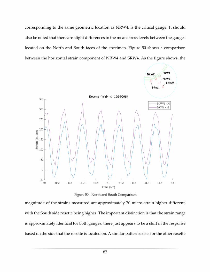
87
corresponding to the same geometric location as NRW4, is the critical gauge. It should
also be noted that there are slight differences in the mean stress levels between the gauges
located on the North and South faces of the specimen. Figure 50 shows a comparison
between the horizontal strain component of NRW4 and SRW4. As the figure shows, the
magnitude of the strains measured are approximately 70 micro-strain higher different,
with the South side rosette being higher. The important distinction is that the strain range
is approximately identical for both gauges, there just appears to be a shift in the response
based on the side that the rosette is located on. A similar pattern exists for the other rosette
Figure 50 - North and South Comparison
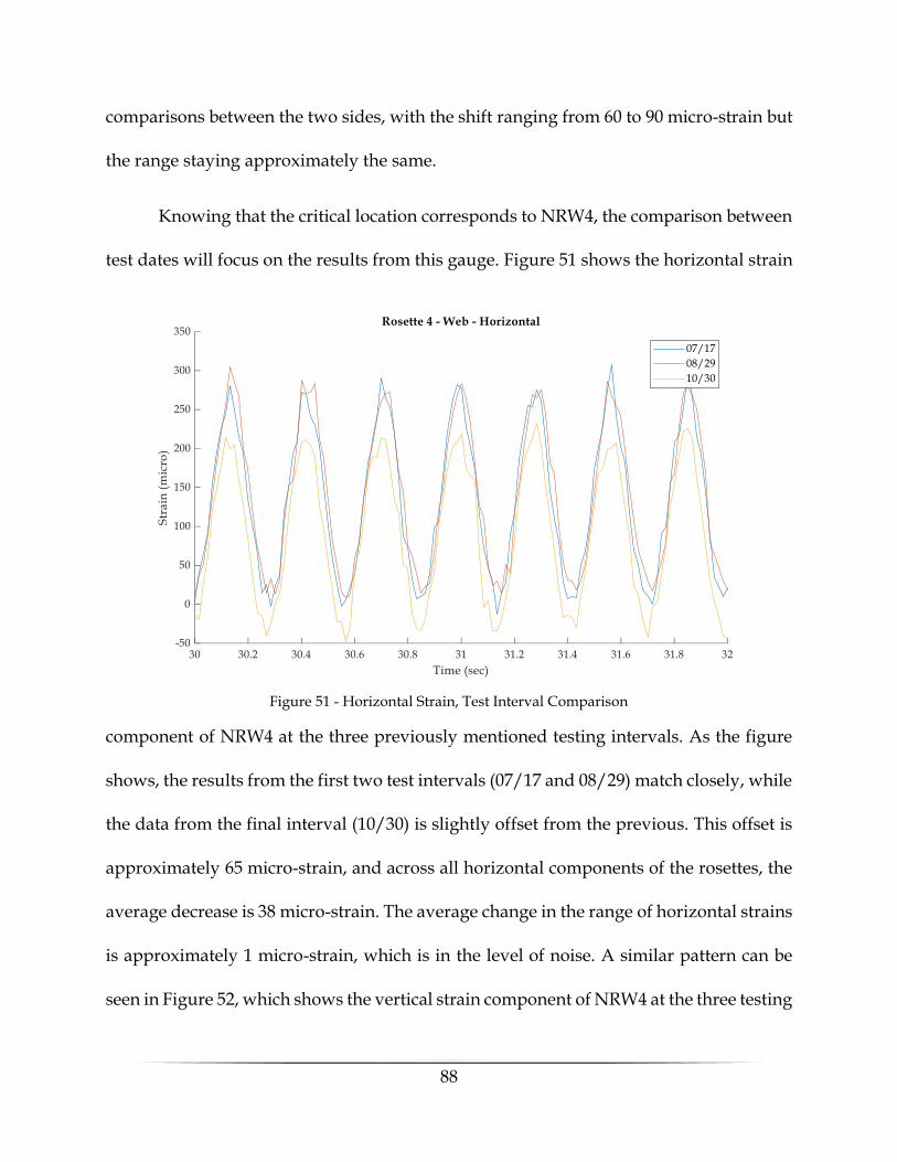
88
comparisons between the two sides, with the shift ranging from 60 to 90 micro-strain but
the range staying approximately the same.
Knowing that the critical location corresponds to NRW4, the comparison between
test dates will focus on the results from this gauge. Figure 51 shows the horizontal strain
component of NRW4 at the three previously mentioned testing intervals. As the figure
shows, the results from the first two test intervals (07/17 and 08/29) match closely, while
the data from the final interval (10/30) is slightly offset from the previous. This offset is
approximately 65 micro-strain, and across all horizontal components of the rosettes, the
average decrease is 38 micro-strain. The average change in the range of horizontal strains
is approximately 1 micro-strain, which is in the level of noise. A similar pattern can be
seen in Figure 52, which shows the vertical strain component of NRW4 at the three testing
Figure 51 - Horizontal Strain, Test Interval Comparison
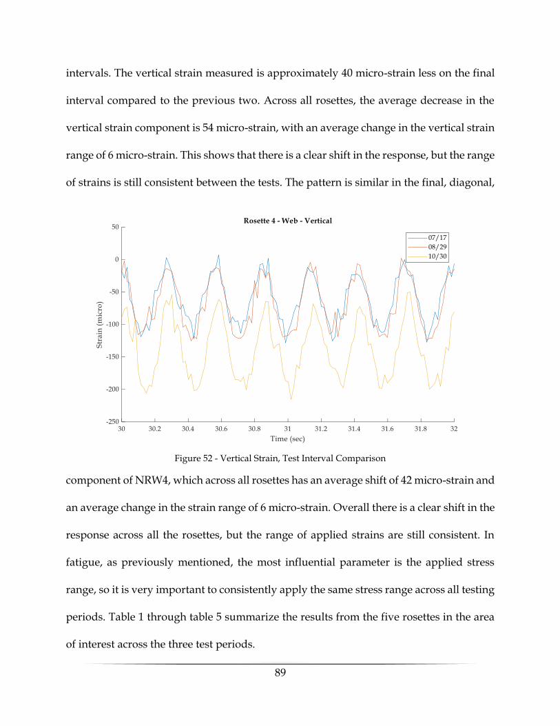
89
intervals. The vertical strain measured is approximately 40 micro-strain less on the final
interval compared to the previous two. Across all rosettes, the average decrease in the
vertical strain component is 54 micro-strain, with an average change in the vertical strain
range of 6 micro-strain. This shows that there is a clear shift in the response, but the range
of strains is still consistent between the tests. The pattern is similar in the final, diagonal,
component of NRW4, which across all rosettes has an average shift of 42 micro-strain and
an average change in the strain range of 6 micro-strain. Overall there is a clear shift in the
response across all the rosettes, but the range of applied strains are still consistent. In
fatigue, as previously mentioned, the most influential parameter is the applied stress
range, so it is very important to consistently apply the same stress range across all testing
periods. Table 1 through table 5 summarize the results from the five rosettes in the area
of interest across the three test periods.
Figure 52 - Vertical Strain, Test Interval Comparison
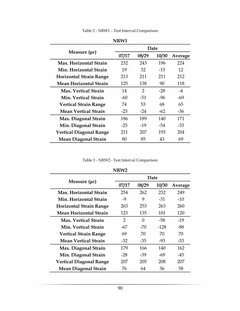
90
Table 2 - NRW1 – Test Interval Comparison
NRW1
Measure (με) Date
07/17 08/29 10/30 Average Max. Horizontal Strain 232 243 196 224 Min. Horizontal Strain 19 32 -15 12
Horizontal Strain Range 213 211 211 212 Mean Horizontal Strain 125 138 90 118
Max. Vertical Strain 14 2 -28 -4 Min. Vertical Strain -60 -51 -96 -69
Vertical Strain Range 74 53 68 65 Mean Vertical Strain -23 -24 -62 -36 Max. Diagonal Strain 186 189 140 171 Min. Diagonal Strain -25 -19 -54 -33
Vertical Diagonal Range 211 207 193 204 Mean Diagonal Strain 80 85 43 69
Table 3 - NRW2 - Test Interval Comparison
NRW2
Measure (με) Date
07/17 08/29 10/30 Average Max. Horizontal Strain 254 262 232 249 Min. Horizontal Strain -9 9 -31 -10
Horizontal Strain Range 263 253 263 260 Mean Horizontal Strain 123 135 101 120
Max. Vertical Strain 2 0 -58 -19 Min. Vertical Strain -67 -70 -128 -88
Vertical Strain Range 69 70 70 70 Mean Vertical Strain -32 -35 -93 -53 Max. Diagonal Strain 179 166 140 162 Min. Diagonal Strain -28 -39 -69 -45
Vertical Diagonal Range 207 205 208 207 Mean Diagonal Strain 76 64 36 58
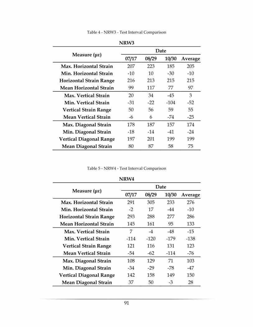
91
Table 4 - NRW3 - Test Interval Comparison
NRW3
Measure (με) Date
07/17 08/29 10/30 Average Max. Horizontal Strain 207 223 185 205 Min. Horizontal Strain -10 10 -30 -10
Horizontal Strain Range 216 213 215 215 Mean Horizontal Strain 99 117 77 97
Max. Vertical Strain 20 34 -45 3 Min. Vertical Strain -31 -22 -104 -52
Vertical Strain Range 50 56 59 55 Mean Vertical Strain -6 6 -74 -25 Max. Diagonal Strain 178 187 157 174 Min. Diagonal Strain -18 -14 -41 -24
Vertical Diagonal Range 197 201 199 199 Mean Diagonal Strain 80 87 58 75
Table 5 - NRW4 - Test Interval Comparison
NRW4
Measure (με) Date
07/17 08/29 10/30 Average Max. Horizontal Strain 291 305 233 276 Min. Horizontal Strain -2 17 -44 -10
Horizontal Strain Range 293 288 277 286 Mean Horizontal Strain 145 161 95 133
Max. Vertical Strain 7 -4 -48 -15 Min. Vertical Strain -114 -120 -179 -138
Vertical Strain Range 121 116 131 123 Mean Vertical Strain -54 -62 -114 -76 Max. Diagonal Strain 108 129 71 103 Min. Diagonal Strain -34 -29 -78 -47
Vertical Diagonal Range 142 158 149 150 Mean Diagonal Strain 37 50 -3 28
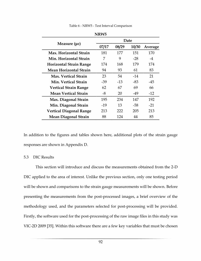
92
Table 6 - NRW5 - Test Interval Comparison
NRW5
Measure (με) Date
07/17 08/29 10/30 Average Max. Horizontal Strain 181 177 151 170 Min. Horizontal Strain 7 9 -28 -4
Horizontal Strain Range 174 168 179 174 Mean Horizontal Strain 94 93 61 83
Max. Vertical Strain 23 54 -14 21 Min. Vertical Strain -39 -13 -83 -45
Vertical Strain Range 62 67 69 66 Mean Vertical Strain -8 20 -49 -12 Max. Diagonal Strain 195 234 147 192 Min. Diagonal Strain -19 13 -58 -21
Vertical Diagonal Range 213 222 205 213 Mean Diagonal Strain 88 124 44 85
In addition to the figures and tables shown here, additional plots of the strain gauge
responses are shown in Appendix D.
5.3 DIC Results
This section will introduce and discuss the measurements obtained from the 2-D
DIC applied to the area of interest. Unlike the previous section, only one testing period
will be shown and comparisons to the strain gauge measurements will be shown. Before
presenting the measurements from the post-processed images, a brief overview of the
methodology used, and the parameters selected for post-processing will be provided.
Firstly, the software used for the post-processing of the raw image files in this study was
VIC-2D 2009 [35]. Within this software there are a few key variables that must be chosen

93
to provide a consistent and accurate correlation. The first is the subset size, or the area
used to track the pixel movement across successive images. The size of the subset is
directly related to the spatial resolution of the analysis, in which as the subset size
increases, spatial resolution is lost due to the averaging effect of the subset tracking.
Additionally, the step size factors into the resolution and run-time because it controls
how often, in terms of pixels, the correlation is performed. If a higher step-size is chosen,
the correlation will be performed less often. Next, the correlation options must be chosen
in terms of interpolation, correlation criterion, and subset weights. A higher order
interpolation provides more accurate results at the cost of analysis time. The correlation
criterion is the statistical method to determine a match for the tracking, the default of
normalized squared differences is suggested due to it not being affected by lighting
changes. The subset weights determine how the movement within a subset is weighted
for the analysis, either uniformly across the subset meaning that each pixel has the same
effect, or center-weighted meaning as the pixels get closer to the edge of the subset their
movement has less effect on the overall movement. Lastly, the strain tensor is chosen
along with the filter size and type. The strain tensor defines the calculation type, while
the filter options how the data is averaged and over what area. The key parameters used
in this study were determined through a sensitivity analysis and are as follows;
• Subset-size – 69,
• Step-size – 8,
• Interpolation - Optimized 8-tap
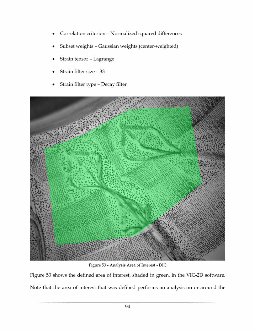
94
• Correlation criterion – Normalized squared differences
• Subset weights – Gaussian weights (center-weighted)
• Strain tensor – Lagrange
• Strain filter size – 33
• Strain filter type – Decay filter
Figure 53 shows the defined area of interest, shaded in green, in the VIC-2D software.
Note that the area of interest that was defined performs an analysis on or around the
Figure 53 - Analysis Area of Interest - DIC
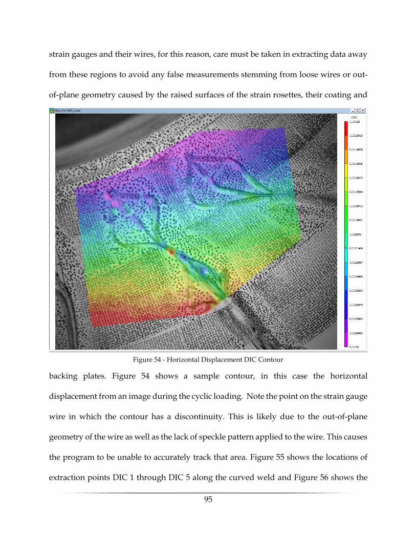
95
strain gauges and their wires, for this reason, care must be taken in extracting data away
from these regions to avoid any false measurements stemming from loose wires or out-
of-plane geometry caused by the raised surfaces of the strain rosettes, their coating and
backing plates. Figure 54 shows a sample contour, in this case the horizontal
displacement from an image during the cyclic loading. Note the point on the strain gauge
wire in which the contour has a discontinuity. This is likely due to the out-of-plane
geometry of the wire as well as the lack of speckle pattern applied to the wire. This causes
the program to be unable to accurately track that area. Figure 55 shows the locations of
extraction points DIC 1 through DIC 5 along the curved weld and Figure 56 shows the
Figure 54 - Horizontal Displacement DIC Contour
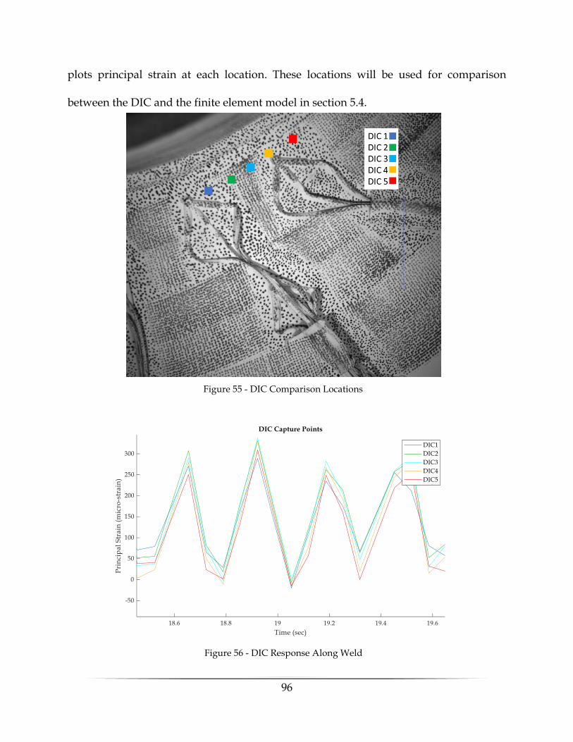
96
plots principal strain at each location. These locations will be used for comparison
between the DIC and the finite element model in section 5.4.
Figure 55 - DIC Comparison Locations
Figure 56 - DIC Response Along Weld

97
5.4 Measurement Comparison
This section will present the comparison between the measured response from the
2-D DIC and two of the relevant strain gauges. This comparison is provided to verify the
two measurements against one another, but mainly to verify the strain measurements
from the 2-D DIC since the strain gauges generally provide a more reliable measurement.
If the DIC matches closely to the strain gauges, it shows that the measured response of
the DIC is accurate. Additionally, comparisons between both measured responses, from
the DIC and the strain gauges, will be compared to the results of the numerical model.
Table 7Error! Reference source not found. shows the comparison of principal
strains measured from strain gauges NRW2 and NRW4, and points from the DIC analysis
near the base of the rosette. As the table shows, the DIC measurements match the strain
gauge measurements well. It should be noted that the verification using NRW3 was not
done due to the wires obstructing the base of the rosette where the DIC measurement
would be taken.
Table 7 - DIC and Strain Gauge
Location Data Source Max Principal
Strain (με)
NRW2
DIC 249
NRW2 268
Difference 7.6%
NRW4
DIC 296
NRW4 301
Difference 1.6%
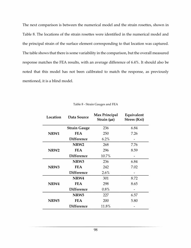
98
The next comparison is between the numerical model and the strain rosettes, shown in
Table 8. The locations of the strain rosettes were identified in the numerical model and
the principal strain of the surface element corresponding to that location was captured.
The table shows that there is some variability in the comparison, but the overall measured
response matches the FEA results, with an average difference of 6.4%. It should also be
noted that this model has not been calibrated to match the response, as previously
mentioned, it is a blind model.
Table 8 - Strain Gauges and FEA
Location Data Source Max Principal
Strain (με) Equivalent Stress (Ksi)
NRW1
Strain Gauge 236 6.84
FEA 250 7.26
Difference 6.2% -
NRW2
NRW2 268 7.76
FEA 296 8.59
Difference 10.7% -
NRW3
NRW3 236 6.84
FEA 242 7.02
Difference 2.6% -
NRW4
NRW4 301 8.72
FEA 298 8.65
Difference 0.8% -
NRW5
NRW5 227 6.57
FEA 200 5.80
Difference 11.8% -
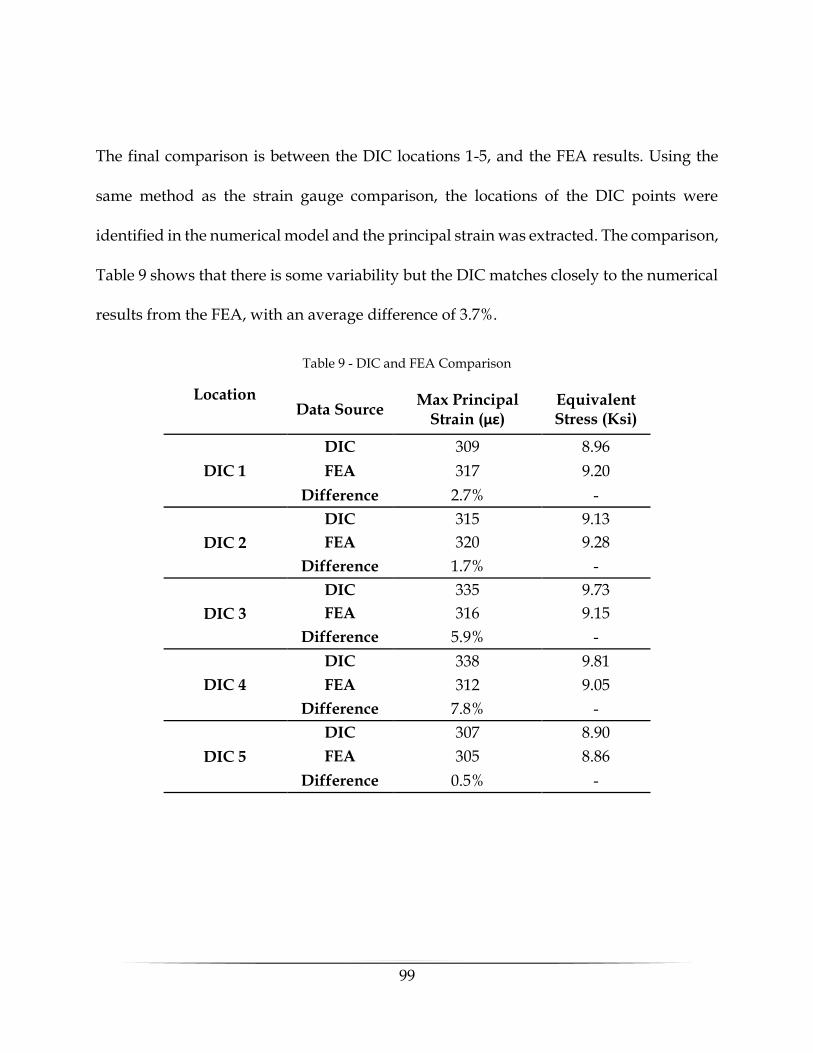
99
The final comparison is between the DIC locations 1-5, and the FEA results. Using the
same method as the strain gauge comparison, the locations of the DIC points were
identified in the numerical model and the principal strain was extracted. The comparison,
Table 9 shows that there is some variability but the DIC matches closely to the numerical
results from the FEA, with an average difference of 3.7%.
Table 9 - DIC and FEA Comparison
Location Data Source
Max Principal Strain (με)
Equivalent Stress (Ksi)
DIC 1
DIC 309 8.96
FEA 317 9.20
Difference 2.7% -
DIC 2
DIC 315 9.13
FEA 320 9.28
Difference 1.7% -
DIC 3
DIC 335 9.73
FEA 316 9.15
Difference 5.9% -
DIC 4
DIC 338 9.81
FEA 312 9.05
Difference 7.8% -
DIC 5
DIC 307 8.90
FEA 305 8.86
Difference 0.5% -

100
5.5 Summary and Discussion
In summary, the two experimental results were compared to one another and were
found to have a similar behavior. It should be noted that since the comparison was limited
to two strain rosette locations, it is difficult to draw conclusions about the measurements
compared to one another. Comparisons were also made between the FEA and the strain
rosettes. This comparison showed there was some variation between the calculated
response of the FEA and the measured response from the strain rosettes, but the overall
difference was 6.4% on average. Lastly, a comparison between the DIC measurements
and the FEA was performed. This comparison showed a relatively close match between
the two, with an average difference of 3.7%.
In terms of fatigue testing results, the measured strain in the specimen indicate
that the corresponding stresses are below the theoretical endurance limit for the design
fatigue category as expected. Since the model is matching the response well, the stresses
can be extrapolated to the weld using the numerical results. Based on this extrapolation
the maximum principal stress applied near the toe of the weld is approximately 14 Ksi.
As previously mentioned, the predicted fatigue life of this specimen, considering the
design assumptions and the 14 Ksi applied stress, was 1,600,000 cycles. In terms of
damage, in this study, fatigue failure, or damage, is defined as a visible crack. These
cycles have been applied and no damage has been detected in the specimen. There are a
few potential conclusions that can be drawn from these results;

101
1. Using the hot-spot stress close to the toe of the weld to predict life using the
AASHTO S-N curves, which were derived for the nominal stress, is not an
appropriate method to predict life for this scenario.
2. The design assumption of a category C fatigue detail was conservative, and
the endurance limit of the actual fatigue specimen may be higher than
expected.

102
6 RESIDUAL STRESSES
This chapter will focus on the investigation of residual stresses with regards to the
gusset-less connection fatigue sample. A brief overview of the importance of residual
stresses regarding fatigue will be provided and the locations of interest will be
introduced. Additionally, the hole-drilling strain gauging method will be discussed along
with the measurement procedure and instrumentation used in this study. Next, the
calculation method will be introduced. Finally, the residual stress results will be shown
and discussed.
6.1 Importance of Residual Stresses
Residual stresses are complex, sometimes difficult to measure, and often
overlooked in terms of civil engineering applications, but they have a significant
influence in fatigue performance nonetheless. As previously mentioned, the variables
with the largest effect on fatigue performance are the stress range, the mean stress, and
the initial stress state, or the residual stresses. Among those, the mean stress and residual
stresses have a comparable influence on the performance. It is often said that the residual
stresses can be thought of, in terms of fatigue performance, as an addition to the mean
stress state. Since the residual stresses are present in the material, the actual mean stress
state that the material is in is the sum of the mean applied stress and the residual stress
from fabrication.
In most cases, at least when using the AASHTO LRFD Bridge Code [20] it is
considered acceptable to overlook the residual stresses. Since the S-N curves used for the

103
fatigue design of welded steel were empirically created using weld test data it is
mentioned that residuals were considered, without measurement, because all test
samples would have similar levels of residual stress. Therefore, it is implied that the
residual stresses are built into the S-N Curve. This is acceptable when the design matches
the assumption made in the making of the code, but for complex and innovate designs
such as the Gusset-less connection, those assumption may not hold true. Specifically, the
residual stress state of the Gusset-less connection is unique due to the cold-bending of
the flanges as well as the multi-pass welds that were used to fabricate this built-up
member, and finally the sand-blasting and metallization to coat the steel.
Given the complex nature, as well as the varying sources, of the residual stresses,
it was decided to investigate multiple locations along the fatigue specimen. The exact
locations will be shown in section 6.4 when discussing the results of the residual stress
measurements. Another important decision made was to take the measurements while
the specimen was installed into the test setup as well as before the specimen was installed.
This was done for three reasons;
1. The installed scenario would be more representative of the actual stress state of
the Gusset-less connection.
2. This would decrease the chances of effecting the results of the fatigue test by
potentially altering the test setup during multiple installations of the specimen.
3. Taking measurements before and after bolting can show the effect of the bolting
on the residual stresses.
104
When the measurements are taken with the specimen loaded, due to the bolting and
dead-loads, the measurement taken are better described as the total stress state rather
than the residual stress state.
6.2 Hole-Drilling Method
The method used to measure the residual stresses in this study was the Hole-
Drilling, Strain Gauging method. In this method, a specialized strain rosette is attached
to the specimen and a small hole is drilled in the center of this gauge, making it a “semi-
destructive” method due to relatively small defect introduced. The removal of material
creates a free surface allowing the residual stresses to be locally relieved and the adjacent
strain surface relieved is measured with the strain rosette. The surface strains relieved at
the location of the gauges are then mathematically converted to residual stresses through
geometric and material relationships. This mathematical relationship will be explained
in detail in section 6.3, but it is important to note that this method assumes a linear-elastic
relationship.
Within the hole-drilling method, there are a few different types of analysis, each
with their own assumptions and limitations. The most common variants are the through-
hole analysis and the blind-hole analysis. The through-hole analysis, as the name
suggests, is a method where the hole is drilled completely through the thickness of the
specimen. The main drawback of this method is that it is limited to “thin” workpieces
where the exact thickness is limited by the geometry of the strain gauge used. This is due
to the geometric relationship between the stresses measured at a depth and the strain
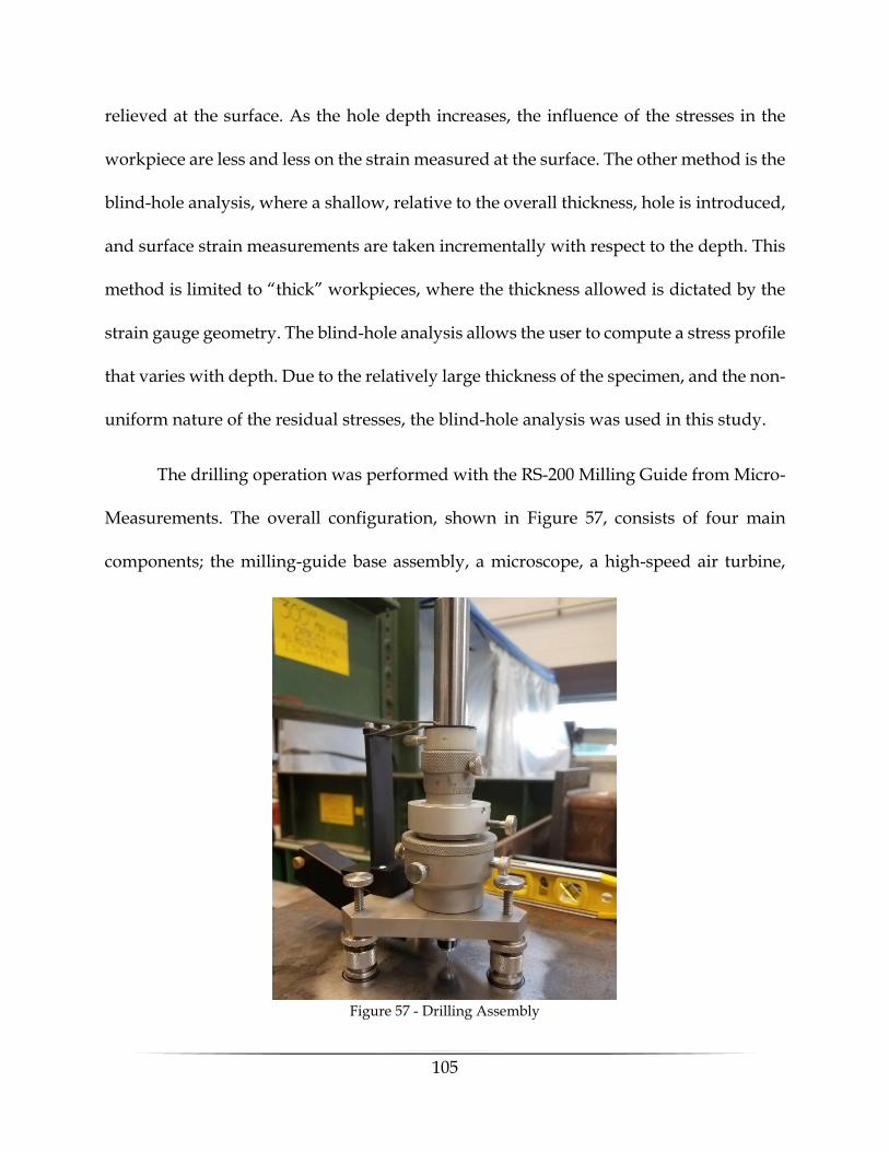
105
relieved at the surface. As the hole depth increases, the influence of the stresses in the
workpiece are less and less on the strain measured at the surface. The other method is the
blind-hole analysis, where a shallow, relative to the overall thickness, hole is introduced,
and surface strain measurements are taken incrementally with respect to the depth. This
method is limited to “thick” workpieces, where the thickness allowed is dictated by the
strain gauge geometry. The blind-hole analysis allows the user to compute a stress profile
that varies with depth. Due to the relatively large thickness of the specimen, and the non-
uniform nature of the residual stresses, the blind-hole analysis was used in this study.
The drilling operation was performed with the RS-200 Milling Guide from Micro-
Measurements. The overall configuration, shown in Figure 57, consists of four main
components; the milling-guide base assembly, a microscope, a high-speed air turbine,
Figure 57 - Drilling Assembly
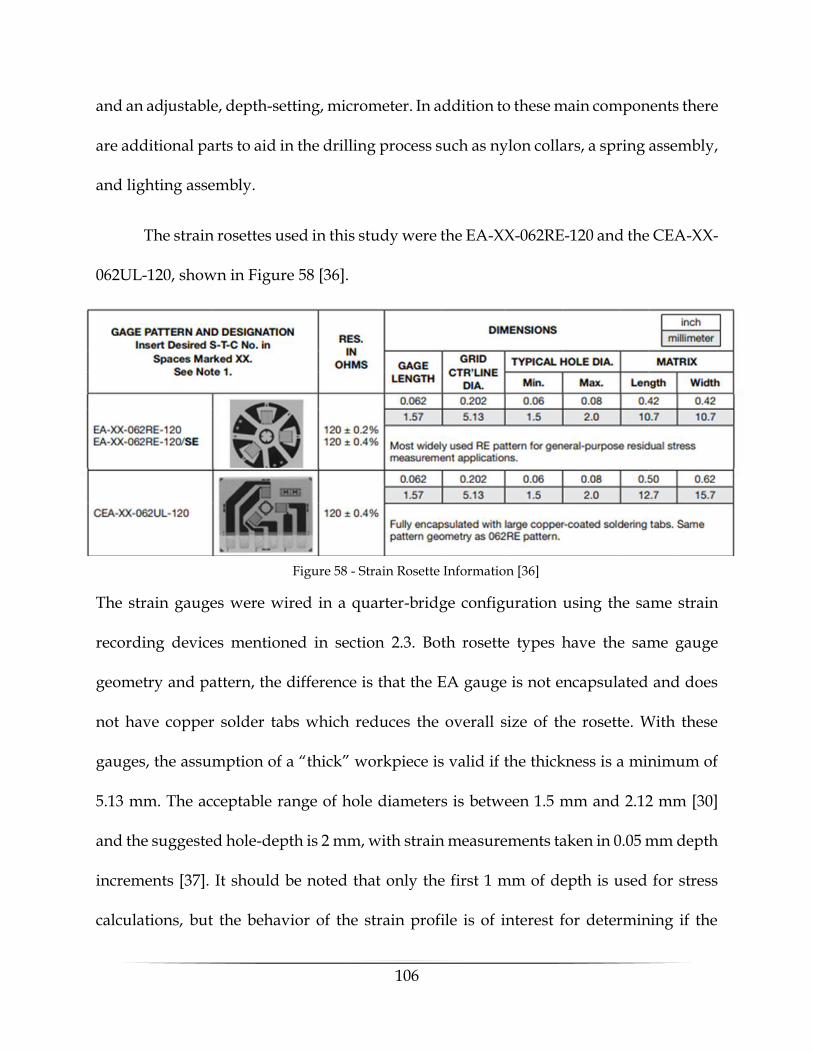
106
and an adjustable, depth-setting, micrometer. In addition to these main components there
are additional parts to aid in the drilling process such as nylon collars, a spring assembly,
and lighting assembly.
The strain rosettes used in this study were the EA-XX-062RE-120 and the CEA-XX-
062UL-120, shown in Figure 58 [36].
The strain gauges were wired in a quarter-bridge configuration using the same strain
recording devices mentioned in section 2.3. Both rosette types have the same gauge
geometry and pattern, the difference is that the EA gauge is not encapsulated and does
not have copper solder tabs which reduces the overall size of the rosette. With these
gauges, the assumption of a “thick” workpiece is valid if the thickness is a minimum of
5.13 mm. The acceptable range of hole diameters is between 1.5 mm and 2.12 mm [30]
and the suggested hole-depth is 2 mm, with strain measurements taken in 0.05 mm depth
increments [37]. It should be noted that only the first 1 mm of depth is used for stress
calculations, but the behavior of the strain profile is of interest for determining if the
Figure 58 - Strain Rosette Information [36]
107
uniform analysis can be performed instead of the non-uniform analysis. With these
geometric limitations, the diameter of the tungsten carbide inverted-cone cutting head
used was 1.6 mm. When using the plunging method, this results in a hole diameter of
approximately 1.66 mm. When using the orbital method, the measured hole diameter was
approximately 2.05 mm. It should be noted that the offset of the cutting head was not
measured, it was adjusted using trial and error until the desired hole diameter was
achieved.
A general procedure [37] for performing residual stress measurements with the
RS-200 milling guide is as follows;
1. Prepare the surface of the workpiece for the strain gauge and the milling
guide. This consists of sanding an area that will be large enough for the
specialized strain rosette and the three swivel pads for the milling guide.
After sanding, the area should be cleaned with a degreaser.
2. Attach the specialized rosette at the location of interest. The method for
attaching the rosette is the same as listed in section 2.3, the only difference
is that care should be taken to align the grids of the rosette with the
directions of interest.
3. Test that the strain rosette is functioning, and the strains are zeroed.
4. Position the milling-guide base assembly such that the center of the journal
hole is approximately centered over the strain rosette. Once it is in a

108
satisfactory position mark the locations of the swivel pads on the
workpiece.
5. Adhere the swivel pads to the workpiece.
6. After bonding the swivel pads, level the milling guide such that the guide
is perpendicular to the workpiece surface while keeping the guide as close
to the surface as possible. Note: on curved surfaces care should be taken to
ensure that it is as close to perpendicular as possible.
7. Use the microscope assembly to align the cross-hairs with the target on the
specialized strain rosette. Great care should be taken to ensure that the
cross-hair of the microscope is in the center of the target on the rosette. Any
eccentricity can have a significant effect on the stress calculations.
8. At this point, the strain rosette should be checked again to ensure that no
wires became disconnected during the installation process. Once the
drilling has begun any measurement error can render the results useless.
9. Install a new tungsten carbide cutter into the air-turbine collet. At this point
the cutter should be offset from the center the appropriate distance to create
the desired hole diameter while using the orbital drilling method1. If the
plunging method2 is used, the cutter should be centered.
1 The orbital drilling method uses an offset cutting head. There are two steps in the drilling process; 1) advancing to the desired depth increment and 2) rotating the turbine one full revolution within the journal hole. This allows the cutter to remove material with the sides instead of the face, resulting in a cleaner cut. 2 The plunging method uses a centered cutting head. The cutting is done in one step by advancing the cutting head to the desired depth. This results in a rougher cut.
109
10. Install the anti-rotation adapter and micrometer over the journal hole. The
micrometer should be adjusted to read zero-depth.
11. Insert the air-turbine into the journal hole and position the nylon collar such
that the cutting head is just above the gauge. It is easiest to lower the turbine
assembly into the hole until contact with the rosette is made and then pull
it back out very slightly before tightening the collar.
12. With the turbine in place, install the spring assembly and attach the air
supply to the turbine.
13. Establish “zero-depth”, or the depth setting of the micrometer at which the
cutting head cuts through the gauge backing but not the workpiece surface.
This should be done by supplying the air-turbine with air while advancing
the turbine downward, very slowly, with the micrometer. Great care should
be taken to use the smallest micrometer increments possible to ensure
minimal drilling of the workpiece surface. This is a critical step because the
calculations are highly dependent on the depth of the hole with respect to
the surface when the strains relieved are measured.
14. Once zero-depth is established, the strains should be recorded and noted as
the strain measured before any material removal.
15. While powering the turbine, advance the micrometer the appropriate
increment, being sure to rotate the turbine within the journal hole after an
increment. Note: when using the orbital drilling method, the desired

110
measurement increment should be sub-divided into smaller increments in
which the drill is orbited.
16. Once the appropriate depth increment is reached, stop the air flow to the
turbine and allow ~10 seconds before recording the strain for ~10 seconds
and noting the current hole depth based on the micrometer.
17. Repeat step 15 and 16 until the desired hole depth is achieved.
18. Remove the turbine assembly and use the microscope assembly to visually
inspect the hole, making a note of the final diameter.
19. Remove the strain rosette by lifting a corner with a blade and then peeling
it back by hand. This step serves as a check on the bond strength of the
gauge to ensure there was no significant debonding.
The procedure is designed to produce accurate and consistent measurements of the
surface strains relieved from the drilling process while also checking for any potential
errors in the experiment. Generally, the biggest source of error is the skill of the operator
[38] performing the hole-drilling and measurement operations, therefore great care
should be taken in this procedure.
6.3 Blind-Hole Residual Stress Calculations
In this research, as previously stated, the method for measuring residual stresses
is the blind-hole method. Within the blind-hole method, the calculations are carried out
assuming a non-uniform stress distribution through the thickness using the integral
method. The conversion between measured strains relieved on the surface, in proximity
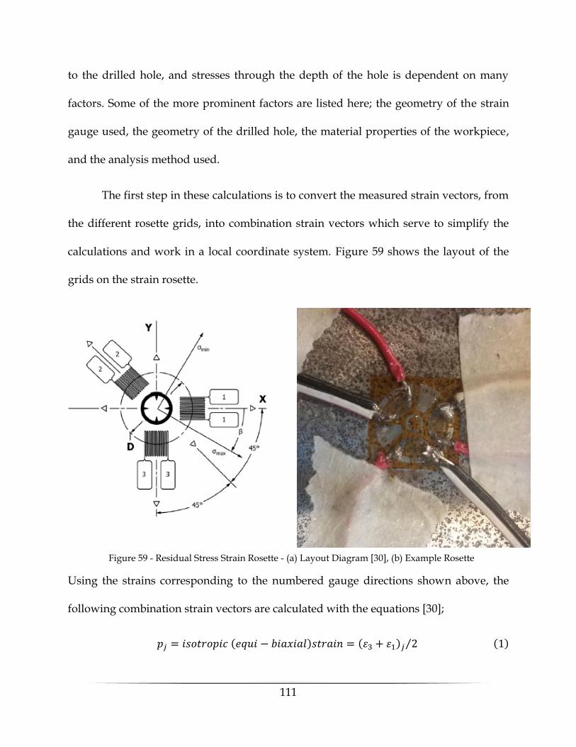
111
to the drilled hole, and stresses through the depth of the hole is dependent on many
factors. Some of the more prominent factors are listed here; the geometry of the strain
gauge used, the geometry of the drilled hole, the material properties of the workpiece,
and the analysis method used.
The first step in these calculations is to convert the measured strain vectors, from
the different rosette grids, into combination strain vectors which serve to simplify the
calculations and work in a local coordinate system. Figure 59 shows the layout of the
grids on the strain rosette.
Using the strains corresponding to the numbered gauge directions shown above, the
following combination strain vectors are calculated with the equations [30];
𝑝𝑗 = 𝑖𝑠𝑜𝑡𝑟𝑜𝑝𝑖𝑐 (𝑒𝑞𝑢𝑖 − 𝑏𝑖𝑎𝑥𝑖𝑎𝑙)𝑠𝑡𝑟𝑎𝑖𝑛 = (𝜀3 + 𝜀1)𝑗 2⁄ (1)
Figure 59 - Residual Stress Strain Rosette - (a) Layout Diagram [30], (b) Example Rosette

112
𝑞𝑗 = 45° 𝑠ℎ𝑒𝑎𝑟 𝑠𝑡𝑟𝑎𝑖𝑛 = (𝜀3 − 𝜀1)𝑗 2⁄ (2)
𝑡𝑗 = 𝑥𝑦 𝑠ℎ𝑒𝑎𝑟 𝑠𝑡𝑟𝑎𝑖𝑛 = (𝜀3 + 𝜀1 − 2𝜀2)𝑗 2⁄ (3)
In equations 1-3 it is important to note that the strains that are used at a generic position
k in the vector are the cumulative strain after drilling to a hole depth corresponding to
step k. Additionally, the raw strain data must be manipulated to ensure at zero-depth the
strains are zero. Once the combination strain vectors are calculated, the standard errors
in the combination strains should be estimated using equations 4-6 [30];
𝑝𝑠𝑡𝑑2 = ∑
(𝑝𝑗 − 3𝑝𝑗+1 + 3𝑝𝑗+2 − 𝑝𝑗+3)2
20(𝑛 − 3)
𝑛−3
𝑗=1
(4)
𝑞𝑠𝑡𝑑2 = ∑
(𝑞𝑗 − 3𝑞𝑗+1 + 3𝑞𝑗+2 − 𝑞𝑗+3)2
20(𝑛 − 3)
𝑛−3
𝑗=1
(5)
𝑡𝑠𝑡𝑑2 = ∑
(𝑡 − 3𝑡𝑗+1 + 3𝑡𝑗+2 − 𝑡𝑗+3)2
20(𝑛 − 3)
𝑛−3
𝑗=1
(6)
Where n = the total number of data points for the strain vector. These standard errors will
be used to create a smoothing criterion later.
The next step in the calculations is manipulating the calibration matrices and the
combination strain vectors depending on the number and depth of increments used in
the drilling. The calibration matrices were derived from finite element work and
standardized for the common rosette geometries [30]. These matrices, represented
visually in Figure 60 [30], relate the surface strain relieved during the drilling to a unit
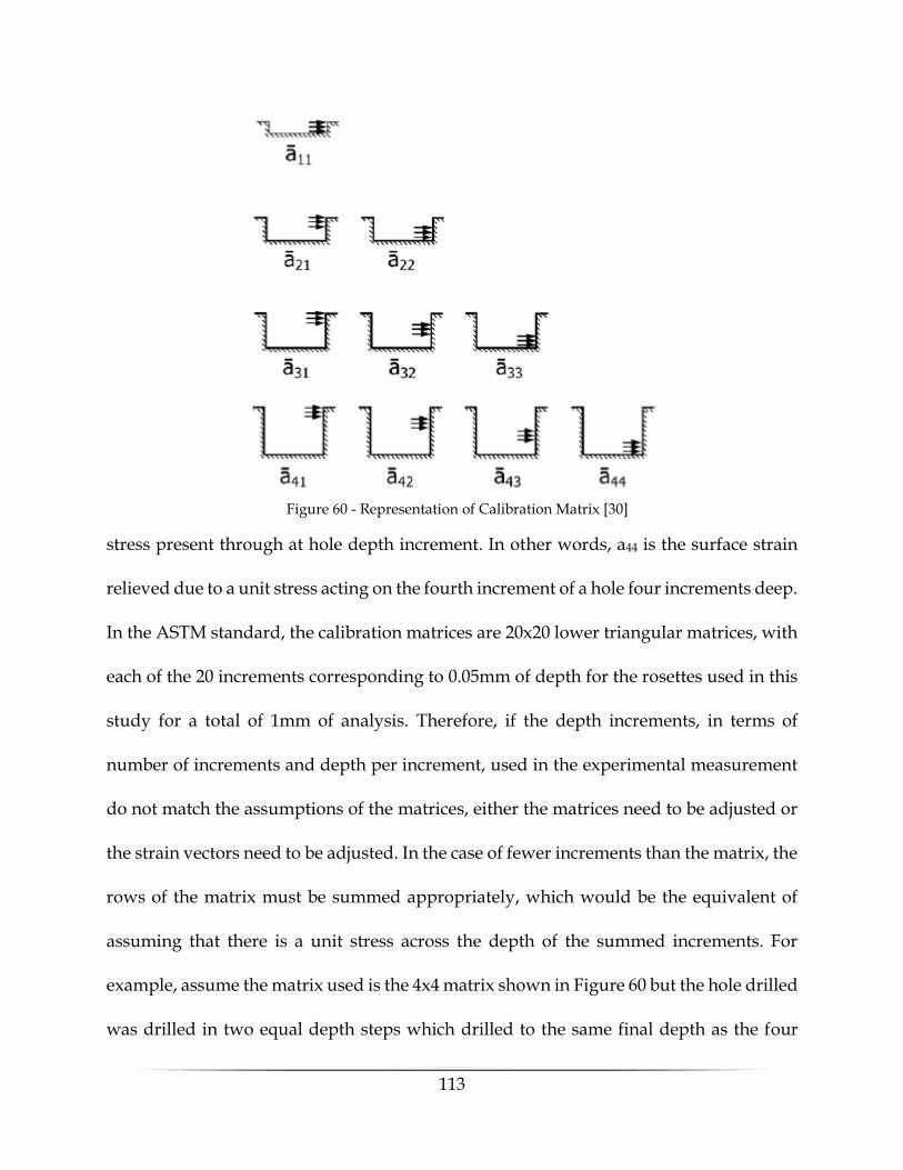
113
stress present through at hole depth increment. In other words, a44 is the surface strain
relieved due to a unit stress acting on the fourth increment of a hole four increments deep.
In the ASTM standard, the calibration matrices are 20x20 lower triangular matrices, with
each of the 20 increments corresponding to 0.05mm of depth for the rosettes used in this
study for a total of 1mm of analysis. Therefore, if the depth increments, in terms of
number of increments and depth per increment, used in the experimental measurement
do not match the assumptions of the matrices, either the matrices need to be adjusted or
the strain vectors need to be adjusted. In the case of fewer increments than the matrix, the
rows of the matrix must be summed appropriately, which would be the equivalent of
assuming that there is a unit stress across the depth of the summed increments. For
example, assume the matrix used is the 4x4 matrix shown in Figure 60 but the hole drilled
was drilled in two equal depth steps which drilled to the same final depth as the four
Figure 60 - Representation of Calibration Matrix [30]

114
increments assumed by the matrix. In this case the summation of a21 and a22 would be the
equivalent of a11 for the new matrix, the summation of a41 and a42 would be the equivalent
of a21 for the new matrix, and the summation of a43 and a44would be the equivalent of a22
for the new matrix. This manipulation changes the size of the matrix to the appropriate
size for the input data set. In the other case, when the depth increments are smaller than
the matrix assumes, the strain at the correct depth increments must be interpolated from
the original data. After manipulation, the calibration matrices should be a lower
triangular matrix with the same characteristic length as the combination strain vector. In
addition to manipulating the calibration matrices for size, they must be scaled by a factor
equal to the square of the diameter of the drilled hole divided by the square of the
assumed diameter for the matrix, in this study the assumed diameter for the matrix is
2mm and the actual drilled hole diameter is variable. Once the calibration matrices and
strain vectors are properly manipulated, the stresses at each depth can be calculated
through the integral method using equations 7-9 [30];
(�̅�𝑇�̅� + 𝛼𝑝𝑐𝑇𝑐)𝑃 = 𝐸
1 + 𝑣�̅�𝑇𝑝 (7)
(𝑏𝑇�̅� + 𝛼𝑄𝑐𝑇𝑐)𝑄 = 𝐸�̅�𝑇𝑞 (8)
(𝑏𝑇�̅� + 𝛼𝑇𝑐𝑇𝑐)𝑇 = 𝐸�̅�𝑇𝑡 (9)
Where; �̅� = calibration matrix for isotropic stresses
�̅� = calibration matrix for shear stresses

115
𝛼 = regularization factor for respective stress P, Q, or T.
𝑐 = tri-diagonal “second derivative” matrix for Tikhonov regularization
𝑃 = uniform isotropic stress
𝑄 = uniform 45° shear stress
𝑇 = uniform x-y shear stress
These equations can be solved for the stress vectors P, Q, and T respectively. It is
important to note that since the integral method is known to be numerically ill-
conditioned as the number of increments increase, regularization is generally required.
As the equation above shows, regularization is done using a regularization matrix c and
a corresponding regularization coefficient 𝛼. The matrix c is a tri-diagonal matrix in
which the size is the same as the calibration matrix, the first and last row are zeros, and
other than the first and last row, all rows have [-1 2 -1] centered on the diagonal [30]. The
amount of regularization must be optimized using the 𝛼 term, which is generally limited
to numbers between 10-4 and 10-6 [30], in an iterative process to minimize the misfit
between the unregularized strains and the calculated stresses. The misfit vectors are
calculated using the following equations [30];
𝑝𝑚𝑖𝑠𝑓𝑖𝑡 = 𝑝 − 1 + 𝑣
𝐸�̅�𝑃 (10)
𝑞𝑚𝑖𝑠𝑓𝑖𝑡 = 𝑞 − 1
𝐸�̅�𝑄 (11)

116
𝑡𝑚𝑖𝑠𝑓𝑖𝑡 = 𝑡 − 1
𝐸�̅�𝑇 (12)
Using the misfit vectors, the mean squares should be calculated as follows;
𝑝𝑟𝑚𝑠2 =
1
𝑛∑(𝑝𝑚𝑖𝑠𝑓𝑖𝑡)𝑗
2
𝑛
𝑗=1
(13)
𝑞𝑟𝑚𝑠2 =
1
𝑛∑(𝑞𝑚𝑖𝑠𝑓𝑖𝑡)𝑗
2
𝑛
𝑗=1
(14)
𝑡𝑟𝑚𝑠2 =
1
𝑛∑(𝑡𝑚𝑖𝑠𝑓𝑖𝑡)𝑗
2
𝑛
𝑗=1
(15)
Now a comparison must be made between the mean square of the misfits and the
standard errors, calculated in equations 1-3, of the combination strain vectors. If the
values for the mean square of the misfit is within 5% of the value of the standard error
of the combination strains, the calculated stresses from equations 7-9 are acceptable. If
the values are more than 5% different, the regularization coefficient must be adjusted as
follows;
(𝛼𝑃)𝑛𝑒𝑤 = 𝑝𝑠𝑡𝑑
2
𝑝𝑟𝑚𝑠2
(𝛼𝑃)𝑜𝑙𝑑 (16)
(𝛼𝑄)𝑛𝑒𝑤
= 𝑞𝑠𝑡𝑑
2
𝑞𝑟𝑚𝑠2
(𝛼𝑄)𝑜𝑙𝑑
(17)
(𝛼𝑇)𝑛𝑒𝑤 = 𝑡𝑠𝑡𝑑
2
𝑡𝑟𝑚𝑠2
(𝛼𝑇)𝑜𝑙𝑑 (18)

117
With the new regularization coefficient, the stresses must be recalculated, and this
process is repeated until the difference is less than 5%. Once the stresses are accepted,
they can be converted back to cartesian coordinates as follows [30];
(𝜎𝑥)𝑗 = 𝑃𝑗 − 𝑄𝑗 (19)
(𝜎𝑦)𝑗 = 𝑃𝑗 + 𝑄𝑗 (20)
(𝜏𝑥𝑦)𝑗 = 𝑇𝑗 (21)
As part of this thesis, a MATLAB code was developed for these calculations and can be
seen in Appendix E.
6.4 Results – Residual Stresses
This section will introduce the preliminary results of the residual stress
measurements performed on the gusset-less fatigue specimen. A total of six
measurements were taken on the gusset-less fatigue specimen, five of those
measurements were on specimen one, which was the one tested for fatigue, and one of
those measurements was on specimen two, which has not been tested or used for any
purpose as of this time. In addition to measurements on the fatigue specimen,
measurements were taken on a variety of other metal samples, but the focus of this section
will be on the measurements taken on the fatigue specimen. Before introducing the data
from the fatigue specimen, data will be presented in order to show a verification of the
methods used in this study.
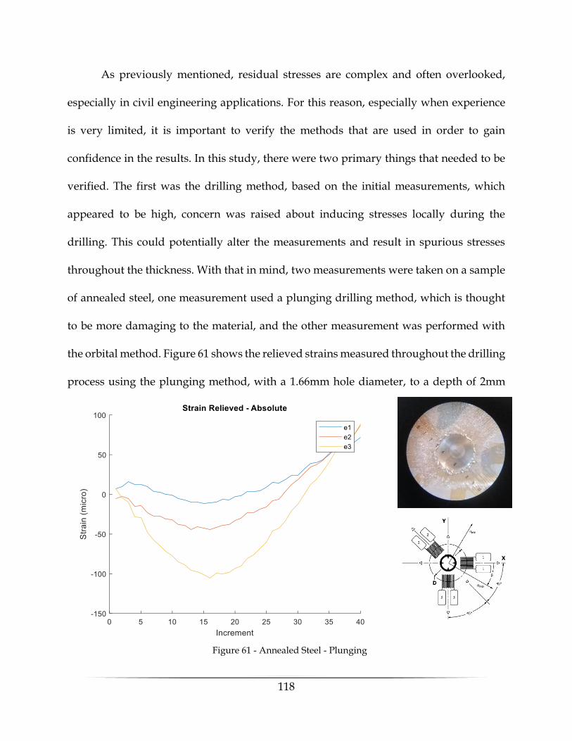
118
As previously mentioned, residual stresses are complex and often overlooked,
especially in civil engineering applications. For this reason, especially when experience
is very limited, it is important to verify the methods that are used in order to gain
confidence in the results. In this study, there were two primary things that needed to be
verified. The first was the drilling method, based on the initial measurements, which
appeared to be high, concern was raised about inducing stresses locally during the
drilling. This could potentially alter the measurements and result in spurious stresses
throughout the thickness. With that in mind, two measurements were taken on a sample
of annealed steel, one measurement used a plunging drilling method, which is thought
to be more damaging to the material, and the other measurement was performed with
the orbital method. Figure 61 shows the relieved strains measured throughout the drilling
process using the plunging method, with a 1.66mm hole diameter, to a depth of 2mm
Figure 61 - Annealed Steel - Plunging
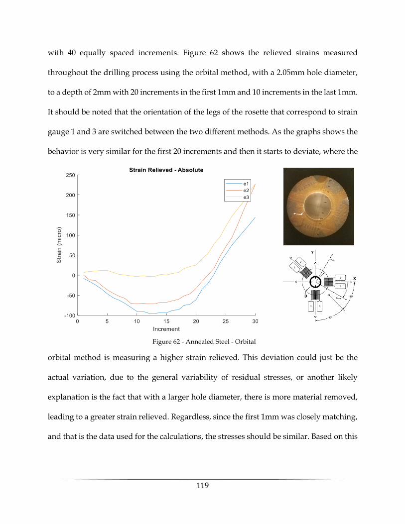
119
with 40 equally spaced increments. Figure 62 shows the relieved strains measured
throughout the drilling process using the orbital method, with a 2.05mm hole diameter,
to a depth of 2mm with 20 increments in the first 1mm and 10 increments in the last 1mm.
It should be noted that the orientation of the legs of the rosette that correspond to strain
gauge 1 and 3 are switched between the two different methods. As the graphs shows the
behavior is very similar for the first 20 increments and then it starts to deviate, where the
orbital method is measuring a higher strain relieved. This deviation could just be the
actual variation, due to the general variability of residual stresses, or another likely
explanation is the fact that with a larger hole diameter, there is more material removed,
leading to a greater strain relieved. Regardless, since the first 1mm was closely matching,
and that is the data used for the calculations, the stresses should be similar. Based on this
Figure 62 - Annealed Steel - Orbital
120
experiment, it was concluded that the drilling method was not inducing significant
strains during the measurement procedure.
The next verification was regarding the calculation method. Since the calculation
for non-uniform residual stress profiles can be complex, ensuring the developed
MATLAB code was properly calculating the stresses was a challenge. To accomplish this
verification, a few data sets, and the corresponding stress profiles were provided by Dr.
Gary Schajer, a professor of mechanical engineering at the University of British Columbia.
Using these data sets, and the code developed in this research, the stress profiles were
calculated and compared to those calculated by Dr. Schajer, using the H-Drill software
he developed for residual calculations. Figure 63 shows one of the comparisons made
between the two calculated stress profiles. The stress vectors shown with a dashed line
are those calculated from the H-Drill software, and the stress vectors shown with the solid
lines are those calculated with the code developed in this research. As the figure shows,
the stresses are in very good agreement, even with the highly non-uniform nature of the
stresses. This verification, along with the verification of the drilling methods, provided
confidence in the methodology used to measure and calculate the residual stresses in the
gusset-less fatigue specimen.
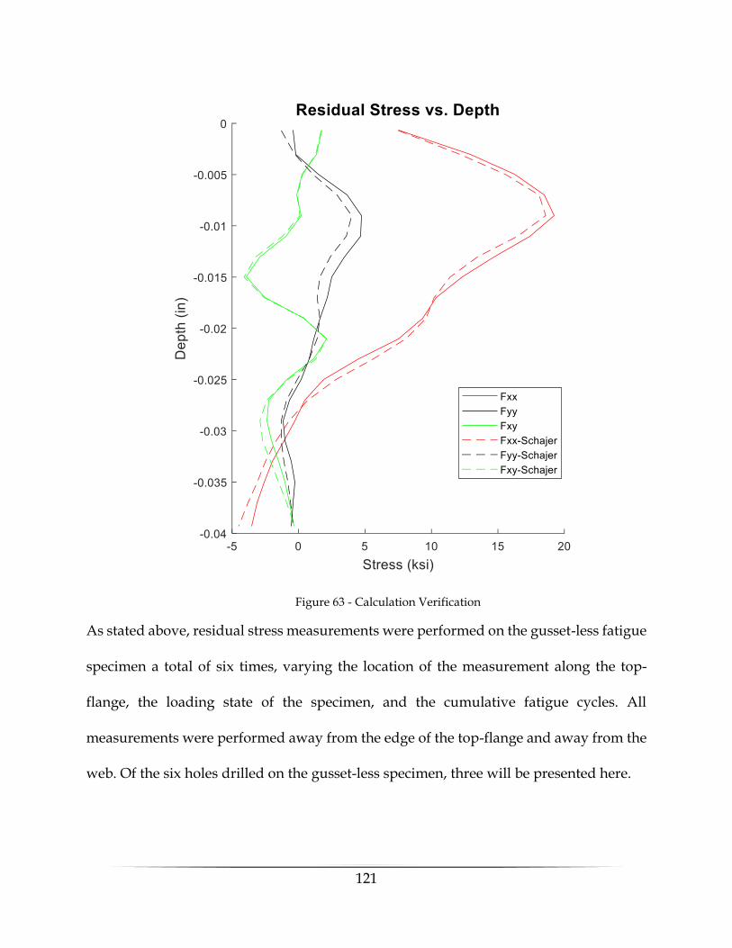
121
As stated above, residual stress measurements were performed on the gusset-less fatigue
specimen a total of six times, varying the location of the measurement along the top-
flange, the loading state of the specimen, and the cumulative fatigue cycles. All
measurements were performed away from the edge of the top-flange and away from the
web. Of the six holes drilled on the gusset-less specimen, three will be presented here.
Figure 63 - Calculation Verification
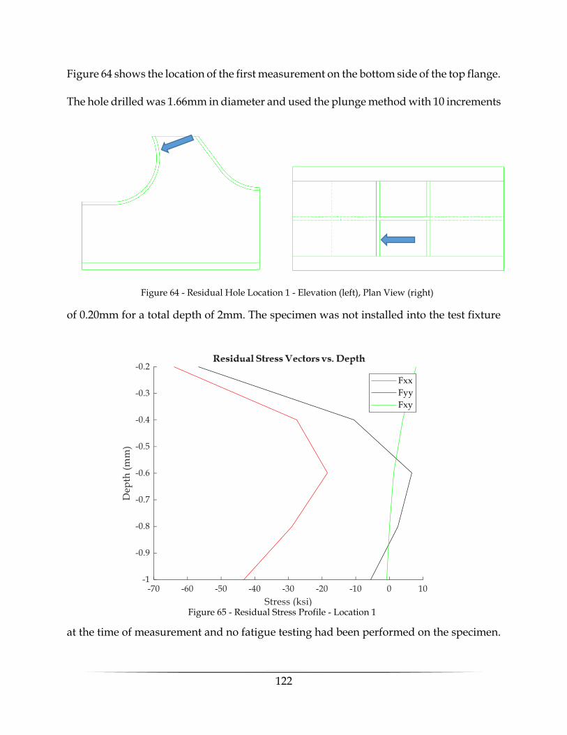
122
Figure 64 shows the location of the first measurement on the bottom side of the top flange.
The hole drilled was 1.66mm in diameter and used the plunge method with 10 increments
of 0.20mm for a total depth of 2mm. The specimen was not installed into the test fixture
at the time of measurement and no fatigue testing had been performed on the specimen.
Figure 64 - Residual Hole Location 1 - Elevation (left), Plan View (right)
Figure 65 - Residual Stress Profile - Location 1
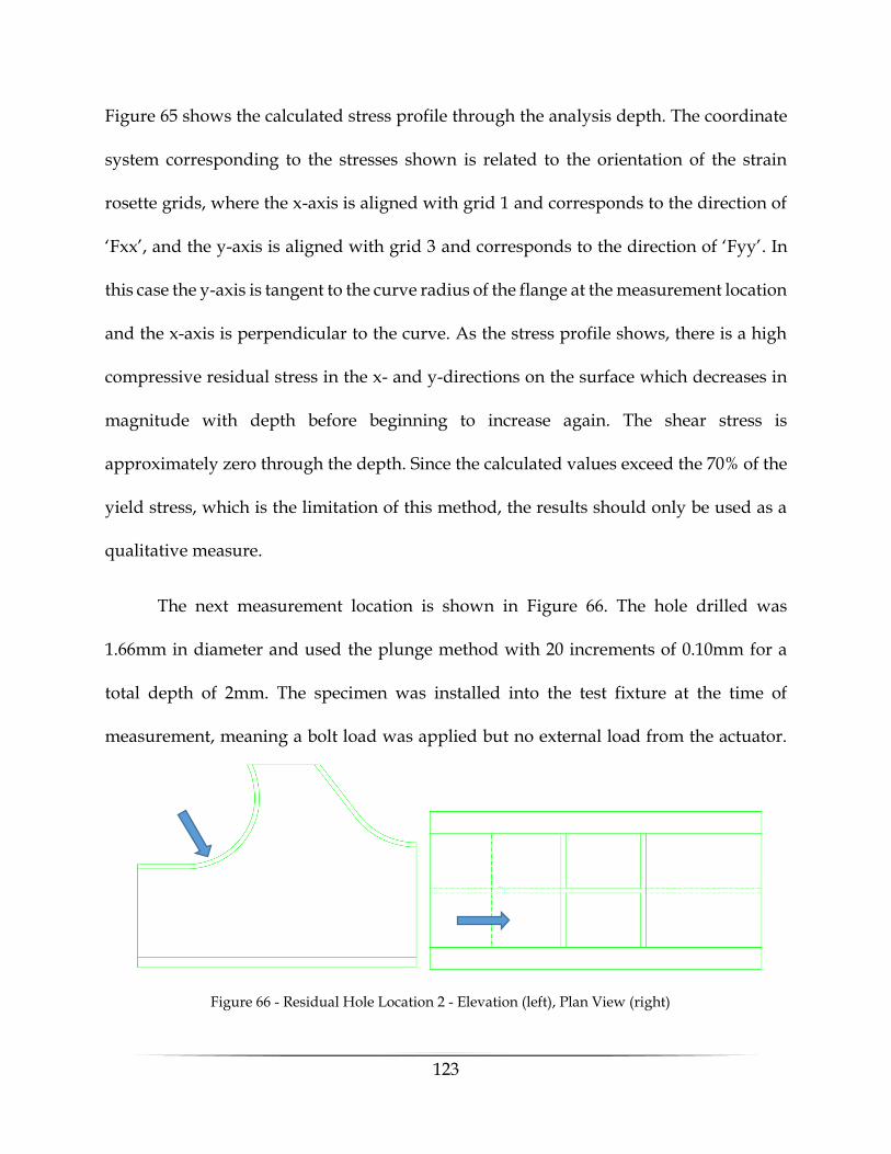
123
Figure 65 shows the calculated stress profile through the analysis depth. The coordinate
system corresponding to the stresses shown is related to the orientation of the strain
rosette grids, where the x-axis is aligned with grid 1 and corresponds to the direction of
‘Fxx’, and the y-axis is aligned with grid 3 and corresponds to the direction of ‘Fyy’. In
this case the y-axis is tangent to the curve radius of the flange at the measurement location
and the x-axis is perpendicular to the curve. As the stress profile shows, there is a high
compressive residual stress in the x- and y-directions on the surface which decreases in
magnitude with depth before beginning to increase again. The shear stress is
approximately zero through the depth. Since the calculated values exceed the 70% of the
yield stress, which is the limitation of this method, the results should only be used as a
qualitative measure.
The next measurement location is shown in Figure 66. The hole drilled was
1.66mm in diameter and used the plunge method with 20 increments of 0.10mm for a
total depth of 2mm. The specimen was installed into the test fixture at the time of
measurement, meaning a bolt load was applied but no external load from the actuator.
Figure 66 - Residual Hole Location 2 - Elevation (left), Plan View (right)
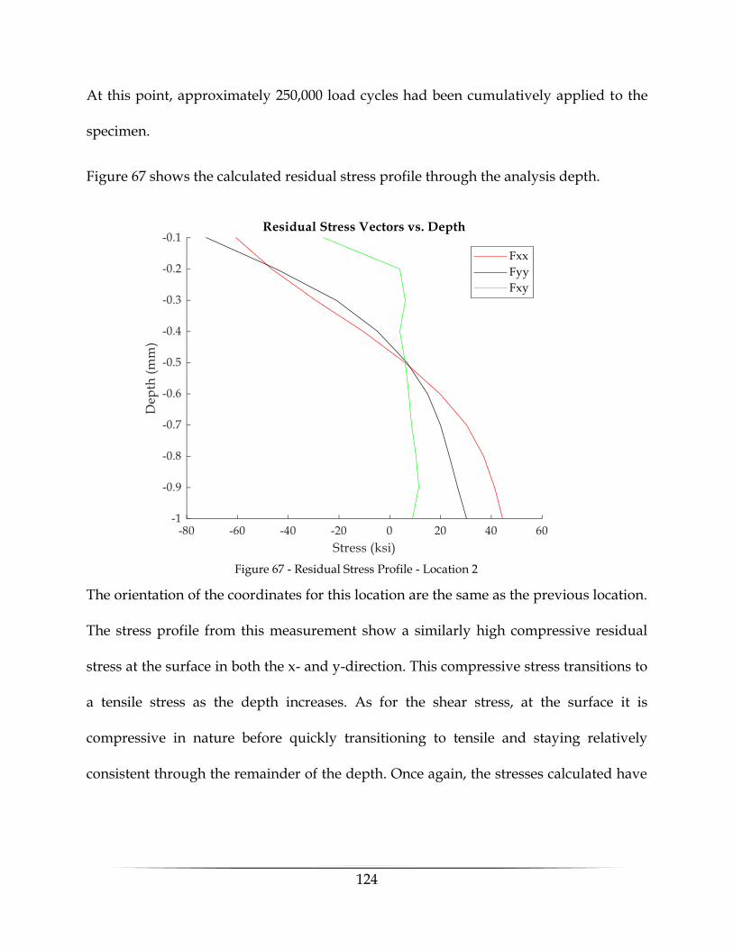
124
At this point, approximately 250,000 load cycles had been cumulatively applied to the
specimen.
Figure 67 shows the calculated residual stress profile through the analysis depth.
The orientation of the coordinates for this location are the same as the previous location.
The stress profile from this measurement show a similarly high compressive residual
stress at the surface in both the x- and y-direction. This compressive stress transitions to
a tensile stress as the depth increases. As for the shear stress, at the surface it is
compressive in nature before quickly transitioning to tensile and staying relatively
consistent through the remainder of the depth. Once again, the stresses calculated have
Figure 67 - Residual Stress Profile - Location 2
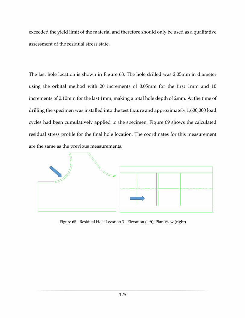
125
exceeded the yield limit of the material and therefore should only be used as a qualitative
assessment of the residual stress state.
The last hole location is shown in Figure 68. The hole drilled was 2.05mm in diameter
using the orbital method with 20 increments of 0.05mm for the first 1mm and 10
increments of 0.10mm for the last 1mm, making a total hole depth of 2mm. At the time of
drilling the specimen was installed into the test fixture and approximately 1,600,000 load
cycles had been cumulatively applied to the specimen. Figure 69 shows the calculated
residual stress profile for the final hole location. The coordinates for this measurement
are the same as the previous measurements.
Figure 68 - Residual Hole Location 3 - Elevation (left), Plan View (right)
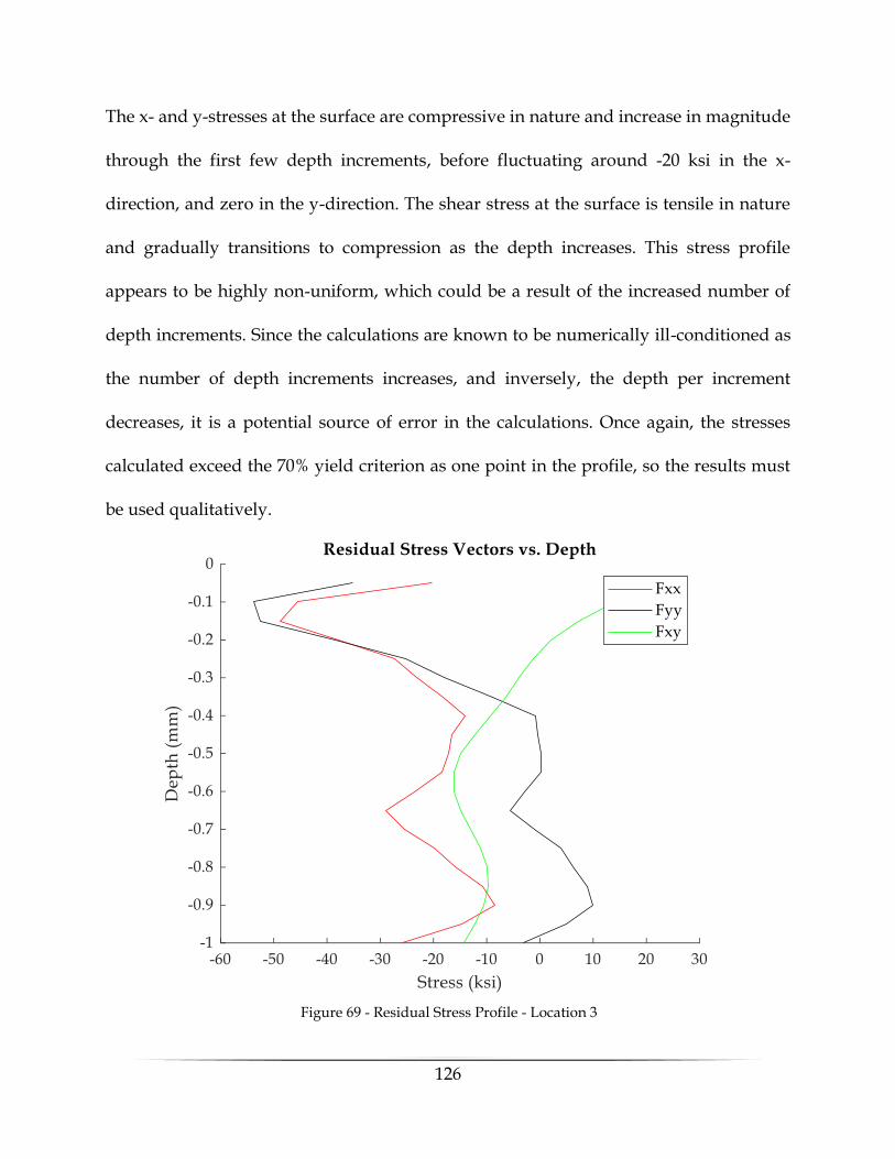
126
The x- and y-stresses at the surface are compressive in nature and increase in magnitude
through the first few depth increments, before fluctuating around -20 ksi in the x-
direction, and zero in the y-direction. The shear stress at the surface is tensile in nature
and gradually transitions to compression as the depth increases. This stress profile
appears to be highly non-uniform, which could be a result of the increased number of
depth increments. Since the calculations are known to be numerically ill-conditioned as
the number of depth increments increases, and inversely, the depth per increment
decreases, it is a potential source of error in the calculations. Once again, the stresses
calculated exceed the 70% yield criterion as one point in the profile, so the results must
be used qualitatively.
Figure 69 - Residual Stress Profile - Location 3

127
In addition to the measurements presented in this section, additional
measurements will be presented in Appendix F. Based on the results shown here, the
measurements obtained using the hole-drilling method are to be used as a qualitative tool
to estimate the behavior of the residual stresses with depth. Although they are qualitative,
the general profile is close to what is expected in a steel sample which has undergone
sand-blasting [39]. With that in mind, the residual stresses at the surface, which is
generally the critical fatigue location, are high in magnitude and compressive in nature.
In terms of fatigue, this is considered beneficial for fatigue performance, since a fatigue
crack that initiates in an area of compressive stress, residual or otherwise, will not
propagate.

128
7 SUMMARY, CONCLUSIONS, AND FUTURE WORK
This chapter will summarize the work from this thesis including the results from the
fatigue testing and the residual stress. Next, there will be a section listing the overall
conclusions made from the work presented in this thesis. Lastly, future work is discussed
regarding this project.
7.1 Summary
The objective of this research was to investigate the fatigue performance of the
Gusset-less truss connection used in place on the Memorial bridge. To investigate the
performance, a scale-model of the connection was designed and fabricated in a previous
research [31]. In addition to the scaled-connection, a test setup for an experimental fatigue
test was designed given the limitations of the current UNH Structural Engineering
Laboratory [31]. In this work, adjustments were made to the original test setup to correct
undesirable behavior. These adjustments were in the form of providing additional
rigidity to the reaction block by adding concrete and adding a steel shim support under
the tip of the specimen to restrain vertical movement. Modifications were also made to
the original instrumentation plan [31] with the addition of 2-Dimensional Digital Image
Correlation (DIC).
Given that the infrastructure available for this fatigue test was limited, the test
setup was not traditional. With that, there were concerns about ensuring consistency
across multiple testing periods in a high-cycle fatigue test. For this reason, an approach
to monitoring the response of the fatigue test specimen and the overall setup was
129
developed in this work. The protocol that was presented is a systematic method that
combines visual and physical inspections, along with periodic, full characterizations of
the structural response of the test setup through a System Identification (System ID). The
System ID method used in this study captures the structural response at key locations
along the test setup using DIC measurements along with LVDTs. In addition to the
periodic characterization provided by the System ID, the actuator force-displacement
relationship was used to quickly indicate if there has been a change in the overall
response of the system.
In this work several finite element models (FEM) of the test setup were developed
and refined. The final model used in this study is a detailed, blind, model with the
objective of capturing the structural response of not only the fatigue specimen, but the
test setup as well. This model underwent a mesh sensitivity study and was refined until
the response was acceptable.
During this work the Gusset-less fatigue specimen was tested with the presented
fatigue loading. The structural response was captured through strain gauges and DIC
measurements. The response of these measurements was also compared to the numerical
model to check the validity of the model. In terms of loading the specimen in fatigue, a
life prediction was estimated using the design assumptions and the specimen was loaded
to the expected number of cycles to failure, which was 1,600,000 cycles. No damage was
detected in the test specimen.
130
Lastly, an investigation of the residual stress state of the fatigue specimen was
carried out. In this study, the hole-drilling method was applied to measure the near
surface residual stresses in the top-flange of the fatigue specimen. The drilling methods
used were verified against one another to ensure that the effect of the drilling on the
residual stresses was not significant. Additionally, a MATLAB code was developed for
the calculations, using the integral method, of the residual stresses. These calculations
were compared to the output of the software H-Drill [40] and found to produce the same
results.
7.2 Conclusions
Based on the work presented in this thesis, the following conclusions are
presented;
• The monitoring protocol developed in this study provides a way to ensure
consistent behavior across a high-cycle fatigue test in which the test is performed
in multiple testing intervals. [Section 3.1]
• The System ID was used to characterize the response at key locations along the
test setup. The responses across different testing periods were compared, and
the average change in response was approximately 5%. [Section 3.2]
• The actuator force-displacement relationship was used as an indicative
measurement between System IDs in this study. It was found that the
relationship could reliably indicate a change in the test setup based on the change
in the response. [Section 3.3]

131
• Based on the results from the System IDs, supplemented by the force-
displacement relationship, it is shown that the overall response of the test setup
was consistent across the high-cycle fatigue test. [Section 3.4]
• Comparisons between all forms of measurement were performed. The
displacements measured with DIC matched closely with the LVDT response in
the System ID. [Section 3.2]
• The principal strains measured with DIC matched closely with the
measurements from the strain gauges, but the comparison was limited to two
gauges. [Section 5.4]
• The principal strains measured with DIC and the strain gauges were compared
to the numerical model. It was found that the average difference between the
DIC and the model was approximately 3.7%. The average difference between the
strain gauges and the model was approximately 6.4%. This suggests that the
model is matching the measured response relatively well, but further refinement
is needed. [Section 5.4]
• Under the most conservative assumptions, using a hot-spot stress of 14 Ksi at the
toe of the weld, the AASHTO S-N curve, and a category C fatigue detail, the
connection has been tested and the results show that the design expectations are
exceeded. As a reference, the highest stress measured at the Gusset-less
connection on the Memorial bridge is 6 Ksi, therefore the assumption of infinite
life is confirmed. [Section 5.5]

132
• Given the assumptions regarding the fatigue life, further research is needed to
appropriately categorize the Gusset-less connection in terms of fatigue details to
be able to apply the S-N curves and estimate life. [Section 5.5]
• The residual stresses were investigated in the top-flange of the fatigue specimen.
The stresses indicate a compressive stress at the surface of the specimen, which
is consistent with the residual stress profile of a sand blasted metal. The
magnitude of the stresses was higher than the theoretical limits of the calculation
method and therefore must be used qualitatively, not quantitatively. [Section 6.4]
7.3 Future Work
After finishing the work in this thesis, the following recommendations are
presented for future work relating to this study;
• Additional research is needed to categorize, or develop a fatigue category, based
on a curved weld loaded for fatigue.
• The energy, based on the strain gauges in the critical fatigue area, should be
quantified and monitored to indicate damage in the area.
• The numerical model used in this study should be calibrated to match the
measured response from the experiment more closely.
• Once the model is calibrated, multiple damage scenarios to the weld should be
modeled to see the response of a damaged weld.
• Damage should be induced, based on the results of the modeling, to the fatigue
specimen to create a more severe fatigue detail.

133
• Once damage is induced, the specimen should be tested to failure and the crack
propagation should be studied.
• Residual stresses should be investigated in other locations, besides the top-
flange, on the test specimen.
• An investigation into the residual stresses caused by metalizing on the Memorial
bridge should be explored.
• Destructive testing should be performed at multiple locations along the test
specimen to better understand the stresses through the thickness.

134
REFERENCES
1. Contractors, H.C.A.W., Portsmouth Memorial Bridge Replacement: An Exploration of Truss Design without Gusset Plates. 2013: New York.
2. Instruments, N. Measuring Strain with Strain Gages. White Papers 2016; Available from: http://www.ni.com/white-paper/3642/en/#top.
3. Group, V.P., Fatigue Characteristics of Micro-Measurements Strain Gages, in Tech Note. 2010.
4. D. A. Skolnik, W.J.K., J. W. Wallace, Instrumentation For Structural Health Monitoring: Measuring Interstory Drift, in World Conference on Earthquake Engineering. 2008: Beijing, China.
5. Instruments, N. Measuring Position and Displacement with LVDTs. White Papers 2018; Available from: http://www.ni.com/white-paper/3638/en/.
6. Bing, P., et al., Two-dimensional digital image correlation for in-plane displacement and strain measurement: a review. Measurement Science and Technology, 2009. 20(6): p. 062001.
7. Aktan, A.E., et al., Structural identification for condition assessment: experimental arts. 1997. 123(12): p. 1674-1684.
8. F. Catbas, T.K.-C., A Emin Aktan, Structural Identification of Constructed Systems, in Structural Identification of Constructed Systems, T.K.-C. F. Catbas, A Emin Aktan, Editor.
9. Pan, Q., System identification of constructed civil engineering structures and uncertainty. Vol. 68. 2007: Citeseer.
10. Dutt, A., Effect of Mesh Size on Finite Element Analysis of Beam. Vol. 2. 2015. 11. Abaqus/CAE User's Guide, ed. D. Systèmes. 2011, Providence, RI, USA. 12. Choi, C.K. and H.G. Kwak, The effect of finite element mesh size in nonlinear analysis
of reinforced concrete structures. Computers & Structures, 1990. 36(5): p. 807-815. 13. Liu, Y., Effects of Mesh Density on Finite Element Analysis. Vol. 2. 2013. 14. Fatigue (Material). 2018 [cited 2018; Available from:
https://en.wikipedia.org/wiki/Fatigue_(material). 15. Campbell, F.C., Elements of MEtallurgy and Engineering Alloys. 2008: ASM
International. 16. Transportation, O.D.O., Structure Project Manager Seminar - Fatigue Analysis. 2005. 17. Dong, P., A structural stress definition and numerical implementation for fatigue analysis
of welded joints. International Journal of Fatigue, 2001. 23(10): p. 865-876. 18. Fisher, J. and B. T. Yen, FATIGUE STRENGTH OF STEEL MEMBERS WITH
WELDED DETAILS. Vol. 14. 1977. 118-129. 19. Fisher, J.W., EVALUATION OF TYPICAL WELDED BRIDGE DETAILS FOR
FATIGUE DESIGN 1973. 20. AASHTO LRFD bridge design specifications. 2008: Fourth edition with 2008 interim
revisions. Washington, D.C. : American Association of State Highway and Transportation Officials, [2008] ©2007.
135
21. Socie, D.F., Fatigue of Welds. 2014: efatigue.com. 22. Kamaya, M. and M. Kawakubo, Mean stress effect on fatigue strength of stainless steel.
International Journal of Fatigue, 2015. 74: p. 20-29. 23. Kumbhar, S. and R. Tayade, A Case Study on Effect of Mean Stress on Fatigue life.
2014. 24. Susmel, L., R. Tovo, and P. Lazzarin, The mean stress effect on the high-cycle fatigue
strength from a multiaxial fatigue point of view. International Journal of Fatigue, 2005. 27(8): p. 928-943.
25. Wehner, T. and A. Fatemi, Effects of mean stress on fatigue behaviour of a hardened carbon steel. International Journal of Fatigue, 1991. 13(3): p. 241-248.
26. Fatemi, A., Fatigue Tests and Stress-Life (S-N) Approach. 2014: efatigue.com. 27. University, I.S., Fatigue Life Evaluation. 28. Fatemi, A., Residual Stresses and Their Effects On Fatigue Resistance. 2014:
efatigue.com. 29. S. Schajer, G. and C. O. Ruud, Practical Residual Stress Measurement Methods. 2013.
1-27. 30. International, A., ASTM E837-13a, Standard Test Method for Determining Residual
Stresses by the Hole-Drilling Strain-Gage Method. 2013, ASTM: West Conshohocken, PA.
31. Fischer, F., DESIGN AND FABRICATION OF A SPECIMEN AND EXPERIMENTAL SETUP FOR FATIGUE TESTING OF A GUSSET-LESS BRIDGE CONNECTION, in Civil and Environmental Engineering. 2018, University of New Hampshire.
32. Corporation, M.S., Series 244 Hydraulic Actuators. 33. Corporation, M.S., MTS Series 793 Tuning and Calibration. 34. Corp., D.S., ABAQUS. 2013. 35. Solutions, C., VIC-2D 2009. 2009. 36. Group, V.P., Special Use Sensors - Residual Stress Strain Gauges. 2018. 37. Group, V.P., Measurement of Residual Stresses
by the Hole-Drilling* Strain Gage Method. 2010. 38. Gary S. Schajer, P.S.W., Practical Residual Stress Measurement Methods, in Practical
Residual Stress Measurement Methods, G.S. Schajer, Editor. 2013, John Wiley & Sons. 39. Lestari, S., Residual Stress Measurements of Unblasted and Sandblasted Mild Steel
Specimens Using X-Ray Diffraction, StrainGage
Hole Drilling, and Electronic Speckle Pattern Interferometry (ESPI) Hole Drilling Methods, in Civil Engineering. 2004, University of New Orleans.
40. Schajer, G.S., H-Drill Hole-Drilling Residual Stress Calculation Program. 41. MicroMeasurements, General Purpose Strain Gages - Linear Pattern. 2018. 42. Correlated Solutions, I., Minimizing Noise and Bias in 3-D DIC. 43. Simonsen, M., Strain Tensors and Criteria in Vic. 2018, Correlated Solutions, Inc.:
Correlated Solutions Knowledge Base.

136

A-1
APPENDICIES

A-2
APPENDIX A – INSTRUMENTATION
This appendix will provide additional information regarding the instrumentation. This
will include the data sheets [41] for the strain gauges used and a mathematical
background on the digital image correlation.
Figure 70 - Strain Rosette Data Sheet
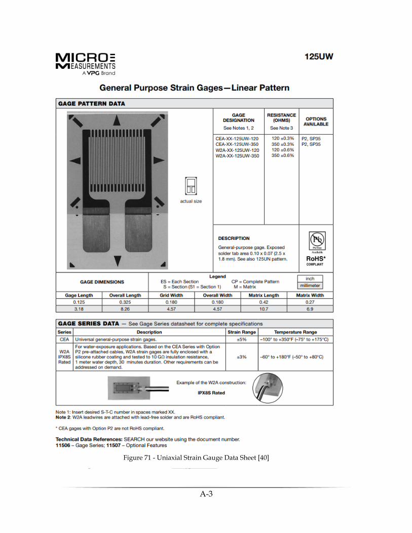
A-3
Figure 71 - Uniaxial Strain Gauge Data Sheet [40]

A-4
The following section will provide a mathematical background on the DIC correlation. In
VIC-2D the first step in measurement is dividing the image into a grid of subsets. The
subsets serve to divide the image and create unique blocks of pixels used for tracking.
Within the subset, a gray value for each of the pixels is assigned as a value from 0 (black)
to 100 (white) based on the speckle pattern captured. Once the gray values are assigned
for the subsets on the reference image, the correlation can begin on the successive images.
The correlation attempts to track the movement of the subsets in the deformed
images compared to the reference image. This is done through a correlation function
which used a statistical relationship, one example of which is the sum of squared
differences. What the correlation function does is compare the gray values of each pixel
within the subset of the reference image against the image that has been displaced by a
value of u and y, which correspond to the horizontal and vertical displacements. This
comparison is repeated at multiple u and y values until the difference in the gray values
are minimized according to the sum of squared differences, or whatever correlation
criterion are selected. Figure 72 is the generalized equation for the tracking performed in
the DIC program VIC-2D [42].
Figure 72 - DIC Correlation [41]
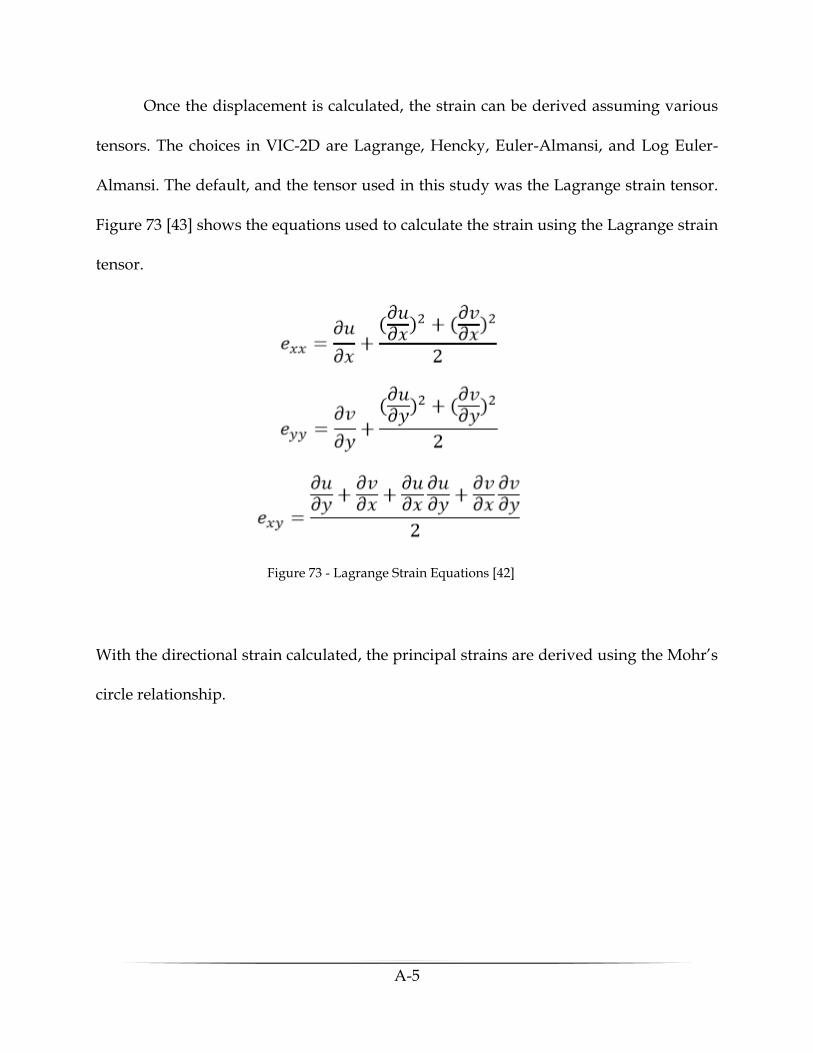
A-5
Once the displacement is calculated, the strain can be derived assuming various
tensors. The choices in VIC-2D are Lagrange, Hencky, Euler-Almansi, and Log Euler-
Almansi. The default, and the tensor used in this study was the Lagrange strain tensor.
Figure 73 [43] shows the equations used to calculate the strain using the Lagrange strain
tensor.
With the directional strain calculated, the principal strains are derived using the Mohr’s
circle relationship.
Figure 73 - Lagrange Strain Equations [42]
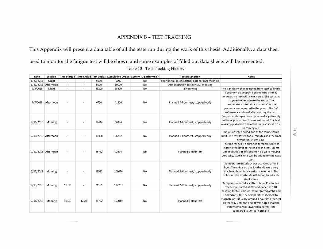
A-6
APPENDIX B – TEST TRACKING
This Appendix will present a data table of all the tests run during the work of this thesis. Additionally, a data sheet
used to monitor the fatigue test will be shown and some examples of filled out data sheets will be presented.
Date Session Time Started Time Ended Test Cycles Cumulative Cycles System ID performed? Test Description Notes
6/20/2018 Night - - 5000 5000 No Short initial test to gather data for DOT meeting
6/21/2018 Afternoon - - 5000 10000 No Demonstration test for DOT meeting
7/3/2018 Night - - 25200 35200 No 2-hour test No significant change noted from start to finish
7/7/2018 Afternoon - - 6700 41900 No Planned 4-hour test, stopped early
Specimen tip support became free after 30
minutes, no instability was noted. The test was
stopped to reevaluate the setup. The
temperature intelock activated after the
pressure was released in the pump. The DIC
software also closed after starting the test.
7/10/2018 Morning - - 14444 56344 Yes Planned 4-hour test, stopped early
Support under specimen tip moved significantly
in the opposite direction as last noted. The test
was stopped when one of the supports was close
to coming out.
7/10/2018 Afternoon - - 10368 66712 No Planned 4-hour test, stopped early
The pump interlocked due to the temperature
limit. The test lasted for 49 minutes and the final
temperature was 137F.
7/11/2018 Afternoon - - 25782 92494 No Planned 2-Hour test
Test ran for full 2-hours, the temperature was
close to the limit at the end of the test. Shims
under South side of specimen tip were moving
vertically, steel shims will be added for the next
test.
7/12/2018 Morning - - 13582 106076 No Planned 2-Hour test, stopped early
Temperature interlock was activated after 1
hour. The shims on the South side were very
stable with minimal vertical movement. The
shims on the North side will be replaced with
steel shims.
7/13/2018 Morning 10:02 - 21191 127267 No Planned 2-Hour test, stopped earlyTemperature interlock after 1 hour 41 minutes.
The temp. started at 88F and ended at 134F
7/16/2018 Morning 10:24 12:28 25782 153049 No Planned 2-Hour test
Test ran for full 2-hours. Temp started at 97F and
ended at 130F. The temperature seemed to
stagnate at 130F since around 1 hour into the test
all the way until the end. It was noted that the
water temp. was lower than normal (60F
compared to 70F as "normal").
Table 10 - Test Tracking History
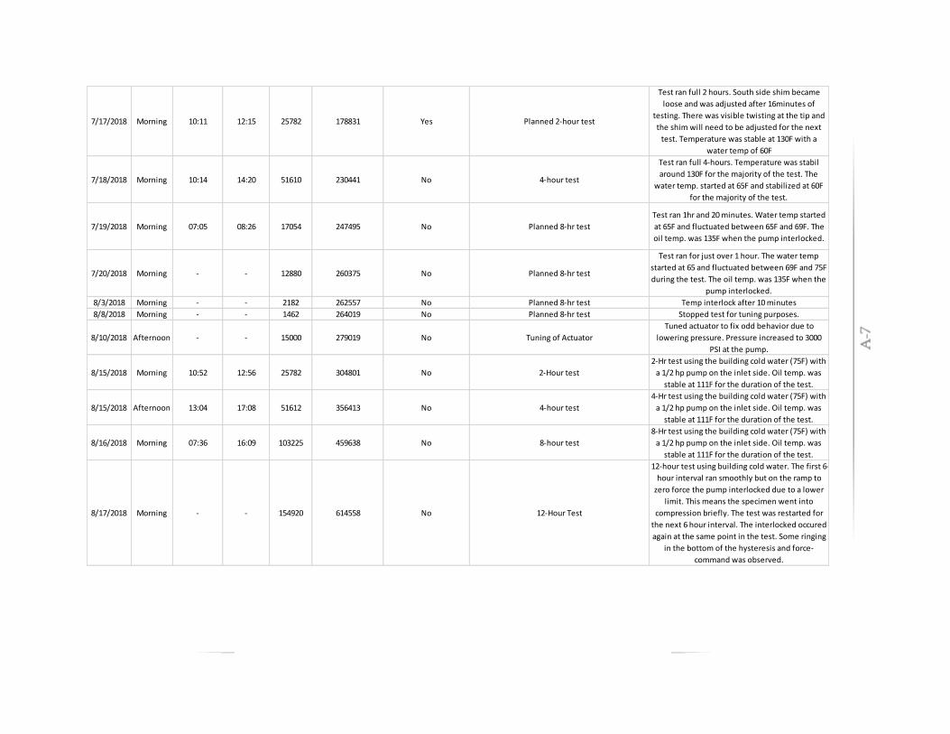
A-7
7/17/2018 Morning 10:11 12:15 25782 178831 Yes Planned 2-hour test
Test ran full 2 hours. South side shim became
loose and was adjusted after 16minutes of
testing. There was visible twisting at the tip and
the shim will need to be adjusted for the next
test. Temperature was stable at 130F with a
water temp of 60F
7/18/2018 Morning 10:14 14:20 51610 230441 No 4-hour test
Test ran full 4-hours. Temperature was stabil
around 130F for the majority of the test. The
water temp. started at 65F and stabilized at 60F
for the majority of the test.
7/19/2018 Morning 07:05 08:26 17054 247495 No Planned 8-hr test
Test ran 1hr and 20 minutes. Water temp started
at 65F and fluctuated between 65F and 69F. The
oil temp. was 135F when the pump interlocked.
7/20/2018 Morning - - 12880 260375 No Planned 8-hr test
Test ran for just over 1 hour. The water temp
started at 65 and fluctuated between 69F and 75F
during the test. The oil temp. was 135F when the
pump interlocked.
8/3/2018 Morning - - 2182 262557 No Planned 8-hr test Temp interlock after 10 minutes
8/8/2018 Morning - - 1462 264019 No Planned 8-hr test Stopped test for tuning purposes.
8/10/2018 Afternoon - - 15000 279019 No Tuning of Actuator
Tuned actuator to fix odd behavior due to
lowering pressure. Pressure increased to 3000
PSI at the pump.
8/15/2018 Morning 10:52 12:56 25782 304801 No 2-Hour test
2-Hr test using the building cold water (75F) with
a 1/2 hp pump on the inlet side. Oil temp. was
stable at 111F for the duration of the test.
8/15/2018 Afternoon 13:04 17:08 51612 356413 No 4-hour test
4-Hr test using the building cold water (75F) with
a 1/2 hp pump on the inlet side. Oil temp. was
stable at 111F for the duration of the test.
8/16/2018 Morning 07:36 16:09 103225 459638 No 8-hour test
8-Hr test using the building cold water (75F) with
a 1/2 hp pump on the inlet side. Oil temp. was
stable at 111F for the duration of the test.
8/17/2018 Morning - - 154920 614558 No 12-Hour Test
12-hour test using building cold water. The first 6-
hour interval ran smoothly but on the ramp to
zero force the pump interlocked due to a lower
limit. This means the specimen went into
compression briefly. The test was restarted for
the next 6 hour interval. The interlocked occured
again at the same point in the test. Some ringing
in the bottom of the hysteresis and force-
command was observed.
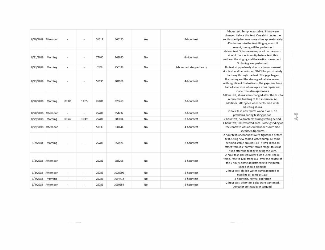
A-8
8/20/2018 Afternoon - - 51612 666170 Yes 4-hour test
4-hour test. Temp. was stable. Shims were
changed before this test. One shim under the
south side tip became loose after approximately
40 minutes into the test. Ringing was still
present, tuning will be performed.
8/21/2018 Morning - - 77460 743630 No 6-Hour test
6-hour test. Shims were replaced on the south
side of the specimen tip before test, this
reduced the ringing and the vertical movement.
No tuning was performed.
8/23/2018 Morning - - 6708 750338 No 4-hour test stopped early 4hr test stopped early due to shim movement
8/23/2018 Morning - - 51630 801968 No 4-hour test
4hr test, odd behavior on SRW1H approximately
half-way through the test. The gage began
fluctuating and the strain gradually increased
with significant fluctuations. The gage may have
had a loose wire where a previous repair was
made from damaged wires.
8/28/2018 Morning 09:00 11:05 26482 828450 No 2-hour test
2-Hour test, shims were changed after the test to
reduce the twisting of the specimen. An
additional 700 cycles were performed while
adjusting shims.
8/28/2018 Afternoon - - 25782 854232 No 2-hour test2-hour test, new shims worked well. No
problems during testing period.
8/29/2018 Morning 08:45 10:49 25782 880014 No 2-hour test 2-hour test, no problems during testing period.
8/29/2018 Afternoon - - 51630 931644 No 4-hour test
4-hour test, DIC restarted once. Some grinding of
the concrete was observed under south side
specimen tip shims.
9/2/2018 Morning - - 25782 957426 No 2-hour test
2-hour test, anchor bolts were tightened before
test. Using new chilled water pump, oil temp
seemed stable around 113F. SRW1-D had an
offset from it's "normal" strain range, this was
fixed after the test by moving the wire.
9/2/2018 Afternoon - - 25782 983208 No 2-hour test
2-hour test, chilled water pump used. The oil
temp. rose to 123F from 113F over the course of
the 2 hours, some adjustments to the pump
speed should be made.
9/3/2018 Afternoon - - 25782 1008990 No 2-hour test2-hour test, chilled water pump adjusted to
stabilize oil temp at 113F.
9/4/2018 Morning - - 25782 1034772 No 2-hour test 2-hour test, normal operation
9/4/2018 Afternoon - - 25782 1060554 No 2-hour test2-hour test, after test bolts were tightened.
Actuator bolt was over torqued.
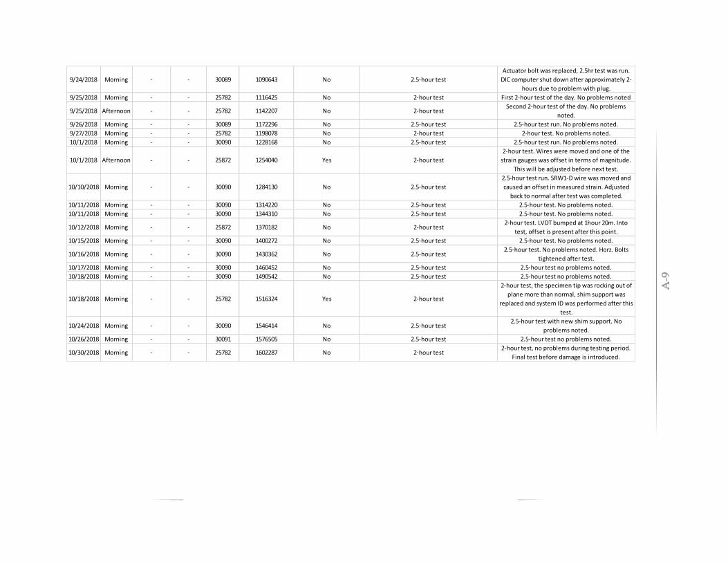
A-9
9/24/2018 Morning - - 30089 1090643 No 2.5-hour test
Actuator bolt was replaced, 2.5hr test was run.
DIC computer shut down after approximately 2-
hours due to problem with plug.
9/25/2018 Morning - - 25782 1116425 No 2-hour test First 2-hour test of the day. No problems noted
9/25/2018 Afternoon - - 25782 1142207 No 2-hour testSecond 2-hour test of the day. No problems
noted.
9/26/2018 Morning - - 30089 1172296 No 2.5-hour test 2.5-hour test run. No problems noted.
9/27/2018 Morning - - 25782 1198078 No 2-hour test 2-hour test. No problems noted.
10/1/2018 Morning - - 30090 1228168 No 2.5-hour test 2.5-hour test run. No problems noted.
10/1/2018 Afternoon - - 25872 1254040 Yes 2-hour test
2-hour test. Wires were moved and one of the
strain gauges was offset in terms of magnitude.
This will be adjusted before next test.
10/10/2018 Morning - - 30090 1284130 No 2.5-hour test
2.5-hour test run. SRW1-D wire was moved and
caused an offset in measured strain. Adjusted
back to normal after test was completed.
10/11/2018 Morning - - 30090 1314220 No 2.5-hour test 2.5-hour test. No problems noted.
10/11/2018 Morning - - 30090 1344310 No 2.5-hour test 2.5-hour test. No problems noted.
10/12/2018 Morning - - 25872 1370182 No 2-hour test2-hour test. LVDT bumped at 1hour 20m. Into
test, offset is present after this point.
10/15/2018 Morning - - 30090 1400272 No 2.5-hour test 2.5-hour test. No problems noted.
10/16/2018 Morning - - 30090 1430362 No 2.5-hour test2.5-hour test. No problems noted. Horz. Bolts
tightened after test.
10/17/2018 Morning - - 30090 1460452 No 2.5-hour test 2.5-hour test no problems noted.
10/18/2018 Morning - - 30090 1490542 No 2.5-hour test 2.5-hour test no problems noted.
10/18/2018 Morning - - 25782 1516324 Yes 2-hour test
2-hour test, the specimen tip was rocking out of
plane more than normal, shim support was
replaced and system ID was performed after this
test.
10/24/2018 Morning - - 30090 1546414 No 2.5-hour test2.5-hour test with new shim support. No
problems noted.
10/26/2018 Morning - - 30091 1576505 No 2.5-hour test 2.5-hour test no problems noted.
10/30/2018 Morning - - 25782 1602287 No 2-hour test2-hour test, no problems during testing period.
Final test before damage is introduced.
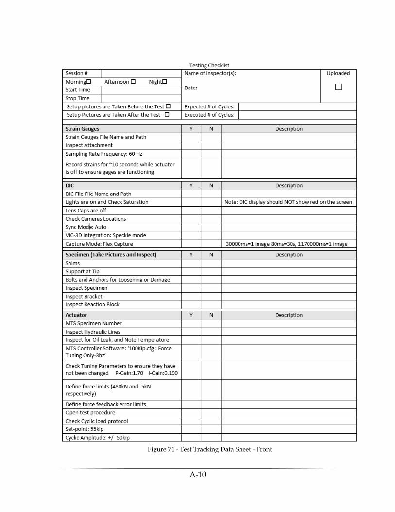
A-10
Figure 74 - Test Tracking Data Sheet - Front

A-11
Figure 75 - Test Tracking Data Sheet - Back
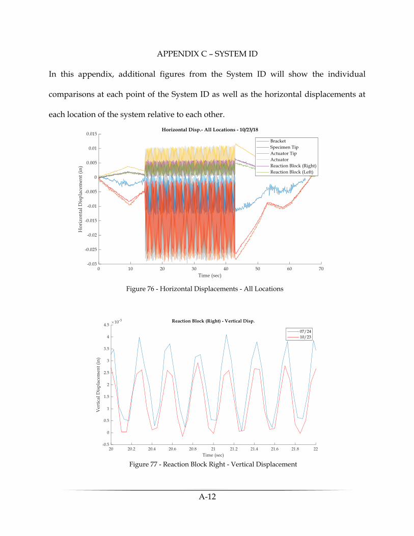
A-12
APPENDIX C – SYSTEM ID
In this appendix, additional figures from the System ID will show the individual
comparisons at each point of the System ID as well as the horizontal displacements at
each location of the system relative to each other.
Figure 76 - Horizontal Displacements - All Locations
Figure 77 - Reaction Block Right - Vertical Displacement
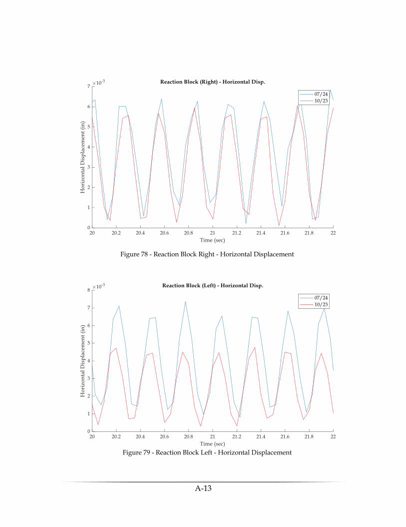
A-13
Figure 78 - Reaction Block Right - Horizontal Displacement
Figure 79 - Reaction Block Left - Horizontal Displacement
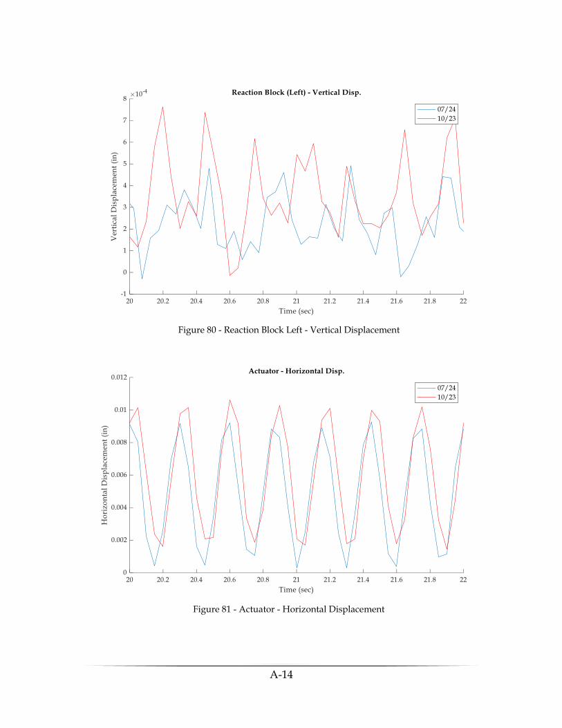
A-14
Figure 80 - Reaction Block Left - Vertical Displacement
Figure 81 - Actuator - Horizontal Displacement
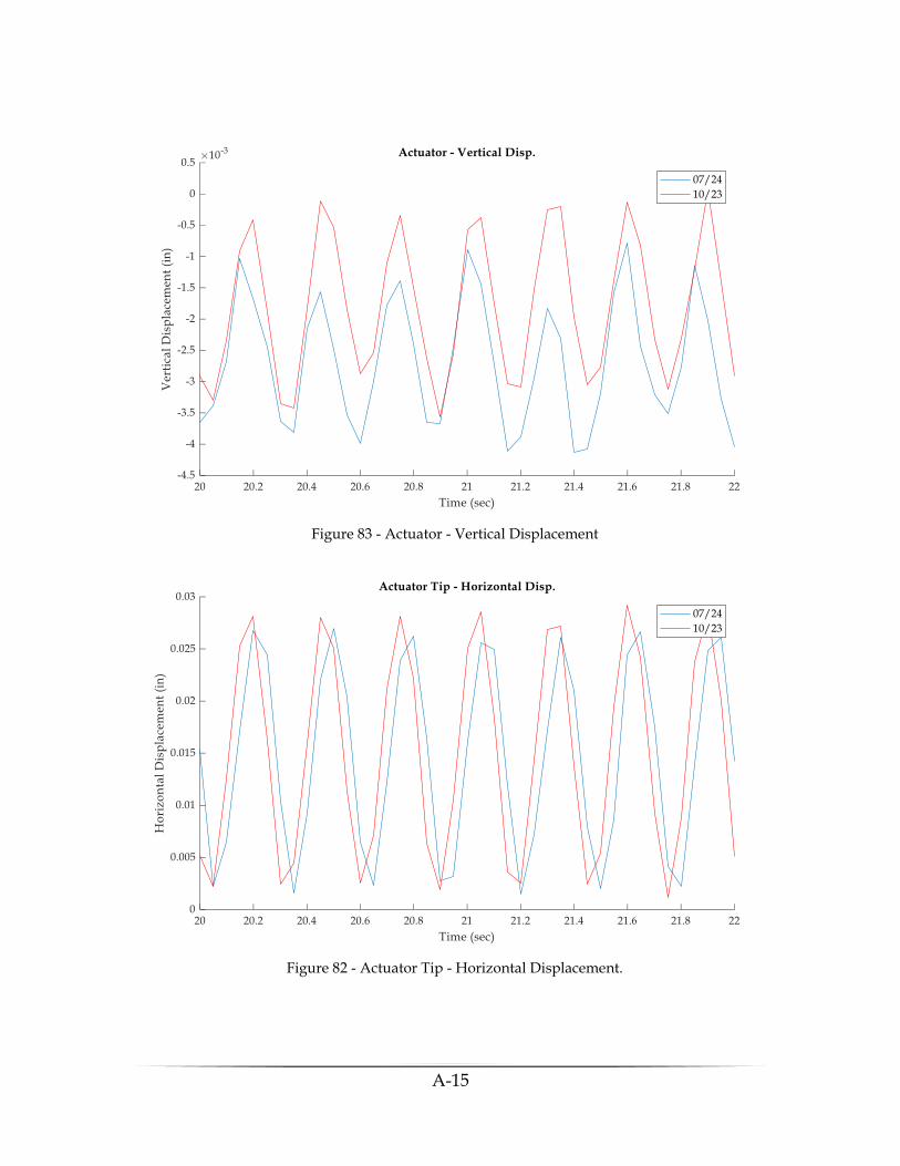
A-15
Figure 83 - Actuator - Vertical Displacement
Figure 82 - Actuator Tip - Horizontal Displacement.
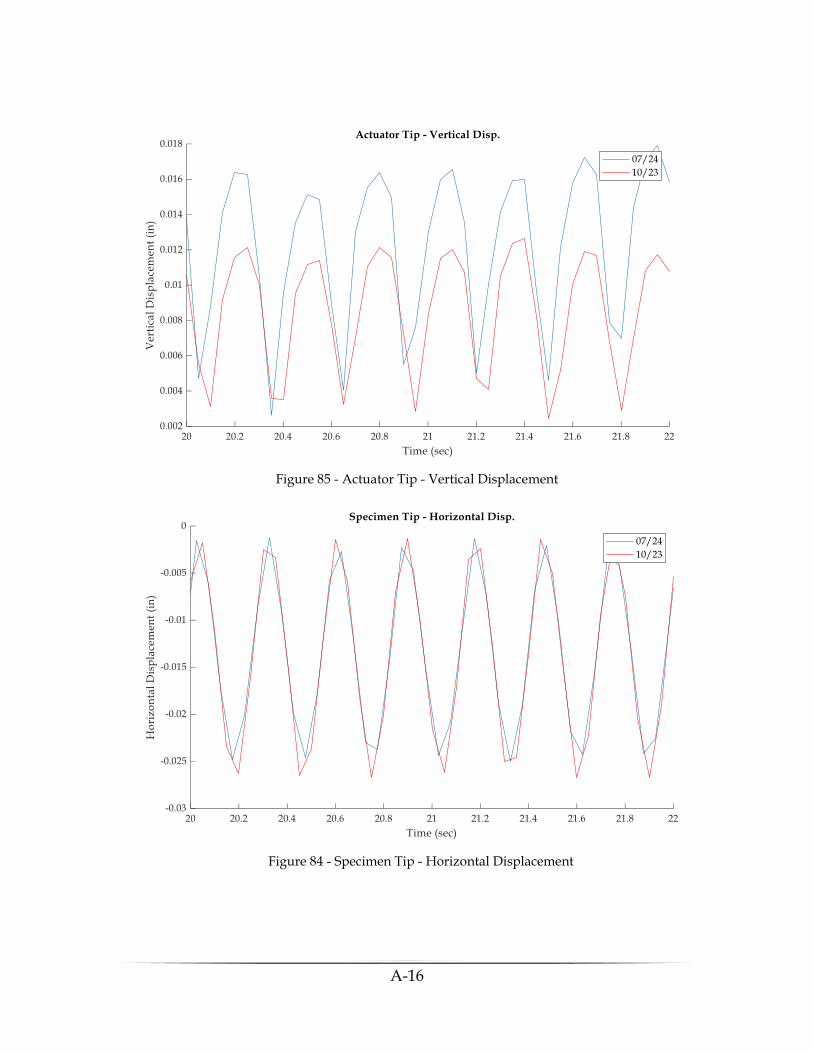
A-16
Figure 85 - Actuator Tip - Vertical Displacement
Figure 84 - Specimen Tip - Horizontal Displacement
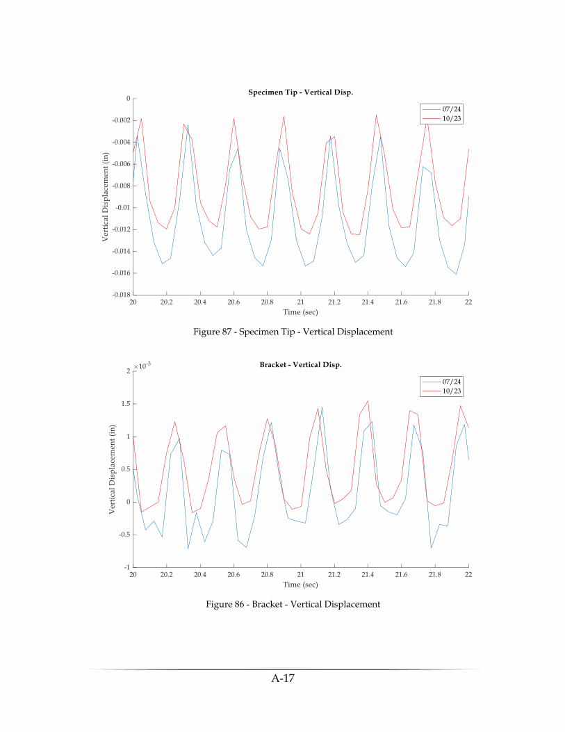
A-17
Figure 87 - Specimen Tip - Vertical Displacement
Figure 86 - Bracket - Vertical Displacement
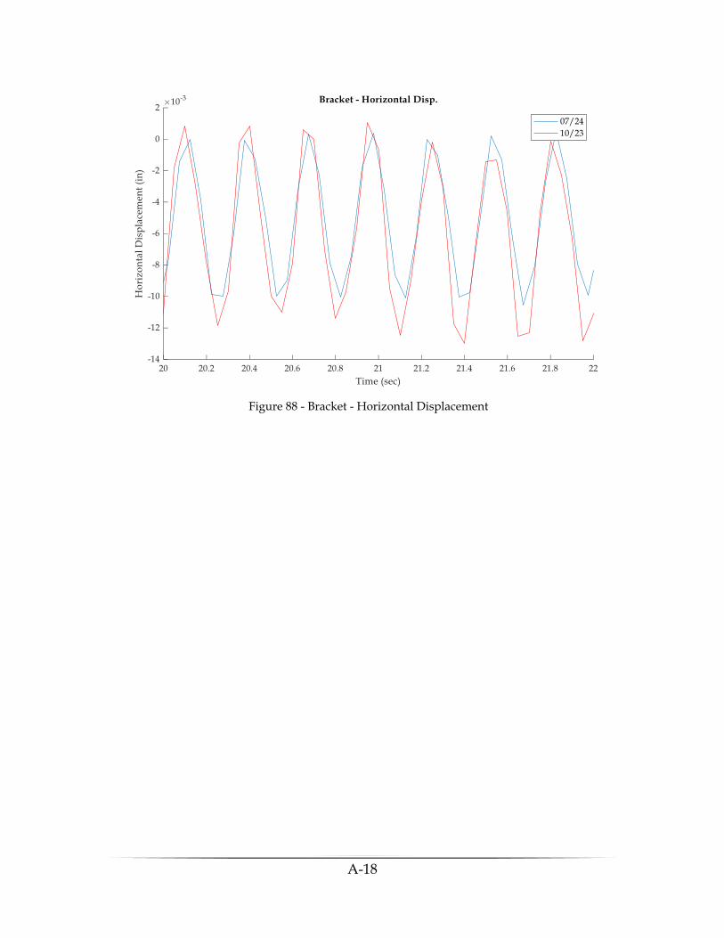
A-18
Figure 88 - Bracket - Horizontal Displacement
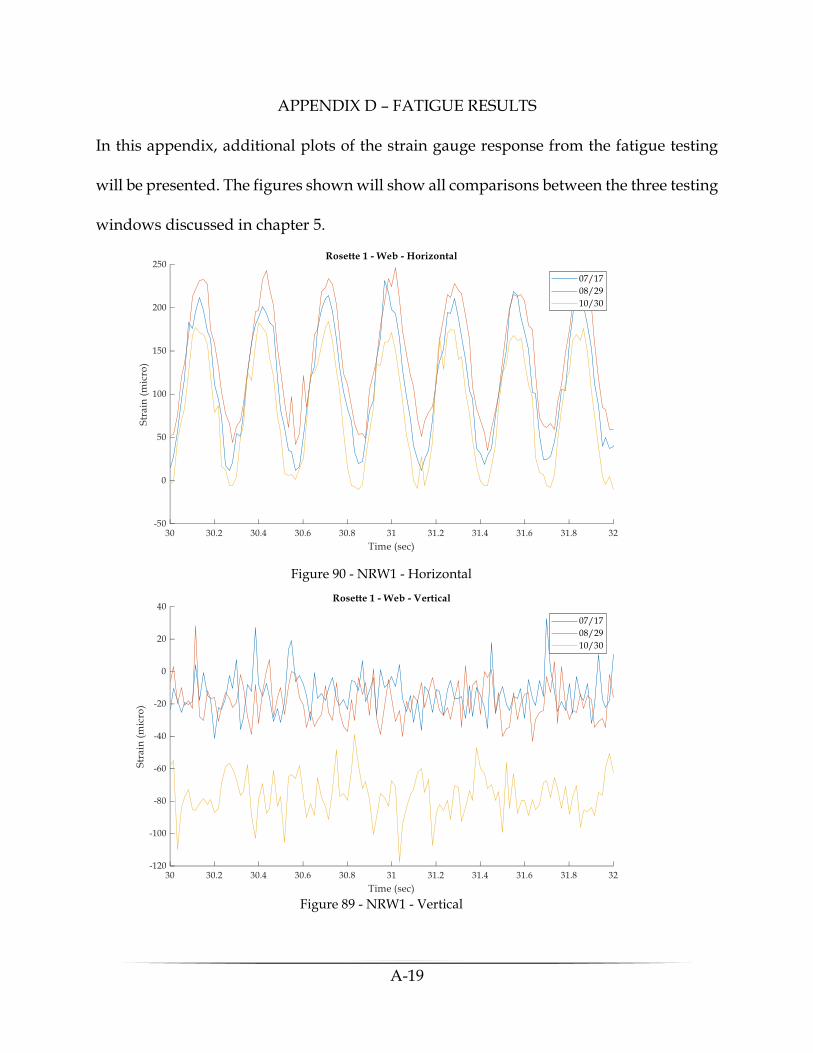
A-19
APPENDIX D – FATIGUE RESULTS
In this appendix, additional plots of the strain gauge response from the fatigue testing
will be presented. The figures shown will show all comparisons between the three testing
windows discussed in chapter 5.
Figure 90 - NRW1 - Horizontal
Figure 89 - NRW1 - Vertical
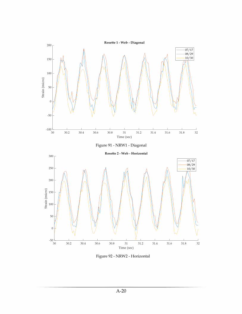
A-20
Figure 91 - NRW1 - Diagonal
Figure 92 - NRW2 - Horizontal
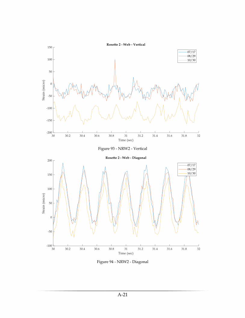
A-21
Figure 93 - NRW2 - Vertical
Figure 94 - NRW2 - Diagonal
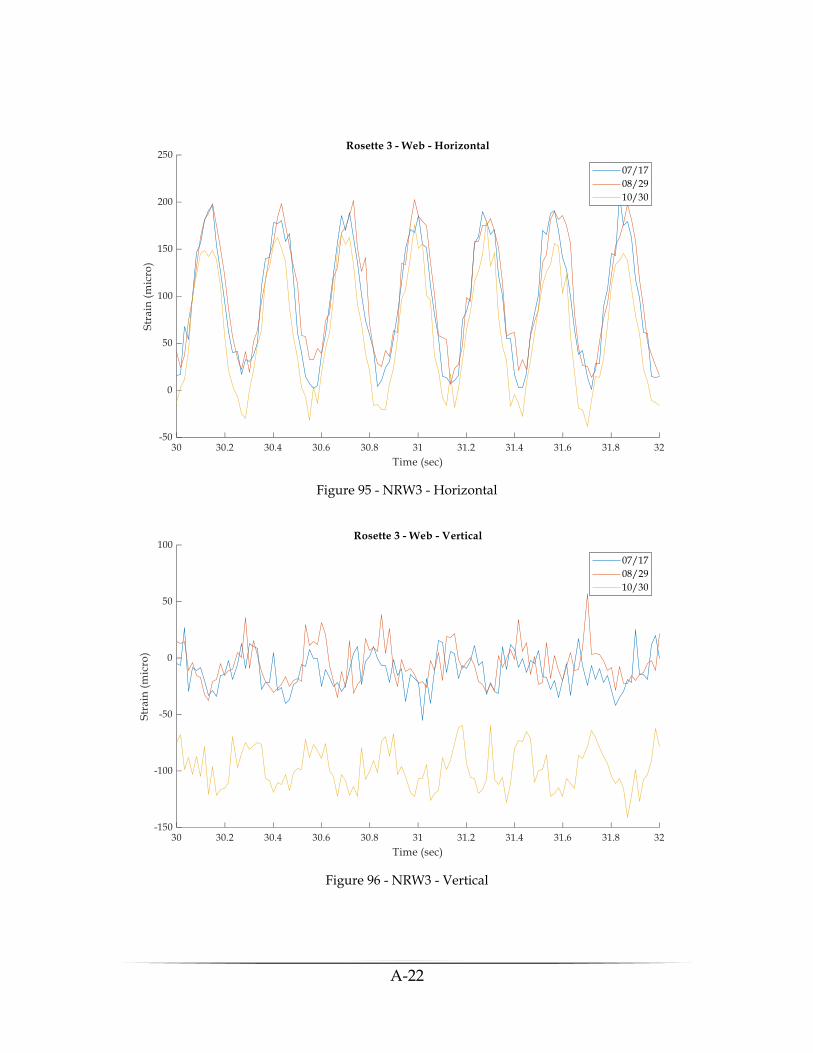
A-22
Figure 95 - NRW3 - Horizontal
Figure 96 - NRW3 - Vertical
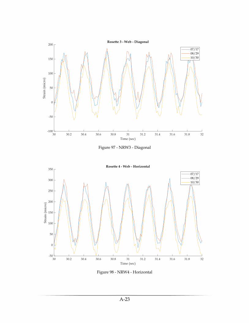
A-23
Figure 97 - NRW3 - Diagonal
Figure 98 - NRW4 - Horizontal
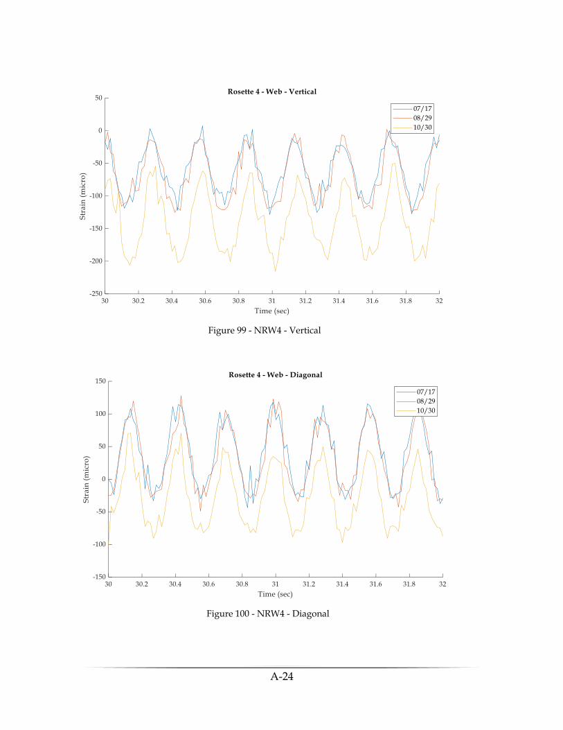
A-24
Figure 99 - NRW4 - Vertical
Figure 100 - NRW4 - Diagonal
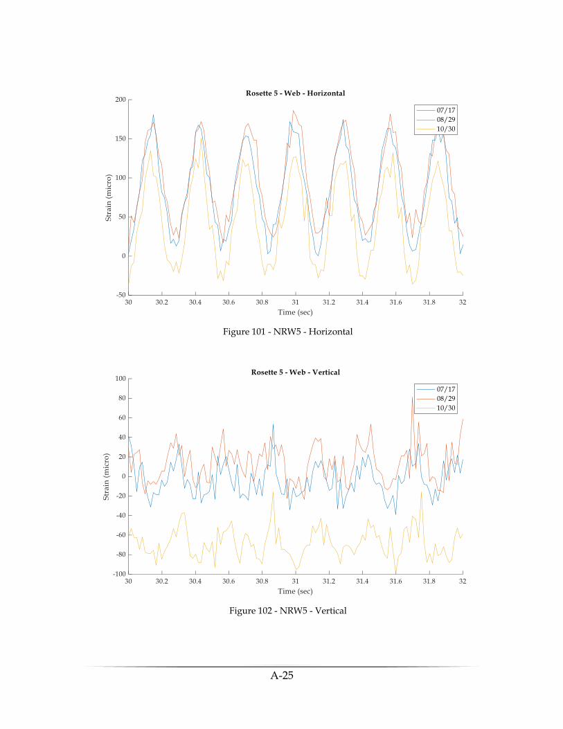
A-25
Figure 101 - NRW5 - Horizontal
Figure 102 - NRW5 - Vertical
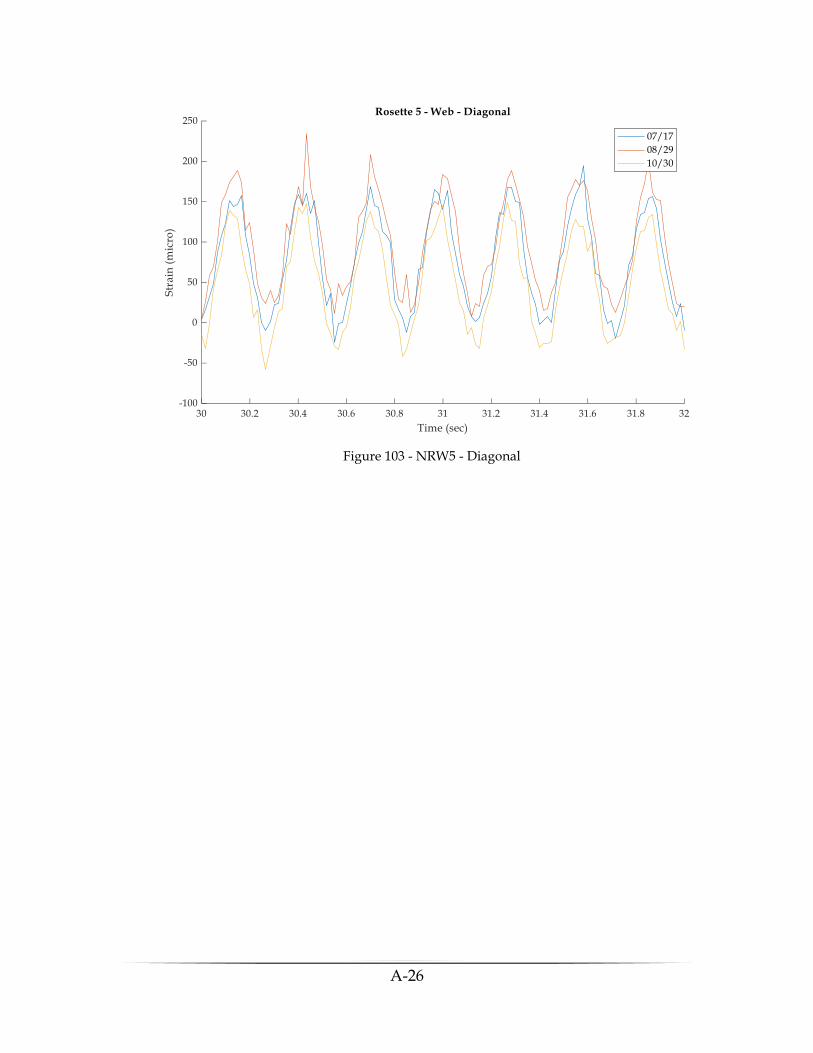
A-26
Figure 103 - NRW5 - Diagonal
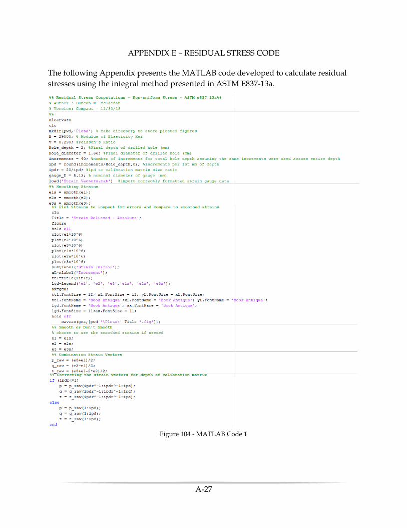
A-27
APPENDIX E – RESIDUAL STRESS CODE
The following Appendix presents the MATLAB code developed to calculate residual
stresses using the integral method presented in ASTM E837-13a.
Figure 104 - MATLAB Code 1

A-28
Figure 105 - MATLAB Code 2
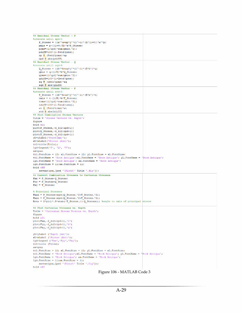
A-29
Figure 106 - MATLAB Code 3
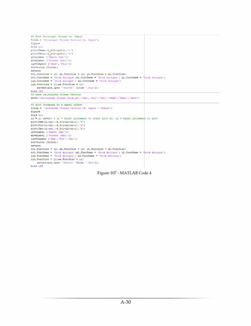
A-30
Figure 107 - MATLAB Code 4

A-31
APPENDIX F – RESIDUAL STRESS RESULTS
This appendix will present the measured strains relieved, and the resulting calculated
stresses from each of the holes drilled in this study. The following table provides a
numbered list of the measurements made during this study with a brief description and
some of the characteristic parameters.
# Specimen Description LoadingDrilling
Method
Hole
Diameter
(mm)
Hole
Depth
(mm)
Calc.
increments
Total
Increments
1 Gussetless 1
Underside of the top flange (left) near the diagonal termination. The
hole is significantly far from the weld area. The specimen was on the
ground and the 2mm was drilled in 10 equal depth increments
None Plunge 1.66 2 5 10
2 Gussetless 1
Topside of the top flange (left) near the diagonal termination. The
hole is in the same location as Res_in - 10i2mm but on the topside of
the flange. The specimen was on the ground and the 2mm was
drilled in 20 equal depth increments
None Plunge 1.66 2 10 20
3 Gussetless 1
Topside of top flange (left), the location is close to the beginning of
the curved section (measured in the curved section). It is placed
away from the edge and the weld area similarly to the res_in and
res_out measurements. The hole was drilled 2mm in 20 equal depth
steps
Bolted Plunge 1.66 2 10 20
4 Gussetless 1
Topside of top flange (left), the location is close to the baseline
measurement but advanced further away from the flat portion of
the flange. It is placed away from the edge and the weld area
similarly to the res_in and res_out measurements. The hole was
drilled 1mm in 20 equal depth steps. At 1mm the drill bit sheared
off and the measurements were stopped.
Bolted Plunge 1.66 1 20 20
5Flat Plate -
Flange Steel
The hole was drilled in the center of a flat plate made of the flange
material from the gussetless specimen. The hole was drilled 2mm in
40 equal increments, but there was a discontinuity in the measured
strain after the 20th increment.
None Plunge 1.66 2 20 40
6Flat Plate -
Flange Steel
Hole drilled close to center of flange flat plate. The hole was drilled
2mm in 40 equal increments. None Plunge 1.66 2 20 40
7Flat Plate -
Annealed Steel
Hole drilled in the center of the "annealed" steel plate. Drilled 2mm
in 40 increments.None Plunge 1.66 2 20 40
8 Flat Plate - SteelHole drilled in actuator transfer plate (for green frame). 2mm in 40
increments. Orbital method.None Orbital 2.045 2 20 40
9Flat Plate -
Annealed Steel
Center of annelead plate. Orbital method 20 increments for first
1mm, 10 increments for following 1mm.None Orbital 2.045 2 20 30
10 Gussetless 1
Hole drilled on top side of top flange (left). This measurement was
in the same line as the previous top flange but moved further up the
curve. This hole was drilled in 30 increments, the first 20 were
evenly spaced across 1mm and the last 10 were evenly spaced across
1mm.
Bolted Orbital 2.045 2 20 30
11 Gussetless 2Hole drilled on top side of top flange on specimen two. The location
was the same as Res_out -20i2mm.None Orbital 2.045 2 20 30
Table 11 - Residual Stress Table of Measurements
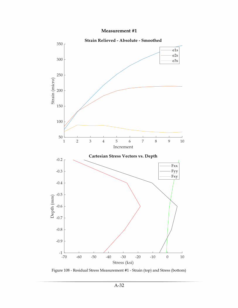
A-32
Measurement #1
Figure 108 - Residual Stress Measurement #1 - Strain (top) and Stress (bottom)
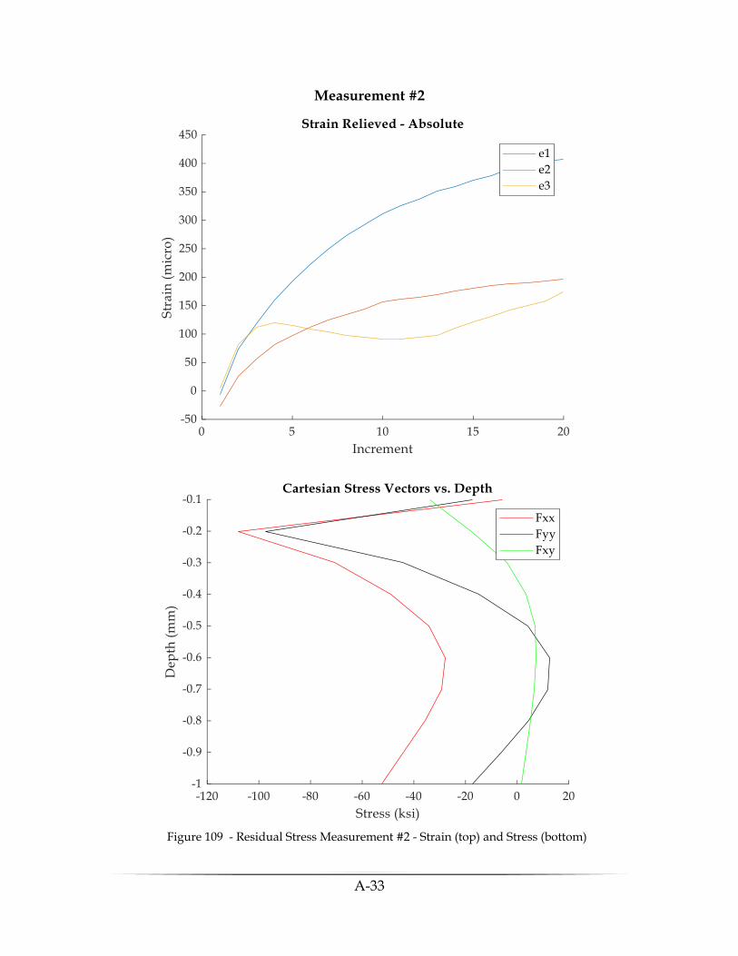
A-33
Measurement #2
Figure 109 - Residual Stress Measurement #2 - Strain (top) and Stress (bottom)
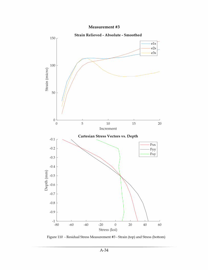
A-34
Measurement #3
Figure 110 - Residual Stress Measurement #3 - Strain (top) and Stress (bottom)
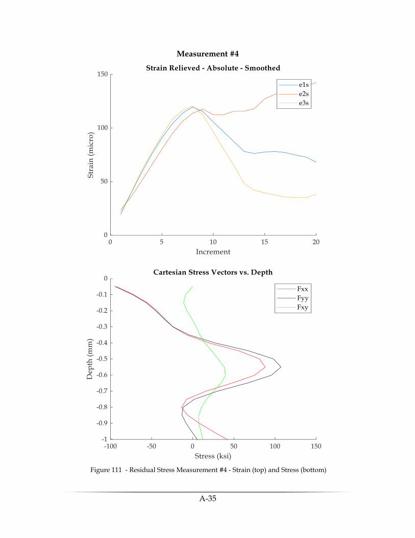
A-35
Measurement #4
Figure 111 - Residual Stress Measurement #4 - Strain (top) and Stress (bottom)
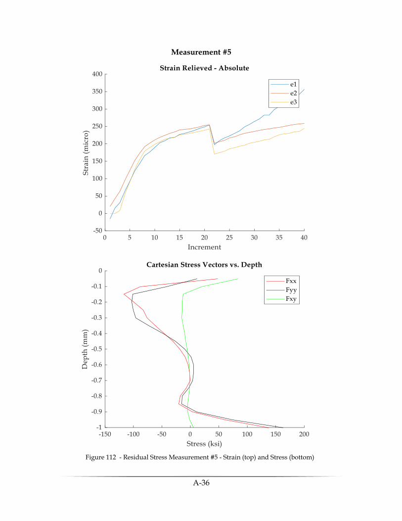
A-36
Measurement #5
Figure 112 - Residual Stress Measurement #5 - Strain (top) and Stress (bottom)
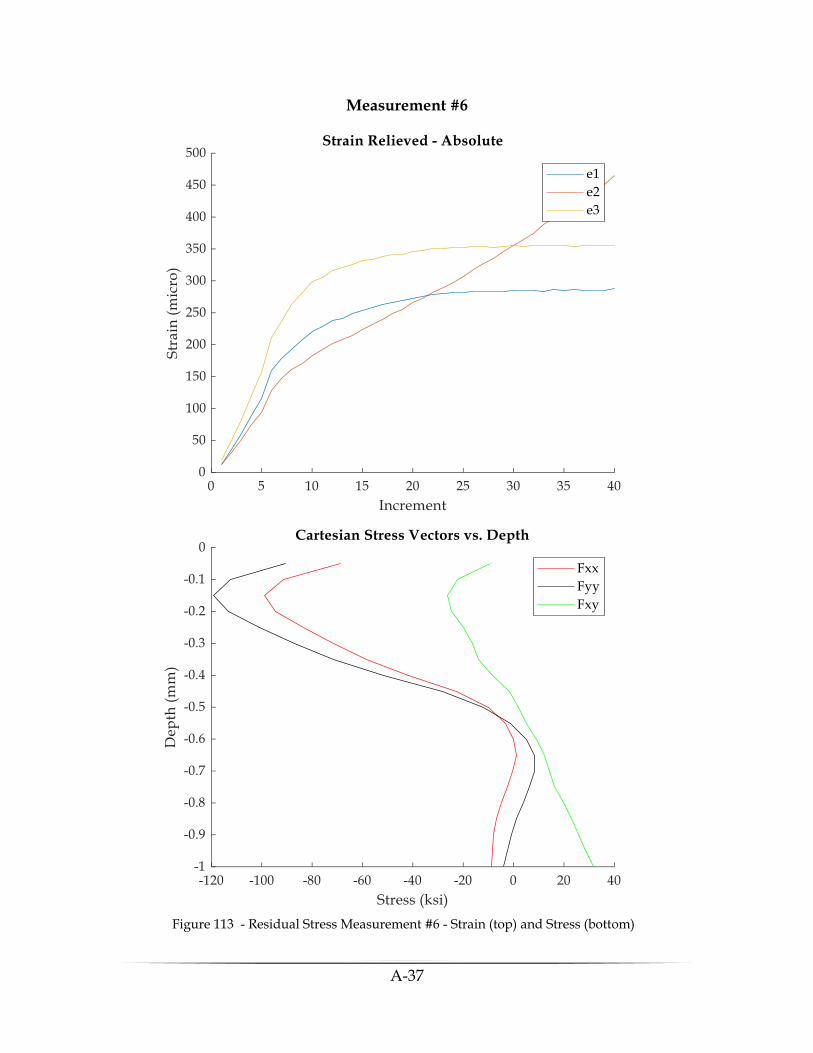
A-37
Measurement #6
Figure 113 - Residual Stress Measurement #6 - Strain (top) and Stress (bottom)
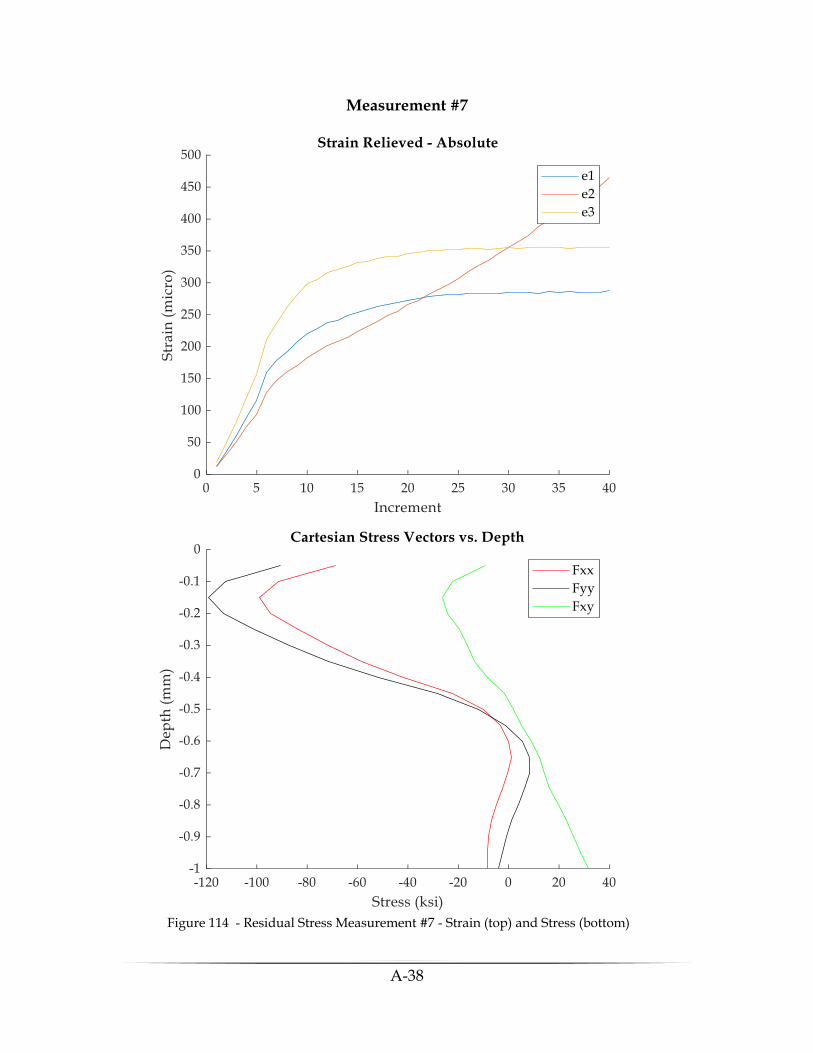
A-38
Measurement #7
Figure 114 - Residual Stress Measurement #7 - Strain (top) and Stress (bottom)
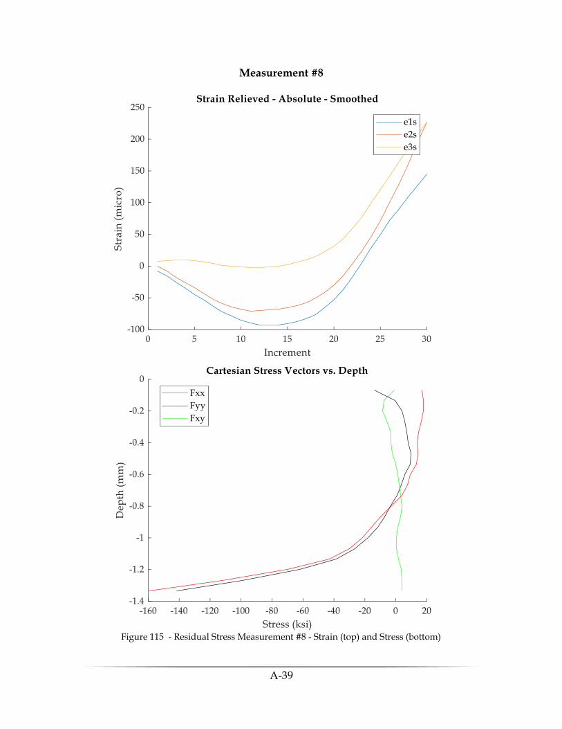
A-39
Measurement #8
Figure 115 - Residual Stress Measurement #8 - Strain (top) and Stress (bottom)
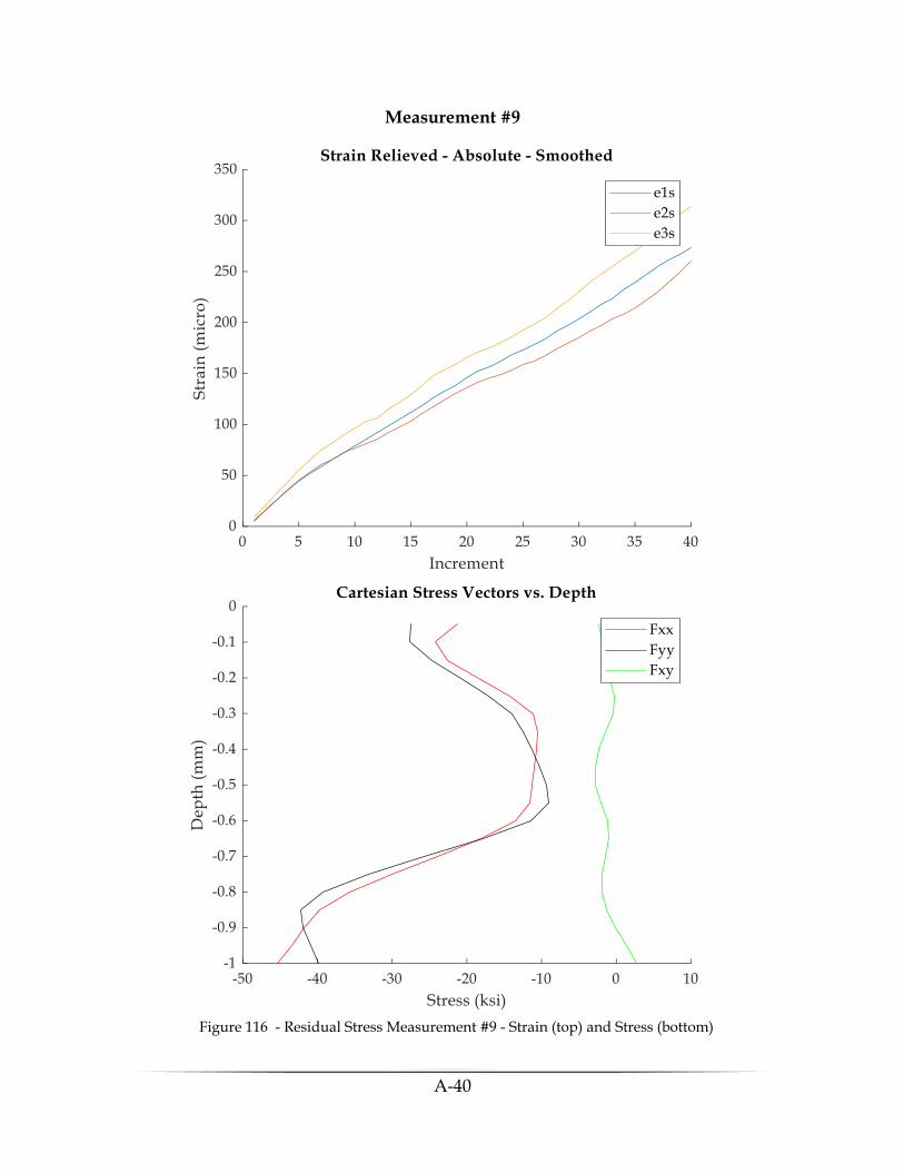
A-40
Measurement #9
Figure 116 - Residual Stress Measurement #9 - Strain (top) and Stress (bottom)
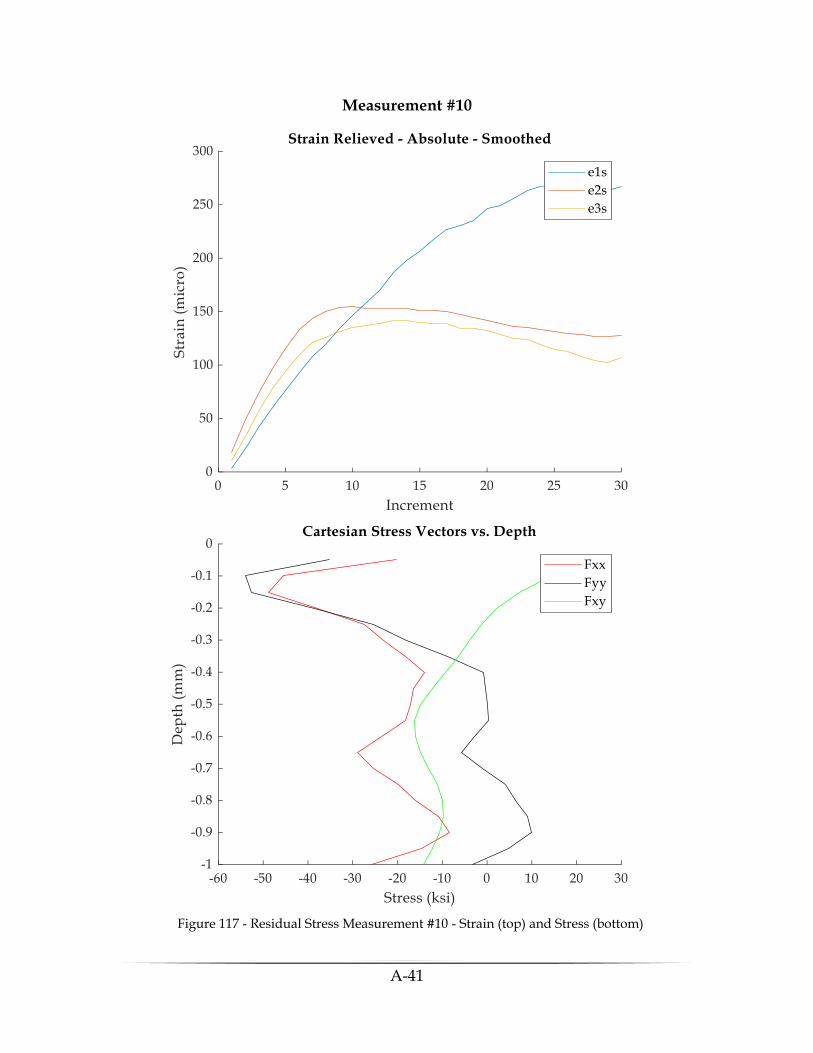
A-41
Measurement #10
Figure 117 - Residual Stress Measurement #10 - Strain (top) and Stress (bottom)

A-42
Measurement #11
Figure 118 - Residual Stress Measurement #11 - Strain (top) and Stress (bottom)