Semi-Intrusive Multivariable Model

Invalidation 1

Leonardo C. Kammer a,∗ Dimitry Gorinevsky b

Guy A. Dumont a

aPulp and Paper Centre, University of British Columbia, 2385 East Mall,Vancouver, BC V6T 1Z4, Canada

b Honeywell Global Control Laboratory, One Results Way, Cupertino, CA 95014,U.S.A.

Abstract

This paper introduces a mechanism for testing multivariable models employed bymodel-based controllers. Although external excitation is not necessary, the datacollection includes a stage where the controller is switched to open-loop operation(manual mode). The main idea is to measure a certain “distance” between theclosed-loop and the open-loop signals, and then trigger a flag if this “distance” islarger than a threshold level. Moreover, a provision is made for accommodatingmodel uncertainty. Since no hard bounds are assumed with respect to the noiseamplitude, the model invalidation mechanism works in a probabilistic framework.

Key words: Model invalidation; performance monitoring; model-based control;multivariable control systems; stochastic noise; model uncertainty.

1 Introduction

Advanced multivariable controllers in process industries are typically model-based predictive control algorithms implemented as proprietary software. Mostof the commercially available controllers allow a user to access process dataand models, but not the details of the controller design. Hence, a practical

∗ Corresponding author. Current address: Paprican, 3800 Wesbrook Mall, Vancou-ver, BC V6S 2L9, Canada. Fax: +1 604 222-3207. E-mail: lkammer@paprican.ca1 The original version of this paper was presented at ECC 2001, which was held inPorto, Portugal during September 2001.

Preprint submitted to Automatica 28 March 2003

Automatica, Vol. 39, 2003, pp. 1461–1467

performance monitoring method ought not to rely on detailed knowledge ofthe controller itself.

If the process suffers an upset resulting in suboptimal operation of the plant,it is important to know whether the problem is caused by process disturbancesor by an error in the process model used by the controller. A typical operatorreaction is to put some supervisory control loops in manual mode, wait andsee if the process variables settle down. These data, collected in open loop, canbe used for testing the model. Problems related to a bad model could be fixedby re-identifying the entire multivariable model and re-tuning the controller.However, this is a very expensive procedure and it should not be undertakenunless there is certainty about the existing model being a problem.

Our goal is to provide a signal processing mechanism that deals with the sce-nario described above to reveal if the model embedded in the controller is nolonger valid. Moreover, the mechanism shall indicate which part of the mul-tivariable model is wrong, so that only that part of the model needs to bere-identified. The worst-case scenario is assumed: the only data available fromthe system are collected after the problem has been detected and no mea-surable external excitation occurs during data collection. That is, the onlyexcitation driving the loop come from stationary stochastic process distur-bances.

Traditional mechanisms of “model validation” (Ljung, 1999) use high excita-tion not only to falsify the estimated model, but also to gain confidence on amodel that passes the test. In contrast we use the term “model invalidation”to characterize simple tests, with little or no excitation, that put the plantmodel on trial without aiming at increasing the confidence on this model.

The mechanisms for performance monitoring are the ones best suited forachieving model invalidation. These excitation-free mechanisms are dedicatedto analyzing the loop performance with respect to a specific criterion likeminimum variance (Harris, 1989), or to a specific problem like valve stiction(Hagglund, 1995; Horch, 1999) or sluggish control (Hagglund, 1999). In ourproblem, the loop performance is not described by a single numerical indexand we also wish to account for a certain degree of uncertainty in the model.

The mechanism introduced in this paper compares two sets of data (timeseries) associated with each output: the model output error (y(t)− y(t)), col-lected during normal operation, and the open-loop output, collected when thecontroller is put in manual. In Section 2 it is shown that if the process model iscorrect and the disturbance is stationary, then those two time series present thesame behaviour. Thus, we need a tool that quantifies the “distance” betweenthe behaviour of two independent time series. Section 3 develops such a tool,in a probabilistic framework, along with a threshold value for rejecting the

2

hypothesis that part of the model is correct. Given that in real-life modellingerrors are always present, Section 4 extends the mechanism to accommodatefor uncertainties in the closed-loop response. A simulation example is pre-sented in Section 5, where the “actual plant” is modified to test the behaviourof the invalidation mechanism.

2 Model Output Error

The scenario analyzed in this work is restricted to plants with unmeasurablesources of stochastic noise:

y(t) = G(q) u(t) + H(q) e(t), (1)

where y(t) is the vector of ny output signals, u(t) is the vector of nu inputsignals and {e(t)} is a vector of ne independent zero-mean Gaussian white-noise processes. The transfer-function matrices G(q) and H(q) have dimensionsny ×nu and ny ×ne, respectively. G(q) must be stable, but H(q) may containpoles at z = 1.

The control action is also restricted to minimal excitation (constant referencesignals). This leads to the following structure for the control action:

u(t) = −C(q) y(t). (2)

C(q) is an unknown operator designed from a known model of the process:

y(t) = G(q) u(t). (3)

From (1) and (3) we define the model output error as

ε(t) , y(t)− y(t)

= [G(q)− G(q)] u(t) + H(q) e(t) (4)

= [I + G(q)C(q)][I + G(q)C(q)]−1H(q) e(t).

These expressions show that if the model is perfect (G(q) ≡ G(q)) then themodel output error presents the same dynamics as the process noise, H(q) e(t).This fact is essential to our mechanism, as we compare two time series for eachprocess output: the model output error, ε(t), and the open-loop output signal,

yo(t) = H(q) e(t). (5)

It is imperative that the noise dynamics, H(q), be time invariant, at least forthe duration of the experiment. Although in practice this assumption might

3

not always hold, the development of a mechanism to test this assumption isbeyond the scope of the paper. As a minimal practical check, the user cancollect data in the following sequence: normal operating data, open-loop data,normal operating data; and compare the noise dynamics in both regions ofclosed-loop data.

The invalidation test thus becomes a trial of the assumption that, for eachprocess output j = 1, . . . , ny, the time series {εj(t)} and {yo

j (t)} are realiza-tions of the same stationary process. If H(q) contains poles at z = 1, then bothtime series must be differenced an appropriate amount of times for {yo

j (t)} tobecome stationary (Box et al., 1994).

A closer look at the centre line in (4) reveals that, in principle, the test iscompletely independent on the type of controller being used. That is, thecontroller could be nonlinear, time-variant, etc. Nevertheless, under this widerscenario the conclusions about the loop uncertainty are no longer valid. Thisalso applies when the reference signals are not constant. That is, changes in thereference signals would emphasize existing plant-model mismatches, affectingthe uncertainty analysis presented here.

3 Comparison of Two Time Series

The problem statement addressed in this section is: Given two independenttime series, {z1(t)} and {z2(t)}, test the assumption that they are realizationsof the same stationary process.

This problem has been considered before and several solutions were proposedin the literature, both in the time domain (Quenouille, 1958; Pudney et al.,1999) and the frequency domain (Coates and Diggle, 1986; Diggle and Fisher,1991). Another distinction between these solutions is whether they are para-metric or nonparametric. Analyses consistently conclude that the parametricmethods are more powerful, in the sense of being able to detect smaller differ-ences in the time series (Coates and Diggle, 1986; Diggle and Fisher, 1991).On the other hand, the nonparametric methods are simpler as they do notrequire building an auxiliary parametric model of the series.

Herein we propose a frequency-domain method based on the work by Coatesand Diggle (1986). This solution has immediate connection with the frequency-domain characterization of loop uncertainty. The method of Coates and Diggleis modified in our work to improve its power. Instead of deriving the prob-ability distribution of the periodogram ordinates, we start by smoothing theperiodogram and then derive the corresponding distributions.

4

3.1 Smoothed Periodogram

The periodogram of a time series {z1(t)} of length N is the set of m = b(N −1)/2c values

I1(ωk) = (2πN)−1

∣∣∣∣∣N∑

t=1

z1(t) e−iωkt

∣∣∣∣∣

2

, (6)

where ωk = 2πk/N , k = 1, . . . , m. It is assumed that the process generat-ing {z1(t)} is a stationary general linear process with independent identicallydistributed innovations. Therefore, asymptotically, 2I1(ω)/ E{I1(ω)} has a chi-squared distribution with two degrees of freedom and, for l 6= k, I1(ωl) andI1(ωk) are independent (Jenkins and Watts, 1968). It is important to empha-size that I1(0) and I1(π) are excluded since their sampling distribution areproportional to χ2

1 rather than χ22 (Coates and Diggle, 1986).

At this point our analysis deviates from that of (Coates and Diggle, 1986) as wesmooth the periodogram. Actually, prior to smoothing the periodogram it isimportant to reduce large differences in amplitude at the various frequencies.That is, one of the two time series is whitened, then the same whiteningfilter, W (q), is used on the other time series. The whitening is performedby fitting an auto-regressive model of low order to the time series, which isthen filtered through the inverse of this model (a moving average filter). Thiswhitening/filtering automatically differences the time series an appropriateamount of times in those situations where H(q) contains poles at z = 1. Theorder of the auto-regressive model is increased until the filtered time seriespasses a whiteness test.

For our particular application, the time series containing the open-loop outputsignal, {yo(t)}, is the natural choice for being initially whitened. For eachoutput j, the signals to be compared are:

z1(t) , Wj(q) yoj (t), (7)

z2(t) , Wj(q) εj(t). (8)

Once the time series have been formed, their periodograms are smoothed viathe convolution of a finite-length weight function (due to the special distri-bution of I1(0) and I1(π)) and the frequency ordinates. Our choice of weightfunction is a triangular one,

I1(ωk) =l−1∑

j=−l+1

λjI1(ωk+j), k = l, . . . , m− l + 1 (9)

λj =l − |j|

l2, (10)

5

which emphasizes the mid-frequencies relative to the fringes.

The length of the weight function reflects the type of mismatch we expect todetect between the periodograms I1(ω) (of (7)) and I2(ω) (of (8)). Mismatchesthat occur at a small frequency range are typical in closed-loop systems, there-fore we adopt the following filter length:

l =

⌊√N

2

⌋. (11)

Given I1(ω) and I2(ω), their difference at each frequency is measured by

J(ω) , lnI1(ω)

I2(ω). (12)

Notice that the order in which the time series are taken in (12) is important.The convention adopted in (7) and (8) implies that for scalar systems:

• a large positive value of J(ωk) indicates that |1 + G(eiωk)C(eiωk)| À |1 +G(eiωk)C(eiωk)|, that is, at frequency ωk the Nyquist plot of G(eiωk)C(eiωk)is closer to the critical point −1 than the designed Nyquist plot;

• a large negative value of J(ωk) indicates that |1 + G(eiωk)C(eiωk)| ¿ |1 +G(eiωk)C(eiωk)|.

Loosely speaking, the former situation is associated with reduction of thestability margin, while the latter is associated with reduction of performance.

For multivariable systems one can take the absolute value of J(ω) and limitthe analysis to the conclusion that large values imply a mismatch betweendesigned and actual closed-loop behaviour.

3.2 The Threshold Level

Asymptotically, νI1(ωk)/ E{I1(ωk)} is approximately distributed as χ2ν (Jenk-

ins and Watts, 1968), where ν = 2/(∑l−1

j=−l+1 λ2j), or more specifically, using

(10), ν = 6l3/(2l2 + 1).

A very important characteristic of J(ωk) is that if {z1(t)} and {z2(t)} arerealizations of the same stationary process, then its (cumulative) distributionfunction depends only on ν, and not on either ωk or the original frequencydistribution of the time series {yo(t)} and {ε(t)} (due to the pre-whitening).

6

The cumulative distribution function is

F (J(ωk) < x) =Γ(ν)

Γ2(ν/2)

∫ x

−∞

eβ ν/2

(1 + eβ)νdβ, (13)

where Γ(b) is the Gamma function. Expression (13) gives the probability thatJ(ωk) at a particular frequency ωk is less than a certain value x. In orderto test the hypothesis that {z1(t)} and {z2(t)} are realizations of the samestationary process, we have to consider the set of m − 2l + 2 frequencies atwhich we smooth the periodogram:

J∗ , maxω|J(ω)| . (14)

If {z1(t)} and {z2(t)} are realizations of the same stationary process, then thedistribution function of J∗ depends only on N ; from this particular situationwe derive the function ζ:

ζ(N, α) , x |P{J∗ ≤ x |E[I1(ω)] = E[I2(ω)]} = 1− α, (15)

which provides the threshold level for testing the null hypothesis with signifi-cance level α.

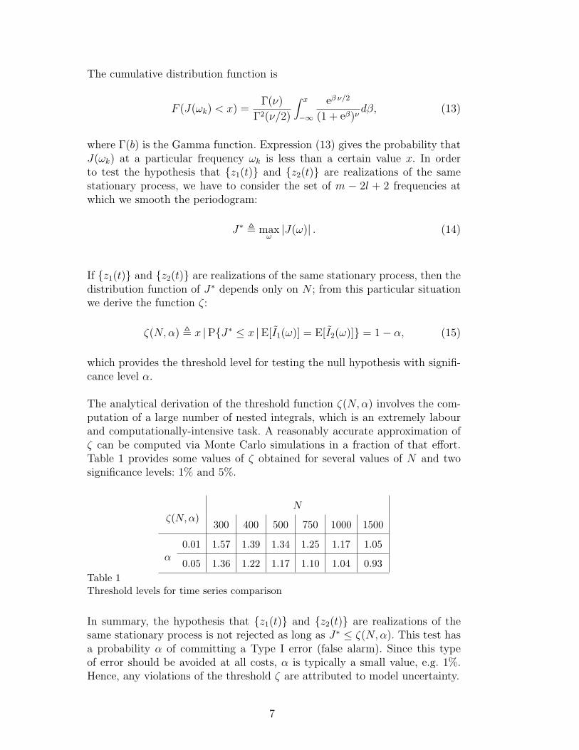
The analytical derivation of the threshold function ζ(N, α) involves the com-putation of a large number of nested integrals, which is an extremely labourand computationally-intensive task. A reasonably accurate approximation ofζ can be computed via Monte Carlo simulations in a fraction of that effort.Table 1 provides some values of ζ obtained for several values of N and twosignificance levels: 1% and 5%.

Nζ(N, α)

300 400 500 750 1000 1500

0.01 1.57 1.39 1.34 1.25 1.17 1.05α

0.05 1.36 1.22 1.17 1.10 1.04 0.93Table 1Threshold levels for time series comparison

In summary, the hypothesis that {z1(t)} and {z2(t)} are realizations of thesame stationary process is not rejected as long as J∗ ≤ ζ(N, α). This test hasa probability α of committing a Type I error (false alarm). Since this typeof error should be avoided at all costs, α is typically a small value, e.g. 1%.Hence, any violations of the threshold ζ are attributed to model uncertainty.

7

4 Model Uncertainty

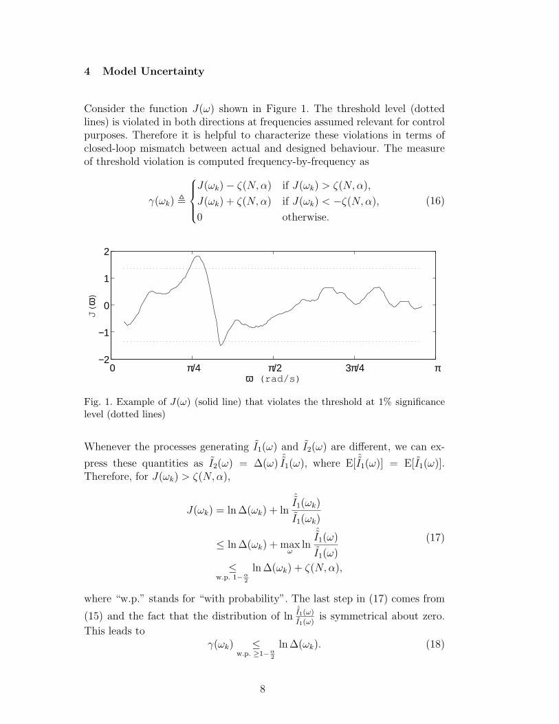
Consider the function J(ω) shown in Figure 1. The threshold level (dottedlines) is violated in both directions at frequencies assumed relevant for controlpurposes. Therefore it is helpful to characterize these violations in terms ofclosed-loop mismatch between actual and designed behaviour. The measureof threshold violation is computed frequency-by-frequency as

γ(ωk) ,

J(ωk)− ζ(N, α) if J(ωk) > ζ(N,α),

J(ωk) + ζ(N, α) if J(ωk) < −ζ(N, α),

0 otherwise.

(16)

0 π/4 π/2 3π/4 π −2

−1

0

1

2

ω (rad/s)

J(

ω)

Fig. 1. Example of J(ω) (solid line) that violates the threshold at 1% significancelevel (dotted lines)

Whenever the processes generating I1(ω) and I2(ω) are different, we can ex-

press these quantities as I2(ω) = ∆(ω) ˆI1(ω), where E[ ˆI1(ω)] = E[I1(ω)].Therefore, for J(ωk) > ζ(N, α),

J(ωk) = ln ∆(ωk) + lnˆI1(ωk)

I1(ωk)

≤ ln ∆(ωk) + maxω

lnˆI1(ω)

I1(ω)

≤w.p. 1−α

2

ln ∆(ωk) + ζ(N,α),

(17)

where “w.p.” stands for “with probability”. The last step in (17) comes from

(15) and the fact that the distribution of lnˆI1(ω)

I1(ω)is symmetrical about zero.

This leads toγ(ωk) ≤

w.p. ≥1−α2

ln ∆(ωk). (18)

8

That is, with a probability of at least 1 − α2

we can conclude that the multi-

plicative discrepancy between I1(ωk) and I2(ωk) is at least as large as eγ(ωk).Similar result is straightforwardly obtained when J(ωk) < −ζ(N,α):

γ(ωk) ≥w.p. ≥1−α

2

ln ∆(ωk). (19)

The connection between ∆(ω) and model uncertainty is established for scalarsystems. For these systems the following holds:

limN→∞

E

[I2(ω)

I1(ω)

]=

∣∣∣∣∣W [1 + GC][1 + GC]−1H

WH

∣∣∣∣∣

2

=

∣∣∣∣∣1 + G(eiω)C(eiω)

1 + G(eiω)C(eiω)

∣∣∣∣∣

2

= ∆(ω),

(20)

where |1+G(eiω)C(eiω)| gives the distance from the Nyquist plot of G(eiω)C(eiω)to the point −1. This distance, at each frequency, is part of the designedclosed-loop behaviour, where a reduction in |1 + G(eiω)C(eiω)| decreases thestability margin at that particular frequency and a move in the opposite di-rection tends to decrease the closed-loop performance. Hence we conclude,with a probability of at least 1 − α

2, that asymptotically the ratio between

|1 + G(eiωk)C(eiωk)| and |1 + G(eiωk)C(eiωk)| is at least as far from 1 as the

value√

e−γ(ωk), at those frequencies where γ(ωk) 6= 0. Thus, as one can see,∆(ω) gives a characterization of a feedback loop gain uncertainty.

For multivariable systems the value of γ(ω) is affected by a combination ofseveral transfer functions, instead of a single one (G(eiω)C(eiω)), and by therelative ratio between the amplitudes of the individual open-loop output sig-nals. Consequently it is not as simple to interpret the function γ(ω) when weare dealing with more than one input or output.

It is left for the user to decide whether the closed-loop mismatch is withinexpectations given the uncertainty in the model. If one decides a priori themaximum acceptable mismatch in the closed-loop response, at each frequency,then the model invalidation test has all information needed to diagnose theloop and raise a flag whenever the maximum allowable mismatch is violated.

9

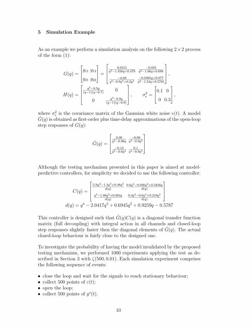
5 Simulation Example

As an example we perform a simulation analysis on the following 2×2 processof the form (1):

G(q) =

g11 g12

g21 g22

=

0.0315q2−1.458q+0.479

−0.025q2−1.66q+0.688

−0.09q5−0.9q4+0.2q3

−0.0385q+0.077q2−1.54q+0.5785

,

H(q) =

q2−0.5q(q−1)(q−0.7)

0

0 q2−0.9q(q−1)(q−0.8)

, σ2

e =

0.1 0

0 0.3

,

where σ2e is the covariance matrix of the Gaussian white noise e(t). A model

G(q) is obtained as first-order plus time-delay approximations of the open-loopstep responses of G(q):

G(q) =

0.06q2−0.96q

−0.09q3−0.9q2

−0.12q5−0.6q4

0.1q4−0.9q3

Although the testing mechanism presented in this paper is aimed at model-predictive controllers, for simplicity we decided to use the following controller:

C(q) =

5/6q4−1.3q3+0.48q2

d(q)0.6q3−0.936q2+0.3456q

d(q)

q3−1.86q2+0.864qd(q)

0.4q4−0.6q3+0.216q2

d(q)

d(q) = q4 − 2.0417q3 + 0.6945q2 + 0.9259q − 0.5787

This controller is designed such that G(q)C(q) is a diagonal transfer functionmatrix (full decoupling) with integral action in all channels and closed-loopstep responses slightly faster then the diagonal elements of G(q). The actualclosed-loop behaviour is fairly close to the designed one.

To investigate the probability of having the model invalidated by the proposedtesting mechanism, we performed 1000 experiments applying the test as de-scribed in Section 3 with ζ(500, 0.01). Each simulation experiment comprisesthe following sequence of events:

• close the loop and wait for the signals to reach stationary behaviour;• collect 500 points of ε(t);• open the loop;• collect 500 points of yo(t).

10

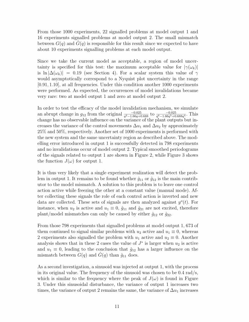
From those 1000 experiments, 22 signalled problems at model output 1 and16 experiments signalled problems at model output 2. The small mismatchbetween G(q) and G(q) is responsible for this result since we expected to haveabout 10 experiments signalling problems at each model output.

Since we take the current model as acceptable, a region of model uncer-tainty is specified for this test: the maximum acceptable value for |γ(ωk)|is ln |∆(ωk)| = 0.19 (see Section 4). For a scalar system this value of γwould asymptotically correspond to a Nyquist plot uncertainty in the range[0.91, 1.10], at all frequencies. Under this condition another 1000 experimentswere performed. As expected, the occurrences of model invalidations becamevery rare: two at model output 1 and zero at model output 2.

In order to test the efficacy of the model invalidation mechanism, we simulatean abrupt change in g12 from the original −0.025

q2−1.66q+0.688to −0.025

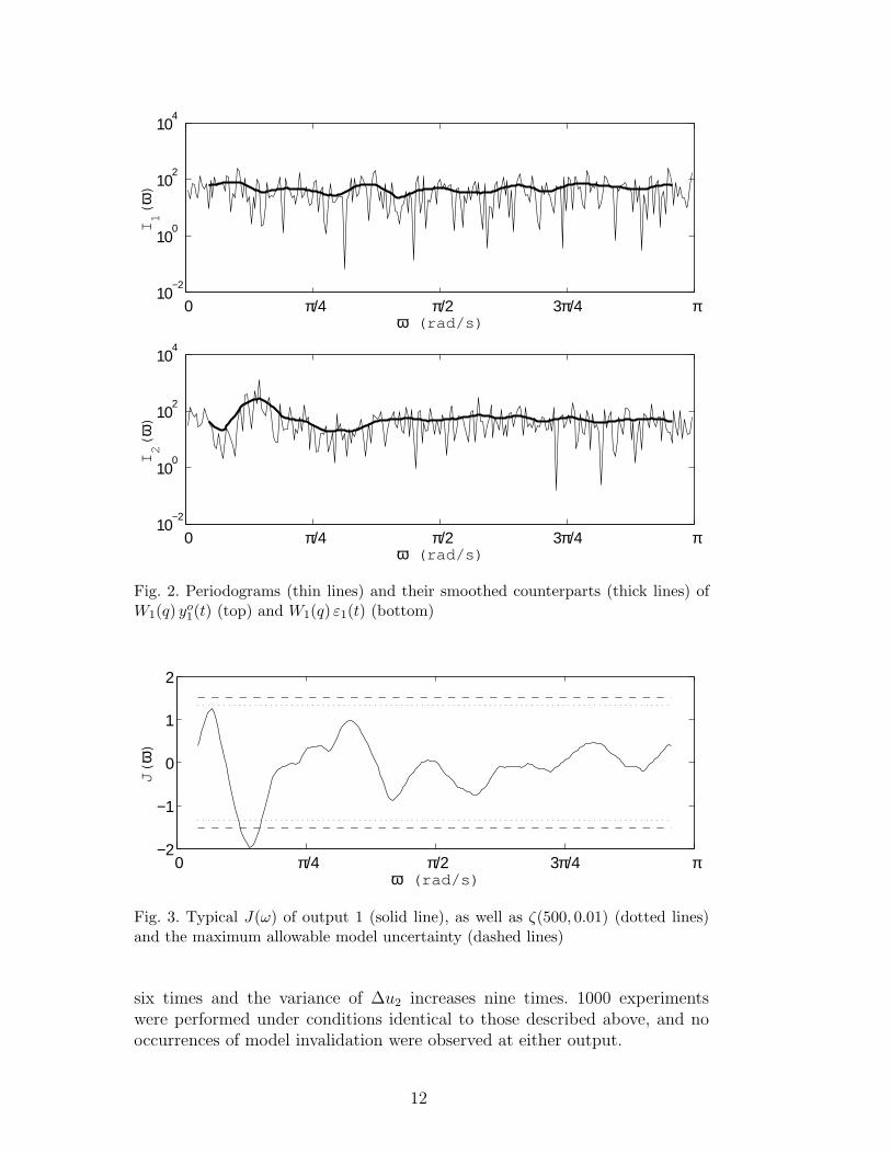
q6−1.66q5+0.688q4 . Thischange has no observable influence on the variance of the plant outputs but in-creases the variance of the control movements ∆u1 and ∆u2 by approximately25% and 50%, respectively. Another set of 1000 experiments is performed withthe new system and the same uncertainty region as described above. The mod-elling error introduced in output 1 is successfully detected in 798 experimentsand no invalidations occur of model output 2. Typical smoothed periodogramsof the signals related to output 1 are shown in Figure 2, while Figure 3 showsthe function J(ω) for output 1.

It is thus very likely that a single experiment realization will detect the prob-lem in output 1. It remains to be found whether g11 or g12 is the main contrib-utor to the model mismatch. A solution to this problem is to leave one controlaction active while freezing the other at a constant value (manual mode). Af-ter collecting these signals the role of each control action is inverted and newdata are collected. These sets of signals are then analyzed against yo(t). Forinstance, when u2 is active and u1 ≡ 0, g11 and g21 are not excited, thereforeplant/model mismatches can only be caused by either g12 or g22.

From those 798 experiments that signalled problems at model output 1, 673 ofthem continued to signal similar problems with u2 active and u1 ≡ 0, whereas2 experiments also signalled the problem with u1 active and u2 ≡ 0. Anotheranalysis shows that in these 2 cases the value of J∗ is larger when u2 is activeand u1 ≡ 0, leading to the conclusion that g12 has a larger influence on themismatch between G(q) and G(q) than g11 does.

As a second investigation, a sinusoid was injected at output 1, with the processin its original value. The frequency of the sinusoid was chosen to be 0.4 rad/s,which is similar to the frequency where the peak of J(ω) is found in Figure3. Under this sinusoidal disturbance, the variance of output 1 increases twotimes, the variance of output 2 remains the same, the variance of ∆u1 increases

11

0 π/4 π/2 3π/4 π 10

−2

100

102

104

ω (rad/s)

I1(

ω)

0 π/4 π/2 3π/4 π 10

−2

100

102

104

ω (rad/s)

I2(

ω)

Fig. 2. Periodograms (thin lines) and their smoothed counterparts (thick lines) ofW1(q) yo

1(t) (top) and W1(q) ε1(t) (bottom)

0 π/4 π/2 3π/4 π −2

−1

0

1

2

ω (rad/s)

J(

ω)

Fig. 3. Typical J(ω) of output 1 (solid line), as well as ζ(500, 0.01) (dotted lines)and the maximum allowable model uncertainty (dashed lines)

six times and the variance of ∆u2 increases nine times. 1000 experimentswere performed under conditions identical to those described above, and nooccurrences of model invalidation were observed at either output.

12

6 Conclusion

This article describes a novel approach to testing multivariable models em-ployed in control systems design. The term “model invalidation” is used hereto characterize simple tests, with little excitation, that put the plant modelon trial. This is in sharp contrast to “model validation” tests, which applyhigh excitation in order to “prove” that the model is good. Our testing mech-anism is well suited to the type of data readily available from industrial sites,especially when model-based predictive controllers are employed.

The test is based on the comparison of pairs of time series: one series is col-lected during normal closed-loop operation and the second one is collected un-der open-loop operation. This comparison provides means for assessing whichmodel outputs are incorrect, but it remains to be identified which model in-puts are problematic. A solution is provided in Section 5, where it is suggestedthat subsets of the controller outputs be inactive in order to test only partsof the model.

Similar to other mechanisms that extract information from measured data, likemodel identification and performance monitoring/assessment, deterministicload disturbances affect the final result. Periods with changes in load shouldbe detected and excluded from the analysis.

The results obtained on simulation examples are very encouraging. Several as-pects of the mechanism can be improved as the idea matures and new tests areperformed. Ultimately, our goal is to have an automated tool for monitoringmodel-based controllers.

References

Box, G. E. P., G. M. Jenkins and G. C. Reinsel (1994). Time Series Analysis:Forecasting and Control. third ed.. Holden-Day.

Coates, D. S. and P. J. Diggle (1986). Tests for comparing two estimatedspectral densities. Journal of Time Series Analysis 7(1), 7–20.

Diggle, P. J. and N. I. Fisher (1991). Nonparametric comparison of cumulativeperiodograms. Applied Statistics 40(3), 423–434.

Hagglund, T. (1995). A control loop performance monitor. Control Engineer-ing Practice 3(11), 1543–1551.

Hagglund, T. (1999). Automatic detection of sluggish control loops. ControlEngineering Practice 7(12), 1505–1511.

Harris, T. J. (1989). Assessment of control loop performance. The CanadianJournal of Chemical Engineering 67, 856–861.

13

Horch, A. (1999). A simple method for detection of stiction in process controlloops. Control Engineering Practice 7(10), 1221–1231.

Jenkins, G. M. and D. G. Watts (1968). Spectral Analysis and its Applications.Holden-Day. San Francisco, U.S.A.

Ljung, L. (1999). System Identification: Theory for the User. 2nd ed.. PTRPrentice Hall. Upper Saddle River, USA.

Pudney, S. E., D. F. Deadman and F. Clark (1999). A simple nonparametrictest for the equality of autocorrelation structures of two stochastic processes,with application to experimental data. Pub. Inst. Stat. Univ. Paris 43(2-3), 85–101.

Quenouille, M. H. (1958). The comparison of correlations in time-series. Jour-nal of the Royal Statistical Society 20(1), 158–164.

14