A supervised event-based non-intrusive load monitoring for non-linear appliances

Zheng, Zhuang; Chen, Hainan; Luo, Xiaowei

Published in:Sustainability (Switzerland)

Published: 01/04/2018

Document Version:Final Published version, also known as Publisher’s PDF, Publisher’s Final version or Version of Record

License:CC BY

Publication record in CityU Scholars:Go to record

Published version (DOI):10.3390/su10041001

Publication details:Zheng, Z., Chen, H., & Luo, X. (2018). A supervised event-based non-intrusive load monitoring for non-linearappliances. Sustainability (Switzerland), 10(4). https://doi.org/10.3390/su10041001

Citing this paperPlease note that where the full-text provided on CityU Scholars is the Post-print version (also known as Accepted AuthorManuscript, Peer-reviewed or Author Final version), it may differ from the Final Published version. When citing, ensure thatyou check and use the publisher's definitive version for pagination and other details.

General rightsCopyright for the publications made accessible via the CityU Scholars portal is retained by the author(s) and/or othercopyright owners and it is a condition of accessing these publications that users recognise and abide by the legalrequirements associated with these rights. Users may not further distribute the material or use it for any profit-making activityor commercial gain.Publisher permissionPermission for previously published items are in accordance with publisher's copyright policies sourced from the SHERPARoMEO database. Links to full text versions (either Published or Post-print) are only available if corresponding publishersallow open access.

Take down policyContact lbscholars@cityu.edu.hk if you believe that this document breaches copyright and provide us with details. We willremove access to the work immediately and investigate your claim.

Download date: 16/03/2022

sustainability

Article

A Supervised Event-Based Non-Intrusive LoadMonitoring for Non-Linear Appliances

Zhuang Zheng 1,2, Hainan Chen 1,2 and Xiaowei Luo 1,2,*1 Department of Architecture and Civil Engineering, City University of Hong Kong, Tat Chee Avenue,

Kowloon, Hong Kong 999077, China; zhuazheng3-c@my.cityu.edu.hk (Z.Z.); hn.chen@live.com (H.C.)2 Architecture and Civil Engineering Research Center, Shenzhen Research Institute of City University of

Hong Kong, 8 Yuexing 1st Road, Shenzhen Hi-tech Industrial Park, Nanshan District, Shenzhen 518057, China* Correspondence: xiaowluo@cityu.edu.hk; Tel.: +852-3442-2971

Received: 28 February 2018; Accepted: 26 March 2018; Published: 28 March 2018�����������������

Abstract: Smart meters generate a massive volume of energy consumption data which can beanalyzed to recover some interesting and beneficial information. Non-intrusive load monitoring(NILM) is one important application fostered by the mass deployment of smart meters. This paperpresents a supervised event-based NILM approach for non-linear appliance activities identification.Firstly, the additive properties (stating that, when a certain amount of specific appliances’feature is added to their belonging network, an equal amount of change in the network’sfeature can be observed) of three features (harmonic feature, voltage–current trajectory feature,and active–reactive–distortion (PQD) power curve features) were investigated through experiments.The results verify the good additive property for the harmonic features and Voltage–Current (U-I)trajectory features. In contrast, PQD power curve features have a poor additive property. Secondly,based on the verified additive property of harmonic current features and the representation ofwaveforms, a harmonic current features based approach is proposed for NILM, which includestwo main processes: event detection and event classification. For event detection, a novel modelis proposed based on the Density-Based Spatial Clustering of Applications with Noise (DBSCAN)algorithm. Compared to other event detectors, the proposed event detector not only can detectboth event timestamp and two adjacent steady states but also shows high detection accuracy overpublic dataset with F1-score up to 98.99%. Multi-layer perceptron (MLP) classifiers are then builtfor multi-class event classification using the harmonic current features and are trained using thedata collected from the laboratory and the public dataset. The results show that the MLP classifiershave a good performance in classifying non-linear loads. Finally, the proposed harmonic currentfeatures based approach is tested in the laboratory through experiments, in which multiple on–offevents of multiple appliances occur. The research indicates that clustering-based event detectionalgorithms are promising for future works in event-based NILM. Harmonic current features haveperfect additive property, and MLP classifier using harmonic current features can accurately identifytypical non-linear and resistive loads, which could be integrated with other approaches in the future.

Keywords: event-based NILM; additive property; harmonic currents; DBSCAN clustering basedevents detector; MLP classifier; non-linear appliances

1. Introduction

The building sector is one of the primary energy consumers. Studies show that more than 38% ofprimary energy and 76% of electrical energy are consumed in buildings in the United States. The energyconsumption can be reduced by up to 15–40% with the use of the home energy management system(HEMS) [1]. Within the HEMS, the smart meter is a critical element to measure the energy consumption

Sustainability 2018, 10, 1001; doi:10.3390/su10041001 www.mdpi.com/journal/sustainability

Sustainability 2018, 10, 1001 2 of 28

of the household in real time. Energy consumption data are fed into the HEMS for analysis with othersfor controlling and optimizing the energy usage. Most existing HEMSs monitor the household-levelelectricity usage and therefore lack detailed knowledge on the energy consumption at appliance-level.More smart meters need to be plugged into the appliances to collected fine-grained electricity data,posing higher initial cost for the homeowners. Instead of installing multiple appliance-level meters,NILM uses the aggregate energy consumption data from the household-level smart meter anddesegregates it to the appliance-level data. It is acknowledged as an efficient solution for monitoringindividual electrical appliance without extra sub-meters.

Appliance-level energy consumption data can benefit different stakeholders. (1) For consumers,the appliance-level energy consumption provides them insight on the detailed energy consumption torealize the opportunities for energy saving through behavior intervention. For example, in real-timemarket, the electricity price may be low during some period of the day. People may use applianceswith high-level energy consumption during this period. With knowledge of where the electricalenergy goes, measures can also be taken to reduce energy consumption for appliances with highconsumption level. Other services can also be provided such as fault detection of electrical appliancesand recommendation of energy-saving appliances. (2) For electrical industry, the implementation ofNILM provides an assessment of end-uses and the time of these usages in the buildings, which couldplay an important role in demand side management and penetration of renewable energy sources. In anelectrical system, to ensure the satisfaction of demand, the power generators usually need to provideexpensive reserve services. Demand side management is proposed to reduce the reserve service levelby demand prediction and demand scheduling. Appliance-level load curves are valuable in demandprediction and scheduling. Prior studies [2–4] pointed out that the analysis and sound understandingof demand profile on smaller consumer level could provide reasonably accurate information forpredicting peak and average demand and demand shifting. Besides, NILM can also increase thepenetration of renewable sources by maintaining the cost and revenue balance in micro-grid [5]. Due tothe fluctuations induced by wind speed variability or passing cloud, the main drawback of renewableenergy resources such as wind or solar power plants is that they introduce large voltage fluctuationsand supply uncertainty into distribution network [6–8]. Many solutions are proposed to eliminatethis problem including prediction models of wind speed or solar irradiation and storage systemoptimization [9]. However, the literature has paid little attention to demand-side which also containssignificant variability. The understanding of demand behavior in appliance-level may help reducethe load uncertainty and benefit the size determination of storage battery in micro-grid. This willbenefit the system maintenance and cost control. For building sector, NILM can make a differencefor human behavior inference in private homes which can be used for health and safety monitoringfor the elderly and building occupancy inference. The inference of human behavior through energyconsumption data will also benefit the energy reduction of lighting, space heating and cooling systemin buildings [10].

As shown in [11–14], the existing implementation of NILM can be classified into two categories:optimization methods and pattern recognition methods.

In the implementation using optimization method, the NILM problem can be formulated asa combinatorial optimization problem or a single source separation problem, since the aggregatehousehold-level electricity consumption data comprise the electricity consumptions of differentappliances. The optimization approach seeks the best appliances combination to minimize the sum ofsquares of the residuals between estimated signal and real signal. The solution to the optimizationproblem tells which appliances are on in the household at a specific time. Typical algorithms to solvethis type of optimization problem include Hidden Markov model (HMM) and its extensions [15–18],discriminative sparse coding [19] and tensor factorization [20]. Kolter and colleagues used the additiveand difference formulations of Factorial Hidden Markov Model (FHMM) for energy disaggregationtask by exploiting the additive structure of the FHMM and maximum a posteriori approximateinference algorithm [21]. They stated that, through approximate inference, the proposed method is

Sustainability 2018, 10, 1001 3 of 28

computationally efficient and free of local optimal. Based on Kolter’s work, Bonfigli and his colleaguesextended the feature dimension from one (active power) to two (active and reactive power) [18], leadingproposed solution to outperform the original Additive Factorial Approximate Map algorithm basedon one dimension only. The discriminative sparse coding and tensor factorization methods considerNILM as single source separation problem. Both methods assume that the appliances’ energy usage isalways nonnegative, neglecting the existence of distributed photovoltaic and wind power systems.In fact, Dinesh has considered the solar power influx which consumes negative active power [22].Nevertheless, Dinesh and colleagues utilized a subspace component power level matching algorithmwhich needs optimization over every subspace component and poses high computational requirement.These optimization methods are mainly unsupervised, and all of them used low-resolution powerfeatures (≤1 Hz). The most significant limitation of these methods is that they need to build a modelbeforehand for every appliance or source, making the methods unreliable when unknown appliancesappear. The second limitation is that it is an NP-hard (non-deterministic polynomial-time hard)problem because of the exponentially increasing number of combinations of appliance states [23].

The NILM can also be considered as a pattern recognition problem. The objective is to recognizethe state-transiting appliance one by one using pattern recognition algorithms (e.g., clusteringtechniques and classification algorithms). Typical approaches include event-based algorithms [11,24,25]and deep learning (DNN) based algorithms [13,26]. Kelly et al. adapted three deep neural networkarchitectures in their NILM approach: (1) a long short-term memory (LSTM) recurrent neural network;(2) denoising autoencoders; and (3) a neural network trained to estimate the start time, the end timeand the average power demand of each appliance activation [26]. However, Kelly’s approach doesnot perform well when appliances outside the training set are included in the house. Lukas andYang utilized LSTM network to developed an energy disaggregation approach in 2015 [13] and laterimproved it by combining the HMM with DNN together to extract single target load in 2016, in whichmultiple important appliances can be identified by using multiple neural networks [27]. Recently,Bonfigli and colleagues treated the NILM problem as a noise reduction problem and proposed anencoder-decoder deep convolution network, in which multiple neural networks were trained to meetthe NILM requirement. Previous studies [13,26,27] showed that deep learning based algorithmscan handle with situations where complex and variable appliances exist. These algorithms cater forappliances with complex and apparent operation patterns, such as washing machines, dish-washers,fridges, etc. However, they are unsuitable for simple ON/OFF or multi-state appliances such as lampsor hairdryers because fewer features can be learned from their energy consumption patterns and theyare limited for lack of training data. Therefore, integration of different algorithms is imperative becausethey can identify different types of appliance.

Apparently, the optimization method needs to identify all kinds of the appliance operating on thepower network every timestamp while the pattern recognition approach only needs to make eventdetection and classification at specific timestamp when the network changes state. The former methodposes higher requirements on computational capability of smart meters which is not practical.

NILM algorithms can also be categorized into supervised one and unsupervised one according towhat data they use [28]. Supervised algorithms not only need the aggregate house-level data but alsoa massive volume of appliance-level data while unsupervised algorithms (e.g., HMM) only need theaggregate house-level data. Although supervised methods require prior knowledge about appliancesand involve an intensive training process, they do not require the one-time manual appliance namingintervention when applied to real life. While unsupervised methods do not need a large trainingdataset, they require one-time appliance naming which can be more intrusive to the users [24].In addition, the accuracy of unsupervised methods is usually lower than the supervised methods.Apparently, the supervised algorithm is more advanced and practical for generalizing the patternsof appliances of the same type and can minimize the interference to users. Therefore, many NILMimplementations use supervised methods [13,23,27,29]. Recently, semi-supervised methods have beenproposed by researchers to make the tradeoff [28,30,31]. Liu et al. [30] proposed a similarity metric

Sustainability 2018, 10, 1001 4 of 28

between aggregate signals of a few sampled homes and other out-of-sample homes. The proposedsimilarity metric allows them to train the supervised models on a few houses and generalize thesemodels to some unmodeled homes. This implementation is a typical case semi-supervised models.

In this context, a supervised event-based NILM approach was proposed using harmonic currentfeatures, which have a good additive property. The additive property of feature refers to the propertythat when appliances are connected or disconnected to the power network, the corresponding feature ofthe network will increase or decrease by an amount equal to that produced by these appliances workingindividually. This property should hold independent of power network states. Hart [24] stated thatsteady-state features are additive while transient features are not. However, no substantial proof wasprovided. Since then, little attention has been given to features’ additive property except for Liang andcolleagues in 2010 [11]. The features’ additive property is important for the event-based NILM system,as it guarantees that the appliance features stay unchanged in different power network states and thefeatures can be extracted by subtracting the baseline data from the live data. Therefore, harmoniccurrent features are verified first regarding its perfect additive property in Section 2. For event-basedNILM systems, effective and efficient event detection algorithms still need to be researched andconcluded. Besides, NILM systems using harmonic features may work well for non-linear appliancesbut have not been well researched and commented using the real-life dataset to our best knowledge.Therefore, this paper focuses on the following three objectives: (1) verify that harmonic based featureshave a good additive property independent of practical power network states; (2) find which eventdetection algorithm has the best performance in NILM; and (3) demonstrate which types of appliancecan be identified accurately by harmonic features based NILM system.

The remainder of this paper is organized as follows. Section 2 provides a brief background workof event-based NILM including event identification algorithms and summarizes the features used inNILM. Then, the additive property of several features is tested by experiments. Section 3 describes theframework of the proposed approach, followed by the details of the two components in the framework:event detection model and classification model. Section 4 describes the two data sources and theevaluation metrics. Section 5 analyzes and discusses the performance of the proposed event detectionmodel and classification model, which is followed by a laboratory validation of the whole approach.Section 6 concludes the paper and envisions the future work.

2. Background Research

Event-based NILM methods mainly comprise two processes: event detection and eventclassification, in which different features may be used. There is no single algorithm or feature that canbe used to identify all kinds of appliance, even though 25 years have passed since the original work ofHart [32].

2.1. Event Detection and Classification Algorithms

Alcalá et al. [23] agree that the aim of event detection is to capture transient intervals andthe existing event detection approaches can be categorized into three types: (1) expert heuristics;(2) probabilistic models; and (3) matched filters. Expert heuristic algorithms need prior knowledgeabout appliances to be detected and are less practical. Probabilistic models require a parameterinitialization and a training process, although it may work better than other two methods.Matched filters poses a higher requirement on data acquisition rate and computational capability,although training process is not needed [23]. Apart from these three types of approaches,clustering with bucketing technique is used for event detection and has the best performancein the Building-Level fully-labeled dataset for Electricity Disaggregation (BLUED) dataset in theliterature [33,34]. This method has fewer parameters to be determined and can label points locatedin the transient interval and two adjacent steady states. However, bins need to be pre-defined andan “eight-neighbor” rule is used to detect objects and clusters. Besides, many iterations of wideningand narrowing of window length are used to conduct the “fine event detection”. These will slow

Sustainability 2018, 10, 1001 5 of 28

down the real-time data processing. Previous studies [23,35] simply performed first order differenceand threshold filtering to detect events. Their threshold determination is complex and not universal,especially for cases with noise, small step-change or slow-changing events. For event classification,machine learning algorithms such as MLP, Support Vector Machine (SVM), and Radial Basis Function(RBF) neural network are used and the result shows that MLP performs better than the other two [25].In [23], Principal Component Analysis (PCA) is used for event classification and compared to otherclassifiers such as K-Nearest Neighbor, Random Forest, etc. Wang et al. [35] utilized SVM to builda multi-class classifier using U-I trajectories and claimed a perfect performance. The proposedalgorithm only used data from one house for training and testing, limiting the generalizability ofcross-home and cross-instance of the same appliance type. Therefore, the performance of the algorithmproposed by Wang et al. might degrade rapidly in practice.

2.2. Features and Features Additive Property

Features refer to characteristics that can be used to distinguish different types of appliance.An ideal feature should be able to minimize the difference of instances in the same class andmaximize the difference of instances in different classes. Unfortunately, such features are still underinvestigation. Prior literature [11,12,31] has made a great effort and reviewed many features to giveinsights about feature engineering in NILM. The most widely used features of appliances includeactive power, reactive power and on/off durations, especially for those low-frequency samplingmethods [13,16,18–22,24,26,27,29,36]. The major drawback of those three features is that differenttypes of appliances may consume the same active power and they behave similarly, in whichcase these features cannot work. Alcala and his colleagues used power quantities’ trajectories asfeatures such as active (P), reactive (Q) and distortion (D) power considering the distortion of currentwaveforms [23]. Although their approach is event-based, transient intervals are considered, and theyachieve a remarkable accuracy on Plug-Level Appliance Identification Dataset (PLAID) dataset ofup to 88%, while not paying attention to the additive property of features. Moreover, Alcala gavea vague definition of reactive and distortion power and not all these power quantities are additivein mathematics. The same appliance may have different PQD trajectories under different powernetworks. In fact, except for active power’s definition, reactive power and distortion power havedifferent versions of definition in different power theories including the widely used Budeanu’ powertheory [37], Slonim’s theory [38] and Sun’s theory [39]. Further work is still needed in interpretingthe difference between active power and apparent power. Note that active power is usually additivebecause it is calculated from harmonics and harmonics have good additive property. On top of activepower, other additive power quantities need to be defined in event-based NILM system in the future.Lam and his team defined a novel load feature: Voltage–Current (U-I) trajectory by removing timevariable and combining voltage and current waveforms together [40]. Seven shape features wereextracted from each appliance trajectory and treated as a seven-dimensional feature vector. The shapefeatures were extended to 10 elements by Wang et al. [35]. Instead of quantifying the shape featuresmanually, Gao and colleagues converted the amplitude-normalized U-I trajectories into binary imagesby setting up mesh grids and doing binarization on each cell [41]. They reached the best accuracywith 81.75% using random forest algorithm over PLAID dataset. Some transformations of time-seriessignals were conducted to shed light on feature engineering including Fourier transformation [25],Wavelet Packet transformation [42], Stockwell transformation [43,44] and Hilbert transformation [45].Fourier transformation of features are well-known for harmonic vectors or harmonic spectrogram.This transformation is not suitable for low-resolution and un-stationary data series, and is oftencriticized for its infinite number of trigonometric function bases. Chan et al. [42] took advantage ofwavelet transformation features and represented them by a normalized energy vector consisting offive. The authors show that wavelet transformation based features can realize harmonic load signaturerecognition and consume lower computation time with good time-frequency resolution comparedto Fourier transformation. Martins et al. [43] applied the Stockwell transformation features firstly in

Sustainability 2018, 10, 1001 6 of 28

NILM system and then performed load identification with an optimization approach in the laboratoryshowing preliminary prospect of Stockwell transformation features. Jimenez and colleague extendedthis work by mapping the Stockwell transformation complex matrix into new space with extractedstatistical attributes [44]. They compared their work with wavelet transformation based public datasetand Stockwell transformation features were presented with similar or superior performance thanwavelet transformation features based NILM method.

2.2.1. Formulation of Features Additive Property

The features additive property can be formulated as below.Suppose an appliance i changes state at timestamp t; the appliance’s feature q (single dimension

or multi-dimension) has good additive property if it satisfies the conditions shown in Equation (1):

Qt−pre = ∑N1n=1 qn

Qt−a f ter = ∑N1n=1 qn

qi =

{Qt−a f ter −Qt−pre, if load is increasedQt−pre −Qt−a f ter, if load is reduced

(1)

where qi denotes the feature of appliance i working individually, Qt−pre denotes the observed featureof the power network before the event generated by appliance i at timestamp t, Qt−a f ter denotes theobserved feature of the power network after the event, and N1, N2 denote the number of appliancesoperating on the network before and after the event, respectively. The unit of q and Q depend on whatfeatures are selected. For example, if current features are used, the dimension should be “A”.

From the formulation above, it is observed that the additive appliance feature is independentof the event timestamps and the power network topologies before and after the event. Note that theformulation caters for both steady-state features and transient-state features. The qi can be representedby a time-series curve when transient intervals are considered. When only steady-state features areconsidered, the qi is usually a scalar or scalar vector. It can be used to extract appliance features fromaggregate electrical signals and compared similarity with the appliances’ feature database. Therefore,this property is imperative for event-based NILM system when choosing features.

2.2.2. Validation of Features Additive Property

In this section, the authors first verified the good additive property of harmonic current andthe poor additive property of power quantities defined by Alcalá [23] in the laboratory. The resultsare shown in Table 1. According to Alcalá, the active, reactive, distortion, apparent power P(W),Q(Var), D(VA), and S(VA) are defined by Equation (2). This definition only considers the fundamentalharmonic and pays no attention to the additive property.

S2 = P2 + Q2 + D2

S = Urms × Irms

P = Urms × Irms,1 × cos(ϕ1)

Q = Urms × Irms,1 × sin(ϕ1)

D =√(S2 −Q2 − P2)

Root−mean− square(RMS) value : Irms =√

1T∫ T

0 i(t)2dt, Urms =√

1T∫ T

0 u(t)2dt

(2)

To take advantage of the additive property of harmonic currents, their formulations are revisedinto Equation (3) based on 50 orders of harmonic currents.

Sustainability 2018, 10, 1001 7 of 28

S2 = P2 + Q2 + D2

S = Urms × Irms ≈ Urms,1 × Irms

P = ∑50i=1 Urms,i × Irms,i × cos(ϕi) ≈ Urms,1 × Irms,1 × cos(ϕ1)

Q = ∑50i=1 Urms,i × Irms,i × sin(ϕi) ≈ Urms,1 × Irms,1 × sin(ϕ1)

D =√(S2 −Q2 − P2)

Irms =√

∑50i=1 Irms,i

2, Urms =√

∑50i=1 Urms,i

2

(3)

In Equations (2) and (3), ϕ1 (degree) denotes phase angle between the 1st order ofvoltage and current. Urms(V) and Irms(A) denote the RMS value of voltage and current,Urms,i(V) and Irms,i(A) (i = 1, 2, . . . , 50) denote the RMS value of ith harmonic voltage and current.u(t)(V) and i(t)(A) denote the waveform functions in time domain of voltage and current.

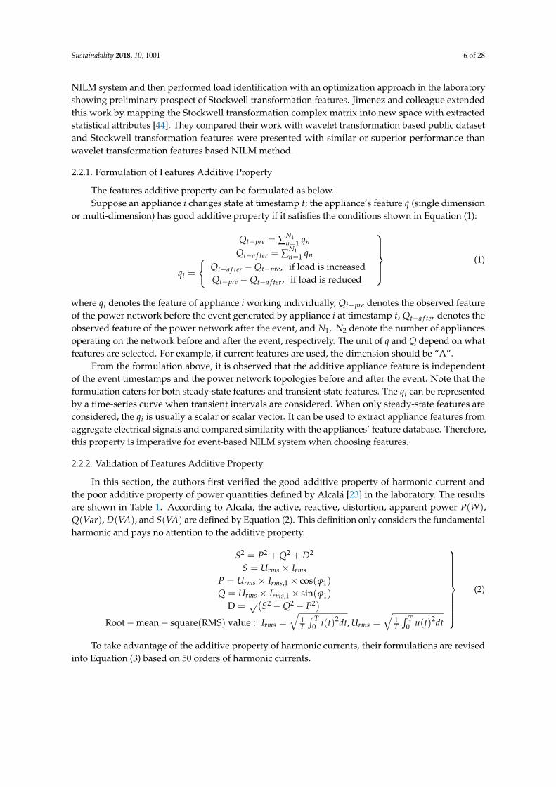
In Table 1, (1), (2), (3), and (4) represent four types of appliance: compact fluorescent lamp (1),laptop (2), LED lamp (3) and hairdryer (4). The hairdryer was turned on for four times when the powernetwork operates in four different states and calculate the responsive difference value of quantitiesfor each state transition. For example, the “Null + (4)” transition means the hairdryer was turnedon when no appliance is operating on the power network. The “(1)(2)(3) + (4)” transition meansthe hairdryer is turned on when compact fluorescent lamp, laptop, and led lamp are operating onthe network simultaneously. The second column calculates the third order of harmonic current ofhairdryer in different power network configurations. The authors used the complex form of harmoniccurrents and made average and subtraction between adjacent steady states to calculate differencevalue of the third order of harmonic current for each transition. I3rd and θ denote the RMS value andphase angle of the third order of harmonic current of the hair dryer. It can be seen from the secondcolumn of Table 1 that the difference value of RMS amplitude and phase angle of the third order ofharmonic current in four transitions almost stay unchanged. Therefore, the harmonic current featureshave good additive property and they are independent of power network states. Alcalá defined theactive power (P), reactive power (Q), apparent power (S) and distortion power (D) in Equation (2)with no consideration of their additive property [23]. The authors calculated the power quantitiesaccording to Alcalá’s definitions and found that only P and Q have good additive property while Dand S do not. Therefore, the power quantities without consideration of the harmonic features [23]have a poor additive property, indicating that the same appliance may have different PQD trajectoryunder different power network states. Finally, the authors calculated the power quantities by takingadvantage of harmonic currents’ additive property by Equation (3) and found the P, Q, S, and D havegood additive property, as shown in the third column in Table 1.

Table 1. Verification of additive property of harmonic features and non-additive property ofpower quantities.

Transition3rd Harmonic

QuantityPower Quantities Calculated by

Equation (2) [23]Power Quantities Calculated by

Equation (3)

I3rd/A θ/degree S/VA P/W Q/Var D/VA S/VA P/w Q/Var D/VA

Null + (4) 1.94 −2.84 490.03 445.49 −22.07 202.94 491.24 446.59 −22.12 203.44(1) + (4) 1.93 −3.09 470.90 445.10 −23.98 169.58 491.07 446.25 −24.10 203.54

(1)(2) + (4) 1.93 −3.08 442.61 444.43 −23.81 125.44 488.78 445.28 −23.92 200.13(1)(2)(3) + (4) 1.94 −3.17 435.11 446.79 −24.66 113.32 491.59 448.00 −24.81 200.85

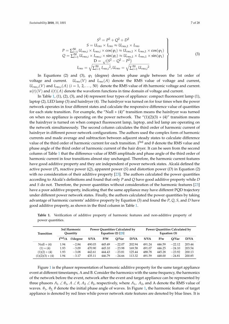
Figure 1 is the phasor representation of harmonic additive property for the same target applianceevent at different timestamps, A and B. Consider the harmonics with the same frequency, the harmonicsof the network before the event, network after the event and target appliance can be represented bythree phasors A1 ∠ θ1, A ∠ θ, A2 ∠ θ2, respectively, where A1, A2, and A denote the RMS value ofwaves. θ1, θ2, θ denote the initial phase angle of waves. In Figure 1, the harmonic feature of targetappliance is denoted by red lines while power network state features are denoted by blue lines. It is

Sustainability 2018, 10, 1001 8 of 28

observed that the appliance harmonics are identical, although network state features are differentat event timestamp A and B. Thus, the harmonics have good additive property as a result of thegood mathematic relationships of wave addition. By taking the advantage of the additive property ofharmonics, the power quantities in Equation (2) can be revised into Equation (3). Since the voltage isassumed to be constant, only fundamental voltage is considered. The RMS current is calculated byharmonic currents which ensures that the power quantities of target appliance calculated are identicalat different power network states.

Figure 1. Harmonic phasor representation of the same appliance event at different network states.

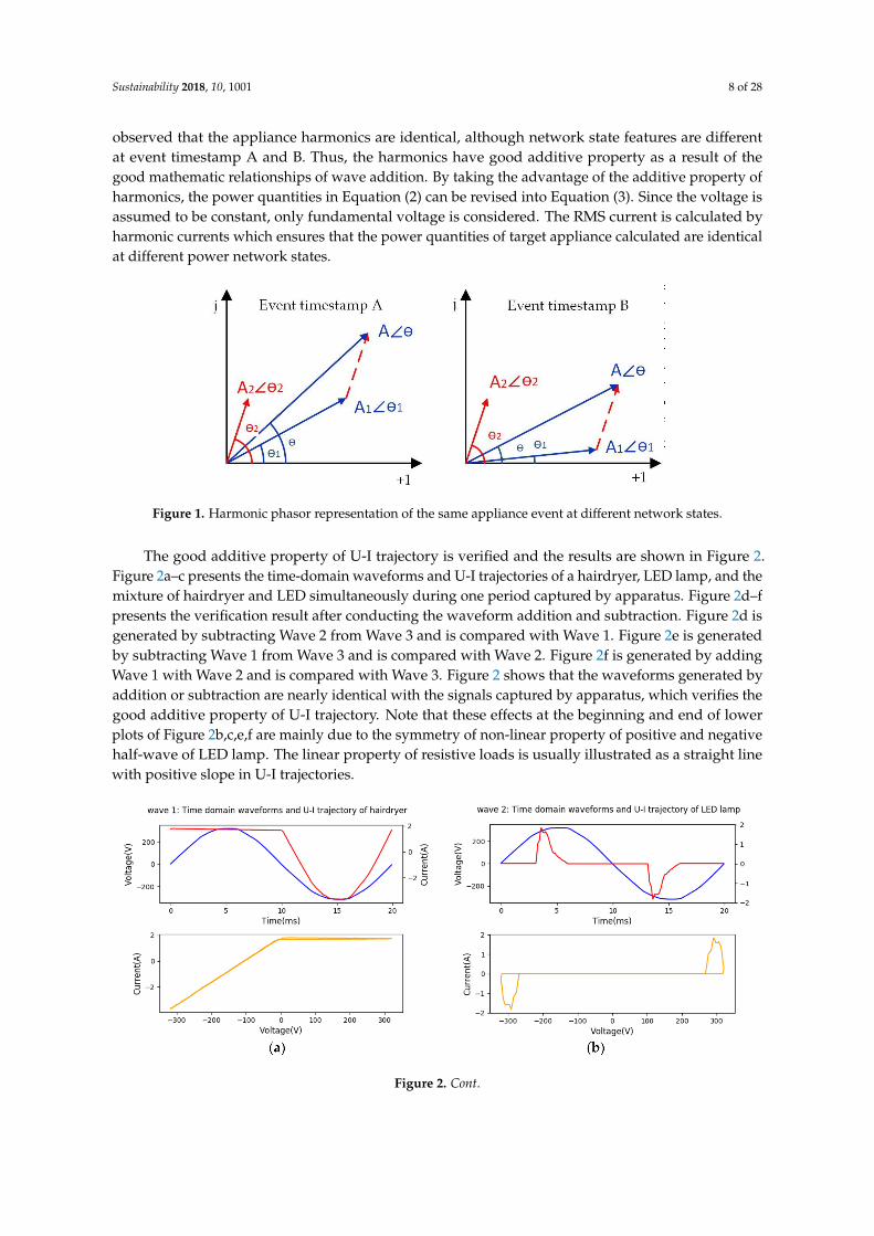
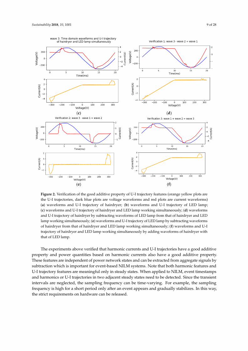
The good additive property of U-I trajectory is verified and the results are shown in Figure 2.Figure 2a–c presents the time-domain waveforms and U-I trajectories of a hairdryer, LED lamp, and themixture of hairdryer and LED simultaneously during one period captured by apparatus. Figure 2d–fpresents the verification result after conducting the waveform addition and subtraction. Figure 2d isgenerated by subtracting Wave 2 from Wave 3 and is compared with Wave 1. Figure 2e is generatedby subtracting Wave 1 from Wave 3 and is compared with Wave 2. Figure 2f is generated by addingWave 1 with Wave 2 and is compared with Wave 3. Figure 2 shows that the waveforms generated byaddition or subtraction are nearly identical with the signals captured by apparatus, which verifies thegood additive property of U-I trajectory. Note that these effects at the beginning and end of lowerplots of Figure 2b,c,e,f are mainly due to the symmetry of non-linear property of positive and negativehalf-wave of LED lamp. The linear property of resistive loads is usually illustrated as a straight linewith positive slope in U-I trajectories.

Figure 2. Cont.

Sustainability 2018, 10, 1001 9 of 28

Figure 2. Verification of the good additive property of U-I trajectory features (orange yellow plots arethe U-I trajectories, dark blue plots are voltage waveforms and red plots are current waveforms)(a) waveforms and U-I trajectory of hairdryer; (b) waveforms and U-I trajectory of LED lamp;(c) waveforms and U-I trajectory of hairdryer and LED lamp working simultaneously; (d) waveformsand U-I trajectory of hairdryer by subtracting waveforms of LED lamp from that of hairdryer and LEDlamp working simultaneously; (e) waveforms and U-I trajectory of LED lamp by subtracting waveformsof hairdryer from that of hairdryer and LED lamp working simultaneously; (f) waveforms and U-Itrajectory of hairdryer and LED lamp working simultaneously by adding waveforms of hairdryer withthat of LED lamp.

The experiments above verified that harmonic currents and U-I trajectories have a good additiveproperty and power quantities based on harmonic currents also have a good additive property.These features are independent of power network states and can be extracted from aggregate signals bysubtraction which is important for event-based NILM systems. Note that both harmonic features andU-I trajectory features are meaningful only in steady states. When applied to NILM, event timestampsand harmonics or U-I trajectories in two adjacent steady states need to be detected. Since the transientintervals are neglected, the sampling frequency can be time-varying. For example, the samplingfrequency is high for a short period only after an event appears and gradually stabilizes. In this way,the strict requirements on hardware can be released.

Sustainability 2018, 10, 1001 10 of 28

3. Methodology

3.1. Overall Framework

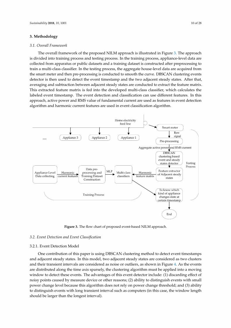
The overall framework of the proposed NILM approach is illustrated in Figure 3. The approachis divided into training process and testing process. In the training process, appliance-level data arecollected from apparatus or public datasets and a training dataset is constructed after preprocessing totrain a multi-class classifier. In the testing process, the aggregate house-level data are acquired fromthe smart meter and then pre-processing is conducted to smooth the curve. DBSCAN clustering eventsdetector is then used to detect the event timestamp and the two adjacent steady states. After that,averaging and subtraction between adjacent steady states are conducted to extract the feature matrix.This extracted feature matrix is fed into the developed multi-class classifier, which calculates thelabeled event timestamp. The event detection and classification can use different features. In thisapproach, active power and RMS value of fundamental current are used as features in event detectionalgorithm and harmonic current features are used in event classification algorithm.

Figure 3. The flow chart of proposed event-based NILM approach.

3.2. Event Detection and Event Classification

3.2.1. Event Detection Model

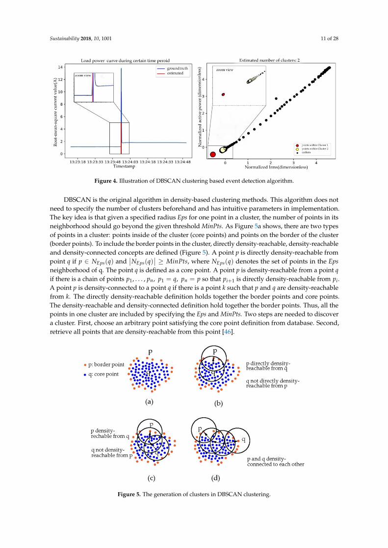
One contribution of this paper is using DBSCAN clustering method to detect event timestampsand adjacent steady states. In this model, two adjacent steady states are considered as two clustersand their transient intervals are considered as noise or outliers, as shown in Figure 4. As the eventsare distributed along the time axis sparsely, the clustering algorithm must be applied into a movingwindow to detect these events. The advantages of this event detector include: (1) discarding effect ofnoisy points caused by measure device or other reasons; (2) ability to distinguish events with smallpower change level because this algorithm does not rely on power change threshold; and (3) abilityto distinguish events with long transient interval such as computers (in this case, the window lengthshould be larger than the longest interval).

Sustainability 2018, 10, 1001 11 of 28

Figure 4. Illustration of DBSCAN clustering based event detection algorithm.

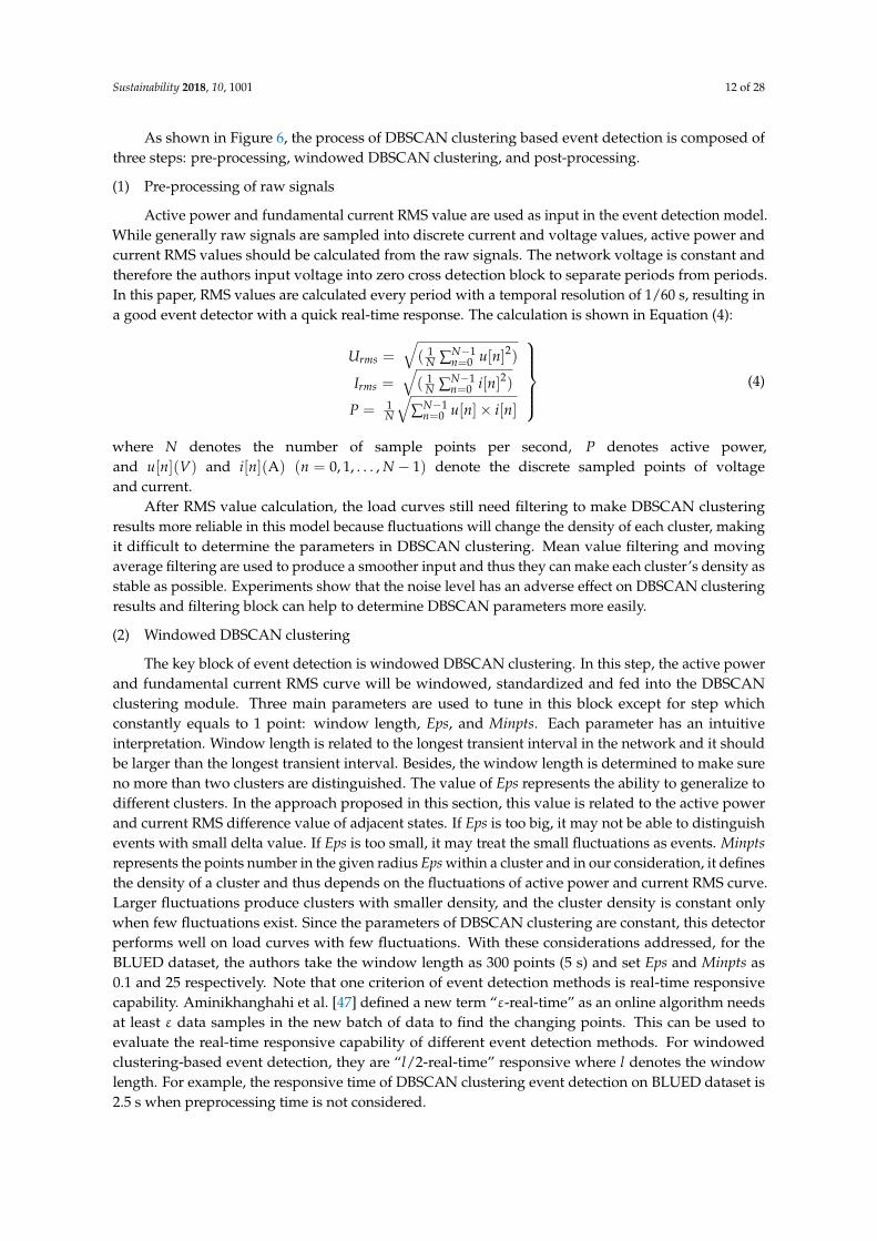
DBSCAN is the original algorithm in density-based clustering methods. This algorithm does notneed to specify the number of clusters beforehand and has intuitive parameters in implementation.The key idea is that given a specified radius Eps for one point in a cluster, the number of points in itsneighborhood should go beyond the given threshold MinPts. As Figure 5a shows, there are two typesof points in a cluster: points inside of the cluster (core points) and points on the border of the cluster(border points). To include the border points in the cluster, directly density-reachable, density-reachableand density-connected concepts are defined (Figure 5). A point p is directly density-reachable frompoint q if p ∈ NEps(q) and

∣∣NEps(q)∣∣ ≥ MinPts, where NEps(q) denotes the set of points in the Eps

neighborhood of q. The point q is defined as a core point. A point p is density-reachable from a point qif there is a chain of points p1, . . . , pn, p1 = q, pn = p so that pi+1 is directly density-reachable from pi.A point p is density-connected to a point q if there is a point k such that p and q are density-reachablefrom k. The directly density-reachable definition holds together the border points and core points.The density-reachable and density-connected definition hold together the border points. Thus, all thepoints in one cluster are included by specifying the Eps and MinPts. Two steps are needed to discovera cluster. First, choose an arbitrary point satisfying the core point definition from database. Second,retrieve all points that are density-reachable from this point [46].

Figure 5. The generation of clusters in DBSCAN clustering.

Sustainability 2018, 10, 1001 12 of 28

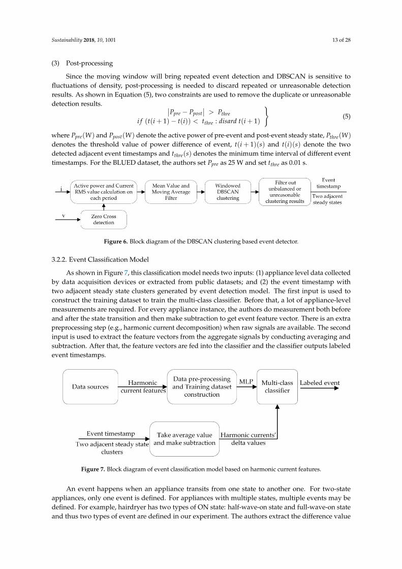
As shown in Figure 6, the process of DBSCAN clustering based event detection is composed ofthree steps: pre-processing, windowed DBSCAN clustering, and post-processing.

(1) Pre-processing of raw signals

Active power and fundamental current RMS value are used as input in the event detection model.While generally raw signals are sampled into discrete current and voltage values, active power andcurrent RMS values should be calculated from the raw signals. The network voltage is constant andtherefore the authors input voltage into zero cross detection block to separate periods from periods.In this paper, RMS values are calculated every period with a temporal resolution of 1/60 s, resulting ina good event detector with a quick real-time response. The calculation is shown in Equation (4):

Urms =√( 1

N ∑N−1n=0 u[n]2)

Irms =√( 1

N ∑N−1n=0 i[n]2)

P = 1N

√∑N−1

n=0 u[n]× i[n]

(4)

where N denotes the number of sample points per second, P denotes active power,and u[n](V) and i[n](A) (n = 0, 1, . . . , N − 1) denote the discrete sampled points of voltageand current.

After RMS value calculation, the load curves still need filtering to make DBSCAN clusteringresults more reliable in this model because fluctuations will change the density of each cluster, makingit difficult to determine the parameters in DBSCAN clustering. Mean value filtering and movingaverage filtering are used to produce a smoother input and thus they can make each cluster’s density asstable as possible. Experiments show that the noise level has an adverse effect on DBSCAN clusteringresults and filtering block can help to determine DBSCAN parameters more easily.

(2) Windowed DBSCAN clustering

The key block of event detection is windowed DBSCAN clustering. In this step, the active powerand fundamental current RMS curve will be windowed, standardized and fed into the DBSCANclustering module. Three main parameters are used to tune in this block except for step whichconstantly equals to 1 point: window length, Eps, and Minpts. Each parameter has an intuitiveinterpretation. Window length is related to the longest transient interval in the network and it shouldbe larger than the longest transient interval. Besides, the window length is determined to make sureno more than two clusters are distinguished. The value of Eps represents the ability to generalize todifferent clusters. In the approach proposed in this section, this value is related to the active powerand current RMS difference value of adjacent states. If Eps is too big, it may not be able to distinguishevents with small delta value. If Eps is too small, it may treat the small fluctuations as events. Minptsrepresents the points number in the given radius Eps within a cluster and in our consideration, it definesthe density of a cluster and thus depends on the fluctuations of active power and current RMS curve.Larger fluctuations produce clusters with smaller density, and the cluster density is constant onlywhen few fluctuations exist. Since the parameters of DBSCAN clustering are constant, this detectorperforms well on load curves with few fluctuations. With these considerations addressed, for theBLUED dataset, the authors take the window length as 300 points (5 s) and set Eps and Minpts as0.1 and 25 respectively. Note that one criterion of event detection methods is real-time responsivecapability. Aminikhanghahi et al. [47] defined a new term “ε-real-time” as an online algorithm needsat least ε data samples in the new batch of data to find the changing points. This can be used toevaluate the real-time responsive capability of different event detection methods. For windowedclustering-based event detection, they are “l/2-real-time” responsive where l denotes the windowlength. For example, the responsive time of DBSCAN clustering event detection on BLUED dataset is2.5 s when preprocessing time is not considered.

Sustainability 2018, 10, 1001 13 of 28

(3) Post-processing

Since the moving window will bring repeated event detection and DBSCAN is sensitive tofluctuations of density, post-processing is needed to discard repeated or unreasonable detectionresults. As shown in Equation (5), two constraints are used to remove the duplicate or unreasonabledetection results. ∣∣Ppre − Ppost

∣∣ > Pthrei f (t(i + 1)− t(i)) < tthre : disard t(i + 1)

}(5)

where Ppre(W) and Ppost(W) denote the active power of pre-event and post-event steady state, Pthre(W)

denotes the threshold value of power difference of event, t(i + 1)(s) and t(i)(s) denote the twodetected adjacent event timestamps and tthre(s) denotes the minimum time interval of different eventtimestamps. For the BLUED dataset, the authors set Ppre as 25 W and set tthre as 0.01 s.

Figure 6. Block diagram of the DBSCAN clustering based event detector.

3.2.2. Event Classification Model

As shown in Figure 7, this classification model needs two inputs: (1) appliance level data collectedby data acquisition devices or extracted from public datasets; and (2) the event timestamp withtwo adjacent steady state clusters generated by event detection model. The first input is used toconstruct the training dataset to train the multi-class classifier. Before that, a lot of appliance-levelmeasurements are required. For every appliance instance, the authors do measurement both beforeand after the state transition and then make subtraction to get event feature vector. There is an extrapreprocessing step (e.g., harmonic current decomposition) when raw signals are available. The secondinput is used to extract the feature vectors from the aggregate signals by conducting averaging andsubtraction. After that, the feature vectors are fed into the classifier and the classifier outputs labeledevent timestamps.

Figure 7. Block diagram of event classification model based on harmonic current features.

An event happens when an appliance transits from one state to another one. For two-stateappliances, only one event is defined. For appliances with multiple states, multiple events may bedefined. For example, hairdryer has two types of ON state: half-wave-on state and full-wave-on stateand thus two types of event are defined in our experiment. The authors extract the difference value

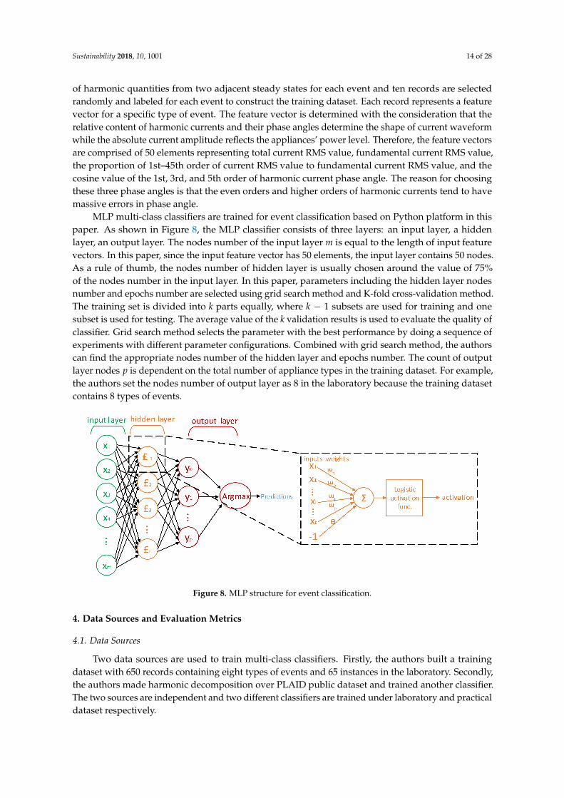
Sustainability 2018, 10, 1001 14 of 28

of harmonic quantities from two adjacent steady states for each event and ten records are selectedrandomly and labeled for each event to construct the training dataset. Each record represents a featurevector for a specific type of event. The feature vector is determined with the consideration that therelative content of harmonic currents and their phase angles determine the shape of current waveformwhile the absolute current amplitude reflects the appliances’ power level. Therefore, the feature vectorsare comprised of 50 elements representing total current RMS value, fundamental current RMS value,the proportion of 1st–45th order of current RMS value to fundamental current RMS value, and thecosine value of the 1st, 3rd, and 5th order of harmonic current phase angle. The reason for choosingthese three phase angles is that the even orders and higher orders of harmonic currents tend to havemassive errors in phase angle.

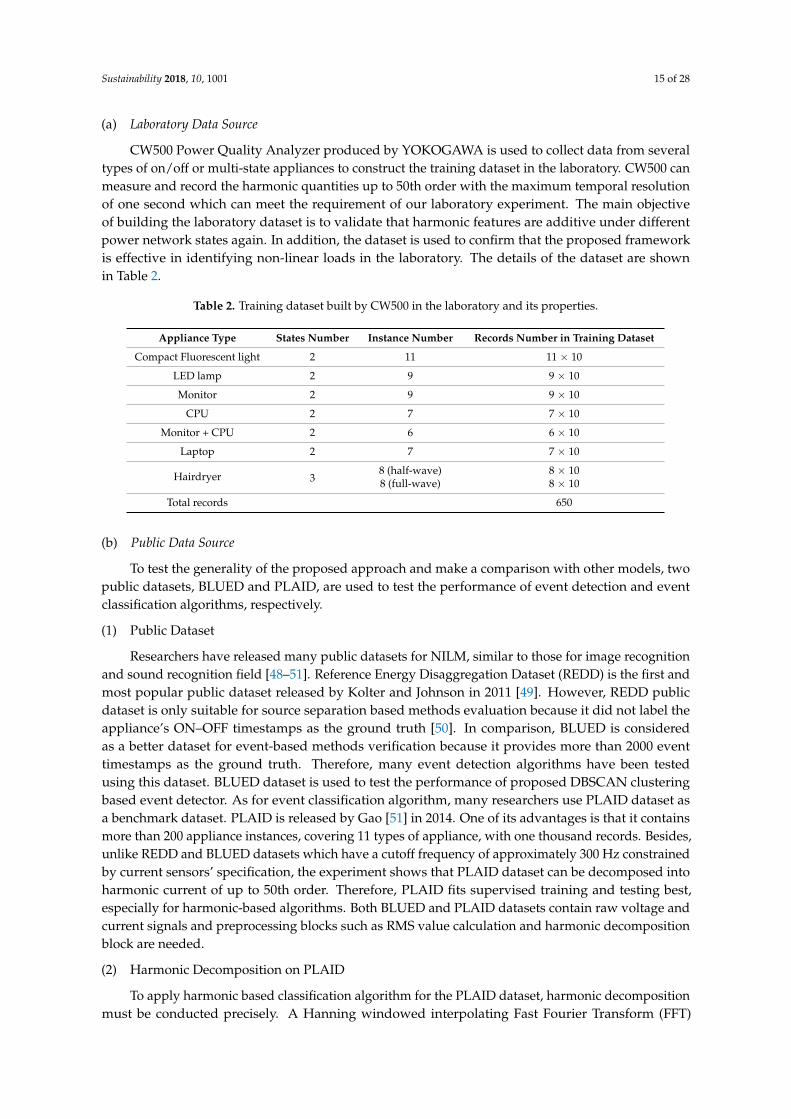
MLP multi-class classifiers are trained for event classification based on Python platform in thispaper. As shown in Figure 8, the MLP classifier consists of three layers: an input layer, a hiddenlayer, an output layer. The nodes number of the input layer m is equal to the length of input featurevectors. In this paper, since the input feature vector has 50 elements, the input layer contains 50 nodes.As a rule of thumb, the nodes number of hidden layer is usually chosen around the value of 75%of the nodes number in the input layer. In this paper, parameters including the hidden layer nodesnumber and epochs number are selected using grid search method and K-fold cross-validation method.The training set is divided into k parts equally, where k − 1 subsets are used for training and onesubset is used for testing. The average value of the k validation results is used to evaluate the quality ofclassifier. Grid search method selects the parameter with the best performance by doing a sequence ofexperiments with different parameter configurations. Combined with grid search method, the authorscan find the appropriate nodes number of the hidden layer and epochs number. The count of outputlayer nodes p is dependent on the total number of appliance types in the training dataset. For example,the authors set the nodes number of output layer as 8 in the laboratory because the training datasetcontains 8 types of events.

Figure 8. MLP structure for event classification.

4. Data Sources and Evaluation Metrics

4.1. Data Sources

Two data sources are used to train multi-class classifiers. Firstly, the authors built a trainingdataset with 650 records containing eight types of events and 65 instances in the laboratory. Secondly,the authors made harmonic decomposition over PLAID public dataset and trained another classifier.The two sources are independent and two different classifiers are trained under laboratory and practicaldataset respectively.

Sustainability 2018, 10, 1001 15 of 28

(a) Laboratory Data Source

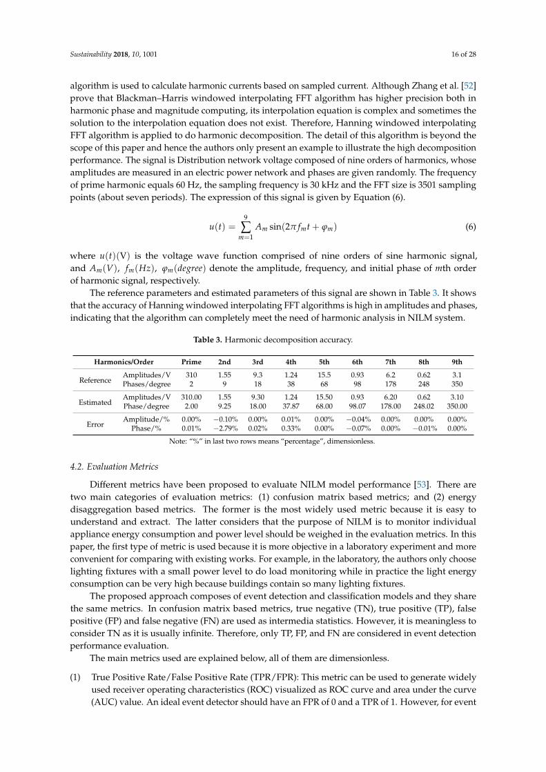
CW500 Power Quality Analyzer produced by YOKOGAWA is used to collect data from severaltypes of on/off or multi-state appliances to construct the training dataset in the laboratory. CW500 canmeasure and record the harmonic quantities up to 50th order with the maximum temporal resolutionof one second which can meet the requirement of our laboratory experiment. The main objectiveof building the laboratory dataset is to validate that harmonic features are additive under differentpower network states again. In addition, the dataset is used to confirm that the proposed frameworkis effective in identifying non-linear loads in the laboratory. The details of the dataset are shownin Table 2.

Table 2. Training dataset built by CW500 in the laboratory and its properties.

Appliance Type States Number Instance Number Records Number in Training Dataset

Compact Fluorescent light 2 11 11 × 10

LED lamp 2 9 9 × 10

Monitor 2 9 9 × 10

CPU 2 7 7 × 10

Monitor + CPU 2 6 6 × 10

Laptop 2 7 7 × 10

Hairdryer 38 (half-wave) 8 × 108 (full-wave) 8 × 10

Total records 650

(b) Public Data Source

To test the generality of the proposed approach and make a comparison with other models, twopublic datasets, BLUED and PLAID, are used to test the performance of event detection and eventclassification algorithms, respectively.

(1) Public Dataset

Researchers have released many public datasets for NILM, similar to those for image recognitionand sound recognition field [48–51]. Reference Energy Disaggregation Dataset (REDD) is the first andmost popular public dataset released by Kolter and Johnson in 2011 [49]. However, REDD publicdataset is only suitable for source separation based methods evaluation because it did not label theappliance’s ON–OFF timestamps as the ground truth [50]. In comparison, BLUED is consideredas a better dataset for event-based methods verification because it provides more than 2000 eventtimestamps as the ground truth. Therefore, many event detection algorithms have been testedusing this dataset. BLUED dataset is used to test the performance of proposed DBSCAN clusteringbased event detector. As for event classification algorithm, many researchers use PLAID dataset asa benchmark dataset. PLAID is released by Gao [51] in 2014. One of its advantages is that it containsmore than 200 appliance instances, covering 11 types of appliance, with one thousand records. Besides,unlike REDD and BLUED datasets which have a cutoff frequency of approximately 300 Hz constrainedby current sensors’ specification, the experiment shows that PLAID dataset can be decomposed intoharmonic current of up to 50th order. Therefore, PLAID fits supervised training and testing best,especially for harmonic-based algorithms. Both BLUED and PLAID datasets contain raw voltage andcurrent signals and preprocessing blocks such as RMS value calculation and harmonic decompositionblock are needed.

(2) Harmonic Decomposition on PLAID

To apply harmonic based classification algorithm for the PLAID dataset, harmonic decompositionmust be conducted precisely. A Hanning windowed interpolating Fast Fourier Transform (FFT)

Sustainability 2018, 10, 1001 16 of 28

algorithm is used to calculate harmonic currents based on sampled current. Although Zhang et al. [52]prove that Blackman–Harris windowed interpolating FFT algorithm has higher precision both inharmonic phase and magnitude computing, its interpolation equation is complex and sometimes thesolution to the interpolation equation does not exist. Therefore, Hanning windowed interpolatingFFT algorithm is applied to do harmonic decomposition. The detail of this algorithm is beyond thescope of this paper and hence the authors only present an example to illustrate the high decompositionperformance. The signal is Distribution network voltage composed of nine orders of harmonics, whoseamplitudes are measured in an electric power network and phases are given randomly. The frequencyof prime harmonic equals 60 Hz, the sampling frequency is 30 kHz and the FFT size is 3501 samplingpoints (about seven periods). The expression of this signal is given by Equation (6).

u(t) =9

∑m=1

Am sin(2π fmt + ϕm) (6)

where u(t)(V) is the voltage wave function comprised of nine orders of sine harmonic signal,and Am(V), fm(Hz), ϕm(degree) denote the amplitude, frequency, and initial phase of mth orderof harmonic signal, respectively.

The reference parameters and estimated parameters of this signal are shown in Table 3. It showsthat the accuracy of Hanning windowed interpolating FFT algorithms is high in amplitudes and phases,indicating that the algorithm can completely meet the need of harmonic analysis in NILM system.

Table 3. Harmonic decomposition accuracy.

Harmonics/Order Prime 2nd 3rd 4th 5th 6th 7th 8th 9th

ReferenceAmplitudes/V 310 1.55 9.3 1.24 15.5 0.93 6.2 0.62 3.1Phases/degree 2 9 18 38 68 98 178 248 350

EstimatedAmplitudes/V 310.00 1.55 9.30 1.24 15.50 0.93 6.20 0.62 3.10Phase/degree 2.00 9.25 18.00 37.87 68.00 98.07 178.00 248.02 350.00

ErrorAmplitude/% 0.00% −0.10% 0.00% 0.01% 0.00% −0.04% 0.00% 0.00% 0.00%

Phase/% 0.01% −2.79% 0.02% 0.33% 0.00% −0.07% 0.00% −0.01% 0.00%

Note: “%” in last two rows means “percentage”, dimensionless.

4.2. Evaluation Metrics

Different metrics have been proposed to evaluate NILM model performance [53]. There aretwo main categories of evaluation metrics: (1) confusion matrix based metrics; and (2) energydisaggregation based metrics. The former is the most widely used metric because it is easy tounderstand and extract. The latter considers that the purpose of NILM is to monitor individualappliance energy consumption and power level should be weighed in the evaluation metrics. In thispaper, the first type of metric is used because it is more objective in a laboratory experiment and moreconvenient for comparing with existing works. For example, in the laboratory, the authors only chooselighting fixtures with a small power level to do load monitoring while in practice the light energyconsumption can be very high because buildings contain so many lighting fixtures.

The proposed approach composes of event detection and classification models and they sharethe same metrics. In confusion matrix based metrics, true negative (TN), true positive (TP), falsepositive (FP) and false negative (FN) are used as intermedia statistics. However, it is meaningless toconsider TN as it is usually infinite. Therefore, only TP, FP, and FN are considered in event detectionperformance evaluation.

The main metrics used are explained below, all of them are dimensionless.

(1) True Positive Rate/False Positive Rate (TPR/FPR): This metric can be used to generate widelyused receiver operating characteristics (ROC) visualized as ROC curve and area under the curve(AUC) value. An ideal event detector should have an FPR of 0 and a TPR of 1. However, for event

Sustainability 2018, 10, 1001 17 of 28

detection assignments, TN can be infinite and it makes FPR always close to 0. Therefore, TN andFPR make no sense in this context and ROC curve and AUC value cannot be generated, either.

FPR = FPFP+TN

TPR = TPTP+FN

}(7)

(2) True/False Positive Percentage (TPP/FPP): In this metric, the authors focus on the ratio of eventscorrectly/wrongly detected (TP/FP) to the actual total events number (E).

TPP = TPE

FPP = FPE

}(8)

(3) F− 1 measure: Recall reflects how many actual events are detected and precision reflects howmany detected events are actual. Recall and precision is a pair of metrics with paradox. Generally,if recall is high, precision may be low and vice versa. They can be visualized as a P-R curve withrecall and precision as horizontal and vertical axes, respectively. F− 1 measure is proposed tomake a tradeoff between recall and precision.

Recall (R) = TPTP+FN

Precision (P) = TPTP+FP

F1 = 2×precision×recallprecision+recall = 2TP

2TP+FN+FP

(9)

(4) Accuracy: It measures how often the system makes correct decision by taking the ratio betweenthe number of correct decisions and the total number of system output as Equation (10) illustrates.

Acc =TP + TN

TP + TN + FP + FN(10)

However, this definition makes no sense in event detection as there is no available count ofTN. To solve the problem, Dixon [54] proposed another definition by discarding TN as Equation(11) illustrates.

Score =TP

TP + FP + FN(11)

As for event classification process, confusion matrix is used and the corresponding meaningfulTP, FP, TN, FN are calculated to get other metrics in traditional classification assignments.

5. Results and Discussion

5.1. Event Detection on BLUED

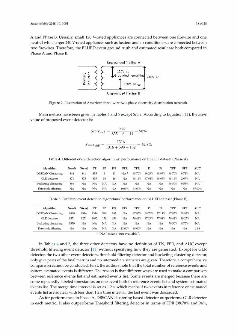
This section presents the performance of proposed DBSCAN clustering-based event detectorand makes a comparison with other three event detectors over BLUED dataset. A python evaluationtoolbox for sound event detection sed_eval is introduced to compare the estimated events list with thereference events list [55]. The other three detectors give no information about how reference eventsand estimated events are compared and this may lead to vagueness in algorithm comparison andreproduction. sed_eval is an evaluation toolbox designed in 2016 for polyphonic sound event detectionand it can be applied to NILM field directly without much revising. In sed_eval, a tolerance betweenreference events and estimated events collar needs to be specified. It means that, if the estimatedevent is located within the collar radius of reference event, it is considered as true positive. In thispaper, the authors set collar as 3.0 s. It is worth noting that BLUED dataset is constructed in America,where there are three electricity feed lines for ordinary houses: two firewires and one neutral line.As Figure 9 shows, the two firewires have 120 V amplitude of voltage and they are named as Phase

Sustainability 2018, 10, 1001 18 of 28

A and Phase B. Usually, small 120 V-rated appliances are connected between one firewire and oneneutral while larger 240 V-rated appliances such as heaters and air conditioners are connected betweentwo firewires. Therefore, the BLUED event ground truth and estimated result are both compared inPhase A and Phase B.

Figure 9. Illustration of American three-wire two-phase electricity distribution network.

Main metrics have been given in Tables 4 and 5 except Score. According to Equation (11), the Scorevalue of proposed event detector is:

ScorephA =835

835 + 6 + 11= 98%

ScorephB =1316

1316 + 598 + 182= 62.8%

Table 4. Different event detection algorithms’ performance on BLUED dataset (Phase A).

Algorithm N(ref) N(sys) TP FP FN FPR TPR P F1 TPP FPP AUC

DBSCAN Clustering 846 841 835 6 11 NA 1 98.70% 99.29% 98.99% 98.70% 0.71% NA

GLR detector 871 873 855 18 16 NA 98.16% 97.94% 98.05% 98.16% 2.07% NA

Bucketing clustering 886 NA NA NA NA NA NA NA NA 98.50% 0.55% NA

Threshold filtering NA NA NA NA NA 0.09% 94.00% NA NA NA NA 97.00%

Table 5. Different event detection algorithms’ performance on BLUED dataset (Phase B).

Algorithm N(ref) N(sys) TP FP FN FPR TPR P F1 TPP FPP AUC

DBSCAN Clustering 1498 1914 1316 598 182 NA 87.85% 68.76% 77.14% 87.85% 39.92% NA

GLR detector 1551 1251 1092 159 459 NA 70.41% 87.29% 77.94% 70.41% 10.25% NA

Bucketing clustering 1579 NA NA NA NA NA NA NA NA 70.50% 8.75% NA

Threshold filtering NA NA NA NA NA 12.00% 88.00% NA NA NA NA 0.941 “NA” means “not available”.

In Tables 4 and 5, the three other detectors have no definition of TN, FPR, and AUC exceptthreshold filtering event detector [11] without specifying how they are generated. Except for GLRdetector, the two other event detectors, threshold filtering detector and bucketing clustering detector,only give parts of the final metrics and no intermediate statistics are given. Therefore, a comprehensivecomparison cannot be conducted. First, the authors note that the total number of reference events andsystem estimated events is different. The reason is that different ways are used to make a comparisonbetween reference events list and estimated events list. Some events are merged because there aresome repeatedly labeled timestamps on one event both in reference events list and system estimatedevents list. The merge time interval is set as 1.2 s, which means if two events in reference or estimatedevents list are so near with less than 1.2 s time interval, the last event was discarded.

As for performance, in Phase A, DBSCAN clustering based detector outperforms GLR detectorin each metric. It also outperforms Threshold filtering detector in terms of TPR (98.70% and 94%,

Sustainability 2018, 10, 1001 19 of 28

respectively). Compared with Bucketing clustering detector, it has better performance in TPP (98.70%)while worse performance in FPP (0.71%). Threshold filtering event detector has the worst resultand clustering-based event detectors have better performance than the other two (TPP for DBSCANclustering event detector is 98.70% and for bucketing clustering, it is 98.5%). In Phase B, DBSCANdetector has higher TPR and TPP (87.85%) but it has many false positive (FP) events. Compared toPhase A, all the detectors have worse performance in Phase B. The main reason is that more eventsexist in Phase B and they distribute more intensively.

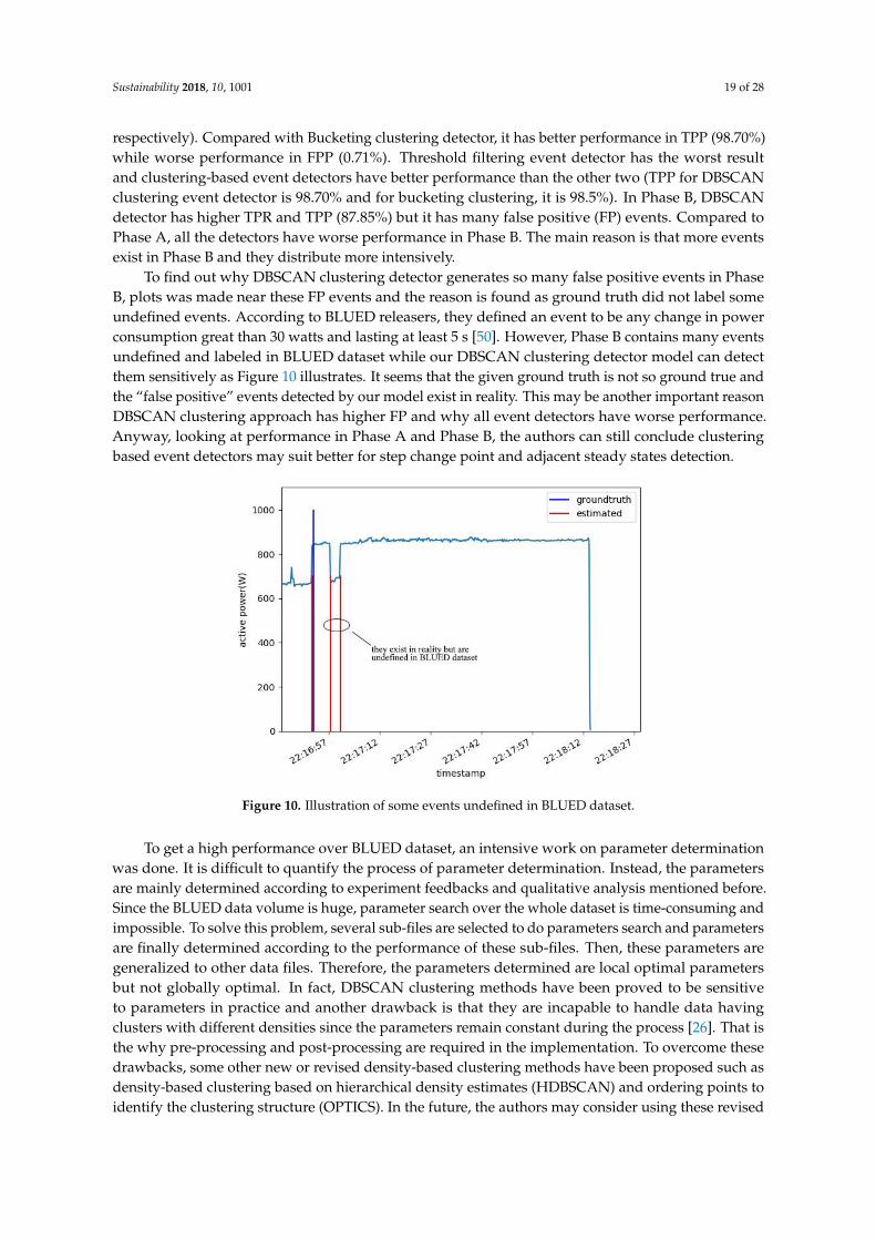
To find out why DBSCAN clustering detector generates so many false positive events in PhaseB, plots was made near these FP events and the reason is found as ground truth did not label someundefined events. According to BLUED releasers, they defined an event to be any change in powerconsumption great than 30 watts and lasting at least 5 s [50]. However, Phase B contains many eventsundefined and labeled in BLUED dataset while our DBSCAN clustering detector model can detectthem sensitively as Figure 10 illustrates. It seems that the given ground truth is not so ground true andthe “false positive” events detected by our model exist in reality. This may be another important reasonDBSCAN clustering approach has higher FP and why all event detectors have worse performance.Anyway, looking at performance in Phase A and Phase B, the authors can still conclude clusteringbased event detectors may suit better for step change point and adjacent steady states detection.

Figure 10. Illustration of some events undefined in BLUED dataset.

To get a high performance over BLUED dataset, an intensive work on parameter determinationwas done. It is difficult to quantify the process of parameter determination. Instead, the parametersare mainly determined according to experiment feedbacks and qualitative analysis mentioned before.Since the BLUED data volume is huge, parameter search over the whole dataset is time-consuming andimpossible. To solve this problem, several sub-files are selected to do parameters search and parametersare finally determined according to the performance of these sub-files. Then, these parameters aregeneralized to other data files. Therefore, the parameters determined are local optimal parametersbut not globally optimal. In fact, DBSCAN clustering methods have been proved to be sensitiveto parameters in practice and another drawback is that they are incapable to handle data havingclusters with different densities since the parameters remain constant during the process [26]. That isthe why pre-processing and post-processing are required in the implementation. To overcome thesedrawbacks, some other new or revised density-based clustering methods have been proposed such asdensity-based clustering based on hierarchical density estimates (HDBSCAN) and ordering points toidentify the clustering structure (OPTICS). In the future, the authors may consider using these revised

Sustainability 2018, 10, 1001 20 of 28

algorithms to do event detection, as no filtering block, easier parameter determination, and betterperformance are expected.

5.2. Event Classification on PLAID

The data in the PLAID dataset are all appliance level data containing 11 appliances with on–offstates: compact fluorescent lamp, laptop, vacuum, microwave, fan, hairdryer, air conditioner, fridge,heater, incandescent lightbulb, and washing machine. Since washing machine has variable currentwaveforms in practice and is not stable during operation, the authors discard washing machine fromconsideration. Harmonic decomposition is conducted over each record to construct experimentaldataset from PLAID. Then, it is split into a training dataset and a testing dataset with a ratio of 3:1to test the performance of harmonic-based classification over real-life data and the result is given bya normalized confusion matrix (Figure 11).

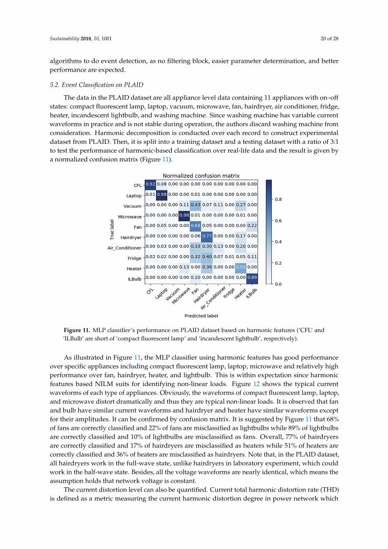
Figure 11. MLP classifier’s performance on PLAID dataset based on harmonic features (‘CFL’ and‘ILBulb’ are short of ‘compact fluorescent lamp’ and ‘incandescent lightbulb’, respectively).

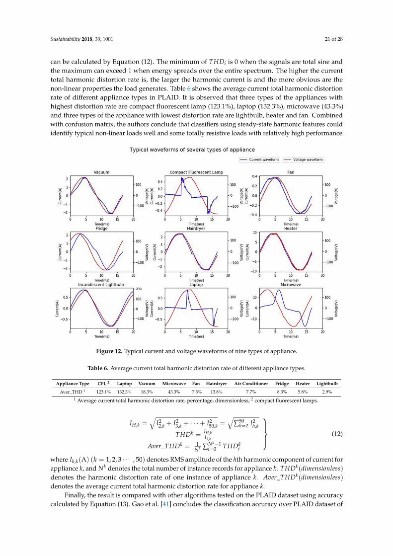
As illustrated in Figure 11, the MLP classifier using harmonic features has good performanceover specific appliances including compact fluorescent lamp, laptop, microwave and relatively highperformance over fan, hairdryer, heater, and lightbulb. This is within expectation since harmonicfeatures based NILM suits for identifying non-linear loads. Figure 12 shows the typical currentwaveforms of each type of appliances. Obviously, the waveforms of compact fluorescent lamp, laptop,and microwave distort dramatically and thus they are typical non-linear loads. It is observed that fanand bulb have similar current waveforms and hairdryer and heater have similar waveforms exceptfor their amplitudes. It can be confirmed by confusion matrix. It is suggested by Figure 11 that 68%of fans are correctly classified and 22% of fans are misclassified as lightbulbs while 89% of lightbulbsare correctly classified and 10% of lightbulbs are misclassified as fans. Overall, 77% of hairdryersare correctly classified and 17% of hairdryers are misclassified as heaters while 51% of heaters arecorrectly classified and 36% of heaters are misclassified as hairdryers. Note that, in the PLAID dataset,all hairdryers work in the full-wave state, unlike hairdryers in laboratory experiment, which couldwork in the half-wave state. Besides, all the voltage waveforms are nearly identical, which means theassumption holds that network voltage is constant.

The current distortion level can also be quantified. Current total harmonic distortion rate (THD)is defined as a metric measuring the current harmonic distortion degree in power network which

Sustainability 2018, 10, 1001 21 of 28

can be calculated by Equation (12). The minimum of THDi is 0 when the signals are total sine andthe maximum can exceed 1 when energy spreads over the entire spectrum. The higher the currenttotal harmonic distortion rate is, the larger the harmonic current is and the more obvious are thenon-linear properties the load generates. Table 6 shows the average current total harmonic distortionrate of different appliance types in PLAID. It is observed that three types of the appliances withhighest distortion rate are compact fluorescent lamp (123.1%), laptop (132.3%), microwave (43.3%)and three types of the appliance with lowest distortion rate are lightbulb, heater and fan. Combinedwith confusion matrix, the authors conclude that classifiers using steady-state harmonic features couldidentify typical non-linear loads well and some totally resistive loads with relatively high performance.

Figure 12. Typical current and voltage waveforms of nine types of appliance.

Table 6. Average current total harmonic distortion rate of different appliance types.

Appliance Type CFL 2 Laptop Vacuum Microwave Fan Hairdryer Air Conditioner Fridge Heater Lightbulb

Aver_THD 1 123.1% 132.3% 18.3% 43.3% 7.5% 13.8% 7.7% 8.3% 5.8% 2.9%1 Average current total harmonic distortion rate, percentage, dimensionless; 2 compact fluorescent lamps.

IH,k =√

I22,k + I2

3,k + · · ·+ I250,k =

√∑50

h=2 I2h,k

THDk =IH,kI1,k

Aver_THDk = 1Nk ∑Nk−1

i=0 THDki

(12)

where Ih,k(A) (h = 1, 2, 3 · · · , 50) denotes RMS amplitude of the hth harmonic component of current forappliance k, and Nk denotes the total number of instance records for appliance k. THDk(dimensionless)denotes the harmonic distortion rate of one instance of appliance k. Aver_THDk(dimensionless)denotes the average current total harmonic distortion rate for appliance k.

Finally, the result is compared with other algorithms tested on the PLAID dataset using accuracycalculated by Equation (13). Gao et al. [41] concludes the classification accuracy over PLAID dataset of

Sustainability 2018, 10, 1001 22 of 28

five classifiers using different features such as current, active/reactive power, harmonic, U-I image,etc. For algorithms using individual feature, the best classifier is random forest using U-I image withan accuracy of 81.75%. When all features are combined, the accuracy is improved to 86.03%. Alcaláclaims that the PQD-PCA classification algorithm outperforms the best classifier in the literature [41]with an accuracy of 88% [23]. However, one drawback of the PLAID dataset is that it only containsappliance instance data for training and does not contain aggregated data for testing. Therefore,although PQD-PCA algorithm outperforms other methods, it may decrease dramatically when appliedto aggregated signals for the sake of lousy additive property mentioned in Section 2. Although theMLP classifier using harmonic current features only have an accuracy of 75.38%, it is still valuablebecause it can identify some non-linear appliances accurately and harmonic features make it morepractical on its excellent additive property.

Acc =number o f correct predictionsnumber o f total predictions

(13)

5.3. Laboratory Validation by Combinational Experiments

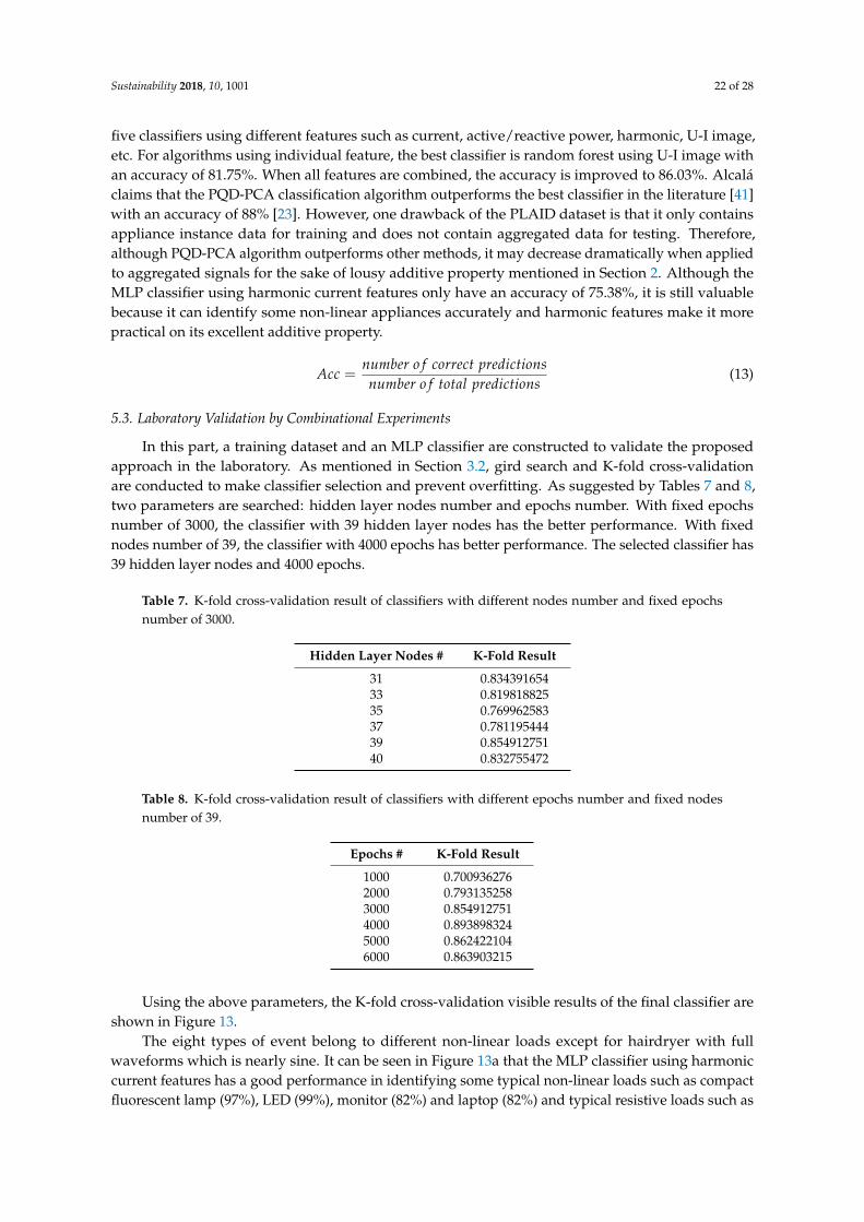
In this part, a training dataset and an MLP classifier are constructed to validate the proposedapproach in the laboratory. As mentioned in Section 3.2, gird search and K-fold cross-validationare conducted to make classifier selection and prevent overfitting. As suggested by Tables 7 and 8,two parameters are searched: hidden layer nodes number and epochs number. With fixed epochsnumber of 3000, the classifier with 39 hidden layer nodes has the better performance. With fixednodes number of 39, the classifier with 4000 epochs has better performance. The selected classifier has39 hidden layer nodes and 4000 epochs.

Table 7. K-fold cross-validation result of classifiers with different nodes number and fixed epochsnumber of 3000.

Hidden Layer Nodes # K-Fold Result

31 0.83439165433 0.81981882535 0.76996258337 0.78119544439 0.85491275140 0.832755472

Table 8. K-fold cross-validation result of classifiers with different epochs number and fixed nodesnumber of 39.

Epochs # K-Fold Result

1000 0.7009362762000 0.7931352583000 0.8549127514000 0.8938983245000 0.8624221046000 0.863903215

Using the above parameters, the K-fold cross-validation visible results of the final classifier areshown in Figure 13.

The eight types of event belong to different non-linear loads except for hairdryer with fullwaveforms which is nearly sine. It can be seen in Figure 13a that the MLP classifier using harmoniccurrent features has a good performance in identifying some typical non-linear loads such as compactfluorescent lamp (97%), LED (99%), monitor (82%) and laptop (82%) and typical resistive loads such as

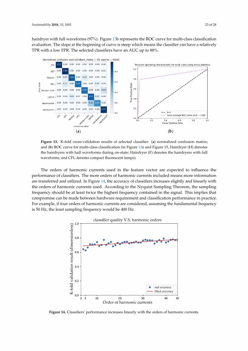
Sustainability 2018, 10, 1001 23 of 28

hairdryer with full waveforms (97%). Figure 13b represents the ROC curve for multi-class classificationevaluation. The slope at the beginning of curve is steep which means the classifier can have a relativelyTPR with a low FPR. The selected classifiers have an AUC up to 88%.

Figure 13. K-fold cross-validation results of selected classifier: (a) normalized confusion matrix;and (b) ROC curve for multi-class classification (in Figure 13a and Figure 15, Hairdryer (H) denotesthe hairdryers with half waveforms during on-state; Hairdryer (F) denotes the hairdryers with fullwaveforms; and CFL denotes compact fluorescent lamps).

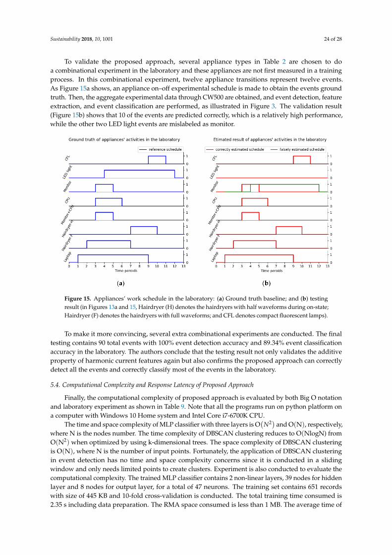
The orders of harmonic currents used in the feature vector are expected to influence theperformance of classifiers. The more orders of harmonic currents included means more informationare transferred and utilized. In Figure 14, the accuracy of classifiers increases slightly and linearly withthe orders of harmonic currents used. According to the Nyquist Sampling Theorem, the samplingfrequency should be at least twice the highest frequency contained in the signal. This implies thatcompromise can be made between hardware requirement and classification performance in practice.For example, if four orders of harmonic currents are considered, assuming the fundamental frequencyis 50 Hz, the least sampling frequency would be 400 Hz.

Figure 14. Classifiers’ performance increases linearly with the orders of harmonic currents.

Sustainability 2018, 10, 1001 24 of 28

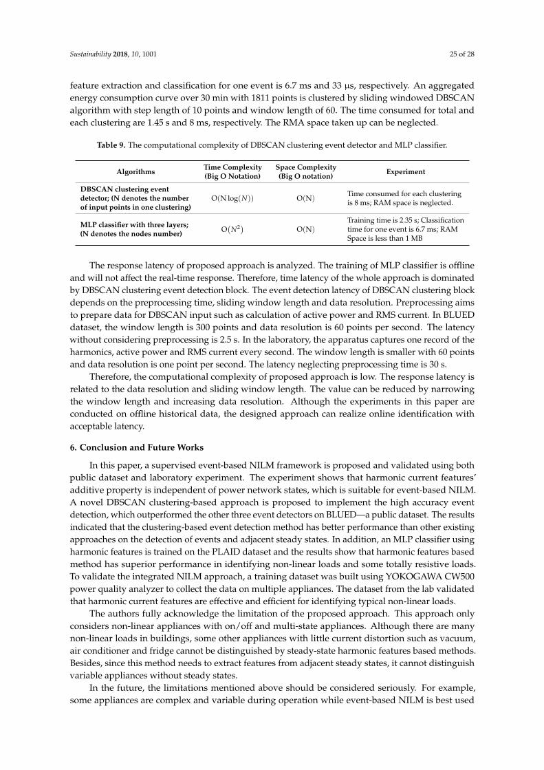
To validate the proposed approach, several appliance types in Table 2 are chosen to doa combinational experiment in the laboratory and these appliances are not first measured in a trainingprocess. In this combinational experiment, twelve appliance transitions represent twelve events.As Figure 15a shows, an appliance on–off experimental schedule is made to obtain the events groundtruth. Then, the aggregate experimental data through CW500 are obtained, and event detection, featureextraction, and event classification are performed, as illustrated in Figure 3. The validation result(Figure 15b) shows that 10 of the events are predicted correctly, which is a relatively high performance,while the other two LED light events are mislabeled as monitor.

Figure 15. Appliances’ work schedule in the laboratory: (a) Ground truth baseline; and (b) testingresult (in Figures 13a and 15, Hairdryer (H) denotes the hairdryers with half waveforms during on-state;Hairdryer (F) denotes the hairdryers with full waveforms; and CFL denotes compact fluorescent lamps).

To make it more convincing, several extra combinational experiments are conducted. The finaltesting contains 90 total events with 100% event detection accuracy and 89.34% event classificationaccuracy in the laboratory. The authors conclude that the testing result not only validates the additiveproperty of harmonic current features again but also confirms the proposed approach can correctlydetect all the events and correctly classify most of the events in the laboratory.

5.4. Computational Complexity and Response Latency of Proposed Approach

Finally, the computational complexity of proposed approach is evaluated by both Big O notationand laboratory experiment as shown in Table 9. Note that all the programs run on python platform ona computer with Windows 10 Home system and Intel Core i7-6700K CPU.

The time and space complexity of MLP classifier with three layers is O(

N2) and O(N), respectively,where N is the nodes number. The time complexity of DBSCAN clustering reduces to O(NlogN) fromO(N2) when optimized by using k-dimensional trees. The space complexity of DBSCAN clusteringis O(N), where N is the number of input points. Fortunately, the application of DBSCAN clusteringin event detection has no time and space complexity concerns since it is conducted in a slidingwindow and only needs limited points to create clusters. Experiment is also conducted to evaluate thecomputational complexity. The trained MLP classifier contains 2 non-linear layers, 39 nodes for hiddenlayer and 8 nodes for output layer, for a total of 47 neurons. The training set contains 651 recordswith size of 445 KB and 10-fold cross-validation is conducted. The total training time consumed is2.35 s including data preparation. The RMA space consumed is less than 1 MB. The average time of

Sustainability 2018, 10, 1001 25 of 28

feature extraction and classification for one event is 6.7 ms and 33 µs, respectively. An aggregatedenergy consumption curve over 30 min with 1811 points is clustered by sliding windowed DBSCANalgorithm with step length of 10 points and window length of 60. The time consumed for total andeach clustering are 1.45 s and 8 ms, respectively. The RMA space taken up can be neglected.

Table 9. The computational complexity of DBSCAN clustering event detector and MLP classifier.

Algorithms Time Complexity(Big O Notation)

Space Complexity(Big O notation) Experiment

DBSCAN clustering eventdetector; (N denotes the numberof input points in one clustering)

O(N log(N)) O(N)Time consumed for each clusteringis 8 ms; RAM space is neglected.

MLP classifier with three layers;(N denotes the nodes number) O

(N2) O(N)

Training time is 2.35 s; Classificationtime for one event is 6.7 ms; RAMSpace is less than 1 MB

The response latency of proposed approach is analyzed. The training of MLP classifier is offlineand will not affect the real-time response. Therefore, time latency of the whole approach is dominatedby DBSCAN clustering event detection block. The event detection latency of DBSCAN clustering blockdepends on the preprocessing time, sliding window length and data resolution. Preprocessing aimsto prepare data for DBSCAN input such as calculation of active power and RMS current. In BLUEDdataset, the window length is 300 points and data resolution is 60 points per second. The latencywithout considering preprocessing is 2.5 s. In the laboratory, the apparatus captures one record of theharmonics, active power and RMS current every second. The window length is smaller with 60 pointsand data resolution is one point per second. The latency neglecting preprocessing time is 30 s.

Therefore, the computational complexity of proposed approach is low. The response latency isrelated to the data resolution and sliding window length. The value can be reduced by narrowingthe window length and increasing data resolution. Although the experiments in this paper areconducted on offline historical data, the designed approach can realize online identification withacceptable latency.

6. Conclusion and Future Works

In this paper, a supervised event-based NILM framework is proposed and validated using bothpublic dataset and laboratory experiment. The experiment shows that harmonic current features’additive property is independent of power network states, which is suitable for event-based NILM.A novel DBSCAN clustering-based approach is proposed to implement the high accuracy eventdetection, which outperformed the other three event detectors on BLUED—a public dataset. The resultsindicated that the clustering-based event detection method has better performance than other existingapproaches on the detection of events and adjacent steady states. In addition, an MLP classifier usingharmonic features is trained on the PLAID dataset and the results show that harmonic features basedmethod has superior performance in identifying non-linear loads and some totally resistive loads.To validate the integrated NILM approach, a training dataset was built using YOKOGAWA CW500power quality analyzer to collect the data on multiple appliances. The dataset from the lab validatedthat harmonic current features are effective and efficient for identifying typical non-linear loads.

The authors fully acknowledge the limitation of the proposed approach. This approach onlyconsiders non-linear appliances with on/off and multi-state appliances. Although there are manynon-linear loads in buildings, some other appliances with little current distortion such as vacuum,air conditioner and fridge cannot be distinguished by steady-state harmonic features based methods.Besides, since this method needs to extract features from adjacent steady states, it cannot distinguishvariable appliances without steady states.

In the future, the limitations mentioned above should be considered seriously. For example,some appliances are complex and variable during operation while event-based NILM is best used

Sustainability 2018, 10, 1001 26 of 28

for the event with adjacent steady states. In this case, methods without detecting events and draftinghand-engineering features may work better such as deep neural network models. Moreover, differentalgorithms based on different features may be effective for certain types of appliances. Therefore,integrating complementary NILM models together is necessary and feasible.

Acknowledgments: This work was supported by the Shenzhen Science and Technology Funding Programs(JCYJ20150902162946055). The conclusions herein are those of the authors and do not necessarily reflect the viewsof the sponsoring agency.

Author Contributions: Xiaowei Luo and Zhuang Zheng conceived key ideas and designed the experiments;Zhuang Zheng performed the experiments; Zhuang Zheng and Hainan Chen analyzed the data; Zhuang Zhengwrote the paper; and Xiaowei Luo and Hainan Chen edited the paper.

Conflicts of Interest: The founding sponsors had no role in the design of the study; in the collection, analyses,or interpretation of data; in the writing of the manuscript, and in the decision to publish the results.

References

1. United States Department of Energy (U.S. DOE). Quadrennial Technology Review: An Assessment of EnergyTechnologies and Research Opportunities; U.S. DOE: Washington, DC, USA, 2015; pp. 1–505.

2. Gabaldón, A.; Álvarez, C.; Ruiz-Abellón, M.; Guillamón, A.; Valero-Verdú, S.; Molina, R.; García-Garre, A.Integration of Methodologies for the Evaluation of Offer Curves in Energy and Capacity Markets throughEnergy Efficiency and Demand Response. Sustainability 2018, 10, 483. [CrossRef]

3. Firth, S.; Lomas, K.; Wright, A.; Wall, R. Identifying trends in the use of domestic appliances from householdelectricity consumption measurements. Energy Build. 2008, 40, 926–936. [CrossRef]

4. Kong, W.; Dong, Z.Y.; Jia, Y.; Hill, D.J.; Xu, Y.; Zhang, Y. Short-Term Residential Load Forecasting based onLSTM Recurrent Neural Network. IEEE Trans. Smart Grid 2017, 3053, 1–11. [CrossRef]

5. Boait, P.; Gammon, R.; Advani, V.; Wade, N.; Greenwood, D.; Davison, P. ESCoBox: A set of tools formini-grid sustainability in the developing world. Sustainability 2017, 9, 738. [CrossRef]

6. Woyte, A.; Van Thong, V.; Belmans, R.; Nijs, J. Voltage fluctuations on distribution level introduced byphotovoltaic systems. IEEE Trans. Energy Convers. 2006, 21, 202–209. [CrossRef]

7. Albarracín, R.; Amarís, H. Power Quality in distribution power networks with photovoltaic energy sources.In Proceedings of the 8th EEEIC International Conference Environment and Electrical Engineering, Karpacz,Poland, 10–13 May 2009; pp. 360–363.

8. Albarracin, R.; Alonso, M. Photovoltaic reactive power limits. In Proceedings of the 12th EEEIC InternationalConference Environment and Electrical Engineering, Wroclaw, Poland, 5–8 May 2013; pp. 13–18. [CrossRef]

9. Karaki, S.H.; Chedid, R.B.; Ramadan, R. Probabilistic performance assessment of autonomous solar-windenergy conversion systems. IEEE Trans. Energy Convers. 1999, 14, 766–772. [CrossRef]

10. Hong, T.; Lin, H. Occupant Behavior: Impact on Energy Use of Private Offices. In Proceedings of the AsimIBSPA Asia Conference, Shanghai, China, 25–27 November 2012.

11. Liang, J.; Ng, S.K.K.; Kendall, G.; Cheng, J.W.M. Load signature studypart I: Basic concept, structure,and methodology. IEEE Trans. Power Deliv. 2010, 25, 551–560. [CrossRef]

12. Zeifman, M.; Roth, K. Nonintrusive Appliance Load Monitoring (NIALM): Review and Outlook. In Proceedingsof the International Conference on Consumer Electronics, Las Vegas, NV, USA, 9–12 January 2011; Volume 80,pp. 1–10. [CrossRef]

13. Mauch, L.; Yang, B. A new approach for supervised power disaggregation by using a deep recurrent LSTMnetwork. In Proceedings of the 2015 IEEE Global Conference on Signal and Information Processing (GlobalSIP),Orlando, FL, USA, 14–16 December 2015; pp. 63–67. [CrossRef]

14. Bonfigli, R.; Squartini, S.; Fagiani, M.; Piazza, F. Unsupervised algorithms for non-intrusive load monitoring:An up-to-date overview. In Proceedings of the IEEE 15th International Conference on Environment andElectrical Engineering, Rome, Italy, 10–13 June 2015; pp. 1175–1180. [CrossRef]

15. Kim, H.; Marwah, M.; Arlitt, M.F.; Lyon, G.; Han, J. Unsupervised Disaggregation of Low Frequency PowerMeasurements. In Proceedings of the 2011 SIAM International Conference on Data Mining, Mesa, AZ, USA,28–30 April 2011; pp. 747–758. [CrossRef]

Sustainability 2018, 10, 1001 27 of 28

16. Pattem, S. Unsupervised disaggregation for non-intrusive load monitoring. In Proceedings of the 201211th International Conference on Machine Learning and Applications (ICMLA), Boca Raton, FL, USA,12–15 December 2012; Volume 2, pp. 515–520. [CrossRef]

17. Kong, W.; Dong, Z.Y.; Hill, D.J. A Hierarchical Hidden Markov Model Framework for Home ApplianceModelling. IEEE Trans. Smart Grid 2016, 3053, 1. [CrossRef]

18. Bonfigli, R.; Principi, E.; Fagiani, M.; Severini, M.; Squartini, S.; Piazza, F. Non-intrusive load monitoringby using active and reactive power in additive Factorial Hidden Markov Models. Appl. Energy 2017, 208,1590–1607. [CrossRef]

19. Kolter, J.Z.; Batra, S.; Ng, A.Y. Energy disaggregation via discriminative sparse coding. In Advances in NeuralInformation Processing Systems; MIT Press: Cambridge, MA, USA, 2010; pp. 1153–1161.

20. Figueiredo, M.; Ribeiro, B.; DeAlmeida, A. Electrical signal source separation via nonnegative tensorfactorization using on site measurements in a smart home. IEEE Trans. Instrum. Meas. 2014, 63, 364–373.[CrossRef]

21. Kolter, Z.; Jaakkola, T.; Kolter, J.Z. Approximate Inference in Additive Factorial HMMs with Applicationto Energy Disaggregation. In Proceedings of the International Conference on Artificial Intelligence andStatistics, La Palma, Spain, 21–23 April 2012; Volume XX, pp. 1472–1482.

22. Dinesh, C.; Welikala, S.; Liyanage, Y.; Ekanayake, M.P.B.; Godaliyadda, R.I.; Ekanayake, J. Non-intrusiveload monitoring under residential solar power influx. Appl. Energy 2017, 205, 1068–1080. [CrossRef]

23. Alcalá, J.; Ureña, J.; Hernández, Á.; Gualda, D. Event-based Energy Disaggregation Algorithm for ActivityMonitoring from a Single-Point sensor. IEEE Trans. Instrum. Meas. Rev. 2017, 66, 2615–2626. [CrossRef]

24. Hart, G.W. Nonintrusive Appliance Load Monitoring. Proc. IEEE 1992, 80, 1870–1891. [CrossRef]25. Srinivasan, D.; Ng, W.S.; Liew, A.C. Neural-network-based signature recognition for harmonic source

identification. IEEE Trans. Power Deliv. 2006, 21, 398–405. [CrossRef]26. Kelly, J.; Knottenbelt, W. Neural NILM: Deep Neural Networks Applied to Energy Disaggregation.

In Proceedings of the 2nd ACM International Conference on Embedded Systems for Energy-EfficientBuilt Environments, Seoul, Korea, 4–5 November 2015; pp. 55–64. [CrossRef]

27. Mauch, L.; Yang, B. A novel DNN-HMM-based approach for extracting single loads from aggregate powersignals. In Proceedings of the 2016 IEEE International Conference on Acoustics, Speech and Signal Processing(ICASSP), Shanghai, China, 20–25 March 2016; pp. 2384–2388.

28. Paulo, P. Applications of Deep Learning Techniques on Nilm. Ph.D. Thesis, Universidade Federal do Rio deJaneiro, Rio de Janeiro, Brazil, 2016; pp. 4–6.

29. Basu, K.; Debusschere, V.; Bacha, S.; Hably, A.; VanDelft, D.; Jan Dirven, G. A generic data driven approachfor low sampling load disaggregation. Sustain. Energy Grids Netw. 2017, 9, 118–127. [CrossRef]

30. Liu, C.; Akintayo, A.; Jiang, Z.; Henze, G.P.; Sarkar, S. Multivariate exploration of non-intrusive loadmonitoring via spatiotemporal pattern network. Appl. Energy 2018, 211, 1106–1122. [CrossRef]

31. Tabatabaei, S.M.; Dick, S.; Xu, W. Toward Non-Intrusive Load Monitoring via Multi-Label Classification.IEEE Trans. Smart Grid 2017, 8, 26–40. [CrossRef]

32. Zeifman, M.; Roth, K. Nonintrusive appliance load monitoring: Review and outlook. IEEE Trans.Consum. Electron. 2011, 57, 76–84. [CrossRef]

33. Streubel, R.; Yang, B. Identification of electrical appliances via analysis of power consumption. In Proceedingsof the 2012 47th International Universities Power Engineering Conference (UPEC), Uxbridge, UK,4–7 September 2012; pp. 1–6. [CrossRef]

34. Barsim, K.S.; Streubel, R.; Yang, B. Unsupervised Adaptive Event Detection for Building-Level EnergyDisaggregation. In Proceedings of the Power and Energy Student Summt (PESS), Stuttgart, Germany,23–24 January 2014; pp. 1–6.

35. Wang, A.L.; Chen, B.X.; Wang, C.G.; Hua, D. Non-intrusive load monitoring algorithm based on features ofV–I trajectory. Electr. Power Syst. Res. 2018, 157, 134–144. [CrossRef]

36. Bonfigli, R.; Felicetti, A.; Principi, E.; Fagiani, M.; Squartini, S.; Piazza, F. Denoising autoencoders forNon-Intrusive Load Monitoring: Improvements and comparative evaluation. Energy Build. 2018, 158,1461–1474. [CrossRef]

37. Jeltsema, D. Budeanu’s concept of reactive and distortion power revisited. In Proceedings of the2015 International School on Nonsinusoidal Currents and Compensation (ISNCC), Lagow, Poland,15–18 June 2015; pp. 68–73. [CrossRef]

Sustainability 2018, 10, 1001 28 of 28

38. Slonim, M.A.; Van derWyk, J.D. Power components in a system with sinusoidal and nonsinusoidal voltagesand/or currents. IEE Proc. B Electr. Power Appl. 1988, 135, 76–84. [CrossRef]

39. Sun, S.; Xiang, Q.R. Waveform distortion and distortion power. IEE Proc. B Electr. Power Appl. 1992, 139,303–306. [CrossRef]

40. Lam, H.Y.; Fung, G.S.K.; Lee, W.K. A novel method to construct taxonomy electrical appliances based onload signatures. IEEE Trans. Consum. Electron. 2007, 53, 653–660. [CrossRef]

41. Gao, J.; Kara, E.C.; Giri, S.; Berges, M. A feasibility study of automated plug-load identification fromhigh-frequency measurements. In Proceedings of the 2015 IEEE Global Conference on Signal and InformationProcessing (GlobalSIP), Orlando, FL, USA, 14–16 December 2015; pp. 220–224. [CrossRef]

42. Chan, W.L.; So, A.T.; Lai, L.L. Harmonics load signature recognition by wavelets transforms. In Proceedingsof the International Conference on Electric Utility Deregulation and Restructuring and Power Technologies,DRPT2000, London, UK, 4–7 April 2000.

43. Martins, J.F.; Lopes, R.; Lima, C.; Romero-Cadaval, E.; Vinnikov, D. A novel nonintrusive load monitoringsystem based on the S-Transform. In Proceedings of the 13th International Conference on Optimization ofElectrical and Electronic Equipment, Brasov, Romania, 24–26 May 2012; pp. 973–978. [CrossRef]

44. Jimenez, Y.; Duarte, C.; Petit, J.; Carrillo, G. Feature extraction for nonintrusive load monitoring based onS-Transform. In Proceedings of the Clemson University Power Systems Conference, Clemson, SC, USA,11–14 March 2014; pp. 1–5. [CrossRef]

45. Gabaldón, A.; Ortiz-García, M.; Molina, R.; Valero-Verdú, S. Disaggregation of the electric loads of smallcustomers through the application of the Hilbert transform. Energy Effic. 2014, 7, 711–728. [CrossRef]

46. Daszykowski, M.; Walczak, B. Density-Based Clustering Methods. Compr. Chemom. 2010, 2, 635–654.[CrossRef]

47. Aminikhanghahi, S.; Cook, D.J. A survey of methods for time series change point detection. Knowl. Inf. Syst.2017, 51, 339–367. [CrossRef] [PubMed]

48. Hosseini, S.S.; Agbossou, K.; Kelouwani, S.; Cardenas, A. Non-intrusive load monitoring through homeenergy management systems: A comprehensive review. Renew. Sustain. Energy Rev. 2017, 79, 1266–1274.[CrossRef]

49. Kolter, J.Z.; Johnson, M.J. REDD: A Public Data Set for Energy Disaggregation Research. In Proceedings ofthe SustKDD Work, San Diego, CA, USA, 21 August 2011; pp. 1–6.

50. Anderson, K.; Ocneanu, A.F.; Benitez, D.; Carlson, D.; Rowe, A.; Bergés, M. BLUED: A Fully Labeled PublicDataset for Event-Based Non-Intrusive Load Monitoring Research. In Proceedings of the 2nd Workshop onData Mining Applications in Sustainability (SustKDD), Beijing, China, 12 August 2012; pp. 1–5.

51. Gao, J.; Giri, S.; Kara, E.C.; Bergés, M. PLAID: A public dataset of high-resoultion electrical appliancemeasurements for load identification research. In Proceedings of the 1st ACM Conference on EmbeddedSystems for Energy-Efficient Buildings, Memphis, TN, USA, 4–6 November 2014; pp. 198–199.

52. Zhang, F.; Geng, Z.; Yuan, W. The algorithm of interpolating windowed FFT for harmonic analysis of electricpower system. IEEE Trans. Power Deliv. 2001, 16, 160–164. [CrossRef]

53. Benitez, D.; Anderson, K.D.; Bergest, M.E.; Ocneanut, A.; Benitez, D.; Moura, J.M.P. Event detection for NonIntrusive load monitoring Event Detection for Non Intrusive Load Monitoring. In Proceedings of the IECON2012—38th Annual Conference on IEEE Industrial Electronics Society, Montreal, QC, Canada, 25–28 October 2012;pp. 3312–3317. [CrossRef]

54. Dixon, S. On the computer recognition of solo piano music. In Proceedings of the Australasian ComputerMusic Conference, Brisbane, Australia, July 2000; pp. 31–37.

55. Mesaros, A.; Heittola, T.; Virtanen, T. Metrics for Polyphonic Sound Event Detection. Appl. Sci. 2016, 6, 162.[CrossRef]

© 2018 by the authors. Licensee MDPI, Basel, Switzerland. This article is an open accessarticle distributed under the terms and conditions of the Creative Commons Attribution(CC BY) license (http://creativecommons.org/licenses/by/4.0/).