Commission of the European Communities

technical steel researc

Properties and service performance

Seismic resistance of composite structures SRCS

Ρ Commission of the European Communities

Properties and service performance

Seismic resistance of composite structures SRCS

Department manager J.B. Schleich

Ingénieur civil des constructions Chef de service

Project manager R. Pepin

Ingénieur diplômé EPFZ Service recherches et promotion techniques structures

(RPS) Arbed­recherches

66, rue de Luxembourg L­4002 Esch/AIzette

Contract No 7210­SA/506 (1.7.1987­31.12.1990)

Final report

Directorate­General Science, Research and Development

1992

PARL EURC­P. Dbïioth.

N.C. E U R 14428 EN

C1.

Published by the COMMISSION OF THE EUROPEAN COMMUNITIES

Directorate-General Information Technologies and Industries, and Telecommunications

L-2920 Luxembourg

LEGAL NOTICE Neither the Commission of the European Communities nor any person acting on behalf of the Commission is responsible for the use which might

be made of the following information

Cataloguing data can be found at the end of this publication

Luxembourg: Office for Official Publications of the European Communities, 1992

ISBN 92-826-4667-X

© ECSC-EEC-EAEC, Brussels · Luxembourg, 1992

Printed in Luxembourg

C O N F I D E N T I A L

Title of Research:

Agreement :

Executive Committee:

Commencement of Research:

Seismic Resistance of Composite Structures (S.R.C.S.)

N°7210-SA/506

F6

01.07.1987

1 st Scheduled Completion Date: 30.06.1990

Extended Completion Date: 31.12.1990

Beneficiary:

Technical Support:

Software Developments:

ARBED-Luxembourg

Service Ponts et Charpentes, Université de Liège (B)

Dipartimento di Ingegneria Strutturale, Politecnico di Milano (I)

Institut für Stahlbau und Werkstoffmechanik, Technische Hochschule Darmstadt (D)

Lehrstuhl für Baustofftechnologie und Brandschutz, Bergische Universität Wuppertal (D)

Lehrstuhl für Stahlbau, RWTH Aachen (D)

ACKNOWLEDGEMENTS During over three and a half year, five European universities collaborated with an European steel producer in order to analyze the behaviour of composite structures under earthquake action from a common European point of view. This international cooperation, which in our minds gives already a taste what can be the European Community of tomorrow, became only possible by the generous sponsorship of C.E.C., the Commission of the European Community.

Therefore, we want to acknowledge first of all the important financial support from the Commission of the European Community, as well as the moral support given to this research by the ECSC Executive Committee F6 "Steel Structures", former committee F8 "Light Weight Structures".

Special thanks are due to the scientific contributors to this research, namely: ■ Prof. SEDLACEK, Dipl. Ing. KUCK and Dipl. Ing. HOFFMEISTER from

the RWTH Aachen

■ Prof. BOUWKAMP, Dipl. Ing. SCHNEIDER and Dipl. Ing. KANZ from the TH Darmstadt,

■ Dr. Ir. PLUMIER and Dipl. Ing. TUNHUS from the University of Liège,

■ Prof. BALLIO from the Politecnico di Milano and

■ Prof. KLINGSCH, Dipl. Ing. HAMME and Dipl. Ing. KOENIG from the BU Wuppertal.

Thanks to their experience in the field of seismic action, fire action and composite structures, it was possible to analyze the cohabitation of these three factors. As most of the participants are also involved very closely in the elaboration of European standards and guidelines, there is a serious hope that the results obtained during this research will not end in a lonely drawer, but will be taken into account within these standards.

We also wish to record our appreciation of the efforts and cooperation of the laboratories in Darmstadt, Liège, Milan and Wuppertal, which executed the 50 tests with an excellent knowledge and experience, as well as of the workshops involved in the fabrication of the test specimens and the testing installations.

Finally, thanks are due to all, who by any means may have contributed tothe success of the present research.

-v -

Research: "SEISMIC RESISTANCE OF COMPOSITE STRUCTURES"

Agreement 7210-SA/506 C.E.C. - ARBED

SUMMARY The first period of this research was devoted to the realization of nearly quasi-static cyclic 50 tests on full sized composite specimen which may be divided in four series:

■ Series 1 : tests on T-shaped exterior column/beam joints ■ Series 2: tests on cross-shaped interior columns/beam joints ■ Series 3: tests on complete frames ■ Series 4: partial tests on different elements

During each of these series different types of connections were analyzed. As the series were realized successively, the specimens could be continously improved. Several tests realized in series 3 are among the biggest ones ever realized in Europe.

A second period allowed to develop a numerical code, which can simulate concrete structures under seismic action by taking into account geometrical non-linearities as well as the elasto-plastic behaviour of steel and the deterioration of concrete.

The present research showed that it is interesting of using composite structures in earthquake prone zones, as

■ concrete increases the resistance by about 50% in the elastic field

■ concrete increases the stiffness

■ concrete largely prevents local buckling

■ concrete contributes to the shear panel behaviour

■ after complete concrete crushing the structure behaves always like a bare steel structure when submitted to very large displacements

VII -

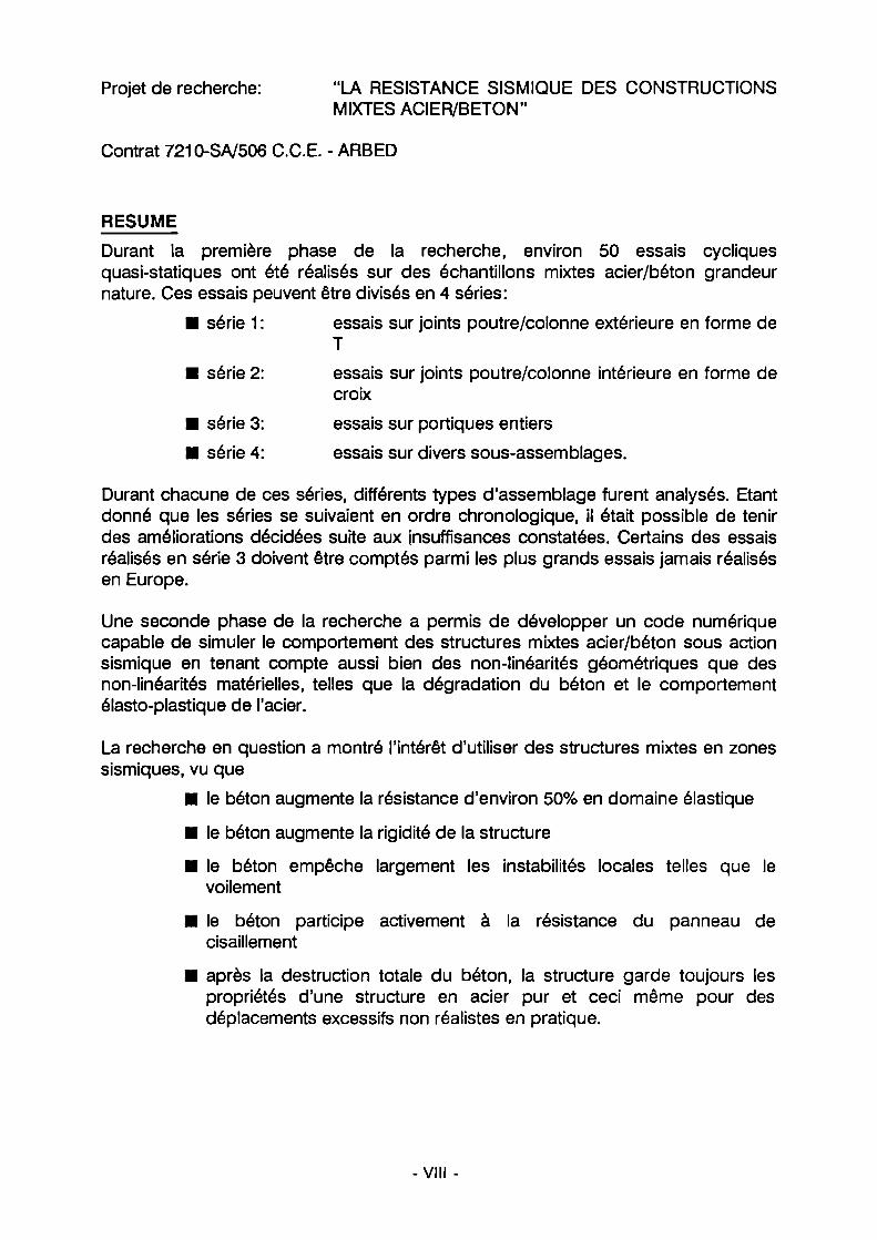
Projet de recherche: "LA RESISTANCE SISMIQUE DES CONSTRUCTIONS MIXTES ACIER/BETON"

Contrat 7210-SA/506 C.C.E. - ARBED

RESUME Durant la première phase de la recherche, environ 50 essais cycliques quasi-statiques ont été réalisés sur des échantillons mixtes acier/béton grandeur nature. Ces essais peuvent être divisés en 4 séries:

■ série 1 : essais sur joints poutre/colonne extérieure en forme de Τ

■ série 2: essais sur joints poutre/colonne intérieure en forme de croix

■ série 3: essais sur portiques entiers ■ série 4: essais sur divers sous-assemblages.

Durant chacune de ces séries, différents types d'assemblage furent analysés. Etant donné que les séries se suivaient en ordre chronologique, il était possible de tenir des améliorations décidées suite aux insuffisances constatées. Certains des essais réalisés en série 3 doivent être comptés parmi les plus grands essais jamais réalisés en Europe.

Une seconde phase de la recherche a permis de développer un code numérique capable de simuler le comportement des structures mixtes acier/béton sous action sismique en tenant compte aussi bien des non-linéarités géométriques que des non-linéarités matérielles, telles que la dégradation du béton et le comportement élasto-plastique de l'acier.

La recherche en question a montré l'intérêt d'utiliser des structures mixtes en zones sismiques, vu que

■ le béton augmente la résistance d'environ 50% en domaine élastique

■ le béton augmente la rigidité de la structure

■ le béton empêche largement les instabilités locales telles que le vouement

■ le béton participe activement à la résistance du panneau de cisaillement

■ après la destruction totale du béton, la structure garde toujours les propriétés d'une structure en acier pur et ceci même pour des déplacements excessifs non réalistes en pratique.

-VIII -

Forschungsprojekt: "ERDBEBENSICHERHEIT VON VERBUND­

KONSTRUKTIONEN"

Forschungsauftrag 7210­SA/506 K.EG. ­ ARBED

ZUSAMMENFASSUNG In einer ersten Phase wurden ca. 50 Versuche an Verbundprüfkörpern im Massstab 1:1 durchgeführt. Diese Versuche lassen sich in vier Klassen einteilen:

■ Reihe 1 : Versuche an T­förmigen Aussenstütze/Träger­

Verbindungen ■ Reihe 2: Versuche an kreuzförmigen Innenstütze/Träger­

Verbindungen ■ Reihe 3: Versuche an vollständigen Rahmensystemen ■ Reihe 4: Versuche an verschiedenen zusätzlichen Anschlüssen

Während jeder dieser Reihen wurden verschiedene Anschlusstypen analysiert. Da die Versuchsreihen sich zeitlich folgten, war es möglich Verbesserungsvorschläge aus vorhergehenden Versuchen zu berücksichtigen. Einige der Versuche in Reihe 3 zählen zu den grössten Versuchen die je in Europa durchgeführt wurden.

Ein zweiter Schritt galt der Entwicklung eines numerischen Modells, das es ermöglichte Verbundkonstruktionen unter Erdbebenbelastung rechnerisch zu erfassen. Hierbei werden sowohl Verformungsanteile zweiter Ordnung als auch materielles nicht lineares Verhalten wie Betonzerstörung und Stahlfliessen berücksichtigt.

Das vorliegende Forschungsprojekt zeigte, dass die Anwendung von Verbundkonstruktionen in Erdbebengebieten durchaus interessant ist, da

■ der Beton die Tragfähigkeit der Struktur um bis zu 50% im elastischen Bereich erhöht

■ der Beton zu grösseren Steifigkeiten führt

■ der Beton lokale Instabilitäten wie Beulen teilweise behindert

■ der Beton massgeblich zum Tragverhalten des Schubpanels mitbeiträgt

■ nach der Zerstörung des Betons, die Struktur sich weiterhin wie eine reine Stahlkonstruktion verhält und dies auch unter sehr grossen Verformungen

IX­

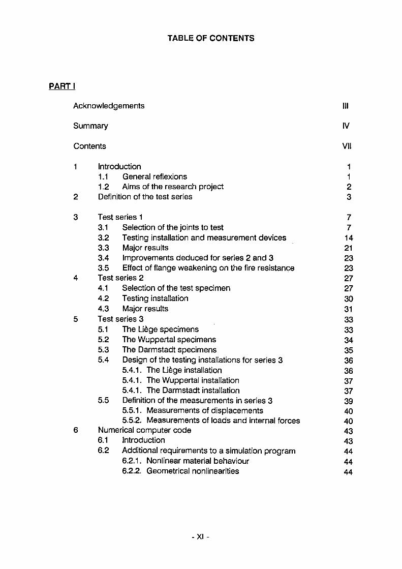
TABLE OF CONTENTS

PARTI

Acknowledgements III

Summary IV

Contents VII

1 Introduction 1 1.1 General reflexions 1 1.2 Aims of the research project 2

2 Definition of the test series 3

3 Test series 1 7 3.1 Selection of the joints to test 7 3.2 Testing installation and measurement devices 14 3.3 Major results 21 3.4 Improvements deduced for series 2 and 3 23 3.5 Effect of flange weakening on the fire resistance 23

4 Test series 2 27 4.1 Selection of the test specimen 27 4.2 Testing installation 30 4.3 Major results 31

5 Test series 3 33 5.1 The Liège specimens 33 5.2 The Wuppertal specimens 34 5.3 The Darmstadt specimens 35 5.4 Design of the testing installations for series 3 36

5.4.1. The Liège installation 36 5.4.1. The Wuppertal installation 37 5.4.1. The Darmstadt installation 37

5.5 Definition of the measurements in series 3 39 5.5.1. Measurements of displacements 40 5.5.2. Measurements of loads and internal forces 40

6 Numerical computer code 43 6.1 Introduction 43 6.2 Additional requirements to a simulation program 44

6.2.1. Nonlinear material behaviour 44 6.2.2. Geometrical nonlinearities 44

XI

6.2.3. Shear forces 44 6.2.4. Load history and strength degradation 44 6.2.5. Short calculation time 44 6.2.6. Additional requirements 44

6.3 Implementation of the requires features 45 6.3.1. Nonlinear material behaviour 45 6.3.2. Geometrical nonlineahties 47 6.3.3. Modelling of the beam-to-column and shear panel 47 6.3.4. Load history and strength degradation 48 6.3.5. Short calculation time 51 6.3.6. Additional features 51

6.4 Examples of calculation 51 6.4.1. Simulation of the beam-to-column connection tests 51 6.4.2. Cyclic behaviour of a frame 53 6.4.3. Frame under earthquake action 53

7 Recommendations from the amendment and complexion of EC 8 57

8 Recommendations to improve ECCS document 45 59 8.1 Introduction 59 8.2 Proposed modifications 60

9 Economic interest of using composite structures 65

10 Conclusions 69 10.1 General remarks 69 10.2 Standards and recommendations 70 10.3 Designproblems 71 10.4 Manufacturing and quality insurance problems 71

Bibliography 73

PART II

Appendix A Test report of the Milan laboratory 75

Appendix Β Test report of the Liège laboratory 201

Appendix C Test report of the Wuppertal laboratory 279

Appendix D Test report of the Darmstadt laboratory 339

Appendix E Material lists from comparing concrete to 441 composite structures

-XII

Chapter 1

INTRODUCTION

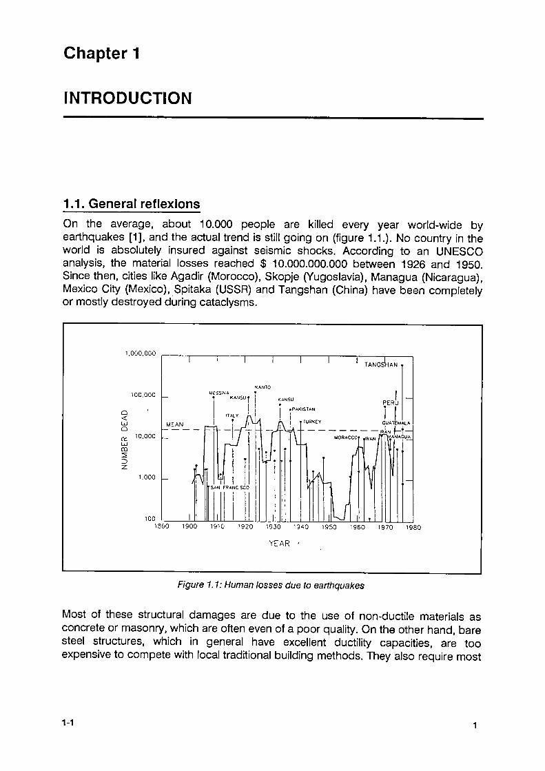
1.1. General reflexions On the average, about 10.000 people are killed every year world-wide by earthquakes [1], and the actual trend is still going on (figure 1.1.). No country in the world is absolutely insured against seismic shocks. According to an UNESCO analysis, the material losses reached $ 10.000.000.000 between 1926 and 1950. Since then, cities like Agadir (Morocco), Skopje (Yugoslavia), Managua (Nicaragua), Mexico City (Mexico), Spitaka (USSR) and Tangshan (China) have been completely or mostly destroyed during cataclysms.

1.000.000

100,000

α < υ Q

CC LU m

10,000

1.000

100

Ί Ι Γ

MESSINA t KANSU t

TANGSHAN τ

MEAN

1390 1900 1910 '920 1930 1910 1950 1960 1970 1980

YEAR '

Figure 1.1: Human losses due to earthquakes

Most of these structural damages are due to the use of non-ductile materials as concrete or masonry, which are often even of a poor quality. On the other hand, bare steel structures, which in general have excellent ductility capacities, are too expensive to compete with local traditional building methods. They also require most

1-1

of the time on adequate fire protection in order to resist the fires following in general an earthquake.

In that case, composite structures offer a good compromise between tradition and safety: They are more ductile than reinforced concrete structures, yet they are stiffer and less prove to buckling than steel structures [2] and they have very good fire resistance properties. Very often composite buildings are erected by concrete contractors. Unfortunately up to nowadays composite structures in aseismic design were only used in Japan as concrete encased structures.

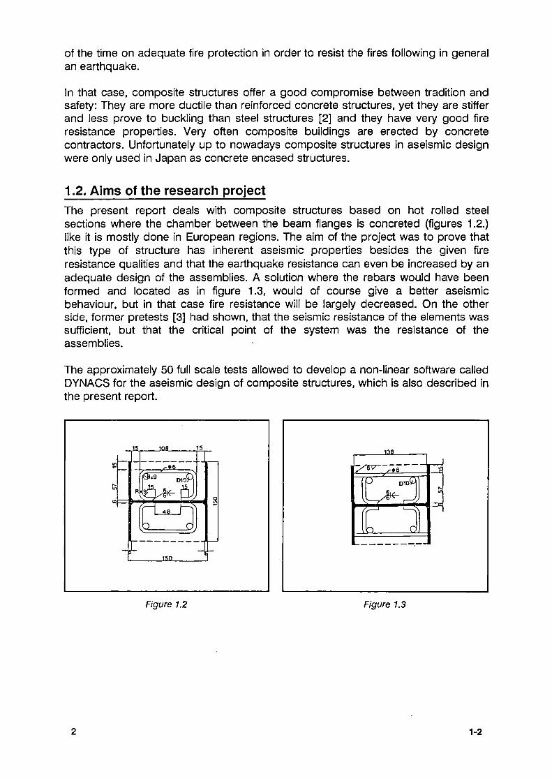
1.2. Aims of the research project The present report deals with composite structures based on hot rolled steel sections where the chamber between the beam flanges is concreted (figures 1.2.) like it is mostly done in European regions. The aim of the project was to prove that this type of structure has inherent aseismic properties besides the given fire resistance qualities and that the earthquake resistance can even be increased by an adequate design of the assemblies. A solution where the rebars would have been formed and located as in figure 1.3, would of course give a better aseismic behaviour, but in that case fire resistance will be largely decreased. On the other side, former pretests [3] had shown, that the seismic resistance of the elements was sufficient, but that the critical point of the system was the resistance of the assemblies.

The approximately 50 full scale tests allowed to develop a non-linear software called DYNACS for the aseismic design of composite structures, which is also described in the present report.

Figure 1.2 Figure 1.3

1-2

Chapter 2

DEFINITION OF THE TEST SERIES

Several tests realized in Milan before 1987 on composite columns [3] have shown a good behaviour when comparing the results to those obtained on equivalent bare steel columns:

■ the stiffness of the structure was increased

■ the elastic moment was considerably higher for the composite specimens

■ the local buckling of the steel section flanges was largely restrained due to the presence of concrete poured between the flanges, avoiding this way clearly low cycle fatigue failure.

As the structural elements seemed to be alright, the main effort was then devoted to the design of the connections. This item was of a crucial importance, as:

■ joints designed for fire resistance and/or for normal static loads are not necessary automatically resistant to cyclic loads

■ hinges and semi-rigid connections lead to higher inter-storey drift when submitted to horizontal forces, inducing by that way higher second order effects, called also Ρ-δ effects.

Among the various types of composite sections, the AF-system (figure 2.1.) was retained for testing, as it is one of the most popular European composite building system. The AF (anti-fire) system was developed by ARBED in collaboration with Prof. JUNGBLUTH from the Technical University of Darmstadt (D) [4],[5]. The AF-technology offers a good fire resistance, while showing the steel profiles and without loosing the advantages of steel structures for connections for instance. The total weight of this kind of structures is smaller than for a reinforced -

Figure 2.1: AF-column

2-1

concrete structure and the dimensions of the different elements are also reduced.

Further developments [6] on the original system led to the creation of an universal fire-resistant composite system and to the elaboration of an adequate numerical computer code called CEFICOSS, calibrated by 15 full-scale fire tests. By these means, ARBED was well positioned to realize the present research work on the given AF-system.

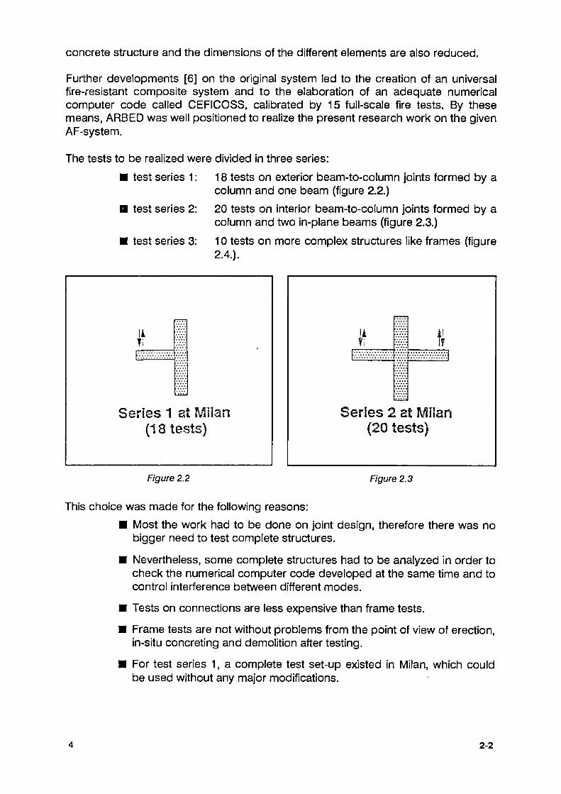
The tests to be realized were divided in three series: ■ test series 1 :

test series 2:

test series 3:

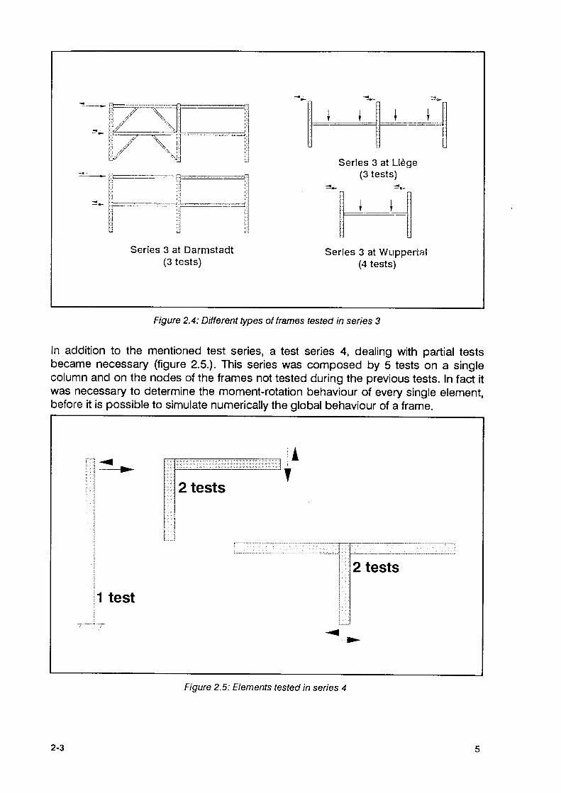
18 tests on exterior beam-to-column joints formed by a column and one beam (figure 2.2.) 20 tests on interior beam-to-column joints formed by a column and two in-plane beams (figure 2.3.) 10 tests on more complex structures like frames (figure 2.4.).

Series 1 ai Milan (18 tests)

Figure 2.2

ti

Series 2 at Milan (20 tests)

Figure 2.3

This choice was made for the following reasons: ■ Most the work had to be done on joint design, therefore there was no

bigger need to test complete structures.

■ Nevertheless, some complete structures had to be analyzed in order to check the numerical computer code developed at the same time and to control interference between different modes.

■ Tests on connections are less expensive than frame tests.

■ Frame tests are not without problems from the point of view of erection, in-situ concreting and demolition after testing.

■ For test series 1, a complete test set-up existed in Milan, which could be used without any major modifications.

2-2

- ^ ­ ­ η

f

1 Τ ^ Ν Γ " \f "Η

i·

t.

Series 3 at Darmstadt (3 tests)

­̂ . ­

\ \

­ * j

ι * 1 i í

Series 3 at Liège 13 testsï

=*­ — «­

1 í

i]

Series 3 at Wupp« (4 tests)

3 rial

Figure 2.4: Different types of frames tested in series 3

In addition to the mentioned test series, a test series 4, dealing with partial tests became necessary (figure 2.5.). This series was composed by 5 tests on a single column and on the nodes of the frames not tested during the previous tests. In fact it was necessary to determine the moment­rotation behaviour of every single element, before it is possible to simulate numerically the global behaviour of a frame.

L.J

2 tests

|1 test

2 tests

Figure 2.5: Elements tested in series 4

2­3

While test series 1 and 2 were realized in Milan, test series 3 was divided between Darmstadt, Liège and Wuppertal. Series 4 was done in Darmstadt, as the nodes to be tested corresponded all to the Darmstadt frames.

All the tests were realized on full-scale specimen, as it is very difficult to simulate the behaviour of non-heterogenous structures like composite ones on reduced scale models (for instance half-scale as it is often used in seismic engineering).

Regarding the testing procedure, a cyclic but quasi-static loading was chosen as this is the most convenient method when testing both connection and frames. The tests were carried out according to the relative ECCS procedures [7]. These guide-lines allowed to obtain comparable results at the different testing sites. The design of the specimens was done according to Eurocode 3 [8] and Eurocode 8 [9]. In order to show the benefit of composite structures each type of joint was also tested on a reference bare steel specimen.

The sections used during the whole project were HEB 300 for columns, HEA 260 for beams and slabs of 1000 mm width and 120 mm thickness. Steel grade was Fe 360 for structural steels and Fe 510 for plates while concrete used was of grade C25. All the sections were designed according to the tables of [10] and [11].

2-4

Chapter 3

TEST SERIES 1

3.1. Selection of the joints to test

Originally, 21 types of connection were proposed for testing. After discussion, six types named type A to F were retained, among which were as well bolted as welded specimens. The characteristics of each type and of his derivations are given on the following specification sheets. The choice of the specimens was made by the way to obtain existing joints to be used occasionally together with other, more moment resisting joints or with concrete cores or bracing; slightly modified joints and completely new joints not yet used in the AF fire proof system.

Specimen of series 1 during testing

3-1

Type: Figure:

Number of specimens: 1 Specifications

A1: - Composite specimen with slab anchored to the column

- Beam and column hold together by two pins welded

to the beam by fillet welds

- No stiffeners in the column

Remarks: . Existing AF-joint

- Bare steel specimen or specimen without slab

not tested as they are completely hinged

- Good results in fire resistance

Specification sheet 1

3-2

Type: Figure:

Number of specimens: 1 Specifications

B1: - Composite specimen with slab anchored

to the column

- Beam and column joined by web plate

with 4 bolts M27 10.9

- Semi-rigid joint

- No stiffeners in the column

Remarks: Existing AF-joint

Practically hinged , therefore only

test with slab

Good behaviour in fire testing

Specification sheet 2

3-3

Type: Figure:

8 111 X

M

'1'

¿ΛΛ ΛνΛν.ν.ν.ν.­.V.V.V.·.·.·.·.·.­.·.·.·.­.·.·.·.·.·.·.·.·.·.·.·.·.·.·.·.·.·.·.·.·.

^ WMA

fl

Number of specimens: 3 Specifications :

­ Fully rigid design with column stiffeners

­ Web plate with 2 M20 10.9 bolts

for erection facilities

­ Flange plates welded to the column

in the workshop

­ Fillet weld plate­to­beam realized on site

­ Lower plate larger than beam

­ Upper plate smaller than beam

C1 : ­ Bare steel specimen

C2 : ­ Composite specimen without slab

C3 : ­ Composite specimen with slab

Remarks: ­ Slightly modified joint

Specification sheet 3

10 3­4

Type: Figure:

Number of specimens: 8 Specifications

­ Bolted joint using 10.9 bolts or tendons for

an easier erection

­ Stiffening assured by classical stiffeners (bolts)

or by channels (tendons)

­ Semi­rigid and fully­rigid specimens with

endplates of 26mm respectively 44mm

bare steel

AF without slab

AFwith slab

full­rigid (8 bolts) .

tendons

+ steel channel

φ

D4

bolta

+ stiffeners

θ D1

D2

©

D3

tendons

+ PVC channel

Φ

D5

semi­rigid (4 bolts)

tendons

+ steel channel

φ

D7

bolts

+ stiffeners

θ D6

tendons

+ PVC channel

Φ

D8

Remarks: ­ Usual AF­joint with light improvements

Specification sheet 4

3­5 11

Type: Figure:

Number of specimens: Specifications

- Welded fully rigid joint (fillet welds)

- Classical joint used in the United States

Column stiffeners used

No slab used

E1 : - bare steel specimen

E2 : - bare beam / composite column specimen

E3 : - composite specimen

Remarks: - Welds to be realized on site

Specification sheet 5

12 3-6

Type: Figure:

ΑΓ "φ A

A-A

m ^ Number of specimens: 2 Specifications :

- Welded rigid joint (fillet welds)

- Beam weakened by flange cutting in order to

insure a plastic hinge in the beam and not

in the column or the joint

- Beam weakened by 20% in order to equalize

Eurocode 8 requirement ^ ^ £ 1,2*^

- No stiffeners used

F1 : - Bare steel specimen

F2 : - Composite specimen without slab

Remarks: - Completely new type of joint according to the weak beam / strong column concept

Specification sheet 6

3-7 13

3.2. Testing installation and measurement devices

The eighteen tests of series 1 were realized at the Structural Engineering Department of the Politecnio di Milano.

The equipment, which is able to test:

■ framed structures

■ truss braced structures

■ eccentric braced structures and

■ cantilever structures, has the following characteristics:

■ equipment capable of applying horizontal cyclic actions in an quasi-static way;

■ possible specimen size: 3.0 m approximately: forces F and displacements ν varying within a range of +/- 100 kN and +/- 15 cm, respectively; axial load Ν of 800 kN approximately;

■ power jackscrews, which enable displacements to be assumed as control parameters and, consequently, the unstable branches of the structure's behaviour to be followed fairly gradually.

In addition, as axial loading Ν is applied to specimens, in terms of axial strain, no continual adjustment of its value is required as with hydraulically-operated systems.

The outcome is illustrated in Figure 3.1 as far as its main components are concerned, whereas auxiliary components used to provide out of plane bracing to the specimens are shown in Figure 3.2. Figure 3.3 schematically illustrates the basic equipment with a specimen of series 1 on.

Its main components are the following:

a. foundation (Fig. 3.1a)

b. supporting girder (Fig. 3.1b)

c. counterframe (Fig. 3.1c)

d. main jack (Fig. 3.1 d)

e) axial - loading system (Fig. 3.1 e)

f) lateral bracing (Fig. 3.2)

g) measuring instruments

14 3-8

Figure 3.1: Main components of the testing set-up

'.

■Ï ι ■:

τ ψ TT

* * * * £ :

Χ

-ψ-

Figure 3.2: Out-of-plane bracing of the set-up

3­9 15

Figure 3.3: Basic equipment of series 1 set-up

a) Foundation This is provided by the reinforced concrete slab which is part of the testing apparatus available in the Laboratory of the Structural Engineering Department of the Politecnico di Milano.

The slab is 1.50 m thick and is designed so as to withstand maximum bending moments of 2000 kNm/m.

It is covered by a 20 mm thick steel plate connected to the concrete which serves the purpose of evenly distributing and balancing horizontal forces. A series of through holes, 180 mm in diameter, arranged so as to form equilateral triangles with 980 mm sides, provides for an adjustable anchorage of the equipment depending on the individual needs.

b) Supporting girder This 6,57 m long member acts as a mounting, specimen and axial-loading system are bolted on. Its top flange is provided with a double row of 29 mm diameter holes to fit in bolts 27 mm in diameter, equally spaced at 100 mm intervals, so as to make a wide range of different mounting positions of the specimen and their supports possible.

16 3-10

The cross girder is fastened to the foundation slab by means of four anchor bolts 60 mm in diameter and to the column of the counterframe through a 160 mm diameter pin. It is also fitted with two jaws to clamp the cam of the axial-loading system.

c) Counterframe This consists c other (Fig. 3.1). This consists of one column and two truss systems inclined at 60° towards each

The column, 3.67 m high, is a welded asymmetric Η-profile, which both jacks (applying alternate displacements and axial loading respectively) are fastened to.

A doubled row of 29 mm diameter holes equally spaced at 75 mm intervals is provided on its inward flange to allow the jack to be positioned at the required height.

Anchorage to the foundation slab is secured by means of one 100 mm diameter anchor. Truss systems are jointed to the columns via end plate connections and to the foundation slab by means of 60 mm anchor bolts. The frame is designed so that its own deformability can only negligibly affect the test results.

d) Main jack The power jackscrew displays a 100 kN capacity, a 300 mm stroke, a 1:35 screw gear ratio and a 7 % efficiency. Worm screw is 120 mm in diameter. It is connected, through a reduction gear, to a 3 KW motor. Feed rate is 1,7 cm/min.

e) Axial-loading system The main function of this system is to cause specimens undergo axial deformation. The jack hinged to the column has a 150 kN capacity, a 480 mm stroke and is driven by a 0.55 kW motor which it is connected to by means of a reduction gear.

f) Lateral bracing All along its sides, the equipment is provided with a bracing system specially designed to prevent specimens lateral displacements (Fig. 3.2). This is made up to 8 uprights (4 on each side) fastened to the foundation. Two cross beams are clamped to it, at the desired height, by means of stirrups.

These, in turn, support four plates. Specimens are equipped with two devices having two hemispherical elements at their ends, the distance between which is adjusted so that a contact with the plates is established. Both plates and spherical elements are made of hardened steel and have perfectly smooth surfaces so as to minimize wear, tear and friction.

3-11 17

g) Measuring Instruments Throughout a cyclic test, at least the following must be measured continuously:

■ loading applied to the specimen;

■ one of its displacement components;

■ axial loading applied, if any. Loading applied to the specimen is measured by means of a dynamometer (fig. 3.3) which forms integral part of the equipment. This consists of a round bar connected through a cylindrical hinge to the jack and through a spherical hinge to the specimen. A strain gauge bridge is set in the middle of the bar.

The displacement component may be measured using the device shown in figure 3.4. A wire, having one end glued to the stressed specimen, winds around one of the four races, different in diameter, of a pulley whose base is inclined with respect to its axis. An inductive transducer lies parallel to this axis. As the transducer stroke (10 mm) is made equal to one complete turn of the pulley, four different amplifications of the displacement component value are obtained. This allows to rapidly gear the measurement system to the test features.

Trasduttori Transducer \

t,

Pisa Wtighl

ΙΛ Ptso X

Wt 19M D

Figure 3.4

Signals sent out by the strain gauge bridge and by the transducer are taken up, through two digital amplifiers, by an x-y recorder, thus making possible a real-time control of the test in progress.

18 3-12

In case an axial loading is applied, this is measured by a 1000 kN Hottinger load cell set between the counterpiece and the specimen. Readings are recorded through a third digital amplifier.

The measurements taken during the tests are shown in figure 3.5.

Figure 3.5

These four measurements lead us to the following six terms of deformation (figure 3.6).

■ Plastic hinge deformation in the beam oh

■ Connection deformation 0c

■ Shear panel deformation in the column ös

■ Elastic deformation of the beam Ob

■ Elastic deformation of the column 0Co

■ Settlement of the reaction system or

Only the three first terms describe phenomena which characterize the problem; the other terms allow to evaluate properly the first three terms.

3­13 19

Plastic hinge deformation Connection deformation

Κ 7 .—.\

\

Sheared panel deformation

1/

Í , ­r~~r—

/I Elastic deformation of the beam Elastic deformation of the column Settlement of the reaction system

Figure 3.6: Terms of deformation

When analyzing the test results, by calculating the different values with,

ös = R3 ­ 0co ­ or

0c = R2 ­ R3

0h = D­i/L ­ R3 ­ 0c ­ 0b

one problem arises:

0h is becoming negative, which is physically impossible.

The reason for 0h being negative is the imperfect way in which the rotation at the border between connection and beam is measured; rotation R2 includes a part of 0h. This involves an over­estimating of 0C (=R2­R3) and an underestimating of 0h.

These imperfections are great enough to obtain 0h negative.

In order to by­pass this problem, it was decided for the further considerations to mix 0h and 0c into a unique parameter 0p, called beam plastic deformation. This parameter is estimated to be sufficient for the purpose of this research. Exact measuurement of the factors 0h and 0c would require a different and more complex system of measurements for R2.

20 3­14

Considering in the future öp, extrapolation to other beam sections then HEA 260 will nevertheless remain possible, as far as the geometrical properties of the shape do not differ too much from those analyzed during the tests, which in general practice is the case.

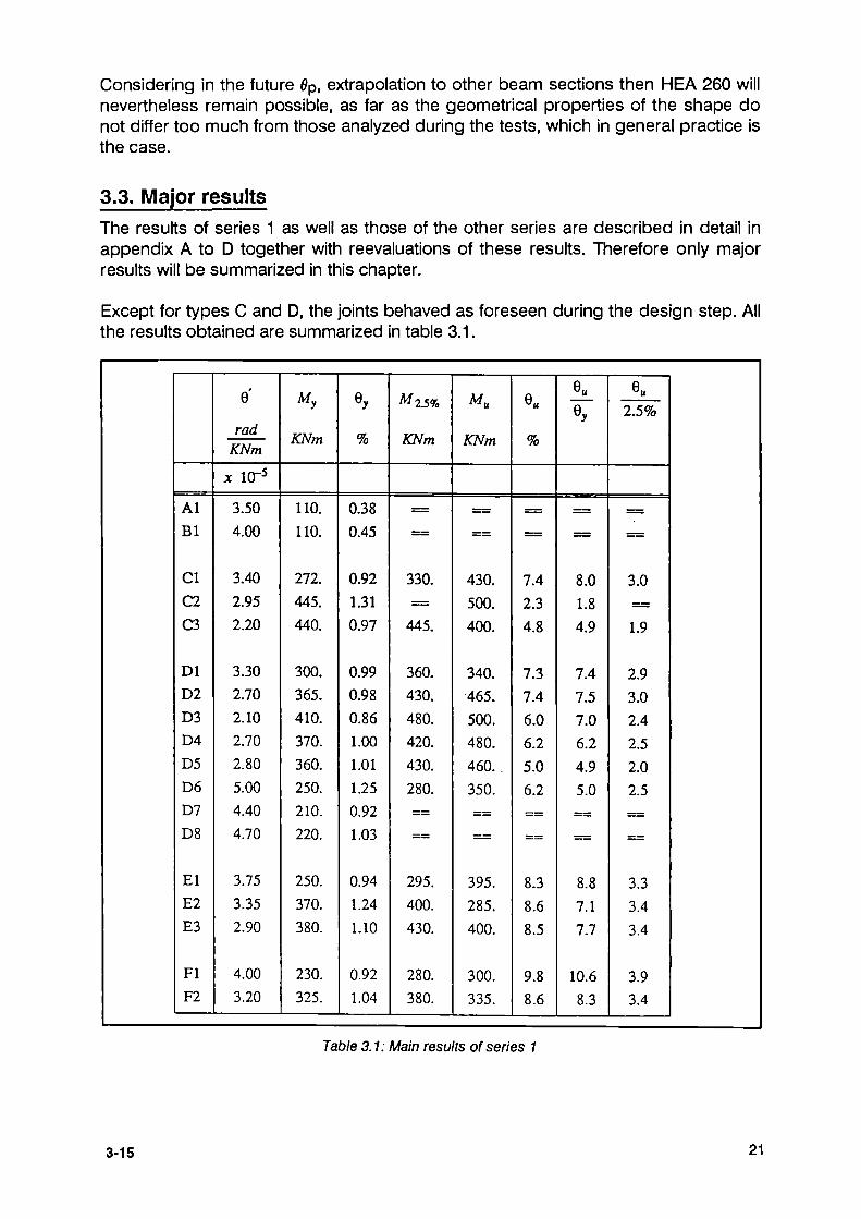
3.3. Major results The results of series 1 as well as those of the other series are described in detail in appendix A to D together with réévaluations of these results. Therefore only major results will be summarized in this chapter.

Except for types C and D, the joints behaved as foreseen during the design step. All the results obtained are summarized in table 3.1.

Al Bl

Cl C2 C3

Dl D2 D3 D4 D5 D6 D7 D8

El E2 E3

Fl F2

θ'

rad KNm

χ IO­5

3.50 4.00

3.40 2.95 2.20

3.30 2.70 2.10 2.70 2.80 5.00 4.40 4.70

3.75 3.35 2.90

4.00 3.20

My

KNm

110. 110.

272. 445. 440.

300. 365. 410. 370. 360. 250. 210. 220.

250. 370. 380.

230. 325.

Qy

%

0.38 0.45

0.92 1.31 0.97

0.99 0.98 0.86 1.00 1.01 1.25 0.92 1.03

0.94 1.24 1.10

0.92 1.04

^ 2 . 5 %

KNm

= =

330. =

445.

360. 430. 480. 420. 430. 280.

~=

295. 400. 430.

280. 380.

Mu

KNm

== ==

430. 500. 400.

340. 465. 500. 480. 460.. 350.

==

395. 285. 400.

300. 335.

Θ«

%

= =

7.4 2.3 4.8

7.3 7.4 6.0 6.2 5.0 6.2

==

8.3 8.6 8.5

9.8 8.6

Qy

= =

8.0 1.8 4.9

7.4 7.5 7.0 6.2 4.9 5.0

==

8.8 7.1 7.7

10.6 8.3

% 2.5%

:—:

=

3.0

= 1.9

2.9 3.0 2.4 2.5 2.0 2.5

==

3.3 3.4 3.4

3.9 3.4

Table 3.1: Main results of series 1

3­15 21

Type A which was a quasi hinged joint, often used in fire-resistant structures failed of course at a low stress range by a shear fracture of the pins. The pins which were welded by fillet welds can be improved by using butt welds. The whole "plasticity" raised of course in the connection.

Type ß showed a poorer behaviour than type to although it is less hinged. Failure arrived by fracture of the net cover-plate section. The plasticity was a pure beam plastic one.

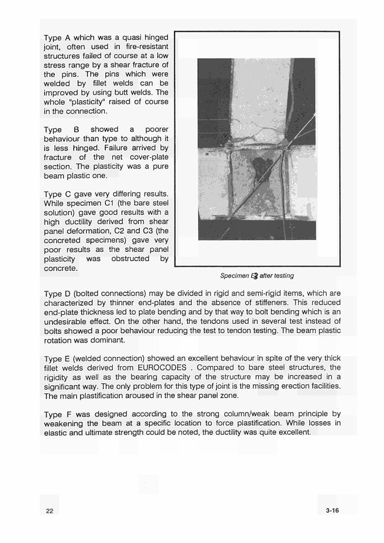
Type C gave very differing results. While specimen C1 (the bare steel solution) gave good results with a high ductility derived from shear panel deformation, C2 and C3 (the concreted specimens) gave very poor results as the shear panel plasticity was obstructed by concrete.

Specimen E& after testing

Type D (bolted connections) may be divided in rigid and semi-rigid items, which are characterized by thinner end-plates and the absence of stiffeners. This reduced end-plate thickness led to plate bending and by that way to bolt bending which is an undesirable effect. On the other hand, the tendons used in several test instead of bolts showed a poor behaviour reducing the test to tendon testing. The beam plastic rotation was dominant.

Type E (welded connection) showed an excellent behaviour in spite of the very thick fillet welds derived from EUROCODES . Compared to bare steel structures, the rigidity as well as the bearing capacity of the structure may be increased in a significant way. The only problem for this type of joint is the missing erection facilities. The main plastification aroused in the shear panel zone.

Type F was designed according to the strong column/weak beam principle by weakening the beam at a specific location to force plastification. While losses in elastic and ultimate strength could be noted, the ductility was quite excellent.

22 3-16

3.4. Improvements deduced for series 2 and 3 Series 1 led to the following preliminary conclusions and guide-lines:

■ Especially for series C and E, the shear panel deformation is not neglectable, leading thus to greater P-d effects in the columns. However it is concluded that this shear panel deformation is admissible as long as the overall stability of the structure is guarantied. One exception should nevertheless be mentioned. If during a test on a bare steel specimen, the global plastic deformation is limited to shear panel deformation, this solution is to be avoided in composite structures, as concrete prevents shear panel deformation.

■ Design of most of the tests of series D was based on the use of high strength tendons (10.9), which are very difficult to find in practice. For this reason, in series 2 and 3 only 10.9 bolts were used together with 2 nuts in order to avoid slipping.

■ In series D, two types of abutting plates, a thin one (26 mm) and a thick one (44 mm), were used. The thin plate caused bolt bending and bolt failure. In order to avoid this, in series 2, only abutting plates thicker then 40 mm were used.

■ In series 1, all the main welds used were fillet welds. According to Eurocode 8 "Seismic Design", connection parts are to be designed for 1.2 times the ultimate element resistance, leading thus to rather important welds with all possible disadvantages. Therefore it was decided for series 2, to use only butt welds.

3.5 Effect of flange weakening on fire resistance One of the discussed methods to shift the plastic hinge away from the direct beam-column connection into the beam region can be realized by a systematic flange weakening of the profile. This can be done by cutting off a defined part of the flanges (series F). Because of the moments under earthquake action the weakening should be done at upper and lower flange.

Figure 3.7 shows such a situation for a composite beam. Cross section design is in accordance with the design of the test of the research program.

The plastic moment capacity in dependence of the rate of the flange weakening "a" was calculated. In addition, the influence of such profile weakening on the ultimate load capacity under ISO-fire conditions was analyzed.

All calculations were done on the following assumptions for the material properties:

Steel profile (St 37) by = 240 N/mm2

Concrete (B 25) bc = 25 N/mm2

Reinforcement (BSt 420/500) by = 420 N/mm2

3-17 23

Figure 3.7

Figure 3.8 shows the time dependence of the ultimate moment capacity under ISO-fire action.

For t = 0 the ultimate moment capacity Mu is given as a function of the weakening of the upper and lower flange.

Figure 3.9 gives the results of this analysis for defined fire resistance classes of 0/30/60/90 minutes ISO-fire. On the horizontal axis the percentage of weakening of each flange is given as a total value or as percentage of the flange width.

This figure manifests, that by profile weakening the plastic moment capacity can be reduced in a way that just for the decreasing values of moment distribution from the seismic loading the weakest point can be shifted away from the connection into the beam. There is a linear dependence with a reduction of the plastic moment capacity of 64% for a total width reduction of 50% for both flanges for the cross section shown in figure 3.7.

On the other hand, the reduction of cold plastic moment capacity will influence the fire resistance of such a cross section. But the decrease of fire resistance is as well nonlinear as of smaller amount than under cold conditions. For 90 minutes ISO-fire the value of Mu (t=90) is reduced of about 20 % for a/s = 50 % compared with the original cross section (a = 0).

These numerical investigations indicate that with a local profile modification, the localisation of plastic hinges can be influenced in a defined way.

Influence on fire resistance of such modified profiles seems to be acceptable, can be calculated and thus, taken into account within the design process.

24 3-18

Figure 3.8: Time dependence of ultimate moment under fire

3-19 25

Mu[kNm

A

240

200

160

120

30

F-0

F-30

F-60

F-90

_^. a/b [ % ]

10 20 30 40 50

-^> ε [ mm ] 52 75 104 130

Figure 3.9: Capacity losses for different fire resistances

26 3-20

Chapter 4

Test series 2

Series 2 was dealing with interior beam­to­column joints presenting a beam connected to each column flange. As in a frame submitted to horizontal forces, the moment applied at both sides has the same sign, the solicitations in the shear panel are doubled and become most of the time dominant. Therefore the parameter of adding doubler plates to the web was added.

4.1. Selection of the test specimen Six types of joint named G to L were defined for test series 2 based on those of series 1 and taking into account the conclusions of chapter 3. In total, 20 test were performed.

Type G (fig. 4.1) is the equivalent of type A in series 1. Two tests G1 and G2 have been realized. In test G1, the welding of the pins was improved by using a butt weld, increasing thus the shear area. For test G2, the philosophy of a shear connection was maintained, but instead of using pins, the fixation was realized directly by the end­plate.

Type H (fig. 4.2) was an exact cross form copy of type Β (series 1). Only one test was performed without modification.

G2 r

j »

Figure 4.1 Figure 4.2

4­1 27

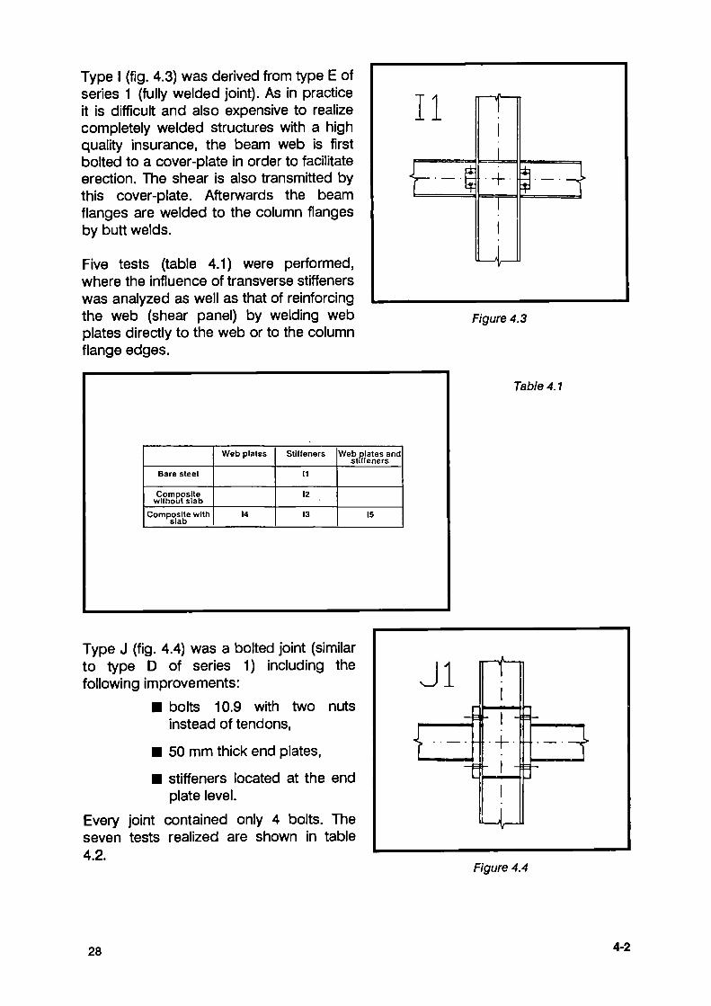
Type I (fig. 4.3) was derived from type E of series 1 (fully welded joint). As in practice it is difficult and also expensive to realize completely welded structures with a high quality insurance, the beam web is first bolted to a cover-plate in order to facilitate erection. The shear is also transmitted by this cover-plate. Afterwards the beam flanges are welded to the column flanges by butt welds.

Five tests (table 4.1) were performed, where the influence of transverse stiffeners was analyzed as well as that of reinforcing the web (shear panel) by welding web plates directly to the web or to the column flange edges.

Figure 4.3

Bare steel

Composite without slab

Composite with slab

Web plates

14

Stiffeners

11

12

13

Web plates and stiffeners

15

Table 4.1

Type J (fig. 4.4) was a bolted joint (similar to type D of series 1) including the following improvements:

■ bolts 10.9 with two nuts instead of tendons,

■ 50 mm thick end plates,

■ stiffeners located at the end plate level.

Every joint contained only 4 bolts. The seven tests realized are shown in table 4.2.

Jl { ■ - -

I - ι -■■+■■ - I - i

I

LU Figure 4.4

28 4-2

□ are steel

Composite without slab

Composite with slab

Web plates

J4

J7

J5

Stiffeners

J1

J2

J3

Web olates and stiffeners

J6

Type Κ (fig. 4.5) was similar to type F. In order to reduce workshop costs the length of the weakened beam section was shortened from 500 to 200 mm. Series 1 had shown that this length was sufficient to develop a plastic hinge. The four tests performed are presented in table 4.3.

Type L (fig. 4.6) was a completely new type of joint not yet tested in series 1. While all the other specimen followed

the principle continuous column/interrupted beams, this specimen had continuous beams in order to facilitate erection. This design is often used under static and fire

Table 4.2

Figure 4.5 Figure 4.6

Bare steel

Composite without slab

Composite with slab

Web platas

K3

Stifieners

K l

K2

Without web plates and stiffeners

K4

Table 4.3

4-3 29

loads, but seemed at a first view not adapted for seismic loads. Stiffeners are unavoidable for this type of joint.

4.2 Testing installation As the test of series 2 were also realized in Milan, it was tried to use the existing testing facilities. Furthermore a major problem consisted in applying at both beams the same force but with opposite signs. This could have been done with complex measuring devices, but the solution shown in figure 4.7 is more accurate and less expensive. Figure 4.7

­B­­E

5=3 Φ Φ

As for series 1, the column is in a horizontal position. But while in series 1 the column ends were fixed, in series 2, two pin­ended columns were used. By that way, the whole horizontal reaction has to be supported by the lower beam support. Thus the forces (action and reaction) are always equal in value

and of opposite signs. No comparison

measures between the two forces are needed. The measurement devices shown in figure 4.8 allow to measure the same data as in series 1.

­ Θ ­ & ­ 5

Φ Φ

dispÌCcenervc

f o r c e

Figure 4.8

30 4­4

4.3. Major results As for series 1, the detailed results are given in Appendix A. Table 4.4 gives a summary of the results obtained during the 20 tests. Concerning the wear (often in fire resistance used) joints G and H, the overall behaviour of type H was better. The solution G1 (with pins) is not recommended, as it is very difficult to control the quality of pin welding. With a higher rebar reinforcement in the slab, the results can nevertheless be increased in a significant way.

Gl G2 HI

11 12

13 14 15

Jl J2 J3 J4

¡5 J6 J7

Kl K2 K3 K4

LI

θ'

rad KNm

χ IO ­5

7.00 3.75

3.10

2.83 2.25

1.50 1.55 1.30

2.50 2.00 1.37 2.25

1.66 1.32 1.77

3.00 1.75 1.75 2.45

2.63

e; rad

KNm

χ IO ­5

0.00

0.00 0.00

1.55 1.03 0.70 0.75 0.50

0.94 0.60 0.40 0.25 0.00 0.37 1.00

1.25 0.78 0.00 1.00

1.30

My

KNm

45.

55. 150.

260. 470. 490. 700. 720.

360. 500. 520. 5S0. 660. 700. 720.

320. 500. 560. 500.

330.

θ>

%

0.30 0.21

0.47

0.75 1.06 0.73 1.00 0.95

0.90 1.00 0.71

1.31 1.10 0.92

1.10

0.9Ó 0.38 0.98 1.23

1.02

M 2.5%

KNm

==

170.

300. 540. 600. 750.

==

420. 600. GÓ0. 620. 740. 800. 660.

460. 620. 660. 530.

440.

Mu

KNm

=

90.

430. 470. 480. 650. 850.

590. 610. 570. 760. 840. 860. 560.

525. 560. 830. 530.

330.

6u

%

==

4.2

>10.0 >10.0

>10.0 6.5 2.1

>10.0 >10.0 >10.0

4.5 4.5

<4.5 6.5

>10.0 >10.0

9.0

>10.0

9.0

Qu

Qy

==

2.9

>13.6 > 9 . 5 >13.0

4.2 2.2

11.1 >10.0 >14.1

3.4 4.1

<4.9 5.9

>10.4 >11.4

9.2 >8.1

8.8

e. 2.5%

==

3.6

>4.0 >4.0 >4.0

2.6 0.8

>4.0 >4.0 >4.0

1.8

1.8 <1.8

2.6

>4.0 >4.0

3.7 3.2

3.6

Table 4.4

4­5 31

For the welded l-series, it can be stated that high rigidity obtained by web plates and stiffeners lead to very high resistance characteristics but to a poor ductility behaviour and brittle fractures. The cyclic behaviour is very regular.

The bolted connections of series J gave similar results than those obtained for series I. However the danger of brittle fracture was smaller. The fact of locating the stiffeners at top and bottom of the end plates instead of top and bottom beam flange was of great benefit as the shear panel zone was increased.

Thicker end plates than for series 1 gave in general better results. As the difference of the column flange thickness and the plate thickness was significant (19 mm to 50 mm), improvements can probably be obtained by inserting back plates at the bolt level.

For type K, the section reduction of the beam was not sufficient to obtain plastic hinges in the beam instead of a shear panel mechanism. The results are nevertheless as good as those of series J from the point of view of resistance and ever better from the point of view of ductility. It is specially interesting that specimen K4 was the only one tested without stiffeners and without web plates (doubler plates). The results obtained are nevertheless comparable to those of K2 and J3 (both with stiffeners), proving that infilled concrete provides bearing capacities similar to those of stiffeners.

Test L1 was the only specimen of series L tested. Due to the fact that the shear panel is reduced by about 30 % (bear section HEA 260 instead of column section HEB 300), the shear panel mechanism became more significant.

Specimen of series 2 after testing

32 4-6

Chapter 5

Test series 3

In series 3, 10 tests were realized on complex frames with concrete slab, which may be divided as follows:

■ 4 tests on single span one­storey frames in Wuppertal

■ 3 tests on double span one­storey frames in Liège and

■ 3 tests on double span two­storey frames in Darmstadt Furthermore, as the Darmstadt tests included connections which have not yet been analyzed in series 1 or 2, for instance the joints of the upper level or the encasing of the columns at the fixations, Darmstadt performed several simple tests on these elements (series 4).

The types of connections to be tested in series 3 were selected from those showing an interesting behaviour in series 1 and 2 and presenting facilities for erection and concreting in order to reduce test preparation time in the laboratory.

As all the results, testing equipments and measurement devices are described in extenso ¡η appendix Β to D, this chapter gives only an overview on the different tests.

5.1 The Liège specimen

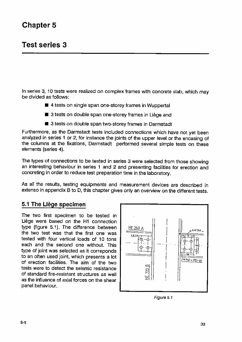
The two first specimen to be tested in Liège were based on the H1 connection type (figure 5.1). The difference between the two test was that the first one was tested with four vertical loads of 10 tons each and the second one without. This type of joint was selected as it correponds to an often used joint, which presents a lot of erection facilities. The aim of the two tests were to detect the seismic resistance of standard fire­resistant structures as well as the influence of axial forces on the shear panel behaviour.

Figure 5.1

5­1 33

HE 260 A ­

Λ 4

­

J± Ä

­­

s SI

' J

'.0

> ­i6.'_

— Φ'.30*300*1,0

The third specimen was connected by type K2 joints (figure 5.2). In this type, the beam section is weakened in order to locate the plastic hinges in the beams and to avoid plastifications in the columns and in the shear panel. This specimen corresponds to a strong one, which is a new solution in seismic engineering and which has been developped by the Liège university . The ductility shown in the previous series was very good for this type and it was interesting to analyze the behaviour of a more complex structure.

Figure 5.2 The specimens corresponded to a modell cut out from a real structure and

containing three columns with the relating composite floors. As the bottoms of the specimen columns are located in the middle of the real column, the contraflexural point, the specimen were hinged at their fixations.

5.2 The Wuppertal specimen The four frames tested in Wuppertal may be divided in two frames with strong joints and in two frames with weak moment resisting joints. The specimens corresponded to the modelling of a composite floor with on the top and on the bottom each time one half of the column. As in the middle of the column, it is behaving like a hinged structure, the specimens were foreseen with articulations at each column end.

The connection types corresponding to the weak joints were the types G1 (figure 5.3) and H1 from series 2. These two joints were especially choosen, as they are corresponding to often used connection types in fire­proof composite structures like the ARBED AF­system.

The aim of this choice was to analyze the inherent seismic resistance of fire resistant designed structures.

The two strong joints tested are I3 and K2. I3 (figure 5.4) was selected for being a traditional joint used in

HE 260 A

I

Ill I

­

01

M l

HE 260 A

ìli φ­­·

■BO-

Γ o S

Figure 5.3

34 5­2

bare steel structures in seismic regions. K2 was choosen as this type behaved very well in the series 1 and 2. It gives the possibility to test a completely new kind on more complete structures.

The four tests were performed with two vertical dead loads of 10 tons each applied on the beams.

HE 260 A

HE 260 A ι — ' —

­ω­

l—I— (

00

o m LU 3Z

..>!

. Λ1 *&.

! 3

1-­©

— BO

ao

" Is

o

Figure 5.4

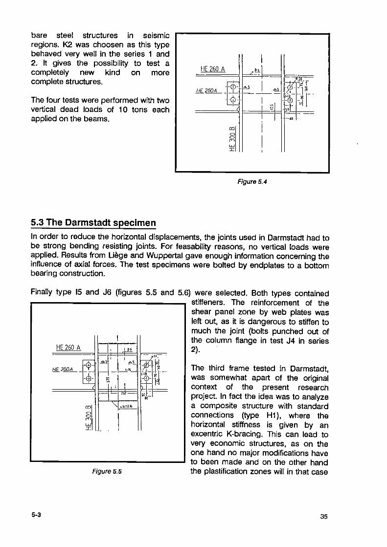
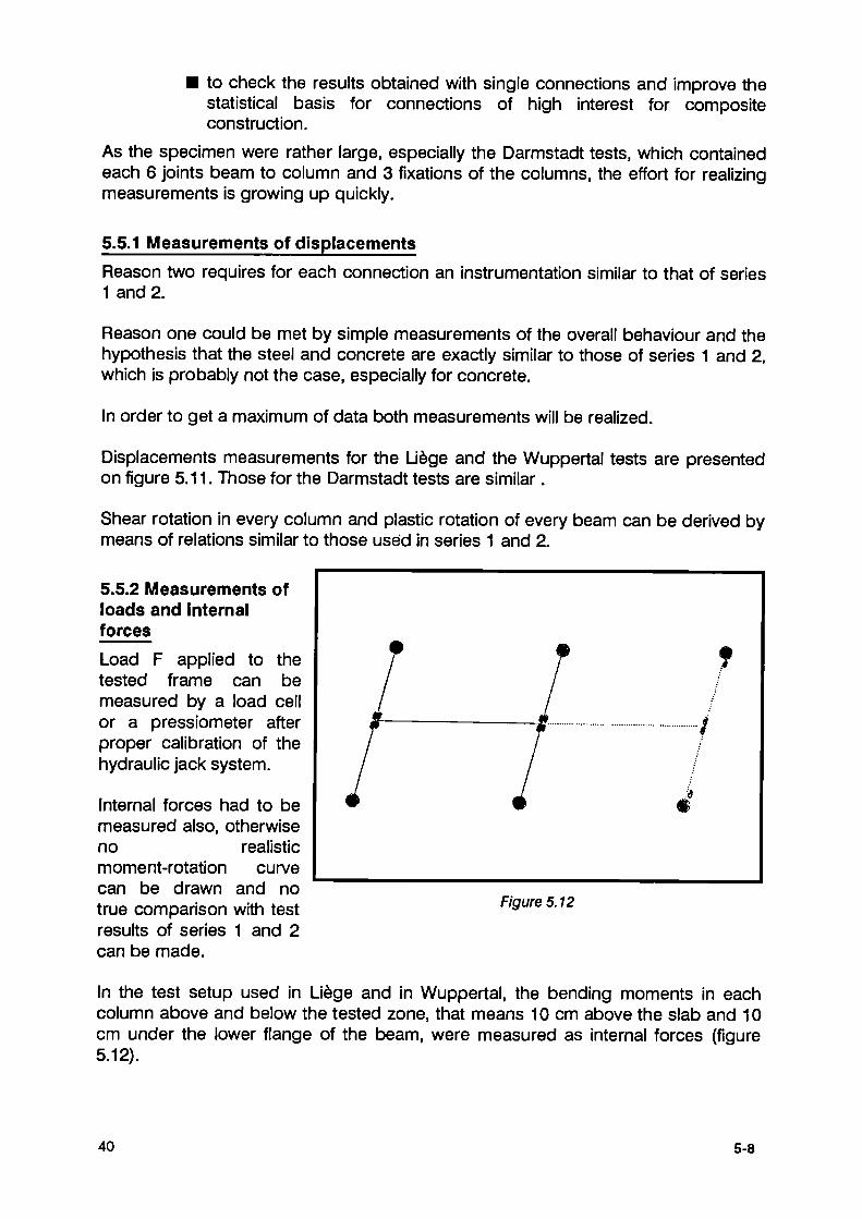
5.3 The Darmstadt specimen In order to reduce the horizontal displacements, the joints used in Darmstadt had to be strong bending resisting joints. For feasability reasons, no vertical loads were applied. Results from Liège and Wuppertal gave enough information concerning the influence of axial forces. The test specimens were bolted by endplates to a bottom bearing construction.

Finally type 15 and J6 (figures 5.5 and 5.6) were selected. Both types contained stiffeners. The reinforcement of the shear panel zone by web plates was left out, as it is dangerous to stiffen to much the joint (bolts punched out of the column flange in test J4 in series 2). HE 260 A

HE 260A ­φ­

J-(

o CD m

Ü :

I g>t

5É=

Ña .­©­

j

M

Ή

Figure 5.5

The third frame tested in Darmstadt, was somewhat apart of the original context of the present research project. In fact the idea was to analyze a composite structure with standard connections (type H1), where the horizontal stiffness is given by an excentric K-bracing. This can lead to very economic structures, as on the one hand no major modifications have to been made and on the other hand the plastification zones will in that case

5-3 35

HE 260 A -

¡n. '

\

-

1

i

It?,

—F5--

is- · ^

.50

!>(.

be located in the beams (shear hinges). Furthermore the design of these shear hinges will become very economic, due to the fact that the stiffening is guaranteed by an adequate design of the stirrups in the beams instead of expensive stiffeners. This kind of structure will be analyzed more in detail in an other project. The present test served as orientation test.

Figure 5.6

5.4 Design of the testing Installation for series 3 5.4.1 The Liège installation The Liège testing installation is shown in figure 5.7. The structure consisted in a bottom bearing construction (a) made from HEB 500 beams and fixed to the soil (b). The specimen are fixed to this beam by hinges (c), in order to simulate the contraflexural point in the columns. On the top of the columns, these are fixed by the same way to a connection beam (d) which is introducing the loads equally in the

Figure 5.7

36 5-4

three columns (e). Between this connection beam and the composite beam with slab (f) will be installed the vertical hydraulic jacks simulating the dead loads on several specimen. The axial forces in the columns created as reactions of the jack action can be neglected. On the right side of the installation is located the counterframe (g) for guiding the horizontal forces to the bottom structure. Two serial connected jacks (max. 1000 kN) are linking the counterframe to the connection beam. The fixations are realized by two hinges. The maximum displacement is about 80 cm (40 cm in both direction). The vertical stability of the jacks is assumed by two counterweights of 600 kg each. The out­of­plane stability is guaranteed by one frame structure for the jacks and by four larger frames for the test specimen. These frames are used as guiding structures for the slab and for the beam.

5.4.2 The Wuppertal installation As the test specimen of Wuppertal are similar to those of Liège, the testing installations are of course also similar (figure 5.8).

The specimen are fixed by the same hinges to the bottom bearing construction (HEB 500). The joint with the load introduction beam is slightly modified in order to save height and to use by that way an existing frame from Wuppertal as counterframe.

w [mm] ­F [kN] _■­ ra r\'"'f\

­111. jtce

• r £·­ΑΕ

DETAIL , Ο Ι , Ρ ^ , Κ / ^ ^

COflPlSITC CïLUHM

'Ë i y ­

J ­

o r>

II I

Figure 5.8

The load introduction beam is connected to this loading frame by the jack (300 kN) which is not hinged at his fixations. The slab is continously secured against out­of­plane instability by two channels.

5.4.3 The Darmstadt installation

5­5 37

Figure 5.9

The Darmstadt installation was the most important one. It is divided in two parts, the testing area and the erection area (figure 5.9). In order to save time, the beams and columns are concreted in an horizontal position on the ground and then erected

ψ Φ Φ Φ ® SCHNITT A­A

KXtpjoo.æ Ξ

Figure 5.10

38 5­6

close together in the erection area. Afterwards the slabs of the three specimen are concreted at the same time. After the concrete has hardened, one specimen after the other is transported on rails to the testing area. The testing installation properly said, consists of a mighty bottom bearing construction made of beams with flange thicknesses of about 70 mm. The counterframe is made from two parallel trusses which are connected by vertical and horizontal bracings (figure 5.10) as well as by two HEB 1000 beams which are used for the fixation of the jacks on every floor. The upper jack has a total displacement capacity of 65 cm. The load of the upper jack was twice that of the lower one. As the specimen were connected in a rigid way to the bottom structure, this displacement was large enough to reach almost the failure of the specimen. The load introduction jack-frame is realized on each level by a fork which is fixed by two articulations to the upper flange of the beams in the span close to the counterframe.

5.5 Definition of the measurements in series 3 The choice of the measurements is a function of the purpose of the tests. The tests in series 3 were realized for the following two reasons:

■ to see whether the behaviour observed on single connections of various kinds (exterior columns and interior columns) can be just superposed or if some mutual influence of elements interferes.

Figure 5.11

5-7 39

■ to check the results obtained with single connections and improve the statistical basis for connections of high interest for composite construction.

As the specimen were rather large, especially the Darmstadt tests, which contained each 6 joints beam to column and 3 fixations of the columns, the effort for realizing measurements is growing up quickly.

5.5.1 Measurements of displacements Reason two requires for each connection an instrumentation similar to that of series 1 and 2.

Reason one could be met by simple measurements of the overall behaviour and the hypothesis that the steel and concrete are exactly similar to those of series 1 and 2, which is probably not the case, especially for concrete.

In order to get a maximum of data both measurements will be realized.

Displacements measurements for the Liège and the Wuppertal tests are presented on figure 5.11. Those for the Darmstadt tests are similar.

Shear rotation in every column and plastic rotation of every beam can be derived by means of relations similar to those used in series 1 and 2.

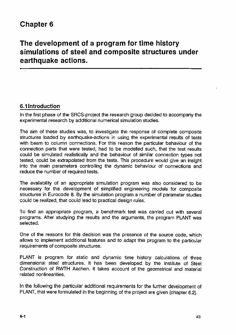
5.5.2 Measurements of loads and internal forces Load F applied to the tested frame can be measured by a load cell or a pressiometer after proper calibration of the hydraulic jack system.

Internal forces had to be measured also, otherwise no realistic moment-rotation curve can be drawn and no true comparison with test results of series 1 and 2 can be made.

Figure 5.12

In the test setup used in Liège and in Wuppertal, the bending moments in each column above and below the tested zone, that means 10 cm above the slab and 10 cm under the lower flange of the beam, were measured as internal forces (figure 5.12).

40 5-8

This was done by strain gage measurements on the outer faces of the flanges of the column and assumed geometrical properties of the column section.

From these measurements we can derive: ■ the shear in the columns and a check of total shear ( or calibration of

the real column section properties)

■ the bending moment in the beam corresponding to an exterior column

■ the sum of the bending moments of the two beams crossing an interior column; this parameter is the same as the one established in tests on interior column connections in Milan.

Figure 5.13

The measurement of internal forces by strain-gages realized in the Darmstadt test setup was similar to that applied in Liège and Wuppertal (figure 5.13).

5-9 41

Chapter 6

The development of a program for time history simulations of steel and composite structures under earthquake actions.

6.1 Introduction In the first phase of the SRCS-project the research group decided to accompany the experimental research by additional numerical simulation studies.

The aim of these studies was, to investigate the response of complete composite structures loaded by earthquake-actions in using the experimental results of tests with beam to column connections. For this reason the particular behaviour of the connection parts that were tested, had to be modelled such, that the test results could be simulated realistically and the behaviour of similar connection types not tested, could be extrapolated from the tests. This procedure would give an insight into the main parameters controlling the dynamic behaviour of connections and reduce the number of required tests.

The availability of an appropriate simulation program was also considered to be necessary for the development of simplified engineering models for composite structures in Eurocode 8. By the simulation program a number of parameter studies could be realized, that could lead to practical design rules.

To find an appropriate program, a benchmark test was carried out with several programs. After studying the results and the arguments, the program PLANT was selected.

One of the reasons for this decision was the presence of the source code, which allows to implement additional features and to adapt this program to the particular requirements of composite structures.

PLANT is program for static and dynamic time history calculations of three dimensional steel structures. It has been developed by the Institute of Steel Construction of RWTH Aachen. It takes account of the geometrical and material related nonlinearities.

In the following the particular additional requirements for the further development of PLANT, that were formulated in the beginning of the project are given (chapter 6.2).

6-1 43

The result of the development is the program DYNACS, that meets these requirements are explained in chapter 6.3.

In chapter 6.4 some examples for the application of DYNACS are presented.

6.2 Additional requirements (to a simulation program for time history calculations of steel- and composite structures under earthquake actions) 6.2.1 Nonlinear material behaviour The program should consider the nonlinear behaviour of the materials, which are parts of composite beams, i.e. steel, concrete and reinforcement and of the shear joints between the concrete and steel parts.

6.2.2 Geometrical nonlinearities To analyze slender structures, the program should be able to take into account geometrical effects due to second order theory.

6.2.3 Shear forces The program has to consider the shear forces and deformations in the panels at the beam to column connections and' other steel parts and the shear forces and deformations in the shear joints.

6.2.4 Load history and strength degradation Because of the cyclic loading and nonlinear material behaviour, the load history has to be taken into consideration. The redistribution of the inner forces in a structure according to partial damage due to low cycle fatigue, has an important influence on the behaviour of the structure. This strength degradation has to be taken into account while describing the load history.

6.2.5 Short calculation time In order to reduce the time needed for the time step analysis of dynamically loaded structures, considering geometrical and material dependant nonlinearities, the program has to be optimized in view of calculation speed.

6.2.6Additional requirements Additional technical and comfort requirements concerning the handling of the program have to be considered.

44 6-2

6.3 Implementation of the required features On the basis of the program PLANT, a new program, called DYNACS, has been developed. This program has the features described in the following.

6.3.1 Nonlinear material behaviour

Additionally to the bilinear stress-strain relationship for steel, which was already implemented in PLANT, the following rules describing the behaviour of composite members have been adopted.

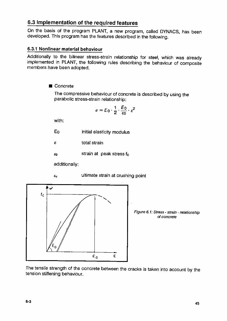
Concrete

The compressive behaviour of concrete is described by using the parabolic stress-strain relationship:

with:

Eo initial elasticity modulus

total strain

co strain at peak stress fc

additionally:

eu ultimate strain at crushing point

Figure 6.1: Stress - strain - relationship of concrete

The tensile strength of the concrete between the cracks is taken into account by the tension stiffening behaviour.

6-3 45

Reinforcement In the compressive area of the concrete section, the reinforcement bars are taken into account in addition to the concrete parts. In the area in tension, the tension stiffness of the concrete between the cracks is approximated by using a fictious enhanced area of the reinforcing bars.

with:

As

As.i

μ-

fc.¡

fs

As,i = 1 ­

As 04 tc,i μ-

real area of the reinforcement cross section

fictious area of the reinforcing bars

percentage of reinforcement

tensile strength of concrete

yield stress of reinforcing steel

σ,

f s ­

E p l ^ ­

/fe( /

is

ε

Figure 6.2: Stress - strain relationship of reinforcement

Figure 6.3: Stress - strain relationship of steel

46 6­4

Structural steel The behaviour of structural steel under cyclic loading is given by a bilinear a - ε hysteresis defined by the following parameters:

Eel

Epl

modulus of elasticity

modulus of plasticity

yield stress

This assumed behaviour of the material considers the hardening rule and the Bauschinger - effect if the direction of the load has changed.

6.3.2 Geometrical nonlinearities The consideration of second order-effects was already implemented in PLANT, therefore no further development was necessary.

Figure 6.4

6.3.3 Modelling of the particular behaviour of the beam to column connections and the shear panel The modelling of complex beam to column connections can be realized with simplified substitute models, which use members with predefined force-deformation relationships (Fig. 6.4), which can be taken directly from the test (Fig. 6.5) or extrapolated from the tests, if structures similar to the test specimens shall be analyzed.

M Ν

Μ- φ curve from test

<P

calculated Ν-ε curve

Figure 6.5

6-5 47

The diagonal spring (a) describes the particular behaviour of the shear panel whereas the other springs (b) define the behaviour of the connections and the plastic moment - rotation - relationship of the beam. 6.3.4 Load history and strength degradation In order to verify the experimental results and to check the accuracy of the chosen simulation models, the possibility of a deformation controlled calculation method for the time history has been adopted. The calculation follows step by step the same rules, as the cyclic tests on the specimens were carried out. Additionally a dynamic time step calculation using any acceleration or time dependant forces can be carried out.

The depth of the plastification during a numerical simulation indicates the degree of the strength degradation for the next cycle. The strength degradation has been taken into account by the hysteresis evolution method. By varying different internal parameters in the degradation function it is possible to approach the behaviour of tested joints very accurately.

The modification of a system concerning its behaviour in the ultimate limit state is determined by the comparison of the energy under cyclic loading with its virgin state.

The energy of the system in a fixed timestep a is defined as Pa, and in the original state as Pao.

Hence, the degradation can be written as:

S - 1 - Pa

The degradation S depends on the load history, the material properties and the structure.

The values of the energy Pa and Pao are obtained under the condition, that the structure has reached its ultimate limit state (i.e. 6P=0). Then:

Pa = 2 " w

a · Fa

PaO = 2 ' w

0 ' F

a0

where F are the forces and w are the dependant deformations.

An other way to describe the upper relationships is given by:

Pa = ^- ka · Wa

PaO = £ · ko · νν§

with:

48 6-6

υ _ Fa . . _ Fa o Ka - Wa ·

K0~~wõ

The equation (6.1) can be written now:

The following general equation for the degradation of a system during a time history is derivated in the doctoral thesis of Dr. Dorka:

Fan (w.) = Fa0 (wa) · Σ n ­ l

1 ­ e 1 ­ F.

("a­Wan' n

) * ~ _£A_ an­1 Kn)

where the "effect function" e describes the distribution of the modification­skeleton­curve in the deformation area w.

Figure 6.6: Example of an energy condition

Model for describing the degradation of nonlinear systems

Dr. Dorka describes several possibilities of evolution models, for instance exponential, consistent, linear or uniform evolution.

In DYNACS the exponential model is used at present. The decrease of F in this model is:

Fa. (W„) = F0 («,„) ­ b ­ ­ b (VU) = ƒ " (%") r a n - l (wanj

6-7 49

with:

Fo(wan) =known force of the original system at the deformation state wan

b =function depending on the load history

Two proposals are made for the function b:

1

1.0 fj

\B ^^ b j = B(waj/w s)

1.0 wa; /w s

Figure 6.7.a: Gradual degradation

1.0

0.5

fj

B\ b - 1

/ ^ 1 + (w a j /w[)B

wj/ws 1.0 w a j /w s

Figure 6.7.b: Sudden degradation

50 6-8

6.3.5 Short calculation time A reduced calculation time has been achieved by the following developments:

■ The solution and distribution of the equation system is done by using the skyline-method.

■ A 'Dynamic' management of the required memory is chosen, only the initial global space must be declared in the main-routine.

■ The dimensions of the used arrays are calculated from the actual investigated system.

■ The Input/Output time has been reduced by taking the stiffness matrix and most of the arrays into the memory.

6.3.6 Additional features ■ Raleigh-damping

DYNACS assumes the damping matrix C as a linear combination of the stiffness matrix Κ and the mass matrix M:

C = aM + βΚ ■ In order to save time, it is possible, to define mass distributions along

the members in the structure. These distributed masses of the members are added to the lumped masses at both nodes of the beams.

■ The lumped masses are not defined only in the three translation degrees of freedom but also in the rotation degrees of freedom.

■ It is possible to define the acceleration in any direction.

■ The weight of a structure can be taken into account by defining a gravity vector.

■ The output of the results can be more easily interpreted by giving the possibility of varying the form and the volume of the output.

6.4 Examples of calculation The following examples illustrate the applicability of the program.

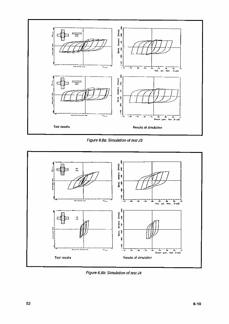
6.4.1 Simulation of the test results of beam to column connections. This examples show comparisons between the experimental and numerical results of cruciform-joints tested in Milano (Fig. 6.8.a - c).

6-9 51

Test results

rTT/ ■m a LULLUS

­ I? ­ 09 ­ 0 6 ­ 03 00 .03 06 09

Tat. pi . Rot Iradl

E

Ζ o

■£ e c «J o O Χ

c ? «ι to I l i .

■ ■ 1 ■ * 1 » ■ r—· . 1

7ll —7—7

II ­.10 ­ 0) ■ o* ­ οι o; « oa Shear pan. not . (radi

Results of simulation

Figure 6.8a: Simulation of test J3

" ξ o χ

« 3 c Τ «ι α

Ş

­ . 1 2 ­ . Μ ­ .06 ­ . 0 J Of .12

Tot. p i . Rot. (rad)

t

!

E

ÎI c * κ å

1

χ ° i c 7 m

Ş

Ş 12 .09 ­ M ­ OJ .00 OJ 06 09 12

Snear pan. Rot.(rad)

Test results Results of simulation

Figure 6.8b: Simulation of test J4

52 6­10

=' 1 «ι m

ş g

#

• . 1 2 - 09

Tot. p i . nat. (radi

ΕΞΙ I f3 ' Lil '

!

11 ν i Shear pan rvjt.lrad]

Test results Results of simulation

Figure 6.8c: Simulation of test J6

6.4.2 Cyclic behaviour of a frame A simulation of the behaviour of a frame tested in Wuppertal was carried out. The numerical results of an extrapolation of the test results are shown in Fig. 6.9.

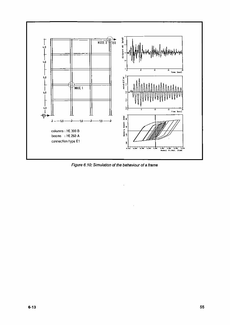
6.4.3 Frame under earthquake action. The dynamic behaviour of a five storey frame was simulated under the load of El-Centro earthquake. The relationship of the beam-to-column connections were taken from experimental results. Some results of the calculation are shown in Fig. 6.10.

6-11 53

F „ δ

//////////J//JJ }////J///>////////JÌl/l/Jl

7&> Jfr

Tested frame

­

" f yff /'

8­

­■ // ι li/

f/7/ ­xw ­zoo tOO 200 300

displacement [mm)

Test results Results of simulation

­«50 ­350 ­M0 ­150 ­50 50 150 250 350 d i s p l a c e m e n t [mm]

Extrapolation of test results

Figure 6.9:Simulation of the cyclic behaviour of a BUW frame

54 6­12

r to

up

Í..0

4.0

4.0

-ψ+-

''NODE 1

NODE 2 ' ­ ■

1 ­5 .0 ­ ­5 .0 ­

columns : HE 300 Β beams : HE 260 A connection type E1

ΔΧ

­5 .0­1 ;

­«.Ml I.Mt I.NI · . · · · · . · « ·.·)■ Nod·!: PI .not . Irstf)

Figure 6.10: Simulation of the behaviour of a frame

6­13 55

Chapter 7

Recommendations for the amendment and completion of Eurocode 8

The results obtained during the realization of the 50 tests and their reelaboration allow to deduct the following principles that should be observed in design and that should therefore be anchored in Eurocode 8 "Structures in seismic regions":

■ The contribution of the shear panel to the overall energy dissipation should not be neglected and is a wanted feature of steel and composite structures. It should occur together with energy dissipation in plastic hinges in beams.

A premature damage of the shear panel could be prevented if the plastic hinges in the beams and the connections (Figure 7.1) form before the shear panel is strained excessively.

5

t

K1 κ2

ι

/"7 / f / / / /

/ in f II11 II

i . . .

r1 r

2 r3 ■

Win . /// IJ'y

■

Vawttf hMl tatatl·* k«*l %êé* »lH(k *ami«* IrMl

! i:

' / / V / / / /

i: ^ ^ !

'r' r2

Γ3 :

Titti Aitttl«n |r*«l

Figure 7.1

7­1 57

Therefore the shear panel should be capacity designed in view of the beam to column connections (beam or connections), taking account of a realistic ultimate strength of the shear panel. The strength of the shear panel should be estimated considering the cooperation of the shear panel with the frame formed by the flanges and stiffeners.

In case of composite shear panels the strength of the panel could be estimated by adding the strength of the reinforced concrete parts against shear deformations to the strength of the steel panel.

After cracks occur in the concrete parts, the concrete infillment continues to cooperate and prevents the steel parts from local buckling. Even in the stage when the concrete crushes, this cooperation continues. The crushing strength of the concrete can be enhanced by the reinforcement bars.

The connections should be designed such, that sufficient rotation is possible without loss of strength. To this end, the following design rules should be applied:

Π In endplate connections, the tension bolts should be capacity designed in view of the plastic design of the endplate. Any welds between endplates and beams should be capacity designed.

Π For shear connections, the shear resistance of bolts should be capacity designed to the bearing resistance in order to prevent shear rupture of the bolts before plastic deformation in the holes. All other welded connections should also be capacity designed.

Yielding of the steel girders in the tension zones of composite beams and yielding of the reinforcement in the concrete slab under negative moments should occur without premature crushing of the concrete slab and premature local buckling of the steel parts in compression. To this end load concentration in the transfer of compression loads from the beam to the column should be prevented unless local crushing is tolerated.

The design of the flexibility of the shear joint of composite beams should be such, that crushing of the concrete slab before yielding of the shear studs and of the steel beam is prevented.

58 7-2

Chapter 8

Recommendations to improve ECCS document 45 "Testing procedure for assessing the behaviour of structural steel elements under cyclic loads"

8.1. Introduction In the context of the present research, about 50 cyclic tests on connections and structures have been performed during the last four years in four european laboratories (Milano, Darmstadt, Wuppertal, Liège).

That experience leads to make some remarks on the existing ECCS testing procedure for assessing the behaviour of structural steel elements under cyclic loads.

The remarks mainly bear on the link which can be wished between the tests and some significant values in a practical design context for structures.

One of these values is the global permanent horizontal displacement of the structure, which should not be allowed to be greater than 2.5 % if the structure is to be kept alive after the earthquake. Thus experimental values far greater than that one are of a reduced practical interest.

Another value is related to the structural behaviour factor q which will be claimed for the structure including the structural component submitted to test. Again rotations far higher than the one corresponding to q times the maximum elastic displacement are of little practical interest.

Another remark bears on the parameters of interpretation of the test. The cumulated absorbed energy has been established in recent research works as being a very significant parameter and it should than be introduced. On the other hand, the rigidity ratios, at least in the way they are computed, are highly sensitive to local changes in the shape of the load-displacement curve at its intersection with the displacement axis (zero divided by zero); as these changes do not have a great meaning, the rigidity ratio is of little interest and could be deleted in its present form or should be defined in another way.

These facts bring us to suggest to introduce several modifications to the ECCS testing procedure.

8-1 59

8.2. PROPOSED MODIFICATIONS IN ECCS TECHNICAL NOTE 45

Postulate 1 The paragraph 3.2. (page 6) 3.2. Second test.

The second test also is a classical monotonic displacement increase test, but it is performed on the compression (negative) range. The procedure is the same as in the first test. F~ and ey are deduced.

should be completed at the end of the paragraph

"If the difference between Fy and Fy and/or eţ and ey is small, an average value of these quantities may be considered in the subsequent steps'.

Postulate 2 The paragraph 3.3. (page 6)

3.3. Third test.

The third test is a cyclic test with increase of displacement, which has the following characteristics :

- one cycle in the e /4, e /4 interval;

- one cycle in the 2e /4, 2e /4 interval; y Y

- one cycle in the 3 e /4, 3 e /4 interval;

- one cycle in the e , e interval;

- three cycles in the 2 e , 2 e interval;

- three cycles in the (2 + 2 n) e+, (2 + 2 n) e interval (n = 1.2,...).

More cvcles or more intervals may be used if necessary.

should be completed at the end of the paragraph

'This is particularly the case when the element submitted to test is used in the context of known drift limits or structural behaviour factor q.

Two suggestions on the cyclic procedure in these two circumstancies are given at paragraph 8."

60 8-2

Postulate 3 The paragraph 3.4. (page 7)

3.4. Parameters of interpretation for one cycle.

The absolute values of the following quantities .are deduced from the F- e diagram after each cycle - Figure 2 - in the range of e > ey .

+ - the extremes of displacement e. and e ;

i i - the values of the forces F. and F corresponding to the extremes of displacement e. and e.;

i i

- the extremes of displacements in the positive and negative range of the applied forces, àe. and Δθ ;

- the tangent modulus corresponding to the change of the sign of the applied load, tg a. and tg α ;

- the areas A. and A. of the positive and negative half cycles . Figure 3.

" F

Figure 3

Figure 2

The following quantities, considered as characterizing parameters are then computed :

+ + + Partial Ductility : y = e / e

οι i y

οi i y

Full Ductility Ae. / e i y

Ae / e i y

8-3 61

+ + , + ­ ­Fu l l D u c t i l i t y r a t i o s : ψ. = ûe. / (e. + (e. ­ e ))

ι ι i i y

ψ 7 = ÄeT / (eT + (e+ ­ e + ) ) i ι i i y

+ f , + Resis tance r a t i o s : ε, ­ F. / F ! i y

ε" = F? / F*" i i y

·.+ + , + Ritr idi ty r a t i o s : ξ. ¡= tg α. / t g α —s. i. ! i

3 y

h = tg«;/ tg cÇ +

Absorbed Energy_ratios : η . - —-" Í~T' Τ

-" Ζ Ζ

F .(e. - e + e. - e ) y i y i y

AT - _ _; 1 ¡__ 1 F~ (eT - e" + e+ - e+

) y

Λ i y ■ ! y

should be completed at the end of the paragraph by the parameter "Cumulated energy ratio"

η η

i=l ij2

i ­ l i ­ 1

Postulate 4 In paragraph 3.6. on page 8: 3.6. Parameters of interpretation for the whole test.

The partial ductility μ being taken as the variable, the test is characterized by the following functions/ which are continuous functions defined on the basis of a limited number of values established in 35 .

- Full ductility function ψ (μ ). o

- Relative resistance function ε(y ). Ρ

- Relative rigidity function ζ(μ ).

- Relative absorbed energy function n (μ ) . o

- Resistance drop function ε (μ ).

The number of cycles η up to the end of test must also be given.

62 8-4

the list of functions should be completed:

"- Cumulated energy function htot ( rrrj) "

Postulate 5 A completely new paragraph 8 should be inserted at the end of the document:

" 8. Commentary on possible definition of other displacement patterns'

Some special significant values of the displacement, related to the practical use of the tested element, may sometimes exist. We call them eref.

One of them corresponds to a horizontal drift of the structure equal to 2.5 %, which is a practical limit over which the structure should rather be demolished than kept alive.

Another reference value is related to the behaviour factor q Intended for the structure using elements of the kind which Is tested : q χ ey Is of the order of magnitude of the displacements which could be undergone by the disslpative zones of the structure.

In such cases where eref is defined, the following displacement pattern Is suggested:

1) 3 steps (loops) of equal displacement at the levels :

6y+K —-ţ—*-

w'rth k =1,2, 3, 4, 5, 6 successively

2) then optionally a) or b) defined as follows

a) 3 steps at the levels :

ey + 1,5 (eref-ey) +2 η ey

with η = 1,2, ....

b) cycles until failure at the level :

ey + 1,5 (eref - ey)

The end of the test according to option a) puts a greater interest on the maximum ductility, while an end of test according to option b) is more oriented towards low cycle fatigue behaviour at displacements which are close to those expected in a severe earthquake.

8-5 63

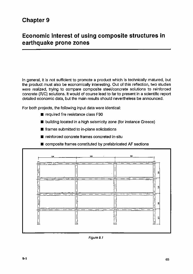
Chapter 9

Economic interest of using composite structures in earthquake prone zones

In general, it is not sufficient to promote a product which is technically matured, but the product must also be economically interesting. Out of this reflection, two studies were realized, trying to compare composite steel/concrete solutions to reinforced concrete (R/C) solutions. It would of course lead to far to present in a scientific report detailed economic data, but the main results should nevertheless be announced.

For both projects, the following input data were identical:

■ required fire resistance class F90

■ building located in a high seismicity zone (for instance Greece)

■ frames submitted to in-plane solicitations

■ reinforced concrete frames concreted in-situ

■ composite frames constituted by prefabricated AF sections

Figure 9.1

9-1 65

■ design according to Eurocode 8

■ same design raster for both solutions. Project 1 dealt with the following characteristics (fig. 9.1):

■ shopping centre with service loads 5 kN/m2

■ 4 storeys (including ground floor) with a height of 3.5 m each

■ 3 spans of 9.0 m

■ distance between frames of 6.0 m.

Project 2 showed some differences with the proceeding one (fig. 9.2):

■ office building with service loads 4 kN/m2

■ 7 storeys with a height of 3.0 m each

■ 3 spans of 6.0 m

■ distance between frames of 5.0 m.

-I

3x6m

L

E CO X

E m χ in

}i mm

++

:= H

:i—κ

++

++

++

44

++

++

++

44

44

Figure 9.2

66 9-2

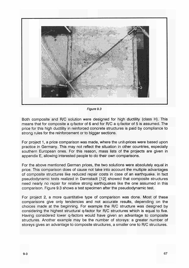
Figure 9.3

Both composite and R/C solution were designed for high ductility (class H). This means that for composite a q-factor of 6 and for R/C a q-factor of 5 is assumed. The price for this high ductility in reinforced concrete structures is paid by compliance to strong rules for the reinforcement or to bigger sections.

For project 1, a price comparison was made, where the unit-prices were based upon practice in Germany. This may not reflect the situation in other countries, especially southern European ones. For this reason, mass lists of the projects are given in appendix E, allowing interested people to do their own comparisons.

For the above mentioned German prices, the two solutions were absolutely equal in price. This comparison does of cause not take into account the multiple advantages of composite structures like reduced repair costs in case of an earthquake. In fact pseudodynamic tests realized in Darmstadt [12] showed that composite structures need nearly no repair for relative strong earthquakes like the one assumed in this comparison. Figure 9.3 shows a test specimen after the pseudodynamic test.

For project 2, a more quantitative type of comparison was done. Most of these comparisons give only tendencies and not accurate results, depending on the choices made at the beginning. For example the R/C structure was designed by considering the highest structural q-factor for R/C structures which is equal to five. Having considered lower q-factors would have given an advantage to composite structures. Another example may be the number of storeys: a greater number of storeys gives an advantage to composite structures, a smaller one to R/C structures.

9-3 67

Table 9.1 gives some quantitative comparisons:

Parameter

Total column surface (m2)

Column surface versus buiding surface (%)

Free space under beams ( 3m storey height ) (m)

Volume of concrete in the beams (m3)

Volume of concrete in the columns (m3)

Resultant base shear per frame (kN)

Period of first mode (s)

Top displacement under maximal earthquake (mm)

Max. beam bending moment under earthquake conditions (kNm)

Composite

1.88

0.3

2.65

33.3

29.1

180

1.6

388

152

R/C

4.82

0.8

2.44

95.3

93.7

341

0.93

185

226

Ratio

0.39

0.39

1.086

0.35

0.31

0.53

1.72

2.09

0.67

As the system dimensions were the same for both solution, an advantage not considered in this study is that storey height can be reduced about 8 to 10% for composite structures, due to the smaller beam height. This leads in general to lower buildings, bringing a further reduction in' masses and resulting base shear, moments,...

68 9-4

Chapter 10

Conclusions

10.1 General remarks The aim of the present work was to show that composite steel/concrete structures provide seismic resistance characteristics which can help promote composite structures in earthquake prone zones of the globe with traditional concrete and masonry building industries.

As quasi no informations were available concerning the behaviour of composite structures, it is quite normal that not all problems in relationship with seismic action could be solved. In order to fill the biggest gaps existing in knowledge and in standards, it was first of all aimed at obtaining qualitative statements, before proceeding to a higher number of more detailed parameter studies and tests. This step should be reserved for a future research project based on the results obtained herein. For the same reason, the developments made inside the DYNACS software, had the target to allow the simulation of the tests which were realized. Predicting the behaviour of completely different structures still remains very unsafe, as the variation of different parameters were not checked sufficiently in order to obtain an accurate and universal numerical model.

These models should be developed during a new research project, which will lead to the development of an aseismic building system and of a user friendly computer program adapted to the solutions proposed by this building system.

Nevertheless, it was possible to deduce a certain number of conclusions from the present project. These conclusions may be classified in three groups:

■ conclusions in relationship with standards and recommendations

■ conclusions in relationship with design problems

■ conclusions in relationship with manufacturing and quality insurance problems.

It schould be noted that 38 different connection types, which were either rigid or semi - rigid, have been tested at the "Politecnico di Milano". The corresponding features are given on pages 3-2 to 3-7 and 4-1 to 4-3 in the main report; more detailed test results are given in Appendix A. The best connection types, selected out of these tests, have been used for the frame

10-1 69

tests at the "Bergische Universität Wuppertal" (appendix C), at the University of Liège (appendix B) and at the 'Technische Hochschule Darmstadt" (appendix D).

10. 2 Standards and recommendations

During the tests, the application of ECCS­recommendations [7] leaded to two problems:

■ the displacement step increment was too large and consequently several specimens failed at an early stage, leading to a poor ductility,

■ several specimens could not be destroyed as the maximum displacement of the testing installation was reached and the testing procedures did not provide regulations for this situation.

Furthermore it makes generally no sense to have excessive plastic displacements in a structure ( or deformations in an element ), if the overall stability of the building cannot be assured or if the building cannot be used any longer after the earthquake. Therefore, the ECCS testing procedures should be completed according to chapter 8 of this report. The user should be given the possibility to claim for ductility or for serviceability.

On the other hand, a new parameter called "cumulated absorbed energy ratio" should be introduced. This parameter, which represents the sum of the really absorbed energy against the sum of the ideally absorbed yield strength energy, becomes even more important, when the testing procedure aiming at low cycle fatigue (during a shakedown test) is adopted.

Relating to the amendments of Eurocode 8 [9] and even Eurocode 3 [8], it can be stated that:

■ the participation of the shear panel to the overall energy dissipation should be allowed by taking into account also the shear resistance of the concrete, as well as the cooperation of the panel with the frame formed by the flanges and the stiffeners

■ a pure shear panel plastification should be prohibited and the shear panel mechanism should in general occur after plastifications in the beams or in the connections

■ shear panel, connections and shear studs should be capacity designed

■ the request of Eurocode 8 for designing the connections for 1.2 times the bearing capacity of the connected element, leads to excessive fillet welds which are not compatible with the state of art in welding. This problem does not exist with butt welds. That's why fillet welds should be forbidden in seismic design, or it should be required that the strength of the welding material is at least 20% higher than that of the ground material in order to fulfil the principle Mu.connection > 1.2 Mu.element·

70 10­2

10.3 Design problems The present project allowed to define in a qualitative way which kind of detail may be used or should not be used in design. Among the most important findings may be noted:

■ Bolted connections should be realized with high strength bolts and the use of two nuts per bolt is recommended. Tendons should not be used as on the one hand most of the time they do not exist in high strength quality and on the other hand their elongation becomes to great, leading to high ductility but unrealistic and unadmittable deformations.

■ The end plates in bolted connections should have a minimal thickness of at least 40 mm. Thinner end plates lead to excessive plate bending and by that way to bolt bending, which is badly supported by HS bolts. A further advantage of using thick plates may be the reduced number of bolts which can be limited to four. If the difference in thickness between the end plate and the connected flange becomes too important, the introduction of back plates may become interesting or even necessary in order to prevent local failure of the flange.

■ In bolted connections, the transverse stiffeners in the column should be located at the upper and lower end plate edges. Thus the shear panel is increased in height leading to lower solicitations. Simultaneously, this is the location of the load introduction point.

■ During the design step, the yield strength of the used steel sections must be known approximately (+/- 15%). Especially for lower yield grades this is very difficult, as standards give a maximum and a minimum for the ultimate strength, but only a minimum for the yield strength. That's why for a grade FeE 235 with a nominal yield strength of 235 MPa, effective yield strengths of 290 MPa and even more are absolutely normal. In these cases, the posterior weakening of the beam sections similar to test series F and Κ can be of a great help, as a new design is not necessary.

10.4 Manufacturing and quality insurance problems For welded structures submitted to cyclic loads it is most important to assure a good quality control. In fact, the specimens used during this project were manufactured in three different workshops with a different know-how in welding. Additional welding was also done at the Universities of Milan, Wuppertal and Darmstadt by the laboratories themselves or by exterior contractors. The results obtained were in direct relationship with the workshop qualification.

The workshop which realized the Wuppertal specimens was the less qualified one, but still corresponding to a good steel fabricator of a country under development. The results were disappointing. Nearly all the specimen collapsed early due to weld failure.

10-3 71

Therefore it ¡s very important to charge a highly qualified workshop with the welding applications and to use whenever it is possible butt welds with a full penetration. Slag inclusions should be limited to those admitted for parts susceptible to fatigue. A visual control of all the welds must always be done and at least a few of the welds should be submitted to ultrasonic or equivalent testing. In case of doubt all the welds must be inspected this way.

Especially when using joint type K, care should be given to the treatment of the flame-cutted surfaces at the beam weakening section. A grinding of this surfaces should always be done in order to eliminate all notches which can lead to low cycle fatigue failure.

72 10-4

Bibliography

[ I ] KANAMORI H. "Quantification of Earthquakes", Nature, Volume 271, 1978

[2] WAKABAYASHI M. "Design of Earthquake ­ Resistant Buildings", Mc GrawHill, 1986

[3] BALLIO G. et al "Sul comportamento di sezioni miste in acciaio e calcestrezzo sottoposte a carichi ciclici: indagine sperimentale e modellazione numerica", Giornate A.I.C.A.P. 1987

[4] JUNGBLUTH O. FEYEREISEN K, OBEREGGE O. "Verbundprofilkonstruktionen mit erhöhten Feuerwiderstandsdauer", Bauingenieur 55,1980

[5] SCHLEICH J.B., HUTMACHER H., LAHODA E., LICKES J.P. " A new technology in fireproof steel construction" ,Acier­Stahl­Steel N3,1983

[6] ARBED Recherches (L) / Université de Liège, Service Ponts et Charpentes (Β), "REFAO/CAFIR, Computer Assisted analysis of the Fire Resistance of steel and composite steel­concrete structures" C.E.C. Research 7210­SA/502 1982­1985 ­ Final Report, March 1986

[7] TC 13, "Recommended Testing Procedure for Assessing the Behaviour of Structural Steel Elements under Cyclic Loads", ECCS, 1986

[8] C.E.C., "EUROCODE N° 3; Common Unified Rules for Steel Structures", 1989

[9] C.E.C., "EUROCODE N° 8; Structures in Seismic Regions/Design",

1989

[10] ARBED, "AF 30/90 Verbundträger; Momenttabellen", 1986

[ I I ] ARBED, "AF 30/120 Verbundstützen; Traglasttabellen", 1986 [12] JRC Ispra, "Experimental and analytical research on the earthquake

resistant response of steel­concrete composite connections", Working Group 3 of the Association of Structural Mechanics Laboratories

BIB­1 73

^^ ÍSS^^AÍ ' ' ^ ' ;vv^>s^Í Í -¿í ' ' Í l í ; fT¿.V

POLITECNICO DI MILANO DIPARTIMENTO DI INGEGNERIA STRUTTURALE

Piaz2a Leonardo da Vinci, 32 20133 Milano (Italy)

Appendix A

Test report of the Milan laboratory

Prof. G. BALLIO

75

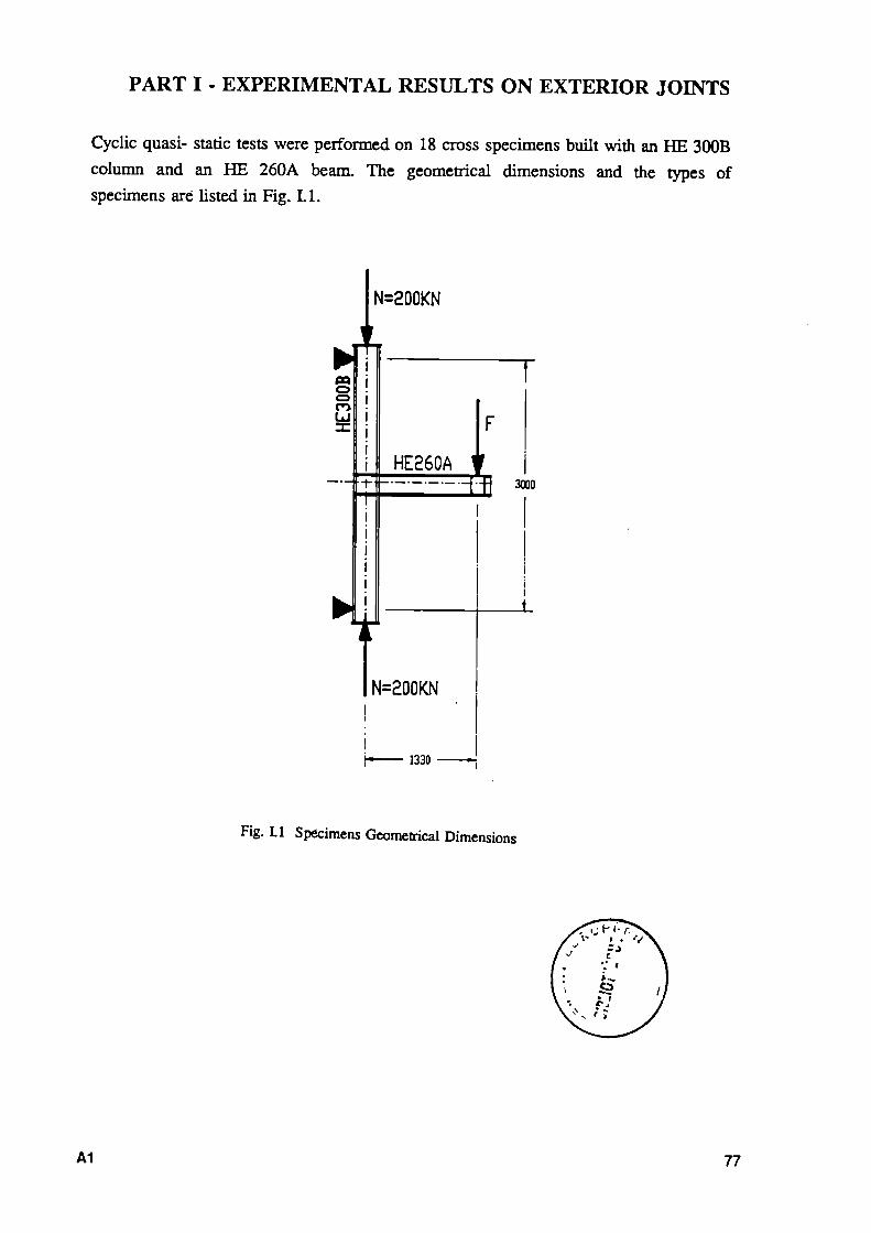
PART I - EXPERIMENTAL RESULTS ON EXTERIOR JOINTS

Cyclic quasi- static tests were performed on 18 cross specimens built with an HE 300B column and an HE 260A beam. The geometrical dimensions and the types of specimens are listed in Fig. 1.1.

N=200KN

PQ C3 <=> CO

►u

HE260A 3 3000

N=200KN

1330

Fig. 1.1 Specimens Geometrical Dimensions

A1 77

H^J

Fig. 1.1 Specimens Types: bare steel, composite without slab, composite with slab

78 A2

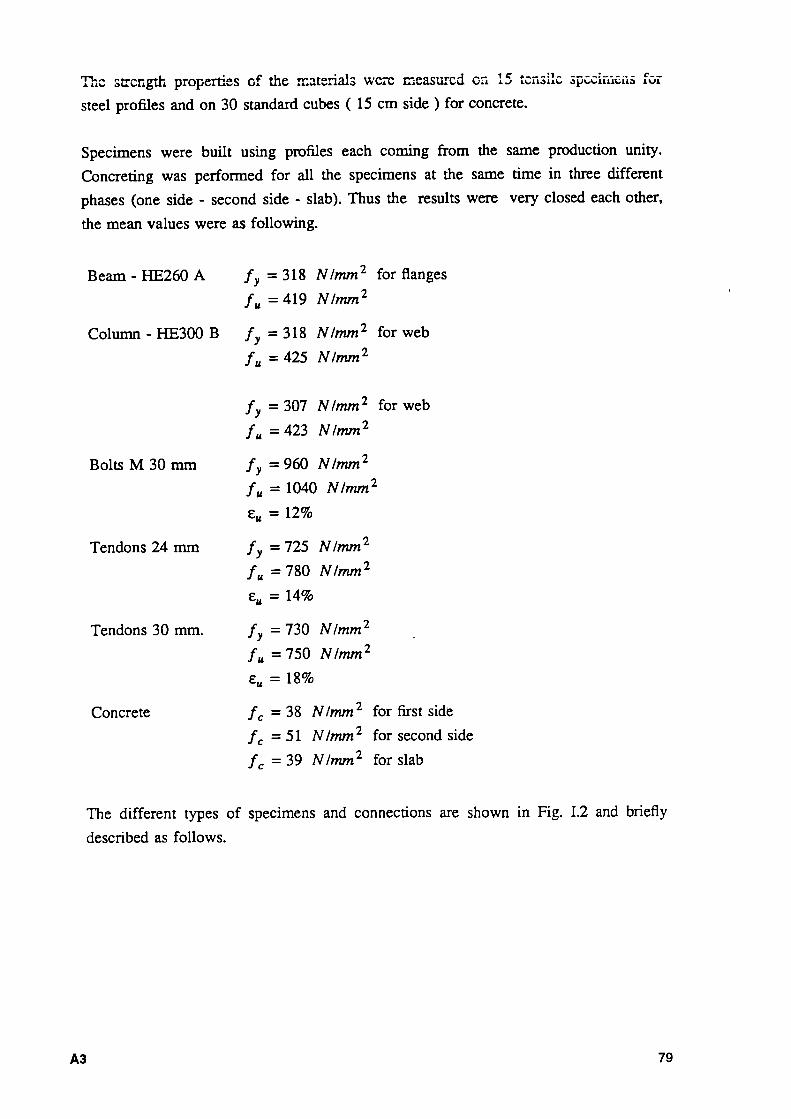
The strength properties of the materials were measured on 15 tensile specimens for steel profiles and on 30 standard cubes ( 15 cm side ) for concrete.

Specimens were built using profiles each coming from the same production unity. Concreting was performed for all the specimens at the same time in three different phases (one side ­ second side ­ slab). Thus the results were very closed each other, the mean values were as following.

Beam ­ HE260 A fy= 318 Nimm2 for flanges fu = 419 Ν/mm2

fy = 318 Nimm2 for web Column ­ HE300 Β fu = 425 Nimm2

Bolts M 30 mm

Tendons 24 mm

Tendons 30 mm.

Concrete

fy fu

fy = fu =

eu =

fy = fu =

εΒ =

fy = fu = ε„ = fc = fc = fc =

307 Nimm2 for web 423 Nimm2

960 Nimm2

: 1040 Nimm2

12%

725 Nimm2

780 Nimm2

14%

730 Nimm2

750 Ν Imme­

lmo

38 Nimm2 for first side 51 Nimm2 for second side 39 Nimm2 for slab

The different types of specimens and connections are shown in Fig. 1.2 and briefly described as follows.

A3 79

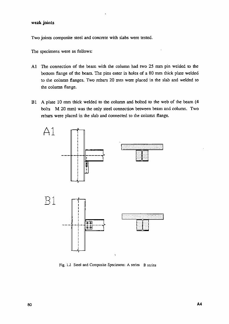
weak joints

Two joints composite steel and concrete with slabs were tested.

The specimens were as follows:

Al The connection of the beam with the column had two 25 mm pin welded to the bottom flange of the beam. The pins enter in holes of a 80 mm thick plate welded to the column flanges. Two rebars 20 mm were placed in the slab and welded to the column flange.

Bl A plate 10 mm thick welded to the column and bolted to the web of the beam (4 bolts M 20 mm) was the only steel connection between beam and column. Two rebars were placed in the slab and connected to the column flange.

A l

B l

s—τ

Fig. 1.2 Steel and Composite Specimens: A series Β series

80 A4

welded plate beam io column joints

Three specimens were tested. Plates 15 mm thick were connected by 10 mm side fillet welds to the flanges of the beam and by 14 mm side fillet welds to the flanges of the columns. Beam web were connected with two M 20 mm bolts to a 10 mm one side plate welded to the column. Süffeners across the column (12.5 mm thick) were placed at the beam flange levels. Specimen CI was bare steel, specimen C2 was composite without slab, specimen C3 was composite with slab.

CI to

19 Ξ3 I

C2 ¿1 + Ξ3

C3

]

Fig. 1.2 Steel and Composite Specimens: C series

A5 81

end piales beam to column joints

Eight specimens were tested. Beams were fully welded to end plates, bolted to the flange of the column. The specimens were as follows:

Dl Bare steel without back plates on the panel zone. Stiffeners across the column (12.5 mm thick) were placed at the beam flange levels. The end plate, 44 mm thick, was connected to the column flange with 8 M 24 bolts placed on 4 rows (two at the top and two at the bottom). The distance beetween the interior rows was 330 mm, the distance beetween the exterior ones was 450 mm.

D2 Same as Dl, but composite without slab.

D3 Same as Dl, but composite with slab.

D4 Same as D2 but bolts were substituted by tendons of the same diameter going across the concrete and bolted against the outside flange of the column. Four [ stiffeners, able to separate tendons from concrete, were welded to the web of the column.

D5 Same as D4, but withot stiffeners. Plastic tubes separate tendons from concrete.

D6 Same as Dl, but semirigid. The end plate, 26 mm thick, was connected to the column flange with 4 M 30 bolts placed on 2 rows with a distance of 350 mm.

D7 Same as D6 but composite without slab. In addition bolts were substituted by tendons of the same diameter going across the concrete and bolted against the outside flange of the column. Four [ stiffeners, able to separate tendons from concrete, were welded to the web of the column.

D8 Same as D7, but without stiffeners. Plastic tubes separate tendons from concrete.

82 A6

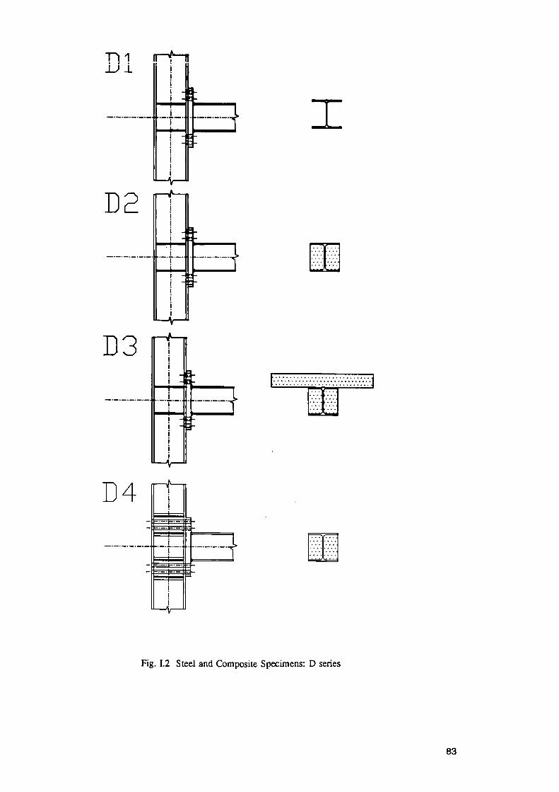
ni

3 I

D2 ; = ;

D3

D4 —•H— — ι —

ΞΞφΞΞ

3

3

Fig. 1.2 Steel and Composite Specimens: D series

83

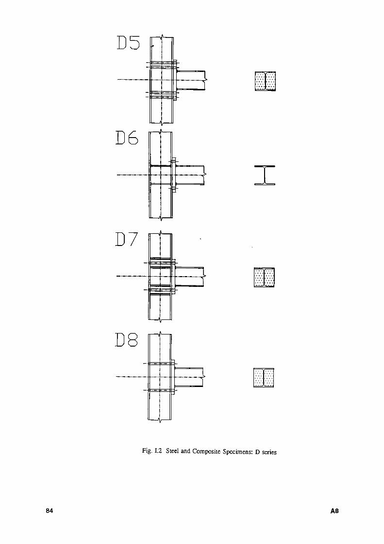
D5 Ε Ξ ΕΞΞΟ-

Ε Ξ

D6 =(—*

=4=

ν.1..

Ι

D7

D8

Ξ ^ Ξ

■ 1 ·-!> Λ·Λ

Fig. 1.2 Steel and Composite Specimens: D series

84 A8

weided plate beam to column joints

Three specimens were tested. Beams flanges and web had full penetration welds to the column flanges. No back plates on the panel zone were present. Stiffeners across the column (12.5 mm thick) were placed at the beam flange levels. Specimen El was bare steel, specimen E2 had the column composite but the beam bare steel, specimen E3 was composite without slab.

El

Ζ

E2 bean

column

E3

3

-Fig. 1.2 Steel and Composite Specimens: E series

A9 85

end piates reduced beam io cuiuhili joint

Two specimens were tested. The connection was fully welded as for E series. Specimen Fl was bare steel, specimen E2 was composite withot slab

τ

F2

5

t Fig. 1.2 Steel and Composite Specimens: F series

86 A10

Tests were performed with the experimental equipments [ 1 ] of the Department of Structural Engineering of Politecnico di Milano University. The procedures followed during the tests and the rehalaboration of the results were in compliance with [ 2 ].

The experimental set-up is shown in Fig. 1.3. The column is in horizontal position. A mechanical jack with a capacity of 1000 KN and a maximum elongation of 300 mm impresses a controlled cyclic displacement to the top of the beam. The resultant force is measured by a dynamometer. An additional jack impress an axial displacement to the column in order to have an axial force in the column with a mean value of 200 KN. Displacements were measured with inductive trasducers. The following quantities were continously recorded on a computer.

force impressed by the jack to the top of the beam

applied to the column

displacement at the top of the beam

at the 2 supports of the column

at the column at the level of the 2 flanges of the beam

A11 87

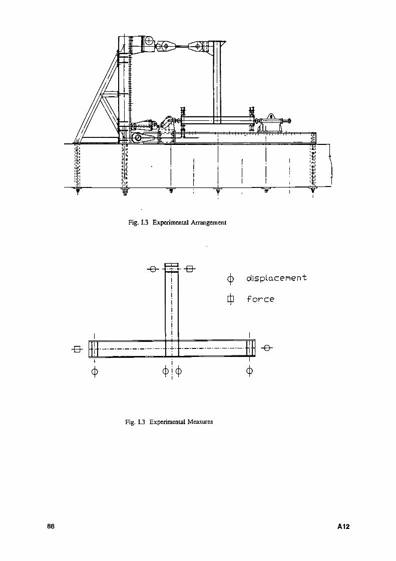
Fig. 1.3 Experimental Arrangement

•Β- -r·

Φ

-θ--3--Β-

Φ Φ

φ displacement

φ f o r c e

■ - θ -

Φ

Fig. 1.3 Experimental Measures

88 A12

T U , τ ? : ^ Τ Λ ­ ι »ι. . . A:CC. _ . l a w Α l g A . T d i l U W ü l W «Ì­LXI' trcnt plots of the total applied Bending Moment /Vi ­ F L versus total rotation θ = ν IL, ν beeing the relative displacement between the ends of the beam. The rotation value θ corresponds to the storey drift divided by the height of the storey.

Fig. 1.5 show the different pattern of the Total Dissipated Energy Ratio versus the adimensional elongation as stated in [ 2 ].

The Energy Dissipated Ratio were not significant in specimens Al and Bl; thus the corrisponding figures are omitted.

In Fig. 1.6 the most significant collapse mechanisnms are shown.

M 3 89

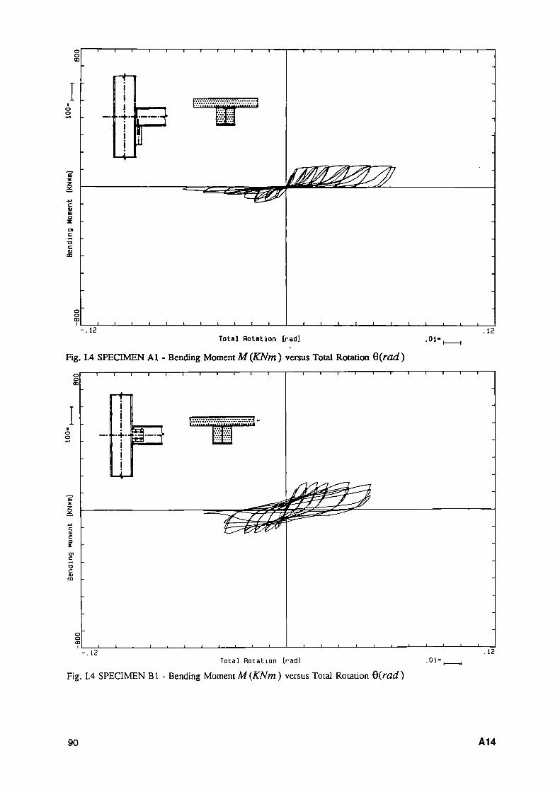
-ι 1 1 Γ τ 1 1 Γ

~"tt=* "y.Y.y.y¿yy¿yy.':. .y.*.·.·. J

_l I I i_ _l I l_

π ι ι ι i r ^

­I I I L ­1 I I I I L ­ . 1 2 .12

Total Rotation [rad] . 01­

Fig. 1.4 SPECIMEN Al ­ Bending Moment M(KNm ) versus Total Rotation Q(rad) η 1 1 1 1 1 1 Γ π 1 1 1 1 1 1 1 1 Γ

^•'•'•"""•"•'uimtll

+·1Ξ —

Ι Ι Γ

­J I l_ 12 .12

Total Rotation [radi .01 =

Fig. 1.4 SPECIMEN Bl ­ Bending Moment M (KNm ) versus Total Rotation Q(rad)

90 A14

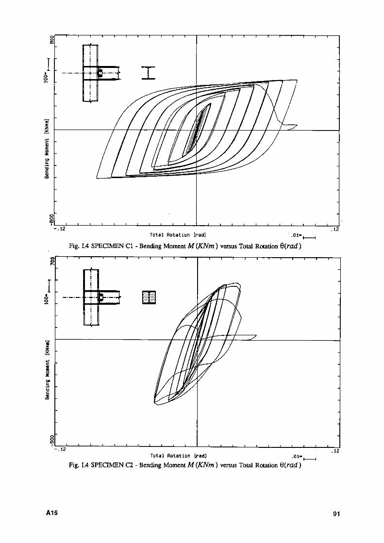
o o m

c Ό

- l I L· - 1 I I 1 I I I I ι ι - .12 .12

Total Rotation [rad] -01

"i

Fig. 1.4 SPECIMEN CI - Bending Moment M(KNm) versus Total Rotation Q(rad) — ι 1 1 1 1 1 1 1 ~i 1 1 1 r

ζ

O) I

-.12 - l I L·

Total Rotation [rad] .12

. 01 -

Fig. 1.4 SPECIMEN C2 - Bending Moment M {KNm ) versus Total Rotation tì(rad )

A15 91

τ 1 r

-.13

π 1 1 r

ι ι I t

Total Rotation [rad] .11

.01-

Fig. 1.4 SPECIMEN C3 - Bending Moment M (KNm ) versus Total Rotation Q(rad )

92 A16

Total Rotation [rad] .12

.01· ι 1

Fig. 1.4 SPECIMEN Dl - Bending Moment M(KNm) versus Total Rotation Q(rad) ι 1 1 1 1 1 1 1-

Total Rotation [rad] .12

.01·

Fig. 1.4 SPECIMEN D2 - Bending Moment M {KNm ) versus Total Rotation Q(rad)

A17 93

- . 1 2 .12 Total Rotation [rad] . 01-

Fig. 1.4 SPECIMEN D3 - Bending Moment M(KNm) versus Total Rotation Q(rad)

Total Rotation [rad] . 0 1 - t

Fig. 1.4 SPECIMEN D4 - Bending Moment M (KNm ) versus Total Rotation Q(rad)

94 A18

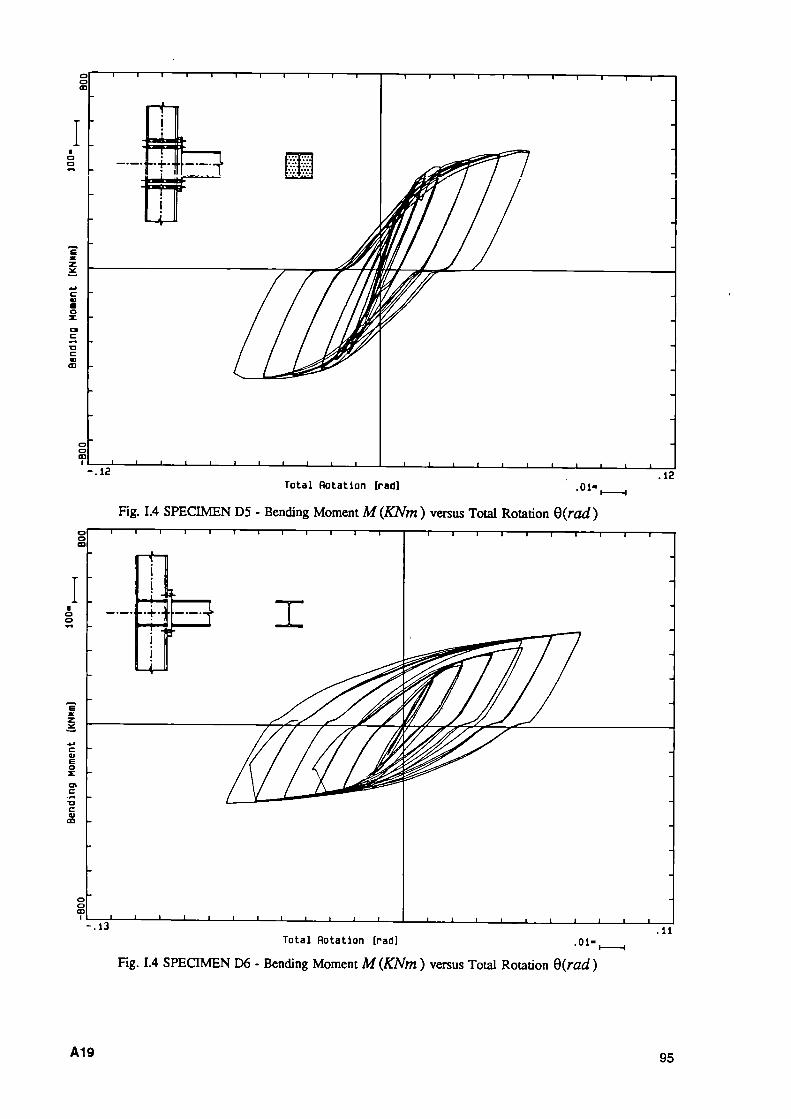
Total Rotation [rad]

Fig. 1.4 SPECIMEN D5 - Bending Moment M(KNm ) versus Total Rotation Q(rad) τ 1 1 1 1 Γ

- . 1 3 Total Rotation [rad]

.11 .01-

Fig. 1.4 SPECIMEN D6 - Bending Moment M (KNm ) versus Total Rotation Q(rad)

A19 95

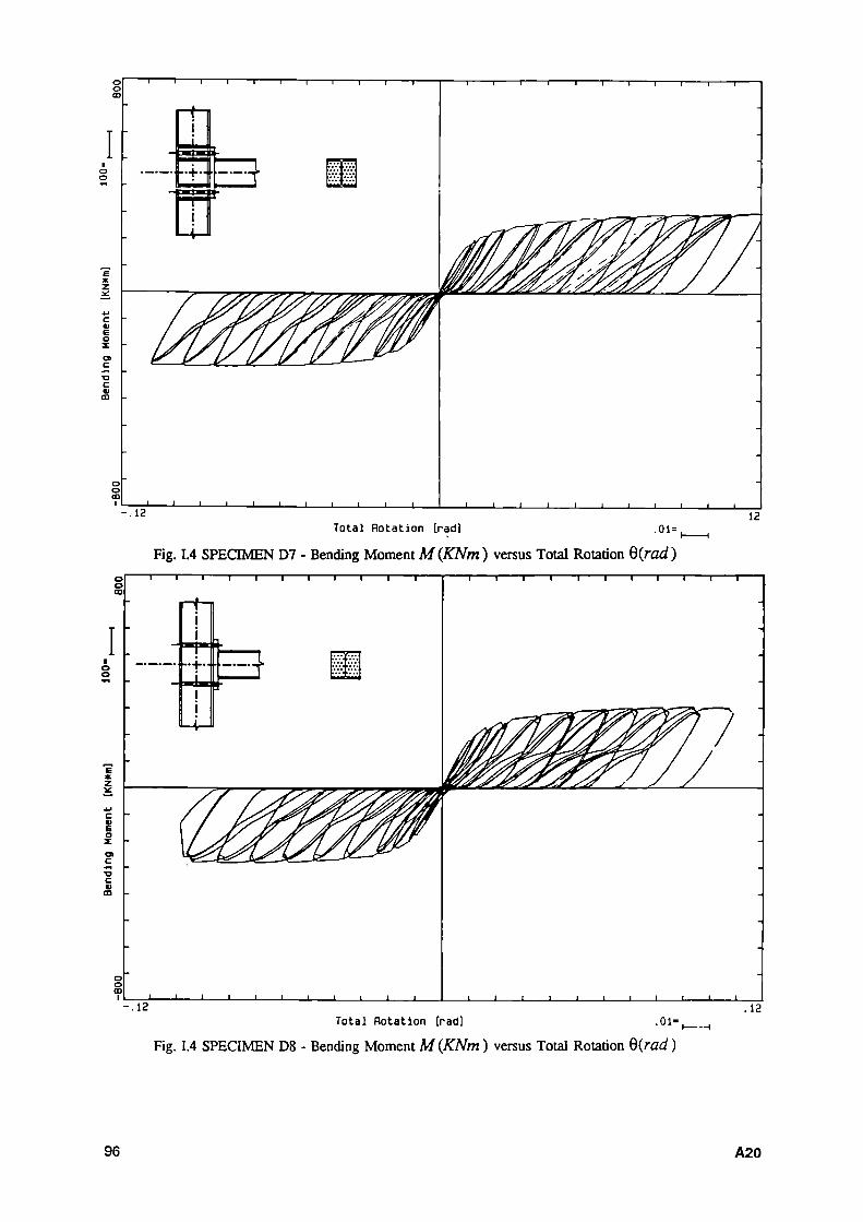
Total Rotat ion [rad] .01=,

Fig. 1.4 SPECIMEN D7 - Bending Moment M (KNm ) versus Total Rotation Q(rad)

Total flotation [rad]

Fig. 1.4 SPECIMEN D8 - Bending Moment M (KNm ) versus Total Rotation Q(rad )

96 A20

Total Rotation [rad]

Fig. 1.4 SPECIMEN El - Bending Moment M(KNm ) versus Total Rotation Q(rad) o o αϊ

τ ι ι ι τ

ι ι ι ι ι ι ι ι - Ι ' ■ _Ι Ι L - . 1 2 .12

Total Rotation [rad] . 01 -

Fig. 1.4 SPECIMEN E2 - Bending Moment M {KNm ) versus Total Rotation Q(rad)

A21 97

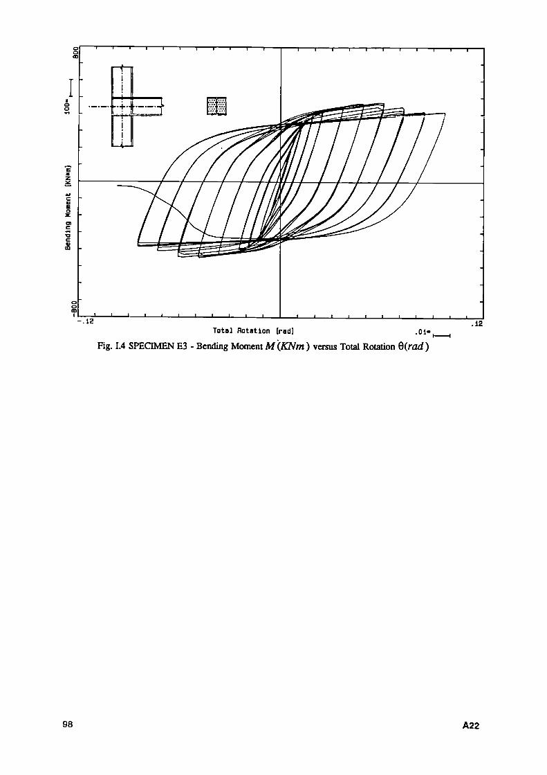
o o m

π 1 τ τ 1 r

•α c υ ο

-.12 -Ι 1 Ι L

τ 1 1 ι ι ι ι 1 ι 1 r

Total Rotation [rad] .12

.01-

Fig. 1.4 SPECIMEN E3 - Bending Moment M {KNm ) versus Total Rotation Q(rad )

98 A22

Total Rotation [rad]

Fig. 1.4 SPECIMEN Fl ­ Bending Moment M (KNm ) versus Total Rotation Q(rad ) o o m

I ■ o o

ζ

*j

c 03 E O Ζ Ol

c OJ m

o o CD

ι

i

I 1

­ . 12

ι

i i

¡ i j

I Τ ­ ι ι ι ι ι 1

m

1 fl 111 lili

1 1 1 l i l i l í

■ i l i — ι 1

// / / / / / y

KO

Total Rotation [rad] .01­

Fig. 1.4 SPECIMEN F2 ­ Bending Moment M (KNm ) versus Total Rotation Q(rad )

A23 99

τ 1 1 Γ τ 1 1 1 1 1 1 1 1 ι 1 r

Ζ

l i l i

5 10 15 20 Cycle Total Elongation Ratio

Fig. 1.5 SPECIMEN CI - Cumulated Energy ratio versus Elongation ratio π 1 1 1 1 1 1 1 1 1 1 Γ τ 1 1 r

f>-

_ l l ι l | I I I I I - J 1 I I I I I I -

5 10 15 Cycle Total Elongation Ratio Fig. 1.5 SPECIMEN C2 - Cumulated Energy ratio versus Elongation ratio

20

100 A24

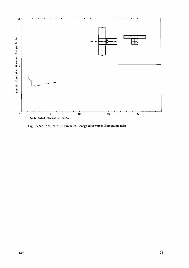
τ 1 1 1 1 1 1 1 1 1 1 1 1 1 1 1 1 1 ι 1 1 1 Γ

- f -

■·+·-

-Λ-

M

I I ι I I I I I I I I I I I I I { 1 5 10

Cycle Total Elongation Ratio 15 20

Fig. 1.5 SPECIMEN C3 - Cumulated Energy ratio versus Elongation ratio

A25 101

3 E U

5 10 15 Cycle Total Elongation Ratio

Fig. 1.5 SPECIMEN DI - Cumulated Energy ratio versus Elongation ratio

20

5 10 15 Cycle Total Elongation Ratio

Fig. 1.5 SPECIMEN D2 - Cumulated Energy ratio versus Elongation ratio

102 A26

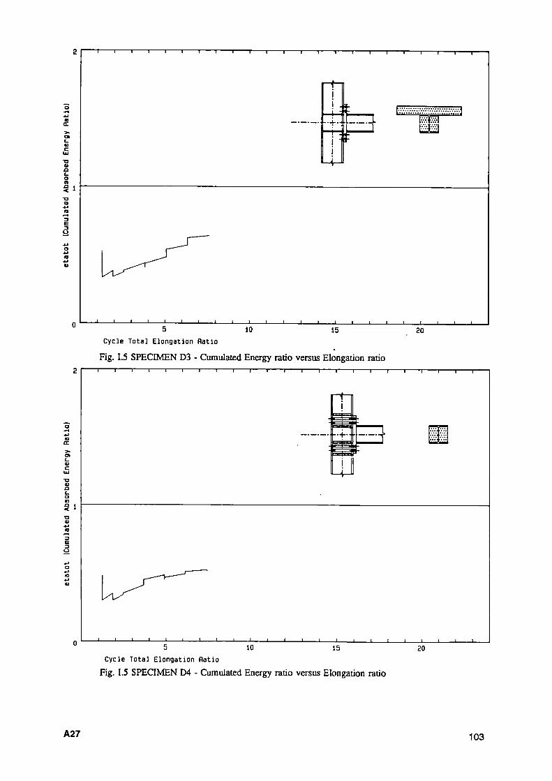
"Τ 1 1 1 r "i 1 1 1 1 1 1 1 1 1 r

Hf m

- J 1 1 1 I I I 1_ _1 ι ' -1 I L 10 15

Cycle Total Elongation Ratio

Fig. 1.5 SPECIMEN D3 - Cumulated Energy ratio versus Elongation ratio

20

5 10 15 Cycle Total Elongation Ratio

Fig. 1.5 SPECIMEN D4 - Cumulated Energy ratio versus Elongation ratio

20

A27 103

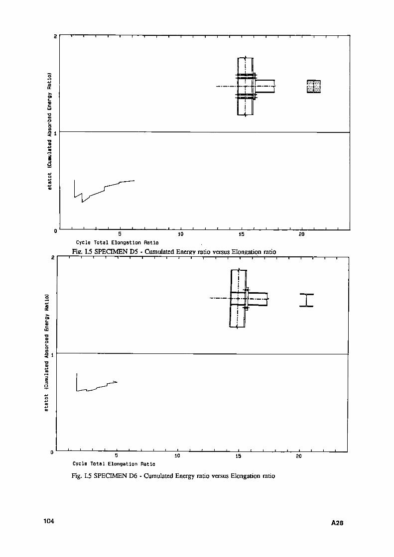
ι ι ι ι ι ι ι ι 1 1~ ι ι ι ι ι ι π

01 a c. o η

2 ι

Π

3 α

- I I I Ι Ι ' ' ' ' '

5 10 15 20 Cycle Total Elongation Ratio

Fie. 1.5 SPECIMEN D5 - Cumulated Energy ratio versus Elongation ratio ~i 1 1 1 1 Γ" ~i 1 Γ

I

η 5 ι

- 1 I I I ι ' 10 15 20

Cycle Total Elongation Ratio

Fig. 1.5 SPECIMEN D6 - Cumulated Energy ratio versus Elongation ratio

104 A28

π 1 1 Γ τ 1 1 1 1 ι 1 Γ

Ξ3

3 υ

-Ι Ι Ι Ι Ι Ι Ι Ι Ι_ _Ι ι ι ι ι -1 ι ι ι_ 10 15

Cycle Total Elongation Ratio 20

5 10 15 Cycle Total Elongation Ratio Fig. 1.5 SPECIMEN D8 - Cumulated Energy ratio versus Elongation ratio

20

A29 105

ι I I T^ τ 1 1 1 r

t=l

-I 1 I I 5 10 15 20

Cycle Total Elongation Ratio Fig. 1.5 SPECIMEN El - Cumulated Energy ratio versus Elongation ratio

~i 1 1 1 1 1 1 1 1 1 r ι ι 1 1 1 1 1 1 1 1 I

J Ξ3 I bean

colLrm

-1 1 I [_ -1 I I L· 5 10 15

Cycle Total Elongation Ratio Fig. 1.5 SPECIMEN E2 - Cumulated Energy ratio versus Elongation ratio

20

106 A30

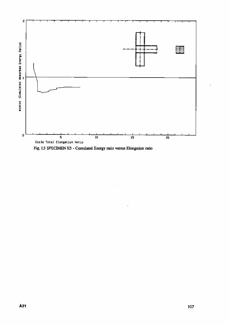
2 I 1 1 1 1 1 1 1 1 1 1 1 r ­ ι 1 1 1 1 1 I

rï­

ΓΓ­Ρ^

ra

­ l I I I ' ■ ' ■ ' ' 5 10 15

Cycle Total Elongation Ratio

Fig. 1.5 SPECIMEN E3 ­ Cumulated Energy ratio versus Elongation ratio

­I I L 20

A31 107

"Τ I I I I I I I 1 1 1 I 1 1 1-

- ţ -

4-

Χ

-J 1 I l_ -I 1 I I ' ' 10

-i ι ι ■ ■ 15

Cycle Total Elongation Ratio

Fig. 1.5 SPECIMEN Fl - Cumulated Energy ratio versus Elongation ratio

20

5 10 15 Cycle Total Elongation Ratio Fig. 1.5 SPECIMEN F2 - Cumulated Energy ratio versus Elongation ratio

so

108 A32

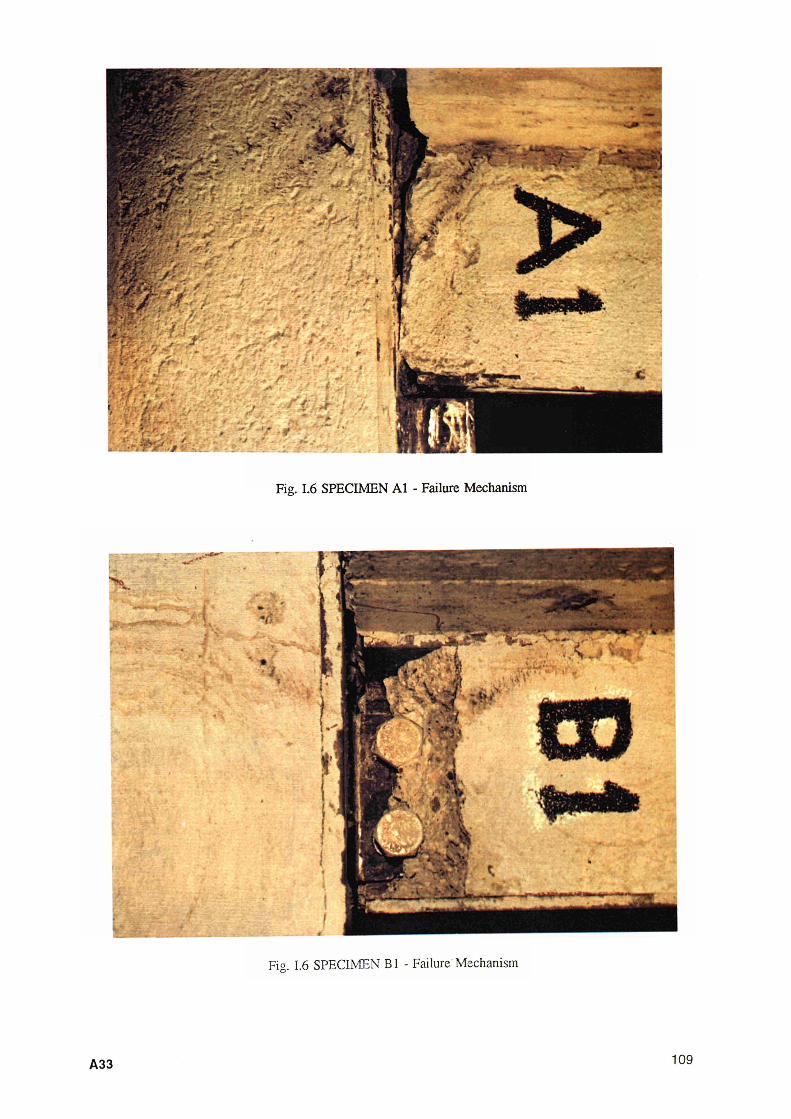
r"

Fig. 1.6 SPECIMEN Al - Failure Mechanism

>■>

Fig. 1.6 SPECIMEN Bl - Failure Mechanism

A33 109

Fig. 1.6 SPECIMEN Cl - Failure Mechanism

< \

Fig. 1.6 SPECIMEN C2 - Failure Mechanism

110 A34

Fig. 1.6 SPECIMEN C3 - Failure Mechanism

A35 111

Fig. 1.6 SPECIMEN Dl - Failure Mechanism

Fig. 1.6 SPECIMEN D2 - Failure Mechanism

112 A36

Fig. 1.6 SPECIMEN D3 - Failure Mechanism

■Λ

■Λ

Fig. 1.6 SPECIMEN D4 - Failure Mechanism

A37 113

Fig. 1.6 SPECIMEN D5 - Failure Mechanism

Fig. 1.6 SPECIMEN D6 - Failure Mechanism

114 A38

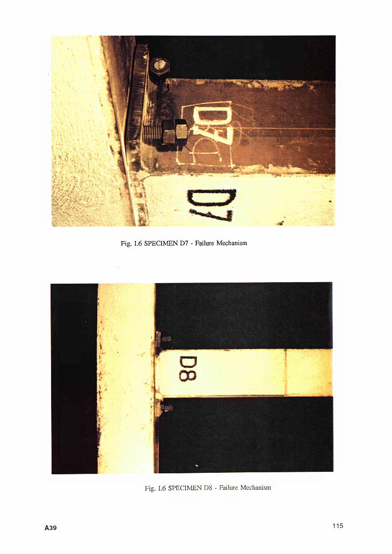
if- -»'

T r ø V ^ i

Fig. 1.6 SPECIMEN D7 - Failure Mechanism

Fig. 1.6 SPECIMEN D8 - Failure Mechanism

A39 115

Fig. 1.6 SPECIMEN El - Failure Mechanism

is' "'

Γ

Fig. 1.6 SPECIMEN E2 - Failure Mechanism

116 A40

Fig. 1.6 SPECIMEN E3 - Failure Mechanism

A41 117

Fig. 1.6 SPECIMEN Fl - Failure Mechanism

/ VC·* · ,

Fig. 1.6 SPECIMEN F2 - Failure Mechanism

118 A42

In order to compare the experimentai results, the following q u a a i u i u e s w i l l be

introduced and compared:

θ Global Flexibility of the joint in the elastic field measured as the slope in

θ — M experimental diagram (rad/KN m)

My Conventional elastic limit (KN m) measured on the experimental diagram

as indicated in [ 2 ] . My corresponds to the intersection between the

elastic slope and the line tangent to the plastic branch having a slope of

1/10 of the elastic one

Qy Total rotation corresponding to My

M2.5 Bending Moment (KN m) corresponding to a total rotation θ = 2 .5%

θ„ M a x i m u m Total Rotation reached during the test and allowing three

complete cycles without failure

Mu Bending moment corresponding to θ„

θ„ / Qy Conventional maximum ductility ratio

Qu 12.5 Ductil i ty margin in respect the limit of 2.5 % assumed by many

researchers as the maximum value of storey drift allowable during a severe

seismic event.

In Fig. 1.7 the values of the above quantities are listed for each specimen.

Specimen A l has a significant non symmetric behaviour; the table reports the values

corresponding to the maximum resistence of the joint.

The behaviour of the other specimens is practically symmetric; in the table the mean

value of the various quantities are Usted.

A43 119

Al Bl

Cl C2 C3

Dl D2 D3 D4 D5 D6 D7 D8

El E2 E3

FI F2

Θ'

rad KNm

χ 1(T5

3.50 4.00

3.40 2.95 2.20

3.30 2.70 2.10 2.70 2.80 5.00 4.40 4.70

3.75 3.35 2.90

4.00 3.20

My

KNm

110. 110.

272. 445. 440.

300. 365. 410. 370. 360. 250. 210. 220.

250. 370. 380.

230. 325.

Qy

%

0.38 0.45

0.92 1.31 0.97

0.99 0.98 0.86 1.00 1.01 1.25 0.92 1.03

0.94 1.24 1.10

0.92 1.04

^ 2 . 5 %

KNm

=

=

330. =

445.

360. 430. 480. 420. 430.

­280.

—

295. 400. 430.

280. 380.

Mu

KNm

==

==

430. 500. 400.

340. 465. 500. 480. 460. 350.

395. 285. 400.

300. 335.

Θ«

%

=

=

7.4 2.3 4.8

7.3 7.4 6.0 6.2 5.0 6.2

8.3 8.6 8.5

9.8 8.6

Qy

=

=

8.0 1.8 4.9

7.4 7.5 7.0 6.2 4.9 5.0

8.8 7.1 7.7

10.6 8.3

% 2.5%

= ==

3.0 = 1.9

2.9 3.0 2.4 2.5 2.0 2.5

3.3 3.4 3.4

3.9 3.4

Fig. 1.7 Experimenial Results

120 A44

1.1 The Experimental Behaviour of Weak Connections

With reference to the collapse mechanisms shown in Fig. 1.6 and to the results listed in Fig. 1.7 the following may be noted.

The plastic hinge always formed in the connections for a limited value of the bending moment. The overall behaviour of specimen Bl appears better than the one of specimen Al. Nevertheless a better quality of the welds connecting the pins may probably improve the strength of the joints type A.

1.2 The Experimental Behaviour of welded plate connection

With reference to the collapse mechanisms shown in Fig. 1.6 and to the results listed in Fig. 1.7 the following may be noted.

The bare steel specimen behaves very well; the plastic hinge forms in the panel zone; cycles are stable.

Concrete gives an improvement of rigidity and increases the strength of the panel zone. As a consequence the welding of the plate to the column flange may become critical as the ductility concerns.

Such a type of joint may be used only guaranteing a very good control of welding procedures.

A45 121

1.3 The Experimental Behaviour of End Plates Connection

With reference to the collapse mechanisms shown in Fig. 1.6 and to the results listed in Fig. 1.7 the following may be noted.

The specimens with bolted thick end plate (Dl - D2 - D3) behave as expected. The connection had a sufficient restence in order to allow the formation of the plastic hinge in the beam. Concrete gave an improvement both to stiffness and strength of the joint.

The specimens with the bolted tendons and thick end plate (D4 - D5) behave in a different way. The elastic limit was reached in the tendons causing a loss of the stiffness of the whole joint. This was due to the fact that was impossible to find tendons with a material grade as specified in the design. Permanent deformations of tendons caused also a gap beetween the end plate and the column flange. Such a gap became greater as the total rotation of the joint was increasing.

In the semirigid joint (specimen D6) the end plate becomes plastic and the bolts collapsed because the bending effects caused by the deformation of the plate. Ductility and energy dissipation are poor.

In specimens with flexible end plate and tendons (D7 - D8) the elastic strength of tendons was not sufficient. Therefore the plastic behaviour of the tendons and their permanent deformations did not allow energy dissipation.

Summing up the following conclusions may be given.

From a qualitative point of vew it may be stated that thick end plate connection gives good results if the bolts are stressed in the elastic field. Semirigid connections have a worse behaviour. Tendons may be used only if adeguate strength is provided. During the specimen construction it was not possible to find tendons compling with the design requirements.

122 A46

From a quantitative point of vew the tests have shown that concrete increases the performances of the joint if the plastic hinge does not forai in the connection.

Attention must be paied to the material properties of the bolts and/or tendons.

The joint must be overdesigned according to Eurocode provisions in order to allow the formation of the plastic hinges in the beam rather than the connection.

L4 The Experimental Behaviour of Welded Beam to Column Joint

With reference to the collapse mechanisms shown in Fig. 1.7 and to the results listed in Fig. 1.8 the following may be noted.

In bare steel specimen plasticity was reached both in the panel zone and in the beam. Local failure mechanism near the welds occurred due to secondary bending effects caused by the deformation of the panel zone.

If the stiffness of panel zone is increased by the addition of concrete, plastic hinge forms in the beam, without significant permanent deformations of the panel zone or cracking of the welds.

For concrete specimen both panel both panel zone and beam dissipate energy in plastic field.

Summing up it may be stated that concrete gives a good contribution increasing stiffness without a significant loss of ductility.

A47 123

1.5 The Experimental Behaviour of Welded Reduced Beam

With reference to the collapse mechanisms shown in Fig. 1.7 and to the results listed in Fig. 1.8 the following may be noted.

The reduction of the flange caused a loss of strength but was able to avoid the panel shear mechanism: the plastic hinge located in the beam.

As for the previous specimens concrete gives a good contribution both to stiffness and strength.

1.6 References

[1] Bailio G. and Zandonini R. (1985) An Experimental Equipment to Test Steel Structural Members and Subassemblages Subject to Cyclic Loads Ingegneria Sismica, Anno II, 2, pp 25-40

[2] ECCS, CECM, EKS Technical Committee 1, WG 1.3 - Seismic Design (1986) Recommended Testing Procedure for Assessing the Behaviour of Structural Steel Elements under Cyclic Loads Publication n. 45

124 A48

PART Π - EXPERIMENTAL RESULTS ON INTERIOR JOINTS

Cyclic quasi- static tests were performed on 20 cross specimens built with an HE 300B column and an HE 260A beam. The geometrical dimensions and the types of specimens are listed in Fig. Π.Ι.

Ϊ

N=200KN

2

i

2806

HE260A

å 2740

N=2Q0KN

Fig. 1.1 Specimens Geometrical Dimensions

A49 125

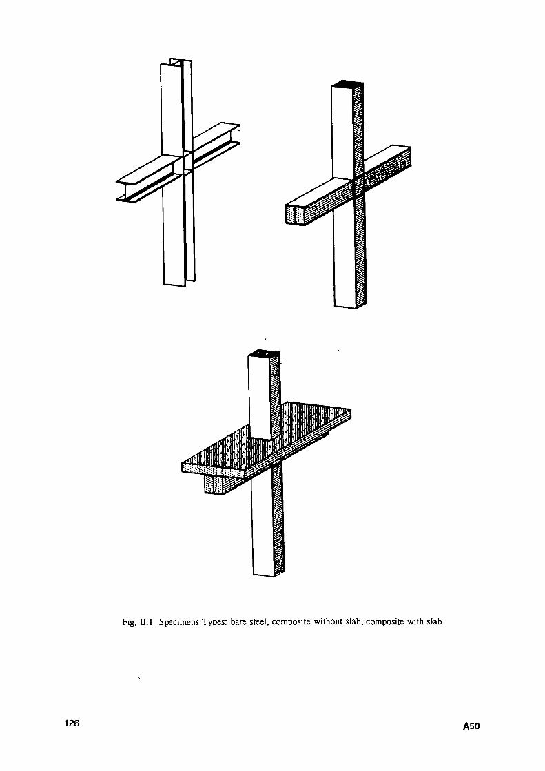
Fig. II. 1 Specimens Types: bare steel, composite without slab, composite with slab

126 A50

The strength properties of the materials were measured on 16 tensile specimens for steel profiles and on 80 standard cubes (15 cm side ) for concrete.

Specimens were built using profiles each coming from the same production unity. Concreting was performed for all the specimens at the same time in three different phases (one side - second side slab). Thus the results were very closed each other, the mean values were as follows.

Beam - HE 260 A ƒy = 302 Nimm1 for flanges ƒ„ = 416 Nimm1

Column - HE 300 Β ƒy = 282 Nimm1 for flanges fu = 404 Nimm1

fy = 307 Nimm1 for web fu = 423 Nimm1

Bolts M 30 fy = 960 Nimm1

fu = 1040 N/mm1

εα = 12%

Concrete fc = 38 Ν/mm1 for first side fc = 33 Ν/mm1 for second side fc = 27 Ν/mm1 for slab

The different types of specimens and connections are shown in Fig. II.2 and briefly described as follows.

A51 127

weak joints

Three joints composite steel and concrete with slabs were tested. No additional rebars were placed in the slab and connected to the column flange.

The specimens were as follows:

Gl The connection of the beam with the column had two 25 mm pin welded to the bottom flange of the beam. The pins enter in holes of a 80 mm thick plate welded to the column flanges.

G2 The connection of the beams with the column had end plates welded to the beam. The end plates enter in a special notchs of the 80 mm thick plates welded to the column flanges.

HI A plate 10 mm thick welded to the column and bolted to the web of the beam (4 bolts M 27 mm) was the only steel connection between beam and column.

G l

Ρ LU

Fig. II.2 Steel and Composite Specimens: G series

128 A52

G2

E3

Fig. Π.2 Steel and Composite Specimens: G series

Fig. Π.2 Steel and Composite Specimens: Η series

A53 129

welded beam TO column joints

Five specimens were tested. Beams flanges had full penetration welds to column flanges; beam webs were connected with two M27 mm bolts to a 12 mm one side plate welded to the column.

The specimens were as follows:

11 Bare steel without back plates on the panel zone. Stiffeners across the column, 12.5 mm thick, make continous the beam flanges.

12 Same as II but composite without slab.

13 Same as II but composite with slab.

14 Composite with slab. Two back plates each 15 mm thick welded to the panel web and without the stiffeners corresponding to the beam flanges.

15 Same as 14 but with stiffeners corresponding to beam flanges.

130 A54

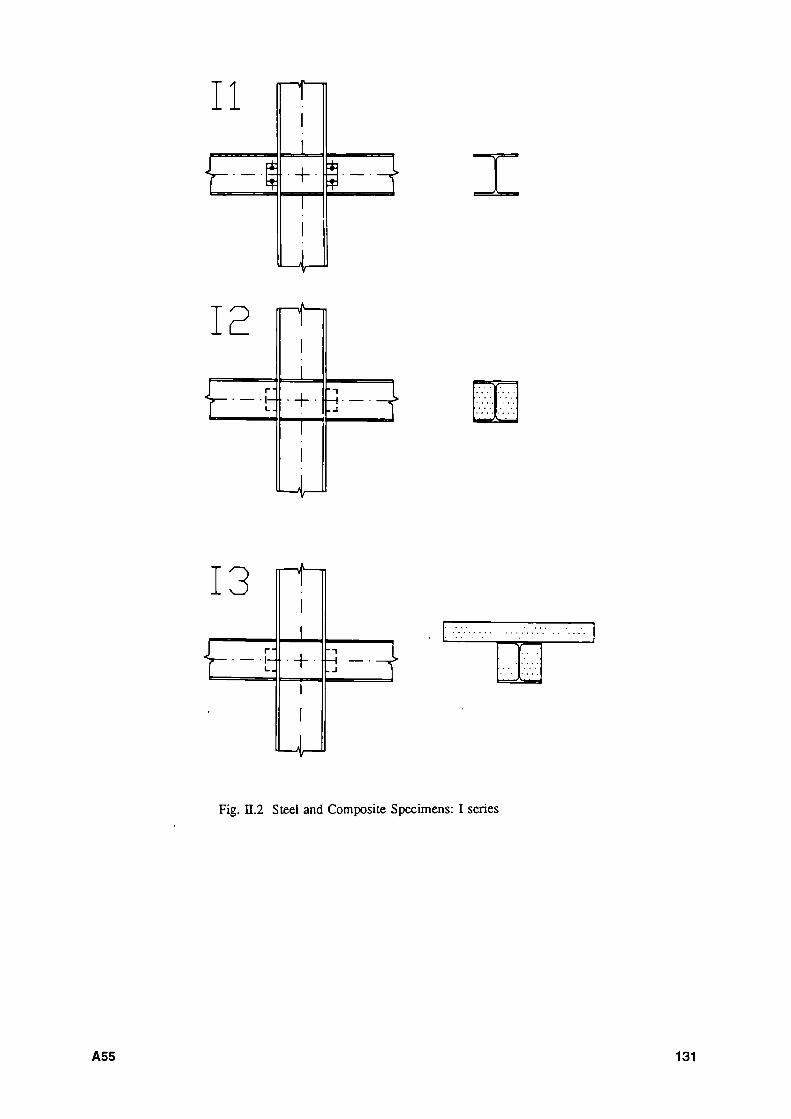
Il

12

I-ES I

Β + Ε3

13

E +

Fig. Π.2 Steel and Composite Specimens: I series

A55 131

14

ΕΞΙ +

Lp

S

Fig. 1.2 Steel and Composite Specimens: I series

132 A56

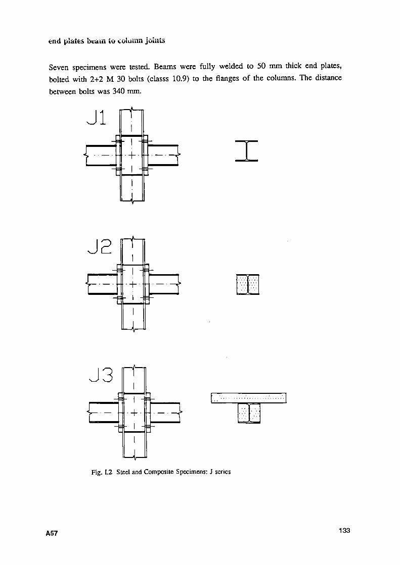
end plates beáiii ίο column joints

Seven specimens were tested. Beams were fully welded to 50 mm thick end plates, bolted with 2+2 M 30 bolts (classs 10.9) to the flanges of the columns. The distance between bolts was 340 mm.

Jl } ■ -

I - ι -■■+■ - ι -

1

- 4 I

J2

£ + ■ 3

J3 1

- 1 -) 1

- t - ■

- 1 -1

- 4 Fig. 1.2 Steel and Composite Specimens: J scries

A57 133

The specimens were as follows:

Jl Bare steel without back plates on the panel zone. Stiffeners across the column (12.5 mm thick) were placed at the top and the bottom of the end plate at a distance of 465 mm, thus nearly doubling the dimension of the panel in respect to I specimens.

J2 Same as Jl, but composite without slab.

J3 Same as Jl, but composite with slab.

J4 Bare steel; stiffners were substituted by two exterior plates (10 mm thick) welded to the ends of column flanges.

J5 Same as J4, but composite with slab.

J6 Same as J3, with the addition of two back plates 10 mm thick welded to the web of the column (stiffeners are present).

J7 Same as J6 but without stiffeners across the column.

J4

E + · --ά

Fig. Π.2 Steel and Composite Specimens: J series

134 A58

J5

Γ +

J6

f -

-1-1

- I -

■ + · I

1 = —

J7 - 1 -

• I ■

■ + ■

• 1 · f=l Fig. 1.2 Steel and Composite Specimens: J senes

<V59 135

end plaies reduced beam iu column joint

Four specimens were tested. Beams were fully welded to 40 mm. thick end plates, bolted with 2+2 M 30 bolts (classs 10.9) to the flanges of the columns. The distance between bolts was 340 mm.

kl

E +

<^m^m^mm M ^ t f W J M I M J M « ^ ^ ^

kZ

ΕΞ 4 ­Ξ3

Ζ

k3

E3 — · ­ ·

ι _ =

Fig. 1.2 Steel and Composite Specimens: Κ senes

136 A60

The specimens were as follows:

Kl Bare steel without back plates on the panel zone. Stiffeners across the column (12.5 mm thick) were placed at the top and the bottom of the end plate at a distance of 430 mm, thus nearly doubling the dimension of the panel in respect to I specimens.

K2 Same as Kl, but composite with slab.

K3 Composite with slab. Stiffeners were substituted by two 10 mm thick plates welded to the ends of column flanges.

K4 Composite without slab. The column web was unstiffened and without back plates.

k4 t

Fig. 1.2 Steel and Composite Specimens: K series

A61 137

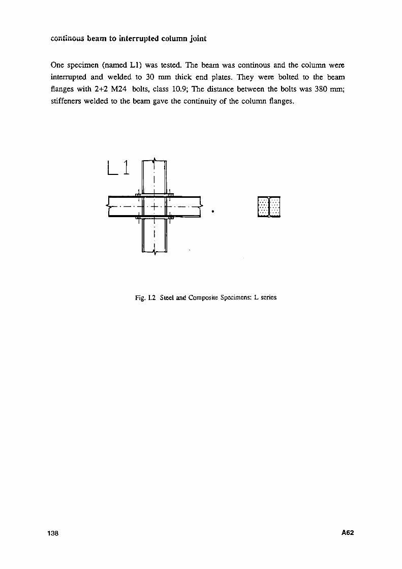
, - „ _ * : u s beam to interrupted column joint

One specimen (named LI) was tested. The beam was continous and the column were interrupted and welded to 30 mm thick end plates. They were bolted to the beam flanges with 2+2 M24 bolts, class 10.9; The distance between the bolts was 380 mm; stiffeners welded to the beam gave the continuity of the column flanges.

LI

L-—é

t

m + .

Fig. 1.2 Steel and Composite Specimens: L series

138 A62

Tesis were performed with 'die experimental equipments [ 1 ] of the Department ùf Structural Engineering of Politecnico di Milano University. The procedures followed during the tests and the rehalaboration of the results were in compliance with [ 2 ].

The experimental set-up is shown in Fig. n.3.The column is in horizontal position; two tendons impress a force of 200 KN. A mechanical jack with a capacity of 1000 KN and a maximum elongation of 600 mm impresses a controlled cyclic displacement to the top of the beam. The resultant force is measured by a dynamometer. Displacements were measured with inductive trasducers. The following quantities were continously recorded on a computer.

force impressed by the jack to the top of the beam

given by the restraint at the bottom of the beam

impressed by the tendons to the column

displacement at the top of the beam

at the bottom of the beam

at the column in the direction of the applied force

at the 2 supports of the column

length variation of the 2 diagonals of the panel

A63 139

Fig. Π.3 Experimental Arrangement

-Β - ■■

Φ

-Β--Ξ—θ

- θ - - # - &

ι - θ -

Φ

φ displacement

φ f o r ce

Fig. Π.3 Experimental Measures

140 Α64

The Fig IL 4 show the different plots of the tola! applied Bending Moment M = F L versus total rotation θ = v IL, ν beeing the relative displacement between the ends of the beam. The rotation value θ corresponds to the storey drift divided by the height of the storey. The bending moment M corresponds to the double of the bending value applied to one beam.

Fig Π.5 show the different relations between the total applied Bending Moment M = F L versus the shear deformation of the panel zone θ = a v s where:

a _ ^db2 + dc

2

dbdc

vs the measured value of the elongation of the panel diagonal

db , dc the length of the panel

Fig. Π.6 show the different pattern of the Total Dissipated Energy Ratio versus the adimensional elongation as stated in [ 2 ].

The shear deformation Qs and the Energy Dissipated Ratio were not sgnificant in specimens Gl, G2, HI; thus the corrisponding figures are omitted.

In Fig. Π.7 the most significant collapse mechanisnms are shown.

(V65 141

­ ι 1 1 1 1 1 r ι i 1 ι τ « 1 1 1 1 1 1 1 1

^"'"""""MMIIIÏÎ^""****"*'^

. 4 ^

!

2

­ . 1 3 ­ l 1 1 1 I I I I I I I l_

Total Rotation Irid] _i ι ι ι .—ι J l ­

• " ­ ι — « .11

Fig. Π.4 SPECIMEN Gl ­ Bending Moment M(KNm) versus Total Rotation B(rad) 1 ι

­~ ι ι ι ι ι ι I 1 1 1 1 1 1 1 1 1 1 1 1 r

Ly.v.v.y.v.~v^~v.y.v.v.v."J

­T2^P /iflgft­n

rL .12

_i ι ι ι ι ι ­1 1 1 L ­J I [_

Total Rotation [rad] .12

.01=

Fig. II.4 SPECIMEN G2 ­ Bending Moment M (KNm ) versus Total Rotation Q(rad )

142 A66

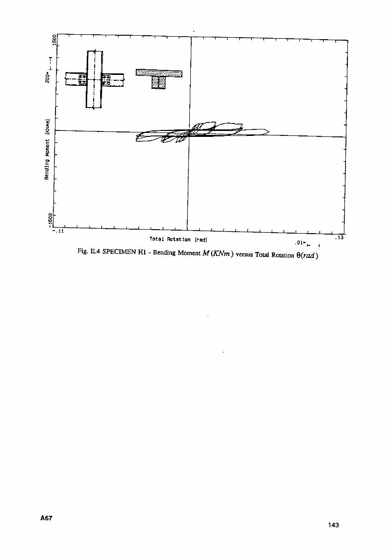
τ 1 1 r ~i ι - 1 1 ρ 1 1 r τ 1 1 r ι ι Γ

LU ζ ■χ.

ΊΕϊ^Ζ ~>

c OJ m

rf ' ' ' 1 1 1 1 1 i_ -

1 1 1 1 1 ι ι -1 1 L

. 01-Total flotation [radj

Fig. Π.4 SPECIMEN HI - Bending Moment M (KNm ) versus Total Rotation 6(rad)

.13

A67 143

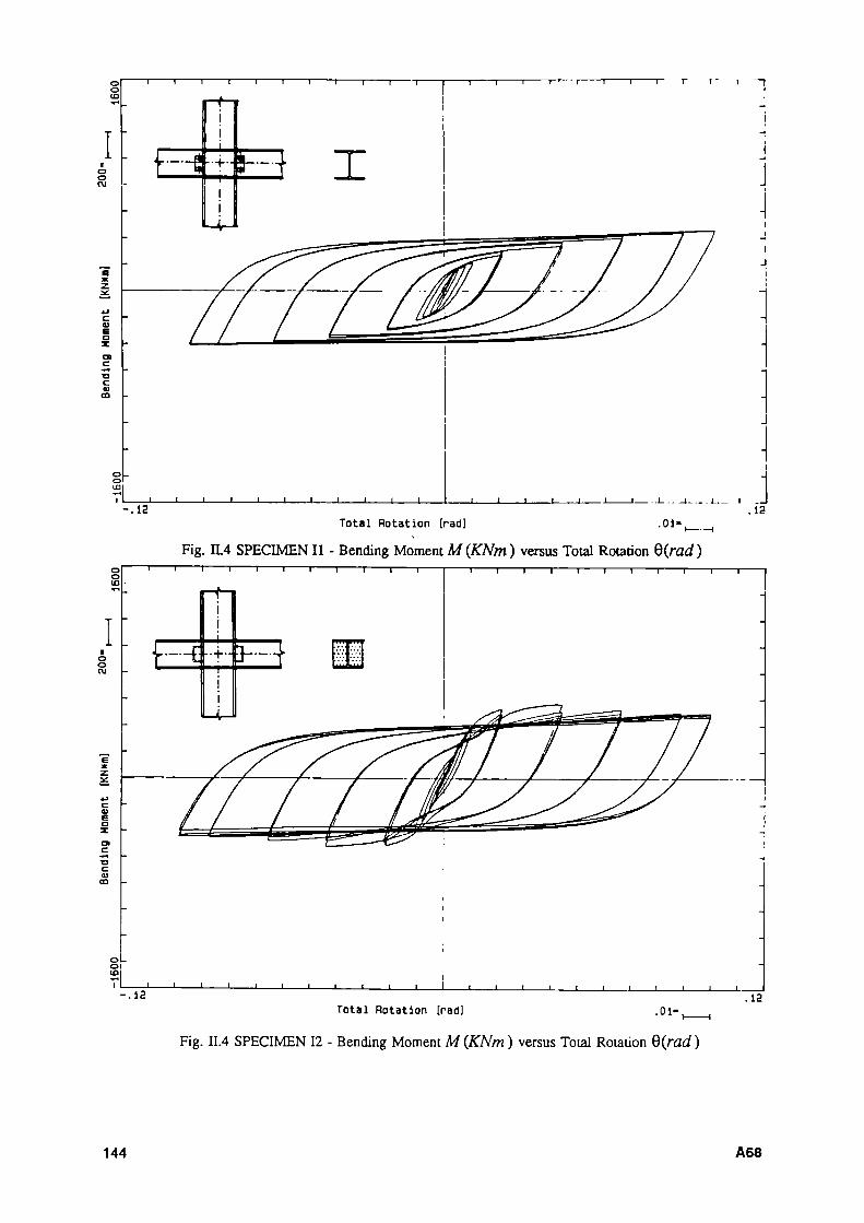
n 1 1 1 1 1 Γ

c OJ m

- .12

Ζ

- ι 1 Γ - *-- ι 1 1 Γ

- Τ Γ" ι —

Ι Ι 1 Ι Ι Ι Ι Ι U -1 ι ι_

Total Rotation [rad]

_j ι J ι ι ι J ι Ι .13

. 0 1 - ,

Fig. Π.4 SPECIMEN II - Bending Moment M{KNm) versus Total Rotation Q(rad) o l I I I ι ι 1 1 Γ

o o cu

—L "t" J —

-i-

τ 1 r "Τ Ι 1 Ι Ι Ι Γ"

ι Ι 1 1 1 1 1 1 1 1 1 ι ι Ι ι ι ι ι ι ι ι ι_ .12 .12

Total Rotation [rad] . 0 1 -

Fig. II.4 SPECIMEN 12 - Bending Moment M (KNm ) versus Total Rotation Q(rad )

144 A68

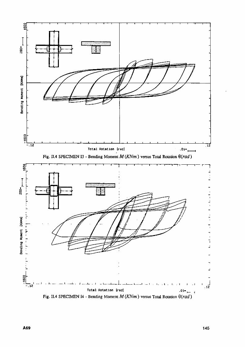
Total Rotation [rad]

Fig. H.4 SPECIMEN 13 - Bending Moment M(KNm) versus Total Rotation Q(rad)

ο Γ O '

u o O ' cu Γ

"τ 1 1 1 1 1 1 1 1 Γ τ 1 Γ ~Ι Γ Γ 1 Γ

*> ι £ Γ

ο . ο to

.12 Ι - - Ι . 1 . -L- . J - Ι Ι J

Total Rotation [rad] — ι 1 -- ι . i- . ι . ι. . ι ι . ι ι J

. 1 2 . 0 1 - ,

Fig. ΙΙ.4 SPECIMEN 14 - Bending Moment M (KNm ) versus Total Rotation Q(rad )

A69 145

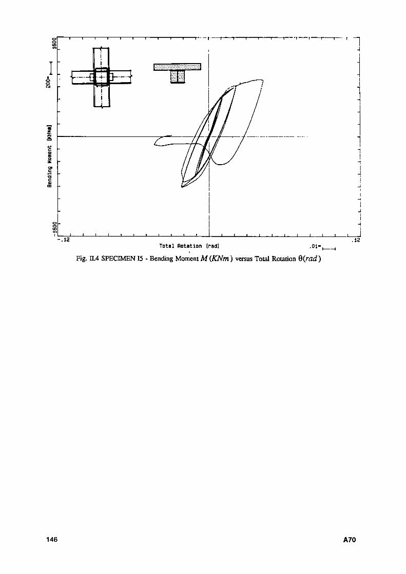
Total Rotation [rad] ·0 1

Ί

Fig. Π.4 SPECIMEN 15 - Bending Moment M(KNm) versus Total Rotation B(rad)

146 A70

ι 1 Γ · τ Γ 1 1 1 1 1 Γ­ Η 1 1 1 τ 1 1 Γ" ι ­ τ τ"

V L I J ι . ι ι ­.12

ι ι 1 Ι Ι Ι Ι J Ι Ι 1 ­

Total Rotation [rad] .12

. 01­

Fig. Π.4 SPECIMEN Jl ­ Bending Moment M(KNm) versus Total Rotation B(rad)

°r~ "T 1 r 1 1 Γ­ Η 1 1 1 r 1 r 1 1 r τ­

w

­ f ­

­Λ­

ζ

Ο ί ­Ο (£>.

7 ι_ ι — L J I L· ­J I 1_ ­.12 .12

Total Rotation [rad] ·01

"ι­

Fig. II.4 SPECIMEN J2 ­ Bending Moment M (KNm ) versus Total Rotation Q(rad )

A71 147

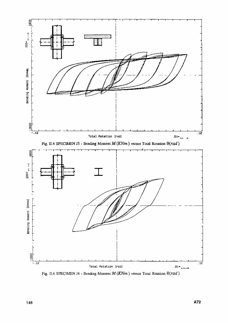
Total Rotation (rad] ·01

"ι

Fig. Π.4 SPECIMEN J3 - Bending Moment M (KNm ) versus Total Rotation Q(rad)

Total Hotation [rad]

Fig. II.4 SPECIMEN J4 - Bending Moment M (KNm ) versus Total Rotation Q(rad)

148 A72

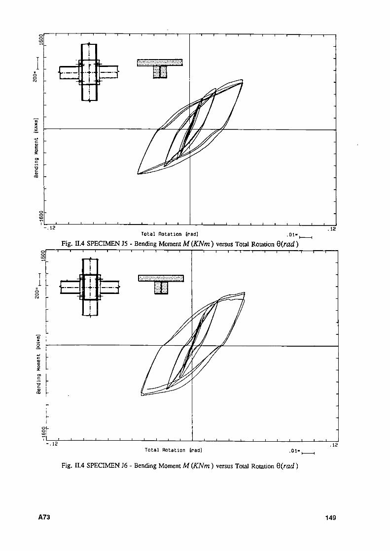
Total Rotation [rad]

Fig. Π.4 SPECIMEN J5 - Bending Moment M (KNm ) versus Total Rotation Q(rad)

_I ι t t ι - l 1 I L -J I ι ι ι ι ι ι - . 1 2

Total Rotation [rad] .12

.01·

Fig. II.4 SPECIMEN J6 - Bending Moment M (KNm ) versus Total Rotation Q(rad )

A73 149

ι 1 1 1 1 1 1 r

o . o

- . 1 1 -ι 1 1 1 ι ι i_ Total Rotation [rad]

.13 • 0 1 - .

Fig. Π.4 SPECIMEN J7 - Bending Moment M(KNm) versus Total Rotation Q(rad)

150 A74

π 1 1 1 1 1 1 1 1 r ι 1 1 τ 1 1 r 1 τ r

■

ρ

r­t­i ¡ ¡ ι ­

—f— ¡ . I

!

. — . . ,

§ L

I

o L 0 1 in

.12 _l J I I I_ ­J 1 1 I I . . I . . L .

Total Rotation [rad] .01· Fig. II.4 SPECIMEN Kl ­ Bending Moment M(KNm) versus Total Rotation Q(rad)

-ι Γ

.12

S

8

ΓΗΙ i . i 1 ! 1 • —i—|

1

τ 1 Γ τ 1 Γ

I

s

s ­ .12

­J 1 1 I I 1_ ­ I I 1_ _J I I I­

Total Rotation [rid] .01· Fig. II.4 SPECIMEN K2 ­ Bending Moment M(KNm) versus Total Rotation Q(rad)

.12

A75 151

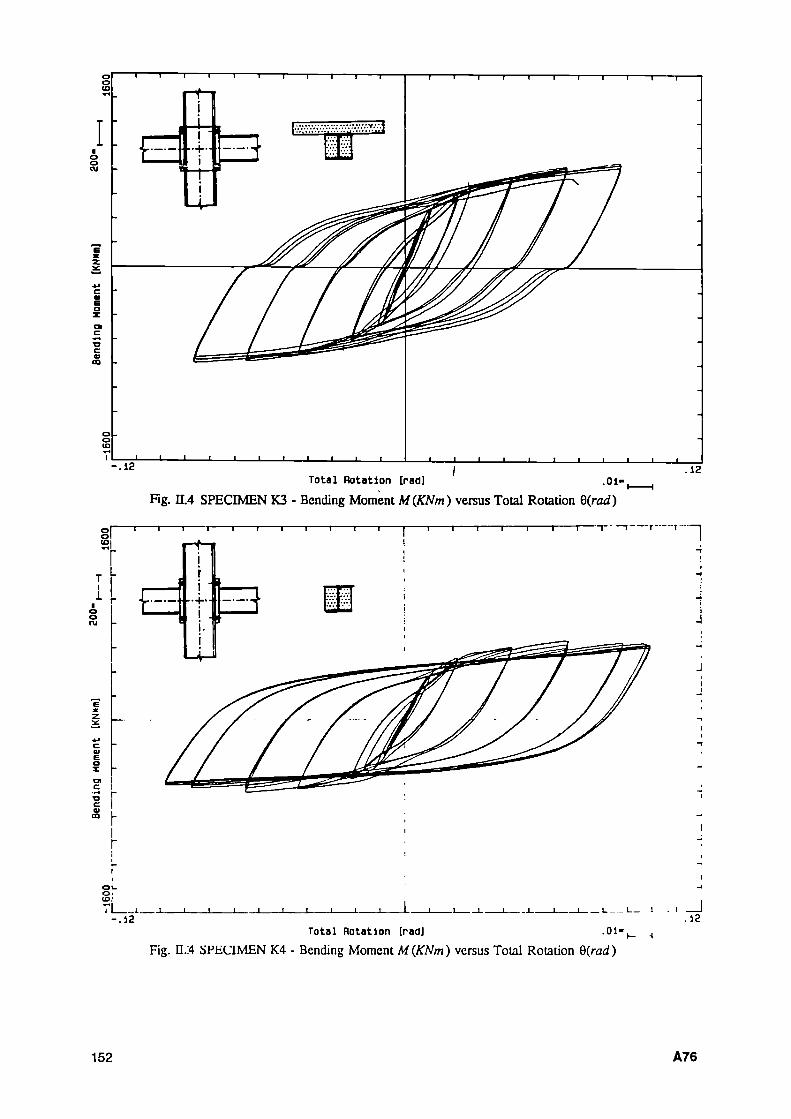
Total Rotation [rad] .01· Fig. U.4 SPECIMEN K3 - Bending Moment M(KNm) versus Total Rotation Q(rad)

Total Hotatlon [rad] .01-

Fig. Π.:4 SPECIMEN K4 - Bending Moment M(KNm) versus Total Rotation Q(rad)

152 A76

Fig. Π.4 SPECIMEN LI - Bending Moment M(KNm) versus Total Rotation Q(rad)

hrr 153

Sheared Panel Rotation [rad] .01=.

Fig. Π.5 SPECIMEN II - Bending Moment M(KNm) versus Shear Rotation Q,(rad)

M — I I I I I I

- . 1 3 L i . . L _ _ 1 . .1 1 . . ..

Sheared Panel Rotation [rad]

Fig. II.5 SPECIMEN 12 - Bending Moment M(KNm) versus Shear Rotation Qs(rad)

ι ι ι ι ι ι ι ι ι J .11

. 0 1 - _ ,

154 A78

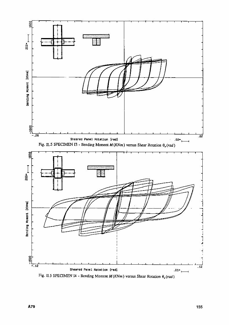
π 1 1 1 1 1 Γ

Eáte -ι 1 Γ -ι 1 Γ

.26 -I I I I L

Sheared Panel Rotation [rad] .02·

Fig. Π..5 SPECIMEN 13 - Bending Moment M(KNm) versus Shear Rotation Qt(rad) I 1

.22

Sheared Panel Rotation [rad] Fig. II.5 SPECIMEN 14 - Bending Moment M(KNm) versus Shear Rotation Qs(rad)

A79 155

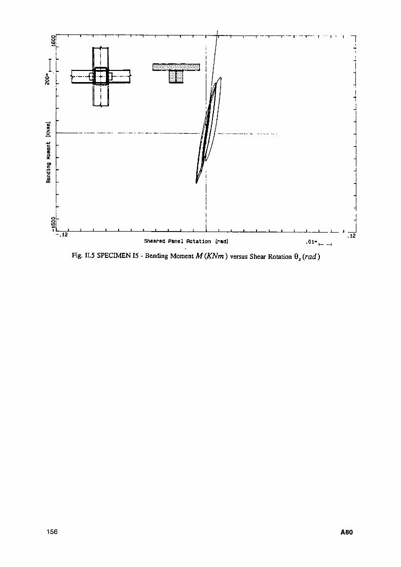
o l 1 1 1 Γ ο< CD |

ι : ■ ο ο

~l 1 1 1 1 1 1 Π 1 Γ Γ

*t

ι · - r - Ι Ί

c υ m

.12 -Ι Ι Ι 1 ι ι

Sheared Panel Rotation [rad] ·01

"μ-

Fig. II.5 SPECIMEN 15 - Bending Moment M (KNm ) versus Shear Rotation θ Arad)

J .12

156 A80

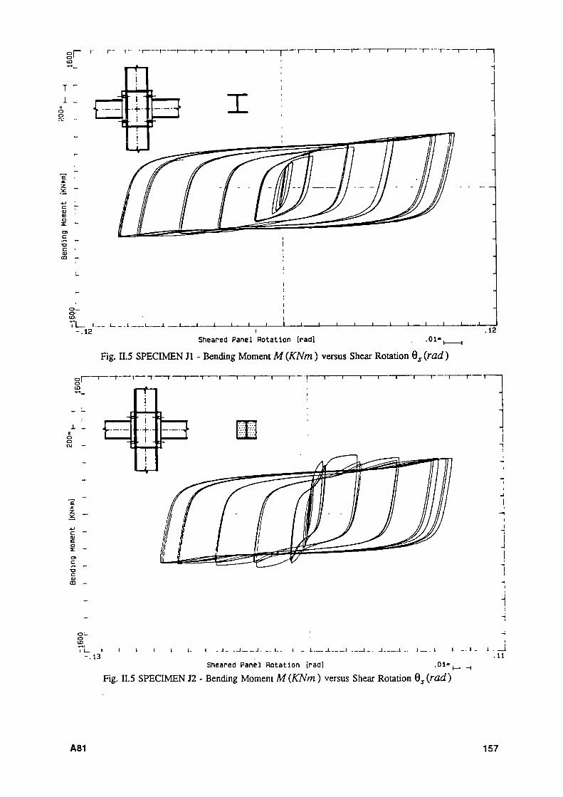
?Γ ■■

y EU

i l 1 I 1 1 L J I 1_ - . 1 2

_1 I L _ I I l _

Sheared Panel Rotat ion [rad] . 0 1 - ,

Fig. Π.5 SPECIMEN Jl - Bending Moment M (KNm ) versus Shear Rotation Qs (rad )

.12

π 1 !" -| 1 1 1 1 1 1 1 τ 1 1 1 1 1 1 I I I T"

i ■ ^ ^ ^ ■

■4-

O l o Cu

- . 1 3 ι I I 1 1 I. 1 . J_ ..J J . _. I . . 1 L 1 I _ . J 1 .. I 1 I -■ I

S h e a r e d P a n e l R o t a t i o n [ r a d ] ·0 1

" ι Η

Fig. II.5 SPECIMEN J2 - Bending Moment M (KNm ) versus Shear Rotation Qs(rad)

.11

A81 157

Sheared Panel Rotation [rad]

Fig. Π.5 SPECIMEN J3 - Bending Moment M (KNm ) versus Shear Rotation Qs (rad )

τ 1 1 1 1 1 1 1 1 1 r τ 1 1 1 1 1 1 1 1 1 r

Σ Γ

-f-

■À-

-I 1 I 1 I ' ' ' L -1 Ι Ι Ι Ι L .12

Sheared Panel flotation [rad] • 01=.

Fig. II.5 SPECIMEN J4 - Bending Moment M (KNm ) versus Shear Rotation Qs (rad)

158 A82

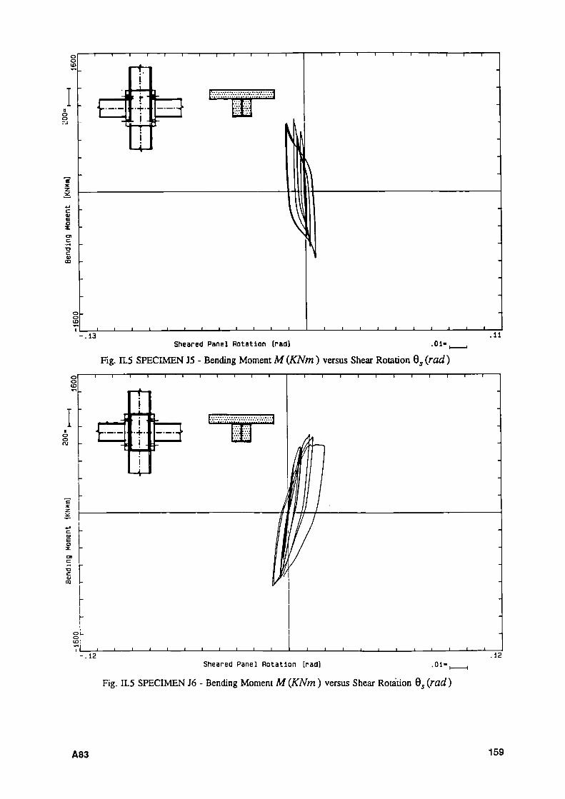
­τ 1 1 1 1 1 1 1 1 1 r

I

r *■+·■#

t ¡

­τ 1 1 1 1 1 1 Γ

' ' ■ ' ι i_ _l I l_ ­ .13 .11

Sheared Panel Rotation (rad] . 0 1 ­

Fig. IL5 SPECIMEN J5 ­ Bending Moment M (KNm ) versus Shear Rotation Qs (rad ) τ 1 1 1 1 1 1 r τ 1 r

#·+·■ I ­ i

m t¿LUA¿j!uM|U¡hM¡Ü*hUjiU!tJ

­ l I I 1 _ ­.12 .12

Sheared Panel Rotation [rad] . 01­

Fig. II.5 SPECIMEN J6 ­ Bending Moment M (KNm ) versus Shear Rotation Qs (rad)

A83 159

τ 1 1 1 1 1 1 1 Γ

, ,

- f -

-4-

gp - i 1 ; 1 1 1 1 Γ

c m

_ι ι ι ι ι ι i_ -I I L -.12

Sheared Panel Rotation [rad] . 01-.12

Fig. Π.5 SPECIMEN J7 - Bending Moment M(KNm) versus Shear Rotation Θ, (rad)

160 A84

ι l i r ­

τ 1

° ί

Ε Μ

en ! c ι

s Γ c: ι υ ι

■

ι

¡ ¡ ι ­

i . I i

_

•

■ | — i ­ I " 1 — i Τ r ­ ■ I I I I I ι ­i

I

­ . 1 1 ­

1­ L ' ' 1 1 1 1 1 1 1 L ι ι [_ ι ■ ι j _ „ i . ._ j ι _J

.13 Sheared Panel Rotation [rad] . 0 1 ­

Fig. Π.5 SPECIMEN Kl ­ Bending Moment M(KNm) versus Shear Rotation Q,(rad)

­i r

Shiarid Pinil Rotation [rid] .01­

Fig. II.5 SPECIMEN K2 ­ Bending Moment MiKNm) versus Shear Rotation Qs(rad)

A85 161

Sheared Panel Rotation [rad]

Fig. Π.5 SPECIMEN K3 - Bending Moment M(KNm) versus Shear Rotation Q,(rad)

"~!

I I . 1 . . I . I . I . I I I . .

- . 1 3 .1 I L-. - - ! - . L I . . . I . I

Sheared Panel Rotation [rad]

Fig. II.5 SPECIMEN K4 - Bending Moment M(KNm) versus Shear Rotation Qs(rad)

1 I 1 I I I J

.11 .01= Λ

162 A86

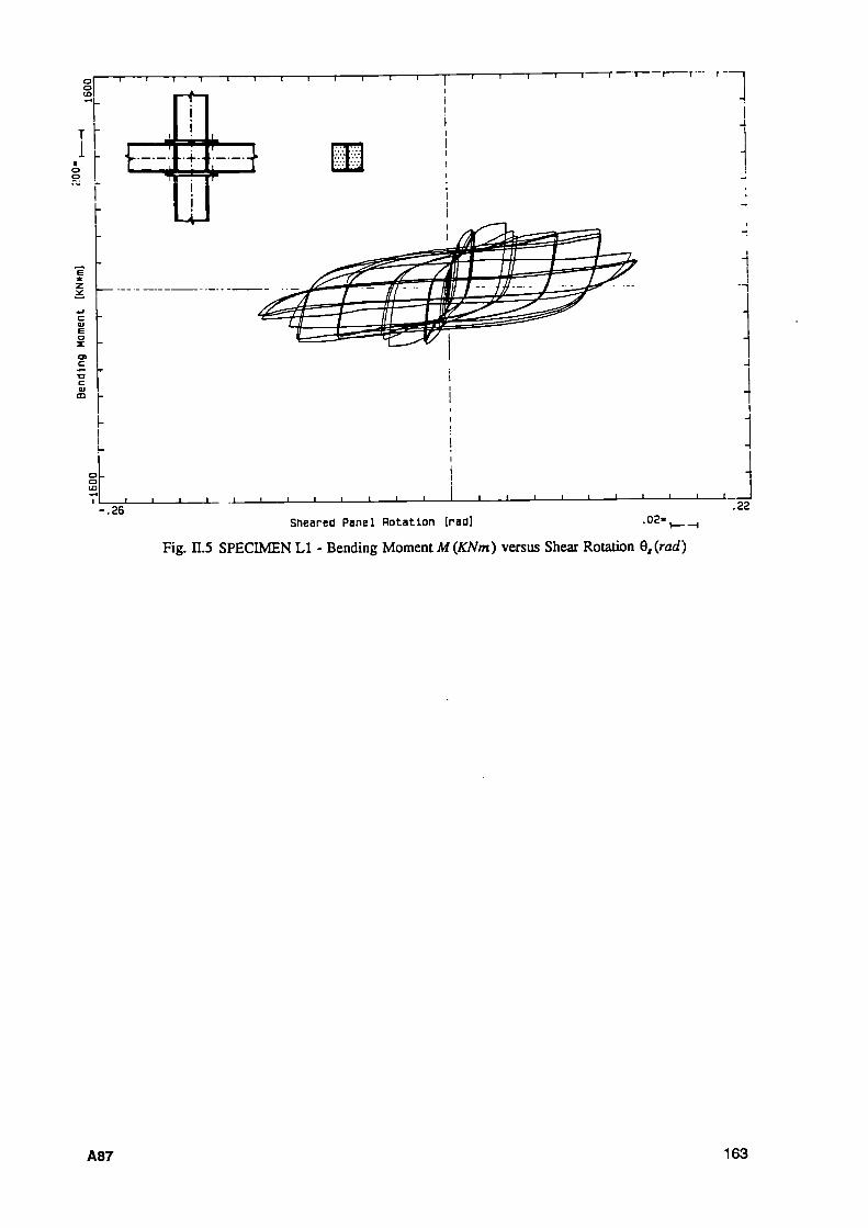
­τ 1 1 1 1 1 1 1 1 1 1 ι [~ τ 1 1 1 r r — τ ­

1

[ lf

t­­,i 4

i i

I ■ i ¡

U­i

ψ

ι I ι ι ι i _ ­.26

' i ' ' i _ ι ■ ' I 1 1 1­.22

Sheared Panel Rota t ion [rad] . 0 2 ­ ,

Fig. Π.5 SPECIMEN LI ­ Bending Moment M(KNm) versus Shear Rotation Q,(rad)

A87 163

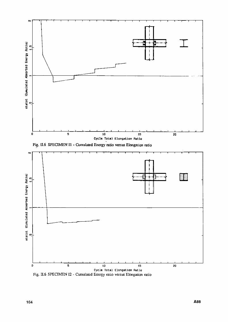
10 15 Cycle Total Elongation Ratio

20

Fig. Π.6 SPECIMEN II - Cumulated Energy ratio versus Elongation ratio

τ 1 1 r

4J "

0 5 10 15 Cycle Total Elongation Ratio

Fig. II.6 SPECIMEN 12 - Cumulated Energy ratio versus Elongation ratio

20

164 A88

m

U m cr ~* □ι c υ c Ό «I .α C O η

■ <

­α αϊ 4­1 IO

f—í

e u 4­>

o IO 4­1 01

ι ι ι ι ι —ι 1 ι ι 1 1 1 1—

■

1 1

1 _ _ ^

1 1

­ ­ ­ Q

ι ι ι — ι 1 1 1 1 ■

­L' ' ■·+·■

¡ ¡

p­­i M_J

ii

I I L. _j ι ι ι | l_ D 5 10 15

Cycle Total Elongation Ratio

Fig. Π.6 SPECIMEN 13 ­ Cumulated Energy ratio versus Elongation ratio

20

τ 1 1 r

·" " ■ lllllllla4Jd*¿jAAI«U*¿«Ux*J

_1 I l_ ­1 I L ­1 I 1 1 I I L· 5 5 10 15

Cycle Total Elongation Hatlo Fig. II.6 SPECIMEN 14 ­ Cumulated Energy ratio versus Elongation rauo

20

A89 165

S 10 15 Cycle Total Elongation Ratio

Fig. Π.6 SPECIMEN 15 - Cumulated Energy ratio versus Elongation ratio

20

166 A90

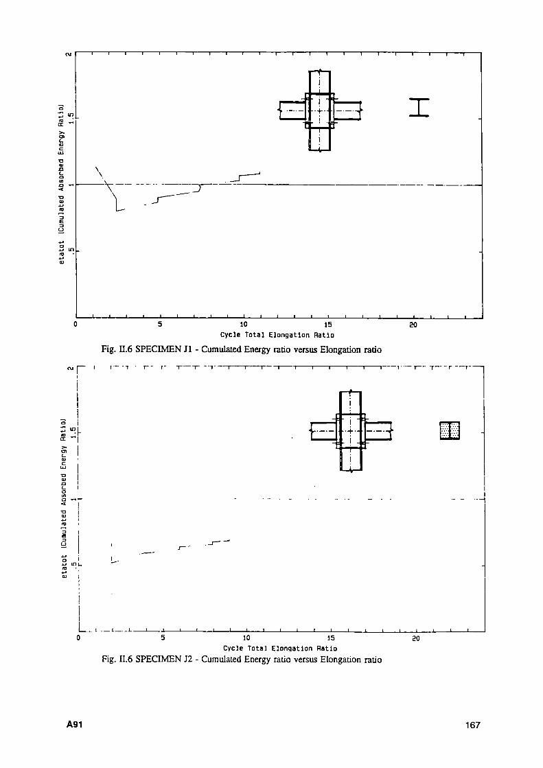
ι 1 Γ τ 1 1 1 1 1 1 1 1 1 1 r

^ m .

-f ..... _j

ΓΠ i

i - i -

m

, I

- \

I ;zr

I I I I I I 1 I 1_ -J I 1_ -1 I L· 5 10 15

Cycle Total Elongation Hatlo

Fig. II.6 SPECIMEN Jl - Cumulated Energy ratio versus Elongation ratio

Γ

20

ι ι 1 ι- τ τ - - ι 1 1 T _i 1 1 1 ι r r — T -

tr ~ |

CB V. ι

E

I I 1 J 1_ -1 1 1 I 1 I I L· 5 10 15

Cycle Total Elongation Ratio Fig. II.6 SPECIMEN J2 - Cumulated Energy ratio versus Elongation ratio

20

A91 167

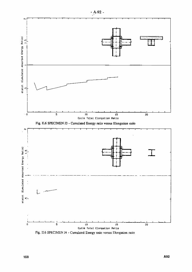
-τ 1 r

- A^2 "Τ 1 1 1 1 1 1 1 1 1 1 r-

_l I I L -I I I L 5 10 15 20

Cycle Total Elongation Ratio Fig. Π.6 SPECIMEN J3 - Cumulated Energy ratio versus Elongation ratio

ü *>;

-f-

-i-

I

L

- .1 -L-

5 10 15 Cycle Total Elongation Ratio

Fig. II.6 SPECIMEN J4 - Cumulated Energy ratio versus Elongation ratio

20

168 A92

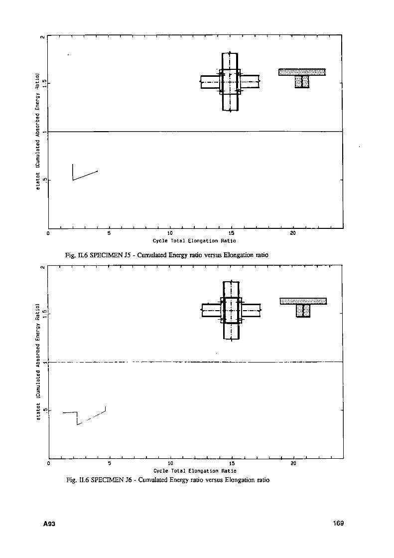
Ζ ^ (Ο ^

­< 1 τ

Γ*"Ι i

! Γ '

­ ! ­i i

M ­ ·

< TD

_ι ι_ 10 15

Cycle Total Elongation Ratio

Fig. Π.6 SPECIMEN J5 ­ Cumulated Energy ratio versus Elongation ratio

π 1 r τ 1 1 1 1 1 r

20

π 1 1 1 1 1 Γ

Ζ tf\ ,

ΓΠ i

■•i— i . ¡

M ­1

— . , ţ.y.y.y.y.' — ζ

U J

5 10 15 Cycle Total Elongation Ratio

Fig. II.6 SPECIMEN J6 ­ Cumulated Energy ratio versus Elongation ratio

20

A93 169

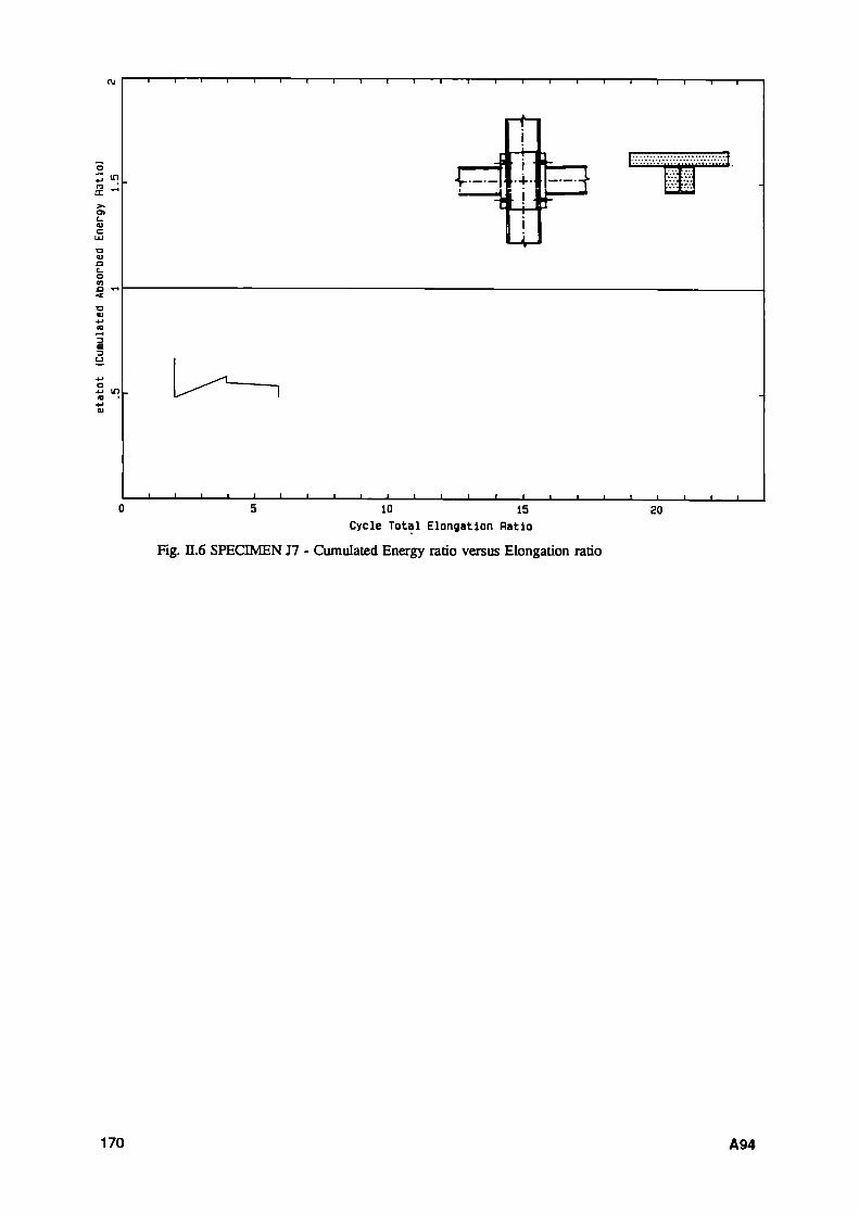
τ 1 1 ι 1 1 1 1 1 1 r I I I I I 1 1 1 1 τ-

Ι. ™ . TIT'

-I I L· -I I I L -J I L 10 15

Cycle Total Elongation Ratio 20

Fig. Π.6 SPECIMEN J7 ­ Cumulated Energy ratio versus Elongation ratio

170 A94

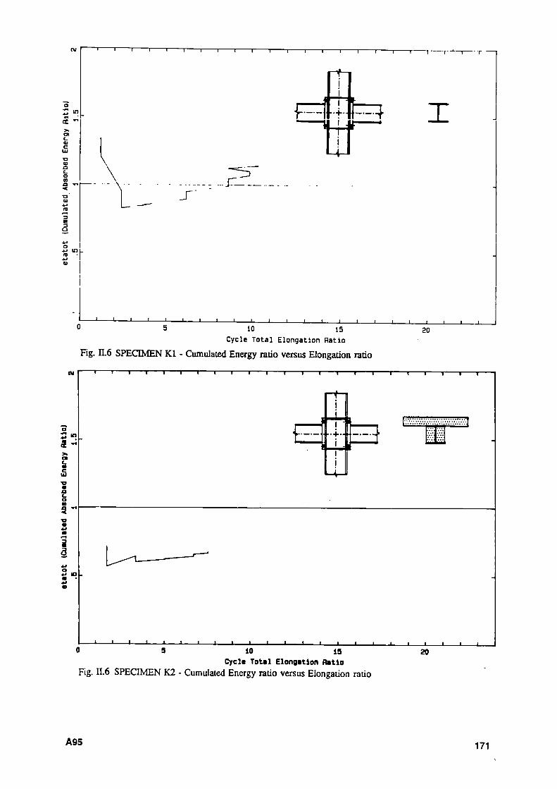
CE **

ι ι π 1

\ \

\

­

ι ι [

S'

- ι 1 Γ -, ι ι , r , 1--1—ι Γ

ζ

-. ...Γ

-1 Ι ι t ι -1 1 Ι ' ι υ 5 10 15

Cycle Total Elongation Ratio Fig. Π.6 SPECIMEN Kl ­ Cumulated Energy ratio versus Elongation ratio

20

a ­>> α c β ã

9

a

τ 1 1 Γ ι ι 1 ι ι ι ι 1 1 1 Ì 1 1 Ι Ι

,

ρΜι i i .

t ι ¡

M­JI

-ι 1 ι u -J 1 1 I I L -I I L· 0 9 10 19

Cycle Total Elongation Ratio Fig. II.6 SPECIMEN K2 ­ Cumulated Energy ratio versus Elongation ratio

20

A95 171

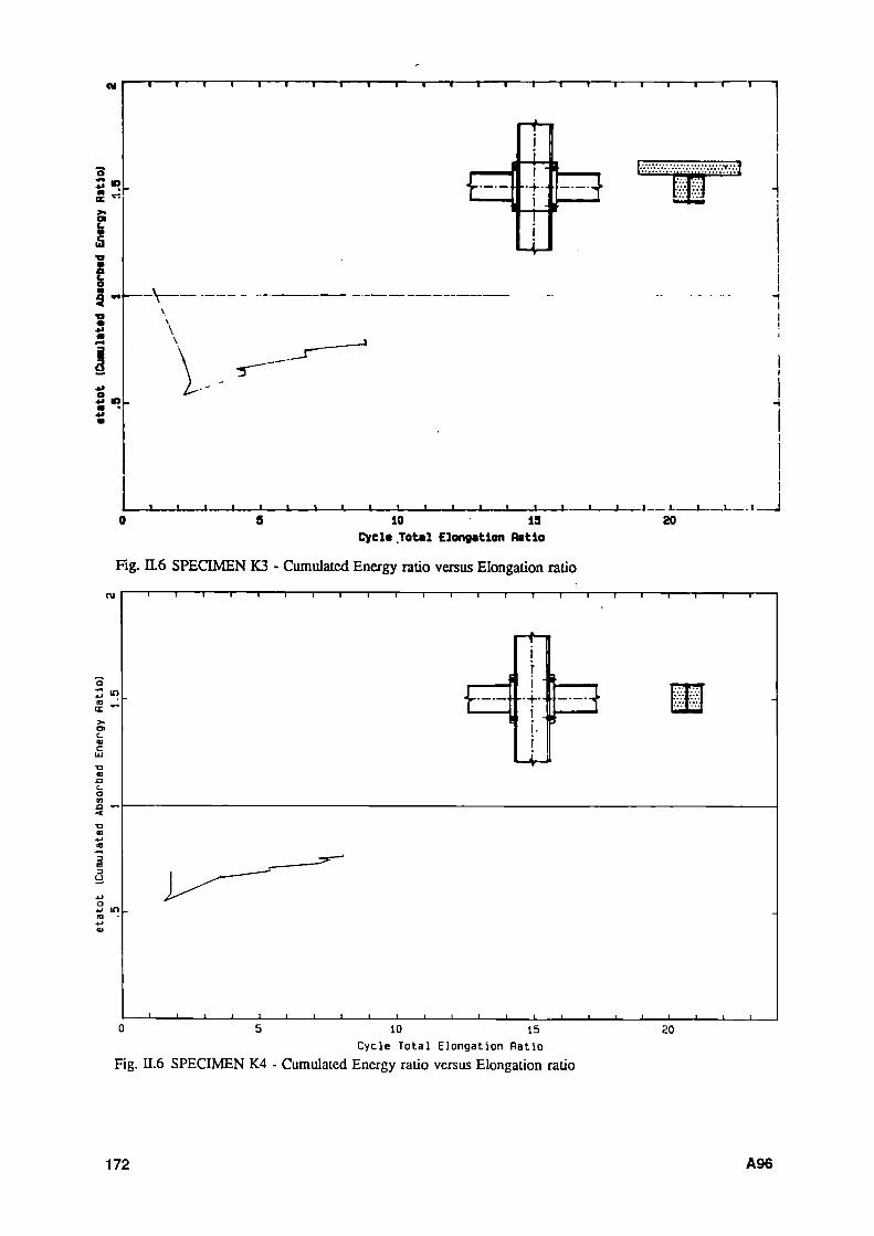
Μ Γ ' ' ' ' ' · "

O

« . E » ca c. •

τ 1 1 1 1 1 1 1 1 1 1 1 1 1 1 1

m ,

ι ■

i ­I i

MJ

— ■ ··' Í!!:B>

­J 1 1 l_ ­I I I I I I L 10 IS

Cycle .Total Elongation Ratio

_i ι ι ι ι ι 20

Fig. Π.6 SPECIMEN K3 ­ Cumulated Energy ratio versus Elongation ratio

C\J

CE ~

>» σι c tu c LU Ό dl £3 C_ α m

< TD αι

4­1 ΙΌ 3 Ε 3 CJ _'

4 J ο 4J m 4­> Ο)

• ι ι ί Ι Ι ι ι ι —Γ

«

f

! ­

j

ι ■

_—· , —— —"̂

^ χ · * " ^

¿,*^ _

1 1 L ι ι ι ι ι ι ι ι ι r ι t

τ 1 Γ

■

ι ι ι

0 5 10 15 Cycle Total Elongation Ratio

Fig. II.6 SPECIMEN K4 ­ Cumulated Energy ratio versus Elongation ratio

20

172 A96

c ν 5

υ η 3

τ 1 1 1 1 1 1 1 1 1 1 1 1 1 1 1 1 1 1 1 ; 1 τ

Ι

μ...' τ

ΓΜ i i

..+.. i ¡

M­l

­ l f

­ l I I I I I I I I I I I L i ι ι ι ι ι

} 5 10 15 Cycle Total Elongation Ratio

Fig. Π.6 SPECIMEN LI ­ Cumulated Energy ratio versus Elongation ratio

20

A97 173

Fig. II.7 SPECIMEN Gl - Failure Mechanism

Fi«. II.7 SPECIMEN Gl - Failure Mechanism

174 A98

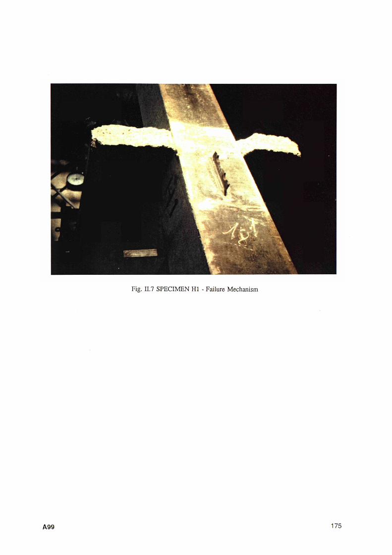
Fig. II.7 SPECIMEN Hl - Failure Mechanism

A99 175

Fig. II.7 SPECIMEN II - Failure Mechanism

Fis?. II.7 SPECIMEN 12 - Failure Mechanism

176 A100

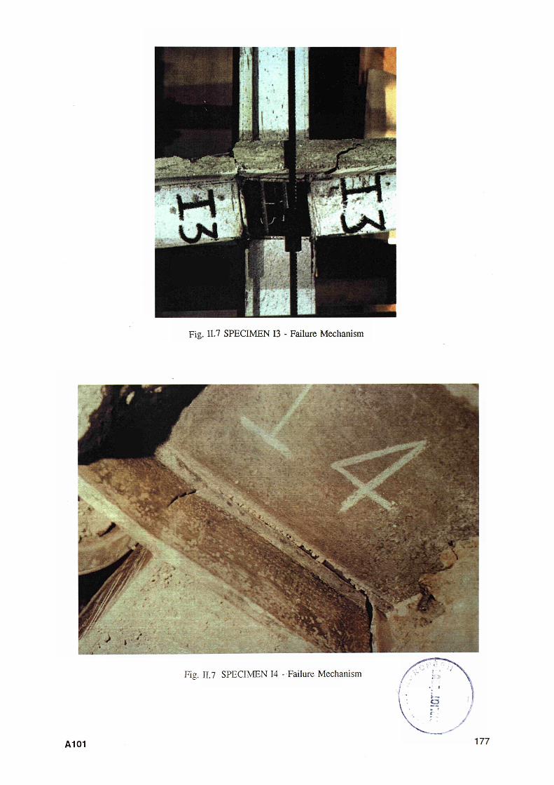
Fig. II.7 SPECIMEN 13 - Failure Mechanism

Fig. II. 7 SPECIMEN 14 - Failure Mechanism

A101 177

Fig. II.7 SPECIMEN 15 - Failure Mechanism

178 A102

Fig. II.7 SPECIMEN J1 - Failure Mechanism

Fis;. II.7 SPECIMEN J2 - Failure Mechanism

A103 179

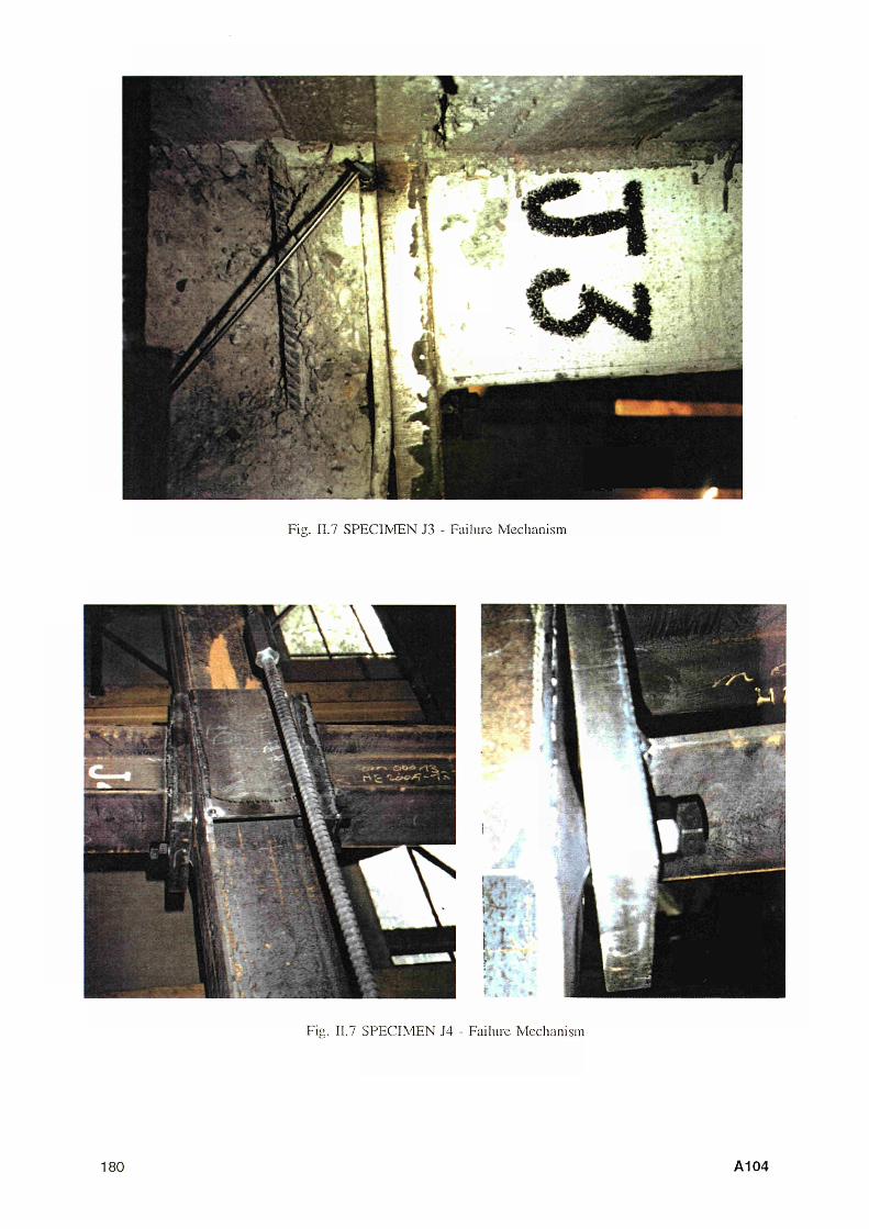
Fig. II.7 SPECIMEN J3 - Failure Mechanism

Fig. 11.7 SPECIMEN J4 - Failure Mechanism

180 A104

Fig. II.7 SPECIMEN J5 - Failure Mechanism

Fig. II.7 SPECIMEN J6 - Failure Mechanism

A105 181

Fig. II.7 SPECIMEN J7 - Failure Mechanism

182 A106

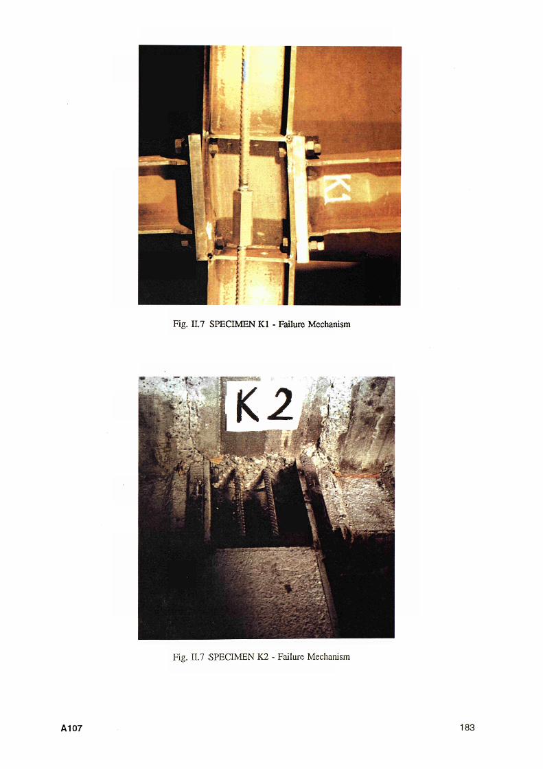
Fig. Π.7 SPECIMEN Kl - Failure Mechanism

Fig. II.7 SPECIMEN Κ2 - Failure Mechanism

A107 183

Fig. II.7 SPECIMEN K3 - Failure Mechanism

Fig. II.7 SPECIMEN K4 - Failure Mechanism

184 A108

Fig. II.7 SPECIMEN LI - Failure Mechanism

A109 185

In order to compare the experimental resulís, the follo wing quantities will be in t roduced and compared:

θ Global Flexibility of the joint in the elastic field measured as the slope in θ ­ M experimental diagram (rad/KN m)

Qs Flexibility of the panel zone in the elastic field measured as the slope in Qs ­ M experimental diagram (rad/KN m)

My Convent ional elastic limit (KN m) measured on the experimental diagram as indicated in [ 2 ] . My corresponds to the intersection between the elastic slope and the l ine tangent to the plastic branch having a slope of 1/10 of the elastic one

Qy Total rotation corresponding to My

M2.5 Bending Moment (KN m) corresponding to a total rotation θ = 2.5%

θ„ Maximum Total Rotation reached during the test and allowing three

complete cycles without failure

Mu Bending moment corresponding to Qu

Qu I Qy Conventional maximum ductility ratio Qu 12.5 Ductility margin in respect the limit of 2.5 % assumed by many

researchers as the maximum value of storey drift allowable during a severe seismic event.

In Fig. Π.8 the values of the above quantities are listed for each specimen.

Specimen Gl has a significant non symmetric behaviour; the table reports the values corresponding to the maximum resistence of the joint. The behaviour of the other specimens is practically symmetric; in the table the mean value of the various quantities are listed.

186 A110

Gl G2 Hl

II 12 13 14 15

Jl J2 J3 J4 J5 J6 J7

Kl K2 K3 K4

LI

θ

rad KNm

χ IO"5

7.00 3.75 3.10

2.88 2.25 1.50 1.55 1.30

2.50 2.00 1.37 2.25 1.66 1.32 1.77

3.00 1.75 1.75 2.45

2.63

Θ;

rad KNm

χ IO-5

0.00 0.00 0.00

1.55 1.08 0.70 0.75 0.50

0.94 0.60 0.40 0.25 0.00 0.37 1.00

1.25 0.78 0.00 1.00

1.30

My

KNm

45. 55.

150.

260. 470. 490. 700. 720.

360. 500. 520. 580. 660. 700. 720.

320. 500. 560. 500.

330.

Qy

%

0.30 0.21 0.47

0.75 1.06 0.73 1.00 0.95

0.90 1.00 0.71 1.31 1.10 0.92 1.10

0.96 0.88 0.98 1.23

1.02

M2.5%

KNm

—

170.

300. 540. 600. 750.

==

420. 600. 600. 620. 740. 800. 660.

460. 620. 660. 530.

440.

Mu

KNm

==

90.

430. 470. 480. 650. 850.

590. 610. 570. 760. 840. 860. 560.

525. 560. 830. 530.

330.

%

%

—

4.2

>10.0 >10.0 >10.0

6.5 2.1

>10.0 >10.0 >10.0

4.5 4.5

<4.5 6.5

>10.0 >10.0

9.0 >10.0

9.0

Qy

—

2.9

>13.6 >9.5 >13.0

4.2 2.2

11.1 >10.0 >14.1

3.4 4.1

<4.9 5.9

>10.4 >11.4

9.2 >8.1

8.8

% 2.5%

3.6

>4.0 >4.0 >4.0

2.6 0.8

>4.0 >4.0 >4.0

1.8 1.8

<1.8 2.6

>4.0 >4.0

3.7 3.2

3.6

Fig. II.8 Experimental Results

A111 187

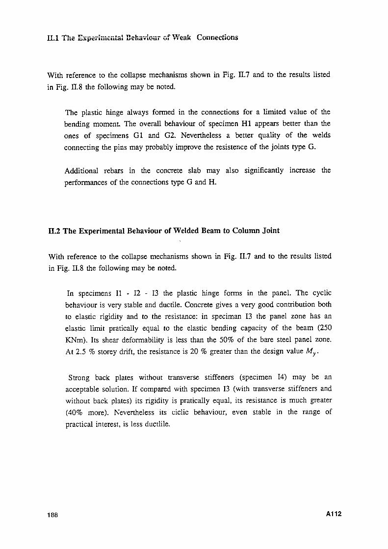
C l The Experimentai Behaviour of Weak Connections

With reference to the collapse mechanisms shown in Fig. Π.7 and to the results listed in Fig. Π.8 the following may be noted.

The plastic hinge always formed in the connections for a limited value of the bending moment The overall behaviour of specimen HI appears better than the ones of specimens Gl and G2. Nevertheless a better quality of the welds connecting the pins may probably improve the resistence of the joints type G.

Additional rebars in the concrete slab may also significantly increase the performances of the connections type G and H.

Π.2 The Experimental Behaviour of Welded Beam to Column Joint

With reference to the collapse mechanisms shown in Fig. II.7 and to the results listed in Fig. II. 8 the following may be noted.

In specimens II - 12 - 13 the plastic hinge forms in the panel. The cyclic behaviour is very stable and ductile. Concrete gives a very good contribution both to elastic rigidity and to the resistance: in speciman 13 the panel zone has an elastic limit pratically equal to the elastic bending capacity of the beam (250 KNm). Its shear deformability is less than the 50% of the bare steel panel zone. At 2.5 % storey drift, the resistance is 20 % greater than the design value My.

Strong back plates without transverse stiffeners (specimen 14) may be an acceptable solution. If compared with specimen 13 (with transverse stiffeners and without back plates) its rigidity is pratically equal, its resistance is much greater (40% more). Nevertheless its ciclic behaviour, even stable in the range of practical interest, is less ductlile.

188 A112

Strong back plates with transverse siiffcucii (specimen 15) caused a premature failure due to the collapse of the welds connecting the beam flange to the column. The solution may appear critical and perhaps unaccettable if a severe plan of quality control for welding is not accomplished.

Summing up the following conclusions may be given.

From a qualitative point of vew, it may be stated that concrete gives a good contribution both to resistance and rigidity of panel zone without reducing its ductility.

From a quantitative point of vew, the tests have shown that concrete gives an extrastrength of 80% to the panel zone reducing of about the 50% its deformability. Of course it is not possible to generalize such a results without other experimental analysis on different profiles sizes.

In principle, transverse stiffeners to the column may be substituted by strong back plates. It is thus possible to increase the strength of the panel zone up to the plastic bending capacity of the beams. The web of the column may be stretched away from the column flange, limiting the ductility ratio. For the above reason such a solution must be carefully studied both experimentally and numerically.

A structural solution considering concrete, strong back plates on the web, transverse stiffeners in the column does not appear acceptable without a very severe control of welding. The test has shown an increase of strength but a brittle behaviour due to local collapse of welds.

Π.3 The Experimental Behaviour of End Plates Connection

With reference to the collapse mechanisms shown in Fig. II.7 and to the results listed

A113 189

in Hg. li.» the following may be noted.

In specimens Jl - J2 - J3 the plastic hinge forms in the panel; some plastic deformations in the column flanges are also present; the end plate is practically indeformed. Comparing the behaviour of the welded specimens (I series) it must be noted that the dimensions of the panel zone are different (db = 465 mm instead of 225 mm). As a consequence the shear flexibility decrease significantly to 60%, 46% , 57% for J l , J2, J3 respectively. The total flexibility is reduced, but not in the same proportion due to the local elastic deformations of the bolted connections. The increase of resistance is not so evident: it is significant in the bare steel specimen ( approximately 38%); it is negligible for the composite specimens.

Exterior plates show a greater shear rigidity in respect to the stiffener solution; from the other hand the bolted connection rigidity is reduced and the benefit on the total rigidity of the specimen is negligible (compare J4 with J l ; J5 with J3) The resistance increases significantly , but the ductility reduces because the collapse is caused by the bolt failure and/or the local plastic failure of the column flange around the bolt hole.

Comparing J6 to J3, back plates give a significant increase (30%) to the resistance.The shear panel mechanism does not take place. The flanges of the columns fail significantly reducing the ductility.

Back plates without stiffeners may be a convenient solution. It is possible to reach the same level of strength allowed by stiffeners; ductility is reduced but it is greater than for J4 - J5. The global rigidity is also reduced.

Summing up the following conclusions may be given.

From a qualitative point of vew it may be stated that thick end plates are acceptable even without locally increasing the thickness of the column flanges. Transverse stiffners located at the top and bottom of the end plates enlarge the

190 A114

panei zone increasing strength and rigidity. Concrete increases the performances of the joint; the presence of the slab does not influence very much strength but it is useful for ductility.

From a quantitative point of vew the test have shown that concrete increases the strength of the panel zone of about the 50% without reducing the ductile behaviour.

Exterior plates substituting the transverse stiffeners are able to increase the strength but reduce significantly the ductility. They forbid the formation of the panel shear mechanism and cause a significant reduction of ductility. The same effects are given by back plates welded to the web of the column.

A structural solution considering concrete and exterior or back plates may probably be found, looking for a compromise between the ductility demand and the strength of the panel zone and of the bolted connection.

Π.4 The Experimental Behaviour of End Plates Reduced Beam

With reference to the collapse mechanisms shown in Fig. II.7 and to the results listed in Fig. II.8 the following may be noted.

The reduction of the flange was not sufficient to substitute the panel shear mechanism with a plastic hinge located in the beam. For this reason the behaviour of specimens Kl and K2 is very similar to the one of specimend Jl and J2 The incease of shear flexibility and the decrease of strenth may be explained by the reduction of the shear panel size.

The specimen K3 has exterior plates: it does not reach the same strength of the similar joint J5 but it shows a sufficient ductility. This fact is another proof of the interest of the solution.

A115 191

The specimen K4 is the oniy one without any device reinforcing die panei zone (no transverse stiffeners, no exterior or back plates). Its behaviour shows that concrete alone is able to give a design bending capacity of the same order of magnitude of the one provided by tranverse stiffeners, allowing the good ductility of panel mechanism.

Summing up the most interesting results concrete seems to be able to allow the elimination of transverse stiffeners, if one wish to design the joint for panel action. In other words the panel shear strength in the composite structure is not reduced if the stiffeners are absent; of course this statement must be confirmed by other tests on different panel sizes before being accepted for design purposes.

Π.5 The Experimental Behaviour of Continous Beam Connection

Only one test was performed. The panel zone has a size comparable with the ones of specimens of I series but its thickness is only 6.5 mm instead of 11 mm (approximately 60%). Its design bending capacity My is greater than 80% of the the corresponding one of specimen 14 and its ductility is equivalent. Shear rigidity is decreased of approximately the 30% thus increasing the total flexibility of about the 15%

Summing up it seems that the composite solution of this kind of joint may have great advantages in the economy of the construction.

192 A116

Π.6 References

[1] Bailio G. and Zandonini R. (1985) An Experimental Equipment to Test Steel Structural Members and Subassemblages Subject to Cyclic Loads Ingegneria Sismica, Anno Π, 2, pp 25-40

[2] ECCS, CECM, EKS Technical Committee 1, WG 1.3 - Seismic Design (1986) Recommended Tesnng Procedure for Assessing the Behaviour of Structural Steel Elements under Cyclic Loads Publication n. 45

U17 193

PART IH - COMPUTED AND EXPERIMENTAL STRENGTH

The design strength were computed according to EUROCODE formulas. The following criteria were be adopted.

Ultimate bending capacity of the beam

For the bare steel specimens the ultimate plastic bending moment of the beam was computed according to the nominal properties of the section ( Wpl = 920 cm3

for HE A 260) and the actual value of yield strength ( fy =31.8 KNIcm1 and fy = 30.2 KN lem1 for exterior and interior joints respectively). For F and Κ series the flange reduction was designed considering a linear distribution of bending moment. Thus the same value of the applied force causes, in principle, the atteinmènt of the ultimate capacity both at the reduced section and at the end of the beam where the section is fully effective.

In composite joints without slab the rebars were not connected to the column. Thus the ultimate bending capacity of the beam was assumed equal to the one of bare steel specimens, disregarding concrete in tension.

In composite exterior joints with slab the two 20 mm upper rebars were connected to the columns. Thus the ultimate bending capacity of the beam was computed according to the properties of the composite section.

In composite interior joints with slab the only rebars across the column were eight 6 mm bars. Their contribution was neglected assuming the bending ultimate capacity of the beam equal to the one of the bare steel beam.

A118 195

Ultimate capacity of the connection

The strength of the connections located beetween the beam and the column flange was evaluated considering the most weak element, but disregarding:

the local effects on the column flange caused by bolts in tension;

the tensile stresses in the column at the junction beetween the web and the flange.

Strength of the panel zone

The panel strength may be computed by the formula:

V —A —— + V r w ~

nw ης ^

r w,c

Mw = Vw dc

where:

Aw = dc tw with dc = 28.1 cm is the depth of the column an tw is the thickness of the web and of back plates, if any. It was assumed tw = 11 mm for all the specimens except for LI (tw = 7.5 mm), for 14 and 15 (rw = 41 mm), for J4, J5, J6, J7 andK3 (rw =31 mm);

f y = 31.8 KN/cm2 for exterior joints and 30.7 KNIcm1 for interior joint;

db = 27.5 cm for joints type C; 23.75 cm for joints type D, E, F and I; 46.5 cm for joint type J; 34.0 cm for joint type K;

Vwc taking into account the contribution of the concrete, computed as:

0.85/c

Vw,c = { 3 ¿cCOSCt

with fc the cubic strength ( 4.0 KNlem1 for exterior joints and 3.5 KNIcm2 for

196 A119

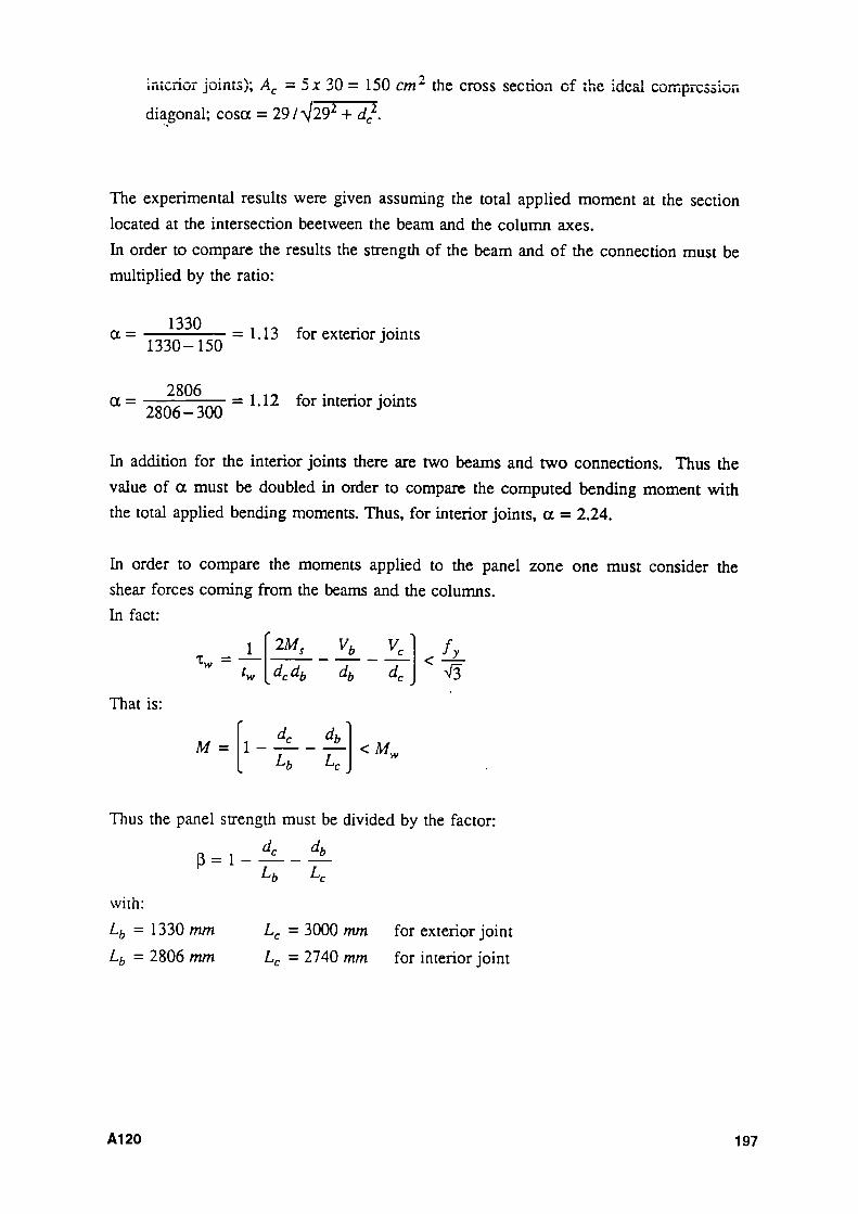
interior joints); Ac = 5 α: 30 = 150 cm "■ the cross section of the ideal compression diagonal; cosa = 29/^29 2 + dc

2.

The experimental results were given assuming the total applied moment at the section located at the intersection beetween the beam and the column axes. In order to compare the results the strength of the beam and of the connection must be multiplied by the ratio:

α = 1330

1330-150 = 1.13 for exterior j oin ts

a = 2806

2806-300 = 1.12 for interior joints

In addition for the interior joints there are two beams and two connections. Thus the value of α must be doubled in order to compare the computed bending moment with the total applied bending moments. Thus, for interior joints, α = 2.24.

In order to compare the moments applied to the panel zone one must consider the shear forces coming from the beams and the columns. In fact:

That is:

τ* =

M =

J_

1 -

2MS

dcdb

dc

Lb

vb yc

db dc

db

Lc <MW

V3

Thus the panel strength must be divided by the factor:

β = 1 - — -

with: Lh = 1330 mm

Lb = 2806 mm

db

Lc = 3000 mm for exterior joint Lc = 2740 mm for interior joint

A120 197

In Fig. HI. 1 and ΠΙ.2 ihe most significam resuiis of the comparison are reponed. If omitted, the strength of the connection is greater than 1.2 times the strength of the beam. The following may be noted.

when the plastic hinge forms in the beam, the computed values are generally in compliance with the value of My ;

when the plastic hinge forms in the connection, the computed values are lower than the experimental ones. This fact suggest that some improvements in design formulas are perhaps needed in order to have less complicate beam to columns joints.

when the plastic hinge forms in the panel, computations underestimate the strength of the panel even of 50%. This fact suggest that an improvement of design formulas are necessary mainly for what EUROCODE η. 8 concerns.

198 A121

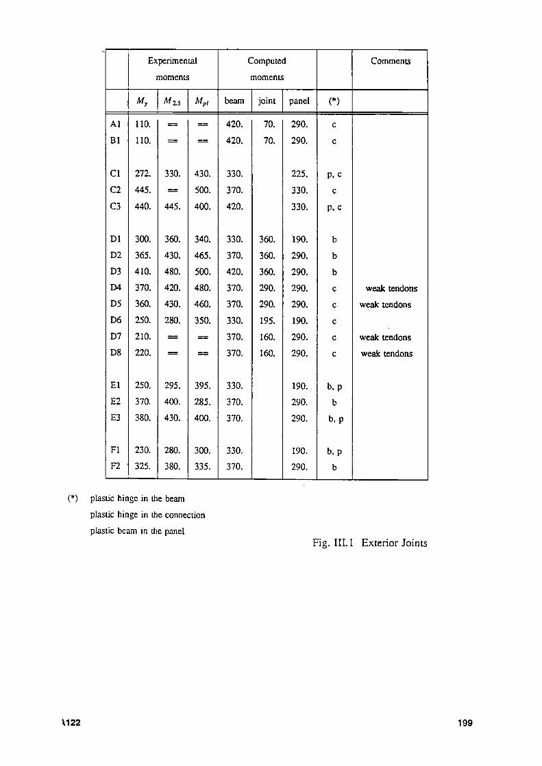
Al

Bl

Cl

C2

C3

Dl

D2

D3

D4

D5

D6

D7

D8

El

E2

E3

FI

F2

Experimental

moments

M,

110.

110.

272.

445.

440.

300.

365.

410.

370.

360.

250.

210.

220.

250.

370.

380.

230.

325.

Mzs

=

=

330.

= 445.

360.

430.

480.

420.

430.

280.

=

=

295.

400.

430.

280.

380.

Mp,

==

==

430.

500.

400.

340.

465.

500.

480.

460.

350.

=

=

395.

285.

400.

300.

335.

Computed

I

beam

420.

420.

330.

370.

420.

330.

370.

420.

370.

370.

330.

370.

370.

330.

370.

370.

330.

370.

îioments

joint

70.

70.

360.

360.

360.

290.

290.

195.

160.

160.

panel

290.

290.

225.

330.

330.

190.

290.

290.

290.

290.

190.

290.

290.

190.

290.

290.

190.

290.

(*)

c

c

P.c

c

ρ, c

b

b

b

c

c

c

c

c

b, ρ

b

b, ρ

b, ρ

b

Comments

weak tendons

weak tendons

weak tendons

weak tendons

(*) plastic hinge in the beam

plastic hinge in the connection

plastic beam in the panel Fig. III. 1 Exterior Joints

V122 199

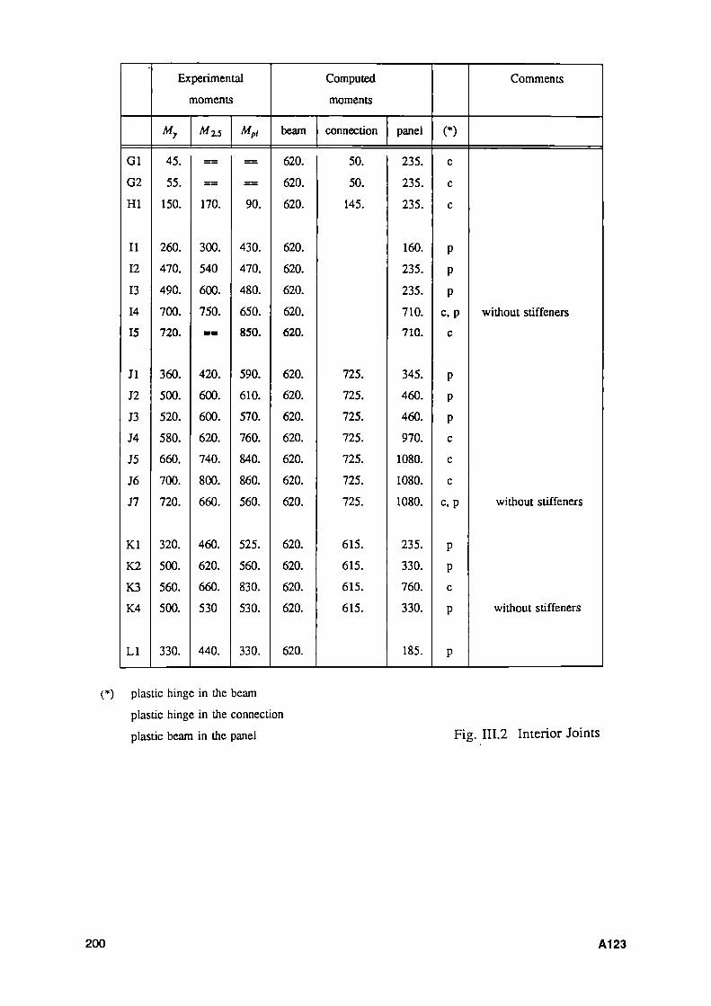
Gl

G2

Hl

II

12

13

14

15

Jl

J2

J3

J4

J5

J6

J7

Kl

K2

K3

K4

LI

Experimental

My

45.

55.

150.

260.

470.

490.

700.

720.

360.

500.

520.

580.

660.

700.

720.

320.

500.

560.

500.

330.

moments

Mu

=

= 170.

300.

540

600.

750. ■ a

420.

600.

600.

620.

740.

800.

660.

460.

620.

660.

530

440.

MP,

=

= 90.

430.

470.

480.

650.

850.

590.

610.

570.

760.

840.

860.

560.

525.

560.

830.

530.

330.

beam

620.

620.

620.

620.

620.

620.

620.

620.

620.

620.

620.

620.

620.

620.

620.

620.

620.

620.

620.

620.

Computed

moments

connection

50.

50.

145.

725.

725.

725.

725.

725.

725.

725.

615.

615.

615.

615.

panel

235.

235.

235.

160.

235.

235.

710.

710.

345.

460.

460.

970.

1080.

1080.

1080.

235.

330.

760.

330.

185.

(*)

c

c

c

Ρ

Ρ

Ρ

c, ρ

c

Ρ

Ρ

Ρ c

c

c

C P

Ρ

Ρ c

Ρ

Ρ

Comments

without stiffeners

without stiffeners

without stiffeners

(*) plastic hinge in the beam

plastic hinge in lhe connection

plastic beam in the panel Fig. III.2 Interior Joints

200 A123

Service : Ponts & Charpentes

APPENDIX Β

TEST REPORT OF THE LIEGE LABORATORY

Dr. Ir. A. PLUMIER

201

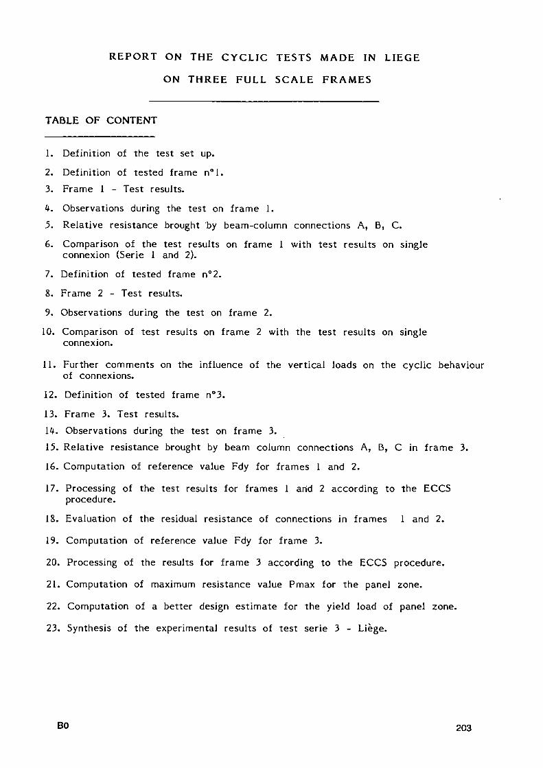
REPORT ON THE CYCLIC TESTS MADE IN LIEGE

ON THREE FULL SCALE FRAMES

TABLE OF CONTENT

1. Definition of the test set up.

2. Definition of tested frame n° l .

3. Frame 1 - Test results.

k. Observations during the test on frame 1.

5. Relative resistance brought "by beam-column connections A, B, C.

6. Comparison of the test results on frame 1 with tes t results on single connexion (Serie 1 and 2).

7. Definition of tested frame n°2.

8. Frame 2 - Test results.

9. Observations during the test on frame 2.

10. Comparison of test results on frame 2 with the test results on single connexion.

11. Further comments on the influence of the vertical loads on the cyclic behaviour of connexions.

12. Definition of tested frame n°3.

13. Frame 3. Test results.

14. Observations during the test on frame 3. 15. Relative resistance brought by beam column connections A, B, C in frame 3.

16. Computation of reference value Fdy for frames 1 and 2.

17. Processing of the test results for frames 1 arid 2 according to the ECCS procedure.

18. Evaluation of the residual resistance of connections in frames 1 and 2.

19. Computation of reference value Fdy for frame 3.

20. Processing of the results for frame 3 according to the ECCS procedure.

21. Computation of maximum resistance value Pmax for the panel zone.

22. Computation of a better design est imate for the yield load of panel zone.

23. Synthesis of the experimental results of test serie 3 - Liège.

BO 203

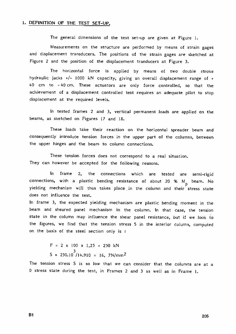
1. DEFINITION OF THE TEST SET-UP.

The general dimensions of the tes t set-up are given at Figure 1.

Measurements on the structure are performed by means of strain gages and displacement transducers. The positions of the strain gages are sketched at Figure 2 and the position of the displacement tranducers at Figure 3.

The horizontal force is applied by means of two double stroke hydraulic jacks +/- 1000 kN capacity, giving an overall displacement range of + 40 cm to - 40 cm. These actuators are only force controlled, so that the achievement of a displacement controlled test requires an adequate pilot to stop displacement at the required levels.

In tested frames 2 and 3, vertical permanent loads are applied on the beams, as sketched on Figures 17 and 18.

These loads take their reaction on the horizontal spreader beam and consequently introduce tension forces in the upper part of the columns, between the upper hinges and the beam to column connections.

These tension forces does not correspond to a real situation. They can however be accepted for the following reasons.

In frame 2, the connections which are tested are semi-rigid connections, with a plastic bending resistance of about 20 % M beam. No yielding mechanism will thus takes place in the column and their stress s ta te does not influence the tes t .

In frame 3, the expected yielding mechanism are plastic bending moment in the beam and sheared panel mechanism in the column. In that case, the tension s ta te in the column may influence the shear panel resistance, but if we look to the figures, we find that the tension stress S in the interior column, computed on the basis of the steel section only is :

F = 2 χ 100 χ 1,25 = 250 kN 3

S = 250.10 /14.910 = 16, 7N/mm 2

The tension stress S is so low that we can consider that the columns are at a 0 stress state during the tes t , in Frames 2 and 3 as well as in Frame 1.

B1 205

The data acquisition is running automatically on the following basis :

- at every peak of displacement reached, the next "target" of displacement is introduced

- the data acquisition is ordered by computer at every 1/50 of the distance between the previous peak and the next one

- each data acquisition requires a pair of seconds so that the tes t needs not be stopped since the measured values do not change substantially in such a short period of t ime.

DEFINITION OF TESTED FRAME N°l .

The first two frames tested in LIEGE use type Β connexion for the exterior and type Η connexion for the interior column. Figure 4.

The characteristics of the steel of the beams are :

yield strength : 380 N/mm 2

tensile strength : 537 N/mm 2

elongation at failure : 27 %.

The steel of the columns HE 300 Β is characterized as follows :

yield strength : 404 N/mm 2

tensile strength : 489 N/mm 2

elongation at failure : 36,6 %

The dimensions of the slab are sketched at Figure 5. The slab is

reinforced by two layers of steel net 150 χ 6 mm.

The resistance of the concrete measured on cubes of 15 cm. side are as follows, on the day of the test on frame 1 : encased concrete : 42 N/mm 2 (age 45 days) slab of frame 1 : 32 N/mm 2 (age 31 days)

The high strength M 27 bolts used for the connexion are pretensioned.

The applied couple for pretensionning is 1670 Ν χ m. This value comes out of

the application of E C 3 formula :

C = k . d . 0,75 . fur . As = 0,2 χ 27 χ 0,75 χ 900 χ 459 = 1,67 . 106 Ν χ mm.

206 Β2

3. FRAME 1. TEST RESULTS.

The applied load Ρ - total rotation TETA diagram is given at Figure 6. Total rotation is computed here as :

TETA = D 13 - D 1* /DIST 1314

From this diagram, we can deduce the following experimental values : Py+ = 100 kN

p y - = 105 kN

TETAY+ = 6,6 . 10-3 r a d

TETAY- = 10 . IO"3 rad

Pu+ = 1*5 kN

Pu" = 170 kN

At the end of the test , TETA+ = 8,6 . IO - 2 rad

TETA- = 8,6 . IO"2 rad

Maximum ductility MU+ = 13

M U - = 8,6

<f. OBSERVATIONS DURING THE TEST ON FRAME 1.

The first cracks on the upper side of the slab at the intermediate column are observed for a 8 mm. displacement.

These cracks go through the slab for a 10 mm. displacement. They look like an effect of shear in the slab rather than bending.

The shear in this case mainly results from a geometrical effect rather than of the shear computed in a classical way :

indeed discontinuities between the axis lines of each beam appear, because the center of rotation of the end a beam lies in the connection to the column and not at the intersection of the end of a beam lies in the connection to the column and not at the intersection of the axis of beams and columns. The result is an imposed relative vertical displacement d between the slab covering the right end of the left beam and the left end of the right beam. Figure 16. This results in a strong shear effect Vg, which brings a major crack and a failure in tension of the longitudinal steel reinforcement of the slab.

B3 207

This geometrical shear effect is strong in case of semi rigid con­

nections. The situation is probably different in rigid connections, because in that

case the rotation in the connection itself is weak.

Cracks in the encased concrete of column Β are observed for a 20 mm. displacement. Cracks in the concrete surrounding the connexions are observed for the same displacement.

The test is stopped without any real failure, on the basis of a large enough deformation : ductility greater than 10, displacement at floor level from + to ­ 130 mm., displacement at actuator level from + to ­ 300 mm. These values are greater than any practical value required for the background of design.

The observation of the structure during the test indicates that the main resistance is to be found in the steel connexion : 2 plates bolted together by means of 4 pretensioned bolts. One basic resistance term is given by the friction between the two planes. This term is the only one up to the moment when there is a contact between the bolt and the edges of the holes. Then a diametral pressure plus concrete crushing term is activated, to which correspond the increase in resistance. Figure 6. Of course this second term is mainly valid at the first cycle at each step of displacement. A sharp decrease of this term takes place during the two further cycles at the same step of displacement and almost nothing of this term remains when the new increase in displacement is performed. Then resistance only corresponds to friction and the diagram is characterized by yield plateau at level P + = 44 kN and P" = 50 kN, approximately.

This yielding mechanism is very ductile and t rue failure of the plate elements only depends on the elongation capacity of the particular steel used in the connecting plate as well as in the beam. True failure could also be a weld failure as observed during the tes ts on single connexions at Politecnico di Milano.

5. RELATIVE RESISTANCE BROUGHT BY BEAM ­COLUMN CONNECTIONS A, B,

Ç.

5.1. General principle.

The measurements at the strain gages allow us to compute the bending moments realized during the test at connection A (one beam), Β (two beams) and C (one beam) and their relative values.

208 B4

The data processing is as follows.

- we compute the quantities MA, MB, MC which are proportional to the

bending moment in the beams ;

MA = (EPS. - EPS, + EPS - EPS.) χ ΕΙ/ν 4 5 s b

MB = (EPS14 - E P S 1 3 + EPS 1 5 - EPS 1 6 ) χ EI/v

MC = ( E P ^ - E P S 2 3 + E P S 2 5 - E P S 2 6 ) X E I / V

For EI/v, we consider the value of the composite section of the HE 300 Β :

I = 3f.265cmZf and EI/v = 464.109N χ mm.

- Total resisting moment MT :

MT = MA + MB + MC

- Relative resistance brought by each column

MRA = MA/MT

MRB = MB/MT

MRC = MC/MT

The diagrammes of MA, MB, MC, MRA, MRB, MRC are presented as

function of TETA = D 14/1500.

5.2. Results in Frame 1.

Figures 7 and 8 present MŢ deduced from strain gage measurements,

which are similar to the global exterior diagramme of Figure 6.

Figures 68, 69, 70 present MA, MB, MC.

Figure 9 to 14 present MRA, MRB and MRC. We can observe:

- The diagrammes of MRA, MRB, MRC have an irregular shape, mainly when the displacement reversal brings the applied force close to zero. Then some small inequalities in values of resistances, some residual stresses in the frame bring high changes in relative values MRA, MRB, MRC. The diagrammes have been "cleaned" of these values which are not of great interest, since they concern only small resistances.

B5 209

­ On the mean, MRB = 2MRA = 2MRC in the small as well as in the large

displacement range.

­ There is a dissymetry in the relative resistances MRA and MRC, with the

highest resistance when the slab is in action (TETA ­ for MRA, TETA + for MRC).

6. COMPARISON OF THE TEST RESULTS ON FRAME 1 WITH THE TEST RESULTS ON SINGLE CONNEXION (SERIE I AND 2).

If we apply the virtual work relation to the structure sketched at Figure 15, we have :

P.D = 4 M c u . TETA

D = TETA.h

h = 3 450 mm. (3000 + 250 + 200) 250 : hinge axle ­ support

200 : half heigth HEB 400 Finally Mcu = _ M 2 _ Ρ

4 If we use this relation with a mean value of P u , we find

Mcu = 3^5 (145 + 170) = 136 kN.m. 2.4

This result should be compared to a mean of ultimate resistances found in Milano tests on single connexions :

Mu+ = (2 χ Mu type Bl + Mu type Hl)/4

we find MÛ+ = (2 χ 150 + 200)/4 = 125 kNm

Mu"­ = (2 χ 130 + 180)/4 = 110 kNm

If we take a mean value for + and ­ sides, we obtain for Mu :

MILANO 117,5 kNm

LIEGE 136 kNm F = 136/117,5 = 1,16

These results differ by a factor F of 1,16, which is not very different of the factor F' between yield strengthes :

MILANO fy = 317 N/mm 2

LIEGE fy = 377 N/mm2 ρ = 377/317 = 1,19

210 B6

We can conclude that the simple addition plastic resisting moment of individual connexions gives a sound evaluation of the global resistance of the frame.

7. DEFINITION OF TESTED FRAME N°2.

Frame n°2 is identical to frame n ° l . Only the load pattern is different, in the sense that permanent vertical loads are applied during the test . Their position and value are given at Figure 17.

The character is t ics of the steel of the beam and of the encased concrete are similar to those of frame n ° l .

Steel : fy = 380 N/mm 2 fu = 537 N/mm 2

Encased concrete : 42 N/mm 2 45 days after concreting.

The frame n°2 is tested 105 days after concreteing between the flanges of the sections.

The strength in compression on cubes of 15 cm. side of the concrete of the slab is : 32 N/mm 2 on the day of the test on frame n°2.

8. FRAME 2 - TEST RESULTS.

The applied load Ρ - Total rotation TETA diagram is given at Figure 19.

From this diagram, we can deduce the following experimental values

Py+ = 160 kN

Py" = 170 kN

TETAY+ = 16.IO"3 rad

TETAY- = 16.10 - 3 rad

Pu+ = 150 kN. Pu" = 135 kN

At the end of the test TETA+ = 8.10"2 rad

TETA- = 8.IO"2 rad

Maximum ductility : MU = 5.

B7 211

9- OBSERVATION DURING THE TEST ON FRAME 2.

The first cracks on the upper side of the slab are observed for a <i mm. displacement.

These cracks go through the slab for a 12 mm. displacement. Like in frame 1, they mainly come from a geometrical effect.

The experimental yielding level appears different of the one observed in the test on frame 1 : yield resistance Py as well as yield rotation TETAY are higher in frame 2 than in frame 1. The difference is however very dependant upon the way these parameters are estimated.

The other observations are similar to those made for frame 1.

10. COMPARISON OF TEST RESULTS ON FRAME 2 WITH THE TEST RESULTS ON SINGLE CONNEXION.

This comparison gives similar result to the comparison at paragraph 5, since we have :

LIEGE Frame 1

LIEGE Frame 2

This last result is different by a factor F = 145/175,5 = 1,23 of the results obtained in Milano. This result is again of the order of the factor F' between the yield strengthes of the steel used in Milano and LIEGE.

11. FURTHER COMMENTS ON THE INFLUENCE OF THE VERTICAL LOADS ON THE CYCLIC BEHAVIOUR OF CONNEXIONS.

Some differences appear between the test involving a vertical load (Frame 2) or no vertical load (Frame 1).

a. Yield load P y and yield rotation TETAy a r e higher in Frame 2.

b. Current maximum resistance Ρ of each loop of similar displacement is

higher for Frame 2 than for Frame 1, but the difference decreases as

TETA increases - Figure 20.

mean

mean

mean mean

P u = 157,5 kN M c u = 138 kN.

P u = 165 kN.

M c u = 145 kNm.

212 B8

c. At the end of test , which here correspond to a high enough rotation for

practical use (TETA = 8. I O - 2 rad), the resistance is finally similar for

frames 1 and 2.

d. Current loops at 3r<^ cycle of equal displacement are very similar in frames

1 and 2 - Figure 21.

e. A basic reliable elastic perfectly plastic behaviour which could be used as a design resistance of this type of connection then appears quite independant of the level of vertical loading on the beams - Figure 21.

P y d = (35 + 55)12 = 45 kN.

My(j = 0,863 Pyd (cfr. paragraph 6).

= 38,8 kNm.

The origin of the difference in behaviour between Frames 1 and 2 is

not established. It might be a result of the positioning of the bolts in the holes

of the connecting plate, which in Frame 2 might be forced to remain in

contact with the edges of the holes.

12. DEFINITION OF TESTED FRAME N°3.

Frame n°3 is built with a connection design similar to type Kl or K3 of Serie 2. A slab is concreted on the elements and vertical loads similar to those of Frame 2 - Figure 17 are applied.

Because of a major difference between the design yield strength of the steel of the HE 260 A beams (300 N/mm2) and the real yield strength (470 N/mm2) , it was decided to make a further width reduction of the flanges of the beams - Figure 22 - in such a way that the real resistance of the beam remain equal to the design resistance and to comply with the overstrength condition for the connection.

The characterist ics of the concrete are : encased concrete : 42 N/mm 2 45 days after concreting. The frame n°3 is tested 183 days after that concreting concrete of the slab : 42 N/mm 2 on the day of the test (age 49 days).

The characterist ics of the steel of the columns are :

Yield strength : 404 N/mm 2

Tensile sress : 489 N/mm2

elongation at failure : 36,6 96.

B9 213

13. FRAME 3 - TEST RESULTS.

The applied load Ρ - Total Rotation TETA diagram is given at Figure

23.

From this diagram, we deduce the following experimental values.

P y+ = 550 kN.

P y+ = 620 kN.

TETAY+ = + 2,8.10-2 rad

ΤΕΤ A Y- = - 2,5. IO"2 rad

PU+ = 580 kN. PU" = -680 kN.

At the end of the test TETA+ = 9,5.IO -2

TETA- = 9,3.10"2

Maximum ductility MU+ = 3,Ψ

MU- = 3,7

1*. OBSERVATIONS DURING THE TEST ON FRAME 3.

Cracks in the slab appear for a 5 mm. displacement. They,are bending

cracks. The failure of the steel reinforcement in the slab is observed for a

displacement of 55 mm. in the positive direction.

The yielding zones observed during the tes t are :

- plastic hinge in the beam itself close to the exterior column ; in this case,

the shear resistance of the panel zone of the column is higher than the

plastic resistance of the beam in bending

- sheared panel zone in the interior column ; the value of the shear, which is there twice the value in the exterior column is such that the plastic resistance of the sheared panel zone is reached before the plastic bending of the adjacent beams.

The failure takes place in the reduced sections of the beams, close to

the exterior columns : a crack propagates through the lower flange of the

beam, on both side of the frame. The bad surface aspect corresponding to

manual oxygen cutting without surface cleaning in the reduced section certainly

is a cause for an early crack propagation.

214 B10

15. RELATIVE RESISTANCE BROUGHT BY BEAM COLUMN-CONNECTIONS Af B, C in FRAME 3.

The data processing is similar to the one done for frame 1 (see paragraph 5).

Figures 24 and 25 present MT deduced from the strain gage measurements. They are very similar to the diagramm based on the exterior applied force measurement.

Figure 71 to 73 present MA, MB, MC.

Figure 26 to 31 present MRA, MRB, MRC -

We make the following observations :

- in the first cycles, the shares of resistance are distributed in the following way A - 28 % , Β - 46 %, C 28 %

- in the great displacement cycles, the mean shares are :

A - 30 96, Β - 46 % , C - 25 %.

- the shares for great displacements are distributed in a dissymetrical way ; for TETA +, they are

A - 25 96, Β - 40 %, C - 35 % ;

for TETA - they are

A - 35 %, Β - 55 %, C - 10 %

No simple comment can explain these figure. The only direct practical information we obtain in that in the great displacement range, the mean share are close to a proportion of resistance equal to 1/4 for each connection :

A : 30 96, Β : 46 %, C : 25 %

A complete explanation of the obtained values would require a complet analysis of the results and a simulation by means of DYNACS in which MRA, MRB, MRC would be computed.

B11 215

16. COMPUTATION OF REFERENCE VALUE Fdy FOR FRAMES 1 AND 2.

Fdy is intended to be the maximum elastic computed value oí the applied load Ρ to the tested frame.

Connections in Frames 1 and 2 being semi-rigid, the computation oí Fdy cannot be done one the basis of a classical elastic analysis of the tested frame in a simple engineering model. This model would assume stiffness of full sections, but sections are uncomplete in the more stressed zones of the structure, the ends of the beams.

Our analysis must then be based on these uncomplete sections and refers to values computed in the SRCS research document "Draft on the bending moment transmission of AF/AS connections for test series I - February 1988 - By PLUMIER - THUNUS" and similar document for test series 2 -

January 1989.

In that document, we find the possibilities for mechanical behaviour, with corresponding maximum elastic design values of force in the bolted connection.

We can deduce the equivalent values in frames 1 and 2 by proportion in yield strength (380/355).

The lower value of F corresponds to the maximum elastic event. It cannot however be the ovalization of holes, because this event can only take place after sliding appears between the two plates, that event should not take place in the first cycles and should not be considered as the basis of Fdy.

The next event is the yielding of the strap in tension, which will be

considered as the basis to Fdy.

To compute Fdy, we use the same approach as in paragraph 6, which is supported by the results given in paragraph 15, at least in the plastic range : Fdy = f Mu/3,45.

Mu is computed on the basis of internal forces in the section including

an active slab.

216 B12

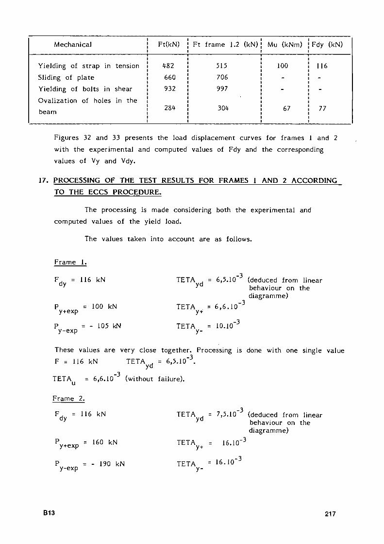
Mechanical

Yielding of strap in tension

Sliding of plate Yielding of bolts in shear

Ovalization of holes in the beam

Ft(kN)

482 660 932

284

Ft frame 1.2

515 706 997

304

(kN) Mu (kNm)

100 -

-

67

Fdy (kN)

116 -

-

Π

Figures 32 and 33 presents the load displacement curves for frames 1 and 2 with the experimental and computed values of Fdy and the corresponding values of Vy and Vdy.

17. PROCESSING OF THE TEST RESULTS FOR FRAMES 1 AND 2 ACCORDING TO THE ECCS PROCEDURE.

The processing is made considering both the experimental and computed values of the yield load.

The values taken into account are as follows.

Frame 1.

F , = 116 kN dy

Ρ = 100 kN y+exp

TETA yd

TETA y+

_3 = 6,5.10 (deduced from linear

behaviour on the diagramme)

= 6 ,6 . IO" 3

Ρ = - 105 kN y-exp

TETA = 10.10 y-

These values are very close together. Processing is done with one single value F = 116 kN TETA . = 6,5.10"3.

yd _3

TETA = 6,6.10 (without failure), u

Frame 2.

F . - 116 kN dy

Ρ = 160 kN y+exp

TETA , = 7,5.10 (deduced from linear y behaviour on the

diagramme)

TETA = 16.10" y+

Ρ = - 190 kN y-exp

TETA = 16.10" y-

B13 217

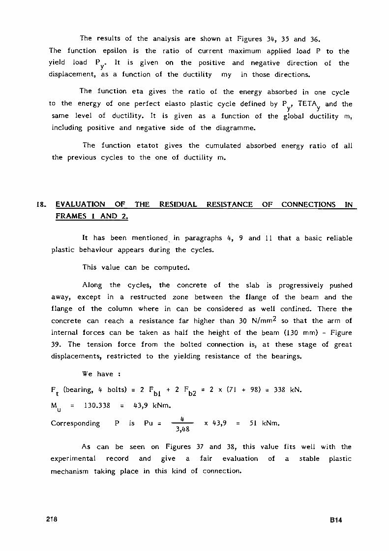
The results of the analysis are shown at Figures 34, 35 and 36. The function epsilon is the ratio of current maximum applied load Ρ to the yield load Ρ . It is given on the positive and negative direction of the displacement, as a function of the ductility my in those directions.

The function eta gives the ratio of the energy absorbed in one cycle to the energy of one perfect elasto plastic cycle defined by Ρ , TETA and the same level of ductility. It is given as a function of the global ductility m, including positive and negative side of the diagramme.

The function etatot gives the cumulated absorbed energy ratio of all the previous cycles to the one of ductility m.

18. EVALUATION OF THE RESIDUAL RESISTANCE OF CONNECTIONS IN FRAMES 1 AND 2.

It has been mentioned in paragraphs 4, 9 and 11 that a basic reliable plastic behaviour appears during the cycles.

This value can be computed.

Along the cycles, the concrete of the slab is progressively pushed away, except in a restructed zone between the flange of the beam and the flange of the column where in can be considered as well confined. There the concrete can reach a resistance far higher than 30 N/mm^ so that the arm of internal forces can be taken as half the height of the beam (130 mm) - Figure 39. The tension force from the bolted connection is, at these stage of great displacements, restricted to the yielding resistance of the bearings.

We have :

F (bearing, 4 bolts) = 2 Ffa + 2 Ffa2 = 2 χ (71 + 98) = 338 kN.

M = 130.338 = 43,9 kNm. u '

Corresponding Ρ is Pu = χ 43,9 = 51 kNm. 5 3,48

As can be seen on Figures 37 and 38, this value fits well with the experimental record and give a fair evaluation of a stable plastic mechanism taking place in this kind of connection.

218 B14

Of course, when the displacement is increased in a way such that the slab comes again in contact with the flange of the column, the arm of internal forces increases, as well as the resistance. But the resistance drop at a second cycle of same displacement is important, because the concrete of the slab is in a very cracked s ta te .

19. COMPUTATION OF REFERENCE VALUE Fdy FOR FRAME 3.

From the design of the structure, we know that the weak point in

which the first yielding will appear is the panel zone of the interior column.

The forces applied to the panel zone are computed in a simple way as indicated in Figure 39. Given the relative rigidities of the interior and exterior columns, the interior column carries a Fdy/2 shear force. We derive M at the end of the beams and the shear Τ in the panel zone :

M = Fdy.h/4

Τ = 2M/h Ρ

Fdy = 2 h .T/h Ρ

The shear resistance of the panel zone based on EC 3 is :

Τ = f . t . h l/T s y w c

The shear resistance brought by the concrete can be computed as follows.

Figure 39.

compressed strut strength : D = 2 A' . f .

A' = strut section (one side) = t W c c

W = strut width = 1/2 strut length

T = D cos ALFA concrete

The numerical data are as follows :

t w = 11 m

f = 404 N/mm2 (column)

y

B15 219

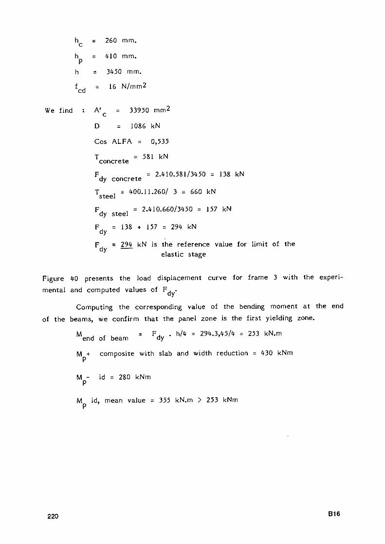
h c

h Ρ

h

fc d

We f ind :

=

=

=

=

A'

D

260 mm.

410 mm.

3450 mm.

16 N/mm2

= 33950 mm2 c

= 1086 kN

Cos ALFA = 0,535

Τ = 581 kN concrete

F_, = 2.410.581/3450 = 138 kN dy concrete

Τ , = 400.11.260/ 3 = 660 kN steel

F , . = 2.410.660/3450 = 157 kN dy steel

F J = 138 + 157 = 294 kN dy

F , = 294 kN is the reference value for limit of the dy —

elastic stage

Figure 40 presents the load displacement curve for frame 3 with the experi­

mental and computed values of F . .

Computing the corresponding value of the bending moment at the end

of the beams, we confirm tha t the panel zone is the first yielding zone.

M . . u = F . . h/4 = 294.3,45/4 = 253 kN.m end of beam dy

M + composite with slab and width reduction = 430 kNm Ρ

M ­ id = 280 kNm Ρ

M id, mean value = 355 kN.m > 253 kNm Ρ

220 B 1 6

Pv­exp

= ­ 6 2

° k N TETA =

2'

5·

1 0"

2 r a d

20. PROCESSING OF THE RESULTS FOR FRAME 3 ACCORDING TO THE ECCS

PROCEDURE.

The processing is made considering both the experimental and computed

values of the yield load. The values are as follows :

F., = 294 kN TETA . (mean value) = l . lO"2

dy yd Ρ = 550 kN TETA = 2 ,5 .10 _ 2

r a d y+exp y+ l d U

y­exp

The results of the analysis are shown at Figures 41 and 42.

21. COMPUTATION OF MAXIMUM RESISTANCE VALUE Pmax FOR THE PANEL

ZONE.

In the approach of paragraph 19, three factors contributing to the resis­

tance of the panel zone are not considered because they involve larger yielding

than those of the first yield estimated there :

­ panel zone resistance would be better approached by

Τ = F . t . h , s y w c

Then T = 1 1 4 3 kN s

­ the ultimate resistance brought by the concrete is better approached by

fu = 30 N/mm 2

T = 1089 kN c

­ a term of plastic moment of the flanges of the column exists with a corres­

ponding t f shear value :

T = 1,9 t 2 . W. . f /h f fe fe y ρ

Τ = 1,9 . 192 . 300 . 400/410 = 201 kN

Then, the est imate for Τ would be : max

Tm a v = 1143 + 1089 + 201 = 2433 kN.

Ρ = 2.410.2433/3450 = 578 kN max

This estimation fits well with the experimental value ­ Figure 43.

B17 221

22. COMPUTATION OF A BETTER DESIGN ESTIMATE FOR THE YIELD LOAD OF PANEL ZONE.

Using the same terms as in the approach oí paragraph 19, but with an estimate of the panel shear resistance equal to

TS = F y " lw " h c ^ l i k e i n P a r a g r a P n 2 1 )

We approach the yield load of the panel zone by

Τ = 1143 + 581 = 1724 kN

Fd y * = 2.410.1724/3450 = 409 kN.

This est imate also fits well with the experimental value. Figure 42.

23. SYNTHESIS OF THE EXPERIMENTAL RESULTS OF TEST SERIE 3 - LIEGE.

In order to compare the experimental results, we give the following quantities in the next table

M Elastic limit of the bending moment

TETA Total rotation corresponding to M

M2 . 5 Bending Moment (KN m) corresponding to a total rotation TETA = 2.5 %

2.5

TETA Maximum Total Rotation reached during the tes t and allowing three u complete cycles without failure

M Bending moment corresponding to TETA

TETA /TETA Conventional maximum ductility ratio u

TETA / 2 . 5 Ductility margin in respect to the limit of 2.5 % rotation assumed

by many researchers as the maximum value of storey drift allowable during a severe seismic event.

The experimental values given in the following Table are mean value of the ones obtained in the positive and negative directions of the displacement.

222 B18

Frame 1 - Experim.

Frame 1 - Design

Frame 2 - Experim.

Frame 2 - Design

Frame 3 ~ Experim.

Frame 3 ~ Design

M y

KNm

88

100

142

100

585

253

TETA y

0,83

0,65

1,60

0,65

2,5

1,00

M 2.5%

135

-

175

-

560

-

M u

150

-

162

-

630

-

TETA u %

> 6,6

-

> 6,6

-

*,7

TETA u TETA

y

> 8

> 10

> 4,1

> 10

1,88

4,7

TETA u 2.5%

> 3,2

-

> 2,64

-

1,88

-

B19 223

ro ro f

H " ^

1 1 H

r ­— ­ ν» ■ ­ V J L —

K­i*. Λ · « . · ^^¿tev&iglft&y

UNIVERSITE DE LIEGE Service "PONTS & CHARPENTES"

RECHERCHE ARBED­CECA SUR LA RESISTANCE SISMIQUE DES STRUCTURES MIXTES

Ing. Resp. A. PLUMIER B. THUNUS

m ro o

Figure 1

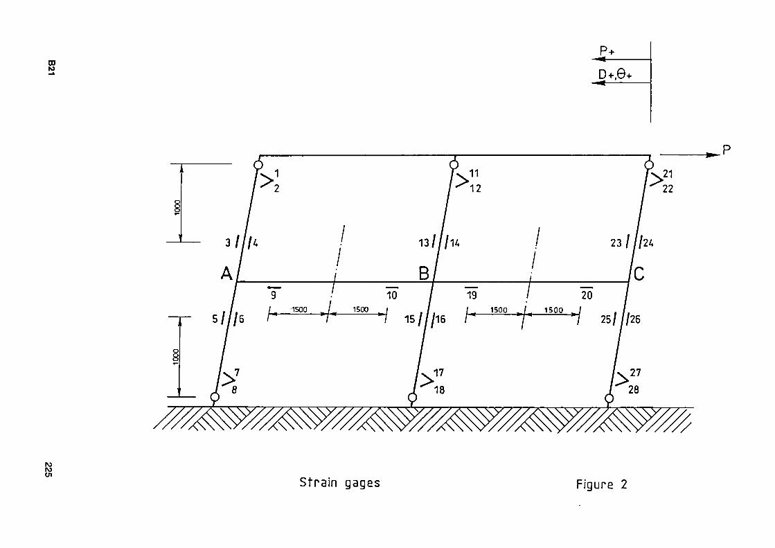
CD ro

- *

D+.6+ - *

> :

3 I¡li

A f

o 8

!>!

í / 9 ·' 1 0 / 1 9 / 20 / f / . / - 1500 ^L· 1500 - < . ƒ L 1500 _ / 1500 / . ƒ

/ / /e r ■+· -ƒ 15Wy16 ƒ- ■ƒ* ·ƒ 25/ //25

y ro ro en

Strain gages Figure 2

ro ro

P + ­ ^ D+.e+

■ * —

o o to

*-P

Β

f_,12¿0 ¿0 ƒ I /¿O 12A0 ^

ι3 Αι

(D ro

Displacement transducers Figure 3

Exterior columns Aand C

M 27

150 US ι 70 135

Interior columns Β

Figure 4

B23 227

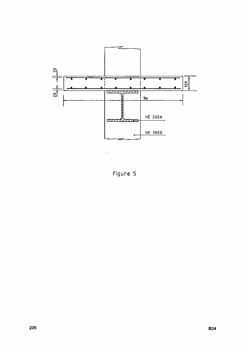
o CM

O CM

— I λ • . · 4

ι I

• I a ·

• f

• ·

■ - 4 "

• \ 7 / / / / / ; / / / \

• • •

—.r..—JK—.. w / / / r

==■-

s ss ytr^-t-

1m

HE 260A

HE 300B

o CM

Figure 5

228 B24

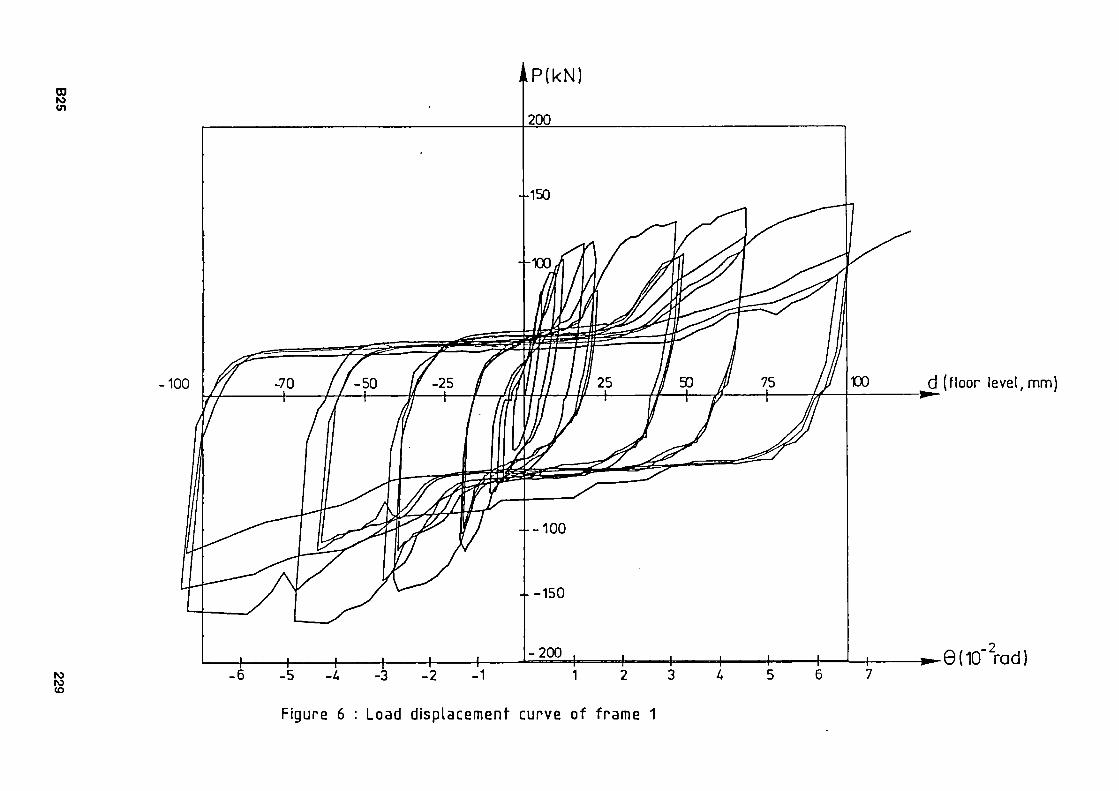
co ro ui

ro ro to

100 d (floor level, mm)

θ(10" rad)

Figure 6 : Load displacement curve of frame 1

M Τ Frame 1 Cycles 1 to U

-10 _ 1 L

θ (10 rad ι I I

10

Figure 7

230 B26

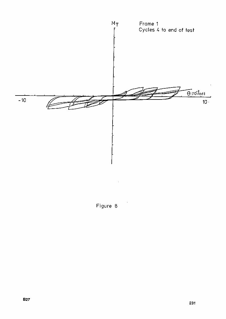
M- Frame 1 Cycles U to end of test

Figure 8

B27 231

-10 -5

MRA Frame 1 Cycles 1 to U

θ (10"rad)

0 10

-0.5

-1

Figure 9

232 B28

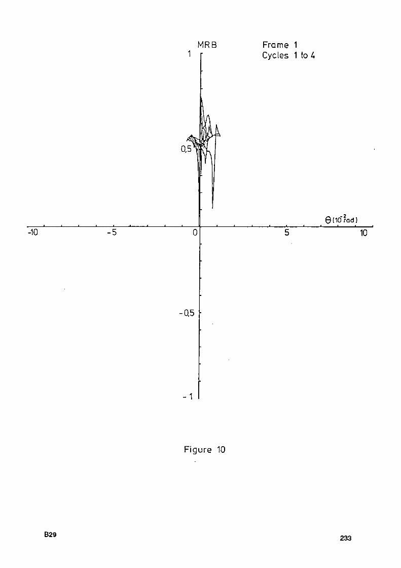
- J — - ■ I

MRB Frame 1 Cycles 1 to U

θ(10 rad! ■ ■

' -10 -5 0

-Q5

- 1

10

Figure 10

B29 233

-10 -5

MRC

■ ■ ■ ■

0

Frame 1 Cycles 1 to U

θ MO rad)

10

0,5

-1

Figure 11

234 B30

MRA Frame 1 Cycles 4 to end of test

-0,5

-1

Figure 12

B31 235

MRB Frame 1 Cycles U to end of test

-0,5 ■

_1

Figure 13

236 B32

MRC Frame 1 Cycles k to end of test

-0.5

-1

Figure %

B33 237

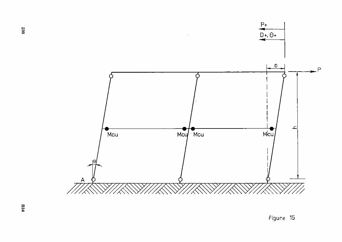
NS ω oo

- ^ —

Meu Meu/ Meu

θ/

co ω

Figure 15

Y':n^:-:b^^n^^^:^o.O^CS. >ttïQMKU.&mmsi

dv = Q.d

Figure 16

B35 239

to •Ρ-o

3250 1150

Figure 17 : Vertical loads applied in test on frame 2 and 3

CD w σ>

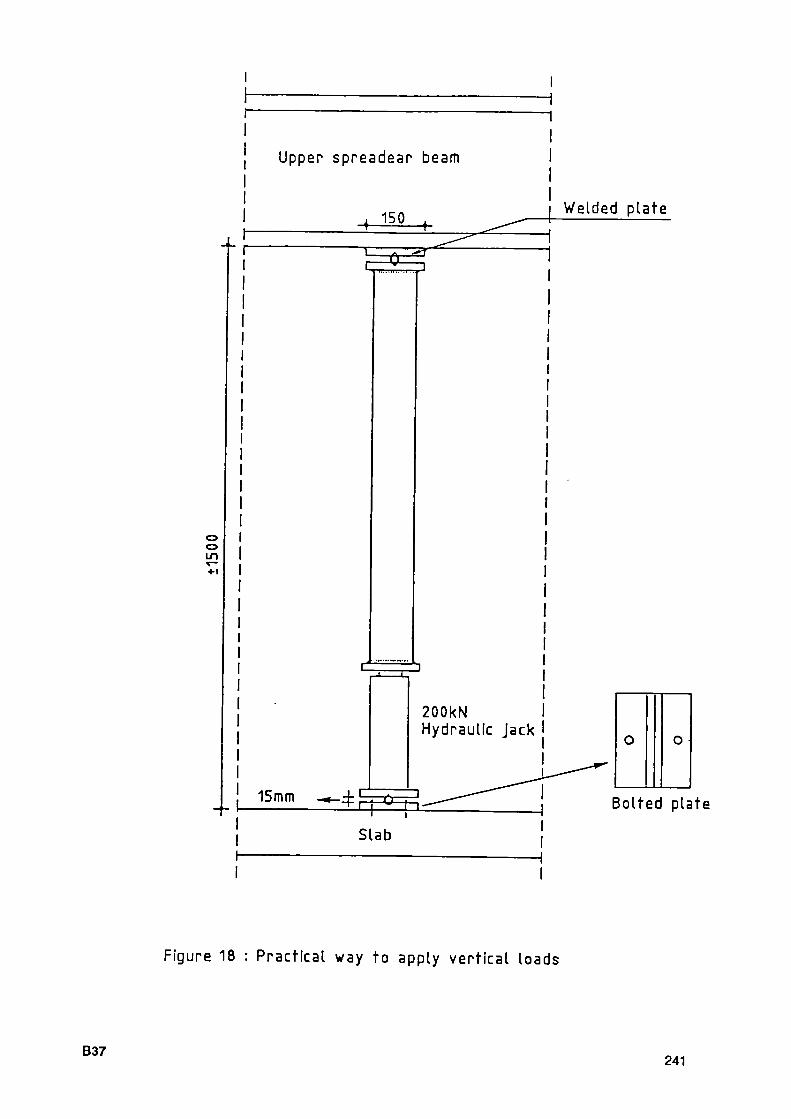
o o LD

Upper spreadear beam

I 1 5

° ♦ l~3^

Welded plate

1

200kN Hydraulic jack

15mm ——­}­1—^—Q—' ■ι ! ' · ' ' ■·

Slab

o o

Bolted plate

Figure 18 : Practical way to apply vertical loads

B37 241

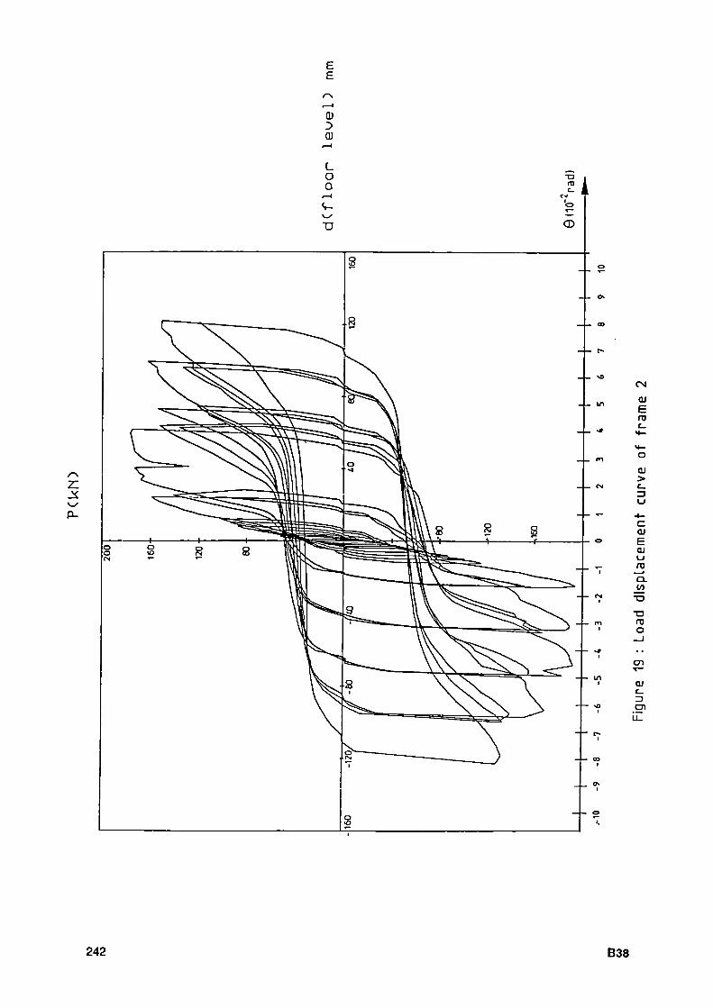
ε E

ω D Q)

7L .S \-/ P-

OJ

Π3

OJ

>

c ω E OJ l_l Π3 CL

TD ro o

OJ

c en

242 B38

CD ω (O

ω

— Frame 1 Frame 2

θ (10 rad)

Figure 20 : Envelope curves of maxima in P-θ loops for frame 1 and 2

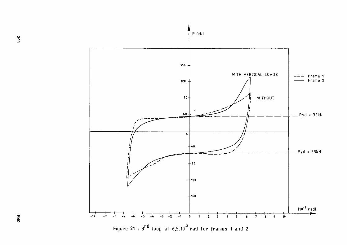
ro ■t*

co u o

— Frame 1 Frame 2

é = ^ r r r _ // Pyd = 35kN

Pyd = 55kN

-9 -8 -7 -6 - 5 -k -3 - 2 -1 10

rd -2 Figure 21 : 3 loop at 6,5.10 rad for f rames 1 and 2

Concreted before erection

Concrete on site / (slat + panel zone)

300

40(501 200

100, /

uv

4 bolts M 30

Figure 22 : Detailing of the connection zone of frame 3

B41 245

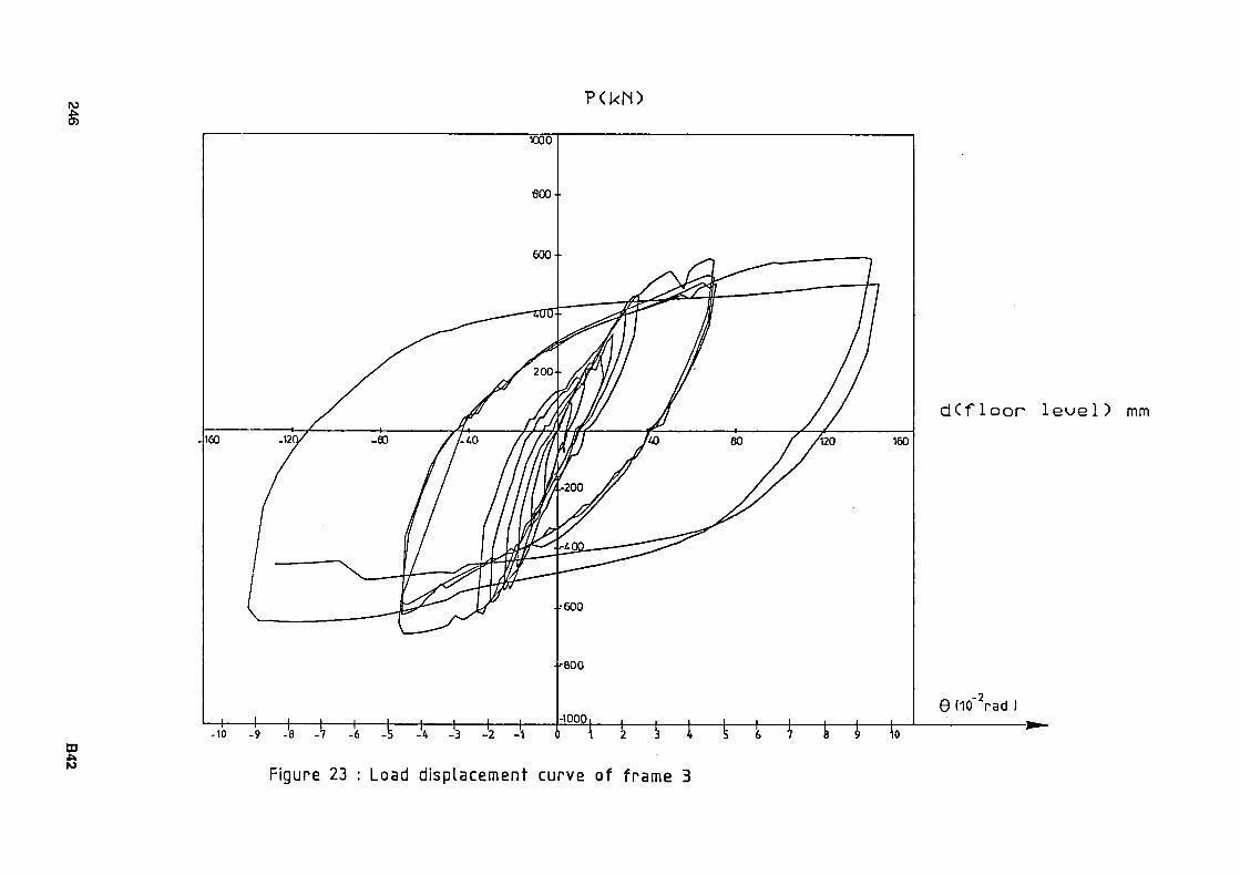
ro -Pt O)

PCkM)

CD ik ro

dCfloor leuel) mm

Figure 23 : Load displacement curve of frame 3

-10 -5

Frame 3

θΠΟ rad) ■

10

Figure 2U

B43 247

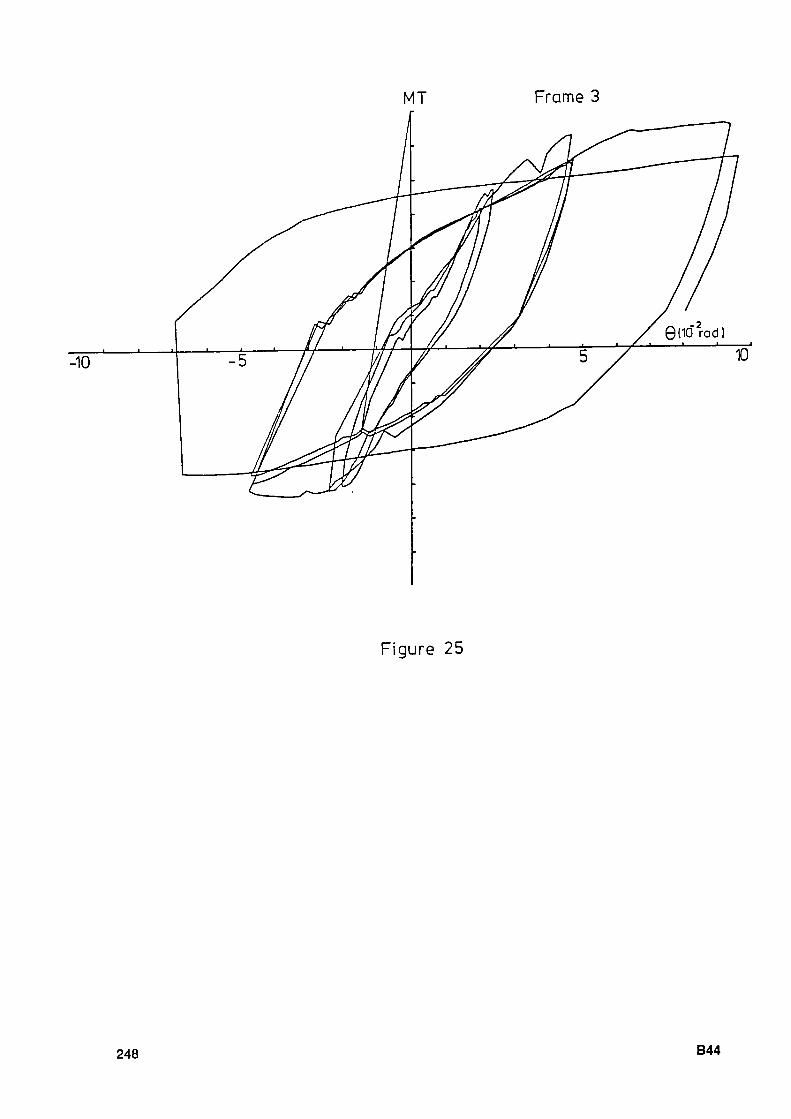
Frame 3

Figure 25

248 B44

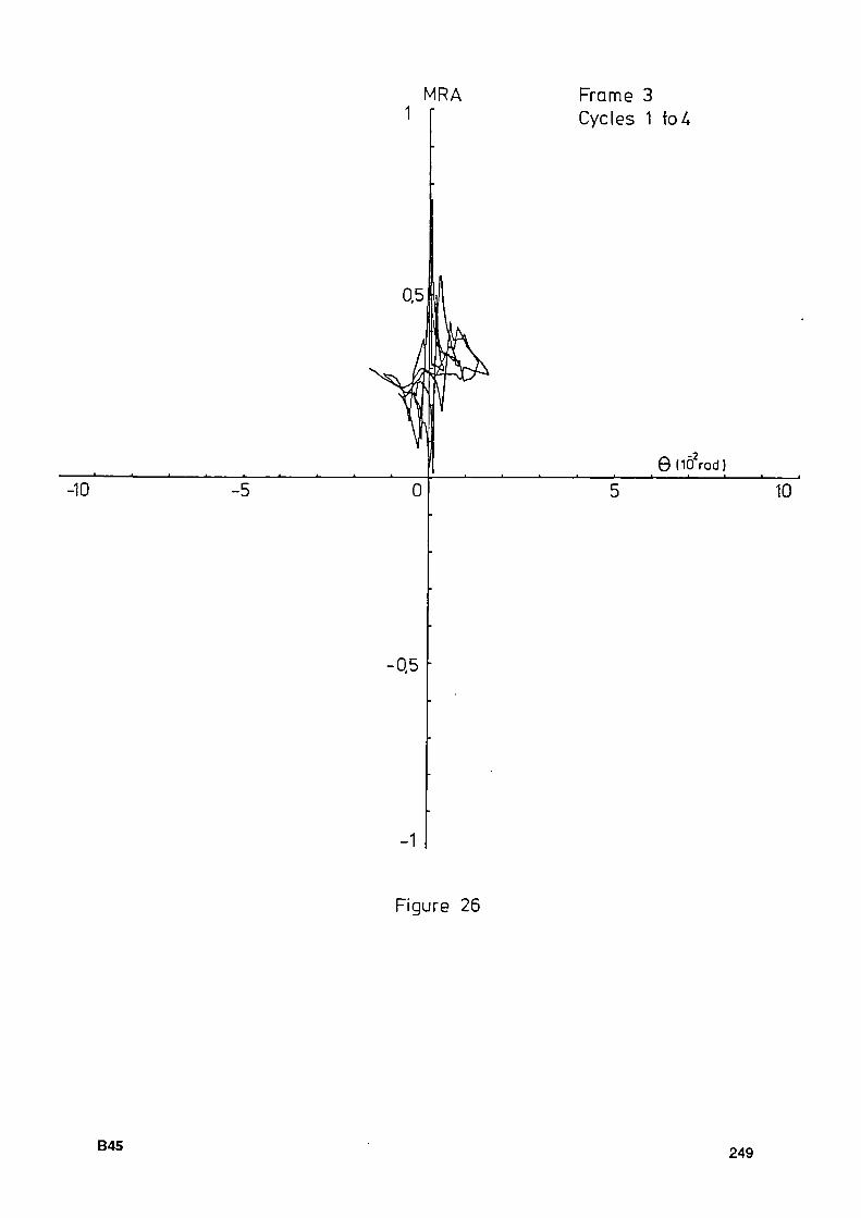
-10 -5

MRA

* ■ * ■ ■

0

Frame 3 Cycles 1 to Λ

θ HO rad]

10

-Q5

-1

Figure 26

Β45 249

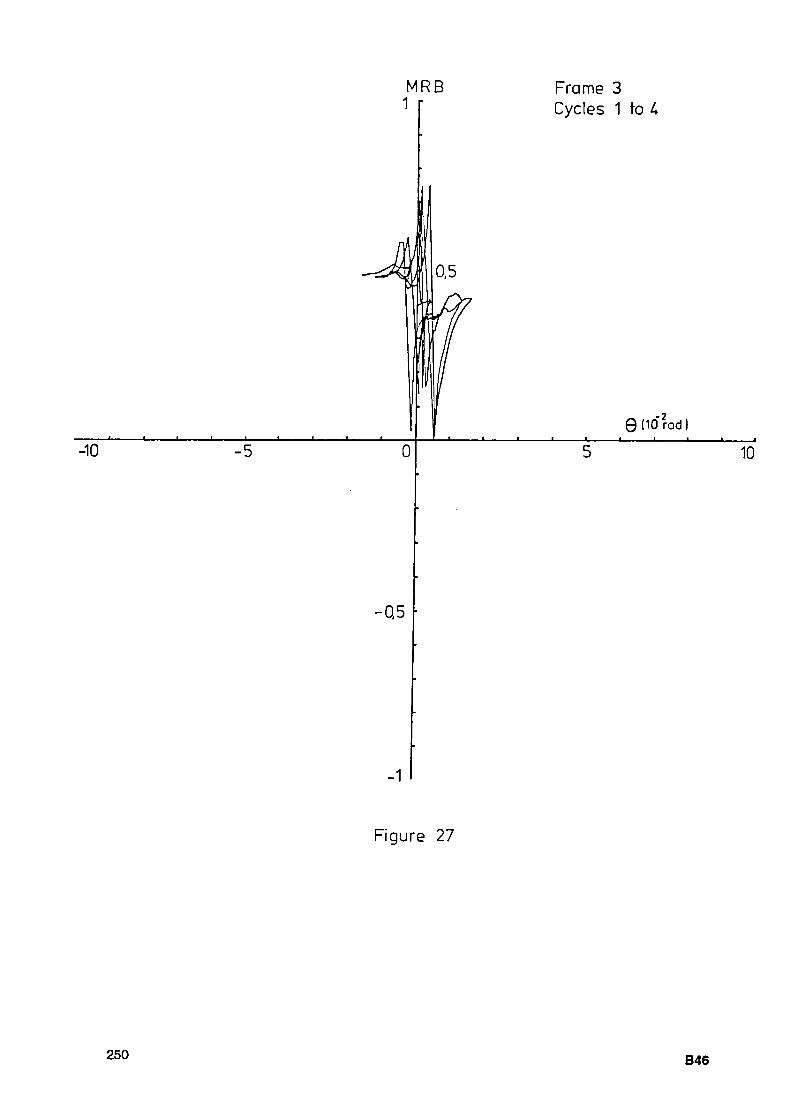
­10 • ' ■ '

­5

M R B 1 Γ

l i l i

o

Frame 3 Cycles 1 to A

θ dû rad I ­■ 1 1 1 1 ■

10

­Q5

Figure 27

250 B46

MRC

-10 -5

Frame 3 Cycles 1 to U

θ HO"rad) ■

10

■0,5

-1

Figure 28

B47 251

MRA Frame 3 Cycles U to end of test

0,5

-1

Figure 29

252 B48

MRB Frame 3 Cycles 4 to end of test

-0,5

-1

Figure 30

B49 253

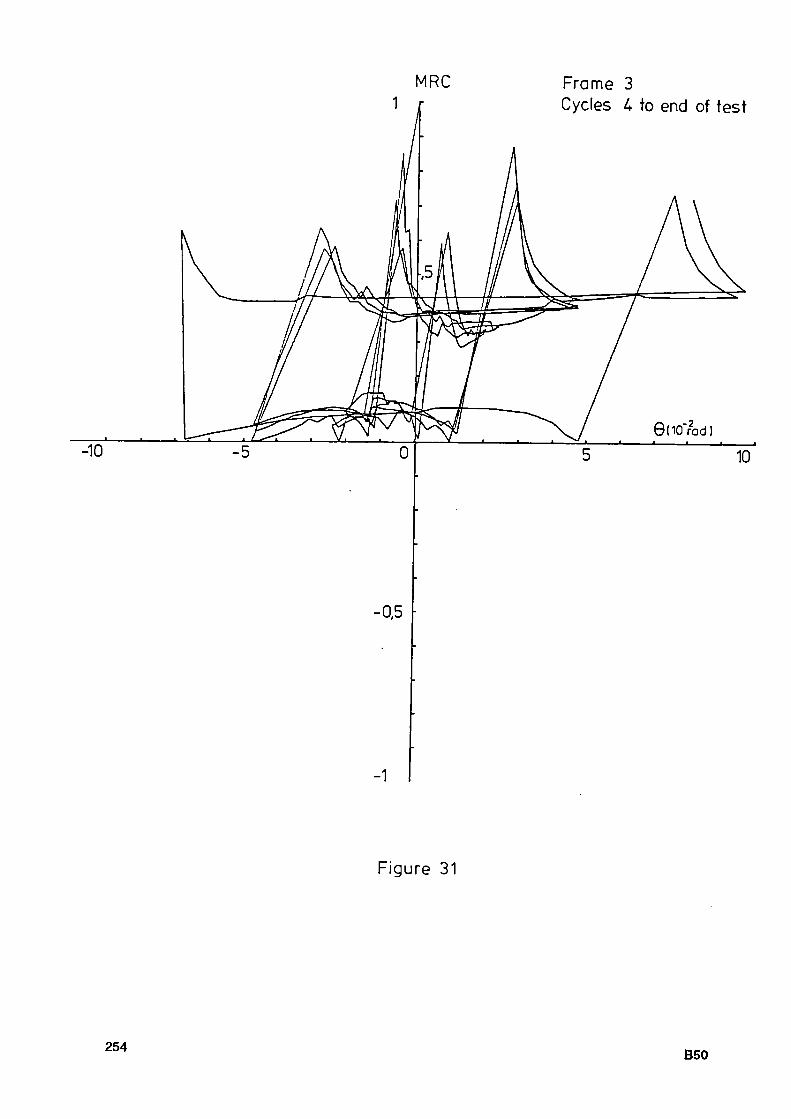
MRC Frame 3 Cycles U to end of test

-0.5

-1

Figure 31

254 B50

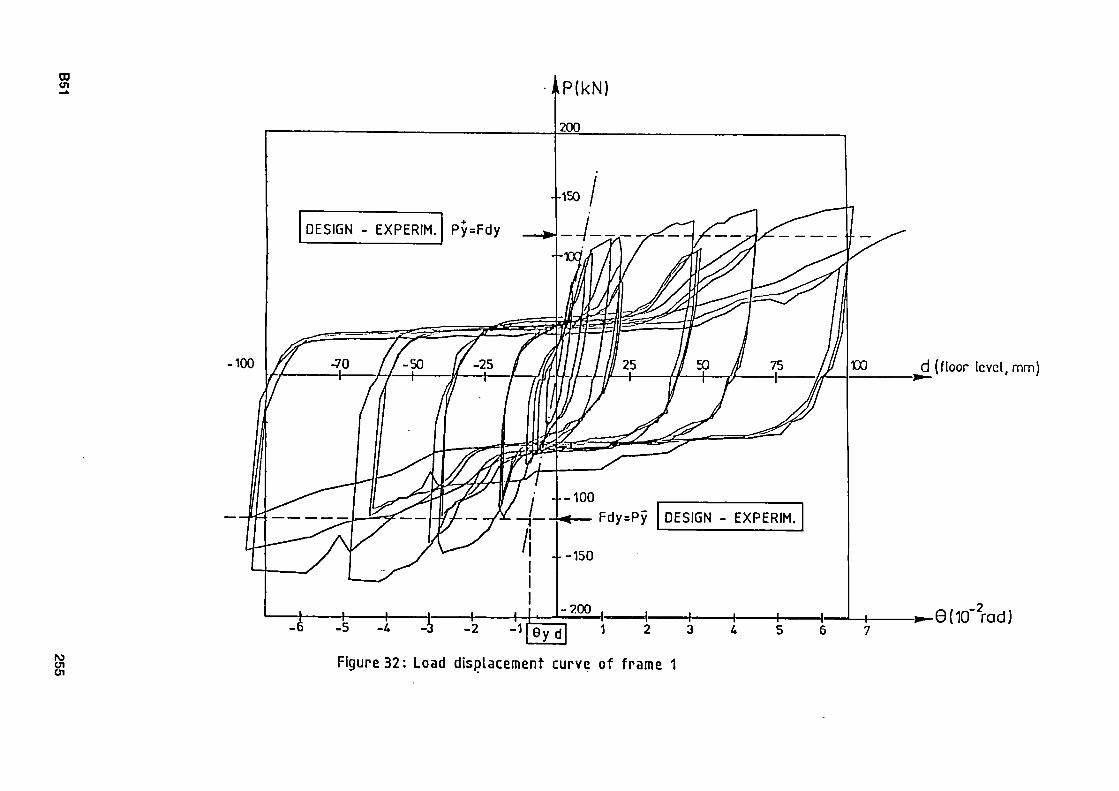
00 Ui

IV3 CTI UI

nP(kN)

200

DESIGN - EXPERIM.

Figure 32: Load displacement curve of frame 1

d (floor level, mm]

-^ØdCfrad)

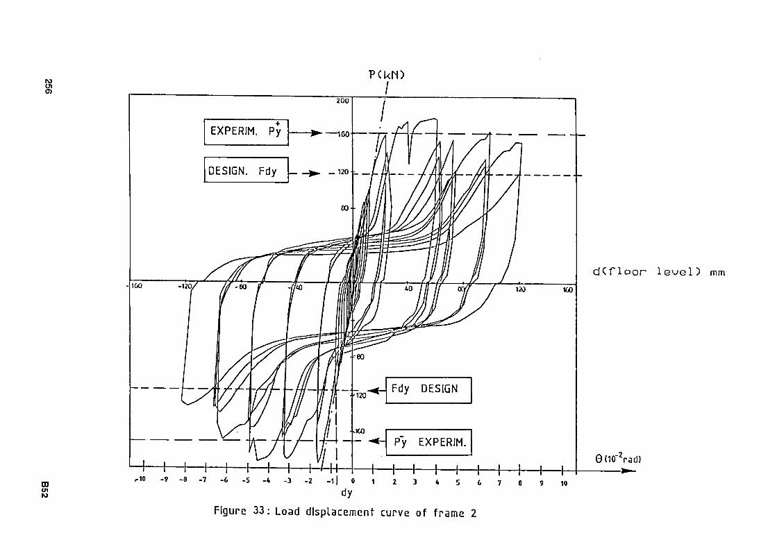
ro ω

CO ui ro

160

EXPERIM. Py

DESIGN. Fdy

-10

ico

d C f l o o r l e u e l ) mm

9l10_2

rad) ^ -

9 10

Figure 33: Load displacement curve of frame 2

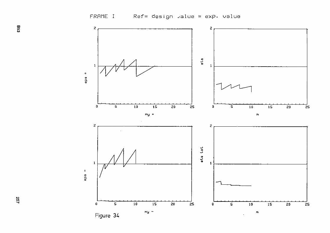
FRflflE I Ref= design ^alue = exp· value CD οι ω

(η

α (S

, Λ Α Α/

ν Λ V

^

10 15

my +

20

(D »J O

25

ro ui ­»4

οι α

A o

(0

β

10 15 20 25

-Λ.

» * * ■

10 * 15 20 25

Figure 34 my ­

FRfìdE I I Ref= des ign .a lue

ro Ol co

α Φ

Λ / \AM

10 15

my +

20 25

co Φ

00 (Π

(ι) α o

Figure 35 my -

co ^ - > φ

10 15 20 25

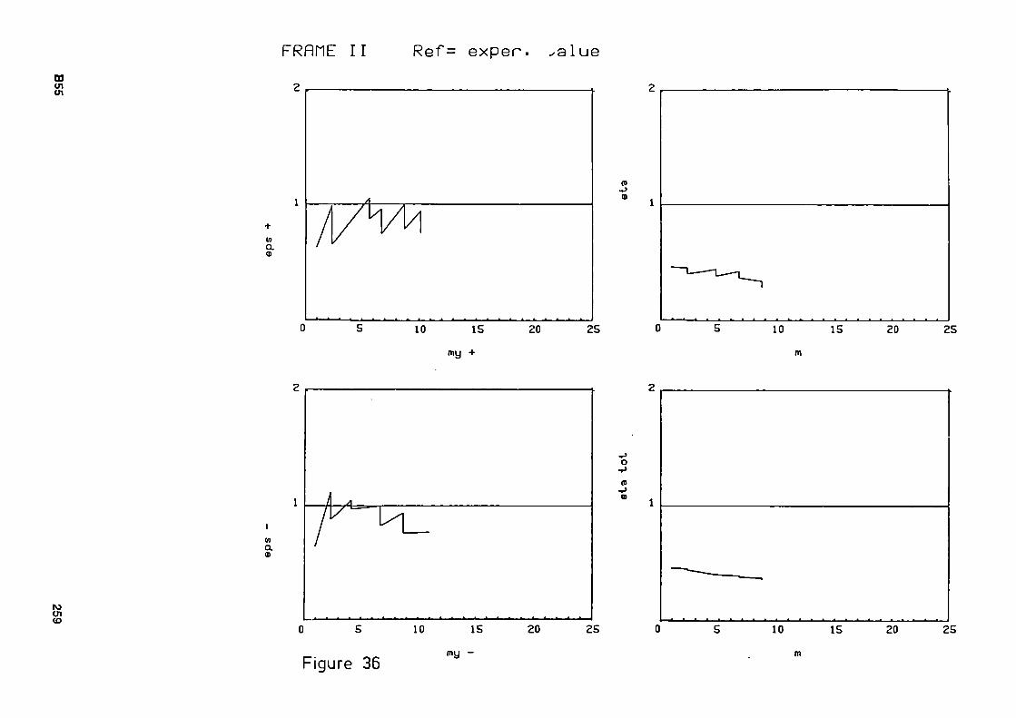
FRfìllE I I Ref= exper. . a lue co υι m

(O α Φ

ο

(Ο α ο

οι (Ο

Figure 36 my -

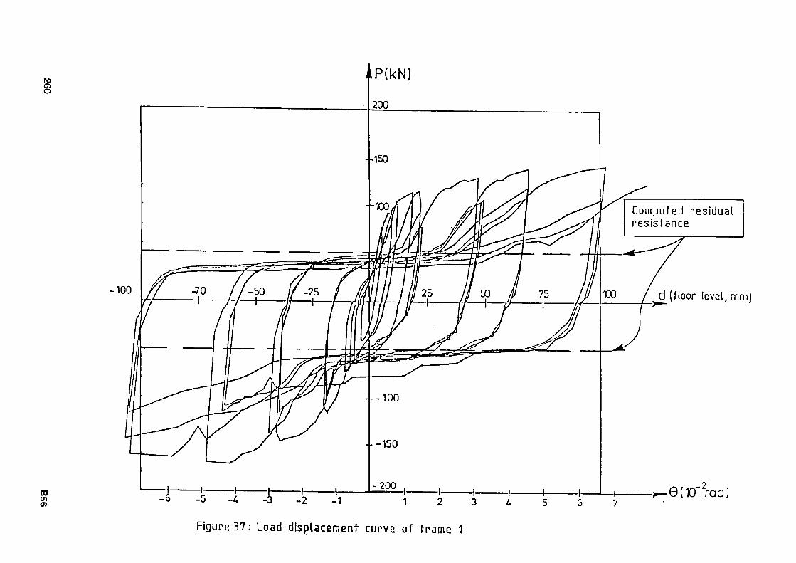
IO 05 O

m in σ>

|P(kN)

200

­150

Η l· t ­l h

­ ­ ­150

200

Computed residual resistance

■5 ­4 ­ 3 ­ 2 ­ 1 1 2 3

Figure 37: Load displacement curve of frame 1

* ί­

α (floor level, mm)

­^­ØdO'radJ

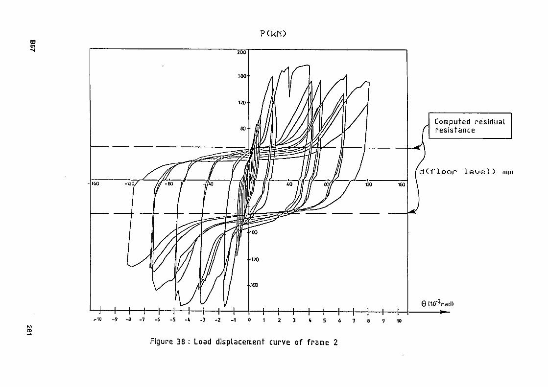
P(UM) CD Ui - « J

Computed residual resistance

c K f l o o r l e o e l ) mm

Figure 38 : Load displacement curve of frame 2

M-

M=1/2(M+ + M-)

o η

crushed concrete

M

Figure 39

262 B58

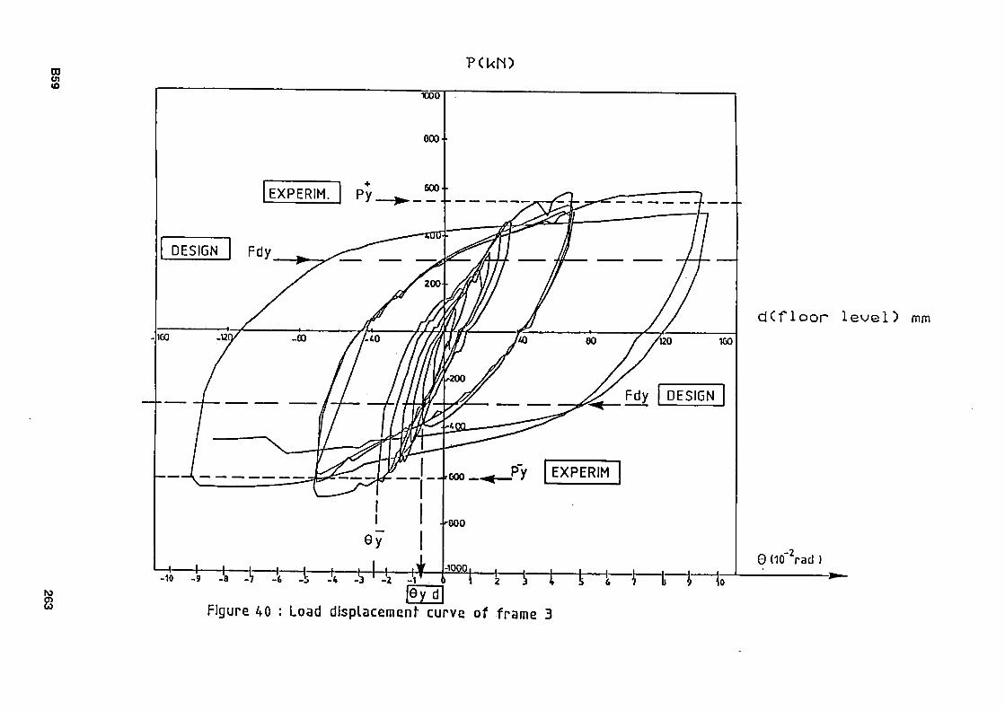
CD ui

ro

S

PCkN)

■eoo

000

EXPERIM. 600··

DESIGN Fdy ^

DESIGN

EXPERIM

dCfloor leuel) mm

θ (10"2rad )

Figure 40 : Load displacement curve of frame 3

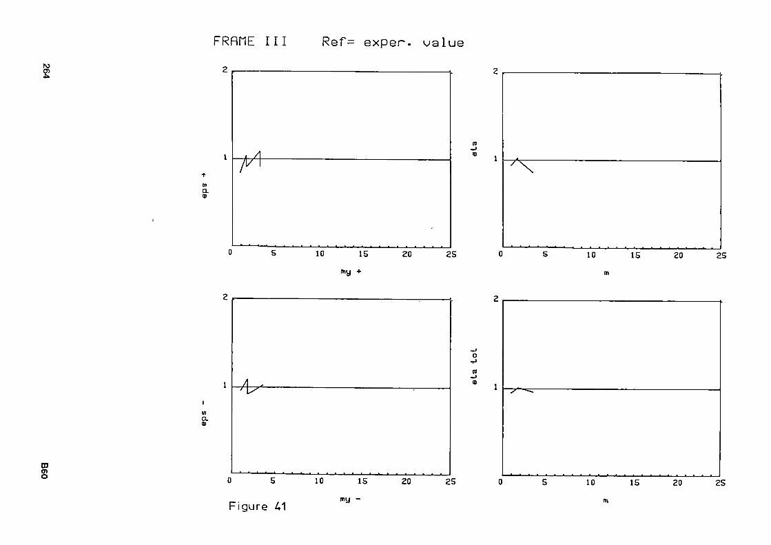
FRAME III Ref= exper. ualue ro

0) α Φ

co Φ

my

CO O) o

η α o

o ti

φ

FRflHE I I I Ref= des ¡ gr. v a l u e

co

co α CD

to α ω

to en en

CD ^ >

CO

• Ρ

o (0

■+> CD

• 10 15

m

20 25

Figure U2 my

PCkM) ro co co

□α σ> ro

1—t—t-

Figure 43 : Load displacement curve of frame 3

1G0

r-i—is

Computed maximum resistance Fmax

Computed better approach Fdy *

d C f l o o r l e * j e l ) m m

Λ Fmax

Θ (10 rad )

G . C . L I E G E a.s.b.i. LABORATOIRES D'ESSAIS DES CONSTRUCTIONS DU GENIE CIVIL ET D'HYDRAULIQUE FLUVIALE DE L'UNIVERSITE DE LIEGE a.s.b.l.

Procès-verbal n° de l'essai n° Planche

Figure 44 - Frame 1 - Overall view of t es t set -up

B63 267

G . C . L I E G E a.s.b.i. LABORATOIRES D'ESSAIS DES CONSTRUCTIONS DU GENIE CIVIL ET D'HYDRAULIQUE FLUVIALE DE L'UNIVERSITE DE LIEGE a.s.b.l.

Procès­verbal n° de l'essai n° Planche

01

Π3

O l _ C XJ C ω

­O

ÍO eu

01

V) οι Π3 c_ ai c ai σι

ru

ai

ai σι _c '>% c

Q. ι

ω e ro

LD

3 σι

268 B64

G . C . L I E G E a.s.b.i. LABORATOIRES D'ESSAIS DES CONSTRUCTIONS DU GENIE CIVIL ET D'HYDRAULIQUE FLUVIALE DE L'UNIVERSITE DE LIEGE a.s.b.l.

Procès­verbal n° de l'essai n° Planche

< c E 3 o 11

c ro αι c

F ro αι . o

Ol ­C

L­

QJ CTI C

ST 1­1

Ϊ Ζ

ro Q_

m αι e ro c

u_

vO ­d· Ol c_ 3 σ ι

u_

ro C/) c Ol > Ol c_

T3 ro o —' c_ Ol ­*­M ­

ro Ol

­ t ­Ol c_ 1 _ P

C o !_/

T3 C ro Ol σ ι c ro

ν ­

α e o l_l

C Ol Ol >

+— Ol

­ O

α. ro

13

B65 269

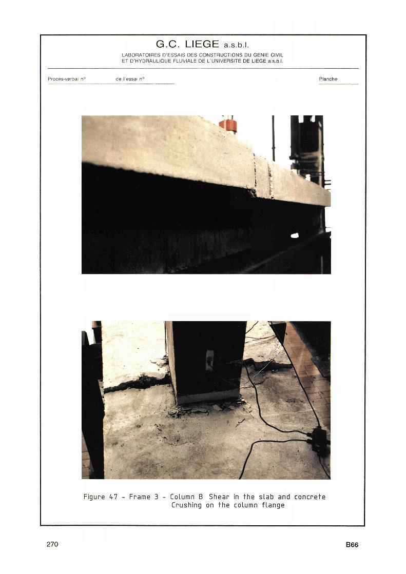
G . C . L I E G E a.s.b.i. LABORATOIRES O'ESSAIS DES CONSTRUCTIONS DU GENIE CIVIL ET D'HYDRAULIQUE FLUVIALE DE L'UNIVERSITE DE LIEGE a.s.b.l.

Procès­verbal n° de l'essai n° Planche

Figure 47 ­ Frame 3 ­ Column Β Shear ¡η the slab and concrete Crushing on the column f lange

270 B66

G . C . L I E G E a.s.b.i. LABORATOIRES D'ESSAIS DES CONSTRUCTIONS DU GENIE CIVIL ET D'HYDRAULIQUE FLUVIALE DE L'UNIVERSITE DE LIEGE a.s.b.l.

Procès-verbal n° de l'essai n° Planche

CD

e

o ■i—

ro e c o

< < -O)

•α οι c o Ν Ol C Π)

Q-

αι e ra

co O· οι C_

en

B67 271

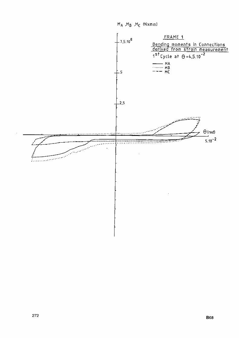
MA -MB ^ c 'Nxmm)

--7,5.10 8

- 1 5

__2,5

FRAME 1

Bending moments in Connections derived from strain measurement 1

s tCycle at θ=4,5.10"

2

MA MB MC

272 B68

MA .Mß .MC (Nxmm)

­ ­ 7 , 5 . 1 0 8

­ ­ 5

­­2,5

FRAME 1

Bending moments in Connections derived from strain measuremërTF 2

n d Cycle at θ =4.5.10"2

MA MB MC

θ (rad) 5.10"

B69 273

M ,M ,M (Nxmm)

--7.5.10 8

- - 5

- - 2 . 5

FRAME 1

Bending moments in Connections derived from strain measurement

3 r d Cycle at θ =4.5.10"2

MA MB MC

' ' ' '2. ■■" ι'

/ θ (rad) ,-2

5.10

274 B70

MA .MB .MC (Nxrnm)

- - 7 . 5 . 1 08

FRAME

Bending moments in Connections derived from strain measurement 1 s t Cycle at θ =4,5.1(Γ2

MA MB MC

B71 275

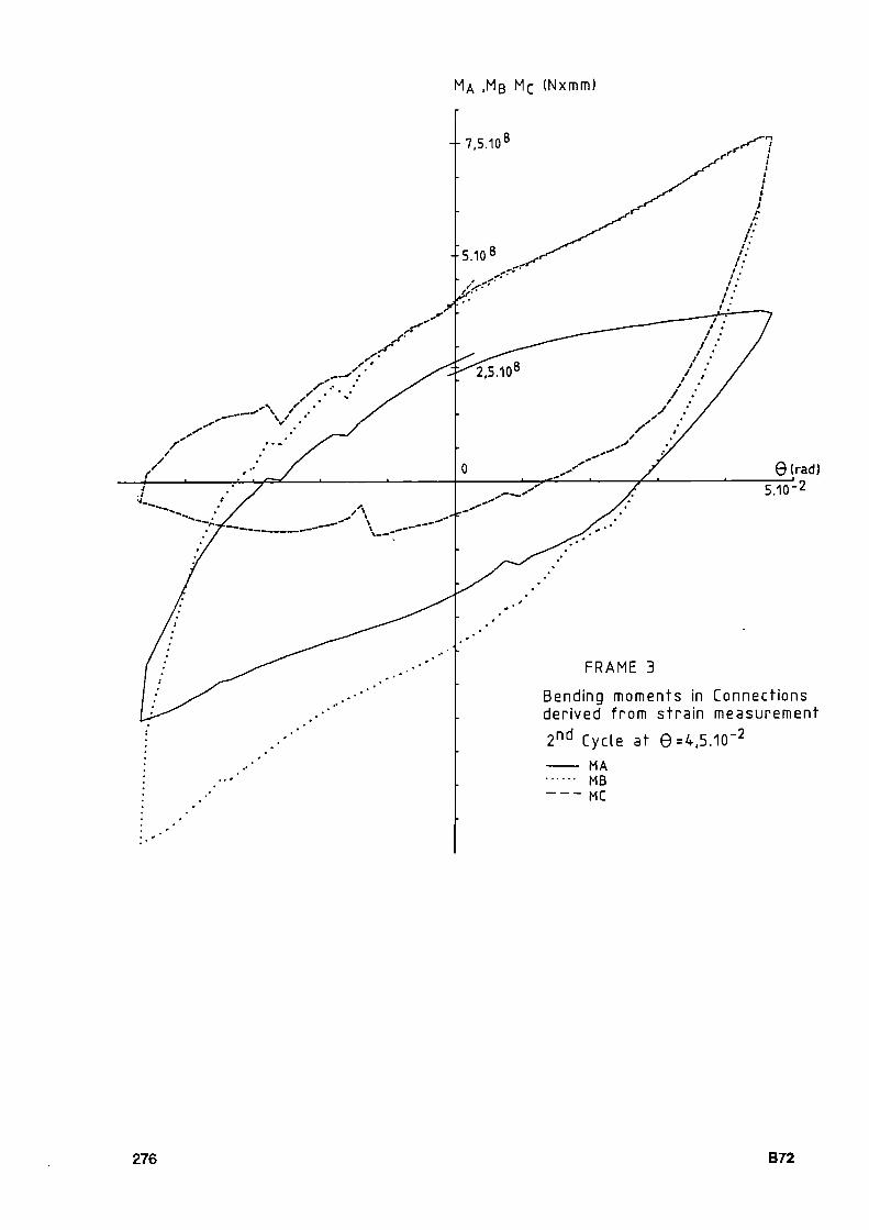
ΜΑ ,Mø Mc (Nxmm)

--7,5.10 s

--5.10 8

FRAME

Bending moments in Connections derived from strain measurement >nd 2

π α Cycle at 6=4.5.10-

MA MB MC

276 B72

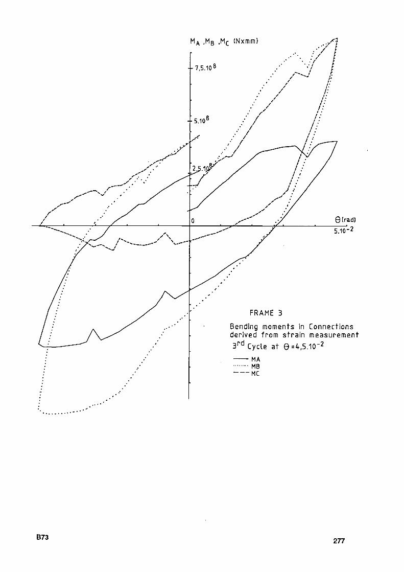
MA ,MB ,MC (Nxmm)

ments in Connections m strain measurement

3r d Cycle at Θ=4.5.1(Γ

2

MA MB

B73 277

PROF. DR.-ING. WOLFRAM KLINGSCH Baustofftechnologie und Brandschutz Baustoffprüfstelle Forschungszentrum für Konstruktiven Ingenieurbau

BERGISCHE UNIVERSITÄT WUPPERTAL

APPENDIX C:

TEST REPORT OF THE WUPPERTAL LABORATORY

SEISMIC RESISTANCE OF COMPOSITE STRUCTURES

S . R . C . S .

Prof. Dr.-Ing. W. Klingsch Dipl.-Ing. B. König Dipl.-Ing. W. Weber

July 1991

Postanschrift Telefon Telex Telefax

• Pauluskirchstr 7 (0202) 439-31 28 8 592 262 ghw (0202) 8 2560

(Laborgebäude), 5600 Wuppertal 2

279

APPENDIX C; TEST REPORT OF THE WUPPERTAL LABORATORY

TABLE OF CONTENTS

1. 2. 2.1 2.2 3. 4. 5. 5.1 5.2 5.3 5.4 6

TEST BODIES MATERIALS STEEL CONCRETE TESTING INSTALLATION QUALITY ASSURANCE TEST RESULTS JOINT TYPE 13 JOINT TYPE HI JOINT TYPE Gl JOINT TYPE Κ ANALYSIS

C2 281

1. TEST BODIES

All steel components (beams, columns, bolts, weldings) of the frames were prefabricated by a ARBED-subcontractor in Luxembourg and shipped to Wuppertal. At Wuppertal institute reinforcement was built in and the single members were concreted. Connecting to frames was made by high tension bolts and - depending on the different connecting types -by additional welding of the beam flanges to the column flange or by anchoring of the reinforcement to the column.

C3 283

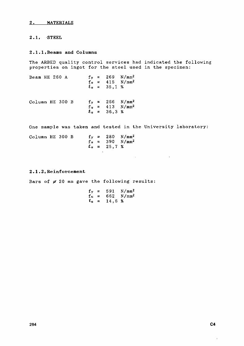
2. MATERIALS

2.1, STEEL

2.1.1« Beams and Columns The ARBED quality control services had indicated the following properties on ingot for the steel used in the specimen: Beam HE 260 A fy = 269 N/mm

2

fu = 415 N/mm2

¿u = 35,1 %

Column HE 300 B fy = 266 N/mm2

fu = 413 N/mm2

¿u = 36,3 %

One sample was taken and tested in the University laboratory: Column HE 300 Β fy = 280 N/mm

2

fu = 3 90 N/mm2

£u = 25,7 %

2.1.2« Reinforcement Bars of çf 20 mm gave the following results:

fy = 591 N/mm2

fu = 662 N/mm2

£u = 14,6 %

284 C4

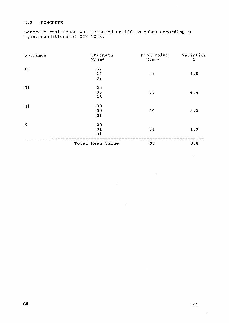
2.2 CONCRETE Concrete resistance was measured on 150 mm cubes according to aging conditions of DIN 1048:

Specimen Strength Mean Value Variation N/mm

2 % 13

Gl

HI

Κ

Strength N/mm

2

37 34 37 33 35 36 30 29 31 30 31 31

36 4.8

35 4.4

30 3.3

31 1.9

Total Mean Value 33 8.8

C5 285

3. TESTING INSTALLATION

Four frames were tested in Wuppertal. They can be divided into

two frames with strong joints (13 and K) and two frames with weak joints (HI and Gl).

The specimen were designed to simulate a section of a multistorey composite frame (figure 1). The columns were hinged at both ends. The four tests were loaded vertically on the beams with 2 * 100 kN. Figures 1 - 3 show the testing installation with the counterframe and the hydraulic jack.

286 C6

Figure 1: Testing Installation

w [mm] ■F [kN]

C7 287

PROF. DR.-ING. W. KLINGSCH

Figure 2 and 3: Testing I n s t a l l a t i o n

288 C8

4. QUALITY ASSURANCE

The first three tests failed early in the elastic range, due to unsatisfying welding quality of the subcontractor. Poor welding quality of the joints could not be recognized by visual control. Detailed analysis after welding failure showed some heavy mistakes. Therefore, the following requirements should be fulfilled for each welded construction for seismic design:

Failures of welding constructions occur by bad design and poor workmanship. It is important to choose the right material, to avoid an accumulation of weldings, to make sure that all weldings are good accessible. It is necessary to use the right welding electrodes and electrode diameters and to prepare the steel surface. In order to avoid singular stresses in the welding, it is necessary to preheat thick structural components. Butt welds are better than fillet welds under dynamic loads.

The welders have to be highly qualified, they have to get a welding qualification.

Non-destructive methods for determining invisible defects of weldings like the ultrasonic testing and the radio materiology are necessary to avoid failures which happened in the first three tests.

As the specimen were fabricated in another workshop then those of Milan, Liege and Darmstadt, the results obtained are not comparable from the point of view of the weld reliability,

C9 289

5. TEST RESULTS

5.1 JOINT TYPE 13

The first frame test was designed with joint type 13 (figure 4).

Welding of the flanges failed within the elastic field at both joints (figure 5). At one side the welding of connecting plate to column flange failed immediately (figure 6). Analysis of the other joint after test showed also failure by pressure of the bolts on the face of the holes in the connecting plate. The holes of the other web plate were largely ovalized in the horizontal direction, which means no significant influence of shear forces.

Figure 7 - 7b show the load-deformation behaviour of test 13.

290 C10

o

ro to

DETAIL 13' NO CONN£CT\ON OF T H E Ş L f t B

Ή£ΜΖ3Ζ&ΕΠΠ7Ά ^2fi£KZ£-

HE 2bo A

\l Ψ

¡s. S

γ///// /ζ?// /// szzt

\///////7r//////>/\

*1 H ·

ß M (D

4 *

η o D D (D η π­ρ­ο D η­<̂

t ) (Β

Μ

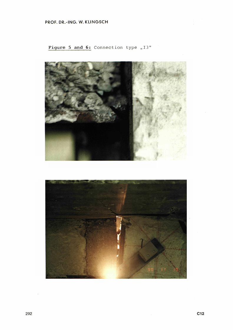
PROF. DR.-ING. W. KLINGSCH

Figure 5 and 6 : Connection type „13"

292 C12

" I / " " » » '

o . Λ co

ro co co

£ 2 j ¿

f ­2 ÜJ

O

­0.1

TEST SPECIMEN "13

­0.08 ­0.06 ­0.04 ­0.02 0 0.02

TOTAL ROTATION [rad]

0.04 0.06

C

tu

>­3 (D

ri­co Ό (D o Η· 3 fD 3

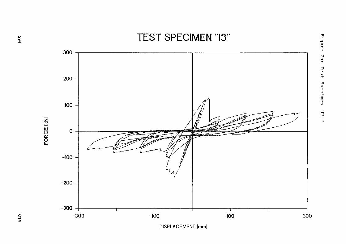
IO (O ■Pk

TEST SPECIMEN "13" 300

200

100

Ld ü OL O L L

0

­100 ­

­200 ­

­300

o ­300 ­100 100 300

Η· iQ C H Π)

»J Ρ)

tü en rí­en Ό ro η

3 ro

DISPLACEMENT [mm]

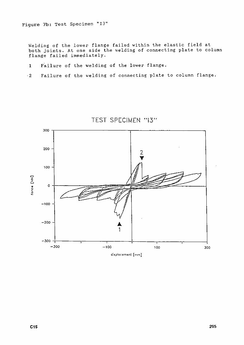
Figure 7b: Test Specimen "13"

Welding of the lower flange failed within the elastic field at both joints. At one side the welding of connecting plate to column flange failed immediately. 1 Failure of the welding of the lower flange. 2 Failure of the welding of connecting plate to column flange.

300

200 -

100 -

-100

-200

-300 -{ -300

TEST SPECIMEN "13"

-100 100 300

displacement [rr.m]

C15 295

5.2 JOINT TYPE HI

The second frame test was designed with joint type HI (figure 8).

The welding of the web plate to the column flange failed early (figures 9 and 10). The connection of slab reinforcement bars (two rebars o 16 mm) to the columns did not fail.

Figure 11 - lib show the load-deformation curve of test HI.

296 C16

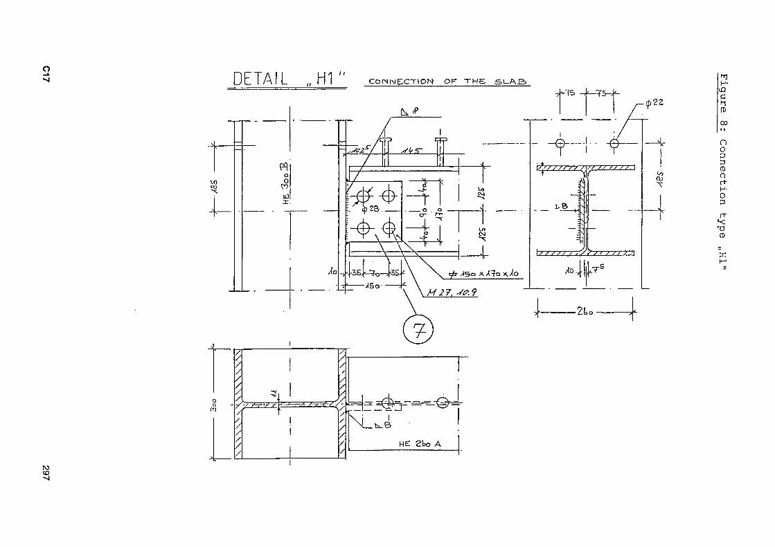
o —k, DETAIL „H1 C O ( N N E C T \ O N O F T H E S­t­A­B»

Ν) CO ­ J

*1 Η ·

C h Π)

co

η o 3 D Π) η (ϊ­ρ · ο

rt >< Ό ro

ι­·

PROF. DR.-ING. W. KLINGSCH

Figure 9 and 10: Connection Type „Hl"

298 C18

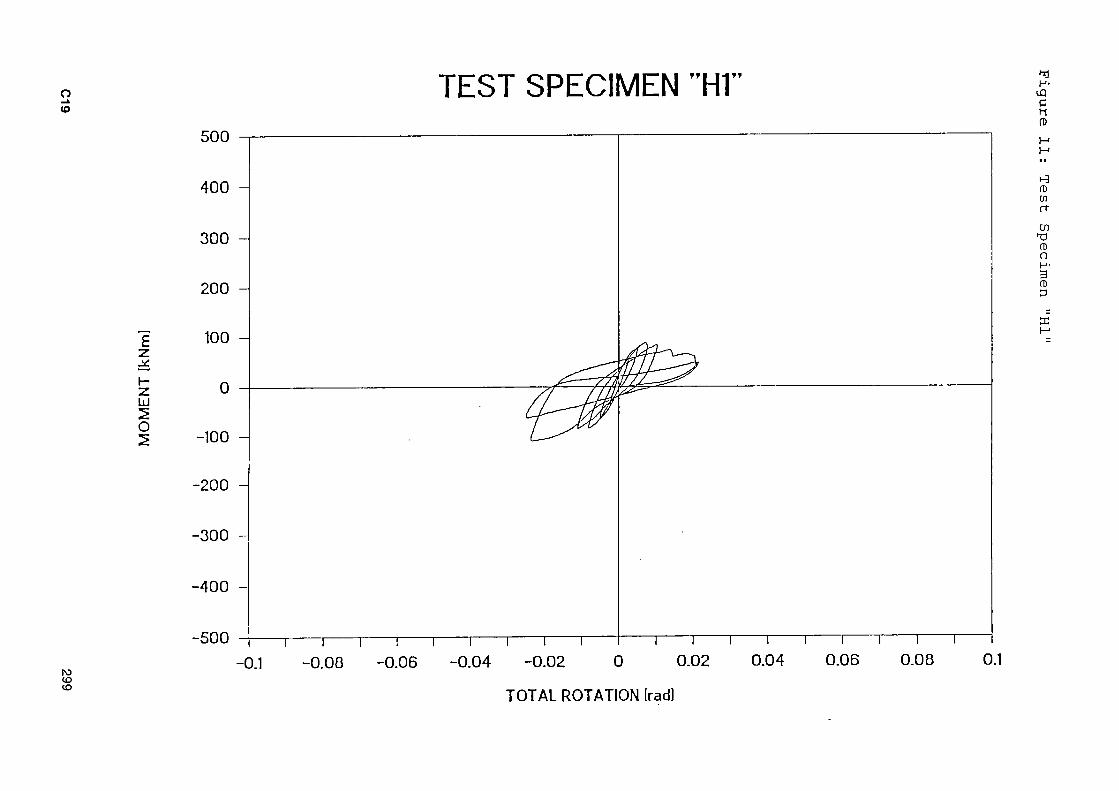
o —k

TEST SPECIMEN "HI" 500

£ ζ ¿¿ l·­ζ LU

O 2

400 ­

300 ­

200

100

0

­100 ­

­200 ­

­300

­400

­500

IO CO co

— ι 1 1 1 1 1 I I ­0.1 ­0.08 ­0.06 ­0.04 ­0.02 0 0.02

TOTAL ROTATION [rad]

— ι 1 1 — 0.04 0.06 0.08 0.1

H-

M Π)

Η Η

Φ w

co

CB O

g (D

ne

»τι M " ω o o

TEST SPECIMEN "HI 300

200

100

ζ

LI ϋ Oí O Lu

0

­100

­200 ­

­300

H­

C h (0

1­3 CD en ri­en Π) O Η · 3 ω

Œ

ο ro ο

­300 ­100 100 300

DISPLACEMENT [mm]

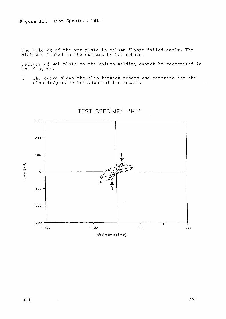
Figure lib: Test Specimen "HI"

The welding of the web plate to column flange failed early. The slab was linked to the columns by two rebars. Failure of web plate to the column welding cannot be recognized in the diagram. 1 The curve shows the slip between rebars and concrete and the

elastic/plastic behaviour of the rebars.

TEST SPECIMEN " H 1 " 300

200 -

100 -

- 1 0 0 -

-200 -

- 3 0 0

- 3 C 0

1 V

A 1

-100 100 300

displacement [mm]

C21 301

5.3 JOINT TYPE Gl

The third frame test was designed with joint type Gl (figure 12).

The pins failed after first cycle (figures 13 and 14). The slab was linked to the columns by two rebars. This additional connection did not fail and explains the residual load bearing capacity.

Figure 15 - 15b show the load-deformation behaviour of test Gl. Figure 16-26 show the functions according to the ECCS-Recommandations 45.

302 C22

o ω

DETAIL Gì

ω o ω

l o CONHJECT\OM' O P THE­ SUAS Γ .„Γ

/ / / / /

r / / / /

■ /

¿Δ ­:=Ε!©^«©­­«^Φ4

►t Η·

C

Π)

H

η o 3 (D η rt Η­O

rt ··< Π)

Ο

PROF. DR.-ING. W. KLINGSCH

F i g u r e 13 and 1 4 : C o n n e c t i o n t y p e „Gl"

*A

304 C24

o to ui

TEST SPECIMEN "G1

ε ζ ¡χ \-ζ Ld

O

­0.1 Ί 1 Γ

­0.08 ­0.06 ΟΙ

­0.04 ­0.02 0 0.02

TOTAL ROTATION [rad]

0.04 0.06

0)

U i

Π) ϋ)

π­

ω TD (D O Η· 3 fl) D

O

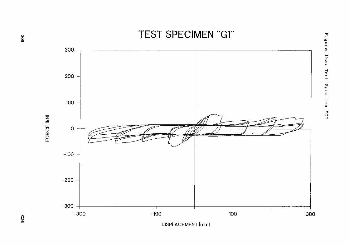
ω

8 TEST SPECIMEN "G1"

300

200 ­

100 ­

ÜJ ü OL o li.

o

­100 ­

­200

­300

o ro σ>

­300 ­100 100 300

DISPLACEMENT [mm]

h1·

C

en fu

1­3 CD en rt

en

(D o Η· 3 Π) α

ο

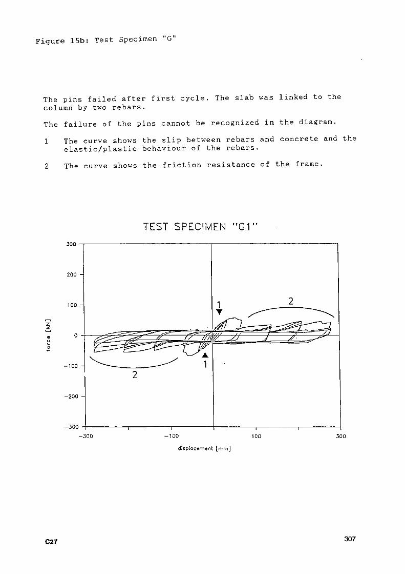
Figure 15b: Test Specimen "G'

The pins failed after first cycle. The slab was linked to the column by two rebars. The failure of the pins cannot be recognized in the diagram. 1 The curve shows the slip between rebars and concrete and the

elastic/plastic behaviour of the rebars. 2 The curve shows the friction resistance of the frame.

TEST SPECIMEN " G 1 " 300

200 -

100 -

- 1 0 0 -

-200 -

-300

- 3 0 0 -100 100 300

displacement [mm]

C27 307

Figure 16: Test Specimen "Gl"-Definition of F

DEFINITION OF Fy

There are different definitions of the limit of the elastic range Fy. Because of the low load bearing capacity of the joint, in this case the following definition was applied:

Definition Definition by ECCS

d]

308 C28

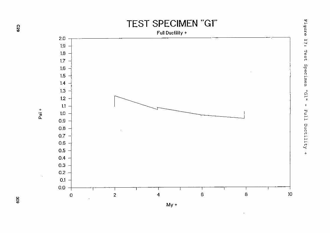
o ro «o

« Q.

TEST SPECIMEN "G1 Full Ductility +

ω o (O

h" lu C h (T)

1­3 ro t/)

ri­

cri

Π) ο 3 Π)

en

•η c

D c η rt

f t κ: +

My +

ω Ο

0)

TEST SPECIMEN "G1" Full Ductility -

o ω o

d i-i Π)

00

Π) ω rt en

(ϋ Ο Η· 3

Ο

ΤΙ

D C o ( t

π-

M y -

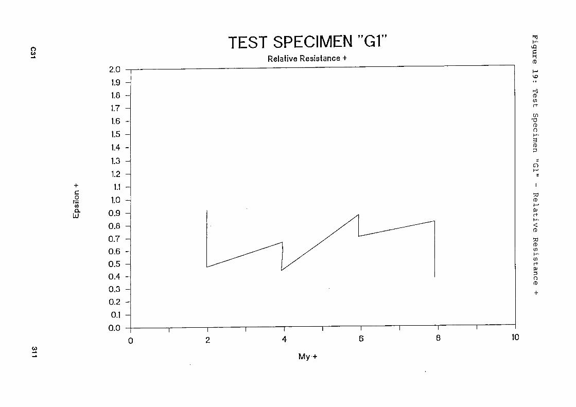
o w

C j3 'cõ Q.

LU

TEST SPECIMEN "G1" Relative Resistance +

Η·

C h (D

H VD

Π) en ri­en Ό (D η 3 α>

Ω

Π) h­' (D r t Η­< Π)

W Π) (/) π­ω ri­fu D o CD

+

ω My ·+

ω ro

l c

co α

ld

TEST SPECIMEN "G1 Relative Resistance -

o CO to

vT) C h ro M o

H3 ro ω rt

en ro η Η-3 ω

Ο

0)

DJ

rt < ω W ω (Λ Η-en rt cu D η ro

M y -

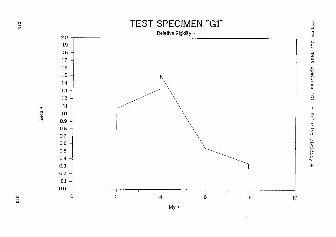
o w

+

Ν

TEST SPECIMEN "Gl" Relative Rigidity +

ω ω

Φ en rt

en ro o Η· 3 Π) 3

Ο

(Ό Μ 0J

η·

<

Π)

Η·

α

My +

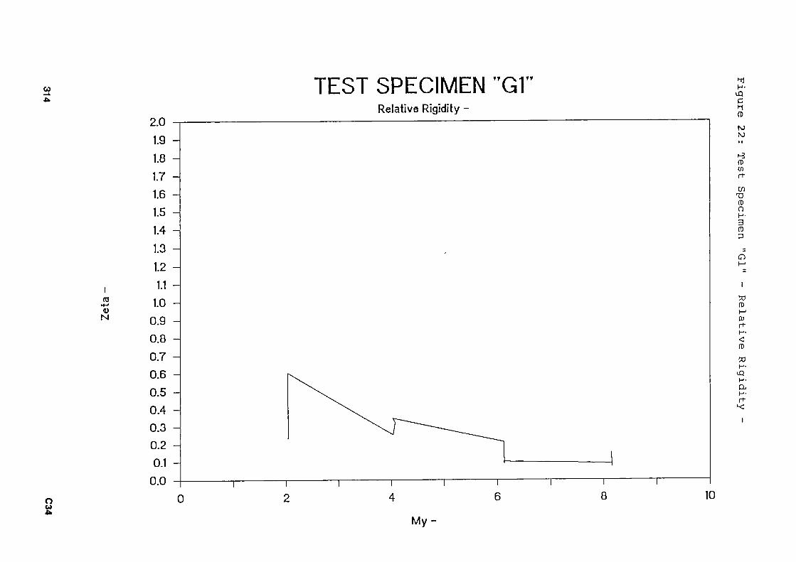
ω TEST SPECIMEN "Gl

ι ro ω Ν

O ω ik

Relative Rigidity ­

Η ·

C M (D

M

ÍD 01

rt

σι Τ! φ η ρ· 3 Π) 3

O

» 0) M OJ rt Η· < (D S3 Η­·

uà

rt

Ι

M y ­

o w ui

+

ω en

O

TEST SPECIMEN "G1" Relative Absorbed Energy +

8 10

h

Ν) LO

>­3 ω en Π­ω

ω ο Η· 3 Π) 3

ο

Π)

0) r t Η· < (D

> σ ο σ Π) Di D (D

iQ

My +

co TEST SPECIMEN "G1" Relative Absorbed Energy ­

o ω σ>

H­

M fD

M

1­3 fD

rt

en Ό (D O Η · 3 fD 3

CD

» fD M OJ rt H· < fD

> σ ω O ι­<

σ fD & M fD »I

iQ

M y ­

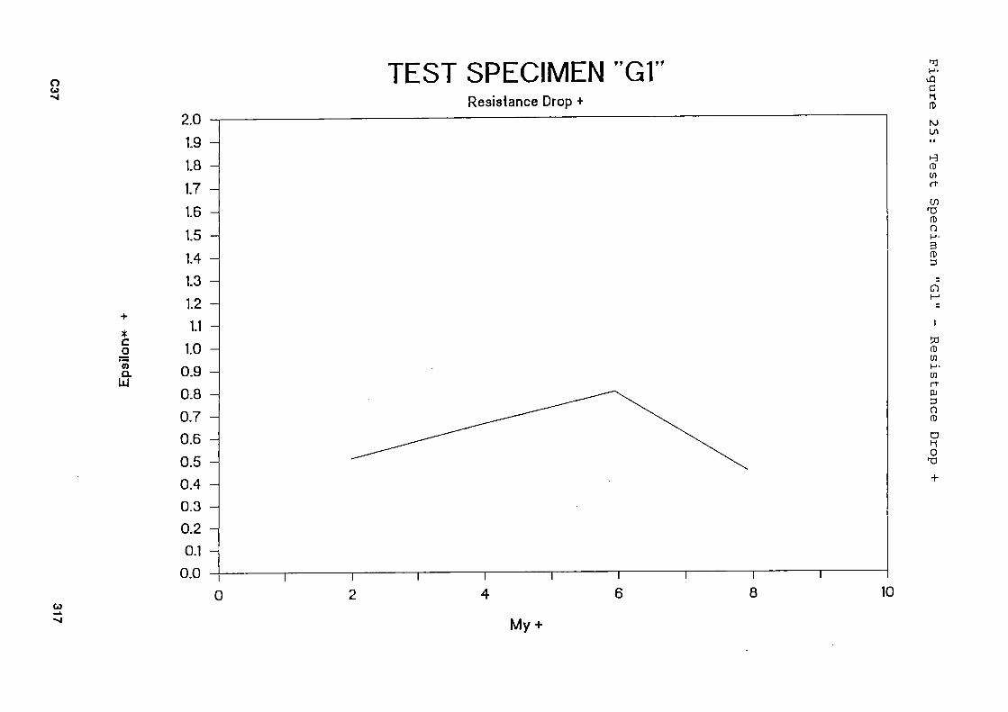
o ω

C O

'm a.

ÜJ

TEST SPECIMEN "GT Resistance Drop +

►η

c h tí M UI

1­3 Π) [Λ et

en τι Π) η Ρ· 3 α> 3

Ο

W en ρ­ω π cu ο (0

ο »­ι ο

ΤΙ

ω ­ν| My +

ω οο

TEST SPECIMEN "G1"

c

'55 Q.

Resistance Drop -

o Gl οβ

Tl

c H (D M σι

1-3 Π) en rt

en Ti ro η Η· 3 Π) 3

Η ·

id ω (Λ ρ-[Λ rt DJ

η Π)

ο ο no

M y -

5.4 JOINT TYPE Κ

The fourth frame test was designed with joint type Κ (figure 27). This joint design was strong. By its rigidity the maximum load of the hydraulic jack was reached about within the elastic region.

After reaching the 210 mm - displacement the test had to be stopped because of the limited capacity of the hydraulic jack.

After this point, the test was continued in a shake down procedure with constant displacements until load decreasing. After that point, displacements increased. Failure occurs by punching out of bolts. Shear panel of the column and upper and lower flange of the beam showed extensive plastifications and cracks (figures 28-30). Figure 31 - 31b show the load-deformation curve of test K.

Figure 32-42 show the functions according to the ECCS-

Recommandations 45.

C39 319

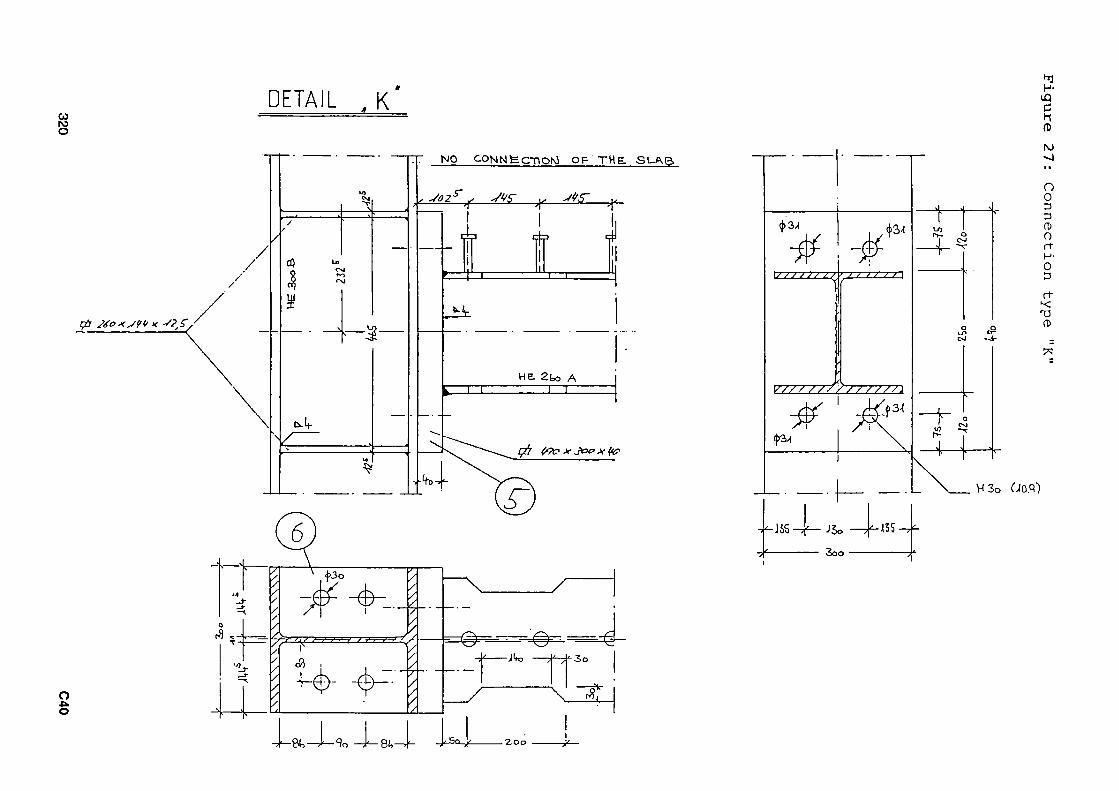
ω ο

φ 2¿oxsW χ ­/?'C

Ο ο

DETAIL , Κ

NO CONNfcC­nOhJ O F T H E , S U A S

I / / / / / / / > / / / / / / J

<ţ>3/l

IQ Ρ

h

^1 o o D D 0) O r t Η· O 3 ri­

>< Ό Φ

VI 3ο (JtOPÌ)

-χ-

■J5S­7p—J5o — f ­ « 5 ­

• 3oo ■—

­5a­J¿ 2 . 0 0 ^¿­

PROF. DR.-ING. W. KLINGSCH

Figure 28 and 29 : Connec t ion t y p e "K"

C41 321

PROF. DR.-ING. W. KLINGSCH

Figure 30: Connection type "Κ"

322 C42

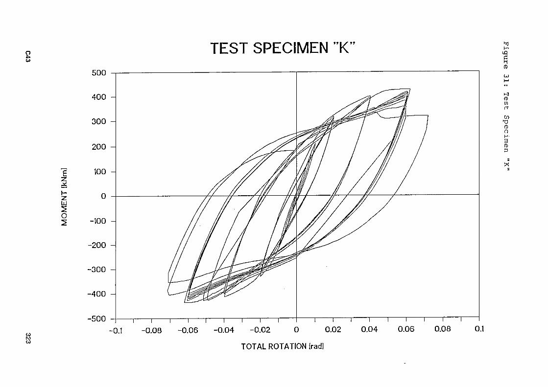
o f» w

ω ro ω

Ζ UJ

ο

500

TEST SPECIMEN "Κ"

Ί 1 1 1 1 Γ

­0.1 ­0.08 ­0.06 ­0.04 ­0.02 0 Ί Γ

0.02 0.04 0.06

ui

(D (Λ r+

ω Ό 0) η Η· 3 Π) D

TOTAL ROTATION [rad]

ω ro TEST SPECIMEN "Κ"

300

200 ­

100

l i j ϋ α o iL

0

­100

­200 ­

­300

o ■u

­300 ­100 100 300

d Π)

ui Η 0)

1­3 ro en ci­en Ti Π) η Η­3 0) 3

«

DISPLACEMENT [mm]

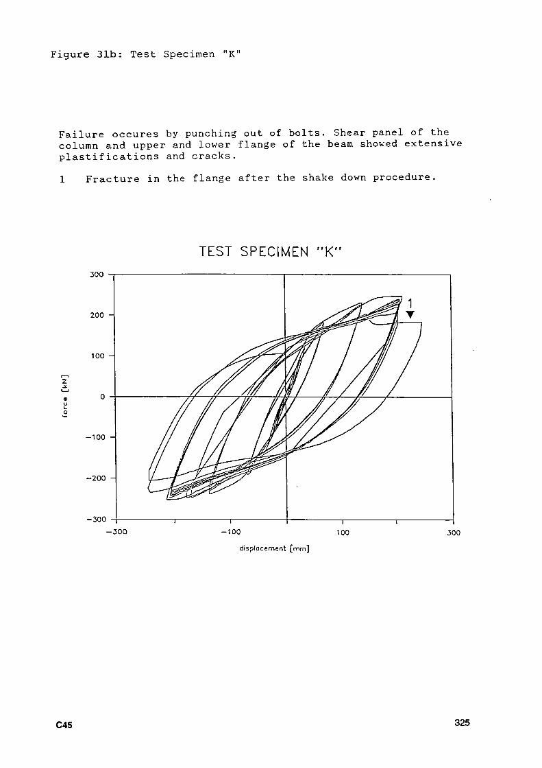
Figure 31b: Test Specimen MK'

Failure occures by punching out of bolts. Shear panel of the column and upper and lower flange of the beam showed extensive plastifications and cracks. 1 Fracture in the flange after the shake down procedure.

TEST SPECIMEN "K " 300

200 -

100 -

Ζ

- 1 0 0 -

-200

- 3 0 0

- 3 0 0 - 1 0 0 100 300

displacement [mm]

C45 325

Figure 32: Test Specimen "K"-Definition of F

DEFINITION OF Fy

There are different definitions of the limit of the elastic range Fy. Because of the low capacity of the hydraulic jack, in this case the following definition was applied:

Definition Definition by ECCS

d]

326 C46

o ¿k

η Q.

TEST SPECIMEN "K" Full Ductility +

H· iQ

H Π)

LO UI

(0 UI rí­en Τ) fl) η Η· 3 fD 3

c

D C η rt­Η· h­· Η· η­

ω ro ­vi

My +

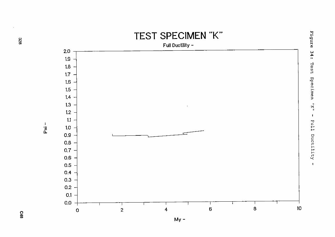
ω ro οο

co o.

TEST SPECIMEN "Κ" Full Ductility -

o co

va 0 h

ω Λ.

1-3 (t) en rt-cn

73 Π) η Η· 3 tí 3

^ C

α o η· Η· Μ Η-rt

M y -

o ¿k «o

C o 'm α. LI

TEST SPECIMEN "Κ" Relative Resistance +

ω ro (O

Η· «η e Π)

OJ UI

1­3 ro rt en

13 ro η Η· 3 ro

î *

» ro t ­

1

OJ r+ H· < ro

ro en Ρ­ΙΟ ri­fu 3 O ro

My +

" I X »»

I c

j 3 '55 α

o ui o

TEST SPECIMEN "Κ Relative Resistance ­

H· tQ C H Π)

OJ σι

1­3 ro rí­

en TD fD η Η· 3 α> D

» Π) Μ Ρ) f t

< (ΐ)

Π) ω π­ω r t Ρ) 3 η

M y ­

o ui

+ ro

■ * ■ >

α) Ν

TEST SPECIMEN "Κ" Relative Rigidity +

ω ω

►fl Η ·

C H CD

OJ

•­3 ÍD ω l i­

en Π) η ρ · 3 (Τ)

«

ro M DJ f t Ρ· < ÍD

Ρ­ίο ρ­

Ρ· rt

My +

δ M

ro 0)

Ν

TEST SPECIMEN "Κ" Relative Rigidity -

o οι ro

►ή H­

iQ C

ro ω co

>­3 Π)

rt

en to o Η· 3 0) 3

ϊ*

W Π) Μ 0) r t Ι­"· < »

ρ­α ρ­

rt

Ι

M y ­

o ui o»

+ ro

·** UJ

TEST SPECIMEN "Κ" Relative Absorbed Energy +

H·

Η 0)

ui io

1­3 (C en t i ­

en

fD η h·· 3 CD 3

Π) h­

1

PJ r f H· < (D

> σ ω o M D" π> & M D Π) •­ι

My +

ro LU

TEST SPECIMEN "Κ" Relative Absorbed Energy ­

o

H ·

(Τ)

.** O

Π) Cf) r t

Ui <Ό (0 O Η· 3 fD 3

«

50 CD M CU rt

< fD

> σ ω o •ι cr ω α 3 CD Μ

M y ­

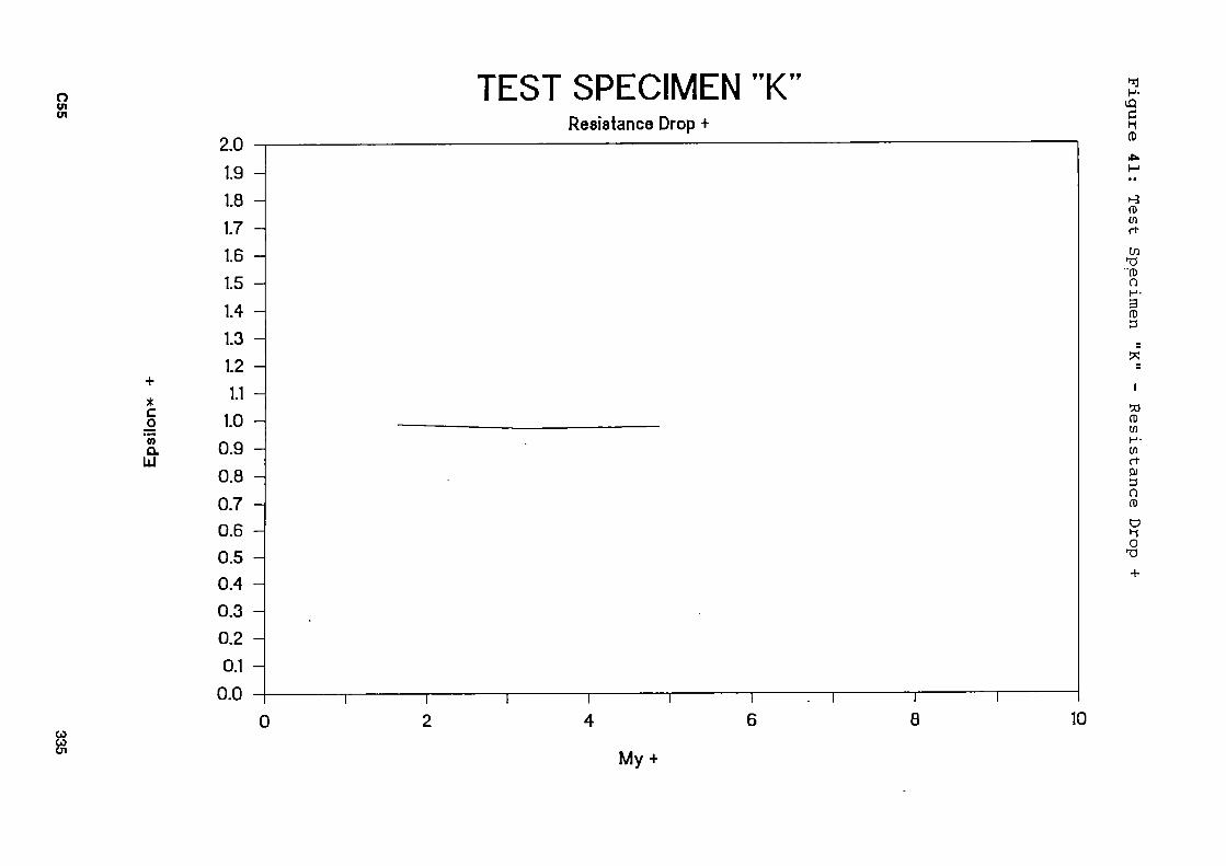
o ui

C o

'M a U

TEST SPECIMEN "Κ" Resistance Drop +

H·

C

Π)

1­3 fi) ω rt en

"CD o Η· 3 (D 3

«

50 (0 C/l ρ­ω rt 0)

o α> σ ι­! ο

ω My +

c O '55 α LI

TEST SPECIMEN "Κ" Resistance Drop ­

o UI O)

α>

M

►9 ro ω ri­co Π) o Η· 3 tl)

to Π) en π­ω rt­0) o ro

D i­i o

M y ­

6 . ANALYSIS

Results of test 4 were be processed according to the ECCS-Recomraandations 45 "Recommended Testing Procedure for Assessing the Behaviour of Structural Steel Elements under Cyclic Loads".

In accordance with the defined evaluation procedure the tests were considered until the displacements allow three complete cycles with a resistance not less than 60% of the maximum resistance obtained during the test.

For that reason and because of the early failure in the elastic range tests 1 - 3 were declared as misfitted. Nevertheless, test 3 was processed.

Test 4 proves that it is not sufficient to investigate the behaviour of the joints under cyclic loads only with respect to increasing displacements. It is also important to examine the behaviour of joints under cyclic displacements with constant maximum amplitudes, in order to estimate the pulsating fatigue limit of strength.

C57 337

TECHNISCHE HOCHSCHULE DARMSTADT

Institut für Stahlbau und Werkstoffmechanik

C.E.C.-PROJECT NO. 7210-SA/506 SEISMIC RESISTANCE OF COMPOSITE STRUCTURES S.R.C.S.

TEST SERIES 3 - FINAL REPORT

Darmstadt May 1991

by

J.G. Bouwkamp B. Schneider

R.Kanz

339

Table of Contents

D.I. Introduction 343 D.2.Test Specimen 343

D.2.1.Moment Resistant Frame 1 344 D.2.2.Moment Resistant Frame 2 344 D.2.3.Eccentrically Braced Frame (EBF) 344 D.2.4,Subassemblages 345

D.3.Test Setup 345 D.4.Material Properties 345 D.5, Instrumentation 346

D. 5.1. General 346 D.5.2 .Moment Resistant Frames 346

D.5.2.1.Global Measurements 346 D.5.2.2.Local Measurements 346

D.5.3,Eccentrically Braced Frame 347 D.5.3.1.Global Measurements 347 D.5.3.2.Local Measurements 347

D. 5.4 .Subassemblages 347 D.6.Data Acquisition System and Testing Procedure 348

D.6.1.Data Acquisition 348 D.6.2 .Test Procedure 348

D.6.2.1· General 348 D.6.2.2.Displacement Sequence 349

D.6.2.2.1/Frames 1 and 2 349 D.6.2.2.2.Frame 3 350 D.6.2.2.3/Subassemblages 350

D.7,Test Performance 350 D. 7.11 Test Behaviour 351

D.7.1.1.Behaviour of MRF test frames 1 and 2 351 D.7.1.2,Behaviour of EBF test frame 3 352 D.7.1.3 »Behaviour of Subassemblages 352

341

Table of Contents

D.8 Test Results 353 D.8.1. General 353 D.8.2 Test Results Frame 1 354 D.8.3 Test Results Frame 2 355 D.8.4 Test Results Frame 3 355 D.8.5 Test Results Subassemblages 357

D.8.5.1 Test Results Subassemblage 1 357 D.8.5.2 Test Results Subassemblage 2 357 D.8.5.3 Test Results Subassemblage 3 358 D.8.5.4 Test Results Subassemblage 4 358 D.8.5.5 Test Results Subassemblage 5 358

D.8.6 Interpretated Test Results,following ECCS Recommendation No. 45 359 D.8.7 Synthesis of the Experimental Results 359

Tables 361 Figures 364

342

D.l Introduction This report covers the full scale studies of two steel concrete composite moment resistant frames, five subassemblages belonging to the moment­resistant frames and far off one steel concrete eccentrically braced frame. These studies formed integral part of a cooperative research project under the management of ARBED Recherches ­ Luxembourg.

In the following sections Information is provided about the test specimen (section D.2), test setup (section D.3) and material properties (section D.4). Subsequently, the instrumentation for all frames and subassemblages is described in section D.5. The data acquisition system and test procedure is presented in section D.6. The test performance, describing the general observed response of the tested frames and subassemblages, and the test results, showing actual test­performance data, are being covered in section D.7 and D.8.

D.2 Test Specimen Within the scope of the overall cooperative program the Technical University at Darm­

stadt, Institute for Steelcon6truction, was selected to perform the large scale tests of composite steel­ concrete moment­resistant frames. Following earlier results of beam­

column studies, carried at the Politechnico dir Milano, it was decided, tha t one test frame should be designed with HS­bolted endplated beam­column connections, while the second test frame should be developed having welded beam­column joints.

In addition to the above indicated moment resistant frames (MRFs), it was decided also to study a test frame with the same overall dimensions but with an eccentrically braced stiffening arrangement in one bay.

Accordingly, three, two­story, two­bay test frames with overall dimensions of 5.50 m by 10.00 m (2 χ 2.75 m in height and 2 χ 5.00 m in length) have been tested. In accordance with earlier beam­ column connection tests, HEA­260 and HEB­300 sections were choosen, respectively, for all beams and columns (see figure D­l) . A concrete slab with width and height dimensions of 1.00 m χ 0.12 m was connected to the beams by means of headed studs ( ø 19, 1 = 100 m m ). The slab reinforcement consisted of two Q221 bi­axial reinforcing mats, positioned near the top and the bottom of the slab.

For fire­resistant requirements, filled­in concrete, reinforced by rebars 4 ø 20 and stirrups ø 8 spaced 20 cm, had been placed symmetrically on either side of the web between the flanges of the beam and column sections (see figure D­l) . In the connec­

tion regions the column shear­panel zones of both the exterior and interior columns had not been reinforced by doubler plates. At the base of the fixed­ended columns, base plates were designed elastically to asure the plastic moment development of the

D1 343

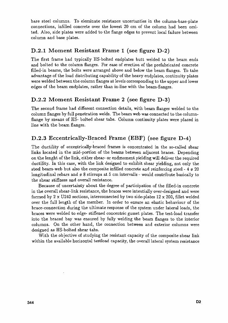
bare steel columns. To eleminate resistance uncertanties in the column-base-plate connections, infilled concrete over the lowest 20 cm of the column had been omi-

ted. Also, side plates were added to the flange edges to prevent local failure between column and base plates.

D.2.1 Moment Resistant Frame 1 (see figure D-2) The first frame had typically HS-bolted endplates butt welded to the beam ends and bolted to the column flanges. For ease of erection of the prefabricated concrete filled-in beams, the bolts were arranged above and below the beam flanges. To take advantage of the load distributing capability of the heavy endplates, continuity plates were welded between the column flanges at levels corresponding to the upper and lower edges of the beam endplates, rather than in-line with the beam-flanges.

D.2.2 Moment Resistant Frame 2 (see figure D-3) The second frame had different connection details, with beam flanges welded to the column flanges by full penetration welds. The beam web was connected to the column-

flange by means of HS- bolted shear tabs. Column continuity plates were placed in line with the beam flanges.

D.2.3 Eccentrically-Braced Frame (EBF) (see figure D-4) The ductility of eccentrically-braced frames is concentrated in the so-called shear links located in the mid-portion of the beams between adjacent braces. Depending on the lenght of the link, either shear- or endmoment yielding will deliver the required ductility. In this case, with the link designed to exhibit shear yielding, not only the steel beam-web but also the composite infilled concrete and reinforcing steel - 4 ø 20 longitudinal rebars and ø 8 stirrups at 5 cm intervalls - would contribute basically to the shear stiffness and overall resistance.

Because of uncertainty about the degree of participation of the filled-in concrete in the overall shear-link resistance, the braces were intentially over-designed and were formed by 2 χ U240 sections, interconnected by two side-plates 12 χ 200, fillet welded over the full length of the member. In order to ensure an elastic behaviour of the brace-connection during the ultimate response of the system under lateral loads, the braces were welded to edge- stiffened concentric gusset plates. The test-load transfer into the braced bay was ensured by fully welding the beam flanges to the interior columns. On the other hand, the connection between and exterior columns were designed as HS-bolted shear tabs.

With the objective of studying the resistant capacity of the composite shear link within the available horizontal testload capacity, the overall lateral system resistance

344 D2

was intentionally lowered by reducing the column base fixity moment resistance (re­ducing the width of the column flanges over a certain distance immediately above the base plates).

D.2.4 Subassemblages (see figure D-5) In as f ax as earlier studies had been focused on assessing the moment-rotaion capacity of full interior and exterior beam-column connections, the response for the beam-column connections at the roof level could only be extrapolated from these earlier test results. However, in order to permit a better evaluation of the overall frame response, it was decided, to test also subassemblages of the roof beam-column connections and the column footing. Particularly, the five tested subassemblages were one footing point (named Subassemblage 1), two Knee-Joints (Subassemblage 2: HS-bolted and 3: welded) and two T-Joints (Subassemblage 4: HS-bolted and 5: welded).

D.3 Test-Setup For the test performance a special reaction frame had been designed with a heavy base-beam (HD400x400x551) pre-stressed to the laboratory tie-down slab and connected by means of a transverse beam at one end to two vertical, parallel loading- trusses (see figure D-6). The column base plates of the test structures were HS-bolted to the base-beam. The trusses, interconnected by means of transverse beams, allowed the application of horizontal loads at each floor level of the test frame through two double-acting hydraulic actuators. Special loading jokes were designed to introduce the actuators loads into the test frame at the loading-side at points mid-way between the outer and inner columns. This loading arrangement had been necessary in order to prevent direct loading of the exterior column (see figure D-7). Movement normal to the test-frame was restrained by a stability frame which provided guidance to the frame at two location at each floor level (see figure D-8).

Considering the large amount of concreting necessary (7.2.m3 for the beam slabs) and the serious time limitations set for the test performance, the three full-scale test specimen were erected immediately adjacent to the loading frame and were concreted at the same time. After the necessary concrete strength had been reached, test frames were moved successively into the test position, instrumented and tested.

D.4 Material Properties The material properties were determined from tensile coupon tests of the steel secti­ons (both flanges and webs), and through concrete compression tests. The E-Modulus

D3 345

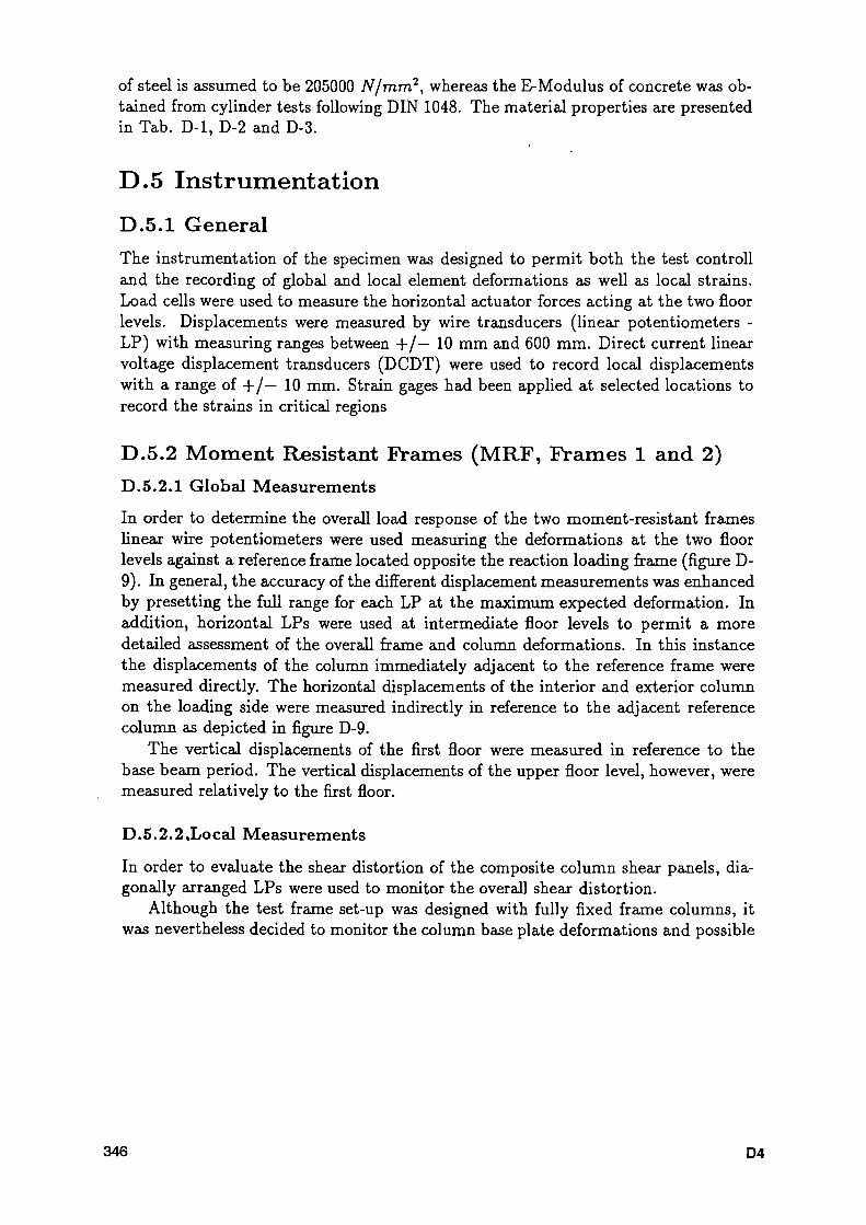
of steel is assumed to be 205000 Ν ¡mm2, whereas the Ε­Modulus of concrete was ob­

tained from cylinder tests following DIN 1048. The material properties axe presented in Tab. D­l, D­2 and D­3.

D.5 Instrumentation D.5.1 General The instrumentation of the specimen was designed to permit both the test controll and the recording of global and local element deformations as well as local strains. Load cells were used to measure the horizontal actuator forces acting at the two floor levels. Displacements were measured by wire transducers (linear potentiometers ­

LP) with measuring ranges between +/— 10 mm and 600 mm. Direct current linear voltage displacement transducers (DCDT) were used to record local displacements with a range of +/— 10 mm. Strain gages had been applied at selected locations to record the strains in critical regions

D.5.2 Moment Resistant Frames (MRF, Frames 1 and 2) D.5.2.1 Global Measurements

In order to determine the overall load response of the two moment­resistant frames linear wire potentiometers were used measuring the deformations at the two floor levels against a reference frame located opposite the reaction loading frame (figure D­

9). In general, the accuracy of the different displacement measurements was enhanced by presetting the full range for each LP at the maximum expected deformation. In addition, horizontal LPs were used at intermediate floor levels to permit a more detailed assessment of the overall frame and column deformations. In this instance the displacements of the column immediately adjacent to the reference frame were measured directly. The horizontal displacements of the interior and exterior column on the loading side were measured indirectly in reference to the adjacent reference column as depicted in figure D­9.

The vertical displacements of the first floor were measured in reference to the base beam period. The vertical displacements of the upper floor level, however, were measured relatively to the first floor.

D.5.2.2Xocal Measurements

In order to evaluate the shear distortion of the composite column shear panels, dia­

gonally arranged LPs were used to monitor the overall shear distortion. Although the test frame set­up was designed with fully fixed frame columns, it

was nevertheless decided to monitor the column base plate deformations and possible

346 D4

horizontal displacements by means of DCGTs. These measurements were taken in reference to the tie down slab and base beam, respectively.

In order to possibly determine the normal column forces as well as the column shear forces and bending moment distributions in each story column, each column was instrumented with strain gages located at two sections along the column length. These sections were placed at locations where the column response was expected to be elastic. In each section single strain gages were positioned oppositely in the middle of the column flanges.

D.5.3 Eccentrically Braced Frame (EBF, Frame 3) D.5 .3 .1 G l o b a l M e a s u r e m e n t s

In as far as it was considered necessarry to monitor specifically the behaviour of the braced bay, the arrangement of the LPs has been concentrated in that region. The overall horizontal displacements were recorded with respect to the reference frame. In addition to the horizontal floor displacements necessary to control the test, sup­plemental horizontal column displacements were taken at locations directly opposite the gusset plate stiffeners (see figure D-10).

In order to monitor the overall shear link displacements, distortions and rotations for both floor beams, sets of four LP wire gages have been used. For the first floor link these measurements were taken directly in reference to the base beam. However, for the upper floor beam these measurements were taken indirectly in reference to the shear-link portion of the lower floor beam as shown in figure D-10.

D.5 .3 .2 Local Measurements

In addition to the global measurements of the shear link distortion, local distortions were measured by one-sided LPs monitoring the diagonal total shear link deformation at each floor level.

For measuring the possible slip between the concrete composite floor slab and steel beam at each floor level in the braced bay, two sets of two transducers (DCDTs) have been installed as shown in figure D-10.

In order to evaluate the force distribution (axial force, shear force and bending moment) in the diagonal box-sections, each diagonal was instrumented with two sets of two strain gages. These gage pairs were located at opposite sides of the box-sections at cross sections 60 cm away from the edge of the immediately adjacent gusset plate.

D.5.4 Subassemblages The instrumentation used in the testing of the column base footing involved only linear displacement transducers (LTs) for the horizontal displacement measurements.

D5 347

This arrangement, together with the three DCDTs layed out to monitor possible base plate movement and rotation, is shown in figure D- l l .

The instrumentation used in the testing of both, the welded and the HS-bolted Knee-Joint, consisted of two DCDT's, measuring the shear panel rotation at each side of the specimen, and two linear transducers, one measuring the control displacement at the load introduction point at the lower end of the specimen, the other one mea­sured the vertical displacement in the middle of the composite steel-concrete beam. The instrumentation scheme is showed in figure D-12.

The instrumentation of the T-Joints were almost the same like the above described of the Knee-Joints. The only difference was a second linear transducer at the other side of the composite steel-concrete beam column as shown in figure D-13.

The instrumentation was designed basically to permit a deformation-load history assessment similar to that obtained in the connection tests carried out at the Poly-technico di Milano.

D.6 Da ta Acquisition System and Testing Proce­dure

D.6.1 Da ta Acquisition The Data Acquisition System consists of 64 channel high-speed data collection unit controlled by a Micro-Vax computer. Using amplifiers and analog-to-digital converters the various displacement, load and strain measurements were recorded in digitized form for further data reduction and subsequent interpretation.

An interactive data analysis package for graphical data presentation was used in conjunction with a PC and commercial software.

D.6.2 Test Procedure D.6 .2 .1 General

In order to determine the cyclic force-displacement characteristics of each test-frame in both the elastic and non-linear ranges, the test specimen were subjected to displacement-controlled forces. Specifically, the upper floor level was displacement controlled, while the associated horizontal force at that level was used to force-control the actuator at the lower floor level at a ratio of 50 % of the recorded upper floor force.

Considering the anticipated overall lateral resistance of the moment test frames, it was decided to use two servo-controlled actuators with forcing capacities of 1000 kN in compression and 700 kN in tension (pushing, respectively, pulling). Reflecting the overall frame stiffness and associated deformations under the above forcing conditions,

348 D6

actuator displacement capacities of +/— 650 m m for the upper and +/— 500 mm for the lower floor actuators were selected.

It should be noted here that during the first frame test the tensile actuator force capacity was found to be insufficient to introduce the desirable inelastic displacements over 190 mm. In as far as similar difficulties could be expected in the EBF test, it was decided to increase for that purpose, the load capacity of the actuators. This was achieved by increasing the oil pressure in the hydraulic system from 210 to 280 bar. This pressure increase required a modification of the servo valves. The resulting actuator capacities were thus raised to approximate values of 1300 kN in compression and 960 kN in tension.

The actual cyclic alternating displacement history for all tests was preprogrammed and controlled by the Micro-Vax computer. A general overview of the test-control layout is shown in figure D-14.

D.6 .2 .2 D i s p l a c e m e n t S e q u e n c e

In general, in the elastic range, the horizontal alternating cyclic displacements were introduced in half-amplitudes of +/— 0.25, +/— 0.50, +/— 0.75 and +/— 1.00 ey, with ey being a value which was deliberately chosen to be less than the estimated top-floor yield displacement at first yielding. This procedure was selected to be certain that it would be possible to test the structure for at least four cycles in the elastic range. These increasing cycles were introduced singly. Subsequent cycles were repeated for a total of three cycles at each displacement step. After the initial first post-yield cycle of +/— 2 ey had been introduced, subsequent displacement magnitudes to assess the cyclic alternating post-yield response were increased in even steps of +/— 2 ey. The above procedure reflects the "Short Testing Procedure" described in ECCS-Recommendation No. 45. A graphical presentation of a typical displacement sequence is shown in figure D-15.

D .6 .2 .2 .1 F r a m e s 1 a n d 2

Specifically, for both moment-resistant frames the initial elastic horizontal top floor displacement values were alternatingly 10, 20, 30 and 40 mm, respectively. For test frame 1, the subsequent displacements were alternatingly 70, 130, 190, 250, 310, 370, 430, 490 mm. Admittedly, these intervalls did not fully agree with the above noted test procedure. However, for the second test frame the test objectives were fully implemented and displacements of 80, 160, 240, 320, 400 m m were alternatingly introduced. After having reached the maximum amplitude the test sequence was terminated. However, it was decided to use the frame for investigating a typical post-earthquake frame response after substantial damages had already been introduced. Details are presented in Section D.8.

D7 349

D.6 .2 .2 .2 F r a m e 3

In principle, recognizing the increased lateral load capacity of the EBF test frame it had been decided, as noted previously in Section D.6.2.1 under General, to increase the actuator capacities to about 1300 kN in compression and 960 kN in tension.

Reflecting the considerable stiffness of the excentrically braced frame the elastic alternating cyclic top-floor displacements to be introduced initially were set at ma­ximum values of 2, 4, 6 and 8 mm, respectively. Subsequently, it was intended to introduce horizontal displacements with increasing steps of 8 mm, thus resulting in total alternating displacements of 16 mm, 24 mm, 32 mm, 40 mm, etc. at the top-floor level. These displacements were to be applied three times at each displacement increment.

Unfortunately, the above intended testing schedule could not be executed because of load capacity limitations. Instead an alternative test procedure was selected during the actual test. Details will be presented as part of Section D.8 .

D.6 .2 .2 .3 S u b a s s e m b l a g e s

In the single column test, controlled alternating elastic displacements with maximum values of 5, 10, 15 and 20 mm, respectively, were introduced at the actuator load level. Hereby, reflected the 20 mm single-displacement amplitude the yield displacement at tha t level associated with first yielding due to the column base yield moment. These initial cycles were applied singly. The inelastic colunm base behaviour was studied under increasing alternating displacements at the actuator level of respectively, 40, 80, 120, 160, 200 and 240 mm.

During the remaining four tests of the roof-subassemblages the same controlled alternating displacements were introduced at the actuator load level. Particularly, cycles with maximum values of 2.5, 5, 7.5 and 10 m m displacement were applied singly. Hereby, the amplitude of 10 mm represented the analysed yield displacement associated with first yielding due to the shear panel moment. The following cycles were repeated for a total of three cycles at each displacement step. The first post yield cycles had a maximum alternating displacement of 20 mm. Afterwards the displacement steps were increased in even steps of alternatingly + / - 20 m m (40, 60, 80 mm,...) until a significant loss of the stiffness of the specimen appeared.

D.7 Test Performance In this chapter experimental data obtained from the tests will be presented in de­tail. Firstly, the behaviour of the specimen during the tests is described. Subse­quently, load-displacement relationships as well as moment-rotation curves are pre­sented. Also, curves showing the relation between the story-shear force and the

350 D8

story-drift for the different specimen are shown. In addition to the above presentations describing the overall response of the tested

frames under cyclic alternating increasing displacements a number of graphs have been prepared following ECCS Recommendation No.45 concerning such quantities as "partial ductility", "full ductilty ratio", "resistance-" and "rigidity ratio" and at least "absorbed energy" and "resistance drop" ratios.

D.7.1 Test Behaviour D.7.1.1 B e h a v i o u r of M R F t e s t f r a m e s 1 a n d 2

The response of the two moment resistant frames was basically similar. As such, the first frame ( with HS-bolted beam-column connections) exhibited first yielding simul­taneously in both the lower panel zone of the interior column and in the end regions of the first floor beams near the exterior columns. Specifically, diagonal cracking of the concrete in the panel zone and vertical cracking of the concrete near the girder ends (reflecting the plastic moment development) was observed. Under increasing displacements additional shear cracks in the slab above the first-floor inner column-girder connection occured because of progressive shear distortion of the panel zone and associated angular rotation. At this stage also slight diagonal cracking at the panel zone of the exterior columns at the first floor level was observed.

Meanwhile, at the base of both the interior and exterior columns extensive yielding signified the development of plastic moments in these regions. In fact, with the lower-column yield zone in each of the columns gradually extending over a height of about 80 cm, a significant strain hardening effect in this overall region must have occured.

Under increased loading the same response described above for the first-floor level was also observed at the upper floor-level column panel zones and beams.

In the ult imate testing phase a significant loss of resistance was observed under repeated cyclic displacements. This behaviour could basically be attributed to the local connection response. The frame with the HS-bolted endplate connections sho­wed increasing local plastic deformations of the column flanges in the bolted region; particularly, at the first-floor exterior beam-column connections where the column shear panel zone provided effectively a 100 % larger connection resistance than at the interior beam-column joint. Failure resulted from either bolt fracture or a tearing of the column flanges. In both instances extensive local destruction did occur.

In the initial test phases, up to overall yielding, the frame with fully-welded beam-column connections exhibited basically the same response as noted before. In the final phase, however, the response of the welded connections was locally less ductile than observed for the basically semi-rigid bolted joints. The ultimate behaviour of the welded beam flanges was affected by a nonuniform strain distribution across the width of the lower flanges under positive bending moments. For the first-floor

D9 351

beams connected to the exterior columns initial cracking in the heat-affected zones of the mid-flange region underneath the beam web was noted. Under increasing loads, sudden failure of beam flanges occured through a full-width tearing of the flanges. This behaviour caused a significant loss of overall stiffness and resistance.

D.7 .1 .2 Behaviour of E B F t e s t frame 3

The behaviour of the EBF differed fundamentally from that observed in the MRF tests. Here, the energy dissipation was concentrated in the beam shear-links formed by the eccentric bracing arrangement. Because of the intentionally reduced column cross sections at the base plates, throughout most of the test only yielding in the link regions could be observed. This development signified a shear yielding of the steel beam web and was associated with diagonal cracking of the beam filled-in concrete (resulting in a concrete truss action). In this stage the composite slab, showing also strongly inclined shear cracks, followed the observed link shear distortions. A significant loss of stiffnes and resistance which was observed near the end of the test could, after post-test removal of the concrete in the link zone, be attributed to a shear tearing of the beam web near the bottom flange adjacent to the vertical stiffener. In the final phase limited yielding occured in the reduced lower column sections as well as at the semi-rigid shear tab connections in the unbraced bay.

D.7 .1 .3 Behaviour of Subassemblages

D.7.1.3.1 Behaviour of Subassemblage 1 The column footing test showed an excellent ductile behaviour associated with the

typical phenomenon of flange yielding and buckling, diagonal cracking of the infilled concrete and ultimate failure of the flanges in the heat-affected zone. As observed also in the subsequent moment frame tests a considerable strain hardening over a significant region of the lower column occured. This resulted in an extended yield zone of up to 80 cm above the base plate.

D.7.1.3.2 Behaviour of Subassemblage 2 In a very early state of the test the failure mechanism, which was observed during

the HS-bolted Knee-joint test, could be attributed to the plastic deformation of the column flange assisted by bolt fracture at the lower end of the beam-end plate. Concrete failure appeared hardly, either in the shear panel nor the infilled concrete of the beam or the floor concrete.

D.7.1.3.3 Behaviour of Subassemblage 3 The response of the welded Knee-Joint differed fundamentally from the above

described behaviour of the HS-bolted one. The specimen exhibited first yielding at the lower beam-flange. Afterwards initial cracking in the infilled concrete of the beam

352 D10

occured, followed by first diagonal cracking in the shear panel concrete. The floor concrete cracked in a typical manner as a result of the compression forces at the upper connection region. In the ul t imate testing phase the lower beam-flange buckled and cracked afterwards.

D.7.1.3.4 Behaviour of Subassemblage 4 The HS-bolted T-Joint exhibited first yielding in the panel zone. Specifically,

diagonal cracking of the concrete in the panel zone was observed. Under increasing displacements additional shear cracks in the slabs occured because of progressive shear distorsion of the panel zone and associated angular rotation. Flange yielding of the lower beam flange did not occur during the test. This behaviour could basically be attributed to bolt slippage of the lower bolts at a very early phase of the test. In the final phase the steel-panel zone fractured. This behaviour caused a significant loss of overall stiffness and resistance.

D.7.1.3.5 Behaviour of Subassemblage 5 The response of the welded T-Joint was similar to the response of subassemblage

4 described above. Both joints exhibited yielding mainly in the shear panels. First damage took place in the shear-panel infilled concrete, after initial diagonal cracking during the first cycles, extensive destruction of the shear panel concrete did occur. Afterwards the composite slab cracked followed by the fracture of the column flange near the weld. The severe loss of resistance at the end of the test could be attributed to the horizontal fracture of the shear panel starting from the cracked beam flange.

D.8 Test Results D.8.1 General In this section the different load displacement histories are presented graphically for each of the three frames tested. Specifically the following graphs are presented:

• Force - Displacement Diagram

• Moment - Total Rotation Diagram

• Shear - Story-Drift (1.Story) Diagram

• Shear - Story-Drift (2.Story) Diagram

In formulating these diagrams the following defined quantities as shown in figure D-16 are presented:

• Force / Displacement

D11 353

•

•

— Displacement ­ top floor displacement recorded at the upper right hand corner (Displacement A)

— Force ­ sum of the forces of the upper and lower actuator (i*i + F?)

Moment / Total Rotation

— Rotation ­ system rotation ( Displacement A / H)

— Moment ­ total moment under the acting forces (Fi · hi + F2 · H)

Shear / Story­Drift (l.Story)

— Rotation ­ rotation in lower story ( Displacement Β / hi)

— Shear Force ­ total shear­force in lower story (F\ + F2)

Shear / Story­Drift (2.story)

— Rotation ­ rotation in upper story ((Displacement A ­ Displacement B ) / ^ ) — Shear Force ­ total shear­force in upper story (F2)

Afterwards the different load displacement histories are presented graphically for each of the five subassemblages tested. For each specimen, besides Subassemblage 1, the following two graphs are presented:

• Moment vs. Total Rotation

• Moment vs. Shear Panel Rotation

For Subassemblage 1 only the Moment vs. Total Rotation diagram is presented.

D.8.2 Test Results Frame 1 The force­displacement diagram for test frame 1 is presented in figure D­17. Although it was intended to follow the cyclic alternating displacement sequence discussed in Sec­

tion D.6.2 and shown in figure D­15, difficulties arose because of insufficient actuator capacity under tension (pulling on the frame). In fact the maximum tensile capacity of both actuators (1.5 χ 700 kN) failed to cause systematically top floor displacements beyond about 220 mm. As a result, the force­displacement diagram shows a stagnated displacement sequence in tension between about 220 mm and 300 mm. Only after the load resistance had dropped again below the 1050 kN force level it was possible again to introduce the prescribed frame displacements.

Results indicated that up to a level of 190 m m the hysteretic behaviour is very stable. Even up to a level of 370 mm the load resistance drop is less than 10 %.

354 D12

However, an unstable nonlinear stiffness behaviour could be observed in the earlier displacement cycles; particularly, in the cycle with a maximum displacement of 130 mm. This latter behaviour can most likely be attributed to a nonlinear behaviour of the column-flange at the concrete interface.

The moment-total rotation and the shear-story drift diagrams, for both the first and second stories, are presented in figures D-18, D-19 and D-20. All three graphs show a similar displacement stagnation pattern as noted before.

D.8.3 Test Results Frame 2 The force-displacement diagram for test frame 2 is presented in figure D-21. Basically the record shows that the tensile actuator forcing capacity was adequate to induce systematic cyclic displacements. Results indicated that the hysteretic loops were stable up to a displacement level of at least 160 mm. Unfortunately the large, ECCS recommended, displacement intervalls did not permit capturing the instance in which the hysteretic loops started to show a reduction of the lateral load resistance under repeated displacement applications. However, this loss of resistance could clearly be first observed at a displacement of 240 mm. Repeated loads at tha t level showed a resistance drop which can be attr ibuted to failure of the beam-to-column flange welds (identified typically by small kinks in the force-displacement diagram).

Similar to the diagrams presented for frame 1, figures D-22, D-23 and D-24 pre­sent the moment-rotation and the two shear-story drift relationships for frame 2, respectively.

Following the completion of the typical test a post-earthquake response study was undertaken. In that case, as shown in figure D-25, the test frame was loaded again to induce a tensile lateral displacement of 320 mm. From that level the specimen was subjected to a displacement of — 320 m m and subsequently, cyclically to displace­ments of nominally + / - 240, 160, 80, 40 and 20 mm. The results show an excellent response whereby , despite the high nonlinear exposure and damages experienced before, the frame returned basically to the. original undistorted load-free position. Figure D-26 shows the moment-total rotation relationship of the frame during the latter test sequence.

D.8.4 Test Results Frame 3 As noted before in Section D.6.2.1 the actuator capacities for the EBF test frame stu­dies had been raised to about 1300 kN in compression and 960 kN in tension through increasing the operating oil pressure from 210 to 280 bars. This load capacity limit can be identified in the force-displacement diagram shown in figure D-27. The results indicated that it was only possible to introduce the initially specified displacements only up to a maximum level of +/— 16 mm. At that stage the total tensile actuator

D13 355

forcing capacity of about 1.4 MN (1.5 χ 0.96 MN) had been reached. As a result, only a programmed lateral displacement sequence under compression could be attained up to a horizontal displacement of — 32 mm.

Similar to the test presentation for frames 1 and 2, figure D­28 shows the EBF moment­total rotation relationship. Figures D­29 and D­30 show the story­shear versus story­drift graphs for the first and second story, respectively.

After this displacement level had been reached three times, it was decided to re­

duce the displacement magnitudes cyclically to 24, 16 and 8 mm, successively. This displacement load­history was considered to reflect a decreasing earthquake displa­

cement exposure following an initial increasing displacement sequence. The above procedure was deemed important to assess the cyclic response of the EBF test frame before further introducing large displacement excursions into the inelastic compres­

sive load range. In this displacement reducing phase only single full displacement cycles were introduced as can be seen in figure D­27; note the reduced load resistance in the compression side of the single hysteric loops at — 24, — 16 and — 8 mm.

The same single cyclic­alternating exposure (maximum displacements of 16, 24 and 32 mm) was followed in order to bring the test frame back to a maximum displacement of — 32 mm.

After having reached this displacement the original testing procedure was conti­

nued with introducing three maximum alternating displacement cycles of — 40, — 48 and — 56 mm, respectively. It was recognized that in the tensile side of the cycles the corresponding displacements could not be reached because of the previously noted tensile load limit. However, unfortunately, the calibration setting of the actuators in compression brought a further limitation, resulting in the fact that the actual loads associated with displacements of more than about — 40 m m could not be recorded (see figure D­27). Fortunately, an independent recording of the actuator loads indi­

cated that the maximum total horizontal forces at — 40, — 48 and — 56 mm were equal to about 1.84 MN, 1.91 MN and 1.95 MN, respectively. In the third cycle at — 56 m m the load resistance had only dropped to about 1.80 MN, showing a quite stable hysteretic behaviour of the frame. Following this load sequence the test was stopped at a zero level displacement.

Because of load limitations in general which prevented studying the EBF test frame as far as possible it was decided to alter the load arrangement in principle by load­controlling the lower actuator at 100 %, rather than 50 %, of the top floor load. Also, the calibration setting for both actuators were altered to permit full recording of the actuator loads in the data acquisition system.

In the next test sequence the tensile loads were brought to their maximum capacity of about 1.9 MN in total without reaching the intended displacement of + 56 mm. From that point on the test sequence was programmed to reach a displacements of — 56 mm and subsequently cyclic nominal alternating displacements of +/— 48, 40, 32, 24, 16 and 8 mm. This single cyclic hysteretic behaviour is depicted in figure D­31.

356 D14

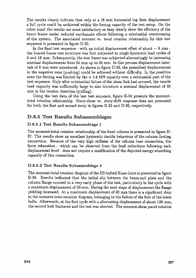
The results clearly indicate that only at a 16 mm horizontal top floor displacement a full cycle could be archieved within the forcing capacity of the test setup. On the other hand the results are most satisfactory as they clearly show the efficiency of the brace frame under reduced earthquake effects following a substantial overstressing of the system. The associated moment vs. total rotation relationship for this test sequence is presented in figure D-32.

In the final test sequence - with an initial displacement offset of about — 6 mm -the braced-frame test structure was first subjected to single hysteretic load cycles of 8 and 16 mm. Subsequently, the test frame was subjected alternatingly to increasing nominal displacements from 24 m m up to 96 mm. In this process displacement inter­vals of 8 m m were introduced. As shown in figure D-33, the prescribed displacements in the negative zone (pushing) could be achieved without difficulty. In the possitive zone the forcing was limited by the + 1.9 MN capacity over a substantial part of the test sequence. Only after substantial failure of the shear link had occured, the tensile load capacity was sufficiently large to also introduce a nominal displacement of 88 mm in the tension direction (pulling).

Using the test data of the last test sequence, figure D-34 presents the moment-total rotation relationship. Story-shear vs. story-drift response data are presented for both the first and second story in figures D-35 and D-36, respectively.

D.8.5 Test Results Subassemblages D . 8 . 5 . 1 T e s t R e s u l t s Subassemblage 1

The moment-total rotation relationship of the fixed column is presented in figure D-37. The results show an excellent hysteretic ductile behaviour of the column footing connection. Because of the very high stiffness of the column base connection, the force relaxation - which can be observed from the load reductions following each displacement level - does not require a modification of the depicted energy-absorbing capacity of this connection.

D .8 .5 .2 T e s t R e s u l t s S u b a s s e m b l a g e 2

The moment-total rotation diagram of the HS-bolted Knee-joint is presented in figure D-38. Results indicated that the initial slip between the beam-end plate and the column flange occured in a very early phase of the test, particularly in the cycle with a maximum displacement of 20 mm. During the next steps of displacement the flange yielding increased. At a maximum displacement of 80 mm there is a significant drop in the moment-total rotation diagram, belonging to the failure of the first of the lower bolts. Afterwards, at the first cycle with a alternating displacement of about 100 mm, the second bolt fractured and the test was aborted. The moment-shear panel rotation

D15 357

diagram (Fig. D-39) shows a very small maximum shear-panel rotation of about 0.7 % according to the failure mechanism at the column flange.

D.8.5.3 Test Results Subassemblage 3

The moment-total rotation relationship of the welded Knee-Joint (Fig. D-40) shows a very stable hysteretic ductile behaviour during the test. Up to a level of alternating displacements of about 120 mm there was no significant loss of resistance. Because of the quality of the welding (half sided full penetration weld with an added filled weld on the back side) no brittle fracture of the welds occured. The severe loss of resistance, according to the cracking of the lower flange occurs during the first cycle with a maximum displacement of 140 mm. As shown in figure D-41 (moment - shear-panel rotation diagram) an unstable nonlinear stiffness behaviour of the shear panel could be observed. This behaviour can be attributed to the nonlinear behaviour of the infilled shear-panel concrete (diagonal cracking, according to concrete truss action in the column shear panel) up to the fracture of the concrete strut during the third cycle of about 120 mm.

D.8.5.4 Test Results Subassemblage 4

The moment vs. total rotation diagram of the HS-bolted T-Joint, as presented in figure D-42, shows a very stable hysteretic ductile behaviour also. During the cycles with the same displacement amplitudes the resistance decreased according to the con­crete failure in the panel zone. During the cycle with a maximum displacement of 140 mm the shear panel fractured and the test was aborted. Although the moment-total rotation relationship is nearly symmetric, the hysteresis of the shear panel rotation, depicted in figure D-43, is removed to the positive rotation range. This could be achie­ved to the sum of the effects of bolt-slippage and local destruction of the composite slab.

D.8.5.5 Test Results Subassemblage 5

The results of the last test (welded T-Joint) are presented in figures D-44 and D-45. The moment-total rotation rotationship of the subassemblage 5 is similar to the above described one of subassemblage 4. During the first cycle with a maximum displacement of +/— 100 mm the column flange fracture (as can be seen in figure D-44) caused a sudden decrease of the load resistance. Afterwards the horizontal cracking of the shear panel took place, according to the severe loss of resistance and the test was aborted. The moment-shear panel rotation relationship is shown in figure D-45.

358 D16

D.8.6 In te rpre ta ted Test Results following ECCS Recom­

mendation No. 45 In order to permit an assessment of the response of the moment test frames according to the ECCS Recommendations No.45, a number of graphs have been prepared and are presented in the following manner:

• Full ductility funktion φ (μ0)

• Relative resistance function e (μο)

• Relative rigidity function ζ (μ0)

• Relative absorbed energy function η (μο)

• Resistance drop function e* (μ0)

For each frame two sets of graphs have been developed. In the first set the first­

yield event has been defined according to the Recommendations and reflected the force or a moment associated with the point of intersection between the elastic and reduced (10 % of elastic) stiffness values of each frame (see figure D­46). These graphs are depicted in figures D­48 ­ D­57 for frame 1 and in figures D­58 ­ D­67 for frame 2.

In the second set the first yield event has been defined as the force or moment associated with first observed yielding; specifically, the point at which the load or moment curves start to deviate from the observed initial linear­elastic response (see figure D­47). These graphs are depicted in figures D­68 ­ D­77 for frame 1 and in figures D­78 ­ D­87 for frame 2.

D.8.7 Synthesis of the Experimental Results In order to compare the experimental results, we give the following quantities in Tab. D­4 and D­5.

My ­ Elastic limit of the bending moment Θν ­ Total rotation corresponding to My M* ­ Elastic limit of the bending moment Θ* ­ Total rotation corresponding to M* M2.5 ­ Bending moment [kNm] corresponding to a total rotation Θ = 2.5% Θ« ­ Maximum total rotation reached during the test and allowing

three complete cycles without failure Mu ­ Bending moment corresponding to Θ„ ®u/®v " Conventional maximum ductility ratio Θ„/2.5% ­ Ductility margin in respect the limit of 2.5% assumed by many

D17 359

researchers as the maximum value of story drift allowable during a severe seismic event

Hereby, according to section D.8.6, two different definitions of the yield moment had been used. My corresponds to the intersection between the elastic slope and the line tangent to the plastic branch having a slope of 1/10 of the elastic stiffness. M* corresponds to the first yield event during the test.

360 D18

TABLES

0 1 9 361

STEEL SECTIONS

FRAME 1 GIRDER COLUMN

FRAME 2 G I R D E R

COLUMN FRAME 3 G I R D E R

COLUMN SUB 1 GIRDER SUB 2 5 GIRDER

COLUMN

Flanges

kN/cm2

31.8 25.9 28.3 25.1 27.7 26.6 27.6 34.7 27.3

kN/cm2

43.3 40.0 42.0 39.6 41.4 41.1 40.0 43.6 40.9

% 26.7 31.9 33.3 36.7 32.3 35.4 27.8 30.2 33.2

Webs

kN/cm2

34.6 33.3 33.6 31.6 34.9 32.0 30.6 37.6 30.5

kN/cm2

43.8 42.7 44.5 40.5 42.4 42.4 41.3 47.1 40.8

% 21.1 26.2 27.1 31.3 24.0 27.2 25.6 27.3 32.3

TABLE D­l : Steel­Sections Material Properties

REBARS

σν kN/cm2

56.3

σ„ kN/cm2

63.3

e« %

15.1

TABLE D­2 : Rebars Material Properties

CONCRETE

FRAME 1/2

FRAME 3

SUB 2­5

INF. CONCR. SLAB

PANEL ZONE INF. CONCR.

SLAB SLAB

fed (7c = 1.0) kN/cm2

2.64 2.35 2.99 2.90 2.18

­

E kN/cm2

2665 2020

­

2617 1826 1943

TABLE D­3 : Concrete Material Properties

362 D20

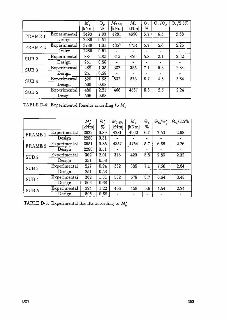
FRAME 1 E x P e r i m e n t a l

Design FRAME 0 Experimental

Design ς,γγ­ρ 0 Experimental

Design çTT­p Q Experimental

Design ςττ­ρ , Experimental

" Design Ç T m j. Experimental

Design

My [kNm] 3490 2280 3780 2280 384 251 288 251 520 506 480 506

% 1.03 0.51 1.01 0.51 2.85 0.58 1.35 0.58 1.95 0.68 2.21 0.68

M2.5% [kNm] 4281

­

4357 ­

315 ­

332 ­

532 ­

466 ­

Mu [kNm] 4990

­

4754 ­

420 ­

385 ­

578 ­

458? ­

% 6.7

­

5.7 ­

5.8 ­

7.1 ­

8.7 ­

5.6 ­

Θ„/Θν

6.5 ­

5.6 ­

2.1 ­

5.3 ­

4.5 ­

2.5 ­

0u/2.5%

2.68 ­

2.26 ­

2.32 ­

2.84 ­

3.84 ­

2.24 ­

TABLE D­4: Experimental Results according to My

FRAME 1 E x P e r i m e n t a l

Design FRAME ° Experimental

Design QTŢ­p 0 Experimental

Design QŢŢ­R Q Experimental

Design ς­rypv . E x p e r i m e n t a l

Design CTT­p ,, Experimental

Design

M* y

[kNm] 3022 2280 3051 2280 302 251 217 251 362 506 324 506

Θ; %

0.89 0.51 0.85 0.51 2.01 0.58 0.94 0.58 1.31 0.68 1.22 0.68

[kNm] 4281

­

4357 ­

315 ­

332 ­

532 • ­

466 ­

Mu [kNm] 4990

­

4754 ­

420 ­

385 ­

578 ­

458 ­

% 6.7

­

5.7 ­

5.8 ­

7.1 ­

8.7 ­

5.6 ­

Θ„/Θ;

7.53 ­

6.66 ­

2.89 ­

7.56 ­

6.64 ­

4.54 ­

Θυ/2.5%

2.68 ­

2.26 ­

2.32 ­

2.84 ­

3.48 ­

2.24 ­

TABLE D­5: Experimental Results according to M*

D21 363

FIGURES

364 D22

1000

HEA260 HEB 300

Figure D­l: Cross Sections ­ Girder aud Column

\ HEA260

HEB 300

\ HEA260

rfcr

HEB300

\ HEA260

Π ί Τ ^ ^ Η τ Ρ ­ ϊ ­1 — I I I

\HEA260

LLL

HEB 300

m w J ­F^

45W 1000 4000 JCjJO woo . 1000 J SDP L sooo 5O00

4

2­M 30 (10.91

HEB 300

300

m ■fS­f­

­+­¡i+­

Figure D­2: Moment Resistant Frame 1 ­ HS­bolted

D23 365

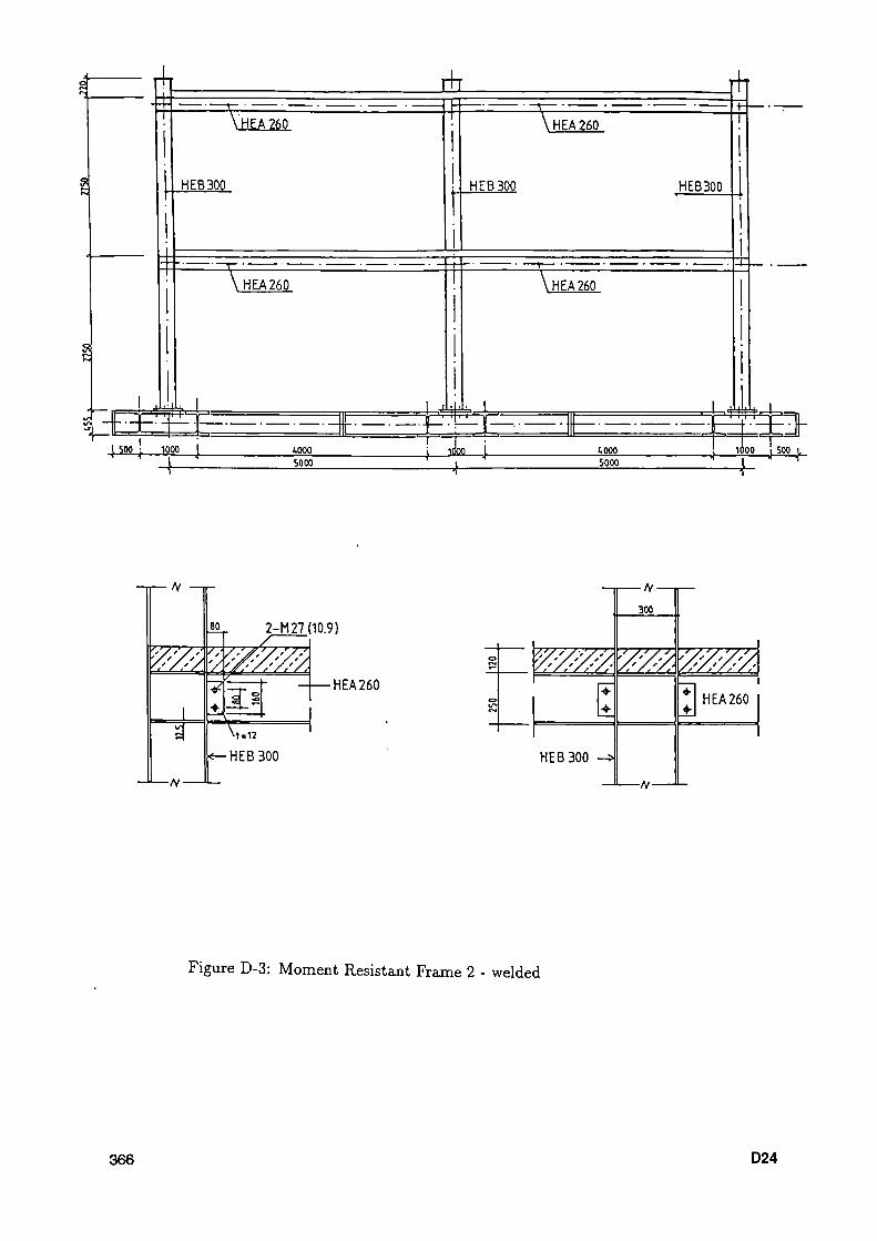
r+T J+L ι H EA 260

H EB 300

^ H EA 260

\HEA 260

HEB 300

Τ Η EA 260

'ΦΓΈΞΞΞΖ-—^ ­t­^d

ih

HEB300

H^H

l· [ SOO ι 1000 j tooo looo 1000 TOPO ι 500

±»?4­f 5000 5000

2­H27 (10.9)

HEA260

Figure D­3: Moment Resistant Frame 2 ­ welded

366 D24

-Ε5Ξ3ΕΞΞΞΞ: ^ρψ^==. \ SOO ^ 1000 j coco 1000 1.000

5000 5000 1000 ι 500

±m±

Figure D-4: Eccentrically Braced Frame 3

D25 367

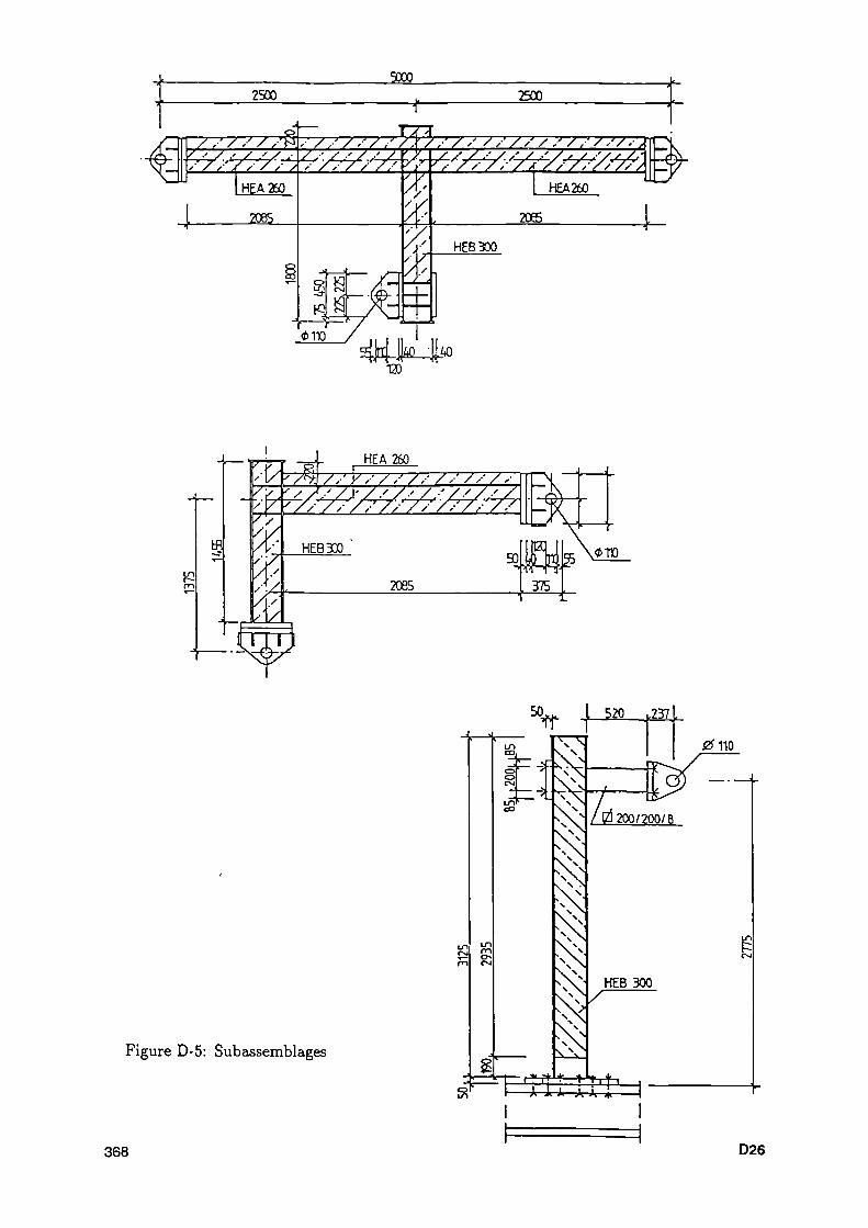
5000 2500 2500

/////$. / / / /,'/ / W;,' / // / /; / s / / y ;ττ

HEA260 ' / / / / / / / / / / y

2085

Figure D-5: Subassemblages

'/y.'Λ-///s ζ-///'/ Λ 7 V • ■ ^ ' 7 ^ 7 ^ ' V ^ / ν · " 7 ν " Q) '

r

375

vOTD

368 D26

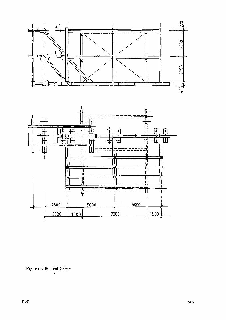
1

f

Æ ­ii

i ι

­3. Í_L

ra ι ta

m ¥

Ε3 Τ *

a H3

1" 2500

AA. ¥ ΒΓ

s

ES

­=3­­

5000

I I

4 ft& Ή iff

Β ι,ι

f­

ι!ι Β

Τ 5000

2500 , 1500 Λ

7000 ,1500

Figure D­6: Test Setup

D27 369

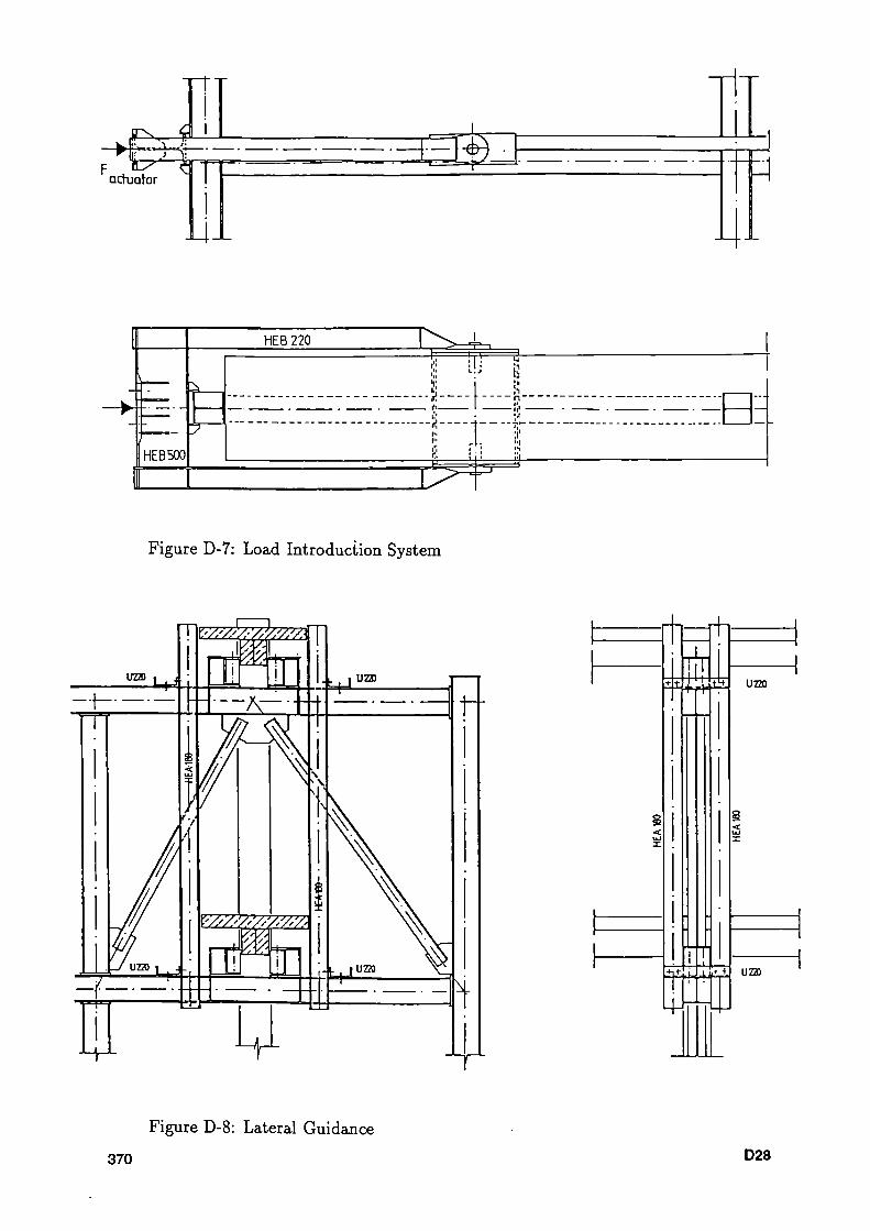
Ά

7 HEB50Q

ΠΠ.

HEB 220 ^

'X £ ^ τ

:­Ξ

Figure D­7: Load Introduction System

T\Y////.^y)///77T[\ r

< UJ

| 1

1

• ,| i

' t

I 1

♦ni. 1 ­Η

ι I

I ! t Η

I AtóJ.

ι

Ι I

uzzo

< UJ χ

U 220

Figure D­8: Lateral Guidance

370 D28

2 F­

•If i ra. _nai

. ­ '

rao

_JCi».

t • if

!

^ I

^

I s

*t\ ! ; I S ><

^ r

s/n?/tíyjAj'/*¿¿/¿.<y/).\Jj#.\//

i-SB

-i—*?—ι

ι ;<·

ffiC­Ξ

T7SQ

^

;<

1 M 1

MJ9UŞI\H£&IU£H

2 5 û _ . ■f ™ , ­

• t 3 ^

^Γ

ë* ­# tjt

^1i V

^r

Η·—«f—j « I f­

® ® ^ ­ L P

— Strain Gage Figure D­5: Measuring Equipment Frames 1 and 2

t­V *:

­ ^ LP Strain Gage

Figure D­10: Measuring Equipment Frame 3

D29 371

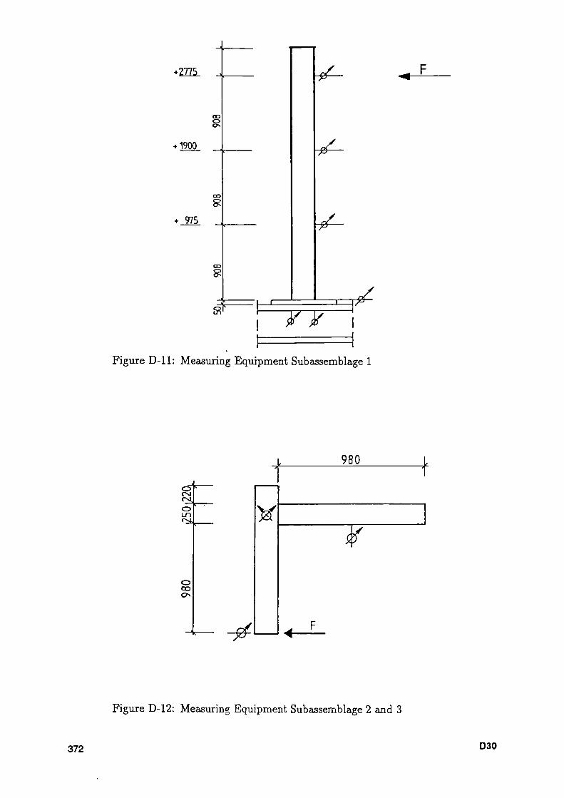
2775

1900

975

CD O ON

CO

co s?

' s

*¿

*¿

*¿

^T ^

Figure D­ll: Measuring Equipment Subassemblage 1

^ F

Ln

o co

^

κ

980

f

Figure D­12: Measuring Equipment Subassemblage 2 and 3

372 D30

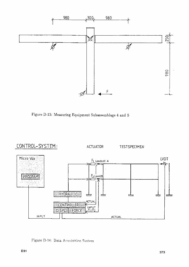
980

¿

,300^ 980

Y

-&

¿ o LTI CNI

o CO

Figure D­13: Measuring Equipment Subassemblage 4 and 5

CONTROL­SYSTEM: ACTUATOR TESTSPECIMEN

Micro Vax

. M H ».»»ν

■RR.Q6RÁM

INPUT

Fi Loadcell A »loCl·—or

ACTUAL

IMTRÖEËRiii;^­j.v.v.'.v.'.'i'.'.O.'A'.'.'.'I'.'A'.'i'X' ;;D;Î.Ş BJiii

■ ' ­ · ­ · * · · ­ · ­ ' ■ ' ■ " ·

NPUT ñ/F2

^fe?

LVD Τ

TOT V777, V777Z

ACTUAL

Figure D­14: Data Arouisit.ion System

D31 373

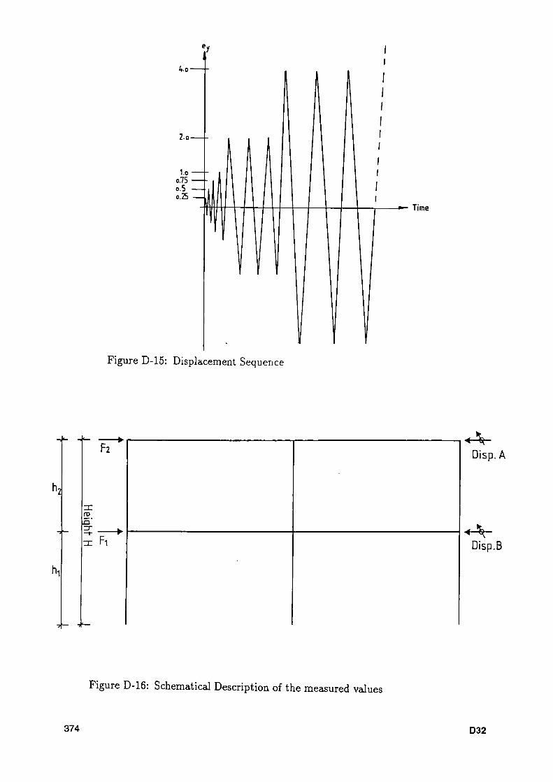
- Time

Figure D-15: Displacement Sequence

ZT

► F2

Fi

Disp.A

Disp.B

Figure D-16: Schematical Description of the measured values

374 D32

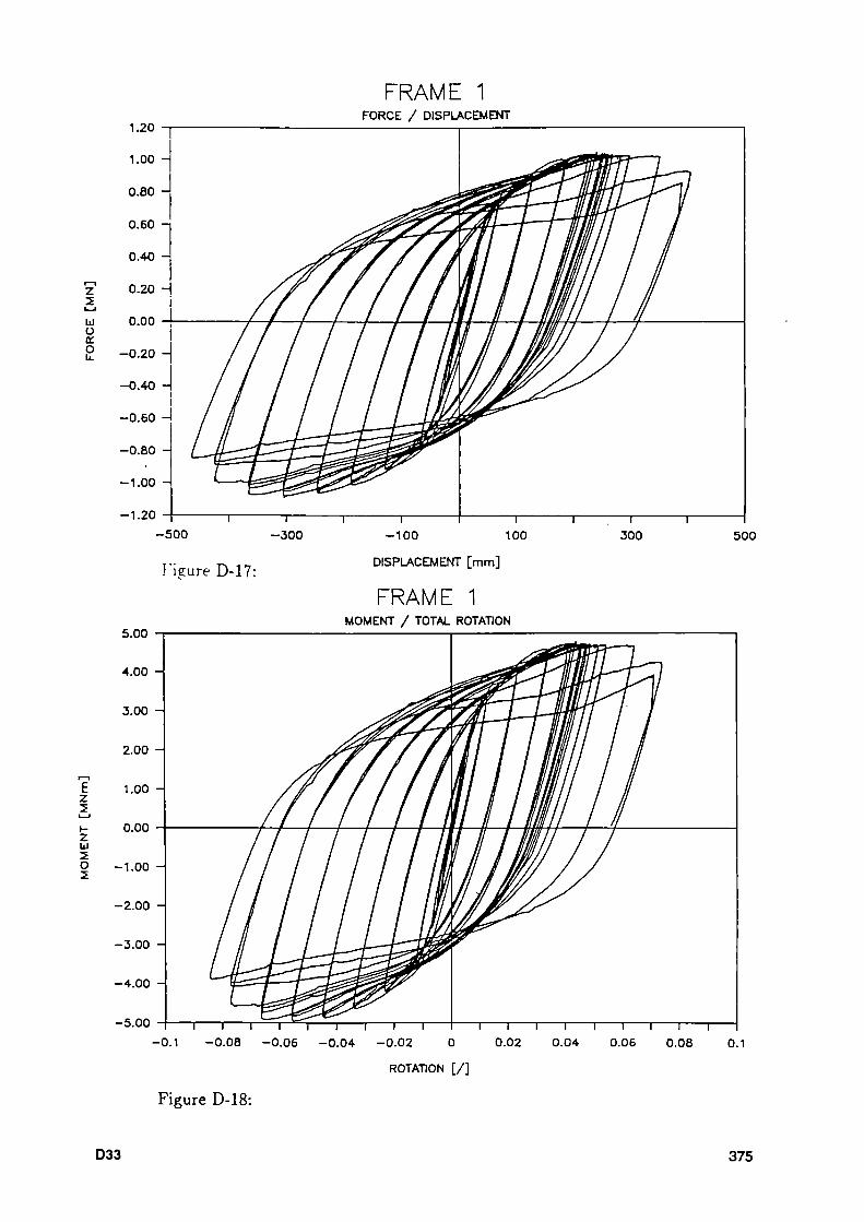
ζ 2 ι ι ld ο Κ. Ο ϋ.

Ε ζ 2

Ζ ω 2 Ο 2

1.20

FRAME 1 FORCE / DISPLACEMENT

- 5 0 0

Figure D-17

5.00

4.00

3.00

2.00

1.00

0.00

- 1 . 0 0 -

- 2 . 0 0 -

- 3 . 0 0

- 4 . 0 0

- 5 . 0 0

- 1 0 0 100

DISPLACEMENT [ m m ]

FRAME 1 MOMENT / TOTAL ROTATION

500

ROTATION [ / ]

Figure D-18:

D33 375

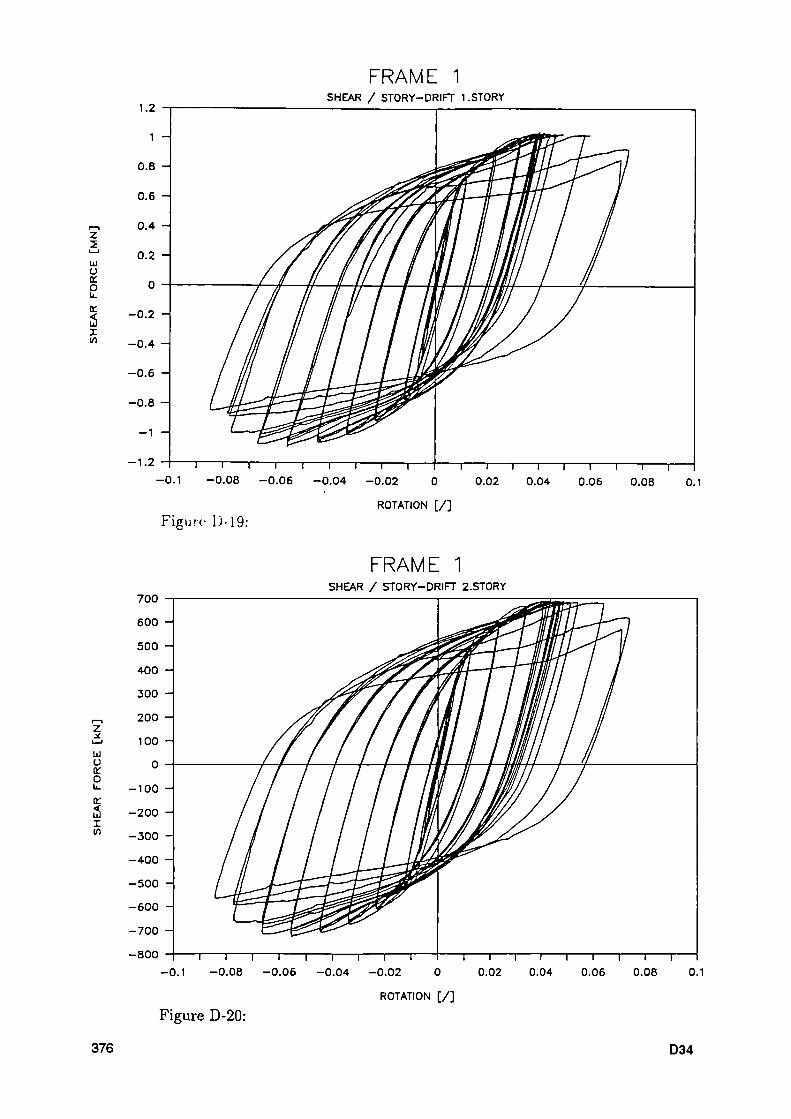
ζ

ι ι ω ϋ ir ο

ι (Λ

1.2

FRAME 1 SHEAR / STORY-DRIFT 1 .STORY

Figure D-19: ROTATION [ / ]

ζ ì—l

[il O (Τ O

I V)

700

FRAME 1 SHEAR / STORY-DRIFT 2.ST0RY

ROTATION [ / ]

Figure D-20:

376 D34

ζ 2

l—l

UI υ ir o

E ζ 2 l _ l

I -Z UJ

o 2

FRAME 2 FORCE / DISPLACEMENT

-400 - 2 0 0 200 400

Figure D-21: DISPLACEMENT [mm]

FRAME 2 MOMENT / TOTAL ROTATION

ROTATION [ / ]

Figure D-22:

D35 377

ζ 2 ω υ Ο U.

Ι V)

ζ ι ι U1 υ ir ο li.

Ι (η

1.1 1

0.9 -

0.Β -

0.7 -

0.6 -

0.5 -

0.4 0.3 -

0.2 -

0.1 -

Ο -0.1 -

-0.2 -

-0.3 -0,4 -

-0.5 -

-0.6 -

-0.7 -0.8 -0.9 -

- 1 -

-1.1

FRAME 2 SHEAR / STORY-DRIFT 1.STORY

- 0 . 0 8 — ι — - 0 . 0 6

~~I ι 1 Γ -0.04. - 0 . 0 2

Ί Ι Ι 1 0.02 0.04 0.06 Ο.ΟΒ

Figure D-23: ROTATION [ / ]

700

FRAME 2 SHEAR / STORY-DRIFT 2.ST0RY

Ί 1 Γ - 0 . 0 6 - 0 . 0 4 0.08

Figure D-24: ROTATION [ / ]

378 D36

ζ

UI υ (Τ ο

Ε ζ

2 I -

ζ UI 2 ο 2

600

-400

Figure D-25:

FRAME 2Β FORCE / DISPLACEMENT

- 2 0 0

DISPLACEMENT [mm]

FRAME zb MOMENT / TOTAL ROTATION

200 400

0.04 0.06

ROTATION [ / ]

Figure D-26:

D37 379

ζ 2 ι—ι ω υ ο: ο

Ε ζ 2

Ζ ω 2 Ο 2

FRAME 3 FORCE / DISPLACEMENT

Figure D-27:

- 2 0 0

DISPLACEMENT [ m m ]

FRAME 3 7 —

6 -

5 -

4 -

3 -

2 -

1 -

0 —

•1 -

2 -

3 -

4 -

5 -

6 -

7 -

8 -

9 -

MOMENT / TOTAL ROTATION

1 1 1 1 1 ι I I I 1 - 0 . 0 1 2 -0.008 - 0 .004 0.004 0.008 0.012

Figure D-28: ROTATION [ / ]

380 D38

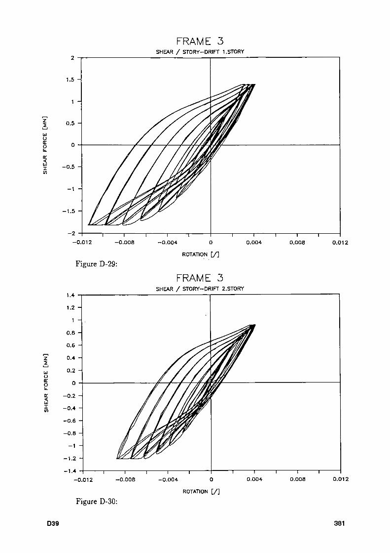
ζ 2 ι_ι ω υ χ ο

ce

ι

ζ 2 ω υ ο

ι

FRAME 3 SHEAR / STORY-DRIFT 1.STORY

- 0 . 5 -

- 1 . 5 -

0.012

Figure D-29: ROTATION [ / ]

FRAME 3 SHEAR / STORY-DRIFT 2.STORY

- 1 . 4

-0 .012 - 0 . 0 0 4 0

ROTATION [ / ]

0.012

Figure D-30:

D39 381

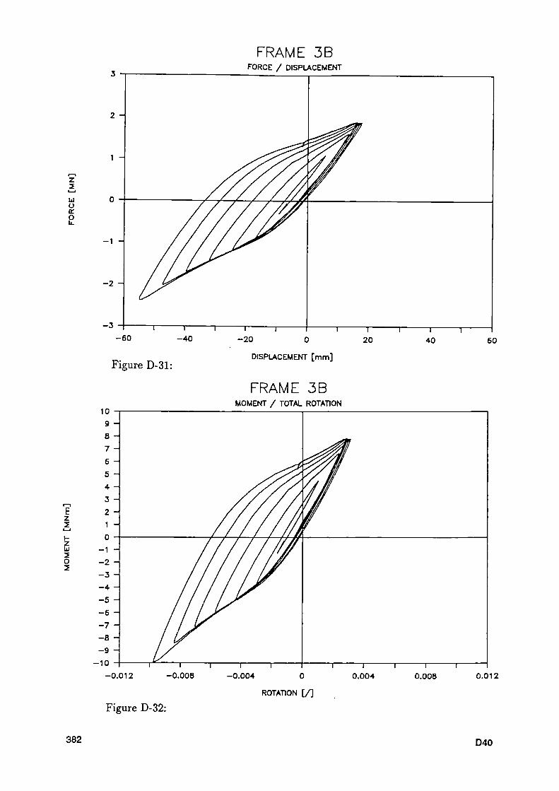
ζ 2 t—ι

UI υ α: o

E ζ 2

Ζ UI 2 O 2

FRAME 3B FORCE / DISPLACEMENT

Figure D-31: DISPLACEMENT [mm]

FRAME 3B MOMENT / TOTAL ROTATION

-0 .012 -0.004 0

ROTATION [ / ]

Figure D-32:

382 D40

ζ

2 UJ υ cu o

E ζ 2 i _ l H Z LU

O 2

FRAME 3C FORCE / DISPLACEMENT

­ 0 . 5 ­

Ι Γ

­ 1 0 0 ­ 8 0

Figure D­33:

­ 2 0 o

DISPLACEMENT [mm]

FRAME 3C

100

7 ­

6 ­

5 ­

4 ­

3 ­

2 ­

1 ­

­ 1 ­

­ 2 ­

­ 3 ­

­ 4 ­

­ 5 ­

­ 6 ­

­ 7 ­

­ 8 ­

­ 9 ­

MOMENT / TOTAL

^ j ^ ^ V y / 7

/¿T/Y/zr//, ///¿ml' 1

1 1 1

ROTATION

ι ι 1 ­ 0 . 0 2 ­0 .01 0.01 0.02

Figure D­34: ROTATION [ / ]

D41 383

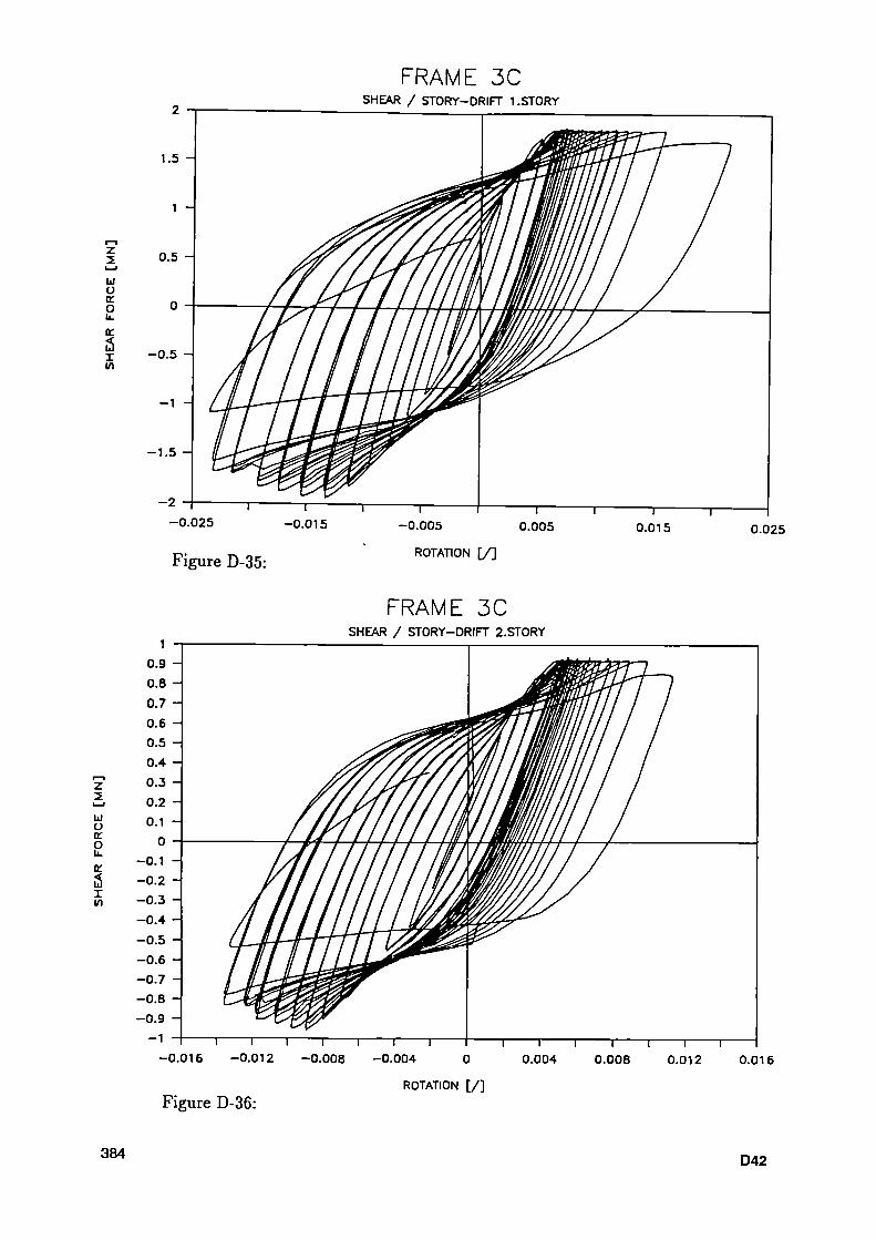
ζ

2 IxJ υ κ o li.

ι - 0 . 5 -

- 1 . 5 -

- 0 . 0 2 5

FRAME 3C SHEAR / STORY-DRIFT 1.STORY

Figure D-35:

-0.005

ROTATION [ / ]

0.005 0.015 0.025

Ζ I—I

ω o ir o u.

i

FRAME 3C SHEAR / STORY-DRIFT 2.ST0RY

- 0 . 0 1 6 ι Γ

0.004 0.00B 0.012 0.016

Figure D-36: ROTATION [ / ]

384 D42

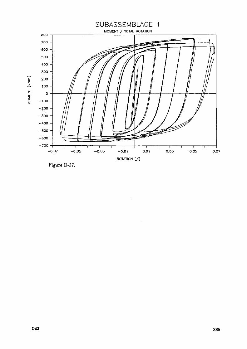
E ζ JÉ

ζ iii

O 2

BOO

SUBASSEMBLAGE 1 MOMENT / TOTAL ROTATION

- 0 . 0 1 0.01

ROTATION [ / ]

0.07

Figure D-37:

D43 385

E ζ χ i—ι \-z hi 2 O 2

SUBASSEMBLAGE 2: KNEE­JOINT HS­BOLTED 500

400 ­

­ 1 0 0 ­

­ 4 0 0 ­

­ 5 0 0

MOMENT/TOTAL ROTATION

­O.OB ­ 0 . 0 6 ­ 0 . 0 4 ­ 0 . 0 2 0

Figure D­38: *°™°Ν ^

ι ι Γ 0.04 0.06 0.08

E Ζ

ζ UI 2 O 2

500

SUBASSEMBLAGE 2: KNEE­JOINT HS­BOLTED MOMENT/SHEAR PANEL ROTATION

­ 0 . 0 0 7 ­ 0 . 0 0 5

Figure D­39: 0.001 0.003 0.005 0.007

ROTATION [ / ]

386 D44

E ζ JÉ

I -z LI 2 O 2

400

300 -

200 -

SUBASSEMBLAGE 3: KNEE-JOINT WELDED MOMENT/TOTAL ROTATION

Figure D-40: ROTATION [ / ]

E z j f

ζ UI 2 O 2

400

300 -

200 -

SUBASSEMBLAGE 3: KNEE-JOINT WELDED MOMENT/SHEAR PANEL ROTATION

- 1 0 0 -

- 3 0 0 -

- 4 0 0

- 0 . 0 4

Figure D-41:

- 0 . 0 2

ROTATION [ / ]

0.02 0.04

D45 387

E ζ 1—1

Η Ζ ω 2 Ο 2

700

SUBASSEMBLAGE 4: T-JOINT HS-BOLTED MOMENT / TOTAL ROTATION

0.11

E z ι ι I-

z UJ 2 o 2

Rotation [ / ] Figure D-42:

SUBASSEMBLAGE 4: T-JOINT HS-BOLTED 700

- 6 0 0 - 0 . 0 2

MOMENT / SHEAR PANEL ROTATION

0.02 0.04

Rotation [ / ]

Figure D-43:

388 D46

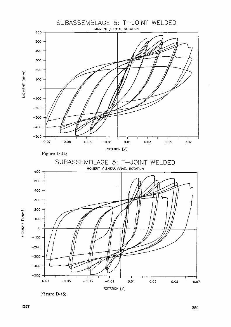
SUBASSEMBLAGE 5: T­JOINT WELDED

ζ JÉ

\-z LJ ­¿ O Ί.

E ζ je L_i

Η Z UJ

O 2

MOMENT / TOTAL ROTATION

­ 4 0 0

1 I I Γ 0.01 0.03

Ί Γ 0.05 0.07

ROTATION [ / ]

600

500 ­

Figure D­44:

SUBASSEMBL^GE 5: T­JOINT WELDED MOMENT / SHEAR PANEL ROTATION

­ 0 . 0 1 0.01

ROTATION [ / ]

0.03 0.05 0.07

Fieure D­45:

D47 389

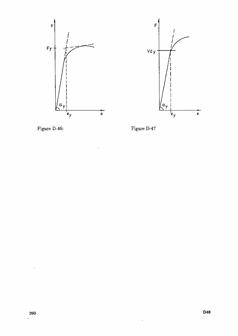
F y -

Figure D-46: Figure D-47

390 D48

2 - τ 1.9 -

i.a -

1.7 -

1.6 -

1.5 -

1,4 -

1.3 -

1.2 -

1.1 -

1 -

0.9 -

0.8 -

0.7 -

0 , 6 . -

0,5 -

0.4 -

0,3 -

0.2 -

0,1 -

0 -

FRAME 1 Full Ductility +

2 μ

+ 10

Figure D-48:

FRAME 1 Full Ductility -

Figure D-49:

D49 391

+

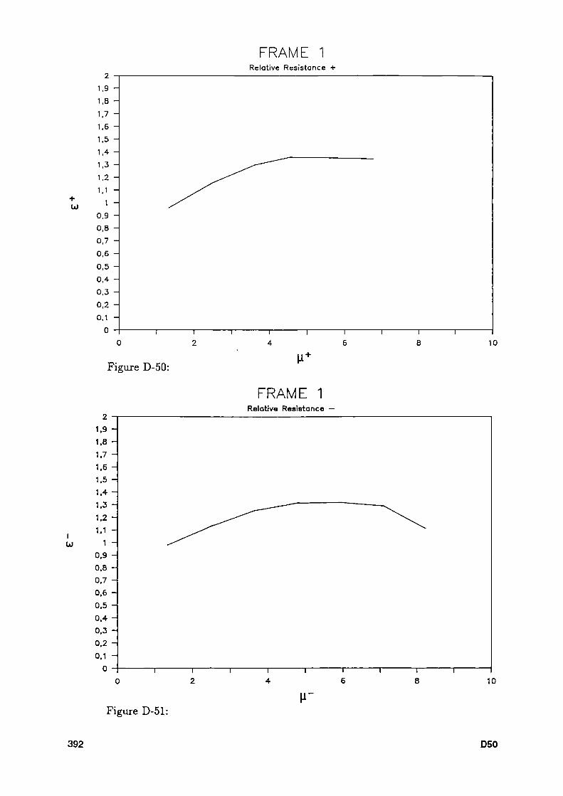
2 -r

1,9 -

1.8 -

1.7 -

1.6 -

1.5 -

1,4 -

1.3 -

1.2 -

1.1 -

1 -

0,9 -

0,8 -

0.7 -

0.6 -

0,5 -

0,4 -

0.3 -

0,2 -

0.1 -

0 -

FRAME Ί Relative Resistance

4 10

Figure D-50: μ+

ι ω

FRAME 1 Relative Resistance

Figure D-51:

392 D50

+

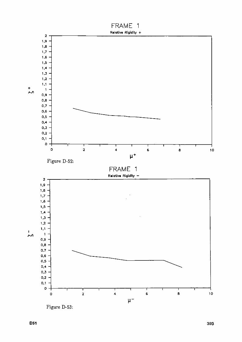
ι

FRAME 1 Relative Rigidity +

1.9 -

1.8 -

1.7 -

1.6 -

1.5 -

1.4 -

1.3 -

1.2 -

1.1 -

1 -

0.9 -

0.8 -

0.7 -

0.6 -

0.5 -

0.4 -

0.3 -

0.2 -

0.1 -

0 -

2 4 10

Figure D-52:

2 - -

1.9 -

1.8 -

1.7 -

1,6 -

1.5 -

1.4 -

1.3 -

1.2 -

1.1 -

1 -

0.9 -

0,8 -

0.7 -

0.6 -

0,5 0.4 -

0,3 0.2 -

0.1 -

0

FRAME 1 Relative Rigidity -

T 4 10

Figure D-53:

D51 393

FRAME 1 Relative Absorbed Energy +

Figure D-54:

FRAME 1 Relative Absorbed Energy —

Figure D-55:

394 D52

I

ω

FRAME 1 Resistance Drop +

1.9 -

1.8 -

1.7 -

1.6 -

1.5 -

1.4 1.3 -

1.2 -

1.1 -

1 0.9 -

0.8 -

0.7 -

0.6 -

0.5 -

0.4 0.3 -

0.2 -

0.1 0 T

2 4 8 10

μ+

Figure D-56:

FRAME 1 Resistance Drop -

Figure D-57:

D53 395

FRAME 2 Full Ductility +

1.9 -

1.8 -

1.7 -

1.6 -

1.5 -

1.4 -

1.3 -

1.2 -

1.1 -

1 -

0.9 -

0.8 -

0.7 -

0.6 -

0.5 -

0.4 -

0.3 -

0.2 -

0.1 -

0 - ■

Figure D-58:

FRAME 2 Full Ductility -

Figure D-59:

396 D54

+ ω

ι ω

FRAME 2 Relative Resistance +

1.9 -

1.8 -

1.7 -

1.6 1.5 -

1.4 -

1.3 -

1.2 1.1 -

1 -

0.9 -

0.8 -

0.7 -

0.6 -

0.5 -

0.4 -

0.3 -

0.2 -

0.1 -

0

Figure D-60:

π ι 1 2 4

μ +

FRAME 2 Relative Resistance

1.9 -

1.8 -

1.7 -

1.6 -

1.5

1.4 Η 1.3 1.2 -

1.1 -

1 -

0.9 -

0.8 -

0.7 -

0.6 -

0.5 0.4 0.3 -

0.2 -

0.1 -

0

Figure D-61:

D55 397

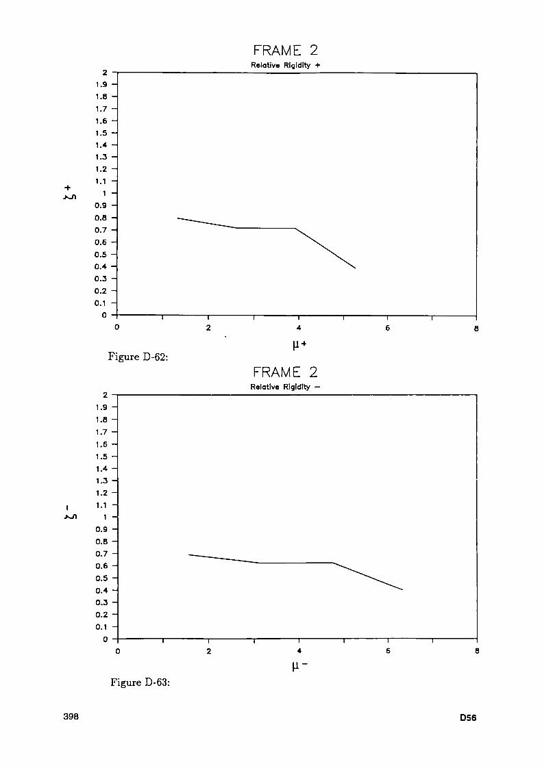
JsJI

FRAME 2 Relative Rigidity +

Figure D-62:

I

FRAME 2 Relative Rigidity -

Figure D-63:

398 D56

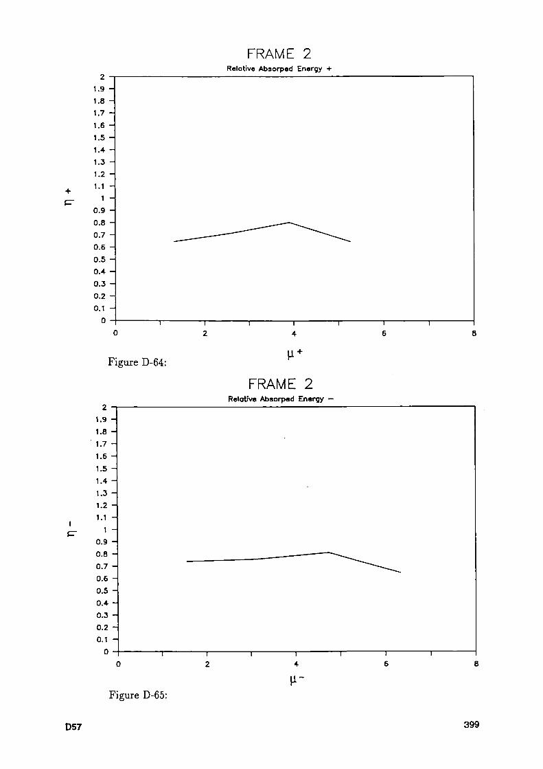
FRAME 2 Relative Absorped Energy +

Figure D-64:

FRAME 2 Relative Absorped Energy —

Figure D-65:

D57 399

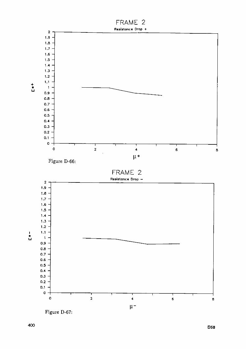
+ ω

1.9 -

1.8 -

1.7 -

1.6 -

1.5 -

1.4 -

1.3 -

1.2 -

1.1 -

1 -

0.9 -

0.8 -

0.7 -

0.6 -

0.5 -

0.4 -

0.3 -

0.2 -

0.1 -

0

FRAME 2 Resistance Drop +

Figure D-66: μ

+

ι *

FRAME 2 Resistance Drop —

Figure D-67:

400 058

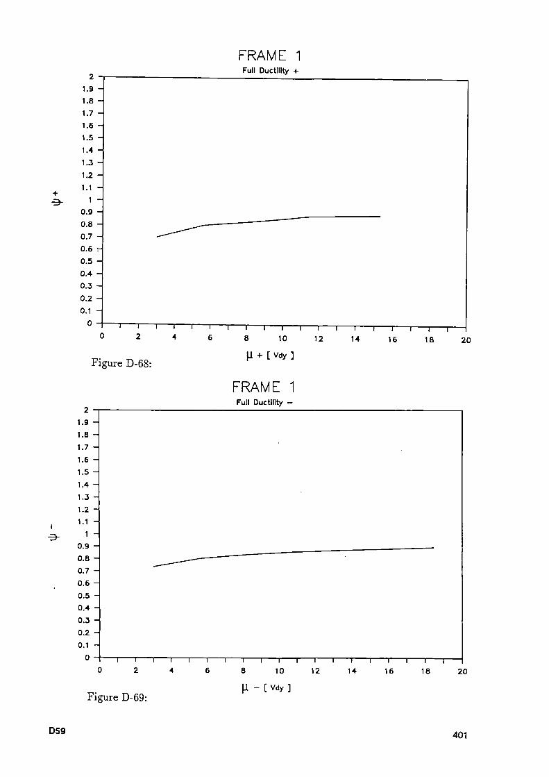
FRAME 1 Full Ductility +

1.9 -

1.8 1.7 -

1.6 -

1.5 -

1.4 -

1.3 -

1.2 -

1.1

1 -

0.9 -

0.8 -

0.7 -

0.6 0.5 -

0.4 -

0.3 -

0.2 -

0.1 -

0 ι

10 12 " T

-

14 ι

16 18 20

Figure D-68: μ + [ Vdy ]

FRAME 1 Full Ductility -

Figure D-69: μ - [ Vdy ]

D59 401

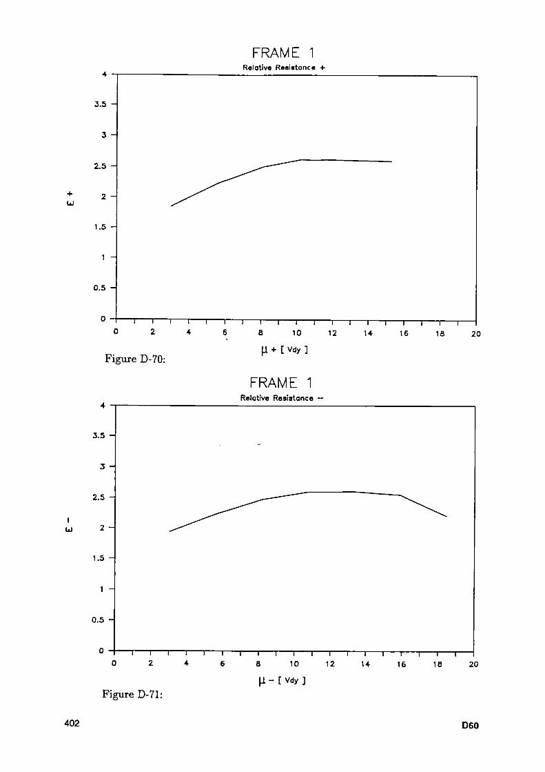
+ ω

ι ω

3.5 -

3 -

2.5

2 -

1.5 -

1 -

0.5 -

~ι 1 r 2 4

Figure D-70:

3.5 -

3 -

2.5 -

2 -

1.5 -

1 -

0.5 -

Figure D-71:

FRAME 1 Relative Resistance +

~i ι 1 1 1 1 1 1 1 1 r~ 8 10 12 14 16 18

μ + [ Vdy ]

FRAME 1 Relative Resistance —

"1 I I I 1 1 1 1 1 1 1 1 1 1 1 Γ-

4 6 8 10 12 14 16 18 μ - [ Vdy ]

20

20

402 D60

+

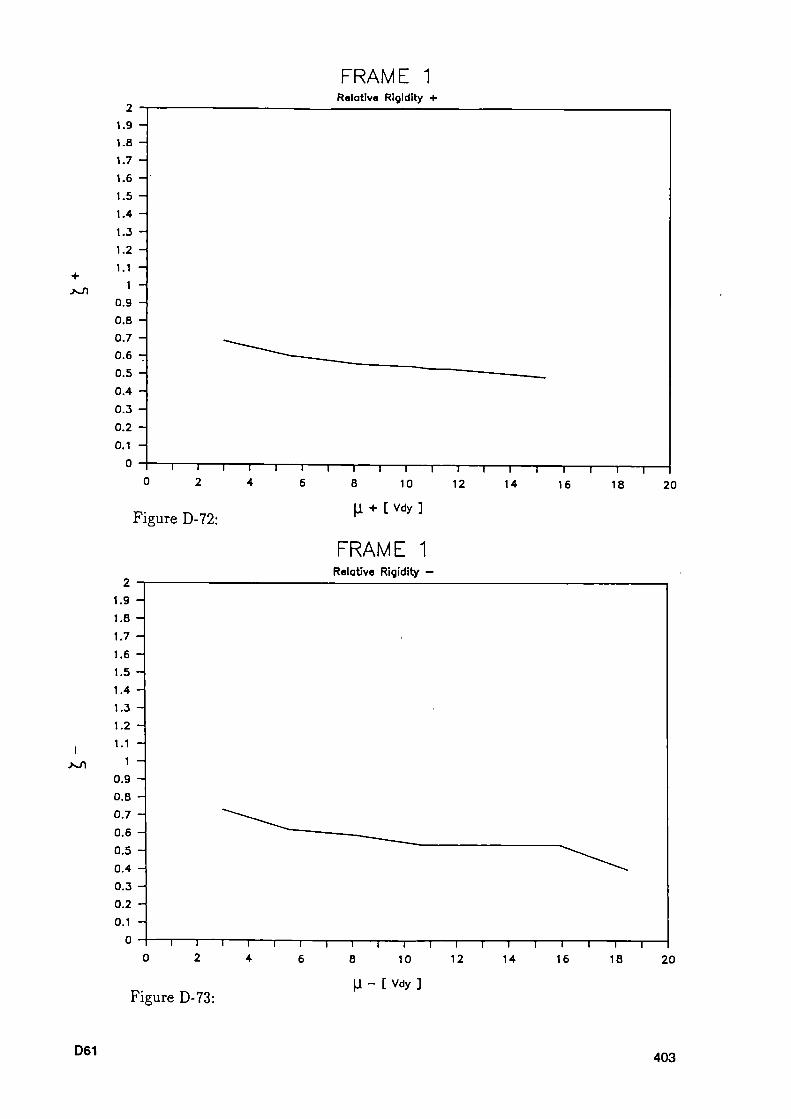
ι

FRAME 1 Relative Rigidity ­»

1.9 ­

1.B ­

1.7 ­

1.6 ­

1.5 ­

1.4 ­

1.3 ­

1.2 ­

1.1 ­

1 ­

0.9 ­

0.8 ­

0.7 ­

0.6 ­

0.5 ­

0.4 ­

0.3 ­

0.2 ­

0.1 ­

0 ­ ■ ~T I I I I I I I 1 1 1 1 1 1 1 1 1 1— 2 4 6 8 10 12 14 16 18 20

Figure D­72: μ + [ Vdy ]

FRAME 1 Relative Rigidity ­

Figure D­73: μ ­ [ Vdy ]

D61 403

FRAME 1 Relative Absorbed Energy +

Figure D-74: μ + [ Vdy ]

FRAME 1 Relative Absorbed Energy —

Figure D-75: μ - [ Vdy ]

404 D62

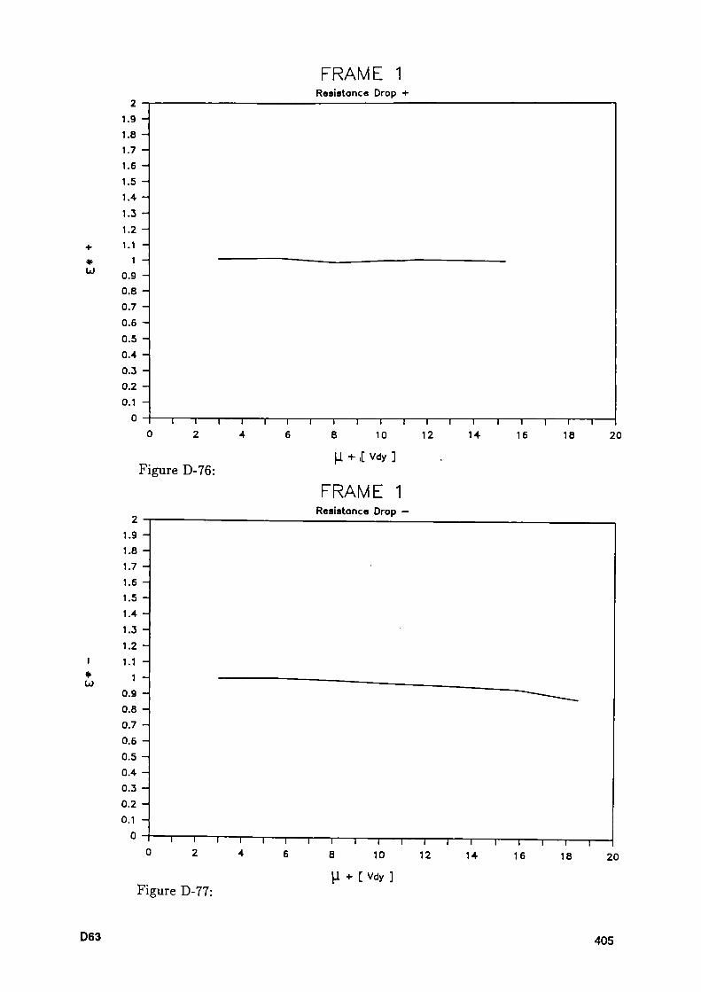
ω

ω

FRAME 1 Resistance Drop +

Figure D-76: μ + I Vdy ]

FRAME 1 Resistance Drop —

Figure D-77:

D63 405

FRAME 2 Full Ductility +

1.9 -

1.8 -

1.7 -

1.6 -

1.5 -

1.4 -

1.3 -

1.2 -

1.1 -

1 -

0.9 -

0.8 -

0.7 -

0.6 -

0.5 -

0.4 -

0.3 -

0.2 -

0.1 -

0 - Π Γ 4 10

- ι 1 1 Γ 12 14 16

Figure D-78: μ + [ Vdy ]

FRAME 2 Full Ductility -

1.9 -

1.8 -

•1.7 -

1.6 -

1.5 -

1.4 -

1.3 -

1.2 -

1.1 -

1 -

0.9 -

0.8 -

0.7 -

0.6 -

0.5 -

0.4 -

0.3 -

0.2 -

0.1 -

0 -

0

Figure D-79:

-τ 1 1 ι 1 Γ 4 6 8

μ - [ Vdy ]

- Γ-

10 Ί Γ

-

12 ι

14 16

406 D64

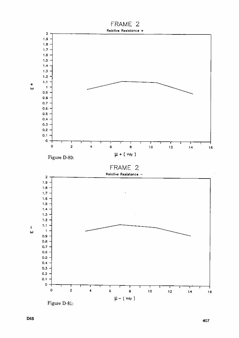
+ ω

1.9 -

1.8 -

1.7 -

1.6 -

1.5 -

1.4 -

1.3 -

1.2 -

1.1 -

1 -

0.9 -

0.8 -

0.7 -

0 . 6 . -

0.5 -

0.4 -

0.3 -

0.2 -

0.1 -

0 - ■

FRAME 2 Relative Resistance +

τ Γ 4 8

ι 10 12

~ι 1 — 14 16

Figure D-80: μ + [ Vdy ]

ι ω

FRAME 2 Relative Resistance —

Figure D-81: μ - [ Vdy ]

D65 407

+

2 - ■

1.9 -

1.8 -

1.7 -

1.6 -

1.5 -

1.4 -

1.3 -

1.2 -

1.1 -

1 -

0.9 -

0.8 -

0.7 -

0.6 -

0.5 -

0.4 -

0.3 -

0.2 -

0.1 -

0 -

FRAME 2 Relative Rigidity +

4 - Γ

-

10 -τ— 12

—Γ-

14 16

Figure D-82: μ + [ Voy ]

I

2 - ■

1.9 -

1.8 -

Ί .7 -

1.6 -

1.5 -

1.4 -

1.3 -

1.2 -

1.1 -

1 -

0.9 -

0.8 -

0.7 -

0.6 -

0.5 -

0.4 -

0.3 -

0.2 -

0.1 -

0 -

FRAME 2 Relative Rigidity —

Π Γ 4 10

Τ-

12 Τ

-

14

μ - [ Vdy ]

Figure D-83:

408

16

D66

FRAME 2 Relative Absorped Energy +

Figure D-84: μ + [ Vdy ]

FRAME 2 Relative Absorped Energy —

3.5 -

3 -

2.5 -

2 -

1.5 -

1 -

0.5 -

Figure D-85: μ - [ Vdy ]

D67 409

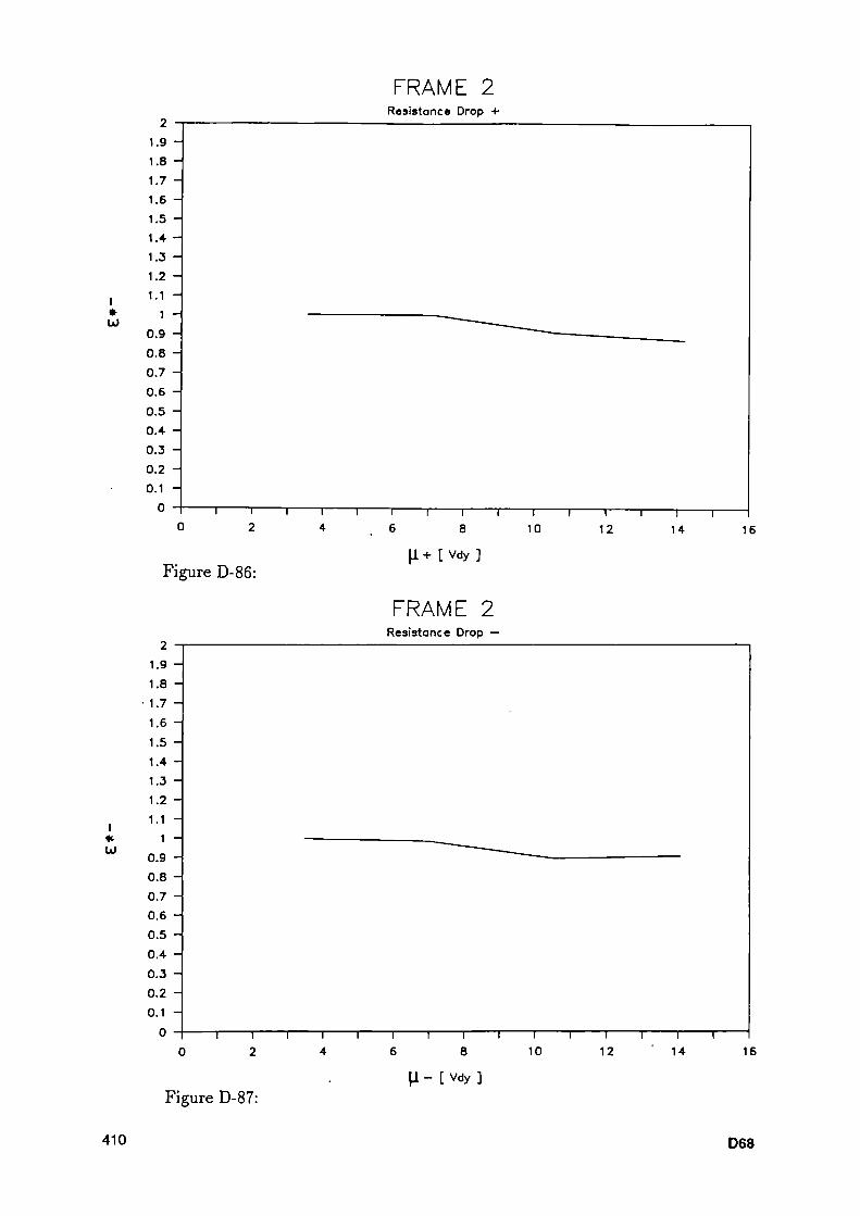
I

2 1.9 1.8 -

1.7 -

1.6 -

1.5 -

1.4 -

1.3 -

1.2 -

1.1 -

1 -

0.9 -

0.8 -

0.7 -

0.6 -

0.5 -

0.4 -

0.3 -

0.2 -

0.1 -

0

FRAME 2 Resistance Drop +

Figure D-86: μ + [ Vdy ]

10 12 -T— 14 16

I

ω

FRAME 2 Resistance Drop —

Figure D-87: μ - [ Vdy ]

410 D68

Appendix E

Material list

from comparing concrete to composite structures

411

Project 1

Reinforced concrete solution

E1 413

Basic Conditions warehouse building, 4 storeys strong earthquake, Greece 3 bays, 9 m each 6 m spacing of frames frames loaded in plane only live load 5 kN/m/m fire resistance class R 90 composite frame suited for préfabrication

EC 8 ­ Design Response spectra Composite Frame and R/C­Frame

0.4

a) g 0.3

ω ω 8 0.2 Π3 <υ co c o Q. ω ω

CC

0.1

0

,

\

\

0 0.

^ ν > · . .

5 1

■ * ^ : : . : ; S . ^ , . .

1. 5 2 > 2 ¡ 5 G

ι $ 3. 5 4

Period [s]

Composite: q=6.0 R/C: q=5.0

414 E2

m co

t­6025 (e.s.)

6025, {es.)

7025^ 2 020 (e.s.) 7 025. 2020 (e.s.)

7025^ 2028 (e.s.)

7ø25v 2028 (e.s.)

7025 ' (e.s.)

7025+/ 2028 each side

­50/60

*00

, 50/60

x 50/60

­50/60

.50/60

9,00 4016 2020

r~t 9,00

^

/ tø25 ies.)

6016 "Χ"

• ε ζ Ζ Ζ0

Ζ Σ Σ } 5­St 6016

60

Λ 025 (e.s.) 50'

4025 (e.s.)

•4ø25(e.s.)

7020 ■ χ :

7020

w / .·· ¿// ,·■ / / j ­ i i 8 f

"6025 (as.)

­I—60/60

6ø25(e.sJ

H025 (e.s.)

¿025 eqch

. side

+50+

7020

7020 7~

,9025

-¿-9025

6016

9ø25v

1

7020

9ø25x

Τ 7020

9ø25v

7016 ~r

8020 V

7020 V

7020 7""

.6016

~7~ 6016

,6025

50 20

,7025

~ 5020

,7025

6025

o in m

Ln

o LO

LT» m'

en

d) OJ

χ

o ω

9,00 cu cu

9.00 9.00

1 1

J L . 2 Ì

Λ. 1

s

o t—

2 r ­ ^ ¡ [

co in

o ■β rñ

LTl

o Sr

m 4k

Interior transverse stirrups ot columns not included !

84*8/10

18*8/15

60*8/10, 1112*10/10

82*8/10

84*10/10

20*10/15

(D 84*8/10

©18*8/10 @|12*8/10

84*10/10

20*10/15

12*10/10|| © 6 2 * 6 / 1 0 '10010/10 ©32*8/10 |

© 46 15

en [©34*8 /10

©

©84*10/10

©20*10/15 [©19*10/15

©84*10/10

©20*10/15| |©19*10/15

ILL Φ 46 15

CU

o LD m"

o Ln

o Ln

o Ln rn

© ILL.

m ui •

• .

• ·

f­ t

4

•

•

\ / Φ 12

Λ 5 ^ • • •

* ·

• ·

*

• •

•

• «

• ^

•

•

•

0 12

ft· •

• · ·

• ·

¿ .

· · •

i 1

4 0 25 (e.s.)

6 0 25 (e.s.)

4 0 25 (G.S.)

Interior Columns­Cross Sections

Second Story and above

10 0 28 each side

First Story

Ground Floor (Top)

Ground Floor (Column Base)

00

m σ>

• •

* • • •

• ·

* 1

4 « • • •

\ / Φ12

Λ • ·

· ·

• · • * •

2*.

* ·

• a

' *

t f

•

* •

*

· ·

· «

V 0 12

Λ · · • • * •

· ·

• <r

• ·

•4 • • • •

· ·

6 0 25 (e.s.)

7 0 25 2 0 20 (e.s.)

7 0 25 2 0 28 (e.s.)

7 0 25 2 0 28 each side

Exterior Columns­Cross Sections

Third Story

Second Story

First Story

Ground Floor

Project 2

Composite solution

E7 419

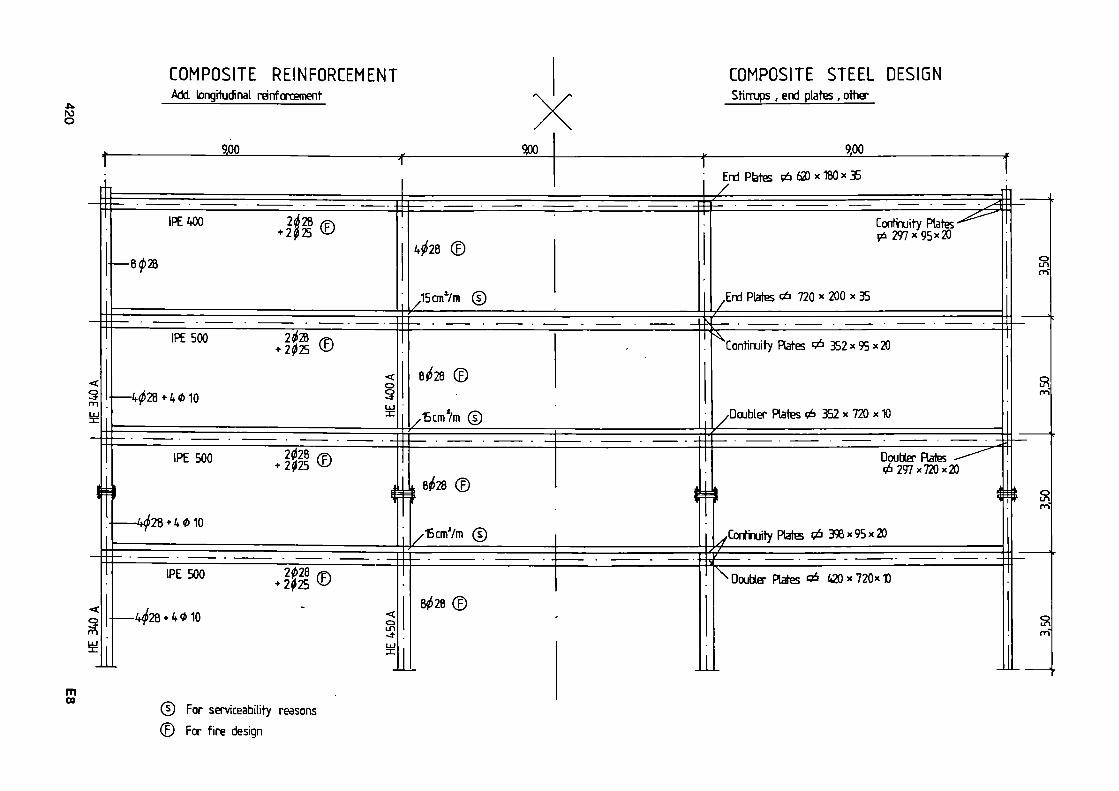
■b. ro o

COMPOSITE REINFORCEMENT

Add, longitudinal reinforcement

900

sţoo

COMPOSITE STEEL DESIGN

Stirrups , end plates , ottier

3P0 End Plates ţa 62) χ 180x35 J.

IPE WO

8028

2á28 ÆN + 2025 V

Φ& ©

Κ

Continuity Plates' ϊώ 297x95x20

Ζ End Plates Φ 720 χ 200 χ 35

o LTl m'

IPE 500

< S m

­ΚφΊΆ *K «10

20Í2B (p, + 2025 ©

8¿28 ©

Ζ 15cm7m ©

' ^ Continuity Rates Φ 352 χ 95 χ 20

/ Doubler Plates (ó 352χ720χ10

S

IPE 500

MO ­4^28 + 4 Φ 10

2<¿28 ø + 2025

8¿28 ©

•"Bcrn'/m ©

Doubler Plates ­0 297x720x20

H

É Continuity Plates tá 398x95x20

n i

IPE 500

4^28 + 4<* 10

U

m 00

2028 ÆN 2025 <y

8?$28 ©

1 © For serviceability reasons

© For fire design

^ Doubler Plates & 420*720x10

pri

Stirrups Φ8/150

IPE500 2 0 25 2 028

Stirrups 08 /150

IPE 400 -2 025

2028

ΕΘ 421

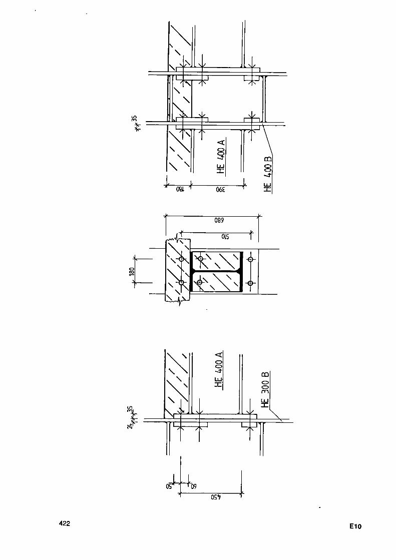
LTI

m

\

\

±ά

7ς\

\ \

^

— τ

J i '

\ \

\ Ν

Γ / ^

OBI ■+■

06£

^ ¿ _

/ \

_ i ¿ .

7 V

4

\

\ \

\

Nr*­

ο ο

^ ¿ _

"7 ζ 7 ~

CÛ Ο Ο ηη

^ d .

7 \

05" 09 OS4/

422 Ε10

Project 2

Synthesis of quantities for composite solution

Slab: ■ 47922 kg rebars

■ 439 m3 concrete Beams In x-direction:

■ 36446 kg rolled sections

■ 4713 kg rebars

■ 29 m3 concrete Beams In y-direction:

■ 16704 kg rolled sections

■ 2160 kg rebars

■ 13 m3 concrete Columns:

■ 48312 kg rolled sections

■ 6838 kg rebars

■ 30 m3 concrete

Total: 101468 kg rolled sections

61633 kg rebars

511 m3 concrete

E11 423

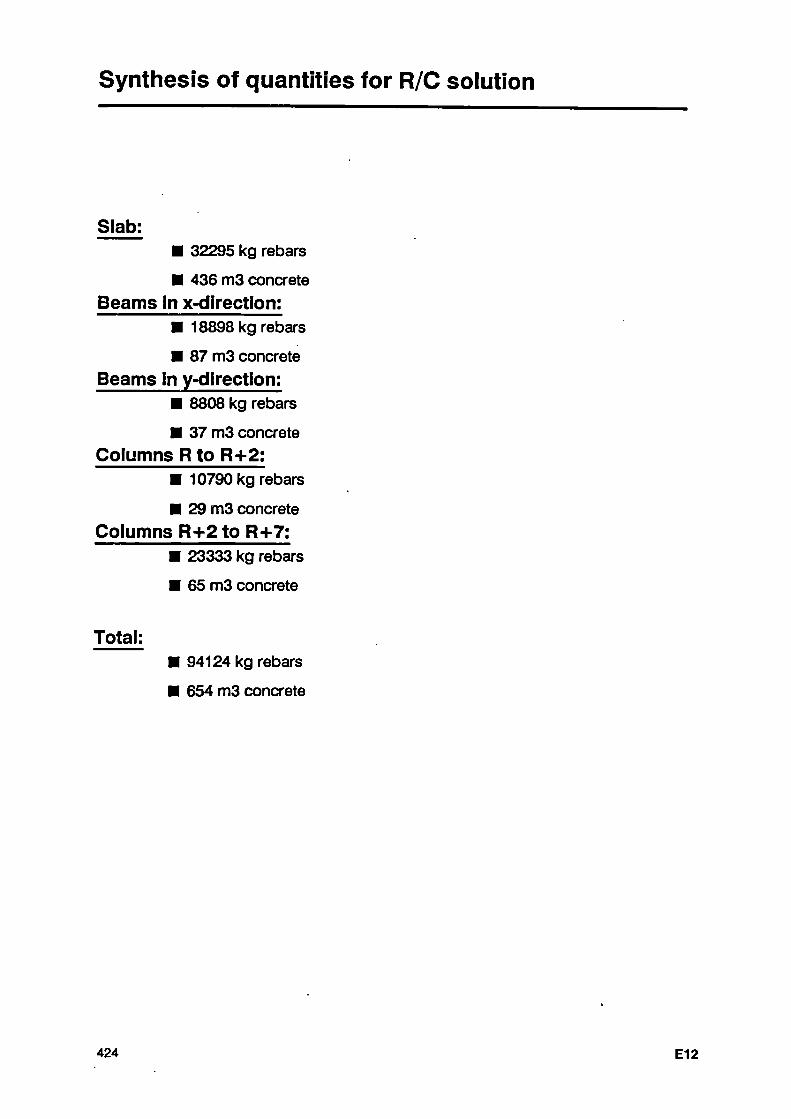
Synthesis of quantities for R/C solution

Slab: ■ 32295 kg rebars

■ 436 m3 concrete Beams In x-direction:

■ 18898 kg rebars

■ 87 m3 concrete Beams In y-dlrectlon:

■ 8808 kg rebars

■ 37 m3 concrete Columns R to R+2:

■ 10790 kg rebars

■ 29 m3 concrete Columns R+2 to R+7:

■ 23333 kg rebars

■ 65 m3 concrete

Total: ■ 94124 kg rebars

■ 654 m3 concrete

424 E12

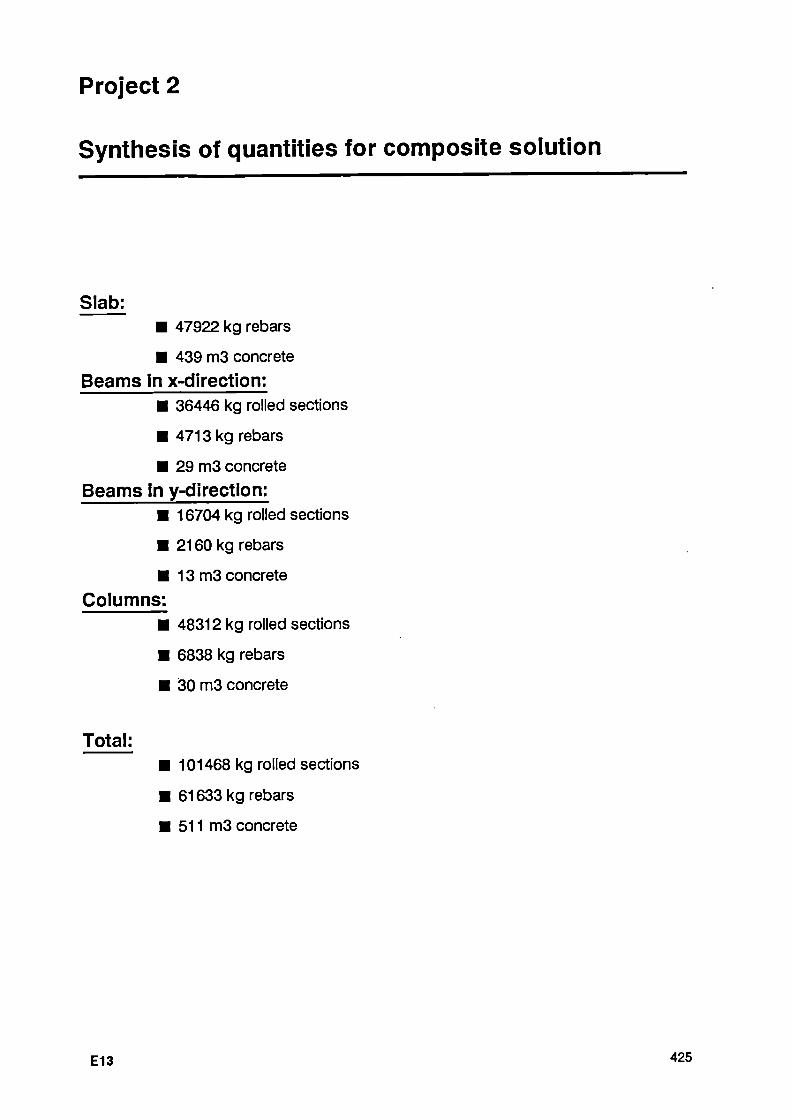
Project 2

Synthesis of quantities for composite solution

Slab: ■ 47922 kg rebars

■ 439 m3 concrete Beams In x-direction:

■ 36446 kg rolled sections

■ 4713 kg rebars

■ 29 m3 concrete Beams in y-direction:

■ 16704 kg rolled sections

■ 2160 kg rebars

■ 13 m3 concrete Columns:

■ 48312 kg rolled sections

■ 6838 kg rebars

■ 30 m3 concrete

Total: 101468 kg rolled sections

61633 kg rebars

511 m3 concrete

E13 425

Synthesis of quantities for R/C solution

Slab: ■ 32295 kg rebars

■ 436 m3 concrete Beams in x-direction:

■ 18898 kg rebars

■ 87 m3 concrete Beams in y-direction:

■ 8808 kg rebars

■ 37 m3 concrete Columns R to R+2:

■ 10790 kg rebars

■ 29 m3 concrete Columns R+2 to R+7:

■ 23333 kg rebars ■ 65 m3 concrete

Total: ■ 94124 kg rebars

■ 654 m3 concrete

426 E14

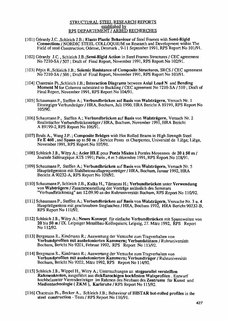
STRUCTURAL STEEL RESEARCH REPORTS established by

RPS DEPARTEMENT / ARBED RECHERCHES

101] Gérardy J.C. .Schleich J.B.; Elasto Plastic Behaviour of Steel Frames with Semi­Rigid Connections / NORDIC STEEL COLLOQUIUM on Research and Development within The Field of steel Construction; Odense, Denmark ,9­11 September 1991, RPS Report No 101/91.

102] Gérardy J.C., Schleich J.B.;Semi­Rigid Action in Steel Frames Structures / CEC agreement No 7210­SA / 507 ; Draft of Final Report, November 1991, RPS Report No 102/91.

103] Pépin R.,Schleich J.B.; Seismic Resistance of Composite Structures, SRCS / CEC agreement No 7210­SA / 506 ; Draft of Final Report, November 1991, RPS Report No 103/91.

104] Chantrain Ph.,Schleich J.B.; Interaction Diagrams between Axial Load Ν and Bending Moment M for Columns submitted to Buckling / CEC agreement No 7210­SA / 510 ; Draft of Final Report, November 1991, RPS Report No 104/91.

105] Schaumann P., Steffen Α.; Verbundbrücken auf Basis von Walzträgern, Versuch Nr. 1 Einstegiger Verbundträger / HRA, Bochum, Juli 1990, HRA Bericht A 89199, RPS Report No 105/90.

106] Schaumann P., Steffen Α.; Verbundbrücken auf Basis von Walzträgern, Versuch Nr. 2 Realistischer Verbundbrückenträger / HRA, Bochum, November 1991, HRA Bericht A 89199­2, RPS Report No 106/91.

107] Bruis Α., Wang J.P. ; Composite Bridges with Hot Rolled Beams in High Strength Steel Fe E 460 , and Spans up to 50 m / Service Ponts et Charpentes, Université de Liège; Liège, November 1991, RPS Report No 107/91.

108] Schleich J.B., Witry Α.; Acier HLE pour Ponts Mixtes à Portées Moyennes de 20 à 50 m / Journée Sidérurgique ATS 1991; Paris, 4 et 5 décembre 1991, RPS Report No 108/91.

109] Schaumann Ρ, Steffen Α.; Verbundbrücken auf Basis von Walzträgern, Versuch Nr. 5 Hauptträgerstoss mit Stahlbetonauflagerquerträger / HRA, Bochum, Januar 1992, HRA Bericht A 90232­A, RPS Report No 109/92.

110] Schaumann P, Schleich J.B., Kulka H., Tilmanns H.; Verbundbrücken unter Verwendung von Walzträgern / Zusammenstellung der Vorträge anlässlich des Seminars "Verbundbrückentag" am 12.09.90 an der Ruhruniversität Bochum, RPS Report No 110/92.

I l l ] Schaumann P., Steffen Α.; Verbundbrücken auf Basis von Walzträgern, Versuche Nr. 3 u. 4 Hauptträgerstoss mit geschraubten Steglaschen / HRA, Bochum 1992, HRA Bericht 90232­B, RPS Report No 111/92.

112] Schleich J.B., Witry Α.; Neues Konzept für einfache Verbundbrücken mit Spannweiten von 20 bis 50 m / IX. Leipziger Metallbau­Kolloquium; Leipzig, 27. März 1992, RPS Report No 112/92.

113] Bergmann R., Kindmann R.; Auswertung der Versuche zum Tragverhalten von Verbundprofilen mit ausbetonierten Kammern; Verbundstützen / Ruhruniversität Bochum, Bericht No 9201, Februar 1992, RPS Report No 113/92.

114] Bergmann R., Kindmann R.; Auswertung der Versuche zum Tragverhalten von Verbundprofilen mit ausbetonierten Kammern; Verbundträger / Ruhruniversität Bochum, Bericht No 9202, März 1992, RPS Report No 114/92.

115] Schleich J.B., Wippel H., Witry Α.; Untersuchungen an stegparallel versteiften Rahmenknoten, ausgeführt aus dickflanschigen hochfesten Walzprofilen . Entwurf hochbelasteter Vierendeelträger im Rahmen des Neubaus des Zentrums für Kunst und Medientechnologie ( ZKM ), Karlsruhe / RPS Report No 115/92.

116] Chantrain Ph., Becker Α., Schleich J.B.; Behaviour of HIST AR hot­rolled profiles in the steel construction ­ Tests / RPS Report No 116/91.

427

— ^

For up-to-date information on European Community research

consult

CORDIS The Community Research

and Development Information Service

CORDIS is an on-line service set up under the VALUE programme to give quick and easy access to information on European Community research programmes.

The CORDIS service is at present offered free-of-charge by the European Commission Host Organisation (ECHO). A menu-based interface makes CORDIS simple to use even if you are not familiar with on-line information services. For experienced users, the standard Common Command Language (CCL) method of extracting data is also available.

CORDIS comprises eight databases:

RTD-News: short announcements of Calls for Proposals, publications and events in the R&D field

RTD-Programmes: details of all EC programmes in R&D and related areas

RTD-Projects: containing 14,000 entries on individual activities within the programmes

RTD-Publications: bibliographic details and summaries of more than 50,000 scientific and technical publications arising from EC activities

RTD-Results: provides valuable leads and hot tips on prototypes ready for industrial exploitation and areas of research ripe for collaboration

RTD-Comdocuments: details of Commission communications to the Council of Ministers and the European Parliament on research topics

RTD-Acronyms: explains the thousands of acronyms and abbreviations current in the Community research area

RTD-Partners: helps bring organisations and research centres together for collaboration on project proposals, exploitation of results, or marketing agreements.

For more information and CORDIS registration forms, contact ECHO Customer Service

CORDIS Operations BP 2373

L-1023 Luxembourg Tel,: (+352) 34 98 11 Fax: (+352) 34 98 12 34

If you are already an ECHO user, please indicate your customer number.

European Communities ­ Commission

EUR 14428 ­ Properties and service performance

Seismic resistance of composite structures ­ SRCS

J.B. Schleich, R. Pepin

Luxembourg: Office for Official Publications of the European Communities

1992 ­ XII, 435 pp., num. tab., fig. ­ 21.0 χ 29.7 cm

Technical steel research series

ISBN 92­826­4667­X

Price (excluding VAT) in Luxembourg: ECU 45

The first period of this research was devoted to the realization of nearly quasi­static cyclic 50 tests on full­sized composite specimen which may be divided into four series: • Series 1 : tests on T­shaped exterior columns/beam joints; • Series 2 : tests on cross­shaped interior columns/beam joints; • Series 3: tests on complete frames; • Series 4: partial tests on different elements. During each of these series different types of connections were analysed. As the series were realized successively, the specimens could be continu­ously improved. Several tests realized in Series 3 are among the biggest ones ever realized in Europe. A second period allowed to develop a numerical code, which can simulate concrete structures under seismic action by taking into account geomet­rical non­linearities as well as the elasto­plastic behaviour of steel and the deterioration of concrete. The present research showed that it is interesting to use composite struc­tures in earthquake­prone zones, since • concrete increases the resistance by about 50% in the elastic field; • concrete increases the stiffness; • concrete largely prevents local buckling; • concrete contributes to the shear panel behaviour; • after complete concrete crushing the structure always behaves like a

bare steel structure when submitted to very large displacements.

Venta y suscripciones · Salg og abonnement · Verkauf und Abonnement · Πωλήσεις και συνδρομές Sales and subscriptions * Vente et abonnements ■ Vendita e abbonamenti

Verkoop en abonnementen · Venda e assinaturas

BELGIQUE / BELGIË FRANCE SUOMI TÜRKIYE

Moniteur belge / Belgisch Staatsblad Rue de Louvain 42 / Leuvenseweg 42 B­1000 Bruxelles / Β­100Ό Brussel Tél. (02)512 00 26 Fax (02) 511 01 84

Autres distributeurs / Overige verkooppunten Librairie européenne/ Europese boekhandel Rue de la Loi 244/Wetstraat 244 B­1040 Bruxelles / B­1040 Brussel Tél. (02) 231 04 35 Fax (02) 735 08 60

Jean De Lannoy Avenue du Roi 202 /Koningslaan 202 B­1060 Bruxe l les /B­1060 Brussel Tél. (02) 538 51 69 Télex 63220 UNBOOK Β Fax (02) 538 08 41

Document delivery: Credoc Rue de la Montagne 34 / Bergstraat 34 Bte 11 / Bus 11 B­1000 Bruxelles / B­1000 Brussel Tél. (02) 511 69 41 Fax (02) 513 31 95

DANMARK

J. H. Schultz Information A/S Herstedvang 10­12 DK­2620 Albertslund Tlf. (45) 43 63 23 00 Fax (Sales) (45) 43 63 19 69 Fax (Management) (45) 43 63 19 49

DEUTSCHLAND

Bundesanzeiger Verlag Breite Straße Postfach 10 80 06 D­W­5000 Köln 1 Tel. (02 21) 20 29­0 Telex ANZEIGER BONN 8 882 595 Fax 2 02 92 78

GREECE/ΕΛΛΑΔΑ

G.C. Eleftheroudakis SA International Bookstore Nikis Street 4 GR­10563 Athens Tel. (01) 322 63 23 Telex 219410 ELEF Fax 323 98 21

ESPANA

Boletfn Oficial del Estado Trafalgar, 29 E­28071 Madrid Tel. (91)538 22 95 Fax (91)538 23 49

Mundi­Prensa Libros, SA Castelló, 37 E­28001 Madrid Tel. (91) 431 33 99 (Libros)

431 32 22 (Suscripciones) 435 36 37 (Dirección)

Télex 49370­MPLI­E Fax (91) 575 39 98

Sucursal: Librería Internacional AEDOS Consejo de Ciento, 391 E­08009 Barcelona Tel. (93) 488 34 92 Fax (93) 487 76 59

Llibreria de la Generalitat de Catalunya Rambla dels Estudis, 118 (Palau Moja) E­08002 Barcelona Tel. (93) 302 68 35

302 64 62 Fax (93) 302 12 99

Journal officiel Service des publications des Communautés européennes 26, rue Desaix F­75727 Paris Cedex 15 Tél. (1) 40 58 75 00 Fax (1) 40 58 77 00

IRELAND

Government Supplies Agency 4­5 Harcourt Road Dublin 2 Tel. (1) 61 31 11 Fax (1) 78 06 45

ITALIA

Licosa SpA Via Duca di Calabria, 1/1 Casella postale 552 1­50125 Firenze Tel. (055) 64 54 15 Fax 64 12 57 Telex 570466 LICOSA I

GRAND­DUCHÉ DE LUXEMBOURG

Messageries Paul Kraus 11 , rue Christophe Plantin L­2339 Luxembourg Tél. 499 88 88 Télex 2515 Fax 499 88 84 44

NEDERLAND

SDU Overheidsinformatie Externe Fondsen Postbus 20014 2500 EA 's­Gravenhage Tel. (070) 37 89 911 Fax (070) 34 75 778

PORTUGAL

Imprensa Nacional Casa da Moeda. EP Rua D. Francisco Manuel de Melo, 5 P­1092 Lisboa Codex Tel. (01)69 34 14 Distribuidora de Livros Bertrand, Ld." Grupo Bertrand, SA Rua das Terras dos Vales, 4­A Apartado 37 P­2700 Amadora Codex Tel. (01) 49 59 050 Telex 15798 BERDIS Fax 49 60 255

UNITED KINGDOM

ÖSTERREICH

Akateeminen Kirjakauppa Keskuskatu 1 PO Box 128 SF­00101 Helsinki Tel. (0) 121 41 Fax (0) 121 44 41

HIVISO Books (Agency section) HMSO Publications Centre 51 Nine Elms Lane London SW8 5DR Tel. (071) 873 9090 Fax 873 8463 Telex 29 71 138

NORGE

Narvesen information center Bertrand Narvesens vei 2 PO Box 6125 Etterstad N­0602 Oslo 6 Tel. (2) 57 33 00 Telex 79668 NIC Ν Fax (2) 68 19 01

SVERIGE

BTJ Tryck Traktorwägen 13 S­222 60 Lund Tel. (046) 18 00 00 Fax (046) 18 01 25

SCHWEIZ / SUISSE / SVIZZERA

OSEC Stampfenbachstraße 85 CH­8035 Zürich Tel. (01)365 54 49 Fax (01) 365 54 11

CESKOSLOVENSKO

NIS Havelkova 22 13000 Praha 3 Tel. (02) 235 84 46 Fax 42­2­264775

MAGYARORSZÄG

Manz'sche Verlags­und Universitätsbuchhandlung Kohlmarkt 16 A­1014 Wien Tel. (0222)531 61­0 Telex 112 500 B O X A Fax (0222) 531 61­39

Euro­Info­Service Pf. 1271 H­1464 Budapest Tel./Fax(1) 111 60 61/111 62 16

POLSKA

Business­ Foundation ul. Krucza 38/42 00­512 Warszawa Tel. (22) 21 99 93. 628­28­82 International Fax&Phone

(0­39) 12­00­77

ROUMANIE

Euromedia 65, Strada Dionisie Lupu 70184 Bucuresti Tel./Fax 0 12 96 46

BULGARIE

D.J.B. ­59, bd Vitocha 1000 Sofia Tel./Fax 2 810158

RUSSIA

CCEC (Centre for Cooperation with the European Communities) 9. Prospekt 60­let Oktyabria 117312 Moscow Tel. 095 135 52 87 Fax 095 420 21 44

CYPRUS

Cyprus Chamber of Commerce and Industry Chamber Building 38 Grivas Dhigenis Ave 3 Deligiorgis Street PO Box 1455 Nicosia Tel. (2)449500/462312 Fax (2) 458630

Pres Gazete Kitap Dergi Pazariama Dagitim Ticaret ve sanayi AŞ Narlibahçe Sokak N. 15 Istanbul­Cagaloglu Tel. (1) 520 92 96 ­ 528 55 66 Fax 520 64 57 Telex 23822 DSVO­TR

ROY International PO Box 13056 41 Mishmar Hayarden Street Tel Aviv 61130 Tel. 3 496 108 Fax 3 544 60 39

CANADA

Renouf Publishing Co. Ltd Mail orders — Head Office: 1294 Algoma Road Ottawa, Ontario K1B 3W8 Tel. (613) 741 43 33 Fax (613) 741 54 39 Telex 0534783

Ottawa Store: 61 Sparks Street Tel. (613) 238 89 85

Toronto Store: 211 Yonge Street Tel. (416)363 31 71

UNITED STATES OF AMERICA

UNIPUB 4611 ­F Assembly Drive Lanham, MD 20706­4391 Tel. Toll Free (800) 274 4888 Fax (301) 459 0056

AUSTRALIA

Hunter Publications 58A Gipps Street Coll ingwood Victoria 3066 Tel. (3)417 5361 Fax (3)419 7154

JAPAN

Kinokuniya Company Ltd 17­7 Sh njuku 3­Chome Shinjuku­ku Tokyo 160­91 Tel. (03) 3439­0121

Journal Department PO Box 55 Chitose Tokyo 156 Tel. (03)3439­0124

SINGAPORE

Legal Library Services Ltd STK Agency Robinson Road PO Box 1817 Singapore 9036

AUTRES PAYS OTHER COUNTRIES ANDERE LANDER Office des publications officielles des Communautés européennes 2, rue Mercier L­2985 Luxembourg Tél. 499 28 1 Télex PUBOF LU 1324 b Fax 48 85 73/48 68 17

Illllililllill'ill "426709 41

Ui

NOTICE TO THE READER

All scientific and technical reports published by the Commission of the European Communities are announced in the monthly periodical 'euro abstracts'. For subscription (1 year: ECU 110) please write to the address below. o

t ro 00

O

Price (excluding VAT) in Luxembourg: ECU 45

* * * OFFICE FOR OFFICIAL PUBLICATIONS

ISBN ^-a^-Hhhl-X

* o p * OF THE EUROPEAN COMMUNITIES

L-2985 Luxembourg