PROCEEDINGS, Thirty-Fourth Workshop on Geothermal Reservoir Engineering Stanford University, Stanford, California, February 9-11, 2009 SGP-TR-187

SEISMIC MONITORING OF EGS STIMULATION TESTS AT THE COSO GEOTHERMAL FIELD, CALIFORNIA, USING MICROEARTHQUAKE LOCATIONS

AND MOMENT TENSORS

Bruce R. Julian1, Gillian R. Foulger2 & Francis C. Monastero3

1U.S. Geological Survey, 345 Middlefield Rd., MS 977,

Menlo Park, CA 94025. email: julian@usgs.gov

2Dept. Earth Sciences, University of Durham,

Science Laboratories, South Rd., Durham, DH1 3LE, U.K.

email: g.r.foulger@durham.ac.uk

3Magma Energy U.S. Corp., 9740 S. McCarran Blvd., Ste. 103,

Reno NV 89523 email: fmonastero@magmaenergycorp.com

ABSTRACT

We calculated high-resolution relative locations and full moment tensors for microearthquakes that occurred before, during, and following EGS stimulation experiments in two wells at the Coso Geothermal Field, California. Our objective was to map new fractures, determine the mode and sense of failure, and characterize the stress cycle associated with reservoir stimulation. As part of this work, we developed new and improved software to combine waveform cross-correlation measurements of arrival times with relative hypocenter relocation methods, and to assess confidence regions for moment tensors derived using linear-programming methods. This software was applied for the first time to data in this study. We used data from the US Navy’s permanent network of three-component digital borehole seismometers, which we supplemented by 14 surface-mounted portable three-component digital instruments. We studied injection experiments in well 34A-9 in 2004 and well 34-9RD2 in 2005. These injectors are on the same surface well pad but they are deviated in different directions so their bottoms are ~ 1 km apart. Despite this, both injections activated the same region, a well-defined planar structure 700 m long and 600 m high in the depth range 0.8 to 1.4 km below sea level, striking N 20 degrees E and dipping 75 degrees to the WNW. The moment tensors show that this structure corresponds to a mode I (opening) crack. Perturbations to the seismicity rate and source orientations near the

bottom of the well persisted for at least two months following the injection. These results show significant flow of injection fluids across the dominant NE tectonic trend of the area. This result is a proof-of-concept that microearthquake analysis techniques are now of sufficient quality to provide sufficiently detailed and comprehensive information about stimulated fractures to be useful in operational decision making.

BACKGROUND

When high-pressure fluids are injected into boreholes in geothermal areas, they flow into hot rock at depth inducing cracking and activating critically stressed pre-existing faults. The resulting earthquake activity can provide information on the locations of the cracks formed, their development in time and the type of cracking underway, e.g., whether shear movement on faults occurred or whether cracks opened up. Ultimately it may be possible to monitor critical earthquake parameters in near-real-time so the information can be used to guide hydraulic injection while it is in progress. In order to achieve this goal, it is necessary to mature existing microearthquake analysis techniques and software to provide state-of-the-art tools that are customized for Enhanced Geothermal Systems (EGS). This includes techniques and software for calculating accurate earthquake locations and source mechanisms (moment tensors). Furthermore, at present few case histories are available with which to

assess the value of different analysis approaches, and to develop EGS into a predictable industrial procedure. In this paper we describe new advances in data processing techniques, and application to two injection tests at the Coso geothermal field, California.

THE COSO GEOTHERMAL FIELD

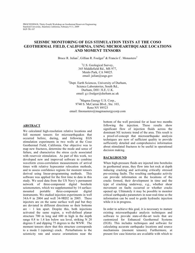
The Coso geothermal area is in the SW of the Basin and Range province in E California. It lies at a right (releasing) fault step-over between the right-lateral Little Lake fault zone to the SW and the Wild Horse Mesa fault to the NE. The whole zone undergoes 6.5 ± 0.7 mm/year of dextral shearing [Monastero et al., 2005]. The area is divided by the main faults into three main sub-regions (Fig. 1), the Main Field, a central spine of exposed bedrock which includes the East Flank of the geothermal area, and Coso Wash to the east. The Main Field is highly active seismically, and has temperatures up to ~ 340˚C in the top ~ 3 km (640ºF at 10,000 ft depth). The intensely normal-faulted eastern margin of the central spine contains the East Flank reservoir, which is also seismically active and associated with high temperatures. Coso Wash is a series of sub-basins associated with segments of the Coso Wash fault and has low seismicity and temperatures.

Fig. 1: Fault-controlled sub-divisions of the Coso

geothermal area. These are distinct as regards temperature and seismicity. The Main Field and the East Flank are the primary producing and seismically active regions.

The area has been exploited since the 1980s and currently produces about 400 MW of electrical power. Approximately 100 wells have been drilled. As much condensate as possible is reinjected in order to maintain reservoir fluid pressure. Wells that prove to be poor producers are generally used for this purpose.

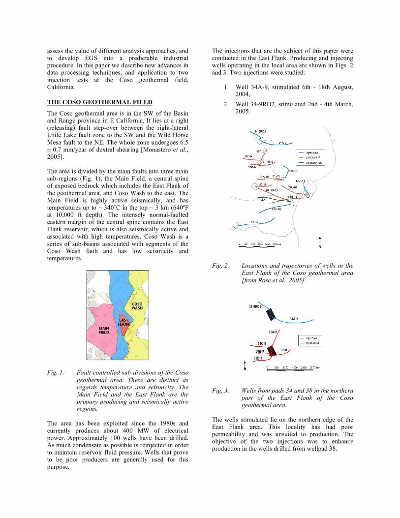
The injections that are the subject of this paper were conducted in the East Flank. Producing and injecting wells operating in the local area are shown in Figs. 2 and 3. Two injections were studied:

1. Well 34A-9, stimulated 6th - 18th August, 2004,

2. Well 34-9RD2, stimulated 2nd - 4th March, 2005.

Fig. 2: Locations and trajectories of wells in the

East Flank of the Coso geothermal area [from Rose et al., 2005].

Fig. 3: Wells from pads 34 and 38 in the northern

part of the East Flank of the Coso geothermal area.

The wells stimulated lie on the northern edge of the East Flank area. This locality has had poor permeability and was unsuited to production. The objective of the two injections was to enhance production in the wells drilled from wellpad 38.

THE SEISMIC DATA

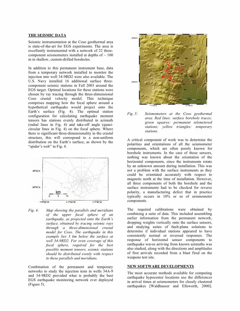
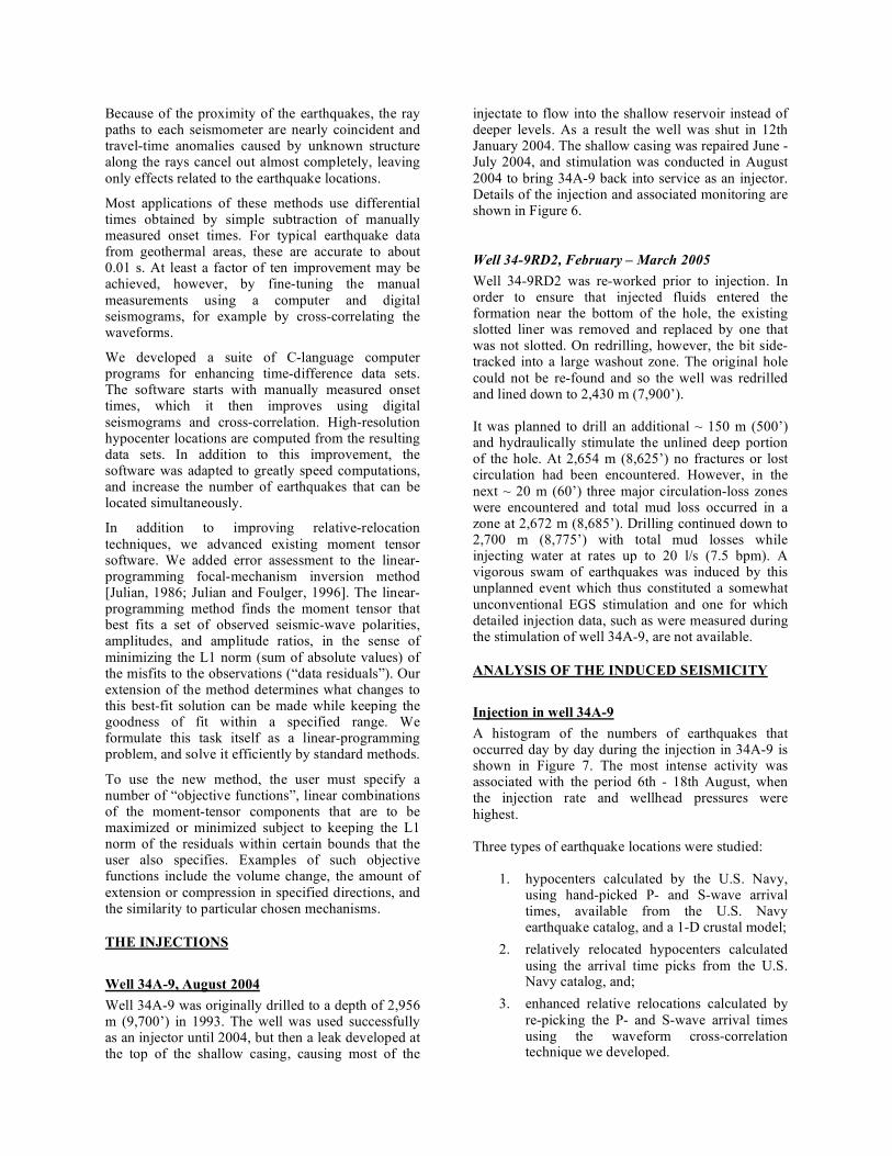
Seismic instrumentation at the Coso geothermal area is state-of-the-art for EGS experiments. The area is excellently instrumented with a network of 22 three-component seismometers installed at depths of ~ 100 m in shallow, custom-drilled boreholes. In addition to this permanent instrument base, data from a temporary network installed to monitor the injection into well 34-9RD2 were also available. The U.S. Navy installed 16 additional surface three-component seismic stations in Fall 2003 around the EGS target. Optimal locations for these stations were chosen by ray tracing through the three-dimensional Coso crustal velocity model. This technique comprises mapping how the focal sphere around a hypothetical earthquake would project onto the Earth’s surface (Fig. 4). The optimal station configuration for calculating earthquake moment tensors has stations evenly distributed in azimuth (radial lines in Fig. 4) and take-off angle (quasi-circular lines in Fig. 4) on the focal sphere. Where there is significant three-dimensionality in the crustal structure, this will correspond to a non-uniform distribution on the Earth’s surface, as shown by the “spider’s web” in Fig. 4.

Fig. 4: Map showing the parallels and meridians

of the upper focal sphere of an earthquake, as projected onto the Earth’s surface, obtained by tracing seismic rays through a three-dimensional crustal model for Coso. The earthquake in this example lies 3 km below the surface at well 34-9RD2. For even coverage of this focal sphere, required for the best possible moment tensors, seismic stations should be distributed evenly with respect to these parallels and meridians.

Combination of the permanent and temporary networks to study the injection tests in wells 34A-9 and 34-9RD2 provided what is probably the best EGS earthquake monitoring network ever deployed (Figure 5).

Fig. 5: Seismometers at the Coso geothermal

area. Red lines: surface borehole traces; green squares: permanent telemetered stations; yellow triangles: temporary stations.

A critical component of work was to determine the polarities and orientations of all the seismometer components, which are often poorly known for borehole instruments. In the case of those sensors, nothing was known about the orientation of the horizontal components, since the instruments rotate by an unknown amount during installation. This was not a problem with the surface instruments as they could be orientated accurately with respect to magnetic north at the time of installation. However, all three components of both the borehole and the surface instruments had to be checked for reverse polarity, a manufacturing defect that in practice typically occurs in 10% or so of seismometer components. The required calibrations were obtained by combining a suite of data. This included assembling earlier information from the permanent network, dropping weights vertically onto the surface sensors, and studying suites of fault-plane solutions to determine if individual stations appeared to have consistently normal or reversed responses. The response of horizontal sensor components to earthquake waves arriving from known azimuths was also studied, along with the directions and amplitudes of first arrivals recorded from a blast fired on the weapons test site.

NEW SOFTWARE DEVELOPMENTS

The most accurate methods available for computing earthquake hypocenter locations use the differences in arrival times at seismometers for closely clustered earthquakes [Waldhauser and Ellsworth, 2000].

Because of the proximity of the earthquakes, the ray paths to each seismometer are nearly coincident and travel-time anomalies caused by unknown structure along the rays cancel out almost completely, leaving only effects related to the earthquake locations.

Most applications of these methods use differential times obtained by simple subtraction of manually measured onset times. For typical earthquake data from geothermal areas, these are accurate to about 0.01 s. At least a factor of ten improvement may be achieved, however, by fine-tuning the manual measurements using a computer and digital seismograms, for example by cross-correlating the waveforms.

We developed a suite of C-language computer programs for enhancing time-difference data sets. The software starts with manually measured onset times, which it then improves using digital seismograms and cross-correlation. High-resolution hypocenter locations are computed from the resulting data sets. In addition to this improvement, the software was adapted to greatly speed computations, and increase the number of earthquakes that can be located simultaneously.

In addition to improving relative-relocation techniques, we advanced existing moment tensor software. We added error assessment to the linear-programming focal-mechanism inversion method [Julian, 1986; Julian and Foulger, 1996]. The linear-programming method finds the moment tensor that best fits a set of observed seismic-wave polarities, amplitudes, and amplitude ratios, in the sense of minimizing the L1 norm (sum of absolute values) of the misfits to the observations (“data residuals”). Our extension of the method determines what changes to this best-fit solution can be made while keeping the goodness of fit within a specified range. We formulate this task itself as a linear-programming problem, and solve it efficiently by standard methods.

To use the new method, the user must specify a number of “objective functions”, linear combinations of the moment-tensor components that are to be maximized or minimized subject to keeping the L1 norm of the residuals within certain bounds that the user also specifies. Examples of such objective functions include the volume change, the amount of extension or compression in specified directions, and the similarity to particular chosen mechanisms.

THE INJECTIONS

Well 34A-9, August 2004 Well 34A-9 was originally drilled to a depth of 2,956 m (9,700’) in 1993. The well was used successfully as an injector until 2004, but then a leak developed at the top of the shallow casing, causing most of the

injectate to flow into the shallow reservoir instead of deeper levels. As a result the well was shut in 12th January 2004. The shallow casing was repaired June - July 2004, and stimulation was conducted in August 2004 to bring 34A-9 back into service as an injector. Details of the injection and associated monitoring are shown in Figure 6.

Well 34-9RD2, February – March 2005 Well 34-9RD2 was re-worked prior to injection. In order to ensure that injected fluids entered the formation near the bottom of the hole, the existing slotted liner was removed and replaced by one that was not slotted. On redrilling, however, the bit side-tracked into a large washout zone. The original hole could not be re-found and so the well was redrilled and lined down to 2,430 m (7,900’). It was planned to drill an additional ~ 150 m (500’) and hydraulically stimulate the unlined deep portion of the hole. At 2,654 m (8,625’) no fractures or lost circulation had been encountered. However, in the next ~ 20 m (60’) three major circulation-loss zones were encountered and total mud loss occurred in a zone at 2,672 m (8,685’). Drilling continued down to 2,700 m (8,775’) with total mud losses while injecting water at rates up to 20 l/s (7.5 bpm). A vigorous swam of earthquakes was induced by this unplanned event which thus constituted a somewhat unconventional EGS stimulation and one for which detailed injection data, such as were measured during the stimulation of well 34A-9, are not available.

ANALYSIS OF THE INDUCED SEISMICITY

Injection in well 34A-9 A histogram of the numbers of earthquakes that occurred day by day during the injection in 34A-9 is shown in Figure 7. The most intense activity was associated with the period 6th - 18th August, when the injection rate and wellhead pressures were highest. Three types of earthquake locations were studied:

1. hypocenters calculated by the U.S. Navy, using hand-picked P- and S-wave arrival times, available from the U.S. Navy earthquake catalog, and a 1-D crustal model;

2. relatively relocated hypocenters calculated using the arrival time picks from the U.S. Navy catalog, and;

3. enhanced relative relocations calculated by re-picking the P- and S-wave arrival times using the waveform cross-correlation technique we developed.

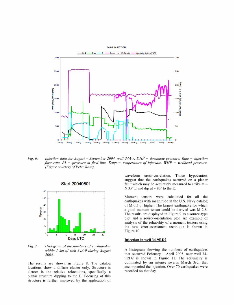
Fig. 6: Injection data for August – September 2004, well 34A-9. DHP = downhole pressure, Rate = injection

flow rate, P1 = pressure in feed line, Temp = temperature of injectate, WHP = wellhead pressure. (Figure courtesy of Peter Rose).

Fig. 7. Histogram of the numbers of earthquakes

within 1 km of well 34A-9 during August 2004.

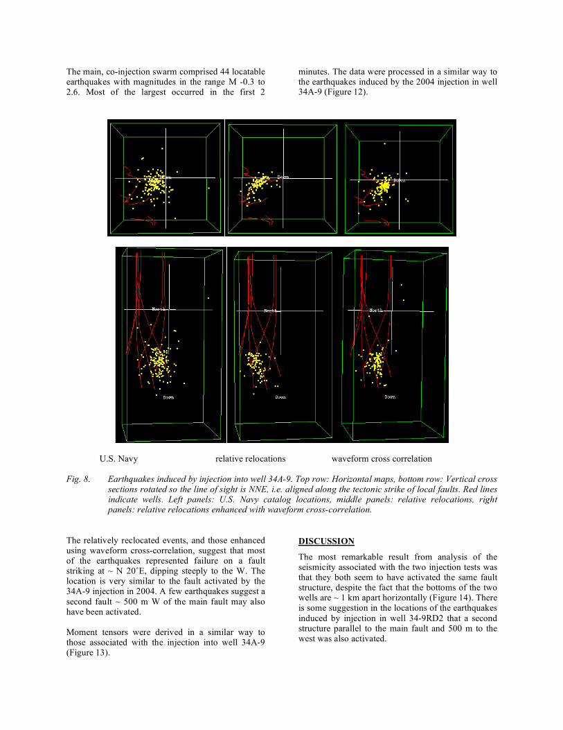
The results are shown in Figure 8. The catalog locations show a diffuse cluster only. Structure is clearer in the relative relocations, specifically a planar structure dipping to the E. Focusing of this structure is further improved by the application of

waveform cross-correlation. Those hypocenters suggest that the earthquakes occurred on a planar fault which may be accurately measured to strike at ~ N 35˚ E and dip at ~ 83˚ to the E. Moment tensors were calculated for all the earthquakes with magnitude in the U.S. Navy catalog of M 0.5 or higher. The largest earthquake for which a good moment tensor could be derived was M 2.8. The results are displayed in Figure 9 as a source-type plot and a source-orientation plot. An example of analysis of the reliability of a moment tensors using the new error-assessment technique is shown in Figure 10.

Injection in well 34-9RD2 A histogram showing the numbers of earthquakes that occurred February – April 2005, near well 34-9RD2 is shown in Figure 11. The seismicity is dominated by an intense swarm March 3rd, that accompanied the injection. Over 70 earthquakes were recorded on that day.

The main, co-injection swarm comprised 44 locatable earthquakes with magnitudes in the range M -0.3 to 2.6. Most of the largest occurred in the first 2

minutes. The data were processed in a similar way to the earthquakes induced by the 2004 injection in well 34A-9 (Figure 12).

U.S. Navy relative relocations waveform cross correlation Fig. 8. Earthquakes induced by injection into well 34A-9. Top row: Horizontal maps, bottom row: Vertical cross

sections rotated so the line of sight is NNE, i.e. aligned along the tectonic strike of local faults. Red lines indicate wells. Left panels: U.S. Navy catalog locations, middle panels: relative relocations, right panels: relative relocations enhanced with waveform cross-correlation.

The relatively reclocated events, and those enhanced using waveform cross-correlation, suggest that most of the earthquakes represented failure on a fault striking at ~ N 20˚E, dipping steeply to the W. The location is very similar to the fault activated by the 34A-9 injection in 2004. A few earthquakes suggest a second fault ~ 500 m W of the main fault may also have been activated. Moment tensors were derived in a similar way to those associated with the injection into well 34A-9 (Figure 13).

DISCUSSION

The most remarkable result from analysis of the seismicity associated with the two injection tests was that they both seem to have activated the same fault structure, despite the fact that the bottoms of the two wells are ~ 1 km apart horizontally (Figure 14). There is some suggestion in the locations of the earthquakes induced by injection in well 34-9RD2 that a second structure parallel to the main fault and 500 m to the west was also activated.

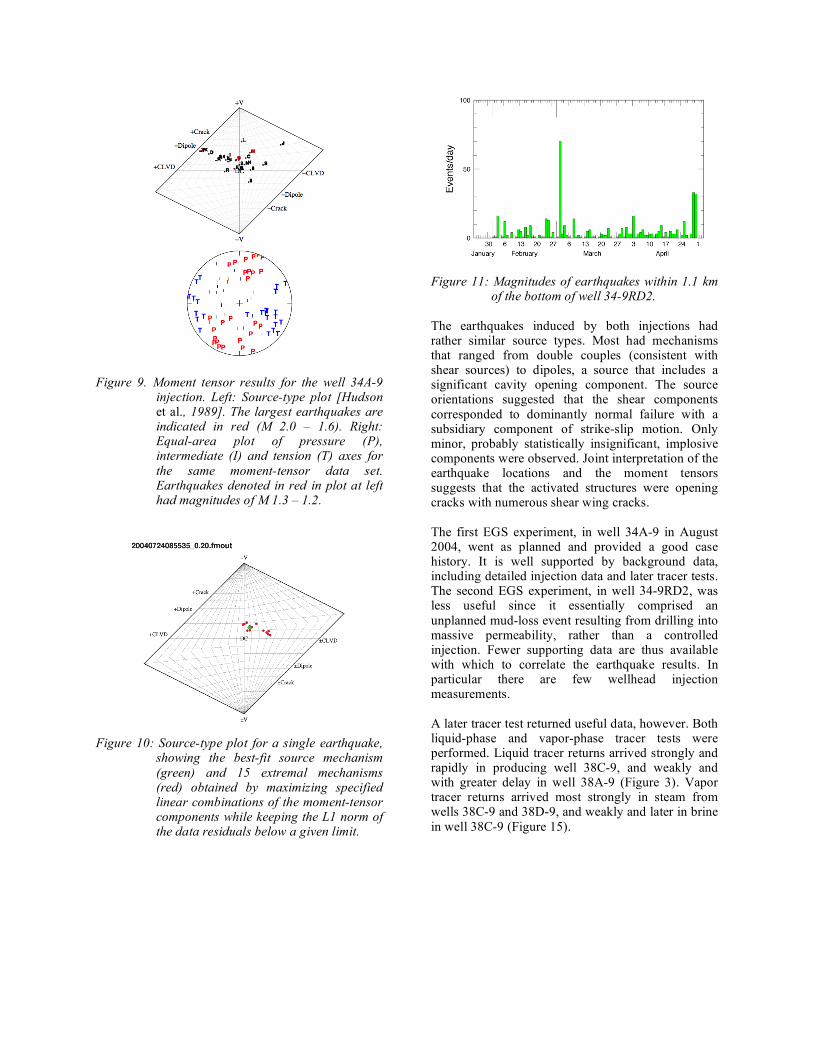
Figure 9. Moment tensor results for the well 34A-9

injection. Left: Source-type plot [Hudson et al., 1989]. The largest earthquakes are indicated in red (M 2.0 – 1.6). Right: Equal-area plot of pressure (P), intermediate (I) and tension (T) axes for the same moment-tensor data set. Earthquakes denoted in red in plot at left had magnitudes of M 1.3 – 1.2.

Figure 10: Source-type plot for a single earthquake,

showing the best-fit source mechanism (green) and 15 extremal mechanisms (red) obtained by maximizing specified linear combinations of the moment-tensor components while keeping the L1 norm of the data residuals below a given limit.

Figure 11: Magnitudes of earthquakes within 1.1 km

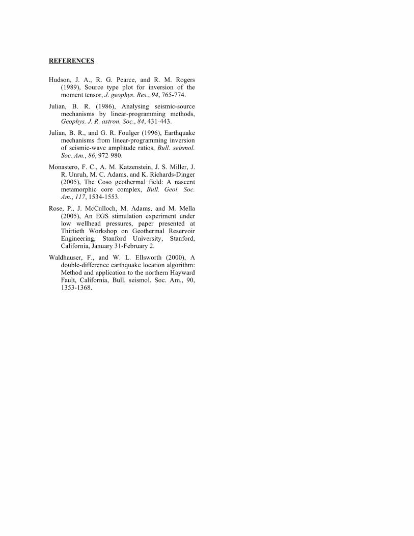
of the bottom of well 34-9RD2. The earthquakes induced by both injections had rather similar source types. Most had mechanisms that ranged from double couples (consistent with shear sources) to dipoles, a source that includes a significant cavity opening component. The source orientations suggested that the shear components corresponded to dominantly normal failure with a subsidiary component of strike-slip motion. Only minor, probably statistically insignificant, implosive components were observed. Joint interpretation of the earthquake locations and the moment tensors suggests that the activated structures were opening cracks with numerous shear wing cracks. The first EGS experiment, in well 34A-9 in August 2004, went as planned and provided a good case history. It is well supported by background data, including detailed injection data and later tracer tests. The second EGS experiment, in well 34-9RD2, was less useful since it essentially comprised an unplanned mud-loss event resulting from drilling into massive permeability, rather than a controlled injection. Fewer supporting data are thus available with which to correlate the earthquake results. In particular there are few wellhead injection measurements. A later tracer test returned useful data, however. Both liquid-phase and vapor-phase tracer tests were performed. Liquid tracer returns arrived strongly and rapidly in producing well 38C-9, and weakly and with greater delay in well 38A-9 (Figure 3). Vapor tracer returns arrived most strongly in steam from wells 38C-9 and 38D-9, and weakly and later in brine in well 38C-9 (Figure 15).

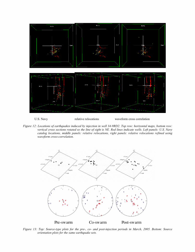
U.S. Navy relative relocations waveform cross correlation Figure 12: Locations of earthquakes induced by injection in well 34-9RD2. Top row: horizontal maps, bottom row:

vertical cross sections rotated so the line of sight is NE. Red lines indicate wells. Left panels: U.S. Navy catalog locations, middle panels: relative relocations, right panels: relative relocations refined using waveform cross-correlation.

Figure 13: Top: Source-type plots for the pre-, co- and post-injection periods in March, 2005. Bottom: Source

orientation plots for the same earthquake sets.

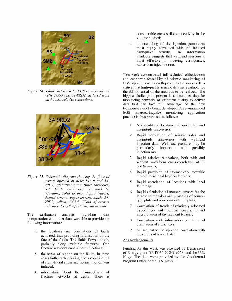
Figure 14: Faults activated by EGS experiments in

wells 34A-9 and 34-9RD2, deduced from earthquake relative relocations.

Figure 15: Schematic diagram showing the fates of

tracers injected in wells 34A-9 and 34-9RD2, after stimulation. Blue: boreholes, red: faults seismically activated by injections, solid arrows: liquid tracers, dashed arrows: vapor tracers, black: 34-9RD2, yellow: 34A-9. Width of arrows indicates strength of returns, not to scale.

The earthquake analysis, including joint interpretation with other data, was able to provide the following information:

1. the locations and orientations of faults activated, thus providing information on the fate of the fluids. The fluids flowed south, probably along multiple fractures. One fracture was dominant in both injections;

2. the sense of motion on the faults. In these cases both crack opening and a combination of right-lateral shear and normal motion was induced;

3. information about the connectivity of fracture networks at depth. There is

considerable cross-strike connectivity in the volume studied;

4. understanding of the injection parameters most highly correlated with the induced earthquake activity. The information available suggests that wellhead pressure is most effective in inducing earthquakes, rather than injection rate.

This work demonstrated full technical effectiveness and economic feasability of seismic monitoring of EGS injections using earthquakes as the sources. It is critical that high-quality seismic data are available for the full potential of the methods to be realized. The biggest challenge at present is to install earthquake monitoring networks of sufficient quality to deliver data that can take full advantage of the new techniques rapidly being developed. A recommended EGS microearthquake monitoring application practice is thus proposed as follows:

1. Near-real-time locations, seismic rates and magnitude time-series;

2. Rapid correlation of seismic rates and magnitude time-series with wellhead injection data. Wellhead pressure may be particularly important, and possibly injection rate;

3. Rapid relative relocations, both with and without waveform cross-correlation of P- and S-waves;

4. Rapid provision of interactively rotatable three-dimensional hypocenter plots;

5. Rapid correlation of locations with local fault maps;

6. Rapid calculation of moment tensors for the largest earthquakes and provision of source-type plots and source-orientation plots;

7. Correlation of trends of relatively relocated hypocenters and moment tensors, to aid interpretation of the moment tensors;

8. Correlation with information on the local orientation of stress axes;

9. Subsequent to the injection, correlation with the results of tracer tests.

Acknowledgements Funding for this work was provided by Department of Energy grant DE-FG36-06GO16058, and the U.S. Navy. The data were provided by the Geothermal Program Office of the U.S. Navy.

REFERENCES

Hudson, J. A., R. G. Pearce, and R. M. Rogers

(1989), Source type plot for inversion of the moment tensor, J. geophys. Res., 94, 765-774.

Julian, B. R. (1986), Analysing seismic-source mechanisms by linear-programming methods, Geophys. J. R. astron. Soc., 84, 431-443.

Julian, B. R., and G. R. Foulger (1996), Earthquake mechanisms from linear-programming inversion of seismic-wave amplitude ratios, Bull. seismol. Soc. Am., 86, 972-980.

Monastero, F. C., A. M. Katzenstein, J. S. Miller, J. R. Unruh, M. C. Adams, and K. Richards-Dinger (2005), The Coso geothermal field: A nascent metamorphic core complex, Bull. Geol. Soc. Am., 117, 1534-1553.

Rose, P., J. McCulloch, M. Adams, and M. Mella (2005), An EGS stimulation experiment under low wellhead pressures, paper presented at Thirtieth Workshop on Geothermal Reservoir Engineering, Stanford University, Stanford, California, January 31-February 2.

Waldhauser, F., and W. L. Ellsworth (2000), A double-difference earthquake location algorithm: Method and application to the northern Hayward Fault, California, Bull. seismol. Soc. Am., 90, 1353-1368.