size and geometry of microearthquake seismic ruptures from p and s pulse width data

Geophys. J. Int. (2003) 155, 422–442

Size and geometry of microearthquake seismic ruptures from Pand S pulse width data

Salvatore de Lorenzo1 and Aldo Zollo2

1Dipto. di Geologia e Geofisica, Universita di Bari, Campus Universitario, Via Orabona 4, 70125 Bari, Italy. E-mail: [email protected]. di Scienze Fisiche, Universita di Napoli, Naples, Italy

Accepted 2003 May 20. Received 2003 March 14; in original form 2002 April 8

S U M M A R YWe propose a method to estimate the radius, dip and strike of a circular seismic rupture throughthe inversion of first P- and S-wave pulse widths measured on microearthquake records.

The method is based on quite general, numerically calibrated relationships relating sourceand Q parameters under the assumption that the waves are radiated by a circular crack propa-gating at a constant rupture velocity.

To study the influence of both the source and receiver configuration and the propertiesof seismic rupture, a detailed resolution study on synthetic data has been carried out. For amicroearthquake rupture, the pulse width variations with azimuths depend critically on the faultplane orientation and the resolution on fault angle parameters can be qualitatively assessedby the parameter η, defined as the relative variation of the take-off angles with respect totheir average value. A statistical approach based on mapping random deviations on data in the(δ, φ) parameter space has been adopted to quantify the uncertainty affecting the fault planeestimates. The method is applied to estimate the source parameters of an ML = 3.1 eventrecorded during the 1997 Umbria-Marche earthquake sequence.

For the considered event, the fault plane solution is in good agreement with the δ–φ estimatesobtained by the method of the joint inversion of P polarities and S polarizations.

Key words: directivity, fault plane orientation, multipathing, pulse width.

1 I N T RO D U C T I O N

In the recent past, many efforts have been made in an attempt to de-tail seismic source properties of low and moderate earthquakes bythe study of the recorded waveforms (Mori & Hartzell 1990; Mori1996; Deichmann 1997, 1999). This can become a complex problemsince the source and propagation parameters (fault dimension, rup-ture velocity, quality factor) can trade-off on seismograms, in thefrequency and/or the time domain (Scherbaum 1990; Deichmann1997).

Concerning the amplitude and shape of first P- and S-wave ar-rivals, the dominant propagation effects are the geometrical spread-ing and the anelastic attenuation. Generally, homogeneous or verti-cally varying elastic media are assumed to evaluate the geometricalamplitude decay with distance. Instead, the anelastic effect of theEarth is accounted by the P and S quality factors, controlling theexponential decay of the amplitude spectrum and the pulse broad-ening with the travel distance and frequency. Several Q studies haveshown that, as a consequence of the heterogeneity of the crust andsite effects, Q can suffer significant lateral and vertical variationsand these result in differential variations of the shape of the waves

recorded at different sites, thus increasing the complexity of theproblem.

On the other hand, the seismic moment, the radiation pattern andthe rupture directivity are the main source effect. Then the effect ofthe seismic source may also be more complex, since the shape ofthe recorded waves is a function of several source parameters suchas the fault dimensions, the rupture velocity and the fault planeorientation.

At least three general different approaches to the joint modellingof source parameters of low magnitude earthquakes and Q have beenproposed over the last 20 years.

The most used techniques are the spectral methods (see, e.g.Abercrombie 1995); these consist of assuming that the far-fieldsource spectra can be described through a circular crack model(Brune 1970; Boatwright 1980), which predicts a flat spectrum be-low the corner frequency f 0 and decaying as an inverse power of thefrequency (with a source-model-dependent exponent) above f 0; theeffect of attenuation on seismic spectra is modelled as an exponentialdecreasing function of the ratio 2π f t/Q, where t is the traveltimeand f is the frequency. This approach, first proposed by Anderson& Hough (1984), has been largely adopted (e.g. Scherbaum 1990;

422 C© 2003 RAS

Size and geometry of microearthquake ruptures 423

Ichinose et al. 1997; Hough et al. 1999). Since the technique isbased on an isotropic source model it is not required to invert forthe fault orientation and this allows for a reduction of the numberof parameters (the corner frequency and the high-frequency fall-offexponent) to be inferred.

Another approach to the study of the seismic source propertiesfor moderate (M > 4) and great earthquakes is based on the use ofthe empirical Green function (EGF) (Zollo et al. 1995; Courboulexet al. 1996; Abercrombie et al. 2001). The EGF technique consists ofextracting directly from the data an empirical function F selected insuch a way as to be representative only of instrument and path effects(Hartzell 1978); after the deconvolution of the other waveforms withF a representation of the source far field is achieved.

Finally, in the time domain, the most used technique is repre-sented by the rise time or pulse width method (Gladwin & Stacey1974; Wu & Lees 1996). Deichmann (1999) showed that the meth-ods based on pulse widths tend to better estimate seismic sourceparameters compared with the EGF technique, since the spectralratio operated in the EGF deconvolution process tends to producenoise magnification that could mask the initial onset of the consid-ered wave, in particular when this is slow. Wu & Lees (1996) showedthat the linear relationships on which the rise time method is basedstill remain valid if we consider a finite-dimension isotropic seismicsource characterized by a frequency cut-off at the source greaterthan or equal to 20 Hz, also if the slope of the pulse width versust∗ is source dependent. Nevertheless, experimental results (Blair& Spathis 1982) and theoretical analyses (Liu 1988; de Lorenzo1998) indicated that the linearity on which the method is basedis only apparent, in that the slope of the straight line describingpulse width versus traveltime is a function of the source frequencycontent.

Since the source frequency content is different at different sites,as a consequence of the finiteness of the rupture velocity and thesource dimensions (Sato & Hirasawa 1973; Madariaga 1976) insome cases the plots of pulse width versus distance do not exhibit aclear increasing trend; in particular, this could happen if the mediumis not strongly attenuating and/or the epicentre of the event lies insidethe area enclosed by the acquisition network, so that the attenuationterm is almost the same at different stations. In these cases theduration of signals may be more sensitive to directivity variationsthan to attenuation. Based on these grounds, Zollo & de Lorenzo(2001) (hereafter referred to as Z&D) modified the pulse widthmethod to account for these effects; they calibrated, for a fixed valueof V p velocity at the source, the numerical equations representingthe dependence of rise time and pulse width of first P arrivals asa function of source parameters (fault radius, dip and strike of thefault plane) and Qp; through a resolution study on synthetic datasets, based on the sources and receivers geometry of the CampiFlegrei 1984 microearthquake sequence, they showed that sourcedimensions and Qp can be adequately recovered, whereas dip (δ)and strike (φ) estimates are usually less reliable.

In this article the Z&D method has been generalized to account fordifferent values of V p and V s at the source; this allows for the appli-cation of the method to different areas and/or to different hypocentraldepth ranges. In the previous study, based on the acquisition layoutof the Campi Flegrei 1984 swarm, it has been shown that the lim-ited number of only P pulses can lead to a loss of resolution on thefault plane estimates. Starting from this observation, in this articlewe focus more closely on the properties of the relative geometry ofsource and receivers and on the joint use of P and S pulse widthdata that are required to infer reliable estimates of the fault planeorientation.

The method has been applied to a low-magnitude earthquake(Ml = 3.1) of the Umbria-Marche seismic sequence (central Italy)that occurred in the period 1997 September–October. The resultshave been compared with those obtained by inverting P polaritiesand S polarizations according to the method of Zollo & Bernard(1991).

2 T H E G E N E R A L R E L AT I O N S H I P SB E T W E E N P U L S E W I D T H S , S O U RC EPA R A M E T E R S A N D Q

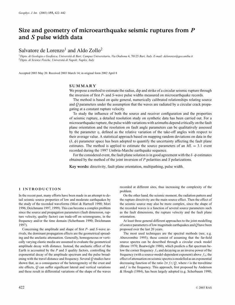
On a velocity seismogram, the pulse width �T of a seismic phasecan be defined as the time interval between the arrival time of thesignal and its second zero crossing time ( Fig. 1). If we consider thesignal radiated by a point-like and impulsive source time function(a Dirac delta function) and recorded at an assigned distance, �T isa linear function of the attenuation term t∗ = T /Q that accounts forthe propagation effects, where T is the traveltime of the wave andQ is the constant quality factor of the medium (Kjartansson 1979).

Let us now consider the wavefield radiated by a finite-dimensionseismic source, and assume that this is due to a circular crack ruptur-ing at a constant velocity. In the far-field range (Fraunhofer approx-imation), the source pulse width (i.e. the pulse width of the signalin the absence of attenuation) is given by (Aki & Richards 1980)

�T0 = L

Vr+ L

csin θ. (1)

In eq. (1) L is the final radius of the crack, V r is the average rupturevelocity, c is the phase velocity at the source and θ is the take-off angle (i.e. the angle formed by the ray leaving the source withthe normal to the fault plane). By considering the propagation inan attenuating medium of a phase radiated by a finite-dimensionseismic source, the relationship that accounts for both source andpropagation effects can be written as (Gladwin & Stacey 1974)

�T = �T0 + CT

Q. (2)

As we discussed in the previous section, C depends on the sourcefrequency content; this makes the problem of retrieving Q and sourceparameters by inverting the pulse width data complex, since weneed to assume a source model. Z&D determined C by consideringthe source and receiver geometry of low-magnitude earthquakesrecorded during the period 1984 January–July at the Campi Flegreicaldera, by fixing the body wave velocity at the source; the circularcrack model of Sato & Hirasawa (1973) was adopted as the sourcemodel, and the Azimi attenuation operator (Azimi et al. 1968) wasassumed to account for the anelastic attenuation of rocks.

Figure 1. The pulse widths on a velocity seismogram.

C© 2003 RAS, GJI, 155, 422–442

424 S. de Lorenzo and A. Zollo

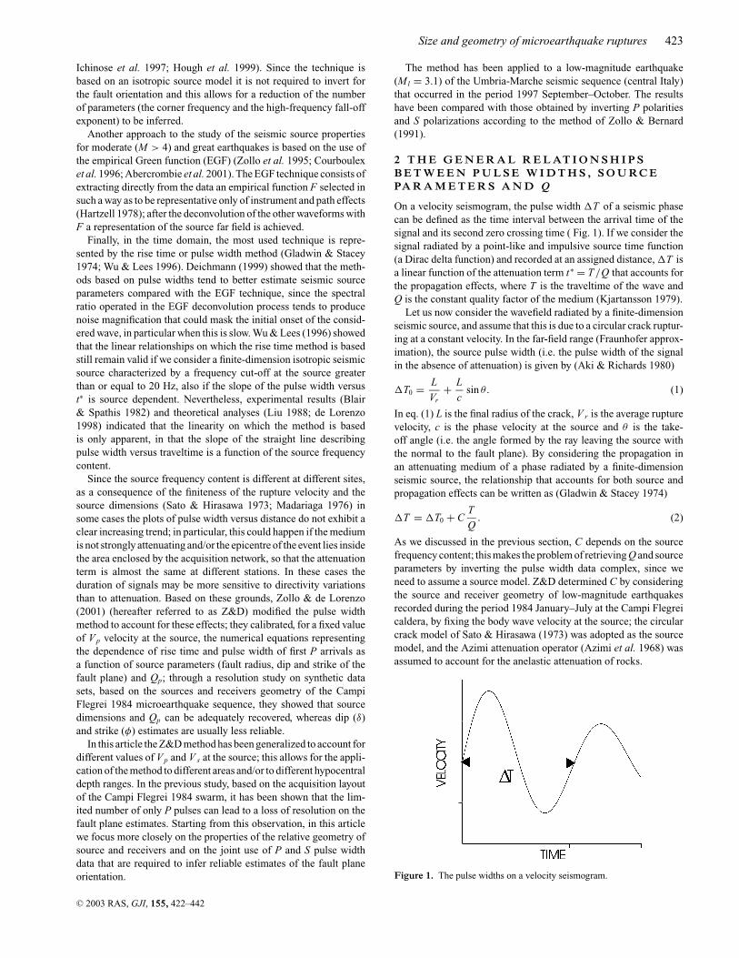
Figure 2. (a) The slope C of �T versus t∗ for P and S waves as a function of V p and V s (V r = 0.9V s), (b) the slope C of �T versus t∗ for P and S waves asa function of V r, for V p = 6.1 km s−1 and V s = 3.5 km s−1 (see the text). Each dot in the figure has been computed through a regression analysis of synthetic�T versus t∗ measured over 960 synthetic seismograms.

In order to obtain a more general formulation of the Z&D methodfor crustal ranges of the body wave velocities, one must evaluatethe dependence of the slope Cp of the P pulse width versus t∗ asa function of V p velocity (at a given rupture velocity) and also theslope Cs of the S pulse width versus t∗ as a function of V s velocity (ata given rupture velocity). To this end, we have applied the numericaltechnique described in Z&D to compute C for different values ofthe body wave velocity at the source and of the rupture velocity.This procedure has been repeated for each of the V p and V s valuesshown in Fig. 2(a) and for each of the V r values shown in Fig. 2(b).

The results of our calculation can be summarized in the followingway.

(1) For a given V r/V s ratio Cp and Cs decrease with increasingof V p and V s, respectively.

(2) The dependence of Cp and Cs coefficients as a function ofV p and V s, respectively (for the cases V p/V s = 1.73 and V r/V s =0.9) is shown in Fig. 2(a). The least-squares fit to the results led usto the following relationships:

CP (VR = 0.9VS) = 4.362 − 0.216VP + 0.019V 2P (3)

CS(VR = 0.9VS) = 4.518 − 0.372VS + 0.047V 2S . (4)

(3) At a fixed V p (or V s) Cp (or Cs) decreases with increasingV r/V s ratio.

(4) The Cp and Cs coefficients versus the rupture velocity (forthe case V p = 6.1, V s = 3.5 km s−1) are plotted in Fig. 2(b). Theresults of our calculation led to the following regression equations:

CP (VP = 6.1 km s−1) = 3.986 − 0.640VR + 0.389V 2R (5)

CS(VS = 3.5 km s−1) = 4.097 − 0.755VR + 0.471V 2R . (6)

As we will detail in the next section, it is very difficult to jointlyinfer the source radius and the rupture velocity by inverting pulsewidth data of low-magnitude earthquakes. For this reason we think

that a further extension of the relations (5) and (6) to other V p andV s values is useless.

Details of the non-linear inversion technique for inferring modelparameters, based on the simplex downhill method (Nelder & Mead1965) are given in Z&D.

3 S T U DY O F T H E U N C E RTA I N T I E SO N M O D E L PA R A M E T E R S

In this section we present a detailed resolution study based on in-versions of synthetic data sets, aimed at assessing the accuracy ofthe model parameter estimates. In particular, we are interested inquantifying the dependence of the fault plane resolution both on thesource properties and on the geometry of the acquisition network.

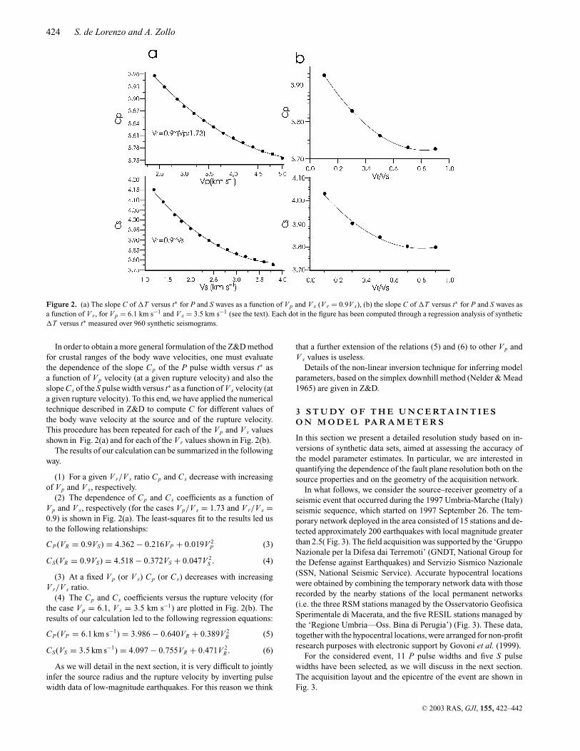
In what follows, we consider the source–receiver geometry of aseismic event that occurred during the 1997 Umbria-Marche (Italy)seismic sequence, which started on 1997 September 26. The tem-porary network deployed in the area consisted of 15 stations and de-tected approximately 200 earthquakes with local magnitude greaterthan 2.5( Fig. 3). The field acquisition was supported by the ‘GruppoNazionale per la Difesa dai Terremoti’ (GNDT, National Group forthe Defense against Earthquakes) and Servizio Sismico Nazionale(SSN, National Seismic Service). Accurate hypocentral locationswere obtained by combining the temporary network data with thoserecorded by the nearby stations of the local permanent networks(i.e. the three RSM stations managed by the Osservatorio GeofisicaSperimentale di Macerata, and the five RESIL stations managed bythe ‘Regione Umbria—Oss. Bina di Perugia’) (Fig. 3). These data,together with the hypocentral locations, were arranged for non-profitresearch purposes with electronic support by Govoni et al. (1999).

For the considered event, 11 P pulse widths and five S pulsewidths have been selected, as we will discuss in the next section.The acquisition layout and the epicentre of the event are shown inFig. 3.

C© 2003 RAS, GJI, 155, 422–442


Figure 3. The source–receivers configuration of the low-magnitude earthquake (Ml = 3.1) considered in this study. (a) The complete (temporary + permanent)array deployed in the Umbria-Marche (central Italy) region (modified by Govoni et al. 1999). (b) The stations considered in this study for which P and S pulsewidths are available. Triangles refers to P pulse widths and circles to S pulse widths.

The following parameters have been assumed: V p = 6.1 km s−1,V s = V p/1.9 (Cattaneo et al. 2000) and V r = 0.9V s.

In order to study the fault plane resolution the following procedurehas been used.

(1) First of all, synthetic noise-free P and S pulse widths havebeen computed through the above calibrated equations, by fixingthe model parameters. To simulate the effect of noise on data weused the random deviations technique (Vasco et al. 1995). Eachsynthetic data set has then been modified, by adding to each dataa random quantity selected in the range of a given uncertainty (weassumed a percentage error of 5 per cent for both P and S waves).

This procedure has been repeated 50 times in order to obtain 50independent data sets. These have then been inverted in order toobtain 50 estimates of each model parameter and the best-fittingmodel parameters mest = (L , δ, φ, Qp, Qs) have been retrieved fromthe statistical analysis of the results.

(2) Secondly, we fixed L , Qp and Qs at the values inferred by theinversion and computed the variations of the standard deviation σ

among data and their estimates with varying dip and strike of thefault. The σ values were computed on a dense grid (5 × 5 deg2)in the δ–φ plane. The standard deviation was normalized to theaverage residual σ 0 on pulse widths, this last being computed bythe relation σ0 = 1

N

∑Ni=1 |0.05�T i

obs|. The σ/σ 0 plot in the (δ, φ)

C© 2003 RAS, GJI, 155, 422–442


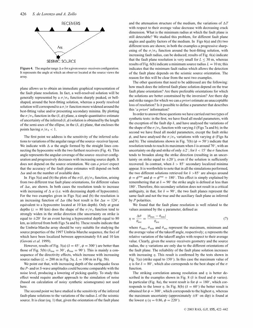
Figure 4. The angular range�α for a given source–receivers configuration.It represents the angle at which an observer located at the source views thearray.

plane allows us to obtain an immediate graphical representation ofthe fault plane resolution. In fact, a well-resolved solution will begenerally represented by a σ/σ 0 function sharply peaked, or bell-shaped, around the best-fitting solution, whereas a poorly resolvedsolution will correspond to a σ/σ function more widened around thebest-fitting value and/or presenting secondary minima. By plottingthe σ/σ 0 function in the (δ, φ) plane, a simple quantitative estimateof uncertainty of the inferred (δ, φ) solution is obtained by the lengthof the semi-axes of the ellipse, in the (δ, φ) plane, that encloses thepoints having σ/σ 0 < 1.

The first point we address is the sensitivity of the inferred solu-tions to variations of the angular range of the source–receiver layout.We indicate with � α the angle formed by the straight lines con-necting the hypocentre with the two furthest receivers (Fig. 4). Thisangle represents the angular coverage of the source–receiver config-uration and progressively decreases with increasing source depth. Itdoes not depend on the source orientation. We can a priori expectthat the accuracy of the fault plane estimates will depend on both�α and on the number of available data.

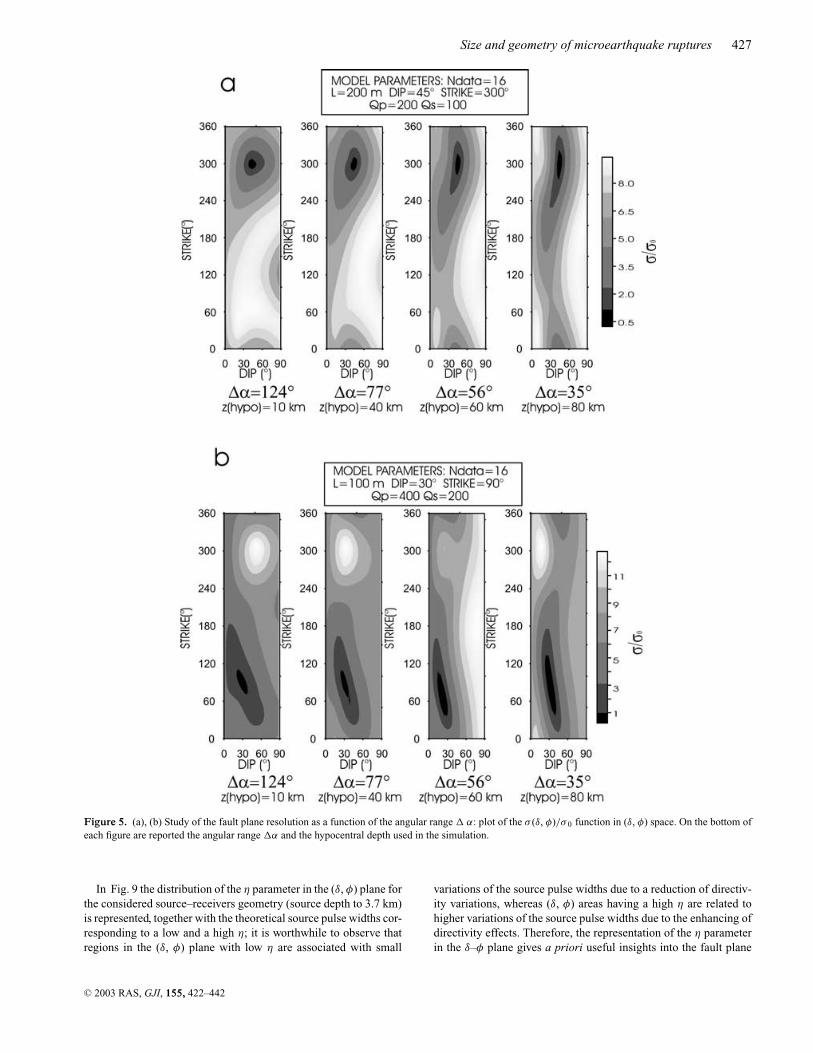
In Figs 5(a) and (b) the plots of the σ (δ, φ)/σ 0 function, arisingfrom two different true fault plane orientations, for different valuesof �α, are shown. In both cases the resolution tends to increasewith increasing of � α (i.e. with decreasing depth of hypocentre).For the two examples given in Figs 5(a) and (b) the resolution isan increasing function of �α (the best result is for �α = 124◦,equivalent to a hypocentre located at 10 km depth). Only at greatdepths (z = 80 km) does the shape of the σ/σ 0 function tend tostrongly widen in the strike direction (the uncertainty on strike isequal to ±20◦ for an event having a hypocentral depth equal to 80km, as inferred from both Figs 5a and b). These results indicate thatthe Umbria-Marche array should be very suitable for studying thesource properties of the 1997 Umbria-Marche sequence, the foci ofwhich have been localized between approximately 0.6 and 10 km(Govoni et al. 1999).

However, results of Fig. 5(a) (δ = 45◦, φ = 300◦) are better thanthose of Fig. 5(b) (δtrue = 30◦, φtrue = 90◦). This is mainly a con-sequence of the directivity effects, which increase with increasingsource radius (L = 200 m in Fig. 5a, L = 100 m in Fig. 5b).

We point out that, with increasing depth of the earthquake focusthe P- and/or S-wave amplitudes could become comparable with thenoise level, producing a lowering of picking quality. To study thiseffect would require another approach to the simulation of noise(based on calculation of noisy synthetic seismograms) not usedhere.

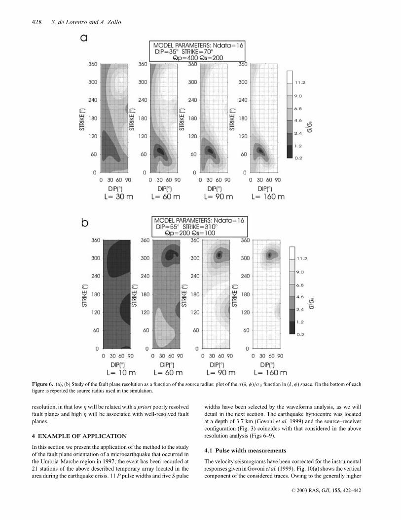
The second point we have studied is the sensitivity of the inferredfault-plane solutions to the variations of the radius L of the seismicsource. It is clear (eq. 1) that, given the orientation of the fault plane

and the attenuation structure of the medium, the variations of �Twith respect to their average value decrease with decreasing crackdimension. What is the minimum radius at which the fault plane isstill detectable? We studied this problem, for different fault planeangles and quality factors of the medium. In Figs 6(a) and (b) twodifferent tests are shown; in both the examples a progressive sharp-ening of the σ/σ 0 function around the best-fitting solution, withincreasing fault radius, can be deduced; results of Fig. 6(a) indicatethat the fault plane resolution is very small for L ≤ 30 m, whereasresults of Fig. 6(b) indicate a minimum source radius L = 10 m; thisindicates that the minimum fault radius which allows the detectionof the fault plane depends on the seismic source orientation. Thereason for this will be clear from the next two examples.

The other questions that need to be addressed are the following:how much does the inferred fault plane solution depend on the truefault plane orientation? Are there preferable orientations for whichthe solutions are better constrained by the inversion? Are there dipand strike ranges for which we can a priori estimate an unacceptableloss of resolution? Is it possible to define a parameter that describesthis ‘a priori’ information?

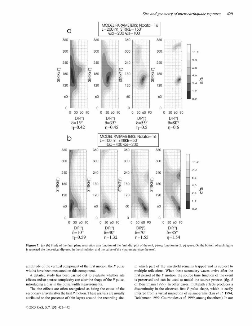
In order to answer these questions we have carried out two types ofsynthetic tests: in the first, we have fixed all model parameters, withthe exception of the fault dip δ, and have analysed the variations ofthe shape of the σ/σ 0 function with varying δ (Figs 7a and b); in thesecond we have fixed all model parameters, except the fault strikeφ, and have analysed the σ/σ 0 variations with varying φ (Figs 8aand b). The simulations shown in Fig. 7(b) (φ = 50◦) indicate thatresolution tends to reach its maximum when δ is around 70◦, with anuncertainty on dip and strike of only ±2◦; for δ < 15◦ the σ functiontends to broaden along the strike direction (resulting in an uncer-tainty on strike equal to ±20◦), even if the solution is sufficientlyrecovered. In contrast, when δ > 85◦ secondary localized minimaappear. It is worthwhile to note that in all the simulations performed,the two different solutions retrieved for δ >85◦ are always aroundφ = φtrue and φ = φtrue + 180◦. This effect is simply explained byremembering that at δ = 90◦ the strike angle is defined at less than180◦. Therefore, this secondary solution does not result in a criticalambiguity, in that, for δ = 90◦, the two fault planes represent thesame fault and not the true and the auxiliary fault plane as inferredby P polarities.

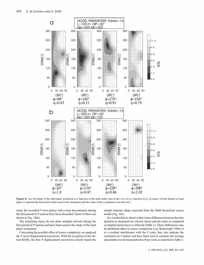
We found that the fault plane resolution is well related to thevalues assumed by the η parameter, defined as

η = �θ

θave= |θmax − θmin|

θave, (7)

where θmax, θmin and θ ave represent the maximum, minimum andthe average value of the takeoff angle, respectively; η represents therelative variation of the takeoff angles with respect to their averagevalue. Clearly, given the source–receivers geometry and the sourceradius, the η variations are only due to the different orientations ofthe fault plane. The reliability of the fault plane solution increaseswith increasing η. This result is confirmed by the tests shown inFig. 7(a) (strike equal to 150◦). In this case the maximum value ofη is for δ = 80◦, which also corresponds to the best shape of the σ

function.The striking correlation among resolution and η is better de-

scribed in the examples shown in Fig. 8 (δ is fixed and φ varies).In particular (Fig. 8a), the worst result is for φ = 180◦, which cor-responds to the lower η. In Fig. 8(b) (δ = 60◦) the better result isobtained for φ = 300◦, which corresponds to the highest η, whereasthe maximum uncertainty (approximately ±8◦ on dip) is found atthe lowest η (η = 0.86, φ = 220◦).

C© 2003 RAS, GJI, 155, 422–442


Figure 5. (a), (b) Study of the fault plane resolution as a function of the angular range � α: plot of the σ (δ, φ)/σ 0 function in (δ, φ) space. On the bottom ofeach figure are reported the angular range �α and the hypocentral depth used in the simulation.

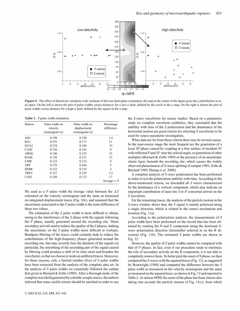
In Fig. 9 the distribution of the η parameter in the (δ, φ) plane forthe considered source–receivers geometry (source depth to 3.7 km)is represented, together with the theoretical source pulse widths cor-responding to a low and a high η; it is worthwhile to observe thatregions in the (δ, φ) plane with low η are associated with small

variations of the source pulse widths due to a reduction of directiv-ity variations, whereas (δ, φ) areas having a high η are related tohigher variations of the source pulse widths due to the enhancing ofdirectivity effects. Therefore, the representation of the η parameterin the δ–φ plane gives a priori useful insights into the fault plane

C© 2003 RAS, GJI, 155, 422–442


Figure 6. (a), (b) Study of the fault plane resolution as a function of the source radius: plot of the σ (δ, φ)/σ 0 function in (δ, φ) space. On the bottom of eachfigure is reported the source radius used in the simulation.

resolution, in that low η will be related with a priori poorly resolvedfault planes and high η will be associated with well-resolved faultplanes.

4 EXAMPLE OF APPLICATION

In this section we present the application of the method to the studyof the fault plane orientation of a microearthquake that occurred inthe Umbria-Marche region in 1997; the event has been recorded at21 stations of the above described temporary array located in thearea during the earthquake crisis. 11 P pulse widths and five S pulse

widths have been selected by the waveforms analysis, as we willdetail in the next section. The earthquake hypocentre was locatedat a depth of 3.7 km (Govoni et al. 1999) and the source–receiverconfiguration (Fig. 3) coincides with that considered in the aboveresolution analysis (Figs 6–9).

4.1 Pulse width measurements

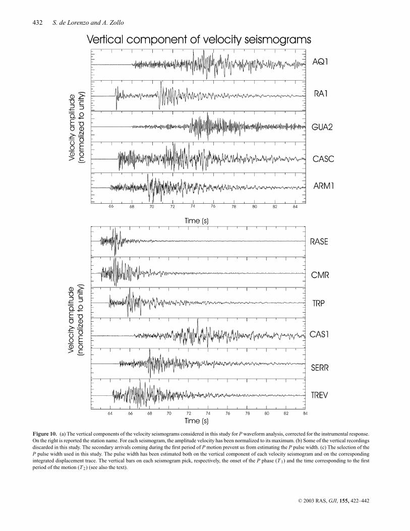
The velocity seismograms have been corrected for the instrumentalresponses given in Govoni et al. (1999). Fig. 10(a) shows the verticalcomponent of the considered traces. Owing to the generally higher

C© 2003 RAS, GJI, 155, 422–442


Figure 7. (a), (b) Study of the fault plane resolution as a function of the fault dip: plot of the σ (δ, φ)/σ 0 function in (δ, φ) space. On the bottom of each figureis reported the theoretical dip used in the simulation and the value of the η parameter (see the text).

amplitude of the vertical component of the first motion, the P pulsewidths have been measured on this component.

A detailed study has been carried out to evaluate whether siteeffects and/or source complexity can alter the shape of the P pulse,introducing a bias in the pulse width measurements.

The site effects are often recognized as being the cause of thesecondary arrivals after the first P motion. These arrivals are usuallyattributed to the presence of thin layers around the recording site,

in which part of the wavefield remains trapped and is subject tomultiple reflections. When these secondary waves arrive after thefirst period of the P motion, the source time function of the eventis preserved and can be used to model the source process (fig. 5of Deichmann 1999). In other cases, multipath effects produces adiscontinuity in the observed first P pulse shape, which is easilyinferred from a visual inspection of seismograms (Liu et al. 1994;Deichmann 1999; Courboulex et al. 1999, among the others). In our

C© 2003 RAS, GJI, 155, 422–442


Figure 8. (a), (b) Study of the fault plane resolution as a function of the fault strike: plot of the σ (δ, φ)/σ 0 function in (δ, φ) space. On the bottom of eachfigure is reported the theoretical strike used in the simulation and the value of the η parameter (see the text).

work, the recorded P-wave pulses with a clear discontinuity duringthe first period of P motion have been discarded. Some of these areshown in Fig. 10(b).

The remaining traces do not show multiple arrivals during thefirst period of P motion and have been used in the study of the faultplane orientation.

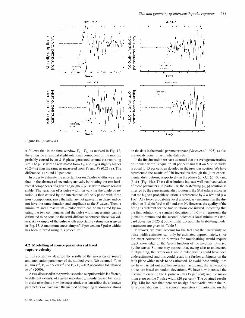
Concerning the possible effect of source complexity, we analysedthe P-wave displacement waveforms. With the exception of the sta-tion RASE, the first P displacement waveforms closely match the

simple unipolar shape expected from the S&H theoretical sourcemodel (Fig. 10c).

It is worthwhile to observe that a time difference between the timeduration as measured on velocity traces and the same as computedon displacement traces is inferred (Table 1). These differences maybe attributed either to source complexity (e.g. Boatwright 1984) orto a residual interference with the P coda; they also indicate theresolution on P pulses and have been used to estimate the averageuncertainty on our measurements (9 per cent), as reported in Table 1.

C© 2003 RAS, GJI, 155, 422–442


Figure 9. The effect of directivity variations with variation of the true fault plane orientation; the map at the centre of the figure gives the η distribution in (δ,φ) space. On the left is shown the plot of pulse widths versus distances for a low-η fault, defined by the circle in the η map. On the right is shown the plot ofpulse widths versus distance for a high-η fault, defined by the square in the η map.

Table 1. P pulse width estimation.

Station Pulse width on Pulse width on Percentagevelocity displacement difference

seismogram (s) seismogram (s)

AQ1 0.148 0.150 1.4RA1 0.193 0.171 11GUA2 0.218 0.186 19CASC 0.156 0.143 8ARM1 0.146 0.125 13RASE 0.138 0.121 12CMR 0.123 0.133 8TRP 0.176 0.166 5SERR 0.122 0.119 2TREV 0.127 0.129 1.5CAS1 0.148 0.173 17

Average = 9

We used as a P pulse width the average value between the �Testimated on the velocity seismogram and the same as measuredon integrated displacement traces (Fig. 10c), and assumed that theuncertainty associated to the P pulse width is the semi-difference ofthese two values.

The estimation of the S pulse width is more difficult to obtain,owing to the interference of the S phase with the signals followingthe P phase, usually generated around the recording site. Thesesecondary arrivals tend to reduce the quality of the S phases, makingthe uncertainty on the S pulse widths more difficult to evaluate.Bandpass filtering of the traces could certainly help to reduce thecontributions of the high-frequency phases generated around therecording site, but may severely bias the duration of the signals (inparticular, the smoothing of the ascending part of the signal causedby filtering could produce a shift of its time onset and broaden thewaveform), so that we choose to work on unfiltered traces. Moreover,for these reasons, only a limited number (five) of S pulse widthshave been extracted from the analysis of the complete data set. Inthe analysis of S pulse widths we essentially followed the outlinefirst given in Bernard & Zollo (1989). After a thorough study of thecomplete wavefield generated by a double-couple source, the authorsinferred that some useful criteria should be satisfied in order to use

the S-wave waveforms for source studies. Based on a parametricstudy on complete waveform synthetics, they concluded that thestability with time of the S polarization and the dominance of thehorizontal motion are good criteria for selecting S waveforms to beused for source parameter investigation.

When data are far from these criteria there may be several causes.In the near-source range the most frequent are the generation of alocal SP phase caused by coupling at a free surface of incident SVwith reflected P and SV near the critical angle, or generation of othermultiples (Bernard & Zollo 1989) or the presence of an anisotropicelastic layer, beneath the recording site, which causes the widelyobserved phenomenon of S-wave splitting (Crampin 1985; Zollo &Bernard 1989; Huang et al. 2000).

A complete analysis of S-wave polarization has been performedin order to test the polarization stability with time. According to theabove-mentioned criteria, we discarded all S waves characterizedby the dominance of a vertical component, which may indicate animportant contribution of near-site S-to-P converted arrival on theS waveform.

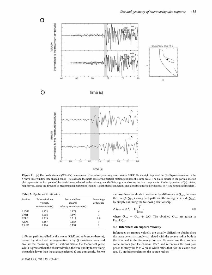
For the remaining traces, the analysis of the particle motion in theS-wave window shows that, the S signal is mainly polarized alonga single direction, which is related to the source mechanism andlocation (Fig. 11a).

According to the polarization analysis, the measurements of Spulse width have been performed on the record that has been ob-tained by rotating the N and E component along the dominant S-wave polarization direction (hereinafter referred to as the R di-rection) (Fig. 11b). The estimated S pulse widths are shown inFig. 12.

However, the quality of S pulse widths cannot be compared withthat of P phases. In fact, even if our procedure tends to minimizethe role of secondary arrivals on the R component, it is not able tocompletely remove them. To better pick the onset of S phase, we thencompared the S waves with the squared traces (Fig. 12), as suggestedby Boatwright (1980) and computed the difference between the Spulse width as measured on the velocity seismogram and the sameas measured on the squared trace, as shown in Fig. 12 and reported inTable 2. At station SPRE the onset of the phase has been chosen alsotaking into account the particle motion of Fig. 11(c), from which

C© 2003 RAS, GJI, 155, 422–442


Figure 10. (a) The vertical components of the velocity seismograms considered in this study for P waveform analysis, corrected for the instrumental response.On the right is reported the station name. For each seismogram, the amplitude velocity has been normalized to its maximum. (b) Some of the vertical recordingsdiscarded in this study. The secondary arrivals coming during the first period of P motion prevent us from estimating the P pulse width. (c) The selection of theP pulse width used in this study. The pulse width has been estimated both on the vertical component of each velocity seismogram and on the correspondingintegrated displacement trace. The vertical bars on each seismogram pick, respectively, the onset of the P phase (T 1) and the time corresponding to the firstperiod of the motion (T 2) (see also the text).

C© 2003 RAS, GJI, 155, 422–442


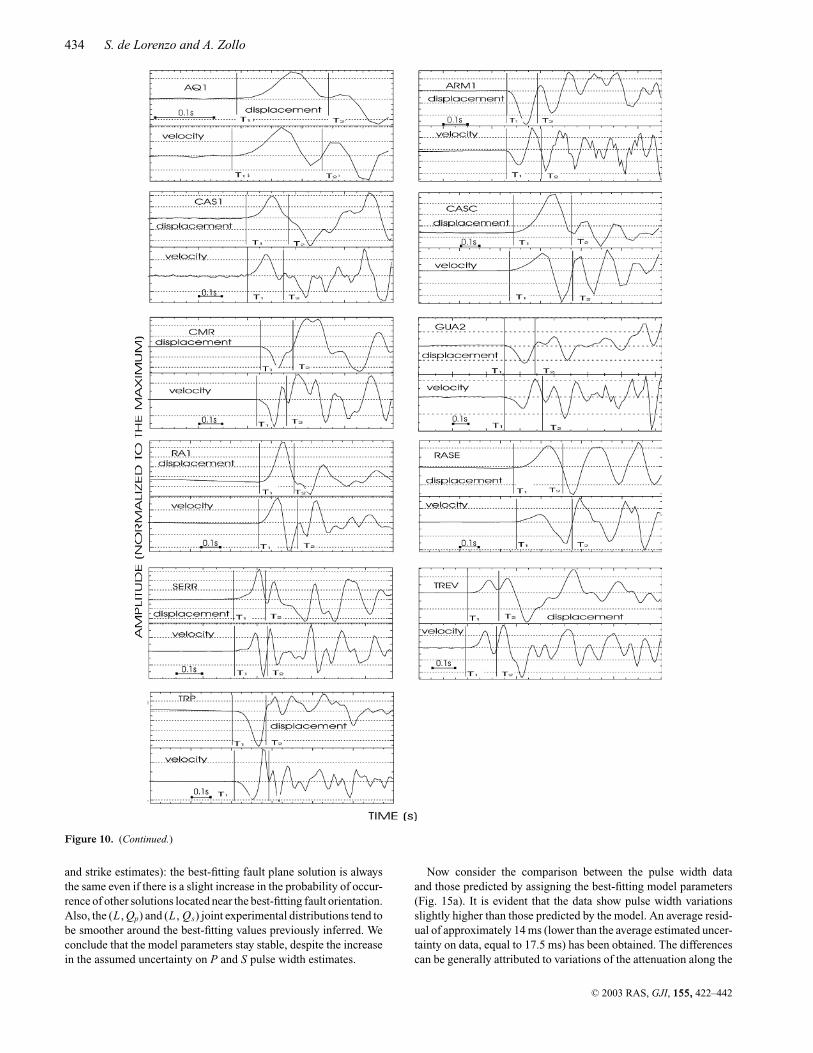
Figure 10. (Continued.)

it follows that in the time window T 01–T 02 as marked in Fig. 12,there may be a residual slight rotational component of the motion,probably caused by an S–P phase generated around the recordingsite. The pulse width as estimated from T 01 and T 02 is slightly higher(0.244 s) than the same as measured from T 1 and T 2 (0.219 s). Thedifference is around 10 per cent.

In order to estimate the uncertainties on S pulse widths we stressthat, in the absence of secondary arrivals, by rotating the two hori-zontal components of a given angle, the S pulse width should remainstable. The variation of S pulse width on varying the angle of ro-tation is then caused by the interference of the S phase with thesenoisy components, since the latter are not generally in phase and donot have the same duration and amplitude as the S waves. Then, aminimum and a maximum S pulse width can be measured by ro-tating the two components and the pulse width uncertainty can beestimated to be equal to the semi-difference between these two val-ues. An example of the pulse width uncertainty estimation is givenin Fig. 13. A maximum uncertainty of 15 per cent on S pulse widthshas been inferred using this procedure.

4.2 Modelling of source parameters at fixedrupture velocity

In this section we describe the results of the inversion of sourceand attenuation parameter of the studied event. We assumed V p =6.1 km s−1, V s = 3.5 km s−1 and V r/V s = 0.9, according to Cattaneoet al. (2000).

As we discussed in the previous section our pulse width is affected,to different extents, of a given uncertainty, mainly caused by noise.In order to evaluate how the uncertainties on data affect the unknownparameters we have used the method of mapping random deviations

on the data in the model parameter space (Vasco et al. 1995), as alsopreviously done for synthetic data sets.

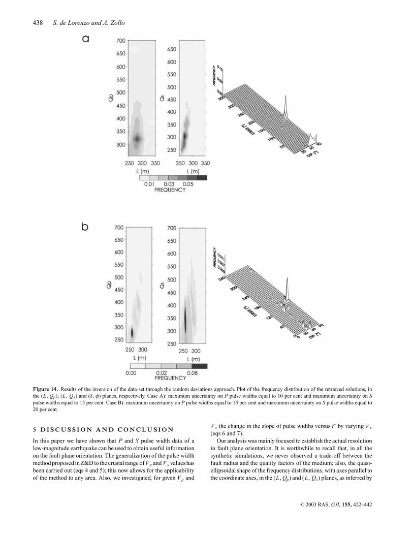
In the first inversion we have assumed that the average uncertaintyon P pulse width is equal to 10 per cent and that on S pulse widthis equal to 15 per cent, as detailed in the previous section. We haverepresented the results of 250 inversions through the joint experi-mental distributions, respectively, in the planes (L , Qp), (L , Qs) and(δ, φ) (Fig. 14a). These distributions indicate well-resolved valuesof these parameters. In particular, the best-fitting (δ, φ) solution asinferred by the experimental distribution in the (δ, φ) plane indicatesthat the highest probable solution is represented by δ = 89◦ and φ =156◦. At a lower probability level a secondary maximum in the dis-tribution (δ, φ) is for δ = 65◦ and φ = 0◦. However, the quality of thefitting is different for the two solutions considered, indicating thatthe first solution (the standard deviation of 0.014 s) represents theglobal minimum and the second indicates a local minimum (stan-dard deviation 0.025 s) of the misfit function. The best-fitting modelparameters are given in Table 3.

Moreover, we must account for the fact that the uncertainty onpulse width estimates can only be estimated approximately, sincethe exact correction on S waves for multipathing would requireexact knowledge of the Green function of the medium traversedby the waves. So, one may suspect that, owing also to undetectedmultipathing, the errors on P and S pulse widths could have beenunderestimated, and this could result in a further ambiguity on thefault plane which needs to be estimated. To avoid these ambiguitieswe have carried out another inversion run, using the same aboveprocedure based on random deviations. We have now increased themaximum error on the P pulse width (15 per cent) and the maxi-mum error on the S pulse width (20 per cent). The obtained results(Fig. 14b) indicate that there are no significant variations in the in-ferred distributions of the source parameters (in particular, on dip

C© 2003 RAS, GJI, 155, 422–442


Figure 10. (Continued.)

and strike estimates): the best-fitting fault plane solution is alwaysthe same even if there is a slight increase in the probability of occur-rence of other solutions located near the best-fitting fault orientation.Also, the (L , Qp) and (L , Qs) joint experimental distributions tend tobe smoother around the best-fitting values previously inferred. Weconclude that the model parameters stay stable, despite the increasein the assumed uncertainty on P and S pulse width estimates.

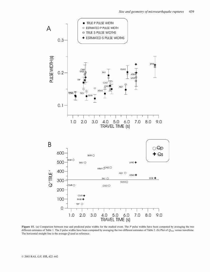
Now consider the comparison between the pulse width dataand those predicted by assigning the best-fitting model parameters(Fig. 15a). It is evident that the data show pulse width variationsslightly higher than those predicted by the model. An average resid-ual of approximately 14 ms (lower than the average estimated uncer-tainty on data, equal to 17.5 ms) has been obtained. The differencescan be generally attributed to variations of the attenuation along the

C© 2003 RAS, GJI, 155, 422–442


Figure 11. (a) The two horizontal (WE–SN) components of the velocity seismogram at station SPRE. On the right is plotted the (E–N) particle motion in theS-wave time window (the shaded zone). The east and the north axis of the particle motion plot have the same scale. The black square in the particle motionplot represents the first point of the shaded zone selected in the seismogram. (b) Seismograms showing the two components of velocity motion of (a) rotated,respectively, along the direction of predominant polarization (named R on the top seismogram) and along the direction orthogonal to R (the bottom seismogram).

Table 2. S pulse width estimation.

Station Pulse width on Pulse width on Percentagevelocity squared difference

seismogram (s) velocity seismogram (s)

LAVE 0.178 0.171 4CMR 0.204 0.198 3SPRE 0.219 0.217 0.9ARM1 0.187 0.185 1RASE 0.196 0.194 1

different paths travelled by the waves (Z&D and references therein),caused by structural heterogeneities or by Q variations localizedaround the recording site: at stations where the theoretical pulsewidth is greater than the observed value, the true quality factor alongthe path is lower than the average inferred Q and conversely. So, we

can use these residuals to estimate the difference �Qpath betweenthe true Q (Qtrue), along each path, and the average inferred (Qave),by simply assuming the following relationship:

�Ttrue = �T0 + CT

Qtrue, (8)

where Qtrue = Qave + �Q. The obtained Qtrue are given inFig. 15(b).

4.3 Inferences on rupture velocity

Inferences on rupture velocity are usually difficult to obtain sincethis parameter is strongly correlated with the source radius both inthe time and in the frequency domain. To overcome this problemsome authors (see Deichmann 1997, and references therein) pro-posed to study the P-to-S pulse width ratios that, for the elastic case(eq. 1), are independent on the source radius:

C© 2003 RAS, GJI, 155, 422–442


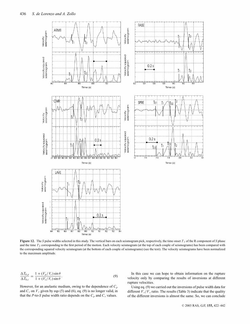
Figure 12. The S pulse widths selected in this study. The vertical bars on each seismogram pick, respectively, the time onset T 1 of the R component of S phaseand the time T 2 corresponding to the first period of the motion. Each velocity seismogram (at the top of each couple of seismograms) has been compared withthe corresponding squared velocity seismogram (at the bottom of each couple of seismograms) (see the text). The velocity seismograms have been normalizedto the maximum amplitude.

�T0,p

�T0,s= 1 + (Vp/Vr ) sin θ

1 + (Vs/Vr ) sin θ. (9)

However, for an anelastic medium, owing to the dependence of Cp

and Cs on V r given by eqs (5) and (6), eq. (9) is no longer valid, inthat the P-to-S pulse width ratio depends on the Cp and Cs values.

In this case we can hope to obtain information on the rupturevelocity only by comparing the results of inversions at differentrupture velocities.

Using eq. (9) we carried out the inversions of pulse width data fordifferent V r/V s ratio. The results (Table 3) indicate that the qualityof the different inversions is almost the same. So, we can conclude

C© 2003 RAS, GJI, 155, 422–442


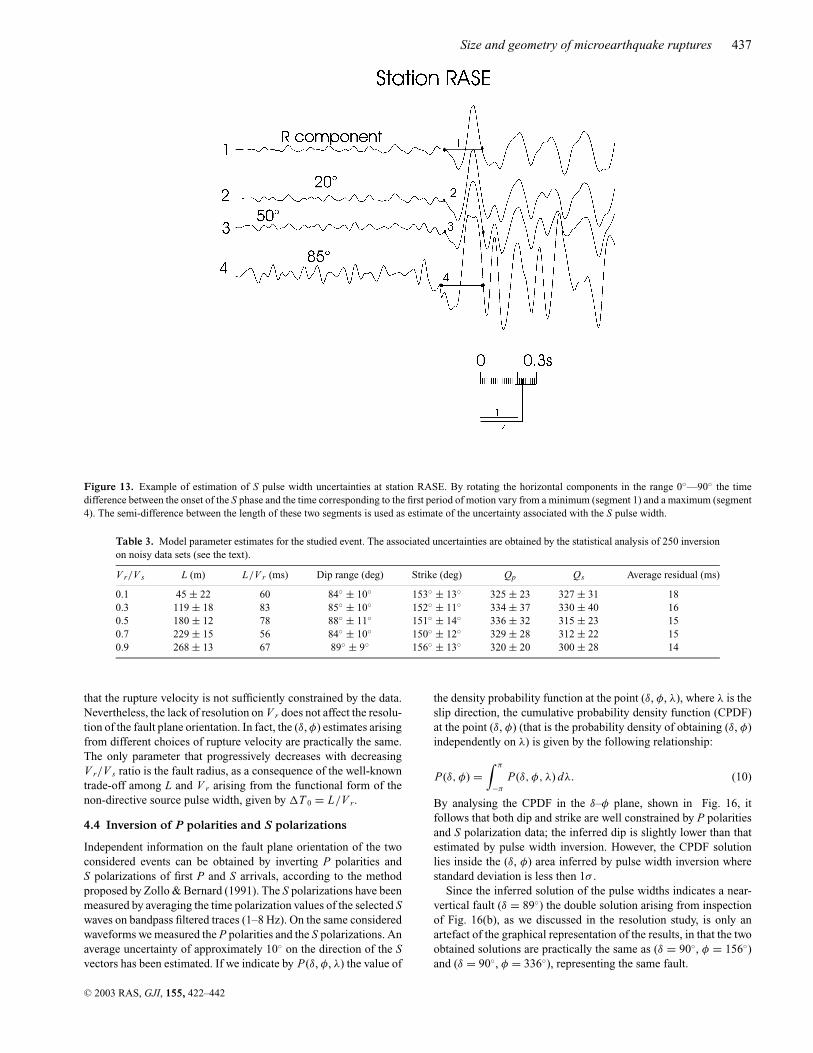
Figure 13. Example of estimation of S pulse width uncertainties at station RASE. By rotating the horizontal components in the range 0◦—90◦ the timedifference between the onset of the S phase and the time corresponding to the first period of motion vary from a minimum (segment 1) and a maximum (segment4). The semi-difference between the length of these two segments is used as estimate of the uncertainty associated with the S pulse width.

Table 3. Model parameter estimates for the studied event. The associated uncertainties are obtained by the statistical analysis of 250 inversionon noisy data sets (see the text).

V r/V s L (m) L/V r (ms) Dip range (deg) Strike (deg) Qp Qs Average residual (ms)

0.1 45 ± 22 60 84◦ ± 10◦ 153◦ ± 13◦ 325 ± 23 327 ± 31 180.3 119 ± 18 83 85◦ ± 10◦ 152◦ ± 11◦ 334 ± 37 330 ± 40 160.5 180 ± 12 78 88◦ ± 11◦ 151◦ ± 14◦ 336 ± 32 315 ± 23 150.7 229 ± 15 56 84◦ ± 10◦ 150◦ ± 12◦ 329 ± 28 312 ± 22 150.9 268 ± 13 67 89◦ ± 9◦ 156◦ ± 13◦ 320 ± 20 300 ± 28 14

that the rupture velocity is not sufficiently constrained by the data.Nevertheless, the lack of resolution on V r does not affect the resolu-tion of the fault plane orientation. In fact, the (δ, φ) estimates arisingfrom different choices of rupture velocity are practically the same.The only parameter that progressively decreases with decreasingV r/V s ratio is the fault radius, as a consequence of the well-knowntrade-off among L and V r arising from the functional form of thenon-directive source pulse width, given by �T 0 = L/V r.

4.4 Inversion of P polarities and S polarizations

Independent information on the fault plane orientation of the twoconsidered events can be obtained by inverting P polarities andS polarizations of first P and S arrivals, according to the methodproposed by Zollo & Bernard (1991). The S polarizations have beenmeasured by averaging the time polarization values of the selected Swaves on bandpass filtered traces (1–8 Hz). On the same consideredwaveforms we measured the P polarities and the S polarizations. Anaverage uncertainty of approximately 10◦ on the direction of the Svectors has been estimated. If we indicate by P(δ, φ, λ) the value of

the density probability function at the point (δ, φ, λ), where λ is theslip direction, the cumulative probability density function (CPDF)at the point (δ, φ) (that is the probability density of obtaining (δ, φ)independently on λ) is given by the following relationship:

P(δ, φ) =∫ π

−π

P(δ, φ, λ) dλ. (10)

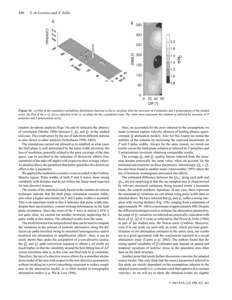
By analysing the CPDF in the δ–φ plane, shown in Fig. 16, itfollows that both dip and strike are well constrained by P polaritiesand S polarization data; the inferred dip is slightly lower than thatestimated by pulse width inversion. However, the CPDF solutionlies inside the (δ, φ) area inferred by pulse width inversion wherestandard deviation is less then 1σ .

Since the inferred solution of the pulse widths indicates a near-vertical fault (δ = 89◦) the double solution arising from inspectionof Fig. 16(b), as we discussed in the resolution study, is only anartefact of the graphical representation of the results, in that the twoobtained solutions are practically the same as (δ = 90◦, φ = 156◦)and (δ = 90◦, φ = 336◦), representing the same fault.

C© 2003 RAS, GJI, 155, 422–442


Figure 14. Results of the inversion of the data set through the random deviations approach. Plot of the frequency distribution of the retrieved solutions, inthe (L , Qp), (L , Qs) and (δ, φ) planes, respectively. Case A): maximum uncertainty on P pulse widths equal to 10 per cent and maximum uncertainty on Spulse widths equal to 15 per cent. Case B): maximum uncertainty on P pulse widths equal to 15 per cent and maximum uncertainty on S pulse widths equal to20 per cent.

5 D I S C U S S I O N A N D C O N C L U S I O N

In this paper we have shown that P and S pulse width data of alow-magnitude earthquake can be used to obtain useful informationon the fault plane orientation. The generalization of the pulse widthmethod proposed in Z&D to the crustal range of V p and V s values hasbeen carried out (eqs 4 and 5); this now allows for the applicabilityof the method to any area. Also, we investigated, for given V p and

V s the change in the slope of pulse widths versus t∗ by varying V r

(eqs 6 and 7).Our analysis was mainly focused to establish the actual resolution

in fault plane orientation. It is worthwhile to recall that, in all thesynthetic simulations, we never observed a trade-off between thefault radius and the quality factors of the medium; also, the quasi-ellipsoidal shape of the frequency distributions, with axes parallel tothe coordinate axes, in the (L , Qp) and (L , Qs) planes, as inferred by

C© 2003 RAS, GJI, 155, 422–442


Figure 15. (a) Comparison between true and predicted pulse widths for the studied event. The P pulse widths have been computed by averaging the twodifferent estimates of Table 1. The S pulse widths have been computed by averaging the two different estimates of Table 2. (b) Plot of Qtrue versus traveltime.The horizontal straight line is the average Q used as reference.

C© 2003 RAS, GJI, 155, 422–442


Figure 16. (a) Plot of the cumulative probability distribution function in the (δ, φ) plane after the inversion of P polarities and S polarizations of the studiedevent. (b) Plot of the σ (δ, φ)/σ 0 function in the (δ, φ) plane for the considered event. The white cross represents the solution as inferred by inversion of Ppolarities and S polarizations in (a).

random deviations analysis (Figs 14a and b) indicates the absenceof correlation (Menke 1984) between L , Qp and Qs in the studiedreal case. This result arises by the use of data from different stationsas also shown in other analyses (Scherbaum 1990, Z&D).

The simulations carried out allowed us to establish in what casesthe fault plane is well determined by the pulse width inversion; theloss of resolution, generally related to the poor coverage of the dataspace, can be ascribed to the reduction of directivity effects (lowvariations of the take-off angles with respect to their average value).As detailed above, the parameter that better quantifies this directivityeffect is the η parameter.

We applied the method to a seismic event recorded in the Umbria-Marche region. Pulse widths of both P and S waves show strongvariability with distance and do not follow the linear trend expectedfor non-directive sources.

The results of the statistical study based on the random deviationstechnique indicate that the fault plane orientation remains stable,also when a higher uncertainty on P and S pulse widths is assumed.This is an important result in that it indicates that pulse width data,despite their uncertainties, contain striking information on the faultplane orientation. Since the onset of the S wave at station LAVE isnot quite clear, we carried out another inversion, neglecting the Spulse width at this station. The obtained results were the same.

The misfit between true and predicted data can be used to computethe variations in the amount of inelastic attenuation along the dif-ferent ray paths travelled owing to structural heterogeneities and/orlocalized site attenuation or amplification effects. Also, it can beeasily shown that, under the assumption of a non-directive source,the Qp and Qs path corrections required to obtain a nil misfit aremuch higher, in that the variability around the best-fitting line of �Tversus traveltime data is, in this case, ascribed only to Q variations.Therefore, the use of a directive source allows for a smoother attenu-ation model of the area with respect to the non-directive assumption,without invoking an a priori smoothing constraint to reduce rough-ness in the attenuation model, as is often needed in tomographicattenuation studies (e.g. Wu & Lees 1996).

Also, we accounted for the error inherent to the assumptions wemade (constant rupture velocity, absence of healing phases, quasi-constant Q attenuation model). Also for this reason we tested thestability of the solution by increasing the expected uncertainty onP and S pulse widths. Always for the same reason, we tested ourresults versus the fault plane solution as inferred by P polarities andS polarizations inversion, obtaining comparable results.

The average Qp and Qs quality factors inferred from the inver-sion assume practically the same value, when we account for theestimated uncertainties on these parameters. Interestingly, Qp = Qs

has also been found in another study (Abercrombie 1995) where theuse of borehole seismograms prevented site effects.

The estimated difference between the Qtrue along each path andQave are not surprising in that the ray-sampled area is characterizedby relevant structural variations, being located inside a mountainchain, the central–northern Apennine; in any case, these representthe minimum Q variations we can obtain using pulse width data, asdetailed above. We have inferred that Qp and Qs suffer a strong vari-ation with varying distance (Fig. 15b), ranging from a minimum ofapproximately 50–100 to a maximum of approximately 600. Despitethe different techniques used to estimate the attenuation parameters,the range of Qs variations we inferred are practically coincident withthose of Qc (Q of S coda) as inferred by Del Pezzo & Zollo (1984)in part of the studied area, the Norcia town (Umbria). Moreover,even if in our study we used only an event, which prevents gener-alization of our attenuation estimates to the entire area, our resultsare in a good agreement with the conclusions reported in a recentattenuation study (Castro et al. 2002). The authors found that thestrong spatial variability of Q estimates may depend on spatial andtemporal variations of tectonic stress in the epicentral area otherthan on the fault structure.

Another point that needs further discussion concerns the adoptedsource model. One may think that the source parameters inferred inthis study are strictly dependent on the assumptions inherent to theadopted source model (i.e. a circular crack that ruptures at a constantvelocity). As we will try to show, the obtained results are slightly

C© 2003 RAS, GJI, 155, 422–442


more general and inherent to the basic assumptions of kinematicsof the seismic source. First, we remark that the starting point ofthe developed model is represented by the functional dependenceof the source pulse width �T 0 on the source parameters, as givenby eq. (1). It is worthwhile to recall that eq. (1) is a simplified re-lationship that arises from the basic assumptions of the kinematicsof the seismic source, in the far-field range (Fraunhofer approxima-tion) (Aki & Richards 1980); it still remains valid if we consider anunidimensional fault model (e.g. Haskell 1964). Then, by consid-ering the inelasticity of rocks, other than the source contribution tothe pulse width, one must account for the attenuation term, given byCt/Q, where C is dependent on the source time function, as shown inseveral papers (Liu 1988; de Lorenzo 1998). Based on this reason-ing, one may expect that, by recalibrating eq. (2) for a rectangularfault model, a different dependence of C on V p and V s values at thesource may be inferred. This is the focus of the discussion in that,as long as eq. (2) remains valid, the use of a different C cannot mod-ify the retrieved fault plane orientation, but only the Q estimates.In fact, since the C/Q term controls only the slope of �T versustraveltime, by using a different C, a different Q will be inferred.Nevertheless, since the source pulse width term �T 0 does not de-pend on C, the use of a different C cannot affect either the interceptterm (from which the fault length or the fault radius can be inferred)or the dispersion of data around the best-fitting straight line due tothe directivity effects (from which δ and φ are estimated).

Owing to the simplicity of the approach, we think that the pro-posed method may also be very useful in a preliminary stage of anEGF source study aimed at inferring the slip distribution of a greaterearthquake (e.g. Fletcher & Spudich 1998). It is, in fact, well knownthat the low-magnitude event one must select for the deconvolutionshould be representative only of instrument, path and site effects.The results of our study indicate that, at the scale of a local array, de-pending on data uncertainties, the directivity of the source may alsobe revealed for earthquakes of very low magnitude; for instance,the example shown in Fig. 6(b) indicates that only for L < 10 mis the directivity quite lost. This clearly implies that, in this case,the low-magnitude event considered for deconvolution in the EGFshould have a fault length of less than 10 m to avoid distortion ofthe inferred directivity function.

Results of this study seem to indicate that pulse width data proba-bly contain a number of pieces of information on the rupture proper-ties higher than those we used in a simplified model (constant rupturevelocity and abrupt stopping of rupture). In fact, the higher variabil-ity of pulse width data with respect to the predicted ones could alsoindicate, other than variability of the site response, source effectsthat cannot be reproduced with the actual model. So we think thatfurther studies, aimed at evaluating the role of a variable rupturevelocity (e.g. Sato 1994) and/or the healing phases (e.g. Fukuyama& Madariaga 1998) on the shape and duration of signals generatedby a microearthquake, could help to better explain the variability ofpulse width data with varying distance.

Finally, the (δ, φ) estimates for the two events are quite stable withvarying rupture velocity and this should indicate the absence of acorrelation between the fault plane orientation and the rupture ve-locity. This is very important as V r is the parameter less constrainedby the inversion of the pulse width data.

A C K N O W L E D G M E N T S

An anonymous reviewer is acknowledged for his criticism concern-ing the importance of the number of degrees of freedom and datauncertainties in the fault plane detection. We are particularly grate-

ful to another anonymous reviewer and to the Editor, R. Madariaga,for their constructive remarks and suggestions, which helped us toimprove the manuscript.

R E F E R E N C E S

Abercrombie, R.E., 1995. Earthquake source scaling relationship from −1to 5 M L using seismograms recorded at 2.5-km depth, J. geophys. Res.,100, 24 015–24 036.

Abercrombie, R.E., Bannister, S., Pancha, A., Webb, T.E. & Mori, J.J., 2001.Determination of fault planes in a complex aftershock sequence usingtwo-dimensional slip inversion, Geophys. J. Int., 146, 134–142

Aki, K. & Richards, P.G., 1980. Quantitative Seismology: Theory and Meth-ods, Vol. I and II, p. 932, Freeman, San Francisco.

Anderson, J.G. & Hough, S.E., 1984. A model for the shape of the Fourieramplitude spectrum at high frequencies, Bull. seism. Soc. Am., 74, 1969–1993.

Azimi, S.A., Kalinin A.V., Kalinin V.V. & Pivovarov, B.L., 1968. Impulseand transient characteristic of media with linear and quadratic absorptionlaws, Izvest., Phys. Solid Earth, 2, 88–93.

Bernard, P. & Zollo, A., 1989. Inversion of near-source S polarization forparameters of double-couple point sources, Bull. seism. Soc. Am., 79,1779–1809.

Blair, D.P. & Spathis, A.T., 1982. Attenuation of explosion generated pulsein rock masses, J. geophys. Res., 87, 3885–3892.

Boatwright, J., 1980. A spectral theory for circular seismic sources: simpleestimates of source dimension, dynamic stress drop and radiated seismicenergy, Bull. seism. Soc. Am., 70, 1–28.

Boatwright, J., 1984. The effect of rupture complexity in estimate of sourcesize, J. geophys. Res., 89, 1132–1146.

Brune, J.N., 1970. Tectonic stress and the spectra of seismic shear wavesfrom earthquakes, J. geophys. Res., 75, 4997–5009.

Castro, R.R., Monachesi, G., Trojani, L., Mucciarelli, M. & Frapiccini, M.,2002. An attenuation study using earthquakes from the 1997 Umbria-Marche sequence, J. Seismol., 6, 43–59.

Cattaneo, M. et al., 2000. The 1997 Umbria-Marche (Italy) earthquake se-quence: analysis of data recorded by the local and temporary network, J.Seismol., 4, 401–414.

Courboulex, F., Virieux, J., Deschamps, A., Gibert, D. & Zollo, A., 1996.Source investigation of a small event using empirical Green functions andsimulated annealing, Geophys. J. Int., 125, 768–780

Courboulex, F., Deichmann, N. & Gariel, J.-C., 1999. Rupture complexityof a moderate intraplate earthquake in the Alps: the 1996 M5 Rpagny-Annecy earthquake, 139, 152–160.

Crampin, S., 1985. Evaluation of anisotropy by shear wave splitting, Geo-physics, 50, 159–170.

de Lorenzo, S., 1998. A model to study the bias on Q estimates obtainedby applying the rise time method to earthquake data, in Q of the Earth,Global, Regional and Laboratory Studies, Vol. 153, pp. 419–438, edsMitchell, B.J. & Romanowicz, B., Pure and Appl. Geophys.

Del Pezzo, E. & Zollo, A., 1984. Attenuation of coda waves and turbiditycoefficient in Central Italy, Bull. seism. Soc. Am., 74, 2665–2679.

Deichmann, N., 1997. Far field pulse shapes from circular sources withvariable rupture velocities, Bull. seism. Soc. Am., 87, 1288–1296.

Deichmann, N., 1999. Empirical Green’s function: a comparison betweenpulse width measurements and deconvolution by spectral division, Bull.seism. Soc. Am., 89, 178–189.

Fletcher, J.B. & Spudich, P., 1998. Rupture characteristics of the threeM 4.7 (1992–1994) Parkfield earthquakes, J. geophys. Res., 103, 835–854.

Fukuyama, E. & Madariaga, R., 1998. Rupture dynamics of a planar fault ina 3D elastic medium: rate-and slip-weakening friction, Bull. seism. Soc.Am., 88, 1–17.

Gladwin, M.T. & Stacey, F.D., 1974. Anelastic degradation of acoustic pulsesin rock, Phys. Earth planet. Inter., 8, 332–336.

Govoni, A., Spallarossa, D., Augliera, P. & Trojani, L., 1999. The1997 Umbria-Marche Earthquake Sequence: the Combined Data Set

C© 2003 RAS, GJI, 155, 422–442


of the GNDT/SSN Temporary and the RESIL/RSM Permanent SeismicNetworks, (Oct. 18–Nov. 3, 1997), Project GNDT-CNR: PROGETTOESECUTIVO 1998, 6a1, “Struttura e sorgente della sequenza” (coor-dinator: M. Cattaneo) (on electronic CD-ROM support).

Hartzell, S.H., 1978. Earthquake aftershocks as Green’s functions, Geophys.Res. Lett., 5, 1–4.

Haskell, N., 1964. Total energy and energy spectral density of elastic waveradiation from propagating faults, Bull. seism. Soc. Am., 54, 1811–1842.

Hough, S.E., Lees, J.M. & Monastero, F., 1999. Attenuation and sourceproperties at the Coso Geothermal Area, California, Bull. seism. Soc.Am., 89, 1606–1619.

Huang, W.C. et al., 2000. Seismic polarization anisotropy beneath the CentralTibetan Plateau, J. geophys. Res., 105, 27 979–27 989.

Ichinose, G.A., Smith, K.D. & Anderson, J.G., 1997. Source parameters ofthe 15 November 1995 Border Town, Nevada, earthquake sequence, Bull.seism. Soc. Am., 87, 652–667.

Kjartansson, E., 1979. Constant Q-wave propagation and attenuation, J. geo-phys. Res., 84, 4737–4748.

Liu, H.-P., 1988. Effect of source spectrum on seismic attenuation measure-ments using the pulse broadening method, Geophysics, 53, 1520–1526.

Liu, H.-P., Warrick, R.E., Westerlund, J.B. & Kayen, E., 1994. In situ mea-surement of seismic shear-wave absorption in the San Francisco HoloceneBay Mud by the pulse-broadening method, Bull. seism. Soc. Am., 84, 62–75.

Madariaga, R., 1976. Dynamics of an expanding circular fault, Bull. seism.Soc. Am., 66, 639–666.

Menke, W., 1984. Gephysical Data Analysis: Discrete Inverse Theory, Aca-demic, New York.

Mori, J., 1996. Rupture directivity and slip distribution of the M 4.3 foreshockto the 1992 Joshua Tree Earthquake, Southern California, Bull. seism. Soc.Am., 86, 805–810.

Mori, J. & Hartzell, S., 1990. Source inversion of the 1988 Upland,California, earthquake. Determination of a fault plane for a small event,Bull. seism. Soc. Am., 80, 507–518.

Nelder, J.A. & Mead, R., 1965. A simplex method for function minimization,Comp. J., 7, 308–313.

Sato, T., 1994. Seismic radiation from circular cracks growing at variablerupture velocity, Bull. seism. Soc. Am., 84, 1199–1215.

Sato, T. & Hirasawa, T., 1973. Body wave spectra from propagating shearcracks, J. Phys. Earth., 21, 415–432.

Scherbaum, F., 1990. Combined inversion for the three-dimensional Q struc-ture and source parameters using microearthquake spectra, J. geophys.Res., 95, 12 423–12 438.

Wu, H. & Lees, M., 1996. Attenuation structure of Coso geothermal area,California, from wave pulse widths, Bull. seism. Soc. Am., 86, 1574–1590.

Vasco, D.W., Johnson, L.R. & Pulliam, J., 1995. Lateral variation in mantlestructure and discontinuities determined from P, PP, S, SS and SS–SdStravel time residuals, J. geophys. Res., 100, 24 037–24 060.

Zollo, A. & Bernard, P., 1989. S-wave polarization inversion of the 15 Octo-ber 1979, 23:19 Imperial Valley aftershock: evidence for anisotropy anda simple source mechanism, Geophys. Res. Lett., 16, 1047–1050.

Zollo, A. & Bernard, P., 1991. Fault mechanisms from near source data:joint inversion of S polarizations and P polarities, Geophys. J. Int., 104,441–451.

Zollo, A. & de Lorenzo, S., 2001. Source parameters and three-dimensionalattenuation structure from the inversion of microearthquake pulsewidth data: method and synthetic tests, J. geophys. Res., 106, 16 287–16 306.

Zollo, A., Capuano, P. & Singh, S.K., 1995. Use of small earthquake recordto determine the source time function of larger earthquakes: an alternativemethod and an application, Bull. seism. Soc. Am., 85, 1249–1256.

C© 2003 RAS, GJI, 155, 422–442

size and geometry of microearthquake seismic ruptures from p and s pulse width data

Documents