Scale-Based Gaussian Coverings: Combining

Intra and Inter Mixture Models in Image

Segmentation

Fionn Murtagh1,2,?, Pedro Contreras2 and Jean-Luc Starck3,4

1 Science Foundation Ireland, Wilton Park House,Wilton Place, Dublin 2, Ireland

2 Department of Computer Science, Royal HollowayUniversity of London, Egham TW20 0EX, England

3 CEA-Saclay, DAPNIA/SEDI-SAP, Service d’Astrophysique,91191 Gif sur Yvette, France

4 Laboratoire AIM (UMR 7158), CEA/DSM-CNRS,Universite Paris Diderot

? Corresponding author: fmurtagh@acm.org

September 3, 2009

Abstract

By a “covering” we mean a Gaussian mixture model fit to observeddata. Approximations of the Bayes factor can be availed of to judge modelfit to the data within a given Gaussian mixture model. Between families ofGaussian mixture models, we propose the Renyi quadratic entropy as anexcellent and tractable model comparison framework. We exemplify thisusing the segmentation of an MRI image volume, based (1) on a directGaussian mixture model applied to the marginal distribution function,and (2) Gaussian model fit through k-means applied to the 4D multivaluedimage volume furnished by the wavelet transform. Visual preference forone model over another is not immediate. The Renyi quadratic entropyallows us to show clearly that one of these modelings is superior to theother.

Keywords: image segmentation; clustering; model selection; minimum descrip-tion length; Bayes factor, Renyi entropy, Shannon entropy

1

arX

iv:0

909.

0481

v1 [

cs.C

V]

2 S

ep 2

009

1 Introduction

We begin with some terminology used. Segments are contiguous clusters. Inan imaging context, this means that clusters contain adjacent or contiguouspixels. For typical 2D (two-dimensional) images, we may also consider the 1D(one-dimensional) marginal which provides an empirical estimate of the pixel(probability) density function or PDF. For 3D (three-dimensional) images, wecan consider 2D marginals, based on the voxels that constitute the 3D imagevolume, or also a 1D overall marginal. An image is representative of a signal.More loosely a signal is just data, mostly here with neccessary sequence oradjacency relationships. Often we will use interchangeably the terms image,image volume if relevant, signal and data.

The word “model” is used, in general, in many senses – statistical [16],mathematical, physical models; mixture model; linear model; noise model; neu-ral network model; sparse decomposition model; even, in different senses, datamodel. In practice, firstly and foremostly for algorithmic tractability, modelsof whatever persuasion tend to be homogeneous. In this article we wish tobroaden the homogeneous mixture model framework in order to accommodateheterogeneity at least as relates to resolution scale. Our motivation is to havea rigorous model-based approach to data clustering or segmentation, that alsoand in addition encompasses resolution scale.

In Figure 1 [5], the clustering task is portrayed in its full generality. One wayto address it is to build up parametrized clusters, for example using a Gaussianmixture model (GMM), so that the cluster “pods” are approximated by themixture made up of the cluster component “peas” (a viewpoint expressed byA.E. Raftery, quoted in [27]).

A step beyond a pure “peas” in a “pod” approach to clustering is a hierar-chical approach. Application specialists often consider hierarchical algorithmsas more versatile than their partitional counterparts (for example, k-means orGaussian mixture models) since the latter tend to work well only on data setshaving isotropic clusters [23]. So in [20], we segmented astronomical images ofdifferent observing filters, that had first been matched such that they related toexactly the same fields of view and pixel resolution. For the segmentation weused a Markov random field and Gaussian mixture model; followed by a within-segment GMM clustering on the marginals. Further within-cluster marginalclustering could be continued if desired. For model fit, we used approxima-tions of the Bayes factor: the pseudo-likelihood information criterion to startwith, and for the marginal GMM work, a Bayesian information criterion. Thishierarchical- or tree-based approach is rigorous and we do not need to go be-yond the Bayes factor model evaluation framework. The choice of segmentationmethods used was due to the desire to use contiguity or adjacency informationwhenever possible, and when not possible to fall back on use of the marginal.This mixture of segmentation models is a first example of what we want toappraise in this work.

What now if we cannot (or cannot conveniently) match the images before-hand? In that case, segments or clusters in one image will not necessarily

2

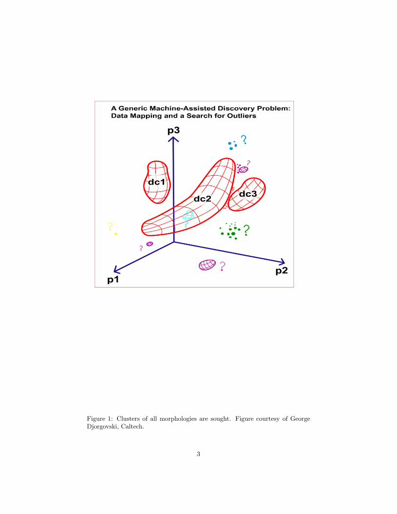
Figure 1: Clusters of all morphologies are sought. Figure courtesy of GeorgeDjorgovski, Caltech.

3

correspond to corresponding pixels in another image. That is a second exampleof where we want to evaluate different families of models.

A third example of what we want to cater for in this work is the use of wavelettransforms to substitute for spatial modeling (e.g. Markov random field model-ing). In this work one point of departure is a Gaussian mixture model (GMM)with model selection using the Bayes information criterion (BIC) approxima-tion to the Bayes factor. We extend this to a new hierarchical context. We useGMMs on resolution scales of a wavelet transform. The latter is used to provideresolution scale. Between resolution scales we do not seek a strict subset orembedding relationship over fitted Gaussians, but instead accept a lattice rela-tion. We focus in particular on the global quality of fit of this wavelet-transformbased Gaussian modeling. We show that a suitable criterion of goodness of fitfor cross-model family evaluations is given by Renyi quadratic entropy.

1.1 Outline of the Article

In section 2 we review briefly how modeling, with Gaussian mixture modelingin mind, is mapped into information.

In section 3 we motivate Gaussian mixture modeling as a general clusteringapproach.

In section 4 we introduce entropy and focus on the additivity property. Thisproperty is importatant to us in the following context. Since hierarchical clustermodeling, not well addressed or supported by Gaussian mixture modeling, is ofpractical importance we will seek to operationalize a wavelet transform approachto segmentation. The use of entropy in this context is discussed in section 5.

The fundamental role of Shannon entropy together with some other defini-tions of entropy in signal and noise modeling is reviewed in section 6. Signaland noise modeling are potentially usable for image segmentation.

For the role of entropy in image segmentation, section 2 presented the stateof the art relative to Gaussian mixture modeling; and section 6 presented thestate of the art relative to (segmentation-relevant) filtering.

What if we have segmentations obtained through different modelings? Sec-tion 7 addresses this through the use of Renyi quadratic entropy. Finally, section8 presents a case study.

2 Minimum Description Length and Bayes In-formation Criterion

For what we may term a homogenous modeling framework, the minimum de-scription length, MDL, associated with Shannon entropy [25], will serve us well.However as we will now describe it does not cater for hierarchically embeddedsegments or clusters. An example of where hierarchical embedding, or nestedclusters, come into play can be found in [20].

Following Hansen and Yu [12], we consider a model class, Θ, and an instanti-ation of this involving parameters θ to be estimated, yielding θ. We have θ ∈ Rk

4

so the parameter space is k-dimensional. Our observation vectors, of dimensionm, and of cardinality n, are defined as: X = {xi|1 ≤ i ≤ n}. A model, M , isdefined as f(X|θ), θ ∈ Θ ⊂ Rk, X = {xi|1 ≤ i ≤ n}, xi ∈ Rm, X ⊂ Rm. Themaximum likelihood estimator (MLE) of θ is θ: θ = argmaxθf(X|θ).

Using Shannon information, the description length of X based on a set ofparameter values θ is: − log f(X|θ). We need to transmit parameters also (as,for example, in vector quantization). So overall code length is: − log f(X|θ) +L(θ). If the number of parameters is always the same, then L(θ) can be constant.Minimizing − log f(X|θ) over θ is the same as maximizing f(X|θ), so if L(θ)is constant, then MDL (minimum description length) is identical to maximumlikelihood, ML.

The MDL information content of the ML, or equally Bayesian maximum aposteriori (MAP) estimate, is the code length of − log f(X|θ) +L(θ). First, weneed to encode the k coordinates of θ, where k is the (Euclidean) dimensionof the parameter space. Using the uniform encoder for each dimension, theprecision of coding is then 1/

√n implying that the magnitude of the estimation

error is 1/√n. So the price to be paid for communicating θ is k · (− log 1/

√n) =

k2 log n nats [12]. Going beyond the uniform coder is also possible with the sameoutcome.

In summary, MDL with simple suppositions here (in other circumstances wecould require more than two stages, and consider other coders) is the sum ofcode lengths for (i) encoding data using a given model; and (ii) transmittingthe choice of model. The outcome is minimal − log f(X|θ) + k

2 log n.In the Bayesian approach we assign a prior to each model class, and then we

use the overall posterior to select the best model. Schwarz’s Bayesian Informa-tion Criterion (BIC), which approximates the Bayes factor of posterior ratios,takes the form of the same penalized likelihood, − log f(X|θ) + k

2 log n, whereθ = ML or MAP estimate of θ. See [7] for case studies using BIC.

3 Segmentation of Arbitrary Signal through aGaussian Mixture Model

Notwithstanding the fact that often signal is not Gaussian, cf. the illustra-tion of Figure 1, we can fit observational data – density f with support in m-dimensional real space, Rm – by Gaussians. Consider the case of heavy taileddistributions.

Heavy tailed probability distributions, examples of which include long mem-ory or 1/f processes (appropriate for financial time series, telecommunicationstraffic flows, etc.) can be modeled as a generalized Gaussian distribution (GGD,also known as power exponential, α-Gaussian distribution, or generalized Lapla-cian distribution):

f(x) =β

2αΓ(1/β)exp−(| x | /α)β

5

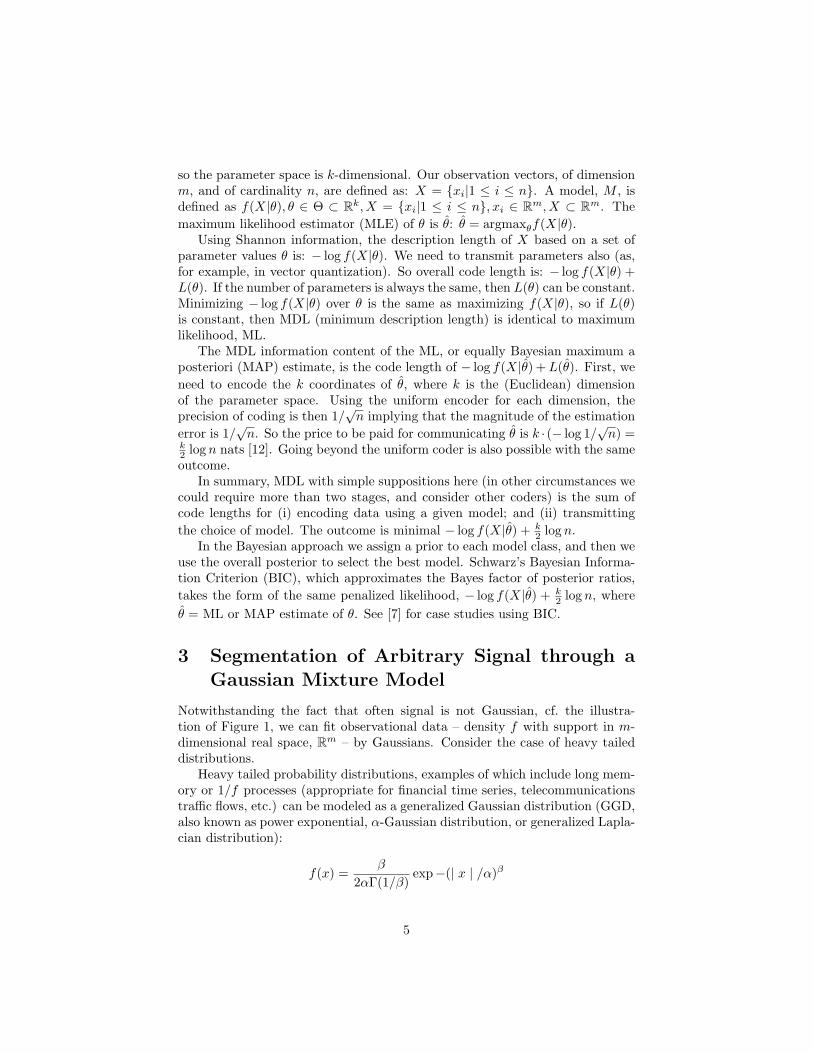
where– scale parameter, α, represents the standard deviation,– the gamma function, Γ(a) =

∫∞0xa−1e−xdx, and

– shape parameter, β, is the rate of exponential decay, β > 0.A value of β = 2 gives us a Gaussian distribution. A value of β = 1 gives a

double exponential or Laplace distribution. For 0 < β < 2, the distribution isheavy tailed. For β > 2, the distribution is light tailed.

Heavy tailed noise can be modeled by a Gaussian mixture model with enoughterms [1]. Similarly, in speech and audio processing, low-probability and large-valued noise events can be modeled as Gaussian components in the tail of thedistribution. A fit of this fat tail distribution by a Gaussian mixture model iscommonly carried out [31]. As in Wang and Zhao [31], one can allow Gaussiancomponent PDFs to recombine to provide the clusters which are sought. Theseauthors also found that using priors with heavy tails, rather than using standardGaussian priors, gave more robust results. But the benefit appears to be verysmall.

Gaussian mixture modeling of heavy tailed noise distributions, e.g. genuinesignal and flicker or pink noise constituting a heavy tail in the density, is there-fore feasible. A solution is provided by a weighted sum of Gaussian densitiesoften with decreasing weights corresponding to increasing variances. Mixingproportions for small (tight) variance components are large (e.g., 0.15 to 0.3)whereas very large variance components have small mixing proportions.

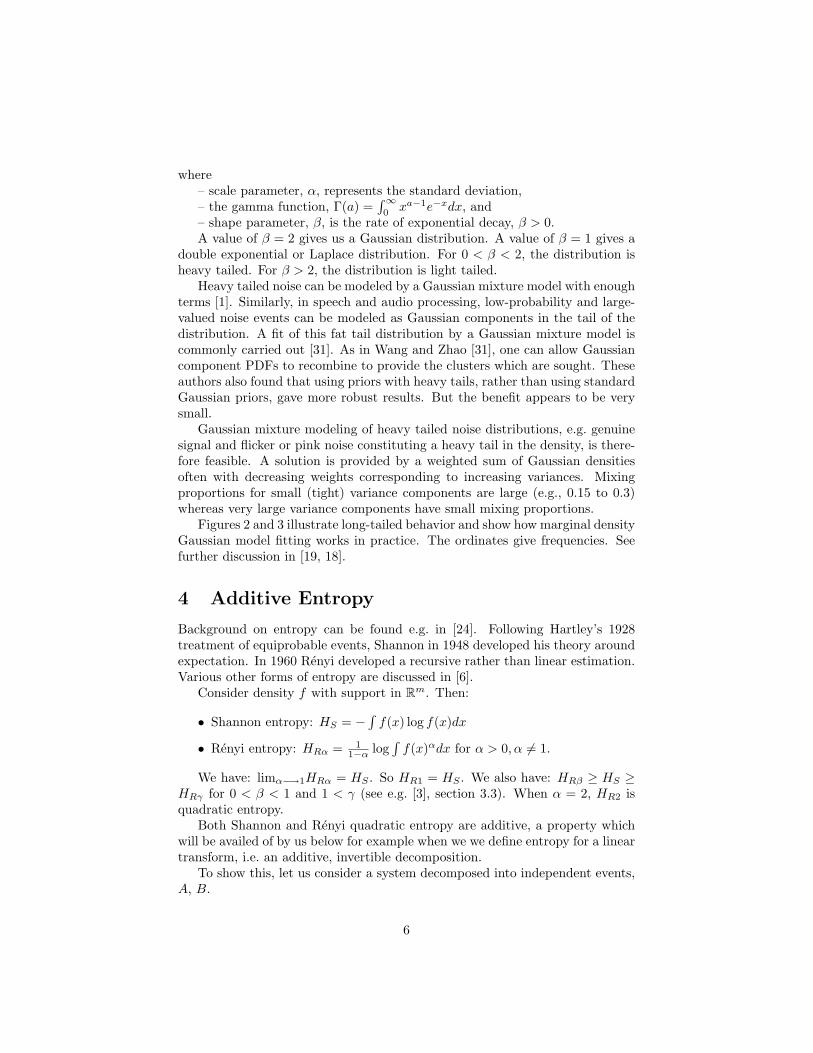
Figures 2 and 3 illustrate long-tailed behavior and show how marginal densityGaussian model fitting works in practice. The ordinates give frequencies. Seefurther discussion in [19, 18].

4 Additive Entropy

Background on entropy can be found e.g. in [24]. Following Hartley’s 1928treatment of equiprobable events, Shannon in 1948 developed his theory aroundexpectation. In 1960 Renyi developed a recursive rather than linear estimation.Various other forms of entropy are discussed in [6].

Consider density f with support in Rm. Then:

• Shannon entropy: HS = −∫f(x) log f(x)dx

• Renyi entropy: HRα = 11−α log

∫f(x)αdx for α > 0, α 6= 1.

We have: limα−→1HRα = HS . So HR1 = HS . We also have: HRβ ≥ HS ≥HRγ for 0 < β < 1 and 1 < γ (see e.g. [3], section 3.3). When α = 2, HR2 isquadratic entropy.

Both Shannon and Renyi quadratic entropy are additive, a property whichwill be availed of by us below for example when we we define entropy for a lineartransform, i.e. an additive, invertible decomposition.

To show this, let us consider a system decomposed into independent events,A, B.

6

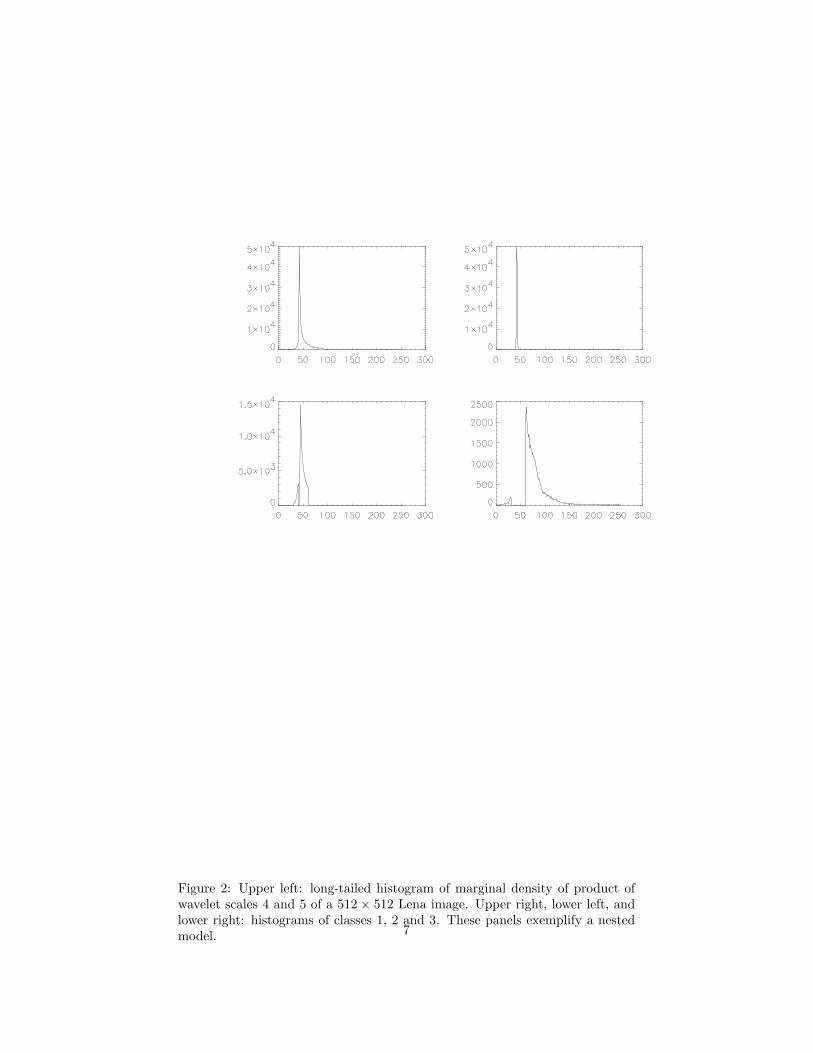
Figure 2: Upper left: long-tailed histogram of marginal density of product ofwavelet scales 4 and 5 of a 512× 512 Lena image. Upper right, lower left, andlower right: histograms of classes 1, 2 and 3. These panels exemplify a nestedmodel. 7

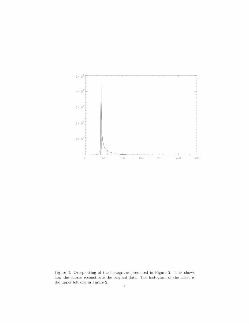
Figure 3: Overplotting of the histograms presented in Figure 2. This showshow the classes reconstitute the original data. The histogram of the latter isthe upper left one in Figure 2.

8

So p(AB) (alternatively written: p(A&B) or p(A+B)) = p(A)p(B). Shan-non information is then IABS = − log p(AB) = − log p(A)− log p(B), so the in-formation of independent events is additive. Multiplying across by p(AB), andtaking p(AB) = p(A) when considering only event A and similarly for B, leadsto additivity of Shannon entropy for independent events, HAB

S = HAS +HB

S .Similarly for Renyi quadratic entropy we use p(AB) = p(A)p(B) and we

have: − log p2(AB) = −2 log p(AB) = −2 log (p(A)p(B)) = −2 log p(A) −2 log p(B) = − log p2(A)− log p2(B).

5 The Entropy of a Wavelet Transformed Signal

The wavelet transform is a resolution-based decomposition – hence with anin-built spatial model: see e.g. [29, 30].

A redundant wavelet transform is most appropriate, even if decimated alter-natives can be considered straightforwardly too. This is because segmentation,taking information into account at all available resolution scales, simply needsall available information. A non-redundant (decimated, e.g., pyramidal) wavelettransform is most appropriate for compression objectives, but it can destroythrough aliasing potentially important faint features.

If f is the original signal, or images, then the following family of redundantwavelet transforms includes various discrete transforms such as the isotropic,B3 spline, a trous transform, called the starlet wavelet transform in [30].

f =S∑s=1

ws + wS+1 (1)

where: wS+1 is the smooth continuum, not therefore wavelet coefficients; ws arewavelet coefficients at scale s. Dimensions of f, ws, wS+1 are all identical.

Nothing prevents us having a redundant Haar or, mutatis mutandis, redun-dant biorthogonal 9/7 wavelet transform (used in the JPEG-2000 compressionstandard). As mentined above, our choice of starlet transform is due to nodamage being done, through decimation, to faint features in the image. Asa matched filter the starlet wavelet function is appropriate for many types ofbiological, astronomical and other images [30].

Define the entropy, H, of the wavelet transformed signal as the sum of theentropies Hs at the wavelet resolution levels, s:

H =S∑s=1

Hs (2)

Shannon and quadratic Renyi entropies are additive, as noted in section4. For additivity, independence of the summed components is required. Aredundant transform does not guarantee independence of resolution scales, s =1, 2, . . . , S. However in practice we usually have approximate independence.Our argument in favor of bypassing indepence of resolution scales is based onthe practical and interpretation-related benefits of doing so.

9

Next we will review the Shannon entropy used in this context. Then wewill introduce a new application of the Renyi quadratic entropy, again in thiswavelet transform context.

6 Entropy Based on a Wavelet Transform and aNoise Model

Image filtering allows, as a special case, thresholding and reading off segmentedregions. Such approaches have been used for very fast – indeed one could saywith justice, turbo-charged – clustering. See [21, 22].

Noise models are particularly important in the physical sciences (cf. CCD,charge-coupled device, detectors) and the following approach was developed in[28]. Observed data f in the physical sciences are generally corrupted by noise,which is often additive and which follows in many cases a Gaussian distribution,a Poisson distribution, or a combination of both. Other noise models may alsobe considered. Using Bayes’ theorem to evaluate the probability distribution ofthe realization of the original signal g, knowing the data f , we have

p(g|f) =p(f |g).p(g)

p(f)(3)

p(f |g) is the conditional probability distribution of getting the data f given anoriginal signal g, i.e. it represents the distribution of the noise. It is given, inthe case of uncorrelated Gaussian noise with variance σ2, by:

p(f |g) = exp

− ∑pixels

(f − g)2

2σ2

(4)

The denominator in equation (3) is independent of g and is considered as aconstant (stationary noise). p(g) is the a priori distribution of the solutiong. In the absence of any information on the solution g except its positivity, apossible course of action is to derive the probability of g from its entropy, whichis defined from information theory.

If we know the entropy H of the solution (we describe below different waysto calculate it), we derive its probability by

p(g) = exp(−αH(g)) (5)

Given the data, the most probable image is obtained by maximizing p(g|f).This leads to algorithms for noise filtering and to deconvolution [29].

We need a probability density p(g) of the data. The Shannon entropy, HS

[26], is the summing of the following for each pixel,

HS(g) = −Nb∑k=1

pk log pk (6)

10

where X = {g1, ..gn} is an image containing integer values, Nb is the number ofpossible values of a given pixel gk (256 for an 8-bit image), and the pk valuesare derived from the histogram of g as pk = mk

n , where mk is the number ofoccurrences in the histogram’s kth bin.

The trouble with this approach is that, because the number of occurrencesis finite, the estimate pk will be in error by an amount proportional to m

− 12

k

[9]. The error becomes significant when mk is small. Furthermore this kind ofentropy definition is not easy to use for signal restoration, because its gradientis not easy to compute. For these reasons, other entropy functions are generallyused, including:

• Burg [2]:

HB(g) = −n∑k=1

ln(gk) (7)

• Frieden [8]:

HF (g) = −n∑k=1

gk ln(gk) (8)

• Gull and Skilling [11]:

HG(g) =n∑k=1

gk −Mk − gk ln(gkMk

)(9)

where M is a given model, usually taken as a flat image

In all definitions n is the number of pixels, and k represents an index pixel.For the three entropies above, unlike Shannon’s entropy, a signal has maximuminformation value when it is flat. The sign has been inverted (see equation (5)),to arrange for the best solution to be the smoothest.

Now consider the entropy of a signal as the sum of the information at eachscale of its wavelet transform, and the information of a wavelet coefficient isrelated to the probability of it being due to noise. Let us look at how thisdefinition holds up in practice. Denoting h the information relative to a singlewavelet coefficient, we define

H(X) =l∑

j=1

nj∑k=1

h(wj,k) (10)

with the information of a wavelet coefficient, h(wj,k) = − ln p(wj,k), (Burg’sdefinition rather than Shannon’s). l is the number of scales, and nj is thenumber of samples in wavelet band (scale) j. For Gaussian noise, and recallingthat wavelet coefficients at a given resolution scale are of zero mean, we get

h(wj,k) =w2j,k

2σ2j

+ constant (11)

11

where σj is the noise at scale j. When we use the information in a functional tobe minimized (for filtering, deconvolution, thresholding, etc.), the constant termhas no effect and we can omit it. We see that the information is proportionalto the energy of the wavelet coefficients. The larger the value of a normalizedwavelet coefficient, then the lower will be its probability of being noise, and thehigher will be the information furnished by this wavelet coefficient.

In summary,

• Entropy is closely related to energy, and as shown can be reduced to it, inthe Gaussian context.

• Using probability of wavelet coefficients is a very good way of addressingnoise, but less good for non-trivial signal.

• Entropy has been extended to take account of resolution scale.

In this section we have been concerned with the following view of the data:f = g + α + ε where observed data f is comprised of original data g, plus(possibly) background α (flat signal, or stationary noise component), plus noiseε. The problem of discovering signal from noisy, observed data is important andhighly relevant in practice but it has taken us some way from our goal of clusteror segmentation modeling of f – which could well have been cleaned and henceapproximate well g prior to our analysis.

An additional reason for discussing the work reported on in this section isthe common processing platform provided by entropy.

Often the entropy provides the optimization criterion used (see [10, 24, 29],and many other works besides). In keeping with entropy as having a key rolein a common processing platform we instead want to use entropy for cross-model selection. Note that it complements other criteria used, e.g. ML, leastsquares, etc. We turn now towards a new way to define entropy for applicationacross families of GMM analysis, wavelet transform based approaches, and otherapproaches besides, all with the aim of furnishing alternative segmentations.

7 Model-Based Renyi Quadratic Entropy

Consider a mixture model:

f(x) =k∑i=1

αifi(x) withk∑i=1

αi = 1 (12)

Here f could correspond to one level of a mutiple resolution transformed signal.The number of mixture components is k.

Now take fi as Gaussian:

fi(x) = fi(x|µ, V ) =(

(2π)−m2 |Vi|−

12

)exp

(−1

2(x− µi)V −1

i (x− µi)t)

(13)

12

where x, µi ∈ Rm, Vi ∈ Rm×m.Take

Vi = σ2i I (14)

(I = identity) for simplicity of the basic components used in the model.A (i) parsimonious (ii) covering of these basic components can use a BIC

approximation to the Bayes factor (see section 2) for selection of model, k.Each of the functions fi comprising the new basis for the observed density f

can be termed a radial basis [15]. A radial basis network, in this context, is aniterative EM-like fit optimization algorithm. An alternative view of parsimonyis the view of a sparse basis, and model fitting is sparsification. This theme ofsparse or compressed sampling is pursued in some depth in [30].

We have: ∫ ∞−∞

αifi(x|µi, Vi) . αjfj(x|µj , Vj) dx (15)

= αiαjfij(µi − µj , Vi + Vj) (16)

See [24] or [10]. Consider the case – apropriate for us – of only distinct clustersso that summing over i, j we get:∑

i

∑j

(1− δij)αiαjfij(µi − µj , Vi + Vj) (17)

HenceHR2 = − log

∫ ∞−∞

f(x)2 dx (18)

can be written as:

− log∫ ∞−∞

αifi(x|µi, Vi) . αjfj(x|µj , Vj) dx (19)

= − log∑i

∑j

(1− δij)αiαjfij(µi − µj , Vi + Vj) (20)

= − log∑i

∑j

(1− δij)fij(µi − µj , 2σ2I) (21)

from restriction (14) and also restricting the weights, αi, αj = 1,∀i 6= j. Theterm we have obtained expresses interactions beween pairs. Function fij is aGaussian. There are evident links here with Parzen kernels [4, 13] and clusteringthrough mode detection (see e.g. [14], and [17] and references therein).

For segmentation we will simplify further expression (20) to take into accountjust the equiweighted segments reduced to their mean (cf. [4]).

In line with how we defined mutiple resolution entropy in section 6, wecan also define the Renyi quadratic information of wavelet transformed data asfollows:

HR2 =S∑s=1

HsR2 (22)

13

8 Case Study

8.1 Data Analysis System

In this work, we have used MRI (magnetic resonance imaging) and PET (positronemission tomography) image data volumes, and (in a separate study) a data vol-ume of galaxy positions derived from 3D cosmology data. A 3D starlet or B3

spline a trous wavelet transform is used with these 3D data volumes. Figures4 and 5 illustrate the system that we built. For 3D data volumes, we supportthe following formats: FITS, ANALYZE (.img, .hdr), coordinate data (x, y, z),and DICOM; together with AVI video format. For segmentation, we cater formarginal Gaussian mixture modeling, of a 3D image volume. For multivalued3D image volumes (hence 4D hypervolumes) we used Gaussian mixture model-ing restricted to identity variances, and zero covariances, i.e. k-means. Basedon a marginal Gaussian mixture model, BIC is used. Renyi quadratic entropyis also supported. A wide range of options are available for presentation anddisplay (traversing frames, saving to video, vantage point XY or YZ or XZ,zooming up to 800%, histogram equalization by frame or image volume). Thesoftware, MR3D version 2, is available for download at www.multiresolution.tv.The wavelet functionality requires a license to be activated, and currently thecode has been written for PCs running Microsoft Windows only.

8.2 Segmentation Algorithms Used

Consider T1, an aggregated representative brain, derived from MRI data. Itis of dimensions 91 × 109 × 91. See Figure 4. In the work described here asimage format for the 3D or 4D image volumes we used the FITS, Flexible ImageTransport System, format.

The first model-based segmentation was carried out as follows.

• We use “Marginal Range” in the “Segmentation” pull-down menu to de-cide, from the plot produced, that the BIC criterion suggests that a 6cluster solution is best.

• Then we use “Marginal” with 6 clusters requested, again in the “Segmen-tation” pull-down menu. Save the output as: T1 segm marg6.fits.

Next an alternative model-based segmentation is carried out in waveletspace.

• Investigate segmentation in wavelet space. First carry out a wavelet trans-form. The B3 spline a trous wavelet transform is used with 4 levels (i.e.3 wavelet resolution scales). The output produced is in files: T1 1.fits,T1 2.fits, T1 3.fits, T1 4.fits.

• Use the wavelet resolution scales as input to “K-Means”, in the “Seg-mentation” pull-down menu. Specify 6 clusters. We used 6 clustersbecause of the evidence suggested by BIC in the former modeling, and

14

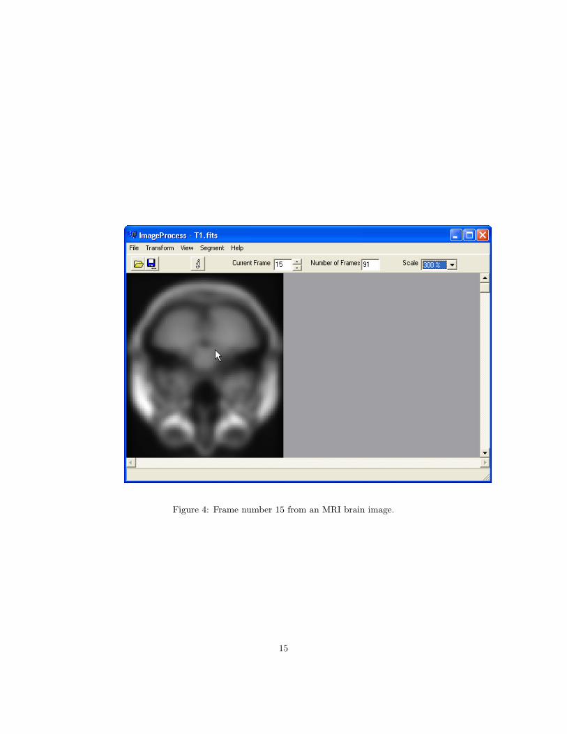
Figure 4: Frame number 15 from an MRI brain image.

15

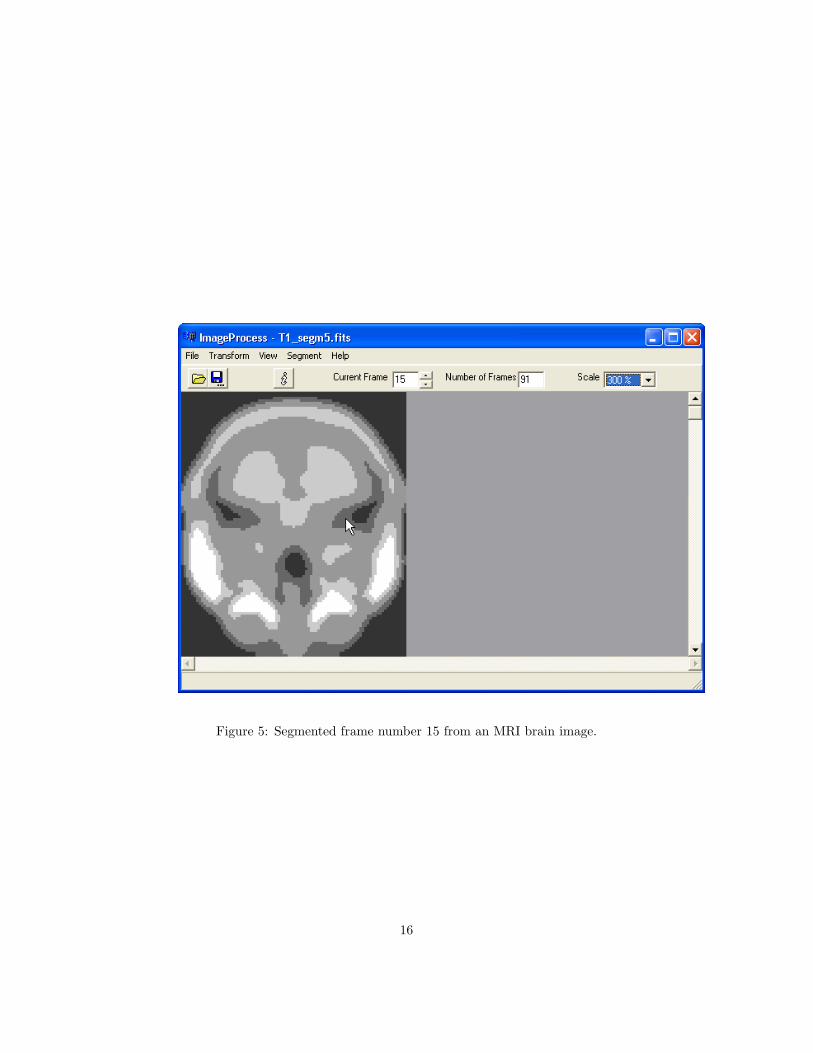
Figure 5: Segmented frame number 15 from an MRI brain image.

16

hence for comparability between the two modelings. Save the output as:T1 segm kmean6.fits.

8.3 Evaluation of Two Segmentations

We have two segmentations. The first is a segmentation found from the voxel’smarginal distribution function. The second outcome is a segmentation foundfrom the multivalued 3D (hence 4D) wavelet transform.

Now we will assess T1 segm marg6 versus T1 segm kmean6. If we use BIC,using the T1 image and first one and then the second of these segmented images,we find essentially the same BIC value. (The BIC values of the two segmenta-tions differ in about the 12th decimal place.) Note though that the model usedby BIC is the same as that used for the marginal segmentation; but it is notthe same as that used for k-means. Therefore it is not fair to use BIC to assessacross models, as opposed to its use within a family of the same model.

Using Renyi quadratic entropy, in the “Segmentation” pull-down menu, wefind 4.4671 for the marginal result, and 1.7559 for the k-means result.

Given that parsimony is associated with small entropy here, this result pointsto the benefits of segmentation in the wavelet domain, i.e. the second of our twomodeling outcomes.

9 Conclusions

We have shown that Renyi quadratic entropy provides an effective way to com-pare model families. It bypasses the limits of intra-family comparison, such asis offered by BIC.

We have offered some preliminary experimental evidence too that directunsupervised classification in wavelet transform space can be more effectivethan model-based clustering of derived data. Intended by the latter (“deriveddata”) are marginal distributions.

Our innovative results are very efficient from computational and storageviewpoints. The wavelet transform for a fixed number of resolution scales iscomputationally linear in the cardinality of the input voxel set. The pairwiseinteraction terms feeding the Renyi quadratic entropy are also efficient. Forboth of these aspects of our work, iterative or other optimization is not calledfor.

Acknowledgements

Dimitrios Zervas wrote the graphical user interface and contributed to otherparts of the software described in section 8.

17

References

1. Blum, R.S.; Zhang, Y.; Sadler, B.M.; Kozick, R.J. On the approximation ofcorrelated non-Gaussian noise PDFs using Gaussian mixture models, Con-ference on the Applications of Heavy Tailed Distributions in Economics,Engineering and Statistics, American University, Washington DC, 1999.

2. Burg, J. Multichannel maximum entropy spectral analysis, MultichannelMaximum Entropy Spectral Analysis, Annual Meeting International SocietyExploratory Geophysics, reprinted in Modern Spectral Analysis, Ed. D.G.Childers, IEEE Press, 34–41, 1978.

3. Cachin, C. Entropy Measures and Unconditional Security in Cryptography,PhD Thesis, ETH Zurich, 1997.

4. Youngjin Lee; Seungjin Choi, Minimum entropy, k-means, spectral cluster-ing, Proceedings of the International Joint Conference on Neural Networks(IJCNN), pp. 117–122, Budapest, Hungary, July 25-29, 2004.

5. Djorgovski, S.G.; Mahabal, A.; Brunner, R.; Williams, R.; Granat, R.;Curkendall, D.; Jacob, J.; Stolorz, P. Exploration of parameter spaces in aVirtual Observatory 2001, in Astronomical Data Analysis, eds. J.-L. Starck& F. Murtagh, Proceedings of the SPIE Volume 4477, 43–52.

Djorgovski, S.G.; Brunner, R.; Mahabal, A.; Williams, R.; Granat, R.;Stolorz, P. Challenges for cluster analysis in a Virtual Observatory, in Sta-tistical Challenges in Astronomy III, eds. E. Feigelson and J. Babu, NewYork: Springer Verlag, p. 125.

6. Esteban, M.D.; Morales, D. A summary of entropy statistics, Kybernetika1995, 31, 337–346.

7. Fraley, C.; Raftery, A.E., How many clusters? Which clustering method?– answers via model-based cluster analysis, Computer Journal 1998, 41,578–588.

8. Frieden, B. Image enhancement and restoration, in Topics in AppliedPhysics, vol. 6, Springer-Verlag, 1975, 177–249.

9. Frieden, B. Probability, Statistical Optics, and Data Testing: A ProblemSolving Approach, 2nd ed., Springer-Verlag, 1991.

10. Gokcay, E.; Principe, J.C. Information theoretic clustering, IEEE Trans-actions on Pattern Analysis and Machine Intelligence 2002, 24, 158–171.

11. Gull, S.; Skilling, J. MEMSYS5 Quantified Maximum Entropy User’s Man-ual, 1991.

12. Hansen, M.H.; Bin Yu, Model selection and the principle of minimum de-scription length, Journal of the American Statistical Association 2001, 96,746–774.

18

13. Jenssen, R., Information theoretic learning and kernel methods, in Infor-mation Theory and Statistical Learning, F. Emmert-Streib and M. Dehmer,eds., Springer, 2009.

14. Katz, J.O.; Rohlf, F.J., Function-point cluster analysis, Systematic Zoology1973, 22, 295–301.

15. MacKay, D.J.C. Information Theory, Inference, and Learning Theory,Cambridge University Press, 2003.

16. McCullagh, P., What is a statistical model?, Annals of Statistics 2002, 30,1225–1310.

17. Murtagh, F., A survey of algorithms for contiguity-constrained clusteringand related problems, Computer Journal 1985, 28, 82–88.

18. Murtagh, F.; Starck, J.L., Quantization from Bayes factors with applicationto multilevel thresholding, Pattern Recognition Letters 2003, 24, 2001–2007.

19. Murtagh, F.; Starck, J.L. Bayes factors for edge detection from waveletproduct spaces, Optical Engineering 2003, 42, 1375–1382.

20. Murtagh, F.; Raftery, A.E.; Starck, J.L., Bayesian inference for multibandimage segmentation via model-based cluster trees, Image and Vision Com-puting 2005, 23, 587–596.

21. Murtagh, F.; Starck, J.L.; Berry, M., Overcoming the curse of dimension-ality in clustering by means of the wavelet transform, Computer Journal2000, 43, 107–120.

22. Murtagh, F.; Starck, J.L., Pattern clustering based on noise modeling inwavelet space, Pattern Recognition 1998, 31, 847–855.

23. Nagy, G. State of the art in pattern recognition, Proceedings of the IEEE1968, 56, 836–862.

24. Principe, J.C.; Dongxin Xu, Information-theoretic learning using Renyi’squadratic entropy, International Conference on ICA and Signal Separation,August 1999, pp. 245–250.

25. Rissanen, J., Information and Complexity in Statistical Modeling, Springer,2007.

26. Shannon, C.E., A mathematical theory for communication, Bell SystemsTechnical Journal 1948, 27, 379–423.

27. Silk, J., An astronomer’s perspective on SCMA III, in Statistical Challengesin Modern Astronomy, E.D. Feigelson and G.J. Babu, Eds., Springer, 2003,pp. 387–394.

19

28. Starck, J.L.; Murtagh, F.; Gastaud, R., A new entropy measure based onthe wavelet transform and noise modeling, IEEE Transactions on Circuitsand Systems – II: Analog and Digital Signal Processing 1998, 45, 1118–1124.

29. Starck, J.L.; Murtagh, F., Astronomical Image and Data Analysis,Springer, 2002. 2nd edition, 2006.

30. Starck, J.L., Murtagh, F.; Fadili, J., Sparse Image and Signal Processing:Wavelets, Curvelets, Morphological Diversity, Cambridge University Press,forthcoming.

31. Wang, S.; Zhao, Y., Online Bayesian tree-structured transformation ofHMMs with optimal model selection for speaker adaptation, IEEE Trans-actions on Speech and Audio Processing 2001, 9, 663–677.

20