Scalable Planning and Learning for Multiagent POMDPs:Extended Version

Christopher AmatoCSAIL, MIT

Cambridge, MA 02139camato@csail.mit.edu

Frans A. OliehoekInformatics Institute, University of Amsterdam

Dept. of CS, University of Liverpoolfrans.oliehoek@liverpool.ac.uk

December 1, 2014

Abstract

Online, sample-based planning algorithms for POMDPs have shown great promise in scaling to problemswith large state spaces, but they become intractable for large action and observation spaces. This is partic-ularly problematic in multiagent POMDPs where the action and observation space grows exponentially withthe number of agents. To combat this intractability, we propose a novel scalable approach based on sample-based planning and factored value functions that exploits structure present in many multiagent settings. Thisapproach applies not only in the planning case, but also in the Bayesian reinforcement learning setting. Ex-perimental results show that we are able to provide high quality solutions to large multiagent planning andlearning problems.

1 IntroductionOnline planning methods for POMDPs have demonstrated impressive performance Ross et al. (2008) on largeproblems by interleaving planning with action selection. The leading such method, partially observable MonteCarlo planning (POMCP) Silver and Veness (2010), achieves performance gains by extending sample-basedmethods based on Monte Carlo tree search (MCTS) to solve POMDPs.

While online, sample-based methods show promise in solving POMDPs with large state spaces, they be-come intractable as the number of actions or observations grow. This is particularly problematic in the caseof multiagent systems. Specifically, we consider multiagent partially observable Markov decision processes(MPOMDPs), which assume all agents share the same partially observable view of the world and can coordi-nate their actions. Because the MPOMDP model is centralized, POMDP methods apply, but the fact that thenumber of joint actions and observations scales exponentially in the number of agents renders current POMDPmethods intractable.

To combat this intractability, we provide a novel sample-based online planning algorithm that exploits mul-tiagent structure. Our method, called factored-value partially observable Monte Carlo planning (FV-POMCP),is based on POMCP and is the first MCTS method that exploits locality of interaction: in many MASs, agentsinteract directly with a subset of other agents. This structure enables a decomposition of the value functioninto a set of overlapping factors, which can be used to produce high quality solutions Guestrin, Koller, and Parr(2001); Nair et al. (2005); Kok and Vlassis (2006). But unlike these previous approaches, we will not assume afactored model, but only that the value function can be approximately factored. We present two variants of FV-POMCP that use different amounts of factorization of the value function to scale to large action and observationspaces.

Not only is our FV-POMCP approach applicable to large MPOMDPs, but it is potentially even more im-portant for Bayesian learning where the agents have uncertainty about the underlying model as modeled byBayes-Adaptive POMDPs (BA-POMDPs) Ross et al. (2011). These models translate the learning problem

1

to a planning problem, but since the resulting planning problems have an infinite number of states, scalablesample-based planning approaches are critical to their solution.

We show experimentally that our approach allows both planning and learning to be significantly moreefficient in multiagent POMDPs. This evaluation shows that our approach significantly outperforms regular(non-factored) POMCP, indicating that FV-POMCP is able to effectively exploit locality of interaction in bothsettings.

2 BackgroundWe first discuss multiagent POMDPs and previous work on Monte Carlo tree search and Bayesian reinforcementlearning (BRL) for POMDPs.

2.1 Multiagent POMDPsAn MPOMDP Messias, Spaan, and Lima (2011) is a multiagent planning model that unfolds over a numberof steps. At every stage, agents take individual actions and receive individual observations. However, in anMPOMDP, all individual observations are shared via communication, allowing the team of agents to act in a‘centralized manner’. We will restrict ourselves to the setting where such communication is free of noise, costsand delays.

An MPOMDP is a tuple 〈I, S, {Ai}, T,R, {Zi}, O, h〉 with: I , a set of agents; S, a set of states withdesignated initial state distribution b0; A = ×iAi, the set of joint actions, using action sets for each agent, i;T , a set of state transition probabilities: T s~as

′= Pr(s′|s,~a), the probability of transitioning from state s to s′

when actions ~a are taken by the agents; R, a reward function: R(s,~a), the immediate reward for being in state sand taking actions ~a; Z = ×iZi, the set of joint observations, using observation sets for each agent, i; O, a setof observation probabilities: O~as

′~z = Pr(~z|~a,s′), the probability of seeing observations ~o given actions ~a weretaken and resulting state s′; h, the horizon.

An MPOMDP can be reduced to a POMDP with a single centralized controller that takes joint actions andreceives joint observations Pynadath and Tambe (2002). Therefore, MPOMDPs can be solved with POMDPsolution methods, some of which will be described in the remainder of this section. However, such approachesdo not exploit the particular structure inherent to many MASs. In Sec. 4, we present a first online planningmethod that overcomes this deficiency.

2.2 Monte Carlo Tree Search for (M)POMDPsMost research for (mutliagent) POMDPs has focused on planning: given a full specification of the model,determine an optimal policy, π, mapping past observation histories (which can be summarized by distributionsb(s) over states called beliefs) to actions. An optimal policy can be extracted from an optimal Q-value function,Q(b,a) =

∑sR(s,a) +

∑z P (z|b,a)maxa′ Q(b′,a′), by acting greedily. Computing Q(b,a), however, is

complicated by the fact that the space of beliefs is continuous.POMCP Silver and Veness (2010), is a scalable method which extends Monte Carlo tree search (MCTS) to

solve POMDPs. At every stage, the algorithm performs online planning, given the current belief, by incremen-tally building a lookahead tree that contains (statistics that represent) Q(b,a). The algorithm, however, avoidsexpensive belief updates by creating nodes not for each belief, but simply for each action-observation historyh. In particular, it samples hidden states s only at the root node (called ‘root sampling’) and uses that state tosample a trajectory that first traverses the lookahead tree and then performs a (random) rollout. The return ofthis trajectory is used to update the statistics for all visited nodes. Because this search tree can be enormous,the search is directed to the relevant parts by selecting actions to maximize the ‘upper confidence bounds’:U(h,a) = Q(h, a) + c

√log(N + 1)/n. Here, N is the number of times the history has been reached and n

is the number of times that action a has been taken in that history. POMCP can be shown to converge to anε-optimal value function. Moreover, the method has demonstrated good performance in large domains with alimited number of simulations.

2

2.3 Bayesian RL for (M)POMDPsReinforcement learning (RL) considers the more realistic case where the model is not (perfectly) known inadvance. Unfortunately, effective RL in POMDPs is very difficult. Ross et al. Ross et al. (2011) introduced aframework, called the Bayes-Adaptive POMDP (BA-POMDP), that reduces the learning problem to a planningproblem, thus enabling advances in planning methods to be used in the learning problem.

In particular, the BA-POMDP utilizes Dirichlet distributions to model uncertainty over transitions and ob-servations. Intuitively, if the agent could observe states and observations, it could maintain vectors φ and ψof counts for transitions and observations respectively. Let φass′ be the transition count of the number timesstate s′ resulted from taking action a in state s and ψas′z be the observation count representing the number oftimes observation z was seen after taking action a and transitioning to state s′. These counts induce a proba-bility distribution over the possible transition and observation models. Even though the agent cannot observethe states and has uncertainty about the actual count vectors, this uncertainty can be represented using thePOMDP formalism — by including the count vectors as part of the hidden state of a special POMDP, called aBA-POMDP.

The BA-POMDP can be extended to the multiagent setting Amato and Oliehoek (2013), yielding the Bayes-Adaptive multiagent POMDP (BA-MPOMDP) framework. BA-MPOMDPs are POMDPs, but with an infinitestate space since there can be infinitely many count vectors. While a quality-bounded reduction to a finite statespace is possible Ross et al. (2011), the problem is still intractable; sample-based planning is needed to providesolutions. Unfortunately, current methods, such as POMCP, do not scale well to multiple agents.

3 Exploiting Graphical StructurePOMCP is not directly suitable for multiagent problems (in either the planning or learning setting) due to thefact that the number of joint actions and observations are exponential in the number of agents. We first elaborateon these problems, and then sketch an approach to mitigate them by exploiting locality between agents.

3.1 POMCP for MPOMDPs: BottlenecksThe large number of joint observations is problematic since it leads to a lookahead tree with very high branchingfactor. Even though this is theoretically not a problem in MDPs Kearns, Mansour, and Ng (2002), in partiallyobservable settings that use particle filters it leads to severe problems. In particular, in order to have a goodparticle representation at the next time step, the actual joint observation received must be sampled often enoughduring planning for the previous stage. If the actual joint observation had not been sampled frequently enough(or not at all), the particle filter will be a bad approximation (or collapse). This results in sampling starting fromthe initial belief again, or alternatively, to fall back to acting using a separate (history independent) policy suchas a random one.

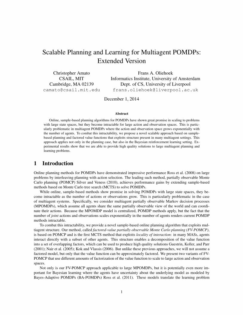
The issue of large numbers of joint actions is also problematic: the standard POMCP algorithm will, at eachnode, maintain separate statistics, and thus separate upper confidence bounds, for each of the exponentiallymany joint actions. Each of the exponentially many joint actions will have to be selected at least a few timesto reduce their confidence bounds (i.e., exploration bonus). This is a principled problem: in cases where eachcombination of individual actions may lead to completely different effects, it may be necessary to try all ofthem at least a few times. In many cases, however, the effect of a joint action is factorizable as the effects ofthe action of individual agents or small groups of agents. For instance, consider a team of agents that is fightingfires at a number of burning houses, as illustrated in Fig. 1(a). The rewards depend only on the amount of waterdeposited on each house rather than the exact joint action taken Oliehoek et al. (2008). While this problem lendsitself to a natural factorization, other problems may also be factorized to permit approximation.

3.2 Coordination GraphsIn certain multiagent settings, coordination (hyper) graphs (CGs) Guestrin, Koller, and Parr (2001); Nair et al.(2005) have been used to compactly represents interactions between subsets of agents. In this paper we extend

3

(a) (b) (c)

Figure 1: (a) Illustration of ‘fire fighting’ (b) Coordination graph with 4 houses and 3 agents (c) Illustration ofa sensor network problem on a grid that is used in the experiments.

this approach to MPOMDPs. We first introduce the framework of CGs in the single shot setting.A CG specifies a set of payoff components E = {Qe}, and each component e is associated with a subset

of agents. These subsets (which we also denote using e) can be interpreted as (hyper)-edges in a graph wherethe nodes are agents. The goal in a CG is to select a joint action that maximizes the sum of the local payoffcomponents Q(~a) =

∑eQe(~ae).

1 A CG for the fire fighting problem is shown in Fig. 1(b). We follow thecited literature in assuming that a suitable factorization is easily identifiable by the designer, but it may alsobe learnable. Even if a payoff function Q(~a) does not factor exactly, it can be approximated by a CG. Forthe moment assuming a stateless problem (we will consider the case where histories are included in the nextsection), an action-value function can be approximated by

Q(~a) ≈∑e

Qe(~ae), (1)

We refer to this as the linear approximation of Q, since one can show that this corresponds to an instance oflinear regression (See Sec. 5).

Using a factored representation, the maximization max~a∑eQe(~ae) can be performed efficiently via vari-

able elimination (VE) Guestrin, Koller, and Parr (2001), or max-sum Kok and Vlassis (2006). These algorithmsare not exponential in the number of agents, and therefore enable significant speed-ups for larger number ofagents. The VE algorithm (which we use in the experiments) is exponential in the induced width w of thecoordination graph.

3.3 Mixture of Experts OptimizationVE can be applied if the CG is given in advance. When we try to exploit these techniques in the context ofPOMCP, however, this is not the case. As such, the task we consider here is to find the maximum of an estimatedfactored function Q(~a) =

∑e Qe(~ae). Note that we do not necessarily require the best approximation to the

entire Q, as in (1). Instead, we seek an estimation Q for which the maximizing joint action ~aM is close to themaximum of the actual (but unknown) Q-value: Q(~aM ) ≈ Q(~a∗).

For this purpose, we introduce a technique called mixture of experts optimization. In contrast to methodsbased on linear approximation (1), we do not try to learn a best-fit factored Q function, but directly try to estimatethe maximizing joint action. The main idea is that for each local action ~ae we introduce an expert that predictsthe total value Q(~ae) = E[Q(~a) | ~ae]. For a joint action, these responses—one of each payoff component e—are put in a mixture with weights αe and used to predict the maximization joint action: argmax~a

∑e αeQ(~ae).

This equation is the sum of restricted-scope functions, which is identical to the case of linear approximation (1),so VE can be used to perform this maximization effectively. In the remainder of this paper, we will integratethe weights and simply write Qe(~ae) = αeQ(~ae).

The experts themselves are implemented as maximum-likelihood estimators of the total value. That is, eachexpert (associated with a particular ~ae) keeps track of the mean payoff received when ~ae was performed, which

1Since we focus on the one-shot setting here, the Q-values in the remainder of this section should be interpreted as those for one specificjoint history h, i.e.: Q(~a) ≡ Q(h,~a).

4

~a 1

~o 1

~a 2

~o 1

~a 2

~o 1 ~o 2

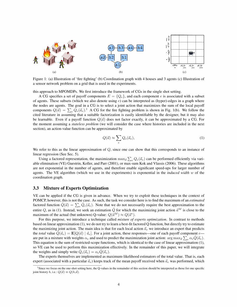
Figure 2: Factored Statistics: joint histories are maintained (for specific joint actions and observations specifiedby ~a j and ~o k), but action statistics are factored at each node.

can be done very efficiently. An additional benefit of this approach is that it allows for efficient estimation ofupper confidence bounds by also keeping track of how often this local action was performed, which in turnsfacilitates easy integration in POMCP, as we describe next.

4 Factored-Value POMCPThis section presents our main algorithmic contribution: Factored-Value POMCP, which is an online planningmethod for POMDPs that can exploit approximate structure in the value function by applying mixture of ex-perts optimization in the POMCP lookahead search tree. We introduce two variants of FV-POMCP. The firsttechnique, factored statistics, only addresses the complexity introduced by joint actions. The second technique,factored trees, additionally addresses the problem of many joint observations. FV-POMCP is the first MCTSmethod to exploit structure in MASs, achieving better sample complexity by using factorization to generalizethe value function over joint actions and histories. While this method was developed to scale POMCP to largerMPOMDPs in terms of number of agents, the techniques may be beneficial in other multiagent models andother factored POMDPs.

4.1 Factored StatisticsWe first introduce Factored Statistics which directly applies mixture of experts optimization to each node in thePOMCP search tree. As shown in Fig. 2, the tree of joint histories remains the same, but the statistics retainedat for each history is now different. That is, rather than maintaining one set of statistics in each node (i.e, jointhistory ~h) for the expected value of each joint action Q(~h,~a), we maintain a set of statistic for each componente that estimates the values Qe(~h,~ae) and corresponding upper confidence bounds.

Joint actions are selected according to the maximum (factored) upper confidence bound:

max~a

∑e

Ue(~h,~ae),

Where Ue(~h,~ae) , Qe(~h,~ae) + c√log(N~h + 1)/n~ae using the Q-value and the exploration bonus added for

that factor. For implementation, at each node for a joint history ~h, we store the count for the full history N~h aswell as the Q-values, Qe, and the counts for actions, n~ae , separately for each component e.

Since this method retains fewer statistics and performs joint action selection more efficiently via VE, weexpect that it will be more efficient than plain application of POMCP to the BA-MPOMDP. However, thecomplexity due to joint observations is not directly addressed: because joint histories are used, reuse of nodesand creation of new nodes for all possible histories (including the one that will be realized) may be limited ifthe number of joint observations is large.

5

. . . e . . .

~a 11

~o 11

~a 21

~o 11

~a 21

~o 11 ~o 2

1

~a 1|E|

~o 1|E|

~a 2|E|

~o 1|E|

~a 2|E|

~o 1|E|

~o 2|E|

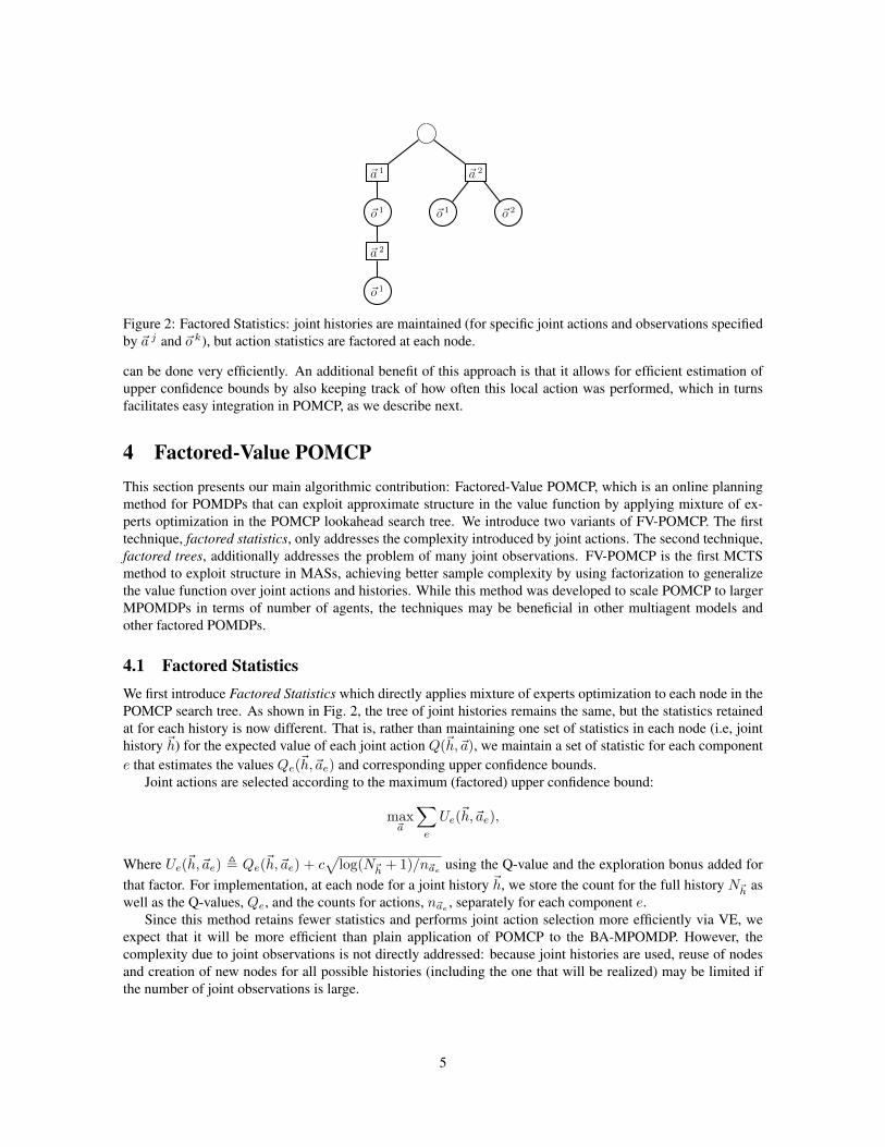
Figure 3: Factored Trees: local histories for are maintained for each factor (resulting in factored history andaction statistics). Actions and observations for component i are represented as ~a ji and ~o ki )

4.2 Factored TreesThe second technique, called Factored Trees, additionally tries to overcome the large number of joint observa-tions. It further decomposes the local Qe’s by splitting joint histories into local histories and distributing themover the factors. That is, in this case, we introduce an expert for each local ~he,~ae pair. During simulations, theagents know ~h and action selection is conducted by maximizing over the sum of the upper confidence bounds:

max~a

∑e

Ue(~he,~ae),

where Ue(~he,~ae) = Qe(~he,~ae)+c√log(N~he

+ 1)/n~ae . We assume that the set of agents with relevant actionsand histories for component Qe are the same, but this can be generalized. This approach further reduces thenumber of statistics maintained and increases the reuse of nodes in MCTS and the chance that nodes in the treeswill exist for observations that are seen during execution. As such, it can increase performance by increasinggeneralization as well as producing more robust particle filters.

This type of factorization has a major effect on the implementation: rather than constructing a single tree,we now construct a number of trees in parallel, one for each factor e as shown in Fig. 3. A node of the tree forcomponent e now stores the required statistics: N~he

, the count for the local history, n~ae , the counts for actionstaken in the local tree and Qe for the tree. Finally, we point out that this decentralization of statistics has thepotential to reduce communication since the components statistics in a decentralized fashion could be updatedwithout knowledge of all observation histories.

5 Theoretical AnalysisHere, we investigate the approximation quality induced by our factorization techniques.2 The most desirablequality bounds would express the performance relative to ‘optimal’, i.e., relative to flat POMCP, which con-verges in probability an ε-optimal value function. Even for the one-shot case, this is extremely difficult forany method employing factorization based on linear approximation of Q, because Equation (1) corresponds toa special case of linear regression. In this case, we can write (1) in terms of basis functions and weights as:∑eQe(~ae) =

∑e,~ae

we,~aehe,~ae(~a), where the he,~ae are the basis functions: he,~ae(~a) = 1 iff ~a specifies ~ae forcomponent e (and 0 otherwise). As such, providing guarantees with respect to the optimal Q(~a)-value wouldrequire developing a priori bounds for the approximation quality of (a particular type of) basis functions. Thisis a very difficult problem for which there is no good solution, even though these methods are widely studied inmachine learning.

However, we do not expect our methods to perform well on arbitrary Q. Instead, we expect them to performwell when Q is nearly factored, such that (1) approximately holds, since then the local actions contain enough

2Proofs can be found in the Appendix B

6

information to make good predictions. As such, we analyze the behavior of our methods when the samples ofQ come from a factored function (i.e., as in (1) ) contaminated with zero-mean noise. In such cases, we canshow the following.

Theorem 1. The estimate Q of Q made by a mixture of experts converges in probability to the true value plusa sample policy dependent bias term: Q(~a)

p→ Q(~a) +B~π(~a). The bias is given by a sum of biases induced bypairs e,e′:

B~π(~a) ,∑e

∑e′ 6=e

∑~ae′\e

~π(~ae′\e|~ae)Qe′(~ae′\e,~ae′∩e).

Here, ~ae′∩e is the action of the agents that participate both in e and e′ (specified by ~a) and ~ae′\e are the actionsof agents in e′ that are not in e.

Because we observe the global reward for a given set of actions, the bias is caused by correlations in thesampling policy and the fact that we are overcounting value from other components. When there is no overlap,and the sampling policy we use is ‘component-wise’: ~π(~ae′\e|~ae) = ~π(~ae′\e|~a′e) = ~π(~ae′\e), this over countingis the same for all local actions ~ae:

Theorem 2. When value components do not overlap and a component-wise sampling policy is used, mixture ofexperts optimization recovers the maximizing joint action.

Similar reasoning can be used to establish bounds on the performance in the case of overlapping compo-nents, subject to assumptions about properties of the true value function.

Theorem 3. If for all overlapping components e,e′, and any two ‘intersection action profiles’ ~ae′∩e,~a′e′∩e fortheir intersection, the true value function satisfies

∀~ae′\e Qe′(~ae′\e,~ae′∩e) − Qe′(~ae′\e,~a′e′∩e) ≤ ε/(|E| · |N (e)| · | ~Ae′\e| · ~π(~ae′\e)), (2)

with | ~Ae′\e| the number of intersection action profiles, then mixture of experts optimization, in the limit, willreturn a joint action whose value lies within ε of the optimal solution.

The analysis shows that a sufficiently local Q-function can be effectively optimized when using a sufficientlylocal sampling policy. Under the same assumptions, we can also derive guarantees for the sequential case. It isnot directly possible to derive bounds for FV-POMCP itself (since it is not possible to demonstrate that the UCBexploration policy is component-wise), but it seems likely that UCB exploration leads to an effective policy thatnearly satisfies this property. Moreover, since bias is introduced by the interaction between action correlationsand differences in ‘non-local’ components, even when using a policy with correlations, the bias may be limitedif the Q-function is sufficiently structured.

In the factored tree case, we can introduce a strong result. Because histories for other agents outside thefactor are not included and we do not assume independence between factors, the approximation quality maysuffer: where ~h is Markov, this is not the case for the local history ~he. As such, the expected return for such alocal history depends on the future policy as well as the past one (via the distribution over histories of agentsnot included in e). This implies that convergence is no longer guaranteed:

Proposition 1. Factored-Trees FV-POMCP may diverge.

Proof. FT-FV-POMCP (with c = 0) corresponds to a general case of Monte Carlo control (i.e., SARSA(1))with linear function approximation that is greedy w.r.t. the current value function. Such settings may result indivergence Fairbank and Alonso (2012).

Even though this is a negative result, and there is no guarantee of convergence for FT-FV-POMCP, in practicethis need not be a problem; many reinforcement learning techniques that can diverge (e.g., neural networks) canproduce high-quality results in practice, e.g., Tesauro (1995); Stone and Sutton (2001). Therefore, we expectthat if the problem exhibits enough locality, the factored trees approximation may allow good quality policiesto be found very quickly.

7

Finally, we analyze the computational complexity. FV-POMCP is implemented by modifying POMCP’sSIMULATE function (as described in Appendix A). The maximization is performed by variable elimination,which has complexity O(n|Amax|w) with w the induced width and |Amax| the size of the largest action set.In addition, the algorithm updates each of the |E| components, bringing the total complexity of one call ofsimulate to O(|E|+ n|Amax|w).

6 Experimental ResultsHere, we empirically investigate the effectiveness of our factorization methods by comparing them to non-factored methods in the planning and learning settings.Experimental Setup. We test our methods on versions of the firefighting problem from Section 4 and onsensor network problems. In the firefighting problems, fires are suppressed more quickly if a larger number ofagents choose that particular house. Fires also spread to neighbor’s houses and can start at any house with asmall probability. In the sensor network problems (as shown by Fig. 1(c)), sensors were aligned along discreteintervals on two axes with rewards for tracking a target that moves in a grid. Two types of sensing could beemployed by each agent (one more powerful than the other, but using more energy) or the agent could donothing. A higher reward was given for two agents correctly sensing a target at the same time. The firefightingproblems were broken up into n − 1 overlapping factors with 2 agents in each (representing the agents on thetwo sides of a house) and the sensor grid problems were broken into n/2 factors with n/2 + 1 agents in each(representing all agents along the y axis and one agent along the x axis). For the firefighting problem with 4agents, |S| = 243, |A| = 81 and |Z| = 16 and with 10 agents, |S| = 177147, |A| = 59049 and |Z| = 1024. For thesensor network problems with 4 agents, |S| = 4, |A| = 81 and |Z| = 16 and with 8 agents, |S| = 16, |A| = 6561and |Z| = 256.

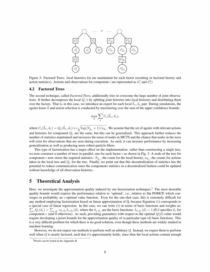
Each experiment was run for a given number of simulations, the number of samples used at each step tochoose an action, and averaged over a number of episodes. We report undiscounted return with the standarderror. Experiments were run on a single core of a 2.5 GHz machine with 8GB of memory. In both cases, wecompare our factored representations to the flat version using POMCP. This comparison uses the same codebase so it directly shows the difference when using factorization. POMCP and similar sample-based planningmethods have already been shown to be state-of-the-art methods in both POMDP planning Silver and Veness(2010) and learning Ross et al. (2011).MPOMDPs. We start by comparing the factored statistics (FS) and factored tree (FT) versions of FV-POMCPin multiagent planning problems. Here, the agents are given the true MPOMDP model (in the form of a simula-tor) and use it to plan. For this setting, we compare to two baseline methods: POMCP: regular POMCP appliedto the MPOMDP, and random: uniform random action selection. Note that while POMCP will converge to anε-optional solution, the solution quality may be poor when using small number of simulations.

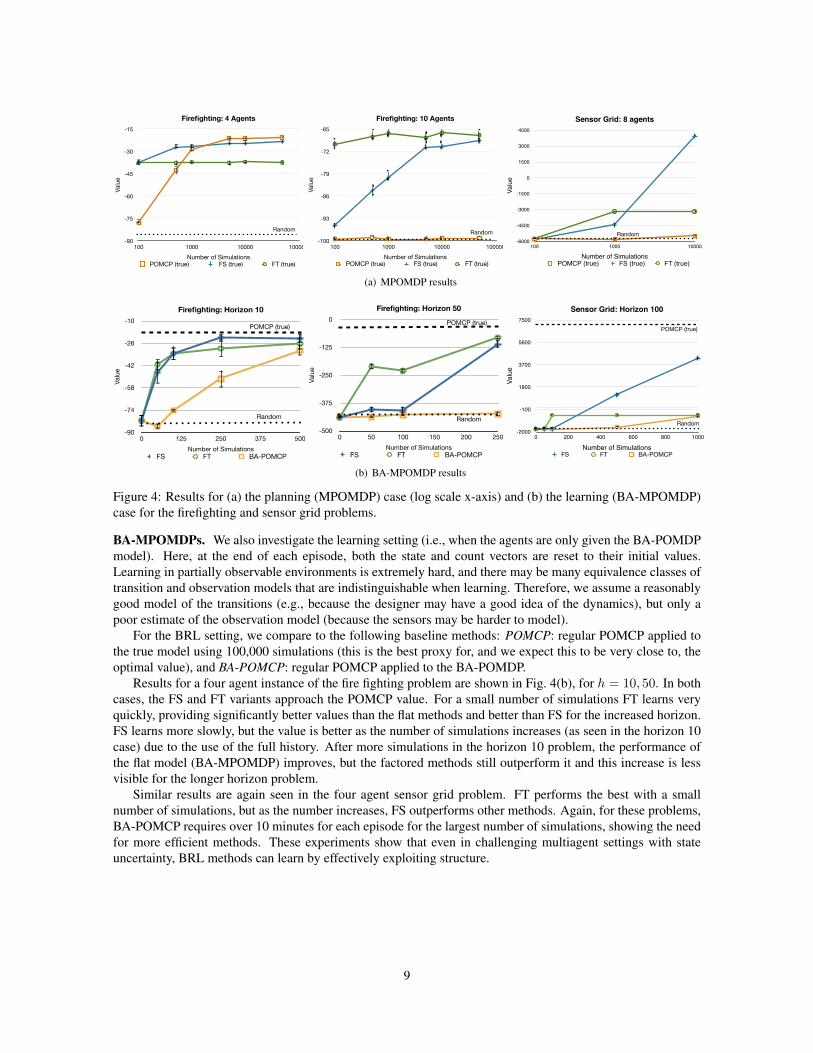
The results for 4-agent and 10-agent firefighting problems with horizon 10 are shown in Figure 4(a). For the4-agent problem, POMCP performs poorly with a few simulations, but as the number of simulations increasesit outperforms the other methods (presumably converging to an optimal solution). FT provides a high-qualitysolution with a very small number of simulations, but the resulting value plateaus due to approximation error.FS also provides a high-quality solution with a very small number of simulations, but is then able to convergeto a solution that is near POMCP. In the 10-agent problem, POMCP is only able to generate a solution that isslightly better than random while the FV-POMCP methods are able to perform much better. In fact, FT performsvery well with a small number of samples and FS continues to improve until it reaches solution that is similarto FT.

Similar results are seen in the sensor grid problem. POMCP outperforms a random policy as the numberof simulations grows, but FS and FT produce much higher values with the available simulations. FT seemsto converge to a low quality solution (in both planning and learning) due to the loss of information about thetarget’s previous position that is no longer known to local factors. In this problem, POMCP requires over 10minutes for an episode of 10000 simulations, making reducing the number of simulations crucial in problemsof this size. These results clearly illustrate the benefit of FV-POMCP by exploiting structure for planning inMASs.

8

1 100 500 1000 5000 10000 50000 75000 0 100 500 1000 5000 10000 50000 75000

POMCP (true) -85.97 -77.74 -42.53 -28.48 -21.16 -21.26 -20.6 0.948415 1.14661 2.35085 1.99687 0.79721 0.971969 0.853698

FS (true) -85.97 -37.44 -27.14 -26.66 -24.67 -24.65 -23.36 0.948415 2.01417 1.20706 1.25182 1.00768 0.934813 0.928388

FT (true) -85.97 -37.14 -37.7229 -37.3 -37.6 -36.91 -37.44 0.948415 1.42464 1.24872 1.25479 1.28973 1.23993 1.25142

Random -85.97 0.948415

Firefighting: 4 AgentsVa

lue

-90

-75

-60

-45

-30

-15

Number of Simulations100 1000 10000 100000

POMCP (true) FS (true) FT (true)

Random

�1

Firefighting: 10 Agents

Valu

e

-100

-93

-86

-79

-72

-65

Number of Simulations100 1000 10000 100000

POMCP (true) FS (true) FT (true)

errors

1 100 500 1000 5000 10000 50000 0 100 500 1000 5000 10000 50000 0 100 500 1000 5000 10000 50000 0 100 500 1000 5000 10000 50000

POMCP (true) -99.5 -99.56 -98.97 -99.49 -99.51 -99.29 -99.18 0.140357 0.151208 0.25979 0.176349 0.178603 0.28576 0.227324 POMCP (true) -99.5 -99.56 -98.97 -99.49 -99.51 -99.29 -99.18 0.140357 0.151208 0.25979 0.176349 0.178603 0.28576 0.227324

FS (true) -99.5 -95.17 -84.24 -80.12 -70.65 -70.49 -68.66 0.140357 0.603062 1.46042 1.51964 1.08743 1.17197 1.14273 Factored statistics (true)

-99.5 -97.46 -85.24 -80.64 -75.94 -75.64 -71.24 0.140357 0.603062 1.46042 1.51964 1.08743 1.17197 1.14273

FT (true) -99.5 -69.77 -67.37 -66.25 -67.7172 -66.19 -66.9 0.140357 1.52062 1.3457 1.29859 1.26737 1.76766 1.19686 Factored tree (true) -99.5 -74.51 -72.51 -72.31 -72.59 -76.2353 -75.7188 0.140357 1.52062 1.3457 1.29859 1.26737 1.76766 1.19686

Random -99.5 -99.5 -99.5 -99.5 -99.5 -99.5 -99.5 0.140357 0.140357 0.140357 0.140357 0.140357 0.140357 0.140357 Random -99.5 -99.5 -99.5 -99.5 -99.5 -99.5 -99.5 0.140357 0.140357 0.140357 0.140357 0.140357 0.140357 0.140357

FFG: Horizon 10

Valu

e

-100

-93

-86

-79

-72

-65

Number of Simulations0 10000 20000 30000 40000 50000

POMCP (true) FS (true) FT (true) Random

Random

�1

errors

0 100 1000 10000 0 100 1000 10000

POMCP (true) -5772.08 '5796.7 '5823.9 '5488.18 12.0325 41.0094 41.4847 70.783

FS (true) -5772.08 '5814.7 '4460.1 3907.14 12.0325 32.2606 101.214 46.4984

FT (true) -5772.08 '5785.9 '3220.85 '3181.92 12.0325 39.2071 53.393 105.117

Random -5772.08 -5772.08 -5772.08 -5772.08 12.0325 12.0325 12.0325 12.0325

Sensor Grid: 8 agents

Valu

e

-6000

-4500

-3000

-1500

0

1500

3000

4500

Number of Simulations100 1000 10000

POMCP (true) FS (true) FT (true)

Random

�1

(a) MPOMDP results

Firefighting: Horizon 10

Valu

e

-90

-74

-58

-42

-26

-10

Number of Simulations0 125 250 375 500

FS FT BA-POMCP

POMCP (true)

Random

�9

Firefighting: Horizon 50Va

lue

-500

-375

-250

-125

0

Number of Simulations0 50 100 150 200 250

FS FT BA-POMCP

Random

POMCP (true)

�3

errors

0 50 100 500 1000 5000 0 50 100 500 1000 5000

POMCP (true) -1749 -1765.95 -1664.6 2715.05 36.3051

FS '1767.68 '1765.91 '1746.04 1127.31 4247.21 5752.47 10.6662 10.7417 10.9585 149.315 40.4285 51.1254

FT '1767.68 '1692.69 '611.47 '603.59 '593.521 '599.286 10.6662 11.3504 12.3876 20.5541 12.2871 153.548

BA-POMCP '1775.16 '1783.55 '1775.73 '1609.37 '682.32 4997.73 10.8695 10.7143 10.2748 12.0041 32.6295 41.4148

No learning '1775.16 '1783.55 '1779.22 '1610.55 '804.615 4667 10.8695 10.7143 10.3674 11.3882 28.5594 92.9594

Random '1767.68 '1767.68 '1767.68 '1767.68 '1767.68

POMCP1100001sims err

7403.65 13.4053

Sensor Grid: Horizon 100

Valu

e

-2000

-100

1800

3700

5600

7500

Number of Simulations0 1000 2000 3000 4000 5000

FS FT BA-POMCP No learning

Random

POMCP (true)

Sensor Grid: Horizon 100

Valu

e

-2000

-100

1800

3700

5600

7500

Number of Simulations0 200 400 600 800 1000

FS FT BA-POMCP

Random

POMCP (true)

�1

(b) BA-MPOMDP results

Figure 4: Results for (a) the planning (MPOMDP) case (log scale x-axis) and (b) the learning (BA-MPOMDP)case for the firefighting and sensor grid problems.

BA-MPOMDPs. We also investigate the learning setting (i.e., when the agents are only given the BA-POMDPmodel). Here, at the end of each episode, both the state and count vectors are reset to their initial values.Learning in partially observable environments is extremely hard, and there may be many equivalence classes oftransition and observation models that are indistinguishable when learning. Therefore, we assume a reasonablygood model of the transitions (e.g., because the designer may have a good idea of the dynamics), but only apoor estimate of the observation model (because the sensors may be harder to model).

For the BRL setting, we compare to the following baseline methods: POMCP: regular POMCP applied tothe true model using 100,000 simulations (this is the best proxy for, and we expect this to be very close to, theoptimal value), and BA-POMCP: regular POMCP applied to the BA-POMDP.

Results for a four agent instance of the fire fighting problem are shown in Fig. 4(b), for h = 10, 50. In bothcases, the FS and FT variants approach the POMCP value. For a small number of simulations FT learns veryquickly, providing significantly better values than the flat methods and better than FS for the increased horizon.FS learns more slowly, but the value is better as the number of simulations increases (as seen in the horizon 10case) due to the use of the full history. After more simulations in the horizon 10 problem, the performance ofthe flat model (BA-MPOMDP) improves, but the factored methods still outperform it and this increase is lessvisible for the longer horizon problem.

Similar results are again seen in the four agent sensor grid problem. FT performs the best with a smallnumber of simulations, but as the number increases, FS outperforms other methods. Again, for these problems,BA-POMCP requires over 10 minutes for each episode for the largest number of simulations, showing the needfor more efficient methods. These experiments show that even in challenging multiagent settings with stateuncertainty, BRL methods can learn by effectively exploiting structure.

9

7 Related WorkMCTS methods have become very popular in games, a type of multiagent setting, but no action factorizationhas been exploited so far Browne et al. (2012). Progressive widening Coulom (2007) and double progressivewidening Couetoux et al. (2011) have had some success in games with large (or continuous) action spaces.The progressive widening methods do not use the structure of the coordination graph in order to generalizevalue over actions, but instead must find the correct joint action out of the exponentially many that are available(which may require many trajectories). They are also designed for fully observable scenarios, so they do notaddress the large observation space in MPOMDPs.

The factorization of the history in FTs is not unlike the use of linear function approximation for the statecomponents in TD-Search Silver, Sutton, and Muller (2012). However, in contrast to that method, due to ourparticular factorization, we can still apply UCT to aggressively search down the most promising branches of thetree. While other methods based on Q-learning Guestrin, Lagoudakis, and Parr (2002); Kok and Vlassis (2006)exploit action factorization, they assume agents observe individual rewards (rather than the global reward thatwe consider) and it is not clear how these could be incorporated in a UCT-style algorithm.

Locality of interaction has also been considered previously in decentralized POMDP methods Oliehoek(2012); Amato et al. (2013) in the form of factored Dec-POMDPs Oliehoek, Whiteson, and Spaan (2013);Pajarinen and Peltonen (2011) and networked distributed POMDPs (ND-POMDPs) Nair et al. (2005); Kumarand Zilberstein (2009); Dibangoye et al. (2014). These models make strict assumptions about the informationthat the agents can use to choose actions (only the past history of individual actions and observations), therebysignificantly lowering the resulting value Oliehoek, Spaan, and Vlassis (2008). ND-POMDPs also impose addi-tional assumptions on the model (transition and observation independence and a factored reward function). TheMPOMDP model, in contrast, does not impose these restrictions. Instead, in MPOMDPs, each agent knowsthe joint action-observation history, so there are not different perspectives by different agents. Therefore, 1)factored Dec-POMDP and ND-POMDP methods do not apply to MPOMDPs; they specify mappings from in-dividual histories to actions (rather than joint histories to joint actions), 2) ND-POMDP methods assume thatthe value function is exactly factored as the sum of local values (‘perfect locality of interaction’) while in anMPOMDP, the value is only approximately factored (since different components can correlate due to condition-ing the actions on central information). While perfect locality of interaction allows a natural factorization of theMPOMDP value function, but our method can be applied to any MPOMDP (i.e., given any factorization of thevalue function). Furthermore, current factored Dec-POMDP and ND-POMDP models generate solutions giventhe model in an offline fashion, while we consider online methods using a simulator in this paper.

Our approach builds upon coordination-graphs Guestrin, Koller, and Parr (2001), to perform the joint actionoptimization efficiently, but factorization in one-shot problems has been considered in other settings too. Aminet al. Amin, Kearns, and Syed (2011) present a method to optimize graphical bandits, which relates to our opti-mization approach. Since their approach replaced the UCB functionality, it is not obvious how their approachcould be integrated in POMCP. Moreover, their work, focuses on minimizing regret (which is not an issue in ourcase), and does not apply when the factorization does not hold. Oliehoek et al. Oliehoek, Whiteson, and Spaan(2012) present an factored-payoff approach that extends coordination graphs to imperfect information settingswhere each agent has its own knowledge. This is not relevant for our current algorithm, which assumes thatjoint observations will be received by a centralized decision maker, but could potentially be useful to relax thisassumption.

8 ConclusionsWe presented the first method to exploit multiagent structure to produce a scalable method for Monte Carlo treesearch for POMDPs. This approach formalizes a team of agents as a multiagent POMDP, allowing planningand BRL techniques from the POMDP literature to be applied. However, since the number of joint actions andobservations grows exponentially with the number of agents, naıve extensions of single agent methods will notscale well. To combat this problem, we introduced FV-POMCP, an online planner based on POMCP Silver andVeness (2010) that exploits multiagent structure using two novel techniques—factored statistics and factored

10

trees— to reduce 1) the number of joint actions and 2) the number of joint histories considered. Our empiricalresults demonstrate that FV-POMCP greatly increases scalability of online planning for MPOMDPs, solvingproblems with 10 agents. Further investigation also shows scalability to the much more complex learningproblem with four agents. Our methods could also be used to solve POMDPs and BA-POMDPs with largeaction and observation spaces as well the recent Bayes-Adaptive extension Ng et al. (2012) of the self interestedI-POMDP model Gmytrasiewicz and Doshi (2005).

AcknowledgmentsF.O. is funded by NWO Innovational Research Incentives Scheme Veni #639.021.336. C.A was supported byAFOSR MURI project #FA9550-09-1-0538 and ONR MURI project #N000141110688.

ReferencesAmato, C., and Oliehoek, F. A. 2013. Bayesian reinforcement learning for multiagent systems with state

uncertainty. In Workshop on Multi-Agent Sequential Decision Making in Uncertain Domains, 76–83.

Amato, C.; Chowdhary, G.; Geramifard, A.; Ure, N. K.; and Kochenderfer, M. J. 2013. Decentralized controlof partially observable Markov decision processes. In CDC, 2398–2405.

Amin, K.; Kearns, M.; and Syed, U. 2011. Graphical models for bandit problems. In UAI, 1–10.

Browne, C.; Powley, E. J.; Whitehouse, D.; Lucas, S. M.; Cowling, P. I.; Rohlfshagen, P.; Tavener, S.; Perez, D.;Samothrakis, S.; and Colton, S. 2012. A survey of Monte Carlo tree search methods. IEEE Trans. Comput.Intellig. and AI in Games 4(1):1–43.

Couetoux, A.; Hoock, J.-B.; Sokolovska, N.; Teytaud, O.; and Bonnard, N. 2011. Continuous upper confidencetrees. In Learning and Intelligent Optimization. 433–445.

Coulom, R. 2007. Computing elo ratings of move patterns in the game of go. International Computer GamesAssociation (ICGA) Journal 30(4):198–208.

Dibangoye, J. S.; Amato, C.; Buffet, O.; and Charpillet, F. 2014. Exploiting separability in multi-agent planningwith continuous-state MDPs. In AAMAS.

Fairbank, M., and Alonso, E. 2012. The divergence of reinforcement learning algorithms with value-iterationand function approximation. In International Joint Conference on Neural Networks, 1–8. IEEE.

Gmytrasiewicz, P. J., and Doshi, P. 2005. A framework for sequential planning in multi-agent settings. JAIR24.

Guestrin, C.; Koller, D.; and Parr, R. 2001. Multiagent planning with factored MDPs. In NIPS, 15.

Guestrin, C.; Lagoudakis, M.; and Parr, R. 2002. Coordinated reinforcement learning. In ICML, 227–234.

Kearns, M.; Mansour, Y.; and Ng, A. Y. 2002. A sparse sampling algorithm for near-optimal planning in largeMarkov decision processes. MLJ 49(2-3).

Kok, J. R., and Vlassis, N. 2006. Collaborative multiagent reinforcement learning by payoff propagation. JMLR7.

Kumar, A., and Zilberstein, S. 2009. Constraint-based dynamic programming for decentralized POMDPs withstructured interactions. In AAMAS.

Messias, J. V.; Spaan, M.; and Lima, P. U. 2011. Efficient offline communication policies for factored multiagentPOMDPs. In NIPS 24.

11

Nair, R.; Varakantham, P.; Tambe, M.; and Yokoo, M. 2005. Networked distributed POMDPs: a synthesis ofdistributed constraint optimization and POMDPs. In AAAI.

Ng, B.; Boakye, K.; Meyers, C.; and Wang, A. 2012. Bayes-adaptive interactive POMDPs. In AAAI.

Oliehoek, F. A.; Spaan, M. T. J.; Whiteson, S.; and Vlassis, N. 2008. Exploiting locality of interaction infactored Dec-POMDPs. In AAMAS.

Oliehoek, F. A.; Spaan, M. T. J.; and Vlassis, N. 2008. Optimal and approximate Q-value functions fordecentralized POMDPs. JAIR 32:289–353.

Oliehoek, F. A.; Whiteson, S.; and Spaan, M. T. J. 2012. Exploiting structure in cooperative Bayesian games.In UAI, 654–664.

Oliehoek, F. A.; Whiteson, S.; and Spaan, M. T. J. 2013. Approximate solutions for factored Dec-POMDPswith many agents. In AAMAS, 563–570.

Oliehoek, F. A. 2012. Decentralized POMDPs. In Wiering, M., and van Otterlo, M., eds., ReinforcementLearning: State of the Art. Springer.

Pajarinen, J., and Peltonen, J. 2011. Efficient planning for factored infinite-horizon DEC-POMDPs. In IJCAI,325–331.

Pynadath, D. V., and Tambe, M. 2002. The communicative multiagent team decision problem: Analyzingteamwork theories and models. JAIR 16.

Ross, S.; Pineau, J.; Paquet, S.; and Chaib-draa, B. 2008. Online planning algorithms for POMDPs. JAIR 32(1).

Ross, S.; Pineau, J.; Chaib-draa, B.; and Kreitmann, P. 2011. A Bayesian approach for learning and planningin partially observable Markov decision processes. JAIR 12.

Silver, D., and Veness, J. 2010. Monte-carlo planning in large POMDPs. In NIPS 23.

Silver, D.; Sutton, R. S.; and Muller, M. 2012. Temporal-difference search in computer Go. MLJ 87(2):183–219.

Stone, P., and Sutton, R. S. 2001. Scaling reinforcement learning toward RoboCup soccer. In ICML, 537–544.

Tesauro, G. 1995. Temporal difference learning and TD-Gammon. Commun. ACM 38(3):58–68.

A FV-POMCP Pseudo codeHere we describe in more detail the algorithms for the proposed FV-POMCP variants. Both methods can bedescribed as a modification of POMCP’s SIMULATE procedure, which is shown in Algorithm 1. Each simulationis started by calling this procedure on the root node (corresponding to the empty history, or ‘now’) with a statesampled from the current belief. The comments in Algorithm 1 should make the code self-explanatory, but fora further explanation we refer to Silver and Veness (2010).

The pseudo code for the factored statistics case (FS-FV-POMCP) is shown in Algorithm 2. The commentshighlight the important changes: there is no need to loop over the joint actions for initialization, or for selectingthe maximizing action. Also, the same return R is used to update the active expert in each component e.

Finally, Algorithm 3 shows the pseudo code for the factored trees variant of FV-POMCP. Like FSs, FT-FV-POMCP performs the simulations in lockstep. However, as we now maintain statistics and particle filters foreach component e in separate trees, the initialization and updating of these statistics is slightly different. Assuch, the algorithm makes clear that there is no computational advantage to factored trees (when compared toFSs), but that the big difference is in the additional generalization it performs.

12

Algorithm 1 POMCP1: procedure SIMULATE(s,h,depth)2: if γdepth < ε then3: return 0 . Stop when desired precision reached4: end if5: if h 6∈ T then . if we did not visit this h yet6: for all a ∈ A do7: T (h,a)← (Ninit(h,a),Vinit(h,a),∅) . initialize counts for all a, and particle filter8: end for9: return Rollout(s,h,depth) . do a random rollout from this node

10: end if11: a← argmax′aQ(h,a′) + c

√logN(h)N(h,a′) . max via enumeration

12: (s′,o,r) ∼ G(s,a) . sample a transition, observation and reward13: R← r + γSimulate(s′,(hao),depth+ 1) . Recurse and receive the return R14: B(h)← B(h) ∪ {s} . Add s to the particle filter maintained for h15: N(h)← N(h) + 1 . Update the number of times h is visited. . .16: N(h,a)← N(h,a) + 1 . . . . and how often we selected action a here17: Q(h,a)← Q(h,a) + R−Q(h,a)

N(h,a) . Incremental update of mean return18: return R19: end procedure

Algorithm 2 Factored Statistics

1: procedure SIMULATE(s,~h,depth)2: if γdepth < ε then3: return 04: end if5: if ~h 6∈ T then6: for all e ∈ E do . initialize statistics for component e7: for all ~ae ∈ ~Ae do . only loop over local joint actions8: T (~h,~ae)← (Ninit(~h,~ae),Vinit(~h,~ae),∅)9: end for

10: end for11: return Rollout(s,~h,depth)12: end if13: ~a← argmax′~a

∑e

[Qe(~h,~a

′e) + c

√logN(~h+1)

n~a′e

]. via variable elimination

14: (s′,~o,r) ∼ G(s,~a)15: R← r + γSimulate(s′,(~h~a~o),depth+ 1)16: B(~h)← B(~h) ∪ {s}17: N(~h)← N(~h) + 118: for all ~e ∈ E do . update the statistics for each component19: n~ae ← n~ae + 1

20: Qe(~h,~ae)← Qe(~h,~ae) +R−Qe(~h,~ae)

n~ae. update the estimation of the expert for ~ae

21: end for22: return R23: end procedure

13

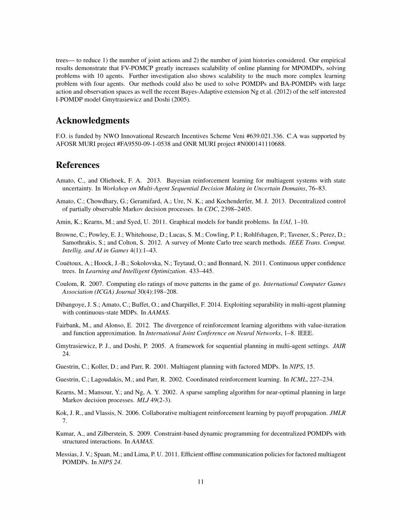
The actual planning could take place in a number of ways: one agent could be designated the planner, whichwould require this agent to broadcast the computed joint action. Alternatively, each agent can in parallel performan identical planning process (by, in the case of randomized planning, syncing the random number generators).Then each agent will compute the same joint action and execute its component. An interesting direction offuture work is whether the planning itself can be done more effectively by distributing the task over the agents.

Algorithm 3 Factored Trees

1: procedure SIMULATE(s,~h,depth)2: if γdepth < ε then3: return 04: end if5: for all e ∈ E do . check all components e6: if ~he 6∈ Te then . if there is no node for ~he in the tree for component e yet7: for all ~ae ∈ ~Ae do . only loop over local joint actions8: Te(~he,~ae)← (Ninit(~he,~ae),Vinit(~he,~ae),∅)9: end for

10: end if11: end for12: return Rollout(s,~h,depth)

13: ~a← argmax′~a∑e

[Qe(~he,~a

′e) + c

√logN(~he+1)

n~a′e

]. via variable elimination

14: (s′,~o,r) ∼ G(s,~a)15: R← r + γSimulate(s′,(~h~a~o),depth+ 1)16: for all ~e ∈ E do . update the statisitics for each component17: B(~he)← B(~he) ∪ {s} . update the particle filter of each tree e with the same s18: N(~he)← N(~he) + 119: n~ae ← n~ae + 1

20: Qe(~he,~ae)← Qe(~he,~ae) +R−Qe(~he,~ae)

n~ae. update expert for ~he,~ae

21: end for22: return R23: end procedure

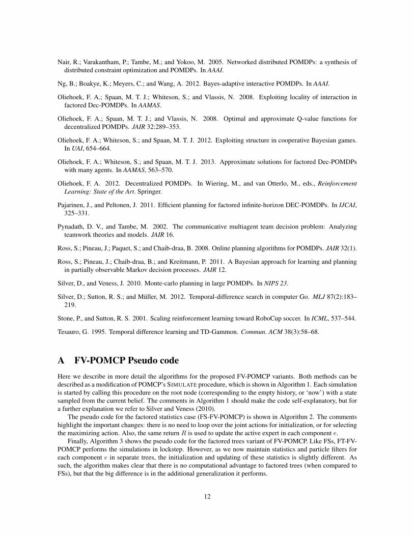
B Analysis of Mixture of Experts OptimizationHere we analyze the behavior of our mixtures of experts under sample policy ~π. In performing this analysis wecompare to the case where the true value function Q(~a) is factored in E components

Q(~a) =

E∑e=1

Qe(~ae)

and corrupted by zero-mean noise ν. As such we establish the performance in cases where the actual valuefunction is ‘close’ to factored. In the below, we will write N (e) for the neighborhood of component e. Thatis the set of other components e′ which have an overlap with e: those that have at least one agent participatingin them that also participates in e). In this analysis, we will assume that all experts are weighted uniformly(αe = 1

E ), and ignore this constant which is not relevant for determining the maximizing action.

Theorem 4. The estimate Q of Q made by a mixture of experts converges in probability to the true value plusa sample policy dependent bias term:

Q(~a)p→ Q(~a) +B~π(~a).

14

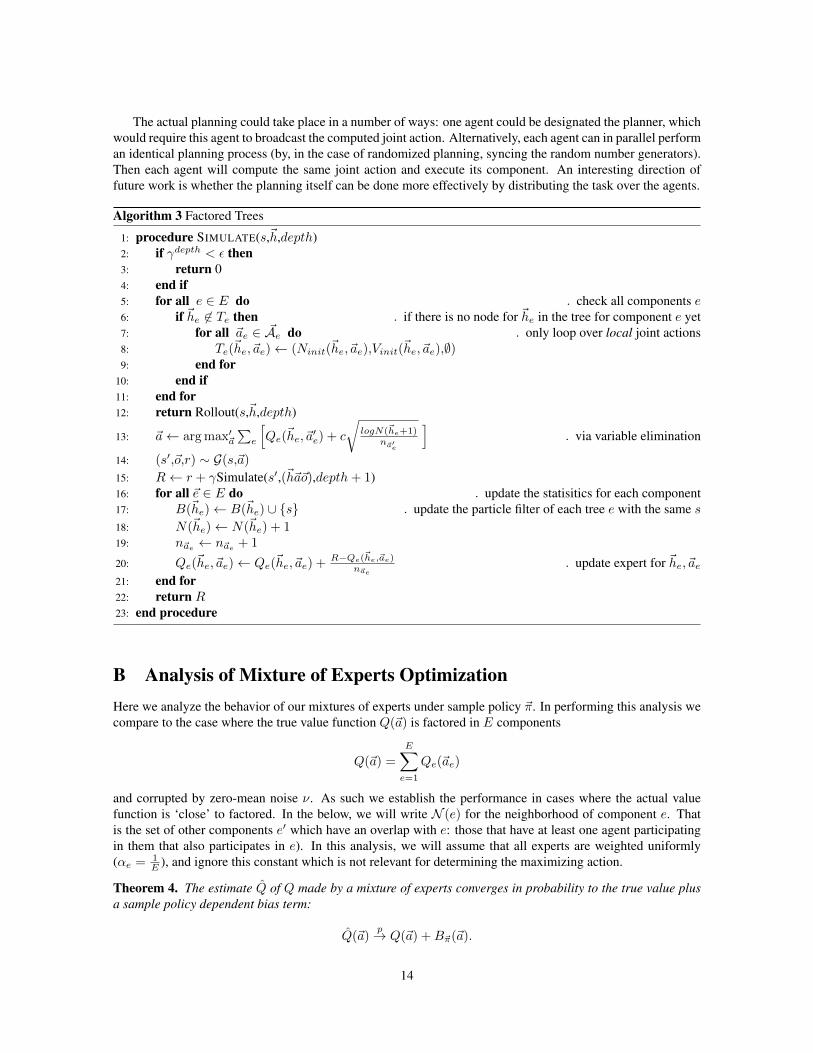
The bias is given by a sum of biases induced by pairs e,e′ of overlapping value components:

B~π(~a) ,∑e

∑e′ 6=e

∑~ae′\e

~π(~ae′\e|~ae)Qe′(~ae′\e,~ae′∩e).

Here ~ae′∩e is the action of the agents that participate both in e and e′ (specified by ~a) and ~ae′\e are the actionsof agents in e′ that are not in e (these are summed over as emphasised by the overlining).

Proof. Suppose that we have drawn a set of samples r1, . . . ,rK according to ~π. For each component e and ~ae,we have an expert that estimates Q(~ae). LetR(~ae) be the subset of samples received where we took local jointaction ~ae. The corresponding expert will estimate

Q(~ae) :=1

R(~ae)∑

r~ae∈R(~ae)

r~ae

Now, the expected sample that this expert receives is

E [r~ae |~π] = Eν

∑~a−e

~π(~a−e|~ae)Q(~a) + ν

=∑~a−e

~π(~a−e|~ae)

[∑e′

Qe′(~ae′)

]+Eνν

= Qe(~ae) +∑~a−e

~π(~a−e|~ae)∑e′ 6=e

Qe′(~ae′) + 0

= Qe(~ae) +∑e′ 6=e

∑~ae′\e

~π(~ae′\e|~ae)Qe′(~ae′\e,~ae′∩e)

which means that the estimate of an expert converges in probability to a biased estimate

Q(~ae)p→ Qe(~ae) +

∑e′ 6=e

∑~ae′\e

~π(~ae′\e|~ae)Qe′(~ae′\e,~ae′∩e).

This, in turn means that the mixture of experts

Q(~a) =∑e

Qe(~ae)p→∑e

Qe(~ae) +∑e′ 6=e

∑~ae′\e

~π(~ae′\e|~ae)Qe′(~ae′\e,~ae′∩e)

=∑e

Qe(~ae) +∑e

∑e′ 6=e

∑~ae′\e

~π(~ae′\e|~ae)Qe′(~ae′\e,~ae′∩e)

=∑e

Qe(~ae) +B~π(~a),

as claimed.

As is clear from the definition of the bias term, it is caused by correlations in the sample policy and the factthat we are over counting value from other components. When there is no overlap in the payoff components,and we use a sample policy we use is ‘component-wise’, i.e., ~π(~ae′\e|~ae) = ~π(~ae′\e|~a′e) = ~π(~ae′\e), the effectof this bias can be disregarded: in such a case, even though all components e′ 6= e contribute to the bias ofexpert e this bias is constant for those components e′ 6∈ N (e). Since we care only about the relative values ofjoint actions ~a, only overlapping components actually contribute to introducing error. This is clearly illustratedfor the case where there are no overlapping components.

15

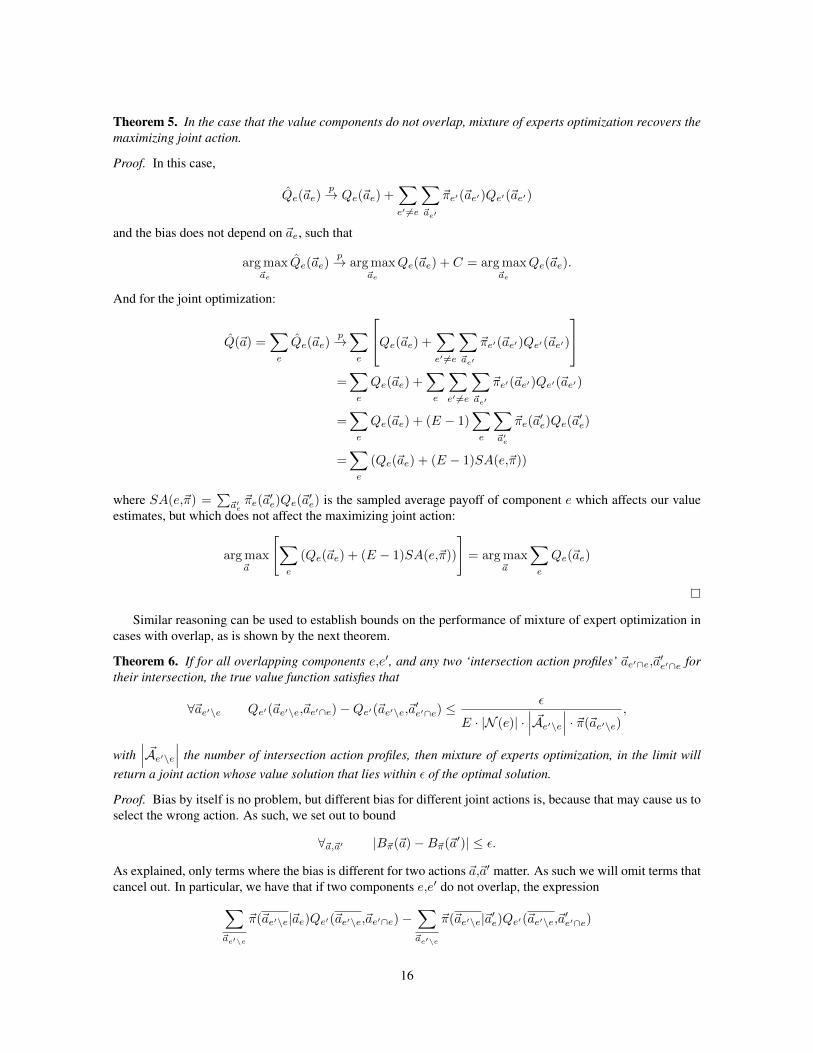
Theorem 5. In the case that the value components do not overlap, mixture of experts optimization recovers themaximizing joint action.

Proof. In this case,

Qe(~ae)p→ Qe(~ae) +

∑e′ 6=e

∑~ae′

~πe′(~ae′)Qe′(~ae′)

and the bias does not depend on ~ae, such that

argmax~ae

Qe(~ae)p→ argmax

~ae

Qe(~ae) + C = argmax~ae

Qe(~ae).

And for the joint optimization:

Q(~a) =∑e

Qe(~ae)p→∑e

Qe(~ae) +∑e′ 6=e

∑~ae′

~πe′(~ae′)Qe′(~ae′)

=∑e

Qe(~ae) +∑e

∑e′ 6=e

∑~ae′

~πe′(~ae′)Qe′(~ae′)

=∑e

Qe(~ae) + (E − 1)∑e

∑~a′e

~πe(~a′e)Qe(~a

′e)

=∑e

(Qe(~ae) + (E − 1)SA(e,~π))

where SA(e,~π) =∑~a′e~πe(~a

′e)Qe(~a

′e) is the sampled average payoff of component e which affects our value

estimates, but which does not affect the maximizing joint action:

argmax~a

[∑e

(Qe(~ae) + (E − 1)SA(e,~π))

]= argmax

~a

∑e

Qe(~ae)

Similar reasoning can be used to establish bounds on the performance of mixture of expert optimization incases with overlap, as is shown by the next theorem.

Theorem 6. If for all overlapping components e,e′, and any two ‘intersection action profiles’ ~ae′∩e,~a′e′∩e fortheir intersection, the true value function satisfies that

∀~ae′\e Qe′(~ae′\e,~ae′∩e)−Qe′(~ae′\e,~a′e′∩e) ≤ε

E · |N (e)| ·∣∣∣ ~Ae′\e∣∣∣ · ~π(~ae′\e) ,

with∣∣∣ ~Ae′\e∣∣∣ the number of intersection action profiles, then mixture of experts optimization, in the limit will

return a joint action whose value solution that lies within ε of the optimal solution.

Proof. Bias by itself is no problem, but different bias for different joint actions is, because that may cause us toselect the wrong action. As such, we set out to bound

∀~a,~a′ |B~π(~a)−B~π(~a′)| ≤ ε.

As explained, only terms where the bias is different for two actions ~a,~a′ matter. As such we will omit terms thatcancel out. In particular, we have that if two components e,e′ do not overlap, the expression∑

~ae′\e

~π(~ae′\e|~ae)Qe′(~ae′\e,~ae′∩e)−∑~ae′\e

~π(~ae′\e|~a′e)Qe′(~ae′\e,~a′e′∩e)

16

reduces to∑~ae′

~π(~ae′ |~ae)Qe′(~ae′)−∑~ae′

~π(~ae′ |~a′e)Qe′(~ae′) and hence vanishes under a componentwise pol-icy. We use this insight to define the bias in terms of neighborhood bias. Let us write N (e) for the set ofedges {e′} that have overlap with e, and let’s write ~aN (e) for the joint action that specifies actions for that entireoverlap, then we can write this as:

B~π(~a) ,E∑e=1

Be~π(~aN (e))

withBe~π(~aN (e)) =

∑e′∈N (e)

Be′∩e~π (~ae′∩e)

component e’s ‘neighborhood bias’, with

Be′→e~π (~ae) ,

∑~ae′\e

~π(~ae′\e|~ae)Qe′(~ae′\e,~ae′∩e)

the ‘intersection bias’: the bias introduced on e via the overlap between e′ and e.Now, we show how we can guarantee that the bias is small, by guaranteeing that the intersection biases are

small. This gives a conservative bound, since different biases may very well cancel out. Artbitrarily select twoactions, W.l.o.g. we select ~a to be the larger-biased joint action. We need to guarantee that

B~π(~a)−B~π(~a′) ≤ ε

↔E∑e=1

∑e′∈N (e)

Be′→e~π (~ae)−

E∑e=1

∑e′∈N (e)

Be′→e~π (~a′e) ≤ ε

↔E∑e=1

∑e′∈N (e)

Be′→e~π (~ae)−

∑e′∈N (e)

Be′→e~π (~a′e)

≤ ε←

∑e′∈N (e)

Be′→e~π (~ae)−

∑e′∈N (e)

Be′→e~π (~a′e) ≤

ε

E∀e

↔∑

e′∈N (e)

[Be′→e~π (~ae)−Be

′→e~π (~a′e)

]≤ ε

E∀e

←[Be′→e~π (~ae)−Be

′→e~π (~a′e)

]≤ ε

E × |N (e)|∀e,e′

let ε′ , εE×|N (e)| , we want[

Be′→e~π (~ae)−Be

′→e~π (~a′e)

]≤ ε′∑

~ae′\e

~π(~ae′\e|~ae)Qe′(~ae′\e,~ae′∩e)−∑~ae′\e

~π(~ae′\e|~a′e)Qe′(~ae′\e,~a′e′∩e) ≤ ε′

↔∑~ae′\e

[~π(~ae′\e|~ae)Qe′(~ae′\e,~ae′∩e)− ~π(~ae′\e|~a′e)Qe′(~ae′\e,~a′e′∩e)

]≤ ε′

← ~π(~ae′\e|~ae)Qe′(~ae′\e,~ae′∩e)− ~π(~ae′\e|~a′e)Qe′(~ae′\e,~a′e′∩e) ≤ε′∣∣∣ ~Ae′\e∣∣∣ ∀~ae′\e

17

Under a component-wise policy ~π(~ae′\e|~ae) = ~π(~ae′\e|~a′e) = ~π(~ae′\e) and thus

~π(~ae′\e)[Qe′(~ae′\e,~ae′∩e)−Qe′(~ae′\e,~a′e′∩e)

]≤ ε′∣∣∣ ~Ae′\e∣∣∣ ∀~ae′\e

↔ Qe′(~ae′\e,~ae′∩e)−Qe′(~ae′\e,~a′e′∩e) ≤ε′∣∣∣ ~Ae′\e∣∣∣~π(~ae′\e) ∀~ae′\e

Putting it all together, if the factorized Q function satisfies that, for all the component intersections, the followingholds:

∀~ae′\e,~ae′∩e,~a′e′∩e Qe′(~ae′\e,~ae′∩e)−Qe′(~ae′\e,~a′e′∩e) ≤ε

E |N (e)|∣∣∣ ~Ae′\e∣∣∣~π(~ae′\e)

we are guaranteed to find an ε-(absolute-error)-approximate solution.

18