A Fugal Discourse on the Electromagnetic Coupling of Electromagnetic Processes in the

Earth-Ionosphere and the Human Brain

by

Kevin S. Saroka

A thesis submitted in partial fulfillment of the requirements for the degree of

Doctor of Philosophy (PhD) in Human Studies

The Faculty of Graduate Studies Laurentian University

Sudbury, Ontario

© Kevin S. Saroka, 2016

ii

THESIS DEFENCE COMMITTEE/COMITÉ DE SOUTENANCE DE THÈSE Laurentian Université/Université Laurentienne

Faculty of Graduate Studies/Faculté des études supérieures Title of Thesis Titre de la thèse A Fugal Discourse on the Electromagnetic Coupling of Electromagnetic Processes

in the Earth-Ionosphere and the Human Brain Name of Candidate Nom du candidat Saroka, Kevin Degree Diplôme Doctor of Philosophy Department/Program Date of Defence Département/Programme Human Studies Date de la soutenance November 26, 2015

APPROVED/APPROUVÉ Thesis Examiners/Examinateurs de thèse: Dr. Michael Persinger (Supervisor/Directeur(trice) de thèse) Dr. Cynthia Whissell (Committee member/Membre du comité) Dr. John Lewko (Committee member/Membre du comité) Approved for the Faculty of Graduate Studies Approuvé pour la Faculté des études supérieures Dr. David Lesbarrères Monsieur David Lesbarrères Dr. Thilo Hinterberger Dean, Faculty of Graduate Studies (External Examiner/Examinateur externe) Doyen, Faculté des études supérieures Dr. Robert Lafrenie (Internal Examiner/Examinateur interne)

ACCESSIBILITY CLAUSE AND PERMISSION TO USE I, Kevin Saroka, hereby grant to Laurentian University and/or its agents the non-exclusive license to archive and make accessible my thesis, dissertation, or project report in whole or in part in all forms of media, now or for the duration of my copyright ownership. I retain all other ownership rights to the copyright of the thesis, dissertation or project report. I also reserve the right to use in future works (such as articles or books) all or part of this thesis, dissertation, or project report. I further agree that permission for copying of this thesis in any manner, in whole or in part, for scholarly purposes may be granted by the professor or professors who supervised my thesis work or, in their absence, by the Head of the Department in which my thesis work was done. It is understood that any copying or publication or use of this thesis or parts thereof for financial gain shall not be allowed without my written permission. It is also understood that this copy is being made available in this form by the authority of the copyright owner solely for the purpose of private study and research and may not be copied or reproduced except as permitted by the copyright laws without written authority from the copyright owner.

iii

Abstract

There exists a space between the ionosphere and the surface of the earth within which

electromagnetic standing waves, generated by lightning strikes, can resonate around the

earth; these standing waves are known collectively as the Schumann resonances. In the

late 1960s König and Ankermuller already reported striking similarities between these

electromagnetic signals and those recorded from the electroencephalograms (EEG) of

the human brain; both signals exhibit similar characteristics in terms of frequency and

electric and magnetic field intensity. The analyses reported here demonstrate that 1)

microscopic (brain) and macroscopic (earth) representations of natural electromagnetic

fields are conserved spatially, 2) that electric fields recorded from human brains exhibit

strong correlation with the strength of the these parameters and 3) that the human brain

periodically synchronizes with signals generated within the earth-ionosphere waveguide

at frequencies characteristic of the Schumann resonance for periods of about 300 msec.

These findings recapitulate 17th century ideas of harmony amongst the cerebral and

planetary spheres and may provide the means necessary to quantitatively investigate

concepts of early 20th century psychology.

iv

Acknowledgements

First I would like to thank the committee members Dr. Cynthia Whissell and Dr. John

Lewko as well as internal examiner Dr. Robert Lafrenie whose questions, comments,

and close reading of this manuscript were appreciated. I would also like to extend

thanks to the Neuroscience Research Group for their endless supply of ideas during the

development of many of the analyses employed in the following pages.

Acknowledgements are also credited to Sam, Helen, Matthew and Stephany Saroka who

all played a bigger role in the overall completion of this project than they will ever know.

Finally thanks are directed to my supervisor and mentor Dr. Michael Persinger without

whom the passion and curiosity to pursue many of the ideas explored in this dissertation

would be absent—his patience and expertise were critical to the composition of this

manuscript.

v

Table of Contents

Abstract .......................................................................................................................... iii Acknowledgements ....................................................................................................... iv Table of Contents ........................................................................................................... v List of Figures .............................................................................................................. viii List of Tables ............................................................................................................... xvii

Chapter 1-Introduction ................................................................................................... 1

1.0 General Introduction .................................................................................... 1 2.0 Basic Concepts ............................................................................................ 6

2.1 Natural Magnetic Fields ........................................................................... 6 2.2 Quantitative Electroencephalography (QEEG) ...................................... 17 2.3 Biological Effects of Natural and Experimental Electromagnetic Fields . 28

3.0 Apparent Earth-Ionosphere-Brain Connection .......................................... 32 3.1 Experimental Motivations for Investigation ............................................ 32 3.2 Quantitative Motivations for Investigation .............................................. 34

4.0 Interdisciplinay Approach .......................................................................... 36 5.0 Proposed Research and Methods ............................................................. 50

5.1 Relationships between brain activity and measures of the static geomagnetic field ................................................................................ 50

5.2 Explorative Application of QEEG-related Methods to Investigate the Static Geomagnetic Field .................................................................... 51

5.3 Relationships between brain activity and measures of background AC magnetic fields .................................................................................... 52

5.4 Schumann Resonance Signatures in the Human Brain ......................... 53 5.5 Relationships Between Extremely-Low Frequency Spectral Density and

Human Brain Activity and Construction and Characterization of an Induction Coil Magnetometer For Measuring Extremely-Low Frequency Earth-Ionospheric Perturbations ......................................................... 55

5.6 Construction and Characterization of an Induction Coil Magnetometer For Measuring Extremely-Low Frequency Earth-Ionospheric Perturbations ....................................................................................... 56

5.7 Simultaneous Measurements of the Schumann Resonance and Brain Activity ................................................................................................. 57

6.0 References ............................................................................................... 58 Chapter 2- Greater electroencephalographic coherence between left and right temporal lobe structures during increased geomagnetic activity ........................... 71

2.1 Abstract ..................................................................................................... 71 2.2 Introduction ................................................................................................ 72 2.3 Methods and Materials .............................................................................. 74 2.4 Results ....................................................................................................... 77 3.5 Discussion and Conclusion ....................................................................... 80 3.6 References ................................................................................................ 84

vi

Chapter 3- Assessment of Geomagnetic Coherence and Topographic Landscapes of the Static Geomagnetic Field in Relation to the Human Brain Employing Electroencephalographic Methodology ..................................................................... 88

3.1 Introduction ................................................................................................ 88 3.2 Materials and Methods .............................................................................. 91 3.3 Results ....................................................................................................... 93 3.4 Discussion and Conclusion ....................................................................... 98 3.5 References .............................................................................................. 100

Chapter 4- The Proximal AC Electromagnetic Environment and Human Brain Activity ......................................................................................................................... 104

4.1 Introduction .............................................................................................. 104 4.2 Methods and Materials ............................................................................ 106 4.3 Results ..................................................................................................... 109 4.4 Discussion and Conclusion ..................................................................... 112 4.5 References .............................................................................................. 115

Chapter 5-Quantitative Convergence of Major-Minor Axes Cerebral Electric Field Potentials and Spectral Densities: Consideration of Similarities to the Schumann Resonance and Practical Implications ..................................................................... 119

4.1 Introduction .............................................................................................. 119 4.2 Materials and Methods ............................................................................ 120 5.3 Results ..................................................................................................... 125 5.4 Discussion ............................................................................................... 133 5.5 References .............................................................................................. 140

Chapter 6-Quantitative Evidence for Direct Effects Between Earth-Ionosphere Schumann Resonances and Human Cerebral Cortical Activity ............................ 146

6.1 Introduction .............................................................................................. 146 6.2 Construction and Characterization of an Induction Coil Magnetometer .. 156 6.3 Potential Fugal Patterns in the Schumann Resonance Signal ................ 161 6.4 Correlation between Real Schumann and Cerebral Coherence Values .. 168 6.5 The Parahippocampal Region as a Locus of Interaction ......................... 174 6.6 Extended Correlations ............................................................................. 179 6.7 Implications of Schumann Amplitude Facilitation of Interhemispheric Coherence in the Human Brain ..................................................................... 183 6.8 Real-time Coherence Between Brain Activity and Schumann Frequencies ....................................................................................................................... 185 6.7 The Importance of Human Density For Potential Convergence Between Global Schumann Frequencies and Aggregates of Human Brains ............... 190 6.8 Conclusions ............................................................................................. 193 6.9 References .............................................................................................. 193

vii

Chapter 7-Occurrence of Harmonic Synchrony Between Human Brain Activity and the Earth-Ionosphere Schumann Resonance Measured Locally and Non-locally199

7.1 Introduction .............................................................................................. 199 7.2 Materials and Methods ............................................................................ 202 7.3 Results ..................................................................................................... 207 7.4 Discussion ............................................................................................... 212 7.5 Conclusion ............................................................................................... 217 7.6 References .............................................................................................. 217

Chapter 8-Synthesis, Implications, and Conclusion ............................................... 220

viii

List of Figures

Figure 1.1 Fugue in D Major from “The Well-Tempered Clavier, Book 2”. In this fugal

passage, the subject melody (red) is repeated verbatim in 3 other voices. ............... 3

Figure 1.2 Fugue in C-Minor from “The Well-Tempered Clavier, Book 2”. The subject in

this passage is stated along two different speeds (green=fast, blue=slow) in a way

that can be likened to celestial bodies rotating around the sun with different temporal

periods. ...................................................................................................................... 4

Figure 1.3 Classical example of electric fields generated by a positively-charged (proton)

and negatively-charged (electron) particles. .............................................................. 7

Figure 1.4 The magnetosphere and associated boundaries. Picture from (Russell,

1972). ......................................................................................................................... 8

Figure 1.5 Example of a geomagnetic storm. The y-axis refers to gammas (each gamma

represents one nanoTesla) and x-axis is time. Picture in (Bleil, 1964). .................. 10

Figure 1.6 Schamatic diagram of the cavity bounded by the earth and the ionosphere. 11

Figure 1.7 (A) Spectral density profile of the Schumann resonance (B) Exemplary time-

series from which Schumann resonance spectra are obtained. .............................. 13

Figure 1.8 (Above) Time-series and (Below) sonogram of a Pc1 micropulsation event

showing ‘rising-tones’ in the range of 0.4 to 0.5Hz. Picture in Volume 2 of

Matsushita and Campbell (1967). ............................................................................ 16

ix

Figure 1.10 Schematic of a typical spectral analysis performed on quantitative EEG data.

The original signal (top) is modeled after a series of sine waves (middle) and the

area under the curve of each signal is then calculated and graphed (bottom). ....... 20

Figure 1.11 The 4 classes of normative microstates as originally discovered by Koenig

and Lehmann (2002). .............................................................................................. 23

Figure 1.12 (Top) Two signals derived from P3 and P4 sensors on the scalp show

evident synchronicity (Bottom) Coherence analysis indicating that both sensors are

periodically coherent within the 9-10Hz range. ........................................................ 26

Figure 1.13 Original comparison between electromagnetic signals (Left) and signals

derived from human electroencephalograms (right) made by Konig. Picture found in

Persinger (1974). ..................................................................................................... 32

Figure 1.14 Schamatic diagram of a section of neocortex that can be modeled as two

parallel plates with the positive plate closer to cortex/white matter interface and the

negative plate closer to the surface of the cortex. ................................................... 35

Figure 1.15 The ‘holographic’, or fractal relationships explored in a mathematical set (A),

a musical fugue (B), and the proposed connection between electromagnetic

processes of the human brain and the earth-ionosphere (C). (A) Example of a

fractal mathematical set known as the Sierpinski Triangle. The process shows how

the information within one component of the object can be broken down into

constituent parts, each possessing the same informational content. (Image Source:

http://math.bu.edu/DYSYS/chaos-game/node2.html) (B) Fugue in C-Minor from “The

Well-Tempered Clavier, Book 2 ”. The subject in this passage is stated along two

x

different speeds (green=fast, blue=slow) in a way that can be likened to celestial

bodies rotating around the sun with different temporal periods. (C) Relationship

between standing waves formed within the earth-ionosphere cavity and the human

brain. (Image Source: Nunez (1995), p.83) ............................................................. 47

Figure 1.16 Temporal courses of amplitude frequency spectra averaged over five

minutes (from Kloppel in Popp, 1979). .................................................................... 54

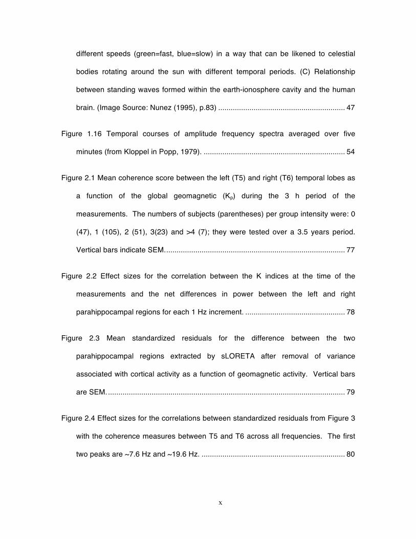
Figure 2.1 Mean coherence score between the left (T5) and right (T6) temporal lobes as

a function of the global geomagnetic (Kp) during the 3 h period of the

measurements. The numbers of subjects (parentheses) per group intensity were: 0

(47), 1 (105), 2 (51), 3(23) and >4 (7); they were tested over a 3.5 years period.

Vertical bars indicate SEM. ...................................................................................... 77

Figure 2.2 Effect sizes for the correlation between the K indices at the time of the

measurements and the net differences in power between the left and right

parahippocampal regions for each 1 Hz increment. ................................................ 78

Figure 2.3 Mean standardized residuals for the difference between the two

parahippocampal regions extracted by sLORETA after removal of variance

associated with cortical activity as a function of geomagnetic activity. Vertical bars

are SEM. .................................................................................................................. 79

Figure 2.4 Effect sizes for the correlations between standardized residuals from Figure 3

with the coherence measures between T5 and T6 across all frequencies. The first

two peaks are ~7.6 Hz and ~19.6 Hz. ..................................................................... 80

xi

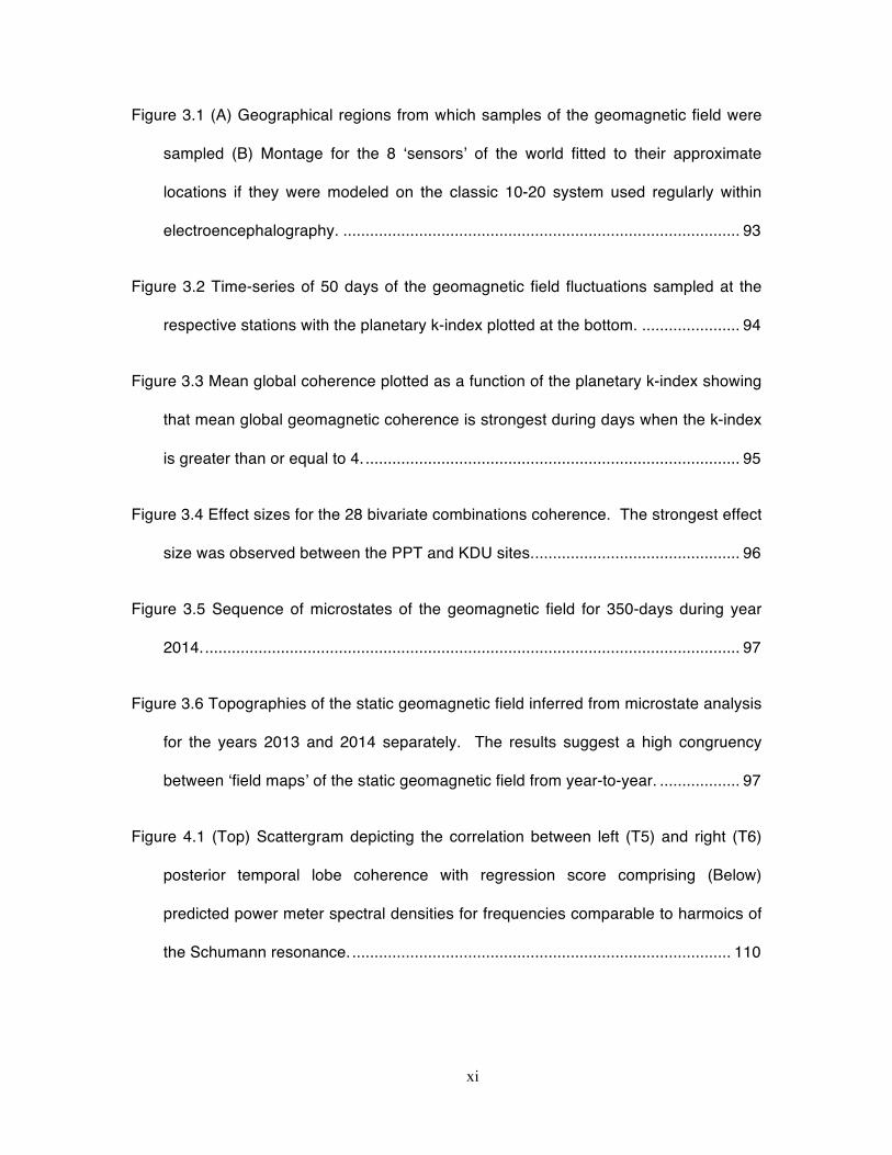
Figure 3.1 (A) Geographical regions from which samples of the geomagnetic field were

sampled (B) Montage for the 8 ‘sensors’ of the world fitted to their approximate

locations if they were modeled on the classic 10-20 system used regularly within

electroencephalography. ......................................................................................... 93

Figure 3.2 Time-series of 50 days of the geomagnetic field fluctuations sampled at the

respective stations with the planetary k-index plotted at the bottom. ...................... 94

Figure 3.3 Mean global coherence plotted as a function of the planetary k-index showing

that mean global geomagnetic coherence is strongest during days when the k-index

is greater than or equal to 4. .................................................................................... 95

Figure 3.4 Effect sizes for the 28 bivariate combinations coherence. The strongest effect

size was observed between the PPT and KDU sites. .............................................. 96

Figure 3.5 Sequence of microstates of the geomagnetic field for 350-days during year

2014. ........................................................................................................................ 97

Figure 3.6 Topographies of the static geomagnetic field inferred from microstate analysis

for the years 2013 and 2014 separately. The results suggest a high congruency

between ‘field maps’ of the static geomagnetic field from year-to-year. .................. 97

Figure 4.1 (Top) Scattergram depicting the correlation between left (T5) and right (T6)

posterior temporal lobe coherence with regression score comprising (Below)

predicted power meter spectral densities for frequencies comparable to harmoics of

the Schumann resonance. ..................................................................................... 110

xii

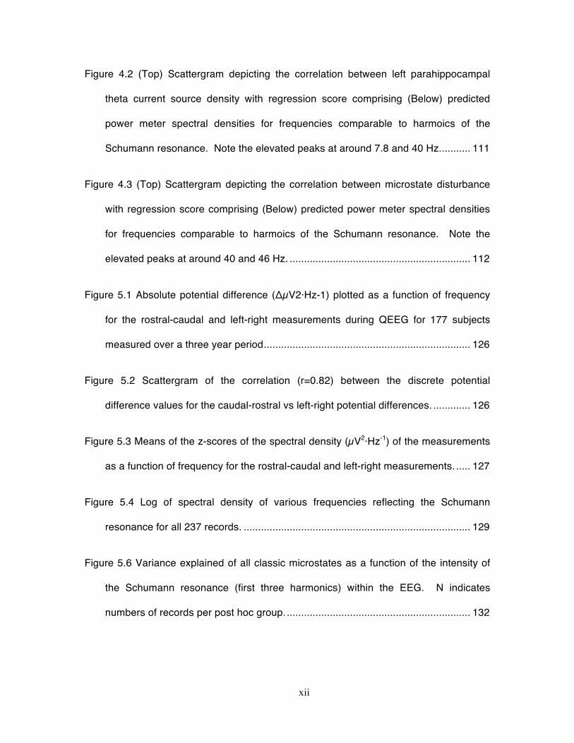
Figure 4.2 (Top) Scattergram depicting the correlation between left parahippocampal

theta current source density with regression score comprising (Below) predicted

power meter spectral densities for frequencies comparable to harmoics of the

Schumann resonance. Note the elevated peaks at around 7.8 and 40 Hz. .......... 111

Figure 4.3 (Top) Scattergram depicting the correlation between microstate disturbance

with regression score comprising (Below) predicted power meter spectral densities

for frequencies comparable to harmoics of the Schumann resonance. Note the

elevated peaks at around 40 and 46 Hz. ............................................................... 112

Figure 5.1 Absolute potential difference (ΔµV2·Hz-1) plotted as a function of frequency

for the rostral-caudal and left-right measurements during QEEG for 177 subjects

measured over a three year period ........................................................................ 126

Figure 5.2 Scattergram of the correlation (r=0.82) between the discrete potential

difference values for the caudal-rostral vs left-right potential differences. ............. 126

Figure 5.3 Means of the z-scores of the spectral density (µV2·Hz-1) of the measurements

as a function of frequency for the rostral-caudal and left-right measurements. ..... 127

Figure 5.4 Log of spectral density of various frequencies reflecting the Schumann

resonance for all 237 records. ............................................................................... 129

Figure 5.6 Variance explained of all classic microstates as a function of the intensity of

the Schumann resonance (first three harmonics) within the EEG. N indicates

numbers of records per post hoc group. ................................................................ 132

xiii

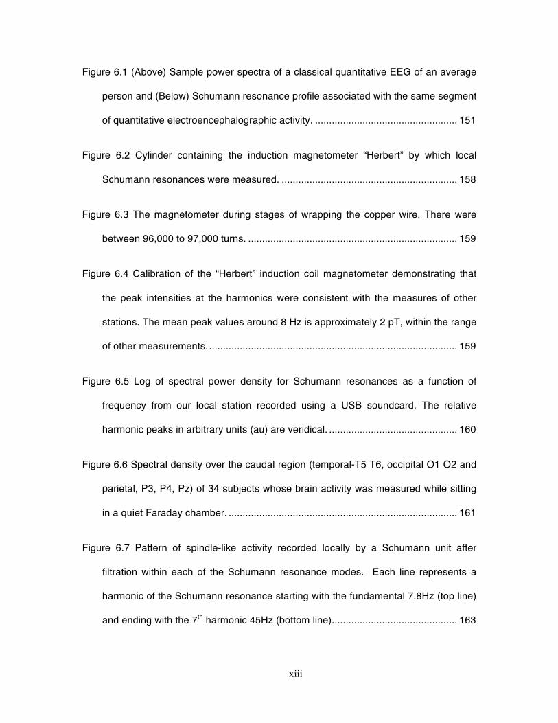
Figure 6.1 (Above) Sample power spectra of a classical quantitative EEG of an average

person and (Below) Schumann resonance profile associated with the same segment

of quantitative electroencephalographic activity. ................................................... 151

Figure 6.2 Cylinder containing the induction magnetometer “Herbert” by which local

Schumann resonances were measured. ............................................................... 158

Figure 6.3 The magnetometer during stages of wrapping the copper wire. There were

between 96,000 to 97,000 turns. ........................................................................... 159

Figure 6.4 Calibration of the “Herbert” induction coil magnetometer demonstrating that

the peak intensities at the harmonics were consistent with the measures of other

stations. The mean peak values around 8 Hz is approximately 2 pT, within the range

of other measurements. ......................................................................................... 159

Figure 6.5 Log of spectral power density for Schumann resonances as a function of

frequency from our local station recorded using a USB soundcard. The relative

harmonic peaks in arbitrary units (au) are veridical. .............................................. 160

Figure 6.6 Spectral density over the caudal region (temporal-T5 T6, occipital O1 O2 and

parietal, P3, P4, Pz) of 34 subjects whose brain activity was measured while sitting

in a quiet Faraday chamber. .................................................................................. 161

Figure 6.7 Pattern of spindle-like activity recorded locally by a Schumann unit after

filtration within each of the Schumann resonance modes. Each line represents a

harmonic of the Schumann resonance starting with the fundamental 7.8Hz (top line)

and ending with the 7th harmonic 45Hz (bottom line). ............................................ 163

xiv

Figure 6.8 Frequency pattern within each envelope or spindle from Figure 6 after Hilbert

transformation. ....................................................................................................... 163

Figure 6.9 Demonstration of a type of fugal coupling between the various harmonics of

the Schumann values. This example depicts coupling specifically between the first

and seventh Schumann harmonics. Red and yellow areas indicate cross-frequency

coherence intervals. ............................................................................................... 164

Figure 6.10 Correlation between the coherence strength between the left (T3) and right

(T4) temporal lobes for subjects whose QEEGs were measured in Sudbury, Ontario

and the electric field strength of the first two Schumann harmonics in California .. 173

Figure 6.11 Correlation between the intensity of the contemporary fundamental electric

field of the Schumann resonance in California and the net difference in current

density as measured by sLORETA for the 9 to 10 Hz band between the left and right

parahippocampal regions for 49 subjects whose QEEGs were measured between

2009 and 2010. ...................................................................................................... 177

Figure 6.12 The effect size (correlation coefficient squared) for the association between

the caudal 14.7 Hz QEEG activity in Sudbury and Schumann E field spectral density

in Italy and the frequency band of the E field. Note the strongest correlation for the

first three harmonics of the Schumann resonance. ............................................... 180

Figure 6.13 Sample (about 5 s) electroencephalographic voltage pattern from the

different sensor sites over the skull (indicated by traditional identifiers) and the

voltage fluctuations associated with the simultaneous recording of the Schumann.

............................................................................................................................... 186

xv

Figure 6.14 Sample record (about 10 s) of the composite EEG from the caudal portions

of the subject’s cerebrum (EEG) and the Schumann resonance (EM) measured 1 m

away. The horizontal axis is real time in ms while the vertical axis is frequency. The

first, second and third harmonic of the Schumann resonance measured with the

magnetometer were coherent with the 8, 13, and 20Hz activity occurring within the

integrated caudal root-mean-square signal. The yellow indicates weak (0.30

coherence while the red indicates stronger (0.5 to 0.7) coherence. In the first panel

(below the raw data) the coherence durations in the indicated frequencies occurred

primarily as brief periods between 0.3 s to about 2 s. The phase shift is noted in the

lower panel. The phase shift for this event at 7.8 Hz with cerebral activity was

equivalent to about 41.9 ms. “Harmonic synchrony” or simultaneous coherence

across two or more harmonics (possibly 4 or 5 with different magnitudes of

coherence) is indicated by the vertical dotted line. ................................................ 187

Figure 7.1 Examples of harmonic synchrony observed between a male and female

participant during simultaneous measurements of their EEG and ELF activity

measured with a magnetometer locally in Sudbury, Canada. ................................ 207

Figure 7.2 Examples of harmonic synchrony observed between a male and female

participant during simultaneous measurements of their EEG and ELF activity

measured with a magnetometer non-locally in Cumiana, Italy. ............................. 208

Figure 7.3 Averaged coherence between the caudal root-mean-square and ELF activity

recorded in Italy plotted as a function of frequency. .............................................. 209

Figure 7.4 (A) Topographical maps of clusters before (top line) and during (middle line)

the onset of harmonic synchronous events. NC refers to the number of clusters

xvi

contributing to the grand mean cluster. (B) Standardized differences between the

two conditions (bottom line). Colour bar indicates z-score. .................................. 211

xvii

List of Tables Table 1-1 Nomenclature for geomagnetic micropulsations with their associated

frequencies and intensities. Adapted from Bianchi and Meloni (2007). .................. 15

Table 5-1 Range of the standardized (z-score) for the raw spectral density values for the

peak band (in Hz) for the 10 randomly selected subjects. The “band width” for the

peak band range is also shown. ............................................................................ 128

Table 5-2 Means and Standard Errors of the Means (in parentheses) for current source

density (µA·mm-2) of the parahippocampal gyrus within the classical frequency

bands. .................................................................................................................... 132

1

Chapter 1

Introduction

1.0 General Introduction

The possibility of a harmonic connection between all natural phenomena, ranging

from the circling of subatomic particles around a nucleus to the orbit of the planets

around the sun has gradually become more and more substantive (Persinger and

Lavallee 2012; Persinger, 2012). During the time of Pythagoras, Ancient Greeks were

already aware of a musica univeralis, or Harmony of the Spheres, which proposed the

idea that the orbit of planets followed a geometrical proportionality around the center of

the galaxy. Today we now know that gravitational and electromagnetic forces propel the

planets around the sun in a quasi-periodic fashion that is also influenced by the planet’s

size and mass. We now also understand that living creatures existing on Earth display

changes (such as hibernation and food consumption) in accordance with the season. In

addition, we now understand that environmental conditions, such as weather and the

geomagnetic field, which are both influenced by solar activity, can influence subtle

biological processes like the behaviour of an organism. Finally, we are now beginning to

understand how behaviour and structure of cellular constituents of the organism are

dynamically interconnected such that behaviour (X) can influence cellular processes (Y)

and vice versa. In conclusion, life on earth together with the environment that influences

it is also a part of a ‘cosmic dance’ that exists within the universe itself (Capra, 1976).

Human subjective experiences, such as observation, are then reflections of changes

2

within any of the aforementioned levels of discourse and exist on a continuum of macro-

to-microcosm.

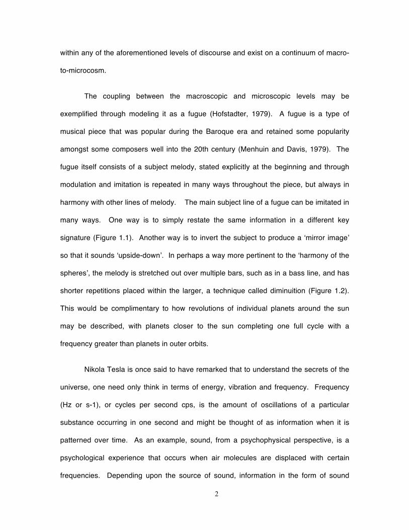
The coupling between the macroscopic and microscopic levels may be

exemplified through modeling it as a fugue (Hofstadter, 1979). A fugue is a type of

musical piece that was popular during the Baroque era and retained some popularity

amongst some composers well into the 20th century (Menhuin and Davis, 1979). The

fugue itself consists of a subject melody, stated explicitly at the beginning and through

modulation and imitation is repeated in many ways throughout the piece, but always in

harmony with other lines of melody. The main subject line of a fugue can be imitated in

many ways. One way is to simply restate the same information in a different key

signature (Figure 1.1). Another way is to invert the subject to produce a ‘mirror image’

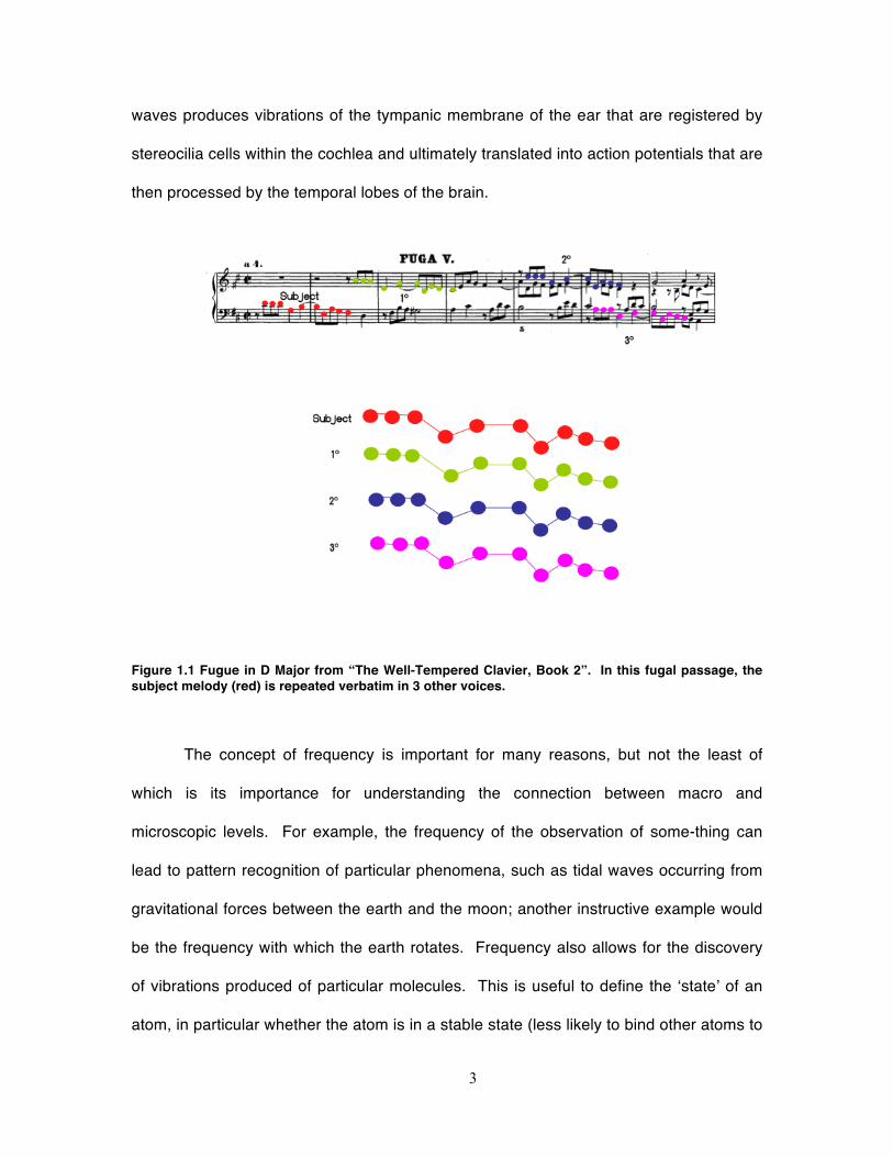
so that it sounds ‘upside-down’. In perhaps a way more pertinent to the ‘harmony of the

spheres’, the melody is stretched out over multiple bars, such as in a bass line, and has

shorter repetitions placed within the larger, a technique called diminuition (Figure 1.2).

This would be complimentary to how revolutions of individual planets around the sun

may be described, with planets closer to the sun completing one full cycle with a

frequency greater than planets in outer orbits.

Nikola Tesla is once said to have remarked that to understand the secrets of the

universe, one need only think in terms of energy, vibration and frequency. Frequency

(Hz or s-1), or cycles per second cps, is the amount of oscillations of a particular

substance occurring in one second and might be thought of as information when it is

patterned over time. As an example, sound, from a psychophysical perspective, is a

psychological experience that occurs when air molecules are displaced with certain

frequencies. Depending upon the source of sound, information in the form of sound

3

waves produces vibrations of the tympanic membrane of the ear that are registered by

stereocilia cells within the cochlea and ultimately translated into action potentials that are

then processed by the temporal lobes of the brain.

Figure 1.1 Fugue in D Major from “The Well-Tempered Clavier, Book 2”. In this fugal passage, the subject melody (red) is repeated verbatim in 3 other voices.

The concept of frequency is important for many reasons, but not the least of

which is its importance for understanding the connection between macro and

microscopic levels. For example, the frequency of the observation of some-thing can

lead to pattern recognition of particular phenomena, such as tidal waves occurring from

gravitational forces between the earth and the moon; another instructive example would

be the frequency with which the earth rotates. Frequency also allows for the discovery

of vibrations produced of particular molecules. This is useful to define the ‘state’ of an

atom, in particular whether the atom is in a stable state (less likely to bind other atoms to

4

produce derivative molecules) or excited state (more likely to form bonds with other

atoms).

Figure 1.2 Fugue in C-Minor from “The Well-Tempered Clavier, Book 2”. The subject in this passage is stated along two different speeds (green=fast, blue=slow) in a way that can be likened to celestial bodies rotating around the sun with different temporal periods.

Frequency is also an important feature when discussed within the context of

behavioural and geophysical sciences. One of the most useful tools for understanding

the distributions of frequencies is spectral analysis. Given a time-series x with

observations made at regular intervals, spectral analysis can be used to decompose the

time-series into a series of sine waves in order to predict the occurrence of a

phenomenon, such as brain waves.

It will be proposed in this dissertation that ‘fugal’ relationship exists between the

electromagnetic activity generated within the earth and the electromagnetic activity

5

generated within the human brain. As Persinger has discussed on many occasions, the

special and temporal properties of the earth are all within the same range as those

measured frequently by the brain and might indicate a scale-invariant or fractal

relationship between both (Persinger, 2008; Persinger et al., 2008; Persinger 2012,

Persinger, 2013). One way that this harmony of the spheres (earth and brain) could

exist is because of the coupling of frequency, namely that the natural resonant

electromagnetic frequencies of the earth are similar in magnitude and intensity to those

generated within the brain, specifically within the extremely-low frequency domain of 0.1

to 100Hz.

6

2.0 Basic Concepts

2.1 Natural Magnetic Fields

2.1.1 Description of Electromagnetic Fields

Electromagnetic fields can be described as a force exerted on particulate matter

and exist in all points of space. A classic way of describing the electric field, for

example, is the force a point charge (almost always positively-charged particle such as a

proton) will experience when immersed within a field (Serway and Jewett, 2004).

Whereas the velocity, or drift velocity, of an electron within a given substance is about 1

mm/s due to resistive and capacitive characteristics within the medium, the velocity of a

electromagnetic field approaches the speed of light and extends everywhere in space

(Giancoli, 1984). Therefore, stated simply, electromagnetic fields influence the

consequence of matter immersed within it.

An electric field can be described in terms of the units V·m-1, or kg·m·A-1s-3. An

electric field or electric force of one particle due to the proximity of another particle can

be described by the equation FE=q1·q2/4·π·ε·r2, which is very similar to the formula for

gravitation, where q is charge of the particle, and ε is the electric permittivity of free-

space (Serway and Jewett, 2004). One can see from the formula that the electric field

strength at any point is proportional to the inverse square of the distance separating the

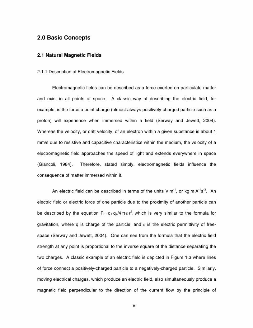
two charges. A classic example of an electric field is depicted in Figure 1.3 where lines

of force connect a positively-charged particle to a negatively-charged particle. Similarly,

moving electrical charges, which produce an electric field, also simultaneously produce a

magnetic field perpendicular to the direction of the current flow by the principle of

7

electromagnetic induction developed originally by Faraday (Serway and Jewett, 2004).

The intensity of the magnetic field, which can be ascribed the unit Tesla or kg·A-1·s-2, can

be calculated using the formula B=µ·I/2Πr2 where µ is the permeability of free space, I is

the electrical current strength and r is the radial distance from the current source.

Figure 1.3 Classical example of electric fields generated by a positively-charged (proton) and negatively-charged (electron) particles.

2.1.2 Geomagnetic Field

Surrounding the earth there exists a magnetic field. There are many theories as to

how this field is generated, but it is generally accepted that the earth’s magnetic field is

generated by electrical current loops produced by moving liquid iron within the earth’s

outer core (Roberts, 1992). Due to convection and temperature disparities between the

earth’s core and the layer containing the metallic fluid, the fluid moves around the solid

iron core and generates an electrical current loop that in turn produces a magnetic field.

8

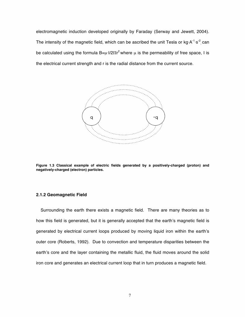
Around the earth outside of the earth’s atmosphere exists a region that is known as

the magnetosphere that hugs the earth and rejoins to form the magnetotail (Figure 1.4).

The dynamics of this region are influenced by the solar wind, which can be described as

a steady ‘laminar’ flow of particles (mostly protons) similar to a stream of water moving

around a rock (Bleil, 1964). The study of the interaction between the solar wind and its

associated magnetic field with the earth, which is about 1-5 nanoTesla, is known as

electromagnetic hydrodynamics.

Figure 1.4 The magnetosphere and associated boundaries. Picture from (Russell, 1972).

The strength of the earth’s magnetic field, measured in Teslas or kg·A-1·s2 is

usually measured with a digital magnetometer. Due to the three-dimensional nature of

magnetic fields, there are usually three measurements that are required to more

accurately describe its intensity, namely the x, y, and z-components. In addition, two

9

other measures describe the angle of the flux lines with respect to the horizontal

component, called declination, as well as the angle from which it deviates around the

earth’s meridian, called declination (Chapman and Bartels, 1940).

The typical intensity of the geomagnetic field is approximately 20-60 microTesla,

or 20,000 to 60,000 nanoTesla depending upon what component is measured

(Chapman and Bartels, 1940). This intensity varies in time depending upon

geographical location and external solar forces such as proton storms generated from

coronal mass ejections. It is generally accepted that the strength of the field increases

as a function of latitude, with highest intensities recorded in aurora regions of the

Northern hemisphere relative to the equator.

The sun periodically produces coronal mass ejections, which are high-energy

bursts of protons that can interact with the earth’s geomagnetic field to produce

geomagnetic storms. These bursts of energy travel via the solar wind with velocities that

can range from about 300-400 km·s-1 background velocities to about 600-900 km·s-1

(Matsushita and Campbell, 1967). Due to the higher density of protons and the increase

in speed of the solar wind, it produces a disturbance in the geomagnetic field and

displaces the background geomagnetic field from anywhere between 30-300 nanoTesla

(Bleil, 1964). Julius Bartels developed a scale by which the strength of the geomagnetic

disturbance could be quantified and is called the K-index. K-indices below 4 are

commonly known as ‘low disturbance’, whereas K-indices at 4 or above 4 are regarded

as moderate to active-level disturbances respectively.

While the initial displacement can take place anywhere between seconds and

minutes, there is usually a longer ‘recovery’ time which can last anywhere from days to

10

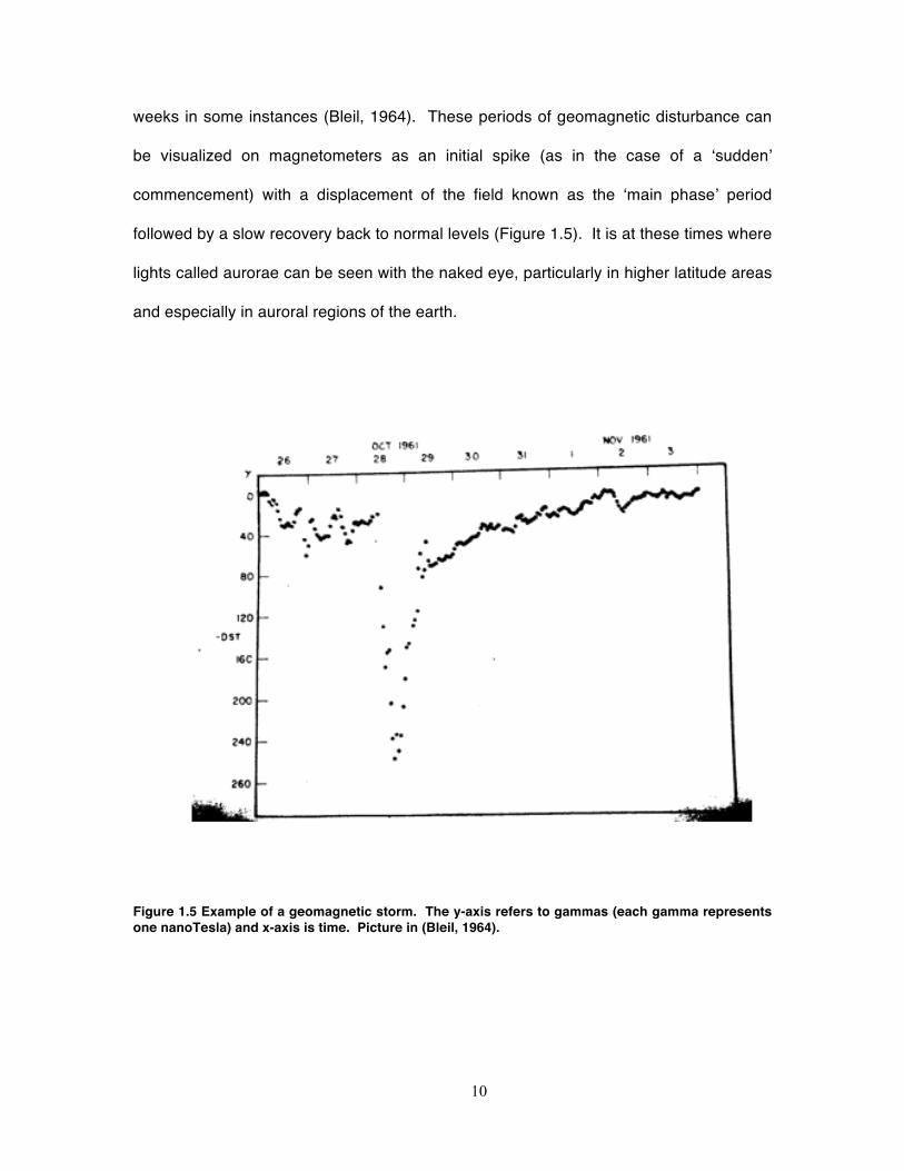
weeks in some instances (Bleil, 1964). These periods of geomagnetic disturbance can

be visualized on magnetometers as an initial spike (as in the case of a ‘sudden’

commencement) with a displacement of the field known as the ‘main phase’ period

followed by a slow recovery back to normal levels (Figure 1.5). It is at these times where

lights called aurorae can be seen with the naked eye, particularly in higher latitude areas

and especially in auroral regions of the earth.

Figure 1.5 Example of a geomagnetic storm. The y-axis refers to gammas (each gamma represents one nanoTesla) and x-axis is time. Picture in (Bleil, 1964).

11

2.1.3 Earth-Ionospheric Schumann Resonance

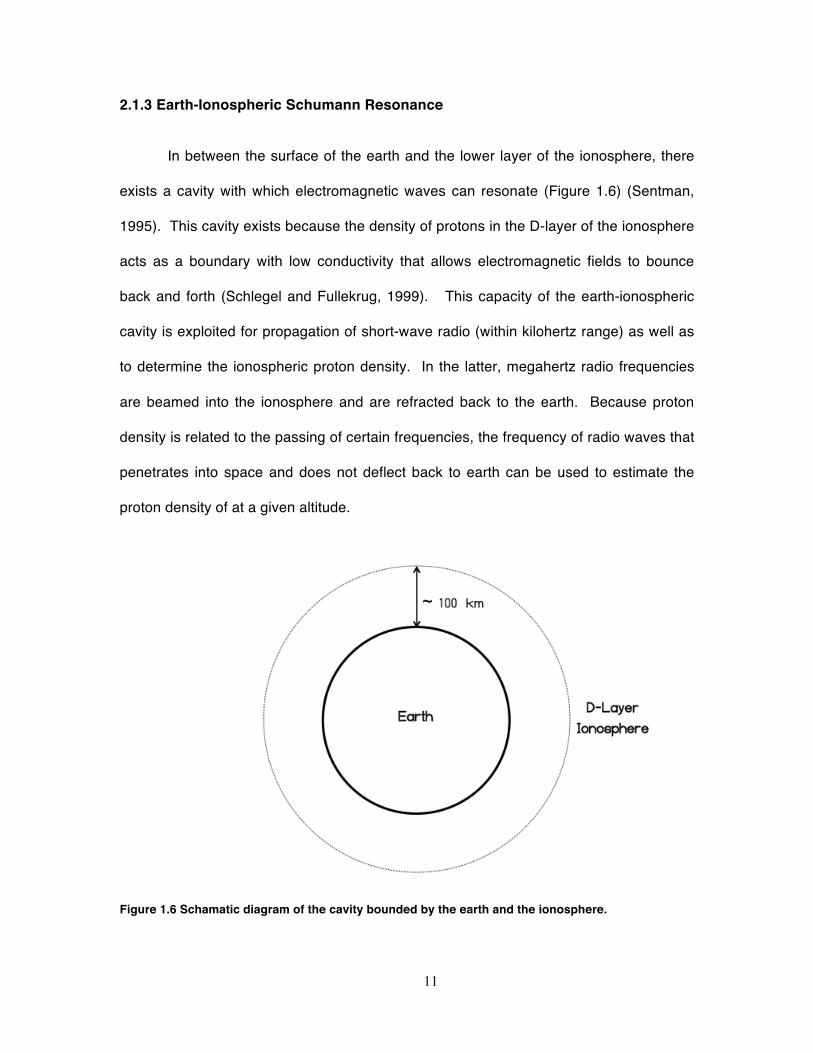
In between the surface of the earth and the lower layer of the ionosphere, there

exists a cavity with which electromagnetic waves can resonate (Figure 1.6) (Sentman,

1995). This cavity exists because the density of protons in the D-layer of the ionosphere

acts as a boundary with low conductivity that allows electromagnetic fields to bounce

back and forth (Schlegel and Fullekrug, 1999). This capacity of the earth-ionospheric

cavity is exploited for propagation of short-wave radio (within kilohertz range) as well as

to determine the ionospheric proton density. In the latter, megahertz radio frequencies

are beamed into the ionosphere and are refracted back to the earth. Because proton

density is related to the passing of certain frequencies, the frequency of radio waves that

penetrates into space and does not deflect back to earth can be used to estimate the

proton density of at a given altitude.

Figure 1.6 Schamatic diagram of the cavity bounded by the earth and the ionosphere.

12

In the 1950s Winfried Otto Schumann predicted that the boundaries formed by

the earth and the ionosphere could function as a waveguide for resonant

electromagnetic frequencies (Besser, 2007). Resonance can be expressed as a

property of all matter such that its physical characteristics produce a structure that allows

the object to oscillate at particular frequencies. A common example would be that of a

wine glass. When a particular frequency of sound is injected into the glass, it produces

standing waves with the structure of the silica. Depending upon the amplitude of the

injected sound at a resonant frequency, the standing waves can become so large that it

shatters the glass.

Because electromagnetic waves travel at a velocity similar to light, and because

of the circumference of the earth is approximately 40000 kilometers, one can obtain a

frequency by inserting these two values into the classic equation for velocity of a wave

v=fλ where v is velocity (m·s-1), f is frequency (s-1) and λ is wavelength (m). Solving for

the frequency one obtains 3·108 divided by 4·107m to yield a frequency of approximately

7.5Hz. This theoretical fundamental frequency of this cavity has since been measured

many times to be approximately 7.8Hz, however like all natural phenomena the

fundamental frequency is organized along a normal distribution such that the it can vary

between 7.3 and 8.3Hz.

Harmonics of a fundamental frequency can be explained as octaves of the same

pitch within a musical context. For example if one pictured middle C on a piano, the C

occurring one octave above could, for demonstrative purposes, be considered a

harmonic of middle C. Just like most standing waves, the Schumann resonance

fundamental frequency has harmonic frequencies spaced by approximately 6Hz intervals

to yield harmonics of approximately 14, 20, 26, 33, 39, 45 and 51 Hz (Figure 1.7) (Rakov

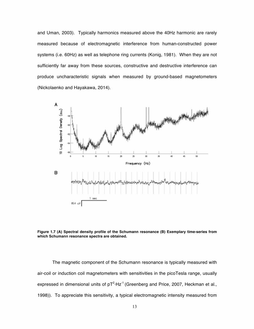
13

and Uman, 2003). Typically harmonics measured above the 40Hz harmonic are rarely

measured because of electromagnetic interference from human-constructed power

systems (i.e. 60Hz) as well as telephone ring currents (Konig, 1981). When they are not

sufficiently far away from these sources, constructive and destructive interference can

produce uncharacteristic signals when measured by ground-based magnetometers

(Nickolaenko and Hayakawa, 2014).

Figure 1.7 (A) Spectral density profile of the Schumann resonance (B) Exemplary time-series from which Schumann resonance spectra are obtained.

The magnetic component of the Schumann resonance is typically measured with

air-coil or induction coil magnetometers with sensitivities in the picoTesla range, usually

expressed in dimensional units of pT2·Hz-1 (Greenberg and Price, 2007, Heckman et al.,

1998)). To appreciate this sensitivity, a typical electromagnetic intensity measured from

14

a computer screen is about a microTesla, or a million times stronger than the Schumann

resonance whereas typical magnetic resonance imaging devices are within the order of

1-2 Teslas, or a trillion times stronger than natural earth background ‘noise’. The

induction coil itself is a cylinder wrapped with tens to hundreds of thousands of thin

copper wire (with approximately .2-.3 millimeter diameter). A paramagnetic material,

such as mu-metal, is then inserted into the center coil to increase its inductance (ability

to attract a magnetic field) by a factor of 100 to 1000 times. Because a time-varying

electrical current is associated with a time-varying magnetic field by electromagnetic

induction, the magnetic field picked-up within the coil produces electric current within the

copper wire. The time-varying voltages are then fed into equipment that filters out

unwanted artifacts and magnifies the signal. The resultant time-series (signal) is then

recorded on a computer and is entered into software that can analyze the frequency

characteristics of the signal.

The Schumann resonance displays peak intensities at times that roughly

correspond to peak thunderstorm activity at equatorial levels, such as Southeast Asia

and Africa (Price and Melnikov, 2004). Konig found that the Schumann resonance was

stronger during daytime periods (Konig, 1974); other researchers later confirmed this

finding (Price and Melnikov, 2004). In addition, the Schumann resonance displays a

characteristic seasonal variation with the highest variation in the first fundamental

frequencies occurring in the winter as opposed to the summer (Satori, 1996). The

Schumann resonance can also be used as a measure to infer global temperature

(Sekiguchi et al, 2006).

15

2.1.4 Geomagnetic Micropulsations

Geomagnetic micropulsations are visualized in strip-chart recordings of the

earth’s time-varying electromagnetic field as periodic fluctuations with intensities of about

1 to 5 nanoTesla (Bleil, 1964). They are generated by changes in solar wind and their

nomenclature can be divided into two classes of occurrences (Jacobs, 1970).

Micropulsations with a regular periodicity are labeled as ‘continuous’ (Pc) whereas

micropulsations that appear to be spontaneously arranged are called ‘irregular’ (Pi).

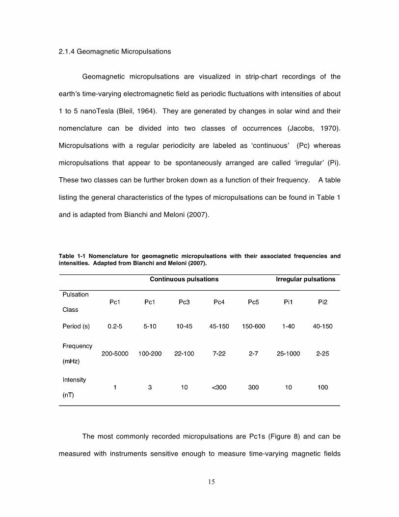
These two classes can be further broken down as a function of their frequency. A table

listing the general characteristics of the types of micropulsations can be found in Table 1

and is adapted from Bianchi and Meloni (2007).

Table 1-1 Nomenclature for geomagnetic micropulsations with their associated frequencies and intensities. Adapted from Bianchi and Meloni (2007).

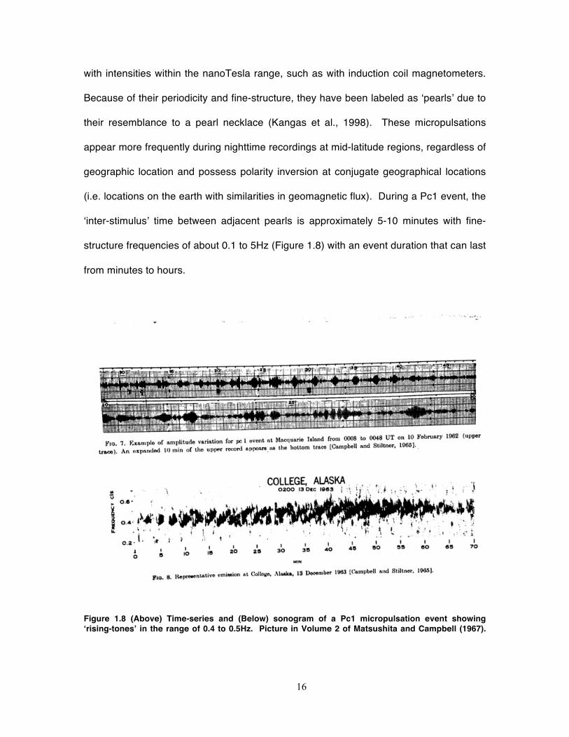
The most commonly recorded micropulsations are Pc1s (Figure 8) and can be

measured with instruments sensitive enough to measure time-varying magnetic fields

16

with intensities within the nanoTesla range, such as with induction coil magnetometers.

Because of their periodicity and fine-structure, they have been labeled as ‘pearls’ due to

their resemblance to a pearl necklace (Kangas et al., 1998). These micropulsations

appear more frequently during nighttime recordings at mid-latitude regions, regardless of

geographic location and possess polarity inversion at conjugate geographical locations

(i.e. locations on the earth with similarities in geomagnetic flux). During a Pc1 event, the

‘inter-stimulus’ time between adjacent pearls is approximately 5-10 minutes with fine-

structure frequencies of about 0.1 to 5Hz (Figure 1.8) with an event duration that can last

from minutes to hours.

Figure 1.8 (Above) Time-series and (Below) sonogram of a Pc1 micropulsation event showing ‘rising-tones’ in the range of 0.4 to 0.5Hz. Picture in Volume 2 of Matsushita and Campbell (1967).

17

2.2 Quantitative Electroencephalography (QEEG)

2.2.1 Equipment and Methods

The quantitative electroencephalograph is a modified version of the

electroencephalograph discovered by Hans Berger and allows for the digital recording of

voltages that are recorded from the surface of the scalp (Millett, 2001; Niedermeyer

2005). Whereas during the discovery of the electroencephalograph data analysis was

performed mostly by qualitative visual inspection or coarse frequency approximation by

counting the number of peaks per second (indication of frequency), in a modern context

computers are used to record raw voltages at high sampling frequencies (the number of

recordings per second) which allows researchers to quantify the ‘peaks and valleys’ of

electrical activity from the brain in terms of frequency and amplitude. Most contemporary

quantitative electroencephalographs are battery-operated and fed into laptop computers

making them portable and adaptable to most conceivable experimental settings.

In standard procedures, sensors with an approximate diameter of 1 cm are

placed on the scalp with some conductive paste (usually a compound containing

sodium) sandwiched between the sensor and the scalp. In some QEEG apparatuses,

the sensors are embedded in a cap that can simply be applied over the scalp. Each

sensor is then placed according to standardized sensor placements, known more

commonly as the 10-20 International Standard of Electrode Placement. This

standardization ensures that results are generalizeable to other researchers and also

facilitates replicability within different laboratories.

Once the sensors/cap have been applied and impedances of each sensor have

been appropriately set (by adding or subtracting the conductive paste), measurements of

18

voltages at a fixed sampling rate are collected and digitized, with a digital-to-analog

converter system, and recorded by a computer system.

2.2.2 Nature of the Data

The intensities of the voltages typically recorded with the QEEG are within the

range of 50-100 microvolts, or 10-6 kg·m2·A-1·s-3. For comparative purposes, this voltage

is approximately a million times less than batteries that supply power for television

remote controls. The intensity of the scalp recordings is approximately proportional to

the numbers of action potentials, whose voltages are within the order of 10-3 volts of

neurons firing synchronously. It may seem counter-intuitive that the voltage associated

with neuronal assemblies is a thousand times less than the voltage associated with one

action potential; however scalp voltages are not only attenuated by the physical

impedance by the skull and cerebrospinal fluid, but also by constructive and destructive

interference (adding and subtracting) of proximal neuronal discharges. The mechanism

by which the ‘squiggles’ observed in the strip chart are generated has been summarized

in Figure 1.9 which shows that the voltage of the local field potentials (recorded within a

defined area of the scalp) are approximately proportional to the integrated neuronal

activity below the surface.

2.2.3 Spectral Analysis

The obtained signal can be expressed in terms of a time-series and is thus

entered into appropriate statistical analysis. One of the most common techniques for

understanding the frequency characteristics of the time-series is to apply a Fast Fourier

19

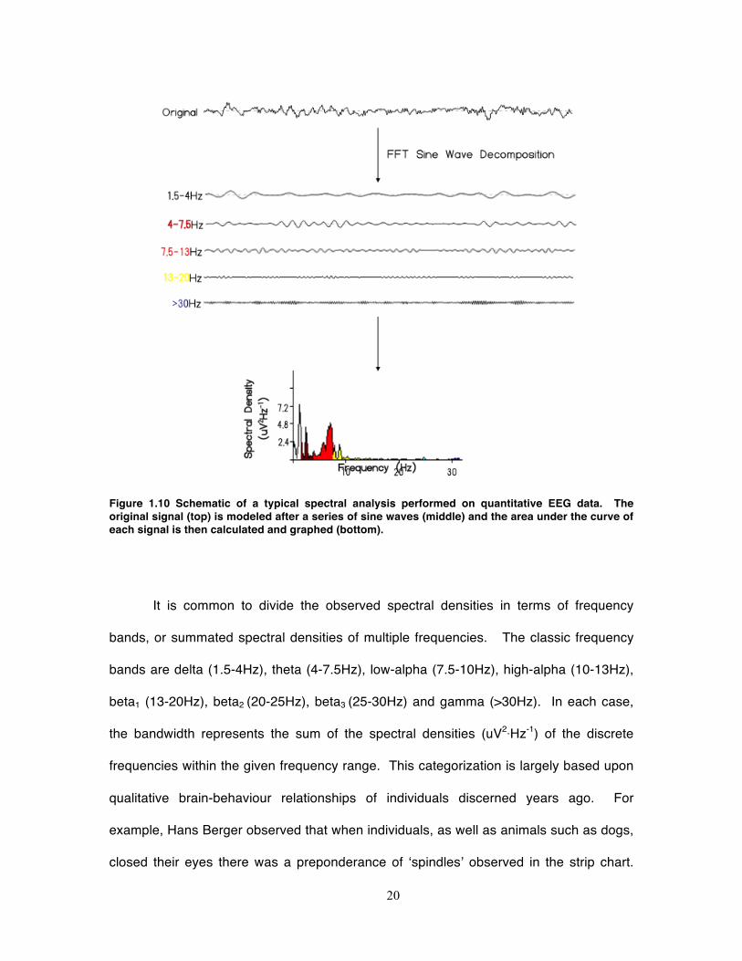
Transform. This equation models the ‘irregular’ time-series into a series of sinusoidal

waves of increasing frequency and then calculates the spectral density of each

sinusoidal component. A summary of the FFT procedure is depicted in Figure 1.10.

Due to the nature of the algorithm as well as the Nyquist limit, the maximum frequency of

a given time-series that can be characterized is dependent upon sampling rate such that

the upper limit is one-half the original sampling rate, or expressed more consisely Fs/2

where Fs is the sampling frequency. Therefore sampling the observed voltages at higher

frequencies allows a greater characterization of the signal’s spectral characteristics.

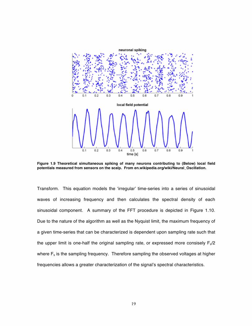
Figure 1.9 Theoretical simultaneous spiking of many neurons contributing to (Below) local field potentials measured from sensors on the scalp. From en.wikipedia.org/wiki/Neural_Oscillation.

20

Figure 1.10 Schematic of a typical spectral analysis performed on quantitative EEG data. The original signal (top) is modeled after a series of sine waves (middle) and the area under the curve of each signal is then calculated and graphed (bottom).

It is common to divide the observed spectral densities in terms of frequency

bands, or summated spectral densities of multiple frequencies. The classic frequency

bands are delta (1.5-4Hz), theta (4-7.5Hz), low-alpha (7.5-10Hz), high-alpha (10-13Hz),

beta1 (13-20Hz), beta2 (20-25Hz), beta3 (25-30Hz) and gamma (>30Hz). In each case,

the bandwidth represents the sum of the spectral densities (uV2·Hz-1) of the discrete

frequencies within the given frequency range. This categorization is largely based upon

qualitative brain-behaviour relationships of individuals discerned years ago. For

example, Hans Berger observed that when individuals, as well as animals such as dogs,

closed their eyes there was a preponderance of ‘spindles’ observed in the strip chart.

21

These spindles are usually between 8-13Hz and are now classified as ‘alpha’ activity. In

contrast when individuals are asked to mentally solve mathematical problems, the strip-

charts of the individuals displayed fast-frequency activity, now characterized under ‘beta’

and ‘gamma’ frequency domains.

2.2.4 Brain Microstates

The shape of the electric field of the brain can be modeled with isocontour lines

similar to those used in demarcating geographic altitudes in mapping. The isocontour

lines, rather than height in the example of geography, indicate voltage gradients. The

lines are then connected where the voltage is roughly approximate, which is almost the

exact same process used to map the electric and magnetic flux lines outlined in

examples from the physical sciences and is a popular technique in

electroencephalography (Duffy, 1986).

While there are many algorithms that can model the contour lines, one of the

most popular methods reported in the literature was described by Lehmann and Koenig

(2004) almost 20 years ago and almost 40 years ago by Skrandies and Lehmann

(1980). The basic idea was to treat the arrangement of sensors on the scalp as probes

of an electric field and study the resulting shapes that were produced during experiments

designed to elicit a response to a visual stimulus. By computing a spatial standard

deviation, which is more popularly known within the literature as global field potential, a

reference-free indication of the global output of the brain could be obtained, independent

on the choice of reference electrodes at the time of measurement (Skrandies, 1990).

Originally, it was found that this measure correlated significantly with changes in the

electric field of the brain evoked with images. Thus, when a visual stimulus was

22

presented to the participant, a peak in global field power was observed. The 'shape' of

the 'electric field landscape' was then visualized by computing a Principal Components

Analysis on all channels recorded simultaneously. PCA is similar to factor analysis in

that it is used to reduce a set of variables into mutually exclusive 'factors'. For example,

in principle a PCA, when looking at the complexity of different musical songs, might be

able to categorize them into "electronic", "country", "classical" and "rock and roll. In the

case of EEG, the electric field inferred from multiple recording can be factored into a

handful of basic shapes.

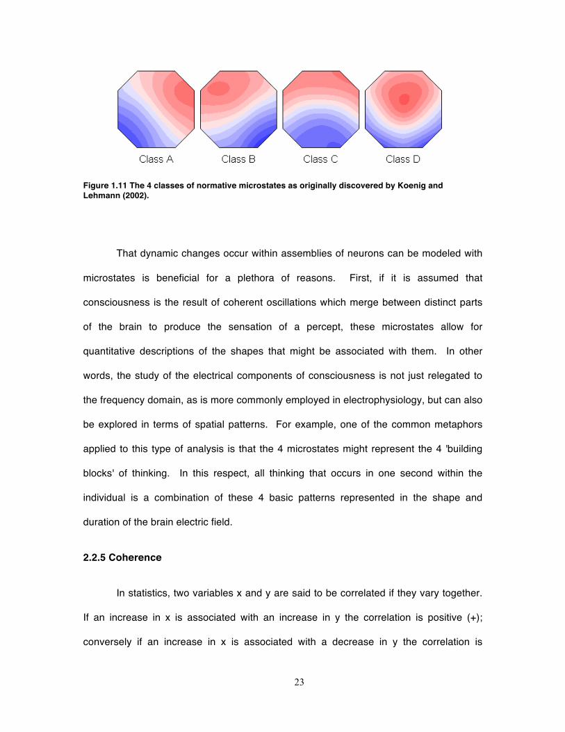
In a paper published by Koenig and Lehmann in NeuroImage in 2002, the

authors reported that 4 classes or shapes of electric fields (Figure 1.11) represented

~80% of the variance in cortical electric field topographies; these shapes have been

confirmed by many other researchers. These electric field microstates have a mean

duration of about 80-100 millseconds whose duration changes as a function of age. In

addition, the occurrence or frequency of each microstate as well as the time spent in one

microstate versus the other 4 also change as a function of age, and also in certain

clinical populations. For example, the average microstate duration was found to be

shorter in people who exhibited symptoms of schizophrenia, as well as general cognitive

impairment (Lehmann et al., 2005; Stretlets et al., 2003; Koenig et al., 1999). Recently,

Corradini and Persinger (2014) showed that the average microstate duration was

significantly correlated with measures of global impairment as inferred by psychometric

indicators of cerebral assessment.

23

Figure 1.11 The 4 classes of normative microstates as originally discovered by Koenig and Lehmann (2002).

That dynamic changes occur within assemblies of neurons can be modeled with

microstates is beneficial for a plethora of reasons. First, if it is assumed that

consciousness is the result of coherent oscillations which merge between distinct parts

of the brain to produce the sensation of a percept, these microstates allow for

quantitative descriptions of the shapes that might be associated with them. In other

words, the study of the electrical components of consciousness is not just relegated to

the frequency domain, as is more commonly employed in electrophysiology, but can also

be explored in terms of spatial patterns. For example, one of the common metaphors

applied to this type of analysis is that the 4 microstates might represent the 4 'building

blocks' of thinking. In this respect, all thinking that occurs in one second within the

individual is a combination of these 4 basic patterns represented in the shape and

duration of the brain electric field.

2.2.5 Coherence

In statistics, two variables x and y are said to be correlated if they vary together.

If an increase in x is associated with an increase in y the correlation is positive (+);

conversely if an increase in x is associated with a decrease in y the correlation is

24

negative (-). The concept of correlation can also be extended to describe functional

connectivity between two recording sites of an EEG and is called coherence. Coherence

measures the strength of the relationship between two EEG recording sites recorded

simultaneously. It can also be described as harmonies of the brain. In this case the two

EEG recording sites can be expressed as a violin and a cello. The amount of

consonance between the two instruments would be a metaphor for coherence.

If the brain is assumed to have distinct areas, based upon cytoarchitecture or

function, then coherence can be described as how these brain areas interact over time.

For example a conversation might be described as coherence between the left temporal

and left frontal regions. While activation within the left temporal region, more specifically

Wernicke’s area, is classically associated with the reception of speech, the left frontal

region, called Broca’s area, is associated with initiating speech. Because conversation

is an interaction between listening to and understanding language (left temporal) and

responding (left frontal), one might expect that the coherence between these two regions

is significant.

Coherence analyses have been used in many research endeavors to

characterize the functional connectivity of the brain when individuals perform a multitude

of different tasks. For example, a recent study investigated coherence of the brain when

individuals were asked to discern the emotional prosody of speech (Rusalova et al.,

2014). It was found that overall coherence was decreased for individuals who could

sense the emotional component of speech more easily. In a study investigating ‘resting’

state EEG, it was found that coherence between the pre-motor cortex and the parietal

lobe could predict with ~85% accuracy how fast an individual could acquire a specific

motor skill (.

25

Coherence analyses have also been used to assess responses to

electromagnetic stimuli when applied to the brain. Recently, Saroka and Persinger

(2013) found that when individuals experience a sensed presence there is greater

coherence within the alpha band between the left and right temporal lobes of the brain.

Hill and Saroka (2010) utilized coherence analysis to discern functional connectivity

changes in individuals who listened to binaural recordings of ‘sacred sites’ found within

Canada. They found that there was increased coherence between the left temporal and

right frontal regions). Finally, it has also been found that coherence between the left and

right temporal regions increases as a function of the disturbance of the static

geomagnetic field (2014). In this study, coherence measures derived from

approximately 200 individual recordings of ‘resting-state’ eyes closed

electroencephalographic baselines were used.

Coherence is usually expressed in terms of its frequency characteristics and

ranges between 0 (no coherence) and 1 (perfectly coherent). Mathematically coherence

Cxy between to EEG recording sites x and y is described as Cxy=Sxy2/SxSy where the

numerator is equal to the square-root of the cross-spectrum of the two signals and the

denominator is the product of the spectrums of x and y (Knott and Mahoney, 2001). An

example is depicted in Figure 1.12. In the upper part of the figure, two signals recorded

from the left and right parietal recording sites are shown. Already, one can see how the

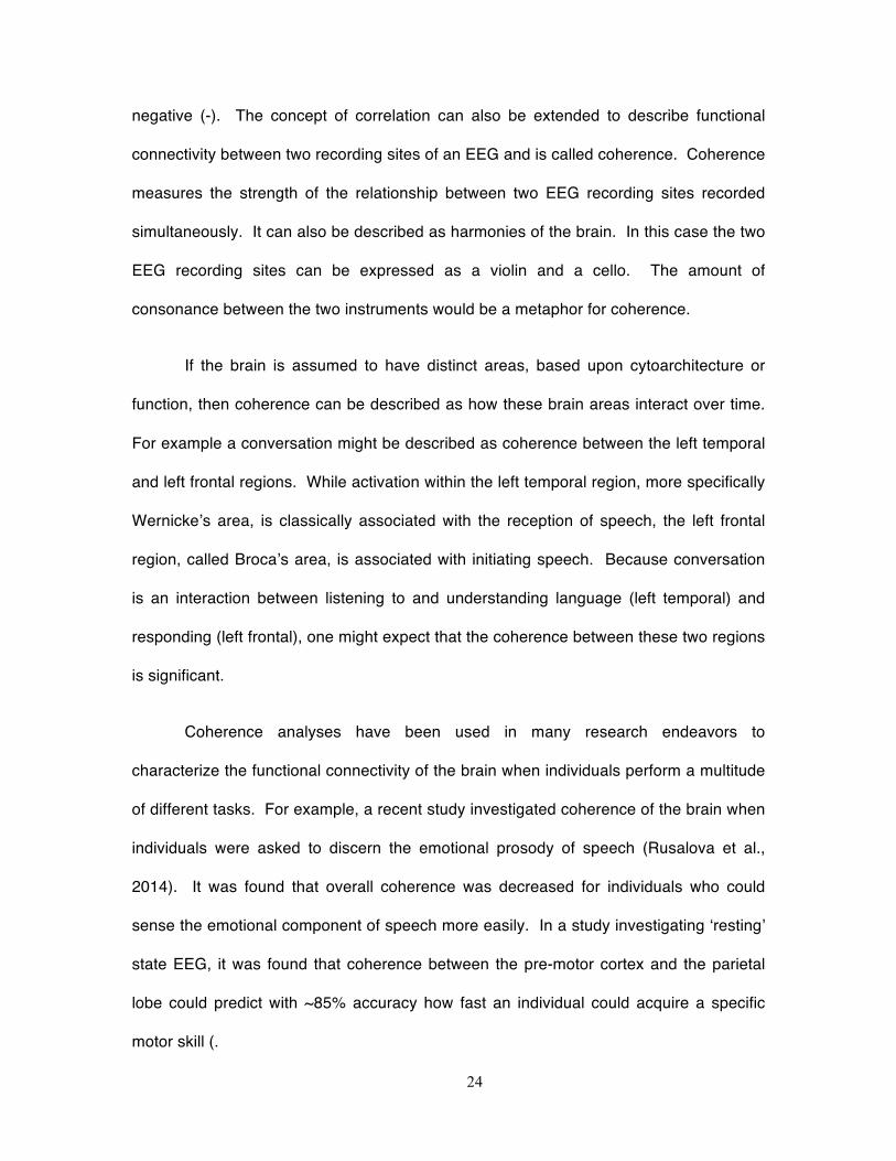
voltages in both signals seem to increase and decrease together. The bottom part of the

figure shows the results of the analysis. It is clear that these two signals are coherent at

10Hz by inspecting two components of the figure; the left side of the figure depicts the

coherence magnitude peaks at 10Hz and the spectrogram shows a band of yellow, red,

blue, and green occurring at the same 10Hz component where the x-axis indicates time.

26

The colours can be compared to real coherence values by reference to the colour legend

on the right.

Figure 1.12 (Top) Two signals derived from P3 and P4 sensors on the scalp show evident synchronicity (Bottom) Coherence analysis indicating that both sensors are periodically coherent within the 9-10Hz range.

2.2.6 Source Localization

Source localization is a relatively new technique for the quantitative

electroencephalograph and is used to discern “where” a particular kind of activity was

derived from. Because fluctuations within the electric field of the brain can be highly

redundant, source localization provides a way of discerning the source of a particular

type of activity. While the spatial resolution is dependent upon the number of sensors

sampling the brain’s electric field, it is a relatively accurate tool with quantitative

electroencephalographs with as little as 16-19 sensors. The unit of measure for source

localization is current source density (uAmm-2) and can range from anywhere between

50 and 2000 units.

27

One of the most commonly used software for source localization analysis is

called sLORETA, which is short for standardized low-resolution electromagnetic

tomography (Pascual-Marqui, 2002). The software itself is free to use for any researcher

and comes equipped with many different functions that allow for statistical comparisons

to be performed between two groups, utilites that can save activation of specific regions

of the brain for implementation into other statistical packages like SPSS, as well as

explorer tools that can be used for visual mapping and computation of functional

connectivity of distinct brain regions. This software has been reliably tested against

other measures such as fMRI. For example, one EEG-fMRI study has shown that an

increase in alpha electrical activity measured with the QEEG over the occipital regions

when analyzed using source localization techniques is also associated with a decrease

in blood-oxygenation visualized with fMRI.

Source localization, specifically using sLORETA, may also be a valid indicator of

brain function within clinical settings. Corradini and Persinger (2013) performed a study

which assessed the accuracy with which sLORETA could localize specific sources of

activity while performing various neuropsychological tests from the Halstead-Reitan

battery. It was found that many of the tests assessing function of specific regions of the

brain were congruent with sLORETA activations during the time of the performance of

those tests.

28

2.3 Biological Effects of Natural and Experimental Electromagnetic Fields

Because all matter, including living organisms, is composed of particles the

importance of the influence of electromagnetic fields on biological systems can be

appreciated. In addition, because living systems are aggregates of particles, the study

of electromagnetic fields on biology and behavior can help to understand how they

influence living systems macroscopically.

Over the past few decades an abundant literature has been created suggesting

that brain activity and behavior can be influenced by applying weak-intensity

electromagnetic fields within the microTesla range. In 2009, Tsang and Persinger

published a study showing that subjective mood, as measured by the Profile of Mood

States questionnaire, is significantly affected by application of different patterns of

electromagnetic activity. Changes in depression and fatigue were both significantly

decreased by the application of a particular pattern modeled after burst-firing neurons

recorded from the amygdala. This pattern was also employed by Baker-Price and

Persinger in a study investigating the possible treatment of depressed individuals

following closed-head injury (Baker-Price and Persinger, 1996; Baker-Price and

Persinger, 2003). The results showed that symptoms of depression, inferred using the

Beck Inventory for Depression, significantly decreased during a 6-week program in

which BurstX was applied for 50 minutes once per week.

Weak-intensity electromagnetic fields, when applied across the bilateral temporal

regions, have also been shown to induce the sensed presence and out-of-body

experiences experimentally. Saroka and Persinger (2013) showed that individuals who

experienced a sensed presence also displayed changes in brain activity. The sensed

29

presence protocol consists of a 30-minute bilateral temporo-parietal application of a

frequency-modulated pattern (also called the Thomas pattern), followed by a 30-minute

application of the BurstX pattern. Individuals who experienced a sensed presence also

displayed an increase in bilateral-temporal coherence after approximately 10-15 minutes

after the initial frequency-modulated application. This change was also accompanied by

an increase in right frontal theta (4-7Hz) activity. This finding replicated previous work

showing that the sensed presence is more probable when there is coherence between

the right and left temporal lobes whereas out-of-body experiences are associated with

increased coherence within the left-temporal lobe and the right-frontal lobe.

In a study published in 1999 Cook and Persinger showed that the experience of

subjective time could be influenced by the application of a frequency-modulated pattern

(Thomas pulse) with a device called the Octopus. This device is comprised of 8

solenoids that are arranged around the head. Upon initiation of a field pattern, each

solenoid is activated in a counter-clockwise manner individually for a period of time.

Using the same device, Lavallee and Persinger (2011) showed that application of a suite

of patterns (each 5 minutes in duration) not only affected microstate descriptors but also

produced the sensed presence in individuals exposed to the ‘forward’ as opposed to the

same set of patterns presented in reverse. This finding further confirmed that the

presentation of the patterns is of critical importance for the elicitation of experiences

within subjects.

The electromagnetic field strengths are about 1000 times less than those used in

conventional studies investigating transcranial magnetic stimulation (TMS). Whereas the

former have intensities within the milliTesla to Tesla range, those employed in the above

cited studies are within microTesla range. One of the suspected reasons for their

30

efficacy is that the patterns mimic natural processes within the brain, whereas TMS

studies usually employ simple sine waves that the brain may habituate to in a matter of

seconds due to their intrinsic redundancy (1995).

Changes in the static geomagnetic field have also been demonstrated to be

correlated with changes in brain activity has been suggested by many individuals. In a

series of experiments Mulligan and Persinger (2010) showed that geomagnetic

disturbances influence brain activity. The first correlative study replicated a previous

study conducted by Babayev and Allahverdiyeva (2007) and indicated that ‘resting’ theta

(4-7Hz) and gamma (40+ Hz) activity occurring within the right prefrontal cortex while

individuals were sitting with eyes-closed was highly correlated with the atmospheric

power obtained from polar orbiting satellites. In a second experimental study

complimenting the first, Mulligan and Persinger (2012) applied electromagnetic fields

(comparable in pattern and strength to natural geomagnetic storms) to individuals while

their brain activity was monitored with a quantitative electroencephalograph. The results

indicated that the individuals exposed to the 20 nT simulated geomagnetic storm showed

an increase in theta activity within the right parietal and a suppression by application of

70 nT strength geomagnetic simulations.

Dr. Neil Cherry published many manuscripts investigating the relationship

between the strengths of the Schumann resonances and human health (Cherry, 2002;

Cherry, 2003). In particular he has found that increases in sunspot number, which he

has shown to be positively correlated with Schumann resonance intensity, is also highly

correlated with induced and accidental death rates in Thailand. As was demonstrated by

Cosic (2006) who showed that the spinal cord exhibits its own selective response profile

with frequencies similar to the Schumann resonance, Cherry further extrapolated on the

31

apparent similarity between the spectral densities of the Schumann resonance and the

brain synthesized originally by Konig (1974, 1984). Based upon these observations in

combination with works by other researchers including Wever (1974) who demonstrated

that human circadian rhythms are disrupted by insulation from the natural ELF

electromagnetic activity, Dr. Cherry proposed that human biological systems are

synchronized with the Schumann resonance and that disruption in the connection can

produce deleterious effects on human health.

32

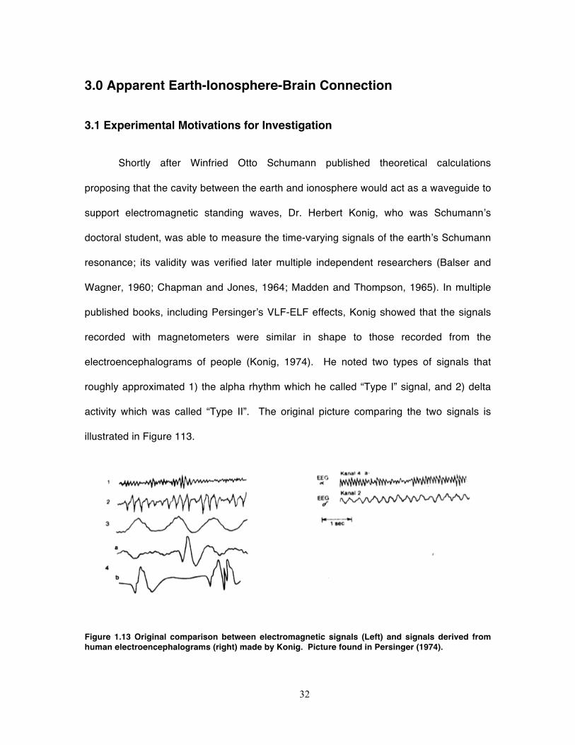
3.0 Apparent Earth-Ionosphere-Brain Connection

3.1 Experimental Motivations for Investigation

Shortly after Winfried Otto Schumann published theoretical calculations

proposing that the cavity between the earth and ionosphere would act as a waveguide to

support electromagnetic standing waves, Dr. Herbert Konig, who was Schumann’s

doctoral student, was able to measure the time-varying signals of the earth’s Schumann

resonance; its validity was verified later multiple independent researchers (Balser and

Wagner, 1960; Chapman and Jones, 1964; Madden and Thompson, 1965). In multiple

published books, including Persinger’s VLF-ELF effects, Konig showed that the signals

recorded with magnetometers were similar in shape to those recorded from the

electroencephalograms of people (Konig, 1974). He noted two types of signals that

roughly approximated 1) the alpha rhythm which he called “Type I” signal, and 2) delta

activity which was called “Type II”. The original picture comparing the two signals is

illustrated in Figure 113.

Figure 1.13 Original comparison between electromagnetic signals (Left) and signals derived from human electroencephalograms (right) made by Konig. Picture found in Persinger (1974).

33

To assess how the Schumann resonance may influence human behavior, Konig

measured the reaction times of people as well as the Schumann resonance

simultaneously. The analysis indicated that human reaction time was significantly

correlated with the intensity of the Type I signal. In particular he found that as the

relative intensity of the Type I signal increased, human reaction time (measured in

milliseconds) decreased.

Since this time, multiple papers have been published on the convergence

between brain electrical activity and the Schumann resonance. In 1995, Paul Nunez

published a theoretical chapter on classical physics models and brain activity (Nunez,

1995). In the chapter, Nunez drew a direct comparison to standing waves, a type of

physical wave produced by constructive/destructive interference of two waves with

similar amplitude and frequency, generated by the earth-ionosphere and theoretical

standing waves that might be produced by the cavity formed between the brain and the

skull. A standing-wave can be visualized when one pictures an individual holding a

string at which is fixed to a wall. If one oscillates the string up and down with a stable

frequency and amplitude, one would observe that that the string seems to produce a

steady wave that does not oscillate between + and – but rather seems to ‘stand’.

Standing waves can be described in terms of their fundamental frequency (f0)

and its harmonics (fn). Depending upon the shape of the cavity, the harmonics of the

fundamental frequency may vary. This property is utilized in the formation of musical

instruments such as guitars and violins. By changing the shape of the cavity within

which the pitch resonates, the timbre or tone of the plucked string changes. A classic

example would be the differences in tones generated by an electrical guitar (without

amplification or cavity) and a classical or acoustic guitar. Whereas the electrical guitar

34

may be described as sounding ‘tinny’, the acoustic guitar would be described as having

‘tone’.

3.2 Quantitative Motivations for Investigation

Employing dimensional analyses and quantification of known physical aspects

of geophysical and cerebral function, Persinger (2012b) predicted that there is a

fundamental scale-invariant relationship between processes that occur globally around

the earth during lightning storms (with comparable current densities as action potentials

as they travel along the axon when diameter is accommodated) and within the brain

itself. For example, the operating intensity of brain activity as well as the Schumann

resonances are both within picoTesla range. In addition, using an average bulk velocity

of ~4.5 ms divided by the average circumference of the human brain, Persinger obtained

a fundamental frequency of approximately 7.8Hz.

This relationship may not just be coincidental. The average intensity of the time-

varying magnetic field measured from the scalp is about 0.1 to 2 picoTeslas. These

fields have been hypothesized to originate from activity perpendicular to the electric field,

in accordance with the general relationship between electric and magnetic fields.

Similarly the average intensity of the magnetic field recorded by the earth-ionosphere is

between 0.1 and 1 picoTesla. Therefore despite the differences in size between the

brain and the earth, there might exist a harmonic relationship between the two by means

of average intensities.

To continue further, electric field strengths of the Schumann resonance have

been measured to be between .1 and 1 mV·m-1. Paul Nunez in his book Electric Fields

of the Brain (1984) models the cortex after a dipole layer with positive charge located

ventrally towards the underlying white matter and negative charge located close to layer

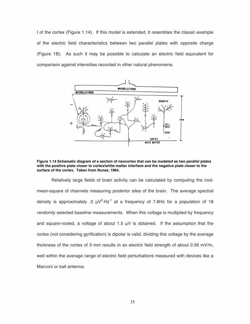
35

I of the cortex (Figure 1.14). If this model is extended, it resembles the classic example

of the electric field characteristics between two parallel plates with opposite charge

(Figure 1B). As such it may be possible to calculate an electric field equivalent for

comparison against intensities recorded in other natural phenomena.

Figure 1.14 Schamatic diagram of a section of neocortex that can be modeled as two parallel plates with the positive plate closer to cortex/white matter interface and the negative plate closer to the surface of the cortex. Taken from Nunez, 1984.

Relatively large fields of brain activity can be calculated by computing the root-

mean-square of channels measuring posterior sites of the brain. The average spectral

density is approximately .3 μV2·Hz-1 at a frequency of 7.8Hz for a population of 18

randomly selected baseline measurements. When this voltage is multiplied by frequency

and square-rooted, a voltage of about 1.5 μV is obtained. If the assumption that the

cortex (not considering gyrification) is dipolar is valid, dividing this voltage by the average

thickness of the cortex of 3 mm results in an electric field strength of about 0.56 mV/m,

well within the average range of electric field perturbations measured with devices like a

Marconi or ball antenna.

36

4.0 Interdisciplinay Approach

Ultimately all knowledge is acquired, codified, interpreted, and communicated by

processes that exist within the human brain. According to Nunez only about 5-10

percent of all white matter fibers in the brain, which relay information from one region to

another, are purely sensory (Nunez, 1995). This would suggest that most aspects of

‘objective’ reality are the result of internal processes that have been acquired and

developed through the experiences of the individual; however the possibility that only 5-

10 percent is sufficient to gain an understanding of this reality cannot be dismissed.

Either way, this fact would seem to indicate that perceived differences between concepts

such as mono versus interdisciplinarity are the function of how the human brain

constructs the environment and in this particular case the distinction. If this is the case,

it would be advantageous to describe the two phenomena as though they were variables

displaced from context. For example, a relationship between ‘x’ and ‘y’ may not exist

until it is framed within a field of study, such as mathematics or molecular biology.

4.1 Disciplinarity

The concept of ‘disciplinarity’ has been explored from multiple perspectives.

Within the context of epistemology and political science Turner (2000) has likened the

idea of a discipline to a ‘cartel’ in a market. Such a comparison would imply that

members of a particular discipline utilize standardized tools to produce knowledge that is

largely communicable only amongst those who are immersed within the discipline.

Because of the social structure of the discipline, languages are conceived to act as

heuristics in communicating information from one research institute to another.

37

Others have argued that ‘disciplinarity’ is like a machine (Chettiparamb, 2007),

similar to Newton’s mechanistic model of the universe. In this sense, disciplines are

necessarily a set of algorithms that allow for production of information by specializing in

one particular function or set of problems. As a result a constricted view of how ‘nature’

functions could be built rapidly to allow for further technological advancements where

needed. This conception of the term ‘discipline’ was potentially born historically out of

the necessity in Germany to train individuals as technicians and professionals for

industry (Salter and Hearn, 1996, p.19). As such, the concept of a discipline could be

defined more generally as a collection of ‘axioms’ or rules that attempt to provide

structure for the conception, acquisition, and realization of knowledge/information of a

particular topic. The major thrust in the case of disciplinarity is the methodology and

‘where’ best to study a particular topic (Chettiparamb, 2007).

It has been suggested that the conception of the problem, eventually lending to

the attained knowledge, is largely based upon the perceived boundaries of a given topic

and how it may be categorized into a particular field (Moran, 2010). For example,

understanding the morphology of bone structures within the mandibles of the mouth are

best suited to taxonometric methods that currently exist within the genre of ‘biology’.

The acquisition phase would then be described as the methods of analysis used by that

discipline to get some answer or output. Finally the output of the analysis would then

enter a ‘realization’ phase by which the problem, the analysis, and the implications are

framed within a literary work that is communicable to other members of the same

discipline. This process is largely formalized, but plastic, depending upon shared beliefs

and traditions, and by extension the language embedded within an associated discipline.

In a sense, as described by Chandler (2009), there can be imposed a distinction

38

between what constitutes a doctrine and a discipline, the former having associated with it

the concepts of subscription to some assumption; he revisits this idea by recapitulating

Cohen’s response of the irrelevance of association with a particular discipline where the

necessary ‘becoming embarassed’ of one’s own practices suggests an attachment of

identity of the researcher which perpetuates the notion of the ‘sense of self’ in part

defined by the discipline. In short, a discipline is defined by the formalized process by

which information is organized. While usually applied within the context of academia,

one could extend this definition within art-forms. For example, what defines musical

genres (here paralleled with discipline-concept) is the instrumentation, the intervals

between different pitches and temporal and linguistic patterns that are employed in

composition.

This 'self-concept' that defines the discipline can then be taken to represent the

left hemispheric processes of the brain that act as a filter by which relevant information is

acquired, organized and communicated. Not surprisingly, left hemispheric functions

include logic, mathematical reasoning, verbal reasoning and other linear processes that

can be likened to the linear process of 'knowledge production' within the discipline and

are all required for deductive processes involved within the sciences in general.

4.2 Interdisciplinarity

In a chapter written on holistic approaches to research, Sarewitz (2010)

discusses the possibility that the boundaries found at the edges of a discipline are

inherently a result of perception. In this case, there is no ‘real’ boundary between

discipline X and discipline Y, and that the boundaries that do exist are simply illusions

imposed by the cognitive structure of the inquisitor. The approach of ‘blurring’ is echoed

39

by Geertz (1983) who observed that many of the social sciences began to ‘role-play’ by

the usage of analogies derived from other fields including literature and theatre; his

thoughtful treatise demonstrated that the acquisition of knowledge can be facilitated

through examination of the relationship between disciplines such that for example, a

scientific problem could be viewed ‘from the lense’ of a fiction writer. Indeed if one were

to apply a statistical ‘analysis of covariance’ for language imbued by each discipline, one

might find that fundamental patterns exist between disciplines. For example, consider

the concepts of harmony in music, correlation in statistics and coherence in physics. In

all three cases the implied meaning is that there is an aesthetic or mathematical

relationship between two sets of variables-in the case of harmony two consonant

melodic lines, in the case of correlation and coherence two variables-that are linear.

Thus, it might be suggested that if boundary lines do exist between predefined

disciplines, they exist because of the language used to describe a fundamental process.

In some respects the interdisciplinarity, a concept that has been paired

synonymously with ‘creativity’, ‘crossing-boundaries’ and ‘blending’ (Frodeman, Klein

and Mictcham, 2010; Klein, 2005, Geertz, 1980), that began to emerge in the 1960s

(Newell, 2008), possesses ideals that were explored by many early Greek philosophers

such as Socrates and Pythagorus as well as individuals during the Renaissance period

from which the concept of the ‘polymath’ or ‘Renaissance man’ originated (Klein, 2005).

In such methods of education and learning, a wide variety of topics such as

mathematics, music, geometry, and philosophy were studied simultaneously. These

ideas were then later explored by physiologists and physicists in the 19th century.

Individuals such as Hermann von Helmholtz, the developer of the theory of conservation

of energy, and Thomas Young, who demonstrated that Newton’s particle theory of light

40

could also be accommodated by wave-physics and would later attempt to study the

interaction between light and sound (Young, 1800), both integrated aspects of different

‘disciplines’ to understand aspects of others.

Interdisciplinarity, as it is regarded today, is thought to have been born out of a

necessity to solve big-picture problems that cannot be adequately assessed through the

lens of one discipline alone. With the increased specialization observed within the

disciplines, individuals began to assess applicability to ‘real-world’ situations (Shailer,

2005). As such, while disciplinary research can be described as focal and rigorous

methodology as it pertains to a given ‘territory’ of reality, interdisciplinary research

attempts to exploit the holistic ability within the human brain to integrate seemingly

disparate knowledge to explore topics that are by nature complex by application of

multiple processes used throughout the disciplines. Thus in contrast to ‘disciplinarity’ as

it has been outlined here, interdisciplinary research is not rigid or stereotyped, but

flexible to allow for as many different possibilities to gain a more complete understanding

of the problem.

According to Salter and Hearn (1996) as well as Repko (2008), there are two

types of interdisciplinary categories by which research is conducted. The first is called

‘conceptual’ interdisciplinarity and is epistemological in nature and deals with

understanding the limitations of the insights of a problem explored by a single discipline.

The second is called “instrumental interdisciplinarity”, in which the concepts, knowledge

and methods from “two or more” disciplines are borrowed in order to solve a problem

that cannot be addressed by one field alone; in this way the disciplines fuse together

seamlessly. According to Aboelela and colleaguess’ (2007) qualitative review of the

literature surrounding the definition of interdisciplinarity, a variant of this conception or

41

“positivist” interpretation would likely to be endorsed by the physical and social sciences.

Disciplines are then viewed as a foundational starting point for interdisciplinary studies

such that the “perspectives, epistemologies, assumptions, theories, concepts, methods

that inform our ability as humans to understand our world” (Repko 2008, p. 21) are not

deteriorated.

Such a view has exhaustive implications for the advancement of creative ideas

and consolidation of information. For example studies within the neurosciences have

demonstrated that what is called “creativity” may be ‘cross-wiring’ between brain regions

that are rarely connected. Synaesthesia, a common condition reported by composers

like Alexander Scriabin, in which individuals can “hear” colour or “taste” music, has been

hypothesized to be caused by enhancement of connections between regions of the brain

that normally process sound and colour separately (Brang and Ramachandran, 2011). If

this is the case, then exploring the same problem from different disciplinary paradigms,

such as mathematics commonly linked to the left cerebral hemisphere and music which

is traditionally associated with the right hemisphere, could allow for the enhancement of

‘accidents’ to occur that allow for creative insights observed biologically as the expansion

or re-molding of dendritic spines.

As has been stated from the outset, there is sufficient evidence to suggest that

information is largely organized by the structure and function of the human brain.

Therefore, if the processes inherent in a discipline are taken metaphorically to function

as the left-hemisphere where linear processes, such as those engaged by the

disciplines, are largely performed, it is tempting to equate the seemingly parallel

processes involved in interdisciplinary research to represent the right hemisphere which

is by nature spatial and pattern based. Consequently from a sociological standpoint the

42

emergence of interdisciplinary studies could be interpreted as an expansion and

development of right-left hemispheric coherence within the human brain. From this

perspective the differences between mono-and inter-disciplinarity would be described by

functional differences between the left and right hemispheres of the brain.

If one of the major thrusts for interdisciplinary research is to enhance creativity,

the aforementioned analogy to left and right hemispheric processes for disciplinarity and

interdisciplinarity is apt. One major finding is that the sensed presence is the product of

coherence between the left and right hemispheres. As Persinger and Makarec (1992)

have previously stated, the sensed presence may be the process by which the muses

were experienced by Greek artists. If this is the case, then creativity is necessarily a left

and right hemispheric process and by definition experience in both disciplinary and

interdisciplinary endeavors are required for creativity to flourish, or stated alternatively by

Repko (2012, p.71) “intuition and method”. It may be relevant that according to

Simonton’s (1975) quantitative review of creative individuals, there appears to be 3

major ‘factors’ of interdisciplinary individuals who fall into the categories of discursive

creativity (with the physical, biological, chemical sciences), presentational creativity (i.e.

painting architecture), and rational-mystic creativity (physical sciences, religion, and

general philosophy); these clusters may highlight that the propensity for interdisciplinary

studies is innate and that learning one particular discipline already allows ‘cross-talk’ to

occur with others.

This view of creativity is recapitulated by Morin (2008) who synthesizes many

Eastern philosophies on his views of complexity within the natural and social sciences;

complexity here is synonymous with the term ‘predictability’ and relates to Strathern’s

(2004) reiteration of cold (unpredictability but with a ‘strategic plan’ in the case of events)

43

and hot (unpredictability arising from the interactions of multiple factors not originally

incorporated into an equation) situations. Complexity, a necessary and perhaps

impending change in thought processes accompanying the acquisition of information, is

thought to be accompanied by the integration of opposites, in the same way that would

have been described by Hegel and within the psychology of Jung (1959) who

emphasized ‘individuation’ as a necessary process of merging the ‘unconscious’ with the

‘conscious’ for individual development. This view is also echoed by other contemporary

authors, such as Tononi and Edelman (1998), who describe consciousness as a process

that is simultaneously integrating and differentiating experiences acquired subjectively

and whose process may be described mathematically, like Morin’s perspective, by

Shannonian information theory, or entropy. In this vein and to extrapolate, science is not

only objective, but also subjective. Perhaps one important example of the relationship

between subject-object can be found within the domain of quantum physics. Whereas a

mechanistic and seemingly objective model of the universe, with a natural order that

could be formalized, pervaded much of scientific thought up until time 19th century,

discoveries within quantum physics included the observer as part of the interaction

between the molecules that composed the universe where the observer can affect the

consequences of the experiment.

4.3 Interdisciplinary Requirement and Methodology

The topic that has been chosen for the thesis is a comparative exploration

between the processes that are observed naturally within the context of geomagnetism

and processes observed with brain function. Multiple research endeavours have been

conducted that demonstrate that the earth’s geomagnetic field influences human

behaviour, and more specifically, brain activity. For example Mulligan et al. (2010)

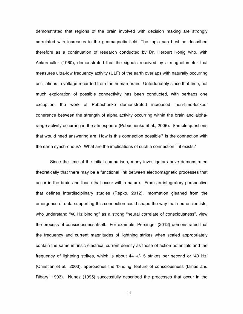
44

demonstrated that regions of the brain involved with decision making are strongly

correlated with increases in the geomagnetic field. The topic can best be described

therefore as a continuation of research conducted by Dr. Herbert Konig who, with

Ankermuller (1960), demonstrated that the signals received by a magnetometer that

measures ultra-low frequency activity (ULF) of the earth overlaps with naturally occurring

oscillations in voltage recorded from the human brain. Unfortunately since that time, not

much exploration of possible connectivity has been conducted, with perhaps one

exception; the work of Pobachenko demonstrated increased ‘non-time-locked’

coherence between the strength of alpha activity occurring within the brain and alpha-

range activity occurring in the atmosphere (Pobachenko et al., 2006). Sample questions

that would need answering are: How is this connection possible? Is the connection with

the earth synchronous? What are the implications of such a connection if it exists?

Since the time of the initial comparison, many investigators have demonstrated

theoretically that there may be a functional link between electromagnetic processes that

occur in the brain and those that occur within nature. From an integratory perspective

that defines interdisciplinary studies (Repko, 2012), information gleaned from the

emergence of data supporting this connection could shape the way that neuroscientists,

who understand “40 Hz binding” as a strong “neural correlate of consciousness”, view

the process of consciousness itself. For example, Persinger (2012) demonstrated that

the frequency and current magnitudes of lightning strikes when scaled appropriately

contain the same intrinsic electrical current density as those of action potentials and the

frequency of lightning strikes, which is about 44 +/- 5 strikes per second or ‘40 Hz’

(Christian et al., 2003), approaches the ‘binding’ feature of consciousness (Llinás and

Ribary, 1993). Nunez (1995) successfully described the processes that occur in the

45

brain by using fundamental models, similar to the models approached by von Bekesey in

trying to discern the psychophysics of hearing. In Nunez’s approach he treated the brain

and skull as an earth-ionospheric cavity and predicted a dominant frequency, ~10 cycles

per second, using the bulk velocity of action potentials.

The current dissertation is designed to continue assessing the potential earth-

brain connection by using modern technology that is portable and readily available.

From a cursory review, multiple methods and knowledges from backgrounds such as

electrophysiology, geomagnetism, signal processing, mathematics, electronics and

geophysics are required in order to make an accurate assessment. Repko (2008)

described a 10-step ‘nonlinear and iterative’ process, similar to Szostak’s 12-step

process, for steps on possible ways to conduct interdisciplinary research; this process

has been used with degrees of success for studies in linguistics (van der Lecq, 2012),

understanding the cognitive science of action understanding in humans (Keestra, 2012),

and understanding stress episodes as experienced by NHL hockey players (Battochio,

2013). According to Repko, the process of identifying disciplines (Step 3) is necessary in

order to achieve some integration of the insights drawn amongst the disparate

knowledges.

The principle thrust can thus be described as convergence rather than

divergence, with the patterns observed in the brain and the earth linking both. The

fundamental ‘connection’ points, or concepts, associating the disciplines explored within

this project are frequency and intensity. The principle operating frequency of electrical

potentials recorded with an electroencephalograpm is approximately 8-13 Hz.

Depending upon approaches, the associated electric and magnetic field strengths of the

8-13Hz activity recorded over the back of the brain when individuals have their eyes

46

closed is approximately .4-.5 mV/m and 1-2 picoTesla. As it turns out, the Schumann

resonance, which is a global resonance affecting all regions of the earth, displays a peak

frequency of about 8Hz (Balser and Wagner, 1960) with electric field and magnetic field

strengths approaching .1-1 mV/m and 1-3 picoTesla. This convergence suggests that

there may be indeed a connection between the two processes occurring at a micro (the

human brain) and a macro (the earth) level (Figure 1C).

This approach to interdisciplinarity might best be described as Mode I according

to criteria outlined by Chettiparamb (2006). In this mode, “…the attempt is to

demonstrate that two things are actually the manifestation of the same structure…”. This

method is also related to one of Morin’s (2008) principles for a framework by which

complexity can be used as a mode of scientific inquiry; here he specifies the idea of a

holographic relationship wherein the individual components of an object contain the

information of the whole, as in the case of the fractal mathematical set known as the

Sierpinski triangle (Figure 1.15A). The relationships that will be investigated within the

dissertation are modeled after the “fugue” musical form (Figure 1.15B), which at its core

relies upon recapitulation and imitation of a central melodic theme (Menuhim, 1986).

Based upon the quantitative and qualitative convergences of the two phenomena

outlined above one might speculate that the two processes (brain and earth) are derived

from the same source of variance.

The overall methodology to be employed within the dissertation is a combination

of statistical and analytical techniques widely practiced within the social and physical

sciences. Spectral analysis, a tool that is used in a broad array of natural sciences, is

slowly becoming the ‘universal tool’ for communicating discrete quantifications between

different fields and observes the conception of the “methodology” as a stand-alone

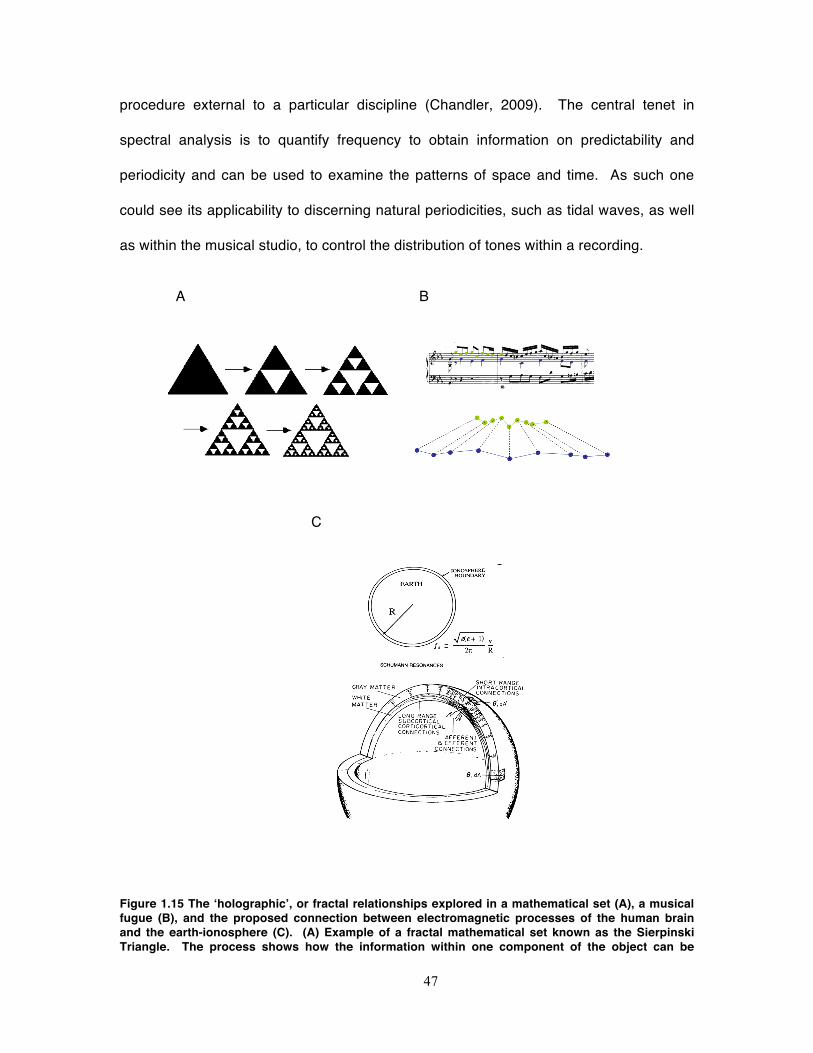
47

procedure external to a particular discipline (Chandler, 2009). The central tenet in

spectral analysis is to quantify frequency to obtain information on predictability and

periodicity and can be used to examine the patterns of space and time. As such one

could see its applicability to discerning natural periodicities, such as tidal waves, as well

as within the musical studio, to control the distribution of tones within a recording.

A B

C

Figure 1.15 The ‘holographic’, or fractal relationships explored in a mathematical set (A), a musical fugue (B), and the proposed connection between electromagnetic processes of the human brain and the earth-ionosphere (C). (A) Example of a fractal mathematical set known as the Sierpinski Triangle. The process shows how the information within one component of the object can be

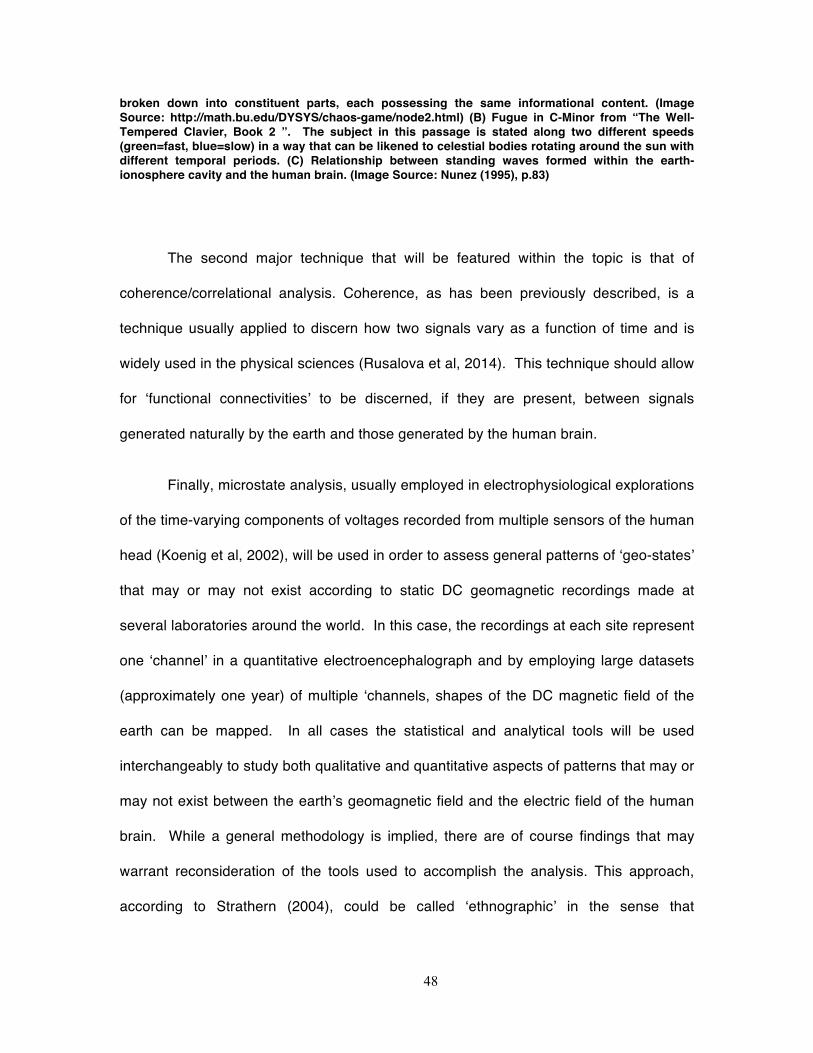
48

broken down into constituent parts, each possessing the same informational content. (Image Source: http://math.bu.edu/DYSYS/chaos-game/node2.html) (B) Fugue in C-Minor from “The Well-Tempered Clavier, Book 2 ”. The subject in this passage is stated along two different speeds (green=fast, blue=slow) in a way that can be likened to celestial bodies rotating around the sun with different temporal periods. (C) Relationship between standing waves formed within the earth-ionosphere cavity and the human brain. (Image Source: Nunez (1995), p.83)

The second major technique that will be featured within the topic is that of

coherence/correlational analysis. Coherence, as has been previously described, is a

technique usually applied to discern how two signals vary as a function of time and is

widely used in the physical sciences (Rusalova et al, 2014). This technique should allow

for ‘functional connectivities’ to be discerned, if they are present, between signals

generated naturally by the earth and those generated by the human brain.

Finally, microstate analysis, usually employed in electrophysiological explorations

of the time-varying components of voltages recorded from multiple sensors of the human

head (Koenig et al, 2002), will be used in order to assess general patterns of ‘geo-states’

that may or may not exist according to static DC geomagnetic recordings made at

several laboratories around the world. In this case, the recordings at each site represent

one ‘channel’ in a quantitative electroencephalograph and by employing large datasets

(approximately one year) of multiple ‘channels, shapes of the DC magnetic field of the

earth can be mapped. In all cases the statistical and analytical tools will be used

interchangeably to study both qualitative and quantitative aspects of patterns that may or

may not exist between the earth’s geomagnetic field and the electric field of the human

brain. While a general methodology is implied, there are of course findings that may

warrant reconsideration of the tools used to accomplish the analysis. This approach,

according to Strathern (2004), could be called ‘ethnographic’ in the sense that

49

methodologies are devised ‘after the fact’ in order to cater to the individual needs of the

data.

50

5.0 Proposed Research and Methods

Given the research cited above, which by no means is complete, demonstrating

connections between the earth’s time-varying and static geomagnetic field and brain

activity, and also given the paucity of research showing direct connections between the

naturally generated Schumann resonance and brain activity, the research will attempt to

continue to investigate for other possible interfaces between the two phenomena. The

principle method of the research will be investigating measures derived from

magnetometers, measuring both static and time-varying components of the earth’s

magnetic field, in combination with various statistical and analytical techniques using the

QEEG. While there have been indicators suggesting that a ‘fugal’ relationship between

the two phenomena exists, few studies have investigated a direct one-to-one

correspondence between earth-generated time-varying electromagnetic fields and

human brain activity.

5.1 Relationships between brain activity and measures of the static

geomagnetic field

This research will continue in the same vein as that already performed by

Mulligan and Persinger. Over the last 3-4 years, an extensive database of QEEG

baselines from approximately 180 individuals has accumulated from various experiments

performed within the Neuroscience Research Group laboratory. These eyes-closed

‘resting’ baselines will be employed to discern additional potential relationships between

the geomagnetic field and human brain-activity.

51

The general methodology will be simple. Simultaneous measurements of the

brain’s electrical activity as well as the earth’s magnetic field will be recorded. The

resultant signals will be subjected to a myriad of different analytical techniques in order

to discern if additional relationships exist. Data representing the state of the

geomagnetic activity at the time of each measurement will be obtained from various

online monitoring stations. Variables such as the K-index and measures of solar

sunspot numbers will be obtained from these databases and correlational analyses will

be performed to discern relationships between the two general classes of phenomena:

brain activity and earth static geomagnetic field.

5.2 Explorative Application of QEEG-related Methods to Investigate the

Static Geomagnetic Field

To further characterize the potential ‘fugal’ relationship between brain activity and

the earth’s geomagnetic field, the application of methodologies typically employed in

quantitative electroencephalography will be engaged. If both phenomena are related or

produce or are produced from shared sources of variance, then the inter-mingling of

methods should produce comparable time and space dependent properties when scale

is accommodated.

In this very exploratory study, approximately one-year of the static geomagnetic

field, sampled at once per minute, will be extracted from online repositories from 8

regions roughly approximating the scaled-locations of sensors typically placed on the

scalp to measure brain-generated electrical activity. These ‘geo-channels’ will be

synchronized into one record and microstate analyses will be employed to discern the

52

spatial orientation of the field to produce ‘geostate’ maps. In addition, coherence

analyses typical of QEEG research will be applied to discern periods ‘geo-synchronicity’

between distant locations around the earth.

5.3 Relationships between brain activity and measures of background AC

magnetic fields

While the earth’s DC geomagnetic field is relatively static (with the exception of

normal diurnal variations in its intensity), there also exists smaller time-coupled

perturbations that are within nanoTesla to picoTesla range. Research investigating

potential influences of 60Hz electromagnetic fields in North America on biological

systems, generated primarily from AC power line electricity delivery systems, is copious

and many studies have suggested that that they can effect biology. Within rural

environments 60-Hz power-line frequencies, with electric field intensities ranging

between between 10-2-10-4 V/m depending upon source distance and have discrete

harmonics produced according to basic physical principles, and magnetic fields

generated by electronics may produce changes in physiology. There have been

extensive correlative researches demonstrating that some residents living proximal to

powerline generators show increased incidences of leukemia, breast-cancer, and

general malaise and fatigue. With this motivation, one proposed study would be to

investigate the changes in the AC background and measure real-time relationships with

brain activity.

The methodology in this research will require simultaneous recordings of the AC-

background electromagnetic field and brain activity monitored with a QEEG. Indicators

53

of the background AC field will be measured with a power meter, a standard device

typically used in laboratories to measure electromagnetic field strengths in milliGauss

units where 1 milliGauss is equal to 100 nanoTesla. This same sensor has previously

been utilized in a study investigating the transmission of artificial time-varying

electromagnetic fields through simulated skull. This sensor will be connected to a laptop

that will record the perturbations in the local electromagnetic field inside of an acoustic

sound-proof chamber while the brain activity of individuals situated inside the chamber is

monitored simultaneously.

The general statistical approach will be correlational and spectral densities

(milliGauss2Hz-1) from the time-varying AC magnetic field will be correlated with a variety

of time-frequency dependent changes in brain activity (i.e. spectral density, coherence).

5.4 Schumann Resonance Signatures in the Human Brain

In 1979, Dr. Konig published a chapter within Persinger’s ELF and VLF

Electromagnetic Effects discussing extremely-low and very-low electromagnetic

frequencies occurring naturally with possible connections with biology. In particular he

discussed the concepts of ELF-VLF frequencies within the context of holographic

memory and electroencephalography. Figure 15 depicts a condensed spectral array of

an electroencephalographic recording of an individual who has been monitored during

their sleep found within his chapter in “Electromagnetic Bio-Information” (Popp, 1984). It

is obvious that there are two major peaks that occur together and apart: peaks at 8 and

14 Hz. These two frequencies constitute the first and second harmonics of the

Schumann resonance.

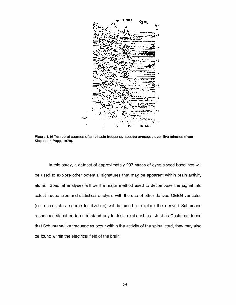
54

Figure 1.16 Temporal courses of amplitude frequency spectra averaged over five minutes (from Kloppel in Popp, 1979).

In this study, a dataset of approximately 237 cases of eyes-closed baselines will

be used to explore other potential signatures that may be apparent within brain activity

alone. Spectral analyses will be the major method used to decompose the signal into

select frequencies and statistical analysis with the use of other derived QEEG variables

(i.e. microstates, source localization) will be used to explore the derived Schumann

resonance signature to understand any intrinsic relationships. Just as Cosic has found

that Schumann-like frequencies occur within the activity of the spinal cord, they may also

be found within the electrical field of the brain.

55

5.5 Relationships Between Extremely-Low Frequency Spectral Density and

Human Brain Activity and Construction and Characterization of an

Induction Coil Magnetometer For Measuring Extremely-Low Frequency

Earth-Ionospheric Perturbations

While reading the studies written by Dr. Neil Cherry on human health

relationships to the Schumann resonance and sunspot numbers, a database from which

he was able derive intensities of extremely-low frequency spectral densities was

discovered. Perusing the site further, it contains not only magnetic and electric field

time-series sampled at 40Hz, but also seismometers (sampled at 80Hz), geophones and

other instruments used to study earthquake activity for prediction. The site is a joint

collaboration between many geophysical loboratories within California, including USGS

and Berkeley. Access to data from at least 1995 can be found at

http://ncedc.org/ncedc/other-geophysical-datasets.html. The data can be requested at

lengths up to a couple of years and software (rdseed) can be used to extract specific

times of interest.

Because there is a large dataset of baseline eyes-closed encephalograms

available, this study will attempt to draw a relationship between the strength of various

quantitative electroencephalographic measures and extreme-low frequency spectral

densities obtained from the aforementioned database in California. The study will

fundamentally be correlational. Multiple linear regressions will be performed in order to

predict fundamental Schumann frequency intensities from the database of eyes-closed

baselines.

56

5.6 Construction and Characterization of an Induction Coil Magnetometer

For Measuring Extremely-Low Frequency Earth-Ionospheric Perturbations

The intensity of extremely-low frequency (0.1-100Hz) electromagnetic activity

generated within the earth-ionosphere cavity is about one million times less than the

geomagnetic field and is typically measured within the picoTesla range. As a result,

specialized sensors are required in order to measure time-dependent changes within the

scale of seconds. This component of the dissertation will describe the methodology

used to construct an induction-coil manometer, an instrument typically utilized within the

field of geophysics, and its characterization using raw electronic components.

The purpose of constructing the magnetometer is two-fold. One reason for its

construction is that the Schumann resonance and micropulsations can be monitored

daily with the hope of further applying time-frequency methods typically employed in

QEEG research to discern more information about the nature of the phenomena. While

a vast literature on the topic of the Schumann resonance has accrued, there has been

little research investigating ‘phase-coherence’ relationships between the different

harmonics. For example, one potential avenue for research is to investigate how often

the fundamental 7.8 Hz becomes coherent with the 39Hz harmonic. The relationship

between these two frequencies in particular has been thoroughly investigated within the

context of neuroscience where 7 Hz frequencies generated within the hippocampus, also

known as the ‘gateway to memory’, are correlated with 40Hz ripples which are

superimposed upon the fundamental 7Hz carrier frequency and often correlated with the

‘binding’ factor required to produce a cohesive consolidation of various sensory

components of consciousness. Investigating the phase relationships between these two

57

frequencies within the context of geophysics may be of relevance for its comparison to

human consciousness.

5.7 Simultaneous Measurements of the Schumann Resonance and Brain

Activity

The second reason for constructing a magnetometer sensitive enough to

measure extremely-low frequency electromagnetic fields is to discern if real-time or time-

lagged coupling exists between the Schumann resonance and human brain activity.

While many publications have appeared suggesting a coherence between the two

phenomena, few have investigated the basic physical units in real-time. One exception

is the study performed by Konig who discovered a relationship between reaction times of

people the occurrence or intensity of Type 1 natural electromagnetic signals that also

overlap with brain activity.

The approach to this component of the dissertation will be to measure both

signals (brain and earth) simultaneously by feeding the perturbations in ELF-range

electromagnetic recordings into the QEEG to be measured as a channel appearing

amongst the array of sensors recording the electric field of the brain. As with other

proposed methods, both time-series will be decomposed according to frequency and

other derived QEEG-measures (i.e. source localization, coherence) to investigate a

potential coupling of the two phenomena.

58

6.0 References

Aboelela SW et al. (2007). Defining Interdisciplinary Research: Conclusions from a

Critical Review of the Literature. Health Services Research 42: 329-346.

Babayev, E. S., & Allahverdiyeva, A. A. (2007). Effects of geomagnetic activity variations

on the physiological and psychological state of functionally healthy humans:

some results of Azerbaijani studies. Advances in Space Research, 40(12), 1941-

1951.

Baker-Price, L. A., and Michael A. Persinger. "Weak, but complex pulsed magnetic fields

may reduce depression following traumatic brain injury." Perceptual and motor

skills 83.2 (1996): 491-498.

Baker-Price, L., & Persinger, M. A. (2003). Intermittent burst-firing weak (1 microTesla)

magnetic fields reduce psychometric depression in patients who sustained closed

head injuries: A replication and electroencephalographic validation. Perceptual

and motor skills, 96(3), 965-974.

Balser, M., & Wagner, C. A. (1960). Observations of Earth-ionosphere cavity

resonances. Nature, 188(4751), 638-641.

Battochio RC. (2013). An Interdisciplinary Take on Stress, Coping, and Adaptation in the

National Hockey League. In Reguigui A (Ed): Perspectives sur l’interdisciplinarité

/ Perspectives on Interdisciplinarity, Sudbury, Série monographique en sciences

humaines / Human Sciences Monograph Series, vol 13, 2013.

59

Brang D and Ramachandran VS. (2011). Survival of the Synaesthesia Gene: Why Do

People Hear Colors and Taste Words? PLoS Biology 9: e1001205.

Besser, B. P. (2007). Synopsis of the historical development of Schumann resonances.

Radio Science, 42(2).

Bianchi, C. (2007). Natural and man-made terrestrial electromagnetic noise: an

outlook.Annals of Geophysics.

Bleil, D. F. (1964). Natural electromagnetic phenomena below 30 kc/s. In Natural

Electromagnetic Phenomena (Vol. 1).

Capra, F. (1976). The Tao of Physics. London: Fontana.

Chandler J. (2009). Introduction: Doctrines, Disciplines, Discourses, Departments.

Critical Inquiry 35: 729:746.

Chapman, F. W., & Jones, D. L. (1964). Observations of earth-ionosphere cavity

resonances and their interpretation in terms of a two-layer ionosphere model.

Radio Science, Journal of Research National Bureau of Standards D, 68(11),

1177-1185.

Chapman, S., & Bartels, J. (1940). Geomagnetism. Oxford: Clarendon Press.

Cherry, N. (2002). Schumann Resonances, a plausible biophysical mechanism for the

human health effects of Solar. Natural Hazards, 26(3), 279-331.

Cherry, N. (2003). Schumann resonance and sunspot relations to human health effects

in Thailand. Natural hazards, 29(1), 1-11.

60

Chettiparamb A. (2007). Interdisciplinarity: A Literature Review, Southampton (UK),The

Higher Education Academy, Interdisciplinary Teaching and Learning Group.

Christian HJ et al. (2003). Global frequency and distribution of lightning as observed

from space by the Optical Transient Detector. Journal of Geophysical Research

108.D1: ACL-4.

Cook, C. M., Koren, S. A., & Persinger, M. A. (1999). Subjective time estimation by

humans is increased by counterclockwise but not clockwise circumcerebral

rotations of phase-shifting magnetic pulses in the horizontal plane. Neuroscience

Letters, 268(2), 61-64.

Corradini, P. L., & Persinger, M. A. (2013). Standardized Low Resolution

Electromagnetic Tomography (s_LORETA) is a Sensitive Indicator of Protracted

Neuropsychological Impairments Following “Mild”(Concussive) Traumatic Brain

Injury. Journal of Neurology & Neurophysiology.

Corradini, P. L., & Persinger, M. A. (2014). Spectral power, source localization and

microstates to quantify chronic deficits from'mild'closed head injury: Correlation

with classic neuropsychological tests. Brain Injury, (0), 1-11.

Ćosić, I., Cvetković, D., Fang, Q., & Lazoura, H. (2006). Human electrophysiological

signal responses to ELF Schumann resonance and artificial electromagnetic

fields. FME Transactions, 34(2), 93-103.

61

Duffy, F. H. (1986). Topographic mapping of brain electrical activity. In The impetus for

this volume was an international symposium," Progress in Topographic Mapping

of Neurophysiological Data," held in Boston, MA at The Children's Hospital,

Harvard Medical School on Oct 16-17, 1984.. Butterworth Publishers.

Frodeman R, Klein JT, Mitcham C. (2010). The Oxford Handbook of Interdisciplinarity.

Oxford, Oxford Press.

Geertz C. (1980). Blurred Genres: The Reconfiguration of Social Thought. The

American Scholar 49, 165-179.

Giancoli, D. C. (1984). General physics (p. 503). Englewood Cliffs, NJ: Prentice-Hall.

Greenberg, E., & Price, C. (2007). Diurnal variations of ELF transients and background

noise in the Schumann resonance band. Radio Science, 42(2).

Heckman, S. J., Williams, E., & Boldi, B. (1998). Total global lightning inferred from

Schumann resonance measurements. Journal of Geophysical Research:

Atmospheres(1984–2012), 103(D24), 31775-31779.

Hill, D. R., & Saroka, K. S. (2010). Sonic Patterns, Spirituality and Brain Function: The

Sound Component of Neurotheology. NeuroQuantology, 8(4).

Hofstadter, D. R. (2000). Godel, Escher, Bach (p. 168). Penguin.

Jacobs, J. A. (1970). Geomagnetic micropulsations. New York: Springer-Verlag.

62

Jung CG. (1959). Conscious, Unconscious, and Individuation. In Read H, Fordham M

and Adler G (Eds) The Collected Works of C.G. Jung: The Archetypes and The

Collective Unconscious (pp. 275-289). New York, Pantheon Books.

Kangas, J., Guglielmi, A., & Pokhotelov, O. (1998). Morphology and physics of short-

period magnetic pulsations. Space Science Reviews, 83(3-4), 435-512.

Keestra M. (2012). Understanding Human Action: Integrating Meanings, Mechanisms,

Causes and Contexts. In Repko AF, Newell WH, Szostak R (Eds): Case Studies

in Interdisciplinary Research. Thousand Oaks (CA), Sage.

Klein JT. (2005). Humanities, Culture, and Interdisciplinarity. New York, State University

of New York Press.

Koenig, T., Lehmann, D., Merlo, M. C., Kochi, K., Hell, D., & Koukkou, M. (1999). A

deviant EEG brain microstate in acute, neuroleptic-naive schizophrenics at rest.

European archives of psychiatry and clinical neuroscience, 249(4), 205-211.

Koenig, T., Prichep, L., Lehmann, D., Sosa, P. V., Braeker, E., Kleinlogel, H., ... & John,

E. R. (2002). Millisecond by millisecond, year by year: normative EEG

microstates and developmental stages. Neuroimage, 16(1), 41-48.

König, H. L. (1974). ELF and VLF signal properties: Physical characteristics. In

Persinger (Ed.) ELF and VLF electromagnetic field effects (pp. 9-34). Springer

US.

63

König, H. L. (1974). Behavioural changes in human subjects associated with ELF electric

fields. In Persinger (Ed.) ELF and VLF Electromagnetic Field Effects (pp. 81-99).

Springer US.

König, H., & Ankermüller, F. (1960). Über den Einfluss besonders niederfrequenter

elektrischer Vorgänge in der Atmosphäre auf den Menschen.

Naturwissenschaften, 47(21), 486-490.

König, H. L., Krueger, A. P., Lang, S., & Sönning, W. (1981). Biologic effects of

environmental electromagnetism. New York, Inc: Springer-Verlag.

Knott, V., Mahoney, C., Kennedy, S., & Evans, K. (2001). EEG power, frequency,

asymmetry and coherence in male depression. Psychiatry Research:

Neuroimaging, 106(2), 123-140.

Lavallée, C. (2011). Cerebral Dynamics Characterizing Normal and Altered States of

Consciousness and Cognition.

Lehmann, D., & Skrandies, W. (1980). Reference-free identification of components of

checkerboard-evoked multichannel potential fields. Electroencephalography and

clinical neurophysiology, 48(6), 609-621.

Lehmann, D., Faber, P. L., Galderisi, S., Herrmann, W. M., Kinoshita, T., Koukkou, M., ...

& Koenig, T. (2005). EEG microstate duration and syntax in acute, medication-

naive, first-episode schizophrenia: a multi-center study. Psychiatry Research:

Neuroimaging, 138(2), 141-156.

64

Llinás R and Ribary U. (1993). Coherent 40-Hz oscillation characterizes dream state in

humans. Proc. Natl. Acad. Sci. 90: 2078-2081.

Madden, T., & Thompson, W. (1965). Low‐frequency electromagnetic oscillations of the

Earth‐ionosphere cavity. Reviews of Geophysics, 3(2), 211-254.

Matsushita, S., and Campbell, W. H. (1967). Physics of geomagnetic phenomena (Vol.

2). Academic Press.

Menuhin, Y., & Davis, C. W. (1986). The Music of Man. Methuen.

Millett, D. (2001). Hans Berger: From psychic energy to the EEG. Perspectives in biology

and medicine, 44(4), 522-542.

Moran, Joe, Interdisciplinarity, 2nd ed., London, Routledge, 2010.

Morin E. (2008). On Complexity. New Jersey, Hampton Press.

Mulligan, B. P., Hunter, M. D., & Persinger, M. A. (2010). Effects of geomagnetic activity

and atmospheric power variations on quantitative measures of brain activity:

replication of the Azerbaijani studies. Advances in Space Research, 45(7), 940-

948.

Mulligan, B. P., & Persinger, M. A. (2012). Experimental simulation of the effects of

sudden increases in geomagnetic activity upon quantitative measures of human

brain activity: validation of correlational studies. Neuroscience letters, 516(1), 54-

56.

65

Newell WH. (2008). The Intertwined History of Interdisciplinary Undergraduate

Education and the Association for Integrative Studies: An Insider’s View. Issues

in Integrative Studies 26, 1-59.

Nickolaenko, A., & Hayakawa, M. (2014). Schumann Resonance for Tyros: Essentials of

Global Electromagnetic Resonance in the Earth-ionosphere Cavity. Springer.

Niedermeyer, E., & da Silva, F. L. (Eds.). (2005). Electroencephalography: basic

principles, clinical applications, and related fields. Lippincott Williams & Wilkins.

Nunez, P. L., & Srinivasan, R. (1984). Electric fields of the brain: the neurophysics of

EEG. Oxford university press.

Nunez, P. L. (1995). Neocortical dynamics and human EEG rhythms. Oxford University

Press, USA.

Pascual-Marqui, R. D. (2002). Standardized low-resolution brain electromagnetic

tomography (sLORETA): technical details. Methods Find Exp Clin Pharmacol,

24(Suppl D), 5-12.

Persinger, M. A. (1995). On the possibility of directly accessing every human brain by

electromagnetic induction of fundamental algorithms. Perceptual and Motor

Skills, 80(3), 791-799.

Persinger, M. A. (2008). On the possible representation of the electromagnetic

equivalents of all human memory within the earth’s magnetic field: implications

for theoretical biology. Theoretical Biology Insights, 1, 3-11.

66

Persinger, M. A. (2012). Brain electromagnetic activity and lightning: potentially

congruent scale-invariant quantitative properties. Frontiers in integrative

neuroscience, 6.

Persinger, M. A. (2013). Billions of human brains immersed within a shared geomagnetic

field: Quantitative solutions and implications for future adaptations. Open Biology

Journal, 6, 8-13.

Persinger, M. A., Koren, S. A., & Lafreniere, G. F. (2008). A neuroquantologic approach

to how human thought might affect the universe. NeuroQuantology, 6(3).

Persinger, M. A., & Lavallee, C. (2012) . The sum of n = n concept and the quantitative

support for the cerebral-holographic and electromagnetic configuration of

consciousness. Journal of Consciousness Studies, 19, 128-153.

Persinger MA and Makarec K. (2002). The feeling of a presence and verbal

meaningfulness in context of temporal lobe function: Factor analytic verification of

the muses? Brain and Cognition, 20(2); 217-226.

Pobachenko SV, Kolesnik AG, Borodin AS, and Kalyuzhin VV. (2006). The contingency

of parameters of human encephalograms and Schumann Resonance

Electromagnetic Fields Revealed in Monitoring Studies. Journal of Biophysics,

51: 480-483.

Popp, F. A., & Becker, G. (1989). Electromagnetic Bio-Information.

67

Price, C., & Melnikov, A. (2004). Diurnal, seasonal and inter-annual variations in the

Schumann resonance parameters. Journal of atmospheric and solar-terrestrial

physics, 66(13), 1179-1185.

Rakov, V. A., & Uman, M. A. (2003). Lightning: physics and effects. Cambridge

University Press.

Repko AF. (2012). Interdisciplinary Research: Process and Theory, 2nd Edition.

Thousand Oaks (CA), Sage.

Roberts, P. H. (1992). Dynamo theory. In Chaotic processes in the geological sciences

(pp. 237-280). Springer US.

Rusalova, M. N., Kislova, O. O., & Obraztsova, G. V. (2014). Dynamics of EEG

Coherence Connections in Humans with Different Abilities to Recognize

Emotional Expression in Speech. Neuroscience and Behavioral Physiology,

44(1), 93-100.

Russell, C. T.: 1972, in E. R. Dyer (ed.), Critical Problems of Magnetospheric Physics,

IUCSTP Secretariat, Washington, D.C., p. 1.

Salter L and Hearn A. (1996). Outside the Lines: Issues in Interdisciplinary Research,

Montreal, McGill-Queen’s Press.

Saretz D. Against Holism. In Frodeman R, Klein JT, and Mitcham (Eds.) The Oxford

Handbook of Interdisciplinarity (pp. 65-75).

68

Saroka, K. S., & Persinger, M. A. (2013). Potential production of Hughlings Jackson's

“parasitic consciousness” by physiologically-patterned weak transcerebral

magnetic fields: QEEG and source localization. Epilepsy & Behavior, 28(3), 395-

407.

Saroka, K. S., Caswell, J. M., Lapointe, A., & Persinger, M. A. (2014). Greater

electroencephalographic coherence between left and right temporal lobe

structures during increased geomagnetic activity. Neuroscience letters, 560, 126-

130.

Satori, G. (1996). Monitoring schumann resonances-11. Daily and seasonal

frequencyvariations. Journal of Atmospheric and Terrestrial Physics, 58(13),

1483-1488.

Schlegel, K., & Füllekrug, M. (1999). Schumann resonance parameter changes during

high‐energy particle precipitation. Journal of Geophysical Research: Space

Physics (1978–2012), 104(A5), 10111-10118.

Sekiguchi, M., Hayakawa, M., Nickolaenko, A. P., & Hobara, Y. (2006, August).

Evidence on a link between the intensity of Schumann resonance and global

surface temperature. In Annales geophysicae (Vol. 24, No. 7, pp. 1809-1817).

Sentman, D. D. (1995). Schumann resonances: In Volland, H. (Ed.). (1995).

Handbook of atmospheric electrodynamics (Vol. 1). CRC Press.

Serway, R. A., & Jewett, J. W. (2004). Physics for scientists and engineers (6th edn.)

Thomson Learning.

69

Shailer K. (2005). Interdisciplinarity in a Disciplinary Universe: A Review of Key Issues.

Faculty of Liberal Studies, Ontario College of Art and Design. Item 7a.

Simonton, D.K. (1975). Interdisciplinary Creativity Over Historical Time: A Correlational

Analysis of Generational Fluctuations. Social Behaviour and Personality, 3(2):

181-188.

Skrandies, W. (1990). Global field power and topographic similarity. Brain topography,

3(1), 137-141.

Strathern, M. (2004). Commons and Borderlands: Working Papers on Interdisciplinarity,

Accountability and the Flow of Knowledge. Oxon, Sean Kingston Publishing.

Strelets, V., Faber, P. L., Golikova, J., Novototsky-Vlasov, V., Koenig, T., Gianotti, L. R.

R., ... & Lehmann, D. (2003). Chronic schizophrenics with positive

symptomatology have shortened EEG microstate durations. Clinical

Neurophysiology, 114(11), 2043-2051.

Szostak R. (2002). How to do Interdisciplinarity: Integrating the Deabte. Issues in

Integrative Studies, 20: 103:122.

Tononi G and Edelman GM. (1998). Consciousness and Complexity. Science 282:1846-

1851.

Tsang, E. W., Koren, S. A., & Persinger, M. A. (2009). Specific patterns of weak (1

microTesla) transcerebral complex magnetic fields differentially affect depression,

fatigue, and confusion in normal volunteers. Electromagnetic biology and

medicine, 28(4), 365-373.

70

Turner S (2000). What are Disciplines? And How Is Interdisciplinarity Different?. In

Weingart P and Stehr N (Eds.) Practising Interdisiplinarity (pp. 46-p. 65).

University of Toronto Press.

Van der Lecq R. (2012). Why we talk: An interdisciplinary approach to the Evolutionary

Origin of Language. In Repko AF, Newell WH, Szostak R (Eds): Case Studies in

Interdisciplinary Research. Thousand Oaks (CA), Sage.

Wever, R. (1974). ELF-effects on human circadian rhythms. In Persinger (Ed) ELF and

VLF electromagnetic field effects (pp. 101-144). Springer US.

Young T. (1800). Outlines of Experiments and Inquiries Respecting Sound and Light.

Philisophical Transactions of the Royal Society of London 90, 106-150.

71

Chapter 2 Greater electroencephalographic coherence between left

and right temporal lobe structures during increased geomagnetic activity

Published in Neuroscience Letters

Co-Authors: Joey Caswell, Adnrew Lapointe and Michael Persinger

2.1 Abstract

Interhemispheric coherence for 19 channel EEG activity collected over a three

year period from 184 men and women who relaxed in a quiet, darkened chamber

showed significant increased coherence between caudal temporal regions for the 11 Hz

frequency band during increased (>∼8 nT) global geo- magnetic activity at the time of

measurement. Detailed analyses from source-localization indicated that a likely origin

was the parahippocampal regions whose net differences at 10, 11 and 12 Hz intervals

were significantly correlated with geomagnetic activity. Analyses of residuals to obtain a

“purer” mea- sure of parahippocampal contributions indicated that interhemispheric

temporal lobe coherence across unit increments between 1 and 40Hz revealed the most

statistically significant peaks at 7.5Hz and 19.5 Hz. These weak but reliable correlations

between global geomagnetic activity and the degree of inter-temporal lobe coherence for

normal people relaxing in a dark, quiet area are consistent with the results of multiple

studies indicating that intrusive experiences such as “presences” or “hallucinations” are

more frequent when global geomagnetic activity increases above ∼15–20 nT.

72

2.2 Introduction

Although the static magnetic field of the earth averages ∼50,000 nT perturbations

more than 1000 times smaller in magnitude are associated with significant changes in

the incidence rates of broad classes of behavior (Bureau and Persinger, 1992; Michon

and Persinger, 1997; Persinger et al., 2013; Subrahmanyam et al., 1985). Small

increases (>20 nT) in global geomagnetic intensity have been correlated with increased

display of epileptic convulsions in clinical patients (Rajaram and Mitra, 1981) as well as

rats in which epilepsy has been induced experimentally (Persinger, 1995). That the

effects were associated with the magnetic field component rather than the multiple

correlative variables such as proton flux and electric field changes was demonstrated

with experimental simulations (Michon and Persinger, 1997; St-Pierre et al., 2007).

Human experiences, often described as hallucinations or “altered states” (Persinger,

1988; Randall and Randall, 1991) that are consistent with increased electrical activity

within the temporal lobes have also been correlated with increases in daily geomagnetic

activity. Reports of bereavement apparitions occurred on days when the mean global

perturbation was ∼28 nT compared to days before or after (as well as monthly averages)

that averaged 20–21 nT (Persinger, 1988).

The development of easily available quantitative electroencephalographic

(QEEG) techniques and the statistical software to effectively extract information

concerning specific activity has shown that the human brains, or at least a subset of

them, dis- play clear changes in power within specific frequency bands over specific

regions during very intense geomagnetic activity (Babyev and Allahverdiyeva, 2007).

Mulligan et al. (2010) showed that even daily global changes in aa (average antipodal

73

indices) values of between 20 and 50 nT were associated with robust changes in

electroencephalographic power in normal volunteers. Young adults whose whole bodies

were exposed to experimental simulation of components of geomagnetic activity at

natural intensities exhibited changes in QEEG patterns within a few minutes (Mulligan

and Persinger, 2012).

The preferential sensitivity of the right hemisphere to subtle increases in

geomagnetic activity has been reported (Booth et al, 2005). For decades neurosurgeons

and epileptologists have reported that individuals who exhibit electrical foci within the

right temporal lobe were more likely to report unusual experiences such as “sensed

presences”, detachment, and exotic experiences including frank hallucinations (Babb et

al., 1987; Persinger and Saroka, 2013). Over the last 20 years we have been examining

the hypothesis that differential exposure of the right hemispheres of volunteers to

physiologically patterned, weak magnetic fields followed by bilateral stimulation

enhances the report of intrusive experiences of “presences” and other representations of

the “right hemispheric sense of self” (Persinger, 2003; Persinger et al, 2010; St-Pierre

and Persinger, 2006; Saroka and Persinger, 2013).

In other words the experimental protocol (Saroka et al., 2010) produces a

condition that is similar to that during enhanced geomagnetic activity which has been

shown to be correlated with “out-of-body” experiences in certain populations (Persinger,

1995). Persinger and Richards (1995) reported a threshold for the enhanced numbers of

reports for a cluster of items which involved “vestibular themes”, i.e., detachment,

floating. These experiences markedly increased when the global geomagnetic activity

increased over a Kp (‘kennziffer’ or index of the logarithm of a number) of 3 or between

15nT and 25 nT.

74

Within the last five years we have measured hundreds of subjects within various

experimental setting by 19 channel QEEG and discerned source localizations with Low

Resolution Electromagnetic Tomography (sLORETA). We reasoned that if increased

geomagnetic activity was associated with enhanced coherence between the right and

left hemispheres (and this condition was primarily involved with the report of vestibular

experiences and often the “detection” of a sensed presence) then recent computational

software with greater sensitivity that measures enhanced interhemispheric coherence

should reveal a comparable threshold. Here we show that within a population of 184

subjects tested over a period of several years this coherence increased significantly

when the global geomagnetic activity increased beyond 20 nT.

2.3 Methods and Materials

A total of 184 men and women, ages 20 through 80 years, were tested singly

over a 3.5 year period as a part of a larger study involved with examining source

localizations during periods of relaxation in quiet settings when the eyes were opened or

closed. Because a subset of these subjects had been measured several times under

different experimental conditions, 233 records were avail- able for this study.

Quantitative electroencephalographic (QEEG) recordings were collected with a

Mitsar-201 amplifier connected to a Dell laptop equipped with WinEEG v. 2.8. Each

subject wore a 19-channel Electro-Cap, which recorded activity from 19 sites (Fp1, Fp2,

F7, F3, Fz, F4, F8, T3, C3, Cz, C4, T4, T5, P3, Pz, P4, T6, O1, O2) commensurate with

the International Standard of Electrode Placement. All electrode impedances were

maintained below 5kΩ. For each subject, sixteen-second segments of artifact free eyes

closed data was extracted and filtered between 1.5 and 40 Hz.

75

Spectral analyses were completed with MATLAB software equipped with

EEGLab (Delorme and Makeig, 2004). We used the bandpower.m function to compute

spectral power for each sensor within the delta (1.5–4 Hz), theta (4–7.5 Hz), low-alpha

(7.5–10 Hz), high- alpha (10–13 Hz), beta-1 (13–20 Hz), beta-2 (20–25 Hz) beta-3 (25–

30 Hz) gamma-1 (30–35 Hz) and gamma-2 (35–40 Hz) bands. Coherence analyses

were also completed using the EEGLab toolbox. Specifically, we used the coherence.m

function (script available at http://sccn.ucsd.edu/pipermail/eeglablist/2005/001056.html)

to calculate coherence between the left (T5) and right (T6) posterior temporal sites. Both

the spectral power and the coherence magnitudes for each individual were saved for

further analysis with SPSS.

Source localization using sLORETA (Pasqual-Marquis, 2002) software was

employed to infer bilateral activation within the parahippocampal gyri. sLORETA

software models the current source density (µA/mm2) distribution [9] of activity recorded

from scalp electrodes onto a 3D reconstruction of the human brain. For this study, we

first translated the 19-channel time-series into the frequency-domain by means of cross-

spectral analysis within discrete 1-Hz frequency bins from 1 to 40 Hz using the EEG to

Cross-Spectrum function. Current source density was then computed using Cross-

Spectrum to sLORETA. The results of this computation were then entered into the

sLORETA to ROI function to obtain regional-specific activation of the bilateral

parahippocampal gyri using its approximate MNI co-ordinates (right: X = 28, Y = −40, Z

= −12; left: X = −28, Y = −40, Z = −12). As a result both left and right parahippocampal

sLORETA activation scores were obtained for discrete 1-Hz frequency bins from 1 to 40

Hz. These scores were also saved and imported into SPSS for further analyses.

76

Considering the frequent occurrence of increased activation within the right

parahippocampal region as inferred by source localization (sLORETA) during conditions

associated with both sensed presences and increased geomagnetic activity (Saroka and

Persinger, 2013), we computed net differences between the left and right

parahippocampal scores as a function of 1 Hz increments by subtracting activation in the

left parahippocampal gyrus from the right; therefore the scores reflected right

parahippocampal activation with respect to the left and positive values indicated greater

right parahippocampal involvement. Preliminary analyses of variance (described below)

suggested similar effects for the 10, 11, and 12 Hz bands, which also comprise what is

commonly known as the “high-alpha” band. Hence the sum of the activation of 10, 11,

and 12Hz bands for the net changes in parahippocampal activation was employed as

the predictor and all channels and bands were employed as independent variables in a

step-wise multiple regression. In order to discern the intrinsic activity in right

parahippocampal regions after the removal of cortical components, the residuals were

analyzed as a function of the different levels of K values at the time of the measurement.

Because activation of intracortical regions inferred by sLORETA is ultimately based upon

electrical activity derived from the outer surface of the brain, we reasoned that controlling

for cortical activity by removing shared sources of variance contributed by the sensors

would provide a more accurate representation of activity within the parahippocampal

region. Finally the strength (Rho2) of the correlations between this residual and the T5–

T6 coherence values for each of the frequencies between 1 and 40 Hz were completed.

All analyses involved PC SPSS 16 software.

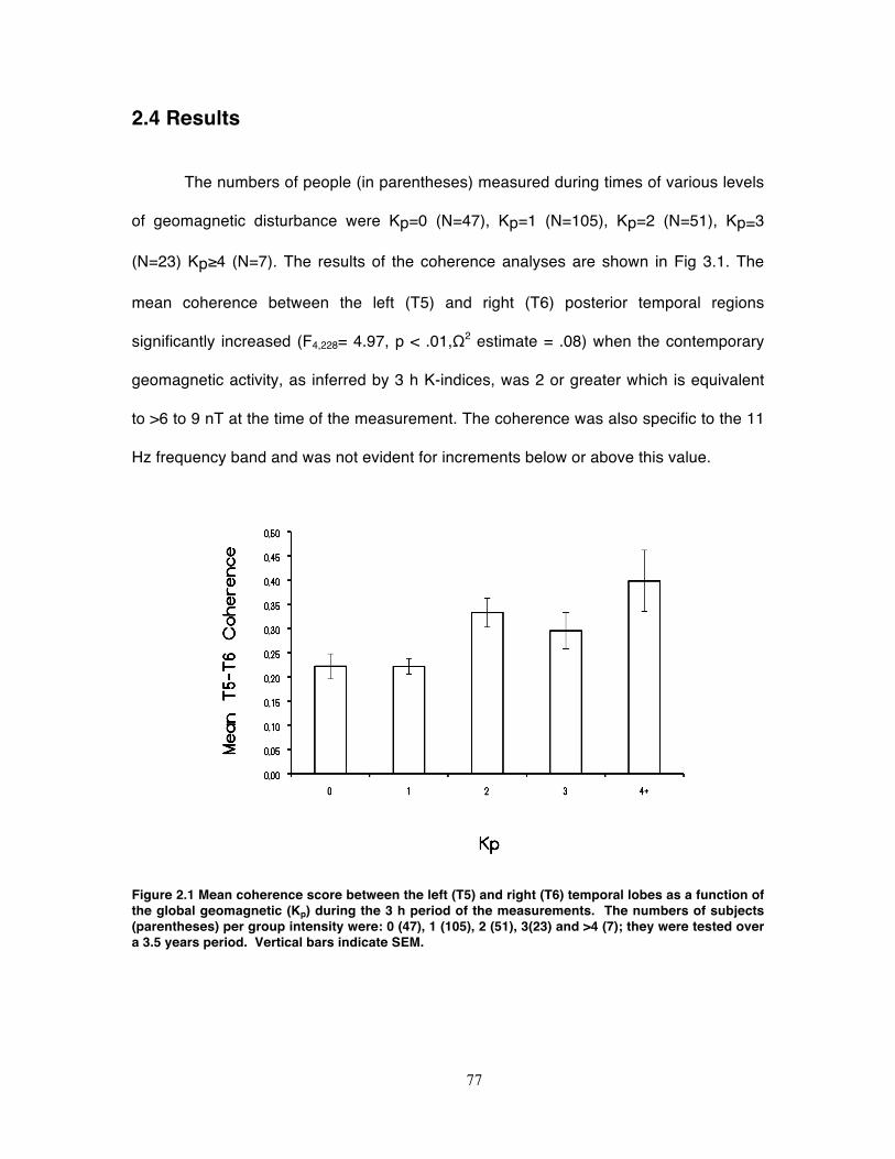
77

2.4 Results

The numbers of people (in parentheses) measured during times of various levels

of geomagnetic disturbance were Kp=0 (N=47), Kp=1 (N=105), Kp=2 (N=51), Kp=3

(N=23) Kp≥4 (N=7). The results of the coherence analyses are shown in Fig 3.1. The

mean coherence between the left (T5) and right (T6) posterior temporal regions

significantly increased (F4,228= 4.97, p < .01,Ω2 estimate = .08) when the contemporary

geomagnetic activity, as inferred by 3 h K-indices, was 2 or greater which is equivalent

to >6 to 9 nT at the time of the measurement. The coherence was also specific to the 11

Hz frequency band and was not evident for increments below or above this value.

Figure 2.1 Mean coherence score between the left (T5) and right (T6) temporal lobes as a function of the global geomagnetic (Kp) during the 3 h period of the measurements. The numbers of subjects (parentheses) per group intensity were: 0 (47), 1 (105), 2 (51), 3(23) and >4 (7); they were tested over a 3.5 years period. Vertical bars indicate SEM.

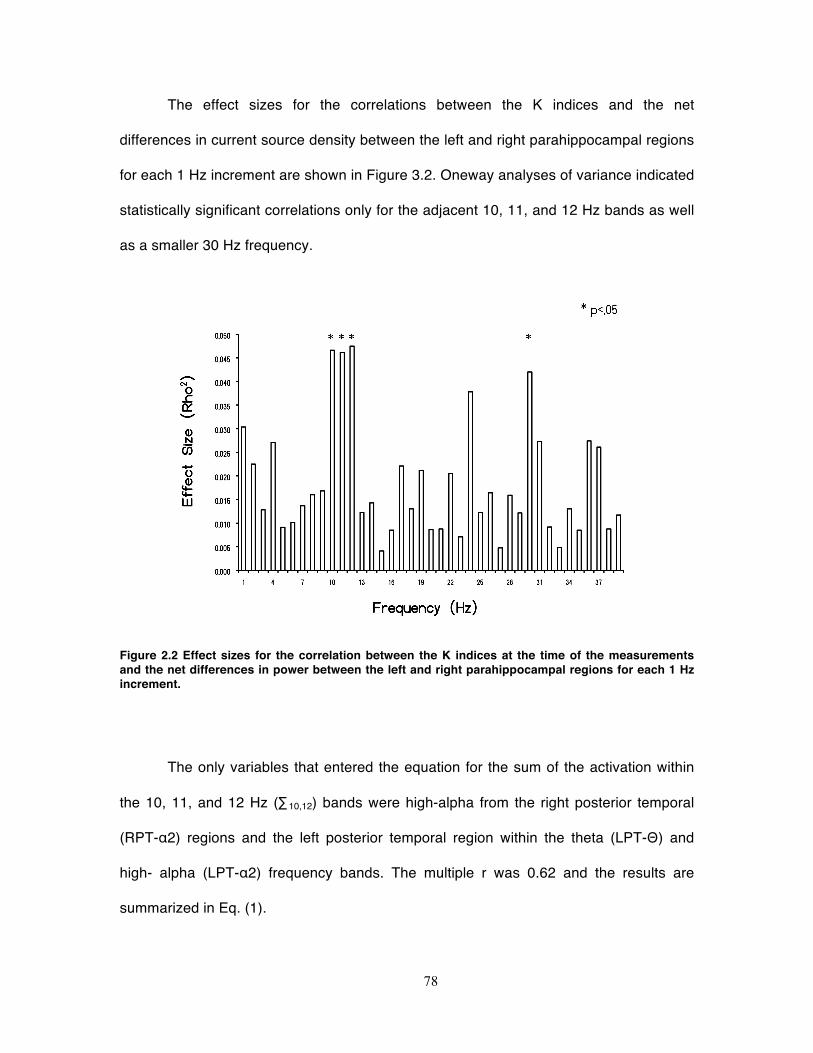
78

The effect sizes for the correlations between the K indices and the net

differences in current source density between the left and right parahippocampal regions

for each 1 Hz increment are shown in Figure 3.2. Oneway analyses of variance indicated

statistically significant correlations only for the adjacent 10, 11, and 12 Hz bands as well

as a smaller 30 Hz frequency.

Figure 2.2 Effect sizes for the correlation between the K indices at the time of the measurements and the net differences in power between the left and right parahippocampal regions for each 1 Hz increment.

The only variables that entered the equation for the sum of the activation within

the 10, 11, and 12 Hz (∑10,12) bands were high-alpha from the right posterior temporal

(RPT-α2) regions and the left posterior temporal region within the theta (LPT-Θ) and

high- alpha (LPT-α2) frequency bands. The multiple r was 0.62 and the results are

summarized in Eq. (1).

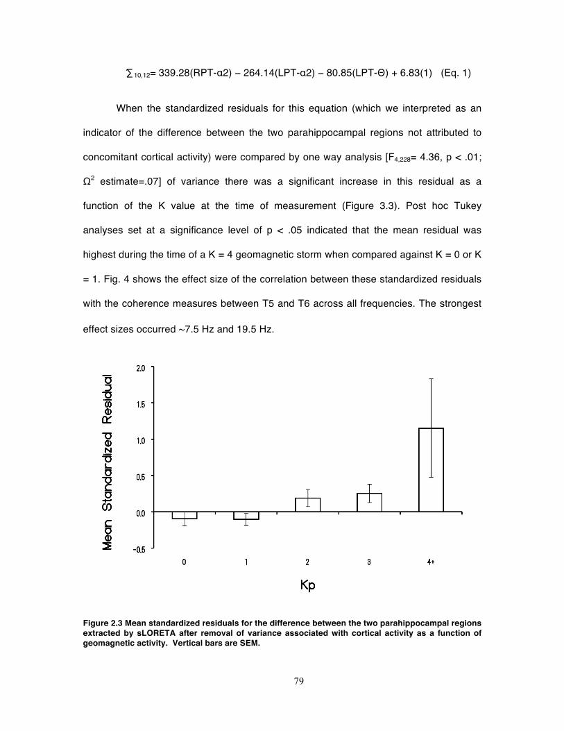
79

∑10,12= 339.28(RPT-α2) − 264.14(LPT-α2) − 80.85(LPT-Θ) + 6.83(1) (Eq. 1)

When the standardized residuals for this equation (which we interpreted as an

indicator of the difference between the two parahippocampal regions not attributed to

concomitant cortical activity) were compared by one way analysis [F4,228= 4.36, p < .01;

Ω2 estimate=.07] of variance there was a significant increase in this residual as a

function of the K value at the time of measurement (Figure 3.3). Post hoc Tukey

analyses set at a significance level of p < .05 indicated that the mean residual was

highest during the time of a K = 4 geomagnetic storm when compared against K = 0 or K

= 1. Fig. 4 shows the effect size of the correlation between these standardized residuals

with the coherence measures between T5 and T6 across all frequencies. The strongest

effect sizes occurred ∼7.5 Hz and 19.5 Hz.

Figure 2.3 Mean standardized residuals for the difference between the two parahippocampal regions extracted by sLORETA after removal of variance associated with cortical activity as a function of geomagnetic activity. Vertical bars are SEM.

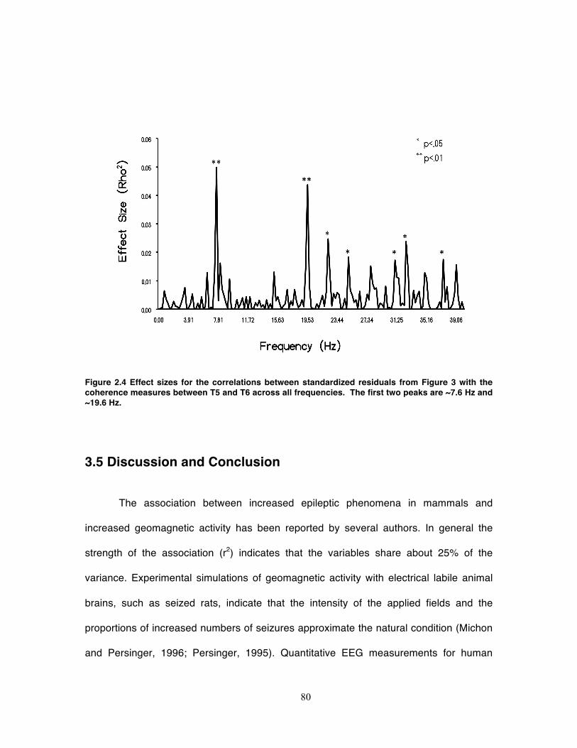
80

Figure 2.4 Effect sizes for the correlations between standardized residuals from Figure 3 with the coherence measures between T5 and T6 across all frequencies. The first two peaks are ~7.6 Hz and ~19.6 Hz.

3.5 Discussion and Conclusion

The association between increased epileptic phenomena in mammals and

increased geomagnetic activity has been reported by several authors. In general the

strength of the association (r2) indicates that the variables share about 25% of the

variance. Experimental simulations of geomagnetic activity with electrical labile animal

brains, such as seized rats, indicate that the intensity of the applied fields and the

proportions of increased numbers of seizures approximate the natural condition (Michon

and Persinger, 1996; Persinger, 1995). Quantitative EEG measurements for human

81

subjects have revealed consistent correlations between the intensity of global

geomagnetic activity and the proportion of power within specific frequency bands

(usually theta and gamma) particularly over the right hemisphere (Babayev and

Allahverdiyeva, 2007; Mulligan and Persinger, 2010). Again, comparable effects in the

change in cerebral EEG power over similar regions of the right hemisphere have been

reproduced experimentally (Mulligan and Persinger, 2012).

The results of the present study replicate and extend the thresh- old values for

significant changes in biological measurements that have been observed for a number of

species. Increased aggression between rats with seizure-induced brain damage

(Persinger, 1997), mortality of rats with acute epileptic limbic lability (Bureau and

Persinger, 1995) and the occurrence of “spontaneous” seizures in populations of

epileptic rats (Persinger, 1995) have indicated thresholds of >15 nT for global

geomagnetic activity at the time of the behaviors.

In the original Persinger and Richards (1995) study involving 127 human

subjects, most of whom were exposed to weak transcerebral fields, the report of

vestibular experiences were conspicuously increased while sitting blind folded within the

same acoustic chamber employed in this study. However in that study the effect was

most associated with the activity during the night before the experiment. In the present

study the increased coherence between the left and right posterior temporal lobes was

directly associated with the global geomagnetic activity at the time of the QEEG

measurements. All of these volunteers were sitting quietly in the darkened chamber,

were not blind folded, and did not receive any transcerebral weak magnetic fields.

The increased coherence between the left and right temporal lobes in normal

82

subjects simply sitting alone in a quiet, darkened place during periods when

geomagnetic activity increased above 6–9nT suggests that more direct quantitative brain

measurements are most sensitive to ambient geomagnetic activity or that transcerebal

magnetic fields compete for similar processes and hence increase the threshold (15–20

nT) for the detection of any effect. We suggest a continuum might exist similar to that

reported for surgical stimulation between the proportion of coherence of neuronal

populations and the intensity of the effect. Babb et al. (1987) reported that as more and

more neurons became coherent the subject’s experiences shifted along a continuum

from “normal ideation” to vestibular and powerful thoughts, to “vivid perceptual

experiences” and ultimately to convulsions. That discrete cerebral changes can occur

without awareness of discernable changes in subjective experiences is well documented

(Berns et al., 1997).

The increased coherence between the left and right posterior temporal lobes,

given the functional correlates of this region, should encourage visual and auditory

phenomena. The report of bereavement apparitions are more likely to occur when the

ambient geomagnetic activity during the experience increases from about 20–28 nT, an

average increase of about 8 nT. A similar observation was reported by Randall and

Randall (1991). It may be relevant to note that the magnitude of the 11 Hz posterior

temporal coherence displayed by individuals measured on days where the geomagnetic

disturbance exceeded ∼8nT approximated the magnitude of the 10–13 Hz anterior

temporal coherence displayed by individuals who had experienced an experimentally-

induced sensed presence approximately 5–10 min following exposure to a frequency-

modulated electromagnetic field (St-Pierre and Persginer, 2006; Saroka and Persinger,

2013).

83

The particular involvement of the parahippocampal region is important for several

reasons. First it contains structures, the hippocampus and amygdala, which were the

regions from which “hallucinations” or experiences have been most easily evoked by

direct surgical stimulation (Persinger et al., 2013; Persinger et al, 2010). Second this

area includes the perirhinal and entorhinal cortices, the “gatekeepers” of the

hippocampus, that mediate input that originates from large areas of the cerebral cortices

and visa versa (Gloor, 1997). Because it relays spatial information and receives more

powerful inputs from the frontal and cingulate regions, second-order visual and auditory

association areas, and the parietal and temporoparietal multimodal centers for language

(of the dominant hemisphere) the role of expectation, linguistic labels and visuo-auditory

spatial details would be expected to dominate subjective experiences when it is

activated.

We have postulated that the prototype for many mystical experiences involves a

“sensed presence” which has been interpreted as the awareness of the right

hemispheric equivalent of the left hemispheric sense of self (Persinger, 2003; St-Pierre

and Persinger, 2006). Although there were many inferential studies, recent source-

localization and QEEG vectorial measurements have indicated that these experiences

when elicited by transcerebral magnetic fields within the laboratory involve a right

temporal to left temporal lobe direction (Persinger et al, 2010). That geomagnetic activity

above ∼8 nT at the time of the measurements increased coherence may increase our

understanding of how these experiences might be encouraged by subtle ambient forces

and energies.

The neurophysical mechanisms by which the presumed effects from the

84

increased geomagnetic activity produced the increased coherence measured in this

study must still be identified. The traditional limits of “kT boundaries” may not be

applicable (Cifra et al., 2010). There would certainly be sufficient energy available.

Modified calculations from Mulligan et al. (Kesser et al., 2011) indicates that increased

perturbations of 10nT would be associated with ∼10 J within the average human brain.

Assuming ∼10-20J per action potential (Persinger, 2010) this increased energy would be

equivalent to one million neurons each discharging around 10 Hz.

3.6 References

Babb TL, Wilson CL, Isokawa-Akesson M, Firing patterns of human limbic neurons

during stereocephalography (SSEG) and clinical temporal lobe seizures,

Electroencephalography and Clinical Neurophysiology 66 (1987) 467–482.

Babayev ES, Allahverdiyeva AA. Effects of geomagnetic activity variations on the

physiological and psychological state of functionally healthy humans: some results

of the Azerbaijani studies. Advances in Space Research 40 (2007) 1941–1951.

Berns GS, Cohen JD, Mintun MA. Brain regions responsive to novelty in the absence of

awareness. Science 276 (1997) 1272–1275.

Booth JN, Koren SA, Persinger MA. Increased feelings of the sensed pres- ence and

increased geomagnetic activity at the time of the experience during exposure to

transcerebral weak magnetic fields. International Journal of Neuroscience 115

(2005) 1053–1079.

Bureau YR, Persinger MA. Geomagnetic activity and enhanced mortality in rats with

acute (epileptic) limbic lability. International Journal of Biometeorology 36 (1992)

226–232.

85

Cifra M, Fields JZ, Farhadi A. Electromagnetic cellular interactions. Progress in

Biophysics and Molecular Biology 105 (2010) 223–246.

Delorme A, Makeig S. EEGLAB: an open source toolbox for analysis of single- trial EEG

dynamics including independent component analysis. Journal of Neuroscience

Methods 134 (2004) 9–21.

Gloor P. The Temporal Lobe and Limbic System. Oxford University Press, N.Y, 1997.

Keeser D, Padberg F, Reisinger E, Pogarell O, Kirsch V, Palm U, Karch V, Möller HJ,

Nitsche MA, Mulert C. Prefrontal direct current stimulation modulates resting EEG

and event-related potentials in healthy subjects: a standardized low resolution

tomography (sLORETA) study. NeuroImage 55 (2011) 644–657.

Michon AL, Persinger MA. Experimental simulation of the effects of increased

geomagnetic activity upon nocturnal seizures in rats. Neuroscience Letters 224

(1997) 53–56.

Mulligan BP, Hunter MD, Persinger MA. Effects of geomagnetic activity and atmospheric

power variations on quantitative measures of brain activity: replication of the

Azerbaijani studies. Advances in Space Research 45 (2010) 940–948.

Mulligan BP, Persinger MA. Experimental simulation of the effects of sudden increases

in geomagnetic activity upon quantitative measures of human brain activity:

validation of correlational studies. Neuroscience Letters 516 (2012) 54–56.

Pasqual-Marquis RD. Standardized low resolution brain electromagnetic tomography

(sLORETA): technical details. Methods and Findings in Experimental

Pharmacology 24 (2002) D5–D12.

Persinger MA. Increased geomagnetic activity and the occurrence of bereavement

hallucinations: evidence for melatonin-mediated microseizuring in the temporal

lobe. Neuroscience Letters 88 (1988) 271–274.

86

Persinger MA. Geophysical variables and behavior: LXXIX. Overt limbic seizures are

associated with concurrent and premidscotophase geomagnetic activity:

synchronization by prenocturnal feeding. Perceptual and Motor Skills 81 (1995)

83–93.

Persinger MA. Out-of-body-like experiences are more probable in people with elevated

complex partial epileptic-like signs during periods of enhanced geo- magnetic

activity: a non-linear effect. Perceptual and Motor Skills 80 (1995) 563–569.

Persinger MA. Geomagnetic variables and behavior: LXXXIII. Increased geo- magnetic

activity and group aggression in chronic epileptic rats. Perceptual and Motor Skills

85 (1997) 395–402.

Persinger MA. The sensed presence within experimental settings: implication for the

male and female concept of self. The Journal of Psychology 137 (2003) 5–16.

Persinger MA. 10−20 Joules as a neuromolecular quantum in medicinal chemistry: an

alternative approach to myriad molecular pathways. Current Medicinal Chemistry

17 (2010) 3094–3098.

Persinger MA, Dotta BT, Saroka KS, Scott MA. Congruence of energies for cerebral

photon emissions, quantitative EEG activities and ∼5 nT changes in proximal

geomagnetic field support spin-based hypothesis of consciousness. Journal of

Consciousness Exploration and Research 4 (2013) 1–24.

Persinger MA, Saroka KS. Comparable proportions of classes of experiences and

intracererbal consequences for surgical stimulation and external application of

weak magnetic field patterns: implications for converging effects in complex partial

seizures. Epilepsy and Behavior 27 (2013) 220–224.

Persinger MA, Saroka KS, Koren SA, St-Pierre LS. The electromagnetic induction of

87

mystical and altered states within the laboratory. Journal of Con- sciousness

Exploration and Research 1 (2010) 808–830.

Persinger MA, Richards PM. Vestibular experiences of humans during brief periods of

partial sensory deprivation are enhanced when daily geomagnetic activity exceeds

15–20 nT. Neuroscience Letters 194 (1995) 69–72.

Rajaram M, Mitra S. Correlations between convulsive seizure and geomagnetic activity.

Neuroscience Letters 24 (1981) 187–191.

Randall W, Randall S. The solar wind and hallucinations – a possible relation due to

magnetic disturbances. Bioelectromagnetism 12 (1991) 67–70.

St-Pierre LS, Parker GH, Bubenik GA, Persinger MA. Enhanced mortality of rat pups

following inductions of epileptic seizures after perinatal exposures to 5 nT, 7 Hz,

magnetic fields. Life Sciences 81 (2007) 1496–1500.

St-Pierre LS, Persinger MA. Experimental facilitation of the sensed presence is predicted

by specific patterns of applied magnetic fields not by suggestibility: re-analysis of

19 experiments. International Journal of Neuroscience 116 (2006) 1–18.

Saroka KS, Mulligan BP, Murphy TR, Persinger MA. Experimental elicitation of an out of

body experience and concomitant cross-hemispheric electroen- cephalographic

coherence. Neuroquantology 8 (2010) 466–477.

Saroka KS, Persinger MA. Potential production of Hughling Jackson’s parasitic

consciousness by physiologically-patterned weak transcerebral magnetic fields:

QEEG and source localization. Epilepsy and Behavior 28 (2013) 395–407.

Subrahmanyam S, Sanker PV, Narayan, Srinivasan TM. Effects of magnetic

micropulsations on biological systems: a bioenvironmental effect. International

Journal of Biometeorology 29 (1985) 293–305.

88

Chapter 3 Assessment of Geomagnetic Coherence and Topographic Landscapes of the Static Geomagnetic Field in Relation to

the Human Brain Employing Electroencephalographic Methodology

3.1 Introduction

The earth is surrounded by a geomagnetic field that is influenced by solar

activity. The average intensity of the earth’s magnetic field is approximately 50,000 nT

(Chapman and Bartels, 1940), which is approximately a million times stronger than the

intensities of the earth’s intrinsic Schumann resonance. During geomagnetic storms,

precipitated by changes in the solar wind which is comprised of protons, the

geomagnetic field displays sudden shifts in its activity that can deviate by approximately

200-300 nT during extreme storms or 20-30 nT during low-level disturbances (Bleil,

1964).

One property of the brain is that sudden disturbances (i.e. closed head injuries,

seizures) can change the electrical landscape of its electric field topography. We have

found that post-concussion, alpha activity of one individual displayed a ‘ring’ type pattern

when measurements were taken everyday for 7-8 days post-injury. This “ringing” has

also been observed for several hours to days after a sudden impulse of protons that

disturb the static geomagnetic field and are typically observed after sudden storm

commencements particularly in high latitudes (Bleil 1964) with durations that are

approximately proportional to the degree of geomagnetic disturbance.

89

One approach to scientific inquiry is that processes that occur at a microscopic

level are related to processes that occur at a macroscopic scale. For example, small

changes in molecular concentration of certain neurochemical compounds can alter the

way that the individual experiences his or her environment as in the case with

psychotropic substances. Scale invariance, or fractal geometry, assumes that an object

retains its geometrical (either in space or time) shape as one proceeds to “zoom in” or

“zoom out”. In this case, the introduction of selective serotonin reuptake inhibitors to

some depressed individuals minimizes a negative biased towards experience. Thus,

small microscopic molecular differences influence macroscopic behaviour.

Such scale-invariance can be found within a variety of natural settings. For

example, if one were to view the landscape of Northern coniferous trees from a distance

of some kilometers above the tree line, the trees would look like moss that can be found

buried deep within its forests. Modern quantitative electroencephalographic techniques

now employ measures of fractal geometry (Georgiev et al., 2009). When such algorithms

are applied to time-series signals such as EEG, one can discern the “level of

consciousness” of individuals who are under the influence of anaesthetic compounds

(Nan and Jingua, 1988).

Theoretically the concept of a connection between processes that influence the

earth and those that influence the brain has been demonstrated quantitatively.

Persinger (2012) demonstrated that the electrical properties of lightning strikes are

similar to those produced naturally within the brain during action potentials when scale,

or size, is accommodated. In addition, the intensity and resonant frequencies of the

cavity generated between brain tissue and the skull are similar to those produced in the

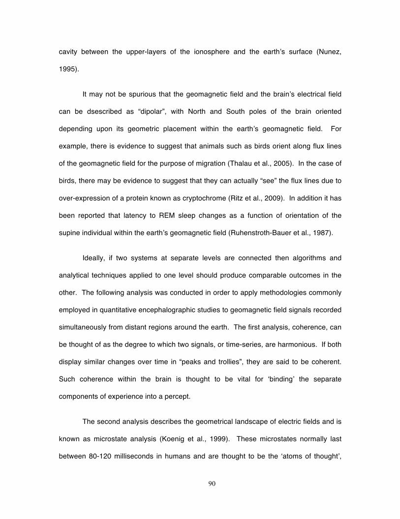
90

cavity between the upper-layers of the ionosphere and the earth’s surface (Nunez,

1995).

It may not be spurious that the geomagnetic field and the brain’s electrical field

can be dsescribed as “dipolar”, with North and South poles of the brain oriented

depending upon its geometric placement within the earth’s geomagnetic field. For

example, there is evidence to suggest that animals such as birds orient along flux lines

of the geomagnetic field for the purpose of migration (Thalau et al., 2005). In the case of

birds, there may be evidence to suggest that they can actually “see” the flux lines due to

over-expression of a protein known as cryptochrome (Ritz et al., 2009). In addition it has

been reported that latency to REM sleep changes as a function of orientation of the

supine individual within the earth’s geomagnetic field (Ruhenstroth-Bauer et al., 1987).

Ideally, if two systems at separate levels are connected then algorithms and

analytical techniques applied to one level should produce comparable outcomes in the

other. The following analysis was conducted in order to apply methodologies commonly

employed in quantitative encephalographic studies to geomagnetic field signals recorded

simultaneously from distant regions around the earth. The first analysis, coherence, can

be thought of as the degree to which two signals, or time-series, are harmonious. If both

display similar changes over time in “peaks and trollies”, they are said to be coherent.

Such coherence within the brain is thought to be vital for ‘binding’ the separate

components of experience into a percept.

The second analysis describes the geometrical landscape of electric fields and is

known as microstate analysis (Koenig et al., 1999). These microstates normally last

between 80-120 milliseconds in humans and are thought to be the ‘atoms of thought’,

91

similar to base pairs in a sequence of DNA. Theoretically a sequence of these states

could be the language with which information generated exogenously and endogenously

is consolidated, described and ultimately communicated within a social setting.

3.2 Materials and Methods

Approximately one year of the X-component of the static geomagnetic field was

collected from IntraMagnet from locations depicted in Figure 3.1A for years 2013 and

2014. The sampling rate of this data was 1/60Hz, or one observation per minute. This

data was then imported into MATLAB software where the magnetic field measurements

of 8 regions were consolidated into one variable. Because intensities of the static

geomagnetic field were stronger in certain geographical regions, within-channel z-scores

were obtained so as to normalize the measurements.

The resultant 8-channel time series was then imported into EEGLab (Delorme

and Makeig, 2004) software for visualization and artifact correction (i.e. power outages)

using an interpolation method which identified points in the time-series with z-scores

greater than 3, removed them, and then interpolated an average. The resultant time-

series was then 100 points constituted one days worth of data therefore 1 second was

equivalent to 10 days. Once artifacts were removed and the data was re-sampled it

was saved as an ASCII text file for later importation into MapWin software.

Based upon earlier findings indicating greater coherence between the left and

right temporal region during times of geomagnetic disturbance (Saroka et al., 2013)

coherence was computed for each bi-channel combination (total=28) for each day

(N=715) between January 1, 2013 and December 15, 2014. 1/604800. Coherence

92

within the 0 to 1 microHertz (approximately equivalent to 7 days) bandwidth was then

averaged. Global averages of coherence were computed from obtaining the mean of all

28 possible bivariate combinations of channels for each channel.

Within MapWin software, a specialized but approximate montage was defined

based upon the geographical locations of the magnetometers. This montage can be

viewed in Figure 3.1B. The entire ~35 earth-second epoch was imported into MapWin

with a pass-band filter of 0-20Hz, as is employed regularly in the literature. Microstate

clusters were computed using the “Construct Microstate Maps” option, forcing the

analysis to produce 4 clusters with pre-cluster normalization. To compute inferences of

coverage, occurrence and duration of each of the 4 classes of microstate, the 35 second

record was segmented according to each day (i.e. 350 days). The microstate clusters

produced in the original analysis were then applied to each segment individually and

conventional microstate parameters were then saved for further SPSS analysis.

To compare the results of the microstate analysis against some measure of

validity, the daily Kp index was obtained from the OMNI online geophysical database

(http://omniweb.gsfc.nasa.gov/form/dx1.html) for each day for both years.

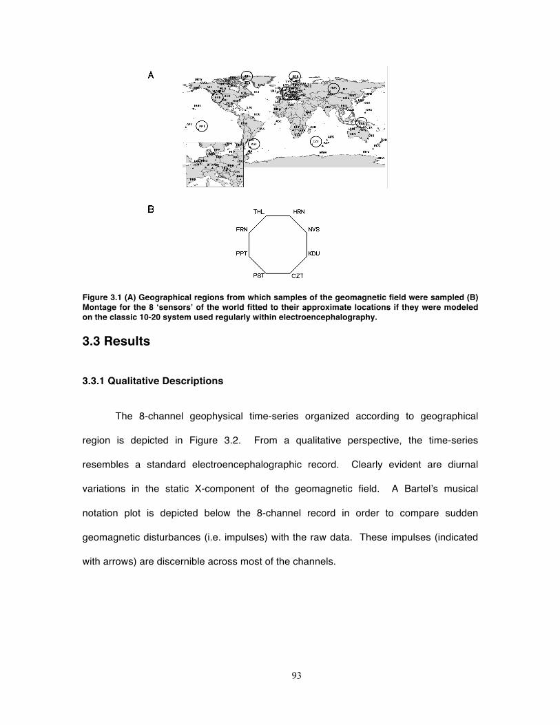
93

Figure 3.1 (A) Geographical regions from which samples of the geomagnetic field were sampled (B) Montage for the 8 ‘sensors’ of the world fitted to their approximate locations if they were modeled on the classic 10-20 system used regularly within electroencephalography.

3.3 Results

3.3.1 Qualitative Descriptions

The 8-channel geophysical time-series organized according to geographical

region is depicted in Figure 3.2. From a qualitative perspective, the time-series

resembles a standard electroencephalographic record. Clearly evident are diurnal

variations in the static X-component of the geomagnetic field. A Bartel’s musical

notation plot is depicted below the 8-channel record in order to compare sudden

geomagnetic disturbances (i.e. impulses) with the raw data. These impulses (indicated

with arrows) are discernible across most of the channels.

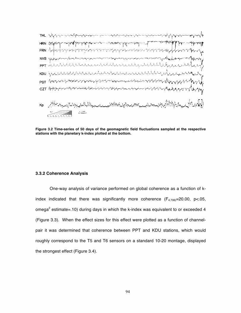
94

Figure 3.2 Time-series of 50 days of the geomagnetic field fluctuations sampled at the respective stations with the planetary k-index plotted at the bottom.

3.3.2 Coherence Analysis

One-way analysis of variance performed on global coherence as a function of k-

index indicated that there was significantly more coherence (F4,706)=20.00, p<.05,

omega2 estimate=.10) during days in which the k-index was equivalent to or exceeded 4

(Figure 3.3). When the effect sizes for this effect were plotted as a function of channel-

pair it was determined that coherence between PPT and KDU stations, which would

roughly correspond to the T5 and T6 sensors on a standard 10-20 montage, displayed

the strongest effect (Figure 3.4).

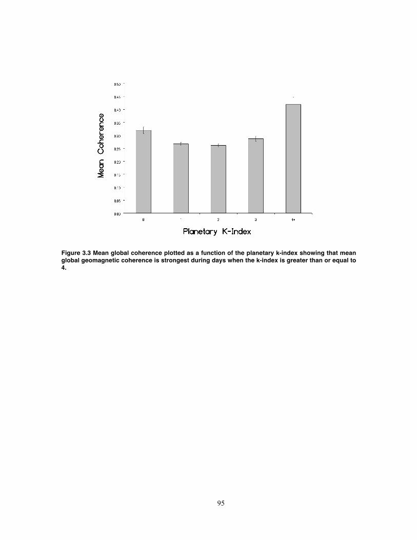
95

Figure 3.3 Mean global coherence plotted as a function of the planetary k-index showing that mean global geomagnetic coherence is strongest during days when the k-index is greater than or equal to 4.

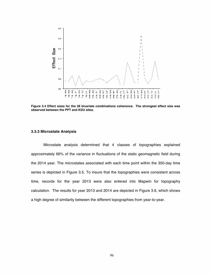
96

Figure 3.4 Effect sizes for the 28 bivariate combinations coherence. The strongest effect size was observed between the PPT and KDU sites.

3.3.3 Microstate Analysis

Microstate analysis determined that 4 classes of topographies explained

approximately 66% of the variance in fluctuations of the static geomagnetic field during

the 2014 year. The microstates associated with each time point within the 350-day time

series is depicted in Figure 3.5. To insure that the topographies were consistent across

time, records for the year 2013 were also entered into Mapwin for topography

calculation. The results for year 2013 and 2014 are depicted in Figure 3.6, which shows

a high degree of similarity between the different topographies from year-to-year.

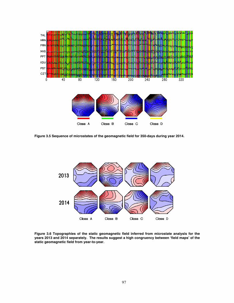
97

Figure 3.5 Sequence of microstates of the geomagnetic field for 350-days during year 2014.

Figure 3.6 Topographies of the static geomagnetic field inferred from microstate analysis for the years 2013 and 2014 separately. The results suggest a high congruency between ‘field maps’ of the static geomagnetic field from year-to-year.

98

3.4 Discussion and Conclusion

The relationship between the earth’s geomagnetic field and human brain activity

has been assessed qualitatively and quantitatively. The waveforms generated by the

electroencephalograms of humans show remarkable congruence with that of

atmospheric noise showing on average identities in the frequency range between 0 and

about 50 Hz (König and Ankermüller, 1960). Several groups have demonstrated direct

coherence between the Schumann resonance, which is observable within the spectrums

of human brains and strongest primarily over the caudal aspect of the cerebrum, and the

brain’s electric field within specific frequency ranges of about 8 to 30 Hz (Pobachenko,

2006; Saroka and Persinger, 2014). The frequency of these coherences is about 1-2

times per second with average durations of about 300 milliseconds and approximates

the duration of about 2-3 microstates.

Because the basic assumption motivating this analysis was that there is a direct

connection between processes occurring on both microscopic (human brain) and

macroscopic (the earth) levels, we assumed that analytic methods commonly employed

within one level should reveal comparable outcomes in the other. The main requirement

was that these similarities should be internally consistent from year-to-year and valid

within the context of the knowledge base of that level. The results of the coherence

analysis indicated that average coherence of the channels recording the geomagnetic

field at different sites was strongest during periods of disturbance and was pronounced

between recording sites that would have been comparable to the left and right posterior

temporal sites if the nasion was localized around the North pole of the earth. Increased

coherence within human electroencephalographic activity between the left and right

99

temporal lobes has been observed during the incidences of geomagnetic disturbances

(Saroka et al., 2013). The coherence between these two regions was strongest within

frequency bands approaching the fundamental (~8 Hz) and third harmonic (~20 Hz) of

the Schumann resonance. Pobachenko et al. (2006) previously reported that the

correlation between simultaneous measurements of atmospheric noise and human

electroencephalograms was strongest during periods of geomagnetic disturbance. The

integration of these results with those found previously would suggest a mirrored fugal-

coupling of processes occurring at both levels whereby events such as sudden

commencements simultaneously produce coherences within the earth and the human

brain.

The microstate analysis revealed 4 topographies that cumulatively explained

between 62-66% of the variance in the variations of the topographies of the static

geomagnetic field that were relatively consistent between the two years. The first

microstate (Class A) reiterates that the magnetic fields are strongest at the North and

South poles of the earth and resembles Class C commonly observed in human brains

(Koenig et al., 2002). Class C begins to resemble isocontour maps showing that total

magnetic field is strongest over the Canadian Northwest Territories and portions of

Antarctica south of Australia and conversely in parts of Russia north of China and in the

Pacific Ocean west of Antarctica. Interestingly Class D appears to be most sensitive to

abrupt changes in the geomagnetic field that can partially be explained by the tilt of the

North Pole relative to the Sun.

In conclusion, while open to speculation, the analyses conducted in this chapter

support a fractal relationship between electromagnetic processes occurring within the

human brain and the earth. The shapes of microstates as well as the coherencies

100

observed in cross-station analysis potentially demonstrate that it is possible to explore

time-varying (in this case the static geomagnetic field) signals in congruous ways.

For centuries the explanation behind near-simultaneous appearances of

phenomena like cave art and scientific discoveries has been labeled with various

rationalizations such as impending coincidence, evolutionary adaptation and others, all

of which assume random chance expectancies either through eventual transmission of

ideas from region-to-region or mutations in the sequencing of DNA. However, these

findings may offer an alternative, but equally compatible dimension consistent with

Sheldrake’s (2011) morphogenetic resonance hypothesis that implies that conspecific

species of animals learn faster once the original behaviour has been performed. In this

case the information in the form of electromagnetic patterns generated from the brains of

individuals could produce changes within the earth’s geomagnetic field that then

influence other human brains through resonance processes. Therefore the

geomagnetic field could function as a source of ideas in the form of energy, the

transmission medium by which ideas are transferred between geographic regions, or

both. Although seemingly improbable, both Persinger (2010) and Dotta (2010) have

shown that stimuli applied to one person in isolation produces comparable changes in

another person sitting in another room when both individuals share the same temporally-

patterned and circumcerebrally rotating electromagnetic field.

3.5 References

Bleil, D. F. (1964). Natural electromagnetic phenomena below 30 kc/s. In Natural

Electromagnetic Phenomena (Vol. 1).

101

Chapman, S., & Bartels, J. (1940). Geomagnetism. Oxford: Clarendon Press.

Delorme, A., & Makeig, S. (2004). EEGLAB: an open source toolbox for analysis of

single-trial EEG dynamics including independent component analysis. Journal of

neuroscience methods, 134(1), 9-21.

Dotta, B. T., Buckner, C. A., Lafrenie, R. M., & Persinger, M. A. (2011). Photon

emissions from human brain and cell culture exposed to distally rotating magnetic

fields shared by separate light-stimulated brains and cells. Brain research, 1388,

77-88.

Georgiev, S., Minchev, Z., Christova, C., & Philipova, D. (2009). EEG fractal dimension

measurement before and after human auditory stimulation. Bioautomation, 12.

Koenig, T., Prichep, L., Lehmann, D., Sosa, P. V., Braeker, E., Kleinlogel, H., ... & John,

E. R. (2002). Millisecond by millisecond, year by year: normative EEG

microstates and developmental stages. Neuroimage, 16(1), 41-48.

Koenig, T., Lehmann, D., Merlo, M. C., Kochi, K., Hell, D., & Koukkou, M. (1999). A

deviant EEG brain microstate in acute, neuroleptic-naive schizophrenics at rest.

European archives of psychiatry and clinical neuroscience, 249(4), 205-211.

König, H., & Ankermüller, F. (1960). Über den Einfluss besonders niederfrequenter

elektrischer Vorgänge in der Atmosphäre auf den Menschen.

Naturwissenschaften, 47(21), 486-490.

102

Nan, X., & Jinghua, X. (1988). The fractal dimension of EEG as a physical measure of

conscious human brain activities. Bulletin of Mathematical Biology, 50(5), 559-

565.

Nunez, P. L. (1995). Neocortical dynamics and human EEG rhythms. Oxford University

Press, USA.

Persinger, M. A. (2012). Brain electromagnetic activity and lightning: potentially

congruent scale-invariant quantitative properties. Frontiers in integrative

neuroscience, 6.

Persinger, M. A., Saroka, K. S., Lavallee, C. F., Booth, J. N., Hunter, M. D., Mulligan, B.

P., ... & Gang, N. (2010). Correlated cerebral events between physically and

sensory isolated pairs of subjects exposed to yoked circumcerebral magnetic

fields. Neuroscience Letters, 486(3), 231-234.

Pobachenko, S. V., Kolesnik, A. G., Borodin, A. S., & Kalyuzhin, V. V. (2006). The

contingency of parameters of human encephalograms and Schumann resonance

electromagnetic fields revealed in monitoring studies. Biophysics, 51(3), 480-483.

Ritz, T., Wiltschko, R., Hore, P. J., Rodgers, C. T., Stapput, K., Thalau, P., ... &

Wiltschko, W. (2009). Magnetic compass of birds is based on a molecule with

optimal directional sensitivity. Biophysical journal, 96(8), 3451-3457.

Ruhenstroth-Bauer, G., Rüther, E., & Reinertshofer, T. H. (1987). Dependence of a

sleeping parameter from the NS or EW sleeping direction. Zeitschrift für

Naturforschung C, 42(9-10), 1140-1142.

103

Saroka, K. S., Caswell, J. M., Lapointe, A., & Persinger, M. A. (2014). Greater

electroencephalographic coherence between left and right temporal lobe

structures during increased geomagnetic activity. Neuroscience letters, 560, 126-

130.

Saroka, K. S., & Persinger, M. A. (2014). Quantitative evidence for direct effects

between Earth-ionosphere Schumann resonances and human cerebral cortical

activity. International Letters of Chemistry, Physics and Astronomy, 20.

Sheldrake, R. (2011). The presence of the past: Morphic resonance and the habits of

nature. Icon Books.

Thalau, P., Ritz, T., Stapput, K., Wiltschko, R., & Wiltschko, W. (2005). Magnetic

compass orientation of migratory birds in the presence of a 1.315 MHz oscillating

field. Naturwissenschaften, 92(2), 86-90.

104

Chapter 4 The Proximal AC Electromagnetic Environment and Human

Brain Activity

4.1 Introduction

All biological systems exist within a complex environment composed of many

features including electromagnetic waves. The frequency of these oscillations ranges

from extremely low-frequency oscillations (~10Hz) frequencies, which are not directly

perceived but are produced naturally by the earth and the brain, to high-frequency ~1014

Hz which are processed by the human retina and experienced psychologically as colour.

As such there are frequencies that are directly perceived and many that are not.

That electromagnetic signals generated by modern technology can influence

subtle changes in physiology has been explored extensively. Psychological phenomena

such as the ‘sensed presence’, ‘out-of-body experience’ and pain diminishment have all

been demonstrated to be influenced by application of weak-intensity physiologically-

patterned magnetic fields (Saroka and Persinger, 2013; Persinger et al., 2010). Within

rural environments 60-Hz power-line frequencies, with electric field intensities ranging

between between 10-2-10-4 V/m (König, 1984) depending upon source distance and have

discrete harmonics produced according to basic physical principles, and magnetic fields

generated by electronics may produce changes in physiology. There have been

extensive correlative researches demonstrating that some residents living proximal to

powerline generators show increased incidences of leukemia, breast-cancer, and

105

general malaise and fatigue (Feychting and Ahibom, 1994; Feychting et al., 1998; Kaprio

et al., 1997).

From a psychological viewpoint, we have shown that recordings of spoken-words

which have been digitized and translated into a magnetic field equivalent can affect

decision-making without direct awareness when subjects were asked to select the ‘best

choice’ from a list of words (Healey and Persinger, 1997; Saroka and Persinger, 2011).

Such simple, and perhaps subliminal, effects may be a product of brain function; it is well

known that only 5% of connective fibers within the brain are associated with external

sensory stimuli with the majority of 90-95% originating to and terminating within the

cerebral cortices (Nunez, 1995). From a more holistic perspective, that would mean that

90-95% of the information processing within the brain is focused internally.

We have seen that disturbances within the earth’s electromagnetic environment

are correlated with disturbances in brain function. In a study published by Mulligan et al

(2010), theta-band spectral density occurring within the right frontal cortices was

elevated during times of geomagnetic storms. The same authors later found that when

geomagnetic storms were simulated using devices which produce electromagnetic fields,

there was an enhancement of low-frequency range activation within the brain after 15-20

minutes of continuous application (Mulligan and Persinger, 2012). We have also seen

that disturbances in geomagnetic activity are also associated with changes in the

coherence between the two temporal lobes. The magnitude of the coherence during

these times was remarkably similar to that observed in an experiment which involved the

encouragement of the sensed presence (Saroka et al., 2013).

106

The purpose of this study was to discern if brain activity of normal healthy

individuals sitting quietly with their eyes closed show changes in brain activity that are

correlated with crude measurements of the background AC-magnetic field occurring

within the environment recorded simultaneously.

4.2 Methods and Materials

Participants

Participants were 4 healthy volunteers (1 male, 3 females) who were recruited

from the laboratory. Each subject was asked to sit in a comfortable chair housed in an

acoustic chamber which also served as a Faraday cage. Each subject was asked to

remain seated with their eyes closed for 2-minutes.

Data Acquisition

Brain activation was monitored using a Mitsar-201 amplifier (sampling

rate=250Hz) fitted with a 19-channel Electro-Cap that was placed on the heads of the

participants. Electro-Gel was used to bridge contact between the scalp and the surface

of the sensors in each channel. Voltages recorded from the cap were translated from

analog-to-digital and were ultimately recorded and viewed on a Dell Inspiron laptop

equipped with WinEEG v.2.82 software. The data was saved for further analysis within

the MATLAB platform.

107

AC-generated electromagnetic activity was measured with an Alpha-Lab

Milligauss meter. The milligauss meter was placed approximately 2-5 cm behind the

heads (occipital notch) of each participant. Data was fed from the milligauss meter to an

Apple Macbook equipped with Audacity recording software via coaxial cable. Data was

recorded at a sampling rate of 250Hz and was later saved as a *.WAV file for further

analysis within MATLAB software.

Signal Processing

All milligauss recordings were imported into MATLAB for processing and spectral

analyses. The 120-second long records pertaining to each of the 4 participants was

divided into 4-second segments. Consequently there were 30 observations available for

each participant. The records were then submitted to a spectral analysis available within

the EEGLab toolbox. The spectopo.m (Delorme and Makeig, 2004) function was used to

generate discrete spectral densities within frequencies ranging from 1-50Hz. This

spectral data was then saved and imported into SPSS for further statistical analysis with

measures of brain activity.

The brain activity recorded with the QEEG was also imported into MATLAB.

Each 120-second measurement was divided into 30x4-second chunks and re-filtered

using a band-pass filter of 1.5-40Hz. Within MATLAB, coherence between the left

anterior (T3) and right anterior (T4) as well as the left posterior (T5) and right posterior

(T6) channels was calculated according to previously defined methods using the

coherence.m function. The mean of the coherence values between the 7 and 10-Hz

was computed and saved for later statistical analysis.

108

The same raw segments of EEG data were also used in a source localization

analysis (Pascual-Marqui, 2002) to predict activity within the parahippocampal region.

All data was imported into sLORETA and processed according to standard and

previously-used techniques. The current source densities (uA/mm2) within the classical

frequency bands (delta, theta, low-alpha, high-alpha, beta-1, beta-2, beta-3 and gamma)

were then saved and imported into the SPSS database already containing inferences of

the background AC-magnetic field as well as the coherence.

Finally, topographies and microstate descriptors of the brain’s electric field were

computed using freely available MapWin software. All data was imported and re-filtered

between 2-20Hz according to standard procedures (Koenig et al., 1999). Next, the

microstate topographies for each of the segments were computed separately using the

“Construct Microstates” function within the software without pre-standardized clustering.

Next average clusters were then computed for each participant separately using the 30

available epochs. The resultant participant-specific clusters were then combined into a

grandmean set of clusters and re-arranged according to the topographies published by

Lehmann and Koenig. This resultant topographical template was then applied to each

segment of each participant separately; descriptive microstate descriptors (i.e. duration,

occurrence, coverage) were then computed separately, saved, and imported into the

SPSS database.

Once all data (i.e. spectral analyses of background EM and QEEG descriptors)

was consolidated, statistical analyses was performed on within-subject z-scored

normalized derivations through Pearson and Spearman correlation analyses and linear

multiple regression. For the dataset, a total of 120 cases (30 for each participant) were

available.

109

4.3 Results

A linear stepwise multiple regression predicting mean 7-10Hz coherence from the

spectral densities of the background EM revealed a significant (R=.46, p<.05)

relationship. The frequencies of the spectral densities predicting the coherence were

approximately 13, 19.5, 27 and 46Hz. The saved predicted scores were then entered

into separate Spearman-rank correlational analyses separately for each individual. The

correlations were significant across the sampled population. Results of the analysis can

be seen in Figure 4.1.

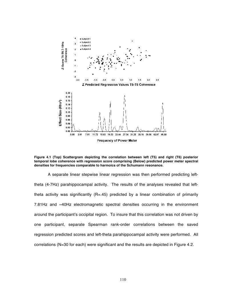
110

Figure 4.1 (Top) Scattergram depicting the correlation between left (T5) and right (T6) posterior temporal lobe coherence with regression score comprising (Below) predicted power meter spectral densities for frequencies comparable to harmoics of the Schumann resonance.

A separate linear stepwise linear regression was then performed predicting left-

theta (4-7Hz) parahippocampal activity. The results of the analyses revealed that left-

theta activity was significantly (R=.45) predicted by a linear combination of primarily

7.81Hz and ~40Hz electromagnetic spectral densities occurring in the environment

around the participant’s occipital region. To insure that this correlation was not driven by

one participant, separate Spearman rank-order correlations between the saved

regression predicted scores and left-theta parahippocampal activity were performed. All

correlations (N=30 for each) were significant and the results are depicted in Figure 4.2.

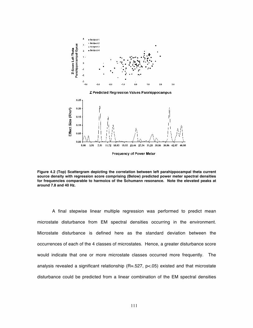
111

Figure 4.2 (Top) Scattergram depicting the correlation between left parahippocampal theta current source density with regression score comprising (Below) predicted power meter spectral densities for frequencies comparable to harmoics of the Schumann resonance. Note the elevated peaks at around 7.8 and 40 Hz.

A final stepwise linear multiple regression was performed to predict mean

microstate disturbance from EM spectral densities occurring in the environment.

Microstate disturbance is defined here as the standard deviation between the

occurrences of each of the 4 classes of microstates. Hence, a greater disturbance score

would indicate that one or more microstate classes occurred more frequently. The

analysis revealed a significant relationship (R=.527, p<.05) existed and that microstate

disturbance could be predicted from a linear combination of the EM spectral densities

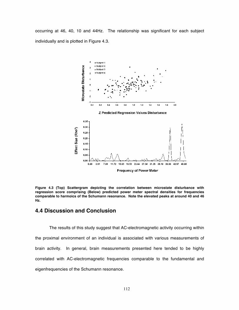
112

occurring at 46, 40, 10 and 44Hz. The relationship was significant for each subject

individually and is plotted in Figure 4.3.

Figure 4.3 (Top) Scattergram depicting the correlation between microstate disturbance with regression score comprising (Below) predicted power meter spectral densities for frequencies comparable to harmoics of the Schumann resonance. Note the elevated peaks at around 40 and 46 Hz.

4.4 Discussion and Conclusion

The results of this study suggest that AC-electromagnetic activity occurring within

the proximal environment of an individual is associated with various measurements of

brain activity. In general, brain measurements presented here tended to be highly

correlated with AC-electromagnetic frequencies comparable to the fundamental and

eigenfrequencies of the Schumann resonance.

113

First, we found that 7-10Hz left-right temporal coherence was positively

correlated with the electromagnetic intensity of frequencies around 20 and 27Hz. In a

previous study, we observed that coherence between the left and right was elevated

during times of geomagnetic storms (Saroka et al., 2013). We have also observed

coherence magnitudes increases within the bilateral temporal regions increase ~10-15

minutes after the application of a frequency-modulated electromagnetic pattern for

individuals who experienced a sensed presence (Saroka and Persinger, 2013).

Second, left parahippocampal activity was associated primarily with 7 and 40Hz

activity occurring within the environment. This region is strongly associated with the

encoding of memory because of its central location in receiving information from

widespread cortical areas (Powell et al., 2004). That the left and not the right

parahippocampal region was sensitive to these Schumann frequencies may be

accommodated by its role in verbal encoding. For example Wagner and colleagues

(1998) demonstrated that higher recall of verbal information is associated greater

increases in fMRI bold activation within the left parahippocampal region. If the data

presented above is applicable, then subtle changes in the electromagnetic environment

could affect the consolidation of verbal information and thus influence the trajectory of

future experiences of an individual.

Finally, we found that the topography of the brain’s electric field was correlated

with activity specifically with frequencies almost identical to the 5th and 6th harmonics of

the Schumann resonance (Balser and Wagner, 1960). Specifically, we found that 40Hz

and 45Hz background electromagnetic activity was strongly correlated with

displacements in the distribution of the occurrence of microstate classes. These

frequencies are a candidate for the ‘binding factor’ suspected to consolidate all sensory

114

and cognitive information into a percept. Recurrent 40-Hz oscillations occurring between

the thalamus and the cortex have been measured by Llinas and Ribrary (1993), who

also demonstrated that these gamma oscillations are also present during REM sleep

when an individual dreaming. If consciousness is considered to be highly correlated with

electric, and by Farady induction, magnetic fields the data may suggest that other

extracerebral sources of information may play a stronger role in a person’s experiences

than previously suspected. Because the energies and frequencies for both the

environment and the human brain are comparable it is unclear in which direction one is

affected by the other or whether they are simultaneously affected by a third factor.

It is unclear weather the Schumann resonance generated naturally by the earth

was associated with the measurements presented in this chapter. Using the same

milligauss meter, we have measured an enhancement of Schumann frequencies at

Agawa Provicincial Park situated on Lake Superior. This special location contains rock

art produced by indigenous peoples approximately 400 years ago. This recorded

Schumann profile was not observed overtly within other locations around Lake Superior;

however when calibration curves were calculated to discern the intensities at these

Schumann peaks we found that they were within nanoTesla range, or about 1000 times

that measured routinely by other investigators (Davis, 1995). While others have

measured Schumann intensities within nanoTesla range, it is still uncertain whether the

findings presented here are artifacts of the 60Hz power-line harmonics or other

anomalous human-made signals.

Whether the measured AC-electromagnetic field is a reflection of processes

produced by the earth, or whether they were generated by human intervention, the data

suggests that the brains of individuals have a natural proclivity to synchronize with

115

frequencies similar to the Schumann Resonance. This may not be surprising given that

biological systems developed in an environment where its presence is strong and that it

occurs predominantly within caudal aspects of the brain during periods of eyes closed

relaxation. The results may have special importance when one considers that the sub-

harmonic frequencies of 60-Hz power lines extend well into frequencies resonant to the

brain itself, including 10-Hz. Such findings may warrant re-consideration of the optimal

frequencies of power-line transmission to minimize adverse human health effects.

4.5 References

Balser, M., & Wagner, C. A. (1960). Observations of Earth-ionosphere cavity

resonances. Nature, 188(4751), 638-641.

Davis, D. (1995). Schumann resonances. Handbook of atmospheric electrodynamics, 1,

267.

Delorme, A., & Makeig, S. (2004). EEGLAB: an open source toolbox for analysis of

single-trial EEG dynamics including independent component analysis. Journal of

neuroscience methods, 134(1), 9-21.

Feychting, M., & Ahlbom, A. (1994). Magnetic fields, leukemia, and central nervous

system tumors in Swedish adults residing near high-voltage power lines.

Epidemiology, 5(5), 501-509.

116

Feychting, M., Forssén, U., Rutqvist, L. E., & Ahlbom, A. (1998). Magnetic fields and

breast cancer in Swedish adults residing near high-voltage power lines.

Epidemiology, 9(4), 392-397.

Healey, F.Y., Persinger M.A., Koren, S.A. (1997). Control of ‘choice’ by application of

the electromagnetic equivalents of spoken words: Mediation by emotional rather

than linguistic dimensions? Perceptual and Motor Skills, 85(3f), 1411-1418.

Llinas, R., & Ribary, U. (1993). Coherent 40-Hz oscillation characterizes dream state in

humans. Proceedings of the National Academy of Sciences, 90(5), 2078-2081.

Kaprio, J., Varjonen, J., Romanov, K., Heikkilä, K., & Koskenvuo, M. (1997). Magnetic

fields of transmission lines and depression. American journal of epidemiology,

146(12), 1037-1045.

Koenig, T., Lehmann, D., Merlo, M. C., Kochi, K., Hell, D., & Koukkou, M. (1999). A

deviant EEG brain microstate in acute, neuroleptic-naive schizophrenics at rest.

European archives of psychiatry and clinical neuroscience, 249(4), 205-211.

König, H. L., Krueger, A. P., Lang, S., & Sönning, W. (2012). Biologic effects of

environmental electromagnetism. Springer Science & Business Media.

Mulligan, B. P., Hunter, M. D., & Persinger, M. A. (2010). Effects of geomagnetic activity

and atmospheric power variations on quantitative measures of brain activity:

replication of the Azerbaijani studies. Advances in Space Research, 45(7), 940-

948.

117

Mulligan, B. P., & Persinger, M. A. (2012). Experimental simulation of the effects of

sudden increases in geomagnetic activity upon quantitative measures of human

brain activity: validation of correlational studies. Neuroscience letters, 516(1), 54-

56.

Nunez, P. L., & Cutillo, B. A. (Eds.). (1995). Neocortical dynamics and human EEG

rhythms. Oxford University Press, USA.

Pascual-Marqui, R. D. (2002). Standardized low-resolution brain electromagnetic

tomography (sLORETA): technical details. Methods Find Exp Clin Pharmacol,

24(Suppl D), 5-12.

Persinger, M. A., Saroka, K. S., Mulligan, B. P., & Murphy, T. R. (2010). Experimental

elicitation of an out of body experience and concomitant cross-hemispheric

electroencephalographic coherence. NeuroQuantology, 8(4).

Saroka, K. S., Caswell, J. M., Lapointe, A., & Persinger, M. A. (2014). Greater

electroencephalographic coherence between left and right temporal lobe

structures during increased geomagnetic activity. Neuroscience letters, 560, 126-

130.

Saroka, K. S., & Persinger, M. A. (2011). Detection of electromagnetic equivalents of the

emotional characteristics of words: implications for the electronic-listening

generation. Open Behavioral Sciences Journal, 5, 24-27.

Saroka, K. S., & Persinger, M. A. (2013). Potential production of Hughlings Jackson's

“parasitic consciousness” by physiologically-patterned weak transcerebral

118

magnetic fields: QEEG and source localization. Epilepsy & Behavior, 28(3), 395-

407.

Powell, H. W. R., Guye, M., Parker, G. J. M., Symms, M. R., Boulby, P., Koepp, M. J., ...

& Duncan, J. S. (2004). Noninvasive in vivo demonstration of the connections of

the human parahippocampal gyrus. Neuroimage, 22(2), 740-747.

Wagner, A. D., Schacter, D. L., Rotte, M., Koutstaal, W., Maril, A., Dale, A. M., ... &

Buckner, R. L. (1998). Building memories: remembering and forgetting of verbal

experiences as predicted by brain activity. Science, 281(5380), 1188-1191.

119

Chapter 5 Quantitative Convergence of Major-Minor Axes Cerebral

Electric Field Potentials and Spectral Densities: Consideration of Similarities to the Schumann Resonance

and Practical Implications Published in Plos One

Co-Authors: David E. Vares, Michael A. Persinger

4.1 Introduction

One of the basic assumptions of modern Neuroscience is that ultimately all of the

qualitative features of the ephemeral cognitive processes such as thinking and

consciousness will be interpretable as quantitative configurations (Wackermann, 1999)

of the complex temporal patterns of electromagnetic values that can be measured from

the surface of the human cerebrum. The similarity of average duration of microstates

and the duration of the human percept is an example of such transformation of

perspective. The clever consideration (Lehmann et al, 1995; 1998) that four microstates

(Koenig et al, 2002) could reflect functional cognitive units or “atoms of thought” that are

the information within the stream of dynamic process within cerebral space, analogous to

base nucleotide pairs for genetic information within DNA sequences, exemplifies the

significance of this approach. The shift towards biophysical analyses (Johnson, 1980;

Nunez, 1995; Balazsi and Kish, 2000; Park and Lee, 2007; Persinger and Lavallee,

2012) of complex cerebral functions once relegated to the domain of the philosopher and

psychologist requires a verification of the physical parameters for these operations. Here

we reiterate and report validation of quantitative phenomena that define the electric and

120

potentially magnetic features of our primary inferential measurement: quantitative

electroencephalography (QEEG).

Our approach is that the human cerebrum is a functional, dynamic dipole whose

voltage, or potential difference, is reflected as more or less steady-state potentials in the

order of 10 to 30 mV (Rowland, 1967) and extremely low frequency time-varying

components whose average intensities are about three orders of magnitudes less (µV

range). Because the human cerebral volume is not a sphere but more typical of an

elliptoid there should be a slight difference in average µV intensity that reflects this ratio.

The relatively fixed volume and surface area of the cerebrum and rostral-caudal bulk

velocity of ~4.5 m·s-1 should generate constant standing waves (Nunez, 1995; Persinger

and Lavallee, 2012) with parameters much like the fundamental Schumann resonance of

~7.5 to 8 Hz (Campbell, 1967; Polk, 1982; Koenig et al, 1981; Schlegel and Fullekrug,

1999) which is the resonance solution for the velocity of light (3·108 m·s-1) and the

earth’s fixed circumference (4·107 m). The Schumann resonances were likely present

during the origin of living systems (Persinger, 1974). The precision of the verification of

measurement of QEEG data is important for developing models and extending physical

interpretations of brain function.

4.2 Materials and Methods

Subjects

The subjects in this study were 184 individuals, measured singly, who had

participated in various experiments within the laboratory between 2009 and 2013. Some

subjects were measured more than once so that the total numbers of records were 238.

121

As part of the laboratory protocol, eyes-closed measurements were collected at the

beginning of each experiment before testing. The majority of the individuals included in

this study were university students between 19 and 25 years of age. The proportion of

men and women were similar. Most measurements were completed within a commercial

acoustic (echoic) chamber under dim light conditions.

Equipment and Recordings

Brain electrical activity was monitored using a Mitsar 201 amplifier equipped with

a 19-channel Electro-Cap International. Measurements from 19 sites (Fp1, Fp2, F7, F3,

Fz, F4, F8, T3, C3, Cz, C4, T4, T5, P3, Pz, P4, T6, O1, O2) consistent with the

International Standard of Electrode Placement were obtained. Impedance for all

measurements was maintained below 5 kOhms. The data recorded from the amplifier

was delivered to a Dell laptop equipped with WinEEG v.2.8 that produced a digital copy

of the recorded voltages. Sixteen-second epochs of eyes-closed data were extracted

from each participant and exported into MATLAB software for further filtering and

processing.

While most data collected with the amplifier were obtained using a sampling rate

of 250 Hz, some measurements were collected with a sampling rate of 500 Hz. To

insure homogeneity across subjects, data that were collected using a sampling rate of

500 Hz was re-sampled to 250 Hz using the resample function within the MATLAB

platform. The data for each subject was then filtered between 1.5 and 40 Hz using the

122

eegfiltfft.m function within the freely available EEGLab toolbox (Delorme and Makeig,

2004). Once filtered, the data were submitted to spectral analysis, using the spectopo.m

function, which computed spectral density within discrete frequencies for the Fp1 O2 T3

and T4 sensors.

These data was then imported into SPSS for further analysis for the computation

of mean absolute potential difference along the rostral-caudal (Fp1-O2) axis as well as

between the left-right temporal (T3 and T4) sensors. Absolute differences between

rostral-caudal and left and right temporal sensors were also obtained by subtracting the

absolute raw voltages (independent from spectral density) from the extracted EEG

record for each 4-millesecond point interval over 16 seconds.

Random Sample of 10 Brain Measurements

To appreciate the difference between a sub-sample of the total population and

the total population, 16 s of QEEG data (Fp1 02, T3 T4) for 10 subjects were randomly

selected using a random number generator. Z-scores for the µV2·Hz-1 values for the

rostral-caudal, left-right measures were obtained first in order to minimize individual

differences in absolute baseline values. Spectral analyses from SPSS 16 (a different

algorithm from the one applied in the previous section) were then applied to each of the

two measures for each of the 10 subjects. The frontal spectral density scores were then

subtracted from the occipital spectral density scores for each subject. The z-scores for

each of these new means were calculated so that there would be a standardized score

for these differences to compare directly across individuals. The average values for the

two orthogonal measures were calculated.

123

In order to examine the degree of individual differences of the spectral analyses

each subject’s results were assessed visually for the peak spectral density within the 10

Hz range. Because the Δf (increment of frequency) within this frequency range for 250

Hz samples is fractional (less than an integer, i.e., about .01 Hz), the bandwidth of the

peak spectral density could be inferred. This was discerned by direct inspection of the

quantitative values where the decline in z-scores on either side of the peak was

conspicuous and greater than 2 standard deviations for the interval.

Discerning the Schumann Resonance Signature

Our approach is that the human cerebrum is a functional, dynamic dipole whose

voltage, or potential difference, is reflected as more or less steady-state potentials in the

order of 10 to 30 mV (Rowland, 1967) and extremely low frequency time-varying

components whose average intensities are about three orders of magnitudes less (µV

range). Because the human cerebral volume is not a sphere but more typical of an

elliptoid there should be a slight difference in average µV intensity that reflects this ratio.

The relatively fixed volume and surface area of the cerebrum and rostral-caudal bulk

velocity of ~4.5 m·s-1 should generate constant standing waves (Nunez, 1995; Persinger

and Lavallee, 2012) with parameters much like the fundamental Schumann resonance of

~7.5 to 8 Hz (Campbell, 1967; Polk, 1982; Koenig et al, 1981; Schlegel and Fullekrug,

1999) which is the resonance solution for the velocity of light (3·108 m·s-1) and the

earth’s fixed circumference (4·107 m). The Schumann resonances were likely present

during the origin of living systems (Cole and Graf, 1974).

124

After re-sampling and re-filtering between 1.5 and 40 Hz for the 184 individuals

by eegfiltfft.m, the anterior, middle, and caudal root mean square signals were derived

from integrating frontal (Fp1,Fp2,F7,F3,Fz,F4,F8), middle (T3,C3,Cz,C4,T4) and caudal

(T5,P3,Pz,P4,T6,O1,O2) sensors. These derived signals were spectral analyzed by

spectropo.m with a window size equal to 2048 FFT points to maximize spectral

resolution. Other researchers, e.g., Abeyuriya et al (2014), have recently employed the

same approach to discern non-linear harmonics of sleep spindles in human

electroencephalographic recordings.

Because of a connection between activity within the parahippocampus and

naturally-occurring geomagnetic activity established in a previous publication (Saroka et

al, 2013) and it's prominent role as an integrator of experience before long-term memory

processes within the hippocampus, inferences of left and right parahippocampal current

source density (µA·mm-2) were computed in sLORETA (Pasqual-Marquis, 2002) within

the classical frequency bands used in more conventional electroencephalographic

studies [i.e. delta (1.5-4 Hz); theta (4-7 Hz); low-alpha (7-10 Hz); high-alpha (10-13 Hz);

beta-1 (13-20 Hz); beta-2 (20-25 Hz); beta-3 (25-30 Hz); gamma (>30 Hz)].

The same epochs of electroencephalographic activity used in the sLORETA

analyses were also imported into MapWin software (Koenig et al, 1999) for the

computation of microstates and their related parameters (i.e. duration of microstate,

occurrence of microstate class, etc.). During importation into MapWin, all epochs of

QEEG observations were filtered digitally between 2-20 Hz, according to standard

techniques. Average clusters of microstates were produced from 4x4-second epochs

were produced for each individual. The resultant clusters (maximum=4) were then

entered into a built-in cluster analysis that produced 4 topographical maps explaining

125

approximately 72% of the variance with topologies almost identical to those produced in

the original publication by Koenig et al (2002). Finally, all data derived from the different

softwares were integrated into an SPSS database for statistical analyses.

5.3 Results

Differential Potential Differences

The means for the µV2 for global frequencies between the rostral-caudal (RC)

axis and the left-right (LR) temporal lobe for the 177 records available for this study are

shown in Figure 1. For this analysis, we only selected individuals whose z-score was

within +/- one standard deviation from the mean. The amount of shared variance (r2)

was 67% (i.e., r=0.82). The square root of the two mean values was 3.89 µV and 3.05

µV, respectively, or a major (RC)-to-minor (LR) axis ratio of 1.27. According to Blenkov

and Glazer (1968) the mean rostral-caudal length of the cerebrum is 172.5 mm (155-190

mm) while the RL length is 136 mm (131-141). The ratio is 1.27. Consequently the

average disparity of potential difference between the two axes reflects the proportional

distance between the sensors. The scattergram displaying the correlation between the

discrete quantitative values for the RC and LR measurements is shown in Figure 2.

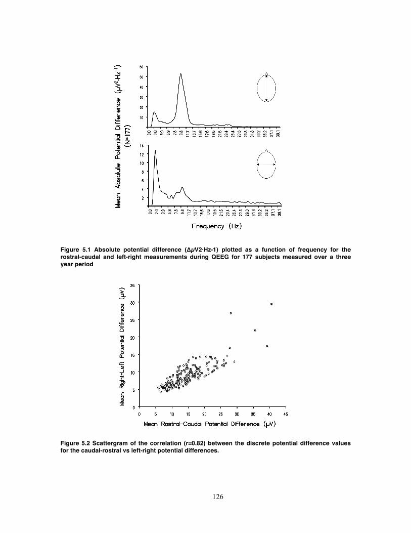
126

Figure 5.1 Absolute potential difference (ΔµV2·Hz-1) plotted as a function of frequency for the rostral-caudal and left-right measurements during QEEG for 177 subjects measured over a three year period

Figure 5.2 Scattergram of the correlation (r=0.82) between the discrete potential difference values for the caudal-rostral vs left-right potential differences.

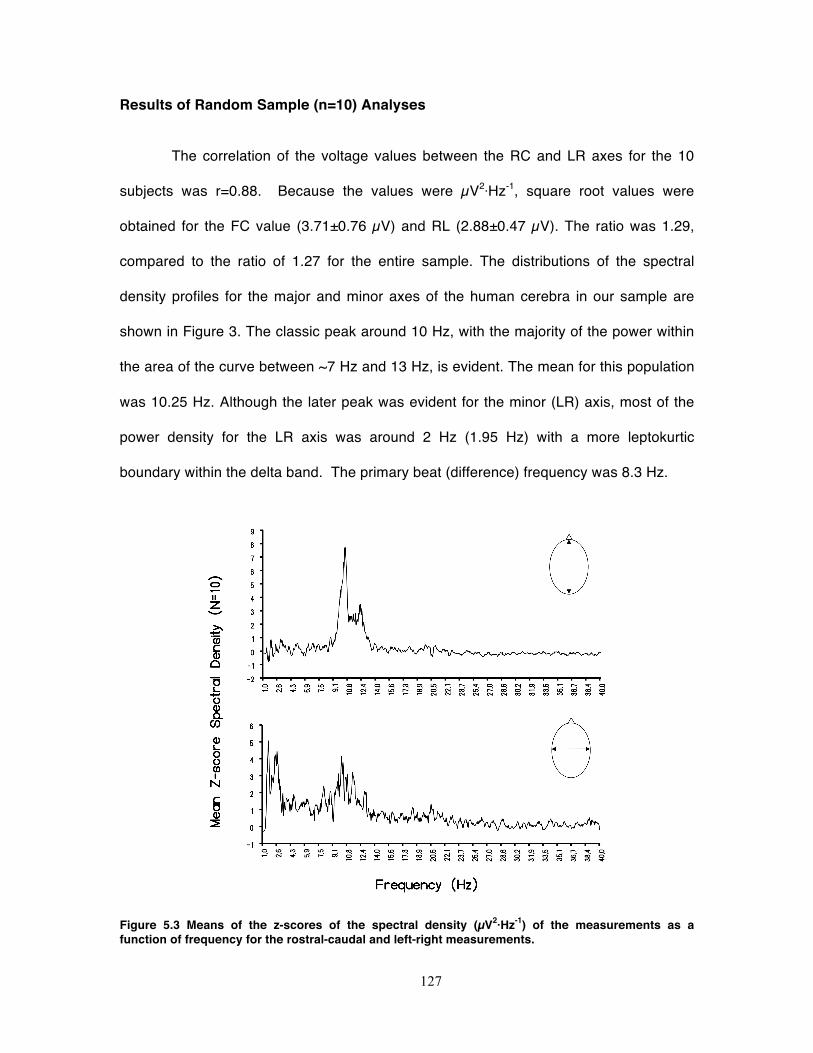
127

Results of Random Sample (n=10) Analyses

The correlation of the voltage values between the RC and LR axes for the 10

subjects was r=0.88. Because the values were µV2·Hz-1, square root values were

obtained for the FC value (3.71±0.76 µV) and RL (2.88±0.47 µV). The ratio was 1.29,

compared to the ratio of 1.27 for the entire sample. The distributions of the spectral

density profiles for the major and minor axes of the human cerebra in our sample are

shown in Figure 3. The classic peak around 10 Hz, with the majority of the power within

the area of the curve between ~7 Hz and 13 Hz, is evident. The mean for this population

was 10.25 Hz. Although the later peak was evident for the minor (LR) axis, most of the

power density for the LR axis was around 2 Hz (1.95 Hz) with a more leptokurtic

boundary within the delta band. The primary beat (difference) frequency was 8.3 Hz.

Figure 5.3 Means of the z-scores of the spectral density (µV2·Hz-1) of the measurements as a function of frequency for the rostral-caudal and left-right measurements.

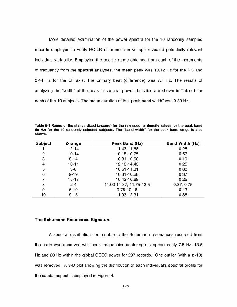
128

More detailed examination of the power spectra for the 10 randomly sampled

records employed to verify RC-LR differences in voltage revealed potentially relevant

individual variability. Employing the peak z-range obtained from each of the increments

of frequency from the spectral analyses, the mean peak was 10.12 Hz for the RC and

2.44 Hz for the LR axis. The primary beat (difference) was 7.7 Hz. The results of

analyzing the “width” of the peak in spectral power densities are shown in Table 1 for

each of the 10 subjects. The mean duration of the “peak band width” was 0.39 Hz.

Table 5-1 Range of the standardized (z-score) for the raw spectral density values for the peak band (in Hz) for the 10 randomly selected subjects. The “band width” for the peak band range is also shown.

Subject Z-range Peak Band (Hz) Band Width (Hz) 1 12-14 11.43-11.68 0.25 2 10-14 10.18-10.75 0.57 3 8-14 10.31-10.50 0.19 4 10-11 12.18-14.43 0.25 5 3-6 10.51-11.31 0.80 6 9-19 10.31-10.68 0.37 7 15-18 10.43-10.68 0.25 8 2-4 11.00-11.37, 11.75-12.5 0.37, 0.75 9 6-19 9.75-10.18 0.43

10 9-15 11.93-12.31 0.38

The Schumann Resonance Signature

A spectral distribution comparable to the Schumann resonances recorded from

the earth was observed with peak frequencies centering at approximately 7.5 Hz, 13.5

Hz and 20 Hz within the global QEEG power for 237 records. One outlier (with a z>10)

was removed. A 3-D plot showing the distribution of each individual's spectral profile for

the caudal aspect is displayed in Figure 4.

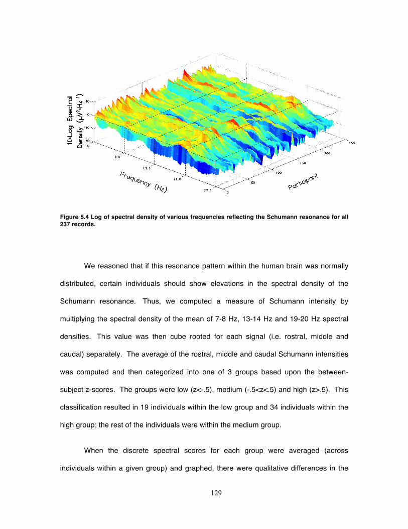
129

Figure 5.4 Log of spectral density of various frequencies reflecting the Schumann resonance for all 237 records.

We reasoned that if this resonance pattern within the human brain was normally

distributed, certain individuals should show elevations in the spectral density of the

Schumann resonance. Thus, we computed a measure of Schumann intensity by

multiplying the spectral density of the mean of 7-8 Hz, 13-14 Hz and 19-20 Hz spectral

densities. This value was then cube rooted for each signal (i.e. rostral, middle and

caudal) separately. The average of the rostral, middle and caudal Schumann intensities

was computed and then categorized into one of 3 groups based upon the between-

subject z-scores. The groups were low (z<-.5), medium (-.5<z<.5) and high (z>.5). This

classification resulted in 19 individuals within the low group and 34 individuals within the

high group; the rest of the individuals were within the medium group.

When the discrete spectral scores for each group were averaged (across

individuals within a given group) and graphed, there were qualitative differences in the

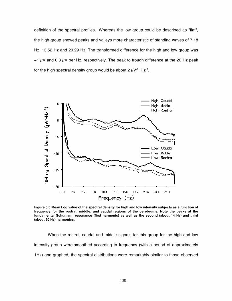
130

definition of the spectral profiles. Whereas the low group could be described as "flat",

the high group showed peaks and valleys more characteristic of standing waves of 7.18

Hz, 13.52 Hz and 20.29 Hz. The transformed difference for the high and low group was

~1 µV and 0.3 µV per Hz, respectively. The peak to trough difference at the 20 Hz peak

for the high spectral density group would be about 2 µV2 · Hz-1.

When the rostral, caudal and middle signals for this group for the high and low

intensity group were smoothed according to frequency (with a period of approximately

1Hz) and graphed, the spectral distributions were remarkably similar to those observed

Figure 5.5 Mean Log value of the spectral density for high and low intensity subjects as a function of frequency for the rostral, middle, and caudal regions of the cerebrums. Note the peaks at the fundamental Schumann resonance (first harmonic) as well as the second (about 14 Hz) and third (about 20 Hz) harmonics.

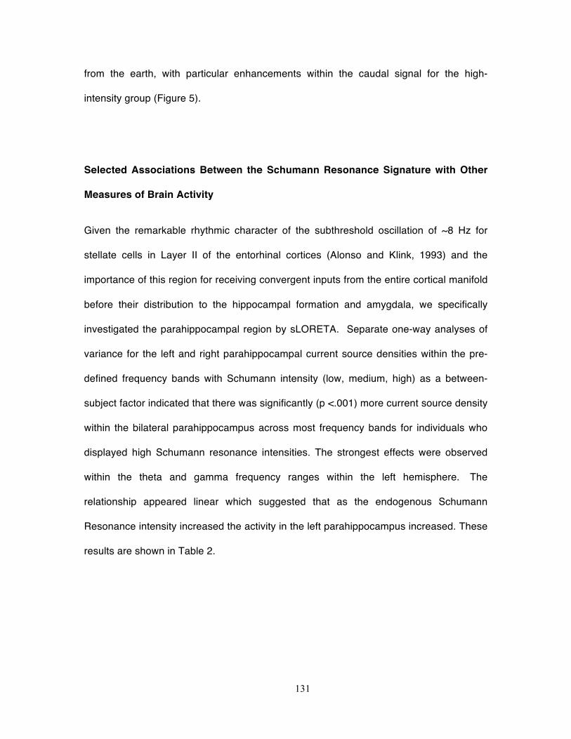
131

from the earth, with particular enhancements within the caudal signal for the high-

intensity group (Figure 5).

Selected Associations Between the Schumann Resonance Signature with Other

Measures of Brain Activity

Given the remarkable rhythmic character of the subthreshold oscillation of ~8 Hz for

stellate cells in Layer II of the entorhinal cortices (Alonso and Klink, 1993) and the

importance of this region for receiving convergent inputs from the entire cortical manifold

before their distribution to the hippocampal formation and amygdala, we specifically

investigated the parahippocampal region by sLORETA. Separate one-way analyses of

variance for the left and right parahippocampal current source densities within the pre-

defined frequency bands with Schumann intensity (low, medium, high) as a between-

subject factor indicated that there was significantly (p <.001) more current source density

within the bilateral parahippocampus across most frequency bands for individuals who

displayed high Schumann resonance intensities. The strongest effects were observed

within the theta and gamma frequency ranges within the left hemisphere. The

relationship appeared linear which suggested that as the endogenous Schumann

Resonance intensity increased the activity in the left parahippocampus increased. These

results are shown in Table 2.

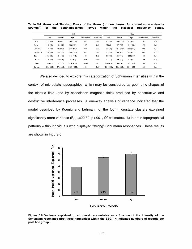
132

Table 5-2 Means and Standard Errors of the Means (in parentheses) for current source density (µA·mm-2) of the parahippocampal gyrus within the classical frequency bands.

We also decided to explore this categorization of Schumann intensities within the

context of microstate topographies, which may be considered as geometric shapes of

the electric field (and by association magnetic field) produced by constructive and

destructive interference processes. A one-way analysis of variance indicated that the

model described by Koenig and Lehmann of the four microstate clusters explained

significantly more variance (F2,234=22.89, p<.001, Ω2 estimate=.16) in brain topographical

patterns within individuals who displayed “strong” Schumann resonances. These results

are shown in Figure 6.

Figure 5.6 Variance explained of all classic microstates as a function of the intensity of the Schumann resonance (first three harmonics) within the EEG. N indicates numbers of records per post hoc group.

133

5.4 Discussion

Our results confirm and extend the results of relatively large samples of human

brains from other researchers (e.g., Nunez, 1995). The absence of statistically

significant differences between the strengths of the correlations of power between the

RC and LR comparisons and their ratios of power for the total sample and the random

sub-sample of 10 subjects indicates the robust nature of these relationships. The

precision of the ratio of the physical differences in RC and LR distances of a population

of adult cerebrums and the differences in the power densities of electrical activity support

our disciplines assumption that the amplitude of QEEG activity is a physical reflection of

potential difference (voltage).

Quantitative Inference of Cerebral Magnetic Field Strength

We reasoned that if the cerebral and earth-ionospheric resonances shared some

characteristic that could allow potential interaction, some variant of “diffusivity” should be

involved. Magnetic diffusivity, ή=(µoσ)-1 , where µo is magnetic susceptibility (4π·10-7 N·A-

2) and σ=electrical conductivity, is a concept relevant to geophysical (Ryskin, 2009) and

neurophysical phenomena. Assuming the average resistivity of 2 Ω·m (σ~ 0.5 S·m-1) for

extracellular fluid, and the average potential difference of 3 µV, the resulting estimate for

the magnetic field strength is (3·10-6 kg·m2·A-1·s-3) divided by 1.58·106 m2·s-1 or ~1.9·10-12

T, that is about 2 picoTeslas (pT). This is well within the range based upon direct

measurement from of action potentials from isolated frog sciatic nerves at distance of 1

mm (Wikswo et al, 1980) as well as the typical intensities of Schumann ressonances.

The spatial domain is sufficiently large to have major influence upon the integrated

cerebral field. This magnitude is within a factor of 10 of the transient magnetic oscillatory

134

response (Pantev et al, 1991) evoked in the human cerebrum, with a peak near 10 Hz

and 30-40 Hz, when the measured values in 20 fT·Hz-1/2 are applied over the full

frequency range of 100 Hz.

Although these intensities appear small, experimental application of pT, spatial

and temporally-patterned magnetic fields have been reported to produce discernable

improvement in some clinical disorders, such as Tourette’s and multiple sclerosis

(Sandyk, 1995; 1997) as well as some electrical foci associated with partial seizures

(Anninos et al, 1991). Correlative responses associated with subjects’ experiences have

been associated with geomagnetic changes in the order of pT·s-1 (Booth et al, 2005).

The latter occurred when ambient geomagnetic changes displayed progressive

increases at this rate over an approximately 15 min interval.

Comparisons with the Fundamental Schumann Resonance and Interhemispheric

Beats

It may be relevant that the recondite “beat” (the difference between the

frequencies) between the rostral-caudal and left-right power peaks was between 7 Hz

and 8 Hz, the range of the fundamental (first harmonic) of the Schumann resonance.

This compliments the more global QEEG emergence of the first, second and third

harmonics when a different method of analysis was employed. The intrinsic resonance

frequency” mediated through the “external shell” of the cerebral cortices (Persinger and

Lavallee, 2012) is also within this interval. Precise frequencies in this range can be

important. For example Harmony (2013) found that 7.8 Hz power within the frontal lobes

decreased in adults but increased in children during a task that emphasized short-term

memory.

135

Resonances often arise in a cavity with sharp, homogeneous, and isotropic

boundaries. The Schumann resonances, with a fundamental frequency around 7.8 Hz

and harmonics around 14.1, 20.3, 26.4, and 32.5 Hz (Campbell, 1967), are generated

within the approximately 100 km earth-ionospheric cavity. The higher modes (harmonics)

are separated by ~6 Hz according to the general formula fn=f1[(n(n+1)]1/2 although some

authors include geometric coefficients. Primary origins of the energy are attributed to

global lightning activity (Persinger, 2012). The typical median value for the electric field is

~1 mV m-1 while the magnetic field strengths are in the order of 1 pT. At the lowest

mode, around 8 Hz, the attenuation is ~1 db per 2000 km (Polk, 1982). The significance

of these “weak amplitudes” become salient to neuroscience when one realizes that the

potential differences involved with reconnection of flux lines within the geomagnetic field

when solar wind energy is transferred into the magnetosphere is actually about 4 µV·cm-

1 (Phan et al, 2000), which is within cerebral parameters.

Although popular authors emphasize the exactness of the fundamental (first

harmonic) frequency, empirical measurements indicate a range that would be significant

from a QEEG perspective. For example injections of energies from protons (solar proton

events) into the upper atmosphere are followed by systematic increases of between 0.04

to 0.14 Hz above the fundamental (7. 5 Hz) and amplitude enhancements of between

0.11 and 0.42 pT relative to the 1 pT background (Schlegel and Fullekrug, 1999). In

addition, splitting of Schumann resonances have been measured intermittently for

decades (Fraser-Smith and Buxton, 1975). While pursuing the theoretical predictions of

Madden et al (1965), Tanahashi (1976) noted doublet and triplet “split” peaks at 7.1,

7.85 and 8.5 Hz for the first mode and 12.4, 13.3, 14.0 and 14.8 Hz in the second mode.

Fraser-Smith and Buxton (1975) showed that doublets (8 and 10 Hz) occurred for

136

several tens of minutes. The amplitudes of these discrete peaks were in the order of 1 or

2 pT·Hz-1/2.

Analyses of global power of 16-second samples of QEEG data from almost 200

subjects over a three-year period indicated that spectral densities exhibited relatively

wide-band peaks within the first three harmonics of the Schumann resonance. The

origins of these fundamental and harmonic enhancements with the QEEG data cannot

be identified at this time. One possibility is that the Schumann peaks may reflect some

intrinsic feature of the cerebral space due to the average circumference and bulk velocity

(Nunez, 1995; Persinger and Lavallee, 2012) or even a coupling between cerebral and

ionospheric frequencies through mechanisms yet to be identified. If the latter condition is

valid then intrinsic interactions, most likely intermittent, might occur and could be

potentially quantified by near-future QEEG and source-location technology. Transience

may define these phenomena within QEEG profiles. In our studies the harmonics were

not obvious within single 16-s samples but were clear when aggregates from many

subjects were averaged. Interestingly this process is also required to obtain spectral

profiles (such as in Figure 5 for brain activity) even with direct environmental

measurement of Schumann resonances (Nickolaenko and Hayakawa, 2014). It is also

noteworthy that optimal filtering between 1.5-40 Hz was required in order to observe

Schumann frequency peaks. When the low-cut frequency was set to below 1.5 Hz or

above 3 Hz, the characteristic peaks were not observed. This may indicate that energies

represented within the 1.5-3Hz frequency band are crucial in discerning the Schumann

resonance within the brain.

137

Individual Differences

Although the statement that individual differences is the largest source of

variance is well known to any first year psychology student, the relevance to

electrophysiological measurements was obscured until QEEG became the general tool.

If there is intercalation between exogenous sources of Schumann resonances and

comparable global cerebral frequencies then quantifying and classifying these features

may help explain sensitive populations. The individual differences were remarkable. In

Table 1 the z-score for the peak band in the spectral densities for each person are

shown. A representation of the 7.5 Hz Schumann line in brain activity would occur in only

two of the 10 subjects. Line splitting of the Schumann resonance displays peaks with

frequency spacing between ~ 0.2 to ~0.6 Hz. This overlaps with the bandwidth of the

peak power frequency. That only about 10% to 13% of all brains showed enhancements

in the intensity of the Schumann resonance may be useful for defining the characteristics

of this subpopulation.

There were also individual differences (or more accurately group differences) for

the amount of variance in the four classic microstates as a function of the intrinsic power

of the first three harmonics of the Schumann frequencies within the cerebral volume. As

the power for these bands increased the percentage of variance explaining the four

microstates increased from about 48% to 68%. Or stated alternatively, less of the total

variance for the classic microstates was explained for those brains that displayed the

lowest Schumann spectral density. This could be interpreted as Schumann power

functions like a “homogenizer” by removing “random” or “unique” sources of variation

and enhancing the prevalence of the four basic microstates. Considering its global

nature, a direct contribution of Schumann resonance-induced power to the proportional

138

predominance of the four major microstates if they are the building blocks of thought

(Lehmann et al, 1998), could potentially affect large numbers of the human species for

transient periods.

Potential Interactions Between Human Brain and Schumann Dynamics

Whether or not information from the cerebral volume could be represented within

the Schumann volume (or visa versa) has significant philosophical and social

implications that QEEG and neuroimaging could soon address. Even relatively complex

mathematical solutions suggest that gravity waves would interface with the earth’s

second harmonic (14 Hz) Schumann resonance (Minakov et al, 1992). The energy

associated with the loss or gain of a bit of information according to the Landauer Limit (ln

2 kT where k is the Boltzmann constant and T is temperature) is equivalent to about

2.97·10-21 J, at brain temperature. In comparison, the energy upon a unit charge from

the ~2.6 (±0.5) mV of stellate cells that occurs within the upper (Layer II) cortical neurons

within the entorhinal cortices or parahippocampal region (Alonso and Klink, 1993), which

is 4.16·10-22 J would be precisely within this range because this energy is generated

about 8 times per second (~8 Hz) by the persistent subthreshold oscillations. The

stellate cells in the medial entorhinal cortices are involved with convergences of

information from the entire cortices and are a primary origin of the perforant path fibers

to the dentate gyrus of the hippocampal formation.

Our results indicated that the average current source density within the

parahippocampal regions was greatest within the theta and gamma bands for individuals

who displayed elevated amplitudes for the three first harmonics of the Schumann

139

resonance. This may be relevant not only because the “gamma” or “40 Hz” ripples are

superimposed upon hippocampal theta oscillations (Buzsaki, 2002). The

interconnectedness between hippocampal theta and cerebral cortical gamma activity has

been considered an important electrophysiological correlate for the intercalation between

neurocognitive processes such as consciousness and memory (Whitman et al, 2013).

Theta phase can modify the synchrony or coherence between gamma oscillations

originating in multiple regions. It may also be relevant that the hippocampal formation

and the parahippocampal regions, particularly within the right hemisphere appear, to be

particularly responsive to small changes in geomagnetic activity and experimentally

applied fields within the pT range (Booth et al, 2005; Mulligan et al, 2010; Sandyk, 1995;

1997).

One of the basic assumptions of modern Neuroscience is that ultimately all of the

qualitative features of the ephemeral cognitive processes such as thinking and

consciousness will be interpretable as quantitative configurations (Wackermann, 1999)

of the complex temporal patterns of electromagnetic values that can be measured from

the surface of the human cerebrum. The similarity of average duration of microstates

and the duration of the human percept is an example of such transformation of

perspective. The clever consideration (Lehmann et al, 1995; 1998) that four microstates

(Koenig et al, 2002) could reflect functional cognitive units or “atoms of thought” that are

the information within the stream of dynamic process within cerebral space, analogous to

base nucleotide pairs for genetic information within DNA sequences, exemplifies the

significance of this approach. The shift towards biophysical analyses (Johnson, 1980;

Nunez, 1995; Balazsi and Kish, 2000; Park and Lee, 2007; Persinger and Lavallee,

2012) of complex cerebral functions once relegated to the domain of the philosopher and

140

psychologist requires a verification of the physical parameters for these operations. Here

we reiterate and report validation of quantitative phenomena that define the electric and

potentially magnetic features of our primary inferential measurement: quantitative

electroencephalography (QEEG) and how their characteristics are shared by a unique

pervasive property of the earth-ionosphere cavity.

5.5 References

Alonso A and Klink R (1993) Differential electroresponsiveness of stellate and

pyramidal-like cells of medial entorhinal cortex Layer II. J Neurophysiol 70:128-

143.

Anninos PA, Tsagas N, Sandyk R and Derpapas K (1991) Magnetic stimulation in the

treatment of partial seizures. Int J Neurosci 60:141-171.

Balazsi G, Kish LB (2000) From stochastic resonance to brain waves. Phys Lett A

265:304-316.

Blinkov SM and Glezer II (1968) The human brain in figures and tables: a quantitative

handbook. Basic Books: N.Y.

Booth JN, Koren SA and Persinger MA (2005) Increased feelings of the sensed

presence and increased geomagnetic activity at the time of the experience during

exposures to transcerebral weak complex magnetic fields. Int J Neurosci

115:1053-1079.

Buzaski G (2002) Theta oscillations in the hippocampus. Neuron 33:325-340.

141

Campbell WH (1967) Geomagnetic pulsations. In: Physics of Geomagnetic phenomena,

Matshushita A and Campbell WA (eds). Academic Press: N.Y., pp 821-909.

Delorme A and Makeig S (2004) EEGLAB: an open source toolbox for analysis of single-

trial EEG dynamics including independent component analysis. J Neurosci

Methods 134:9-21.

Fraser-Smith AC and Buxton JL (1975) Superconducting magnetometer measurements

of geomagnetic activity in the 0.1- to-14 Hz frequency range. J Geophys Res

80:3141-3147.

Harmony T (2013) The functional significance of delta oscillations in cognitive

processing. Front Integrat Neurosci 7:Article 83.

Johnson LC (1980) Measurement, quantification, and analysis of cortical activity. In

Martin, I. and Venables, P. H. (eds). Techiques in Psychophysiology. John Wiley:

N.Y, pp 329-429.

Koenig T, Lehmann D, Merlo MCG, Kochi K, Hell D, Koukkou M (1999) A Deviant EEG

Brain Microstate in Acute, Neuroleptic-Naïve Schizophrenics at Rest. European

Eur Arch Psychiatry and Clin Neurosci 249:205-211.

Koenig T, Prichep L, Lehmann D, Sosa DV, Braker E, Kleinlogel H, Ishehart R and John

ER (2002) Millisecond by millisecond, year by year: normative EEG microstates

and developmental stages. NeuroImage 16:41-48.

Konig HL, Krueger AP, Lang S and Sonnig W (1981) Biologic effects of environmental

electromagnetism. Springer-Verlag: N.Y.

142

Lehmann D, Grass P and Meier B (1995) Spontaneous conscious covert cognition states

and brain electric spectral states in canonical correlations. Int J Pschophysiol

19:41-52.

Lehmann D, Strik WK, Henggeler B, Koenig T and Koukkou M (1998) Brain electric

microstates and momentary conscious mind states as building blocks of

spontaneous thinking: visual imagery and abstract thoughts. Int J Psychophysiol

29:1-11.

Madden T and Thompson W (1965) Low-frequency electromagnetic oscillations of the

earth-ionosphere cavity. Rev Geophys 3:211-254.

Minakov AA, Nikolaenko AP and Rabinovich LM (1992) Gravitational-to-electromagnetic

wave conversion in electrostatic field of earth-ionosphere resonator. Radiofizika

35:488-497.

Mulligan BP, Hunter MD and Persinger MA (2010) Effects of geomagnetic activity and

atmospheric power variations on quantitative measures of brain activity:

replication of the Azerbaijani studies. Adv Space Res 45:940-948.

Nickolaenko A and Hayakawa M (2014) Schumann Resonance for Tyros. Springer:

Tokyo.

Nunez PL (1995). Towards a physics of neocortex. In: Nunez PL (ed) Neocortical

dynamics and human EEG rhythms. Oxford University: N.Y., pp 68-130.

143

Pantev C, Makeig S, Hoke M, Galambos R, Hampson S, Gallen C (1991) Human

auditory evoked gamma-band magnetic fields. Proc Natl Acad Sci USA 88:8996-

9000.

Park TS and Lee YL (2007) Effects of neuronal magnetic fields on MRI: numerical

analysis with axon and dendritic models. NeuroImage 35:531-538.

Pasqual-Marquis RD (2002) Standardized low resolution brain electromagnetic

tomography (sLORETA): technical details. Methods Find Exp Pharmacol 24:D5-

D12.

Persinger MA (1974) ELF and VLF electromagnetic field effects. Plenum Press: N.Y.

Persinger MA (2012) Brain electromagnetic activity and lightning: potentially congruent

scale-invariant quantitative properties. Front Integrat Neurosci 6:Article 19.

Persinger MA and Lavallee C (2012) The Sum of N=N concept and the quantitative

support for the cerebral-holographic and electromagnetic configurations of

consciousness. J Conscious Stud 19:128-153.

Phan TD, Kistler LM, Klecker B, Haerendel G, Paschmann G, et al. (2000) Extended

magnetic reconnection at the earth’s magnetopause from detection of bi-

directional jets. Nature 404:848-850.

Polk C (1982) Schumann resonances. In: Volland H (ed) CRC Handbook of

atmospherics. CRC Press: Boca Raton (Fla), pp 111-178.

144

Rowland V, Bradley H, School P (1967) Cortical steady-potential shifts in conditioning.

Cond Reflex 2:3-22.

Ryskin G (2009) Secular variation of the earth’s magnetic field: induced by ocean flow?

New J Physics 11:1-23, 063015.

Sandyk R (1995) Improvement of right hemispheric function in a child with Gilles de la

Tourette’s syndrome by weak electromagnetic fields. Int J Neurosci 81:199-213.

Sandyk R (1997) Therapeutic effects of alternating current pulsed electromagnetic fields

in multiple sclerosis. J Alt Compar Med 3:365-386.

Saroka KS, Caswell JC, Lapointe A, Persinger MA (2013) Greater

electroencephalographic coherence between left and right temporal lobe

structures during increased geomagnetic activity. Neurosci Lett 560:126-130.

Schlegel K and Fullekrug M (1999) Schumann resonance parameter changes during

high-energy particle participation. J Geophys Res 104:10111-10118.

Tanahashi S (1976) Detection of line splitting of Schumann resonances from ordinary

data. J Atmosph Terr Phys 38:135-142.

Wackermann J (1999) Towards a quantitative characterization of functional states of the

brain: from the non-linear methodology to the global linear description. Int J

Psychophysiol 34:65-80.

145

Whitman JC, Ward LM and Woodward TS (2013) Patterns of cortical oscillations

organize neural activity into whole-brain functional networks evident in the fMRI

bold signal. Front Human Neurosci 7:Article 80.

Wikswo JP, Barach JP, Freeman JA (1980) Magnetic field of a nerve impulse: first

measurements. Science 208:53-55.

146

Chapter 6 Quantitative Evidence for Direct Effects Between Earth-

Ionosphere Schumann Resonances and Human Cerebral Cortical Activity

Published in International Letters of Chemistry, Physics and Astronomy

Co-Author: Michael A. Persinger

6.1 Introduction

When two systems share remarkably similar physical characteristics such as

dynamic amplitudes and intrinsic frequencies the possibility for direct interaction

emerges. This assumes impedances and reluctances match or shared resonance

occurs between the electromagnetic energies. The thin shell between the ionosphere

and earth generates continuous harmonics of frequencies from a fundamental of about 7

to 8 Hz that is caused by global lightning which occurs between 40 to 100 times per

second (40 to 100 Hz). These frequencies are the Schumann resonances.

The bulk velocity of neuronal activity around the human cerebral cortices caused

by discharge of action potentials within this thin shell of tissue generates a resonance

with a fundamental between 7 to 8 Hz. On the bases of the average durations of the

travelling waves over the cerebral cortices the repetition rate and phase velocities are in

the order of 40 to 80 times per second (40 to 80 Hz). The current density around the

annulus of an axon associated with a single action potential is equivalent to about 105

A·m-1 or the value associated with a single lightning discharge [1].

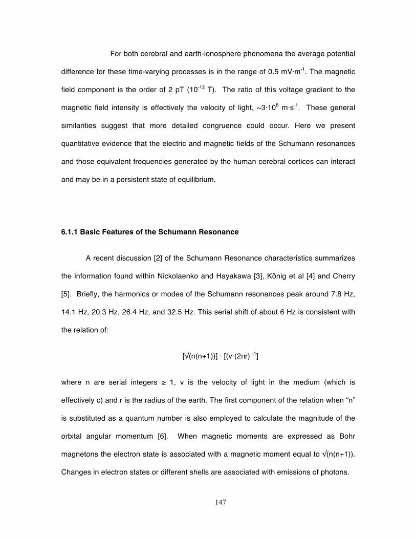
147

For both cerebral and earth-ionosphere phenomena the average potential

difference for these time-varying processes is in the range of 0.5 mV·m-1. The magnetic

field component is the order of 2 pT (10-12 T). The ratio of this voltage gradient to the

magnetic field intensity is effectively the velocity of light, ~3·108 m·s-1. These general

similarities suggest that more detailed congruence could occur. Here we present

quantitative evidence that the electric and magnetic fields of the Schumann resonances

and those equivalent frequencies generated by the human cerebral cortices can interact

and may be in a persistent state of equilibrium.

6.1.1 Basic Features of the Schumann Resonance

A recent discussion [2] of the Schumann Resonance characteristics summarizes

the information found within Nickolaenko and Hayakawa [3], König et al [4] and Cherry

[5]. Briefly, the harmonics or modes of the Schumann resonances peak around 7.8 Hz,

14.1 Hz, 20.3 Hz, 26.4 Hz, and 32.5 Hz. This serial shift of about 6 Hz is consistent with

the relation of:

[√(n(n+1))] · [(v·(2πr) -1]

where n are serial integers ≥ 1, v is the velocity of light in the medium (which is

effectively c) and r is the radius of the earth. The first component of the relation when “n”

is substituted as a quantum number is also employed to calculate the magnitude of the

orbital angular momentum [6]. When magnetic moments are expressed as Bohr

magnetons the electron state is associated with a magnetic moment equal to √(n(n+1)).

Changes in electron states or different shells are associated with emissions of photons.

148

The peak values are not precise and can vary by ± 0.2 Hz depending upon

ionospheric-earth conditions, time of day, season, influx of protons from solar events,

pre-earthquake conditions, and yet to be identified sources. According to Nickolaenko

and Hayakawa [3] monthly variations in the first mode (7.8 Hz) range between 7.8 and

8.0 Hz. The diurnal variation in frequency shift has been attributed to drifts in global

lightning or alterations in ionospheric height. Peak frequencies and amplitudes occur in

May whereas minima occur in October-November. The peak to peak modulations are

about ±25% of the median value.

The optimal metaphor is that every lighting strike of the approximately 40 to 100

per second between the ionosphere and ground is an expanding wave that moves until it

ultimately interfaces with itself on the earth’s spherical surface. The resulting interface

elicits a return wave that arrives at the original source within about 125 ms after the

initiation. The approximate equivalent frequency is 8 Hz. The attenuation is minimal over

megameters.

Resonance amplitudes are remarkably similar even when recorded

simultaneously at observatories separated by large distances and reflect the variations

in global thunderstorm activity. The maximum intensities, displayed by the first and

second harmonic, are ~3 pT which diminish to ~1 pT around 20.3 Hz and less than 0.5

pT for the higher harmonics. The vertical electric (E) field strengths display ranges in the

order of 0.3 to 1.0 mV·m-1. The coherence of the E field strength for the first harmonic is

about 0.8 to 0.9 over thousands of km.

To discern the Schumann spectral densities continuous measurements between

10 and 100 s are required. This is similar to the optimal sampling for clear resolution for

149

spectral densities of human cerebral activity. With 10 s and 100 s samples the spectral

resolutions are between 0.1 Hz and 0.01 Hz, respectively. For discerning the

relationship between phase shift and frequency at various stations record lengths are

about 10 min.

The first or fundamental resonance “splits” into three subfrequencies because of

the different phase velocities and attenuation rates corresponding to standing waves and

those moving in either an east-west or west-east direction. Because the peak width of

the fundamental or base frequency is 2 Hz (7 to 9 Hz) and separation is in the order of a

few 0.1 Hz, discrimination has been a technical challenge. A frequency shift between 7

Hz and 9 Hz with 8 Hz as the reference involves a phase shift between -20° and +20°.

The Schumann resonances are subject to modification by imminent

seismological and thermal energies. Different amplitudes of the fourth harmonic,

concurrent with a shift as much as 1 Hz, can appear approximately one week before an

earthquake. The modification remains for days and can still be present during

aftershocks [3]. For every 1 deg C increase in tropical temperature the magnetic field

measured increases by about 3 μA·m-1 or 3.8 pT. Recently Streltsov et al [7]

experimentally doubled the amplitude of the 8 Hz E field of the Schumann resonance by

focusing packets of energy into the cavity that matched the second to third gyroharmonic

electromagnetic wave (MHz range) values of electrons.

The spherical cavity of the earth-ionosphere that “traps the Schumann

resonances” exhibits Eigen values that can be characterized by the first three

equivalents of the quantum numbers: p, n, and m. P indicates how many half-

wavelengths can fit the ionospheric height which reflect the Eigen-values or resonance

150

frequencies. N (zonal number) describes how many wavelengths fit around the

circumference of the earth. M, the azimunthal number, reflects the numbers of

wavelengths along the equator moving from east to west or west to east [3].

These descriptors are similar to the four quantum numbers that have been

employed to describe the primary dynamic features of the atom that is the electron.

These are mentioned from the perspective of integrating physics, chemistry and

astronomy within the interdisciplinary framework. The similarity may also support the

traditional philosophical concept that microcosm reflects macrocosm.

6.1.2 Basic Features of the Dynamic Human Brain

The human cerebrum (1.35 kg) is an ellipsoid aggregate of matter that occupies

about 1.3·10-3 m3. The three-dimensional metrics [8] are: length (155-190 mm), width

(131-141 mm), depth (108-117 mm). The cerebral cortices are approximately 1 to 4 mm

thick but occupy almost 40% of the cerebral volume with an average value of 490 cc [9].

The surface area of the human brain is not smooth but exhibits convexities (gyri) and

concavities (sulci).

Two-thirds of the surface is buried within the sulci. Mathematical modeling

indicates that this topological surface is similar to that of a flat surface “wrinkled” into the

third dimension. Secondary extrusions with widths of about 1 mm emerge intermittently

along the trough of the sulci and the apex of the gyri [10].

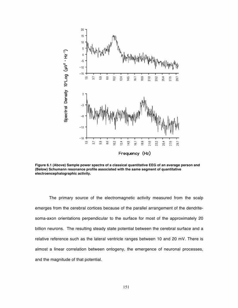
151

Figure 6.1 (Above) Sample power spectra of a classical quantitative EEG of an average person and (Below) Schumann resonance profile associated with the same segment of quantitative electroencephalographic activity.

The primary source of the electromagnetic activity measured from the scalp

emerges from the cerebral cortices because of the parallel arrangement of the dendrite-

soma-axon orientations perpendicular to the surface for most of the approximately 20

billion neurons. The resulting steady state potential between the cerebral surface and a

relative reference such as the lateral ventricle ranges between 10 and 20 mV. There is

almost a linear correlation between ontogeny, the emergence of neuronal processes,

and the magnitude of that potential.

152

Superimposed upon the steady potential are fluctuating voltages that define the

electroencephalogram (EEG). Most of the discernable frequencies occur within the ELF

(extremely low frequency) range or 1 and 100 Hz. However, fast frequencies up to 300

to 400 Hz, approaching the absolute refractory period of an axon, have been measured

in epileptic brains [11]. An example of a traditional spectral density from an average adult

human brain is shown in Figure 6.1.

The amplitudes of the scalp EEG range between 10 and 100 μV. In comparison

corticographic discharges exhibit amplitudes between 0.5 and 1.5 mV [12]. The most

prominent dynamic pattern is the alpha rhythm (8 to 13 Hz) which during wakefulness is

more evident over the posterior cerebral space with amplitudes in most (68%) of the

population between 20 and 60 μV.

The average frequency increases from about 4 Hz in the 4 month old to 10 Hz by

10 years of age. The mean frequency in adults is 10.2 ± 0.9 Hz. Within the adult human

alpha frequency slows between 0.3 and 1 Hz after ovulation. Amplitude asymmetry

favors the right hemisphere in normal people [12].

Theta rhythms (4-8 Hz) have been considered “intermediate waves” that are

significantly involved with processes associated with infancy and childhood as well as

drowsiness and specific stages of sleep. The power of theta activity is evident even

within the third decade (25 to 30 years of age) when the EEG parameters asymptote.

This inflection is sometimes considered an index of cerebral maturation.

A transient 6 Hz to 7 Hz rhythm, which disappears by adolescence, is common

over the frontal midline and is enhanced by mental tasks related to memory function.

Theta activity is the prominent frequency band within which most of the power within the

153

hippocampus, the critical structure for consolidation of “memory”, is displayed. The

power or proportion of voltage within the theta range is associated with hypnogogic

(dreamy or “apparitional” transitions) states particularly in late infancy and childhood.

For adults drowsiness is associated with the disappearance of the alpha rhythm

and the emergence of low voltage 2 to 7 Hz activity intermixed with 15 to 25 Hz bursts.

The hall mark of deep drowsiness is the appearance of vertex waves over the posterior

portion of the supplementary motor area of the frontal lobe along the interhemispheric

fissure. These transients are analogous to Q-bursts recorded from the Schumann cavity

[3]. They are transient events of natural radio pulses with durations between 0.3 and 1.5

s detected globally due to exclusively powerful lightning discharges. The amplitude of Q-

bursts, like vertex waves, can exceed the background by a factor of 10 and emerge as

elevations in the Schumann harmonics in spectral analyses.

The theta-alpha range occurs within the band of the fundamental Schumann

harmonic. The second harmonic, 14 Hz, also has an equivalent within the EEG that

emerges during light sleep (Stage 2). Sleep spindles or sigma waves are trains or

envelopes of synchronous activity between 12.5 and 15.5 Hz with a peak around 14 Hz.

As alpha rhythms dominate the posterior region of the cerebrum, spindles emerge

primarily over the frontal and frontal midline.

The other classical “frequency” bands associated with the human EEG are delta

(1- 4 Hz), which are the highest amplitude time-variations associated with Stage IV

sleep, beta (13-30 Hz) and gamma (30 to 50 Hz) patterns. The ranges are effectively

arbitrary and related to EEG features associated with particular behaviors or power

densities.

154

Large areas of the cerebral cortices demonstrate integrated spatial and temporal

characteristics. Two that are relevant to Schumann interfaces involve the rostral-caudal

“travelling waves” that are recursively (recreated) every 20 to 25 ms with an implicit

frequency of about 40 Hz [13]. The bulk velocity is about 4.5 m·s-1[14]. Assuming an

average cerebral circumference of 0.6 m the resonance frequency is 7.5 Hz, or within

range of the fundamental harmonic of the Schumann Resonance. Llinas and Pare [15]

also showed that there is a phase modulation of the 40 Hz recursive wave that was

equivalent to 80 Hz or about 12.5 ms.

The second major organization of human brain activity involves microstates

which are defined by specific configurations of dipoles with isopotential lines over the

entire cerebral cortices [16]. Most of the variance can be accommodated by four

microstates whose patterns are similar across the human population and over ontogeny.

According to convention these A, B, C and D states are characterized by polarity from

the right frontal to left occipital region, left frontal to right occipital region, equally

distributed between the frontal and occipital region, and a dorsal central to caudal

arrangement, respectively.

Together each state explains about three-quarters of the variance in EEG voltage

variations. Each microstate’s duration exits for between 80 and 120 ms. These primarily

four discrete and spatially-temporally bounded organizations could correspond to the

“building blocks” for cognition and may be the basis for the unit “percept” of experience.

This is equivalent to 8.3 to 12.5 Hz, the inclusive band of the alpha range. Assuming

these microstates are the “basic units” for thinking in a manner similar to the digital units

(base pairs) for DNA [17] there would be 410 or about 106 possible different combinations

or “serial patterns” per second.

155

The magnetic field component of human cerebral function is the same order of

magnitude as the Schumann resonances. Although ~10-12 T divided into ~10-3 V·m-1

results in a velocity term that, with the appropriate coefficients, is the velocity of light (c),

intrinsic magnetic properties of space can produce this value through spatial diffusion.

Magnetic diffusivity is:

ή=(µoσ)-1 (2),

where µo is magnetic susceptibility (4π·10-7 N·A-2) and σ=electrical conductivity [18].

Assuming the average resistivity of 2 Ω·m (σ~ 0.5 S·m-1) for extracellular fluid, and the

average potential difference of 3 µV, the resulting estimate for the magnetic field strength

is (3·10-6 kg·m2·A-1·s-3) divided by 1.58·106 m2·s-1 or ~1.9·10-12 T (about 2 picoTeslas, pT).

This is well within the range based upon direct measurement from of action potentials

from isolated frog sciatic nerves at distance of 1 mm [19]. The spatial domain is

sufficiently large to have major influence upon the integrated cerebral field. This

magnitude is within a factor of 10 of the transient magnetic oscillatory response Pantev

et al [20] evoked in the human cerebrum (with a peak near 10 Hz and 30-40 Hz) when

their measured values for 20 fT·Hz-1/2 are applied over the full frequency range of 100

Hz.

Although these intensities appear small, experimental application of pT-intensity,

spatial and temporally-patterned magnetic fields have been reported to produce

discernable improvement in some clinical disorders, such as Tourette’s and multiple

sclerosis [21] as well as some electrical foci associated with partial complex seizures

[22]. As shown by Booth et al [23] correlative responses associated with subjects’

experiences that suggest more input from the right temporal lobe into the left temporal

156

lobe (the sense of a presence) have been associated with geomagnetic changes in the

order of pT·s-1. The latter occurred when ambient geomagnetic changes displayed

progressive increases at this rate over an approximately 15 min interval.

6.2 Construction and Characterization of an Induction Coil

Magnetometer

In order to compare directly the properties and interactions between human

electroencephalographic activity and Schumann resonances, sensitive equipment is

required. For the brain activity the standard 10-20 sensor array directly connect to a

Mistar 201 Amplifier System. The standard configuration is all sensors are referenced

the ears, i.e., “monopolar” recording.

The induction coil employed to detect the Schumann frequencies was modeled

after a designed outlined by Hans Michlmayr (http://www.vlf.it/inductor/inductor.htim).

The length of the coil was designed to be 80 cm with copper wire wrapped around a 5

cm pipe. Approximately 15 kg of 0.3 mm (AWG 28) copper magnet wire were wound

onto the PVC pipe with an electric power drill as suggested by Michlmayr. Our “Herbert”

(after H. L. König) induction coil magnetometer is shown in Figure 6.2. The copper wire

wrapping procedure is shown in Figure 6.3.

Assuming the weight associated with one turn of the pipe was 144 mg, division

by the total weight indicates there were between 96,000 and 97,000 turns. The total

resistance of the coil measured after winding was 3.97 kΩ. The induction was 1000

157

Henrys once 182 cm insulated welding steel sheets were placed inside of the coil’s

frame. The finished coil was then housed in a larger PVC pipe for protection.

The preamplifier circuit was modeled after the ICS101 magnetometer designed

by Renato Romero who operates an open-source website for the monitoring of VLF

frequencies. The circuit can be found at http://www.vlf.it/romero3/ics101.html. For our

preamplifier we omitted the 0-30 Hz low-pass filter. When the magnetometer was

connected the pre-amplifier operated with a gain of 40 db.

The signal was sent to a USB soundcard, recorded and spectral analyzed

automatically by SpectrumLab software designed by Wolfgang Buscher. The free source

is located at: http://www.qsl.net/dl4yhf/spectra1.html. The software contains filters (set

between 0 and 55 Hz) and a 60 Hz notch filter that removed power-line frequencies

before it was encoded into a Microsoft WAVE file with the sampling rate set at 204 Hz.

For calibration purposes as well as for real-time coherence measurements between

human electroencephalographic activity and the Schumann resonance, the output from

the preamplifier was directed to the ECG input of a Mitsar-201 amplifier.

With the Mistar interface, we calculated the gain ratio of the signal after

amplification through the preamplifier was 3.85·101. Using this gain ratio we calculated

the approximate magnetic field intensity by integrating Faraday’s Law of induction or

V=-n·[Δ(BA)Δt-1]

where V is the voltage generated, n is the number of turns of the coil, A is the area of the

coil and ΔB/Δt is the changing magnetic field intensity in Teslas per second. Substituting

the appropriate values for n (96,000 turns) and A (0.125 m2) we obtained a constant by

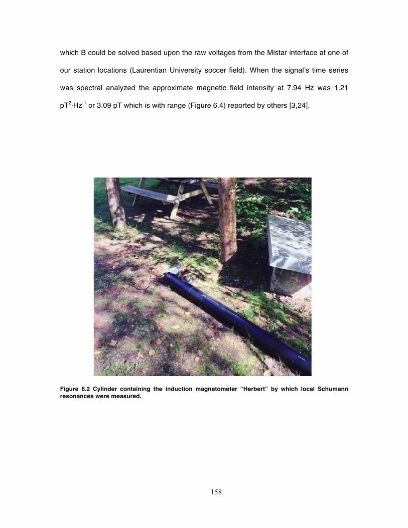
158

which B could be solved based upon the raw voltages from the Mistar interface at one of

our station locations (Laurentian University soccer field). When the signal’s time series

was spectral analyzed the approximate magnetic field intensity at 7.94 Hz was 1.21

pT2·Hz-1 or 3.09 pT which is with range (Figure 6.4) reported by others [3,24].

Figure 6.2 Cylinder containing the induction magnetometer “Herbert” by which local Schumann resonances were measured.

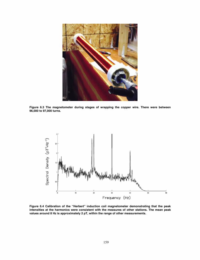
159

Figure 6.3 The magnetometer during stages of wrapping the copper wire. There were between 96,000 to 97,000 turns.

Figure 6.4 Calibration of the “Herbert” induction coil magnetometer demonstrating that the peak intensities at the harmonics were consistent with the measures of other stations. The mean peak values around 8 Hz is approximately 2 pT, within the range of other measurements.

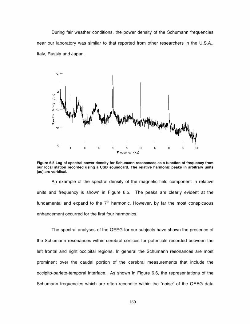
160

During fair weather conditions, the power density of the Schumann frequencies

near our laboratory was similar to that reported from other researchers in the U.S.A.,

Italy, Russia and Japan.

Figure 6.5 Log of spectral power density for Schumann resonances as a function of frequency from our local station recorded using a USB soundcard. The relative harmonic peaks in arbitrary units (au) are veridical.

An example of the spectral density of the magnetic field component in relative

units and frequency is shown in Figure 6.5. The peaks are clearly evident at the

fundamental and expand to the 7th harmonic. However, by far the most conspicuous

enhancement occurred for the first four harmonics.

The spectral analyses of the QEEG for our subjects have shown the presence of

the Schumann resonances within cerebral cortices for potentials recorded between the

left frontal and right occipital regions. In general the Schumann resonances are most

prominent over the caudal portion of the cerebral measurements that include the

occipito-parieto-temporal interface. As shown in Figure 6.6, the representations of the

Schumann frequencies which are often recondite within the “noise” of the QEEG data

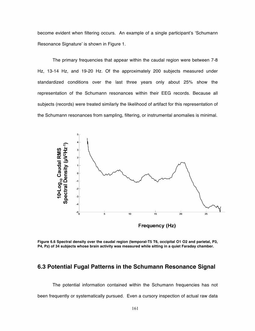
161

become evident when filtering occurs. An example of a single participant’s ‘Schumann

Resonance Signature’ is shown in Figure 1.

The primary frequencies that appear within the caudal region were between 7-8

Hz, 13-14 Hz, and 19-20 Hz. Of the approximately 200 subjects measured under

standardized conditions over the last three years only about 25% show the

representation of the Schumann resonances within their EEG records. Because all

subjects (records) were treated similarly the likelihood of artifact for this representation of

the Schumann resonances from sampling, filtering, or instrumental anomalies is minimal.

Figure 6.6 Spectral density over the caudal region (temporal-T5 T6, occipital O1 O2 and parietal, P3, P4, Pz) of 34 subjects whose brain activity was measured while sitting in a quiet Faraday chamber.

6.3 Potential Fugal Patterns in the Schumann Resonance Signal

The potential information contained within the Schumann frequencies has not

been frequently or systematically pursued. Even a cursory inspection of actual raw data

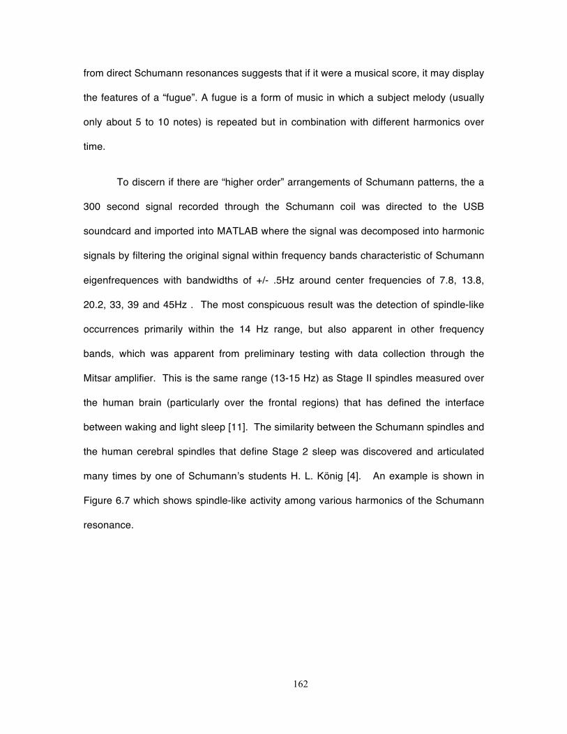
162

from direct Schumann resonances suggests that if it were a musical score, it may display

the features of a “fugue”. A fugue is a form of music in which a subject melody (usually

only about 5 to 10 notes) is repeated but in combination with different harmonics over

time.

To discern if there are “higher order” arrangements of Schumann patterns, the a

300 second signal recorded through the Schumann coil was directed to the USB

soundcard and imported into MATLAB where the signal was decomposed into harmonic

signals by filtering the original signal within frequency bands characteristic of Schumann

eigenfrequences with bandwidths of +/- .5Hz around center frequencies of 7.8, 13.8,

20.2, 33, 39 and 45Hz . The most conspicuous result was the detection of spindle-like

occurrences primarily within the 14 Hz range, but also apparent in other frequency

bands, which was apparent from preliminary testing with data collection through the

Mitsar amplifier. This is the same range (13-15 Hz) as Stage II spindles measured over

the human brain (particularly over the frontal regions) that has defined the interface

between waking and light sleep [11]. The similarity between the Schumann spindles and

the human cerebral spindles that define Stage 2 sleep was discovered and articulated

many times by one of Schumann’s students H. L. König [4]. An example is shown in

Figure 6.7 which shows spindle-like activity among various harmonics of the Schumann

resonance.

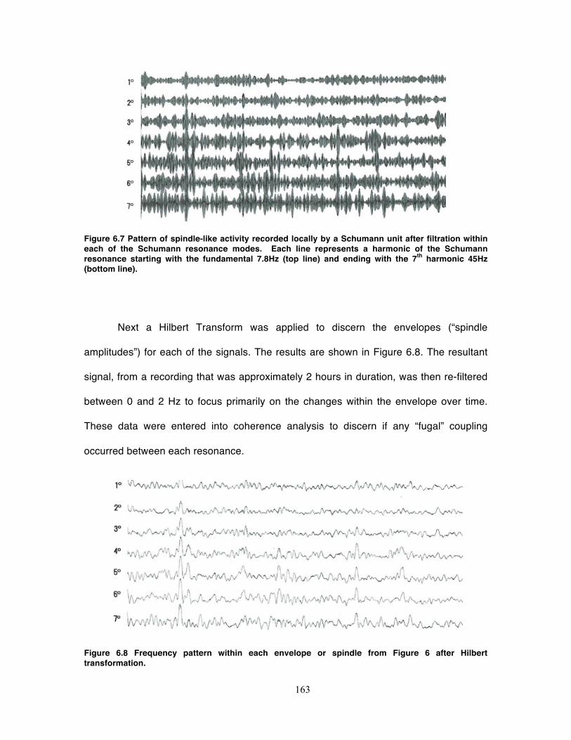
163

Figure 6.7 Pattern of spindle-like activity recorded locally by a Schumann unit after filtration within each of the Schumann resonance modes. Each line represents a harmonic of the Schumann resonance starting with the fundamental 7.8Hz (top line) and ending with the 7th harmonic 45Hz (bottom line).

Next a Hilbert Transform was applied to discern the envelopes (“spindle

amplitudes”) for each of the signals. The results are shown in Figure 6.8. The resultant

signal, from a recording that was approximately 2 hours in duration, was then re-filtered

between 0 and 2 Hz to focus primarily on the changes within the envelope over time.

These data were entered into coherence analysis to discern if any “fugal” coupling

occurred between each resonance.

Figure 6.8 Frequency pattern within each envelope or spindle from Figure 6 after Hilbert transformation.

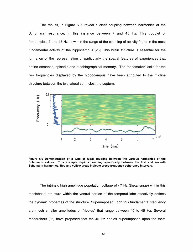
164

The results, in Figure 6.9, reveal a clear coupling between harmonics of the

Schumann resonance, in this instance between 7 and 45 Hz. This couplet of

frequencies, 7 and 45 Hz, is within the range of the coupling of activity found in the most

fundamental activity of the hippocampus [25]. This brain structure is essential for the

formation of the representation of particularly the spatial features of experiences that

define semantic, episodic and autobiographical memory. The “pacemaker” cells for the

two frequencies displayed by the hippocampus have been attributed to the midline

structure between the two lateral ventricles, the septum.

Figure 6.9 Demonstration of a type of fugal coupling between the various harmonics of the Schumann values. This example depicts coupling specifically between the first and seventh Schumann harmonics. Red and yellow areas indicate cross-frequency coherence intervals.

The intrinsic high amplitude population voltage of ~7 Hz (theta range) within this

mesiobasal structure within the ventral portion of the temporal lobe effectively defines

the dynamic properties of the structure. Superimposed upon this fundamental frequency

are much smaller amplitudes or “ripples” that range between 40 to 45 Hz. Several

researchers [26] have proposed that the 45 Hz ripples superimposed upon the theta

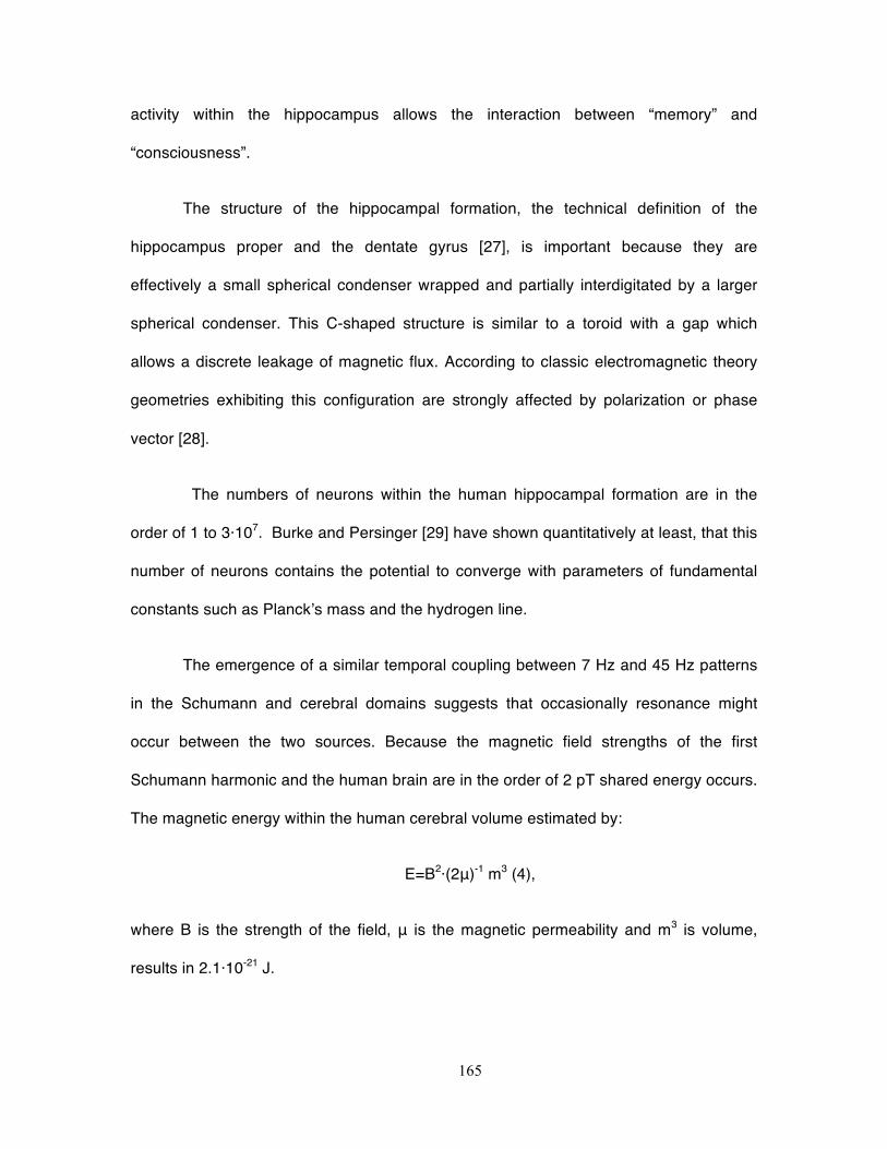
165

activity within the hippocampus allows the interaction between “memory” and

“consciousness”.

The structure of the hippocampal formation, the technical definition of the

hippocampus proper and the dentate gyrus [27], is important because they are

effectively a small spherical condenser wrapped and partially interdigitated by a larger

spherical condenser. This C-shaped structure is similar to a toroid with a gap which

allows a discrete leakage of magnetic flux. According to classic electromagnetic theory

geometries exhibiting this configuration are strongly affected by polarization or phase

vector [28].

The numbers of neurons within the human hippocampal formation are in the

order of 1 to 3·107. Burke and Persinger [29] have shown quantitatively at least, that this

number of neurons contains the potential to converge with parameters of fundamental

constants such as Planck’s mass and the hydrogen line.

The emergence of a similar temporal coupling between 7 Hz and 45 Hz patterns

in the Schumann and cerebral domains suggests that occasionally resonance might

occur between the two sources. Because the magnetic field strengths of the first

Schumann harmonic and the human brain are in the order of 2 pT shared energy occurs.

The magnetic energy within the human cerebral volume estimated by:

E=B2·(2μ)-1 m3 (4),

where B is the strength of the field, μ is the magnetic permeability and m3 is volume,

results in 2.1·10-21 J.

166

The energy lost when 1 bit of information is removed into entropy (or gained if

accessed from this source) according to Landauer is ln2 kT, where k is the Boltzmann

constant (1.38·10-23 J·T-1) and T is the temperature in degrees K for brain temperature is

~4.3·10-21 J. This convergence suggests that the energy shared by both the magnetic

field strength of the first harmonic of the Schumann resonance and the human cerebrum

are equivalent to the threshold where bits of information are dissipated into or acquired

from entropy. At this threshold intercalation of energy sources may not be restricted

necessarily by conventional limits of impedance, masking by thermal agitation, the

“weak” strength, or distance.

If the volume of both left and right hemispheric hippocampal formations (6 cc)

were substituted for the total cerebral volume the energy equivalence would be ~9.6

J·10-24 J. However the power (J·s-1) required to approach the Landauer threshold would

require a frequency equivalent to the duration between 1 and 3 ms, the approximate

duration of an action potential. This value is the shortest interval for inter-hemispheric

communication and is the duration for the expansions of electrons and protons by one

Planck’s length [29]. Thus from a simplistic resonance approach, the loss or gain of bits

of information between the Schumann sources and the human brain, would require this

weak intensity magnetic field and the fluctuating range of perturbations that are routinely

generated by the human brain.

Although 1 bit per second could be considered minimal, within 24 hrs the

information would be within the tens of kilobytes. Within a 15 min period, the time

required for the growth of a new dendritic spine in the hippocampus and cerebral

cortices and the spatial representation of a “memory”, the potential shared information

would be in the order of 1 kbit. This would be sufficient to affect the occurrence or non-

167

occurrence of information during the ephemeral period (about 15 minutes) of memory

consolidation which can be quickly “erased” by excessive electrical stimulation. When

the research by Li, Poo and Dan [31] is considered that experimentally demonstrated

that the activity of only one neuron can affect the state of the entire cerebral cortices,

such small values are not trivial.

Additional analyses indicated in Figure 6.9 indicate that incidence rate at which

the couplings occurred between the 7 and 45 Hz Schumann sources. The vertical axis

displays the frequency at which the couplings occur while the horizontal axis reveals the

numbers of times they occur. The value was about 2 to 2.5 times per 1000 s or

approximately once every 7 seconds. Hence even if the estimates for direct addition or

removal of information is diluted by a factor or about 10, there would be sufficient

intercalation to affect neuronal processes at the synaptic level.

Figure 6.9 suggests that these complex analyses of direct measurements of local

Schumann features reveal temporal clusters. If the envelopes of spindles are

considered analogous to “subject melodies” then the frequencies ‘harmonize” with each

other over time. The second and third order derivatives or “harmonies” could have the

potential to interact with similar changes within the human brain volume. In other words

the mode of interaction between the ionosphere-earth cavity and the cerebral cortices

would me mediated through the fugal patterns rather than the single frequency

resonances.

168

6.4 Correlation between Real Schumann and Cerebral

Coherence Values

One of the most common comments concerning the “impossibility” of the

potential interaction between or representations of Schumann resonances within human

brain activity as defined by QEEG is the very weak magnitudes of the vertical electric

field (about 0.1 to 1 mV·m-2) and the horizontal magnetic field (~2 pT) for both sources.

Yet most physical perspectives one smaller volume (the human cerebrum) immersed

within a much larger volume (the earth-ionospheric shell) should share quantitative

values for primary parameters. This would be expected for organic systems that have

been organized, evolved and maintained this system since abiogenesis [32].

Empirical support for this expected interaction should be apparent

considering the sensitivity of modern QEEG and Schumann technology. There are

several processes that could facilitate interactions. If they occurred and equilibrium

(B+E=k) occurred between the Schumann (E) and brain (B) sources, negative

correlations would be expected between the magnetic field and electric field strengths for

the harmonics for the Schumann modes and corresponding power or distribution of

“energy” within specific frequency intervals or “bands” within the quantitative

electroencephalographic activity for the human brain.

If an immersion model were valid it might be tested by the effect of the more

expansive source (the transglobal Schumann field strengths) upon the coherence of the

more localized source (the human brain). Coherence can be defined as the proportion

of congruence between power spectra of one source with that of another. It is typically

169

expressed as a correlation coefficient or its squared value which is an indicator of shared

temporal variance. Hence coherence values range from 0 to 1.

Coherence is functionally a juxtaposition of two or more or “identical” complex

temporal patterns that are usually displaced in time with respect to each other. One

common description is “phase-shifted”. If two sources with “identical” complex

oscillations are phase shifted completely by 90 degrees, the average would be a form of

cancellation that would emerge as “random” noise. However if the two patterns from the

two sources were shifted to overlap precisely within each other at the same “time”, then

the coherence would be maximum and the average strength of the coherence would be

maximum.

Coherence from shifting phases requires, usually, minimal energy because the

larger proportion of energy that constructs the complex patterns is not changed. What is

changed is the energy of the dynamic process that produces the rate of change which

will determine when the patterns will occur in real time within each locus as well as the

transposition of axes. In this situation each locus is each cerebral hemisphere. This is

often reflected as a first or second derivative and is implicitly associated with symmetry

of a process moving in a circle.

The immersion model predicts that as the intensity of the primary field (the

Schumann sources) increases, the intercalation between disparate but coupled

asymmetrical processes in a more or less equal volume should increase. For the human

brain the two volumes refer to the left and right hemisphere. On average the volumes of

the cortices of the two hemispheres (right larger) differ by about 10 cc. The effect should

170

be most evident between the maximum widths of two hemi-ellipsoids which would occur

approximately at the level of the temporal lobes.

The dynamic asymmetry of the human brain has been attributed to the

approximately 10% greater white-to-grey matter ratios and blood flow in the right

hemisphere which is slightly larger and heavier than the left. The structural component

for most interactions between the two hemispheres, primarily the corpus callosum and

anterior commissure, is composed of numbers of axons that are less than 1% of the

numbers of neurons within the cerebral cortices of either hemisphere. Hence there

should be specific latencies for quantities of information to be transmitted between the

two loci.

Effectively the human cerebrum is two boundaries or loci within which processes

associated with more than 90% of the neurons in each locus remain and do not interact

directly with the homologous area in the other hemisphere. The differences in

morphological structure between the two cerebral hemispheres have been

underestimated. As shown by Van Essen and Drury [10], only four of the shapes and

lengths of the approximately 176 sulci and gyri that comprise both human cerebral

hemispheres are very similar. If structure dictates function than the two hemispheres

should have qualitatively different functions whose integration or interface is limited by

the fidelity and accuracy of interhemispheric communication.

“Awareness” or “consciousness” in the classic “awake” sense involves a dynamic

dominance of more left hemispheric activity information. During this state the temporal

patterns (information) from right hemisphere must be represented within left hemispheric

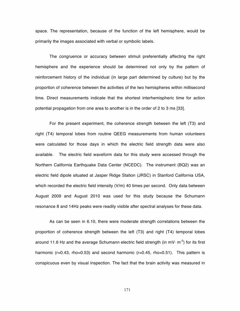
171

space. The representation, because of the function of the left hemisphere, would be

primarily the images associated with verbal or symbolic labels.

The congruence or accuracy between stimuli preferentially affecting the right

hemisphere and the experience should be determined not only by the pattern of

reinforcement history of the individual (in large part determined by culture) but by the

proportion of coherence between the activities of the two hemispheres within millisecond

time. Direct measurements indicate that the shortest interhemispheric time for action

potential propagation from one area to another is in the order of 2 to 3 ms [33].

For the present experiment, the coherence strength between the left (T3) and

right (T4) temporal lobes from routine QEEG measurements from human volunteers

were calculated for those days in which the electric field strength data were also

available. The electric field waveform data for this study were accessed through the

Northern California Earthquake Data Center (NCEDC). The instrument (BQ2) was an

electric field dipole situated at Jasper Ridge Station (JRSC) in Stanford California USA,

which recorded the electric field intensity (V/m) 40 times per second. Only data between

August 2009 and August 2010 was used for this study because the Schumann

resonance 8 and 14Hz peaks were readily visible after spectral analyses for these data.

As can be seen in 6.10, there were moderate strength correlations between the

proportion of coherence strength between the left (T3) and right (T4) temporal lobes

around 11.6 Hz and the average Schumann electric field strength (in mV· m-2) for its first

harmonic (r=0.43, rho=0.53) and second harmonic (r=0.45, rho=0.51). This pattern is

conspicuous even by visual inspection. The fact that the brain activity was measured in

172

Sudbury, Ontario, Canada and the electric field measurements of the Schumann data

were recorded in Italy supports the concept of the global nature of the effect.

Within the 95% confidence band for the linear regression, the minimum to

maximum change in interhemispheric coherence involved an increase of o.2 mV·m-1 in

the global field strength. The slope was 0.32 and 0.41 respectively indicating that for

every 0.1 mV·m-1 increase in the Schumann E field, coherence increased by 0.32 and

0.41 within the potential range of 0 to 1.

If a similar field strength was induced within the human cerebral cortices, the

potential difference would be 2·10-4 V·m-1 over the cerebral length of 10-1 m or 2·10-5 V.

Assuming the classic resistivity of extracellular fluid within the brain of 2 Ω·m, the current

would be 10-5 A·m-1 or, over the averaged length of the cerebrum, 10-6 A.

This current value when divided by 1.6·10-19 (A·s) ·q-1 (unit charge), indicates that

the change would be equivalent to 0.6·1013 q·s-1. Because approximately 106 unit

charges are associated with the membrane potential [34], ~0.6·107 neurons could be

involved. The estimated numbers of soma whose axons compose the corpus callosum

and that intercalate the functions of the left and right hemispheres are about 2 ·108.

On the other hand if only the fibers within the dorsal hippocampal commissure

were considered [35], approximately 0.5 to 0.7·107 neurons would be involved. This is

remarkably similar to the numbers of neurons within the hippocampal formation.

Because the dynamic changes within the parahippocampal gyrus are strongly affected

by the hippocampal input and this gyrus can influence the entire cortical manifold, this

small number of neurons could affect hemispheric coherence.

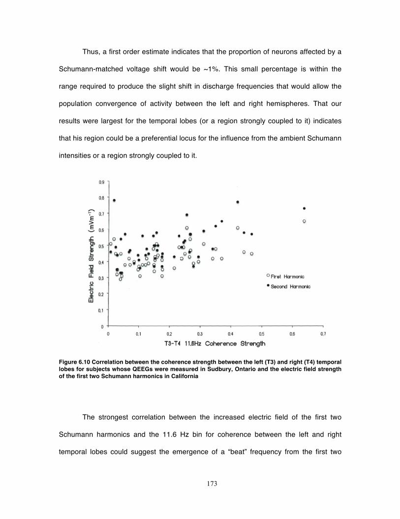
173

Thus, a first order estimate indicates that the proportion of neurons affected by a

Schumann-matched voltage shift would be ~1%. This small percentage is within the

range required to produce the slight shift in discharge frequencies that would allow the

population convergence of activity between the left and right hemispheres. That our

results were largest for the temporal lobes (or a region strongly coupled to it) indicates

that his region could be a preferential locus for the influence from the ambient Schumann

intensities or a region strongly coupled to it.

Figure 6.10 Correlation between the coherence strength between the left (T3) and right (T4) temporal lobes for subjects whose QEEGs were measured in Sudbury, Ontario and the electric field strength of the first two Schumann harmonics in California

The strongest correlation between the increased electric field of the first two

Schumann harmonics and the 11.6 Hz bin for coherence between the left and right

temporal lobes could suggest the emergence of a “beat” frequency from the first two

174

harmonics within brain space. If the first and second harmonic of the Schumann sources

were 7.8 Hz and 14.1 Hz, the beat would be approximately 11 Hz, assuming equal

biases for the intensities. The “11.6” Hz bin is within the normal variation of the classic

peak alpha power in human EEG profiles. The width of most power curves before

attenuation into background variations is between ~7 to 14 Hz.

6.5 The Parahippocampal Region as a Locus of Interaction

The maximum correlation between Schumann electric field shifts and the

coherence between the left and right temporal lobes compared to other regions should

reflect a structural or dynamic difference compared to other regions of the brain. The

ventral portions of the temporal lobe are unique in that interhemispheric intercalation is

primarily determined through the anterior commissure rather than the corpus callosum

only. The hippocampal formation, the gateway to the representation of experiences

(memory), is connected interhemispherically through the dorsal hippocampal

commissure. It occupies the anterior one third of the splenium of the caudal corpus

callosum.

In addition the middle and particularly the inferior temporal gyri are

strongly influenced by the parahippocampal gyrus. This area of the human brain may be

essential for the transduction and transformation of Schumann frequency changes for

several reasons. First, neurons within the two upper layers of the entorhinal cortices that

form a significant portion of the parahippocampal region (and the uncus) display an

intrinsic (subthreshold) oscillation with a peak around 8 Hz. The prominent sub-threshold

175

oscillations ranged between 5.5 Hz and 14.5 Hz [36] which would include the first and

second Schumann harmonics.

This region is unique structurally. Layer II, or the layer of star cells (stratum

stellare of Stephan) exhibits large, dark staining stellar-shaped neurons with spine-

covered dendrites radiating into all three planes of space. The neurons in Layer II are

clustered in “islands” or “bands” which define the characteristics of the entorhinal

cortices. These protrusions on the cortical surface (“verrucae gyri hippocampi”) are

visible macroscopically. Fibers originating from these cells terminate in the dentate gyrus

before the information is propagated to the hippocampus proper [37].

The mean amplitude of these subthreshold oscillations averaged 2.6 mV. This

periodic increment of potential difference upon a unit charge is equivalent to 4.2·10-21 J

of energy which is within the Landauer limit for the loss or gain of one bit of information

into or from entropy. The access to energy contained within the “random” processes that

defines entropy may reflect a component of the Zero Point Vacuum Fluctuations [38].

These phenomena, especially when Casimir forces are considered, are

interconnected with the transformation of virtual particles into real particles and could

alter the limit for interaction between and information of the “weak” electric and magnetic

fields shared by the Schumann and brain sources. As stated by Bordag et al [39] the

creation of particles from a vacuum requires energy transference from the external field

to the virtual particles or vacuum oscillations. However the boundary conditions must be

dynamic or dependent upon time.

Secondly, neurons within the parahippocampal gyrus, particularly the

upper two layers of the entorhinal cortices, are the major pathway to and from the

176

hippocampal formation. Third, through a cascade of corticocortical projections the entire

manifold of the cerebral cortices converges within the second and third layers of the

entorhinal cortices. This allows all of the activity of the cerebral cortices to be affected by

and to affect the entorhinal area. A specific coupling or resonance between the

Schumann fields and this portion of the human brain could affect the entire cerebral

cortical manifold for protracted durations. These durations are juxtaposed and could

certainly exceed the time required to form new synapses and patterns of neuronal

connections that define and determine “memory”. From some perspectives a person is

defined by his or her memories.

The parahippocampal region preferentially relays more spatial

information, an essential component for most memories. It contains dominating

reciprocal connections with the prefrontal cortices, especially the dorsolateral aspect.

Consequently changes within the parahippocampal region could alter the major cerebral

region associated with reasoning, self-monitoring and decision-making. The second

major input, from the cingulate, would add the component of emotion of the type

commonly associated with bonding to another human being.

Fourth, the parahippocampal region is an intermodality integrator where “line

codes” from different sensory modalities such as vision and hearing are transformed to

equivalent and potentially interactive frequencies. E. R. John [40] had shown

experimentally several decades ago that learning through different modalities was

transferable in a single trial if the frequency patterns of the pulses from different

modalities were identical. Interactions of input from different modalities information could

be synthesized into experiences.

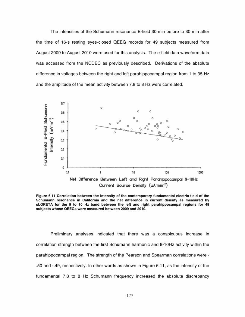
177

The intensities of the Schumann resonance E-field 30 min before to 30 min after

the time of 16-s resting eyes-closed QEEG records for 49 subjects measured from

August 2009 to August 2010 were used for this analysis. The e-field data waveform data

was accessed from the NCDEC as previously described. Derivations of the absolute

difference in voltages between the right and left parahippocampal region from 1 to 35 Hz

and the amplitude of the mean activity between 7.8 to 8 Hz were correlated.

Figure 6.11 Correlation between the intensity of the contemporary fundamental electric field of the Schumann resonance in California and the net difference in current density as measured by sLORETA for the 9 to 10 Hz band between the left and right parahippocampal regions for 49 subjects whose QEEGs were measured between 2009 and 2010.

Preliminary analyses indicated that there was a conspicuous increase in

correlation strength between the first Schumann harmonic and 9-10Hz activity within the

parahippocampal region. The strength of the Pearson and Spearman correlations were -

.50 and -.49, respectively. In other words as shown in Figure 6.11, as the intensity of the

fundamental 7.8 to 8 Hz Schumann frequency increased the absolute discrepancy

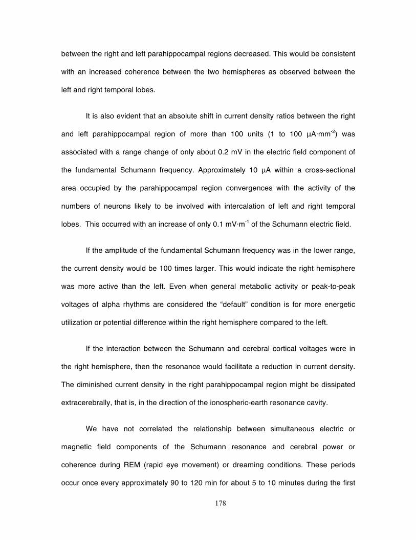
178

between the right and left parahippocampal regions decreased. This would be consistent

with an increased coherence between the two hemispheres as observed between the

left and right temporal lobes.

It is also evident that an absolute shift in current density ratios between the right

and left parahippocampal region of more than 100 units (1 to 100 μA·mm-2) was

associated with a range change of only about 0.2 mV in the electric field component of

the fundamental Schumann frequency. Approximately 10 μA within a cross-sectional

area occupied by the parahippocampal region convergences with the activity of the

numbers of neurons likely to be involved with intercalation of left and right temporal

lobes. This occurred with an increase of only 0.1 mV·m-1 of the Schumann electric field.

If the amplitude of the fundamental Schumann frequency was in the lower range,

the current density would be 100 times larger. This would indicate the right hemisphere

was more active than the left. Even when general metabolic activity or peak-to-peak

voltages of alpha rhythms are considered the “default” condition is for more energetic

utilization or potential difference within the right hemisphere compared to the left.

If the interaction between the Schumann and cerebral cortical voltages were in

the right hemisphere, then the resonance would facilitate a reduction in current density.

The diminished current density in the right parahippocampal region might be dissipated

extracerebrally, that is, in the direction of the ionospheric-earth resonance cavity.

We have not correlated the relationship between simultaneous electric or

magnetic field components of the Schumann resonance and cerebral power or

coherence during REM (rapid eye movement) or dreaming conditions. These periods

occur once every approximately 90 to 120 min for about 5 to 10 minutes during the first

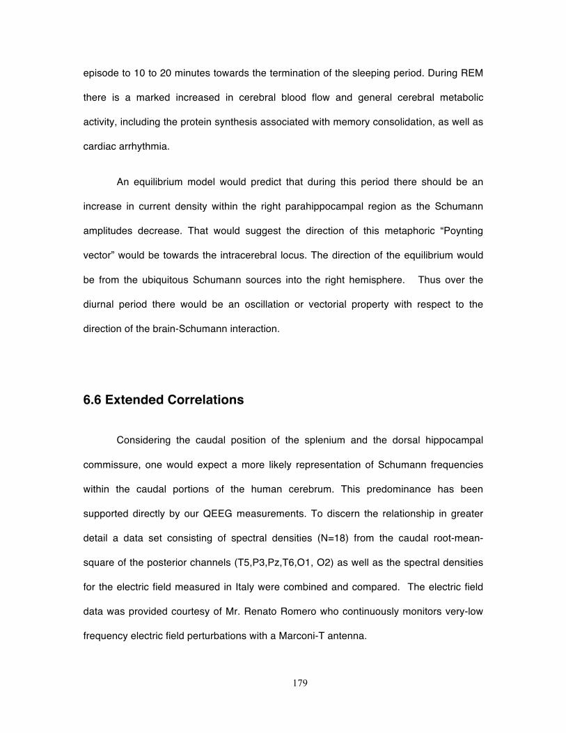
179

episode to 10 to 20 minutes towards the termination of the sleeping period. During REM

there is a marked increased in cerebral blood flow and general cerebral metabolic

activity, including the protein synthesis associated with memory consolidation, as well as

cardiac arrhythmia.

An equilibrium model would predict that during this period there should be an

increase in current density within the right parahippocampal region as the Schumann

amplitudes decrease. That would suggest the direction of this metaphoric “Poynting

vector” would be towards the intracerebral locus. The direction of the equilibrium would

be from the ubiquitous Schumann sources into the right hemisphere. Thus over the

diurnal period there would be an oscillation or vectorial property with respect to the

direction of the brain-Schumann interaction.

6.6 Extended Correlations

Considering the caudal position of the splenium and the dorsal hippocampal

commissure, one would expect a more likely representation of Schumann frequencies

within the caudal portions of the human cerebrum. This predominance has been

supported directly by our QEEG measurements. To discern the relationship in greater

detail a data set consisting of spectral densities (N=18) from the caudal root-mean-

square of the posterior channels (T5,P3,Pz,T6,O1, O2) as well as the spectral densities

for the electric field measured in Italy were combined and compared. The electric field

data was provided courtesy of Mr. Renato Romero who continuously monitors very-low

frequency electric field perturbations with a Marconi-T antenna.

180

Canonical correlations between the various frequencies from this cerebral

composite and the spectral densities of the E-field data from the Schumann frequencies

indicated that 14.65 Hz or the presence of the second Schumann harmonic within brain

activity was a strong predictor. Both parametric and non-parametric correlations showed

consistent negative correlations. The effect sizes, the square of the correlation

coefficient, when graphed as a function of frequency displayed peaks that were very

similar to Schumann resonances with the strongest effects for the first three harmonics.

Figure 6.12 shows this association. The effect size was about 0.4,

indicating that 40% of the variance was shared between the route-mean-square of the

posterior brain activity and the range of the Schumann electric field. The overlap is

particularly prevalent for the second and third harmonic. The second harmonic has been

shown mathematically to be a possible interface between gravitational waves and the

earth’s ionospheric-earth cavity [41].

Figure 6.12 The effect size (correlation coefficient squared) for the association between the caudal 14.7 Hz QEEG activity in Sudbury and Schumann E field spectral density in Italy and the frequency band of the E field. Note the strongest correlation for the first three harmonics of the Schumann resonance.

181

The increased coherence between left and right temporal lobes by an increase of

only 0.1 mV·m-1 may be critical for cosmological interface. A comparable change in

potential over the cerebral cortices, assuming a length of 10-1 m, is 1·10-5 V. The effect

on a unit charge of 1.6·10-19 A·s would be 1.6·10-24 J. The quantum frequency, obtained

by dividing by Planck’s constant (6.626·10-34 J·s) is 2.4·109 Hz which is very proximal to

the neutral hydrogen line that permeates the universe.

When the correlations between cerebral spectral density and the Schumann E

fields were lagged and lead, the associations were still statistically significant within a

three day window. Additional lag/lead analyses indicated that the relationship was no

longer statistically significant for two weeks. This suggests that the temporal interval for

direct coupling between the cerebral and terrestrial sources could be limited. Interesting

10 days was the first peak in power density for spectral analyses of Schumann

intensities that were not related to solar effects according to Nicolaenko and Hayakawa

[3].

If “gravity” waves share a similar source of variance to Zero Point Vacuum

Potentials [37], then the “coincidental” similarities of the threshold Landauer value for

information dissipation into entropy or its emergence from it and the amplitude

fluctuations of the ~8 Hz subthreshold variations could reflect one intercept between

human brain activity, the Schumann frequencies and “gravitational” phenomena.

Although gravitational phenomena are often considered too weak to be of

significance for biological matter, there is quantitative evidence that the energies are

within the range of those relevant to cell membranes [42] and interactions with cerebral-

electromagnetic interactions [43]. The alternative explanation for gravitational

182

phenomena and dark matter developed by Borowski [44] suggests there are

relationships yet to be discerned.

Applications of the calculations by Ahmed et al [45] to bulk cerebral cortical

velocities of 4.5 m·s-1 indicated that the effects of gravity as inferred by weightlessness

upon the human EEG would be about ~3 to 4 parts per 10 million. When divided by the

common frequency in the universe, 1.42 GHz, the emergent duration would be 20 and

30 ms or the recursive cerebral waves associated with consciousness. This interesting

solution suggests that the subtle effects of gravity or its intrinsic variations [46] could

interface with the phase-modulations of cerebral activity.

Phase-modulation has often been considered the most effective means to

propagate the most information over great distances. One solution is:

t/(v2·c-2) (5),

where, t is the reference time, v is the velocity and c is the velocity of light.

Because the median frequency of the electromagnetic fields associated with lightning,

the sources of the Schumann resonance, is between 10 kHz and 100 kHz, the ∆c·c-1 is

0.05 according to Tu et al [47]. This indicates that the means of the phase shifts for

every second would be ~(0.9897)-1 or in the order of 15 to 20 ms. This value is

congruent with the phase comparisons of approximately 10 to 20 ms associated with the

~40 Hz integrated waves that spread over the entire cerebral cortical mantle.

Quantitatively, the conditions are set for resonance interactions and exchange of

information between the cerebrum, the ionospheric-earth cavity, gravitational waves, and

potentially astronomical sources.

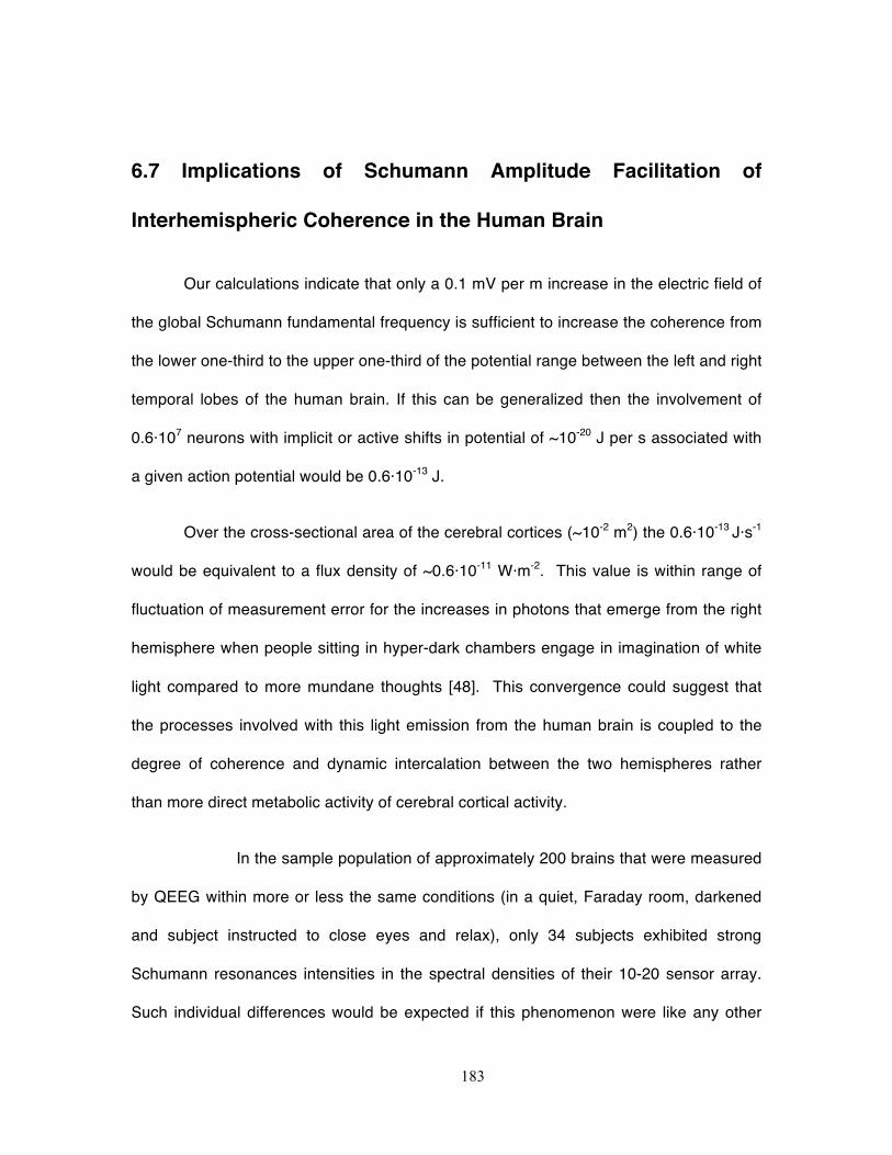
183

6.7 Implications of Schumann Amplitude Facilitation of

Interhemispheric Coherence in the Human Brain

Our calculations indicate that only a 0.1 mV per m increase in the electric field of

the global Schumann fundamental frequency is sufficient to increase the coherence from

the lower one-third to the upper one-third of the potential range between the left and right

temporal lobes of the human brain. If this can be generalized then the involvement of

0.6·107 neurons with implicit or active shifts in potential of ~10-20 J per s associated with

a given action potential would be 0.6·10-13 J.

Over the cross-sectional area of the cerebral cortices (~10-2 m2) the 0.6·10-13 J·s-1

would be equivalent to a flux density of ~0.6·10-11 W·m-2. This value is within range of

fluctuation of measurement error for the increases in photons that emerge from the right

hemisphere when people sitting in hyper-dark chambers engage in imagination of white

light compared to more mundane thoughts [48]. This convergence could suggest that

the processes involved with this light emission from the human brain is coupled to the

degree of coherence and dynamic intercalation between the two hemispheres rather

than more direct metabolic activity of cerebral cortical activity.

In the sample population of approximately 200 brains that were measured

by QEEG within more or less the same conditions (in a quiet, Faraday room, darkened

and subject instructed to close eyes and relax), only 34 subjects exhibited strong

Schumann resonances intensities in the spectral densities of their 10-20 sensor array.

Such individual differences would be expected if this phenomenon were like any other

184

natural phenomenon. If the data are representative of the human population than about

25% of the population would exhibit electroencephalographic power densities that reflect

the Schumann harmonics.

The most conspicuous appearance of the Schumann resonances within the brain

power densities occurred for the caudal regions of the cerebrum. This would be

consistent with a particular sensitivity of this region. We suggest that the source of this

sensitivity may be to the influence from the parahippocampal region because the actual

locus for the dorsal hippocampal commissure is located within the anterior one-third of

the splenium of the corpus callosum. The splenium is the primary source of

interhemispheric fibers that intercalate visual, auditory-visual, and visual-spatial

information between the left and right hemispheres.

If the primary means by which the effects of the Schumann-related intensities

and information are mediated between the “dreaming” and “unconscious” right

hemisphere and the left hemisphere (associated with awareness and consciousness) is

the dorsal hippocampal commissure within the anterior one-third of the corpus callosum,

then “memory” would be one of the primary areas of influence for the Schumann-

cerebrum interaction. It is relevant that electrical lability or (limbic) epileptic events

involving this pathway produce a single, powerful effect: amnesia [35].

A less extreme condition where mass depolarization would not occur but rather

the normal flow of information between the hippocampal structures would only be

modulated by Schumann-sourced electromagnetic fields could modify the memory

consolidation. The retrieval and experience of “a memory” that is different from a fantasy,

a dream, or an actual representation of experience involve the integrity and integrative

185

activity of the right prefrontal region. The modified “consolidations of experiences” could

be experienced as actual memories.

6.8 Real-time Coherence Between Brain Activity and Schumann

Frequencies

Although the moderate correlations between the averaged values per day for the

measures of mV·m-1 (vertical) from the Schumann measurements at a distance and

QEEG activity completed in our laboratory strongly supports effects from distal sources,

a real time-coupled demonstration was ultimately required. For this measurement a

volunteer lay in supine position approximately 1 m away from and parallel with the

Schumann (Herbert) system shown in Figure 6.2. The subject wore the 10-20 sensor

cap (Electro-Cap International; 19 AgCl sensors). Thirty (30) minutes of simultaneous

data were collected.

The input from the sensory (EEG) cap and the input from the induction

coil magnetometer were directed to the Mitsar 201 amplifier (input range ±500 μV, 16 bit

analogue-digital conversion) system so the raw voltage fluctuations in real time could be

visualized. An example of the results is shown in Figure 6.13.

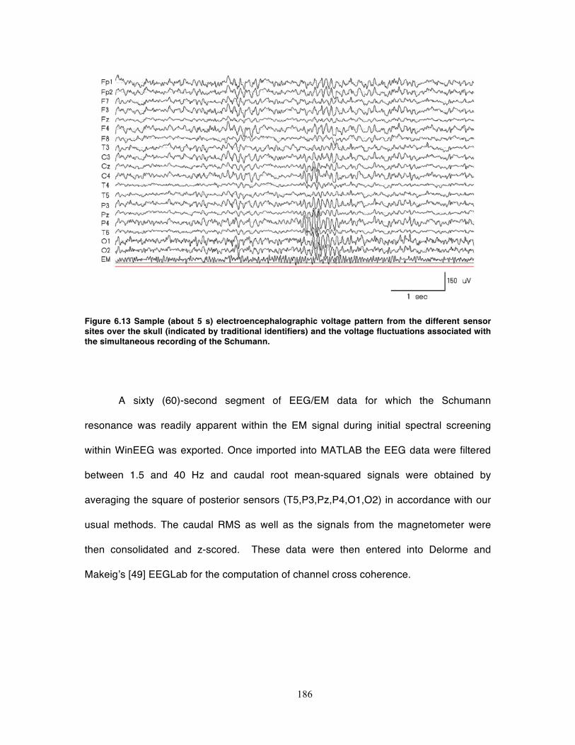
186

Figure 6.13 Sample (about 5 s) electroencephalographic voltage pattern from the different sensor sites over the skull (indicated by traditional identifiers) and the voltage fluctuations associated with the simultaneous recording of the Schumann.

A sixty (60)-second segment of EEG/EM data for which the Schumann

resonance was readily apparent within the EM signal during initial spectral screening

within WinEEG was exported. Once imported into MATLAB the EEG data were filtered

between 1.5 and 40 Hz and caudal root mean-squared signals were obtained by

averaging the square of posterior sensors (T5,P3,Pz,P4,O1,O2) in accordance with our

usual methods. The caudal RMS as well as the signals from the magnetometer were

then consolidated and z-scored. These data were then entered into Delorme and

Makeig’s [49] EEGLab for the computation of channel cross coherence.

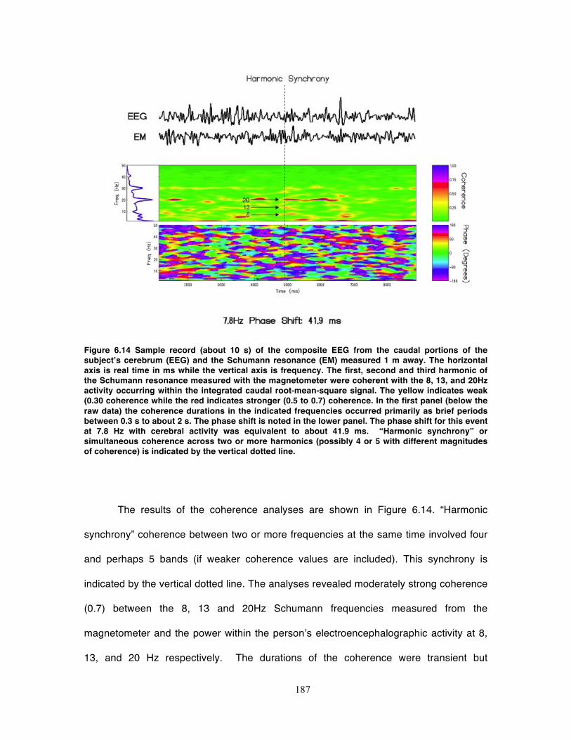
187

Figure 6.14 Sample record (about 10 s) of the composite EEG from the caudal portions of the subject’s cerebrum (EEG) and the Schumann resonance (EM) measured 1 m away. The horizontal axis is real time in ms while the vertical axis is frequency. The first, second and third harmonic of the Schumann resonance measured with the magnetometer were coherent with the 8, 13, and 20Hz activity occurring within the integrated caudal root-mean-square signal. The yellow indicates weak (0.30 coherence while the red indicates stronger (0.5 to 0.7) coherence. In the first panel (below the raw data) the coherence durations in the indicated frequencies occurred primarily as brief periods between 0.3 s to about 2 s. The phase shift is noted in the lower panel. The phase shift for this event at 7.8 Hz with cerebral activity was equivalent to about 41.9 ms. “Harmonic synchrony” or simultaneous coherence across two or more harmonics (possibly 4 or 5 with different magnitudes of coherence) is indicated by the vertical dotted line.

The results of the coherence analyses are shown in Figure 6.14. “Harmonic

synchrony” coherence between two or more frequencies at the same time involved four

and perhaps 5 bands (if weaker coherence values are included). This synchrony is

indicated by the vertical dotted line. The analyses revealed moderately strong coherence

(0.7) between the 8, 13 and 20Hz Schumann frequencies measured from the

magnetometer and the power within the person’s electroencephalographic activity at 8,

13, and 20 Hz respectively. The durations of the coherence were transient but

188

consistent and extended between 0.3 s to about 2 s (red). The weaker coherences

(yellow) were more protracted. Less frequent episodes of very brief strong coherence

was evident in the 30 Hz range.

The phase shift (in degrees) of the coherence is shown in the multicolored

bottom panel for this “Harmonic” event. The green indicates no phase shift, that is, a

coupling between the 7.8 Hz Schumann fundamental and the various spectral power

bands of the EEG. Qualitatively the periods of no phase shift suggested as irregular

vertical patterns across most frequencies are interspersed with more irregular

distributions over scattered frequencies at the ±180° shift. The mean phase shift for this

subject was about 42 ms or -118° which indicated that, for example, the 7.8Hz activity

occurring within the earth-ionosphere lead the 7.8 Hz activity occurring in the caudal

regions of the cerebrum.

To our knowledge this is the first demonstration of a functional and time-coupled

relationship between the areas of the human brain associated with the representation of

Schumann resonances and the actual real-time occurrence of these resonances. The

moderate strength coherence value was similar to what was found for the brain activity

of our larger population and Schumann E field values from Italy and California, based

upon daily values. The present measurement involved effectively continuous 2 ms to 2

ms (500 Hz sampling for both the Schumann and brain activity) sequences and revealed

similar strength concordance.

The fact that the periods of coherence between Schumann resonance and brain

activity within frequencies that matched the Schumann harmonics were brief, ranging

from about 0.25 s to about 2 s and irregular temporally is more typical of nature

189

phenomena than of artifact. If they were related to a shared artifact the coherence would

be have been continuous which it was not.

Although perhaps spurious we think it is interesting that the range of the strength

of the coherence between the Schumann eigenfrequencies and the harmonics within the

cerebral cortical activity of this subject would be consistent with the standard deviations

of the magnetic component for the 7.8 Hz fundamental, about 2 to 3 pT, and the

calculated and inferred strength of the global cerebral cortical of 2 to 3 pT. From this

perspective the inclusion of diffusivity term (Equation 2) for the calculation of the 2 to 3

pT we derived from the μV variations for the cerebral magnetic field is directly relevant.

If the human cerebral and the Schumann resonances are coupled then a

mechanism implicitly connected to diffusivity through a magnetic medium would be

expected if not required [50]. The involvement of the magnetic diffusivity term in deriving

pT fields which when divided into the range of potential differences generated by

Schumann resonances and cerebral cortical activity (10-3 V· m-1) approaches a velocity

term for photons in a vacuum might help relate the chemistry, physics and astronomical

variables shared by these “micro” and “macro” spherical wave conductors.

The representation of Schumann resonances within the human EEG profile in

context of the normal power peak of ~10-11 Hz or between the first and second

harmonic of the Schumann series could have had adaptive value. If the cerebral power

profile was bimodal or 8 Hz and 14 Hz, the probability of more continuous congruence

with the information contained within the Schumann carriers or wave guide would have

increased.

190

If our inferences are even partially valid concerning the coupling or equilibrium of

the magnetic field and electric field intensities between the Schumann and human

cerebral cortical sources, then near-continuous earth-ionosphere-brain interaction could

dominate brain activity. It may be relevant that two major populations of human beings

sometimes display a “splitting” power spectrum that drifts upwards toward 14 Hz and

downwards towards 7 Hz. The first is a subpopulation of human beings often diagnosed

with terms such as schizophrenia. The second is the geriatric population, particularly

when the cerebral histological changes emerge that are most frequently correlated with

senile dementia.

The physical properties, complexity, and temporal congruence between real-time

Schumann and brain values in our laboratory indicate that these considerations may

have significant implications for the recondite influence of this planetary biofrequency

source.

6.7 The Importance of Human Density For Potential

Convergence Between Global Schumann Frequencies and

Aggregates of Human Brains

The phenomena of consciousness are often attributed to a relatively wide band of

electrical fluctuations in the order of about 2 μV·Hz-1 within the 40 Hz range. This is

equivalent to about 25 ms which is within the range of the recursive, coherent waves of

electroencephalographic potentials that move in a rostral to caudal direction over the

191

cerebral hemispheres during the waking and rapid eye movement (REM) or dream

states [15].

Assuming the average of 2·10-6 V for this activity through the cerebral cortical

tissue for which the intracellular resistivity is ~2 Ω·m, the current would be 10-6 A·m-1 and

when applied across the averaged linear distance of the cerebrum (~10-1 m), would be

10-7 A per human brain. For the present population of ~7·109 human brains, the summed

current is 7·102 A and when spread over the surface of the earth (5·1014 m2) is about

1.4·10-12 A·m-2. For comparison the mean of the air-earth current over land is about

2.0±0.3 ·10-12 A·m-2 [51].

There are several independent indicators to discern this current density.

According to Hill [52] a typical columnar resistance of 6·1016 Ω·m2 is evident up to 6 km;

the total columnar resistance is ~8·1016 Ω·m2. The fair weather field at an altitude of 6

km is 2.2·105 V with a slight increase to 2.8·105 V within the domain of the electrosphere.

Distributed over the surface of the earth, the current might be as high as 3.5·10-12 A·m-2.

One increment of magnetic field intensity associated with QEEG activity within

the human cerebrum has been shown to be ~2·10-12 T. The product of magnetic flux

density (kg·A-1·s-2), current density (A·m-2) and magnetic diffusivity (m2·s-1), one potential

process by which brain that share the earth’s magnetic field or common current density

might be associated, is kg·s-3 or W·m-2. Assuming the value of 10-12 T for either the

functional magnetic field intensity of human cerebral activity or the first harmonic of the

Schumann Resonance, 10-12 A·m-2 current density for either the earth-air value or the

average for all of the brains of the human population, and 106 m2·s-1 (from (μ·ρ)-1 where

192

μ is magnetic permeability (4π·10-7 N·A-2) and ρ=the inverse of 2·Ω·m or 0.5 S, the

radiant flux density would be ~10-18 W·m-2.

The significance of this relatively small flux density becomes apparent when it is

applied over the cross-sectional area of human cerebrum (cortex), about 10-2 m2. The

resulting value is 10-20 W or J·s-1. This is the unit energy for a single action potential.

Energy is the square root of the product of voltage-squared, the band width, and

Coulombs (A·s) 2. For the typical voltage (2μV) of the QEEG across a band width of 100

Hz (where actual cerebral activity can range over 500 Hz) and unit charge is 1.6·10-19

A·s, the square root of the E2 of 1·10-40 J2 is about 1·10-20 J [53]. This relates the single

energy associated with the action potential with the unit reflective of the operation of the

whole cortices.

In addition the sharing of the solution for a velocity term that approaches c for the

fundamental electric and magnetic fields for both the human brain and the earth-

ionosphere cavity introduces the potential for quantum process coupled with photons

emission and absorption. The time required for a photon with a velocity of c to traverse

the plasma cell membrane (10-8 m) of a neuron is about 10-16 s which is sufficient to

converge with a single orbit of an electron thus allowing information from outside of the

brain to influence brain matter and for brain matter to affect the photons emitted into

space.

193

6.8 Conclusions

The quantitative mathematical solutions and data presented here strongly

support previous and pioneering research that there is a direct connection between

electromagnetic properties of the earth-ionosphere cavity and human cerebral activity.

Generally speaking, the correlations observed between human quantitative

encephalograms measured within our laboratory and the Schumann resonance

measured here, in California and Italy suggests that the earth-ionosphere-brain

connection is not bounded by local perturbations but exists across the entirety of the

planet. The cerebral representations appear to be mediated through structures located

within the caudal aspect of the brain, especially the temporal lobe.

While we have not systematically assessed structures outside of this general

locus, previous experiments involving correlation and simulated geomagnetic activity

suggest a strong involvement. The simultaneous recording of the Schumann

resonances within an induction magnetometer and brain activity with a QEEG indicates

that there are discrete temporal increments in which the Schumann resonances

harmonize with the brain with phase shifts approaching 40 milliseconds.

6.9 References

[1] M. A. Persinger, Frontiers in Neuroscience 6 (2012), article 19.

[2] M. A. Persinger, International Letters of Chemistry, Physics and Astronomy 11

(2014) 24-32.

194

[3] A. Nickolaeno, M. Hayakawa, Schumann Resonances for Tyros. Springer, Tokyo,

2014.

[4] H. L. König, A. P. Krueger, S, Lang, W. Sonnig, Biologic Effects of Environmental

Electromagnetism. Springer-Verlag, New York, 1981.

[5] N. Cherry, Natural Hazards 26 (2002) 279-331.

[6] W. Hume-Rothery, Electrons, Atoms, Metals and Alloys 1963 Dover, N.Y.

[7] A. V. Streltsov, T. Guido, B. Tulegenov, J. Labenski, C.-L. Chang, Journal of

Atmospheric and Solar-Terrestrial Physics 119 (2104) 110-115.

[8] S. M. Blinkov, I. I. Glezer, The Human Brain in Figures and Tables: A Quantitative

Handbook. Plenum Press, New York, 1968.

[9] B. Pakkenberg, J. G. Gundersen, The Journal of Comparative Neurology 384 (1997)

312-320.

[10] D. C. Van Essen, H. A. Drury, The Journal of Neuroscience 17 (1997) 7079-7102.

[11] A. Bragin, C. L. Wilson, R J. Staba, M. Reddick, I. Fried, J. Engel, Annals of

Neurology 52 (2002) 407-415.

[12] E. Niedermeyer, F. Lopes Da Silva, Electroencephalography: Basic Principles,

Clinical Applications and Related Fields. Urban and Schwartzenbert, Baltimore,

1987.

[13] D. Kahn, H. F. Pace-Schott, J. A. Hobson, Neuroscience 78 (1997) 13-38.

195

[14] P. L. Nunez, Neocortical Dynamics and Human EEG Rhythms. Oxford University

Press, New York, 1995.

[15] R. R. Llinas, D. Pare, Neuroscience 44 (1991) 521-535.

[16] T. Koenig, L. Prichep, L. Lehmann, D. V. Sosa, E. Braker, H. Kleinlogel, R. Ishehart,

E. R. John, NeuroImage 16 (2002) 41-48.

[17] D. Lehmann, W. K. Strik, B. Henggeler, T. Koenig, M. Koukkou, International

Journal of Psychophysiology 29 (1998) 1-11.

[18] G. Ryskin, New Journal of Physics 11 (1995) 0603015.

[19] J. P. Wilswo, J. P. Barach, J. A. Freeman, Science 208 (1980) 53-55.

[20] C. Pantev, S. Makeig, M. Joke, R. Galambos, S. Hampson, C. Gallen, Proceedings

for the National Academy of Sciences U.S.A. 88 (1991) 8996-9000.

[21] R. Sandyk, Journal of Alternative and Complimentary Medicine 3 (1997) 365-386.

[22] P. A. Anninos, N. Tsagas, R. Sandyk, K. Derpapas, International Journal of

Neuroscience 60 (1991) 141-171.

[23] J. C. Booth, S. A. Koren, M. A. Persinger, International Journal of Neuroscience 115

(2005) 1039-1065.

[24] D.D. Sentman, in Handbook of Atmospheric Electrodynamics Vol I, H. Volland

(Editor). CRC Press, Boca Raton, 1995.

[25] G. Buzaski, Neuron 33 (2002) 325-340.

196

[26] M. F. Bear, Proceedings of the National Academy of Sciences, U.S.A. 93 (1996)

13453-13459.

[27] D. G. Amaral, R. Insausti, in G. Paxinos (Ed) The Human Nervous System,

Academic Press, New York, 1990, pp. 711-754.

[28 D. R. Corson, D. Lorrain, Introduction to Electromagnetism and Waves. W. H.

Freeman, San Francisco, 1962.

[29] R. C. Burke, M. A. Persinger, NeuroQuantology 11 (2013) 1-7.

[30] M. A. Persinger, S. A. Koren, International Journal of Neuroscience 117 (2007) 157-

175.

[31] C-Y. T. Li, M-m. Poo, Y. Dan, Science 324(2009) 643-645.

[32] Graf, Cole in M. A. Persinger (ed) ELF and VLF Electromagnetic Field Effects,

Plenum Press, N.Y., 1974.

[33] F. Aboitz, A. B. Scheibel, R. S. Fisher, E. Zaidel, Brain Research 2 (1992) 143-153.

[34] M. A. Persinger, Current Medicinal Chemistry 17 (2010) 3094-3098.

[35] P. Gloor, V. Salanova, A. Olivier, L. F. Quesney, Brain 116(1993) 1249-1273.

[36] A. Alonso, R. Klink, Journal of Neurophysiology 70 (1993) 128-143.

[37] P. Gloor, The Temporal Lobe and Limbic System. Oxford, N.Y., 1997.

[38] H. E. Puthoff, Physical Review A General Physics 39 (1989) 2333-2342.

[39] M. Bordag, U. Mohideen, V. M. Mostepanenko, Physics Reports 353 (2001) 1-205.

197

[40] E. R. John, Mechanisms of Memory. New York: Academic Press, 1967.

[41] A. A. Minakov, A. P. Nikolaenko, L. M. Rabinovich, Radiofizika 35 (1992) 488-497.

[42] M. A. Persinger, International Letters of Chemistry, Physics and Astronomy 2 (2014)

15-21.

[43] M. A. Persinger, International Letters of Chemistry, Physics and Astronomy 19

(2014) 181-190.

[44] T. Borowski, International Letters of Chemistry, Physics and Astronomy 11 (2013)

44-53.

[45] S. N. Ahmed, S. A. Kamal, K. A. Siddiqui, S. A. Husain, M. Naeem, Kar University

Journal of Science 5 (1997) 19024.

[46] M. A. Persinger, L. S. St-Pierre, International Journal of Geosciences 5 (2014) 450-

452.

[47] L. C. Tu, J. Luo, G. T. Gilles, Reports on Progress in Physics 68 (2005) 1-110.

[48] B. T. Dotta, K. S. Saroka, M. A. Persinger, Neuroscience Letters 513 (2012) 72-80.

[49] A. Delorme, S. MaKeig, Journal of Neuroscience Methods 134 (2004) 9-21.

[50] M. A. Persinger, The Open Biology Journal 6 (2013) 8-13.

[51] H. Volland, Handbook of Atmospherics Volume I, CRC Press, Boca Baton (Fla),

1982, pp. 66

[52] R. Hill, Pure and Applied Geophysics 84 (1971) 67-74.

198

[53] M. A. Persinger, C. F. Lavallee, Journal of Consciousness Studies 19 (2012) 128-

153.

199

Chapter 7 Occurrence of Harmonic Synchrony Between Human Brain Activity and the Earth-Ionosphere Schumann Resonance

Measured Locally and Non-locally

7.1 Introduction

That a possible temporal relationship between electrical components of the time-

varying potentials produced by the brain may occasionally overlap and become

synchronous with activity occurring within the earth-ionosphere was originally observed

by Konig and his colleague Angermuller (1960). In their publication they noted

qualitative congruencies between the waveforms of electroencephalographic activity

recorded from the scalps of human subjects and patterns of naturally occurring

electromagnetic activity (Type I and II signals). This observation is now supported by

additional quantifications showing that the space-time parameters of signals derived

from both the earth-ionosphere and brain electrical activity are complimentary. In

particular the Schumann resonances, which are traditionally defined by spectral peaks at

approximately 8, 14, 20, 26, and 33 Hz (Balser and Wagner, 1960), show remarkable

consistency with electroencephalographic activity in terms of frequency and intensity;

both exhibit average magnetic field intensities of about 1-2 picoTeslas and when the

average cortical thickness of about 3 mm is accommodated both exhibit electric field

intensities approaching .1 to 1 mV/m.

200

The apparent relationship between the Schumann resonance and brain activity

has been assessed theoretically. Nunez modeled the skull-brain cavity after the earth-

ionospheric cavity and predicted mathematically that the dominant resonant frequency of

the brain would be about 10 Hz (Nunez, 1995); this peak frequency decreased as a

function of increasing skull size of the individual (Nunez, 1978). Persinger, applying the

concepts of scale-invariance, showed that the current densities of action potentials

propagating along an axon were similar to those of lightning strikes suggesting that a

fractal relationship between processes occurring within the brain were reflective of

processes occurring over the entire planet (Persinger, 2012).

Many research groups have quantitatively assessed coupling of activities

occurring globally and electrically within the human brain. Replicating observations made

by Azerbaijini, Mulligan and Persinger (2010) described that theta (4-7 Hz) activity within

the right prefrontal sensor was positively correlated with terrestrial atmospheric power,

an indicator of the strength of the DC magnetic field of the earth. Later, Saroka et al.

(2013) showed that both bi-temporal coherence and parahippocampal activity was

positively correlated with the strength of geomagnetic displacement, the k-index. More

detailed analyses indicated that the strength of the relationship between posterior left-

right temporal lobe coherence and geomagnetic activity was strongest for coherences at

7.81 and approximately 20Hz, or stated alternatively the first and third harmonic of the

Schumann resonance.

Recently Saroka and Persinger (2015) found that the Schumann resonances

could be discerned within human brain electroencephalographic activity when averages

of spectral analyses were computed over a large population. While the spectral peaks at

~8, 13 and 20 Hz were apparent over most averaged sensor sites it was most evident

201

over the caudal portions encompassing the posterior temporal lobes to the traditional

occipital sensors, regions of the brain that classically display higher densities of 8-13 Hz

alpha activity when the eyes are closed. Schumann-like frequencies were also reported

by Cosic who showed that the spinal cord exhibits its own selective response profile

when stimulated electrically (2006).

To test direct synchrony between magnetic processes occurring in the earth-

ionosphere cavity and the human brain, Saroka and Persinger (2014) measured

simultaneously the Schumann resonance and brain electrical activity of a single

individual that was sitting quietly outside with eyes-closed. Results of the analysis

indicated the presence of transient periods of ‘harmonic synchrony’ that appeared when

cross-channel coherence was computed between the caudal root-mean-square signal

derived from the brain and the extremely-low frequency (ELF) magnetic activity occurring

in the proximal environment. These periods of harmonic synchrony lasted approximately

200-300 msec and consisted of simultaneous coherence within the 7-8, 13-14 and 19-

20Hz bands.

The purpose of the following analyses was to 1) replicate earlier findings of

harmonic synchrony between the Schumann resonance and brain electrical activity, 2) to

explore potential biophysical relationships that might be predictive of the probability for

this coherence using measures of skull size and 3) to assess the degree to which current

models of human thought, defined by quantitative electroencephalography and

implementation of microstate analysis, are possibly influenced by signals generated

within the earth-ionosphere.

202

7.2 Materials and Methods

Data Acquisition

Experiment 1

To replicate previous findings indicating a synchrony between signals measured

from the earth-ionospheric cavity and electroencephalographic activity two participants

(1 male and 1 female) were recruited to participate. Both individuals were outfitted with

a 19-channel QEEG cap (Electro-Cap International) which was connected to a Mitsar-

201 amplifier while laying in a supine position outside the Laurentian Univeristy

Arboretum, which was distant enough from sources of electrical interference (i.e. power

and telephone lines) to allow for relatively noise-free recordings. All sensor impedences

were maintained below 5 kOhms and were sampled at 500 Hz within WinEEG 2.8

software. A lead from a custom-constructed induction coil magnetometer system was

fed into the ECG input of the amplifier in order to allow simultaneous recordings of brain

electrical activity and electromagnetic perturbations occuring within the local earth-

ionosphere.

The exact specifications and methodology of the experiment and equipment were

identical to a protocol previously described (Saroka and Persinger, 2014). For brevity,

the coil was composed of 28 gauge copper wire (approximately 14 kg) wound around a

5-cm diameter PVC pipe and was connected into a pre-amplifer with a gain of 40 dB.

Calibration with the Mitsar box demonstrated that the magnetometer was sensitive to

changes on the order of a picoTesla and on clear and cloudy days with minimal wind

203

Schumann resonances were readily observable in the averaged spectrum after 1-2

minutes of continuous sampling.

Experiment 2

Seventy-two males and females were recruited from Introduction to Psychology

(N=43) and Brain and Behaviour (N=29) courses taught locally at Laurentian University

to participate in this study. After informed consent was obtained each participant was

invited to sit in a comfortable chair located inside of a sound-proof chamber. Once

seated, the 19-channel QEEG used in the previous experiment was applied with the

same specifications; however the sampling rate in this instance was 250 Hz. The source

of the ELF electromagnetic signal was obtained from Mr. Renato Romero's live feed of a

Marconi antenna located in Cumiana, Italy which measured the electric-field

perturbations (http://78.46.38.217/vlf15.m3u). This audio stream was directed from a

separate computer into the ECG input of the Mitsar amplifier.

Each participant was tested singly in the darkened acoustic chamber. Before any

brain electrical measurements were initated, various indicators of skull size

(circumference, nasion-inion distance and ear-ear distance) were obtained in

accordance with methods developed by Nunez. Approximately 5-minutes of eyes-open

and 5-minutes of eyes closed measurements were collected from each individual along

with the e-field occurring simultaneously in Italy.

Signal Processing and Analysis

All data from both experiments was processed and analyzed with the same

techniques. Sixty seconds of the 20 channels sampled during the baseline collections

204

were exported into an ASCII text file and imported into MATLAB software. The 20

channels (19 QEEG + 1 ELF) collected for each participant were then further segmented

into 12x5-second segments, filtered between 1.5 and 40Hz using the eegfiltfft.m function

found inside the EEGLab toolbox (Delorme and Makeig, 2002), and a measure of caudal

root-mean-square (cRMS) was computed. This derivation has been shown to produce

spectral profiles very similar to the Schumann resonance in a separate population ( ) and

is defined as the sqared mean of the integrated posterior channels

(T5,P3,Pz,P4,T6,O1,O2). The 2-channel data that was composed of the cRMS and the

ELF activity of either station, were then merged and entered into EEGLab (Delorme and

Makeig, 2002) where cross-channel coherence was computed to display time-frequency

decompositions of maximal coherence in 10-second bins using sinusoidal wavelet

transforms, 3 cycles in length.

The cRMS derivation was entered into a coherence analysis with the ELF

occuring either in Italy; the script for this computation can be found at

http://sccn.ucsd.edu/pipermail/eeglablist/2005/001056.html. This data was then saved

for further statistical analysis with other variables, including head size defined as the

cube root of the product of head circumference, rostral-caudal length, and ear-to-ear

length.

205

Identification of Occurrence, Duration and Topographies Associated with Harmonic

Synchrony

Based upon the same analysis presented to find harmonic synchronies, cross-

channel coherence between cRMS-ELF was completed for 41 participants in 30-second

time bins. Selection criteria for 'harmonic synchrony' included simultaneous coherence

across the 7.8-8 Hz, 13.7-14.3 Hz and 19-20 Hz frequency bands. Any occurrences that

did not meet the criteria were not extracted. The onset and offset times, as indicated by

the cross-channel spectrograms, of each of the occurrences was then recorded and

extraction of only these time-periods was performed and mean occurrence and duration

were calculated.

For each occurrence, 4 topographical maps were produced based upon the 19

channels of time-varying voltages associated with the 200 milliseconds before and after

onset of harmonic synchrony separately using a k-means clustering algorithm within

SPSS. The resultant 4 topographical maps for each baseline and onset conditions were

then saved and entered into a secondary clustering procedure (N=228 per condition) for

each condition separately, again using the k-means clustering algorithm. The resultant

cluster centers were then saved and interpolated onto 2-D scalp maps based upon the

locations of the channel using the topoplot.m function within EEGLab software.

To compare directly differences between average topographies associated with

baseline and 'harmonic synchrony' occurrences, within-topography z-scores for each of

the 8 clusters that characterized baseline (4) and harmonic synchronies (4). Because of

the high degree of similarity between the two cluster sets, similar topographies from both

conditions were simply subtracted from each other.

206

Microstate Analysis

Microstates can be described as transient organizations of the brain’s intrinsic

electric field. Koenig and Lehmann (2002) reported that approximately 4 classes of

microstates could explain approximately 80 percent of the variance in electric field

topography. Interestingly it has been reported that schizophrenic and closed head injury

populations display shortened durations of some of these microstates lending to the

hypothesis that the sequence of these 4 topographies may define the information

component of consciousness (Corradini and Persinger, 2014). To assess the degree to

which ‘normal’ consciousness is influenced by coupling with naturally-occurring ELF

activity, a microstate analysis (Koenig et al., 1999) was performed on the raw EEG data

collected during Experiment 2. In brief, the 12x5 second samples of each participant

were entered into MapWin where electric field maps were created without normalization

and averaged for each participant. The resultant maps were then clustered using the

“Combine Microstate” function within the software. The clustering algorithm produced 4

topographies which were subsequently rearranged according to the norms published by

Koenig and Lehmann (2002); the shapes of the topographies were almost identical to

those originally described and explained approximately 64% of the variance in brain

electrical topographic categorization. The mean microstate parameters of each

participant (coverage, occurrence, duration, etc.) were then saved for further statistical

analysis within the SPSS platform.

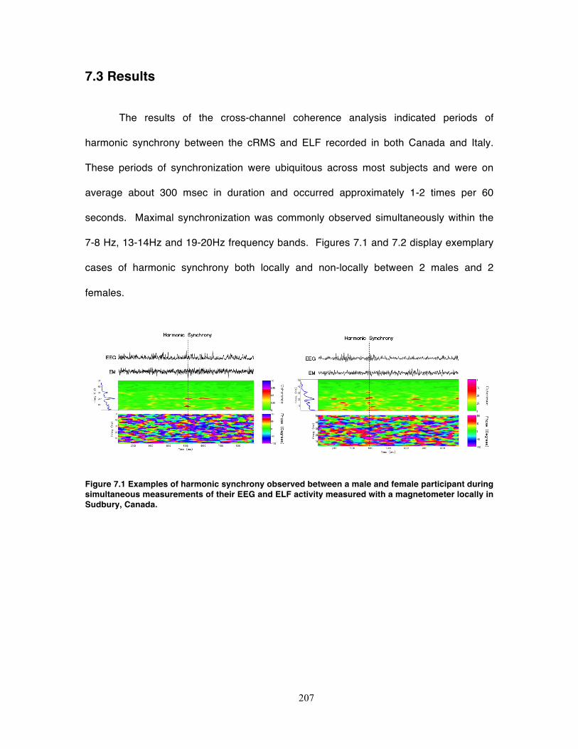
207

7.3 Results

The results of the cross-channel coherence analysis indicated periods of

harmonic synchrony between the cRMS and ELF recorded in both Canada and Italy.

These periods of synchronization were ubiquitous across most subjects and were on

average about 300 msec in duration and occurred approximately 1-2 times per 60

seconds. Maximal synchronization was commonly observed simultaneously within the

7-8 Hz, 13-14Hz and 19-20Hz frequency bands. Figures 7.1 and 7.2 display exemplary

cases of harmonic synchrony both locally and non-locally between 2 males and 2

females.

Figure 7.1 Examples of harmonic synchrony observed between a male and female participant during simultaneous measurements of their EEG and ELF activity measured with a magnetometer locally in Sudbury, Canada.

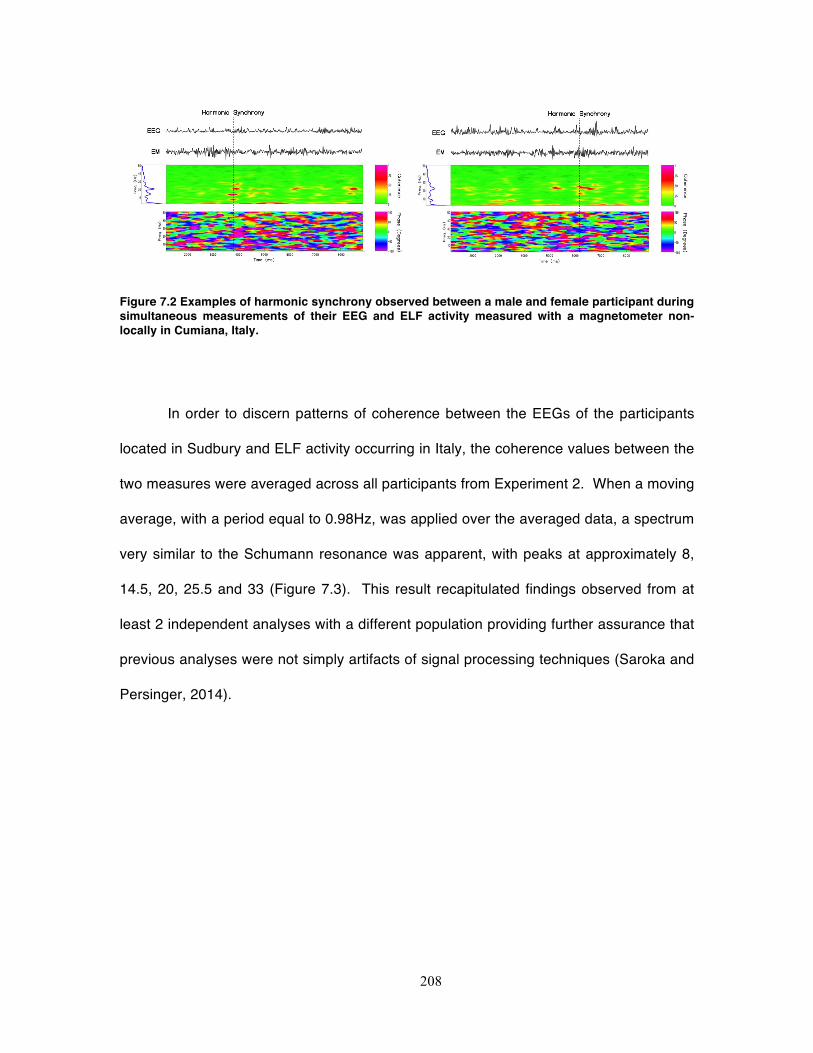
208

Figure 7.2 Examples of harmonic synchrony observed between a male and female participant during simultaneous measurements of their EEG and ELF activity measured with a magnetometer non-locally in Cumiana, Italy.

In order to discern patterns of coherence between the EEGs of the participants

located in Sudbury and ELF activity occurring in Italy, the coherence values between the

two measures were averaged across all participants from Experiment 2. When a moving

average, with a period equal to 0.98Hz, was applied over the averaged data, a spectrum

very similar to the Schumann resonance was apparent, with peaks at approximately 8,

14.5, 20, 25.5 and 33 (Figure 7.3). This result recapitulated findings observed from at

least 2 independent analyses with a different population providing further assurance that

previous analyses were not simply artifacts of signal processing techniques (Saroka and

Persinger, 2014).

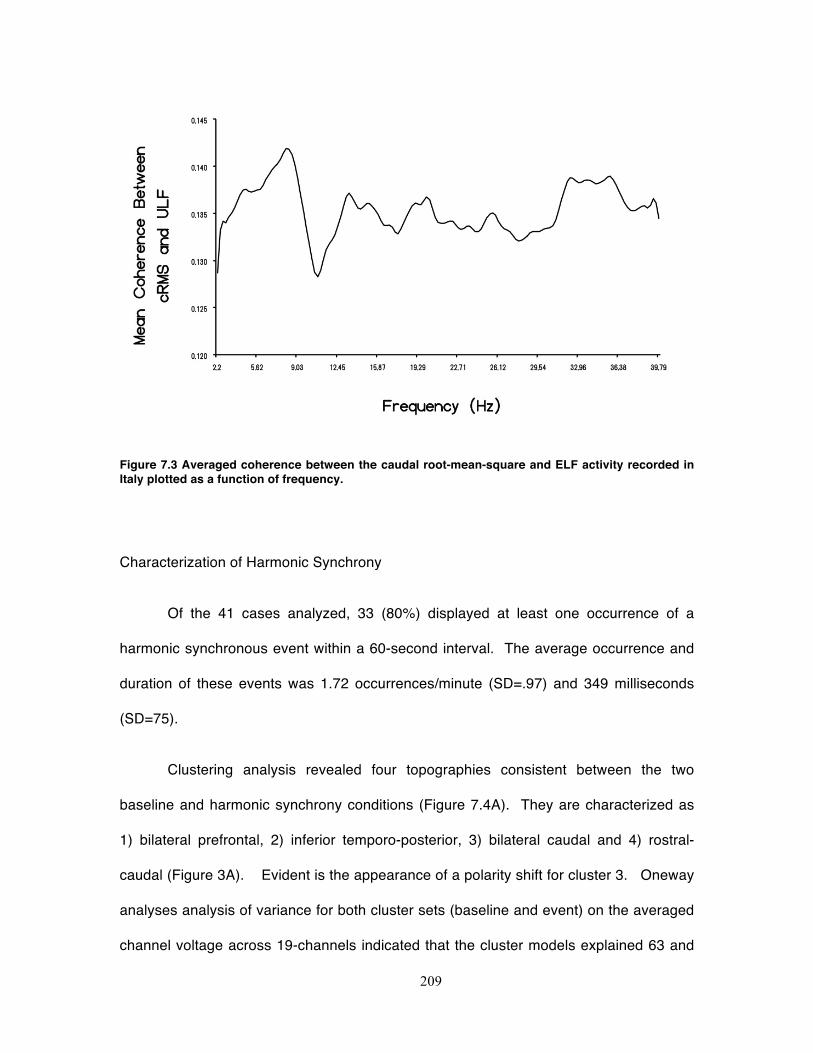
209

Figure 7.3 Averaged coherence between the caudal root-mean-square and ELF activity recorded in Italy plotted as a function of frequency.

Characterization of Harmonic Synchrony

Of the 41 cases analyzed, 33 (80%) displayed at least one occurrence of a

harmonic synchronous event within a 60-second interval. The average occurrence and

duration of these events was 1.72 occurrences/minute (SD=.97) and 349 milliseconds

(SD=75).

Clustering analysis revealed four topographies consistent between the two

baseline and harmonic synchrony conditions (Figure 7.4A). They are characterized as

1) bilateral prefrontal, 2) inferior temporo-posterior, 3) bilateral caudal and 4) rostral-

caudal (Figure 3A). Evident is the appearance of a polarity shift for cluster 3. Oneway

analyses analysis of variance for both cluster sets (baseline and event) on the averaged

channel voltage across 19-channels indicated that the cluster models explained 63 and

210

65 percent of the variance in classification. To ascertain that the clusters were

consistent between conditions (baseline versus harmonic synchrony), Spearman rank-

order correlations were completed between the arrays of cluster channel mean centers.

The results indicated significant relationships for each cluster between conditions with

respective correlation coefficients of 1) Rho=.59, p<.05, 2) -.85 (p<.05), 3) Rho=.54

(p<.05) and 4) Rho=.77 (p<.05).

To directly compare differences in topographical orientations between baseline

conditions (200 milliseconds before the event) and during the occurrence of harmonic

synchrony, each map was z-scored separately. The z-scores of topographies were then

simply subtracted from each other. The results (Figure 7.4B) indicated that only the

second cluster, characterized by the right inferior temporo-parietal focus, displayed z-

score differences greater than 3, likely attributed to the polarity shift observed between

conditions. Here, positive z-scores (red) indicate that the standardized voltage for the

synchronous event is greater than baseline while negative z-scores (blue) indicate the

opposite.

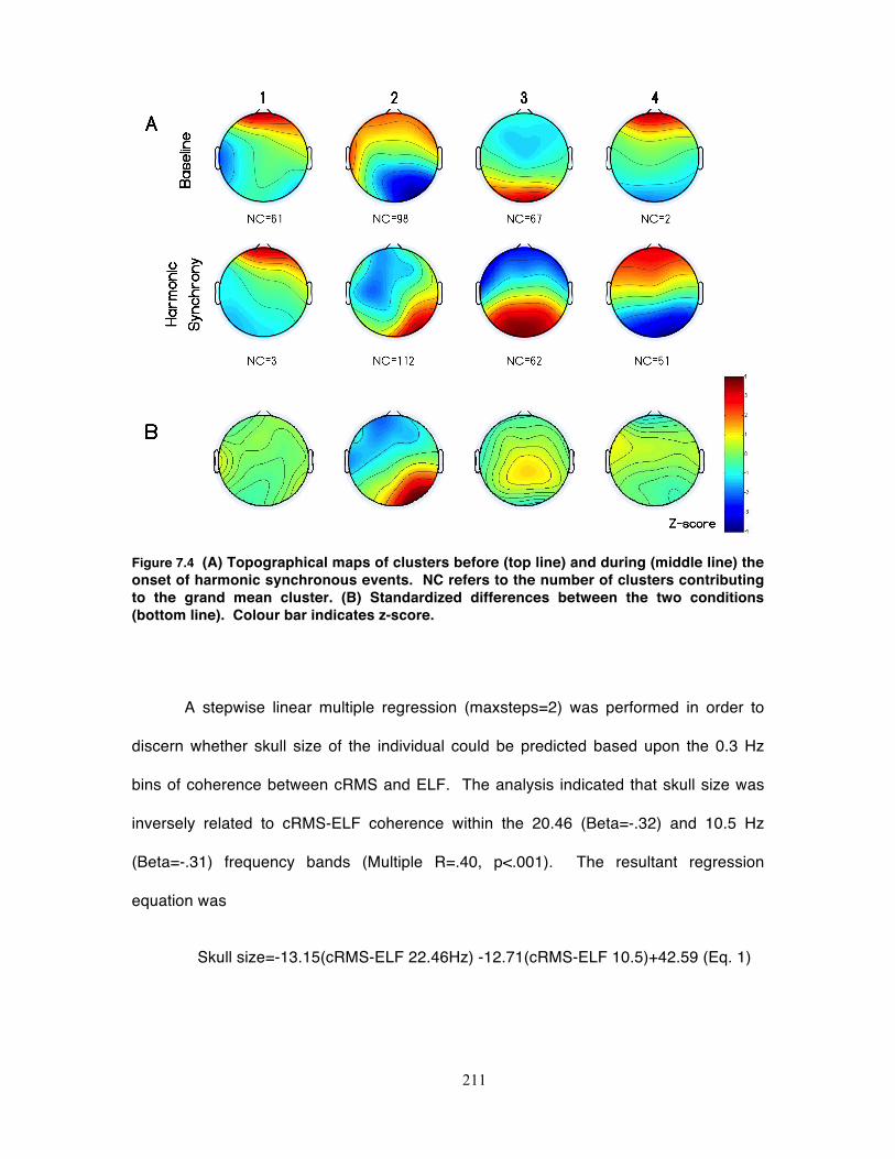
211

Figure 7.4 (A) Topographical maps of clusters before (top line) and during (middle line) the onset of harmonic synchronous events. NC refers to the number of clusters contributing to the grand mean cluster. (B) Standardized differences between the two conditions (bottom line). Colour bar indicates z-score.

A stepwise linear multiple regression (maxsteps=2) was performed in order to

discern whether skull size of the individual could be predicted based upon the 0.3 Hz

bins of coherence between cRMS and ELF. The analysis indicated that skull size was

inversely related to cRMS-ELF coherence within the 20.46 (Beta=-.32) and 10.5 Hz

(Beta=-.31) frequency bands (Multiple R=.40, p<.001). The resultant regression

equation was

Skull size=-13.15(cRMS-ELF 22.46Hz) -12.71(cRMS-ELF 10.5)+42.59 (Eq. 1)

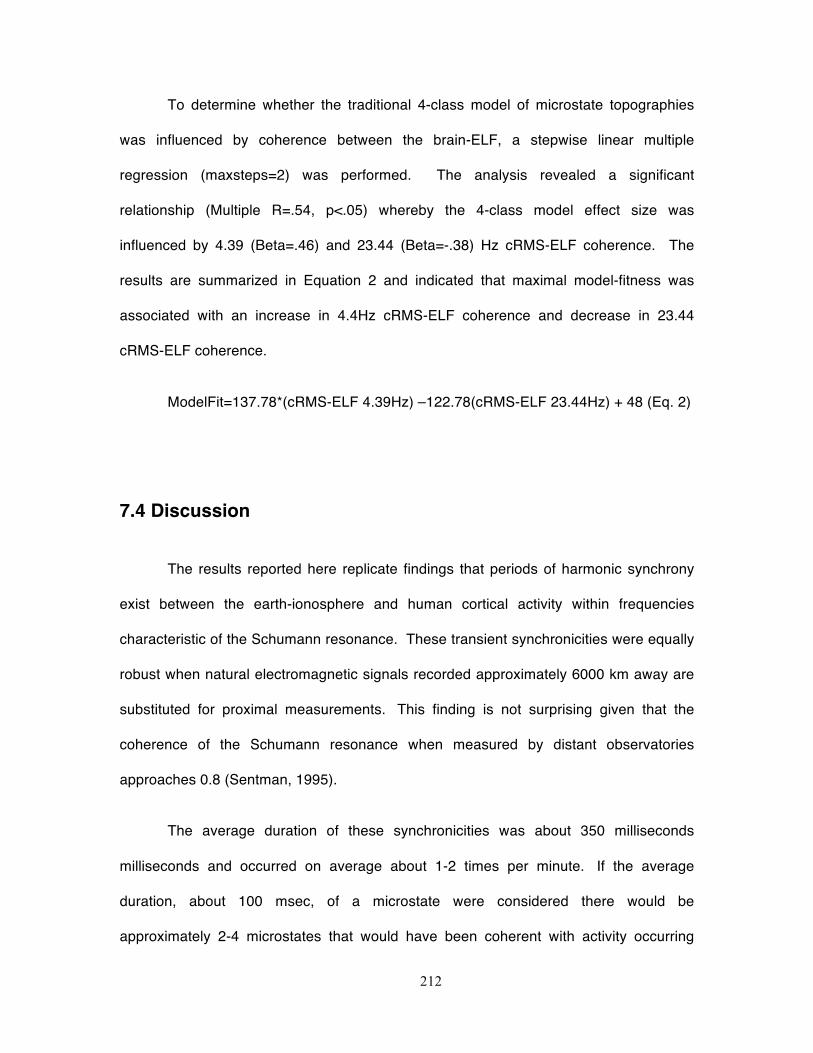
212

To determine whether the traditional 4-class model of microstate topographies

was influenced by coherence between the brain-ELF, a stepwise linear multiple

regression (maxsteps=2) was performed. The analysis revealed a significant

relationship (Multiple R=.54, p<.05) whereby the 4-class model effect size was

influenced by 4.39 (Beta=.46) and 23.44 (Beta=-.38) Hz cRMS-ELF coherence. The

results are summarized in Equation 2 and indicated that maximal model-fitness was

associated with an increase in 4.4Hz cRMS-ELF coherence and decrease in 23.44

cRMS-ELF coherence.

ModelFit=137.78*(cRMS-ELF 4.39Hz) –122.78(cRMS-ELF 23.44Hz) + 48 (Eq. 2)

7.4 Discussion

The results reported here replicate findings that periods of harmonic synchrony

exist between the earth-ionosphere and human cortical activity within frequencies

characteristic of the Schumann resonance. These transient synchronicities were equally

robust when natural electromagnetic signals recorded approximately 6000 km away are

substituted for proximal measurements. This finding is not surprising given that the

coherence of the Schumann resonance when measured by distant observatories

approaches 0.8 (Sentman, 1995).

The average duration of these synchronicities was about 350 milliseconds

milliseconds and occurred on average about 1-2 times per minute. If the average

duration, about 100 msec, of a microstate were considered there would be

approximately 2-4 microstates that would have been coherent with activity occurring

213

within the earth-ionosphere. Flashes of ‘insight’, which are more probable during periods

of frontal alpha-synchronization, have been reported historically for years by many

individuals and often occur ‘out of nowhere’, such as in the case of the of the Kekule

(benzene) ring; however whether or not these ‘spontaneous’ insights occur more

frequently during EEG-ELF coherence cannot be discerned at this time.

We considered the possibility of time-lags between the live feed originating in

Cumiana, Italy and measured average ping times to assess the duration of these

latencies. Measurements of ping times indicated 4-60 msec delays indicating that the

synchronicities occurring in the experiments would not have been sufficient to produce

false time-frequency representations because the duration of the delay was a factor of 2

smaller then the average occurrence of the duration of a synchronicity.

Averaged data indicated that maximal coherence between EEG-ELF occurred at

the classic Schumann frequencies. The coherence values for these peaks ranged

between .1 and .16. These results support previous findings demonstrating that 14Hz

cRMS activity occurring in Sudbury was associated with maximal coherence in

Schumann frequency bands recorded in Italy when broad non-time-locked averages

were employed. Although they may be considered minimal, these values reflect an

average of 60 seconds of data. Our observations indicated that periods of harmonic

synchrony rarely occurred more than 2 times per second. Taking into consideration the

average duration and frequency of these synchronicities, low coherence values within

Schumann resonance frequencies would be expected.

The topographical mapping analysis revealed that the cluster characterized by a

right inferior temporoparietal focus was most sensitive to the occurrence of a harmonic

214

synchronous event. This topography corresponds to the class B microstate typically

observed in microstate analyses and is shortened in patients who are clinically labeled

as ‘schizophrenic’. Recently Persinger et al (2015) showed that an individual whose

cognitive abilities were within average range but heared voices not attributed to the

environment, showed elevated beta-band activity within the right temporal region and the

right parahippocampal gyrus inferred by source localization. She also displayed an

increased sensitivity to an applied magnetic field modeled after amygdaloid burst activity

with an associated spectral peak at around 8-12 Hz. If the analyses presented here are

relevant it is possible that the voices, attributed to non-local sources, could have

occurred during these transient synchronies along the earth-ionosphere-brain axis.

The shift in polarity could be a revealing characteristic of these events with

respect to mechanism. It is well known that a static magnet accelerating into or out of a

coil induces a voltage with a respective polarity. Moving the magnet out of the coil

induces negative voltage across the coil terminals while moving in produces a positive

voltage. If this principle is applicable to the observed topographical orientations and a

reflective process is assumed, the data would suggest that 200 milliseconds prior to

brain-atmosphere synchrony the direction of the magnetic flux is from the head to the

atmosphere, while 200 milliseconds during the event the direction is from the

atmosphere to the head. In information technology, this would classified as a ‘ping’.

Mathematically the magnetic field strengths associated with the change in

frequency would be consistent with this model. If the ping reached the lower D-layer of

the atmosphere and was reflected back towards the human brain, the total distance

travelled would be about 200 km. If the ping time was 400 milliseconds to complete one

full cycle, the quantum of information would be travelling at a velocity of 5x105 m/s. The

215

absolute potential difference between the two conditions within the right inferior

temporoparietal focus was about 10 microVolts. Dividing 1x10-5 volts by 5x105 m/s

results in 20 picoTesla·metres. In radio science, bursts of megahertz frequencies are

sent into the ionosphere and reflect back to a sensor in order to infer ionospheric

density. For the D layer, frequencies which reflect back to the earth are between 1 and 5

megaHertz. If the ping associated with harmonic synchrony were a megahertz burst

superimposed upon the Schumann waveguide, the wavelength would be about 10

meters. Dividing 20 picoTesla·metres by 10 metres reveals a magnetic field magnitude

of 2 pT which is the operating intensity of the magnetic field of the brain and the

approximate intensity of the Schumann resonance.

We found that skull size was negatively related to EEG-ELF coherence within

around the 10.5 and 22.5Hz frequency bands. The most consistent finding of

quantitative EEG in general is that the dominant frequency displayed by the adult human

brain is on average 10 Hz. We have previously demonstrated that when rostral-caudal

differences in spectral density are calculated, there was a conspicuous peak at 10

Hz. This finding is also consistent with Nunez and colleagues (1978) original work who

showed that peak alpha frequency was inversely correlated with skull size. In light of

recent analyses demonstrating the existence of harmonic relationships between 10 and

20Hz cerebral activity (Abeysuriya et al., 2014) we contend that these harmonic

connections between ELF and EEG exist along a continuum of strengths that are

strongly influenced by biophysical resonant features of the human brain.

Microstate analysis coupled with regression indicated that the fitness of the 4-

class model was moderately influenced by the degree of EEG-ELF coherence within the

4 and 23 Hz frequency bands, the latter of which is correlated with the action of ‘creative

216

thinking’. According to the microstate analysis, the occurrence of a given microstate was

between 3.5 and 4 times per second. While it was not formally assessed here, this

convergence in frequency suggests the possibility of a ‘pacemaker’ microstate by which

the brain becomes synchronized with electromagnetic signals generated within the

earth-ionosphere and would be consistent Wever’s (1974) original work demonstrating

that occlusion of the Schumann resonance was associated with shifts in human

circadian rhythms. This would mean that the sequence of microstates that are

correlated with patterns of human thought are synchronized by the activity occurring

within the earth-ionosphere cavity.

Such synchronization may be a potential quantitative method of assessing Carl

Jung’s theory of archetypes within a biophysical context (Jung, 1964); here patterns of

behaviour ‘inherited’ by the individual would be a function of the physical features of their

brain and electrophysiology and could be modulated by the patterns of intermittent

harmonic synchronies with the Schumann resonance. It is not uncommon for individuals

who have sustained mild closed head injuries to report shifts in personality that are often

sources of tremendous stress for themselves and those within their social group. Such

shifts, while largely associated with the integrity and reinforcement of the neuronal

networks that define the “self”, could produce shifts in the synchrony of assemblages of

neurons that change the individual’s connection with the Schumann resonance by

modulation of alpha spectral density. Therefore stimulation of the brain by means of

weak-intensity magnetic fields for re-synchronization with previous ‘selves’ might be a

potential treatment for these populations in the future.

217

7.5 Conclusion

The data and analyses presented here support further the observations originally

made by Konig and Angermuller (1960) and replicate earlier findings. In particular, the

results indicate transient periods of harmonic synchrony between human brain electrical

activity and earth-ionosphere electromagnetic activity within Schumann frequencies that

are equally strong irrespective of location on the planet. Coupling of the two phenomena

was strongly related to the physical dimensions of the skull and by extension the human

brain and are predictable by simple biophysical principles of resonance and standing

waves. Finally the ‘fitness’ of the model that governs the classical arrangement of

microstate topographies was strongly related to EEG-ELF coherence within the 4 Hz

frequency band.

7.6 References

Abeysuriya, R.G., Rennie, C.J., Robinsin, P.A., Kim, J.W. (2014). Experimental

observation of a theoretically predicted nonlinear sleep spindle harmonic in

human EEG. Clinical Neurophysilogy 125(10), 2016-2023.

Balser, M., & Wagner, C. A. (1960). Observations of Earth-ionosphere cavity

resonances. Nature, 188(4751), 638-641.

Ćosić, I., Cvetković, D., Fang, Q., & Lazoura, H. (2006). Human electrophysiological

signal responses to ELF Schumann resonance and artificial electromagnetic

fields. FME Transactions, 34(2), 93-103.

218

Jung, C.G. (1964). Man and his symbols. Dell U.S.

Koenig, T., Lehmann, D., Merlo, M. C., Kochi, K., Hell, D., & Koukkou, M. (1999). A

deviant EEG brain microstate in acute, neuroleptic-naive schizophrenics at rest.

European archives of psychiatry and clinical neuroscience, 249(4), 205-211.

Koenig, T., Prichep, L., Lehmann, D., Sosa, P. V., Braeker, E., Kleinlogel, H., ... & John,

E. R. (2002). Millisecond by millisecond, year by year: normative EEG

microstates and developmental stages. Neuroimage, 16(1), 41-48.

König, H. L. and Angermüller, F. 1960, Einfluß niederfrequenter elektrischer Vorgange in der

Atmosphare. Die Naturwissenschaft, 47, 485-490

Mulligan, B. P., Hunter, M. D., & Persinger, M. A. (2010). Effects of geomagnetic activity

and atmospheric power variations on quantitative measures of brain activity:

replication of the Azerbaijani studies. Advances in Space Research, 45(7), 940-

948.

Nunez, P. L. (1995). Neocortical dynamics and human EEG rhythms. Oxford University

Press, USA.

Nunez, P.L., Reid, L. and Bickford, R.G. (1978). The relationship of head size to alpha

frequency with implications to a brain wave model. Electroencephalography and

Clinical Neurophysiology, 44: 344-362.

Persinger, M. A. (2012). Brain electromagnetic activity and lightning: potentially

congruent scale-invariant quantitative properties. Frontiers in integrative

neuroscience, 6.

219

Pobachenko SV, Kolesnik AG, Borodin AS, Kalyuzhin VV. The contigency of parameters

of human encephalograms and schumann resonance electromagnetic fields

revealed in monitoring studies. Complex Syst Biophys. 2006;51(3):480–3

Saroka, K. S., Caswell, J. M., Lapointe, A., & Persinger, M. A. (2014). Greater

electroencephalographic coherence between left and right temporal lobe

structures during increased geomagnetic activity. Neuroscience letters, 560, 126-

130.

Saroka, K.S. and Persinger, M.A. (2015). Quantitative convergence of major-minor axes

cerebral electric field potentials and spectral densities: Consideration of

similarities to the Schumann resonance and practical implications. Submitted to

Naturwissenshaften.

Saroka, K.S. and Persinger M.A. (2014). Quantitative evidence for direct effects

between earth-ionosphere Schumann resonances and human cerebral cortical

activity. International Letters of Chemistry, Physics and Astronomy, 20(2): 166-

194.

Sentman, D. D. (1995). Schumann resonances: In Volland, H. (Ed.). (1995). Handbook

of atmospheric electrodynamics (Vol. 1). CRC Press.

Wever, R. (1974). ELF-effects on human circadian rhythms. In Persinger (Ed) ELF and

VLF electromagnetic field effects (pp. 101-144). Springer US.

220

Chapter 8 Synthesis, Implications and Conclusion

The fugue is by definition a song with a repeating pattern consisting of multiple

probabilities of convergence and divergence of a central melody all within an over-

arching harmonic context. The recapitulated ‘subject’, here proposed as the

convergences of earth-ionosphere-brain electromagnetic activity, has taken its form in

the collection of analyses presented here. According to Diane Ackermann’s insight into

the nature of the relationship between human beings and patterns,

“Once is an instance. Twice may be an accident. But three times or more makes

a pattern.” (Ackerman, 1994).

Whether observed pattern is an artifact of perception and observation of the subject

rather than an indication of some element of ‘truth’ cannot readily be discerned. Indeed

this question has occupied considerable attention from many lines of philosophical and

cosmological inquiry and its effect is evidenced in the apparent duplicity of the behaviour

of particles when in the presence of an observer. However, within the constraints of the

analyses presented here the data seems to indicate that the relationship between the

human brain and the earth’s geomagnetic field, a concept previously described by many

theologians scientists and artists, is more robust than may have been expected, given its

occurrence in the multitude of analytic approaches on the micro (human) and macro

(earth) scale.

221

Synthesis

The first convergence is the synonymous correlation between left and right

temporal lobe coherence and indices of geomagnetic disturbance (Chapter 2) within

frequencies related to the Schumann resonance (~8 and 20Hz) that was recapitulated in

a separate analysis which demonstrated that the electric field strength (measured in

California) at the first and second harmonics of the Schumann resonance were positively

correlated with coherence within the T3-T4 sensors at frequencies approximating the

alpha frequency (Chapter 6). The third restatement of this finding was found on a

‘macroscopic’ scale with increases in coherence at approximate ‘T5-T6’ sensors of the

earth when electroencephalographic analytic techniques were applied to magnetometer

data collected around the world; the same analysis indicated the presence of similar

patterns of electromagnetic field topographies observed within the human brain (Chapter

3).

Left and right temporal lobe coherence has been shown to be a potential

correlate of the experience of the ‘sensed presence’ (Saroka and Persinger, 2013). In

this case, electromagnetic fields, approximating microTesla intensity and similar to

background static geomagnetic field, applied in a pattern that imitates signals derived

from nature elevated this left-right interaction for individuals who reported the experience

of the sensed presence. On average, the coherence doubled from 0.2 (4 % of the

variance) to .4 (16 % of variance). The magnitudes observed in this collection of

correlational analyses reported here were similar and may re-affirm a fundamental

‘fractal’ electromagnetic relationship between the two spheres as predicted by Persinger

(2012).

222

The Class A microstate (Figure 3.6), explaining the most variance within the 4-

class model, of the earth is similar in topography to the Class C microstate measured

from human cerebrums (Figure 1.11) and is evident even in raw strip-chart recordings

when the eyes are closed with preponderances of alpha activity observed over the

caudal hemisphere. According to Koenig and colleagues’ (2002) normative data this

microstate remains the most preponderant (30-40% of the time) of the 4 microstates

starting in early adulthood. If the relationship were valid, this representation of the

topography in the human brain might represent an interface that allows the interaction

with the earth’s geomagnetic field to occur for alignment and disturbance during solar

proton events. This relationship may be valid when the data indicating changes in the

migration behaviour of birds (Thalau et al, 2005), or increases in aggression in

populations male rats (St-Pierre et al., 1998), during the time of geomagnetic

disturbance is considered.

The second and most instructive convergence observed during the analysis of

the data presented in this dissertation were the almost ubiquitous and numerous

correlations between brain activity and electromagnetic activity within the ultra-low

frequency range, and more specifically the frequencies that define the Schumann

resonance. The data presented in Chapter 4 indicated that the brain becomes resonant

with background AC magnetic field measurements specifically at frequencies that

approximate 8, and 40 Hz even though the instrumentation was sensitive to only

nanoTesla rather than the expected picoTesla fluctuations. This pattern was observed

two additional times when the Schumann resonances were found to be an intrinsic

signature within the averaged brain activity of a large population (Chapter 5) and when

the greatest effect sizes between the relationship of the 8-Hz electric field activity

223

measured in Italy and 14 Hz caudal activity within the cerebrums of individuals located in

Sudbury occurred at frequencies characteristic of the Schumann resonance, specifically

at frequencies of 8, 14, 20, 26 and 33 Hz (Chapter 6).

The validity of these correlations was internally verified through the simultaneous

measurement of brain and the earth-ionosphere where intermittent periods of coherence,

lasting on average about 300 millisecond once every minute, were observed over the

caudal hemisphere within frequencies of the Schumann resonance when ‘atmospheric

noise’ was measured locally in Sudbury, Canada and over 6000 kilometers away in Italy

(Chapters 6 and 7). The term ‘harmonic synchrony’ was employed in order to illustrate

that the caudal electrical activity becomes synchronous with this noise at precisely

harmonics of the Schumann resonance. In more detailed analyses, these events were

shown to have considerable overlap in terms of localization when compared against

previous data. For instance, the right caudal hemisphere was shown to be mostly

affected during the times of synchronous events.

Implications

Dr. Carl Gustav Jung proposed the concept of ‘synchronicity’ as an unconscious

process where symbols in dreams and lucid thoughts manifest physical representation in

‘reality’ (Jung, 1964). These occurrences are taken by many as personal ‘totems’ that

validate their decision-making process while others view these occurrences as mere

‘coincidence’ that would have been bound to happen by chance due to their

infrequency.

224

The findings reported here may add quantitatively to the hypotheses offered by

Jung; the seemingly irregular interface between the electrical activity of the cerebrums of

individuals may approximate the temporal durations associated with insight, a likely

correlate of synchronicity. While measuring the electroencephalograms of individuals

engaging in compound-remote-associates problem-solving in which one word can form a

compound-word with three supplied words, those instances where the individuals ‘felt’

the solution (the word connecting the three) rather than logically derived it were

associated with gamma (>30 Hz) and alpha (~7-13 Hz) bursts localized over the right

caudal hemisphere 300 milliseconds prior to overt verbal indications of their

methodology for problem-solving (Kounios et al, 2009).

In addition to the data presented in Chapter 7 (localization of harmonic

synchrony) and Chapter 4 (correlations with the proximal electromagnetic environment

precisely within these two frequency bands), this region was also activated in a unique

individual during times when he interpreted the personal histories of individuals sitting in

close proximity (Persinger and Saroka, 2012). If these earth-ionosphere interactions

are viewed as ‘rewards’ in a classical behaviourist context, their occurrences should

follow the principles of learning and would be associated with subtle elevations in

dopmanergic activity, particularly mediated from the ventral tegmental area to medial

prefrontal regions, including the anterior cingulate and a primary correlate of bonding

between human beings. It may be relevant that this neurochemical compound is also

elevated during experiences of the ‘musical chill’ phenomenon frequently reported within

the normal population and described phenomenologically as a pleasurable ‘shiver down

the spine’ (Blood et al., 2001). Experience of this chill can be encouraged through

225

appropriate stimulation of the medial frontal regions with an electromagnetic field pattern

modeled after burst-firing dopaminergic neurons (Saroka and Persinger, 2013).

The recruitment of neuronal assemblages within a locus of the right caudal

hemisphere that predicts activity within the parahippocampal gyrus, a region highly

associated with the integration of multiple streams of information into memory

unconsciously, may also be supportive of the work of Dr. Jung. This region displays a

negative voltage of about 10 microvolts prior to a ‘harmonic synchrony’ event followed by

a positive voltage of the same magnitude and may be akin to simultaneous sending and

receiving of packets of information or ‘bouncing’, if the model of a static magnet moving

into and out of a coil is apt. If so, this model might predict a ‘pay-it-forward’ mechanism

whereby individuals experience synchronicity, and while perceived as an isolated

(between two people) incident, is actually occurring globally in a chain of reactions or

simultaneously. In summary the ideas of ‘synchronicity’, ‘collective unconscious’, and

‘archetype’ (which may be recognized in modern times as the patterns of interaction

between the earth-ionosphere), may now have a metric by which it can be explored

quantitatively.

As has been demonstrated numerously within the context of psychology, the

boundaries of working memory are 7 +/- 2 items. However, if one applied the concept of

the fractal arrangmenets, it may be argued that this is true at several temporal scales; for

example, the amount of personally significant events within one day, one month, one

year, or one lifetime may approach the same figure. If this is true then consciousness as

experienced by the human being may exist on alternative temporal and spatial levels, as

would have been predicted by many Eastern philosophies. Persinger’s (2010)

calculations indicate that the energy equivalent of all human memory from every human

226

being that has ever existed could potentially be stored within the earth’s geomagnetic

field. Accordingly, the transient interactions that occur along the earth-ionosphere-brain

axis approximately once every minute may be indicative of levels of consciousness that,

by definition, can only be perceived on their respective time scale and would potentially

be evidenced by the repeated but independent re-visiting of concepts and ideas that

permeated throughout the course of history, such as the interdisciplinarity that was once

central to the major creative achievements of the Renaissance period as well as during

the times of Ancient Greece. If this is true, Jung’s ‘collective unconscious’ may have

more relevance than suspected.

Conclusion

The fugal, scale-invariant, or fractal coupling between human cortical activity and

earth-ionospheric electromagnetic parameters has been thoroughly explored. In all

analyses similar shapes, intensities, frequencies, activations and energies have been

observed from the perspective of a multitude of different analytic approaches. The three

major findings are that 1) the spatial and temporal properties of natural electromagnetic

fields are similar at microscopic and macroscopic scales, 2) as predicted by König

(1960) and Persinger (2012) the interface between the two systems converges at the

nano-to-picotesla range intensity at frequencies characteristic of the Schumann

resonance, and 3) this interface is a regular occurrence within all human beings, within

cerebral loci that are traditionally associated with memory and for durations (300 msec)

that approximate insight and creativity.

227

References

Ackerman, D. (2011). A Natural History of Love: Author of the National Bestseller A

Natural History of the Senses. Vintage.

Blood, A. J., & Zatorre, R. J. (2001). Intensely pleasurable responses to music correlate

with activity in brain regions implicated in reward and emotion. Proceedings of

the National Academy of Sciences, 98(20), 11818-11823.

Koenig, T., Prichep, L., Lehmann, D., Sosa, P. V., Braeker, E., Kleinlogel, H., ... & John,

E. R. (2002). Millisecond by millisecond, year by year: normative EEG

microstates and developmental stages. Neuroimage, 16(1), 41-48.

König, H. L. and Angermüller, F. 1960, Einfluß niederfrequenter elektrischer Vorgange in

der Atmosphare. Die Naturwissenschaft, 47, 485-490

Kounios, J., & Beeman, M. (2009). The Aha! Moment the cognitive neuroscience of

insight. Current directions in psychological science, 18(4), 210-216.

Jung, C.G. (1964). Man and his symbols. Dell U.S.

Persinger, M. A. (2012). Brain electromagnetic activity and lightning: potentially

congruent scale-invariant quantitative properties. Frontiers in integrative

neuroscience, 6.

Persinger, M. A., & Saroka, K. S. (2012). Protracted parahippocampal activity associated

with Sean Harribance. International journal of yoga, 5(2), 140.

228

St-Pierre, L. S., Persinger, M. A., & Koren, S. A. (1998). Experimental induction of

intermale aggressive behavior in limbic epileptic rats by weak, complex magnetic

fields: Implications for geomagnetic activity and the modern habitat?.

International journal of neuroscience, 96(3-4), 149-159.

Saroka, K. S., & Persinger, M. A. (2013). Potential production of Hughlings Jackson's

“parasitic consciousness” by physiologically-patterned weak transcerebral

magnetic fields: QEEG and source localization. Epilepsy & Behavior, 28(3), 395-

407.

Thalau, P., Ritz, T., Stapput, K., Wiltschko, R., & Wiltschko, W. (2005). Magnetic

compass orientation of migratory birds in the presence of a 1.315 MHz oscillating

field. Naturwissenschaften, 92(2), 86-90.