Lincoln University Digital Thesis 

  

Copyright Statement 

The digital copy of this thesis is protected by the Copyright Act 1994 (New Zealand). 

This thesis may be consulted by you, provided you comply with the provisions of the Act and the following conditions of use: 

you will use the copy only for the purposes of research or private study   you will recognise the author's right to be identified as the author of the thesis and 

due acknowledgement will be made to the author where appropriate   you will obtain the author's permission before publishing any material from the 

thesis.  

 

Evaluating the economic and financial impact of the Millennium

Villages Project on farming households: Evidence from Bonsasso,

Ghana

A thesis

submitted in partial fulfilment

of the requirements for the Degree of

Doctor of Philosophy

at

Lincoln University

by

Cephas Joshua Beujung Samwini

Lincoln University

2021

ii

Abstract of a thesis submitted in partial fulfilment of the

requirements for the Degree of Doctor of Philosophy.

Abstract

Evaluating the Economic and Financial Impact of the Millennium Villages

Project on Farming Households: Evidence from Bonsasso, Ghana

by

Cephas Joshua Beujung Samwini

The Millennium Village Project (MVP) was a cross-sectoral, integrated rural development programme

based on the 'big push' approach to development assistance. It was intended to provide a pathway

and model for achieving the Millennium Development Goals (MDGs) in rural communities in ten Sub-

Saharan African countries. Implemented over ten years in two five-year phases, Ghana's first MVP,

the Bonsaaso MVP is the focus of this research. Several studies on the Bonsaaso MVP have

concentrated on how MVP has influenced community cohesion, ownership of the development

process, and health and education outcomes. Despite the focus on the agricultural sector as an

'engine' to drive the local economy of the project villages, there have been no studies evaluating its

impact on farm households. Given the importance of agriculture as a source of employment and

livelihood for most inhabitants in the MVP area, it is crucial to understand the effectiveness of the

project interventions as tools for rural development. Therefore, this study assessed the MVP's

economic and financial impact on farm households in Bonsaaso, Ghana. The study applied mixed

methods to address the research questions. A multistage sampling technique was used to collect a

sample of 202 households from three MVP villages and 97 households from a non-MVP household

for the analysis to determine the impact of the MVP. Propensity score matching (PSM) was used to

assess the impact of the MVP while a recursive instrumental variables model was developed for

checking the validity of the estimated coefficients under PSM. The mean value of assets added was

74% greater for the MVP households. Similarly, gross farm output, total farm expenditure, and net

farm income were 44%, 41% and 52% greater respectively for the MVP households than the

comparison group. The sustainability of livelihood outcomes for MVP households is also evaluated

qualitatively as they ranked various interventions on a 5-point Likert scale. Although a sharp decline

in access to training and extension services indicate that the gains from the MVP may not be

sustainable, about 53% of MVP households indicated that they could sustain the level of farm input

use that they attained during the duration of the project. By employing a mixed-method approach

for assessing the livelihood impacts and their sustainability, this research provides insights for

iii

policymakers into the effectiveness of long-term interventions for achieving sustainable

development goals ( SDGs) in low income and lower-middle-income countries

Keywords: Millennium Villages Project, rural development, sustainable development goals, MDGs,

poverty, food security and 'big push.'

iv

List of Publications and Presentations

This thesis is the result of the original research carried out by myself, under the supervision of Prof.

Hugh Bigsby and Dr Nazmun Ratna. The contents of this thesis have not been submitted for an award

of any other degrees or diplomas in any universities or institutions.

Parts of this thesis have been published as conference proceedings listed below:

Conference presentation

Samwini C. J. B., Lyne, M., Lucock, S., (November 2018) Impact of the Millennium Villages in Ghana,

Paper presented at the 10th Biennial DevNet Conference. Organised by the Aotearoa New

Zealand International Development Studies Network (DevNet) University of Canterbury,

Christchurch

Samwini C. J. B., Lyne, M., Lucock, S., (October 2019) Impact of the Bonsaaso millennium villages

project in Ghana, Paper presented at the AEASA Conference in South Africa

Presentation Sessions

Samwini, C. J. B., (October 2016) An Impact Assessment of the Bonsaaso Millennium Villages, A

proposal presentation to the Faculty of Agribusiness and Commerce, Lincoln University

Samwini C J B., (August 2017) An Impact Assessment of the Millennium Villages in Ghana, 2017: A

paper presented at the 2017 Lincoln University Post-graduate conference at Lincoln

University

Samwini C J B., (June 2017) An Impact Assessment of the Millennium Villages in Ghana, 26 June 2017:

A presentation at the 2017 Thr3sis competition at Lincoln University

Cephas Joshua Beujung Samwini February 2021

v

Acknowledgements

This journey has been an intense period of growth and learning for me. Naturally, so many people

have helped and supported me on this journey. The next few paragraphs will acknowledge the most

notable. First of all, thanks be to God for the gift of life, strength, and the opportunity to pursue this

course. Thanks to my dear wife Sarah, for her patience, kindness and support throughout this period.

Thanks also to my parents and siblings, for their inspiration and prayers. I would like to thank the

Ghana Education Trust Fund (GETFund) for sponsoring my studies. Special thanks to Mr Baffoe and

Mrs Addoteye, staff of GETFund.

My sincere thanks and appreciation to my supervisors Prof. Hugh Bigsby and Dr Nazmun Ratna for

their guidance, patience, critical reviews and incisive comments. Prof. Bigsby’s commitment, despite

his very busy schedule, has been crucial in my continued training as a researcher and for this thesis. I

have learnt to broaden my thinking and be more expressive, not taking things for granted. Dr Ratna

has been invaluable to me at a personal level as well, advocating for me where required and

encouraging me when the going got tough. Thanks also to Assoc. Prof. Michael Lyne, and Dr Sharon

Lucock for their guidance and tutelage in the earlier stages of my course. I had to learn to be very

conscientious as no error escaped the keen eye of Assoc. Prof Lyne. I also extend my appreciation to

the administrative staff of the Faculty of Agribusiness and Commerce, particularly, Anne and Rianne

for their support on administrative matters. Special thanks to Denise Pelvin for their support

throughout my course. Thanks to Sedzro for the tablet computers, my research team, Bernard

Appiah, Alex, Laud Asante, William Owiredu, and Douglas Kusi and the chief farmers who helped to

make the fieldwork successful.

Special thanks to the Rt. Rev. Charles Konadu for his constant encouragement even when multiple

applications for sponsorship failed to materialise and for seeking out the GETfund sponsorship for my

studies. I really wouldn't be here without you. I, together with Sarah are very grateful to Neil and

Karen France, for their immense support in helping to secure a visa for Sarah to join me and for

helping us settle for my studies. Sincerest thanks to Miriam Pascoe, and Isabel Lambrecht, and Joris

who generously helped us out at various stages when we were in financial distress. Miriam also lent

us her car for the duration of my studies. Special thanks to Noel and Robin Dunlop for their

encouragement, advice and support during stressful times.

I would like to express my appreciation for the help, support, friendship and fellowship of Rev. Phillis

Harris, Trevor Harris, Mark and Julie Sutherland (for continuous prayer support), Jenni Baxter (for

certification of documents), Grant and Jenni Sutherland and the entire congregation of Lincoln Union

Church, the Nimako family, the France family, Hugh and Sue Mingard, the LUC Tuesday prayer group,

vi

Ani and the post-graduate fellowship at Lincoln University, the Omegas and the Ghanaian community

in Christchurch, thanks to you I felt at home in Lincoln. Thanks to my friends Enoch Mensah,

Emmanuel Apiors, Caesar Ximenes, Yaa Mawufemor Akufia, Bismark Asumadu, Seth, Dennis, Umar,

Huy, Man, Hoan, Tina, Yunlong, and numerous other friends and colleagues who have been with me

throughout this journey encouraging and egging me on regardless. Particular thanks to Dr Jackie

Blunt, Hamish Johnson and Jayne Smith for helping me deal with health issues, and the Mingards for

proofreading my drafts and suggesting various improvements. I dedicate this work to Sarah and our

family, my parents Rt. Rev. Dr and Mrs Nathan I Samwini, Esther, Hezekiah, Nehemiah and Abigail.

Any errors in this thesis are fully my responsibility.

vii

Table of Contents

Abstract ....................................................................................................................................... ii

List of Publications and Presentations .......................................................................................... iv

Acknowledgements ...................................................................................................................... v

Table of Contents ....................................................................................................................... vii

List of Tables ................................................................................................................................ x

List of Figures .............................................................................................................................. xi

Glossary of acronyms .................................................................................................................. xii

Chapter 1 Introduction ............................................................................................................ 1

Historical background to the study ...........................................................................................3

Problem statement ................................................................................................................ 11

Research objectives and questions ........................................................................................ 13

Contribution of the study....................................................................................................... 13

Organisation of the thesis ...................................................................................................... 14

Chapter 2 Literature Review.................................................................................................... 15

Introduction ........................................................................................................................... 15

Concept and definition of development ................................................................................ 15 Income growth ...........................................................................................................16 Human development .................................................................................................17 Post-development ......................................................................................................22 A summary of the concept of development ..............................................................24

Poverty trap ........................................................................................................................... 25 Village level poverty trap ...........................................................................................26 Household level poverty trap .....................................................................................27 A summary of the poverty trap ..................................................................................30

The definition and history of development assistance .......................................................... 30 Approaches to development assistance ....................................................................33

2.5 The role of agriculture in economic growth .......................................................................... 52

2.6 Chapter summary .................................................................................................................. 54

Chapter 3 Research Methods and Empirical Strategy ............................................................... 55

Introduction ........................................................................................................................... 55

Conceptual framework .......................................................................................................... 55

Methods and empirical strategy ............................................................................................ 59 The difference between MVP and non-MVP households. .........................................59 Impact of the Bonsaaso MVP on assets, income and expenditure ............................61 Sustainability of the MVP interventions ....................................................................74

Survey Instrument .................................................................................................................. 75

Study area .............................................................................................................................. 77

3.6 Sampling method and data collection ................................................................................... 81 3.6.1 Sampling method .......................................................................................................81 3.6.2 Data collection ...........................................................................................................85

viii

3.7 Chapter summary .................................................................................................................. 85

Chapter 4 Descriptive statistics ............................................................................................... 86

4.1 Introduction ........................................................................................................................... 86

4.2 Households characteristics .................................................................................................... 86

4.3 Assets ..................................................................................................................................... 90 4.3.1 Land ............................................................................................................................94 4.3.2 Fixed farm improvements ..........................................................................................97 4.3.3 Household assets .......................................................................................................99

4.4 Household agricultural enterprise ....................................................................................... 103 4.4.1 Crop enterprises .......................................................................................................104 4.4.2 Livestock income and expenditures .........................................................................107

4.5 Access to services................................................................................................................. 109

4.6 Chapter Summary ................................................................................................................ 110

Chapter 5 The Financial and Economic Impact of the Bonsaaso MVP ..................................... 111

5.1 Introduction ......................................................................................................................... 111

5.2 Propensity score model ....................................................................................................... 111 5.2.1 Balancing Tests .........................................................................................................115 5.2.2 Univariate assessment of MVP treatment effect.....................................................118 5.2.3 Assets .......................................................................................................................119 5.2.4 Agricultural Enterprises ............................................................................................121 5.2.5 Robustness check: Recursive IV model estimates of MVP impact ..........................124 5.2.6 Multivariate assessment of the MVP treatment effect ...........................................124

5.3 Chapter summary ................................................................................................................ 130

Chapter 6 Sustainability of the MVP's agricultural interventions ............................................ 132

6.1 Introduction ......................................................................................................................... 132

6.2 MVP impact on access to training and extension services .................................................. 132 6.2.1 MVP impact on access to agro-inputs and services .................................................136

6.3 Agricultural Interventions of MVP ...................................................................................... 141

6.4 Sustainability of input level .................................................................................................. 143

6.5 Overall satisfaction with the MVP interventions ................................................................. 144

6.6 Chapter Summary ................................................................................................................ 145

Chapter 7 Discussion of Results and Policy Implications ......................................................... 146

7.1 Introduction ......................................................................................................................... 146

7.2 Impact on asset accumulation ............................................................................................. 146

7.3 Impact of the MVP on gross farm output ............................................................................ 152 7.3.1 MVP interventions affecting production output .....................................................153 7.3.2 Livestock production ................................................................................................156

7.4 Impact of MVP on Input expenditure .................................................................................. 157

7.5 Impact of the MVP on Net farm income .............................................................................. 160

7.6 Sustainability of the MVP’s agricultural gains ..................................................................... 161

7.7 Chapter Summary ................................................................................................................ 162

Chapter 8 Summary, Conclusions and recommendations. ...................................................... 164

ix

8.1 Summary .............................................................................................................................. 164

8.2 Contribution of this study .................................................................................................... 168

8.3 Recommendations ............................................................................................................... 169

8.4 Limitations of the study ....................................................................................................... 170

8.5 Conclusions .......................................................................................................................... 170

References ............................................................................................................................... 172

Appendix A : Household Questionnaire ................................................................................. 194

Appendix B : Variable Definitions .......................................................................................... 209

Appendix C : Assessment of Instrument Validity and Relevance ............................................. 215

x

List of Tables

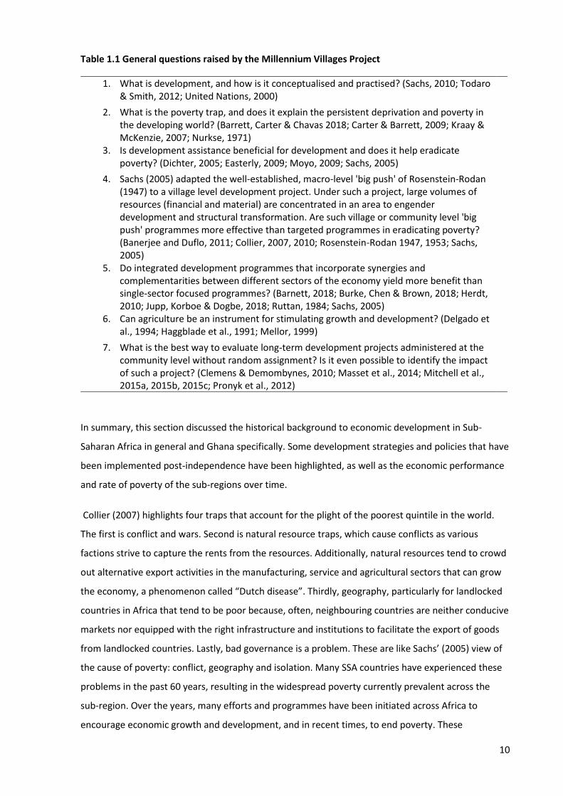
Table 1.1 General questions raised by the Millennium Villages Project ...........................................10 Table 3.1 Household characteristics, farm characteristics and farm enterprises to be compared ..60 Table 3.2 Bonsaaso MVP villages ......................................................................................................82 Table 4.1 Household characteristics of the MVP and non-MVP households....................................87 Table 4.2 Household composition of MVP and non-MVP households .............................................88 Table 4.3 Distribution of land, farm and household assets ..............................................................91 Table 4.4 Distribution of landholding sizes by households in both villages ......................................97 Table 4.5 Fixed improvements owned by households before 2006 and after 2015 ........................98 Table 4.6 Proportion of household ownership of household assets before and after the MVP ....100 Table 4.7 Value of asset categories accounting for household size (Ghs/adult equivalent) ..........102 Table 4.8 Value of asset categories accounting for farm size (Ghs/ha) ..........................................103 Table 4.9 Proportion of farm households engaged in various farm enterprises ...........................104 Table 4.10 Food crop, cash crop and Fruit crop production per household ...................................105 Table 4.11 Crop Production per household (Ghs) ...........................................................................106 Table 4.12 Animal production per household.................................................................................107 Table 4.13 Comparison of mean outcomes across treatment and control groups before propensity

score matching ...........................................................................................................108 Table 5.1 Logit and probit regression results for MVP participation ..............................................112 Table 5.2 The average marginal effect of logit and probit model of MVP participation ................113 Table 5.3 Matching summary ..........................................................................................................114 Table 5.4 Balance of covariates before matching ...........................................................................116 Table 5.5 Balance of covariates after matching ..............................................................................116 Table 5.6 Logit model of MVP participation for joint significance and pseudo-R2 test .................117 Table 5.7 Comparison of mean outcomes across treatment and control groups after propensity

score matching ...........................................................................................................118 Table 5.8 Distribution of land, farm and household assets after matching ....................................120 Table 5.9 Food crop, cash crop, and Fruit crop production per household after matching ...........121 Table 5.10 Crop Production per household for the treatment and comparison groups (Ghs) ......122 Table 5.11 Animal production per household for the treatment and comparison group ..............123 Table 5.12 Impact of MVP participation on assets added ..............................................................126 Table 5.13 Impact of assets added -farm outcomes .......................................................................128 Table 5.14 Post-MVP predicted value of assets and outcomes ......................................................130 Table 6.1 Reasons for inability to sustain the level of input use (n = 95) .......................................143 Table 6.2 How has the MVP impacted your livelihood ...................................................................145

xi

List of Figures

Figure 1.1 GDP per capita of the five developing regions of the world .............................................. 4 Figure 1.2 The poverty headcount of the developing sub-regions of the world ................................ 7 Figure 2.1 The poverty trap based on Solow growth model .............................................................26 Figure 2.2 Map of topic for Section 2.4.1 ..........................................................................................34 Figure 3.1 Conceptual framework of the study ................................................................................56 Figure 3.2 Causal flows specified in the recursive IV regression model ...........................................71 Figure 3.3 Map showing the MVP area in the Ashanti Region and Ghana .......................................78 Figure 3.4 Map of the MVP villages ..................................................................................................80 Figure 3.5 Sections of roads before and after improvement by the MVP interventions .................81 Figure 3.6 Map of Amansie West District showing the sampled MVP villages and non-MVP village

(Nyankomase) ...............................................................................................................84 Figure 4.1 Distribution and reasons for migration into the MVP area in the last 10 years ..............90 Figure 4.2 Distribution chickens by household in the non-MVP and MVP villages ..........................93 Figure 4.3 Distribution goats by household in the non-MVP and MVP villages ...............................93 Figure 4.4 Distribution of agricultural land owned by the household ..............................................94 Figure 4.5 Distribution of agricultural land farmed by households ..................................................96 Figure 4.6 Access to services in the MVP and non-MVP villages ....................................................109 Figure 6.1 Proportion of households accessing training and extension services over time in the

MVP villages ................................................................................................................133 Figure 6.2 Proportion of household with access to farm inputs, credit and markets ....................136 Figure 6.3 Perceived improvements in community life in MVP villages .........................................138 Figure 6.4 Proportion of household indicating a perceived improvement in conditions of the

villages ........................................................................................................................140 Figure 6.5 MVP Interventions (extract from Conceptual framework) ............................................141 Figure 6.6 Proportion of Household accessing agricultural interventions .....................................142 Figure 6.7 Overall satisfaction with MVP Interventions .................................................................144 Figure 7.1 Chart of farm sector linkages .........................................................................................157

xii

Glossary of acronyms

2SLS Two-Stage Least Squares

BRAC Bangladesh Rural Advancement Committee

CPI Consumer Price Index CGE Computable General Equilibrium

DAC Development Assistance Committee

DADU District Agricultural Development Unit

DD Double Difference DFID Department for International Development now called the Foreign

Commonwealth Development Office (FCDO)

ERP Economic Recovery Programme

FAO Food and Agriculture Organisation

GDP Gross Domestic Product GIS Geographic Information System

GLSS Ghana Living Standards Survey

GPRS Ghana Poverty Reduction Strategy

GSGDA Ghana Shared Growth and Development Agenda

GSS Ghana Statistical Service HIV/AIDS Human immune deficiency virus / Acquired immune deficiency

syndrome

ICT Information and Communications Technology

IMF International Monetary Fund

INFB Incremental Net Financial Benefit

I-PRSP Interim Poverty Reduction Strategy Paper

IV Instrumental Variables LBC Licenced Buying Company

MDGs Millennium Development Goals

MVP Millennium Villages Project

NGO Non-governmental Organisation

ODA Official Development Assistance

OECD Organisation for Economic Co-operation And Development

OLS Ordinary Least Squares PPR Peste des Petits Ruminants

PSM Propensity score matching

PSU Primary sampling units

PWR Participatory wealth ranking

RD Regression Discontinuity

SADA Savannah Agricultural Development Authority

SAM Social Accounting Matrix

SAPs Structural Adjustment Programmes

SDGs Sustainable Development Goals

SHEP Self-help Electrification Programme SRID Statistics Research and Information Division of the Ministry of Food and

Agriculture SSU Secondary Sampling Units

SVP Sustainable Villages Project

VIF Variance Inflation Factor

1

Chapter 1

Introduction

In 2000, world leaders adopted the Millennium Development Goals (MDGs) that drove the

international development agenda for 15 years until 2015. The eight MDGs were expanded into a set

of 21 targets and 60 indicators to be achieved in the areas of combating extreme poverty, hunger,

failure in primary education, gender inequality, child mortality, maternal health problems, malaria

and HIV/AIDS, environmental damage and ineffective global cooperation o. Despite the progress in

eradicating poverty at the global level, the slower pace of poverty reduction in Sub-Saharan Africa

has meant that extreme poverty is becoming more concentrated in Africa o. About 836 million

people lived in extreme poverty in 2015 compared with 1.9 billion in 1990 (United Nations, 2015),

with 41 per cent of the population in Sub-Saharan Africa (SSA) were living on less than $ 1.25 a day in

2015. The slower pace of poverty alleviation in SSA ( 28% only) is because of the slower rate of

economic growth and weak institutions leading to corruption, conflict and a failure by Sub-Saharan

African governments to channel growth into poverty reduction (Collier, 2007; World Bank, 2018).

In 2005, while the MDGs were still the global development priority, and with 10 years left to the

target date, studies showed that many African countries were in danger of missing the MDGs targets

(Naschold, 2004; United Nations Development Programme (UNDP), 2003). As a result of these

reports, Jeffery Sachs, then special advisor to the United Nations (UN) Secretary-General on the

MDGs, initiated the Millennium Villages Project (MVP). The MVP was designed as a proof of concept

for the model proposed by Sachs (2005) to deal with the poverty trap, the low-level steady-state that

keeps poor households from making long term progress out of poverty and achieve MDGs in rural

communities in Africa. If successful, the model would be scaled up to the Sustainable Villages Project

(SVP) to achieve the MDGs in other parts of the world where poverty is prevalent (Millennium

Promise Alliance, 2013; Sanchez et al., 2007). The MVP was conceived as an integrated rural

development project to successfully achieve the targets of multiple MDGs in a cost-effective manner

(Mitchell et al., 2015a; Mitchell et al., 2015b; Pronyk et al., 2012). The goal was to lift poor people in

rural areas out of the poverty trap and to set them on a self-sustaining path to economic freedom,

prosperity and self-sufficiency (Sachs, 2005). The project was piloted in 2005 in the Kenyan and

Ethiopian districts of Sauri and Koraro, respectively. It was extended to 10 other African countries

that satisfied the preconditions of reasonable peace and stability, good governance and

accountability, and a commitment to achieving the MDGs. Within the ten countries, the selection of

target villages was based on the following criteria: the prevalence of severe chronic malnutrition;

2

variation in agro-ecological zones; and the recommendations of experts, communities and

government officials (Mitchell et al., 2015a).

In each village, the 10-year MVP was implemented in two phases, each lasting five years. The first

phase consisted of what was termed 'quick wins' (Pronyk et al., 2012, p. 2186; Sachs & McArthur,

2005, p. 349). These quick wins sought to improve the health, school attendance, infrastructure and

farm productivity while setting the stage for the long term economic progress of the MVP villages.

The 'quick wins' interventions included: (i) the distribution of free insecticide-treated bed nets to halt

the spread of malaria; (ii) elimination of user fees at primary school level and at hospitals to increase

the use of these services; (iii) expansion of the school feeding programme; (iv) construction of roads

and physical infrastructures like mechanised wells and crop storage facilities to facilitate access to

water and sanitation; and (v) distribution of subsidised fertiliser, improved crop varieties, tree seed

and seedlings to replenish degraded land through agroforestry (Pronyk et al, 2012).

The primary goal of the MVP's agricultural and business development sector interventions was to

contribute towards MDG 1, which was to halve extreme poverty by 2015. Agricultural sector

interventions were also expected to build a basis for sustaining the MVP's impact into the future

when the project ended (Mitchell et al., 2015a). As such, the MVP sought an agriculture centric

sustainable development track for the rural economies of participating villages. This is the type of

growth argued for by AGRA (2017); Haggblade, Hammer & Hazell (1991); Haggblade & Hazell (1989);

Haggblade, Hazell & Brown (1989); and Haggblade et al. (2002) in areas rich in agricultural resources.

The second phase of the MVP focussed on putting systems in place to ensure the long-term

sustainability of the gains made during the first phase (quick wins) by: (i) increasing and sustaining

agricultural productivity; (ii) strengthening monitoring and advisory services; (iii) supporting value

chain development; and (iv) promoting access to financial services. The project’s second phase

carried out electrification; facilitated the formation of farmer-based organisations and cooperatives;

and improved the health and education systems (Mitchell et al., 2015a).

Studies on the impact of the MVP have primarily focussed on consumption outcomes, food insecurity

and stunting (Pronyk et al., 2012) and health sector outcomes like child mortality (Masset et al.,

2020; Mitchell et al., 2018). There is, however, a dearth of analyses on the impact of the MVP’

agricultural sector interventions on beneficiary households. Agricultural outcomes are very

important as agriculture is the primary source of employment, income, and food security for rural

households in low and lower-middle-income countries. The overarching goal of this study is to

address this research gap.

In order to contextualise and understand the nature of the problem to be addressed in this study, it

is crucial to gain a historical understanding of the development challenges that have confronted Sub-

3

Saharan Africa, bringing it to the point where it currently is the poorest sub-region of the world

(Barrett, Carter & Chavas, 2019; World Bank Group, 2019), and the continent is forecast to be the

home of the remainder of the world's extremely poor (Beegle & Christiaensen, 2019; Beegle et al.,

2016). The next section provides a historical background to contextualise the study. Section 1.2

discusses the research problem followed by the research objective and questions in Section 1.3. The

contribution of the study is discussed in Section 1.4 and the chapter concludes with the organisation

of the thesis.

Historical background to the study

Most Sub-Saharan African (SSA) countries gained political independence from their colonial powers

in the middle of the 20th century. Sub-Saharan Africa is endowed with good agricultural potential in

terms of arable land across a range of agro-ecological zones well suited to various agricultural

products. At the time of their independence, most SSA countries relied heavily on the export of

unprocessed agricultural products and minerals as their primary income source (Brückner & Ciccone,

2010). As a result, their economies were vulnerable to adverse shifts in international commodity

markets (Deaton & Miller, 1995). In the years following independence, SSA countries pursued policies

aimed at industrialisation (Mytelka, 1989). In Ghana, the industrialisation strategy aimed to promote

import substitution (Killick, 2010). This shift in economic policy from the colonial status quo of

growing and exporting raw materials was consistent with mainstream development theories of that

time. The balanced growth theories of Lewis (1954), Nurkse (1952; 1971) and Rosenstein-Rodan

(1943) viewed the agrarian sector as a source of surplus labour for industrial production. Transferring

surplus workers to the industrial sector would result in growth since there would be an expansion of

industrial output, without a reduction in agricultural output. This strategy contributed to decades of

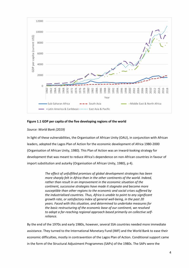
slow growth in SSA. Figure 1.1 shows the GDP per capita from the 1960s to 2018 for the five

developing sub-regions of the world.

Although the 1970s saw some growth in income per capita, this was a turbulent time for Sub Saharan

Africa and Africa as a whole. SSA nations were increasingly caught in the middle as the western and

eastern blocs sought to increase their spheres of influence. The same decade saw many of the

pioneering heads of state, including Nkrumah of Ghana, ousted in coup d’états. Governments were

saddled with large inefficient industries and farms as a result of the policies of accelerated state-led

industrialisation (including large scale mechanised state farms) pursued post-independence (Killick,

2001). Political instability, aggravated by the oil price crisis of 1973 and the debt that SSA countries

had incurred to finance projects in the preceding decades. These factors caused the near-collapse of

many SSA economies (Baah 2003).

4

Figure 1.1 GDP per capita of the five developing regions of the world

Source: World Bank (2019)

In light of these vulnerabilities, the Organisation of African Unity (OAU), in conjunction with African

leaders, adopted the Lagos Plan of Action for the economic development of Africa 1980-2000

(Organisation of African Unity, 1980). This Plan of Action was an inward-looking strategy for

development that was meant to reduce Africa's dependence on non-African countries in favour of

import substitution and autarky (Organisation of African Unity, 1980), p 4).

The effect of unfulfilled promises of global development strategies has been more sharply felt in Africa than in the other continents of the world. Indeed, rather than result in an improvement in the economic situation of the continent, successive strategies have made it stagnate and become more susceptible than other regions to the economic and social crises suffered by the industrialised countries. Thus, Africa is unable to point to any significant growth rate, or satisfactory index of general well-being, in the past 20 years. Faced with this situation, and determined to undertake measures for the basic restructuring of the economic base of our continent, we resolved to adopt a far-reaching regional approach based primarily on collective self-reliance.

By the end of the 1970s and early 1980s, however, several SSA countries needed more immediate

assistance. They turned to the International Monetary Fund (IMF) and the World Bank to ease their

economic difficulties, mostly in contravention of the Lagos Plan of Action. Conditional support came

in the form of the Structural Adjustment Programmes (SAPs) of the 1980s. The SAPs were the

0

2000

4000

6000

8000

10000

12000

19

60

19

62

19

64

19

66

19

68

19

70

19

72

19

74

19

76

19

78

19

80

19

82

19

84

19

86

19

88

19

90

19

92

19

94

19

96

19

98

20

00

20

02

20

04

20

06

20

08

20

10

20

12

20

14

20

16

20

18

Year

GD

P p

er c

apit

a (c

urr

ent

US$

)

Sub-Saharan Africa South Asia Middle East & North Africa

Latin America & Caribbean East Asia & Pacific

5

brainchild of the Washington Consensus comprising three institutions, the World Bank, the

International Monetary Fund and the United States (US) Department of Treasury. The neoliberal

ideologies of the Washington Consensus shaped the predominant economic policies of developing

countries, which were heavily dependent on foreign aid and foreign direct investment. These policies

then informed the structural adjustment programmes in developing countries based on 10 points of

reform: fiscal discipline, pro-growth expenditure, interest rate and exchange rate liberalisation,

privatisation of state-owned enterprises, deregulation, and property rights (Williamson, 2008). In

essence, the SAPs were a suite of programmes implemented to drastically reduce the size and scope

of governments in the participating countries (United Nations, 2017). The neoliberal principles

underpinning the SAPs were consistent with the dominant economic thought of that era, e.g., the

supply-side economics of the Reagan administration in the United States of America and the

Thatcher government in the United Kingdom. The laissez-faire approach initiated through the SAPs

was a radical departure from the statist approach of African governments in the preceding decades

(Killick, Malik & Manuel, 1992). The retrenchment of public sector staff and the privatisation of

parastatals led to increased unemployment and has been widely criticised for many of the economic

difficulties encountered by countries in SSA (Killick et al., 1992).

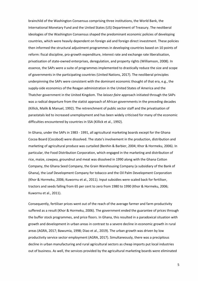
In Ghana, under the SAPs in 1983 - 1991, all agricultural marketing boards except for the Ghana

Cocoa Board (Cocobod) were dissolved. The state's involvement in the production, distribution and

marketing of agricultural produce was curtailed (Benhin & Barbier, 2004; Khor & Hormeku, 2006). In

particular, the Food Distribution Corporation, which engaged in the marketing and distribution of

rice, maize, cowpea, groundnut and meat was dissolved in 1990 along with the Ghana Cotton

Company, the Ghana Seed Company, the Grain Warehousing Company (a subsidiary of the Bank of

Ghana), the Leaf Development Company for tobacco and the Oil Palm Development Corporation

(Khor & Hormeku, 2006; Kuwornu et al., 2011). Input subsidies were scaled back for fertiliser,

tractors and seeds falling from 65 per cent to zero from 1980 to 1990 (Khor & Hormeku, 2006;

Kuwornu et al., 2011).

Consequently, fertiliser prices went out of the reach of the average farmer and farm productivity

suffered as a result (Khor & Hormeku, 2006). The government ended the guarantee of prices through

the buffer stock programmes, and price floors. In Ghana, this resulted in a paradoxical situation with

growth and development in urban areas in contrast to a severe decline in economic growth in rural

areas (AGRA, 2017; Bawumia, 1998; Diao et al., 2019). The urban growth was driven by low

productivity service sector employment (AGRA, 2017). Simultaneously, there was a precipitous

decline in urban manufacturing and rural agricultural sectors as cheap imports put local industries

out of business. As well, the services provided by the agricultural marketing boards were eliminated

6

and never replaced. As a result, Ghana's production of agricultural products like tobacco, coffee, oil

palm and rubber nearly disappeared (Houssou et al., 2018).

Contrary to the initial assumptions of the SAPs, the private sector did not respond to the void created

by market liberalisation. For instance, the void left by the removal of the monopsonist powers of the

agricultural marketing boards were not filled readily (Barrett & Mutambatsere, 2005). As a result, the

ancillary services that marketing boards previously provided to farmers, short-term credit and input

subsidies, were curtailed. In their absence, farmers were exposed to market volatility because

surpluses and shortages were no longer being smoothed out by the marketing boards (Barrett &

Mutambatsere, 2005; Kuwornu et al., 2011). Other agricultural services that suffered as a result of

the SAPs included extension services, agricultural research and rural banking. These institutions

played an integral role in the production of tree and plantation crops like cocoa, coffee and para

rubber (Nyemeck, Gockowski & Nkamleu, 2007; Wilcox & Abbott, 2006). The absence of subsidies for

fungicides, herbicides, fertilisers, and technical training in the years following liberalisation resulted

in declining yields. It increased revenue volatility for producers, particularly for the rural poor who

live on marginal land susceptible to weather and yield variability (Nyemeck et al., 2007). Despite

multiple rounds of structural adjustment programmes in 12 SSA countries from 1980 -2000, on the

whole, economic growth in the region did not respond for close to two decades as shown in Figure

1.1 (Easterly, 2005).

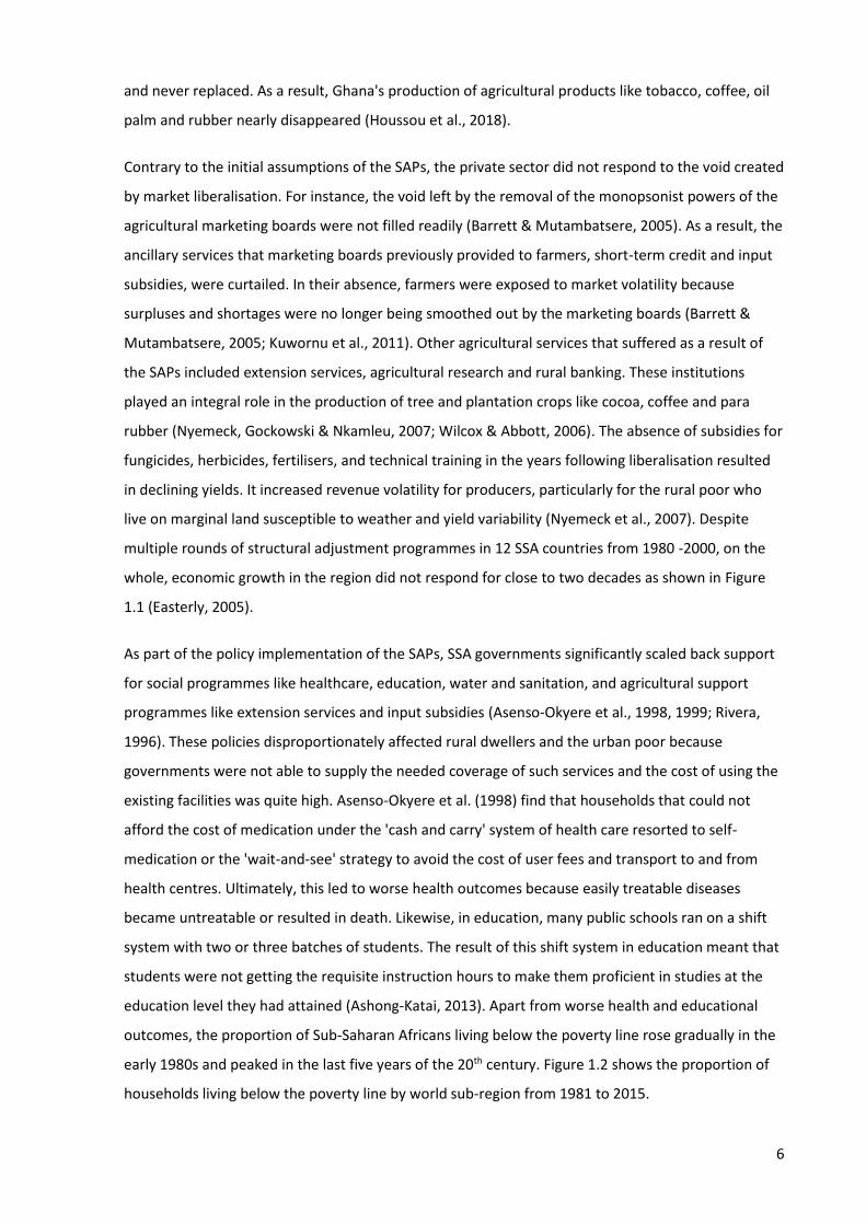
As part of the policy implementation of the SAPs, SSA governments significantly scaled back support

for social programmes like healthcare, education, water and sanitation, and agricultural support

programmes like extension services and input subsidies (Asenso-Okyere et al., 1998, 1999; Rivera,

1996). These policies disproportionately affected rural dwellers and the urban poor because

governments were not able to supply the needed coverage of such services and the cost of using the

existing facilities was quite high. Asenso-Okyere et al. (1998) find that households that could not

afford the cost of medication under the 'cash and carry' system of health care resorted to self-

medication or the 'wait-and-see' strategy to avoid the cost of user fees and transport to and from

health centres. Ultimately, this led to worse health outcomes because easily treatable diseases

became untreatable or resulted in death. Likewise, in education, many public schools ran on a shift

system with two or three batches of students. The result of this shift system in education meant that

students were not getting the requisite instruction hours to make them proficient in studies at the

education level they had attained (Ashong-Katai, 2013). Apart from worse health and educational

outcomes, the proportion of Sub-Saharan Africans living below the poverty line rose gradually in the

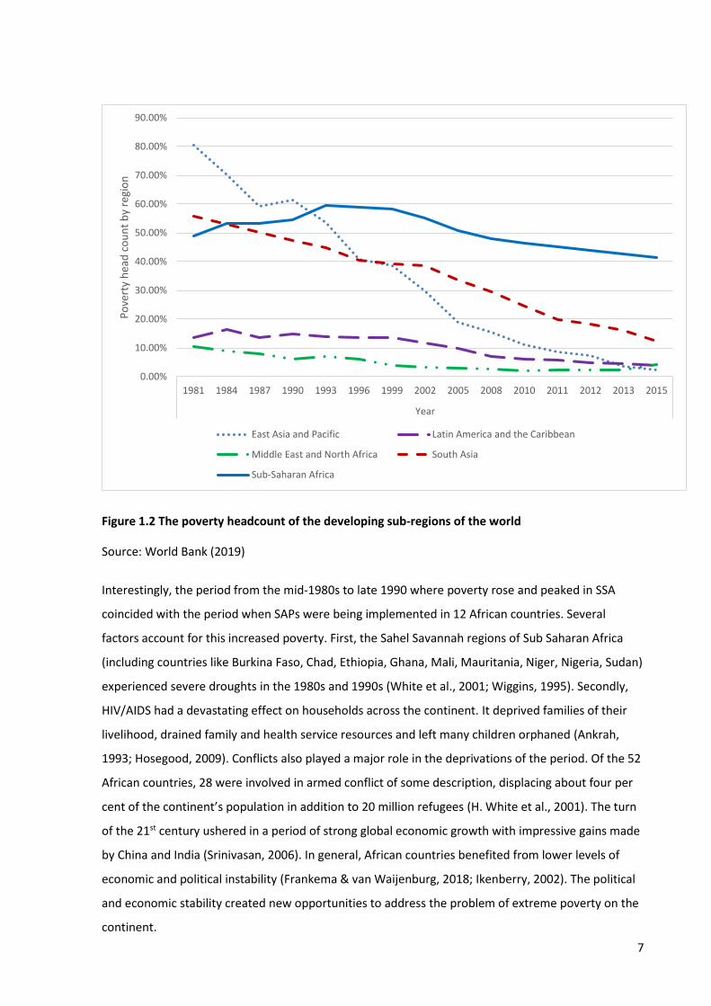
early 1980s and peaked in the last five years of the 20th century. Figure 1.2 shows the proportion of

households living below the poverty line by world sub-region from 1981 to 2015.

7

Figure 1.2 The poverty headcount of the developing sub-regions of the world

Source: World Bank (2019)

Interestingly, the period from the mid-1980s to late 1990 where poverty rose and peaked in SSA

coincided with the period when SAPs were being implemented in 12 African countries. Several

factors account for this increased poverty. First, the Sahel Savannah regions of Sub Saharan Africa

(including countries like Burkina Faso, Chad, Ethiopia, Ghana, Mali, Mauritania, Niger, Nigeria, Sudan)

experienced severe droughts in the 1980s and 1990s (White et al., 2001; Wiggins, 1995). Secondly,

HIV/AIDS had a devastating effect on households across the continent. It deprived families of their

livelihood, drained family and health service resources and left many children orphaned (Ankrah,

1993; Hosegood, 2009). Conflicts also played a major role in the deprivations of the period. Of the 52

African countries, 28 were involved in armed conflict of some description, displacing about four per

cent of the continent’s population in addition to 20 million refugees (H. White et al., 2001). The turn

of the 21st century ushered in a period of strong global economic growth with impressive gains made

by China and India (Srinivasan, 2006). In general, African countries benefited from lower levels of

economic and political instability (Frankema & van Waijenburg, 2018; Ikenberry, 2002). The political

and economic stability created new opportunities to address the problem of extreme poverty on the

continent.

0.00%

10.00%

20.00%

30.00%

40.00%

50.00%

60.00%

70.00%

80.00%

90.00%

1981 1984 1987 1990 1993 1996 1999 2002 2005 2008 2010 2011 2012 2013 2015

Year

Po

vert

y h

ead

co

un

t b

y re

gio

n

East Asia and Pacific Latin America and the Caribbean

Middle East and North Africa South Asia

Sub-Saharan Africa

8

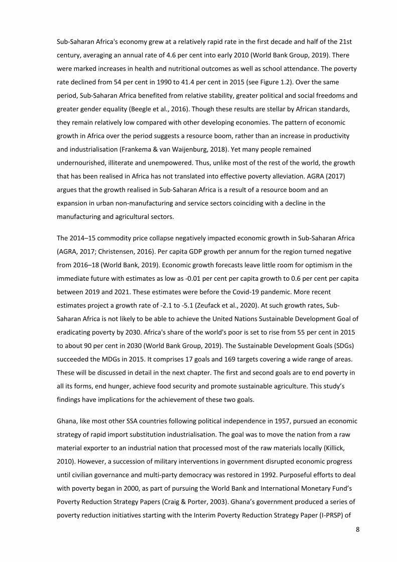
Sub-Saharan Africa's economy grew at a relatively rapid rate in the first decade and half of the 21st

century, averaging an annual rate of 4.6 per cent into early 2010 (World Bank Group, 2019). There

were marked increases in health and nutritional outcomes as well as school attendance. The poverty

rate declined from 54 per cent in 1990 to 41.4 per cent in 2015 (see Figure 1.2). Over the same

period, Sub-Saharan Africa benefited from relative stability, greater political and social freedoms and

greater gender equality (Beegle et al., 2016). Though these results are stellar by African standards,

they remain relatively low compared with other developing economies. The pattern of economic

growth in Africa over the period suggests a resource boom, rather than an increase in productivity

and industrialisation (Frankema & van Waijenburg, 2018). Yet many people remained

undernourished, illiterate and unempowered. Thus, unlike most of the rest of the world, the growth

that has been realised in Africa has not translated into effective poverty alleviation. AGRA (2017)

argues that the growth realised in Sub-Saharan Africa is a result of a resource boom and an

expansion in urban non-manufacturing and service sectors coinciding with a decline in the

manufacturing and agricultural sectors.

The 2014–15 commodity price collapse negatively impacted economic growth in Sub-Saharan Africa

(AGRA, 2017; Christensen, 2016). Per capita GDP growth per annum for the region turned negative

from 2016–18 (World Bank, 2019). Economic growth forecasts leave little room for optimism in the

immediate future with estimates as low as -0.01 per cent per capita growth to 0.6 per cent per capita

between 2019 and 2021. These estimates were before the Covid-19 pandemic. More recent

estimates project a growth rate of -2.1 to -5.1 (Zeufack et al., 2020). At such growth rates, Sub-

Saharan Africa is not likely to be able to achieve the United Nations Sustainable Development Goal of

eradicating poverty by 2030. Africa's share of the world's poor is set to rise from 55 per cent in 2015

to about 90 per cent in 2030 (World Bank Group, 2019). The Sustainable Development Goals (SDGs)

succeeded the MDGs in 2015. It comprises 17 goals and 169 targets covering a wide range of areas.

These will be discussed in detail in the next chapter. The first and second goals are to end poverty in

all its forms, end hunger, achieve food security and promote sustainable agriculture. This study’s

findings have implications for the achievement of these two goals.

Ghana, like most other SSA countries following political independence in 1957, pursued an economic

strategy of rapid import substitution industrialisation. The goal was to move the nation from a raw

material exporter to an industrial nation that processed most of the raw materials locally (Killick,

2010). However, a succession of military interventions in government disrupted economic progress

until civilian governance and multi-party democracy was restored in 1992. Purposeful efforts to deal

with poverty began in 2000, as part of pursuing the World Bank and International Monetary Fund’s

Poverty Reduction Strategy Papers (Craig & Porter, 2003). Ghana’s government produced a series of

poverty reduction initiatives starting with the Interim Poverty Reduction Strategy Paper (I-PRSP) of

9

2000-2002. This was followed by the Ghana Poverty Reduction Strategy I (GPRS I) for 2003-2005. The

third initiative was GPRS II (2006-2009). These policies helped to grow Ghana's economy at an

average annual rate of 5.8 per cent, and the country achieved lower-middle-income status in 2010

(National Development Planning Commission, 2014).

The country’s economic growth pattern after the structural adjustment programmes (1984 – 1990) is

like that described by Gollin, Jedwab and Vollrath (2016) as 'urbanisation without industrialisation'.

Under this development model, rents from the export of natural resources fuel urbanisation through

service sector employment. AGRA (2017) argues that this development model does not foster

employment and poverty reduction. As a result, people in rural areas remained largely poor. The

Medium-Term National Development Policy Framework: Ghana Shared Growth Development

Agenda (GSGDA) 2010-2013 was conceived to correct this anomaly by promoting more participatory

growth throughout the country (National Development Planning Commission, 2010). Meanwhile, in a

bid to address the high rate of poverty in the northern part of Ghana, the government set up the

Savannah Accelerated Development Authority (SADA) with a mandate to accelerate development in

the savannah zone of Ghana covering the five northern regions and some areas in the Volta and

Brong Ahafo regions (Cao, 2017).

Many interventions have been undertaken under these strategies and programmes over the years,

particularly to modernise agriculture, diversify household livelihood strategies, in some cases to

promote high-value cash crops to foster local economic growth in the rural economy. However, little

concrete information has been generated about the gains of these programmes to farm households

and Ghana’s economic development in general. The MVP implemented similar agricultural

interventions in the villages where it was implemented. It, therefore, provides an opportunity to

evaluate the impact of such programmes on farm households.

The MVP is arguably the most high profile development project of the 21st century. It is at the nexus

of a wide range of debates in development economics and development studies. Some of the

questions raised are detailed in Table 1.1. The topics in Table 1.1 are interesting questions arising

from MVP. The topics are not the research questions of this study. However, the research problem

and objectives discussed in the next two sections will address some of these questions to determine

the impact of MVP on farm households in Bonsaaso. Chapter 2 will discuss in detail some of the

salient questions relevant to the impact of the MVP on farm households in Bonsaaso, Ghana.

10

Table 1.1 General questions raised by the Millennium Villages Project

1. What is development, and how is it conceptualised and practised? (Sachs, 2010; Todaro & Smith, 2012; United Nations, 2000)

2. What is the poverty trap, and does it explain the persistent deprivation and poverty in the developing world? (Barrett, Carter & Chavas 2018; Carter & Barrett, 2009; Kraay & McKenzie, 2007; Nurkse, 1971)

3. Is development assistance beneficial for development and does it help eradicate poverty? (Dichter, 2005; Easterly, 2009; Moyo, 2009; Sachs, 2005)

4. Sachs (2005) adapted the well-established, macro-level 'big push' of Rosenstein-Rodan (1947) to a village level development project. Under such a project, large volumes of resources (financial and material) are concentrated in an area to engender development and structural transformation. Are such village or community level 'big push' programmes more effective than targeted programmes in eradicating poverty? (Banerjee and Duflo, 2011; Collier, 2007, 2010; Rosenstein-Rodan 1947, 1953; Sachs, 2005)

5. Do integrated development programmes that incorporate synergies and complementarities between different sectors of the economy yield more benefit than single-sector focused programmes? (Barnett, 2018; Burke, Chen & Brown, 2018; Herdt, 2010; Jupp, Korboe & Dogbe, 2018; Ruttan, 1984; Sachs, 2005)

6. Can agriculture be an instrument for stimulating growth and development? (Delgado et al., 1994; Haggblade et al., 1991; Mellor, 1999)

7. What is the best way to evaluate long-term development projects administered at the community level without random assignment? Is it even possible to identify the impact of such a project? (Clemens & Demombynes, 2010; Masset et al., 2014; Mitchell et al., 2015a, 2015b, 2015c; Pronyk et al., 2012)

In summary, this section discussed the historical background to economic development in Sub-

Saharan Africa in general and Ghana specifically. Some development strategies and policies that have

been implemented post-independence have been highlighted, as well as the economic performance

and rate of poverty of the sub-regions over time.

Collier (2007) highlights four traps that account for the plight of the poorest quintile in the world.

The first is conflict and wars. Second is natural resource traps, which cause conflicts as various

factions strive to capture the rents from the resources. Additionally, natural resources tend to crowd

out alternative export activities in the manufacturing, service and agricultural sectors that can grow

the economy, a phenomenon called “Dutch disease”. Thirdly, geography, particularly for landlocked

countries in Africa that tend to be poor because, often, neighbouring countries are neither conducive

markets nor equipped with the right infrastructure and institutions to facilitate the export of goods

from landlocked countries. Lastly, bad governance is a problem. These are like Sachs’ (2005) view of

the cause of poverty: conflict, geography and isolation. Many SSA countries have experienced these

problems in the past 60 years, resulting in the widespread poverty currently prevalent across the

sub-region. Over the years, many efforts and programmes have been initiated across Africa to

encourage economic growth and development, and in recent times, to end poverty. These

11

programmes include industrialisation, integrated rural development, structural adjustment, debt

forgiveness and poverty reduction strategies. Many of these programmes took place when there was

significant unrest across the sub-region. Since the early 2000s, however, the number of conflicts in

the sub-region have declined significantly; this also coincided with the Millennium Declaration and

the MDGs. These provided an opportunity to deal with the problems of poverty and deprivation. One

programme that sought to do so was the Millennium Villages Project. The next section defines the

research question followed by the problem statement.

Problem statement

In Ghana, there were two Millennium Village sites. The first in Ghana was the Bonsaaso MVP village,

which targeted 30 communities in the Amansie West District of the Ashanti Region. This project was

initiated in 2006 and ended in 2015. The MVP was implemented by the UNDP and the Millennium

Promise Alliance Inc., an international non-governmental organisation (NGO) founded by Jeffery

Sachs and Ray Chambers to implement the model of development explained in Sachs (2005). The

second MVP in Ghana, the Northern Ghana MVP, was established in 2012 with funding from the

Ghana government through SADA (the government agency mandated to accelerate the development

of the savannah zone) and the UK Department for International Development (DFID) (Masset et al.,

2014). The Northern Ghana MVP was implemented by SADA and the Millennium Promise Alliance

Inc. in the Builsa district of the Upper East Region and the West Mamprusi district of the Northern

Region of Ghana. In the run-up to the Presidential and Parliamentary elections in December 2012,

each of these districts was split into two districts to give better representation to their relatively large

population and geographic area. The Builsa district was divided into Builsa North and Builsa South

while the West Mamprusi was divided into West Mamprusi and Mamprugu Muagduri. These more

recent MVPs will be referred to as the Northern Ghana MVP in contrast to the Bonsaaso MVP. The

Northern Ghana MVP was implemented in all four districts, reaching 3,900 households (27,000

people) living in 34 communities. The Bonsaaso MVP covered 6,500 households with a population of

approximately 35,000 people (Mitchell et al., 2015). Small scale mining and cocoa farming are the

main economic activities in the Amansie West District where the Bonsaaso MVP is located. Farming

alone is the main economic activity in the Northern Ghana MVP area.

The Northern Ghana MVP was explicitly designed to allow an independent impact evaluation

following controversies that emerged over the mid-line impact evaluation of the other 14 MVPs in

Africa (Masset et al., 2013; Masset et al., 2014; Masset, García-Hombrados & Acharya, 2020; Pronyk,

2012; Pronyk et al., 2012). There was public controversy over portions of the results published by

Pronyk et al. (2012) in which the authors compared analyses from different periods: the MVP villages

from 2006 to 2009 with rural communities in Ghana from 2001 to 2010. There was also a slight error

12

in the calculation of the rate of decline in under-5 mortality. These errors were outlined in Pronyk

(2012) and by the Editors of The Lancet (2012). Clemens and Demombynes (2010) critiqued the MVP

design and some of the preliminary results published by the implementors. They proposed more

rigorous methods to assess the impact of the MVP. In response, to these controversies, the

Department for International Development (DfID) of the United Kingdom (UK) provided funding for

the creation of an MVP in a manner that permitted a rigorous impact evaluation. The fourth issue of

the Institute of Development Studies (IDS) Bulletin volume 49 was dedicated to the strategy used to

estimate the impact of the SADA MVP and the lessons learnt in evaluating it (Barnett, 2018). The

SADA MVP of Northern Ghana was scheduled to end in 2016 but was still being implemented at the

time this study began in April 2016. Therefore, this study focussed only on the Bonsaaso MVP.

MVPs, in general, were developed as an integrated multi-sector approach to rural development

aimed at providing a pathway towards achieving the MDGs and reaching self-sustained economic

development cost-effectively and fruitfully. It used a 'bottom-up approach to lifting developing

country villages out of the poverty trap' (Cabral, Farrington & Ludi, 2006). Its interventions were

mainly inspired by the 'big push' approach to development. However, aspects of the 'selectivity and

conditionality', and the 'incremental change' approaches were also incorporated into the project.

Many investments were made in infrastructure, health, education, agriculture and business

development under the MVP. Farmers were given training in a range of agricultural activities, and the

programme facilitated farmers' access to credit and yield-enhancing technologies such as improved

seeds, fertiliser, and market access for their farm produce. These interventions were delivered at

USD 120 per person per year for ten years, in 2005 dollars. Agricultural sector interventions

constituted about 18 per cent of the cost of the MVP. However, no study to date has assessed the

impact of the MVP on the economic and financial impacts on the farming households who are the

beneficiaries of those agricultural interventions.

The MVP was an integrated rural development programme. These are development interventions

implemented across different sectors to take advantage of positive interactions between

interventions in different sectors. Integrated rural development programmes were popular in the

1960s. However, this popularity waned over time due to their complexity in implementation, cost,

and inconclusive evidence of their impact (Herdt, 2010; Ruttan, 1984). MVP in particular leveraged

the agricultural sector for economic growth in the local economy. This sector is the main source of

livelihood, employment and income for households in rural Ghana. It also generates local economic

growth by stimulating demand through its forward and backward linkages, most importantly, the

forward linkage for local non-tradable goods, the demand for which cannot be stimulated from

outside the local economy. Despite the importance of agriculture to the local economy and the

prominence of agricultural interventions in the MVP, the agricultural outcomes reported in Mitchell

13

et al. (2018) are too aggregated to provide a meaningful picture of the impact on the sector. This

calls for a granular assessment at the household level and provides the rationale for this

investigation. 'Big push' projects tend to be costly, complex and challenging to implement (Collier,

2006). As such, positive outcomes and returns are required to justify their funding by policymakers

and donors. Therefore, to justify the high cost of the MVP, a substantial return is required. Also, the

long duration over which the MVP was implemented poses an interesting challenge for impact

assessment.

Research objectives and questions

The main objective of this study is to assess the economic and financial impact of the MVP on farm

households in Bonsaaso, Ghana.

The specific research questions to be addressed are:

1. What are the differences in financial and economic conditions between MVP and non-MVP

households?

2. What were the impacts of the Bonsasso MVP on the value of assets, farm produce, net farm

income and farm expenditure of agricultural households?

3. How sustainable are the agricultural interventions of the MVP?

Contribution of the study

The MVP had its origin mainly in the 'big push' approach. Although agricultural development was not

explicitly targeted as part of the MDGs, the MVP project recognised the role of farm income as an

appropriate driver of broad-based economic growth in poor regions endowed with agricultural

resources (Delgado et al., 1994; Haggblade & Hazell, 1989). The first MVPs have run their 10-year

course, but their impact on farm income and other farm household outcomes remains largely

unknown. Wanjala and Muradian (2013) investigated the impact of the Sauri MVP on productivity,

household consumption of farm produce and household income. That study was conducted midway

through the project and not at the end of the project. It is expected that farmers continue to learn,

benefit and improve their household outcomes as the project continued. Only an end-line impact

assessment will shed light on the MVP's true impact on farm households.

Mitchell et al. (2018) conducted an end-line study that examined MVP’s impact on the adoption of

improved seeds and chemical fertiliser. This was a meta-analysis of the earliest MVPs in Africa, but,

since MDG targets do not include any agricultural outcomes, Mitchell et al. (2018) and Masset,

García-Hombrados & Acharya (2020) did not report the impact of the MVP on agricultural outcomes

at the household level. To date, no studies have reported end-line impacts of MVPs on farm produce,

14

expenditure, income and asset accumulation at the household level. As MVP interventions were

designed to leverage the agricultural sector to drive the local economy, this represents a serious gap

in the academic literature and policy discourse. As the policymakers in Ghana need to make informed

decisions about the effective use of development assistance, this investigation provides crucial

insights on how the agricultural interventions under Bonsaaso MVP provided productivity-enhancing

opportunities in an area where households are poor and rely heavily on farming.

Over the years several interventions have been implemented in an attempt to alleviate the plight of

the poor; however, poverty persists in Africa. The subject has received attention with the poverty

reduction papers of the world bank and IMF in the 2000s, the Millennium Development Goals and

the Sustainable Development Goals (SDGs). Lastly, the study makes a methodological contribution to

the field of impact assessment by modifying the standard treatment model to account for the MVPs’

long duration and sequenced interventions by allowing intermediate outcomes to influence the

project's end-line outcomes.

Organisation of the thesis

This thesis comprises eight chapters. Following this introductory chapter, Chapter 2 reviews the

literature relevant to this study. It starts with the concept and definition of development and how it

has evolved over the post-war period, culminating in the Millennium Development Goals and

Sustainable Development Goals, which inspired the MVP. The chapter then discusses the mechanism

through which agriculture-led intervention and strategies lead to development. Followed by a

discussion of the poverty trap, the underlying theoretical assumption underlying the MVP and

approaches to development assistance. Chapter 3 describes the specific methods used in this study

to assess the impact of the MVP. Chapter 4 presents the descriptive statistics that discuss the

statistical significance of the difference in financial and socioeconomic conditions in MVP and non-

MVP households. Chapter 5 presents the average treatment effect estimates of MVP's impact at the

household level and the results of the robustness check using the recursive instrumental variables

model. Chapter 6 assesses the sustainability of the MVP’s agricultural interventions based on MVP

participants views of the changes from the MVP. Chapter 7 discusses the study’s results and the

thesis ends with the summary, conclusions and recommendations in Chapter 8.

15

Chapter 2

Literature Review

Introduction

As outlined in Chapter 1, the study seeks to assess the economic and financial impact of the MVP on

farm households in Bonsaaso, Ghana. The MVP was designed to assist rural households in Africa to

achieve the Millennium Development Goals. This chapter will trace the origins and design of the

MVP, the mechanism by which its agricultural sector interventions lead to wider development and

the measures needed to determine the effects. This review begins by tracing the evolution of the

concept of development that led to the global consensus on the implementation of the Millennium

Development Goals in 2000 and the Sustainable Development Goals in 2015. The review then

discusses the dissenting view of development - the post-development - in Section 2.2.3. Section 2.5

discusses the role that agriculture plays in an agriculture-centred economic development strategy for

low and lower-middle-income regions like South Asia and Sub-Saharan Africa. The theory of the

poverty trap, which MVP was designed to break, is discussed in Section 2.3. Section 2.5 discusses the

definition and history of development assistance and alternative approaches to the use of

development assistance for economic development and the sorts of programmes that each of these

approaches advocates. This is because Sachs (2004) advocates the use of development assistance to

provide a ‘big push’ for development. MVP is premised on the notion that development assistance is

essential to break the poverty cycle.

Concept and definition of development

Todaro and Smith (2012) defined development as “the process of improving the quality of all human

lives and capabilities by raising people's levels of living, self-esteem, and freedom” (p. 5). Yet through

the decades, development has been conceptualised and operationalised in a variety of ways ranging

from the income growth approach of the early 1950s to the capability approach by Nobel Laureate

Amartya Sen that has informed the human development reports of the United Nations (UN) since the

1990s. This section explores the historical background of the concept of development in the post-war

period. Three main concepts were used to characterise development in the 1950s –income growth,

human development and post-development. Although development has been the dominant

international agenda since the second half of the 20th century, there is no standard accepted

definition for the term agreed by all disciplines, be they economic, sociological or development

studies. Nevertheless, there are certain widely accepted components of the concept of development.

These include raising the standard and quality of life of the population; the creation and expansion of

16

aggregate income and employment; the expansion of opportunities for human beings to reach their

fullest potential; and doing all these without causing irreparable damage to the environment

(Aghion, Akcigit & Howitt, 2014; Srinivasan, 1988).

Income growth

By and large, development is visible, although it is difficult to fully describe it verbally. In the early

decades of the post World War II period, the main focus for all countries was economic growth and

development, defined in terms of growth in income per capita. This framework had intuitive appeal

since a society, household or a person's standard of living is influenced, to a large extent, by their

command over material goods and services that, in turn, are influenced by the amount of money

they possess (Sen, 1988). Sustained rates of economic growth, especially when such growth exceeds

the rate of population growth and is accompanied by structural transformation of the economy from

a predominantly agrarian to an industrialised economy, was the dominant view of economic

development. Consequently, the earliest work and writing in development focussed on

industrialisation, increasing employment, and structural transformation from less efficient agrarian

systems to industrialised economies (Overseas Development Institute, 1978). As a result, this period

has been described as the era of modernisation or development-as-growth (Kendall, Linden &

Murray, 2005).

The primary measure in the income growth approach is per capita income as a proxy for standard of

living and development. This is, however, problematic for several reasons. Economic growth defined

as the rate of change in per capita income does not account for variations in wealth. GDP per capita,

in particular, does not account for international income flows such as remittances (which, by various

accounts, are major contributors to economic growth and well-being (Ajayi et al, 2009; Ziesemer,

2012). Similarly, income per capita does not account for non-market traded goods and services such

as those produced in the household (like care of children) nor externalities in the production of

goods and services. Furthermore, the value of goods and services is arbitrary, reflecting the biases of

market participants (Fleurbaey & Gaulier, 2009). Also, income per capita reflects well-being at a

particular time without accounting for the entire span of an individual's life. For these reasons,

income per capita, at best, measures the means by which individuals can achieve a variety of ends

that ensure their well-being (Sen, 1988). More importantly, income per capita does not measure the

quality of social relationships in society, economic security, personal safety, health and longevity

(Sen, 2001).

17

Human development

Among other reasons, the shortcomings of the income growth approach to defining development led

to a call for a reconsideration of how development is perceived and measured. The Cocoyac

declaration of 1974 was a statement by a group of social and natural scientists who advocated at a

United Nations Seminar for a reorientation of development towards people because the basic needs

of people across the world were not being met through economic growth (Cocoyac, 1974). Their call

was for economic growth to improve the conditions for the poorest in society (Cocoyac, 1974). They

argued in 1974 that economic growth increased the disparities between the rich and the poor

qualified as exploitation rather than development (Cocoyac, 1974). About a year later, a group from

the Dag Hammarskjold Foundation argued for the importance of political, psychological and physical

needs in development at the seventh special session of the United Nations (Dag Hammarskjold

Foundation, 1975; Overseas Development Institute, 1978). The result of these calls materialised in

1976 with the adoption of the Basic Needs working paper by the World Employment Conference of

the International Labour Organisation (Streeten et al., 1981). The evolution of the human

development approach continued with Sen's (1988) capability approach.

2.1.2.1 Basic needs

Streeten (1979), the strongest proponent of the basic needs approach, noted that the pattern of

growth in the first quarter-century of the post-WW II era showed that though the world economy, in

general, grew at an unprecedented rate, this growth was not accompanied by a reduction in poverty

or increased employment. Furthermore, redistributive policies failed to ensure the spreading of

wealth to the poor (Hicks & Streeten, 1979; Streeten, 1979). An account of this divergence between

the development trajectory of developed countries and developing countries concerning

employment showed that there were differences in living conditions, attitudes and institutions. First,

nutrition, health and education, which are important factors for full labour force utilisation, tend to

be lacking or deficient in developing countries. Though these may be viewed as consumption goods

in developed countries, they are better categorised as investment goods in developing countries

because they are necessary for production (Sen, 1988; Stewart, 1985; Streeten, 1979).

Although earlier discussions of development were concerned with deprivation, they saw economic

growth as the instrument for achieving the goal of eradicating deprivation (Sen, 1988). However, the

economic growth of Africa, Asia and Latin America in the 1960s did not result in a decrease in the

poverty and unemployment levels, contrary to the prevailing orthodoxy (Overseas Development

Institute, 1978). Because of the unequal distribution of assets and income, as well as other barriers,

economic growth gains that occurred tended to concentrate with the rich (Streeten, 1982).

18

The basic needs approach was introduced in the 1970s following a period of modernisation as a way

of dealing with mass deprivation. Streeten (1979) describes the evolution of the discourse from

growth in income per capita to basic needs as a logical progression of development thought and

approaches. The basic needs approach sought to improve income-earning opportunities for the poor;

improve public services and utilities; ensure the flow of goods and services met the needs of the

poor; and promote the poor’s political participation to ensure their interests were represented

(Overseas Development Institute, 1978).

Streeten (1979) argues that in developing countries most members of the typical household are

unable to work and earn an income because of infirmity, disability, age, and orphaned children. Of

particular concern were the ’working poor‘, who, though technically employed, worked long hours in

unremunerated and unproductive self-employed activities or employment by family members. As a

result, the basic needs approach was proposed as a progression of the development paradigm that

emphasised meeting human basic needs like health, food, education, shelter, water, transport and

household goods. ODI (1978) and Streeten et al. (1981) stress that addressing the basic needs of

developing nations will result in improvements in other aspects of development, such as urban drift,

the environment, equality, rural development and industrialisation.

At the micro-level, the basic needs approach improves on the preceding income growth approach in

many regards. First, evidence from expenditure patterns of subsistence farmers showed that

increases in income from shifts to cash crops and dairy production resulted in the consumption of

less nutritious food and non-food items (Streeten, 1981). Thus, such increases in income do not

necessarily result in increased human wellbeing, mainly pertaining to nutritional and health

outcomes. However, a focus on basic needs ensures that the household is not adversely affected.

Furthermore, income increases often accrue to male household heads of families (Streeten, 1981).

The expenditure patterns of male household heads do not necessarily meet the needs of other

household members, particularly women and children (Dei, 1994). Unemployable members are also

left out in the income approach (Streeten et al., 1981). Lastly, increases in personal income,

regardless of the magnitude of such increases, are not sufficient to meet certain life necessities, such

as health facilities, safe water, education, sewerage, electricity and public infrastructure, which are

most efficiently provided publicly (Sen, 1988). The basic needs approach achieves the widely

accepted, high priority objectives economically, rather than taking the route of raising employment

and income (in some instances redistributing the earned income) before waiting to achieve people’s

basic needs (ODI, 1978).

19

2.1.2.2 Capability approach

The capability approach to human development was a further evolution of the concept of

development because of deficiencies in the income-based approach of early development theorists

and the consumption-based approach of the Basic Needs approach of the 1970s. The capability

approach was conceptualised by Sen (1979) and has since gained increasing prominence in a wide

range of fields including public health (Anand, 2005; Davidson et al., 2009; Venkatapuram, 2013),

development ethics, education (Flores-Crespo, 2007; Walker, 2005; Walker & Unterhalter, 2007),

welfare economics (Alkire, 2005b; Kaushik & Lòpez-Calva, 2011) poverty indicators (Alkire, 2005c),

and social science (Anderson, 1999; Basu & Lòpez-Calva, 2011; Fukuda-Parr, 2003; Nussbaum, 2001;

Robeyns, 2017). Nevertheless, the greatest influence of the capability approach is arguably in

development studies and development economics where it has helped shape the definition of the

term development and how it is conceived in ‘human terms’ (Fukuda-Parr, 2003; Haq, 1995). It has

also influenced the UNDP’s Human Development Report from 1990 to date and the Human

Development Index (HDI) measure of development (United Nations Development Programme, 1990).

The capability approach draws on ideas from Aristotle and Adam Smith (Sen, 1979). From Aristotle,

wealth is not the good that people seek; it is only instrumental for other ends:

“The life of making money is a life people are, as it were, forced into, and wealth is clearly not the good we seek, since it is merely useful for getting something else. One would be better off seeing as ends the things mentioned before, because they are valued for themselves”. (Aristotle, trans, 2004 p. 1096a).

Since wealth is not valued for its own sake but merely as an instrument to other ends, Aristotle

viewed wealth, not as an end in itself. Therefore, the measurement of progress by changes in

aggregate national income is problematic. Sen (1979), referring to Adam Smith, drew on the idea of

conditions and necessities of living that are deemed as indispensable for a dignified life by any group

of people. The capability approach conceptualises human well-being as comprising various beings

and doings called ‘functionings’ (Sen, 1979). Examples of functionings include, but are not limited to,

being nourished compared with being undernourished, being adequately housed compared with

being homeless, being educated compared with being illiterate, being part of a supportive social

network compared with being isolated, or being depressed compared with enjoying a balanced life

(Sen, 1988). Commodities, income and wealth, which are the primary measures of well-being in the

income centred approach, are means by which functionings are achieved, although not exclusively.

Though many functionings can be achieved with commodities, a myriad of other functionings exist

that cannot be achieved with them. For this reason, even though income is pertinent for achieving

some functionings, it cannot achieve all functionings necessary for human well-being and flourishing

(Sen, 1988; Nussbaum, 2003).

20

The capability approach, rather than providing a unified theory of development, serves as a

conceptual framework for assessing the well-being of individuals, evaluating social arrangements and

institutions under which people live, and design policies and proposals to effect social change of

existing systems (Robeyns, 2016, 2017; Sen, 2001). The capability approach takes a wholistic view

and treats, as a priority, the opportunities and freedoms that individuals have to achieve the

functionings that they deem valuable. These freedoms and opportunities are defined as capabilities

and are in contrast to subjective standards or externally imposed categories such as income,

consumption or wealth. As such, whereas the income growth approach or the basic needs approach

define poverty as a deprivation of income or consumption below a given threshold, the capability

approach, on the other hand, defines poverty in terms of deprivation of opportunities (capability) to

fulfil certain functionings that an individual values (Fukuda-Parr, 2003, 2003; Robeyns, 2016; Sen,

1988). The capability approach explores whether people, for instance, can live healthy lives, but goes

further to assess whether the means and resources necessary for healthy living are available, such as

clean water, adequate sanitation, adequate access to health care, knowledge of health issues and

safety from infections. Likewise, to fulfil the functioning of political participation may require

relatively informed populations with a requisite education to allow them to decipher information

(Sen, 1988).

This focus on the ends of human functionings differentiates the capability approach from the

traditional method of measuring development in economic growth rate terms and other concepts of

development and social justice on how human well-being is achieved. The capability approach entails

not only the commodities that an individual owns to fulfil their functionings but also the availability

of public goods and services and the freedom to use private goods personally supplied or provided by

the state (Sen, 1988, 2001). Perhaps, the most important factor in the capability approach, according

to Sen (1988), is the value of ‘freedom of choice’, which is reflected in the nature and range of

capability sets available to the individual and the latitude to choose from those capability sets.

The basic needs approach to development discussed in the previous section and the capability

approach discussed in this section together constitute the human development approach to

development (Alkire, 2002). The two approaches have been influential in charting the course of

international development, particularly since the launch of the United Nations (UN) Human

Development Reports in 1990. UNDP (1990) defined development as a process of expanding people’s

choices; critical among them is the choice to live long healthy lives, to be educated, access to

resources for a respectable standard of living, political freedom, human rights and personal self-

respect. These themes, among others, have been in the basic needs and capability literature and the

subsequent human development reports since the 1970s.

21

The insights of the human development approach informed and led to the ratification of the UN

Millennium Declaration on 6th - 8th September 2000, by the United Nations General Assembly, the

highest decision-making body of the organisation comprising heads of state from 189 nations around

the world (Fukuda-Parr & Greenstein, 2010; Fukuda-Parr & Yamin, 2015). Among other things, the

Millennium Declaration outlined various objectives that the heads of state of the ratifying nations

would commit to achieving over the first decade and half of the new millennium. The heads of state

reaffirmed the UN's charter for a peaceful, prosperous and just world (United Nations, 2000). The

heads of state set out to 'spare no effort to free men, women and children from the abject and

dehumanising conditions of extreme poverty and to create a local and global environment conducive

to development and the eradication of extreme poverty’ (UN, 2000; Ghai & Cottrell, 2011, p.1).

The declaration resolved to halve the proportion of the world's people whose income is less than one

dollar a day as well as those that suffer from hunger and lack of access to affordable, safe drinking.

Secondly, there was a goal to ensure that boys and girls everywhere can complete a full course of

primary education (UN, 2000). The third goal is to reduce maternal mortality by three quarters and

under-five mortality by two-thirds of the baseline rate. The fourth goal is to halt and reverse the

spread of HIV/AIDS, malaria and other diseases that afflict humanity; to provide special assistance to

children orphaned by HIV/AIDS, and to improve the living conditions of approximately 100 million

slum dwellers. The fifth goal is to promote gender equality and the empowerment of women to

effectively combat poverty and stimulate development. Apart from the resolutions on development

outlined in the Millennium Declaration, additional resolutions were included to protect the

environment and ensure sustainability, to promote democracy, strengthen the rule of law and

ensure respect of internationally recognised human rights and fundamental freedoms, protect the

vulnerable in society, meet the special needs of Africa and strengthen the United Nations (United

Nations, 2000).

The development resolutions in the Millennium declaration were then summarised and formulated

into the eight Millennium Development Goals (MDGs) that were broken down into 21 targets and 60

indicators. The eight goals are:

1. Eradicate extreme poverty and hunger 2. Achieve universal primary education 3. Promote gender equality and empower women 4. Reduce child mortality 5. Improve maternal health 6. Combat HIV/AIDs, malaria and other diseases 7. Ensure environmental sustainability 8. Develop a global partnership for development

22

When the duration of the MDGs lapsed, the Sustainable Development Goals (SDGs) succeeded them

at the end of 2015. They originated from the Rio + 20 summit held in Brazil in 2012, 20 years after

the first United Nations Conference on Environment and Development (UNCED) - Earth Summit -

Hence the name Rio + 20. The first Earth Summit saw the adoption of the Agenda for Environment

and Development, known as Agenda 21 (United Nations, 1992). Agenda 21 was an action plan

encouraging economic policy reforms that promote the efficient planning and use of resources for

sustainable development. This was to be achieved through sound economic and social policies,

fostering entrepreneurship while incorporating social and environmental costs in the pricing of

resources and removing distortions in trade investment (United Nations, 1992). The SDGs were

developed by incorporating the MDGs into the Agenda 21 framework to achieve development in a

manner that assures the stability of the earth’s systems. The MDGs and SDGs were a departure from

the traditional concept of development in the preceding decades, where development goals

corresponded to certain measures of economic growth rate, employment rate and other

macroeconomic indicators. Rather, the goals reflect the human development approach particularly

the capability approach (Fukuda-Parr, 2003).

The human development concept has spawned a wide range of indicators for development including

the human development index (Anand & Sen, 1994) and the Multidimensional Poverty Index (MPI)

proposed by Alkire & Foster (2009) and Alkire, Foster & Santos (2011). These indices stand in

contrast to the unidimensional growth in income per capita measure used in the income growth

approach to development. The human development index consists of measures of life expectancy,

literacy and education and national income. The MPI is a measure of poverty designed by the Oxford

Poverty and Human Development Initiative (OPHI) in 2010 to capture the various dimensions of

deprivation in a single index and support the monitoring of the SDG. The MPI replaced the Human

Poverty Index in the UN’s Human Development Reports. It measures poverty across three

dimensions: education, health, and standard of living (Alkire & Foster, 2011). The indicators covered

in these categories are years of schooling, school attendance, nutrition, child mortality, cooking fuel,

sanitation, water, electricity, flooring and asset ownership.

Post-development

The discussion so far has centred on the evolution of the concept of economic development in the

post-WWII era. It began with the income growth approach, through the basic needs approach to the

capability approach. The latter two approaches culminated in the globally adopted MDGs and SDGs.

This section focuses on the robust dissent to the concept and practice of development in the post-

WW II era, the post-development approach. Post-development thinking emerged and gained

prominence in the 1980s as a critique of the concept and practice of development in the post-WW II

23

period (Sachs, 1997). Post-development is a post-modern deconstruction of the concept of

development (Escobar, 2001; Lehmann, 1997). Among the most prominent proponents of post-

development thought are Escobar (2001), Esteva (2010), Illich (1979), Latouche (1993) and Sachs

(2010).

The 'Age of Development' is said to have begun in January 1949 with the inaugural address of

President Harry Truman (Sachs, 2010). During his inaugural speech, he expressed the need to make

the benefits of scientific and industrial progress available for the improvement and growth of

underdeveloped areas (Sachs, 2010). Post-developmentalists point to the expression

“underdeveloped areas” as the start of development. They contend that the age of development has

been characterised by the Euro-Atlantic hegemony over the concept of development (Sachs, 2010;

Ziai, 2017). It is described as a failed project of universalising the way of life of the Western,

developed world to other nations of the world (Matthews, 2004, 2017). According to Escobar (2001),

the dominant development discourse has been based on modernity (the societal mood that stresses

the rise of science and technology, decline in religious belief, expansion of markets and

commodification resulting from capitalism) and progress grounded in Western frames of reference

that view non-western, non-industrialised ways of life as inferior. Consequently, the third world has

become a collection of disadvantaged, needy populations requiring support and solutions from

external actors to raise their levels of development (Escobar, 2001). In the view of post-

developmentalists, this is the expression of western hegemony over the third world (Brigg, 2002;

Escobar, 2001; Sachs, 1997).

Post-developmentalists describe the income growth approach as the development-as-growth

paradigm that has worked for the Western world. However, this paradigm has been very resource-

intensive, requiring fossil fuels, biotic resources (tea, coffee, sugar, medicines and other resources

from plant and animal sources), minerals and land, most of which, were acquired through colonialism

(Sachs 2010). In a changing global climate and dwindling natural and land resources, the Euro-

Atlantic model of development has become untenable for other parts of the world (Sachs, 1997). In

that regard, post-development theory is like the neoclassical dependence theory that argues that the

world’s nations are divided into primary and peripheral nations (Cardoso, 1977; Ghosh, 2019). The

poverty of poor nations, argues the post-developmentalist, stems from an exploitative relationship

with primary nations (Ghosh, 2019). On the other hand, post-developmentalism departs from the

dependency theory in the assertion that development, as conceptualised and practised in the past six

decades, is itself the problem and needs to be reimagined rather than reformed (Sachs, 2010). In

addition to the strain on the biosphere, there is a strain on human relations and indigenous culture,

because individualism replaced community and good neighbourliness was conceived in development

terms (Sachs, 2010).

24

Post-developmentalism does not propose any practical alternative programmes to development as

to do so is, itself, born out of the modernist construct that has dominated Western thinking since the

era of the enlightenment (Zaia, 2017). This modernist construct envisions universal systems for

solving problems for people and nations across the world. Instead, post-development theorists

encourage communities of people to pursue their own paths of progress based on self-governance,

community rights over resources, and indigenous knowledge without the influence of the

modernising forces of the west like consumerism and the unrelenting quest for economic growth

(Rahnema & Bawtree, 1997). That notwithstanding, Sachs (2010) cites eco-fair manufacturing

initiatives, open-source collaborations, the self-sufficiency movement and common pool resources in

nature and society as instances of post-development action in the global north.

A summary of the concept of development

The review of the concept of development began with the income growth approach. In this

approach, development occurred when the nations, regions, villages or households expanded their

aggregate income per capita over time and transformed the economy to a more industrialised one at

the macro-level. However, this approach has been found lacking in many respects with regard to

distribution and equity aspects at the household level. The basic needs and capability approaches

were advances in the concept and measurement of development. They have contributed to evolving

development from the aggregate level represented by the rate of growth in national income to the

human level by accounting for the basic needs and aspirations of individuals while upholding the role

of the state in providing an enabling environment for individuals and households to flourish in

freedom (Alkire, 2005c, 2005a; Robeyns, 2005; Wong, 2012). There are significant differences

between the basic needs and capability approaches. Contrasts between the two approaches include:

poverty in the basic needs approach is conceptualised as a deprivation of the consumption of factors

such as food, whereas, the capability approach conceives poverty as a deprivation of the opportunity

or capability to fulfil the functioning of being fed.

A person who is hungry because of a lack of food and one who is hungry because of fasting for

religious purposes are categorised on their consumption level of food under the basic needs

approach as food poor. However, the capability approach rightly distinguishes between a person who

is without the ability to feed and one who intentionally foregoes their functioning of being fed for

religious reasons (Sen, 1988; Wong, 2012). Consequently, the basic needs approach is more

generalised and the capability approach is more specific and individualised. The basic needs

approach lends itself to top-down, paternalistic programmes with little scope for the voices of the

deprived to be heard. On the contrary, the capability approach makes room for people to share

25

views in the deliberations that shape policy and express their views about the functionings that they

value.

The post-development critique has some merit with respect to the development-as-growth or

income growth model of development, which began in the 1950s. It describes the income growth

approach as socially isolating for individuals, resource-intensive and damaging to the environment.

For this reason, it is untenable as a model for the world’s nations, especially in light of dwindling

resources (Sachs, 2010). However, the post-development critique doesn’t address much of the

human development approach. It offers no critique of the basic needs approach’s goal of ensuring

that humans attain the basic necessities of life that society deems important for a decent life.

Similarly, the post-development approach does not address the notion of development in the

capability approach, which defined development as providing the capabilities for people to attain

their desired functionings.

Most importantly, when given a choice, most people across space and time, even in developing

countries, choose the path of development, urbanisation and seeking out opportunities, e.g., the

Heads of State of developing countries voluntarily ratified the UN Millennium declaration that

ushered in the Millennium Development Goals (MDGs). In essence, the post-development critique

does not extend to the goal of development that seeks to improve the quality of human life and

capabilities. These goals were the framework on which the MDGs and SDGs were formulated.

Therefore, the MVPs were implemented under the human development framework. This study will

proceed with the human development concept of development as defined and discussed in Section

2.2.2. The poverty trap is an essential assumption underlying the MVP. IN the next section the

poverty trap is discussed.

Poverty trap

The poverty trap is among the oldest theories in development economics; it is a central assumption

that informed the design of the MVP (Sachs 2005; Sachs & McArthur, 2005; Sachs, 2005; Sachs et al.,

2004). Early references to the theory appear in Rosenstein-Rodan (1943); Nurske (1953); Coats (2011);

Leibenstein (1957); Myrdal (1957) and Jorgenson (1961). Nelson (1956) formalised a macroeconomic

model of the theory for underdeveloped nations. More recent household level formulations of the

theory can be found in Azariadis (1996); Azariadis and Stachurski (2005); Sachs (2005); and Sachs et al.

(2004). The poverty trap sometimes referred to as “the vicious cycle of poverty”, is a locally stable

equilibrium level of income at or near subsistence (Nelson, 1956; Nurkse, 1971, p. 115). In general, it

is a self-reinforcing mechanism that causes poverty to persist. It explains why households that begin

in poverty find it difficult to escape.

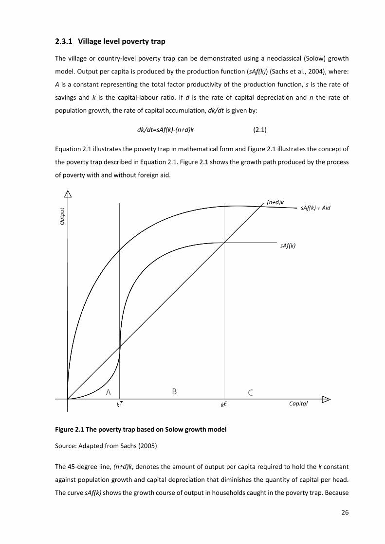
26

Village level poverty trap

The village or country-level poverty trap can be demonstrated using a neoclassical (Solow) growth

model. Output per capita is produced by the production function (sAf(k)) (Sachs et al., 2004), where:

A is a constant representing the total factor productivity of the production function, s is the rate of

savings and k is the capital-labour ratio. If d is the rate of capital depreciation and n the rate of

population growth, the rate of capital accumulation, dk/dt is given by:

dk/dt=sAf(k)-(n+d)k (2.1)

Equation 2.1 illustrates the poverty trap in mathematical form and Figure 2.1 illustrates the concept of

the poverty trap described in Equation 2.1. Figure 2.1 shows the growth path produced by the process

of poverty with and without foreign aid.

Figure 2.1 The poverty trap based on Solow growth model

Source: Adapted from Sachs (2005)

The 45-degree line, (n+d)k, denotes the amount of output per capita required to hold the k constant

against population growth and capital depreciation that diminishes the quantity of capital per head.

The curve sAf(k) shows the growth course of output in households caught in the poverty trap. Because

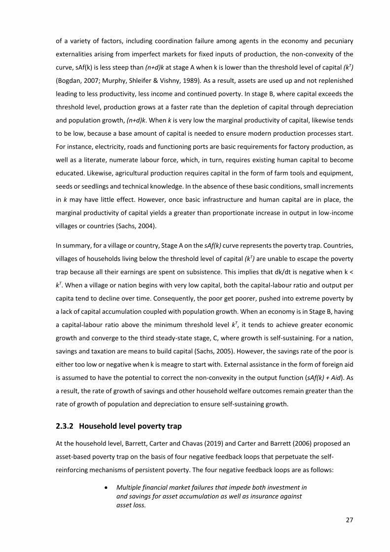
27

of a variety of factors, including coordination failure among agents in the economy and pecuniary

externalities arising from imperfect markets for fixed inputs of production, the non-convexity of the

curve, sAf(k) is less steep than (n+d)k at stage A when k is lower than the threshold level of capital (kT)

(Bogdan, 2007; Murphy, Shleifer & Vishny, 1989). As a result, assets are used up and not replenished

leading to less productivity, less income and continued poverty. In stage B, where capital exceeds the

threshold level, production grows at a faster rate than the depletion of capital through depreciation

and population growth, (n+d)k. When k is very low the marginal productivity of capital, likewise tends

to be low, because a base amount of capital is needed to ensure modern production processes start.

For instance, electricity, roads and functioning ports are basic requirements for factory production, as

well as a literate, numerate labour force, which, in turn, requires existing human capital to become

educated. Likewise, agricultural production requires capital in the form of farm tools and equipment,

seeds or seedlings and technical knowledge. In the absence of these basic conditions, small increments

in k may have little effect. However, once basic infrastructure and human capital are in place, the

marginal productivity of capital yields a greater than proportionate increase in output in low-income

villages or countries (Sachs, 2004).

In summary, for a village or country, Stage A on the sAf(k) curve represents the poverty trap. Countries,

villages of households living below the threshold level of capital (kT) are unable to escape the poverty

trap because all their earnings are spent on subsistence. This implies that dk/dt is negative when k <

kT. When a village or nation begins with very low capital, both the capital-labour ratio and output per

capita tend to decline over time. Consequently, the poor get poorer, pushed into extreme poverty by

a lack of capital accumulation coupled with population growth. When an economy is in Stage B, having

a capital-labour ratio above the minimum threshold level kT, it tends to achieve greater economic

growth and converge to the third steady-state stage, C, where growth is self-sustaining. For a nation,

savings and taxation are means to build capital (Sachs, 2005). However, the savings rate of the poor is

either too low or negative when k is meagre to start with. External assistance in the form of foreign aid

is assumed to have the potential to correct the non-convexity in the output function (sAf(k) + Aid). As

a result, the rate of growth of savings and other household welfare outcomes remain greater than the

rate of growth of population and depreciation to ensure self-sustaining growth.

Household level poverty trap

At the household level, Barrett, Carter and Chavas (2019) and Carter and Barrett (2006) proposed an

asset-based poverty trap on the basis of four negative feedback loops that perpetuate the self-

reinforcing mechanisms of persistent poverty. The four negative feedback loops are as follows:

• Multiple financial market failures that impede both investment in and savings for asset accumulation as well as insurance against asset loss.

28

• Psychological feedback loops in which poverty undercuts human cognitive and pro-social capabilities and performance, thereby entrenching one’s poverty.

• Deterioration in or premature cessation of investments in health and human capital caused by uninsured shocks and poverty.

• Bio-physical feedback loops in which environmental shocks and poverty undercut the productive capacity of natural resource systems.

Barrett et al. (2019) argue that household output is a function of productive assets such as land,

livestock, machinery, savings, cash and other forms of physical capital as well as human capabilities

like skills, self-efficacy, and other forms of human capital. Poverty manifests itself across multiple

dimensions at the household level, including financial, natural and social capital. These tend to be

correlated with other indicators of household ill-wellbeing such as poor physical and mental health,

limited education, exposure to crime, violence, disease and uninsured risks. Poor households,

particularly those that are liquidity constrained, are more conservative in their investments in assets,

choosing relatively liquid, consumable assets such as grains and locally adapted domesticated

livestock, which tends to be less productive and offer a low return. Such low yield investments come

at the cost of foregoing more lucrative investments that have greater associated risks (Deaton, 1991;

Zimmerman & Carter, 2003).

The low returns on such conservative household portfolios create poverty traps since they offer less

disposable income and fewer avenues to accumulate more productive assets. Households vary their

consumption to stabilize their portfolio of assets and future income (Zimmerman and Carter, 2003).

De Quidt and Haushofer (2016) and Dean, Schilbach and Schofield (2017) find that when decision-

makers are exposed to negative exogenous shocks, the experience tends to lead them to reassess

their efforts and behaviour in pessimistic ways consistent with the symptoms of depression. As a

result, the household tends to withdraw and exert less effort. They choose a safe, more conservative

and risk-averse approach that perpetuates low returns for effort. Such mental incapacitation further

perpetuates poverty (de Quidt & Haushofer, 2016). Other formulations of the poverty trap exist

including nutrition (Kraay & McKenzie, 2014; Kraay & Raddatz, 2005), education (Zhang, 2014) and

geography (Sachs, 2005). Sachs et al. (2004) formulated a macroeconomic variant of the savings

poverty trap as the theoretical basis of the MVP’s approach to dealing with poverty in rural Sub-

Saharan Africa.

Despite the explanatory power of the poverty trap, it is by no means considered a stylised fact. Bauer

(1972) asserts that the thesis of the poverty trap is challenged by the existence of developed

countries, all of which started poor at some stage. These currently rich countries used to have low

per capita incomes and low levels of capital accumulated, essentially the same economic features

29

that define underdeveloped countries currently. Bauer (1959, 1969) argues that were the model of

the poverty trap to be valid, numerous individuals, groups and communities around the world who

are currently wealthy could not have made it out of poverty. It is, therefore, likely, that the variables

in the model are either not as important as determinants of development as the model suggests, or

that they do not interact in the manner implied.

Bauer (2013) also notes that 19th century colonial Malaya (Malaysia) and colonial West Africa were

underdeveloped regions that achieved rapid progress through specialisation in rubber and cocoa

production, respectively, by local farmers without external assistance. In the space of 63 years, from

1900 – 1963, Malaya went from producing no rubber to producing and exporting over 800,000 tons

of rubber. In the same period, the export revenue of Malaya rose from £8 million per annum to

about £300 million. Likewise, on the Gold Coast (present-day Ghana), there were no cocoa exports in

1890. By the early 1960s, cocoa exports exceeded 400,000 tons. These advances happened without

external public assistance (Bauer, 2013). Bauer (1913) concludes that these outcomes suggest that

the poverty trap is inconsistent with the phenomenon of development.

Kraay and McKenzie (2014) assessed the empirical evidence for the existence of the poverty trap in

practice and the underlying mechanisms by which the trap operates. The study outlined a simple

model of a poverty trap at the country level consistent with most macro views of development in the

1950s and 1960s. The model was then used to examine the persistence of poverty at the country and

household levels. Kraay and McKenzie (2014) did not find much empirical evidence in support of the

notion that saving and productivity traps exist. Although saving rates and productivity do increase

with income levels, the function does not increase in the nonlinear manner required to generate the

low-level stable equilibrium that can plausibly account for the persistent income differences across

developing countries. The study also found that the typical poor country grew at least as fast as the

global average from 1960-2010. As a result of these findings, Kraay and McKenzie (2014) raise

scepticism over the idea that large increases in aid could result in economic growth in low-income

countries. They did not find evidence of a threshold effect based on the leading explanations for the

poverty trap whereby sufficiently high levels of aid are necessary to “jump-start” a sustainable

development process.

In a similar vein, Easterly (2008b), a sceptic of the poverty trap and the ‘big push’ approach, asserts

that a simultaneous relationship between savings and capital is not a sufficient reason to account for

the ‘vicious cycle’ of poverty predicted by the theory of the poverty trap. Such a cycle can occur only

if the elasticity of capital with respect to savings is greater than one, i.e., a change in savings results

in a more than proportional change in capital. Although he does not completely dismiss the theory of

the poverty trap, Easterly (2009) questions its existence. The poverty trap predicts a more than

30

proportionate increase in income resulting from an increase in capital stock. This is because of the

low initial capital stock at the disposal of poor households and the concavity of the income

production function (Kraay & McKenzie, 2014). Easterly (2006, 2008a), argues that years of research

have not generated evidence of the expected rapid income growth resulting from aid flows. In

Easterly’s (2002, 2006, 2008b) view, a variety of development efforts, including aid and debt

forgiveness, have failed to sustain growth - especially in Africa. He attributes these failures to a

disregard for the incentives faced by actors in development. He argues that governments that

receive development assistance are not motivated to promote free markets and fight corruption as

these reforms increase their accountability to citizens. On the other hand, donor performance is

measured by the number of disbursements made (Williamson, 2010). This motivates donors to

continually give aid irrespective of its effectiveness in beneficiary countries (Williamson, 2010).

A summary of the poverty trap

Sachs (2005), contends that the reason for persistent poverty among families in rural Africa is the

poverty trap. The theory asserts that because of the non-convexity of the production function for

various welfare outcomes along with coordination failure in investment decision making among

economic agents, means that poor households do not experience a sustained increase in income per

capita over time. This is a result of households falling back to lower-level equilibria. At the low-level

stable equilibrium, households live at a subsistence level. They, therefore, need external assistance

to rise to a higher equilibrium level. Furthermore, depreciation of their assets stock leaves them

exposed to external shocks. The solution is to accumulate assets at a faster rate than the rate of

depreciation. Sachs (2005) proposes that at least one of four interventions are necessary to break the

cycle of subsistence for such households. The four interventions are savings and investment;

specialisation and commercialisation of production; new resources; and technological change. With

the exception of new resources, Sachs (2005) argues that development assistance supplied by

external actors is indispensable to providing the requisite interventions in a coordinated effort to

break the poverty cycle and spur households to self-sustaining economic progress and development.

However, Sachs’ view of development assistance is one of four prominent views in the literature. The

next section defines development assistance, highlights key historical aspects in its evolution and

discusses the four major approaches to development assistance proposed by scholars and

practitioners along with some programmes and interventions that they advocate.

The definition and history of development assistance

The Development Assistance Committee (DAC) of the Organisation for Economic Co-operation and

Development (OECD, 2008, p. 376) and the International Monetary Fund (IMF, 2003, p. 263) define

Official Development Assistance (ODA) as:

31

“Flows of official financing administered with the promotion of the economic development and welfare of developing countries as the main objective, and which are concessional in character with a grant element of at least 25 per cent (using a fixed 10 per cent rate of discount). By convention, ODA flows comprise contributions of donor government agencies, at all levels, to developing countries (“bilateral ODA”) and to multilateral institutions. ODA receipts comprise disbursements by bilateral donors and multilateral institutions.” (OECD, 2008 p. 376)

This definition excludes humanitarian assistance that is often necessitated by catastrophic events,

such as natural disasters and wars. ODA is used interchangeably with development assistance, aid,

foreign aid and official aid, in the development literature (OECD, 2008).

Although evidence of various types of aid exists as far back as 226 BC, the history of modern foreign

aid dates back to the 19th century (Hjertholm & White, 2000). Among the earliest forms of bilateral

aid is the ‘Act for the Relief of the Citizens of Venezuela’, 1812 (Hjertholm & White, 2000; Van Bilzen,

2015). This aid sought to provide humanitarian assistance for the victims of famine in Venezuela.

During the Irish Great Famine of 1845-1849, the Ottoman empire provided food and monetary aid to

relieve the suffering of the Irish (Hjertholm and White, 2000). Later in the century, in 1896, the

concept of ‘tied aid’ emerged as the United States of America used its stock of surplus food as food

aid and as a means of developing new markets for the nation’s agricultural products (Van Bilzen,

2015). In the 20th century, Britain enacted the Colonial Development Act 1929 (Kanbur, 2000; Van

BIlzen, 2015). With this act, the British government moved towards a more active role in the

development of its colonies. Britain did this by providing grants and loans for infrastructure

development, improved transport, research, power, water supply and a land survey among others.

The initial Act excluded education but the sector was added in the 1940s and to the 1945 successor

to the 1929 Act, the Colonial Development Welfare Act 1945. The Roosevelt administration of the

1930s and 1940s provided ‘tied aid’ to Latin American countries under the ’Good Neighbor Policy‘

(Hjertholm & White, 2000). The year 1944 was a momentous year with regard to multilateralism in

aid with the formation of the Bretton Woods institutions – the International Monetary Fund (IMF)

and the World Bank – and non-governmental donor organisations like Oxfam and Centre for

American Relief in Europe (CARE) International (Hjertholm and White, 2000).

International activities in the aftermath of WWII were major factors in the development of foreign

aid in its modern form. Organisations like Oxfam and CARE were first established to cater for the

relief needs of post-war European refugees (Black, 1992; O’Keefe et al., 1991). Their activities for

development were extended to other parts of the world. The United Nations Relief and

Rehabilitation Agency was formed in 1943 to plan, coordinate and administer measures for the relief

of the victims of war (Kanbur, 2003). It was later incorporated into the United Nations organisation in

1945 but became defunct in 1947. The International Bank for Reconstruction and Development (The

32

World Bank) and the International Monetary Fund (IMF) formed in 1944 initially provided loans for

reconstruction and coordination of the international monetary system, respectively (Kanbur, 2003;

Van Bilzen, 2015).

Finally, the Marshall Plan was, perhaps, the most important intervention that greatly influenced the

role of foreign aid in the development agenda of the post-war period (De Long & Eichengreen, 1991).

Poverty, unemployment and economic dislocation in the aftermath of WW II reinforced the appeal of

communist parties around Western Europe (Van Bilzen, 2015). Interruption of the pre-war trading

patterns and the inability of European countries to meet their balance of payment obligations for

imported food led to a dire situation. To stave off these challenges in Europe, the United States

government passed the European Recovery Program, also known as the Marshall Plan, named after

the then Secretary of State (Jackson, 1979).

Over three years from 1948-1951, the Marshall Plan disbursed approximately $13.3 billion

(approximate 143 billion in 2017 dollars) to 16 countries in Western Europe including Belgium, Great

Britain, France, Norway, The Netherlands (De Long & Eichengreen, 1991; Eichengreen, 2013). The

successful recovery of post-war Europe has been largely credited to the Marshall Plan (De Long &

Eichengreen, 1991). As a result of this success, the Marshall Plan has been invoked as a model for the

role of foreign aid in the development programming of other parts of the world. This includes The

Colombo Plan for Cooperative Economic and Social Development in Asia and the Pacific (Basch, 1955;

Benham, 1954). The Marshall Plan and the Colombo Plan are examples of programme aid.

Programme aid is aid provided for a very large project with many subordinate objectives, or a group

of projects that are linked together (Van Bilzen, 2015). In 1949, President Harry Truman delivered his

inaugural address, famously referred to as the Point Four Speech (Leonard, 2012). The speech

outlined four major points of action for peace and freedom and assisting in the development of

'underdeveloped areas'. The points of the speech supported multilateralism in development and

technical assistance that have been salient parts of development assistance in the post-war period.

Lastly, the Development Assistance Group, later called the Development Assistance Committee (DAC

of the OECD) was formed in January 1960 as a forum for consultation and coordination among aid

donors on assistance to less-developed countries (Hjertholm & White, 2000).

There have been many motivations for development assistance espoused in the post-WWII era.

These range from the aid realist argument that aid is used to increase the sphere of influence and

broaden access to foreign markets for the goods of donor nations (Carbonnier, 2010; Gulrajani &

Calleja, 2019). Idealists, on the other hand, view aid as a moral imperative to help nations out of

humanitarian motives (Carbonnier, 2010). Aid idealists advocate the use of aid as a tool to combat

deprivation and engender development in the recipient country. Another strand of idealist

33

motivations sees aid as a means to compensate for past wrongs such as colonialism and the trans-

Atlantic slave trade (Burnell, 1997). The Sachs (2005) MVP proposed the use of foreign aid as a

catalyst to develop and raise the economic, social and health wellbeing of poor rural households

using a ‘big push’ approach to aid. Under the ‘big push’ approach, large volumes of development

assistance are applied in multisectoral packages of interventions in a concerted effort to break the

poverty trap and generate self-sustained economic development and meet the various goals of

human development. However, the big push approach is only one of a wide range of approaches to

the use of development assistance in the literature. In the next section, four major approaches to

development assistance in the literature and in practise are discussed along with the sorts of

development interventions that are suited to the respective approach.

Approaches to development assistance

The debate about development assistance and its role in advancing economic development falls into

four main categories on a continuum. At one extreme are scholars and practitioners such as

Rosenstein-Rodan (1943) and Sachs (2005), who believe that development assistance is essential for

the ‘take-off’ of poor countries and households into sustained economic development. This view of

development assistance is commonly referred to as the big push approach. The ‘big push’ is one of

the oldest concepts in development economics and has always been associated with the poverty trap

(Easterly, 2006; Murphy et al., 1989; Rosenstein-Rodan, 1961; Sachs et al., 2004). In that regard, the

big push used to be associated with the income growth concept of development. It justified propping

up the industrial sector in an unbalanced growth framework (Nurkse, 1971). Sachs et al. (2004) are

major proponents of the big push approach. However, the recent view of the ‘big push’ argues that

development assistance is essential to fill the ‘financing gap’, the shortfall between the stock of

capital currently available to poor nations and the threshold level of capital required to escape

poverty. Sachs (2005), therefore, designed the MVP on the ‘big push’ approach.

At the opposite pole, are scholars and practitioners who believe that aid is harmful and creates

corrupt incentives that undermine the goal of development. Among those scholars and practitioners

are Bauer (1972), Ditcher (2005), Moyo (2009) and Shleifer (2009). Between these two opposing

views are two other major views of development assistance. The ‘Selectivity and Conditionality’

approach advocates aid to countries that have a conducive governance and policy framework to

make meaningful and accountable use of the aid funds. The ‘Incremental Change’ approach

advocates aid for the support of proven programmes that are focused on addressing particular

developmental challenges as opposed to blanket aid programmes. Major proponents of the two

approaches include Burnside and Dollar (2000) and Easterly (2009), respectively. All these

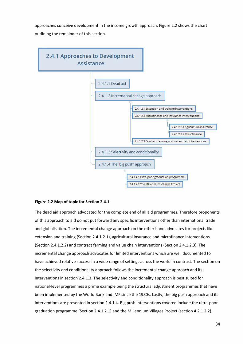
34

approaches conceive development in the income growth approach. Figure 2.2 shows the chart

outlining the remainder of this section.

Figure 2.2 Map of topic for Section 2.4.1

The dead aid approach advocated for the complete end of all aid programmes. Therefore proponents

of this approach to aid do not put forward any specific interventions other than international trade

and globalisation. The incremental change approach on the other hand advocates for projects like

extension and training (Section 2.4.1.2.1), agricultural insurance and microfinance interventions

(Section 2.4.1.2.2) and contract farming and value chain interventions (Section 2.4.1.2.3). The

incremental change approach advocates for limited interventions which are well documented to

have achieved relative success in a wide range of settings across the world in contrast. The section on

the selectivity and conditionality approach follows the incremental change approach and its

interventions in section 2.4.1.3. The selectivity and conditionality approach is best suited for

national-level programmes a prime example being the structural adjustment programmes that have

been implemented by the World Bank and IMF since the 1980s. Lastly, the big push approach and its

interventions are presented in section 2.4.1.4. Big push interventions covered include the ultra-poor

graduation programme (Section 2.4.1.2.1) and the Millennium Villages Project (section 4.2.1.2.2).

35

2.4.1.1 Dead aid

On the opposite pole to the ‘big push’, the notion that aid is critical to development for individuals,

households and nations that live in the poverty trap, is the view that aid is detrimental to the interest

of all parties concerned. Proponents of the dead aid approach argue that aid distorts incentives for

both donors and recipients and so leads to harmful effects (C. R. Williamson, 2010). Dichter (2005)

and Moyo (2009) strongly argue that rich nations should reject calls for increasing aid and funding for

development in less developed countries. The ineffectiveness of development assistance as a vehicle

for development is a result of three main factors. First is the complex nature of the problem of

poverty (Dichter, 2015). He points out that poverty is as much a matter of social, cultural and political

position as it is of material and economic deprivation for people living on less than USD 2 a day.

Poverty can be related to castes, classes, ethnic groups, tribes, gender and the shades of colour with

which people are born. As a result, attempts to address material poverty through aid programmes,

while ignoring the complexity of the phenomenon, are in danger of failure (Dichter, 2015). On the

other hand, trying to incorporate these factors into development projects increases their complexity

along with an increased likelihood of project failure (Dichter, 2005).

Moyo (2009), likewise, an extreme antagonist of aid interventions, argues that the assistance given

to Sub-Saharan Africa has been unlike that given to Western European countries after World War II

under the Marshall Plan. Rather than rebuilding broken cities and institutions, development

assistance has been largely ineffective in Africa. As much as 85 per cent of aid flowing into Africa has

been used for purposes other than those for which they were meant (Moyo, 2009). Although there is

a dearth of studies in Africa on the disciplined use of aid funds, Pack and Pack (1993) found the

fungibility of money meant that aid funds were often diverted to other applications. These

diversions, however, are not often reported in donor evaluations and completion reports (Riddell,

2009). Moyo (2009) further argues that aid promotes corruption by providing cheap financial capital

with little accountability. This position agrees with Easterly’s (2006) assertion. Moyo (2009) sums up

her thesis saying:

‘the notion that aid can alleviate systemic poverty, and has done so is a myth. Millions of Africans are poorer today because of aid, misery and poverty have not ended but increased. Aid has been and continues to be an unmitigated political, economic and humanitarian disaster for most parts of the developing world’ (p. xix).

Moyo (2009) suggests that aid is not only ineffective in addressing developmental challenges in Africa

but is, to a certain extent, responsible for the chronic problem of poverty. This is a serious claim

given the tenuous evidence provided by Moyo (2009).

36

Moyo (2009) proposes that in the place of development assistance, free trade, foreign direct

investment, microfinance and wage remittances to Africa should be promoted. Furthermore, African

countries should trade more with China so that ‘the pull of China will jumpstart their economies’.

Where finance is needed, African countries should be encouraged to deal in international capital

markets, which are a more transparent and accountable source of funding than aid, and which will

keep African governments responsible and accountable to their citizens. Dichter (2005) on the other

hand advocates for a more light-handed and pragmatic approach to aid with fewer agencies and

‘experts’ involved.

2.4.1.2 The incremental change approach

Being sceptical about the poverty trap and the effectiveness of development assistance in creating

economic development, Easterly (2002, 2006, 2008b, 2009) advocates incremental support for

programmes that are proven to make a positive impact on the poor. In so doing, according to

Easterly (2008), the incentives faced by actors in developing countries will change, removing the

layers of vested interest that thwart growth-enhancing reforms. The view that aid intervention

should be tested and supported only if it impacts positively on the lives of the poor is shared by

Banerjee and Duflo (2012) and Karlan and Appel (2011) who advocate randomised control trials as a

means of testing programmes for poverty eradication. To some extent, MVP incorporates elements

of this approach. The use of insecticide-treated nets, fertiliser and improved seed reduce malaria and

improve agricultural productivity (Gallup & Sachs, 2001; Gallup, Sachs & Mellinger, 1999; Havlin et

al., 2005; Sachs & Malaney, 2002). In agriculture and rural development, some programmes for

which strong evidence of positive impacts exist include extension and farmer training programmes,

microfinance and insurance intervention and value chain and contract farming schemes.

2.4.1.2.1 Extension and training interventions

The agricultural extension helps to bridge the gap between the actual and potential yields of farmers’

fields by facilitating the transmission of technological and managerial acumen to farmers.

Agricultural extension is a very important function in the agricultural sector. It transfers knowledge

and innovations from researchers to farmers, gives advice on farming decisions, educates farmers

and helps them with production goals for development and progress (Anderson & Feder, 2007;

Hazell & Anderson, 1984). By its nature, the products of agricultural extension services tend to bear

the attributes of public goods. They are non-rivalrous and non-excludable, their supply cannot be

exhausted with use, and non-payers cannot be excluded from participating. A study by Buadi,

Anaman and Kwarteng (2013) assessed farmers' perception of the quality of agricultural extension

service provided by Non-Governmental Organisations (NGOs) in two districts of the Central Region of

Ghana. Farmers perceived the services of agricultural extension agents to be relevant for their

agricultural activities. However, since farmers stand to benefit most from extension services, it stands

37

to reason that they bear the cost of the service. Nevertheless, there are market failures through

unorganised demand and supply of extension services and limited purchasing power on the part of

the farmer. However, as the private sector does not readily provide these services, there is ample

justification for public sector provision (Byerlee et al., 1988; Mullen, Vernon & Fishpool, 2000).

Consequently, agricultural extension programmes tend to be publicly funded (Anderson & Feder,

2007). The wider context of extension services is defined broadly as the rural knowledge and

innovation system. Alex et al. (2002) argue that such services are essential to informing and

influencing rural household decisions that can unleash the potential of rural people, bringing a

change to their living situation and enabling sustainable rural development.

Farmers are usually faced with two productivity differential gaps classified as a technology gap,

which entails additional investment and higher recurring costs for inputs such as seed of improved

cultivars, or fertilizers, and a management gap, which offers the farmer a low-cost means of raising

productivity by applying improved management practices (Byerlee, 1988). Extension services help to

reduce the gaps between potential and actual yields in farmers’ fields by accelerating technology

transfer that reduces the technology gap and helps farmers become better farm managers. This

enables farmers to increase their productivity. This has been observed in many developing countries

(Feder, Lau & Slade, 1987).

Scientists also benefit from the feedback of agricultural extension agents about the on-farm

performance of their innovations and techniques as well as about the resource circumstances of

farmers to help tailor innovations to better suit farmers’ needs. Agricultural extension service is,

therefore, a very important tool for building farmers’ human capital. This is especially true in Sub-

Saharan Africa where the average farmer has less than six years of formal education (Rapsomanikis,

2015). Many studies have found positive external effects of access to agricultural extension services

including crop and livestock health, farmer health, improved food security, and economic

development (Thirtle, Lin & Peisse, 2003). Consumers eventually benefit from the gains in

productivity through lower prices and more choices.

Extension delivery is not homogenous. There are four main extension delivery modalities (Anderson

& Feder, 2007): training and Visits, decentralised, fee-for-service and privatisation, and farmer field

schools. The training and visits method is commonly used in Africa whereas private financing options

like fee-for-service are well established in the OECD countries (Marsh, Pannell & Lindner, 2000).

Agricultural extension services in Ghana began as a service by the United Gold Coast farmers (Killick

2010). Government expenditure on agricultural extension in Ghana has been meagre (Diao et al.,

2019). The result is inadequate coverage because staff numbers are insufficient to reach all farmers

on a regular basis. Public extension services clients in Ghana are geographically dispersed. Even

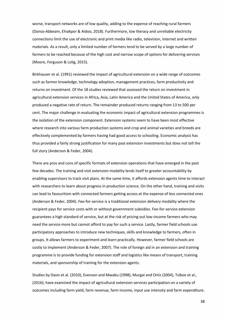
38

worse, transport networks are of low quality, adding to the expense of reaching rural farmers

(Danso-Abbeam, Ehiakpor & Aidoo, 2018). Furthermore, low literacy and unreliable electricity

connections limit the use of electronic and print media like radio, television, internet and written

materials. As a result, only a limited number of farmers tend to be served by a large number of

farmers to be reached because of the high cost and narrow scope of options for delivering services

(Moore, Ferguson & Lolig, 2015).

Birkhauser et al. (1991) reviewed the impact of agricultural extension on a wide range of outcomes

such as farmer knowledge, technology adoption, management practices, farm productivity and

returns on investment. Of the 18 studies reviewed that assessed the return on investment in

agricultural extension services in Africa, Asia, Latin America and the United States of America, only

produced a negative rate of return. The remainder produced returns ranging from 13 to 500 per

cent. The major challenge in evaluating the economic impact of agricultural extension programmes is

the isolation of the extension component. Extension systems seem to have been most effective

where research into various farm production systems and crop and animal varieties and breeds are

effectively complemented by farmers having had good access to schooling. Economic analysis has

thus provided a fairly strong justification for many past extension investments but does not tell the

full story (Anderson & Feder, 2004).

There are pros and cons of specific formats of extension operations that have emerged in the past

few decades. The training and visit extension modality lends itself to greater accountability by

enabling supervisors to track visit plans. At the same time, it affords extension agents time to interact

with researchers to learn about progress in production science. On the other hand, training and visits

can lead to favouritism with connected farmers getting access at the expense of less connected ones

(Anderson & Feder, 2004). Fee-for-service is a traditional extension delivery modality where the

recipient pays for service costs with or without government subsidies. Fee-for-service extension

guarantees a high standard of service, but at the risk of pricing out low-income farmers who may

need the service more but cannot afford to pay for such a service. Lastly, farmer field schools use

participatory approaches to introduce new techniques, skills and knowledge to farmers, often in

groups. It allows farmers to experiment and learn practically. However, farmer field schools are

costly to implement (Anderson & Feder, 2007). The role of foreign aid in an extension and training

programme is to provide funding for extension staff and logistics like means of transport, training

materials, and sponsorship of training for the extension agents.

Studies by Davis et al. (2010), Evenson and Mwabu (1998), Murgai and Ortiz (2004), Tsiboe et al.,

(2016); have examined the impact of agricultural extension services participation on a variety of

outcomes including farm yield, farm revenue, farm income, input use intensity and farm expenditure.

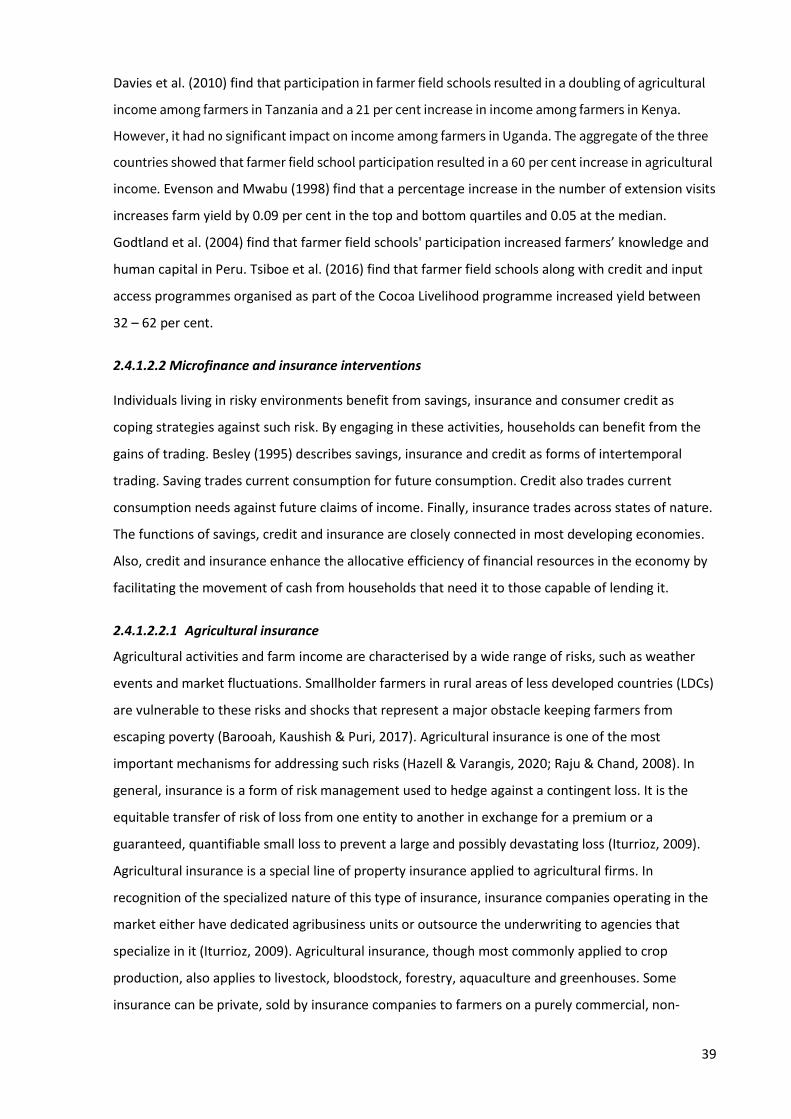
39

Davies et al. (2010) find that participation in farmer field schools resulted in a doubling of agricultural

income among farmers in Tanzania and a 21 per cent increase in income among farmers in Kenya.

However, it had no significant impact on income among farmers in Uganda. The aggregate of the three

countries showed that farmer field school participation resulted in a 60 per cent increase in agricultural

income. Evenson and Mwabu (1998) find that a percentage increase in the number of extension visits

increases farm yield by 0.09 per cent in the top and bottom quartiles and 0.05 at the median.

Godtland et al. (2004) find that farmer field schools' participation increased farmers’ knowledge and

human capital in Peru. Tsiboe et al. (2016) find that farmer field schools along with credit and input

access programmes organised as part of the Cocoa Livelihood programme increased yield between

32 – 62 per cent.

2.4.1.2.2 Microfinance and insurance interventions

Individuals living in risky environments benefit from savings, insurance and consumer credit as

coping strategies against such risk. By engaging in these activities, households can benefit from the

gains of trading. Besley (1995) describes savings, insurance and credit as forms of intertemporal

trading. Saving trades current consumption for future consumption. Credit also trades current

consumption needs against future claims of income. Finally, insurance trades across states of nature.

The functions of savings, credit and insurance are closely connected in most developing economies.

Also, credit and insurance enhance the allocative efficiency of financial resources in the economy by

facilitating the movement of cash from households that need it to those capable of lending it.

2.4.1.2.2.1 Agricultural insurance

Agricultural activities and farm income are characterised by a wide range of risks, such as weather

events and market fluctuations. Smallholder farmers in rural areas of less developed countries (LDCs)

are vulnerable to these risks and shocks that represent a major obstacle keeping farmers from

escaping poverty (Barooah, Kaushish & Puri, 2017). Agricultural insurance is one of the most

important mechanisms for addressing such risks (Hazell & Varangis, 2020; Raju & Chand, 2008). In

general, insurance is a form of risk management used to hedge against a contingent loss. It is the

equitable transfer of risk of loss from one entity to another in exchange for a premium or a

guaranteed, quantifiable small loss to prevent a large and possibly devastating loss (Iturrioz, 2009).

Agricultural insurance is a special line of property insurance applied to agricultural firms. In

recognition of the specialized nature of this type of insurance, insurance companies operating in the

market either have dedicated agribusiness units or outsource the underwriting to agencies that

specialize in it (Iturrioz, 2009). Agricultural insurance, though most commonly applied to crop

production, also applies to livestock, bloodstock, forestry, aquaculture and greenhouses. Some

insurance can be private, sold by insurance companies to farmers on a purely commercial, non-

40

subsidized basis, but most agricultural insurance is provided on a subsidized basis as part of

government efforts to further development, social or political goals (Mahul & Stutley, 2010).

The World Bank estimated that, in 2007, 104 countries had some form of agricultural insurance

(Mahul & Stutley, 2010). In the same year, about $20 billion was collected in premiums and premium

subsidies (Hazell & Varangis, 2020; Mahul & Stutley, 2010). Based on a recent review of documented

index-based agricultural insurance programmes in the developing world, Hess and Hazell (2016)

estimate that about 198 million farmers were insured in 2014. Of this number, approximately

650,000 lived in Africa, 3.3 million in Latin America and the Caribbean and about 194.2 million in Asia

(160 million in China and 33.2 million in India).

Three main factors may have contributed to the growth in agricultural insurance (Iturrioz, 2009).

First, is the recent increase in the underlying value of agricultural production that has impacted

directly on the agricultural insurance premium volume. The second factor is the increase in the value

of agricultural assets, which has increased the sensitivity to loss for agricultural value chain

participants, consequently raising their demand for insurance (Iturrioz, 2009). The third factor is the

development of new markets for agricultural insurance and increased public sector support in

existing markets, which have contributed to an increased demand for agricultural insurance (Iturrioz,

2009). The majority of agricultural insurance premiums are underwritten in the United States and

Canada, covering approximately 62 per cent of the market (Iturrioz, 2009). Asia follows at 18 per cent,

Europe with 16 per cent, Latin America 2 per cent and 1 per cent in Oceania and Africa. Despite these

numbers, market penetration remains small, even in rich countries (Hazell, Sberro-Kessler & Varanjis,

2017). Moreover, insurance coverage typically represents just a small fraction of farmers’ total

exposure to farm income and asset risks at less than 1 per cent of the global value of agricultural GDP

(Mahul & Stutley, 2010).

Apart from stabilizing farm income, agricultural insurance, helps farmers to reinitiate production

activity following adverse production seasons, thereby preventing the dissolution of accumulated

assets to cope with shocks or to restart production (Raju & Chand, 2008). Agricultural insurance

purchases can be deemed as more beneficial on the part of smallholder farmers when the insurance

is part of a package of other financial (e.g., access to credit) and non-financial services (e.g.. access to

improved inputs and technologies, access to markets, contract farming). Otherwise, farmers tend to

view insurance as merely a cost item (Hess et al., 2016).

Agricultural insurance has been found to increase rural poor households’ willingness to adopt new

technologies and invest more in production activities that, in turn, raise both the level and riskiness

of income (Karlan et al., 2013). Essentially, farmers are more likely to invest in or adopt technologies

under uncertainty if they know that their insurance will cover the possible loss of income should the

41

technologies and input fail (Besley, 1995). In most cases, agricultural insurance is based on farmers’

contributions and premiums. However, there is a scope for incorporating government-based

subsidies or foreign aid to support such programmes (Hazell et al., 2017; Hazell & Varangis, 2020).

Risks are distributed across space and time as losses suffered by farmers in a particular locality are

shared by farmers in other areas and with reserves accumulated through premiums in good years. A

good agricultural insurance programme, therefore, combines self-help and mutual help principles

(Raju & Chand, 2008).

Despite all the benefits of agricultural insurance, there is a danger of incentivising farmers to assume

too much risk, such as growing unsuitable crops in risky environments. This is especially true where

premiums are subsidised below fair market value. Such behaviour increases the costs of subsidies to

the government and risks to insurance companies (Hazell & Varangis, 2020). Insurance subsidies are

also difficult to phase out or remove once established. In fact, like most input subsidies, costs to

government tend to grow over time as more of the input is used and larger crop areas are insured

(O’Donoghue, 2014; Yu, Smith & Sumner, 2018). Insurance subsidies can also lead to undesired

distributional consequences. For example, the benefits from proportional subsidies are skewed

towards farmers who buy more insurance, despite the fact that they are less likely to be poor (Hazell

& Varangis, 2020).

2.4.1.2.2.2 Microfinance

Poor households in urban areas and, in particular, rural areas in developing countries, lack access to

basic financial services. Such systematic exclusion from formal financial services has led to the

evolution of microfinance as an alternative mode of finance in which financial services are provided

not through traditional means, such as local moneylenders, cooperatives and banks, but by NGOs or

microfinance institutions (MFIs) (Hamada, 2010). “Microfinance is extending formal financial

services, especially credit, to low-income families and small enterprises” (Caprio et al, 2012, p 489).

Farmers ordinarily have informal credit sources, such as local money lenders, trading credit, relatives,

friends and neighbours. MFIs, however, ensure repayment by giving small short-term loans, requiring

frequent payback, refusing new loans when older loans have been in default, increasing loans and

maturity when old loans have been repaid. In some cases, MFIs require borrowers to form groups

where members monitor and hold each other accountable (Armendariz & Morduch, 2010).

In addition to small loans, certain MFIs provide training in business management (Brau & Woller,

2004). Participation in such programmes can provide certain advantages to clients for the growth and

stability of their businesses and improving household wellbeing (Banerjee et al., 2014). The number

of MFIs, loan portfolios and customers has recently grown significantly (Mersland & Strøm, 2013;

Mersland et al., 2011). Another recent trend is the consensus that access to savings positively

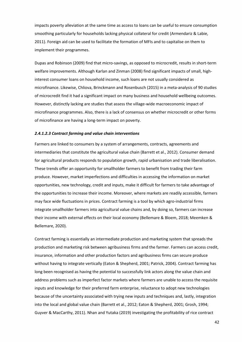
42

impacts poverty alleviation at the same time as access to loans can be useful to ensure consumption

smoothing particularly for households lacking physical collateral for credit (Armendariz & Labie,

2011). Foreign aid can be used to facilitate the formation of MFIs and to capitalise on them to

implement their programmes.

Dupas and Robinson (2009) find that micro-savings, as opposed to microcredit, results in short-term

welfare improvements. Although Karlan and Zinman (2008) find significant impacts of small, high-

interest consumer loans on household income, such loans are not usually considered as

microfinance. Likewise, Chliova, Brinckmann and Rosenbusch (2015) in a meta-analysis of 90 studies

of microcredit find it had a significant impact on many business and household wellbeing outcomes.

However, distinctly lacking are studies that assess the village-wide macroeconomic impact of

microfinance programmes. Also, there is a lack of consensus on whether microcredit or other forms

of microfinance are having a long-term impact on poverty.

2.4.1.2.3 Contract farming and value chain interventions

Farmers are linked to consumers by a system of arrangements, contracts, agreements and

intermediaries that constitute the agricultural value chain (Barrett et al., 2012). Consumer demand

for agricultural products responds to population growth, rapid urbanisation and trade liberalisation.

These trends offer an opportunity for smallholder farmers to benefit from trading their farm

produce. However, market imperfections and difficulties in accessing the information on market

opportunities, new technology, credit and inputs, make it difficult for farmers to take advantage of

the opportunities to increase their income. Moreover, where markets are readily accessible, farmers

may face wide fluctuations in prices. Contract farming is a tool by which agro-industrial firms

integrate smallholder farmers into agricultural value chains and, by doing so, farmers can increase

their income with external effects on their local economy (Bellemare & Bloem, 2018; Meemken &

Bellemare, 2020).

Contract farming is essentially an intermediate production and marketing system that spreads the

production and marketing risk between agribusiness firms and the farmer. Farmers can access credit,

insurance, information and other production factors and agribusiness firms can secure produce

without having to integrate vertically (Eaton & Shepherd, 2001; Patrick, 2004). Contract farming has

long been recognised as having the potential to successfully link actors along the value chain and

address problems such as imperfect factor markets where farmers are unable to access the requisite

inputs and knowledge for their preferred farm enterprise, reluctance to adopt new technologies

because of the uncertainty associated with trying new inputs and techniques and, lastly, integration

into the local and global value chain (Barrett et al., 2012; Eaton & Shepherd, 2001; Grosh, 1994;

Guyver & MacCarthy, 2011). Nhan and Yutaka (2019) investigating the profitability of rice contract

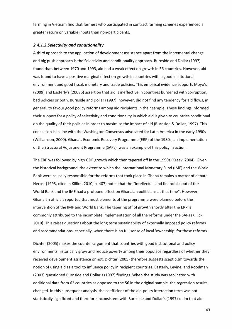
43

farming in Vietnam find that farmers who participated in contract farming schemes experienced a

greater return on variable inputs than non-participants.

2.4.1.3 Selectivity and conditionality

A third approach to the application of development assistance apart from the incremental change

and big push approach is the Selectivity and conditionality approach. Burnside and Dollar (1997)

found that, between 1970 and 1993, aid had a weak effect on growth in 56 countries. However, aid

was found to have a positive marginal effect on growth in countries with a good institutional

environment and good fiscal, monetary and trade policies. This empirical evidence supports Moyo’s

(2009) and Easterly’s (2008b) assertion that aid is ineffective in countries burdened with corruption,

bad policies or both. Burnside and Dollar (1997), however, did not find any tendency for aid flows, in

general, to favour good policy reforms among aid recipients in their sample. These findings informed

their support for a policy of selectivity and conditionality in which aid is given to countries conditional

on the quality of their policies in order to maximise the impact of aid (Burnside & Dollar, 1997). This

conclusion is in line with the Washington Consensus advocated for Latin America in the early 1990s

(Williamson, 2000). Ghana’s Economic Recovery Programme (ERP) of the 1980s, an implementation

of the Structural Adjustment Programme (SAPs), was an example of this policy in action.

The ERP was followed by high GDP growth which then tapered off in the 1990s (Kraev, 2004). Given

the historical background, the extent to which the International Monetary Fund (IMF) and the World

Bank were causally responsible for the reforms that took place in Ghana remains a matter of debate.

Herbst (1993, cited in Killick, 2010, p. 407) notes that the “intellectual and financial clout of the

World Bank and the IMF had a profound effect on Ghanaian politicians at that time”. However,

Ghanaian officials reported that most elements of the programme were planned before the

intervention of the IMF and World Bank. The tapering off of growth shortly after the ERP is

commonly attributed to the incomplete implementation of all the reforms under the SAPs (Killick,

2010). This raises questions about the long term sustainability of externally imposed policy reforms

and recommendations, especially, when there is no full sense of local ‘ownership’ for these reforms.

Dichter (2005) makes the counter-argument that countries with good institutional and policy

environments historically grow and reduce poverty among their populace regardless of whether they

received development assistance or not. Dichter (2005) therefore suggests scepticism towards the

notion of using aid as a tool to influence policy in recipient countries. Easterly, Levine, and Roodman

(2003) questioned Burnside and Dollar’s (1997) findings. When the study was replicated with

additional data from 62 countries as opposed to the 56 in the original sample, the regression results

changed. In this subsequent analysis, the coefficient of the aid-policy interaction term was not

statistically significant and therefore inconsistent with Burnside and Dollar’s (1997) claim that aid

44

was more effective in countries with sound economic policy. In light of Easterly et al.’s (2003) finding,

the selectivity criteria used in choosing countries for the MVP may not be a sufficient condition to

guarantee the desired results.

The structural adjustment programmes had a mixed legacy among the participant countries. In the

initial years following its implementation in Ghana, per capita income rose while inflation fell (Killick,

2010; Bawumia, 1996). By contrast, the SAPs in Zimbabwe resulted in a decline in the GDP growth

rate from 7.3 in 1988 to -7.7 per cent in 1992. Inflation also increased from 7.9 per cent to 46.3 per

cent over the same period (Bawumia, 1996). The restructuring of the public sector during the SAPs

resulted in the retrenchment of thousands of workers. However, the private sector was not able to

absorb these workers leading to a decline in the living standards of many households ("Zimbabwe -

falling wages", 1993).

2.4.1.4 The ’big push’ approach

Rosenstein-Rodan (1957) asserts that there is a minimum level of resources required to be dedicated

to any development programme to ensure success; small increments tend to fall short of creating the

desired results. As such, Rosentein-Rodan (1957) argue that the ‘big push’ is necessary because the

markets for investment in assets are not perfect, thereby resulting in sub-optimal allocation of

resources. This calls for deliberate programming of investment decisions in a concerted effort to

adjust markets. The 'big push' approach inspired many development projects in the post-colonial era,

e.g., the Volta River project that created the Akosombo hydroelectric dam in Ghana (Lumsden, 1973).

Most of the projects in those earlier years were at the country-level; there were very few

communities or village level ‘big push’ programmes in the 20th century. This is perhaps because of

the large sums of money required for ‘big push’ programmes. However, in the 21st century, a few ‘big

push’ programmes have been implemented at the community level. Sachs (2005) argues that the

problem in developing countries is that tax receipts are not sufficient for governments to engage in

the interventions required for the local economy to take off into self-sustained economic

development. Sachs (2005), therefore, proposes that the ‘financing gap’ ought to be filled by

development assistance from wealthier countries. Two of the most prominent household level big

push projects are the Ultra-Poor Graduation Programme pioneered by BRAC, the Bangladeshi Non-

Governmental Organisation (Bandiera et al., 2013; Banerjee et al., 2015) and the MVP.

2.4.1.4.1 Ultra-Poor Graduation programme

The second prominent big push programme is the Ultra-Poor graduation programme. While

households that are slightly above and below the poverty line can have access to microfinance

services relatively easily, the same is not the case for extremely poor households who tend not to

have access to microfinance services (Daidone, Pellerano, Handa, & Davis, 2015; Dupas, Karlan,

45

Robinson, & Ubfal, 2018). Moreover, the microfinance industry raises ethical concerns about making

money from the plight of the poor, as well as the burden of indebtedness, levied on households and

communities (Karlan & Zinman, 2009). Where households do have access, they are unable to reap

the full benefit of microfinance programmes in reduced poverty. Realising this BRAC, an NGO in

Bangladesh initiated a programme to 'graduate' the extremely poor by providing, in addition to

microfinance services, food aid, skill training, mandatory savings, small loans to facilitate livelihood

development (Bandiera et al., n.d.; A. Banerjee et al., 2015; Hashemi & de Montesquiou, 2011). The

programme targeted the ultra-poor, defined as people who spent 80 per cent or more of their total

expenditure on food and could not attain 80 per cent of their needed calories (Hashemi & de

Montesquiou 2011). The graduation programme was modelled on five primary elements: targeting,

savings, consumption support, skills training and regular coaching, and assets transfer (Hashemi & de

Montesquiou 2011). There was room, however, to adapt these elements to fit the contextual needs

of the respective community.

The project was first implemented by BRAC, a Bangladeshi Non-Governmental Organisation (NGO).

The original ultra-poor graduation programme in Bangladesh reached an estimated 650,000 women

from 2011 through 2016. The project implemented a range of interventions aimed at increasing

consumption among ultra-poor households (Banerjee et al., 2015). Participant households were

selected from the bottom rungs of a participatory wealth ranking (PWR) process hence the ultra-poor

description (Banerjee et al., 2015). Among the interventions implemented by the project were

distributing of productive assets (typically livestock), training and support on tending the livestock,

life skills coaching, temporary cash transfer for consumption support, and access to savings accounts

and health services.

In Bangladesh, BRAC transferred USD 140 in assets to participant households (Bandiera, et al., 2013).

Bandiera et al. (2013) assessed the impact of the Ultra-poor graduation programme on occupational

choice and household income of participant households. The study found that Ultra-poor graduation

programmes had a statistically significant impact on household engagement in wage employment

and self-employment, as well as household productivity and well-being outcomes such as livestock

assets, land rental, savings and household expenditures. Banerjee et al. (2015) conducted a meta-

analysis on a variant of the TUP project called 'Graduation programs' implemented across six

countries, namely, Ethiopia, Ghana, Honduras, India, Pakistan and Peru. The study found statistically

significant impacts in ten outcome categories including household consumption of food, non-food

and durable goods, food security, household and productive assets, financial inclusion, income and

revenue, time use for paid and self-employment, mental health, political involvement and women's

empowerment.

46

2.4.1.4.2 The Millennium Villages Project

As mentioned in Chapter 1, the MVP was initiated to help rural communities in Sub-Saharan Africa to

achieve the MDGs using large doses of development assistance from foreign nations (Cabral,

Farrington & Ludi, 2006). Sachs (2005) argues that the most difficult part of the economic

development endeavour is to get the poorest one-sixth of the world's population up to the ‘first rung

of the development ladder’. This is a term coined by Sachs (2005) to portray the process of wealth

accumulation and the advancement of human wellbeing. As such, the primary goal of the global

development agenda should be to provide basic standards of nutrition, health, water, sanitation,

shelter and other minimum ‘basic needs’ for survival, well-being and participation in society. The

second goal is to ensure that the poor and moderately poor have a chance to climb the ladder.

Sachs (2005) argues that by saving a portion of a household’s crop revenue, families could invest in a

livestock venture, for instance, thereby increasing their household income stream. Also, they could

improve food crop yields by fertilising farmland with the manure from animal production. The

addition and use of draught animals to household cropping enterprises would help to reduce human

effort and increase soil fertility and productivity. Such capital accumulation, Sachs (2005) stresses,

raises household productivity, income and prosperity. Though mixed farming systems described in

Sachs (2005) have many advantages, their application in the forest zones of Sub-Saharan Africa is

limited because of the prevalence of numerous debilitating animal diseases like trypanosomiasis,

rinderpest and ‘peste des petits’ ruminants (PPR) that make small ruminants and draught animal

production unprofitable (Ford, 1971; Gray, 1971; Jones et al., 2016).

Sachs (2005) stresses that savings, investment and capital accumulation raise household productivity.

Contrary to the assertion by Sachs (2005) that the poor do not save, studies have shown that poor

smallholders have a latent propensity to save and borrow (Rutherford, 1998; Zeller & Sharma, 2000;

Karlan, Ratan and Zinman, 2014). However, they tend to keep their savings in informal instruments

like livestock, jewellery, under mattresses and in informal savings groups. This is largely because of

the birth of formal savings instruments available to the poor, which are, in turn, because of

transaction costs, regulatory barriers and lack of trust that constrain the supply of formal saving

instruments (Karlan et al., 2014). On the demand side, social demands, lack of knowledge and

distrust or behavioural biases tend to suppress the availability of formal savings and credit

instruments on the part of the poor ( Karlan et al, 2014).

Sachs (2005) further argues that by specialising in high-value cash crops and selling their output,

households could increase their income and purchase more of their annual food requirements.

Specialisation and trading activities, Sachs (2005) points out, have the potential to fuel other local

economic activities such as transportation, food and farm input trade, and provision of services, a

47

point borne out by other studies including Achterboschet al. (2014), Delgado et al. (1994), Diao et al.

(2007). Poor infrastructure and weak institutions that constrain markets for inputs, products, land,

finance, insurance and knowledge in Sub-Saharan Africa limit smallholder opportunities for

commercial farming (Besley, 1995; Fenwick and Lyne, 1998; Karlan, Osei, Osei-Akoto, & Udry, 2012;

Lyne, Roth, & Troutt, 1997; Place, 2009). Furthermore, political instability and regular changes in

governments with the attendant lack of continuity in policies and projects creates an environment of

uncertainly that discourages such risk-taking among farms.

The use of new technology and improved farming methods and technologies also has the potential to

raise yields and generate extra income for farmers, thereby eradicating poverty (Sachs, 2005). There

is a wide variety of improved technologies available to farmers in Africa, and the productivity and

financial gains from improved technology adoption are widely documented (Dixon et al., 2006;

Minten & Barrett, 2008). These points notwithstanding, Reardon, Kelly, Yanggen, and Crawford

(1999) document a number of factors that serve to inhibit farmers’ adoption of these technologies.

Among the factors outlined include access to cash and liquidity (which is in turn influenced by access

to credit and non-farm wage work), human capital including formal education attainment and risks

such as pests, diseases, weather, market and land tenure. Furthermore, human capital in the form of

access to extension services are crucial determinants of technology adoption in addition to social

learning (Conley & Udry, 2010; Reardon et al., 1999), but access to such services are limited in Sub-

Saharan African mostly constrained by limited public finance. Private sector delivery of services like

extension, inputs credit are only recently taking off in Africa and are yet to gain widespread

patronage.

Lastly, Sachs (2005) argues that farm income would rise significantly if households benefitted from a

meaningful increase in the productive resources available to them. Sachs (2005) cites the case of

river blindness (Onchocerciasis) as an example. In parts of Africa where this disease and its vector,

the black fly (Simulium damnosum), are endemic, governments commonly evacuate the area leaving

vast quantities of fertile land unsued. Although there is an effective treatment for the disease, the

vast majority of cases are not diagnosed early enough to prevent blindness. If the government could

find a means of controlling the black fly, thousands of hectares of fertile arable land would be freed

for additional cultivation. A similar argument can be applied to malaria and other diseases that

adversely affect the productivity of labour in the tropics (Gallup & Sachs, 2001). The release of new

resources like land and labour to farmers could boost their productive capacities, enable them to

increase their income. However, the institutional arrangements that govern access to resources such

as land and other productive resources in most of Sub-Saharan Africa adversely affect non-member

of the “land-owning” community (Goldstein & Udry, 2008; Migot-Adholla, Hazell, Blarel, & Place,

1991).

48

According to Sachs (2005), these interventions: (i) savings, investment and capital accumulation, (ii)

specialisation in high-value cash crops, (iii) adoption of new technologies, and (iv) increases in

productive resources are a necessary condition to break the cycle of poverty. Otherwise, persistent

conditions such as inadequate savings, the absence of trade, technological stagnation, natural

resource depletion, adverse shocks, and population growth are likely to reduce per capita income

and shrink the aggregate economy, plunging households into deeper poverty.

The theory of the poverty trap is essential to understanding the approach of the Millennium Villages

Project and the vision to end poverty outlined by Sachs (2005). As explained in Section 2.3 the

poverty trap theory predicts that people living in extreme poverty cannot escape poverty without

external assistance. Sachs (2005) argues that a ‘big push’ is needed to lift people out of poverty to a

self-sustained path to prosperity. The ‘big push’ theory was first espoused by Rosenstein-Rodan

(1943). The theory posits that there is a minimum level of resources that must be devoted to a

development program if it is to have any chance of success (Rosenstein-Rodan, 1957; Tarp &

Hjertholm, 2000). As such, if a threshold level of capital is not reached, households are unable to

escape the poverty trap. Sachs (2005) identified six types of capital (human, business, infrastructure,

natural, knowledge, and public institutional capital) that needed to be increased to set households

on a path to self-sustained economic wellbeing. Small increments in the capital below the threshold

level, according to Sachs (2005), do not suffice in spurring long-term growth as capital depreciation

reduces the stock of capital over time. By contrast, where a greater-than-threshold level of

infrastructure and human capital is present, the marginal productivity of capital can proliferate in

low-income countries (Sachs, 2005).

Savings and taxation are a means by which individuals and nations build capital (Sachs, 2005).

However, according to Sachs (2005), the savings rate of the poor is exceptionally low or

even negative when capital is limited. This is because poor people do not save but rather use all their

income for household consumption. This assertion, however, contrasts with empirical evidence

which suggests that poor households have the propensity to save, but a lack of formal savings

products constrains them (Eckel, Johnson, & Montmarquette, 2005; Karlan, Ratan, & Zinman, 2014;

Ravallion & Chen, 2005; Rutherford, 1998; Zeller & Sharma, 2000). Furthermore, Karlan et al. (2014)

emphasise that a lack of trust, transaction cost, and unfavourable regulatory framework inhibit the

delivery of formal savings products. On the other hand, poor households resort to saving extra

income under mattresses, in informal groups and through building up their livestock numbers. By so

doing, a lot of capital is tied up in informal savings instruments and are, therefore, not available to

finance productive economic activities (through the intermediation processes) that spur self-

sustaining growth. Sachs (2005) further asserts that until the capital-labour ratio reaches a threshold

49

level where the rate of capital accumulation becomes positive, it is challenging for the poor to

achieve self-sustaining growth.

In addition, adverse shocks encourage poor people to convert existing capital into income to cope,

thereby deepening their poverty (Sachs et al., 2004; Sanchez et al., 2007). Consequently, when an

economy or household begins with low levels of capital, both the capital-labour ratio and output per

capita tend to decline over time. To prevent further losses of capital, it is necessary to increase levels

of capital beyond the threshold level. Sachs (2005) proposes that for poor countries to reach the

threshold level of capital needed to begin self-sustaining economic growth, rich donor countries have

to fill the ‘financing gap’. The financing gap is defined as the difference between the threshold level

of capital and the stock of capital currently available in poor countries. Sachs (2005) argues that rich

countries should give a ‘big push’ to poor countries by filling the financing gap with development

assistance over a sustained period of time.

Sachs (2005, p. 232) offers a proposal aimed at ending the plight of the poor at a cost that is “trivial

for the world but too high for the poor people themselves”. The proposal laid out in Sachs (2005)

formed the basis of the Millennium Villages Project. He outlined the ‘Big Five’ sectors of the rural

economy for development interventions that should bring an end to the symptoms of poverty and

initiate economic development. The first of these interventions relate to agricultural technology.

Sachs (2005) contends that yields can be increased multiple-fold with fertiliser, improved fallows,

green manure, cover cropping, rainwater harvesting, small-scale irrigation and improved seeds.

Construction of storage facilities will enable farmers to extend the storage life of their products and

allow them to sell in the lean season when they can obtain better prices. Second, it is important to

invest in health. Sachs (2005) argues that there should be at least one doctor and a nurse for each

village of 5,000 residents, with accompanying investments in antimalarial drugs, antiretroviral drugs

for HIV/AIDS, skilled birth attendants, and sexual and reproductive health education. The third

intervention is an investment in education. He argues that meals for children at primary school level

will not only improve the health of pupils but will also improve attendance and learning outcomes.

Expansion of vocational education to teach modern methods of farming, computer literacy, basic

maintenance of infrastructure, carpentry and the like will improve local economic activities and

provide employment. Other suggestions include village classes to train adults in hygiene, HIV/AIDS

prevention, malaria control, and computer and mobile phone technology. Fourth, Sachs (2005)

advocates investment in power, transportation, and communication services, arguing that provision

of electricity will go a long way toward increasing economic activity, promoting education and

providing for the storage of perishable agricultural produce. Transportation infrastructure will reduce

the cost of bringing inputs to the village, and taking agricultural output to the markets. Mobile

phones for the community could be used for emergencies, market information, and to connect rural

50

communities to the rest of the world. Finally, provision of safe, accessible water will significantly

reduce the number of hours spent by women and children fetching water and will reduce the spread

of water-borne diseases.

Sachs (2005) used Sauri village in Kenya to run a pilot study to determine the scalability of the project

across villages in Africa. Sachs (2005) initially estimated that the investments outlined in his big push

integrated development project could be made at the cost of USD350,000 per year, benefitting a

population of about 5,000 inhabitants at a rate of USD70 per person per year. At this cost, the

benefits would be reaped in the forms of saved lives, educated children, raised crop yields, and

communities set on a self-sustaining path to prosperity and development. Eventually, the cost person

per annum for the actual project stood at USD 150 per person per annum. Sachs (2005), however,

does not believe that the interventions should go on forever. He states ‘… in the first few years,

fertiliser and improved fallows should be given largely for free to the villages to boost nutrition and

health, and to build a small financial cushion. Later on, it will be possible to share the costs with the

community and eventually over a decade or so the farmers will be ready to bear the full cost’.

Although the MVP addresses problems of access to inputs, improved technology, specialisation,

infrastructure, and credit, the plan for the MVP described by Sachs (2005) and Sachs & McArthur

(2005) does not address the myriad risks and institutional factors that limit agricultural production in

rural areas in Africa. This could have implications for the long-term sustainability of gains from the

project.

Since its inception, a number of studies have been conducted on the MVPs collectively and

individually, including the projects’ effects on child mortality (Pronyk, et al., 2012), agricultural

production (Wanjala and Muradian (2013) and a wide range of outcomes across all sites (Mitchell et

al., 2018). Pronyk et al. (2012), found significant improvement in under-5-year old’s mortality

outcomes, and households’ food security between the MVP and comparable villages. The study,

however, did not assess the impact of the MVP on agricultural outcomes. An end-line evaluation of

the MVP assessed its impact on 40 outcomes covering poverty, agriculture, nutrition, education,

child health, maternal health, HIV and malaria morbidity, and water and sanitation (Mitchell et al.,

2018). The outcome indices covered some of the MDGs including the goals on poverty, education,

HIV and malaria. The study found a statistically significant impact of the MVP across 30 of the 40

outcomes, mainly in the health and agriculture categories, all in favour of the MVP villages. Although

the results showed no negative impacts of the MVP on any of the outcomes evaluated, there were

inconclusive impacts on poverty, nutrition and education outcomes. The agricultural index

comprising of the quantities of mineral fertiliser and improved seeds used per household yielded

among the largest impacts on the MVP households. Of the three components of the poverty index

(population consuming below USD1.25 per day, poverty gap ratio and asset index), the assets index

51

showed a statistically significant impact across all ten countries whereas the other indices showed an

inconclusive impact.

Wanjala and Muradian (2013) studied the impact of the MVP on a range of agriculture-related

outcomes in the Sauri village, Kenya. The results highlighted statistically significant and positive

impacts of the MVP on agricultural productivity, self-consumption of agricultural products, and total

income (defined as the sum of cash income + self-consumption). However, no statistically significant

impact was found for cash income from agriculture, cash income from farm employment and cash

income from non-farm employment. Wanjala and Muradian (2013) also found that an index of all

assets held by households had a statistically significant impact on agricultural cash income, non-

agricultural cash income, and total cash income. In contrast to Bandiera et al. (2013); Banerjee et al.

(2015) and Mitchell et al. (2018); Wanjala and Muradian (2013) did not test the impact of the MVP

on household and productive assets. This study expands the literature by addressing these gaps and

further assessing the impact of the MVP on assets, household welfare outcomes, and its contribution

to the local economy and the financial return to the investment made in the MVP.

The MVP was also implemented as an Integrated Rural Development Programme (IRDP). IRDPs were

a form of development programming that was pioneered by the World Bank and the United States

Agency for International Development (USAID). IRDP were very prominent in the 1960s and 1970s

and were based on the notions of synergies and complementarities among different sectors of rural

life (Barnett, 2018). For instance, healthy farmers are more likely to be more productive and earn

more income than less healthy farmers. Masset et al. (2020)’s assessment of the Northern Ghana

MVP showed no cost-saving synergies, and less cost-effective execution of the project’s

interventions. Ultimately, the SADA-MVPs had a statistically significant impact on nine out of the 29

MDG indicators. Poor project design, excessively high expectations and redundancy of the

interventions as causes of the project’s low impact in Northern Ghana. Given the important role that

agriculture played in the MVP’s interventions as well as the theoretical and empirical evidence for

the sector in eradicating poverty, the fostering the development process as a whole, it is important

to assess the impact of the agricultural sector interventions on the MVP.

In summary, this Section (Section 2.4) has discussed the definition of development assistance and the

four major approaches to development assistance in the literature and in practise. The section also

considered the kinds of interventions that each of the major approaches would take implement. The

selectivity and conditionality approach and the Dead aid approach are mainly macro-level approach,

therefore they do not propose any type of household-level interventions. The ‘big push’ and

incremental change approaches, however, propose various interventions at the household level

52

some of which have been reviewed in the last two subsections of this section. I the next section, the

role of agriculture in local economic development is discussed above.

2.5 The role of agriculture in economic growth

So far, the review has defined development and traced its evolution and how it culminated in MDGs

and SDGs. The MVP was implemented in rural communities in Africa, where it was designed to help

villages achieve the MDGs using agriculture as the driver for local economic development. Starting

with the work of Hirschman (1958) on sectoral linkages, the role of the agricultural sector was

brought into a new light. It is generally accepted that broad-based agricultural development can

promote economic growth and reduce poverty in poor countries where large numbers of people

earn a living as farmers or farm workers (Delgado, Hopkins & Kelly, 1998b; Diao et al., 2007;

Haggblade & Hazell, 1989). However, this has not always been the case. Proponents of balanced

growth theories like Nurkse (1971) and Rosenstein-Rodan (1943) saw the agrarian sector as merely a

source of surplus labour at a low cost that industry could capitalise on for growth. As discussed in the

previous chapter, this view of how the economy works informed much post-independence economic

policy of Sub-Saharan Africa. This resulted in a focus on industrialisation to the neglect of the

agricultural sector (Killick, 2010).

However, recently, the role of agriculture in economic development has been cast in a new light,

especially in rural areas. Higher incomes from agriculture and access to cheaper food have helped lift

populations out of poverty (World Bank, 2005). In low-income countries, growth in agricultural

production the most efficient way of reducing poverty because it increases incomes in rural areas

where most of the poor are concentrated and increases the local food supply (Mellor, 1999). A

reduction in food prices resulting from gains in productivity reduces the share of poor households’

budgets spent on food, freeing resources for other uses. For instance, Afolami and Falusi (1999) find

that improved cassava varieties introduced in the 1980s increased yields by about 30 per cent.

Consumers captured an estimated 72 per cent of the benefits of the new varieties through lower

prices.

Apart from direct benefits realised through cheaper food and higher incomes, agriculture’s major

contribution to local economic growth is through its production and consumption linkages

(Christiaensen, Demery & Kuhl, 2011; Reardon, Stamoulis & Pingali, 2007). An exogenous income

shock to the agricultural sector acting through the production linkage results in an increased demand

for various production inputs such as fertiliser, seeds and farm machinery. The consumption linkage

acts through increased demand for non-tradable goods in the local economy (Delgado et al., 1994;

Haggblade & Hazell, 1989; Hendriks & Lyne, 2003). Rural households spend a significant proportion

of their income increment on locally produced, non-tradable, non-farm goods and services such as

53

housing and construction, personal services, local manufacturing, small-scale agricultural processing

and local transport (Mellor, 1999). These goods and services are collectively termed ‘non-tradables’

because they are difficult to source outside the local economy. Demand for these non-tradables

causes an increase in employment in the local non-farm sector. The combined effect of these

linkages is called the ‘agricultural growth multiplier’ (Breisinger, Thomas & Thurlow, 2009). The

multiplier reflects the amount of extra currency generated in the local economy by the introduction

of one unit of currency in the sector. Neglect of the consumption linkages led early studies

conducted in the 1950s to conclude that agriculture did not make a significant contribution to

economic development (Hirschman, 1960; 1954, cited in Christiaensen, Demery & Kuhl, 2011).

However, more recent empirical studies show that consumption linkages generate substantial

growth multipliers in the local economy (Al-Hassan & Jatoe, 2007; Delgado et al., 1998a; Haggblade,

Hammer & Hazell, 1991; Haggblade, Hazell & Reardon, 2010; Hendriks & Lyne, 2003).

Studies in Kenya by Block and Timmer (1994) show that agricultural growth multipliers were up to

ree times larger than those estimated for non-agricultural sectors. They measured multipliers of 1.8

in Malaysia, 1.5 in Sierra Leone and Nigeria, 1.96 in Niger, 2.88 in Burkina Faso and 1.6 in India. In

Ghana, Al-Hassan and Jatoe (2007) applied the four-sector structure semi input-output model

developed by Delgado et al. (1998) and estimated a multiplier of 2.46 for the agricultural sector. In

this instance, an additional dollar generated by agricultural tradables produces 1.46 extra dollars in

the local economy. Local economy multipliers tend to be high in remote rural areas where fewer

products are tradable because of distance and poor physical infrastructure. In most parts, the

development strategy that leverages the agricultural growth linkages in the local economy will fall

into the income growth or modernisation category.

In both the MDGs and SDGs, the eradication of poverty is the foremost priority. Sachs (2005) is a

strong proponent of the poverty trap as an explanation of the widespread, intractable poverty in

Sub-Saharan Africa. He, therefore, designed the MVP on that basis and intending to help households

break the poverty trap and be set on a path of self-sustaining economic prosperity. The goal was to

be achieved through external aid in the form of development assistance.

In summary, this section has shown both theoretically and empirically, the viability of agriculture as a

lead sector to drive local development. Hence the basis for the use of this sector to stimulate the

local economy, despite the preceding discussion and the role of agriculture in the MVP interventions,

little is known about the impact of the sector interventions on farm households. In Section 2.4, the

theory of the poverty trap, which is a fundamental assumption in Sachs’ (2005) concept of poverty,

and the strategy to end it is discussed. This is followed by a history of development assistance and

alternative approaches proposed for development assistance.

54

2.6 Chapter summary

This chapter has discussed the definition and evolution of development, leading to the MDGs and

SDGs, which motivated the MVP programmes in rural Africa. This was followed by a discussion of the

mechanism by which an agriculture centric programme can lead to local economic development,

especially in areas where agricultural resources are abundant. The MVP was premised on the notion

of a ‘poverty trap’ which predicts that poor households below a threshold level of capital cannot

sustainably escape poverty. The poverty trap, which has been proposed as the cause of persistent

poverty, was discussed in Section 2.4 followed by the major approaches to the application of

development assistance. Particular attention is paid to the ‘big push’ approach which was taken by

Sachs (2005) in the MVP. The MVP also includes elements of the incremental change approach and

the selectivity and conditionality approach to development assistance. Various studies have assessed

the MVP's impact on the MDGs, namely its effect on poverty, nutrition, education water and

sanitation and health. However, given the prominence of the MVP's agricultural interventions and

the role agriculture plays in development in the local economy, information on the impact of the

MVP’s agricultural interventions will be essential to a full understanding the project. These

approaches are discussed along with ‘dead aid’ – a school of thought that advocates against

development assistance.

55

Chapter 3

Research Methods and Empirical Strategy

Introduction

This chapter presents the methods used to collect data to address the research questions of this

study. It begins by describing the conceptual framework that underpins this study. The conceptual

framework was developed from the issues arising from the literature review in the previous Chapter.

The survey instrument developed to collect primary data for this study is then discussed detailing the

type of questions asked to farm households. This discussion was followed by the methods used to

address each research objective. In Section 3.3.2, for the second research question, special

methodological issues concerning project impact assessment are discussed. The main challenge of

quantitative impact assessment of development projects is the identification of a suitable

counterfactual against which the project participants can be compared. The two types of

counterfactuals were discussed in Section 3.3.2 along with their shortcomings. The problem of

selection bias which arises when programme participation or placement is not done at random was

discuss followed by common methods used in impact assessment and their advantages and

disadvantages to provide justification for the empirical strategy taken in this research for the impact

evaluation question. Additionally, an innovative model was developed to serve as a robustness check

on the estimates of the MVP’s average treatment effect, to control for unobserved factors that may

result in endogeneity in MVP participation and to provide a multivariate framework to control for

contemporaneous factors and to account for the long life of the project. Section 3.5 discusses the

study area including various characteristics of the area, such as climate and demographic

information. Section 3.5 discusses the detailed data collection procedure followed in this study. The

population and sub-populations of interest were defined along with the sampling methods used to

select households for the research.

Conceptual framework

Sachs (2005) argued there are three root causes of persistent poverty in Sub-Saharan Africa,

conflicts, geography, and isolation. Poverty itself is perpetuated by the poverty trap, making it

difficult for poor households to escape poverty (Sachs, 2005). These root causes are depicted in the

conceptual framework in Figure 3.1. Sub-Saharan Africa's physical geography is characterised by vast

landlocked nations in the centre of Africa, mountain ranges in the east, a lack of navigable rivers and

long coastlines that are not conducive for natural harbours. These make the cost of trade and

transporting goods prohibitive, an observation that goes back to Adam Smith (Sachs, 2005).

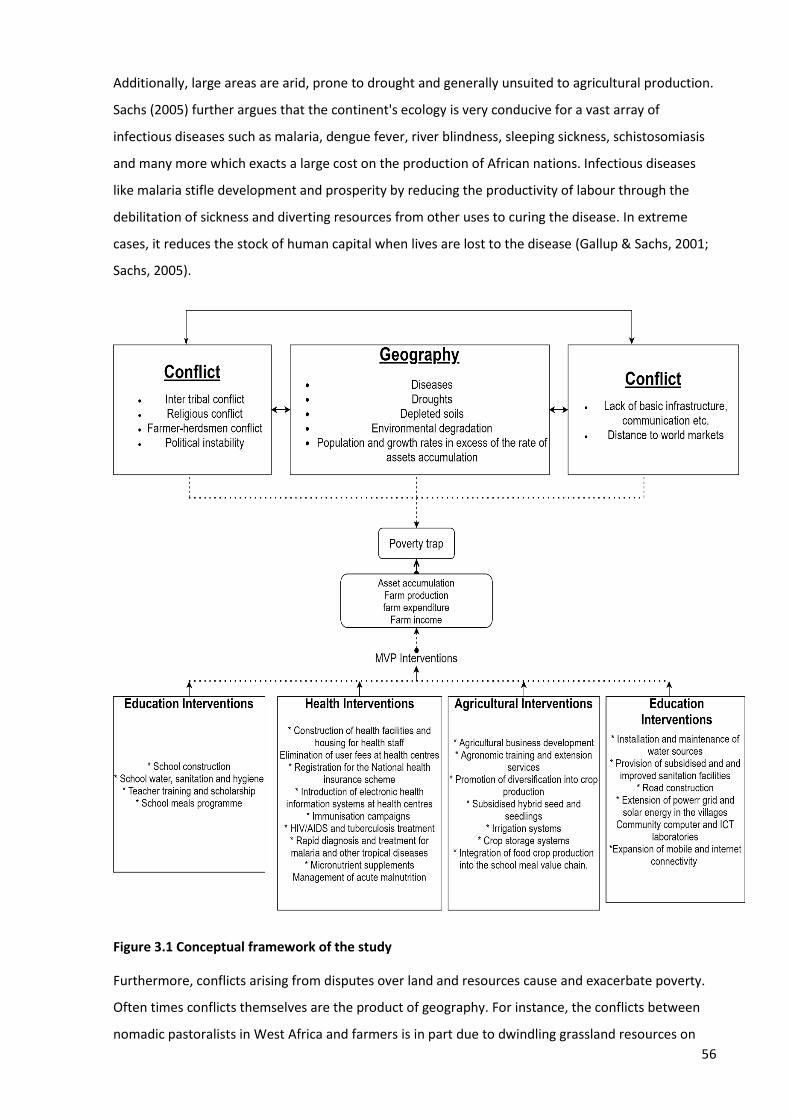
56

Additionally, large areas are arid, prone to drought and generally unsuited to agricultural production.

Sachs (2005) further argues that the continent's ecology is very conducive for a vast array of

infectious diseases such as malaria, dengue fever, river blindness, sleeping sickness, schistosomiasis

and many more which exacts a large cost on the production of African nations. Infectious diseases

like malaria stifle development and prosperity by reducing the productivity of labour through the

debilitation of sickness and diverting resources from other uses to curing the disease. In extreme

cases, it reduces the stock of human capital when lives are lost to the disease (Gallup & Sachs, 2001;

Sachs, 2005).

Figure 3.1 Conceptual framework of the study

Furthermore, conflicts arising from disputes over land and resources cause and exacerbate poverty.

Often times conflicts themselves are the product of geography. For instance, the conflicts between

nomadic pastoralists in West Africa and farmers is in part due to dwindling grassland resources on

57

which their cattle feed (Bukari & Schareika, 2015; Kuusaana & Bukari, 2015; Tonah, 2002). Lastly,

Sub-Saharan Africa has been historically isolated from each other and the rest of the world due to a

lack of basic infrastructures like road networks and communication. In part, the isolation itself is a

product of the geography of Sub-Saharan Africa as vast oceans, deserts, rainforests and rivers that

cannot be navigated on separate nations, tribes and people. Therefore, each of the three root causes

of poverty interacts, with geographic factors causing and exacerbating conflict, which causes

dislocation and emigration of people often to marginal areas where they may be more isolated due

to remoteness or be vulnerable to certain infectious diseases.

The three themes cause Africa’s poverty. However, the poverty trap perpetuates poverty making it

difficult for African Nations to escape poverty (Azariadis & Stachurski, 2005b; Sachs et al., 2004). The

resultant trap of underdevelopment and poverty, according to Sachs (2005) requires a big push to

rectify. The MVP interventions, seen in the bottom half of Figure 3.1, were the means by which these

problems were to be addressed. The interventions are suited to address the various root causes of

poverty. For instance, education reduces the likelihood of people resorting to strength and brawl to

settle their differences. It also tempers the effect of geography, as people are equipped with the

knowledge to combat the adverse effects. Likewise, infrastructure development interventions tackle

the graphics and isolation roots of poverty.

The place of agricultural sector interventions in the MVP in this model is to drive the local economy

through the production and expenditure linkages. This comes about when farmers spend the

revenue and income they earn on locally sourced items, as inputs for production, services for farm

activity, investments or just consumption. However, before spending can occur, the household must

realise an increase in revenue and farm income. To determine the impact the MVP had on assets,

farm output, farm income and farm expenditure, a random sample of MVP households were

surveyed for information on household characteristics, farm characteristics and various qualitative

views about the MVP their community and their lives. In the sections that follow the instrument used

to collect the data and the methods used to analyse the data are presented.

While this latter point about agriculture is alluded to in Sachs (2005) it is not stressed with the

emphasis that this study places on the sector. Moreover, the internal evaluation of the MVPs by

Mitchel et al. (2018) and the external evaluation by Masset et al. (2020) did not focus on the

agricultural sector interventions. This study focuses on the agricultural sector interventions which

has not received as much attention as the health sector impact (Pronyk et al., 2012), the MDG targets

and indicators (Masset et al., 2020; Mitchell et al., 2018). Portions of this conceptual framework were

deduced from Sachs (2005) and the MVP implementation documents (The Earth Institute, &

Millennium Promise, n.d.). However, the agricultural sectors intervention’s impact relationships were

58

a novel development of this research. MVP ran for ten years in the Bonsaaso area. Its primary

interventions were administered in the first five years. The MVP introduced a wide range of

agricultural interventions, most of which are listed in Figure 3.1. Overall, MVP started with the 'quick

wins'. Insecticide-treated bed nets were supplied for free to halt the spread of malaria. Medical care

was administered fee-free at health centres to encourage patronage. Meals were served free in

primary schools to encourage school enrolment. In addition to the 'quick wins', other intervention

areas included education, health, infrastructure, and agriculture (Mitchel et al., 2015a). These

intervention areas have synergies and complementarities with each other. For instance, healthier

farmers should be more productive.

In the first five years of the MVP, farmers were trained in good agronomic practices to boost their

productivity. Extension services were intensified, and farmers were given subsidised fertiliser on an

annual basis for the first three years. The MVP supplied cocoa seedlings to farmers to replace their

ageing tree stock, and it provided seeds for improved breeds of annual food crops like maize and

cowpea. Moreover, the MVP in Bonsaaso trained farmers to grow cowpeas (Vigna unguiculata) and

maize (Zea mays), and constructed storage facilities for these food crops. The purpose of promoting

these food crops in an area dominated by cocoa production was to supply grain to the school meals

programme. Farmers were then paid for two-thirds of the portion of harvest supplied to help pay for

the school meals programme (T. Akowuah, personal conversation, November 20, 2017). The

agricultural interventions listed above were phased out 3-5 years into the MVP's ten-year life. To

address this primary objective, three research questions were set. The first was to ascertain the

differences between MVP and non-MVP households in their financial and socioeconomic conditions.

The second was to determine the impact of the Bonsaaso MVP on the value of assets, gross farm

output, net farm income and farm expenditure of agricultural households. The last was to examine

the sustainability of the agricultural interventions of the MVP.

Chen (2012) distinguishes between three impact assessment paradigms. These include the theory of

change paradigm in which the design and application of evaluation need to be guided by a

conceptual framework called the program theory. Program theory consists of the set of explicit or

implicit assumptions by stakeholders about the actions required to solve the problem that the

programme or intervention seeks to address and the reasons why the problem will respond to them

(Chen, 2012, p. 18). Alternatively, black-box evaluation mainly assesses whether an intervention has

an impact on outcomes without probing the transformational processes that occur between the

intervention and the outcomes. Lastly, method driven evaluations base the evaluation on a

predetermined research method, such as qualitative methods, quantitative methods or mixed

methods. Chen further argues that mixed methods tend to pay less attention to the project’s

59

stakeholders’ views. With regard to the MVP, Jupp and Barnett (2018) and Sachs (2005) have

extensively discussed the theory of change of the MVP in Ghana and Africa respectively.

Methods and empirical strategy

The methods used to address each of the three research questions are presented and discussed in

this section. To recap, the research questions of the study are, (i) what are the differences between

MVP and non-MVP households in their financial and socioeconomic conditions? (ii) what is the

impact of the Bonsaaso MVP on the value of assets, net farm income and farm expenditure of

agricultural households?, and (iii) how sustainable are the agricultural interventions arising from the

MVP intervention?

The difference between MVP and non-MVP households.

The first research question sought to determine whether there are differences between MVP and

non-MVP households with respect to their household characteristics, asset accumulation, and the

characteristics of their farm production enterprises. The variables to be compared are shown in Table

3.1.

Descriptives statistics, namely means, standard errors were used to analyse these variables and

characteristics. A wide range of statistical tests exists for examining various statistical properties

among variables and groups. Some of these properties include the association between variables,

independence between variables and differences between variables and groups. Factors that

influence the statistical methods applied include the research question that the study seeks to

achieve, the types of variables to be assessed and the statistical assumptions on the variable with

respect to the underlying population (Hollander, Wolfe, & Chicken, 2014; Newbold, Carlson, &

Thorne, 2013). Generally, parametric methods are used when the distribution of the variable in

question for the underlying population is assumed to be normal (bell-shaped). In contrast non-

parametric methods do not assume a normal distribution for the variables in the underlying

population. Some parametric methods include independent t-test, paired t-tests, one-way analysis of

variance (ANOVA) Pearson correlation coefficients. Non-parametric methods include the Mann-

Whitney test, Wilcoxon signed-rank test, Kruskal-Wallis test, Spearman’s correlation coefficient and

Chi-squared test.

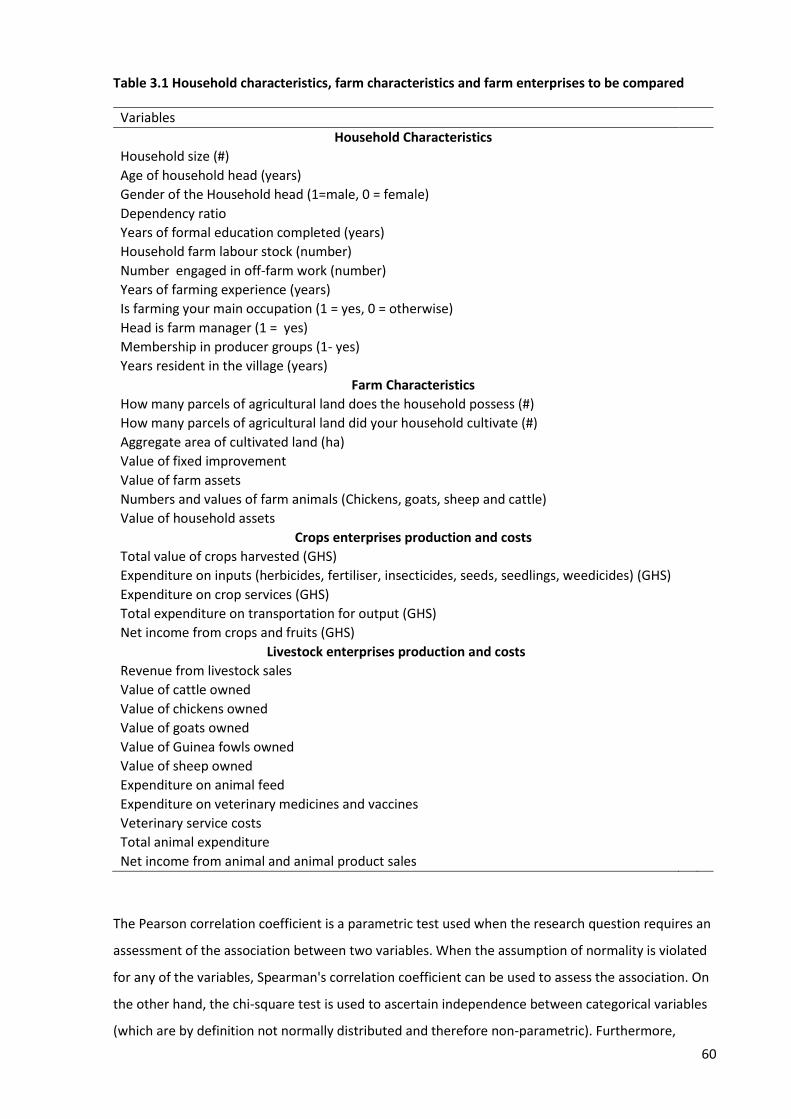
60

Table 3.1 Household characteristics, farm characteristics and farm enterprises to be compared

Variables

Household Characteristics

Household size (#)

Age of household head (years)

Gender of the Household head (1=male, 0 = female)

Dependency ratio

Years of formal education completed (years)

Household farm labour stock (number)

Number engaged in off-farm work (number)

Years of farming experience (years)

Is farming your main occupation (1 = yes, 0 = otherwise)

Head is farm manager (1 = yes)

Membership in producer groups (1- yes)

Years resident in the village (years)

Farm Characteristics

How many parcels of agricultural land does the household possess (#)

How many parcels of agricultural land did your household cultivate (#)

Aggregate area of cultivated land (ha)

Value of fixed improvement

Value of farm assets

Numbers and values of farm animals (Chickens, goats, sheep and cattle)

Value of household assets

Crops enterprises production and costs

Total value of crops harvested (GHS)

Expenditure on inputs (herbicides, fertiliser, insecticides, seeds, seedlings, weedicides) (GHS)

Expenditure on crop services (GHS)

Total expenditure on transportation for output (GHS)

Net income from crops and fruits (GHS)

Livestock enterprises production and costs

Revenue from livestock sales

Value of cattle owned

Value of chickens owned

Value of goats owned

Value of Guinea fowls owned

Value of sheep owned

Expenditure on animal feed

Expenditure on veterinary medicines and vaccines

Veterinary service costs

Total animal expenditure

Net income from animal and animal product sales

The Pearson correlation coefficient is a parametric test used when the research question requires an

assessment of the association between two variables. When the assumption of normality is violated

for any of the variables, Spearman's correlation coefficient can be used to assess the association. On

the other hand, the chi-square test is used to ascertain independence between categorical variables

(which are by definition not normally distributed and therefore non-parametric). Furthermore,

61

where the research question seeks to determine whether differences exist between the means of

two variables or groups, the independent t-test can be used for parametric data whereas the Mann-

Whitney test can be used for the non-parametric test. Lastly, ANOVA and Kruskal-Wallis can be used

to test the differences between the means of three or more groups (Hollander et al., 2014; Newbold

et al., 2013).

As the first research question of this study is to assess the differences between the MVP and non-

MVP households across the variables identified in Table 3.1. This study used independent t-tests to

compare the mean values of the variables across the non-MVP and MVP household on the variables

under the following null hypothesis and alternate hypothesis:

Ho : mvpnonmvp XX −=

H1 : mvpnonmvp XX −

Where mvpX is the mean value of a variable for the MVP households and mvpnonX − is the mean of

same variable for the non-MVP households. Where significant differences were found, the

differences are further explored using counts, percentages, and bar graphs in so doing a preliminary

depiction of the two groups to contextualise the impact evaluation achieved.

Impact of the Bonsaaso MVP on assets, income and expenditure

This section presents the methods used to achieve the second research question - to assess the

impact of the MVP on Households. In this study, the impact is measured in terms of the value of

assets, net farm income gross farm output and farm expenditure. Propensity score matching was

chosen as the best approach to address this objective due to three issues, (i) the MVP was not

designed as a randomised experiment, and there was no designated control village from the onset to

compare with, (ii) there is no baseline data on the Bonsaaso MVP. Lastly (iii) the project was run for a

long time. In the next section the methodological issues that arise from the design of the MVP, the

lack of baseline data and the long life of the project are discussed along with the common methods

used in evaluating the impact of projects and justification for the propensity score matching as the

best method settled on. I recursive instrumental variables (IV) model was developed to serve as a

robustness check on the propensity score matching estimates while testing and controlling for

unobserved factors that may influence participation and outcomes, causing endogeneity. This is the

critical research question, therefore, it merits careful consideration of the alternatives available to

the study and a rigorous discussion of the steps taken to arrive at the methods used to assess the

second research question.

62

3.3.2.1 Methodological Issues in Impact Assessment

This section discusses the issues that need to be addressed and methods commonly used to assess

the impact of interventions. The discussion begins with the core issue of impact assessment, which is

to identify a suitable counterfactual, i.e. what would have been the social and economic outcomes of

interest for an individual had they not received the intervention. Two distinct types of

counterfactuals are discussed, along with their shortcomings and implications for the estimated

impact highlighted. The discussion then shifts to the problem of selection bias (in Section 3.4) and

the resultant endogeneity problem it poses for the general treatment model. Conventional methods

used to address the shortcomings of common counterfactuals and to estimate project impacts are

then presented in Section 3.3.2.4.

3.3.2.2 Defining the counterfactual

Impact assessment seeks to address the causality between an intervention and subsequent

outcomes. Attempting to evaluate if the changes in an outcome can be attributed to a particular

treatment, project or intervention sets impact assessment apart from regular monitoring and

evaluation for a project. Monitoring and evaluation apply management tools to track progress and

key performance indicators during project implementation (Khandker, Koolwal, & Samad, 2010).

Impact assessment on the other hand determines if a change in an outcome is caused by the

intervention only. Impact assessment can be either quantitative or qualitative. Qualitative impact

assessment is beneficial as it unearths knowledge about the mechanisms by which a project helps its

beneficiaries. Such knowledge is, however, contextual and not generalisable (Khandker et al., 2010).

By contrast, quantitative evaluation methods use quantitative data on the beneficiaries to measure

the impact of the intervention (Khandker et al., 2010) and are more prominent in the economics

literature. Data for such an evaluation can be collected either before and after, or simply after, the

project. The impact or treatment effect (Ii) of a treatment (T) (scoring 1 for treated and 0 for

untreated) on a unit (individual, household, country or other entity that is the subject of the study) i

is defined as:

Ii = yi1 -yi

0, ………….. (3.1)

where yi1 is the outcome observed for unit i and yi

0 is a missing value representing the value taken

by the outcome had unit i not received the treatment. The value yi0 is the counterfactual. The

primary conceptual challenge of an impact assessment is how to identify the counterfactual

(Khander, Koolwal, & Samad, 2010; Ravallion, 2008). The counterfactual is defined as 'what would

have happened had the project never taken place or what otherwise would have been true' (Baker,

2000; Khandker et al., 2009; Ravallion, 2001). For instance, the counterfactuals for the value of assets

63

for an MVP household (h1), would be the value of assets for that particular household (h1) if the

MVP had not taken place. An ideal situation would be to make a comparison of the outcome of

interest in the same household or individual with and without the MVP (the treatment). However,

such a comparison is impossible as the individual, household, nation, or other entity being assessed

cannot have two simultaneous lives, one in which they benefit from the MVP (treatment) and the

other in which they do not benefit from the MVP. Two approaches commonly used to establish a

counterfactual are the 'with-and-without' counterfactual method and the 'before-and-after'

counterfactual method (Khandker et al., 2010). Khander et al. (2010) describe these counterfactuals

as 'counterfeit' as they have severe shortcomings which undermine the accuracy of their estimated

impacts.

The before-and-after counterfactual approach takes a baseline measure of the outcome before the

intervention (y0) and a final measure of the outcome after the intervention (y1) for a reflexive

comparison. The impact of the treatment is measured as the difference between the outcome

measured after treatment and the outcome measured before treatment (y1-y0) (Baker, 2000;

Khandker et al., 2010). The before-and-after counterfactual, though straightforward, is unlikely to

yield an accurate estimate of the impact of the intervention because factors other than the project

also affect the outcome. These factors, such as changes in the environment and the individual's

characteristics and ability, must be controlled for when assessing the impact of the intervention if the

estimate of the treatment is to be accurate.

The with-and-without counterfactual takes the difference in the outcome variable between a treated

group that received the intervention and an untreated group that did not receive the intervention

(Gertler et al., 2011; Khandker et al., 2010). The problem with this approach is that individuals in the

treated and untreated groups are not identical, and their differences could affect the outcomes of

interest. Such a comparison, which does not account for differences between individuals, does not

reflect the impact of the project fairly. As discussed in Section 1.1, the MVP villages, for instance,

were selected because they met certain governance and poverty criteria. If the poverty levels of the

Millennium Villages were different from other villages at the start of the project, any difference in

poverty and other related outcomes measured at the end of the MVP could not be entirely

attributed to the MVP. The targeting of the MVP also gives rise to the problem of selection bias

explained in the next section.

The standard solution to the counterfactual problem has been to assign the treatment at random to

the units under study. Well-designed randomised experiments are the best way to determine

causality in socioeconomic and development settings et al., 2007; White & Raitzer, 2017). It entails

the random assignment of members of a target group for treatment to one or more treatment

64

groups and a control group (Duflo et al., 2007). The treatment group receives the intervention,

project or treatment, and the control group does not. The membership of any of these two groups is

assigned at random, giving every member an equal chance of being selected to their respective

groups (Gertler et al., 2016; Khandker et al., 2009). Randomisation ensures that balance is achieved

among the characteristics of the two groups (White & Raitzer, 2017). Balance is achieved when the

average baseline observed, and unobserved characteristics of the treatment and control groups are

equal, effectively eradicating the problem of selection bias. If certain assumptions hold, the

difference in the average outcome variables between the treatment and control groups of a

balanced sample at the end-line gives an effective measure of the impact of the intervention. The

differences observed in the outcomes at the end of the treatment would, therefore, be a result of

the treatment. The MVP, however, was not designed as a randomised experiment. Therefore,

observed and unobserved characteristics could affect participation. Therefore, a sample of MVP

participants and non-participants will not have similar characteristics (not balanced) and therefore

cannot be compared.

3.3.2.3 The problem of selection bias

Selection bias is one of three potential causes of the broader problem of endogeneity. The second is

reverse causality or simultaneity between the outcome and at least one of the explanatory variables

(the endogenous variable). A typical example of a simultaneity relationship in economics is the

relationship between demand and supply. The third cause of endogeneity is omitted variable bias

where the variable omitted from the model is correlated with the dependent variable and at least

one of the explanatory variables. For instance, Rauscher, Shaw, and Ky (1993) reported of the

“Mozart effect” where students who listened to Mozart’s sonata, experienced an 8-9 point increase

in intelligence quotient (IQ) for spatial tasks. However, there are strong indications that the

experiment was missing important explanatory variables which affect both IQ and listening to

classical music, resulting in biased estimates of the impact of listening to Mozart on IQ (Stock &

Watson, 2012). Selection bias commonly occurs when participation or assignment to a treatment is

not randomised. As a result, the factors that influence placement or selection into a project could

also affect the outcomes under examination. The Millennium Villages (MVs) for instance, were

selected purposively based on criteria described in section 1.2. As a result, the problem of selection

bias threatens to undermine any estimates of the project's impact if the issue is not addressed.

Equation 3.2 shows the generalised 'treatment' model that expresses the typical impact assessment

problem (Khandker et al., 2009). It compares an outcome (Y) across households i, that have either

had the treatment (T=1) or not had the treatment (T=0):

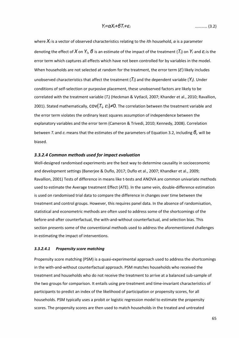
65

Yi=αXi+βTi+εi ………… (3.2)

where Xi is a vector of observed characteristics relating to the ith household, α is a parameter

denoting the effect of X on Yi, β is an estimate of the impact of the treatment (Ti) on Yi and εi is the

error term which captures all effects which have not been controlled for by variables in the model.

When households are not selected at random for the treatment, the error term (ε) likely includes

unobserved characteristics that affect the treatment (Ti) and the dependent variable (Yi). Under

conditions of self-selection or purposive placement, these unobserved factors are likely to be

correlated with the treatment variable (Ti) (Heckman & Vytlacil, 2007; Khander et al., 2010; Ravallion,

2001). Stated mathematically, cov(Ti, εi)≠0. The correlation between the treatment variable and

the error term violates the ordinary least squares assumption of independence between the

explanatory variables and the error term (Cameron & Trivedi, 2010; Kennedy, 2008). Correlation

between Ti and εi means that the estimates of the parameters of Equation 3.2, including β, will be

biased.

3.3.2.4 Common methods used for impact evaluation

Well-designed randomised experiments are the best way to determine causality in socioeconomic

and development settings (Banerjee & Duflo, 2017; Duflo et al., 2007; Khandker et al., 2009;

Ravallion, 2001) Tests of difference in means like t-tests and ANOVA are common univariate methods

used to estimate the Average treatment Effect (ATE). In the same vein, double-difference estimation

is used on randomised trial data to compare the difference in changes over time between the

treatment and control groups. However, this requires panel data. In the absence of randomisation,

statistical and econometric methods are often used to address some of the shortcomings of the

before-and-after counterfactual, the with-and-without counterfactual, and selection bias. This

section presents some of the conventional methods used to address the aforementioned challenges

in estimating the impact of interventions.

3.3.2.4.1 Propensity score matching

Propensity score matching (PSM) is a quasi-experimental approach used to address the shortcomings

in the with-and-without counterfactual approach. PSM matches households who received the

treatment and households who do not receive the treatment to arrive at a balanced sub-sample of

the two groups for comparison. It entails using pre-treatment and time-invariant characteristics of

participants to predict an index of the likelihood of participation or propensity scores, for all

households. PSM typically uses a probit or logistic regression model to estimate the propensity

scores. The propensity scores are then used to match households in the treated and untreated

66

groups. Households that fall outside the range of overlapping propensity scores (region of common

support) for the two groups are often discarded. Households within the region of common support

are further matched to increase the similarity among the treatment group and the control group,

thereby making them more comparable.

Four algorithms commonly used for the matching process include nearest-neighbour matching,

calliper matching, stratified matching and kernel matching (Ho, Imai, King, & Stuart, 2007; Khandker

et al., 2009). After matching, independent variables used to estimate the propensity score model, are

tested for balance (Ravallion, 2008; Rosenbaum & Rubin, 1983). The balance test determines the

extent of the success of the matching process. According to Guo and Fraser (2014), covariate balance

can be assessed using any of the following techniques: standardised mean differences, variance

ratios, Kolmogorov-Smirnov-test p-values and univariate t-tests. Caliendo & Kopeinig (2008) further

suggest a joint significance and pseudo-R2 test to determine covariate balance. In this approach the

model used to estimate the propensity score is reestimated using the matched dataset. Since

matching is intended to remove any systemic difference in the two groups with respect to their pre-

treatment characteristics, the reestimated propensity score model should produce a reasonably low

pseudo-R2 if the matching was successful. Where the balancing test returns no statistically significant

differences in the covariates among the two groups in the matched subset, the matching is deemed

successful. When well-balanced subsets have been identified, the mean outcomes are then

compared between the matched subsets, i.e., the treatment and control groups that have similar

predicted values of participation. PSM is effective in controlling for differences in observed, pre-

treatment, time-invariant characteristics that may have contributed to differences in outcomes for

the treated households and the untreated households.

PSM is based on two assumptions. First, individuals were selected for participation in the programme

based only on observed and time-invariant characteristics. This assumption is called conditional

independence (Khander et al., 2009; Ravallion, 2001), unconfoundedness (Rosenbaum & Rubin,

1983), selection on observables (Frölich, 2007; Huber, 2014) or exogeneity (Imbens, 2004). This

means that no unobserved factors affect participation in the treatment. The second assumption is

that, there exists a large enough overlap (common support) between the propensity scores (i.e., the

predicted probabilities) of the participants and non-participants. Heckman, Ichimura, and Todd

(1997) strongly advocate the exclusion of cases outside the region of common support. PSM is

ineffective when participants self-select on unobservable attributes. It can be used on cross-sectional

data as well as panel data. Moreover, because it helps to achieve balance between two groups it is

sometimes combined with other methods such as double difference.

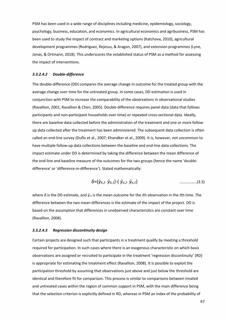
67

PSM has been used in a wide range of disciplines including medicine, epidemiology, sociology,

psychology, business, education, and economics. In agricultural economics and agribusiness, PSM has

been used to study the impact of contract and marketing options (Katchova, 2010), agricultural

development programmes (Rodriguez, Rejesus, & Aragon, 2007), and extension programmes (Lyne,

Jonas, & Ortmann, 2018). This underscores the established status of PSM as a method for assessing

the impact of interventions.

3.3.2.4.2 Double-difference

The double-difference (DD) compares the average change in outcome for the treated group with the

average change over time for the untreated group. In some cases, DD estimation is used in

conjunction with PSM to increase the comparability of the observations in observational studies

(Ravallion, 2001; Ravallion & Chen, 2005). Double difference requires panel data (data that follows

participants and non-participant households over time) or repeated cross-sectional data. Ideally,

there are baseline data collected before the administration of the treatment and one or more follow-

up data collected after the treatment has been administered. The subsequent data collection is often

called an end-line survey (Duflo et al., 2007; Khandker et al., 2009). It is, however, not uncommon to

have multiple follow-up data collections between the baseline and end-line data collections. The

impact estimate under DD is determined by taking the difference between the mean difference of

the end-line and baseline measure of the outcomes for the two groups (hence the name 'double-

difference’ or 'difference-in-difference’). Stated mathematically:

δ=(ӯb,2- ӯb,1)-( ӯa,2- ӯa,1) ………………(3.3)

where δ is the DD estimate, and ӯi,t is the mean outcome for the ith observation in the tth time. The

difference between the two mean differences is the estimate of the impact of the project. DD is

based on the assumption that differences in unobserved characteristics are constant over time

(Ravallion, 2008).

3.3.2.4.3 Regression discontinuity design

Certain projects are designed such that participants in a treatment qualify by meeting a threshold

required for participation. In such cases where there is an exogenous characteristic on which basis

observations are assigned or recruited to participate in the treatment 'regression discontinuity’ (RD)

is appropriate for estimating the treatment effect (Ravallion, 2008). It is possible to exploit the

participation threshold by assuming that observations just above and just below the threshold are

identical and therefore fit for comparison. This process is similar to comparisons between treated

and untreated cases within the region of common support in PSM, with the main difference being

that the selection criterion is explicitly defined in RD, whereas in PSM an index of the probability of

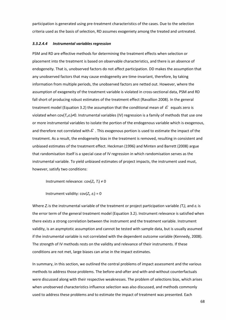
68

participation is generated using pre-treatment characteristics of the cases. Due to the selection

criteria used as the basis of selection, RD assumes exogeniety among the treated and untreated.

3.3.2.4.4 Instrumental variables regression

PSM and RD are effective methods for determining the treatment effects when selection or

placement into the treatment is based on observable characteristics, and there is an absence of

endogeneity. That is, unobserved factors do not affect participation. DD makes the assumption that

any unobserved factors that may cause endogeneity are time-invariant, therefore, by taking

information from multiple periods, the unobserved factors are netted out. However, where the

assumption of exogeneity of the treatment variable is violated in cross-sectional data, PSM and RD

fall short of producing robust estimates of the treatment effect (Ravallion 2008). In the general

treatment model (Equation 3.2) the assumption that the conditional mean of equals zero is

violated when cov(Ti,εi)≠0. Instrumental variables (IV) regression is a family of methods that use one

or more instrumental variables to isolate the portion of the endogenous variable which is exogenous,

and therefore not correlated with . This exogenous portion is used to estimate the impact of the

treatment. As a result, the endogeneity bias in the treatment is removed, resulting in consistent and

unbiased estimates of the treatment effect. Heckman (1996) and Minten and Barrett (2008) argue

that randomisation itself is a special case of IV regression in which randomisation serves as the

instrumental variable. To yield unbiased estimates of project impacts, the instrument used must,

however, satisfy two conditions:

Instrument relevance: cov(Zi, Ti) ≠ 0

Instrument validity: cov(Zi, εi) = 0

Where Zi is the instrumental variable of the treatment or project participation variable (Ti), and εi is

the error term of the general treatment model (Equation 3.2). Instrument relevance is satisfied when

there exists a strong correlation between the instrument and the treatment variable. Instrument

validity, is an asymptotic assumption and cannot be tested with sample data, but is usually assumed

if the instrumental variable is not correlated with the dependent outcome variable (Kennedy, 2008).

The strength of IV methods rests on the validity and relevance of their instruments. If these

conditions are not met, large biases can arise in the impact estimates.

In summary, in this section, we outlined the central problems of impact assessment and the various

methods to address those problems. The before-and-after and with-and-without counterfactuals

were discussed along with their respective weaknesses. The problem of selections bias, which arises

when unobserved characteristics influence selection was also discussed, and methods commonly

used to address these problems and to estimate the impact of treatment was presented. Each

69

method imposes a range of assumptions and data requirements that should hold for their respective

impact estimates to be accurate and unbiased.

3.3.2.4.5 The rationale for Empirical Strategy

For this investigation, PSM and IV regression were determined to be the most appropriate estimation

techniques for estimating the average causal effect as the MVP project was not designed as a

randomised control experiment. It was discovered during the fieldwork and in later MVP

documentation that baseline data was collected. However, all attempts to acquire these data were

unsuccessful. Moreover, the endline impact analysis done by the project partners did not make use

of this baseline data (Mitchell et al., 2018; The Earth Institute, & Millennium Promise, n.d.). The

baseline survey did not include control villages, and the baseline data are not publicly available

(Mitchell et al, 2015). Selection criteria were not applied to individual households. As a result, this

study could not apply the double-difference or regression discontinuity methods to estimate the

impact of the MVP. This study, therefore, resorted to PSM and IV regression to estimate the project

impact. Although instrumental variables regression can control for unobserved factors that might

affect participation, the estimates of the instrumental variables regression are properly local average

treatment effects instead of the average treatment effects desired in this research (Angrist &

Pischke, 2009). The interpretation of LATE is the treatment effect for participants who comply with

the project rather than the general population of participants. This interpretation is problematic

given the design and implementation of the MVP. In which entire villages and their inhabitants

participated in the project. However, due to the lack of baseline data for the MVP and non-MVP

households, PSM and IV are the most appropriate methods.

To accommodate these techniques, end-line data were gathered from both MVP and non-MVP

households. A village that had not received the MVP intervention, Nyankomase was purposively

selected to be similar to the MVP villages - having the same majority ethnic group, traditional

authority, local government policy, and livelihoods. This village was equally affected by the gold rush

that peaked in the MVP area in 2012. As the global price of gold peaked from mid-2011 – to mid-

2013, there was a lot of small-scale and illegal gold mining activities in the area. This had a significant

impact on the MVP area and neighbouring communities (Wilson, 2017). However, the non-MVP

village was sufficiently distant from the MVP and so was not likely to have been influenced by the

project's interventions. Observed characteristics that affected placement in the MVP were controlled

using PSM, while unobserved characteristics were controlled using IV regression thereby serve as a

robustness check on the PSM estimates.

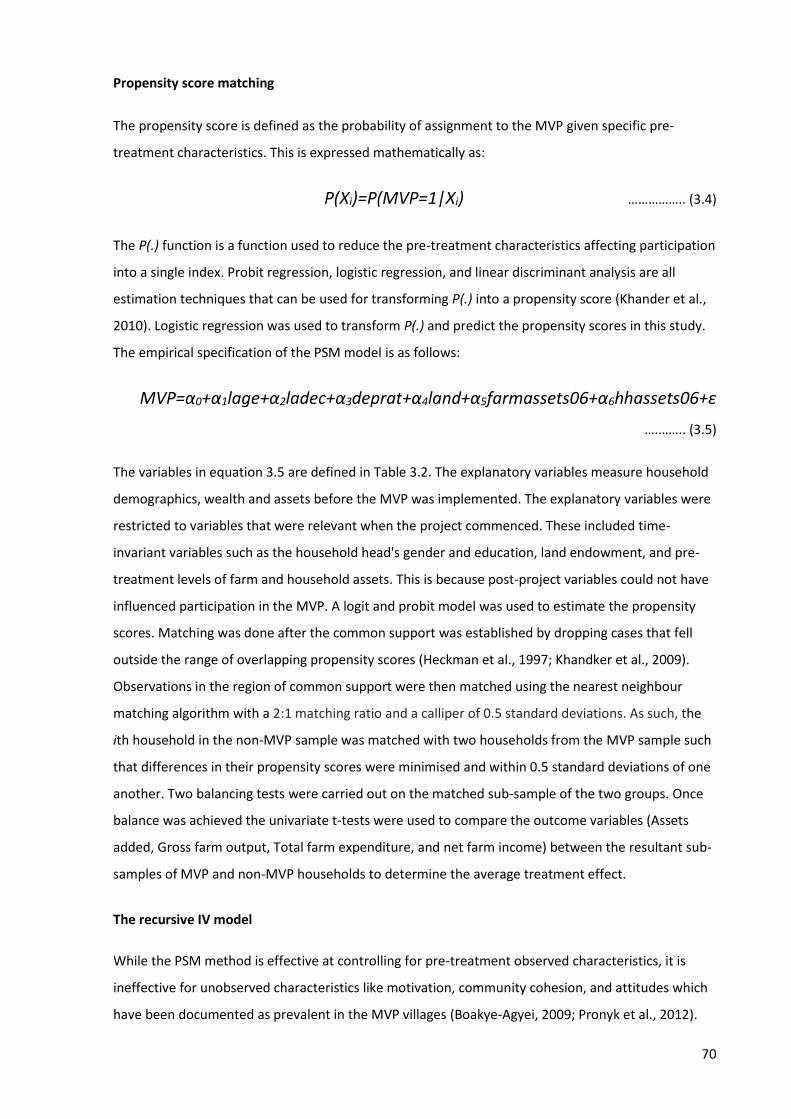
70

Propensity score matching

The propensity score is defined as the probability of assignment to the MVP given specific pre-

treatment characteristics. This is expressed mathematically as:

P(Xi)=P(MVP=1|Xi) …………….. (3.4)

The P(.) function is a function used to reduce the pre-treatment characteristics affecting participation

into a single index. Probit regression, logistic regression, and linear discriminant analysis are all

estimation techniques that can be used for transforming P(.) into a propensity score (Khander et al.,

2010). Logistic regression was used to transform P(.) and predict the propensity scores in this study.

The empirical specification of the PSM model is as follows:

MVP=α0+α1lage+α2ladec+α3deprat+α4land+α5farmassets06+α6hhassets06+ε

….…….. (3.5)

The variables in equation 3.5 are defined in Table 3.2. The explanatory variables measure household

demographics, wealth and assets before the MVP was implemented. The explanatory variables were

restricted to variables that were relevant when the project commenced. These included time-

invariant variables such as the household head's gender and education, land endowment, and pre-

treatment levels of farm and household assets. This is because post-project variables could not have

influenced participation in the MVP. A logit and probit model was used to estimate the propensity

scores. Matching was done after the common support was established by dropping cases that fell

outside the range of overlapping propensity scores (Heckman et al., 1997; Khandker et al., 2009).

Observations in the region of common support were then matched using the nearest neighbour

matching algorithm with a 2:1 matching ratio and a calliper of 0.5 standard deviations. As such, the

ith household in the non-MVP sample was matched with two households from the MVP sample such

that differences in their propensity scores were minimised and within 0.5 standard deviations of one

another. Two balancing tests were carried out on the matched sub-sample of the two groups. Once

balance was achieved the univariate t-tests were used to compare the outcome variables (Assets

added, Gross farm output, Total farm expenditure, and net farm income) between the resultant sub-

samples of MVP and non-MVP households to determine the average treatment effect.

The recursive IV model

While the PSM method is effective at controlling for pre-treatment observed characteristics, it is

ineffective for unobserved characteristics like motivation, community cohesion, and attitudes which

have been documented as prevalent in the MVP villages (Boakye-Agyei, 2009; Pronyk et al., 2012).

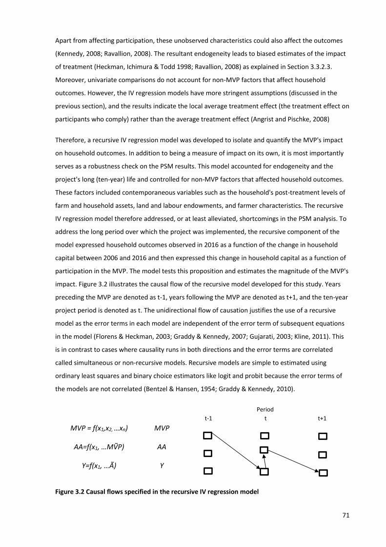
71

Apart from affecting participation, these unobserved characteristics could also affect the outcomes

(Kennedy, 2008; Ravallion, 2008). The resultant endogeneity leads to biased estimates of the impact

of treatment (Heckman, Ichimura & Todd 1998; Ravallion, 2008) as explained in Section 3.3.2.3.

Moreover, univariate comparisons do not account for non-MVP factors that affect household

outcomes. However, the IV regression models have more stringent assumptions (discussed in the

previous section), and the results indicate the local average treatment effect (the treatment effect on

participants who comply) rather than the average treatment effect (Angrist and Pischke, 2008)

Therefore, a recursive IV regression model was developed to isolate and quantify the MVP's impact

on household outcomes. In addition to being a measure of impact on its own, it is most importantly

serves as a robustness check on the PSM results. This model accounted for endogeneity and the

project's long (ten-year) life and controlled for non-MVP factors that affected household outcomes.

These factors included contemporaneous variables such as the household's post-treatment levels of

farm and household assets, land and labour endowments, and farmer characteristics. The recursive

IV regression model therefore addressed, or at least alleviated, shortcomings in the PSM analysis. To

address the long period over which the project was implemented, the recursive component of the

model expressed household outcomes observed in 2016 as a function of the change in household

capital between 2006 and 2016 and then expressed this change in household capital as a function of

participation in the MVP. The model tests this proposition and estimates the magnitude of the MVP's

impact. Figure 3.2 illustrates the causal flow of the recursive model developed for this study. Years

preceding the MVP are denoted as t-1, years following the MVP are denoted as t+1, and the ten-year

project period is denoted as t. The unidirectional flow of causation justifies the use of a recursive

model as the error terms in each model are independent of the error term of subsequent equations

in the model (Florens & Heckman, 2003; Graddy & Kennedy, 2007; Gujarati, 2003; Kline, 2011). This

is in contrast to cases where causality runs in both directions and the error terms are correlated

called simultaneous or non-recursive models. Recursive models are simple to estimated using

ordinary least squares and binary choice estimators like logit and probit because the error terms of

the models are not correlated (Bentzel & Hansen, 1954; Graddy & Kennedy, 2010).

Period

t-1 t t+1

MVP = f(x1,x2, …xn) MVP

AA=f(x1, …MṼP) AA

Y=f(x1, …Ã) Y

Figure 3.2 Causal flows specified in the recursive IV regression model

72

Source: Author (2018) adapted from Bentzel and Hansen (1954) Estimation of the model proceeded in three steps. The first step estimated a logit model of MVP

participation (Equation 3.6) with instrumental variables (IVs) added to the set of explanatory farm

and household characteristics. The second step regressed the change in household capital, defined as

the real value of assets and fixed improvements added to the household's stock of capital denoted as

AA in Equation 3.7 on predicted MVP participation (MṼP) and a set of explanatory farm and

household characteristics. Substituting actual MVP participation with predicted MVP participation

addresses the endogeneity problem caused by selection bias because predicted MVP excludes the

effects of unobserved variables that may influence both participation and outcomes. In practice,

steps 1 and 2 represent an estimation of the general treatment model using two-stage least squares

(2SLS) regression. The impact of the MVP on AA, the value of assets added, is measured by the

regression coefficient estimated for predicted MVP in Equation 3.7.

Several studies have assessed the efficacy of IVs in addressing the problem of endogeneity (Angrist,

Imbens, & Rubin, 1993; Heckman, Urzua, & Vytlacil, 2006; Heckman et al., 1998; Imbens, 2010). The

consensus is that IV methods are effective in addressing endogeneity if the instruments chosen are

both relevant and valid. Relevance requires that the instruments are strongly correlated with the

endogenous variable, in this case, MVP participation, while validity requires that the instruments are

not correlated with the outcomes under consideration (Kennedy 2004). This study used distance to

the nearest metropolitan district as the instrumental variable for MVP participation. This variable

satisfied the conditions required both for instrument relevance and instrument validity.

The third and final step of the recursive model regressed end-line household outcomes on the

predicted value of assets (Ã) and a set of explanatory farm and household characteristics (Equation

3.8). As with Equation 3.7, the standard errors of the estimated regression had to be corrected for the

2SLS process. These corrections were made using the method described by Gujarati (2003, p. 791).

In general terms, the postulated recursive IV regression model is expressed in Equations 3.6 – 3.8.

MVP = f(x1,x2,IV) ……………… (3.6)

AA=f(x1,X2,MṼP) ……………… (3.7)

y=f(x1,x2,Ã) ……………… (3.8)

where, MVP scores 1 for MVP participants and 0 otherwise, x1 and x2 are farm and household

characteristics, IV is the instrumental variable (distance to the nearest metropolitan district); AA is

the value of assets added over the project's life; MṼP is the predicted probability of MVP

participation, Ã represents the predicted value of assets in 2016 (defined as predicted AA plus the

73

baseline level of assets in 2006), and y1 represents an outcome variable (Gross farm output, Total

farm expenditure and Net farm income).

The empirical recursive IV regression model was specified as follows:

MVP=α0+α1lage+α2leduc+α3deprat+α4land+α5farmassets06+α6hhassets06+α7dist+ε1

..….……….. (3.9)

AA= β0+β1MṼP+β2educ+β3age+β4age2+β5farmlabour+β6offfarmlabour+β7male+β8deprat+

β9prodgrp+β10land+β11lassets06+β12electricity0615+ε2 ..….……….. (3.10)

Y1=γ0+γ1Ã+γ2land+ γ3offfarmlabour +γ4goats +γ5prodgrp+ε3 ……………… (3.11)

Table 3.2 below defines the variables used in the models and their units of measure. In Equations 3.9

– 3.11, α0 – α7, β0 – β12 and γ0 – γ5 were parameters estimated for the models. β1 represents the

impact of MVP participation on assets added while γ1 is the impact of assets added on end-line

outcomes. ε1, ε2, and ε3, are error terms for the participation, assets added and outcome models

respectively. These error terms are assumed to be independent of one another in the recursive

model.

Table 3.2 Variables used in the recursive IV regression model

Variable Unit Description

MVP 1 = participant, otherwise 0 MVP participation

deprat dependents/workers Dependency ratio of household

land Ha/adult equivalent Stock of land available to the household for farming

farmassets06 Ghs /adult equivalent Value of farm equipment, assets, and improvements

hhassets06 Ghs/adult equivalent Value of household assets

dist km Distance to the nearest metropolitan district

MṼP # Predicted probability of MVP participation

AA Ghs/adult equivalent Value of assets added

educ years Years of schooling completed

age years Age of Household head

farmlabour #/adult equivalent Household stock of farm labour

offfarmlabour #/adult equivalent Number of members engaged in off-farm work

male 1 = male, otherwise 0 Household head is male

prodgrp 1 = member, otherwise 0 Membership of producer groups

lassets06 Ghs Log of baseline (2006) level of assets

electricity06 1 = yes, otherwise 0 Access to electricity

à Ghs Predicted value of assets added

goats Ghs Market value of goats owned (liquidity)

Source: Author (2018)

74

Equation 3.9 is essentially the same model of MVP participation used for the PSM except for the

addition of the instrumental variable. The instrumental variable was the distance to the nearest

metropolitan district. This was chosen because it satisfied all the requirements for an instrumental

variable discussed in Section 3.3.2.4 and shown in Appendix C. It was not included in the Propensity

score model (Equation 5.1 and Table 5.1) because its relevance to this model would have resulted

from two things.

1. Its influence on access to markets for farm products and farm inputs

2. Its influence on access to amenities such as healthcare, education, electricity, entertainment

and so on.

However, it wasn’t relevant for market access because cocoa is the main crop grown in the MVP

area. Given the strategic importance of cocoa to the economy of Ghana, the Ghana Cocoa Marketing

Board along with its licensed buying companies have outlets in almost every town in the district to

purchase cocoa beans and sell farm inputs to farmers. Therefore farmers do not have to transport

their cocoa beans to the metropolitan district to sell them. Similarly, access to amenities was not a

relevant factor as more urban towns in the district like the district capital are closer to the villages

and easier to assess than the metropolitan district.

In Equation 3.9, MVP participation was expected to have a positive impact on assets added. Likewise,

the household's labour and land endowments, its baseline level of assets, access to electricity during

the MVP, and membership of producer groups were all expected to bear positively on assets added.

The age of the household head was expected to have a positive but diminishing effect on assets

added.

In Equation 3.11, the value of assets added was expected to have a positive impact on household

outcomes. As in Equation 3.10, land endowment, the number of off-farm wage workers, and

membership of producer groups were all expected to bear positively on outcomes. Goats are a

popular form of informal savings in rural Ghana and the market value of goats owned was included in

Equation 3.10 as a proxy for household liquidity. This is because goats, being a delicacy are relatively

easier to sell in the villages. This variable was also expected to impact positively on household

outcomes.

Sustainability of the MVP interventions

To address the third question. MVP participants' were asked the questions in Section C of the

questionnaire presented in the next section and Appendix A. The questions covered households’

access to the MVP’s agricultural interventions perceptions of project outcomes, households were

75

asked to express their views on the benefits and services delivered by the MVP, the project's

performance and a variety of questions about the agricultural interventions of the MVP.

Respondents were also asked about their access to services (such as extension and training, saving

and credit services and crop storage), markets, food, employment, and general living conditions

before, during and after the project. These data were analysed using descriptive statistics.

Descriptive statistics and graphs were used to analyse the data and for presentation.

Survey Instrument

This study relied on primary data collected from farm households for the variables needed to answer

the research question. The MVP had not made the baseline data collected at the start of the project

publicly available. Furthermore, their internal impact assessment did not use the baseline data, citing

data quality issues (Mitchell et al., 2015). An attempt was made to construct a baseline data set from

the fifth iteration of the Ghana Living Standards Survey (GLSS5). However, a lack of village codes

made it impossible to properly select households that would have been in the vicinity of the MVP.

This is critical, as the Ashanti Region has at least two agro-ecological zones suited to cultivating

different crops. In addition to the governmental, institutional and cultural differences that

characterise different people across the region. Doing so would have introduced biases that would

have been difficult to account for. Therefore, this study designed a structured questionnaire as the

main instrument used for collecting household-level data to answer the research questions of this

study.

From the conceptual framework, the research questions and the methods discussed in Section 3.2

and 3.3 the data required were categorised into three groups for the questionnaire. The full

questionnaire is presented in see Appendix A. the three categories were grouped into Section A, B

and C of the questionnaire. The goal of Section A was to obtain a good description of the farm

household, their composition, people involved in farming and off-farm activities and roles in the

community. Section B on the other have was to collect information on all aspect of the farm

enterprises of the household and condition in the community over time. At the same time, Section C

was for the MVP participants to express their views about the project.

Section A. Household characteristics elicited information about household composition, including

household size, the number of male and female household members, the number of children under

15, adults (aged 16 – 65), pensioners (over 65), the number of members enrolled in school, as well as

those working on-farm and off-farm. Additionally, information on the household members

responsible for farm decision making, years of education, marital status, membership of producer

groups and leadership role (if any) played in the community.

76

Section B. Farm enterprise(s). The questions in this section covered all aspects of the households’

farming activities. Section B.1 started with the landholdings specifically, the number of parcels

owned by the household, their respective sizes, sources or how they obtained their land, and the

duration that the households have managed the parcels. Sections B.2 and B.3 captured cash and

food crop enterprises. Specifically, the crops produced and the production information including area

cultivated, quantity harvested in the production season, revenue realised and costs of inputs and

services. Fruit crops were covered in Section B.4. It is customary for rural households to grow one or

more fruit trees for household consumption without the intention of selling commercially. Therefore,

there was a question on the reason for planting the crop, whether for household consumption or

commercial sale, and the quantity harvested of fruits during the season, and the unit price realised.

Where multiple prices were obtained, the weighted average price was calculated. Section B5 covered

questions of livestock enterprises, namely the number of animals, owned, the number sold during

the production season, income realised from the sale of animals and income realised from the sale of

animal products like eggs, manure and milk. The section continued in Section B 5b with questions on

the livestock expenditure. Namely, the amount spent on feed, veterinary services, vaccines and

medicines, labour for animal production jobs, maintenance costs and compensation for property

destruction done by the households’ animals. Section B.6-B.8 covered investment in fixed

improvements, farm assets and equipment, and household assets. For fixed improvements, the

questionnaire further elicited the present value, estimated replacement cost and the year in which

the improvement was acquired. For farm assets and equipment, and household assets, the study

elicited information on the quantity owned, estimated market value and the year in which the asset

was acquired. Section B.9 sort to capture information on non-farm income-earning activities engaged

in by the household and the amount of income generated over the production season from non-farm

sources.

Sections B.10-B11 sought information about changes perceived over time by the household on

access to services and conditions of the community in 2006, 2006 – 2015 and after 2015,

corresponding before, during and after the MVP. Specifically, categories covered include access to

training and extension for crop and animal production, access to subsidised inputs, access to training

and irrigation equipment and credit. Similarly, information on aspects of community life in the village

such as employment in the community, stability of income, health of children, education of children,

quality of housing, access to safe food, clean drinking water, irrigation water, electricity, safety and

the quality of the natural environment were collected.

Lastly, Section C presented questions pertaining to the MVP participants exclusively. In this section

questions were asked about the degree to which people participated in the MVP interventions, the

sorts of agricultural interventions that they benefited from, and their ability or otherwise of

77

sustaining the level of input use they attained during the MVP. Households were then asked to rate

their overall satisfaction with the MVP interventions, and how they feel it has impacted on their lives.

Their future prospect in light of the end of the MVP and any undesirable effect that they perceived to

have emanated from the MVP.

Study area

Political governance in Ghana is decentralised at two levels. The Regional level and the district level.

At the time of the start of the MVP, Ghana had ten regions and 138 districts. Since then a number of

districts have been divided up to bring the current number of districts to 216 and 16 regions. The

MVP, which is the subject of this study, is located in the Amansie West District in the Ashanti Region

of Ghana. The district is in the south-western part of the Ashanti Region and is bordered by five

districts in the Ashanti Region and one district each in the Western and Central Regions. It has a land

area of 214.3 square kilometres, accounting for 5 per cent of the Ashanti Region's land area and 2.8

per cent of its population. Figure 3.3 shows a map of Ghana and the Ashanti Region with the MVP in

perspective. The Amansie West District lies between longitudes 6.05o and 6.35o W and latitudes 1.40o

and 2.05o N at an average altitude of 210m above sea level. It is in the semi-deciduous forest zone

(FAO, 2005). The climate is suitable for cultivating tree crops like oil palm, coconut, and cocoa, and

food crops like cassava, cocoyam, plantain, yam, and maize (GSS, 2014). Annual rainfall ranges from

855mm to 1500mm, and the average monthly temperature is approximately 27 0C (GSS, 2014). The

area has a bimodal rainfall pattern; the major wet season runs from April to July and the minor wet

season from September to November. Conversely, the dry season starts in November and ends in

March. The base soil is derived from plinthic luvisols (FAO, 2005; GSS, 2014). The District's wet

climate and numerous wetlands make it prone to a host of tropical diseases including Buruli ulcer

(caused by Mycobacterium ulcerans), tuberculosis, onchocerciasis, malaria, guinea worm and

trypanosomiasis (GSS, 2014). In fact, The district was one of the first in Ghana to report the incidence

of Buruli ulcer (Amofah et al., 2002; Merritt et al., 2010; Wansbrough-Jones & Phillips, 2006). The soil

in the area is also rich in alluvial gold (Jagadesh et al., 2019; Wilson, 2017).

The district has a population of about 130,000 people in about 29,000 households (Ghana Statistical

Service, 2014). Some 75 per cent of households in the District are engaged in agriculture. Of the

agricultural households, 99 per cent were involved in crop farming. Local-level agricultural policy

objectives are set and implemented at the regional and district levels. For this reason, to select an

untreated village from outside the Ashanti Region as shown in Figure 3.3 and the Amansie West

District would be to introduce significant policy differences into the data from the untreated village

which will mean that they operate in an entirely different environment compared to the treated

household. Such differences will be difficult to correct using statistical and econometric means.

78

Therefore, the untreated village had to be selected from within the Ashanti Region. Therefore, as the

MVP was established in the southernmost part of the district, it was not feasible to select the

untreated village from the south or west as that will be outside both the region and district of the

MVP.

Figure 3.3 Map showing the MVP area in the Ashanti Region and Ghana

Source: Wilson (2015)

The MVP area is divided into six clusters. Within these clusters, there are 30 villages with a total

population of about 35,000. The villages and their respective populations (in 2006) are indicated on

the map. Figure 3.4 presents a map of the MVP area. When the MVP commenced in 2006, access to

modern energy technologies was minimal. Most of the MVP villages had no access to electricity. The

primary sources of energy were batteries, kerosene and charcoal (Columbia University, 2013).

Inhabitants in possession of mobile phones had to travel an average of 3.2 km to access electricity to

Image removed for Copyright compliance

79

charge their phones (The Earth Institute, & Millennium Promise, n.d.). Such charging services were

mostly provided for a fee from small generators powered by petrol (Columbia University, 2013). The

MVP played a key role in extending the national grid to the MVP villages by liaising with the Ministry

of Energy of the Government of Ghana and strongly advocating for an extension of the grid to the

area. The MVP also mobilised businesses and households in the villages to apply for connections

once the grid had been extended. It further facilitated the process by contributing to the

community's share of the Self-help Electrification Programme (SHEP), a scheme where applicant

households contribute to subsequent electrification by purchasing the low-voltage electric poles and

cables used in electricity delivery (Barfour, 2013; Columbia University, 2013). For rural folk, the cost

of low-voltage electric poles and cables represents a significant barrier to accessing the national grid.

Due to practical difficulties such as the distance and terrain of the area, however, one of the villages,

Akyerekyerekrom was not connected to the grid. The MVP instead provided solar panels to power

the clinic, school, and the community ICT centre. As of 2011, five years into the MVP, the rate of

electricity access was at about 85 per cent, a marked increase from the baseline level of virtually zero

access.

The MVP constructed six clinics and one medical store in the MVs. Before the MVP there were only

two clinics in the area (The Earth Institute, & Millennium Promise, n.d.). The project also provided

solar electric panels to supply electricity to the existing health facilities and connected these facilities

to the grid when it was extended to the villages (Earth Institute, n.d.). It is important to state that the

MVP did not directly build any schools in the villages, The project, however, provided solar power to

17 of the 22 schools and equipped the schools with computer laboratories to train pupils in

Information and Communications Technology (ICT) (The Earth Institute, & Millennium Promise, n.d.).

80

Figure 3.4 Map of the MVP villages

Source: Columbia University (2013) Road and transportation infrastructure, water and sanitation were among the most significant

investments made by the MVP (Columbia University, 2013). Poor roads were identified as a

significant obstacle to achieving the goals of the project, and the MVP undertook significant road and

infrastructure works aimed at putting 52 per cent of village residents within 2 km of a sealed road.

This is particularly important as unsealed roads in the forest area tend to be impassable in the wet

season, cutting villages off from markets and neighbouring towns. In 2006, less than 20 per cent of

the district's population were located within 2 km of an all-weather road (Columbia University, 2013).

Figure 3.5 shows sections of roads and culverts before and after the MVP constructed the roads with

assistance from the Government of Ghana. In total, some 160 km of roads were rehabilitated in the

MVP villages and extended to key external towns, such as the district capital. The MVP also improved

access to potable drinking water by installing more than 100 km of piping, overhead water storage

tanks, pumping infrastructure and public taps in each of the MVP villages. Approximately 17,000

people, or 50 per cent of the target population, were given access to clean potable water.

Image removed for Copyright compliance

81

Figure 3.5 Sections of roads before and after improvement by the MVP interventions

Source: Columbia University (2013)

3.6 Sampling method and data collection

This section describes the sampling method and data collection of the study and discusses the

methods used to obtain the data to address the research questions. The discussion begins by

identifying the population and observational units, primary and secondary sampling units and how

they were selected for the MVP and non-MVP villages to arrive at a representative sample of data for

the two groups. This is followed by the procedure and tools used to collect data from the sampled

households.

3.6.1 Sampling method

The MVP interventions were administered at the household level, therefore, since this study assesses

the impact of the agricultural sector of the MVP, the observation units are farm households. The

target population are farming households in the MVP villages and farming households in a non-MVP

village in the Amansie West District to serve as a comparison group for the MVP household. A multi-

stage sampling technique was used to select a sample of 202 households from the MVP villages, and

a sample of 97 households from a non-MVP village was chosen for its similarity to the MVP villages.

Material removed for copyright compliance

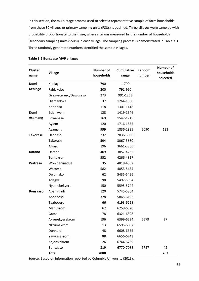
82

In this section, the multi-stage process used to select a representative sample of farm households

from these 30 villages or primary sampling units (PSUs) is outlined. Three villages were sampled with

probability proportionate to their size, where size was measured by the number of households

(secondary sampling units (SSUs)) in each village. The sampling process is demonstrated in Table 3.3.

Three randomly generated numbers identified the sample villages.

Table 3.2 Bonsaaso MVP villages

Cluster

name Village

Number of

households

Cumulative

range

Random

number

Number of

households

selected

Domi

Keniago

Keniago 790 1-790

Fahiakobo 200 791-990

Gyegyetereso/Dawusaso 273 991-1263

Hiamankwa 37 1264-1300

Kobririso 118 1301-1418

Domi

Asamang

Esienkyem 128 1419-1546

Edwenase 169 1547-1715

Ayiem 120 1716-1835

Asamang 999 1836-2835 2090 133

Takorase Dadease 232 2836-3066

Takorase 594 3067-3660

Afraso 196 3661-3856

Datano Datano 409 3857-4265

Tontokrom 552 4266-4817

Watreso Wonipaninadue 35 4818-4852

Watreso 582 4853-5434

Dwumako 62 5435-5496

Adagya 98 5497-5594

Nyamebekyere 150 5595-5744

Bonsaaso Apenimadi 120 5745-5864

Aboaboso 328 5865-6192

Taabosere 66 6193-6258

Manukrom 62 6259-6320

Groso 78 6321-6398

Akyerekyerekrom 196 6399-6594 6579 27

Nkrumakrom 13 6595-6607

Dunhura 48 6608-6655

Yawkasakrom 88 6656-6743

Kojonsiakrom 26 6744-6769

Bonsaaso 319 6770-7088 6787 42

Total 7088

202

Source: Based on information reported by Columbia University (2013).

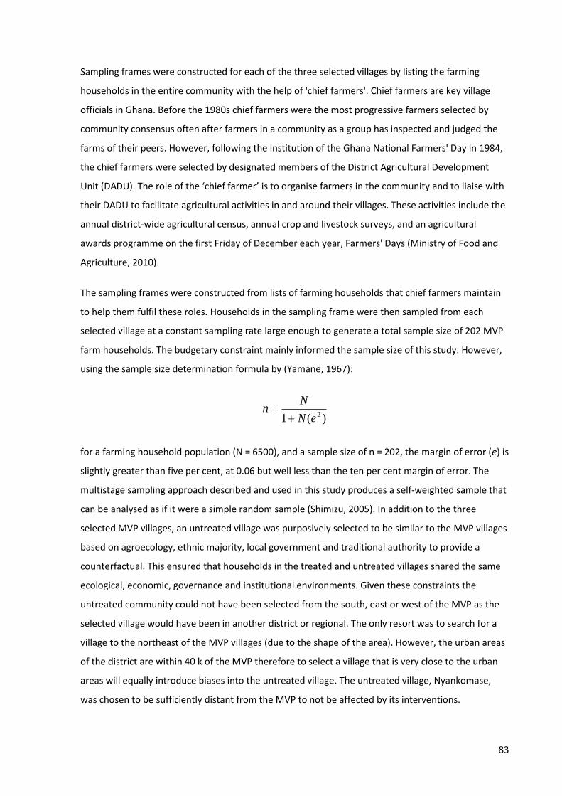
83

Sampling frames were constructed for each of the three selected villages by listing the farming

households in the entire community with the help of 'chief farmers'. Chief farmers are key village

officials in Ghana. Before the 1980s chief farmers were the most progressive farmers selected by

community consensus often after farmers in a community as a group has inspected and judged the

farms of their peers. However, following the institution of the Ghana National Farmers' Day in 1984,

the chief farmers were selected by designated members of the District Agricultural Development

Unit (DADU). The role of the ‘chief farmer’ is to organise farmers in the community and to liaise with

their DADU to facilitate agricultural activities in and around their villages. These activities include the

annual district-wide agricultural census, annual crop and livestock surveys, and an agricultural

awards programme on the first Friday of December each year, Farmers' Days (Ministry of Food and

Agriculture, 2010).

The sampling frames were constructed from lists of farming households that chief farmers maintain

to help them fulfil these roles. Households in the sampling frame were then sampled from each

selected village at a constant sampling rate large enough to generate a total sample size of 202 MVP

farm households. The budgetary constraint mainly informed the sample size of this study. However,

using the sample size determination formula by (Yamane, 1967):

)(1 2eN

Nn

+=

for a farming household population (N = 6500), and a sample size of n = 202, the margin of error (e) is

slightly greater than five per cent, at 0.06 but well less than the ten per cent margin of error. The

multistage sampling approach described and used in this study produces a self-weighted sample that

can be analysed as if it were a simple random sample (Shimizu, 2005). In addition to the three

selected MVP villages, an untreated village was purposively selected to be similar to the MVP villages

based on agroecology, ethnic majority, local government and traditional authority to provide a

counterfactual. This ensured that households in the treated and untreated villages shared the same

ecological, economic, governance and institutional environments. Given these constraints the

untreated community could not have been selected from the south, east or west of the MVP as the

selected village would have been in another district or regional. The only resort was to search for a

village to the northeast of the MVP villages (due to the shape of the area). However, the urban areas

of the district are within 40 k of the MVP therefore to select a village that is very close to the urban

areas will equally introduce biases into the untreated village. The untreated village, Nyankomase,

was chosen to be sufficiently distant from the MVP to not be affected by its interventions.

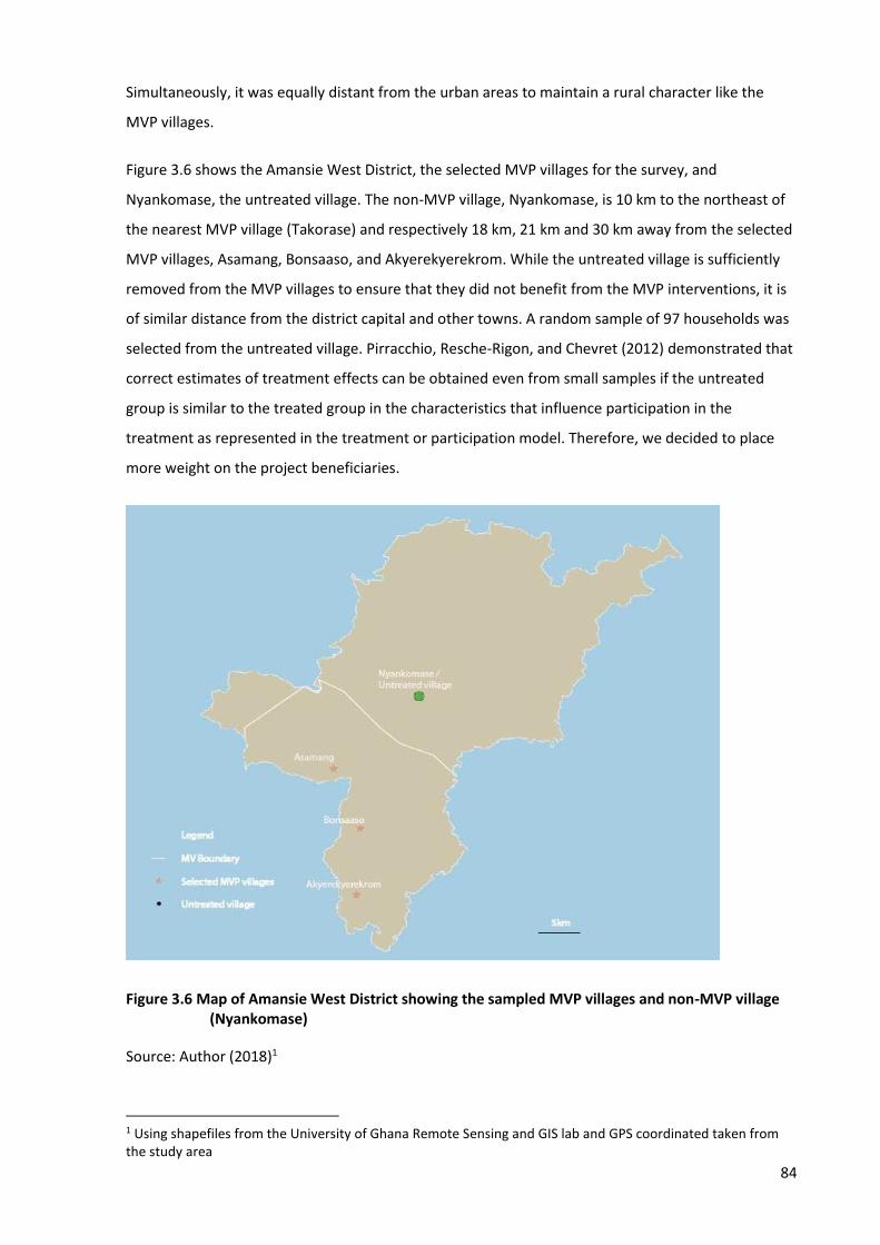
84

Simultaneously, it was equally distant from the urban areas to maintain a rural character like the

MVP villages.

Figure 3.6 shows the Amansie West District, the selected MVP villages for the survey, and

Nyankomase, the untreated village. The non-MVP village, Nyankomase, is 10 km to the northeast of

the nearest MVP village (Takorase) and respectively 18 km, 21 km and 30 km away from the selected

MVP villages, Asamang, Bonsaaso, and Akyerekyerekrom. While the untreated village is sufficiently

removed from the MVP villages to ensure that they did not benefit from the MVP interventions, it is

of similar distance from the district capital and other towns. A random sample of 97 households was

selected from the untreated village. Pirracchio, Resche-Rigon, and Chevret (2012) demonstrated that

correct estimates of treatment effects can be obtained even from small samples if the untreated

group is similar to the treated group in the characteristics that influence participation in the

treatment as represented in the treatment or participation model. Therefore, we decided to place

more weight on the project beneficiaries.

Figure 3.6 Map of Amansie West District showing the sampled MVP villages and non-MVP village (Nyankomase)

Source: Author (2018)1

1 Using shapefiles from the University of Ghana Remote Sensing and GIS lab and GPS coordinated taken from the study area

85

3.6.2 Data collection

The structured questionnaire used in this study has been discussed in Section 3.4. Discussions were

held with community leaders, chief farmers, and opinion leaders in the sample villages in November

and December 2016 to gain a deeper understanding of MVP implementation in the area. During this

period, additional information was gathered about the MVP project, the sampling frames were

constructed, and the questionnaires were programmed for SurveyCTO software, and tested on

tablets. Data collection paused briefly from 5-11 December due to the presidential and parliamentary

elections held in Ghana on 7 December 2016.

Four local enumerators were selected and trained to use the questionnaires and tablets. The

questionnaires were then pretested on twenty farm households in the Datano township, an MVP

village that was not selected as one of the three in the multi-stage sampling. The pretesting was done

to clarify the questions, determine the range of specific answers, and to establish the time taken for

a typical farm household to complete the survey. After the Christmas and New Year holidays,

personal interviews were conducted with the heads of selected households from 7 January to 10

February 2017. The data were cleaned from February to May 2017 and aggregated for analysis. All

currency values were adjusted for inflation and expressed in 2016 prices using the formula (Vt *

[CPI2016 / CPIt]): where Vt is the item price in year t, CPI2016 is Ghana's consumer price index (CPI) value

in 2016, and CPIt is the CPI value in year t when the item was acquired or its cost incurred.

3.7 Chapter summary

This chapter has presented the conceptual framework of the study; the methods used the assess the

three research questions as well as some methodological issues to be considered in impact

evaluation. The discussion showed that given the data available and the absence of randomisation in

the selection of participants and baseline data, propensity score matching is the most appropriate

method for estimating the impact of the MVP. However, since PSM does not account for unobserved

characteristics, a recursive IV model was developed to serve as a robustness check on the PSM

estimates. Following the discussion on the methods used to address the research questions, the

questionnaire used in the data collection was discussed as well as a brief description of the study

area and concluding with the sampling methods.

86

Chapter 4

Descriptive statistics

4.1 Introduction

In this chapter serves a dual purpose. Its presents the descriptive statistics of household and farm

characteristics collected during the household survey. Second, it addresses the first research

question of determining the differences between MVP households and non-MVP households. The

key summary statistics for the quantitative data collected from the household survey. The survey was

conducted in three MVP villages, namely, Asamang, Akyerekyerekrom and Bonsaaso as well as the

non-MVP villages, Nankomase as described in Chapter 3. The study collected data from the two

groups of households and aimed to verify if the differences between MVP and non-MVP households

are statistically significant in terms of demographic characteristics, socioeconomic status, asset

ownership, and household agricultural production characteristics.

4.2 Households characteristics

Table 4.1 presents summary statistics for various household characteristics of the non-MVP and MVP

households. The results show that in terms of household characteristics, the Non-MVP and MVP

households have statistically significant differences for the average age of household head,

dependency ratio, educational attainment and managerial role of household head in farming

activities. In other words, irrespective of their participation in the MVP, sampled household heads

are similar in terms of household size, the gender of the household head, household stock of farm

labour and off-farm labour.

Table 4. 1 indicates that the average age of household heads in the MVP and non-MVP villages is 51

years and 54 years, respectively. Based on the t-statistics for household head age, it can be

concluded that household heads in the MVP villages are slightly younger than those in the non-MVP

household. Likewise, the MVP household heads were slightly more formally educated (mean years of

formal education 6.6) than the household heads in the non-MVP villages with average years of

schooling of 4.9. Under the Ghanaian education system, this means that the average MVP household

almost completed a year of secondary school education. And therefore would have initiated

preparation towards a middle school qualification. In contrast, the average non-MVP household

barely completed a full course of primary education. As such, in this instance, the 1.7-year difference

in average years of formal education between the non-MVP and MVP household heads is non-trivial.

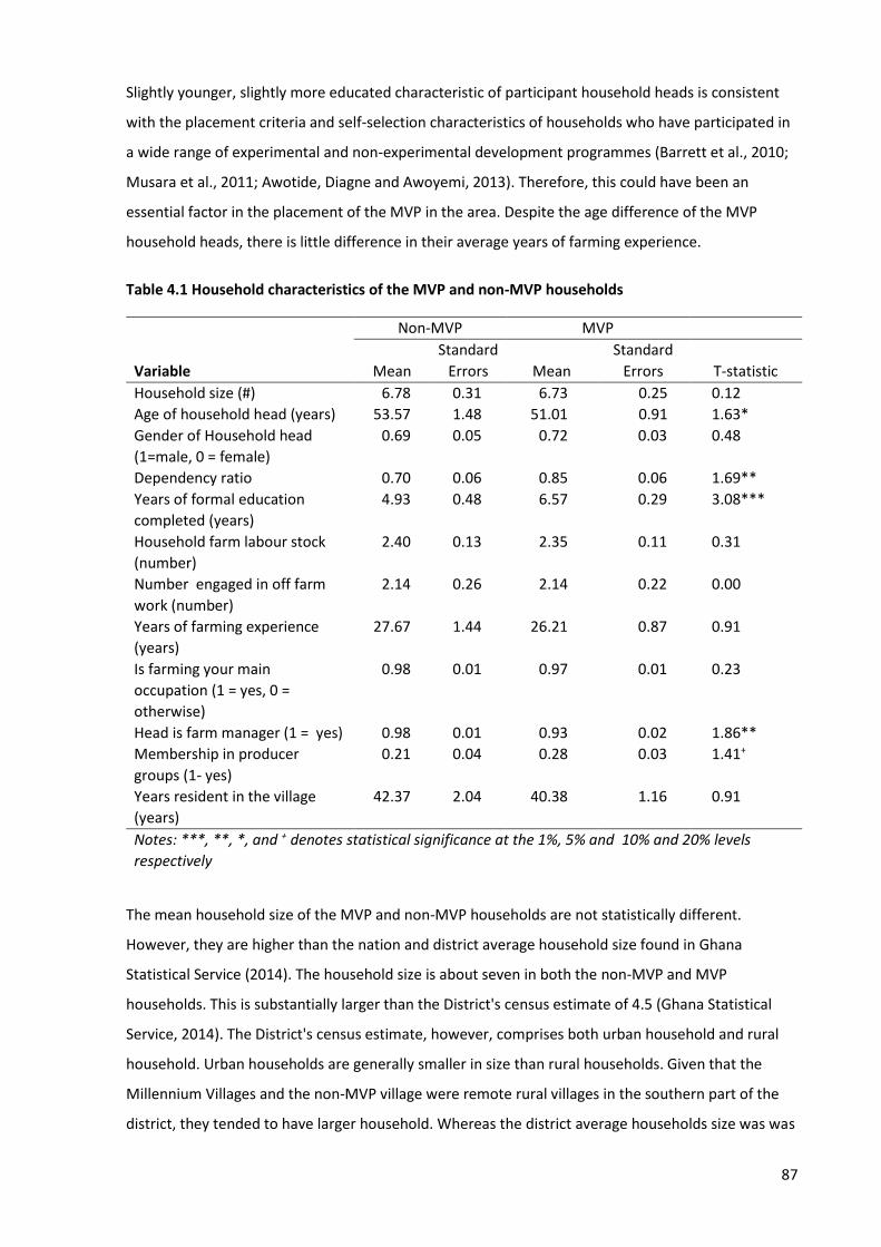
87

Slightly younger, slightly more educated characteristic of participant household heads is consistent

with the placement criteria and self-selection characteristics of households who have participated in

a wide range of experimental and non-experimental development programmes (Barrett et al., 2010;

Musara et al., 2011; Awotide, Diagne and Awoyemi, 2013). Therefore, this could have been an

essential factor in the placement of the MVP in the area. Despite the age difference of the MVP

household heads, there is little difference in their average years of farming experience.

Table 4.1 Household characteristics of the MVP and non-MVP households

Variable

Non-MVP MVP

Mean

Standard

Errors Mean

Standard

Errors T-statistic

Household size (#) 6.78 0.31 6.73 0.25 0.12

Age of household head (years) 53.57 1.48 51.01 0.91 1.63*

Gender of Household head

(1=male, 0 = female)

0.69 0.05 0.72 0.03 0.48

Dependency ratio 0.70 0.06 0.85 0.06 1.69**

Years of formal education

completed (years)

4.93 0.48 6.57 0.29 3.08***

Household farm labour stock

(number)

2.40 0.13 2.35 0.11 0.31

Number engaged in off farm

work (number)

2.14 0.26 2.14 0.22 0.00

Years of farming experience

(years)

27.67 1.44 26.21 0.87 0.91

Is farming your main

occupation (1 = yes, 0 =

otherwise)

0.98 0.01 0.97 0.01 0.23

Head is farm manager (1 = yes) 0.98 0.01 0.93 0.02 1.86**

Membership in producer

groups (1- yes)

0.21 0.04 0.28 0.03 1.41+

Years resident in the village

(years)

42.37 2.04 40.38 1.16 0.91

Notes: ***, **, *, and + denotes statistical significance at the 1%, 5% and 10% and 20% levels

respectively

The mean household size of the MVP and non-MVP households are not statistically different.

However, they are higher than the nation and district average household size found in Ghana

Statistical Service (2014). The household size is about seven in both the non-MVP and MVP

households. This is substantially larger than the District's census estimate of 4.5 (Ghana Statistical

Service, 2014). The District's census estimate, however, comprises both urban household and rural

household. Urban households are generally smaller in size than rural households. Given that the

Millennium Villages and the non-MVP village were remote rural villages in the southern part of the

district, they tended to have larger household. Whereas the district average households size was was

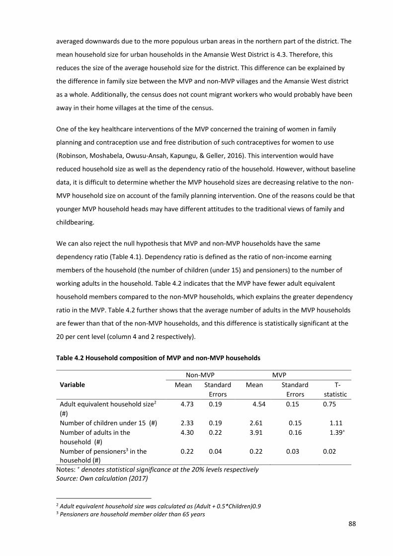
88

averaged downwards due to the more populous urban areas in the northern part of the district. The

mean household size for urban households in the Amansie West District is 4.3. Therefore, this

reduces the size of the average household size for the district. This difference can be explained by

the difference in family size between the MVP and non-MVP villages and the Amansie West district

as a whole. Additionally, the census does not count migrant workers who would probably have been

away in their home villages at the time of the census.

One of the key healthcare interventions of the MVP concerned the training of women in family

planning and contraception use and free distribution of such contraceptives for women to use

(Robinson, Moshabela, Owusu-Ansah, Kapungu, & Geller, 2016). This intervention would have

reduced household size as well as the dependency ratio of the household. However, without baseline

data, it is difficult to determine whether the MVP household sizes are decreasing relative to the non-

MVP household size on account of the family planning intervention. One of the reasons could be that

younger MVP household heads may have different attitudes to the traditional views of family and

childbearing.

We can also reject the null hypothesis that MVP and non-MVP households have the same

dependency ratio (Table 4.1). Dependency ratio is defined as the ratio of non-income earning

members of the household (the number of children (under 15) and pensioners) to the number of

working adults in the household. Table 4.2 indicates that the MVP have fewer adult equivalent

household members compared to the non-MVP households, which explains the greater dependency

ratio in the MVP. Table 4.2 further shows that the average number of adults in the MVP households

are fewer than that of the non-MVP households, and this difference is statistically significant at the

20 per cent level (column 4 and 2 respectively).

Table 4.2 Household composition of MVP and non-MVP households

Variable

Non-MVP MVP

Mean Standard

Errors

Mean Standard

Errors

T-

statistic

Adult equivalent household size2

(#)

4.73 0.19 4.54 0.15 0.75

Number of children under 15 (#) 2.33 0.19 2.61 0.15 1.11

Number of adults in the

household (#)

4.30 0.22 3.91 0.16 1.39+

Number of pensioners3 in the household (#)

0.22 0.04 0.22 0.03 0.02

Notes: + denotes statistical significance at the 20% levels respectively Source: Own calculation (2017)

2 Adult equivalent household size was calculated as (Adult + 0.5*Children)0.9 3 Pensioners are household member older than 65 years

89

Although the MVP villages have marginally fewer adults in the household, Table 4.1, shows that there

is no significant difference in the number of household members engaged in both farm and non-farm

labour between the MVP and non-MVP households. From the survey data, 48 per cent of MVP

households had at least one person engaged in non-farm work, compared to 46 per cent in the non-

MVP households. Moreover, there was a greater range of non-farm activities engaged in MVP sample

than the non-MVP sample. This subject is further discussed in Section 4.4. However, 93 per cent of

household heads in the MVP villages manage their household farming activities compared to 98 per

cent in the non-MVP villages. These high proportions engaged in farming are consistent with the

census results for the district which states that 98 per cent of households are engaged in agriculture

as a source of employment and income (Ghana Statistical Service, 2014). Being younger and more

educated, MVP household heads would be in a position to take on off-farm employment

opportunities compared to the non-MVP household heads. On the other hand, from the survey data,

the farmers in the MVP villages were more engaged in producer groups and other farmer-based

organisations. This further bolsters the point of the characteristics of the MVP village farmers which

made them attractive for the placement of the project. In addition to being younger and more

educated, their greater rate of participation in producer groups suggests that they may be more

entrepreneurial and driven, seeking ways to improve their participation in the agricultural value

chain.

Munk (2013) observed that there was an influx of migrants into the MVP villages of Dertu, Kenya

when the interventions started. With this information in mind, the survey questionnaire discussed in

Chapter 3, Section 3.4 had questions about the number of years that households have been resident

in the community. Further questions about the reason for migration were asked if the household had

lived in the community for ten years or less. Apart from the intrinsic importance of migration in the

demographics of the villages it has implications for the impact evaluation as well. Both MVP and non-

MVP villages have benefitted from long-term residents, averaging over 40 years each (Table 4.1). The

difference in years resident in their village can also be attributable to the younger age of the average

MVP household heads.

Of the 202 MVP households, only nine households (5%) have been in the MVP villages for ten years

or less. The distributions and rationale for the recent migrant households relocating to the MVP

villages are shown in Figure 4.1 below. This observation, contrasts with that of Munk (2013) who

observed that the influx of migrants from neighbouring villages lured in by the various packages

being given by the MVP with the likely effect of elevating rental and real estate prices in the MVP

areas. This further worsened the plight of the poor in the MVP villages. More importantly, as units

other than the intended treatment groups were affected by the interventions, namely, the migrants

who came into the MVP villages, the Stable Unit Treatment Value Assumption (SUTVA) on which

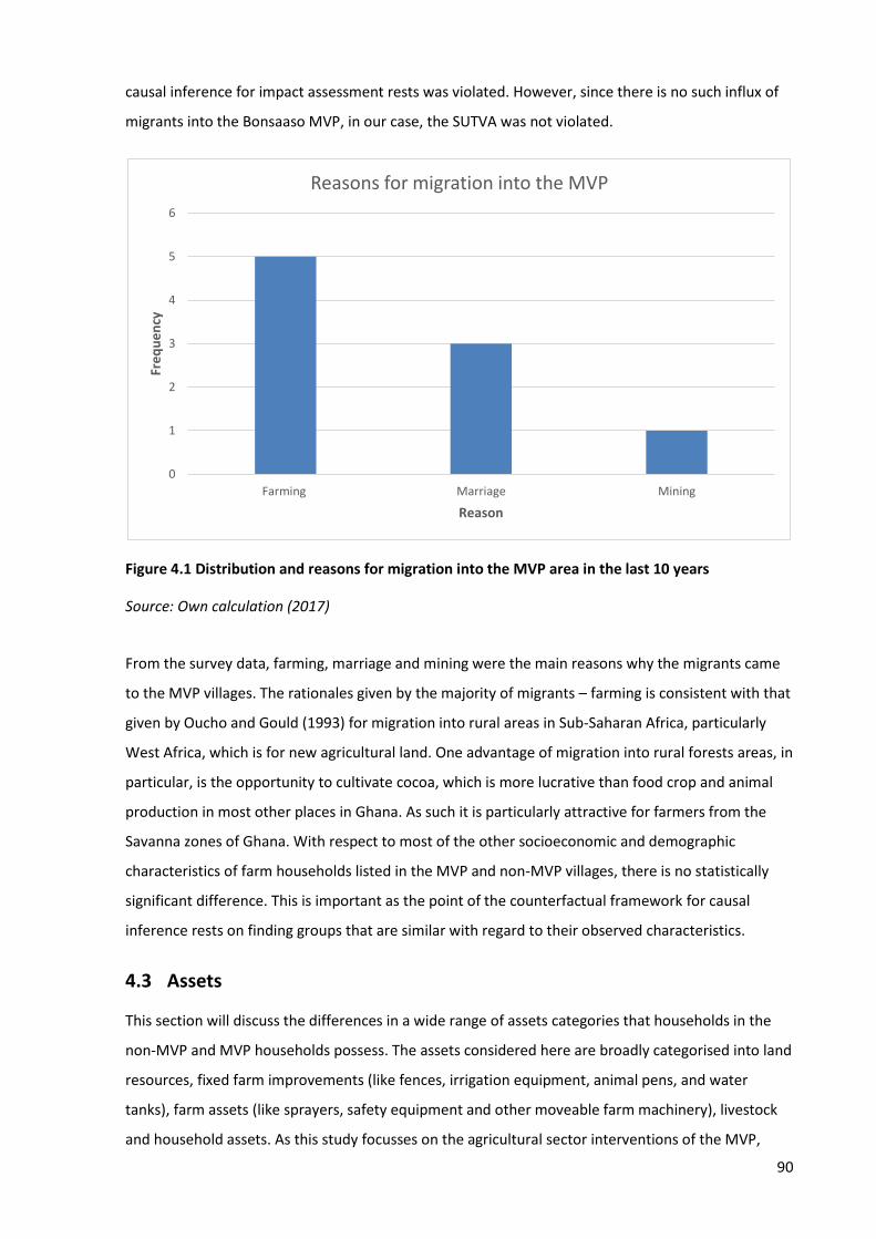
90

causal inference for impact assessment rests was violated. However, since there is no such influx of

migrants into the Bonsaaso MVP, in our case, the SUTVA was not violated.

Figure 4.1 Distribution and reasons for migration into the MVP area in the last 10 years

Source: Own calculation (2017)

From the survey data, farming, marriage and mining were the main reasons why the migrants came

to the MVP villages. The rationales given by the majority of migrants – farming is consistent with that

given by Oucho and Gould (1993) for migration into rural areas in Sub-Saharan Africa, particularly

West Africa, which is for new agricultural land. One advantage of migration into rural forests areas, in

particular, is the opportunity to cultivate cocoa, which is more lucrative than food crop and animal

production in most other places in Ghana. As such it is particularly attractive for farmers from the

Savanna zones of Ghana. With respect to most of the other socioeconomic and demographic

characteristics of farm households listed in the MVP and non-MVP villages, there is no statistically

significant difference. This is important as the point of the counterfactual framework for causal

inference rests on finding groups that are similar with regard to their observed characteristics.

4.3 Assets

This section will discuss the differences in a wide range of assets categories that households in the

non-MVP and MVP households possess. The assets considered here are broadly categorised into land

resources, fixed farm improvements (like fences, irrigation equipment, animal pens, and water

tanks), farm assets (like sprayers, safety equipment and other moveable farm machinery), livestock

and household assets. As this study focusses on the agricultural sector interventions of the MVP,

0

1

2

3

4

5

6

Farming Marriage Mining

Fre

qu

en

cy

Reason

Reasons for migration into the MVP

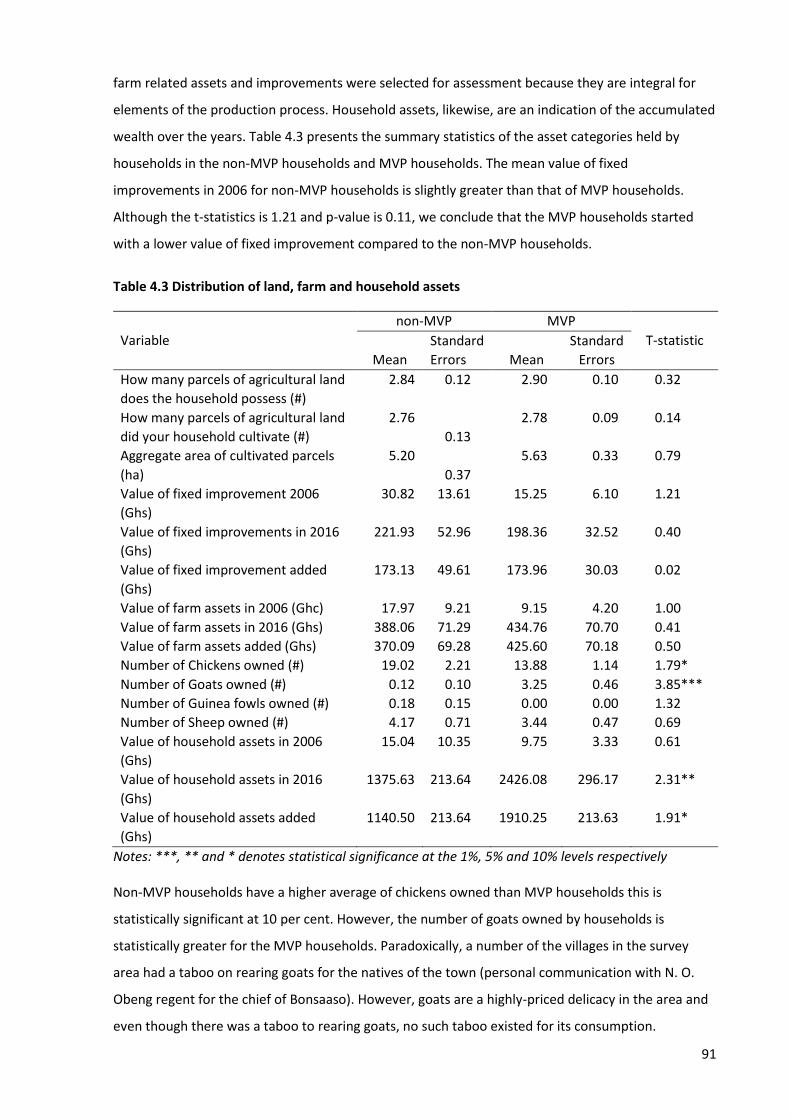
91

farm related assets and improvements were selected for assessment because they are integral for

elements of the production process. Household assets, likewise, are an indication of the accumulated

wealth over the years. Table 4.3 presents the summary statistics of the asset categories held by

households in the non-MVP households and MVP households. The mean value of fixed

improvements in 2006 for non-MVP households is slightly greater than that of MVP households.

Although the t-statistics is 1.21 and p-value is 0.11, we conclude that the MVP households started

with a lower value of fixed improvement compared to the non-MVP households.

Table 4.3 Distribution of land, farm and household assets

Variable

non-MVP MVP

T-statistic

Mean

Standard

Errors Mean

Standard

Errors

How many parcels of agricultural land

does the household possess (#)

2.84 0.12 2.90 0.10 0.32

How many parcels of agricultural land

did your household cultivate (#)

2.76

0.13

2.78 0.09 0.14

Aggregate area of cultivated parcels

(ha)

5.20

0.37

5.63 0.33 0.79

Value of fixed improvement 2006

(Ghs)

30.82 13.61 15.25 6.10 1.21

Value of fixed improvements in 2016

(Ghs)

221.93 52.96 198.36 32.52 0.40

Value of fixed improvement added

(Ghs)

173.13 49.61 173.96 30.03 0.02

Value of farm assets in 2006 (Ghc) 17.97 9.21 9.15 4.20 1.00

Value of farm assets in 2016 (Ghs) 388.06 71.29 434.76 70.70 0.41

Value of farm assets added (Ghs) 370.09 69.28 425.60 70.18 0.50

Number of Chickens owned (#) 19.02 2.21 13.88 1.14 1.79*

Number of Goats owned (#) 0.12 0.10 3.25 0.46 3.85***

Number of Guinea fowls owned (#) 0.18 0.15 0.00 0.00 1.32

Number of Sheep owned (#) 4.17 0.71 3.44 0.47 0.69

Value of household assets in 2006

(Ghs)

15.04 10.35 9.75 3.33 0.61

Value of household assets in 2016

(Ghs)

1375.63 213.64 2426.08 296.17 2.31**

Value of household assets added

(Ghs)

1140.50 213.64 1910.25 213.63 1.91*

Notes: ***, ** and * denotes statistical significance at the 1%, 5% and 10% levels respectively Non-MVP households have a higher average of chickens owned than MVP households this is

statistically significant at 10 per cent. However, the number of goats owned by households is

statistically greater for the MVP households. Paradoxically, a number of the villages in the survey

area had a taboo on rearing goats for the natives of the town (personal communication with N. O.

Obeng regent for the chief of Bonsaaso). However, goats are a highly-priced delicacy in the area and

even though there was a taboo to rearing goats, no such taboo existed for its consumption.

92

Therefore, the most plausible explanation is that migrant farmers in the MVP villages are responsible

for rearing the goats in the Bonsaaso area4.

Lastly, there was a statistical difference in the mean value of household assets in 2016 between the

the non-MVP and MVP households. The estimated results in Table 4.3 indicates that household asset

added over the course of the project in the MVP villages on average increased by over Ghs 800 more

than the assets added to the non-MVP households over the same period. The asset categories

described in Table 4.3 are aggregates of various types of assets from the Questionnaire (Appendix A).

In the next three sub-sections, a more detailed breakdown of the assets will be given to explain the

composition and differences in the non-MVP and MVP groups. Although land was not statistically

significant, given its importance as a factor of agricultural production, the next sub-section will

explore the distribution of land in both samples and attempt to explain the lack of differences in the

light of the institutional arrangements in land in the Ashanti (the major ethnic group in this area)

community in the district. Section 4.3.2 discusses the composition and distribution of fixed farm

improvement across the non-MVP and MVP since the t-statistic is high. Section 4.3.3 discusses the

distribution of livestock between the two groups while the concluding subsection, 4.3.4 discusses

household assets.

The last four rows of Table 4.3 shows the distribution of various live farm animals owned by

households across the non-MVP and MVP groups. As discussed earlier, animal production is mostly

done on an extensive basis, chickens and goats were the only farm animals for which significant

differences were found between the non-MVP and MVP groups. Guinea fowls and cattle are mostly

reared in Northern Ghana. Figure 4.2 below presents the distribution of chickens by households in

the non-MVP and MVP villages. It can be observed that the non-MVP households concentrate more

at the higher end of the distribution, justifying the higher average compared to the MVP village.

4 Due to the political climate at the time of the survey (with the impending national election and the death of the Queen mother of the Ashanti kingdom), we did not collect information about the ethnicity and tribe in order not to alienate the respondents.

93

Figure 4.2 Distribution chickens by household in the non-MVP and MVP villages

The converse is the case for the distribution of goats is shown in Figure 4.3, which shows the

distribution of goats by household in the non-MVP and MVP villages. Apart from being a source of

nutrition to households and their guests, keeping animals provides the household with the option to

trade the animal to meet their short-term monetary needs.

Figure 4.3 Distribution goats by household in the non-MVP and MVP villages

0

10

20

30

40

50

60

0 1-10 11-20 21 - 30 31 - 40 41 - 50 51 - 100

Per

cen

tage

Number of chickens owned

Number of chickens owned by household in the two groups

Non-MVP MVP

0

20

40

60

80

100

120

0 1-10 11-20 21 - 30

Per

cen

t h

ou

seh

old

Number of goats

Number of goats owned by household in the two groups

Non-MVP MVP

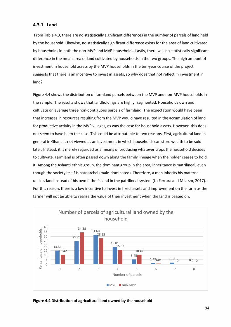
94

4.3.1 Land

From Table 4.3, there are no statistically significant differences in the number of parcels of land held

by the household. Likewise, no statistically significant difference exists for the area of land cultivated

by households in both the non-MVP and MVP households. Lastly, there was no statistically significant

difference in the mean area of land cultivated by households in the two groups. The high amount of

investment in household assets by the MVP households in the ten-year course of the project

suggests that there is an incentive to invest in assets, so why does that not reflect in investment in

land?

Figure 4.4 shows the distribution of farmland parcels between the MVP and non-MVP households in

the sample. The results shows that landholdings are highly fragmented. Households own and

cultivate on average three non-contiguous parcels of farmland. The expectation would have been

that increases in resources resulting from the MVP would have resulted in the accumulation of land

for productive activity in the MVP villages, as was the case for household assets. However, this does

not seem to have been the case. This could be attributable to two reasons. First, agricultural land in

general in Ghana is not viewed as an investment in which households can store wealth to be sold

later. Instead, it is merely regarded as a means of producing whatever crops the household decides

to cultivate. Farmland is often passed down along the family lineage when the holder ceases to hold

it. Among the Ashanti ethnic group, the dominant group in the area, inheritance is matrilineal, even

though the society itself is patriarchal (male-dominated). Therefore, a man inherits his maternal

uncle's land instead of his own father's land in the patrilineal system (La Ferrara and Milazzo, 2017).

For this reason, there is a low incentive to invest in fixed assets and improvement on the farm as the

farmer will not be able to realise the value of their investment when the land is passed on.

Figure 4.4 Distribution of agricultural land owned by the household

14.85

25.25

31.68

18.81

5.451.49 1.98 0.5

10.42

34.38

28.13

15.63

10.42

1.04 0 00

5

10

15

20

25

30

35

40

1 2 3 4 5 6 7 8Per

cen

tage

of

ho

sueh

old

s

Number of parcels

Number of parcels of agricultural land owned by the household

MVP Non-MVP

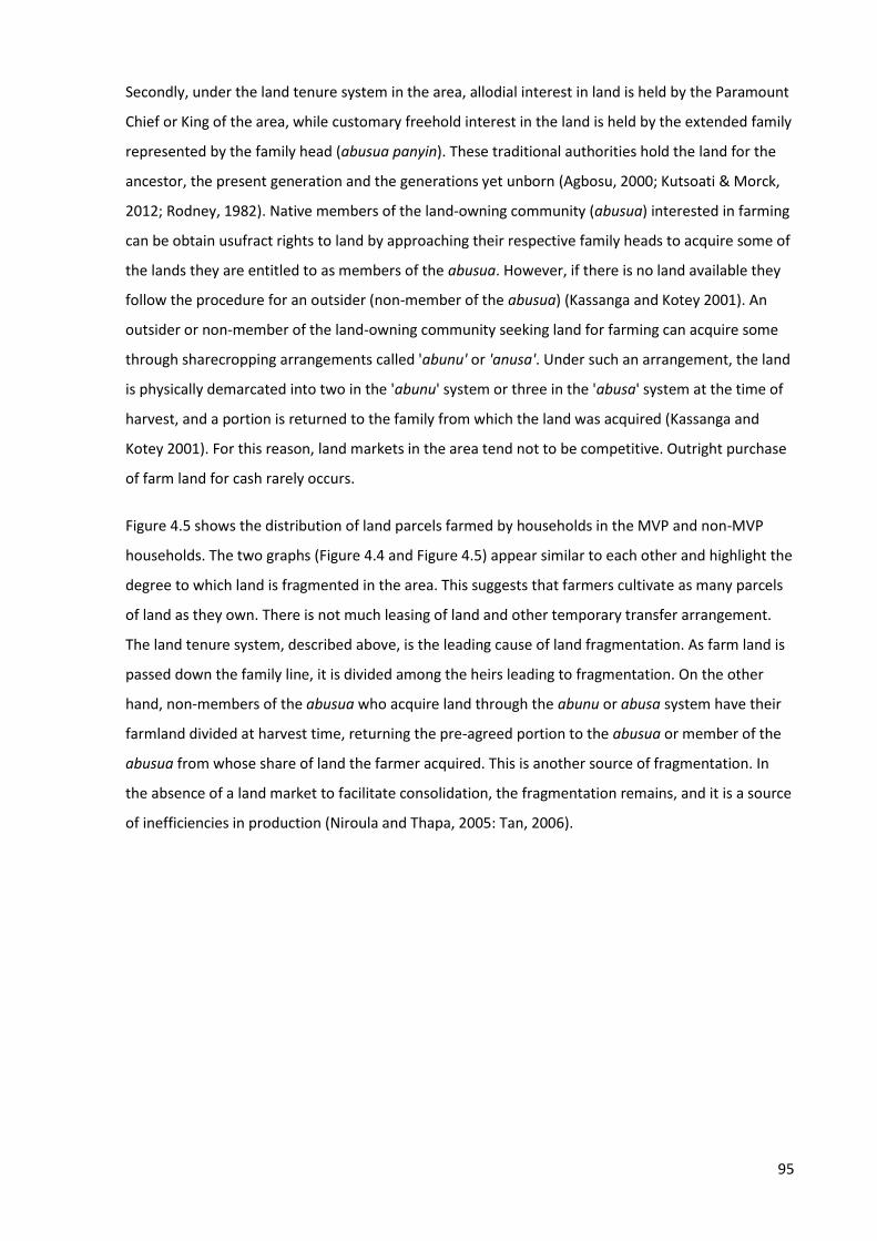
95

Secondly, under the land tenure system in the area, allodial interest in land is held by the Paramount

Chief or King of the area, while customary freehold interest in the land is held by the extended family

represented by the family head (abusua panyin). These traditional authorities hold the land for the

ancestor, the present generation and the generations yet unborn (Agbosu, 2000; Kutsoati & Morck,

2012; Rodney, 1982). Native members of the land-owning community (abusua) interested in farming

can be obtain usufract rights to land by approaching their respective family heads to acquire some of

the lands they are entitled to as members of the abusua. However, if there is no land available they

follow the procedure for an outsider (non-member of the abusua) (Kassanga and Kotey 2001). An

outsider or non-member of the land-owning community seeking land for farming can acquire some

through sharecropping arrangements called 'abunu' or 'anusa'. Under such an arrangement, the land

is physically demarcated into two in the 'abunu' system or three in the 'abusa' system at the time of

harvest, and a portion is returned to the family from which the land was acquired (Kassanga and

Kotey 2001). For this reason, land markets in the area tend not to be competitive. Outright purchase

of farm land for cash rarely occurs.

Figure 4.5 shows the distribution of land parcels farmed by households in the MVP and non-MVP

households. The two graphs (Figure 4.4 and Figure 4.5) appear similar to each other and highlight the

degree to which land is fragmented in the area. This suggests that farmers cultivate as many parcels

of land as they own. There is not much leasing of land and other temporary transfer arrangement.

The land tenure system, described above, is the leading cause of land fragmentation. As farm land is

passed down the family line, it is divided among the heirs leading to fragmentation. On the other

hand, non-members of the abusua who acquire land through the abunu or abusa system have their

farmland divided at harvest time, returning the pre-agreed portion to the abusua or member of the

abusua from whose share of land the farmer acquired. This is another source of fragmentation. In

the absence of a land market to facilitate consolidation, the fragmentation remains, and it is a source

of inefficiencies in production (Niroula and Thapa, 2005: Tan, 2006).

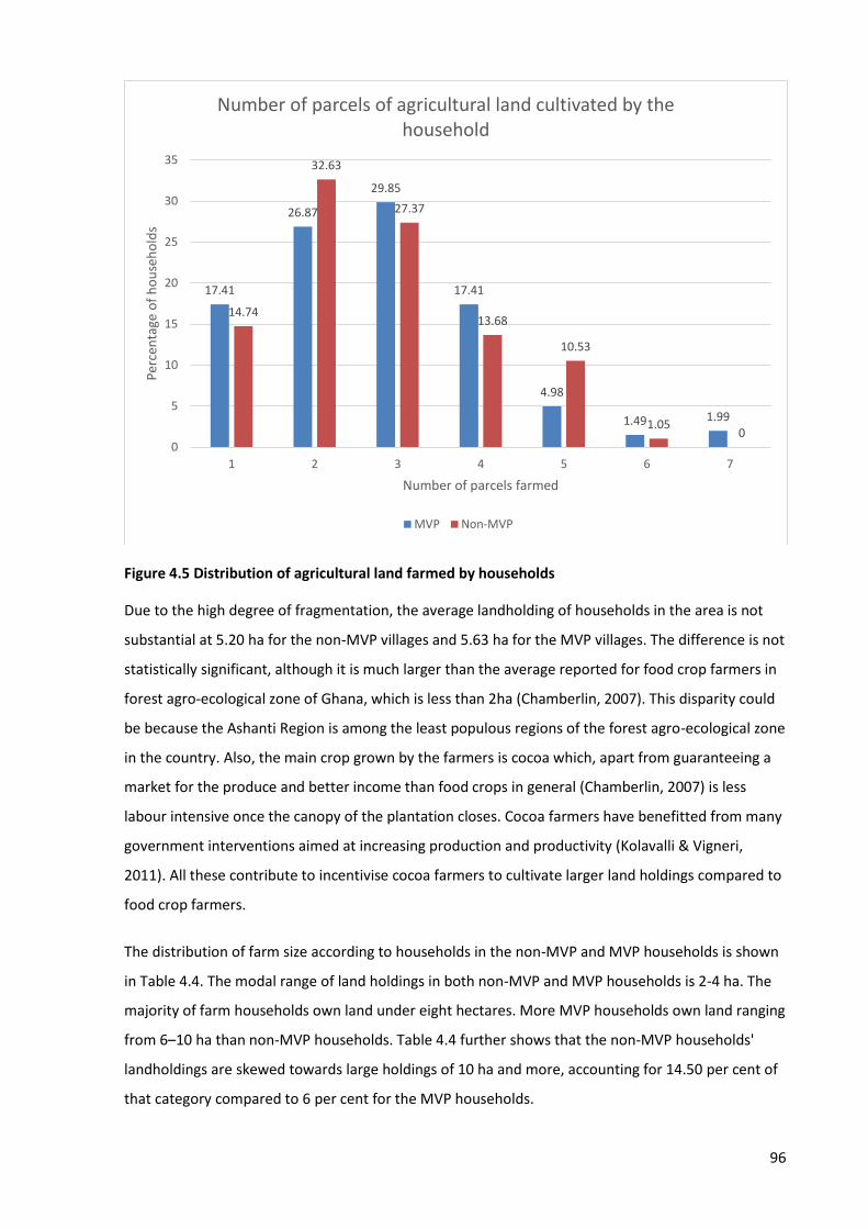
96

Figure 4.5 Distribution of agricultural land farmed by households

Due to the high degree of fragmentation, the average landholding of households in the area is not

substantial at 5.20 ha for the non-MVP villages and 5.63 ha for the MVP villages. The difference is not

statistically significant, although it is much larger than the average reported for food crop farmers in

forest agro-ecological zone of Ghana, which is less than 2ha (Chamberlin, 2007). This disparity could

be because the Ashanti Region is among the least populous regions of the forest agro-ecological zone

in the country. Also, the main crop grown by the farmers is cocoa which, apart from guaranteeing a

market for the produce and better income than food crops in general (Chamberlin, 2007) is less

labour intensive once the canopy of the plantation closes. Cocoa farmers have benefitted from many

government interventions aimed at increasing production and productivity (Kolavalli & Vigneri,

2011). All these contribute to incentivise cocoa farmers to cultivate larger land holdings compared to

food crop farmers.

The distribution of farm size according to households in the non-MVP and MVP households is shown

in Table 4.4. The modal range of land holdings in both non-MVP and MVP households is 2-4 ha. The

majority of farm households own land under eight hectares. More MVP households own land ranging

from 6–10 ha than non-MVP households. Table 4.4 further shows that the non-MVP households'

landholdings are skewed towards large holdings of 10 ha and more, accounting for 14.50 per cent of

that category compared to 6 per cent for the MVP households.

17.41

26.87

29.85

17.41

4.98

1.49 1.99

14.74

32.63

27.37

13.68

10.53

1.050

0

5

10

15

20

25

30

35

1 2 3 4 5 6 7

Per

cen

tage

of

ho

use

ho

lds

Number of parcels farmed

Number of parcels of agricultural land cultivated by the household

MVP Non-MVP

97

Table 4.4 Distribution of landholding sizes by households in both villages

Share of farmers by landholding category

MVP

participation

Less than

2ha 2-4 ha 4-6 ha 6-8 ha 8-10 ha

10-12

ha < 12ha

Mean

holding

non-MVP 12.38% 32.67% 24.26% 8.91% 7.43% 5.45% 8.91% 5.20

MVP 14.58% 29.17% 22.92% 15.63% 11.46% 2.08% 4.17% 5.63

In summary, therefore, the majority of household in the MVP and non-MVP villages are bona fide

smallholder farmers who can benefit from a meaningful increase in their assets, incomes and other

household outcomes. However, the land tenure system and the process of land acquisition is

cumbersome. Landholdings are highly fragmented for this reason. There often exists multiple

interests in a single parcel of land, and higher-order rights such as the right to convey one's property

in land to another party without the approval of a third party are rare unless the conveyor is an

abusua panyin or a paramount chief. As a result, even members of the abusua – the land-owning

community, constantly live with the awareness that their land can be conveyed to another person by

the family head (abusua panyin) or the paramount chief at any time for activities such as mining or

large scale farming by a corporation or a wealthy individual. Therefore, property rights in land are

quite insecure.

4.3.2 Fixed farm improvements

During the survey, households were given a list of farm-based fixed improvements, farm assets, and

moveable household assets from which they selected the ones they owned. They also provided the

years in which the assets were acquired and the replacement costs of the respective improvement.

Due to poor record-keeping, most of the responses were based on the recollection of the

respondents. From Table 4.3, the mean value of fixed farm improvements held by MVP households

before 2006 was lower than that of non-MVP households and was significant at 15 per cent level

with a t-statistics of 1.21. There was a significant increase in the value of fixed improvements across

both the MVP and non-MVP households over the period from 2006-2015, when the MVP was

implemented. The difference between the two groups was, however, not statistically significant.

Likewise, the ending (2016) value of non-MVP and MVP households' fixed improvements were not

statistically significant. Table 4.5 shows the distribution of fixed improvements owned by households

before 2006 when the MVP started. As the numbers of these fixed improvements are small in

proportion to the respective sample sizes of the non-MVP and MVP households, proportions were

calculated instead of mean differences.

98

Table 4.5 Fixed improvements owned by households before 2006 and after 2015

Variable

Fixed improvements

non-MVP (n=97) MVP (n=202)

Before 2006 After 2015 Before 2006 After 2015

Animal pens 5 (5.1%) 13 (13.4%) 5 (2.4%) 27 (13.45%)

Crop storage facilities 5 (5.1%) 12 (12.37%) 8 (3.9%) 20 (9.9%)

Irrigation 0 0 1 (0.5%) 3 (1.5%)

Water tanks 0 5 (5.15%) 3 (1.4%) 26 (12.9%)

Other fixed assets

(drainage and erosion

control) 2 (2.1%) 20 (20.62%) 2 (1%) 32 (15.8%)

Notes: The values in parenthesis are percentages of households who own the respective asset

On the whole, the non-MVP households were marginally better endowed with fixed improvements

than the MVP households before the Project. The results show that a slightly smaller proportion of

the MVP households own farm improvement compared to the non-MVP village. Animal production

in this part of Ghana is mainly limited to small-scale poultry and small ruminant production on an

extensive basis. Farmers often provide rudimentary shelter for the farm animals near the farmers'

homestead to shelter the animals from the elements and to keep predators and thieves from taking

the animals at night. The proportion of MVP households who invested in animal pens over the ten-

year course of the project increased by 11 per cent compared to an 8 per cent increase in the non-

MVP households.

It is documented that the MVP trained and encouraged diversification in the agricultural production

of the household. The MVP households' investments in crop storage facilities trailed that of the non-

MVP household, at 6 per cent and 7 per cent respectively. The MVP introduced maize and cowpea

farming into the project villages. They then facilitated the vertical coordination between the growers

of these food crops and the school meals programme which provides lunches for school pupils in the

MVP villages. As part of this set of interventions, the MVP constructed storage silos in selected MVP

villages including Bonsaaso and Akyerekyerekrom. It is likely that the MVP's construction of the

storage facilities reduced the need for the household to construct storage facilities for themselves.

However, at the time of the data collection the relationship between the MVP farm households and

the school meals programme had broken down. With regard to the storage of cocoa, the main crop

in the area, the presence of licenced cocoa buying companies in almost every village along with the

fixed producer price offered by these companies on behalf of the Cocoa Marketing Board (Cocobod)

renders it unnecessary for farmers to keep large inventories of cocoa in storage. As such, crop

storage is not a priority for cocoa producers in contrast to food crop producers.

The number of households with investments in irrigation increased by about 1.50 per cent for the

MVP households compared 0.5 per cent for the non-MVP while investment in water storage

99

increased by 12 per cent for the MVP villages compared to 5 per cent for the non-MVP village. The

entire district lies in the forest agro-ecological zone, and enjoys a bimodal rainy season. There is

often enough water for the production of a wide range of crops suited for this zone. Consequently,

investment in irrigation and water storage facilities remain low even after the MVP. This is shown in

Table 4.5, which shows the distribution of fixed improvement in 2016 after the MVP had ended.

Other fixed improvement included drainage and erosions control, which increased by about 15 per

cent for the MVP villages compared to about 19 per cent in the non-MVP villages. Fencing of

farmland was a fixed improvement in the list in the questionnaire. However, no farmers reported any

investment in the practice. It is seen as an act of expropriating land for personal use which goes

against the tenets of communal land ownership by the family. Table 4.5 further shows that in

general, even though the MVP households started the project behind the non-MVP households in

the proportions that had invested in fixed improvements, the MVP households had largely caught up

to the investment level of the non-MVP households by the end of the project. Despite this, there is

no statistically significant difference in the values of farm improvements invested in by both groups

of households as shown in Table 4.3.

4.3.3 Household assets

From Table 4.3, the mean value of household assets added for the MVP households was statistically

different from that of the non-MVP households at the ten per cent level. Similarly, and the mean

value of household assets in 2016 for the MVP households was statistically different from that of the

non-MVP households at the five per cent level. The difference in the mean value of household assets

added for the MVP villages is over 65 per cent more than the mean value of household assets added

for the non-MVP villages. Likewise, the mean value of household assets in 2016 for the MVP

households were over 75 per cent more than that of the non-MVP households. As was the case for

fixed farm improvements discussed in the previous section, the value of household assets was an

aggregate of a wide range of moveable household assets. Table 4.6 shows the breakdown of these

assets among the MVP and non-MVP household before and after the project. A very important point

of note is that the MVP villages were not connected to the national grid when the MVP began (Earth

Institute, n.d.). The same situation was the case for seven other MVPs across Africa (Adkins,

Oppelstrup & Modi, 2012). Their sources of power back in those days were mainly dry and wet cell

batteries, crop residue, kerosene and firewood. MVP played a pivotal role in connecting these

villages to the grid.

Notwithstanding, the southernmost villages in the Bonsaaso MVP were still without grid electricity at

the time of the survey for the study. In the absence of electricity in those villages, wet cell batteries,

diesel or petrol generator sets and solar chargers of a wide range of sizes continue to be used to

100

power various house appliance. From Table 4.6, it can be observed that the MVP households have

acquired substantial household assets, even though they began with less than their counterparts in

the non-MVP village. Among the major assets invested in were mobile phones, radio and television

sets. Mobile phones, in particular, have become an essential tool for financial inclusion in recent

times. Mobile phone numbers are operated as bank accounts allowing for the payments, receipts

and transfers over the mobile network. This has been transformational as banking facilities have

been almost non-existent in rural Ghana. But before the recent use of mobile phones for financial

inclusion, the MVP in the early phases used mobile phones to deliver the Telemedicine program in

partnership with Novartis (Sarma et al., 2018).

Table 4.6 Proportion of household ownership of household assets before and after the MVP

Notes: The values in parenthesis are percentages MVP established several computing centres in selected MVP villages where members of the

community were trained in the use of computers. The computing centres in the Bonsaaso MVP

villages were attached to schools. In the day time, they served pupils in the schools but were open to

the public after school. Until the villages were connected to the grid, the computing centres were

powered by solar panels provided by MVP. Similar panels powered the newly built clinics and

hospitals and remain as backup power options during power outages on the grid. This exposure to

computers could explain the presence of computers in the MVP households while none was

registered in non-MVP households.

Insecticide-treated bed nets remain very important in the prevention of malaria and were provided

free of charge to the MVP villages. This was done as part of the 'quick-wins' interventions to achieve

the sixth MDG of combating HIV/AIDS, malaria and other diseases. Since the bed nets begin to wear

away severely after the third year of use, it could be that the MVP villages have lost nets and yet to

Before 2006 After 2006

Variable non-MVP

(n=97) MVP (n=202)

non-MVP

(n=97) MVP (n=202) Household moveable

assets

Cell phone 6 (6.19%) 5 (2.46%) 70 (72.16%) 161 (80%)

Computer 0 0 0 6 (3%)

Fridge/freezer 5 (5.15%) 9 (4.43%) 29 (29.9%) 74 (37%)

Generator 1 (1.03%) 1 (0.49%) 5 (5.15%) 10 (5%)

Insecticide treated bed

nets

1 (1.03%) 11 (5.42%) 60 (61.86%) 102 (50%)

Motor car or truck 0 0 0 7 (3%)

Motorbike 0 0 12 (12.37%) 35 (17%)

Radio 2 (2.06%) 6 (2.96%) 63 (64.95%) 132 (65%)

Solar charging system 0 0 1 (1.03%) 1 (0.49%)

Television 3 (3.09%) 7 (3.45%) 56 (57.72%) 120 (59%)

101

replace them. On the other hand, it could also be the case that the ease of access to healthcare

resulting from the MVP may have caused households to be lax with the prevention methods for the

disease. The MVP villages were ahead also in the proportion of households who own motor vehicles,

refrigerators and TV sets after 2006.

The focus of the analysis up to this point has been on the household measures of outcomes without

accounting for the resources employed to produce the various outcomes. The study will now extend

the analysis by accounting for the labour and land factors used in producing the assets. Labour was

measured in adult equivalent terms of the household size while land was measured as the aggregate

number of hectares of all land parcels that a household farms. Table 4.7 shows summary statistics for

various categories of assets per adult equivalent household size. It shows that only the value of

household assets in 2016 and the value of households assets added were statistically significant at

one per cent and five per cent respectively. Unlike in Table 4.3 where the value of fixed

improvements in 2006 was significant at the 20 per cent level. In Table 4.7 it is not statistically

significant until an alpha level of 85 per cent.

The MVP households have on average Ghs 222 more household assets per adult equivalent

households member than non-MVP households. Likewise, the average MVP household had over Ghs

135 more household assets added per adult equivalent household member. It is noteworthy that the

adult equivalent households size used in the calculation are the 2016 level. The value of assets per

adult equivalent households size, is good proxy for the capital-labour ratio at the households level.

The capital-labour ratio has been extensively discussed in the macroeconomic literature, including

the poverty trap model used by Sachs (2005) to justify the need for the ‘big push’ MVP in Africa. The

capital-labour ratio is a prime determinant of productivity growth (McCombie, 1988). Sachs (2005)

argued that rural African communities suffer from very low capital-labour ratios. This preliminary

analysis suggests that there was no significant difference in investment in farm assets and farm

improvements despite MVP. Accordingly, there was no significant growth in the capital-labour ratio

with respect to productive assets for MVP households compared to non-MVP households. Since the

capital labour ratio is a determinant of productivity, this result means that the MVP households’

investment decision could have kept them from reaching their potential productivity levels. By

contrast, the capital-labour ratio pertaining to household assets increased significantly for the MVP

household compared to the non-MVP households. This study did not apply direct human capital

measures such as those applied by Godtland, et al. (2004). Instead, the value of household assets was

used as a proxy for the human capital accumulated over the course of the MVP.

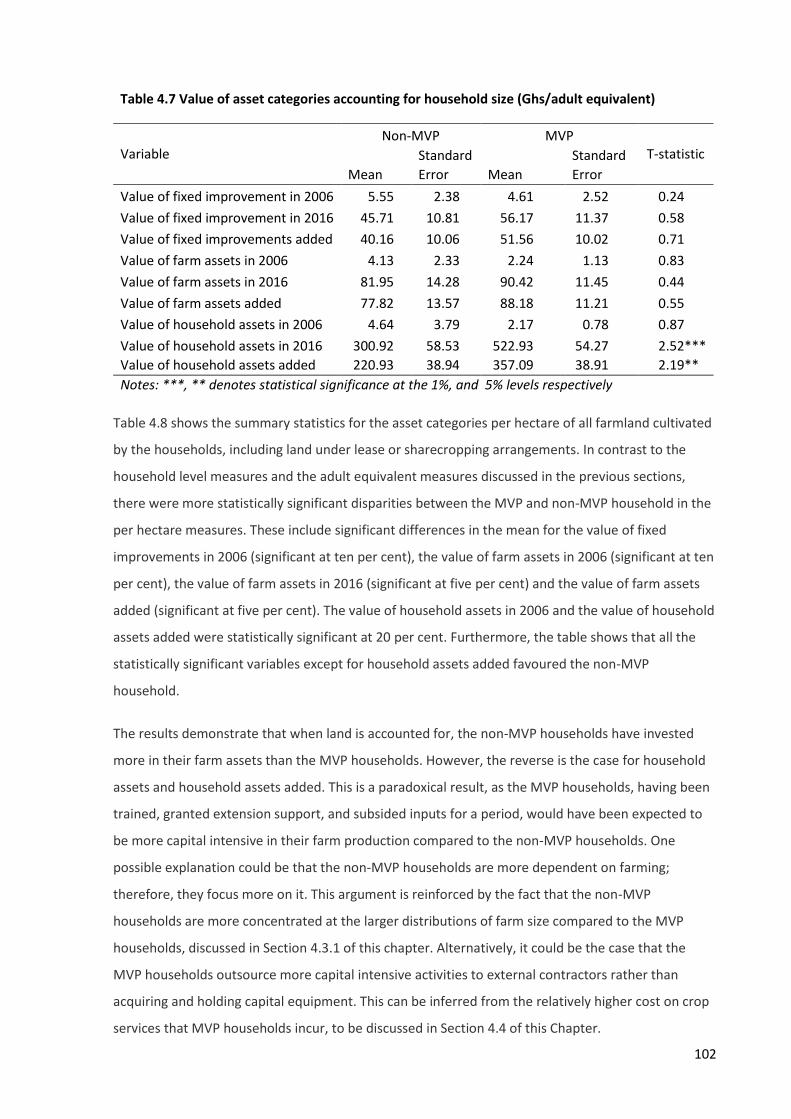
102

Table 4.7 Value of asset categories accounting for household size (Ghs/adult equivalent)

Variable Non-MVP MVP

T-statistic

Mean

Standard

Error Mean

Standard

Error

Value of fixed improvement in 2006 5.55 2.38 4.61 2.52 0.24

Value of fixed improvement in 2016 45.71 10.81 56.17 11.37 0.58

Value of fixed improvements added 40.16 10.06 51.56 10.02 0.71

Value of farm assets in 2006 4.13 2.33 2.24 1.13 0.83

Value of farm assets in 2016 81.95 14.28 90.42 11.45 0.44

Value of farm assets added 77.82 13.57 88.18 11.21 0.55

Value of household assets in 2006 4.64 3.79 2.17 0.78 0.87

Value of household assets in 2016 300.92 58.53 522.93 54.27 2.52***

Value of household assets added 220.93 38.94 357.09 38.91 2.19**

Notes: ***, ** denotes statistical significance at the 1%, and 5% levels respectively

Table 4.8 shows the summary statistics for the asset categories per hectare of all farmland cultivated

by the households, including land under lease or sharecropping arrangements. In contrast to the

household level measures and the adult equivalent measures discussed in the previous sections,

there were more statistically significant disparities between the MVP and non-MVP household in the

per hectare measures. These include significant differences in the mean for the value of fixed

improvements in 2006 (significant at ten per cent), the value of farm assets in 2006 (significant at ten

per cent), the value of farm assets in 2016 (significant at five per cent) and the value of farm assets

added (significant at five per cent). The value of household assets in 2006 and the value of household

assets added were statistically significant at 20 per cent. Furthermore, the table shows that all the

statistically significant variables except for household assets added favoured the non-MVP

household.

The results demonstrate that when land is accounted for, the non-MVP households have invested

more in their farm assets than the MVP households. However, the reverse is the case for household

assets and household assets added. This is a paradoxical result, as the MVP households, having been

trained, granted extension support, and subsided inputs for a period, would have been expected to

be more capital intensive in their farm production compared to the non-MVP households. One

possible explanation could be that the non-MVP households are more dependent on farming;

therefore, they focus more on it. This argument is reinforced by the fact that the non-MVP

households are more concentrated at the larger distributions of farm size compared to the MVP

households, discussed in Section 4.3.1 of this chapter. Alternatively, it could be the case that the

MVP households outsource more capital intensive activities to external contractors rather than

acquiring and holding capital equipment. This can be inferred from the relatively higher cost on crop

services that MVP households incur, to be discussed in Section 4.4 of this Chapter.

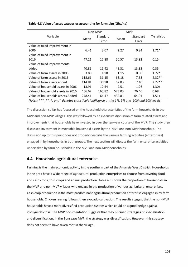
103

Table 4.8 Value of asset categories accounting for farm size (Ghs/ha)

Variable

Non-MVP MVP

T-statistic Mean

Standard

Error Mean

Standard

Error

Value of fixed improvement in

2006 6.41 3.07 2.27 0.84 1.71*

Value of fixed improvement in

2016 47.21 12.88 50.57 13.92 0.15

Value of fixed improvements

added 40.81 11.42 48.31 13.82 0.35

Value of farm assets in 2006 3.80 1.98 1.15 0.50 1.72*

Value of farm assets in 2016 118.61 31.15 63.18 7.53 2.32**

Value of farm assets added 114.81 30.98 62.03 7.40 2.22**

Value of household assets in 2006 13.91 12.54 2.51 1.26 1.30+

Value of household assets in 2016 466.67 163.82 573.03 76.46 0.68

Value of households assets Added 278.41 64.47 432.81 64.01 1.51+

Notes: ***, **, *, and + denotes statistical significance at the 1%, 5% and 10% and 20% levels

The discussion so far has focussed on the household characteristics of the farm households in the

MVP and non-MVP villages. This was followed by an extensive discussion of farm related assets and

improvements that households have invested in over the ten-year course of the MVP. The study then

discussed investment in moveable household assets by the MVP and non-MVP household. The

discussion up to this point does not properly describe the various farming activities (enterprises)

engaged in by households in both groups. The next section will discuss the farm enterprise activities

undertaken by farm households in the MVP and non-MVP households.

4.4 Household agricultural enterprise

Farming is the main economic activity in the southern part of the Amansie West District. Households

in the area have a wide range of agricultural production enterprises to choose from covering food

and cash crops, fruit crops and animal production. Table 4.9 shows the proportion of households in

the MVP and non-MVP villages who engage in the production of various agricultural enterprises.

Cash crop production is the most predominant agricultural production enterprise engaged in by farm

households. Chicken rearing follows, then avocado cultivation. The results suggest that the non-MVP

households have a more diversified production system which could be a good hedge against

idiosyncratic risk. The MVP documentation suggests that they pursued strategies of specialisation

and diversification. In the Bonsaaso MVP, the strategy was diversification. However, this strategy

does not seem to have taken root in the village.

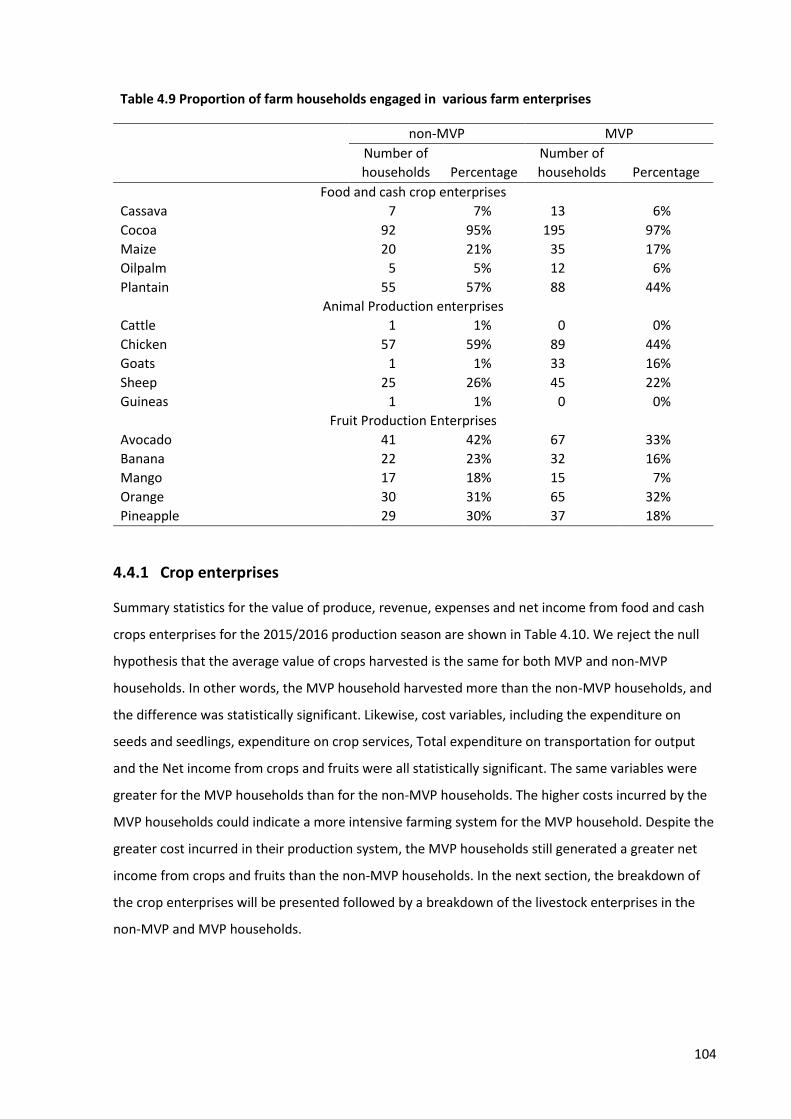
104

Table 4.9 Proportion of farm households engaged in various farm enterprises

non-MVP MVP

Number of

households Percentage

Number of

households Percentage

Food and cash crop enterprises

Cassava 7 7% 13 6%

Cocoa 92 95% 195 97%

Maize 20 21% 35 17%

Oilpalm 5 5% 12 6%

Plantain 55 57% 88 44%

Animal Production enterprises

Cattle 1 1% 0 0%

Chicken 57 59% 89 44%

Goats 1 1% 33 16%

Sheep 25 26% 45 22%

Guineas 1 1% 0 0%

Fruit Production Enterprises

Avocado 41 42% 67 33%

Banana 22 23% 32 16%

Mango 17 18% 15 7%

Orange 30 31% 65 32%

Pineapple 29 30% 37 18%

4.4.1 Crop enterprises

Summary statistics for the value of produce, revenue, expenses and net income from food and cash

crops enterprises for the 2015/2016 production season are shown in Table 4.10. We reject the null

hypothesis that the average value of crops harvested is the same for both MVP and non-MVP

households. In other words, the MVP household harvested more than the non-MVP households, and

the difference was statistically significant. Likewise, cost variables, including the expenditure on

seeds and seedlings, expenditure on crop services, Total expenditure on transportation for output

and the Net income from crops and fruits were all statistically significant. The same variables were

greater for the MVP households than for the non-MVP households. The higher costs incurred by the

MVP households could indicate a more intensive farming system for the MVP household. Despite the

greater cost incurred in their production system, the MVP households still generated a greater net

income from crops and fruits than the non-MVP households. In the next section, the breakdown of

the crop enterprises will be presented followed by a breakdown of the livestock enterprises in the

non-MVP and MVP households.

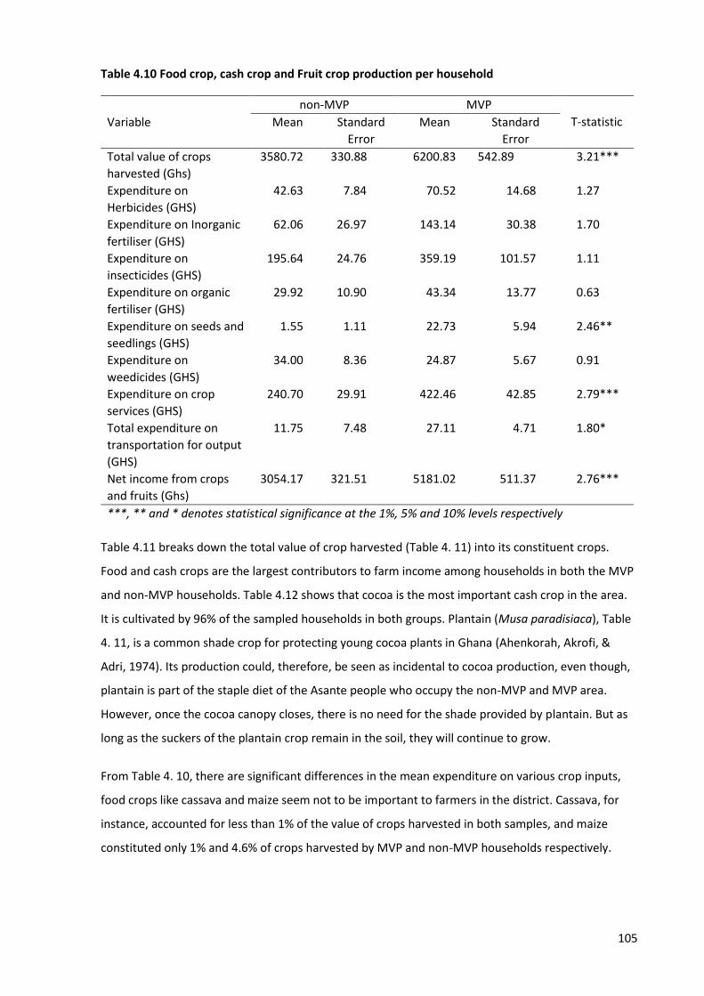
105

Table 4.10 Food crop, cash crop and Fruit crop production per household

non-MVP MVP

T-statistic Variable Mean Standard

Error

Mean Standard

Error

Total value of crops

harvested (Ghs)

3580.72 330.88 6200.83 542.89 3.21***

Expenditure on

Herbicides (GHS)

42.63 7.84 70.52 14.68 1.27

Expenditure on Inorganic

fertiliser (GHS)

62.06 26.97 143.14 30.38 1.70

Expenditure on

insecticides (GHS)

195.64 24.76 359.19 101.57 1.11

Expenditure on organic

fertiliser (GHS)

29.92 10.90 43.34 13.77 0.63

Expenditure on seeds and

seedlings (GHS)

1.55 1.11 22.73 5.94 2.46**

Expenditure on

weedicides (GHS)

34.00 8.36 24.87 5.67 0.91

Expenditure on crop

services (GHS)

240.70 29.91 422.46 42.85 2.79***

Total expenditure on

transportation for output

(GHS)

11.75 7.48 27.11 4.71 1.80*

Net income from crops

and fruits (Ghs)

3054.17 321.51 5181.02 511.37 2.76***

***, ** and * denotes statistical significance at the 1%, 5% and 10% levels respectively

Table 4.11 breaks down the total value of crop harvested (Table 4. 11) into its constituent crops.

Food and cash crops are the largest contributors to farm income among households in both the MVP

and non-MVP households. Table 4.12 shows that cocoa is the most important cash crop in the area.

It is cultivated by 96% of the sampled households in both groups. Plantain (Musa paradisiaca), Table

4. 11, is a common shade crop for protecting young cocoa plants in Ghana (Ahenkorah, Akrofi, &

Adri, 1974). Its production could, therefore, be seen as incidental to cocoa production, even though,

plantain is part of the staple diet of the Asante people who occupy the non-MVP and MVP area.

However, once the cocoa canopy closes, there is no need for the shade provided by plantain. But as

long as the suckers of the plantain crop remain in the soil, they will continue to grow.

From Table 4. 10, there are significant differences in the mean expenditure on various crop inputs,

food crops like cassava and maize seem not to be important to farmers in the district. Cassava, for

instance, accounted for less than 1% of the value of crops harvested in both samples, and maize

constituted only 1% and 4.6% of crops harvested by MVP and non-MVP households respectively.

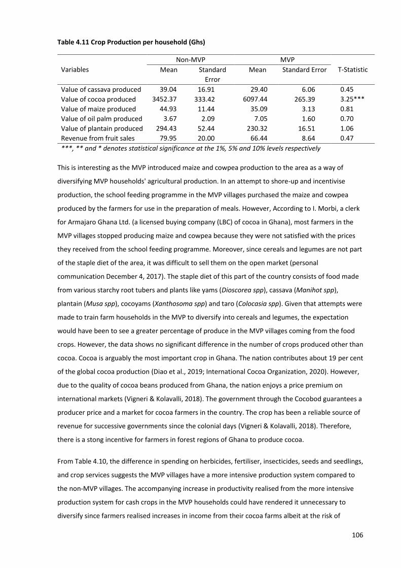
106

Table 4.11 Crop Production per household (Ghs)

Variables

Non-MVP MVP

T-Statistic Mean Standard

Error

Mean Standard Error

Value of cassava produced 39.04 16.91 29.40 6.06 0.45

Value of cocoa produced 3452.37 333.42 6097.44 265.39 3.25***

Value of maize produced 44.93 11.44 35.09 3.13 0.81

Value of oil palm produced 3.67 2.09 7.05 1.60 0.70

Value of plantain produced 294.43 52.44 230.32 16.51 1.06

Revenue from fruit sales 79.95 20.00 66.44 8.64 0.47

***, ** and * denotes statistical significance at the 1%, 5% and 10% levels respectively

This is interesting as the MVP introduced maize and cowpea production to the area as a way of

diversifying MVP households' agricultural production. In an attempt to shore-up and incentivise

production, the school feeding programme in the MVP villages purchased the maize and cowpea

produced by the farmers for use in the preparation of meals. However, According to I. Morbi, a clerk

for Armajaro Ghana Ltd. (a licensed buying company (LBC) of cocoa in Ghana), most farmers in the

MVP villages stopped producing maize and cowpea because they were not satisfied with the prices

they received from the school feeding programme. Moreover, since cereals and legumes are not part

of the staple diet of the area, it was difficult to sell them on the open market (personal

communication December 4, 2017). The staple diet of this part of the country consists of food made

from various starchy root tubers and plants like yams (Dioscorea spp), cassava (Manihot spp),

plantain (Musa spp), cocoyams (Xanthosoma spp) and taro (Colocasia spp). Given that attempts were

made to train farm households in the MVP to diversify into cereals and legumes, the expectation

would have been to see a greater percentage of produce in the MVP villages coming from the food

crops. However, the data shows no significant difference in the number of crops produced other than

cocoa. Cocoa is arguably the most important crop in Ghana. The nation contributes about 19 per cent

of the global cocoa production (Diao et al., 2019; International Cocoa Organization, 2020). However,

due to the quality of cocoa beans produced from Ghana, the nation enjoys a price premium on

international markets (Vigneri & Kolavalli, 2018). The government through the Cocobod guarantees a

producer price and a market for cocoa farmers in the country. The crop has been a reliable source of

revenue for successive governments since the colonial days (Vigneri & Kolavalli, 2018). Therefore,

there is a stong incentive for farmers in forest regions of Ghana to produce cocoa.

From Table 4.10, the difference in spending on herbicides, fertiliser, insecticides, seeds and seedlings,

and crop services suggests the MVP villages have a more intensive production system compared to

the non-MVP villages. The accompanying increase in productivity realised from the more intensive

production system for cash crops in the MVP households could have rendered it unnecessary to

diversify since farmers realised increases in income from their cocoa farms albeit at the risk of

107

greater risk exposure than in a more diversified production system. Fruit production is on a very

small scale basis and mostly for household consumption.

4.4.2 Livestock income and expenditures

The earlier discussion of livestock in Chapter 4, Section 4.3.3 discussed livestock as an asset, including

the numbers that households possessed. However, this section addresses the enterprise (production)

aspects of livestock in the household. Table 4.12 shows the information on the value of livestock

production among the MVP and non-MVP households. From the data in Table 4.12 we rejected the

null hypothesis of no difference in the mean value of cattle, the value of chickens value of goats,

expenditure on veterinary medicines and vaccines, veterinary service costs and the total animal

expenditure. The number of livestock for the statistically significant variables has been discussed

earlier in Section 3.3.3. Therefore, this section will discuss some of the constraints on livestock

production in the district.

Table 4.12 Animal production per household

Variable non-MVP MVP

t-statistic Mean Standard

Error

Mean Standard Error

Revenue from livestock

sales

351.19 104.97 458.07 105.60 0.33

Value of cattle owned 49.48 49.95 0.00 0.00 1.44+

Value of chickens owned 382.27 61.29 232.87 29.35 2.50**

Value of goats owned 16.49 16.62 363.37 71.80 3.32***

Value of Guinea fowls

owned

4.95 4.97 0.00 0.00 1.45

Value of sheep owned 838.14 186.16 577.72 110.82 1.27

Expenditure on animal

feed

0.00 0.00 0.45 32.81 0.93

Expenditure on veterinary

medicines and vaccines

2.35 1.69 0.15 0.07 1.93+

Expenditure on veterinary

services

7.47 3.98 0.40 0.29 2.59***

Total animal expenditure 19.65 8.46 1.98 0.56 2.93***

Net income from animal

and animal product sales

342.05 104.35 457.82 215.46 0.36

Notes: ***, **, *and + denotes statistical significance at the 1%, 5%, 10% and 20% levels respectively The value of cattle is only significant for an alpha level of 20 per cent. However, the mean values are

so small as to be practically insignificant. This is because livestock rearing particularly of cattle, sheep

and goats is more prevalent in the northern parts of Ghana where the climate is less humid and the

savannah grassland vegetation has provided more grazing resources that are available in the forests

zone to the south. Moreover, the climate of the southern forest zone (which includes the district of

108

the MVP and non-MVP villages) is conducive to the tsetse fly (Glossina sp). The Tsetse fly is the

vector for the trypanosome (Trypanosoma brucei) parasite among ruminants and humans. The

resultant debilitating disease, trypanosomiasis (sleeping sickness), has stifled cattle production in this

part of the country. Although small ruminants are susceptible to the disease, the indigenous

landraces of goats and sheep, West African Dwarf and Djallonké respectively, have a tolerance for

the disease (Osaer et al., 1994). However, these breeds are not productive milk, fibre or meat

producers. Unlike crop production, in the case of livestock, farming systems tend to be extensive

with animals left to roam and find their own food. Market offtake rates are very low as livestock are

mainly kept as a store of wealth in the virtual absence of banking and savings institutions (Doran,

Low, & Kemp, 1979). Small livestock like fowls, sheep and goats are a vital source of liquidity,

especially in areas where there are no formal savings institutions.

From Table 4.12, the expenditure on veterinary services for the non-MVP was almost ten times

higher compared to the MVP villages, and this difference was statistically significant at the one per

cent level. This raises a long-standing question as to whether expenditure on veterinary services is

prophylactic (to prevent disease) or curative (Ma, Bicknell and Renwick, 2020). However, in this case,

the expenditure on animal feed may provide additional insight. It would be expected that households

which are conscientious about preventing disease in their livestock will be more likely be concerned

about providing proper nutrition as well. However, the non-MVP households did not spend a

significantly different amount on feed for their animals compared to the MVP households. As such it

is more likely that the expenditure on veterinary services and veterinary medicines and vaccines was

for curing diseases that affected farm animals. Having considered the main outcomes – assets, farm

production, farm expenditure and net farm income in a disaggregated form. Table 4.13 presents the

results of the t-tests comparison of means for aggregate assets added, gross farm produce, total farm

expenditure and net farm income under the null hypotheses that there is no statistically significant

difference between their means.

Table 4.13 Comparison of mean outcomes across treatment and control groups before propensity score matching

Variable / Outcome

MVP Villages Non-MVP villages

t-tstatistics

Per adult equivalent Household

Per adult equivalent Household

Assets added (Ghs) 509.10 2259.96 271.39 1259.29 3.29*** Gross farm produce (Ghs) 1876.20 7901.03 1221.15 5313.71 2.71*** Total farm expenditure (Ghs) 242.86 1088.23 151.12 626.14 2.65*** Net farm income (Ghs) 1434.77 6007.03 860.29 3625.07 2.89***

Notes: *** denotes statistical significance at the 1% level Source: Authors' computation from field data (2017)

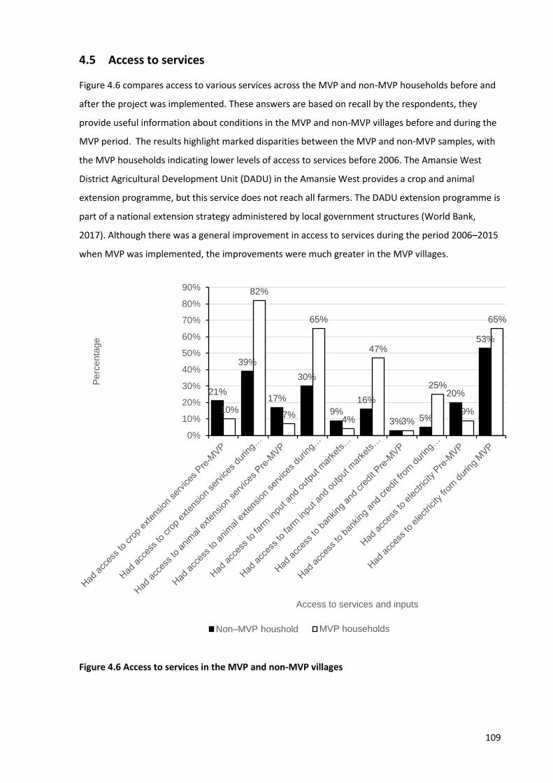
109

4.5 Access to services

Figure 4.6 compares access to various services across the MVP and non-MVP households before and

after the project was implemented. These answers are based on recall by the respondents, they

provide useful information about conditions in the MVP and non-MVP villages before and during the

MVP period. The results highlight marked disparities between the MVP and non-MVP samples, with

the MVP households indicating lower levels of access to services before 2006. The Amansie West

District Agricultural Development Unit (DADU) in the Amansie West provides a crop and animal

extension programme, but this service does not reach all farmers. The DADU extension programme is

part of a national extension strategy administered by local government structures (World Bank,

2017). Although there was a general improvement in access to services during the period 2006–2015

when MVP was implemented, the improvements were much greater in the MVP villages.

Figure 4.6 Access to services in the MVP and non-MVP villages

21%

39%

17%

30%

9%

16%

3% 5%

20%

53%

10%

82%

7%

65%

4%

47%

3%

25%

9%

65%

0%

10%

20%

30%

40%

50%

60%

70%

80%

90%

Perc

enta

ge

Access to services and inputs

Non–MVP houshold MVP households

110

Similarly, there was a marked increase in access to farm inputs and output markets, for both MVP

and non-MVP households, however, the increase for the MVP households was larger than that of the

non-MVP households. Pre-MVP, nine per cent of non-MVP households reported having access to

markets compared to four per cent for the MVP households. During the MVP 16 per cent of non-MVP

households reported having access to markets an increase of five per cent, while 47 per cent of MVP

households reported having access an increase of 43 per cent. A similar pattern was seen for access

to credit (an increase of two per cent for the non-MVP households compared to 22 per cent for the

MVP households) and access to electricity ( an increase of 23 per cent for the non-MVP villages

compared to 46 per cent for the MVP villages.

4.6 Chapter Summary

This chapter serves a dual role. It presents descriptive statistics for the data as well as results of the

first research question – comparing the differences between the MVP and non-MVP household in a

naïve manner, without controlling for any of the factors discussed in Chapter 3. The results of the

households characteristics comparison shows that the two groups have similar characteristics except

for the age of the household head, years of schooling, and dependency ratio. The value of household

assets in 2016 and the value of assets added, the number of goats and chickens owned were the

assets for which statistical differences were found for the two groups. The results show that the MVP

had a significant effect on crop production, particularly, cocoa. It also had a significant effect on total

expenditure and net income. However, the statistical impact of the MVP on livestock production

were all in favour of the non-MVP group. While these descriptive statistics presented in this chapter

show clear differences in outcomes between the MVP and non-MVP samples, these differences

cannot be attributed only to the project as they may have been caused by other contemporaneous

factors, and the MVP and non-MVP households may have been substantively different before the

project was implemented. Although there are large differences between the two groups, these

univariate differences do not reflect the impact of the MVP for the reasons described in Chapter 3,

Section 3.3.2.

111

Chapter 5

The Financial and Economic Impact of the Bonsaaso MVP

5.1 Introduction

As part of addressing research question 1, some differences between MVP and non-MVP households

were analysed in Chapter 4. The analyses of the descriptive statistics cover a wide range of

household characteristics, farm characteristics, and village level conditions that are relevant to

farming. In this chapter research question 2 is addressed and the impact of the MVP on farming

households are evaluated. Propensity score matching (PSM) was used to determine the impact of the

MVP on comparable households. In section 5.2, the PSM results of the impact of the MVP are

presented along with balancing tests to determine the quality of the matching achieved under PSM.

The PSM comparison of the two groups is then presented. Section 5.3 presents the results of the

recursive instrumental variables (IV) model estimation as a robustness test for the PSM.

5.2 Propensity score model

The study applied propensity score matching to identify subsets of MVP and non-MVP households

with similar time-invariant pre-treatment household and farm characteristics. The first step in the

PSM is to estimate the propensity scores. In Chapter 3, Section 3.3.2 a model was formulated that

comprised of relatively time-invariant household characteristics. In this chapter, Equation (5.1)has

been estimated. The time-invariant variables in the model were years of schooling completed by

adult household heads (in log form), and the gender of the household head. Other variables in the

model include the age of the household head, dependency ratio of the household to capture the

composition of the household. Also included in the model were the land endowment of household,

baseline (2006) value of farm assets, fixed improvements and household assets. As such, the model

captures household demographic characteristics as well as wealth endowments of both the MVP and

non-MVP groups at the start of the project.

MVP= α0 + α1lage + α2ledec+ α3deprat+ α4land+ α5farmassets06+ α6hhassets06+ε (5.1)

The convention in most studies applying PSM is to include as many pre-treatment variables in the

PSM model as can be obtained (Adelson et al., 2017). However, in this study, the participation model,

Equation 5.1, was developed based on the socio-economic variables that could have influenced the

decision to place the MVP in Bonsaaso (Caliendo & Kopeinig, 2008; Mitchell et al., 2015a). Table 5.1

presents the results of the logit and probit models used to estimate Equation 5.1, the likelihood of

MVP participation, and subsequently, the propensity scores.

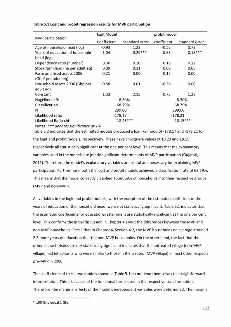
112

Table 5.1 Logit and probit regression results for MVP participation

MVP participation logit Model probit model

Coefficient Standard error coefficient standard error

Age of household head (log) -0.93 1.23 -0.52 0.73 Years of education of household head (log)

1.04 0.29*** 0.63 0.18***

Dependency ratio (number) 0.30 0.20 0.18 0.12 Stock farm land (ha per adult eq) 0.09 0.11 0.06 0.06 Farm and fixed assets 2006 (Ghp5 per adult eq)

-0.21 0.00 -0.12 0.00

Household assets 2006 (Ghp per adult eq)

-0.58 0.01 -0.36 0.00

Constant 1.33 2.15 0.73 1.28

Nagelkerke R2 8.30% 8.30% Classification 68.79% 68.79% N 299.00 299.00 Likelihood ratio -178.17 -178.21 Likelihood Ratio chi2 18.23*** 18.15***

Notes: *** denotes significance at 1% Table 5.2 indicates that the estimated models produced a log-likelihood of -178.17 and -178.21 for

the logit and probit models, respectively. These have chi-square values of 18.23 and 18.15

respectively all statistically significant at the one per cent level. This means that the explanatory

variables used in the models are jointly significant determinants of MVP participation (Gujarati,

2011). Therefore, the model’s explanatory variables are useful and necessary for explaining MVP

participation. Furthermore, both the logit and probit models achieved a classification rate of 68.79%.

This means that the model correctly classified about 69% of households into their respective groups

(MVP and non-MVP).

All variables in the logit and probit models, with the exception of the estimated coefficient of the

years of education of the household head, were not statistically significant. Table 5.1 indicates that

the estimated coefficients for educational attainment are statistically significant at the one per cent

level. This confirms the initial discussion in Chapter 4 about the differences between the MVP and

non-MVP households. Recall that in Chapter 4, Section 4.2, the MVP households on average attained

2.5 more years of education that the non-MVP households. On the other hand, the fact that the

other characteristics are not statistically significant indicates that the untreated village (non-MVP

village) had inhabitants who were similar to those in the treated (MVP village) in most other respects

pre-MVP in 2006.

The coefficients of these two models shown in Table 5.1 do not lend themselves to straightforward

interpretation. This is because of the functional forms used in the respective transformation.

Therefore, the marginal effects of the model's independent variables were determined. The marginal

5 100 Ghp equal 1 Ghs

113

effects have a more intuitive interpretation. It shows the change in the probability of participation

when a unit change occurs in the independent variable. The results shown in Table 5.2 are the

average marginal effects of the logit and probit models of participation.

The average estimated marginal effect for education in Table 5.2 show that a percentage increase in

the years of schooling results in a 0.22 per cent increase in the probability of the MVP being placed in

the area. Years of education is widely used as a proxy for human capital indicating capability for

technology adoption and the ability to acquire and assess all sorts of information. Educational

attainment, in turn, impacts the households' livelihood and welfare outcomes over time. From the

regression results, it is possible that the educational difference between the MVP and surrounding

non-MVP villages may have been a factor considered in the placement of the MVP in the Bonsaaso

area. However, further analysis in this regard is carried out in the next section.

Table 5.2 The average marginal effect of logit and probit model of MVP participation

Variables Logit Probit

dy/dx Standard error

dy/dx Standard error

Age of household head (log)

-0.2 0.26 -0.19 0.26

Years of education of households head (log)

0.22 0.06*** 0.22 0.06***

Dependency ratio (number)

0.06 0.04+6 0.06 0.04+

Stock of farm land (ha per adult eq)

0.02 0.23 0.02 0.02

Farm and fixed assets 2006 (per adult eq)

-0.0004 0.0007 -0.0005 0.0007

Household assets 2006 (per adult eq)

-0.001 0.001 -0.001 0.001

Notes: *** and + denotes significance at 1% and 20% respectively

Cameron & Trivedi (2009) showed that the central tendencies of the logit and probit models are

similar, but the differences appear at the tails of the distribution. The differences in the estimated

parameters of the two models arise from the functional forms employed. The logit model employs a

logarithmic transformation of the odds ratio. Whereas the probit model employs the standard

normal cumulative distribution function (CDF). Consequently, the error term of the probit model is

normally distributed while that of the logit model has a logistic distribution (Gujarati, 2011). Caliendo

and Kopeinig (2008) argue that the choice of logit or probit is not a critical one as the two estimators

yield similar results. Given that the goodness of fit measures of the logit and probit models are

6 At an alpha level (𝛼) of 20 per cent dependency ratio would have been statistically significant with an increase resulting in a 0.06 per cent increase in the probability of participating in the MVP.

114

almost identical, and the parameters are similarly close, it is a matter of preference the final model

used. This study, therefore, proceeds with the logit model for PSM.

To verify the impact of the MVP interventions, the predicted probabilities (propensity scores) were

estimated for each household using the logit model. The propensity scores are indices reflecting the

probability that a household participated in the MVP given their respective pre-treatment

characteristics. The propensity scores, which represent the probability of participation in the MVP,

were used to match households in the MVP and non-MVP villages. The propensity scores for the

pooled data of MVP and non-MVP villages ranged from 0.04 to 0.99. The mean propensity score was

0.68 with an attached standard error of 0.02. For the non-MVP households, the estimated

propensity scores ranged from a minimum of 0.06 to a maximum of 0.90, the mean was 0.37, and

the standard error was 0.02. On the other hand, for the MVP sample, the propensity scores ranged

from a minimum of 0.04 to a maximum of 0.99, and the mean propensity score was 0.82, with a

standard error of 0.02. The range of propensity scores indicates that the distribution of MVP

household propensity scores covers the entire propensity score distribution in the non-MVP sample.

As stated in Chapter 3, Heckman et al. (1997) strongly recommend establishing a region of common

support by discarding non-overlapping observations from both the MVP and non-MVP groups at the

tails of the two distributions before matching. As such, establishing a region of common support will

remove the extreme propensity scores in the MVP sample, and increase the similarity in the two

groups. The summary of the resultant data after matching are shown in Table 5.3.

Table 5.3 Matching summary

Sample sizes MVP Non-MVP Total

Matched 154 90 244

Unmatched 43 7 50

Outside region of common support 5 0 5

Total 202 97 299

Households in the non-MVP sample were then matched with households in the MVP sample

according to their propensity scores of MVP participation. The matching was completed using

'MatchIt' an add-on package available in the R statistical software, which can run a wide range of

matching algorithms, including nearest-neighbour, greedy, and optimal matching algorithms (Ho et

al., 2007; Ho, Imai, King, & Stuart, 2011). The nearest-neighbour matching algorithm was applied to

match the households in this study. In the matching process, five households that fell outside the

region of common support (the range of overlapping propensity scores between the MVP and non-

MVP participants) for the propensity scores were dropped from the dataset. The matched cases from

the MVP and non-MVP villages constitute the treatment and comparison groups, respectively. A total

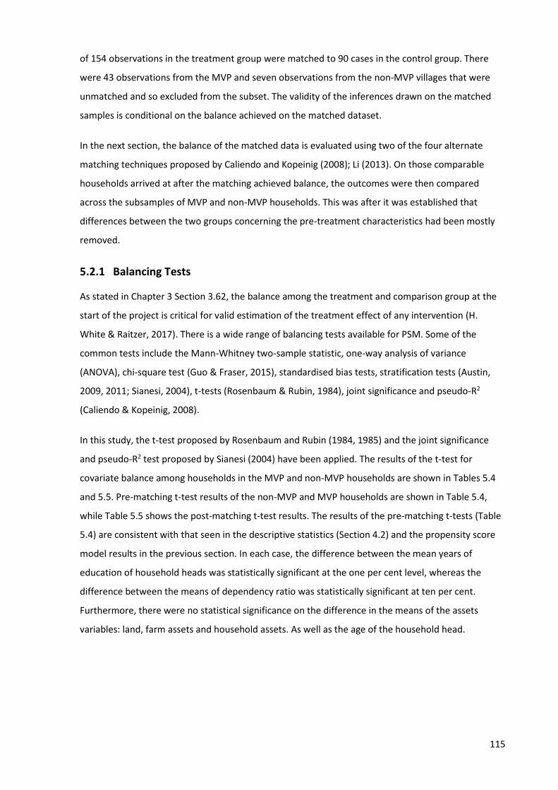
115

of 154 observations in the treatment group were matched to 90 cases in the control group. There

were 43 observations from the MVP and seven observations from the non-MVP villages that were

unmatched and so excluded from the subset. The validity of the inferences drawn on the matched

samples is conditional on the balance achieved on the matched dataset.

In the next section, the balance of the matched data is evaluated using two of the four alternate

matching techniques proposed by Caliendo and Kopeinig (2008); Li (2013). On those comparable

households arrived at after the matching achieved balance, the outcomes were then compared

across the subsamples of MVP and non-MVP households. This was after it was established that

differences between the two groups concerning the pre-treatment characteristics had been mostly

removed.

5.2.1 Balancing Tests

As stated in Chapter 3 Section 3.62, the balance among the treatment and comparison group at the

start of the project is critical for valid estimation of the treatment effect of any intervention (H.

White & Raitzer, 2017). There is a wide range of balancing tests available for PSM. Some of the

common tests include the Mann-Whitney two-sample statistic, one-way analysis of variance

(ANOVA), chi-square test (Guo & Fraser, 2015), standardised bias tests, stratification tests (Austin,

2009, 2011; Sianesi, 2004), t-tests (Rosenbaum & Rubin, 1984), joint significance and pseudo-R2

(Caliendo & Kopeinig, 2008).

In this study, the t-test proposed by Rosenbaum and Rubin (1984, 1985) and the joint significance

and pseudo-R2 test proposed by Sianesi (2004) have been applied. The results of the t-test for

covariate balance among households in the MVP and non-MVP households are shown in Tables 5.4

and 5.5. Pre-matching t-test results of the non-MVP and MVP households are shown in Table 5.4,

while Table 5.5 shows the post-matching t-test results. The results of the pre-matching t-tests (Table

5.4) are consistent with that seen in the descriptive statistics (Section 4.2) and the propensity score

model results in the previous section. In each case, the difference between the mean years of

education of household heads was statistically significant at the one per cent level, whereas the

difference between the means of dependency ratio was statistically significant at ten per cent.

Furthermore, there were no statistical significance on the difference in the means of the assets

variables: land, farm assets and household assets. As well as the age of the household head.

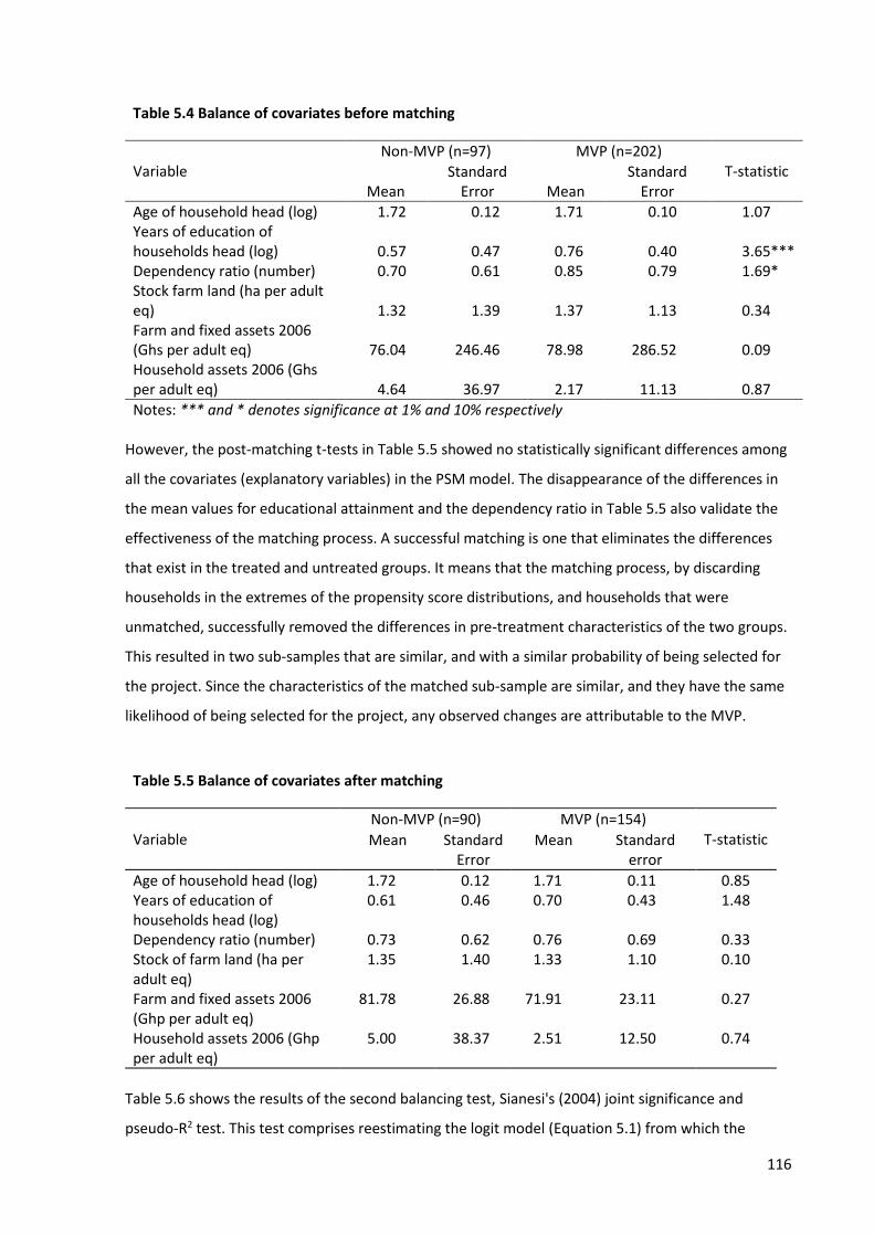
116

However, the post-matching t-tests in Table 5.5 showed no statistically significant differences among

all the covariates (explanatory variables) in the PSM model. The disappearance of the differences in

the mean values for educational attainment and the dependency ratio in Table 5.5 also validate the

effectiveness of the matching process. A successful matching is one that eliminates the differences

that exist in the treated and untreated groups. It means that the matching process, by discarding

households in the extremes of the propensity score distributions, and households that were

unmatched, successfully removed the differences in pre-treatment characteristics of the two groups.

This resulted in two sub-samples that are similar, and with a similar probability of being selected for

the project. Since the characteristics of the matched sub-sample are similar, and they have the same

likelihood of being selected for the project, any observed changes are attributable to the MVP.

Table 5.6 shows the results of the second balancing test, Sianesi's (2004) joint significance and

pseudo-R2 test. This test comprises reestimating the logit model (Equation 5.1) from which the

Table 5.4 Balance of covariates before matching

Variable Non-MVP (n=97) MVP (n=202)

T-statistic Mean

Standard Error Mean

Standard Error

Age of household head (log) 1.72 0.12 1.71 0.10 1.07 Years of education of households head (log) 0.57 0.47 0.76 0.40 3.65*** Dependency ratio (number) 0.70 0.61 0.85 0.79 1.69* Stock farm land (ha per adult eq) 1.32 1.39 1.37 1.13 0.34 Farm and fixed assets 2006 (Ghs per adult eq) 76.04 246.46 78.98 286.52 0.09 Household assets 2006 (Ghs per adult eq) 4.64 36.97 2.17 11.13 0.87

Notes: *** and * denotes significance at 1% and 10% respectively

Table 5.5 Balance of covariates after matching

Variable Non-MVP (n=90) MVP (n=154)

T-statistic Mean Standard Error

Mean Standard error

Age of household head (log) 1.72 0.12 1.71 0.11 0.85 Years of education of households head (log)

0.61 0.46 0.70 0.43 1.48

Dependency ratio (number) 0.73 0.62 0.76 0.69 0.33 Stock of farm land (ha per adult eq)

1.35 1.40 1.33 1.10 0.10

Farm and fixed assets 2006 (Ghp per adult eq)

81.78 26.88 71.91 23.11 0.27

Household assets 2006 (Ghp per adult eq)

5.00 38.37 2.51 12.50 0.74

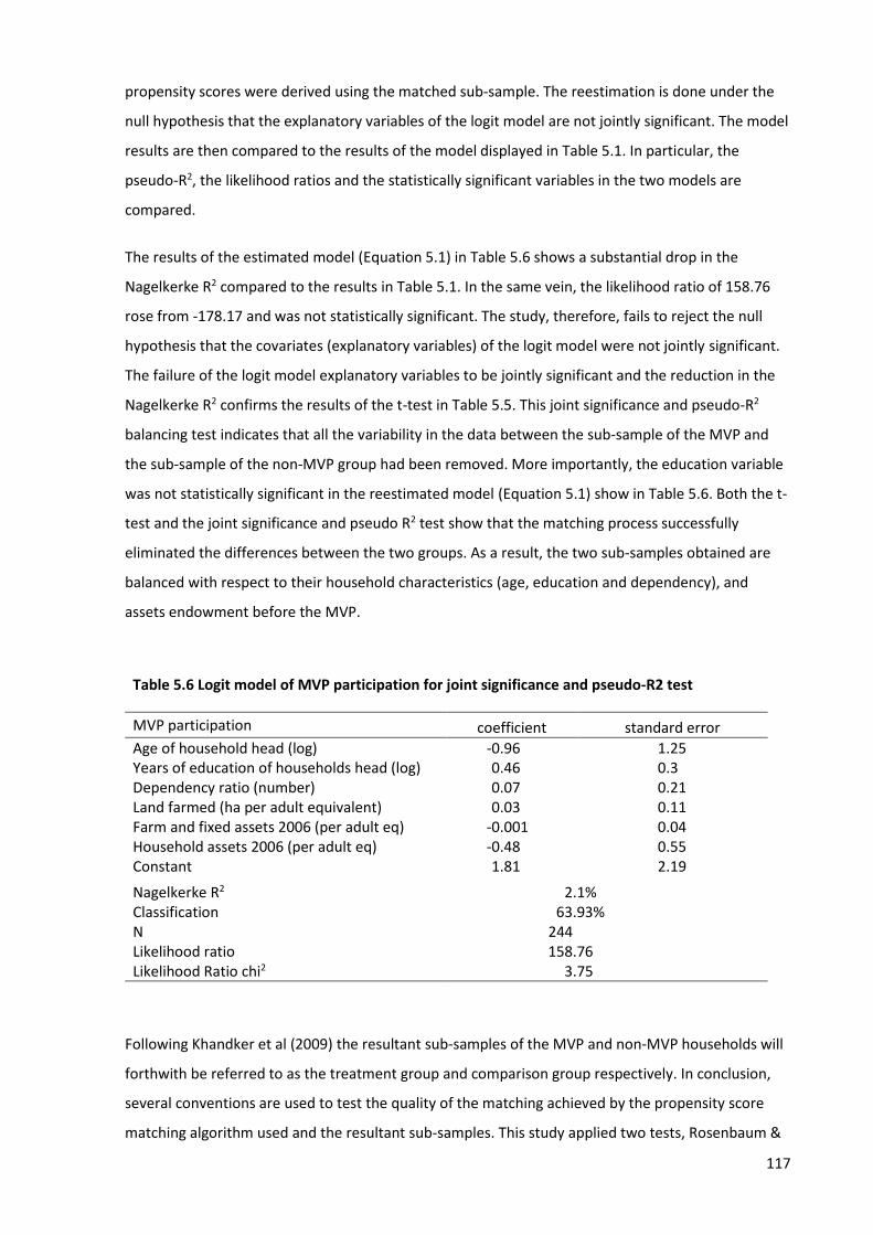
117

propensity scores were derived using the matched sub-sample. The reestimation is done under the

null hypothesis that the explanatory variables of the logit model are not jointly significant. The model

results are then compared to the results of the model displayed in Table 5.1. In particular, the

pseudo-R2, the likelihood ratios and the statistically significant variables in the two models are

compared.

The results of the estimated model (Equation 5.1) in Table 5.6 shows a substantial drop in the

Nagelkerke R2 compared to the results in Table 5.1. In the same vein, the likelihood ratio of 158.76

rose from -178.17 and was not statistically significant. The study, therefore, fails to reject the null

hypothesis that the covariates (explanatory variables) of the logit model were not jointly significant.

The failure of the logit model explanatory variables to be jointly significant and the reduction in the

Nagelkerke R2 confirms the results of the t-test in Table 5.5. This joint significance and pseudo-R2

balancing test indicates that all the variability in the data between the sub-sample of the MVP and

the sub-sample of the non-MVP group had been removed. More importantly, the education variable

was not statistically significant in the reestimated model (Equation 5.1) show in Table 5.6. Both the t-

test and the joint significance and pseudo R2 test show that the matching process successfully

eliminated the differences between the two groups. As a result, the two sub-samples obtained are

balanced with respect to their household characteristics (age, education and dependency), and

assets endowment before the MVP.

Following Khandker et al (2009) the resultant sub-samples of the MVP and non-MVP households will

forthwith be referred to as the treatment group and comparison group respectively. In conclusion,

several conventions are used to test the quality of the matching achieved by the propensity score

matching algorithm used and the resultant sub-samples. This study applied two tests, Rosenbaum &

Table 5.6 Logit model of MVP participation for joint significance and pseudo-R2 test

MVP participation

coefficient standard error

Age of household head (log) -0.96 1.25 Years of education of households head (log) 0.46 0.3 Dependency ratio (number) 0.07 0.21 Land farmed (ha per adult equivalent) 0.03 0.11 Farm and fixed assets 2006 (per adult eq) -0.001 0.04 Household assets 2006 (per adult eq) -0.48 0.55 Constant 1.81 2.19

Nagelkerke R2 2.1% Classification 63.93% N 244 Likelihood ratio 158.76 Likelihood Ratio chi2 3.75

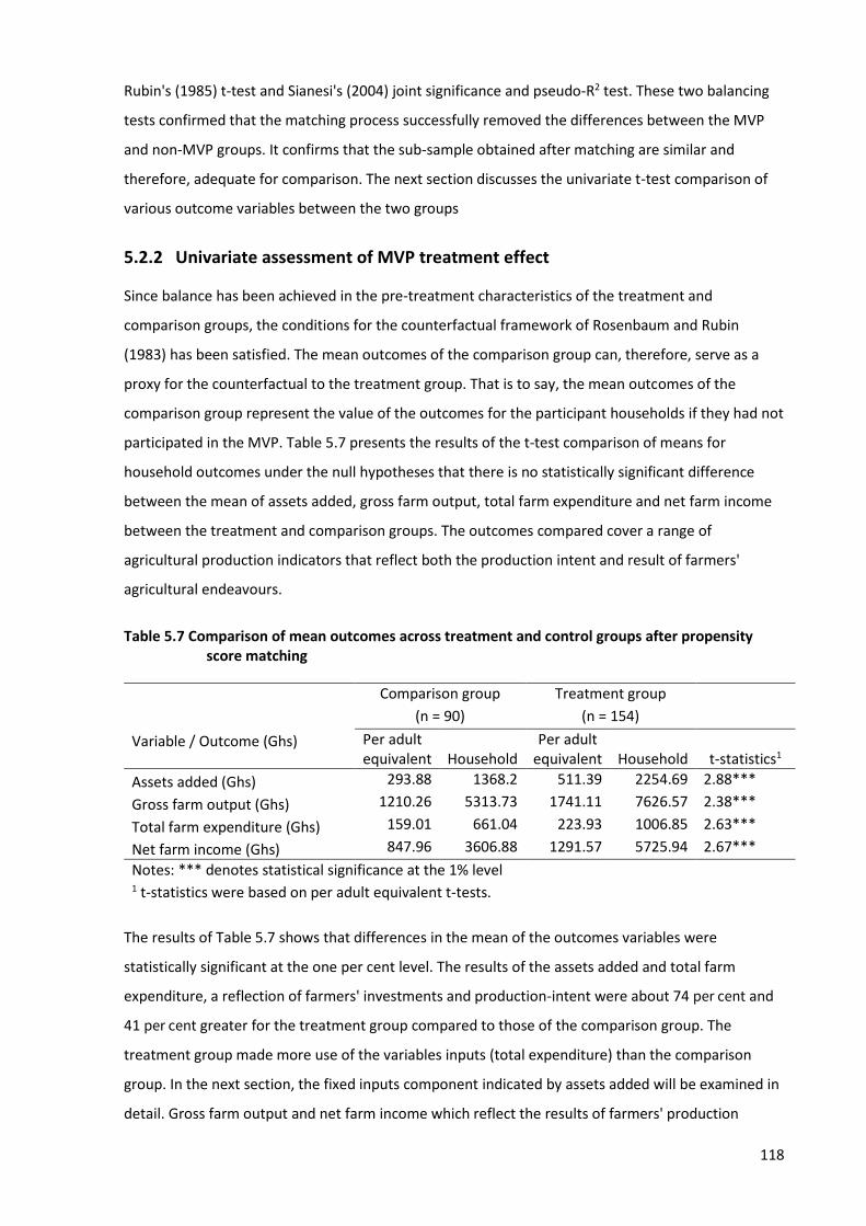
118

Rubin's (1985) t-test and Sianesi's (2004) joint significance and pseudo-R2 test. These two balancing

tests confirmed that the matching process successfully removed the differences between the MVP

and non-MVP groups. It confirms that the sub-sample obtained after matching are similar and

therefore, adequate for comparison. The next section discusses the univariate t-test comparison of

various outcome variables between the two groups

5.2.2 Univariate assessment of MVP treatment effect

Since balance has been achieved in the pre-treatment characteristics of the treatment and

comparison groups, the conditions for the counterfactual framework of Rosenbaum and Rubin

(1983) has been satisfied. The mean outcomes of the comparison group can, therefore, serve as a

proxy for the counterfactual to the treatment group. That is to say, the mean outcomes of the

comparison group represent the value of the outcomes for the participant households if they had not

participated in the MVP. Table 5.7 presents the results of the t-test comparison of means for

household outcomes under the null hypotheses that there is no statistically significant difference

between the mean of assets added, gross farm output, total farm expenditure and net farm income

between the treatment and comparison groups. The outcomes compared cover a range of

agricultural production indicators that reflect both the production intent and result of farmers'

agricultural endeavours.

Table 5.7 Comparison of mean outcomes across treatment and control groups after propensity score matching

Comparison group

(n = 90)

Treatment group

(n = 154) Variable / Outcome (Ghs) Per adult

equivalent Household Per adult

equivalent Household t-statistics1

Assets added (Ghs) 293.88 1368.2 511.39 2254.69 2.88***

Gross farm output (Ghs) 1210.26 5313.73 1741.11 7626.57 2.38***

Total farm expenditure (Ghs) 159.01 661.04 223.93 1006.85 2.63***

Net farm income (Ghs) 847.96 3606.88 1291.57 5725.94 2.67***

Notes: *** denotes statistical significance at the 1% level 1 t-statistics were based on per adult equivalent t-tests.

The results of Table 5.7 shows that differences in the mean of the outcomes variables were

statistically significant at the one per cent level. The results of the assets added and total farm

expenditure, a reflection of farmers' investments and production-intent were about 74 per cent and

41 per cent greater for the treatment group compared to those of the comparison group. The

treatment group made more use of the variables inputs (total expenditure) than the comparison

group. In the next section, the fixed inputs component indicated by assets added will be examined in

detail. Gross farm output and net farm income which reflect the results of farmers' production

119

activity are 44 per cent and 52 per cent greater for the treatment group compared to the comparison

group.

On the other hand, the naïve comparison of the households’ farm-level outcomes before the PSM

showed the differences were 88 per cent for assets added, 54 per cent for gross farm output, 61 per

cent for total farm expenditure and 67 per cent for net farm income. All these differences were in

favour of the MVP households. Following the PSM comparison, the differences in the two groups for

the outcome variables were reduced but remained statistically significant. This means that the

differences between the comparable households in the treatment and comparison groups were

closer than for all the household together. While these aggregate measures of farm outcomes are

useful, a disaggregated breakdown of the components will give more detailed information to show

the sources of the differences among the treatment and comparison households.

5.2.3 Assets

In this section, the aggregate results shown in Table 5.7 are broken down to show in more detail the

asset outcome variable constituents that contributed most significantly to the impact of the MVP.

Table 5.8 shows the t-test results of land, farm assets and household assets for the treatment and

comparison group after matching. On the other hand, the MVP sample had 48 more households than

the treatment group as a result of the matching. The results of the two tables are quite similar. The

difference in the mean of the land variables remained statistically insignificant. In that regard, the

result has not changed concerning the previous analysis.

As such, the MVP had no statistically significant impact on participants' investment in Land. The land

tenure and property rights regime in this part of the country has been discussed extensively in

Chapter 4. This land rights regime is lacking in providing the breadth, duration and assurance

necessary for defining a secure property right system (Maxwell & Wiebe, 1999). The system is

particularly detrimental to women as they are unable to hold land independently. Despite the

matrilineal system of inheritance practised in the Bonsaaso areas the society is patriarchal (male-

dominated). In traditional Ghanaian society, it is thought that giving land to women is a sure way to

alienate family land as they may transfer it to their husband’s family through marriage.

Consequently, women who intend to farm acquire farmland through their male relatives such as

fathers, husbands, brothers and sons. These often tend to be marginal lands that are the least fertile

(Gray & Kevane, 1999).

Similarly, the difference in the mean value of fixed improvements and the mean value of farm assets

in 2006 were not statistically significant between the treatment and comparison groups (Table 5.8).

Numerous theoretical and empirical studies show that insecure property rights in land and other

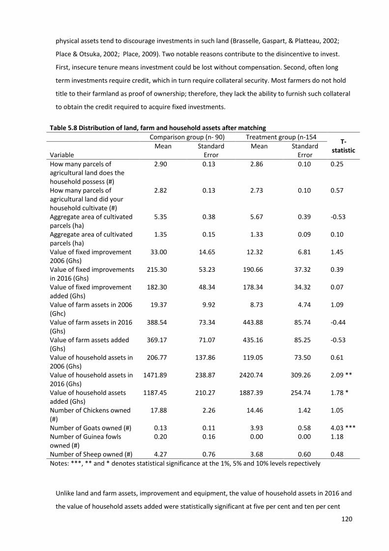
120

physical assets tend to discourage investments in such land (Brasselle, Gaspart, & Platteau, 2002;

Place & Otsuka, 2002; Place, 2009). Two notable reasons contribute to the disincentive to invest.

First, insecure tenure means investment could be lost without compensation. Second, often long

term investments require credit, which in turn require collateral security. Most farmers do not hold

title to their farmland as proof of ownership; therefore, they lack the ability to furnish such collateral

to obtain the credit required to acquire fixed investments.

Table 5.8 Distribution of land, farm and household assets after matching

Comparison group (n- 90) Treatment group (n-154 T-

statistic Variable

Mean Standard Error

Mean Standard Error

How many parcels of agricultural land does the household possess (#)

2.90 0.13 2.86 0.10 0.25

How many parcels of agricultural land did your household cultivate (#)

2.82 0.13 2.73 0.10 0.57

Aggregate area of cultivated parcels (ha)

5.35 0.38 5.67 0.39 -0.53

Aggregate area of cultivated parcels (ha)

1.35 0.15 1.33 0.09 0.10

Value of fixed improvement 2006 (Ghs)

33.00 14.65 12.32 6.81 1.45

Value of fixed improvements in 2016 (Ghs)

215.30 53.23 190.66 37.32 0.39

Value of fixed improvement added (Ghs)

182.30 48.34 178.34 34.32 0.07

Value of farm assets in 2006 (Ghc)

19.37 9.92 8.73 4.74 1.09

Value of farm assets in 2016 (Ghs)

388.54 73.34 443.88 85.74 -0.44

Value of farm assets added (Ghs)

369.17 71.07 435.16 85.25 -0.53

Value of household assets in 2006 (Ghs)

206.77 137.86 119.05 73.50 0.61

Value of household assets in 2016 (Ghs)

1471.89 238.87 2420.74 309.26 2.09 **

Value of household assets added (Ghs)

1187.45 210.27 1887.39 254.74 1.78 *

Number of Chickens owned (#)

17.88 2.26 14.46 1.42 1.05

Number of Goats owned (#) 0.13 0.11 3.93 0.58 4.03 *** Number of Guinea fowls owned (#)

0.20 0.16 0.00 0.00 1.18

Number of Sheep owned (#) 4.27 0.76 3.68 0.60 0.48

Notes: ***, ** and * denotes statistical significance at the 1%, 5% and 10% levels repectively

Unlike land and farm assets, improvement and equipment, the value of household assets in 2016 and

the value of household assets added were statistically significant at five per cent and ten per cent

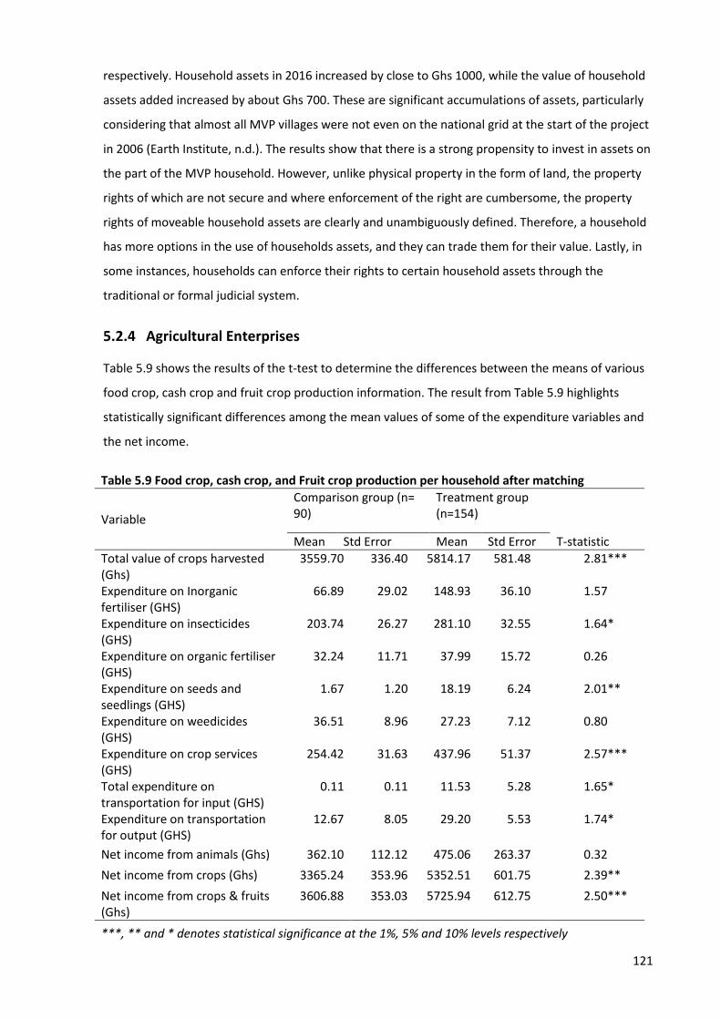
121

respectively. Household assets in 2016 increased by close to Ghs 1000, while the value of household

assets added increased by about Ghs 700. These are significant accumulations of assets, particularly

considering that almost all MVP villages were not even on the national grid at the start of the project

in 2006 (Earth Institute, n.d.). The results show that there is a strong propensity to invest in assets on

the part of the MVP household. However, unlike physical property in the form of land, the property

rights of which are not secure and where enforcement of the right are cumbersome, the property

rights of moveable household assets are clearly and unambiguously defined. Therefore, a household

has more options in the use of households assets, and they can trade them for their value. Lastly, in

some instances, households can enforce their rights to certain household assets through the

traditional or formal judicial system.

5.2.4 Agricultural Enterprises

Table 5.9 shows the results of the t-test to determine the differences between the means of various

food crop, cash crop and fruit crop production information. The result from Table 5.9 highlights

statistically significant differences among the mean values of some of the expenditure variables and

the net income.

Table 5.9 Food crop, cash crop, and Fruit crop production per household after matching

Variable

Comparison group (n= 90)

Treatment group (n=154)

T-statistic

Mean Std Error Mean Std Error

Total value of crops harvested (Ghs)

3559.70 336.40 5814.17 581.48 2.81***

Expenditure on Inorganic fertiliser (GHS)

66.89 29.02 148.93 36.10 1.57

Expenditure on insecticides (GHS)

203.74 26.27 281.10 32.55 1.64*

Expenditure on organic fertiliser (GHS)

32.24 11.71 37.99 15.72 0.26

Expenditure on seeds and seedlings (GHS)

1.67 1.20 18.19 6.24 2.01**

Expenditure on weedicides (GHS)

36.51 8.96 27.23 7.12 0.80

Expenditure on crop services (GHS)

254.42 31.63 437.96 51.37 2.57***

Total expenditure on transportation for input (GHS)

0.11 0.11 11.53 5.28 1.65*

Expenditure on transportation for output (GHS)

12.67 8.05 29.20 5.53 1.74*

Net income from animals (Ghs) 362.10 112.12 475.06 263.37 0.32

Net income from crops (Ghs) 3365.24 353.96 5352.51 601.75 2.39**

Net income from crops & fruits (Ghs)

3606.88 353.03 5725.94 612.75 2.50***

***, ** and * denotes statistical significance at the 1%, 5% and 10% levels respectively

122

The Gross farm output is an aggregate of all cash crops, food crops, fruits and animal production

information. This section breaks down the individual farm enterprise components to show how each

contributes to the total farm output, expenditure, and net farm income of the matched subsets of

MVP and non-MVP households: the treatment and comparison groups. To gain more insight into the

individual enterprises that constitute the MVP Table 5.9 shows the results of the food crops, cash

crops, and fruit crop produced and expenses of crop inputs. The table has the same variables as

Table 4.10 in Chapter 4.

However, the sample sizes of the data used are different as a result of the matching. The results

highlight statistical differences between, the total crops harvested, expenditure on insecticides,

expenditure on seeds and seedlings, expenditure on crop services, expenditure on transportation for

outputs and income from crops and fruits. The results from Table 5.9 contrasts with that of Table

4.10 in the number of statistically significant variables, the size of the differences in the significant

variables and the size of the t-statistic of some variables. Notably, the expenditure on insecticides

was not statistically significant in Table 4.10. However, it is significant in Table 5.9. The treatment

group used about Ghs 77 more insecticide compared to the treatment group. However, this

difference is lower than that of Table 4.10 (Ghs 163), which was not significant. Other insignificant

variables remained so.

However, the size of the significant difference was reduced for the total value of crops harvested, the

expenditure on seeds and seedlings, and income from fruits crops and fruits after matching. At the

same time, the differences increased for the expenditure on crop services and the expenditure on

transportation for output. Table 5.10 shows the result of the crops that make up the top line of the

value of crops harvested.

Table 5.10 Crop Production per household for the treatment and comparison groups (Ghs)

Variable

Comparison group (n= 90)

Treatment group (n=154

T-statistic

Mean Standard

Error Mean

Standard Error

Value of cassava produced (Ghs) 42.07 17.98 16.50 7.18 1.54 Value of cocoa produced (Ghs) 3432.16 334.27 5724.05 579.91 2.86*** Value of maize produced (Ghs) 38.40 9.42 33.82 6.94 0.39 Value of oil palm produced (Ghs) 3.95 2.19 9.11 4.18 -0.90 Value of plantain produced (Ghs) 311.78 55.49 221.82 37.82 1.38 Revenue from fruit sales (Ghs) 83.30 21.19 68.96 21.85 0.44

*** denotes statistical significance at the 1% level

123

After matching, the table results show that cocoa remains crop that was statistically different

between the treatment and comparison groups. This is a similar result to that of Table 4.11 in

Chapter 4. However, the size of the difference reduced from Ghs 2645 in the MVP and non-MVP

group to Ghs 2292 in the treatment and comparison group. Also, the t-statistics fell from 3.25 to 2.86

in the comparison treatment and comparison groups.

Table 5.11 shows the estimated results of the set of economic and financial variables related to

animal production. The results of the crop enterprise variables were mostly in favour of the

treatment group; in contrast to the animal enterprise variables which were in favour of the

comparison group. The difference between the treatment group and comparison group were

statistically significant for multiple variables; namely, the value of chickens owned, the value of goats

owned, expenditure on veterinary medicines and vaccines, and the total animal expenditure. By

contrast, the value of cattle, value of chickens, value of goats, expenditure on veterinary medicines

and vaccines, veterinary service expenditure and total animal expenditure were statistically

significant in the unmatched sample result in Table 4.12 of Chapter 4. Although the treatment group

incurred more in animal related expenditure, this increased expenditure did not show in their

revenue and net income from animal sources. This has been discussed in Chapter 4, Section 4.4.2. To

summarise, the expenditure on medicines and vaccines, and veterinary services were determined to

be curative rather than prophylactic, owing to the lack of significant spending on animal feed by

farmers in the treatment group.

***, ** and * denotes statistical significance at the 1%, 5% and 10% levels respectively

Table 5.11 Animal production per household for the treatment and comparison group

Variable

Comparison group (n= 90)

Treatment group (n=154

T-statistic Mean

Standard Error

Mean Standard

Error

Revenue from livestock sales (GHS)

383.28 1086.44 476.23 3269.86 -0.26

Value of cattle owned (GHS) 53.33 505.96 0.00 0.00 1.31

Value of chickens owned (GHS) 357.67 581.24 236.69 444.52 1.83 *

Value of goats owned (GHS) 17.78 168.65 428.57 1134.93 3.41 ***

Value of Guinea fowls owned (GHS)

5.33 50.60 0.00 0.00 1.31

Value of sheep owned (GHS) 853.33 1858.55 601.95 1727.46 1.07

Expenditure on animal feed (GHS)

0.00 0.00 0.19 2.42 -0.76

Expenditure on veterinary medicines and vaccines (GHS)

8.06 39.89 0.19 2.42 2.44 **

Total animal expenditure (GHS) 21.18 85.50 1.17 7.67 2.89 ***

Net income from animal and animal product sales (GHS)

362.10 1063.67 475.06 3268.37 -0.32

124

The results also show that the treatment group kept more poultry than sheep and goats. While

poultry are easier to keep, goats are easier to sell as they are a delicacy in this part of Ghana. Despite

these differences, the revenue and net income from livestock and livestock products were not

statistically significant between the treatment group and the comparison group. According to the

Earth Institute, & Millennium Promise (n.d.) part of the MVP’s strategy was to foster animal

production to increase food and nutrition security through meat being the source of proteins and

micronutrients the MVP villages. However, its appears the MVP villages have not adopted livestock

production as they did cash crop production.

5.2.5 Robustness check: Recursive IV model estimates of MVP impact

The analysis in Section 5.2 has focussed on the propensity score matching (PSM) estimates of the

average treatment effects of the MVP on farming households’ income, asset and expenditure

variables. Basically, the PSM controls for observed pre-treatment characteristics to arrive at a set of

matched samples that are similar before the intervention or treatment is administered. Having

arrived at two sub-samples that are similar in their pre-treatment characteristics (demonstrated by

the two balancing test in Section 5.2.1) the treatment and comparison groups were then compared.

However, the PSM is inadequate when there are unobserved characteristics that influence

participation or placement of a project (Khandker et al., 2009). As stated in Chapter 1, among the

criteria outlined by the MVP implementers as the basis for selecting villages include the

concentration of chronic poverty and malnutrition, agroecological zones, and expert opinion. This

study found no documentation for the specific application of these criteria in the Baonsaaso MVP.

However, any of these criteria could have introduced unobserved factors that may have influenced

the decision to place the project in Bonsaaso. In such an instance, and instrumental variables (IV)

estimation can control for the unobserved characteristics. On the other hand, the estimates of an

instrumental variables model represent the local average treatment effect (LATE) instead of the

average treatment effect (Angrist & Pischke, 2009) implying that the results of the recursive

instrumental variables model is not applicable to an entire population of project participants, but

only to those who chose to comply (Imbens, 2010; Imbens & Angrist, 1994). Therefore, the recursive

instrumental variables model is employed in this study as a robustness check on the PSM estimates.

Moreover, the instrumental variables model allows for the control of other contemporaneous

variables that may have affected the outcome variables.

5.2.6 Multivariate assessment of the MVP treatment effect

In this section the results of the recursive IV regression model are presented. This model was

designed with three goals in mind. First is to address unobserved factors that may have affected MVP

125

participation. The second is to address the long life of the MVP and the accumulated resources that

accrued over the ten-year period. The last goal of the model is to account for contemporaneous

factors that may have affected the outcomes assessed in the PSM analysis. To recall, the empirical

recursive IV regression model developed in Section 3.3.2 are as follows:

MVP=α0+ α1lage+ α2leduc+ α3deprat+ α4land+ α5farmassets06+ α6hhassets06+ α7dist+ ε1

..….……….. (5.2)

AA= β0+ β1MṼP+ β2educ+ β3age+ β4age2+ β5farmlabour+ β6offfarmlabour+ β7male+

β8deprat+ β9prodgrp+ β10land+ β11lassets06+ β12electricity0615+ ε2 ..….……….. (5.3)

Y1=γ0+ γ1Ã+ γ2land+ γ3offfarmlabour + γ4goats + γ5prodgrp+ ε3 ……………… (5.4)

The first step in the recursive IV regression model was to estimate a model that predicts a

household's probability of participating in the MVP (Equation 5.2). This model was identical to the

bivariate logistical regression model estimated for the PSM analysis, except that the instrumental

variable (distance to the nearest metropolitan district) was added to the set of explanatory variables

to address endogeneity resulting from unobserved characteristics. All of the cases in the MVP and

non-MVP samples were used to estimate the participation model. The results of this analysis are not

presented in full as the model is not intended to explain participation in the MVP. Notably, the

instrumental variable's inclusion increased the Nagelkerke R2 from 8 per cent to almost 60 per cent,

and the instrumental variable was statistically significant at the 1 per cent level of probability. The

estimated model correctly classified 82 per cent of the sample households as MVP participants or

non-participants. These results highlight the strong positive correlation between the instrument and

MVP participation (r=0.62) and demonstrate the relevance of the instrument (See Appendix C).

While the convenience of being close to a metropolitan area was expected to have influenced MVP

placement, it was not expected to be correlated with MVP outcomes as it is not a good determinant

of access to agricultural markets. Market access is independent of distance to metropolitan areas

because Ghana's Cocoa Board (Cocobod) and its licenced buying firms provide marketing services in

rural villages where cocoa is grown. To be valid, the instrument should 'not be correlated with the

outcomes under investigation' (Kennedy, 2008, p.144). The validity of the instrumental variable is

presented in Appendix C, which shows that the strongest correlation between the instrument and

any of the outcome variables is less than 0.18.

The second step of the recursive IV regression model estimates the impact of MVP participation on

the real value of farm assets added and fixed improvements added and household assets added to

the households' stock of capital (assets added), as specified in Equation 5.3. Ideally, the model should

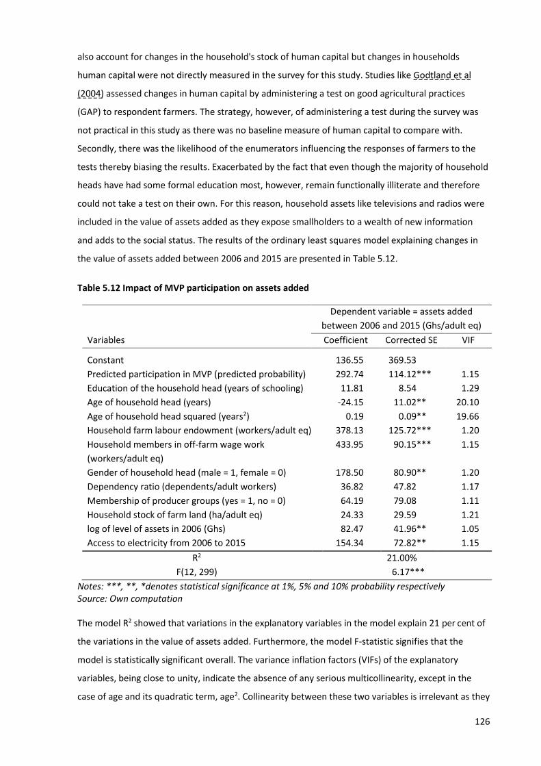
126

also account for changes in the household's stock of human capital but changes in households

human capital were not directly measured in the survey for this study. Studies like Godtland et al

(2004) assessed changes in human capital by administering a test on good agricultural practices

(GAP) to respondent farmers. The strategy, however, of administering a test during the survey was

not practical in this study as there was no baseline measure of human capital to compare with.

Secondly, there was the likelihood of the enumerators influencing the responses of farmers to the

tests thereby biasing the results. Exacerbated by the fact that even though the majority of household

heads have had some formal education most, however, remain functionally illiterate and therefore

could not take a test on their own. For this reason, household assets like televisions and radios were

included in the value of assets added as they expose smallholders to a wealth of new information

and adds to the social status. The results of the ordinary least squares model explaining changes in

the value of assets added between 2006 and 2015 are presented in Table 5.12.

Table 5.12 Impact of MVP participation on assets added

Variables

Dependent variable = assets added

between 2006 and 2015 (Ghs/adult eq)

Coefficient Corrected SE VIF

Constant 136.55 369.53 Predicted participation in MVP (predicted probability) 292.74 114.12*** 1.15

Education of the household head (years of schooling) 11.81 8.54 1.29

Age of household head (years) -24.15 11.02** 20.10

Age of household head squared (years2) 0.19 0.09** 19.66

Household farm labour endowment (workers/adult eq) 378.13 125.72*** 1.20

Household members in off-farm wage work

(workers/adult eq)

433.95 90.15*** 1.15

Gender of household head (male = 1, female = 0) 178.50 80.90** 1.20

Dependency ratio (dependents/adult workers) 36.82 47.82 1.17

Membership of producer groups (yes = 1, no = 0) 64.19 79.08 1.11

Household stock of farm land (ha/adult eq) 24.33 29.59 1.21

log of level of assets in 2006 (Ghs) 82.47 41.96** 1.05

Access to electricity from 2006 to 2015 154.34 72.82** 1.15

R2 21.00%

F(12, 299) 6.17***

Notes: ***, **, *denotes statistical significance at 1%, 5% and 10% probability respectively Source: Own computation The model R2 showed that variations in the explanatory variables in the model explain 21 per cent of

the variations in the value of assets added. Furthermore, the model F-statistic signifies that the

model is statistically significant overall. The variance inflation factors (VIFs) of the explanatory

variables, being close to unity, indicate the absence of any serious multicollinearity, except in the

case of age and its quadratic term, age2. Collinearity between these two variables is irrelevant as they

127

are interpreted jointly. Substitution of actual MVP participation with its predicted value requires that

standard errors estimated for the regression coefficients by OLS must be adjusted to account for the

2SLS estimation of the model's parameters. The standard errors presented in Table 5.12 were

corrected using the procedure described by Gujarati (2003, p. 791).

The a priori expectations for the explanatory variables were all met. The results show that

participation in the MVP was a statistically significant determinant of assets added, adding Ghs

292.74 per adult equivalent over the period 2006-2015. This finding is consistent with those reported

by Bandiera et al. (2013), Banerjee et al. (2015), and Mitchell et al. (2018) who respectively found

statistically significant impacts for the TUP, 'Graduation program' and MVP on aggregate household

and productive assets. In addition to predicted MVP participation, the coefficients for age and gender

of the household head, the household's farm labour endowment, off-farm wage workers, the initial

level of assets in 2006, and access to electricity during the MVP implementation are reported to be

statistically significant in Table 5.12. Assets added per adult equivalent decreased as age increases

until age 63.16 years, when it begins to increase. Incidentally, the minimum age which serves as the

inflexion point is almost equivalent to the life expectancy of Ghana. But at a slightly increased rate.

Increases in household farm labour and members engaged in off-farm wage work caused an increase

in assets added.

The final stage of the recursive model is an assessment of the effect of assets on various outcomes

related to household agricultural activities. This model is shown in Equation 5.4. Table 5.13 presents

the results of the final stage regression models. The models are used to identify the effect of the

MVP on outcomes covering farm expenditure, gross farm output and net income. The F-statistics for

the outcome models were all statistically significant at the 1 per cent level of probability. The models'

explanatory variables explained 25 per cent of the variations in total farm expenditure, 21 per cent of

the variations in gross farm output and 16 per cent of the variation in net farm income. The variance

inflation factors (VIF) for the explanatory variables are all close to unity, indicating that the results

were not affected by multicollinearity.

In the outcome models Equation 5.4, the predicted value of assets was substituted for the observed

value (as explained in Sub-section 3.3). Since the predicted values rather than the observed values

are used in the model, the standard errors were corrected using the correction procedure described

by Gujarati (2003, p. 791). The predicted value of assets (Ã) from Equation 5.4 was found to be a

statistically significant determinant of all three outcomes total farm expenditure, gross farm output

and net farm income. A Ghs 1 increase in asset added results in a Ghs 0.06, in total farm expenditure,

while a Ghs 1 increase in assets added results in Ghs 0.47 increase in gross farm output. Lastly a Ghs

1 increase in assets added results in a Ghs 0.18 in net farm income per adult equivalent in 2016.

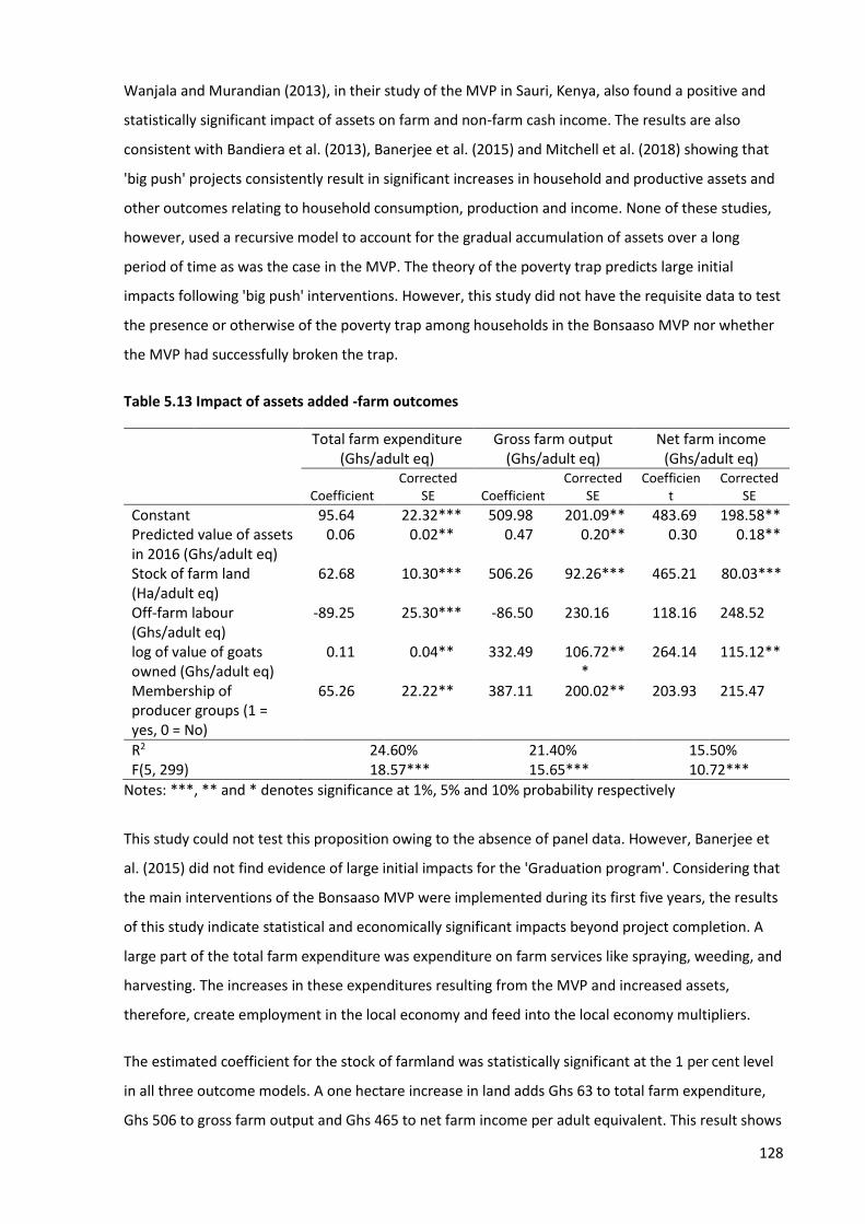
128

Wanjala and Murandian (2013), in their study of the MVP in Sauri, Kenya, also found a positive and

statistically significant impact of assets on farm and non-farm cash income. The results are also

consistent with Bandiera et al. (2013), Banerjee et al. (2015) and Mitchell et al. (2018) showing that

'big push' projects consistently result in significant increases in household and productive assets and

other outcomes relating to household consumption, production and income. None of these studies,

however, used a recursive model to account for the gradual accumulation of assets over a long

period of time as was the case in the MVP. The theory of the poverty trap predicts large initial

impacts following 'big push' interventions. However, this study did not have the requisite data to test

the presence or otherwise of the poverty trap among households in the Bonsaaso MVP nor whether

the MVP had successfully broken the trap.

Table 5.13 Impact of assets added -farm outcomes

Total farm expenditure

(Ghs/adult eq) Gross farm output

(Ghs/adult eq) Net farm income

(Ghs/adult eq)

Coefficient Corrected

SE Coefficient Corrected

SE Coefficien

t Corrected

SE

Constant 95.64 22.32*** 509.98 201.09** 483.69 198.58** Predicted value of assets in 2016 (Ghs/adult eq)

0.06 0.02** 0.47 0.20** 0.30 0.18**

Stock of farm land (Ha/adult eq)

62.68 10.30*** 506.26 92.26*** 465.21 80.03***

Off-farm labour (Ghs/adult eq)

-89.25 25.30*** -86.50 230.16 118.16 248.52

log of value of goats owned (Ghs/adult eq)

0.11 0.04** 332.49 106.72***

264.14 115.12**

Membership of producer groups (1 = yes, 0 = No)

65.26 22.22** 387.11 200.02** 203.93 215.47

R2 24.60% 21.40% 15.50% F(5, 299) 18.57*** 15.65*** 10.72***

Notes: ***, ** and * denotes significance at 1%, 5% and 10% probability respectively

This study could not test this proposition owing to the absence of panel data. However, Banerjee et

al. (2015) did not find evidence of large initial impacts for the 'Graduation program'. Considering that

the main interventions of the Bonsaaso MVP were implemented during its first five years, the results

of this study indicate statistical and economically significant impacts beyond project completion. A

large part of the total farm expenditure was expenditure on farm services like spraying, weeding, and

harvesting. The increases in these expenditures resulting from the MVP and increased assets,

therefore, create employment in the local economy and feed into the local economy multipliers.

The estimated coefficient for the stock of farmland was statistically significant at the 1 per cent level

in all three outcome models. A one hectare increase in land adds Ghs 63 to total farm expenditure,

Ghs 506 to gross farm output and Ghs 465 to net farm income per adult equivalent. This result shows

129

that interventions that ease access to land could help to significantly improve farm outcomes, all

other factors held constant. Unfortunately, lack of land use plans in this area has meant that arable

land and some farms have been converted to gold mines with a resultant negative impact on Ghana's

cocoa output (Snapir, Simms, & Waine, 2017; Taylor, 2018; Wilson, 2015; Wilson, 2016). Ghana's

land administration remains a dualistic system with customary land tenure and statutory land

management running concurrently (Kasanga & Kotey, 2001; Kidido, Bugri, & Kasanga, 2017; Samwini,

2013).

Between 80 to 90 per cent of all land in Ghana is administered under the customary system. Allodial

interest in land in the Amansie West District is vested in the paramount chief of the Ashantis, the

Ashantihene (Kasanga & Kotey, 2001). Land for agriculture is acquired through the 'Abunu' or 'Abusa'

sharecropping schemes. Under these sharecropping systems, the tenant farmer plants and manages

crops on the land parcel to maturity. At the time of first harvest the land parcel is physically divided

into two or three equal portions under 'Abunu' and 'Abusa', respectively. The landlord takes one

portion, leaving the remaining to the tenant farmer who is then allowed to hold his or her portion for

between 25 to 50 years depending on the agreement with the landlord (Kasanga & Kotey, 2001). The

multiplicity of interests in a single parcel of land stifles investment in productivity-enhancing

technologies (Brasselle, Gaspart, & Platteau, 2002; Migot-adholla et al., 1991; Place, 2009).

In addition to land, the coefficient of off-farm labour was statistically significant at the 1 per cent

level in the Total farm expenditure model (Table 5.13) but was not significant in either of the other

two models (Table 5.13). This suggests that households with less off-farm labour opportunities tend

to spend more on their farming activities, as was the expectation. Value of goats owned, the proxy

measure for liquidity, was a statistically significant determinant of all three outcomes. Liquidity is

especially important as it helps farmers to finance seasonal inputs purchased during the off-season

(Fenwick & Lyne, 1999). In the absence of formal banking and credit facilities livestock serve the role

of savings.

Finally, the coefficient of the membership of producer groups was a statistically significant

determinant of the total farm income and gross farm output but not net farm income. Due to

competition for farmers by the licensed cocoa buying companies (LBCs), cocoa farmers do not often

organise collectively for marketing purposes. The MVP, however, encouraged the formation of

producer groups to facilitate the delivery of extension training, subsidised inputs, and other

agricultural intervention under the MVP (Cabral, Farrington, & Ludi, 2006). The knowledge and skill

gained from these training programmes administered through the producers' groups, therefore,

could have played a key role in the differences in agricultural outcomes.

130

This study has accounted for endogeneity in MVP participation, the long life of the MVP

implementation, and the contemporaneous factors affecting outcomes in the multivariate regression

model (Table 5.13). Having accounted for all these factors, the parameters of the outcome models

(Equation 5.4 and Table 5.14 ) were used to estimate the post-MVP mean outcomes across the MVP

and non-MVP villages. These post-MVP predicted mean estimates of household outcomes for both

household and per adult equivalent levels are shown in Table 5.14. The t-statistics reported in table

5.14 are related to the per adult equivalent means. The estimates reflect the expected values of the

outcomes after controlling for endogeneity in MVP participation, the long life of the MVP, and other

factors affecting observed outcomes. The results still highlight large differences in the mean value of

the outcomes between MVP participants and non-participants - these differences are all statistically

significant and indicate sizeable positive impacts of the MVP project.

Table 5.14 Post-MVP predicted value of assets and outcomes

Non-MVP group

(n =97)

MVP group

(n = 202) Outcome

Per adult

equivalent

Household Per adult

equivalent

Household t-statistic

Predicted assets (Ghs) 407.37 1,850.49 572.13 2,525.35 2.42**

Predicted gross farm

output (Ghs)

1,422.84 6,197.60 1,685.00 7,419.71 2.57***

Predicted total farm

expenditure (Ghs)

177.07 764.66 207.34 896.73 2.19**

Predicted net farm

income (Ghs)

1,321.78 5,778.85 1,512.93 6,672.25 2.25**

***, **, and * denotes statistical significance at the 1%, 5% and 10% levels respectively

Differences in the outcome variables between the MVP and non-MVP villages were smaller than

those estimated by the PSM in Table 5.7. In the PSM, the MVP group exceeded the non-MVP group

by 74 per cent, 44 per cent, 41 per cent and 52 per cent respectively, for Assets added, Gross farm

output, Total farm expenditure, and Net farm income. However, these differences reduced to 36 per

cent, 20 per cent, 17 per cent and 15 per cent respectively when estimated by the recursive

treatment model. Despite the reduction in size, the differences remained large and statistically

significant at the 1 per cent level of probability.

5.3 Chapter summary

This chapter extended the analysis in Chapter 4 by controlling for various factors that were not

accounted for in the comparison of non-MVP and MVP households. The first part used the propensity

131

score matching technique to control for observed pre-treatment characteristics of the two groups to

arrive as a sub-samples the MVP and non-MVP group, subsequently called the treatment and

comparison groups. This treatment and comparison groups had similar characteristics pre-MVP and

were, therefore, fit for comparison. The results of the t-test comparison highlighted significant

differences in the assets added, gross farm output, total farm expenditure, net farm income. A

breakdown of the components of assets showed that household assets added were the main

contributor to the differences. Similarly, the value of crops harvested was the greatest contributor to

the differences in gross farm output, while crop expenditure contributed the most to total farm

expenditure. On the other, whereas, the comparison group had a greater expenditure on livestock

inputs, this did not result in a greater revenue from livestock and livestock products. The second part

of the analysis was a robustness test on the propensity score matching results. With slight variations,

the results were consistent with the PSM results, confirming their validity. The results overall show

that the naïve comparison, despite the differences tightening there were statistically significant c

132

Chapter 6

Sustainability of the MVP's agricultural interventions

6.1 Introduction

This chapter addresses research question three and presents the results of farmers qualitative views

about the MVP interventions. First, the changes in access to various agricultural services over time in

the MVP village are discussed. Section 6.3 analyses the conditions of a wide range of factors that

affect farm production in the MVP communities before, during and after the MVP. Qualitative

evaluation of the determinants for the quality of life such as the education and health of children,

access to clean water, quality of the natural environment and income stability are then reported in

Section 6.4. To conclude, the perceptions of households about MVP agricultural interventions and

their overall satisfaction with the MVP interventions are discussed as a basis for the sustainability of

the MVP’s agricultural interventions and outcomes.

6.2 MVP impact on access to training and extension services

The importance of human capital for development and poverty alleviation and livelihood outcomes,

in general, have been long recognised in the literature (Foster & Rosenzweig, 1995; Heckman, 2000;

Morse & McNamara, 2013; Scoones, 1998; Serrat, 2017). A key contributor to human capital is

formal education. However, as the results in Chapter 4 indicate, households in the non-MVP villages

on average completed five years of formal education while MVP households completed on average

seven years of formal education. As such both non-MVP and MVP households had not attained the

minimum of nine years of basic formal education stipulated in the constitution of the Republic of

Ghana (The Government of Ghana, 1996). They were therefore mostly functionally illiterate

(Aryeetey & Kwakye, 2005). Apart from the primary functions of agricultural extension discussed in

Chapter 2, the need for agricultural extension programmes is more important in light of the low

levels of formal education attainment of the household heads. This is because it adds to the human

capital of the participating farmers. The knowledge and capital accumulated from extension services

in turn increase households’ ability to sustain their productivity and incomes into the future. Figure

6.1 shows the proportion of households in the MVP villages who reported having access to various

extension and training services for three periods: 1. Pre-MVP (before 2006), 2. MVP (2006-2015),

and 3. Post-MVP (2016 when the survey for this study was conducted). Training and extension

services were categorised as follows:

1. training in irrigation and equipment maintenance;

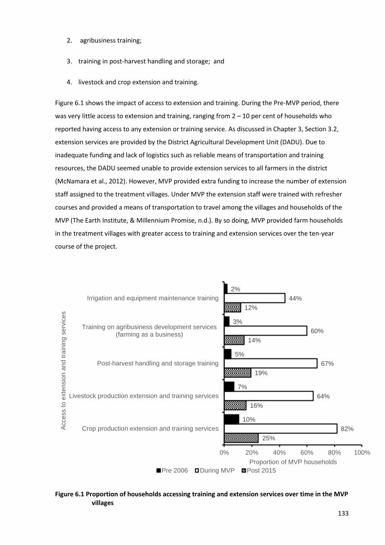
133

2. agribusiness training;

3. training in post-harvest handling and storage; and

4. livestock and crop extension and training.

Figure 6.1 shows the impact of access to extension and training. During the Pre-MVP period, there

was very little access to extension and training, ranging from 2 – 10 per cent of households who

reported having access to any extension or training service. As discussed in Chapter 3, Section 3.2,

extension services are provided by the District Agricultural Development Unit (DADU). Due to

inadequate funding and lack of logistics such as reliable means of transportation and training

resources, the DADU seemed unable to provide extension services to all farmers in the district

(McNamara et al., 2012). However, MVP provided extra funding to increase the number of extension

staff assigned to the treatment villages. Under MVP the extension staff were trained with refresher

courses and provided a means of transportation to travel among the villages and households of the

MVP (The Earth Institute, & Millennium Promise, n.d.). By so doing, MVP provided farm households

in the treatment villages with greater access to training and extension services over the ten-year

course of the project.

Figure 6.1 Proportion of households accessing training and extension services over time in the MVP villages

25%

16%

19%

14%

12%

82%

64%

67%

60%

44%

10%

7%

5%

3%

2%

0% 20% 40% 60% 80% 100%

Crop production extension and training services

Livestock production extension and training services

Post-harvest handling and storage training

Training on agribusiness development services(farming as a business)

Irrigation and equipment maintenance training

Proportion of MVP households

Access to e

xte

nsio

n a

nd t

rain

ing s

erv

ices

Pre 2006 During MVP Post 2015

134

Access to crop extension and training services for the MVP households increased by about 82 per

cent while livestock extension and training services increased by 64per cent during the project. This is

a marked increase given the pre-MVP level of extension and training access was barely 10 per cent

of households in the entire MVP village. This increase in access to training and extensions services

would undoubtedly have contributed to the MVP households' human capital, which includes the

skills and techniques used in productive activities (Foster & Rosenzweig (1995); Godtland et al.

(2004); and Heckman (2000). This finding is particularly important for an increase in agricultural

productivity as the training complements the generally low levels of formal education attained by

household heads in this part of the Amansie West District.

The accumulated human capital, the knowledge that farmers would have acquired from MVP's

extension programmes would have contributed to the large differences in the production between

the MVP and non-MVP participant households (74 per cent higher for gross output and 52 per cent

higher for net farm income), shown in Chapter 5. However, since all the interventions were

administered as a package in the MVP, the decomposition of the impact of individual interventions

was beyond the scope of this study. Notably Foster and Rosenzweig (1995) reported significant spill-

over effects of extension programmes. Therefore, even households in the MVP who did not benefit

by directly participating in extension programmes, do so indirectly by imitating their peers.

Similar to crop extension and training services, access to livestock extension and training services for

the MVP households increased significantly over the course of the project. Livestock extension

officers play a crucial role in rural Ghana. They are often the most accessible animal health

professionals in Ghana, as there is a severe shortage of qualified veterinary doctors (Ghana News

Agency, 2017). Livestock extension staff are trained at the Pong Tamale Animal Health and

Production College, the sole institute for such training in Ghana (Turkson, 2009). Besides providing

extension services and training households on all aspects of animal production, the livestock

extension agents procure and administer medications and vaccinations for livestock. Livestock

extension staff also play a crucial role in Ghanaian public health by conducting surveillance and

monitoring of endemic zoonotic diseases in Ghana such as rabies, anthrax, bovine tuberculosis,

rinderpest and more (Adomako et al., 2018; Vieira et al., 2017; Wastling et al., 1999). This essential

but under-appreciated function has become increasingly important in recent times following the

Ebola epidemic of 2014 - 2016 in West Africa and the Covid-19 pandemic.

The third type of training that farmers received is in post-harvest and storage. Post-harvest losses

were a topical issue in Ghana in the early 2000s when studies showed that a large portion of crop

harvests in the country are lost between the farm gate at harvest and the consumer. For instance,

Aidoo, Danfoku, & Mensah (2014) estimated losses between 14 – 40 per cent for tomatoes while

135

Danso et al. (2017) estimate that 5 – 45 per cent of maize is lost before reaching the consumers.

Fortunately, cocoa is not as perishable as vegetables and grains, and therefore post-harvest handling

is not as critical. However, proper fermentation is essential if the cocoa beans' flavour is to be

optimal. Most Ghanaian cocoa farmers would be quite conversant with the fermentation and drying

process of their cocoa beans. Since MVP introduced two new crops, maize and cowpeas, farmers

would not have been familiar with the production and handling of the two crops. Therefore, post-

harvest training in those crops would have been beneficial.

The fourth element of the extension and training services was training in agribusiness development.

According to The Earth Institute and Millennium Promise (n.d.), agribusiness development included

training farm households on oil palm production and processing, management skills training and

credit access, particularly for female-headed households. In addition, there was the provision of a

community truck to transport farm produce to market centres within and outside the district (The

Earth Institute & Millennium Promise, n.d.). MVP staff facilitated most of the agribusiness activities

pertaining to food crops, including vertical coordination with the school meals programme.

Unfortunately, the contract to supply maize and cowpea to the school meals programme broke down

when the project ended. Oil palm seemed to be a minor crop in MVP villages with about six per cent

of households cultivating it in the post MVP (Section 4.4). Therefore, even though Figure 6.1 shows

access to agribusiness training increased over the period of the MVP implementation, it is not clear

whether the full complement of the training acquired is being used by the participant households.

Lastly, MVP households were asked about their access to training in irrigation and farm equipment

maintenance. The results followed the same pattern as the other training and extension

programmes. There was a sharp rise in the proportion of households with access to irrigation and

farm equipment maintenance (Table 6.1) However, this fell to a level still higher than the pre-MVP

level of access. But as the results in Chapter 4 show, there wasn’t much investment in irrigation and

equipment by the farmers. Since the values of farm assets and equipment were not statistically

different between the MVP and non-MVP groups, this research did not discuss the components of

farm assets and equipment. However, the main farm equipment households possessed were

knapsack sprayers for dealing with the pests of cocoa.

Figure 6.1 in general, shows a drop in the proportion of households with access to extension and

training services fall from highs of 44 – 82 per cent during the MVP period to 12 -25 per cent when

the MVP ended in 2015. However, access to extension and training services post-MVP was higher

than the level of access that farm households had pre-MVP for the MVP households. A possible

reason could be that some extension staff reassigned to the MVP villages may have remained after

the MVP ended. Also, the MVP's infrastructure intervention, particularly road construction, may have

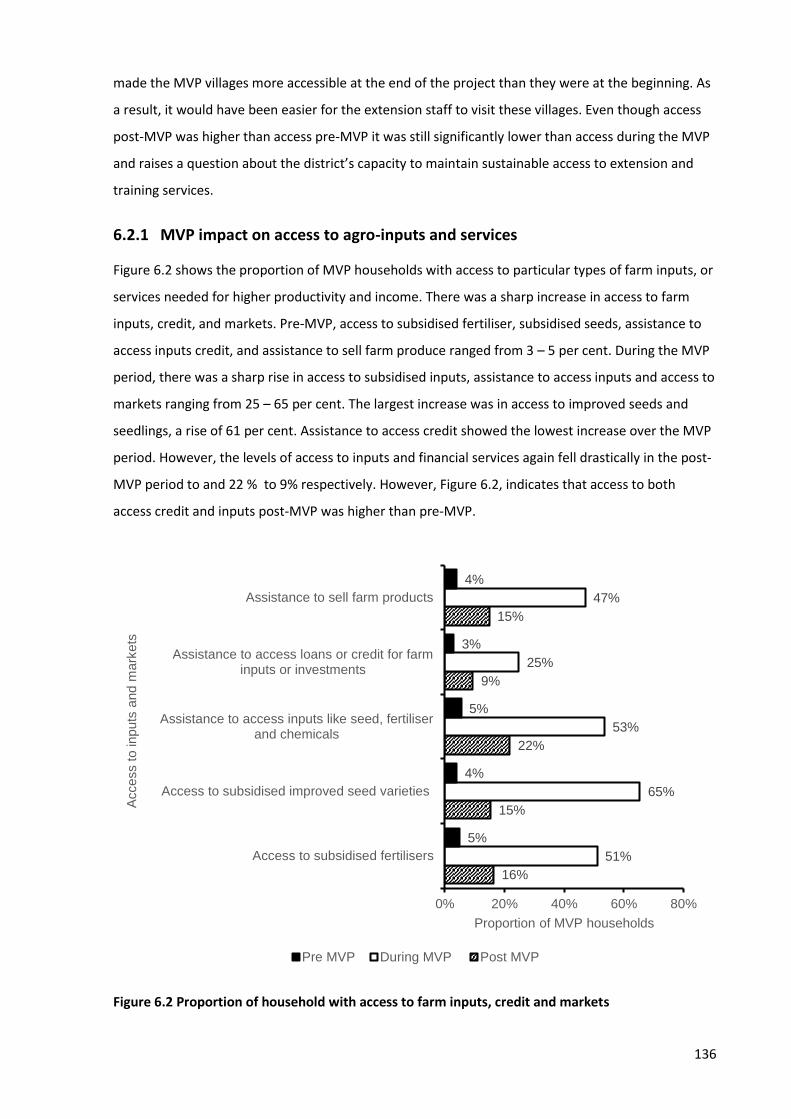
136

made the MVP villages more accessible at the end of the project than they were at the beginning. As

a result, it would have been easier for the extension staff to visit these villages. Even though access

post-MVP was higher than access pre-MVP it was still significantly lower than access during the MVP

and raises a question about the district’s capacity to maintain sustainable access to extension and

training services.

6.2.1 MVP impact on access to agro-inputs and services

Figure 6.2 shows the proportion of MVP households with access to particular types of farm inputs, or

services needed for higher productivity and income. There was a sharp increase in access to farm

inputs, credit, and markets. Pre-MVP, access to subsidised fertiliser, subsidised seeds, assistance to

access inputs credit, and assistance to sell farm produce ranged from 3 – 5 per cent. During the MVP

period, there was a sharp rise in access to subsidised inputs, assistance to access inputs and access to

markets ranging from 25 – 65 per cent. The largest increase was in access to improved seeds and

seedlings, a rise of 61 per cent. Assistance to access credit showed the lowest increase over the MVP

period. However, the levels of access to inputs and financial services again fell drastically in the post-

MVP period to and 22 % to 9% respectively. However, Figure 6.2, indicates that access to both

access credit and inputs post-MVP was higher than pre-MVP.

Figure 6.2 Proportion of household with access to farm inputs, credit and markets

16%

15%

22%

9%

15%

51%

65%

53%

25%

47%

5%

4%

5%

3%

4%

0% 20% 40% 60% 80%

Access to subsidised fertilisers

Access to subsidised improved seed varieties

Assistance to access inputs like seed, fertiliserand chemicals

Assistance to access loans or credit for farminputs or investments

Assistance to sell farm products

Proportion of MVP households

Access to inputs

and m

ark

ets

Pre MVP During MVP Post MVP

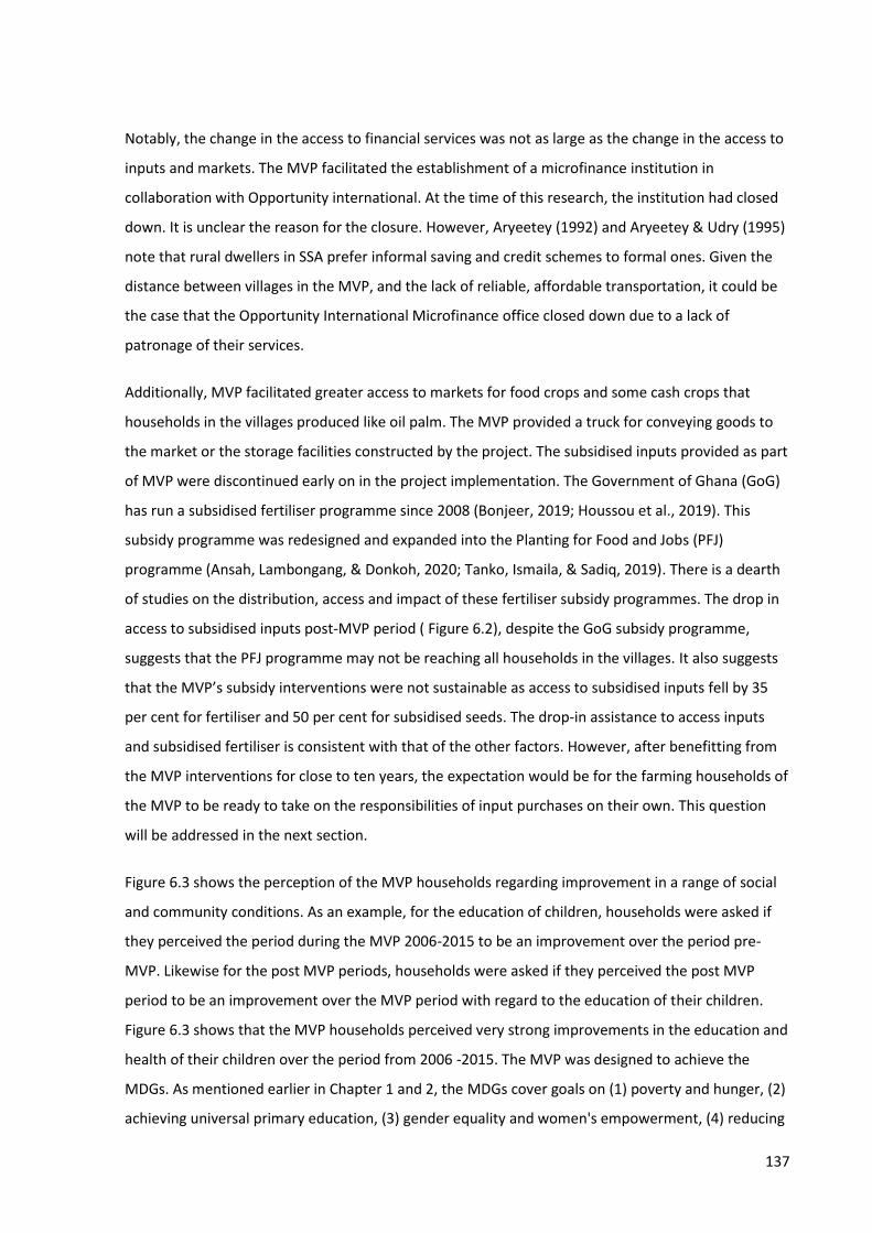
137

Notably, the change in the access to financial services was not as large as the change in the access to

inputs and markets. The MVP facilitated the establishment of a microfinance institution in

collaboration with Opportunity international. At the time of this research, the institution had closed

down. It is unclear the reason for the closure. However, Aryeetey (1992) and Aryeetey & Udry (1995)

note that rural dwellers in SSA prefer informal saving and credit schemes to formal ones. Given the

distance between villages in the MVP, and the lack of reliable, affordable transportation, it could be

the case that the Opportunity International Microfinance office closed down due to a lack of

patronage of their services.

Additionally, MVP facilitated greater access to markets for food crops and some cash crops that

households in the villages produced like oil palm. The MVP provided a truck for conveying goods to

the market or the storage facilities constructed by the project. The subsidised inputs provided as part

of MVP were discontinued early on in the project implementation. The Government of Ghana (GoG)

has run a subsidised fertiliser programme since 2008 (Bonjeer, 2019; Houssou et al., 2019). This

subsidy programme was redesigned and expanded into the Planting for Food and Jobs (PFJ)

programme (Ansah, Lambongang, & Donkoh, 2020; Tanko, Ismaila, & Sadiq, 2019). There is a dearth

of studies on the distribution, access and impact of these fertiliser subsidy programmes. The drop in

access to subsidised inputs post-MVP period ( Figure 6.2), despite the GoG subsidy programme,

suggests that the PFJ programme may not be reaching all households in the villages. It also suggests

that the MVP’s subsidy interventions were not sustainable as access to subsidised inputs fell by 35

per cent for fertiliser and 50 per cent for subsidised seeds. The drop-in assistance to access inputs

and subsidised fertiliser is consistent with that of the other factors. However, after benefitting from

the MVP interventions for close to ten years, the expectation would be for the farming households of

the MVP to be ready to take on the responsibilities of input purchases on their own. This question

will be addressed in the next section.

Figure 6.3 shows the perception of the MVP households regarding improvement in a range of social

and community conditions. As an example, for the education of children, households were asked if

they perceived the period during the MVP 2006-2015 to be an improvement over the period pre-

MVP. Likewise for the post MVP periods, households were asked if they perceived the post MVP

period to be an improvement over the MVP period with regard to the education of their children.

Figure 6.3 shows that the MVP households perceived very strong improvements in the education and

health of their children over the period from 2006 -2015. The MVP was designed to achieve the

MDGs. As mentioned earlier in Chapter 1 and 2, the MDGs cover goals on (1) poverty and hunger, (2)

achieving universal primary education, (3) gender equality and women's empowerment, (4) reducing

138

child mortality, (5) improving maternal health, (6) combating HIV/AIDS and other diseases, (7)

environmental sustainability, and (8) global cooperation.

Figure 6.3 Perceived improvements in community life in MVP villages

Consequently, a large portion of its interventions and budget were expended on educational and

health sectors. These included the construction and staffing of health centres, for a while the

removal and subsequently subsidisation of user fees for health centres and the sponsorship of locals

to be professional healthcare workers (The Earth Institute, & MIllennium Promise, n.d.). In an

integrated rural development framework, these sectoral interventions would have synergistic

relationships with other sectors within the local economy including the agricultural sector (Barnett,

2018). For instance, the improvements in health resulting from the health sector interventions could

help to boost productivity as farmers and farm workers will take fewer days off sick. The results

shows that the sectoral interventions have an impact on the circumstances and quality of life of the

MVP villages.

Similar interventions were undertaken in the education sector. The MVP constructed five new

schools and sponsored promising students to teacher training colleges in the view that they will

return to the villages to work as teachers after their course is over to ameliorate the deficit in

teaching staff in the MVP villages. This was a very important programme as one of the most difficult

challenges facing rural communities across Ghana is the reluctance of trained teachers and health

care workers to accept postings to rural villages. By sponsoring teachers from within the MVP villages

93%

95%

65%

75%

81%

33%

42%

32%

29%

36%

0% 10% 20% 30% 40% 50% 60% 70% 80% 90% 100%

Education of children

Health of children

Quality of housing

Access to safe food

Access to clean drinking water

proportion of MVP householdsPerc

ieved im

pro

vem

ent over

the p

receedin

g y

ears

Percieved improvement over the preceeding years Post MVP period

Percieved improvement over the preceeding years MVP period

139

themselves, the projects were therefore increasing the chances of securing qualified teachers and

health care workers for the villages for a long time.

Seven health clinics were constructed or renovated and connected to running water, solar energy,

and sanitation. As part of the MVP health staff also run various educational and sensitisation

programmes on hygiene, nutrition, family planning, and disease (The Earth Institute, & Millennium

Promise, n.d.). These interventions would have undoubtedly contributed to improving the health of

children, access to safe food and drinking water. A total of 25 boreholes were drilled during the

project to facilitate access to drinking water. Households were assisted by the project to construct

latrines and were educated on proper hygiene practices (The Earth Institute, & Millennium Promise,

n.d.). The quality of housing, though, is a function of the household's income and resourcefulness.

There were no MVP interventions to help with the construction of individual houses. However, the

improved infrastructure and well-trained tradesmen would have facilitated the transport of more

building materials into the district and construction, reinforcing the synergies and complementarities

in the project as shown in the MVP interventions portion in the conceptual framework In chapter 3.

Figure 6.4 shows households' perceptions of how income, employment, safety and the natural

environment changed with MVP. Households indicated that over the course of the project there was

a marked improvement in income and employment in the community. In particular, households

reported an improvement in income stability (79%) and employment in their community (80%).

However, post MVP, 20 per cent of households reported improvements in the stability of income,

while 22 per cent reported improvements in employment in the community. They also perceived

improvements in personal safety and the quality of the natural environment. During the fieldwork, it

was observed that the MVP villages were generally very busy with economic activities of all kinds.

There was a wide variety of trades like carpentry, auto mechanics, metal works, transportation

services, and petty trading absent in the neighbouring non-MVP villages. These would contribute to

the ease of employment opportunities in the MVP villages and the stability of incomes. The linkage

effect of agriculture to other sectors of the economy creates a stimulating effect through the

multiplier discussed in Section 2.2.

140

Figure 6.4 Proportion of household indicating a perceived improvement in conditions of the villages

There was also substantial improvements in safety and the quality of the natural environment.

However, post-PSM only 17 per cent reported improvements in the natural environment, a 32 per

cent drop (Figure 6.4). The sanitation infrastructure and sanitation education focus of the MVP

contributed to a more clean environment in the MVP villages. The simple latrine systems that the

project helped households to construct were a more sanitary alternative to the open-air defecation

that was previously practised (The Earth Institute, & Millennium Promise, n.d.). Lastly, the MVP

interventions did not include any direct security interventions like the police force and justice

system. However, the introduction of electricity meant that the surroundings of houses could be

illuminated at night, which significantly discourages theft and other forms of anti-social behaviour.

In summary, this section has presented results of MVP households access to training and extension

services before during and after MVP, this was followed by the result on access to farm inputs and

market and households perceptions about the conditions of various aspects of their community lives.

The main results

79%

58%

49%

80%

20%

27%

17%

22%

0

0.1

0.2

0.3

0.4

0.5

0.6

0.7

0.8

0.9

Stability of income Personal safety andsecurity

Quality of the naturalenvironment

Employment in thecommunity (both farm

and off-farm)

Pro

port

ion o

f M

VP

household

s

Condition in the Villages

MVP (2006 - 2015) Post-MVP (after 2015)

141

6.3 Agricultural Interventions of MVP

As discussed in the conceptual framework in Section 3.2 (Page 55), the MVP interventions were

implemented across four main sectors of the local economy, An extract from the conceptual

framework is shown in Figure 6.5. The sectoral interventions under MVP were implemented as an

integrated rural development programme meant to take advantage of synergies and

complementarities among the various sectors to increase and reinforce the outcomes and make

them self-sustaining (Barnett, 2018).

Figure 6.5 MVP Interventions (extract from Conceptual framework)

The focus of this study is the agricultural sector programmes of the MVP. However, due to the nature

of the MVP’s design, all the sectoral interventions interact. This means that gains from one sector are

reinforced by those of another such that their combined effect is greater than individual effect. An

example used previously in Chapter 2 was that healthy farmers, having benefited from the health

interventions, will be more productive compared to unhealthy farmers. While this study does not

intend to examine these synergistic and complimentary relationships between different sectoral

interventions, it is important to address their existence.

The MVP main office was located in Manso Nkwanta, the capital town of the Amansie West District

of the Ashanti region. The MVP administrative staff, therefore, lived and worked in the district

capital, about 50 km away by road from the nearest MVP village. The design of the MVP was to

administer the interventions to the entire village that is selected. The project, therefore, relied

heavily on village and community leaders to assist in handing out tangible items like treated bed

nets, fertiliser pesticides and so on. Households were asked if they benefited from specific

agricultural interventions. Of the 202 MVP households sampled, 183 representing about 91 per cent

of the sample reported having benefitted from at least one the MVP agricultural interventions. This is

a reasonably high rate of participation. The breakdown of the interventions received by households

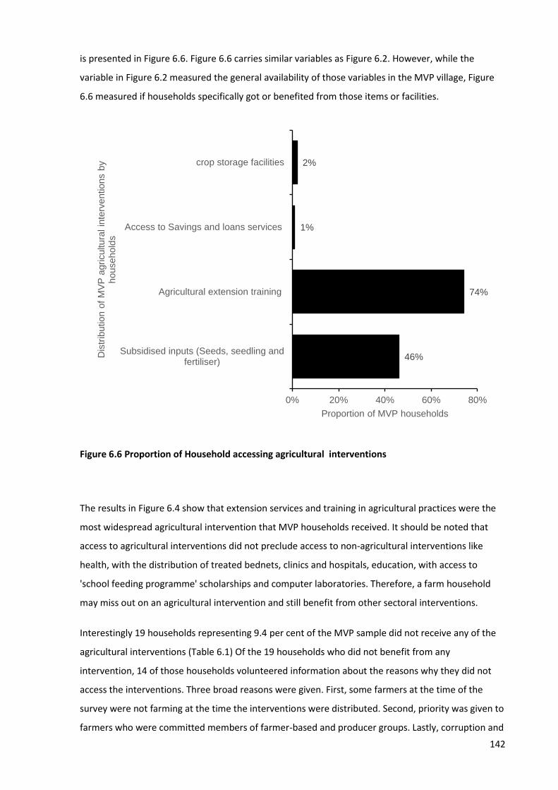
142

is presented in Figure 6.6. Figure 6.6 carries similar variables as Figure 6.2. However, while the

variable in Figure 6.2 measured the general availability of those variables in the MVP village, Figure

6.6 measured if households specifically got or benefited from those items or facilities.

Figure 6.6 Proportion of Household accessing agricultural interventions

The results in Figure 6.4 show that extension services and training in agricultural practices were the

most widespread agricultural intervention that MVP households received. It should be noted that

access to agricultural interventions did not preclude access to non-agricultural interventions like

health, with the distribution of treated bednets, clinics and hospitals, education, with access to

'school feeding programme' scholarships and computer laboratories. Therefore, a farm household

may miss out on an agricultural intervention and still benefit from other sectoral interventions.

Interestingly 19 households representing 9.4 per cent of the MVP sample did not receive any of the

agricultural interventions (Table 6.1) Of the 19 households who did not benefit from any

intervention, 14 of those households volunteered information about the reasons why they did not

access the interventions. Three broad reasons were given. First, some farmers at the time of the

survey were not farming at the time the interventions were distributed. Second, priority was given to

farmers who were committed members of farmer-based and producer groups. Lastly, corruption and

46%

74%

1%

2%

0% 20% 40% 60% 80%

Subsidised inputs (Seeds, seedling andfertiliser)

Agricultural extension training

Access to Savings and loans services

crop storage facilities

Proportion of MVP households

Dis

trib

ution o

f M

VP

agricultura

l in

terv

entions b

y household

s

143

bias on the part of the community leaders tasked with distributing the interventions. Of the 14

households who gave reasons for not getting access, four farming households indicated that they

were not farming at the time the interventions were distributed. A further four farming households

stated that they were either not members of producers groups or were not committed enough and

were, therefore, not prioritised when the interventions were distributed. The most predominant

reason given for farmers who were not able to get access to agricultural interventions was bias and

corruption on the part of the community leaders who were responsible for distributing the inputs. Six

households cited corruption and bias as the reason for their inability to access agricultural

interventions.

6.4 Sustainability of input level

MVP farming households were also asked if they could sustain the MVP level of farm inputs use.

Ninety-five households of the 202 MVP households, (47%) maintained that they could not keep up

the level of input use that they attained under the MVP. The reasons for farmers' inability to sustain

their input use are shown in Table 6.1. Financial constraints were the most common reasons given by

farming households. The most frequently cited reason was that they do not have the cash flow to

maintain those input use levels. Other farmers cited the high expenditure on input, or simply that

they could not afford the inputs. According to some of the farmers interviewed, the MVP subsidised

inputs like fertiliser and herbicides and, occasionally provided the inputs on credit and provided a

truck to transport these inputs to the villages that participated in the project. With the completion of

the MVP, many farmers were left to bear the full expenditure on such inputs. About three per cent of

farming households stated that they had returned to their previous farming methods after the MVP

(Table 6.1).

Table 6.1 Reasons for inability to sustain the level of input use (n = 95)

Reason Frequency

Percentage of

households*

Lack of funds to pay for the inputs (Lack of funds,

financial hardship, expensive inputs )

65 68.3%

Returned to old production systems 3 3.2%

Unable to access the inputs 1 1.1%

Small farm holdings (uneconomical to use inputs) 1 1.1%

Absence of the MVP 6 6.3%

Did not benefit from the tangible MVP interventions 19 20.0%

*percentage of households who stated that they could not sustain the level of input use

In a similar vein, six per cent of farming households stated that it had been difficult for them to

sustain their level of input use in the post-MVP period. This suggests that a certain degree of

144

dependency had developed among households on the MVP. Another possibility is that the systemic

institutions were inadequate to provide the incentives for farm households to produce and invest.

This study contends that part of the reason is that there is an attitudinal aversion to farming in rural

Ghana. Farming ranks low in the order of occupational preference especially when there are off-farm

opportunities in the community (Anyidoho et al., 2012; J. Leavy, 2010; Jennifer Leavy & Hossain,

2014; B. White, 2012). This issue is discussed further in the next chapter.

6.5 Overall satisfaction with the MVP interventions

Overall, MVP beneficiaries expressed a high degree of satisfaction with the Millennium Villages

Project, as indicated in Figure 6.7. About 76 per cent of households were completely satisfied with

the MVP’s interventions while only nine per cent if households were either completely unsatisfied

(6%) or slightly unsatisfied (3%). Overall, the MVP households rated their satisfaction with the

project as 4.65 on a five-point Likert scale with 1 representing 'completely unsatisfied' and 5

representing 'completely satisfied'.

Figure 6.7 Overall satisfaction with MVP Interventions

.6%3% 3%

17%

76%

0%

10%

20%

30%

40%

50%

60%

70%

80%

Completelyunsatisfied

Slightlyunsatisfied

Neithersatisfied orunsatisfied

Slightlysatisfied

Completelysatistied

Pro

port

ion o

f M

VP

household

s

Degree of satisfaction

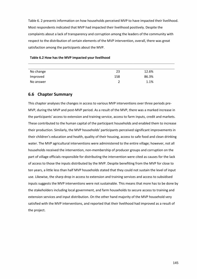
145

Table 6. 2 presents information on how households perceived MVP to have impacted their livelihood.

Most respondents indicated that MVP had impacted their livelihood positively. Despite the

complaints about a lack of transparency and corruption among the leaders of the community with

respect to the distribution of certain elements of the MVP intervention, overall, there was great

satisfaction among the participants about the MVP.

6.6 Chapter Summary

This chapter analyses the changes in access to various MVP interventions over three periods pre-

MVP, during the MVP and post-MVP period. As a result of the MVP, there was a marked increase in

the participants' access to extension and training service, access to farm inputs, credit and markets.

These contributed to the human capital of the participant households and enabled them to increase

their production. Similarly, the MVP households' participants perceived significant improvements in

their children’s education and health, quality of their housing, access to safe food and clean drinking

water. The MVP agricultural interventions were administered to the entire village; however, not all

households received the intervention, non-membership of producer groups and corruption on the

part of village officials responsible for distributing the intervention were cited as causes for the lack

of access to those the inputs distributed by the MVP. Despite benefiting from the MVP for close to

ten years, a little less than half MVP households stated that they could not sustain the level of input

use. Likewise, the sharp drop in access to extension and training services and access to subsidised

inputs suggests the MVP interventions were not sustainable. This means that more has to be done by

the stakeholders including local government, and farm households to secure access to training and

extension services and input distribution. On the other hand majority of the MVP household very

satisfied with the MVP interventions, and reported that their livelihood had improved as a result of

the project.

Table 6.2 How has the MVP impacted your livelihood

No change 23 12.6%

Improved 158 86.3%

No answer 2 1.1%

146

Chapter 7

Discussion of Results and Policy Implications

7.1 Introduction

The purpose of this study was to analyse the impact of the MVP's agricultural interventions on the

economic and financial outcomes of farming households in Bonsaaso, Ghana. The three research

questions are addressed in Chapter 4, 5 and 6. Differences among the MVP and non-MVP households

are explored in Chapter 4. Changes to asset accumulation, income and expenditure at the household

level that are attributable to the MVP alone are evaluated in Chapter 5. The results about

participants’ views about changes in their community are presented in Chapter 6 to inform on the

sustainability of the interventions going forward.

In this chapter, the results in Chapter 4, 5 and 6 and their implications, are discussed in light of

existing literature to understand the effectiveness of the MVP interventions and their sustainability

in the long run. The household outcomes considered in this study were, broadly, asset accumulation

(represented by assets added), gross farm output which aggregates all farm production for the

household, farm expenditure and net farm income. The next four sections, I,e, Section 7.2-7.5

discusses these categories respectively with results drawn from Chapters 4 and 5. Section 7.6 then

discusses the sustainability of MVP interventions based on the findings of Chapter 6. The chapter

then concludes with a summary in Section 7.7.

7.2 Impact on asset accumulation

The results from the MVP’s impact on asset accumulation are presented in Chapter 5. However,

differences in the value of assets pre and post MVP as well as assets added over the course of MVP

were first highlighted in Chapter 4. From Chapter 4, this study determined that differences in the

mean values of fixed farm improvements, farm assets and equipment, and household assets in the

pre-MVP period were not statistically significant. Even though the difference in the mean values pre-

MVP was not statistically significant, the mean values of the non-MVP households were greater than

that of the MVP households in the three asset classes. Over the ten years of the MVP there was

considerable asset accumulation for all three classes of assets.

Assets added for the MVP treatment group after matching was Ghs 218 per adult equivalent (74%)

more than for the comparison group. The differences narrowed from the initial Ghs 238 per adult

equivalent (87%) that the MVP households had over the non-MVP households when matching had

not been done. Notwithstanding the narrowing of the differences as a result of the matching, mean

147

value of assets added was statistically different and greater for the treatment group. Chapter 5

further shows that the value of fixed improvements added was greater for the comparison group

compared to the treatment group. The difference was, however, not statistically significant. On the

other hand, the difference in farm assets, and household assets added were greater for the

treatment group than the comparison group, also, only the difference in household assets added was

statistically significant. Essentially, the treatment group came from behind to outperform the

comparison group in asset accumulation as a result of the MVP, particularly for household assets.

Asset-based approaches to poverty, according to Carter & Barrett (2006); Moser (2006); Moser &

Felton (2007), provides a better picture of long-term living standards compared to income and

expenditure approaches to poverty. In the same vein, asset accumulation over time has the potential

to ensure that households escape the poverty trap in a sustainable manner (Barrett & Carter, 2013;

Carter & Barrett, 2006). Also, assets are fundamental aspects of the life of the household. They

constitute the resources with which households make a living. This has long been recognised in the

literature including the sustainable livelihood framework (SLF) derived from the human development

approach. The SLF bridges the basic needs approach and capabilities approach (Chambers & Conway,

1991; Morse, McNamara, & Acholo, 2009). The SLF identifies five forms of capital or assets at the

disposal of the household with which they can generate their livelihood outcomes (Scoones, 1998).

These include natural capital such as soil, air, water and other natural resources. Second, human

capital, which consists of the skills, knowledge, health and labour of household members which they

apply to their livelihood activities. Physical capital is the third class of assets, and it consists of land,

infrastructure, and buildings used in productive activities fourth, financial capital, which is the focus

of this research. comprises of the cash, savings, credit, bank accounts and other resources of a

financial nature at the disposal of the household for conducting livelihood activities. The kind of

assets a household possesses is a major determinant of the sort of livelihood strategies that the

households can embarks on (Chambers & Conway, 1991). Lastly, social capital comprising the

networks, social claims, relationships, and affiliations which the household possesses in the

community and beyond. The livelihood strategies then influence the livelihood outcome achieved.

Assets are necessary not only for production but also as a form of savings (Zimmerman and Carter,

2003). Adoption of improved technologies forms part of the physical capital stock of the household,

and it contributes to improvements in the production technology and earning potential.

MDGs did not focus on the institutional framework that engenders the accumulation of productive

assets. The asset accumulation found in this study are therefore a result of the households’ own

propensity to invest and suggests a systemic pattern in asset investment arising from the property

rights regime on the results observed in the MVP and non-MVP villages.

148

In addition to being essential resources for generating households’ livelihood outcomes, assets build

resilience against shocks (Barrett, Carter, & Chavas, 2019); De Janvry, Sadoulet, & Murgai, 2002). As

asset accumulation was not one of the MDG indicators, Mitchell et al. (2018) and Masset et al. (2020)

in their impact evaluation studies of the African MVPs and the Northern Ghana MVPs, did not assess

the asset accumulation of the beneficiary households. None of the MDGs captured the importance of

assets to the livelihood of the household and its contribution to long term poverty reduction.

Consequently, the MDGs had no targets for strengthening property rights or broadening them to all

segments of the community, particularly for women and youth. As a result,in a follow-up comment

to Mitchell et al. (2018), Sachs (2018) recognised the significant asset accumulation that had accrued

to the MVP household. In contrast to the MDGs, the SDGs placed a greater emphasis on asset

accumulation as part of the multidimensional measurement of poverty (Alkire & Foster, 2011; Alkire

& Jahan, 2018). Under the SDG 1: To end poverty in all its forms everywhere,

In the light of the importance of assets stressed in the literature, and the meaningful increase in

assets caused by participation in the MVP, the Bonsaaso MVP, has set the beneficiary villages up to

achieve the SDGs with the assets accumulated over the project years. The results of this study are

consistent with other 'big push' programmes such as Bandiera et al. (2017) and Banerjee et al.

(2015), two large scale and reasonably long term 'big push' programmes that are similar to the MVP

discussed in Chapter 2. The ultra-poor graduation programmes and the MVP show that other 'big

push' projects result in significant accumulation of household assets and in the case of the ultra-poor

graduation programme, an increase in productive assets like livestock, land, farm and business

assets. In a similar vein, Daidone, Pellerano, Handa, & Davis, (2015) found that various conditional

cash transfer programmes like the Zambian Cash Transfer for Orphans and Vulnerable Children (CT-

OVC) and the Child Grants Programme (CGP) of Lesotho, programmes which bear similarities with

the ultra-poor graduation programme led to an increase in the use of various farm inputs and farm

assets. Cash transfer programmes also led to an increase in investment in productive assets like

livestock.

The Bonsaaso-MVP increased aggregate household and farm assets; however, a breakdown of the

asset components shown in Chapter 4 and 5 indicated that the most significant contributor to the

difference was household assets. Similarly, Daidone et al. (2015) found that the Livelihood

Empowerment Against Poverty (LEAP), another conditional cash transfer programme in Ghana

similar to the CT-OVC and CGP, did not generate any significant impact on households’ investment in

productive assets. This result contrasts to the ultra-poor graduation programme and the Zambian

and Lesotho conditional cash transfer programmes, where the main drivers of asset investments

were productive assets like livestock, farm assets and fixed improvements.

149

The investment motive has been proposed in the literature to explain asset accumulation in the

household (De Janvry et al., 2002). The investment motive posits that households set up their

investments in a manner as to maximise the rate of return on their asset portfolio. Arguably, the

monetary return on productive assets are greater than that of household assets mobile phones and

televisions. Therefore, this raises the question as to why farmers in the Bonsaaso MVP and the LEAP

beneficiaries in Ghana did not invest more in productive assets for their farm activities, including

increasing their stock of livestock, fixed farm improvements, farm assets and increasing their

landholdings. This study posits this state of affairs arises for two reasons. First, the institutional

arrangements around land ownership – the property rights in land. Second is an attitudinal posture

about farming as an occupation in Ghana. The land tenure system in Ghana varies with location, land

scarcity, and the majority ethnic groups of an area (Kasanga & Kotey, 2001). The Land tenure system

in this part of Ghana has been discussed in Chapter 4.

The is a strong reluctance to alienate family farmland. This emanates from the belief that the present

generation is merely a custodian of family farmland for the present, past and future generation.

Therefore, they ought to hold it and not lose for the next generations. The reluctance to alienate

family farmland along with the diversity of interest in land single land parcels means that land

markets in Ghana, like many developing countries, do not function properly. This raises uncertainty

about the security of tenure for landholdings. Three dimensions of secure property rights have been

put forward in the literature. They include breadth, duration, and assurance (Maxwell & Wiebe,

1999; Migot-Adholla et al., 1991). Breadth covers the range of rights at the disposal of the asset

owner, for instance, the right to permanently convey ownership without seeking approval from

another party. Duration refers to the length of time that the rights are enjoyed. Finally, assurance

refers to the mechanism available for a person to assert their rights to the property where conflicts

arise. For non-statutory land, disputes are usually resolved by traditional authorities: kings, chiefs,

tendambas and abusua panyin. As a result, ones’ social capital, and proximity to the authorities

significantly infleunces they access to, and ability to assert their rights to land (Goldstein & Udry,

2008). Even though the property rights regime recognises private ownership of farmland, the

diversity of interests in a single parcel of land undermines the breadth dimension of secure property

rights. For instance, an individual, who is not a family head cannot convey or transfer ownership of

land to a non-member of the land-owning community without the approval of the head of the family.

Since a landowner is constrained in their exercise of this crucial right, under the breadth, duration,

and assurance framework of property rights, such a landowner has a less secure property right to the

land than one who has the right to transfer ownership without the permission of another party.

As land is fundamental to every agricultural production, secure property rights in land are essential.

Studies have shown that weak property right undermines farmers' incentive to engage in productive

150

investments (Brasselle, Gaspart, & Platteau, 2002; Deininger & Jin, 2006; Maxwell & Wiebe, 1999;

Place & Otsuka, 2002; Place, 2009). On the other hand, weak property rights in the land could help

incentivise farmers to invest in specific categories of assets such as tree crops as a means of securing

their rights in the land since it is more challenging to expropriate land with a stand of productive

trees. Therefore, this could explain the lack of investment in fixed farm improvements, farm assets,

and farm equipment, along with the high favourability of investment in cocoa trees. Unlike land,

where the property rights are complicated, the property right in household assets is more clearly

defined, with the household holding the full complement of rights, including the right to convey the

assets without seeking the permission of third parties. Consequently, the results showed a

substantial investment in household assets.

With respect to livestock ownership. Only the value of goats and the value of chicken were

statistically different between the matched MVP and non-MVP groups. There were hardly any cattle

rearing in either group, while no difference was found sheep rearing between the two group. The

number, however, show that livestock rearing was as important an enterprise as crop production.

The traditional explanation has been that the presence of debilitating zoonotic diseases like sleeping

sickness and anthrax in southern Ghana deters farmers from raising cattle and small ruminants in

large quantities (Amissah-Reynolds, 2020; Courtin et al., 2008). However, most of the diseases

prevalent in southern Ghana are endemic in northern Ghana as well. Yet, there is a higher

concentration of livestock rearing in the north than in the south (Ministry of Food and Agriculture,

2004). Moreover, the LEAP programme reported by Daidone et al. (2015) consisted of households

across different geographical areas in Ghana. Yet Daidone et al. (2015) found no statistical

significance for the coefficient of the investment variable on productive assets in the Ghanaian LEAP,

particularly investment in livestock among the households in the LEAP programme. As the result in of

the LEAP indicate that households across both northern and southern Ghana did not invest in

livestock, this suggests that the debilitating disease hypothesis proposed as a justification for the lack

of investment in farm animals in the forests zones of Ghana is not the most salient reason for the

lack of investment in livestock.

This lack of investment in livestock has to do with the perception of farming among Ghanaian rural

dwellers. Leavy and Smith (2010 p.9) summarised the point as such 'Status is important …: and

agriculture is unappealing because it does not bring status regardless of the economic outcomes that

result from it". Small-scale farming, in particular, is not attractive to rural households. The most

preferred occupations are formal salaried jobs such as government-employed officials. Following that

rank are the trades like carpentry, metalwork, electrical and electronic work. The last rung of the

occupational choice hierarchy is agriculture, which is considered the last resort for most Ghanaian

households. Furthermore, Anyidoho, Leavy and Asenso-Okyere (2012) stress that for most younger

151

people with some level of formal education, undertaking farming as their occupation is merely a

means of sustenance. In some cases, farming is considered as a mean to finance their training for the

careers that they aspire to have. Farming is often the last resort of less-educated who do not have

the training or the skill to engage in off-farm work. Respondents in the Leavy and Smith (2010) study

who expressed an interest in farming preferred large scale commercial farming. However, it is

difficult to acquire large parcels of land if one is not a member of the land-owning community or in

the social network of the local authorities (Goldstein & Udry, 2008). That is, people who enjoy a close

and cordial relationship with local authorities or their close relatives and friends. Anyidoho, Leavy

and Asenso-okyere (2012) conclude that there is an inverse preference relationship between the

educational attainment of an individual and their occupational aspirations. At the bottom of the

occupational scale of preference is farming. The preference for farming as an occupation diminishes

with their actual or perceived educational attainment. This framework could explain the lack of

investment in farm assets and improvement on the part of the MVP households compared to the

non-MVP households, as households focus on the alternative livelihoods to agriculture that satisfy

their desires and aspirations. The capabilities approach to development and the sustainable

livelihood approach would affirm the freedom of households to pursue such aspirations as the end

goal of the process of development. Sen (2001) defined development as the expansion of individuals'

freedoms to pursue the things they value. In large part, the increase in income of the MVP had

helped farmers to pursue these functionings, that is, the sort of careers that the farmers desire.

Accumulated assets often serve to buffer consumption in the event of adverse exogenous shocks

(Barrett et al., 2019). It also enables the household to pursue the livelihood strategies they prefer

(Morse et al., 2009). In the rural farm households, such shocks happen most often in the dry or lean

season, when stocks are lowest. Under such circumstances, households often convert assets to cash

and other liquid assets to meet their consumption needs (Zimmerman & Carter, 2003). Furthermore,

asset accumulation is seen as the lasting solution to the poverty trap Barrett et al. (2019); Carter &

Barrett (2006); and Dillon (2011). For this reason, interventions that increase the accumulation of

assets by the household should be encouraged to alleviate the plight of the poor. The 'big push'

programmes reviewed in this study (namely, the MVP), the Ultra-poor graduation programme, and

conditional cash transfer programmes have been shown to result in asset accumulation at the

household level consistently. The results show that there is a strong incentive to invest in household

assets. The asset-based poverty trap put forward by Carter & Barrett (2006) predicts large initial

impacts on asset accumulation in the initial stages of the cycle in response to external stimulus.

While this research found significantly higher rates of assets accumulation for MVP villages compared

to the non-MVP villages for the entire duration of the project, the research did not attempt to test

the theory of the poverty trap, as the time dimension required to do so is absent in the dataset.

152

Banerjee et al. (2015), however, deemed the assets accumulations in the ultra-poor programme as

not large enough.

Apart from participation in MVP, the estimated coefficients in Table 5.12 (Section 5.3.1) indicated

that socio-economic variables like the age of the household head, household farm and off-farm

labour endowment, and the gender of the household head influence the asset accumulation. The

coefficient of the Age of household heads was found to have a negative and statistically significant

effect on assets added (Table 5.12 in Section 5.3.1). Assets added decreases u with the increase in

age until the age of 63 when it reaches the inflexion point and begins to increase. This pattern of

investment in assets is mainly attributable to the sort of things that households in both villages

invested in mostly. From Chapter 4, households invested mostly in moveable household assets that

were of a technological nature, for instance, cellphones, refrigerators and freezers, power

generators, motorbikes, radios and televisions. These are assets that appeal to a younger rather than

an older generation.

Similarly, a one adult equivalent increase in household members engaged in farm activities results in

a Ghs 378 per adult equivalent increase in the value of assets added. An adult equivalent increase in

household members engaged in off-farm wage work resulted in a Gh 434 per adult equivalent

increase in the value of assets added. These results are as expected since more employment

opportunities on-farm and off-farm means income for households, which they can use to invest and

improve their resilience against poverty. Over 80 per cent of MVP household reported an

improvement in employment in their communities during the MVP period compared to 45 per cent

in the non-MVP communities. Lastly, male-headed households spent Ghs 179 assets added per adult

equivalent household member over the ten years of the project compared to female-headed

households. As discussed in Section 7.2, the land tenure regime in the district and most parts of

Ghana takes an adverse position on women's ability to hold and manage farmland freely. This is

because giving family land to women is deemed equivalent to alienating the land (Duncan, 2010;

Goldstein & Udry, 2008; Grier, 1992). Instead, women obtain land from their male relatives. Often

these are marginal lands that are not the most productive. This affects female-headed households'

ability to increase their productivity and income, and it also undermines MDG 3 and SDG 5, which are

to achieve gender equality and empower all women and girls.

7.3 Impact of the MVP on gross farm output

Gross farm output is an aggregate of all the production output from households’ farm enterprise

activities including (1) cash crop production, (2) food crop production, (3) fruit crop production and

(4) animal production. The results from Chapter 5 showed that MVP interventions had a significant

and positive impact on gross farm output. Participation in the MVP resulted in a 44 per cent increase

153

in gross farm output over the comparison group. The main contributor to the increase in gross farm

output is the value of cocoa produced. There seems to be a contradiction in the blueprint of the

MVP interventions as laid out by Sachs (2005), who proposed both specialisation and diversification

in agricultural production as a means of breaking the poverty trap and setting households on a

trajectory of self-sustaining growth and development. Under specialisation, a farming household was

to focus their production on a single high-value cash crop like cocoa or oil palm. By contrast, under

diversification, the farming household produces multiple farming products to avoid over-reliance on

any single crop and their idiosyncratic risks. In the Bonsaaso MVP, one of the pillars of MVP

interventions was to foster diversification in the agricultural production of participant households.

MVP did this through training in agroforestry and introduction of food crops to the participants

(Mitchell et al., 2015; The Earth Institute, & MIllennium Promise, n.d.). However, from the results of

the farm enterprises in Section 5.2.4, it can be inferred that the MVP villages were less diversified

than the non-MVP village. The crop of specialisation in MVP villages is cocoa, a crop of critical

importance to the economy of Ghana. One possible explanation of the cocoa specialisation is that,

the Government of Ghana guarantees a producer price at the beginning of each production season

(Ghana Cocoa Board, 2017). The government also provides various subsidies and rewards to support

farmers in their production of cocoa. Consequently, in addition to the point made in the previous

section about farmers growing tree crops like cocoa as a means of securing their property rights in

their land, cocoa is also the safest and most profitable crop to produce in Ghana.

7.3.1 MVP interventions affecting production output

A number of the MVP's interventions are yield-enhancing and could account for the higher yields

observed in the MVP villages compared to the comparison village as depicted in Section 5.2.4.

Among the interventions are programmes that first exposed households to the use of farm inputs

and subsequently facilitated access to inputs like fertiliser, improved seeds and seedlings. Secondly,

the results in Chapter 5 indicate that access to agronomic training and agricultural extension services,

and improved crop varieties (Mitchell et al., 2018; The Earth Institute, & Millennium Promise, n.d.)

contributed to enhanced farm production. Other factors not associated with the MVP interventions

include the stock of farmland owned by the household, the liquidity variable indicated by the value

of goats owned, and lastly, membership of producer groups which increased gross farm output.

7.3.1.1 Subsidised fertiliser

The benefits of input use and fertiliser application for cocoa plantations (and crops in general) have

been demonstrated extensively in the literature over the years (Snoeck et al., 2016). The findings in

section 5.2.4 indicate that the matched MVP group spent over double that of the matched non-MVP

group on fertiliser, both organic and chemical, to enhance productivity. MVP provided subsidised

154

fertiliser and other farm inputs to the treatment households for the first three years of the project

(The Earth Institute, & Millennium Promise, n.d.). While the supply of subsidised inputs ended earlier

in the first phase of the project, households' exposure to these inputs and the resultant/ increased

yields would have encouraged the matched MVP group households to continue to invest in these

inputs after the project. The results suggests that farmers in the MVP area employed these

technologies in greater amounts compared to the non-MVP area. These have been proven to

increase yields.

7.3.1.2 Extension and training

Another intervention that the MVP carried out in the villages was agricultural extension programmes.

The Ministry of Food and Agriculture (MoFA) in Ghana mostly delivers extension by the Training and

Visits (T&V) modality nationally (J. R. Anderson & Feder, 2007; MOFA, n.d.). Following a general push

towards decentralisation in governance, the agricultural extension services delivery function was

shifted from the Ministry of Food and Agriculture (MoFA) at the national level to MoFA at the district

level called the District Agricultural Development Unit (DADU) (Amezah & Hesse, 2002). Inadequate

personnel numbers have constrained extension delivery under the training and visit modality at the

district level. For instance, Anang, Bäckman, & Sipiläinen (2020) suggest that if all Ghana's

agricultural extension agents were deployed, their ratio to farmers would be about 1:1,300.

However, most districts cannot afford to keep all their extension staff in the field. Moreover,

extension staff often lack the means of transportation to reach all but the farmers closest to urban

areas or rural areas with properly sealed roads (Buadi, Anaman & Kwarteng, 2013). This leaves a lot

of farmers unserved. Other constraints include financial difficulties to maintain the operations at the

local level and logistical difficulties with teaching resources and materials (Amezah & Hesse, 2002).

Before 2000, extension services for cocoa farmers were provided by COCOBOD. However, their

function was transferred to the DADU as well. This change, argue Amezah & Hesse (2002), has had a

detrimental effect on extension coverage for cocoa farmers as the district extension staff are not

specialists in cocoa production and practices. At the same time, most districts were not able to

provide adequate coverage of farmers. These factors resulted in a situation where only 10 per cent of

the MVP households reported having access to agricultural extension services before MVP started in

2006. This contrasts with that of the Non-MVP households where over 20 per cent had access to

agricultural extension services before the MVP (see Figure 4.6 Chapter 4, Section 4.5). For this

reason, the delivery of extension services to the MVP villages was positive for the farmers

/appreciated by the farmers (?)

MVP modified the extension delivery system in the treatment villages and increased the number of

extension staff serving in the Bonsaaso area. It also added farmer field schools, which is a

155

participatory approach to the delivery of agricultural extension (Shira Mitchell et al., 2015). The

results in Section 6.2 indicate that up to 82 per cent of MVP households reported getting access to

crop extension and training, a 72 per cent increase over the pre-MVP period. Likewise, 62 per cent of

MVP households said that they got access to livestock production training and extension services, a

57 per cent increase over the pre-MVP period. Farm households also reported access to post-harvest

training, agribusiness training, and irrigation and maintenance training. MVP extension programme

instructed farmers on good agricultural practices and agronomy in general. By so doing, the MVP not

only enhanced the human capital of participating households, it also enabled them to enhance their

agricultural output and livelihood outcomes. Some studies evaluated the skills and knowledge sets of

farmers by administering a written test for the survey participants (Godtland et al., 2004). The test

covered a variety of areas of agricultural knowledge including, cultural practices, crop diseases and

pests. While this is a commendable approach, it significantly increases the cost of data collection.

Due to the budgetary constraint on this study, no such test was conducted on the respondents.

There is a strong indication though that agricultural extension services delivered by MVP could have

contributed to the enhancement of farm output.

7.3.1.3 Improved seeds

In addition to extension services, MVP participation made a push through the farmer field schools to

replace ageing cocoa plantations with newer hybrid varieties of cocoa (The Earth Institute, &

Millennium Promise, n.d.). Despite being earlier and higher-yielding than the older 'Amazon' and

'Amelonado' varieties of cocoa, the relatively newer hybrid varieties of cocoa, have not seen wide

adoption. Despite having been in circulation for close to three decades by 2000, the adoption rate

has been slow. The hybrid variety begins to fruit in three years compared to five or six years in the

older varieties (Kolavalli & Vigneri, 2011). Edwin & Masters (2005) found that the newer hybrid

varieties of cocoa yield 42 per cent more than the older varieties. However, according to Kolavalli &

Vigneri (2011), hybrid cocoa are more sensitive to unfavourable climate and require more cultural

practices like spraying, pruning, and more complementary inputs like insecticides fertiliser. Lastly, the

new varieties are labour-intensive to manage, particularly at the beginning and end of harvest time

(Kolavalli & Vigneri, 2011). For these reasons and the inadequacy of extension services provision,

historically, adoption of the hybrid variety has been low (Edwin & Masters, 2005; Kolavalli & Vigneri,

2011). As of 2002, about four years before the MVP, only about 57 per cent of cocoa farmers had

adopted the hybrid variety nationwide (Kolavalli & Vigneri, 2011). Therefore, by making seedlings of

the new variety widely available along with complementary inputs such as fertiliser, herbicides,

insecticides, and technical support through the agricultural extension services farm households in the

MVP villages were provided with the resources they need to cultivate the new varieties successfully.

The results in Chapters 5 show that the MVP had a positive impact on the expenditure on seeds with

156

the MVP households spending close to 10 times the amount that the non-MVP households spent on

seeds and seedlings.

7.3.1.4 Infrastructure and credit

Infrastructural intervention under MVP like repairing the road network of the villages and providing a

truck also contributed significantly to the productive capabilities of the MVP villages. The

infrastructural interventions not only reduced the expenditure for transporting farm inputs to the

villagers but also facilitated the formation of producer groups for the farmers in the MVP villages

Furthermore, in the earlier years of MVP, there was a liaison with Opportunity International to

operate a branch of their microfinance offices in Datano, one of the 30 MVP villages. A synergistic

relationship exists between these interventions working together to enhance household outcomes.

For instance, the road network made it easy to transport complementary inputs into the villages. At

the same time, the extension services provide the knowledge and skills that farmers need to manage

the farms, including the new variety properly. Since MVP was delivered as a package with all these

interventions administered together, and the last of the agricultural interventions ended about three

years into the project, it is unfeasible to isolate the impact of these individual interventions.

7.3.2 Livestock production

The results ( see chapter 5) of the livestock production enterprises show that there were no

statistically significant differences in the means of livestock revenue and net income. However, the

results from Chapter 5 shows that the matched MVP group owned significantly more goats than the

matched non-MVP group while the matched non-MVP group owned more chickens than the

matched MVP group. There was, however, no difference in the value of cattle and sheep kept

between the two groups. Livestock production and husbandry, has not received as much attention in

Ghanaian agricultural policy as crop production. The MVP encouraged poultry and goats production

for food security and nutrition as part of MDG 1C: to halve the proportion of people who suffer from

hunger. The results in Section 5.2.4 indicate that of the major farm animals types only the goat

production data is positive for the MVP. Interestingly there is a taboo for natives rearing goats.

Therefore, migrant farmers may be responsible for the rearing of goats in the area, however, due to

reasons discussed in Section 4.3, this study did not ask about the ethnicities of respondents.

The role of livestock production has been highlighted in recent times, as a tool for improved nutrition

security. In a recent post on the GatesNotes website, Gates (2016) most recently advocated and

committed to supplying chickens to poor households in Africa to aid the fight against poverty. There

is a long-established model that has been implemented by Heifer International (HI) since 1944 (De

Vries, 2008; Dierolf et al., 2002). In this system, recipients of HI livestock pay forward the aid they

receive using the offspring of their own livestock. Studies have reported positive increased

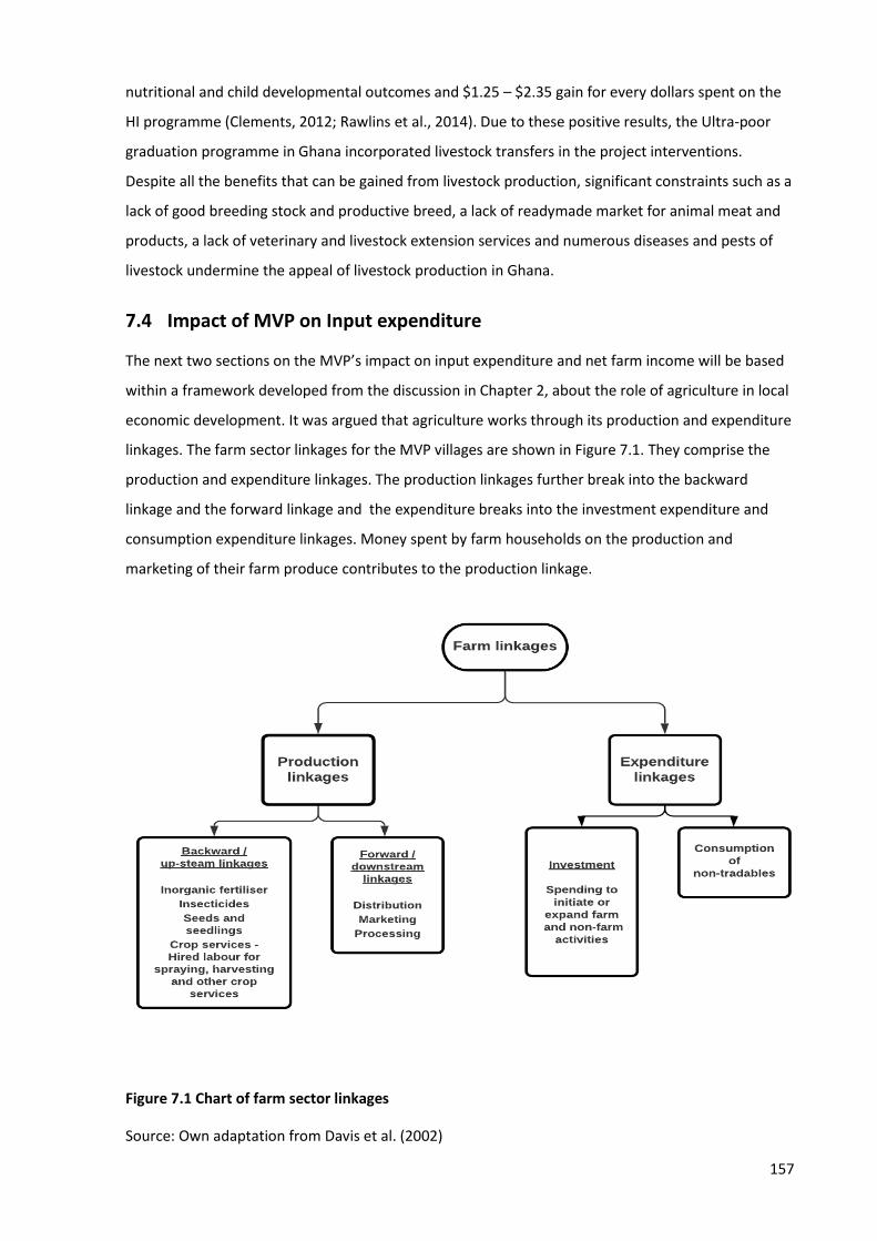
157

nutritional and child developmental outcomes and $1.25 – $2.35 gain for every dollars spent on the

HI programme (Clements, 2012; Rawlins et al., 2014). Due to these positive results, the Ultra-poor

graduation programme in Ghana incorporated livestock transfers in the project interventions.

Despite all the benefits that can be gained from livestock production, significant constraints such as a

lack of good breeding stock and productive breed, a lack of readymade market for animal meat and

products, a lack of veterinary and livestock extension services and numerous diseases and pests of

livestock undermine the appeal of livestock production in Ghana.

7.4 Impact of MVP on Input expenditure

The next two sections on the MVP’s impact on input expenditure and net farm income will be based

within a framework developed from the discussion in Chapter 2, about the role of agriculture in local

economic development. It was argued that agriculture works through its production and expenditure

linkages. The farm sector linkages for the MVP villages are shown in Figure 7.1. They comprise the

production and expenditure linkages. The production linkages further break into the backward

linkage and the forward linkage and the expenditure breaks into the investment expenditure and

consumption expenditure linkages. Money spent by farm households on the production and

marketing of their farm produce contributes to the production linkage.

Figure 7.1 Chart of farm sector linkages

Source: Own adaptation from Davis et al. (2002)

158

The backward production linkage of the MVP villages is indicated by farm households’ expenditure

on fertiliser, insecticides, seeds and seedlings, and crop services. Crop services included contract

labour for all farm production activities ranging from sowing to harvesting. Input expenditure

includes expenditure on farm inputs and farm services. The results from Chapter 5 shows that the

MVP treatment group spent Ghs 92 (61%) more per adult equivalent on farm expenditure than the

comparison group. MVP had a statistically significant impact on total farm expenditure. As discussed

earlier, the crop input expenditures were greater for the treatment group, whiles the livestock

expenditure was higher for the non-MVP comparison group. Whereas the higher expenditure on

crop inputs resulted in a statistically significant and positive impact on crop output for the matched

MVP group, the higher expenditure on animal inputs did not translate into higher output for animal

production and animal product.

A breakdown of the total farm expenditure showed that the biggest contributor to the difference in

total farm expenditure was expenditure on crop services, seed, and seedlings, insecticides, while

chemical fertiliser was only marginally significant. Even though fertiliser, insecticides and other

manufactured crop inputs are mostly imported into the district, various local distributors and

retailers earn their living from the sale of these products. On a typical cocoa plantation, the hired

labour is mainly employed locally for spraying to control insects and pests, harvesting and fermenting

the cocoa pods, and weeding the cocoa plantation. The results in Section 5.2.4 show that the MVP

has a significant and meaningful impact on households’ expenditure on crop inputs. This is good for

employment in the area, contributing to the stimulation of the local economy. This premise is

corroborated by the respondents' qualitative views, 45.4 per cent of whom reported an

improvement in employment in the non-MVP village compared to the 80.2 per cent who reported an

improvement in employment in the MVP villages over the same period.

In contrast to the backward production linkage, the forward production linkage shown in Figure 7.1

does not grant as many avenues for the local economy to capture as many benefits from cocoa the

main crop produced in the area. From Table 5.9 ( Section 5.2.4), gains from the forward production

linkage in the MVP is mainly through transportation of farm produce to the cocoa purchasing clerks

or market centres like Datano. Cocoa purchasing clerks are mostly local agents of licensed buying

companies. Therefore, the agricultural sector indirectly supports the employment of porters, local

marketing clerks of the licensed buying companies, as well as truck drivers who transport the

products. Unfortunately, not many downstream value chain activities like grading and processing of

food crops, cash crops, fruits and animals go on in this part of the district. Therefore the local

economy does not directly benefit from such activities.

159

Historical adoption rates of improved seeds and seedlings, insecticides, and fertiliser among cocoa

farmers have been very low, ranging from five per cent to 13 per cent. In an effort to increase the

productivity of cocoa production in Ghana, the government of Ghana implemented its mass spraying

and Hi-tech programmes for cocoa farmers in 2002 (Kolavalli & Vigneri, 2011). The mass spraying

exercise was to control the capsid or mirid bug and the mealybug, two major pests of cocoa farms

nationwide. These pests spread the black pod and swollen shoot diseases, respectively. However, the

hi-tech intervention was a bundle of seedlings of new cocoa varieties, insecticides, fertiliser, and

other farm inputs for farmers. The Government hi-tech intervention was implemented for cocoa

farmers nationwide from 2002 - 2004 (Aneani et al., 2012; Aneani & Ofori-Frimpong, 2013;

Gockowski et al., 2013). The high-tech intervention by the government was vital as it exposed

farmers to the productivity enhancing benefits of the use of these farm inputs. However, the high-

tech programme did not address systemic problems that keep farmers from accessing these inputs

including a lack of local suppliers, thereby requiring farmers to travel long distances to urban areas to

purchase farm inputs (Krausova & Banful, 2010). MVP's intervention for cocoa farmers, though

similar, was implemented later, 2006 – 2015. It initially started with subsidised inputs, with the

subsidies scaled back over time. The MVP also provided road infrastructure and a truck to transport

inputs to the MVP area. Mitchell et al. (2018) reported in the endline evaluation that over 80 per

cent of farmers in the MVP households adopted the use of improved seeds and seedlings about the

same number used inorganic fertiliser.

Extension programmes such as discussed by Evenson & Mwabu (2001); Feder et al. (2004) and Tsiboe

et al. (2016), likewise resulted in an increase in the expenditure on farm inputs and services by the

participant farmers who produced food crops and cocoa. This results from farmers having to

complement the knowledge gained from extension and training programmes with productivity-

enhancing inputs leading to the rise is expenditure on farm inputs. Moreover, Karlan et al. (2014)

found that farmers increase expenditure on their farm activities when various uninsured risk

constraints are relaxed. While the risks were mainly farm-related such as crop failure, it is

conceivable that the synergies from the other sectoral interventions of the MVP could have acted as

a form of insurance against the undesirable consequences. They were thus freeing farmers to spend

more on their farms. Some of those interventions include free health care (in the first two years) and

health insurance after that, fee-free schooling for primary education and scholarships for the best

performing students in each village as well as school lunch programmes , All of these interventions

enabled the farming households to focus on their farming activities (The Earth Institute, &

MIllennium Promise, n.d.).

The results in Chapter 4 and 5 show that the largest component of the total farm expenditure was

the expenditure on crop services, consisting of hired labour for services such as spraying, weeding,

160

pruning and harvesting. This was followed by the expenditure on crop inputs like fertiliser and

insecticides.

Lastly, the production information of the MVP villages suggests a more intensive production

technology than the non-MVP village. The MVP households use more labour, seeds and seedlings,

and insecticides per hectare than the non-MVP households. This difference raises issues about the

sustainability of such intensive agricultural production methods. Singh (2000) documents that the

intensive agriculture in India following the green revolution led to nitrate and phosphate

contamination of groundwater. Furthermore, there was a decline in nutrient use efficiency in the

soil, a breakdown of the soil physical and chemical characteristics, including an increase in the acidity

of soils due to excessive fertiliser use, as well as a reduction in soil biodiversity. These ultimately

undermine the long-run ability of the farmer to continue to farm the land. This is further exacerbated

by the fact that the absence of land tenure security discourages farmers’interest to extract as much

from the land resources in the production year as possible. Long-run sustainability is of minor

importance as the household could lose their right to farm by parties with higher-order rights. The

Earth Institute & Millennium Promise, (n.d.) noted that the farmers in the treatment villages were

trained on certain sustainable intensification practices mainly intercropping or mixed cropping and

agroforestry (The Earth Institute, & Millennium Promise, n.d.). These practices have the potential to

conserve soil organic matter content, conserve water, improve soil structure and prevent erosion

(Campbell, Thornton, Zougmoré, van Asten, & Lipper, 2014; Dalton, Yahaya, & Naab, 2014).

However,

7.5 Impact of the MVP on Net farm income

An increase in crop or animal expenditure is good only to the extent that it results in a greater than

proportionate increase in revenue. Participation in MVP resulted in a 59 per cent increase in the net

farm income of the treatment group for the entire household. Net farm income per adult equivalent

for the matched MVP group was about 52 per cent greater than that of the matched non-MVP group.

Given that the total farm expenditure of the matched MVP group was about 41 per cent greater than

the matched non-MVP group, the MVP participation resulted in a greater return on inputs

employed. This is consistent with the general results found in extension and training programmes like

Davis et al. (2012); Hamilton & Hudson (2017) and Cawley, O'Donoghue, Heanue, Hilliard, & Sheehan

(2018) who found that participant farmers realised an increase in their crop yield and farm income,

and associated their increase to their participation in the extension and training programmes.

The expenditure linkages portion of Figure 7.1 derives from the net farm income realised from

farming. After production and investment decisions have been accounted for. The expenditure

linkage consists of investments and consumption expenditure. Investment expenditure consists of

161

the portion of net farm income used to initiate or expand the farm and non-farm ventures of the

household. For instance, acquiring new land, farm tools, and equipment for farm production are

investment decisions. Likewise, diversification into other production activities other than farming can

also be constituted a an investment. The analysis and discussion in Chapter 4, Chapter 5, and Section

7.2 have shown that farming households in the MVP have a higher propensity to invest in assets and

capital. However, households invested more in the assets to which they had the most secure

property rights. In the MVP villages, these were mostly durable household assets listed in Section

4.3.3 rather than productive assets such as livestock or farm assets, fixed improvements and

equipment. The possible reasons for this pattern of investment behaviour have been discussed in

Section 7.2.

The second portion of the expenditure linkage is the consumption expenditure. This, like the

investment expenditure linkage, comes directly from the net incomes of farm households.

Consumption expenditure comprises expenditure on all goods and services not related to farm

production or investment. The consumption expenditure linkage is arguably the most crucial linkage

for generating local economic growth as it stimulates that portion of the economy that produces

non-tradable goods and services. the goods (J. Sachs & Larrain, 1993). These non-tradable goods

include local trade jobs like masonry, carpentry, haircuts, local transportation services, perishable

farm produce, and many more. These services are not affected by external demand; neither can they

be exported to meet such demands. Without local demand, these goods and services will not be

produced. The producers of these goods and services will likely not be employed.

7.6 Sustainability of the MVP’s agricultural gains

The MVP households reported significant improvements in their access to extension and training

services, farm inputs, markets, and credit as a direct result of the MVP. They also perceived

improvements in various socio-economic conditions in their village over time. Households reported

marked increases in all categories for the MVP household, namely, the stability of their income,

personal safety and security, the quality of the natural environment, and employment in the

community. The results in Section 6. 3 indicate that sharp improvements in these conditions and

access to inputs and services were followed by an equally large drop during the post- MVP period.

However, despite the sharp drop at the end of the MVP, the percentage of households with access to

extension and training, input and markets were generally greater than the proportion of households

with such access during the pre-MVP period. While this is encouraging it is still unsatisfactory that

the capacity of local actors to fill the gap for these goods and services did not seem to have risen to

the MVP level. This situation is reminiscent of what occurred with Ghana’s Economic Recovery

Programme in the 1980s (Killick, 2010). When the government retrenched its activities in the open

162

market for agricultural products, the private sector failed to fill the gap for the services provided by

the government for many cash crops.

Of the four agricultural interventions implemented by the MVP: crop storage facilities, access to

savings and credit, subsidised inputs, and extension and training, majority of households got access

to agricultural extension and training compared to subsidised inputs ( see section 6.2 and 6.3). Even

fewer households had access to savings and credit. and the Opportunity International savings and

loans office had closed down at the time of this research. Similarly, only two per cent of households

accessed crop storage facilities in the MVP. The crop storage facility, like the saving and loans

company had not been in use for a long time at the time of this research. The tangible inputs

supplied by the were limited compared to the extension service, which is only limited by the capacity

of the classroom, farm or other meeting places. Hence the more widespread participation in the

extension and training services.

Some MVP households decried the distribution methods used by the MVP for the farm inputs.

Households complained about not having access because they were not the members of the

producer groups which were prioritised for distribution. The lack of access can also be attributed to

the corruption among the community leaders. This is akin to the findings of (Goldstein & Udry, 2008),

who found that proximity to the traditional authorities' social network was the prime determining

factor for acquiring and keeping farmland. Acemoglu & Verdier (2000) argued that corruption

happens as the interventions require the use of agents to implement; secondly, these agents are self-

interested, and they possess superior information while being hard to monitor perfectly. This set of

circumstances creates incentives to engage in corrupt practices. Despite this set back over 86 per

cent of the MVP households reported improvements in their livelihoods which they attributed to the

direct impact of the MVP ( see section 6.5).

7.7 Chapter Summary

This chapter has discussed the results of the three chapters each addressing one of the research

questions for this study. The results show that MVP participation resulted in a significant impact on

assets accumulation, gross farm output, farm expenditure and net farm income. MVP households

showed a preference for investment in household assets and variable inputs, compared to fixed farm

assets, improvements and equipment. The increased expenditure on variable inputs was evident in

the MVP's gross produce and net farm income, which was greater than that of the matched non-MVP

households. This study argues that the MVP through its various interventions resulted in significant

asset accumulation of assets over the project's ten years. Even though neither were studied in this

research, the property rights regime and the attitude of Ghanaians towards agriculture are possible

163

reasons that discourage the investment in farm assets and improvements. These findings are critical

for providing fresh insights for the development of policies to address SDG 1 and 2.

164

Chapter 8

Summary, Conclusions and recommendations.

8.1 Summary

This chapter concludes the thesis with a summary of the results and discussions, a discussion of the

contribution that this research has made and the recommendations from the study. Limits of the

study are then outlined and conclusions drawn from the study.

The MVP was a cross-sectoral, integrated rural development programme based on the ‘big push’

approach to development assistance. Integrated rural development was a concept of development

programming developed in the 1970s by the World Bank and USAID. Integrated rural development

programmes are designed to take advantage of synergies and complementarities that exists among

various sectors of the rural economy. The MVP was intended to provide a pathway and model for

achieving the MDGs in impoverished rural communities, particularly those in Sub-Saharan Africa. The

project was piloted in two rural communities in Kenya and Ethiopia, and then implemented in ten

other African countries that had demonstrated a commitment to achieving MDGs and which met the

preconditions of peace, stability, good governance, and accountability.

The MVP was implemented over ten years in two five-year phases. Immediate support termed quick

wins included the distribution of free insecticide-treated bed nets to halt the spread of malaria;

elimination of user fees in primary schools and hospitals; expansion of school meals programmes;

provision of electricity, and construction of hospitals; roads, silos, and other infrastructure to link the

villages to market centres. These investments were complemented with agribusiness development

interventions such as the distribution of subsidised fertiliser, improved crop varieties, tree seedlings,

and seeds to encourage agroforestry. The MVP also offered agricultural extension services; provided

training in crop and animal production; and facilitated access to savings and microcredit schemes.

The use of these proven interventions is consistent with the incremental change approach to

development, which advocates that development assistance should only be applied in piecemeal

portions and only to scientifically proven development programmes that have a track record of

yielding positive outcomes for project beneficiaries. In the second phase of the MVP (the last five

years of the programme), the focus shifted from the physical outputs of various household and

project indicators to the systems needed to sustain the MVP outcomes. These systems included

functional value chains, financial services and strengthening the capacity of local producer

organisations. All these were to be accomplished in a ten-year time frame consistent with the dead

165

aid approach to development assistance. In that regard, the MVP combined the four major

approaches to development assistance discussed in detail in Chapter 2.

The MVP implementors, Millennium Promise and the United Nations Development Programme

chose Ghana as one of ten Sub-Saharan African nations for the MVP. There were two MVPs

established in Ghana. The first was the Bonsaaso MVP, a cluster of 30 villages located in the Amansie

West District of the Ashanti Region. The district, being in the southern part of the Ashanti Region,

falls in the forest agroecological zone of Ghana. The Bonsaaso MVP started in 2006 and ended in

2015. Ghana’s second MVP, the Northern Ghana MVP, was a special case that was designed after

certain controversies arose concerning the attribution of improvements in various household

outcomes to the MVP in its mid-term impact assessment. Therefore, the Northern Ghana MVPs were

designed specifically to be evaluated in a rigorous manner. This research is focused on the Bonsaaso

MVP, as the second MVP had not been completed at the time of the study. Also, the Northern Ghana

MVP did not follow the archetypical model of the MVPs designed by Sachs, in that it was five years

short of the standard durations and there were more actors involved than in the other MVPs.

Over the years there have been a number of studies on the Bonsaaso MVP. These studies have

concentrated on fostering community cohesion and ownership of the MVP programme among

participant villages, the impact of the MVP on the MDG’s indicators, and the effect of some of the

MVP’s health interventions. Despite the MVP interventions use of the agricultural sector as an

‘engine’ to drive the local economy of the Millennium Villages, there has been no studies on its

impact on farm households. Given the importance of agriculture as a source of employment and

livelihood for a majority of inhabitants in the MVP area and the sectoral linkages with other sectors

of the local economy, it is crucial to assess the impact of MVP on farm households of the MVP on

agriculture in the MVP, to gain a deeper understanding of the project as a tool for rural development

and achieving the SDGs. Therefore, the main objective of this study was to assess the economic and

financial impact of the MVP on farm households in Bonsaaso, Ghana. To achieve this goal, three

specific research questions were devised (1) what are the differences in financial and socioeconomic

conditions between MVP and non-MVP households? (2) What were the impacts of the Bonsasso

MVP on the value of assets, farm produce, net farm income, and farm expenditure of agricultural

households? (3) How sustainable were the changes to agriculture arising from MVP interventions?

A multistage sampling technique was used to collect a sample of 202 households from three MVP

villages and 97 households from a non-MVP household for the analysis to determine the impact of

the MVP. The sample sizes were constrained mainly by the budget of the study. However, using the

Yamane sample size formula, the number falls slightly above the five per cent margin of error. The 30

MVP villages were the primary sampling units. These primary sampling units were sampled with a

166

probability of selection proportional to the respective size of the village, where size referred to the

number of households in each village instead of the geographic area. In the second stage of the

multistage sampling, the secondary sampling unit, comprising of farming households, were selected

at a constant rate to generate the required sample size. The sampling frame for each village was

constructed with the help of the village’s ‘chief farmer’. Data for the study was collected using a

structured questionnaire in the survey of the selected households. The questionnaire elicited

information on household characteristics, farm enterprises, input use, assets purchases, production

information, and MVP participant's views about the project and their communities.

The result of the first research question, determining the financial and socioeconomic differences

between MVP and non-MVP groups, is presented in Chapter 4. T-tests were used to determining the

difference in means between the two groups. The differences were further explored using the

counts, percentages, means, and standard errors. The results showed that MVP households were

slightly younger, and slightly more educated than the non-MVP household. MVP households had a

higher dependency ratio than non-MVP households. The naïve comparison of the two groups

showed that the non-MVP households owned more chickens on average than MVP households,

while MVP households owned more goats on average than MVP households. MVP households

owned 76 per cent more household assets than non-MVP households and 68 per cent more

household assets added than non-MVP households. Furthermore, MVP households produced on

average more crops than non-MVP households. They also spent more on crop inputs than non MVP

households.

The results of the second research question on determining the impact of the Bonsaaso MVP on the

value of assets, farm produce, net income and farm expenditure were mainly presented in Chapter 5.

Propensity score matching was used to control for pre-treatment, and time-invariant observed

characteristics to arrive at a sub-sample of like households in the MVP sample called the treatment

group, and the non-MVP sample called the comparison group. The outcomes were compared

between these two sub-samples. This left 154 MVP households matched to 90 households in the

non-MVP sample, making up the treatment group and the comparison group respectively. After

matching, balancing tests showed that the matching process had removed the differences between

the identified treatment group and comparison groups. Univariate t-test comparison of the

outcomes (assets added, gross farm output, total farm expenditure, and net farm income) across the

treatment group and comparison groups showed statistically significant differences in all of the

outcome variables. The mean value of assets added gross farm output, total farm expenditure and

net farm income were 74 per cent, 44 per cent, 41 per cent and 52 per cent greater in the treatment

group than in the comparison group. The results indicated superior asset accumulation for the

167

treatment group compared to the comparison group as well as on farm production, farm

expenditure, and net income. These are all the impacts of the MVP.

The estimates of MVP’s impact are quite encouraging, however, the main assumption underlying the

causal inference framework of the PSM is that participation in the intervention was based only on

observed factors at the start of the project. If this assumption is relaxed in any manner, the PSM

estimates of the MVP treatment effects or impact will fail to reflect the real impact of the project.

However, where the initial selection of project participants is not done at random, endogeneity from

selection bias results and unobserved factors affecting participation cannot be ruled out.

To control for unobserved characteristics that could have affected treatment, the project’s long life

and to account for contemporaneous factors that affected participation, a recursive IV model was,

developed to address these unique challenges posed by the MVP design and the data issues. The

model estimates the impact of the MVP controlling for endogeneity and the time-lag in the MVP

implementation in a multivariate framework. The first step in the recursive model used an

instrumental variable, distance to the nearest metropolitan district, to control endogeneity in MVP

participation. The second step in the recursive model tested the hypothesis that MVP participation

still had a positive impact on asset accumulation after controlling for contemporaneous factors. The

last step of the recursive model then tested the hypothesis that asset accumulation as a result of the

MVP, in turn, resulted in an increase in farm produce, farm expenditure, and farm income. An

important caveat is that the estimates of the recursive IV model reflect the local average treatment

effect (LATE) of the project and not the average treatment effect. Therefore the results of the

recursive model serve mainly as a robustness check on the PSM estimates. This is because the LATE

measures the impact of the project on those who choose to ‘comply’ with the project. This is because

the IV model inevitably pushes out some subjects of the treatment group into the comparison group

and vice versa, whereas the PSM simply discards subjects that fall outside the common support. This

phenomenon is similar to dropouts or attrition in randomised trials it, therefore, essentially defeats

the purpose of randomisation.

The result of the second step regression showed that the MVP had a statistically significant impact on

assets added. Participation in the MVP resulted in a Ghs 293 per adult equivalent increase in assets

added over the ten years of the project this is compared to Ghs 218 per adult equivalent from the

PSM estimation. The asset build-up was so significant that even though the MVP villages started with

a lower mean value of assets, they had surpassed the non-MVP household to attain a higher mean

value of assets by the end of the MVP. The final stage of the recursive model was an estimation of

the effect of assets on the MVP. The regression result showed that predicted assets had a positive

and statistically significant impact on gross farm output, total farm expenditure, and net farm

168

income. A Ghs 1 increase in assets increases gross farm output by Ghs 2.17, total farm expenditure

by Ghs 0.28, and net farm income by Ghs 1.38. The post-MVP estimates of outcomes predicted from

the recursive model were compared between the treated and untreated villages. Although the

differences in the post-MVP predicted outcomes reduced after controlling for contemporaneous

factors, the gap between the MVP and non-MVP households remained large and statistically

significant in favour of the MVP households. In conclusion, the MVP had a positive impact on assets

added, which then had a substantial positive impact on gross farm output, total farm expenditure,

and net farm income.

The last research question of this study was to determine the long term sustainability of the gains

from the MVP. With the MVP implementers having left the villages, the responsibility for sustaining

the gains falls to two parties. The local government and individual MVP households. Factors such as

access to training and extension programmes, access to inputs and markets, health and education of

children, income stability, personal safety quality natural environment and employment in the

community were in the purview of the local government. The results in Chapter 6 indicate that there

were sharp declines in those factors that were under the purview of the local government (mostly

public goods) after the MVP. However, the level of access post-MVP was still higher than pre-MVP

levels of access. Ultimately, individual households were are for sustaining the level of input use that

they attained after MVP. About 53 per cent of households reported that they could sustain the level

of input use. Of the 95 (47%) who respondents reported that they could not sustain the level of input

use they attained under MVP 65 (68%) cited finances as the cause of their inability to sustain the

level of input use they attained under the MVP. About 20 per cent of the 95 respondents did not

benefit from the tangible items provided by the MVP and therefore could not compare the before

and after. Other reasons for the decline were a return to old production techniques and

smallholdings for which it would be uneconomical to use inputs.

MVP participants expressed generally positive sentiments on the impact of the MVP on their lives.

Therefore, while a majority of individual households were doing their best to sustain the gains from

the MVP, there is more that the local government could do if the gains from the MVP are to be

sustained. A majority of MVP participants expressed their satisfaction with the MVP and its

interventions, ranking it 4.7 on a 5-point Likert scale.

8.2 Contribution of this study

This study contributes to a fuller understanding of the MVP by showing its impact on asset

accumulation, farm production and sustainability of the gains from the project on farm households in

the Bonsaaso MVP. Previous studies have looked at its impact on health outcomes (P. M. Pronyk et

al., 2012), education and the MDGs (Masset et al., 2020; Shira Mitchell et al., 2018), agricultural

169

production midway through the project (Wanjala & Muradian, 2013). However, no study to date has

considered the impact of the MVP on farm households’ asset accumulation, farm production and

sustainability of the gains made.

The study makes a methodological contribution. The methodological challenges posed by this study

has been discussed in detail in Chapter 3 and 5. In summary, this study was not designed as a

randomised experiment, there was no control group from the outset, no publicly available baseline

data and the project was implemented over a decade (a long period of time for a household level

development programme). This study, therefore, developed a recursive IV regression model that

accounted for all these difficulties to estimate the local average treatment effect of the MVP and

served as a robustness check on the average treatment effect estimates of the propensity score

matching.

8.3 Recommendations

These results highlight the gains that ‘big push’ projects can have when sustained over the long term.

However, there is a strong indication that such gains are highly contextual, depending on the

conditions of the community where the project was implemented. MVP beneficiaries also reported

many socioeconomic benefits in access to agricultural services, employment in the community,

income stability, health education, safe food and water, and security. The MVP was deemed as

satisfying to the beneficiaries, rating on average 4.65 out of five.

These results imply that development policies that implement programmes like the MVP will result in

a significant build-up of household assets at the household level. This will further lead to marked

increases in farm income, expenditure, and gross production. With the promise of substantial

multiplier effects as incomes gained are spent and respent throughout the local economy.

This study took the entirety of the MVP as a composite for analysis. No attempt was made to

decompose the MVP into its constituent parts and to assess the impact of each constituent part on

farm households’ outcomes. Similarly, at the time of data collection, the political climate was quite

active with the upcoming Ghanaian presidential and parliamentary elections and the death and

funeral rights of the queen-mother of the Ashanti Kingdom. Therefore, this research did not ask any

questions pertaining to membership of the land-owning community, land ownership and ethnicity so

as not to alienate any respondents. Further studies on the MVP can collect these information to gain

a deeper understanding of the effect that institutional factors have on investment in household and

productive assets and on other household outcomes. As well as the impact of individual

interventions (such as extension and training services, subsidised inputs) on the MVP household

outcomes. Lastly, it is worth exploring the MVP households general views and attitude to farming as

170

a profession. With the completion of the Northern Ghana MVP, it could be enlightening to conduct a

comparative analysis of the Bonsaaso and the Northern Ghana MVP to show their relative effects.

Particularly since the Northern Ghana MVP catchment has no viable cash crop for farmers to

specialise in, unlike the Bonsaaso area where cocoa is prevalent.

8.4 Limitations of the study

Since 2005, 15 Millennium Village projects have been undertaken across ten Sub-Saharan African

countries. These countries include Ethiopia, Tanzania, Uganda, Senegal and Rwanda each of which

had one MVP, while Kenya, Mali, Malawi, Nigeria, and Ghana on the other hand had two MVPs each.

Of the two MVPs in Ghana, the Northern Ghana MVP was still under implementation during this

study. The Northern Ghana MVP was atypical of the initial MVP designed by Sachs and McArthur

(2005); Sachs et al. (2004). Unlike the other MVPs, it ran for five years rather than the ten years for

the conventional MVPs. In order not to prejudice the second MVP, or interfere with the

implementation because it had not ended, this study focussed on the Bonsaaso MVP in southern

Ghana. As such this study was limited to the Bonsaaso MVP. Additional research may focus on the

SADA MVP.

Apart from the unavailability of the baseline data, there was no designated comparison village.

Therefore, even in the event of access to baseline data, the data would have been an unbalanced

panel data with no baseline data available for the comparison village. In the absence of such

balanced panel data, this study used a recursive model that accounts for asset build-up and its

subsequent impact on current outcomes. While this an innovative approach, a balanced panel data

would have afforded greater scope in the analysis of the impact of the MVP.

The MVP was designed as a development intervention to break the cycle of the poverty trap

launching rural households on a self-sustaining path of economic prosperity. This study, however,

focused on the financial and socio-economic impact of the project on farming households. It,

therefore, did not test the theory of the poverty trap, nor the effectiveness of the MVP in breaking

the cycle to ensure self-sustained economic development. Such an endeavour would also require

panel data.

8.5 Conclusions

In conclusion, MVP appears to have had positive and significant effects on households. The findings

suggest that MVP and non-MVP households were similar on average in most of their household

characteristics, the endowment of physical and productive assets and household assets pre-MVP.

However, they differed slightly, in the average age and educational attainment of the households

head. Post-MVP however, the MVP participants realised large increases in their households assets.

171

MVP households also produced more gross farm output and spent more on-farm inputs than the

non-MVP household. Despite the greater expenditure on farm inputs, MVP households’ net income

was greater than that of the non MVP households. With these encouraging differences, the impact of

the MVP was determined. The results showed that MVP resulted in significant asset accumulation for

the project participants, even though they started behind the non-participants in most asset

categories. However, the project participants invested largely in household assets like mobile

phones, computers, refrigerators, motor vehicles and televisions sets. The project had little impact

on investment in productive assets like land, fixed farm improvements and farm assets which could

improve participants’ productivity and sustainability of the gains from the project. Lastly, on the

sustainability of the gains from MVP, the results show that majority of farm households were

endeavouring to sustain the gains from the MVP by maintaining the level of input use. However, the

local government and the DADU need to supplement these efforts with extension services and

infrastructure to link markets to ensure that the gains from the MVP are sustained.

172

References

Acemoglu, D., & Verdier, T. (2000). The Choice between Market Failures and Corruption. American Economic Review, 90(1), 194–211. https://doi.org/10/c36wzd

Acemoglu, D., Johnson, S., & Robinson, J. A. (2005). Chapter 6 Institutions as a Fundamental Cause of Long-Run Growth. In Handbook of Economic Growth (Vol. 1, pp. 385–472). Elsevier. https://doi.org/10.1016/S1574-0684(05)01006-3

Achterbosch, T., Berkum, S. van, Meijerink, G., Asbreuk, H., & Oudendag, D. A. (2014). Cash crops and food security: Contributions to income, livelihood risk and agricultural innovation. The Hague: LEI Wageningen UR. Retrieved from http://edepot.wur.nl/305638

Adams, D. W. (1978). Mobilizing household savings through rural financial markets. Economic Development and Cultural Change, 26(3), 547-560.

Adelson, J. L., McCoach, D. B., Rogers, H. J., Adelson, J. A., & Sauer, T. M. (2017). Developing and Applying the Propensity Score to Make Causal Inferences: Variable Selection and Stratification. Frontiers in Psychology, 8(1413). https://doi.org/10/gbth9h

Adomako, B.-Y., Baiden, F., Sackey, S., Ameme, D. K., Wurapa, F., Nyarko, K. M., … Afari, E. (2018). Dog Bites and Rabies in the Eastern Region of Ghana in 2013–2015: A Call for a One-Health Approach. Journal of Tropical Medicine, 2018, 6139013. https://doi.org/10/ghwgkp

Afolami, C. A., & Falusi, A. O. (1999). Effect of technology change and commercialization on income equity in Nigeria: The case of improved cassava. 14--16.

African Development Bank. (2002). Achieving the Millennium Development Goals in Africa: Progress, Prospects and Policy Implications. Abidjan: African Development Bank. Retrieved from African Development Bank website: http://www.cpahq.org/cpahq/cpadocs/Achieving%20the%20MDGs%20in%20Africa.pdf

Agbosu, L. K. (2000). Land Law in Ghana: Contradiction between Anglo-American and Customary Conceptions of Tenure and Practices (No. 33).

Aghion, P., Akcigit, U., & Howitt, P. (2014). What Do We Learn From Schumpeterian Growth Theory? In Handbook of Economic Growth (Vol. 2, pp. 515–563). Elsevier. https://doi.org/10.1016/B978-0-444-53540-5.00001-X

AGRA,. (2017). Africa Agriculture Status Report: The Business of Smallholder Agriculture in Sub-Saharan Africa (Issue 5) (Issue 5). Nairobi, Kenya: Alliance for a Green Revolution in Africa (AGRA).

Ahenkorah, Y., Akrofi, G., & Adri, A. (1974). The end of the first cocoa shade and manurial experiment at the Cocoa Research Institute of Ghana. Journal of horticultural science, 49(1), 43-51.

Aidoo, R., Danfoku, R. A., & Mensah, J. O. (2014). Determinants of postharvest losses in tomato production in the Offinso North District of Ghana. Journal of Development and Agricultural Economics, 6(8), 338–344. https://doi.org/10/ghwgph

Al-Hassan, R. M., & Jatoe, J. B. D. (2007). Ghana. In F. Bresciani & A. Valdés (Eds.), Beyond Food Production: The Role of Agriculture in Poverty Reduction (pp. 160-187). Cheltenham, UK: Food and Agriculture Organisation of the United Nations and Edward Elgar.

Alkire, S. (2002). Dimensions of Human Development. World Development, 30(2), 181–205. https://doi.org/10/ccrznz

Alkire, S. (2005a). Valuing Freedoms: Sen’s Capability Approach and Poverty Reduction. Oxford University Press.

Alkire, S. (2005). Why the Capability Approach? Journal of Human Development, 6(1), 115–135. https://doi.org/10.1080/146498805200034275

Alkire, S., & Foster, J. (2009). Counting and multidimensional poverty measurement. Oxford Poverty & Human Development Initiative (OPHI). Retrieved from https://ora.ox.ac.uk/objects/uuid:410bf696-61c2-4d0a-919d-8d8b8968efb6

Alkire, S., & Foster, J. (2009). Counting and multidimensional poverty measurement. Oxford Poverty & Human Development Initiative (OPHI). Retrieved from https://ora.ox.ac.uk/objects/uuid:410bf696-61c2-4d0a-919d-8d8b8968efb6

173

Alkire, S., & Foster, J. (2011). Counting and multidimensional poverty measurement. Journal of Public Economics, 95(7), 476–487. https://doi.org/10/dbz8z4

Alkire, S., & Jahan, S. (2018). Aligning with the Sustainable Development Goals (HDRO Occasional Paper No. HDRO United Nations Development Programme; p. 21). New York: United Nations Development Programme (UNDP).

Alkire, S., Foster, J., & Santos, M. E. (2011). Where did identification go? The Journal of Economic Inequality, 9(3), 501. https://doi.org/10/btxj4g

Alvarez, R. M., & Glasgow, G. (1999). Two-Stage Estimation of Nonrecursive Choice Models. Political Analysis, 8(2), 147–165. https://doi.org/10.1093/oxfordjournals.pan.a029810

Amezah, K., & Hesse, J. (2002). Reforms in the Ghanaian extension system [Extension and Rural Development: A Convergence of Views on International Approaches]. Washington D. C.: World Bank.

Amissah-Reynolds, P. K. (2020). Zoonotic Risks from Domestic Animals in Ghana. International Journal of Pathogen Research, 4(3), 17–31. https://doi.org/10/ghmsvz

Amofah, G., Bonsu, F., Tetteh, C., Okrah, J., Asamoa, K., Asiedu, K., & Addy, J. (2002). Buruli Ulcer in Ghana: Results of a National Case Search. Emerging Infectious Diseases, 8(2), 167–170. https://doi.org/10/fn74hx

Anand, P. (2005). Capabilities and health. Journal of Medical Ethics, 31(5), 299–303. Anand, S., & Sen, A. K. (1994). Human Development Index: Methodology and Measurement [Human

Development report]. New York: United Nations Development Programme. Anang, B. T., Bäckman, S., & Sipiläinen, T. (2020). Adoption and income effects of agricultural

extension in northern Ghana. Scientific African, 7, e00219. https://doi.org/10/ghf3p7 Anderson, E. S. (1999). What Is the Point of Equality? Ethics, 109(2), 287–337. (world).

https://doi.org/10/fk2ggj Anderson, J. R., & Feder, G. (2004). Agricultural Extension: Good Intentions and Hard Realities. The

World Bank Research Observer, 19(1), 41–60. https://doi.org/10/cb4kj5 Anderson, J. R., & Feder, G. (2007). Chapter 44 Agricultural Extension. In Handbook of Agricultural

Economics (Vol. 3, pp. 2343–2378). Amsterdam: Elsevier. https://doi.org/10.1016/S1574-0072(06)03044-1

Aneani, F., & Ofori-Frimpong, K. (2013). An Analysis of Yield Gap and Some Factors of Cocoa (Theobroma cacao) Yields in Ghana. Sustainable Agriculture Research, 2(4), 117. https://doi.org/10/ghmf8k

Aneani, F., Anchirinah, V. M., Owusu-Ansah, F., & Asamoah, M. (2012). Adoption of Some Cocoa Production Technologies by Cocoa Farmers in Ghana. Sustainable Agriculture Research, 1(1), p103. https://doi.org/10/fxp2hh

Angrist, J. D., & Pischke, J.-S. (2009). Mostly harmless econometrics: An empiricist’s companion. Princeton: Princeton University Press.

Angrist, J. D., Imbens, G. W., & Rubin, D. B. (1993). Identification of Causal Effects Using Instrumental Variables. Journal of the American Statistical Association, 91(434), 444-455. Retrieved from http://www.nber.org/papers/t0136

Ankrah, E. M. (1993). The impact of HIV/AIDS on the family and other significant relationships: The African clan revisited. AIDS Care, 5(1), 5–22. https://doi.org/10/bx945f

Anonymous. (1993). Zimbabwe - Falling wages and rising unemployment: The negative side of structural adjustment. International Labour Review, 132(5,6), 567-571.

Ansah, I. G. K., Lambongang, M., & Donkoh, S. A. (2020). Ghana’s Planting for Food and Jobs Programme: A Look at the Role of Capability in Farmers’ Participation. Journal of Human Development and Capabilities, 21(2), 161–182. https://doi.org/10/ghtgv6

Anyidoho, N. A., Kayuni, H., Ndungu, J., Leavy, J., Sall, M., Tadele, G., & Sumberg, J. (2012). Young People and Policy Narratives in sub-Saharan Africa (Working Paper Series No. 32). Brighton, UK: Future Agricultures Consortium. Retrieved from Future Agricultures Consortium website: https://opendocs.ids.ac.uk/opendocs/handle/20.500.12413/2257

Armendariz, B., & Labie, M. (2011). The Handbook of Microfinance. https://doi.org/10/ghf3px Aryeetey, E. (1992). The relationship between the formal and informal sectors of the financial market

in Ghana. Oxford, England: Centre for the Study of African Economies.

174

Aryeetey, E., & Kwakye, E. (2005). National Functional Literacy Programme (Policy Brief No. 9). London, UK: Overseas Development Institute.

Aryeetey, E., & Udry, C. (1995). The characteristics of informal financial markets in Africa. African Economic Research Consortium. Presented at the bi-annual research conference of the African Economic Research Consortium, Nairobi, Kenya.

Asenso-Okyere, W. K., Anum, A., Osei-Akoto, I., & Adukonu, A. (1998). Cost recovery in Ghana: Are there any changes in health care seeking behaviour? Health Policy and Planning, Vol. 13, pp. 181–188. https://doi.org/10.1093/heapol/13.2.181

Asenso-Okyere, W. K., Osei-Akoto, I., Anum, A., & Adukonu, A. (1999). The behaviour of health workers in an era of cost-sharing: Ghana’s drug cash and carry system. Tropical Medicine and International Health, 4(8), 586–593. https://doi.org/10.1046/j.1365-3156.1999.00438.x

Ashong-Katai, L. N. D. (2013). Abolition of the Double Shift System of Schooling in Ghana: Policy and its Implementation in Public Basic Schools A Case Study of Schools Under the Accra Metropolitan Assembly (MPhil Thesis). University of Oslo, Oslo, Norway.

Austin, P. C. (2009). Using the Standardized Difference to Compare the Prevalence of a Binary Variable Between Two Groups in Observational Research. Communications in Statistics - Simulation and Computation, 38(6), 1228–1234. https://doi.org/10/bmgnng

Austin, P. C. (2011). A Tutorial and Case Study in Propensity Score Analysis: An Application to Estimating the Effect of In-Hospital Smoking Cessation Counseling on Mortality. Multivariate Behavioral Research, 46(1), 119–151. https://doi.org/10/cn8xtq

Awotide, B. A., Karimov, A. A., & Diagne, A. (2016). Agricultural technology adoption, commercialization and smallholder rice farmers’ welfare in rural Nigeria. Agricultural and Food Economics, 4(1), 3. https://doi.org/10/ghfp4p

Azariadis, C. (1996). The Economics of Poverty Traps Part One: Complete Markets. 486(December), 449–486.

Azariadis, C. (1996). The Economics of Poverty Traps Part One: Complete Markets. Journal of economic growth, 1(4), 449-486.

Azariadis, C., & Stachurski, J. (2005). Chapter 5 Poverty Traps. In Handbook of Economic Growth (Vol. 1, pp. 295–384). Elsevier. https://doi.org/10.1016/S1574-0684(05)01005-1

Baker, J. L. (2000). Evaluating the impact of development projects on poverty: A handbook for practitioners. Washington, D.C: The World Bank. https://doi.org/10.1596/0-8213-4697-0

Bandiera, O., Burgess, R., Das, N., Gulesci, S., Rasul, I., & Sulaiman, M. (n.d.). Labor Markets and Poverty in Village Economies. 58. https://doi.org/10/gbg47g

Bandiera, O., Burgess, R., Das, N., Gulesci, S., Rasul, I., & Sulaiman, M. (2013). Can basic entrepreneurship transform the economic lives of the poor? (IZA Discussion Papers No. 7386).

Banerjee, A. V., & Duflo, E. (2017). An Introduction to the “Handbook of Field Experiments.” In Handbook of Economic Field Experiments (Vol. 1, pp. 1–24). Elsevier. https://doi.org/10.1016/bs.hefe.2016.09.005

Banerjee, A., & Duflo, E. (2012). Poor economics: A radical rethinking of the way to fight global poverty. New York: PublicAffairs.

Banerjee, A., Duflo, E., Glennerster, R., & Kinnan, C. (2014). The miracle of microfinance? Evidence from a randomized evaluation. American economic journal: Applied economics, 7(1), 22-53.

Banerjee, A., Duflo, E., Goldberg, N., Karlan, D., Osei, R., Parienté, W., … Udry, C. (2015). A multifaceted program causes lasting progress for the very poor: Evidence from six countries. Science, 348(6236), 1260799–1260799. https://doi.org/10.1126/science.1260799

Barfour, A. T. (2013). Universal access to energy: Ghana's rural electrification -A case study Symposium conducted at the meeting of the African Utility Week, Cape Town.

Barnett, C. (Ed.). (2018). The Millennium Villages: Lessons on Evaluating Integrated Development Rural Development. IDS Bulletin, 49(4). https://doi.org/10.19088/1968-2018.155

Barooah, B., Kaushish, B., & Puri, J. (2017). Understanding financial risks for smallholder farmers in low-and middle-income countries: What do we know and not know? (2017th ed.) [Scoping paper]. New Delhi: International Initiative for Impact Evaluation. https://doi.org/10.23846/SP0009

175

Barrett, C. B., & Carter, M. R. (2013). The Economics of Poverty Traps and Persistent Poverty: Empirical and Policy Implications. The Journal of Development Studies, 49(7), 976–990. https://doi.org/10/ggzmzk

Barrett, C. B., & Mutambatsere, E. (2005). Marketing Boards. In L. E. Blume & S. N. Durlauf (Eds.), The New Palgrave Dictionary of Economics (2nd Editio, pp. 1–12). London, UK: Palgrave Macmillan.

Barrett, C. B., Bachke, M. E., Bellemare, M. F., Michelson, H. C., Narayanan, S., & Walker, T. F. (2012). Smallholder Participation in Contract Farming: Comparative Evidence from Five Countries. World Development, 40(4), 715–730. https://doi.org/10/cd8bvs

Barrett, C. B., Bachke, M. E., Bellemare, M. F., Michelson, H. C., Narayanan, S., & Walker, T. F. (2010). Smallholder Participation in Agricultural Value Chains: Comparative Evidence from Three Continents (SSRN Scholarly Paper No. ID 1733942). Rochester, NY: Social Science Research Network. https://doi.org/10.2139/ssrn.1733942

Barrett, C. B., Carter, M. R., & Chavas, J.-P. (2019). The Economics of Asset Accumulation and Poverty Traps. In The Economics of Poverty Traps (pp. 1–20). Cambridge, MA: National Bureau of Economic Research. Retrieved from https://www.nber.org/books/barr-3

Basch, A. (1955). The Colombo Plan: A Case of Regional Economic Cooperation. International Organization, 9(1), 1–18. JSTOR. Retrieved from https://www.jstor.org/stable/2704960

Bass, H. H. (2012). Ragnar Nurkse’s Development Theory: Influences and Perceptions. In R. Kattel, J. A. Kregel, & E. S. Reinert (Eds.), Ragnar Nurkse (1907–2007) (pp. 183–202). London: Anthem Press. https://doi.org/10.7135/UPO9781843318194.011

Basu, K., & Lòpez-Calva, L. F. (2011). Functionings and Capabilities. In Handbook of Social Choice and Welfare (Vol. 2, pp. 153–187). Amsterdam: Elsevier. https://doi.org/10.1016/S0169-7218(10)00016-X

Bauer, P. T. (1959). International economic development. The Economic Journal, 69(273), 105–123. https://doi.org/10/c8vhrv

Bauer, P. T. (1965). The Vicious Circle of Poverty: Reality or Myth? (1965). Retrieved October 15, 2020, from https://www.panarchy.org/bauer/viciouscircle.html

Bauer, P. T. (1969). Dissent on development. Scottish Journal of Political Economy, 16(3), 75–94. https://doi.org/10/dmvbnp

Bauer, P. T. (1972). Dissent on development. Cambridge, MA: Harvard University Press. Bauer, P. T. (2013). West African trade: A study of competition, oligopoly and monopoly in a changing

economy. Cambridge University Press. Bauer, Peter T. (1959). International economic development. The Economic Journal, 69(273), 105–

123. https://doi.org/10/c8vhrv Bauer, Peter T. (1969). Dissent on development. Scottish Journal of Political Economy, 16(3), 75–94.

https://doi.org/10/dmvbnp Bawumia, M. (1996). The Sequencing of Fiscal Reform During Stabilization and Structural Adjustment:

Lessons from Ghana, Uganda and Zimbabwe. Comparative Economic Studies, 38(2-3), 113-133.

Bawumia, M. (1998). Understanding the rural–urban voting patterns in the 1992 Ghanaian presidential election. A closer look at the distributional impact of Ghana’s Structural Adjustment Programme. The Journal of Modern African Studies, 36(1), 47–70.

Becerril, J., & Abdulai, A. (2010). The impact of improved maize varieties on poverty in Mexico: a propensity score-matching approach. World Development, 38(7), 1024-1035.

Beegle, K., Christiaensen, L., Dabalen, A., & Gaddis, I. (2016). Poverty in a Rising Africa. Washington D. C.: International Bank for Reconstruction and Development The World Bank.

Bellemare, M. F., & Bloem, J. R. (2018). Does contract farming improve welfare? A review. World Development, 112, 259–271. https://doi.org/10/gf7hhn

Benham, F. (1954). The Colombo Plan. Economica, 21(82), 93–112. JSTOR. https://doi.org/10.2307/2551661

Bentzel, R., & Hansen, B. (1954). On Recursiveness and Interdependency in Economic Models. The Review of Economic Studies, 22(3), 153–168. https://doi.org/10/b28pv3

176

Besley, T. (1995). Chapter 36 Savings, credit and insurance. In Handbook of Development Economics (Vol. 3, pp. 2123–2207). Elsevier. https://doi.org/10.1016/S1573-4471(05)80008-7

Besley, T. (1995). Property Rights and Investment Incentives: Theory and Evidence from Ghana. The Journal of Political Economy, 103(5), 903-937.

Birkhaeuser, D., Evenson, R. E., & Feder, G. (1991). The economic impact of agricultural extension: A review. Economic development and cultural change, 39(3), 607-650.

Black, M. (1992). A cause for our times: Oxfam: the first 50 years. Oxford: Oxfam and Oxford University Press.

Block, S., & Timmer, C. P. (1994). Agriculture and Economic Growth: Conceptual Issues and the Kenyan Experience (CAER Discussion Paper No. No. 26; p. 111). Cambridge, MA: Consulting Assistance on Economic Reform.

Boakye-Agyei, K. (2009). Fostering civic engagement: Stakeholder participation in rural projects in Ghana (PhD Thesis). George Mason University, Fairfax, VA. Retrieved from http://digilib.gmu.edu/jspui/handle/1920/4543

Bogdan, G. (2007). Coordination failures, poverty traps, “Big Push” policy and entrepreneurship: A critical view (p. 18) [MPRA Paper No. 5757,]. Munich: MPRA. Retrieved from MPRA website: https://mpra.ub.uni-muenchen.de/5757/

Bogdan, G. (2007). Coordination failures, poverty traps, “Big Push” policy and entrepreneurship: A critical view (p. 18) [MPRA Paper No. 5757,]. Munich: MPRA. Retrieved from MPRA website:

Bonjeer, T. (2019). Understanding the factors that affect the uptake of subsidised mineral fertilisers in Northern Ghana: A case study of the Bunkpurugu-Yunyoo district (Unpublished Master’s Thesis, Norwegian University of Life Sciences). Norwegian University of Life Sciences, Ås, Norwey. Retrieved from https://nmbu.brage.unit.no/nmbu-xmlui/handle/11250/2611328

Brasselle, A.-S., Gaspart, F., & Platteau, J.-P. (2002). Land tenure security and investment incentives: Puzzling evidence from Burkina Faso. Journal of Development Economics, 67(2), 373–418. https://doi.org/10/frg49m

Brau, J., & Woller, G. (2004). Microfinance: A Comprehensive Review of the Existing Literature. The Journal of Entrepreneurial Finance, 9(1), 1–28. Retrieved from https://digitalcommons.pepperdine.edu/jef/vol9/iss1/2

Breisinger, C., Thomas, M., & Thurlow, J. (2009). Social accounting matrices and multiplier analysis An Introduction with Exercises. Washington, D.C.: International Food Policy Research Institute. https://doi.org/10.2499/9780896297838fsp5

Brigg, M. (2002). Post-development, Foucault and the colonisation metaphor. Third World Quarterly, 23(3), 421–436. https://doi.org/10/fvkw8v

Brückner, M., & Ciccone, A. (2010). International Commodity Prices, Growth and the Outbreak of Civil War in Sub‐Saharan Africa. The Economic Journal, 120(544), 519–534. https://doi.org/10/ftfs73

Buadi, D. K., Anaman, K. A., & Kwarteng, J. A. (2013). Farmers’ perceptions of the quality of extension services provided by non-governmental organisations in two municipalities in the Central Region of Ghana. Agricultural Systems, 120, 20–26. https://doi.org/10.1016/j.agsy.2013.05.002

Bukari, K. N., & Schareika, N. (2015). Stereotypes, prejudices and exclusion of Fulani pastoralists in Ghana. Pastoralism, 5(1), 20. https://doi.org/10/ghszxf

Burnell, P. J. (1997). Foreign aid in a changing world. Buckingham, England: Open University Press. Burnside, A. C., & Dollar, D. (1997). Aid, policies, and growth. World Bank policy research working

paper(569252). Byerlee, D., Collinson, M. P., Winkelmann, D., Biggs, S., Moscardi, E. R., Martinez, J. C., … Benjamin, A.

(1988). Planning technologies appropriate to farmers: Concepts and procedures. Lisboa, Mexico: Cimmyt.

Cabral, L., Farrington, J., & Ludi, E. (2006). The Millennium Villages Project – a new approach to ending rural poverty in Africa? Natural Resource Perspectives, 101(August 2006), 1–5.

Caliendo, M., & Kopeinig, S. (2008). Some Practical Guidance for the Implementation of Propensity Score Matching. Journal of Economic Surveys, 22(1), 31–72. https://doi.org/10/fdp2px

177

Cameron, A. C., & Trivedi, P. K. (2010). Microeconometrics using Stata. College Station, Texas: Stata Press.

Campbell, B. M., Thornton, P., Zougmoré, R., van Asten, P., & Lipper, L. (2014). Sustainable intensification: What is its role in climate smart agriculture? Current Opinion in Environmental Sustainability, 8, 39–43. https://doi.org/10/f6qkk5

Cao, J. (2017). An Economic Analysis of Ghana’s Savannah Accelerated Development Program (PhD Thesis). Texas A&M University, College Station, Texas.

Carbonnier, G. (2010). Official development assistance once more under fire from critics. International Development Policy | Revue Internationale de Politique de Développement, (1), 137–142. https://doi.org/10/b7vh5x

Cardoso, F. H. (1977). The Consumption of Dependency Theory in the United States. Latin American Research Review, 12(3), 7–24. JSTOR. Retrieved from https://www.jstor.org/stable/2502466

Carter, M. R., & Barrett, C. B. (2006). The economics of poverty traps and persistent poverty: An asset-based approach. Journal of Development Studies, 42(2), 178–199. https://doi.org/10/dbp2fg

Cawley, A., O’Donoghue, C., Heanue, K., Hilliard, R., & Sheehan, M. (2018). The Impact of Extension Services on Farm-level Income: An Instrumental Variable Approach to Combat Endogeneity Concerns. Applied Economic Perspectives and Policy, 40(4), 585–612. https://doi.org/10/ghf469

Chamberlin, J. (2008). It's Small World After All: Defining Smallholder Agriculture in Ghana (Vol. 823): Intl Food Policy Res Inst.

Chambers, R., & Conway, G. R. (1991). Sustainable rural livelihood: Practical concepts for the 21st Century (IDS DIscussion Paper No. 296). Brighton, UK: Instititute of Development Studies.

Chauvin, N. D., Mulangu, F., & Porto, G. (2012). Food Production and Consumption Trends in Sub-Saharan Africa: Prospects for the Transformation of the Agricultural Sector (No. 2012–11).

Chen, S., & Ravallion, M. (2004). How have the world's poorest fared since the early 1980s? The World Bank Research Observer, 19(2), 141-169.

Chliova, M., Brinckmann, J., & Rosenbusch, N. (2015). Is microcredit a blessing for the poor? A meta-analysis examining development outcomes and contextual considerations. Journal of Business Venturing, 30(3), 467–487. https://doi.org/10/ggt2hq

Christensen, B. V. (2016). Challenges of Low Commodity Prices for Africa (Bank for International Settlement Paper No. 87 No. 87). Rochester, NY: Bank for International Settlement. Retrieved from Bank for International Settlement website: https://papers.ssrn.com/abstract=2844325

Christiaensen, L., Demery, L., & Kuhl, J. (2011). The (evolving) role of agriculture in poverty reduction—An empirical perspective. Journal of Development Economics, 96(2), 239–254. https://doi.org/10/dvpmxn

Clay, D. C., & Reardon, T. (1997). Determinants of Farm-Level Conservation Investments in Rwanda. In 1997 Occasional Paper Series No. 7 (No. 198060). International Association of Agricultural Economists. Retrieved from International Association of Agricultural Economists website: https://ideas.repec.org/p/ags/iaaeo7/198060.html

Clements, P. (2012). Evaluating the Cost Effectiveness of Heifer International Country Programs. Journal of MultiDisciplinary Evaluation, 8(18), 16–28. Retrieved from https://journals.sfu.ca/jmde/index.php/jmde_1/article/view/341

Coats, A. W. (2011). American Economic Association. The New Palgrave Dictionary of Economics, 46(5), 1. https://doi.org/10.1057/9780230226203.1976

Cocoyac. (1974). Cocoyac Declaration—1974. Cocoyac Editorial Board. Retrieved from https://helsinki.at/projekte/cocoyoc/COCOYOC_DECLARATION_1974.pdf/at_download/file

Collier, P. (2006). African growth: why a ‘big push’?. Journal of African Economies, 15(suppl_2), 188-211.

Collier, P. (2007). The bottom billion: Why the poorest countries are failing and what can be done about it. Oxford ; New York: Oxford University Press.

Columbia University. (2013). Site Profile: Bonsaaso, Ghana. Retrieved 31st March, 2014, from http://modi.mech.columbia.edu/wp-content/uploads/2013/06/Chapter-6.-Site-Profile-Bonsaaso-Ghana.pdf.

178

Comin, D. (2010). Total factor productivity. In Economic Growth (pp. 260-263): Springer. Conley, T. G., & Udry, C. R. (2010). Learning about a new technology: Pineapple in Ghana. The

American Economic Review, 100(1) 35-69. Courtin, D., Berthier, D., Thevenon, S., Dayo, G.-K., Garcia, A., & Bucheton, B. (2008). Host genetics in

African trypanosomiasis. Infection, Genetics and Evolution, 8(3), 229–238. https://doi.org/10/bxbfv8

Craig, D., & Porter, D. (2003). Poverty Reduction Strategy Papers: A New Convergence. World Development, 31(1), 53–69. https://doi.org/10/cmdqpp

Dag Hammarskjold Foundation,. (1975). What Now? Towards Another Development (Report No. No 1/2). Uppsala, Sweden: Dag Hammarskjold Foundation.

Daidone, S., Pellerano, L., Handa, S., & Davis, B. (2015). Is Graduation from Social Safety Nets Possible? Evidence from Sub-Saharan Africa. IDS Bulletin, 46(2), 93–102. https://doi.org/10/ghfsfw

Dalton, T. J., Yahaya, I., & Naab, J. (2014). Perceptions and performance of conservation agriculture practices in northwestern Ghana. Agriculture, Ecosystems & Environment, 187, 65–71. https://doi.org/10/ghj52p

Danso, J. K., Osekre, E. A., Manu, N., Opit, G. P., Armstrong, P., Arthur, F. H., … Mbata, G. (2017). Moisture content, insect pests and mycotoxin levels of maize at harvest and post-harvest in the Middle Belt of Ghana. Journal of Stored Products Research, 74, 46–55. https://doi.org/10/gcqqmr

Danso-Abbeam, G., Ehiakpor, D. S., & Aidoo, R. (2018). Agricultural extension and its effects on farm productivity and income: Insight from Northern Ghana. Agriculture & Food Security, 7(1), 74. https://doi.org/10/ghk7t8

Davidson, L., Ridgway, P., Wieland, M., & O’Connell, M. (2009). A capabilities approach to mental health transformation: A conceptual framework for the recovery era. Canadian Journal of Community Mental Health, 28(2), 35–46. https://doi.org/10.7870/cjcmh-2009-0021

Davis, B., Reardon, T., Stamoulis, K., & Winters, P. (2002). Chapter 1: Promoting farm/non-farm linkages in developing countries. In Promoting farm/non-farm linkages for rural development: Case studies from Africa and Latin America (p. 9). Rome, Italy: Food and Agricuture Organization of the United Nations (FAO).

Davis, K., Nkonya, E., Kato, E., Mekonnen, D. A., Odendo, M., Miiro, R., & Nkuba, J. (2012). Impact of Farmer Field Schools on Agricultural Productivity and Poverty in East Africa. World Development, 40(2), 402–413. https://doi.org/10.1016/j.worlddev.2011.05.019

De Janvry, A., Sadoulet, E., & Murgai, R. (2002). Chapter 31 Rural development and rural policy. In Agriculture and Its External Linkages: Vol. 2. Handbook of Agricultural Economics (pp. 1593–1658). Elsevier. https://doi.org/10.1016/S1574-0072(02)10013-2

De Long, J. B., & Eichengreen, B. (1991). The Marshall Plan: History’s most successful structural adjustment program (Working Paper No. Working Paper No. 3899). Cambridge, MA: National Bureau of Economic Research.

de Quidt, J., & Haushofer, J. (2016). Depression for Economists (No. w22973; p. w22973). Cambridge, MA: National Bureau of Economic Research. https://doi.org/10.3386/w22973

De Vries, J. (2008). Goats for the poor: Some keys to successful promotion of goat production among the poor. Small Ruminant Research, 77(2), 221–224. https://doi.org/10/cqjtz6

Dean, E. B., Schilbach, F., & Schofield, H. (2017). Poverty and Cognitive Function. NBER Chapters, 57–118.

Deaton, A. (1991). Saving and Liquidity Constraints. Econometrica, 59(5), 1221–1248. JSTOR. https://doi.org/10/ckg5fp

Deaton, A., & Miller, R. I. (1995). International commodity prices, macroeconomic performance, and politics in Sub-Saharan Africa. Princeton, N.J: International Finance Section, Department of Economics, Princeton University.

Dei, G. J. S. (1994). The Women of a Ghanaian Village: A Study of Social Change. African Studies Review, 37(2), 121–145. https://doi.org/10/fdvbjr

Deininger, K., & Jin, S. (2006). Tenure security and land-related investment: Evidence from Ethiopia. European Economic Review, 50(5), 1245–1277. https://doi.org/10/dwf8q2

179

Delgado, C. L., Hopkins, J., & Kelly, V. A. (1998). Agricultural growth linkages in sub-Saharan Africa: International Food Policy Research Institute.

Delgado, C., Hazell, P., Hopkins, J., & Kelly, V. (1994). Promoting Intersectoral Growth Linkages in Rural Africa through Agricultural Technology and Policy Reform. American Journal of Agricultural Economics, 76(5), 1166–1171. https://doi.org/10/c7kmv6

Diao, X., Fekadu, B., Haggblade, S., Taffesse, A. S., Wamisho, K., & Yu, B. (2007). Agricultural growth linkages in Ethiopia: Estimates using fixed and flexible price models: International Food Policy Research Institute Washington DC. Retrieved from https://www.researchgate.net/profile/Bingxin \_ Yu/publication/5056583 \_ Agricultural \_ growth \_ linkages \_ in \_ Ethiopia \_ estimates \_ using \_ fixed \_ and \_ flexible \_ price \_ models/links/0912f5065aa9e88b1b000000.pdf

Diao, X., Hazell, P. B. R., Kolavalli, S., & Resnick, D. (Eds.). (2019). Ghana’s economic and agricultural transformation: Past performance and future prospects (First edition). Oxford ; New York: Oxford University Press.

Diao, X., Hazell, P., Resnick, D., & Thurlow, J. (2007). The Role of Agriculture in Development: Implications for Sub-Saharan Africa. Washington, D.C: International Food Policy Research Institute. https://doi.org/10.2499/9780896291614RR153

Dichter, T. (2005). Time to Stop Fooling Ourselves about Foreign Aid. Washington DC. Dichter, T. W. (2003). Despite good intentions: Why development assistance to the Third World has

failed: Univ of Massachusetts Press. Dierolf, T. S., Kern, R., Ogborn,Easterly, W. (2006). The Big Push Déjà Vu: A Review of Jeffrey Sachs's

The End of Poverty: Economic Possibilities for Our Time. Journal of Economic Literature, 44(1), 96-105. doi:10/cxtppv

Easterly, W. (2008). Reinventing foreign aid (Vol. 1). Boston; The MIT Press. Easterly, W. (2008a). Can the west save Africa?: National Bureau of Economic Research. Retrieved

from http://www.nber.org/papers/w14363 Easterly, W. (2009). Can the west save Africa? Journal of economic literature, 47(2), 373-447. Easterly, W., Levine, R., & Roodman, D. (2003). New data, new doubts: A comment on Burnside and

Dollar’s“ aid, policies, and growth”. National Bureau of Economic Research. Eaton, C., & Shepherd, A. W. (2001). Contract farming: Partnership for growth (Guide No. 145).

Rome: Food and Agriculture Organisation of the United Nations. Eckel, C., Johnson, C., & Montmarquette, C. (2005). Saving decisions of the working poor: Short-and

long-term horizons. In Field experiments in economics (pp. 219-260): Emerald Group Publishing Limited.

Edwin, J., & Masters, W. A. (2005). Genetic improvement and cocoa yields in Ghana. Experimental Agriculture, 41(4), 491–503. https://doi.org/10/bm39s3

Eichengreen, B. (2013). International policy coordination: The long view. In Globalization in an age of crisis: Multilateral economic cooperation in the twenty-first century (pp. 43–82). Chicago: University of Chicago Press.

Escobar, A. (2001). Encountering Development: The Making and Unmaking of the Third World. Princeton; Princeton University Press.

Esteva, G. (2010). Development. In The Development Dictionary: A guide to Knowledge as power (Second Edition, pp. 1–23). London: Zed Books.

Jackson, S. (1979). European Recovery Program. The Journal of American History, 65(4), 1043–1068. https://doi.org/10/df5h7x

Evenson, R., & Mwabu, G. (2001). The Effect of Agricultural Extension on Farm Yields in Kenya. African Development Review, 13, 1–23. https://doi.org/10/dgsr98

Feder, G., Murgai, R., & Quizon, J. B. (2004). Sending Farmers Back to School: The Impact of Farmer Field Schools in Indonesia. Review of Agricultural Economics, 26(1), 45–62. Retrieved from http://www.jstor.org/stable/1349787

Fenwick, L. J., & Lyne, M. C. (1998). Factors influencing internal and external credit rationing among small-scale farm households in KwaZulu-Natal. Agrekon, 37(4), 495--505.

180

Fleurbaey, M., & Gaulier, G. (2009). International Comparisons of Living Standards by Equivalent Incomes. Scandinavian Journal of Economics, 111(3), 597–624. https://doi.org/10.1111/j.1467-9442.2009.01578.x

Florens, J., & Heckman, J. J. (2003). Causality and econometrics. Department of Economics, University of Chicago. Unpublished working paper.

Flores-Crespo, P. (2007). Situating Education in the Human Capabilities Approach. In M. Walker & E. Unterhalter (Eds.), Amartya Sen’s Capability Approach and Social Justice in Education (pp. 45–65). New York: Palgrave Macmillan US. https://doi.org/10.1057/9780230604810_3

Food and Agriculture Organization. (2005). Fertilizer use by crop in Ghana. Rome: Food and Agriculture Organization of the United Nations.

Ford, J. (1971). The role of the trypanosomiases in African ecology. A study of the tsetse fly problem. London: Clarendon Press, Oxford University Press.

Foster, A. D., & Rosenzweig, M. R. (1995). Learning by Doing and Learning from Others: Human Capital and Technical Change in Agriculture. Journal of Political Economy, 103(6), 1176–1209. https://doi.org/10/b476hg

Frankema, E., & van Waijenburg, M. (2018). Africa rising? A historical perspective. African Affairs, 117(469), 543–568. https://doi.org/10/ghjh3s

Frölich, M. (2007). Propensity score matching without conditional independence assumption—with an application to the gender wage gap in the United Kingdom. Econometrics Journal, 10(2), 359-407. doi:10.1111/j.1368-423X.2007.00212.x

Fukuda-Parr, S. (2003). The Human Development Paradigm: Operationalizing Sen’s Ideas on Capabilities. Feminist Economics, 9, 301–317. https://doi.org/10.1080/1354570022000077980

Fukuda-Parr, S., & Greenstein, J. (2010). How should MDG implementation be measured: Faster progress or meeting targets? (Working Paper No. 63). Working Paper. Retrieved from Working Paper website: https://www.econstor.eu/handle/10419/71808

Fukuda-Parr, S., & Yamin, A. E. (Eds.). (2015). The MDGs, Capabilities and Human Rights: The power of numbers to shape agendas. London and New York: Routledge. https://doi.org/10.4324/9781315718743

Gallup, J. L., & Sachs, J. D. (2001). The economic burden of malaria. The American Journal of Tropical Medicine and Hygiene, 64(1_suppl), 85–96. https://doi.org/10/gfjw6v

Gallup, J. L., Sachs, J. D., & Mellinger, A. D. (1999). Geography and economic development. International regional science review, 22(2), 179-232.

Gates, B. (2016). Why I would raise chickens. Retrieved November 26, 2019, from Gatesnotes.com website: https://www.gatesnotes.com/Development/Why-I-Would-Raise-Chickens

Gertler, P. J., Martinez, S., Premand, P., Rawlings, L. B., & Vermeersch, C. M. (2011). Impact evaluation in practice: World Bank Publications.

Ghai, Y. P., & Cottrell, J. (2011). The millennium declaration, rights, and constitutions. New Delhi: Oxford University Press.

Ghana Cocoa Board,. (2017). 48th Annual Report and Financial Statements. Accra: Ghana Cocoa Board. Retrieved from https://cocobod.gh/resource_files/201617.pdf

Ghana News Agency,. (2017, August 23). Ghana has only 32 practicing veterinary doctors – Council. Retrieved January 19, 2020, from Citi 97.3 FM - Relevant Radio. Always website: https://citifmonline.com/2017/08/ghana-has-only-32-practicing-veterinary-doctors-council/

Ghana Statistical Service. (2014). 2010 Population & Housing census District Analytical report: Amansie West District. Accra: Ghana Statistical Service.

Ghosh, B. N. (2019). Dependency Theory Revisited. London: Routledge. Gittinger, J. P. (1982). Economic analysis of agricultural projects: Baltimore: John Hopkins University

Press. Gockowski, J., Afari-Sefa, V., Sarpong, D. B., Osei-Asare, Y. B., & Agyeman, N. F. (2013). Improving the

productivity and income of Ghanaian cocoa farmers while maintaining environmental services: What role for certification? International Journal of Agricultural Sustainability, 11(4), 331–346. https://doi.org/10/ghmpm8

181

Godtland, E. M., Sadoulet, E., Janvry, A. de, Murgai, R., & Ortiz, O. (2004). The Impact of Farmer Field Schools on Knowledge and Productivity: A Study of Potato Farmers in the Peruvian Andes. Economic Development and Cultural Change, 53(1), 63–92. https://doi.org/10.1086/423253

Goldstein, M., & Udry, C. (2008). The Profits of Power: Land Rights and Agricultural Investment in Ghana. Journal of Political Economy, 116(6), 981–1022. https://doi.org/10/dgdrpx

Graddy, K., & Kennedy, P. (2010). When Are Supply And Demand Determined Recursively Rather Than Simultaneously? Eastern Economic Journal, 36(2), 188–197. https://doi.org/10/bcx3hf

Gray, D. (1971). Africa's Bane: The Tsetse Fly. Canadian Journal of Comparative Medicine, 35(1), 92. Gray, L., & Kevane, M. (1999). Diminished Access, Diverted Exclusion: Women and Land Tenure in

Sub-Saharan Africa. African Studies Review, 42(2), 15–39. https://doi.org/10/drmg57 Grier, B. (1992). Pawns, Porters, and Petty Traders: Women in the Transition to Cash Crop Agriculture

in Colonial Ghana. Signs: Journal of Women in Culture and Society, 17(2), 304–328. https://doi.org/10/b2phjs

Grosh, B. (1994). Contract Farming in Africa: An Application of the New Institutional Economics. Journal of African Economies, 3(2), 231–261. https://doi.org/10.1093/oxfordjournals.jae.a036805

Gujarati, D. N. (2003). Basic Econometrics. New York: McGraw-Hill. Gujarati, D. N. (2011). Econometrics by example. Houndmills, Basingstoke, Hampshire ; New York:

Palgrave Macmillan. Gulrajani, N., & Calleja, R. (2019). Understanding donor motivations (p. 44) Working Paper. London:

Overseas Development Institute. Guo, S., & Fraser, M. W. (2015). Propensity score analysis: Statistical methods and applications

(Second edition). Los Angeles: SAGE. Guyver, P., & MacCarthy, M. (2011). The Ghana Grains Partnership. International Journal of

Agricultural Sustainability, 9(1), 35–41. https://doi.org/10.3763/ijas.2010.0564 Haavelmo, T. (1943). The statistical implications of a system of simultaneous equations.

Econometrica, Journal of the Econometric Society, 1-12. Haggblade, S., & Hazell, P. (1989). Agricultural technology and farm-nonfarm growth linkages.

Agricultural Economics, 3(4), 345-364. Haggblade, S., Hammer, J., & Hazell, P. (1991). Modeling agricultural growth multipliers. American

Journal of Agricultural Economics, 73(2), 361--374. Haggblade, S., Hazell, P., & Brown, J. (1989). Farm-nonfarm linkages in rural Sub-Saharan Africa.

World Development, 17(8), 1173--1201. Haggblade, S., Hazell, P., & Reardon, T. (2010). The Rural Non-farm Economy: Prospects for Growth

and Poverty Reduction. World Development, 38(10), 1429--1441. doi:10.1016/j.worlddev.2009.06.008

Hamada, M. (2010). Financial Services to the Poor: An Introduction to the Special Issue on Microfinance. The Developing Economies, 48(1), 1–14. https://doi.org/10/cr4pht

Hamilton, A., & Hudson, J. (2017). The perceived impact of agricultural advice in Ethiopia. The Journal of Agricultural Education and Extension, 23(2), 159–173. https://doi.org/10/ghf9fr

Haq, M. ul. (1995). Reflections on Human Development. New York: Oxford University Press. Hashemi, S. M., & de Montesquiou, A. (2011). Reaching the Poorest: Lessons from the Graduation

Model (p. 16) [CGAP Focus note no. 69]. Washington D. C.: CGAP. Havlin, J. L., Beaton, J. D., Tisdale, S. L., & Nelson, W. L. (2005). Soil fertility and fertilizers: An

introduction to nutrient management (Vol. 515): Upper Saddle River, NJ: Pearson Prentice Hall.

Hazell, P., & Varangis, P. (2020). Best practices for subsidizing agricultural insurance. Global Food Security, 25, 100326. https://doi.org/10/ghfsrc

Hazell, P., Sberro-Kessler, R., & Varanjis, P. (2017). When and How Should Agricultural Insurance Be Subsidized? New York, NY: World Bank.

Heckman, J. J. (1996). Randomization as an Instrumental Variable. The Review of Economics and Statistics, 78(2), 336-341. doi:10.2307/2109936

Heckman, J. J. (2000). Policies to foster human capital. Research in Economics, 54(1), 3–56. https://doi.org/10/bm48w8

182

Heckman, J., & Navarro-Lozano, S. (2004). Using Matching, Instrumental Variables, and Control Functions to Estimate Economic Choice Models. Review of Economics and Statistics, 86(1), 30-57. doi:10.1162/003465304323023660

Heckman, J. J., and Vytlacil, E. J. (2007). Chapter 70 Econometric Evaluation of Social Programs, Part I: Causal Models, Structural Models and Econometric Policy Evaluation. In J. J. Heckman and E. E. Leamer (Eds.), Handbook of Econometrics (Vol. 6, pp. 4779–4874). Elsevier. https://doi.org/10.1016/S1573-4412(07)06070-9

Heckman, J., Ichimura, H., & Todd, P. (1998). Matching as an econometric evaluation estimator. The Review of Economic Studies, 65(2), 261-294.

Heckman, J., Urzua, S., & Vytlacil, E. (2006). Understanding Instrumental Variables in Models with Essential Heterogeneity. Review of Economics and Statistics, 88(3), 389-432. doi:10.1162/rest.88.3.389

Hendriks, S. L., & Lyne, M. C. (2003). Agricultural growth multipliers for two communal areas of Kwazulu-Natal. Development Southern Africa, 20(3), 423-444.

Herdt, R. W. (2010). Chapter 63 Development Aid and Agriculture. In Handbook of Agricultural Economics (Vol. 4, pp. 3253–3304). Elsevier. https://doi.org/10.1016/S1574-0072(09)04063-8

Hicks, N., & Streeten, P. (1979). Indicators of development: The search for a basic needs yardstick. World Development, 7(6), 567–580. https://doi.org/10.1016/0305-750X(79)90093-7

Hirschman, A. O. (1960). The strategy of economic development (Vol. 40). New Haven: Yale University Press.

Hjertholm, P., & White, H. (2000). Foreign aid in historical perspective. New York: Routledge. Ho, D. E., Imai, K., King, G., & Stuart, E. A. (2007). Matching as Nonparametric Preprocessing for

Reducing Model Dependence in Parametric Causal Inference. Political Analysis, 15(3), 199–236. https://doi.org/10/ctfsg5

Ho, D. E., Imai, K., King, G., & Stuart, E. A. (2011). MatchIt: Nonparametric Preprocessing for Parametric Causal Inference. Journal of Statistical Software, 42(8), 1--28. https://doi.org/10/gdwtnq

Hollander, M., Wolfe, D. A., & Chicken, E. (2014). Nonparametric statistical methods (Third edition). Hoboken, New Jersey: John Wiley & Sons, Inc.

Hosegood, V. (2009). The demographic impact of HIV and AIDS across the family and household life-cycle: Implications for efforts to strengthen families in sub-Saharan Africa. AIDS Care, 21(sup1), 13–21. https://doi.org/10/bsrxj6

Houssou, N., Asante-Addo, C., Andam, K. S., & Ragasa, C. (2019). How Can African Governments Reach Poor Farmers with Fertiliser Subsidies? Exploring a Targeting Approach in Ghana. The Journal of Development Studies, 55(9), 1983–2007. https://doi.org/10/ghtgc5

Houssou, N., Johnson, M., Kolavalli, S., & Asante-Addo, C. (2018). Changes in Ghanaian farming systems: Stagnation or a quiet transformation? Agriculture and Human Values, 35(1), 41–66. https://doi.org/10/gc5f8d

Huber, M. (2014). Identifying Causal Mechanisms (primarily) Based on Inverse Probability Weighting. Journal of Applied Econometrics, 29(6), 920-943. doi:10.1002/jae.2341

Hulme, D. (2009). The Millennium Development Goals (MDGs): A Short History of the World’s Biggest Promise (BWPI Working Paper No. 100). Manchester: Brooks World Poverty Institute, The University of Manchester. Retrieved from Brooks World Poverty Institute, The University of Manchester website: http://www.ssrn.com/abstract=1544271

Ikenberry, G. J. (2002). Human Development Report 2002. In Foreign Affairs (Vol. 81). https://doi.org/10.2307/20033361

Illich, I. (1979). Outwitting the “Developed” Countries. In C. K. Wilber & K. P. Jameson (Eds.), The Political Economy of Development and Underdevelopment (2nd Edn, pp. 401–409). New York: Random House.

Imbens, G. W. (2004). Nonparametric estimation of average treatment effects under exogeneity: A review. Review of Economics and statistics, 86(1), 4-29.

Imbens, G. W. (2010). Better LATE Than Nothing: Some Comments on Deaton (2009) and Heckman and Urzua (2009). Journal of Economic Literature, 48(2), 399–423. https://doi.org/10/bq85zm

183

Imbens, G. W., & Angrist, J. D. (1994). Identification and Estimation of Local Average Treatment Effects. Econometrica, 62(2), 467. https://doi.org/10/dq96ph

International Cocoa Organization,. (2020). Production of Cocoa Beans. ICCO Quarterly Bulletin of Cocoa Statistics, XLVI(4), 1.

International Council for Science (ICSU), & International Social Science Council (ISSC),. (2015). Review of the Sustainable Development Goals: The Science Perspective. Paris: International Council for Science (ICSU). Retrieved from International Council for Science (ICSU) website: https://council.science/wp-content/uploads/2017/05/SDG-Report.pdf

International Monetary Fund. (2003). External Debt Statistics: Guide for Compilers and Users. New York: International Monetary Fund. Retrieved from https://www.imf.org/external/pubs/ft/eds/Eng/Guide/file6.pdf

Iturrioz, R. (2009). Agricultural Insurance [Working Paper]. Washington D. C.: The World Bank. Jackson, S. (1979). Prologue to the Marshall Plan: The Origins of the American Commitment for a

European Recovery Program. The Journal of American History, 65(4), 1043–1068. https://doi.org/10/df5h7x

Jagadesh, S., Combe, M., Couppié, P., Nacher, M., & Gozlan, R. E. (2019). Global Emergence of Buruli Ulcer. EcoHealth, 16(4), 591–593. https://doi.org/10/ghs2gh

Jerven, M., & Johnston, D. (2015). Statistical Tragedy in Africa? Evaluating the Data Base for African Economic Development. The Journal of Development Studies, 51(2), 111--115. doi:10.1080/00220388.2014.968141

Johnston, B. F., & Mellor, J. W. (1961). The role of agriculture in economic development. The American Economic Review, 51(4), 566-593.

Jones, B. A., Rich, K. M., Mariner, J. C., Anderson, J., Jeggo, M., Thevasagayam, S., . . . Roeder, P. (2016). The Economic Impact of Eradicating Peste des Petits Ruminants: A Benefit-Cost Analysis. PLoS ONE, 11(2), e0149982. doi:10.1371/journal.pone.0149982

Jorgenson, D. W. (1961). The Development of a Dual Economy. The Economic Journal, 71(282), 309–334.

Kanbur, R. (2000). Aid, conditionality and debt in Africa. In P. Hjertholm & F. Tarp (Eds.), Foreign Aid and Development. Routledge. https://doi.org/10.4324/9780203461761.ch18

Kanbur, R. (2003). The Economics of International Aid (Working Paper No. WP 2003-39; p. 32). Ithaca, New York: Cornell Univeristy.

Karlan, D. S., & Zinman, J. (2009). Expanding Microenterprise Credit Access: Using Randomized Supply Decisions to Estimate the Impacts in Manila. SSRN Electronic Journal. https://doi.org/10/fzd2xf

Karlan, D., & Appel, J. (2011). More than good intentions. How a new economics is helping to solve global poverty, New York: Dutton,

Karlan, D., & Zinman, J. (2008). Lying about Borrowing. Journal of the European Economic Association, 6(2–3), 510–521. https://doi.org/10/bfq32d

Karlan, D., & Zinman, J. (2009). Expanding Microenterprise Credit Access: Using Randomized Supply Decisions to Estimate the Impacts in Manila. SSRN Electronic Journal. https://doi.org/10/fzd2xf

Karlan, D., Osei, R. D., Osei-Akoto, I., & Udry, C. (2012). Agricultural decisions after relaxing credit and risk constraints: National Bureau of Economic Research.

Karlan, D., Osei, R., Osei-Akoto, I., & Udry, C. (2014). Agricultural Decisions after Relaxing Credit and Risk Constraints. The Quarterly Journal of Economics, 129(2), 64. https://doi.org/10/f54m2j

Kasanga, K., & Kotey, N. A. (2001). Land Management in Ghana: Building on Tradition and Modernity. London: International Institute for Environment and Development.

Katchova, A. L. (2010). Agricultural Cooperatives and Contract Price Competitiveness. Journal of Cooperatives, Volume 24, 13.

Kaushik, B., & Lòpez-Calva, L. F. (2011). Functionings and Capabilities. Handbook of Social Choice and Welfare, 2(10), 153–187. https://doi.org/10.1016/S0169-7218(10)00016-X

Kendall, D. E., Linden, R., & Murray, J. L. (2005). Sociology in our times. Belmont, CA: Thomson Wadsworth.

Kennedy, P. (2008). A guide to econometrics (6th edition ed.). Malden: Blackwell Publishing.

184

Khandker, S., B. Koolwal, G., & Samad, H. (2009). Handbook on Impact Evaluation. Washington D. C.: The World Bank. https://doi.org/10.1596/978-0-8213-8028-4

Kidido, J. K., Bugri, J. T., & Kasanga, R. K. (2017). Dynamics of youth access to agricultural land under the customary tenure regime in the Techiman traditional area of Ghana. Land Use Policy, 60, 254-266. doi:10.1016/J.LANDUSEPOL.2016.10.040

Killick, T. (2001). Globalisation and the Rural Poor The rural poor in a changing environment. Development Policy Review, 19(2), 155–180.

Killick, T. (2010). Development economics in action: A study of economic policies in Ghana (2nd ed). Milton Park, Abingdon, Oxon ; New York, NY: Routledge.

Killick, T., Malik, M., & Manuel, M. (1992). What Can We Know About the Effects of IMF Programmes? World Economy, 15(5), 575–598. https://doi.org/10.1111/j.1467-9701.1992.tb00538.x

Kline, R. B. (2011). Principles and practice of structural equation modelling. New York: Guilford publications.

Kolavalli, S., & Vigneri, M. (2011). Cocoa in Ghana: Shaping the Success of an Economy. In Yes, Africa can: Success stories from a dynamic continent (pp. 201–217). Washington, D.C: World Bank.

Kraay, A., & McKenzie, D. (2014). Do Poverty Traps Exist? Assessing the Evidence. Journal of Economic Perspectives, 28(3), 127–148. https://doi.org/10/gfjxwz

Kraay, A., & Raddatz, C. (2005). Poverty Traps, Aid, And Growth. Washington, D.C.: The World Bank. https://doi.org/10.1596/1813-9450-3631

Kraay, A., & Raddatz, C. (2007). Poverty traps, aid and growth. Journal of Development Economics, 82(2007), 315-347.

Kraev, E. (2004). Structural adjustment policies in Ghana in the 1990s: an empirical analysis and policy recommendations. UNDP commissioned paper.

Krausova, M., & Banful, A. B. (2010). Overview of the Agricultural Input Sector in Ghana (Discussion Papers No. 01024; p. 44). Accra, Ghana: International Food Policy Research Institute.

Kutsoati, E., & Morck, R. (2012). Family ties, inheritance rights, and successful poverty alleviation: Evidence from Ghana. In NBER Working Paper Series (No. 18080). Cambridge Massachusettts.

Kuusaana, E. D., & Bukari, K. N. (2015). Land conflicts between smallholders and Fulani pastoralists in Ghana: Evidence from the Asante Akim North District (AAND). Journal of Rural Studies, 42, 52–62. https://doi.org/10/ghmf79

Kuwornu, J. K. M., Mensah-Bonsu, A., & Ibrahim, H. (2011). Analysis of Foodstuff Price Volatility in Ghana: Implications for Food Security. European Journal of Business and Management, 3(4), 20.

Latouche, S. (1993). In the Wake of the Affluent Society: An exploration of post-development. London & New Jersey: Zed Books.

Leavy, J. (2010). Future Farmers? Exploring Youth Aspirations for African Agriculture. Retrieved from https://agris.fao.org/agris-search/search.do?recordID=GB2013201508

Leavy, Jennifer, & Hossain, N. (2014). Who Wants to Farm? Youth Aspirations, Opportunities and Rising Food Prices. IDS Working Papers, 2014(439), 1–44. https://doi.org/10/gg3mwr

Lehmann, D. (1997). An opportunity lost: Escobar’s deconstruction of development. The Journal of Development Studies, 33(4), 568–578. https://doi.org/10/cvr3f3

Leibenstein, H. (1957). The theory of underemployment in backward economies. Journal of Political Economy, 65(2), 91–103. https://doi.org/10.1086/257894

Leonard, T. M. (Ed.). (2012). Point Four Program. In Encyclopedia of U.S.-Latin American Relations. Washington DC United States: CQ Press. https://doi.org/10.4135/9781608717613.n702

Levine, S. (2014). How to study livelihoods: Bringing a sustainable livelihoods framework to life (Working Paper No. 22). London, Uk: Secure Livelihood Research Consortium. Retrieved from Secure Livelihood Research Consortium website: https://securelivelihoods.org/wp-content/uploads/How-to-study-livelihoods-Bringing-a-sustainable-livelihoods-framework-to-life.pdf

Lewis, W. A. (1954). Economic Development with Unlimited Supplies of Labour. Manchester School of Economics and Social Studies, 22(2), 119–197.

185

Li, M. (2013). Using the Propensity Score Method to Estimate Causal Effects: A Review and Practical Guide. Organizational Research Methods, 16(2), 188–226. https://doi.org/10/f5qhjf

Lipsey, R. G., & Carlaw, K. I. (2004). Total factor productivity and the measurement of technological change. Canadian Journal of Economics/Revue canadienne d'économique, 37(4), 1118-1150.

Lumsden, D. P. (1973). “The Volta River Project: Village Resettlement and Attempted Rural Animation.” Canadian Journal of African Studies / Revue Canadienne Des Études Africaines, 7(1), 115–132. https://doi.org/10.1080/00083968.1973.10803690

Lynch, L., Gray, W., & Geoghegan, J. (2007). Are farmland preservation program easement restrictions capitalized into farmland prices? What can a propensity score matching analysis tell us? Review of agricultural economics, 29(3), 502-509.

Lyne, M. C., Jonas, N., & Ortmann, G. F. (2018). A quantitative assessment of an outsourced agricultural extension service in the Umzimkhulu District of KwaZulu-Natal, South Africa. The Journal of Agricultural Education and Extension, 24(1), 51-64. doi:10.1080/1389224X.2017.1387159

Maddala, G. S., & Lee, L.-F. (1976). Recursive Models with Qualitative Endogenous Variables. Annals of Economic and Social Measurement, 5(4), 525–545.

Mahul, O., & Stutley, C. J. (2010). Government Support to Agricultural Insurance: Challenges and Options for Developing Countries. The World Bank. https://doi.org/10.1596/978-0-8213-8217-2

Marsh, S. P., Pannell, D. J., & Lindner, R. K. (2000). The impact of agricultural extension on adoption and diffusion of lupins as a new crop in Western Australia. Australian Journal of Experimental Agriculture, 40(4), 571. https://doi.org/10/b75rdm

Masset, E., Barnett, C., Jupp, D., Korboe, D., & Dogbe, T. (2014). Millennium Villages Impact Evaluation, Baseline Summary Report. Itad, Hove

Masset, E., García-Hombrados, J., & Acharya, A. (2020). Aiming high and falling low: The SADA-Northern Ghana Millennium Village Project. Journal of Development Economics, 143, 102427. https://doi.org/10.1016/j.jdeveco.2019.102427

Matthews, S. (2004). Post-development theory and the question of alternatives: A view from Africa. Third World Quarterly, 25(2), 373–384. https://doi.org/10/dkck5k

Matthews, S. (2017). Colonised minds? Post-development theory and the desirability of development in Africa. Third World Quarterly, 38(12), 2650–2663. https://doi.org/10.1080/01436597.2017.1279540

Maxwell, D., & Wiebe, K. (1999). Land Tenure and Food Security: Exploring Dynamic Linkages. Development and Change, 30(4), 825–849. https://doi.org/10/ddbm5k

McCombie, J. S. L. (1988). A Synoptic View of Regional Growth and Unemployment: I - The Neoclassical Theory. Urban Studies, 25(4), 267–281. https://doi.org/10/frnx6s

McNamara, P., Dale, J., Keane, J., & Ferguson, O. (2012). Strengthening pluralistic agricultural extension in Ghana [Modernising Extension and Advisory Services (MEAS)]. Washington, D.C: USAID and MEAS Project.

Meemken, E.-M., & Bellemare, M. F. (2020). Smallholder farmers and contract farming in developing countries. Proceedings of the National Academy of Sciences, 117(1), 259–264. https://doi.org/10.1073/pnas.1909501116

Mellor, J. W. (1999). Pro-poor growth: The relation between growth in agriculture and poverty reduction. Unpublished Paper Prepared for USAID. Retrieved from http://pdf.usaid.gov/pdf_docs/Pnach598.pdf

Mendola, M. (2007). Agricultural technology adoption and poverty reduction: A propensity-score matching analysis for rural Bangladesh. Food policy, 32(3), 372-393.

Merritt, R. W., Walker, E. D., Small, P. L. C., Wallace, J. R., Johnson, P. D. R., Benbow, M. E., & Boakye, D. A. (2010). Ecology and Transmission of Buruli Ulcer Disease: A Systematic Review. PLOS Neglected Tropical Diseases, 4(12), e911. https://doi.org/10/cn4cvj

Mersland, R., & Øystein Strøm, R. (2013). Microfinance. In Handbook of Key Global Financial Markets, Institutions, and Infrastructure (pp. 489–499). Elsevier. https://doi.org/10.1016/B978-0-12-397873-8.00046-3

186

Mersland, Roy, Randøy, T., & Strøm, R. Ø. (2011). The impact of international influence on microbanks’ performance: A global survey. International Business Review, 20(2), 163–176. https://doi.org/10/b4dxz2

Migot-Adholla, S., Hazell, P., Blarel, B., & Place, F. (1991). Indigenous Land Rights Systems in Sub-Saharan Africa: A Constraint on Productivity? The World Bank Economic Review, 5(1), 155–175. https://doi.org/10/bbpg8n

Millennium Promise Alliance,. (2013, August 13). Islamic Development Bank and Earth Institute Partner To Meet Millennium Development Goals In Rural Africa. Retrieved January 15, 2021, from Millennium Promise Alliance, Inc. website: http://www.millenniumpromise.org/islamic-development-bank-and-earth-institute-partner-to-meet-millennium-development-goals-in-rural-africa

Millennium Promise. (2010). Harvests of Development in Rural Africa: The Millennium Villages After Three Years: The Earth Institute, Columbia University; Millennium Promise. Retrieved from https://idasa.wordpress.com/2010/06/30/harvests-of-development-in-rural-africa-the-millennium-villages-after-three-years/

Millennium Promise. (2011). The Millennium Villages Project: the Next five years. New York: Millennium Promise.

Ministry of Finance and Economic Planning. (2017). Ghana Infrastructure Investment Fund: Investment Policy Statement. Accra: Ministry of Finance and Economic Planning,.

Ministry of Food and Agriculture, G. (2010). Medium Term Agriculture Sector Investment Plan (METASIP)—2011–2015. Accra, Ghana: Ministry of Food and Agriculture.

Ministry of Food and Agriculture,. (2004). Livestock Development in Ghana: Policies and Strategies. Accra, Ghana: Animal Production DIrectorate, MoFA.

Ministry of Food and Agriculture. (2015). Youth in agriculture. Retrieved 1st May 2018, 2018,from http://mofa.gov.gh/site/?page_id=1173.

Minten, B., & Barrett, C. B. (2008). Agricultural Technology, Productivity, and Poverty in Madagascar. World Development, 36(5), 797-822. doi:10.1016/j.worlddev.2007.05.004

Mitchell, S., Gelman, A., Ross, R., Chen, J., Bari, S., Huynh, U. K., . . . Sachs, J. D. (2018). The Millennium Villages Project: a retrospective, observational, endline evaluation. The Lancet Global Health, 6(5), e500-e513.

Mitchell, S., Gelman, A., Ross, R., Huynh, U. K., McClellan, L., Harris, M., . . . Palm, S. E. S. C. (2015a). The Millennium Villages Project: A protocol for the final evaluation. Submitted to The Lancet, Retrieved from http://millenniumvillages.org/wpcontent/uploads/2015/07/MVP_paper_Lancet_FINAL.pdf

Mitchell, S., Ross, R., Makela, S., Stuart, E. A., Feller, A., Zaslavsky, A. M., . . . Gelman, A. (2015b). Design of the Millennium Villages Project Sampling Plan: a simulation study for a multi-module survey. arXiv preprint arXiv:1507.02739.

MOFA,. (n.d.). Agricultural Extension Approaches Being Implemented in Ghana (p. 57). Accra, Ghana: Minnistry of Food and Agriculture.

Moore, D. A., Ferguson, O., & Lolig, V. (2015). Assessment of Extension and Advisory Services in Ghana’s Feed the Future Zone of Influence (p. 56) [MEAS Country Assessment]. Accra: Engineers Without Borders, University of Illinois at Urbana-Champaign, and the MEAS Project.

Morse, S., & McNamara, N. (2013). Sustainable Livelihood Approach: A Critique of Theory and Practice. Netherlands: Springer. https://doi.org/10.1007/978-94-007-6268-8

Morse, S., McNamara, N., & Acholo, M. (2009). Sustainable Livelihood Approach: A critical analysis of theory and practice. (Geographical Paper No. 189; p. 68). Reading: The University of Reading.

Moser, C. (2006). Asset-Based Approaches to Poverty Reduction in a Globalized Context. SSRN Electronic Journal. https://doi.org/10/fzkpmv

Moser, C., & Felton, A. (2007). The Construction of an Asset Index Measuring Asset Accumulation in Ecuador. SSRN Electronic Journal. https://doi.org/10/fxkpww

Moyo, D. (2009). Dead Aid. New York, USA: Farrar, Straus and Giroux.

187

Mullen, J. D., Vernon, D., & Fishpool, K. I. (2000). Agricultural extension policy in Australia: Public funding and market failure. Australian Journal of Agricultural and Resource Economics, 44(4), 629–645. https://doi.org/10/bj3bxt

Murphy, K. M., Shleifer, A., & Vishny, R. W. (1989). Industrialization and the big push. Journal of Political Economy, 97(5), 1003–1026. https://doi.org/10/fd2qzf

Musara, J. P., Zivenge, E., Chagwiza, G., Chimvuramahwe, J., & Dube, P. (2011). Determinants of smallholder cotton contract farming participation in a recovering economy: Empirical results from patchway district, Zimbabwe. Journal of Sustainable Development in Africa, 13(4), 12.

Myrdal, G. (1957). Economic theory and underdeveloped regions (First edition). London, UK: Gerald Duckworth and Co Ltd.

Naschold, F. (2004). Growth, distribution, and poverty reduction: LDCs are falling further behind. In A. Shorrocks & R. Van der Hoeven (Eds.). Perspectives on Growth and Poverty. London: Oxford University Press. doi:10.1093/0199268657.001.0001

National Development Planning Commission,. (2010). Ghana Shared Growth and Development Agenda (GSGDA) 2010-2013. Accra: National Development Planning Commission; Government of Ghana.

National Development Planning Commission. (2014). Medium-term national development policy framework: Ghana shared growth and development agenda (GSGDA) II, 2014-2017. Accra, Ghana: National Development Planning Commission.

Nelson, R. R. (1956). A Theory of the Low-Level Equilibrium Trap in Underdeveloped Economies. The American Economic Review, 46(5), 894–908. JSTOR. Retrieved from https://www.jstor.org/stable/1811910

Newbold, P., Carlson, W. L., & Thorne, B. (2013). Statistics for business and economics (8th ed). Boston: Pearson.

Nhan, T. Q., & Yutaka, T. (2019). Contract Farming and Profitability: Evidence from Rice Crop in the Central Mekong Delta, Vietnam. Agris On-Line Papers in Economics and Informatics, XI(1), 83–91. https://doi.org/10/ghrvhq

North, D. C. (1991). Institutions. Journal of Economic Perspectives, 5(1), 97–112. Nurkse, R. (1971). The Theory of Development and the Idea of Balanced Growth. In A. B. Mountjoy

(Ed.), Developing the Underdeveloped Countries. Geographical Readings (pp. 115–128). London: Palgrave Macmillan UK. https://doi.org/10.1007/978-1-349-15452-4_9

Nurske, R. (1953). Problems of capiital formation in underdeveloped countries. New York: Oxford University Press.

Nussbaum, M. (2003). Capabilities as fundamental entitlements: Sen and social justice. Feminist Economics, 9(2–3), 33–59. https://doi.org/10.1080/1354570022000077926

Nussbaum, M. C. (2001). Women and human development: The capabilities approach (Vol. 3). Cambridge University Press.

Nyanteng, V., & Seini, A. W. (2000). Agricultural policy and the impact on growth and productivity 1970-95. In Aryeetey, E., Harrigan, J., & Nissanke, M. (2000) (Eds). Economic Reforms in Ghana: The Miracle and the Mirage.

Nyemeck, J. B., Gockowski, J., & Nkamleu, G. B. (2007). The Role of Credit Access in Improving Cocoa Production in West African Countries. Presented at the African Association of Agricultural Economists (AAAE), Accra, Ghana. https://doi.org/10/ghfsnv

O’Donoghue, E. (2014). The Effects of Premium Subsidies on Demand for Crop Insurance. SSRN Electronic Journal. https://doi.org/10/ghf3p4

O’Keefe, L. K., Drew, J. S., Bailey, L., & Ford, M. (1991). Guide to the Records of CARE. New York: CARE. Retrieved from https://www.nypl.org/sites/default/files/archivalcollections/pdf/care.pdf

OECD. (2008). OECD Glossary of Statistical Terms. Paris: Organisation for Economic Co-operation and Development. Retrieved from www.oecd.org/publishing/corrigenda

Organisation of African Unity. (1980). Lagos plan of action for the economic development of Africa, 1980-2000. Addis Ababa: Organisation of African Unity.

Osaer, S., Goossens, B., Clifford, D. J., Kora, S., & Kassama, M. (1994). A comparison of the susceptibility of Djallonké sheep and West African Dwarf goats to experimental infection with

188

two different strains of Trypanosoma congolense. Veterinary Parasitology, 51(3), 191-204. doi:https://doi.org/10.1016/0304-4017(94)90156-2

Overseas Development Institute,. (1978). Basic needs. 5. London: Overseas Development Institute. Retrieved from https://www.odi.org/sites/odi.org.uk/files/odi-assets/publications-opinion-files/6616.pdf

Owusu, V., & Abdulai, A. (2009). Nonfarm Employment and Poverty Reduction in Rural Ghana: A Propensity-Score Matching Analysis, Paper prepared at the International Association of Agricultural Economists conference, Beijing, China (No. 1005-2016-78992)

Pack, H., & Pack, J. R. (1993). Foreign aid and the question of fungibility. The Review of Economics and statistics, 258-265.

Patrick, I. (2004). Contract farming in Indonesia: Smallholders and agribusiness working together. Canberra: Australian Center for International Agricultural Research.

Place, F. (2009). Land tenure and agricultural productivity in Africa: A comparative analysis of the economics literature and recent policy strategies and reforms. World Development, 37(8), 1326-1336.

Place, F., & Otsuka, K. (2002). Land Tenure Systems and Their Impacts on Agricultural Investments and Productivity in Uganda. The Journal of Development Studies, 38(6), 105–128. https://doi.org/10/cfcg62

Place, Frank. (2009). Land Tenure and Agricultural Productivity in Africa: A Comparative Analysis of the Economics Literature and Recent Policy Strategies and Reforms. World Development, 37(8), 1326–1336. https://doi.org/10/ftsjfs

Pronyk, P. (2012). Errors in a paper on the Millennium Villages project. The Lancet, 379(9830), 1946. https://doi.org/10/f2ftdr

Pronyk, P. M., Muniz, M., Nemser, B., Somers, M.-A., McClellan, L., Palm, C. A., … Sachs, J. D. (2012). The effect of an integrated multisector model for achieving the Millennium Development Goals and improving child survival in rural sub-Saharan Africa: A non-randomised controlled assessment. The Lancet, 379(9832), 2179–2188. https://doi.org/10/hwb

Rahnema, M., & Bawtree, V. (Eds.). (1997). The post-development reader. London: Zed Books. Retrieved from https://agris.fao.org/agris-search/search.do?recordID=GB1997039684

Raju, S. S., & Chand, R. (2008). Agricultural Insurance in India Problems and Prospects (NCAP Working Paper No. No. 8; p. 87). New Delhi: Indian Council of Agricultural Research.

Rapsomanikis, G. (2015). The economic lives of smallholder farmers (p. 48). Rome: Food and Agriculture Organisation of the United Nations.

Rauscher, F. H., Shaw, G. L., & Ky, C. N. (1993). Music and spatial task performance. Nature, 365(6447), 611–611. https://doi.org/10/crd62w

Ravallion, M. (2001). The Mystery of the Vanishing Benefits: An Introduction to Impact Evaluation. The World Bank Economic Review, 15(1), 115–140. https://doi.org/10/d6r8b7

Ravallion, M. (2003). The debate on globalization, poverty and inequality: why measurement matters. International Affairs, 79, 739–753.

Ravallion, M. (2008). Evaluating anti-poverty programs. Handbook of development economics, 4, 3787-3846.

Ravallion, M., & Chen, S. (2005). Hidden impact? Household saving in response to a poor-area development project. Journal of Public Economics, 89(11–12), 2183-2204. doi:10.1016/j.jpubeco.2004.12.003

Rawlins, R., Pimkina, S., Barrett, C. B., Pedersen, S., & Wydick, B. (2014). Got milk? The impact of Heifer International’s livestock donation programs in Rwanda on nutritional outcomes. Food Policy, 44, 202–213. https://doi.org/10/ghmbp9

Reardon, T., Delgado, C., & Matlon, P. (1992). Determinants and effects of income diversification amongst farm households in Burkina Faso. The Journal of Development Studies, 28(2), 264–296. https://doi.org/10/fcwgmz

Reardon, T., Kelly, V. A., Yanggen, D., & Crawford, E. W. (1999). Determinants of fertilizer adoption by African farmers: Policy analysis framework, illustrative evidence, and implications: Michigan State University, Department of Agricultural, Food, and Resource Economics.

189

Reardon, T., Stamoulis, K., & Pingali, P. (2007). Rural nonfarm employment in developing countries in an era of globalization. Agricultural Economics, 37(s1), 173–183. https://doi.org/10/fsnwp7

Riddell, R. C. (2009). Does foreign aid work? In M. Kremer, P. Van Lieshout & R. Went (Eds.), Doing Good or Doing Better: Development policies in a globalizing world (pp. 47). Amsterdam: Amsterdam University Press.

Rivera, W. M. (1996). Agricultural extension in transition worldwide: Structural, financial and managerial strategies for improving agricultural extension. Public Administration and Development, 16(2), 151–161. https://doi.org/10.1002/(SICI)1099-162X(199605)16:2<151::AID-PAD868>3.0.CO;2-S

Robeyns, I. (2005). The Capability Approach: A theoretical survey. Journal of Human Development, 6(1), 93–117. https://doi.org/10.1080/146498805200034266

Robeyns, I. (2016). Capabilitarianism. Journal of Human Development and Capabilities, 17(3), 397–414. https://doi.org/10.1080/19452829.2016.1145631

Robeyns, I. (2017). Wellbeing, Freedom and Social Justice: The Capability Approach Re-Examined. Open Book Publishers. https://doi.org/10.11647/OBP.0130

Robinson, N., Moshabela, M., Owusu-Ansah, L., Kapungu, C., & Geller, S. (2016). Barriers to Intrauterine Device Uptake in a Rural Setting in Ghana. Health Care for Women International, 37(2), 197–215. https://doi.org/10.1080/07399332.2014.946511

Rodney, W. (1982). How Europe Underdeveloped Africa (Revised Ed). Washington DC: Howard University Press.

Rodriguez, D. G. P., Rejesus, R. M., & Aragon, C. T. (2007). Impacts of an Agricultural Development Program for Poor Coconut Producers in the Philippines: An Approach Using Panel Data and Propensity Score Matching Techniques. Journal of Agricultural and Resource Economics, 32(3), 24.

Rosenbaum, P. R., & Rubin, D. B. (1983). The central role of the propensity score in observational studies for causal effects. Biometrika, 70(1), 41–55. https://doi.org/10/dbstnf

Rosenbaum, P. R., & Rubin, D. B. (1984). Reducing Bias in Observational Studies Using Subclassification on the Propensity Score. Journal of the American Statistical Association, 79(387), 516–524. https://doi.org/10/gdvmzn

Rosenbaum, P. R., & Rubin, D. B. (1985). Constructing a Control Group Using Multivariate Matched Sampling Methods That Incorporate the Propensity Score. The American Statistician, 39(1), 33–38. https://doi.org/10/gg5fn2

Rosenstein-Rodan, P. (1957). Notes on the theory of the “big push”. Centre for International Studies. Massachusetts Institute of Technology.

Rosenstein-Rodan, P. N. (1943). Problems of Industrialisation of Eastern and South-Eastern Europe. The Economic Journal, 53(210/211), 202–211. https://doi.org/10.2307/2226317

Rosenstein-Rodan, Paul N. (1961). Notes on the theory of the ‘big push.’ In Economic Development for Latin America (pp. 57–81). London: Springer.

Rutherford, S. (1998). The savings of the poor: improving financial services in Bangladesh. Journal of International Development, 10(1), 1-15. doi:doi:10.1002/(SICI)1099-1328(199801)10:1<1::AID-JID426>3.0.CO;2-#

Ruttan, V. W. (1984). Integrated rural development programmes: A historical perspective. World Development, 12(4), 393–401. https://doi.org/10/ffkqvd

Sachs, J. (2005). The end of poverty: Economic possibilities for our time. New York: Penguin Press. Sachs, J. D., & McArthur, J. W. (2005). The Millennium Project: A plan for meeting the Millennium

Development Goals. The Lancet, 365(9456), 347–353. https://doi.org/10/d476qd Sachs, J. D., McArthur, J. W., Schmidt-Traub, G., Kruk, M., Bahadur, C., Faye, M., & McCord, G. (2004).

Ending Africa's Poverty Trap. Brookings Papers on Economic Activity, 35(1), 117--240. Sachs, J., & Larrain, F. B. (1993). Tradable and Nontradable Goods. In Macroeconomics in the Global

Economy (p. 778). Englewood Cliffs, NJ: Prentice-Hall. Retrieved from https://gdsnet.org/SachsChapter21part1_read.pdf

Sachs, J., & Malaney, P. (2002). The economic and social burden of malaria. Nature, 415(6872), 680-685.

190

Sachs, J., McArthur, J. W., Schmidt-Traub, G., Kruk, M., Bahadur, C., Faye, M., & McCord, G. (2004). Ending Africa’s Poverty Trap. Brookings Papers on Economic Activity, 2004(1), 117–240. https://doi.org/10/fb5czz

Sachs, Jeffrey D. (2005). Can Extreme Poverty Be Eliminated? Scientific American, 293(3), 56–65. https://doi.org/10/d4p5vm

Sachs, W. (1997). Development dictionary, The: A guide to knowledge as power. Orient: Blackswan. Sachs, W. (Ed.). (2010). The Development Dictionary: A guide to knowledge as power (Second

Edition). London: Zed Books. Samwini, C. J. B. (2013). The Effect of Land Tenure Security on the Productivity of Food Crop farmers

in the West Mamprusi District (Unpublished MPhil dissertation). University of Ghana, Unpublished.

Sanchez, P., Palm, C., Sachs, J., Denning, G., Flor, R., Harawa, R., … Zamba, C. (2007). The African Millennium Villages. Proceedings of the National Academy of Sciences, 104(43), 16775–16780. https://doi.org/10/bjmkqt

Sarma, S., Nemser, B., Cole-Lewis, H., Kaonga, N., Negin, J., Namakula, P., … Kanter, A. S. (2018). Effectiveness of SMS Technology on Timely Community Health Worker Follow-Up for Childhood Malnutrition: A Retrospective Cohort Study in sub-Saharan Africa. Global Health: Science and Practice, 6(2), 345–355. https://doi.org/10/ghsffk

Scoones, I. (1998). Sustainable rural livelihoods a framework for analysis (IDS Working Paper No. 72; p. 22). Brighton, UK: Institute of Development Studies.

Sen, A. (1979). Equality of What. The Tanner Lecture on Human Values, 1(1979). Sen, A. (1988). The concept of development. Handbook of Development Economics, 1, 9–26. Sen, A. (2001). Development as Freedom. Oxford: Oxford University Press. Serrat, O. (2017). The Sustainable Livelihoods Approach. In O. Serrat (Ed.), Knowledge Solutions:

Tools, Methods, and Approaches to Drive Organizational Performance (pp. 21–26). Singapore: Springer. https://doi.org/10.1007/978-981-10-0983-9_5

Shimizu, I. (2005). Multistage Sampling. In Encyclopedia of Biostatistics: John Wiley & Sons, Ltd. Retrieved from http://dx.doi.org/10.1002/0470011815.b2a16041. doi:10.1002/0470011815.b2a16041

Shleifer, A. (2009). Peter Bauer and the failure of foreign aid. Cato Journal, 29(3), 379. Sianesi, B. (2004). An Evaluation of the Swedish System of Active Labor Market Programs in the

1990s. The Review of Economics and Statistics, 86(1), 133–155. https://doi.org/10/bhxd2s Singh, R. B. (2000). Environmental consequences of agricultural development: A case study from the

Green Revolution state of Haryana, India. Agriculture, Ecosystems & Environment, 82(1), 97–103. https://doi.org/10/ckhc8g

Smith-Asante, E. (2018). Kufuor rues ageing cocoa farmer population. Retrieved 09th September, 2018, 2018,from https://www.graphic.com.gh/news/general-news/kufuor-rues-ageing-cocoa-farmer-population.html.

Snapir, B., Simms, D. M., & Waine, T. W. (2017). Mapping the expansion of galamsey gold mines in the cocoa growing area of Ghana using optical remote sensing. International Journal of Applied Earth Observation and Geoinformation, 58, 225-233.

Snoeck, D., Koko, L., Joffre, J., Bastide, P., & Jagoret, P. (2016). Cacao Nutrition and Fertilization. In Sustainable Agriculture Reviews (Vol. 19, pp. 155–202). Cham: Springer International Publishing. https://doi.org/10.1007/978-3-319-26777-7_4

Srinivasan, T. N. (1988). Introduction to part 1. In Handbook of Development Economics (Vol. 1, pp. 3–8). Elsevier. https://doi.org/10.1016/S1573-4471(88)80021-4

Srinivasan, T. N. (2006). China, India and the world economy. Economic and Political Weekly, 3716-3727.

Stewart, F. (1985). Planning to Meet Basic Needs. London and Basingstoke: The Macmillan Press Ltd. Stock, J. H., & Watson, M. W. (2012). Introduction to econometrics (3. ed., internat. global ed).

Boston, Mass: Pearson. Streeten, P. P. (1979). Basic Needs: Premises and Promises. Journal of Policy Modeling, 1(62), 1–14. Streeten, P., Burki, S. J., Haq, M. ul, Hicks, N., & Stewart, F. (1981). First Things First: Meeting Basic

Human Needs in the Developing Countries. Oxford,: Oxford University Press for The World

191

Bank. Retrieved from http://documents.worldbank.org/curated/en/882331468179936655/First-things-first-meeting-basic-human-needs-in-the-developing-countries

Stuart, E. A., King, G., Imai, K., & Ho, D. E. (2011). MatchIt: nonparametric preprocessing for parametric causal inference. Journal of Statistical Software, 42(8).

Tanko, M., Ismaila, S., & Sadiq, S. A. (2019). Planting for Food and Jobs (PFJ): A panacea for productivity and welfare of rice farmers in Northern Ghana. Cogent Economics & Finance, 7(1), 1693121. https://doi.org/10/ghtgv5

Tarp, F., & Hjertholm, P. (2000). Foreign aid and development: lessons learnt and directions for the future. London; New York: Routledge. Retrieved from http://www.crcnetbase.com/isbn/9780203461761

Taylor, K. (2018). Illegal Gold Mining Boom Threatens Cocoa Farmers (And Your Chocolate). Retrieved July 23, 2018,from https://news.nationalgeographic.com/2018/03/ghana-gold-mining-cocoa-environment/.

The Earth Institute, & Millenium Promise,. (n.d.). Harvests of Development in Rural Africa. New York: The Earth Institute.

The Editors of The Lancet. (2012). Errors in a paper on the Millennium Villages project – Editors’ reply. The Lancet, 379(9830), 1946–1947. https://doi.org/10/f2ftdq

The Government of Ghana,. (1996). The Consitution of the Republic of Ghana (Amendment) Act, 1996. Accra: Government of Ghana.

Todaro, M. P., & Smith, S. C. (2012). Economic development 11th edition. Boston, Addison-Wesley Tonah, S. (2002). Fulani Pastoralists, Indigenous Farmers and the Contest for Land in Northern

Ghana. Africa Spectrum, 37(1), 43–59. Tsiboe, F., Dixon, B. L., Nalley, L. L., Popp, J. S., & Luckstead, J. (2016). Estimating the impact of farmer

field schools in sub-Saharan Africa: The case of cocoa. Agricultural Economics, 47(3), 329–339. https://doi.org/10.1111/agec.12233

Turkson, P. K. (2009). Clients’ perceptions of delivery of veterinary services in peri-urban Ghana. Tropical Animal Health and Production, 41(1), 121–128. https://doi.org/10/fq8mct

UNDP. (2003). Human development report 2003: Millennium development goals A compact among nations to end human poverty.: United Nations Development Programme. Retrieved from http://hdr.undp.org/en/media/hdr03 \_ complete.pdf

United Nation,. (1992). United Nations Sustainable Development (United Nations Report No. Agenda 21). Rio de Janerio: United Nations. Retrieved from United Nations website: https://sustainabledevelopment.un.org/content/documents/Agenda21.pdf

United Nations Development Programme, (Ed.). (1990). Human Development Report 1990. New York: Oxford University Press for United Nations Development Programme. Retrieved from http://www.hdr.undp.org/en/reports/global/hdr1990.

United Nations. (2000). United Nations Millennium Declaration [United Nations Declaration]. New York, NY: United Nations. Retrieved from United Nations website: https://www.ohchr.org/EN/ProfessionalInterest/Pages/Millennium.aspx

United Nations. (2017). World economic and social survey 2017: Reflecting on seventy years of development policy analysis. Washington, DC: United Nations.

Van Bilzen, G. (2015). The development of aid. Cambridge Scholars Publishing. Venkatapuram, S. (2013). Health justice: An argument from the capabilities approach. New York:

John Wiley & Sons. Vieira, A. R., Salzer, J. S., Traxler, R. M., Hendricks, K. A., Kadzik, M. E., Marston, C. K., … Walke, H. T.

(2017). Enhancing Surveillance and Diagnostics in Anthrax-Endemic Countries. Emerging Infectious Diseases, 23(Suppl 1), S147–S153. https://doi.org/10/ghwgkk

Vigneri, M., & Kolavalli, S. (2018). Growth through pricing policy: The case of cocoa in Ghana. Rome: Food and Agricultural Organization.

Walker, M. (2005). Amartya Sen’s capability approach and education. Educational Action Research, 13(1), 103–110. https://doi.org/10.1080/09650790500200279

Walker, M., & Unterhalter, E. (2007). Amartya Sen’s Capability Approach and Social Justice in Education. Berlin; Germany: Springer.

192

Wanjala, B. M., & Muradian, R. (2013). Can Big Push Interventions Take Small-Scale Farmers out of Poverty? Insights from the Sauri Millennium Village in Kenya. World Development, 45, 147–160. https://doi.org/10/gfwgv4

Wansbrough-Jones, M., & Phillips, R. (2006). Buruli ulcer: Emerging from obscurity. The Lancet, 367(9525), 1849–1858. https://doi.org/10/c2g2wz

Wastling, J. M., Akanmori, B. D., & Williams, D. J. L. (1999). Zoonoses in West Africa: Impact and Control. Parasitology Today, 15(8), 309–311. https://doi.org/10/d572p6

White, B. (2012). Agriculture and the Generation Problem: Rural Youth, Employment and the Future of Farming. IDS Bulletin, 43(6), 9–19. https://doi.org/10/ghfpxx

White, H. (2006). Impact evaluation: the experience of the Independent Evaluation Group of the World Bank. Washington DC: The World Bank

White, H. (2009). Theory-based impact evaluation: principles and practice. Journal of development effectiveness, 1(3), 271-284.

White, H., & Raitzer, D. (2017). Impact Evaluation of Development Interventions: A Practical Guide. Manilla: Asian Development Bank. Retrieved from https://www.adb.org/publications/impact-evaluation-development-interventions-practical-guide

White, H., Killick, T., Kayizzi-Mugerwa, S., & Savane, M.-A. (2001). African poverty at the Millennium: Causes, complexities, and challenges. In The World Bank (Vol. 26). Washington, DC: The World Bank. https://doi.org/10.1016/s0197-3975(01)00039-x

Wiggins, S. (1995). Change in African farming systems between the mid-1970s and the mid-1980s. Journal of International Development, 7(6), 807–848. https://doi.org/10.1002/jid.3380070603

Wilcox, M. D., & Abbott, P. C. (2006). Can Cocoa Farmer Organizations Countervail Buyer Market Power? Presented at the American Agricultural Economics Association (AAEA), Long Beach CA. https://doi.org/10/ghfsns

Williamson, C. R. (2010). Exploring the failure of foreign aid: The role of incentives and information. The Review of Austrian Economics, 23(1), 17–33. https://doi.org/10/cpd7f5

Williamson, J. (2000). What should the World Bank think about the Washington Consensus? The World Bank Research Observer, 15(2), 251-264.

Williamson, J. (2008). A Short History of the Washington Consensus 1. In N. Senna & J. E. Stiglitz (Eds.), The Washington Consensus Reconsidered (pp. 14–30). Oxford: Oxford University Press. https://doi.org/10.1093/acprof:oso/9780199534081.003.0002

Wilson, J. (2015). Paradoxical Utopia: The Millennium Villages Project in Theory and Practice. Journal of Agrarian Change, n/a-n/a. doi:10.1111/joac.12133

Wilson, J. (2016). The Village that Turned to Gold: A Parable of Philanthrocapitalism. Development and Change, 47(1), 3-28. doi:10.1111/dech.12163

Wong, S. Y. (2012). Understanding Poverty: Comparing Basic Needs Approach and Capability Approach (SSRN Scholarly Paper No. ID 2066179). Rochester, NY: Social Science Research Network. https://doi.org/10.2139/ssrn.2066179

Wooldridge, J. M. (2002). Econometric analysis of cross section and panel data. Cambridge, Massachusetts: The MIT Press.

World Bank Group. (2019). Africa’s Pulse: An analysis of issues shaping Africa’s economic future (Vol. 20; C. Calderón, G. Kambou, V. Korman, M. Kubota, & C. C. Canales, Eds.). Washington, DC: International Bank for Reconstruction and Development / The World Bank. https://doi.org/10.1596/978-1-4648-1509-6

World Bank. (2005). ss. Washington, D.C: The Bank for Reconstruction and Development. World Bank. (2017). Ghana - Agriculture sector policy note : transforming agriculture for economic

growth, job creation, and food security (English). Washington, D.C. Retrieved from http://documents.worldbank.org/curated/en/336541505459269020/Ghana-Agriculture-sector-policy-note-transforming-agriculture-for-economic-growth-job-creation-and-food-security

Yamane, T. (1967). Statistics, An Introductory Analysis (2nd Ed). New York: Harper and Row.

193

Yamin, A. E. (2015). The MDGs, Capabilities and Human Rights: The power of numbers to shape agendas (S. Fukuda-Parr & A. E. Yamin, Eds.). London and New York: Routledge. https://doi.org/10.4324/9781315718743

Yu, J., Smith, A., & Sumner, D. A. (2018). Effects of Crop Insurance Premium Subsidies on Crop Acreage. American Journal of Agricultural Economics, 100(1), 91–114. https://doi.org/10/ghf3p2

Zeller, M., & Sharma, M. (2000). Many borrow, more save, and all insure: implications for food and micro-finance policy. Food policy, 25(2), 143-167.

Zeufack, A. G., Calderon, C., Kambou, G., Djiofack, C. Z., Kubota, M., Korman, V., & Cantu Canales, C. (2020). Africa’s Pulse, No. 21, Spring 2020: An Analysis of Issues Shaping Africa’s Economic Future. World Bank, Washington, DC. https://doi.org/10.1596/978-1-4648-1568-3

Zhang, H. (2014). The poverty trap of education: Education–poverty connections in Western China. International Journal of Educational Development, 38, 47–58. https://doi.org/10/f6f25b

Ziai, A. (2017). Post-development 25 years after The Development Dictionary. Third World Quarterly, 38(12), 2547–2558. https://doi.org/10.1080/01436597.2017.1383853

Zimmerman, F. J., & Carter, M. R. (2003). Asset smoothing, consumption smoothing and the reproduction of inequality under risk and subsistence constraints. Journal of Development Economics, 71(2), 233–260. https://doi.org/10.1016/S0304-3878(03)00028-2

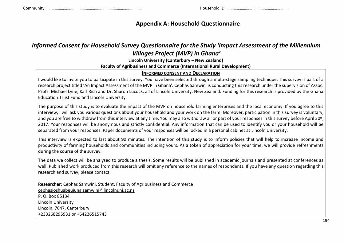
Community ………………………………………………………………………………… Household ID………………………………………………………

194

Appendix A: Household Questionnaire

Informed Consent for Household Survey Questionnaire for the Study ‘Impact Assessment of the Millennium Villages Project (MVP) in Ghana’

Lincoln University (Canterbury – New Zealand)

Faculty of Agribusiness and Commerce (International Rural Development)

INFORMED CONSENT AND DECLARATION I would like to invite you to participate in this survey. You have been selected through a multi-stage sampling technique. This survey is part of a research project titled ‘An Impact Assessment of the MVP in Ghana'. Cephas Samwini is conducting this research under the supervision of Assoc. Profs. Michael Lyne, Karl Rich and Dr. Sharon Lucock, all of Lincoln University, New Zealand. Funding for this research is provided by the Ghana Education Trust Fund and Lincoln University.

The purpose of this study is to evaluate the impact of the MVP on household farming enterprises and the local economy. If you agree to this interview, I will ask you various questions about your household and your work on the farm. Moreover, participation in this survey is voluntary, and you are free to withdraw from this interview at any time. You may also withdraw all or part of your responses in this survey before April 30th, 2017. Your responses will be anonymous and strictly confidential. Any information that can be used to identify you or your household will be separated from your responses. Paper documents of your responses will be locked in a personal cabinet at Lincoln University.

This interview is expected to last about 90 minutes. The intention of this study is to inform policies that will help to increase income and productivity of farming households and communities including yours. As a token of appreciation for your time, we will provide refreshments during the course of the survey.

The data we collect will be analysed to produce a thesis. Some results will be published in academic journals and presented at conferences as well. Published work produced from this research will omit any reference to the names of respondents. If you have any question regarding this research and survey, please contact: Researcher: Cephas Samwini, Student, Faculty of Agribusiness and Commerce

cephasjoshuabeujung.samwini@lincolnuni.ac.nz

P. O. Box 85134

Lincoln University

Lincoln, 7647, Canterbury

+233268295931 or +64226515743

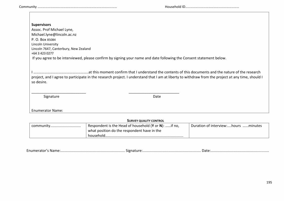
Community ………………………………………………………………………………… Household ID………………………………………………………

195

Supervisors

Assoc. Prof Michael Lyne, Michael.lyne@lincoln.ac.nz

P. O. Box 85084

Lincoln University

Lincoln 7647, Canterbury, New Zealand

+64 3 423 0277

If you agree to be interviewed, please confirm by signing your name and date following the Consent statement below.

I …………………………………………………..at this moment confirm that I understand the contents of this documents and the nature of the research project, and I agree to participate in the research project. I understand that I am at liberty to withdraw from the project at any time, should I so desire.

___________________________ _________________________

Signature Date

Enumerator Name:

SURVEY QUALITY CONTROL

community.............................. Respondent is the Head of household (Y or N): ……if no, what position do the respondent have in the household…….......................................................................

Duration of interview:....hours …...minutes

Enumerator’s Name:............................................................... Signature:......................................................... Date:.........................................................

Community ………………………………………………………………………………… Household ID………………………………………………………

196

A. Household Characteristics

A.1. Size of household (family or relatives who sleep here every day or at least on the weekends)

Total Males Females ≤ 15 years 16 – 65years ≥ 66years Attend school

Working on farm

Working off-farm

Studying off-farm

2.6.1.2 A.2. Information on the household head and of the person responsible for farming activities in the household

Age in years

Male or female

Married or single

Years of formal schooling

Years of farming experience

Relationship with household head

Household head

Farmer 1*

Farmer 2*

* Person responsible for farm management if not the household head.

A.3. Are you a member of a farmer based organisation (FBO)? (Y or N)...........................

If yes, name of the farmer group/organisation(s)? Organisation 1 ..………………………………………………… Did you join this FBO before the MVP (2006)? (Y or N) ……………………… Organisation 2 ..………………………………………………… Did you join this FBO before the MVP (2006)? (Y or N) ………………………

What is the main activity of the farmer group/organisation?

Organisation 1.. ..………………………………………………… Was this FBO established before the MVP (2006)? (Y or N) …………………… Organisation 2 ..………………………………………………… Was this FBO established before the MVP (2006)? (Y or N) ……………………

Community ………………………………………………………………………………… Household ID………………………………………………………

197

A4. Do you or any member of this household play a leadership role in these groups/organisation(s)? (Y or N) ………………………

If yes, what leadership role(s) do they have? ……………………………………………………………………………………………………………….

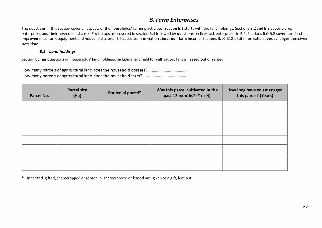
198

B. Farm Enterprises

The questions in this section cover all aspects of the households’ farming activities. Section B.1 starts with the land holdings. Sections B.2 and B.3 capture crop enterprises and their revenue and costs. Fruit crops are covered in section B.4 followed by questions on livestock enterprises in B.5. Sections B.6-B.8 cover farmland improvements, farm equipment and household assets. B.9 captures information about non-farm income. Sections B.10-B12 elicit information about changes perceived over time.

B.1 Land holdings

Section B1 has questions on households’ land holdings, including land held for cultivation, fallow, leased out or rented.

How many parcels of agricultural land does the household possess? ……………………………… How many parcels of agricultural land does the household farm? ………………………………

Parcel No.

Parcel size (Ha)

Source of parcel* Was this parcel cultivated in the

past 12 months? (Y or N) How long have you managed

this parcel? (Years)

* Inherited, gifted, sharecropped or rented in, sharecropped or leased out, given as a gift, lent out.

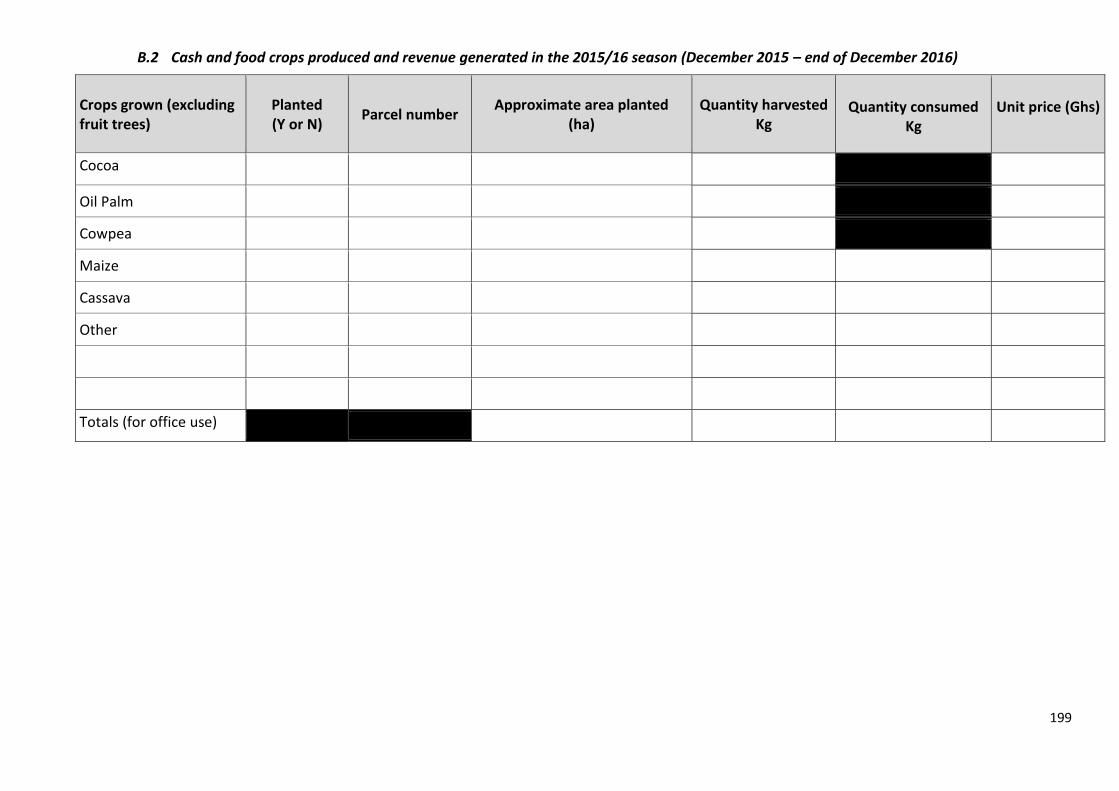
199

B.2 Cash and food crops produced and revenue generated in the 2015/16 season (December 2015 – end of December 2016)

Crops grown (excluding fruit trees)

Planted (Y or N)

Parcel number Approximate area planted

(ha) Quantity harvested

Kg

Quantity consumed

Kg

Unit price (Ghs)

Cocoa

Oil Palm

Cowpea

Maize

Cassava

Other

Totals (for office use)

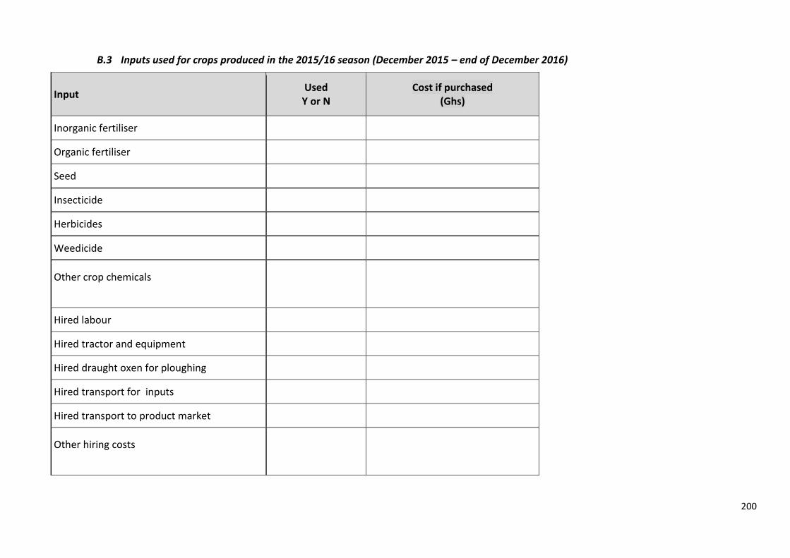
200

B.3 Inputs used for crops produced in the 2015/16 season (December 2015 – end of December 2016)

Input Used Y or N

Cost if purchased (Ghs)

Inorganic fertiliser

Organic fertiliser

Seed

Insecticide

Herbicides

Weedicide

Other crop chemicals

Hired labour

Hired tractor and equipment

Hired draught oxen for ploughing

Hired transport for inputs

Hired transport to product market

Other hiring costs

201

B.4 Fruits produced in the 2015/16 season (December 2015 – end of December 2016)

Fruits produced Planted Y or N

Main reason for planting (a)

Quantity harvested Kg or no of fruits

Unit price

(Ghs)

Mangoes

Pineapples

Avocados

Oranges

Lime

Bananas

Totals (for office use)

(a) 1 = only for household consumption, 2 = mainly for household consumption, 3 = equally for household consumption and cash income, 4 = mainly for cash income, 5 = only for cash income.

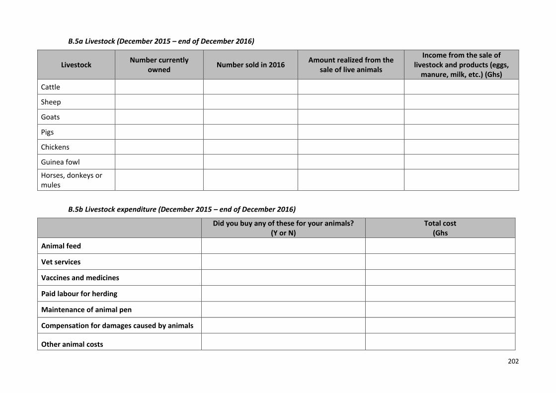
202

B.5a Livestock (December 2015 – end of December 2016)

Livestock

Number currently owned

Number sold in 2016 Amount realized from the

sale of live animals

Income from the sale of livestock and products (eggs,

manure, milk, etc.) (Ghs)

Cattle

Sheep

Goats

Pigs

Chickens

Guinea fowl

Horses, donkeys or mules

B.5b Livestock expenditure (December 2015 – end of December 2016)

Did you buy any of these for your animals?

(Y or N) Total cost

(Ghs

Animal feed

Vet services

Vaccines and medicines

Paid labour for herding

Maintenance of animal pen

Compensation for damages caused by animals

Other animal costs

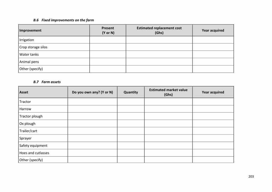
203

B.6 Fixed improvements on the farm

Improvement Present (Y or N)

Estimated replacement cost (Ghs)

Year acquired

Irrigation

Crop storage silos

Water tanks

Animal pens

Other (specify)

B.7 Farm assets

Asset Do you own any? (Y or N) Quantity Estimated market value

(Ghs) Year acquired

Tractor

Harrow

Tractor plough

Ox plough

Trailer/cart

Sprayer

Safety equipment

Hoes and cutlasses

Other (specify)

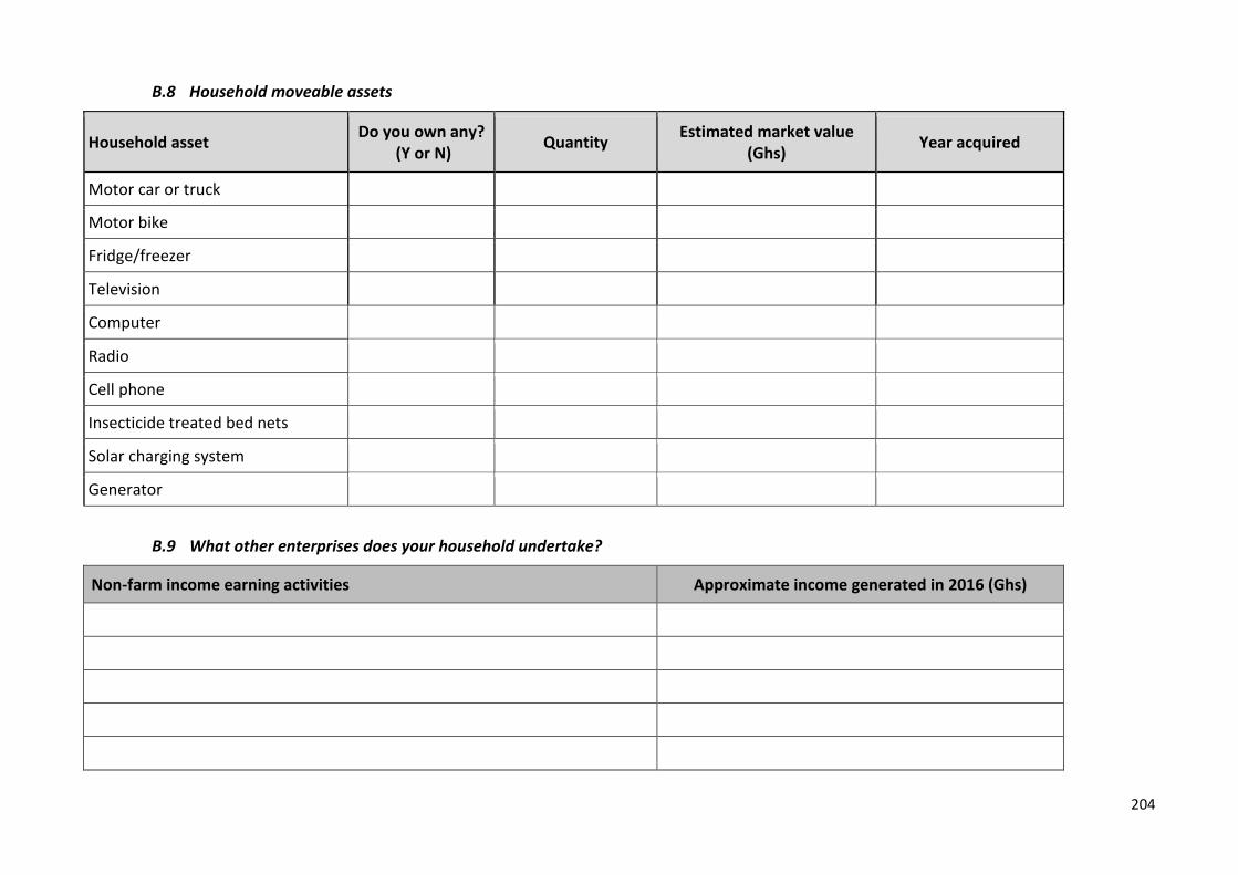
204

B.8 Household moveable assets

Household asset Do you own any?

(Y or N) Quantity

Estimated market value (Ghs)

Year acquired

Motor car or truck

Motor bike

Fridge/freezer

Television

Computer

Radio

Cell phone

Insecticide treated bed nets

Solar charging system

Generator

B.9 What other enterprises does your household undertake?

Non-farm income earning activities Approximate income generated in 2016 (Ghs)

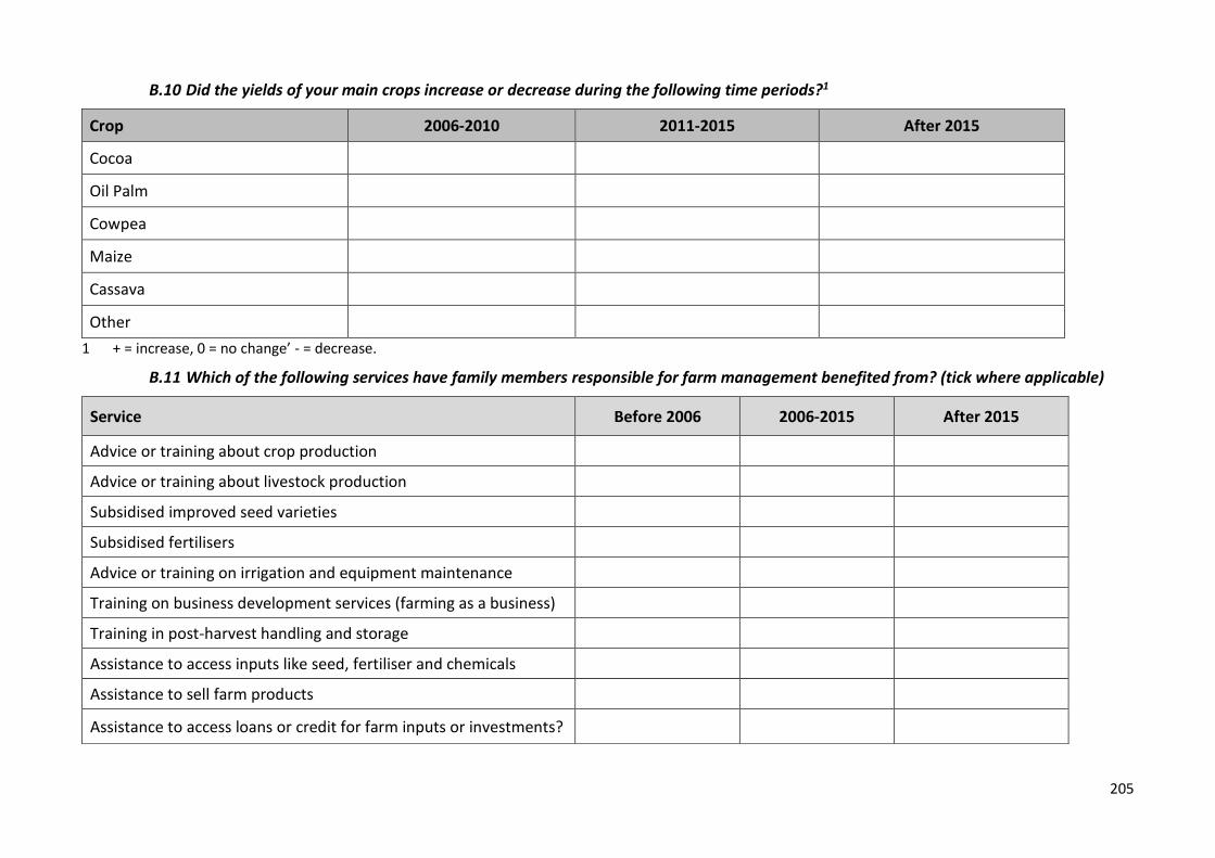
205

B.10 Did the yields of your main crops increase or decrease during the following time periods?1

Crop 2006-2010 2011-2015 After 2015

Cocoa

Oil Palm

Cowpea

Maize

Cassava

Other

1 + = increase, 0 = no change’ - = decrease.

B.11 Which of the following services have family members responsible for farm management benefited from? (tick where applicable)

Service Before 2006 2006-2015 After 2015

Advice or training about crop production

Advice or training about livestock production

Subsidised improved seed varieties

Subsidised fertilisers

Advice or training on irrigation and equipment maintenance

Training on business development services (farming as a business)

Training in post-harvest handling and storage

Assistance to access inputs like seed, fertiliser and chemicals

Assistance to sell farm products

Assistance to access loans or credit for farm inputs or investments?

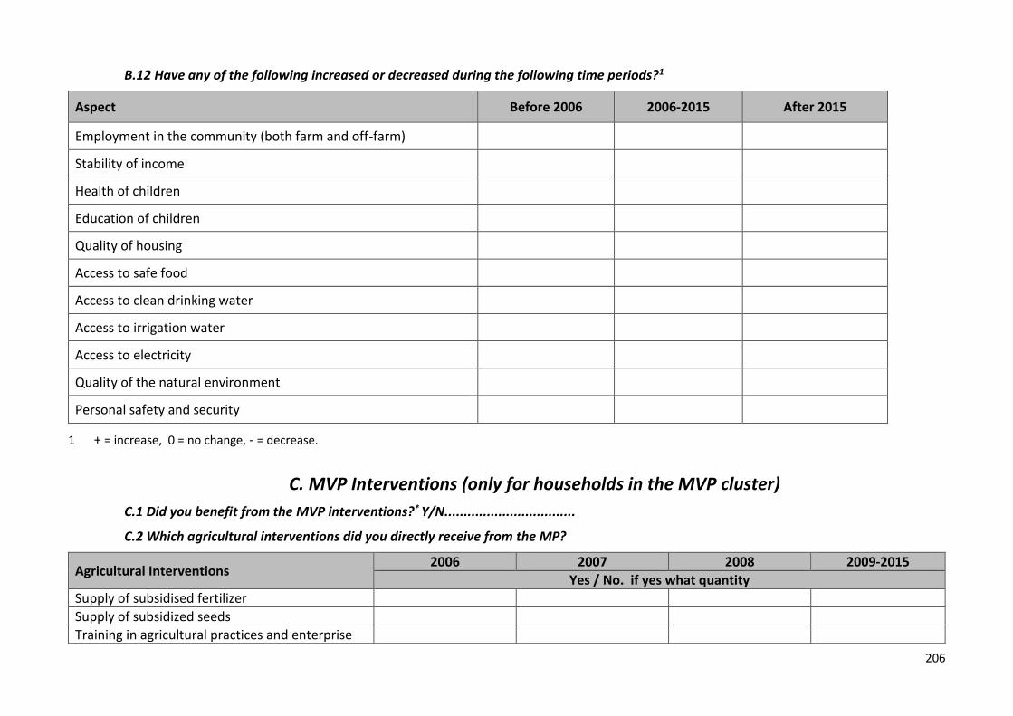
206

B.12 Have any of the following increased or decreased during the following time periods?1

Aspect Before 2006 2006-2015 After 2015

Employment in the community (both farm and off-farm)

Stability of income

Health of children

Education of children

Quality of housing

Access to safe food

Access to clean drinking water

Access to irrigation water

Access to electricity

Quality of the natural environment

Personal safety and security

1 + = increase, 0 = no change, - = decrease.

C. MVP Interventions (only for households in the MVP cluster)

C.1 Did you benefit from the MVP interventions?* Y/N..................................

C.2 Which agricultural interventions did you directly receive from the MP?

Agricultural Interventions 2006 2007 2008 2009-2015

Yes / No. if yes what quantity

Supply of subsidised fertilizer

Supply of subsidized seeds

Training in agricultural practices and enterprise

207

Training in diversification

Access to loans

Extension training

Storage facilities.

C.3 Will you be able to sustain the level of inputs you use on your farm now that the MVP has ended? Y/N………………………………….

Why?.................................................................................................................................................................................................................................................................................................................................................................................................................................................................................................................................................................................................................................................................................................................................................................

C.4 Overall, how satisfied are you with MVP’s interventions?*...........

*1 = not at all, 2 = slightly, 3 = somewhat, 4 = mostly, 5 = completely

C.5. How has the MVP impacted your livelihood? *………………………………………………………………….

*Positive impact - 3, Neither positive nor negative – 2, Negative impact - 1

C.6 What are the 3 main contributions of the MVP to your life in order of importance

1………………………………………………………………………………………………….......................................................................................................................................................................................................................................................................................................................................................................................................................................................................................................................................................................................................................................................................................................................................................................................................................................................................................................................................................................................................................................................................................

2…………………………………………………………………………………………………………………………………………………………………………………………………………………………………………………………………………………………………………………………………………………………………………………………………………………………………………………………………………………………………………………………………………………………………………………………………………………………………………………………

3.…………………………………………………………………………………………………………………………………………………………………………………………………………………………………………………………………………………………………………………………………………………………………………………………………………………………………………………………………………………………………………………………………………………………………………………………………………………………………………………………

208

C.7 How do you view your future development prospect after the MVP?

…………………………………………………………………………………………………………………………………………………………………………………………………………………………………………………………………………………………………………………………………………………………………………………………………………………………………………………………………………………………………………………………………………………………………………………………………………………………………………………………….

C. 8 Did you percieve any undesirable effects of the MVP?

1………………………………………………………………………………………………………………………………………………………………………………………………..………………………………………………………………………………………………………………………………………………………………………………………………………………………………………………………………

209

Appendix B: Variable Definitions

Variable Definition id ID

mvp Treatment variable (1 = MVP, 0 = non-MVP)

hhs Household size (number)

hhmales Number of male household members (number)

hhfemales Number of female household member (number)

children Number of children under 15 (number)

adults Number of adults in the household (number)

elderly Number of elderly household members (number)

schooling Number of children in school (number)

hhfarmlabour Household farm labour stock (number)

hhofffarmlab Number engaged in off farm work (number)

years Years resident (years)

hhhage Age of household head (years)

malehh Gender of household head (1 = male, 0 = female)

sch Years of formal education completed by the household head (years)

mainoccfarming 1 if farming is the household head’s main occupation, 0 otherwise

yrs_of_farming_exp Years of farming experience (years)

hhh_fbo Membership of producer groups (1 = yes, 0 = no)

hhhmarsta Marital status (1 =Single, 2 = Married, 3 = separated, 4 = Divorced)

hhhyearjoined 1 if member joined before the 2006, 0 otherwise farming Head is manager of farming operation (1 = yes, 0 = no)

parcels_owned Number of parcels of agricultural land owned by household (number)

parcels_farmed Number parcels of agricultural land cultivated by household (number)

b406cropprodadvice Crop production extension access prior to 2006 (1 = yes, 0 = no)

b406animprodavice Livestock production extension access prior to 2006 (1 = yes, 0 = no)

b406subsidseeds Access to subsidised improved seed varieties prior to 2006 (1 = yes, 0 = no)

b406subsidfert Access to subsidised fertiliser prior to 2006 (1 = yes, 0 = no)

b406irrigatitraining Access to irrigation, equipment training and maintenance prior to 2006 (1 = yes, 0 = no)

b406businessdev Training on business development services (farming as a business) prior to 2006 (1 = yes, 0 = no)

b406postharvhandling Training in post-harvest handling and storage prior to 2006 (1 = yes, 0 = no)

b406inputaccess Access to inputs like seed, fertiliser and chemicals prior to 2006 (1 = yes, 0 = no)

b406marketaccess Market access for farm products prior to 2006 (1 = yes, 0 = no)

b406creditacccess Access to loans or credit for farm inputs and investments prior to 2006 (1 = yes, 0 = no)

o615cropprodadvice Crop production extension access from 2006 to 2015 (1 = yes, 0 = no)

o615animprodavice Livestock production extension access from 2006 to 2015 (1 = yes, 0 = no)

o615subsidseeds Access to subsidised improved seed varieties 2006 to 2015 (1 = yes, 0 = no)

o615subsidfert Access to subsidised fertilisers from 2006 to 2015 (1 = yes, 0 = no)

o615irrigatitraining Access to irrigation, equipment training and maintenance from 2006 to 2015 (1 = yes, 0 = no)

o615businessdev Access to training on business development (farming as a business) from 2006 to 2015 (1 = yes, 0 = no)

o615postharvhandling Training in post-harvest handling and storage from 2006 to 2015 (1 = yes, 0 = no)

o615inputaccess Access to inputs like seed, fertiliser and chemicals from 2006 to 2015 (1 = yes, 0 = no)

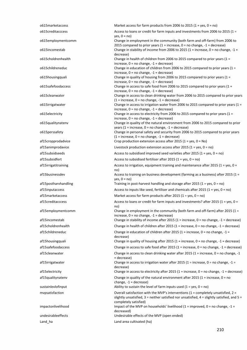
210

o615marketaccess Market access for farm products from 2006 to 2015 (1 = yes, 0 = no)

o615creditacccess Access to loans or credit for farm inputs and investments from 2006 to 2015 (1 = yes, 0 = no)

o615employmentcomm Change in employment in the community (both farm and off-farm) from 2006 to 2015 compared to prior years (1 = increase, 0 = no change, -1 = decrease)

o615incomestab Change in stability of income from 2006 to 2015 (1 = increase, 0 = no change, -1 = decrease)

o615choldrenhealth Change in health of children from 2006 to 2015 compared to prior years (1 = increase, 0 = no change, -1 = decrease)

o615childreneduc Change in education of children from 2006 to 2015 compared to prior years (1 = increase, 0 = no change, -1 = decrease)

o615housingquali Change in quality of housing from 2006 to 2015 compared to prior years (1 = increase, 0 = no change, -1 = decrease)

o615safefoodaccess Change in access to safe food from 2006 to 2015 compared to prior years (1 = increase, 0 = no change, -1 = decrease)

o615cleanwater Change in access to clean drinking water from 2006 to 2015 compared to prior years (1 = increase, 0 = no change, -1 = decrease)

o615irrigatwater Change in access to irrigation water from 2006 to 2015 compared to prior years (1 = increase, 0 = no change, -1 = decrease)

o615electricity Change in access to electricity from 2006 to 2015 compared to prior years (1 = increase, 0 = no change, -1 = decrease)

o615qualitynatenv Change in quality of the natural environment from 2006 to 2015 compared to prior years (1 = increase, 0 = no change, -1 = decrease)

o615perssafety Change in personal safety and security from 2006 to 2015 compared to prior years (1 = increase, 0 = no change, -1 = decrease)

af15cropprodadvice Crop production extension access after 2015 (1 = yes, 0 = No)

af15animprodavice Livestock production extension access after 2015 (1 = yes, 0 = no)

af15subsidseeds Access to subsidised improved seed varieties after 2015 (1 = yes, 0 = no)

af15subsidfert Access to subsidised fertiliser after 2015 (1 = yes, 0 = no)

af15irrigatitraining Access to irrigation, equipment training and maintenance after 2015 (1 = yes, 0 = no)

af15businessdev Access to training on business development (farming as a business) after 2015 (1 = yes, 0 = no)

af15postharvhandling Training in post-harvest handling and storage after 2015 (1 = yes, 0 = no)

af15inputaccess Access to inputs like seed, fertiliser and chemicals after 2015 (1 = yes, 0 = no)

af15marketaccess Market access for farm products after 2015 (1 = yes, 0 = no)

af15creditacccess Access to loans or credit for farm inputs and investments? after 2015 (1 = yes, 0 = no)

af15employmentcomm Change in employment in the community (both farm and off-farm) after 2015 (1 = increase, 0 = no change, -1 = decrease)

af15incomestab Change in stability of income after 2015 (1 = increase, 0 = no change, -1 = decrease)

af15choldrenhealth Change in health of children after 2015 (1 = increase, 0 = no change, -1 = decrease)

af15childreneduc Change in education of children after 2015 (1 = increase, 0 = no change, -1 = decrease)

af15housingquali Change in quality of housing after 2015 (1 = increase, 0 = no change, -1 = decrease)

af15safefoodaccess Change in access to safe food after 2015 (1 = increase, 0 = no change, -1 = decrease)

af15cleanwater Change in access to clean drinking water after 2015 (1 = increase, 0 = no change, -1 = decrease)

af15irrigatwater Change in access to irrigation water after 2015 (1 = increase, 0 = no change, -1 = decrease)

af15electricity Change in access to electricity after 2015 (1 = increase, 0 = no change, -1 = decrease)

af15qualitynatenv Change in quality of the natural environment after 2015 (1 = increase, 0 = no change, -1 = decrease)

sustainlevlofinput Ability to sustain the level of farm inputs used (1 = yes, 0 = no)

mvpsatisfaction Overall satisfaction with the MVP's interventions (1 = completely unsatisfied, 2 = slightly unsatisfied, 3 = neither satisfied nor unsatisfied, 4 = slightly satisfied, and 5 = completely satisfied)

impactonlivelihood Impact of the MVP on households’ livelihood (1 = improved, 0 = no change, -1 = decreased)

undesirableeffects Undesirable effects of the MVP (open ended)

Land_ha Land area cultivated (ha)

211

animal_prod_cost Expenditure on animal products (Ghs)

ctanimfed Expenditure on animal feed (Ghs)

ctvaccmed Expenditure on vaccines and medicines for livestock (Ghs)

smctvets Expenditure on veterinary services (Ghs)

amount_animal_products Revenue from animal products sales (Ghs)

hhasset_yrsacq Year acquired of household asset (year)

market_value_sum Value of Farm assets (Ghs)

year_acq_farmasset Year of farm asset acquisition (years)

animpens_ini Initial expenditure on animal pens (Ghs)

Cropsilos_ini Initial expenditure on crop silos (Ghs)

irrigation_ini Initial expenditure on irrigation improvement (Ghs)

others_ini Initial expenditure on other fixed improvements (Ghs)

watertankini Initial expenditure on water tanks (Ghs)

animpens_sum Replacement value of animal pens (Ghs)

cropsilos_sum Replacement value of crop silos (Ghs)

irrig_sum Replacement value of irrigation improvements (Ghs)

others_sum Replacement value of other improvements (Ghs)

watertank_sum Replacement value of water tanks (Ghs)

cattle_sum Number of cattle owned (#)

chicken_sum Number of chickens owned (#)

goats_sum Number of goats owned (#)

guineas_sum Number of guinea fowls owned (#)

sheep_sum Number of sheep owned (#)

price_of_animal Average price of animals in 2015 (Ghs)

no_sold_2015_sum Number of animals sold in 2015 (#)

qhiredlab_sum Quantity of hired labour (#)

qhiredeqt_sum Quantity of hired equipment (#)

crop_harvested Quantity of crop harvested in 2015 (kg)

cassava_wt Weight of cassava produced (kg)

cocoa_wt Weight of cocoa produced (kg)

maize_wt Weight of maize produced (kg)

oilpalm_wt Weight of oil palm produced (kg)

plantain_wt Weight of plantain produced (kg)

nonfarm_income Earnings from non-farm income earning activities (Ghs)

hhasset_mktvalue Market value of household assets (Ghs)

valanimalssold_sum Value of animals sold in 2015 (Ghs)

valcattle_sum Value of cattle owned (Ghs)

valchicken_sum Value of chickens owned (Ghs)

valgoats_sum Value of goats owned (Ghs)

valguineas_sum Value of guineas owned (Ghs)

valsheep_sum Value of sheep owned (Ghs)

totanimexp Total animal expenditure (Ghs)

totvalfixedimp Total value of fixed improvements (Ghs)

fruitsale Total amount realised from the sale of fruits (Ghs)

weedicidq Quantity of weedicides (l)

herbiciq Quantity of herbicides (l)

inorgfertq Quantity of inorganic fertiliser (kg)

insecticq Quantity of insecticides (l)

orgfertq Quantity of organic fertiliser (kg)

seedsq Quantity of Seeds (kg)

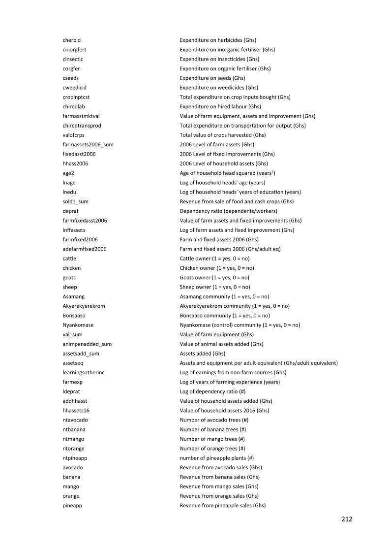
212

cherbici Expenditure on herbicides (Ghs)

cinorgfert Expenditure on inorganic fertiliser (Ghs)

cinsectic Expenditure on insecticides (Ghs)

corgfer Expenditure on organic fertiliser (Ghs)

cseeds Expenditure on seeds (Ghs)

cweedicid Expenditure on weedicides (Ghs)

cropinptcst Total expenditure on crop inputs bought (Ghs)

chiredlab Expenditure on hired labour (Ghs)

farmasstmktval Value of farm equipment, assets and improvement (Ghs)

chiredtransprod Total expenditure on transportation for output (Ghs)

valofcrps Total value of crops harvested (Ghs)

farmassets2006_sum 2006 Level of farm assets (Ghs)

fixedasst2006 2006 Level of fixed improvements (Ghs)

hhass2006 2006 Level of household assets (Ghs)

age2 Age of household head squared (years2)

lnage Log of household heads' age (years)

lnedu Log of household heads’ years of education (years)

sold1_sum Revenue from sale of food and cash crops (Ghs)

deprat Dependency ratio (dependents/workers)

farmfixedasst2006 Value of farm assets and fixed improvements (Ghs)

lnffassets Log of farm assets and fixed improvement (Ghs)

farmfixed2006 Farm and fixed assets 2006 (Ghs)

adefarmfixed2006 Farm and fixed assets 2006 (Ghs/adult eq)

cattle Cattle owner (1 = yes, 0 = no)

chicken Chicken owner (1 = yes, 0 = no)

goats Goats owner (1 = yes, 0 = no)

sheep Sheep owner (1 = yes, 0 = no)

Asamang Asamang community (1 = yes, 0 = no)

Akyerekyerekrom Akyerekyerekrom community (1 = yes, 0 = no)

Bonsaaso Bonsaaso community (1 = yes, 0 = no)

Nyankomase Nyankomase (control) community (1 = yes, 0 = no)

val_sum Value of farm equipment (Ghs)

animpenadded_sum Value of animal assets added (Ghs)

assetsadd_sum Assets added (Ghs)

assetseq Assets and equipment per adult equivalent (Ghs/adult equivalent)

learningsotherinc Log of earnings from non-farm sources (Ghs)

farmexp Log of years of farming experience (years)

ldeprat Log of dependency ratio (#)

addhhasst Value of household assets added (Ghs)

hhassets16 Value of household assets 2016 (Ghs)

ntavocado Number of avocado trees (#)

ntbanana Number of banana trees (#)

ntmango Number of mango trees (#)

ntorange Number of orange trees (#)

ntpineapp number of pineapple plants (#)

avocado Revenue from avocado sales (Ghs)

banana Revenue from banana sales (Ghs)

mango Revenue from mango sales (Ghs)

orange Revenue from orange sales (Ghs)

pineapp Revenue from pineapple sales (Ghs)

213

cropassets Value of crop assets added (Ghs/adult equivalent)

lcropassets Value of crop assets added (log(number))

lcropassetspred Crop assets added (predicted values (log))

lage Age of household head (log)

valanims Value of animals possessed (Ghs)

fruits Revenue from fruit Crops (Ghs)

cassava1 Value of cassava produced (Ghs)

cocoa1 Value of cocoa produced (Ghs)

maize1 Value of maize produced (Ghs)

oilpalm1 Value of oil palm produced (Ghs)

plantain1 Value of plantain produced (Ghs)

ade1 Adult equivalent household size (#)

adehhass2006 Household assets 2006 (per adult eq)

ccropinps Total expenditure on crop inputs (Ghs)

ccropserv Total expenditure on crop services (Ghs)

ccropinpserv Total expenditure on crop inputs and services (Ghs)

netcropinc Net crop income (Ghs)

animrev Revenue from animal and animal product sales (Ghs)

netaniminc Net animal income (Ghs)

cropandfruit Net income from crops and fruits (Ghs)

netfarminc Net farm income including labour and machinery (Ghs)

netfarmincome Net farm income excluding labour and machinery (Ghs)

adenetfarmincome Net farm income (Ghs/adult equivalent)

adesold1_sum Revenue from food and cash crop sales (Ghs/adult equivalent)

adeanimrev Revenue from livestock and livestock products (Ghs/adult equivalent)

adefruits Revenue from fruit sales (Ghs/adult equivalent)

adeearnings_other_income_act_sum Income from non-farm activities (Ghs/adult equivalent)

adeccropinpserv Expenditure on crop inputs and services (Ghs/adult equivalent)

adetotanimexp Expenditure on livestock inputs (Ghs/adult equivalent)

adefarmeqtasstsimp Value of farm equipment, assets and improvements (Ghs/adult equivalent)

adehhasset_mktvalue Value of household assets (Ghs/adult equivalent)

dist_agro Distance to nearest hospital in 2006 (km)

dist_manso Distance to district capital (km)

dist_obuasi Distance to Obuasi in 2006 (km)

mvppart Predicted probability of MVP participation (predicted values from logit regression)

adeassetsadd_sum Farm and fixed assets added (Ghs/adult equivalent)

adeaddhhasst Household assets added (Ghs/adult equivalent)

adeallassetsadded Farm, fixed and household assets added (Ghs/adult equivalent)

adeallassets2006 Value of all assets in 2006 (Ghs/adult equivalent)

ladeallassets2006 Log of value of all assets in 2006 (Ghs/adult equivalent)

adehhofffarmlab Off-farm labour (Ghs/adult equivalent)

adehhfarmlabour Household stock of farm labour (Ghs/adult equivalent)

adeland_ha Stock of farm land (Ghs/adult equivalent)

predassetsadded Predicted value of assets added (Ghs/adult equivalent)

predallassets2016 Predicted value of all assets in 2016 (Ghs/adult equivalent)

adevalanims Value of animals (Ghs/adult equivalent)

adevalofcrps Value of crops harvested (Ghs/adult equivalent)

adegrossagricprod Gross farm output (Ghs/adult equivalent)

adetotalexp Total farm expenditure (Ghs/adult equivalent)

VAL Net farm income (Ghs/adult equivalent)

214

adetotalanimexp1 Total animal expenditure (Ghs/ adult equivalent)

Adechiredlab Total expenditure on hired lab (Ghs/ adult equivalent)

adeccropinpserv1 Expenditure on crop inputs and services (Ghs/adult equivalent)

farmeqt Value of farm equipment (Ghs)

farmeqt06 Pre-MVP value of farm equipment (Ghs)

farmeqt16 Post-MVP value of farm equipment (Ghs)

farmeqtadded Value of farm equipment added (Ghs)

fixedassets Value of fixed assets (Ghs)

fixedassets06 Pre-MVP value of fixed assets (Ghs)

fixedassets16 Post-MVP value of fixed assets (Ghs)

fixedassetsadded Value of fixed assets added (Ghs)

hhassetsval Value of household assets (Ghs)

hhassetsval06 Pre-MVP value of household assets (Ghs)

hhassetsval16 Post-MVP value of household assets (Ghs)

hhassetsadded Value of household assets added (Ghs)

adefarmeqt Value of farm equipment (Ghs) (Ghs/adult equivalent)

adefarmeqt06 Pre-MVP value of farm equipment (Ghs) (Ghs/adult equivalent)

adefarmeqt16 Post-MVP value of farm equipment (Ghs) (Ghs/adult equivalent)

adefarmeqtadded Value of farm equipment added (Ghs) (Ghs/adult equivalent)

adefixedassets Value of fixed assets (Ghs) (Ghs/adult equivalent)

adefixedassets06 Pre-MVP value of fixed assets (Ghs) (Ghs/adult equivalent)

adefixedassets16 Post-MVP value of fixed assets (Ghs) (Ghs/adult equivalent)

adefixedassetsadded Value of fixed assets added (Ghs) (Ghs/adult equivalent)

adehhassetsval Value of household assets (Ghs) (Ghs/adult equivalent)

adehhassetsval06 Pre-MVP value of household assets (Ghs) (Ghs/adult equivalent)

adehhassetsval16 Post-MVP value of household assets (Ghs) (Ghs/adult equivalent)

adehhassetsadded Value of household assets added (Ghs) (Ghs/adult equivalent)

adenonfarminc Earnings from non-farm sources (Ghs) (Ghs/adult equivalent)

adeallassets06 Pre-MVP value of all assets (Ghs/adult equivalent)

adefarmfixed06 Pre-MVP value of farm and fixed assets (Ghs/adult equivalent)

mvppartIV Predicted probability of participation with IV

ladeallassets06 Log pre-MVP value of all assets (Ghs/adult equivalent)

predadeallassetsadded Predicted value of all assets added (Ghs/adult equivalent)

adeallassets16 Value of all assets in 2016 (Ghs/adult equivalent)

predadeallassets Predicted value of assets in 2016 (Ghs/adult equivalent)

adefarmexpenditure Total farm expenditure (Ghs/adult equivalent)

adevalgoats_sum Value of goats owned (Ghs/adult equivalent)

adegoats_sum Value of goats owned (Ghs/adult equivalent)

ladevalgoats_sum Log value of goats owned (Ghs/adult equivalent)

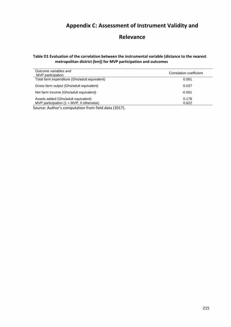
215

Appendix C: Assessment of Instrument Validity and

Relevance

Table D1 Evaluation of the correlation between the instrumental variable (distance to the nearest metropolitan district (km)) for MVP participation and outcomes

Outcome variables and MVP participation

Correlation coefficient

Total farm expenditure (Ghs/adult equivalent) 0.061

Gross farm output (Ghs/adult equivalent) 0.037

Net farm Income (Ghs/adult equivalent) -0.001

Assets added (Ghs/adult equivalent) 0.178

MVP participation (1 = MVP, 0 otherwise) 0.622

Source: Author’s computation from field data (2017).