salton sea salinity control research project
TRANSCRIPT

Salton Sea Salinity Control Research Project
Research conducted at the Salton Sea Test Base
Joint Research Project
U.S. Department of the Interior Bureau of Reclamation Lower Colorado Region Boulder City, Nevada
and
Salton Sea Authority La Quinta, California
Principal Investigator: Paul A. Weghorst, PE Bureau of Reclamation Technical Service Center Denver, Colorado
August 2004

vi

vii
Acknowledgments
The research presented in the following document is the culmination of the efforts of many contractors, as well as Federal and local agency employees. The highest acknowledgement is given to contractor Herbert Hein Jr. who lived and worked on the Salton Sea Test Base. Without him, this project would not have been possible. Herb and his assistant, Luis Garcia, solved untold numbers of problems in conditions that few would have tolerated. Great respect and gratitude is given to each of these two gentlemen who sacrificed much in making their contributions to the research effort. Others who contributed significantly to the research effort include Cheryl Rodriquez of the Bureau of Reclamation and Dan Cain of the Salton Sea Authority. These two managed the permitting, construction, and decommissioning of the project site and provided critical support in keeping the project site functioning. Their contributions to the project are highly respected.
Gratitude is also extended to Gregg Day, Zeynep Erdogan, and Mark Gemperline of the Denver Technical Service Center for their contributions in executing a successful core drilling and laboratory analysis program. Operations at the Salton Sea Test Base culminated with their contributions, and their professional and efficient efforts are applauded. The contributions of Sharon Nuanes of the Denver Technical Service Center need to also be acknowledged. Sharon managed and analyzed the massive amounts of data collected during the course of the research project.
Finally, much appreciation is given to Barry Drake and his crew at Snow Making, Incorporated, along with Paul Larimore of the Bureau of Reclamation, who all endured, with much patience, the often chaotic process and harsh climate conditions under which they were asked to work during the construction of the project site facilities. There are many others that contributed to the research effort, and their assistance is greatly appreciated.

ix
Contents
1 INTRODUCTION................................................................................ 1
2 OBJECTIVES..................................................................................... 1 2.1 Objectives of Disposal Pond Research ........................................................................... 1 2.2 Objectives of Evaporation Research .............................................................................. 3 2.3 Objectives of Weather Research..................................................................................... 4
3 RESEARCH METHODS .................................................................... 4 3.1 Facilities ............................................................................................................................ 5
3.1.1 Solar Evaporation Ponds ............................................................................................... 6 3.1.2 Enhanced Evaporation Systems .................................................................................... 9 3.1.3 Disposal Pond.............................................................................................................. 12 3.1.4 Sea Intake .................................................................................................................... 16 3.1.5 Electrical System......................................................................................................... 17
3.2 Operating Procedures.................................................................................................... 18 3.2.1 Solar Pond Procedures ................................................................................................ 18 3.2.2 Enhanced Evaporation System Procedures ................................................................. 19
3.3 Testing Procedures......................................................................................................... 21 3.3.1 Phased Testing Approach............................................................................................ 21 3.3.2 Disposal Test Facility Procedures ............................................................................... 23 3.3.3 Evaporations Research Procedures.............................................................................. 27 3.3.4 Weather Monitoring .................................................................................................... 28
4 RESULTS......................................................................................... 29 4.1 EES Phase Chemistry versus Agrarian Research Results.......................................... 29 4.2 Brine Evaporation Rates ............................................................................................... 29
4.2.1 Historic Evaporation Measurements ........................................................................... 29 4.2.2 Monthly Evaporation Distribution .............................................................................. 31 4.2.3 Historic Monthly Pan Evaporation.............................................................................. 31 4.2.4 Historic Monthly Open Water Surface Evaporation ................................................... 33 4.2.5 Evaporation Brine Factors........................................................................................... 34 4.2.6 Monthly Pan Brine Evaporation vs. Percent Weight Magnesium............................... 36 4.2.7 Monthly Open Brine Surface Evaporation vs. Percent Weight Magnesium ............... 38
4.3 Salt Disposal Test Results.............................................................................................. 40 4.4 Salt Sampling and Testing............................................................................................. 43
4.4.1 Index Properties Tests ................................................................................................. 44 4.4.2 One Dimensional Consolidation Test.......................................................................... 46 4.4.3 Direct Shear Test......................................................................................................... 49
4.5 Mineralogical Compositions.......................................................................................... 62
x
5 FINDINGS ........................................................................................ 67 5.1 Salinity Control Projects Design Issues........................................................................ 68
5.1.1 Fouling of Closed Conduits......................................................................................... 68 5.1.2 Fouling of Canals and Control Structures ................................................................... 69 5.1.3 Pumping Saturated Brine ............................................................................................ 69 5.1.4 Brine Entrainment ....................................................................................................... 70 5.1.5 Draining of Entrained Brines ...................................................................................... 71 5.1.6 Bittern Properties......................................................................................................... 72 5.1.7 Mix Salts Domination ................................................................................................. 74
5.2 Enhanced Evaporator Issues......................................................................................... 74 5.2.1 Fouling of Closed Conduits......................................................................................... 74 5.2.2 Biological Fouling....................................................................................................... 75 5.2.3 Mist Fouling of Evaporators........................................................................................ 75
5.3 Intake Problems and Issues........................................................................................... 77 5.3.1 Barnacle Fouling ......................................................................................................... 77 5.3.2 Barnacle Remediation ................................................................................................. 79 5.3.3 Intake Priming............................................................................................................. 80 5.3.4 Intake Degassing Problems ......................................................................................... 80
5.4 EES Efficiency and Energy Costs ................................................................................. 81 5.4.1 Microclimate Effects ................................................................................................... 88
6 RECOMMENDATIONS.................................................................... 88 6.1 Disposal Recommendations........................................................................................... 88
6.1.1 Concentrate Near the Disposal Facility ....................................................................... 88 6.1.2 Gravity Flow in Open Channels .................................................................................. 88 6.1.3 If Pumping is Unavoidable.......................................................................................... 89 6.1.4 Mechanical Consolidation........................................................................................... 89 6.1.5 Disposal Pond Design and Operations ........................................................................ 89 6.1.6 Dike Embankment Design........................................................................................... 90 6.1.7 Bittern Management.................................................................................................... 92
6.2 EES Recommendations.................................................................................................. 92 6.2.1 Pretreatment Research to Remove Calcium ................................................................ 92 6.2.2 Pretreatment Research to Remove Biologic Materials................................................ 92 6.2.3 Robotic Wind Alignment ............................................................................................ 92 6.2.4 Unit Spacing and Configuration.................................................................................. 93
6.3 Intake Recommendations .............................................................................................. 93 6.4 Proposal for Behavior Model ........................................................................................ 93
7 REFERENCES................................................................................. 95

xi
Appendix A – Photos Showing Field Sampling
Appendix B – Physical Properties Test Data
Appendix C – One Dimensional Consolidation Test Data
Appendix D – One Dimensional Consolidation Test Photos
Appendix E – Direct Shear Test Data
Appendix F – Direct Shear Test Photos
Appendix G – Climate Data for Year 2001
Appendix H – Climate Data for Year 2002
Appendix I – Status Report: Salton Sea Study
Figures Figure 2.1—Salinity control research facility......................................................... 2 Figure 2.2—Class A pans for brine evaporation studies. ....................................... 3 Figure 2.3a—Meteorological tower and related equipment. .................................. 4 Figure 2.3b—Location of meteorological tower at the Salton Sea Test Base.................................................. follows page 4 Figure 3.1—Cells 6b and 7 of solar ponds. ............................................................ 5 Figure 3.2—Pumping between major ponds .......................................................... 8 Figure 3.3—Gravity flow between cells. ................................................................ 8 Figure 3.4—Metering of flow from Sea intake and between ponds....................... 9 Figure 3.5—Enhanced evaporators in operation. ................................................. 10 Figure 3.6—Slimline S30P evaporator. ................................................................ 10 Figure 3.7—SMI Polecat Evaporator. .................................................................. 11 Figure 3.8—Disposal pond after pretesting EES evaporators. ............................. 13 Figure 3.9—Disposal pond core sampling pads. .................................................. 14 Figure 3.10—Disposal pond core pad locations and numbering scheme............. 15 Figure 3.11—Sea intake pump. ............................................................................ 16 Figure 3.12—Self-cleaning intake screen............................................................. 17 Figure 3.13—Electrical control box for enhanced evaporators. ........................... 18 Figure 3.14—Core drill and platform. .................................................................. 21 Figure 3.15—Center-raise dike configuration. ..................................................... 26 Figure 3.16—Upstream-raise dike configuration. ................................................ 26 Figure 4.1—Monthly evaporation distribution. .................................................... 31 Figure 4.2—Fraction of fresh water evaporation (brine factor) versus percent weight of magnesium. ......................................................................... 34

xii
Figure 4.3—Fraction of fresh water evaporation (brine factor) versus specific gravity...................................................................................... 35 Figure 4.4—Average monthly class A pan brine evaporation by percent weight of magnesium. .................................................................... 37 Figure 4.5—Class A pan brine evaporation as function of percent weight of magnesium by month...................................................... 37 Figure 4.6—Average monthly open brine surface evaporation by percent weight of magnesium. .................................................................... 39 Figure 4.7—Open brine surface evaporation as function of percent weight of magnesium by month. ......................................................... 39 Figure 4.8—Percent weight of magnesium in disposal pond (March 29, 2002, to December 3, 2002.)......................................................... 40 Figure 4.9—Salts reached dryness in disposal pond ............................................ 41 Figure 4.10—Heavy brine dripping onto deposits on core pad 7. ........................ 42 Figure 4.11—Supply tanks with heavy brine used in salt deposit density increase test (test 2). ......................................................... 43 Figure 4-12—Shear stress versus horizontal strain, 54F-128............................... 52 Figure 4.13—Shear stress versus horizontal strain, 54F-132. .............................. 53 Figure 4.14—Shear stress versus horizontal strain, 54F-135. .............................. 54 Figure 4.15—Shear stress versus horizontal strain, 54F-136. .............................. 55 Figure 4.16—Shear stress versus horizontal strain, 54F-138. .............................. 56 Figure 4.17—Peak shear stress versus normal stress, 54F-128. ........................... 57 Figure 4.18—Peak shear stress versus normal stress, 54F-132. ........................... 58 Figure 4.19—Peak shear stress versus normal stress, 54F-135. ........................... 59 Figure 4.20—Peak shear stress versus normal stress, 54F-136. ........................... 60 Figure 4.21—Peak shear stress versus normal stress, 54F-138. ........................... 61 Figure 4.22—Salton Sea undisturbed salt block sample 54F-138, pad 6, excavation No. 13.................................................................................. 63 Figure 4.23—Salton Sea undisturbed salt block sample 54F-138, 54F-138, pad 6, No. 13. ................................................................................... 63 Figure 4.24—Salton Sea undisturbed salt block sample 54F-138, pad 6, excavation No. 13.................................................................................. 64 Figure 4.25—Salton Sea undisturbed salt block sample 54F-138, pad 6, excavation No. 13.................................................................................. 64 Figure 4.26—Back-scattered electron image........................................................ 65 Figure 4.27—Back scattered electron image. ....................................................... 65 Figure 4.28—Elemental composition determined by energy dispersive spectroscopy........................................................................ 66 Figure 4.29—Elemental composition determined by energy dispersive spectroscopy........................................................................ 67 Figure 5.1—Gypsum fouling of closed conduits.................................................. 69 Figure 5.2—Brine entrainment in disposal pond.................................................. 70 Figure 5.3—Drained salt deposits......................................................................... 71

xiii
Figure 5.4—Sump used to drain and pump entrained brines................................ 72 Figure 5.5—Bitterns during final evaporation at Salton Sea Test Base. .............. 73 Figure 5.6—Bitterns after 2 weeks of evaporation at Salton Sea Test Base. ....... 73 Figure 5.7—Bitterns after 3 months of evaporation at Salton Sea Test Base....... 74 Figure 5.8—Salt deposits on evaporators from mist ingestion............................. 76 Figure 5.9—Barnacle fouling of Salton Sea Test Base fish screen. ..................... 78 Figure 5.10—Barnacle fouling of intake structure and fish screens at Bombay Beach solar pond facility. ..................................................................................... 78 Figure 5.11—REF barnacle removal system. ....................................................... 79 Figure 5.12—Intake structure degassing facility. ................................................. 80 Figure 5.13—Slimline evaporator used in power use study. ................................ 81 Figure 5.14—Specific gravity measurements in EES pond.................................. 82 Figure 5.15—Accumulated power usage and cost to concentrate 3 million gallons....................................................................... 83 Figure 5.16—Projected energy usage to produce 1 million tons per yr of salt. ... 84 Figure 5.17—Projected energy costs to produce 1 million tons per yr of salt..... 85 Figure 5.18—Projected number of EES units to produce 1 million tons per year of salt. ......................................................................... 85 Figure 5.19—Number of EES units and energy costs versus EES pond size to produce 1 million tons per year of salt. ............................... 86 Figure 5.20—Comparison of evaporation with EES and solar ponds. ................. 87
Tables Table 3.1—Solar pond cell, surface areas .............................................................. 6 Table 3.2—Solar pond and cell hydraulic data....................................................... 7 Table 4.1—Historic Imperial pan and net water surface evaporation .................. 30 Table 4.2—Historic estimated monthly Imperial pan evaporation....................... 32 Table 4.3—Estimated historic net monthly open water surface evaporation ....... 33 Table 4.4—Monthly pan brine evaporation vs. percent weight magnesium ........ 36 Table 4.5—Monthly open brine surface evaporation vs. percent weight magnesium .............................................................................. 38 Table 4.6—Soil sample index, Salton Sea Disposal Pond Salt, Salton Sea reclamation project, California ...................................................... 45 Table 4.7a—Physical properties test results ......................................................... 47 Table 4.7b—Weighted average specific gravity from petrography test results.... 47 Table 4.8a—Unit weights and void ratios from one-dimensional consolidation tests ....................................................................................................................... 48 Table 4.8b—One dimensional consolidation test results...................................... 48 Table 4.9—Direct shear test results, Salton Sea Salt............................................ 51 Table 4.10—Petrographic Lab sample numbers................................................... 62 Table 4.11—Block sample (54F-138) particle size data ...................................... 66 Table 5.1—Slimline EES power usage................................................................. 83

Summary This report presents the findings of the Salton Sea Salinity Control Research Project that the Bureau of Reclamation and the Salton Sea Authority conducted at the Salton Sea Test Base from July 2000 until December 2002. This research was undertaken to further understand the use of solar ponds and enhanced evaporation system (EES) technology to evaporate Salton Sea water, as well as to understand the issues related to disposing of the salt deposits that likely would be produced from using these systems or any other salt concentrating technology.
Objectives
A Salton Sea Reclamation Project to reduce salinity levels in the Sea could involve a salt export project, which involves removing and evaporating Salton Sea water from the Sea. Solar pond evaporation and ground-based enhanced evaporation system or any other salt concentrating technology produces saturated brine that needs further reduction and disposal.
This research involved a pilot project to develop salt deposits representative of those that might be expected in a full-scale salinity control project. Physical and chemical analyses were performed on the salt deposits to obtain information that could potentially be used for full-scale design. In addition, tests were performed on bitterns to help develop a bittern management technique.
The effects of wind, humidity, and temperature changes that occur seasonally are important. Understanding how evaporation rates differ with magnesium concentrations as high as 9 percent is critical because this factor will control the size of the salt disposal facilities. Research was conducted on its evaporation rate as a function of concentration.
Research Methods
This section describes the facilities and materials that were used, how the systems were operated, and laboratory tests performed. The basic systems are the solar evaporation ponds, the enhanced evaporation systems, the disposal pond, and the Salton Sea intake structure.
Facilities
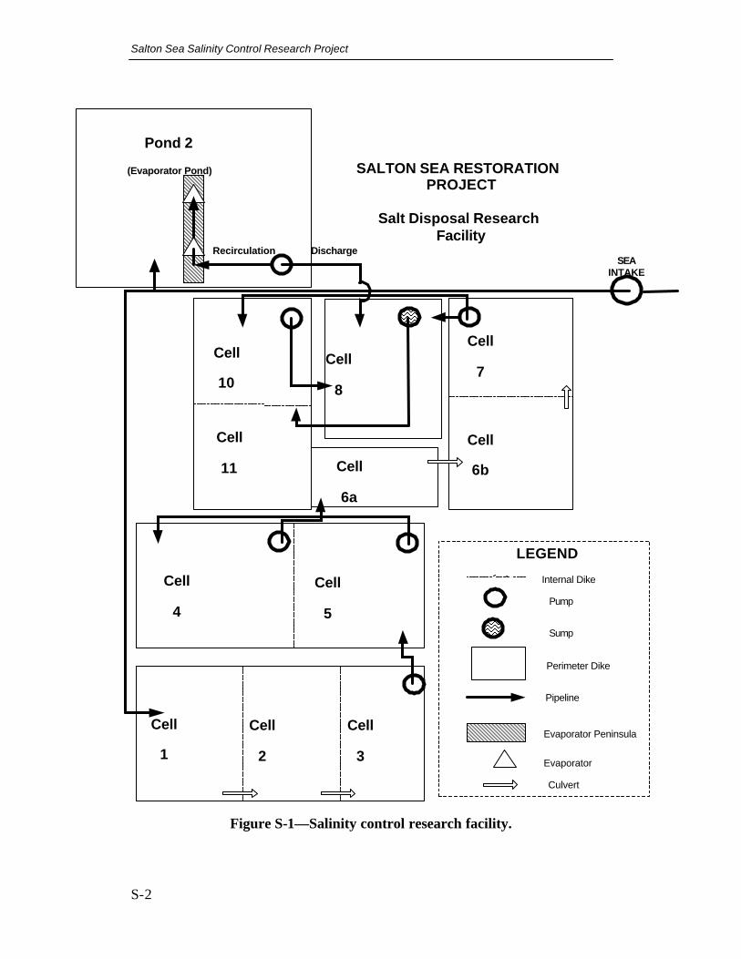
The project site included seven solar evaporation ponds used to concent rate Salton Sea water into saturated brine (cells 1 through 7). Two additional cells were used for salt disposal testing (cells 8 and 10), and one was used for bittern evaporating testing (cell 11). Figure S-1 shows a sketch of the salt disposal research facility.
Salton Sea Salinity Control Research Project
S-2
Figure S-1—Salinity control research facility.
`
SEA INTAKE
SALTON SEA RESTORATION PROJECT
Salt Disposal Research Facility
LEGEND
Pipeline
Evaporator Culvert
Recirculation Discharge
Cell
10
Pond 2
(Evaporator Pond)
Evaporator Peninsula
Perimeter Dike
Sump
Pump Internal Dike
Cell
11
Cell
8
Cell
7
Cell
6b Cell
6a
Cell
4
Cell
5
Cell
1
Cell
2
Cell
3
Salton Sea Test Base
S-3
The EES included two turbo-enhanced ground-based evaporators used for additional saturated brine production. One was a Mobile S30P evaporator complete with electric starter and controls by Slimline Manufacturing. The other was a Super Polecat evaporator with electric starter and controls manufactured by SMI Systems.
The disposal pond was lined with 40 mil plastic liner and included a 36- inch diameter sump that was 4 feet deep at the lowest point in the pond. Five 16-square feet core sampling pads were placed at intervals diagonally across the pond prevent damaging the lining when samples were taken.
Salton Sea water was pumped into both the EES pond (cell 2) and to cell 1 of the solar ponds through an intake system placed next to and in the Salton Sea. Two pumps were in a temporary pump house on shore.
Electricity was provided by Imperial Irrigation District.
Operating Procedures
Salton Sea water was discharged into the southwest corner of solar cell 1 (figure S-1). The Sea water intake facility provided for a maximum 400 gallons per minute (gpm) discharge to cell 1. Water then flowed by gravity over an adjustable pipe culvert through a dike into cell 2 and through another into cell 3. From there, a 120-gpm pump carried water to the southeast corner of cell 5. A 12-gpm pump moved water into cell 4. Another 120-gpm pump then moved water to the southeast corner of cell 6a with gravity flow through a culvert to cells 6b and 7. The specific gravity of the water in pond 7 was monitored to determine when the water needed to be moved to the disposal pond. The specific gravity of brine marking the need to move it to crystallizers was 1.20.
Cells 1 through 7 required continuous 24-hour-per-day movements of water. Once the target specific gravity was achieved in cell 7, then continuous flow of nearly saturated brine commenced into the disposal pond, cell 8.
Enhanced evaporation system devices were used in addition to using solar ponds to develop saturated brine. Two turbo-enhanced, ground-based EES units were operated in pond 2—depicted as triangles in figure S-1. Pond 2 was filled with Salton Sea water and then the EES units recirculated water as winds allowed until the water in the pond was nearly saturated. This water was then moved as a batch to the disposal pond.
Testing Procedures
The core samples extracted from the disposal test facility were tested by different procedures. X-ray diffractometry was used to detect and identify crystalline minerals, compounds, and materials, some of which are too small for microscopic analysis, and to estimate volume percentages.

Salton Sea Salinity Control Research Project
S-4
Electron bombardment of the sample using scanning electron microscopy (SEM) and its accompanying energy dispersive spectrometer (EDS) was used to analyze both crystalline and noncrystalline materials. SEM and EDS analyzed variations in crystal shape or surface textures, such as flaws and impurities, determined elemental composition of specific particles or areas, and determined the addition or depletion of certain elements in specific areas.
Another salt testing program quantified salt strength and stress-strain characteristics required to perform static and dynamic analyses of dikes constructed partly of precipitated salt. The dikes are required to contain liquid brine as salt precipitates. Stress-strain and strength characteristics of the salt are important parameters to stability analysis. If the salt and soil berm have inadequate strength, then any one of many possible failure planes would develop through the salt, resulting in dike failure.
Evaporation research was conducted using evaporation pans at the Test Base. Different evaporation pans with different waters and brines were maintained and tested. Concentrated brine and three different concentrations of magnesium were also tested.
Weather conditions were monitored continuously at the meteorological tower. Measurements were taken and stored every 15 minutes at 3 meters, 15 meters, and 45 meters above ground for wind speed and direction, temperature, relative humidity, rainfall, and dew point.
Results
X-ray Diffractometry
X-ray powder diffraction and grain mounts indicate that the salt is halite, NaCl, and bloedite, Na2 Mg (SO4)2 2H2O. Grain amounts of powdered samples immersed in refractive index compounds suggest that halite is usually the more abundant mineral; however, composite samples appear to be about 1:1 halite – bloedite.
Evaporation Rates
As the brine is concentrated, corresponding reductions in evaporation rates occur. This research developed the relationships of brine evaporation as a function of both time and concentration.
Brine evaporation as a fraction of fresh water evaporation varies as a function of percent weight magnesium. The fraction of fresh water evaporation decreases from 1.00 to below 0.60 as the percent weight of magnesium increases to 6 percent. As brine concentration increases, the evaporation rate levels off between 2 and 4 percent weight of magnesium. As concentrations increase, the evaporation rate decreases.

Salton Sea Test Base
S-5
The lowest evaporation rates apply to the highest concentrations and the lowest brine factors.
Salt Samples Materials Testing
One-dimensional consolidation test results indicate that upslope areas of the disposal pond would have slightly lower dry unit weights than downslope areas. On average, a dry unit weight of 98 pounds per cubic foot can be expected.
Observations made during consolidation tests suggest that several uncontrolled variables probably influenced test results significantly. These variables are temperature, evaporation, and ion exchange with brass testing equipment.
The observation suggests that salt in a saturated brine solution in the field will experience crystal growth and continuous solutioning and recrystallization when the brine solution is under pressure from the weight of overlying salt and undergoing continuous evaporation and temperature changes. The net effect would be a decrease in void space between crystals and greater matrix density. It is concluded that the salt samples obtained from shallow depths in the relatively dry evaporation pond probably do not reflect the conditions expected in deep, brine saturated salt fills. It is expected that salt in a deep evaporation pond would be much denser, less compressible, and not be composed of small individual particles.
Findings
Numerous problems were encountered at the Test Base in the operation of the solar ponds, the EES, and in operating the intake facility. A summary of those problems follows.
Salinity Control Project Design Issues
Problems observed at the Test Base project that will have an impact on the design and operation of any salt concentration and disposal facility include gypsum fouling, saturated brine pumping difficulties, and brine entrainment within the salt deposits. It was observed that bittern properties were not difficult to deal with and the evaporation to very near dryness is possible.
Gypsum fouling occurred in all closed conduits that carried brine around and between ponds. Salton Sea brines were also observed to precipitate gypsum in open ponds.
Large amounts of brine will be trapped below a thick surface crust in a disposal facility unless there are features designed to drain the material. The structural integrity of the salts will be substantially reduced without project features to drain the disposal facility. Draining entrained brines in the test disposal pond at the Test Base was accomplished via gravity flow to the lowest spot in the pond. The

Salton Sea Salinity Control Research Project
S-6
lowest portion of the pond was a concrete sump. Entrained brine drained very slowly over the course of a couple of months to achieve the level of dryness desired.
The heaviest brines produced at the Test Base were those left in the disposal pond sump after the EES pre-test that was conducted in 2001. This test produced a thin layer of salts in the disposal pond and the quantity of entrained brines was relatively small. These brines drained towards the sump, where they evaporated over a period of months. These highly concentrated bitterns were pumped to the pond cell. The bitterns were moved before new saturated brines were pumped into the disposal pond from EES and solar ponds. Over a period of weeks, nearly all the bitterns were evaporated and precipitates were formed. Although not completely dry, and when mixed with the blowing sands that are omnipresent at the Test Base, the materials were more of a firm mud with an oily consistency than a liquid state. The final characteristics of the bitterns did not change beyond this muddy-like consistency.
EES Problems and Issues
Problems observed at the Test Base project that will have an impact on the design and operation of EES based salt concentration include gypsum and biologic fouling. Following are discussions and recommendations related to these issues.
Significant gypsum fouling occurred in all closed conduits that carried brine around and between ponds, including pumping water to EES units. A large EES project would include many miles of such pipe, and fouling of these would be impossible to avoid without significant pretreatment to remove calcium prior to pumping through the system. At the Test Base, there was no pretreatment and the nozzles on the units plugged regularly with gypsum. The nozzles had to be cleaned and/or replaced daily.
Brine fly populations were very large in the EES test pond. As a result, these flies and brine fly larvae were perpetually picked up by the pump. Two inline filters had to be installed before the EES units could remove this biologic material. Without the filters, the nozzles on the EES units plugged up. The inline filters had to be cleaned numerous times per day to keep the units in operation.
Mist fouling of the evaporators was a major problem. Any winds at all from a nonaligned direction resulted in mist surrounding the units, and much of it was sucked into the impellers of the turbo fans. Left unattended, enough mist could be digested into the units to force the impeller blades out of balance. The devices had to be shut down every couple of days and pressure washed both inside and outside of the housings. This process was time consuming and was an endless task in the course of project operations.

Salton Sea Test Base
S-7
Intake Facility Problems
The Salton Sea is home to an extremely large and healthy barnacle population. Infestation was observed on both interior and exterior components of the submerged intake structure.
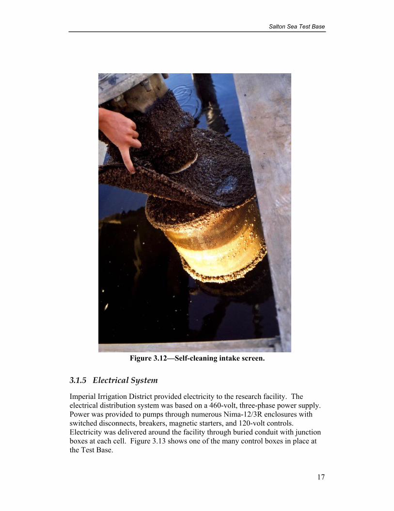
The fish screen removed from the water depicts significant fouling after operating for only 2 months. The screen had stopped turning and barnacles had attached and grown over the nozzle jets that facilitate the rotation of the screen, resulting in reduced flow rates and pressures being delivered through the nozzles. The screen and intake structure had to be serviced weekly to keep the screen in operation.
The intake pipeline became almost completely choked with barnacle growth within 3 months after the project began pumping Sea water to the Test Base ponds. An alternate intake pipe with an attached fish screen had to be constructed. Clearing the main intake pipe was difficult and time consuming.
To alleviate the problem of barnacle fouling of the intake screen and pipeline, a Radiant Energy Forces (REF) Barnacle Removal System was provided by Water Savers Worldwide. The system was provided for testing purposes. The system worked effectively to discourage barnacle growth within the pipe and on the screen; however, loose barnacle shells settled continuously in the lowest elevations of the pipeline. Back flushing every few months resolved the problem.
Electrical failures occurred several times during the research project, which resulted in the loss of prime on the intake pump. Priming with a manual diaphragm pump was possible only through strenuous labor because the intake pipe was 600 feet long.
Cavitation of both the intake and fish screen flushing pumps occurred often throughout the beginning stages of the project because the pressure in the intake line was, at times, below the vapor pressure of the fluid being pumped. To alleviate this problem, a degassing column was constructed on the intake pipe. The gasses that were being generated under these low pressures were removed under a vacuum generated from the flushing pump discharge line. The column substantially reduced cavitation in both of the pumps and facilitated a pump life beyond the project duration
Micro-Climate Effects
Because of the scope and scale of the Test Base project, it was not possible to study the potential for micro-climate changes due to large-scale EES operations on efficiency and costs. With hundreds of these devices in operation, it would seem logical that base evaporation rates would decline because of increased humidity. These effects are anticipated to be significant, and additional research would be required before consideration could ever be given to applying EES technologies at the Salton Sea.

Salton Sea Salinity Control Research Project
S-8
Recommendations
The production and disposal of salts from a salinity control project at the Salton Sea should take into consideration lessons learned at the Test Base. Recommendations follow.
Disposal System
Pumping saturated and/or nearly saturated brines will require special attention and should be avoided. Enough Salton Sea water or fresh water needs to be injected to break the saturation of the brine being transported to avoid precipitation of salts within the pumps and pipes.
Saturated and nearly saturated brines should be moved with gravity flow in open canals and ditches that can be oversized and excavated to control gypsum fouling. The disposal facility should be placed near the salt concentrating project or near the final stages of the concentrating features. If pumping is unavoidable, it should be done over short distances, and the pipelines will have to be cleaned regularly. The pipelines will have to be designed for a much greater capacity and eventually will have to be replaced.
If on-land disposal is a consideration for salt extracted from the Salton Sea, then it is recommended that the disposal facility be divided into four separate cells. This would allow one cell to be drained of entrained brines while the other three cells continue to receive saturated brine and precipitate salt. Once an idle cell is drained, it should be mechanically consolidated to decrease the porosity and, subsequently, increase the density of the salt deposits. Once the deposits are consolidated, the idle cell would be put back into rotation to receive saturated brine from the concentrating features of the project. Another one of the active cells would then be idled, drained, and consolidated. This rotation process would continue endlessly among the four disposal cells. The draining process would take numerous months.
Entrained brines from the idle cell that are being drained and pumped would have to be extracted using fresh or Salton Sea water injection at the pump intakes, which would significantly reduce salt deposits from severely fouling the pumps and pipelines. The pumps and pipes would have to be cleaned at least once a day with fresh water that would dissolve the deposits. The brines extracted from the idle cell should be discharged into the active cells. The cells that are receiving saturated brine should receive the brine in parallel and not in series.
Sump facilities would have to be maintained in each of the four disposal cells. Additional sump culverts would have to be installed as deposits increase in depth through time. Periodic flushing of the sumps with fresh or Salton Sea water will keep the sumps clear of salt deposits.
The method of construction for the embankments around the disposal cells must include consideration of the results of the materials testing results presented

Salton Sea Test Base
S-9
herein. At the present time, no assessment of these testing results has been made and no recommendation can be made as to which method of construction is preferable.
Bittern management will not have to be considered in a salt deposit disposal project. The very small quantities of bitterns will be entrained in the final salt deposits during the course of operating a facility, as described above. Bitterns are defined as those brines that will be impossible to evaporate and will be very small in volume.
Enhanced Evaporation System
To alleviate gypsum fouling problems in the use of enhanced evaporators, it will be necessary to remove the calcium in the Salton Sea water before delivery to the distribution system. This would be required even with a single pass sys tem whereby Salton Sea water was delivered directly to the evaporators.
Filtering brine fly larva and brine flies would be necessary before distribution to the EES units. Experiences gained at the Test Base project indicate that the loading of brine flies can be large enough to foul the nozzles on the units. This foulding results in significant reductions in efficiency of the units along with increased energy costs.
To reduce the possibility but not completely eliminate the risk of mist digestion by the EES units, it would be necessary to robotically slave each of the EES units to multiple wind direction, wind speed, and wind shear detection systems. Any fouling by mist digestion by a significant number of EES units would be very expensive and time consuming to clean up. For a project forecasted to include hundreds, if not thousands, of these units, such a cleanup event would require thousands of hours of labor.
Based on experience gained in the operation of EES units at the Test Base, it would be necessary to space the devices at least 250 feet apart in long rows. Salt and/or mist from the evaporators can travel 1,300 feet. Therefore, the rows of evaporators should be placed at least 1,300 feet apart. The ideal configuration would be to place the units in long rows over a large pond. The system should be designed to shut down anytime the winds exceeded 10 miles per hour.
Efficiency of the EES units compares performance to a solar pond facility without EES blowers. The energy costs are representative of the operation of the Slimline enhanced evaporators.
One test was performed to monitor time to saturate 3 million gallons of Salton Sea water. This test was run during the winter between December 31, 2001, and April 11, 2002, using both the SMI and Slimline evaporators. It took 102 days for the 3 million gallons to come to saturation and resulted in 198,000 gallons of saturated brine. Operating EES units to concentrate 3 million gallons of Salton Sea water during this time period resulted in a cost of $8,350.

Salton Sea Salinity Control Research Project
S-10
This test produced 526 tons of salt in saturated brine and evaporated 8.6 acre-feet of water. To remove 1 million tons per year would require 719 EES units, assuming a Test Base pond size ratio of 2.5 acres per unit. The project would require 111,800,000 kilowatt-hours of electricity and $10,450,000 to concentrate a million tons of salt in Salton Sea water to saturated brine.
The efficiency of the evaporators can be measured in comparison to solar pond project without evaporators. Based on the climate conditions that occurred during the period of EES testing at the Test Base, and on the results of the testing, it can be concluded that placing two evaporators on a 5-acre pond can increase evaporation and salt production by 44 percent over a sole 5-acre solar pond.
The efficiency and cost studies presented herein are based on the assumption that the evaporators could be operated 63 percent of the time, as was possible for the December 31, 2001 to April 11, 2002 test. The analyses were also dependent on the power usage and costs associated with the pumps and evaporators used at the Test Base. Other equipment would certainly yield different results.
Sea Intake Structure
Future intake structures at the Salton Sea would be much easier to maintain and to operate if they were shoreline based. Elements of such a system would include a shoreline stilling basin with a dredged trench from the basin, located a significant distance into deep water in the Sea. Intake pumps could then extract water from the shoreline basin without the need for a long and difficult-to-maintain pipeline. Fish screens, however, would still be necessary.
Parametric Study Proposal
A parametric study is proposed that develops first and second order relationships between time, temperature, pressure, and salt density. The behavior of solid salt under load is dependent on time, temperature, pressure, mineral content, liquid brine chemical composition, and ion and vapor exchange with the surrounding environment. Mathematical expressions are sought to predict salt strength and density in terms of the above-mentioned variables, to evaluate the stability of retention pond dikes and to improve estimates of the expected capacity of evaporation ponds.

1
1 Introduction This report presents the findings of the Salton Sea Salinity Control Research Project (Research Project) that the Bureau of Reclamation and the Salton Sea Authority conducted at the Salton Sea Test Base from July 2000 until July 2003. This research was undertaken to further understand the use of solar ponds and enhanced evaporation system (EES) technology to evaporate Salton Sea water, as well as to understand the issues related to disposing of the salt deposits that likely would be produced from using these systems. The Salinity Control Research Facility is located along the southwest shore of the Salton Sea on the former Navy Salton Sea Test Base (SSTB), Imperial County, California (see frontispiece map figure 1.1).
2 Objectives A Salton Sea Reclamation Project could require design and construction of a disposal facility to accept salt produced from a salt export project. The term “export” is used to represent the removal and evaporation of Salton Sea water from the Sea for the purpose of reducing salinity levels in the Sea. Many questions are answered herein relative to the physical and chemical properties of the salts that might be produced in a prototype disposal pond. Answers to these questions could help provide data needed to design the proposed disposal facilities. Figure 2.1 presents a layout of the solar pond complex (cells 1 through 11) and the EES ponds at the SSTB project site.
2.1 Objectives of Disposal Pond Research
Solar ponds and ground-based turbo EES were operated during the course of the Research Project, which produced hundreds of thousands of gallons of saturated brine from which salts were crystallized in a small-scale disposal facility. The objective of saturated brine production was to develop salt deposits that are representative of those that might be expected in a full scale salinity control project. Physical and chemical analyses were performed on the salt deposits to obtain information that could potentially be used for disposal facility design.
Much concern existed within the Salton Sea Reclamation Study team that the permanent placement of salt solids is only a portion of the disposal problem. Salt production experts had provided a mixed set of opinions on whether bittern will be produced from solar extraction of salts from Salton Sea water. In addition there are no consistent definitions of bittern. For the purpose of the Research Project, bittern was then defined as brine waters that are physically impossible, if not impossible, to evaporate, and which remain at the end of salt crystallization in solar ponds at the Salton Sea.

Salton Sea Salinity Control Research Project
2
Figure 2.1—Salinity control research facility.
`
SEAINTAKE
SALTON SEA RESTORATION PROJECT
Salt Disposal Research Facility
LEGEND
Pipeline
Evaporator Culvert
Recirculation Discharge
Cell
10
Pond 2 (Evaporator Pond)
Evaporator Peninsula
Perimeter Dike
Sump
Pump Internal Dike
Cell
11
Cell
8
Cell
7
Cell
6b Cell
6a
Cell
4
Cell
5
Cell
1
Cell
2
Cell
3
Peninsula
North

Salton Sea Test Base
3
2.2 Objectives of Evaporation Research
Evaporation of Salton Sea brines at different concentrations will be important in designing a reclamation project at the Salton Sea. The collection of brine evaporation data is a difficult operation. To develop preliminary information, Reclamation conducted brine evaporation research in its environmental facilities at Denver, Colorado. This research did not consider effects due to wind, humidity, and temperature changes that occur seasonally. To further study the effects of these factors on evaporation of brines at varying concentrations, the Research Project included a study of evaporation under real-time weather conditions. Agrarian Research conducted a similar study, using sunken Class A pans[4]. At the Test Base, the research was conducted using standard raised Class A pan techniques. Figure 2.2 depicts the Class A pans in place at the Test Base. Evaporation rates are expected to be different at the east and west locations of the Salton Sea. The Agrarian site developed evaporation data for the east side and the Test Base project will develop data for the west side of the Salton Sea.
Figure 2.2—Class A pans for brine evaporation studies.
Designing a disposal facility as part of a salinity control project will require an understanding of the way evaporation rates will reduce with magnesium (Mg) concentrations as high as 9 percent. Evaporation rates of brines with high concentrations of Mg will control the size of the disposal facilities. If the surface areas are too small, then it will be impossible to achieve the throughput of water required for adequate salinity control within the Salton Sea. This information is,

Salton Sea Salinity Control Research Project
4
therefore, the most important requirement for successful design of a salinity control project.
2.3 Objectives of Weather Research
Climate conditions at the Salton Sea are variable, with significant variations in temperatures, relative humidity, wind speed, and direction. In addition, these same parameters vary by altitude. A 50-meter high meteorological tower was installed at the Test Base about 200 yards away from the shore of the Salton Sea. Figure 2.3a shows the tower and related equipment, and figure 2.3b shows the location. Data were collected in real time at heights of 3, 15, and 45 meters above ground level. Measurements are taken at 15 -minute intervals of:
• Temperature • Relative humidity • Wind speed • Wind direction
Figure 2.3a—Meteorological tower and related equipment.
3 Research Methods This section describes the facilities and materials that were used, how the systems were operated, and the laboratory tests performed. The basic systems are the solar evaporation ponds, the enhanced evaporation systems, the disposal pond, and the Salton Sea intake structure.


Salton Sea Test Base
5
3.1 Facilities
For accuracy of project findings, all ponds were lined with 40-millimeter thick polyvinyl liner. The liner prevented loss due to seepage of water into the soils beneath the ponds, which in turn allowed for evaporation only readings. Figure 2.1 presents a layout of the solar pond complex (cells 1 through 11) and the EES ponds at the SSTB project site. Figure 3.1 is a picture of several of the cells that make up the solar pond complex. Salton Sea water was discharged into the southwest corner of cell 1. The Salton Sea water intake facility provided a maximum 400 gallons per minute (gpm) discharge to cell 1. Water then flowed by gravity through an adjustable pipe culvert, through a dike into cell 2, and through another dike into cell 3. From there, a 120-gpm pump pumped water to the southeast corner of cell 5. A 120-gpm pump then moved water from cell 5 into cell 4. From there, a 120 gpm pump moved water to the southwest corner of cell 6a, with gravity flow through a culvert to cells 6b and 7. The specific gravity of the water in cell 7 was monitored to determine when water was to be moved to the disposal pond or crystallizers (cells 8 and 10). The specific gravity of brine,
Figure 3.1—Cells 6b and 7 of solar ponds.
Salton Sea Salinity Control Research Project
6
marking the need to move it to the crystallizers, was 1.20. Based on the research at the Agrarian solar pond facility, it was expected that crystallization of salts would begin above specific gravity of 1.21.
Cells 1 through 7 required continuous 24-hour-per-day movements of water. Once the target specific gravity was achieved in cell 7, then continuous flow of nearly saturated brine commenced into the disposal pond (cell 8).
3.1.1 Solar Evaporation Ponds
The Research Project involved the operation of solar ponds to produce saturated brine waters from which salts were crystallized to form enough material to perform both physical and chemical analyses of salt deposits. The objective was to develop deposits that are representative of those expected in a full-scale Salton Sea export project. The saturated brines collected from the solar ponds were combined with those produced from EES devices that were also operated at the project site. The intent was to produce 6 to 18 inches of salt deposits within the shortest time possible, to obtain design information for a disposal facility.
3.1.1.1 Surface Areas
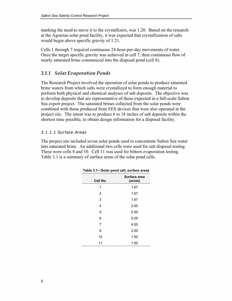
The project site included seven solar ponds used to concentrate Salton Sea water into saturated brine. An additional two cells were used for salt disposal testing. These were cells 8 and 10. Cell 11 was used for bittern evaporation testing. Table 3.1 is a summary of surface areas of the solar pond cells.
Table 3.1—Solar pond cell, surface areas
Cell No. Surface area
(acres)
1 1.67
2 1.67
3 1.67
4 2.00
5 2.00
6 0.25
7 4.00
8 2.00
10 1.50
11 1.50

Salton Sea Test Base
7
3.1.1.2 Hydraulic Features
Figure 2.1 depicts an overview of the solar pond cell configurations. Table 3.2 presents a list of flow “to/from” cells as well as the hydraulic features used to move water between cells. Pumping transports water between major ponds through flexible hoses, as shown in figure 3.2. Water is moved between most cells by gravity through pipes, as shown in figure 3.3. All water moved by pumping is metered, as shown in figure 3.4 using either analog or digital flow meter.
Table 3.2—Solar pond and cell hydraulic data
Cell No. Flow from
cell No.
Gravity flow
to cell No.
Metered pump flow to
cell No.
Pipe diameter
(in)
Initial Pump type
Peak pump capacity
(gpm)
Salton Sea — 1 10-inch and 8-inch combination poly pipe
7.5 hp cast iron centrifugal pump
250
1 Salton Sea 2 — 6-inch PVS SCH 40
— —
2 1 3 — 6-inch PVS SCH 40
— —
3 2 — 5 3-inch suction discharge hose
2 hp Zolar effluent sump pump
148
4 5 — 6 3-inch suction discharge hose
2 hp Zolar effluent sump pump
148
5 3 — 4 3-inch suction discharge hose
2 hp Zolar effluent sump pump
148
6 4 7 — 6-inch PVS SCH 40
— —
7 6 — 10 6-inch poly pipe ¾ hp TEEL stainless steel, close-coupled pump
45
10 7 — — 3-inch suction discharge hose
¾ hp TEEL stainless steel, close-coupled pump
45
hp = horsepower

Salton Sea Salinity Control Research Project
8
Figure 3.2—Pumping between major ponds.
Figure 3.3—Gravity flow between cells.

Salton Sea Test Base
9
Figure 3.4—Metering of flow from Sea intake and between ponds.
3.1.2 Enhanced Evaporation Systems
Enhanced evaporation system devices were used in addition to using solar ponds to develop saturated brine. Two turbo enhanced EES units were operated in cell 2 depicted as triangles in figure 2.1. Cell 2 was filled with Salton Sea water and then the EES units re-circulated water as winds allowed until the water in the pond was nearly saturated. This water was then moved as a batch to the disposal pond (cell 8). Figure 3.5 shows the EES units in operation.
Two turbo-enhanced evaporators were used at the research facility for additional saturated brine production. These units were from the following manufacturers.
• Mobile S30P evaporator, complete with electric starter and controls (Slimline Manufacturing).
• Super Polecat evaporator, with electric starter and controls (SMI Systems).
Figure 3.6 is a photograph of the Slimline unit, and figure 3.7 is a picture of the SMI Polecat, both in place on the peninsula of the EES pond (cell 2).

Salton Sea Salinity Control Research Project
10
Figure 3.5—Enhanced evaporators in operation.
Figure 3.6—Slimline S30P evaporator.

Salton Sea Test Base
11
Figure 3.7—SMI Polecat Evaporator.
3.1.2.1 Pond Configuration
The EES pond (cell 2) is 5 acres in surface area and includes a peninsula in the center of the pond, as shown in figure 2.1. This peninsula served as the platform on which the two evaporators were operated.
3.1.2.2 Pumping Facilities
The two evaporators received a combined metered flow rate of 120 gpm peak flow at 115 pounds per square inch (psi) from a 20-horsepower (hp) centrifugal pump through 1.5-inch diameter pressure hose. Water was pumped from the lowest portion of the pond through the units. Water sprayed out from the devices, so that a portion was evaporated and a portion fell back to the pond. The water was recirculated through the evaporators until the brine was nearly saturated.
3.1.2.3 Wind Control
The air quality permit to operate the evaporators required that the devices be shut down any time the wind speeds reached 15-minute average wind speeds of 21 miles per hour (mph) or greater; however, it was found to be more beneficial to the operation if the equipment was shut down when 15-minute average wind speeds reached 10 mph or greater. The meteorological tower was equipped with a controller that sounded a siren whenever the wind speed was 10 mph or greater.

Salton Sea Salinity Control Research Project
12
The site operator would then shut the systems down. A beep tone was sounded once the winds dropped below 10 mph for an extended period. The operator would then place the evaporators back into operation.
3.1.3 Disposal Pond
The conceptual design of an on-land salt disposal facility has been made. This concept involves the construction of shallow solar-evaporation ponds impounded by earthfill dikes. These earthfill dikes would probably involve the construction of a starter dike, followed by the construction of additional dike raises after the initial pond filled with salt. The dike raise(s) would use the center-raise design and construction approach, in which the dike centerline remains fixed and most of the raised dike’s earthfill is constructed on the crest and on the downstream slope of the lower dike(s). This approach minimizes the amount of earthfill required and maximizes the stability of the dike section, compared to the upstream-raise and downstream-raise concepts. The center-raise dike configuration is shown later in this section.
In the center-raise design, the upstream portion of the raised dike would be constructed on top of the salt pond material, creating a “christmas-tree” interface between the upstream edge of the dikes and the downstream edge of the salt pond material. The salt pond material would probably form part of the foundation for the upstream portion of the dike raises. Because of its function as part of the dike(s) foundation, the engineering properties and other characteristics of the salt pond material need to be determined or estimated. Hence, the best approach would be to obtain some Salton Sea salt pond material and perform the appropriate tests to determine its engineering properties and other characteristics.
A test disposal pond was constructed and operated at the Salton Sea Test Base. Although dike raises were not constructed at the site, the test disposal pond provided utility study of the characteristics and engineering properties of salts that would be deposited in a full scale project.
3.1.3.1 Pond Configuration
The disposal test pond (cell 10) was 2 acres in surface area and included a 36-inch-diameter sump that is 4 feet deep at the lowest point in the pond. Figure 3.8 depicts the disposal pond looking towards the sump. The salt shown in the pictures was deposited during the 700-hour pretesting of the enhanced evaporators performed in 2001.
3.1.3.2 Pumping Facilities
A small ¼-hp sump pump, with 1-inch hose attached, was placed in the bottom of the sump to extract bittern from the pond. Brines pumped from the sump were discharged to cell 11.

Salton Sea Test Base
13
Figure 3.8—Disposal pond after pretesting EES evaporators.
3.1.3.3 Core Pads
The extraction of cores for materials testing of the salt products was an intrusive operation that ran the risk of damaging the disposal pond liner. To eliminate this risk, five 16-square foot pads were constructed of 1.5-inch-thick, 8-inch by 16-inch paving stones. The core pads were placed at about 25 foot intervals along a diagonal line through the pond. Numerous cores were extracted using specialized drilling techniques described later in the research plan. Core pads were placed as shown in figure 3.9 in locations that would provide core samples representative of shallow and deep brine deposits both near and far away from the edges of the disposal pond. Figure 3.10 is a schematic, showing the locations and numbering of the pads. It was expected that significant differences in structural characteristics of the deposits would be identified as a result of these pad placements.

Salton Sea Salinity Control Research Project
14
Figure 3.9—Disposal pond core sampling pads.

Salton Sea Test Base
15
SUMP
1
2
3
4
5
6
7
NotUsed
North
25 F
eet
Salton Sea Test Base Disposal Pond
Cell 10
Core Pad Locations
US Bureau of ReclamationNot Drawn to Scale
Figure 3.10—Disposal pond core pad locations and numbering scheme.
Salton Sea Salinity Control Research Project
16
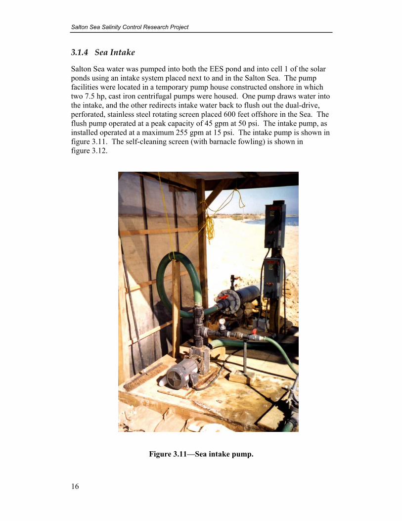
3.1.4 Sea Intake
Salton Sea water was pumped into both the EES pond and into cell 1 of the solar ponds using an intake system placed next to and in the Salton Sea. The pump facilities were located in a temporary pump house constructed onshore in which two 7.5 hp, cast iron centrifugal pumps were housed. One pump draws water into the intake, and the other redirects intake water back to flush out the dual-drive, perforated, stainless steel rotating screen placed 600 feet offshore in the Sea. The flush pump operated at a peak capacity of 45 gpm at 50 psi. The intake pump, as installed operated at a maximum 255 gpm at 15 psi. The intake pump is shown in figure 3.11. The self-cleaning screen (with barnacle fowling) is shown in figure 3.12.
Figure 3.11—Sea intake pump.
Salton Sea Test Base
17
Figure 3.12—Self-cleaning intake screen.
3.1.5 Electrical System
Imperial Irrigation District provided electricity to the research facility. The electrical distribution system was based on a 460-volt, three-phase power supply. Power was provided to pumps through numerous Nima-12/3R enclosures with switched disconnects, breakers, magnetic starters, and 120-volt controls. Electricity was delivered around the facility through buried conduit with junction boxes at each cell. Figure 3.13 shows one of the many control boxes in place at the Test Base.

Salton Sea Salinity Control Research Project
18
Figure 3.13—Electrical control box for enhanced evaporators.
3.2 Operating Procedures
3.2.1 Solar Pond Procedures
Operating procedures for the solar ponds at the Salton Sea Test Base are described in the following sections.
3.2.1.1 Flow Maintenance
The maintenance of flows within the solar ponds was based on downstream control at cell 7. The objective was to maintain cell 7 at a static water surface elevation representative of about 300,000 gallons of storage that would, once equalized, provide for a continuous feed of saturated brine into the disposal pond, while at the same time receiving an identical amount of supply from cell 6. The stage at the lowest point in cell 7 was maintained at about 36 inches. The discharge from the Salton Sea intake to cell 1 was monitored with respect to the water demands at cell 7 and the brines in storage and in transit among the other

Salton Sea Test Base
19
cells. The feed to cell 1 varied from about 10 gpm to 100 gpm, depending on the time of year of operation.
3.2.1.2 Daily Specific Gravity, Magnesium, and Temperature Measurements
It was necessary to measure and record specific gravity and temperature from each of the ponds daily. The measurements were taken consistently within a few hours of each other; for example, between 8:00 a.m. and 10:00 a.m. each morning. It was not necessary to take the measurements at exactly the same time each day. Specific gravity and temperature measurements were made using an Anton Par digital density meter. Specific gravity measurements will be adjusted to 23 degrees Celsius. The measurements were reported daily onto field data sheets and then entered into an Excel spreadsheet, so that specific gravity profiles throughout the pond system will be developed. Each day, brine samples from the disposal and EES ponds and from cell 7 were evaluated for percent weight of magnesium. The specific gravity of brine will eventually level off as concentrations increase beyond saturation. Tracking changes in concentration by specific gravity is not accurate. Tracing concentration by percent weight of magnesium was a reliable method.
3.2.2 Enhanced Evaporation System Procedures
3.2.2.1 Pond Filling
The EES pond was filled in batches of 2 million to 3 million gallons directly from the Salton Sea intake system. Beginning and ending total cumulative flow measurements were taken from the EES pond intake meter.
3.2.2.2 Recirculation Plan
Water was recirculated through the evaporators until the specific gravity of the brine in the EES pond reached 1.2, which is just before the point where saturation and subsequent crystal formation will begin. The brine was discharged through in-line filters prior to entering the evaporators to remove organic materials, such as brine-fly larvae and brine-shrimp. In addition, the filters forced the formation of some gypsum (CaSO4) prior to discharge through the nozzles, which significantly reduced clogging problems. The small gypsum crystals formed in the turbulence caused by the filters passed through the filters and nozzles. However, gypsum fouling was not eliminated. Filtering only slowed the fouling down. The brine was recirculated with the evaporators elevated at angles away from each other to reduce drift to the surrounding area and to the evaporators themselves.

Salton Sea Salinity Control Research Project
20
3.2.2.3 Brine Chemistry Verification
Before the saturated brines produced by the EES units were mixed in the disposal pond with the saturated brines from the solar ponds, it was necessary to verify that the brines were chemically identical. The procedures used were consistent with the approach being taken by Agrarian Research for the East Side Solar Pond Project, located near Niland. It was fully expected that the brines would be identical. Once it was verified that the brines were identical, the EES-generated brines were transferred to the disposal pond in conjunction with continuous feeds of saturated brine from cell 7 of the solar ponds.
3.2.2.4 Saturated Brine Handling
The nearly saturated brine from the EES pond was pumped to the disposal pond using a 6-hp gasoline-powered, plastic trash pump that had a pumping capacity of about 200 gpm. The pumped brine was metered, and beginning and ending meter readings were recorded. Oil changes within the pump engine were made after every 5 hours of use.
3.2.2.5 Energy Usage
Energy usage of the EES units was not metered for most of the project life. However, usage was metered when EES efficiencies were studied in greater detail in the later phases of the project. Metering was not required over the entire period of the project because energy use by the devices was constant from hour to hour. The collected usage data were applicable to extrapolation over any period of use.
3.2.2.6 Wind Monitoring and Operations
The EES units were operated 24 hours per day, or whenever the winds were blowing below 10 mph. During the winter and spring, the hours of operation likely were more limited by wind speed than they were during other times of the year. A siren sounded on the meteorological tower whenever the winds exceeded 10 mph. This signaled the operator to shut down the EES systems. A beep tone sounded at the tower whenever the winds dropped below 10 miles per hour for 15 sustained minutes. The operator agreed to accommodate the tower signals 24 hours per day so that operating hours could be maximized.
3.2.2.7 Core Drilling
The drill used in core removal was a Hilti model DD250 E stand-type drill. The drill bits used were 6-inch inner diameter, and were also manufactured by Hilti. The bits were of the impregnated type. A special cart was constructed to serve as drill platform. This cart was constructed with pneumatic tires and four hand jacks. Weight was added to the platform using sand bags to allow for adequate

Salton Sea Test Base
21
pressure for stabilization purposes. The platform and drill are depicted in figure 3.14.
Figure 3.14—Core drill and platform.
3.2.2.8 Operations Logs
Logs were kept of the operating start and stop times of each EES unit. In addition, records were kept of the electrical loading of the equipment.
3.3 Testing Procedures
3.3.1 Phased Testing Approach
A phased testing approach was used for the project. It included three testing phases (tests 1, 2, and 3) that were implemented, depending upon the results of

Salton Sea Salinity Control Research Project
22
the previous test (excluding test 1). Test phases 1 and 2 were implemented during this research project. The results of these tests are presented in this report.
For simplicity, the following tests are described as though only cell 7 would be providing saturated brine. Wherever a reference is made to pumping saturated brine from cell 7, it can be inferred that this also means from the EES Test Pond.
3.3.1.1 Test 1
The first test (test 1) involved crystallizing salts in a single cell until the evaporation rate within the cell became hindered by increased concentrations of magnesium (Mg) and potassium (K). These are the two most soluble ions within Salton Sea water. The disposal pond (cell 8) was used for test 1. It is possible that all salts could be disposed of in a small number of disposal cells without the need for large, permanent bittern ponds. However, it was anticipated that the evaporation rate in a single cell would decline through time. Evaporation was monitored closely via accurate measurements of brines as they moved throughout the pond systems.
Undesirable evaporation rates at the crystallizer pond were obvious from a reduction of discharges into the crystallizer pond, compared to brine production throughout the concentrators. Once the evaporation rate was deemed problematic, water was removed from the sump at the lowest point in the pretest pond to the farthest southeast portion of cell 11. At that time, the chemistry of the brine moved to cell 11 was analyzed with special attention given to noting what percent of magnesium the sample contained. Once in cell 11, the bittern was allowed to evaporate until dry, while evaporation rates were again restored in cell 8, which continued to receive brine from cell 7. It was possible that the evaporation rate would not become problematic and that evaporation to dryness could occur unimpeded within the disposal pond. If this happened, the bittern entrained in the pores of the salt crystals would be pumped from the sump in cell 8 to cell 11, where observations were made to see if the bittern evaporated to dryness.
3.3.1.2 Test 2
If it was observed that the bittern in cell 11 was not evaporating, then test 2 would be implemented. Discharges to cell 8 would stop, and water would be allowed to evaporate until magnesium was the same percentage it was when evaporation became problematic (if at all) in cell 8 in test 1. At this time, as much as possible of the bittern would be removed from the sump to cell 11. Cell 8 would then be allowed to evaporate to dryness. This set the stage for the primary purpose of test 2. In the mean time, saturated brine from cell 7 was placed in cell 10, where salt crystallization continued as before in cell 8. Once cell 8 reached its steady state, where no further brine was left to evaporate, the bittern in cell 11 was pumped onto the solids in cell 8. The purpose of the test is to see whether the heavy bittern would percolate into the salt pavement, subsequently mixing with the pore waters between salt crystals. Because the pore water was likely to be

Salton Sea Test Base
23
saturated with sodium chloride and sodium sulfate, which was less soluble than the magnesium-rich bittern, the result should be additional precipitation of salts involving sodium, sulfate, and chloride. This would result in denser pavement of salts, which would be more desirable from both strength of materials and reduced disposal volume. The resulting pavement should still contain magnesium-rich bittern in the form of pore waters. If this method worked, it would likely be the preferred method of bittern disposal. If this method failed, then the stage was set for test 3.
3.3.1.3 Test 3
This test involved alternating the destination cell of saturated brine from cell 7 between cells 10 and 8. During test 2, saturated brine was placed in cell 10. Under test 3, this ceased, and cell 10 was allowed to evaporate without removing bittern. Saturated brine from cell 7 was placed onto the pavement in cell 8. Complete precipitation to solids might not occur in cell 11, possibly resulting in large amounts of pore waters, softer salts, and, subsequently, a less dense pavement. Once evaporation stopped or became slow in cell 10, then saturated brine from cell 7 was placed on top of the soft pavement in cell 10, with the purpose of crystallizing denser salts in a stratified fashion. The purpose was the consolidation of the materials below. If this test were deemed necessary, it would likely require operation of the Disposal Pilot Project in a second year. This alternating process could be repeated numerous times, resulting in stratified disposal materials.
3.3.2 Disposal Test Facility Procedures
3.3.2.1 X-Ray Diffractometry
Salt crystals removed from the core samples taken from the disposal pond were identified using X-ray Diffractometry. X-ray bombardment of the prepared sample surface allows the detection and identification of crystalline materials. Samples can be foundation rock, soil, riprap, concrete, Portland cement grout, and compounds and materials such as precipitates, cement, pozzolan, stains, scales, coatings, paint pigments, sludge, filter residues, organics, corrosion products, metals, and alloys. X-ray diffraction analysis is a nondestructive method (sample may be reanalyzed) performed on a representative sample of submitted material that may consist of the entire sample, a portion adjacent to a thin section, or a split sample. The sample is ground to an impalpable powder and packed into a sample holder. During analysis, a spectrum is produced, exhibiting peaks that correspond to the diffraction lines of the minerals present in the sample. The minerals are identified by the presence of characteristic peaks, and their volumetric amounts are roughly estimated by heights of certain peaks. By using the X-ray diffractometer to examine representative samples, the petrographer can identify crystalline minerals, compounds, and other materials, some of which are too small for microscopic analysis, as well as estimate volume percentages. X-ray

Salton Sea Salinity Control Research Project
24
diffraction analysis cannot determine noncrystalline (amorphous) materials; detect low volume percentages of certain common minerals, such as pyroxene; identify some minerals if present in only trace or minor amounts; or determine texture, fabric, structure, or physical properties of materials. Quantification only approximates volume percentages of minerals present.
3.3.2.2 Scanning Electron Microscope
In scanning electron microscopy (SEM), electron bombardment of the sample produces images with magnifications up to 200,000 times. The instrument and its accompanying energy dispersive spectrometer (EDS) can be used to analyze both crystalline and noncrystalline materials.
Scanning electron microscopic analysis is performed on a representative sample of material that may consist of the entire sample or a split sample. The Petrographic Laboratory’s SEM is the JEOL JSM-5400, with a low-vacuum module and LaB6 cathode electron-gun system. Sample preparation varies, depending on the material being analyzed. Generally, the sample is affixed to a sample holder and inserted into the sample chamber. If the sample is nonconductive, it may be vacuum coated with gold. During analysis, electrons from the sample surface are converted into a magnified image on a CRT monitor that can be held in memory or printed as an electron photomicrograph.
X-radiation is produced when a specimen is bombarded by high-energy electrons. The X-ray energy level is displayed as the number of counts for each element and appears as a series of peaks. Peak locations correspond to particular elements. Elements are identified using both peak position and relative peak intensity. The X-ray signal can be used for (1) spectrum analysis to determine which elements are present and in what concentration; (2) line scan analysis to display the relative concentration changes along a line of traverse on the sample; and (3) X-ray imaging of element distribution and relative concentrations.
By using the SEM and EDS, the petrographer can examine microstructure of materials, analyze variations in crystal shape or surface textures such as flaws and impurities, determine elemental composition of specific particles or areas, and determine addition or depletion of certain elements in specific areas.
Scanning electron microscopic analysis cannot identify the elemental composition of liquids or some substances that sublimate with heat, and cannot determine physical properties of materials.
3.3.2.3 Salt Strength-Stress-Strain Testing
The following shear strength testing program was designed to quantify salt’s shear strength and stress-strain characteristics, which are required to perform static and dynamic stability analyses for design of disposal pond dikes that would be partially founded on precipitated salt. The dikes are required to contain liquid

Salton Sea Test Base
25
brine and salt precipitates. Inadequate shear strength in the salt precipitate can, depending on the dike’s configuration, cause slope instability of the dike. As depicted on figure 3.15 (Center-raise Dike Configuration), the upstream base of each dike raise rests on salt precipitates. The “upstream-raise” dike configuration (shown in figure 3.16) originally proposed by URS Corporation would have a far greater portion of the upstream base of each dike raise resting on salt precipitates than would the centerline-raise dike configuration. The shear strength and stress-strain characteristics of the salt precipitates are, therefore, very important parameters for proper dike analysis and design, under both static and seismic loading conditions.
Compression of the salt, due to increased pressure as dike raises are constructed and the height of the salt disposal pond increases, may cause undesirable vertical and horizontal displacement of the upstream portion of the dike. It is well known that salt exhibits time-dependent stress-strain and strength properties. Therefore, several of the tests placed stress on specimens for extended periods of time, so that time-dependent relationships can be developed. Mineralogical changes to salt, due to solutioning and/or remineralization, likely occurred over long periods of time and have significant bearing on stress-strain and strength characteristics. Characteristics needed to address these mineralogical change issues were not evaluated by this testing program.
The following properties of the precipitated salt deposits are required for static stability analysis.
Time-dependent deformation
Stress-dependent deformation
Coupled effect of time on stress-dependent deformation
Post-peak shear strength
Unit weight
These properties were determined from tests performed on the salt cores removed from the disposal pond by Reclamation’s Materials Engineering and Research Laboratory Group in Denver, Colorado. Following is a description of these tests and core sample requirements for each. Section 4.4 presents a detailed description of each test and the test results.

Salton Sea Salinity Control Research Project
26
Figure 3.15—Center-raise dike configuration.
Figure 3.16—Upstream-raise dike configuration.
Stress path test for one-dimensional strain: Modeled stress path for one-dimensional compression/consolidation. Required approximately 8 inches of representative 4-1/4 inch or larger diameter core.
(Raises)
Starter Dike
Original Ground Surface
Layers of Precipitated Salt
Earth dike raises
Starter Dike
Liquid Brine

Salton Sea Test Base
27
1. Performed three one-dimensional consolidation tests.
2. Calculated coefficient of consolidation and compression index by standard test methods.
Direct shear tests: Performed three direct shear test series at different shear rates. Required six 4-1/4 to 5 inch diameter cores, 12 inches long.
1. Four specimens per series with different normal loads
2. Use Mohr-Coulomb model to describe failure envelope.
3. Extrapolated time dependence of model parameters.
Unit weight determinations: Minimum of five unit weight determinations 300 lb. Determinations performed on core samples of any diameter. Larger samples gave better results.
3.3.3 Evaporations Research Procedures
3.3.3.1 Evaporation Measurements
Two methods of data collection were performed using the evaporation pans at the Salton Sea Test Base. The first method used automated stage recorders that were connected to a data logger. Measurements of stage in each of five Class A pans occurred automatically every 15 minutes through each 24-hour day. These data were downloaded from the data logger daily and stored on a computer located at the Test Base. These data were sent via e-mail to technical staff at Reclamation, where they were analyzed monthly. The second method of stage measurements occurred manually, using point gauges mounted to the sides of each of the evaporation pans. Such measurements were made daily, and resulting data were maintained in an Excel database. These data were sent via e-mail weekly to technical staff at Reclamation, where they were analyzed weekly.
3.3.3.2 Evaporation Pan Brine Maintenance
Five different evaporation pans with five different waters and brines were maintained at the Test Base. The following waters and brines were maintained:
• Fresh water (Coachella Canal water)
• Salton Sea water at about 0.14 percent magnesium
• Concentrated brine at about 0.6 percent magnesium
• Concentrated brine at about 2 percent magnesium
• Concentrated brine at about 6 percent magnesium

Salton Sea Salinity Control Research Project
28
Evaporation pans were refilled regularly so that the stage in the pans did not drop more than 1 inch. This was necessary to prevent crusting over of the concentrated brine pans. Each pan was refilled with fresh water and thoroughly mixed. All fresh water for the evaporation pan studies were taken from a nearby irrigation canal containing Colorado River water.
3.3.3.3 Evaporation Analyses
Data collected through the automated and manual measurement programs were converted to monthly total evaporation rates for each of the five waters and brines. These data were then analyzed as follows:
• Evaporation against time as function of percent magnesium
• Evaporation against time as function of specific gravity
• Evaporation against percent of fresh water pan evaporation as function of percent magnesium
• Evaporation against percent of fresh water pan evaporation as function of specific gravity
3.3.4 Weather Monitoring
Weather conditions at the Salton Sea Test Base were monitoring continuously at the meteorological tower shown in figure 2.3. Measurements were taken and stored on a data logger every 15 minutes for the following weather items:
At 3 meters: Wind Speed Wind direction Temperature Daily maximum temperature Daily minimum temperature Relative humidity Rainfall Dew point
At 15 meters: Wind speed Wind direction Temperature Daily maximum temperature Daily minimum temperature Relative humidity Rainfall Dew point

Salton Sea Test Base
29
At 45 meters: Wind speed Wind direction Temperature Daily maximum temperature Daily minimum temperature Relative humidity Rainfall Dew point
Data from the data logger was downloaded onto a laptop computer running Micromet software. The data was exported to Excel, and weather charts were developed for the operations in years 2001 and 2002. These charts are presented in Appendices G and H of this report.
4 Results 4.1 EES Phase Chemistry versus Agrarian Research Results
Agrarian Research, with the assistance of consultant David Butts, has developed phase chemistry curves and tables for Salton Sea brines at a full range of concentrations. Research conducted at the Research Project Test Base verified the phase chemistry work of these contractors. The phase chemistry of brines produced by both solar ponds and EES technology has been the same in this research.
4.2 Brine Evaporation Rates
All Salton Sea Reclamation concepts will involve the concentration of Salton Sea water at some location, either in the Sea itself or at some external location. As the brine is concentrated, there will be corresponding reductions in evaporation rates. Research was conducted at the Salton Sea Test Base to develop relationships describing how brine evaporations would vary as a function of both time and concentration. This section presents the results of this research.
4.2.1 Historic Evaporation Measurements
The Imperial Irrigation District (IID) has historically measured freshwater evaporation and precipitation. These data can be used to forecast future evaporation rates around the Salton Sea. Table 4.1 presents a history of both Class A pan evaporation and rainfall at the Imperial station. Net pan evaporation and net open water surface evaporation are also presented. Net pan evaporation is computed by subtracting rainfall from the historic pan evaporation measurements. Net open water surface evaporation was computed by multiplying the resulting net pan data by a pan factor of 0.69 [3].
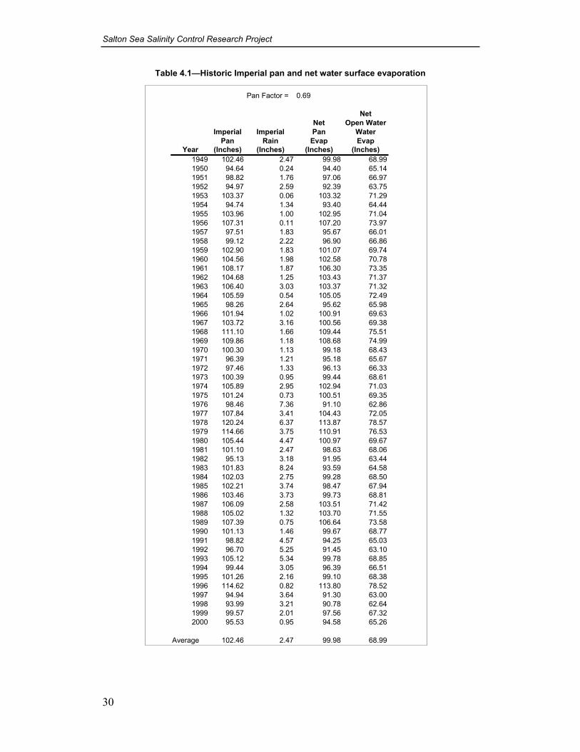
Salton Sea Salinity Control Research Project
30
Table 4.1—Historic Imperial pan and net water surface evaporation
Pan Factor = 0.69
NetNet Open Water
Imperial Imperial Pan WaterPan Rain Evap Evap
Year (Inches) (Inches) (Inches) (Inches)1949 102.46 2.47 99.98 68.991950 94.64 0.24 94.40 65.141951 98.82 1.76 97.06 66.971952 94.97 2.59 92.39 63.751953 103.37 0.06 103.32 71.291954 94.74 1.34 93.40 64.441955 103.96 1.00 102.95 71.041956 107.31 0.11 107.20 73.971957 97.51 1.83 95.67 66.011958 99.12 2.22 96.90 66.861959 102.90 1.83 101.07 69.741960 104.56 1.98 102.58 70.781961 108.17 1.87 106.30 73.351962 104.68 1.25 103.43 71.371963 106.40 3.03 103.37 71.321964 105.59 0.54 105.05 72.491965 98.26 2.64 95.62 65.981966 101.94 1.02 100.91 69.631967 103.72 3.16 100.56 69.381968 111.10 1.66 109.44 75.511969 109.86 1.18 108.68 74.991970 100.30 1.13 99.18 68.431971 96.39 1.21 95.18 65.671972 97.46 1.33 96.13 66.331973 100.39 0.95 99.44 68.611974 105.89 2.95 102.94 71.031975 101.24 0.73 100.51 69.351976 98.46 7.36 91.10 62.861977 107.84 3.41 104.43 72.051978 120.24 6.37 113.87 78.571979 114.66 3.75 110.91 76.531980 105.44 4.47 100.97 69.671981 101.10 2.47 98.63 68.061982 95.13 3.18 91.95 63.441983 101.83 8.24 93.59 64.581984 102.03 2.75 99.28 68.501985 102.21 3.74 98.47 67.941986 103.46 3.73 99.73 68.811987 106.09 2.58 103.51 71.421988 105.02 1.32 103.70 71.551989 107.39 0.75 106.64 73.581990 101.13 1.46 99.67 68.771991 98.82 4.57 94.25 65.031992 96.70 5.25 91.45 63.101993 105.12 5.34 99.78 68.851994 99.44 3.05 96.39 66.511995 101.26 2.16 99.10 68.381996 114.62 0.82 113.80 78.521997 94.94 3.64 91.30 63.001998 93.99 3.21 90.78 62.641999 99.57 2.01 97.56 67.322000 95.53 0.95 94.58 65.26
Average 102.46 2.47 99.98 68.99

Salton Sea Test Base
31
4.2.2 Monthly Evaporation Distribution
Monthly breakdowns of evaporation at the Imperial pan station were not available from IID. However, historic potential evapotranspiration (PET) data for Brawley were available from the University of California Statewide Integrated Pest Management Weather Database. These data were analyzed to develop the relationship in figure 4.1. This chart depicts monthly evaporation as a percent of total annual evaporation. Data to develop this chart were for PET. Use of the PET data to develop an understanding of how evaporation varies on a monthly basis is a common practice in hydrologic investigations, as applied herein. In this instance, it is assumed that the average monthly distribution of evaporation is the same as PET from a percentage point of view.
Figure 4.1—Monthly evaporation distribution.
4.2.3 Historic Monthly Pan Evaporation
The monthly distribution in figure 4.1 was applied to the annual fresh water pan evaporation measurements in table 4.1. The results are shown in table 4.2, which contains monthly pan evaporation estimates for the period 1949 through 2000.
Monthly Evaporation Distribution
3.36
4.58
7.41
9.70
12.3012.84 12.96
12.20
9.86
7.27
4.37
3.15
0.00
2.00
4.00
6.00
8.00
10.00
12.00
14.00
Jan Feb Mar Apr May June July Aug Sept Oct Nov Dec
Month
Perc
ent
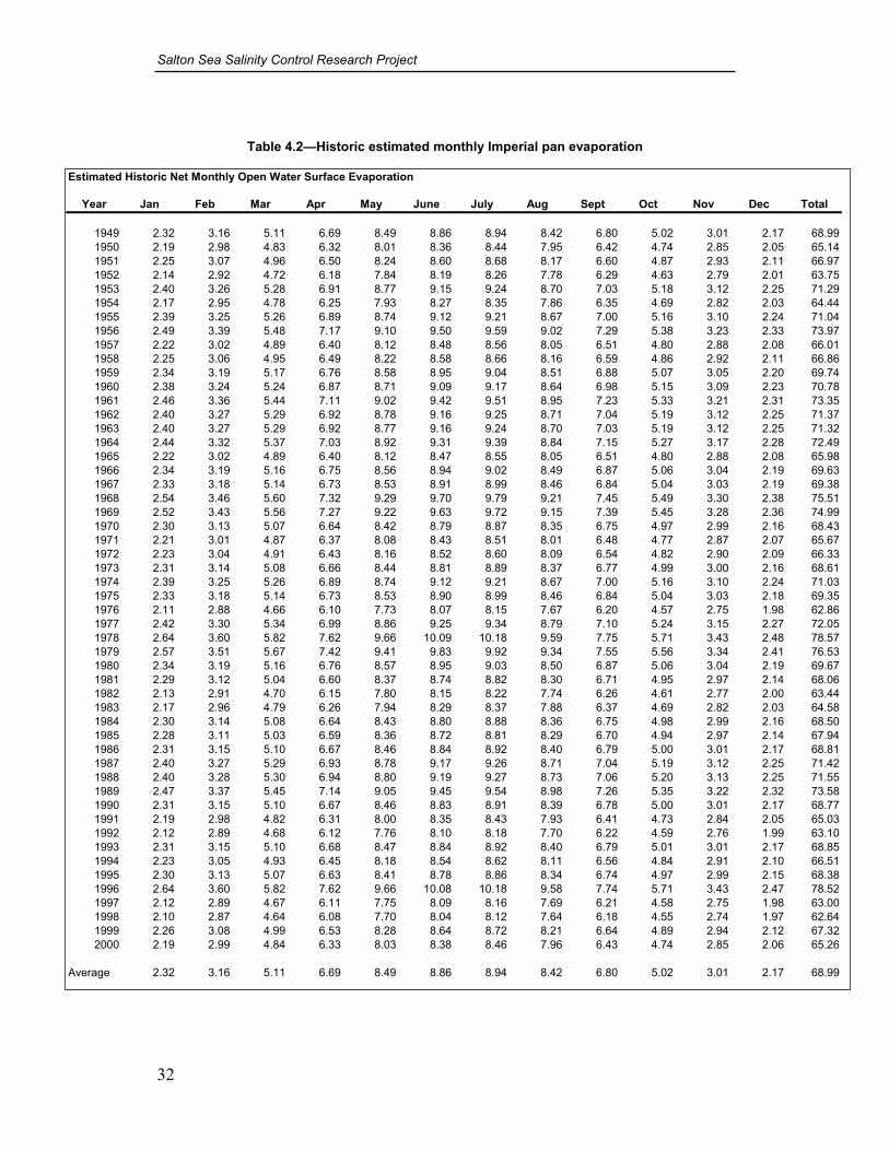
Salton Sea Salinity Control Research Project
32
Table 4.2—Historic estimated monthly Imperial pan evaporation
Estimated Historic Net Monthly Open Water Surface Evaporation
Year Jan Feb Mar Apr May June July Aug Sept Oct Nov Dec Total
1949 2.32 3.16 5.11 6.69 8.49 8.86 8.94 8.42 6.80 5.02 3.01 2.17 68.991950 2.19 2.98 4.83 6.32 8.01 8.36 8.44 7.95 6.42 4.74 2.85 2.05 65.141951 2.25 3.07 4.96 6.50 8.24 8.60 8.68 8.17 6.60 4.87 2.93 2.11 66.971952 2.14 2.92 4.72 6.18 7.84 8.19 8.26 7.78 6.29 4.63 2.79 2.01 63.751953 2.40 3.26 5.28 6.91 8.77 9.15 9.24 8.70 7.03 5.18 3.12 2.25 71.291954 2.17 2.95 4.78 6.25 7.93 8.27 8.35 7.86 6.35 4.69 2.82 2.03 64.441955 2.39 3.25 5.26 6.89 8.74 9.12 9.21 8.67 7.00 5.16 3.10 2.24 71.041956 2.49 3.39 5.48 7.17 9.10 9.50 9.59 9.02 7.29 5.38 3.23 2.33 73.971957 2.22 3.02 4.89 6.40 8.12 8.48 8.56 8.05 6.51 4.80 2.88 2.08 66.011958 2.25 3.06 4.95 6.49 8.22 8.58 8.66 8.16 6.59 4.86 2.92 2.11 66.861959 2.34 3.19 5.17 6.76 8.58 8.95 9.04 8.51 6.88 5.07 3.05 2.20 69.741960 2.38 3.24 5.24 6.87 8.71 9.09 9.17 8.64 6.98 5.15 3.09 2.23 70.781961 2.46 3.36 5.44 7.11 9.02 9.42 9.51 8.95 7.23 5.33 3.21 2.31 73.351962 2.40 3.27 5.29 6.92 8.78 9.16 9.25 8.71 7.04 5.19 3.12 2.25 71.371963 2.40 3.27 5.29 6.92 8.77 9.16 9.24 8.70 7.03 5.19 3.12 2.25 71.321964 2.44 3.32 5.37 7.03 8.92 9.31 9.39 8.84 7.15 5.27 3.17 2.28 72.491965 2.22 3.02 4.89 6.40 8.12 8.47 8.55 8.05 6.51 4.80 2.88 2.08 65.981966 2.34 3.19 5.16 6.75 8.56 8.94 9.02 8.49 6.87 5.06 3.04 2.19 69.631967 2.33 3.18 5.14 6.73 8.53 8.91 8.99 8.46 6.84 5.04 3.03 2.19 69.381968 2.54 3.46 5.60 7.32 9.29 9.70 9.79 9.21 7.45 5.49 3.30 2.38 75.511969 2.52 3.43 5.56 7.27 9.22 9.63 9.72 9.15 7.39 5.45 3.28 2.36 74.991970 2.30 3.13 5.07 6.64 8.42 8.79 8.87 8.35 6.75 4.97 2.99 2.16 68.431971 2.21 3.01 4.87 6.37 8.08 8.43 8.51 8.01 6.48 4.77 2.87 2.07 65.671972 2.23 3.04 4.91 6.43 8.16 8.52 8.60 8.09 6.54 4.82 2.90 2.09 66.331973 2.31 3.14 5.08 6.66 8.44 8.81 8.89 8.37 6.77 4.99 3.00 2.16 68.611974 2.39 3.25 5.26 6.89 8.74 9.12 9.21 8.67 7.00 5.16 3.10 2.24 71.031975 2.33 3.18 5.14 6.73 8.53 8.90 8.99 8.46 6.84 5.04 3.03 2.18 69.351976 2.11 2.88 4.66 6.10 7.73 8.07 8.15 7.67 6.20 4.57 2.75 1.98 62.861977 2.42 3.30 5.34 6.99 8.86 9.25 9.34 8.79 7.10 5.24 3.15 2.27 72.051978 2.64 3.60 5.82 7.62 9.66 10.09 10.18 9.59 7.75 5.71 3.43 2.48 78.571979 2.57 3.51 5.67 7.42 9.41 9.83 9.92 9.34 7.55 5.56 3.34 2.41 76.531980 2.34 3.19 5.16 6.76 8.57 8.95 9.03 8.50 6.87 5.06 3.04 2.19 69.671981 2.29 3.12 5.04 6.60 8.37 8.74 8.82 8.30 6.71 4.95 2.97 2.14 68.061982 2.13 2.91 4.70 6.15 7.80 8.15 8.22 7.74 6.26 4.61 2.77 2.00 63.441983 2.17 2.96 4.79 6.26 7.94 8.29 8.37 7.88 6.37 4.69 2.82 2.03 64.581984 2.30 3.14 5.08 6.64 8.43 8.80 8.88 8.36 6.75 4.98 2.99 2.16 68.501985 2.28 3.11 5.03 6.59 8.36 8.72 8.81 8.29 6.70 4.94 2.97 2.14 67.941986 2.31 3.15 5.10 6.67 8.46 8.84 8.92 8.40 6.79 5.00 3.01 2.17 68.811987 2.40 3.27 5.29 6.93 8.78 9.17 9.26 8.71 7.04 5.19 3.12 2.25 71.421988 2.40 3.28 5.30 6.94 8.80 9.19 9.27 8.73 7.06 5.20 3.13 2.25 71.551989 2.47 3.37 5.45 7.14 9.05 9.45 9.54 8.98 7.26 5.35 3.22 2.32 73.581990 2.31 3.15 5.10 6.67 8.46 8.83 8.91 8.39 6.78 5.00 3.01 2.17 68.771991 2.19 2.98 4.82 6.31 8.00 8.35 8.43 7.93 6.41 4.73 2.84 2.05 65.031992 2.12 2.89 4.68 6.12 7.76 8.10 8.18 7.70 6.22 4.59 2.76 1.99 63.101993 2.31 3.15 5.10 6.68 8.47 8.84 8.92 8.40 6.79 5.01 3.01 2.17 68.851994 2.23 3.05 4.93 6.45 8.18 8.54 8.62 8.11 6.56 4.84 2.91 2.10 66.511995 2.30 3.13 5.07 6.63 8.41 8.78 8.86 8.34 6.74 4.97 2.99 2.15 68.381996 2.64 3.60 5.82 7.62 9.66 10.08 10.18 9.58 7.74 5.71 3.43 2.47 78.521997 2.12 2.89 4.67 6.11 7.75 8.09 8.16 7.69 6.21 4.58 2.75 1.98 63.001998 2.10 2.87 4.64 6.08 7.70 8.04 8.12 7.64 6.18 4.55 2.74 1.97 62.641999 2.26 3.08 4.99 6.53 8.28 8.64 8.72 8.21 6.64 4.89 2.94 2.12 67.322000 2.19 2.99 4.84 6.33 8.03 8.38 8.46 7.96 6.43 4.74 2.85 2.06 65.26
Average 2.32 3.16 5.11 6.69 8.49 8.86 8.94 8.42 6.80 5.02 3.01 2.17 68.99

Salton Sea Test Base
33
4.2.4 Historic Monthly Open Water Surface Evaporation
The monthly distribution in figure 4.1 was applied to the annual net open water evaporation measurements in table 4.1. The results are shown in table 4.3 that contains monthly net open water evaporation estimates for the period 1949 through 2000.
Table 4.3—Estimated historic net monthly open water surface evaporation
Estimated Historic Net Monthly Open Water Surface Evaporation
Year Jan Feb Mar Apr May June July Aug Sept Oct Nov Dec Total
1949 2.32 3.16 5.11 6.69 8.49 8.86 8.94 8.42 6.80 5.02 3.01 2.17 68.991950 2.19 2.98 4.83 6.32 8.01 8.36 8.44 7.95 6.42 4.74 2.85 2.05 65.141951 2.25 3.07 4.96 6.50 8.24 8.60 8.68 8.17 6.60 4.87 2.93 2.11 66.971952 2.14 2.92 4.72 6.18 7.84 8.19 8.26 7.78 6.29 4.63 2.79 2.01 63.751953 2.40 3.26 5.28 6.91 8.77 9.15 9.24 8.70 7.03 5.18 3.12 2.25 71.291954 2.17 2.95 4.78 6.25 7.93 8.27 8.35 7.86 6.35 4.69 2.82 2.03 64.441955 2.39 3.25 5.26 6.89 8.74 9.12 9.21 8.67 7.00 5.16 3.10 2.24 71.041956 2.49 3.39 5.48 7.17 9.10 9.50 9.59 9.02 7.29 5.38 3.23 2.33 73.971957 2.22 3.02 4.89 6.40 8.12 8.48 8.56 8.05 6.51 4.80 2.88 2.08 66.011958 2.25 3.06 4.95 6.49 8.22 8.58 8.66 8.16 6.59 4.86 2.92 2.11 66.861959 2.34 3.19 5.17 6.76 8.58 8.95 9.04 8.51 6.88 5.07 3.05 2.20 69.741960 2.38 3.24 5.24 6.87 8.71 9.09 9.17 8.64 6.98 5.15 3.09 2.23 70.781961 2.46 3.36 5.44 7.11 9.02 9.42 9.51 8.95 7.23 5.33 3.21 2.31 73.351962 2.40 3.27 5.29 6.92 8.78 9.16 9.25 8.71 7.04 5.19 3.12 2.25 71.371963 2.40 3.27 5.29 6.92 8.77 9.16 9.24 8.70 7.03 5.19 3.12 2.25 71.321964 2.44 3.32 5.37 7.03 8.92 9.31 9.39 8.84 7.15 5.27 3.17 2.28 72.491965 2.22 3.02 4.89 6.40 8.12 8.47 8.55 8.05 6.51 4.80 2.88 2.08 65.981966 2.34 3.19 5.16 6.75 8.56 8.94 9.02 8.49 6.87 5.06 3.04 2.19 69.631967 2.33 3.18 5.14 6.73 8.53 8.91 8.99 8.46 6.84 5.04 3.03 2.19 69.381968 2.54 3.46 5.60 7.32 9.29 9.70 9.79 9.21 7.45 5.49 3.30 2.38 75.511969 2.52 3.43 5.56 7.27 9.22 9.63 9.72 9.15 7.39 5.45 3.28 2.36 74.991970 2.30 3.13 5.07 6.64 8.42 8.79 8.87 8.35 6.75 4.97 2.99 2.16 68.431971 2.21 3.01 4.87 6.37 8.08 8.43 8.51 8.01 6.48 4.77 2.87 2.07 65.671972 2.23 3.04 4.91 6.43 8.16 8.52 8.60 8.09 6.54 4.82 2.90 2.09 66.331973 2.31 3.14 5.08 6.66 8.44 8.81 8.89 8.37 6.77 4.99 3.00 2.16 68.611974 2.39 3.25 5.26 6.89 8.74 9.12 9.21 8.67 7.00 5.16 3.10 2.24 71.031975 2.33 3.18 5.14 6.73 8.53 8.90 8.99 8.46 6.84 5.04 3.03 2.18 69.351976 2.11 2.88 4.66 6.10 7.73 8.07 8.15 7.67 6.20 4.57 2.75 1.98 62.861977 2.42 3.30 5.34 6.99 8.86 9.25 9.34 8.79 7.10 5.24 3.15 2.27 72.051978 2.64 3.60 5.82 7.62 9.66 10.09 10.18 9.59 7.75 5.71 3.43 2.48 78.571979 2.57 3.51 5.67 7.42 9.41 9.83 9.92 9.34 7.55 5.56 3.34 2.41 76.531980 2.34 3.19 5.16 6.76 8.57 8.95 9.03 8.50 6.87 5.06 3.04 2.19 69.671981 2.29 3.12 5.04 6.60 8.37 8.74 8.82 8.30 6.71 4.95 2.97 2.14 68.061982 2.13 2.91 4.70 6.15 7.80 8.15 8.22 7.74 6.26 4.61 2.77 2.00 63.441983 2.17 2.96 4.79 6.26 7.94 8.29 8.37 7.88 6.37 4.69 2.82 2.03 64.581984 2.30 3.14 5.08 6.64 8.43 8.80 8.88 8.36 6.75 4.98 2.99 2.16 68.501985 2.28 3.11 5.03 6.59 8.36 8.72 8.81 8.29 6.70 4.94 2.97 2.14 67.941986 2.31 3.15 5.10 6.67 8.46 8.84 8.92 8.40 6.79 5.00 3.01 2.17 68.811987 2.40 3.27 5.29 6.93 8.78 9.17 9.26 8.71 7.04 5.19 3.12 2.25 71.421988 2.40 3.28 5.30 6.94 8.80 9.19 9.27 8.73 7.06 5.20 3.13 2.25 71.551989 2.47 3.37 5.45 7.14 9.05 9.45 9.54 8.98 7.26 5.35 3.22 2.32 73.581990 2.31 3.15 5.10 6.67 8.46 8.83 8.91 8.39 6.78 5.00 3.01 2.17 68.771991 2.19 2.98 4.82 6.31 8.00 8.35 8.43 7.93 6.41 4.73 2.84 2.05 65.031992 2.12 2.89 4.68 6.12 7.76 8.10 8.18 7.70 6.22 4.59 2.76 1.99 63.101993 2.31 3.15 5.10 6.68 8.47 8.84 8.92 8.40 6.79 5.01 3.01 2.17 68.851994 2.23 3.05 4.93 6.45 8.18 8.54 8.62 8.11 6.56 4.84 2.91 2.10 66.511995 2.30 3.13 5.07 6.63 8.41 8.78 8.86 8.34 6.74 4.97 2.99 2.15 68.381996 2.64 3.60 5.82 7.62 9.66 10.08 10.18 9.58 7.74 5.71 3.43 2.47 78.521997 2.12 2.89 4.67 6.11 7.75 8.09 8.16 7.69 6.21 4.58 2.75 1.98 63.001998 2.10 2.87 4.64 6.08 7.70 8.04 8.12 7.64 6.18 4.55 2.74 1.97 62.641999 2.26 3.08 4.99 6.53 8.28 8.64 8.72 8.21 6.64 4.89 2.94 2.12 67.322000 2.19 2.99 4.84 6.33 8.03 8.38 8.46 7.96 6.43 4.74 2.85 2.06 65.26
Average 2.32 3.16 5.11 6.69 8.49 8.86 8.94 8.42 6.80 5.02 3.01 2.17 68.99

Salton Sea Salinity Control Research Project
34
4.2.5 Evaporation Brine Factors
Research conducted at the Salton Sea Test Base provided for the development of a relationship between brine concentration and freshwater evaporation rates. Two different indicators of concentrations were evaluated: percent weight of magnesium and specific gravity. The evaporation pans shown in figure 2.2 each contained different brine at a different concentration. As evaporation was monitored in these pans, periodic measurements were made of percent weight of magnesium. By compiling monthly evaporation in each pan as a fraction of freshwater evaporation, it then was possible to develop figure 4.2 that shows how brine evaporation as a fraction of freshwater evaporation varies as a function of percent weight magnesium. The fraction of fresh water evaporation is referred to in this document as “brine factor.” The chart in figure 4.2 can be used to determine evaporation rates by knowing the percent weight of magnesium and then applying the corresponding brine factor to data in either table 4.1 or 4.2.
Figure 4.2—Fraction of fresh water evaporation (brine factor) versus percent weight of magnesium.
Fraction of Fresh Water Evaporation vs Percent Weight of Magnesium
y = 0.0008x4 - 0.0179x3 + 0.118x2 - 0.3273x + 1.0317R2 = 0.9495
0.00
0.20
0.40
0.60
0.80
1.00
1.20
0.00 1.00 2.00 3.00 4.00 5.00 6.00 7.00
Percent Weight Mg
Frac
tion
of F
resh
Wat
er E
vapo
ratio
n

Salton Sea Test Base
35
According to figure 4.2, as brine concentration increases, the evaporation rate will level off between 2 and 4 percent weight of magnesium. As concentrations increase, the evaporation rate decreases. When concentrations get above 6 percent, there is very little brine remaining and most of it will evaporate. By 8 percent weight of magnesium, the evaporation rate will be very slow and remaining volume will be very small.
The graph in figure 4.3 is similar to figure 4.2, but instead represents a comparison of brine factor versus specific gravity. Specific gravity is a poor indicator of concentration. Specific gravity has a tendency to remain unchanged as concentrations increase. This is why much of the data shown in figure 4.3 is clumped together, rather than depicting a smooth transition. Because of this, the correlation between brine factor and specific gravity is not as good as with percent weight of magnesium.
Figure 4.3—Fraction of fresh water evaporation (brine factor) versus specific gravity.
Fraction of Fresh Water Evaporation vs Specific Gravity
y = -1.2298x2 + 1.5085x + 0.7299R2 = 0.8977
0.00
0.20
0.40
0.60
0.80
1.00
1.20
1.000 1.050 1.100 1.150 1.200 1.250 1.300 1.350 1.400
Specific Gravity
Frac
tion
of F
resh
Wat
er E
vapo
ratio
n

Salton Sea Salinity Control Research Project
36
Net Average Monthly Pan Evaporation as a Function of Concentration by % Weight Mg
Brine Factor % Mg Jan Feb Mar Apr May June July Aug Sept Oct Nov Dec Total1.00 0.00 3.44 4.69 7.59 9.94 12.60 13.16 13.28 12.50 10.10 7.45 4.48 3.23 102.460.98 0.16 3.38 4.61 7.46 9.76 12.38 12.92 13.04 12.28 9.92 7.32 4.40 3.17 100.640.96 0.25 3.29 4.49 7.27 9.51 12.06 12.59 12.71 11.96 9.67 7.13 4.28 3.09 98.050.90 0.50 3.08 4.20 6.80 8.90 11.28 11.78 11.89 11.19 9.05 6.67 4.01 2.89 91.740.81 1.00 2.77 3.78 6.11 8.00 10.15 10.59 10.69 10.07 8.14 6.00 3.61 2.60 82.510.75 1.50 2.58 3.52 5.69 7.45 9.45 9.87 9.96 9.37 7.58 5.59 3.36 2.42 76.830.72 2.00 2.47 3.37 5.46 7.14 9.06 9.45 9.54 8.98 7.26 5.35 3.22 2.32 73.640.70 2.50 2.42 3.30 5.33 6.98 8.85 9.24 9.33 8.78 7.10 5.23 3.15 2.27 71.980.69 3.00 2.39 3.25 5.26 6.89 8.74 9.12 9.21 8.67 7.00 5.16 3.10 2.24 71.030.68 3.50 2.36 3.21 5.19 6.80 8.62 9.00 9.09 8.55 6.91 5.10 3.06 2.21 70.100.67 4.00 2.31 3.14 5.08 6.66 8.44 8.81 8.89 8.37 6.77 4.99 3.00 2.16 68.620.65 4.50 2.22 3.03 4.90 6.41 8.13 8.49 8.57 8.07 6.52 4.81 2.89 2.08 66.110.61 5.00 2.09 2.85 4.61 6.04 7.66 7.99 8.07 7.60 6.14 4.53 2.72 1.96 62.260.55 5.50 1.91 2.60 4.21 5.52 6.99 7.30 7.37 6.94 5.61 4.13 2.48 1.79 56.860.49 6.00 1.67 2.28 3.69 4.83 6.13 6.40 6.46 6.08 4.91 3.62 2.18 1.57 49.820.40 6.50 1.38 1.89 3.05 4.00 5.07 5.29 5.34 5.03 4.06 2.99 1.80 1.30 41.190.30 7.00 1.05 1.43 2.31 3.02 3.83 4.00 4.03 3.80 3.07 2.26 1.36 0.98 31.120.19 7.50 0.67 0.91 1.47 1.93 2.45 2.55 2.58 2.43 1.96 1.45 0.87 0.63 19.890.08 8.00 0.27 0.36 0.59 0.77 0.97 1.02 1.03 0.97 0.78 0.58 0.35 0.25 7.92
4.2.6 Monthly Pan Brine Evaporation vs. Percent Weight Magnesium
The relationship in figure 4.2 demonstrates that as concentration increases as represented by percent weight of magnesium then the brine factor decreases. Application of this relationship to average monthly pan evaporation data from table 4.2 results in what is shown in table 4.4 and figure 4.4. This table and chart show average monthly pan evaporation as a function of percent weight of magnesium. The lowest evaporation rates apply to the highest concentrations and the lowest brine factors.
Table 4.4—Monthly pan brine evaporation vs. percent weight magnesium
The same information can be depicted differently, as shown figure 4.5. In this instance, evaporation is shown as a function of percent weight of magnesium by month. From this chart, it is clear that regardless of the time of year, the evaporation rate, relative to concentration, will level off between 2 and 4 percent magnesium but will decrease for higher concentrations. The dropoff for higher concentrations is more pronounced in the warmer months of the year.

Salton Sea Test Base
37
Figure 4.4—Average monthly class A pan brine evaporation by percent weight of magnesium.
Figure 4.5—Class A pan brine evaporation as function of percent weight of magnesium by month.
0.00
2.00
4.00
6.00
8.00
10.00
12.00
14.00
1 2 3 4 5 6 7 8 9 10 11 12
Month
Evap
orat
ion
(Inch
es p
er m
onth
)0.000.160.250.501.002.003.004.005.006.007.008.00
% Wt
0.00
2.00
4.00
6.00
8.00
10.00
12.00
14.00
0.00 1.00 2.00 3.00 4.00 5.00 6.00 7.00 8.00 9.00
% Mg
Evap
orat
ion
(Inch
es p
er m
onth
)
JanFebMarAprMayJuneJulyAugSeptOctNovDec

Salton Sea Salinity Control Research Project
38
4.2.7 Monthly Open Brine Surface Evaporation vs. Percent Weight Magnesium
The relationship in figure 4.2 demonstrates that as concentration increases as represented by percent weight of magnesium then the brine factor decreases. Application of this relationship to average open-water surface evaporation data from table 4.3 results in the values shown in table 4.5 and figure 4.6, which show average monthly open brine surface evaporation as a function of percent weight of magnesium. The lowest evaporation rates apply to the highest concentrations and the lowest brine factors.
Table 4.5—Monthly open brine surface evaporation vs. percent weight magnesium
The same information can be depicted differently as shown figure 4.7. In this instance, open brine surface evaporation is shown as a function of percent weight of magnesium by month. From this chart, it is clear that regardless of the time of year, the evaporation rate, relative to concentration, will level off between 2 and 4 percent magnesium but will decrease for higher concentrations. The dropoff for higher concentrations is more pronounced in the warmer months of the year.
Net Average Annual Open Water Surface Evaporation as a Function of Concentration % Weight Mg
Brine Factor % Mg Jan Feb Mar Apr May June July Aug Sept Oct Nov Dec Total1.00 0.00 2.32 3.16 5.11 6.69 8.49 8.86 8.94 8.42 6.80 5.02 3.01 2.17 68.990.98 0.16 2.28 3.10 5.02 6.57 8.34 8.70 8.78 8.27 6.68 4.93 2.96 2.13 67.770.96 0.25 2.22 3.02 4.89 6.40 8.12 8.48 8.56 8.05 6.51 4.80 2.89 2.08 66.020.90 0.50 2.08 2.83 4.58 5.99 7.60 7.93 8.01 7.54 6.09 4.49 2.70 1.95 61.770.81 1.00 1.87 2.54 4.12 5.39 6.83 7.13 7.20 6.78 5.48 4.04 2.43 1.75 55.560.75 1.50 1.74 2.37 3.83 5.02 6.36 6.64 6.70 6.31 5.10 3.76 2.26 1.63 51.730.72 2.00 1.67 2.27 3.67 4.81 6.10 6.37 6.43 6.05 4.89 3.60 2.17 1.56 49.580.70 2.50 1.63 2.22 3.59 4.70 5.96 6.22 6.28 5.91 4.78 3.52 2.12 1.53 48.460.69 3.00 1.61 2.19 3.54 4.64 5.88 6.14 6.20 5.84 4.72 3.48 2.09 1.51 47.830.68 3.50 1.59 2.16 3.50 4.58 5.81 6.06 6.12 5.76 4.65 3.43 2.06 1.49 47.200.67 4.00 1.55 2.12 3.42 4.48 5.68 5.93 5.99 5.64 4.56 3.36 2.02 1.46 46.200.65 4.50 1.50 2.04 3.30 4.32 5.48 5.72 5.77 5.43 4.39 3.24 1.95 1.40 44.520.61 5.00 1.41 1.92 3.11 4.07 5.16 5.38 5.43 5.11 4.13 3.05 1.83 1.32 41.920.55 5.50 1.29 1.75 2.84 3.71 4.71 4.92 4.96 4.67 3.78 2.78 1.67 1.21 38.290.49 6.00 1.13 1.54 2.49 3.25 4.13 4.31 4.35 4.09 3.31 2.44 1.47 1.06 33.550.40 6.50 0.93 1.27 2.06 2.69 3.41 3.56 3.59 3.38 2.73 2.02 1.21 0.87 27.730.30 7.00 0.70 0.96 1.55 2.03 2.58 2.69 2.72 2.56 2.07 1.52 0.92 0.66 20.950.19 7.50 0.45 0.61 0.99 1.30 1.65 1.72 1.74 1.63 1.32 0.97 0.59 0.42 13.390.08 8.00 0.18 0.24 0.40 0.52 0.66 0.68 0.69 0.65 0.53 0.39 0.23 0.17 5.33

Salton Sea Test Base
39
0.00
1.00
2.00
3.00
4.00
5.00
6.00
7.00
8.00
9.00
10.00
0.00 1.00 2.00 3.00 4.00 5.00 6.00 7.00 8.00 9.00
% Mg
Evap
orat
ion
(Inch
es p
er m
onth
)
JanFebMarAprMayJuneJulyAugSeptOctNovDec
g
0.00
1.00
2.00
3.00
4.00
5.00
6.00
7.00
8.00
9.00
10.00
1 2 3 4 5 6 7 8 9 10 11 12
Month
Evap
orat
ion
(Inch
es p
er m
onth
)0.000.160.250.501.002.003.004.005.006.007.008.00
% Wt Mg
Figure 4.6—Average monthly open brine surface evaporation by percent weight of magnesium.
Figure 4.7—Open brine surface evaporation as function of percent weight of magnesium by month.

Salton Sea Salinity Control Research Project
40
4.3 Salt Disposal Test Results
The purpose of test 1 of the research operations plan was to determine if salt could be crystallized in a single disposal cell without hindering the evaporation rate with increased concentrations of magnesium and potassium (K). Research results indicate that this is possible. Figure 4.2, presented earlier, revealed only minor changes in the evaporation rate above 2 percent magnesium by weight. Field research at the Salton Sea Test Base disposal pond indicates that only minor reductions in evaporation rates will occur in a disposal pond. As long as the disposal pond continues to receive saturated brine, no significant increases in percent weight of magnesium will occur. Figure 4.8 is a graph of percent weight of magnesium in the Test Base disposal pond through time. Magnesium levels varied between 1.50 and 2.25 percent, by weight. Therefore, there was no significant reduction in evaporation due to brine concentration in the test pond. Significant reductions do not occur until concentrations exceed 4 percent magnesium, by weight (figure 4.2).
Field results from the test disposal pond indicate that if entrained brines are drained from the pond, the surface will evaporate to dryness, while inner layers remain partially hydrated (not soggy), with no significant reduction is evaporation
Figure 4.8—Percent weight of magnesium in disposal pond (March 29, 2002, to December 3, 2002.).
0
0.5
1
1.5
2
2.5
02/13/02 04/04/02 05/24/02 07/13/02 09/01/02 10/21/02 12/10/02 01/29/03
Date
Perc
ent W
eigh
t of M
agne
sium

Salton Sea Test Base
41
rate. Figure 4.9 is a picture of the test pond after it was allowed to dry out. The dry condition of the test pond, when observed, made the second part of test 1 (removing the bitterns to an adjacent pond to see if they evaporate to dryness) unnecessary. Therefore, this portion of the test was conducted by evaporating the bitterns left over from the year 2001 EES pretest.
Test 2 involved placing concentrated bitterns on top of the dried-out test disposal pond, with the hope of increasing the density of the salt deposits. This test was conducted by draining the entrained brines from the disposal pond into an adjacent pond and letting it evaporate. This concentrated brine was mixed with new saturated brine from the last concentrator for a short time, and then it was allowed to concentrate. In the next stage of test 2, the barrier between the adjacent cell and the disposal pond was breached, allowing the brine to flow into the disposal pond salt deposits. Unfortunately the disposal pond did not appear to increase in density. The pore spaces within the deposit were too large. As a result, the final condition of the disposal pond was the same as it was before the entrained brines were drained with the sump. The brine did not remain exposed, where it could be evaporated. Instead it infiltrated down into the voids of the salt deposits.
Figure 4.9—Salts reached dryness in disposal pond

Salton Sea Salinity Control Research Project
42
In conclusion, if additional brine is placed on top of an already drained salt deposit, the brines will infiltrate and fill the open pore spaces. Therefore, at project disposal facilities, it is recommended that salt deposits be consolidated with heavy equipment to close up the pore spaces before additional brines are placed on them. This should increase deposit density and reduce brine entrainment substantially.
Test 2 was also performed using a different method, whereby dense brine was dripped slowly onto the salt deposits on core pad 7 (see figure 3.10) from valves installed in the buckets, as shown in figure 4.10. The brine supply for this test was stored in two 1,000-gallon tanks, shown in figure 4.11. These tanks were filled with concentrated brine from the disposal pond sump while the disposal pond was drained of entrained brines. The rate at which this brine was dripped onto the core pad 7 deposits was very slow. The test was conducted to determine if the salt deposits would become denser as the brine on the pads evaporated, leaving behind additional salt. Test results indicated no increase in density. In fact, the deposits on core pad 7 were too soft to be drilled while taking cores. The dripping of the brines onto the pad deposits actually softened the deposits.
Figure 4.10—Heavy brine dripping onto deposits on core pad 7.

Salton Sea Test Base
43
Figure 4.11—Supply tanks with heavy brine used in salt deposit density increase test (test 2).
Test 3 was conducted to determine whether denser salts could be precipitated over what was expected to be softer salts deposited from brines that were drained from the sump in the disposal pond. Field research at the site yielded a different conclusion than was expected. In fact, the salts were observed to be the same consistency in both ponds. Therefore, stratification will not occur if operated as proposed in test 3. As shown in test 2, brine placed on top of a salt deposit will infiltrate and become entrained.
4.4 Salt Sampling and Testing
Core drilling was performed on six core pads (pads 1 through 6) located approximately diagonal from east to west, and on one core pad (pad 7) located on the north side. The locations of the drilling pads in the disposal pond are shown in figure 3.10. A total of 13 samples; 11 core samples from all pads, one 1.0 ft x 1.0 ft x 1.5 ft undisturbed block sample from pad 6, one 1.5 ft high with 6-in. diameter PVC tube sample from pad 6, and two buckets of brine solution were collected at the pond as presented in table 4.6. Sample locations in table 4.6 are decoded as in the following example:
DH-6-5: Drill hole number 5 on pad 6

Salton Sea Salinity Control Research Project
44
Samples of salt from the Salton Sea Test Base disposal pond and brine solutions were collected at the site, and brought to the Reclamation Earth Sciences and Research Laboratory to determine index and engineering properties. The samples were collected from the disposal pond during December 11 through 14, 2002, and are listed in table 4.6.
The material depth and brine content1 varied; salt was deeper and drier at the east side, and shallower and wetter at the Southwest side of the test pond. All of the core samples were disturbed during the drilling as shown in appendix A, figures A1 through A7. The core samples were put into the PVC pipe halves, wrapped in plastic, sealed, and given field identification numbers. Tube sample and block sample were covered with plastic and cheesecloth, and then sealed with wax as shown in appendix A, figures A8 and A9.
Collected samples and two buckets of brine solution were brought to the Earth Sciences and Research Laboratory on December 17, 2002, and samples were given laboratory identification numbers 54F-126 through -138 as indicated in table 4-6. Samples were placed in sealed plastic bags, covered with wet towels, and stored in a humidity controlled room maintained at 75 percent relative moisture. Index properties, one-dimensional consolidation, and direct shear tests were performed on specimens from selected samples in accordance with Reclamation’s Earth Manual [1] soil test procedures, unless otherwise noted. Whenever the procedures required the addition of water, brine solution from the site was used instead, and calculations used in test analyses were adjusted to accommodate this change in procedures.
4.4.1 Index Properties Tests
Natural water content,2 brine content, and dry sieve analysis were performed on salt core samples 54F-128, -132, -135, -136, and on block sample 54F-138. Weighted average specific gravity values were calculated using the estimated salt (Halite and Bloedite minerals) density data for each sample tested [2].
1 Brine content is the ratio of the mass of dissolved salt to the mass of water in decimal form. 2 Natural water content is the ratio of the mass of water to the mass of solid salt in decimal form.

Salton Sea Test Base
45
126 DH-1-1 1.5 1 - Core127 DH-1-2 1.5 1 - Core128 DH-1-3 1.5 1 - Core129 DH-6-4 1.67 1 - Core130 DH-6-5 1.67 1 - Core131 DH-6-6 1.67 1 - Core132 DH-7-7 1.25 1 - Core133 DH-2-8 1.5 1 - Core134 DH-3-9 1 1 - Core135 DH-4-10 1 1 - Core136 DH-5-11 0.92 1 - Core137 Pad No. 6 Excavation No. 12 1.5 1 – 6.00 PVC (Half Rounds)138 Pad No. 6 Excavation No. 13 1.5 1 – Block, 12-in.
Sample No. 54F- Sampling Location Depth (ft) Quantity - Container
Table 4.6—Soil sample index, Salton Sea Disposal Pond Salt, Salton Sea reclamation
project, California
Water content test samples were allowed to air dry at laboratory ambient temperature and relative humidity. The natural water content is calculated using the mass of water and the solid salt.
Brine content was determined in addition to the natural water content test. Brine solutions were prepared separately for each specimen by pouring approximately 50-milliliter (mL) salt sample into 500-mL brine solution from the site. This solution was decanted into another beaker with predetermined mass; salt mostly stayed at the bottom of the first beaker; however, some of the salt, as suspended in brine, transferred into the next beaker with the brine. Brine with suspended salt was weighed to determine the wet mass. This mass was allowed to air dry in the laboratory ambient temperature also and weighed periodically until the mass became constant. The brine content was calculated by dividing the mass of dissolved salt by the mass of evaporated water.
Natural water content and brine content values were used to calculate the initial water content of specimens prepared for one-dimensional consolidation and direct shear tests described in the next section.
Sieve analysis was accomplished by hand-sieving the samples. Dispersing agent, mechanical stirring device, and powered sieve shaker were not used because their use might have caused degradation of salt particles. The samples at natural water content were placed into the top sieve of the sieve set and shaken gently by hand until the water was evaporated and sieving was accomplished. The cumulative masses of dry material retained on each sieve were recorded.
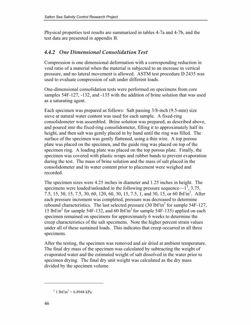
Salton Sea Salinity Control Research Project
46
Physical properties test results are summarized in tables 4-7a and 4-7b, and the test data are presented in appendix B.
4.4.2 One Dimensional Consolidation Test
Compression is one dimensional deformation with a corresponding reduction in void ratio of a material when the material is subjected to an increase in vertical pressure, and no lateral movement is allowed. ASTM test procedure D 2435 was used to evaluate compression of salt under different loads.
One-dimensional consolidation tests were performed on specimens from core samples 54F-127, -132, and -135 with the addition of brine solution that was used as a saturating agent.
Each specimen was prepared as follows: Salt passing 3/8-inch (9.5-mm) size sieve at natural water content was used for each sample. A fixed-ring consolidometer was assembled. Brine solution was prepared, as described above, and poured into the fixed-ring consolidometer, filling it to approximately half its height, and then salt was gently placed in by hand until the ring was filled. The surface of the specimen was gently flattened, using a thin wire. A top porous plate was placed on the specimen, and the guide ring was placed on top of the specimen ring. A loading plate was placed on the top porous plate. Finally, the specimen was covered with plastic wraps and rubber bands to prevent evaporation during the test. The mass of brine solution and the mass of salt placed in the consolidometer and its water content prior to placement were weighed and recorded.
The specimen sizes were 4.25 inches in diameter and 1.25 inches in height. The specimens were loaded/unloaded in the following pressure sequence—13, 3.75, 7.5, 15, 30, 15, 7.5, 30, 60, 120, 60, 30, 15, 7.5, 1, and 30, 15, or 60 lbf/in2. After each pressure increment was completed, pressure was decreased to determine rebound characteristics. The last selected pressure (30 lbf/in2 for sample 54F-127, 15 lbf/in2 for sample 54F-132, and 60 lbf/in2 for sample 54F-135) applied on each specimen remained on specimens for approximately 6 weeks to determine the creep characteristics of the salt specimens. Note the higher percent strain values under all of these sustained loads. This indicates that creep occurred in all three specimens.
After the testing, the specimen was removed and air dried at ambient temperature. The final dry mass of the specimen was calculated by subtracting the weight of evaporated water and the estimated weight of salt dissolved in the water prior to specimen drying. The final dry unit weight was calculated as the dry mass divided by the specimen volume.
3 1 lbf/in2 = 6.8948 kPa

Salton Sea Test Base
47
Table 4.7a—Physical properties test results
Sample Identification
Sample No.54F -
Sampling Location Depth (ft)
4.75
- 19
mm
(%)
0.07
5 - 4
.75
mm
(%)
< 0.
075
mm
(%)
Liq
uid
Lim
it (%
)
Plas
ticity
Inde
x (%
)
127 DH-1-2 1.50 Salt 2.19128 DH-1-3 1.50 Salt 4.0 95.9 0.1 N/A* N/A 2.19 8.8 0.6647132 DH-7-7 1.25 Salt 5.6 93.2 1.2 N/A N/A 2.21 9.7 0.6742135 DH-4-10 1.00 Salt 10.8 89.0 0.2 N/A N/A 2.20 16.7 0.6735136 DH-5-11 0.92 Salt 10.7 89.0 0.3 N/A N/A 2.20 12.0 0.7709***
138 Pad No. 6, Excavation No. 13 1.50 Salt 3.5 95.9 0.6 N/A N/A 7.6 0.7716***
* Not Applicable** One hundred times the ratio of the mass of water to the sum of the mass of the dissolved and solid salt. *** Value is not final. Test is not completed yet.
Wei
ghte
d A
vera
ge
Spec
ific
Gra
vity
(See
T
able
2)
Nat
ural
Wat
er C
onte
nt
(%) *
*
Particle Size
Material Type
Atterberg Limits
Bri
ne C
onte
nt (d
ecim
al)
Table 4.7b—Weighted average specific gravity from petrography test results
54F-127 54F-128 54F-132 54F-135 54F-136Halite* 2.17 3 3 1 2 2
Bloedite* 2.25 1 1 1 1 12.19 2.19 2.21 2.20 2.20
DensityMineralogyHalite/Bloedite Ratio Estimate
* Hurcomb, Doug. "Preliminary Halite/Bloedite Estimate". February 2003.
Weighted Average Specific Gravity

Salton Sea Salinity Control Research Project
48
Table 4.8a—Unit weights and void ratios from one-dimensional consolidation tests
Sample Number Drill Hole
Pad No.
Initial Water
Content %
Final Water
Content %
Initial Void Ratio
Final Void Ratio
Initial Dry Unit
Weight lb/ft3
Final Dry Unit
Weight lb/ft3
54F-127 DH-1-2 1 24.1 12.6 0.47 0.33 92.9 102.4
54F-132 DH-7-7 7 22.0 14.8 0.59 0.42 86.5 97.1
54F-135 DH-4-10 4 34.7 16.9 0.73 0.43 79.1 95.9
Table 4.8b—One dimensional consolidation test results
Sample Identification
Sam
ple
No.
54F
-
Sam
plin
g L
ocat
ion
Dep
th In
terv
al
(ft)
Dry
Den
sity
(lb
/ft3 )
Wat
er C
onte
nt
(%)
Deg
ree
of
Satu
ratio
n (%
)
1 lb
/in2
3.75
lb/in
2
7.5
lb/in
2
15 lb
/in2
30 lb
/in2
15 lb
/in2
7.5
lb/in
2
30 lb
/in2
60 lb
/in2
120
lb/in
2
60 lb
/in2
30 lb
/in2
15 lb
/in2
7.5
lb/in
2
1 lb
/in2
30 lb
/in2
15 lb
/in2
60 lb
/in2
127 DH-1-2 1.50 Salt 89.3 24.1 100.0 3.9 4.5 5.4 6.9 7.8 8.2 8.4 8.6 9.1 10.2 10.5 10.7 11.0 11.0 11.1 12.8 99.5
132 DH-7-7 1.25 Salt 85.5 22.0 79.8 1.1 2.1 3.1 4.1 6.1 6.2 6.2 6.9 8.7 11.8 11.6 11.3 10.9 10.7 10.1 12.0 96.9
135 DH-4-10 1.00 Salt 77.7 34.7 100.0 1.7 2.7 3.9 6.3 8.2 8.4 8.5 9.5 11.4 15.6 15.7 15.7 15.7 15.6 15.0 18.9 92.2
Axial Strain (%)
Dry
Den
sity
(lb/
ft3 ) a
t M
axim
um L
oad
Mat
eria
l Typ
e
Initial Specimen Data

Salton Sea Test Base
49
One-dimensional consolidation test results are summarized in tables 4.8a and 4.8b, and the data and specimen photos taken after each test are presented in Appendices C and D, respectively. Unit weights and void ratios that can be expected to occur in a disposal facility are presented in table 4.8a. This table indicates that upslope areas of the disposal pond would have slightly lower dry unit weights then down slope areas. On average, a dry unit weight of 98 pounds per cubic foot can be expected.
4.4.3 Direct Shear Test
The direct shear test is used to determine frictional shear strength of a material. A vertical pressure is applied to the top of the specimen, and when the specimen’s consolidation stops, the shear stress is gradually applied in the horizontal direction at a slow (drained) rate of strain. The shearing action is caused by moving the top and bottom halves of the shear box relative to each other. The shear force is measured with the corresponding strain displacement. Three or more specimens are tested at different vertical stresses. The shear stress at failure versus the normal stress is plotted. Linear regression was used to determine a Mohr-Coulomb type linear frictional strength model, using the failure conditions representing the normal stresses tested.
Direct shear tests were performed on specimens from salt core samples 54F-128, -132, -135, -136, and -138, with the addition of brine solution that was used as a saturating agent.
Each salt specimen preparation followed the same procedure mentioned in the section describing consolidation tests, except the specimens were placed in the direct shear apparatuses. The mass of brine solution, and the mass of salt placed in the direct shear mold and its water content prior to placement, were determined and recorded. Following the direct shear tests, the final water content was determined using the previously described method.
The specimens were tested at four normal stresses in the following order— 7.5 lb/in2 (52 kPa), 15 lb/in2 (103 kPa), 30 lb/in2 (207 kPa), and 60 lb/in2 (414 kPa). The horizontal surface area was determined from measurements to be 4.00 in2 (25.8 cm2). This area was subsequently used to calculate the normal loads to be applied to the sample by the test machine to obtain the desired normal test pressures of 7.5 lb/in2 (52 kPa), 15 lb/in2 (103 kPa), 30 lb/in2 (207 kPa), and 60 lb/in2 (414 kPa). The specimen length in the direction of shear was measured to be 2.00 inches (5.1 cm). Relative horizontal displacement (strain) was calculated by dividing the horizontal displacement measured during the test by the specimen length.
Table 4.9 summarizes test conditions and results. Figures 4.12 through 4.16 show shear stress versus horizontal strain plots for all tests of each sample. Figures 4.17 through 4.21 show plots of peak shear stress versus normal stress at failure for all tests of each sample. The friction angle and cohesion intercept are

Salton Sea Salinity Control Research Project
50
estimated to be between 37.7 and 41.0 degrees, and between 3.7 lb/in2 (25 kPa) and 6.7 lb/in2 (46 kPa), respectively.
Test data are presented in Appendix E, and the photographs of the specimens taken after the test are shown in Appendix F.

Salton Sea Test Base
51
Table 4.9—Direct shear test results, Salton Sea Salt
Sample Identification
Sample No.54F -
Sampling Location
Depth (ft)
Initial FinalNormal Stress (lb/in2)
Shear Stress (lb/in2)
Strain (%)Cohesion,
lbf/in2
Friction Angle,
degrees
Correlation Coefficient
Squared
1 0.005 87.9 39.0 19.8 100.0 7.5 10.3 4.02 0.005 83.6 36.2 17.3 100.0 15 20.6 7.53 0.005 78.2 37.7 18.8 100.0 30 33.9 5.94 0.005 82.4 36.9 20.4 100.0 60 57.1 7.41 0.005 113.4 44.8 18.3 100.0 7.5 10.6 5.52 0.005 105.0 43.3 15.8 100.0 15 15.0 4.03 0.005 111.9 43.4 16.2 100.0 30 32.1 4.44 0.005 112.0 45.6 16.0 100.0 60 50.4 5.51 0.005 80.4 54.6 19.6 100.0 7.5 7.8 7.52 0.005 89.0 59.3 19.8 100.0 15 19.3 5.93 0.005 81.6 60.8 20.8 100.0 30 28.3 7.14 0.005 83.6 63.1 20.2 100.0 60 53.4 7.91 0.005 86.6 19.5 20.7 73.7 7.5 12.5 5.62 0.005 92.9 15.9 18.4 73.6 15 20.3 6.53 0.005 94.4 23.5 19.7 100.0 30 33.2 7.14 0.005 89.6 17.6 17.9 73.1 60 58.6 7.2
5* 0.00003 96.6 16.1 20.5 84.6 30 34.4 3.31 0.005 105.7 18.7 9.2 100.0 7.5 7.7 5.12 0.005 99.5 19.1 10.1 100.0 15 16.0 3.83 0.005 105.9 13.4 8.7 100.0 30 32.0 3.54 0.005 93.6 24.4 10.7 100.0 60 51.3 5.1
* The specimen at 30 lb/in2 Normal Stress was rerun at slower strain rate (0.00003 in/min). Test result of this specimen is not included in the analysis.
** Specific gravity is assumed equal to 2.19.
Shear Value
Material Type
Rate of Strain
(in/min)
Test Value at FailureAverage Weighted Specific Gravity
Initial Dry Unit Weight
(lbf/ft3)
Water Content (%) Initial Degree of Saturation
(%)
Specimen Number
138
DH-1-3
DH-7-7
DH-4-10
Pad No. 6, Excavation No. 13
128
132
135
2.19
2.21
1.50
1.25
1.00 2.20
1.50 Salt
Salt
Salt
6.1
5.3
3.9
6.7
40.9
37.7
39.7
41.0
0.9904
0.9812
0.9872
0.9991
0.9812
136 DH-5-11 0.92 Salt 2.20
2.19** 3.7 39.4Salt

Salton Sea Salinity Control Research Project
52
Figure 4-12—Shear stress versus horizontal strain, 54F-128.
Drill Hole: DH-1-3Depth: 0.00 - 1.50 ft
Sample No. 54F-128Specimen No: 1, 2, 3, 4
-10
0
10
20
30
40
50
60
70
-1 0 1 2 3 4 5 6 7 8 9
Horizontal Strain - %
She
ar S
tress
- lb
f/in2
Specimen No. 1 - 7.5 lb/in2 Normal Stress
Specimen No. 2 - 15 lb/in2 Normal Stress
Specimen No. 3 - 30 lb/in2 Normal Stress
Specimen No. 4 - 60 lb/in2 Normal Stress

Salton Sea Test Base
53
Drill Hole: DH-7-7Depth: 0.00 -1.25 ft
Sample No. 54F-132Specimen No: 1, 2, 3, 4
-10
0
10
20
30
40
50
60
-1 0 1 2 3 4 5 6 7 8
Horizontal Strain - %
She
ar S
tress
- lb
f/in2
Specimen No. 1 - 7.5 lb/in2 Normal Stress
Specimen No. 2 - 15 lb/in2 Normal Stress
Specimen No. 3 - 30 lb/in2 Normal Stress
Specimen No. 4 - 60 lb/in2 Normal Stress
Figure 4.13—Shear stress versus horizontal strain, 54F-132.

Salton Sea Salinity Control Research Project
54
Drill Hole: DH-4-10Depth: 0.00 - 1.00 ft
Sample No. 54F-135Specimen No: 1, 2, 3, 4
-10
0
10
20
30
40
50
60
-1 0 1 2 3 4 5 6 7 8 9 10
Horizontal Strain - %
Shea
r Stre
ss -
lbf/i
n2
Specimen No. 1 - 7.5 lb/in2 Normal Stress
Specimen No. 2 - 15 lb/in2 Normal Stress
Specimen No. 3 - 30 lb/in2 Normal Stress
Specimen No. 4 - 60 lb/in2 Normal Stress
Figure 4.14—Shear stress versus horizontal strain, 54F-135.

Salton Sea Test Base
55
Drill Hole: DH-5-11Depth: 0.00 - 0.92 ft
Sample No. 54F-136Specimen No: 1, 2, 2 Repeat (0.00003 in/min strain rate), 3, 4
* Fluctuations in shear stress appear to coincide with daily changes in laboratory ambient temperature.
-10
0
10
20
30
40
50
60
70
-2 0 2 4 6 8 10 12
Horizontal Strain - %
She
ar S
tress
- lb
f/in2
Specimen No. 1 - 7.5 lb/in2 Normal Stress
Specimen No. 2 - 15 lb/in2 Normal Stress
Specimen No. 3 - 30 lb/in2
Normal Stress
Specimen No. 4 - 60 lb/in2 Normal Stress
Specimen No. 3 - 30 lb/in2
Normal Stress and 0.00003 in/min Strain Rate*
Figure 4.15—Shear stress versus horizontal strain, 54F-136.
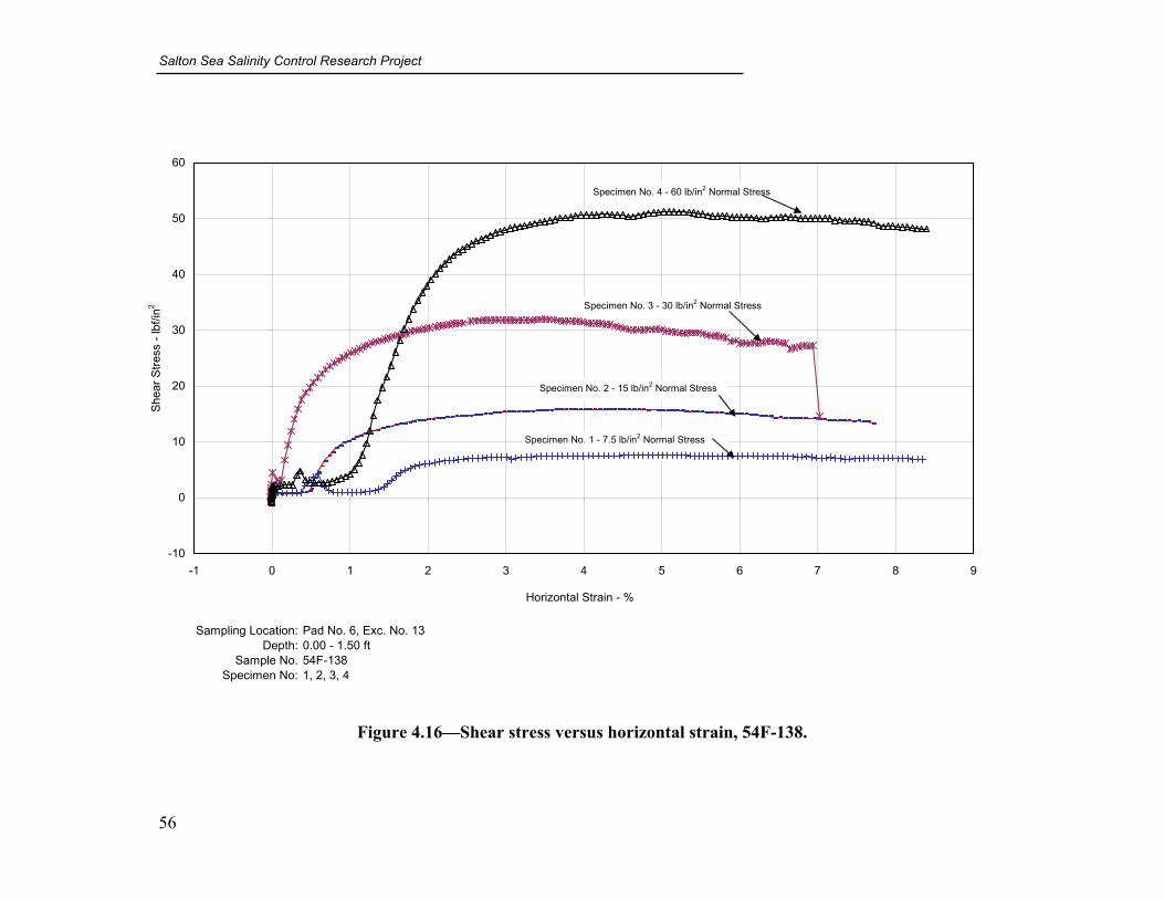
Salton Sea Salinity Control Research Project
56
Sampling Location: Pad No. 6, Exc. No. 13Depth: 0.00 - 1.50 ft
Sample No. 54F-138Specimen No: 1, 2, 3, 4
-10
0
10
20
30
40
50
60
-1 0 1 2 3 4 5 6 7 8 9
Horizontal Strain - %
Shea
r Stre
ss -
lbf/i
n2
Specimen No. 1 - 7.5 lb/in2 Normal Stress
Specimen No. 2 - 15 lb/in2 Normal Stress
Specimen No. 3 - 30 lb/in2 Normal Stress
Specimen No. 4 - 60 lb/in2 Normal Stress
Figure 4.16—Shear stress versus horizontal strain, 54F-138.
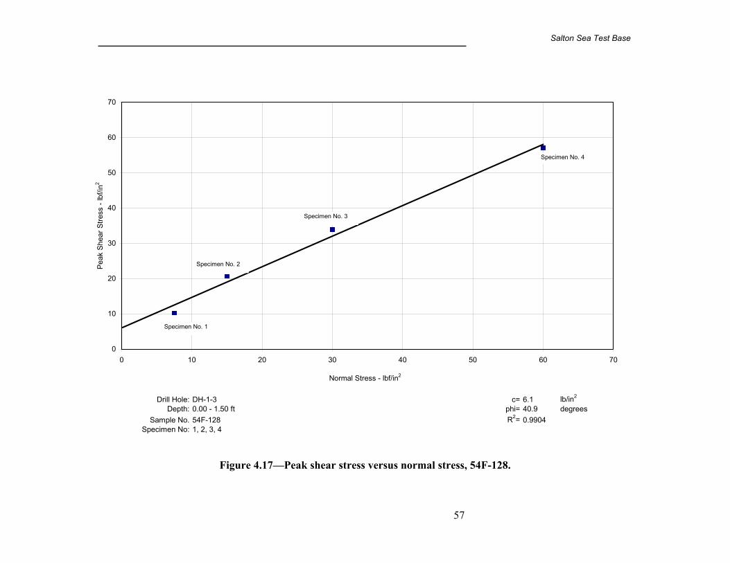
Salton Sea Test Base
57
Drill Hole: DH-1-3 c= 6.1 lb/in2
Depth: 0.00 - 1.50 ft phi= 40.9 degreesSample No. 54F-128 R2= 0.9904
Specimen No: 1, 2, 3, 4
0
10
20
30
40
50
60
70
0 10 20 30 40 50 60 70
Normal Stress - lbf/in2
Peak
She
ar S
tress
- lb
f/in2
Specimen No. 1
Specimen No. 2
Specimen No. 3
Specimen No. 4
Figure 4.17—Peak shear stress versus normal stress, 54F-128.

Salton Sea Salinity Control Research Project
58
Figure 4.18—Peak shear stress versus normal stress, 54F-132.
Drill Hole: DH-7-7 c= 5.3 lb/in2
Depth: 0.00 -1.25 ft phi= 37.7 degreesSample No. 54F-132 R2= 0.9812
Specimen No: 1, 2, 3, 4
0
10
20
30
40
50
60
0 10 20 30 40 50 60 70
Normal Stress - lbf/in2
Pea
k S
hear
Stre
ss -
lbf/i
n2
Specimen No. 1
Specimen No. 2
Specimen No. 3
Specimen No. 4

Salton Sea Test Base
59
Figure 8-8 – Peak Shear Stress versus Normal Stress, 54F-135
Figure 4.19—Peak shear stress versus normal stress, 54F-135.
Drill Hole: DH-4-10 c= 3.9 lb/in2
Depth: 0.00 - 1.00 ft phi= 39.7 degreesSample No. 54F-135 R2= 0.9872
Specimen No: 1, 2, 3, 4
0
10
20
30
40
50
60
0 10 20 30 40 50 60 70
Normal Stress - lbf/in2
Pea
k Sh
ear S
tress
- lb
f/in2
Specimen No. 1
Specimen No. 2
Specimen No. 3
Specimen No. 4
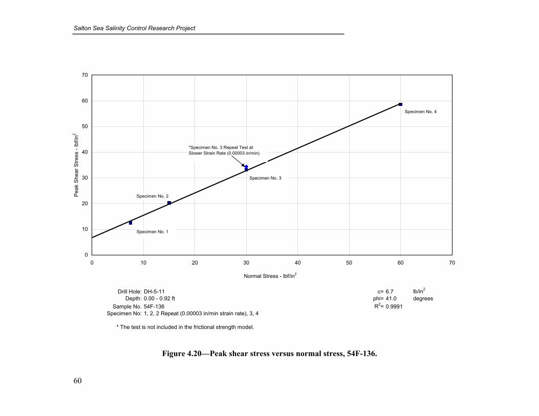
Salton Sea Salinity Control Research Project
60
Figure 4.20—Peak shear stress versus normal stress, 54F-136.
Drill Hole: DH-5-11 c= 6.7 lb/in2
Depth: 0.00 - 0.92 ft phi= 41.0 degreesSample No. 54F-136 R2= 0.9991
Specimen No: 1, 2, 2 Repeat (0.00003 in/min strain rate), 3, 4
* The test is not included in the frictional strength model.
0
10
20
30
40
50
60
70
0 10 20 30 40 50 60 70
Normal Stress - lbf/in2
Pea
k S
hear
Stre
ss -
lbf/i
n2
Specimen No. 1
Specimen No. 2
Specimen No. 3
Specimen No. 4
*Specimen No. 3 Repeat Test at Slower Strain Rate (0.00003 in/min)

Salton Sea Test Base
61
Figure 4.21—Peak shear stress versus normal stress, 54F-138.
Sampling Location: Pad No. 6, Exc. No. 13 c= 3.7 lb/in2
Depth: 0.00 - 1.50 ft phi= 39.4 degreesSample No. 54F-138 R2= 0.9812
Specimen No: 1, 2, 3, 4
0
10
20
30
40
50
60
0 10 20 30 40 50 60 70
Normal Stress - lbf/in2
Pea
k S
hear
Stre
ss -
lbf/i
n2
Specimen No. 1
Specimen No. 2
Specimen No. 3
Specimen No. 4

Salton Sea Salinity Control Research Project
62
4.5 Mineralogical Compositions
Salt materials from the cores extracted from the disposal pond were submitted to the Earth Sciences and Research Laboratory for physical properties testing. Selected salt samples were examined in the Petrographic Laboratory. The samples were labeled as shown in table 4.10. The location of the sample pads is shown in figure 3.10.
Table 4.10—Petrographic Lab sample numbers
Sample No. 54F- Pad No. Sample location
126 1 DH 1-1; Excavation No. 1
129 6 DH 6-4; Excavation No. 4
132 7 DH 7-7; Excavation No. 7
133 2 DH 2-8; Excavation No. 8
134 3 DH 3-9; Excavation No. 9
135 4 DH 4-10; Excavation No. 10
136 5 DH 5-11; Excavation No. 11
138 6 Pad 6; Excavation No. 13
The purpose of the examination was to determine the mineralogical composition of the salt and to document any texture information.
The petrographic examination consisted of megascopic and microscopic examination, X-ray diffraction analysis, and a few physical and chemical tests. An undisturbed block sample and several disturbed core samples were examined. The undisturbed block sample (54F-138) was sampled at 0.2-foot intervals from 0.0 to 1.2 feet (figures 4.22 through 4.25). A composite sample was also taken from top to bottom. A single composite sample was taken from each examined core. In general, the cores were disturbed during field sampling. Figures 4.22 through 4.25 show laminations, color variations, and voids in the block sample (54F-138). The samples were air dried before petrographic examination.
X-ray powder diffraction and grain mounts indicate that the salt is halite, NaCl, and bloedite, Na2 Mg (SO4)2 2H2O. Grain mounts of powdered samples immersed in refractive index compounds suggest that halite is usually the more abundant mineral; however, composite samples 54F-132 and 54F-133 appear to be about 1:1 halite - bloedite. An unidentified mineral was observed by scanning electron microscopy, which appears to be present only in trace to minor amounts. Images of selected salt aggregates from the 1.0 to 1.2-foot interval of the block sample (54F-138) are shown on figures 4.26 and 4.27. Table 4.11 provides particle size information.
Figures 4.28 and 4.29 depict the elemental compositions as a result of energy dispersive spectroscopy for the minerals identified as halite and bloedite.

Salton Sea Test Base
63
Figure 4.22—Salton Sea undisturbed salt block sample 54F-138, pad 6, excavation No. 13.
Photograph shows bedding and indistinct voids between bedding. Sample is encased in wax impregnated cheesecloth. Scale in tenths of a foot.
Figure 4.23—Salton Sea undisturbed salt block sample 54F-138, 54F-138, pad 6, No. 13.
Photograph shows detail of bedding and voids. Scale in tenths of a foot.

Salton Sea Salinity Control Research Project
64
Figure 4.24—Salton Sea undisturbed salt block sample 54F-138, pad 6, excavation No. 13.
Photograph shows detail of bedding and voids. Scale in tenths of a foot.
Figure 4.25—Salton Sea undisturbed salt block sample 54F-138, pad 6, excavation No. 13.
Photograph shows detail of bedding and voids. Scale in tenths of a foot.

Salton Sea Test Base
65
Figure 4.26—Back-scattered electron image.
The composition image shows two minerals. The lighter-colored, cubic mineral is halite, NaCl, and the darker-colored mineral is bloedite, Na2 Mg (SO4)2 2H2O. The image shows that the salt is composed of mineral aggregates. Optical grain mounts indicated numerous inclusions of dust-size particles which contaminate the crystals. Bar scale is 500µm; 75X.
Figure 4.27—Back scattered electron image.
The lighter-colored, cubic mineral is halite, NaCl, and the darker-colored mineral is bloedite, Na2 Mg (SO4)2 2H2O. The needle-like mineral is unidentified. Bar scale is 20µm; 750X.

Salton Sea Salinity Control Research Project
66
Figure 4.28—Elemental composition determined by
energy dispersive spectroscopy.
Elemental composition determined during back-scattered image analysis (figure 4.26). Elemental analysis indicates the light-colored minerals in the salt are chiefly composed of elements Na and Cl.
Table 4.11—Block sample (54F-138) particle size data
Depth interval Particle size (diameter)
0.0-0.2 foot 0.5- to 3-mm crystals with a few soil particles; aggregates to 12 mm
0.2-0.4 foot 0.25- to 8-mm crystals; aggregates to 12 mm
0.4-0.6 foot <0.25- to 2-mm; aggregates to 10 mm
0.6-0.8 foot <0.25- to 6-mm; aggregates to 10 mm
0.8-1.0 feet <0.25- to 5-mm; aggregates to 20 mm
1.0-1.2 feet <0.25- to 5-mm; aggregates to 2 mm

Salton Sea Test Base
67
Figure 4.29—Elemental composition determined by
energy dispersive spectroscopy.
Elemental composition determined during back-scattered image analysis (figure 4.27). Elemental analysis indicates the dark-colored minerals in the salt are chiefly composed of elements Na, Mg, S, and O.
5 Findings Observations made during consolidation tests suggest that there are several uncontrolled variables that probably influenced test results in a significant manner. These variables are temperature, evaporation, and ion exchange with brass and copper testing equipment.
Small variations in laboratory temperature are believed to have resulted in solutioning at or near contacts between salt crystals concurrent with and crystallization of salt elsewhere in test specimens. Areas of contact between salt particles are in compression when an external load is applied. It is hypothesized that solutioning of salt at these contacts will cause reduction of the contact area, thereby causing higher particle contact stresses and, consequently, specimen compression. This may be an irreversible action and could explain the observed long-term compression of salt particles under load.
Evaporation occurred despite an effort to control it by sealing the sample with plastic, using elastic bands to hold a plastic cover to the specimen container wall. Salt precipitated on test equipment surfaces, and brine was added frequently to keep specimens saturated. Undoubtedly, some salt also crystallized inside the specimen, as evidenced by an increase in specimen dry mass between the start and finish of all tests.

Salton Sea Salinity Control Research Project
68
Metal ions from brass and copper components of the testing equipment entered into the brine solution, causing a general change in brine chemistry. Salt used in the tests was typically white to pink, while salt crystallizing on the surface of the test equipment, and to a lesser extent in specimens, was generally green, indicating a different mineral. Consequently, the mineral content of specimens changed during the lengthy consolidation tests.
Direct shear tests were probably not as significantly influenced by the above-mentioned uncontrolled variables as consolidation tests, due to the relatively short duration of the test—a few days compared to months. However, direct shear tests were displacement rate controlled rather than stress controlled, thereby preventing observation, or measurement of creep that may have occurred. Much lower strengths may be realized if stress controlled tests were used.
The observation described suggests that salt in a saturated brine solution in the field, under pressure from the weight of overlying salt and undergoing continuous evaporation and temperature changes, will experience crystal growth and continuous solutioning and recrystalization. The net effect would be a decrease in void space between crystals and greater matrix density. It is concluded that the salt samples obtained from shallow depths in the relatively dry evaporation pond probably do not reflect the conditions expected in deep brine-saturated salt fills. It is expected that salt in a deep evaporation pond would be much more dense, less compressible, and not composed of small individual particles.
5.1 Salinity Control Projects Design Issues
Problems observed at the Salton Sea Test Base project that will have an impact on the design and operation of any salt concentration and disposal facility include gypsum fouling, saturated brine pumping difficulties, and brine entrainment within the salt deposits. It was observed that bittern properties were not difficult to deal with, and evaporation to very near dryness is possible. Following are discussions and recommendations related to these issues.
5.1.1 Fouling of Closed Conduits
It was observed during the course of the Test Base research project that significant gypsum fouling occurred in all closed conduits that carried brine around and between ponds. Figure 5.1 presents a cross section of one such pipe. This particular 6-inch-diameter pipe was 80 percent plugged with gypsum. This type of fouling will occur in any Salton Sea reclamation project involving evaporation of Sea water with movement of brine in any closed conduit. Therefore, using pipes to move brine within such a project is strongly discouraged. Even if pipelines were overdesigned, relative to capacity, they would eventually be entirely closed off by these types of deposits.

Salton Sea Test Base
69
Figure 5.1—Gypsum fouling of closed conduits.
5.1.2 Fouling of Canals and Control Structures
Just as Salton Sea brines were observed to precipitate gypsum in closed conduits, gypsum was also observed to precipitate in the open ponds. It can, therefore, be assumed that transport of brines between project features in open canals will also lead to gypsum forming on the bottom and sides of the canals. Therefore, any canals and ditches will have to be substantially overdesigned and/or excavated on a regular basis. Research into gypsum growth rates on these structures is necessary to estimate design or maintenance requirements. Likewise, any control structures also must be properly designed and maintained.
5.1.3 Pumping Saturated Brine
Pumping saturated and/or nearly saturated brines requires special attention and should be avoided. It can be accomplished, however, through continuous injection of Salton Sea water or freshwater. Enough water must be injected to break the saturation of the brine being transported. This will prevent the precipitation of salts within the pumps and pipes. Other requirements include cooling the pumps and using the bearings that have flushing features to prevent deterioration, due to the corrosive actions of the brines.

Salton Sea Salinity Control Research Project
70
5.1.4 Brine Entrainment
Large amounts of brine will be trapped below a thick surface crust in a disposal facility unless there are features designed to drain the material. Without project features to drain the disposal facility, the structural integrity of the salts will be substantially reduced. Figure 5.2 shows that the consistency of the salts within the test disposal pond before entrained brines were drained. Figure 5.3 shows the same hole after the entrained brines were drained.
Figure 5.2—Brine entrainment in disposal pond.

Salton Sea Test Base
71
Figure 5.3—Drained salt deposits.
5.1.5 Draining of Entrained Brines
The draining of entrained brines in the test disposal pond at the Test Base was accomplished via gravity flow to the lowest spot in the pond. The lowest portion of the pond was a concrete sump. Entrained brines drained very slowly over the course of a couple months to achieve the level of dryness shown above in figure 5.3. The brine was removed via a small sump pump placed in the bottom of the sump. To prevent salts from precipitating inside the flexible discharge hose, a small stream of Salton Sea water was injected at the discharge point on the pump, as required. The stream of much less concentrated water was used to break the saturation of the brine for conveyance to the adjacent test pond.
Before sump pumping operations could begin, very dense salts in the bottom of the sump were required to be cleared out. The sump was flushed out with Salton Sea water using a 10-hp trash pump. The flushing action dissolved the salts, enabling them to be pumped to an adjacent test pond. The sump used to remove the entrained brines from the disposal pond is shown in figure 5.4.

Salton Sea Salinity Control Research Project
72
Figure 5.4—Sump used to drain and pump entrained brines
5.1.6 Bittern Properties
The heaviest brines produced at the Test Base were those left in the disposal pond sump after the EES pretest that was conducted in 2001. This test produced a thin layer of salts in the disposal pond, and the quantities of entrained brines were relatively small. These brines drained towards the sump (figure 5.4), where they evaporated over a period of months. These highly concentrated bitterns were pumped to the pond cell shown in figure 5.5. The bitterns were moved before new saturated brines were pumped into the disposal pond from EES and solar ponds. Over a period of weeks, all the bitterns had evaporated down and precipitants were formed. The precipitants were not completely dry, however. When mixed with the blowing sands that are omnipresent at the Salton Sea Test Base, the materials resembled firm mud with an oily consistency, rather than a liquid. This mud-like consistency can be seen in figure 5.6, which shows the same pond 3 weeks later (mid-April 2002). Figure 5.7 is the same pond in mid-June. The mud-like characteristic of the bitterns remained. Observations made in late summer again revealed no change. Definite characteristics of bittern from the Salton Sea water are yet to be determined.

Salton Sea Test Base
73
Figure 5.5—Bitterns during final evaporation at Salton Sea Test Base.
Figure 5.6—Bitterns after 2 weeks of evaporation at Salton Sea Test Base.

Salton Sea Salinity Control Research Project
74
Figure 5.7—Bitterns after 3 months of evaporation at Salton Sea Test Base
5.1.7 Mix Salts Domination
Observation and analysis of salts deposited in the disposal pond at the Test Base indicate the materials were a continuous mixture of Halite (NaCL) and Bloedite (Na2Mg(SO4)22H20). No stratification of salts was observed. These deposits are therefore described as mixed salt dominate.
5.2 Enhanced Evaporator Issues
Problems observed at the Salton Sea Test Base research project that will have an impact on the design and operation of EES based salt concentration includes gypsum and biologic fouling. Following are discussions and recommendations related to these issues.
5.2.1 Fouling of Closed Conduits
It was observed during the course of the Test Base research project that significant gypsum fouling occurred in all closed conduits that carried brine around and between ponds. This was also the case in pumping water to EES units. Figure 5.1 presents a cross section of a pipe almost entirely closed because

Salton Sea Test Base
75
of gypsum deposits. A large EES project would include many miles of such pipe, and fouling of them would be impossible to avoid without significant pretreatment to remove calcium before pumping through the system. At the Test Base, there was no pretreatment; therefore, the nozzles on the units plugged up regularly with gypsum and had to be cleaned and/or replaced daily.
5.2.2 Biological Fouling
Brine fly populations were very large in the EES test pond. As a result, these flies and brine fly larvae were perpetually picked up by the pump. Two inline filters had to be installed before the EES units could remove this biologic material. Without the filters, the nozzles on the EES units plugged up. The inline filters had to be cleaned numerous times per day to keep the units in operation at proper flow rates and pressures.
5.2.3 Mist Fouling of Evaporators
Mist fouling of the evaporators was a major problem. Any wind from a non-aligned direction resulted in mist surrounding the units. Much of the mist was sucked into the impellers of the turbo fans, resulting in deposits like those shown in figure 5.8. Left unattended, enough mist could be ingested into the units to force the impeller blades out of balance. The devices had to be shut down every couple of days and pressure washed, both inside and outside of the housings. This process was repetitive and time consuming over the course of project operations.

Salton Sea Salinity Control Research Project
76
Figure 5.8—Salt deposits on evaporators from mist ingestion.

Salton Sea Test Base
77
5.3 Intake Problems and Issues
Numerous problems were experienced in the operation of the sea water intake facility at the Salton Sea Test Base. This section summarizes these problems.
5.3.1 Barnacle Fouling
The Salton Sea is home to an extremely large and healthy barnacle population. Anything left standing in the water for numerous days will become a site for barnacle growth. Infestation was observed on both interior and exterior components of the submerged sea water intake structure. A lesser problem was also observed in the intake structure at the Agrarian Research solar pond research facility near Bombay Beach. The problem may have been less severe at the Bombay Beach facility, due to lower levels of nutrients available at the site. The intake facility at the Test Base was constructed along the remains of the old Navy pier. This pier is a well-used roosting site for birds at the Salton Sea…particularly brown pelicans. As a result, the birds contribute significant nutrients to the surrounding waters, which encourage barnacle growth on anything near by.
5.3.1.1 Fish Screen Fouling
Figure 5.9 shows the Test Base fish screen that was removed from the water and placed on the bed of a pickup. Figure 5.10 shows the structure from the Bombay Beach site. Both photos depict significant fouling. The screen shown in figure 5.9 was in operation for only 2 months at the time of this photo. The screen had stopped turning probably weeks before this time. Barnacles had also attached and grown over the nozzle jets that facilitate the rotation of the screen, resulting in reduced flow rates and pressures being delivered through the nozzles. As a result of this problem, the screen and intake structure required weekly service to keep the screen in operation. This process involved removing the screen, taking it to shore, and pressure washing it. Additional manual chipping and scraping were also required. This problem was minor, compared to problems experienced with barnacles fouling the intake pipeline.
5.3.1.2 Intake Pipeline Fouling
The intake pipeline became almost complete choked of with barnacle growth within 3 months after the project began pumping Salton Sea water to the Test Base ponds. As a result, intake performance was severely degraded, forcing the construction of an alternate intake pipe with a fish screen attached. It was difficult and time-consuming to clear the main intake pipe, but it was accomplished by using a portable industrial drain-cleaning machine with 300 feet of cable. This cleaning process took numerous days and required operations from both the sea and land sides of the intake pipe.

Salton Sea Salinity Control Research Project
78
Figure 5.9—Barnacle fouling of Salton Sea Test Base fish screen.
Figure 5.10—Barnacle fouling of intake structure and fish screens at Bombay Beach solar pond facility.

Salton Sea Test Base
79
5.3.2 Barnacle Remediation
To alleviate the problem of barnacle fouling of the intake screen and pipeline, a Radiant Energy Forces (REF) barnacle removal system was provided by Water Savers Worldwide. This system was provided to the Salton Sea Authority for testing purposes. The photos in figure 5.11 show the two main features of the REF system. The system worked effectively to discourage barnacle growth within the pipe and on the screen. However, loose barnacle shells settled continuously in the lowest elevations of the pipeline. It was apparent that the REF system was dislodging the barnacles before significant growth could occur. The problem of shells settling within the pipe was easily solved by backflushing the pipeline with the alternate intake. Back flushing was only required every few months.
Figure 5.11—REF barnacle removal system.

Salton Sea Salinity Control Research Project
80
5.3.3 Intake Priming
Electrical failures occurred several times during the research project. Electrical failures in excess of a few seconds resulted in the loss of prime on the intake pump. A manual diaphragm pump was always available for prime restoration. Priming was only possible through strenuous labor. The length of the sea water intake pipe was 600 feet.
5.3.4 Intake Degassing Problems
Cavitation of both the intake and fish screen flushing pumps occurred often throughout the beginning stages of the project because the pressure in the intake line was, at times, below the vapor pressure of the fluid being pumped. To alleviate this problem, a degassing column was constructed on the intake pipe. The gasses that were being generated under these low pressures were removed under a vacuum generated from the flushing pump discharge line. The only other way to deal with this problem would have been to change out the pumps or drop the intake pumps to a lower elevation than the fish screen out in the Salton Sea. The degassing column was a much simpler and less expensive solution to the problem. The column substantially reduced cavitation in both of the pumps and facilitated a pump life beyond the project duration. Figure 5.12 shows the degassing column on the sea water intake line.
Figure 5.12—Intake structure degassing facility.

Salton Sea Test Base
81
5.4 EES Efficiency and Energy Costs
The following cost estimates are the best available at this time. Future costs for salt production will depend on evaporation pond size, microclimate effects, and the price of electricity. Additional research on pond size and microclimate effects is needed to help predict future costs of a salt production facility.
To evaluate the efficiency and costs of operations of ground-based EES units, a number of operational tests were performed. Efficiency of the EES units is defined, for the purposes of this research, to reference performance in comparison to a solar pond facility without EES blowers. The energy costs are representative of the operation of the Slimline enhanced evaporators, as described in Section 3.1 of this report.
During testing, the evaporators were run over the 5-acre EES test pond shown in figure 2.1. Figure 5.13 shows the Slimline evaporator online over the test pond. One test was performed to monitor the time to saturate 3 million gallons of Salton Sea water. This test was run during the winter, between the dates of December 31, 2001, and April 11, 2002, using both the SMI and Slimline evaporators. Figure 5.14 displays how specific gravity increased in the EES pond over this period. It took 102 days for the 3 million gallons to come to saturation in this test, and it resulted in 198,000 gallons of saturated brine.
Figure 5.13—Slimline evaporator used in power use study.

Salton Sea Salinity Control Research Project
82
Specific Gravity MeasurementsEES Test Pond
1.020
1.040
1.060
1.080
1.100
1.120
1.140
1.160
1.180
1.200
1.220
1.240
12/2
5/20
01
1/4/
2002
1/14
/200
2
1/24
/200
2
2/3/
2002
2/13
/200
2
2/23
/200
2
3/5/
2002
3/15
/200
2
3/25
/200
2
4/4/
2002
4/14
/200
2
4/24
/200
2
Date
Spec
ific
Gra
vity
Saturation
Start With 3 Mgal of Sea Water
Test 2 Produced 0.198 Mgal Saturated Brine
Figure 5.14—Specific gravity measurements in EES pond.
Another series of tests were performed in November, 2002. The purpose of these tests was to develop power consumption and cost data for the operation of a single Slimline EES unit. The Slimline Evaporator, as shown in figure 5.13, was selected for these tests. Four separate power usage tests were performed, and the results are shown in table 5.1. Using $0.097 per kwh, it was determined that on average it cost $2.44 per hour to get water to and through the Slimline evaporator. This rate applied to the two EES units operating to concentrate 3 million gallons of Salton Sea water between December 31, 2001, and April 11, 2002, results in a cost of $8,350. Accumulated energy usage and costs for concentrating the water are shown in figure 5.15. A total of 86,100 kwh of energy was consumed in this test. Assuming that there are no significant microclimate effects of operating hundreds of ground-based units, these costs can be extrapolated based on the monthly evaporation distribution presented in figure 4.1 for a much larger salt producing project. The December 31 to April 11 test produced 526 tons of salt in saturated brine and evaporated 8.6 acre-feet of water. By applying the additional evaporation that would occur over the course of a year, it was estimated that 2,783 tons of dissolved salt in saturated brine would be produced and 45.5 acre-feet of

Salton Sea Test Base
83
Accumulated Power Usage and Costto Saturate 3 Millions Gallons of Salton Sea Water
Over a 5 Acre Pond Using 2 EES Units12/31/01 to 4/11/02
0
10000
20000
30000
40000
50000
60000
70000
80000
90000
100000
12/15/2001 1/4/2002 1/24/2002 2/13/2002 3/5/2002 3/25/2002 4/14/2002 5/4/2002
Date
Acc
umul
ated
kw
h
$-
$1,000
$2,000
$3,000
$4,000
$5,000
$6,000
$7,000
$8,000
$9,000
Acc
umul
ated
Pow
er C
osts
Accumulated Power in kwhAccumulated Power Costs
Table 5.1—Slimline EES power usage
Test date Duration of test (hrs)
Volume pumped through
Slimline EES unit (gal)
Rate (gpm)
Power use by
EES unit (kwh)
Power use by feed
pump (kwh)
Total energy
used (kwh)
Energy use per hour of operation (kwh/hr)
Total Energy
cost at
$.097/kwh ($)
11/4/02 3.4 10,496 52 46 41 87 25.3 8.44
11/6/02 4.1 15,590 62 55 51 106 25.6 10.28
11/19/02 3.7 10,978 53 49 44 93 24.9 9.02
11/20/02 3.4 9,618 49 46 40 86 25.0 8.34
Average
3.7
11,671
54
49
44
93
25.2
9.02
Figure 5.15—Accumulated power usage and cost to concentrate 3 million gallons.

Salton Sea Salinity Control Research Project
84
311,129
111,804,059
1
10
100
1000
10000
100000
1000000
10000000
100000000
1000000000
Ener
gy (k
wh)
Scaled Energy Usage for 1 Mtons Per YearSalt Production Using Ground Based EES
Energy to Produce 2783 Tons in One YearEnergy to Produce 1 Mtons in One Year
2783 Tons/Yr 1 Mtons/Yr
kwh
kwh
water would have been evaporated over a period between December 31, 2001, and December 30, 2002. Figures 5.16 through 5.18 present results of extrapolating these results on up to a 1-million-ton-per-year project. To remove 1 million tons per year would require 719 EES units, assuming the Test Base pond size ratio of 2.5 acres per unit. This is depicted in figure 5.18. The amount of energy and cost thereof for a project of this size are presented in figures 5.16 and 5.17. It would take 111,800,000 kwh of electricity to concentrate a million tons of salt in Salton Sea water to saturated brine at a cost of $10,450,000.
The number of EES required to concentrate 1 million tons per year is dependent on the size of the pond on which the units are operating. At the Test Base, the two evaporators were operated on a 5-acre test pond. Due to requirements described, it is clear that 2.5 acres per evaporator is too low and would need to be increased significantly.
Figure 5.16—Projected energy usage to produce 1 million tons per yr of salt.

Salton Sea Test Base
85
$30,180
$10,844,994
$1.00
$10.00
$100.00
$1,000.00
$10,000.00
$100,000.00
$1,000,000.00
$10,000,000.00
$100,000,000.00
Ener
gy C
ost (
$)
Scaled Energy Costs for 1 Mtons Per YearSalt Production Using Ground Based EES
Cost Energy to Produce 2783 Tons in One Year
Cost of Energy to Produce 1 Mtons in One Year
2783 Tons/Yr 1 Mtons/Yr
2
719
1
10
100
1000
Num
ber E
ES U
nits
Scaled Number of EES Units for 1 MtonsSalt Production In One Year
Number of EES Units to Produce 2,783 Tons in One Year
Number of EES Units to Produce 1 Mtons in One Year
2783 Tons/Yr 1 Mtons/Yr
Assuming Pond Sizeof 2.5 Acres
Per EES Unit
Figure 5.17—Projected energy costs to produce 1 million tons per yr of salt.
Figure 5.18—Projected number of EES units to produce 1 million tons per year of salt.

Salton Sea Salinity Control Research Project
86
Number of Ground Based EES Units vs Pond Size to Concentrate 1 Mtons/yr of Salt
0
100
200
300
400
500
600
700
800
1700 1800 1900 2000 2100 2200 2300 2400 2500 2600
Pond Size (acres)
# EE
S U
nits
$-
$2,000,000
$4,000,000
$6,000,000
$8,000,000
$10,000,000
$12,000,000
$14,000,000
$16,000,000
$18,000,000
$20,000,000
Ener
gy C
osts
($)
Number of EES Units to Produce 1 Mtons/yr
Energy Costs
0.91 EES Units Can Be Removed For Every Acre Added to the EES Pond
Calculations were performed to determine how many EES units could be eliminated for each acre added to the 1 million tons per year project pond. It was determined that a theoretical 0.91 evaporators could be removed for each acre of increase. Another way of viewing this is that an evaporator is equivalent to 1.1 acres of open water surface. Extrapolating this concept to a wide range of pond sizes results in the information shown in figure 5.19. The pond sizes analyzed range from 1,800 to 2,570 acres.
As the number of evaporators is reduced and pond acreage is increased, the energy requirements to produce 1 million tons per year are reduced. The cost of operating one evaporator over 1 year 63 percent (based on winds) of the time was determined to be $15,090. Therefore, removing a unit from the project would reduce the energy costs by an equal amount. Figure 5.19 also contains information about the cost of energy based on pond size. The costs for energy are linear; for the 1,800-acre pond, the costs would be about $10,800,000. For a 2,570-acre pond, the costs could be only about $280,000
Figure 5.19—Number of EES units and energy costs versus EES pond size to produce 1 million tons per year of salt.

Salton Sea Test Base
87
0
1
2
3
4
5
6
7
8
9
Evap
orat
ion
(af)
Evaporaton Using 2 EES Units on a 5 Acre Pondvs a 5 Acre Solar Pond
for the Period 12/31/02 Thru 4/11/02
Using EES Operating 63 Percent ofTimeUsing Solar Pond
44 PercentIncrease inEvaporationUsing 2 EESUnits on 5Acre Pond
Power Costs=$41/day
EES Solar Pond
The efficiency of the evaporators can be measured in comparison to solar pond project without evaporators. Based on the climate conditions that occurred during the period of EES testing at the Test Base, and on the results of the testing, it can be concluded that by placing two evaporators on a 5-acre pond, evaporation and salt production can be increased by 44 percent over a sole 5-acre solar pond. This depicted in figure 5.20.
The efficiency and cost studies presented herein are based on the assumption that the evaporators could be operated 63 percent of the time, as was possible for the December 31, 2001, to April 11, 2002, test. The analyses were also dependent on the power usage and costs associated with the pumps and evaporators used at the Test Base. Other equipment would certainly yield different results.
Figure 5.20—Comparison of evaporation with EES and solar ponds.
Salton Sea Salinity Control Research Project
88
5.4.1 Microclimate Effects
Because of the scope and scale of the Test Base project, it was not possible to study the potential for microclimate changes, due to large-scale EES operations on efficiency and costs. With hundreds of these devices in operation, it would seem logical that base evaporation rates would decline because of increased humidity. These effects are anticipated to be very significant. Additional research would be required before consideration could be given to applying EES technologies at the Salton Sea.
The preceding cost estimates are the best available at this time. Future costs for salt production will depend on evaporation pond size, microclimate effects, and the price of electricity. Additional research on pond size and microclimate effects is needed to help predict future costs of a salt production facility.
6 Recommendations 6.1 Disposal Recommendations
Lessons learned at the Test Base should be considered when producing and disposing of salts from a salinity control project at the Salton Sea. Following is a summary of recommendations for further consideration of salinity control projects at the Salton Sea.
6.1.1 Concentrate Near the Disposal Facility
Saturated and nearly saturated brines should be moved with gravity flow and not transported long distances because saturated brine drops salts while in transit and can foul any canal or pipeline in which it is being moved. Fresh or Salton Sea water injection into pipelines and/or pumps is expected to only work over short distances. Therefore, it is recommended that the disposal facility be placed near the salt concentrating project or near the final stages of the concentrating features. This will greatly simplify transportation of the denser brines.
6.1.2 Gravity Flow in Open Channels
Pumping of brines developed from the evaporation of Salton Sea water at any stage should be strictly avoided. Fouling by gypsum occurs in closed conduits almost immediately after Salton Sea water begins to evaporate. Instead, project features should be designed for gravity flow in open canals and ditches, which can be oversized and excavated at scheduled and lengthy intervals. All control structures will also be exposed to fouling and must be designed for ease of maintenance and removal of gypsum deposits.

Salton Sea Test Base
89
6.1.3 If Pumping is Unavoidable
If pumping is unavoidable, it should be restricted to short distances, and the pipelines must be cleaned regularly. Drain cleaning equipment will probably not be effective, nor will flushing the deposits out with fresh water. The dense, hard gypsum deposits that form in the pipes will not be subject to redilution. The pipelines will have to be extensively overdesigned in capacity and will have to eventually be replaced. If the brine being pumped is saturated or nearly saturated, it will be necessary to perform fresh or Salton Sea water injection into the intakes of the pumps to limit precipitation within the pumps and pipelines. This injection will reduce but not eliminate fouling issues within the pipes. Even with injection, it will be necessary to service and clean the pumps on a frequent—if not daily—basis. When pumping saturated or nearly saturated brine, the intake and discharge pipes should be limited to a few meters in length. All pumps used at any stage of a project must be designed with self-cleaning bearings and seals. Pump motors must include some feature for cooling. Summer temperatures at the Salton Sea severely impact the performance and life of electric motors.
6.1.4 Mechanical Consolidation
To reduce the space available for brine entrainment, it will be necessary to consolidate the salt deposits in a disposal facility. This will substantially increase the density of the materials and will extend the life of the disposal cells by providing more space for salt precipitation. It will be necessary to research methods of consolidation at a later date.
6.1.5 Disposal Pond Design and Operations
If on-land disposal is a consideration for salt extracted from the Salton Sea then it is recommended that the disposal facility be divided into four separate cells. This would allow one cell to be drained of entrained brines while the other three cells continue to receive saturated brine and precipitate salt. Once an idle cell is drained, it should be mechanically consolidated to decrease the porosity and, subsequently, increase the density of the salt deposits. Based on the materials testing results presented herein, it can be assumed that 98 lb/ft3 can easily be achieved under consolidation. After the deposits are consolidated, the idle cell would be put back into rotation to receive saturated brine from the concentrating features of the project. Another one of the active cells would then be idled, drained, and consolidated. This rotation process would continue endlessly among the four disposal cells, and draining would continue for several months.
Entrained brines from the cells that are being drained and pumped from the idle cell will have to be extracted using fresh or Salton Sea water injection at the pump intakes. This will prevent salt deposits from severely fouling the pumps and pipelines. This technique will not stop the fouling but will reduce it significantly. The pumps and pipes will require cleaning at least once a day with fresh water

Salton Sea Salinity Control Research Project
90
that will dissolve the deposits. Gypsum deposits will not occur from these brines. Most of the calcium will have dropped out long before this stage of concentration. The brines extracted from the idle cell should be discharged into the active cells. The cells that are receiving saturated brine should receive the brine in parallel, not in series.
Sump facilities will have to be maintained in each of the four disposal cells. Additional sump culverts will have to be installed as deposits increase in depth through time. Periodic flushing of the sumps with fresh or Salton Sea water will keep the sumps clear of salt deposits.
6.1.6 Dike Embankment Design
As noted earlier in this report, the upstream-raise dike configuration (figure 3.16) had originally been proposed by URS Corporation for the salt disposal cell embankments. The fact that the upstream-raise dike design requires less earthfill and, therefore, costs less to construct probably was a factor in that recommendation by URS. However, Reclamation noted the fact that the upstream-raise embankment design is almost never used in seismic areas of the world on mining projects (where dike raises for tailing impoundments are common practice), which is the reason for a counter-proposal to use a more conservative (stable) dike configuration. The Salton Sea vicinity has historically experienced major seismic events and significant loading conditions, which should be expected to continue to occur during the project’s operational life. The upstream-raise dike configuration should be removed from further consideration. Hence, the center-raise (figure 3.15) and downstream-raise dike embankment configurations should be considered the only realistic design concepts for the salt disposal cells, depending on the results of the design data acquisition and analyses that need to be performed.
The design work for these salt disposal cell embankments will need to include both static and seismic (dynamic) stability analyses. Those analyses will require the proper characterization of the salt and earthfill materials involved at the potential salt disposal facility sites. In addition to the shear strength, stress-strain, and consolidation characteristics of the salt precipitates herein reported, the static and seismic stability analyses will require the dike earthfill and foundation materials to be similarly characterized for each facility site. At present, the dike earthfill and foundation materials at the proposed facility sites have not been sampled or tested. Until such sampling and laboratory testing can be performed and the results documented, geotechnical characterization of the dike earthfill and foundation materials will need to make assumptions about such properties, which is often done during early design stages.
The salt material testing results herein presented indicate that the precipitated salt is an unusual material compared to commonly encountered soils. While precipitated salt appears to possess soil-like shear strength and stress-strain characteristics, it also appears to exhibit a phenomenon called “creep” (using

Salton Sea Test Base
91
geotechnical terminology) based on the results of the one-dimensional consolidation testing performed. In this case, creep is defined as “continued strain (consolidation) at constant stress levels.” Creep behavior of the precipitated salt needs to be properly considered in the design of the dike embankments. It may be related to the brine entrainment problem discussed in sub-section 5.1.4. This concern about salt’s apparent creep behavior involves the fact that a portion of the dike raise embankment rests on precipitated salt material, which would be even more of a problem with the upstream-raise dike configuration where the upstream portion of the dike raise resting on precipitated salt is much greater. If the salt material does continue to compress and consolidate under the load imposed by the overlying dike embankment, and by additional dike and disposal pond raises, the support provided by the salt for the upstream portion of the stiffer raised dike(s) could decrease over time due to the salt continuing to consolidate, and it could lead to overall instability of the raised dike embankment’s slopes. This potential slope instability problem would be even more severe for the upstream-raise dike configuration, especially under seismic loading conditions.
As mentioned above, the embankment and foundation materials need to be characterized to design the disposal pond dikes. To date, only limited information has been developed on the site-specific geology and the soils that would become the dike foundations at the potential disposal pond sites. The soils found at the potential disposal pond sites are generally alluvial (Qal) and/or lacustrine (Ql). The alluvial soils will generally consist of layers of clays, silts, and sands, with some gravel layers possible. The lacustrine soils will primarily consist of lean to fat clays. To date, no assessment or information has been developed on the earthfill borrow materials available for dike construction in the Salton Sea vicinity. However, it is expected that earthfill borrow sources containing clay, silt, sand, and gravel materials will be identified for possible use, which will require appropriate sampling and laboratory testing.
The engineering properties and characteristics of the foundation and dike embankment materials must, therefore, be assumed until such time as appropriate field investigations and laboratory testing can be conducted. Reclamation and others have done much soil testing and research that enables the engineering properties of soil materials like lean and fat clays, silt, sand, and gravel materials to be estimated with reasonable confidence. Parametric stability analyses can be performed, which would involve varying the assumed soil properties, such as shear strength, to determine how sensitive different dike designs might be to the assumed soil property variations. Once the actual site(s) and borrow soils have been sampled and tested, the resulting soil properties can be plugged into the previous analyses to validate and finalize the dike design(s).
One other important soil characteristic that needs to be incorporated into the dike design process is the permeability of the foundation and dike embankment soils. Because the salt disposal cells will continually receive concentrated brine that will evolve into precipitated salt, the dike design should assume that brine fluid will percolate into and through the dike embankment and foundation soils. Laboratory

Salton Sea Salinity Control Research Project
92
testing of dike foundation and borrow soils will probably need to include permeability testing, which may need to evaluate the effect of water versus brine fluid as the test’s permeating fluid. The dike’s design will need to control seepage of the brine fluid and/or entrained moisture out through the dike embankment and foundation, and may need to mitigate the related effect on the dike’s static and seismic stabilities.
6.1.7 Bittern Management
Bittern management need not be considered in a salt deposit disposal project. The very small quantities of bitterns will be entrained in the final salt deposits during the course of operating a facility, as described above. Bitterns are defined as those brines that will be impossible to evaporate and will be very small in volume.
6.2 EES Recommendations
6.2.1 Pretreatment Research to Remove Calcium
To alleviate gypsum fouling problems when using enhanced evaporators, it will be necessary to remove the calcium in the Salton Sea water prior to delivery to the distribution system. This would be required even with a single pass system, whereby Salton Sea water would be delivered directly to the evaporators. As the water exits the nozzles, it begins evaporation immediately and gypsum scales up the nozzles. Research and testing of methods to perform pretreatment will need to occur before any serious attempt is made to apply enhanced evaporation system technology to Salton Sea reclamation projects.
6.2.2 Pretreatment Research to Remove Biologic Materials
Filtering of brine fly larva and brine flies will need to occur before distribution to the EES units. Experiences gained at the Test Base project indicate that the loading of brine flies can be large enough to foul the nozzles on the units, which results in significant reductions in efficiency and increased energy costs. Before a large scale EES project could be designed and implemented, it would be necessary to research methods of self-cleaning inline screens.
6.2.3 Robotic Wind Alignment
To reduce, but not completely eliminate, the risk of mist digestion by the EES units, each EES unit would need to be robotically slaved to multiple wind direction, wind speed, and wind shear detection systems. Any fouling by mist digestion by a significant number of EES units would be very expensive and time consuming to clean up. For a project forecasted to include hundreds, if not thousands, of these units, such a cleanup event would require thousands of hours of labor.

Salton Sea Test Base
93
6.2.4 Unit Spacing and Configuration
Based on experience gained in the operation of EES units at the test base, it would be necessary to space the devices at least 250 apart. The devices should be placed in long rows. A survey of operations at the Test Base yielded the conclusion that salt and/or mist from the evaporators can travel 1,300 feet. Therefore, the rows of evaporators should be placed at least 1,300 feet apart. The ideal configuration would be to place the units in long rows over a large pond. The system should be designed to shut down any time the winds exceed 10 miles per hour. Otherwise, the 1,300 feet will not be adequate. Determining drift characteristics at speed in excess of 10 miles per hour was not possible at the Test Base. The permits for the operation of the EES units limited operations to 10 miles and hour or less. Additional research into drift distances at higher speeds would be required before a large-scale system could be designed. However, increased drift distances would only translate into much larger pond sizes and row spacing.
6.3 Intake Recommendations
The following recommendation is made based on experience with operations of the intake structure at the Salton Sea.
Future intake structures at the Salton Sea would be much easier to maintain and to operate if they were shoreline based. System elements would include a shoreline stilling basin with a dredged trench from the basin to a significant distance out into the deep water of the Salton Sea. Intake pumps could then extract water from the shoreline basin without the need for a long, difficult-to-maintain pipeline. Fish screens would, however, still be necessary. The stilling basin would not only provide a deep source for pumping, but it would also act as a sedimentation pond whereby suspended particles would settle before being picked up by the pumps. Protection against barnacle fouling of these screens and inland pipelines could be accomplished through the application of an REF system, as shown in figure 5.11. It would be necessary to give consideration to redundant pump and screen facilities to guarantee reliability of project deliveries. Redundant screens and pumps would also facilitate backflushing of onshore lines to remove settled barnacle shells.
6.4 Proposal for Behavior Model
The behavior of solid salt under load is dependent on time, temperature, pressure, mineral content, liquid brine chemical composition, and ion and vapor exchange with the surrounding environment. Mathematical expressions are sought to predict salt strength and density in terms of the above-mentioned variables, in order to evaluate the stability of retention pond dikes and to improve estimates of the expected capacity of evaporation ponds.
A parametric study is proposed which develops first and second order relationships between time, temperature, pressure, and salt density. It is

Salton Sea Salinity Control Research Project
94
hypothesized that the density of granular salt in a saturated brine solution will increase and its volume will decrease with time when subject to constant pressure and cyclic fluctuations in temperature4. Average temperature, range of temperature fluctuations, and fluctuation frequency are additional variables in this experiment. Experimentation will involve placing samples of granular Salton Sea salt, obtained from test evaporation ponds, into a specially made consolidation test container.5 The specimen will be submerged in a saturated brine solution. A constant pressure will be applied and the specimen subject to temperature cycles in the range considered typical for expected field conditions. The initial and final densities of the specimen will be determined. The experiment will be repeated using different pressures, temperature fluctuation frequencies, and experiment duration. The results will be used to create a mathematical expression relating test variables to salt density.
A parametric study is also proposed which develops first and second order relationships between time, salt density, pressure and shear strength. The experiment will be similar to that described above with the following exceptions. A specially designed, direct shear test specimen container will be used rather than a consolidation test container.6 The specimen, submerged in brine, will be subject to a normal load and cyclic temperatures until a predetermined density is achieved. Then, while holding the temperature constant, shear stress will be incrementally applied until failure occurs. During the test, each applied shear stress will be held constant until shear strain has ceased. Then, a new increment of shear stress will be added. The results will be used to create a mathematical expression relating test variables to salt shear strength.
4 A rise in temperature is expected to dissolve salt at or near contacts between salt crystals, while a fall in temperature is expected to result in recrystallization of salt elsewhere in test specimens. Areas of contact between salt particles are in compression when an external load is applied. It is hypothesized that solutioning of salt at these contacts will cause reduction of the contact area, thereby causing higher particle contact stresses and, consequently, specimen compression. 5 The test container will resemble that which is used for tests typically performed to evaluate soil consolidation characteristics (See ASTM D-2435-96, “Standard Test Method for One-Dimensional Consolidation Properties of Soils”). The container will be made of an inert material to avoid ion exchange with brine solutions and be sealed to prevent evaporation. 6 The test container will resemble the one used for tests typically performed to evaluate soil strength characteristics by direct shearing (See ASTM D-3080-98, “Standard Test Method for Direct Shear Test of Soils under Consolidated Drained Conditions”). The container will be made of an inert material to avoid ion exchange with brine solutions and be sealed to prevent evaporation.

Salton Sea Test Base
95
7 References [1] “A Water Resources Technical Publication,” Earth Manual, Part 2, Third Edition, U.S. Department of the Interior, Bureau of Reclamation, Materials Engineering Branch, Research and Laboratory Services Division, Denver Office, 1990.
[2] "Petrographic Examination of Salt - Salton Sea Dike, Salton Sea Reclamation Project, California," Memorandum No. 8340-03-14, Bureau of Reclamation, Denver, Colorado, March 2003.
[3] “Salton Sea Accounting Model,” Bureau of Reclamation, 2001.
[4] “Salton Sea Solar Pilot Ponds Project (Final Report),” Agrarian Research and Management Company, June 2003.