*

To be submitted to IEEE Trans. Geosci. & Remote Sens., 1998. ——..—.—. .. —————.-.—..——_- .———_— ————.—______ _—— —————_

Saline Ice Thickness Retrieval underDiurnal Thermal Cycling Conditions

S. E. Shih, K. H. Ding, and J. A. KongDepartment of Electrical Engineering and Computer Scienceand Research Laboratory of 131ectronicsMassachusetts Institute of TechnologyCambridge, MA 02139

S. V. N hiemFCenter or Space Microelectronics Technology

Jet Propulsion LaboratoryCalifornia Institute c)f TechnologyPasadena, CA 91109

A. K. JordanRemote Sensing DivisionNaval Research LaboratoryWashington, DC 20375

——____ ———.—.——.—.———. . .. ..—.——. —-——__———_ —_.————— —— ——.

Mailing address : Dr. S. V. Nghiem, Jet Propulsion LaboratoryMail Stop 300-235, 4800 Oak Grove Drive, Pasadena, CA 91109

,

. Saline Ice Thickness Retrieval under Diurnal Thermal Cycling ConclitioIls

Shih-ltn Slli}l, I{ung-lIau I)ing, and Jin Au KoIIg

l)cpartmcnt of Ilcctrica.1 ltngirlecring and Coll]putcr Scicllcc

ancl Ilcsearch I,ahoratory of Itlcctronics

Massachusetts institute of Technology, Cambridge, MA 02139

Soli V. Nghicm

Center for Space Microelectronics ‘1’echno]ogy

Jet Propulsion I,ahoratory

California Institute of ‘1’ethnology, Pasadena, CA 91109

Arthur K. Jordan

Remote Sensing Division

Naval Research I,aboratory, Washington, I)C 20375

Abstract

An inversion algorithm is presented to reconstruct icc growth under thermal cycling

conditions by using time-series active nlicrowavc measurements. ‘1’hc Inethoc] uses a direct

scattering model consisting of a one-cl itllensiona] thermodynamic Illoclel of saline ice growth

that includes the thermal interactions with atmosphere, and a pllysical-based electromag-

netic model that takes into account the thermal and electromagnetic properties of icc and the

combined volume and surface scattering ef[ects. ‘l’lie combined thermodynamic electromag-

netic scattering model is applied to interpret the CR IU’II,H 94 experimental observations

on both the ice growth and the diurnal cycles in the C-band polarimctric backscattcr. ‘1’hc

crucial part of the inversion algorithm is to usc sccluentially nleasurcd radar data together

with the dcvelopccl direct scattering n~odel to retrieve the sea ice parameters. ‘1’hc algo-

rithm is applied to tile CR1{II;I,I;X 94 clata and successfully reconstruct the evolution of icc

growth under a thermal cycling c]~vironnlcnt. This work shows that the inversion algorit}lm

using time-series data offers a distinct accuracy over the algorithlns using only individual

microwave clata.

I. INTRODUCTION

%a ice thickness is an i[]lportant parameter in the llcat exchal~gc bctwccll tllc occa[l allcl

the atmosphere and Inass balance of polar oceans [1]. Satellite remote scnsi~lg oflirs ample

opportunities to monitor sea ice routinely. ‘1’bus, to retrieve ice thickness using remote

sensing data becomes an attractive and important is. sucfor the sea icc research community.

In the past two clccaclcs, there have been consiclerab]c stuclics rcgarciing the tnicrowave

signatures of sea ice [2- 4], and both passive and active spaceborne sensor ilnages have been

applied in mapping the icc extent and identifying the ice types [5,6]. however, there still

remains a basic issue for a direct determination of sea icc thickness from space. Some recent

work has addressed on using clec.tromagnetic remote sensing data to rctricvc sca icc thickness

[6--8].

In a previous paper [8], wc have dcvclopcd an icc thickness retrieval algorithm that

uscs time-series active microwave data and an clcctrotnagnetic scat~cring model consisting

of an icc constant growth model. ‘1’his inversion algorithm was applied and accurately

reconstructed the thickness of a laboratory-grown thin saline icc shccl by using the C-band

polarimctric radar measurements from CRREI,EX 93 cxpcrilncnt [9]. It was found that by

incorporating the ice growth mc)dcl into the inversion algorithm, the thickness estimation

can be constrained sufficiently to predict more accurate results. In adclition, the usc of

time series data is helpful for resolving the non-unicluencss and stability problems which arc

common for parametric estimation methods.

I’he formation and growth c)f sca ice is generally influenced by the changing cllviron-

mental conditions. ‘1’hcthermal interaction bctwccn sca ice and atmosphere strongly affects

the thermodynamic processes within the icc layer. ‘1’he thcrma]ly varying icc physical prop-

erties also significantly alter the electromagnetic interactions with the sea icc mcclium. In

this study, wc cxtelld our previous work to investigate the retrieval of ice thickness under

a thermal cycling growth collclition. A one-dimensional t~lcll~loclyllatllic mocle] of sea ice is

constructccl, that includes the thermal illtcractic)ns betwccrl ice ancl atlnosphcre, dcsalinatio]l

effect, and brine volutne thermal variation, to characterize the saline icc pl)ysical proper-

ties under thermodynamically varying conditions, An clcctlomagnctic moclel based on the

radiative transfer theory with multi layer structure and rough interface is usccl to calculate

wave propagation and scattering in the icc Inedium. Small perturbation mcthocl is al)plicd

to account for the sea ice surface roughness [10]. ‘1’hecombined thermodynamic clcctron~ag-

nctic scattering model is applied to interpret tile CI{I{F; I,FIX 94 cxpcri]ncntal observations

2

on both tile ice growth and the cliurl~al cycles in the C-band polarimctric backscattcr. As in

the previous study, this direct scattering model is then employed ill a paralllctric cstilllation

scllcrnc and uses time-series measured data to corlstruct the inversio[l algorithnl.

~’hc CIUtKt,EX 94 cxpcrimcnt [11], which was carriccl out at the outdoor Geophysical

Research 1+’acility in the U.S. Army Cold Regions Research ancl llnginccring Laboratory

(CRREL) during January 19--22, 1994, is briefly clcscribed in Scctiol~ II. In Section 111, the

saline ice thermodynamic electromagnetic scattering model is developed, ‘l’his direct scat-

tering model consists of a saline ice physical model describing the dynamic variation of ice

characteristics coupled with an electromagnetic scattering model accounting for wave propa-

gation and scattering in a random medium. Interpretations of CRRE1,EX 94 measurements

on the diurnal ice radar signatures are also demonstrated in this section, The inversion

algorithm using time series data based on this direct scattering model and a parametric

estimation approach is described in Section IV. The ice thickness retrieval and comparisons

with CRRE1,EX 94 ground truth are also presented in this section, followed by summary

section.

Il. CRRELEX 94 SALINE ICE EXPERIMENT

The varying environmental conditions affect the growth process of ice which in turn

influence the interaction between electromagnetic radiation and ice. ‘1’0 investigate the

diurnal therlnal effects on the polarimctric C-band radar signatures of sea ice, laboratory

experiments were carried out at tllc outdoor Geophysical Research l“acility in CRREI, during

January 1994. A more detailed description about the experimental set up, procedures, and

findings can be found in [11].

In the CRRELEX 94, an ice sheet was grown from open saline water with an initial

salinity of 30.0 0/00, the growth lasted for three days until the ice grown up to 10 cm in

thickness. 7’o characterize the ice physical properties, samples were taken from the pond to

measure their thickness, temperature, and salinity for approximately eve,ry I cm during the

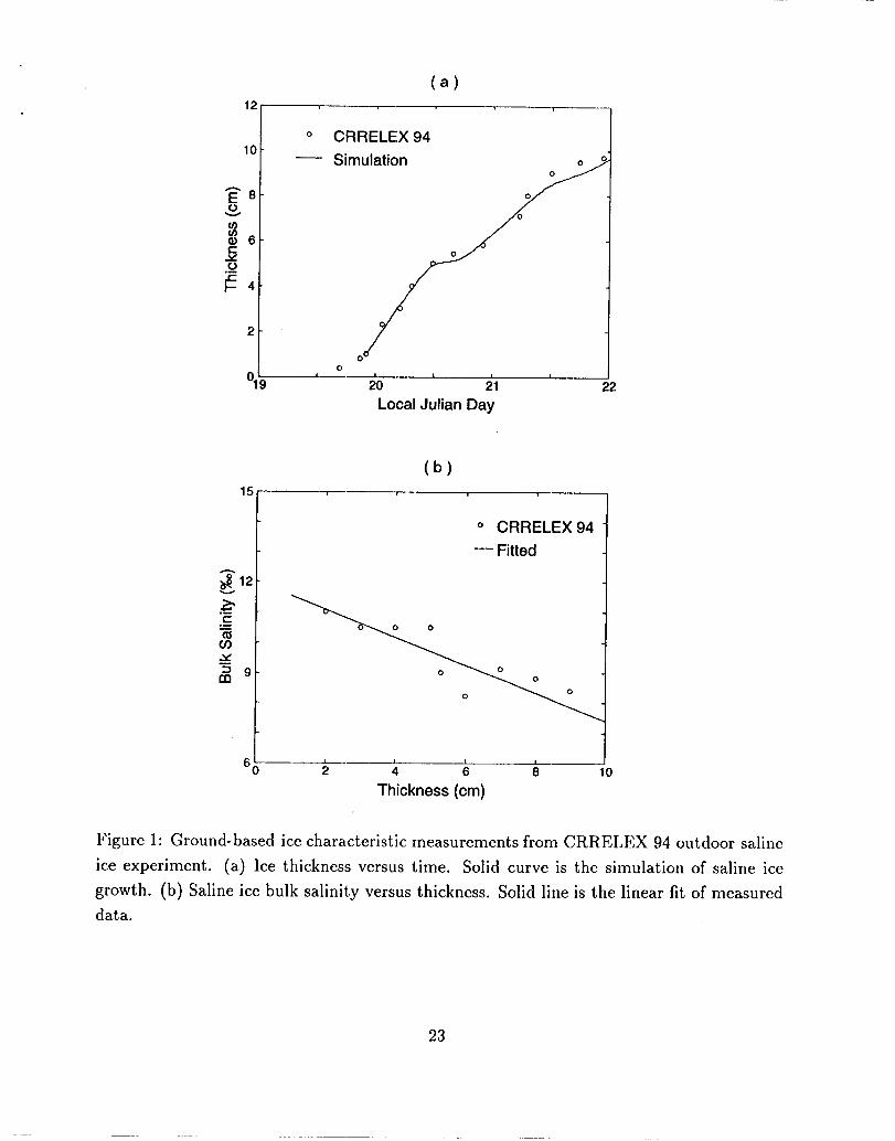
ice growth, ‘1’he evolution of ice thickness is shown in Figure 1(a), where circles rcprcscnts

the measurements and the continuous curve is obtainccl from an ice growth model which will

bc described in the next sectioll. ‘1’hc desalination is showli in F’igurc 1(b), where a roughly

30’% brine loss is observed as the thickness rcachecl 10 cnl. ‘1’hc linear fittccl curve has an

extrapolated value of salinity at // ==O, Siol be 12.0 0/00 and a rlcgativc slope of 0.458 0/00 pcr

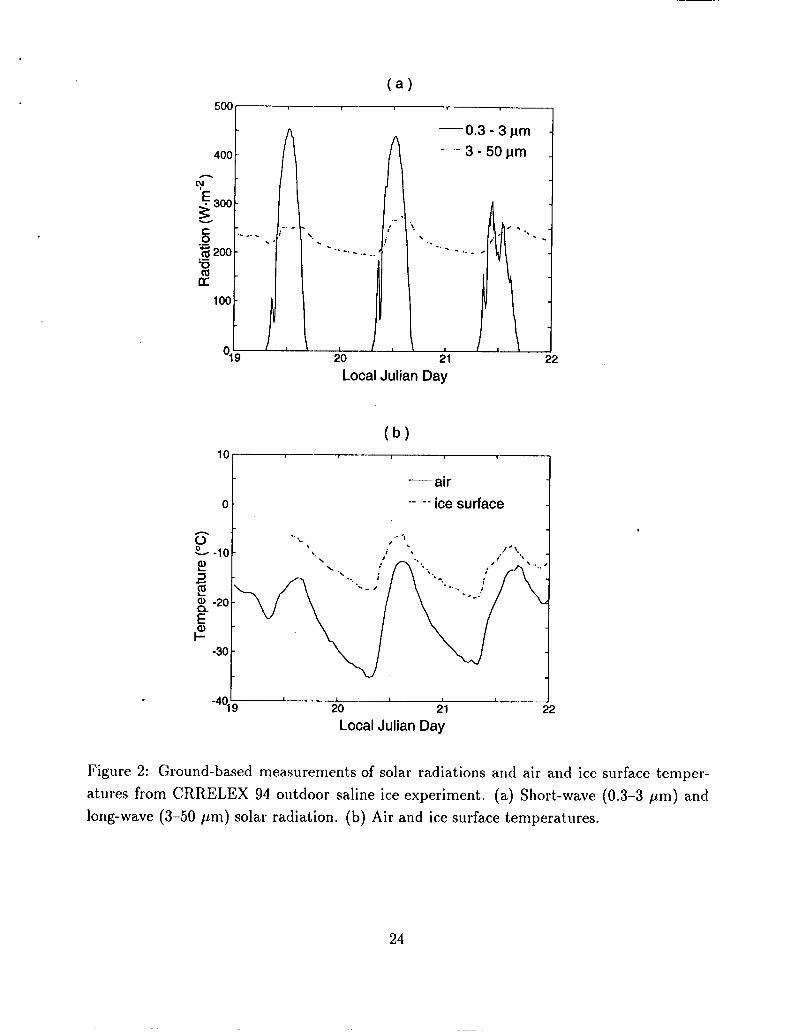
cm. The meteorological information, inducting air tcmpcraturc, stlort-wave (0.3 to 3 pm)

3

and long-wave (3 to 50 pm) solar radiations,

were collected by a nearby weather station.

wind speed, relative humidity, ancl air pressure,

The integrated values of sllort-wave and long-

wavc radiation arc shown in U’igure 2(a), and the measured air tcl~]pcrature and ice surface

temperature are shown in Figure 2(b). From Figures 1 and 2, it shows that the variation

of growth rate is consistent with the change of inciclcnt radiation ancl air temperature. A

slowdown in the ice growth during the second day in Figure 1(a) corresponds to the warming

daytime in Figure 2(a).

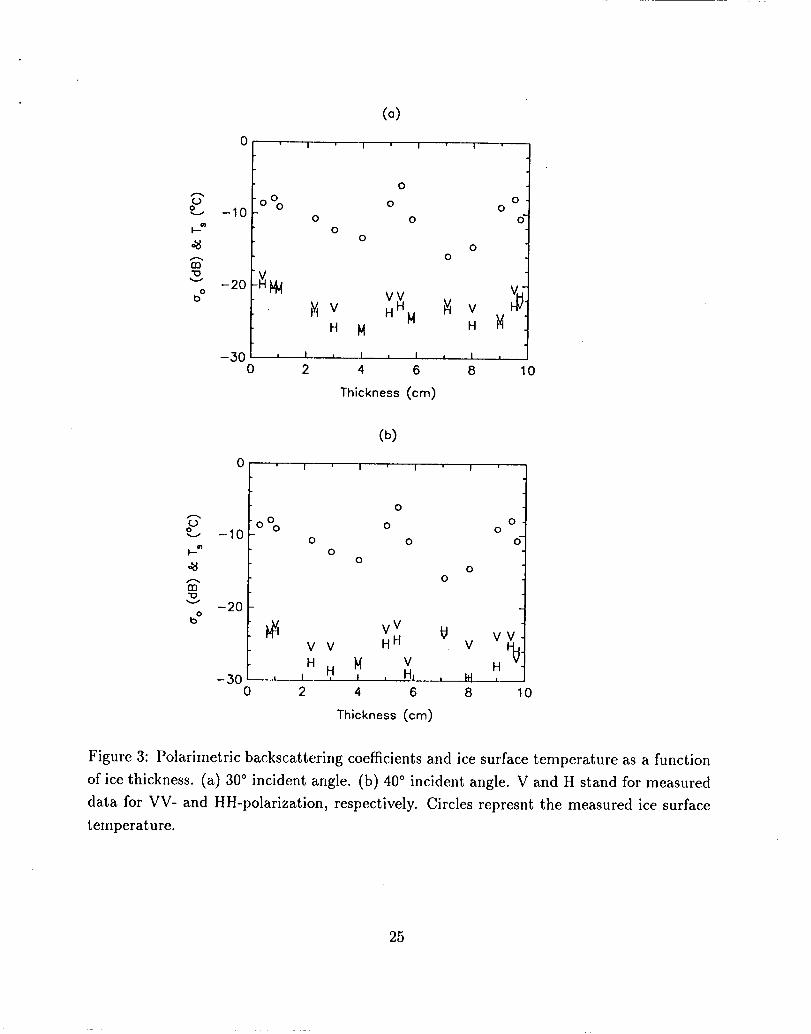
During the course of experiment, time-series of C-band (5 Gliz) polarimetric backscatter

data were collected at roughly every centimeter of ice growth and at various incidence angles.

The measured co-polarization (1111and VV) backscattering coemcients are shown in Figures

3(a) and 3(b) for 30° and 40° incidence angles, respectively. g’he backscatter signatures

show a substantial diurnal variation of 4–6 d13 for both polarizations. As shown in the same

figure, the backscatter variation is also synchronous and well correlated with the temperature

cycle. It suggests that the scattering mechanism is related to the diurnal variations of the

thermophysica] properties of sea ice, Toward the later stage of experiment, more frost flowers

appeared on the ice surface which may increase the rough sulfacc scattering effect, especially

at small incidence angles [11].

111. THERMODYNAMIC ELECTROMAGNETIC SCATTERING MODEL

As indicated in the previous section, the temperature variation of icc physical properties

is important in the interpretation of sea ice diurnal electromagnetic characteristics. In this

section, we present an extension of the sea ice scattering model developed in [8] to further

take into account the thermal cycling environmental conditicms, the diurnal ice growth, and

the rough air-ice interface scattering ef[ect. Applications of this diurnal scattering model

are demonstrated by comparing the simulations with the measured ice growth and radar

backscatters in this section, and the ice thickness retrieval in Section IV.

A. Electromagnetic Scattering Model

in this study to consicler the combined volume ancl

ice medium [10]. A thrwc layer discrete random

Radiative transfer theory is applied

rough surface scattering effects of sea

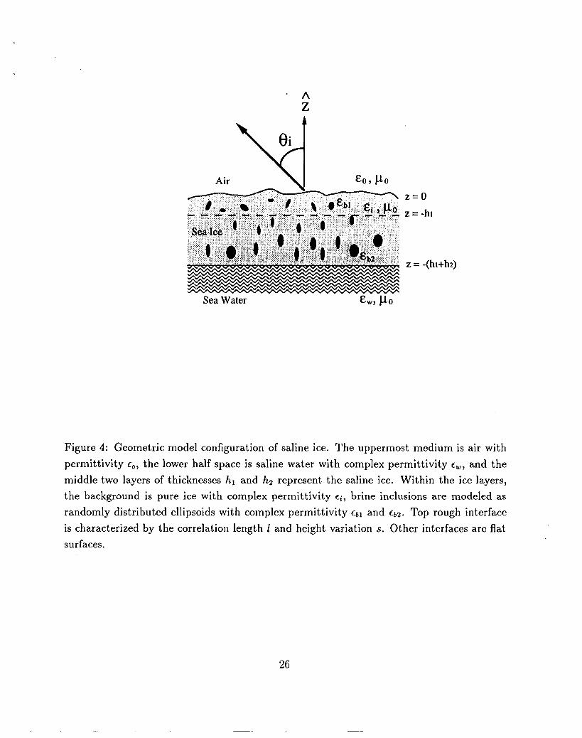
mec!ium model with rough interface, as shown in Figure 4, is USCC1to rcprcsellt the scattering

configuration. The uppermost mmlium is air with pcrmittivity COand the lower half space

4

is saline water with complex pcrmittivity (W. ‘l’he roug}l air-ice intcrfacc is assumed to he

Gaussian with mean surface at z = O, a[ld the roug}lness is clcscribcd by the correlation length

1 anti the root mean square (rms) heighl s, The sea ice layer is dividcc! into two sub-layers of

thicknesses hl and hz. ‘I)he brine inclusions in the lower sea ic.c layer (–hi – }12< z < –hl )

are assumed to be vertically oriented, but arc randomly oriented in the upper sea ice layer

(–hl < z < O), which corresponds to the incubation layer described in [11], The background

medium of sea ice is pure ice with complex pcrmittivity ~i. The ellipsoids of semi-axes an, bm,

and Cn (n= 1, 2) represent the brine pockets in the n-th ice layer. q’he complex pcrrnittivities

of brine inclusions are Cbn, and their fractional volumes arc jV.. I’hcse model parameters

are subject to dynamic changes during the ice growth process.

In each sea ice layer, the wave propagation and scattering can be described by the

radiative transfer equations [1O],

with n=l, 2, 0 ~ O ~ n, ancl O < qL~ 27r. In (1 ), ~n represents t}~e Stokes vector, Fen the

extinction matrix which includes both scattering and absorption 10SSCS,and F,l(O, ~; 0’, #)

the phase matrix which dcscribcs how particles scatter radiation from the direction (0’, qY)

into the direction (0, ~), in the n-th layer. The elements of extinction matrix and phase

matrix for small ellipsoids with prescribed orientation distribution are given in [10].

The boundary conditions for the vector radiative transfer equations arc as follows. At

~ =: (),

Tl(n”–o, (i5,z= o) =+“

at z=–hl,

71(0,4,2 “ –hi) = 72(0,4,2 = --/11) (3)

72(7r -- f?,&2 = –h~) = 7~(7r –o, ~,z ==–hi), (4)

ancl at .2 = –hl – h’,

72(0,4,2 = –h~ – h’) = F23(o, @).7’(7r -- O,$i,z = –h~ – h’) (5)

for O ~ d < n/~. 111(2), ~oi(~ - ~oll @oi) is tile incident Stokes vector in rcgioxl O (air)

from direction (n – Ooij@oi), and ~01 and ~~10 are the rmpectivc transmission ancl reflection

5

matrices for the rough interface between regions O ancl 1 (upper sea icc Iaycr). In this stucly,

~01 and RIO arc calculated based on the small pcrturbaticm methocl (S1)M) [10], detailed

expressions of these matrices are given in the Appendix, The matrix fi23 in (5) is the

reflection matrix for the flat, interface between regions 2 (lower sca ice Iaycr) ancl 3 (sea

water) [1O]. The effects of reflection and refraction between regions 1 and 2 arc neglected

due to the small difference between their effective pcrmittivities.

The radiative transfer equations (1) together with the boundary conditions (2)-(5) are

solved using the discrete eigen-analysis techniques [10]. ‘l’he backscattering coefficient is

expressed in terms of the incident and scattered Stokes vectors loi and lo~ as— —

(6)

where CY,~ can be vertical (v) c)r horizontal (h) polarization, and the subscripts i and s

denote the incident and scattered waves, respectively,

B. Thin Saline Ice Growth Model

The growth of sea ice is generally determined by both thermodynamic processes of freez-

ing and melting and dynamic processes of ice drift and deformation [12,13]. IIowever, a

simplified growth model is applied in this study which neglects the ice drift and deformat-

ion. The ice freezing and melting processes are primarily influenced by heat and radia-

tion exchanges between atmosphere and ocean. We usc a olle-dilllel”lsiollal thermodynamic

model of sea ice developed in [1,15] to model the time-dependent thermodynamic processes

occurring within the ice basecl on energy balance equations at the atmospheric ancl oceanic

boundaries.

The balance of fluxes at the upper surface of the icc can be expressed as

(1 - Q)Fr -- F’i + FI, -- ~cT(!7~+ 273)4 + -F;+ ~. + 1: = O

[1,13-15]

(7)

where the terms a and E are the albedo and the long-wave emissivity of sca ice, respectively.

a is the Stefan-Boltzmann constant, and 7: is the ice surface temperature in “C. In (7), F.

represents the downward short-wave radiation, and J;i is the amount of short-wave energy

that penetrates through the sca ice layer, ‘l’he sum of F, and l’~i gives the net flUX of

short-wave radiation absorbed in the interior of the icc layer, FL is the downward long-

wave insolation and eo(7~ + 273)4 is the long-wave radiation emitted by the ice. These two

6

terms account for the net flux of long-wave energy. ‘1’hc two cluantitics F., the .scnsible heat

flux, and F,, the latent heat flux, represent the atmospheric turbulent heat fluxes which

arc relatccl with the rncteorological factors like air clcnsity, wind spcecl, humidity, and air

temperature. l’he last term I’C in (7) is the upward conductive heat flux which is the heat

from the bottom interface conducted through the ice to the upper surface,

At the bottom boundary of ice, by neglecting the contribution from oceanic heat flux,

the conductive heat flux is related to the ice growth rate according to [12,15]

(8)

where h is the ice thickness, p is the density of sea ice, and Lj is the latent heat of freezing

in Jkg-l.

Equations (7) and (8) are coupled via the heat conduction term FC, whose solution

generally requires the information about air and ice surface temperature, solar insolation,

wind speed, humidity, etc. In this model, an approximation of ice albcdo a is used [15]

~ = ().44h028+-().()8 (9)

which is parameterized to bc a function of ice thickness. e is assumed to bc unity in this

study [1]. The short and long-wave fluxes I’, and Fz, are acquired from the measurement

as shown in Figure 2(a). J;i is assumed to be 90% of the net short-wave radiation, i.e.,

Fri = 0.9(1 – Q)F,, passes throug;h the icc completely and is absorbed in the sea water.

Over the ice surface, the turbulent fluxes F’s and FL are [1,13,15]

F. = pacpc.u(Ta – T,) (lo)

Fe = p. L.c,u(qa – q,) (11)

where pa and C’Pare the density and specific heat of the air, respectively. C, is the transfer

coefhcient for sensible heat, 1: is the air temperature, 7) is the ice surface tcrnpcrature,

and u is the wind speed, 1,. is the latent heat of vaporization, ancl C. is the vaporation

coefficient. The terms qa and q. in (1 1) are the specific humidities in the air and at the ice

surface, respectively. The relation of (q. — qb) given in [1] is usecl in this study. The relation

is a pararneterized function of air temperature, ice surface temperature, air pressure (po),

and relative humidity (R]]), which arc all measurable quantities. Va]ucs of these parameters

usccl in this study are given in Table 1.

7

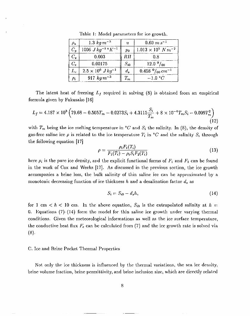
Table 1: Model parameters for ice growth.

E5iEH

The latent heat of freezing Lf required in solving (8) is obtained from an empirical

formula given by Fukusako [16]

Lf =(

4.187 X 103 79.68_ 0.505T~ _ 0.0273Si + 4.3115#- + 8 X 10-4T~Si _ ().009T~nt )

(12)

with Tm being the ice melting temperature in ‘C and Si the salinity. In (8), the density of

gas-free saline ice p is related to the ice temperature Ti in “C and the salinity S; through

the following equation [17]__ piR(Ti)

p = F1(Ti) – ~iSiF2(Ti)(13)

here pi is the pure ice density, and the explicit functional forms of FI and Fz can be found

in the work of Cox and Weeks [17]. As discussed in the previous section, the ice growth

accompanies a brine loss, the bulk salinity of thin saline ice can be approximated by a

monotonic decreasing function of ice thickness h and a desalination factor d, as

Si =: SiO– d~h, (14)

for 1 cm < h < 10 cm. In the above equation, SiO is the extrapolated salinity at h =

O. Equations (7)-(14) form the model for thin saline ice growth under varying thermal

conditions. Given the meteorological information as well as the ice surface temperature,

the conductive heat flux FC can be calculated from (7) and the ice growth rate is solved via

(8).

C. Ice and Brine Pocket Thermal Properties

Not only the ice thickness is influenced by the thermal variations, the sea ice density,

brine volutne fraction, brine permittivity, and brine inclusion size, which are directly related

8

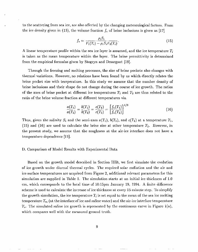
to the scattering from sea ice, arc also affected by

the ice density given in (13), the volume fraction

the changing meteorological factors. From

~. of brine inclusions is given as [17]

A linear temperature profile within the sea ice layer is assumed,

is taken as the mean temperature within the layer. The brine

(15)

and the ice temperature Ti

permittivity is determined

from the empirical formulas given by Stogryn and Desargant [19].

Through the freezing and melting processes, the size of brine pockets also changes with

thermal variations. However, no relations have been found by us which directly relates the

brine pocket size with temperature. In this study we assume that the number density of

brine inclusions and their shape do not change during the course of ice growth. The ratios

of the axes of brine pocket at different ice temperatures T1 and 7> are thus related to the

ratio of the brine volume fraction at different temperatures via

a(T’l) = b(T1) C(T1)—.—— —. =— =a(T2) b(T2) C(T2)

Thus, given the salinity Si and the semi-axes a(T1 ),

[1f.(T,) ’13—.fv(T2)

(16)

b(T1), and c(~i) at a temperature T1,

(15) and (16) are used to calculate the brine size at other temperature T2. However, in

the present study, we assume that the roughness at the air-ice interface does not have a

temperature dependence

D. Comparison of Model

Based on the growth

[11].

Results with Experimental Data

model described in Section IIIB, we first simulate the evolution

of ice growth under diurnal thermal cycles. The required solar radiation and the air and

ice surface temperatures are acquired from Figure 2, additional relevant parameters for this

simulation are supplied in Table 1. The simulation starts at an initial ice thickness of 1.0

cm, which corresponds to the local time of 10: 15pm January 19, 1994. A finite difference

scheme is used to calculate the increase of ice thickness at every 15-minute step. To simplify

the growth simulation, the ice temperature Ti is set equal to the mean of the sea ice melting

temperature Tm (at the interface of ice ancl saline water) and the air-ice interface temperature

T,. The simulated saline ice growth is represented by the continuous curve in Figure 1(a),

which compares well with the measured ground truth.

9

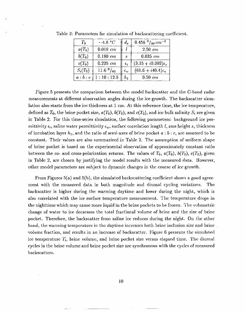
Table 2: Parameters for simulation of backscattering coefhcient,.

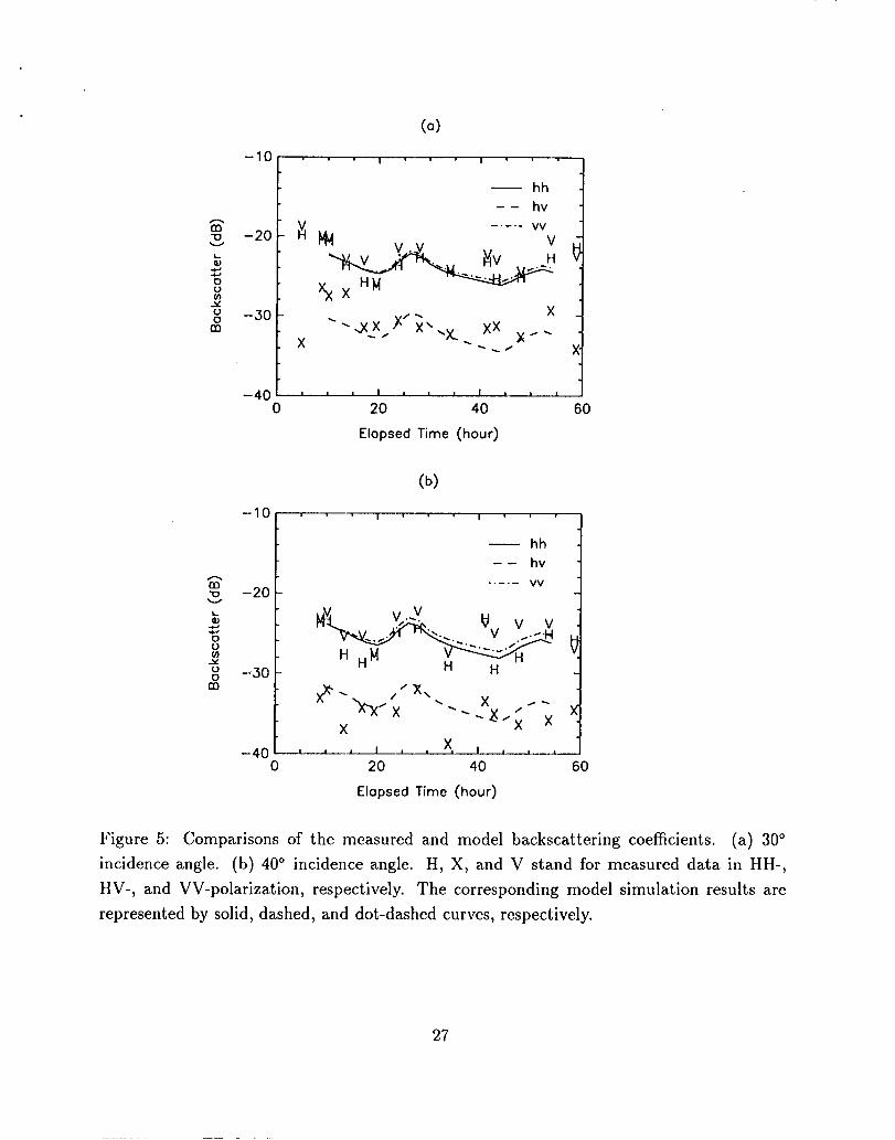
Figure 5 presents the comparison between the model backscatter and the C-band radar

measurements at different observation angles during the ice growth. The backseat ter simu-

lation also starts from the ice thickness at 1 cm. At this reference time, the ice temperature,

defined as To, the brine pocket size, a(To), b(To), and C(TO), and ice bulk salinity S; are given

in Table 2. For this time-series simulation, the following parameters: background ice per-

mittivity ti, saline water permittivity Cti,,surface correlation length 1, rms height s, thickness

of incubation layer hl, and the ratio of semi-axes of brine pocket a : b : c, are assumed to be

constant. Their values are also summarized in Table 2. The assumption of uniform shape

of brine pocket is based on the experimental observation of approximately constant ratio

between the co- and cross-polarization returns. The values of To, a(To), b(To), C(TO), given

in Table 2, are chosen by justifying the model results with the measured data. However,

other model parameters are subject to dynamic changes in the course of ice growth.

From Figures 5(a) and 5(b), the simulated backscattering coefficient shows a good agree-

ment with the measured data in both magnitude and diurnal cycling variations. The

backscatter is higher during the warming daytime and lower during the night, which is

also correlated with the ice surfi~ce temperature measurement. The temperature drops in

the nighttime which may cause more liquid in the brine pockets to be frozen. ‘I’he volumetric

change of water to ice decreases the total fractional volume of brine and the size of brine

pocket. Therefore, the backscatter from saline ice reduces cluring the night. On the other

hand, the warming temperature in the daytime increases both brine inclusion size and brine

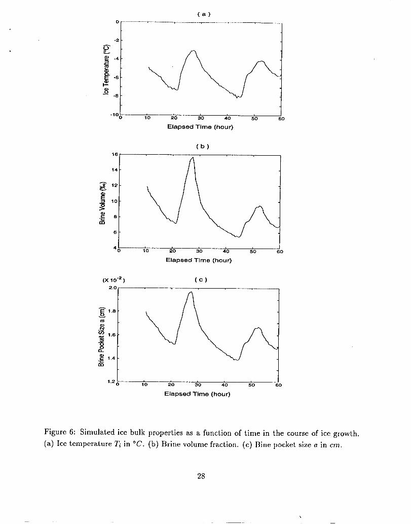
volume fraction, and results in an increase of backscatter. Figure 6 presents the simulated

ice temperature Ti, brine volume, and brine pocket size versus elapsed time. The diurnal

cycles in the brine volume and brine pocket size are synchronous with the cycles of measured

backseat ters.

10

IV. TIME SERIES ICE THICKNESS INVERSION

In a previous paper [8], wc developed an ice thickness inversion algorithm which em-

ployes time-series radar measurements. The algorithm was applied to a set of indoor saline

ice experimental data [9], and successfully retrieved the evolution of ice thickness under a

constant growth condition [8]. It was found that by incorporating an ice thermodynamic

model into the inversion algorithm, the thickness estimation can be constrained sufficiently

to predict more accurate results, The use of time series data is also helpful for resolving

the non-uniqueness and stability problems [8,20]. In this section, we further apply this al-

gorithm to reconstruct the evolution of ice growth under diurnal thermal conditions using

the time-series outdoor radar observations.

A. Inversion Algorithm

In the electromagnetic remote sensing of sea ice medium, the radiations are randomly

scattered by its volume and surface inhomogeneities, and therefore the relation between the

sea ice physical properties and radar measurement is non-linear. Generally, we can define a

non-linear forward operator ‘~ which relates the data, sensor, environment, and medium’s

characteristics as follows:

6, ‘= ~(t,,Z,E) + ‘j (17)

where Fi represents radar data at the measurement time ii, and ~i is the discrepancy between

the observation and model response, The vector z denotes the set of pertinent model

parameters of saline ice:

Z = [ho, ‘@, ‘s, ‘0,1, ‘1 (18)

here ho= h(I!o) is the ice thickness at time to (a reference time) when the first set of data

is taken, and a. = a(to) the corresponding brine pocket size at this time. The other terms

Sio, d., 1, and s have been defined in Section IIIB. The array z encompasses all the other

known parameters. To solve z from equation (17), a non-linear least-squares approach can

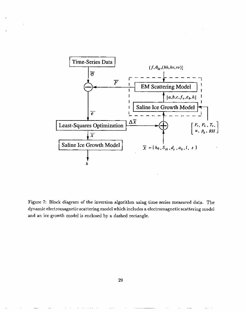
be used to minimize the error function between the observation and the model. Figure 7

summarizes the reconstruction algorithm using time-series radar data for the ice thickness.

The retrieval steps are described in the following.

Given the initial guess of model parameters Z, the ice growth model first predicts the

subsequent ice characteristics (a, 6, c, jV, ~b, h) by using the specified time intervals between

11

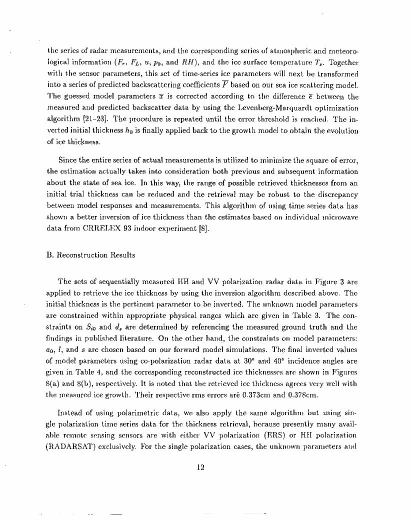
the series of radar rncasurements, and the corresponding series of atmospheric ancl meteoro-

logical information (F’., FL, u, pO, and RI1), and the ice surface temperature 7:. Together

with the sensor parameters, this set of time-series ice parameters will next be transformed

into a series of predicted backscattering cc)efhcients ~ based on our sea ice scattering model.

The guessed model parameters z is corrected according to the difference z between the

measured and predicted backscatter data by using the Levenberg-Marquardt optimization

algorithm [21–23]. The procedure is repeated until the error threshold is reached. The in-

verted initial thickness ho is finally applied back to the growth model to obtain the evolution

of ice thickness.

Since the entire series of actual measurements is utilized to minimize the square of error,

the estimation actually takes into consideration both previous and subsequent information

about the state of sea ice. In this way, the range of possible retrieved thicknesses from an

initial trial thickness can be reduced and the retrieval may be robust to the discrepancy

between model responses and measurements. This algorithm of using time series data has

shown a better inversion of ice thickness than the estimates based on individual microwave

data from CRRELEX 93 indoor experiment [8].

B. Reconstruction Results

The sets of sequentially measured HH and VV polarization radar data in Figure

applied to retrieve the ice thickness by using the inversion algorithm described above.

3 are

The

initial thickness is the pertinent parameter to be inverted. The unknown model parameters

are constrained within appropriate physical ranges which are given in Table 3. The con-

straints on Sio and d. are determined by referencing the measured ground truth and the

findings in published literature. On the other hand, the constraints on model parameters:

ao, 1, and s are chosen based on our forward model simulations. The final inverted values

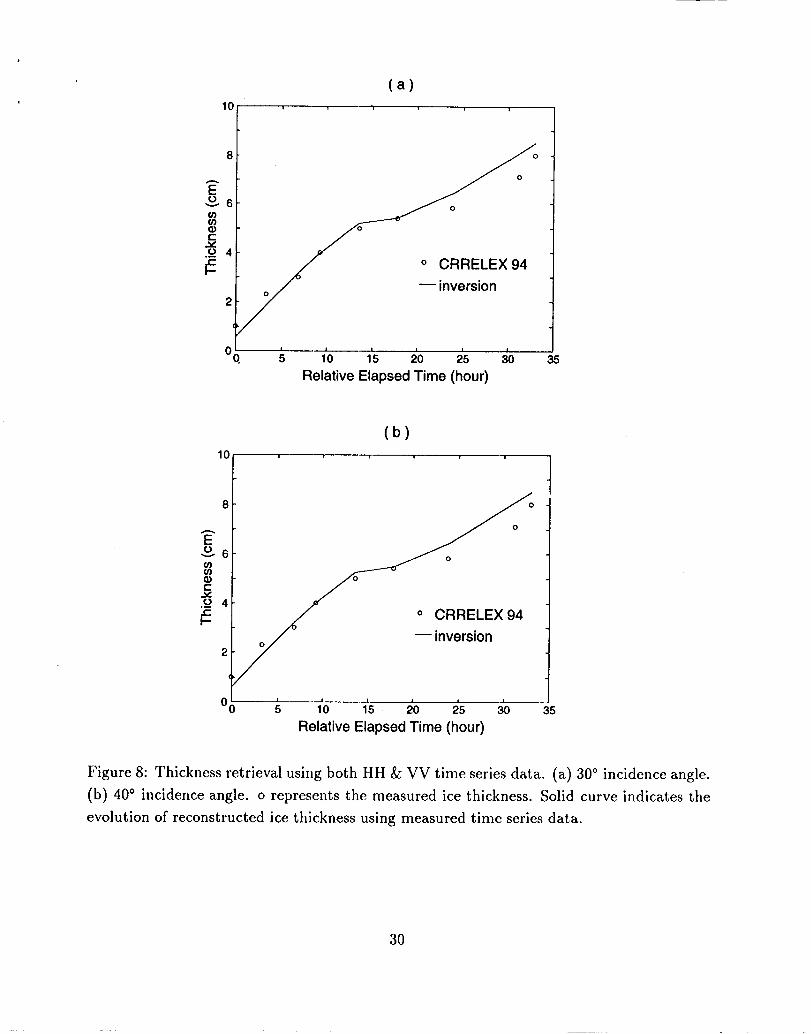
of model parameters using co-polarization radar data at 30° and 40° incidence angles are

given in Table 4, and the corresponding reconstructed ice thicknesses are shown in Figures

S(a) and 8(b), respectively. It is noted that the retrieved ice thickness agrees very well with

the measured ice growth. Their respective rms errors ar+ 0.373cm ancl 0.378cnl.

Instead of using polarimetric data, we also apply the same algorithm but using sin-

gle polarization time series data for the thickness retrieval, because presently many avail-

able remote sensing sensors are with either VV polarization (ERS) or HH polarization

(RADARSAT) exclusively. For the single polarization cases, the unknown parameters and

12

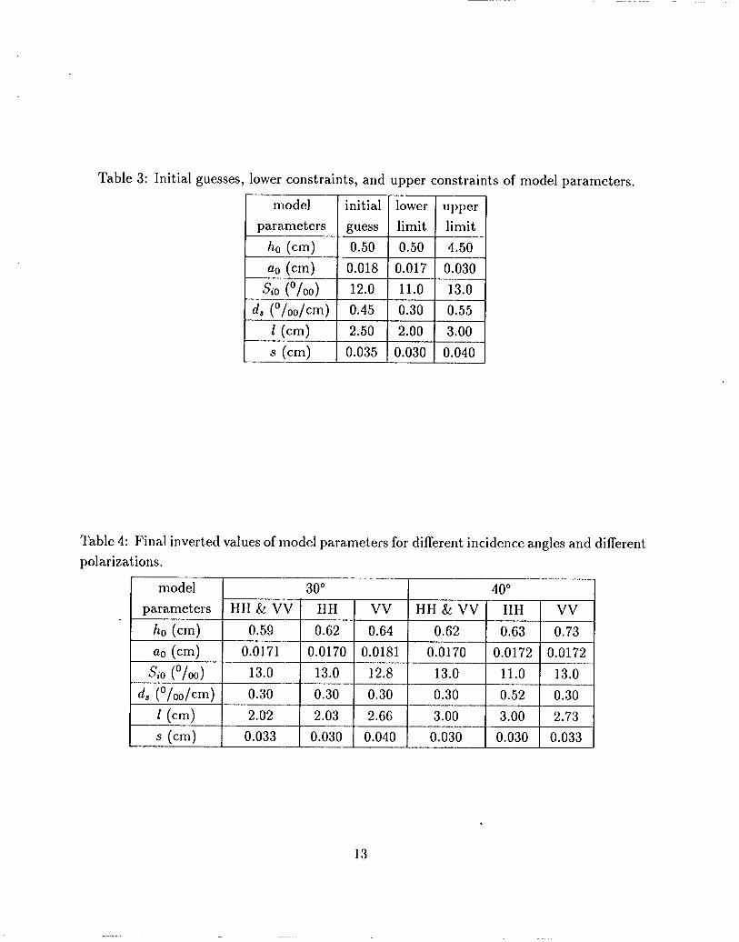
Table 3: Initial guesses, lower constraints, and upper constraints of model parameters.

Table 4: Final inverted

polarizations.

r.——model

parameters

I hO (cm)

I a. (cm)I Sio (0/00)

t

4 (O/OO/cm)-—1 (cm) -

L s (cm).— —

initial lower

guess I limit

0.50 ( 0.50

1=0.018 0.017

12.0 11.0

0.45 0.30

2.50 2.00

0.035 0.030

upper

limit

4.50

0.030

13.0——0.55

3.00

0.040

values of model parameters for different incidence angles and different

—-——.

‘1‘;model 30° 40°——

parameters HH & VV H H Vv HH & VV HH Vv-—ho (cm) 0.59 0.62 0.64 0.62 0.63 0.73——ao (cm) o.oi71 0.0170 0.0181 0.0170 0.0172 0.0172-— ——

SjO (0/00) 13.0 13.0 12.8 13.0 11.0 13.0

~$ (O/OO/cm)0.30 O.ii 0.30 0.30 0.52 0.30-— —1 (cm) 2.02 2.6 2.66 3.00 3.00 2.73-—s (cm) 0.033 0.030 0.040 0.030 0.030 0.033.— ——

13

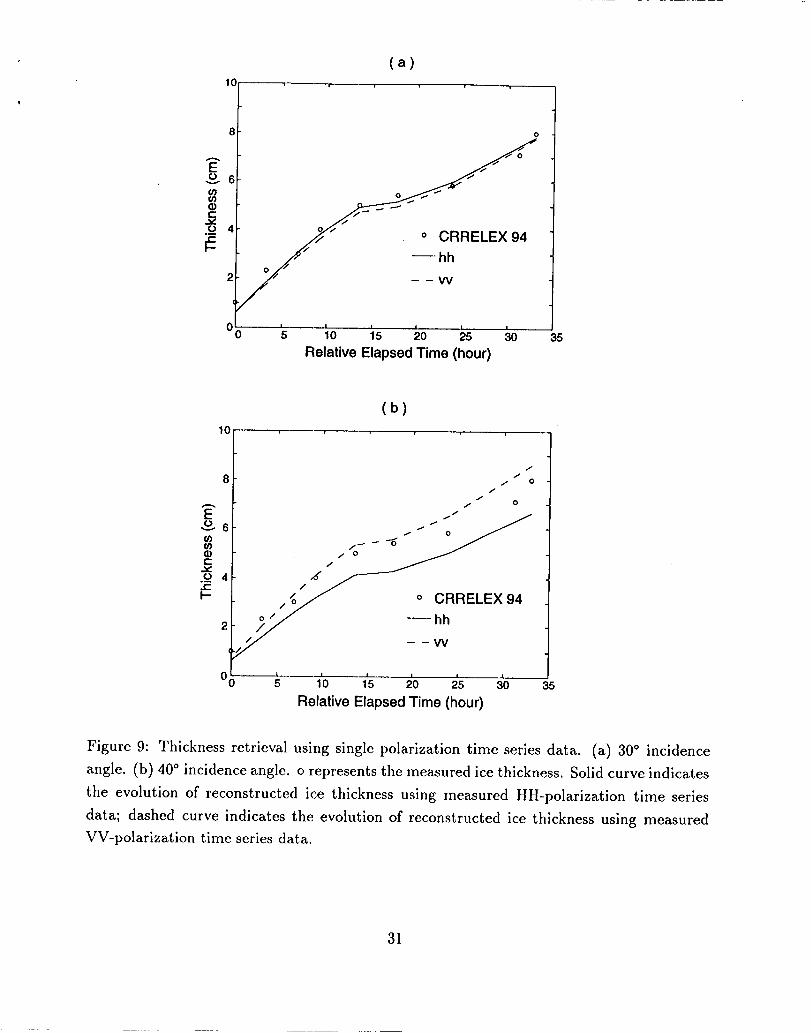
limits are the same as before. Table 4 gives the final invertccl values of model parameters

using either HII or VV polarization radar data at 30° and 40° incidence angles. Figures

9(a) and 9(b) illustrate the respective inversion results of ice thickness evolution. The re-

trieved ice thickness from single polarization data also shows reasonable agreement with

the measured ground truth. Their rms errors are 0.267cm and 0.339cm for HH and VV

polarization, respectively, at 30° incident angle, and 0.860cm (HH) and 0.407cm (VV) at

40° incident angle. The retrieved thickness from HH polarization data at 40° has a larger

discrepancy compared with the ground truth, this may be due to the larger noisy level for

the HH polarization at 40° which degraded the inversion result.

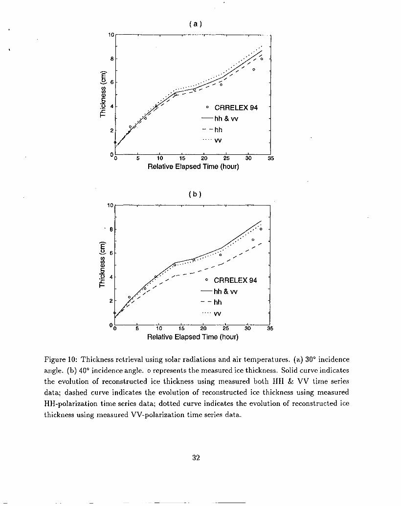
The thickness inversion presented above is subject to the time-series meteorological ob-

servations. Solar radiations and air temperature are required to deduce the surface fluxes.

In lieu of supplied radiation measurements, we thus modify the inverse model such that

the model provides estimates of solar radiations and air temperature on an average basis.

Actually, in the polar areas these monthly-averaged estimates may be available in the lit-

erature [15]. In the following inverse scattering simulations, we instead use some estimated

constant values for daily solar radiations and air temperatures: 400 W/rn2 for short-wave

and 250 W’/m2 for long-wave solar radiations in the daytime, and O W/rn2 and 200 W/m2 in

the night, respectively; and -- 10”C for the air temperature during the daytime and –30”C

during night. The wind speed is kept to be a constant of 0.6 m/s. The estimated con-

stant values of solar radiations are chosen to give the same total energy when integrates the

radiations shown in Figure 2(a) over time for day or night. The temperatures are chosen

as the mean temperatures during day and night. With these estimated parameters, the

retrieved ice thicknesses are shown in Figures 10(a) and 10(b) by using 30° incidence angle

measurements and 40° incidence angle rneasurements, respectively. The rms errors for these

retrievals are 0.284 cm, 0.593 cm, 0.396cm by using the 30° incidence angle measurements of

HH-, VV-, and HH & VV polarization, respectively, and 0.812cm (HH), 0.308cm (VV), and

0.394cm (HH & VV) for the case of 40” incidence angle.

V. SUMMARY

The thermal interaction between sea ice and atmosphere strongly affects the thermody-

namic processes associated with the ice growth. The thermally-induced varying ice physi-

cal properties also significantly influence the electromagnetic interactions with the sea ice

medium, In this paper, we extend our previously developed sea ice inverse scattering model

to further investigate the retrieval of ice thickness under diurnal thermal cycling conditions.

14

We use a one-dimensional thermoclynamic model that includes thermal interactions with

atmosphere for the ice growth using measured or estimated solar insolation ancl air tem-

peratures. We provide a physically-based sea ice electromagnetic model with a multilayer

random medium structure with rough surfaces, which can take into account the dynami-

cally varying thermal and electromagnetic properties of saline ice and the combined volume

and surface scattering effects. q“’hedirect scattering model interprets the large diurnal vari-

ations in the radar backscatter observed in the CRRELEX 94 experiment. By using the

same set of data, the developed inversion algorithm has successfully reconstructs the evo-

lution of ice growth under a thermal cycling environment. The good agreement between

the reconstructed ice thickness and ground-based measurements confirms the usefulness of

incorporating ice growth physics

scattering problem of sea ice,

and using time series data in the electromagnetic

ACKNOWLEDGMENT

inverse

The research in this paper was partially supported by the OffIce of Naval Research Con-

tract No. NOO014-92-J-4098 with the Massachusetts Institute of Technology. The research

performed by the Center for Space Microelectronics Technology, Jet Propulsion Laboratory,

California Institute of Technology was supported by the Office of Naval Research through

an agreement with the National Aeronautics and Space Administration.

APPENDIX

In this appendix, we give the reflection matrix ~.p(O, O; 0’, #’), and transmission matrix

~aO(O, ~; 0’, @’)for a slightly rough interface between a-th and @-th layers, Each matrix can

be separated into two terms; coherent and incoherent:

Z@, 4; ~’, 4’) = E:P(O, +)6(4 – 4’)J(COSO – CoSo’)

+ E:@(e,@; 0’, 4’)

Tad(o, 4; 0’, +’) = T:p(o, 0)6(4 – #’)J(cos o – Cos 0’)

+ Tao(o, ~; 0’, +’)

(Al)

(A.2)

15

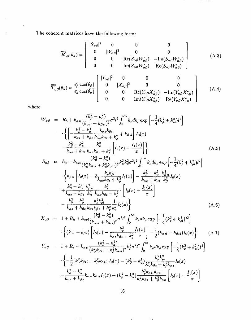
‘The coherent matrices have the following form:

16

(A.5)

(A.6)

kaz + k~.—kpkpi(k~kpzi – kjkazi)~l(~)

+ k:kflz+k;k.z }(AA)

In the above equations, R~ and RV are the TE and TM Fresnel reflection coefficients, x =

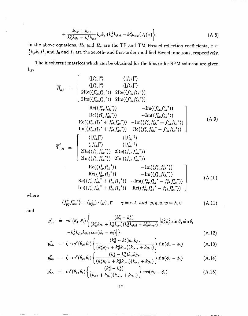
~kPkfli12,and 10 and 11 are the zeroth- and first-order modified Bessel functions, respectively.

The incoherent matrices which can be obtained for the first order SPM solution are given

by:

[ (1.f:v12) (lf:h12)

where

and

‘e((fivfih”)) ‘lm((fivfih*))Re((f~Vf~~* + f~hfiv’)) –lm((fi~f~h* – f;hf;v*))

lm((j:vf;h* + f:hf;v”)) Re((f:vfih” – f;hfiv”)) I

{

(k; – k:)k.kpzg;h = ~ . mr(~~,di) ‘—

}- sin(~~ – ~i)

(k~koz + k$kaz)(kazi + k~zi)

{

(kj – k~)kakozi9;. = ~ . mr(O~, Oi) —

(k~kozi + k~kcxzi)(kcrz + kozj }

sin(~. – ~i)

{

(k; - k:)dh = 7T2r(0~,0i)—

(koz + kpz~kazi + kOzi) }COS(@~– ~i)

(A.9)

(A.1O)

(All)

(A.12)

(A.13)

(A.14)

(A.15)

17

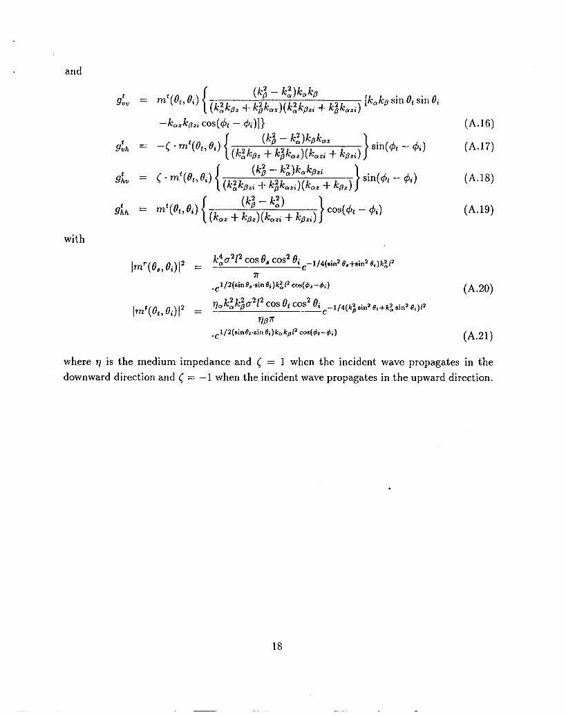
(A.16)

(A.17)

(A.18)

(A.19)

(A.20)

(A.21)

where q is the medium impedance and ( = 1 when the incident wave propagates in the

downward direction and ~ = --1 when the incident wave propagates in the upward direction.

18

[1]

[2]

[3]

[4]

[5]

[6]

[7]

[8]

[9]

REFERENCES

G.A. Maykut, “13nergy exchange over young sea ice in the central Arctic,” J. Geophys.

Res., vol. 83, no. C7, pp. 3646-3658, 1978.

F.D. Carsey, cd., Microwave Remote Sensing of Sea Ice, DC: American Geophysical

Union, 1992.

F.T. Ulaby, R.K. Moore, and A.K. Fung, Microwave Remote Sensing, Vol. I and 11,

Reading, MA: Addison-Wesley, 1982.

S.V. Nghiem, R. Kwok, S.H. Yueh, and M.R. Drinkwater, ‘(Polarimetric signature of

sea ice, 2. Experimental observations,” J. Geophys. Res., vol. 100, no. C7, pp.

13681-13698, 1995.

R. Kwok, E. Rignot, B. Holt, and R. Onstott, “Identification of sea ice types in space-

borne synthetic aperture radar data,” J. Geophys. Res., vol. 97, no. C2, pp. 2391-

2402, 1992.

D.P. Winebrenner, L.D. Farmer, and I.R. Joughin, “On the response of polarimetric

synthetic aperture radar signatures at 24-cm wavelength to sea ice thickness in Arctic

leads,” Radio Sci., vol. 30, no. 2, pp. 373-402, 1995.

R. Kwok, S.V. Nghiem, S.H. Yueh, and D.D. Huynh, “Retrieval of thin ice thickness

from multifrequency polarimetric SAR data,” Remote Sens. Environ., VO1.51, no. 3,

pp. 361-374, 1995.

S.E. Shih, K.H. Ding, S.V. Nghiem, C.C. Hsu, J.A. Kong, and A.K. Jordan, “Thin saline

ice thickness retrieval using time series C-band polarimetric radar measurements,”

IEEE Trans. Geosci. Remote Sens., in press, 1998.

S.V. Nghiem, R. Kwok, S.H. Yueh, A.J. Gow, D.K. Perovich, J.A. Kong, and C.C. Hsu,

‘(Evolution in polarimetric signatures of thin saline ice under constant growth,” Radio

Sci., vol. 32, no. 1, pp. 127-151, 1997.

[10] L. Tsang, J.A. Kong, and R.T. Shin, Theory of Microwave Remote Sensing, New York:

Wiley-Interscience, 1985.

[11] S.V. Nghiem, R. Kwok, S.H. Yueh, A.J. Gow, D.K. Perovich, C.C. lIsu, K.H. Ding, J,A.

Kong, and T.C. Grenfell, “I)iurnal thermal cycling effects on microwave signatures of

thin sea ice,” IEEE Trans. Geosci. Remote Sens., vol. 36, no. 1, pp. 111-124, 1998.

19

[12]

[13]

[14]

[15]

[16]

[17]

[18]

[19]

[20]

[21]

W. F. Weeks and S. F. Ackley, The Growth, Structure, and Properties ojSea Ice, CRREL

Monograph 82-1, US Army Corps of Eng,, Cold Regions Research and Engineering

Lab., 1982.

G.A. Maykut, “The surface heat and mass balance,” The Geophysics oj Sea Ice, Chap-

ter 5, pp. 395-463, N, Untersteiner cd,, New York: Plenum Press, 1986.

G.F.N. Cox and W.F. Weeks, “Numerical simulations of the profile properties of un-

deformed first-year sea ice during the growth season,” J. Geoph ys. Res., vol. 93, no.

C1O, pp. 12449-12460, 1988.

G.A. Maykut, “Large-scale heat exchange and ice production in the central Arctic,”

J. Geophys. Res., vol. 87, no. C1O, pp. 7971-7984, 1982.

S. Fukusako, “Thermophysical properties of ice, snow, and sea ice,” Int. J. Thermo-

phys., vol. 11, no. 2, pp. 353-372, 1990.

G.F.N. Cox and W.F. Weeks, “Equations for determining the gas and brine volumes

in sea-ice samples,” J. Glaciol., vol. 29, no. 102, pp. 306-316, 1983.

L.A. Klein and C. Swift, “An improved model for the dielectric constant of sea water

at microwave frequencies,” IEEE Trans. Antennas Propagat., vol. AP-25, no. 1, pp.

104-111, 1977.

A. Stogryn and G.J. I)esargant, “The dielectric properties of brine in sea ice at mi-

crowave frequencies,” IEEE Trans. Antennas Propagat., vol. AP-33, no. 5, pp. 523-

532, 1985.

A.K. Jordan and M.E. Veysoglu, ‘(Electromagnetic remote sensing of sea ice,” Inverse

Problems, vol. 10, no. 5, pp. 1041-1058, 1994.

D.W. Marquardt, “An algorithm for least-squares estimation of nonlinear parameters,”

J. Sot. Indust. Appl, Math., vol. 11, pp. 431-441, 1963.

[22] J.L. Kuester and J.H. Mize, Optimization Techniques with Fortran, New York: McGraw-

Hillj 1973.

[23] J.E. Dennis and R. El. Schnabel, Numerical Methods jor Unconstrained Optimization

and Nonlinear Equations, Englewood Cliffs, NJ: Prentice-Hall, 1983.

20

Figure Captions

Figure 1. Ground-based ice characteristic measurements from CRRELEX 94 outdoor saline

ice experiment. (a) Ice thickness versus time. Solid curve is the simulation of saline ice

growth. (b) Saline ice bulk salinity versus thickness. Solid line is the linear fit of measured

data.

Figure 2. Ground-based measurements of solar radiations and air and ice surface temper-

atures from CRRELEX 94 outdoor saline ice experiment, (a) Short-wave (0.3–3 pm) and

long-wave (3-50 pm) solar radiation. (b) Air and ice surface temperatures.

Figure 3. Polarimetric backscattering coefficients and ice surface temperature as a function

of ice thickness. (a) 30° incident angle. (b) 40° incident angle. V and H stand for measured

data for VV- and HH-polarization, respectively. Circles represnt the measured ice surface

temperature.

Figure 4. Geometric model configuration of saline ice. The uppermost medium is air with

permittivity CO,the lower half space is saline water with complex permittivity CW,and the

middle two layers of thicknesses hl ancl h2 represent the saline ice. Within the ice layers,

the background is pure ice with complex permittivity ~i, brine inclusions are modeled as

randomly distributed ellipsoids with complex permittivity ~bl and ~bz. Top rough interface

is characterized by the correlation length 1 and height variation s. Other interfaces are flat

surfaces.

Figure 5. Comparisons of the measured and model backscattering coefficients. (a) 30°

incidence angle. (b) 40° incidence angle. H, X, and V stand for measured data in HH-,

HV-, and VV-polarization, respectively. The corresponding model simulation results are

represented by solid, dashed, and dot-dashed curves, respectively.

Figure 6. Simulated ice bulk properties as a function of time in the course of

(a) Ice temperature Ti in “C. (b) Brine volume fraction. (c) Bine pocket size a

ice growth.

in cm.

Figure 7. Block diagram of the inversion algorithm using time series measured data. The

dynamic electromagnetic scattering model which includes a electromagnetic scattering model

and an ice growth model is enclosed by a dashed rectangle.

Figure S. Thickness retrieval using both HH & VV time series data. (a) 30° incidence angle.

(b) 40° incidence angle. o represents the measured ice thickness. Solid curve indicates the

21

evolution of reconstructed ice thickness using measured time series data.

Figure 9. Thickness retrieval using single polarization time series data. (a) 30° incidence

angle. (b) 40° incidence angle. o represents the measured ice thickness. Solid curve indicates

the evolution of reconstructed ice thickness using measured HH-polarization time series

data; dashed curve indicates the evolution of reconstructed ice thickness using measured

VV-polarization time series data.

Figure 10. Thickness retrieval using solar radiations and air temperatures. (a) 30° incidence

angle. (b) 40° incidence angle. o represents the measured ice thickness. Solid curve indicates

the evolution of reconstructed ice thickness using measured both HH & VV time series

data; dashed curve indicates the evolution of reconstructed ice thickness using measured

HH-polarization time series data; dotted curve indicates the evolution of reconstructed ice

thickness using measured VV-polarization time series data.

22

12

la

gawu)coa)6cg,

2

0,

(a)——l———————

0 CRRELEX 94

‘- Simulation0

0

0

0

. . ..~o

20 22Local Julian Day

(b)

“r- “ I

0 CRRELEX 94

— Fitted

0

0

f30~_J——_d_ I2 4 6 8 10

Thickness (cm)

Figure 1: Ground-based ice characteristic measurements from CRREI,EX 94 outdoor saline

ice experiment. (a) Ice thickness versus time. Solid curve is the simulation of saline ice

growth. (b) Saline ice bulk salinity versus thickness. Solid line is the linear fit of measured

data.

23

(a)

‘“”l—————~

Local Julian Day

(b)

10

r“”

‘air

o7

‘- ‘-ice surface

. .4” I.——_—J.—.19

J20 21 22

Local Julian Day

Figure 2: Ground-based measurements of solar radiations and air and ice surface temper-

atures from CRRELEX 94 outdoor saline ice experiment. (a) Short-wave (0.3–3 pm) and

long-wave (3-50 pm) solar radiation. (b) Air and ice surface temperatures.

24

(a)

b“

-’FT’7t

-30i

IL I I I I I-o 2 4 6 8 10

Thickness (cm)

(b)

0. 1 I I I

o0

-lo -000 00 0

0 00

00

0

–20 -

: wVvHH v v Vv.

Vv$:

dHv!i:lH

-30 hio 2 4 6 8 10

Thickness (cm)

Figure 3: Polarimetric backscattering coefficients and ice surface temperature as a function

of ice thickness. (a) 30° incident angle. (b) 40° incident angle. V and H stand for measured

data for VV- and HH-polarization, respectively. Circles represnt the measured ice surface

temperature.

25

Z=o

Z=-hi

Z= -(hl+hz)

Figure 4: Geometric model configuration of saline ice. The uppermost medium is air with

permittivity CO,the lower half space is saline water with complex permittivity CW,and the

middle two layers of thicknesses hl and h2 represent the saline ice. Within the ice layers,

the background is pure ice with complex permittivity ~i, brine inclusions are modeled as

randomly distributed ellipsoids with complex permittivity ~bl and ~bz. Top rough interface

is characterized by the correlation length 1 and height variation s. Other interfaces are flat

surfaces.

26

(a)

-1o- 1 I

— hh

-- hv

-20 - h!----- Vv

y.v v

v )& H Q~.-.

~~

–30 - x‘.+(, )(’; .,X xx ~..

x ‘.. , x-

.,o~0 20 40 60

Elapsed Time (hour)

(b)

t~

v ~,.tvWvv;

“..-., . /.a”-...-,- ,.

H H~ .-.

–30 HHHi

_40L2x2Lz!!4o 20 40 60

Elopsed Time (hour)

Figure 5: Comparisons of the measured and model backscattering coefficients. (a) 30°

incidence angle. (b) 40° incidence angle. H, X, and V stand for measured data in HH-,

HV-, and VV-polarization, respectively. The corresponding model simulation results are

represented by solid, dashed, and dot-dashed curves, respectively.

27

.

(a)o

-Lk

——–—————v.-.. .7—... -—-—

-2

GL

~ .4

g

~6

$

.&-8

.1OO10 -—z%—— 30 40 60 60

Elapsed Time (hour)

(b)16

w

———

*4

~ 12

g ,0

3al

&6

m

6

.——40 10 20 30 40 50 60

Elapsed Time (hour)

,.2 o+o—___20 30 40 50 60

Elapsed Time (hour)

Figure 6: Simulated ice bulk properties as a function of time in the course of ice growth.

(a) Ice temperature Ti in “C. (b) Brine volume fraction. (c) Bine pocket size a in cm.

28

Time-Series Data[f, q)j,(hkhv,vv)]

5 —.— —_ 1

ring Model

I [u,hc>f,t~bt~] [I

Saline Ice Growth ModelF I _— _ ___

~Least-Squares Optimization ‘

— AZ,

[

F,, FL, T,,

u, PO, RHY

Saline Ice Growth Model T =[k), sio, d,, uo,l, S1

h

Figure 7: Block diagram of theinversion algorithm using time series measured data. The

dynamic electromagnetic scattering model which includes a electromagnetic scattering model

and an ice growth model is enclosed by a dashed rectangle.

29

(a)10

8 -

F~6 -u)(na)&.2 4 -

e o CRRELEX 94

— inversion

<b

‘Q 5 10 15 20 25 30 35

Relative Elapsed Time (hour)

(b)

lo- —--r-

8 -

-F~6 -(nu)a)c

0 CRRELEX 94

— inversion

{h

00 5 -’-% 15 20 25 30 35

Relative Elapsed Time (hour)

Figure 8: Thickness retrieval using both HH & VV time series data. (a) 30° incidence angle.

(b) 40° incidence angle. o represents the measured ice thickness. Solid curve indicates the

evolution of reconstructed ice thickness using measured time series data.

30

,

,

(a)

‘:r”nI

0 CRRELEX94

— hh

;~10 15 20 25 30 35

Relative Elapsed Time (hour)

(b)

‘or—–’—’—————lL

/

8 - // o

/0

E-/ 0

=8 -/“/0

m0 0

.<

2/-

c

0 CRRELEX94~/

2- / — hh

/ -— w

(-Jo~.—.5

~+10 15 20 25 35

Relative Elapsed Time (hour)

Figure 9: Thickness retrieval using single polarization time series data. (a) 30° incidence

angle. (b) 40° incidence angle. o represents the measured ice thickness, Solid curve indicates

the evolution of reconstructed ice thickness using measured HH-polarization time series

data; dashed curve indicates the evolution of reconstructed ice thickness using measured

VV-polarization time series data.

31

(a)

‘“r-–—-”,’

.’

8 -,’

,“

-S~6 . . . .m%5Q 4 -

c0 CRRELEX94

—hh&vv

2 - --hh. . . .cL w

~o+—~10 35

Relative Elapsed Time (hour)

(b)

‘“r—~

‘8 -

-z-=6 -

805.2 4 -

0 CRRELEX 94

—hh&w2 - --hh

tb .. . . w() ~— ~

0 5 10 15 20 35

Relative Elapsed Time (hour)

Figure 10: Thickness retrieval using solar radiations and air temperatures. (a) 30° incidence

angle. (b) 40° incidence angle. o represents the measured ice thickness. Solid curve indicates

the evolution of reconstructed ice thickness using measured both HH & VV time series

data; dashed curve indicates the evolution of reconstructed ice thickness using measured

HH-polarization time series data; dotted curve indicates the evolution of reconstructed ice

thickness using measured VV-polarization time series data.

32