Where is the Opportunity in Opportunity Zones??

Alan Sage

Center for Real Estate, Massachusetts Institute of Technology

Mike Langen

Henley Business School, University of Reading

Alex van de Minne∗

School of Business, University of Connecticut

February 19, 2021

Abstract

In December 2017, the U.S. Congress passed into law the Opportunity Zone (OZ)program. As an opportunity zone, designated low-income census tracts provideconsiderable tax benefits to investors who are willing to renovate / redeveloptheir properties in the OZ. Intended to spur economic growth, a success of theOZ program should result in higher property values, even for properties withoutredevelopments / renovations. In this study, we compare property prices indesignated and eligible (but not designated) OZ census tracts in a difference-in-differences framework. We find that OZ designation did not impact propertiesprices in general but resulted in a 10% – 20% price increase for properties withhigh redevelopment / renovation requirements and vacant land. These findingssuggest that tax benefits are priced in but investor anticipate limited futureeconomic growth of OZ census tracts.

Keywords: Opportunity Zones, Real Estate, Tax PolicyJEL codes: R11, R14, R38, R51, R52, R58

?We would like to thank participants of the Urban Economics seminar at MIT in 2018, andspecifically Siqi Zheng and Jeff Zabel. We are also grateful for the attendees at an internalUConn seminar in 2020. Finally, we would like to thank Real Capital Analytics, the dataprovider, for making this research possible.

∗Corresponding authorEmail addresses: arzage720@gmail.com (Alan Sage), m.langen@reading.ac.uk (Mike

Langen), avdminne@uconn.edu (Alex van de Minne)

1. Introduction

In December 2017, the United States Congress passed the Tax Cuts and Jobs

Act of 2017, including numerous widely publicized provisions to reduce corporate

tax rates and modify income tax brackets for individuals. Many criticized the

reform for increasing income inequality and deepening the US budget deficit.1

However, at its heart comes a measure with unambiguous potential to stimulate

low-income neighborhoods: Opportunity Zones (OZ). Meant as a development

tool, the OZ program intends to spur local economic growth and job creation in

distressed communities by offering location-based (census tract) tax breaks and

deferrals to investors in commercial real estate.

Following a selection process with strict eligibility requirements, such as

poverty rates above 20 percent and median family income below 80 percent

of the metro or state average, approximately 8,800 census tracts across the US

were officially designated as OZs between April and July 2018.2 To qualify for

the tax incentive, investors must acquire properties in OZ designated census

tracts. Acquired properties must further undergo a capital improvement at least

equal to the initial acquisition expense within 30 months of purchase. Therefore,

the OZ program specifically targets economically obsolete, heavily depreciated

properties, as well as development sides (vacant land).

In this paper, we analyze investors’ response to the OZ program, examining

the effect on commercial property markets and providing an early indication of

its success. Due to the design of the OZ program, it ultimately targets commer-

cial property investors. The program intends to spur positive economic spillover

effects, such as job growth and land price appreciation, through commercial

investments. Assuming that real estate markets are efficient, we use the het-

erogeneity in eligible properties to analyze if future expected spillover effects

1Retrieved Spring 2019: https://wapo.st/2XG5DWl.2A US census tract covers a population of 1,200 to 8,000 people with an optimal size of

4,000. The spatial size varies based on density.

2

are priced today (Smith, 2009). Properties with development potential should

increase in value as they allow for tax benefits. In contrast, properties with

little improvement potential should only show price effects due to anticipated

economic spillover effects (Lin et al., 2009).

To our knowledge, there are two studies examining the effects of OZ designa-

tion on property prices, focusing on housing and reaching different conclusions.

Whereas a study by Zillow finds two-digit, positive price effect using a moving

average of house prices in all OZs (Casey, 2019), a study by Chen et al. (2019)

finds negligible price effects using repeat sales-indices at census tract and zip

code level. In addition, Arefeva et al. (2020) find positive employment effects

for OZs in metropolitan areas. Out study adds to the literature by focusing

on the mechanisms to these economic outcomes, the response of commercial in-

vestors. Given the recency of the designation, we argue it is important to focus

on commercial investments first and economic outcomes in due time.

We use a difference-in-differences (DiD) setup and individual property trans-

actions, analyzing prices and market liquidity in eligible and designated OZs

before and after designation. For better comparability we use propensity score

matching (PSM) on income and poverty to select only the nearest eligible census

tracts. We focus on commercial real estate transactions of existing properties and

development sites (vacant land). We disentangle tax and anticipated economic

effect by grouping properties based on requirements for heavy capital expen-

ditures. The latter is proxied by effective property age (Bokhari and Geltner,

2018)

We find no general property price effect after OZ designation. However,

redevelopment properties, old & depreciated properties likely to be redeveloped,

increase by 7 – 20 percent in price compared to similar properties in eligible

census tracts, on average. Vacant land increases by up to 40 percent in price

compared to vacant land in eligible census tracts fulfilling the OZ criteria. For

both existing properties (young and old) and vacant land we find initial drops

3

in liquidity. However, afterwards liquidity restores or slightly increases. Our

results suggest mixed evidence for the success of the OZ program. We find no

general positive price effect, but an effect limited to properties benefiting directly

from OZ tax benefits. This indicates that investors expect limited to no positive

spillover effects, such as from land value appreciation. However, we further find

that more vacant land is sold, which might lead to more developments in the

future.

To our knowledge, this is among the first academic paper estimating the

property price and liquidity effects of the OZ program. We are also among

the first to show how place-based tax incentives translate into commercial real

estate property prices, giving insights into the investor’s believes. Prior research

on similar place-based tax incentives has primarily discussed second-order effects

on socioeconomic indicators and residential housing prices growth rather than

on changes in commercial real estate values (see Section 2.1).

2. Background and Theory

2.1. The history of location-based tax incentives

Bernstein and Hassett (2015) first proposed the framework for the OZ program,

since previous state and federal location-based tax incentives yielded mixed re-

sults. Prior and existing programs, such as enterprise zones (EZ), Empowerment

Zone / Enterprise Community (EZ/EC) program and the federal New Markets

Tax Credit (NMTC) program, have suffered from complex tax regulations and

shallow subsidy levels, failing to sufficiently spur investments and employment in

distressed communities. The state-level EZ and federal-level EZ/EC programs

are the most relevant predecessors to the OZ program. While the exact form

and magnitude of EZs incentives differ from state to state, they all include some

combination of wage tax credits for employees, capital investment tax credits

(ITCs), property tax credits, and sales tax exemptions within a specific desig-

nated geographic region.

4

Even though 75% of all states across the U.S. established some EZ program

by 1990 (Peters and Fisher, 2002), their incentives were significantly smaller

than those of the OZ program. Peters and Fisher (2004) note that the principal

benefit of EZs, the wage tax credit, was often too small to matter, as a firm’s

wage expense is about 11 times the size of its tax expenses. Hebert et al. (2001)

show that 65% of all businesses in EZs report no noticeable benefits associated

with being located in an EZ. Studies on socioeconomic measures, such as em-

ployment, wages, and business starts, show mixed effects. Some find significant

positive effects (see Busso et al., 2013; Hanson and Rohlin, 2011; Papke, 1993,

1994; Greenbaum and Engberg, 2004), whereas others show limited to no effects

(see Elvery, 2009; Neumark and Kolko, 2010; Engberg and Greenbaum, 1999).

Boarnet (2001) argue that findings diverge due to methodological inconsistency

in addressing quasi-random designation from a pool of eligible zones.

Three studies look at the impact of incentive programs on real estate, but

none on commercial real estate, potentially because of data limitations around

commercial properties. Krupka and Noonan (2009) find that median home price

appreciate 25% faster in federal EZs compared to what would have happened

without the program. In contrast, Boarnet and Bogart (1996) find that New

Jersey’s state EZ program did not have a statistically significant impact on

property values. Evaluating the New Markets Tax Credit (NMTC) program,

Freedman (2012) find a 2% increase in median home values for every $1 million

in NMTC investment in low-income neighborhoods.3

OZs were first formally introduced at the federal level within the Investing in

Opportunity Act in February 2017.4 After the bill passed as part of the larger

Tax Cuts and Jobs Act in December 2017, census tracts were first required

3The New Markets Tax Credit (NMTC) program is also restricted to low-income commu-nities. However it differs somewhat from OZs and EZs, providing a capped allocation of taxcredits which are competitively awarded to individual projects or companies.

4See: https://eig.org/opportunityzones/history

5

to meet one of a number of eligibility requirements, specifically a poverty rate

of greater than 20% or a tract median family income below 80% of that of

the corresponding metro area or state. From the approximately 42,000 eligible

census tracts, state governors nominated up to 25% in their respective states to

be designated. Tracts were then designated in state-level cohorts between April

and July of 2018.

The designation process was not unified across the country. While some

states explicitly scored different census tracts for designation using socioeco-

nomic factors, others also considered recommendations from relevant stakehold-

ers. For example, New Jersey did not only account for socioeconomic indicators

such as poverty rate and unemployment, but also transit access and existing in-

vestments.5 In contrast, New York designated tracts based on recommendations

from the state economic development and housing agencies, along with regional

councils.6 Frank et al. (2020) further find a higher probability of designation

if the census tract representative and state governor shared the same political

party.

2.2. Benefits of the OZ program

To qualify for the three main incentives, investors have to deploy capital through

an Opportunity Fund (OF), an investment vehicle set up for making qualified

investments in OZ census tracts. As a first benefit, investors are permitted to

defer taxes on previous capital gains invested in the OF. Capital gains have to

be invested in the OF within 180 days and can be deferred until the earlier of

2026 or the date on which the property is sold. This benefit is broader than,

but in many ways similar to, the benefit provided through Section 1031 of the

Internal Revenue Code, allowing for a deferral of capital gains taxes upon selling

real property and subsequently reinvesting proceeds within the same tax year in

5https://www.state.nj.us/dca/6https://esd.ny.gov/opportunity-zones

6

other real property. In contrast, OZ investors may defer any prior capital gains,

such as from the sale of public equities, as opposed to only capital gains from

the sale of real property.7

Second, in addition to deferred capital gains OZ investors receive a reduction

of 15% on the amount of prior capital gains tax when it finally comes due, pro-

vided the investment in the OF is held for more than 7 years and the investment

was made before the end of 2019 (there is a 10% discount if the investment is

held for more than 5 years and made before the end of 2021). Third, if the

investment is held for at least 10 years, the investor also receives an increase

in tax basis equal to the investment’s fair market value upon sale, effectively

eliminating the exit tax due from any new capital gains generated by the OF’s

investment activities.

Investors may avail themselves of the aforementioned tax benefits only to

the extent an OF successfully makes qualified investments in OZs. Most im-

portantly for OF investments in real estate, properties must undergo a capital

improvement at least equal to the OF’s initial acquisition expense within 30

months of purchase, thereby privileging development and significant rehab over

acquisition. The program allows for a wide range of asset classes without any

blanket restrictions, and so can be used to finance industrial facilities, hotels,

commercial space, and residential properties, to name a few.

In order to qualify for the benefits mechanically, a partnership or other invest-

ing vehicle needs only to self-certify to the U.S. Treasury and Internal Revenue

Service (IRS) its status as an eligible OF concurrently with filing its federal tax

return. As of December 2018, 53 legal entities across the country had certified

as OFs, with a total capitalization of approximately $15 billion.8 To set this in

context, the total commercial real estate transaction volume across the U.S. in

7https://www.irs.gov/pub/irs-news/fs-08-18.pdf8Opportunity Zone Fund Directory, retrieved 2019 from https://bit.ly/2VSLAGW

7

2018 was $394 billion.9

2.3. Theoretical effects of OZ investing

Due to the required capital expenses on top of the transaction value (> 100%

of property price), the OZ program is preliminary targeted at (re)development

structures and land and effectively excludes properties with low capital require-

ments, since the additional costs for investors would outweigh all potential tax

benefits. However, qualifying properties, such as (re)development structures,

should appreciate in value equal to potential tax gains, assuming that real es-

tate markets are efficient.

To understand the magnitude of direct tax benefits, we illustrate the OZ

designation effects for a simple investment example. We assume an unlevered

redevelopment investment in 2018 with a 10 year investment horizon. Following

the income approach, we show the difference in investment value with and with-

out OZ designation status. As shown in equation (1), the market value (MV) of

a property in period t = 0 equals the sum of discounted future free cash flows

(CF ), plus its after-tax and discounted terminal value (TV ). Since we assume

that the efficient market hypothesis holds, Net Present Value equals 0 and the

total investment I0 (transaction price plus capital expenses) equals the market

value MV0.

It=0 = MVt=0 =

T∑t=1

CFt

(1 + c)t+

TV

(1 + c)T(1)

Equation (2) shows the investment from an after-tax perspective without OZ

designation status, where PATCF is the property after-tax free cash flow, x the

capital gains and income tax rate (assumed to be equal for simplicity), and c the

after-tax discount rate.10 We assume the initial investment It=0 constitutes of

9Retrieved 2019 from statistica.10With “property” cash flow we mean we ignore debt payments. If debt is included we call

it an “equity” cash flow, see Geltner et al. (2013)

8

prior, taxable capital gains.11 In addition to equation (1), investors have to pay

capital gains tax on the initial investment I0x, assuming it results from prior

capital gains, and the gain from sale of the OZ investment at the end of the

investment horizon.

no OZ: I0 = −I0x+

T∑t=1

CFt

(1 + c)t+

TV

(1 + c)T− (TV − I0)x

(1 + c)T(2)

Equation (3) shows the same investment with OZ designation status, where ti is

the maximum deferral period of prior capital gains. We assume the maximum

capital gains tax discount of 15 percent. As we can see, the exist capital gains

tax on the sale of the OZ investment is eliminated, while the tax on prior capital

gains is reduced and discounted.

OZ: I0 =T∑t=1

CFt

(1 + c)t+

TV

(1 + c)T− (1− 0.15)I0x

(1 + c)ti(3)

Ceteris paribus, the investment difference for opportunity zones (IOZ − Ino OZ)

can therefore be reduced to:

∆OZ = I0x

(1− 0.85

(1 + c)ti

)︸ ︷︷ ︸

Term 1

+(TV − I0)x

(1 + c)T︸ ︷︷ ︸Term 2

(4)

where ∆OZ is the post-tax difference of an investment and can be explained by

the reduction and deferral of prior capital gains tax (Term 1), and the effective

elimination of the exit tax on new capital gains (Term 2). Considering ∆OZ

as a percentage of the initial investment I0, the difference for investors can be

11This is a crucial assumption but also a main argument to invest in OZ, making up a majorpart of the direct tax benefits. We acknowledge that this condition might cause a barrier toentry for investors, resulting in a potential selection effect. However, our data do not allow todetermine the tax status of initial investments. We therefore assume that investors generallystructure their investments efficiently, making use of the maximum in potential OZ benefits.

9

defined as:

pOZ =∆OZ

I0= x

(1− 0.85

(1 + c)ti− 1

(1 + c)T+

TV

I0(1 + c)T

)(5)

Assuming constant annual capital appreciation, the terminal value (TV) can

be expressed as a function of the initial investment and the average annual

growth rate g, shown in equation (6).12 Substituting equation(6) into equation

(5) shows that the expected percentage tax benefit of OZ investments can be

expressed independently of the initial investment I0, solely defined by the tax

rate, assumed growth, discount rate, and deferral and investment horizon.

TV = I0 × (1 + g)T . (6)

pOZ = x

(1− 0.85

(1 + c)ti+

(1 + g)T − 1

(1 + c)T

)(7)

Figure 1 shows a range of theoretical OZ tax benefits pOZ, fixing all parame-

ters, except growth and discount rate. We assume a tax rate, x of 21 percent,

investment period T of 10 years, and a deferral of capital gains tax until 2026

(ti = 8). Testing a discount rate between 3 to 10 percent and a growth rate

between 0 to 12 percent, we find theoretical tax benefits between 6.9 and 39.8

percent. The potential benefits are more sensitive to growth rate assumptions

than to discount rates. Figure 1 demonstrates that OZ tax benefits do not out-

weigh additional, potentially unnecessary, capital expenditures to qualify for the

OZ status. Therefore, the program preliminary benefits investments with high

capital requirements, such as (re)development sites.

12Alternatively, TV can be estimated by a perpetuity formula using the last cash flow, an exitdiscount rate and a growth factor: CFT

(cexit−g). However, for simplicity we use the definition of

equation (6) as the difference is a numbers game and we only need to introduce one additionalparameter.

10

Figure 1.Theoretical tax benefits of OZs (in percent)

Notes: The values are the theoretical difference in investment valueof similar properties in OZs compared to non-OZs as a percent of theinitial investment (pOZ) as described in Section 2.3. We use a tax ratex at 21 percent, investment period T of 10 years, and an deferral ofcapital gains tax until 2026 (ti = 8). The simulated benefits do nottake into account possible rent incresaes due to gentrification effects ofOZ designation.

2.4. Qualified OZ properties

As Titman (1985) show, potential future land price appreciation increases the

option value of properties and should therefore result in present price increases.

If we assume that investors believe in the success of the OZ program, properties

in OZ census tracts should consequently sell at a higher price after designa-

tion. Properties qualified for the OZ program should show an additional price

increase due to opportunities of tax benefits. In contrast, if investors don’t antic-

ipate future land price appreciation, only qualified properties should show price

effects due to tax benefits. We therefore distinguish qualified and non-qualified

transactions and examine the OZ designation effects for the two groups.

The two extreme definitions for qualified and non-qualified transactions are:

vacant land and newly built properties. Development sites or vacant land has the

11

highest option value and capital requirements as there is no structure (e.g. see

Cunningham, 2006; Titman, 1985). The land value fraction ( land valuetotal property value)

is close to 100% by definition. In contrast, newly built properties are very

likely built according to the Highest-and-Best-Use (HBU) and therefore have

the highest structure value and lowest capital requirements. Several studies find

that the average land value fraction for newly constructed commercial properties

in the US is approximately 20% (Bokhari and Geltner, 2018; Geltner et al., 2020;

Albouy et al., 2018).

To define qualified, redevelopment properties between the two extreme cases,

we are interested in properties with a high land value fraction. Since the land

value fraction is complemented by the structure value fraction it can also be

expressed as 1 − structure valuetotal property value . As the structure value decreases through

depreciation over time, we determine qualified properties by a high effective

age (Lusht, 2001). Francke and van de Minne (2017) explore the link between

depreciation and capital expenditures. They define three forms of depreciation,

causing heavy capital expenditures and being correlated with age: (1) physical

deterioration, (2) functional obsolescence and (3) economic obsolescence.

Physical deterioration is the decay of structure over time. Even though it

is typically deferred by regular maintenance activities, regular maintenance cost

increase as a function of property age, up to a point where the cost of a ren-

ovation are below future cumulative maintenance cost (Bokhari and Geltner,

2019). Functional obsolescence, occurs if properties no longer correspond with

current tastes and preferences. This could be anything from an antiquated heat-

ing, ventilation, and air conditioning (HVAC) system, lack of electrical plugs, to

the architectural style of the property. Functional obsolescence makes it diffi-

cult to attract prospective tenants or charge higher rents, up to the point that

an investment in large scale renovations or redevelopment becomes a positive

NPV project. Newly constructed buildings are usually built according to cur-

rent tastes and preferences, thus functional obsolescence is arguably a function

12

of property age.

Finally, economic obsolescence is not related to a change of the building

itself, but of its surroundings. If a property is newly constructed, it will be built

according to its HBU. It will have the optimal density (measured by its floor-

area-ratio), and “best” property type to maximize its NPV (see Geltner et al.,

2020; Buchler et al., 2020, among others). However, the HBU might change

over time, leading to building types that are “better” suited for the buildings’

location. Economic obsolescence can only be cured by very extreme renovations

or by a complete redevelopment. Therefore, economic obsolescence is a function

of the effective age of the property.

As result, we identify OZ qualified properties by comparing older properties

to newer properties. The starting point for effective age is either the development

time or - if applicable - the time of last large renovation, but not necessarily the

original building time (Lusht, 2001).

3. Methodology

We explore the effect of OZ designation on two market outcomes: price and

liquidity. If OZ designation increases the expected future growth of rents in

the census tract and real estate markets are efficient, we expect to measure an

effect in property prices. We further examine market liquidity, measured by

the probability to sell, since it is possible that liquidity improves without price

changes, especially for older properties and vacant land. Tax benefits might turn

negative NPV to zero or positive NPV properties. The literature shows that in

real estate, liquidity typically moves ahead of prices after positive shocks, due

to long search and match processes (van Dijk et al., 2020). In this case liquidity

moves first, until the market reaches a new price-equilibrium, at which point

liquidity reverts back to its long-run average.13

13This process of “Tatonnement” was first discussed by Walras.(e.g. see Uzawa, 1960)

13

We use a difference-in-difference (DID) setup to identify designation effects,

comparing outcome variables between eligible, but not designated census tracts

(“runner-ups”), with those of designated OZs. Since designation might have not

been completely random but influenced by census tract characteristics, we use

propensity score matching (PSM) to find a representative control group within

the “runner-ups” (see Section 4.1 for details). We only focus on transactions

within one year around the treatment moment, reducing concerns of non-parallel

trends between OZ and non-OZ areas, before and after treatment. OZ desig-

nations occurred early 2018 and we consequently limit our data to include only

transaction between 2017 and 2019.

3.1. Main models

Equation 8 shows the model to estimate the effects on price. The model follows

a hedonic regression model with a log-linear specification (log dependent vari-

able) (Rosen, 1974). The model is estimated by OLS with county location and

time fixed-effects. This reduced form model allows for the inclusion of various

unobserved heterogeneous characteristics in the form of fixed effects.

lnYjtz = βjt + γXt + θz + µt≥td,z + εjtz (8)

In the model, Y is a vector of dependent variables - prices - for individual

transactions at time of sale t, in county j.14 Subscript z indicates that a property

is located in an opportunity zone census tract, before or after designation, and

βjt is an interaction between county and year of sale dummies. Location dummy

θz indicates if a transaction took place in an opportunity zone census tract

(before or after designation). Our variable of interest is the interaction dummy

µt≥td,z, indicating that a property is transacted in an opportunity zone, after

14Since this equation and all following equations are vectorized, we drop the subscript i forindividual properties.

14

OZ designation td. X controls for other building characteristics, such as size,

age and property type. The residual is designated ε and assumed to be normally

distributed with zero mean.

Since prices might not capture the full success of the program, we further

explore market liquidity. If prices stay flat after OZ designation but more

capital expenditures are incurred, such as from renovations and developments,

it could mean that previously negative NPV projects became positive NPV

projects. However, this would effect most likely vacant land and properties up

for (re)development. The literature shows that liquidity tends to move before

prices and that reservation prices from potential buyers typically move earlier

compared to reservation prices of owners (van Dijk et al., 2020).15

We follow van Dijk et al. (2020) and define liquidity as the probability of a

property to sell in any specific time period. We interpolate our data into a full

panel, resulting in a full, quarterly time-series for every property, allowing us to

observe every property in every quarter, even if the property never got transacted

in our analyzed time period (2017 – 2019).16 The dependent variable is a binary

(1/0) indicator, measuring whether or not a property is sold in a certain time

period. For transactions the indicator is 1 and for interpolated quarters it is 0.

Consequently, the number of observations increases through this process.

The logit model for the estimation is shown in equation (9), where p =

P (Y = 1) indicates that property i is sold in period t and l is the log-odds. All

15This classical perspective on the dynamics of market equilibrium was put forth by Walras,with the concept of “tatonnement”. Essentially, at any given price, the observable differencein the quantity of supply offered and the quantity of demand bid determines how the pricemust change in order to balance those two quantities. The Walrasian auctioneer calls out aprice, and if there are more buyers than sellers she adjusts the price upward, and vice versa.It is the empirical observation of quantities that moves the price toward equilibrium over time.Fundamentally, quantity changes are observed first, followed by price adjustments. Pricesrespond to imbalances in quantity.

16The full data set provided to us, contains close to the full population of commercial propertytransactions between 2000 and 2020. This allows us to identify close to the full populationproperties in the US, assuming all properties would have been sold at least once during theyears 2000 – 2020.

15

explanatory variables and subscripts are similar to the previous linear models.

We estimate the model by Generalized Least Squares (GLM) using a logit-link

function. The coefficients can be interpreted as follows: a positive (negative)

and significant parameter increases (decreases) the probability of a property to

get sold. If properties become more attractive to investors (e.g. positive NPV)

after OZ designation, we would expect the coefficient for µt≥td,z to be positive

and significant, increasing market liquidity.

l = ln

(p

1− p

)= βjt + γXt + θz + µt≥td,z (9)

We apply both models to different sub-samples, sorted by property age. Ad-

ditionally, we use a rolling window estimation. To identify proper age brackets

and window size, we estimate a survival function using a Kaplan-Meier estimator

similar to Hulten and Wykoff (1981, 1996); Bokhari and Geltner (2018); Buchler

et al. (2020). Since our data contain information if a property is bought with the

intend to do heavy capital expenditures (CAPEX), we use this information to

estimate the probability that properties receive no CAPEX at certain effective

ages.

3.2. Heterogeneity analysis & robustness tests

Due to three reasons, it might be that designation effects vary over time: (1)

Some details of the OZ program were not ironed out immediately after designa-

tion, (2) to take full advantage of the program, investors would need to perform

capital expenditures as soon as possible, and (3) buying and selling (commercial)

real estate can take a long time, potentially delaying the effect of OZ designation.

We therefore explore trend differences after OZ designations by extending our

models. We add a time-designation interaction term, as shown in equations (10)

and (11). Using semi-annual time periods, µt≥td,z, dt measures the interaction

of µt≥td,z with the four half-years after designation (2018-1, 2018-2, 2019-1 and

16

2019-2).17

lnYjtz = βjt + γXt + θz + f(µt≥td,z, t ≥ td) + εjtz, (10)

l = ln

(p

1− p

)= βjt + γXt + θz + f(µt≥td,z, t ≥ td) (11)

Examining potential investor preferences, we further group the data based

on other property characteristics than age. We distinguish for different property

types, such as apartments and office properties, since different property type

investments lead arguably to different spill-over effects, such as job creation. We

further examine spatial heterogeneity, distinguishing for urban and rural census

tracts by estimating distance to the seven biggest US metropolitan regions. Due

to the proximity to US metropolitan regions, urban OZ cenus tracts might be

preferred by investors. Lastly, we sort properties by transaction price, examining

if investors with different capital constraints or investment target volumes act

differently.

Assuming that OZ designation increases future land values due to economic

growth, it is hard to believe that the effects stop at the census tract border. In-

stead, spillover effects might also affect neighboring, eligible census tracts. Since

we compare OZ to eligible census tracts, this would potentially understate our

designation effect estimates or make them insignificant. We therefore run a ro-

bustness test, using only properties in eligible census tracts. For every property,

we measure the distance to the closest property transactions in an OZ census

tract. The model is shown in equation (12), where φt is the distance to the near-

est OZ transaction in log(meters), ωt≥td indicates if a property is transacted after

designation in the nearest OZ census tract took place (D = 1), and φt ∗ ωt≥td

measures the interaction of the two. We are interested to compare the effect of

φt, the location effect, to φt ∗ ωt≥td , the change in location effect after designa-

17We use semi-annual dummies for the OZ area interaction term, since we found that quar-terly dummies are affected by too much noise, resulting in volatile estimates.

17

tion.18 If OZ designation lead to positive spillover effects, we expect φt ∗ ωt≥td

to be negative.19

lnYjt = βjt + γXt + φt + ωt≥td + φt ∗ ωt≥td + εjt (12)

4. Data and Descriptive Statistics

4.1. Opportunity Zones

Opportunity zone data are provided by the Community Development Financial

Institutions (CDFI) Fund of the U.S. Treasury. Figure 2 shows the locations

of all eligible and designated census tracts across the U.S. (excluding Alaska,

Hawaii and territories for illustrative purposes). There are approximately 42,000

eligible census tracts, of which approximately 8,800 tracts (21%) were designated

by the U.S Treasury and Internal Revenue Service (IRS) between April and July

2018. We focus on census tracts with observed commercial property transactions,

resulting in 10,994 eligible census tracts, of which 21% were designated as OZs.

We match the data with census-level median household income and poverty

rates from the American Community Survey data. Panel A in Table 1 shows

descriptive statistics on household income and poverty rates for our sample at the

timing of the Tax Cuts and Jobs Act of 2017. The average median household

income in eligible, non-designated census tracts is $44,604. In contrast, the

median household income in designated census tracts is $35,242. Similarly, the

average poverty rate is higher in designated zones (28 percent) compared to

eligible zones (20 percent). This indicates that the designation process was

potentially not completely random, but favored census tracts with lower socio-

economic status.

18Since we only compare among properties in eligible census tract, ωt≥td only captures thetime effect but cannot be interpreted as a designation effect.

19We assume that spillover effects spread and decay over distance. If spillover effects are veryhigh, affecting the entire eligible census tract equally, our analysis is limited.

18

Figure 2.Geographic distribution of opportunity zones (OZs)

Notes: Illustrated are all eligible and designated opportunity zones inmainland U.S., excluding Hawaii, Alaska and territories. White censustracts were non-eligible.

We use propensity score matching to match runners-up 1:1 to designated cen-

sus tracts. Ensuring geographic comparability, we only match within NCREIF20

regions. Appendix A describes the process in more detail and Table Appendix

A.1 shows the regional logit model results, indicating that lower (log) median

household income and higher poverty rates have significant effects on the OZ

designation outcome. Panel B in Table 1 provides summary statistics of the

“matched” census tract data. After matching, both groups show a median house-

hold income close to $35,000 and a poverty rate close to 28 percent.

4.2. Commercial Property Transactions

We use commercial property transactions between 2017 and 2019 (including)

provided by Real Capital Analytics (RCA), which cover over 90% of all U.S.

commercial real estate transactions in the institutional investor space.21 The

data consists of existing property transactions and development site (vacant

land) transactions. The data contain information on transaction price, land

20National Council of Real Estate Investment Fiduciaries, an industry group for pension andinsurance funds that invest in real estate.

21Generally, RCA covers properties above $2 million in transaction value. For more informa-tion, see https://www.rcanalytics.com

19

Table 1.Income & Poverty Statistics - Census Tracts

Panel A: Before Propensity Score MatchingEligible OZ

Avg. median income $ 44,604 $ 35,252Std. $ 14,560 $ 13,405Poverty rate 0.198 0.283Std. 0.114 0.135N. 10,994 (79%) 2,979 (21%)

Panel B: After Propensity Score MatchingEligible OZ

Avg. median income $ 35,481 $ 35,252Std. $ 12,755 $ 13,405Poverty rate 0.277 0.283Std. 0.135 0.135N. 2,979 (50%) 2,979 (50%)

Notes: Socioeconomic data for designated and eligi-ble census tracts before and after PSM was conducted.Includes only tracts where repeat sale pairs were ob-served. Opportunity Zones (OZ) are designated cen-sus tracts, Eligible are non-designated tracts (controlgroup).

size, structure, location and property type. For existing properties, we observe

all commercial property types, but focus on apartments, industrial, office and

retail. We filter out properties older than 120 years, as these might have special

monumental status.

Panel A of Table 2 shows summary statistics for the sample of existing prop-

erty transactions. The first column gives descriptive statistics of the entire sam-

ple, the second (third) column shows descriptive statistics for properties outside

(within) OZ census tracts before and after designation. The fourth (fifth) column

shows descriptive statistics for properties sold within OZ census tracts, before

(after) designation. The number of observations show that 55% of the total

sample are located in OZ census tracts (before and after designation) and 31%

of transactions are in OZ census tracts after OZ designation (post-treatment).

Our variable of interest is the price per square foot of land, the dependent

variable throughout most of our analysis. Controlling for the capital intensity of

20

the property (measured by the Floor-to-Area Ratio, FAR), the price per square

foot of land proxies the productive capacity of the land (Buchler et al., 2020;

Geltner et al., 2020; Clapp et al., 2012). Using price per square foot of land

further makes the results more comparable with the results from the vacant land

analysis. The average sales price per square foot of land in the full sample is

$326. For non-OZ and OZ properties it is $384 and $279, on average, resulting in

significant average price difference of $105. For OZ properties, the average price

per square foot of land increases by $10 after designation. A similar overview for

redevelopment sites (vacant land) is shown in Appendix Table Appendix B.2.

The price per square foot of land is approximately 10 percent higher after the

designation.

Panel B of Table 2 shows descriptive statistics for the data on probability

to sell. As described in Section 3, the data includes interpolated observations

to reach a full panel, including non-transacted properties in some quarters and

therefore increasing the number of observations considerably. Only 4% of obser-

vations are actual transactions during the sample period in any given quarter

(Dummy: Sold). Through the interpolation, characteristics change slightly. For

example, effective age increases by 4 years due to the fact that younger proper-

ties are sold more frequently. We do not observe a clear increase in liquidity in

OZ census tracts after designation.

Figure 3 shows the distribution of effective age, indicating that most prop-

erties are younger than 40 years. The results for the Kaplan-Meier estimator

are shown in Appendix Figure Appendix B.1. Based on the results and sim-

ilar to Bokhari and Geltner (2018), we define three stages of a property’s life;

early (up to 30 years) when practically no CAPEX is received, medium (30 to

80 years) when more properties receive CAPEX, and old (after 80 years) when

there is high probability of redevelopment / large renovations. We use the three

age brackets to define sub-samples and a window size of 30 years in the rolling

21

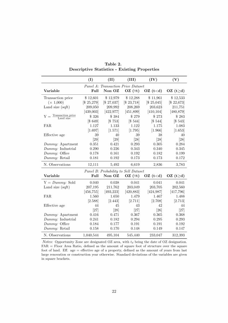
Table 2.Descriptive Statistics - Existing Properties

(I) (II) (III) (IV) (V)

Panel A: Transaction Price DatasetVariable Full Non OZ OZ (∀t) OZ (t<d) OZ (t≥d)

Transaction price $ 12,601 $ 12,979 $ 12,288 $ 11,961 $ 12,533(× 1,000) [$ 25,279] [$ 27,037] [$ 23,718] [$ 25,045] [$ 22,673]

Land size (sqft) 209,050 209,992 208,269 203,623 211,751[439,003] [422,977] [451,899] [410,104] [480,879]

Y = Transaction priceLand size $ 326 $ 384 $ 279 $ 273 $ 283

[$ 649] [$ 753] [$ 544] [$ 544] [$ 543]FAR 1.127 1.133 1.122 1.175 1.083

[1.697] [1.571] [1.795] [1.966] [1.653]Effective age 39 40 39 38 40

[29] [29] [28] [28] [28]Dummy: Apartment 0.351 0.421 0.293 0.305 0.284Dummy: Industrial 0.290 0.226 0.343 0.340 0.345Dummy: Office 0.178 0.161 0.192 0.182 0.199Dummy: Retail 0.181 0.192 0.173 0.173 0.172

N. Observations 12,111 5,492 6,619 2,836 3,783

Panel B: Probability to Sell DatasetVariable Full Non OZ OZ (∀t) OZ (t<d) OZ (t≥d)

Y = Dummy: Sold 0.040 0.038 0.041 0.041 0.041Land size (sqft) 207,195 211,762 203,049 203,705 202,560

[456,755] [493,223] [420,883] [424,987] [417,796]FAR 1.560 1.650 1.479 1.467 1.488

[2.588] [2.443] [2.711] [2.708] [2.713]Effective age 44 45 43 42 44

[27] [28] [27] [26] [27]Dummy: Apartment 0.416 0.471 0.367 0.365 0.368Dummy: Industrial 0.241 0.182 0.294 0.295 0.293Dummy: Office 0.184 0.177 0.191 0.191 0.192Dummy: Retail 0.158 0.170 0.148 0.149 0.147

N. Observations 1,040,544 495,104 545,440 233,047 312,393

Notes: Opportunity Zone are designated OZ area, with td being the date of OZ designation.FAR = Floor Area Ratio, defined as the amount of square foot of structure over the squarefoot of land. Eff. age = effective age of a property, defined as the amount of years from lastlarge renovation or construction year otherwise. Standard deviations of the variables are givenin square brackets.

22

regression (1 year step size), providing sufficient observations per bracket.22

Lastly, we test if there is sufficient variation between OZ and control census

tracts within counties, as we use county-level time year fixed effects (D: county×

year). On average, a county consists of six census tracts. Appendix Figure

Appendix B.2 shows the distribution of opportunity zones per county. A darker

color highlights counties dominated by OZ transactions, whereas a light green

color highlights counties dominated by transactions in the control group. There

are 576 counties with (enough) commercial property transactions between 2017

and 2019. 218 counties have no variation in OZ designation, meaning transaction

in these counties are not used to identify the treatment effect. For vacant land

we have 181 counties with enough transactions during our analyzed period, of

which 79 counties have no variation in OZ designation.

Figure 3.Effective Age of Sample Properties

Effective age of property (in years)

Fre

quen

cy

0 20 40 60 80 100 120

010

0020

0030

0040

0050

0060

00

Notes: Effective age is the age of a property (in years) since it was last(considerably) renovated. If we do not observe any renovations, we usethe age since construction.

22We use effective age as a proxy in our analysis instead of the CAPEX variable directly. Asshown by Buchler et al. (2020); Clapp et al. (2012), CAPEX and prices are endogenous, sinceCAPEX is mostly done if there is a positive outlook in future price. Furthermore, our variabledoesn’t allow to observe the CAPEX size in dollars, creating a lot of noise.

23

5. Results

5.1. Main Results

Table 3 shows the results for price per square foot of land as the explanatory

variable. Column (I) shows the estimates for the full sample, while columns

(II) – (IV) show estimates for different age sub-samples. Column (V) shows the

estimates for vacant land. The model shows a good general fit, with an adjusted

R-squared between 0.87 and 0.79. All control variables are significant and in

line with expected results. A density increase of 1 percent, measured by ln FAR,

leads to a 0.876 percent increase in transaction price, on average. Property age

has a negative effect on price, showing a -0.115 percent discount on price for

every 1 percent increase in age. However, the effect is not stable among all age

groups but reverts for very old properties, suggesting a U-turn pattern in line

with the literature (Coulson and McMillen, 2008), caused by survival bias and

vintage effects (Francke and van de Minne, 2017). Compared to apartments,

industrial properties show a discount (-43.3 percent), while office (19.8 percent)

and retail (36 percent) properties show a premium, on average. In line with the

literature, we document that lot size has a negative effect on price per square

foot of land (bulk discount).

Properties located in OZ census tracts show an average location discount of

6.3 percent compared to properties in eligible but not designated census tracts.

Similarly, vacant land in OZ census tracts trades at a discount of 15.4 percent

(significant within the 10% probability). For designation, we document no statis-

tically significant effect on property prices for the full sample. However, looking

at different age groups, we document a price increase of 6.8 percent for old prop-

erties, on average (significant within the 10% probability). For vacant land, we

estimate a land price increase of 37.7 percent after designation.

Figure 4a plots the estimates for the rolling window model on property price,

using a time window of 30 years for effective age and moving in one year steps.

24

The black line shows the point estimate of the designation effect µt≥td,z, including

95% confidence bounds. We document a positive trend in designation effects over

property age. Even though the estimates are noisier for older properties, we see

significant positive designation effects for properties of 60 years and older (at a

95% confidence level).

Table 3.Effect of OZ designation on price

(I) (II) (III) (IV) (V)Age group / Land: [1 – 120] [1 – 30] [31 – 80] [81 – 120] Land

Intercept 5.010*** 5.133*** 3.609*** 2.052** 9.866***[14.19] [15.05] [15.04] [2.43] [16.96]

OZ area (θz) -0.061*** -0.043 -0.081*** -0.075* -0.143*(1=yes) [-3.51] [-1.63] [-2.91] [-1.83] [-1.75]

OZ designation (µt≥td,z) 0.001 -0.014 -0.014 0.066* 0.320***(1=yes) [0.07] [-0.61] [-0.57] [1.75] [3.19]

Property type:Industrial -0.362*** -0.293*** -0.402*** -0.361***

(1=yes) [-22.32] [-10.89] [-16.60] [-8.35]Office 0.181*** 0.253*** 0.138*** 0.181***

(1=yes) [10.04] [9.61] [4.68] [3.43]Retail 0.308*** 0.390*** 0.179*** 0.415***

(1=yes) [16.60] [13.48] [5.77] [10.48]

ln Eff. age -0.114*** -0.158*** 0.150*** 0.622***(years) [-19.81] [-16.79] [3.64] [4.12]

ln FAR 0.876*** 0.944*** 0.803*** 0.713***[116.94] [86.01] [61.28] [32.21]

ln Land size -0.529***[-22.47]

County × Year FE Yes Yes Yes Yes YesAdj. R2 0.847 0.870 0.804 0.821 0.790RMSE 0.373 0.346 0.383 0.279 0.530N. Observations 12,111 5,251 5,217 1,643 922

Notes: Dependent variable = log of sales prices per square foot of land. Eff. age = the effectiveage of properties, meaning the amount of years since last large renovation, or construction year ifno heavy renovations were reported in the data. OZ = Opportunity zone, with OZ designationindicating the transaction took place after designation. FAR = floor area ratio, a density measure.Apartments are the reference group for the property types. T-stats are given in parenthesis. ∗∗∗

= significant within 99% probability, ∗∗ = significant within 95% probability and ∗ = significantwithin 90% probability. The control group consists of transactions or development sites in eligiblecensus tracts with similar median income and poverty levels.

Table 4 shows the results for the probability to sell, measuring the effect of

25

Figure 4.Rolling window estimate

(a) Designation effect on price

−0.

10−

0.05

0.00

0.05

0.10

0.15

0.20

0.25

[1 −

31]

[6 −

36]

[11

− 4

1]

[16

− 4

6]

[21

− 5

1]

[26

− 5

6]

[31

− 6

1]

[36

− 6

6]

[41

− 7

1]

[46

− 7

6]

[51

− 8

1]

[56

− 8

6]

[61

− 9

1]

[66

− 9

6]

[71

− 1

01]

[76

− 1

06]

[81

− 1

11]

[86

− 1

16]

(b) Designation effect on probability to sell

−0.

4−

0.3

−0.

2−

0.1

0.0

0.1

0.2

[1 −

31]

[6 −

36]

[11

− 4

1]

[16

− 4

6]

[21

− 5

1]

[26

− 5

6]

[31

− 6

1]

[36

− 6

6]

[41

− 7

1]

[46

− 7

6]

[51

− 8

1]

[56

− 8

6]

[61

− 9

1]

[66

− 9

6]

Notes: The horizontal axis shows the windows of effective ages (length 30 years),which is moved in one-year steps. Effective age is the age of a property (in years)since the last (major) renovation. In the absence of renovations, we use age sinceconstruction. The vertical axis shows the designation of the respective model µt≥td,z

and the 95% confidence intervals (grey).

26

OZ designation on liquidity. We use the same hedonic controls as in Table 3 but

report only estimates related to OZ designation due to space constraints.23 In

general, we do not find a significant location difference for OZ census tract (θz).

However, for young properties (up to 30 years), we find an increased liquidity

of 14.6 percent. In contrast, for middle aged properties, we document a lower

probability to sell (-5%) compared to the control group. OZ designation does

not show significant effect on liquidity of existing properties. Figure 4b shows

the estimates for the rolling window model, including 95% confidence bounds.

Even though we observe a drop in probability to sell for older properties, it

is not significant at a 95% significance level. However, designation shows a

positive effect on vacant land, increasing the probability to sell by 28.5 percent,

on average.

Table 4.Effect of OZ designation on probability to sell

(I) (II) (III) (IV) (V)

Age group / Land: [1 – 120] [1 – 30] [31 – 80] [81 – 120] Land

Intercept -1.999*** -2.185*** -2.497*** -3.180*** -2.432***[-23.46] [-18.55] [-13.00] [-8.24] [-5.25]

OZ area (θz) -0.013 0.146*** -0.058*** -0.011 -0.049(1=yes) [-0.82] [1.82] [-2.61] [1.38] [-0.46]

OZ designation (µt≥td,z) 0.020 -0.048 0.092 0.054 0.285**(1=yes) [1.04] [-1.50] [3.49] [1.38] [2.22]

AIC 267,543 121,627 168,059 79,972 8,708Hedonic controls Yes Yes Yes Yes YesCounty × Year FE Yes Yes Yes Yes YesN. Observations 398,712 150,632 183,104 64,976 33,948

Notes: Dependent variable is a (1/0) dummy indicating that a property is sold in a specific quar-ter. This panel also includes properties that were not sold between 2017 – 2019. The model isestimated using a Logit regression. OZ = Opportunity zone. Z-stats are given in parenthesis. ∗∗∗

= significant within 99% probability, ∗∗ = significant within 95% probability and ∗ = significantwithin 90% probability. We use the same hedonic controls and control group as in Table 3.

23Full results for this Table and following Tables are available upon request.

27

5.2. Heterogeneity analysis

Examining the timeliness of the OZ designation effects, Panel A and B of Table

5 show the results for interacting the designation dummy (µt≥td,z) with semi-

annual dummies, providing a more nuanced picture. We use the same controls

as those reported in the baseline model of Table 3. Even though the Root Mean

Squared Error (RMSE) is similar between all models, on an adjusted R2 basis

the baseline model in Table 3 fits best.

As shown in Panel A of Table 5, we do not find an immediate designation

effect on prices, i.e. within the first half of 2018, except for vacant land. Vacant

land prices in OZ census tracts increase by 39 percent in the first months after

designation, on average (significant at 10% probability). For the second half

of 2018, we document significant price effects for nearly all properties, except

young properties (<30 years). For middle aged properties we find a 8.2 per-

cent increase, on average (significant at 10% probability). As shown in Figure

Appendix B.1 around 15 percent of these properties experience heavy capital

expenditures, which could explain some effects. For old properties and vacant

land, the estimates are 15.1 and 45.5 percent price increase, on average. The

effect for old properties and vacant land remains in the first half of 2019, but

becomes insignificant in the second half of 2019.

As shown in Panel B of Table 5, the results for probability to sell are more

heterogeneous. We find a 19.9 percent reduction in probability to sell for the

first half of 2018 for old properties or 9 percent reduction for the full sample.

However, the effect does not persist for the second half of 2018. For the first

half of 2019, we find an increase in probability to sell for old properties (17.1

percent) and vacant land (68.3 percent), but a decrease for young properties (-

13.6 percent). For the second half of 2019, we only find an increased probability

to sell for young properties (12.4 percent) but not for other properties. Assuming

that liquidity tends to move before prices, our findings could be an indication

for future price increases in OZ areas.

28

In line with previous findings, our results show that OZ designation does not

affect young properties but primarily older properties. The estimated designa-

tion effects are not persistent over time, which fits more to temporary tax gains

rather than long-term future land price appreciations. The initial absence of ef-

fects could be explained by little initial information about achievable benefits of

the OZ program. Our results indicate investors where either careful, conservative

or needed time at first but did not increase demand immediately.

In Table 6, we examine the OZ designation effect by property type instead

of age.24 We estimate our models by sub-samples of different property types,

comparing only properties of the same type in eligible and OZ census tracts.

Examining price in Panel A, we document a general OZ location discount (θz) for

all property types except industrial, which shows a premium of 8.5 percent. OZ

designation does not significantly affect property prices except for apartments,

increasing 5.9 percent on average. For probability to sell we only find a general

OZ location effect for industrial, showing a 12 percent higher probability to sell

compared to industrial properties in eligible census tracts. For OZ designation,

we document positive effects on probability to sell for retail properties (14.4

percent) and office (18.3 percent), and a negative effects on industrial (11.8

percent).

As shown in Table 2, we the share of apartments is generally lower in OZ

census tracts compared to eligible census tracts. Vice versa, the share of indus-

trial properties is generally higher in OZ census tracts. Our findings suggest that

this relationship might shift through the OZ designation. Apartments increase

in price, while industrial properties decrease in the probability to sell (but not

necessarily in price).

Since Arefeva et al. (2020) find different effects for urban and rural OZ census

24Our number of observations does not allow for double sorting by type and age. Vacantland is excluded from the analysis.

29

Table 5.OZ price effects with post-designation trend

(I) (II) (III) (IV) (V)Age group / Land: [1 – 120] [1 – 30] [31 – 80] [81 – 120] Land

Panel A: Dependent variable = price

OZ area (θz) -0.061*** -0.045* -0.081*** -0.073* -0.134(1=yes) [-3.49] [-1.67] [-2.86] [-1.77] [-1.61]

OZ designation-time interaction:µt=2018.I&t≥td,z -0.004 -0.054 -0.008 0.125 0.330*

(1=yes) [-0.11] [-0.92] [-0.13] [1.27] [1.73]µt=2018.II,z 0.068** 0.035 0.079* 0.141** 0.375***

(1=yes) [2.53] [0.85] [1.86] [2.29] [3.04]µt=2019.I,z 0.048 0.017 0.022 0.182** 0.271*

(1=yes) [1.58] [0.35] [0.47] [2.43] [1.91]µt=2019.II,z 0.064** 0.048 0.082* 0.028 0.223

(1=yes) [2.12] [1.04] [1.76] [0.36] [1.45]

County × Year FE Yes Yes Yes Yes YesHedonic controls Yes Yes Yes Yes YesAdj. R2 0.836 0.849 0.778 0.798 0.739RMSE 0.372 0.346 0.382 0.278 0.531N. Observations 12,111 5,251 5,217 1,643 922

Panel B: Dependent variable = probability to sell

OZ area (θz) 0.014 0.102*** 0.009 0.069 -0.086(1=yes) [0.47] [3.37] [0.30] [1.29] [-0.79]

OZ designation-time interaction:µt=2018.I&t≥td,z -0.090** -0.063 -0.049 -0.199** -0.053

(1=yes) [-2.23] [-1.00] [-0.85] [-1.96] [-0.23]µt=2018.II,z -0.059* -0.075 -0.024 -0.069 0.192

(1=yes) [-1.92] [-1.58] [-0.55] [-0.88] [1.21]µt=2019.I,z -0.058 -0.136** -0.039 0.171* 0.683***

(1=yes) [-1.63] [-2.44] [-0.77] [1.80] [3.75]µt=2019.II,z 0.078** 0.124** 0.078 -0.109 0.314

(1=yes) [2.24] [2.34] [1.59] [-1.08] [1.63]

County × Year FE Yes Yes Yes Yes YesHedonic controls Yes Yes Yes Yes YesAIC 82,756 42,803 50,808 16,241 8,697N. Observations 398,712 150,632 183,104 64,976 33,948

Notes: Dependent variable Panel A: log of sales prices per square foot of land. Panel B: (1/0)dummy indicating that a property is sold in a specific quarter. Panel B also includes proper-ties that were not sold between 2017 – 2019. OZ = Opportunity zone, with OZ designationindicating the transaction took place after designation. Z-stats are given in parenthesis. ∗∗∗ =significant within 99% probability, ∗∗ = significant within 95% probability and ∗ = significantwithin 90% probability. We use the same hedonic controls and control group as in Table 3.

30

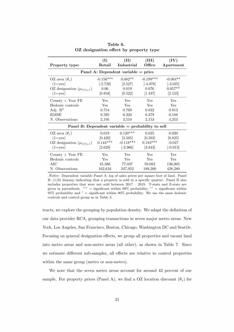
Table 6.OZ designation effect by property type

(I) (II) (III) (IV)Property type: Retail Industrial Office Apartment

Panel A: Dependent variable = price

OZ area (θz) -0.156*** 0.082** -0.199*** -0.064**(1=yes) [-2.720] [2.527] [-4.076] [-3.025]

OZ designation (µt≥td,z) 0.06 0.019 0.076 0.057**(1=yes) [0.858] [0.522] [1.337] [2.153]

County × Year FE Yes Yes Yes YesHedonic controls Yes Yes Yes YesAdj. R2 0.754 0.769 0.832 0.913RMSE 0.595 0.320 0.379 0.188N. Observations 2,195 3,510 2,153 4,253

Panel B: Dependent variable = probability to sell

OZ area (θz) 0.019 0.120*** 0.025 0.020(1=yes) [0.420] [3.505] [0.593] [0.825]

OZ designation (µt≥td,z) 0.144*** -0.118*** 0.183*** -0.027(1=yes) [2.629] [-2.966] [3.843] [-0.913]

County × Year FE Yes Yes Yes YesHedonic controls Yes Yes Yes YesAIC 45,386 77,037 59,082 136,005N. Observations 162,616 247,952 189,200 428,280

Notes: Dependent variable Panel A: log of sales prices per square foot of land. PanelB: (1/0) dummy indicating that a property is sold in a specific quarter. Panel B alsoincludes properties that were not sold between 2017 – 2019. T-stats and Z-stats aregiven in parenthesis. ∗∗∗ = significant within 99% probability, ∗∗ = significant within95% probability and ∗ = significant within 90% probability. We use the same hedoniccontrols and control group as in Table 3.

tracts, we explore the grouping by population density. We adapt the definition of

our data provider RCA, grouping transactions in seven major metro areas: New

York, Los Angeles, San Francisco, Boston, Chicago, Washington DC and Seattle.

Focusing on general designation effects, we group all properties and vacant land

into metro areas and non-metro areas (all other), as shown in Table 7. Since

we estimate different sub-samples, all effects are relative to control properties

within the same group (metro or non-metro).

We note that the seven metro areas account for around 42 percent of our

sample. For property prices (Panel A), we find a OZ location discount (θz) for

31

existing properties across all OZ census tracts. For vacant land, we only find a

location discount in non-metro areas (-44 percent), showing that land values in

metro areas are not statistically different across groups. OZ designation shows a

positive price effect for existing properties in metro areas (9.5 percent) but not

for non-metro areas. For vacant land, we find a significant OZ designation effect

across both groups. For probability to sell (Panel B), we find an OZ location

premium (θz) for existing properties in metro areas (17.1 percent). However, OZ

designation lowers the probability to sell for existing properties in metro areas by

-14.9 percent. In contrast we find an increase in non-metro areas (3.6 percent).

For vacant land, we do not find a significant designation effect in metro areas

but an higher probability to sell in non-metro areas (48.3 percent). Overall, our

results suggest heterogeneity between metro and non-metro census tracts. OZ

designation shows limited effects on existing properties in non-metro areas and

vacant land in metro areas.

In Table 8, we distinguish by transaction size, sorting transactions by price

into two brackets: up to (and including ) $10 million and above $10 million. For

price (Panel A), general location effects do not differ for different size groups.

Existing properties show a discount, whereas land shows not significant effect.

OZ designation effects are limited to larger properties of more than $10 million

(9.6 percent) and vacant land below $10 million (20 percent). For probability to

sell (Panel B), we document negative OZ designation effects for properties above

$10 million (-7.1 percent) and positive effects for land above $10 million (46.8

percent, significant at 10% probability). Due to spatial land value heterogeneity,

we cannot rule out that the effects coincide with the estimates in Table 7.

Table 9 examines the spatial spillover effects of OZ designation on eligi-

ble (control) census tracts. We find that OZ distance φt has a negative effect

on property prices. One percent increase in distance leads to a price discount

of -3.8 percent for existing properties and 34.6 percent for vacant land. For

probability to sell we do not find a significant effect. OZ designation shows no

32

significant effect, except for probability sell of existing properties. Contradicting

positive spillover effects, the probability to sell of existing properties increases

with distance to the OZ census tract relative to other properties in the census

tract.

Finally, we test the robustness of our findings with regard to the control

census tract selection. Instead of using propensity score matching, we therefore

match the OZ census tracts in our sample with random eligible census tract in

the same area. Table Appendix B.1 shows the income and poverty statistics

by census tract groups, indicating that the difference between OZ and eligible

tracts is significantly higher. Table Appendix B.3 shows the results focusing

on price. OZ designation effects are of a higher magnitude but generally in line

with our previous findings, being predominantly visible for older, redevelopment

properties and vacant land.

6. Discussion and Conclusion

Even though the success of the OZ program should ultimately be measured on

economic growth, this study provides a first, early analysis on the success factors

– institutional investments and property market reactions. Assuming efficient

markets, the OZ program should increase property prices as investors price in

future expected economic growth, through higher land values. In contrast, if the

effects are limited to temporary tax benefits, only qualified properties should

show an effect. We therefore examine the effects of OZ designation on commercial

properties, comparing to similar properties in eligible, but not designated census

tracts.

Our results show that the effect of OZ designation is limited to old properties

and vacant land, both qualified for tax benefits. The significant positive price

effects for old properties is 6.8 percent, on average. To put this effect in context,

we estimated a theoretical tax benefit of approximately 10 to 25 percent in Table

1. However, our empirical estimates cannot be compared to the theoretical effects

33

Table 7.OZ designation effect metro areas

(I) (II) (III) (IV)Metro No-Metro Metro No-Metro

Existing properties Vacant Land

Panel A: Dependent variable = price

OZ area (θz) -0.073*** -0.049** -0.001 -0.368***(1=yes) [-3.027] [-1.987] [-0.013] [-2.967]

OZ designation (µt≥td,z) 0.091*** 0.025 0.254* 0.416***(1=yes) [3.071] [0.828] [1.930] [2.736]

County × Year FE Yes Yes Yes YesHedonic controls Yes Yes Yes YesAdj. R2 0.824 0.739 0.752 0.625RMSE 0.322 0.409 0.537 0.492N. Observations 5,140 6,971 497 425

Panel B: Dependent variable = probability to sell

OZ area (θz) 0.171*** -0.009 -0.010 -0.083(1=yes) [11.363] [-0.611] [-0.073] [-0.570]

OZ designation (µt≥td,z) -0.149*** 0.036** 0.055 0.483***(1=yes) [-7.995] [2.026] [0.340] [2.740]

County × Year FE Yes Yes Yes YesHedonic controls Yes Yes Yes YesAIC 343,526 326,209 5,225 4,633N. Observations 1,137,372 548,292 20,796 16,932

Notes: Dependent variable Panel A: log of sales prices per square foot of land. PanelB: (1/0) dummy indicating that a property is sold in a specific quarter. Panel B alsoincludes properties that were not sold between 2017 – 2019. T-stats and Z-stats aregiven in parenthesis. ∗∗∗ = significant within 99% probability, ∗∗ = significant within95% probability and ∗ = significant within 90% probability. We use the same hedo-nic controls and control group as in Table 3.

directly, as the required capital expenditures are not yet included and unknown

to us. Assuming the minimum required capital expenditures are invested (at

least equal to purchase price), the price effect of OZ designation on the property

before refurbishments should be twice the estimated effect or between 13.6 to 40

percent.25 Previous literature shows us that the average land value fraction for

new buildings is approximately 20% (Bokhari and Geltner, 2018). This means

25This calculation is obviously back-of-the-envelope without knowing the actual capital ex-penditures. If investors would do more capital expenditures, tax benefits would decrease, onaverage.

34

Table 8.OZ designation effect by property value

(I) (II) (III) (IV)<$10m >$10m <$10m >$10m

Existing properties Vacant Land

Panel A: Dependent variable = price

OZ area (θz) -0.056*** -0.062* -0.010 -0.038(1=yes) [-2.729 ] [-1.876 ] [-0.175 ] [-0.251 ]

OZ designation (µt≥td,z) 0.034 0.092** 0.183** 0.108(1=yes) [1.340] [2.301] [2.347 ] [0.648 ]

County × Year FE Yes Yes Yes YesHedonic controls Yes Yes Yes YesAdj. R2 0.818 0.879 0.913 0.842RMSE 0.379 0.317 0.256 0.332N. Observations 8,689 3,422 667 255

Panel B: Dependent variable = probability to sell

OZ area (θz) -0.008 0.044** 0.032 -0.402*(1=yes) [-0.561] [2.269] [0.279] [-1.870]

OZ designation (µt≥td,z) 0.022 -0.071*** 0.199 0.468*(1=yes) [1.241 ] [-2.989] [1.447] [1.882 ]

County × Year FE Yes Yes Yes YesHedonic controls Yes Yes Yes YesAIC 333,010 198,543 7,235 2,849N. Observations 559,204 342,480 27,516 10,212

Notes: Dependent variable Panel A: log of sales prices per square foot of land.Panel B: (1/0) dummy indicating that a property is sold in a specific quarter.Panel B also includes properties that were not sold between 2017 – 2019. T-statsand Z-stats are given in parenthesis. ∗∗∗ = significant within 99% probability, ∗∗

= significant within 95% probability and ∗ = significant within 90% probability.We use the same hedonic controls and control group as in Table 3.

that the initial 6.8 % has to be multiplied by 5 to find the possible land value

increase is 34% after capital improvements. This effect is approximately in line

with our estimated for vacant land price increases of 37.7 percent.

We further examine market liquidity for two reasons (measured by the prob-

ability to sell). First, even if designation price effects are insignificant, the pro-

gram is still a success if more (re)developments would take place, suggesting

that more (re)developments became positive NPV projects. This argument is

especially important for vacant land and older “redevelopment” properties. Sec-

ondly, liquidity tends to move before prices. Given the recentness of the program

35

Table 9.Spillover effect on eligible properties

Dependent variable: Price Probability to sell

Properties Land Properties Land

Designation nearby (ωt≥td) 0.262** 0.372 -0.343** -1.069(1=yes) [0.049] [0.544] [0.011] [0.209 ]

OZ distance (φt) -0.037*** -0.297*** -0.026 -0.030(log meters) [0.007 ] [0.000] [0.120] [0.710]

Distance*Designation (φt ∗ ωt≥td) -0.028 -0.035 0.051*** 0.093(log meters) [0.105 ] [0.637 ] [0.004 ] [0.376 ]

County × Year FE Yes Yes Yes YesHedonic controls Yes Yes Yes YesAdj. R2 0.864 0.816RMSE 0.332 0.569AIC 65,167 3,032N. Observations 5,492 527 102,956 4,800

Notes: We focus on transactions in eligible census tracts only, measuring spillover effects. ωt≥td ,controls for OZ designation in the nearest OZ census tract and φt controls for the distance tothe nearest OZ property in meters. Our variable of interest is: φt ∗ ωt≥td . T-stats and Z-statsare given in parenthesis. ∗∗∗ = significant within 99% probability, ∗∗ = significant within 95%probability and ∗ = significant within 90% probability. We use the same hedonic controls andcontrol group as in Table 3.

and how slow information travels in real estate markets, perhaps we only observe

an impact on liquidity at this point. We do not find general effects on liquidity,

except for vacant land. However, examining the designation effect over time, we

see positive effects in the last half-year of our sample, potentiality providing a

silver lining.

Has the opportunity zone program worked? Even though we do not document

general price increases, we do find a small increase in liquidity at the end of the

sample period. Finding evidence of more vacant land sales, could mean negative

NPV projects have turned into zero or positive NPV projects. However, we find

a lot of heterogeneity in effects. We can therefore say that the OZ program

did not yet show any general effects on land price appreciation. The estimated

effects are temporarily and spatially limited, and do not affect all property of

all type equally. These findings suggest that investors cherry-pick, which will

consequently lead to partly failures of the OZ program.

36

References

Albouy, D., Ehrlich, G., Shin, M., 2018. Metropolitan land values. Reviewof Economics and Statistics 100, 454–466. doi:https://doi.org/10.1162/rest_a_00710.

Arefeva, A., Davis, M.A., Ghent, A.C., Park, M., 2020. Who benefits fromplace-based policies? job growth from opportunity zones. Available at SSRNdoi:http://dx.doi.org/10.2139/ssrn.3645507.

Bernstein, J., Hassett, K., 2015. Unlocking Private Capital to Facilitate Eco-nomic Growth in Distressed Areas. Technical Report. Economic InnovationGroup.

Boarnet, M., Bogart, W., 1996. Enterprise zones and employment: Evidencefrom new jersey. Journal of Urban Economics 40, 198–215. doi:https://doi.org/10.1006/juec.1996.0029.

Boarnet, M.G., 2001. Enterprise zones and job creation: Linking evaluationand practice. Economic Development Quarterly 15, 242–254. doi:10.1177/089124240101500304.

Bokhari, S., Geltner, D., 2018. Characteristics of depreciation in commercialand multifamily property: An investment perspective. Real Estate Economics46, 745–782. doi:https://doi.org/10.1111/1540-6229.12156.

Bokhari, S., Geltner, D., 2019. Commercial buildings capital consumption andthe united states national accounts. Review of Income and Wealth 65, 561–591.doi:https://doi.org/10.1111/roiw.12357.

Buchler, S.C., van de Minne, A., Schoni, O., 2020. Redevelopment option valuefor commercial real estate. working paper doi:10.7892/boris.143537.

Busso, M., Gregory, J., Kline, P., 2013. Assessing the incidence and efficiencyof a prominent place based policy. American Economic Review 103, 897–947.doi:10.1257/aer.103.2.897.

Casey, A., 2019. Sale prices surge in neighborhoods with new tax break. https://bit.ly/2UXK8SB. Accessed: 2019-12-30.

Chen, J., Glaeser, E.L., Wessel, D., 2019. The (Non-) Effect of OpportunityZones on Housing Prices. Working Paper 26587. National Bureau of EconomicResearch. doi:10.3386/w26587.

Clapp, J.M., Jou, J.B., (Charlene) Lee, T., 2012. Hedonic models with rede-velopment options under uncertainty. Real Estate Economics 40, 197–216.doi:https://doi.org/10.1111/j.1540-6229.2011.00323.x.

Coulson, E.N., McMillen, D.P., 2008. Estimating time, age and vintage effectsin housing prices. Journal of Housing Economics 17, 138–151. doi:https://doi.org/10.1016/j.jhe.2008.03.002.

37

Cunningham, C.R., 2006. House price uncertainty, timing of development, andvacant land prices: Evidence for real options in seattle. Journal of UrbanEconomics 59, 1–31. doi:https://doi.org/10.1016/j.jue.2005.08.003.

van Dijk, D.W., Geltner, D.M., van de Minne, A.M., 2020. The dynamics ofliquidity in commercial property markets: Revisiting supply and demand in-dexes in real estate. The Journal of Real Estate Finance and Economicsdoi:https://doi.org/10.1007/s11146-020-09782-5.

Elvery, J., 2009. The impact of enterprise zones on resident employment: Anevaluation of the enterprise zone programs of California and Florida. Eco-nomic Development Quarterly 23, 44–59. doi:https://doi.org/10.1177/0891242408326994.

Engberg, J., Greenbaum, R., 1999. State enterprise zones and local housingmarkets. Journal of Housing Research 10, 163–187. doi:https://doi.org/10.1080/10835547.1999.12091946.

Francke, M.K., van de Minne, A.M., 2017. Land, structure and deprecia-tion. Real Estate Economics 45, 415–451. doi:https://doi.org/10.1111/1540-6229.12146.

Frank, M.M., Hoopes, J.L., Lester, R., 2020. What determines where opportu-nity knocks? political affiliation in the selection of opportunity zones (june 20,2020). Available at SSRN doi:http://dx.doi.org/10.2139/ssrn.3534451.

Freedman, M., 2012. Teaching new markets old tricks: The effects of subsidizedinvestment on low-income neighborhoods. Journal of Public Economics 96,1000–1014. doi:https://doi.org/10.1016/j.jpubeco.2012.07.006.

Geltner, D., Kumar, A., Van de Minne, A.M., 2020. Riskiness of real estate de-velopment: A perspective from urban economics and option value theory. RealEstate Economics 48, 406–445. doi:https://doi.org/10.1111/1540-6229.12258.

Geltner, D., Miller, N.G., Clayton, J., Eichholtz, P., 2013. Commercial realestate analysis and investments. volume 3. South-western Cincinnati, OH.

Greenbaum, R., Engberg, J., 2004. The impact of state enterprise zones on urbanmanufacturing establishments. Journal of Policy Analysis and Management23, 315–339. doi:https://doi.org/10.1002/pam.20006.

Hanson, A., Rohlin, S., 2011. Do location-based tax incentives attract newbusiness establishments? Journal of Regional Science 51, 427–449. doi:https://doi.org/10.1111/j.1467-9787.2010.00704.x.

Hebert, S., Vidal, A., Mills, G., James, F., Gruenstein, D., 2001. Interim assess-ment of the empowerment zones and enterprise communities (ez/ec) program:A progress report. Office of Policy Development and Research URL: https://www.huduser.gov/portal/publications/econdev/ezec_rpt.html.

38

Ho, D.E., Imai, K., King, G., Stuart, E.A., 2007. Matching as nonparametricpreprocessing for reducing model dependence in parametric causal inference.Political analysis 15, 199–236. doi:10.1093/pan/mpl013.

Hulten, C.R., Wykoff, F.C., 1981. The estimation of economic depreciationusing vintage asset prices: An application of the box-cox power transforma-tion. Journal of Econometrics 15, 367–396. doi:https://doi.org/10.1016/0304-4076(81)90101-9.

Hulten, C.R., Wykoff, F.C., 1996. Issues in the measurement of eco-nomic depreciation: introductory remarks. Economic inquiry 34, 10.URL: https://search.proquest.com/docview/200870445?pq-origsite=

gscholar&fromopenview=true.

Krupka, D., Noonan, D., 2009. Empowerment zones, neighborhood change andowner-occupied housing. Regional Science and Urban Economics 39, 386–396.doi:https://doi.org/10.1016/j.regsciurbeco.2009.03.001.

Lin, Z., Rosenblatt, E., Yao, V.W., 2009. Spillover effects of foreclosures onneighborhood property values. The Journal of Real Estate Finance and Eco-nomics 38, 387–407. doi:https://doi.org/10.1016/j.regsciurbeco.2009.03.001.

Lusht, K.M., 2001. Real estate valuation: principles and applications. KMLpublishing.

Neumark, D., Kolko, J., 2010. Do enterprise zones create jobs? evidence fromcalifornia’s enterprise zone program. Journal of Urban Economics 68, 1–19.doi:https://doi.org/10.1016/j.jue.2010.01.002.

Papke, L.E., 1993. What do we know about enterprise zones? Tax Policy andthe economy 7, 37–72. doi:https://doi.org/10.1086/tpe.7.20060629.

Papke, L.E., 1994. Tax policy and urban development: evidence from the indianaenterprise zone program. Journal of Public Economics 54, 37–49. doi:https://doi.org/10.1016/0047-2727(94)90069-8.

Peters, A.H., Fisher, P., 2002. State enterprise zone programs: Have theyworked? WE Upjohn Institute.

Peters, A.H., Fisher, P., 2004. The failures of economic development incentives.Journal of the American Planning Association 70, 27–37. doi:https://doi.org/10.1080/01944360408976336.

Rosen, S., 1974. Hedonic prices and implicit markets: Product differentiation inpure competition. The Journal of Political Economy 82, 34–55. doi:https://doi.org/10.1086/260169.

Smith, B., 2009. If you promise to build it, will they come? the interaction be-tween local economic development policy and the real estate market: Evidence

39

from tax increment finance districts. Real Estate Economics 37, 209–234.doi:https://doi.org/10.1111/j.1540-6229.2009.00240.x.

Titman, S., 1985. Urban land prices under uncertainty. The American EconomicReview 75, 505–514. URL: https://www.jstor.org/stable/1814815.

Uzawa, H., 1960. Walras’ tatonnement in the theory of exchange. The Reviewof Economic Studies 27, 182–194. URL: https://www.jstor.org/stable/2296080.

40

Appendix A. Propensity Score Matching

We perform propensity score matching (PSM) to match designated OZ census

tracts 1:1 to eligible census tracts, using a simple logit model as shown in equation

(A.1) (for details see: Ho et al., 2007). The dependent variable is the final OZ

designation status (OZi = 1) of census tract i. As explanatory variables, we

use log median income and poverty rate, as these characteristics were influential

for the decision and differ between eligible and designated census tracts. We

estimate the model for every NCREIF region separately.

OZi = α+ τ ln(income)i + δpovertyi + εi (A.1)

Table Appendix A.1 shows that the explanatory variables are indeed significant

for all regions, meaning that median income and poverty rates affected the OZ

designation outcome. Based on the coefficients, we fit the model for every census

tract and estimate the likelihood of every eligible census tract to be designated

(OZi). Finally, we use nearest neighbor matching to match every designated

census tract to the runner-up tract in the same region with the highest propensity

score.

Table Appendix A.1.Propensity Score Matching estimates

Region Intercept Ln median income Poverty rate AIC N

Mid-Atlantic 10.843*** -1.123*** 0.493*** 1,207 1,110Midwest 17.577*** -1.794*** 0.032*** 1,681 1,700Northeast 7.489*** -0.856*** 2.301*** 2,103 1,934Southeast 18.962*** -2.017*** 2.375*** 2,927 3,481Southwest 9.032*** -1.057*** 1.651*** 1,643 1,951West 15.380*** -1.647*** 3.497*** 3,498 3,797

Notes: AIC = Akaike Information Criterium. *** = significant at the 1% level.We use a logit model with opportunity zone designation (1/0) as explained vari-able, comparing eligible with designated census tracts. The scoring is done on acensus tract level. Regions are defined by NCREIF (National Council for RealEstate Investment Fiduciaries).

41

Appendix B.

Figure Appendix B.1.Kaplan-Meier Curve to CAPEX

0 20 40 60 80 100 120

0.4

0.5

0.6

0.7

0.8

0.9

1.0

Effective age (in years)

Pro

babi

lity

of n

o C

AP

EX

Notes: Heavy capital expenditures (CAPEX) are modeled in a Hazard framework. The censoringvariable are properties bought with the intent to be completely redeveloped or to undergo a largerenovation. Displayed on the x-axis, the baseline is modelled as the effective age of the structure inyears, using construction date or date of the last (considerably) renovation. The y-axis shows thepercentage of properties left without any heavy CAPEX spending until the corresponding age onthe x-axis. The 95% confidence intervals are given by the dotted line.

Table Appendix B.1.Robustness sample: Income & Poverty Statistics

Eligible OZAvg. median income $44,935 $35,206Std. $14,730 $13,256Poverty rate 0.196 0.282Std. 0.116 0.135

N. 3,157 3,157

Notes: Socioeconomic census tract charac-teristics for OZ and random control censustracts. Includes only tracts where repeat salepairs were observed.

42

Table Appendix B.2.Descriptive Statistics - Vacant Land

Panel A: Transaction Price Dataset(I) (II) (III) (IV) (V)

Variable Full Non OZ OZ (∀t) OZ (t<d) OZ (t ≥ d)

Transaction price ($) $ 10,528 $ 10,292 $ 10,733 $ 9,972 $ 11,264(× 1,000) [$ 18,318] [$ 20,425] [$ 16,266] [$ 17,107] [$ 15,657]Land size (sqft) 476,183 335,444 599,388 702,691 527,513

[1,265,128] [1,054,580] [1,413,541] [1,728,601] [1,141,566]Transaction price

Land size $ 237 $ 264 $ 213 $ 203 $ 221[$ 411] [$ 431] [ $ 392] [$ 411] [$ 379]

N. observations 1,129 527 602 247 355

Panel B: Probability to Sell DatasetVariable Full Non OZ OZ (∀t) OZ (t<d) OZ (t ≥ d)

Dummy: Sold 0.026 0.024 0.028 0.026 0.029Land size (sqft) 633,185 485,453 779,042 772,446 784,084

[3,587,906] [3,304,049] [3,842,181] [3,795,442] [3,877,672]

N. observations 43,236 21,480 21,756 9,425 12,331

Notes: Opportunity Zone are designated OZ area, with td being the date of OZ designation. Stan-dard deviations of the variables are given in square brackets. Column (I) shows the full sample,columns (II) and (III) the sample divided by non OZ and OZ transactions, respectively. Columns(IV) and (V) show transactions within OZ census tracts before and after designation, respectability.

Table Appendix B.3.Robustness check: alternative control census tracts

(I) (II) (III) (IV) (V)Age group / Land: [1 – 120] [1 – 30] [31 – 80] [81 – 120] Land

OZ area (θz) -0.054*** -0.064** -0.048* -0.125*** -0.031(1=yes) [-3.07] [-2.41] [-1.73] [-2.61] [-0.43]

OZ designation (µt≥td,z) 0.049** -0.002 0.07** 0.171*** 0.236***(1=yes) [2.32] [-0.07] [2.08] [3.1] [2.59]

Hedonic controls Yes Yes Yes Yes YesCounty × Year FE Yes Yes Yes Yes YesAdj. R2 0.82 0.826 0.771 0.787 0.838RMSE 0.37 0.352 0.365 0.293 0.535N. Observations 12,004 5,394 5,060 1,326 1,178

Notes: Dependent variable = log of sales prices per square foot of land. OZ = Opportunityzone, with OZ designation indicating the transaction took place after designation. T-stats aregiven in parenthesis. ∗∗∗ = significant within 99% probability, ∗∗ = significant within 95% prob-ability and ∗ = significant within 90% probability. We use the same hedonic controls and controlgroup as in Table 3. The control group consists of transactions or development sites in eligiblerandomly selected eligible census tracts.

43

Figure Appendix B.2.Sample: Opportunity Zones vs Control Groups

(a) Existing Properties

(b) Redevelopment Sites

Notes: Grey areas = no observations or excluded from the sample.Lighter color corresponds with more transactions in the control groupin that county, dark (black) color represents counties dominated byopportunity zones. The control group consists of transactions in censustracts with similar median income and poverty levels and that weremade eligible but did not get designated OZ.

44