safe and accurate mav control, navigation and manipulation
TRANSCRIPT

Imperial College London
Department of Computing
Safe and Accurate MAV Control,
Navigation and Manipulation
Dimosthenis Tzoumanikas
29th November 2020
Supervised by Dr Stefan Leutenegger
Submitted in part fulfilment of the requirements for the degree of PhD in
Computing and the Diploma of Imperial College London. This thesis is entirely
my own work, and, except where otherwise indicated, describes my own research.

Copyright Declaration
The copyright of this thesis rests with the author. Unless otherwise in-
dicated, its contents are licensed under a Creative Commons Attribution-Non
Commercial 4.0 International Licence (CC BY-NC).
Under this licence, you may copy and redistribute the material in any me-
dium or format. You may also create and distribute modified versions of the
work. This is on the condition that: you credit the author and do not use it,
or any derivative works, for a commercial purpose.
When reusing or sharing this work, ensure you make the licence terms clear
to others by naming the licence and linking to the licence text. Where a work
has been adapted, you should indicate that the work has been changed and
describe those changes.
Please seek permission from the copyright holder for uses of this work that
are not included in this licence or permitted under UK Copyright Law.

Abstract
This work focuses on the problem of precise, aggressive and safe Micro
Aerial Vehicle (MAV) navigation as well as deployment in applications which
require physical interaction with the environment.
To address these issues, we propose three different MAV model based con-
trol algorithms that rely on the concept of receding horizon control. As a
starting point, we present a computationally cheap algorithm which utilises an
approximate linear model of the system around hover and is thus maximally
accurate for slow reference maneuvers. Aiming at overcoming the limitations of
the linear model parameterisation, we present an extension to the first control-
ler which relies on the true nonlinear dynamics of the system. This approach,
even though computationally more intense, ensures that the control model is
always valid and allows tracking of full state aggressive trajectories. The last
controller addresses the topic of aerial manipulation in which the versatility of
aerial vehicles is combined with the manipulation capabilities of robotic arms.
The proposed method relies on the formulation of a hybrid nonlinear MAV-arm
model which also takes into account the effects of contact with the environ-
ment. Finally, in order to enable safe operation despite the potential loss of an
actuator, we propose a supervisory algorithm which estimates the health status
of each motor. We further showcase how this can be used in conjunction with
the nonlinear controllers described above for fault-tolerant MAV flight.
While all the developed algorithms are formulated and tested using our spe-
cific MAV platforms (consisting of underactuated hexacopters for the free flight
experiments, hexacopter-delta arm system for the manipulation experiments),
we further discuss how these can be applied to other underactuated/overactu-
ated MAVs and robotic arm platforms. The same applies to the fault tolerant
control where we discuss different stabilisation techniques depending on the
capabilities of the available hardware.
Even though the primary focus of this work is on feedback control, we
thoroughly describe the custom hardware platforms used for the experimental
evaluation, the state estimation algorithms which provide the basis for control
as well as the parameter identification required for the formulation of the various
control models.
We showcase all the developed algorithms in experimental scenarios de-
signed to highlight the corresponding strengths and weaknesses as well as show
that the proposed methods can run in realtime on commercially available hard-
ware.

Acknowledgements
A big part of my academic life has come to an end. I would like to thank
those who helped me and inspired me throughout these years.
I would like to begin by thanking my supervisor Dr Stefan Leutenegger
for providing me with the opportunity to pursue a PhD under his guidance.
Stefan has been extremely supportive and generous with sharing his time and
knowledge. He gave me the freedom to follow research topics I found inter-
esting whilst being there to give his input when required. Special thanks also
go to my co-supervisor Prof. Andrew Davison for his overall support, advice
and encouragement during these years. Since day one, Stefan and Andy have
supplied an easygoing and inspiring working environment while they both acted
as academic role models for us younger researchers.
As a member of the Smart Robotics Lab it was an honor working with,
sharing concerns and joys with the past and present members of the group:
Wenbin Li, Binbin Xu, Nils Funk, Chris Choi, Sotiris Papatheodorou and Masha
Popovic; all the MSc/UROP students who contributed to the experiments:
Felix Graule, Marius Grimm and Qingyue Yan; as well as the many excellent
researchers from the Dyson Robotics Lab including: Michael Bloesch, Sajaad
Saeedi, Ronnald Clark, John McCormac, Andrea Nicastro, Jan Czarnowski and
Tristan Laidlow.
I would also like to thank Iosifina Pournara and Amani El-Kholy for or-
ganising everything related to my PhD studies as well as the Engineering and
Physical Sciences Research Council (EPSRC) and Imperial College London for
funding this research.
Personally, I owe my deepest thanks to my parents, Petros, Panagiota, my
sisters Athena and Georgia and my partner in life Naya who throughout these
years have always stood by my side and supported me in every way possible.

Contents
Contents
1 Introduction 1
1.1 Motivation . . . . . . . . . . . . . . . . . . . . . . . . . . . . . . . . 1
1.2 Background . . . . . . . . . . . . . . . . . . . . . . . . . . . . . . . . 2
1.3 Contributions . . . . . . . . . . . . . . . . . . . . . . . . . . . . . . . 10
1.4 Publications . . . . . . . . . . . . . . . . . . . . . . . . . . . . . . . . 14
1.5 Thesis structure . . . . . . . . . . . . . . . . . . . . . . . . . . . . . . 15
2 Preliminaries 17
2.1 Notation . . . . . . . . . . . . . . . . . . . . . . . . . . . . . . . . . . 18
2.2 Multirotor platforms . . . . . . . . . . . . . . . . . . . . . . . . . . . 21
2.3 Aerial manipulator . . . . . . . . . . . . . . . . . . . . . . . . . . . . 33
2.4 State estimation . . . . . . . . . . . . . . . . . . . . . . . . . . . . . 37
3 Linear Model Predictive Control 43
3.1 Introduction . . . . . . . . . . . . . . . . . . . . . . . . . . . . . . . . 44
3.2 Related work . . . . . . . . . . . . . . . . . . . . . . . . . . . . . . . 44
3.3 Contribution . . . . . . . . . . . . . . . . . . . . . . . . . . . . . . . 46
3.4 System overview . . . . . . . . . . . . . . . . . . . . . . . . . . . . . 46
3.5 MPC with soft constraints . . . . . . . . . . . . . . . . . . . . . . . . 52
3.6 Experimental results: Landing on a moving platform at MBZIRC . . 55
3.7 Experimental results: Application to AABM . . . . . . . . . . . . . 74
3.8 Discussion . . . . . . . . . . . . . . . . . . . . . . . . . . . . . . . . . 78
4 Nonlinear Model Predictive Control 79
4.1 Introduction . . . . . . . . . . . . . . . . . . . . . . . . . . . . . . . . 80
4.2 Related work . . . . . . . . . . . . . . . . . . . . . . . . . . . . . . . 81
4.3 Contribution . . . . . . . . . . . . . . . . . . . . . . . . . . . . . . . 83
vi

Contents
4.4 System overview . . . . . . . . . . . . . . . . . . . . . . . . . . . . . 84
4.5 Model based control . . . . . . . . . . . . . . . . . . . . . . . . . . . 85
4.6 Motor failure in a hexacopter . . . . . . . . . . . . . . . . . . . . . . 89
4.7 Fault identification . . . . . . . . . . . . . . . . . . . . . . . . . . . . 95
4.8 Experimental results . . . . . . . . . . . . . . . . . . . . . . . . . . . 97
4.9 Discussion . . . . . . . . . . . . . . . . . . . . . . . . . . . . . . . . . 103
5 Nonlinear Model Predictive Control for aerial manipulation 107
5.1 Introduction . . . . . . . . . . . . . . . . . . . . . . . . . . . . . . . . 108
5.2 Related work . . . . . . . . . . . . . . . . . . . . . . . . . . . . . . . 108
5.3 Contribution . . . . . . . . . . . . . . . . . . . . . . . . . . . . . . . 111
5.4 System overview . . . . . . . . . . . . . . . . . . . . . . . . . . . . . 112
5.5 Hybrid modelling . . . . . . . . . . . . . . . . . . . . . . . . . . . . . 113
5.6 NMPC for aerial manipulation . . . . . . . . . . . . . . . . . . . . . 115
5.7 Extrinsics calibration . . . . . . . . . . . . . . . . . . . . . . . . . . . 117
5.8 Reference computation . . . . . . . . . . . . . . . . . . . . . . . . . . 120
5.9 Experimental results . . . . . . . . . . . . . . . . . . . . . . . . . . . 120
5.10 Discussion . . . . . . . . . . . . . . . . . . . . . . . . . . . . . . . . . 128
6 Conclusions 131
6.1 Summary of results . . . . . . . . . . . . . . . . . . . . . . . . . . . . 131
6.2 Future work . . . . . . . . . . . . . . . . . . . . . . . . . . . . . . . . 134
Bibliography 139
vii

viii

List of Figures
List of Figures
1.1 Four snapshots of our MAVs performing autonomous missions. . . . . . 3
2.1 The hexacopter frame used for our custom-built platforms. . . . . . . . 22
2.2 The MAV onboard computer. . . . . . . . . . . . . . . . . . . . . . . . . 23
2.3 The mRo PixRacer flight controller used in both MAVs. . . . . . . . . . 24
2.4 The two different propulsion systems used in our MAVs. . . . . . . . . . 25
2.5 Per motor absolute thrust versus power consumption of the two propul-
sion systems. . . . . . . . . . . . . . . . . . . . . . . . . . . . . . . . . . 26
2.6 Identification results of the thrust and moment coefficients of propulsion
system #1. . . . . . . . . . . . . . . . . . . . . . . . . . . . . . . . . . . 27
2.7 Identification results of the thrust and moment coefficients of propulsion
system #2. . . . . . . . . . . . . . . . . . . . . . . . . . . . . . . . . . . 28
2.8 Experimental identification of the relationship between the Pulse Width
Modulation (PWM) command and the achieved angular velocity. . . . . 30
2.9 Camera sensors used for Simultaneous Localization And Mapping (SLAM). 30
2.10 Cameras used for the target tracking experiments presented in Chapter 3. 31
2.11 Two additional platforms used during this research. . . . . . . . . . . . 32
2.12 A snapshot of our MAV-arm system performing the same “aerial-writing”
task in reality (left) and in the simulation environment (right). . . . . . 32
2.13 The delta arm used in the aerial manipulation experiments. . . . . . . . 33
2.14 The reachable workspace of the end-effector from two different views. . 34
2.15 The 3D model of delta arm used and the virtual spheres and disks used
in the forward and inverse kinematics. . . . . . . . . . . . . . . . . . . . 35
3.1 A generic system overview of the various software components used in
the Experiments presented in Sections 3.6 and 3.7. . . . . . . . . . . . . 47
3.2 Illustration of the different coordinate frames from two different views. . 47
3.3 Results of the experimental identification of the unkown parameters. . . 51
ix

List of Figures
3.4 Experimental identification of the relationship between the normalised
normalised command for hovering thrust T r ≈ Tff and the battery
voltage. . . . . . . . . . . . . . . . . . . . . . . . . . . . . . . . . . . . . 52
3.5 Coordinate frames of the system used in MBZIRC 2017 . . . . . . . . . 57
3.6 Hardware components of the system used in MBZIRC 2017 . . . . . . . 58
3.7 Software components of the system used in MBZIRC 2017 . . . . . . . . 58
3.8 Process of extracting the measurements that form the Extended Kalman
Filter (EKF) residuals. . . . . . . . . . . . . . . . . . . . . . . . . . . . . 60
3.9 Tracking and landing on a moving target: The reference generation scheme 61
3.10 Flowchart indicating the transition between the various operating modes. 64
3.11 Position and attitude data for experiment #11. . . . . . . . . . . . . . . 66
3.12 Position and attitude data for experiment #1. . . . . . . . . . . . . . . 67
3.13 MAV and target position visualised in 3D. . . . . . . . . . . . . . . . . . 68
3.14 The MAV and target position in 3D for the experiment #1 . . . . . . . 68
3.15 Position and attitude data for experiment #12. . . . . . . . . . . . . . . 69
3.16 The MAV and target position in 3D for the experiment #12 . . . . . . . 70
3.17 The two failed landing attempts . . . . . . . . . . . . . . . . . . . . . . 73
3.18 Three different views of a 10-layer virtual 3D printing experiment. . . . 75
3.19 Reference and actual MAV trajectory during an Aerial Additive Build-
ing Manufacturing (AABM) printing experiment. . . . . . . . . . . . . . 77
3.20 MAV position error statistics for the first ten layers of the AABM print-
ing experiment. . . . . . . . . . . . . . . . . . . . . . . . . . . . . . . . . 77
4.1 Our MAV maintaining full position and yaw controllability after a pro-
peller loss . . . . . . . . . . . . . . . . . . . . . . . . . . . . . . . . . . . 81
4.2 Overview of the various software components that run onboard the
MAV. The control loop runs at 100Hz while the failure detection EKF
at 400Hz. . . . . . . . . . . . . . . . . . . . . . . . . . . . . . . . . . . . 84
4.3 Motor layout of the hexacopter used in our experiments. . . . . . . . . . 88
4.4 Potential uses of the reverse thrust capability. . . . . . . . . . . . . . . . 90
4.5 The three different cases considered for the controllability analysis. . . . 91
4.6 Visualisation of the admissible control input set cut at Mz = 0 for our
hexacopter experiencing a complete failure of motor #1. . . . . . . . . . 93
4.7 Visualisation of the admissible control input set cut at T = mg for our
hexacopter experiencing a complete failure of motor #1. . . . . . . . . . 93
x

List of Figures
4.8 Visualisation of the admissible control input set cut at Mz = 0, T = mg
for our hexacopter experiencing a complete failure of motor #1. . . . . . 93
4.9 Waypoint following despite the loss of a single motor. . . . . . . . . . . 94
4.10 The symmetric motor layout used in this work and the fault tolerant
asymmetric one. . . . . . . . . . . . . . . . . . . . . . . . . . . . . . . . 94
4.11 The logistic function used for the EKF. Notice, that it is appropriately
scaled such that h = L−1(1) has finite value. . . . . . . . . . . . . . . . 95
4.12 The MAV position while performing the 2 m and 180° jump in position
and yaw with low orientation gains. . . . . . . . . . . . . . . . . . . . . 99
4.13 The MAV position while performing the 2 m and 180° jump in position
and yaw with high orientation gains. . . . . . . . . . . . . . . . . . . . . 100
4.14 The MAV orientation while performing the position-yaw step with high
orientation gains . . . . . . . . . . . . . . . . . . . . . . . . . . . . . . . 100
4.15 Autonomous fault detection and recovery during hover . . . . . . . . . . 102
4.16 The online estimates of the health status L(hi) and their corresponding
3σ upper and lower bounds for the hovering experiment . . . . . . . . . 102
4.17 Autonomous fault detection and recovery for two additional hovering
experiments. . . . . . . . . . . . . . . . . . . . . . . . . . . . . . . . . . 103
4.18 Autonomous fault detection and recovery while following setpoint com-
mands . . . . . . . . . . . . . . . . . . . . . . . . . . . . . . . . . . . . . 104
4.19 The online estimates of the health status L(hi) and their corresponding
3σ upper and lower bounds for the setpoint experiment . . . . . . . . . 104
4.20 Autonomous fault detection and recovery for two additional setpoint
experiments. . . . . . . . . . . . . . . . . . . . . . . . . . . . . . . . . . 105
5.1 Our MAV-arm system performing an ‘aerial-writing’ task. . . . . . . . . 109
5.2 An overview of the software running onboard our MAV in an aerial
manipulation task. . . . . . . . . . . . . . . . . . . . . . . . . . . . . . . 113
5.3 The different coordinate frames used in the aerial manipulation task . . 113
5.4 The aerial manipulation platform used in the ‘aerial writing’ experiments. 122
5.5 Reference and actual tip position for the RSS experiment based on the
Vicon measurements and the visual based analysis. . . . . . . . . . . . . 124
5.6 Position and force tracking error for the RSS experiment. . . . . . . . . . 124
5.7 Reference and actual tip position for the equation experiment based on
the Vicon measurements and the visual based analysis. . . . . . . . . . . 125
5.8 Position and force tracking error for the equation experiment. . . . . . . 125
xi

List of Figures
5.9 MAV and end effector accuracy statistics for multiple experiment iter-
ations. . . . . . . . . . . . . . . . . . . . . . . . . . . . . . . . . . . . . . 126
5.10 MAV and end effector box plots(top) and visual errors(bottom) for 5
iterations of the Hello trajectory. Different iterations correspond to
different velocity and acceleration profiles. . . . . . . . . . . . . . . . . . 127
5.11 Visual error plot showing consistent results for varying text sizes . . . . 127
6.1 Examples of experiments and live demos accomplished with our software
framework. . . . . . . . . . . . . . . . . . . . . . . . . . . . . . . . . . . 134
xii
List of Tables
List of Tables
2.1 Thrust and moment coefficients of the two propulsion systems. . . . . . 28
2.2 Dimensions of the delta arm components. . . . . . . . . . . . . . . . . . 36
3.1 Successful/unsuccessful landings . . . . . . . . . . . . . . . . . . . . . . 65
3.2 Landing software parameters. . . . . . . . . . . . . . . . . . . . . . . . . 65
4.1 Numeric values of the fault detection EKF Parameters. . . . . . . . . . 97
4.2 Numeric values of control model parameters. . . . . . . . . . . . . . . . 98
5.1 Numeric values of control model parameters. . . . . . . . . . . . . . . . 121
xiii

List of Tables
xiv

Chapter 1
Introduction
Contents
1.1 Motivation . . . . . . . . . . . . . . . . . . . . . . . . . . . . . . 1
1.2 Background . . . . . . . . . . . . . . . . . . . . . . . . . . . . . 2
1.2.1 Platform design . . . . . . . . . . . . . . . . . . . . . . . 2
1.2.2 Model based control . . . . . . . . . . . . . . . . . . . . 3
1.2.3 Fault tolerant control . . . . . . . . . . . . . . . . . . . . 6
1.2.4 Aerial manipulation . . . . . . . . . . . . . . . . . . . . 7
1.2.5 Learning based frameworks . . . . . . . . . . . . . . . . 9
1.3 Contributions . . . . . . . . . . . . . . . . . . . . . . . . . . . . 10
1.3.1 Paper I: Linear MPC with soft constraints. . . . . . . . 10
1.3.2 Paper II: Fault tolerant NMPC . . . . . . . . . . . . . . 11
1.3.3 Paper III: NMPC for aerial manipulation . . . . . . . . 13
1.4 Publications . . . . . . . . . . . . . . . . . . . . . . . . . . . . . 14
1.5 Thesis structure . . . . . . . . . . . . . . . . . . . . . . . . . . . 15
1.1 Motivation
During the past years, MAVs have obtained significant popularity in the robotics
community and have attracted the attention of both the academic and industrial
world. The latest technological advancements in areas ranging from battery and
computer systems design to the software-related engineering optimisation, computer
vision and automatic control have enabled the cheap and successful MAV deployment
in civil applications. Among those are: (i) search and rescue [Doherty and Rudol,
1

1. Introduction
2007], (ii) agricultural monitoring [Zhang and Kovacs, 2012, Sa et al., 2018b], (iii)
infrastructure inspection [Liu et al., 2014, Ozaslan et al., 2017] and (iv) parcel
delivery [Rose, 2013, Dorling et al., 2017].
From a research perspective, development of aerial vehicles and their deployment
in the unstructured real world, requires combination of multiple scientific topics,
ranging from the actual hardware design to the software related algorithms that en-
able autonomous navigation. In this work, we discuss topics related to: (i) platform
design, (ii) state estimation and (iii) control.
Particularly, a focus on MAV control will be given, with the emphasis on: (i)
the design and implementation of algorithms which exploits the specific system’s
capabilities and constraints, (ii) the robust operation under actuator faults and (iii)
the integration of physical interaction capabilities. Regarding the state estimation,
we mainly rely on existing works appropriately re-purposed to fit our needs and
sensor setups while the same applies to the platform design, where we use already
proposed platforms to showcase our algorithms.
1.2 Background
In this Section we provide a brief overview of the research topics discussed in this
work in order to set the scene for the contributions listed in the next Section. A
more specific comparison of the contributions of this work with related research is
provided in the individual Chapters.
1.2.1 Platform design
Depending on the target application numerous different platform designs have been
proposed, ranging from simple quadrotors [Castillo et al., 2003], multirotors with
non collinear motors [Rajappa et al., 2015, Brescianini and D’Andrea, 2016], more
complex designs which actively control the per-motor thrust direction [Papachristos
et al., 2016, Ryll et al., 2016, Kamel et al., 2018] or even platforms which can –on
command– adapt their morphology [Riviere et al., 2018, Falanga et al., 2019, Bucki
and Mueller, 2019].
Since the main focus of this work in on the software side and not the platform
design by itself, we adopt the most common type of multirotors, those equipped with
collinear motors and fixed pitch propellers. Control of these underactuated vehicles,
2

1.2. Background
(a) Tracking and landing on a moving target.Two cameras were used for localisation andtarget detection. [Tzoumanikas et al., 2019]
(b) Fault detection and recovery despite theloss of an actuator. MAV maintains control ofposition and yaw. [Tzoumanikas et al., 2020b]
(c) Indoor exploration of an unknown area us-ing a depth sensor for online mapping. [Daiet al., 2020]
(d) Joint MAV-aerial manipulator control fortasks including contact. [Tzoumanikas et al.,2020a]
Figure 1.1: Four snapshots of our MAVs performing autonomous missions.
is solely achieved by varying the speed of each motor which results in a change of
the produced thrust and torque. A few illustrative examples of our MAVs executing
autonomous missions are shown in Figure 1.1.
Regarding the required payload such as onboard sensors and computers which is
also part of the platform design, we use commercially available products. When
this is not possible e.g. the MAV mounted robotic arm for interaction tasks, we use
already proposed in literature platforms modified to meet our needs.
1.2.2 Model based control
In early MAV control works such as [Castillo et al., 2003, Bouabdallah et al.,
2004, Bouabdallah, 2007] simple Proportional Integral Derivative (PID) or Linear
Quadratic Regulator (LQR) controllers based on linearised system models were pro-
posed. These works relied on using Euler angles as a parameterisation for rotation.
Aiming at overcoming the singularities introduced by the use of Euler angles and
3

1. Introduction
using the nonlinear MAV model, [Lee et al., 2010] proposed a geometric tracking
controller operating on SE(3) which is nowadays one of the commonly used con-
trol approaches as it has been successfully deployed with appropriate modifications
(e.g. including extra feedforward and integral terms) in various different vehicles
and applications with examples in [Mellinger and Kumar, 2011, Rajappa et al.,
2015, Richter et al., 2016, Invernizzi and Lovera, 2017, Bodie et al., 2018, Ryll
et al., 2019].
While the aforementioned approaches rely on some MAV model they lack the
capability of explicitly handling specific state, input or actuator constraints. An
indirect way of ensuring minimum state constraint violation (e.g. maximum linear
velocity) is by providing the controller a constraint-safe trajectory [Achtelik et al.,
2013] obtained by a separate path planning module. Regarding infeasible input or
actuator commands, this is usually handled by re-projecting them onto the boundary
of the admissible input set [Schneider et al., 2012, Brescianini and D’Andrea, 2018].
A generic model based approach, also capable of handling constraints, adopted
in this work is Model Predictive Controller (MPC) [Garcia et al., 1989, Morari and
Lee, 1999, Findeisen and Allgower, 2002]. Briefly, the control input is computed
by minimizing a cost function which is a metric of the system performance over a
time horizon. The future system state is predicted by forward simulation using the
latest system state x0 and the system dynamics fd which are incorporated in the
optimisation as appropriate equality constraints. The concept is illustrated bellow:
u∗ = argminu0,...,uN−1
N∑n=0
Φ(xn,un), (1.1a)
s.t. : xn+1 = fd(xn,un), (1.1b)
x0 known, (1.1c)
where x, u denote the control state and input respectively and N the discrete time
horizon. The reference for the state and input is included in the function Φ. Given
a computed optimal input sequence u∗ = [u>0 ,u>1 , . . . ,uN−1]>, u0 is applied to the
system and the whole optimisation is repeated using an updated system state x0 at
a constant rate.
Main advantages of MPC compared to traditional techniques include:
4
1.2. Background
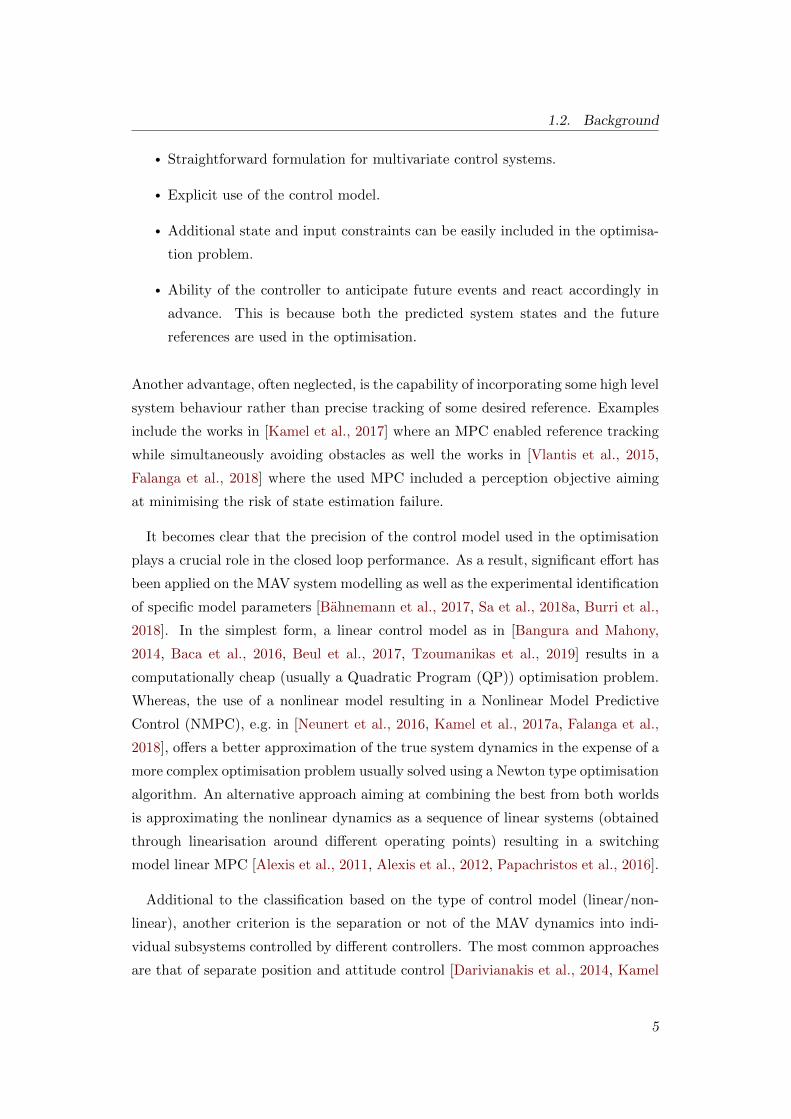
• Straightforward formulation for multivariate control systems.
• Explicit use of the control model.
• Additional state and input constraints can be easily included in the optimisa-
tion problem.
• Ability of the controller to anticipate future events and react accordingly in
advance. This is because both the predicted system states and the future
references are used in the optimisation.
Another advantage, often neglected, is the capability of incorporating some high level
system behaviour rather than precise tracking of some desired reference. Examples
include the works in [Kamel et al., 2017] where an MPC enabled reference tracking
while simultaneously avoiding obstacles as well the works in [Vlantis et al., 2015,
Falanga et al., 2018] where the used MPC included a perception objective aiming
at minimising the risk of state estimation failure.
It becomes clear that the precision of the control model used in the optimisation
plays a crucial role in the closed loop performance. As a result, significant effort has
been applied on the MAV system modelling as well as the experimental identification
of specific model parameters [Bahnemann et al., 2017, Sa et al., 2018a, Burri et al.,
2018]. In the simplest form, a linear control model as in [Bangura and Mahony,
2014, Baca et al., 2016, Beul et al., 2017, Tzoumanikas et al., 2019] results in a
computationally cheap (usually a Quadratic Program (QP)) optimisation problem.
Whereas, the use of a nonlinear model resulting in a Nonlinear Model Predictive
Control (NMPC), e.g. in [Neunert et al., 2016, Kamel et al., 2017a, Falanga et al.,
2018], offers a better approximation of the true system dynamics in the expense of a
more complex optimisation problem usually solved using a Newton type optimisation
algorithm. An alternative approach aiming at combining the best from both worlds
is approximating the nonlinear dynamics as a sequence of linear systems (obtained
through linearisation around different operating points) resulting in a switching
model linear MPC [Alexis et al., 2011, Alexis et al., 2012, Papachristos et al., 2016].
Additional to the classification based on the type of control model (linear/non-
linear), another criterion is the separation or not of the MAV dynamics into indi-
vidual subsystems controlled by different controllers. The most common approaches
are that of separate position and attitude control [Darivianakis et al., 2014, Kamel
5

1. Introduction
et al., 2017a, Tzoumanikas et al., 2019], separate position and rotational rate control
[Falanga et al., 2018] as well as the less popular unified approaches [Neunert et al.,
2016]. The dynamics separation is often introduced to simplify the control model
as well as enable low rate control updates since the fast attitude/rate dynamics are
independently controlled.
In this thesis, we present three different MPC controllers. The first one relies on
a linear control model and is based on the position-attitude dynamics separations.
This makes it applicable to any MAV platform equipped with a tuned attitude
controller and suitable for simple, non aggressive maneuvers. The second controller
is an NMPC, with the body moments and collective thrust as control inputs, that
jointly controls the full MAV state. The use of a nonlinear model which also captures
coupling between the different Degrees of Freedom (DoFs) enables flying aggressive
maneuvers while fully exploiting the dynamic capabilities of the system. The last
one is an NMPC jointly controlling the motion of an MAV-arm system targeted for
aerial manipulation applications. As it will be shown later it is able of handling the
effects of the arm movement and its interaction with the environment in the MAV
dynamics.
1.2.3 Fault tolerant control
A desirable property for every MAV operating in the real world is the ability to
return to a home position and perform a safety landing in the event of a motor
failure. Here, we use the term motor failure for the case of either an actual motor
malfunction or a propeller snap which results in thrust loss. While the problem of
a partial loss (i.e. when the produced thrust is a fraction of the commanded one)
has also been studied in literature [Ranjbaran and Khorasani, 2010, Izadi et al.,
2011, Giribet et al., 2017, Nguyen and Hong, 2018], here we focus on the more
challenging and more realistic event of complete thrust loss.
There exist two distinct approaches of handling this in practice. The first one is
by using MAV platforms which can withstand a motor failure. Examples include,
octacopters [Marks et al., 2012, Saied et al., 2015, Saied et al., 2017], hexacopters
with unconventional motor layouts [Schneider et al., 2012, Michieletto et al., 2018] or
tilted motors [Ryll et al., 2016, Michieletto et al., 2017] which with the appropriate
software adaptations (i.e. distributing the control effort to the functional motors) can
withstand a motor failure. The second approach is entirely software-based and relies
6
1.2. Background
on the prioritisation of position control over other –possibly uncontrollable– DoFs
such as yaw. Examples of the latter applied on quadcopters is given in [Freddi et al.,
2011, Mueller and D’Andrea, 2014, de Crousaz et al., 2015, Wu et al., 2019, Sun
et al., 2020] and hexacopters with symmetric motor layout in [Kamel et al., 2015].
Additionally, fault tolerant control requires the existence of a supervisory al-
gorithm which monitors the health status of the actuators and accordingly signals
a failure. In other words, a motor failure can only be handled if it can be detec-
ted. We categorise the different proposed motor failure observers based on the input
data required for fault detection. We distinguish those which rely on direct actu-
ator measurements (e.g. encoder, current measurements) such as [Saied et al., 2017],
those which rely on the knowledge of the full MAV state [Nguyen et al., 2019, Nguyen
and Hong, 2019] and finally those that only require inertial measurements [Lu and
van Kampen, 2015, Saied et al., 2015].
In our work, we propose a software-based fault handling technique which can
be applied on any hexacopter irrespective of the motor layout. It further enables
full position and yaw controllability when this is physically possible while enabling
prioritisation of certain DoFs when full state tracking is not feasible. As far as the
fault detection is concerned, we adopt an actuator effectiveness metric similar to the
ones in [Izadi et al., 2011, Lu and van Kampen, 2015] while the designed observer
solely depends on inertial measurements and can thus be applied as an algorithmic
update to any MAV.
1.2.4 Aerial manipulation
Aerial manipulation aims at combining the maneuverability of MAVs with the pre-
cision and the fast dynamics of robotic manipulators. This union is particularly
useful for application requiring physical contact with the environment but comes at
the cost of increased control complexity due to the coupling of the dynamics of the
two systems.
The simplest approach, with examples in [Orsag et al., 2013, Jimenez-Cano et al.,
2013, Chermprayong et al., 2019], is to separate the problem into independent MAV
and arm control and totally ignore the existence of coupling. The effects of coupling
can be minimised by adopting clever manipulator designs such as [Ruggiero et al.,
2015, Ohnishi et al., 2017] which actively move the battery in order to counteract
7

1. Introduction
the torques acting on the MAV as a result of the arm displacement. In alternative
software-based approaches such as [Mellinger et al., 2011, Ruggiero et al., 2015, Fresk
et al., 2017, Suarez et al., 2018] the control problem remains separated but some
of the effects introduced in the MAV dynamics, such as payload mass or Centre
of Mass (CoM) displacement and internal torques, are estimated and compensated
online. Unifying the control problem, as for example in [Garimella and Kobilarov,
2015, Kamel et al., 2016b, Lunni et al., 2017] for free flight tasks, results in superior
performance compared to decoupled approaches since the effects of the arm motion
on the MAV dynamics are compensated prior to their propagation into tracking
errors. Additionally, systems and methods such as [Nguyen and Lee, 2013, Cataldi
et al., 2016, Ryll et al., 2019, Bodie et al., 2020] which were successfully used in
experiments that include contact with a surface, also considered the effect of the
contact forces in the control model. In these works the external forces and moments
(as a result of contact) acting on the MAV body were either directly measured or
estimated using appropriate observers.
Regarding the control of the system ability to exert desired forces in the environ-
ment, the different approaches vary depending on the type of the used MAV. For
example, omnidirectional vehicles [Bodie et al., 2019, Tognon et al., 2019, Ryll et al.,
2019] are capable of independently controlling the translational and angular accel-
eration and when in contact can exploit this property to apply a reference force at a
desired position and direction without the absolute need of the additional degrees of
freedom introduced by an attached arm. In contrast, approaches applied on under-
actuated MAVs [Lippiello and Ruggiero, 2012, Nguyen and Lee, 2013, Darivianakis
et al., 2014], irrespectively of the use of an arm or not, rely on the dynamical/inertial
coupling between the MAV and the end effector in order to counteract the vehicle
inability to exert lateral forces.
As mentioned in Section 1.2.2, in this work we propose a NMPC that jointly con-
trols our custom built MAV-arm system. Apart from the benefits of the coupled
control approach listed above, our approach further enables reference force track-
ing as the contact force acting on the end effector is expressed as a function of the
system states. We showcase our algorithm using our underactuated MAV and fur-
ther discuss how it can be applied on omnidirectional vehicles which have superior
capabilities for manipulation tasks.
8
1.2. Background
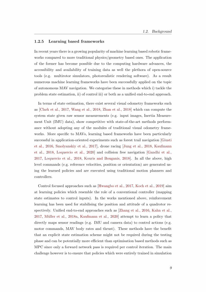
1.2.5 Learning based frameworks
In recent years there is a growing popularity of machine learning based robotic frame-
works compared to more traditional physics/geometry based ones. The application
of the former has become possible due to the computing hardware advances, the
accessibility and availability of training data as well the plethora of open-source
tools (e.g. multirotor simulators, photorealistic rendering software). As a result
numerous machine learning frameworks have been successfully applied on the topic
of autonomous MAV navigation. We categorise these in methods which i) tackle the
problem state estimation, ii) of control iii) or both as a unified end-to-end approach.
In terms of state estimation, there exist several visual odometry frameworks such
as [Clark et al., 2017, Wang et al., 2018, Zhan et al., 2018] which can compute the
system state given raw sensor measurements (e.g. input images, Inertia Measure-
ment Unit (IMU) data), show competitive with state-of-the-art methods perform-
ance without adopting any of the modules of traditional visual odometry frame-
works. More specific to MAVs, learning based frameworks have been particularly
successful in application-oriented experiments such as forest trail navigation [Giusti
et al., 2016, Smolyanskiy et al., 2017], drone racing [Jung et al., 2018, Kaufmann
et al., 2018, Loquercio et al., 2020] and collision free navigation [Gandhi et al.,
2017, Loquercio et al., 2018, Kouris and Bouganis, 2018]. In all the above, high
level commands (e.g. reference velocities, position or orientation) are generated us-
ing the learned policies and are executed using traditional motion planners and
controllers.
Control focused approaches such as [Hwangbo et al., 2017, Koch et al., 2019] aim
at learning policies which resemble the role of a conventional controller (mapping
state estimates to control inputs). In the works mentioned above, reinforcement
learning has been used for stabilising the position and attitude of a quadrotor re-
spectively. Unified end-to-end approaches such as [Zhang et al., 2016, Kahn et al.,
2017, Muller et al., 2018a, Kaufmann et al., 2020] attempt to learn a policy that
directly maps sensor readings (e.g. IMU and camera data) to control actions (e.g.
motor commands, MAV body rates and thrust). These methods have the benefit
that an explicit state estimation scheme might not be required during the testing
phase and can be potentially more efficient than optimisation based methods such as
MPC since only a forward network pass is required per control iteration. The main
challenge however is to ensure that policies which were entirely trained in simulation
9
1. Introduction
generalise well in real life in the presence of unmodeled disturbances and dynamics.
Our work follows the rather classic division between perception and control. Des-
pite the great works in learning based navigation, neither the state estimation nor
the control algorithms presented in this work rely on a learnt model. We believe
however that our MAV navigation pipeline can be used to provide optimal responses
which can be utilised during the training phase of a supervised learning framework.
1.3 Contributions
The main results presented in this work have been published in three different re-
search papers. The full list of publications done in conjunction with this work as
well as the video material that provides visualisation of the algorithms developed,
are given in Section 1.4.
1.3.1 Paper I: Linear MPC with soft constraints.
Tzoumanikas, D., Li, W., Grimm, M., Zhang, K., Kovac, M., and Leutenegger, S.
(2019). Fully autonomous micro air vehicle flight and landing on a mov-
ing target using visual-inertial estimation and model-predictive control.
Journal of Field Robotics. [Tzoumanikas et al., 2019].
In this paper we present an MPC for controlling the MAV position that relies on
an approximate linear model of the vehicle. Regarding the control model we follow
a very similar formulation to the ones presented in [Alexis et al., 2013, Darivianakis
et al., 2014, Kamel et al., 2017a] where it was assumed that the MAV position and
attitude dynamics can be controlled independently. Using this assumption, the full
state MAV response can be controlled by a cascade connection of a position and an
attitude controller with the latter receiving orientation and collective thrust com-
mands from the former. The desired orientation, parameterised using Euler angles,
as well as the collective thrust is thus considered the control input of the linear
MPC which is obtained by solving the corresponding optimisation problem as pre-
viously discussed. Compared to the aforementioned approaches we also incorporate
soft state constraints in the optimisation problem. These are used to prevent oper-
ation close to gimbal lock as well as impose operation within a safe state envelope
which further guarantees that the control model remains valid. Modelling the state
constraints as soft, which can be violated if necessary, ensures that the underlying
10

1.3. Contributions
optimisation solver will never face an infeasible problem. Additionally, we formulate
the resulting optimisation problem as a QP, in a canonical form, that can be solved
online using any generic QP solver without requiring pre-computation of an explicit
solution.
In addition to the MPC, we present a vision-based framework for tracking and
landing on a moving target as required from the MBZIRC1 challenge in which we
participated in March 2017. We showcase the performance of the MPC and the
vision based tracking in experiments resembling the challenge were our method
results in successful landings for target velocities up to 5.0 m/s.
We further evaluate the performance of the controller in the experiments conduc-
ted for the purposes of the AABM2 project where the main objective was tracking
precision. In particular, we show that the controller is capable of tracking slow
reference trajectories (umax ≤ 1 cm/s) with a maximum per-axis error of 1.5 cm.
The linear MPC and the corresponding experiments are presented in Chapter 3.
1.3.2 Paper II: Fault tolerant NMPC
Tzoumanikas, D., Yan, Q., and Leutenegger, S. (2020). Nonlinear MPC with
Motor Failure Identification and Recovery for Safe and Aggressive Mul-
ticopter Flight. In Proceedings of the IEEE International Conference on Robotics
and Automation (ICRA). [Tzoumanikas et al., 2020b].
Drawing inspiration from approaches such as [Kamel et al., 2015, Falanga et al.,
2018, de Crousaz et al., 2015, Neunert et al., 2016] that rely on the non-linear model
of the system, we present a quaternion based NMPC designed in order to overcome
the limitations (i.e. use of Euler angles for the orientation, model is accurate for op-
eration around hover) of its linear counterpart presented in Chapter 3. Compared to
our linear MPC [Tzoumanikas et al., 2019] as well as similar in concept approaches
[Kamel et al., 2017a, Falanga et al., 2018, Faessler et al., 2017] our NMPC does
not rely on the existence of an attitude or rate controller. The full MAV state
is controlled by a single control block which enables full state tracking (given dy-
namically feasible trajectories) while allowing the same controller to be used as an
attitude, rate or mixed mode (e.g. altitude and orientation) controller by penalising
1See https://www.mbzirc.com/challenge/2017. Accessed April 2020.
2See http://www.aerial-abm.com/. Accessed April 2020.
11

1. Introduction
the appropriate optimisation terms. This approach further eliminates the need for
identification of approximate closed loop dynamics for the attitude or rate response
while it only requires the knowledge of physical quantities such as the MAV mass,
inertia matrix as well as motor thrust and moment coefficients.
In order to ensure that our method can be easily transferred to any underactu-
ated MAV we select the MAV body moments and collective thrust as the control
input. This choice yields a constant computational complexity for the NMPC op-
timisation problem irrespectively of the number of motors. The control input is
then transformed into motor commands using a separate algorithm which we refer
to as control allocation. We propose an optimisation-based control allocation which,
compared to traditional approaches [Achtelik et al., 2013, Lee et al., 2010] that em-
ploy the pseudoinverse, can prioritise the tracking of certain control inputs and most
importantly produces feasible motor commands. We further show how our control
allocation algorithm can be used when bidirectional motors are present and we ex-
plain how it can be adapted in case of a complete failure of a single motor. Following
a controllability analysis of our MAV, we use these two properties to stabilise the
position and yaw of our hexacopter MAV under a complete failure of a single motor.
Compared to approaches such as [Schneider et al., 2012, Mazeh et al., 2018, Nguyen
et al., 2019] which rely on asymmetric motor layouts and can only handle a failure
of specific motors, our approach can also be applied on hexacopters with symmetric
motor layouts ensuring that failure of any motor can be handled equally well.
Finally, in order to handle a motor failure which may occur in mid-flight, we
developed an EKF observer which monitors the health status of all the motors
and accordingly notifies the control allocation block in the event of a failure. The
estimated health status corresponds to the percentage of motor thrust acting on
the MAV body, thus providing an easy to tune threshold for triggering the failsafe.
Our implementation relies on inertial measurements and can thus be applied as an
algorithmic only update to any MAV.
These algorithms and the corresponding experimental results with and without
failures are presented in Chapter 4.
12

1.3. Contributions
1.3.3 Paper III: NMPC for aerial manipulation
Tzoumanikas, D., Graule, F., Yan, Q., Shah, D., Popovic, M., and Leutenegger,
S. (2020). Aerial Manipulation Using Hybrid Force and Position NMPC
Applied to Aerial Writing. In Proceedings of Robotics: Science and Systems
(RSS). [Tzoumanikas et al., 2020a].
In this paper, we present an extension of the NMPC, briefly described above,
targeted for applications requiring interaction between the MAV and its environment
such as inspection through contact. We consider the case where the MAV is equipped
with a robotic arm with the main idea being the fast arm dynamics to compensate
for errors occuring on the MAV base. In our approach we tackle the control problem
in a model based way by using a NMPC that jointly controls the MAV-arm system.
This is done by formulating a hybrid control model where the MAV is modeled
as a single rigid body object and the quasi-static forces introduced by the arm
and its interaction with the environment are taken into account. Compared to
approaches such as [Darivianakis et al., 2014, Kamel et al., 2016b, Lunni et al., 2017]
which either use two models (one for free flight and another for physical interaction)
or only consider the free flight case, including the effect of contact forces into a
single control model, eliminates the need of a switching mode controller, allows the
NMPC to reason about contact before it actually happens and to natively handle
the disturbance forces and moments (as a result of contact) acting on the MAV
body. This approach further enables automatic compensation of the effects of the
arm motion on the MAV dynamics such as the system’s CoM displacement due to
arm movement.
Similar to the NMPC presented in Chapter 4 the controller does not rely on the
existence of a closed loop attitude/rate controller as we consider the MAV body mo-
ments, the collective thrust and the end-effector position as the control input. For
the MAV related inputs we use the same control allocation algorithm also described
in Chapter 4 while the end-effector position is transformed into actuator commands
using the arm-specific forward kinematics which are separately described in Section
2.3.1. The specific choice of the control input enables easy adaptation to similar sys-
tems and omnidirectional vehicles [Bodie et al., 2019, Ryll et al., 2019, Brescianini
and D’Andrea, 2018b] which have superior force exertion capabilities, since the con-
trol allocation and forward kinematics are the only platform-dependent components.
13

1. Introduction
We evaluate the accuracy of the MAV-arm system using our custom built under-
actuated MAV and delta arm in aerial writing experiments that require multiple
transitions between free flight and contact. Our system shows accuracy in the order
of millimeters and repeatability in tracking trajectories of different type, size and
with different velocity and acceleration profiles.
These algorithms and the corresponding experimental results are presented in
Chapter 5.
1.4 Publications
The work described in this thesis resulted in the following publications:
• Tzoumanikas, D., Li, W., Grimm, M., Zhang, K., Kovac, M., and Leutenegger,
S. (2019). Fully autonomous micro air vehicle flight and landing on a
moving target using visual-inertial estimation and model-predictive
control. Journal of Field Robotics. [Tzoumanikas et al., 2019].
• Tzoumanikas, D., Yan, Q., and Leutenegger, S. (2020). Nonlinear MPC
with Motor Failure Identification and Recovery for Safe and Ag-
gressive Multicopter Flight. In Proceedings of the IEEE International
Conference on Robotics and Automation (ICRA). [Tzoumanikas et al., 2020b].
• Tzoumanikas, D., Graule, F., Yan, Q., Shah, D., Popovic, M., and Leuteneg-
ger, S. (2020). Aerial Manipulation Using Hybrid Force and Position
NMPC Applied to Aerial Writing. In Proceedings of Robotics: Science
and Systems (RSS). [Tzoumanikas et al., 2020a].
The following video material provides visualisation of some of the algorithms de-
veloped in this thesis:
• Landing on a moving target using visual-inertial estimation and model pre-
dictive control, https://youtu.be/0RW68FGHVX8.
• Nonlinear MPC with autonomous motor failure identification and recovery,
https://youtu.be/cAQeSZ3tIqY.
• Nonlinear MPC for aerial manipulation, https://youtu.be/iE--MO0YF0o.
14

1.5. Thesis structure
While not described directly, the following publications were done in conjunction
with this thesis:
• Dai, A., Papatheodorou, S., Funk, N., Tzoumanikas, D. and Leutenegger S.
(2020). Fast Frontier-based Information-driven Autonomous Explor-
ation with an MAV.In Proceedings of the IEEE International Conference
on Robotics and Automation (ICRA). [Dai et al., 2020].
• Xu, B., Li, W., Tzoumanikas, D., Bloesch, M., Davison, A. and Leutenegger
S. (2019). MID-Fusion: Octree-based Object-Level Multi-Instance
Dynamic SLAM. In Proceedings of the IEEE International Conference on
Robotics and Automation (ICRA). [Xu et al., 2019].
• Zhang, K., Chermprayong, P., Tzoumanikas, D., Li, W., Grimm, M., Smentoch,
M., Leutenegger, S. and Kovac, M. (2019). Bioinspired design of a land-
ing system with soft shock absorbers for autonomous aerial robots.
Journal of Field Robotics. [Zhang et al., 2019].
• Saeedi, S., Carvalho, E., Li, W., Tzoumanikas, D., Leutenegger, S., Kelly, P.
and Davison, A. (2019). Characterizing Visual Localization and Map-
ping Datasets. In Proceedings of the IEEE International Conference on
Robotics and Automation (ICRA). [Saeedi et al., 2019].
• Li, W., Saeedi, S., McCormac, J., Clark, R., Tzoumanikas, D., Ye, Q., Huang,
Y., Tang, R. and Leutenegger, S. (2018). InteriorNet: Mega-scale Multi-
sensor Photo-realistic Indoor Scenes Dataset. British Machine Vision
Conference (BMVC). [Li et al., 2018].
1.5 Thesis structure
The remainder of this thesis is structured as follows:
Chapter 2 introduces basic notation, the multirotor platforms and their sensor setup
as well as the different state estimation algorithms used in this work.
Chapter 3 describes a simple linear model predictive controller that relies on de-
coupling of the position and attitude dynamics. Its capabilities and limitations are
15
1. Introduction
illustrated through experiments including tracking and landing on a fast moving tar-
get (as required in MBZIRC 2017 Challenge 1) and following trajectory commands
for the purposes of the AABM project
Chapter 4 describes a non-linear model predictive controller developed to overcome
the limitations of the one presented in Chapter 3. Additionally, it is shown how
motor failures can be identified and handled by the developed algorithm. Its flight
performance is evaluated on experiments with and without motor failures.
Chapter 5 extends the controller presented in Chapter 4 for aerial manipulation
tasks. A hybrid model for the combined MAV-manipulator system is formulated that
also takes into account the interaction forces from the environment. The combined
system is jointly controlled by a single control block. The achieved accuracy and
repeatability are shown in a series of “aerial-writing” tasks.
Chapter 6 concludes this thesis with a summary of the results presented and sug-
gestions for future work.
16

Chapter 2
Preliminaries
Contents
2.1 Notation . . . . . . . . . . . . . . . . . . . . . . . . . . . . . . . 18
2.1.1 General notation . . . . . . . . . . . . . . . . . . . . . . 18
2.1.2 Spaces and manifolds . . . . . . . . . . . . . . . . . . . . 19
2.1.3 Frames and transformations . . . . . . . . . . . . . . . . 19
2.2 Multirotor platforms . . . . . . . . . . . . . . . . . . . . . . . . 21
2.2.1 Onboard computer . . . . . . . . . . . . . . . . . . . . . 21
2.2.2 Flight controller . . . . . . . . . . . . . . . . . . . . . . . 22
2.2.3 Propulsion system . . . . . . . . . . . . . . . . . . . . . 25
2.2.4 Cameras . . . . . . . . . . . . . . . . . . . . . . . . . . . 29
2.2.5 Additional platforms and simulation environment . . . . 32
2.3 Aerial manipulator . . . . . . . . . . . . . . . . . . . . . . . . . 33
2.3.1 Forward kinematics . . . . . . . . . . . . . . . . . . . . . 34
2.3.2 Inverse kinematics . . . . . . . . . . . . . . . . . . . . . 36
2.4 State estimation . . . . . . . . . . . . . . . . . . . . . . . . . . . 37
2.4.1 EKF for IMU and pose sensor fusion . . . . . . . . . . . 37
2.4.2 Simultaneous Localisation and Mapping (SLAM) . . . . 40
In this Chapter, we present the software and hardware components that form the
foundations for the algorithms presented ahead. In terms of layout, we start with
the mathematical notation and continue with the presentation of the main MAV
and payload hardware components. We conclude with the pipelines used for MAV
state estimation.
17

2. Preliminaries
2.1 Notation
In this work we use the following notation:
2.1.1 General notation
a A lower-case symbol denotes a scalar apart from common capital exceptions.
a A bold lower-case symbol denotes an m-dimensional column vector with ai the
ith element as:
a =
a1
a2
...
am
,a> = [a1, a2, . . . , am]. (2.1)
We use ai:j to denote the vector consisting of the elements of a with indices in
the [i, j] range.
a A bold italic lower-case symbol represents an homogeneous vector defined as:
a = [a, 1]>.
A A bold capital symbol denotes an m × n matrix with ai,j the element at the
ith row and jth column:
A =
a1,1 a1,2 · · · a1,n
a2,1 a2,2 · · · a2,n
...... . . .
...
am,1 am,2 · · · am,n
(2.2)
I The identity matrix, optionally with dimensions as subscript.
0 The zero matrix, optionally with dimensions as subscript.
[·]× The cross-product matrix that produces a skew symmetric matrix from a 3D
vector such that a×b = [a]×b. Given the vector a = [ax, ay, az]>, [a]× can be
computed by:
[a]× =
0 −az ay
az 0 −ax−ay ax 0
. (2.3)
A A calligraphic capital symbol denotes a set.
18

2.1. Notation
2.1.2 Spaces and manifolds
R The set of real numbers.
R+ The set of positive real numbers.
Rm The vector space of real m-dimensional vectors.
Rm×n The vector space of real m× n-dimensional matrices.
Z The set of integers.
N (µ,Σ) The Normal distribussion with mean µ and covariance Σ.
S3 The 3-sphere group.
SO(3) The group of 3D rotations.
SE(3) The group of 3D rigid transformations.
The “box-plus” operator that applies a perturbation expressed in a tangent
space to a manifold state.
The “box-minus” operator that expresses the difference of two manifold states
in the tangent space.
2.1.3 Frames and transformations
F−→A A cartesian coordinate frame in R3.
Av A vector v expressed in the frame F−→A.
ArP The position vector from the origin of F−→A to the point P represented in the
coordinate frame F−→A.
ArP The position vector represented in homogeneous coordinates: ArP = [Ar>P , 1]>.
AvBC The linear velocity of F−→C with respect to F−→B expressed in F−→A.
AωBC The rotational velocity of F−→C with respect to F−→B expressed in F−→A.
φ The roll angle.
θ The pitch angle.
19

2. Preliminaries
ψ The yaw angle.
CAB The rotation matrix that transforms the vector Bv expressed in F−→B to one
expressed in F−→A as: Av = CAB Bv. The inverse rotation CBA can be computed
as: CBA = C−1AB = C>AB .
q The quaternion following the Hamiltonian convention with vector part qv and
real part qw give by: q = [q>v , qw]>. When used for representing orientation,
the unit length qAB represents the quaternion equivalent of the rotation matrix
CAB .
q∗ The conjugate of the quaternion q defined by: q∗ = [−q>v , qw]>. For the
rotation quaternion qAB , its conjugate represents the inverse rotation as:
q∗AB = q−1AB = qBA .
⊗ The quaternion multiplication such that qAC = qAB ⊗ qBC .
[·]+ The left-hand quaternion matrix such that qAC = [qAB ]+ qBC . In matrix
form [q ]+ is given by:
[q ]+ =
[qw −q>vqv qwI + [qv ]×
]. (2.4)
[·]⊕ The right-hand quaternion matrix such that qAC = [qBC ]⊕ qAB . In matrix
form [q ]⊕ is given by:
[q ]⊕ =
[qw −q>vqv qwI− [qv ]×
]. (2.5)
TAB The transformation matrix that transforms homogeneous vectors from F−→B to
F−→A as ArP = TAB BrP . The relationship between TAB , the rotation matrix
CAB and the position vector ArB is given by:
TAB =
[CAB ArB01×3 1
], (2.6)
while the inverse transformation TBA can be computed as:
TBA = T−1AB =
[C>AB −C>AB ArB01×3 1
](2.7)
20

2.2. Multirotor platforms
2.2 Multirotor platforms
In this section, we present the main hardware components of the MAV platforms
used in the experiments presented in this work. As our main focus is not the platform
design by itself, we briefly describe the essential hardware components while we put
special emphasis on the identification of physical quantities (e.g motor coefficients)
that are crucial for our system’s performance when operating with our model based
controllers.
Two different vehicles were built, based on the same frame shown in Figure 2.1,
using off the shelf components and 3D printed parts. They were designed according
to the following general specifications:
• The MAV including the extra payload (e.g. cameras, manipulator) has to be
small enough ( < 1.0 m in diagonal) and thus suitable for indoor operation.
• Its thrust to weight ratio should ideally exceed 2 : 1 in order to enable suffi-
ciently fast closed loop response and allow for additional payload.
• It should be equipped with sufficient onboard computing resources in order to
be able to run the state estimation and control algorithms.
• It should support additional sensors required for completely autonomous nav-
igation e.g. cameras, Global Positioning System (GPS).
Hexacopters (i.e. vehicles with six motors) were preferred due to their payload
capacity and compact size compared to heavy lift quadcopters. Additionally, as
discussed in Chapter 4 when equipped with bidirectional motors and the appropriate
software, they can maintain full position and yaw controllability despite the loss of
a single motor.
2.2.1 Onboard computer
All the developed algorithms run on an Intel NUC-7567U onboard computer run-
ning Ubuntu Server 16.04 shown in Figure 2.2. Its Intel Core i7 Central Processing
Unit (CPU) coupled with 32GB of RAM provide enough computational capabilit-
ies for the estimation and control algorithms developed, while providing additional
overhead if required.
21

2. Preliminaries
Figure 2.1: The custom-built platforms use a 0.55 m wide frame while the overalldiameter (which depends on the propeller choice) is less than 0.8 m.
In order to maximise performance the CPU governor is permanently set to the
performance mode. Additionally, we have modified the Operating System (OS)
kernel to enable faster communication with the peripherals connected through serial.
Finally, all the OS related power management settings (e.g. the WiFi adapter power
saving mode) have been disabled in order to minimise delays. All these modifications
come at the cost of increased power consumption. However, even at full load this
remains bellow 40 W (not including the power consumption of connected peripherals
e.g. cameras) which is a fraction of the power consumed by the motors (up to
6×170 W).
All our algorithms are implemented using C++, where when required we use
multithreading, vectorisation and appropriate compiler optimisation flags in order
to boost performance.
2.2.2 Flight controller
With the term flight controller, we refer to the board which contains the absolute
necessary sensors for stable flight (such as the IMU) and which also interfaces with
the motors. It is essentially the main hardware component of every commercially
available MAV that can be remotely controlled with a joystick. It mainly consists
22

2.2. Multirotor platforms
Figure 2.2: The MAV onboard computer.
of the following elements:
• Sensors required for MAV state estimation such as IMUs, magnetometers,
barometer, GPS.
• Necessary hardware for interfacing with the MAV motors such as: PWM or
I2C drivers.
• Communication ports (e.g. UART, USB) required for data exchange with
external devices (e.g additional sensors, onboard computers, RC receivers).
• An onboard CPU handling the interface with the sensors and motors as well
as running the necessary estimation and control algorithms.
In all our platforms, the commercially available mRo PixRacer1 flight controller,
shown in Figure 2.3, was preferred for two main reasons: (i) its compact size
(36 mm×36 mm) and low weight (< 11 g) without compromising functionalities of
a complete autopilot system (i.e. 168 MHz Cortex M4 CPU, 5×UART, 6×PWM
outputs, 2×IMU for redundancy) (ii) its capability to be flashed with widely used
in research open-source software such as PX42 or ArduPilot3.
1See https://docs.px4.io/v1.9.0/en/flight_controller/pixracer.html. Accessed April
2020.2See https://github.com/PX4/Firmware. Accessed April 2020.
3See https://github.com/ArduPilot/ardupilot. Accessed April 2020.
23

2. Preliminaries
Figure 2.3: The mRo PixRacer flight controller used in both MAVs.
Special attention was paid on how the flight controller was mounted on the MAV.
In order to reduce the high frequency vibrations (originating from the motor ro-
tation) that affect the natively noisy IMU measurements, the device was rigidly
attached on the onboard computer which was soft-mounted on the MAV frame.
Another possible solution adopted in the MAV shown in Figure 2.11 (right) is to
soft-mount the motors on the frame and thus preventing the transfer of vibrations
on the frame.
On the software side, we flashed the flight controller with a modified PX42 firm-
ware. Briefly, we kept the main software components such as the EKF-based state
estimator, the attitude-rate controllers and device drivers while our modifications
included:
• Reducing the CPU load and minimising communication delays.
• Modifying the IMU drivers in order to accessing the raw measurements at the
highest possible rate.
• Adding support for bidirectional capable motors.
The PX4 firmware comes with a wide variety of pre-implemented estimation and
control algorithms and can be deployed for autonomous missions without the need
of additional software. However, in our work we mainly used the flight controller
as a middleware used for reading of the IMU measurements and interfacing with
the motors. Apart from the algorithms presented in Chapter 3 where the pre-
implemented attitude controller was used, the algorithms in Chapters 4 and 5 do
24

2.2. Multirotor platforms
not use any of the estimators or controllers of PX4. In these experiments, the flight
controller which runs independent estimation and control algorithms (than the ones
implemented on the onboard computer), acted as a safety backup in the event of a
malfunction of the primary software/hardware stack.
2.2.3 Propulsion system
Two different propulsion systems were employed depending on the desired applic-
ation. The individual components of each one, consisting of the Electronic Speed
Controller (ESC), motor and propeller are shown in Figure 2.4.
(a) Propulsion system #1 is sold as a single kit and consists of the DJI420 ESC, the DJI 2312E 960Kv motors and the self tightening DJI 9450propellers.
(b) Propulsion system #2 consists of the bidirectional capable DYS 35AAria ESC, the DJI 2312E 960Kv motors and the carbon reinforced Aero-naut CAMcarbon Light 9545 propellers. In order to cope with the largeangular acceleration/deceleration due to direction change, the propellerswere secured with elastic stop nuts.
Figure 2.4: The two different propulsion systems used in our MAVs.
Main difference between the two is that propulsion system #2 can reverse the
direction of motor rotation in mid-flight. Based on that the motors can either
rotate in a normal or inverted direction and thus generate thrust and moment in
two directions. This property was used for stabilising the yaw in the event of a motor
failure (experiments presented in Chapter 4). Unlike, conventional system designs
that use symmetrical propellers (which have identical characteristics irrespectively
of direction of rotation), we preferred propellers that are optimised for rotation in
one direction.
25
2. Preliminaries
10 30 50 70 90 110 130 150
0
2
4
6
8
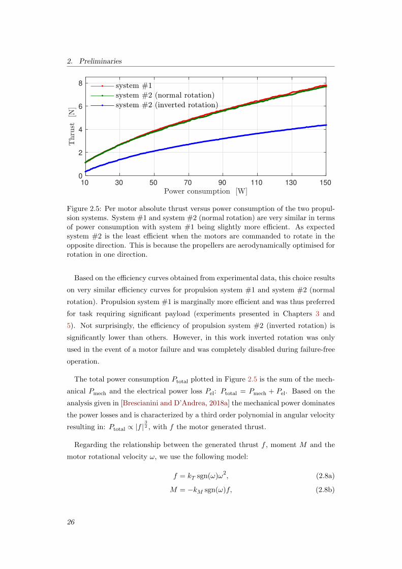
Figure 2.5: Per motor absolute thrust versus power consumption of the two propul-sion systems. System #1 and system #2 (normal rotation) are very similar in termsof power consumption with system #1 being slightly more efficient. As expectedsystem #2 is the least efficient when the motors are commanded to rotate in theopposite direction. This is because the propellers are aerodynamically optimised forrotation in one direction.
Based on the efficiency curves obtained from experimental data, this choice results
on very similar efficiency curves for propulsion system #1 and system #2 (normal
rotation). Propulsion system #1 is marginally more efficient and was thus preferred
for task requiring significant payload (experiments presented in Chapters 3 and
5). Not surprisingly, the efficiency of propulsion system #2 (inverted rotation) is
significantly lower than others. However, in this work inverted rotation was only
used in the event of a motor failure and was completely disabled during failure-free
operation.
The total power consumption Ptotal plotted in Figure 2.5 is the sum of the mech-
anical Pmech and the electrical power loss Pel: Ptotal = Pmech + Pel. Based on the
analysis given in [Brescianini and D’Andrea, 2018a] the mechanical power dominates
the power losses and is characterized by a third order polynomial in angular velocity
resulting in: Ptotal ∝ |f |32 , with f the motor generated thrust.
Regarding the relationship between the generated thrust f , moment M and the
motor rotational velocity ω, we use the following model:
f = kT sgn(ω)ω2, (2.8a)
M = −kM sgn(ω)f, (2.8b)
26

2.2. Multirotor platforms
0 100 200 300 400 500 600 700 800 900
0
5
10
0 1 2 3 4 5 6 7 8
0
0.05
0.1
0.15
Figure 2.6: Identification results of the thrust and moment coefficients of propulsionsystem #1. Each dot corresponds to an average of 100 measurements and the solidline to the fitted model as defined in (2.8). The least squares fit error for the thrustand moment model is 4.8× 10⁻² N and 5.3× 10⁻⁴ N m respectively.
with kT , kM thrust and moment constants. These were estimated using a load cell
and an optical encoder for accurate rotational measurements. Figures 2.6 and 2.7
show the results of the experimental identification for system #1 and #2 respect-
ively. The numeric values of the identified constants are given in Table 2.1. Note
that in propulsion system #2 (which can switch direction of rotation on demand)
we use non symmetrical propellers which results in different coefficients depending
on the direction of rotation. We thus identified two sets of parameters, with k+T , k+
M
and k−T , k−M corresponding to normal and inverted rotation respectively.
Unfortunately, conventional ESCs do not directly control the angular velocity
of the motor. They are responsible for swtiching on and off the transistors that
supply the motor coils with a fixed proportion (based on the PWM command) of
the battery voltage. Consequently, the achieved angular velocity depends on the
PWM command and the battery voltage which gradually decreases during flight.
In our application we are interested in controlling the motor angular velocity and
consequently the thrust and moment as accurately as possible. To achieve this
with our sensorless ESC-motor setup, we experimentally determined the relation-
ship between a PWM command and the achieved thrust and moment. Our model
27

2. Preliminaries
-800 -600 -400 -200 0 200 400 600 800
-5
0
5
10
-8 -6 -4 -2 0 2 4 6 8
-0.2
-0.1
0
0.1
Figure 2.7: Identification results of the thrust and moment coefficients of propulsionsystem #2. Each dot corresponds to an average of 100 measurements and the solidline to the fitted model as defined in (2.8). Since non symmetrical propellers wereused two sets of coefficients corresponding to normal (k+
T , k+M ) and inverted rotation
(k−T , k−M ) were identified. The least-squares fit error for the thrust and momentmodel for normal motor rotation is 5×10⁻² N and 8.5×10⁻⁴ Nm respectively. Thesame quantities for inverted rotation are 4.4× 10⁻² N and 1.3× 10⁻³ Nm.
Description Symbol Value Unit
Propulsion system #1
Thrust coefficient kT 1.1090× 10⁻⁵ N/(rad/s)2
Moment coefficient kM 1.5864× 10⁻² Nm/N
Propulsion system #2
Normal rotation thrust coefficient k+T 9.7408× 10⁻⁶ N/(rad/s)2
Normal rotation moment coefficient k+M 1.4873× 10⁻² Nm/N
Inverted rotation thrust coefficient k−T 6.3309× 10⁻⁶ N/(rad/s)2
Inverted rotation moment coefficient k−M 2.7928× 10⁻² Nm/N
Table 2.1: Thrust and moment coefficients of the two propulsion systems.
28

2.2. Multirotor platforms
also takes into account the effect of the varying battery voltage. Regarding, the
relationship between the rotational velocity ω and the PWM command c this was
approximated using the following second order polynomial:
ω = aV,2c2 + aV,1c+ aV,0, (2.9)
where the coefficients aV,i were identified for different battery voltage levels V , stored
in lookup tables and used online depending on the measured battery voltage. The
identification results of the model defined in (2.9) for the two propulsion systems
are shown in Figure 2.8 where for visualisation purposes we only show the identified
curves for 12 different voltage levels.
To summarise, given a desired motor force f , the desired angular velocity ω is
computed using the model defined in (2.8) and the identified coefficients in Table
2.1. The desired angular velocity ω is then converted to a PWM command c us-
ing the model in (2.9) with the coefficients aV,i that correspond to the measured
voltage V . We would like to highlight that our approach is open loop and thus
natively inferior to closed loop approaches such as [Papachristos et al., 2012] or
[Brescianini and D’Andrea, 2018b] where the velocity loop was closed using encoder
feedback. However, it is superior than open loop approaches that do not include
voltage compensation. An easier way of tackling the same problem would be to
use commercially available hardware able to perform closed loop angular control.
Unfortunately, these motors4 are mainly designed for small MAVs and not ones like
ours that carry significant payload.
2.2.4 Cameras
In this work we used cameras for two different purposes. The first being running
SLAM for navigation not requiring external sensors (e.g motion capture system) and
the second for generic environment perception (e.g. detecting, following and landing
on a moving target as shown in Chapter 3). The cameras used for navigation,
shown in Figure 2.9, are also equipped with an onboard IMU as the used SLAM
algorithms also require inertial measurements. For simpler tasks, we used global
shutter cameras as the ones shown in Figure 2.10.
Regarding the relationship between a 3D point CrP := [rx, ry, rz]> in space and
its corresponding projection u := [u, v]> onto the camera plane, we use a standard
4See https://iq-control.com/. Accessed April 2020.
29

2. Preliminaries
0 0.2 0.4 0.6 0.8 1
0
200
400
600
800
1000
13.8
14.0
14.2
14.4
14.6
14.8
15.0
15.2
15.4
15.6
15.8
16.0
-1 -0.5 0 0.5 1
-1000
-500
0
500
1000
13.8
14.0
14.2
14.4
14.6
14.8
15.0
15.2
15.4
15.6
15.8
16.0
Figure 2.8: Experimental identification of the relationship between the PWM com-mand and the achieved angular velocity for system #1 (top) and system #2 (bot-tom). For visualisation purposes we only show 12 different curves that correspondto different voltage levels.
(a) The Skybotix Visual-Inertial (VI)-sensor with modified drivers that enablethe use of one of its pins as an externaltrigger for data synchronisation with ex-ternal devices.
(b) The Intel Realsense ZR300 Red GreenBlue Depth (RGBD)-inertial sensor.
Figure 2.9: Camera sensors used for SLAM.
30

2.2. Multirotor platforms
(a) FLIR Chameleon3supporting resolutionsup to 1288 × 964 @ 30FPS.
(b) UI-1221LE sup-porting image resolu-tion up to 752× 480 @87 FPS.
Figure 2.10: Cameras used for the target tracking experiments presented in Chapter3.
pinhole camera model. This is done in the following steps:
1. Projection onto the unit plane: r′P = 1rz
[rx
ry
].
2. Apply the distortion model d: r′′P = d(r′P ).
3. Scale and translate: u =
[fx 0
0 fy
]r′′P +
[cx
cy
].
The projection model is not invertible and the point CrP can only be recovered
when the depth rz is known. In that case, CrP can be recovered by:
1. Convert the pixel coordinates to unit plane coordinates:
r′′P =
1fx
0
0 1fy
(u−[cx cy
] ).
2. Correct for lens distortion: r′P = d−1(r′′P ).
3. Convert to F−→C coordinates: CrP = rz
[r′x r′y 1
]>.
The camera intrinsics (fx, fy, cx, cy ), the distortion model parameters as well as the
transformation between the camera frame F−→C and the IMU frame F−→S were obtained
using Kalibr5 an open source calibration tool based on [Furgale et al., 2013].
5See https://github.com/ethz-asl/kalibr. Accessed April 2020.
31

2. Preliminaries
2.2.5 Additional platforms and simulation environment
Even though not used for experiments presented in this work, the developed al-
gorithms have been also implemented and thoroughly tested on two additional plat-
forms. A commercially available AscTec Firefly hexacopter and a custom-built ra-
cing quadcopter shown in Figure 2.11.
(a) Vision based flight of an AscTec Fireflyequipped with an Intel i7-3612QE.
(b) A racing quadcopter equipped with anNvidia Jetson Tx1 computer.
Figure 2.11: Two additional platforms used during this research.
Prior to deployment on real systems, all our algorithms were thoroughly tested in
simulation. We used the open source MAV simulator RotorS6 described in [Furrer
et al., 2016] which apart from multirotor models, provides simulated measurements
of commonly used sensors (such as IMU, cameras, pose sensors). Conveniently, it
is equipped with a ROS interface plugin allowing seamless transition between the
simulation environment and the real system. A snapshot of our system executing
the same task in real life and in simulation is given in Figure 2.12.
Figure 2.12: A snapshot of our MAV-arm system performing the same “aerial-writing” task in reality (left) and in the simulation environment (right).
6See https://github.com/ethz-asl/rotors_simulator. Accessed April 2020.
32
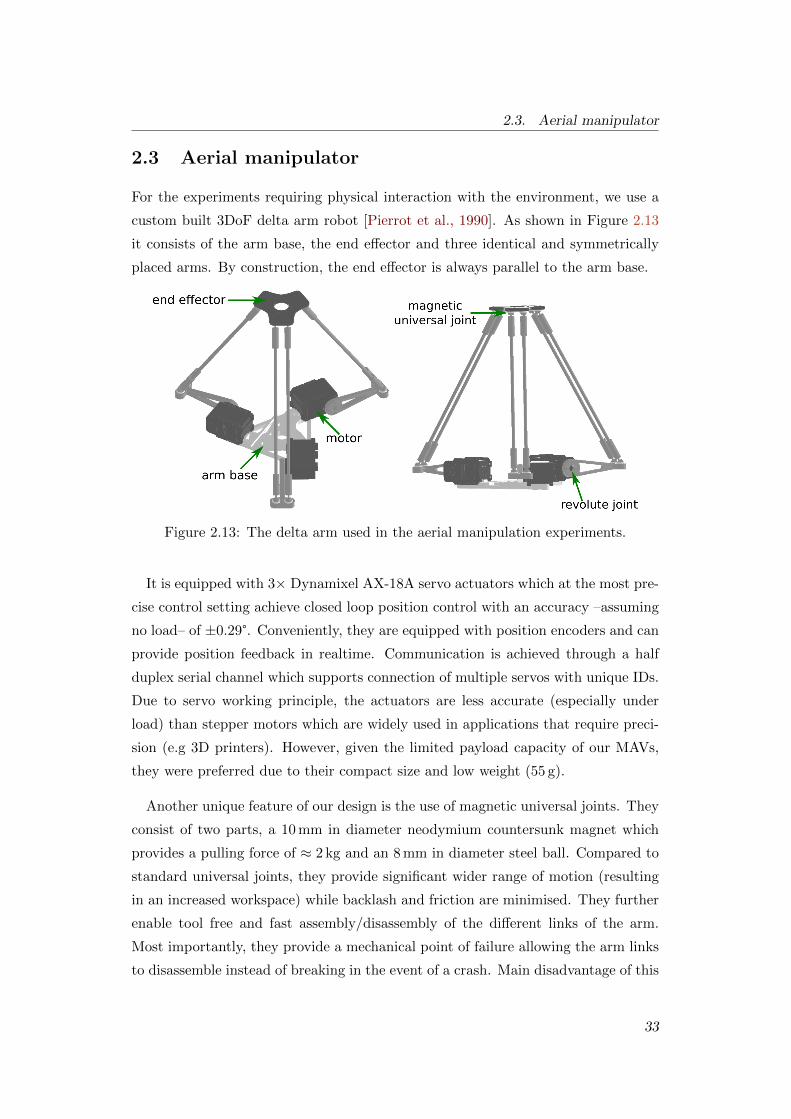
2.3. Aerial manipulator
2.3 Aerial manipulator
For the experiments requiring physical interaction with the environment, we use a
custom built 3DoF delta arm robot [Pierrot et al., 1990]. As shown in Figure 2.13
it consists of the arm base, the end effector and three identical and symmetrically
placed arms. By construction, the end effector is always parallel to the arm base.
Figure 2.13: The delta arm used in the aerial manipulation experiments.
It is equipped with 3× Dynamixel AX-18A servo actuators which at the most pre-
cise control setting achieve closed loop position control with an accuracy –assuming
no load– of ±0.29°. Conveniently, they are equipped with position encoders and can
provide position feedback in realtime. Communication is achieved through a half
duplex serial channel which supports connection of multiple servos with unique IDs.
Due to servo working principle, the actuators are less accurate (especially under
load) than stepper motors which are widely used in applications that require preci-
sion (e.g 3D printers). However, given the limited payload capacity of our MAVs,
they were preferred due to their compact size and low weight (55 g).
Another unique feature of our design is the use of magnetic universal joints. They
consist of two parts, a 10 mm in diameter neodymium countersunk magnet which
provides a pulling force of ≈ 2 kg and an 8 mm in diameter steel ball. Compared to
standard universal joints, they provide significant wider range of motion (resulting
in an increased workspace) while backlash and friction are minimised. They further
enable tool free and fast assembly/disassembly of the different links of the arm.
Most importantly, they provide a mechanical point of failure allowing the arm links
to disassemble instead of breaking in the event of a crash. Main disadvantage of this
33
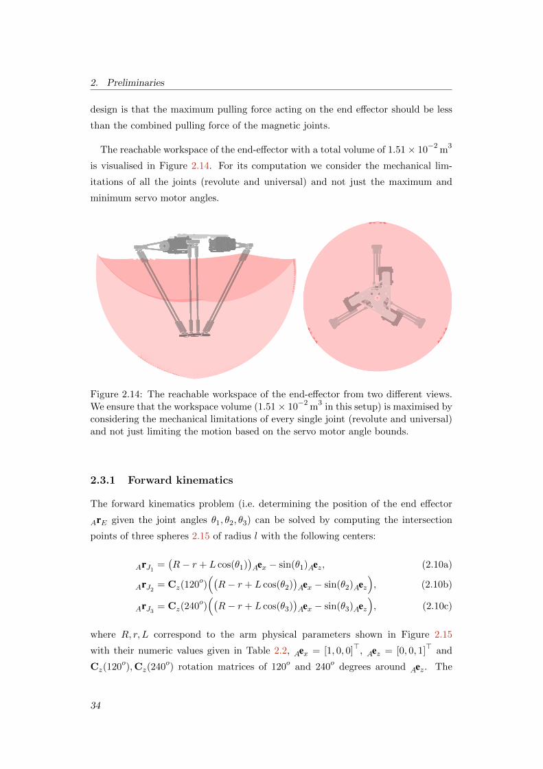
2. Preliminaries
design is that the maximum pulling force acting on the end effector should be less
than the combined pulling force of the magnetic joints.
The reachable workspace of the end-effector with a total volume of 1.51× 10⁻² m3
is visualised in Figure 2.14. For its computation we consider the mechanical lim-
itations of all the joints (revolute and universal) and not just the maximum and
minimum servo motor angles.
Figure 2.14: The reachable workspace of the end-effector from two different views.We ensure that the workspace volume (1.51× 10⁻² m3 in this setup) is maximised byconsidering the mechanical limitations of every single joint (revolute and universal)and not just limiting the motion based on the servo motor angle bounds.
2.3.1 Forward kinematics
The forward kinematics problem (i.e. determining the position of the end effector
ArE given the joint angles θ1, θ2, θ3) can be solved by computing the intersection
points of three spheres 2.15 of radius l with the following centers:
ArJ1 =(R− r + L cos(θ1)
)Aex − sin(θ1)Aez, (2.10a)
ArJ2 = Cz(120o)((R− r + L cos(θ2)
)Aex − sin(θ2)Aez
), (2.10b)
ArJ3 = Cz(240o)((R− r + L cos(θ3)
)Aex − sin(θ3)Aez
), (2.10c)
where R, r, L correspond to the arm physical parameters shown in Figure 2.15
with their numeric values given in Table 2.2, Aex = [1, 0, 0]>, Aez = [0, 0, 1]> and
Cz(120o),Cz(240o) rotation matrices of 120o and 240o degrees around Aez. The
34

2.3. Aerial manipulator
solutions can be then obtained by solving the following system of equations:
(x− xJ1)2 + (y − yJ1)2 + (z − zJ1)2 = l2, (2.11a)
(x− xJ2)2 + (y − yJ2)2 + (z − zJ2)2 = l2, (2.11b)
(x− xJ3)2 + (y − yJ3)2 + (z − zJ3)2 = l2, (2.11c)
with AxJi ,AyJi ,AzJi∀i = 1, 2, 3 the corresponding components of ArJi defined
in (2.10). As an implementation trick, we can simplify the solution of (2.11) by
expressing the centers ArJi of the spheres in a coordinate frame F−→T with its origin
located at ArJ1 and its orientation relative to the frame F−→A given by:
CAT =[xT yT zT
]=[
ArJ2−ArJ1‖ArJ2−ArJ1‖
zT × xT(ArJ2−ArJ1 )×(ArJ3−ArJ1 )
‖(ArJ2−ArJ1 )×(ArJ3−ArJ1 )‖
].
(2.12)
The sphere centers expressed in the frame F−→T are computed using:
T rJi = C>AT ArJi − C>AT ArJ1 ,∀i = 1, 2, 3, (2.13)
and the system of equations (2.11) is transformed to:
x2 + y2 + z2 = l2, (2.14a)
(x− xJ ′2)2 + y2 + z2 = l2, (2.14b)
(x− xJ ′3)2 + (y − yJ ′3)2 + z2 = l2, (2.14c)
Front View Side View
Figure 2.15: Two different views of a 3D model of the delta arm used. The greenareas show the virtual spheres and disks used for the solution of the forward andinverse kinematics.
35
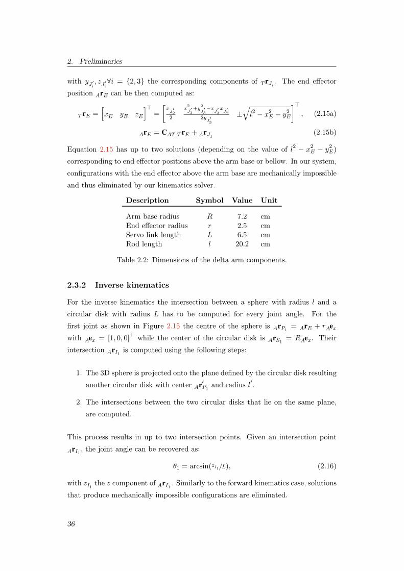
2. Preliminaries
with yJ ′i, zJ ′i∀i = 2, 3 the corresponding components of T rJi . The end effector
position ArE can be then computed as:
T rE =[xE yE zE
]>=
[xJ′2
2
x2
J′3+y
2
J′3−x
J′3xJ′2
2yJ′3
±√l2 − x2
E − y2E
]>, (2.15a)
ArE = CAT T rE + ArJ1 (2.15b)
Equation 2.15 has up to two solutions (depending on the value of l2 − x2E − y
2E)
corresponding to end effector positions above the arm base or bellow. In our system,
configurations with the end effector above the arm base are mechanically impossible
and thus eliminated by our kinematics solver.
Description Symbol Value Unit
Arm base radius R 7.2 cmEnd effector radius r 2.5 cmServo link length L 6.5 cmRod length l 20.2 cm
Table 2.2: Dimensions of the delta arm components.
2.3.2 Inverse kinematics
For the inverse kinematics the intersection between a sphere with radius l and a
circular disk with radius L has to be computed for every joint angle. For the
first joint as shown in Figure 2.15 the centre of the sphere is ArP1= ArE + rAex
with Aex = [1, 0, 0]> while the center of the circular disk is ArS1= RAex. Their
intersection ArI1 is computed using the following steps:
1. The 3D sphere is projected onto the plane defined by the circular disk resulting
another circular disk with center Ar′P1and radius l′.
2. The intersections between the two circular disks that lie on the same plane,
are computed.
This process results in up to two intersection points. Given an intersection point
ArI1 , the joint angle can be recovered as:
θ1 = arcsin(zI1/L), (2.16)
with zI1 the z component of ArI1 . Similarly to the forward kinematics case, solutions
that produce mechanically impossible configurations are eliminated.
36

2.4. State estimation
The joint angles θ2 and θ3 can be computed by performing the same procedure
for the spheres with centers ArP2,ArP3
, same radius l and the unit disks centered at
ArS2and ArS3
with radius L. The points ArPi,ArSi
∀i = 2, 3 can be easily computed
as follows:
ArP2= ArE + r Cz(120o)Aex, (2.17a)
ArP3= ArE + r Cz(240o)Aex, (2.17b)
ArS2= Cz(120o)ArS1
, (2.17c)
ArS3= Cz(240o)ArS1
. (2.17d)
2.4 State estimation
Precise MAV control relies on accurate state estimation that has to run at a rate
equal or greater than the control rate. In this work, depending on the application,
we use two different approaches for MAV state estimation. The first is an EKF able
to fuse data from the onboard IMU and a generic pose sensor, mainly used in indoor
flights with a motion capture system providing the pose measurements. While the
second is visual-inertial SLAM used in outdoor operation or when a motion capture
system or GPS signal is not available.
2.4.1 EKF for IMU and pose sensor fusion
For fusion of inertial measurements and pose estimates, we use a rather standard
error-state Kalman filter formulation similar to the ones presented in [Lynen et al.,
2013, Leutenegger et al., 2014]. In short, we aim to estimate the true system state
given by:
xR := [W r>S ,W v>S ,q>WS ,b
>ω ,b
>a ]> ∈ R6 × S3 × R6, (2.18)
which consists of the position, linear velocity and orientation of the IMU with frame
F−→S with respect to the World fixed frame F−→W as well as the sensor biases. The
true system state xR is the composition of a nominal state and an error-state δxR.
The high frequency IMU measurements can be integrated into the nominal system
state that does not take into account the model uncertainty. The update step of the
EKF is performed at the arrival of new pose data and yields a Gaussian estimate
for the error-state. After this, the error-state mean is incorporated into the nominal
state and the whole process is repeated.
37

2. Preliminaries
IMU model
In our EKF we use the following model for the true IMU dynamics:
W rS = W vS , (2.19a)
W vS = CWS (a− ba +wa) + Wg, (2.19b)
qWS =1
2Ω(ω − bω +wω)qWS , (2.19c)
bω = wbω, (2.19d)
ba = −1
τba +wba
, (2.19e)
where Wg := [0, 0,−9.81]> represents the gravitational acceleration. We assume
that the IMU accelerometer a and gyro ω measurements are biased and disturbed
by white Gaussian noise wa and wω with densities σa and σω respectively. We
model the gyro bias bω as random walk and the accelerometer bias ba as bounded
random walk with time constant τ > 0. The nominal state dynamics correspond to
the equations in (2.19) but without the noise terms.
An expression for the error state dynamics can be found using its definition as
the difference between the true and the nominal state δxR := xR xR and solving
for δxR. In order to obtain a minimal representation for the error state, we express
the orientation error as the quaternion δq = q∗ ⊗ q which for small errors can be
approximated using the angle vector δθ as δq ≈ [12δθ
>, 1]>. We obtain a minimal
error-state representation δxR := [δr>, δv>, δθ>, δb>ω , δb>a ]> ∈ R15 around the state
xR with the following non linear dynamics:
δ r = δv , (2.20a)
δ v = −CWB [a− ba]×δθ − CWB δba + CWB wa, (2.20b)
δθ = −[ω − bω]×δθ + δbω +wω, (2.20c)
δbω = wbω, (2.20d)
δba = −1
τδba +wba
. (2.20e)
Since the zero mean accelerometer noisewa is uniform in all directions, its covariance
ellipsoid is a 3D sphere centered at the origin and thus invariant to rotation. Based
on that, substituting CWB wa with wa in (2.20b) results an equivalent expression.
Linearising the expressions in (2.20) with respect to δxR around xR yields:
δxR = FcδxR + Lcw, (2.21)
38

2.4. State estimation
with w := [w>ω ,w>a ,w
>bω,w>ba ]> the noise vector with covariance Qc := diag(σ2
a, σ2ω,
σ2bω, σ2
ba) and the Jacobians evaluated at xR given by:
Fc =∂δxR∂δxR
, Lc =∂δxR∂w
. (2.22)
Observation model
We perform the EKF updates using 6DoF pose estimates originating from a motion
capture system. As the motion capture system tracks the pose of an object with an
attached frame F−→V which may or may not be perfectly aligned with the IMU frame
F−→S , we introduce additional calibration states SrV , qSV that have no dynamics for
the propagation phase. The augmented state and error state are now given by:
xR := [W r>S ,W v>S ,q>WS ,b
>ω ,b
>a , Sr>V ,q
>SV ]> ∈ R6 × S3 × R9 × S3, (2.23a)
δxR := [δr>, δv>, δθ>WS, δb>ω , δb
>a , δr>, δθ>SV]> ∈ R21. (2.23b)
The observation model for the position and orientation is given by:
zr = W rV + vr = CWS SrV + W rS + vr, (2.24a)
zq = qWV ⊗ δq = qWS ⊗ qSV ⊗ δq , (2.24b)
with vr ∼ N (0, σ2rI), δq = [1
2δθq, 1], δθq ∼ N (0, σ2qI) modelling the position and
orientation measurement noise respectively. We define the position and orientation
residuals y = [y>r ,y>q ]> as:
yr = zr − W rV (2.25a)
yq = 2[q∗WV ⊗ zq]1:3 (2.25b)
which given the pose measurements W rV , qWV is computed as:
yr = W rV − W rV = W rV − (CWS SrV + W rS), (2.26a)
yq = 2[q∗WV ⊗ qWV ]1:3 = 2[(qWS ⊗ qSV )∗ ⊗ qWV ]1:3 (2.26b)
where overbar indicates quantities evaluated using the filter’s current estimate.
The Jacobians H and V with respect to δxR and v := [v>r ,v>q ]> used in the filter
update are computed by:
H =∂y∂δxR
, V =∂y∂v. (2.27)
39

2. Preliminaries
The EKF prediction and update steps are outlined bellow, where we use subscripts
of the form m|n to represent estimated quantities at time m given observations up
to time n with n ≤ m :
Prediction
1. Given the IMU measurements a, ω propagate the state x using (2.19).
2. Calculate the discrete equivalent Fk, Lk of the Jacobians defined in (2.22).
3. Compute the propagated covariance using: Pk|k−1 = FkPk−1|k−1F>k +LkQkL
>k
with Qk the discrete equivalent of the covariance matrix Qc.
Update
1. Given the pose measurements W rV , qWV and the current estimate x, compute
the residual yk defined in (2.26).
2. Compute the innovation Sk|k = HkPk|k−1H>k + VkRkV
>k .
3. Compute the Kalman gain Kk = Pk|k−1H>k S−1
k|k.
4. Update the state estimate xk|k = xk|k−1 Kkyk.
5. Update the state covariance Pk|k =(I−KkHk
)Pk|k−1.
Even though our implementation relies on pose measurements originating from
a motion capture system, it can be accordingly modified to fuse information from
different sensors (e.g. GPS, pressure sensor, magnetometer). In this case the correct
measurement model (depending on the type of sensor) has to be used and if necessary
the filter state has to be augmented with sensor-intrinsic and/or calibration states.
An example includes the work presented in [Weiss et al., 2012] where a visual SLAM
was used as a 6D pose sensor resulting in a loosely coupled visual SLAM capable of
providing estimates at IMU rate.
2.4.2 Simultaneous Localisation and Mapping (SLAM)
For operation in environments where a motion capture system or GPS signal is not
available, we use Open Keyframe-based Visual Inertial SLAM (OKVIS)7 as a basis
for our MAV state estimation. We made, however, several extensions in order for it
to be usable with a low cost RGBD camera.
7Available open-source at http://ethz-asl.github.io/okvis/.
40

2.4. State estimation
OKVIS jointly estimates the robot state xR defined in (2.18) as well as the land-
marks xL by minimising the following cost function consisting of camera reprojection
errors ei,j,kr and IMU errors eks :
J(x) :=
I∑i=1
K∑k=1
∑j∈Jv(k)
ei,j,kr
TWi,j,k
r ei,j,kr +
K−1∑k=1
eksT
Wks eks , (2.28)
with x := [x>R, x>L ]>, i the camera index of the I-camera setup, k the camera frame
index, j the landmark index, Wi,j,kr the information matrix of the corresponding
landmark observation and Wks the information matrix of the kth IMU error. The
set Jv(k) contains the indices of the landmarks visible in the kth frame.
In this work, we use a dual camera setup (I = 2) which either consists of a Red
Green Blue (RGB) stereo pair or an RGB-Depth camera setup shown in Figure 2.9
left and right respectively. For the RGB cameras we use the reprojection error as
in the original OKVIS implementation in [Leutenegger et al., 2014]:
ei,j,kr = zi,j,k − h(TCiST kSW W lj), (2.29)
with z denoting the measurement in image coordinates, h(·) the camera projection
model and W lj the position of the landmark j in World coordinates.
In the RGB-Depth camera setup, we incorporate the depth information by ad-
opting the approach of ORB-SLAM 2 [Mur-Artal and Tardos, 2017] and creating
a virtual stereo camera. We obtain virtual keypoint measurements by projecting
3D points into the virtual second camera with frame F−→Cv. Let u = h(CrP ) and
CrP = h−1(u,D) be the RGB camera projection and back-projection from image
coordinates to a homogeneous point as defined in Section 2.2.4. We can now create
virtual keypoint measurements zj,kv from actual measurements zj,k, iff depth is given
for said pixel, as:
zj,kv = hv(TCvCh−1(zj,k,D)), (2.30)
where the transformation TCvC, and hv(·) stands for the virtual camera projection
model that we define as hv(·) := h(·) for convenience.
Given the virtual keypoint measurements zj,kv , the reprojection error is defined
identical to (2.29). Note that this scheme allows for easy compatibility with a
multi-camera system assumed in [Leutenegger et al., 2014]. Furthermore, since the
depth map of the camera we use was indeed obtained through stereo triangulation,
41

2. Preliminaries
formulating reprojection errors in a stereo setup (even if virtual), correctly accounts
for noise in image space.
42

Chapter 3
Linear Model Predictive Control
Contents
3.1 Introduction . . . . . . . . . . . . . . . . . . . . . . . . . . . . . 44
3.2 Related work . . . . . . . . . . . . . . . . . . . . . . . . . . . . . 44
3.3 Contribution . . . . . . . . . . . . . . . . . . . . . . . . . . . . . 46
3.4 System overview . . . . . . . . . . . . . . . . . . . . . . . . . . . 46
3.4.1 Translational dynamics . . . . . . . . . . . . . . . . . . . 48
3.4.2 System identification . . . . . . . . . . . . . . . . . . . . 50
3.5 MPC with soft constraints . . . . . . . . . . . . . . . . . . . . . 52
3.6 Experimental results: Landing on a moving platform at MBZIRC 55
3.6.1 System overview . . . . . . . . . . . . . . . . . . . . . . 56
3.6.2 Estimation of MAV and target state . . . . . . . . . . . 59
3.6.3 High level mission profile . . . . . . . . . . . . . . . . . . 61
3.6.4 Field experiments . . . . . . . . . . . . . . . . . . . . . . 63
3.6.5 Comparison with other MBZIRC teams . . . . . . . . . 70
3.7 Experimental results: Application to AABM . . . . . . . . . . . 74
3.7.1 Linear MPC modifications . . . . . . . . . . . . . . . . . 74
3.7.2 Selected printing experiments . . . . . . . . . . . . . . . 76
3.8 Discussion . . . . . . . . . . . . . . . . . . . . . . . . . . . . . . 78
Parts of this Chapter appear in: Tzoumanikas, D., Li, W., Grimm, M., Zhang, K., Kovac,
M., and Leutenegger, S. (2019). Fully autonomous micro air vehicle flight and landing on
a moving target using visual-inertial estimation and model-predictive control. Journal of
Field Robotics. [Tzoumanikas et al., 2019]
43

3. Linear Model Predictive Control
3.1 Introduction
Due to its simple formulation as well as the benefits listed in Chapter 1, the concept
of linear MPC has been successfully applied to a variety of aerial vehicles ranging
from fixed wing aircraft [Oettershagen et al., 2016] to more relevant to this work
multirotor platforms [Alexis et al., 2011, Alexis et al., 2012, Darivianakis et al.,
2014, Kamel et al., 2017a, Kamel et al., 2017b]. Its successful deployment on real
systems has been enabled by the existence of efficient toolboxes used to solve the
underlying optimisation problem either online [Mattingley and Boyd, 2012, Ferreau
et al., 2014, Frison and Diehl, 2020] or as an explicit solution in the form of lookup
tables [Kvasnica et al., 2004, Herceg et al., 2013].
Here we present a simple linear MPC originally developed for our participation
in the MBZIRC competition in 2017 as well as for the purposes of the AABM pro-
ject. In the control design, we adopt the position-attitude separation discussed in
Chapter 1 with the position MPC generating reference attitude commands tracked
by an already implemented attitude controller. The control model was built, with
minor adaptations, based on previously published works backed up with experi-
mental results.
In addition to the position controller, we further present the experimental setup
used for our participation in MBZIRC. This includes a generic framework for vision
based detection and tracking, which although tested in an experimental scenario
resembling the MBZIRC Challenge 1, can be used in more generic tracking applic-
ations while exclusively relying on onboard sensors.
3.2 Related work
Amongst the first applications of linear MPC in MAVs, we find the work in [Alexis
et al., 2011] where an attitude controller was proposed. The MAV nonlinear attitude
dynamics were approximated as a sequence of linear systems (each one linearised
around different operating points) resulting in a switching mode MPC based on the
current MAV state and the active subsystem. The same dynamics approximation
principle was applied for the position and attitude control of an MAV in [Alexis
et al., 2012]. The two controllers were connected in a cascaded way with the po-
sition MPC providing the attitude references to the attitude MPC. The reference
attitude commands were assumed to be perfectly tracked by the attitude controller.
44

3.2. Related work
A better approximation, as a second order system, regarding the closed loop atti-
tude dynamics was adopted in [Darivianakis et al., 2014]. There the same cascaded
control architecture was used, with the attitude controller being a pre-tuned PID.
In a very similar approach [Kamel et al., 2017a, Kamel et al., 2017b] the closed loop
attitude dynamics were approximated as a first order system. Another difference
between the approach in [Darivianakis et al., 2014] and [Kamel et al., 2017a, Kamel
et al., 2017b] is that the linearised position dynamics used in the former include
linear damping terms (e.g. to model the effect of aerodynamic friction) whereas the
latter approach relies on the model derived from linearisation at hover. A much
simpler modelling approach, but with very good experimental results, was adopted
in [Beul et al., 2017] where the position dynamics were modelled as a per-axis triple
integrator system with the position MPC producing jerk commands. These were
integrated into acceleration and subsequently, assuming near hover operation, to
orientation commands.
As far as the idea of landing aerial vehicles on moving platforms is concerned, this
has been documented in several works as it can be e.g. used as a failsafe mechanism in
case of a landing gear malfunction [Muskardin et al., 2016], or more relevant to MAVs
observation of moving objects [Thomas et al., 2017] and in package delivery [Murray
and Chu, 2015, Ham, 2018] where the aerial vehicle has to repeatedly takeoff from
and return to a delivery truck upon completing a delivery task. Traditionally, the
problem of landing on a moving platform has been either handled as a cooperative
control task (e.g. control of both vehicles in a centralised way or exchange of data
between the two) or as a tracking problem using onboard sensors such as cameras
which is also the focus of our work.
Regarding the vision based tracking, the proposed methods rely on the specific
experimental setup with e.g. tracking of a spherical object in [Thomas et al., 2017],
In the most common scenario, determining the relative pose between the MAV and
the moving platform can be achieved using a single fiducial marker (e.g. [Kaess,
2013]) attached to the latter as in [Shuo Yang et al., 2015, Lee et al., 2012] or in a
different approach such as [Araar et al., 2017], multiple ones at different scales aim-
ing at handling occlusions and increasing the detection range. Alternative ways of
ensuring visibility of the landing platform after initial detection include the method
in [Vlantis et al., 2015] where the visibility requirement is considered by the track-
ing controller, the method in [Lee et al., 2012] where the control law (ensuring
45

3. Linear Model Predictive Control
visibility) is formulated in image space as well as the hardware-enabled approach
in [Bhargavapuri et al., 2019] where the omnidirectional vehicle used can translate
without altering its orientation and thus not affecting the camera’s field of view. In
order to further increase detection robustness, most of the works with successful ex-
perimental results [Araar et al., 2017, Vlantis et al., 2015] rely on the fusion (usually
in an EKF framework) of the vision observations with some motion model of the
moving target. This further enables the estimation of the moving target velocity
which can be used in the tracking controller and plays a crucial role for successful
tracking and landing especially at high speed.
Finally, as examples of complete software and hardware frameworks, we would
also like to highlight the work of other Mohamed Bin Zayed International Robotics
Challenge (MBZIRC) participants [Bahnemann et al., 2017, Beul et al., 2017] with
a direct comparison of their approach to ours being provided in Section 3.6.5.
3.3 Contribution
In this Chapter we present a linear MPC for MAV position control with the objective
of accuracy (given the limitations of the linear modelling) and ease of use across
different platforms. In short, we show the following contributions:
• A position MPC which relies on a linear model similar to the one presented
in [Darivianakis et al., 2014, Kamel et al., 2017a], incorporates soft state con-
straints and is formulated as a QP in its canonical form that can be solved in
realtime using any generic QP solver.
• A generic framework for vision based detection, tracking and landing on a
moving target. We evaluate its performance in experiments emulating the
MBZIRC 2017 Challenge 1.
• Experimental evaluation of the tracking accuracy in slow maneuvers as re-
quired for the purposes of the AABM project.
3.4 System overview
A generic system overview which is common in both the experiments presented in
Section 3.6 as well as the ones in Section 3.7, is given in Figure 3.1. Main compon-
46

3.4. System overview
ents include: (i) the state estimation block which provides full state estimates and
depending on the experiment’s environment (indoor/outdoor) either relies on vision
or on fusion of IMU and pose measurements provided by a motion capture system as
described in Section 2.4 (ii) the linear MPC which receives trajectory commands and
produces orientation and collective thrust reference commands which are forwarded
to (iii) the attitude controller which is run by the flight controller and produces
PWM commands.
Figure 3.1: A generic system overview of the various software components used inthe Experiments presented in Sections 3.6 and 3.7.
The coordinate frames used in the control formulation are shown in Figure 3.2.
All motion is referenced relative to a World-frame F−→W (Earth-fixed and tangential
to the surface with z-axis upward) that we approximate to be also an inertial frame.
We further consider an MAV body fixed frame F−→B with its origin at the CoM of the
vehicle. We formulate the MAV dynamics in a frame F−→N which is obtained when
the frame F−→W is rotated by the yaw angle ψ around its z axis and translated to the
origin of the body frame F−→B.
Figure 3.2: Illustration of the different coordinate frames from two different views.F−→W : The World frame approximated as inertial where all motion is reference to.F−→B: The MAV body fixed frame. F−→N : The frame used for the control modelformulation.
47

3. Linear Model Predictive Control
3.4.1 Translational dynamics
The linear model used for control uses Euler angles (following the ZYX convention
with yaw ψ ∈ [−π, π], pitch θ ∈ [−π2 ,
π2 ], roll φ ∈ [−π, π]) as a parameterisation
for the MAV orientation. Throughout this work quaternions were always used for
the state estimation pipeline as this has to work for any possible motion or control
algorithm not bound to the application at hand. In the linear MPC case, Euler
angles were preferred as it was easier to derive the corresponding linear model. We
ensure that the MAV operates at angles far from the gimbal lock through appropriate
optimisation constraints.
Since the heading angle ψ does not contribute to the translational motion of the
MAV and in order to eliminate it from the model used for control, we express the
MAV position and linear velocities in the navigation frame F−→N shown in Figure 3.2.
We consider the following control state and input:
x := [x, x, θ, θ, y, y, φ, φ, z, z]>, (3.1a)
u := [θr, φr, T r]>, (3.1b)
with NrB := [x, y, z]>,NvB := [x, y, z]> the MAV position and linear velocity ex-
pressed in the frame F−→N and θ, φ, θ, φ the Euler angles and their respective deriv-
atives. The superscipt r used in (3.1b) denotes the corresponding reference quantity
(e.g. θr is the pitch angle commanded to the attitude controller while θ the one
actually achieved). Estimates of NrB and NvB can be computed by appropriately
transforming the world frame expressed W rB, W vB while θ and φ by converting
the estimated quaternion qWB to Euler angles. Regarding the Euler angle time
derivatives θ, φ, these can be computed using the following:
[φ
θ
]=
[1 sin(φ) tan(θ) cos(φ) tan(θ)
0 cos(φ) − sin(φ)
]︸ ︷︷ ︸
J
Bω , (3.2)
with Bω the estimated rotational velocity of the MAV. Note that the Jacobian J is
undefined for the boundary case θ = ±π2 further signifying the necessity of operation
away from the gimbal lock or ultimately the use of a quaternion based model such
as the one introduced in Chapter 4.
48

3.4. System overview
Regarding the translational dynamics, we use the following linear model:
N v =
gθ − cxx−gφ− cyyT r − cz z
, (3.3)
with g = 9.81 m/s2 the gravitational acceleration constant and T r the desired ver-
tical acceleration which we will define later. The linear model was derived by assum-
ing that the MAV is in a near hover operation and that the translational dynamics
are controlled by the projection of the MAV thrust force on the F−→N in order to
generate translational acceleration. The terms cii, ∀i ∈ x, y, z model the system
damping (approximated as linear) due to aerodynamic friction.
Regarding the closed loop attitude dynamics, we assume that these can be ap-
proximated by the following second order system:
θ = −bθθθ − bθθθ + bθrθr, (3.4a)
φ = −bφφφ− bφφφ+ bφrφr. (3.4b)
Regarding the motor dynamics, it was assumed that these are significantly faster
than the close loop attitude and translational dynamics and can thus be ignored.
This means that a desired thrust command can be instantly achieved by the mo-
tors. The relationship between the desired vertical acceleration T r and the one
commanded to the flight controller T r is given by:
T r = T r + Tff , (3.5)
with Tff = g, a feed forward term which compensates the acceleration due to gravity
and can be easily identified by doing hovering experiments for which z ≈ 0.
By combining (3.3) and (3.4) we can express the system dynamics in the following
continuous time state space representation:
x =
ALon 04×4 02×2
04×4 ALat 02×2
02×4 02×4 AAlt
︸ ︷︷ ︸
A
x +
BLon 04×1 0
04×1 BLat 0
02×1 02×1 BAlt
︸ ︷︷ ︸
B
u, (3.6a)
y = Cx, (3.6b)
49

3. Linear Model Predictive Control
where C = I10×10 and the submatrices ALon, ALat, AAlt, BLon, BLat, BAlt are given
by the following:
ALon =
0 1 0 0
0 −cx g 0
0 0 0 1
0 0 −bθθ −bθθ
, BLon =
0
0
0
bθr
, (3.7)
ALat =
0 1 0 0
0 −cy −g 0
0 0 0 1
0 0 −bφφ −bφφ
, BLat =
0
0
0
bφr
, (3.8)
AAlt =
[0 1
0 −cz
], BAlt =
[0
1
]. (3.9)
Since the controller is implemented in discrete time the above equations are discret-
ised using zero order hold for the input u. The discrete equivalent of the matrices
A, B, C can be obtained by:
Ad = eAdt, (3.10a)
Bd =(∫ dt
0eAτdτ
)B, (3.10b)
Cd = C. (3.10c)
3.4.2 System identification
The linear dynamics defined in (3.3) and (3.4) depend on the unknown constant
parameters ci and bi. These were experimentally identified using frequency domain
grey-box identification with data captured from manual flights. An accurate system
identification would require the application of a chirp signal, which would expose
the dominant frequencies of the system. This would yet lead to an unsafe experi-
ment where the MAV rotates according to the chirp input but its position remains
uncontrolled, and that is why the manual flight was preferred.
Figure 3.3 shows the real and the simulated response of the identified closed loop
attitude dynamics when the inputs of the validation dataset are used and also the
real and simulated response for the translational dynamics.
50

3.4.S
ystem
overv
iew
Figure 3.3: Real and simulated response for θ, φ, x, y, z, x, y and z. Despite the use of a linear model, the simulated and the realattitude response (upper two plots) of the MAV almost always coincide. The simulated translational dynamics best match the realones in the low velocity (< 2.0 m/s) and low acceleration (< 1.0 m/s2) region.51

3. Linear Model Predictive Control
Apart from the attitude and translational dynamics, we perform an experimental
identification of the thrust command T r defined in (3.5) and the one actually
achieved by the MAV. This is necessary as the flight controller interface does not
support collective thrust commands in native units of thrust (i.e. Newtons) but only
allows normalised collective thrust commands in the [0, 1] range. Our model also
considers the effect (approximated as linear) of the varying battery voltage. An
example of the relationship between the normalised command for hovering thrust
T r ≈ Tff and the battery voltage is given in Figure 3.4.
14 14.5 15 15.5 16
0.2
0.4
0.6
0.8
Figure 3.4: Experimental identification of the relationship between the normalisednormalised command for hovering thrust T r ≈ Tff and the battery voltage.
3.5 MPC with soft constraints
The implemented MPC computes the optimal input sequence u∗ = u∗0 . . . u∗N−1 which
is the solution of the following optimization problem:
u∗ = argminu0...uN−1
J,
s.t. : xk+1 = Adxk + Bduk,
yk = Cdxk, (3.11)
x0 = x0,
umin ≤ u ≤ umax,
where: xk ∈ Rn is the system state at time k, x0 ∈ Rn the estimated state at time
0, yk ∈ Rp the system output at time k, syk ∈ Rp the reference output at time k,
suk ∈ Rm is the reference input at time k, N ∈ Z+ the length of the prediction
52

3.5. MPC with soft constraints
horizon and Ad ∈ Rn×n,Bd ∈ Rn×m,Cd ∈ Rp×nare the discrete state, input and
output transition matrices as defined in (3.10).
The cost function
J =N−1∑k=0
(∥∥Qk+1(yk+1 − syk+1)∥∥2
2+ ‖Rk(uk − suk)‖22
)(3.12)
is the quadratic penalty function on the states and inputs commonly used in optimal
control, where the input and output gain matrices Rk ∈ Rm×m and Qk ∈ Rn×n are
tuning parameters. By concatenating the two squared 2-norms that appear in the
cost function J , we can rewrite it as:
J =
∥∥∥∥∥∥∥∥∥∥∥∥∥∥∥∥∥∥∥∥∥∥
Q1(y1 − sy1)
Q2(y2 − sy2)...
QN (yN − syN )
R0(u0 − su0)
R1(u1 − su1)...
RN−1(uN−1 − suN−1)
∥∥∥∥∥∥∥∥∥∥∥∥∥∥∥∥∥∥∥∥∥∥
2
2
(3.13)
and by assigning y = [y1, y2, · · · , yN ]T , u = [u0,u1, · · · ,uN−1]T , sy = [sy1, sy2, · · · , s
yN ]T ,
su = [su0 , su1 , · · · , s
uN−1]T , Q = diag(Q1,Q2, · · · ,QN ) and R = diag(R0,R1, · · · ,RN−1)
the original optimization problem, takes the following form:
u∗ = argminu0...uN−1
∥∥∥∥∥Q(y− sy)R(u− su)
∥∥∥∥∥2
2
,
s.t. : xk+1 = Adxk + Bduk,
yk = Cdxk, (3.14)
x0 = x0,
umin ≤ u ≤ umax.
We can eliminate the model equality constraints from (3.14) by substituting y =
Cx = CΦx + CΓu into the cost function J , where x = [x1,x2, · · · ,xN ]T and the
matrices Φ ∈ RNn×n and Γ ∈ RNn×Nm can be obtained by applying the equations
xk+1 = Adxk + Bduk and yk = Cdxk to every element of x. Specifically, these are
53

3. Linear Model Predictive Control
given by:
Φ =
Ad
A2d
...
ANd
, Γ =
Bd 0 · · · 0
AdBd Bd · · · 0...
.... . .
...
AN−1d Bd AN−2
d Bd · · · Bd
. (3.15)
The optimization problem is transformed into the following equivalent QP with
inequality constraints:
u∗ = argminu
uT(
QCΓ
R
)T (QCΓ
R
)u− 2
(Qsy − QCΦx0
Rsu
)T (QCΓ
R
)u
s.t. : umin ≤ u ≤ umax. (3.16)
In order to ensure operation within a safe state envelope, it is common in MPC
to impose additional state constraints. These can be modeled as hard constraints
similar to the input constraints umin ≤ u ≤ umax. In this case the optimization
solver may face an infeasible problem since the set of admissible points as defined
by the problem constraints is empty e.g. when a large disturbance has occurred or
when the real and the estimated model used for control behave differently.
In order to avoid the case of infeasibility we model the state constraints Gx ≤h, with G ∈ RNl×Nn as soft constraints which can be violated if necessary. We
incorporate them into the cost function J following a similar approach discussed in
[Maciejowski, 2002] and [Kerrigan and Maciejowski, 2000].
The modified cost function Jm is:
Jm = J + λ1T(Gx− h)+. (3.17)
The subscript + implies that (Gx−h)+ = Gx−h when Gx−h ≥ 0 and 0 otherwise.
Overall, the term 1T(Gx − h)+ is the sum of constraints violation while the gain
λ ∈ R is large enough in order to ensure that the modified optimization problem
with soft constraints, when none of the constraints is active, is equivalent to the
optimization problem where the state constraints are modeled as hard.
The optimisation problem with the soft state constraints can be rewritten as the
54

3.6. Experimental results: Landing on a moving platform at MBZIRC
following equivalent QP by introducing the slack variables s.
u∗, s∗ = argminu,s
J + λ1T s
s.t. :
I 0−I 0GΓ −I0 −I
(
us
)≤
umax−umin
h−GΦx0
0
(3.18)
By introducing t = [u, s]T ∈ RN(l+m) the above QP is written in its canonical form
as:
t∗ = argmint
t>
(
QCΓ
R
)T (QCΓ
R
)0
0 0
t +
−2
(Qsy − QCΦx0
Rsu
)Tλ1>
t,
s.t. :
I 0−I 0GΓ −I0 −I
t ≤
umax−umin
h−GΦx0
0
. (3.19)
This can be solved in realtime using any generic QP solver. We use CVXGEN
[Mattingley and Boyd, 2012] which generates a tailored to the specific problem
interior-point based C code and in practice was the fastest QP solver tested. Ac-
cording to the authors of the optimization toolbox, nearly all the computational
effort in each iteration stems from the solution of two linear systems resulting in a
worst case computation complexity of O(n3) where n = N(l + m) corresponds to
the number of optimization variables in the final QP problem and N , l and m to
the length of the prediction horizon, the number of soft constraints and the number
of inputs, respectively, as introduced above.
3.6 Experimental results: Landing on a moving
platform at MBZIRC
In this Section we present the additional software components developed for the pur-
poses of the MBZIRC were we participated in 2017 and corresponding experimental
results. The challenge required an MAV to autonomously detect and land (within 15
minutes) on a flat ferrous target (1.5 m × 1.5 m) placed on top of a moving ground
55

3. Linear Model Predictive Control
vehicle. The moving ground vehicle had a speed of 15 km/h for the first 8 minutes
and 5 km/h for the next 7. A landing was considered successful only if the MAV
neither had visible damage nor fell off from the target. Performing the task in an
autonomous way is challenging, as it requires fast response from sensing, precise
state estimation, as well as good synchronisation to other subsystems i.e. controller
and target tracking.
Rather than custom-tailoring an approach to the specific challenge, we developed
and integrated a suite of algorithms that allow us fully autonomous flight in a wider
range of scenarios and conditions, including the ones of MBZIRC. In the design
of both the platform and the software stack, we decided for a low-cost, yet robust
solution. Specifically, we adopt an extended visual-inertial odometry framework,
OKVIS [Leutenegger et al., 2014], providing the basis for control, even if GPS is
either not available or not reliable enough. A downward-looking fisheye camera is
used for detection and tracking of a moving target, formulated as a tracking problem
in 3D space. We close the position control loop with the MPC described in Section
3.5, which has proven extremely robust even in windy conditions. The overall system
performance is evaluated in outdoor test flights simulating the MBZIRC challenge.
We show that the proposed setup is capable of landing on a target moving at up to
18 km/h in presence of wind in the order of 15 km/h.
3.6.1 System overview
Coordinate frames
Apart from the World F−→W and body frame F−→B introduced in Figure 3.2, we fur-
ther introduce the moving target frame F−→T , the RGBD camera frame F−→C , the
downward-looking camera frame F−→D and the IMU coordinate frame F−→S . The dif-
ferent coordinate frames used are illustrated in Figure 3.5.
Hardware components
For the experiments presented in this Section, we use the custom built hexacopter
equipped with the onboard computer and flight controller described in Section 2.2.
In order to cope with the additional payload we used the more efficient propulsion
system #1 presented in Section 2.2.3.
We use two different camera sensors, one for MAV state estimation and an-
56

3.6. Experimental results: Landing on a moving platform at MBZIRC
Figure 3.5: The different coordinate frames used. Namely, F−→W : the Earth fixedframe, F−→B: the MAV body fixed frame, F−→C : the RGB-D camera frame, F−→S : theIMU sensor frame, F−→D: the downward looking camera frame and F−→T : the movingtarget frame.
other for estimating the target position and velocity. Specifically, the RealSense
ZR300 RGBD+IMU1 sensor is used for the state estimation scheme while a FLIR
Chameleon 32 is mounted on the lower plate of the MAV and is used for the
target tracking. Special attention was payed on the mechanical assembly of the
RGBD+IMU sensor which was soft mounted on the MAV frame to prevent the
mechanical vibrations of the motors from significantly affecting the natively noisy
IMU measurements which are used in OKVIS.
In order to absorb the impact energy when the MAV performs high speed landing
maneuvers, an origami-folding inspired landing pad made from soft materials was
designed using multi-material additive manufacturing techniques. The landing pad
is attached to each of the MAV arms, consists of compliant hinges with geometry in
single curvature shell and morphing shells which can be passively bent by the impact
forces when the six feet make contact with the landing target. The MAV with all
the extra hardware components including the landing mechanisms are illustrated in
Figure 3.6.
Software components
On the software side there are three main components. The visual-inertial odometry
is responsible for the estimation of the MAV position, orientation and the respective
velocities. A target tracking EKF is responsible for the estimation of the landing
target position and velocity. This information is later used by the MPC presented
in Section 3.5 in order to stabilize the MAV and navigate it accordingly to a desired
1See https://click.intel.com/realsense.html. Accessed April 2020.
2See https://www.ptgrey.com/chameleon3-usb3-vision-cameras. Accessed April 2020.
57
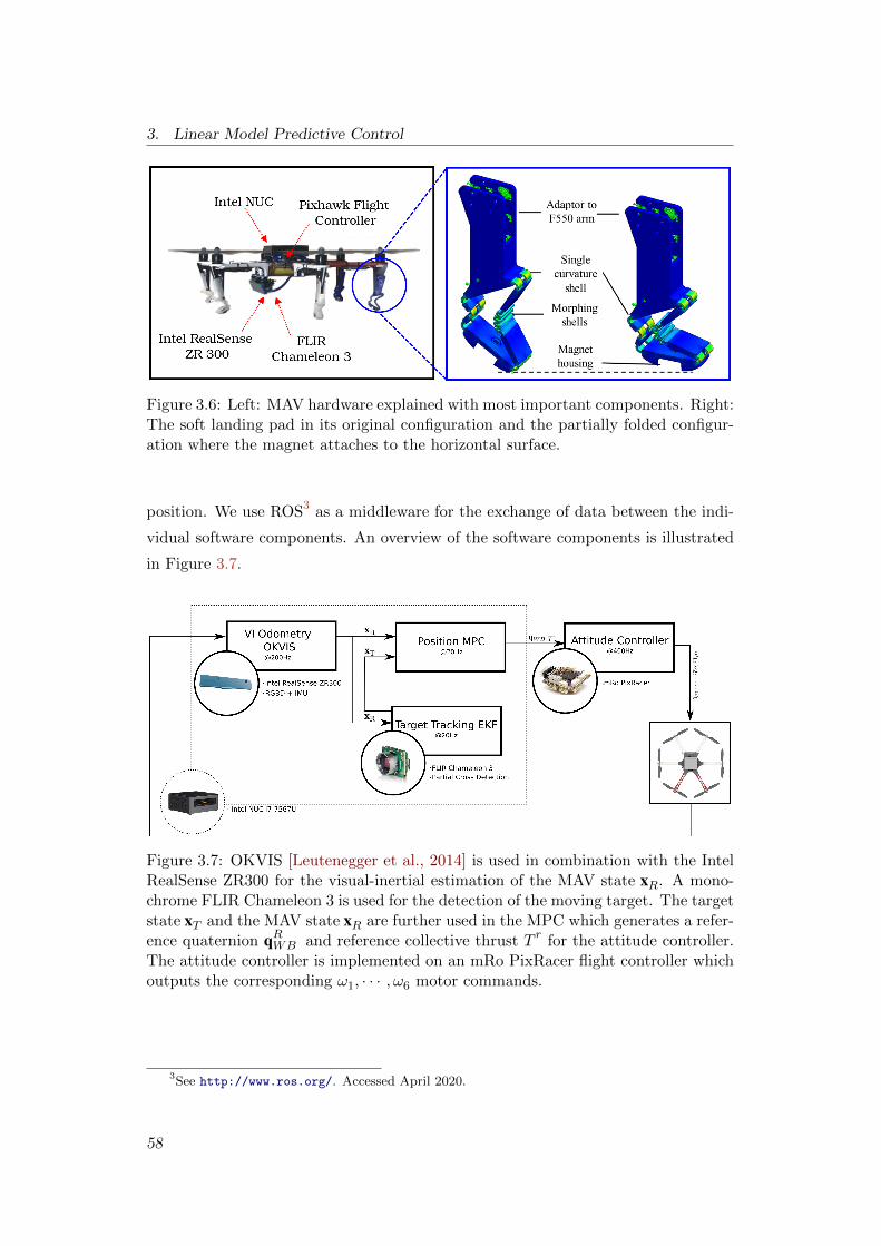
3. Linear Model Predictive Control
Figure 3.6: Left: MAV hardware explained with most important components. Right:The soft landing pad in its original configuration and the partially folded configur-ation where the magnet attaches to the horizontal surface.
position. We use ROS3 as a middleware for the exchange of data between the indi-
vidual software components. An overview of the software components is illustrated
in Figure 3.7.
Figure 3.7: OKVIS [Leutenegger et al., 2014] is used in combination with the IntelRealSense ZR300 for the visual-inertial estimation of the MAV state xR. A mono-chrome FLIR Chameleon 3 is used for the detection of the moving target. The targetstate xT and the MAV state xR are further used in the MPC which generates a refer-ence quaternion qRWB and reference collective thrust T r for the attitude controller.The attitude controller is implemented on an mRo PixRacer flight controller whichoutputs the corresponding ω1, · · · , ω6 motor commands.
3See http://www.ros.org/. Accessed April 2020.
58
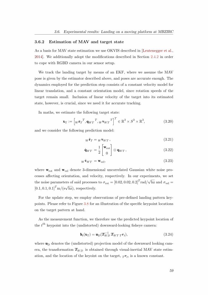
3.6. Experimental results: Landing on a moving platform at MBZIRC
3.6.2 Estimation of MAV and target state
As a basis for MAV state estimation we use OKVIS described in [Leutenegger et al.,
2014]. We additionally adopt the modifications described in Section 2.4.2 in order
to cope with RGBD camera in our sensor setup.
We track the landing target by means of an EKF, where we assume the MAV
pose is given by the estimator described above, and poses are accurate enough. The
dynamics employed for the prediction step consists of a constant velocity model for
linear translation, and a constant orientation model, since rotation speeds of the
target remain small. Inclusion of linear velocity of the target into its estimated
state, however, is crucial, since we need it for accurate tracking.
In maths, we estimate the following target state:
xT :=[W rT
T ,qWTT ,W vWT
T]T∈ R3 × S3 × R3, (3.20)
and we consider the following prediction model:
W rT = W vWT , (3.21)
qWT =1
2
[wrot
0
]⊗ qWT , (3.22)
W vWT = wvel, (3.23)
where wrot and wvel denote 3-dimensional uncorrelated Gaussian white noise pro-
cesses affecting orientation, and velocity, respectively. In our experiments, we set
the noise parameters of said processes to σrot = [0.02, 0.02, 0.2]T rad/√
hz and σvel =
[0.1, 0.1, 0.1]Tm/(s√
hz), respectively.
For the update step, we employ observations of pre-defined landing pattern key-
points. Please refer to Figure 3.8 for an illustration of the specific keypoint locations
on the target pattern at hand.
As the measurement function, we therefore use the predicted keypoint location of
the tth keypoint into the (undistorted) downward-looking fisheye camera:
ht(xT) = uD(T−1WD TWT Trt), (3.24)
where uD denotes the (undistorted) projection model of the downward looking cam-
era, the transformation TWD is obtained through visual-inertial MAV state estim-
ation, and the location of the keyoint on the target, Trt, is a known constant.
59

3. Linear Model Predictive Control
Note that in our implementation, we use a tangent space representation of the
orientation, δαWT , around the current estimate qWT analogous to [Leutenegger
et al., 2014], as
qWT = exp(δαWT )⊗ qWT =
sinc∥∥∥ δαWT
2
∥∥∥ δαWT2
cos∥∥∥ δαWT
2
∥∥∥⊗ qWT , (3.25)
with exp(·) the exponential map.
In order to obtain the keypoint measurements to formulate the EKF update re-
sidual, we employ tracking in image space: we use 20 by 20 pixel patches around the
keypoints warped from the pattern template image using the predicted pose relat-
ive to the camera observing them. Then, using keypoint location predictions from
(3.24), we brute-force search their neighbourhood in the binarised image (60 by 60
pixel) by means of finding the square difference minimum w.r.t. the warped template
patches. In our implementation, we used a keypoint measurement standard devi-
ation of 5 pixels – partly accounting for the lack of proper hardware synchronisation
between the RealSense (used for OKVIS) and the downward looking fisheye camera.
For outlier removal, we discard keypoint measurements where this difference is two
high, and also those whose residuals don’t pass a Chi-square test (threshold: 9).
We illustrate these steps in Figure 3.8.
Figure 3.8: Top row: projected predicted keypoint neighbourhoods (search area) asblue boxes, and actual found detections as green circles (right: zoomed in). Middlerow: binarised search neighbourhoods. Bottom row: respective warped templatesto match.
60

3.6. Experimental results: Landing on a moving platform at MBZIRC
TargetTracking EKF
Position Prediction
Position Low Pass
Velocity Low Pass
Transformto
Navigation Frame
MPC
Figure 3.9: The reference generation scheme. The incorporation of the referencevelocities and not only the position, improves the overall tracking performance ofthe system. The low pass filters for the position and velocity are used in order tofilter out noisy target detections. The target position prediction by the tPrediction
time offset, is performed to counteract unmodeled delays, from target detection toactual maneuver execution, that exist in the system.
3.6.3 High level mission profile
Reference generation
Although our controller can natively handle a time varying (over the prediction
horizon) input su = [su0 , su1 , · · · , s
uN−1]T and output sy = [sy1, s
y2, · · · , s
yN ]T , for simpli-
fication, we do not explicitly generate time varying references but static ones which
remain constant over the prediction horizon.
The approach of position setpoint instead of trajectory control is sufficient for
waypoint navigation but insufficient when tracking of a moving target is required.
Generating a sequence of reference position setpoints based on the observed position
of the moving target will result in a constant offset, similar to the case of PD control,
between the position of the MAV and the target. This is the result of the zero
velocity requirement at each position setpoint which does not hold in the case of
a moving target. We tackle this problem by not only penalizing deviation from a
reference position but also from a reference velocity which in this case corresponds
to the estimated velocity of the target. It is also worth mentioning that in our
implementation, the prediction horizon is relatively short 0.1 s. Similarly, we can
penalize deviation from a reference acceleration by incorporating it in su.
The scheme for the generation of the commanded setpoint (which includes both
reference position and velocity) is illustrated in Figure 3.9. For simpler tasks such
as waypoint navigation we follow the standard approach where position commands
with zero reference velocities are sent to the controller.
We use low pass filters for the reference position and velocity with cutoff frequen-
61

3. Linear Model Predictive Control
cies fCutOffPosition, fCutOffVelocity to filter out the noisy target position and velocity
estimates. The target position prediction by the time offset tPrediction, assuming con-
stant velocity, is used in order to counteract the delay between a successful target
detection and the actual maneuver of the MAV. The use of such a time offset was
also motivated to compensate significant unmodeled delays that exist in the system
such as the one related to the downward looking camera vision processing which
arises from the lack of its hardware synchronization. Notice that the prediction
of the target position also depends on its estimated velocity, while the time offset
tPrediction was a constant parameter determined by tuning of the whole system before
conducting the series of reported experiments. Numeric values of the parameters
used are given in Table 3.2.
State machine
The overall behavior of the MAV is controlled by a state machine with the following
modes which in an ideal experiment, are triggered sequentially.
Idle Mode: This is the default mode when the mission is initially triggered. The
motors are disarmed and a zero thrust and orientation command T r = 0,
qrWB = [1, 0, 0, 0]T is sent to the MAV.
Taking Off Mode: This mode is triggered once the first valid state estimation
message becomes available. An arming command is sent to the motors and
the MAV takes off to the predefined altitude zTakeOffHeight with a predefined
ascending velocity zTakeOffVelocity.
Waypoint Mode: Immediately after take off, the MAV flies towards a predefined
waypoint which coincides with the cross point of the figure-eight trajectory
that the ground vehicle was following in the MBZIRC challenge.
Follow Mode: This mode is triggered when the landing pattern is successfully
detected for the first time. A position and velocity command based on the
procedure described in 3.6.3 is sent to the controller. When the difference
between the current time tCurrentTime and the time of the last target detection
tLastDetection is greater than the timeout parameter tDetectionTimeOut, we assume
that the target is not visible anymore and return back to the waypoint mode.
The tDetectionTimeOut has to be set high enough to allow the MAV to move close
62
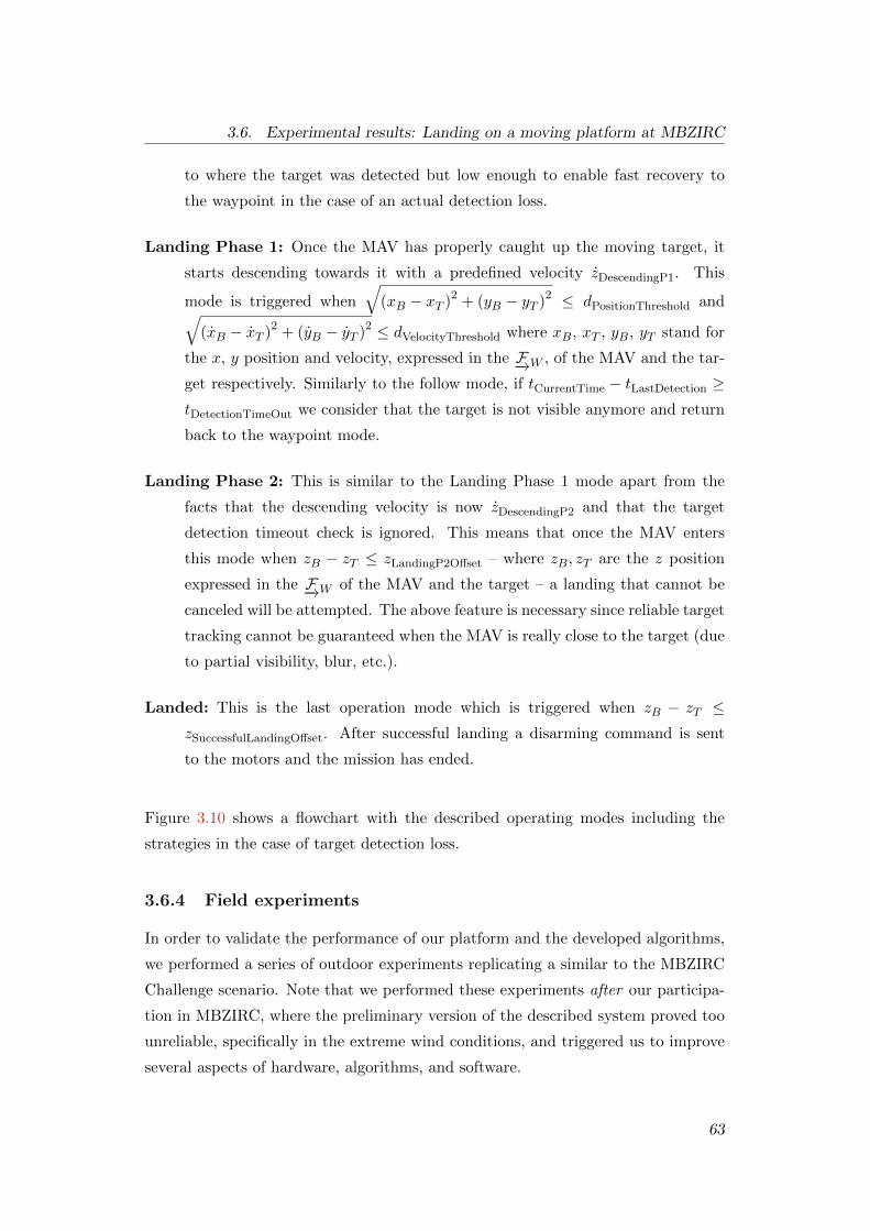
3.6. Experimental results: Landing on a moving platform at MBZIRC
to where the target was detected but low enough to enable fast recovery to
the waypoint in the case of an actual detection loss.
Landing Phase 1: Once the MAV has properly caught up the moving target, it
starts descending towards it with a predefined velocity zDescendingP1. This
mode is triggered when
√(xB − xT )2 + (yB − yT )2 ≤ dPositionThreshold and√
(xB − xT )2 + (yB − yT )2 ≤ dVelocityThreshold where xB, xT , yB, yT stand for
the x, y position and velocity, expressed in the F−→W , of the MAV and the tar-
get respectively. Similarly to the follow mode, if tCurrentTime − tLastDetection ≥tDetectionTimeOut we consider that the target is not visible anymore and return
back to the waypoint mode.
Landing Phase 2: This is similar to the Landing Phase 1 mode apart from the
facts that the descending velocity is now zDescendingP2 and that the target
detection timeout check is ignored. This means that once the MAV enters
this mode when zB − zT ≤ zLandingP2Offset – where zB, zT are the z position
expressed in the F−→W of the MAV and the target – a landing that cannot be
canceled will be attempted. The above feature is necessary since reliable target
tracking cannot be guaranteed when the MAV is really close to the target (due
to partial visibility, blur, etc.).
Landed: This is the last operation mode which is triggered when zB − zT ≤zSuccessfulLandingOffset. After successful landing a disarming command is sent
to the motors and the mission has ended.
Figure 3.10 shows a flowchart with the described operating modes including the
strategies in the case of target detection loss.
3.6.4 Field experiments
In order to validate the performance of our platform and the developed algorithms,
we performed a series of outdoor experiments replicating a similar to the MBZIRC
Challenge scenario. Note that we performed these experiments after our participa-
tion in MBZIRC, where the preliminary version of the described system proved too
unreliable, specifically in the extreme wind conditions, and triggered us to improve
several aspects of hardware, algorithms, and software.
63

3. Linear Model Predictive Control
Figure 3.10: Flowchart indicating the transition between the various operatingmodes.
The experimental flow is as follows: The MAV takes off from the starting point
location where it is initially placed on a 45cm height box. This is necessary in order
to make sure that OKVIS can detect and track salient points on the RGB image.
Once take off is completed, the MAV navigates to the predefined waypoint where it
hovers till the target gets detected. After successful detection, the MAV tries to fol-
low the target and land on it. The transition between the different operating modes
is the one described in Section 3.6.3. The MAV executes the whole task autonom-
ously and does not use any user provided information about the target position and
velocity but it exclusively relies on its onboard sensors and algorithms. A human
pilot triggers the start of the mission and can also manually intervene in order to
prevent a crash in case of an algorithmic failure. We annotate every experiment
as Successful or Failed based on whether the MAV managed to land successfully
on the target according to the MBZIRC Challenge specifications 4. Specifically, a
successful landing is when the MAV comes to a rest on the landing target, with the
MAV intact.
The landing target is identical to the one used in the MBZIRC Challenge and
was being pulled manually, in a random way, with a rope. We tested moving
the target with velocities between 1.3 m/s and 5.7 m/s which exceed the maximum
target velocity of 4.1 m/s during the MBZIRC Challenge. Table 3.1 contains the
results of the conducted experiments while Table 3.2 contains a list for all the
4See https://www.mbzirc.com/faqs/2017. Accessed April 2020.
64

3.6. Experimental results: Landing on a moving platform at MBZIRC
parameters used in the developed algorithms. Alongside the outcome (Success-
ful/Failed) for each experiment, Table 3.1 contains the norm of the position error
exy =
√(xB − xT )2 + (yB − yT )2 between the MAV and target position when the
MAV has landed and the time tTrackingDuration which corresponds to the time that
was needed for a successful landing from the time instant where the target was
initially detected.
Since no motion capture system or RTK GPS was used, we cannot provide ground
truth for the MAV and target position. All the data presented in this section
corresponds to the estimates from OKVIS and the target tracking EKF.
Table 3.1: Successful/unsuccessful landings
Experiment # 1 2 3 4 5 6 7 8 9 10 11 12
Average Velocity v [m s−1] 1.3 1.7 2.0 2.0 2.3 2.4 3.5 3.8 4.0 4.6 5.0 5 .7error exy [cm] 2.5 11.8 5.2 30.6 16.5 6.6 30.2 18.6 15.6 29.8 45.8 7.6Duration [s] 5.1 4.8 5.6 7.7 7.1 5.7 5.0 5.9 7.5 6.1 5.6 5.0
Outcome* S S S S S S S S S F S F
S = Successful, F = Failed.
Table 3.2: Landing software parameters.
fCutOffPosition 30 hz zTakeOffHeight 5.2 m zTakeOffVelocity 0.5 m/sfCutOffVelocity 30 hz dPositionThreshold 0.8 m dVelocityThreshold 0.8 m/stPrediction 0.1 s zLandingP2Offset 2.5 m zDescendingP1 1.3 m/stDetectionTimeOut 0.5 s zSuccessfulLandingOffset 0.35 m zDescendingP2 1.8 m/s
Selected experiments
We present the MAV and target position and attitude data for three selected ex-
periments. Specifically, two of them (Figures figs. 3.11 to 3.14) were successful (one
with low target velocity and another with high), whereas the third one (Figures 3.15,
3.16) was unsuccessful. The figures for the remaining nine experiments can be found
in [Tzoumanikas et al., 2019]. In all the figures presented, solid lines refer to the
estimated values given by OKVIS while the dashed ones refer to their corresponding
reference. Reference position xr, yr, zr was generated as described in Section 3.6.3
while θr, φr and T r were obtained by solving the MPC optimization problem. ψr
was always kept to zero. Also, notice that there is no solid line for T r (plotted in
Newtons) since – as explained in Section 3.4 – the dynamics of the motors were
ignored and it was assumed that the applied thrust coincides with the reference.
65

3. Linear Model Predictive Control
Figure 3.11: Position and attitude data for experiment #11. A successful landingon a target moving with 5.0 m/s was achieved. The dashed lines on the upper 3plots correspond to the reference position which is generated based on the estimatedposition and velocity of the target while the dashed lines on the lower 3 plots cor-respond to the attitude angles and thrust generated by the MPC. The MAV lands5.59 s after the first target detection and 45.8 cm away from the target center.
66

3.6. Experimental results: Landing on a moving platform at MBZIRC
Figure 3.12: Position and attitude data for experiment #1. A successful landingwas achieved on a target moving with 1.3 m/s. The MAV lands 5.06 s after the firsttarget detection and 2.5 cm away from the target center.
67

3. Linear Model Predictive Control
Figure 3.13: The MAV and target position visualised as a 3D plot for the experiment#11. Dashed lines indicate the corresponding target detection/tracking.
Figure 3.14: The MAV and target position in 3D for the experiment #1.
68

3.6. Experimental results: Landing on a moving platform at MBZIRC
Figure 3.15: Position and attitude data for experiment #12. A failed attempt oflanding on a target moving with 5.7 m/s was performed. Although that the finalposition error exy between the target and the MAV is only 7.6 cm, the real MAVposition differs from the target position (See also Figure 3.17). Unreliable estimationof the target position especially when flying close to it led to a landing on a predictedtarget position different from the real one.
69

3. Linear Model Predictive Control
Figure 3.16: The MAV and target position in 3D for the experiment #12.
3.6.5 Comparison with other MBZIRC teams
From the experimental results, we realize that our hardware and software framework
achieves the original goal that it was designed for with high repeatability. The
majority of the experiments (10/12) were successful whereas there were only 2 failed
attempts, both in the high velocity region 4.6 m/s and 5.7 m/s. The worst case
position error exy between the target and the MAV after landing was 45.8 cm which
corresponds to the fastest successful attempt #11. The worst case tracking accuracy
achieved by the controller was more than sufficient especially considering the size of
the MAV and the landing target and the fact that the experiments were conducted in
an outdoor environment. The position error is generally larger in the high velocity
experiments (No 7, 8, 9, 11) and lower in the slower ones (No 1, 2, 3, 4, 5, 6).
We consider the noisy and uncontrolled outdoor environment (presence of wind and
varying lighting conditions, which affect the target state estimation) to be the main
reason.
Concerning MAV state estimation, with appropriate settings of gain and bright-
ness on the Realsense RGB-D camera, we have not experienced any problems related
to lack of tracked keypoints, therefore leaving the visual-inertial estimation system
working flawlessly.
Regarding the attitude commands generated by the MPC, these are generally not
smooth in the high velocity Experiments but smoother for the low velocity ones.
70

3.6. Experimental results: Landing on a moving platform at MBZIRC
This was the result of over-penalizing the position/velocity error compared to the
penalization of the smoothness terms. In other words, the gains of the optimisation
problem are chosen in a way such that position/velocity tracking is prioritized over
smooth attitude changes. Regarding the MAV response to the attitude commands,
there exist a phase and amplitude difference between the commanded attitude angles
and the real ones. Since the linear model also includes an estimated model for the
closed loop attitude dynamics (Equation (3.4)), the difference between a command
and the actual response is taken into account by the MPC. We also observe that
although the ψr was always kept to zero, ψ was minimally affected when aggressive
θr, φr were required. This is the result of existence of coupling between the MAV
degrees of freedom; something not captured by the linear model used for control.
It is important to highlight that our controller does not contain any integral error
term and generally it is not aware of any not modeled disturbance acting on the
system. Hence, it is unable to counteract any constant position/velocity error offset
which is either the result of an external disturbance or imperfect system calibration.
The controller can only compensate non-persistent external disturbances due to the
feedback on the system. Rejection of constant disturbances would only be possible,
if these could be estimated and taken into account from the control model. In order
to make sure that the MAV will remain in a state envelope where the used linear
model remains valid, we use appropriate constraints in the optimization problem.
These also guarantee that the MAV operates far from the gimbal lock (since Euler
angles are used for the control formulation).
In all the successful experiments, the MAV managed to land within less than 7.65 s
after the first target detection.The final time in all the experiments did not exceed
30 s, and this is mainly dominated by the time required for take off and moving
to the waypoint. We cannot make a direct comparison with the performance of
the teams who participated in the real challenge, as the final time also depends on
when the target becomes visible for the first time. We can, however, compare our
approach with the ones by team ETH-MAV [Bahnemann et al., 2017] and NimbRo
[Beul et al., 2017] which both successfully landed on the moving target during the
MBZIRC competition within 56 s and 32 s, respectively.
• ETH-MAV team used two cascaded EKFs that combine data from an RTK
GPS and a Visual Inertial sensor for the MAV state estimation. A downward
71

3. Linear Model Predictive Control
looking camera is used for the target detection. Target tracking and landing
is achieved through a non-linear MPC and a path planning algorithm which
also relies on the prior knowledge of the MBZIRC track shape. They also use
a Lidar sensor in order to check the distance between the MAV and the target
and trigger the final stage of the landing procedure.
• NimbRo team used a GPS + IMU fusion algorithm for the MAV state estim-
ation, along with a fast trajectory planning algorithm. In order to detect and
track the target they use two different cameras. One is looking downwards,
while the other forward-downward. The usage of such a camera configura-
tion, not only robustifies the target detection but also enables faster initial
detection of the moving target. Their MAV was programmed to wait at the
waypoint while rotating around its vertical axis at the same time. Mechanical
switches are placed on the legs of the MAV in order to detect contact and thus
successful landing on the moving target.
Both teams followed a mission profile similar to ours with Wait at waypoint – Follow
– Final approach and landing to be the main modes of operation, while the main
difference was the active rotating/searching performed by the NimbRo team MAV
which can greatly reduce the time needed for initial target detection. Our approach
does not rely on RTK-GPS making it appropriate for similar tasks in GPS denied
environments, and moreover removes the necessity for a ground station (which wire-
lessly sends the GPS corrections to the MAV). We consider our approach to be simple
and general enough to be implemented in similar scenarios. Regarding the software
developed, we consider the lack of dynamically feasible trajectories planning and
the usage of a linear MPC to be the main limitation of our approach compared to
the above. Regarding the hardware, we used – in our opinion – the absolute min-
imum number of sensors/components required for autonomous navigation. Since
we employ only the necessary hardware components, we don’t get the benefits of
more reliable target detection (through use of multiple cameras) and prevention of
unsuccessful landing attempts (through use of extra sensors such as Lidar).
As far as the failed attempts (experiment 10 and 12) are concerned, both of them
seem successful when we look at the position plots and the final position error after
landing. As shown in Figure 3.17 in both Experiment 10 and 12 the MAV landed
really close to the true target position. We argue that the reason behind the failed
72

3.6. Experimental results: Landing on a moving platform at MBZIRC
attempts is the quality of the estimated target state especially when the MAV flies
really close to the target. Specifically, in Experiment 12 (Figure 3.15) the target was
pulled sharply in a different direction while the MAV was in Landing Phase 2. Due
to the proximity between the MAV and target, the latter was partially or completely
invisible due to the horizontally mounted downward looking camera and MAV tilt.
Given the average target velocity in these experiments (4.6 m/s and 5.7 m/s) and
the fact that the frame rate of the downward looking camera was 20 hz, the target
position between two consecutive camera frames was changing by 23 cm and 28.5 cm
respectively. It becomes clear that in this frame rate and high target velocity, even
one frame of lost tracking can result a failed landing attempt.
Figure 3.17: The two failed landing attempts. Experiment #12 on the left andexperiment #10 on the right.
We consider that our approach has two main limitations. The first one is un-
reliable target tracking when the MAV flies close above the target. This could by
either fixed by improving the target tracking when it is partially visible or by mech-
anically rotating the downward looking camera such that the target always remains
in the field of view. The second limitation is the criterion used for triggering the
landing attempt when flying above the MAV. This depends only on the relative
height between the MAV and the target. It would be better to use a criterion which
takes into account the confidence/uncertainty of the estimated target states or use
additional hardware (e.g. Lidar sensor) for more accurate relative height estimation.
This would hopefully lead to higher probability for a successful landing. Never-
theless, we believe to have achieved a respectable success rate given the minimal
hardware/sensor complexity.
73

3. Linear Model Predictive Control
3.7 Experimental results: Application to AABM
In this Section we present experimental results related to the AABM5 project which
aims at developing the hardware and software which will enable aerial robots to
autonomously 3D print small structures. Our role in the project was to provide the
required state estimation and control algorithms which will enable precise trajectory
tracking.
Briefly, the experimental setup consisted of two MAVs with a 4.5 kg payload ca-
pacity which can deposit building material, while flying, through an appropriate
extrusion mechanism. Trajectories containing multiple printing layers were com-
manded to the two MAVs which were serially executing the building task. In order
to enable precision and mainly cope with the limited material extrusion speed, the
maximum velocity of the commanded trajectories was limited to 5 cm/s.
An example of a 10-layer reference printing trajectory and the actual MAV re-
sponse in a virtual printing scenario (without extruding building material) is given
in Figure 3.18.
3.7.1 Linear MPC modifications
In order to cope with the increased need of precision for the AABM and handle
the slowly varying MAV mass due to building material extrusion, we have done the
following modifications to the linear MPC presented in Section 3.5:
1. We reduced the order of the closed loop attitude dynamics given in (3.4) from
a second order model to a first one given by:
θ = −bθθθ + bθrθr, (3.26a)
φ = −bφφφ+ bφrφr. (3.26b)
This approximation also adopted in similar works such as [Kamel et al., 2017a]
results in dimension reduction of the control state x := [x, x, θ, y, y, φ, z, z]>,
while the control input remains unchanged u := [θr, φr, T r]>.
2. We increased the length of the prediction horizon to 1.0 s while keeping the
same discretisation timestep dt = 50 ms.
5See http://www.aerial-abm.com/. Accessed April 2020.
74
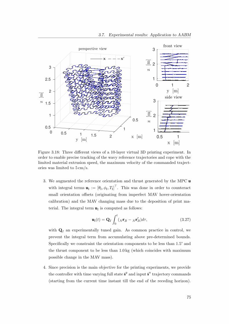
3.7. Experimental results: Application to AABM
0.5
10.5
1
1.5
0
2
0.5
2.5
3
1 1.5 2
0 1 2
1
2
3
0.5 1
1
2
3
Figure 3.18: Three different views of a 10-layer virtual 3D printing experiment. Inorder to enable precise tracking of the wavy reference trajectories and cope with thelimited material extrusion speed, the maximum velocity of the commanded traject-ories was limited to 5 cm/s.
3. We augmented the reference orientation and thrust generated by the MPC uwith integral terms uI := [θI, φI, TI]
>. This was done in order to counteract
small orientation offsets (originating from imperfect MAV hover-orientation
calibration) and the MAV changing mass due to the deposition of print ma-
terial. The integral term uI is computed as follows:
uI(t) = QI
∫ t
0(NrB − NrrB)dτ, (3.27)
with QI an experimentally tuned gain. As common practice in control, we
prevent the integral term from accumulating above pre-determined bounds.
Specifically we constraint the orientation components to be less than 1.5° and
the thrust component to be less than 1.0 kg (which coincides with maximum
possible change in the MAV mass).
4. Since precision is the main objective for the printing experiments, we provide
the controller with time varying full state sy and input su trajectory commands
(starting from the current time instant till the end of the receding horizon).
75

3. Linear Model Predictive Control
This way the controller can react in advance for upcoming references which is
particularly useful for e.g. maneuvers containing sharp turns.
3.7.2 Selected printing experiments
In Figures 3.19-3.20 we show the tracking performance achieved by our controller in
an indoors-performed printing experiment with MAV pose data being provided by
a motion capture system. Specifically, Figure 3.19 (left) shows the complete multi-
layer reference trajectory (subsampled for visibility purposes), while the tracking
performance for a single layer is shown in Figure 3.19 (right). Despite the saw-
tooth like x, y references, the controller enables centimeter-level tracking as at the
visualised scale the reference and actual MAV position are indistinguishable.
The boxplot in Figure 3.20, which contains the tracking statistics of the first ten
layers, reveals that the per-axis error does not exceed 1.5 cm.
76

3.7.E
xp
erimen
talresu
lts:A
pp
licationto
AA
BM
1.8
1.9
2
0.0
2.1
1.9
2.2
0.1
2.3
2.0
2.4
0.2
2.5
2.1
2.6
0.3
2.7
2.8
0.0
0.2
0.4
1.8
2.0
2.2
50 100 150 200 2501.5
1.6
1.7
Figure 3.19: Reference and actual MAV trajectory during an AABM printing experiment. Left: The multi-layer 3D printingreference position. Right: Per-axis reference and actual MAV position for a selected layer.
1 2 3 4 5 6 7 8 9 100
5
10
15
Figure 3.20: MAV position error statistics for the first ten layers of the AABM printing experiment. The per-axis error for thetested trajectories, does not exceed 1.5 cm.77

3. Linear Model Predictive Control
3.8 Discussion
In this Chapter we presented a linear MPC with soft state constraints formulated as
a QP that can be solved with any generic solver. As it can be seen from the exper-
imental results, it can be successfully used for dynamic tasks such as the tracking
and landing scenario while its performance is maximised when slow manoeuvres are
required. This is owing to the linear model being based on near hover operation
assumptions.
Despite the limitations that arise from the use of an approximate linear model, as
well as the use of Euler angles as a parameterisation for orientation, we would like
to comment on the specific advantages which become apparent from the presented
experiments as well as its use in multiple live demonstrations the past four years.
First and foremost, its easy adaptation to other platforms as the linear model is
platform agnostic. The same controller can be applied without modification to a
quadcopter, hexacopter or any other underactuated platform as the only requirement
is the existence of a closed loop attitude controller. Secondly, the position-attitude
dynamics separation allows the position loop to be run at a low update rate which
in our case was 20 Hz. This makes the system less sensitive to e.g. delays in the state
estimation scheme since the fast attitude dynamics are separately controlled using
the onboard IMU. Lastly, the resulting optimisation problem is computationally
cheap to solve (consistently less than 1 ms per control iteration with our hardware)
and is thus suitable for platforms with limited computing resources.
Regarding the possible extensions of the presented linear MPC, the generalisa-
tion to a NMPC is given in the upcoming Chapter. Future work, thus should be
focused on the engineering related improvements. As an example we consider the
use of the fastest QP solver [Frison and Diehl, 2020] currently available. Lastly, a
useful extension would be the online estimation of external forces and moments as in
[Kamel et al., 2017a] and their incorporation in the control model. This would allow
for offset free navigation without the need of additional integral terms and would
further enable the compensation of external disturbances before their integration
into position/velocity error.
78

Chapter 4
Nonlinear Model Predictive
Control
Contents
4.1 Introduction . . . . . . . . . . . . . . . . . . . . . . . . . . . . . 80
4.2 Related work . . . . . . . . . . . . . . . . . . . . . . . . . . . . . 81
4.3 Contribution . . . . . . . . . . . . . . . . . . . . . . . . . . . . . 83
4.4 System overview . . . . . . . . . . . . . . . . . . . . . . . . . . . 84
4.5 Model based control . . . . . . . . . . . . . . . . . . . . . . . . . 85
4.5.1 Nonlinear modelling . . . . . . . . . . . . . . . . . . . . 85
4.5.2 Nonlinear Model Predictive Control . . . . . . . . . . . 86
4.5.3 Control allocation . . . . . . . . . . . . . . . . . . . . . 87
4.6 Motor failure in a hexacopter . . . . . . . . . . . . . . . . . . . . 89
4.7 Fault identification . . . . . . . . . . . . . . . . . . . . . . . . . 95
4.8 Experimental results . . . . . . . . . . . . . . . . . . . . . . . . . 97
4.8.1 Waypoint tracking . . . . . . . . . . . . . . . . . . . . . 97
4.8.2 Fault detection and recovery . . . . . . . . . . . . . . . . 99
4.9 Discussion . . . . . . . . . . . . . . . . . . . . . . . . . . . . . . 103
Parts of this Chapter appear in: Tzoumanikas, D., Yan, Q., and Leutenegger, S. (2020).
Nonlinear MPC with Motor Failure Identification and Recovery for Safe and Aggressive
Multicopter Flight. In Proceedings of the IEEE International Conference on Robotics and
Automation (ICRA). [Tzoumanikas et al., 2020b]
79

4. Nonlinear Model Predictive Control
4.1 Introduction
The linear MPC presented in Chapter 3 is characterised by its ease of use and
its effortless adaptation to any type of multirotor without the absolute need of a
powerful onboard computer. Its per-axis tracking accuracy heavily depends on the
aggressiveness of the reference trajectories and varies from 1 cm for slow trajectories
(< 5 cm/s) to 50 cm for fast ones (> 5 m/s) as tested in the landing experiment. This
is mainly because the linear model is derived assuming a near hover operation which
does not hold when the MAV has to exert motion with significant linear velocity
and acceleration. Additionally, the linear model uses Euler angles for the represent-
ation of orientation and thus the orientation close to gimbal lock is prevented from
additional orientation constraints. Constraining the maximum tilting angle results
in limiting the maximum translational acceleration.
Another issue is the lack of robustness in the case of actuator failures such as
a partially or completely damaged motor/propeller. This is because it relies on
the existence of a stable attitude controller which on most occasions is based on
simple PID implementations and thus unable to handle an actuator failure without
appropriate modifications.
These problems can to some extend be eliminated when the true non linear MAV
model is taken into account in the control design and a unified controller is respons-
ible for the 6DoF motion of the MAV. This is a research topic that has become
particularly popular during the past years thanks to the increasing computation
capabilities and the open source availability of optimisation and control toolboxes
such as [Houska et al., 2011, Giftthaler et al., 2018, Mattingley and Boyd, 2012].
At the same time, robust performance under mechanical failures (such as motor
failures), can only be achieved when the failure can be correctly identified and ap-
propriately handled by the control design. To this purpose, the existence of a model
based supervisory algorithm that monitors the health of the system and accordingly
notifies the controller in the event of a failure, is necessary.
In this Chapter we propose a NMPC aiming at overcoming the limitations of its
linear counterpart. We further suggest an EKF based fault detection algorithm and
a specific to our MAV type stabilisation technique in the event of a motor failure.
An example of our MAV performing online fault detection and stable position and
yaw control despite the loss of a motor is shown in Figure 4.1.
80

4.2. Related work
Figure 4.1: Our MAV experiencing a propeller loss. The fault is identified online,the failsafe enabled and the MAV can still control its position and orientation.
4.2 Related work
As mentioned in Chapter 3, the most common approach regarding MPC in MAVs
is that of a cascade connection between a position and an attitude controller. In the
simplest form, a linear model can be used for the translational dynamics, resulting
in an optimisation problem whose solution can be solved online [Tzoumanikas et al.,
2019, Sa et al., 2018a] or pre-computed in the form of lookup tables [Darivianakis
et al., 2014, Papachristos et al., 2016]. The use of a non-linear model for the transla-
tional dynamics such as the one presented in [Kamel et al., 2017a] presents perform-
ance improvements especially when tracking of aggressive trajectories is required.
The approach of the cascaded position-attitude controllers has become popular due
to its ease of use, since most of the available platforms come with a pre-tuned atti-
tude controller. However, it relies on the assumption that the attitude dynamics can
be controlled independently, requiring bandwidth separation between the successive
loops, i.e. slow control of attitude. The aforementioned works furthermore use Euler
angles for the vehicle orientation which prohibits the operation close to gimbal lock.
Analogously to the position-attitude approach the authors of [Falanga et al., 2018]
and [Foehn and Scaramuzza, 2018] propose a quaternion based position controller
which uses the angular rates as control inputs. These were assumed to be tracked
perfectly by a separate angular rate controller.
The benefits of using the true non-linear model of the MAV has been successfully
illustrated in [Kamel et al., 2015] where an attitude NMPC was employed to stabilise
the position of a hexacopter with a motor failure while control of yaw was lost.
Additionally, the authors of [Neunert et al., 2016] proposed an Sequential Linear
Quadratic (SLQ) MPC algorithm able to run onboard an MAV and capable of
81

4. Nonlinear Model Predictive Control
following full state trajectory commands. Similarly, in [de Crousaz et al., 2015]
simulation results of an SLQ controller stabilizing a quadrotor with slung load and
a quadrotor with motor failure were presented.
For the control allocation problem – that is, the mapping of the body moments
and thrust to actuator commands – the most commonly used method employs the
pseudo-inverse or weighted pseudo-inverse of the allocation matrix (e.g. [Achtelik
et al., 2013, Lee et al., 2010]). The main advantage of this approach is its simplicity
since the pseudo-inverse has to be computed once and the actuator commands can
be obtained through a simple matrix by vector multiplication. However, the main
drawback is the fact that it can produce actuator commands that are not feasible
(e.g. greater thrust than what each motor can provide). Naively, this can be handled
by clipping the actuator command such that it lies in the achievable range. Control
allocation techniques that respect the actuator limits, such as the ones presented in
[Faessler et al., 2017, Brescianini and D’Andrea, 2018], result in better trajectory
tracking. This is partially due to the prioritisation of the roll/pitch moments and
collective thrust over the yaw moment which does not directly contribute to position
tracking.
Another alternative approach is the one presented in [Brescianini and D’Andrea,
2018b], where the minimum energy solution is obtained by solving an optimisation
problem. The authors exploit the structure of the allocation matrix nullspace in or-
der to transform the original optimisation problem into a computationally cheaper
one. Similar to our method, theirs can be used on platforms equipped with bid-
irectional capable motors but requires the use of symmetrical propellers. When non
symmetric propellers are used, the resulting allocation matrix is not constant but
depends on the direction of rotation of each motor.
Regarding the fault tolerant control, the different approaches vary based on whether
the hardware platform can natively handle a motor failure or not. Examples include
the cases of octacopters [Saied et al., 2015, Saied et al., 2017] or, more relevant
to our research, hexacopters with unconventional motor layouts such as [Schneider
et al., 2012, Mazeh et al., 2018, Nguyen et al., 2019] where it was shown that stable
position and yaw tracking can be achieved for failure occurring on specific motors.
When full position and yaw control is not physically possible by the hardware plat-
form (e.g. quadcopters, hexacopters with symmetric motor layout), software based
approaches such as [Mueller and D’Andrea, 2014, de Crousaz et al., 2015, Kamel
82

4.3. Contribution
et al., 2015] attempt to prioritise tracking of the controllable states (e.g. position)
over the uncontrollable ones (e.g. yaw). As far as the fault detection scheme is
concerned, a simple and accurate way of detecting failures is by using direct meas-
urements of motor speed and/or electrical current [Saied et al., 2017]. The deviation
between the speed measurements and the commanded ones can be used to identify
a motor stall/malfunction while the current measurements for detecting a propeller
loss. Alternative software-based methods [Saied et al., 2015, Nguyen et al., 2019]
rely on the formulation of residuals between the measured and predicted –assuming
no failure– system states such as orientation, angular rate or vertical velocity. The
sign of the residuals in combination with some lookup table (that covers all possible
sign combinations) are used for detecting motor failures. The underlying idea is that
losing thrust from a specific motor results in a specific system response which can be
directly compared to the nominal one e.g. a hovering MAV experiencing a sudden
thrust loss from the front-left motor will loose altitude and tilt in the forward left
direction.
4.3 Contribution
With respect to the related works described above, we present a series of algorithms
which address the problem of aggressive, precise and fault tolerant MAV navigation.
Our contributions are as follows:
• The design of a non-linear model predictive controller with body torques and
collective thrust as the control inputs which jointly controls the MAV’s 6D
DoFs. A quaternion based orientation parameterisation is chosen thus avoiding
problems related to gimbal lock while the unified control approach eliminates
assumptions related to the position/attitude dynamics separation since the
NMPC does not require the existence of a separate attitude or rate controller.
• The design of an optimisation based control allocation algorithm that maps
the desired control inputs into feasible thrust commands for each motor. We
consider the general case where the motors can generate both positive and
negative thrust. Our method aims at combining the advantages of the vari-
ous methods described above. Namely, the ability to: (i) prioritise certain
control inputs over others, (ii) generate feasible actuator commands, (iii) cope
83

4. Nonlinear Model Predictive Control
with bidirectional capable motors without the absolute need of symmetrical
propellers.
• The design of a stabilisation technique, based on reversing the motor direction
of rotation, which enables stable position and yaw control. This can be ad-
ditionally applied to hexacopters with symmetric motor layouts ensuring that
due to symmetry, failure in any motor can be handled equally well.
• The design of an EKF, exclusively relying on IMU measurements, which mon-
itors the health of each individual actuator (motor/propeller) which we use
for fast identification of an actuator failure. Compared to similar in concept
approaches, our EKF directly estimates the per-motor ratio of the observed to
commanded thrust (while also considering the motor dynamics), thus provid-
ing a natural way of signalling a motor/propeller failure.
4.4 System overview
The software pipeline presented in this Chapter consists of the following different
blocks: (i) the NMPC which receives the state estimates and reference trajectory
commands and produces body torques and collective thrust as the control inputs; (ii)
the control allocation block which transforms the control inputs to feasible actuator
commands; (iii) the failure detection algorithm which estimates the health status of
each motor and notifies the control allocation block in the case of a failure. We use
the state estimation algorithm outline in Section 2.4.1 which fuses data from the
onboard IMU and the motion capture system. An overview of the system is given
in Figure 4.2.
Figure 4.2: Overview of the various software components that run onboard theMAV. The control loop runs at 100Hz while the failure detection EKF at 400Hz.
84

4.5. Model based control
4.5 Model based control
4.5.1 Nonlinear modelling
The Newton-Euler equations are used to model the MAV dynamics. We ignore
less significant phenomena such as the effect of the aerodynamic friction and the
gyroscopic moments due to the rotation of the propellers (but our model could be
extended accordingly with ease). The MAV dynamics can then be written in the
following form:
W rB = W vB , (4.1a)
qWB =1
2Ω(Bω )qWB , (4.1b)
W vB =1
mCWB BT + Wg, (4.1c)
Bω = J−1(BM− Bω × JBω ), (4.1d)
Ω(Bω ) =
[Bω×
Bω
−Bω> 0
], (4.1e)
where Wg := [0, 0,−9.81]> stands for the gravitational acceleration, m for the MAV
mass, and J for its inertia tensor. The thrust vector BT := [0, 0, T ]> acting on the
MAV CoM solely depends on the collective thrust T generated by the motors. This
together with the moments BM are considered as the control input u := [BM>, T ]> ∈R4. The control state x := [W r>B,q
>WB ,W v>B ,Bω
>]> ∈ R3×S3×R6, consists of the
MAV position, orientation, linear and angular velocities respectively. We consider
that the motor dynamics are significantly faster than the MAV body dynamics and
are thus neglected. Based on the analysis provided in Section 2.2.1, we use the
following model for the thrust and moment generated by the ith motor:
fi = kTω2i , (4.2a)
Mi = (−1)i+1kMfi. (4.2b)
Regarding the relationship between a PWM command and the generated thrust and
moment, we follow the method provided in Section 2.2.1 where the coefficients of
Equation (4.2) were identified using a thrust stand while the relationship between the
PWM command and the achieved angular velocity was identified for different input
voltage levels. As our approach also works for MAV platforms that can generate
both positive and negative thrust, we identified two sets of coefficients: (i) for normal
85

4. Nonlinear Model Predictive Control
motor rotation k+T , k+
M corresponding to positive thrust; (ii) inverted motor rotation
k−T , k−M corresponding to negative thrust.
4.5.2 Nonlinear Model Predictive Control
For the control formulation, we define the following time-varying error functions for
the position, linear and angular velocity, orientation and control input respectively:
er = W rB − W rrB, (4.3a)
ev = W vB − W vrB , (4.3b)
eω = Bω − CBBrB
rωr, (4.3c)
eq = [q−1WB ⊗ qrWB ]1:3, (4.3d)
eu = u− ur. (4.3e)
Apart from the orientation error which is obtained through quaternion multiplica-
tion, the rest corresponds to the Euclidean difference between the actual and desired
(here denoted with the superscript r) quantity.
We compute the optimal control input u∗ sequence online by solving the following
optimisation problem:
u∗ = argminu0,...,uNf−1
Φ(xNf
,xrNf) +
Nf−1∑n=0
L(xn,xrn,un)
, (4.4a)
s.t. : xn+1 = Fd(xn,un), (4.4b)
x0 = x, (4.4c)
ulb ≤ ui ≤ uub, i = 1, . . . , 4 (4.4d)
, where Nf is the number of time steps, x the known initial state, Fd the discrete-time
version of the MAV dynamics given in (4.1) and ulb, uub lower and upper bounds for
the inputs ui. We use quadratic costs for the final and intermediate terms defined
as:
Φ(xNf,xrNf
) = e>r Qrer + e>v Qvev + e>q Qqeq + e>ωQωeω, (4.5a)
L(x,xr,u) = e>r Qrer + e>v Qvev + e>q Qqeq + e>ωQωeω + e>uQueu, (4.5b)
with Q < 0 gain matrices of appropriate dimensions which are considered tun-
ing parameters. In our implementation we use a 10 ms discretisation step and a
86

4.5. Model based control
constant time horizon Tf = 2.0 s. For the online computation of the optimal in-
put we use the CT toolbox [Giftthaler et al., 2018] and the Gauss-Newton Mul-
tiple Shooting (GNMS) algorithm (outlined in [Giftthaler et al., 2017]) which res-
ult in an average computation time of 5.2 ms with standard deviation of 0.6 ms.
At each GNMS iteration dynamically feasible state and input increments δxn, δun(for every stage n) around the state and input trajectories X = x0,x1, · · · ,xNf
,U = u0,u1, · · · ,uNf−1 are computed. We obtain the dynamics of the minimal state
perturbation δx := [δr, δθ, δv , δω ]> ∈ R12 around the state x by introducing the
local quaternion perturbation q = q ⊗ δq with δq :=[sinc
∥∥ δθ2
∥∥ δθ2 , cos
∥∥ δθ2
∥∥]>.
The dynamics for the rotation vector δθ ∈ R3 are given by: ˙δθ = Bω − 12Bω
×δθ,
while the rotation matrix CWB can be approximated as: CWB ≈ CWB (I + δθ×).
After each iteration we use the following rule for the state and input update:
x′ = [wrB + δr,qWB ⊗ δq ,W vB + δv ,Bω + δω ]>.
4.5.3 Control allocation
As stated earlier, the control allocation problem involves mapping the control inputs
u∗ to feasible actuator commands f := [f1, . . . , fN ]>. We tackle this by solving the
following QP:
f∗ = argminf
(∥∥Af− u∗∥∥2
W + λ ‖f‖22), (4.6a)
s.t. : fmin ≤ fi ≤ fmax, i = 1, . . . , N, (4.6b)
where N is the number of motors. The allocation matrix A ∈ R4×N , which we will
present later, depends on the MAV geometry and its motor coefficients, whereas
fmin, fmax correspond to the minimum and maximum attainable thrust. In order to
prioritise the roll/pitch moments and the collective thrust over the yaw moment, we
use the weighting matrix W ∈ R4×4. The scalar λ ∈ R+ is used such that solutions
with smaller norms are preferred. When a feasible control input is commanded,
solution of (4.6) coincides with the one obtained by using the pseudo-inverse of A,
namely f = A†u∗.
Since we are interested in solving the control allocation problem for the general
case where the motors can produce both positive and negative thrust, we introduce
the vector d := [d1, d2, · · · , dN ]> with di ∈ 0, 1, ∀i = 1, . . . N . We thus use the
binary variables di to indicate whether the ith motor is spinning in its intended nor-
87

4. Nonlinear Model Predictive Control
mal direction–corresponding to positive thrust (di = 0)–or otherwise in the inverse
(di = 1).
The original optimisation problem (4.6) is transformed to:
f∗,d∗ = argminf,d
(∥∥A(d)f− u∗∥∥2
W + λ ‖f‖22)
(4.7a)
s.t. : f+min(1− di) + f−mindi ≤ fi ≤ f
+max(1− di) + f−maxdi, (4.7b)
where the superscript + or − in f+min, f−min, f+
max, f−max has been used to indicate
normal and inverted rotation respectively. The binary vector d which encodes the
direction of rotation is now an optimisation variable and the allocation matrix A is
a function of d. For the case of the hexacopter with motor layout and normal motor
rotation as shown in Figure 4.3, A(d) takes the following form:
A(d) =
ls30 l ls30 −ls30 −l −ls30
−lc30 0 lc30 lc30 0 −lc30
kM (d1) −kM (d2) kM (d3) −kM (d4) kM (d5) −kM (d6)
1 1 1 1 1 1
, (4.8)
where l stands for the MAV arm length, s30 = sin (30o), c30 = cos (30o), kM (di) =
(1− di)k+M + dik
−M .
Figure 4.3: Motor layout of the hexacopter used in our experiments. Rotation arrowsshow the direction of rotation that corresponds to positive thrust.
The resulting optimisation described in (4.7) is a Mixed Integer Quadratic Pro-
gramming (MIQP). However, since the possible values of d are finite (64 in the
88

4.6. Motor failure in a hexacopter
case of a hexacopter), we can solve a single QP for every possible value of d. The
global optimum f∗ of Equation (4.7) corresponds to the solution of the QP with the
minimum cost. From a practical perspective solving 64 QPs instead of a single one
does not affect significantly the overall control computation time as this is domin-
ated by the computation of the optimal input u∗ as described in the Section 4.5.2.
This is owing to the small number of optimisation variables in a single QP tailored
to the solver, CVXGEN [Mattingley and Boyd, 2012]. In our implementation, solv-
ing 64 QPs, storing the results in a vector and finally sorting it in ascending order
consistently takes less than 0.4 ms. We acknowledge, however, that our method is
more resource demanding compared to methods using the pseudoinverse which can
be easily implemented on a microcontroller.
It was experimentally found that reverting the direction of rotation during flight
is particularly impractical. This is because the motor dynamics are significantly
slower when a direction change is commanded. As our control model does not
capture this behaviour, we can prevent unnecessary direction change commands by
augmenting the optimisation (4.7) similarly to [Brescianini and D’Andrea, 2018b]
with the f ∈ Fhyst constraint, where Fhyst is the set of rotor thrusts that does not
require a per motor direction change when this has already happened during the past
time interval thyst. The solution satisfying this constraint can be found with a single
iteration over the vector of 64 possibilities. The threshold thyst can be iteratively
decreased until a good (e.g.∥∥Af− u∗
∥∥2
W < ε) solution is found.
4.6 Motor failure in a hexacopter
As mentioned earlier our control allocation can be used in multirotors that can
generate both positive and negative thrust. This capability can be used e.g. to fly
novel maneuvers as shown in Figure 4.4, or in order to increase the agility of the
vehicle by providing negative acceleration along the z-axis of the F−→B frame. In this
work we use this property to perform stable position and yaw control in the event
of a motor failure.
It is important to clarify a common misconception regarding the fault tolerant
capabilities of hexacopters with alternating rotor-turn directions as the one shown
in Figure 4.3. It is often assumed that a hexacopter can handle a motor failure by
simply switching off the opposite motor and consequently flying as a quadcopter.
89

4. Nonlinear Model Predictive Control
Figure 4.4: Potential uses of the reverse thrust capability. Left: provide negativeacceleration along the z-axis of the F−→B thus enabling flying novel maneuvers suchas inverted fligh. Right: stabilise the MAV position and yaw in the event of a motorfailure.
However, this is not possible in practice. This is because, compared to a normal
quadcopter where the opposite motors spin in the same direction, the opposite mo-
tors of a conventional hexacopter rotate in the inverse direction and thus introduce a
positive coupling between the roll/pitch control moments Mx,My and yaw moment
Mz. This can be verified by examining the set of feasible control inputs defined as:
V =
A(d)f ∈ R4| f ∈ R6, d ∈ Z62, fmin(di) ≤ fi ≤ fmax(di), ∀i ∈ 1, . . . , 6
, (4.9)
with A(d) the allocation matrix defined in (4.8) and f := [f1, . . . , f6]>, d := [d1, . . . , d6]>,
fmin(di) := f+min(1 − di) + f−mindi, fmax(di) := f+
max(1 − di) + f−maxdi the quantities
introduced in Section 4.5.3.
The set of feasible control inputs V lies in a four dimensional space and we thus
visualise intersections with Mz = 0 in Figure 4.6, T = mg in Figure 4.7 and Mz =
0, T = mg in Figure 4.8 that correspond to operation around hover. In order to
assess the controllability in the event of a single motor failure, we set fmax = fmin = 0
for motor #1. We consider the following different cases (also shown in Figure 4.5)
depending on the capability of the remaining functioning motors to produce positive
and negative thrust:
1. All the functioning motors #2,. . . ,#6 are capable of producing both positive
and negative thrust (shown in the left side of Figures 4.6, 4.7, 4.8),
2. The opposite of the failed motor is capable of producing both positive and
negative thrust while the rest can only produce positive thrust (shown in the
middle of Figures 4.6, 4.7, 4.8),
90
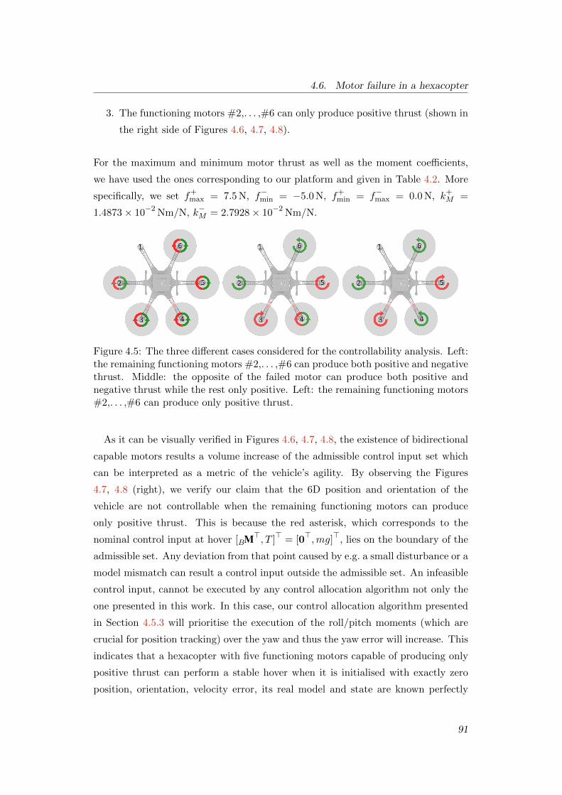
4.6. Motor failure in a hexacopter
3. The functioning motors #2,. . . ,#6 can only produce positive thrust (shown in
the right side of Figures 4.6, 4.7, 4.8).
For the maximum and minimum motor thrust as well as the moment coefficients,
we have used the ones corresponding to our platform and given in Table 4.2. More
specifically, we set f+max = 7.5 N, f−min = −5.0 N, f+
min = f−max = 0.0 N, k+M =
1.4873× 10⁻² Nm/N, k−M = 2.7928× 10⁻² Nm/N.
Figure 4.5: The three different cases considered for the controllability analysis. Left:the remaining functioning motors #2,. . . ,#6 can produce both positive and negativethrust. Middle: the opposite of the failed motor can produce both positive andnegative thrust while the rest only positive. Left: the remaining functioning motors#2,. . . ,#6 can produce only positive thrust.
As it can be visually verified in Figures 4.6, 4.7, 4.8, the existence of bidirectional
capable motors results a volume increase of the admissible control input set which
can be interpreted as a metric of the vehicle’s agility. By observing the Figures
4.7, 4.8 (right), we verify our claim that the 6D position and orientation of the
vehicle are not controllable when the remaining functioning motors can produce
only positive thrust. This is because the red asterisk, which corresponds to the
nominal control input at hover [BM>, T ]> = [0>,mg]>, lies on the boundary of the
admissible set. Any deviation from that point caused by e.g. a small disturbance or a
model mismatch can result a control input outside the admissible set. An infeasible
control input, cannot be executed by any control allocation algorithm not only the
one presented in this work. In this case, our control allocation algorithm presented
in Section 4.5.3 will prioritise the execution of the roll/pitch moments (which are
crucial for position tracking) over the yaw and thus the yaw error will increase. This
indicates that a hexacopter with five functioning motors capable of producing only
positive thrust can perform a stable hover when it is initialised with exactly zero
position, orientation, velocity error, its real model and state are known perfectly
91

4. Nonlinear Model Predictive Control
and there are no external disturbances. Unfortunately, this cannot be achieved in a
real system. An alternative solution, also shown in [Kamel et al., 2015] is to drop
the control of yaw and perform position only control.
When the MAV is equipped with bidirectional capable motors as shown in left and
middle of Figures 4.7, 4.8, the nominal control input at hover [BM>, T ]> = [0>,mg]>
lies inside the admissible control set and away from its boundaries providing enough
control authority including the control of yaw. Clearly, enabling the bidirectional
mode for all the remaining motors instead of a single one (the opposite of the failed
one) increases the volume of the admissible set and thus the agility of the vehicle.
However, in order to keep the motor direction inversions to the absolute minimum,
the second option was preferred for the experiments presented in Section 4.8.2.
It is important to highlight that with our approach we can easily apply any of the
two strategies discussed above. Specifically: (i) drop the yaw control when bidirec-
tional motors are not available; (ii) enable the bidirectional mode for one or more
motors. In the first case, flying with free heading is achieved by setting zero gains for
the orientation term introduced in (4.3). In the latter case the bidirectional mode
for one or more motors should be enabled by appropriately setting the upper and
lower bounds in the optimisation defined in (4.7). An example of our MAV following
setpoint commands (despite the loss of a motor) using the these two different modes
is shown in Figure 4.9.
Another strategy for handling a motor failure was presented in [Schneider et al.,
2012] with more experimental results in [Mazeh et al., 2018] and [Nguyen et al.,
2019]. In these works, it is shown that a hexacopter with a non symmetric motor
layout as shown in Figure 4.10 (right) can –in some cases– handle up to two lost
motors without losing control of yaw. This approach has the clear advantage that
bidirectional motors are not required. However, due to its asymmetric layout it can
only handle a single failure of specific motors. Specifically, a failure of either motor
or #1 or #6 results in an uncontrollable configuration. This is not the case for
our chosen strategy since due to symmetry it can handle failure of any actuator.
This is a very important property for a real system since the failure probability is
similar for every actuator. Another disadvantage of any asymmetric layout is that
the volume (and thus the overall MAV agility) of the admissible set V is less than
the one corresponding to the symmetric one. This is why symmetric layouts are
preferred in most multirotor platforms.
92

4.6. Motor failure in a hexacopter
-20
-10
0
-6 -6
10
20
-4 -4
30
40
-2 -200
2244
6 6
-20
-10
0
-6 -6
10
20
-4-4
30
40
-2 -20 0
2 24 4
6 6
-20
-10
0
-6 -6
10
20
-4 -4
30
40
-2-200
2 244
6 6
Figure 4.6: Visualisation of V defined in (4.9) cut at Mz = 0 for our hexacopterexperiencing a failure of motor #1. Left: Bidirectional mode enabled for the re-maining functioning motors. Middle: Bidirectional mode enabled for the oppositeof the failed motor. Right: Bidirectional mode off. Volume of V (used as a metricof the MAV agility) is maximised when bidirectional mode is on (left plot).
-0.4
-0.2
0
-2
0.2
-4
0.4
0 -202
24
-0.4
-0.2
0
-2
0.2
-4
0.4
0 -202
24
-0.4
-0.2
0
-2
0.2
-4
0.4
0 -202
24
Figure 4.7: V cut at T = mg for our hexacopter experiencing a failure of motor #1.Left: Bidirectional mode enabled for all the motors. Middle: Bidirectional mode onfor the opposite of the failed motor. Right: Bidirectional mode off. The red asterisk,which corresponds to the nominal control input [BM>, T ]> = [0,mg]> at hover, lieson the boundary of the set when the bidirectional mode is off (right plot).
-5 -4 -3 -2 -1 0 1 2
-3
-2
-1
0
1
2
3
4
5
-5 -4 -3 -2 -1 0 1 2
-3
-2
-1
0
1
2
3
4
5
-5 -4 -3 -2 -1 0 1 2
-3
-2
-1
0
1
2
3
4
5
Figure 4.8: V cut at Mz = 0, T = mg, for our hexacopter experiencing a completefailure of motor #1. Left: Bidirectional mode enabled for all the functioning motors.Middle: Bidirectional mode enabled for the opposite of the failed motor. Right:Bidirectional mode off. The control input at hover (red asterisk) lies on the boundaryof the admissible set when the bidirectional mode is off (right plot). Any deviationfrom that point will result in an infeasible control command which cannot be tracked.The same point lies inside V when the bidirectional mode is on, providing enoughcontrol authority for stable position and yaw control.
93

4. Nonlinear Model Predictive Control
Figure 4.9: Waypoint following despite the loss of a single motor. When bidirectionalmotors are available (top) the MAV maintains control of yaw and position. Yawcontrol is lost (bottom) when the remaining motors can only produce positive thrust.
Figure 4.10: Left: The symmetric motor layout used in this work. Right: The asym-metric layout proposed in [Schneider et al., 2012] which can handle a single motorfailure for four out of the six motors, without reverting the direction of rotation. Inthe event of no failure, the volume of the admissible set V is greater (resulting amore agile MAV) in the symmetric layout compared to the asymmetric one. This iswhy symmetric layouts are preferred in most multirotor platforms.
94

4.7. Fault identification
To sum up, we consider that our algorithms are generic enough and can be applied
to any of the strategies of handling a single motor failure discussed above (e.g.
enable bidirectional mode or fly with free heading when bidirectional hardware is
not available). Additionally, they can be applied to a hexacopter with any motor
layout (including non symmetrical motor rotation, or tilted motors) as long as the
relationship between actuator forces f and control inputs u is given by u = Af with
A the allocation matrix that depends on the vehicle’s structure. Combination of
the above (e.g. asymmetric motor layout with bidirectional motors) is also possible
with the appropriate allocation matrix and actuator limits adaptation.
4.7 Fault identification
Our goal is to online estimate whether one or more motors have failed (consequently
resulting in applied moments and collective thrust different from the ones com-
manded). To do so, we introduce the health variable hi ∈ R for each individual
motor i and assume that the effective force acting on the MAV generated from the
ith motor is fei = L(hi)fi, where L(h) = 1.05
1+e−h is the logistic function shown in
Figure 4.11 and fi corresponds to the respective motor thrust. Intuitively, we ex-
pect that L(hi) = 1 for a healthy motor and L(hi) → 0 for a stopped one. We
implemented an EKF that estimates the set of health variables hi online for each
individual motor. The effective body torques and collective thrust are now given
by: [BMT
]= A
[L(h1)f1 · · · L(h6)f6
]>, (4.10)
where A is the allocation matrix defined in (4.8), which depends on the moment
coefficients and the motor direction of rotation.
-6 -4 -2 0 2 4 6
0
0.5
1
Figure 4.11: The logistic function used for the EKF. Notice, that it is appropriatelyscaled such that h = L−1(1) has finite value.
95

4. Nonlinear Model Predictive Control
In our EKF, we use the following prediction model :
Bω = J−1(BM− Bω × JBω ) +wω, (4.11a)
fi =1
τf(f ri − fi + wf ),∀i = 1, . . . , 6, (4.11b)
hi =1
τh(h− hi) + wh,∀i = 1, . . . , 6. (4.11c)
The noises wω, wh, and wf are Gaussian white noise processes with densities σω,
σh, and σf , respectively. Equation (4.11a) corresponds to the MAV angular rate
dynamics while (4.11b) to the first order motor thrust dynamics with f ri the per-
motor reference thrust as given by the control allocation and τf the model time
constant. The first order health variables dynamics (4.11c) with time constant τh,
model how fast a failure can occur as well as ensure that h is an attraction point for
the hi estimates.
The measurement model is given by:
zω = Bω + vω, (4.12a)
zT = T + vT , (4.12b)
with vω ∼ N (0, σ2ωI) and vT ∼ N (0, σ2
T ) modelling the observation noise. The
measurements Bω and T required for the EKF update are obtained using the on-
board IMU. For Bω we use the bias corrected gyro measurements and for measured
collective thrust T we use T ≈ maz with m denoting the known mass of the MAV
and az the accelerometer measurement along the z axis. Notice that our observation
model for the collective thrust does not account for the Bω × Bv term which ap-
pears in the Body frame expressed linear acceleration dynamics. This was a design
choice, allowing the EKF to rely exclusively on inertial measurements and thus able
to be implemented as an algorithmic only update on any multirotor.
The values for the noise parameters and model constants are given in Table 4.1.
In order to avoid false positives due to e.g. inaccurate model, we use the estimated
value of hi and its estimated uncertainty. We consider a motor failed when L(hi +
3σi) < 0.5 (with σi denoting the health state standard deviation obtained as a
marginal from the state covariance matrix). When the above inequality is true
we update the control allocation algorithm by setting fmin = fmax = 0 for the
failed motor and enabling the bidirectional mode for the opposite. In the event of
a detected failure, the number of functional motors is reduced by one. It makes
96

4.8. Experimental results
Description Symbol Value Unit
Angular rate model noise density σω 3.16 rad/(s√
Hz)
Thrust model noise density σf 0.94 N/√
HzThrust model time constant τf 0.01 s
Health variables model noise density σh 0.31√
Hz−1
Health variables model time constant τh 0.3 sHealth variables model constant h 2.99 -Angular rate measurement noise σω 0.01 rad/sCollective thrust measurement noise σT 0.1 N
Table 4.1: Numeric values of the fault detection EKF Parameters.
sense then to continue estimating the health variables for the remaining functional
motors. This is done by introducing appropriate equality constraints f ri = fi = 0
for the failed motor which can be incorporated (following the approach discussed in
[Simon, 2010]) in the EKF through appropriate reduction of the model (4.11).
4.8 Experimental results
The experiments presented in this section were performed using our custom built
hexacopter described in Section 2.2 with the bidirectional propulsion system #2
described in Section 2.2.3. The state estimates are provided by the EKF described
in Section 2.4.1 with pose measurements obtained by a Vicon motion capture system.
The parameters of the control model and the control allocation are provided in Table
4.2.
In the following we present two different types of experiments. In Section 4.8.1
we show how the controller exploits the non-linear MAV model to perform step
commands in position and yaw. In Section 4.8.2, we further test the failure detection
and recovery strategy discussed previously by manually switching off a single motor
while flying.
4.8.1 Waypoint tracking
In both experiments presented, the MAV is first commanded to fly from a waypoint
with reference position W rrB = [1, 0, 3]> and orientation qrWB = [0, 0, 0, 1]> to a way-
point with reference position W rrB = [−1, 0, 1]> and orientation qrWB = [0, 0, 1, 0]>.
This corresponds to a 2 m position jump in x and z and 180° in yaw.
97

4. Nonlinear Model Predictive Control
Description Symbol Value Unit
MAV mass m 1.871 kg
MAV inertia in x axis Jx 0.032 kg/m2
MAV inertia in y axis Jy 0.034 kg/m2
MAV inertia in z axis Jz 0.070 kg/m2
Normal rotation thrust coefficient k+T 9.7408× 10⁻⁶ N/(rad/s)2
Normal rotation moment coefficient k+M 1.4873× 10⁻² Nm/N
Inverted rotation thrust coefficient k−T 6.3309× 10⁻⁶ N/(rad/s)2
Inverted rotation moment coefficient k−M 2.7928× 10⁻² Nm/N
Min thrust in normal motor rotation f+min 0.0 N
Max thrust in normal motor rotation f+max 7.5 N
Min thrust in inverted motor rotation f−min -5.0 N
Max thrust in inverted motor rotation f−max 0.0 NMotor inversion hysteresis threshold thyst 0.1 s
Table 4.2: Numeric values of control model parameters.
Figures 4.12 and 4.13 show the position and orientation response for the same ex-
periment using low Qq = 5 I3×3 and high Qq = 65 I3×3 orientation gains respectively.
Both maneuvers are executed in less than 2.5 s with linear accelerations exceeding
15 m/s2. In the high gain case, the yaw step is mainly performed by a half flip in
roll and pitch as shown in Figure 4.14. This shows an advantage of the model based
design over traditional approaches (e.g. PID) where a yaw maneuver is achieved by
applying Mz moment and subsequently rotating around the zB axis. Additionally,
compared to approaches such as [Brescianini and D’Andrea, 2018] where the shortest
rotation (between the current orientation and the reference one is preferred), our
NMPC always chooses the fastest rotation (which does not always coincide with the
shortest) based on the MAV dynamics.
Figures 4.12 and 4.13 additionally show the position predictions computed by the
NMPC. The predictions are updated at every controller iteration and thus start
from different initial states. In an ideal scenario, where the control and real model
are identical, one would expect all the predicted and real trajectories to perfectly
overlap. In reality, these two are close to its other but never coincide perfectly, as
the control model is an approximation (e.g. control input set approximated as a 4D
hyperrectangle, gyroscopic moments and motor dynamics ignored) of the unknown
real one.
Another observation, is that regarding the predicted and actual response in the
98

4.8. Experimental results
30 31 32 33 34 35 36
-1
0
1
2
3
Figure 4.12: The MAV position while performing the 2 m and 180° jump in positionand yaw with low orientation gains. Top: Two different views of the position andorientation response. Bottom: The per-axis position response (solid lines) alongsidethe NMPC predictions (faint lines). For visualisation clarity, here we plot the NMPCpredictions at 20 Hz compared to their actual update rate of 100 Hz.
y axis. It can be seen that position in y temporarily deviates from its zero refer-
ence. This behaviour is also reflected in the corresponding predictions and is the
result of the existence of coupling between the vehicle’s position and attitude. Even
though not tested in this work, this shows the potential use of a similar optimisation
framework as a discrete time dynamically feasible planner.
4.8.2 Fault detection and recovery
We tested the failure detection and autonomous recovery in two different scenarios
where one motor was switched off (i) while hovering and another (ii) while the
MAV was following setpoint commands. In the first case motor #1 was manually
deactivated by overwriting the thrust command produced by the control allocation
99

4. Nonlinear Model Predictive Control
27 28 29 30 31 32 33
-1
0
1
2
3
Figure 4.13: The MAV position while performing the 2 m and 180° jump in positionand yaw with high orientation gains. Top: Two different views of the position andorientation response. Bottom: The per-axis position response (solid lines) alongsidethe NMPC predictions (faint lines). For visualisation clarity, here we plot the NMPCpredictions at 20 Hz compared to their actual update rate of 100 Hz.
Figure 4.14: The MAV orientation while performing the position-yaw step with highorientation gains. Top: View from above (projection on the x-y plane). Bottom:View from the side (projection on the x-z plane). The yaw step is mainly achievedby a half flip in roll and pitch.
100

4.8. Experimental results
and sending a zero one instead. For the setpoint case, motor #3 was automatically
deactivated once the MAV was at a specific point in space. Due to the symmetric
motor layout we claim that deactivating any other motor would result in very similar
behavior. The failure was detected automatically and the failsafe activated based
on the methods described in Sections 4.6 and 4.7.
Figures 4.15 and 4.16 show the MAV position, the absolute yaw error and the on-
line estimated health status of each motor for the failure while hovering experiment.
The failure was injected at t = 23.68 s and identified at t = 23.85 s resulting in an
overall height loss of 0.3 m. We claim that even this minimal height loss is mainly
because of the slow motor dynamics due to the direction inversion command. This
can be justified as in Figure 4.15 there is no visible red line (indicating operation
with a motor failure that has not been identified yet). The fast detection can be
also verified by the video1 of the conducted experiments where the opposite motor
switches direction of rotation before the failed motor comes to a full stop. We re-
peated the same experiment twice and provide the 3D position data in Figure 4.17.
For these two additional experiments, the worst case detection delay and altitude
loss was 0.18 s and 0.4 m respectively.
For the waypoint experiments, we used four distinct waypoint commands (forming
a 2.0 m wide square) which were passed consecutively to the controller. Yaw and
height reference were kept constant to 0° and 2 m respectively. We define a sphere
around every waypoint as a tolerance to signal a waypoint as complete. That is,
when the MAV is inside the corresponding sphere, the next waypoint is passed to
the controller. Figures 4.18 and 4.19 show the MAV position, the absolute yaw error
and the per-motor estimated health status. Similarly, to the hovering experiments
the failure was identified within 0.16 s and resulted in a 0.5 m height loss. Two
additional experiments are illustrated in Figure 4.20 with a worst case detection
delay and height loss of 0.18 s and 0.52 m.
In both cases tracking of position and yaw is maintained and the MAV can recover
to the hover point for the first case and fly to the next waypoints for the second.
Not surprisingly, the 5-motor asymmetric configuration results in degraded tracking
performance especially for yaw.
Regarding the health status variables of the functioning motors, these always
1See https://youtu.be/cAQeSZ3tIqY
101

4. Nonlinear Model Predictive Control
23 24 25 26 27 28 29 30 31
0
20
40
Figure 4.15: Autonomous fault detection and recovery during hover. The failureis identified within 0.17 s after the manual deactivation of motor #1. Position andyaw tracking is maintained and the MAV recovers to the hovering spot.
0.5
1
0.5
1
0.5
1
0.5
1
0.5
1
24 26 28 30
0.5
1
Figure 4.16: The online estimates of the health status L(hi) and their correspond-ing 3σ upper and lower bounds for the hovering experiment. The upper boundL(h1 + 3σ1) for motor #1 drops below the 0.5 threshold within 0.17 s after themotor deactivation at t = 23.68 s
102

4.9. Discussion
Figure 4.17: Autonomous fault detection and recovery for two additional hoveringexperiments. The detection delay was 0.16 s for the experiment on the left and 0.18 sfor the right while the respective altitude loss was 0.35 m and 0.4 m respectively.
remain close to 1 for both types of experiments. However, in the setpoint case,
there exist some short-in-duration deviations from 1. These spikes correspond to
time instants when large angular accelerations were executed. We consider the
main reason for this behaviour to be the mismatch between the EKF prediction
model (which does not take into account less significant phenomena, such as the
gyroscopic moments) and the measurement model (which does not take into account
the Bω ×Bv ) and the real ones. Despite these temporary inaccuracies, the 3σ upper
bound was always greater than 0.8 and thus unable to trigger a false positive.
4.9 Discussion
In this Chapter we presented a nonlinear model based controller with the body
torques and collective thrust as the control input. We showed how this can be
used for aggressive maneuvers that fully exploit the dynamic capabilities of the
platform. Compared to other approaches such as [Kamel et al., 2017a, Falanga
et al., 2018], we drop the assumption regarding the lack of coupling between different
DoF. Consequently, there is no need for a separate attitude or rate controller and
the MAV position, velocity and orientation are controlled by a single control block.
This further enables the use of the same algorithm without any modifications as an
attitude, rate or mixed mode (e.g. linear velocity and yaw rate) controller by setting
non-zero gains Q to the terms in 4.5 which contain the states we are interested in
and zero for the rest. This property was particularly handy during the execution
of autonomous experiments, where the same algorithm was used as a safety backup
103

4. Nonlinear Model Predictive Control
24 26 28 30 32 34 36
0
10
20
30
Figure 4.18: Autonomous fault detection and recovery while following setpoint com-mands. The failure is identified within 0.16 s after the manual deactivation of motor#3. Position and yaw tracking is maintained and the MAV continues to follow thesetpoint commands.
0.5
1
0.5
1
0.5
1
0.5
1
0.5
1
24 26 28 30 32 34 36
0.5
1
Figure 4.19: The online estimates of the health status L(hi) and their correspond-ing 3σ upper and lower bounds for the setpoint experiment. The upper boundL(h3 + 3σ3) for motor #3 drops below the 0.5 threshold within 0.16 s after themotor deactivation at t = 26.80 s
.104

4.9. Discussion
Figure 4.20: Autonomous fault detection and recovery for two additional setpointexperiments. The detection delay was 0.17 s for the experiment on the left and 0.18 sfor the right while the attitude loss was 0.52 m and 0.5 m respectively.
attitude controller receiving orientation commands by a human operator.
We further proposed an optimisation based control allocation scheme that maps
the control inputs into feasible actuator commands. We showed how this can be
further extended for a platform capable of generating both positive and negative
thrust. We used this capability in order to stabilise the yaw of our hexacopter
experiencing a motor failure.
Finally, we developed an EKF that can be used for fast motor failure detection.
This solely relies on inertial measurements and can be implemented as an algorithmic
only update on any MAV and can be accordingly extended with motor speed and
current measurements.
We argue that all the algorithms presented in this section can be seamlessly imple-
mented on multirotors with different number or types of actuators. In that case the
allocation matrix A (used in the control allocation and the failure detection EKF)
has to be adapted based on the MAV geometry. Additionally, the strategy in the
event of an actuator failure has to be changed accordingly (e.g. no need for direction
inversion in the case of an octacopter or fly without yaw control in the case of a
quadrotor). An effective strategy on the MAV type, can be adopted by examining
the admissible set as discussed in Section 4.6. The NMPC block however, remains
the same irrespectively of the type of the underactuated MAV at hand. This has the
105

4. Nonlinear Model Predictive Control
clear advantage, that the computational complexity of the most resource demanding
part remains unaffected by the number of MAV actuators.
As part of future work, the extension of the model presented in this Chapter
with the effect of unmodeled – in the current implementation – phenomena (e.g.
gyroscopic moments, rotor drag) would be of high interest. Additionally, including
the motor dynamics in a control model with the individual motor thrust as control
input, will eliminate the need of the allocation algorithm. This will also eliminate
the case of not feasible control inputs introduced by the approximation of the feasible
control input set defined in (4.9) as a 4D hyperrectangle.
106

Chapter 5
Nonlinear Model Predictive
Control for aerial manipulation
Contents
5.1 Introduction . . . . . . . . . . . . . . . . . . . . . . . . . . . . . 108
5.2 Related work . . . . . . . . . . . . . . . . . . . . . . . . . . . . . 108
5.3 Contribution . . . . . . . . . . . . . . . . . . . . . . . . . . . . . 111
5.4 System overview . . . . . . . . . . . . . . . . . . . . . . . . . . . 112
5.5 Hybrid modelling . . . . . . . . . . . . . . . . . . . . . . . . . . 113
5.6 NMPC for aerial manipulation . . . . . . . . . . . . . . . . . . . 115
5.7 Extrinsics calibration . . . . . . . . . . . . . . . . . . . . . . . . 117
5.7.1 Arm to body frame transformation . . . . . . . . . . . . 118
5.7.2 Contact to world frame transformation . . . . . . . . . . 119
5.8 Reference computation . . . . . . . . . . . . . . . . . . . . . . . 120
5.9 Experimental results . . . . . . . . . . . . . . . . . . . . . . . . . 120
5.9.1 Trajectory tracking . . . . . . . . . . . . . . . . . . . . . 122
5.9.2 Velocity Sweep . . . . . . . . . . . . . . . . . . . . . . . 126
5.9.3 Trajectory size sweep . . . . . . . . . . . . . . . . . . . . 127
5.10 Discussion . . . . . . . . . . . . . . . . . . . . . . . . . . . . . . 128
Parts of this Chapter appear in: Tzoumanikas, D., Graule, F., Yan, Q., Shah, D., Popovic,
M., and Leutenegger, S. (2020). Aerial Manipulation Using Hybrid Force and Position
NMPC Applied to Aerial Writing. In Proceedings of Robotics: Science and Systems (RSS).
[Tzoumanikas et al., 2020a]
107
5. Nonlinear Model Predictive Control for aerial manipulation
5.1 Introduction
In Chapter 4 we presented a collection of algorithms required for safe and aggress-
ive flight of an MAV for tasks which do not require physical interaction with the
environment. In a more complex scenario, an MAV apart from being able to safely
navigate in space, it should be able to physically interact with its environment by
carrying appropriate mechanisms. Example applications include inspection of in-
frastructure like bridges or manufacturing plants [Ikeda et al., 2017, Angel Trujillo
et al., 2019, Bodie et al., 2019], physical interaction through MAV-attached tools
like grinding, welding, drilling and other maintenance work in hard-to-reach places
[Papachristos et al., 2014b, Bodie et al., 2019] and autonomous pick-up and trans-
port of objects [Kessens et al., 2016, Augugliaro et al., 2014]. Another possible
application includes the AABM scenario introduced in Chapter 3 where multiple
MAVs were used to 3D print a structure.
However, combining the maneuverability of aerial vehicles with the manipulation
capabilities of robotic arms comes at the cost of additional control complexity due to
the coupling of the dynamics of the two systems. The requirements for high precision
in real world aerial manipulation applications further increases the difficulty of the
task.
In this Chapter we extend the NMPC presented in the previous one for a combined
MAV-arm system performing an aerial manipulation task. We formulate a hybrid
control model for the combined system which incorporates interaction forces acting
on the end effector. We explain the practical implementation of our algorithm
and show extensive experimental results of our custom built system performing
multiple ‘aerial-writing’ tasks on a whiteboard revealing millimetre-level accuracy.
An instance of the conducted experiments is shown in Figure 5.1.
5.2 Related work
Aerial manipulation systems can be broadly distinguished based on the MAV type
(as being omnidirectional or underactuated) and the end effector (as being fixed
or moving). In general, using an omnidirectional MAV to fulfill complex aerial
tasks does not require a moving end effector as the necessary 6 DoFs are provided
by the MAV itself. Examples include the works presented by [Brescianini and
D’Andrea, 2016, Brescianini and D’Andrea, 2018a, Ryll et al., 2019]. [Brescianini
108

5.2. Related work
Figure 5.1: Our MAV-arm system performing an ‘aerial-writing’ task. Motion ofthe MAV and arm is jointly controlled by a single control block.
and D’Andrea, 2016] show an omnidirectional MAV called OmniCopter that achieves
6-DoF motion by using eight fixed rotors in a non co-planar configuration. In a sub-
sequent study [Brescianini and D’Andrea, 2018a], this platform is used with a fixed
end effector to fetch moving objects. Using a similar approach with a fixed con-
figuration of tilted rotors, [Ryll et al., 2019] propose a novel paradigm to control
all 6 DoF of the MAV while using a rigid end effector to exert forces and torques
independently. The system is demonstrated in numerous experimental tasks, e.g.
surface sliding.
Following a different approach, [Kamel et al., 2018] develop a setup of six rotors
which tilt individually to control the direction of their thrust vector. [Bodie et al.,
2019] leverage this system, named Voliro, to solve a variety of aerial manipulation
tasks with a rigidly mounted, low complexity end effector. The authors further show
precise force control when in contact with unstructured environments while running
online visual-inertial state estimation. While this platform allows for accurate 6-DoF
flight and longitudinal force exertion with a relatively simplistic control method, it
is mechanically more complex and thus more costly compared to classical multirotor
109

5. Nonlinear Model Predictive Control for aerial manipulation
platforms. Recently, a similar approach was followed by [Angel Trujillo et al., 2019],
who introduce AeroX, an omnidirectional octacopter for contact-based inspection.
Their end effector design minimises the torque caused by contact forces and features
wheels on its base to allow moving along a surface while remaining in contact.
In [Papachristos et al., 2014b, Papachristos et al., 2014a] the authors show a less
complex but highly capable tri-tilt-rotor MAV for surface grinding and obstacle
manipulation. The control model consists of two disjoint modes: one for free-flight
and another for physical interaction. The authors further discuss different force
exertion principles for under- and fully-actuated MAVs.
Employing an underactuated MAVs to perform aerial manipulation typically in-
creases the complexity of the end effector since it has to provide the additional DoFs.
To investigate this, many different end effector designs have been proposed over the
last years. We can categorise these works by the increasing complexity of the end
effector: [Darivianakis et al., 2014] use a fixed end effector on an under-actuated
MAV to perform contact-based tasks. The authors use a hybrid MPC method and
mode switching between a free-flight and in-contact model. Similarly to our work,
they benchmark their approach by performing “aerial-writing”. In [Mellinger et al.,
2011], the authors use different light-weight, low complexity grippers to perch, pick
up, and transport payload. Meanwhile,[Kessens et al., 2016] use a self-sealing suction
mechanism to pick up and carry objects. Moving up in terms of complexity,[Kim
et al., 2013] suggest mounting a 2-DoF robotic arm on a MAV to allow grasping
and transporting of objects. The authors propose an adaptive sliding mode control-
ler for the combined system. In [Orsag et al., 2014] the authors present an aerial
manipulator with two robotic 2-DoF arms to open a valve. The MAV and arms
are controlled as a coupled system which is modeled as a switched nonlinear system
during valve turning. In a more recent work,[Suarez et al., 2018] propose a light-
weight, human-sized dual arm system designed to minimise the inertia transferred
to the MAV. Each of the two arms add 5 DoFs to the system and the applied arm
control law takes into account that low-cost servo motors do not allow torque con-
trol but require position commands. Further, a torque estimator is used to predict
the torques produced by the servos and inform the MAV control algorithm accord-
ingly. In order to minimise such disturbances coming from the end effector, [Nayak
et al., 2018] propose a light-weight design which can produce longitudinal forces for
contact-based inspection using a switched system MPC method incorporating the
contact dynamics. While attaching a serial robotic arm on an MAV increases the
110

5.3. Contribution
number of tasks it can perform, they only provide limited precision when using low-
cost and light-weight actuators. Some previous efforts [Kamel et al., 2016a, Kamel
et al., 2016b] try to mitigate this by mounting a parallel delta arm on an MAV
instead.
As far as the control method is concerned, we distinguish three different ap-
proaches for controlling the motion of the MAV-arm system. The first one is de-
coupled control, with a few illustrative examples of an MAV equipped with a serial
link arm in [Orsag et al., 2013, Jimenez-Cano et al., 2013] and a parallel arm in [Cher-
mprayong et al., 2019]. In the decoupled control approach the MAV and arm motion
are independently controlled, and the effects of the arm on the MAV dynamics are
treated as unknown external disturbances. In the second approach, the control re-
mains decoupled but some of the effects introduced by the arm, are compensated in
a feed forward way. For example in [Mellinger et al., 2011] a mechanically simple
quadrotor-gripper system is used for aerial pick up and transport with the payload
mass and the CoM displacement being estimated by a batch least squares estimator
running online. Similarly in [Fresk et al., 2017] an EKF is used for online estimating
the CoM displacement caused by the arm motion of a hexacopter-arm system. In
both the aforementioned approaches the estimates are used in a feed forward fashion
by the MAV controller to improve tracking. In alternative work [Tognon et al., 2017]
the coupling effect is incorporated into feed forward terms computed exploiting the
differential flatness property of the system. The third approach includes forming a
unified model and controlling the system in a coupled way which overcomes the lim-
itations of the two methods described above. Examples include the work of [Mersha
et al., 2014, Yang et al., 2014] which employ feedback linearisation and LQR con-
trollers respectively and the works of [Garimella and Kobilarov, 2015, Lunni et al.,
2017] which –similar to our method– rely on an NMPC for free flight operation.
5.3 Contribution
In this work, we address the problem of precise aerial manipulation and employ our
underactuated MAV equipped with a 3DoF delta arm to showcase the capabilities
of our approach. In relation to the relevant work presented above, we show the
following contributions:
• The formulation of a hybrid model which captures the non-linear dynamics
111

5. Nonlinear Model Predictive Control for aerial manipulation
of the MAV and considers the quasi-static forces, including contact with the
environment, introduced by the attached manipulator. The control model is
derived using the Newton-Euler equations and can thus be easily extended to
any type of multirotor (underactuated/omnidirectional) and attached manip-
ulator.
• Use of this generic model in a NMPC which jointly controls the MAV and
arm motion. This natively handles the effects of the arm motion to the MAV
dynamics (e.g. displacement of CoM) as well as provides an easy way to control
the force (which is a function of the system states) exerted to the environment
during contact.
• Experimental evaluation of our method in “aerial-writing” tasks using our cus-
tom built system. Our results demonstrate high repeatability and millimeter-
level accuracy across multiple trajectories of varying difficulty.
5.4 System overview
The software components of the proposed system are outlined in Figure 5.2. The
state estimation block that fuses pose data from the motion capture system and the
onboard IMU is identical to the one presented in Section 2.4.1. Same applies to
the control allocation block described in Section 4.5.3 that transforms the control
inputs into actuator commands. As our focus is on precision rather than failure
detection and handling, we have deactivated the fault detection EKF presented in
Chapter 4. The NMPC is given full state trajectory commands for the MAV and
the end effector corresponding to a given aerial manipulation task. Based on these,
it produces the desired MAV body moments, collective thrust, and end effector
position. The desired end effector position is then transformed into joint angle
commands by solving the inverse kinematics problem for the delta arm described in
Section 2.3.1. All algorithms run onboard at a rate of 100 Hz.
In the free flight scenarios presented in previous chapters, equations of motion were
expressed using the MAV Body fixed frame F−→B and the World fixed frame F−→W .
For the setup presented in this Chapter we further introduce: (i) an arm frame F−→A,
an end-effector frame F−→E and the contact surface frame F−→T . An overview of the
different coordinate frames is given in Figure 5.3.
112

5.5. Hybrid modelling
Figure 5.2: An overview of the software running onboard our MAV in an aerialmanipulation task. The NMPC jointly controls the MAV and arm motion. Thedesired moments and thrust are transformed into motor commands using the controlallocation described in Section 4.5.3 while the delta arm joint angles are computedusing the inverse kinematics described in Section 2.3.2.
Figure 5.3: The different coordinate frames used in the aerial manipulation task.Specifically F−→W , F−→B, F−→A, F−→E , and F−→T stand for the World, MAV body, arm, endeffector, and contact frame, respectively.
5.5 Hybrid modelling
The derivation of the hybrid model used for control largely follows the one presented
in Section 4.5.2. It is appropriately augmented with the quasi-static forces intro-
duced by the arm dynamics and its interaction with the environment. Overall, the
113

5. Nonlinear Model Predictive Control for aerial manipulation
combined dynamics take the following form:
W rB = W vB , (5.1a)
qWB =1
2Ω(Bω )qWB , (5.1b)
W vB =1
mcCWB (BFr + BFe) + Wg, (5.1c)
Bω = Jc−1(BMr + BMe − Bω × JcBω ), (5.1d)
Ω(Bω ) =
[Bω×
Bω
−Bω> 0
](5.1e)
where mc, Jc are the combined MAV-arm mass and inertia tensors, respectively.
Regarding the forces and moments BFi,BMi, we use the subscript i ∈ r, e to
distinguish the ones generated by the MAV motors r from the ones caused by the
end effector movement e and its potential contact with the environment. In our
system, the MAV motor-generated forces and moments are given by:
BFr :=[0, 0, T
]>, T =
6∑i=1
fi, (5.2a)
BMr :=6∑i=1
(fiBri × Bez + (−1)i+1kmfiBez
), (5.2b)
with fi ∈ R the thrust produced by the ith motor, Bri its position with respect
to the MAV body frame, kM the known thrust to moment constant (as defined in
the motor model (2.8)) and Bez = [0, 0, 1]>. As shown in Section 4.5.3, Equation
(5.2) can be summarised as[BMr, T
]>= A
[f1 f2 . . . f6
]>with A ∈ R4×6
the constant allocation matrix obtained from (4.8) when all the available motors
can produce positive only thrust. The forces and moments BFe, BMe introduced by
the end-effector are given by:
BFe := CBE EFc, (5.3a)
BMe := BrE × BFe + (BrE − BrE0)× (CBW me Wg), (5.3b)
where EFc is the contact force acting on the end effector expressed in its frame
F−→E and BrE0∈ R3 the nominal end effector position which results in no CoM
displacement. The two terms in (5.3b) represent the moments due to contact and
due to the displacement of the CoM respectively. The combined mass mc = m+me
is the sum of the MAV and end effector, respectively, while the combined rotational
inertia can be computed as Jc = J +mediag(BrE − BrE0)2 with me being the mass
114

5.6. NMPC for aerial manipulation
of the end effector, J = diag(Jx, Jy, Jz) the inertia tensor of the MAV (including the
arm mass in nominal position) and diag(·) the corresponding diagonal matrix.
Regarding the contact force, we assume that this can be approximated with a
linear spring model as:
EFc = CET (ksT rEz), (5.4)
where ks is a known spring coefficient and T rEzis the normal component of the
contact surface penetration. This way, the controller can anticipate contact before
it even happens and there is no need for a switching mode controller (one for free
flight and another one for contact dynamics).
5.6 NMPC for aerial manipulation
For the control formulation we define the following control state and input:
x :=[W r>B,W v>B ,q
>WB ,Bω
>]>∈ R6 × S3 × R3, (5.5a)
u :=[BM>r , T,Ar>E
]>∈ R7. (5.5b)
The definition of the control state coincides with one in Section 4.5.1, whereas the
control input is augmented with the position of the end-effector ArE . Note that we
use BrE for the formulation of the control model, while ArE is used in the control
input. We use the constant and known homogeneous transformation TBA to change
the coordinate representation of these position vectors.
We use the following error functions for the position of the MAV, the position of
the end effector, the MAV linear and angular velocity, the orientation, the contact
force and the control input, respectively:
erB = W rB − W rrB, (5.6a)
erE = W rE − W rrE , (5.6b)
ev = W vB − W vrB , (5.6c)
eω = Bω − CBBrB
rωr, (5.6d)
eq = [q−1WB ⊗ qrWB ]1:3, (5.6e)
ef = fc − frc , (5.6f)
eu = u− ur, (5.6g)
115
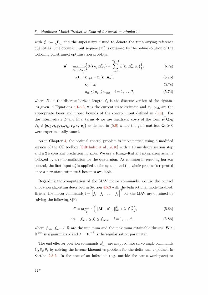
5. Nonlinear Model Predictive Control for aerial manipulation
with fc :=E
Fcz and the superscript r used to denote the time-varying reference
quantities. The optimal input sequence u∗ is obtained by the online solution of the
following constrained optimisation problem:
u∗ = argminu0,...,uNf
Φ(xNf
,xrNf) +
Nf−1∑n=0
L(xn,xrn,un)
, (5.7a)
s.t. : xn+1 = fd(xn,un), (5.7b)
x0 = x, (5.7c)
ulb ≤ ui ≤ uub, i = 1, . . . , 7, (5.7d)
where Nf is the discrete horizon length, fd is the discrete version of the dynam-
ics given in Equations 5.1-5.3, x is the current state estimate and ulb, uub are the
appropriate lower and upper bounds of the control input defined in (5.5). For
the intermediate L and final terms Φ we use quadratic costs of the form e>i Qiei∀ei ∈ erB,erE ,ev,eω,eq, ef ,eu as defined in (5.6) where the gain matrices Qi < 0
were experimentally tuned.
As in Chapter 4, the optimal control problem is implemented using a modified
version of the CT toolbox [Giftthaler et al., 2018] with a 10 ms discretisation step
and a 2 s constant prediction horizon. We use a Runge-Kutta 4 integration scheme
followed by a re-normalisation for the quaternion. As common in receding horizon
control, the first input u∗0 is applied to the system and the whole process is repeated
once a new state estimate x becomes available.
Regarding the computation of the MAV motor commands, we use the control
allocation algorithm described in Section 4.5.3 with the bidirectional mode disabled.
Briefly, the motor commands f =[f1 f2 . . . f6
]>for the MAV are obtained by
solving the following QP:
f∗ = argminf
(∥∥Af− u∗01:4∥∥2
W + λ ‖f‖22), (5.8a)
s.t. : fmin ≤ fi ≤ fmax, i = 1, . . . , 6, (5.8b)
where fmin, fmax ∈ R are the minimum and the maximum attainable thrusts, W ∈R4×4 is a gain matrix and λ = 10−7 is the regularisation parameter.
The end effector position commands u∗05:7 are mapped into servo angle commands
θ1, θ2, θ3 by solving the inverse kinematics problem for the delta arm explained in
Section 2.3.2. In the case of an infeasible (e.g. outside the arm’s workspace) or
116

5.7. Extrinsics calibration
unsafe end effector position command (e.g. one that results collision between the
MAV propellers and the arm’s links), the position command is reprojected onto the
boundary of the feasible and safe to operate workspace. In practice, this was rarely
the case as the MAV and end effector reference trajectories are designed (see Section
5.8) so that the end effector operates close to its nominal position. In this way the
usable workspace is maximised while the effect of the CoM displacement (which is
captured by our control model) is minimised.
Our C++ implementation of the above, requires 6.7 ms with a standard deviation
of 0.57 ms per iteration. On average, 98% of the computation time is spent on the
optimisation problems defined in (5.7) and (5.8).
We would like to highlight that our method is generic enough and can be eas-
ily applied on similar MAV-arm systems. In the case of an underactuated MAV
(similar to this work) the only part that has to be changed is the control allocation
method whcih depends on the vehicle type and its motor layout. In the case of an
overactuated MAV, the Equation 5.2a as well as the control input (5.5) should be
further augmented with the lateral forces. Regarding the arm, our method is arm
type agnostic as it only considers the end effector position. Additionally, the model
can easily be extended to capture aerodynamic friction, gyroscopic moments, handle
multiple contact points or use more sophisticated contact models (e.g. ones that in-
clude combination of linear springs and dampers). Similarly, the ‘aerial-writing’ task
which we use for the experimental evaluation of our framework, is just an example
application that requires precision. We believe that our algorithms are adaptable to
other tasks such as inspection through contact.
5.7 Extrinsics calibration
Apart from the various MAV related parameters (e.g. mass, inertia, motor coeffi-
cients), the control model depends on the arm F−→A to body F−→B frame transformation
TBA as well as the transformation TWT between the contact F−→T and world frame
F−→W . We experimentally observed that the system performance and mainly the
end-effector tracking accuracy are significantly affected by wrong estimates of these
transformations. We thus adopt an optimisation based calibration process.
117

5. Nonlinear Model Predictive Control for aerial manipulation
5.7.1 Arm to body frame transformation
Theoretically, getting an accurate estimate of the constant TBA can be done through
the detailed Computer Aided Design (CAD) of the system. In practice, precise
manufacturing of the aerial system with respect to the reference CAD model is
challenging. An alternative approach would be to separately track the F−→A and
F−→B pose using the motion capture system and compute their relative transform.
Unfortunately, the sideways mounted arm resulted in poor marker visibility for F−→A
and thus inaccurate results. To overcome this we follow an optimisation based
approach where the calibration process consists of the following steps:
1. We command the NMPC a constant position reference W rrE for the end ef-
fector.
2. With the MAV motors disabled, we manually move the MAV in various dif-
ferent positions and orientations. As the NMPC tries to keep the end effector
error as small as possible, the arm is constantly moving in order to counteract
the MAV movement.
3. We record the MAV position and orientation W rB, qWB as well as the end
effector position W rE using the motion capture system.
4. We compute the end effector position ArE expressed in F−→A using the encoder
measurements from the delta arm servos and the forward kinematics described
in Section 2.3.1.
Once the data collection is completed, we offline solve the following optimisation:
J = argminqBA ,BrA
( 1
N
N∑i=1
∥∥TWBiTBA ArEi
− WrEi
∥∥2), (5.9)
where the subscript i denotes the index of the N discrete observations. Since the
motion capture and encoder measurements are collected at different time instants,
we obtained time synchronised measurements W rBi,qWBi
,W rEi,ArEi
by evaluating
(using linear interpolation) the encoder data at the timestamps of the motion capture
data.
A side effect of estimating the TBA using the optimisation problem in (5.9) is that
it ensures that tracking accuracy of the end effector position commands is maxim-
ised. This allows small position and orientation offsets originating from imperfect
118
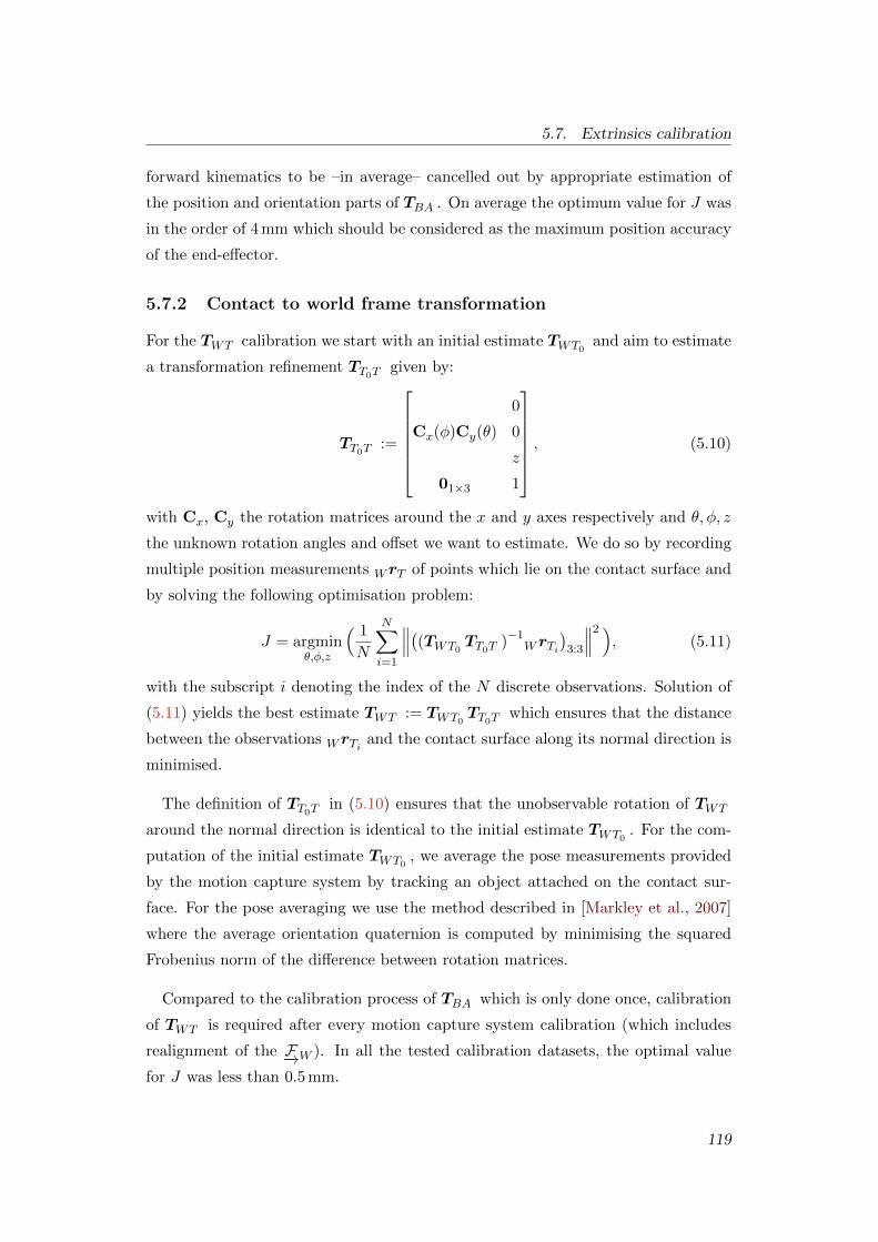
5.7. Extrinsics calibration
forward kinematics to be –in average– cancelled out by appropriate estimation of
the position and orientation parts of TBA . On average the optimum value for J was
in the order of 4 mm which should be considered as the maximum position accuracy
of the end-effector.
5.7.2 Contact to world frame transformation
For the TWT calibration we start with an initial estimate TWT0and aim to estimate
a transformation refinement TT0T given by:
TT0T :=
Cx(φ)Cy(θ)
0
0
z
01×3 1
, (5.10)
with Cx, Cy the rotation matrices around the x and y axes respectively and θ, φ, z
the unknown rotation angles and offset we want to estimate. We do so by recording
multiple position measurements WrT of points which lie on the contact surface and
by solving the following optimisation problem:
J = argminθ,φ,z
( 1
N
N∑i=1
∥∥∥((TWT0TT0T )−1
WrTi)
3:3
∥∥∥2 ), (5.11)
with the subscript i denoting the index of the N discrete observations. Solution of
(5.11) yields the best estimate TWT := TWT0TT0T which ensures that the distance
between the observations WrTi and the contact surface along its normal direction is
minimised.
The definition of TT0T in (5.10) ensures that the unobservable rotation of TWT
around the normal direction is identical to the initial estimate TWT0. For the com-
putation of the initial estimate TWT0, we average the pose measurements provided
by the motion capture system by tracking an object attached on the contact sur-
face. For the pose averaging we use the method described in [Markley et al., 2007]
where the average orientation quaternion is computed by minimising the squared
Frobenius norm of the difference between rotation matrices.
Compared to the calibration process of TBA which is only done once, calibration
of TWT is required after every motion capture system calibration (which includes
realignment of the F−→W ). In all the tested calibration datasets, the optimal value
for J was less than 0.5 mm.
119

5. Nonlinear Model Predictive Control for aerial manipulation
5.8 Reference computation
We use a trajectory generator to map arbitrary sets of characters to end effector
trajectories. We use a constant acceleration motion model to generate trajectories
with a smooth velocity profile. This is of special importance when the reference
path contains sharp edges. Through our software we can adjust the velocity and
acceleration profile by changing the maximum ‖W vrE ‖ and ‖W arE ‖. Once the tra-
jectory for the end effector has been computed, we proceed with the computation
of the reference position W rrB and velocity W vrB for the MAV as follows:
W rrB = W rrE − CWB BrE0, (5.12a)
W vrB = W vrE − CWB Bωr × BrE0
. (5.12b)
The reference MAV orientation qrWB is chosen such that the end effector position
is always perpendicular to the contact surface, assuming perfect position tracking.
Computation of the MAV reference position using the above equations ensures that
the end effector operates close to its nominal position BrE0. Given a dynamically
feasible trajectory for the end effector, the desired acceleration, jerk and snap for
the MAV can be computed by further differentiating (5.12a) and using C = C [ω ]×
for the rotation matrix derivative.
In our framework, each trajectory is accompanied by an appropriate flag which
disables or enables the position tracking for the end effector. This is achieved by
setting the appropriate gains to zero. In that case the NMPC may decide to move the
arm to assist the reference tracking of the MAV due to the CoM displacement. This
– depending on the application – potentially unwanted behaviour can be avoided
by further penalising (i.e. by increasing the input gains) the arm displacement from
its nominal position. However, it is an interesting capability enabled by our hybrid
modeling.
5.9 Experimental results
The experiments presented in this section were performed using the custom built
hexacopter equipped with the sideways mounted delta arm manipulator described
in Sections 2.2 and 2.3 respectively. In order to cope with the increased payload
we used the propulsion system #1 described in Section 2.2.3. The end effector of
the delta arm holds the pen which is mounted on a spring to provide additional
120

5.9. Experimental results
compliance. We set the coefficient of the contact model in Equation (5.4) to match
the used spring. The applied force is measured by a SingleTact1 force sensor, which
provides measurements at a resolution of 9× 10⁻³ N, mounted at the end of the
spring. We estimate the spring coefficient ks by measuring the applied force for
known tip displacements. We measured the inertia of the MAV J by checking its
angular response to constant input torque while it is hanging to freely rotate. A
table with all the numeric values of the system parameters, used in the control
model, is given in Table 5.1 while a photo showing the platform and its different
components is shown in Figure 5.4.
Description Symbol Value Unit
MAV mass m 2.6 kgEnd effector mass me 0.058 kg
MAV inertia in x axis Jx 0.042 kg/m2
MAV inertia in y axis Jy 0.054 kg/m2
MAV inertia in z axis Jz 0.110 kg/m2
Moment coefficient kM 1.5864× 10⁻² Nm/NSpring coefficient ks 42.95 N/m
Table 5.1: Numeric values of control model parameters.
Full state estimates are obtained by the EKF described in Section 2.4.1 which fuses
the onboard IMU measurements and the pose estimates provided by a Vicon motion
capture system. Each experiment consisted of the following different trajectory
stages: (i) approach, (ii) write, and (iii) return home. The end effector tracking
was enabled, using the appropriate flags as mentioned in Section 5.8, for the writing
trajectory and disabled for the rest. Our analysis mainly focuses on the trajectory
writing which includes contact whereas for the other two parts (approach/return) the
MAV performs simple position tracking. We evaluate the accuracy of our system
by comparing the reference trajectories to those estimated by the Vicon motion
capture system. In addition, we use a vision-based error as a performance metric.
This is because we observed inaccuracies in the Vicon measurements stemming from
either bad calibration, poor object visibility, or marker reflections on the whiteboard
surface. The visual error is computed by running a 2D Iterative Closest Point (ICP)
method [Besl and McKay, 1992] on a filtered and rectified photo of the final writing
and a rendering of the planned path. After registration of the two point sets, we
1See https://www.singletact.com/.
121

5. Nonlinear Model Predictive Control for aerial manipulation
Figure 5.4: The aerial manipulation platform used in the ‘aerial writing’ experimentsin Section 5.9 with labels for its individual components.
use the nearest neighbour distance to evaluate the accuracy.
In the following we show four experiments: in Section 5.9.1 we present detailed
and repeatable results for two different trajectories, namely RSS and E = mc2. We
then show consistent tracking performance across varying MAV velocities and text
sizes in Sections 5.9.2 and 5.9.3, respectively.
5.9.1 Trajectory tracking
Figure 5.6 shows the tracking of the RSS trajectory visualised in the contact frame
F−→T for the end effector and the MAV. The maximum reference velocity was set to
7.5 cm/s and the maximum acceleration to 2.5 cm/s2. The trajectory consists of four
contact segments with a combined duration of 65 s. Based on the Vicon estimates
the tracking error of the end effector remains in the [−10, 10] mm range during the
contact segments while the MAV position error is within the [−40, 40] mm range.
This highlights the efficacy of using a manipulator with faster dynamics than the
MAV’s for precision tasks such as ‘aerial-writing’.
Similarly to the above, Figure 5.8 shows the trajectory tracking for the more chal-
122

5.9. Experimental results
lenging E = mc2 experiment which contains ten contact segments with a combined
duration of 63 s. Tracking accuracy is similar as before with the end effector and
MAV tracking error in the [−10, 10] and [−50, 50] mm range. The accuracy can be
visually verified since the overlapping segments of the ‘R’ and ‘m’ coincide almost
perfectly. Additionally, the consistent approaching and retracting from the contact
surface leads to identical starting points of individual letter segments, e.g. the three
horizontal lines of the letter ‘E’. In both cases, the maximum error based on the
visual error analysis is 10 mm mostly originating from temporary loss of contact.
Possible reasons for this are bad estimation of the orientation part of the contact
frame transformation TWT , the assumption of a perfectly flat contact surface being
wrong and most importantly the finite accuracy of the delta arm. The imperfect
tracking along the contact frame normal direction (shown in blue in Figures 5.6,
5.8) is also reflected in the reference force tracking.
In order to prove the repeatability of our approach, we conducted each experiment
thrice. We give the relevant tracking statistics for the MAV and arm separately in
Figure 5.9, in which the textured box plots correspond to MAV data and the plain
ones to that of the end effector. The median and upper values for the end effector
are significantly lower than the ones for the MAV further showing the need of an
aerial manipulator for precise tasks including contact. The MAV tracking accuracy
along the z axis was the lowest amongst all axes, as this was most affected by the
interaction forces and unmodeled torque disturbances due to the movement of the
servos.
123

5.
Non
linea
rM
od
elP
redictive
Con
trolfor
aerialm
anip
ulation
0 0.1 0.2 0.3 0.4 0.5 0.6 0.7 0.8 0.9
0.05
0.15
0.25
0.35
0.45
0.55
0 0.1 0.2 0.3 0.4 0.5 0.6 0.7 0.8 0.9
0.05
0.15
0.25
0.35
0.45
0.55
0
2
4
6
8
10
Figure 5.5: Reference and actual tip position (left) as estimated by Vicon. Blue corresponds to contact segments while orangerefers to free flight. Visual error (right) between reference and actual tip position. The maximum estimated error is lower than10 mm and is located at discontinuous segments as expected.
-10
0
10
-60
-30
0
30
60
0 20 40 60 80 100 1200
0.5
Figure 5.6: Reference tracking error of the tip position (top), MAV (middle), and measured contact force (bottom). The trackingerror is plotted in the contact frame F−→T . The tracking accuracy of the end effector is significantly greater than that of the MAV,given that they remain in the [−10, 10] mm and [−40, 40] mm ranges, respectively.
124

5.9.E
xp
erimen
talresu
lts
0 0.1 0.2 0.3 0.4 0.5 0.6 0.7 0.8 0.9
0.15
0.25
0.35
0 0.1 0.2 0.3 0.4 0.5 0.6 0.7 0.8 0.9
0.15
0.25
0.35
0
2
4
6
8
10
Figure 5.7: Reference and actual tip position (left) as estimated by Vicon. Blue corresponds to contact segments while orangerefers to free flight. Visual error (right) between reference and actual tip position. Similarly as in the RSS experiment shown inFigure 5.6, maximum error does not exceed 1cm.
-10
0
10
-60
-30
0
30
60
0 20 40 60 80 100 1200
0.5
Figure 5.8: Reference tracking error of the tip position (top), MAV (middle) and measured contact force (bottom). The trackingaccuracy of the end effector is significantly greater than that of the MAV, given that they remain in the [−10, 10] mm and[−50, 50] mm ranges, respectively
125

5. Nonlinear Model Predictive Control for aerial manipulation
Figure 5.9: MAV and end effector box plots of the contact segments for 3 iterationsof the RSS trajectory experiment (top) and the more challenging E = mc2 trajectoryexperiment (bottom).
5.9.2 Velocity Sweep
The aim of the next experiments is to demonstrate the effects of the input velo-
city and acceleration on the writing accuracy. We performed five iterations of the
same Hello trajectory experiment with different velocity and acceleration profiles.
These correspond to maximum velocity ‖W vrE ‖ ∈ 7.5, 12.5, 17.5, 22.5, 27.5 cm/s
and maximum acceleration ‖W arE ‖ ∈ 3.75, 6.25, 8.75, 11.25, 13.75 cm/s2.
Figure 5.10 shows the box plots for the MAV and end effector tracking accuracy
based on the Vicon measurements. The plots show that consistent tracking results
are obtained in all the different velocity and acceleration settings tested. The nu-
meric values of the tracking error are similar to the ones previously presented with
the end effector achieving sub centimetre accuracy (per axis) while the MAV error is
consistently less than 50mm. However, by observing the visual error, we verify that
as the reference velocity increases, the system struggles more with the trajectory
segments containing curvature e.g. ‘e’ and ‘o’. In contrast, the performance on the
126

5.9. Experimental results
Figure 5.10: MAV and end effector box plots(top) and visual errors(bottom) for5 iterations of the Hello trajectory. Different iterations correspond to differentvelocity and acceleration profiles.
straight line segments remains similar.
We believe that the tracking error of the MAV can be further reduced if the NMPC
was given dynamically feasible trajectories not only for position and velocity but also
acceleration, jerk, and snap. Regarding the end effector tracking error, we generally
expect this to increase for reference velocities beyond the ones tested here. This
is because our control model assumes that the position of the end effector can be
controlled infinitely fast which is not the case for a real system.
5.9.3 Trajectory size sweep
In Figure 5.11 we show the visual error of our system for the same trajectory in four
different text sizes ranging from 10 to 40 cm. The consistent accuracy observed
shows that the system can handle the fast direction changes imposed by the small
scale.
0 0.1 0.2 0.3 0.4 0.5 0.6 0.7
0.05
0.15
0.25
0.35
0.45
0
2
4
6
8
10
Figure 5.11: Visual error plot showing consistent results for varying text sizes
127

5. Nonlinear Model Predictive Control for aerial manipulation
5.10 Discussion
Overall, our system achieves accurate and consistent results over a series of different
trajectories. The end effector tracking error consistently remains in the [−10, 10] mm
range for trajectories with maximum velocities ranging from 7.5 to 27.5 cm/s,
maximum acceleration from 3.75 to 13.75. The tracking error of the end effector is
significantly lower than the one for the MAV highlighting the accuracy boost due
to the utilisation of the arm. We would like to mention that our system was built
using relatively cheap off-the-shelf components and 3D printed parts. This leads to
errors in the manufacturing of the aerial system with respect to the reference model
e.g. errors in the true inverse kinematics of the arm due to non-identical dimensions
of its links.
Another important issue that we faced during our experiments, was the reliance
on the motion capture system for localisation. Apart from issues related to WiFi
delays which resulted in temporary loss of tracking, we faced issues with poor object
visibility resulting in unreliable estimates of both the static objects, such as the
contact frame, and moving ones such as the MAV. In fact, during our data analysis
we realised that there are segments where Vicon returned mechanically impossible
configurations for our system e.g. end effector position below the surface of the
contact frame. Despite these problems which further propagate into tracking errors,
our system was able to handle well multiple transitions to contact during the same
experiment.
We experimentally verified that for contact tasks, where the main objective is
accuracy instead of speed, using a planner respecting full state dynamic feasibility is
not an absolute necessity. Despite our simplified motion planner, our system achieves
sub-centimeter accuracy. However, we argue that for more aggressive maneuvers, a
full state dynamically feasible planer would be required.
Regarding future work, we consider that online estimation of the contact frame
transformation TWT would be beneficial as our system was very sensitive to its
wrong estimates. This would be very useful in a real life scenario (e.g. inspection
through contact) where the contact surface might not be reachable and thus its
position and orientation not directly measurable. Furthermore, it will provide a
natural way of handling contact with curved or generally non flat surfaces. Another
possible extension is that of using visual feedback to close the (currently open) loop
128

5.10. Discussion
of the aerial manipulation task. This requires the formulation of a visual-based
error metric based on the reference aerial manipulation task and the achieved one
(e.g. reference end effector trajectory and observed one). Closing this feedback loop
would result a major improvement for errors stemming from bad calibration (e.g.
TWT , TBA ), state estimate delays or inaccuracies of the arm. Finally, using a better
model for the combined MAV-arm system, would result better tracking performance.
As a first step, we can approximate the arm response using a first order model (the
current method further assumes an instantaneous end effector position response)
or ultimately, formulate the full multi-body dynamics model. The last would be
beneficial for agile combined maneuvers not tested in this work.
129

5. Nonlinear Model Predictive Control for aerial manipulation
130
Chapter 6
Conclusions
Contents
6.1 Summary of results . . . . . . . . . . . . . . . . . . . . . . . . . 131
6.2 Future work . . . . . . . . . . . . . . . . . . . . . . . . . . . . . 134
6.1 Summary of results
In this section we present a summary of the contributions and results which have
been presented in detail in the previous chapters.
In Chapter 3 a linear MPC incorporating soft state constraints as well as a gen-
eric framework for vision based tracking were presented. A cascaded control ap-
proach was adopted with the position and attitude dynamics being independently
controlled. The position control problem was formulated as a canonical form QP en-
abling online computation using any generic QP solver. The experiments conducted
for the MBZIRC competition showed that the designed controller can be used for
tracking and landing on a target moving with velocities not exceeding 5.0 m/s while
the experiments related to the AABM project revealed that the system is extremely
accurate (maximum per-axis error of 1.5 cm) for slow reference trajectories. Main
benefit of this control approach is its easy deployment on any platform which is
equipped with a closed loop attitude controller. This can be further justified since
the experimental results presented in Chapter 3 were obtained using three different
platforms. These two advantages (accuracy for slow maneuvers, ease of use) made
this controller our preferred choice for the majority of our experiments and live
demos which did not require agile maneuvers.
131
6. Conclusions
The linear MPC was extended to an NMPC in Chapter 4. By using a quaternion
based parameterisation and the non linear model of the system we overcame the main
limitations of the initial approach (i.e. inaccurate system model when operating away
from the linearisation point, gimbal lock due to the use of Euler angles). Through a
simple position-yaw step maneuver we showed how the controller can use the non-
linear dynamics –in an unconventional way– so as to perform the reference task as
fast as possible. In order to enable robust operation despite the loss of a single
actuator, we examined the controllability of our MAV and proposed a stabilisation
technique (based on reversing the motor direction during flight) which ensured stable
position and yaw response. To address the more realistic scenario, of a mid flight
motor failure, we developed an EKF which relies on inertial measurements and
monitors the health status of all the motors. This was used for autonomous detection
and recovery in experiments where one motor was abruptly switched off. Apart from
the advantages presented above (i.e. valid model irrespectively of the MAV state,
robustness in mechanical failures) the developed controller does not rely on the
existence of an attitude or rate controller. This property can be used for tracking of
full state dynamically feasible trajectories and natively enables the use of the same
controller as e.g. an attitude or rate controller by nullifying the cost function terms
that are not required.
A rushed comparison between the linear controller (Chapter 3) and the non linear
one (Chapter 4) would always result in favor of the latter. However, in practice
this is not always the case. The unified control of both the fast attitude and rate
as well as the slow position dynamics of the MAV from a single controller requires
state estimates to be provided at a high update rate. We experimentally identified
that the NMPC controlled system can experience unstable behavior for update rates
lower than 70 Hz while to avoid this, the controller was always run at rates equal
or greater than 100 Hz. To eliminate potential instability issues related to delays
between perception and actuation, the NMPC was only tested on relative powerful
CPUs while special effort was made to phase out potential sources of delays in the
software pipeline. In contrast, the position and attitude dynamics separation of the
linear MPC allows the position controller to run at much lower rates. Specifically,
in the presented experiments the position loop rate was 20 Hz (while the system was
still stable when the rate was reduced to 10 Hz) which shows that the same controller
can be used in conjunction with a low rate state estimation scheme e.g. a SLAM
system that runs at camera rate. As a consequence of the low rate updates and
132

6.1. Summary of results
the simpler optimisation problem, we have successfully run the linear MPC using
less powerful onboard computers such as an Odroid XU41. When available, the
extra computational power can be devoted to increasing the length of the predic-
tion horizon of the linear MPC which given valid model predictions would result
a performance improvement compared to implementations with a shorter horizon.
Given the above, the choice between the two controllers on a real system, should
not solely depend on their theoretical principles but should be a function of the
platform hardware, the available state estimation and more importantly the desired
MAV application.
The final contribution presented in Chapter 5 was an extension of the NMPC for
tasks requiring interaction with the environment. There, the motion of an MAV-arm
system was jointly controlled while also considering the quasi static forces introduced
by the arm and its interaction with the environment. This approach compensates
for the CoM displacement due to the end effector motion as well as the interaction
forces acting on the end effector which are further integrated into forces and moments
acting on the MAV base. We consider the method generic enough to be extended for
multiple contact points as well as to be applied on similar systems since the control
model is platform and arm-type agnostic. Overall, our custom built system achieves
sub centimetre accuracy in “aerial writing” which was used as an example scenario
that requires accuracy.
All in all, the experimental verification presented in this work would not be pos-
sible without the: (i) the hardware platforms built, (ii) the state estimation software,
(iii) the parameter identification all presented in Chapter 2 and (iv) the complete
software framework that enables easy MAV operation. The latter includes the con-
trollers and estimators described in this work, provides an interface for flight tasks,
implements multiple control modes for redundancy as well as contains the state ma-
chines which monitor the health status of all vital components (e.g. IMU and state
estimation rate). So far, our framework has been used in many indoor and outdoor
experiments including more than 100 public demonstrations with some examples
shown in Figure 6.1.
1See https://www.odroid.co.uk/hardkernel-odroid-xu4. Accessed April 2020.
133

6. Conclusions
(a) Initial OKVIS enabled flights, April 2016. (b) Live demo at Imperial Festival, May 2016.
(c) Live demo at Imperial Festival, May 2017. (d) AABM integration week, December 2017.
(e) AABM integration week, July 2018. (f) Initial NMPC tests, September 2018.
(g) Initial MAV-arm tests, May 2019. (h) GPS enabled flights, June 2019.
Figure 6.1: Examples of experiments and live demos accomplished with our softwareframework.
6.2 Future work
Regarding the linear MPC presented in Chapter 3, its natural extension to an NMPC
was presented in Chapter 4. Therefore, future extensions should be focused on the
engineering implementation such as including the effect of external disturbance in
the control model as in [Kamel et al., 2017a] and use the fastest QP solver [Frison
and Diehl, 2020] to date.
Our analysis regarding future work focuses on the two NMPC algorithms presen-
ted in Chapters 4 and 5 respectively.
134

6.2. Future work
More accurate system modelling. In both NMPC formulations we ignored less
significant phenomena such as the gyroscopic moments, the motor dynamics as well
as aerodynamic drag. Incorporation of the first two into the control model, re-
quires the rotor angular velocity to be considered as the control input which further
eliminates the need of the control allocation algorithm as the actuator commands
will be directly computed by the NMPC optimisation. Compared to the existing
approach, this comes at the cost of increased computational complexity for MAVs
with more than four motors. However, it ensures that the motor dynamics are taken
into account (e.g. in practice the motors cannot accelerate or decelerate infinitely
fast as assumed by our approach) and most importantly yields no approximation for
the feasible control input set (e.g. feasible control input set presented in Section 4.6
approximated as a 4D hyperrectangle in the current approach). Regarding the aero-
dynamic effects, recent work [Faessler et al., 2017] showed that tracking performance
(especially when the MAV has to follow long in duration aggressive maneuvers) can
be further improved when these are taken into account by the control model. The
main challenge however is the tedious identification of the drag coefficients which
requires experiments to be done in controlled wind tunnel environments.
Online model refinement. In this work, the model parameters (e.g. MAV mass,
inertia and motor constants) were identified offline and the control model remained
unchanged while flying. We can make the controller adaptive to model changes by
online estimating these by e.g. adopting the approaches discussed in [Bahnemann
et al., 2017] and [Burri et al., 2018] and updating the model online. By doing so, we
do not only take into account for parameters which change over time (e.g. the mass
of the MAV in the AABM experiments), but also correct for model or parameter
estimation errors which affect the flight performance. An example of the latter
includes the online estimation of the position of CoM which is affected even by a
small misplacement of the MAV battery. Online model refinement will eliminate the
need of using integral terms (as done in the experiments presented in Section 3.7) in
order to compensate steady state offsets arising from mismatches between the real
and control model.
Quantitative comparison between the MPC and NMPC. The controller de-
scribed in Chapter 4 was designed in order to overcome the limitations of its linear
counterpart described in Chapter 3. While the two methods were presented in detail,
a quantitative comparison of the tracking performance achieved was not performed.
135

6. Conclusions
As also shown in similar work [Kamel et al., 2017b], we anticipate the NMPC to
dominate when fast maneuvers are required while both the MPC and the NMPC
should perform similar for slow or static trajectories. However, it would be benefi-
cial to further quantify the performance improvement due to the use of a nonlinear
model approach as a function of e.g. the reference velocity, acceleration or the num-
ber of DoFs excited at the same time. Such an analysis can provide an objective
criterion as to when switching to a NMPC is beneficial.
Use the NMPC in a machine learning framework. In recent learning-based
control works such as [Zhang et al., 2016, Muller et al., 2018b, Kaufmann et al.,
2020] the MAV control policy is trained entirely in simulation in a supervised fash-
ion using training data provided by either human demonstrations or a preexisting
closed loop controller. Such approaches have the potential to outperform classic
MPC approaches in terms of computational cost while, depending on the network
structure, may not require an explicit state estimation scheme during test time. We
believe that our NMPC framework can be utilised to provide demonstrations to be
used during the training phase of the neural network while it can be easily adapted
to different MAV models used in the network design (e.g. consider the MAV rates as
the control input). The proven capability of running in real-time enables the NMPC
to run as a safety backup or, as an attempt to handle the simulation-to-reality gap,
provide online training data in the event of e.g. an MAV state or reference on which
the trained policy does not perform well.
Investigate robustness of fault detection EKF. The EKF used for motor fail-
ure detection was only tested in indoor flights in the absence of external disturbances.
Theoretically, a large in magnitude disturbance (e.g. a wind gust) can disturb the
MAV in a way to “trick” the EKF and trigger a false positive. This has to be further
investigated prior to the deployment on an MAV which operates in outdoor envir-
onments. A potential solution to this problem would require the system state to be
augmented with wind states which should also be estimated online. An alternative
solution, which does not require any software modification, includes lowering the
threshold for the health status upper bound L(hi+3σi) used for signalling a fault of
the ith motor. Lowering this threshold will decrease the probability of a false positive
in the expense of an increased detection delay. Finally, a more robust solution would
be to further augment the EKF with per-motor encoder and current measurements
and their corresponding models. However, this option requires additional hardware
136

6.2. Future work
which is not available to every MAV and therefore defeats the main advantage of
the original method which is the algorithmic only implementation.
Multi-body dynamic modelling. The hybrid MAV-arm model only considers
the quasi static forces introduced by the arm. In order to utilise the full potential
of the model based approach, a multi-body dynamic model has to be formulated.
This will allow for agile combined maneuvers, as well as capture the effect of the
servo torque (required for the arm motion) on the MAV base. From a hardware
perspective this approach would require the manipulator motors to support direct
torque control which is not possible with the cheap and lightweight servos used in
this work. Most of the commercially available motors with such a capability are
designed for ground robots and are -due to weight limitations- unsuitable for use in
aerial vehicles of similar scale as ours. A potential solution includes the design of
proprietary motor-controller hardware setups as in [Kamel et al., 2016b] that take
into account the maximum required torque for controlling the arm’s motion as well
as the limited payload capacity of MAVs.
Closed loop control of the manipulation task. As mentioned in Chapter 5 the
overall performance is sensitive to wrong estimates of the contact frame. This is be-
cause the contact forces are part of the model and the NMPC anticipates them to
occur at a known position and time instant. To overcome this, one can use the force
sensor measurements and the MAV state in order to estimate the contact frame
normal direction online. This will not only account for small calibration errors but
will enable aerial interaction with e.g surfaces which are not perfectly flat. Another
possible extension which will improve the overall performance of the system is to
close the loop of the interaction with the environment task with visual feedback.
This will compensate for errors arising from either small MAV model inaccuracies
or arm kinematics mismatches and will handle the existence of drift in the MAV
position estimates which is usually the case for vision based localisation.
Tests with omnidirectional MAVs. A main advantage of the NMPC for aerial
manipulation is that a reference contact force can be provided and followed by the
system. Since the used underactuated MAV cannot produce lateral forces in the
body frame, the desired force was produced through the inertial coupling between
the arm and the MAV. Also, in our experimental setup the maximum contact force
was further constrained by the low stall torque of the delta arm servos. In order to
showcase our algorithm in scenarios requiring exertion of significant lateral forces,
137
6. Conclusions
we would like to test our NMPC with hardware platforms such as the ones presented
in [Bodie et al., 2019] and [Ryll et al., 2019] which have much higher capabilities in
terms of lateral force control.
Collision free navigation. In this work we presented algorithms that can run
in realtime on commercially available hardware and form the basis for more com-
plex/realistic experimental scenarios. However, there are a few missing components
which are crucial for successful deployment in the unstructured real world. The
most important one is the generation of collision free trajectories since all presen-
ted experiments relied on the assumption of an obstacle-free space. This is usually
achieved by online mapping of the environment e.g. [Oleynikova et al., 2017, Vespa
et al., 2018] using onboard sensors such as RGBD cameras and subsequently using
the built map for generation of obstacle free paths e.g [Zucker et al., 2013, Richter
et al., 2016, Oleynikova et al., 2016].
138
Bibliography
Bibliography
[Achtelik et al., 2013] Achtelik, M. W., Lynen, S., Chli, M., and Siegwart, R. (2013).
Inversion based direct position control and trajectory following for micro aerial
vehicles. In 2013 IEEE/RSJ International Conference on Intelligent Robots and
Systems, pages 2933–2939.
[Alexis et al., 2013] Alexis, K., Huerzeler, C., and Siegwart, R. (2013). Hybrid mod-
eling and control of a coaxial unmanned rotorcraft interacting with its environ-
ment through contact. In 2013 IEEE International Conference on Robotics and
Automation, pages 5417–5424.
[Alexis et al., 2011] Alexis, K., Nikolakopoulos, G., and Tzes, A. (2011). Switching
model predictive attitude control for a quadrotor helicopter subject to atmospheric
disturbances. Control Engineering Practice, 19(10):1195 – 1207.
[Alexis et al., 2012] Alexis, K., Nikolakopoulos, G., and Tzes, A. (2012). Model
predictive quadrotor control: attitude, altitude and position experimental studies.
IET Control Theory & Applications, 6:1812–1827(15).
[Araar et al., 2017] Araar, O., Aouf, N., and Vitanov, I. (2017). Vision based
autonomous landing of multirotor uav on moving platform. Journal of Intelli-
gent & Robotic Systems, 85(2):369–384.
[Augugliaro et al., 2014] Augugliaro, F., Lupashin, S., Hamer, M., Male, C., Hehn,
M., Mueller, M. W., Willmann, J. S., Gramazio, F., Kohler, M., and D’Andrea, R.
(2014). The flight assembled architecture installation: Cooperative construction
with flying machines. IEEE Control Systems Magazine, 34(4):46–64.
139
Bibliography
[Baca et al., 2016] Baca, T., Loianno, G., and Saska, M. (2016). Embedded model
predictive control of unmanned micro aerial vehicles. In 2016 21st International
Conference on Methods and Models in Automation and Robotics (MMAR), pages
992–997.
[Bahnemann et al., 2017] Bahnemann, R., Pantic, M., Popovic, M., Schindler, D.,
Tranzatto, M., Kamel, M., Grimm, M., Widauer, J., Siegwart, R., and Nieto,
J. I. (2017). THE ETH-MAV team in the MBZ international robotics challenge.
CoRR, abs/1710.08275.
[Bangura and Mahony, 2014] Bangura, M. and Mahony, R. (2014). Real-time model
predictive control for quadrotors. IFAC Proceedings Volumes, 47(3):11773 – 11780.
19th IFAC World Congress.
[Besl and McKay, 1992] Besl, P. and McKay, N. (1992). A method for Registration
of 3D Shapes. IEEE Transactions on Pattern Analysis and Machine Intelligence
(PAMI), 14(2):239–256.
[Beul et al., 2017] Beul, M., Houben, S., Nieuwenhuisen, M., and Behnke, S. (2017).
Fast autonomous landing on a moving target at mbzirc. In 2017 European Con-
ference on Mobile Robots (ECMR).
[Bhargavapuri et al., 2019] Bhargavapuri, M., Shastry, A. K., Sinha, H., Sahoo,
S. R., and Kothari, M. (2019). Vision-based autonomous tracking and landing of
a fully-actuated rotorcraft. Control Engineering Practice, 89:113 – 129.
[Bodie et al., 2019] Bodie, K., Brunner, M., Pantic, M., Walser, S., Pfandler, P.,
Angst, U., Siegwart, R., and Nieto, J. (2019). An Omnidirectional Aerial Manip-
ulation Platform for Contact-Based Inspection. In Robotics: Science and Systems.
[Bodie et al., 2020] Bodie, K., Brunner, M., Pantic, M., Walser, S., Pfandler, P.,
Angst, U., Siegwart, R., and Nieto, J. (2020). Active interaction force control for
omnidirectional aerial contact-based inspection.
[Bodie et al., 2018] Bodie, K., Taylor, Z., Kamel, M., and Siegwart, R. (2018).
Towards efficient full pose omnidirectionality with overactuated mavs. CoRR,
abs/1810.06258.
[Bouabdallah, 2007] Bouabdallah, S. (2007). Design and control of quadrotors with
application to autonomous flying.
140

Bibliography
[Bouabdallah et al., 2004] Bouabdallah, S., Murrieri, P., and Siegwart, R. (2004).
Design and control of an indoor micro quadrotor. In Proceedings of the IEEE
International Conference on Robotics and Automation (ICRA), volume 5, pages
4393–4398. IEEE.
[Brescianini and D’Andrea, 2016] Brescianini, D. and D’Andrea, R. (2016). Design,
modeling and control of an omni-directional aerial vehicle. In IEEE International
Conference on Robotics and Automation, pages 3261–3266.
[Brescianini and D’Andrea, 2018] Brescianini, D. and D’Andrea, R. (2018). Tilt-
prioritized quadrocopter attitude control. IEEE Transactions on Control Systems
Technology, pages 1–12.
[Brescianini and D’Andrea, 2018a] Brescianini, D. and D’Andrea, R. (2018a). Com-
putationally efficient trajectory generation for fully actuated multirotor vehicles.
IEEE Transactions on Robotics, 34:555–571.
[Brescianini and D’Andrea, 2018b] Brescianini, D. and D’Andrea, R. (2018b). An
omni-directional multirotor vehicle. Mechatronics, 55:76 – 93.
[Bucki and Mueller, 2019] Bucki, N. and Mueller, M. W. (2019). Design and control
of a passively morphing quadcopter. In 2019 International Conference on Robotics
and Automation (ICRA), pages 9116–9122.
[Burri et al., 2018] Burri, M., Bloesch, M., Taylor, Z., Siegwart, R., and Nieto, J.
(2018). A framework for maximum likelihood parameter identification applied on
MAVs. Journal of Field Robotics, 35(1):5–22.
[Bahnemann et al., 2017] Bahnemann, R., Burri, M., Galceran, E., Siegwart, R.,
and Nieto, J. (2017). Sampling-based motion planning for active multirotor system
identification. In Proceedings of the IEEE International Conference on Robotics
and Automation (ICRA), pages 3931–3938.
[Castillo et al., 2003] Castillo, P., Dzul, A., and Lozano, R. (2003). Real-time sta-
bilization and tracking of a four rotor mini-rotorcraft. In 2003 European Control
Conference (ECC), pages 3123–3128.
[Cataldi et al., 2016] Cataldi, E., Muscio, G., Trujillo, M. A., Rodriguez, Y., Pierri,
F., Antonelli, G., Caccavale, F., Viguria, A., Chiaverini, S., and Ollero, A.
(2016). Impedance control of an aerial-manipulator: Preliminary results. In 2016
141

Bibliography
IEEE/RSJ International Conference on Intelligent Robots and Systems (IROS),
pages 3848–3853.
[Chermprayong et al., 2019] Chermprayong, P., Zhang, K., Xiao, F., and Kovac, M.
(2019). An integrated delta manipulator for aerial repair: A new aerial robotic
system. IEEE Robotics Automation Magazine, 26(1):54–66.
[Clark et al., 2017] Clark, R., Wang, S., Wen, H., Markham, A., and Trigoni, N.
(2017). Vinet: Visual-inertial odometry as a sequence-to-sequence learning prob-
lem.
[Dai et al., 2020] Dai, A., Papatheodorou, S., Funk, N., Tzoumanikas, D., and S.,
L. (2020). Fast Frontier-based Information-driven Autonomous Exploration with
an MAV. In Proceedings of the IEEE International Conference on Robotics and
Automation (ICRA).
[Darivianakis et al., 2014] Darivianakis, G., Alexis, K., Burri, M., and Siegwart, R.
(2014). Hybrid predictive control for aerial robotic physical interaction towards
inspection operations. In Proceedings of the IEEE International Conference on
Robotics and Automation (ICRA), pages 53–58.
[de Crousaz et al., 2015] de Crousaz, C., Farshidian, F., Neunert, M., and Buchli, J.
(2015). Unified motion control for dynamic quadrotor maneuvers demonstrated on
slung load and rotor failure tasks. In IEEE International Conference on Robotics
and Automation, pages 2223–2229.
[Doherty and Rudol, 2007] Doherty, P. and Rudol, P. (2007). A uav search and
rescue scenario with human body detection and geolocalization. In Orgun, M. A.
and Thornton, J., editors, AI 2007: Advances in Artificial Intelligence, pages
1–13, Berlin, Heidelberg. Springer Berlin Heidelberg.
[Dorling et al., 2017] Dorling, K., Heinrichs, J., Messier, G. G., and Magierowski,
S. (2017). Vehicle routing problems for drone delivery. IEEE Transactions on
Systems, Man, and Cybernetics: Systems, 47(1):70–85.
[Faessler et al., 2017] Faessler, M., Falanga, D., and Scaramuzza, D. (2017). Thrust
Mixing, Saturation, and Body-Rate Control for Accurate Aggressive Quadrotor
Flight. IEEE Robotics and Automation Letters, 2(2):476–482.
142
Bibliography
[Falanga et al., 2018] Falanga, D., Foehn, P., Lu, P., and Scaramuzza, D. (2018).
Pampc: Perception-aware model predictive control for quadrotors. In 2018
IEEE/RSJ International Conference on Intelligent Robots and Systems (IROS),
pages 1–8.
[Falanga et al., 2019] Falanga, D., Kleber, K., Mintchev, S., Floreano, D., and
Scaramuzza, D. (2019). The foldable drone: A morphing quadrotor that can
squeeze and fly. IEEE Robotics and Automation Letters, 4(2):209–216.
[Ferreau et al., 2014] Ferreau, H., Kirches, C., Potschka, A., Bock, H., and Diehl, M.
(2014). qpOASES: A parametric active-set algorithm for quadratic programming.
Mathematical Programming Computation, 6(4):327–363.
[Findeisen and Allgower, 2002] Findeisen, R. and Allgower, F. (2002). An introduc-
tion to nonlinear model predictive control. In 21ST BENELUX MEETING ON
SYSTEMS AND CONTROL, EIDHOVEN, pages 1–23.
[Foehn and Scaramuzza, 2018] Foehn, P. and Scaramuzza, D. (2018). Onboard
State Dependent LQR for Agile Quadrotors. In Proceedings of the IEEE In-
ternational Conference on Robotics and Automation (ICRA), pages 6566–6572.
[Freddi et al., 2011] Freddi, A., Lanzon, A., and Longhi, S. (2011). A feedback
linearization approach to fault tolerance in quadrotor vehicles. IFAC Proceedings
Volumes, 44(1):5413 – 5418. 18th IFAC World Congress.
[Fresk et al., 2017] Fresk, E., Wuthier, D., and Nikolakopoulos, G. (2017). Gener-
alized center of gravity compensation for multirotors with application to aerial
manipulation. In 2017 IEEE/RSJ International Conference on Intelligent Robots
and Systems (IROS), pages 4424–4429.
[Frison and Diehl, 2020] Frison, G. and Diehl, M. (2020). Hpipm: a high-
performance quadratic programming framework for model predictive control.
[Furgale et al., 2013] Furgale, P., Rehder, J., and Siegwart, R. (2013). Unified tem-
poral and spatial calibration for multi-sensor systems. In Intelligent Robots and
Systems (IROS), 2013 IEEE/RSJ International Conference on, pages 1280–1286.
IEEE.
[Furrer et al., 2016] Furrer, F., Burri, M., Achtelik, M., and Siegwart, R. (2016).
Robot Operating System (ROS): The Complete Reference (Volume 1), chapter
143

Bibliography
RotorS—A Modular Gazebo MAV Simulator Framework, pages 595–625. Springer
International Publishing, Cham.
[Gandhi et al., 2017] Gandhi, D., Pinto, L., and Gupta, A. (2017). Learning to fly
by crashing.
[Garcia et al., 1989] Garcia, C. E., Prett, D. M., and Morari, M. (1989). Model
predictive control: Theory and practice - a survey. Autom., 25(3):335–348.
[Garimella and Kobilarov, 2015] Garimella, G. and Kobilarov, M. (2015). Towards
model-predictive control for aerial pick-and-place. In 2015 IEEE International
Conference on Robotics and Automation (ICRA), pages 4692–4697.
[Giftthaler et al., 2018] Giftthaler, M., Neunert, M., Stauble, M., and Buchli, J.
(2018). The Control Toolbox - an open-source C++ library for robotics, optimal
and model predictive control. In IEEE International Conference on Simulation,
Modeling, and Programming for Autonomous Robots, pages 123–129.
[Giftthaler et al., 2017] Giftthaler, M., Neunert, M., Stauble, M., Buchli, J., and
Diehl, M. (2017). A Family of Iterative Gauss-Newton Shooting Methods for
Nonlinear Optimal Control. CoRR, abs/1711.11006.
[Giribet et al., 2017] Giribet, J. I., Pose, C. D., and Mas, I. (2017). Fault tolerant
control of an hexacopter with a tilted-rotor configuration. In 2017 XVII Workshop
on Information Processing and Control (RPIC), pages 1–6.
[Giusti et al., 2016] Giusti, A., Guzzi, J., Ciresan, D., He, F.-L., Rodriguez, J. P.,
Fontana, F., Faessler, M., Forster, C., Schmidhuber, J., Di Caro, G., Scaramuzza,
D., and Gambardella, L. (2016). A machine learning approach to visual perception
of forest trails for mobile robots. IEEE Robotics and Automation Letters.
[Ham, 2018] Ham, A. M. (2018). Integrated scheduling of m-truck, m-drone, and
m-depot constrained by time-window, drop-pickup, and m-visit using constraint
programming. Transportation Research Part C: Emerging Technologies, 91:1 –
14.
[Herceg et al., 2013] Herceg, M., Kvasnica, M., Jones, C. N., and Morari, M. (2013).
Multi-parametric toolbox 3.0. In 2013 European Control Conference (ECC), pages
502–510.
144

Bibliography
[Houska et al., 2011] Houska, B., Ferreau, H., and Diehl, M. (2011). ACADO
Toolkit – An Open Source Framework for Automatic Control and Dynamic Op-
timization. Optimal Control Applications and Methods, 32(3):298–312.
[Hwangbo et al., 2017] Hwangbo, J., Sa, I., Siegwart, R., and Hutter, M. (2017).
Control of a quadrotor with reinforcement learning. IEEE Robotics and Automa-
tion Letters, 2(4):2096–2103.
[Ikeda et al., 2017] Ikeda, T., Yasui, S., Fujihara, M., Ohara, K., Ashizawa, S.,
Ichikawa, A., Okino, A., Oomichi, T., and Fukuda, T. (2017). Wall contact by
octo-rotor uav with one dof manipulator for bridge inspection. In 2017 IEEE/RSJ
International Conference on Intelligent Robots and Systems (IROS), pages 5122–
5127.
[Invernizzi and Lovera, 2017] Invernizzi, D. and Lovera, M. (2017). Geometric
tracking control of a quadcopter tiltrotor uav. IFAC-PapersOnLine, 50(1):11565
– 11570. 20th IFAC World Congress.
[Izadi et al., 2011] Izadi, H. A., Zhang, Y., and Gordon, B. W. (2011). Fault tolerant
model predictive control of quad-rotor helicopters with actuator fault estimation.
IFAC Proceedings Volumes, 44(1):6343 – 6348. 18th IFAC World Congress.
[Jimenez-Cano et al., 2013] Jimenez-Cano, A. E., Martin, J., Heredia, G., Ollero,
A., and Cano, R. (2013). Control of an aerial robot with multi-link arm for
assembly tasks. In Proceedings of the IEEE International Conference on Robotics
and Automation (ICRA), pages 4916–4921.
[Jung et al., 2018] Jung, S., Hwang, S., Shin, H., and Shim, D. H. (2018). Percep-
tion, guidance, and navigation for indoor autonomous drone racing using deep
learning. IEEE Robotics and Automation Letters, 3(3):2539–2544.
[Kaess, 2013] Kaess, M. (2013). Apriltags c++ library.
[Kahn et al., 2017] Kahn, G., Zhang, T., Levine, S., and Abbeel, P. (2017). Plato:
Policy learning using adaptive trajectory optimization. In 2017 IEEE Interna-
tional Conference on Robotics and Automation (ICRA), pages 3342–3349.
[Kamel et al., 2015] Kamel, M., Alexis, K., Achtelik, M., and Siegwart, R. (2015).
Fast nonlinear model predictive control for multicopter attitude tracking on so(3).
In 2015 IEEE Conference on Control Applications (CCA), pages 1160–1166.
145
Bibliography
[Kamel et al., 2016a] Kamel, M., Alexis, K., and Siegwart, R. (2016a). Design and
modeling of dexterous aerial manipulator. In 2016 IEEE/RSJ International Con-
ference on Intelligent Robots and Systems (IROS), pages 4870–4876.
[Kamel et al., 2017] Kamel, M., Alonso-Mora, J., Siegwart, R., and Nieto, J. (2017).
Robust collision avoidance for multiple micro aerial vehicles using nonlinear model
predictive control. In 2017 IEEE/RSJ International Conference on Intelligent
Robots and Systems (IROS), pages 236–243.
[Kamel et al., 2017a] Kamel, M., Burri, M., and Siegwart, R. (2017a). Linear vs
Nonlinear MPC for Trajectory Tracking Applied to Rotary Wing Micro Aerial
Vehicles. IFAC-PapersOnLine, 50(1):3463 – 3469. 20th IFAC World Congress.
[Kamel et al., 2016b] Kamel, M., Comari, S., and Siegwart, R. (2016b). Full-body
multi-objective controller for aerial manipulation. In 2016 24th Mediterranean
Conference on Control and Automation (MED), pages 659–664.
[Kamel et al., 2017b] Kamel, M., Stastny, T., Alexis, K., and Siegwart, R. (2017b).
Model Predictive Control for Trajectory Tracking of Unmanned Aerial Vehicles
Using Robot Operating System, pages 3–39. Springer International Publishing,
Cham.
[Kamel et al., 2018] Kamel, M., Verling, S., Elkhatib, O., Sprecher, C., Wulkop, P.,
Taylor, Z., Siegwart, R., and Gilitschenski, I. (2018). Voliro: An Omnidirectional
Hexacopter With Tiltable Rotors. arXiv preprint arXiv:1801.04581.
[Kamel et al., 2018] Kamel, M., Verling, S., Elkhatib, O., Sprecher, C., Wulkop, P.,
Taylor, Z., Siegwart, R., and Gilitschenski, I. (2018). The voliro omniorienta-
tional hexacopter: An agile and maneuverable tiltable-rotor aerial vehicle. IEEE
Robotics Automation Magazine, 25(4):34–44.
[Kaufmann et al., 2018] Kaufmann, E., Loquercio, A., Ranftl, R., Dosovitskiy, A.,
Koltun, V., and Scaramuzza, D. (2018). Deep drone racing: Learning agile flight
in dynamic environments.
[Kaufmann et al., 2020] Kaufmann, E., Loquercio, A., Ranftl, R., Muller, M.,
Koltun, V., and Scaramuzza, D. (2020). Deep drone acrobatics.
[Kerrigan and Maciejowski, 2000] Kerrigan, E. C. and Maciejowski, J. M. (2000).
Soft constraints and exact penalty functions in model predictive control. In Proc.
UKACC International Conference (Control.
146

Bibliography
[Kessens et al., 2016] Kessens, C. C., Thomas, J., Desai, J. P., and Kumar, V.
(2016). Versatile aerial grasping using self-sealing suction. In IEEE International
Conference on Robotics and Automation, pages 3249–3254.
[Kim et al., 2013] Kim, S., Choi, S., and Kim, H. J. (2013). Aerial manipulation
using a quadrotor with a two DOF robotic arm. In IEEE/RSJ International
Conference on Intelligent Robots and Systems, pages 4990–4995.
[Koch et al., 2019] Koch, W., Mancuso, R., West, R., and Bestavros, A. (2019).
Reinforcement learning for uav attitude control. 3(2).
[Kouris and Bouganis, 2018] Kouris, A. and Bouganis, C. (2018). Learning to fly by
myself: A self-supervised cnn-based approach for autonomous navigation. In 2018
IEEE/RSJ International Conference on Intelligent Robots and Systems (IROS),
pages 1–9.
[Kvasnica et al., 2004] Kvasnica, M., Grieder, P., Baotic, M., and Morari, M.
(2004). Multi-parametric toolbox (mpt). In Alur, R. and Pappas, G. J., editors,
Hybrid Systems: Computation and Control, pages 448–462, Berlin, Heidelberg.
Springer Berlin Heidelberg.
[Lee et al., 2012] Lee, D., Ryan, T., and Kim, H. J. (2012). Autonomous landing of
a vtol uav on a moving platform using image-based visual servoing. In Proceedings
of the IEEE International Conference on Robotics and Automation (ICRA), pages
971–976. IEEE.
[Lee et al., 2010] Lee, T., Leok, M., and McClamroch, N. H. (2010). Geometric
tracking control of a quadrotor UAV on SE(3). In IEEE Conference on Decision
and Control, pages 5420–5425.
[Leutenegger et al., 2014] Leutenegger, S., Lynen, S., Bosse, M., Siegwart, R.,
and Furgale, P. (2014). Keyframe-based visual–inertial odometry using non-
linear optimization. The International Journal of Robotics Research, page
0278364914554813.
[Leutenegger et al., 2014] Leutenegger, S., Melzer, A., Alexis, K., and Siegwart, R.
(2014). Robust state estimation for small unmanned airplanes. In 2014 IEEE
Conference on Control Applications (CCA), pages 1003–1010.
147
Bibliography
[Li et al., 2018] Li, W., Saeedi, S., McCormac, J., Clark, R., Tzoumanikas, D., Ye,
Q., Huang, Y., Tang, R., and Leutenegger, S. (2018). Interiornet: Mega-scale
multi-sensor photo-realistic indoor scenes dataset. In British Machine Vision
Conference (BMVC).
[Lippiello and Ruggiero, 2012] Lippiello, V. and Ruggiero, F. (2012). Cartesian
impedance control of a uav with a robotic arm. IFAC Proceedings Volumes,
45(22):704 – 709. 10th IFAC Symposium on Robot Control.
[Liu et al., 2014] Liu, P. C. K., Chen, A. Y., Huang, Y.-N., Han, J.-Y., Lai, J.-S.,
Kang, S.-C. J., Wu, T.-H., Wen, M.-C., and Tsai, M.-H. (2014). A review of
rotorcraft unmanned aerial vehicle (uav)developments and applications in civil
engineering.
[Loquercio et al., 2020] Loquercio, A., Kaufmann, E., Ranftl, R., Dosovitskiy, A.,
Koltun, V., and Scaramuzza, D. (2020). Deep drone racing: From simulation to
reality with domain randomization. IEEE Transactions on Robotics, 36(1):1–14.
[Loquercio et al., 2018] Loquercio, A., Maqueda, A. I., del-Blanco, C. R., and Scara-
muzza, D. (2018). Dronet: Learning to fly by driving. IEEE Robotics and Auto-
mation Letters, 3(2):1088–1095.
[Lu and van Kampen, 2015] Lu, P. and van Kampen, E. (2015). Active fault-
tolerant control for quadrotors subjected to a complete rotor failure. In 2015
IEEE/RSJ International Conference on Intelligent Robots and Systems (IROS),
pages 4698–4703.
[Lunni et al., 2017] Lunni, D., Santamaria-Navarro, A., Rossi, R., Rocco, P., Bas-
cetta, L., and Andrade-Cetto, J. (2017). Nonlinear model predictive control for
aerial manipulation. In 2017 International Conference on Unmanned Aircraft
Systems (ICUAS), pages 87–93.
[Lynen et al., 2013] Lynen, S., Achtelik, M., Weiss, S., Chli, M., and Siegwart, R.
(2013). A robust and modular multi-sensor fusion approach applied to mav nav-
igation. In Proc. of the IEEE/RSJ Conference on Intelligent Robots and Systems
(IROS).
[Maciejowski, 2002] Maciejowski, J. (2002). Predictive Control: With Constraints.
Pearson Education. Prentice Hall.
148

Bibliography
[Markley et al., 2007] Markley, L., Cheng, Y., Crassidis, J., and Oshman, Y. (2007).
Averaging quaternions. Journal of Guidance, Control, and Dynamics, 30:1193–
1196.
[Marks et al., 2012] Marks, A., Whidborne, J. F., and Yamamoto, I. (2012). Con-
trol allocation for fault tolerant control of a vtol octorotor. Proceedings of 2012
UKACC International Conference on Control, pages 357–362.
[Mattingley and Boyd, 2012] Mattingley, J. and Boyd, S. (2012). Cvxgen: A code
generator for embedded convex optimization. Optimization and Engineering,
13(1):1–27.
[Mazeh et al., 2018] Mazeh, H., Saied, M., Shraim, H., and Francis, C. (2018).
Fault-tolerant control of an hexarotor unmanned aerial vehicle applying outdoor
tests and experiments. IFAC-PapersOnLine, 51(22):312 – 317. 12th IFAC Sym-
posium on Robot Control SYROCO 2018.
[Mellinger and Kumar, 2011] Mellinger, D. and Kumar, V. (2011). Minimum snap
trajectory generation and control for quadrotors. In 2011 IEEE International
Conference on Robotics and Automation, pages 2520–2525.
[Mellinger et al., 2011] Mellinger, D., Lindsey, Q., Shomin, M., and Kumar, V.
(2011). Design, modeling, estimation and control for aerial grasping and manipu-
lation. In IEEE/RSJ International Conference on Intelligent Robots and Systems,
pages 2668–2673.
[Mersha et al., 2014] Mersha, A. Y., Stramigioli, S., and Carloni, R. (2014). Ex-
ploiting the dynamics of a robotic manipulator for control of uavs. In 2014 IEEE
International Conference on Robotics and Automation (ICRA), pages 1741–1746.
[Michieletto et al., 2017] Michieletto, G., Ryll, M., and Franchi, A. (2017). Control
of statically hoverable multi-rotor aerial vehicles and application to rotor-failure
robustness for hexarotors. In 2017 IEEE International Conference on Robotics
and Automation (ICRA), pages 2747–2752.
[Michieletto et al., 2018] Michieletto, G., Ryll, M., and Franchi, A. (2018). Fun-
damental actuation properties of multirotors: Force–moment decoupling and
fail–safe robustness. IEEE Transactions on Robotics, 34(3):702–715.
149

Bibliography
[Morari and Lee, 1999] Morari, M. and Lee, J. H. (1999). Model predictive control:
past, present and future. Computers & Chemical Engineering, 23(4):667 – 682.
[Mueller and D’Andrea, 2014] Mueller, M. W. and D’Andrea, R. (2014). Stability
and control of a quadrocopter despite the complete loss of one, two, or three
propellers. In 2014 IEEE International Conference on Robotics and Automation
(ICRA), pages 45–52.
[Mur-Artal and Tardos, 2017] Mur-Artal, R. and Tardos, J. D. (2017). Orb-slam2:
An open-source slam system for monocular, stereo, and rgb-d cameras. IEEE
Transactions on Robotics.
[Murray and Chu, 2015] Murray, C. C. and Chu, A. G. (2015). The flying sidekick
traveling salesman problem: Optimization of drone-assisted parcel delivery.
Transportation Research Part C: Emerging Technologies, 54:86 – 109.
[Muskardin et al., 2016] Muskardin, T., Balmer, G., Wlach, S., Kondak, K., Lai-
acker, M., and Ollero, A. (2016). Landing of a fixed-wing uav on a mobile ground
vehicle. In 2016 IEEE International Conference on Robotics and Automation
(ICRA), pages 1237–1242.
[Muller et al., 2018a] Muller, M., Casser, V., Smith, N., Michels, D. L., and
Ghanem, B. (2018a). Teaching uavs to race: End-to-end regression of agile con-
trols in simulation.
[Muller et al., 2018b] Muller, M., Casser, V., Smith, N., Michels, D. L., and
Ghanem, B. (2018b). Teaching uavs to race: End-to-end regression of agile con-
trols in simulation.
[Nayak et al., 2018] Nayak, V., Papachristos, C., and Alexis, K. (2018). Design
and control of an aerial manipulator for contact-based inspection. ArXiv,
abs/1804.03756.
[Neunert et al., 2016] Neunert, M., de Crousaz, C., Furrer, F., Kamel, M., Far-
shidian, F., Siegwart, R., and Buchli, J. (2016). Fast nonlinear model predictive
control for unified trajectory optimization and tracking. In IEEE International
Conference on Robotics and Automation, pages 1398–1404.
[Nguyen and Lee, 2013] Nguyen, H. and Lee, D. (2013). Hybrid force/motion con-
trol and internal dynamics of quadrotors for tool operation. In 2013 IEEE/RSJ
International Conference on Intelligent Robots and Systems, pages 3458–3464.
150
Bibliography
[Nguyen and Hong, 2019] Nguyen, N. and Hong, S. (2019). Fault diagnosis and
fault-tolerant control scheme for quadcopter uavs with a total loss of actuator.
Energies, 12(6):1139.
[Nguyen and Hong, 2018] Nguyen, N. P. and Hong, S. K. (2018). Fault-tolerant
control of quadcopter uavs using robust adaptive sliding mode approach. Energies,
12(1):95.
[Nguyen et al., 2019] Nguyen, N. P., Xuan Mung, N., and Hong, S. K. (2019). Ac-
tuator fault detection and fault-tolerant control for hexacopter. Sensors, 19(21).
[Oettershagen et al., 2016] Oettershagen, P., Melzer, A., Mantel, T., Rudin, K.,
Stastny, T., Wawrzacz, B., Hinzmann, T., Leutenegger, S., Alexis, K., and
Siegwart, R. (2016). Design of small hand-launched solar-powered uavs: From
concept study to a multi-day world endurance record flight. Journal of Field
Robotics.
[Ohnishi et al., 2017] Ohnishi, Y., Takaki, T., Aoyama, T., and Ishii, I. (2017).
Development of a 4-joint 3-dof robotic arm with anti-reaction force mechanism
for a multicopter. In 2017 IEEE/RSJ International Conference on Intelligent
Robots and Systems (IROS), pages 985–991.
[Oleynikova et al., 2016] Oleynikova, H., Burri, M., Taylor, Z., Nieto, J., Siegwart,
R., and Galceran, E. (2016). Continuous-time trajectory optimization for online
uav replanning. In 2016 IEEE/RSJ International Conference on Intelligent Robots
and Systems (IROS), pages 5332–5339.
[Oleynikova et al., 2017] Oleynikova, H., Taylor, Z., Fehr, M., Siegwart, R., and
Nieto, J. (2017). Voxblox: Incremental 3d euclidean signed distance fields for on-
board mav planning. In 2017 IEEE/RSJ International Conference on Intelligent
Robots and Systems (IROS), pages 1366–1373.
[Orsag et al., 2014] Orsag, M., Korpela, C., Bogdan, S., and Oh, P. (2014). Valve
turning using a dual-arm aerial manipulator. In 2014 International Conference
on Unmanned Aircraft Systems (ICUAS), pages 836–841.
[Orsag et al., 2013] Orsag, M., Korpela, C., and Oh, P. (2013). Modeling and con-
trol of mm-uav: Mobile manipulating unmanned aerial vehicle. Journal of Intel-
ligent and Robotic Systems, 69(1):227–240.
151

Bibliography
[Ozaslan et al., 2017] Ozaslan, T., Loianno, G., Keller, J., Taylor, C. J., Kumar, V.,
Wozencraft, J. M., and Hood, T. (2017). Autonomous navigation and mapping for
inspection of penstocks and tunnels with mavs. IEEE Robotics and Automation
Letters, 2(3):1740–1747.
[Papachristos et al., 2012] Papachristos, C., Alexis, K., and Tzes, A. (2012). To-
wards a high-end unmanned tri-tiltrotor: design, modeling and hover control.
In 2012 20th Mediterranean Conference on Control Automation (MED), pages
1579–1584.
[Papachristos et al., 2014a] Papachristos, C., Alexis, K., and Tzes, A. (2014a).
Efficient force exertion for aerial robotic manipulation: Exploiting the thrust-
vectoring authority of a tri-tiltrotor uav. In 2014 IEEE International Conference
on Robotics and Automation (ICRA), pages 4500–4505.
[Papachristos et al., 2014b] Papachristos, C., Alexis, K., and Tzes, A. (2014b).
Technical activities execution with a tiltrotor uas employing explicit model pre-
dictive control. IFAC Proceedings Volumes, 47(3):11036 – 11042. 19th IFAC
World Congress.
[Papachristos et al., 2016] Papachristos, C., Alexis, K., and Tzes, A. (2016). Dual-
authority thrust-vectoring of a tri-tiltrotor employing model predictive control.
Journal of Intelligent & Robotic Systems, 81(3-4):471.
[Pierrot et al., 1990] Pierrot, F., Reynaud, C., and Fournier, A. (1990). Delta: a
simple and efficient parallel robot. Robotica, 8(2):105–109.
[Rajappa et al., 2015] Rajappa, S., Ryll, M., Bulthoff, H. H., and Franchi, A.
(2015). Modeling, control and design optimization for a fully-actuated hexarotor
aerial vehicle with tilted propellers. In 2015 IEEE International Conference on
Robotics and Automation (ICRA), pages 4006–4013.
[Ranjbaran and Khorasani, 2010] Ranjbaran, M. and Khorasani, K. (2010). Fault
recovery of an under-actuated quadrotor aerial vehicle. In 49th IEEE Conference
on Decision and Control (CDC), pages 4385–4392.
[Richter et al., 2016] Richter, C., Bry, A., and Roy, N. (2016). Polynomial trajectory
planning for aggressive quadrotor flight in dense indoor environments. In Springer
Tracts in Advanced Robotics, pages 649–666. Springer International Publishing.
152

Bibliography
[Riviere et al., 2018] Riviere, V., Manecy, A., and Viollet, S. (2018). Agile robotic
fliers: A morphing-based approach. Soft Robotics, 5(5):541–553. PMID: 29846133.
[Rose, 2013] Rose, C. (2013). Amazon unveils futuristic plan: Delivery by
drone. URL: https://www.cbsnews.com/news/amazon-unveils-futuristic-plan-
delivery-by-drone/.
[Ruggiero et al., 2015] Ruggiero, F., Trujillo, M. A., Cano, R., Ascorbe, H., Viguria,
A., Perez, C., Lippiello, V., Ollero, A., and Siciliano, B. (2015). A multilayer
control for multirotor uavs equipped with a servo robot arm. In 2015 IEEE
International Conference on Robotics and Automation (ICRA), pages 4014–4020.
[Ryll et al., 2016] Ryll, M., Bicego, D., and Franchi, A. (2016). Modeling and con-
trol of fast-hex: A fully-actuated by synchronized-tilting hexarotor. In 2016
IEEE/RSJ International Conference on Intelligent Robots and Systems (IROS),
pages 1689–1694.
[Ryll et al., 2019] Ryll, M., Muscio, G., Pierri, F., Cataldi, E., Antonelli, G., Cac-
cavale, F., Bicego, D., and Franchi, A. (2019). 6D interaction control with aerial
robots: The flying end-effector paradigm. The International Journal of Robotics
Research, 38(9):1045–1062.
[Sa et al., 2018a] Sa, I., Kamel, M., Khanna, R., Popovic, M., Nieto, J., and
Siegwart, R. (2018a). Dynamic system identification, and control for a cost-
effective and open-source multi-rotor mav. In Hutter, M. and Siegwart, R., ed-
itors, Field and Service Robotics, pages 605–620, Cham. Springer International
Publishing.
[Sa et al., 2018b] Sa, I., Popovic, M., Khanna, R., Chen, Z., Lottes, P., Liebisch,
F., Nieto, J., Stachniss, C., Walter, A., and Siegwart, R. (2018b). Weedmap: A
large-scale semantic weed mapping framework using aerial multispectral imaging
and deep neural network for precision farming. Remote Sensing, 10(9):1423.
[Saeedi et al., 2019] Saeedi, S., Carvalho, E. D. C., Li, W., Tzoumanikas, D., Leu-
tenegger, S., Kelly, P. H. J., and Davison, A. J. (2019). Characterizing visual
localization and mapping datasets. In 2019 International Conference on Robotics
and Automation (ICRA), pages 6699–6705.
153

Bibliography
[Saied et al., 2015] Saied, M., Lussier, B., Fantoni, I., Francis, C., Shraim, H., and
Sanahuja, G. (2015). Fault diagnosis and fault-tolerant control strategy for ro-
tor failure in an octorotor. In IEEE International Conference on Robotics and
Automation, pages 5266–5271.
[Saied et al., 2017] Saied, M., Lussier, B., Fantoni, I., Shraim, H., and Francis, C.
(2017). Fault diagnosis and fault-tolerant control of an octorotor uav using motors
speeds measurements. IFAC-PapersOnLine, 50(1):5263 – 5268. 20th IFAC World
Congress.
[Schneider et al., 2012] Schneider, T., Ducard, G., Konrad, R., and Pascal, S.
(2012). Fault-tolerant Control Allocation for Multirotor Helicopters Using Para-
metric Programming. In International Micro Air Vehicle Conference and Flight
Competition, Braunschweig, Germany.
[Shuo Yang et al., 2015] Shuo Yang, Jiahang Ying, Yang Lu, and Zexiang Li (2015).
Precise quadrotor autonomous landing with srukf vision perception. In 2015 IEEE
International Conference on Robotics and Automation (ICRA), pages 2196–2201.
[Simon, 2010] Simon, D. (2010). Kalman filtering with state constraints: a survey of
linear and nonlinear algorithms. IET Control Theory & Applications, 4(8):1303–
1318.
[Smolyanskiy et al., 2017] Smolyanskiy, N., Kamenev, A., Smith, J., and Birchfield,
S. (2017). Toward low-flying autonomous mav trail navigation using deep neural
networks for environmental awareness.
[Suarez et al., 2018] Suarez, A., Jimenez-Cano, A. E., Vega, V. M., Heredia, G.,
Rodriguez-Castano, A., and Ollero, A. (2018). Design of a lightweight dual arm
system for aerial manipulation. Mechatronics, 50:30 – 44.
[Sun et al., 2020] Sun, S., Baert, M., van Schijndel, B. S., and de Visser, C. (2020).
Upset recovery control for quadrotors subjected to a complete rotor failure from
large initial disturbances. 2020 IEEE International Conference on Robotics and
Automation (ICRA).
[Thomas et al., 2017] Thomas, J., Welde, J., Loianno, G., Daniilidis, K., and Ku-
mar, V. (2017). Autonomous flight for detection, localization, and tracking of
moving targets with a small quadrotor. IEEE Robotics and Automation Letters,
2(3):1762–1769.
154

Bibliography
[Tognon et al., 2019] Tognon, M., Chavez, H. A. T., Gasparin, E., Sable, Q., Bicego,
D., Mallet, A., Lany, M., Santi, G., Revaz, B., Cortes, J., and Franchi, A. (2019).
A truly-redundant aerial manipulator system with application to push-and-slide
inspection in industrial plants. IEEE Robotics and Automation Letters, 4(2):1846–
1851.
[Tognon et al., 2017] Tognon, M., Yuksel, B., Buondonno, G., and Franchi, A.
(2017). Dynamic decentralized control for protocentric aerial manipulators. In
2017 IEEE International Conference on Robotics and Automation (ICRA), pages
6375–6380.
[Tzoumanikas et al., 2020a] Tzoumanikas, D., Graule, F., Yan, Q., Shah, D., Pop-
ovic, M., and Leutenegger, S. (2020a). Aerial Manipulation Using Hybrid Force
and Position NMPC Applied to Aerial Writing. In Proceedings of Robotics: Sci-
ence and Systems (RSS).
[Tzoumanikas et al., 2019] Tzoumanikas, D., Li, W., Grimm, M., Zhang, K., Kovac,
M., and Leutenegger, S. (2019). Fully autonomous micro air vehicle flight and
landing on a moving target using visual-inertial estimation and model-predictive
control. Journal of Field Robotics, 36(1):49–77.
[Tzoumanikas et al., 2020b] Tzoumanikas, D., Yan, Q., and Leutenegger, S.
(2020b). Nonlinear MPC with Motor Failure Identification and Recovery for
Safe and Aggressive Multicopter Flight. In Proceedings of the IEEE International
Conference on Robotics and Automation (ICRA).
[Vespa et al., 2018] Vespa, E., Nikolov, N., Grimm, M., Nardi, L., Kelly, P. H. J.,
and Leutenegger, S. (2018). Efficient octree-based volumetric slam supporting
signed-distance and occupancy mapping. IEEE Robotics and Automation Letters,
3(2):1144–1151.
[Vlantis et al., 2015] Vlantis, P., Marantos, P., Bechlioulis, C. P., and Kyriako-
poulos, K. J. (2015). Quadrotor landing on an inclined platform of a moving
ground vehicle. In Proceedings of the IEEE International Conference on Robotics
and Automation (ICRA), pages 2202–2207. IEEE.
[Wang et al., 2018] Wang, S., Clark, R., Wen, H., and Trigoni, N. (2018). End-
to-end, sequence-to-sequence probabilistic visual odometry through deep neural
networks. The International Journal of Robotics Research, 37(4-5):513–542.
155

Bibliography
[Weiss et al., 2012] Weiss, S., Achtelik, M. W., Lynen, S., Chli, M., and Siegwart,
R. (2012). Real-time onboard visual-inertial state estimation and self-calibration
of MAVs in unknown environments. In Robotics and Automation (ICRA), 2012
IEEE International Conference on, pages 957–964. IEEE.
[Wu et al., 2019] Wu, Y., Hu, K., Sun, X., and Ma, Y. (2019). Nonlinear control of
quadrotor for fault tolerance: A total failure of one actuator. IEEE Transactions
on Systems, Man, and Cybernetics: Systems, pages 1–11.
[Xu et al., 2019] Xu, B., Li, W., Tzoumanikas, D., Bloesch, M., Davison, A., and
Leutenegger, S. (2019). Mid-fusion: Octree-based object-level multi-instance
dynamic slam. In 2019 International Conference on Robotics and Automation
(ICRA), pages 5231–5237.
[Yang et al., 2014] Yang, B., He, Y., Han, J., and Liu, G. (2014). Rotor-flying
manipulator: Modeling, analysis, and control. Mathematical Problems in Engin-
eering, 2014:492965.
[Zhan et al., 2018] Zhan, H., Garg, R., Weerasekera, C. S., Li, K., Agarwal, H.,
and Reid, I. (2018). Unsupervised learning of monocular depth estimation and
visual odometry with deep feature reconstruction. In Proceedings of the IEEE
Conference on Computer Vision and Pattern Recognition (CVPR).
[Zhang and Kovacs, 2012] Zhang, C. and Kovacs, J. M. (2012). The application
of small unmanned aerial systems for precision agriculture: a review. Precision
Agriculture, 13:693–712.
[Zhang et al., 2019] Zhang, K., Chermprayong, P., Tzoumanikas, D., Li, W.,
Grimm, M., Smentoch, M., Leutenegger, S., and Kovac, M. (2019). Bioinspired
design of a landing system with soft shock absorbers for autonomous aerial robots.
Journal of Field Robotics, 36(1):230–251.
[Zhang et al., 2016] Zhang, T., Kahn, G., Levine, S., and Abbeel, P. (2016). Learn-
ing deep control policies for autonomous aerial vehicles with mpc-guided policy
search.
[Zucker et al., 2013] Zucker, M., Ratliff, N., Dragan, A. D., Pivtoraiko, M., Klingen-
smith, M., Dellin, C. M., Bagnell, J. A., and Srinivasa, S. S. (2013). Chomp: Co-
variant hamiltonian optimization for motion planning. The International Journal
of Robotics Research, 32(9-10):1164–1193.
156
Bibliography
[Angel Trujillo et al., 2019] Angel Trujillo, M., de Dios, J. R. M., Martın, C., Vig-
uria, A., and Ollero, A. (2019). Novel aerial manipulator for accurate and robust
industrial ndt contact inspection: A new tool for the oil and gas inspection in-
dustry. Sensors, 19(6).
157