roe deer capreolus capreolus home-range sizes estimated from vhf and gps data
TRANSCRIPT
Roe deer Capreolus capreolus home-range sizes estimated fromVHF and GPS data
Maryline Pellerin, Sonia Saïd & Jean-Michel Gaillard
Pellerin, M., Saïd, S. & Gaillard, J-M. 2008: Roe deer Capreolus capre-olus home-range sizes estimated from VHF and GPS data. - Wildl.Biol. 14: 101-110.
In this study, we compared kernel estimates of home-range size be-tween VHF and GPS monitoring. We used three types of data to assessthe monthly estimates of individual home-range size (VHF data basedon 17 locations, subsampled GPS data based on 17 locations (with1,000 replicates) and GPS data based on 720 locations) using threeestimation methods for the smoothing parameter, h (reference, least-squares cross-validation (LSCV) and fix). For all the three smooth-ing parameters, individual home ranges estimated from VHF and GPSdata using 17 locations had very similar size. On the other hand, theuse of reference or LSCV h values led home-range sizes from VHF orGPS data using 17 locations to be larger than the estimate obtainedfrom the whole set of GPS data (720 locations). Such results emphasisethe influence of using too few locations per month. On the contrary,using h fixed at 60 led to a home-range size close to that obtainedfrom the whole set of GPS locations. The centroid of locations for agiven individual in a given month only changed a little according tothe data set used (the difference being < 100 m), suggesting a high ac-curacy for our locations. VHF and GPS areas can therefore be pooledwithin the same analysis of habitat use, provided that the smoothingparameter and the number of locations are standardised.
Key words: Capreolus capreolus, Global Positioning System, home range,Kernel estimator, radio-tracking, roe deer, sample size
Maryline Pellerin, Centre d’Etudes Biologiques de Chizé, CNRS UPR1934, BP 14 Villiers en Bois, 79360 Beauvoir sur Niort, France - e-mail:[email protected] Saïd, Office National de la Chasse et de la Faune Sauvage, CentreNational d’Etudes et de Recherches Appliquées sur les Cervidés-Sanglier,1 place Exelmans, 55000 Bar Le Duc, France - e-mail: [email protected] Gaillard, UMR CNRS 5558, Biométrie et Biologie Evolutive,Bâtiment 711, Université Claude Bernard Lyon1, 43 bd du 11 novembre1918, 69622 Villeurbanne Cedex, France - e-mail: [email protected]
Corresponding author: Maryline Pellerin
Received 15 November 2005, accepted 20 June 2006
Associate Editor: Göran Ericsson
© WILDLIFE BIOLOGY · 14:1 (2008) 101
Global Positioning System (GPS) collars are in-creasinglyused inanimal trackingandare graduallyreplacing Very High Frequency (VHF) collars be-cause the use of GPS decreases the time required tomonitor animals and provides a larger number oflocations per animal than do VHF collars. The useof this new technology in the study of animal move-ment requires locations obtained from GPS collarsto be tested for precision, accuracy and potentialbiases. Several authors have analysed location error(precision and accuracy) according to habitat type,vegetation structure, canopy cover, terrain slope,cloud cover, day period or animal position (i.e.lying/moving/standing;Rempel et al. 1995,Moen etal. 1996, Dussault et al. 1999, Bowman et al. 2000,Biggs et al. 2001, D’Eon et al. 2002). In other stud-ies, it has been evaluated how location estimatescould be influenced by collar characteristics. Theseinclude contrasting uncorrected and differentially-corrected GPS locations (Moen et al. 1997, Rempel& Rodgers 1997), choice of location time interval(Adrados et al. 2003), satellite number and HDOP(Horizontal Dilution of Precision; Dussault et al.2001) and collar manufacturer (Di Orio et al.2003).
Further, the relatively high initial costs of GPScollars often donot allowpeople tomonitor as largea number of animals as can be done using VHFtechnology. Moreover, many studies based on GPSmonitoring have been initiated with the use of VHFso that both types of data often occur in the samestudy. One of the most frequent outcomes for stud-ies based on VHF locations is the home-range size,often estimated nowadays using the kernel method(Worton 1989). However, VHF radio-tracking istime-consuming, therefore, only a small numberof locations can be obtained for a given individual.Estimates of home-range size based on VHF datacould consequently be biased, either being over-estimated (Seaman et al. 1999, Girard et al. 2002)or underestimated (Hansteen et al. 1997). To ourknowledge, very few studies had so far reporteda comparison of home-range size estimated fromVHF and GPS data (but see Arthur & Schwartz1999 for a notable exception). We tried to fill thisgapbyassessingwhether home-range size estimatedfrom VHF locations differs from that estimatedfrom GPS locations during a monitoring of femaleroe deerCapreolus capreolus.Weused three types ofdata to estimate monthly home-range sizes: VHFdata based on 17 locations, subsampled GPS data
based on 17 locations (with 1,000 replicates) andGPS data based on 720 locations. We furthermorequantified the differences between centroid coordi-nates of home ranges estimated from the three datatypes in order to check the overall accuracy of thehome-range location in the study site.
Material and methods
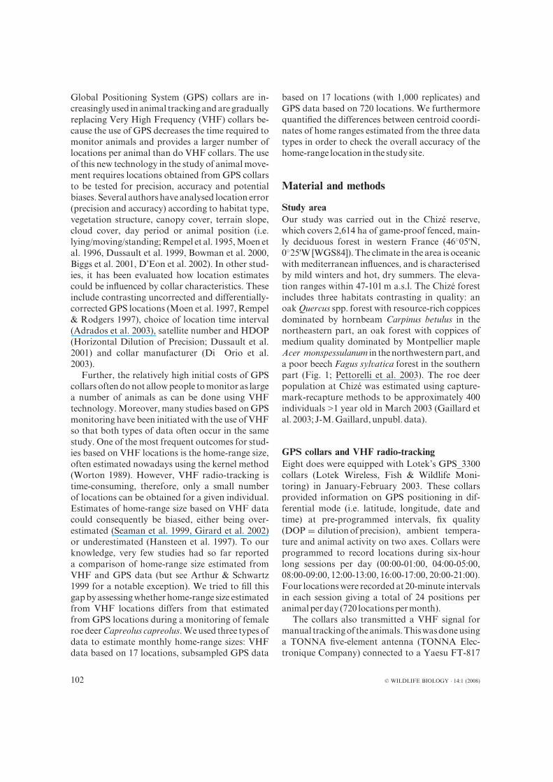
Study areaOur study was carried out in the Chizé reserve,which covers 2,614 ha of game-proof fenced, main-ly deciduous forest in western France (46◦05'N,0◦25'W [WGS84]). The climate in the area is oceanicwith mediterranean influences, and is characterisedby mild winters and hot, dry summers. The eleva-tion ranges within 47-101 m a.s.l. The Chizé forestincludes three habitats contrasting in quality: anoak Quercus spp. forest with resource-rich coppicesdominated by hornbeam Carpinus betulus in thenortheastern part, an oak forest with coppices ofmedium quality dominated by Montpellier mapleAcer monspessulanum in thenorthwesternpart, anda poor beech Fagus sylvatica forest in the southernpart (Fig. 1; Pettorelli et al. 2003). The roe deerpopulation at Chizé was estimated using capture-mark-recapture methods to be approximately 400individuals >1 year old in March 2003 (Gaillard etal. 2003; J-M.Gaillard, unpubl. data).
GPS collars and VHF radio-trackingEight does were equipped with Lotek’s GPS_3300collars (Lotek Wireless, Fish & Wildlife Moni-toring) in January-February 2003. These collarsprovided information on GPS positioning in dif-ferential mode (i.e. latitude, longitude, date andtime) at pre-programmed intervals, fix quality(DOP = dilutionofprecision), ambient tempera-ture and animal activity on two axes. Collars wereprogrammed to record locations during six-hourlong sessions per day (00:00-01:00, 04:00-05:00,08:00-09:00, 12:00-13:00, 16:00-17:00, 20:00-21:00).Four locationswere recordedat 20-minute intervalsin each session giving a total of 24 positions peranimalperday (720 locationspermonth).
The collars also transmitted a VHF signal formanual trackingof theanimals.Thiswasdoneusinga TONNA five-element antenna (TONNA Elec-tronique Company) connected to a Yaesu FT-817
102 © WILDLIFE BIOLOGY · 14:1 (2008)
0 1 2 3 4 kilometers
Figure 1. The Chizé reserve, which covers 2,614 ha of enclosed forest in westernFrance with indication of the three habitat types. The inset shows the position ofthe reserve in France.
receiver (6m, 2 m and 70 cm plus HF receiver, Yae-su; Amateur Radio Division of Vertex Standard).Collared animals were located at least 17 times permonth during April - August 2003. The does weretracked every week to obtain one location in eachof our four sampling periods (i.e. at dawn, midday,in the evening and at night) per week per animal,and equal numbers of observations were performedeachmonth in each samplingperiod.
VHF and total GPS home-rangeRadio-tracking and GPS data were analysed usingthe software R (version 1.9.1; R Development CoreTeam 2004) distributed under the GNU GeneralPublic License and the packages 'ade4' (Chessel etal. 2004), 'adehabitat' (Calenge 2006) and 'maps'(Becker et al. 2007). VHF fixes were assessed bytriangulation (White&Garrott 1990).As thehome-range size of roe deer females varies among monthsduring spring-summer (Linnell 1994, Saïd et al.2005), we analysed the data for each month sepa-rately.Theminimumnumberoffixespermonthwasdetermined by plotting the estimates of home-rangesize against sample size (Stickel 1954, Seaman &Powell 1990) with radio-tracking locations, and
corresponded to a home-rangesize (mean ± SD) between 90 and110% of the home-range size es-timated using all points. We usedthe fixed kernel method with ref-erence smoothing ('ad hoc', href)and Least Square Cross Validationsmoothing (LSCV, hLSCV; Silver-man1986,Worton1989, Seaman&Powell 1996). We obtained a mini-mumofapproximately 16 locationsper animal per month (reference:mean = 16.1, SD = 5.7; LSCV:mean = 16.2, SD = 4.7, N = 25),and we therefore conservativelychose tokeepaminimumof17 loca-tions per month to estimate home-range size. Kernel home rangeswere then calculated using the fixedkernel method with three differentforms of smoothing: href, hLSCVor hfix (h fixed at 60 correspondingto the mean of href values of allanimals and months: mean = 62.8and SD = 25.6). We conducted the
analysis for the 95% kernel (Worton 1989), andalso at the 50% level to obtain core areas. We plot-ted in the same way home-range sizes estimatedfrom GPS locations against sample size and founda minimum of approximately 39 locations (href:mean = 39.4 ± 24.8; hLSCV:mean = 38.8 ± 14.4,N = 8animals*4months).
Kernel home ranges were also calculated withall the GPS locations (720 locations per animal permonth) in order to get the best available estimate ofhome-range size of female roe deer (totalGPShomeranges). We applied the same kernel method andsmoothing parameters as used for the VHF data.Furthermore,wedetermined centroids of the kernelhome ranges of VHF and total GPS data to assesspossible differences in spatial location of homerangeswithinour studyarea.
Sampling and home-range simulations:subsampled GPSTo obtain home ranges of subsampled GPS da-ta, we randomly drew 17 locations per animal permonth among the 720 GPS locations available. Weconstrained the drawings to follow the same distri-bution as VHF monitoring in relation to the periodof the day (i.e. four points, one dawn, one midday,one evening and one night, every week for the first
© WILDLIFE BIOLOGY · 14:1 (2008) 103
four weeks, and one point among the different dayperiods in the fifth week). To reduce autocorre-lation, all points were taken with a minimum timeintervalof15hours (Swihart&Slade1985a,b, 1986,Hansteen et al. 1997). Home-range sizes were thenestimated using the fixed kernel method, with thedifferent forms of smoothing described above: href,hLSCV or hfix. We conducted the analysis for the95% and 50% kernels. We also obtained centroidsof the kernel home ranges. The entire procedure,describedabove,was repeated1,000 times.
Sensitivity analyses from VHF and GPS dataInonesensitivityanalysis,weestimatedhome-rangesizes from the VHF and GPS data using differentnumbers of locations to detect the real minimumnumber of locations required to reliably estimatehome-range sizes. We used N = 10, 12 and 15 ran-domly sampled VHF locations per month andN = 10, 12, 15, 18, 20, 30 and 40 randomly sampledGPS locations permonth (repeated 100 times) to es-timate home-range areas and calculated differencesbetween these areas and total GPS home-rangeareas. We then compared these differences of areaswith those obtained from the comparison between17 locations (VHF or GPS) and total GPS data (seesection Sampling and home-range simulations:subsampledGPS).
In another analysis, we estimated home-rangesizes from GPS data for each hour session of theday (00:00-01:00, 04:00-05:00, 08:00-09:00,12:00-13:00, 16:00-17:00 and 20:00-21:00). Weperformed two types of estimations: one includingall the locations from each session (four locationsper session per day corresponding to 120 locationsper month) and one including 17 locations per ses-sionpermonth (repeated100 times).
Forboth sensitivityanalyses,weapplied thefixedkernel method by considering the different formsof smoothing (href, hLSCV or hfix) and conductedthe analysis for the 95% and 50% kernels. We alsoobtainedcentroidsof thekernel homeranges.
Statistical analysisWe used Wilcoxon tests to determine whetherhome-range sizes differed among the three datatypes, and one-way ANOVAs to test the effect offactor h on differences of home-range sizes and ondistances between centroids. The whole analysiswas performed using the software R (version 1.9.1),and statistical significancewasfixedatP ≤ 0.05.
Results
Precision of the locationsThe location error estimated from VHF and GPSdata was 95 m (mean = 95.3, SD = 43.0) and 25 m(mean= 25.6, SD= 34.0), respectively.
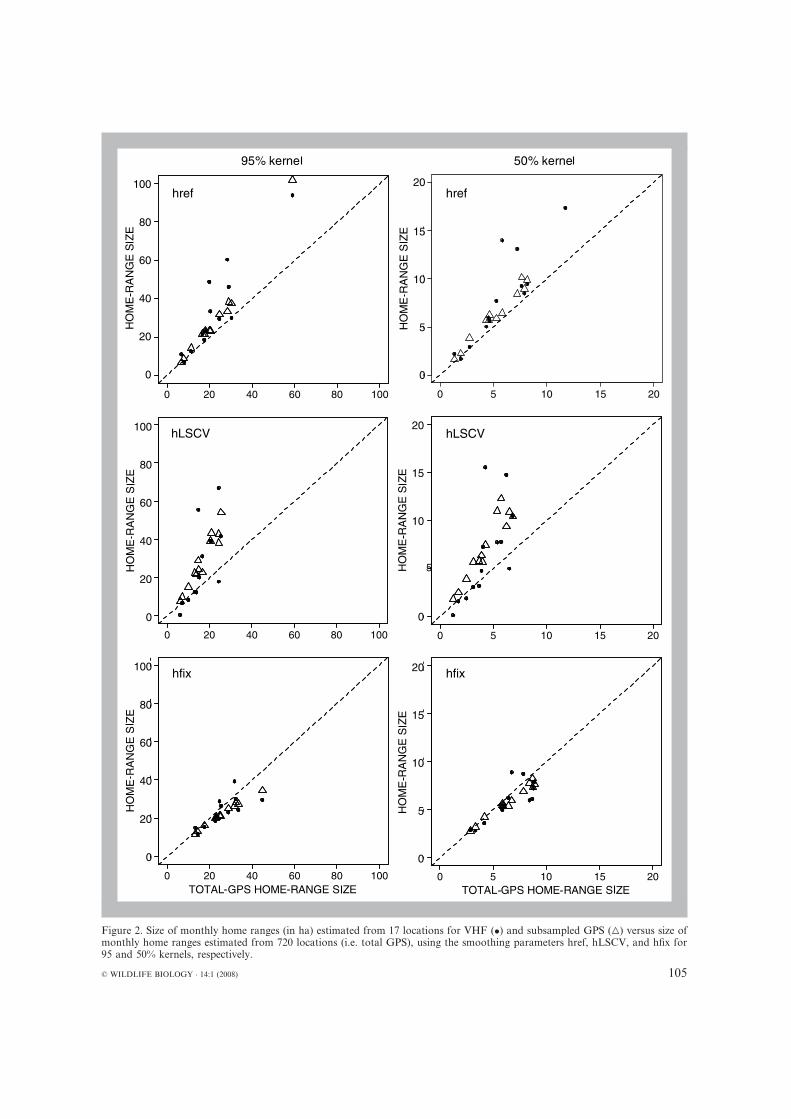
Comparing VHF (17 locations) and GPS (17 and720 locations) home-range sizeWe did not find any effect of the factor h when wecompared differences of home-range sizes betweenVHF and subsampled GPS data according tothe smoothing parameter h (One-way ANOVA:F = 0.75, df = 2, P = 0.48 and F = 0.45, df = 2,P = 0.64 for home-range size at 95 and 50%, re-spectively). For all the three smoothing parame-ters, the home-range sizes estimated from VHF andsubsampled GPS data did not differ at the 95%(Wilcoxon tests: href: V = 22, P = 0.64; hLSCV:V = 12, P = 0.46; hfix: V = 20, P = 0.84) and 50%levels (Wilcoxon tests: href: V = 17, P = 0.94;hLSCV: V = 11, P= 0.383; hfix: V = 17, P= 0.945;Fig. 2).
VHF and subsampled GPS home ranges wereeither overestimated or underestimated comparedwith total GPS home ranges, depending on whichsmoothing parameter h was used (see Fig. 2). Wefound a significant effect of h on the differencebetween total GPS and VHF estimates (One-wayANOVA: F = 5.01, df = 2, P = 0.012 and F =4.54, df = 2, P = 0.017 for home-range size at 95and 50%, respectively) and between total GPS andsubsampled GPS estimates (One-way ANOVA:F = 13.70,df = 2,P <0.001andF = 10.34,df = 2,P < 0.001 for home-range size at 95 and 50%, re-spectively).We then comparedhome-range sizes foreach smoothingparameter.Atboth95and50%ker-nels, the use of href or hLSCV led to overestimatedhome-range sizes from VHF data (Wilcoxon tests:href:V = 36at95%and35at50%,P = 0.008at95%and 0.016 at 50%; hLSCV: V = 32 at 95 and 50%,P = 0.055at 95and50%)and subsampledGPSdata(Wilcoxon tests: href and hLSCV: V = 0 at 95 and50%, P = 0.008 at 95 and 50%) compared with thetotal GPS data. On the other hand, when we usedhfix, the VHF home ranges did not differ signifi-cantly from total GPS home ranges (Wilcoxontests: V = 5 at 95% and 7 at 50%, P = 0.078 at 95%and 0.148 at 50%), but subsampled GPS homeranges were slightly underestimated comparedwith the total GPS home ranges (Difference of area
104 © WILDLIFE BIOLOGY · 14:1 (2008)
5
Figure 2. Size of monthly home ranges (in ha) estimated from 17 locations for VHF (•) and subsampled GPS (�) versus size ofmonthly home ranges estimated from 720 locations (i.e. total GPS), using the smoothing parameters href, hLSCV, and hfix for95 and 50% kernels, respectively.
© WILDLIFE BIOLOGY · 14:1 (2008) 105
= -3.9 ± 2.52; Wilcoxon tests: V = 36 at 95 and50%,P = 0.008at 95and50%).
Effect of sample size on home-range estimatesFor both all the sample sizes and the three smooth-ing parameters, the home-range sizes estimatedfrom VHF and subsampled GPS data did not differat the 95% (Wilcoxon tests for 10, 12 and 15 loca-tions: href: V = 16 to 19, P ≥ 0.47; hLSCV: V = 16to 20, P ≥ 0.375; hfix: V = 17 to 20, P ≥ 0.38) and50% levels (Wilcoxon tests for 10, 12 and 15 loca-tions: href: V = 15 to 18, P ≥ 0.58; hLSCV: V = 16to18,P ≥ 0.58; hfix:V = 17 to21,P ≥ 0.297).
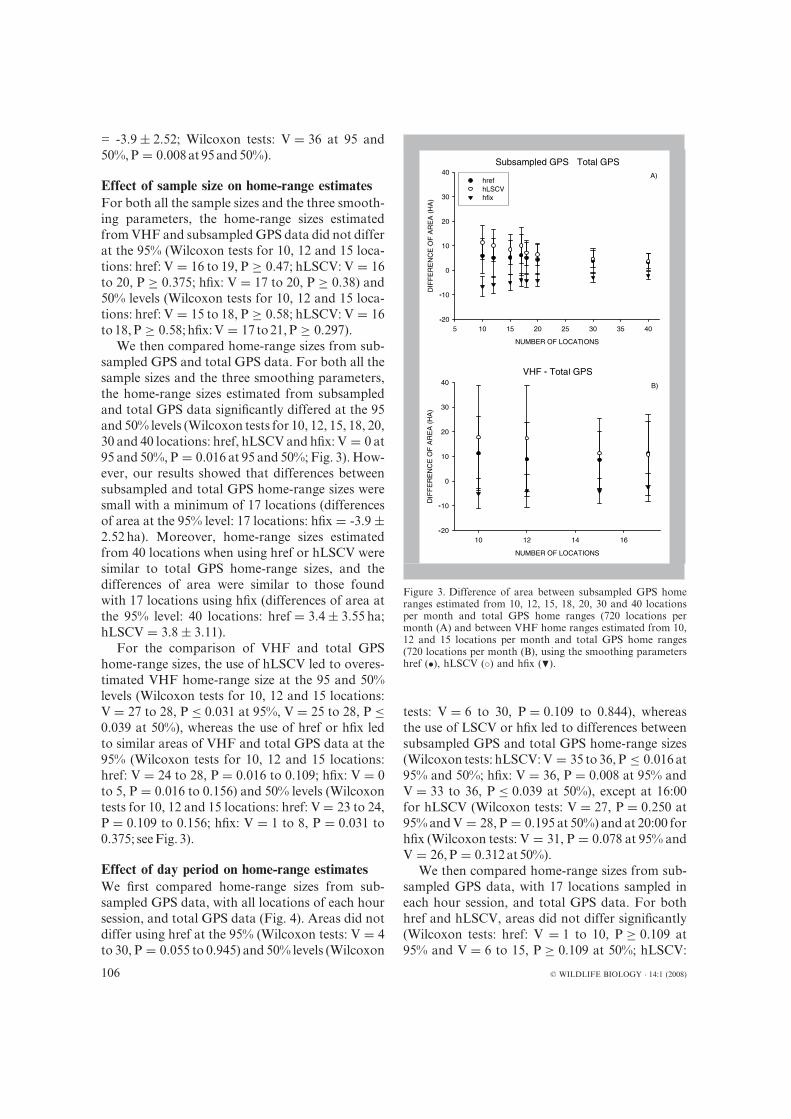
We then compared home-range sizes from sub-sampled GPS and total GPS data. For both all thesample sizes and the three smoothing parameters,the home-range sizes estimated from subsampledand total GPS data significantly differed at the 95and 50% levels (Wilcoxon tests for 10, 12, 15, 18, 20,30 and 40 locations: href, hLSCV and hfix: V = 0 at95 and 50%, P = 0.016 at 95 and 50%; Fig. 3). How-ever, our results showed that differences betweensubsampled and total GPS home-range sizes weresmall with a minimum of 17 locations (differencesof area at the 95% level: 17 locations: hfix = -3.9 ±2.52 ha). Moreover, home-range sizes estimatedfrom 40 locations when using href or hLSCV weresimilar to total GPS home-range sizes, and thedifferences of area were similar to those foundwith 17 locations using hfix (differences of area atthe 95% level: 40 locations: href = 3.4 ± 3.55 ha;hLSCV = 3.8 ± 3.11).
For the comparison of VHF and total GPShome-range sizes, the use of hLSCV led to overes-timated VHF home-range size at the 95 and 50%levels (Wilcoxon tests for 10, 12 and 15 locations:V = 27 to 28, P ≤ 0.031 at 95%, V = 25 to 28, P ≤0.039 at 50%), whereas the use of href or hfix ledto similar areas of VHF and total GPS data at the95% (Wilcoxon tests for 10, 12 and 15 locations:href: V = 24 to 28, P = 0.016 to 0.109; hfix: V = 0to 5, P = 0.016 to 0.156) and 50% levels (Wilcoxontests for 10, 12 and 15 locations: href: V = 23 to 24,P = 0.109 to 0.156; hfix: V = 1 to 8, P = 0.031 to0.375; seeFig. 3).
Effect of day period on home-range estimatesWe first compared home-range sizes from sub-sampled GPS data, with all locations of each hoursession, and total GPS data (Fig. 4). Areas did notdiffer using href at the 95% (Wilcoxon tests: V = 4to 30, P = 0.055 to 0.945) and 50% levels (Wilcoxon
Figure 3. Difference of area between subsampled GPS homeranges estimated from 10, 12, 15, 18, 20, 30 and 40 locationsper month and total GPS home ranges (720 locations permonth (A) and between VHF home ranges estimated from 10,12 and 15 locations per month and total GPS home ranges(720 locations per month (B), using the smoothing parametershref (•), hLSCV (◦) and hfix (�).
tests: V = 6 to 30, P = 0.109 to 0.844), whereasthe use of LSCV or hfix led to differences betweensubsampled GPS and total GPS home-range sizes(Wilcoxon tests: hLSCV:V = 35 to 36, P ≤ 0.016 at95% and 50%; hfix: V = 36, P = 0.008 at 95% andV = 33 to 36, P ≤ 0.039 at 50%), except at 16:00for hLSCV (Wilcoxon tests: V = 27, P = 0.250 at95%andV = 28, P = 0.195 at 50%) and at 20:00 forhfix (Wilcoxon tests: V = 31, P = 0.078 at 95% andV = 26,P = 0.312at 50%).
We then compared home-range sizes from sub-sampled GPS data, with 17 locations sampled ineach hour session, and total GPS data. For bothhref and hLSCV, areas did not differ significantly(Wilcoxon tests: href: V = 1 to 10, P ≥ 0.109 at95% and V = 6 to 15, P ≥ 0.109 at 50%; hLSCV:
106 © WILDLIFE BIOLOGY · 14:1 (2008)
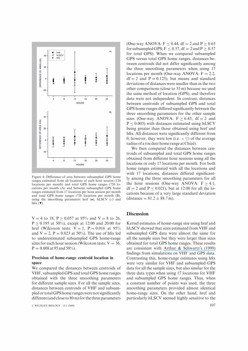
Figure 4. Difference of area between subsampled GPS homeranges estimated from all locations of each hour session (120locations per month) and total GPS home ranges (720 lo-cations per month (A) and between subsampled GPS homeranges estimated from 17 locations per hour session per monthand total GPS home ranges (720 locations per month (B),using the smoothing parameters href (•), hLSCV (◦) andhfix (�).
V = 4 to 18, P ≥ 0.057 at 95% and V = 8 to 26,P ≥ 0.195 at 50%), except at 12:00 and 20:00 forhref (Wilcoxon tests: V = 1, P = 0.016 at 95%and V = 2, P = 0.023 at 50%). The use of hfix ledto underestimated subsampled GPS home-rangesizes for each hour session (Wilcoxon tests: V = 36,P = 0.008at 95and50%).
Precision of home-range centroid location inspaceWe compared the distances between centroids ofVHF, subsampled GPS and total GPS home rangesobtained with the three smoothing parametersfor different sample sizes. For all the sample sizes,distances between centroids of VHF and subsam-pledor totalGPShomerangeswerenot significantlydifferent (andclose to80 m) for the threeparameters
(One-way ANOVA: F ≤ 0.44, df = 2 and P ≥ 0.65for subsampledGPS;F ≤ 0.57, df = 2andP ≥ 0.57for total GPS). When we compared subsampledGPS versus total GPS home ranges, distances be-tween centroids did not differ significantly amongthe three smoothing parameters when using 17locations per month (One-way ANOVA: F = 2.2,df = 2 and P = 0.125), but means and standarddeviations of distances were smaller than in the twoother comparisons (close to 35 m) because we usedthe same method of location (GPS), and thereforedata were not independent. In contrast, distancesbetween centroids of subsampled GPS and totalGPS home ranges differed significantly between thethree smoothing parameters for the other samplesizes (One-way ANOVA: F ≥ 6.43, df = 2 andP ≤ 0.003) with distances estimated using hLSCVbeing greater than those obtained using href andhfix. All distances were significantly different from0, however, they were low (i.e. < 1/3 of the averageradiusof a roedeerhomerangeatChizé).
We then compared the distances between cen-troids of subsampled and total GPS home rangesobtained from different hour sessions using all thelocations or only 17 locations per month. For bothhome ranges estimated with all the locations andwith 17 locations, distances differed significant-ly among the three smoothing parameters for allthe hour sessions (One-way ANOVA: F ≥ 4.1,df = 2 and P ≤ 0.021), but at 12:00 for all the lo-cations because of a very large standard deviation(distance = 81.2 ± 88.7 m).
Discussion
Kernel estimates of home-range size using href andhLSCV showed that sizes estimated from VHF andsubsampled GPS data were almost the same forall the sample sizes but they were larger than sizesobtained for total GPS home ranges. These resultsare consistent with Arthur & Schwartz’s (1999)findings from simulations on VHF and GPS data.Contrasting this, home-range estimates using hfixwere very similar for VHF and subsampled GPSdata for all the sample sizes, but also similar for thethree data types when using 17 locations for VHFand subsampled GPS home ranges. Thus, whena constant number of points was used, the threesmoothing parameters provided almost identicalhome-range sizes. On the other hand, href andparticularly hLSCV seemed highly sensitive to the
© WILDLIFE BIOLOGY · 14:1 (2008) 107
number of locations because they led to smallerareas from total GPS data (i.e. about 720 fixes peranimal and per month), whereas hfix led to totalGPS areas similar to VHF and subsampled GP-S areas. To get reliable estimates, a minimum of17 locations per animal per month seemed to berequired when using VHF locations. However,when plotting home-range sizes estimated fromGPS locations against sample size, we found a min-imum of approximately 39 locations. Moreover,our results showed that home-range sizes estimatedfrom 40 locations when using href or hLSCV weresimilar to total GPS home-range sizes. This indi-cates that 17 locations is not enough, and accountsfor the overestimation we reported when usingeither href and hLSCV from VHF and subsampledGPS data. This overestimation of home-rangesize when using kernel with too small sample sizethus corroborates results of Arthur & Schwartz(1999), Belant & Follmann (2002) and Girard etal. (2002). Our results also support Seaman et al.’s(1999) findings that using the hLSCV value leadsto overestimated home-range size, but they are notconsistent with the underestimation induced byhref valueswhen a small number of locations is usedas reported by Hansteen et al. (1997). Accordingto Seaman et al. (1999), the discrepancy betweenHansteen et al.’s (1997) results and ours wouldresult from the behaviour of hLSCV versus hrefvalues, and from the small number of home rangesinvolved in the comparison. Furthermore, Hemsonet al. (2005) recently showed that the use of hLSCVis not optimal when animals exhibit intensive useof core areas and site fidelity as it is the case for roedeer, and produce variable results at small samplesize and failures at large sample size. Our results onroe deer, a highly sedentary species (Strandgaard1972), support the overestimation and high vari-ability of home-range size using hLSCV values.Finally, our results show that fixing h at the samevalue for all home ranges (i.e. h = 60) stabilisesthe estimate of home-range size and thereby pro-vides a better way to compare home ranges of dif-ferent size and number of locations. On the con-trary, the use of href or hLSCV values requires asimilar or larger number of locations for reliablecomparisons.
The home-range sizes estimated from 17 lo-cations all sampled during a specific day periodwere underestimated compared to total GPS homeranges when using hfix, whereas the use of href orhLSCVled to similar areas.However,wepreviously
showed that home-range sizes were similar betweensubsampled GPS (with 17 locations sampled overall the day periods (i.e. at dawn, midday, in theevening and at night)) and total GPS data usinghfix, and were overestimated using href or hLSCV.Consequently, the estimation of only one part ofthe home range by hour session led to underestima-tion using hfix and to similar areas using href andhLSCV. Moreover, distances between centroids ofsubsampled GPS and total GPS home ranges weresignificantly different and also indicated poor as-sessment of home ranges. These results corroborateBelant & Follmann’s (2002) findings showing thatacquiring locations during only a portion of the24-hour period could involve potential biases whenestimatinghome-range size.
Distances between home-range centroids wereoften significantly different from 0 but consistently< 1/3 of the average radius of a roe deer home rangeat Chizé. This rather good precision of home-rangeposition indicates on the one hand a high accuracyof radio-tracking and GPS positions, and on theother hand, an appropriate sampling of VHF andsubsampled GPS data. In fact, equal numbers ofobservations were made each month at dawn, mid-day, in the eveningandatnight, covering in thatwayall periods of activity and inactivity of the animals.However, we observed a slight difference accordingto the h values usedbecause themeandistanceswiththe href values were smaller than with the hLSCVor the hfix values (h = 60) in the three compari-sons. Thus, the href values seem to provide the mostprecisehome-range centroid.
In this study, we evaluated differences betweenhome-range areas for eight female roe deer mon-itored for four months. Such analyses allowed usto compare the behaviour of kernel estimatorswhen using different h values from field data, andthereby complement the simulations performedby Seaman et al. (1999). However, the scope of ourdata is too limited toallowus togeneralise about theperformanceof the estimators.
The use of field data leads to autocorrelationamong observations. The analyses based on 720GPS locations per month included higher auto-correlation than the analyses based on 17 locations(VHF or subsampled GPS) per month. However,several authors (Reynolds&Laundre 1990,McNayetal.1994,Swihart&Slade1997,Otis&White1999)have concluded that a large set of autocorrelateddata provide a better estimate of the true home-range size thana small set of independentdata.
108 © WILDLIFE BIOLOGY · 14:1 (2008)
Conclusion
Ourresults indicate thathome-range sizes estimatedfrom VHF and GPS data are similar, provided thatthe smoothing parameter and the number of loca-tions are standardised. Both GPS and VHF collarscan therefore be used to estimate home ranges froma given field study, at least when the species understudy share the same spatial patterns as roe deer (i.e.relatively small home range and high site fidelity;Strandgaard 1972). Our work could thus help man-agers to feel more comfortable with mixing datafrom GPS and VHF collars when analysing homeranges. Moreover, our data indicate that, whilemore locations obviously lead to better home-rangeestimates, a minimum sample size of 17, which ismuch smaller than the threshold of 40 assessed fromsimulation studies (Seaman et al. 1999), can pro-vide reliable estimates of home-range size of highlysedentary animals such as roe deer (Saïd et al. 2005).With a careful sampling design, reliable estimatesof home-range size can even be obtained by kernelmethods when using <10 locations (Börger et al.2006).
Acknowledgements - We thank Hervé Fritz, DavidCarslake, Guy Van Laere, Patrick Duncan for use-ful comments on previous drafts of this work andClément Calenge for his help during programming.Maryline Pellerin was granted by the Région Poitou-Charentes. We thank the two anonymous reviewersfor helpful suggestions. This work is part of the project'Consequences of the hurricane lothar on the rela-tionships between roe deer populations and deciduousforests - assessment of its impact and research on ecol-ogical processes for long-term predictions' supported bythe GIPEcoFor ('Groupement d’Intérêt Public Eco-systèmes Forestiers').
References
Adrados, C., Verheyden-Tixier, H., Cargnelutti, B., Pé-pin, D. & Janeau, G. 2003: GPS approach to studyfine-scale site use by wild red deer during active andinactive behaviors. - Wildlife Society Bulletin 31: 544-552.
Arthur, S.M. & Schwartz, C.C. 1999: Effects of samplesize on accuracy and precision of brown bear homerange models. - Ursus 11: 139-148.
Becker, R.A., Wilks, A.R., Brownrigg, R. & Minka, T.P.2007: Original S code by Richard R. Becker & AllanR. Wilks. R version by Ray Brownrigg. Enhance-ments by Thomas P. Minka 2007. Draw GeographicalMaps. R package version 2.0 - 39.
Belant, J.L. & Follmann, E.H. 2002: Sampling consid-erations for American black and brown bear homerange and habitat use. - Ursus 13: 299-315.
Biggs, J.R., Bennett, K.D. & Fresquez, P.R. 2001: Rela-tionship between home range characteristics and theprobability of obtaining successful global positioningsystem (GPS) collar positions for elk in New Mexico.- Western North American Naturalist 61: 213-222.
Börger, L., Franconi, N., De Michele, G., Gantz, A.,Meschi, F., Manica, A., Lovari, S. & Coulson, T.2006: Effects of sampling regime on the mean andvariance of the home range size estimates. - Journal ofAnimal Ecology 75: 1393-1405.
Bowman, J.L., Kochanny, C.O., Demarais, S. & Leo-pold, B.D. 2000: Evaluation of a GPS collar forwhite-tailed deer. - Wildlife Society Bulletin 28: 141-145.
Calenge, C. 2006: The package adehabitat for the Rsoftware: A tool for the analysis of space and habitatuse by animals. - Ecological Modelling 197: 516-519.
Chessel, D., Dufour, A-B. & Thioulouse, J. 2004: Theade4 package-I-one-table methods. - R news 4: 5-10.
D’Eon, R.G., Serrouya, R., Smith, G. & Kochanny,C.O. 2002: GPS radiotelemetry error and bias inmountainous terrain. - Wildlife Society Bulletin 30:430-439.
Di Orio, A.P., Callas, R. & Schaefer, R.J. 2003: Perfor-mance of two GPS telemetry collars under differenthabitat conditions. - Wildlife Society Bulletin 31: 372-379.
Dussault, C., Courtois, R., Ouellet, J.P. & Huot, J. 1999:Evaluation of GPS telemetry collar performance forhabitat studies in the boreal forest. - Wildlife SocietyBulletin 27: 965-972.
Dussault, C., Courtois, R., Ouellet, J.P. & Huot, J. 2001:Influence of satellite geometry and differential cor-rection on GPS location accuracy. - Wildlife SocietyBulletin 29: 171-179.
Gaillard, J-M., Duncan, P., Delorme, D., Van Laere, G.,Pettorelli, N.&Maillard, D. 2003: Effects of hurricaneLothar on the population dynamics of European roedeer. - Journal of Wildlife Management 67: 767-773.
Girard, I., Ouellet, J.P., Courtois, R., Dussault, C. &Breton, L. 2002: Effects of sampling effort based onGPS telemetry on home-range size estimations. - Jour-nal of Wildlife Management 66: 1290-1300.
Hansteen, T.L., Andreassen, H.P. & Ims, R.A. 1997: Ef-fects of spatiotemporal scale on autocorrelation andhome range estimators. - Journal of Wildlife Manage-ment 61: 280-290.
Hemson, G., Johnson, P., South, A., Kenward, R.,Ripley, R. & Macdonald, D. 2005: Are kernels themustard? Data from global positioning system (GPS)collars suggests problems for kernel home-range anal-yses with least-squares cross-validation. - Journal ofAnimal Ecology 74: 455-463.
© WILDLIFE BIOLOGY · 14:1 (2008) 109
Linnell, J.D.C. 1994: Reproductive tactics and parentalcare in Norwegian roe deer. - PhD thesis, NationalUniversity of Ireland, Cork, Ireland, pp. 234.
McNay, J., Morgan, A. & Bunnell, F.L. 1994: Charac-terizing independence of observations in the move-ment of Colombian black-tailed deer. - Journal ofWildlife Management 58: 422-429.
Moen, R., Pastor, J. & Cohen, Y. 1997: Accuracy of GPStelemetry collar locations with differential correction.- Journal of Wildlife Management 61: 530-539.
Moen, R., Pastor, J., Cohen, Y. & Schwartz, C.C. 1996:Effects of moose movement and habitat use on GPScollar performance. - Journal of Wildlife Management60: 659-668.
Otis, D.L. & White, G.C. 1999: Autocorrelation of loca-tion estimates and the analysis of radiotracking data.- Journal of Wildlife Management 63: 1039-1044.
Pettorelli, N., Gaillard, J-M., Duncan, P., Maillard, D.,Van Laere, G. & Delorme, D. 2003: Age and densitymodify the effects of habitat quality on survival andmovements of roe deer. - Ecology 84: 3307-3316.
R Development Core Team 2004: R: A language and en-vironment for statistical computing. - R Foundationfor Statistical Computing, Vienna, Austria. Availableat: http://www.R-project.org.
Rempel, R.S. & Rodgers, A.R. 1997: Effects of differen-tial correction on accuracy of a GPS animal locationsystem. - Journal of Wildlife Management 61:525-530.
Rempel, R.S., Rodgers, A.R. & Abraham, K.F. 1995:Performance of a GPS animal location system underboreal forest canopy. - Journal of Wildlife Manage-ment 59: 543-551.
Reynolds, T.D. & Laundre, J.W. 1990: Time intervalsfor estimating pronghorn and coyote home ranges anddaily movements. - Journal of Wildlife Management54: 316-322.
Saïd, S., Gaillard, J-M., Duncan, P., Guillon, N., Guil-lon, N., Servanty, S., Pellerin, M., Lefeuvre, K., Mar-tin, C. & Van Laere, G. 2005: Ecological correlatesof home-range size in spring-summer for female roe
deer (Capreolus capreolus) in a deciduous woodland.- Journal of Zoology (London) 267: 301-308.
Seaman, D.E., Millspaugh, J.J., Kernohan, B.J., Brun-dige, G.C., Raedeke, K.J. & Gitzen, R.A. 1999: Ef-fects of sample size on kernel home range estimates.- Journal of Wildlife Management 63: 739-747.
Seaman, D.E. & Powell, R.A. 1990: Identifying pat-terns and intensity of home range use. - InternationalConference on Bear Research and Management 8:243-249.
Seaman, D.E. & Powell, R.A. 1996: An evaluation of theaccuracy of kernel density estimators for home rangeanalysis. - Ecology 77: 2075-2085.
Silverman, B.W. 1986: Density estimation for statisticsand data analysis. - Chapman & Hall (Ed.), London,United Kingdom, pp. 176.
Stickel, L.F. 1954: A comparison of certain methodsof measuring ranges of small mammals. - Journal ofMammalogy 35: 1-15.
Strandgaard, H. 1972: The roe deer (Capreolus capreo-lus) population at Kalø and the factors regulating itssize. - Danish Review of Game Biology 7: 1-205.
Swihart, R.K. & Slade, N.A. 1985a: Influence of sam-pling interval on estimates of home range size. - Jour-nal of Wildlife Management 49: 1019-1025.
Swihart, R.K. & Slade, N.A. 1985b: Testing for indepen-dence of observations in animal movements. - Ecology66: 1176-1184.
Swihart, R.K. & Slade, N.A. 1986: The importance ofstatistical power when testing for independence inanimal movements. - Ecology 67: 255-258.
Swihart, R.K. & Slade, N.A. 1997: On testing for inde-pendence of animals movements. - Journal of Agricul-tural, Biological and Environmental Statistics 2: 1-16.
White, G.C. & Garrott, R.A. 1990: Analysis of wildliferadio tracking data. - Academic Press, San Diego,California, USA, pp. 383.
Worton, B.J. 1989: Kernel methods for etimating the uti-lization distribution in home-range studies. - Ecology70: 164-168.
110 © WILDLIFE BIOLOGY · 14:1 (2008)