RESEARCH ARTICLE10.1002/2012WR012922

River-aquifer interactions in a semiarid environmentinvestigated using point and reach measurementsAndrew M. McCallum1, Martin S. Andersen1,2, Gabriel C. Rau1,2, Joshua R. Larsen2,3, andR. Ian Acworth1,2

1Connected Waters Initiative Research Centre, Water Research Laboratory, School of Civil and Environmental Engineering,UNSW Australia, Sydney, New South Wales, Australia, 2National Centre for Groundwater Research and Training, UNSWAustralia, Sydney, New South Wales, Australia, 3School of Geography, Planning, and Environmental Management,University of Queensland, St Lucia, Queensland, Australia

Abstract A critical hydrological process is the interaction between rivers and aquifers. However, accu-rately determining this interaction from one method alone is difficult. At a point, the water exchange in theriverbed can be determined using temperature variations over depth. Over the river reach, differential gaug-ing can be used to determine averaged losses or gains. This study combines these two methods and appliesthem to a 34 km reach of a semiarid river in eastern Australia under highly transient conditions. It is foundthat high and low river flows translate into high and low riverbed Darcy fluxes, and that these are stronglylosing during high flows, and only slightly losing or gaining for low flows. The spatial variability in riverbedDarcy fluxes may be explained by riverbed heterogeneity, with higher variability at greater spatial scales.Although the river-aquifer gradient is the main driver of riverbed Darcy flux at high flows, considerableuncertainty in both the flux magnitude and direction estimates were found during low flows. The reach-scale results demonstrate that high-flow events account for 64% of the reach loss (or 43% if overbankevents are excluded) despite occurring only 11% of the time. By examining the relationship between totalflow volume, river stage and duration for in-channel flows, we find the loss ratio (flow loss/total flow) can begreater for smaller flows than larger flows with similar duration. Implications of the study for the modelingand management of connected water resources are also discussed.

1. Introduction

A critical hydrological process is the interaction between rivers and aquifers [Jones and Mulholland, 2000].Where groundwater levels are naturally or artificially lower than the riverbed, the flux of water from the riverto the aquifer will be controlled by three factors: the differential head between river and aquifer, heteroge-neity of the riverbed hydraulic conductivity, and whether an area of saturation can be maintained betweenthe river and aquifer or whether decoupling will occur [Desilets et al., 2008; Brunner et al., 2009]. Since riversexperience large variations in flow in both space and time, and the hydraulic properties of the riverbed alsovary, determining the river-aquifer interaction processes can be difficult from one field method alone. More-over, many field measurements are often taken at one location and for short periods of time, therefore, theability to extrapolate riverbed exchange over larger spatial and temporal scales is empirically constrained[e.g., Kennedy et al., 2008].

The interaction between rivers and aquifers can be measured at a point within the riverbed, inferred fromhydraulic gradients, estimated from riverbed temperature profiles or using geochemical tracers, computedover a river reach from the water balance of surface flow, and from many other methods [e.g., Cook, 2012;Anderson, 2005; Hatch et al., 2006; Constantz, 2008; Barlow et al., 2000; Harvey and Wagner, 2000; Ruehl et al.,2006; Rosenberry and LaBaugh, 2008] (for a thorough review of many methods see Kalbus et al. [2006]). Gen-erally, the field methods are of two types: those that attempt to measure the flux directly through the river-aquifer interface and those that measure volumetric flow changes along the river [Becker et al., 2004; McCal-lum et al., 2012a]. The first methodology provides estimates of the river-aquifer interactions at the point ofmeasurement, while the second gives spatially averaged estimates. A combination of both approaches cantherefore yield insights into the water exchange process operating within catchments. Despite the generaltheory of river-aquifer interactions being well developed [e.g., Winter et al., 1998], few field studies have

Special Section:New Modelling Approachesand Novel ExperimentalTechnologies for ImprovedUnderstanding of ProcessDynamics at Aquider-SurfaceWater Interfaces

Key Points:� Losing riverbed fluxes under high

flows and approximately neutralunder low flows� Event driven riverbed fluxes

dominate reach losses� Smaller events can have higher loss

ratio than larger events

Correspondence to:M. S. Andersen,m.andersen@unsw.edu.au

Citation:McCallum, A. M., M. S. Andersen, G. C.Rau, J. R. Larsen, and R. Ian Acworth(2014), River-aquifer interactions in asemiarid environment investigatedusing point and reach measurements,Water Resour. Res., 50, doi:10.1002/2012WR012922.

Received 9 SEP 2012

Accepted 26 FEB 2014

Accepted article online 2 MAR 2014

MCCALLUM ET AL. VC 2014. American Geophysical Union. All Rights Reserved. 1

Water Resources Research

PUBLICATIONS

measured both the spatial and temporal variation of water fluxes from multiple methods [e.g., Su et al.,2004; Constantz et al., 2003].

This study examines the river-aquifer flux characteristics along a 34 km reach of a low-gradient alluvialmeandering river in semiarid eastern Australia. By measuring temporal changes in riverbed temperatureswith depth, natural heat is used as a tracer to derive vertical Darcy fluxes at two spatial scales: high-densitysingle pool deployment and evenly spaced reach deployment, over a range of flow conditions. On a largerscale, these results are complemented with an analysis of the water balance between two gauging stationsover the entire 34 km reach in which the point measurements were made. Importantly, this allows for aqualitative assessment of the processes controlling the temporal variations in the reach water balance aswell as river-aquifer interactions in general. This is intended to: (1) identify the processes controlling the var-iation in the timing and magnitude of riverbed Darcy fluxes and (2) compare the processes with the dynam-ics of the reach water balance as determined from differential gauging.

2. Study Area

The Murray-Darling Basin is Australia’s largest river basin (Figure 1a), covering 14% of the continent’s surfacearea, and generates about 40% of the national income derived from agricultural production. Within thebasin, agricultural issues and sustainable water management are environmentally and politically sensitive[MDBA, 2010; ABS, 2012].

The Namoi River Catchment (Figure 1b) is a major subcatchment of the Murray-Darling Basin, with a sur-face area of about 42,000 km2. The Namoi River is over 350 km long, and ranges in elevation from over1500 m in its headwater tributaries in the east to 100 m in the west. It has one of the highest ground-water abstraction levels in Australia. Sharing of water between competing users, as well as the environ-ment, has led to the establishment of rules as to how water can be used and traded in the catchment[Burrell et al., 2011].

The study focuses on a 34 km reach of the Namoi River where it runs south to north through a semiarid trib-utary catchment, Maules Creek. The alluvial plains of the catchment are situated 200–250 m above sea level.To the north and east is the Nandewar Range, which has peaks rising to 1500 m. Below and to the east ofthe Namoi River is a 120 m deep palaeochannel filled with clay, sands, and gravels. Groundwater isabstracted for flood irrigation as well as for stock and domestic use. Some surface water is also diverted forirrigation purposes, although this volume is small and comprises only about 7% of the total irrigation usage[Andersen and Acworth, 2009]. Maules Creek is the main tributary, flowing from the mountains in the east,and is generally ephemeral although it does have perennial flow in its midreach [Rau et al., 2010]. Due to its

T

R1R2

R3

R5

R6

BRiver flow

N Nc da

5 km

River flow

P1

P2 P3

P4P5

P6

50 m

River edge

Aquifer

River

R2

MaulesCreek

NamoiRiver

R4

Namoi RiverCatchment

b

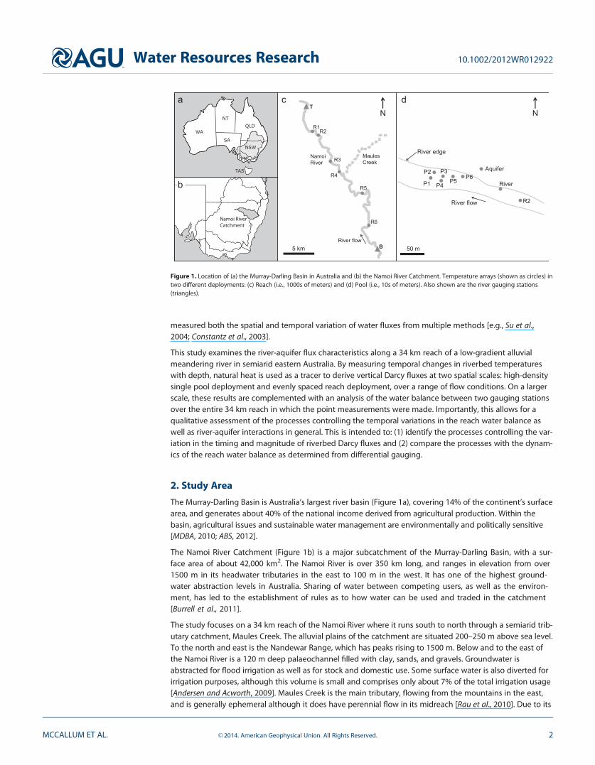
Figure 1. Location of (a) the Murray-Darling Basin in Australia and (b) the Namoi River Catchment. Temperature arrays (shown as circles) intwo different deployments: (c) Reach (i.e., 1000s of meters) and (d) Pool (i.e., 10s of meters). Also shown are the river gauging stations(triangles).

Water Resources Research 10.1002/2012WR012922

MCCALLUM ET AL. VC 2014. American Geophysical Union. All Rights Reserved. 2

intermittent nature, Maules Creek only contributes flow to the Namoi River during infrequent floods [Ander-sen and Acworth, 2009].

Groundwater recharges at the mountain front in the east of the catchment and in the past it dischargedinto the Namoi River in the west. However, due to groundwater abstraction, which started in the 1980s, thegroundwater levels have been lowered such that the river reach has changed from being predominatelygaining to predominantly losing during nonflood periods [McCallum et al., 2013].

Further background information about the catchment, including details of the hydrological and geologicalcontext, can be found in Giambastiani et al. [2012] and McCallum et al. [2013].

3. Methodology

3.1. Point Measurements From Temperature Time Series3.1.1. TheoryThe convection-conduction equation for one-dimensional fully saturated conditions can be formulated as

@T@t

5 D@2T@z2

2v@T@z; (1)

where T is temperature, t is time, z is depth, v is thermal front velocity, and D is effective thermal diffusivity[Suzuki, 1960].

For the situation of a semi-infinite half-space with a sinusoidally varying temperature at the upper surface,the dampening in recorded temperatures can be used to estimate the thermal front velocity by

2v 52DDz

ln Arð Þ1ffiffiffiffiffiffiffiffiffiffiffia1v2

2

r; (2)

and

a 5

ffiffiffiffiffiffiffiffiffiffiffiffiffiffiffiffiffiffiffiffiffiffiffiffiffiffiffiv41

8pDP

� �2s

; (3)

where Ar is amplitude ratio and P is period [Hatch et al., 2006].

The site-specific thermal diffusivity (for substitution into equations (2) and (3)) can be estimated using boththe dampening and phase shift in the recorded temperatures, during nonflow event periods, with

D 5Dz2P2lnA r 4p2DU22P2ln 2Ar

� �DU P2ln 2Ar14p2DU2� �

P2ln 2Ar24p2DU2� � ; (4)

where DA is the phase shift [McCallum et al., 2012a].

The thermal front velocity and Darcy flux are then related using

q 5 cv; (5)

and

c 5nqwcw1 12nð Þqscs

qwcw; (6)

where q is Darcy flux (a negative value indicates losing conditions); n is porosity; qw and cw are the densityand heat capacity of water; and qs and cs are the density and heat capacity of solids [Buntebarth and Schop-per, 1998].

Water Resources Research 10.1002/2012WR012922

MCCALLUM ET AL. VC 2014. American Geophysical Union. All Rights Reserved. 3

It is important to note that this method assumes: (1) the porous media is saturated with a single fluid, (2)fluid flow is in the vertical direction only, (3) fluid flow is in a steady state, (4) fluid and solid properties areconstant in both space and time, and (5) fluid and solid temperatures at any particular point in space areequal at all times [Stallman, 1965].

3.1.2. Field MeasurementsTwo types of temperature array designs were used for field deployment. The first consisted of temperaturesensors (Onset HOBO Pro v2) at 0.00, 0.15, and 0.30 m depth within a 32 mm diameter PVC pipe. The sen-sors were separated by insulating spacers. At each measuring depth the pipe was perforated to allow rapidthermal equilibrium. The second design consisted of pressure/temperature sensors (Solinst Levelogger Gold3001) at 0.00 and 1.00 m depth and temperature sensors (Onset HOBO Pro v2) at 0.18 and 0.34 m depth.The other features remained the same as in the first design. The arrays were installed vertically into the riv-erbed and the locations were determined using Differential Global Positioning System (DGPS).

Temperature arrays were installed in the riverbed in two separate deployments: within a single pooland then evenly spaced along the 34 km reach. For each deployment, six arrays were installed (Fig-ures 1c and 1d). It should be noted that the two deployments spanned different periods: the poolarrays were deployed from November 2007 to April 2008 (i.e., 164 days) and the reach arrays fromOctober 2009 to December 2010 (i.e., 415 days). The pool is monitored for river stage and is adjacentto the site where the groundwater level is measured (�40 m from the river). All parameters werelogged every 15 min.

3.1.3. Data Processing and InterpretationThe raw temperature time series were filtered (i.e., two-pass forward and backward bandwidth filteringusing a Tukey window with all-pass frequencies of 0.9–1.1 cycles per day) to extract time series of tempera-ture amplitudes and phases [see Rau et al., 2010]. Filtering ensures that the dominant daily sinusoid is cor-rectly extracted from all other ‘‘environmental noise’’ contained in the temperature measurements. The dataobtained from filtering complies with the method’s requirement for a sinusoid and contains amplitudesand phases that are free from obfuscation [Lautz, 2012]. Two pairs of temperature time series were usedfrom each array: the upper and second sensors and the second and third sensors. From these, the tempera-ture amplitude ratios and phase shifts were calculated, and then used to create a time series of Darcy flux(q) for each array using equations (2–6).

Basic statistics (i.e., minimum, maximum, average, standard deviation) were computed for all point measure-ments separately for both low flows and high flows. The threshold between low flow and high flow for allanalyses within this paper is defined 1.5 GL/d (n.b. GL is Giga liter, i.e., 1 GL 5 1 3 106 m3), based on a previ-ous analysis of flow duration curves [see McCallum et al., 2013].

The correlation between the riverbed Darcy fluxes obtained from the first and second and that from thesecond and third temperature logger was calculated for each array to check if the 1-D vertical flow assump-tion is valid. The correlation between the river stage and the riverbed Darcy flux was also computed foreach array, to determine the degree to which variation in river stage drives the changes in the riverbedDarcy flux.

3.2. Reach Measurements From Differential GaugingGauging stations are located at the upstream (Boggabri) and downstream (Turrawan) ends of the reach sep-arated by 34 km (Figure 1c). These stations record the river stage each hour which is then postprocessed togive flow using a calibrated rating curve [DNR, 2011]. Hourly data for a 5 year period (2007–2012 wateryears; October to September) were used. This data set covers the period of the temperature array deploy-ments, and also overlaps with that presented in McCallum et al. [2014] (i.e., water years 2000–2010).

For both gauging stations, the cumulative flows, cumulative within-channel flows (defined as <25 GL/d),and cumulative low flows (defined as <1.5 GL/d) were computed. The losses (GL) and time (% of total time)for these different flow regimes were also computed.

Each flow event within this 5 year period was then extracted and analyzed using the method of McCallumet al. [2014]. In this method, the hydrographs recorded at the upstream and downstream ends of a riverreach are used to estimate the loss volume for a flow event, as well as the loss rate during the event.

Water Resources Research 10.1002/2012WR012922

MCCALLUM ET AL. VC 2014. American Geophysical Union. All Rights Reserved. 4

The starting point of the method isthe water balance for a river reach:

Qu1Qi1Qf 5Qd1Qo1Ea1DSDt; (7)

where Qu is flow at the upstreamend of the reach, Qi is flow intothe reach (e.g., tributaries), Qf isriver-aquifer flux, Qd is flow at thedownstream end of the reach, Qo

is flow out of the reach (e.g., sur-face water diversions), Ea is evapo-transpiration from the reach, andDSDt is the change in channel storagewith time. All components of thewater balance have dimensions(L3/T).

For the specific case when flow intoand out of the reach, as well asevapotranspiration, are small com-pared to the magnitude of flow atthe upstream and downstream endsof the reach, the loss volume (LV)can be computed by:

LV 5X

Qd 2X

Qu ; (8)

and the loss ratio (LR; flow loss/total flow) can be computed by:

LR 5

XQu2

XQdX

Qu

: (9)

By introducing the concepts of time-shifted upstream and downstream hydrographs (for details, see McCal-lum et al. [2014]), the loss rate (LRt) at any point in time during an event can then be estimated using:

LRt 5 Qtd2Qt

u: (10)The applicability of these three equations to field data depends on whether the assumption is reasonablethat other loss/gain mechanisms (e.g., evapotranspiration, inflows) are minimal. This is considered in furtherdetail in the discussion below.

For these calculations, the time intervals are equal for each component in the original water balance, andthe integration is over the event duration. The start/end time for each flow event was defined as the timecorresponding to the lowest flow at the upstream gauge in the 7 days prior to/following a recorded flow of1.5 GL/d. For the loss volume (LV) and loss rate (LRt), a negative value indicates a loss from the river, and apositive value indicates a gain to the river.

For each flow event, the event duration, maximum upstream stage and flow, loss volume (i.e., using equa-tion (8)), maximum and average loss rates (i.e., using equation (9)), and loss ratio (i.e., using equation (10))were calculated.

4. Results

4.1. Point Measurements From Temperature Time SeriesA representative 14 day period of temperature data collected during a flood event (Figure 2a) is shown inFigure 2. The measured temperature time series shows strong diel heat patterns as well as longer-term heattrends caused by changes in the weather (i.e., storm) and noise (Figure 2b). The filtered time series moreclearly reveals the dampening of amplitude and shift in phase with depth at each location (Figure 2c).

220

222

224

226 a

Wat

er le

vel [

m A

HD

]

24

26

28b

Tem

pera

ture

[o C]

28 29 30 31 01 02 03 04 05 06 07 08 09 10 11−1

−0.5

0

0.5

1

Dec 2009 - Jan 2010

c

Tem

pera

ture

[o C]

Figure 2. (a) River hydrograph for 14 days. (b) Unprocessed temperature data fromtemperature array P1 for depths 0, 15, and 30 cm, same period. (c) Temperature datafiltered for frequencies of 0.9–1.1 cycles per day using bandwidth filtering.

Water Resources Research 10.1002/2012WR012922

MCCALLUM ET AL. VC 2014. American Geophysical Union. All Rights Reserved. 5

During the monitoring of riverbedtemperatures in the pool four mainflow events were recorded (Figure3). Two of these were large (�3–4 mstage increase) events caused byrainfall-derived runoff and two weresmaller (�1 m stage increase)events caused by upstream damreleases, which preceded each ofthe rainfall events. The groundwaterlevels responded in a damped fash-ion to each of the flow events (Fig-ure 3a, dashed line). Thecorresponding times series of theriver-aquifer gradient was close tozero or slightly negative (toward theaquifer) during low flows, butbecomes distinctively negative(hydraulic gradients of 20.01 to20.04) during the high flows(Figure 3b).

During low flows, the temperaturedata for all arrays in the pool gaveDarcy flux results that indicatedapproximately neutral conditions(�0.0 m/d), while during high flows

they showed losing conditions (up to �20.3 m/d; Figure 3c and Table 1). In some cases, slightly gainingconditions (�0.1 m/d) were observed following flow events. Over depth, the correlation between fluxesestimated from probes 1 and 2 (v1–2) and probes 2 and 3 (v2–3) was significant (r> 0.65) at three locationswithin the pool (i.e., arrays P2, P4, and P6; Table 1). At these same locations, the correlation between stageand flux was also significant (Table 1).

Two main flow events were recorded during the reach monitoring period (Figure 4a, solid line). One was alarge event caused by rainfall (�6 m stage increase) and the other was a smaller event caused by a damrelease (�1 m stage increase), which preceded the rainfall event. As for the pool data, the groundwater

Table 1. River-Aquifer Statistics (See Figures 3 and 4)a

Low Flows High Flows All flows

ArrayData

(-)Minimum

(m/d)Maximum

(m/d)Average(l) (m/d)

StandardDeviation (r)

(m/d)Data

(-)Minimum

(m/d)Maximum

(m/d)Average(l) (m/d)

StandardDeviation(r) (m/d)

Data(-)

Cor. 1(-)

Data(-)

Cor. 2(-)

Pool DataP1 50 20.07 0.02 20.01 0.03 45 20.25 0.18 20.04 0.06 150 0.14 95 20.43P2 58 20.13 0.04 0.02 0.03 62 20.26 0.20 20.08 0.08 93 0.73 120 20.76P3 58 20.23 0.06 0.00 0.04 56 20.28 0.06 20.04 0.07 115 0.33 114 20.41P4 57 20.13 0.03 20.01 0.02 65 20.19 0.04 20.08 0.05 141 0.84 122 20.65P5 35 20.06 0.03 0.00 0.02 12 20.11 0.07 20.06 0.05 44 0.54 47 20.62P6 43 20.04 0.02 0.01 0.02 25 20.21 0.01 20.07 0.07 37 0.97 68 20.86Reach DataR1 233 20.58 0.09 20.05 0.07 31 20.58 0.07 20.17 0.13 264 0.31 264 20.57R2 201 20.07 0.09 0.01 0.02 61 20.84 0.31 20.10 0.23 262 0.79 262 20.66R3 32 20.09 20.02 20.05 0.02 23 20.15 20.02 20.08 0.04 55 0.68 55 20.42R4 34 20.15 0.02 20.06 0.05 24 20.58 0.01 20.34 0.16 58 0.81 58 20.80R5 195 20.99 20.13 20.23 0.13 46 21.20 20.17 20.54 0.26 12 0.92 241 20.52R6 207 20.27 0.04 20.05 0.03 53 20.55 20.05 20.18 0.14 257 0.95 260 20.78

a‘‘Cor. 1’’ refers to correlations between v122 and v223 and ‘‘Cor. 2’’ refers to correlations between stage and flux (v122). Bold indicates |Correlation coefficient|� 0.65.

220

222

224

226 a

Wat

er le

vel [

m A

HD

]

RiverAquifer

−0.06

−0.04

−0.02

0

0.02 bR

-A g

radi

ent [

−]

−0.5

0c

Dar

cy v

eloc

ity [m

/d]

P1P2P3P4P5P6

Dec Jan Feb2007/2008

Mar Apr

Figure 3. Results for the pool deployment. (a) River and aquifer hydrographs.(b) River-aquifer (R-A) gradient (negative value indicates potentially losing condi-tions). (c) Estimated Darcy fluxes from riverbed temperature data.

Water Resources Research 10.1002/2012WR012922

MCCALLUM ET AL. VC 2014. American Geophysical Union. All Rights Reserved. 6

levels responded in a damped fashion to each of the flow events (Figure 4a, dashed line). The correspond-ing river-aquifer gradient in Figure 4b shows losing conditions during the high flood period with hydraulicgradients varying from 20.02 to 20.06. Following the flow events, gaining conditions with hydraulic gra-dients up to 0.01 were observed to last for a period of almost 3 months.

During low flows, the Darcy fluxes from the reach data indicated neutral to slightly losing conditions (10.05to 20.10 m/d) with the exception of array R5 which showed overall losing conditions (approximately 20.15m/d; Figure 4c and Table 1). During high flows, the Darcy fluxes showed losing conditions (up to 21.20 m/d; Figure 4c and Table 1). Immediately after the high-flow event, there were gaining conditions (>0.10 m/d)at array R2 which diminished over one and a half weeks to neutral conditions (Figure 4c). The correlationbetween v1–2 and v2–3 was greater than 0.65 at all locations along the reach except for one (array R1;Table 1). At three locations, the correlation between river stage and flux was greater than 0.65 (i.e., arraysR2, R4, and R6; Table 1).

4.2. Reach Measurements From Differential GaugingThe hydrographs for Boggabri and Turrawan (Figure 5a; black and gray lines) show that river flows are epi-sodic and vary from 0 to 79 GL/d for the 5 year period analyzed. The cumulative hydrographs show that2031 GL entered the catchment while 1719 GL left the catchment over the 5 year period, which corre-sponds to a loss of 311 GL (Figure 5b; solid lines). If the overbank events are excluded from this analysis,then these statistics change to 1758 GL entering, 1558 GL leaving, and a lower total loss of 199 GL (Figure5b; dashed lines). When only low flows are considered (Figure 5c), the corresponding statistics are 711, 589,and 113 GL, respectively (Figure5).

The losses during low flows (which occur 89% of the time) account for 36% of all losses (i.e., 113/311), oralternatively 57% of losses (i.e., 113/199) when overbank events are excluded. The losses during high flows(which occur 11% of the time) account for 64% of all losses, or alternatively 43% when overbank events areexcluded.

For the 5 year period, high-flow events (i.e., flows greater than 1.5 GL/d) were analyzed (Table 2 and Figures6 and 7). The duration of these events varied from 1 to 57 days, maximum stage from 1.2 to 7.6 m,

Table 2. Analysis of High-Flow Events From Upstream and Downstream Gauging Stations (See Figures 6 and 7)a

Event Number Event Start Date Duration (Days) Maximum River Stage (m) Maximum River Flow (GL/d) LV (GL) LR (%) Maximum LRt (GL/d) Average LRt (GL/d)

1 10/12/06 16 1.5 2.1 26.2 29 20.6 20.42 24/12/06 13 1.3 1.8 24.2 23 20.4 20.33 30/12/06 6 1.2 1.6 21.4 20 20.3 20.24 4/3/07 13 3.0 6.5 22.0 26 21.6 20.25 13/6/07 14 3.6 8.7 22.8 18 21.6 20.26 27/12/07 14 4.4 12.4 24.0 17 22.0 20.37 13/2/08 14 4.0 10.5 23.3 9 20.9 20.28 2/12/08 20 7.1 49.1 229.1 22 210.3 21.59 19/12/08 15 6.4 26.4 210.9 13 23.3 20.810 16/12/09 8 1.4 1.8 22.4 22 20.4 20.311 24/12/09 8 1.3 1.6 21.0 12 20.2 20.112 30/12/09 4 2.5 4.7 0.6 28 0.0 0.113 18/1/10 8 1.8 2.8 20.9 14 20.4 20.114 19/7/10 14 2.8 5.6 22.4 16 20.8 20.215 18/8/10 38 6.5 28.1 218.1 8 22.2 20.516 5/9/10 1 1.3 1.5 20.2 20 20.3 20.317 21/10/10 6 1.6 2.4 23.5 48 21.1 20.618 29/10/10 10 1.5 2.0 25.3 46 20.9 20.619 29/10/10 11 1.5 2.0 25.8 46 20.9 20.520 20/11/10 19 5.3 16.8 232.8 27 23.3 21.821 28/12/10 57 7.6 79.4 281.4 11 27.2 21.422 3/2/11 11 1.4 1.9 22.9 17 20.3 20.323 10/2/11 4 1.3 1.6 20.8 15 20.2 20.224 14/2/11 12 1.4 1.7 21.9 13 20.2 20.225 25/6/11 17 2.4 4.4 24.1 13 20.6 20.326 14/9/11 14 1.4 1.7 22.2 16 20.3 20.2

aNote: GL is Giga liter, i.e., 1 GL 5 1 3 106 m3.

Water Resources Research 10.1002/2012WR012922

MCCALLUM ET AL. VC 2014. American Geophysical Union. All Rights Reserved. 7

maximum river flow from 1.2 to76.1 GL/d, loss volume per eventfrom 20.2 to 281.4 GL, maximumloss rate from 20.2 to 210.4 GL/d,average loss rate from 20.1 to21.7 GL/d, and loss ratios from 8 to48%. Excluded from these reportedranges is one event which had apositive reach loss result (i.e., a gainof water to the river; see event 12 inTable 2). It is unlikely this gain is dueto surface flow contributions fromMaules Creek as the flow event wasof comparatively short duration andmagnitude. With the available data,it is not possible to determine thereason for this outlier.

5. Discussion

5.1. Limitations of Point andReach MeasurementsThis study uses two differentmethods to investigate river-aquifer interactions in a semiaridenvironment. In the sections that

follow, the structure of the Methodology and Results is not repeated, where first the point measurementswere considered and then the reach measurements, but rather various processes are discussed, drawingon the different measurements as required. In this connection, it is also important to note that neithermethod directly measures the water volumes exchanged between the river and the aquifer. Rather,whether used independently or together, they provide useful information on the hydrological processesoccurring at different spatial and temporal scales [Scanlon et al., 2002; Kalbus et al., 2006]. Before drawingconclusions from the results, the advantages and limitations of each method are first considered.

While the use of heat as a tracer of water movement through riverbeds has increasingly become popu-lar over the last decade [Constantz, 2008], a number of authors have highlighted the strengths andpotential problems of the method when applied to field data. These problems arise primarily from thepotential for field conditions to differ from the idealized 1-D assumptions, and could be due to nonverti-cal flow fields [e.g., Lautz, 2010; Roshan et al., 2012; Cuthbert and Mackay, 2013], the presence of gas inorganic-rich streambeds [e.g., Cuthbert et al., 2010], hydraulic heterogeneity in the riverbed introducinghorizontal temperature gradients [Schornberg et al., 2010; Ferguson and Bense, 2011; Rau et al., 2012b],and uncertainty in the thermal parameters [Shanafield et al., 2011; Soto-L�opez et al., 2011]. Finally, theheat tracing method only measures fluxes in the shallow streambed and may not accurately distinguishbetween hyporheic and more regional groundwater exchange [e.g., Bhaskar et al., 2012]. However, heattracing using temperature time series has been comprehensively tested in the laboratory, which demon-strates that the flux estimates are robust and reliable when the inherent assumptions are valid [Rauet al., 2012b], even during transient conditions [e.g., Lautz, 2012]. In the context of this study, the fluxesderived from heat tracing at discrete points within the river are largely indicative of vertical streambedflow activity and therefore potential stream-aquifer exchange, with some uncertainties discussed in sec-tion 5.5.

The application of the differential field gauging method also contains important limitations. The mostfundamental is whether the river reach water balance can be simplified to a single input and output.Flow contribution from smaller tributaries, flow abstraction by surface water pumps, and evapotranspira-tion all impact on the results [Lerner et al., 1990]. Based on a previous catchment water balance study ofthe studied catchment, this is a reasonable simplification to make for the present study [Andersen and

220

222

224

226 a

Wat

er le

vel [

m A

HD

]

RiverAquifer

−0.06

−0.04

−0.02

0

0.02 bR

−A g

radi

ent [

−]

−1

−0.5

0c

Dar

cy v

eloc

ity [m

/d]

R1R2R3R4R5R6

Jan Apr2009/2010

Jul

Figure 4. Results for the reach deployment. (a) River and aquifer hydrographs. (b)River-aquifer (R-A) gradient (negative value indicates potentially losing conditions). (c)Estimated Darcy fluxes from riverbed temperature data.

Water Resources Research 10.1002/2012WR012922

MCCALLUM ET AL. VC 2014. American Geophysical Union. All Rights Reserved. 8

Acworth, 2009]. Further issues mayarise because the method is notsensitive to small-scale processesand instead provides an averagedvalue for the interactions over thewhole reach, which may differfrom point measurements [de Vriesand Simmers, 2002]. Thus, small-scale losses and gains may occursimultaneously with the context ofa larger reach-scale net loss orgain [McCallum et al., 2012b]. Also,when interpreting the differentialgauging data, it should be notedthat the concept of river-aquiferinteractions itself may be too sim-plistic [McCallum et al., 2014].Water ‘‘lost’’ from the river mayreturn to the river but on spatialand temporal scales large and longenough to not be considered‘‘return flow’’ or ‘‘bank storage.’’Finally, gauging data itself willalways contain inaccuracies, espe-cially at very low- and very highflows [McCallum et al., 2014].Despite the inherent uncertaintiesin gauging data, the data for thetwo gauges utilized are overall reli-able, and the big picture of theinteractions gained remains robust[Tomkins, 2014].

5.2. River Flow Events and River-Aquifer InteractionsAll the point measurements ofDarcy fluxes within the riverbedshow similar responses to flowevents, however, they have diver-gent responses during recessionand low flows (Figures 3c and 4cand Table 1). During low-flow condi-tions, the point-scale measurements

indicate slightly gaining to slightly losing fluxes. During a flow event, however, these fluxes uniformlyrespond by becoming higher magnitude losses. During flow recession, one point measurement (R5) indi-cates an immediate reversal to gaining conditions (in both riverbed Darcy flux and gradient data), while therest of the measurements return to a low slightly gaining to slightly losing Darcy flux.

The most obvious explanation for the temporal variability of riverbed Darcy fluxes and their magnitudeis the simultaneous variation in river stage, which drives the change in hydraulic gradient throughoutthe reach (Figures 3 and 4). Given the smaller variation in the groundwater level over time, it is clearthat the dynamic variation of river height, particularly the flood wave, is the primary driver of changesin the Darcy flux through the riverbed. The temporal match between the change in hydraulic gradientand the independent measurements of riverbed Darcy fluxes gives confidence in the temperature-basedresults.

0

20

40

60

80

2006 2007 2008 2009 2010 2011

Flow

(GL/

d)

Year

a

0

500

1000

1500

2000

2500

2006 2007 2008 2009 2010 2011

Cum

ulat

ive

flow

s (G

L)

Year

b

0

500

1000

1500

2000

2500

2006 2007 2008 2009 2010 2011

Cum

ulat

ive

low

-flow

s (G

L)

Year

c

Reach event(see Figure 4)

Pool event(see Figure 3)

Figure 5. (a) River hydrographs. (b) Cumulative hydrographs for upstream and down-streams flows for analysis including overbank events (solid lines) and excluding over-bank events (dashed lines). (c) Cumulative hydrographs for low flows. In Figures5a–5c, the black line is upstream flow (at Boggabri) and gray line is downstream flow(at Turrawan). Note: GL is Giga liter, i.e., 1 GL 5 1 3 106 m3.

Water Resources Research 10.1002/2012WR012922

MCCALLUM ET AL. VC 2014. American Geophysical Union. All Rights Reserved. 9

These point-scale observations of thesignificance of river flows on the inter-actions are complemented by an analy-sis of the differential river gauging datafor the river reach (Figure 5). Underhigh flow conditions, which haveoccurred only 11% of the time in the 5year record examined here, lossesthrough the riverbed account for 64%(or 43% if overbank events areexcluded) of all losses in the reachwater balance. This supports the point-scale results in highlighting the impor-tant role of high-flow events in theinteractions between rivers and shal-low alluvial aquifers in semiarid andarid systems, a finding similar to that ofprevious studies [e.g., Shentsis et al.,1999; Dahan et al., 2007].

5.3. Overbank Flow Events andPotential RechargeAdditional insight into the influence ofriver flows on river-aquifer interactionsis gained by further analysis of the flowevents (Table 2 and Figures 6). Throughrainfall-runoff processes and damreleases, the Namoi River experiences awide range of flow magnitudes, with aresulting stage range of almost 8 m atthe upstream gauge. For the 5 year

period analyzed, <1% of flows were overbank at the upstream gauge, while none were overbank at thedownstream gauge as a result of the increased bankfull capacity (>50 GL/d; i.e., water must reenter thechannel along the reach). The low frequency of overbank flows, however, does not diminish their signifi-cance for the reach water balance. Rather, overbank events generate the largest reach loss volumes(between 10 and 80 GL per event) of all the examined flow events. This is intuitive since under these condi-tions a much larger part of the landscape (i.e., surface area) is included in overbank flows. In contrast, thelargest within-channel event has a reach loss volume of only 6.2 GL. Thus, very infrequent overbank reachlosses can be a significant source of potential recharge to the shallow aquifers for this section of the NamoiRiver.

It must be noted that these estimates of loss from the differential gauging represent maximum possible val-ues of aquifer recharge (i.e., potential recharge). Evaporation from stagnant water on the floodplain, as wellas evapotranspiration of floodwaters stored in the soil, will reduce the amount of water that eventually willbecome a flux of water from river to aquifer (i.e., actual recharge). Furthermore, a thin veneer of sedimentsacross the floodplain can be of critical importance in controlling the amount of recharge [Doble et al., 2012].However, given the remote location of this study site there is no data available to estimate evaporationsurfaces or plant available soil moisture, and little work has been done in the area on the significance ofoverbank flow as a recharge mechanism [see Jolly et al., 1994]. Thus, in order to understand the true signifi-cance of overbank flow events for the river-aquifer interactions, further investigation of the evaporative andsoil moisture storage processes is required.

Given that the overbank flow events can skew the interpretation of the loss estimates due to the complica-tion of additional flow processes, it is instructive to exclude them from the water balance analysis. Whenthis is done, the losses during within-channel high flows (which occur only 11% of the time) decrease from

0

2

4

6

8

0 20 40 60 80 100

Riv

er s

tage

(m)

River flow (GL/d)

aa

0

2

4

6

8

-100-80-60-40-200

Riv

er s

tage

(m)

Loss Volume (GL)

b

Figure 6. For all high-flow events (i.e., flows larger than 1.5 GL/d) for the 5 yearperiod analyzed, (a) the observed relationship between river stage and river flowfor upstream (black crosses) and downstream (gray crosses) gauging stations; (b)the observed relationship between river stage and reach loss. For Figure 6b, thetriangles represent events with peak flows less than 4 GL/d, the circles representsbetween 4 and 25 GL/d, and the squares represents more than 25 GL/d (i.e., over-bank flows). Note: GL is Giga liter, i.e., 1 GL 5 1 3 106 m3.

Water Resources Research 10.1002/2012WR012922

MCCALLUM ET AL. VC 2014. American Geophysical Union. All Rights Reserved. 10

64% of all losses to 43%. Despitethis reduction, the percentage oflosses accounted for by high-flowwithin-channel events is still veryhigh compared to their frequency,and therefore the general conclu-sion of the significance of the high-flow events for the river-aquiferinteractions is maintained.

5.4. In-Channel Flow Events andRiver-Aquifer InteractionsWhen focusing on the within-channel flows (Table 2 and Figure7a), the relationship between thetotal reach losses and the river stageis surprisingly weak. Thus, while anincrease in stage potentially leads toincreased reach losses, the point-scale temperature data (Figures 3and 4) demonstrate that additionalfactors must also be controllingthese losses. Further scrutiny of Fig-ure 7a shows that the data fall intotwo groups: one with low riverstages (i.e., 1.2–1.8 m) but with alarge range in loss volumes (0.2–6.2GL; the triangles in Figure 7a), andanother with larger river stages (i.e.,2.4–4.4 m) but without proportion-ally larger loss volumes (3–4.1 GL;the circles in Figure 7a). As someevents with smaller stages clearlylead to greater loss volumes, oneexplanation might be that theseevents are also longer in duration,allowing more time for the loss tooccur. However, this is not thecase, since low-stage high-lossevents (triangles) have a similarduration to the high-stage eventswith moderate loss (the circles

Figure 7b). Therefore, the loss ratio is clearly different as events proceed beyond the 2 m stage range, sug-gesting other factors may be responsible.

These two groups based on stage range also remain apparent when reach loss is considered as a functionof total river flow (Figure 7c). The ratio of the reach loss to cumulative flow (i.e., total river flow) is also indicativeof the loss ratio, with the slope of the trends representing the overall loss ratio for these two groups. For thesmaller events (i.e., the triangles, which have stages<�2 m), this ratio is�25%, much higher than the 6% forthe larger events (i.e., the circles, which have stages>�2 m; see loss ratio results for individual events inTable 2).

One plausible explanation for the importance of river stage in determining reach losses is that the hydraul-ics of the system changes as the stage rises between the different magnitude flow events. That is, as theriver stage increases, there is proportionally more water flowing within the channel due to increased

-8

-6

-4

-2

00 5 10 15 20

Loss

Vol

ume

(GL)

Event duration (d)

b

-8

-6

-4

-2

00 2 4 6

Loss

Vol

ume

(GL)

River stage (m)

a

-8

-6

-4

-2

00 10 20 30 40

Loss

Vol

ume

(GL)

Total river flow (GL)

c

Figure 7. Dependence of reach loss for within-channel high-flow events (i.e., flowslarger than 1.5 GL/d but less than 25 GL/d), on (a) river stage, (b) event duration, and(c) total river flow. In all figures, the triangles represent events with peak flows lessthan 4 GL/d and the circles represents more than 4 GL/d. Note: GL is Giga liter, i.e., 1GL 5 1 3 106 m3.

Water Resources Research 10.1002/2012WR012922

MCCALLUM ET AL. VC 2014. American Geophysical Union. All Rights Reserved. 11

hydraulic efficiency, than is lost from the river. The response of the aquifer heads to the river flow, and theability of the aquifer to transmit away any water lost from the river as the event progresses will also beimportant in controlling overall losses from the reach. However, as detailed piezometric data are unavailablein this river reach, the extent of this influence is not possible to determine here.

Another possible explanation is that the hydraulic conductivity of the riverbed is higher than that withinthe upper banks, and that the riverbed in this case is a more direct route of loss than the riverbanks. This issupported by field observations that the upper banks are generally of clayey or loamy texture along thereach. Further investigation of the channel geometry, aquifer hydraulic heads, as well as the hydraulic con-ductivity distribution of the river system is required to determine which explanation accounts for the pat-terns in reach losses observed.

5.5. Role of Riverbed Sediment Heterogeneity and Hyporheic FlowCompared to the reach scale, considerable heterogeneity in riverbed fluxes should be expected at the pointscale [Buffington and Tonina, 2009; Fleckenstein et al., 2006; Genereux et al., 2008]. Indeed, the heat tracingdata indicates significant spatial variability in vertical Darcy fluxes, both within and between the pool andreach data (see values of l and r in Table 1). This is consistent with recent findings that there is a large spa-tial variability in riverbed fluxes at the reach and even at the meter scale [Lautz and Ribaudo, 2012; Anger-mann et al., 2012]. Point-scale Darcy fluxes are similar during low-flow periods and become increasinglydivergent during higher flow conditions. This divergence in flux is further amplified as the distance betweenarrays increases: i.e., the widely spaced reach measurements show much greater variation in peak Darcyfluxes than those within the pool.

There are at least two possible explanations for the variability in Darcy flux for identical river stage fluctua-tions. First, a variable distribution in riverbed hydraulic conductivity due to the natural variability in riverbedsediments will lead to a spatial variation in vertical fluxes. This heterogeneity in hydraulic conductivity is awell-documented phenomenon of riverbeds [e.g., Storey et al., 2003; Cardenas et al., 2004; Buffington andTonina, 2009]. Second, departures from the 1-D flow field will also lead to spatially variable fluxes. Topo-graphic features (e.g., ripples, bars, meanders) influence flow fields, drive hyporheic exchange, and thushave an effect on the subsurface heat flow [e.g., Cardenas and Wilson, 2007; Roshan et al., 2012; Cuthbertand Mackay, 2013]. Significant hyporheic exchange would therefore affect the estimates of the Darcy fluxdepending on the probe locations within the actual 3-D flow field [Angermann et al., 2012]. Hyun et al.[2011] found that point and area-averaged estimates of flux differed from each other and hypothesizedthat hyporheic exchange was occurring within the regional river-aquifer interactions. In a separate study,Ward et al. [2012] found that local in-river hydraulic gradients did not necessarily reflect the regional gra-dients. Thus, the cause of this spatial heterogeneity in fluxes for low-flow conditions cannot be known withcertainty based on the temperature data alone. Under strongly losing or gaining conditions, however, hypo-rheic exchange is expected to have a diminished effect on the more regional flow field [Cardenas, 2009].Therefore, hyporheic fluxes are more likely to contribute greater uncertainty to the flux estimates underlow-flow conditions than during high flows, and the observed variability during high flows can be largelyattributed to the effects of riverbed heterogeneity.

Assuming that the variability in Darcy fluxes observed at the pool scale is representative for other poolsalong the reach, this uncertainty can be propagated to all reach results under low-flow conditions. Thisallows the estimation of 10th and 90th percentiles (i.e., l 6 1.24 r) for the Darcy fluxes, thereby giving a realis-tic uncertainty range to the reach results, without minimizing the complications of the heterogeneity andhyporheic exchange. Furthermore, this approach provides some guidance as to whether the estimatedfluxes at each reach location are actually losing or gaining, or are simply the result of localized (hyporheic)fluxes.

Adding this uncertainty range to the results shows that the point measurement fluxes during low-flow con-ditions are comparable to a reach averaged low-flow estimate from the differential gauging. The Darcyfluxes derived from the temperature time series along the reach are neutral to slightly losing, with average10th and 90th percentile values of 20.10 and 20.04 m/d. Taking the reach loss during low flows for theanalyzed period, and by using an estimated reach length of 34 km and width of 20 m, the reach-scale 5year average river-aquifer Darcy flux was estimated at 20.09 m/d. This compares favorably, though not

Water Resources Research 10.1002/2012WR012922

MCCALLUM ET AL. VC 2014. American Geophysical Union. All Rights Reserved. 12

exactly, with the results from the temperature time series. The combination of both methods therefore con-firms the reach is slightly losing overall during low-flow periods.

During high-flow events the divergence between point measurements can be large (Table 1). This suggestsdiffering degrees of river-aquifer connectivity along the reach. Other researchers have found that flowthrough higher conductivity ‘‘windows’’ in semiarid and arid riverbeds is a significant pathway of water loss[e.g., Shentsis and Rosenthal, 2003]. The increased importance of these local exchanges under large hydrau-lic gradients must therefore be considered when accounting for the volume of river-aquifer interactions.

In addition to the spatial variability in riverbed sediments and hydraulic conductivity, there are two addi-tional pieces of evidence to suggest that these also vary over time. First, in the case of array R3, the bedscour during the event was sufficient to remove the riverbed installation, and second, in the case of arrayR4, the same event caused deposition of sediment leaving the array buried within the riverbed to such adepth that the temperature sensors were no longer sensitive to diel variations. That riverbed scouring anddeposition was occurring was confirmed during the removal of the temperature arrays. The effect of thissediment transport on hydraulic conductivity over time is difficult to quantify directly, however there are asmall but growing number of field studies which have attempted to measured the temporal variability inriverbed hydraulic conductivity [e.g., Springer et al., 1999; Genereux et al., 2008; Rau et al., 2010; Mutiti andLevy, 2010; Hatch et al., 2010].

5.6. Implications for Numerical Modeling and Resource ManagementBased on surface water hydrograph analysis, river aquifer gradients and modeling of the reach water bal-ance, previous studies [i.e., Giambastiani et al., 2012; McCallum et al., 2013] suggested that the Namoi Rivershould have become overall losing in recent years due to significant groundwater abstraction. The presentresults support the suggestion that the river is indeed losing at low flows by the direct measurements ofthe Darcy flow in the riverbed.

The large variability in vertical riverbed fluxes observed at different locations, and over time, raises ques-tions as to the validity of inferring large-scale processes from point measurements. Whilst this variation issmall during low-flow conditions, even within 10s of meters within the pool the results spanned gaining,neutral and losing conditions. Based on this finding, it would not be justifiable for the purpose ofcatchment-scale water exchange calculations to classify the river-aquifer interaction based on the tempera-ture time series from a single array. However, provided variation at small spatial distances is first acknowl-edged and sufficiently understood, it may be possible to link point measurements of river-aquifer exchangeto volumetric reach estimates for the low-flow conditions as done for this study. On the other hand, duringhigh-flow events the volumes of interactions are not uniformly spread over the reach, which is consistentwith interactions occurring predominantly through higher connectivity ‘‘windows’’ along the reach. Thus,upscaling point measurements without a sufficient understanding of these processes or spatial coverage ofthe reach will result in potentially erroneous estimations of the reach water balance under transient condi-tions. This conclusion is consistent with previous studies which highlight the challenges associated withupscaling point results to the reach and catchment scales under less transient conditions and for shortertime periods [Lautz and Ribaudo, 2012; Angermann et al., 2012].

A final implication of this study is that generalizations made in numerical models concerning the river-aquifer interactions, such as assuming a spatially and temporally invariant conductance term, should beavoided and replaced by concepts-based first on field observations and only then incorporated into numer-ical models.

6. Conclusions

Factors affecting river-aquifer interactions along a reach of the Namoi River in semiarid eastern Australiawere investigated using a comparison between temperature-derived riverbed Darcy fluxes and reach lossesfrom differential river gauging. The study includes highly transient conditions and longer time periods com-pared to previous studies. The results show slightly gaining to slightly losing conditions during low flows, tostrongly losing conditions (i.e., increasing riverbed Darcy fluxes) driven primarily by increases in the riverstage. The reach water balance, determined by differential river gauging, reveals that the increase in riv-erbed flux during high flows, which occur only 11% of the time, accounts for nearly 64% (or 43% whenoverbank events are excluded) of the reach losses.

Water Resources Research 10.1002/2012WR012922

MCCALLUM ET AL. VC 2014. American Geophysical Union. All Rights Reserved. 13

A second factor that may influence variations in the riverbed fluxes examined here is hydraulic conductivity.Although variations in river stage can account for most of the flux variations, large differences in peak losseswere observed during an event between the point measurements. It is suggested that this spatial variationin Darcy riverbed flux magnitude is driven by variations in hydraulic conductivity throughout the reach, andbecomes increasingly significant during high flows.

Using the differential river gauging data, the relationships between the total flow volume, river stage, dura-tion, and reach losses were examined. It was found that not only are the total flow volume, river stage andduration important in determining the volume of reach loss, but other factors play a significant role, severalof which were hypothesized, but all of which require further investigation to resolve.

This study has implications for the conceptual understanding of river-aquifer interactions. Given the largespatial and temporal variations observed in riverbed fluxes for both low and high-flow conditions, it is rea-sonable to question any upscaling of point measurements to reach estimates, especially during high flows,which are not based upon a wider understanding of the catchment. The need to use field observations todrive conceptual generalizations made in numerical models (such as a spatially and temporally invariantconductance term) is also highlighted. Such simplifications, which lack ‘‘grounding’’ in field-based observa-tions such as those made in this study, may well lead to inappropriately constrained models being used forwater management decisions.

ReferencesABS (2012), Completing the Picture—Environmental Accounting in Practice, Aust. Bur. of Stat., Canberra, ACT, Australia.Andersen, M. S., and I. R. Acworth (2009), Stream aquifer interactions in the Maules Creek Catchment, Namoi Valley, NSW, Australia, Hydro-

geol. J., 17, 2005–2021, doi:10.1007/s10040-009-0500-9.Anderson, M. P. (2005), Heat as a ground water tracer, Ground Water, 43(6), 951–968, doi:10.1111/j.1745-6584.2005.00052.x.Angermann, L., J. Lewandowski, J. H. Fleckenstein, and G. N€utzmann (2012), A 3D analysis algorithm to improve interpretation of heat

pulse sensor results for the determination of small-scale flow directions and velocities in the hyporheic zone, J. Hydrol., 475, 1–11, doi:10.1016/j.jhydrol.2012.06.050.

Barlow, P. M., L. A. DeSimone, and A. F. Moench (2000), Aquifer response to stream-stage and recharge variations. II. Convolution methodand applications, J. Hydrol., 230(3–4), 211–229, doi:10.1016/S0022-1694(00)00176-1.

Becker, M. W., T. Georgian, H. Ambrose, J. Siniscalchi, and K. Fredrick (2004), Estimating flow and flux of ground water discharge usingwater temperature and velocity, J. Hydrol., 296(1-4), 221–233, doi:10.1016/j.jhyrol.2004.03.025.

Bhaskar, A. S., J. W. Harvey, and E. J. Henry (2012), Resolving hyporheic and groundwater components of streambed water flux using heatas a tracer, Water Resour. Res., 48, W08524, doi:10.1029/2011WR011784.

Brunner, P., P. G. Cook, and C. T. Simmons (2009), Hydrogeologic controls on disconnection between surface water and groundwater,Water Resour. Res., 45, W01422, doi:10.1029/2008WR006953.

Buffigton, J. M., and D. Tonina (2009), Hyporheic exchange in mountain rivers II: Effects of channel morphology on mechanics, scales, andrates of exchange, Geogr. Compass, 3(3), 1038–1062, doi:10.1111/j.1749-8198.2009.00225.x.

Burrell, M., P. Moss, D. Green, A. Ali, and J. Petrovic (2011), General Purpose Water Accounting Report 2009–2010: Namoi Catchment, N. S. W.Off. of Water, Sydney.

Cardenas, M. B. (2009), Stream-aquifer interactions and hyporheic exchange in gaining and losing sinuous streams, Water Resour. Res., 45,W06429, doi:10.1029/2008WR007651.

Cardenas, M. B., and J. L. Wilson (2007), Effects of current-bed form induced fluid flow on the thermal regime of sediments, Water Resour.Res., 43, W08431, doi:10.1029/2006WR005343.

Cardenas, M. B., J. Wilson, and V. A. Zlotnik (2004), Impact of heterogeneity, bed forms, and stream curvature on subchannel hyporheicexchange, Water Resour. Res., 40, W08307, doi:10.1029/2004WR003008.

Constantz, J. (2008), Heat as a tracer to determine streambed water exchanges, Water Resour. Res., 44, W00D10, doi:10.1029/2008WR006996.

Constantz, J., M. H. Cox, and G. W. Su (2003), Comparison of heat and bromide as ground water tracers near streams, Ground Water, 41(5), 647–656.Cook, P. G. (2012), Estimating groundwater discharge to rivers from river chemistry surveys, Hydrol. Processes, 27, 3694–3707, doi:10.1002/hyp.9493.Cuthbert, M. O., and R. Mackay (2013), Impacts of nonuniform flow on estimates of vertical streambed flux, Water Resour. Res., 49, 19–28,

doi:10.1029/2011wr011587.Dahan, O., Y. Shani, Y. Enzel, Y. Yechieli, and A. Yakirevich (2007), Direct measurements of floodwater infiltration into shallow alluvial aqui-

fers, J. Hydrol., 344(3-4), 157–170, doi:10.1016/j.jhydrol.2007.06.033.de Vries, J. J., and I. Simmers (2002), Groundwater recharge: an overview of processes and challenges, Hydrogeol. J., 10(1), 5–17.Desilets, S. L., T. Ferr�e, and P. A. Troch (2008), Effects of stream-aquifer disconnection on local flow patterns, Water Resour. Res., 44, W09501,

doi:10.1029/2007WR006782.DNR (2011), Surface Water Hydrograph Database, Dep. of Nat. Resour., NSW, Australia.Doble, R. C., R. S. Crosbie, B. D. Smerdon, L. Peeters, and F. J. Cook (2012), Groundwater recharge from overbank floods, Water Resour. Res.,

48, W09522, doi:10.1029/2011WR011441.Ferguson, G., and V. Bense (2011), Uncertainty in 1D heat-flow analysis to estimate groundwater discharge to a stream, Ground Water, 49,

336–347, doi:10.1111/j.1745-6584.2010.00735.x.Fleckenstein, J. H., R. G. Niswonger, and G. E. Fogg (2006), River-aquifer interactions, geologic heterogeneity, and low-flow management,

Ground Water, 44, 837–852.Genereux, D. P., S. Leahy, H. Mitasova, C. D. Kennedy, and D. R. Corbett (2008), Spatial and temporal variability of streambed hydraulic con-

ductivity in West Bear Creek, North Carolina, USA, J. Hydrol., 358(3-4), 332–353.Giambastiani, B., A. McCallum, M. Andersen, B. Kelly, and R. Acworth (2012), Understanding groundwater processes by representing aquifer

heterogeneity in the Maules Creek Catchment, Namoi Valley (New South Wales, Australia), Hydrogeol. J., 20(6), 1027–1044.

AcknowledgmentsFunding for the research was providedby the Cotton CatchmentCommunities CRC (Projects 2.02.03and 2.02.21). In-kind funding wasprovided by the National Centre forGroundwater Research and Training,an Australian Government initiative,supported by the Australian ResearchCouncil and the National WaterCommission. Ian Cartwright, PeterEngesgaard, and three reviewersprovided thoughtful comments ondrafts of the paper. Rosemary Colacinoreviewed a draft of the paper forreadability.

Water Resources Research 10.1002/2012WR012922

MCCALLUM ET AL. VC 2014. American Geophysical Union. All Rights Reserved. 14

Harvey, J. W., and B. J. Wagner (2000), Quantifying hydrologic interactions between streams and their subsurface hyporheic zones, inStreams and Groundwaters, edited by J. B. Jones and P. J. Mulholland, pp. 9–10, Academic, San Diego, Calif.

Hatch, C. E., A. T. Fisher, J. S. Revenaugh, J. Constantz, and C. Ruehl (2006), Quantifying surface water-groundwater interactions using timeseries analysis of streambed thermal records: Method development, Water Resour. Res., 42, W10410, doi:10.1029/2005WR004787.

Hatch, C. E., A. T. Fisher, C. R. Ruehl, and G. Stemler (2010), Spatial and temporal variations in streambed hydraulic conductivity quantifiedwith time-series thermal methods, J. Hydrol., 389(3-4), 276–288, doi:10.1016/j.jhydrol.2010.05.046.

Hyun, Y., H. Kim, S.-S. Lee, and K.-K. Lee (2011), Characterizing streambed water fluxes using temperature and head data on multiple spatialscales in Munsan stream, South Korea, J. Hydrol., 402(3–4), 377–387.

Jolly, I. D., G. R. Walker, and K. A. Narayan (1994), Floodwater recharge processes in the Chowilla anabranch system, South Australia, SoilRes., 32(3), 417–435.

Jones, J. B., and P. J. Mulholland (2000), Streams and ground waters, Ecology, 88, 727–731.Kalbus, E., F. Reinstorf, and M. Schirmer (2006), Measuring methods for groundwater—Surface water interactions: A review, Hydrol. Earth

Syst. Sci., 10(6), 873–887.Kennedy, C. D., D. P. Genereux, H. Mitasova, D. R. Corbett, and S. Leahy (2008), Effect of sampling density and design on estimation of

streambed attributes, J. Hydrol., 355(1), 164–180.Lautz, L. K. (2010), Impacts of nonideal field conditions on vertical water velocity estimates from streambed temperature time series, Water

Resour. Res., 46, W01509, doi:10.1029/2009WR007917.Lautz, L. K. (2012), Observing temporal patterns of vertical flux through streambed sediments using time-series analysis of temperature

records, J. Hydrol., 464–465, 199–215, doi:10.1016/j.jhydrol.2012.07.006.Lautz, L. K., and R. E. Ribaudo (2012), Scaling up point-in-space heat tracing of seepage flux using bed temperatures as a quantitative

proxy, Hydrogeol. J., 20(7), 1223–1238, doi:10.1007/s10040-012-0870-2.Lerner, D. N., A. S. Issar, and I. Simmers (1990), Groundwater Recharge—A Guide to Understanding and Estimating Natural Recharge, Int.

Assoc. of Hydrogeol., Kenilworth, U. K.McCallum, A. M., M. S. Andersen, G. C. Rau, and R. I. Acworth (2012a), A 1-D analytical method for estimating surface water–groundwater

interactions and effective thermal diffusivity using temperature time series, Water Resour. Res., 48, W11532, doi:10.1029/2012WR012007.

McCallum, A. M., M. S. Andersen, B. M. S. Giambastiani, B. F. J. Kelly, and R. I Acworth (2013), River–aquifer interactions in a semi-arid envi-ronment stressed by groundwater abstraction, Hydrol. Processes, 27(7), 1072–1085, doi:10.1002/hyp.9229.

McCallum, A. M., M. S. Andersen, and R. I. Acworth (2014), A new method for estimating recharge to unconfined aquifers using differentialriver gauging, Ground Water, doi:10.1111/gwat.12046.

McCallum, J. L., P. G. Cook, D. Berhane, C. Rumpf, and G. A. McMahon (2012b), Quantifying groundwater flows to streams using differentialflow gaugings and water chemistry, J. Hydrol., 416, 118–132.

MDBA (2010), Guide to the Proposed Basin Plan: Technical Background, Murray–Darling Basin Auth., Canberra.Mutiti, S., and J. Levy (2010), Using temperature modeling to investigate the temporal variability of riverbed hydraulic conductivity during

storm events, J. Hydrol., 388(3-4), 321–334, doi:10.1016/j.jhydrol.2010.05.011.Rau, G. C., M. S. Andersen, A. M. McCallum, R. I. Acworth (2010), Analytical methods that use natural heat as a tracer to quantify surface

water-groundwater exchange, evaluated using field temperature records, Hydrogeol. J., 18, 1093–1110, doi: 10.1007/s10040-010-0586-0.Rau, G. C., M. S. Andersen, R. I. Acworth (2012a), Experimental investigation of the thermal dispersivity term and its significance in the heat

transport equation for flow in sediments, Water Resour. Res., 48, W03511, doi: 10.1029/2011WR011038.Rau, G. C., M. S. Andersen, R. I. Acworth (2012b), Experimental investigation of the thermal time-series method for surface water-ground-

water interactions, Water Resour. Res., 48, W03530, doi: 10.1029/2011WR011560.Rosenberry, D. O., and J. W. LaBaugh (2008), Field Techniques for Estimating Water Fluxes Between Surface Water and Ground Water, Techni-

ques and Methods 4–D2, pp. 17, U.S. Geol. Surv., Denver, Colo.Roshan, H., G. C. Rau, M. S. Andersen, and I. R. Acworth (2012), Use of heat as tracer to quantify vertical streambed flow in a 2-D flow field,

Water Resour. Res., 48, W10508, doi:10.1029/2012WR011918.Ruehl, C., A. T. Fisher, C. Hatch, M. Los Huertos, G. Stemler, and C. Shennan (2006), Differential gauging and tracer tests resolve seepage

fluxes in a strongly-losing stream, J. Hydrol., 330(1-2), 235–248.Scanlon, B. R., R. W. Healy, and P. G. Cook (2002), Choosing appropriate techniques for quantifying groundwater recharge, Hydrogeol. J.,

10(1), 18–39.Schornberg, C., C. Schmidt, E. Kalbus, and J. H. Fleckenstein (2010), Simulating the effects of geologic heterogeneity and transient bound-

ary conditions on streambed temperatures—Implications for temperature-based water flux calculations, Adv. Water Resour., 33, 1309–1319, doi:10.1016/j.advwatres.2010.04.007.

Shanafield, M., C. Hatch, and G. Pohll (2011), Uncertainty in thermal time series analysis estimates of streambed water flux, Water Resour.Res., 47, W03504, doi:10.1029/2010WR009574.

Shentsis, I., and E. Rosenthal (2003), Recharge of aquifers by flood events in an arid region, Hydrol. Processes, 17(4), 695–712, doi:10.1002/hyp.1160.

Shentsis, I., L. Meirovich, A. Ben-Zvi, and E. Rosenthal (1999), Assessment of transmission losses and groundwater recharge from runoffevents in a wadi under shortage of data on lateral inflow, Negev, Israel, Hydrol. Processes, 13(11), 1649–1663.

Soto-L�opez, C. D., T. Meixner, and T. P. A. Ferr�e (2011), Effects of measurement resolution on the analysis of temperature time series forstream-aquifer flux estimation, Water Resour. Res., 47, W12602, doi:10.1029/2011WR010834.

Springer, A. E., W. D. Petroutson, and B. A. Semmens (1999), Spatial and temporal variability of hydraulic conductivity in active reattach-ment bars of the Colorado River, Grand Canyon, Ground Water, 37(3), 338–344.

Storey, R. G., K. W. F. Howard, and D. D. Williams (2003), Factors controlling riffle- scale hyporheic exchange flows and their seasonalchanges in a gaining stream: A three-dimensional groundwater flow model, Water Resour. Res., 39(2), 1034, doi:10.1029/2002WR001367.

Su, G. W., J. Jasperse, D. Seymour, and J. Constantz (2004), Estimation of hydraulic conductivity in an alluvial system using temperatures,Ground Water, 42(6–7), 890–901.

Suzuki, S. (1960), Percolation measurements based on heat flow through soil with special reference to paddy fields, J. Geophys. Res., 65(9),2883–2885.

Ward, A. S., M. Fitzgerald, M. N. Gooseff, T. J. Voltz, A. M. Binley, and K. Singha (2012), Hydrologic and geomorphic controls on hyporheicexchange during base flow recession in a headwater mountain stream, Water Resour. Res., 48, W04513, doi:10.1029/2011WR011461.

Winter, T. C., J. W. Harvey, O. L. Franke, and W. M. Alley (1998), Groundwater and surface water: A single resource, USGS Circ. 1139, U.S.Geol. Surv., Denver, Colo.

Water Resources Research 10.1002/2012WR012922

MCCALLUM ET AL. VC 2014. American Geophysical Union. All Rights Reserved. 15