rigorous global optimization of impulsive planet-to-planet transfers in the patched-conics...

Fields Institute Communications

Volume 00, 0000

Rigorous Global Optimization of Impulsive Planet-to-Planet

Transfers

R. Armellin and P. Di LiziaDipartimento di Ingegneria Aerospaziale

Politecnico di MilanoVia La masa 34, 20156 Milano, Italy

K. Makino and M. BerzDepartment of Physics and Astronomy

Michigan State UniversityEast Lansing, Michigan, 48824, USA

Abstract. The rigorous solution of a generic impulsive planet-to-planet

transfer by means of a Taylor Model based global optimizer is presented.

Although a planet-to-planet transfer represents the simplest case of in-

terplanetary transfer, its formulation and solution is a challenging task

as far as the rigorous global optimum is sought. A customized ephemeris

function is derived from JPL DE405 to allow the Taylor Model evalu-

ation of planets’ positions and velocities. Furthermore, the validated

solution of Lambert’s problem is addressed for the rigorous computa-

tion of transfer fuel consumption. The optimization problem, which

consists in finding the optimal launch and transfer time to minimize the

required fuel mass, is complex due to the abundance of local minima and

relatively high search space dimension. Its rigorous solution by means

of COSY-GO is presented considering Earth–Mars and Earth–Venus

transfers as test cases.

1 Introduction

Interplanetary trajectory design problems are usually stated as optimizationproblems ([13], [7]) with the goal of maximizing the payload mass, or equivalentlyminimizing the fuel necessary on board. Based on the spacecraft propulsion system,transfers can be divided into two main categories: low-thrust and impulsive. In thefirst category engines with high efficiency in terms of mass consumption can delivera small thrust level for long times. The trajectory design is usually approached byapplying optimal control theory, resulting in the solution of two point boundaryvalue problems or large scale parametric optimizations ([6], [5]). The second cat-egory is associated to chemical engine systems capable of high thrust magnitudebut short firing times and low efficiency in terms of mass consumption. In thiscase the thrust action is modeled as a sudden change in the spacecraft velocity and

c©0000 American Mathematical Society

1

2 R. Armellin and P. Di Lizia and K. Makino and M. Berz

the optimization problem aims at finding the values of parameters describing thenumber and the magnitude of the velocity changes and the time instant in whichthey are applied.

An impulsive transfer is generally simpler to be modeled and characterizedby a reduced number of variables. Nevertheless, the solution of the optimizationproblem is challenging as the search space is usually huge and the objective functionexhibits a large number of clustered minima. This feature even shows up in thesimplest case of interplanetary transfer, namely a planet-to-planet transfer, and iseven more emphasized when the gravitational pull of other celestial bodies – knownas gravity assist maneuvers – and deeps space maneuvers are considered. As localgradient based methods converge to solutions corresponding to local minima theirapplications to this category of problem is unsuitable. For this reason, a greateffort has been recently spent to effectively prune unfavorable regions of the searchspace prior to the optimization run [3] and to approach the problem from a globaloptimization point of view (see for example [19] or [18]). The algorithms appliedfor these purpose are usually stochastic global optimizers of different kinds; beingdifferential evolution [16], genetic algorithm [8], and particle swarm optimizers [11]common examples. Within this approach, several runs of the same optimizationcode are necessary to asses the algorithms efficacy, but there is no proof of gainingthe global optimum of the problem at hand.

In the present paper we prepose the application of the verified optimizer COSY-GO [4] to compute the verified global optimum of a simple planet-to-planet transfer.By exploiting the capability of Taylor Model (TM) algebra [12] of delivering thevalidated enclosure of functions, this optimizer returns the mathematically provenenclosure of the global optimum. As a consequence, the present work can be seen asa first step trough the verified global solution of complex impulsive interplanetarytransfers.

The remainder of the paper is as follows. In Section 2 we describe the mathe-matical formalization of the problem focusing on the treatment of the ephemeridesevaluation, Lambert’s problem solution, and objective function evaluation withinthe TM framework. Section 3 contains a brief description of the global optimizerCOSY-GO. We then proceed to the discussions of the results achieved for Earth–Mars and Earth–Venus transfers, leaving conclusions and final comments to Section5. An appendix describing the algorithm for the validated solution of implicit equa-tions concludes the paper.

2 Problem Formulation

Impulsive interplanetary transfers are usually designed in the frame of thepatched-conics approximation. The hypotheses behind this approach can be listedas

1. The trajectory is split into a sequence of two-body problems for which ana-lytical solutions are available (conic sections)

2. Planets’ sphere of influences are infinitely large in planetary reference framebut points in the heliocentric frame

3. Hyperbolic passages occur instantaneously4. Different conic sections are patched together with instantaneous velocity

changes delivered by the propulsion system.

Rigorous Global Optimization of Impulsive Planet-to-Planet Transfers 3

For each arc, the dynamical model is described by Kepler’s gravitational law

r = v

v = −µ

r3r

(2.1)

in which µ is the gravitational parameter of the central body and r = (x, y, z)and v = (vx, vy, vz) the spacecraft position and velocity vectors, respectively. Thesolution to 2.1 is analytical and it is given by the conic section

r =p

1 + e cosϑ, (2.2)

in which p is the semilatus rectus, e the eccentricity, and ϑ the true anomaly [10].If e = 0, the conic is a circle, if 0 < e < 1, the conic is an ellipse, if e = 1, the conicis a parabola, and if e > 1, it is a hyperbola.

The transfer problem of interest is to bring a spacecraft from a circular orbitaround a starting planet — typically the Earth — to a circular orbit around atarget body. As the initial and the final orbit lies inside the planets’ spheres ofinfluence, the first and the last phases of the transfer are hyperbolic legs. Thesetwo legs are then connected outside the planets spheres of influence by an ellipticheliocentric trajectory. The algorithmic flow for the computation of the objectivefunction for a planet-to-planet transfer is

1. Compute the position and the velocity of the planets at two given epochs t1and t2, where t1 is the departure epoch and t2 the arrival one

2. Determine the elliptic arc connecting the two planets in the transfer time∆t = t2 − t1

3. Compute the relative velocity at the planets, the two hyperbolic arcs, andthe associated starting and arrival ∆v.

A different problem is associated to each of the former steps. The first requiresthe evaluation of ephemerides function, the second the solution of a two pointboundary value problem known as Lambert’s problem, and the last simple orbitalmechanics algebra. All these steps are classical astrodynamical problems, but theyrequire particular attention when considered at the validated approach. For thisreason each of these problems is examined separately in the following subsections.Note that throughout this paper the subscript 1 will denote starting conditions,2 the arrival conditions. Furthermore, an Earth–Mars transfer will be adopted asreference planet-to-plenet transfer.

2.1 Ephemerides. In order to design the transfer it is necessary to know theplanets positions and velocities at given epochs. The ephemerides function used inthis work is based on the ephemerides DE405 of Caltechs Jet Propulsion Laboratory(JPL). These have been obtained from a least-square fitting of previously existingephemerides to the available observation data, followed by a numerical integrationof a suitable set of equations describing the motion of the Solar system. Thenumerical integrations were carried out using a variable step-size, variable orderAdams method. The result of the integration is stored in form of interpolatorydata (Chebyshev polynomials, each block of them covers an interval of 32 days).The DE405 ephemerides are valid from Dec 9, 1599 to Feb 1, 2200 [1]. The internalreference system is the so-called J2000 coordinates. A detailed description abouthow these ephemerides are obtained can be found in [15].


3570 3572 3574 3576 3578 35800.4

0.6

0.8

1

1.2

1.4

1.6x 10

8

t1 [MJD2000]

r [k

m]

rx

ry

Figure 1 TM evaluationof Earth position vectorcomponents.

3570 3572 3574 3576 3578 3580−20

−10

0

10

20

30

t1 [MJD2000]

v [k

m/s

]

vx

vy

Figure 2 TM evaluationof Earth velocity vectorcomponents.

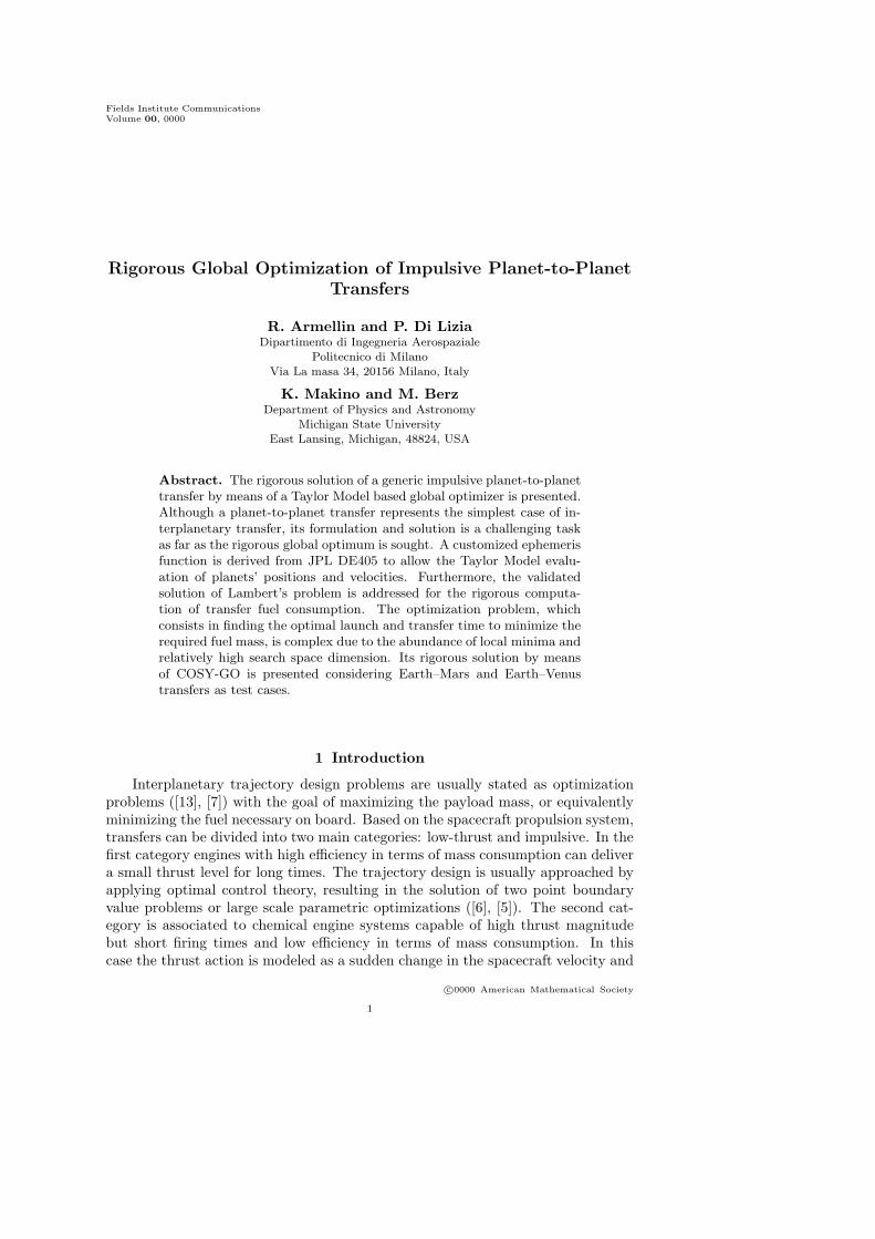
The evaluation of the position and the velocities of planets within TM framedoes not allow the use of any external code. In order to avoid this problem, a Taylorinterpolation in time of planets orbital parameters (a, e, i, ω, Ω, M) obtained throughJPL ephemerides has been carried out. In particular, a third order interpolationis selected to limit the interpolation error to thousands km for the position andm/s for velocities over the time windows of interest, an accuracy compatible withthe preliminary optimization problems at hand. Conversion from orbit elements tocartesian quantities is performed as follows:

x = r[cos(ϑ + ω) cosΩ − sin(ϑ + ω) cos i sinΩ]y = r[cos(ϑ + ω) sin Ω + sin(ϑ + ω) cos i sinΩ]y = r[sin(ϑ + ω) sin i]

vx = v[− sin(ϑ + ω − γ) cosΩ − cos(ϑ + ω − γ) cos i cosΩ]vy = v[− sin(ϑ + ω − γ) sinΩ + cos(ϑ + ω − γ) cos i cosΩ]vz = v[cos(ϑ + ω − γ) sin i]

(2.3)

where the velocity v is

v =

√

µ

r−

µ

a, (2.4)

the true anomaly is related to the eccentric anomaly by

tanE

2=

√

1 − e

1 + etan

ϑ

2, (2.5)

the flight path angle is obtained from

tan γ =e sinϑ

1 + e cosϑ, (2.6)

and the eccentric anomaly is related to the mean anomaly by Kepler’s equation,

M = E − e sinE. (2.7)

Thus, based on the interpolated orbital parameters, the cartesian position andvelocity of planets are computed as a function of time with only the nuisance ofsolving the Kepler’s equation in a validated way as described in the Appendix.

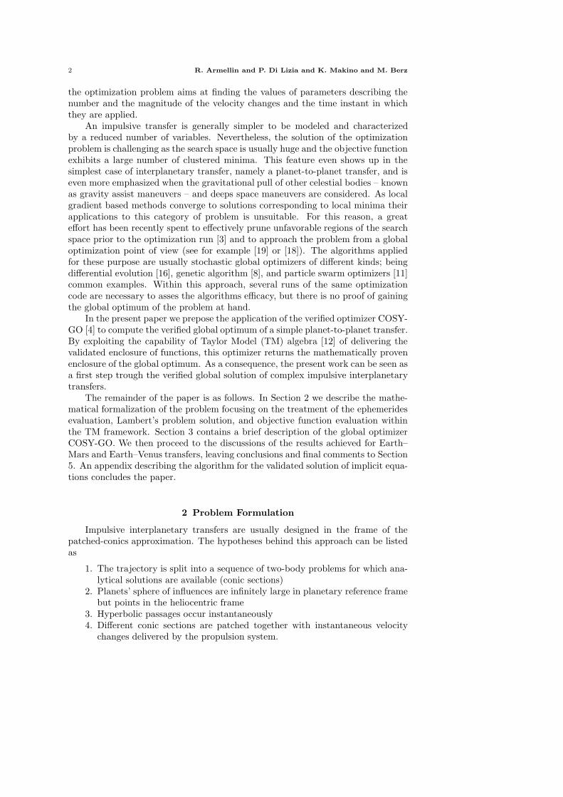
Having the ephemerides evaluated in the TM framework gives the validatedexpansion of planets positions and velocities with the departure and arrival epochs.


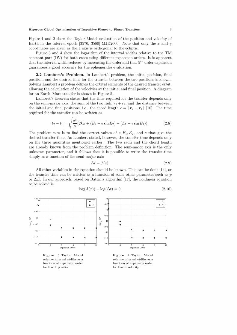
Figure 1 and 2 show the Taylor Model evaluation of the position and velocity ofEarth in the interval epoch [3570, 3580] MJD2000. Note that only the x and ycoordinates are given as the z axis is orthogonal to the ecliptic.

Figure 3 and 4 show the logarithm of the interval widths relative to the TMconstant part (IW) for both cases using different expansion orders. It is apparentthat the interval width reduces by increasing the order and that 5th order expansionguarantees a good accuracy for the ephemerides evaluation.

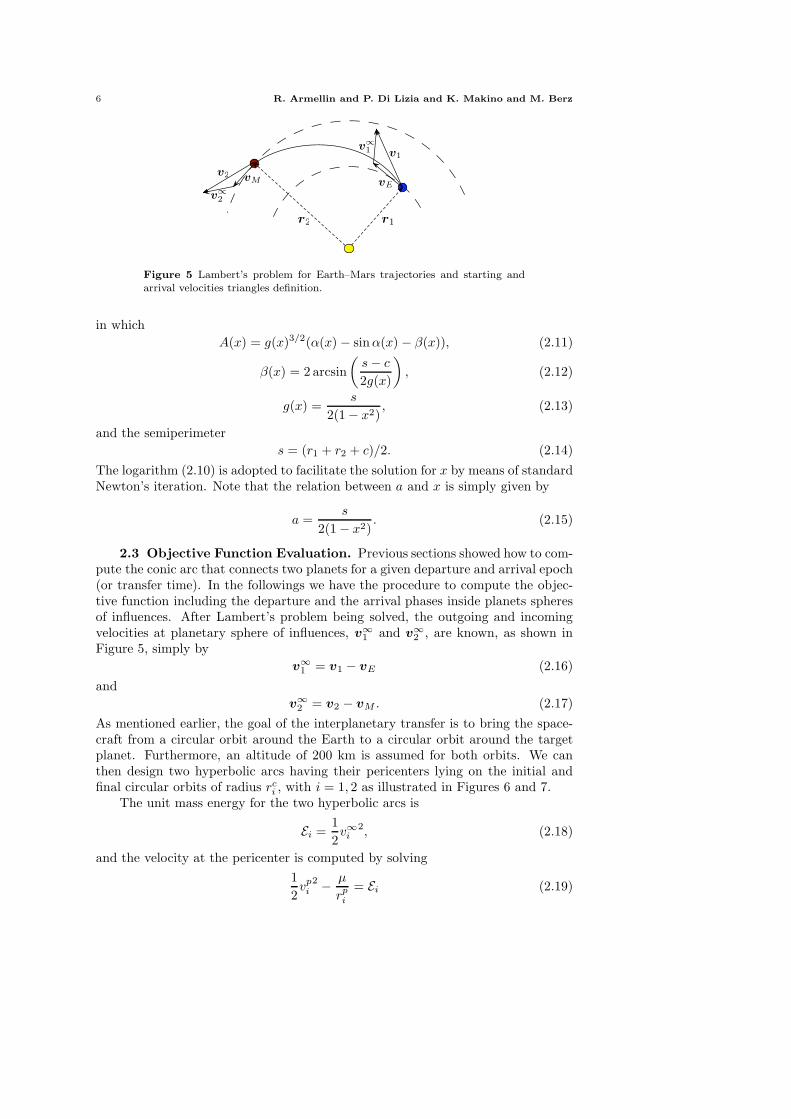
2.2 Lambert’s Problem. In Lambert’s problem, the initial position, finalposition, and the desired time for the transfer between the two positions is known.Solving Lambert’s problem defines the orbital elements of the desired transfer orbit,allowing the calculation of the velocities at the initial and final position. A diagramfor an Earth–Mars transfer is shown in Figure 5.

Lambert’s theorem states that the time required for the transfer depends onlyon the semi-major axis, the sum of the two radii r1 + r2, and the distance betweenthe initial and final positions, i.e., the chord length c = ‖r2 − r1‖ [10]. The timerequired for the transfer can be written as

t2 − t1 =

√

a3

µ(2kπ + (E2 − e sinE2) − (E1 − e sinE1)). (2.8)

The problem now is to find the correct values of a, E1, E2, and e that give thedesired transfer time. As Lambert stated, however, the transfer time depends onlyon the three quantities mentioned earlier. The two radii and the chord lengthare already known from the problem definition. The semi-major axis is the onlyunknown parameter, and it follows that it is possible to write the transfer timesimply as a function of the semi-major axis

∆t = f(a). (2.9)

All other variables in the equation should be known. This can be done [14], orthe transfer time can be written as a function of some other parameter such as por ∆E. In our approach, based on Battin’s algorithm [17], the nonlinear equationto be solved is

log(A(x)) − log(∆t) = 0, (2.10)

5 6 7 8 9 10−12

−11.5

−11

−10.5

−10

−9.5

−9

−8.5

Expansion Order

log 10

IW

rx

ry

Figure 3 Taylor Modelrelative interval widths as afunction of expansion orderfor Earth position.

5 6 7 8 9 10−12

−11.5

−11

−10.5

−10

−9.5

−9

−8.5

−8

Expansion Order

log 10

IW

vx

vy

Figure 4 Taylor Modelrelative interval widths as afunction of expansion orderfor Earth velocity.


v∞

1

v∞

2

vE

v1

vM

v2

r1r2

Figure 5 Lambert’s problem for Earth–Mars trajectories and starting andarrival velocities triangles definition.

in which

A(x) = g(x)3/2(α(x) − sin α(x) − β(x)), (2.11)

β(x) = 2 arcsin

(

s − c

2g(x)

)

, (2.12)

g(x) =s

2(1 − x2), (2.13)

and the semiperimeter

s = (r1 + r2 + c)/2. (2.14)

The logarithm (2.10) is adopted to facilitate the solution for x by means of standardNewton’s iteration. Note that the relation between a and x is simply given by

a =s

2(1 − x2). (2.15)

2.3 Objective Function Evaluation. Previous sections showed how to com-pute the conic arc that connects two planets for a given departure and arrival epoch(or transfer time). In the followings we have the procedure to compute the objec-tive function including the departure and the arrival phases inside planets spheresof influences. After Lambert’s problem being solved, the outgoing and incomingvelocities at planetary sphere of influences, v

∞

1 and v∞

2 , are known, as shown inFigure 5, simply by

v∞

1 = v1 − vE (2.16)

and

v∞

2= v2 − vM . (2.17)

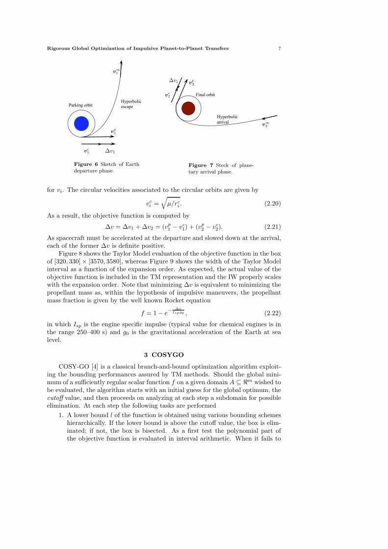
As mentioned earlier, the goal of the interplanetary transfer is to bring the space-craft from a circular orbit around the Earth to a circular orbit around the targetplanet. Furthermore, an altitude of 200 km is assumed for both orbits. We canthen design two hyperbolic arcs having their pericenters lying on the initial andfinal circular orbits of radius rc

i , with i = 1, 2 as illustrated in Figures 6 and 7.The unit mass energy for the two hyperbolic arcs is

Ei =1

2v∞i

2, (2.18)

and the velocity at the pericenter is computed by solving

1

2vp

i2−

µ

rpi

= Ei (2.19)


v∞

1

∆v1

vp

1

vc

1

Parking orbitHyperbolic escape

Figure 6 Sketch of Earthdeparture phase.

v∞

2

vc

2

∆v2v

p

2

Hyperbolic arrival

Final orbit

Figure 7 Steck of plane-tary arrival phase.

for vi. The circular velocities associated to the circular orbits are given by

vci =

√

µ/rci . (2.20)

As a result, the objective function is computed by

∆v = ∆v1 + ∆v2 = (vp1− vc

1) + (vp

2− vc

2). (2.21)

As spacecraft must be accelerated at the departure and slowed down at the arrival,each of the former ∆v is definite positive.

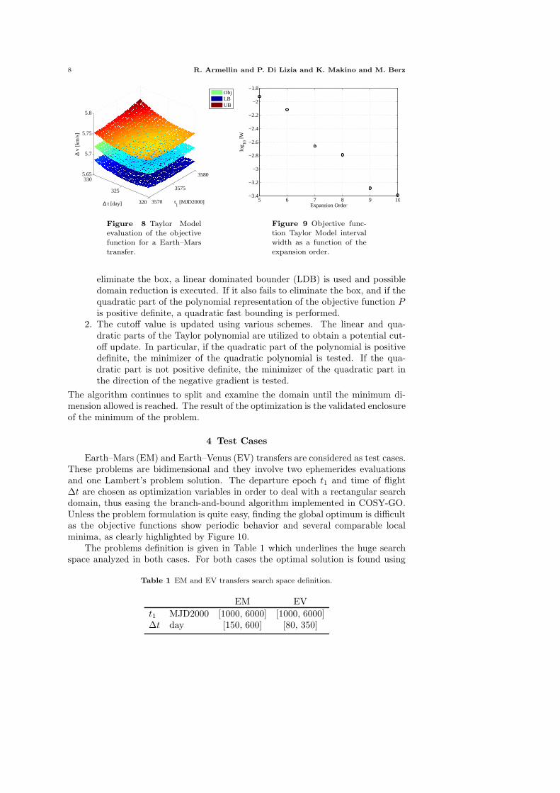
Figure 8 shows the Taylor Model evaluation of the objective function in the boxof [320, 330]× [3570, 3580], whereas Figure 9 shows the width of the Taylor Modelinterval as a function of the expansion order. As expected, the actual value of theobjective function is included in the TM representation and the IW properly scaleswith the expansion order. Note that minimizing ∆v is equivalent to minimizing thepropellant mass as, within the hypothesis of impulsive maneuvers, the propellantmass fraction is given by the well known Rocket equation

f = 1 − e−

∆vIspg0 , (2.22)

in which Isp is the engine specific impulse (typical value for chemical engines is inthe range 250–400 s) and g0 is the gravitational acceleration of the Earth at sealevel.

3 COSYGO

COSY-GO [4] is a classical branch-and-bound optimization algorithm exploit-ing the bounding performances assured by TM methods. Should the global mini-mum of a sufficiently regular scalar function f on a given domain A ⊆ ℜm wished tobe evaluated, the algorithm starts with an initial guess for the global optimum, thecutoff value, and then proceeds on analyzing at each step a subdomain for possibleelimination. At each step the following tasks are performed

1. A lower bound l of the function is obtained using various bounding schemeshierarchically. If the lower bound is above the cutoff value, the box is elim-inated; if not, the box is bisected. As a first test the polynomial part ofthe objective function is evaluated in interval arithmetic. When it fails to


3570

3575

3580

320

325

3305.65

5.7

5.75

5.8

t1 [MJD2000]∆ t [day]

∆ v

[km

/s]

ObjLBUB

Figure 8 Taylor Modelevaluation of the objectivefunction for a Earth–Marstransfer.

5 6 7 8 9 10−3.4

−3.2

−3

−2.8

−2.6

−2.4

−2.2

−2

−1.8

Expansion Order

log 10

IW

Figure 9 Objective func-tion Taylor Model intervalwidth as a function of theexpansion order.

eliminate the box, a linear dominated bounder (LDB) is used and possibledomain reduction is executed. If it also fails to eliminate the box, and if thequadratic part of the polynomial representation of the objective function Pis positive definite, a quadratic fast bounding is performed.

2. The cutoff value is updated using various schemes. The linear and qua-dratic parts of the Taylor polynomial are utilized to obtain a potential cut-off update. In particular, if the quadratic part of the polynomial is positivedefinite, the minimizer of the quadratic polynomial is tested. If the qua-dratic part is not positive definite, the minimizer of the quadratic part inthe direction of the negative gradient is tested.

The algorithm continues to split and examine the domain until the minimum di-mension allowed is reached. The result of the optimization is the validated enclosureof the minimum of the problem.

4 Test Cases

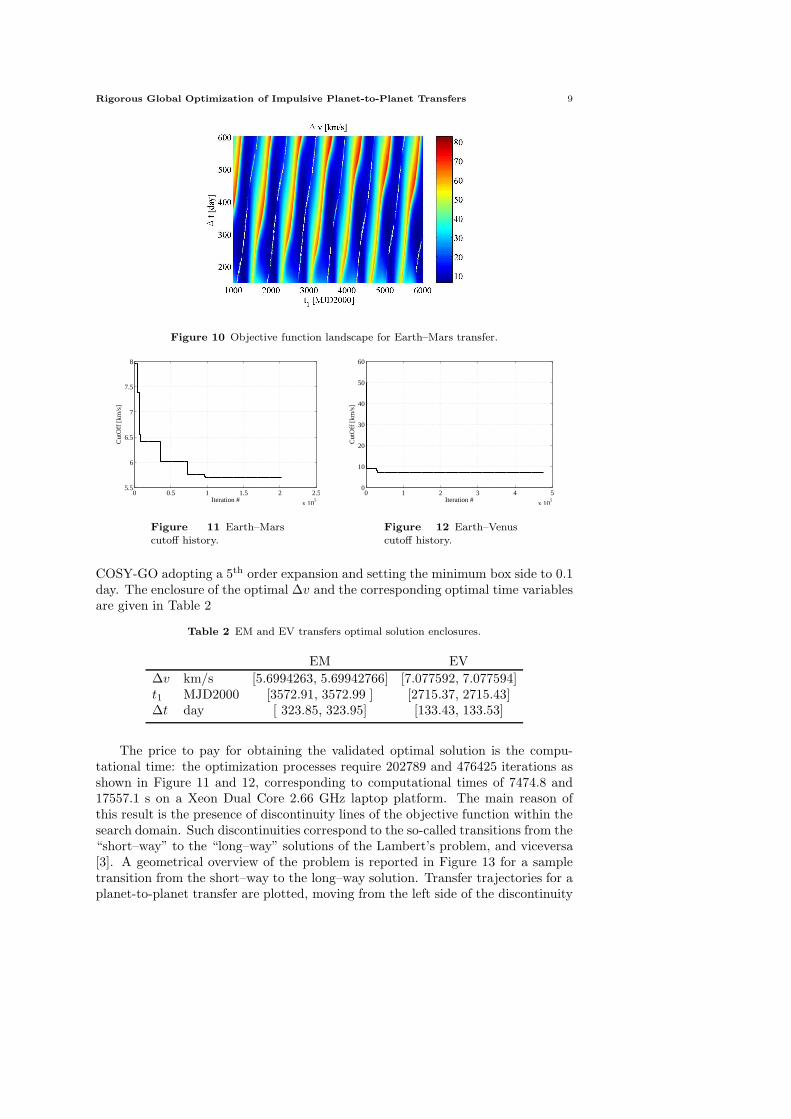
Earth–Mars (EM) and Earth–Venus (EV) transfers are considered as test cases.These problems are bidimensional and they involve two ephemerides evaluationsand one Lambert’s problem solution. The departure epoch t1 and time of flight∆t are chosen as optimization variables in order to deal with a rectangular searchdomain, thus easing the branch-and-bound algorithm implemented in COSY-GO.Unless the problem formulation is quite easy, finding the global optimum is difficultas the objective functions show periodic behavior and several comparable localminima, as clearly highlighted by Figure 10.

The problems definition is given in Table 1 which underlines the huge searchspace analyzed in both cases. For both cases the optimal solution is found using

Table 1 EM and EV transfers search space definition.

EM EV

t1 MJD2000 [1000, 6000] [1000, 6000]∆t day [150, 600] [80, 350]


Figure 10 Objective function landscape for Earth–Mars transfer.

0 0.5 1 1.5 2 2.5

x 105

5.5

6

6.5

7

7.5

8

Iteration #

Cut

Off

[km

/s]

Figure 11 Earth–Marscutoff history.

0 1 2 3 4 5

x 105

0

10

20

30

40

50

60

Iteration #

Cut

Off

[km

/s]

Figure 12 Earth–Venuscutoff history.

COSY-GO adopting a 5th order expansion and setting the minimum box side to 0.1day. The enclosure of the optimal ∆v and the corresponding optimal time variablesare given in Table 2

Table 2 EM and EV transfers optimal solution enclosures.

EM EV

∆v km/s [5.6994263, 5.69942766] [7.077592, 7.077594]t1 MJD2000 [3572.91, 3572.99 ] [2715.37, 2715.43]∆t day [ 323.85, 323.95] [133.43, 133.53]

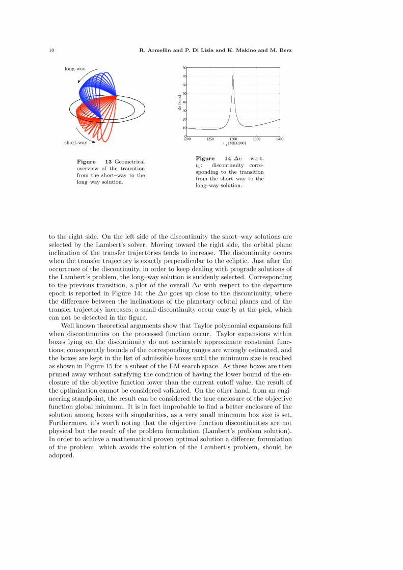
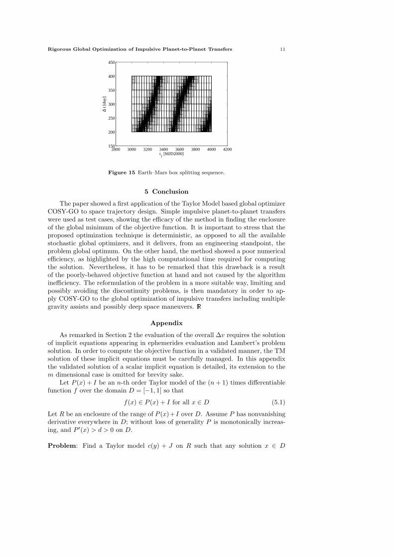
The price to pay for obtaining the validated optimal solution is the compu-tational time: the optimization processes require 202789 and 476425 iterations asshown in Figure 11 and 12, corresponding to computational times of 7474.8 and17557.1 s on a Xeon Dual Core 2.66 GHz laptop platform. The main reason ofthis result is the presence of discontinuity lines of the objective function within thesearch domain. Such discontinuities correspond to the so-called transitions from the“short–way” to the “long–way” solutions of the Lambert’s problem, and viceversa[3]. A geometrical overview of the problem is reported in Figure 13 for a sampletransition from the short–way to the long–way solution. Transfer trajectories for aplanet-to-planet transfer are plotted, moving from the left side of the discontinuity


short-way

long-way

Figure 13 Geometricaloverview of the transitionfrom the short–way to thelong–way solution.

1200 1250 1300 1350 14000

10

20

30

40

50

60

70

80

t1 [MJD2000]

∆v [k

m/s

]

Figure 14 ∆v w.r.t.t1: discontinuity corre-sponding to the transitionfrom the short–way to thelong–way solution.

to the right side. On the left side of the discontinuity the short–way solutions areselected by the Lambert’s solver. Moving toward the right side, the orbital planeinclination of the transfer trajectories tends to increase. The discontinuity occurswhen the transfer trajectory is exactly perpendicular to the ecliptic. Just after theoccurrence of the discontinuity, in order to keep dealing with prograde solutions ofthe Lambert’s problem, the long–way solution is suddenly selected. Correspondingto the previous transition, a plot of the overall ∆v with respect to the departureepoch is reported in Figure 14: the ∆v goes up close to the discontinuity, wherethe difference between the inclinations of the planetary orbital planes and of thetransfer trajectory increases; a small discontinuity occur exactly at the pick, whichcan not be detected in the figure.

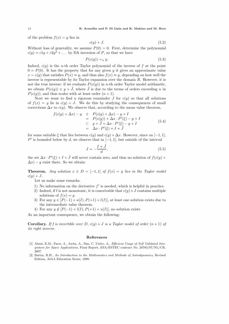
Well known theoretical arguments show that Taylor polynomial expansions failwhen discontinuities on the processed function occur. Taylor expansions withinboxes lying on the discontinuity do not accurately approximate constraint func-tions; consequently bounds of the corresponding ranges are wrongly estimated, andthe boxes are kept in the list of admissible boxes until the minimum size is reachedas shown in Figure 15 for a subset of the EM search space. As these boxes are thenpruned away without satisfying the condition of having the lower bound of the en-closure of the objective function lower than the current cutoff value, the result ofthe optimization cannot be considered validated. On the other hand, from an engi-neering standpoint, the result can be considered the true enclosure of the objectivefunction global minimum. It is in fact improbable to find a better enclosure of thesolution among boxes with singularities, as a very small minimum box size is set.Furthermore, it’s worth noting that the objective function discontinuities are notphysical but the result of the problem formulation (Lambert’s problem solution).In order to achieve a mathematical proven optimal solution a different formulationof the problem, which avoids the solution of the Lambert’s problem, should beadopted.


2800 3000 3200 3400 3600 3800 4000 4200150

200

250

300

350

400

450

t1 [MJD2000]

∆ t [

day]

Figure 15 Earth–Mars box splitting sequence.

5 Conclusion

The paper showed a first application of the Taylor Model based global optimizerCOSY-GO to space trajectory design. Simple impulsive planet-to-planet transferswere used as test cases, showing the efficacy of the method in finding the enclosureof the global minimum of the objective function. It is important to stress that theproposed optimization technique is deterministic, as opposed to all the availablestochastic global optimizers, and it delivers, from an engineering standpoint, theproblem global optimum. On the other hand, the method showed a poor numericalefficiency, as highlighted by the high computational time required for computingthe solution. Nevertheless, it has to be remarked that this drawback is a resultof the poorly-behaved objective function at hand and not caused by the algorithminefficiency. The reformulation of the problem in a more suitable way, limiting andpossibly avoiding the discontinuity problems, is then mandatory in order to ap-ply COSY-GO to the global optimization of impulsive transfers including multiplegravity assists and possibly deep space maneuvers. R

Appendix

As remarked in Section 2 the evaluation of the overall ∆v requires the solutionof implicit equations appearing in ephemerides evaluation and Lambert’s problemsolution. In order to compute the objective function in a validated manner, the TMsolution of these implicit equations must be carefully managed. In this appendixthe validated solution of a scalar implicit equation is detailed, its extension to them dimensional case is omitted for brevity sake.

Let P (x) + I be an n-th order Taylor model of the (n + 1) times differentiablefunction f over the domain D = [−1, 1] so that

f(x) ∈ P (x) + I for all x ∈ D (5.1)

Let R be an enclosure of the range of P (x)+I over D. Assume P has nonvanishingderivative everywhere in D; without loss of generality P is monotonically increas-ing, and P ′(x) > d > 0 on D.

Problem: Find a Taylor model c(y) + J on R such that any solution x ∈ D


of the problem f(x) = y lies in

c(y) + J. (5.2)

Without loss of generality, we assume P (0) = 0. First, determine the polynomialc(y) = c1y + c2y2 + . . . by DA inversion of P , so that we have

P (c(y)) =n y. (5.3)

Indeed, c(y) is the n-th order Taylor polynomial of the inverse of f at the point0 = P (0). It has the property that for any given y it gives an approximate valuex = c(y) that satisfies P (x) ≈ y, and thus also f(x) ≈ y, depending on how well theinverse is representable by its Taylor expansion over the domain R. However, it isnot the true inverse: if we evaluate P (c(y)) in n-th order Taylor model arithmetic,

we obtain P (c(y)) ∈ y + J , where J is due to the terms of orders exceeding n inP (c(y)); and thus scales with at least order (n + 1).

Next we want to find a rigorous remainder J for c(y) so that all solutionsof f(x) = y lie in c(y) + J . We do this by studying the consequences of smallcorrections ∆x to c(y). We observe that, according to the mean value theorem,

f(c(y) + ∆x) − y ∈ P (c(y) + ∆x) − y + I= P (c(y)) + ∆x · P ′(ξ) − y + I

⊂ y + J + ∆x · P ′(ξ) − y + I

= ∆x · P ′(ξ) + I + J

(5.4)

for some suitable ξ that lies between c(y) and c(y)+∆x. However, since on [−1, 1],P ′ is bounded below by d, we observe that in [−1, 1], but outside of the interval

J = −I + J

d, (5.5)

the set ∆x · P ′(ξ) + I + J will never contain zero, and thus no solution of f(c(y) +∆x) − y exist there. So we obtain:

Theorem. Any solution x ∈ D = [−1, 1] of f(x) = y lies in the Taylor model

c(y) + J .Let us make some remarks.

1) No information on the derivative f ′ is needed, which is helpful in practice.2) Indeed, if f is not monotonic, it is conceivable that c(y)+J contains multiple

solutions of f(x) = y3) For any y ∈ [P (−1)+ u(I), P (+1)+ l(I)], at least one solution exists due to

the intermediate value theorem.4) For any y /∈ [P (−1) + l(I), P (+1) + u(I)], no solution exists

As an important consequence, we obtain the following:

Corollary. If f is invertible over D, c(y) + J is a Taylor model of order (n + 1) of

its right inverse.

References

[1] Alessi, E.M., Farrs, A., Jorba, A., Sim, C, Vieiro, A., Efficient Usage of Self Validated Inte-grators for Space Applications, Final Report, ESA/ESTEC contract No. 20783/07/NL/CB,2007.

[2] Battin, R.H., An Introduction to the Mathematics and Methods of Astrodynamics, RevisedEdition, AIAA Education Series, 1999.


[3] Bernelli-Zazzera, F., Berz, M., Lavagna, M., Armellin, R., Di Lizia, P., and Topputo, F.,Global Trajectory Optimization: Can we Prune the Solution Space when Considering DeepSpace Maneuvers, Final Report, ESA/ESTEC contract No. 20271/06/NL/HI, 2007.

[4] Berz, M., Makino, K., and Kim, Y., Long-term stability of the tevatron by verified globaloptimisation, Nuclear Instruments and Methods, A558, 2005, pp. 1–10.

[5] Betts, J.T., Practical Methods For Optimal Control Using Nonlinear Programming, SIAM,2001.

[6] Bryson A.E., Ho Y., Applied Optimal Control, pp. 1–89. Taylor & Francis, New York, 1989.[7] Di Lizia, P., Radice, G., Advanced Global Optimisation for Mission Anal- ysis and Design.

Final Report. ESA/ESTEC contract No.18139/04/NL/MV, 2004.[8] Goldberg, D.E., Genetic Algorithms in Search, Optimization and Machine Learning,

Addison-Wesley Longman Publishing Co., 1989.[9] Izzo, D., Becerra, V., Myatt, D., Nasuto S., and Bishop, J., Search space pruning and global

optimisation of multiple gravity assist spacecraft trajectories, Journal of Global Optimisation,38 (2006), pp. 283–296.

[10] Kaplan, M.H., Modern spacecraft dynamics and control, John Wiley & Sons,1975.[11] Kennedy, J., and Eberhart, R., Particle swarm optimisation, Proc. IEEE Int. Conf. on Neural

Networks, 1995, pp. 1942–1948.[12] Makino, K., Rigorous Analysis of Nonlinear Motion in Particle Accelerators, Ph.D. Thesis,

Michigan State University, East Lansing, Michigan, USA, 1998.[13] Myatt, D.R., Becerra, V.M., Nasuto, S.J., and Bishop, J.M., Advanced Global Op-

timisation for Mission Analysis and Design. Final Report. ESA/ESTEC contract No.18138/04/NL/MV, 2004.

[14] Prussing, J.E. and Conway, B.A., Orbital Mechanics, Oxford University Press, 1993.[15] Standish, M.E. and Williams, J.G., Detailed description of the JPL planetary and

lunar ephemerides, DE405/LE405. Electronically available as a PDF le, http://iau-comm4.jpl.nasa.gov/XSChap8.pdf.

[16] Storn, R. and Price, K., Differential Evolution–A Simple and Efficient Heuristic for globalOptimization over Continuous Spaces, Journal of Global Optimization, 11 (1997), No. 4, pp.341–359.

[17] Vinko, T., Izzo, D., and Bombardelli, C., Benchmarking different global optimisation tech-niques for preliminary space trajectory design 58th International Astronautical Congress,Hyderabad, India, 2007.

[18] Vasile, M., Summerer, L., De Pascale, P., Design of Earth–Mars transfer tra jec- tories using

evolutionary-branching technique, Acta Astronautica, 56 (2005), No. 8, pp. 705–720.[19] Yokoyama, N., Suzuki, S., Modied Genetic Algorithm for Constrained Tra- jectory Optimiza-

tion, Journal of Guidance Control and Dynamics, 28 (2005), No.1, pp. 139–144.

rigorous global optimization of impulsive planet-to-planet transfers in the patched-conics...

Documents