rewarding sequential innovators: prizes, patents, and buyouts
TRANSCRIPT
Federal Reserve Bank of MinneapolisResearch Department Staff Report 273
July 2000
Rewarding Sequential Innovators:Prizes, Patents and Buyouts
Gerard Llobet∗
University of Rochesterand CEMFI
Hugo Hopenhayn∗
Universidad Torcuato Di Tellaand University of Rochester
Matthew Mitchell∗
University of Minnesotaand Federal Reserve Bank of Minneapolis
ABSTRACT
This paper presents a model of cumulative innovation where firms are heterogeneous in theirresearch ability. We study the optimal reward policy when the quality of the ideas and theirsubsequent development effort are private information. The optimal assignment of propertyrights must counterbalance the incentives of current and future innovators. The resultingmechanism resembles a menu of patents that have infinite duration and fixed scope, wherethe latter increases in the value of the idea. Finally, we provide a way to implement thispatent menu by using a simple buyout scheme: The innovator commits at the outset to aprice ceiling at which he will sell his rights to a future inventor. By paying a larger feeinitially, a higher price ceiling is obtained. Any subsequent innovator must pay this price andpurchase its own buyout fee contract.
∗We thank Fernando Alvarez and Narayana Kocherlakota for helpful comments. The views expressed hereinare those of the authors and not necessarily those of the Federal Reserve Bank of Minneapolis or the FederalReserve System.
1. Introduction
A central feature of innovative activity is that research is cumulative. This is relevant
to the way in which research is rewarded. If research is rewarded through the granting of
particular property rights, as for instance in a patent, the cumulative structure leads to the
natural question of what to do when the next improvement arises. How can the property
rights of the previous state-of-the-art be compatible with rewarding the recent improvement
with its own property rights?
A variety of methods are available to reward innovators. Two of the most commonly
discussed (in Wright (1983), for instance) are patents and research prizes. The latter is simply
a transfer to the innovator for development of a particular invention. The former consists of
the granting of some sort of market power to the innovator, perhaps in exchange for a fee. It
is well understood that, when information is complete, it is optimal to choose a prize as the
reward, since it does not result in any of the distortions that may accompany market power.
When the principal charged with rewarding innovators does not have complete information
about the benefits of an invention, however, it has been shown, for instance in Scotchmer
(1999), that it may be optimal to grant a patent, since the value of the reward is then tied
to the innovation’s value through its potential profits in the market.
In this paper we study the optimal mechanism to reward innovations when new ideas
arrive continually, and there is both moral hazard and adverse selection. We allow the patent
office a variety of instruments, but force them to operate with limited information about the
potentially patentable innovations. The optimal reward, it turns out, has a relatively simple
form: it is a patent, with no statutory expiration date, but rather providing a constant
amount of protection against future improvements forever. Under very plausible conditions,
the optimal patent policy involves different types of protection for different innovations. We
show that the optimal mechanism can be instituted through a system of mandatory buyout
fees which can be interpreted as compulsory licensing. This mechanism generates information
which reduces the burden on courts of determining infringement. The menu of contracts
offered by the patent office in order to implement the optimal reward is not time or history
dependent, which is particularly appealing in terms of realistically using such a method.
When the value of an innovation is known, so that there is adverse selection but no
moral hazard, the problem of competing property rights in a cumulative innovation setting
may never arise. In that case, even if costs are unknown, it may be possible to provide
incentive entirely through a simple cash prize. Then, the problem is not compounded by
cumulative innovation, since the reward is paid in full immediately, and is therefore not rel-
evant when the next improvement arrives. Scotchmer (1999) and Cornelli and Schankerman
(1999), however, point to the usefulness of patents when the value of an innovation is un-
known, resulting in a moral hazard problem. If the quality of the innovation is unobserved,
the regulator cannot offer a reward which depends on quality. Therefore the regulator uses a
patent. The monopolist pays a greater fee for a greater time period of patent protection.
When the model is extended to include multiple innovations, however, the optimal
policy can change considerably. When value is unknown, so that patents are employed, the
problem of competing property rights arises. A promise of patent rights to one innovator
might be in conflict with offering another patent to a future innovator, and might discourage
future innovators, as in O’Donoghue, et al. (1998). Lines of what constitutes a “sufficient”
improvement to warrant a new patent must be drawn.
We characterize the optimal reward system in a cumulative innovation context with
2
incomplete information on the part of the patent office. Like Scotchmer (1999), the patent
office offers “better” patent protection in exchange for a higher fee. Here that protection
means that a greater percentage of possible future innovations are precluded by the innovator’s
patent. As in other work such as O’Donoghue, et al. (1998) this ability of a patent to preclude
future innovations is labeled the patent’s “breadth.” We use an extreme model where, if only
one innovator is ever to arrive, the optimal patent policy implements the efficient level of
research. We then show that in the same model, but with multiple innovators arriving in
sequence with cumulative innovations, it is impossible to achieve the efficient level of research.
This reinforces the idea that the cumulative nature of innovation is very relevant to policy.
By using a mechanism design approach, the problem of enforcement of patent breadth,
a contentious one in practice, is studied alongside the optimal breadth itself. The optimal
policy introduced here generates information about the quality of innovations. That is, all
that the government must determine in order to dole out property rights is if an innovation is
related, in the sense of being on the same “ladder” as the previous innovation. We require of
the policy that it generates enough information to solve problems of “infringement” through
the self-selection from a menu of patents. This is in contrast to current policy, where the
courts must determine more than just if two innovations are quality improvements over the
other, but also how much of an improvement has been made. In the mechanism studied
here, infringement is determined by the reports of the innovators, lowering the burden on the
patent system.1
An interesting feature of the optimal policy is that each patent offered consists of a
given breadth, maintained forever. That is, the patent expires only when something better
1See Llobet (1999) for a study on how the legal environment affects cumulative research.
3
than the constant threshold comes along; the optimal policy does not prescribe that the
amount of protection increase or decrease over time. Current patent policy has a clear sense
in which level of protection declines suddenly, at the end of the patent’s statutory life. The
optimal policy here suggests that patents should end only because something better arrives,
and not because of some imposition of a statutory time limit for the protection.
We also show that, under plausible conditions, the menu offers a variety of patent
breadths to different innovators, depending on their costs and the resulting quality of their
innovations. Bigger improvements get greater protection. Interestingly, it has been claimed
that, in fact, the patent courts do provide additional protection for products which represent
large improvements. This result also shows that it may be optimal to provide for a variety
of breadths, which the current US statute does not explicitly allow for.
Given that the optimal policy calls for a variety of patent breadths, it might seem that
implementing the optimal policy would require a very complicated system. To the contrary,
we show that the optimal mechanism can be implemented through mandatory buyout prices
or licensing fees. The idea of mandatory licensing dates back at least as far as the 1800’s, when
such a rule passed the House of Lords (Machlup and Penrose(1950)). Innovators, as part of the
granting of a patent, must commit to a price at which they will relinquish their rights. This
commitment mitigates any bargaining power a patent holder might exert on future innovators.
Tandon (1982) uses similar buyout fees in a complete information model to mitigate monopoly
costs. Here we add the fact that, by offering a menu of compulsory licensing fees to innovators,
the fees can be useful in generating information about the innovators. The fee acts as the
breadth of the patent: the bigger the fee, the greater the patent’s implied breadth, since
future innovators will need a substantial improvement to justify the larger buyout fee.
4
The set of patents, then, offered under the compulsory licensing agreement is a menu
of buyout fees, accompanied with prices paid to the government. In order to take the lead,
an innovator must pay the prearranged buyout amount to the prior innovator, choose its
own buyout fee, and make the appropriate payment to the government as prescribed by the
menu. The menu of contracts offered by the government has a simple, stationary form. The
government has a constant set of posted prices for patents with various buyout amounts, and
innovators choose their favorite whenever they want to take the market lead.
Other authors have studied the trade-off between patents and prizes. Notably, Wright
(1983) argues that prizes may mitigate problems associated with patent races. In our for-
mulation, with ideas private to a single innovator, this argument for prizes is not present.
Shavell and van Ypersele (1999) suggest offering an optional reward, so that some patents
would be replaced with rewards. They do not consider the possibility that this might lead to
adverse selection when the quality of innovations is unobservable and endogenous. In single
innovation formulations such as Scotchmer (1999), it is true that the optimal reward is a prize
if the value is known. The single innovation case with asymmetric information and general
reward mechanisms is considered in Chiesa and Denicolo (1999), with similar results.
Previous models of optimal patent policy have for the most part not considered cu-
mulative research. Exceptions include Scotchmer and Green (1990), Green and Scotchmer
(1995), and O’Donoghue, et al. (1998). The model employed in the latter is most similar
to the one here; a central difference is that in their model the patent office is fully informed
and therefore could offer a prize to reward innovators. We consider a case where research is
cumulative and the patent office’s information is incomplete, and show that it differs from the
optimal mechanism in the one innovation case, in the sense that it departs from the logic of
5
the regulation literature. On the other hand, they consider heterogeneity on the part of the
consumers as well as a form of bargaining between innovators. They consider both infinite
length, finite breadth patents and infinite breadth, finite length patents. We consider the set
of all possible breadths and lengths (in the sense that length can be thought of as breadth
reduced to zero after a certain time), and find that infinitely lived patents are optimal.
The next section sets the stage by studying a version of the model where there will
only ever be one innovator. When costs are unknown but value of the project is observable,
the reward for an innovator is a cash prize. When value is unobservable, patents are employed
as a reward. In the model below, the efficient level can be implemented in either case. These
results mirror the findings of several papers in the patent literature and are similar to the
spirit of mechanisms used in the regulation literature. The main points come in the third
section. There, the general model of many innovations is introduced and the optimal policy
is contrasted with the one for the single innovator. The patent agency must concern itself
with how to provide a reward for one innovator without discouraging future innovators.
2. The Environment
A. Preferences and Technology
There is a single good differentiated by quality q and an infinite horizon of discrete
time periods. A product of quality zero is sold competitively at marginal cost, normalized to
zero. There is a single, infinitely lived consumer with time-additively separable preferences
and per period utility q− p, where p is the price of the good. These preferences are standard
as in, for instance, Anderson, et al. (1992), and can be justified by adding a composite good
and quasilinear utility. The future is discounted according to a discount factor δ.
6
An “idea” is the private property of a single firm. It must be researched, though, to
be made into a viable product. That product can be freely imitated unless the innovator
is given some specific property rights (a patent). Suppose that firms are indexed by their
capabilities to undertake research through a parameter z. We assume z is drawn from a
known distribution Φ(z) with density φ(z). A higher z means that the firm can obtain
improvements at a lower cost.2 The cost of the improvement is a function not only of z but
also of the size ∆ of the improvement (in the quality space) over the state of the art, in this
case q = 0, according to c(∆, z). It is assumed that c1 > 0, c2 < 0, c11 > 0 and c12 < 0.
The first assumption says that bigger improvements are more costly. The second says that
the higher is the firm’s z, the lower are its costs. Costs are convex. The last assumption
is important: the higher is z, the lower are marginal costs c1. Therefore the social planner
prefers that firms which draw high z spend more on research. The higher is z, the more
efficient is the firm at research.
We will, at various points, consider two market structures. The first is simply compe-
tition, where p = 0 is the result of marginal cost pricing. In that case, consumers receive ∆
units of surplus per period. On the other hand, if the innovator is given a monopoly right to
the product, the product is sold for p = ∆, the consumers are left with no surplus, and the
firm makes ∆ units of profits per period.
The size of the innovation ∆ is also the amount of social surplus it generates each pe-
riod. If the product is sold competitively at marginal cost 0, then the homogeneous consumer
enjoys ∆ units of surplus. If the product is sold at a higher price, profits rise one-for-one with
2Alternative interpretations of z could be: quality of the idea that the firm obtains, experience obtainedby marketing similar products, scale economies, know-how, etc.
7
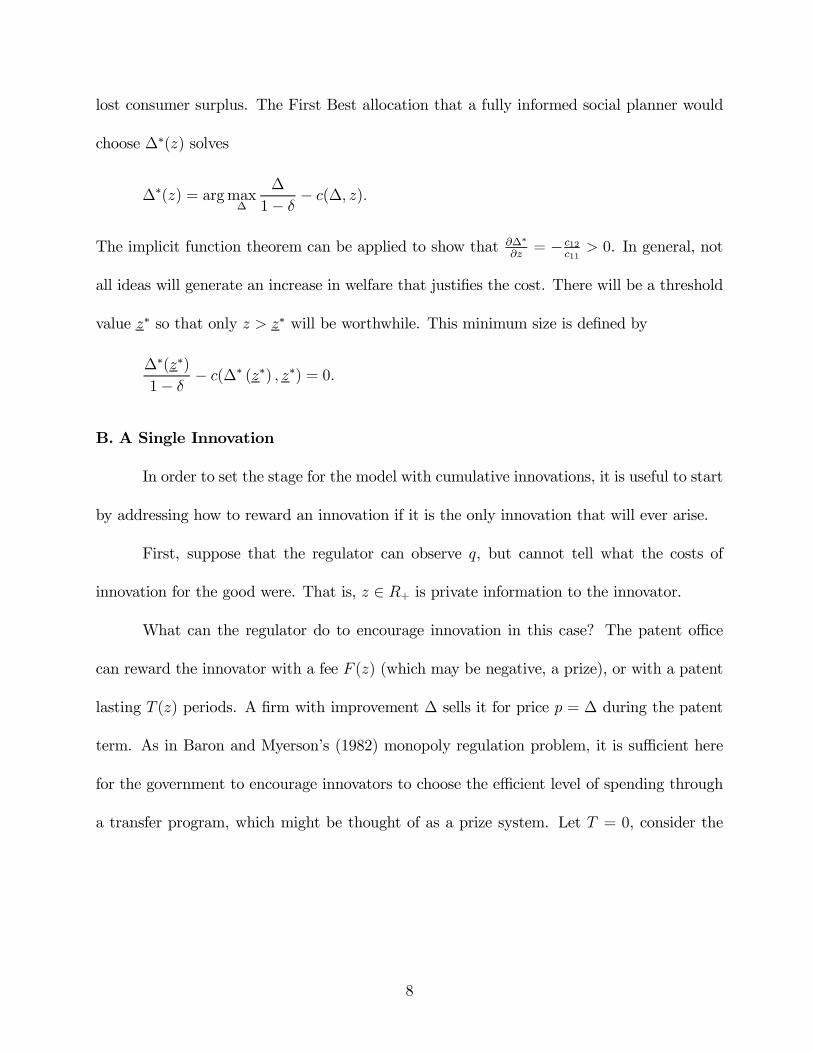
lost consumer surplus. The First Best allocation that a fully informed social planner would
choose ∆∗(z) solves
∆∗(z) = argmax∆
∆
1− δ− c(∆, z).
The implicit function theorem can be applied to show that ∂∆∗∂z= − c12
c11> 0. In general, not
all ideas will generate an increase in welfare that justifies the cost. There will be a threshold
value z∗ so that only z > z∗ will be worthwhile. This minimum size is defined by
∆∗(z∗)1− δ
− c(∆∗ (z∗) , z∗) = 0.
B. A Single Innovation
In order to set the stage for the model with cumulative innovations, it is useful to start
by addressing how to reward an innovation if it is the only innovation that will ever arise.
First, suppose that the regulator can observe q, but cannot tell what the costs of
innovation for the good were. That is, z ∈ R+ is private information to the innovator.
What can the regulator do to encourage innovation in this case? The patent office
can reward the innovator with a fee F (z) (which may be negative, a prize), or with a patent
lasting T (z) periods. A firm with improvement ∆ sells it for price p = ∆ during the patent
term. As in Baron and Myerson’s (1982) monopoly regulation problem, it is sufficient here
for the government to encourage innovators to choose the efficient level of spending through
a transfer program, which might be thought of as a prize system. Let T = 0, consider the
8
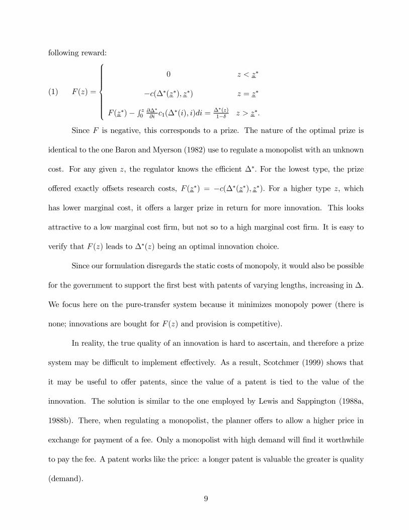
following reward:
F (z) =
0 z < z∗
−c(∆∗(z∗), z∗) z = z∗
F (z∗)− R z0 ∂∆∗∂ic1(∆
∗(i), i)di = ∆∗(z)1−δ z > z∗.
(1)
Since F is negative, this corresponds to a prize. The nature of the optimal prize is
identical to the one Baron and Myerson (1982) use to regulate a monopolist with an unknown
cost. For any given z, the regulator knows the efficient ∆∗. For the lowest type, the prize
offered exactly offsets research costs, F (z∗) = −c(∆∗(z∗), z∗). For a higher type z, which
has lower marginal cost, it offers a larger prize in return for more innovation. This looks
attractive to a low marginal cost firm, but not so to a high marginal cost firm. It is easy to
verify that F (z) leads to ∆∗(z) being an optimal innovation choice.
Since our formulation disregards the static costs of monopoly, it would also be possible
for the government to support the first best with patents of varying lengths, increasing in ∆.
We focus here on the pure-transfer system because it minimizes monopoly power (there is
none; innovations are bought for F (z) and provision is competitive).
In reality, the true quality of an innovation is hard to ascertain, and therefore a prize
system may be difficult to implement effectively. As a result, Scotchmer (1999) shows that
it may be useful to offer patents, since the value of a patent is tied to the value of the
innovation. The solution is similar to the one employed by Lewis and Sappington (1988a,
1988b). There, when regulating a monopolist, the planner offers to allow a higher price in
exchange for payment of a fee. Only a monopolist with high demand will find it worthwhile
to pay the fee. A patent works like the price: a longer patent is valuable the greater is quality
(demand).
9
Consider the model presented above, but where ∆ is unobservable. A prize structure
like the one in (1) will not be effective, since everyone will claim to have the highest z to collect
the largest prize, and there will be no way to verify if the high level of research demanded
for that z has actually been undertaken. However, since the monopolist can extract all the
surplus from the consumers, the efficient outcome can be attained, but only through the
granting of monopoly power. In fact, if T (z) = ∞, it is easy to verify that the innovator
chooses ∆∗(z), since the profits of the firm are exactly equal to the social surplus, and so
profit maximization and the definition of ∆∗ coincide.
Because of the inelastic demand, even unknown ∆ may not prevent the government
from implementing the efficient level of innovation. However, that result can only be attained
through the granting of patent rights, as opposed to the earlier case with known ∆, which
could be implemented entirely with cash payments. This is the important point of this section.
In the next section, we take up the main point of the paper: what happens when innovation
is cumulative. When patents are essential (i.e. when ∆ is unobserved), there will come the
question of how to weigh the property rights of one innovator with that of the next. One of
the important differences in the next section is that the optimal policy will be different and
will be unable to attain the efficient level of research due to the sequential structure.
3. Multiple Innovations
Suppose that each period a new firm arrives with a new idea z, allowing an improve-
ment over the current quality in the amount ∆ with cost c(∆, z) as before. If ∆ is observable,
the government could simply employ the prize system of the last section in sequence to each
innovator. The conclusions of the last section would remain unaltered.
10
When ∆ is unobserved, the optimal mechanism for a single innovator involved an
infinite patent. Offering a patent, however, is quite different when innovation is cumulative,
as pointed out, for instance, in Scotchmer and Green (1990) and O’Donoghue, et al. (1998).
The optimal patent for the sequential case must take into account the fact that property
rights granted to the first innovator might preclude some future improvements. The patent,
in order to be economically meaningful, may have to preclude small improvements, or else
the original innovator’s ability to profit from research may be short lived.
If ex ante contracting were perfect, the optimal policy would remain unchanged: simply
grant an infinite property right to the first innovator, and allow him to license that patent
to future innovators. Since there is no static cost of monopoly, the licensing would allocate
innovation efficiently.
Given the history of innovations and their rewards, though, it is likely that disputes
would emerge. For instance, there may be a hold-up problem. If the patentee cannot commit
beforehand to sell a license to an infringer before the invention is obtained, then once the
development cost is sunk, the patentee can raise the price for the license. This discourages
investment in innovations. Moreover, there may be disputes about what innovations pertain
to which products being sold, since one product may contain many distinct innovations.
These problems lead to potential dynamic costs of monopoly rights, which is our focus here,
as in O’Donoghue et al. (1998).
We assume that the arbiter of the disputes, which we take to be the government, has
no way to learn anything truthful about the dispute from the parties involved. As such, all
that the arbiter can do is assign property rights based on the reports of z that are made
by the innovators. Moreover, the arbiter can make a determination about this mechanism
11
at the outset, as if “owning” the entire ladder; no useful information can be generated from
the parties. Here, the role of the government is one of commitment and independence: it
allocates rewards only on the basis of reports, according to a policy that is fixed ex ante.
Of course, our assumption that there is no way for the patentor to learn about the
innovations from the innovators is extreme. Llobet (1999) studies a simpler model but
where the litigation technology is meaningful. Here, if some perhaps noisy signal about z
or ∆ could be generated, it would simply result in the arbiter using a combination of the
mechanism described here and a reward based on the signal of the underlying information,
using the signal more if it is more precise.
In principle, the government can choose the market structure, in terms of which inno-
vations may be sold and whether or not monopoly rights are granted, at any point in time,
along with transfer payments (or fees) for all the innovators that have arrived up to that
time. The set of possible instruments we allow, then, is very large. Fortunately, we find a
relatively simple characterization of the optimal mechanism, and then focus our attention on
studying that recursive problem.
From the innovator’s perspective, all that matters is how long monopoly power will last
for the innovation. The innovation can make profits ∆ in any period that it is the highest
quality product allowed to be sold, and zero otherwise.3 Denote the expected discounted
duration of the monopoly power granted under the patent for type z by d(z). Since a unit of
d gives the innovator the right to make ∆ profits for one immediate period, the innovator’s
expected revenue from sales of the product are d(z)∆, the product of d(z), the expected
3This assumes that monopoly power for the leading innovation does not preclude earlier innovations frombeing sold. That assumption is not essential; the details are below.
12
discounted duration of monopoly power, and ∆, the per period profits of producing the
innovation. The innovator solves
∆d(z, d) = argmax∆
d(z)∆− c(∆, z)− F (z).(2)
We make one additional assumption which, as can be seen in Appendix A, simplifies
matters considerably. It is that ∂2∆d
∂2d> 0. With the assumption, under the optimal mecha-
nism, a new innovation is either implemented and given the right to produce immediately or
is never given the right to produce.4
Proposition 1. The optimal mechanism gives each innovator a duration of incumbency
d(z), in such a way that whenever a new innovator is awarded a d(z) > 0 the previous one is
immediately replaced.
This allows the state variable of the dynamic program to consist simply of information
from the current market leader. Without it, the analysis would be similar but the state
variable would have to include all of the promised future monopoly rights.5
The previous proposition says nothing about how duration should be allocated; in fact,
since d(z) is expected duration, the property right might be allocated stochastically. The next
proposition shows how duration is allocated: a patent can be defined by its “breadth” z0(z).
That is, a firm reporting that it is of type z receives sole rights until a report of z0 is made
by another innovator.
4We require that the mechanism be immune to simple bribes across agents. The details are contained inAppendix A.
5Other questions would arise if innovations were encouraged but forced to wait; for instance, do subsequentinnovators build on the state-of-the-art invention (patent) or the most advanced product being sold in themarketplace?
13
Proposition 2. Given a duration d(z), it is optimal to grant a constant breadth, infinitely
lived patent z0(z).
In addition to making the analysis substantially simpler, this result points to an im-
portant intuition about optimal property rights for repeated innovators. Take, for instance,
the example of a fixed breadth z for T periods followed by zero breadth after that, which
could be thought of as current US policy. If a longer patent is offered, less breadth needs
to be offered in each period. The extra protection being extended through a longer time is
given for the smallest z, whereas the breadth it reduces comes, at the margin, from large z
near z. The patentee cares only about the cumulative probability of being a leader, but the
patentor cares about the size of the next innovation which is allowed. Therefore, this switch
from protection against high z now to lower z later can improve social welfare, while at the
same time maintaining the expected profits to the innovator. This force pushing for longer,
lower breadth patents in the cumulative context is not an artifact of any particular modeling
assumption, but rather a natural result of the different aims of patentor and patentee. This
complements the result in Gilbert and Shapiro (1990) which suggests that, in terms of static
cost of monopoly, long lived patents may be best.
This formulation assumes that when a new innovation arrives, older ones may still be
produced; in equilibrium of the pricing game they are not sold in positive amounts, though,
although they do have the effect of limiting profits to the incremental quality ∆ rather than
the entire quality of the produced good. This assumption is not material; all of the results
remain unchanged if a patent allows the holder to dominate the entire industry with no fear
of competition. The model is formulated as it is, though, to capture the idea that although
14
legally still a patented product and fit for sale, the effective life comes to an end because
something else comes along and makes the innovation effectively obsolete.6
It remains to be decided how to allocate duration for different types of z; the rest
of the section is concerned with that problem. This mirrors the problem above: in the
one innovation case, it is optimal to provide full protection, i.e. duration ofP∞i=0 δ
i. With
multiple innovations there is the additional trade-off that larger duration means excluding
more future ideas. In order to figure out the optimal z0(z), and hence the optimal duration,
first an inventor’s response, in terms of innovation, to a given breadth z0 must be calculated.
From equation (2) a given firm chooses ∆ to solve
∆p(z, z0) = argmax∆
∆
1− δΦ(z0)− c(∆, z)− F (z),
where 11−δΦ(z0) reflects the expected duration given an infinitely lived patent of breadth z
0.
The corresponding first order condition is
1
1− δΦ(z0)= c1(∆
p, z)(3)
where again ∆p denotes the optimal choice made by the firm. Due to the assumptions on the
cost function, it is immediate that the function ∆p(z, z0) is increasing in both its arguments.
That is,
∂∆p
∂z=
c12(∆p, z)
−c11(∆p, z)> 0,(4)
∂∆p
∂z=
−δφ(z0)(1−δΦ(z0))2
−c11(∆p, z)> 0.(5)
6In O’Donoghue, et al. (1998), the consumer side is set up so that the two best products are sold inpositive quantities, thereby making the obsolescence gradual.
15
The more breadth is granted, the more innovation will be undertaken, since it is likely to
pay off for a longer effective patent life. Of course, the cost is that breadth precludes future
innovations that might be worthwhile.
Although we consider breadth in terms of the quality of the idea z, it is equivalent
to think of breadth in terms of the size of the innovation ∆ required for a noninfringing
innovation since there is a strictly increasing relationship between the size of the invention
achieved, ∆, and the parameter z. Breadth can be thought of in the usual sense: a higher z0
means that it will take a larger improvement for a subsequent product to be produced.
Note that, as before, the first best requires that
1
1− δ= c1(∆
∗, z).
If anything less than an infinite breadth patent is granted, innovation will not be at the
efficient level. But precluding future innovations will not, in general, be optimal; patents will
be weakened to allow for subsequent innovations at the cost of inefficient levels of research
for each innovation.
The condition for truthful revelation given the two instruments, z0 and F , is for the
report bz to be the one that solvesW (z, z0) = maxbz ∆p(z, z0(bz))
1− δΦ(z0(bz)) − c(∆p(z, z0(bz)), z)− F (bz).Checking the Spence-Mirrlees condition we obtain
∂2W
∂z0∂z= −δφ(z0)c1(∆, z)c12(∆
p, z)
c11(∆p, z)> 0.
For the lowest type z which is undertaken, profits are minimized to zero, i.e. W (z, z0(z)) =
0, and every other type z receives positive profits as a result. The expression for F (z, z) is
16
obtained in the standard way as follows:
F (z, z) =∆p(z, z0)1− δΦ(z0)
− c(∆p(z, z0), z) +Z z
zc2(∆
p(x, z0(x)), x)dx.
Because ∂W∂z0 =
δφ(z(bz))∆p(z,z)
(1−δΦ(z(bz)))2 > 0 it must be that F is strictly increasing in z, so that better
inventors obtain more protection at a higher price.
The mechanism designer, then, must choose a protection level z0(z) for any level z that
might arise. The problem has a relatively simple recursive structure. The dynamic problem
of the principal is
V (q, z) = Φ(z) [q + δV (q, z)] +(6)
maxz0(z)
Zz[(q +∆p(z, z0))− c(∆p(z, z0), z) + δV p(q +∆p(z, z0), z0)]φ(z)dz
subject to the constraints
(IC) z0 (z) increasing in z for all z > z,
(IR) W (z, z0(z)) ≥ 0 for all z > z.
The state of the economy is the leading edge quality q and the promised breadth
z. The first term reflects the fact that, if an idea comes along less than z (which happens
with probability Φ(z)), consumer plus producer surplus equals q, since no improvement can be
allowed to arrive, and the state is unchanged. If an idea of type greater than z arrives, though,
the patent authority can offer a new patent with breadth z0. That encourages the innovator
to generate an invention of size∆p(z, z0), leaving the leading edge quality at q+∆p(z, z0). The
formulation assumes that funds are costlessly obtainable by the government; it is completely
straightforward to add a cost µ of acquiring funds, as in Laffont and Tirole (1986). None of
the results presented are adversely affected by the inclusion of such a cost.
17
The two restrictions correspond to the incentive compatibility and individual rational-
ity constraints. The second one implies that the planner will fulfill the promise made to the
previous innovator despite the private information on the quality of the next idea.
A natural question is whether the optimal contract involves a uniform patent or if
the principal will be interested in separating different firms with different capabilities. The
answer is that the optimal patent contract calls for greater breadth for higher z if offering
more breadth has a greater effect on research for innovators with better ideas, i.e. ∂2∆p
∂z0∂z > 0.7
Proposition 3. If ∂2∆p
∂z0∂z > 0, the optimal mechanism satisfies z0(z) strictly increasing in z.
The intuition here is straightforward. The cost of higher breadth in terms of lost future
projects does not depend on z, but the marginal benefit is increasing if ∂2∆p
∂z0∂z > 0, since it has
more of an effect on incentives to innovate.
There is some evidence that courts follow something like this rule. The most common
way to invalidate a patent is to show the courts that it is not a very “big” improvement. In
such cases, the patent may be invalidated (i.e. zero breadth), or it may be that it is quite
easy for other products to be produced. Allison and Lemley (1998) study a sample of 299
patents litigated in 239 cases. These represent all the suits in the period 1989-1996 started
by competitors in order to invalidate existing patents. They find that the most argued reason
to limit the original innovator’s property right is the obviousness of the patented invention,
used in 42% of the cases. In this model, this idea is captured by the size of the innovation,
∆. When z0(z) is strictly increasing in z, small improvements get less protection, while larger
7This condition of ∆p amounts to a condition on a third order cross derivative of c. An example of asimple function satisfying this assumption follows.
18
inventions get more. This additional protection, is, of course, costly. The proof of the prior
proposition, together with the first order condition, implies that ∂V∂z0 (q +∆(z, z0), z0) < 0, so
promises of breadth by the patent office decrease future prospects.
An important feature of the optimal mechanism is that z0 (z) does not depend on the
previous threshold, and the interaction comes exclusively through F (z, z). The reason this
is important is that it means that, in practice, the decision to award a new innovator market
leadership depends only on the report of the current leader and the current innovator. In
particular, F is increasing in z in such a way that the higher was the previous threshold, the
lower will be profits for the subsequent innovator, implementing the higher threshold z0.
One might imagine what cost function might satisfy the assumption made on ∆p. The
following demonstrates one.
Example 1. Consider the cost function c(∆, z) = ∆α
z+ k with α > 1 and k ≥ 0. In this case,
∆p =
"z
α (1− δΦ(z0))
# 1α−1.
Clearly,
∂∆p
∂z=
1
α− 1z2−αα−1
"1
α (1− δΦ(z0))
# 1α−1
> 0,
∂∆p
∂z0=
1
α− 1
z1
α−1
α1
α−1
"1
1− δΦ(z0)
# 2−αα−1 δφ(z0)
1− δΦ(z0)> 0,
and we can compute,
∂2∆p
∂z∂z0=µ
1
α− 1
¶2 1
α1
α−1
"z
1− δΦ(z0)
#2−αα−1 δφ(z0)
1− δΦ(z0)> 0.
Finally, when ∆ is not observable, less inventions will be implemented and they will
have a smaller value.
19
Proposition 4. The optimal mechanism when ∆ is not observable has ∆p(z) ≤ ∆∗(z) and
z0(z) > z∗ for all z.
To show that the results are independent of the market structure chosen consider for
example the case where the producer of the last quality has control over the whole ladder.
Per period profits in this case will be equal to q+∆, and therefore, the value of the innovation
will correspond to,
W (z, z0) = maxbz q +∆p(z, z0(bz))1− δΦ(z0(bz)) − c(∆p(z, z0(bz)), z)− F (bz).
We can define in this case a new fee eF (bz) = F (bz) + q1−δΦ(z0(bz)) , and all the previous results
follow for the contractnz0 (z) , eF (z)o.
4. Decentralization through Compulsory Licensing
When patent breadth is studied in situations with complete information, there is no
discussion about how to enforce the resulting optimal policy. Implicitly, it is assumed that the
courts can be used to implement the appropriate breadth. In practice, though, the definition
of breadth in the patent statute tends to be vague. Given that vast resources are spent
in patent litigation, it seems that enforcement is not at all trivial. The mechanism design
approach implicitly considers enforcement, since it induces agents to truthfully report z and
choose the associated ∆(z). That is, an advantage of the proposal offered above is that the
mechanism itself generates information about the quality of the innovations. If two products
are on the same ladder, the report of the type z is sufficient to determine infringement and
future protection. A system like the one in place in the United States requires the courts to
determine precise infringement; that is, the courts must determine what qualities have arisen.
20
So far we have been using two instruments {z, F} to reward innovators. A natural
question is, how do you implement a system where the market leader is determined by
something as seemingly nebulous as z. This seems particularly difficult in light of the fact
that innovators which report a different z might get different protection. Fortunately, there
is a mechanism to achieve the same allocations, one which has straightforward real-world
analogues. This is important because an important message is that multiple patent breadths
might be optimal.
A way to implement the optimal thresholds is through what we call a compulsory
licensing or buyout fee mechanism. A firm with the invention ∆ has to pay an amount τ
to purchase the previous innovation and with it the right to produce. At the same time,
purchasing a patent from the government with a price σ0 the firm guarantees that anybody in
the future wishing to produce will have to buy his invention for an amount τ 0. We next focus
on whether a compulsory licensing mechanism of this sort can implement the same kind of
allocations as the original one.
The protection for an innovator comes from buyout fees {τ 0(z), σ0(z)}. Notice that the
menu of contracts available to the innovator to protect his innovation does not depend on the
type of patent in place, but only on the report of z. That is, the optimal contract is simply
a set of guaranteed buyout fees τ 0(z) offered at a fixed set of prices σ0(z). Anyone wishing
to sell a product must simply pay the existing fee τ to the current market leader, choose a
contract, and pay σ0 to the government. You can think of the innovator as choosing the fee
{τ 0,σ0}, without having to concern himself with anything like z.
Only the payoff to the prior innovator depends on the past. The set of contracts is not
history dependent, which makes them particularly simple to set up, but potentially restrictive
21
in what they can implement. We show that the optimal patent menu from the prior section
can, in fact, be decentralized with these simple sort of fees.
Denote the minimum entrant under those fees by zτ (z). A firm with capability z facing
an existing innovation with protection {τ ,σ} will obtain profits according to
W τ (z, τ 0, τ ) = maxbz ∆p
1− δΦ(zτ (bz)) +1− Φ(zτ (bz))1− δΦ(zτ (bz))δτ 0(bz)− c(∆p, z)− τ − σ0.
The first term reflects discounted expected profits from sales. The second is discounted
expected receipt of the buyout fee τ 0. Profits, then, are net of costs c and fees τ to the prior
innovator and σ0 to the government. Given zτ (bz), notice that τ , σ, and τ 0 do not affect
the decision of which ∆p to choose. Therefore, this mechanism will induce the same level
of invention if zτ (z) is equivalent to the z0(z) obtained using the other mechanism. The
following results show that a compulsory licensing contract can implement the mechanism
described in the prior section.
Lemma 1. The compulsory licensing contract {τ 0(z),σ0(z)} is implementable and indepen-
dent of τ if
1. τ 0(z) is non-decreasing in z, and
2. σ0(z) is obtained according to the following expression:
σ0(z) =∆p(z, z0τ (z))1− δΦ(z0τ )
+1− Φ(z0τ )1− δΦ(z0τ )
δτ 0 +Z z
z0τ
∂c
∂z(∆p(x, z0τ (x)), x)dx
where W τ (z0τ , τ0, 0) = 0.
Lemma 1 is more restrictive than the usual Spence-Mirrlees condition. We focus on
contracts that are not only incentive compatible but also independent of the previous τ . Still,
this reduced family of contracts is enough to implement the second best.
22
Proposition 5. Any incentive compatible contract {z0(z), F (z)} can be achieved using a
compulsory licensing contract {τ 0(z), σ0(z)} independent of τ . That is, z0(z) = z0τ (z) for all
z. Moreover, τ 0(z) is non-decreasing in z.
The implication of this is that contracts can be simply offered, at a price σ, by the
government, which state that the holder of the contract has exclusive rights to produce on
that ladder until such time as another innovator pays τ and a new price σ0. Better ideas
(higher z) receive more protection through a higher buyout fee τ : they are protected more
by the fact that the next innovator will have to pay more in order to produce.
The fact that the future contract is independent of the existing buyout τ makes this
mechanism especially appealing, since the planner needs to gather little information on the
current leader to offer future contracts, and stationary contracts can be offered.8
These compulsory licensing fees have a natural economic interpretation. As empha-
sized before, the inefficiency that sequential innovation generates is related to the temporary
returns that an innovator obtains with respect to the permanent increase in social welfare
created. These buyouts can be understood as a way to internalize this cost. When a fu-
ture firm pays the prespecified buyout it is partially compensating the incumbent for being
replaced. Therefore, the entrant is taking into account the externality created, and he will
decide according to it. He will enter if his contribution is bigger than the foregone profits for
the incumbent.
8Of course, non-stationary contracts that implement the same allocation can be easily constructed.
23
5. Summary
The patent statute involves a single, somewhat vague definition of breadth for all
innovations, and leaves most of the job of deciding property rights to the courts. In con-
structing rewards for innovators, however, it is possible to generate information through the
self-selection of patent protection. In fact, we show here how patent breadth can be imple-
mented through a system of compulsory licensing, replacing much of the burden now placed
on the courts. This is especially important if one wishes to offer different patent breadth to
different inventions. It is not surprising that in light of the heterogeneity of inventions, the
optimal reward policy may reward different innovations with different breadth.
In this paper, the optimal policy is characterized, and it is found that in many cases
such differentiation is optimal. This is an important practical point: it may be both optimal as
well as feasible to offer multiple patent breadths. In addition, the optimal policy has patents
of infinite statutory duration. The sort of patent policy described here would involve a more
complicated set of patents offered, but a less complicated system to determine infringement,
since the choice of patent would determine who had a right to produce.
A feature of the optimal policy is that patents have infinite statutory duration. They
expire, effectively, only when something suitably better comes along. This results because it
is always better to transfer profits to the leader in a state of the world when some amount
of time has passed, but nothing good enough to supplant it has come along, rather than by
giving extra breadth precluding a useful innovation. Whereas the patentee cares only about
the probability of being the leader, the patentor cares about the size of the innovation when
the new leader comes along.
This is important because it differs from the lessons of the one innovation case, which
24
has been studied in slightly different environments. The cumulative research formulation
used here suggests, as in other papers such as O’Donoghue et al. (1998), that breadth is a
central part of the definition of a patent when further innovations will arrive. It may be more
difficult to achieve efficient research outcomes in the cumulative case. The optimal policy
might require differentiation between innovations through breadth in the cumulative case.
The results also suggest an intuition regarding the question of the optimal length of
patent protection. While this is a classic subject dating back to Nordhaus (1969) and Arrow
(1969), among others, the formulation used here provides a new way to look at the role of
statutory length when patents may become obsolete before the end of the statutory life of the
patent. Long lived patents are beneficial in the sense that they shift the patent’s enforcement
to relatively low value projects, rather than precluding higher value projects for a smaller
length of time.
Here, an infringing improvement is never able to be produced by way of some licensing
agreement. This assumption is made to highlight the role of patents in dissuading future
innovators. For the patent problem to be interesting, of course, licensing must be imperfect,
lest the Coase theorem lead to an efficient outcome. It is possible to imagine that a compulsory
licensing scheme such as the one suggested here might facilitate transactions of patents, since
the protection they provide would be more clearly delineated than under the current patent
law, where the outcome is left entirely to the court’s discretion. It is clear that any policy
which encourages licensing would have that as an extra benefit.
The idea that patents might help solve the hidden information problem faced in de-
signing rewards for innovators is not new. In fact, John Stuart Mill argued in favor of patents
on this basis, stating (from Machlup and Penrose (1950))
25
....an exclusive privilege, of temporary duration is preferable; because it leaves
nothing to anyone’s discretion; because the reward conferred by it depends upon
the invention’s being found useful, and the greater the usefulness, the greater the
reward....
When the rewarder’s information is limited, prizes may not be useful because the
rewarder cannot determine how much to reward. Monopoly rights, on the other hand, have a
reward related to the value of the innovation. The mechanism proposed here leaves nothing
to the discretion of the patentor; the patentee makes incentive-compatible choice of the
appropriate protection. It may be, however, that the duration should not have a fixed length,
but rather only end when a sufficiently good report arrives at the patent office.
Important questions remain. An important issue is that of strategic behavior by in-
vestors. Here each innovator in the sequence is different. This may overlook the fact that
patentees routinely are thinking about future innovations that they will patent themselves
when making research and patenting decisions. Another central question is the role of li-
censing. Incorporating some form of imperfect licensing would add an important element
of the role of patents. All of these issues can be addressed within the structure introduced
here, taking account of both the cumulative nature of research as well as the asymmetry of
information that makes the rewarding of innovation a difficult task of government.
26
6. Appendix A: Recursive Formulation
In Propositions 1 and 2 we claim that the simple structure we study describes the
optimal mechanism of a fairly more general problem. In this appendix we provide a sketch
of the proofs.
A. The General Mechanism (Proof of Proposition 1)
The set of players is ℵ, the set of positive integers. A player’s type is z ∈ Z. Let M
denote the message space and mi (z) ∈M the report of player i of type z. Player i reports his
message mi at time t = i. The information available to the player is his privately observed
zi and the reports of players j < i. The mechanism specifies for all t and as a function of
messages mi for i ≤ t a mixture σit over vectors xt = (Fit, ait) , i ≤ t, where Fit is a fee
(possibly negative) paid by player i and ait ∈ {0, 1} indicates whether the player has a right
to produce or not in the current period.
This mechanism defines a (Bayesian) sequential game. At time t, player i = t makes
its report mi (z) and chooses the level of investment ∆i (z) . These choices may be contingent
on the history of past reports. Let qi =Pj≤i∆j denote the current frontier in the quality
ladder at time i and normalize q0 = 0. A player’s payoff at time t is −Fit if ait = 0 or ajt = 1
for j > i and is equal to qi − qj − Fit when ait = 1 and j = max {l ≤ t|alt = 1} < i. The
player’s investment cost c (∆i, zi) must also be subtracted from the payoffs for t = i.
For any history mt = (m1, ...,mt) of reports and for any i ≤ t, let µj (mt) denote
the common beliefs that all players -excluding j- have on type ∆j and let q̄j denote the
corresponding expected value of qj. Let λij(mt) denote the probability that ai = 1 and that
j is the second highest player (excluding i) that is allowed to produce in period t. Finally,
27
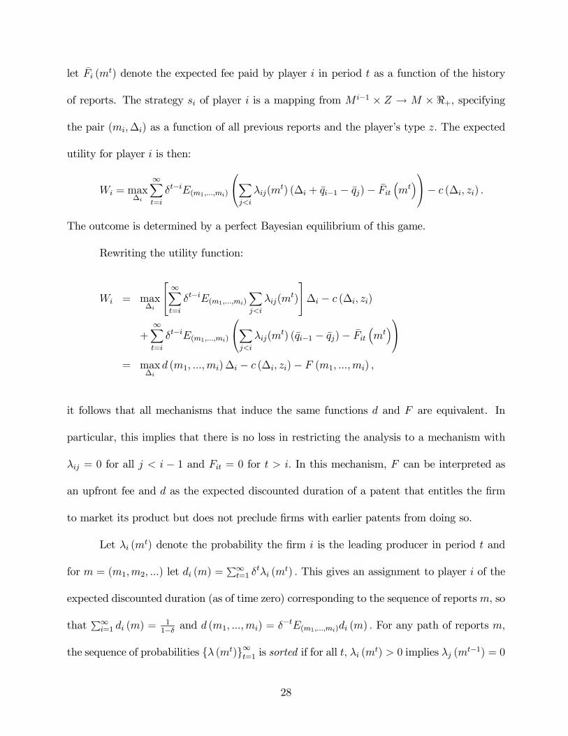
let F̄i (mt) denote the expected fee paid by player i in period t as a function of the history
of reports. The strategy si of player i is a mapping from M i−1 × Z → M × <+, specifying
the pair (mi,∆i) as a function of all previous reports and the player’s type z. The expected
utility for player i is then:
Wi = max∆i
∞Xt=i
δt−iE(m1,...,mi)
Xj<i
λij(mt) (∆i + q̄i−1 − q̄j)− F̄it
³mt´− c (∆i, zi) .
The outcome is determined by a perfect Bayesian equilibrium of this game.
Rewriting the utility function:
Wi = max∆i
∞Xt=i
δt−iE(m1,...,mi)
Xj<i
λij(mt)
∆i − c (∆i, zi)
+∞Xt=i
δt−iE(m1,...,mi)
Xj<i
λij(mt) (q̄i−1 − q̄j)− F̄it
³mt´
= max∆i
d (m1, ...,mi)∆i − c (∆i, zi)− F (m1, ...,mi) ,
it follows that all mechanisms that induce the same functions d and F are equivalent. In
particular, this implies that there is no loss in restricting the analysis to a mechanism with
λij = 0 for all j < i − 1 and Fit = 0 for t > i. In this mechanism, F can be interpreted as
an upfront fee and d as the expected discounted duration of a patent that entitles the firm
to market its product but does not preclude firms with earlier patents from doing so.
Let λi (mt) denote the probability the firm i is the leading producer in period t and
for m = (m1,m2, ...) let di (m) =P∞t=1 δ
tλi (mt) . This gives an assignment to player i of the
expected discounted duration (as of time zero) corresponding to the sequence of reports m, so
thatP∞i=1 di (m) =
11−δ and d (m1, ...,mi) = δ−tE(m1,...,mi)di (m) . For any path of reports m,
the sequence of probabilities {λ (mt)}∞t=1 is sorted if for all t, λi (mt) > 0 implies λj (mt−1) = 0
28
for all j > i. It is easy to see that for any path {λ (mt)}∞t=1 that is not sorted, there exists
a unique sorted pathnλ̃ (mt)
o∞t=1
that gives rise to identical di (m) for all i. Since all payoff
relevant information is contained in the assignments di (m), without loss of generality we
restrict to sorted paths.
Given the sequence of messages (m1, ...,mi−1) , the problem confronted by agent i
satisfies the conditions for the Revelation Principle: the principal can always design a mech-
anism that replicates the message corresponding to the equilibrium strategy for agent i in
this Bayesian game, for every agent i ∈ ℵ. Hence, from now on we restrict the analysis to a
revelation mechanism.
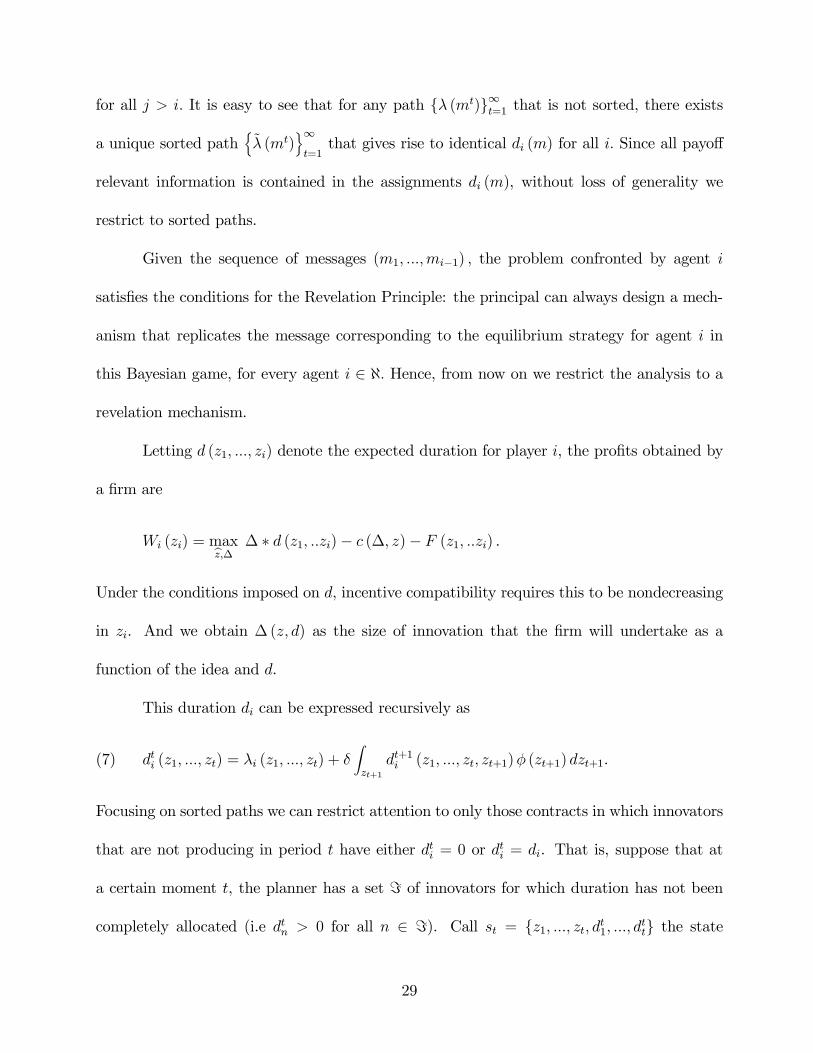
Letting d (z1, ..., zi) denote the expected duration for player i, the profits obtained by
a firm are
Wi (zi) = maxbz,∆ ∆ ∗ d (z1, ..zi)− c (∆, z)− F (z1, ..zi) .
Under the conditions imposed on d, incentive compatibility requires this to be nondecreasing
in zi. And we obtain ∆ (z, d) as the size of innovation that the firm will undertake as a
function of the idea and d.
This duration di can be expressed recursively as
dti (z1, ..., zt) = λi (z1, ..., zt) + δZzt+1
dt+1i (z1, ..., zt, zt+1)φ (zt+1) dzt+1.(7)
Focusing on sorted paths we can restrict attention to only those contracts in which innovators
that are not producing in period t have either dti = 0 or dti = di. That is, suppose that at
a certain moment t, the planner has a set = of innovators for which duration has not been
completely allocated (i.e dtn > 0 for all n ∈ =). Call st = {z1, ..., zt, dt1, ..., dtt} the state
29
variable in period t.9 Hence, the present value of social welfare that the planner maximizes
corresponds to
eV (st) = maxs0
Xn∈=
λti³zt´X
j≤n∆ (zj)
+ δ eV (st+1)s.t.
Xn∈=
λti³zt´= 1
where st+1 evolves according to (7).10
We can rewrite the dynamic programming problem (substracting the present value
social welfare of the innovations already promised to be implemented) as,
V (d) = maxd1(z),d2(z)
Z ½·1
1− δ− d1 (z)
¸∆ (z, d2 (z))− c (∆, z)+
+δV (d1 (z) + d2 (z))}φ (z) dz
s.t.(PK) d− 1 = δ
Rd1 (z)φ (z) dz
d1 (z) ≥ 0, d2 (z) ≥ 0
where d =Pt−1i=1 d
t−1i , is the sum of all the durations allocated, d1 (z) is the sum of these
durations in the next period and d2 (z) is the duration granted to the innovator appearing in
period t.
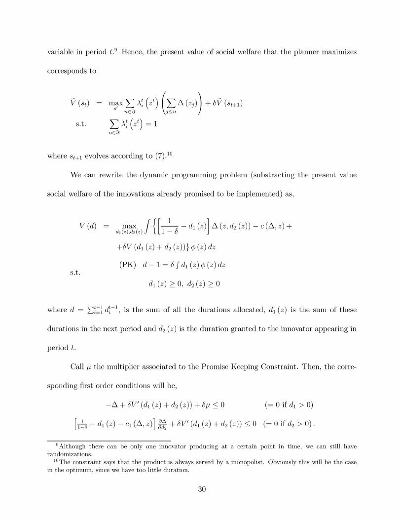
Call µ the multiplier associated to the Promise Keeping Constraint. Then, the corre-
sponding first order conditions will be,
−∆+ δV 0 (d1 (z) + d2 (z)) + δµ ≤ 0 (= 0 if d1 > 0)h11−δ − d1 (z)− c1 (∆, z)
i∂∆∂d2+ δV 0 (d1 (z) + d2 (z)) ≤ 0 (= 0 if d2 > 0) .
9Although there can be only one innovator producing at a certain point in time, we can still haverandomizations.
10The constraint says that the product is always served by a monopolist. Obviously this will be the casein the optimum, since we have too little duration.
30
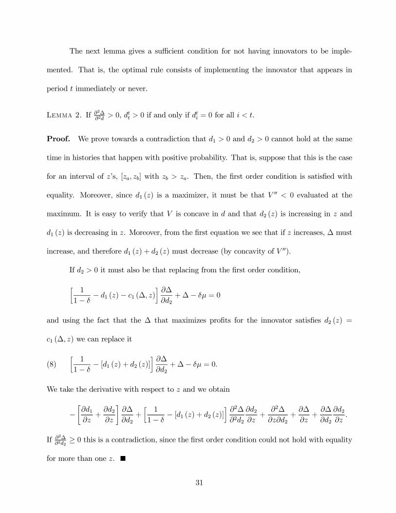
The next lemma gives a sufficient condition for not having innovators to be imple-
mented. That is, the optimal rule consists of implementing the innovator that appears in
period t immediately or never.
Lemma 2. If ∂2∆∂2d
> 0, dtt > 0 if and only if dti = 0 for all i < t.
Proof. We prove towards a contradiction that d1 > 0 and d2 > 0 cannot hold at the same
time in histories that happen with positive probability. That is, suppose that this is the case
for an interval of z’s, [za, zb] with zb > za. Then, the first order condition is satisfied with
equality. Moreover, since d1 (z) is a maximizer, it must be that V 00 < 0 evaluated at the
maximum. It is easy to verify that V is concave in d and that d2 (z) is increasing in z and
d1 (z) is decreasing in z. Moreover, from the first equation we see that if z increases, ∆ must
increase, and therefore d1 (z) + d2 (z) must decrease (by concavity of V 00).
If d2 > 0 it must also be that replacing from the first order condition,
·1
1− δ− d1 (z)− c1 (∆, z)
¸∂∆
∂d2+∆− δµ = 0
and using the fact that the ∆ that maximizes profits for the innovator satisfies d2 (z) =
c1 (∆, z) we can replace it
·1
1− δ− [d1 (z) + d2 (z)]
¸∂∆
∂d2+∆− δµ = 0.(8)
We take the derivative with respect to z and we obtain
−"∂d1∂z
+∂d2∂z
#∂∆
∂d2+·
1
1− δ− [d1 (z) + d2 (z)]
¸∂2∆
∂2d2
∂d2∂z
+∂2∆
∂z∂d2+
∂∆
∂z+
∂∆
∂d2
∂d2∂z.
If ∂2∆∂2d2≥ 0 this is a contradiction, since the first order condition could not hold with equality
for more than one z.
31
This condition is for example satisfied by the cost function introduced in Example 1.
when α < 2.
B. Collusion and Reporting of Quality
Whether or not an innovator knows the inherited q upon which new innovations are
built, there could be information about that q in the profits earned. If the innovator had, for
instance, sole rights to the entire quality spectrum, the realization of demand as a function of
price would generate information about q. Even if q is known to all the innovators, though, it
is not possible to extract that information in a way that is immune to simple collusion based
on bribery. This is in contrast to Crémer and Scotchmer (1997), where private information is
elicited at no cost due to the correlation across innovators. Here the sequential arrival leads
to problems of collusion.
Suppose q is observable to the innovator, and call (bzt, bqt) the report that innovator tmakes about his type and the previous state of the art. We denote bzt = (bz1, bz2, ..., bzt) andbqt = (bq1, bq2, ..., bqt) the history of all reports made by all previous agents up to t.
Just as in the previous section, we focus on revelation mechanisms. Agents declare
a message mi = (qi, zi) corresponding to their type and the state of knowledge that they
inherited. The two instruments that the planner might use, dt(qt, zt) and Ft(qt, zt) can
depend on those messages.
Consider the following strategy space. Firm i with type zi and inherited state qi chooses³bzi, bqi,nBi, qBi+1o´, where bzi and bqi are the reports made to the principal, and nBi, qBi+1o isa bribe: It transfers an amount Bi to the next innovator if he agrees to report qBi+1 to the
planner.
32
Profits can be rewritten in this case as,
Wi(zi) = maxbz,bq,qBi+1,B½max∆i
d (m1, ...,mi)∆i − Fi (m1, ...,mt)− c (∆, zi)− δBi
¾+Bi−1.
Denote the term in brackets Ui³zi, bz, bq, bqBi+1, Bi´. Since c (∆, z) is decreasing in zi, Ui
is increasing in zi. We next define a bribe-proof mechanism to be one where a single innovator
cannot offer a bribe to another innovator and encourage deceit. Note that bribe-proofness is
a very weak form of collusion proofness: it only requires that the mechanism be immune to
collusion between two innovators, for instance the outgoing leader and the new leader.
Definition 1. A mechanism is bribe-proof if there does not exist anBi, q
Bi+1
osuch that
Bi > 0, qBi+1 6= qi+1 that maximizes Ui for inventor i and for all zi+1
Wi+1(zi+1) < maxbqBi+2,Bi+1 Ui+1(zi+1, bzi+1, bqi+1, bqBi+2, Bi+1) +Bi.That is, the profits from accepting the bribe are lower than those from telling the
truth. Here we assume that bribes can only be offered to a firm with the next innovation
that is implemented.
In the next proposition we show that there is no incentive compatible and bribe-proof
mechanism that uses any report on q.
Proposition 6. For any incentive compatible and bribe-proof mechanism {dt(qt, zt), Ft(qt, zt)}
there exists another incentive compatible and bribe-proof mechanism {dt(zt), Ft(zt)} that achieves
the same allocation.
Proof. Assume towards a contradiction that there is an incentive compatible and bribe-
proof mechanism where Ui depends on the vector of reports qt for some t.
33
If Ui³zi, bz, bq, bqBi+1, Bi´ is decreasing in bqi, a firm with type z and state q can always lie
and declare (bq, bz), for example, in such a way that ∆(bz) > ∆i and bq +∆(bz) = q +∆i. Such
a manipulation will always increase profits, since Ui³zi, bz, bq, bqBi+1, Bi´ is decreasing in zi. On
the other hand, if Ui is decreasing in bqi, firms will declare bqi =∞. Hence, Ui is independentof bqi, and profits are the result of Wi(zi) = maxbz,qBi+1,Bi Ui ³z, bz, bqBi+1, Bi´.
Innovator i has a cost ε > 0 of bribing innovator i + 1, since from the previous step
i + 1’s profits do not depend on that report. However, bqi affects the profits for innovator i,and the bribe will be chosen to maximize these profits.
It is important to notice that here we are not solving for what innovator i + 1 will
do, or who will be bribed later. In fact, the intuition is simple. Innovator i + 1 obtains an
invention, investing some costs c(∆i+1, zi+1) but q is not the one that the previous innovator
reported. Since the profits for the innovator remain unchanged regardless of the report, any
bribe will be accepted.
C. Constant Breadth (Proof of Proposition 2)
For a given incumbent z, the optimal policy amounts to determining the fate of that
innovator for each report z0t made by the potential innovator t periods later. It is easy to see
that the optimal policy must be monotone in z0t; i.e. better reports should be more likely
to be allowed to supercede z. Therefore, the optimal policy is determined by a sequence of
thresholds z0t(z), where a new leader is chosen if a report of at least z0t(z) is made t periods
after the report z. The planner must commit to a certain discounted duration of the monopoly
power d, that can be written recursively as,
dt = 1+ δΦ (z0t) dt+1,
34
and d = d1. Therefore, the social planner’s problem can be written in the following way,
V (q, dt) = maxz0t,d0(z)
Zz0t[q +∆ (z, d0 (z))− c (∆ (z, d0 (z)) , z) + V (q, d0 (z))]φ (z) dz +
+δΦ (z0t)V
Ãq,
dt − 1
1− δΦ (z0t)
!.
As stated in Proposition 2., it turns out that using a constant threshold is the optimal
policy, and so, it is without loss of generality that in the rest of the paper we use a threshold
as a measure of the duration of monopoly power.
Proof to Proposition 2.
Proof. Define S (q, z) = q+∆ (z, d0 (z))− c (∆ (z, d0 (z)) , z), increasing in z and q. Consider
all the sequencesnz0t+1, z
0t+2, ...
othat result in a duration d. We prove by contradiction in
two steps that a constant threshold z0 is optimal.
First suppose that the optimal plan consists of different thresholds for some periods
and after that they become constant, i.e.nz0t+1, z
0t+2, ..., z
0t+s, bz, bz, bz, ...o for some s. Take the
problem in period t+ s− 1.. In this case, z0t+s 6= z0t+s+1 must solve the following problem,
V (q, dt+s−1) = maxz0
Zz0S(z)φ (z) dz + δΦ(z0)
Rbz S(z)φ (z) dz1− δΦ (bz)
s.t.1
1− δΦ (bz) = dt+s = dt+s−1 − 1
δΦ(z0).
Therefore, it must be that
−S(z0t+s) + δφ(z0t+s)
Rbz S(z)φ (z) dz1− δΦ (bz) +
δΦ(z0t+s)
" −S (bz)1− δΦ (bz) +
Rbz S(z)φ (z) dδφ (bz)[1− δΦ (bz)]2
#∂bz
∂z0t+s= 0
35
where from the constraint we obtain ∂bz∂z0 = −
φ(z0t+s)[1−δΦ(bz)]δφ(bz)Φ(z0t+s) . Replacing,
φ³z0t+s
´ hS (bz)− S ³z0t+s´i = 0
and so, the maximum is attained at z0t+s−1 = bz, contradicting our premise.Now suppose that instead there is a plan that gives strictly bigger social welfare than
one with a constant threshold and it consists on infinitely different protections. That is, there
is no time bs such that for all s > bs, z0t+s = z0t+s+1. By continuity and discounting, there mustexist another path that has constant protection after a number of periods s > 1 and that it
also gives higher welfare than a constant threshold. However, by the previous step, this is a
contradiction. Therefore, given a duration d the optimal plan has the form,
d =1
1− δΦ (z0).
It can be shown that the value function V (q, d) is strictly concave in d and so, allowing
for random protections will not improve upon it.
7. Appendix B: Other Proofs
Proof to Proposition 3:
Proof. For our result it is enough to show that V is strictly supermodular in z and z0. In
particular, this condition means that the derivative of the first order condition
·1
1− δ− c1(∆p(z, z0), z)
¸∂∆p
∂z0+ δ
∂V
∂z0(q +∆p(z, z0), z0)(9)
with respect to z is strictly positive. Since ∂V∂z0∂q = 0, we obtain that,
−c11(∆p(z, z0), z)∂∆p
∂z0∂∆p
∂z− c12(∆p(z, z0), z)
∂∆p
∂z0+·
1
1− δ− c1(∆p(z, z0), z)
¸∂2∆p
∂z0∂z
=·
1
1− δ− c1(∆p(z, z0), z)
¸∂2∆p
∂z0∂z.
36
Notice that the first term is strictly positive, since the optimal choice of ∆P satisfies
1
1− δ− c1(∆p(z, z0), z) >
1
1− δΦ(z0)− c1(∆p(z, z0), z) = 0.
Therefore, the derivative will be strictly positive if and only if ∂2∆p
∂z0∂z > 0. Function
V represents a contraction mapping. Hence, usual dynamic programming arguments ensure
that this function is weakly supermodular. The proof of strict supermodularity is obtained
by contradiction.
Proof to Proposition 4:
Proof. That ∆p(z, ·) ≤ ∆∗(z) is obvious from the remarks in the text. For the second part,
we take a recursive argument. Assuming that z0 ≥ z∗ we show that z > z∗.
First notice that from equation (6) we can compute
∂V
∂z(q, z) =
−φ(z(z))1− δΦ(z(z))
{∆p(z, z0)− c(∆p(z, z0), z)+
δ [V (q +∆p(z, z0), z0)− V (q, z)]} .
Since for all z, z is the maximizer of this function, it must be that for all x
∆p(z, z)
1− δ− c(∆p(z, z), z) + δV (q, z) ≥ ∆p(z, x)
1− δ− c(∆p(z, x), x) + δV (q, x) ,
and together with the fact that ∂V∂q= 1
1−δ we obtain that
∂V
∂z(q, z) ≥ −φ(z(z))
1− δΦ(z(z))
"∆p(z, z)
1− δ− c(∆p(z, z), z)
#.
If ∆p(z, ·) < ∆∗(z), the FOC implies that ∂V∂z< 0 and,∆
p(z,z)1−δ − c(∆p(z, z), z) > 0, so that
∆∗(z)1− δ
− c(∆∗(z), z) ≥ ∆p(z, z)
1− δ− c(∆p(z, z), z) > 0.
37
Because z∗ is characterized by ∆∗(z∗)1−δ − c(∆∗(z∗), z∗) = 0, and this is a strictly increasing
function, z > z∗.
If ∆p(z, ·) = ∆∗(z), it must be that z =∞ > z∗
Proof to Lemma 1 :
Proof. Suppose that the following innovations are implementable. Using the Revelation
Principle this means in particular that for the worse innovator z0τ ,
z0τ ∈ argmaxbz ∆p
1− δΦ(z00τ (bz)) +1− Φ(z00τ (bz))1− δΦ(z00τ (bz))δτ 00(bz)− c(∆p, z0τ )− τ 0 − σ00.
Using the Implicit Function Theorem and the fact that τ 0(z) and σ(z) are independent
of z, we obtain that for any contract ∂z0τ∂σ0 = 0 and
∂z0τ∂τ 0 > 0.
For the current inventor with quality z, we need to check the Spence-Mirrlees condition,
∂W τ
∂τ 0∂z(z, τ 0, τ) =
δφ(z0τ )1− δΦ(z0τ )
∂∆p
∂z0τ
∂z0τ∂τ 0
> 0.
And this immediately implies using the previous result, that in order for a mechanism
to be implementable, ∂τ 0∂z≥ 0.
From the envelope condition,
∂W τ
∂z= −∂c
∂z(∆p, z),
and by the definition of W τ (z0τ , τ , 0) = 0, this means that W τ (z0τ , τ0, τ) = −τ . Integrating
with respect to z and using this boundary condition we obtain the expression for σ0(z) which
does not depend on τ .
38
Proof to Proposition 5:
Proof. Two contracts {z0(z), F (z)} and {τ 0(z), σ0(z)} will be equivalent if they guarantee
the same profits to innovators of all types z.
Any incentive compatible contract {z0(z), F (z)} achieves profits,
W (z, z) =Z z
z−∂c
∂z(∆p(x, z0(x)), x)dx,
while a compulsory licensing based contract results in profits,
W τ (z, τ 0, τ ) =Z z
z0τ
−∂c
∂z(∆p(x, z0τ (x)), x)dx− τ .
Hence, for both contracts to be equivalent it must be that W (z, z) = W τ (z, τ 0, τ ),
which results in
τ = τ (z) =Z z(z)
z0τ
−∂c
∂z(∆p(x, z0(x)), x)dx,
for all z. It can be verified, using convexity of c with respect to z, that this function is
increasing in z. This result implies that there is an implementable compulsory licensing
scheme that leads to the same profits as any implementable contract {z0(z), F (z)}.
39
References
Allison, John R. and Mark A. Lemley (1998). ‘Empirical Evidence on the Validity of Litigated
Patents,’ Mimeo.
Anderson, Simon P., Andre de Palma and Jacques-Francois Thisse (1992). ‘Discrete choice
theory of product differentiation,’ Cambridge, Mass., M.I.T. Press.
Arrow, Kenneth J. (1969). ‘Classificatory Notes on the Production and Transmission of
Technological Knowledge,’ American Economic Review, 59: 29-35.
Baron, David P. and Roger B. Myerson (1982). ‘Regulating a Monopolist with Unknown
Costs,’ Econometrica, 50: 911-930.
Chiesa, Gabriella and Vincenzo Denicolo (1999). ‘Patents, Prizes, and Optimal Innovation
Policy.’ Mimeo. University of Bologna.
Cornelli, Francesca and Mark Schankerman (1999). ‘Patent Renewals and R&D Incentives,’
Rand Journal of Economics, 30: 197-213.
Crémer, Jacques, and Suzanne Scotchmer (1997). ‘Optimal R&DProcurement: Why Patents?’
Mimeo.
Gilbert, Richard and Carl Shapiro (1990). ‘Optimal Patent Length and Breadth,’ Rand
Journal of Economics, 30: 106-112.
Green, Jerry and Suzanne Scotchmer (1995). ‘On the Division of Profit between Sequential
Innovators’, Rand Journal of Economics 26: 20-33.
Laffont, Jean-Jacques and Jean Tirole (1986). ‘Using Cost Observation to Control a Public
Firm,’ Journal of Political Economy, 94: 614-641.
Lewis, Tracy R. and David E.M. Sappington (1988a). ‘Regulating a Monopolist with Un-
40
known Demand and Cost Functions’ Rand Journal of Economics, 19: 438-57.
Lewis, Tracy R. and David E.M. Sappington (1988b). ‘Regulating a Monopolist with Un-
known Demand,’ American Economic Review, 78: 986-98.
Llobet, Gerard (1999). ‘The Economics of Patent Litigation,’ Mimeo.
Nordhaus, William D. (1969). ‘Invention, growth, and welfare; a theoretical treatment of
technological change,’ Cambridge, Mass., M.I.T. Press.
Machlup, Fritz, and Edith Penrose (1950). ‘The Patent Controversy in the Nineteenth Cen-
tury,’ Journal of Economic History, 10:1-29.
O’Donoghue, Ted, Suzanne Scotchmer and Jacques-Francois Thisse (1998). ‘Patent Breadth,
Patent Life and the Pace of Technological Progress,’ Journal of Economics and Man-
agement Strategy, 7: 1-32.
Shavell, Steven and Tanguy van Ypersele (1999) ‘Rewards versus Intellectual Property Rights,’
Mimeo.
Scotchmer, Suzanne (1999) ‘On the Optimality of the Patent Renewal System,’ Rand Journal
of Economics, 30: 181-96.
Scotchmer, Suzanne, and Jerry Green (1990). ‘Novelty and Disclosure in Patent Law,’ Rand
Journal of Economics, 21: 131-46.
Tandon, Pankaj (1982) ‘Optimal Patents with Compulsory Licensing,’ Journal of Political
Economy, 90: 470-486.
Wright, Brian D. (1983) ‘The Economics of Invention Incentives: Patents, Prizes, and Re-
search Contracts,’ American Economic Review, 73: 691-707.
41