resurgent transseries and the holomorphic anomaly
TRANSCRIPT

Prepared for submission to JHEP
Resurgent Transseries and the Holomorphic Anomaly
Ricardo Couso Santamarıa,a Jose D. Edelstein,a,b Ricardo Schiappa,c Marcel Vonkd
aDepartamento de Fısica de Partıculas and IGFAE, Universidade de Santiago de Compostela,E–15782 Santiago de Compostela, Spain
bCentro de Estudios Cientıficos, CECs, Casilla 1469, Valdivia, Chile
cCAMGSD, Departamento de Matematica, Instituto Superior Tecnico,Av. Rovisco Pais 1, 1049–001 Lisboa, Portugal
dInstitute for Theoretical Physics, University of Amsterdam,Science Park 904, 1090–GL Amsterdam, The Netherlands
E-mail: [email protected], [email protected],[email protected], [email protected]
Abstract: The gauge theoretic large N expansion yields an asymptotic series which requiresa nonperturbative completion in order to be well defined. Recently, within the context of ran-dom matrix models, it was shown how to build resurgent transseries solutions encoding thefull nonperturbative information beyond the ’t Hooft genus expansion. On the other hand, vialarge N duality, random matrix models may be holographically described by B–model closedtopological strings in local Calabi–Yau geometries. This raises the question of constructing thecorresponding holographically dual resurgent transseries, tantamount to nonperturbative topo-logical string theory. This paper addresses this point by showing how to construct resurgenttransseries solutions to the holomorphic anomaly equations. These solutions are built upon(generalized) multi–instanton sectors, where the instanton actions are holomorphic. The asymp-totic expansions around the multi–instanton sectors have both holomorphic and anti–holomorphicdependence, may allow for resonance, and their structure is completely fixed by the holomor-phic anomaly equations in terms of specific polynomials multiplied by exponential factors andup to the holomorphic ambiguities—which generalizes the known perturbative structure to thefull transseries. In particular, the anti–holomorphic dependence has a somewhat universal char-acter. Furthermore, in the nonperturbative sectors, holomorphic ambiguities may be fixed atconifold points. This construction shows the nonperturbative integrability of the holomorphicanomaly equations, and sets the ground to start addressing large–order analysis and resurgentnonperturbative completions within closed topological string theory.
Keywords: Resurgence, Transseries, Topological Strings, Holomorphic Anomaly Equations
arX
iv:1
308.
1695
v1 [
hep-
th]
7 A
ug 2
013
Contents
1 Introduction and Summary 2
2 The Holomorphic Anomaly Equations 62.1 Reviewing the Background Calabi–Yau Geometry 62.2 Rewriting the Holomorphic Anomaly Equations 8
3 A Word on the Transseries Framework 10
4 One–Parameter Resurgent Transseries 134.1 A Closer Look at the Perturbative Sector 134.2 Setting the Transseries Construction 144.3 Structure of the Transseries Solution 18
5 Multi–Parameter Resurgent Transseries 205.1 Setting the Generalized Transseries Construction 215.2 Structure of the Generalized Transseries Solution 225.3 Resonance and Logarithmic Sectors 285.4 Genus Expansions within Transseries Solutions 31
6 A Glimpse of Large–Order Analysis 36
7 Fixing the Holomorphic Ambiguities 417.1 Fixing the Perturbative Ambiguity 417.2 Fixing Holomorphic Ambiguities at the Conifold 427.3 Fixing Ambiguities beyond Conifold Points 45
8 Conclusions and Outlook 46
A Multi–Dimensional Complex Moduli Space 48
B Proof of Set Recursion Lemma 52
– 1 –
1 Introduction and Summary
For over a decade, the idea of large N duality [1] has been a remarkable source of progresswithin the nonperturbative development of strongly coupled gauge theoretic systems. In thisframework one starts off with the partition function of some nonabelian gauge theory, Z, whose’t Hooft large N limit [2] produces an asymptotic expansion, in 1/N . The topological structureof the 1/N expansion is that of a genus expansion, which leads to the holographically dual closedstring theory. In this way, one can think of closed string theory as an asymptotic (large N)approximation to some nonabelian gauge theory. This idea has been applied with success in verylarge classes of examples, see, e.g., [3] for an older review. In the following we shall consider oneof the simplest classes of nonabelian gauge theories, namely, random matrix models [4, 5].
Due to its aforementioned asymptotic nature, the large N expansion by itself is not enoughto define either the gauge theory or the dual string theory. Indeed, in the large N limit, the gaugetheoretic free energy F = logZ has a genus expansion in 1/N2 where its genus g perturbativecontributions1 Fg(t) have large–order behavior Fg ∼ (2g)!, rendering the large N expansion as anasymptotic expansion with zero radius of convergence2 [8]—which in the string theoretic contextis not even Borel summable [9]. In order to go beyond this state of affairs, one has to takeinto account all possible nonperturbative corrections to the large N expansion, typically of theform ∼ exp (−N), into what is known as a transseries expansion; see, e.g., [10–12]. Becausethey include all possible nonperturbative corrections, transseries precisely incorporate Stokesphenomena and, as such, allow us to go beyond the large N expansion obtaining, upon medianresummation [13], analytic results anywhere in the complexN–plane. Within the largeN context,explicit examples have been constructed addressing random matrix models and their double–scaling limits [14–17]. One interesting point found in these analyses is that while one could havenaıvely expected that all the large N nonperturbative content within the transseries would beassociated to multi–instantons, this expectation was actually shown to be incomplete: one furtherneeds to introduce new nonperturbative sectors to fully describe the large N gauge theory beyondits genus expansion. In fact, an important aspect of these transseries solutions is their resurgentnature; see, e.g., [16]. That these transseries are resurgent means that, deep in their large–order behavior, every (generalized) multi–instanton sector is related to each other. Verifying thevalidity of any new nonperturbative sector may be thus thoroughly checked in many examples byexploring the information encoded in the large–order behavior of perturbation theory around anychosen multi–instanton sector [15–17]. Once this is done, the final resurgent transseries solutionmay be constructed yielding results valid for any N .
Our concern in the present work is that most studies carried through so far on the resurgentnature of the large N limit have precisely been done in the gauge theory side, starting off withrandom matrix integrals [18, 19, 14, 20, 21, 15, 22, 16, 17]. But would it be possible to addressthese issues directly in the closed string side? If so, what would this imply towards the verynature of the large N holographic duality, from a nonperturbative point–of–view?
We shall be interested in the rather complete picture of [23, 24], which addresses the ’t Hooftlarge N limit of general matrix models. Let us start off on the gauge theoretic side with ahermitian one–matrix model with polynomial potential V (z) of degree n + 1. In this case it israther well–known that, in the planar limit, saddle–points of the matrix integral are described
1In here t = Ngs is the ’t Hooft coupling. When considering the closed string dual, t will instead be part ofthe geometric moduli associated to the background Calabi–Yau geometry—but more on this in the following.
2The situation is different at fixed genus: although the free energy Fg(t) may also be computed perturbatively—now in the ’t Hooft coupling—one finds a milder expansion with finite (non–zero) convergence radius [6, 7].
– 2 –
by spectral curves [25]. Further, the ’t Hooft 1/N asymptotic expansion follows via a recursivecalculation on this curve [26–28]. The key point of [23] is to notice that the spectral curve isactually part of a Calabi–Yau threefold, and that the ’t Hooft expansion can actually be computedholographically by B–model topological string theory on this specific local geometry.
Let us be a bit more precise, as this will also help explain our main theme. Consider the ncritical points of the potential V ′(z∗) = 0 and distribute the N eigenvalues across these criticalpoints, Nini=1. This saddle configuration is then described by a hyperelliptic curve [25, 28]
y2 = V ′(x)2 − tR(x), (1.1)
where t = gsN is the ’t Hooft coupling, and R(x) is a polynomial of degree n−1 which effectivelyopens up the critical points z∗i into cuts Ai. Different eigenvalue partitions, corresponding todistinct classical vacua of the gauge theory, lead to geometrically distinct spectral curves. Con-versely, given the curve (1.1) all relevant information follows; e.g., the number of eigenvalues ineach cut is given by the partial ’t Hooft couplings ti = gsNi as the A–periods
ti =1
4πi
∮Ai
dx y(x), (1.2)
while the tree–level (genus zero) free energy follows from the integration of the spectral curvealong the dual B–cycles3
∂F0
∂ti=
∫Bi
dx y(x). (1.3)
Further, the topological recursion [28] algorithmically computes all higher–genus contributionsin the ’t Hooft expansion. At the conceptual level one may now ask: why is the matrix modelsolved by a geometrical construction? As explained in [23], this can be best understood by firstreinterpreting the spectral curve solution of the matrix model as being described by a Calabi–Yaugeometry in disguise, and not just a Riemann surface; i.e., (1.1) is actually a subset of the local(non–compact) Calabi–Yau threefold
Xdef = u, v ∈ C, x, y ∈ C∗ |uv +H(x, y) = 0 , (1.4)
where H(x, y) is the polynomial whose zero locus precisely yields the hyperelliptic curve (1.1). Inthis way, the spectral curve clearly encodes all the non–trivial information about this Calabi–Yaugeometry. Its A–cycles are projections of the Calabi–Yau compact three–cycles; the same holdingfor the non–compact canonically conjugated B–cycles. The one–form y dx is a projection of theholomorphic three–form Ω, such that one may write (1.2–1.3) instead as threefold periods4
ti =1
4πi
∮Ai
Ω,∂F0
∂ti=
∫Bi
Ω. (1.5)
These are the special geometry relations of the Calabi–Yau (with F0 the prepotential). In otherwords, the special geometry of Xdef, which solves the tree–level closed topological B–model onthis background, further yields the planar solution to the hermitian one–matrix model.
3This relation expresses the change in the planar free energy as we vary the eigenvalues around the cuts—inthis case as we remove an eigenvalue from the cut Ai all the way up to infinity. The energy cost of tunneling aneigenvalue from the cut Ai to the cut Aj is given by the instanton action A =
∫Bij
dx y(x) [29, 30, 19, 20].4In particular identifying Calabi–Yau periods with ’t Hooft moduli.
– 3 –
So why does this geometry naturally emerge from the matrix eigenvalue dynamics? Geomet-rically, the local Calabi–Yau (1.4) is a deformation of the singular geometry uv+y2−V ′(x)2 = 0.One can now understand the nature of the geometric solution to the hermitian one–matrix modelby thinking about the resolved geometry Xres instead, obtained by blow–up of the aforementionedsingular geometry (see, e.g., [23, 5] for the precise transition functions, which explicitly dependupon V (z)). As it turns out, the string field theory of open topological B–strings on Xres localizesinto the hermitian one–matrix model with potential V (z) [23, 5]. The emergence of the special ge-ometry (1.5) can now be understood as the result of the geometric transition Xres → Xsing → Xdef
[31] implementing a large N duality [32]. In this way, the ’t Hooft resummation of the matrixmodel precisely matches the closed topological B–model on Xdef.
To be fully precise, the results in [23] only show that closed topological strings on Calabi–Yau threefolds are large N solutions to matrix models at the planar level. An extension ofthis derivation to higher genera was later presented in [33]. Generically, one may compute thetopological B–model free energy using the holomorphic anomaly equations [34], which controlthe ti–dependence5 of the closed string amplitudes Fg(ti, ti) and, when combined with extraboundary conditions, turn out to be completely integrable for non–compact Calabi–Yau manifolds[35, 36]. What [33] shows is that the holomorphic limit of these B–model closed string amplitudesFg(ti) ≡ limti→+∞ Fg(ti, ti) exactly matches the components of the large N ’t Hooft expansion ascomputed within the matrix model using the topological recursion [28]. Conversely, the matrixmodel free energy at genus g, may be extended non–holomorphically (by imposing adequaterequirements of modular invariance and modifying the topological recursion accordingly) in sucha way as to satisfy the holomorphic anomaly equations on the corresponding local Calabi–Yau. Inthis way, [33] sets up the complete perturbative equivalence of [23]. Setting up the nonperturbativeequivalence between large N expansions of hermitian one–matrix models and closed B–modelstrings on local Calabi–Yau threefolds is, of course, much harder, as one immediately stumblesupon the problems of first defining exactly what one means by either nonperturbative topologicalstrings or the nonperturbative ’t Hooft expansion of a matrix model. This is one of the mainthemes in the present paper, following previous work in [18, 19, 14, 20, 37, 21, 38, 39, 15, 22, 16,17, 13] (a more detailed description of these recent developments may be found either briefly inthe introduction of [16], or, in greater detail, in the excellent review [40]).
One may now return to our motivating question: can one address the issues of resurgent anal-ysis and transseries solutions directly in the closed string framework? As should be clear fromthe previous paragraph, answering this question entails the construction of resurgent transseriessolutions to the holomorphic anomaly equations along with verifying resurgent large–order rela-tions directly in the closed string sector, and this is what we shall address throughout this work.It is important to stress that, over the years, there have been many other proposals to definenonperturbative topological strings, e.g, [41–45]. Yet, in one way or another, at the end of theday all these proposals have to rely upon large N duality. As was hopefully made clear above,our main goal in this work is to get rid of this requirement by addressing this question strictlywithin closed string theory. In this way, besides eventually validating the nonperturbative dual-ity to random matrix models we described above, our approach may also serve the purpose ofvalidating, within closed strings, the other aforementioned proposals.
5From this closed string perspective, both ti and ti are now geometric moduli associated to the ambient Calabi–Yau geometry. We shall be more precise about their exact definition in the main body of the paper.
– 4 –
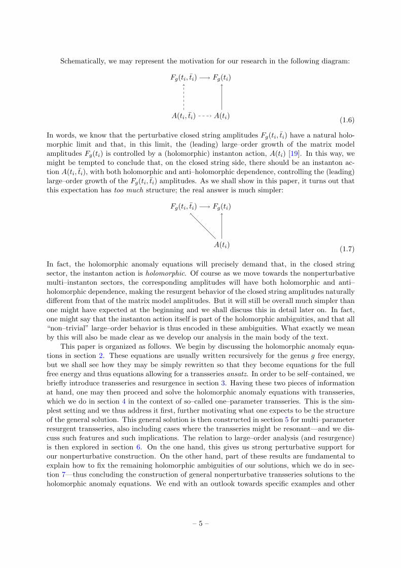
Schematically, we may represent the motivation for our research in the following diagram:
Fg(ti, ti) Fg(ti)
A(ti, ti) A(ti) (1.6)
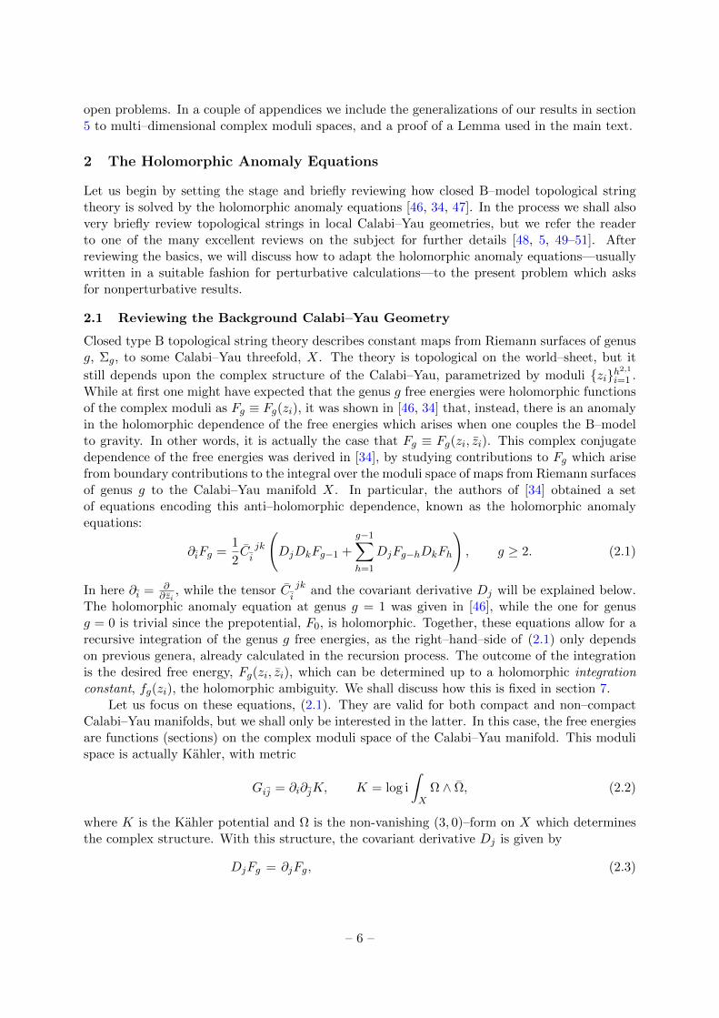
In words, we know that the perturbative closed string amplitudes Fg(ti, ti) have a natural holo-morphic limit and that, in this limit, the (leading) large–order growth of the matrix modelamplitudes Fg(ti) is controlled by a (holomorphic) instanton action, A(ti) [19]. In this way, wemight be tempted to conclude that, on the closed string side, there should be an instanton ac-tion A(ti, ti), with both holomorphic and anti–holomorphic dependence, controlling the (leading)large–order growth of the Fg(ti, ti) amplitudes. As we shall show in this paper, it turns out thatthis expectation has too much structure; the real answer is much simpler:
Fg(ti, ti) Fg(ti)
A(ti) (1.7)
In fact, the holomorphic anomaly equations will precisely demand that, in the closed stringsector, the instanton action is holomorphic. Of course as we move towards the nonperturbativemulti–instanton sectors, the corresponding amplitudes will have both holomorphic and anti–holomorphic dependence, making the resurgent behavior of the closed string amplitudes naturallydifferent from that of the matrix model amplitudes. But it will still be overall much simpler thanone might have expected at the beginning and we shall discuss this in detail later on. In fact,one might say that the instanton action itself is part of the holomorphic ambiguities, and that all“non–trivial” large–order behavior is thus encoded in these ambiguities. What exactly we meanby this will also be made clear as we develop our analysis in the main body of the text.
This paper is organized as follows. We begin by discussing the holomorphic anomaly equa-tions in section 2. These equations are usually written recursively for the genus g free energy,but we shall see how they may be simply rewritten so that they become equations for the fullfree energy and thus equations allowing for a transseries ansatz. In order to be self–contained, webriefly introduce transseries and resurgence in section 3. Having these two pieces of informationat hand, one may then proceed and solve the holomorphic anomaly equations with transseries,which we do in section 4 in the context of so–called one–parameter transseries. This is the sim-plest setting and we thus address it first, further motivating what one expects to be the structureof the general solution. This general solution is then constructed in section 5 for multi–parameterresurgent transseries, also including cases where the transseries might be resonant—and we dis-cuss such features and such implications. The relation to large–order analysis (and resurgence)is then explored in section 6. On the one hand, this gives us strong perturbative support forour nonperturbative construction. On the other hand, part of these results are fundamental toexplain how to fix the remaining holomorphic ambiguities of our solutions, which we do in sec-tion 7—thus concluding the construction of general nonperturbative transseries solutions to theholomorphic anomaly equations. We end with an outlook towards specific examples and other
– 5 –
open problems. In a couple of appendices we include the generalizations of our results in section5 to multi–dimensional complex moduli spaces, and a proof of a Lemma used in the main text.
2 The Holomorphic Anomaly Equations
Let us begin by setting the stage and briefly reviewing how closed B–model topological stringtheory is solved by the holomorphic anomaly equations [46, 34, 47]. In the process we shall alsovery briefly review topological strings in local Calabi–Yau geometries, but we refer the readerto one of the many excellent reviews on the subject for further details [48, 5, 49–51]. Afterreviewing the basics, we will discuss how to adapt the holomorphic anomaly equations—usuallywritten in a suitable fashion for perturbative calculations—to the present problem which asksfor nonperturbative results.
2.1 Reviewing the Background Calabi–Yau Geometry
Closed type B topological string theory describes constant maps from Riemann surfaces of genusg, Σg, to some Calabi–Yau threefold, X. The theory is topological on the world–sheet, but it
still depends upon the complex structure of the Calabi–Yau, parametrized by moduli zih2,1
i=1 .While at first one might have expected that the genus g free energies were holomorphic functionsof the complex moduli as Fg ≡ Fg(zi), it was shown in [46, 34] that, instead, there is an anomalyin the holomorphic dependence of the free energies which arises when one couples the B–modelto gravity. In other words, it is actually the case that Fg ≡ Fg(zi, zi). This complex conjugatedependence of the free energies was derived in [34], by studying contributions to Fg which arisefrom boundary contributions to the integral over the moduli space of maps from Riemann surfacesof genus g to the Calabi–Yau manifold X. In particular, the authors of [34] obtained a setof equations encoding this anti–holomorphic dependence, known as the holomorphic anomalyequations:
∂iFg =1
2C jki
(DjDkFg−1 +
g−1∑h=1
DjFg−hDkFh
), g ≥ 2. (2.1)
In here ∂i = ∂∂zi
, while the tensor C jki
and the covariant derivative Dj will be explained below.The holomorphic anomaly equation at genus g = 1 was given in [46], while the one for genusg = 0 is trivial since the prepotential, F0, is holomorphic. Together, these equations allow for arecursive integration of the genus g free energies, as the right–hand–side of (2.1) only dependson previous genera, already calculated in the recursion process. The outcome of the integrationis the desired free energy, Fg(zi, zi), which can be determined up to a holomorphic integrationconstant, fg(zi), the holomorphic ambiguity. We shall discuss how this is fixed in section 7.
Let us focus on these equations, (2.1). They are valid for both compact and non–compactCalabi–Yau manifolds, but we shall only be interested in the latter. In this case, the free energiesare functions (sections) on the complex moduli space of the Calabi–Yau manifold. This modulispace is actually Kahler, with metric
Gij = ∂i∂jK, K = log i
∫X
Ω ∧ Ω, (2.2)
where K is the Kahler potential and Ω is the non-vanishing (3, 0)–form on X which determinesthe complex structure. With this structure, the covariant derivative Dj is given by
DjFg = ∂jFg, (2.3)
– 6 –
DjDkFg = ∂j∂kFg − Γijk ∂iFg − (2− 2g) ∂jK ∂kFg, (2.4)
where Γijk = Gii∂jGki is the Chistoffel symbol, and where ∂jK acts as the connection for the
line bundle L2−2g associated to the multiplicative freedom in the normalization of Ω. For local(non–compact) Calabi–Yau manifolds this term drops since K is constant in the holomorphiclimit. Finally, the last ingredient is
C jki
= e2K CijkGjj Gkk, (2.5)
where Cijk = Cijk is the complex conjugate of the Yukawa couplings, which are given by thethird holomorphic derivatives of the prepotential, Cijk = ∂i∂j∂kF0.
It turns out that the integration of the equations (2.1) is quite complicated as they stand.The calculation may be made easier with the introduction of propagators, which essentially arepotentials for the Cijk tensors thus simplifying the integration. These propagators were alreadyintroduced in [34], and their interest became explicit in [52, 53]. In fact, in [52] it was shown that,in the example of the local quintic, the anti–holomorphic dependence of the free energies at everygenus may be captured by a finite number of generators, in such a way that this dependence ispolynomial. In [53] this was extended to general compact Calabi–Yau geometries. There, it wasshown that if one defines the propagators Sij , Si, S, by
∂iSjk = C jk
i, ∂iS
j = Gii Sij , ∂iS = Gii S
i, (2.6)
akin to [34], then one can show that any covariant derivative of these propagators, Sij , Si, S,and also of ∂iK, may be expressed back in terms of these objects and the Yukawa couplings,Cijk. For example,
DiSjk = δjiS
k + δki Sj − Ci`mS`jSmk + f jki , (2.7)
where f jki is a holomorphic function related to the fact that Sjk in (2.6) is only defined up to aholomorphic quantity. As we turn to the case of non–compact geometries, one can consistentlyturn off the propagators Si, S, ∂iK, and work only with Sjk [36]. The Christoffel symbols arealso expressable in terms of the propagators. Restricting to the local case, one finds:
Γijk = −Cjk`S`i + f ijk, (2.8)
where f ijk is another holomorphic function. Both f jki and f ijk can be determined within specificexamples, partly by choice and partly by internal consistency of the equations.
The main idea behind the above discussion is that one may now use the propagators Sij totake up the role of the anti–holomorphic variables zi. Using the chain rule and, again, restrictingto the local case,
∂i =∂Sjk
∂zi
∂
∂Sjk= C jk
i
∂
∂Sjk. (2.9)
It follows that the holomorphic anomaly equations (2.1) become
∂Fg∂Sij
=1
2
(DiDjFg−1 +
g−1∑h=1
DiFg−hDjFh
), g ≥ 2, (2.10)
where we have been able to get rid of C jki
. This will be our starting point. Later, in section 4,we shall see how these equations are integrated and what is the structure of the resulting solution
– 7 –
with respect to the propagators. Let us just mention for the moment that because DjF1 = ∂jF1
is linear in the propagators, the recursion (2.10) yields a polynomial dependence in the Sij .Integration also produces a holomorphic ambiguity, whose fixing is discussed in section 7.
Before concluding this subsection, let us point out that the recursion (2.10) starts at g = 2.The free energies F0 and F1 are of a different sort and they are handled separately. On whatconcerns F0, the prepotential, it carries strong geometrical information. The derivative ∂iF0 isactually a period, i.e., a cycle integral of the (3, 0)–form Ω, and taking two more derivativesproduces the Yukawa couplings. Also note that F0 does not appear explicitly in the holomorphicanomaly equations, except through the Yukawa couplings. As to F1, it appears in (2.10) throughderivatives and it has a geometrical interpretation in terms of Ray–Singer torsion. All we willneed later on is that
∂iF1 =1
2CijkS
jk + αi, (2.11)
where αi is a holomorphic quantity that can be fixed for each example.
2.2 Rewriting the Holomorphic Anomaly Equations
As they stand, the holomorphic anomaly equations essentially yield a recursive procedure tocompute the perturbative free energy. Indeed, they are equations precisely for the perturbative Fg.But, in order to address nonperturbative issues, one would need to write these equations eitherfor the full free energy, F , or even the partition function Z = expF . That equivalent formulationsof the holomorphic anomaly equations may be found for F or Z was already anticipated early on[46], as a master equation for the partition function. Shortly before [34], the following explicitmaster equation was suggested in [54], for Z = exp
∑+∞g=0 g
2g−2s Fg,(
∂i −1
2g2s C
jkiDjDk
)Z = 0. (2.12)
Unfortunately, as it stands, this equation does not quite reproduce the holomorphic anomalyequations as the upper and lower summation bounds in the resulting quadratic part are not asin (2.10). Recall that the proper limits, from h = 1 to h = g − 1, are necessary in order tohave a recursion in g. In [34] another version of a master equation was considered, this time forF '
∑+∞g=1 g
2g−2s Fg (note that the sum starts at g = 1, so that F0 is not included). This equation
is
(∂i − ∂iF1) eF =1
2g2s C
jkiDjDke
F , (2.13)
which now does give back the holomorphic anomaly equations for g ≥ 2. As before, F0 hasno direct role in the equations other than through the Yukawa couplings. Later on, in [33], anequivalent version of the holomorphic anomaly master equation was discussed which is closer towhat we are interested in. Defining
Z ' exp+∞∑g=0
g2g−2s Fg, Z = e
− 1
g2sF0−F1
Z, Z = e− 1
g2sF0Z, (2.14)
it is possible to show that the holomorphic anomaly equations may be written in the form6
1
Z∂iZ =
1
2g2s
1
ZC jkiDjDkZ. (2.15)
6[33] works in the language of matrix models, where gs is identified with N−1.
– 8 –

It is noteworthy that these master equations resemble generalized versions of the heat equation,and this has been explored in [54–56] along with the possibility that the partition function isactually described by a Riemann theta function.
Our goal here is to write a master equation for the partition function Z ' exp∑+∞
g=0 g2g−2s Fg,
including both F0 and F1, with the property that it will yield the tower of holomorphic anomalyequations for genus g ≥ 2 in the spirit of the above examples. Let us emphasize that such anequation should be written in terms of Z alone, so that later on one is able to promote Z toa fully nonperturbative partition function. This is in contrast with, e.g., (2.15) above, whichfurther involves the functions Z and Z. The price of working only with Z will be that both F0
and F1 will explicitly appear in the resulting equation. However, this is not a problem since oneshould regard F0 and F1 as geometrical data associated to the specific model under study. Inthis sense, let us stress that (2.15) is naturally already the equation we are looking for; we justneed to rewrite it in a more convenient way.
Before deriving the appropriate form of the master equation, we shall switch to propagatorvariables for the anti–holomorphic dependence. Now, let us first state the master equation, andthen show that it reproduces the familiar holomorphic anomaly equations (2.10). The masterequation is: (
∂
∂Sij+
1
2(UiDj + UjDi)−
1
2g2s DiDj
)Z =
(1
g2s
Wij + Vij
)Z. (2.16)
Here Ui, Vij , and Wij are functions involving F0 and F1 which ensure that we will obtain thecorrect holomorphic anomaly equations and nothing else. They can be thought of as geometricaldata. Switching from the partition function, Z, to the free energy, F = logZ, one may write(2.16) as
∂F
∂Sij+
1
2(UiDjF + UjDiF )− 1
2g2s (DiDjF +DiFDjF ) =
1
g2s
Wij + Vij . (2.17)
Let us now use a perturbative ansatz for the free energy
Fpert ≡ F (0) '+∞∑g=0
g2g−2s F (0)
g (2.18)
and find out what are the values of Ui, Vij , Wij which yield back (2.10). We have explicitly addeda superscript (0) to stress that the free energies are perturbative, anticipating that we shall soonwork with nonperturbative corrections. The quadratic term DiF
(0)DjF(0) yields
DiF(0)DjF
(0) =+∞∑g=0
g2g−4s
g∑h=0
DiF(0)g−hDjF
(0)h , (2.19)
where the limits in the h–sum are not quite the ones we need. It will thus be the role of Ui toremove the first and last terms in the sum. Doing the rest of the calculation and assemblingequal powers of gs together, we find
1
g2s
(∂F
(0)0
∂Sij+
1
2UiDjF
(0)0 +
1
2UjDiF
(0)0 − 1
2DiF
(0)0 DjF
(0)0
)+
+ g0s
(∂F
(0)1
∂Sij+
1
2UiDjF
(0)1 +
1
2UjDiF
(0)1 − 1
2DiDjF
(0)0 − 1
2DiF
(0)0 DjF
(0)1 − 1
2DiF
(0)1 DjF
(0)0
)+
– 9 –

++∞∑g=2
g2g−2s
(∂F
(0)g
∂Sij+
1
2UiDjF
(0)g +
1
2UjDiF
(0)g − 1
2DiDjF
(0)g−1 −
1
2
g∑h=0
DiF(0)h DjF
(0)g−h
)=
=1
g2s
Wij + g0s Vij . (2.20)
The terms at order g−2s and g0
s dictate the values of Wij and Vij , respectively; and we fix Ui by
imposing that the h = 0 and h = g are removed in the g2g−2s term, for each g ≥ 2. It finally
follows
Ui = DiF(0)0 , (2.21)
Vij =∂F
(0)1
∂Sij− 1
2DiDjF
(0)0 , (2.22)
Wij =∂F
(0)0
∂Sij+
1
2DiF
(0)0 DjF
(0)0 . (2.23)
These expressions imply the tower of holomorphic anomaly equations (2.10). Let us stress againthat (2.16) is precisely the well–known master equation version of the holomorphic anomalyequations—as mentioned equivalent to (2.15)—simply rewritten in a version prepared to accepta nonperturbative ansatz for the partition function.
To conclude, we specialize our version of the master equation (2.17) to the case when thebackground geometry has a complex moduli space of dimension one. This means that we onlyhave a single holomorphic coordinate, call it z, and a single propagator7, Szz, that we shalldenote simply by S. In this case, the master equation for the holomorphic anomaly equationshas the form
∂SF + U DzF −1
2g2s (DzDzF +DzFDzF ) =
1
g2s
W + V, (2.24)
where we have removed unnecessary indices in U , V and W .
3 A Word on the Transseries Framework
The concept of a resurgent transseries plays a central role in this paper. As such, in an effort tobe self–contained, we briefly review it in this section. We follow a practical approach: we do notgive the most general definitions possible, but rather introduce transseries based on examples,with our later applications in mind. The reader who wants to know more about the generaltheory of transseries can find a good starting point in [12, 16].
In physics, one often encounters perturbative series of the general form
F (x) '+∞∑g=0
Fg xg, (3.1)
with F some physical quantity and x a (perturbative) coupling. In many examples, the quantityF (x) is known to satisfy some (non–linear) equation although solving such equation exactly andfinding a function F (x) is not possible. What one often can do instead is to solve the relevantequation order by order in x, and in this way inductively find the perturbative coefficients Fg.
7There should be no confusion with the propagator S we defined earlier via ∂iS = GiiSi, as we shall restrict
ourselves to local Calabi–Yau manifolds, for which Si and S play no role and can be set to zero consistently.
– 10 –
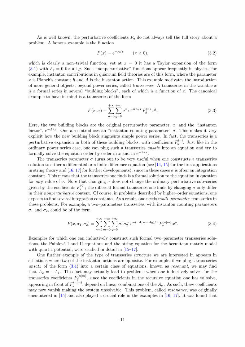
As is well known, the perturbative coefficients Fg do not always tell the full story about aproblem. A famous example is the function
F (x) = e−A/x (x ≥ 0), (3.2)
which is clearly a non–trivial function, yet at x = 0 it has a Taylor expansion of the form(3.1) with Fg = 0 for all g. Such “nonperturbative” functions appear frequently in physics; forexample, instanton contributions in quantum field theories are of this form, where the parameterx is Planck’s constant ~ and A is the instanton action. This example motivates the introductionof more general objects, beyond power series, called transseries. A transseries in the variable xis a formal series in several “building blocks”, each of which is a function of x. The canonicalexample to have in mind is a transseries of the form
F (x, σ) =
+∞∑n=0
+∞∑g=0
σn e−nA/x F (n)g xg. (3.3)
Here, the two building blocks are the original perturbative parameter, x, and the “instantonfactor”, e−A/x. One also introduces an “instanton counting parameter” σ. This makes it veryexplicit how the new building block augments simple power series. In fact, the transseries is a
perturbative expansion in both of these building blocks, with coefficients F(n)g . Just like in the
ordinary power series case, one can plug such a transseries ansatz into an equation and try toformally solve the equation order by order in x and in e−A/x.
The transseries parameter σ turns out to be very useful when one constructs a transseriessolution to either a differential or a finite difference equation (see [14, 15] for the first applicationsin string theory and [16, 17] for further developments), since in these cases σ is often an integrationconstant. This means that the transseries one finds is a formal solution to the equation in questionfor any value of σ. Note that changing σ does not change the ordinary perturbative sub–series
given by the coefficients F(0)g ; the different formal transseries one finds by changing σ only differ
in their nonperturbative content. Of course, in problems described by higher–order equations, oneexpects to find several integration constants. As a result, one needs multi–parameter transseries inthese problems. For example, a two–parameters transseries, with instanton counting parametersσ1 and σ2, could be of the form
F (x, σ1, σ2) =+∞∑n=0
+∞∑m=0
+∞∑g=0
σn1σm2 e−(nA1+mA2)/x F (n|m)
g xg. (3.4)
Examples for which one can inductively construct such formal two–parameter transseries solu-tions, the Painleve I and II equations and the string equation for the hermitean matrix modelwith quartic potential, were studied in detail in [15–17].
One further example of the type of transseries structure we are interested in appears insituations where two of the instanton actions are opposite. For example, if we plug a transseriesansatz of the form (3.4) into a certain class of equations, known as resonant, we may findthat A2 = −A1. This fact may actually lead to problems when one inductively solves for the
transseries coefficients F(n|m)g , since the coefficients in the recursive equation one has to solve,
appearing in front of F(n|m)g , depend on linear combinations of the Aα. As such, these coefficients
may now vanish making the system unsolvable. This problem, called resonance, was originallyencountered in [15] and also played a crucial role in the examples in [16, 17]. It was found that
– 11 –
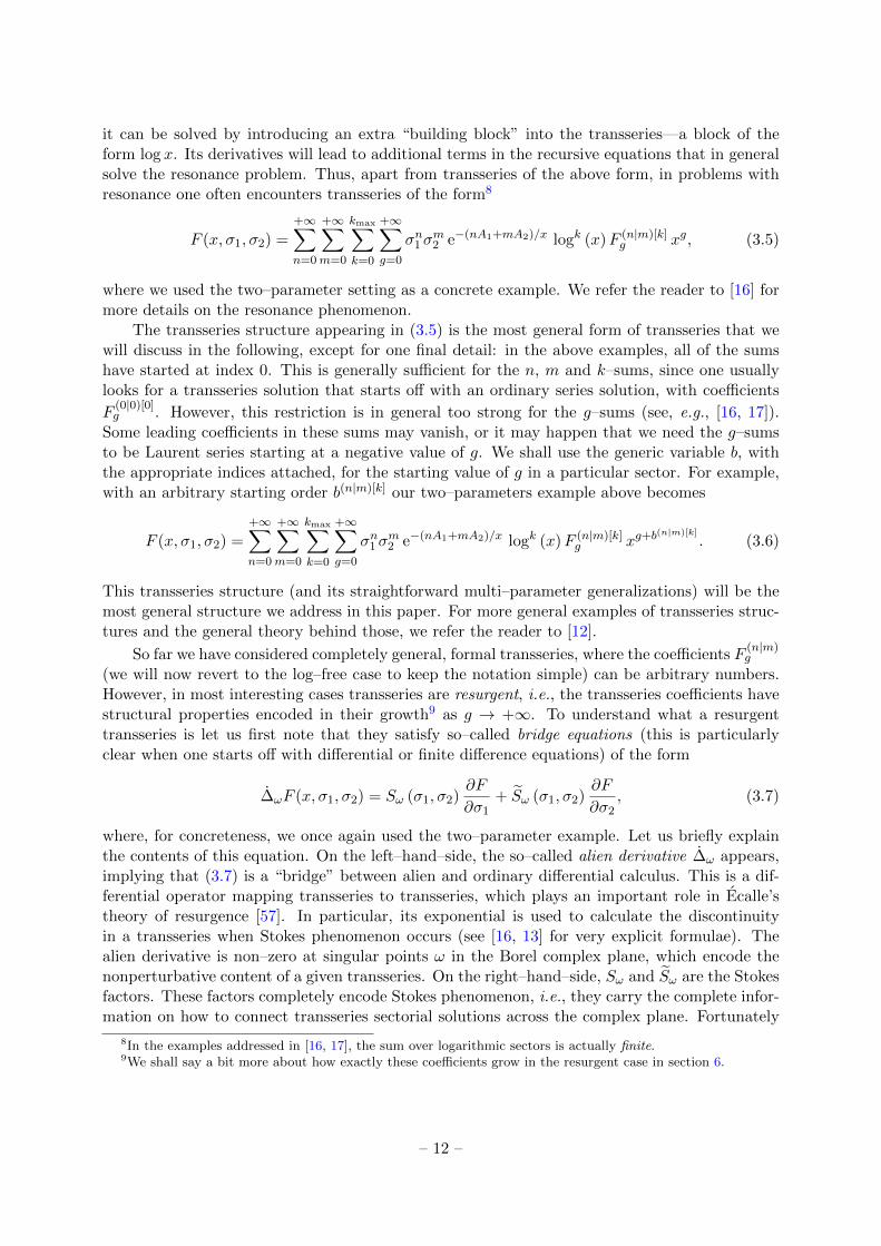
it can be solved by introducing an extra “building block” into the transseries—a block of theform log x. Its derivatives will lead to additional terms in the recursive equations that in generalsolve the resonance problem. Thus, apart from transseries of the above form, in problems withresonance one often encounters transseries of the form8
F (x, σ1, σ2) =
+∞∑n=0
+∞∑m=0
kmax∑k=0
+∞∑g=0
σn1σm2 e−(nA1+mA2)/x logk (x)F (n|m)[k]
g xg, (3.5)
where we used the two–parameter setting as a concrete example. We refer the reader to [16] formore details on the resonance phenomenon.
The transseries structure appearing in (3.5) is the most general form of transseries that wewill discuss in the following, except for one final detail: in the above examples, all of the sumshave started at index 0. This is generally sufficient for the n, m and k–sums, since one usuallylooks for a transseries solution that starts off with an ordinary series solution, with coefficients
F(0|0)[0]g . However, this restriction is in general too strong for the g–sums (see, e.g., [16, 17]).
Some leading coefficients in these sums may vanish, or it may happen that we need the g–sumsto be Laurent series starting at a negative value of g. We shall use the generic variable b, withthe appropriate indices attached, for the starting value of g in a particular sector. For example,with an arbitrary starting order b(n|m)[k] our two–parameters example above becomes
F (x, σ1, σ2) =+∞∑n=0
+∞∑m=0
kmax∑k=0
+∞∑g=0
σn1σm2 e−(nA1+mA2)/x logk (x)F (n|m)[k]
g xg+b(n|m)[k]
. (3.6)
This transseries structure (and its straightforward multi–parameter generalizations) will be themost general structure we address in this paper. For more general examples of transseries struc-tures and the general theory behind those, we refer the reader to [12].
So far we have considered completely general, formal transseries, where the coefficients F(n|m)g
(we will now revert to the log–free case to keep the notation simple) can be arbitrary numbers.However, in most interesting cases transseries are resurgent, i.e., the transseries coefficients havestructural properties encoded in their growth9 as g → +∞. To understand what a resurgenttransseries is let us first note that they satisfy so–called bridge equations (this is particularlyclear when one starts off with differential or finite difference equations) of the form
∆ωF (x, σ1, σ2) = Sω (σ1, σ2)∂F
∂σ1+ Sω (σ1, σ2)
∂F
∂σ2, (3.7)
where, for concreteness, we once again used the two–parameter example. Let us briefly explainthe contents of this equation. On the left–hand–side, the so–called alien derivative ∆ω appears,implying that (3.7) is a “bridge” between alien and ordinary differential calculus. This is a dif-ferential operator mapping transseries to transseries, which plays an important role in Ecalle’stheory of resurgence [57]. In particular, its exponential is used to calculate the discontinuityin a transseries when Stokes phenomenon occurs (see [16, 13] for very explicit formulae). Thealien derivative is non–zero at singular points ω in the Borel complex plane, which encode thenonperturbative content of a given transseries. On the right–hand–side, Sω and Sω are the Stokesfactors. These factors completely encode Stokes phenomenon, i.e., they carry the complete infor-mation on how to connect transseries sectorial solutions across the complex plane. Fortunately
8In the examples addressed in [16, 17], the sum over logarithmic sectors is actually finite.9We shall say a bit more about how exactly these coefficients grow in the resurgent case in section 6.
– 12 –
for us, neither the precise definition of the alien derivative nor the explicit form of the Stokescoefficients is important to convey the main message of the bridge equation (3.7). All we needto know is that the alien derivative ∆ω only acts on power series of x and, as such, it does notchange the powers of σi appearing in the transseries. On the other hand, the σi–derivatives on theright–hand–side of (3.7) clearly do change the powers of σi appearing in a transseries. The result
of this is that the bridge equation, when written out in components, relates coefficients F(n|m)g
to coefficients F(n′|m′)g′ with different n′, m′ and g′. In particular, it gives us relations between
perturbative and nonperturbative coefficients (again, see [16] for very explicit formulae).This is also the origin of the name resurgent: at each singular point ω, a specific nonpertur-
bative sector will see the resurgence of other, different nonperturbative sectors due to the natureof the bridge equations. The relations one thus obtains between different coefficients in differentsectors are so stringent that we could, in principle, determine all nonperturbative coefficients ifthe perturbative coefficients and the Stokes factors are known. In section 6, we shall see that theresulting relations take the form of large–order relations, and discuss how this allows us to testthe resurgent properties of the transseries appearing in topological string theory.
4 One–Parameter Resurgent Transseries
Our main goal in this paper is to construct transseries solutions to the holomorphic anomalyequations. In the previous two sections we have seen how to write these equations in a fashionadapted to nonperturbative solutions, and we have discussed what exactly is the structure oftransseries solutions. We will now show how to construct one–parameter transseries solutionsto the holomorphic anomaly equations, and how their anti–holomorphic dependence is fixed viaexponentials and polynomials in the propagators both at perturbative and nonperturbative levels.
4.1 A Closer Look at the Perturbative Sector
Before diving into the details of a transseries solution for the topological string free energy, let us
review what is the structure of the perturbative solution, F(0)g , as integrated from the holomorphic
anomaly equations. We are particularly interested in the anti–holomorphic moduli dependenceof these free energies, i.e., how they depend on the propagators.
Let us start with [52] where it was pointed out that the holomorphic anomaly equationsmay be efficiently integrated to yield the string perturbative expansion. Within the example ofthe quintic in P4, that work introduced a finite set of generators and proved that the genus gfree energies are polynomials of a certain degree in the generators. These generators captured
the anti–holomorphic dependence of the F(0)g and the degree of the polynomials was found to be
3g − 3. Later, in [53], this result was extended to arbitrary compact Calabi–Yau threefolds withany number of complex moduli. In particular, it was shown that the propagators Sij , Si, S and∂iK, generate a differential ring, i.e., any covariant derivative of a polynomial in these generatorsis again a polynomial in these generators; and it was found that the free energy at genus g is apolynomial of total degree 3g − 3 precisely in the propagators, provided one assigns degree +1to Sij and ∂iK, degree +2 to Si, and degree +3 to S. The same result, but for local Calabi–Yaugeometries, was obtained in [35, 36], but where now only the Sij play a role. Another approachto integration based on the differential ring of quasi–modular forms was followed in [58].
Since we shall later study the structure of higher–instanton free energies F(n)g in great detail,
it will be useful to first derive the polynomial structure of the perturbative free energies, F(0)g . A
nice and elegant way to show that F(0)g is a polynomial of degree 3g−3 is the one used originally
– 13 –

in [53]. Given the holomorphic anomaly equations (2.10), one assigns a degree to each object inthe following way
F (0)g 7→ d(g), Di 7→ +1, Sij 7→ +1. (4.1)
Note that this degree will coincide with the usual notion of polynomial degree in the S–variables.Note also that since
DiSjk = −Ci`m S`jSmk + f jki , (4.2)
it is consistent to assign degree +1 to Di (and zero to any holomorphic quantity like the Yukawacouplings). The idea now is to prove by induction that d(g) = 3g − 3. The base case of the
induction is simply proved by direct integration of (2.10) for g = 2, where one finds that F(0)2
is a polynomial in Sij of degree 3. Then, assuming d(h) = 3h − 3 for h < g, one finds that theright–hand–side of (2.10) has degree 3 (g − 1)− 3 + 1 + 1 = 3g− 4, as it should be, thus provingthe assumption that the left–hand–side has degree 3g − 3− 1 = 3g − 4.
A more pedestrian but equivalent way to obtain the same conclusion is again to prove byinduction that
F (0)g = Pol
(Sij; 3g − 3
)≡ Pol (3g − 3) , g ≥ 2, (4.3)
but this time around without relying directly on the notion of a degree. Instead, one may performthe integration directly once the structure of the right–hand–side of (2.10) is known. In here,Pol
(Sij; d
)stands for a polynomial of total degree d in the propagators, and whose coefficients
are functions of the holomorphic complex moduli. The base case of the induction is the same as
before, proved by explicit integration. Then, assuming F(0)h = Pol (3h− 3) for h < g, and since
DiF(0)h = Pol (3h− 3 + 1) , (4.4)
DiDjF(0)h = Pol (3h− 3 + 2) , (4.5)
where we used (4.2), it follows
RHS of (2.10) = Pol (3 (g − 1)− 3 + 2) +
g−1∑h=1
Pol (3 (g − h)− 3 + 1)× Pol (3h− 3 + 1) =
= Pol (3g − 4) . (4.6)
Integration with respect to the propagators raises the polynomial degree by one, so we find that
indeed F(0)g = Pol (3g − 3) which is what we wanted to prove.
In the analysis of the structure of the higher–instanton free energies we shall make use ofthis latter strategy. The reason for not using the initial degree approach is, as we shall see, theappearance of exponentials of the propagators in the solutions, which would make such approachimpracticable (but in section 5 we will fully explain this point).
4.2 Setting the Transseries Construction
We shall now address the construction of transseries solutions, within the context of one–parameter transseries and for Calabi–Yau geometries with a complex moduli space of dimensionone. Along this paper we shall lift these restrictions and construct completely general solutionsbut, to introduce the overall strategy, it proves useful to start with a simplified setting. Previ-ously, we discussed how to appropriately write the holomorphic anomaly equations as a singleequation for the full partition function, instead of an infinite tower of equations for the pertur-bative genus g free energies. In this way, in the dimension one case, we obtained equation (2.24)
– 14 –
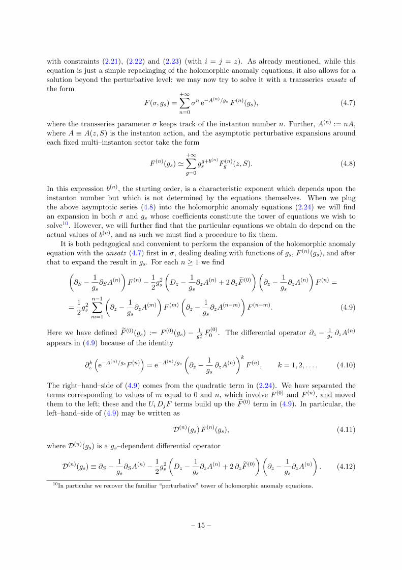
with constraints (2.21), (2.22) and (2.23) (with i = j = z). As already mentioned, while thisequation is just a simple repackaging of the holomorphic anomaly equations, it also allows for asolution beyond the perturbative level: we may now try to solve it with a transseries ansatz ofthe form
F (σ, gs) =
+∞∑n=0
σn e−A(n)/gs F (n)(gs), (4.7)
where the transseries parameter σ keeps track of the instanton number n. Further, A(n) := nA,where A ≡ A(z, S) is the instanton action, and the asymptotic perturbative expansions aroundeach fixed multi–instanton sector take the form
F (n)(gs) '+∞∑g=0
gg+b(n)
s F (n)g (z, S). (4.8)
In this expression b(n), the starting order, is a characteristic exponent which depends upon theinstanton number but which is not determined by the equations themselves. When we plugthe above asymptotic series (4.8) into the holomorphic anomaly equations (2.24) we will findan expansion in both σ and gs whose coefficients constitute the tower of equations we wish tosolve10. However, we will further find that the particular equations we obtain do depend on theactual values of b(n), and as such we must find a procedure to fix them.
It is both pedagogical and convenient to perform the expansion of the holomorphic anomalyequation with the ansatz (4.7) first in σ, dealing dealing with functions of gs, F
(n)(gs), and afterthat to expand the result in gs. For each n ≥ 1 we find(
∂S −1
gs∂SA
(n)
)F (n) − 1
2g2s
(Dz −
1
gs∂zA
(n) + 2 ∂zF(0)
)(∂z −
1
gs∂zA
(n)
)F (n) =
=1
2g2s
n−1∑m=1
(∂z −
1
gs∂zA
(m)
)F (m)
(∂z −
1
gs∂zA
(n−m)
)F (n−m). (4.9)
Here we have defined F (0)(gs) := F (0)(gs) − 1g2sF
(0)0 . The differential operator ∂z − 1
gs∂zA
(n)
appears in (4.9) because of the identity
∂kz
(e−A
(n)/gsF (n))
= e−A(n)/gs
(∂z −
1
gs∂zA
(n)
)kF (n), k = 1, 2, . . . . (4.10)
The right–hand–side of (4.9) comes from the quadratic term in (2.24). We have separated theterms corresponding to values of m equal to 0 and n, which involve F (0) and F (n), and movedthem to the left; these and the UiDjF terms build up the F (0) term in (4.9). In particular, theleft–hand–side of (4.9) may be written as
D(n)(gs)F(n)(gs), (4.11)
where D(n)(gs) is a gs–dependent differential operator
D(n)(gs) ≡ ∂S −1
gs∂SA
(n) − 1
2g2s
(Dz −
1
gs∂zA
(n) + 2 ∂zF(0)
)(∂z −
1
gs∂zA
(n)
). (4.12)
10In particular we recover the familiar “perturbative” tower of holomorphic anomaly equations.
– 15 –

Let us turn to the gs–expansion, using (4.8) and D(n)(gs) =∑+∞
g=−1 ggs D(n)
g , with D(n)−1 :=
−∂SA(n). We find
+∞∑g=−1
ggs
−∂SA(n)F
(n)g+1 +
g∑h=0
D(n)h F
(n)g−h
= (4.13)
=
n−1∑m=1
+∞∑g=0
gg+B(n,m)s
1
2
g∑h=0
(∂zF
(m)h−1 − ∂zA
(m)F(m)h
)(∂zF
(n−m)g−1−h − ∂zA
(n−m)F(n−m)g−h
),
where we have defined B(n,m) := b(m) + b(n−m) − b(n). As we have commented earlier, theholomorphic anomaly equations do not compute the values of the starting genus b(n). This is nota surprise since the values of b(n) are very much dependent upon the model and the geometryone is working with. Note, however, that the values of B(n,m) determine the structure of theequations in the following way. Looking at (4.13) one sees that if B(n,m) is sufficiently negativewe will have terms in the right–hand–side of the equation but not on the left. This is in contrastto what happens when B is sufficiently positive. In that case, after collecting terms with similar
powers in gs, we find an equation for F(n)g which depends on previously computed data (see
below). If B(n,m) ≥ 0 for every n, m, we obtain a system of equations which can be solvedrecursively in n and g, and which has no extra constraint equations. If B(n,m) < 0 for some n,m, some such constraints will appear and they will have to be treated separately.
Let us start with the simplest situation, B(n,m) ≥ 0, and in particular work out the caseB(n,m) = +1 for each n, m. This is the value of B one obtains from b(n) = +1, and it correspondsto the values of b(n) that the pure conifold has [59] (see section 7.2). After solving this case weshall see how it generalizes to any other b(n) such that B(n,m) ≥ 0.
Thus setting B = +1 and collecting terms with the same power in gs, we obtain the towerof equations
∂SA(n)F
(n)g+1 −
g∑h=0
D(n)h F
(n)g−h+ (4.14)
+1
2
n−1∑m=1
g−1∑h=0
(∂zF
(m)h−1 − ∂zA
(m)F(m)h
)(∂zF
(n−m)g−2−h − ∂zA
(n−m)F(n−m)g−1−h
)= 0,
for g = −1, 0, 1, 2, . . .. In the sums over h we are using the convention that F(m)h is zero whenever
h < 0. The explicit form the D(n)g operators, which we defined earlier as coefficients in the
gs–expansion of (4.12), is
D(n)0 = ∂S −
1
2
(∂zA
(n))2, (4.15)
D(n)1 =
1
2D2zA
(n) + ∂zA(n)(Dz + ∂zF
(0)1
), (4.16)
D(n)2 = −1
2D2z − ∂zF
(0)1 Dz, (4.17)
D(n)2h−1 = ∂zA
(n) ∂zF(0)h , h = 2, 3, . . . , (4.18)
D(n)2h = −∂zF (0)
h Dz, h = 2, 3, . . . . (4.19)
– 16 –
Let us have a closer look at the equations (4.14). For g = −1 there is only one term,
∂SA(n) F
(n)0 = 0. (4.20)
Since F(n)0 6= 0 by definition, and A(n) = nA, we arrive at the important equation
∂SA = 0. (4.21)
This means that the instanton action, A, that we presupposed dependent on both z and S turnsout not to depend on the propagator S. In fact, the instanton action is holomorphic. Note,however, that our equations do not determine its z–functional dependence. This suggests thatone may think of the instanton action, A(z), as a holomorphic ambiguity, much in the same wayas the familiar holomorphic ambiguities that appear in the integration of the free energies. Inorder to fix it, first recall the experience from matrix models [19, 38, 60] which tells us that theinstanton action is generically given by a combination of periods of the spectral curve [61]. Onemay then forget about matrix models [62, 60]—albeit keeping its spectral geometry structure—by considering toric Calabi–Yau threefolds, whose mirror is essentially described by a Riemannsurface, the mirror curve [63], and take the instanton action as an appropriate combination ofperiods of this curve, i.e., as an appropriate combination of Calabi–Yau periods.
Using this result back in (4.14) simplifies the equations to(∂S −
1
2
(∂zA
(n))2)F (n)g = (4.22)
= −g∑
h=1
D(n)h F
(n)g−h +
1
2
n−1∑m=1
g−1∑h=0
(∂zF
(m)h−1 − ∂zA
(m)F(m)h
)(∂zF
(n−m)g−2−h − ∂zA
(n−m)F(n−m)g−1−h
).
The operator that appears on the left–hand–side is D(n)0 , (4.15). Note that the right–hand–side
of (4.22) depends only on previous instanton sectors and genera, and it is, therefore, a com-pletely known object in the recursive integration of the equations. Further, the set of operators
D(n)h appearing on the right–hand–side of (4.22) will always include a second–order covariant
derivative, as long as g ≥ 2 (just look at (4.17) above). In other words, (4.22) is, effectively, thenonperturbative analogue of the holomorphic anomaly equations of [34].
As we explained before, (4.22) are the resulting “nonperturbative” holomorphic anomalyequations when b(n) = +1, ∀n (or, more generally, when B(n,m) = +1, ∀n,m). Otherwise, thecalculation simply generalizes to
∂SA(n)F
(n)g+1 −
g∑h=0
D(n)h F
(n)g−h+ (4.23)
+1
2
n−1∑m=1
g−B(n,m)∑h=0
(∂zF
(m)h−1 − ∂zA
(m)F(m)h
)(∂zF
(n−m)g−1−B(n,m)−h − ∂zA
(n−m)F(n−m)g−B(n,m)−h
)= 0.
Let us stress that, independently of the value of B(n,m), the equation for g = −1 and n = 1 is
∂SA(1)F
(1)0 = 0, (4.24)
which implies that A(1) ≡ A is holomorphic also in this general case.
– 17 –

As a final remark, let us note that the one–parameter transseries we addressed may bethought of as a multi–parameters transseries when all sectors but one are switched off. That is, ina general setting, where (generalized) instanton sectors are labelled by integers (n1| · · · |nα| · · · |nk),the n–instanton sector of an one–parameter transseries is embedded as (0| · · · |n| · · · |0). In thisway, it is natural to expect that much of the structure we have uncovered so far will have anatural generalization within multi–parameter transseries.
4.3 Structure of the Transseries Solution
So far we have obtained an infinite tower of equations; a nonperturbative extension of the holo-morphic anomaly equations. The key question is, of course, whether we can solve/integrate themexplicitly, or how much can be said about their (generic) solutions. Similar to what was done inthe perturbative case [52, 53, 36], it turns out that also in the present nonperturbative case wecan be very specific about the general structure of the solutions.
Let us for the moment stick to the case b(n) = 1, ∀n, and let us denote by G(n)g the full
right–hand–side of (4.22). Because of the simple structure of this equation, it is straightforwardto integrate in the propagator, S, and obtain
F (n)g (z, S) = e
12(∂zA(n))
2S
(f (n)g (z) +
∫ S
dS e−12(∂zA(n))
2S G(n)
g (z, S)
), (4.25)
where f(n)g (z) is the holomorphic ambiguity of the nth multi–instanton sector at order g. Notice
here a nonperturbative novelty: the appearance of exponentials in S in the solution (4.25). Onecan already anticipate the presence of different exponentials arising from previous instanton
sectors to build up the actual expression for F(n)g . The reason for these exponentials factors is, of
course, the fact that in the nonperturbative setting the differential operator we are integrating isno longer just a derivative, ∂S , but a derivative with an extra linear term in the instanton action.
Let us first have a look at the actual form of the equations for the one–instanton sector,n = 1. In this sector, the second term of the right–hand–side of (4.22) vanishes, so we have
G(1)g = −
g∑h=1
D(1)h F
(1)g−h. (4.26)
Starting at g = 0, as G(1)0 = 0 the equation for F
(1)0 is simply(
∂S −1
2(∂zA)2
)F
(1)0 = 0, (4.27)
which can be immediately integrated with respect to S to give
F(1)0 = e
12
(∂zA)2S f(1)0 (z). (4.28)
Here, f(1)0 (z) is the holomorphic ambiguity. At next order, for g = 1, we now have
G(1)1 = −D(1)
1 F(1)0 , (4.29)
where D(1)1 is given by (4.16) with n = 1. The exponential which is part of F
(1)0 naturally
survives the action of D(1)1 , while the z–derivative acting on the propagator S, that sits in
– 18 –
the exponential, gives back an S2 term (recall (4.2)). In this way, G(1)1 is the product of the
exponential exp 12 (∂zA)2 S by a polynomial of degree 2 in S. When we plug this expression into
the general form of the solution (4.25), the exponential inside the integral cancels that of G(1)1
and we are left with the integral of a polynomial (of known degree). Thus, from (4.25) we obtain
that F(1)1 is the product of exp 1
2 (∂zA)2 S by a polynomial of degree 3.
This suggests that, in general, F(1)g is of the form
F (1)g = e
12
(∂zA)2S Pol (S; 3g) , (4.30)
where Pol (S; d) stands for a polynomial of degree d in S, with coefficients which are holomorphicfunctions of z. It can be checked by explicit computation that this is indeed the case for low g.
To prove the general case one proceeds by induction, studying the structure of G(1)g and finding
that it is the product of a polynomial of degree 3g−1 by the usual exponential. Integration thenyields the result. We shall be more thorough when looking at the structure of the free energiesfor the multi–parameter transseries, as the strategy for that case will be the same as in here.
Having understood the n = 1 sector we may move on to the n = 2 equations. Now thequadratic terms in (4.22) are present and the structure of the solution is more complicated. Thiscontribution,
g−1∑h=0
(∂zF
(1)h−1 − ∂zA
(1)F(1)h
)(∂zF
(1)g−2−h − ∂zA
(1)F(n−m)g−1−h
), (4.31)
will produce terms with exp 12 (1 + 1) (∂zA)2 S = exp 1
2 2 (∂zA)2 S. There will also be terms with
exp 12
(∂zA
(2))2S = exp 1
2 4 (∂zA)2 S. In this way, in order to specify the structure of the F(2)g
free energies, one needs to know the degrees, d1 and d2, of the polynomials in S that multiplythese exponentials:
F (2)g = e
12
2(∂zA)2S Pol (S; d1) + e12
4(∂zA)2S Pol (S; d2) . (4.32)
Computing the first free energies for g = 0, 1, 2, . . . , suggests d1 = 3(g+1−2) and d2 = 3(g+1−1).Mechanically computing case by case, we find that the next instanton sector, n = 3,
will have exponentials of the type exp 12 a (∂zA)2 S with a ∈ 3, 5, 9 and the associated poly-
nomials will have degrees d = 3 (g + 1− λ), with λ ∈ 3, 2, 1, respectively. These num-bers get more complicated as the instanton number increases. For example, for n = 7, a ∈7, 9, 11, 13, 15, 17, 19, 21, 25, 27, 29, 37, 49 and λ ∈ 7, 6, 5, 4, 4, 3, 3, 3, 2, 3, 2, 2, 1, respectively.
The nature of the numbers a and λ is purely combinatoric, and they actually have aninterpretation11 in terms of integer partitions of the instanton number n. In the next section weshall prove that these numbers are encoded in the generating function
Φ =
+∞∏m=1
1
1− ϕEm2 ρm=
+∞∑n=0
∑γn
Ea(n;γn) ϕλ(n;γn) (1 +O(ϕ)) , (4.33)
where ϕ, E, and ρ are formal variables, and γn is a set of indices; but see section 5 for adetailed explanation and origin of this generating function.
It is also important to note from the general form of the solution (4.25) that the holomorphic
ambiguity, f(n)g , always sits in the polynomial that accompanies exp 1
2 n2 (∂zA)2 S. Interestingly,
11This interpretation becomes too cumbersome when we have a multi–parameters transseries.
– 19 –

this has a theta–function flavor as in [37]. The corresponding polynomial is of degree 3(g+1−1) =3g, which is the highest since λ = 1 only for a = n2 (see section 5 for further details).
In summary, we found that the higher–instanton free energies have the form
F (n)g =
∑γn
e12a(n;γn)(∂zA)2S Pol (S; 3 (g + 1− λ (n; γn))) , (4.34)
where the combinatorial data a, λ, γ is encoded in the generating function (4.33). Similarly,one can derive an analogous structure when b(n) is more general than just +1. Assuming therestriction that B(n,m) ≥ 0, ∀n,m, one would find (and again we refer the reader to section 5for a detailed proof)
F (n)g =
∑γn
e12a(n;γn)(∂zA)2S Pol
(S; 3
(g + b(n) − λb (n; γn)
)), (4.35)
where this time around the combinatorial data is stored in
Φb =+∞∏m=1
1
1− ϕb(m)Em2 ρm
=+∞∑n=0
∑γn
Ea(n;γn) ϕλb(n;γn) (1 +O(ϕ)) . (4.36)
Do note that a and γ are independent of the value of the starting genus b(n).A few comments are now in order. The fact that we have not approached the determination
of the structure of the F(n)g by assigning degrees to the various objects of the corresponding
equations—as was earlier done in the perturbative sector—is because now we do not only havepolynomials. What we actually have is a sum of different exponentials times polynomials of vari-ous degrees, and tracking all those degrees at the same time while capturing all the combinatoricsof the problem makes the approach much less clear than using a more hands–on calculation asabove. Also, as we mentioned before, a detailed analysis of the structure of the solution and arecipe to calculate the a and λ numbers will be studied in the multi–parameters transseries case.The proofs will rely on induction, carefully studying the exponential and polynomial structure of
the G(n)g in (4.25) and tracking what happens when integrating. Finally, it is important to stress
that the holomorphic anomaly equations in (4.22) determine the functional dependence of the
free energies F(n)g (z, S), up to a holomorphic ambiguity, f
(n)g (z), just as in the perturbative case
(see section 7). The anti–holomorphic dependence, encoded in the propagator S, is in the formof polynomials and exponentials. The numbers a and λ, depending on the instanton number n,determine the coefficients in the exponentials and the degree of the polynomials, respectively.
5 Multi–Parameter Resurgent Transseries
In the previous section we have shown how to construct one–parameter transseries solutions tothe holomorphic anomaly equations. These solutions will be adequate nonperturbative solutionswhenever there is a single instanton action in the game. However, most of the time this is notthe case: either there are different instanton actions associated to different (physical) instantoneffects, or resurgence demands that further “generalized” instanton actions should come into playwhen considering the full nonperturbative grand–canonical partition function (see, e.g., [15–17]).In this case, multi–parameter transseries solutions must be considered. We shall now see howour previous discussion generalizes to the multi–parameters case; in fact this section will followclosely its analog for the one–parameter transseries.
– 20 –
5.1 Setting the Generalized Transseries Construction
Let us consider a general multi–parameters transseries ansatz, with the form
F (σ, gs) =∑n∈Nκ0
σn e−A(n)/gs F (n)(gs). (5.1)
We are assuming one has κ distinct instanton actions, Aα, and we are using the shorthandnotation A(n) =
∑κα=1 nαAα to identify all (generalized) multi–instanton sectors. At this moment
we let Aα = Aα(z, S) for absolute generality, but we shall see in the following that all theseinstanton actions are independent of S, i.e., they are all holomorphic functions. At each ofthe multi–instanton sectors, one further finds asymptotic perturbative expansions which for themoment we just denote by F (n)(gs), i.e., in the first few steps it proves useful not to look atthe particular asymptotic expansions in gs. Finally, the transseries parameters encoding thenonperturbative ambiguities are assembled in the expression above as σn :=
∏κα=1 σ
nαα .
If we plug our transseries ansatz (5.1) into the holomorphic anomaly equation12 (2.24), andwe collect terms with the same powers in σ, we find(
∂S −1
gs∂SA
(n)
)F (n) − 1
2g2s
(Dz −
1
gs∂zA
(n) + 2 ∂zF(0)
)(∂z −
1
gs∂zA
(n)
)F (n) =
=1
2g2s
n∑′
m=0
(∂z −
1
gs∂zA
(m)
)F (m)
(∂z −
1
gs∂zA
(n−m)
)F (n−m), (5.2)
where again F (0)(gs) := F (0)(gs)− 1g2sF
(0)0 . The same comments we made to (4.9) apply now in
here. The only novelty is the use of a primed sum over the previous instanton numbers, meaning
n∑′
m=0
≡n1,...,nκ∑
m1,...,mκ=0m 6=0,m6=n
. (5.3)
That is, the sum does not involve either F (0) or F (n). Instead, those terms have been moved tothe left–hand–side of (5.2). Again, as in the previous section, we can define a differential operatorD(n) and its gs–expansion; see (4.12).
Let us now consider the perturbative gs asymptotic expansions of each (generalized) multi–instanton sector,
F (n) '+∞∑g=0
gg+b(n)
s F (n)g , (5.4)
where b(n) is a characteristic exponent that generalizes the one in the last section. Plugging thisexpansion (5.4) back into (5.2), we arrive at
+∞∑g=−1
ggs
−∂SA(n)F
(n)g+1 +
g∑h=0
D(n)h F
(n)g−h
= (5.5)
=
n∑′
m=0
+∞∑g=0
gg+B(n,m)s
1
2
g∑h=0
(∂zF
(m)h−1 − ∂zA
(m)F(m)h
)(∂zF
(n−m)g−1−h − ∂zA
(n−m)F(n−m)g−h
),
12We are still working with complex moduli space of dimension one. This requirement is lifted in appendix A.
– 21 –
where B(n,m) := b(m) + b(n−m) − b(n). In the following we shall carry out the calculation fora general b(n), with the condition B(n,m) ≥ 0 to avoid the case of constraints, but it might beuseful to have the case B(n,m) = +1, ∀n,m, in mind. Collecting terms with the same powerin gs we find the equations
∂SA(n)F
(n)g+1 −
g∑h=0
D(n)h F
(n)g−h + (5.6)
+1
2
n∑′
m=0
g−B(n,m)∑h=0
(∂zF
(m)h−1 − ∂zA
(m)F(m)h
)(∂zF
(n−m)g−1−B(n,m)−h − ∂zA
(n−m)F(n−m)g−B(n,m)−h
)= 0,
for g = −1, 0, 1, 2, . . .. For the one–instanton sectors, that is, those of the form n = (0| · · · |1| · · · |0),the quadratic term in (5.6) drops (for any value of B). If we further focus on g = −1, also thesecond term drops, and we are left with
∂SA(0|···|1|···|0) = 0 (5.7)
for every one–instanton sector, since F(0|···|1|···|0)0 6= 0. We therefore conclude
∂SAα = 0, α = 1, . . . , κ, (5.8)
i.e., every instanton action is holomorphic. This is a fundamental point within the nonpertur-bative structure of topological string theory, and we shall return to it later in the paper.
Finally, if one rewrites (5.6) above as an equation for the unknowns F(n)g —or, more precisely,
for D(n)0 F
(n)g as we are dealing with a differential equation—it follows that(
∂S −1
2
(∂zA
(n))2)F (n)g = −
g∑h=1
D(n)h F
(n)g−h + (5.9)
+1
2
n∑′
m=0
g−B(n,m)∑h=0
(∂zF
(m)h−1 − ∂zA
(m)F(m)h
)(∂zF
(n−m)g−1−B(n,m)−h − ∂zA
(n−m)F(n−m)g−B(n,m)−h
),
where it should be clear that the right–hand–side depends only on previous instanton sectors andgenera, and it is, therefore, a known object in the recursive integration of the equations. The
D(n)h operators can be read from (4.16–4.19), trivially changing n by n and 0 by 0.
5.2 Structure of the Generalized Transseries Solution
If we denote by G(n)g the right–hand–side of (5.9), it is straightforward to find the solution to the
differential equation:
F (n)g (z, S) = e
12(∂zA(n))
2S
(f (n)g (z) +
∫ S
dS e−12(∂zA(n))
2S G(n)
g (z, S)
), (5.10)
where f(n)g (z) is the holomorphic ambiguity of the multi–instanton sector n, at order g. This
expression, (5.10), is very reminiscent of similar formulae we have obtained in section 4 for one–parameter transseries solutions to the holomorphic anomaly equations. As such, it is withoutsurprise that we will find also in here, in the multi–parameter transseries context, that it is
– 22 –
possible to fix the polynomial structure of the many nonperturbative sectors—precisely as finitelinear combinations of exponential terms multiplied by suitable polynomials.
Let us make the aforementioned expectation precise. If correct, this will imply that thestructure of the solution will be specified by the coefficients in the exponentials and the degreeof the polynomials. In this case, one finds expressions of the form
F (n)g =
∑γn
exp
1
2
κ∑α,β=1
aαβ (n; γn) ∂zAα ∂zAβ S
Pol (S; db (n; g; γn)) . (5.11)
Here γn is an index running in some finite set (it may be regarded as a label); aαβ (n; γn) arenon–negative integers (we are already anticipating here that these numbers will not depend on g)and they are the generalization of the a–numbers we found at the end of section 4; and db(n; g; γn)is the degree of the corresponding polynomial in S (whose coefficients will have a holomorphicdependence on z). In the formula for the degree db we shall encounter the generalization of theλb–numbers of section 4; see (5.21) in the following and note the b–dependence.
It turns out that, as we shall see in detail below, all these integers may be codified by asingle generating function
Φb ≡ Φb (ϕ,E, ρ) :=
+∞∏′
m=0
1
1− ϕb(m) ∏κα,β=1E
mαmβαβ
∏κα=1 ρ
mαα
, (5.12)
where Eαβ is taken to be symmetric in (α, β). The prime, ( ′), in the infinite product means thatm = 0 is not considered (if it were we would get an extra term (1−ϕ)−1, so we omit it). Here ϕ,Eαβ, and ρα are formal variables, so that Φb may be expanded in power series using the formalidentity (1− x)−1 = 1 + x+ x2 + x3 + · · · as
Φb =
+∞∏′
m=0
+∞∑r=0
ϕr b(m)
κ∏α,β=1
Ermαmβαβ
κ∏α=1
ρrmαα . (5.13)
Next, we explicitly evaluate the m–products (relabeling r → rm),
Φb =∑rm
ϕ∑+∞
m=0 rm b(m)κ∏
α,β=1
E∑+∞
m=0 rmmαmβαβ
κ∏α=1
ρ∑+∞
m=0 rmmαα , (5.14)
and reorganize the several terms according to their powers in ρα for each α. Thus, for anyfixed n, we select those values of rm which satisfy
∑+∞m=0 rmm = n. For example, in the
case of one–parameter transseries we addressed earlier, one would simply be doing the choice of∑+∞m=0 rmm = n, or 1 · r1 + 2 · r2 + 3 · r3 + · · · = n, that is, one would be selecting those rm
that codify an integer partition of n. It then follows that
Φb =+∞∑n=0
ρn∑
rm :∑+∞
m=0 rm m=n
ϕ∑+∞
m=0 rm b(m)κ∏
α,β=1
E∑+∞
m=0 rmmαmβαβ . (5.15)
Next, one may separate, for each n, the rm (with∑+∞
m=0 rmm = n) according to their valuesof∑+∞
m=0 rmmαmβ
α,β
, and introduce a label γn that runs over these classes. Let us define
aαβ (n; γn) :=+∞∑m=0
rmmαmβ (5.16)
– 23 –
for rm such that∑
m rmm = n. Then, γn is the label that identifies the classes which havedifferent values of aαβ. In the one–parameter example, one had a(n; γn) =
∑m=0 rmm
2 with∑m=0 rmm = n. This means that a(n; γn) is the sum of squares of the parts of the integer
partition of n specified by rm. The value of a breaks the set of partitions of n into equivalenceclasses, labeled by γn. Now, for each γn we have a set of numbers aαβ (n; γn), and we may writeour equation above as
Φb =+∞∑n=0
ρn∑γn
κ∏α,β=1
Eaαβ(n;γn)αβ
∑rm∈γn
ϕ∑+∞
m=0 rm b(m). (5.17)
Finally, let us introduce
λb (n; γn) := minrm∈γn
+∞∑m=0
rm b(m)
. (5.18)
This is simplest to understand in the one–parameter example with b(n) = 1. In that case,λb=1(n; γn) looks at the partitions of n that lie in the class γn, counts the number of parts of eachpartition in the class, and gives the minimum of those. In the end, given all the manipulationsabove, what we have shown is that one can write
Φb =
+∞∑n=0
ρn∑γn
Ea(n;γn) ϕλb(n;γn) (1 +O (ϕ)) , (5.19)
where Ea :=∏κα,β=1E
aαβαβ . On this final expression, note that for every n there is a special
class γn whose only element is specified by rm = δmn, or aαβ (n; γn) = nαnβ, ∀α, β. Furthernotice that λb (n; γn) = b(m). For the one–parameter case when b(n) = 1, this special class hasa(n; γn) = n2 and λ(n; γn) = 1. Recall from our discussion at the end of section 4 that this is
precisely where the holomorphic ambiguity f(n)g sits for each g.
Let us go back one step and recall that the main idea we are exploring is that the collectionsof numbers aαβ(n; γn) and λ(n; γn) are all the required data which is necessary in order to
reconstruct the structure of the nonperturbative sectors F(n)g , for every g. In order to make this
idea precise, the first step needed is to make the identification
Eαβ ←→ e12∂zAα ∂zAβ S , (5.20)
so that the numbers a/aαβ in (5.11) and (5.19) coincide. This is somewhat similar to whathappened in the one–parameter transseries example, in the previous section. The second stepwill be to prove that
db (n; g; γn) = 3(g + b(n) − λb (n; γn)
). (5.21)
Before proving this statement, and as an example to illustrate the general structure, take atransseries with two parameters and restrict to b(n) = 1. Let us determine the structure of theinstanton sector (2|1), for each g. We need to formally expand Φb=1 in (5.12) and look at termsof order ρ2
1ρ12. They are
E411E
2·212 E22 ϕ+ E4
11E22 ϕ2 + E2
11E2·112 E22 ϕ
2 + E211E22 ϕ
3. (5.22)
– 24 –
We now have to compare this with (5.19),
Φb=1 = · · ·+ ρ21ρ
12
∑γ(2|1)
Ea11(2|1;γ(2|1))
11 E2a12(2|1;γ(2|1))
12 Ea22(2|1;γ(2|1))
22 ϕλ(2|1;γ(2|1)) (1 +O(ϕ)) + · · · .
(5.23)We see that there are four classes. The special class is the one with a11 = 2 ·2 = 4, a12 = 2 ·1 = 2,a22 = 1 · 1 = 1, which corresponds to the first term in (5.22). Note that the value of λ at thisspecial class is indeed b(2|1) = 1, as stated before. Using (5.21) we can read
F (2|1)g = e2(∂zA1)2S+2 ∂zA1 ∂zA2 S+ 1
2(∂zA2)2S Pol (S; 3g) + e2(∂zA1)2S+ 1
2(∂zA2)2S Pol (S; 3g − 3) +
+e(∂zA1)2S+2 ∂zA1 ∂zA2 S+ 12
(∂zA2)2S Pol (S; 3g − 3) + e(∂zA1)2S+ 12
(∂zA2)2S Pol (S; 3g − 6) . (5.24)
Here it is important to note that if the degree of the polynomial is negative, we take it to beidentically zero. This means that, for low g, we may not see all the exponentials one can writedown. In the example above, for g = 0 we only have the first term, for g = 1 we have the firstthree, and for g ≥ 2 all four terms appear.
We are now ready to state and prove the following theorem:
Theorem 1. For any n 6= 0 and g ≥ 0, the structure of the nonperturbative free energies hasthe form
F (n)g =
∑γn
e12
∑κα,β=1 aαβ(n;γn)∂zAα ∂zAβ S Pol
(S; 3
(g + b(n) − λ (n; γn)
)), (5.25)
where the set of numbers aαβ (n; γn) and λb (n; γn) are read off from the generating func-tion13
Φb =
+∞∏′
m=0
1
1− ϕb(m) ∏κα,β=1E
mαmβαβ
∏κα=1 ρ
mαα
=
=+∞∑n=0
ρn∑γn
κ∏α,β=1
Eaαβ(n;γn)αβ ϕλb(n;γn) (1 +O (ϕ)) . (5.26)
In here Pol (S; d) stands for a polynomial of degree d in the variable S (and whose coefficientshave a holomorphic dependence on z). Whenever d < 0, the polynomial is taken to be identicallyzero. We are assuming that b(m) + b(n−m) − b(n) ≥ 0.
In order to prove this theorem we will need to make use of the following lemma, whose proof wehave included in appendix B.
Lemma 1. The set of numbers aαβ (n; γn) and λb (n; γn) , and the range of the labels γn,which appear in (5.26) are determined by the recursions
aαβ (n; γn)γn 6=γn =⋃′
m,γm,γn−m
aαβ (m; γm) + aαβ (n−m; γn−m) (5.27)
13Because we are not focusing on the coefficients of the generating function, but only on the combinatorialstructure of the formal variables, note that this generating function is actually not unique.
– 25 –
andλb (n; γn) = min λb (m; γm) + λb (n−m; γn−m) , ∀γn 6= γn, (5.28)
where min ranges over m ∈ 0, . . . ,n′, and γm, γn−m are such that aαβ (m; γm)+aαβ (n−m;γn−m) = aαβ (n; γn), ∀α, β. As always, the prime means that m = 0 and m = n are excluded.Further, we have to specify the initial data:
aαβ (n; γn) = nαnβ, ∀n, α, β, (5.29)
λb (n; γn) = b(n), ∀n. (5.30)
Proof of the Theorem. The proof uses induction in n and g. Let us assume that the structure of
the free energies, F(m)h is known for m ≤ n and h < g. Then we can calculate the complete anti–
holomorphic structure of G(n)g appearing in (5.10), and thus integrate the holomorphic anomaly
equations. In order to see how this may be explicitly done recall the relation (4.2): a z–derivativeon a polynomial raises the degree by 1. Also, if the z–derivative acts on an exponential such as(5.20), the result is the same exponential times a polynomial of degree 2. If we acted twice with
the derivative, the degree would be 4. We will also use that ∂zF(0)h is a polynomial of degree
3h− 2 for h ≥ 1. Finally, in order to ease the notation a little, we are going to use Eαβ insteadof exp 1
2 ∂zAα∂zAβ S and we are going to drop the S in Pol (S; d) since it is always understood.
Recall from (5.9) that G(n)g is composed of two terms. The first may be calculated as
g∑h=1
D(n)h F
(n)g−h =
∑γn)
Ea(n;γn) Pol(
3(g + b(n) − λb (n; γn)
)− 1), (5.31)
where the dominant contribution arises from the term D(n)1 F
(n)g−1, that is, it is the contribution
with the highest degree polynomial accompanying each exponential.
The second term in G(n)g is not so straightforward as it is given by a product. Let us evaluate
it explicitly,
n∑′
m=0
g−B(n,m)∑h=0
(∂zF
(m)h−1 − ∂zA
(m)F(m)h
)(∂zF
(n−m)g−1−B(n,m)−h − ∂zA
(n−m)F(n−m)g−B(n,m)−h
)=
=
n∑′
m=0
g−B∑h=0
∑γm
Ea(m;γm) Pol(
3(h+ b(m) − λb (m; γm)
))× (5.32)
×
∑γn−m
Ea(n−m;γn−m) Pol(
3(g − h−B(n,m) + b(n−m) − λb (n−m; γn−m)
)) =
=
n∑′
m=0
∑γm,γn−m
Ea(m;γm)+a(n−m;γn−m) Pol(
3(g + b(n) − λb (m; γm)− λb (n−m; γn−m)
)),
where we have used the definition of B(n,m) and dropped the sum in h since there is nodependence on it anymore. Now one makes use of Lemma 1 and obtains the final result,
(5.32) =∑′
γn
Ea(n;γn) Pol(
3(g + b(n) − λ (n; γn)
)), (5.33)
– 26 –

where the prime means that γn is not included in the sum. Putting both ingredients of G(n)g
together, one arrives at
G(n)g = Ea(n;γn) Pol
(3(g + b(n) − λb (n; γn)
)− 1)
+
+∑′
γn
Ea(n;γn) Pol(
3(g + b(n) − λb (n; γn)
)), (5.34)
where we have explicitly separated the γn term, and assembled all others together. This separa-tion is convenient since
Ea(n;γn) = e12
∑κα,β=1 aαβ(n;γn)∂zAα ∂zAβ S = e
12
∑κα,β=1 nαnβ ∂zAα ∂zAβ S = e
12(∂zA(n))
2S , (5.35)
and what we have to integrate with respect to S is precisely e−12(∂zA(n))
2S G
(n)g . Consequently,
the first term in (5.34) becomes a polynomial within the integral, while the others keep anexponential part. In fact, using that∫ S
dS Pol (S; d) = Pol (S; d+ 1) ,
∫ S
dS ec S Pol (S; d) = ec S Pol (S; d) , c 6= 0, (5.36)
we finally obtain the result we were looking for
F (n)g = e
12(∂zA(n))
2S
(f (n)g +
∫ S
dS e−12(∂zA(n))
2S G(n)
g (z, S)
)=
= Ea(n;γn)
(f (n)g + Pol
(3(g + b(n) − λb (n; γn)
)− 1 + 1
)+
+∑′
γn
Ea(n;γn)−a(n;γn) Pol(
3(g + b(n) − λb (n; γn)
)))=
=∑γn
Ea(n;γn) Pol(
3(g + b(n) − λb (n; γn)
)). (5.37)
To conclude the proof one has to check the induction base case. For g = 0 and any n,(∂S −
1
2
(∂zA
(n))2)F
(n)0 =
1
2
n∑′
m=0,B(n,m)=0
∂zA(m) ∂zA
(n−m) F(m)0 F
(n−m)0 . (5.38)
For one–instanton sectors, of the form (0| · · · |1| · · · |0), the right–hand–side of (5.38) is zero andwe can integrate directly
F(0|···|1|···|0)0 = e
12(∂zA(0|···|1|···|0))
2S f
(0|···|1|···|0)0 = Ea((0|···|1|···|0);γ(0|···|1|···|0)) Pol (S; 0) , (5.39)
which is exactly the statement of the theorem (5.25) for the one–instanton sector and g = 0.Indeed, because it is an one–instanton sector, there is only one γn precisely given by γn. For
that class∑
αβ aαβ ∂zAα ∂zAβ =∑
αβ nαnβ ∂zAα ∂zAβ =(∂zA
(n))2
, where we have used (5.29).
– 27 –
Further using (5.30) we obtain Pol (S; 0). Now one uses induction in the instanton number n inorder to show that
F(n)0 =
∑γn
λb(n;γn)=b(n)
Ea(n;γn) Pol (S; 0) , (5.40)
which is the expression (5.25) when g = 0 (recall that if the degree of Pol is negative thepolynomial is taken to be zero). Now assume that (5.40) is true for m < n. Because14 λb ≥ b(n),
we can write F(m)0 as ∑
γm
Ea(m;γm) Pol(S; b(m) − λb (m; γm)
). (5.42)
Then, the right–hand–side of (5.38) is
n∑′
m=0B(n,m)=0
∑γm,γn−m
Ea(m;γm)+a(n−m;γn−m) ×
×Pol(b(m) + b(n−m) − λb (m; γm)− λb (n−m; γn−m)
)=
=∑′
γn
Ea(n;γn) Pol(b(n) − λb(n; γn)
)=
∑′
γnλb(n;γn)=b(n)
Ea(n;γn) Pol (0) , (5.43)
where we have used that B(n,m) = 0 means b(m) + b(n−m) = b(n), and the recursions (5.27),(5.28). Integrating (5.38) concludes the proof of the base case and the proof of the theorem.
A generalization of the results in this section to the case of Calabi–Yau geometries withmulti–dimensional complex moduli space is included in appendix A.
5.3 Resonance and Logarithmic Sectors
As we have discussed in section 3, in some situations our models might be resonant. Exactlywhen does a Calabi–Yau geometry yields a resonant solution is an interesting question for fu-ture research; in here we shall only be interested in assuming resonance and investigating itsconsequences on the solutions to the (nonperturbative) holomorphic anomaly equations. We al-ready know we should expect logarithmic sectors and a “reflective” pattern within the instantonactions. In this subsection we shall explore what can be said about these logarithmic sectors.
Recall that the generalization of the transseries ansatz (5.1), (5.4), to incorporate logarithmicsectors is quite straightforward:
F (σ, gs) =∑n∈Nκ0
σn e−A(n)/gs
k(n)max∑k=0
logk (gs) F(n)[k](gs), (5.44)
14If we define λB (n; γn) := λb (n; γn)− b(n), then (5.28) and (5.30) become
λB (n; γn) = min λB (m; γm) + λB (n−m; γn−m) +B (n,m) , (5.41)
with λB (n; γn) = 0. Since we assume B ≥ 0, ∀n,m, induction shows that λB (n; γn) ≥ 0.
– 28 –

with
F (n)[k](gs) '+∞∑g=0
gg+b(n)[k]
s F (n)[k]g . (5.45)
Here kmax is a function that specifies the maximum power of log (gs) that could appear in eachinstanton sector. As it happened with the (generalized) starting order b(n)[k], kmax is not fixed
by the holomorphic anomaly equations. We will assume some generic condition for k(n)max to carry
on with the calculations (see Theorem 2) and leave the special cases for a separate analysis.If we plug (5.44) in the holomorphic anomaly equation we find
k(n)max∑k=0
logk (gs)D(n)F (n)[k] =1
2g2s
n∑′
m=0
k(m)max+k
(n−m)max∑
k=0
logk (gs)× (5.46)
×min
(k,k
(m)max
)∑`=max
(0,k−k(n−m)
max
)(∂z −
1
gs∂zA
(m)
)F (m)[`]
(∂z −
1
gs∂zA
(n−m)
)F (n−m)[k−`].
Let us focus on the situation in which k(n)max ≥ k
(m)max + k
(n−m)max . This case avoids the appearance
of any extra constraints, and it is cleaner to handle. It then follows
D(n)F (n)[k] =
n∑′
m=0
min(k,k
(m)max
)∑`=max
(0,k−k(n−m)
max
)(∂z −
1
gs∂zA
(m)
)F (m)[`]
(∂z −
1
gs∂zA
(n−m)
)F (n−m)[k−`],
(5.47)
for n 6= 0, k = 0, 1, 2, . . . , k(n)max. Using the asymptotic expansion (5.45) we obtain
− ∂SA(n) F(n)[k]g+1 +
g∑h=0
D(n)h F
(n)[k]g−h =
1
2
n∑′
m=0
∑`
g−B(n,m)[k,`]∑h=0
(∂zF
(m)[`]h−1 − ∂zA(m) F
(m)[`]h
)×
×(∂zF
(n−m)[k−`]g−1−B(n,m)[k,`]−h − ∂zA
(n−m) F(n−m)[k−`]g−B(n,m)[k,`]−h
), (5.48)
where the sum in ` has the same limits as in the previous equations, and
B(n,m)[k, `] := b(m)[`] + b(n−m)[k−`] − b(n)[k]. (5.49)
As usual we shall assume that B ≥ 0 in the following.Once more, if we look at the one–instanton sectors (0| · · · |1| · · · |0), g = −1, and also k = 0
for simplicity, we find that the instanton actions are holomorphic,
∂SAα = 0, ∀α. (5.50)
It is important that the equations can be used to conclude the holomorphicity of Aα in everycircumstance (in fact this is also true even if B is not greater or equal to zero for some sectors).
Now notice that the equations (5.48) are only slightly more complicated than those in (5.6),so it is natural to expect a straightforward generalization of both Theorem 1 and the counterpartof Lemma 1. This is in fact true as we shall now show.
– 29 –

Theorem 2. For any n 6= 0, k ∈ 0, . . . , k(n)max, and g ≥ 0, the structure of the nonperturbative
free energies has the form
F (n)[k]g =
∑γn
e12
∑κα,β=1 aαβ(n;γn)∂zAα ∂zAβ S Pol
(S; 3
(g + b(n)[k] − λ[k]
b,kmax(n; γn)
)), (5.51)
where the set of numbers aαβ (n; γn) andλ
[k]b,kmax
(n; γn)
are read off from the generating
function
Φb,kmax =
+∞∏′
m=0
k(m)max∏`=0
1
1− ϕb(m)[`]ψ`∏κα,β=1E
mαmβαβ
∏κα=1 ρ
mαα
=
=
+∞∑n=0
ρnk
(n)max∑k=0
ψk∑γn
κ∏α,β=1
Eaαβ(n;γn)αβ ϕλ
[k]b,kmax
(n;γn) (1 +O (ϕ)) . (5.52)
In here Pol (S; d) stands for a polynomial of degree d in the variable S (and whose coefficientshave a holomorphic dependence on z). Whenever d < 0, the polynomial is taken to be identically
zero. We are assuming that b(m)[`] + b(n−m)[k−`] − b(n)[k] ≥ 0, and k(n)max − k(m)
max − k(n−m)max ≥ 0.
Note in particular that the exponential structure of the free energies has no dependence on
b(n)[k] or k(n)max, since this only comes from the quadratic nature of the differential equation and
the differential operator D. The proof of this theorem is completely analogous to the proof forTheorem 1, modulo the extra index [k], and thus we omit it.
Throughout this section we have been explicitly constructing the anti–holomorphic structureof rather general transseries ansatze. The appearance of exponentials and polynomials, specifiedby combinatorial data, represents the generic situation one may encounter in many particular ex-amples. Nevertheless, models enjoying certain extra symmetries may be expected to depart fromthis generic situation, which means that Theorem 2 may not apply directly. A very importantexample is the one in which there are generalized instanton sectors as in [15–17], i.e., we find in-stanton actions A1 = −A2 or generalizations of this structure. We shall discuss this case in detailin the next subsection. Another obvious situation where Theorem 2 may have to be modified is
when the starting genus b(n)[k] or the function k(n)max do not satisfy the assumptions of the theorem
(specified at the end). When this happens, equations (5.9) and (5.47) give constraints on thefree energies which have already been calculated in the recursion, or they give extra conditionson the instanton actions. The reason is simply because in those equations the left–hand–side iszero while the right–hand–side is not. Note that this is not any inconsistency; particular modelsare indeed expected to satisfy certain extra relations between their free energies and to havespecial values for the instanton actions, across moduli space, which are compatible with theseconstraints. In such cases Theorem 2 will not provide the exact anti–holomorphic structure forthe sectors satisfying the extra constraints, and one should be on the lookout for these effects.
Let us discuss some of these aforementioned possibilities. For example, in a logarithm–freetransseries for which the starting genus satisfies B(n,m) = b(m) + b(n−m) − b(n) < 0, for somen and one particular sector m, one will have an equation coming from (5.9) which is
0 = ∂zA(m) ∂zA
(n−m) F(m)0 F
(n−m)0 . (5.53)
This means that one combination of instanton actions is constant (recall F(m)0 6= 0 by construc-
tion). Something similar happens for a transseries in which k(n)max < k
(m)max + k
(n−m)max , for some n
– 30 –
and m. For example, if, for simplicity, it is only one sector m satisfying this inequality, (5.47)will yield
0 =
(∂z −
1
gs∂zA
(m)
)F (m)[k
(m)max]
(∂z −
1
gs∂zA
(n−m)
)F (n−m)[k
(n−m)max ]. (5.54)
So either one of the terms, or both, cancel. Say the first one does. Then, when using the asymp-
totic expansion in gs for the free energy one will find that A(m) is constant and ∂zF(m)[k
(m)max]
g = 0for every g. In spite of this, and as the propagator variable S includes in itself both z and z, thefree energy may still be z–dependent due to (4.2).
So, we have seen that these non–generic situations are associated to finding constant instan-ton actions (see, e.g., [38] for examples). Since the holomorphic anomaly equations depend onthe derivative of the instanton action this will naturally affect the structure of the solutions,both in the exponential and polynomial parts. For the sake of simplicity, consider a logarithmic–free one–parameter transseries with b(n) = +1. In this case, integrating the equations gives thestructure
F (n)g = Pol
(3[g
2
]− 1), g ≥ 1, (5.55)
and F(n)0 = Pol (0). What we find is that the free energies come in doublets with the same
structure, and that the exponentials have disappeared. The degree dependence resembles thatof the perturbative sector. If the transseries has more parameters but still only one instantonaction is constant, say A1, then we will find the same dependence (5.55) for the correspondinginstanton sectors (n|0| · · · |0). For the other sectors we find the generic structure given by Theorem1, provided we set E1β = 1, ∀β, in the generating function (note (5.20)).
In conclusion, it is important to remark that in each particular example to be worked outone will first have to understand what the structure of the solutions is, taking into account anypossible deviations from Theorem 2 which we have just described.
5.4 Genus Expansions within Transseries Solutions
As described in section 3, resonance is usually associated to the fact that the (generalized) in-stanton actions are not independent of each other. We have already addressed one consequenceof such structure, logarithms, let us now address another. Our transseries are constructed viamulti–instanton sectors F (n)(gs), labeled by integers n = (n1, . . . , nκ) ∈ Nκ0 . Generically, thesesectors are computed as asymptotic power series in gs, but not always: for instance, the pertur-bative sector n = 0 has a well–known genus expansion, i.e., it is given by an asymptotic powerseries in g2
s . Are there other sectors with similar genus expansions? It is at least known that inthe examples studied in [16, 17]—dealing with two–parameters transseries—whenever the actionsin the exponential term would cancel each other out, the corresponding nonperturbative sectorhad an expansion in g2
s . Let us discuss how this may be generalized away from explicit examples,by exploring the holomorphic anomaly equations.
Recall from, e.g., (5.1), the general transseries form
F (σ, gs) =∑n∈Nκ0
σn e−A(n)/gs F (n)(gs). (5.56)
where σn =∏κα=1 σ
nαα and A(n) =
∑κα=1 nαAα. The results that follow are valid in general, but,
as usual, we shall ease the notation by focusing on one–dimensional complex moduli spaces.
– 31 –
Via the holomorphic anomaly equations, the free energy in a fixed multi–instanton sectorsatisfies (5.2)
D(n)(gs)F(n)(gs) = T (n)(gs). (5.57)
Here D(n)(gs) is given by
D(n)(gs) = ∂S −1
2g2s
(Dz −
1
gs∂zA
(n) + 2 ∂zF(0)(gs)
)(∂z −
1
gs∂zA
(n)
), (5.58)
where, recall, F (0)(gs) ≡ F (0)(gs)− 1g2sF
(0)0 (gs) '
∑+∞g=1 g
2g−2s F
(0)g . As to the right–hand–side of
(5.57), T (n)(gs) is the familiar quadratic term
T (n)(gs) :=1
2g2s
n∑′
m=0
(∂z −
1
gs∂zA
(m)
)F (m)
(∂z −
1
gs∂zA
(n−m)
)F (n−m) ≡
≡ 1
2g2s
n∑′
m=0
H(m)(gs)H(n−m)(gs), (5.59)
where we have defined the H(m)(gs) functions for later convenience.Our main goal in here is to show that if a sector r is such that A(r) = 0, then F (r)(−gs) =
+F (r)(gs). The strategy to prove this will consist of studying F (n)(−gs), for any sector n, and seethat, under some conditions, it is equal to F (n?)(+gs) for some other sector n?. It will turn outthat the sectors with vanishing instanton action A(r) = 0 are those for which r? = r, implyingthat the corresponding free energies are even in gs.
Let us start with the simplest example. Consider a two–parameters transseries in which theinstanton actions satisfy the relation
A1 = −A2. (5.60)
The transseries has a Z2–symmetry if this is the case. Then, for any instanton sector (n1|n2),
A(n1|n2) +A(n2|n1) = (n1A1 + n2A2) + (n2A1 + n1A2) = (n1 + n2) (A1 +A2) = 0. (5.61)
Note also thatA(r|r) = r (A1 +A2) = 0, ∀ r. (5.62)
It will prove useful later to rewrite this in the following way. Let ? be defined by
n? ≡ (n1|n2)? := (n2|n1). (5.63)
Then we can write (5.61) and (5.62) as A(n) + A(n?) = 0, and A(r) = 0 if and only if r? = r.Further, because of the gs–dependence of (5.58),
D(n)(−gs) = D(n?)(gs), (5.64)
i.e., the change of sign in gs is compensated by the change of sign of the instanton actions, whichin turn relates to the sector n?. Suppose for a moment that the T (n)(gs) functions satisfy thefollowing relation
T (n)(−gs) = ε(n) T (n?)(gs), (5.65)
where ε(n) is a number which is equal to +1 when n = r = (r|r) = r?. Then we can calculate
D(n)(−gs)(F (n)(−gs)− ε(n) F (n?)(gs)
)= D(n)(−gs)F (n)(−gs)− ε(n)D(n?)(gs)F
(n?)(gs) =
– 32 –
= T (n)(−gs)− ε(n)T (n?)(gs) = 0. (5.66)
This means that the combination F (n)(−gs)−ε(n) F (n?)(gs) is annihilated by a linear differentialoperator. This operator admits the trivial solution, so we can have
F (n1|n2)(−gs) = ε(n1|n2) F (n2|n1)(gs). (5.67)
Finally setting n1 = n2 = r we obtain the desired result
F (r|r)(−gs) = +F (r|r)(gs). (5.68)
There are two things we have not shown in this example. One is the assumption (5.65), withwhich we shall deal in a more general setting to be described below. The other is explaining howthe trivial solution is selected in (5.66). We take care of this in the following lemma.
Lemma 2. For a function y(gs; z, S) such that
D(n)(gs) y(gs; z, S) = 0, (5.69)
we have that y is the trivial solution, y(gs; z, S) = 0, if the ambiguity part y(gs; z, 0), obtained bysetting all the propagators to zero, is also zero.
Proof. Expanding both D(n)(gs) and y(gs) in a gs–series we have
g∑h=0
D(n)h yg−h = 0, g = 0, 1, 2, . . . . (5.70)
For g = 0,
D(n)0 y0 = 0 ⇒ y0(z, S) = e
12(∂zA(n))
2S v0(z), (5.71)
where v0(z) is the corresponding holomorphic ambiguity. If v0 = 0 then y0 = 0. By induction ing, if yh = 0, ∀h < g, then
D(n)0 yg = 0 ⇒ yg(z, S) = e
12(∂zA(n))
2S vg(z). (5.72)
But vg = 0 implies yg = 0, and the proof is complete.
Let us now describe the generalization to the (Z2)p–symmetric case. Consider a 2p–parameterstransseries such that the instanton actions satisfy
Ap+1 = −A1, Ap+2 = −A2, . . . , A2p = −Ap. (5.73)
This means that A(n) = 0 if np+1 = n1, np+2 = n2, . . . , n2p = np. But we will also requirethe converse, so that we do not have situations such as A1 + A2 + A3 = 0 (this would be aZ3–symmetry). We are imposing this extra condition in order to make sure that there are noother sectors with vanishing instanton action, for which our arguments would not apply. If wedefine
n? ≡ (n1|n2| · · · |np|np+1|np+2| · · · |n2p) := (np+1|np+2| · · · |n2p|n1|n2| · · · |np), (5.74)
a 2p–parameters transseries has a (Z2)p–symmetry when
A(n) = 0 ⇔ n? = n. (5.75)
The example we discussed at the beginning is the particular case p = 1.
– 33 –
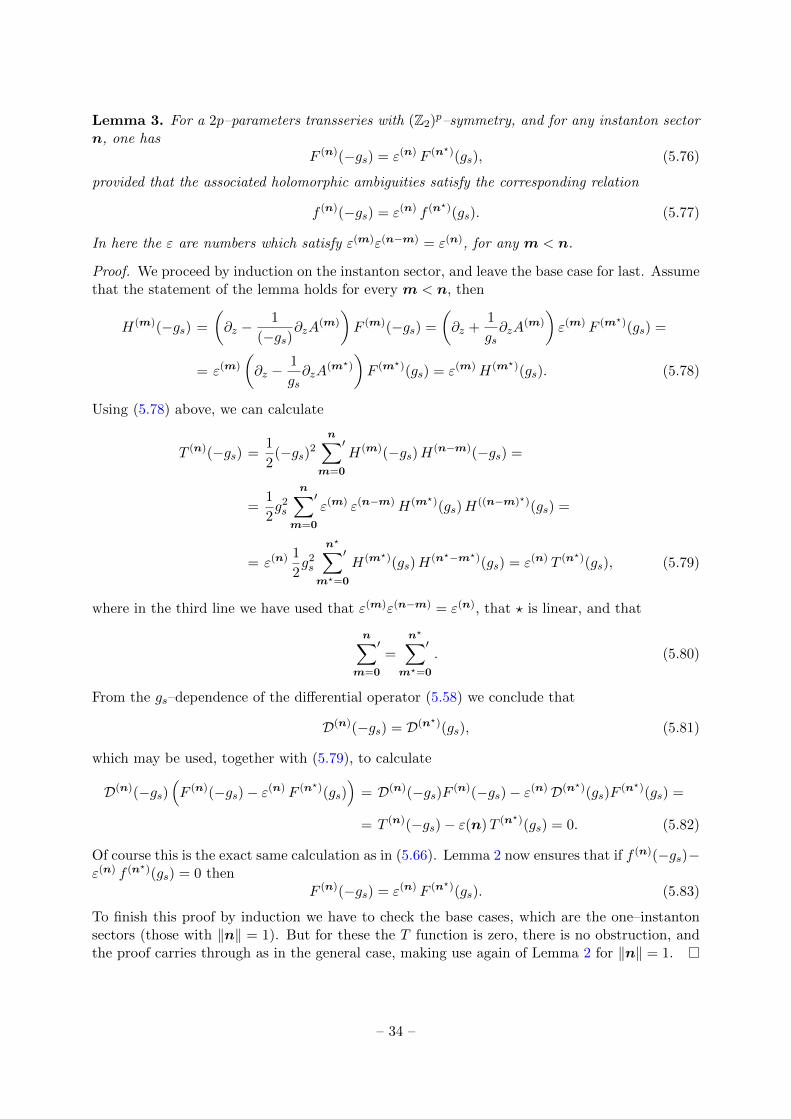
Lemma 3. For a 2p–parameters transseries with (Z2)p–symmetry, and for any instanton sectorn, one has
F (n)(−gs) = ε(n) F (n?)(gs), (5.76)
provided that the associated holomorphic ambiguities satisfy the corresponding relation
f (n)(−gs) = ε(n) f (n?)(gs). (5.77)
In here the ε are numbers which satisfy ε(m)ε(n−m) = ε(n), for any m < n.
Proof. We proceed by induction on the instanton sector, and leave the base case for last. Assumethat the statement of the lemma holds for every m < n, then
H(m)(−gs) =
(∂z −
1
(−gs)∂zA
(m)
)F (m)(−gs) =
(∂z +
1
gs∂zA
(m)
)ε(m) F (m?)(gs) =
= ε(m)
(∂z −
1
gs∂zA
(m?)
)F (m?)(gs) = ε(m)H(m?)(gs). (5.78)
Using (5.78) above, we can calculate
T (n)(−gs) =1
2(−gs)2
n∑′
m=0
H(m)(−gs)H(n−m)(−gs) =
=1
2g2s
n∑′
m=0
ε(m) ε(n−m)H(m?)(gs)H((n−m)?)(gs) =
= ε(n) 1
2g2s
n?∑′
m?=0
H(m?)(gs)H(n?−m?)(gs) = ε(n) T (n?)(gs), (5.79)
where in the third line we have used that ε(m)ε(n−m) = ε(n), that ? is linear, and that
n∑′
m=0
=
n?∑′
m?=0
. (5.80)
From the gs–dependence of the differential operator (5.58) we conclude that
D(n)(−gs) = D(n?)(gs), (5.81)
which may be used, together with (5.79), to calculate
D(n)(−gs)(F (n)(−gs)− ε(n) F (n?)(gs)
)= D(n)(−gs)F (n)(−gs)− ε(n)D(n?)(gs)F
(n?)(gs) =
= T (n)(−gs)− ε(n)T (n?)(gs) = 0. (5.82)
Of course this is the exact same calculation as in (5.66). Lemma 2 now ensures that if f (n)(−gs)−ε(n) f (n?)(gs) = 0 then
F (n)(−gs) = ε(n) F (n?)(gs). (5.83)
To finish this proof by induction we have to check the base cases, which are the one–instantonsectors (those with ‖n‖ = 1). But for these the T function is zero, there is no obstruction, andthe proof carries through as in the general case, making use again of Lemma 2 for ‖n‖ = 1.
– 34 –
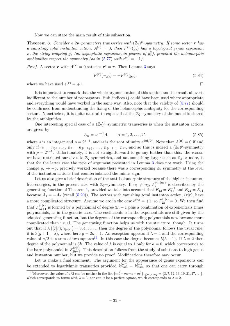
Now we can state the main result of this subsection.
Theorem 3. Consider a 2p–parameters transseries with (Z2)p–symmetry. If some sector r hasa vanishing total instanton action, A(r) = 0, then F (r)(gs) has a topological genus expansionin the string coupling gs (an asymptotic expansion in powers of g2
s), provided the holomorphicambiguities respect the symmetry (as in (5.77) with ε(r) = +1).
Proof. A sector r with A(r) = 0 satisfies r? = r. Then Lemma 3 says
F (r)(−gs) = +F (r)(gs), (5.84)
where we have used ε(r) = +1.
It is important to remark that the whole argumentation of this section and the result above isindifferent to the number of propagators. Sub–indices ij could have been used where appropriateand everything would have worked in the same way. Also, note that the validity of (5.77) shouldbe confirmed from understanding the fixing of the holomorphic ambiguity for the correspondingsectors. Nonetheless, it is quite natural to expect that the Z2–symmetry of the model is sharedby the ambiguities.
One interesting special case of a (Z2)p–symmetric transseries is when the instanton actionsare given by
Aα = ωα−1A, α = 1, 2, . . . , 2s, (5.85)
where s is an integer and p = 2s−1, and ω is the root of unity e2πi/2s . Note that A(n) = 0 if andonly if n1 = n2s−1+1, n2 = n2s−1+2, . . . , n2s−1 = n2s , and so this is indeed a (Z2)p–symmetrywith p = 2s−1. Unfortunately, it is not straightforward to go any further than this: the reasonwe have restricted ourselves to Z2 symmetries, and not something larger such as Z3 or more, isthat for the latter case the type of argument presented in Lemma 3 does not work. Using thechange gs → −gs precisely worked because there was a corresponding Z2 symmetry at the levelof the instanton actions that counterbalanced the minus sign.
Let us also give a brief description of the anti–holomorphic structure of the higher–instanton
free energies, in the present case with Z2–symmetry. If n1 6= n2, F(n1|n2)g is described by the
generating function of Theorem 1, provided we take into account that E12 = E−111 and E22 = E11
because A1 = −A2 (recall (5.20)). The sectors with vanishing total instanton action, (r|r), have
a more complicated structure. Assume we are in the case b(n) = +1, so F(r|r)2h = 0. We then find
that F(r|r)2h+1 is formed by a polynomial of degree 3h− 1 plus a combination of exponentials times
polynomials, as in the generic case. The coefficients a in the exponentials are still given by theadapted generating function, but the degrees of the corresponding polynomials now become morecomplicated than usual. The generating function helps us with the structure, though. It turnsout that if λ
((r|r); γ(r|r)
)= 3, 4, 5, . . ., then the degree of the polynomial follows the usual rule:
it is 3(g + 1− λ), where here g = 2h+ 1. An exception appears if λ = 4 and the correspondingvalue of a/2 is a sum of two squares15. In this case the degree becomes 5(h− 1). If λ = 2 thendegree of the polynomial is 5h. The value of λ is equal to 1 only for a = 0, which corresponds to
the bare polynomial in F(r|r)2h+1. This description follows from the study of solutions to high genus
and instanton number, but we provide no proof. Modifications therefore may occur.Let us make a final comment. The argument for the appearance of genus expansions can
be extended to logarithmic transseries provided k(n?)max = k
(n)max, so that one can carry through
15Moreover, the value of a/2 can be neither in the list m21−m1m2 +m2
21≤m1<m2 = 3, 7, 12, 13, 19, 21, 27, . . .,which corresponds to terms with λ = 3, nor can it be a perfect square, which corresponds to λ = 2.
– 35 –
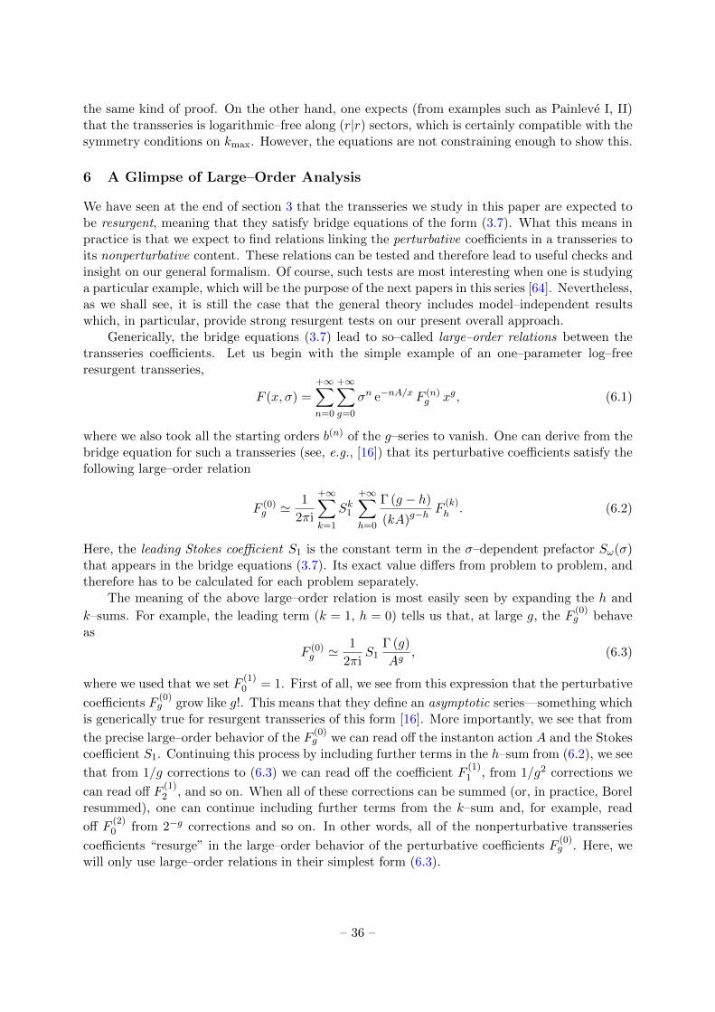
the same kind of proof. On the other hand, one expects (from examples such as Painleve I, II)that the transseries is logarithmic–free along (r|r) sectors, which is certainly compatible with thesymmetry conditions on kmax. However, the equations are not constraining enough to show this.
6 A Glimpse of Large–Order Analysis
We have seen at the end of section 3 that the transseries we study in this paper are expected tobe resurgent, meaning that they satisfy bridge equations of the form (3.7). What this means inpractice is that we expect to find relations linking the perturbative coefficients in a transseries toits nonperturbative content. These relations can be tested and therefore lead to useful checks andinsight on our general formalism. Of course, such tests are most interesting when one is studyinga particular example, which will be the purpose of the next papers in this series [64]. Nevertheless,as we shall see, it is still the case that the general theory includes model–independent resultswhich, in particular, provide strong resurgent tests on our present overall approach.
Generically, the bridge equations (3.7) lead to so–called large–order relations between thetransseries coefficients. Let us begin with the simple example of an one–parameter log–freeresurgent transseries,
F (x, σ) =
+∞∑n=0
+∞∑g=0
σn e−nA/x F (n)g xg, (6.1)
where we also took all the starting orders b(n) of the g–series to vanish. One can derive from thebridge equation for such a transseries (see, e.g., [16]) that its perturbative coefficients satisfy thefollowing large–order relation
F (0)g ' 1
2πi
+∞∑k=1
Sk1
+∞∑h=0
Γ (g − h)
(kA)g−hF
(k)h . (6.2)
Here, the leading Stokes coefficient S1 is the constant term in the σ–dependent prefactor Sω(σ)that appears in the bridge equations (3.7). Its exact value differs from problem to problem, andtherefore has to be calculated for each problem separately.
The meaning of the above large–order relation is most easily seen by expanding the h and
k–sums. For example, the leading term (k = 1, h = 0) tells us that, at large g, the F(0)g behave
as
F (0)g ' 1
2πiS1
Γ (g)
Ag, (6.3)
where we used that we set F(1)0 = 1. First of all, we see from this expression that the perturbative
coefficients F(0)g grow like g!. This means that they define an asymptotic series—something which
is generically true for resurgent transseries of this form [16]. More importantly, we see that from
the precise large–order behavior of the F(0)g we can read off the instanton action A and the Stokes
coefficient S1. Continuing this process by including further terms in the h–sum from (6.2), we see
that from 1/g corrections to (6.3) we can read off the coefficient F(1)1 , from 1/g2 corrections we
can read off F(1)2 , and so on. When all of these corrections can be summed (or, in practice, Borel
resummed), one can continue including further terms from the k–sum and, for example, read
off F(2)0 from 2−g corrections and so on. In other words, all of the nonperturbative transseries
coefficients “resurge” in the large–order behavior of the perturbative coefficients F(0)g . Here, we
will only use large–order relations in their simplest form (6.3).
– 36 –
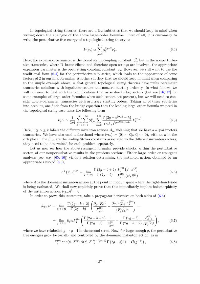
In topological string theories, there are a few subtleties that we should keep in mind whenwriting down the analogue of the above large–order formulae. First of all, it is customary towrite the perturbative free energy of a topological string theory as
F (gs) '+∞∑g=0
g2g−2s Fg. (6.4)
Here, the expansion parameter is the closed string coupling constant, g2s , but in the nonperturba-
tive transseries, where D–brane effects and therefore open strings are involved, the appropriateexpansion parameter is the open string coupling constant, gs. However, we still want to use thetraditional form (6.4) for the perturbative sub–series, which leads to the appearance of somefactors of 2 in our final formulae. Another subtlety that we should keep in mind when comparingto the simple example above, is that general topological string theories have multi–parametertransseries solutions with logarithm–sectors and nonzero starting orders g. In what follows, wewill not need to deal with the complications that arise due to log–sectors (but see [16, 17] forsome examples of large–order formulae when such sectors are present), but we will need to con-sider multi–parameter transseries with arbitrary starting orders. Taking all of these subtletiesinto account, one finds from the bridge equation that the leading large–order formula we need inthe topological string case takes the following form
F (0)g ' 1
2πi
κ∑α=1
+∞∑n=1
Sn1,α
+∞∑h=0
Γ(2g − b(nα) − h
)(nAα)2g−b(nα)−h
F(nα)h . (6.5)
Here, 1 ≤ α ≤ κ labels the different instanton actions Aα, meaning that we have a κ–parameterstransseries. We have also used a shorthand where (nα) := (0| · · · |0|n|0| · · · |0), with an n in theαth place. The S1,α are the leading Stokes constants associated to the different instanton sectors;they need to be determined for each problem separately.
Let us now see how the above resurgent formulae provide checks, within the perturbativesector, of our nonperturbative results in the previous sections. Either large–order or resurgentanalysis (see, e.g., [65, 16]) yields a relation determining the instanton action, obtained by anappropriate ratio of (6.3),
A2(zi, Sij
)= lim
g→+∞
Γ (2g − b+ 2)
Γ (2g − b)F
(0)g
(zi, Sij
)F
(0)g+1 (zi, Sij)
, (6.6)
where A is the dominant instanton action at the point in moduli space where the right–hand–sideis being evaluated. We shall now explicitly prove that this immediately implies holomorphicityof the instanton action; ∂SijA
2 = 0.In order to prove this statement, take a propagator derivative on both sides of (6.6)
∂SijA2 = lim
g→+∞
Γ (2g − b+ 2)
Γ (2g − b)
(∂SijF
(0)g
F(0)g+1
−∂SijF
(0)g+1 F
(0)g
(F(0)g+1)2
)=
= limg→+∞
∂SijF(0)g
(Γ (2g − b+ 2)
Γ (2g − b)1
F(0)g+1
− Γ (2g − b)Γ (2g − b− 2)
F(0)g−1
(F(0)g )2
), (6.7)
where we have relabelled g → g−1 in the second term. Now, for large enough g, the perturbativefree energies grow factorially and controlled by the dominant instanton action, as in
F (0)g ' c(zi, Sij)A(zi, Sij)−(2g−b) Γ (2g − b)
(1 +O(g−1)
), (6.8)
– 37 –
where c(zi, Sij) is a function independent of g. Let us first focus on the term in brackets in (6.7).
For large enough g we can calculate it to give
A2g−b
Γ (2g − b) c(1 +O(g−1)
)− A2g−b
Γ (2g − b) c(1 +O(g−1)
)=
A2g−b
Γ (2g − b)O(g−1), (6.9)
as the leading terms cancel each other out. Let us next turn to the factor of ∂SijF(0)g in (6.7).
The usual holomorphic anomaly equations allow us to express this in terms of z–derivatives,
∂SijF(0)g =
1
2
(∂i∂jF
(0)g−1 − Γkij ∂kF
(0)g−1 +
g−1∑h=1
∂iF(0)g−h ∂jF
(0)h
). (6.10)
In particular, the large–order behavior of the derivatives of the free energies are obtained from(6.8),
∂iF(0)h ∼ ∂ic
Γ (2h− b)A2h−b − c ∂iA
Γ (2h− b+ 1)
A2h−b+1, (6.11)
∂i∂jF(0)h ∼ ∂i∂jc
Γ (2h− b)A2h−b − (∂ic ∂jA+ ∂jc ∂iA+ c ∂i∂jA)
Γ (2h− b+ 1)
A2h−b+1+
+ c ∂iA∂jAΓ (2h− b+ 2)
A2h−b+2. (6.12)
It follows that, at large g,
∂i∂jF(0)g−1 ∼
Γ (2g − b)A2g−b
c ∂iA∂jA− (∂ic ∂jA+ ∂jc ∂iA+ c ∂i∂jA)A
Γ (2g − b− 1)
Γ (2g − b)+
+∂i∂jcA2 Γ (2g − b− 2)
Γ (2g − b)
=
=Γ (2g − b)A2g−b
O(g0) +O(g−1) +O(g−1)
, (6.13)
and
Γkij ∂kF(0)g−1 ∼
Γ (2g − b)A2g−b Γkij
−cA∂kA
Γ (2g − b− 1)
Γ (2g − b)+ ∂kcA
2 Γ (2g − b− 2)
Γ (2g − b)
=
=Γ (2g − b)A2g−b
O(g−1) +O(g−2)
. (6.14)
The quadratic term of the holomorphic anomaly equations is trickier because some factors arenot really large (for either small or large h). However, we can use an inequality that the freeenergies satisfy since they are asymptotic coefficients. In fact, in this case, there must be afunction c(zi, S
ij) such that, for every g,∣∣∣F (0)g
∣∣∣ ≤ c |A|−(2g−b) Γ (2g − b) . (6.15)
Therefore, one can evaluate the quadratic term as∣∣∣∣∣g−1∑h=1
∂iF(0)g−h ∂jF
(0)h
∣∣∣∣∣ ≤g−1∑h=1
∣∣∣∂iF (0)g−h
∣∣∣ ∣∣∣∂jF (0)h
∣∣∣ ≤
– 38 –
≤g−1∑h=1
(∂ic
Γ (2g − 2h− b)|A|2g−2h−b + c ∂i|A|
Γ (2g − 2h− b+ 1)
|A|2g−2h−b+1
)×
×
(∂j c
Γ (2h− b)|A|2h−b
+ c ∂j |A|Γ (2h− b+ 1)
|A|2h−b+1
). (6.16)
Next, we make use of the inequalities
Γ (2g − 2h+ p) Γ (2h+ p) ≤ Γ (2g + p− 2) Γ (p+ 2) , (6.17)
Γ (2g − 2h+ p) Γ (2h+ p+ 1) ≤ Γ (2h+ p− 1) Γ (p+ 2) , (6.18)
in order to find ∣∣∣∣∣g−1∑h=1
∂iF(0)g−h ∂jF
(0)h
∣∣∣∣∣ ≤ Γ (2g − b)|A|2g−b
O(g−1) +O(g0) +O(g0)
, (6.19)
where we have essentially done the same type of manipulations as before. Note that the sum inh has ∼ g terms which must also be taken into account. Now plugging (6.13), (6.14) and (6.19)into (6.7) we finally obtain ∣∣∂SijA2
∣∣ ≤ O (g−1), (6.20)
and as g goes to infinity we prove the holomorphicity of A.It is important to notice that in the above reasoning we have only used the perturbative
formulation of the holomorphic anomaly equations, (2.10), and nothing else besides completelygeneric large–order arguments. Yet, we have obtained a general result which precisely reproduceswhat we had computed earlier via the nonperturbative formulation of the holomorphic anomalyequations we discussed in section 2. In particular, this large–order test independently validatesour approach. As we mentioned earlier, this holomorphicity tells us that, in cases where thereis a known matrix model holographic dual, the instanton action keeps its usual geometric in-terpretation and may be directly computed as an adequate period of the corresponding spectralcurve [19, 38, 60]. Otherwise, strictly within the closed string theoretic approach, this has thenatural generalization of giving the instanton action a threefold geometric interpretation as acombination of holomorphic cycles in the Calabi–Yau geometry.
Having checked our nonperturbative result for the instanton action using a perturbativelarge–order analysis, let us move to the next–to–leading order and address the one–loop one–instanton sector. As we have shown in the previous sections, the anti–holomorphic dependence ofthe higher–instanton free energies is essentially independent of the particular model (geometry)we are dealing with. For the perturbative sector that structure was a polynomial of a certaindegree in the propagators (the coefficients of those polynomials are holomorphic functions thatdo depend on the model). A similar situation happens for the nonperturbative sectors, where wenow encounter not only polynomials but also exponentials in the propagators. The degrees andexponents are almost independent of the model (a mild dependence on the starting genus, recall(5.30)), but, again, the coefficients will be holomorphic and dependent on the model at hand.
This robust anti–holomorphic structure must be compatible with the large–order behavior ofthe perturbative free energies (6.5) and, in general, with the resurgence relations briefly mentionedat the beginning of this section. A detailed check of this has to be done for particular models.Here, as an example, consider the leading term in (6.5)
F (0)g ' S1
2πi
Γ(2g − b(1)
)A2g−b(1)
F(1)0 + · · · , (6.21)
– 39 –
where A is now the instanton action with the smallest absolute value at the point in modulispace we are evaluating our model, i.e., the dominant instanton action. By (1) we denote theassociated one–instanton sector (0| · · · |1| · · · |0). From (6.21) we can easily obtain
S1
2πiF
(1)0 = lim
g→+∞
A2g−b(1)
Γ(2g − b(1)
) F (0)g . (6.22)
Now comes the key point. On the left–hand–side we have an exponential in the propagator S,
since according to our earlier results F(1)0 is of the form
F(1)0 = e
12
(∂zA)2S f(1)0 (z), (6.23)
where f(1)0 is the corresponding holomorphic ambiguity. On the other hand, on the right–hand–
side we have a polynomial, albeit of increasing degree 3g − 3 as g → +∞. Of course that if ournonperturbative results are to be validated by resurgence, and in particular by the resurgence ofthe perturbative sector, the propagator structure of both sides has to match. If we denote
F (0)g =
3g−3∑k=0
pg,k(z)Sk, (6.24)
we must haveS1
2πif
(1)0 (z)
1
k!
(1
2(∂zA)2
)k= lim
g→+∞
A2g−b(1)
Γ(2g − b(1)
) pg,k(z). (6.25)
The left–hand–side of (6.25) is essentially the same for every k, since it arises from the exponential
dependence in S of F(1)0 , while on the right–hand–side one has the large–order values of every
coefficient in F(0)g , g 1. One could go on and include more terms in (6.21), in order to see
what the anti–holomorphic structure of the solutions imposes. More precisely, the left–hand–sideof (6.5) is a polynomial, it has finite degree in the propagators, while the right–hand–side is aninfinite sum involving every possible power of the propagators. This means, that there mustbe a cancellation of powers higher than 3g − 3. Checking this structure in its full generalityis beyond the scope of this paper. Nonetheless, an equivalent approach is to confirm it withinparticular examples and for specified numerical precision. We have done this in the context oflocal P2 around the conifold point and obtained a very precise numerical check of (6.25) [64],again validating our nonperturbative approach with purely perturbative data.
Finally, notice that since pg,0 = f(0)g , the perturbative holomorphic ambiguity, the k = 0
equation in (6.25) is
S1
2πif
(1)0 (z) = lim
g→+∞
A2g−b(1)
Γ(2g − b(1)
) f (0)g . (6.26)
This implies that f(1)0 , the first non–perturbative holomorphic ambiguity, can be fixed, up to
the Stokes constant S1, by the large–order relation above. This is just an example of what oneobtains from resurgent relations such as (6.5) when the propagators are set to zero. In fact, when
Sij = 0, F(n)g reduces to a combination of f
(n)g and all the previous ambiguities. In particular,
this means that the resurgence of the free energies, (6.5), induces a resurgence of the holomorphicambiguities, immediately implying that the fixing of the perturbative ambiguity is equivalent,via resurgence, to the fixing of all nonperturbative ambiguities. Note, however, that while this isin principle a correct strategy to fix all holomorphic ambiguities, in practice it requires a lot ofcomputation and becomes a bit cumbersome. In the next section we shall discuss another, morepractical, approach to fixing perturbative and nonperturbative holomorphic ambiguities.
– 40 –
7 Fixing the Holomorphic Ambiguities
So far we have understood in detail how the holomorphic anomaly equations fix the anti–holomorphic dependence of all (generalized) multi–instanton sectors and, thus, the full S de-pendence of its transseries solution. Akin to the perturbative case, one question remains: is itpossible, in each example, to further fix the holomorphic dependence and thus explicitly solvethe holomorphic anomaly equations? We shall now discuss, generically, how to fix the remainingholomorphic ambiguity—but one should further point out that only in concrete examples willthis fixing become fully explicit [64].
7.1 Fixing the Perturbative Ambiguity
To first set the stage let us review, following [35], how the perturbative holomorphic ambiguityis fixed for each genus, in the case of local Calabi–Yau geometries. For the sake of simplicity wewill assume that the complex moduli space is one–dimensional, but the results are general.
As discussed earlier, the perturbative free energies, F(0)g for g ≥ 2, are polynomials of degree
3g−3 in the propagator. The undetermined term in this polynomial is the holomorphic ambiguitythat appears after integration of the holomorphic anomaly equations, and this is what we need
to fix. Taking the holomorphic limit of the free energies, which we shall denote by F (0)g , one
finds regular functions on the complex moduli space except at a particular set of points at itsboundary. At those points the Calabi–Yau geometry acquires a node. For example, in the case ofgeometries which are fibrations of an elliptic curve, the so called local curves, the singular locusis given by the vanishing of the discriminant of the curve, ∆. Proceeding with this example, itis known that the singular locus, called the conifold divisor, corresponds in the A–model to aphase transition point in which the free energies can undergo a transition whose correspondingdouble–scaling limit is associated to some universality class. If tc is the flat coordinate around theconifold point, then one has the following behavior for the holomorphic limit of the free energiesnear tc = 0,
F (0)g
∣∣∣c
=cg−1B2g
2g (2g − 2) t2g−2c
+O(t0c), g ≥ 2, (7.1)
where c is a constant depending on the model and B2g are the Bernoulli numbers. This behavioris called the gap condition because there is only one singular term with a pole or order 2g − 2at the conifold point, and then a regular tail [34, 59, 66–70]. Having this in mind, consider the
expression for F(0)g integrated from the holomorphic anomaly equations,
F (0)g = C2g−2
3g−3∑k=1
pg,k(z)Sk + f (0)
g (z), (7.2)
where C = Czzz is the Yukawa coupling, pg,k(z) are (rational) functions of the complex modulus
z which depend on the particular model, and f(0)g (z) is the perturbative holomorphic ambiguity.
It is a general property that C ∼ ∆−1, and ∆ ∼ tc. Note that near the conifold point theYukawa coupling reproduces the singular behavior of the gap condition, (7.1), but not the correctcoefficient. To make things right one has to consider a holomorphic ambiguity of the form
f (0)g (z) =
pg,0(z)
∆2g−2. (7.3)
The function pg,0(z) is then determined by imposing that F (0)g is regular at every point in moduli
space—besides at the conifold point—in particular when z → 0 and z → ∞. Assuming for
– 41 –
simplicity that ∆ is linear in z, we find that pg,0(z) cannot have poles (this is regularity atz = 0, the large–radius point), and it can only grow with z as fast as ∆2g−2, in which casepg,0(z) is a polynomial in z. A counting argument then shows that all the coefficients of pg,0(z),except for one, can be fixed by the gap condition (7.1). The remaining coefficient is obtained byimposing the universal behavior of the free energies at the large–radius point, z = 0, which inthe A–model corresponds to the large volume limit. This is called the constant map contribution[34, 71, 67, 72, 68],
F (0)g
∣∣∣cm
=(−1)g χB2g−2B2g
4g (2g − 2) (2g − 2)!+O(z), g ≥ 2, (7.4)
where χ is the Euler characteristic of the Calabi–Yau manifold. This algorithm for fixing theambiguities, with its generalization to multi–dimensional moduli spaces, works for every genusand has been used to solve several topological string theories up to high genus in many examples.
The gap condition represents the phase transition singularity that the free energies undergowhen the model at hand is in the universality class of the c = 1 string at self–dual radius[59]. Models in different universality classes will have phase transitions with a different singularbehavior, controlled by a characteristic exponent γ, in the form
F (0)g ∼ Hg τ
(1−g)(2−γ), g ≥ 2, (7.5)
where τ is a proper coordinate around the phase transition point, and Hg are some particular(fixed) coefficients which play the counterpart of the Bernoulli numbers in (7.1). Usually, in“conventional” topological string theory, we have γ = 0 recovering (7.1). But for other classesγ can be different; e.g., for the class of c = 0 string theory, or pure 2d gravity, one has γ = −1
2[73]. In general these classes are in correspondence to minimal models which have central charge
cp,q = 1− 6 (p−q)2
pq and
γp,q = − 2
p+ q − 1, (7.6)
see [4] for a calculation in terms of multi–matrix models. Topological string theories in thesemore general classes have, however, been scarcely studied. One exception is [73] which address(equivariant) topological strings on the local curve Xp = O(p − 2) ⊕ O(−p) → P1, p ≥ 2,which are in fact in the c = 0 class. In this case it was found that the free energies have astructure somewhat similar to the one described above, in particular resembling the fixing ofthe holomorphic ambiguity. However, without “nice” coordinates around the phase transitionpoint, we cannot be sure a gap condition exists. It would be extremely interesting to studytopological string theory in more general universality classes and find out how more generalboundary conditions fix the holomorphic ambiguities.
7.2 Fixing Holomorphic Ambiguities at the Conifold
The phase transition behavior is a universal property of the given topological string theory class.In this sense, making use of the resurgent equations that relate the large–order behavior of theperturbative free energies to the higher instanton sectors [16], one should be able to concludesomething about those higher instanton free energies near the phase transition point. It turnsout that this is the case under some circumstances and for certain instanton sectors.
Let us be more concrete by considering a model that lies in the universality class of c = 1string theory, and assume that there is only one complex modulus. Near the conifold point,
– 42 –
tc = 0, the holomorphic limit of the perturbative free energies satisfies the gap condition (7.1),which we now write in the form
F (0)g
∣∣∣c
=cg−1B2g
2g (2g − 2) t2g−2c
+ ag + bg tc + · · · , (7.7)
where ag, bg, . . . are numbers that depend on the particular model we are working with. Near
this phase transition point we expect the large–order behavior of the F (0)g to be controlled by an
instanton action proportional to tc [38], which is actually a period and vanishes at the conifoldpoint. Indeed, as we have seen before from large–order behavior in section 6, one can extract thedominant instanton action via
A2 = limg→∞
4g2 F(0)g
F (0)g+1
= limg→+∞
4g2 Gg t2−2gc + ag + bg tc + · · ·
Gg+1 t2−2(g+1)c + ag+1 + bg+1 tc + · · ·
=
= limg→+∞
4g2
(GgGg+1
t2c +agGg+1
t2gc +bgGg+1
t2g+1c + · · ·
), (7.8)
where Gg ≡ cg−1B2g
2g(2g−2) . Note that the first term is of order t2c and then we have a tail starting at t2gc .When we take g to infinity that tail will disappear leaving a result which is model independent(but still depending on the universality class). Now, since for large g one has
B2g = (−1)g−1 2(2g)!
(2π)2g
(1 +
1
22g+ · · ·
), (7.9)
one immediately finds
A2c = −4π2
ct2c . (7.10)
So that indeed Ac ∝ tc and it vanishes at the conifold point. As we shall see in the following,this type of large–order argument in which the model dependence, encoded in the constantsag, bg, . . ., goes away in the large g limit, may be applied to extract the universal behavior ofthe higher–instanton free energies, associated to that instanton action (in the holomorphic limit).
As we discussed in section 6, the leading large–order behavior of F (0)g is given by
F (0)g '
+∞∑k=1
Sk12πi
+∞∑h=0
Γ(2g − b(k) − h
)(kAc)
2g−b(k)−hF (k)h + · · · . (7.11)
Here S1 is the Stokes constant associated to the specific model, (k) refers to the instanton sector(0| · · · |k| · · · |0) associated to the conifold instanton action Ac, given by (7.10), b(k) is the startingorder, and the dots at the end stand for contributions from other (multi) instanton sectorsincluding mixed/generalized sectors. These contributions are necessarily subleading as, aroundthe conifold point, Ac has the smallest absolute value being zero at the phase transition point.
We have already seen how to calculate Ac from the large–order limit of the perturbative freeenergies. In the same spirit we may now calculate b(1),
b(1) = limg→+∞
2g
(1− A2
c
4g2
F (0)g+1
F (0)g
)= lim
g→+∞2g
(1− A2
c
4g2
Gg+1 t2−2(g+1)c + ag+1 + · · ·
Gg t2−2gc + ag + · · ·
)=
– 43 –
= limg→+∞
2g
(1−−4π2
c t2c4g2
(Gg+1
Gg
1
t2c− ag Gg+1
G2g
tg+1c + · · ·
))=
= limg→+∞
4g2 + 2(1 + g − 2g2
)2g
= 1, (7.12)
where, again, the model–dependent data is removed as g goes to infinity. The next step is to
calculate F (1)h , h = 0, 1, 2, . . .. One finds
S1
2πiF (1)
0 = limg→+∞
A2g−b(1)
c
Γ(2g − b(1)
) F (0)g =
= limg→+∞
tci (2g − 1)
2π√c (g − 1)
=i
π√ctc =
1
2π2Ac. (7.13)
Next,
S1
2πiF (1)
1 = limg→+∞
A2g−2c
Γ (2g − 2)
(F (0)g −
Γ (2g − 1)
A2g−1c
S1
2πiF (1)
0
)=
= limg→+∞
(2g − 1
2π2− 2g − 2
2π2
)=
1
2π2. (7.14)
The next free energy is different,
S1
2πiF (1)
2 = limg→+∞
πA2g−3c
Γ (2g − 3)
(F (0)g −
Γ (2g − 1)
πA2g−1c
S1
2πiF (1)
0 − Γ (2g − 2)
πA2g−2c
S1
2πiF (1)
1
)=
= limg→+∞
√c
4π3i tc
1
Γ (2g − 3)
(Γ (2g)
2 (g − 1)− Γ (2g − 1)− Γ (2g − 2)
)= 0, (7.15)
since the term in brackets is identically zero. By induction one proves that F (1)h = 0 for h ≥ 2.
One could now go to the next instanton sector, n = 2, and keep calculating. For thatwe would have to use (7.9) including the term 2−2g. Proceeding in this way we find the sameindependence on the data associated to the specific model; as above all model–dependent datadrops out after taking g to infinity. Doing the same type of calculations, but taking into accountthe new factor of 2 from (7.9), we obtain results which are very similar to the one–instantonsector. Going further we can actually calculate the holomorphic limit of the full n–instantonsector as
b(n) = 1, (7.16)
Sn12πiF (n)
0 =1
n
i
π√ctc, (7.17)
Sn12πiF (n)
1 =1
n2
1
2π2, (7.18)
F (n)g≥2 = 0. (7.19)
What we have found, based on a large–order analysis of the perturbative free energies, is that,in the holomorphic limit, the higher–instanton free energies associated to the conifold instanton
– 44 –
action are universal, in the sense that they only depend on the universality class of the c = 1 stringand the Stokes constant. It is thus no surprise that the above results turn out to be essentiallythe same as the ones obtained in [38]. What is important to notice is that this procedure
provides a rather general method for fixing the nonperturbative holomorphic ambiguity, f(n)g ,
of all these sectors (and up to the Stokes constant): simply grab the solution F(n)g obtained
from the holomorphic anomaly equations, take its holomorphic limit, equate the result with the
appropriate equation of the ones above, and solve for f(n)g .
In retrospect, notice that having found that b(n) = +1 for each n was the reason why wefocused on that case when obtaining the holomorphic anomaly equations and the structure ofthe solution in section 4. Further, it is important to remark that the coordinate tc, which can becalculated from the Picard–Fuchs equations and has the interpretation of a period, is completelydependent on the model we are trying to solve. In that way, the results above are universal inform but the actual expressions do depend on the model.
7.3 Fixing Ambiguities beyond Conifold Points
If the model we are trying to solve lies in an universality class other than c = 1, one might expectto be able to do a similar calculation as above. In that case, if we had a gap condition, we wouldhave
F (0)g = Hg τ
(1−g)(2−γ) + ag + bg τ + · · · , (7.20)
where the coefficients Hg should grow factorially in order to identify the usual dominant instantonaction, and τ is the appropriate coordinate around the phase transition point (which should alsohave a period interpretation, otherwise the gap condition becomes trivial). However, in orderto be as thorough as for the conifold case, we would first need to know the exact form of Hg.For the c = 1 class, the coefficients Gg arise from the Gaussian matrix model which appears asthe double–scaling limit at the phase transition point. For other classes one will have to addressthe double–scaling limit of the model, which naturally depends on the universality class. Thesedouble–scaling limits lie in hierarchies, such as the KdV hierarchy [74], but in full generality itis a complicated problem by itself to identify what the numbers Hg are, and how they behavefor large g, in analogy to (7.9). Without this information it is impossible to carry on the typeof calculation we did in the previous subsection 7.2. Another issue which also needs to be takeninto account is the following. While it might be conceivable that topological string theories in thec = 1 class will not show resonance or logarithmic sectors, a detailed study of the double–scalinglimit of 2d gravity, described by the Painleve I equation, [15, 16], or of 2d supergravity, describedby the Painleve II equation, [17], indicates that other classes will have them. Consequently,large–order expressions such as (7.11) would need careful revision along the lines of [16, 17].
It would also be interesting to address the aforementioned problem of more general phasetransition points from a purely geometric point–of–view, and for example classify the universaltypes of large–order behavior of the perturbative series starting only from a classification ofgeometric Calabi–Yau threefold singularities. Unfortunately, while such a classification is knownfor K3 surfaces (i.e., Calabi–Yau twofolds), not only is it not known in the three–dimensional case,but it is actually believed that such singularities are not classifiable [75]. As a result, it seems tobe quite difficult to prove in full generality that one can always find enough boundary conditionsto completely solve the holomorphic anomaly equations, beyond the c = 1 case. Nevertheless, inpractical examples [64], we find that at least in the c = 1 cases the available boundary conditionsare indeed sufficient to make the problem completely integrable.
– 45 –
8 Conclusions and Outlook
In this work, by making use of resurgent analysis and transseries solutions, we have shown thatthe holomorphic anomaly equations are completely integrable at the nonperturbative level. Inparticular, we have suggested a prescription to solve, at full nonperturbative level, any closedtopological string theory within the local Calabi–Yau B–model setting. Of course the next naturalquestion is to ask how our methods apply in practice to specific examples, not only at the levelof the explicit construction of the transseries solutions but also performing strong checks on thissolution by using resurgent analysis as in [16, 17], finding Stokes constants and so on. We haveapplied our methods to two natural Calabi–Yau examples, local P2 and local P1 × P1, and wewill report on these complete results some time soon [64].
For several reasons, the aforementioned examples are the first natural testing grounds forour general procedure. Recall that one of the simplest examples, precisely the conifold, wasaddressed at the nonperturbative level in [38] (alongside the resolved conifold). In that paper itwas suggested that the techniques used therein, mainly dealing with Borel analysis16, should beapplicable to topological strings in any Calabi–Yau geometry with a finite number of non–zeroGopakumar–Vafa invariants. On the other hand, it was clear that the methods in [38] wouldnot work for threefolds with an infinite number of non–zero Gopakumar–Vafa invariants and itwas already suggested in that reference that one should devise a new approach to tackle localP2; possibly the simplest background to address in this class. The approach in the presentpaper precisely answers what the correct approach is, and in fact shows how general transseriesmethods are as they are essentially applicable to every possible geometry. In the examples oflocal P2 and local P1×P1 [64] we find many new features as compared to the case of the conifold[38]. For example, the mirror curves have genus one and modularity plays an important role. Inparticular, one may now understand when the instanton action is dictated by A–cycle instantons(much like the conifold was [38]) and when is it dictated by B–cycle instantons along the linesof [19]. Generically, there will be several competing instanton actions in the game much alongthe lines of [60] and the resurgent analysis of these models is extremely rich and interesting [64].Another point to explore is what is the proper role of the generating functions which were socentral in our present construction. There is an open possibility that these generating functionsactually turn into “real” functions within specific examples, providing a resummation of thefull nonperturbative solution. Whether this is possible and whether this would relate to thetheta–function resummations in [76, 77, 37] is an extremely interesting route of future research.
Moreover, the issue of modularity is by itself worth further investigation. For example, itwould be very interesting to extend the results in [78, 79] and understand the general modularproperties of the many multi–instanton components of the transseries solutions. At the same time,the question of modularity relates to that of holomorphicity as addressed in [37]. Recall thatwhen working on the gauge theory side, and computing the matrix model partition function, onestarts off with a holomorphic object to which nonperturbative contributions further turn modular[37]. It is thus very natural to ask what happens in the present closed string picture. Of coursethat choosing a background entails breaking holomorphicity (while maintaining modularity) [34],but could it be that the full set of transseries multi–instanton nonperturbative corrections stillconspire in order to recover a holomorphic partition function as the final result? We believe theseare very interesting questions for future research.
As one thinks about possible applications of our methods, many ideas quickly come to mind.For example, we have worked on the B–model side and it would be very interesting to investigate
16The relation to resurgent methods was later pointed out in [16].
– 46 –

what would be the mirror analogue of our results, on the A–model. It is conceivable that thiswould relate to the topological vertex approach in [81, 80]. Still concerning the B–model side, theextension of the matrix model large N duality in [23] from planar level to arbitrary (perturbative)genus, following [33], entailed a rather complete parallel between the closed string holomorphicanomaly equations and the matrix model topological recursion [28, 82]. In this way, our presentconstruction seems to be pointing in the direction that there should also be a nonperturbativeversion of the topological recursion, this time around based on resurgent transseries solutionsand on our general equation (4.22) (and its multi–parameter/multi–dimensional generalizations).Finally, it would be very interesting to extend our results to the compact Calabi–Yau case,perhaps along the lines of [52, 53].
Acknowledgments
We would like to thank Marcos Marino for most insightful comments. RCS would like to thankJose Manuel Queiruga for useful discussions. RCS would like to thank the Institute for Theo-retical Physics at the University of Amsterdam and the Department of Mathematics of InstitutoSuperior Tecnico, for their hospitality while this paper was being written. RS would like tothank the Department of Physics of the University of Geneva and CERN–TH Division for hos-pitality. RCS was supported by a Spanish FPU fellowship. RCS and JDE are supported in partby MICINN and FEDER (grant FPA2011–22594), Xunta de Galicia (Consellerıa de Educacionand grant PGIDIT10PXIB206075PR), and the Spanish Consolider–Ingenio 2010 ProgrammeCPAN (CSD2007–00042). The research of RS was partially supported by the European ScienceFoundation Grant HoloGrav–4076 and by FCT–Portugal grants PTDC/MAT/119689/2010 andEXCL/MAT-GEO/0222/2012. The research of MV was partially supported by the EuropeanResearch Council Advanced Grant EMERGRAV. The Centro de Estudios Cientıficos (CECs) isfunded by the Chilean Government through the Centers of Excellence Base Financing Programof Conicyt.
– 47 –

A Multi–Dimensional Complex Moduli Space
In the main body of the paper we have restricted ourselves to the case where the complexmoduli space of our Calabi–Yau manifold is one–dimensional. A similar analysis of the equations(and solutions) can be carried out in the completely general case where the moduli space hasarbitrary dimension h2,1. We find that no new ingredients are required in this generalizationwhich we shall present in the following, as we will make explicit (but schematic) the derivationof the equations for the higher–instanton free energies, assuming a general transseries ansatz andincluding logarithmic sectors. Recall that indices i, j run from 1 to h2,1.
We start off with the holomorphic anomaly equation
∂F
∂Sij+
1
2(Ui DjF + Uj DiF )− 1
2g2s (DiDjF +DiF DjF ) = g−2
s Wij + Vij , (A.1)
and the usual transseries ansatz
F =∑n∈Nκ0
σn e−A(n)/gs
k(n)max∑k=0
logk (gs) F(n)[k](gs). (A.2)
Next, one first calculates the covariant derivatives and the quadratic terms,
DjF =∑n
σn e−A(n)/gs
k(n)max∑k=0
logk (gs)
(∂j −
1
gs∂jA
(n)
)F (n)[k], (A.3)
DiDjF =∑n
σn e−A(n)/gs
k(n)max∑k=0
logk (gs)×
×(
∂i −1
gs∂iA
(n)
)(∂j −
1
gs∂jA
(n)
)− Γkij
(∂k −
1
gs∂kA
(n)
)F (n)[k], (A.4)
DiF DjF =∑n
σn e−A(n)/gs
n∑m=0
k(m)max+k
(n−m)max∑
k=0
logk (gs)× (A.5)
×min
(k,k
(m)max
)∑`=max
(0,k−k(n−m)
max
)(∂i −
1
gs∂iA
(m)
)F (m)[`]
(∂j −
1
gs∂jA
(n−m)
)F (n−m)[k−`].
In the last equation we have used A(m) + A(n−m) = A(n) in the exponential term. Using theseexplicit expressions, the holomorphic anomaly equation (A.1) reads
∑n
σn e−A(n)/gs
k
(n)max∑k=0
logk (gs)
[(∂Sij −
1
gs∂SijA
(n)
)F (n)[k]+
+1
2Ui
(∂j −
1
gs∂jA
(n)
)F (n)[k] +
1
2Uj
(∂i −
1
gs∂iA
(n)
)F (n)[k] −
−1
2g2s
((∂i −
1
gs∂iA
(n)
)(∂j −
1
gs∂jA
(n)
)− Γkij
(∂k −
1
gs∂kA
(n)
))F (n)[k]
]−
– 48 –
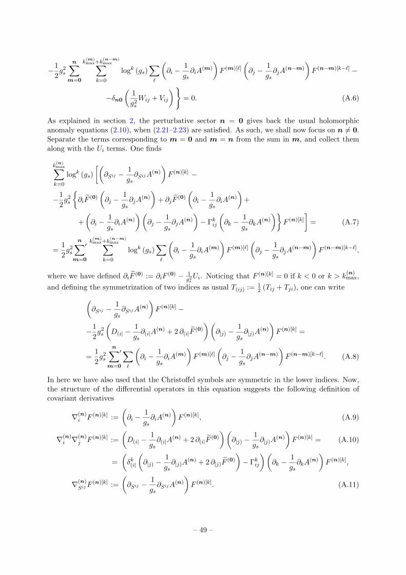
−1
2g2s
n∑m=0
k(m)max+k
(n−m)max∑
k=0
logk (gs)∑`
(∂i −
1
gs∂iA
(m)
)F (m)[`]
(∂j −
1
gs∂jA
(n−m)
)F (n−m)[k−`] −
−δn0
(1
g2s
Wij + Vij
)= 0. (A.6)
As explained in section 2, the perturbative sector n = 0 gives back the usual holomorphicanomaly equations (2.10), when (2.21–2.23) are satisfied. As such, we shall now focus on n 6= 0.Separate the terms corresponding to m = 0 and m = n from the sum in m, and collect themalong with the Ui terms. One finds
k(n)max∑k=0
logk (gs)
[(∂Sij −
1
gs∂SijA
(n)
)F (n)[k] −
−1
2g2s
∂iF
(0)
(∂j −
1
gs∂jA
(n)
)+ ∂jF
(0)
(∂i −
1
gs∂iA
(n)
)+
+
(∂i −
1
gs∂iA
(n)
)(∂j −
1
gs∂jA
(n)
)− Γkij
(∂k −
1
gs∂kA
(n)
)F (n)[k]
]= (A.7)
=1
2g2s
n∑′
m=0
k(m)max+k
(n−m)max∑
k=0
logk (gs)∑`
(∂i −
1
gs∂iA
(m)
)F (m)[`]
(∂j −
1
gs∂jA
(n−m)
)F (n−m)[k−`],
where we have defined ∂iF(0) := ∂iF
(0) − 1g2sUi. Noticing that F (n)[k] = 0 if k < 0 or k > k
(n)max,
and defining the symmetrization of two indices as usual T(ij) := 12 (Tij + Tji), one can write(
∂Sij −1
gs∂SijA
(n)
)F (n)[k] −
−1
2g2s
(D(i| −
1
gs∂(i|A
(n) + 2 ∂(i|F(0)
)(∂|j) −
1
gs∂|j)A
(n)
)F (n)[k] =
=1
2g2s
n∑′
m=0
∑`
(∂i −
1
gs∂iA
(m)
)F (m)[`]
(∂j −
1
gs∂jA
(n−m)
)F (n−m)[k−`]. (A.8)
In here we have also used that the Christoffel symbols are symmetric in the lower indices. Now,the structure of the differential operators in this equation suggests the following definition ofcovariant derivatives
∇(n)i F (n)[k] :=
(∂i −
1
gs∂iA
(n)
)F (n)[k], (A.9)
∇(n)i ∇
(n)j F (n)[k] :=
(D(i| −
1
gs∂(i|A
(n) + 2 ∂(i|F(0)
)(∂|j) −
1
gs∂|j)A
(n)
)F (n)[k] = (A.10)
=
(δk(i|
(∂|j) −
1
gs∂|j)A
(n) + 2 ∂|j)F(0)
)− Γkij
)(∂k −
1
gs∂kA
(n)
)F (n)[k],
∇(n)
SijF (n)[k] :=
(∂Sij −
1
gs∂SijA
(n)
)F (n)[k]. (A.11)
– 49 –
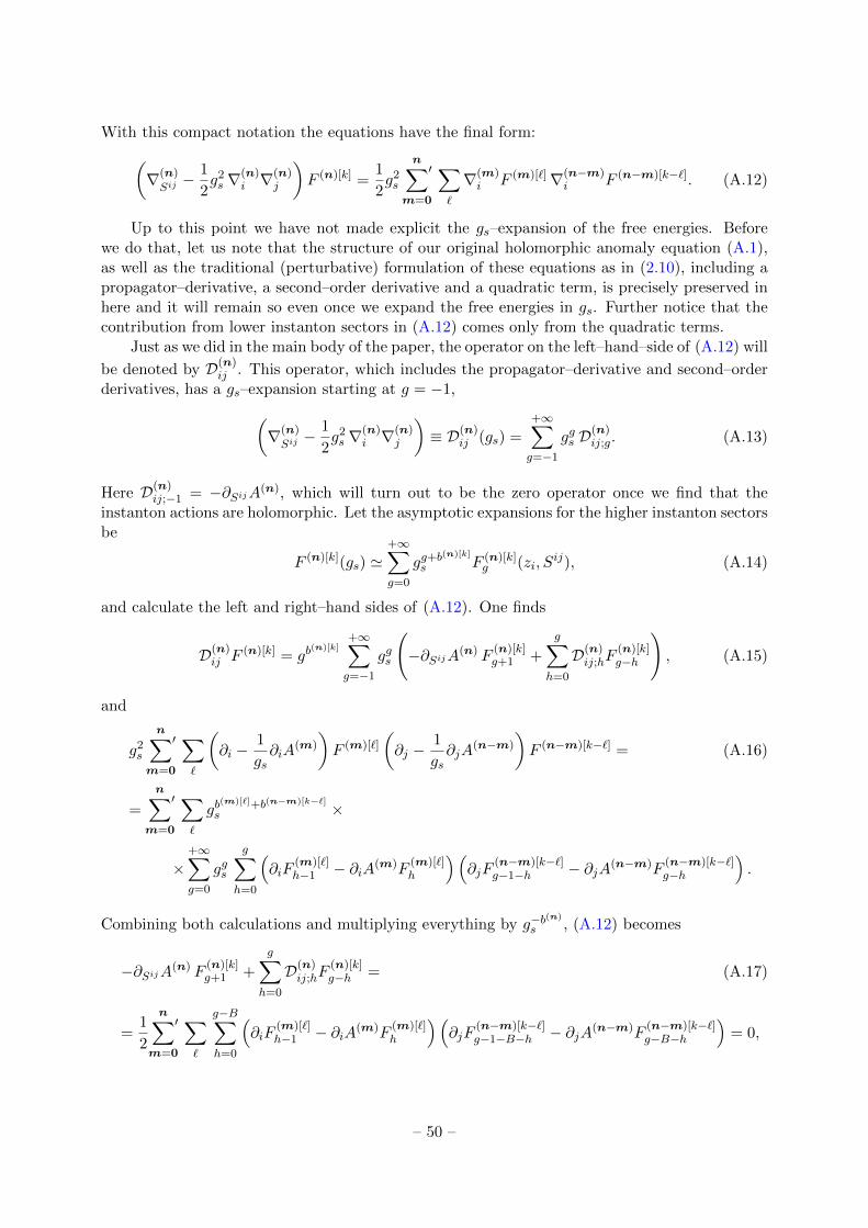
With this compact notation the equations have the final form:(∇(n)
Sij− 1
2g2s ∇
(n)i ∇
(n)j
)F (n)[k] =
1
2g2s
n∑′
m=0
∑`
∇(m)i F (m)[`]∇(n−m)
i F (n−m)[k−`]. (A.12)
Up to this point we have not made explicit the gs–expansion of the free energies. Beforewe do that, let us note that the structure of our original holomorphic anomaly equation (A.1),as well as the traditional (perturbative) formulation of these equations as in (2.10), including apropagator–derivative, a second–order derivative and a quadratic term, is precisely preserved inhere and it will remain so even once we expand the free energies in gs. Further notice that thecontribution from lower instanton sectors in (A.12) comes only from the quadratic terms.
Just as we did in the main body of the paper, the operator on the left–hand–side of (A.12) will
be denoted by D(n)ij . This operator, which includes the propagator–derivative and second–order
derivatives, has a gs–expansion starting at g = −1,(∇(n)
Sij− 1
2g2s ∇
(n)i ∇
(n)j
)≡ D(n)
ij (gs) =+∞∑g=−1
ggs D(n)ij;g. (A.13)
Here D(n)ij;−1 = −∂SijA(n), which will turn out to be the zero operator once we find that the
instanton actions are holomorphic. Let the asymptotic expansions for the higher instanton sectorsbe
F (n)[k](gs) '+∞∑g=0
gg+b(n)[k]
s F (n)[k]g (zi, S
ij), (A.14)
and calculate the left and right–hand sides of (A.12). One finds
D(n)ij F (n)[k] = gb
(n)[k]+∞∑g=−1
ggs
(−∂SijA(n) F
(n)[k]g+1 +
g∑h=0
D(n)ij;hF
(n)[k]g−h
), (A.15)
and
g2s
n∑′
m=0
∑`
(∂i −
1
gs∂iA
(m)
)F (m)[`]
(∂j −
1
gs∂jA
(n−m)
)F (n−m)[k−`] = (A.16)
=
n∑′
m=0
∑`
gb(m)[`]+b(n−m)[k−`]s ×
×+∞∑g=0
ggs
g∑h=0
(∂iF
(m)[`]h−1 − ∂iA(m)F
(m)[`]h
)(∂jF
(n−m)[k−`]g−1−h − ∂jA(n−m)F
(n−m)[k−`]g−h
).
Combining both calculations and multiplying everything by g−b(n)
s , (A.12) becomes
−∂SijA(n) F(n)[k]g+1 +
g∑h=0
D(n)ij;hF
(n)[k]g−h = (A.17)
=1
2
n∑′
m=0
∑`
g−B∑h=0
(∂iF
(m)[`]h−1 − ∂iA(m)F
(m)[`]h
)(∂jF
(n−m)[k−`]g−1−B−h − ∂jA(n−m)F
(n−m)[k−`]g−B−h
)= 0,
– 50 –

for g = −1, 0, 1, 2, . . ., k = 0, 1, 2, . . . , 1 ≤ i ≤ j ≤ h2,1, and n 6= 0. Here B stands forB(n,m)[k, `] := b(m)[`] + b(n−m)[k−`] − b(n)[k]. One has:
D(n)ij;0 = ∂Sij −
1
2∂iA
(n)∂jA(n), (A.18)
D(n)ij;1 =
1
2DiDjA
(n) + ∂(i|A(n)(D|j) + ∂|j)F
(0)1
), (A.19)
D(n)ij;2 = −1
2DiDj − ∂(i|F
(0)1 D|j), (A.20)
D(n)ij;2h−1 = ∂(i|F
(0)h ∂|j)A
(n), h = 2, 3, . . . , (A.21)
D(n)ij;2h = −∂(i|F
(0)h D|j), h = 2, 3, . . . . (A.22)
Going back to (A.17), let us consider the equation for n = (0| · · · |1| · · · |0) (an one–instantonsector), k = 0, and g = −1. The second and third terms are zero and one immediately obtains
∂SijA(0|···|1|···|0) F
(0|···|1|···|0)[0]0 = 0. (A.23)
Since by construction F(0|···|1|···|0)[0]0 6= 0, we find the by now familiar result that the instan-
ton actions are all holomorphic. With this important piece of information the nonperturbativeholomorphic anomaly equations finally read (here we separate the D0 term)(
∂Sij −1
2∂iA
(n)∂jA(n)
)F (n)[k]g = −
g∑h=1
D(n)ij;hF
(n)[k]g−h + (A.24)
+1
2
n∑′
m=0
∑`
g−B∑h=0
(∂iF
(m)[`]h−1 − ∂iA(m)F
(m)[`]h
)(∂jF
(n−m)[k−`]g−1−B−h − ∂jA(n−m)F
(n−m)[k−`]g−B−h
).
Let us make a few remarks concerning this result. First notice the familiar structure whichincludes a propagator–derivative (now enlarged with the instanton action) equated to a second–order derivative (to be found inside D2) added with quadratic terms. Further, the equations arerecursive in the instanton sector n, the logarithmic power k, and the genus g. However, becauseof the functions B and kmax, it may be the case that for some equations the left–hand–side of(A.24) is zero while the right–hand–side is not. This does not break the recursiveness of theequations but introduces some extra constraints that need to be satisfied in the particular modelunder study (see the discussion at the end of subsection 5.3). In the case in which we haveno constraints and the instanton actions are generic (i.e., they are not constant nor linearlydependent over the integers) we can prove that the structure of the free energies obtained assolutions from (A.24) is given by the following theorem.
Theorem 4. For any n 6= 0, k ∈ 0, . . . , k(n)max, and g ≥ 0, the structure of the nonperturbative
free energies has the form
F (n)[k]g =
∑γn
e12
∑κα,β=1 aαβ(n;γn)
∑h2,1
i,j=1 ∂iAα ∂jAβ Sij
Pol(Sij ; 3
(g + b(n)[k] − λ[k]
b,kmax(n; γn)
)),
(A.25)
– 51 –
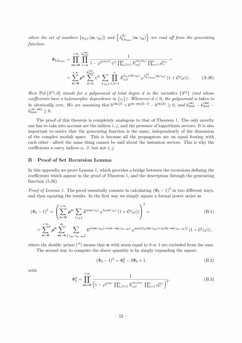
where the set of numbers aαβ (n; γn) andλ
[k]b,kmax
(n; γn)
are read off from the generating
function
Φb,kmax =
+∞∏′
m=0
k(m)max∏`=0
1
1− ϕb(m)[`]ψ`∏κα,β=1E
mαmβαβ
∏κα=1 ρ
mαα
=
=
+∞∑n=0
ρnk
(n)max∑k=0
ψk∑γn
κ∏α,β=1
Eaαβ(n;γn)αβ ϕλ
[k]b,kmax
(n;γn) (1 +O (ϕ)) . (A.26)
Here Pol(Sij ; d
)stands for a polynomial of total degree d in the variables Sij (and whose
coefficients have a holomorphic dependence in zi). Whenever d < 0, the polynomial is taken to
be identically zero. We are assuming that b(m)[`] + b(n−m)[k−`] − b(n)[k] ≥ 0, and k(n)max − k(m)
max −k
(n−m)max ≥ 0.
The proof of this theorem is completely analogous to that of Theorem 1. The only noveltyone has to take into account are the indices i, j, and the presence of logarithmic sectors. It is alsoimportant to notice that the generating function is the same, independently of the dimensionof the complex moduli space. This is because all the propagators are on equal footing witheach other—albeit the same thing cannot be said about the instanton sectors. This is why thecoefficients a carry indices α, β, but not i, j.
B Proof of Set Recursion Lemma
In this appendix we prove Lemma 1, which provides a bridge between the recursions defining thecoefficients which appear in the proof of Theorem 1, and the description through the generatingfunction (5.26).
Proof of Lemma 1. The proof essentially consists in calculating (Φb − 1)2 in two different ways,and then equating the results. In the first way we simply square a formal power series as
(Φb − 1)2 =
+∞∑′
n=0
ρn∑γn
Ea(n;γn) ϕλb(n;γn) (1 +O (ϕ))
2
= (B.1)
=
+∞∑′′
n=0
ρnn∑′
m=0
∑γm,γn−m
Ea(m;γm)+a(n−m;γn−m) ϕminλb(m;γm)+λb(n−m;γn−m) (1 +O (ϕ)) ,
where the double–prime ( ′′) means that n with norm equal to 0 or 1 are excluded from the sum.The second way to compute the above quantity is by simply expanding the square
(Φb − 1)2 = Φ2b − 2Φb + 1, (B.2)
with
Φ2b =
+∞∏′
m=0
1(1− ϕb(m) ∏κ
α,β=1Emαmβαβ
∏κα=1 ρ
mαα
)2 . (B.3)
– 52 –
After using the formal expansion (1 − x)−2 = 1 + 2x + 3x2 + 4x3 + · · · and some familiarmanipulations from our earlier analysis in the main body of the text, one obtains
Φ2b =
+∞∑n=0
ρn∑γn
Ea(n;γn)∑
rm∈γn
ϕ∑+∞
m=0 rm b(m)+∞∏m=0
(rm + 1) . (B.4)
Now, since (B.1) does note have any terms with ‖n‖ = 0, 1 we should check that (B.2) does nothave them either. Let us do this explicitly. For ‖n‖ = 0 one finds
Φ2b
∣∣‖n‖=0
= 1, Φb|‖n‖=0 = 1 ⇒ (Φb − 1)2∣∣∣‖n‖=0
= 1− 2 · 1 + 1 = 0. (B.5)
For ‖n‖ = 1 note that there is only one class (γn) and we thus find
Φ2b
∣∣‖n‖=1
=
κ∑α=1
ραEαα ϕb(n)
(1 + 1) , Φb|‖n‖=1 =
κ∑α=1
ραEαα ϕb(n) ⇒ (Φb − 1)2
∣∣∣‖n‖=1
= 0.
(B.6)In this way, we have obtained a second way of writing (Φ− 1)2, as
+∞∑′′
n=0
ρn∑γn
Ea(n;γn)∑
rm∈γn
ϕ∑+∞
m=0 rm b(m)
(+∞∏m=0
(rm + 1)− 2
). (B.7)
All we have left to do is to notice that∏+∞
m=0 (rm + 1)− 2 ≥ 0 with equality holding only for theclass γn. Therefore,
(Φb − 1)2 =
+∞∑′′
n=0
ρn∑′
γn
Ea(n;γn) ϕλb(n;γn)O(ϕ0). (B.8)
Comparison of (B.1) and (B.8) concludes the proof.
– 53 –
References
[1] J.M. Maldacena, The Large N Limit of Superconformal Field Theories and Supergravity, Adv.Theor. Math. Phys. 2 (1998) 231, arXiv:hep-th/9711200.
[2] G. ’t Hooft, A Planar Diagram Theory for Strong Interactions Nucl. Phys. B72 (1974) 461.
[3] O. Aharony, S.S. Gubser, J.M. Maldacena, H. Ooguri and Y. Oz, Large N Field Theories, StringTheory and Gravity, Phys. Rept. 323 (2000) 183, arXiv:hep-th/9905111.
[4] P. Di Francesco, P.H. Ginsparg and J. Zinn-Justin, 2d Gravity and Random Matrices, Phys. Rept.254 (1995) 1, arXiv:hep-th/9306153.
[5] M. Marino, Les Houches Lectures on Matrix Models and Topological Strings,arXiv:hep-th/0410165.
[6] J. Koplik, A. Neveu and S. Nussinov, Some Aspects of the Planar Perturbation Series, Nucl. Phys.B123 (1977) 109.
[7] G. ’t Hooft, On The Convergence of Planar Diagram Expansions, Commun. Math. Phys. 86 (1982)449.
[8] S.H. Shenker, The Strength of Nonperturbative Effects in String Theory, in Cargese Workshop onRandom Surfaces, Quantum Gravity and Strings (1990).
[9] D.J. Gross and V. Periwal, String Perturbation Theory Diverges, Phys. Rev. Lett. 60 (1988) 2105.
[10] B. Candelpergher, J.C. Nosmas and F. Pham, Premiers Pas en Calcul Etranger, Ann. Inst. Fourier43 (1993) 201.
[11] T.M. Seara and D. Sauzin, Resumacio de Borel i Teoria de la Ressurgencia, Butl. Soc. CatalanaMat. 18 (2003) 131.
[12] G.A. Edgar, Transseries for Beginners, Real Anal. Exchange 35 (2009) 253,arXiv:0801.4877[math.RA].
[13] I. Aniceto and R. Schiappa, Nonperturbative Ambiguities and the Reality of Resurgent Transseries,arXiv:1308.1115[hep-th].
[14] M. Marino, Nonperturbative Effects and Nonperturbative Definitions in Matrix Models andTopological Strings, JHEP 0812 (2008) 114, arXiv:0805.3033[hep-th].
[15] S. Garoufalidis, A. Its, A. Kapaev and M. Marino, Asymptotics of the Instantons of Painleve I, Int.Math. Res. Notices 2012 (2012) 561, arXiv:1002.3634[math.CA].
[16] I. Aniceto, R. Schiappa and M. Vonk, The Resurgence of Instantons in String Theory, Commun.Number Theor. Phys. 6 (2012) 339, arXiv:1106.5922[hep-th].
[17] R. Schiappa and R. Vaz, The Resurgence of Instantons: Multi–Cut Stokes Phases and the PainleveII Equation, arXiv:1302.5138[hep-th].
[18] M. Marino, Open String Amplitudes and Large–Order Behavior in Topological String Theory, JHEP0803 (2008) 060, arXiv:hep-th/0612127.
[19] M. Marino, R. Schiappa and M. Weiss, Nonperturbative Effects and the Large–Order Behavior ofMatrix Models and Topological Strings, Commun. Number Theor. Phys. 2 (2008) 349,arXiv:0711.1954[hep-th].
[20] M. Marino, R. Schiappa and M. Weiss, Multi–Instantons and Multi–Cuts, J. Math. Phys. 50 (2009)052301, arXiv:0809.2619[hep-th].
[21] S. Garoufalidis and M. Marino, Universality and Asymptotics of Graph Counting Problems inNon–Orientable Surfaces, arXiv:0812.1195[math.CO].
[22] A. Klemm, M. Marino and M. Rauch, Direct Integration and Non–Perturbative Effects in MatrixModels, JHEP 1010 (2010) 004, arXiv:1002.3846[hep-th].
– 54 –

[23] R. Dijkgraaf and C. Vafa, Matrix Models, Topological Strings, and Supersymmetric Gauge Theories,Nucl. Phys. B644 (2002) 3, arXiv:hep-th/0206255.
[24] R. Dijkgraaf and C. Vafa, On Geometry and Matrix Models, Nucl. Phys. B644 (2002) 21,arXiv:hep-th/0207106.
[25] E. Brezin, C. Itzykson, G. Parisi and J.B. Zuber, Planar Diagrams, Commun. Math. Phys. 59(1978) 35.
[26] D. Bessis, C. Itzykson and J.B. Zuber, Quantum Field Theory Techniques in GraphicalEnumeration, Adv. Appl. Math. 1 (1980) 109.
[27] J. Ambjørn, L. Chekhov, C.F. Kristjansen and Yu. Makeenko, Matrix Model Calculations beyondthe Spherical Limit, Nucl. Phys. B404 (1993) 127, Erratum–ibid. B449 (1995) 681,arXiv:hep-th/9302014.
[28] B. Eynard and N. Orantin, Invariants of Algebraic Curves and Topological Expansion, Commun.Number Theor. Phys. 1 (2007) 347, arXiv:math-ph/0702045.
[29] F. David, Phases of the Large N Matrix Model and Nonperturbative Effects in 2d Gravity, Nucl.Phys. B348 (1991) 507.
[30] F. David, Nonperturbative Effects in Matrix Models and Vacua of Two–Dimensional Gravity, Phys.Lett. B302 (1993) 403, arXiv:hep-th/9212106.
[31] M. Rossi, Geometric Transitions, J. Geom. Phys. 56 (2006) 1940, arXiv:math/0412514.
[32] R. Gopakumar and C. Vafa, On the Gauge Theory/Geometry Correspondence, Adv. Theor. Math.Phys. 3 (1999) 1415, arXiv:hep-th/9811131.
[33] B. Eynard, M. Marino and N. Orantin, Holomorphic Anomaly and Matrix Models, JHEP 0706(2007) 058, arXiv:hep-th/0702110.
[34] M. Bershadsky, S. Cecotti, H. Ooguri and C. Vafa, Kodaira–Spencer Theory of Gravity and ExactResults for Quantum String Amplitudes, Commun. Math. Phys. 165 (1994) 311,arXiv:hep-th/9309140.
[35] B. Haghighat, A. Klemm and M. Rauch, Integrability of the Holomorphic Anomaly Equations,JHEP 0810 (2008) 097, arXiv:0809.1674[hep-th].
[36] M. Alim, J.D. Lange and P. Mayr, Global Properties of Topological String Amplitudes and OrbifoldInvariants, JHEP 1003 (2010) 113, arXiv:0809.4253[hep-th].
[37] B. Eynard and M. Marino, A Holomorphic and Background Independent Partition Function forMatrix Models and Topological Strings, J. Geom. Phys. 61 (2011) 1181, arXiv:0810.4273[hep-th].
[38] S. Pasquetti and R. Schiappa, Borel and Stokes Nonperturbative Phenomena in Topological StringTheory and c = 1 Matrix Models, Ann. Henri Poincare 11 (2010) 351, arXiv:0907.4082[hep-th].
[39] M. Marino, S. Pasquetti and P. Putrov, Large N Duality Beyond the Genus Expansion, JHEP1007 (2010) 074, arXiv:0911.4692[hep-th].
[40] M. Marino, Lectures on Non–Perturbative Effects in Large N Gauge Theories, Matrix Models andStrings, arXiv:1206.6272[hep-th].
[41] H. Ooguri, A. Strominger and C. Vafa, Black Hole Attractors and the Topological String, Phys.Rev. D70 (2004) 106007, arXiv:hep-th/0405146.
[42] M. Aganagic, D. Jafferis and N. Saulina, Branes, Black Holes and Topological Strings on ToricCalabi–Yau Manifolds, JHEP 0612 (2006) 018, arXiv:hep-th/0512245.
[43] M.C.N. Cheng, R. Dijkgraaf and C. Vafa, Non–Perturbative Topological Strings and ConformalBlocks, JHEP 1109 (2011) 022, arXiv:1010.4573[hep-th].
– 55 –
[44] G. Lockhart and C. Vafa, Superconformal Partition Functions and Non–Perturbative TopologicalStrings, arXiv:1210.5909[hep-th].
[45] Y. Hatsuda, M. Marino, S. Moriyama and K. Okuyama, Non–Perturbative Effects and the RefinedTopological String, arXiv:1306.1734[hep-th].
[46] M. Bershadsky, S. Cecotti, H. Ooguri and C. Vafa, Holomorphic Anomalies in Topological FieldTheories, Nucl. Phys. B405 (1993) 279, arXiv:hep-th/9302103.
[47] H. Ooguri, Note on Holomorphic Anomalies in Topological Field Theories, in Toyonaka 1994,Group Theoretical Methods in Physics (1994).
[48] M. Marino, Chern–Simons Theory and Topological Strings, Rev. Mod. Phys. 77 (2005) 675,arXiv:hep-th/0406005.
[49] A. Neitzke and C. Vafa, Topological Strings and their Physical Applications,arXiv:hep-th/0410178.
[50] M. Vonk, A Mini–Course on Topological Strings, arXiv:hep-th/0504147.
[51] M. Alim, Lectures on Mirror Symmetry and Topological String Theory, arXiv:1207.0496[hep-th].
[52] S. Yamaguchi and S.-T. Yau, Topological String Partition Functions as Polynomials, JHEP 0407(2004) 047, arXiv:hep-th/0406078.
[53] M. Alim and J.D. Lange, Polynomial Structure of the (Open) Topological String Partition Function,JHEP 0710 (2007) 045, arXiv:0708.2886[hep-th].
[54] E. Witten, Quantum Background Independence in String Theory, arXiv:hep-th/9306122.
[55] M. Gunaydin, A. Neitzke and B. Pioline, Topological Wave Functions and Heat Equations, JHEP0612 (2006) 070, arXiv:hep-th/0607200.
[56] A. Neitzke and J. Walcher, Background Independence and the Open Topological StringWavefunction, arXiv:0709.2390[hep-th].
[57] J. Ecalle, Les Fonctions Resurgentes, Prepub. Math. Universite Paris–Sud 81–05 (1981), 81–06(1981), 85–05 (1985).
[58] T.W. Grimm, A. Klemm, M. Marino and M. Weiss, Direct Integration of the Topological String,JHEP 0708 (2007) 058, arXiv:hep-th/0702187.
[59] D. Ghoshal and C. Vafa, c = 1 String as the Topological Theory of the Conifold, Nucl. Phys. B453(1995) 121, arXiv:hep-th/9506122.
[60] N. Drukker, M. Marino and P. Putrov, Nonperturbative Aspects of ABJM Theory, JHEP 1111(2011) 141, arXiv:1103.4844[hep-th].
[61] V.A. Kazakov and I.K. Kostov, Instantons in Noncritical Strings from the Two–Matrix Model, inFrom Fields to Strings (2004), arXiv:hep-th/0403152.
[62] V. Bouchard, A. Klemm, M. Marino and S. Pasquetti, Remodeling the B–Model, Commun. Math.Phys. 287 (2009) 117, arXiv:0709.1453[hep-th].
[63] K. Hori and C. Vafa, Mirror Symmetry, arXiv:hep-th/0002222.
[64] R. Couso Santamarıa, J.D. Edelstein, R. Schiappa and M. Vonk, Resurgent Transseries and theHolomorphic Anomaly II & III, to appear.
[65] J. Zinn-Justin, Perturbation Series at Large Orders in Quantum Mechanics and Field Theories:Application to the Problem of Resummation, Phys. Rept. 70 (1981) 109.
[66] I. Antoniadis, E. Gava, K.S. Narain and T.R. Taylor, N = 2 Type II Heterotic Duality and HigherDerivative F–Terms, Nucl. Phys. B455 (1995) 109, arXiv:hep-th/9507115.
[67] R. Gopakumar and C. Vafa, M–Theory and Topological Strings 1, arXiv:hep-th/9809187.
– 56 –
[68] R. Gopakumar and C. Vafa, M–Theory and Topological Strings 2, arXiv:hep-th/9812127.
[69] M.-x. Huang and A. Klemm, Holomorphic Anomaly in Gauge Theories and Matrix Models, JHEP0709 (2007) 054, arXiv:hep-th/0605195.
[70] M.-x. Huang, A. Klemm and S. Quackenbush, Topological String Theory on Compact Calabi–Yau:Modularity and Boundary Conditions, Lect. Notes Phys. 757 (2009) 45, arXiv:hep-th/0612125.
[71] M. Marino and G.W. Moore, Counting Higher Genus Curves in a Calabi–Yau Manifold, Nucl.Phys. B543 (1999) 592, arXiv:hep-th/9808131.
[72] C. Faber and R. Pandharipande, Hodge Integrals and Gromov–Witten Theory, Invent. Math. 139(2000) 173, arXiv:math/9810173
[73] N. Caporaso, L. Griguolo, M. Marino, S. Pasquetti and D. Seminara, Phase Transitions,Double–Scaling Limit, and Topological Strings, Phys. Rev. D75 (2007) 046004,arXiv:hep-th/0606120.
[74] D.J. Gross and A.A. Migdal, A Nonperturbative Treatment of Two–Dimensional Quantum Gravity,Nucl. Phys. B340 (1990) 333.
[75] Y.-H. He, Lectures on D–Branes, Gauge Theories and Calabi–Yau Singularities,arXiv:hep-th/0408142.
[76] G. Bonnet, F. David and B. Eynard, Breakdown of Universality in Multicut Matrix Models, J.Phys. A33 (2000) 6739, arXiv:cond-mat/0003324.
[77] B. Eynard, Large N Expansion of Convergent Matrix Integrals, Holomorphic Anomalies, andBackground Independence, JHEP 0903 (2009) 003, arXiv:0802.1788[math-ph].
[78] M. Aganagic, V. Bouchard and A. Klemm, Topological Strings and (Almost) Modular Forms,Commun. Math. Phys. 277 (2008) 771, arXiv:hep-th/0607100.
[79] M. Alim, E. Scheidegger, S.-T. Yau and J. Zhou, Special Polynomial Rings, Quasi Modular Formsand Duality of Topological Strings, arXiv:1306.0002[hep-th].
[80] M. Aganagic, A. Klemm, M. Marino and C. Vafa, The Topological Vertex, Commun. Math. Phys.254 (2005) 425, arXiv:hep-th/0305132.
[81] M. Aganagic, R. Dijkgraaf, A. Klemm, M. Marino and C. Vafa, Topological Strings and IntegrableHierarchies, Commun. Math. Phys. 261 (2006) 451, arXiv:hep-th/0312085.
[82] B. Eynard and N. Orantin, Algebraic Methods in Random Matrices and Enumerative Geometry,arXiv:0811.3531[math-ph].
– 57 –