response of iacs uri ship structures to real-time full-scale operational ice loads
TRANSCRIPT
Response of IACS URI Ship Structures to Real-time Full-scale
Operational Ice Loads
Bruce W.T. Quinton1 (M), Claude G. Daley
2 (M), and Robert E. Gagnon
3 (M)
1 Faculty of Engineering, Memorial University of Newfoundland
2 Faculty of Engineering, Memorial University of Newfoundland
3 Ocean, Coastal and River Engineering - National Research Council of Canada
Moving ice loads can incite significantly different structural responses in a steel grillage structure than can
stationary ice loads. This is significant because the accepted standard for the design and analysis of ice-classed ship
structures is to assume a stationary ice load (IACS URI I2.3.1). The following work utilizes the 4D Pressure Method
((Quinton, Daley, and Gagnon 2012)) to apply thirty-five of the most significant ice loads recorded during the
USCGC Polar Sea trials (1982-86), to fourteen IACS URI PC1-7 classed grillages; using explicit finite element
analyses. Two grillage variations for each of the seven PC classes were examined: grillages with "built T" framing
and grillages with "flatbar" framing.
In short, the following simulations directly employ real-time/real-space measured full-scale ice loads, and thus
provide insight into the structural capabilities of the various IACS URI polar classes when subject to actual (moving)
ice loads.
KEY WORDS: Polar Sea; polar class; moving load; ice; 4D
Pressure Method.
INTRODUCTION
Previous works by the authors have demonstrated (numerically)
that the structural response of a steel grillage to a moving load is
significantly different than its response to a similar stationary
load . Specifically, if a load causes a local plastic response in a
grillage, any subsequent lateral movement (i.e. motion in the
plane of the plating) of that load will induce a significant
decrease in the grillage's structural capacity to bear that load.
This is true for cases where the load is supported directly by the
plating; and cases where the load is supported directly by a
frame. Further, moving loads have been shown to incite
stiffener buckling at a much lower load magnitude than would
be necessary for a stationary load.
With this in mind, it was desired to investigate the response of
the various IACS URI polar classes to real ice loads; that is,
real-time moving loads that were measured in the field. The
1980s USCGS Polar Sea trials (Daley et al. 1990; Minnick and
St. John 1990) were chosen for this purpose. Data from these
trials were recorded using a 9.2 m2 (~100 ft
2) pressure panel
located on the bow shoulder of the Polar Sea. This pressure
panel consisted of 80 sub-panels; 60 of which were active at any
given time. The pressure on each sub-panel was recorded in real
time; thus yielding operational ice pressure loads that change in
both space and time.
This paper presents the results of explicit finite element analyses
in which these operational ice loads were applied to various
IACS URI (IACS 2011) polar classed grillages using the 4D
Pressure Method (Quinton, Daley, and Gagnon 2012).
The 4D Pressure Method is a general purpose algorithm,
implemented for LS-Dyna® (Livermore Software Technology
Corp.), that allows pressures that change in both time and space
(i.e. ) to be applied to a structure in real-time.
This method allows the ice loads recorded aboard the Polar Sea,
to be applied directly to a structure without simplification; and
in (at least) the temporal and spatial resolution in which they
were originally measured.
The grillages considered in these analyses were designed based
on the Polar Sea's particulars; with the exception of polar class
and frame type. In other words, ship particulars like
displacement, frame spacing, frame orientation, etc..., were kept
constant, but plate thickness, frame scantlings and frame type
were variable. Fourteen grillages were considered in the
following analyses; two for each of the seven IACS polar
classes, with one of each pair having "built T" frames and the
other having "flatbar" frames. The results presented below
provide a glimpse as to how the Polar Sea may have responded
during the 1980's trials, had she been of a different ice class.
In the following numerical analyses, thirty-five of the largest
Polar Sea ice trials loads (the top five from each of seven sets of
trials) were applied to each of the fourteen grillages; totaling
four-hundred ninety simulations. Each of these simulations was
then examined to determine if the grillage behaved within
design expectations, as set by the IACS URI polar class
requirements.
USCGC POLAR SEA ICE TRIALS
During the period 1982-86, the USCGS Polar Sea was the
subject of a suite of field trials that measured ice loads on the
bow-shoulder during operations in the Antarctic, Beaufort,
Bering and Chukchi seas.
Ice loads were determined by using strain gauges to measure
compression in the USCGC Polar Sea's transverse frames. The
strain gauges were arranged in eight rows, with ten subpanels
per row. Six of the eight rows were actively recording data at
any given time. Each subpanel had an area of 380 mm x 410
mm. The area of the entire panel was 9.2 m2 (~100 ft
2) Data
was recorded at 32 Hz with a filter frequency of 10 Hz.
Eight sets of trials (i.e. data sets) were recorded in all. Seven of
those sets (see Table 1) were used in the following simulations.
The missing data set was not usable in these analyses as some of
the required time-history data was unavailable.
The data in each set are separated into "load events" of
approximately 5 seconds duration. Summary analyses of these
data (Daley et al. 1990) provide "Total Panel Force" and "Peak
Pressure on a Single Subpanel" for each load event. The largest
five load events - as determined by "Total Panel Force" - from
each of the seven data sets were used. The aggregate summary
values for these ice trial loads are shown in Table 1. Multiyear
ice was present during the "Beaufort 1982" and "North Chukchi
1983" trials, and these sets exhibit the highest total loads and
peak pressures.
The unused data set mentioned above is the "1984 Beaufort and
Chukchi Seas" set. The aggregate summary values for the
missing data lie in the 2.6-3.7 [MN] and 4.6-5.8 [MPa] range;
which approach the upper-midrange of the aggregate values for
the other seven sets.
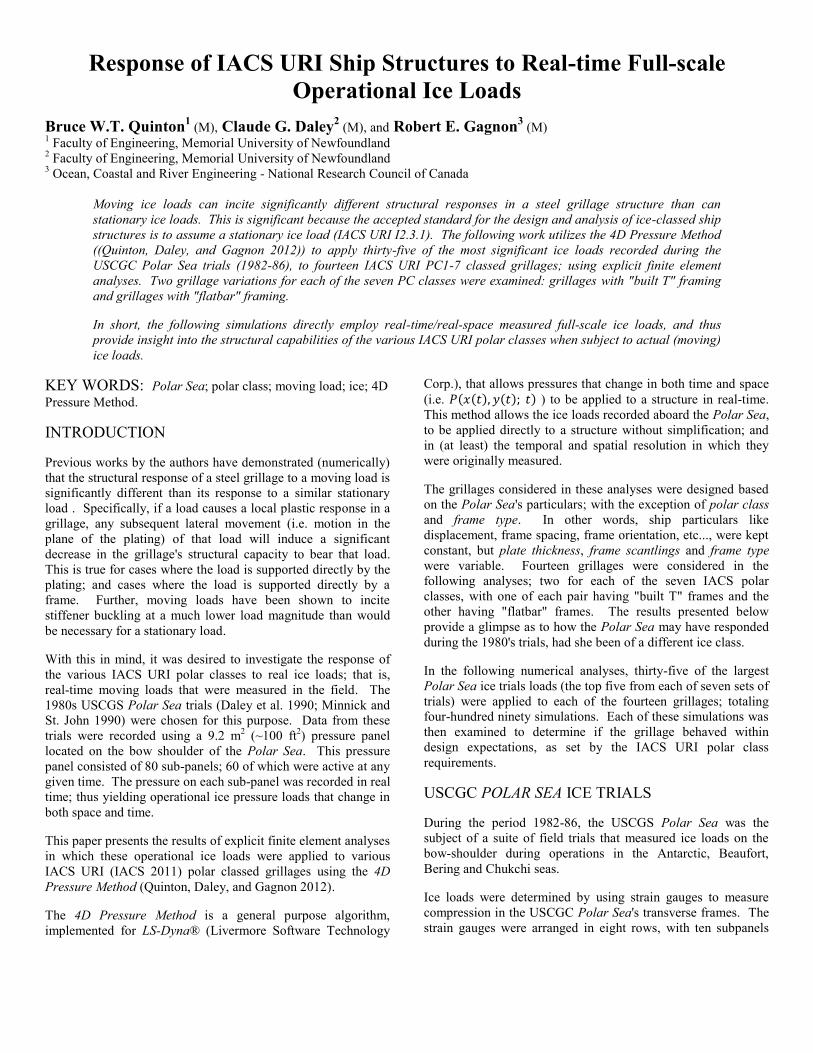
4D PRESSURE METHOD
The 4D Pressure Method is a novel, non-contact loading method
(Quinton, Daley, and Gagnon 2012) that may be used in explicit
finite element analyses to apply ice pressure loads that vary in
both time, and 3-dimensional space. The required input for this
method is of the form of . is the
magnitude of the pressure at time, ; and pinpoint the
location of on a given surface; and and define the
pressure's spatial extent. This method is general in that the
pressure distribution(s) applied may vary in location, size, and
shape, and may consist of uniform, distributed, or a collection of
discrete pressures (uniform or distributed); each of which may
vary in magnitude with time. The generality of the method
implies that it may be used to model everything from uniform,
stationary, steady pressure loads (as is commonly done using
standard finite element techniques), to custom ice pressure load
models utilizing feedback response, to actual field and
laboratory pressure data measured in time from a pressure
sensor array. In addition, the method allows for refinement of
the data's spatial resolution through the use of two-dimensional
interpolation schemes. For example, given data from 6 x 10
pressure sensor array (e.g. the Polar Sea ice trials data), the
method can refine this to any desired resolution (e.g. 11 x 19, 21
x 37, etc.) using either a nearest-neighbor, bilinear, or cubic
interpolation scheme. The type of interpolation scheme utilized
depends on the desired shape of the resulting interpolated data
(see Figure 1). The authors suggest that cubic interpolation
provides pressure shapes in line with those observed in the
laboratory; however, when using the method for design
purposes, the nearest-neighbor method would provide more
conservative results.
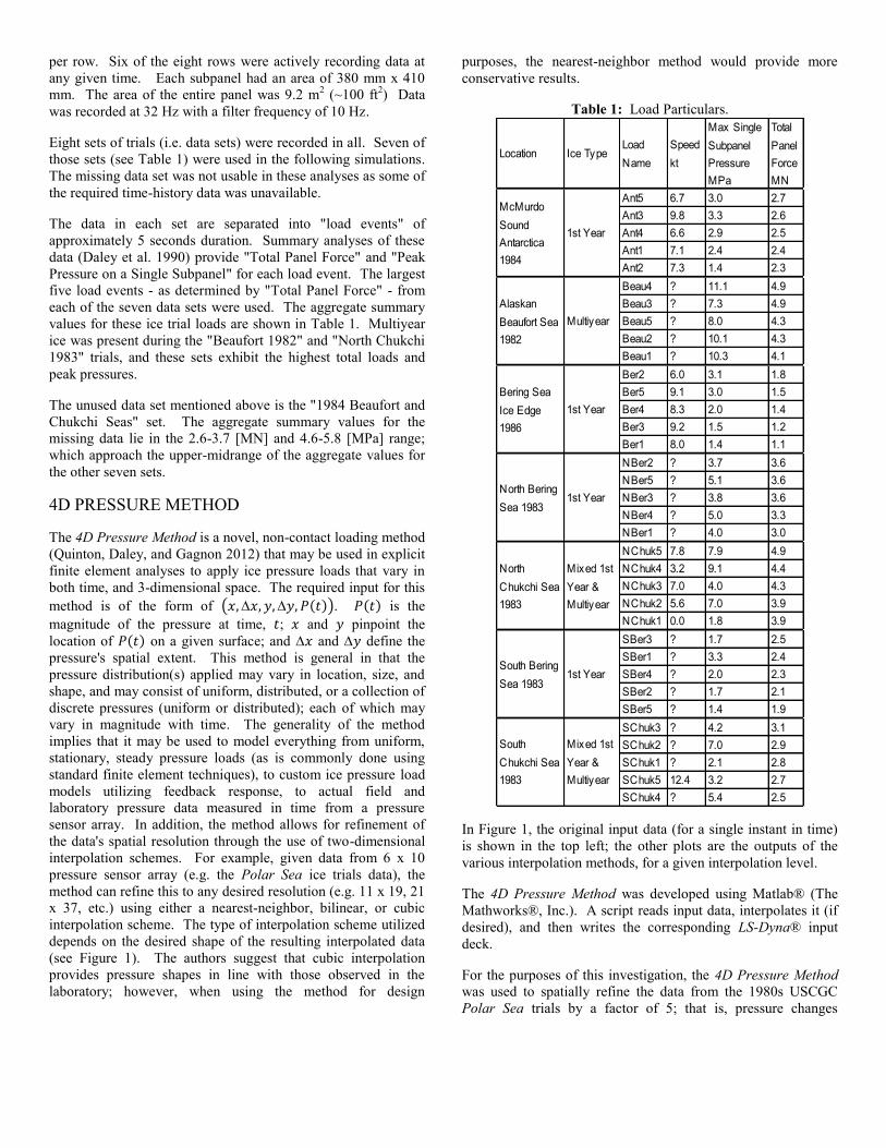
Table 1: Load Particulars.
Location Ice TypeLoad
Name
Speed
kt
Max Single
Subpanel
Pressure
MPa
Total
Panel
Force
MN
Ant5 6.7 3.0 2.7
Ant3 9.8 3.3 2.6
Ant4 6.6 2.9 2.5
Ant1 7.1 2.4 2.4
Ant2 7.3 1.4 2.3
Beau4 ? 11.1 4.9
Beau3 ? 7.3 4.9
Beau5 ? 8.0 4.3
Beau2 ? 10.1 4.3
Beau1 ? 10.3 4.1
Ber2 6.0 3.1 1.8
Ber5 9.1 3.0 1.5
Ber4 8.3 2.0 1.4
Ber3 9.2 1.5 1.2
Ber1 8.0 1.4 1.1
NBer2 ? 3.7 3.6
NBer5 ? 5.1 3.6
NBer3 ? 3.8 3.6
NBer4 ? 5.0 3.3
NBer1 ? 4.0 3.0
NChuk5 7.8 7.9 4.9
NChuk4 3.2 9.1 4.4
NChuk3 7.0 4.0 4.3
NChuk2 5.6 7.0 3.9
NChuk1 0.0 1.8 3.9
SBer3 ? 1.7 2.5
SBer1 ? 3.3 2.4
SBer4 ? 2.0 2.3
SBer2 ? 1.7 2.1
SBer5 ? 1.4 1.9
SChuk3 ? 4.2 3.1
SChuk2 ? 7.0 2.9
SChuk1 ? 2.1 2.8
SChuk5 12.4 3.2 2.7
SChuk4 ? 5.4 2.5
McMurdo
Sound
Antarctica
1984
1st Year
Alaskan
Beaufort Sea
1982
Multiyear
Bering Sea
Ice Edge
1986
1st Year
South
Chukchi Sea
1983
Mixed 1st
Year &
Multiyear
North Bering
Sea 19831st Year
North
Chukchi Sea
1983
Mixed 1st
Year &
Multiyear
South Bering
Sea 19831st Year
In Figure 1, the original input data (for a single instant in time)
is shown in the top left; the other plots are the outputs of the
various interpolation methods, for a given interpolation level.
The 4D Pressure Method was developed using Matlab® (The
Mathworks®, Inc.). A script reads input data, interpolates it (if
desired), and then writes the corresponding LS-Dyna® input
deck.
For the purposes of this investigation, the 4D Pressure Method
was used to spatially refine the data from the 1980s USCGC
Polar Sea trials by a factor of 5; that is, pressure changes
originally recorded between two spatial points in one dimension,
were interpolated over 5 spatial points in that dimension. The
cubic interpolation algorithm employed.
Figure 1: Top left - original 4D pressure data input; Top Right
- nearest neighbor interpolation; Bottom Left - bilinear
interpolation; Bottom Right - cubic interpolation.
POLAR CLASS GRILLAGES
The IACS Unified Requirements for Polar Class (IACS 2011),
in combination with the relevant particulars of the USCGC
Polar Sea (shown in Table 2) were used to design fourteen steel
grillages. Two grillages for each of the seven polar classes were
created; one utilizing "built T" frames and the other "flatbar"
frames. Both frame types were explored in order to gain a better
understanding of their relative behaviours in response to moving
loads..
A program by C.G. Daley called PC Design & Check was used
to calculate the plate thickness and frame scantlings for each
grillage. PC Design & Check is essentially a Microsoft®
Excel™ implementation of the IACS polar rules that has the
capability to recommend minimum scantlings for frames of
various configurations (e.g. flatbar, built-t, angle, etc...). The
parameters shown in Table 2 were common inputs into PC
Design & Check for all fourteen grillages:
Table 2: IACS URI grillage design parameters.
Parameter Value Units
Displacement 13.4 kt
Hull Region Bi -
Frame Orientation Angle 90 DEG
Frame Orientation Type Transverse -
Water Density 1.025 tonne/m3
Frame Attachment Parameter 2 -
Yield Strength of Steel 315 MPa
Young's Modulus of Steel 207 GPa
Main Frame Span 2210 mm
Main Frame Spacing 406 mm
The variable parameters for each of the fourteen grillages were
polar class, which varied between PC1 and PC7, and frame type,
which varied between "built T" and "flatbar".
The primary longitudinal structure (which is actually provided
by decks in the Polar Sea), was modeled for these simulations
using longitudinal "built T" stringers, for all fourteen grillages.
These stringers were designed to remain elastic when subject to
the full load prescribed by the IACS polar rules over the frame
span given in Table 2. The plating's effective width was
included in these calculations, but the attached perpendicular
framing was ignored. This method provides grossly oversized
primary structure; which is desirable in this case as the focus of
this work is on the response of the plating and transverse
framing. Note that the design of primary structure is not
prescribed by the IACS polar rules, but rather left to the member
societies. Table 3 gives the design scantlings for each grillage.
Table 3: Grillage Particulars.
Polar
Class
Frame
Type
Frame Scantlings
mm
Plate
Thickness
mm
Stringer Scantlings mm
built T T 660 x 24, 200 x 24
flatbar F 525 x 37
built T T 500 x 20, 200 x 20
flatbar F 420 x 31
built T T 440 x 16, 200 x 16
flatbar F 360 x 27
built T T 360 x 16, 190 x 16
flatbar F 340 x 24
built T T 300 x 14, 160 x 14
flatbar F 300 x 22
built T T 280 x 12, 150 x 12
flatbar F 280 x 20
built T T 280 x 10, 150 x 10
flatbar F 260 x 19
T 900 x 23, 100 x 20
39.0 T 1700 x 40, 200 x 40
31.5 T 1300 x 32, 175 x 20
15.5 T 600 x 16, 50 x 10
1
2
3
4
5
6
7
20.0 T 750 x 20, 100 x 20
17.5 T 650 x 18, 75 x 15
25.5 T 900 x 30, 150 x 15
22.5
COMPARISON OF POLAR SEA LOADS AND
IACS DESIGN LOADS
Table 4 outlines the IACS URI design loads by polar class for
these grillages. The values in each row represent the static,
stationary load equivalent of a glancing collision on the bow
shoulder of the vessel, for each polar class (IACS 2011).
Table 4: IACS Prescribed Design Loads for these grillages.
Polar
Class
Design
Ice Load
F (MN)
Design Ice
Line Load
Q (MN/m)
Design Avg
Ice Pressure
P (MPa)
Load Patch
Width (m)
Load Patch
Height (m)
1 31.4 9.0 14.6 3.483 0.617
2 17.6 5.5 9.7 3.188 0.565
3 10.8 3.6 6.7 3.013 0.534
4 8.0 2.8 5.4 2.890 0.512
5 5.5 2.0 4.2 2.709 0.480
6 4.3 1.6 3.2 2.745 0.486
7 3.2 1.2 2.7 2.586 0.458
The IACS design load patch parameters from Table 4 were then
used with the pressure-area relationships derived from the Polar
Sea trials (Daley et al. 1990; Minnick and St. John 1990) to
compare the Polar Sea ice trial loads with the IACS design
loads for each polar class on the basis of average pressure.
Table 5 shows the ratio, in percent, of the Polar Sea loads
divided by the IACS design load for each polar class. This table
indicates that the loads experienced by the Polar Sea during her
1980s ice trials are below the IACS PC5 level design loads; at
least on the basis of average load patch pressure. Note the cells
highlighted in red in Table 5. As these loads are greater than the
design loads for their respective PC classes, we would expect to
see significant damage to the PC7 and PC6 grillages for these
loads.
Table 5: Polar Sea loads as a percentage of IACS URI design
load-patch average pressure (Pavg).
Load PC7 PC6 PC5 PC4 PC3 PC2 PC1
Ant1 40% 33% 25% 19% 15% 9% 5%
Ant2 37% 31% 23% 18% 14% 10% 6%
Ant3 32% 25% 19% 14% 10% 7% 4%
Ant4 31% 24% 18% 15% 12% 9% 6%
Ant5 34% 32% 23% 21% 17% 11% 7%
Beau1 125% 96% 75% 52% N/A N/A N/A
Beau2 129% 98% 77% 53% 40% 25% N/A
Beau3 146% 113% 88% N/A N/A N/A N/A
Beau4 143% 108% 84% 59% 45% 28% 16%
Beau5 92% 80% 60% 47% 36% 23% 14%
Ber1 21% 17% 13% 10% 7% 5% 3%
Ber2 43% 34% 26% 19% 14% 9% 5%
Ber3 28% 22% 17% 12% 9% 5% 3%
Ber4 30% 23% 18% 13% 10% 6% 4%
Ber5 27% 20% 16% 11% 8% 5% 3%
NBer1 44% 35% 27% 19% 15% 10% 6%
NBer2 82% 64% 50% 36% 27% 17% 10%
NBer3 60% 48% 37% 27% 21% 13% 8%
NBer4 75% 57% 45% 31% 23% 14% 8%
NBer5 81% 64% 50% 35% 27% 17% 10%
NChuk1 35% 29% 22% 17% 14% 9% 6%
NChuk2 74% 56% 44% 30% 18% 10% 6%
NChuk3 67% 55% 42% 31% 24% 16% 9%
NChuk4 98% 80% 61% 46% 36% 24% 14%
NChuk5 123% 94% 73% 51% 39% 25% 14%
SBer1 41% 33% 25% 19% 15% 10% 6%
SBer2 34% 29% 22% 17% 13% 8% 5%
SBer3 42% 34% 26% 19% 14% 9% 5%
SBer4 34% 28% 21% 16% 13% 8% 5%
SBer5 17% 13% 10% 7% 6% 5% 3%
SChuk1 37% 30% 23% 16% 12% 8% 5%
SChuk2 31% 28% 21% 16% 13% 9% 5%
SChuk3 61% 48% 37% 27% 21% 14% 9%
SChuk4 70% 54% 42% N/A N/A N/A N/A
SChuk5 63% 50% 39% 28% 22% 14% 8%
A similar comparison between the Polar Sea loads and the
IACS design loads was made based on total force. In this case,
if a Polar Sea load was below the design load for a particular
IACS PC class, than it was classified by that PC class. These
results are shown in Table 6 and agree well with those based on
average pressure; that is, the largest load experienced during the
Polar Sea ice trials was within the design limits of similar PC 5
classed vessel of similar particulars to the Polar Sea.
Table 6: Polar Sea equivalent IACS design load by total force.
Load
Name
Fmax
(MN)
IACS PC
Load
Equivalent
Load
Name
Fmax
(MN)
IACS PC
Load
Equivalent
Ant1 2.391 PC7 Beau1 4.115 PC6
Ant2 2.272 PC7 Beau2 4.314 PC5
Ant3 2.561 PC7 Beau3 4.872 PC5
Ant4 2.531 PC7 Beau4 4.932 PC5
Ant5 2.670 PC7 Beau5 4.324 PC5
Ber1 1.126 PC7 NBer1 2.999 PC7
Ber2 1.813 PC7 NBer2 3.577 PC6
Ber3 1.156 PC7 NBer3 3.557 PC6
Ber4 1.415 PC7 NBer4 3.288 PC6
Ber5 1.505 PC7 NBer5 3.577 PC6
NChuk1 3.856 PC6 SBer1 2.352 PC7
NChuk2 3.916 PC6 SBer2 2.112 PC7
NChuk3 4.334 PC5 SBer3 2.461 PC7
NChuk4 4.414 PC5 SBer4 2.322 PC7
NChuk5 4.892 PC5 SBer5 1.933 PC7
SChuk1 2.820 PC7
SChuk2 2.860 PC7
SChuk3 3.089 PC7
SChuk4 2.531 PC7
SChuk5 2.670 PC7
NUMERICAL MODEL
An explicit and nonlinear finite element code is required to
model moving loads. The deleterious effects of moving loads
versus stationary loads are only present after the structure has
plastically deformed (Quinton 2008; Quinton, Daley, and
Gagnon 2012). An elastic structure will not experience any loss
of capacity to a moving load; therefore, a nonlinear numerical
model is necessary to predict structural response to moving
loads. Further, because the deformations associated with
moving loads may be large, geometric nonlinear capability is
also required.
MPP-Dyna® is an explicit nonlinear finite element code that
exhibits these required capabilities. It is a release of the proven
and popular LS-Dyna® code that is capable of running in
parallel on multiple computers in a cluster. MPP-Dyna® was
used exclusively throughout this research.
The numerical models were defined at full scale, and combine
the previously mentioned IACS polar class grillages with the
Polar Sea ice trial loads using the 4D Pressure Method.
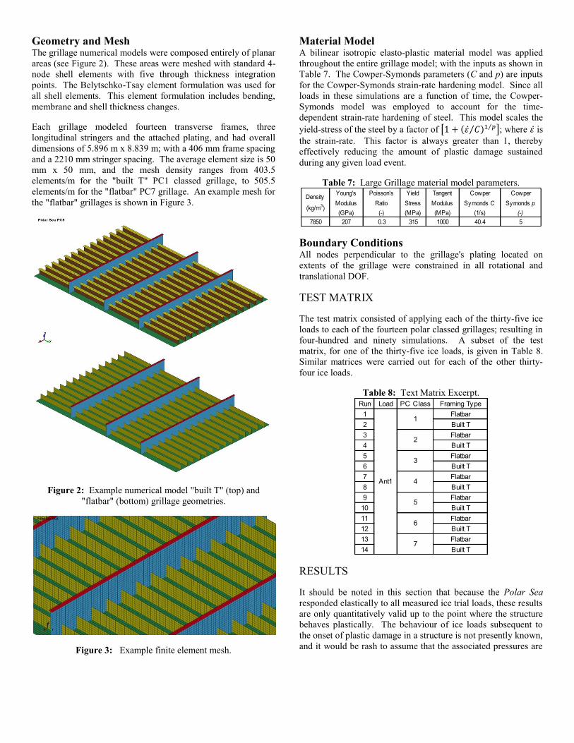
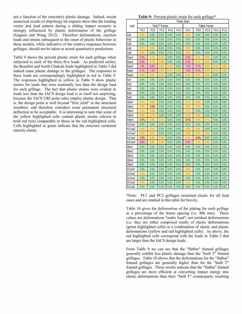
Geometry and Mesh The grillage numerical models were composed entirely of planar
areas (see Figure 2). These areas were meshed with standard 4-
node shell elements with five through thickness integration
points. The Belytschko-Tsay element formulation was used for
all shell elements. This element formulation includes bending,
membrane and shell thickness changes.
Each grillage modeled fourteen transverse frames, three
longitudinal stringers and the attached plating, and had overall
dimensions of 5.896 m x 8.839 m; with a 406 mm frame spacing
and a 2210 mm stringer spacing. The average element size is 50
mm x 50 mm, and the mesh density ranges from 403.5
elements/m for the "built T" PC1 classed grillage, to 505.5
elements/m for the "flatbar" PC7 grillage. An example mesh for
the "flatbar" grillages is shown in Figure 3.
Figure 2: Example numerical model "built T" (top) and
"flatbar" (bottom) grillage geometries.
Figure 3: Example finite element mesh.
Material Model A bilinear isotropic elasto-plastic material model was applied
throughout the entire grillage model; with the inputs as shown in
Table 7. The Cowper-Symonds parameters (C and p) are inputs
for the Cowper-Symonds strain-rate hardening model. Since all
loads in these simulations are a function of time, the Cowper-
Symonds model was employed to account for the time-
dependent strain-rate hardening of steel. This model scales the
yield-stress of the steel by a factor of ; where is
the strain-rate. This factor is always greater than 1, thereby
effectively reducing the amount of plastic damage sustained
during any given load event.
Table 7: Large Grillage material model parameters.
Density
(kg/m3)
Young's
Modulus
(GPa)
Poisson's
Ratio
(-)
Yield
Stress
(MPa)
Tangent
Modulus
(MPa)
Cowper
Symonds C
(1/s)
Cowper
Symonds p
(-)
7850 207 0.3 315 1000 40.4 5
Boundary Conditions All nodes perpendicular to the grillage's plating located on
extents of the grillage were constrained in all rotational and
translational DOF.
TEST MATRIX
The test matrix consisted of applying each of the thirty-five ice
loads to each of the fourteen polar classed grillages; resulting in
four-hundred and ninety simulations. A subset of the test
matrix, for one of the thirty-five ice loads, is given in Table 8.
Similar matrices were carried out for each of the other thirty-
four ice loads.
Table 8: Text Matrix Excerpt. Run Load PC Class Framing Type
1 Flatbar
2 Built T
3 Flatbar
4 Built T
5 Flatbar
6 Built T
7 Flatbar
8 Built T
9 Flatbar
10 Built T
11 Flatbar
12 Built T
13 Flatbar
14 Built T7
Ant1
1
2
3
4
5
6
RESULTS
It should be noted in this section that because the Polar Sea
responded elastically to all measured ice trial loads, these results
are only quantitatively valid up to the point where the structure
behaves plastically. The behaviour of ice loads subsequent to
the onset of plastic damage in a structure is not presently known,
and it would be rash to assume that the associated pressures are
not a function of the structure's plastic damage. Indeed, recent
numerical results of ship/bergy bit impacts show that the loading
vector and load pattern during a sliding impact scenario is
strongly influenced by plastic deformation of the grillage
(Gagnon and Wang 2012). Therefore deformations, reaction
loads and strains subsequent to the onset of plastic behaviour in
these models, while indicative of the relative responses between
grillages, should not be taken as actual quantitative predictions.
Table 9 shows the percent plastic strain for each grillage when
subjected to each of the thirty-five loads. As predicted earlier,
the Beaufort and North Chukchi loads highlighted in Table 5 did
indeed cause plastic damage to the grillages. The responses to
these loads are correspondingly highlighted in red in Table 9.
The responses highlighted in yellow in Table 9 show plastic
strains for loads that were nominally less than the design load
for each grillage. The fact that plastic strains were evident in
loads less than the IACS design load is in itself not surprising,
because the IACS URI polar rules employ plastic design. That
is, the design point is well beyond "first yield" in the structural
members, and therefore considers some permanent structural
deflection to be acceptable. It is interesting to note that some of
the yellow highlighted cells contain plastic strains (shown in
bold red text) comparable to those in the red highlighted cells.
Cells highlighted in green indicate that the structure remained
entirely elastic.
Table 9: Percent plastic strain for each grillage*.
PC7 PC6 PC5 PC4 PC3 PC7 PC6 PC5 PC4 PC3
Ant1 0.0% 0.0% 0.0% 0.0% 0.0% 0.0% 0.0% 0.0% 0.0% 0.0%
Ant2 0.0% 0.0% 0.0% 0.0% 0.0% 0.0% 0.0% 0.0% 0.0% 0.0%
Ant3 0.0% 0.0% 0.0% 0.0% 0.0% 0.0% 0.0% 0.0% 0.0% 0.0%
Ant4 0.1% 0.0% 0.0% 0.0% 0.0% 0.0% 0.0% 0.0% 0.0% 0.0%
Ant5 0.0% 0.0% 0.0% 0.0% 0.0% 0.0% 0.0% 0.0% 0.0% 0.0%
Beau1 0.4% 0.1% 0.0% 0.0% 0.0% 0.3% 0.1% 0.0% 0.0% 0.0%
Beau2 0.4% 0.1% 0.0% 0.0% 0.0% 0.3% 0.1% 0.0% 0.0% 0.0%
Beau3 1.6% 0.9% 0.2% 0.1% 0.0% 1.5% 0.7% 0.2% 0.1% 0.0%
Beau4 2.1% 1.0% 0.3% 0.1% 0.0% 1.8% 0.7% 0.2% 0.1% 0.0%
Beau5 0.4% 0.2% 0.0% 0.0% 0.0% 0.4% 0.1% 0.0% 0.0% 0.0%
Ber1 0.0% 0.0% 0.0% 0.0% 0.0% 0.0% 0.0% 0.0% 0.0% 0.0%
Ber2 0.0% 0.0% 0.0% 0.0% 0.0% 0.0% 0.0% 0.0% 0.0% 0.0%
Ber3 0.0% 0.0% 0.0% 0.0% 0.0% 0.0% 0.0% 0.0% 0.0% 0.0%
Ber4 0.0% 0.0% 0.0% 0.0% 0.0% 0.0% 0.0% 0.0% 0.0% 0.0%
Ber5 0.0% 0.0% 0.0% 0.0% 0.0% 0.0% 0.0% 0.0% 0.0% 0.0%
NBer1 0.1% 0.0% 0.0% 0.0% 0.0% 0.1% 0.0% 0.0% 0.0% 0.0%
NBer2 0.2% 0.9% 0.0% 0.0% 0.0% 0.2% 0.0% 0.0% 0.0% 0.0%
NBer3 0.1% 0.0% 0.0% 0.0% 0.0% 0.1% 0.0% 0.0% 0.0% 0.0%
NBer4 0.2% 0.1% 0.0% 0.0% 0.0% 0.1% 0.0% 0.0% 0.0% 0.0%
NBer5 0.7% 0.2% 0.1% 0.0% 0.0% 0.7% 0.2% 0.1% 0.0% 0.0%
NChuk1 0.0% 0.0% 0.0% 0.0% 0.0% 0.0% 0.0% 0.0% 0.0% 0.0%
NChuk2 0.2% 0.1% 0.0% 0.0% 0.0% 0.2% 0.0% 0.0% 0.0% 0.0%
NChuk3 0.2% 0.1% 0.0% 0.0% 0.0% 0.3% 0.1% 0.0% 0.0% 0.0%
NChuk4 0.5% 0.2% 0.0% 0.0% 0.0% 0.4% 0.5% 0.0% 0.0% 0.0%
NChuk5 0.6% 0.2% 0.0% 0.0% 0.0% 0.4% 0.1% 0.0% 0.0% 0.0%
SBer1 0.0% 0.0% 0.0% 0.0% 0.0% 0.0% 0.0% 0.0% 0.0% 0.0%
SBer2 0.0% 0.0% 0.0% 0.0% 0.0% 0.0% 0.0% 0.0% 0.0% 0.0%
SBer3 0.0% 0.0% 0.0% 0.0% 0.0% 0.0% 0.0% 0.0% 0.0% 0.0%
SBer4 0.0% 0.0% 0.0% 0.0% 0.0% 0.0% 0.0% 0.0% 0.0% 0.0%
SBer5 0.0% 0.0% 0.0% 0.0% 0.0% 0.0% 0.0% 0.0% 0.0% 0.0%
SChuk1 0.0% 0.0% 0.0% 0.0% 0.0% 0.0% 0.0% 0.0% 0.0% 0.0%
SChuk2 0.0% 0.0% 0.0% 0.0% 0.0% 0.0% 0.0% 0.0% 0.0% 0.0%
SChuk3 0.0% 0.0% 0.0% 0.0% 0.0% 0.0% 0.0% 0.0% 0.0% 0.0%
SChuk4 0.1% 0.0% 0.0% 0.0% 0.0% 0.1% 0.0% 0.0% 0.0% 0.0%
SChuk5 0.0% 0.0% 0.0% 0.0% 0.0% 0.0% 0.0% 0.0% 0.0% 0.0%
"Built T" Frames
Plastic Strain
Flatbar FramesLoad
*Note: PC1 and PC2 grillages remained elastic for all load
cases and are omitted in this table for brevity.
Table 10 gives the deformation of the plating for each grillage
as a percentage of the frame spacing (i.e. 406 mm). These
values are deformations "under load"; not residual deformations
(i.e. they are either comprised totally of elastic deformations
(green highlighted cells) or a combination of elastic and plastic
deformations (yellow and red highlighted cells). As above, the
red highlighted cells correspond with the loads in Table 5 that
are larger than the IACS design loads.
From Table 9 we can see that the "flatbar" framed grillages
generally exhibit less plastic damage than the "built T" framed
grillages. Table 10 shows that the deformations for the "flatbar"
framed grillages are generally higher than for the "built T"
framed grillages. These results indicate that the "flatbar" framed
grillages are more efficient at converting impact energy into
elastic deformations than their "built T" counterparts, resulting
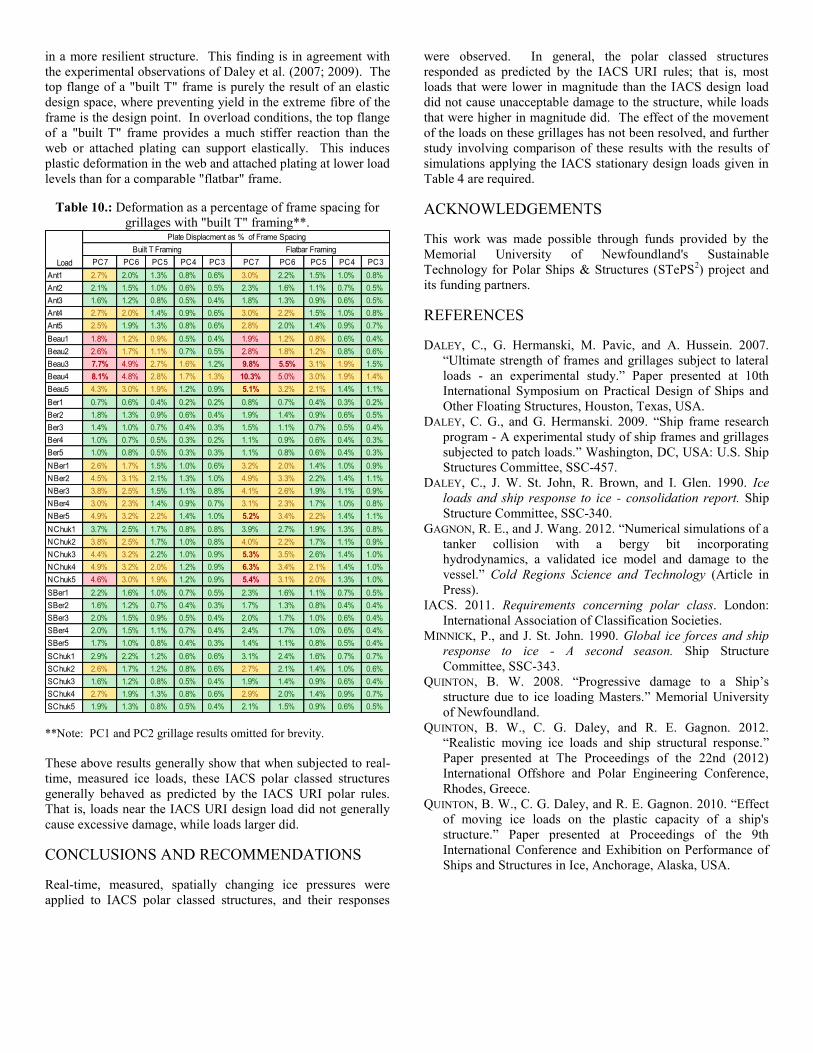
in a more resilient structure. This finding is in agreement with
the experimental observations of Daley et al. (2007; 2009). The
top flange of a "built T" frame is purely the result of an elastic
design space, where preventing yield in the extreme fibre of the
frame is the design point. In overload conditions, the top flange
of a "built T" frame provides a much stiffer reaction than the
web or attached plating can support elastically. This induces
plastic deformation in the web and attached plating at lower load
levels than for a comparable "flatbar" frame.
Table 10.: Deformation as a percentage of frame spacing for
grillages with "built T" framing**.
PC7 PC6 PC5 PC4 PC3 PC7 PC6 PC5 PC4 PC3
Ant1 2.7% 2.0% 1.3% 0.8% 0.6% 3.0% 2.2% 1.5% 1.0% 0.8%
Ant2 2.1% 1.5% 1.0% 0.6% 0.5% 2.3% 1.6% 1.1% 0.7% 0.5%
Ant3 1.6% 1.2% 0.8% 0.5% 0.4% 1.8% 1.3% 0.9% 0.6% 0.5%
Ant4 2.7% 2.0% 1.4% 0.9% 0.6% 3.0% 2.2% 1.5% 1.0% 0.8%
Ant5 2.5% 1.9% 1.3% 0.8% 0.6% 2.8% 2.0% 1.4% 0.9% 0.7%
Beau1 1.8% 1.2% 0.9% 0.5% 0.4% 1.9% 1.2% 0.8% 0.6% 0.4%
Beau2 2.6% 1.7% 1.1% 0.7% 0.5% 2.8% 1.8% 1.2% 0.8% 0.6%
Beau3 7.7% 4.9% 2.7% 1.6% 1.2% 9.8% 5.5% 3.1% 1.9% 1.5%
Beau4 8.1% 4.8% 2.8% 1.7% 1.3% 10.3% 5.0% 3.0% 1.9% 1.4%
Beau5 4.3% 3.0% 1.9% 1.2% 0.9% 5.1% 3.2% 2.1% 1.4% 1.1%
Ber1 0.7% 0.6% 0.4% 0.2% 0.2% 0.8% 0.7% 0.4% 0.3% 0.2%
Ber2 1.8% 1.3% 0.9% 0.6% 0.4% 1.9% 1.4% 0.9% 0.6% 0.5%
Ber3 1.4% 1.0% 0.7% 0.4% 0.3% 1.5% 1.1% 0.7% 0.5% 0.4%
Ber4 1.0% 0.7% 0.5% 0.3% 0.2% 1.1% 0.9% 0.6% 0.4% 0.3%
Ber5 1.0% 0.8% 0.5% 0.3% 0.3% 1.1% 0.8% 0.6% 0.4% 0.3%
NBer1 2.6% 1.7% 1.5% 1.0% 0.6% 3.2% 2.0% 1.4% 1.0% 0.9%
NBer2 4.5% 3.1% 2.1% 1.3% 1.0% 4.9% 3.3% 2.2% 1.4% 1.1%
NBer3 3.8% 2.5% 1.5% 1.1% 0.8% 4.1% 2.6% 1.9% 1.1% 0.9%
NBer4 3.0% 2.3% 1.4% 0.9% 0.7% 3.1% 2.3% 1.7% 1.0% 0.8%
NBer5 4.9% 3.2% 2.2% 1.4% 1.0% 5.2% 3.4% 2.2% 1.4% 1.1%
NChuk1 3.7% 2.5% 1.7% 0.8% 0.8% 3.9% 2.7% 1.9% 1.3% 0.8%
NChuk2 3.8% 2.5% 1.7% 1.0% 0.8% 4.0% 2.2% 1.7% 1.1% 0.9%
NChuk3 4.4% 3.2% 2.2% 1.0% 0.9% 5.3% 3.5% 2.6% 1.4% 1.0%
NChuk4 4.9% 3.2% 2.0% 1.2% 0.9% 6.3% 3.4% 2.1% 1.4% 1.0%
NChuk5 4.6% 3.0% 1.9% 1.2% 0.9% 5.4% 3.1% 2.0% 1.3% 1.0%
SBer1 2.2% 1.6% 1.0% 0.7% 0.5% 2.3% 1.6% 1.1% 0.7% 0.5%
SBer2 1.6% 1.2% 0.7% 0.4% 0.3% 1.7% 1.3% 0.8% 0.4% 0.4%
SBer3 2.0% 1.5% 0.9% 0.5% 0.4% 2.0% 1.7% 1.0% 0.6% 0.4%
SBer4 2.0% 1.5% 1.1% 0.7% 0.4% 2.4% 1.7% 1.0% 0.6% 0.4%
SBer5 1.7% 1.0% 0.8% 0.4% 0.3% 1.4% 1.1% 0.8% 0.5% 0.4%
SChuk1 2.9% 2.2% 1.2% 0.6% 0.6% 3.1% 2.4% 1.6% 0.7% 0.7%
SChuk2 2.6% 1.7% 1.2% 0.8% 0.6% 2.7% 2.1% 1.4% 1.0% 0.6%
SChuk3 1.6% 1.2% 0.8% 0.5% 0.4% 1.9% 1.4% 0.9% 0.6% 0.4%
SChuk4 2.7% 1.9% 1.3% 0.8% 0.6% 2.9% 2.0% 1.4% 0.9% 0.7%
SChuk5 1.9% 1.3% 0.8% 0.5% 0.4% 2.1% 1.5% 0.9% 0.6% 0.5%
Built T Framing Flatbar Framing
Load
Plate Displacment as % of Frame Spacing
**Note: PC1 and PC2 grillage results omitted for brevity.
These above results generally show that when subjected to real-
time, measured ice loads, these IACS polar classed structures
generally behaved as predicted by the IACS URI polar rules.
That is, loads near the IACS URI design load did not generally
cause excessive damage, while loads larger did.
CONCLUSIONS AND RECOMMENDATIONS
Real-time, measured, spatially changing ice pressures were
applied to IACS polar classed structures, and their responses
were observed. In general, the polar classed structures
responded as predicted by the IACS URI rules; that is, most
loads that were lower in magnitude than the IACS design load
did not cause unacceptable damage to the structure, while loads
that were higher in magnitude did. The effect of the movement
of the loads on these grillages has not been resolved, and further
study involving comparison of these results with the results of
simulations applying the IACS stationary design loads given in
Table 4 are required.
ACKNOWLEDGEMENTS
This work was made possible through funds provided by the
Memorial University of Newfoundland's Sustainable
Technology for Polar Ships & Structures (STePS2) project and
its funding partners.
REFERENCES
DALEY, C., G. Hermanski, M. Pavic, and A. Hussein. 2007.
“Ultimate strength of frames and grillages subject to lateral
loads - an experimental study.” Paper presented at 10th
International Symposium on Practical Design of Ships and
Other Floating Structures, Houston, Texas, USA.
DALEY, C. G., and G. Hermanski. 2009. “Ship frame research
program - A experimental study of ship frames and grillages
subjected to patch loads.” Washington, DC, USA: U.S. Ship
Structures Committee, SSC-457.
DALEY, C., J. W. St. John, R. Brown, and I. Glen. 1990. Ice
loads and ship response to ice - consolidation report. Ship
Structure Committee, SSC-340.
GAGNON, R. E., and J. Wang. 2012. “Numerical simulations of a
tanker collision with a bergy bit incorporating
hydrodynamics, a validated ice model and damage to the
vessel.” Cold Regions Science and Technology (Article in
Press).
IACS. 2011. Requirements concerning polar class. London:
International Association of Classification Societies.
MINNICK, P., and J. St. John. 1990. Global ice forces and ship
response to ice - A second season. Ship Structure
Committee, SSC-343.
QUINTON, B. W. 2008. “Progressive damage to a Ship’s
structure due to ice loading Masters.” Memorial University
of Newfoundland.
QUINTON, B. W., C. G. Daley, and R. E. Gagnon. 2012.
“Realistic moving ice loads and ship structural response.”
Paper presented at The Proceedings of the 22nd (2012)
International Offshore and Polar Engineering Conference,
Rhodes, Greece.
QUINTON, B. W., C. G. Daley, and R. E. Gagnon. 2010. “Effect
of moving ice loads on the plastic capacity of a ship's
structure.” Paper presented at Proceedings of the 9th
International Conference and Exhibition on Performance of
Ships and Structures in Ice, Anchorage, Alaska, USA.
Discussion
Jorgen Amdahl, Visitor
I would first like to compliment the authors for their substantial
contributions to research and development on ice loads, load
effects, structural resistance and design of polar ships over the
past decades. There is no doubt that they have a unique
experience and dispose of a wealth of invaluable data from
laboratory and full scale measurements of ice actions.
For that reason I had great expectations upon starting to review
the paper, but I must admit that I am not fully satisfied after
having read it. Certainly, there is a lot of information baked into
the paper, but important data are missing or not clearly
explained (or it may be my failure to understand correctly the
presented information), which makes it difficult to fully
appreciate the results of the study.
The numerical study includes simultaneously the effects of
several important factors into single analyses, and the effects of
each factor on the results become disguised. If each factor had
been isolated and investigated step by step, I believe a more
profound understanding of their significance could have been
obtained.
In my view there are at least four issues that need to be
addressed when the applicability of the IACS URI rules are
investigated:
1. How good are the resistance models for the plating and the
frames compared to nonlinear finite element analyses?
Both the plate and the frame requirements are based on plastic
analysis. I do, indeed, favor this because plastic analysis
provides good estimates of the collapse resistance. Nevertheless,
the collapse models are idealized and simplifications are
introduced. It would, therefore, be very interesting to compare
rule resistances with those predicted with LS-DYNA (which are
considered “true” values). Further, what are the strain levels that
are implicitly accepted by the collapse models? This could be
obtained by reading strains when the collapse mode assumed in
the code has been developed in the simulation with LS-DYNA.
Some engineering judgment will have to be exercised, because
the collapse mode is not formed gradually.
This investigation will reveal any conservatism/non-
conservatism in the IACS URI rules and the implied strains
would set the reference level for the strains that are obtained in
later analyses, for example those in Table 9.
To include assessment of the local plate requirement I believe,
but I am not sure, that the uniform pressure distribution and
patch dimensions according Table 4 should be supplemented
with the peak pressure factor (PPF) and hull area factor (AF) in
a small area (say frame spacing squared) in order to comply
with the IACS URI rules. For better judgment and to avoid
uncertainties the applied AF and PPF should be given.
From the above it transpires that it is basically the cases where
plastic strains are obtained that attract my interest. In my view
the corresponding results for the lower class (stronger) vessels
are obvious (response in the elastic domain), and deserve less
space than they occupy in the paper.
2. How well do the assumed distributions comply with the
measured pressure distribution?
The Beaufort Sea data are especially interesting in this case.
Static or quasi-static simulations with LS-DYNA should be
carried out scaling the pressure distribution from these
measurements. What are the pressure levels (local and average)
compared to the rule values for the same strain levels as with
obtained in Pt. 1? Is the occurrence of plastic strains for loads
that are nominally less than the design load for a grillage due to
higher local pressure versus average pressure than those
assumed in the rules?
The paper contains a lengthy discussion of methods to
interpolate the measured values. In my view this should not be
decoupled from the use of the pressure distributions. It is
noticed that the area of the pressure panels is almost equal to the
frame spacing squared of the numerical model. Local plate
resistance and strains are often estimated on the basis of uniform
pressures over frame spacing squared areas. I would therefore
suggest using the original 4D data with a small correction as
input for the LS-DYNA analysis. The pressures from Beaufort
Sea are very high (> 10 MPa), so comparing this pressure with
the average design pressure multiplied with AF and PPF would
be meaningful. For full appreciation of the results it would be
necessary to know the spatial as well as temporal variation of
the pressures. Presentation of data for a few of the extreme
cases would be welcomed
3. What is the effect of moving the pressure distributions using
the 4D pressure method versus using the “worst “ pressure
distribution?
Of course the plastic deformations will spread over a larger area,
but are the maximum strains/deformations different from those
obtained in Pt. 2?
4. What are the effects of dynamics?
The major dynamic effects are inertia effects and strain rate. The
results of true dynamic analyses should be compared with those
of “static” analysis for otherwise identical cases.
It is very important that the strain rate effect be investigated by
comparing otherwise identical analyss. The effect is uncertain
and very much discussed. The Cowper-Symonds equation gives
a significant increase of yield strength even for moderate strain
rates. We do not know how much the yield strength increased
during the simulations and thus affected the results. If it can be
substantiated that the effect is real, shall it be included in the
rules or shall it be considered a reserve strength factor?
The finite element model seems appropriate as far as mesh size
and boundary conditions are concerned, the latter on the
condition that plastic deformations take place some distance
from the boundaries. It may be discussed whether local
imperfections should be introduced for local web buckling and
tripping mode for stiffeners. Fortunately, explicit programs
more easily trigger buckling than implicit schemes, but do they
occur at the correct load levels for the T-stiffeners and could the
flat bars be susceptible to tripping? The flat bars have a
substantially larger shear area, and is failure of the T-stiffener
webs dominated by shear yielding?
It would be nice if the pressure-area relationships derived from
the Polar Sea trials were given.
In conclusion: I really appreciate the amount of work conducted
by the authors. The approach that is adopted – use of nonlinear
finite element analysis along with measured ice pressure
distribution – is supported. I do hope that the important effects
are better separated in the future investigations so as to provide
rule makers and designers of Arctic marine structures with more
fundamental and in-depth knowledge of ice actions and action
effects.
Roger Basu, Member
Full-scale measurements in engineering are comparatively rare
especially when they involve difficult processes such as the
interaction of ships and ice. Such measurements are conducted
in conditions that are often difficult to control, or define. They
are expensive and this is perhaps the main reason they are rare.
Nevertheless, such measurements are vital since they are the
only practical source of data for the critical task of calibrating
and otherwise improving design equations. Notwithstanding
these comments, high quality data derived using numerical
analysis methods can help reduce the need for full-scale
measurements, although it is difficult to imagine that such
methods can completely eliminate the need for good quality
experimental data especially at full scale. At the very least the
results from full-scale experiments will be needed to validate
numerical models. It for these reasons the work presented in the
subject paper is so valuable.
It is especially gratifying to see the authors using data gathered
some decades ago and applying it to examining a recently
identified issue concerning the differences in structural response
depending on whether the load is applied statically or as a
moving load. The work seems to have uncovered new issues
that may be important in considering the design of ship structure
subject to ice loads. This may also be relevant for offshore
structures.
A number of questions come to mind in reading the paper. It is
recognized that not all the issues and questions raised could
possibly be addressed in a single paper. While some of the
questions can be addressed simply in the subject paper through
minor additions, there are others that should be more properly
addressed in subsequent studies:
1. The IACS Polar Rules assume for each class notional ship
speed and ice thickness. It would be useful in interpreting
the results to compare these with speeds summarized in
Table 1. Are the associated ice thicknesses known?
2. Unfortunately there does not appear to be an easy way to
establish what the measured loads represent in terms of how
much of proportion of the lifetime extreme load they
represent. Presumably the IACS loads as design loads are
representative of lifetime extremes. Additional information
on these aspects would be helpful in interpreting the
percentages presented in Table 5 of the paper.
3. The plastic strain attained, if any, for each of the cases
considered is summarized in Tables 9 and 10. For
comparison purposes an indication of what “percent plastic
strains” would result under the corresponding full PC
design load would be instructive.
4. The 4D Pressure Method is presumably essentially a time
domain analysis. What value for damping was assumed in
the analysis?
5. It would be interesting to know how the fact that the load is
moving influences the response. This could be done by
applying the load that causes the maximum response as
shown in Tables 9 and 10. In other words how would the
values of percent plastic strain change for the case where
the load is applied statically?
6. The study of the response of beams, and other structures, to
moving loads is a well-developed field. It would be
interesting to investigate whether these methods can be
used to model moving ice loads. In that regard greater
discussion in the paper of the dynamics of the response
would be useful.
7. Similarly, in regard to the comment about stiffener buckling
occurring at lower magnitudes of load if it is applied as a
moving load. Again, is this a dynamic effect? If it is, then
how might the speed of the ship influence the response?
8. Perhaps the authors could speculate on how the evenness in
the side shell plating might influence the response?
The paper makes a significant contribution to the numerical
modeling of ship structure-ice interaction and has made good
use of existing full-scale data. The authors are to be
commended for this and are encouraged to explore, if they have
not already done so, some of the issues outlined above.
Pentti Kujala, Visitor
The authors have prepared an interesting and straightforward
paper applying advanced numerical modeling of ship-ice
interaction to capture the effect of real ice induced pressures on
the shell structures of an icebreaker when the shell structures are
designed applying various IACS PC classes. I have mainly two
topics for which I await some further clarification. First is the
calibration of the pressure measuring system onboard USCGC
Polar Sea. As the system is based on the measurements of
compressive stresses on the web of the installed frames, it would
be interesting to know how these compressive stresses are
calibrated to capture the pressure distribution induced by ice.
Secondly, it would be interesting to hear the authors’ opinion of
proper limit states to be used on ice-strengthened structures. In
Table 9 and 10 are given the calculated plastic strains and
permanent deflections occurring on the modeled structures. It
seems that plastic strain higher than 0.3% is selected as “red”
area and similarly 1.9% of permanent deflection is selected as
“red” values. Can the authors clarify somewhat more in detail
why these values have been selected? In addition, it would be
interesting to know whether the conducted analysis gave any
new insight to the proper limit states that should be used when
designing shell structures of ships for various operations in ice.
Dan Masterson, Member
I have read the paper carefully and have discussed it with
colleagues who have knowledge in the field. The work itself has
been done carefully and well. It shows by extrapolation of past
ship ram tests that the lower classes of the Polar Class code are
reasonably correct. We already knew this but confirmation is
always helpful.
The real problem lies in the sideshell pressures specified by
Polar Class for PC1 and PC2. All evidence from various kinds
of tests supports the thesis that these pressures are not
reasonable but are excessively and unjustifiably high. Thus a
real problem is created for higher class icebreaking ship hull
design. This work does nothing to address the issue. This
problem will surely be addressed in future editions of the IACS
standard.
Takahiro Takeuchi, Visitor
The paper provides useful field data based on USCGC Polar
Sea trials. Authors indicate that some of data as shown in Table
5 exceed IACS URI design load. Through a large number of
simulations by FEM using these field data, plastic deformations
of the structure were correspondingly obtained. These findings
will clearly contribute to the design of the polar ships.
I think the following information will enhance the value of the
paper:
1. More explanation of ice conditions for each trials.
2. Description of typical ice failure observed in each trials, and
corresponding ice-load (histories).
Could you prepare further information?
Authors’ Response
The authors would like to thank Professor Amdahl for his in
depth discussion of our paper. We greatly appreciate his
knowledgeable comments; however, we believe that our purpose
in writing this paper was somewhat different than he interpreted.
The four major parts of Dr. Amdahl’s discussion are preceded
by the assertion “In my view there are at least four issues that
need to be addressed when the applicability of the IACS URI
rules are investigated.” It was not our aim to address the
applicability of the IACS URI rules. The goal of the paper was
to explore the effects of the movement of the load on ship
structures. We chose both the Polar Sea data and the IACS
Polar Rules as bases for our study, and we took both as givens.
While one might question either of these items, this was not our
goal. The current standard approaches to the design of ice class
ships (or offshore structures) view the ice load as acting at a
single location on the outer shell. Most actual ice loads do not
remain stationary with respect to a ship’s hull, and our prior
work suggests that a moving load causing a plastic structural
response incites more damage to the structure than an equivalent
stationary load. With the exception of the assumption that loads
are applied quasi-statically at a single location, none of the
premises inherent in the IACS URI rules are in question (in this
paper).
Dr. Amdahl raises the concern that several important factors are
simultaneously included in this study. He is correct that we did
this. In particular, strain rate effects; load movement; varying
pressure amplitudes, distributions, and trajectories; and dynamic
(inertial) effects are all combined. This was done intentionally,
though we agree that we might have looked at the effects in
isolation. We took our approach so as to model, as close as is
possible, real-world ship-ice interactions. Strain-rate effects,
commonly included in crash simulations in other industries (e.g.
automotive and aerospace), were included in these simulations
using the Cowper-Symonds model. The Cowper-Symonds
model is a standard for simulations that ignore temperature
changes, for which there are accepted parameters for common
steels. The Polar Sea trials data provided us with real world
pressure data that varied in amplitude, time and space, and thus
permitted us to examine realistic moving ice loads. We accept
that the Polar Sea data is imperfect, but until we have data of
better temporal and spatial resolution, we feel comfortable in
using it for our purposes.
We would like to emphasize a point about our simulation’s
validity. We used ice loads measured on an elastic structure.
Obviously we have not considered the various dynamic and
rate-dependent effects that would occur when the structure
begins to behave plastically. There is a lack of data regarding
ice loads on a plastically deforming structure. This latter point is
why the authors point out (in the paper) that the results are not
quantitatively valid after plastic yielding begins.
Dr. Amdahl raises many interesting points in his discussion of
our paper. And although we did not intend to discuss the
applicability of the IACS URI rules, we agree that this is an
important issue. We will address his comments in the order he
presented them:
Regarding the resistance models for the plating and framing, the
authors have investigated experimentally and numerically
various PC classed grillage structures. Laboratory experiments
involving a full sized PC6 classed grillage structure were
performed by Daley and Hermanski (2008a; 2008b). The results
of both the experiments and the numerical models agreed very
well with the IACS capacity formulations, though not
necessarily with the exact failure geometry. We would agree
that additional study examining the IACS formulations would be
valuable.
Regarding the pressures given in Table 4, we did not include the
peak pressure factor (PPF) because we compared the average
pressure over the whole patch with the average for the same area
from the Polar Sea data. Comparing the more localized peaks
would be a different exercise. We did not include the area factor
(AF), because the Polar Sea panel was in the bow and the area
factor was 1.0.
Assuming that Dr. Amdahl is referring to the measured Polar
Sea pressure distributions in comparison to the distributions
assumed in the IACS Polar rules, we feel that such a comparison
would be done with caution. The Polar Rules have a pressure
distribution as one part of a complete design process and meant
to be used in that way only. Actual pressure measurements
reflect a variety of effects and specifics. We would find such a
comparison interesting but we would expect that it would be
quite challenging to interpret.
Regarding the suggestion that the Polar Sea data be "corrected",
the authors agree that the Polar Sea data is not perfect.
Certainly, increasing the magnitude of the pressures would have
resulted in greater damage to the grillage structures, but given
the novelty of the investigation of the response of ship structures
to moving loads, the authors did not want to add this additional
level of speculation at this stage. This is for the same reason the
strain-rate effects were not omitted, that is: obtaining results
that are possibly unduly conservative could warrant unnecessary
alarm at this point in the research. Prior work by the authors has
shown that the deleterious effects of moving loads causing
plastic damage to the structural capacity of a ship's grillage can
be substantial. Depending on the load type and trajectory, the
authors have observed structural overload capacities drop to less
than half their assessed value for equivalent stationary loads.
The authors believe that much more research is necessary in
order to more fully understand the effects of moving loads.
This comment gets to the essence of our paper. We do say that
moving loads not only spread the response over a greater area
but that the movement leads to a change in the plastic response
mechanism and results in greater maximum plastic deformations
and strains.
The issue of the two types of dynamic effects (strain rate and
inertial) is important. We included the inertial effects because
they are necessarily included in an LSDyna Explicit analysis.
We suspect that actual inertial effects were quite minor in the
present study. It is debatable whether we should have included
the strain-rate effects (i.e. the Cowper-Symonds model for rate
enhanced material strength). As mentioned above, strain-rate
effects were included in this work because these effects are real
and are commonplace in crash analysis in other industries.
While the Polar Rules and all other ice class rules do not
account for this beneficial effect, neither do the rules account for
the deleterious effect of the moving load. We included both in
an attempt to get a picture of the likely true behavior. We do
not disagree that looking at the various aspects singly would be
useful. The one key additional dynamic effect that we did not
study was the influence of structural plastic response on the ice
failure and consequent loads. We intend to examine this in the
coming months and years.
Regarding Dr. Amdahl’s assessment of our numerical model, we
appreciate his endorsement. We concur that explicit finite
element programs do not generally require a “trigger” to induce
buckling. While this numerical model was not specifically
calibrated against laboratory experiments, it is largely based on
similar models that were. Regarding the issue of the response of
T-stiffeners and flat bars, our experience is that the failure
modes are plastic mechanisms that only resemble elastic
buckling phenomena (tripping, shear buckling), but are actually
quite different. To speculate for a moment, and in hopes of
sparking some further discussion among our readers, in our view
we are dealing with behaviors that might best be termed auto-
plastic mechanisms. As the structure deforms, the plastic
deformations form to adapt to the changing internal load
balance. This is not like the instability phenomena that
constitute various types of elastic buckling. In most cases a good
non-linear analysis will exhibit the main plastic behaviors quite
well. The key error will typically be that analysts will not
properly define the full strain hardening behavior.
We again wish to thank Dr. Amdahl again for his excellent
discussion. His pragmatic questions and recommendations are
much appreciated.
ADDITIONAL REFERENCES
DALEY, C. G. and G. Hermanski. 2008a. Ship Frame Research
Program - an Experimental Study of Ship Frames and
Grillages Subjected to Patch Loads, Volume 1 - Data Report:
Ship Structure Committee.
DALEY, C. G. and G. Hermanski. 2008b. Ship Frame Research
Program - an Experimental Study of Ship Frames and
Grillages Subjected to Patch Loads, Volume 2 - Theory and
Analysis Reports: Ship Structure Committee.
The authors appreciate Dr. Basu's discussion of the issues
surrounding, and possible implications of the subject of this
paper; which focuses on the plastic response to moving ice loads
on steel stiffened panels. The authors will attempt to respond to
Dr. Basu's comments in the order he presented them:
1. Ice conditions data for the Polar Sea trials were generally
recorded every one-half hour, and were neither specific to
impacts, nor very precise. Ice thickness, for example, was only
estimated in a general way. Ice edge shape was not observed.
So, while the authors agree that this would provide a useful base
for interpreting the results of this paper, it would still leave
many questions (see below). We will attempt to provide this sort
of cross comparison in future papers.
2. The issue of the probability level for the Polar Rules
design load and for the Polar Sea measurements is an interesting
but difficult topic. The Polar Rules design point can be thought
of in deterministic terms (i.e. a collision at a certain speed into
ice of a certain shape and strength). It can also be seen in
probabilistic terms because such a collision will be quite rare for
a cautiously operated vessel. Unfortunately, the Polar Sea data is
not ideal for either a deterministic or a probabilistic validation of
the IACS Polar Rules. The reason is that a number of significant
parameters were not precisely measured during the trials. We
would like to echo Dr. Basu's comment on the value of field
data, and the difficulty of gathering it. We would like to add that
future field trials should pay more attention to accurate
characterization of the precise ice geometry and properties in
each impact. As expensive as field data is, researchers and
sponsors should understand that spending much more may be a
wise investment.
3. The "percent plastic strain" of the full PC design load is
presently under consideration by the authors, and will be
presented soon. The authors are examining the cases where the
IACS design load is applied both statically and moving along
the hull.
4. Damping was not actively employed in these simulations.
While structural "ringing" was not observed to be a problem in
these simulations, the authors agree that damping should be
considered in future work. In cases of plastic response, the
response is heavily damped due to the irrecoverable plastic work
done.
5. In previous works, the authors have compared non-moving
and moving loads causing quasi-static plastic damage. For loads
causing large plastic deformation of the structure, the
movements have been found to strongly and detrimentally
influence the response. When there is no plastic deformation,
slow movement is not significantly different from the cases of
no movement. We did not consider dynamic effects and
responses. Whether or not a difference in structural response
will exist for the load cases causing the maximum structural
response in this paper, is an important question. Dr. Basu's
suggestion to investigate this is well taken, and is presently
under consideration.
6. The authors agree that much work has been accomplished in
the field of moving loads in other industries. Considerable work
by civil engineers on the effects of moving loads on bridges,
roads, and train tracks has been done, though normally for
elastic responses. Analytical models for moving loads causing a
plastic response in beams exist, however their applicability to
ship structures needs to be examined. The same cannot be said
for plates. The only publically available literature on the subject
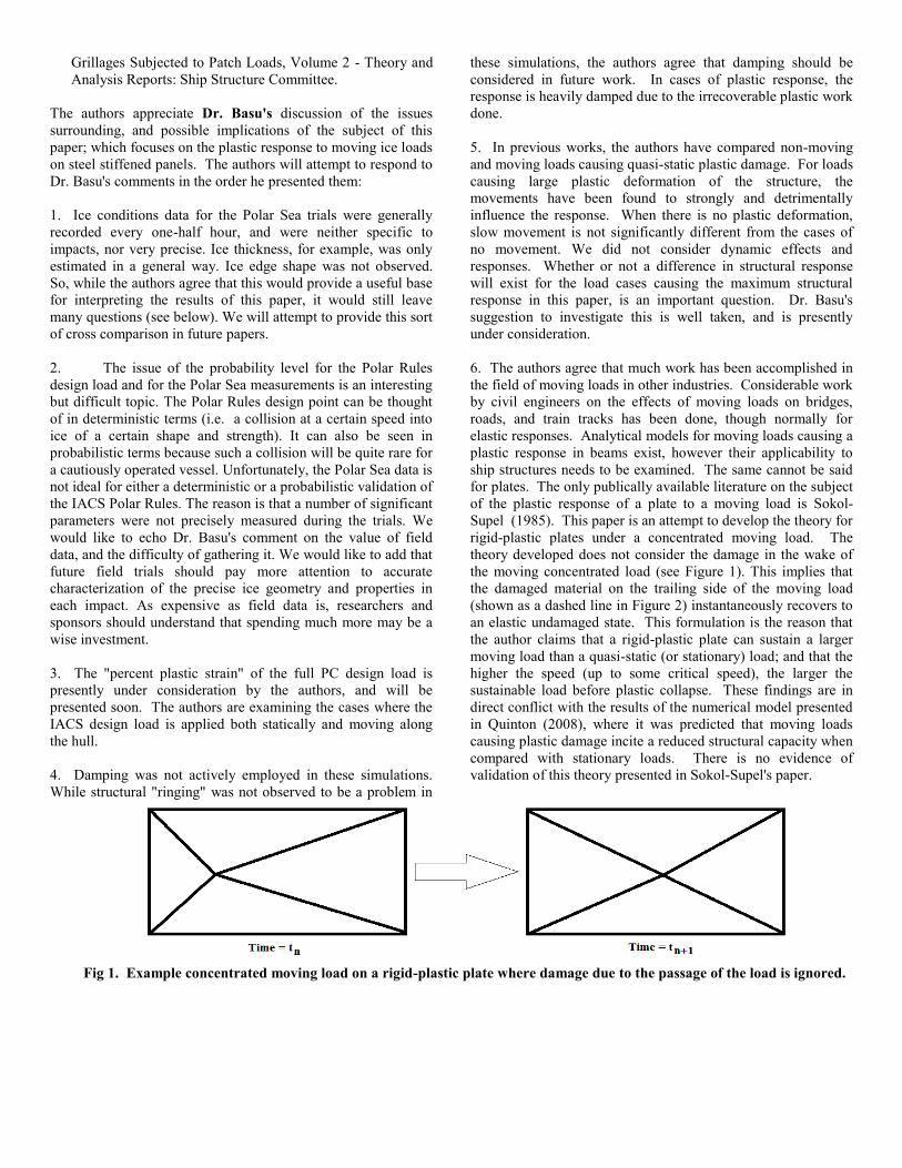
of the plastic response of a plate to a moving load is Sokol-
Supel (1985). This paper is an attempt to develop the theory for
rigid-plastic plates under a concentrated moving load. The
theory developed does not consider the damage in the wake of
the moving concentrated load (see Figure 1). This implies that
the damaged material on the trailing side of the moving load
(shown as a dashed line in Figure 2) instantaneously recovers to
an elastic undamaged state. This formulation is the reason that
the author claims that a rigid-plastic plate can sustain a larger
moving load than a quasi-static (or stationary) load; and that the
higher the speed (up to some critical speed), the larger the
sustainable load before plastic collapse. These findings are in
direct conflict with the results of the numerical model presented
in Quinton (2008), where it was predicted that moving loads
causing plastic damage incite a reduced structural capacity when
compared with stationary loads. There is no evidence of
validation of this theory presented in Sokol-Supel's paper.
Fig 1. Example concentrated moving load on a rigid-plastic plate where damage due to the passage of the load is ignored.
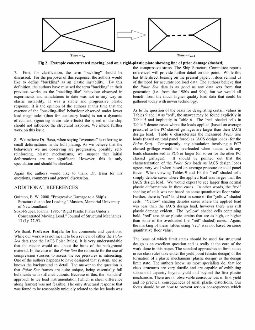
Fig 2. Example concentrated moving load on a rigid-plastic plate showing line of prior damage (dashed).
7. First, for clarification, the term "buckling" should be
discussed. For the purposes of this response, the authors would
like to define "buckling" as an elastic instability. By this
definition, the authors have misused the term "buckling" in their
previous works, as the "buckling-like" behaviour observed in
experiments and simulations to date was not in any way an
elastic instability. It was a stable and progressive plastic
response. It is the opinion of the authors at this time that the
essence of the "buckling-like" behaviour observed under lower
load magnitudes (than for stationary loads) is not a dynamic
effect, and (ignoring strain-rate effects) the speed of the ship
should not influence the structural response. We intend further
work on this issue.
8. We believe Dr. Basu, when saying “evenness” is referring to
small deformations in the hull plating. As we believe that the
behaviours we are observing are progressive, possibly self-
reinforcing, plastic mechanisms, we suspect that initial
deformations are not significant. However, this is only
speculation and should be checked.
Again the authors would like to thank Dr. Basu for his
questions, comments and general discussion.
ADDITIONAL REFERENCES
Quinton, B. W. 2008. "Progressive Damage to a Ship’s
Structure due to Ice Loading." Masters, Memorial University
of Newfoundland.
Sokol-Supel, Joanna. 1985. "Rigid Plastic Plates Under a
Concentrated Moving Load." Journal of Structural Mechanics
13 (1): 77-93.
We thank Professor Kujala for his comments and questions.
While our work was not meant to be a review of either the Polar
Sea data (nor the IACS Polar Rules), it is very understandable
that the reader would ask about the basis of the background
material. In the case of the Polar Sea the rationale for the use of
compression stresses to assess the ice pressures is interesting.
One of the authors happens to have designed that system, and so
knows the background in detail. The answer to the question is
that Polar Sea frames are quite unique, being essentially full
bulkheads with stiffened cutouts. Because of this, the ‘standard’
approach to ice load instrumentation (which is shear difference
along frames) was not feasible. The only structural response that
was found to be reasonably uniquely related to the ice loads was
the compressive stress. The Ship Structure Committee reports
referenced will provide further detail on this point. While this
has little direct bearing on the present paper, it does remind us
of the need for accurate ice load data. The authors believe that
the Polar Sea data is as good as any data sets from that
generation (i.e. from the 1980s and 90s), but we would all
benefit from the much higher quality load data that could be
gathered today with newer technology.
As to the question of the basis for designating certain values in
Tables 9 and 10 as "red", the answer may be found explicitly in
Table 5 and implicitly in Table 6. The "red" shaded cells in
Table 5 denote cases where the loads applied (based on average
pressure) to the PC classed grillages are larger than their IACS
design load. Table 6 characterizes the measured Polar Sea
loads (based on total panel force) as IACS design loads (for the
Polar Sea). Consequently, any simulation involving a PC7
classed grillage would be overloaded when loaded with any
loads characterized as PC6 or larger (on so on for the other PC
classed grillages). It should be pointed out that the
characterization of the Polar Sea loads as IACS design loads
agrees very well when based on average pressure or total panel
force. When viewing Tables 9 and 10, the "red" shaded cells
simply denote cases where the applied load was larger than the
IACS design load. We would expect to see larger than normal
plastic deformations in these cases. In other words, the "red"
shading of cells was not based on some quantitative floor value.
Further, there is "red" bold text in some of the "yellow" shaded
cells. "Yellow" shading denotes cases where the applied load
was less than the IACS design load, however there was still
plastic damage evident. The "yellow" shaded cells containing
bold, "red" text show plastic strains that are as high, or higher
than some of the overloaded (i.e. "red" shaded) cases. Again,
the marking of these values using "red" was not based on some
quantitative floor value.
The issue of which limit states should be used for structural
design is an excellent question and is really at the core of the
work done in this paper. The standard approaches to limit states
in ice class rules take either the yield point (elastic design) or the
formation of a plastic mechanism (plastic design) as the design
limit state. The authors know, as most specialists do, that ice
class structures are very ductile and are capable of exhibiting
substantial capacity beyond yield and beyond the first plastic
mechanism. There are no observable consequences of first yield
and no practical consequences of small plastic distortions. Our
focus should be on how to prevent serious consequences which
occur in overload situations. The paper is an exploration of one
effect that only occurs when the loads are well above even the
plastic design point. We believe this is important because we
believe that the real concern in ice class design is about what
occurs during overloads. We do not mean that we should change
the design point to some extreme limit state. Rather we suggest
that the design should consider the whole range of responses, so
that structures are ensured to have both good initial strength and
good overload capacity. In this way we hope that real safety and
capacity can be achieved in the most cost effective manner. We
realized that a plastic overload assessment, which is normally
done without consideration of movement along the hull, is
strongly influenced by such movement as has been shown in our
prior work, and needs to be studied further. We wrote this paper
to communicate this point to anyone who is similarly interested
in the overload capacity of ice class ships.
We appreciate Dr. Masterson’s comments. We do agree that
our paper does not address the issue of the correctness of the
Polar Rules. We did not examine side shell pressures, so it is
somewhat difficult to address Dr. Masterson’s points and
concerns. It may be useful for us to say what we do feel the data
shows, in terms of the Polar Rules. Our analysis examined the
hypothetical case of a set of vessels of different ice classes, all
of which being the same size and shape (and power) of the
Polar Sea. We took the highest loads measured on the bow
panel on the Polar Sea and examined what the response might
have been had the structure been of any of the Polar Classes.
Now while our aim was to study the effects of moving loads, the
exercise can be seen as an examination of how various ice
classes would have performed during the ice impacts that the
Polar Sea experienced in her ice trials. What is obvious is that a
PC5 class vessel would have been fully capable of the impacts.
We view this as showing that the trials resulted in PC5-type ice
interaction scenarios, and not that PC1 is over-specified. We
should also note that our analysis included a structural behavior
that adds capability to a structure, but that is normally not
considered. As a result, we were less conservative than many
would be. The effect we are describing is real, and helps ships
resist ice impacts. This effect is the strain rate enhancement of
yield strength (implemented via the Cowper-Symonds model).
Most analysts would not have included the effect and it is not
considered in the design rules. Had we left out this effect, we
would have found that the plastic responses would have been
greater and that higher ice classes would have been required to
resist the various load cases. This may partly explain why the
loads caused the relatively low responses in the structure. We
would suggest that the issue of the level of PC1 side shell
pressures is a matter for further study and debate.
The authors would like to thank Professor Takeuchi for his
discussion and endorsement of our paper. We certainly
appreciate his request for clarification of the relevant ice
conditions for each of the trials.
The ice impact data for all of the Polar Sea trials were generally
broken down into 5 second increments. In some cases, the ice
conditions for a particular event are available, but otherwise the
ice conditions were recorded in general, at specific time
intervals. The most relevant cases for this paper are the
Beaufort 1982 and the North Chukchi Sea 1983 impacts, the
details of which are summarized below (St. John, Daley, and
Blount 1984). For further information, interested readers are
referred to Daley et al. (1990b; 1990a).
Case Ice Conditions Speed
Beau1 Multi-year fragments in first-year ice <3 knots
Beau2 Not Available Unknown
Beau3 Steady running through multi-year and first-year ice Unknown
Beau4 Backing & Ramming into multi-year ice 3-4 knots
Beau5 Backing & Ramming into multi-year ice 2-3 knots
Nchuck-AllMulti-year ridges in relatively small multi-year floes
surrounded by first-year ice cover of ~ 5 feet (1.5 m)Unknown
Regarding the typical ice failure modes, record of this
information was impractical during the trials through methods
other than direct observation. All impacts occurred at the bow,
which has a significant slope. Generally speaking, multi-year
ice failed through crushing, and first-year ice failed though
crushing followed by flexural failure.
ADDITIONAL REFERENCES
DALEY, C., J. W. St. John, R. Brown, and I. Glen. 1990a. Ice
Loads and Ship Response to Ice - Consolidation Report.
Washington, D.C.: Ship Structures Committee.
DALEY, C., J. W. St. John, R. Brown, J. Meyer, and I. Glen.
1990b. Ice Loads and Ship Response to Ice - A Second
Season. Washington, D.C.: Ship Structures Committee.
ST. JOHN, J. W., C. Daley, and H. Blount. 1984. Ice Loads and
Ship Response to Ice. Washington, D.C.: Ship Structures
Committee