Biological Conservation 177 (2014) 12–24

Contents lists available at ScienceDirect

Biological Conservation

journal homepage: www.elsevier .com/locate /b iocon

Remaining natural vegetation in the global biodiversity hotspots

http://dx.doi.org/10.1016/j.biocon.2014.05.0270006-3207/� 2014 Elsevier Ltd. All rights reserved.

⇑ Corresponding author. Tel.: +61 7 4042 1835; fax: +61 7 4042 1319.E-mail address: sean.sloan@jcu.edu.au (S. Sloan).

Sean Sloan a,⇑, Clinton N. Jenkins b, Lucas N. Joppa c, David L.A. Gaveau d, William F. Laurance a

a Centre for Tropical Environmental and Sustainability Science, School of Marine and Tropical Biology, James Cook University, Cairns, Queensland 4870, Australiab Department of Biological Sciences, North Carolina State University, Raleigh, NC 27695, USAc Computational Science Laboratory, Microsoft Research, Cambridge CB1 2FB, UKd Centre for International Forestry Research, Bogor 16000, Indonesia

a r t i c l e i n f o

Article history:Received 15 February 2014Received in revised form 19 May 2014Accepted 27 May 2014

Keywords:BiodiversityBiodiversity hotspotsConservation planningNatural areasWilderness

a b s t r a c t

The biodiversity hotspots are 35 biogeographical regions that have both exceptional endemism andextreme threats to their vegetation integrity, and as such are global conservation priorities. Nonetheless,prior estimates of natural intact vegetation (NIV) in the hotspots are generally imprecise, indirect, coarse,and/or dated. Using moderate- and high-resolution satellite imagery as well as maps of roads, settle-ments, and fires, we estimate the current extent of NIV for the hotspots. Our analysis indicates that hot-spots retain 14.9% of their total area as NIV (�3,546,975 km2). Most hotspots have much less NIV thanpreviously estimated, with half now having 610% NIV by area, a threshold beneath which mean NIVpatch area declines precipitously below 1000 ha. Hotspots with the greatest previous NIV estimates suf-fered the greatest apparent losses. The paucity of NIV is most pronounced in biomes dominated by dryforests, open woodlands, and grasslands, reflecting their historic affinities with agriculture, such thatNIV tends to concentrate in select biomes. Low and declining levels of NIV in the hotspots underscorethe need for an urgent focus of limited conservation resources on these biologically crucial regions.

� 2014 Elsevier Ltd. All rights reserved.

1. Introduction

The biodiversity hotspots are 35 biogeographic regions thatcover 17.3% of the Earth’s land surface (excluding Antarctica) andare characterized by both exceptional biodiversity and acuteland-cover disturbance (Mittermeier et al., 2004; Myers et al.,2000). They are, in short, where human settlement, biological rich-ness, and environmental degradation converge (Williams, 2013).Within the hotspots are over 2 billion people (Landscan, 2006;Mittermeier et al., 2011, 2004) increasing at higher-than-averagerates (Cincotta et al., 2000; Williams, 2013), and an estimated85% human-modified landscapes by area (Mittermeier et al.,2004). Hotspots sustain �77% of all mammal, bird, reptile andamphibian species, including 50% of all plant species and 42% ofterrestrial vertebrate species as endemics (Mittermeier et al.,2004), as well as three-quarters of all endangered terrestrial verte-brates (Brooks et al., 2002; Mittermeier et al., 1998, 2004). Culturaldiversity is also high in the hotspots, with half of all indigenouslanguages found therein (Gorenflo et al., 2012).

Since the seminal publication of Myers et al. (2000) the conceptof hotspots as focal points for global conservation action hasbecome one of the foremost global conservation-prioritisation

paradigms (Mittermeier et al., 2011). The concept has attractedover $1 billion in conservation investment from entities like theCritical Ecosystem Partnership Fund (i.e., World Bank, Global Envi-ronment Facility, and The Governments of Japan, France and Eur-ope), The MacArthur Foundation, The Global Conservation Fund(i.e., Moore Foundation), Conservation International and its affili-ated TEAM Program and Centers for Biodiversity Conservation,among many others (Dalton, 2000; Mittermeier et al., 2011,1998, 2004; Myers, 2003; Myers and Mittermeier, 2003). Theseentities have explicitly adopted the hotspot concept as a centralconservation-investment strategy. Whether or not the concepthas garnered the ‘‘largest [monetary] sum ever assigned to a singleconservation strategy’’ (Myers, 2003), its global traction and legacyare indisputable.

While it is accepted that primary vegetation has been widelydisturbed in the hotspots and globally (Vitousek et al., 1997), pre-cise estimates of remaining intact remnant vegetation at very largespatial scales have proven challenging and elusive. Global land-cover maps derived from moderate- or coarse-resolution satelliteimagery have existed since the early 1990s (Bontemps et al.,2011; Dong et al., 2012; Friedl et al., 2010; Loveland et al., 2000)but afford only broad nominal classifications of vegetation reflec-tance, structure, and phenology and do not therefore readily distin-guish disturbed covers from natural, primary, intact covers per se,particularly in environments that are naturally unforested or

S. Sloan et al. / Biological Conservation 177 (2014) 12–24 13

semi-forested, such as savannas. As illustrated below, an uncriticalinterpretation of such classifications in efforts to estimate the areaof remaining natural intact vegetation is prone to significant error(Hoekstra et al., 2005). Global land-cover change analyses usingsatellite imagery are more promising insofar as they may excludeareas known to have undergone certain land-cover conversions(Hansen and DeFries, 2004; Hansen et al., 2013, 2008). Yet theyremain similarly unable to address the integrity of supposedly‘unchanged’ areas, which in a great many cases will be disturbed,and which in any case are observable at large spatial scales onlyat very coarse resolutions since the 1980s and at finer resolutionsonly since ca. 2000 with the advent of moderate-resolution imag-ery. While recent advances now provide relatively nuanced finer-scale measures of ‘percent tree cover’ and changes thereof sinceca. 2000 (Hansen et al., 2003, 2013; Sexton et al., 2013), it hasnot been possible, nor will it likely be possible, to determine reli-able thresholds identifying disturbed and thus undisturbed forestacross large and varied regions, to say nothing of undisturbed veg-etation in naturally semi-forested or unforested environments.

Two sets of relatively-derived estimates of remaining naturalintact vegetation over large spatial scales have arisen in light of suchissues. The first are those of Myers (1988, 1990), Myers et al. (2000),and Mittermeier et al. (1999, 2004), which entailed expert assess-ments of existing vegetation atlases, satellite-image classificationsand similar secondary data for the hotspots. These estimates arenow dated, difficult to replicate, and prone to inconsistency andapproximation. The second set of estimates are those of Sandersonet al. (2002), Schmitt et al. (2009), Potapov et al. (2008), andBryant et al. (1997), among others, which variously mapped intactareas with reference to criteria such as land-cover class, forest patchsize, proximity to infrastructure, and accessibility. These estimatesare problematic because they are either particular to closed-forestbiomes, very large vegetation patches, or tree cover generally, oroptimistically equate an absence of evidence of human disturbancewith evidence of its absence. These are key limitations where habi-tats that are structurally and compositionally varied, heavily frag-mented and under intense, proximate human pressure.

Updated and improved estimates of remaining natural intactvegetation (NIV) area in the hotspots are crucial for appropriateglobal conservation planning. Prior estimates have been used toprioritize hotspots for conservation action (Myers et al., 2000),determine their species-extinction susceptibility (Brooks et al.,2002; Malcolm et al., 2006), and calculate the costs their conserva-tion (Pimm et al., 2001). In light of the uncertainties surroundingprior NIV estimates, such derivations are similarly subject to revi-sion. A revision of hotspot conservation priority and attendant con-servation action could have significant implications for futurebiodiversity loss and particularly its attenuation considering thatbiodiversity loss becomes increasingly exponential as the final ves-tiges of intact habitat are destroyed (Rybicki and Hanski, 2013;Turner, 1996). Rigorously updated NIV estimates for the hotspotsare a matter of improved measurement for improved management.

Here we present updated, transparent, comprehensive and con-sistent estimates of NIV area and fragmentation for the world’s bio-diversity hotspots. The following section briefly reviews the hotspotconcept and previous natural-area estimates. Section 3 discusses ourmethodology, and the subsequent sections present our estimatesand highlight their implications for global conservation planning.

2. Hotspots and remaining natural vegetation

2.1. The hotspot approach and expert estimates

The hotspot concept prioritises the conservation of biologically-exceptional and highly-threatened regions with the explicit goal of

stemming species extinction, as per the irreplaceability-vulnerabil-ity conservation framework articulated by Margules and Pressey(2000). Myers (1988) first encapsulated this concept globally bydelimiting 10 largely tropical biogeographical regions of excep-tional biodiversity and habitat destruction (Table 1) – the first ‘hot-spots’, e.g., Madagascar, New Caledonia. Myers (1990) later addedeight largely semi-arid hotspots to this list, e.g., Southwest Austra-lia (Table 1). Conservation International adopted the hotspot con-cept as its central global conservation strategy in 1989(Conservation International, 1990a,b; Mittermeier et al., 2004),and the concept has since become a major conceptual templateamong conservation scientists (Redford et al., 2003; Robertset al., 2002; Sechrest et al., 2002; Turner et al., 2012; Willis et al.,2006). Myers, Conservation International, and collaborators laterrevised estimates of remaining primary habitat and defined thehotspots formally as biogeographic regions with >1500 endemicvascular plant species and 630% of original primary habitat(Mittermeier et al., 1999; Myers et al., 2000). Species endemism,rather than biodiversity per se, became a key definitional criteriongiven concern over extinction rates (Brooks et al., 2002;Mittermeier et al., 1998). This revision saw the hotspots expandin area as well as in number, to 25. A second global revision andupdate in 2004 (Mittermeier et al., 2004) expanded this count to34 and adjusted hotspot boundaries to concord with the ecore-gions of Olson et al. (2001). Recently, a 35th hotspot was added,the Forests of East Australia (Williams et al., 2011) (Fig. 1).

Mittermeier et al. (1999, 2004), Myers et al. (2000) and Myers(1988, 1990) present areal estimates of remaining natural intacthabitat for the hotspots (Table 1). Their approach entailed first con-sulting estimates of vegetation cover and loss for those countiesand/or regions within each hotspot, including vegetation atlases(e.g., Harcourt and Sayer, 1996), satellite forest-cover inventories(e.g., CCT/CIEDES, 1998), national environmental overviews (e.g.,FWI/GFW, 2002), and occasionally the 1990 FAO Forest ResourceAssessment (FAO, 1993). ‘‘Digitised forest cover data’’ from theWorld Conservation Monitoring Centre were also consulted(Mittermeier et al., 1998) (these data were uncited but are likelyUNEP-WCMC (1996) or UNEP-WCMC (1998)). These estimateswere then adjusted on the basis of expert opinion and unpublisheddata to estimate the area of ‘‘primary’’ or ‘‘more or less pristine’’vegetation per hotspot (Mittermeier et al., 2004). Such adjustmentssometimes reduced initial estimates by as much as 50%. Many ofthe source data were derived prior to the widespread use of GISand satellite imagery at large scales, and no attempt was madeto map primary vegetation in the hotspots.

The final estimates – hereafter termed Expert Estimates – whilegroundbreaking and widely adopted, are difficult to scrutinize andreplicate. Expert adjustments of the initial estimates were not welldocumented and, in the absence of greater transparency, uncer-tainties tend to become generalized. The Expert Estimates derivedfrom sources that were not necessarily comparable and occasion-ally had little explicit bearing on ‘primary’ versus ‘perturbed’ landcovers. Further, many sources pertained to individual countriesand it is unclear how these were adjusted to concord with theirregular biogeographic boundaries of hotspots (Fig. 1).

Perhaps more importantly, the Expert Estimates are increas-ingly dated. Even in the most recent update (Mittermeier et al.,2004) many of the data consulted span the 1980s and early1990s, and habitat loss in the hotspots is certain to have advancedsince (Balmford et al., 2002; Butchart et al., 2010; FAO, 2010;Hassan et al., 2005) as, among other drivers of habitat loss, increas-ing demand for agricultural products has been met in large part viacontinued habitat conversion (Gibbs et al., 2010; Laurance et al.,2014; Rudel et al., 2009). More recent global surveys of naturallyvegetated areas have since been undertaken but, as argued below,these do not offer ready and reliable estimates for the hotspots.

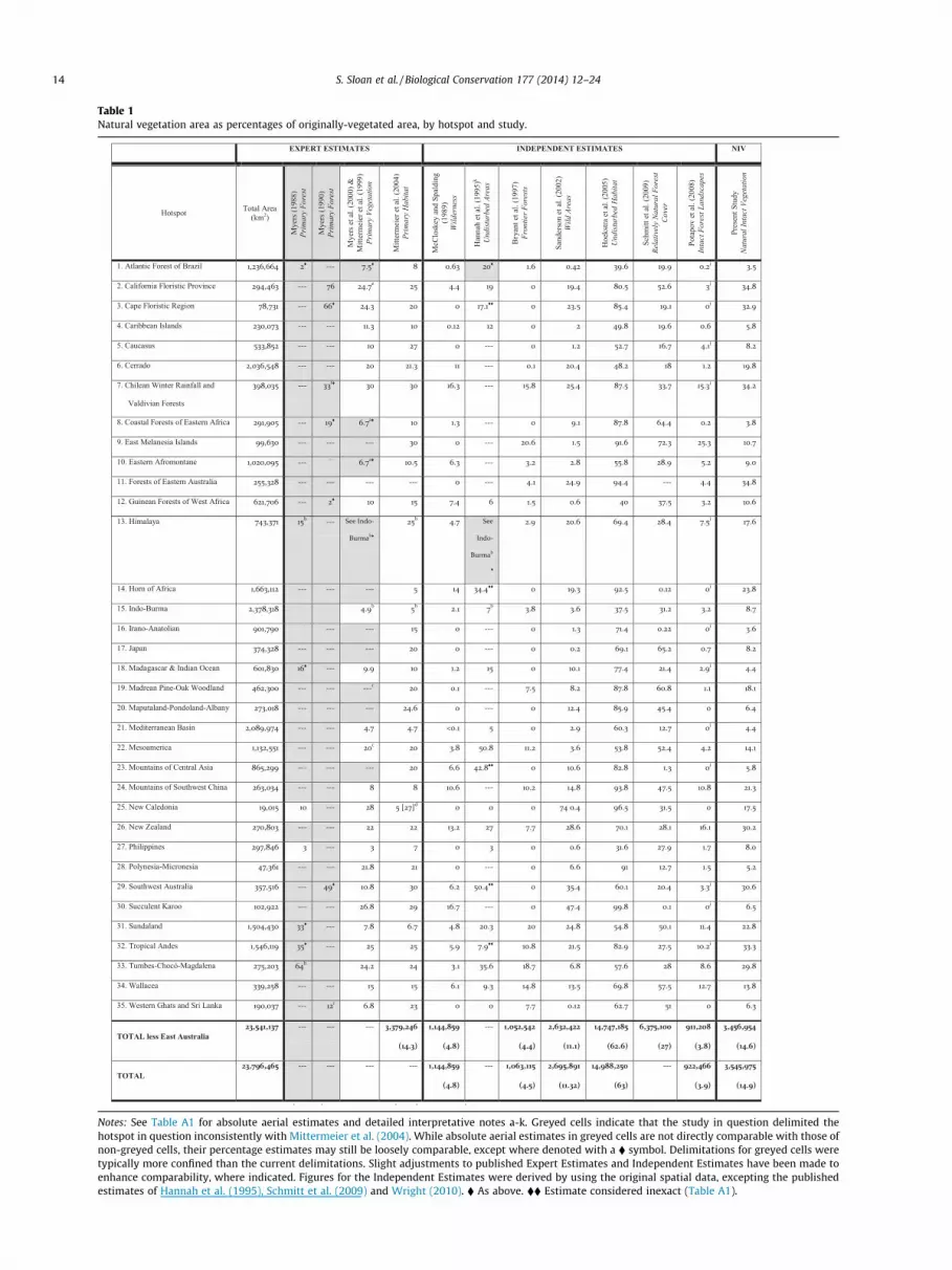
Table 1Natural vegetation area as percentages of originally-vegetated area, by hotspot and study.

Notes: See Table A1 for absolute aerial estimates and detailed interpretative notes a-k. Greyed cells indicate that the study in question delimited thehotspot in question inconsistently with Mittermeier et al. (2004). While absolute aerial estimates in greyed cells are not directly comparable with those ofnon-greyed cells, their percentage estimates may still be loosely comparable, except where denoted with a � symbol. Delimitations for greyed cells weretypically more confined than the current delimitations. Slight adjustments to published Expert Estimates and Independent Estimates have been made toenhance comparability, where indicated. Figures for the Independent Estimates were derived by using the original spatial data, excepting the publishedestimates of Hannah et al. (1995), Schmitt et al. (2009) and Wright (2010). � As above. �� Estimate considered inexact (Table A1).

14 S. Sloan et al. / Biological Conservation 177 (2014) 12–24

Fig. 1. The biodiversity hotspots. Notes: See Table 1 for hotspot names.

S. Sloan et al. / Biological Conservation 177 (2014) 12–24 15

2.2. Independent estimates of natural areas

A second set of global natural-area estimates – here termedIndependent Estimates – variously delineate natural unperturbedareas by combining satellite imagery, vegetation maps, and mapsof human disturbances. These estimates may in turn be subdividedaccording to whether they observe the absence of human distur-bance as a proxy for the presence of natural areas or rather observenatural vegetation more directly. Of the seven estimates discussedbelow, one was realised for the hotspots specifically (Schmitt et al.,2009), one was presented at the hotspot level (Hannah, 2001;Hannah et al., 1995), and the remainder were realised globally.The latter were not designed for the hotspots specifically, nor havethey been explicitly brought to bear on matters of remaining nat-ural area in the hotspots. Nonetheless they do present relevantempirical approaches for consideration, if not insight into theextent of natural areas within the hotspots, in light of the fact thatthe hotspots span nearly one-fifth of the Earth’s land surface.

Among those analyses observing natural vegetation directly,Hoekstra et al. (2005) estimate intact habitat as areas exclusiveof ‘‘cultivated and managed areas [as well as] artificial surfacesand associated areas’’ according to the 1-km Global Land Cover2000 (GLC2000) satellite dataset (ECJRC, 2003). Schmitt et al.(2009) go further to define ‘‘relatively natural forest cover’’ byremoving ‘non-natural’ areas from the satellite-derived 2000 Glo-bal Forest Map (UNEP-WCMC, 2000), namely agro-ecosystemsand similar covers according to the GLC2000 dataset (ECJRC,2003) as well as areas with <10% tree cover according to the MODISVegetation Continuous Field satellite dataset (Hansen et al., 2006).More precisely still, Potapov et al. (2008) delineated ‘intact forestlandscapes’ within the ‘zone of current forest extent’ as contiguousnatural ecosystems at least 1 km removed from settlements, roadsand other infrastructure, agriculture, and burned areas, as visuallyobserved in Landsat satellite imagery for forest patches >500 km2.

While direct, these estimates do not necessarily approximatethe total area and distribution of NIV in the hotspots. Their focuson forested biomes discounts the non-forest and open-forest vege-tation formations such as savannahs or montane shrublands prom-inent in many hotspots, and even overlook some desert hotspotsentirely (also true of Bryant et al. (1997), discussed below). Further,the GLC2000 data used by Hoekstra et al. (2005) and Schmitt et al.(2009) to distinguish natural from non-natural cover are prone tosignificant errors in this respect. Even after accounting for thoseGLC2000 land-cover classes clearly indicative of perturbation,there remain numerous generic classes such as ‘Mosaic Tree

Cover/Other Natural Vegetation’ that often incorporate appreciablydisturbed land covers, agricultural-forest gradations, and evenagro-pastoral covers, as confirmed in the course of the presentstudy. Without additional scrutiny, the GLC2000 dataset and thusHoekstra et al. and Schmitt et al. overestimate what is reasonablytermed natural forest (e.g., Kalacska et al., 2008; Fig. A1).

Among those analyses focusing on an absence of human distur-bance as a proxy for unperturbed natural areas, McCloskey andSpalding (1989) delineated ‘wilderness areas’ as 6 km removedfrom all roads, tracks, and human structures (e.g., towns, gas wells)according to global navigational charts. Hannah et al. (1995, 1994)similarly mapped ‘undisturbed areas’ as having a record of primaryvegetation and <10 people km2 with reference to population andinfrastructure maps as well as compiled land-cover maps, agricul-tural maps, and remote-sensing analyses. Bryant et al. (1997)delineated ‘frontier forests’ as large, natural, relatively undisturbedforests by identifying candidate areas with reference to McCloskeyand Spalding (1989) and The World Forest Map (1996), and thenrevising these on the basis of expert opinion. Finally, Sandersonet al. (2002) made use of global GIS datasets of population density,settlements, major roads and rivers, broad land-cover classes, andcoastlines to delimit ‘wild areas’ by deriving an additive indexreflecting these features, normalizing the index to a 1–100% scaleby biome and biogeographic realm, and then delimiting ‘wildareas’ as the ten largest areas having index values of <10% bybiome and realm.

These estimates are too indirect and coarse to account for thefragmented remnant vegetation patches that, in the hotspots, oftenoccur in close proximity to human disturbances and may comprisean appreciable proportion of total remanent vegetation (Ribeiroet al., 2009). They do not capture unperturbed vegetation per se,but rather conservatively map those larger and remote expansesdistant from the disturbance proxies of interest (minimum mappa-ble areas range from >500 km2 to >4000 km2, with scales around1:1,000,000), as only such areas can be taken as ‘natural’ withany degree of confidence. Sanderson et al. (2002) is illustrative ofthe point. Their index implicitly reflects ‘urbanality’, that is, con-centrations of roads, population, electric lights, and managed landcovers. While high levels of urbanality would correspond with highlevels of disturbance, less ‘urban’ environments are not necessarilyproportionally less disturbed or more natural. Indeed, even a singleroad and sparse rural population can decimate an otherwise intactarea (Laurance et al., 2009). An ‘absence of evidence’ of human dis-turbance is taken as ‘evidence of absence’, so that only the verylowest disturbance values may be taken as indicative of ‘natural

16 S. Sloan et al. / Biological Conservation 177 (2014) 12–24

areas’, and only then at broad scales. These ‘natural areas’ are bydefinition the most remote, extensive, and spatially-confined, andtheir delineation thus neglects vast swaths of the hotspots’ inter-vened and ‘cluttered’ landscapes.

3. Methods

In consideration of such issues, we estimated NIV area in thehotspots via a combination of automated and visual satellite-imageanalyses of land-cover classes and conditions as well as the map-ping of major landscape disturbances. The methodology may besummarised by two stages. In the first we assessed the vegetationcondition, spatial pattern, and local ecological appropriateness ofeach land-cover class of the global GlobCover 2009 satellite-imageclassification (Bontemps et al., 2011) for each ecoregion of Olsonet al. (2001) (Fig. A2) using moderate- and high-resolution satelliteimagery, and defined preliminary ‘naturally occurring’ areas onthat basis. In the second, we removed disturbed areas accordingto various disturbance maps. NIV is defined broadly as mature veg-etation in its natural state having minimal signs of human pertur-bation. The following details our approach (see also Text A1 inonline appendix).

3.1. Stage One: preliminary classification

The moderate-resolution GlobCover global land-cover classifi-cation defining 22 classes (Table 2; Bontemps et al., 2011) wascombined with the ecoregions dataset of Olson et al. (2001) toyield 6863 unique combinations of land-cover class by ecoregionwithin the hotspots. Each class-by-ecoregion combination wasassessed individually in order to account for the biogeographic het-erogeneity within the hotspots. For each class-by-ecoregion com-bination a preliminary classification of ‘naturally occurring’ or‘other’ was made via consideration of three criteria – namely, localecological appropriateness, integral spatial pattern, and vegetationcondition with few signs of human perturbation – with each crite-ria yielding a nominal likelihood that the combination is naturallyoccurring.

Table 2Land-cover classes of the GlobCover 2009 dataset.

Post-flooding or irrigated croplands (or aquatic)Rainfed croplandsMosaic cropland (50–70%)/vegetation (grassland/shrubland/forest) (20–50%)Mosaic vegetation (grassland/shrubland/forest) (50–70%)/cropland (20–50%)Closed to open (>15%) broadleaved evergreen or semi-deciduous forest

(>5 m)Closed (>40%) broadleaved deciduous forest (>5 m)Open (15–40%) broadleaved deciduous forest/woodland (>5 m)Closed (>40%) needleleaved evergreen forest (>5 m)Open (15–40%) needleleaved deciduous or evergreen forest (>5 m)Closed to open (>15%) mixed broadleaved and needleleaved forest (>5 m)Mosaic forest or shrubland (50–70%)/grassland (20–50%)Mosaic grassland (50–70%)/forest or shrubland (20–50%)Closed to open (>15%) (broadleaved or needleleaved, evergreen or deciduous)

shrubland (<5 m)Closed to open (>15%) herbaceous vegetation (grassland, savannas or lichens/

mosses)Sparse (<15%) vegetationClosed to open (>15%) broadleaved forest regularly flooded (semi-

permanently or temporarily) – fresh or brackish waterClosed (>40%) broadleaved forest or shrubland permanently flooded – Saline

or brackish waterClosed to open (>15%) grassland or woody vegetation on regularly flooded or

waterlogged soil – fresh, brackish or saline waterArtificial surfaces and associated areas (Urban areas >50%)Bare areasWater bodiesPermanent snow and ice

The biophysical characteristics of the GlobCover land-coverclasses (Table 2; Bontemps et al. (2011)) were considered relativeto ecoregion descriptions and characteristics in order to flag classesthat were locally ‘ecologically appropriate’, that is, likely (or unli-kely) to be naturally occurring in a mature state a given ecoregion.For example, the class ‘‘closed to open (>15%) shrubland (broad-leaved or needleleaved, evergreen or deciduous, <5 m)’’ was con-sidered unlikely to be naturally occurring in the ‘Araucaria MoistForests’ ecoregion of the Atlantic Forest hotspot, considering thatthis ecoregion is naturally dominated by tall, closed-canopy moisttropical forests exclusive of shrublands. However, this class wasconsidered likely to be naturally occurring within the ‘AtlanticCoast Restingas’ ecoregion of the same hotspot, as this ecoregionis characterised by mixed coastal shrubs, grasses, and low treecover on poor soils.

The spatial pattern of each class-by-ecoregion combination wasvisually assessed at the 300-m spatial resolution of the GlobCoverclassification using both a GIS (Fig. 2) and high-resolution imageryin Google Earth (Fig. 3). This analysis similarly identified class-by-ecoregion combinations that were likely or unlikely to be naturallyoccurring by considering the following three aspects of spatial pat-tern: (i) Spatial associations, principally in the form of consistentadjacency or coincidence with clearly disturbed land covers (e.g.,croplands) or ancillary disturbance on settlements, roads and fires,described below. Such associations frequently identified moder-ately-disturbed covers separating highly-disturbed covers fromintact covers (Fig. 2a–c); (ii) Patch contiguity, shape, texture, andsize, as for example observed as smooth or abrupt vegetation patchedges, gradual or sudden land-cover transition gradients, and acutepatch fragmentation and isolation (Fig. 2d–f). Such aspects of pat-tern often helped identify unmanaged but still disturbed remnantpatches in larger managed landscapes, e.g., disturbed forest/grass-land mosaic patches in pastoral landscapes within a larger humidtropical forest settings;, and (iii) Biogeographic context suggestiveof particular land-cover distributions and gradients, e.g., elevationalgradients from closed forest to montane steppe in mountainous ter-rain, or precipitation gradients from coastal forests to inland grass-lands in semi-arid regions. Such distributions and gradients helpedto more confidently flag non-forest land covers as locally appropri-ate and thus likely to be naturally occurring (Fig. 2d and f). Finally,the vegetation condition and disturbances of each class-by-ecore-gion combination were visually inspected using high-resolutionimagery in Google Earth (Fig. 3). This imagery showed the conditionand context of vegetation cover in minute detail and served to con-firm the general status of a given class-by-ecoregion combination,e.g., whether a given area of ‘Closed to Open Herbaceous Vegeta-tion’ was largely intact remote grasslands or rather fenced andgrazed pasture, or whether ‘Mosaic Forest or Shrubland / Grassland’was indicative of unnatural forest perturbation or rather naturalvariation in the forest canopy or structure. Inspection of this imag-ery also facilitated the detection and appropriate treatment of mis-classified or otherwise incompletely classified nominal land covers,e.g., in certain Mediterranean ecoregions, the ‘Mosaic Grassland/Forest or Shrubland’ class was observed to incorporate disperselow-intensity agriculture alongside extensive grazing (grasslands)and shrubs, and was therefore treated as such when determiningwhether a relevant combination constituted ‘naturally occurring’vegetation. Instances of outright misclassification were rare,whereas instances of incomplete classification such as describedabove were rare but relatively more common, reflecting the markeddiversity and heterogeneity of land covers within and between thehotspots. In this way, the inspection of high-resolution imageryverified not only that a given land-cover class in a given localewas natural and intact, but also that its actual land-cover composi-tion was as described by the GlobCover global land-cover classifica-tion and treated accordingly if otherwise.

Fig. 2. Land-cover association, contiguity, and biogeographic context for visual analysis. *Colour may not correspond to the class in question in a given panel. See interpretivenotes. Interpretive Notes: Panels A and B: Irrigated cultivated river valley in southwest Himalayas hotspot. The coincidence of ‘closed to open shrubland’ in Panel A with firehotspots in Panel B (orange dots), as well as a proximity to agriculture, suggests local perturbation. Panel C: In the Mts of Central China, ‘closed to open mixed broadleavedand needleleaved forest’ (highlighted in aqua) tracks the agriculture-forest interface in narrow bands, including in cultivated river valleys, separating agriculture from moresubstantial expanses of closed forest, thus suggesting that it is naturally occurring. Panel D: In mountainous southern New Zealand, the contiguity of vegetation classesindicates the integrity of vegetation cover, as well an elevational gradient along which shrubland and bare lands occur naturally. Panel E: In contrast, in southwestMaputaland-Pondaland-Albany, sharp and ‘spattered’ fragments of ‘mosaic forest-shrubland/grassland’ (highlighted in red) suggest an intervened state, as does a consistentadjacency with (pastoral) grasslands. Panel F: In the northern reaches of the South West Australia hotspot is a gradient from open forest to shrub-grassland mosaics to opengrasslands and bare areas, tracking a declining precipitation gradient with distance from the coast. Non-forest classes in this context are more confidently interpreted asnaturally-occurring vegetation despite their proximity to (well-fenced) agro-pastoral activities.

S. Sloan et al. / Biological Conservation 177 (2014) 12–24 17

Where the assessments of these three criteria agreed in theirdetermination of ‘naturally occurring’ or ‘other’, a class-by-ecoregioncombination was classified accordingly. In rare cases of disagree-ment or an indeterminacy of a given criterion, the assessmentswere revisited and revised for consensus, typically settling ondeterminations made on the basis of the high-resolution imageryin Google Earth.

Visual analyses in the production of this preliminary ‘naturallyoccurring’ classification were favoured over potential automatedquantitative ‘thresholding’ or change-detection analysis or similar

that might have been adapted (e.g., Hansen and DeFries, 2004). Thegreat diversity and contextuality of land covers, landscapes, distur-bances, biogeographies, and ecosystems in the hotspots precludethe use of quantitative classifiers to this end, which in any casehave no explicit bearing on the status of ‘unchanged’ lands(Hansen et al., 2013). In this respect, visual analysis provides afar more nuanced tool with which to discriminate ‘naturalness’in satellite imagery, and has been increasingly adopted for thispurpose (King, 2002; Margono et al., 2012; Miettinen and Liew,2010; Potapov et al., 2008; Zhuravleva et al., 2013). In the present

Fig. 3. Visual inspection of class-by-ecoregion combinations using google earth: (a)Land-Cover Class ‘Open (15–40%) broadleaved deciduous forest/woodland (>5 m)’in Ecoregion ‘Esperance Mallee’, South West Australian Hotspot (latitude33�16009.6000S, longitude 121�00021.7600E), (b) Land-Cover Class ‘Closed to open(>15%) shrubland (broadleaved or needleleaved, evergreen or deciduous, <5 m)’ inEcoregion ‘Sierra Madre Occidental Pine-Oak Forests’ in Madrean Pine-Oak ForestsHotspot (latitude 29�44022.0300N, longitude 107�17025.0800W).

18 S. Sloan et al. / Biological Conservation 177 (2014) 12–24

study visual analysis was particularly useful for open-forest mosaicand shrubland/grassland mosaic environments wherein intact anddisturbed covers may have similar structures and nominal land-cover classes and where land-cover classification accuracy maybe relatively low.

3.2. Stage Two: human disturbances

This preliminary classification of naturally-occurring areas wassubjected to a series of disturbance ‘filters’ to remove major dis-turbed areas from its extent (Text A1), similar to Potapov et al.(2008), Sanderson et al. (2002), and Hannah et al. (1995). The dis-turbance filters removed the following areas:

(i) Burned sites, observed daily or near-daily at �900 m pixelresolution over 1995–2012 using MODIS FIRMS (Davieset al., 2009; NASA and University of Maryland, 2012) andATSR World Fire Atlas (Arino and Rosaz, 1999; ESA DUE,2012) satellite data (Fig. A3), exempting arid or fire/adaptedhotspots (excluded hotspots are No. 2, 3, 5, 6, 11, 14, 16, 21,26, 29, and 30 in Table 1). Burned sites capture the directspatial and temporal relationships between active agricul-tural disturbance and fires (Eva and Lambin, 2000), both ofwhich have increased exponentially in the tropics and sub-tropics over the 20th Century (Mouillot and Field, 2005;Pechony and Shindell, 2010) to the point where the vast

majority of the tropics and subtropics host highly unnaturalanthropogenic fire regimes (Crutzen and Goldammer, 1993;Hoekstra et al., 2010; Saarnak, 2001; Shlisky et al., 2007);

(ii) Major roadways according to the gROADS v1 (CIESIN, 2013)and VMap0 (NIMA, 2000) global road datasets, valid as of2010 or earlier depending on country. Roads were renderedas 900-m swaths (i.e., 300 m on either side of a road pixel) inkeeping with observations of the proximate ecologicaleffects of roads (Forman, 2000; Forman and Deblinger,2000). Roads not only facilitate habitat conversion(Southworth et al., 2011) but deleteriously divide and isolatehabitats and their fauna locally (Forman and Alexander,1998; Laurance et al., 2009; Trombulak and Frissell, 2000)

(iii) Settlements, including small villages and disperse communi-ties, observed as electric night lights at 500-m pixel resolu-tion via 2010 DMPS-OLS satellite data (NOAA, 2010).Settlements are indicative of local human impacts, such ashunting (Abernethy et al., 2013), fuel-wood collection(Leach and Mearns, 1988), or simply the local displacementof ecological functions. Settlements were not ‘buffered’ spa-tially, but immediately adjacent vegetation illuminated byelectric lights was excluded, typically at distances rangingfrom <�1–2 km for smaller towns to �5–10 km for majorbright cities; and

(iv) Small fragments and patch edges, defined respectively asfragments <100 ha and pixels immediately adjacent tonon-natural areas. These parameters are in keeping withobservations of species extirpation and the loss of ecologicalfunction in small fragments (Gibson et al., 2013; Lauranceet al., 2002; Turner, 1996) as well as a review citing 273 mas the mean distance to which ‘edge effects’ penetrate trop-ical forests patches (Broadbent et al., 2008).

The parameters for these various disturbance filters are conser-vative for their spatial resolution and in comparison to similarparameters in studies distinguishing ‘intact’ from ‘perturbed’ areas(Bucki et al., 2012; Laporte et al., 2007; Margono et al., 2012;Potapov et al., 2008; Sanderson et al., 2002; Zhuravleva et al.,2013). A sensitivity analysis of parameters for the settlement-extent and fragment-size filters – for which a wider range of moreand less conservative parameters were possible – found NIV tovary only by <1.8% by hotspot area relative to current estimatesand recommend the present parameter values as the most preciseand reasonable (Text A2). Following this filtering process, theremaining ‘naturally occurring’ area constituted the final NIVestimate.

Our approach combines fine-scale, direct observation of vegeta-tion condition and ecological appropriateness with local contextualinformation of human activities and disturbances. As such it adoptsthe strengths of previous estimates while avoiding their problem-atic aspects concerning generality, certainty, scale, transparency,and the range of ecotypes surveyed. Assessments of the NIV delin-eation in the Atlantic Forest and Sundaland hotspots confirm thatthe delineation is largely confined to natural, intact, unperturbedvegetation (Text A1). In Sundaland, the NIV delineation excludes95% of the timber and tree-crop plantation area established over1980–2010 and 64–83% of the length of selective-logging roadsestablished over 1972–2010 as manually digitised using time-series Landsat satellite imagery having a 30-m spatial resolution(Gaveau et al., 2009, in press). In the highly fragmented and dis-turbed Atlantic Forest hotspot, the NIV delineation conservativelyencompassed ‘total forest cover’ (including sucessional forestcover) manually digitised using Landsat imagery for 2004/2005(SOSMA/INPE, 2008), excluding some 41% due to the disturbancefilters and approximating at least 79–88% of the total potentialNIV area.

S. Sloan et al. / Biological Conservation 177 (2014) 12–24 19

4. Results

4.1. Natural intact vegetation in the hotspots

While not directly comparable, previous estimates of naturalarea in the hotspots are nonetheless significantly variable, tendingtowards high or low extremes partially reflecting methodologicalapproach (Fig. A1, Table 1). Previous inventories spanning all hot-spots range from 992,466 km2 to just greater than 6,375,100 km2,or higher if considering Hoekstra et al. (2005) (Table A1). Accordingto our estimates, the hotspots retain 3,545,975 km2 of NIV or 14.9%of their original extent (Table 1, Fig. 4, Fig. A1).

Our estimates most resemble those of Mittermeier et al. (2004),at 3,379,246 (excluding East Australia) and give credence to the glo-bal hotspot conservation prioritisation informed by the Expert Esti-mates. However, our estimates also reveal a systematic differencewith these prior estimates. Hotspots which Mittermeier et al.(2004) estimated to retain relatively larger percentage areas of pri-mary vegetation are adjusted downward most severely by the pres-ent analysis (Fig. 5). Hence there is a significant inverse correlationbetween these previous estimates and their discrepancies with thepresent estimates (correlation for hotspots registering downwardadjustments: r = �0.44, p < 0.05, n = 22; correlation for all hotspots:r = �0.37, p < 0.05, n = 34). Therefore, those hotspots previouslydeemed to be least threatened are now those wherein habitatloss appears to have advanced most aggressively. Conservation

Fig. 4. Percent natural intact area in the hotspots, by ecoregion. Note: Ecoregion boundagiven as Fig. A4.

prioritisation among the hotspots may require adjustment to reflectthese trends.

The hotspots are generally more perturbed than previouslyobserved. Of the 20 hotspots with P20% natural area accordingto Mittermeier et al. (2004), only 7 are now estimated to haveP20%, again with many of these suffering significant downwardadjustments (Table 1, Fig. 5). There are now 17 hotspots with610% natural intact vegetation, compared to 10 in Mittermeieret al. (2004) (Table 1, Fig. 5). While the number of hotspots with65% natural vegetation is comparable, at 5 and 4, respectively,10 hotspots cross this threshold once NIV patches <1000 ha areexcluded from consideration (Text A2), highlighting their highlyfragmented status. Indeed, we observe an inverse relationshipbetween mean NIV patch size and the percentage of hotspot areain NIV indicating that that mean patch size drops precipitouslybelow 1000 ha once NIV area falls below 10% (Fig. 6). The apparenttrend towards lower levels of NIV with attendant fragmentationbodes poorly for global biodiversity considering that biodiversitydeclines exponentially with incremental losses of habitat and thateach hotspot is uniquely biodiverse (Rybicki and Hanski, 2013;Storch et al., 2012).

Contrasting these dire hotspots are 10–12 hotspots for whichthe area of natural intact vegetation is greater than previously esti-mated (Fig. 5). These tend to be mountainous, Mediterranean-typeand/or non-tropical hotspots for which non-forest and open-forestland covers contribute relatively large proportions of natural area.

ries not apparent where adjacent ecoregions have the same colour. A global view is

Fig. 5. Present estimates of natural intact vegetation versus estimates ofMittermeier et al. (2004), as percentage of hotspot area. Notes: Y-axes indicatesthe discrepancy between the present NIV estimate and that of Mittermeier et al.(2004), defined as the present estimate less that of Mittermeier et al. (2004),expressed in terms of percent hotspot area. The orange line is a regression line-of-best-fit. (For interpretation of the references to colour in this figure legend, thereader is referred to the web version of this article.)

Fig. 6. NIV Area versus Mean NIV patch size by hotspot. Notes: Sundaland is anextreme outlier on the y axis due to large contiguous forest in highland centralBorneo, and so is excluded to enhance the visibility of the other data. Line-of-best fitis defined by iteratively-weighted lest-squares biweight loess function robust tooutliers (Jacoby, 2000). Mean patch sizes are conservatively high, given themoderate-resolution imagery and filtering process defining NIV, but trends areunaffected. Hotspot grouping by world regions are as follows, where hotspotnumbers are as per Table 1: Africa: 3, 8, 10, 12, 14, 18, 20, 30; Asia–Pacific: 11, 17,27, 29, 31, 34; Central Asia: 13, 15, 16, 23, 24, 35; Europe: 5, 21; North America: 2,19; Oceania: 9, 25, 26, 28; South America: 1, 4, 6, 7, 22, 32, 33.

Table 3Natural intact vegetation for the global 200 Ecoregions and by Biome, for areas withinthe hotspots.

Region Area (km2) % NIVGlobal 200 Ecoregions 15,003,805 18.3

Biom

es

Flooded Grassland and Savanna 31,782 3.8Temperate Grassland, Savanna and Shrub 918,262 3.9Desert and Xeric Shrubland 1,028,587 3.8Tropical/Subtropical Dry Broadleaf Forest 1,589,574 6.5Mangrove 181,851 8.8Mediterranean Forest, Woodland, Scrub 2,757,057 9.9Tropical/Subtropical Coniferous Forest 710,834 14.1Tropical/Subtropical Moist Broadleaf Forest 8,768,717 14.9Montane Grassland and Shrubland 1,848,056 17.6Temperate Broadleaf and Mixed Forest 1,946,196 18.6Tropical/Subtropical Grassland, Savanna, Shrub 3,191,784 24.1Temperate Coniferous Forest 678,548 27.2

Notes: Global 200 Ecoregions are according to Olson and Dinerstein (1998, 2002).Some 65 Global 200 Ecoregions were selected for analysis where contained by orconcordant to the hotspots, or very nearly so. These Global 200 Ecoregionsencompass 178 ecoregions of Olson et al. (2001) (Table A3). Biomes are according toOlson et al. (2001) and mapped by ecoregion. The total area of the biomes is slightlyless than the total area of the hotspots in Table 1 because the ‘lakes’ and ‘rock andice’ biomes are excluded.

20 S. Sloan et al. / Biological Conservation 177 (2014) 12–24

In the vast majority of these cases, present estimates are alsogreater than those of Sanderson et al. (2002) and Potapov et al.(2008). These positive increments therefore likely reflect the moreprecise accounting of such land covers by the present analysis as

well as a finer accounting of non-forest and open-forest fragmentsin proximity to disturbances. For three such hotspots (Sundaland,Mts of SW China, Horn of Africa) the increment is particularly nota-ble, both for its magnitude and for the fact that these hotspotswere previously estimated to be highly disturbed. The other hot-spots experiencing positive increments were relatively less dis-turbed, however, such that their increments represent a morelimited but still important boost to overall biodiversity retention.Indeed, there are now seven hotspots having just over the 30%NIV threshold criterion defining a hotspot.

4.2. The distribution of natural areas

Within the hotspots the spatial distribution of NIV acrossbiomes (Olson et al., 2001) and the Global 200 Ecoregions (Olsonand Dinerstein, 1998, 2002) provides further insight into the pre-carious global status of NIV (Table 3). The Global 200 Ecoregionsare ‘‘the set of ecoregions with the greatest biological distinctive-ness based on . . . species richness, endemism, taxonomic unique-ness . . ., unusual ecological or evolutionary phenomena . . ., andglobal rarity of [major habitat type]’’ (Olson and Dinerstein,1998: 509). These are, in a sense, the priority areas within the pri-ority areas. Analysis of the distribution of NIV across these twobiogeographical classifications yields mixed results. One the onehand, the percentage area of NIV within the Global 200 Ecoregionsis modest but slightly more than for the hotspots generally, at18.3% versus 14.9% respectively (Tables 3 and 1). On the otherhand, the biome-level inventory reveals a marked scarcity of NIVin particular biomes.

Six of the 12 biomes represented across the hotspots are of acritical status, hosting <10% NIV by area (Table 3). These are dom-inated by dry forests and woodlands, grasslands, and savannas, allof which have strong historical affinities with agro-pastoral activ-ity (Baldi et al., 2013; Jones, 1989; Miles et al., 2006) (Text A3).The paucity of NIV within these biomes implies that their floraand fauna are highly and disproportionately perturbed and there-fore that species survival in the hotspots may now be increasinglyconfined to the subset of relatively intact biomes. This paucity isalso manifest in various individual hotspots, most of which are rel-atively perturbed. Of the 25 hotspots with at least two biomes and695% of their total area in their predominant biome (Table A2),nine hotspots register appreciably high ‘coefficients of concentra-tion’ (Joseph, 1982) of NIV across their biomes, at 25–43%

S. Sloan et al. / Biological Conservation 177 (2014) 12–24 21

(Table A2). Of these nine hotspots, seven are relatively disturbed,having <15% NIV by area. Collectively these observations signalthat although the most biologically distinctive ecoregions appearno more perturbed than the hotspots generally, many hotspotshave lost major biogeographical components of their overall biodi-versity, as indeed have the hotspots generally.

5. Discussion

The biodiversity hotspots are a key foundation of global conser-vation prioritisation, action, and funding, and aerial estimates oftheir remnant vegetation are an important metric used to prioritiseamong the hotspots. Despite this and the intimate relationshipbetween biodiversity retention and the extent of remaining habitat(Brook et al., 2006; Brooks et al., 2002; He and Legendre, 1996),prior estimates of remaining natural intact vegetation in the hot-spots were generally wanting. We have presented updated esti-mates, and find the state of the hotspots to be more critical thanpreviously described, particularly for those hotspots consideredto be relatively intact. Our estimates derive from straightforwardobservations of publicly-available data and may therefore serveas a replicable first-order benchmark to periodically track the sta-tus of the hotspots. In this way, conservation priorities may beupdated accordingly, and remedial action taken relatively quickly(Martin et al., 2012).

The present estimates underscore the tough choices facing glo-bal biodiversity conservation. Increased funding is needed to arrestthe decline of the hotspots, but shortfalls are daunting (Balmfordet al., 2003; McCarthy et al., 2012; Waldron et al., 2013).Twenty-nine of the 50 countries with the most underfunded biodi-versity conservation programs are concentrated in the hotspots.These countries require an additional $620 million per year merelyto approximate globally comparable funding levels, and muchmore to meet their conservation targets (Waldron et al., 2013).These countries span only a fraction of the hotspots’ total extent,yet alone their shortfalls are significant if considering that biodi-versity conservation funding in developing countries derivesalmost entirely from $2 billion per annum of international ‘biodi-versity aid’ and NGO support (Waldron et al., 2013). For compari-son, the funding for the effective management of important birdareas globally (BirdLife International, 2014) – a proxy for the hot-spots with about half their global extent – is over $7 billion, andonly half met, while funding requirements for additional protec-tion are orders of magnitude greater (McCarthy et al., 2012).

Against this reality, the hotspots are generally not faring well(Canale et al., 2012). Conservation success stories exist (Kierulffet al., 2012), but they are situated in the context of an ever-steeperuphill battle. The prospect of funding ‘triage’ among hotspots arises(Bottrill et al., 2008), however unthinkable. Yet this prospect wouldultimately present particularly difficult choices in these endemic-rich regions. The most disturbed hotspots, being presumably thefirst choice for triage, will also host the greatest number of endem-ics closer to extinction. Thus, the most disturbed hotspots are thosewherein any conservation expenditure may well have the greatestconservation utility (extinction prevention) but also the greatestfinancial inefficiencies and logistical challenges. By most standardsthis utility prevails over the inefficiencies, once multiplied by thehundreds of vulnerable, endangered, and critically endangeredendemic species within a given hotspot. We therefore renew callsfor increased and targeted funding, but recognise that it willrequire judicious allocation as well as debate over the valuesunderling notions of conservation ‘optimisation’.

The present estimates also highlight the uncertainties of globalbiodiversity retention in the hotspots. The primary habitat ofthe hotspots has long been discussed as essential to biodiversity

retention. In reference to the Expert Estimates, Myers et al.(2000) for example describe the vast endemic biodiversity of thehotspots as being ‘‘confined to [remaining primary habitat] com-prising only 1.4% of the land surface of the Earth’’. This is notentirely the case, however. Recent analyses emphasize the speciesrichness of successional and logged tropical forests (Dent andWright, 2009; Dunn, 2004; Putz et al., 2012), although fewer suchstudies exist for drier or non-forest biomes. Similarly, predictionsof the number of extinct or threatened birds, plants, reptiles, andamphibians in the hotspots based on Myers et al.’s (2000) ‘primaryhabitat’ figures appreciably overestimate the actual numbers,seemingly because secondary vegetation was overlooked, amongother factors (Brooks et al., 2002). Secondary vegetation is increas-ingly ascendant in many regions (Aide et al., 2013; Asner et al.,2009; Gaveau et al., 2013, in press), complementing degraded pri-mary cover. Indeed, there are between 3.1 and 7.5 parts secondary/degraded vegetation for every part NIV estimated here if the esti-mates of Schmitt et al. (2009) and Hoekstra et al. (2005) (Table 1)may be respectively taken as conservatively and liberally inclusiveof secondary/degraded vegetation. While neither secondary nordegraded cover may substitute for the biodiversity of intact pri-mary cover (Gibson et al., 2011), the proportion of species actuallyrequiring primary mature habitats or tolerating disturbed habitatsremains less certain (Wright, 2010), as does therefore their fate in‘mixed landscapes’. Having established the decline of NIV and thatsecondary and degraded formations may retain appreciable speciesrichness, for a time at least, the potential non-linearities of speciestolerances to increasingly secondary and degraded biogeographicregions in the hotspots should receive greater attention. Suchuncertainties should however in no way detract from the Precau-tionary Principal advocating aggressive and urgent NIV conserva-tion in the hotspots.

Acknowledgements

We thank Russ Mittermeier, Tom Brooks, Tim Boucher, JonHoekstra, Michael Jennings, Christian Kull, Lee Hannah, Alex deSherbinin, Milton Ribeiro, and Oscar Venter for advice and materi-als, as well as Safe Software Co. for free access to its FME Desktopsoftware.

Appendix A. Supplementary material

Supplementary data associated with this article can be found, inthe online version, at http://dx.doi.org/10.1016/j.biocon.2014.05.027.

References

Abernethy, K.A., Coad, L., Taylor, G., Lee, M.E., Maisels, F., 2013. Extent and ecologicalconsequences of hunting in Central African rainforests in the twenty-firstcentury. Philosoph. Transact. Roy. Soc. B: Biol. Sci. 368.

Aide, T.M., Clark, M.L., Grau, H.R., López-Carr, D., Levy, M.A., Redo, D., Bonilla-Moheno, M., Riner, G., Andrade-Núñez, M.J., Muñiz, M., 2013. Deforestation andreforestation of Latin America and the Caribbean (2001–2010). Biotropica 45,262–271.

Arino, O., Rosaz, J., 1999. 1997 and 1998 World ATSR fire atlas using ERS-2 ATSR-2data. In: Proceedings of the Joint Fire Science Conference, University of Idahoand the International Association of Wildland Fire, Boise, Idaho, pp. 177–182.

Asner, G.P., Rudel, T.K., Aide, T.M., DeFries, R., Emerson, R., 2009. A contemporaryassessment of global humid tropical forest change. Conserv. Biol. 23,1386–1395.

Baldi, G., Verón, S.R., Jobbágy, E.G., 2013. The imprint of humans on landscapepatterns and vegetation functioning in the dry subtropics. Glob. Change Biol. 19,441–458.

Balmford, A., Aaron, B., Cooper, P., Costanza, R., Farber, S., Green, R.E., Jenkins, M.,Jefferiss, P., Jessamy, V., Madden, J., Munro, K., Myers, N., Naeem, S., Paavola, J.,Rayment, M., Rosendo, S., Roughgarden, J., Trumper, K., Turner, R.K., 2002.Economic reasons for conserving wild nature. Science 297, 950–953.

22 S. Sloan et al. / Biological Conservation 177 (2014) 12–24

Balmford, A., Gaston, K.J., Blyth, S., James, A., Kapos, V., 2003. Global variation interrestrial conservation costs, conservation benefits, and unmet conservationneeds. Proc. Natl. Acad. Sci. USA 100, 1046–1050.

BirdLife International, 2014. IBA (Important Bird Area) Inventory. Regional andNational Inventories of IBAs for the World. BirdLife International, <http://www.birdlife.org/datazone/info/ibainventories> (accessed 10.01.14).

Bontemps, S., Defourny, P., Van Bogaert, E., Arino, O., Kalogirou, V., Ramos Perez, J.,2011. GlobCover 2009: Product Description and Validation Report. Universitecatholoque de Louvain, European Space Agency, Data, <dup.esrin.esa.it/globcover/>.

Bottrill, M.C., Joseph, L.N., Carwardine, J., Bode, M., Cook, C., Game, E.T., Grantham,H., Kark, S., Linke, S., McDonald-Madden, E., Pressey, R.L., Walker, S., Wilson,K.A., Possingham, H.P., 2008. Is conservation triage just smart decision making?Trends Ecol. Evol. 23, 649–654.

Broadbent, E.N., Asner, G.P., Keller, M., Knapp, D.E., Oliveira, P.J.C., Silva, J.N., 2008.Forest fragmentation and edge effects from deforestation and selective loggingin the Brazilian Amazon. Biol. Conserv. 141, 1745–1757.

Brook, B.W., Bradshaw, C.J.A., Koh, L.P., Sodhi, N.S., 2006. Momentum drives thecrash: mass extention in the tropics. Biotropica 38, 302–305.

Brooks, T.M., Mittermeier, R.A., Mittermeier, C.G., Da Fonseca, G.A.B., Rylands, A.B.,Konstant, W.R., Flick, P., Pilgrim, J., Oldfield, S., Magin, G., Hilton-Taylor, C., 2002.Habitat loss and extinction in the hotspots of biodiversity. Conserv. Biol. 16,909–923.

Bryant, D., Nielsen, D., Tangley, L., 1997. The Last Frontier Forests: Ecosystems andEconomies on the Edge. World Resource Institute, Washington, D.C.

Bucki, M., Cuypers, D., Mayaux, P., Achard, F., Estreguil, C., Grassi, G., 2012. AssessingREDD+ performance of countries with low monitoring capacities: the matrixapproach. Environ. Res. Lett. 7, 014031.

Butchart, S.H.M., Walpole, M., Collen, B., Strien, A.V., Scharlemann, J.P.W., Almond,R.E.A., Baillie, J.E.M., Bomhard, B., Brown, C., Bruno, J., Carpenter, K.E., Carr, G.M.,Chanson, J., Chenery, A.M., Csirke, J., Davidson, N., Dentener, F., Foster, M., Galli,A., Galloway, J.N., Genovesi, P., Gregory, R.D., Hockings, M., Kapos, V., Lamarque,J.-F., Leverington, F., Loh, J., McGeoch, M.A., McRae, L., Minasyan, A., Morcillo,M.H., Oldfield, T.E.E., Pauly, D., Quader, S., Revenga, C., Sauer, J.R., Skolnik, B.,Spear, D., Damon, S.-S., Simon, N.S., Symes, A., Tierney, M., Tyrrell, T.D., Vié, J.-C.,Watson, R., 2010. Global biodiversity: indicators of recent declines. Science 328,1164–1168.

Canale, G.R., Peres, C.A., Guidorizzi, C.E., Gatto, C.A.F., Kierulff, M.C.M., 2012.Pervasive defaunation of forest remnants in a tropical biodiversity hotspot. PLoSONE 7, e41671.

CCT/CIEDES, 1998. Estudio de cobertura forestal actual (1986/1997) y de cambio decobertura entre 1986/1987 y 1996/1997 para Costa Rica (Study of present forestcover [1996/1997] and of change in coverage between [1986/1997] for CostaRica). Centre Cientifico Tropical (CCT) and Centro de Investigaciones enDesarrollo Sostenible (CIEDES), University of Costa Rica.

CIESIN, 2013. Global Roads Open Access Data Set (gROADSv1) Version 1 (beta), withdocumentation. Produced: Centre for International Earth Science InformationNetwork (CIESIN) of Columbia University and Information Technology OutreachServices (ITOS) of University of Georgia, Palisades, New York, Distributed: TheSocioeconomic Data and Applications Centre (SEDAC) of Columbia University,Released: June 2013, <http://sedac.ciesin.columbia.edu/data/set/groads-global-roads-open-access-v1>.

Cincotta, R.P., Wisnewski, J., Engelman, R., 2000. Human population in thebiodiversity hotspots. Nature 404, 990–992.

Conservation International, 1990a. Biodiversity at Risk. A Preview of ConservationInternational’s Atlas for the 1990s. Conservation International, Washington,D.C.

Conservation International, 1990b. The Rainforest Imperative. A Ten-Year Strategyto Save Earth’s Most Threatened Ecoystems. Conservation International,Washington, D.C.

Crutzen, P.J., Goldammer, J.G., 1993. Fires In The Environment: The Ecological,Atmospheric and Climatic Importance of Vegetation Fires, Dahlem WorkshopReports, Environmental Science Research Report 13. John Wiley & Sons,Chichester.

Dalton, R., 2000. Biodiversity cash aimed at hotspots. Nature 406, 818.Davies, D.K., Ilavajhala, W., Wong, M.M., Justice, C.O., 2009. Fire Informaion for

Resource Management System: archiving and distributing MODIS active firedata. IEEE Trans. Geosci. Remote Sens. 47, 72–79.

Dent, D.H., Wright, J.S., 2009. The future of tropical species in secondary forests: aquantitative review. Biol. Conserv. 142, 2833–2843.

Dong, J., Xiao, X., Sheldon, S., Biradar, C., Duong, N.D., Hazarika, M., 2012. Acomparison of forest cover maps in Mainland Southeast Asia from multiplesources: PALSAR, MERIS, MODIS and FRA. Remote Sens. Environ. 127, 60–73.

Dunn, R.R., 2004. Recovery of faunal communities during tropical forestregeneration. Conserv. Biol. 18, 302–309.

ECJRC, 2003. GLC 2000: Global Land Cover 2000 Database. Produced: EuropeanCommission Joint Research Centre Institute for Environment and Sustainability(ECJRC), Distributed: European Commission Joint Research Centre LandResource Management Unit, Released: 2002, <http://bioval.jrc.ec.europa.eu/products/glc2000/glc2000.php>.

ESA DUE, 2012. Advanced Along Track Scanning Radiometer (AATSR) World FiresAtlas (Algorithm 2): ATSR-2 Night-Time (1995–2002) onboard the EuropeanRemote Sensing Satellite 2 (ERS-2), and AATSR Night Time (2003–2012)onboard the EnviSat satellite. Produced: Data User Element (DUE) of TheEuropean Space Agency (ESA), Distributed: European Space Agency, <http://due.esrin.esa.int/terms.php>.

Eva, H., Lambin, E.F., 2000. Fires and land-cover change in the tropics: a remotesensing analysis at the landscape scale. J. Biogeogr. 27, 765–776.

FAO, 1993. Forest Resources Assessment 1990: Tropical Countries. The Food andAgricultural Organization of The United Nations, Rome.

FAO, 2010. Global Forest Resources Assessment 2010: Main Report. The Food andAgricultural Organization of the United Nations (FAO), Rome.

Forman, R.T.T., 2000. Estimate of the area affected ecologically by the road system inthe United States. Conserv. Biol. 14, 31–35.

Forman, R.T.T., Alexander, L.E., 1998. Roads and their major ecological effects. Annu.Rev. Ecol. Syst. 29, 207–231.

Forman, R.T.T., Deblinger, R.D., 2000. The ecological road-effect zone of aMassachusetts (U.S.A.) suburban highway. Conserv. Biol. 14, 36–46.

Friedl, M.A., Sulla-Menashe, D., Tan, B., Schneider, A., Ramankutty, N., Sibley, A.,Huang, X., 2010. MODIS Collection 5 global land cover: algorithmrefinements and characterization of new datasets. Remote Sens. Environ.114, 168–182.

FWI/GFW, 2002. The State of the Forest: Indonesia. Forest Watch Indonesia (FWI),Bogor, Indonesia and Global Forest Watch (GFW), Washington, DC.

Gaveau, D.L.A., Epting, J., Lyne, O., Linkie, M., Kumara, I., Kanninen, M., Leader-Williams, N., 2009. Evaluating whether protected areas reduce tropicaldeforestation in Sumatra. J. Biogeogr. 36, 2165–2175.

Gaveau, D.L.A., Kshatriya, M., Sheil, D., Sloan, S., Wijaya, A., Wich, S., Ancrenaz, M.,Hansen, M., Broich, M., Molidena, E., Guariguata, M., Pacheco, P., Potapov, P.,Turubanova, S., Meijaard, E., 2013. Reconciling forest conservation and loggingin Indonesian Borneo. PLoS ONE 8, e69887.

Gaveau, D.L.A., Sloan, S., Molidena, M., Husnayanem, Wijaya, A., Ancrenaz, M., Nasi,R., Wielaard, N., Meijaard, E., 2014. Four decades of forest loss and degradationin Borneo. PLoS ONE (in press).

Gibbs, H.K., Ruesch, A.S., Achard, F., Clayton, M.K., Holmgren, P., Ramankutty,N., Foley, J.A., 2010. Tropical forests were the primary source of newagricultural land in the 1980s and 1990s. Proc. Nat. Acad. Sci. USA 107,16732–16737.

Gibson, L., Lee, T.M., Koh, L.P., Brook, B.W., Gardner, T.A., Barlow, J., Peres, C.A.,Bradshaw, C.J.A., Laurance, W.F., Lovejoy, T.E., Sodhi, N.S., 2011. Primary forestsare irreplaceable for sustaining tropical biodiversity. Nature 478, 378–381.

Gibson, L., Lynam, A.J., Bradshaw, C.J.A., He, F., Bickford, D.P., Woodruff, D.S.,Bumrungsri, S., Laurance, W.F., 2013. Near-complete extinction of native smallmammal fauna 25 years after forest fragmentation. Science 341, 1508–1510.

Gorenflo, L.J., Romaine, S., Mittermeier, R.A., Walker-Painemilla, K., 2012. Co-occurrence of linguistic and biological diversity in biodiversity hotspots andhigh biodiversity wilderness areas. Proc. Natl. Acad. Sci. USA 109, 8032–8037.

Hannah, L., 2001. World wilderness – global assessments and prospects for thefuture. In: Martin, V.G., Parthy Sarathy, M.A. (Eds.), Wilderness and Humanity:The Global Issues. Proceedings of The 6th World Wilderness Congress: The Callfor a Sustainable Future, Bangalore, India, 1998. Fulcrum Publishisher, Golden,CO, pp. 14–19.

Hannah, L., Lohse, D., Hutchinson, C., Carr, J.L., Lankerani, A., 1994. A preliminaryinventory of human disturbance of world ecosystems. Ambio 23, 246–250.

Hannah, L., Carr, J.L., Lankerani, A., 1995. Human disturbance and natural habitat: abiome level analysis for a global data set. Biodivers. Conserv. 4, 128–155.

Hansen, M., DeFries, R., 2004. Detecting long-term global forest change usingcontinuous fields of tree-cover maps from 8-km Advanced Very High ResolutionRadiometer (AVHRR) data for the years 1982–99. Ecosystems 7, 695–716.

Hansen, M.C., DeFries, R.S., Townshend, J.R.G., Carroll, M., Dimiceli, C., Sohlberg, R.A.,2003. Global percent tree cover at a spatial resolution of 500 meters: firstresults of the MODIS vegetation continuous fields algorithm. Earth Interactions7, 1–15.

Hansen, M.C., DeFries, R., Townshead, J., Carroll, M., Dimiceli, C., Sohlberg, R., 2006.Vegetation Continuous Fields MOD44B. 2005 Percent Tree Cover, Collection 4.Produced: University of Maryland, College Park, USA.

Hansen, M.C., Stehman, S.V., Potapov, P.V., Loveland, T.R., Townshend, J.R.G.,DeFries, R.S., Pittman, K.W., Arunarwati, B., Stolle, F., Steininger, M.K., Carroll,M., DiMiceli, C., 2008. Humid tropical forest clearing from 2000 to 2005quantified by using multitemporal and multiresolution remotely sensed data.Proc. Natl. Acad. Sci. USA 105, 9439–9444.

Hansen, M.C., Potapov, P.V., Moore, R., Hancher, M., Turubanova, S.A., Tyukavina, A.,Thau, D., Stehman, S.V., Goetz, S.J., Loveland, T.R., Kommareddy, A., Egorov, A.,Chini, L., Justice, C.O., Townshend, J.R.G., 2013. High-resolution global maps of21st-century forest cover change. Science 342, 850–853.

Harcourt, C.S., Sayer, J.A., 1996. The Conservation Atlas of Tropical Forests: TheAmericas. Simon and Schuster, with The World Conservation MonitoringCenter, Gland, Switzerland, and The International Union for the Conservationof Nature, Cambridge, UK, New York.

Hassan, R., Scholes, R., Ash, N., 2005. Ecosystems and Human Well Being: CurrentState and Trends. Millennium Ecosystem Assessment, Volume 1. Findings of theConditions and Trends Working Group of the Millennium EcosystemAssessment. Island Press, London.

He, F., Legendre, P., 1996. On species-area relations. Am. Nat. 148, 719–737.Hoekstra, J.M., Boucher, T.M., Ricketts, T.H., Roberts, C., 2005. Confronting a biome

crisis: global disparities of habitat loss and protection. Ecol. Lett. 8, 23–29.Hoekstra, J.M., Molnar, J.L., Jennings, M., Revenga, C., Spalding, M.D., Boucher, T.M.,

Robertson, J.C., Hiebel, T.J., Ellison, K., 2010. The Atlas of Global Conservation:Changes, Challenges, and Opportunities to Make a Difference. University ofCalifornia Press, Berkeley, CA.

Jacoby, W.G., 2000. Loess: a non-parametric, graphical tool for depictingrelationships between variables. Elect. Stud. 19, 577–613.

S. Sloan et al. / Biological Conservation 177 (2014) 12–24 23

Jones, J.R., 1989. Human settlement and tropical colonization in Central America. In:Schumann, D.A., Partridge, W.L. (Eds.), The Human Ecology of Tropical LandSettlement in Latin America. Westview, Boulder, CO, pp. 43–85.

Joseph, A.E., 1982. On the interpretation of the coefficient of localization. Prof.Geograp. 34, 443–446.

Kalacska, M., Sanchez-Azofeifa, G.A., Rivard, B., Calvo-Alvarado, J.C., Quesada, M.,2008. Baseline assessment for environmental services payments from satelliteimagery: A case study from Costa Rica and Mexico. J. Environ. Manage. 88,348–359.

Kierulff, M.C.M., Ruiz-Miranda, C.R., de Oliveira, P.P., Beck, B.B., Martins, A., Dietz,J.M., Rambaldi, D.M., Baker, A.J., 2012. The Golden lion tamarin Leontopithecusrosalia: a conservation success story. Int. Zoo Yearbook 46, 36–45.

King, R.B., 2002. Land cover mapping principles: a return to interpretationfundamentals. Int. J. Remote Sens. 23, 3525–3545.

Landscan, 2006. Global Population Database (2006 release). Produced andDistributed: Oak Ridge National Laboratory, Oak Ridge, TN, <http://www.ornl.gov/landscan>.

Laporte, N.T., Stabach, J.A., Grosch, R., Lin, T.S., Goetz, S.J., 2007. Expansion ofindustrial logging in Central Africa. Science 316, 1451.

Laurance, W.F., Lovejoy, T.E., Vasconcelos, H.L., Bruna, E.M., Didhan, R.K., Strouffer,P.C., Gascon, C., Bierregaard, R.O., Laurance, S.G., Sampaio, E., 2002. Ecoystemdecay of Amazonian forest fragments: a 22-year investigation. Conserv. Biol. 16,605–618.

Laurance, W.F., Goosem, M., Laurance, S.G., 2009. Impacts of roads and linearclearings on tropical forests. Trends Ecol. Evol. 24, 659–669.

Laurance, W.F., Sayer, J., Cassman, K.G., 2014. Agricultural expansion and its impactson tropical nature. Trends Ecol. Evolut 29, 107–116.

Leach, G., Mearns, R., 1988. Beyond the Woodfuel Crisis: People, Land and Trees inAfrica. Earthscan, London.

Loveland, T.R., Reed, B.C., Brown, J.F., Ohlen, D.O., Zhu, Z., Yang, L., Merchant, J.W.,2000. Development of a global land cover characteristics database and IGBPDISCover from 1 km AVHRR data. Int. J. Remote Sens. 21, 1303–1330.

Malcolm, J.R., Liu, C., Neilson, R.P., Hansen, L., Hannah, L.E.E., 2006. Global warmingand extinctions of endemic species from biodiversity hotspots. Conserv. Biol. 20,538–548.

Margono, B.A., Turubanova, S., Zhuravleva, I., Potapov, P., Tyukavina, A., Baccini, A.,Goetz, S., Hansen, M.C., 2012. Mapping and monitoring deforestation and forestdegradation in Sumatra (Indonesia) using Landsat time series data sets from1990 to 2010. Environ. Res. Lett. 7, 034010.

Margules, C., Pressey, B., 2000. Systematic conservation planning. Nature 405,243–253.

Martin, T.G., Nally, S., Burbidge, A.A., Arnall, S., Garnett, S.T., Hayward, M.W.,Lumsden, L.F., Menkhorst, P., McDonald-Madden, E., Possingham, H.P., 2012.Acting fast helps avoid extinction. Conserv. Lett. 5, 274–280.

McCarthy, D.P., Donald, P.F., Scharlemann, J.P.W., Buchanan, G.M., Balmford, A.,Green, J.M.H., Bennun, L.A., Burgess, N.D., Fishpool, L.D.C., Garnett, S.T., Leonard,D.L., Maloney, R.F., Morling, P., Schaefer, H.M., Symes, A., Wiedenfeld, D.A.,Butchart, S.H.M., 2012. Financial costs of meeting global biodiversityconservation targets: current spending and unmet needs. Science 338, 946–949.

McCloskey, J.M., Spalding, H., 1989. A reconnaissance level inventory of the amountof wilderness remaining in the world. Ambio 18, 221–227.

Miettinen, J., Liew, S.C., 2010. Status of peatland degradation and development inSumatra and Kalimantan. Ambio 39, 394–401.

Miles, L., Newton, A.C., DeFries, R.S., Ravilious, C., May, I., Blyth, S., Kapos, V., Gordon,J.E., 2006. A global overview of the conservation status of tropical dry forests. J.Biogeogr. 33, 491–505.

Mittermeier, R.A., Myers, N., Thomsen, J.B., Da Fonseca, G.A.B., Olivieri, S., 1998.Biodiversity hotspots and major tropical wilderness areas: approaches tosetting conservation priorities. Conserv. Biol. 12, 516–520.

Mittermeier, R.A., Robles-Gil, P., Mittermeier, C.G., 1999. Hotspots: Earth’sBiologically Richest and Most Endangered Terrestrial Ecoregions. CEMEX/Agrupaión Seirra Madre, Mexico City.

Mittermeier, R.A., Robles Gil, P., Hoffman, M., Pilgrim, J., Brooks, T., Mittermeier,C.G., Lamoreux, J., da Fonseca, G.A.B., 2004. Hotspots Revisited. CEMEX, MexicoCity.

Mittermeier, C.G., Turner, W.R., Larsen, F.W., Brooks, T.M., Gascon, C., 2011. Globalbiodiversity conservation: the critical role of hotspots. In: Zachos, F.E., Habel,J.C. (Eds.), Biodiversity Hotspots: Distribution and Protection of PriorityConservation Areas. Springer-Verlag, Berlin, pp. 3–22.

Mouillot, F., Field, C.B., 2005. Fire history and the global carbon budget: a 1�� 1� firehistory reconstruction for the 20th century. Glob. Change Biol. 11, 398–420.

Myers, N., 1988. Threatened biotas: ‘‘hot spots’’ in tropical forests. Environmentalist8, 187–208.

Myers, N., 1990. The biodiversity challenge: expanded hot-spots analysis.Environmentalist 10, 243–256.

Myers, N., 2003. Biodiversity hotspots revisited. Bioscience 53, 916–917.Myers, N., Mittermeier, R.A., 2003. Impact and acceptance of the Hotspots Strategy:

response to Ovadia and to Brummitt and Lughadha. Conserv. Biol. 17, 1449–1450.Myers, N., Mittermeier, R.A., Mittermeier, C.G., da Fonseca, G.A.B., Kent, J., 2000.

Biodiversity hotspots for conservation priorities. Nature 403, 853–858.NASA, University of Maryland, 2012. MODIS Hotspot/Active Fire Detections.

Distributed: University of Maryland Fire Information for ResourceManagement System (FIRMS), Released: since 2002, <http://earthdata.nasa.gov/data/near-real-time-data/firms/active-fire-data>.

NIMA, 2000. Vector Map Level 0 (VMap0) (previously known as The Digital Chart ofthe World). Produced: National Geodetic Agency (formally National Imagery

and Mapping Centre) of the USA, Distributed: National Geospatial IntelligenceAgency (formally National Imagery and Mapping Centre) of the USA, <gis-lab.info/qa/vmap0-eng.html>.

NOAA, 2010. DMPS-OLS Nighttime Lights Time Series Imagery, satellite F18 year2010 ‘smooth resolution’ ‘stable’ lights product. Produced: NationalGeophysical Data Center of the National Oceanic and Atmospheric Agency(NOAA) of the USA. DMSP imagery collected by the US Air Force WeatherAgency, Boulder, CO, Distributed: National Oceanic and AtmosphericAgency (NOAA) of the USA, <http://ngdc.noaa.gov/eog/dmsp/downloadV4composites.html>.

Olson, D.M., Dinerstein, E., 1998. The Global 200: a representation approach toconserving the Earth’s most biologically valuable ecoregions. Conserv. Biol. 12,502–515.

Olson, D.M., Dinerstein, E., 2002. The Global 200: priority ecoregions for globalconservation. Ann. Mo. Bot. Gard. 89, 199–224.

Olson, D.M., Dinerstein, E., Wikramanayake, E.D., Burgess, N.D., Powell, G.V.N.,Underwood, E.C., D’Amico, J.A., Itoua, I., Strand, H.E., Morrison, J.C., Loucks, C.J.,Allnutt, T.F., Ricketts, T.H., Kura, Y., Lamoreux, J.F., Wettengel, W.W., Hedao, P.,Kassem, K.R., 2001. Terrestrial ecoregions of the world: a new map of life onEarth. Bioscience 51, 933–938.

Pechony, O., Shindell, D.T., 2010. Driving forces of global wildfires over thepast millennium and the forthcoming century. Proc. Natl. Acad. Sci. USA 107,19167–19170.

Pimm, S.L., Ayres, M., Balmford, A., Branch, G., Brandon, K., Brooks, T., Bustamante,R., Costanza, R., Cowling, R., Curran, L.M., Dobson, A., Farber, S., da Fonseca,G.A.B., Gascon, C., Kitching, R., McNeely, J., Lovejoy, T., Mittermeier, R.A.,Myers, N., Patz, J.A., Raffle, B., Rapport, D., Raven, P., Roberts, C., Rodríguez,J.P., Rylands, A.B., Tucker, C., Safina, C., Samper, C., Stiassny, M.L.J., Supriatna,J., Wall, D.H., Wilcove, D., 2001. Can we defy nature’s end? Science 293,2207–2208.

Potapov, P., Yaroshenko, A., Turubanova, S., Dubinin, M., Laestadius, L., Thies, C.,Aksenov, D., Egorov, A., Yesipova, Y., Glushkov, I., Karpachevskiy, M., Kostikova,A., Manisha, A., Tsybikova, E., Zhuravleva, I., 2008. Mapping the world’s intactforest landscapes by remote sensing. Ecology and Society 13, 51.

Putz, F.E., Zuidema, P.A., Synnott, T., Peña-Claros, M., Pinard, M.A., Sheil, D., Vanclay,J.K., Sist, P., Gourlet-Fleury, S., Griscom, B., Palmer, J., Zagt, R., 2012. Sustainingconservation values in selectively logged tropical forests: the attained and theattainable. Conserv. Lett. 5, 296–303.

Redford, K.H., Coppolillo, P., Sanderson, E.W., Da Fonseca, G.A.B., Dinerstein, E.,Groves, C., Mace, G., Maginnis, S., Mittermeier, R.A., Noss, R., Olson, D., Robinson,J.G., Vedder, A., Wright, M., 2003. Mapping the conservation landscape. Conserv.Biol. 17, 116–131.

Ribeiro, M.C., Metzger, J.P., Martensen, A.C., Ponzoni, F.J., Hirota, M.M., 2009.The Brazilian Atlantic Forest: How much is left, and how is the remainingforest distributed? Implications for conservation. Biol. Conserv. 142,1141–1153.

Roberts, C.M., McClean, C.J., Veron, J.E.N., Hawkins, J.P., Allen, G.R., McAllister, D.E.,Mittermeier, C.G., Schueler, F.W., Spalding, M., Wells, F., Vynne, C., Werner, T.B.,2002. Marine biodiversity hotspots and conservation priorities for tropical reefs.Science 295, 1280–1284.

Rudel, T.K., Schneider, L., Uriarte, M., Turner, B.L., DeFries, R., Lawrence, D.,Geoghegan, J., Hecht, S., Ickowitz, A., Lambin, E.F., Birkenholtz, T., Baptista, S.,Grau, R., 2009. Agricultural intensification and changes in cultivated areas,1970–2005. Proc. Natl. Acad. Sci. USA 106, 20675–20680.

Rybicki, J., Hanski, I., 2013. Species–area relationships and extinctions caused byhabitat loss and fragmentation. Ecol. Lett. 16, 27–38.

Saarnak, C.F., 2001. A shift from natural to human-driven fire regime: implicationsfor trace-gas emissions. The Holocene 11, 373–375.

Sanderson, E.W., Jaiteh, M., Levy, M.A., Redford, K.H., Wannebo, A.V., Woolmer, G.,2002. The human footprint and the last of the wild. Bioscience 52, 891–904.

Schmitt, C.B., Burgess, N.D., Coad, L., Belokurov, A., Besançon, C., Boisrobert, L.,Campbell, A., Fish, L., Gliddon, D., Humphries, K., Kapos, V., Loucks, C., Lysenko,I., Miles, L., Mills, C., Minnemeyer, S., Pistorius, T., Ravilious, C., Steininger, M.,Winkel, G., 2009. Global analysis of the protection status of the world’s forests.Biol. Conserv. 142, 2122–2130.

Sechrest, W., Brooks, T.M., da Fonseca, G.A.B., Konstant, W.R., Mittermeier, R.A.,Purvis, A., Rylands, A.B., Gittleman, J.L., 2002. Hotspots and the conservation ofevolutionary history. Proc. Natl. Acad. Sci. USA 99, 2067–2071.

Sexton, J.O., Song, X.-P., Feng, M., Noojipady, P., Anand, A., Huang, C., Kim, D.-H.,Collins, K.M., Channan, S., DiMiceli, C., Townshend, J.R., 2013. Global, 30-mresolution continuous fields of tree cover: Landsat-based rescaling of MODISvegetation continuous fields with lidar-based estimates of error. Int. J. DigitalEarth 6, 427–448.

Shlisky, A., Waugh, J., Gonzalez, P., Gonzalez, M., Manta, M., Santoso, H., Alvarado, E.,Nuruddin, A.A., Rodríguez-Trejo, D.A., Swaty, R., Schmidt, D., Kaufmann, M.,Myers, R., Alencar, A., Kearns, F., Johnson, D., Smith, J., Zollner, D., 2007.Condition of natural fire regime by terrestrial ecoregion (map). In: Fire,Ecosystems and People: Threats and Strategies for Global BiodiversityConservation. The Nature Conservancy Global Fire Initiative Technical Report2007-2. The Nature Conservancy, Arlington, VA, GIS Data, <http://databasin.org/datasets/bc0f2102d5044d9aaeb3569802da3b3e>.

SOSMA/INPE, 2008. Atlas dos Remanescentes Florestais da Mata Atlântica, Períodode 2000 a 2005 (Atlas of the Remnants of the Atlantic Forest, Period 2000 to2005). Produced: SOS Mata Atlântica and Instituto Nacional de PesquisasEspaciais, Distributed: SOS Mata Atlantica, Released: ca. 2008, <http://www.sosmatatlantica.org.br>.

24 S. Sloan et al. / Biological Conservation 177 (2014) 12–24

Southworth, J., Marsik, M., Qiu, Y., Perz, S., Cumming, G., Stevens, F., Rocha, K.,Duchelle, A., Barnes, G., 2011. Roads as drivers of change: trajectories acrossthe tri-national frontier in MAP, the Southwestern Amazon. Remote Sens. 3,1047–1066.

Storch, D., Keil, P., Jetz, W., 2012. Universal species-area and endemic-arearelationships at continental scales. Nature 488, 78–83.

Trombulak, S.C., Frissell, C.A., 2000. Review of ecological effects of roads onterrestrial and aquatic communities. Conserv. Biol. 14, 18–30.

Turner, I.M., 1996. Species loss in fragments of tropical rain forest: a review of theevidence. Applied Ecology 33, 200–209.

Turner, W.R., Brandon, K., Brooks, T.M., Gascon, C., Gibbs, H.K., Lawrence, K.S.,Mittermeier, R.A., Selig, E.R., 2012. Global biodiversity conservation and thealleviation of poverty. Bioscience 62, 85–92.

UNEP-WCMC, 1996. The World Forest Map (Global Compilation at Approx.1:1,000,000). The United Nations Environment Program – World ConservationMonitoring Centre (UNEP-WCMC), with The World Wildlife Fund and TheCentre for International Forestry Research Cambridge, UK.

UNEP-WCMC (1998) Global Generalised Original and ‘Current’ Forests. Producedand Distrubed: United Nations Environment Program - World ConservatonMonitoring Centre (UNEP-WCMC), Cambridge, UK. Released: March 1998,Available at: www.unep-wcmc.org/generalised-original-and-current-forests-1998_718.html.

UNEP-WCMC (2000) Global Distribution of Current Forests. Produced: UnitedNations Environment Program - World Conservaton Monitoring Centre (UNEP-WCMC), Cambridge, Available at: www.unep-wcmc.org/forest/global_map.htm.

Vitousek, P.M., Mooney, H.A., Lubchenco, J., Melillo, J.M., 1997. Human dominationof Earth’s ecosystems. Science 277, 494–499.

Waldron, A., Mooers, A.O., Miller, D.C., Nibbelink, N., Redding, D., Kuhn, T.S., Roberts,J.T., Gittleman, J.L., 2013. Targeting global conservation funding to limitimmediate biodiversity declines. Proc. Natl. Acad. Sci. USA 110, 12144–12148.

Williams, J., 2013. Humans and biodiversity: population and demographic trends inthe hotspots. Popul. Environ. 34, 510–523.

Williams, K.J., Ford, A., Rosauer, D., De Silva, N., Mittermeier, R., Bruce, C., Larsen,F.W., Margules, C., 2011. Forests of East Australia: the 35th biodiversity hotspot.In: Zachos, F.E., Habel, J.C. (Eds.), Biodiversity Hotspots: Distribution andProtection of Conservation Priority Areas. Springer-Verlag, Berlin, pp. 295–310.

Willis, K.J., Gillson, L., Knapp, S., 2006. Biodiversity hotspots through time: anintroduction. Philosoph. Transact. Roy. Soc. B: Biol. Sci. 362, 169–174.

Wright, S.J., 2010. The future of tropical forests. Ann. N. Y. Acad. Sci. 1195, 1–27.Zhuravleva, I., Turubanova, S., Potapov, P., Hansen, M., Tyukavina, A., Minnemeyer,

S., Laporte, N., Goetz, S., Verbelen, F., Thies, C., 2013. Satellite-based primaryforest degradation assessment in the Democratic Republic of the Congo, 2000–2010. Environ. Res. Lett. 8, 024034.