reliability analysis of fabric structures
TRANSCRIPT
i
RELIABILITY ANALYSIS OF FABRIC
STRUCTURES
A Thesis submitted to the degree of Doctor of Philosophy in the
School of Civil Engineering and Geosciences at Newcastle University
by
ZHANG LEI
Supervisor: Prof. P. D. Gosling
Newcastle upon Tyne, 2010
Abstract
This PhD thesis demonstrates a reliability analysis methodology to solve the safety issues
existing in the current structural design of fabric structures: The safety coefficients proposed
by different countries and academic institutes are not consistent, and the leading structural
safeties are obscure and require a justification. A reliability tool specific for fabric structures
is developed to estimate the structural safety and justify the safety coefficients for structural
design based on the variations of the design variables like loads, material strength.
The research work includes three main parts: the first one aims at a finite element formulation
proposed for a highly accurate and efficient deterministic analysis. Four element types have
been compared and discussed, and the linear strain triangle coupled with Dynamic Relaxation
algorithm are shown to be most efficient with the satisfactory accuracy,
The second part is focus on a probabilistic methodology to identify and analyze the material
uncertainties based on the experiment data. The probabilistic models to qualify the variation
in the fabric strength and Young’s modulus under uniaxial tension are demonstrated, and a
practical algorithm to determine best data-fit distributions is also presented.
The third part is the reliability formulation which consists of first order reliability method(FORM)
and the finite element method based on the six node linear strain triangles. The analytical
method with the principle of chain rule is applied in deriving the gradients of the limit state
functions. The sensitivities of the structural safety corresponding to different uncertainties
are compared and analyzed through numerical examples. Finally a case study based a real-
istic design example is undertaken, and safety factors for loads, materials, and other design
elements are justified and discussed.
This thesis demonstrates that the safety coefficients currently used in the fabric structure
design may not be either economic or safe. Based on the uncertainty information of the design
elements, the appropriate safety factors required for the structural safety standards can be
evaluated using the reliability tool, and then an optimized design decision in consideration of
safety and cost can be subsequently determined.

Acknowledgement
I would like to acknowledge my supervisor Professor P.D Gosling for his great guidance and
supports. I would like thank Mr. Bill Cragie for his technical supports for the experiments. I
also thank all the other technician and staffs the civil Engineering and Geo-sciences, especially
Mr. Fred Beadle and Mr. Stuart Patterson for their technical helps and advices. I would
like to thank Dr. Ben Bridgens, Dr. Sean Wilkinson and Dr. Colin Davie for their academic
supports.
I acknowledge my industry sponsors: Architen-Landrell, ARUP, FERRARI and TENSYS for
their financial and academic supports. Especially thanks to Mr. Lance Rowell, Mr. Alex
Heslop, Dr. Ben Bridgens, Mr. Matthew Birchall, Dr. Farid Sahnoune and Dr. David
Wakefield for all the valuable advices.
I would like to thank my colleagues Dr. Peng Jing Rui, Dr. Arthit Petchsasithon and Mr
Faimun Faimun for their helps and advices for this research.
I would like to thank my parents Mr. Zhang Yuan Ji and Mrs,Huang You Ju for encouraging
me to pursue this degree, and my uncle Mr.Zhang Yuan Huan for his sponsorship for my
study in UK. Special thanks to my wife Mrs. Gao Yixin for her supporting and encouraging
to finish this research.
I also thank my friends Mr. Liu Shih Yun, Mr. He Wei, Mr. Qiu Fan, and Miss Li Jing for
their supports in life and spirit during my PhD study.
1
Contents
notation 15
1 Introduction 22
1.1 Background . . . . . . . . . . . . . . . . . . . . . . . . . . . . . . . . . . . . . 22
1.1.1 Design and construction . . . . . . . . . . . . . . . . . . . . . . . . . . 25
1.1.2 Structural safety . . . . . . . . . . . . . . . . . . . . . . . . . . . . . . 28
1.2 Aim and objectives . . . . . . . . . . . . . . . . . . . . . . . . . . . . . . . . . 29
1.3 Scope . . . . . . . . . . . . . . . . . . . . . . . . . . . . . . . . . . . . . . . . 29
1.4 Thesis structure . . . . . . . . . . . . . . . . . . . . . . . . . . . . . . . . . . . 30
2 Literature Review 31
2.1 A probabilistic approach to the analysis of fabric structures . . . . . . . . . . . 31
2.1.1 Conclusion . . . . . . . . . . . . . . . . . . . . . . . . . . . . . . . . . . 37
2.2 Modelling of fabric structures . . . . . . . . . . . . . . . . . . . . . . . . . . . 38
2.2.1 Physical model of fabric structures . . . . . . . . . . . . . . . . . . . . 38
2.2.2 Surface representation and structural mechanics . . . . . . . . . . . . . 40
2.2.3 Finite element formulation for membrane structures . . . . . . . . . . . 47
2.2.4 Numerical method for solving the state equations . . . . . . . . . . . . 50
2.2.5 Conclusion . . . . . . . . . . . . . . . . . . . . . . . . . . . . . . . . . . 55
2.3 Probabilistic testing of fabric materials . . . . . . . . . . . . . . . . . . . . . . 56
2.3.1 Nature of coated woven fabric . . . . . . . . . . . . . . . . . . . . . . . 56
2.3.2 Determination of fabric material properties(structural analysis & prob-
abilistic analyasis . . . . . . . . . . . . . . . . . . . . . . . . . . . . . . 60
2.3.3 Manipulation /transformation of material property data into a statisti-
cal form and available statistical forms . . . . . . . . . . . . . . . . . . 68
2.3.4 Conclusion . . . . . . . . . . . . . . . . . . . . . . . . . . . . . . . . . . 70
2.4 The reliability approach . . . . . . . . . . . . . . . . . . . . . . . . . . . . . . 72
2.4.1 General uncertainties involved in a structural reliability
analysis . . . . . . . . . . . . . . . . . . . . . . . . . . . . . . . . . . . 72
2.4.2 A review of general reliability theories and methods . . . . . . . . . . . 75
2.4.3 Finite element probability approach . . . . . . . . . . . . . . . . . . . . 78
2.4.4 Conclusion . . . . . . . . . . . . . . . . . . . . . . . . . . . . . . . . . . 80
2
CONTENTS 3
2.5 Summary & Conclusion . . . . . . . . . . . . . . . . . . . . . . . . . . . . . . 82
3 Finite Element Formulation For Fabric Structures 83
3.1 Constant Strain Triangular Element (CST) . . . . . . . . . . . . . . . . . . . . 84
3.1.1 CST small strains formulation . . . . . . . . . . . . . . . . . . . . . . . 84
3.1.2 Enhanced CST meso strains formulation . . . . . . . . . . . . . . . . . 90
3.1.3 CST with large strain formulation . . . . . . . . . . . . . . . . . . . . . 94
3.1.4 Stiffness Matrix Definitions . . . . . . . . . . . . . . . . . . . . . . . . 98
3.2 Six-node Linear Strain Triangular Element with Element Curvatures . . . . . 101
3.2.1 Fundamental geometric . . . . . . . . . . . . . . . . . . . . . . . . . . . 101
3.2.2 Relationship between element strains and element curvatures . . . . . . 104
3.2.3 Finite Element Formulation . . . . . . . . . . . . . . . . . . . . . . . . 104
3.3 Solution Algorithm . . . . . . . . . . . . . . . . . . . . . . . . . . . . . . . . . 115
3.3.1 Dynamic Relaxation Algorithm . . . . . . . . . . . . . . . . . . . . . . 115
3.3.2 Newton-Raphson Method . . . . . . . . . . . . . . . . . . . . . . . . . 123
3.3.3 Potential of ”floating” mid side nodes . . . . . . . . . . . . . . . . . . . 125
3.4 Wrinkling procedure . . . . . . . . . . . . . . . . . . . . . . . . . . . . . . . . 127
3.5 Numerical Examples and Comparison of CSTs and LST . . . . . . . . . . . . . 131
3.5.1 Hypar Test . . . . . . . . . . . . . . . . . . . . . . . . . . . . . . . . . 131
3.5.2 Shear Patch Test . . . . . . . . . . . . . . . . . . . . . . . . . . . . . . 140
3.5.3 Verification of the Shear ”Patch Test” . . . . . . . . . . . . . . . . . . 148
3.5.4 Simulation of The Newcastle University Biaxial Cruciform Test . . . . 153
3.5.5 Wrinkling procedure – shear test demonstration . . . . . . . . . . . . . 168
3.5.6 Computing Cost Comparison . . . . . . . . . . . . . . . . . . . . . . . 174
3.6 Conclusions . . . . . . . . . . . . . . . . . . . . . . . . . . . . . . . . . . . . . 177
4 Probabilistic Properties of Structural Fabric 179
4.1 Introduction . . . . . . . . . . . . . . . . . . . . . . . . . . . . . . . . . . . . . 179
4.2 Deterministic(uniaxial) test procedure and statistical models . . . . . . . . . . 181
4.2.1 Strength measurement . . . . . . . . . . . . . . . . . . . . . . . . . . . 186
4.2.2 Stress-strain relations . . . . . . . . . . . . . . . . . . . . . . . . . . . . 186
4.3 Test investigation for statistical analysis
methodology . . . . . . . . . . . . . . . . . . . . . . . . . . . . . . . . . . . . . 187
4.3.1 Uniaxial strength . . . . . . . . . . . . . . . . . . . . . . . . . . . . . . 188
4.3.2 Stress-strain relationship . . . . . . . . . . . . . . . . . . . . . . . . . . 189
4.4 Statistical investigation methodology . . . . . . . . . . . . . . . . . . . . . . . 194
4.4.1 General statistical investigation principal . . . . . . . . . . . . . . . . . 194
4.4.2 Description of randomness . . . . . . . . . . . . . . . . . . . . . . . . . 194
4.4.3 Determination of distributions and parameters . . . . . . . . . . . . . . 202
4.4.4 Candidate distributions and the parameter estimation . . . . . . . . . . 203
CONTENTS 4
4.4.5 Goodness-of-fit tests . . . . . . . . . . . . . . . . . . . . . . . . . . . . 203
4.5 Probabilistic analysis of the mechanical properties . . . . . . . . . . . . . . . . 207
4.5.1 Randomness analysis with basic statistical parameters . . . . . . . . . 208
4.5.2 Mathematical presentation of the randomness of the test samples . . . 212
4.6 Summary . . . . . . . . . . . . . . . . . . . . . . . . . . . . . . . . . . . . . . 228
5 Reliability Analysis of Fabric Structures 229
5.1 Safety criterion and limit state functions . . . . . . . . . . . . . . . . . . . . . 231
5.2 FORM analysis - principles . . . . . . . . . . . . . . . . . . . . . . . . . . . . 233
5.3 Sensitivity Analysis . . . . . . . . . . . . . . . . . . . . . . . . . . . . . . . . . 241
5.3.1 Finite Difference Method . . . . . . . . . . . . . . . . . . . . . . . . . . 241
5.3.2 Classical Analytical Method . . . . . . . . . . . . . . . . . . . . . . . . 242
5.3.3 Solution procedure of structural sensitivity analysis using analytical
method . . . . . . . . . . . . . . . . . . . . . . . . . . . . . . . . . . . 272
5.3.4 Examples of Structural sensitivity analysis . . . . . . . . . . . . . . . . 274
5.4 Reliability algorithm specific to fabric structural analysis . . . . . . . . . . . . 279
5.4.1 Numerical Example of Reliability Analysis . . . . . . . . . . . . . . . . 281
5.5 Conclusion . . . . . . . . . . . . . . . . . . . . . . . . . . . . . . . . . . . . . . 303
6 Conclusion & Recommendations 304
6.1 Conclusion . . . . . . . . . . . . . . . . . . . . . . . . . . . . . . . . . . . . . . 304
6.2 Recommendations for future work . . . . . . . . . . . . . . . . . . . . . . . . . 306
6.2.1 Finite element formulation . . . . . . . . . . . . . . . . . . . . . . . . . 306
6.2.2 Material investigation . . . . . . . . . . . . . . . . . . . . . . . . . . . 306
6.2.3 Reliability Analysis . . . . . . . . . . . . . . . . . . . . . . . . . . . . . 307
A Test Data, Statistical Distributions 326
A.1 Uniaxial Test Data and Estimated Young’s Modulus . . . . . . . . . . . . . . . 326
A.2 Types of Distribution . . . . . . . . . . . . . . . . . . . . . . . . . . . . . . . . 333
B Derivation of Finite Element Formulations 353
B.1 Appendix B1: Derivation of the [B] matrix in the LST element formulation . . 353
B.2 Appendix B2: G matrix in LST formulation element . . . . . . . . . . . . . . 366
B.3 Transformation between different coordinate systems . . . . . . . . . . . . . . 367
C Derivations of Reliability Formulations 380
C.1 Appendix C1:Derivation of principal curvatures . . . . . . . . . . . . . . . . . 380
C.2 Appendix C2:B matrix derivatives . . . . . . . . . . . . . . . . . . . . . . . . . 382
C.3 Fortran 95 reliability program descriptor . . . . . . . . . . . . . . . . . . . . . 391
C.3.1 The Main structure of the Fortran Code . . . . . . . . . . . . . . . . . 391
C.4 Data Preparation, Pre- and Post- processing . . . . . . . . . . . . . . . . . . . 392
List of Figures
1.1 Henry Keene’s design for a Turkish Kent (c1755), as used for the re-construction
at Painshill . . . . . . . . . . . . . . . . . . . . . . . . . . . . . . . . . . . . . 22
1.2 Student Center (University of La Verne) La Verne, California, USA, 1973 . . . 23
1.3 Price Waterhouse - Cooper building, Brussels,2003 . . . . . . . . . . . . . . . . 24
1.4 II Grande Bigo, Genova, Italy, 1992 . . . . . . . . . . . . . . . . . . . . . . . . 24
1.5 Three basic shapes of modern fabric structures . . . . . . . . . . . . . . . . . . 25
1.6 Soap film model of a Starwave tent. Studies for the fountain tent, Cologne [3] 26
1.7 Digital Form finding process with PAM Lisa: Architekturburo Rasch + Bra-
datsch 2003 [3] . . . . . . . . . . . . . . . . . . . . . . . . . . . . . . . . . . . 26
1.8 Digital Cutting patterns layout, stripes and cutting patterns: Tent for Mercedes
Benz Magdeburg, SL Rasch, Germany, 1994 [3] . . . . . . . . . . . . . . . . . 27
1.9 Wind tunnel stadium, Wacker Ingenleure . . . . . . . . . . . . . . . . . . . . . 28
2.1 Soap film model applied by Frei Otto . . . . . . . . . . . . . . . . . . . . . . . 38
2.2 Exploring potential membrane geometries with different boundaries using soap
film . . . . . . . . . . . . . . . . . . . . . . . . . . . . . . . . . . . . . . . . . 39
2.3 Soap film model making [3] . . . . . . . . . . . . . . . . . . . . . . . . . . . . 39
2.4 Form-finding using minimal surfaces(Grundig [213]) . . . . . . . . . . . . . . . 41
2.5 Cantilever Beam And Finite Element Mesh [103] . . . . . . . . . . . . . . . . . 43
2.6 Cantilever Beam :Comparison between LST and CST [103] . . . . . . . . . . . 44
2.7 Plate with a Circular Hole under Uniaxial Tension [110] . . . . . . . . . . . . . 45
2.8 Plate with Circular Hole:Comparison of LST and CST Stress Concentration
Factors [110] . . . . . . . . . . . . . . . . . . . . . . . . . . . . . . . . . . . . . 46
2.9 F.E analysis of an initially flat synthetic rubber membrane due to uniform
pressure (Oden [90]) . . . . . . . . . . . . . . . . . . . . . . . . . . . . . . . . 48
2.10 Form-finding using F.E method(Tabarrok & Qin [85]) . . . . . . . . . . . . . . 49
2.11 Stress contour obtained using F.E method(Tabarrok & Qin [85]) . . . . . . . . 49
2.12 Form finding using quadrilateral element (Gosling [212]) . . . . . . . . . . . . 50
2.13 The components of coated woven fabric [12] . . . . . . . . . . . . . . . . . . . 56
2.14 Stress-strain relation of polyester yarns [12] . . . . . . . . . . . . . . . . . . . . 57
2.15 Stress-strain relation of glassfiber1 yarns [12] . . . . . . . . . . . . . . . . . . . 57
2.16 Plain weave pattern and basket weave pattern [12] . . . . . . . . . . . . . . . . 58
5
LIST OF FIGURES 6
2.17 Commonly used standards for fabric tests [12] . . . . . . . . . . . . . . . . . . 60
2.18 Biaxial test of a Cruciform fabric specimen [152] . . . . . . . . . . . . . . . . . 61
2.19 Biaxial test for shear modulus [13] . . . . . . . . . . . . . . . . . . . . . . . . . 62
2.20 Uniaxial test for shear modulus [13] . . . . . . . . . . . . . . . . . . . . . . . . 63
2.21 Geometry proposed by Peirce(1937) [50] . . . . . . . . . . . . . . . . . . . . . 63
2.22 Geometry proposed by Kawabata et. al. (1973) [144] . . . . . . . . . . . . . . 64
2.23 Fabric lattice geometry propsed by Kato et. al. (1999) [163] . . . . . . . . . . 64
2.24 Shockey’s detailed FE model of a plain weave reinforcing fabric (Shockey et
al.,1999 [164] . . . . . . . . . . . . . . . . . . . . . . . . . . . . . . . . . . . . 65
2.25 Overview of Reliability methods in Euro code [253] . . . . . . . . . . . . . . . 78
3.1 Plane element subject to displacement vector . . . . . . . . . . . . . . . . . . 85
3.2 Triangular Element made of 3-Cable . . . . . . . . . . . . . . . . . . . . . . . 86
3.3 Geometry of the bar Element . . . . . . . . . . . . . . . . . . . . . . . . . . . 88
3.4 The pseudo cable forces . . . . . . . . . . . . . . . . . . . . . . . . . . . . . . 89
3.5 3-node Triangular Element . . . . . . . . . . . . . . . . . . . . . . . . . . . . . 90
3.6 Error of linear cable analogy formulation under large strains . . . . . . . . . . 92
3.7 Area coordinate system . . . . . . . . . . . . . . . . . . . . . . . . . . . . . . . 95
3.8 Local coordinate system for large strain CST formulation . . . . . . . . . . . . 96
3.9 Local Curved Co-ordinate System . . . . . . . . . . . . . . . . . . . . . . . . 101
3.10 Curvilinear coordinate system . . . . . . . . . . . . . . . . . . . . . . . . . . . 102
3.11 Gauss point position of numerical integration . . . . . . . . . . . . . . . . . . 112
3.12 Distortion of 6 node curved triangular element . . . . . . . . . . . . . . . . . . 113
3.13 The relationship between the element shape and coefficient β1 . . . . . . . . . 113
3.14 Definition of element side curvature coefficient β2 . . . . . . . . . . . . . . . . 114
3.15 Numerical Integration for distorted element . . . . . . . . . . . . . . . . . . . 115
3.16 CST solution algorithm . . . . . . . . . . . . . . . . . . . . . . . . . . . . . . . 119
3.17 LST solution algorithm . . . . . . . . . . . . . . . . . . . . . . . . . . . . . . . 121
3.18 The Element Distortion Problem by using Dynamic Relaxation with coarse mesh122
3.19 The Element Distortion Problem by using Dynamic Relaxation with refine mesh122
3.20 N-R solution for uB caused by PB starting from point A . . . . . . . . . . . . 124
3.21 Possibility of ”Free” Movement of mid side node of the 6 node element . . . . 125
3.22 Possibility of ”Free” Movement of mid-side node of the 6 node element . . . . 126
3.23 Wrinkling solution algorithm . . . . . . . . . . . . . . . . . . . . . . . . . . . . 130
3.24 A Saddle membrane supported by boundary cables . . . . . . . . . . . . . . . 131
3.25 Initial and balanced geometry with initial stress σx = σy = 4kN/m and bound-
ary cable forces N = 20kN . . . . . . . . . . . . . . . . . . . . . . . . . . . . 132
3.26 Formfinding of the Hypar membrane using 256 CST elements . . . . . . . . . . 132
3.27 Formfinding of the Hypar membrane using 128 LST elements . . . . . . . . . . 132
3.28 Stress along the warp direction — large strain CST . . . . . . . . . . . . . . . 133
LIST OF FIGURES 7
3.29 Stress along the fill direction — large strain CST . . . . . . . . . . . . . . . . 134
3.30 Shear stress across the warp and fill direction — large strain CST . . . . . . . 134
3.31 Stress along the warp direction — large strain LST . . . . . . . . . . . . . . . 135
3.32 Stress along the fill direction — large strain LST . . . . . . . . . . . . . . . . . 135
3.33 Shear stress across the warp and fill direction — large strain LST . . . . . . . 136
3.34 Warp stress as a function of the number of D.O.F . . . . . . . . . . . . . . . . 137
3.35 Fill stress as a function of the number of D.O.F . . . . . . . . . . . . . . . . . 137
3.36 Shear stress as a function of the number of D.O.F Number . . . . . . . . . . . 138
3.37 Central node displacement as a function of the number of D.O.F Number . . . 138
3.38 Stress along warp direcion - large strain CST with refined mesh . . . . . . . . 139
3.39 Shear patch test and the element mesh . . . . . . . . . . . . . . . . . . . . . . 140
3.40 Deformed mesh — large CST with Fx=75 kN/m . . . . . . . . . . . . . . . . 140
3.41 Stress σx — small strain CST . . . . . . . . . . . . . . . . . . . . . . . . . . . 141
3.42 Stress σx — meso-strain CST . . . . . . . . . . . . . . . . . . . . . . . . . . . 141
3.43 Stress σx — large strain CST . . . . . . . . . . . . . . . . . . . . . . . . . . . 142
3.44 Stress σx – LST . . . . . . . . . . . . . . . . . . . . . . . . . . . . . . . . . . 142
3.45 Stress σx along y axis from the left edge of the patch . . . . . . . . . . . . . . 143
3.46 Stress σy — small strain CST . . . . . . . . . . . . . . . . . . . . . . . . . . . 143
3.47 Stress σy — meso-strain CST . . . . . . . . . . . . . . . . . . . . . . . . . . . 144
3.48 Stress σy — large strain CST . . . . . . . . . . . . . . . . . . . . . . . . . . . 144
3.49 Stress σy — LST . . . . . . . . . . . . . . . . . . . . . . . . . . . . . . . . . . 145
3.50 Shear τxy — small strain CST . . . . . . . . . . . . . . . . . . . . . . . . . . . 146
3.51 Shear τxy — meso-strain CST . . . . . . . . . . . . . . . . . . . . . . . . . . . 146
3.52 Shear τxy — large strain CST . . . . . . . . . . . . . . . . . . . . . . . . . . . 147
3.53 Shear τxy — LST . . . . . . . . . . . . . . . . . . . . . . . . . . . . . . . . . . 147
3.54 Stress σx — LST . . . . . . . . . . . . . . . . . . . . . . . . . . . . . . . . . . 149
3.55 Stress σx — LUSAS . . . . . . . . . . . . . . . . . . . . . . . . . . . . . . . . 149
3.56 Stress σy — LST . . . . . . . . . . . . . . . . . . . . . . . . . . . . . . . . . . 150
3.57 Stress σy — LST with a similar scale range as that of the equivalent LUSAS
solution(fig. 31) . . . . . . . . . . . . . . . . . . . . . . . . . . . . . . . . . . . 150
3.58 Stress σy — LUSAS . . . . . . . . . . . . . . . . . . . . . . . . . . . . . . . . . 151
3.59 Shear stress τxy — LST . . . . . . . . . . . . . . . . . . . . . . . . . . . . . . . 151
3.60 Shear stress τxy — LST with a similar scale range as that of the equivalent
LUSAS solution(fig. 34) . . . . . . . . . . . . . . . . . . . . . . . . . . . . . . 152
3.61 Shear stress τxy — LUSAS . . . . . . . . . . . . . . . . . . . . . . . . . . . . . 152
3.62 Numerical example of membrane biaxial test . . . . . . . . . . . . . . . . . . . 153
3.63 Mesh of biaxial cruciform . . . . . . . . . . . . . . . . . . . . . . . . . . . . . . 154
3.64 Max principal stress σx of biaxial cruciform with Fx = Fy = 30kN/m . . . . . 155
LIST OF FIGURES 8
3.65 Central selected principal stress σx of biaxial cruciform with Fx = Fy =
30kN/m . . . . . . . . . . . . . . . . . . . . . . . . . . . . . . . . . . . . . . 155
3.66 Central selected shear stress τxy of biaxial cruciform with Fx = Fy = 30kN/m 156
3.67 Central selected principal stress σx of biaxial cruciform with Fx = Fy =
60kN/m . . . . . . . . . . . . . . . . . . . . . . . . . . . . . . . . . . . . . . 157
3.68 Central selected shear stress τxy of biaxial cruciform with Fx = Fy = 60kN/m 157
3.69 Central selected principal stress σx of biaxial cruciform with Fx = 30kN/m,Fy =
60kN/m . . . . . . . . . . . . . . . . . . . . . . . . . . . . . . . . . . . . . . 158
3.70 Central selected shear stress τxy of biaxial cruciform with Fx = 30kN/m,Fy =
60kN/m . . . . . . . . . . . . . . . . . . . . . . . . . . . . . . . . . . . . . . 158
3.71 Max principal stress σx of biaxial cruciform with Fx = Fy = 30kN/m . . . . . 159
3.72 Central selected principal stress σx of biaxial cruciform with Fx = Fy =
30kN/m . . . . . . . . . . . . . . . . . . . . . . . . . . . . . . . . . . . . . . 160
3.73 Central selected shear stress τxy of biaxial cruciform with Fx = Fy = 30kN/m 160
3.74 Max principal stress σx of biaxial cruciform with Fx = Fy = 60kN/m . . . . . 161
3.75 Central selected principal stress σx of biaxial Cruciform with Fx = Fy =
60kN/m . . . . . . . . . . . . . . . . . . . . . . . . . . . . . . . . . . . . . . 161
3.76 Central selected shear stress τxy of biaxial Cruciform with Fx = Fy = 60kN/m 162
3.77 Max Principal Stress σx of biaxial cruciform with Fx = 30kN/m,Fy = 60kN/m 162
3.78 Central selected principal stress σx of biaxial Cruciform with Fx = 30kN ,Fy =
60kN/m . . . . . . . . . . . . . . . . . . . . . . . . . . . . . . . . . . . . . . 163
3.79 Central selected shear stress τxy of biaxial Cruciform with Fx = 30kN ,Fy =
60kN/m . . . . . . . . . . . . . . . . . . . . . . . . . . . . . . . . . . . . . . 163
3.80 Central selected principal stress σx of biaxial cruciform with Fx = Fy =
30kN/m . . . . . . . . . . . . . . . . . . . . . . . . . . . . . . . . . . . . . . 164
3.81 Central selected shear stress τxy of biaxial cruciform with Fx = Fy = 30kN/m 165
3.82 Central selected principal stress of biaxial cruciform with Fx = Fy = 60kN/m 165
3.83 Central selected shear stress of biaxial cruciform with Fx = Fy = 60kN/m . . 166
3.84 Central selected principal stress of biaxial cruciform with Fx = 30kN/m,Fy =
60kN/m . . . . . . . . . . . . . . . . . . . . . . . . . . . . . . . . . . . . . . 166
3.85 Central selected shear stress of biaxial cruciform with Fx = 30kN/m,Fy =
60kN/m . . . . . . . . . . . . . . . . . . . . . . . . . . . . . . . . . . . . . . 167
3.86 Stress along the centreline with Fx = 30kN/m,Fy = 30kN/m . . . . . . . . . 167
3.87 Geometry, boundary and loading conditions for the shear test calculation . . . 168
3.88 Displacement uz [mm] normal to the membrane plane for the development of
wrinkles for selected shear displacements uy in reference test . . . . . . . . . . 169
3.89 LST F.E Mesh for the wrinkle patch . . . . . . . . . . . . . . . . . . . . . . . 170
3.90 CST F.E Mesh for the wrinkle patch . . . . . . . . . . . . . . . . . . . . . . . 170
3.91 Detected wrinkle points and directions for selected shear displacement uy - LST 171
LIST OF FIGURES 9
3.92 Detected wrinkle points and directions for selected shear displacement uy - CST
with mesh I . . . . . . . . . . . . . . . . . . . . . . . . . . . . . . . . . . . . . 171
3.93 CST F.E Mesh for wrinkle patch . . . . . . . . . . . . . . . . . . . . . . . . . 172
3.94 Detected Wrinkle points and directions for selected shear displacement uy -CST
with the mesh II . . . . . . . . . . . . . . . . . . . . . . . . . . . . . . . . . . 173
3.95 Comparison of computing cost between CST and LST formulations with D.O.F
– Hypar . . . . . . . . . . . . . . . . . . . . . . . . . . . . . . . . . . . . . . . 175
3.96 Comparison of computing cost between CST and LST formulations with D.O.F
– Hypar and Cruciform test . . . . . . . . . . . . . . . . . . . . . . . . . . . . 176
3.97 Comparison of computing cost between CST and LST formulations with ele-
ment number – Hypar and Cruciform test . . . . . . . . . . . . . . . . . . . . 176
4.1 Fabric roll (Ferrari precontraint 1002) . . . . . . . . . . . . . . . . . . . . . . . 182
4.2 Possible distribution of Yarns in the specimen cut by direct method owing to
the imperfections . . . . . . . . . . . . . . . . . . . . . . . . . . . . . . . . . . 183
4.3 Initial, yarn-stripping and trimmed test specimen . . . . . . . . . . . . . . . . 184
4.4 Test equipment: Shimadzu AG-250KNE and Laser Housefield 500L . . . . . . 185
4.5 Different loading procedure for observing stress-strain relations . . . . . . . . . 187
4.6 Ferrari cutting and bow allowances . . . . . . . . . . . . . . . . . . . . . . . . 189
4.7 Typical uniaxial stress-strain curves of linear and cycle loading samples(fill and
warp) . . . . . . . . . . . . . . . . . . . . . . . . . . . . . . . . . . . . . . . . 191
4.8 Trilinear model for Young’s modulus of the samples under linear loading . . . 192
4.9 Trilinear model for Young’s modulus of the samples under cycle loading . . . . 193
4.10 Measurement of randomness asymmetry using the skew coefficient θXs . . . . . 195
4.11 Histogram and Frequency Diagram of material test data . . . . . . . . . . . . 198
4.12 Cutting plan of the plain cutting samples . . . . . . . . . . . . . . . . . . . . . 200
4.13 Cutting plan of the yarn-stripping samples . . . . . . . . . . . . . . . . . . . . 201
4.14 Block definition for plain cutting and yarn-stripping fabric . . . . . . . . . . . 202
4.15 Histograms with 4 interval for the same data . . . . . . . . . . . . . . . . . . . 206
4.16 Histograms with 8 interval for the same data . . . . . . . . . . . . . . . . . . . 207
4.17 Probability interverals of normal distribution . . . . . . . . . . . . . . . . . . . 208
4.18 KS test result of different distributions for fill strength of sample by plain cutting216
4.19 KS test for Young’s modulus in Zone III of sample by plain cutting . . . . . . 219
4.20 Distributions for fill Young’s modulus in Zone III of Sample under linear loading 220
4.21 Distributions for warp Young’s modulus in Zone III of samples by linear loading
(part I) . . . . . . . . . . . . . . . . . . . . . . . . . . . . . . . . . . . . . . . 220
4.22 Distributions for fill Young’s modulus in Zone III of samples by linear loading
(part II) . . . . . . . . . . . . . . . . . . . . . . . . . . . . . . . . . . . . . . . 221
4.23 Fill Young’s modulus along the longitude direction of the fabric roll(Ferrari
1002 - Group I) . . . . . . . . . . . . . . . . . . . . . . . . . . . . . . . . . . . 222
LIST OF FIGURES 10
4.24 KS test of warp Young’s modulus in Zone I of sample by linear loading) . . . . 223
4.25 KS test of warp Young’s modulus in Zone II of sample by linear loading) . . . 224
4.26 KS test of warp Young’s modulus in Zone I of sample by cycle loading) . . . . 225
4.27 KS test of warp Young’s modulus in Zone II of sample by cycle loading) . . . . 226
5.1 Illustrative limit state function ,safe and unsafe regions . . . . . . . . . . . . . 233
5.2 Hasofer-Lind reliability index: nonlinear limit state function [184] . . . . . . . 235
5.3 Basic algorithm to compute the safety index using FORM [70] . . . . . . . . . 237
5.4 Linearized limit state function in HL-RF(Hasofer-Lind and Rackwitz-Fiossler)
algorithm . . . . . . . . . . . . . . . . . . . . . . . . . . . . . . . . . . . . . . 238
5.5 Illustrative solution procedure of safety index using HL-RF(Hasofer-Lind and
Rackwitz-Fiossler) algorithm [70] . . . . . . . . . . . . . . . . . . . . . . . . . 240
5.6 Diagram of the structure of sensitivity formulations . . . . . . . . . . . . . . . 248
5.7 Sensitivity solution algorithm . . . . . . . . . . . . . . . . . . . . . . . . . . . 274
5.8 Patch test for structural sensitivity analysis . . . . . . . . . . . . . . . . . . . 275
5.9 Deterministic analysis solution and the positions of the structural responses of
interest . . . . . . . . . . . . . . . . . . . . . . . . . . . . . . . . . . . . . . . . 275
5.10 Hypar test for sensitivity and reliability analysis . . . . . . . . . . . . . . . . . 278
5.11 Reliability solution algorithm . . . . . . . . . . . . . . . . . . . . . . . . . . . 280
5.12 pf of the fabric failure changes with the increasing uncertainties . . . . . . . . 283
5.13 pf of the wrinkling failure changes with the increasing uncertainties . . . . . . 284
5.14 pf of the serviceability failure (deformation) changes with the increasing un-
certainties . . . . . . . . . . . . . . . . . . . . . . . . . . . . . . . . . . . . . . 285
5.15 Creche Canopy in Doncaster (Arup) . . . . . . . . . . . . . . . . . . . . . . . . 287
5.16 Design 3D view of Creche Canopy in Doncaster (Arup) . . . . . . . . . . . . . 287
5.17 Elevation of Creche Canopy in Doncaster (Arup) . . . . . . . . . . . . . . . . 288
5.18 Plan showing pretensions in cables of Creche Canopy (Arup) . . . . . . . . . . 288
5.19 Form-finding of Creche Canopy using 656 LST elements . . . . . . . . . . . . . 289
5.20 Nodal displacement(m) in vertical direction (z is upward direction . . . . . . . 290
5.21 Membrane stress along global y axis(kN/m2) . . . . . . . . . . . . . . . . . . . 291
5.22 Membrane stress along global x axis(kN/m2) . . . . . . . . . . . . . . . . . . . 291
5.23 Membrane shear stress across global xy axis(kN/m2) . . . . . . . . . . . . . . 292
5.24 pf of the fabric failure in fill changes with the increasing uncertainties . . . . . 294
5.25 pf of the fabric failure in warp changes with the increasing uncertainties . . . . 295
5.26 pf of the wrinkling failure changes with the increasing uncertainties . . . . . . 296
5.27 pf of the fabric failure changes with the increasing uncertainties . . . . . . . . 297
B.1 Local Plane Co-ordinate System . . . . . . . . . . . . . . . . . . . . . . . . . . 367
C.1 Co-ordinate systems for the ith element surface . . . . . . . . . . . . . . . . . 380
C.2 The flow chart for Reliability.exe . . . . . . . . . . . . . . . . . . . . . . . . . 391

LIST OF FIGURES 11
C.3 The code structure and subroutines of Realiability.exe . . . . . . . . . . . . . . 392
C.4 Definition of α and β for an anisotropic material . . . . . . . . . . . . . . . . . 396
C.5 Reliability analysis of Patch test using LST meshes . . . . . . . . . . . . . . . 396
C.6 ”input.txt” for reliability program. . . . . . . . . . . . . . . . . . . . . . . . . 397
C.7 Safety index calculated by the reliability program. . . . . . . . . . . . . . . . . 398
List of Tables
2.1 A review of safety coefficient on fabric strength by European Design Guide [4] 35
2.2 Target Reliabilities for different building categories given by Euro code 0 [253] 36
2.3 Target Reliability of RC2 building type in different limit states given by Euro
code [253] . . . . . . . . . . . . . . . . . . . . . . . . . . . . . . . . . . . . . . 36
2.4 Wrinkling criteria based on principal stresses . . . . . . . . . . . . . . . . . . . 53
2.5 Wrinkling criteria based on principal strains . . . . . . . . . . . . . . . . . . . 53
2.6 Wrinkling criteria based on principal strains and stresses . . . . . . . . . . . . 54
2.7 Structural Uncertainty Source reviewed by Freudenthal [29] . . . . . . . . . . 73
2.8 Uncertainty Resource in engineering system reviewed by Haldar (2000) . . . . 74
3.1 The necessary Gauss point number according the highest order . . . . . . . . . 111
3.2 Coefficients of numerical integration by 12 Gauss points . . . . . . . . . . . . . 112
3.3 Error of numerical integration for distorted element . . . . . . . . . . . . . . . 115
3.4 Computing costs of LST elements using Dynamic Relaxation and Newton-
Raphson Algorithms . . . . . . . . . . . . . . . . . . . . . . . . . . . . . . . . 174
4.1 Uniaxial strength of test sample made by plain cut preparation . . . . . . . . . 188
4.2 Uniaxial strength of test sample made by yarn-stripping preparation . . . . . . 188
4.3 Example of fabric test data (n=32) . . . . . . . . . . . . . . . . . . . . . . . . 197
4.4 Data for Histogram and Frequency Diagrams . . . . . . . . . . . . . . . . . . . 197
4.5 Ferrari 1002 Manufacturer’s information of the test fabric material . . . . . . . 199
4.6 Temperatures and quantities of the fabric test . . . . . . . . . . . . . . . . . . 199
4.7 Critical Value of Dαn in the Kolmogorov-Smirnov Test . . . . . . . . . . . . . . 205
4.8 Basic statistical description of the uniaxial strength of samples by plain cut . . 209
4.9 Basic statistical description of the unaixial of samples by yarn-stripping cut . . 210
4.10 Basic statistical description of Young’s modulus of samples under linear loading 211
4.11 Basic statistical description of Young’s modulus of samples under cycle loading 212
4.12 The PDF and CDF functions of location and shape parameters. . . . . . . . . 213
4.13 Estimated distribution parameters for uniaxial strength of samples by plain
cutting . . . . . . . . . . . . . . . . . . . . . . . . . . . . . . . . . . . . . . . . 215
4.14 K-S test Dαn values for uniaxial strength of samples by plain cutting . . . . . . 216
12

LIST OF TABLES 13
4.15 Estimated distribution parameters for uniaxial strength of samples by yarn-
stripping cutting . . . . . . . . . . . . . . . . . . . . . . . . . . . . . . . . . . 217
4.16 K-S test Dαn values for uniaxial strength of samples by yarn-stripping cutting . 217
4.17 Estimated distribution parameters for Young’s modulus of samples under linear
loading . . . . . . . . . . . . . . . . . . . . . . . . . . . . . . . . . . . . . . . . 218
4.18 K-S test Dαn values of Young’s modulus of samples under linear loading . . . . 218
4.19 K-S test Dαn values of fill Young’s modulus under linear loading in Zone III . . 221
4.20 Estimated distribution parameters for Young’s modulus of samples under cycle
loading . . . . . . . . . . . . . . . . . . . . . . . . . . . . . . . . . . . . . . . . 224
4.21 K-S test Dαn values of Young’s modulus of samples under cycle loading . . . . 225
4.22 Summary of best data-fitting distribution for the uniaxial strength . . . . . . . 226
4.23 Summary of best data-fitting distribution for the linear testing data . . . . . . 227
4.24 Summary of best data-fitting distribution for the cycle loading data . . . . . . 227
5.1 Convergence verification of the sensitivity of σfillmax using different ∆X . . . . . 276
5.2 Sensitivity analysis using finite difference (∆ = 0.1%) and analytical approaches 276
5.3 Errors of ∂Dmax/∂Xj from the finite difference method with different ∆X . . . 277
5.4 Sensitivity analysis using finite difference and classic perturbation (∆ = 0.1%) 279
5.5 Distributions and parameters of the random variables . . . . . . . . . . . . . . 282
5.6 Safety indices for the fabric failure mode with COV . . . . . . . . . . . . . . . 282
5.7 Safety indices for the wrinkling failure mode with COV values . . . . . . . . . 283
5.8 Safety indices for the serviceability failure mode with COV values . . . . . . . 284
5.9 Safety indices for the fabric failure mode (fill) with ˆCOV . . . . . . . . . . . . 293
5.10 Safety indices for the fabric failure mode (warp) with ˆCOV . . . . . . . . . . . 293
5.11 Safety indices for the wrinkling failure mode with COV values . . . . . . . . . 294
5.12 Safety index for the serviceability failure mode with COV values . . . . . . . . 295
5.13 Distributions and parameters of the random variables . . . . . . . . . . . . . . 298
5.14 The minimum strength and safety margin according to the reliability require-
ment given by Eurocode 0 . . . . . . . . . . . . . . . . . . . . . . . . . . . . . 300
5.15 A review of safety coefficients on fabric strength(European Design Guide for
Tensile Surface Structures [3]) . . . . . . . . . . . . . . . . . . . . . . . . . . . 301
5.16 The minimum strength and safety margin according to the reliability require-
ment given by Eurocode 0 . . . . . . . . . . . . . . . . . . . . . . . . . . . . . 302
A.1 Test data of plain-cut specimens (Ferrari 1002 Fill.1) . . . . . . . . . . . . . . 326
A.2 Test data of plain-cut specimens (Ferrari 1002 Fill.2) . . . . . . . . . . . . . . 327
A.3 Test data of plain-cut specimens (Ferrari 1002 Fill.3) . . . . . . . . . . . . . . 328
A.4 Test data of plain-cut specimens (Ferrari 1002 Warp.1) . . . . . . . . . . . . . 328
A.5 Test data of plain cut specimens (Ferrari 1002 Warp.2) . . . . . . . . . . . . . 329
A.6 Test data of yarn-stripping cut specimens (Ferrari 1002 Fill) . . . . . . . . . . 330

LIST OF TABLES 14
A.7 Test data of yarn-striping cut specimens (Ferrari 1002 Warp.1) . . . . . . . . . 330
A.8 Test data of yarn-stripping cut specimens (Ferrari 1002 Warp.2) . . . . . . . . 331
A.9 Test data of group II specimens (Ferrari 1202 Fill) . . . . . . . . . . . . . . . . 331
A.10 Test data of group II specimens (Ferrari 1202 Warp) . . . . . . . . . . . . . . 332
A.11 Relations Among Parameters of Weibull distribution . . . . . . . . . . . . . . 341
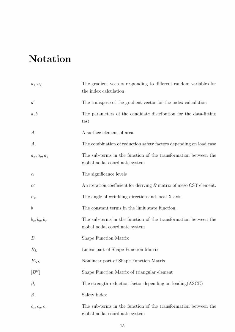
Notation
a1, a2 The gradient vectors responding to different random variables for
the index calculation
at The transpose of the gradient vector for the index calculation
a, b The parameters of the candidate distribution for the data-fitting
test.
A A surface element of area
Ai The combination of reduction safety factors depending on load case
ax, ay, az The sub-terms in the function of the transformation between the
global nodal coordinate system
α The significance levels
αc An iteration coefficient for deriving B matrix of meso CST element.
αw The angle of wrinkling direction and local X axis
b The constant terms in the limit state function.
bx, by, bz The sub-terms in the function of the transformation between the
global nodal coordinate system
B Shape Function Matrix
BL Linear part of Shape Function Matrix
BNL Nonlinear part of Shape Function Matrix
[Btr] Shape Function Matrix of triangular element
βs The strength reduction factor depending on loading(ASCE)
β Safety index
cx, cy, cz The sub-terms in the function of the transformation between the
global nodal coordinate system
15
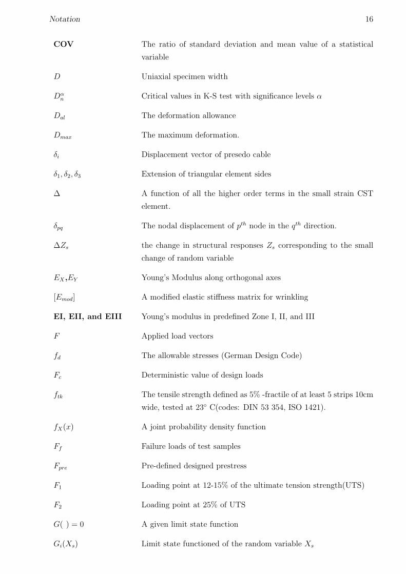
Notation 16
COV The ratio of standard deviation and mean value of a statistical
variable
D Uniaxial specimen width
Dαn Critical values in K-S test with significance levels α
Dal The deformation allowance
Dmax The maximum deformation.
δi Displacement vector of presedo cable
δ1, δ2, δ3 Extension of triangular element sides
∆ A function of all the higher order terms in the small strain CST
element.
δpq The nodal displacement of pth node in the qth direction.
∆Zs the change in structural responses Zs corresponding to the small
change of random variable
EX,EY Young’s Modulus along orthogonal axes
[Emod] A modified elastic stiffness matrix for wrinkling
EI, EII, and EIII Young’s modulus in predefined Zone I, II, and III
F Applied load vectors
fd The allowable stresses (German Design Code)
Fc Deterministic value of design loads
ftk The tensile strength defined as 5% -fractile of at least 5 strips 10cm
wide, tested at 23 C(codes: DIN 53 354, ISO 1421).
fX(x) A joint probability density function
Ff Failure loads of test samples
Fpre Pre-defined designed prestress
F1 Loading point at 12-15% of the ultimate tension strength(UTS)
F2 Loading point at 25% of UTS
G( ) = 0 A given limit state function
Gi(Xs) Limit state functioned of the random variable Xs
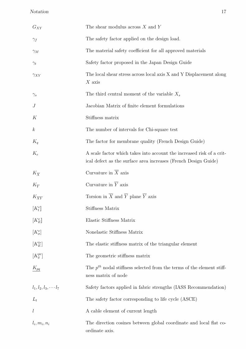
Notation 17
GXY The shear modulus across X and Y
γf The safety factor applied on the design load.
γM The material safety coefficient for all approved materials
γt Safety factor proposed in the Japan Design Guide
γXY The local shear stress across local axis X and Y Displacement along
X axis
γs The third central moment of the variable Xs
J Jacobian Matrix of finite element formulations
K Stiffness matrix
k The number of intervals for Chi-square test
Kq The factor for membrane quality (French Design Guide)
Ke A scale factor which takes into account the increased risk of a crit-
ical defect as the surface area increases (French Design Guide)
KX Curvature in X axis
KY Curvature in Y axis
KXY Torsion in X and Y plane Y axis
[Ket ] Stiffness Matrix
[KeE] Elastic Stiffness Matrix
[Keσ] Nonelastic Stiffness Matrix
[KtrE ] The elastic stiffness matrix of the triangular element
[Kpcδ ] The geometric stiffness matrix
Kpq The pth nodal stiffness selected from the terms of the element stiff-
ness matrix of node
l1, l2, l3, · · · l7 Safety factors applied in fabric strengths (IASS Recommendation)
Lt The safety factor corresponding to life cycle (ASCE)
l A cable element of current length
li,mi, ni The direction cosines between global coordinate and local flat co-
ordinate axis.
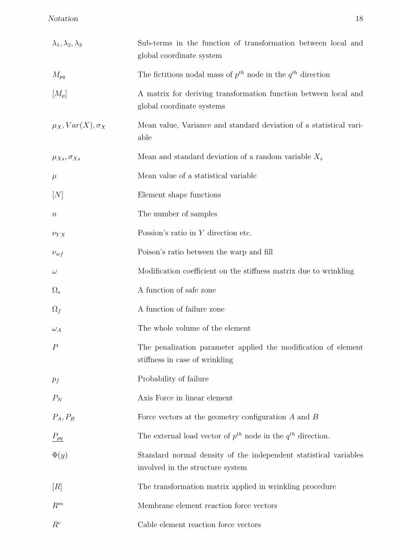
Notation 18
λ1, λ2, λ3 Sub-terms in the function of transformation between local and
global coordinate system
Mpq The fictitious nodal mass of pth node in the qth direction
[Mp] A matrix for deriving transformation function between local and
global coordinate systems
µX , V ar(X), σX Mean value, Variance and standard deviation of a statistical vari-
able
µXs, σXs Mean and standard deviation of a random variable Xs
µ Mean value of a statistical variable
[N ] Element shape functions
n The number of samples
νY X Possion’s ratio in Y direction etc.
νwf Poison’s ratio between the warp and fill
ω Modification coefficient on the stiffness matrix due to wrinkling
Ωs A function of safe zone
Ωf A function of failure zone
ωA The whole volume of the element
P The penalization parameter applied the modification of element
stiffness in case of wrinkling
pf Probability of failure
PN Axis Force in linear element
PA, PB Force vectors at the geometry configuration A and B
Ppq The external load vector of pth node in the qth direction.
Φ(y) Standard normal density of the independent statistical variables
involved in the structure system
[R] The transformation matrix applied in wrinkling procedure
Rm Membrane element reaction force vectors
Rc Cable element reaction force vectors
Notation 19
Rpq The out-of-balance nodal force (or residual) of pth node in the qth
direction
Sf The security factor depending on level of pollution/environment
degradation (French Design Guide)
Sn(Xs), F (Xs) Judgement functions for K-S test
σ A surface element of isotropic stress
σI Maximum element principal stress
σII Minimum element principal stress
σX Element Stress along X axis
σY Element Stress along Y axis
σi Element strains in presedo cable
σn The normal stress
σI , σ11 The max element principal stress
σII , σ22 The minimum element principal stress
σult Ultimate uniaxial stress of a test sample
σ0 Stress vectors from the pretension
σE Stress vectors from the elastic deformation
σfper Permissible stress in the fill direction
σwper Permissible stress in the warp direction
σfmax Maximum stress in the fill direction
σwmax Maximum stress in the warp direction
σfult Ultimate fill strength
σwult Ultimate warp strength
σpmin Minimum principal membrane stress
σpper A predefined lower limit of membrane stresses
σs Standard derivation of a statistical variable
T Cable element tension
Notation 20
[T ] Transformation Matrix
Tp The permissible stress of a coated woven fabric (French Design
Guide)
Tsm The specified minimum breaking strength (French Design Guide)
Tsw Minimum breaking strengths in warp.
Tsf Minimum breaking strengths in weft.
T1, T2, T3 The element side force
Tc1, Tc2, Tc3 The pseudo cable element forces
[T1] The transformation matrix between the global and local flat coor-
dinate systems
[T2] The transformation matrix between the local flat and local curved
coordinate spaces
TN Axis tension force in presedo cable
t, t∗ Nearest point coordinate vector of the limit state surface in the
standard normal space.
tload The ratio of applied load F and deterministic load Fc
Tc The linear element force vector
T c Transformation vector for cable elements
τXY Element Shear Stress between X and Y axis
θp The angle between wrinkle direction and local X axis
θXs The skewness coefficient of the variable Xs
Ud The nodal displacements in local coordinate system
ud The nodal displacements in global coordinate system
u , v , w Displacements separately along x , y , z axis in global coordinate
system
U , V ,W Displacements along X ,Y , Z axis in Local curved coordinate
system
U , V ,W Displacements along X ,Y , Z axis in Local Plane coordinate sys-
tem

Notation 21
uA, uB Displacements at the geometry configuration A and B
εX Stress along local axis X
εY Stress along local axis Y
εI , ε11 The max element principal strain
εII , ε22 The minimum element principal strain
V ar(Xs) The variance of the random variable Xs
Xs Statistical variables
Xs1, Xs2, Xs3, · · · , Xs7 Defined random variables for a reliability analysis
x , y , z Coordinate in Global coordinate system
X ,Y , Z Coordinate in Local curved coordinate system
X ,Y , Z Coordinate in Local plane coordinate system
xi, yi, zi The global nodal coordinates of ith node.
xp, yp, zp The global coordinates of a single point p along the local Y axis
−→X ,
−→Y ,
−→Z The vectors representing the local flat coordinate axes
Xs Statistical random variables
x∗s The minimum distance point on the limit state surface in the orig-
inal coordinate system
x′∗s The minimum distance point on the limit state surface in the re-
duced coordinate system.
ξ1 , ξ2 , ξ3 Coordinates in the Local Area coordinated system
Zs The structural response variables

Chapter 1
Introduction
1.1 Background
Ancient fabric structures in the form of tents(fig.1.1) have existed for thousands of years.
Most structures of this types were designed and constructed for temporary use. Ancient fabric
structures may have been constructed and erected from a variety of basic materials such as
cloth, animal skins forming the membrane, ropes and tree branches, for example forming the
other structural components. The reliability of such structures was comparatively low when
subject to environmental loading.
Figure 1.1: Henry Keene’s design for a Turkish Kent (c1755), as used for the re-constructionat Painshill
22
CHAPTER 1. INTRODUCTION 23
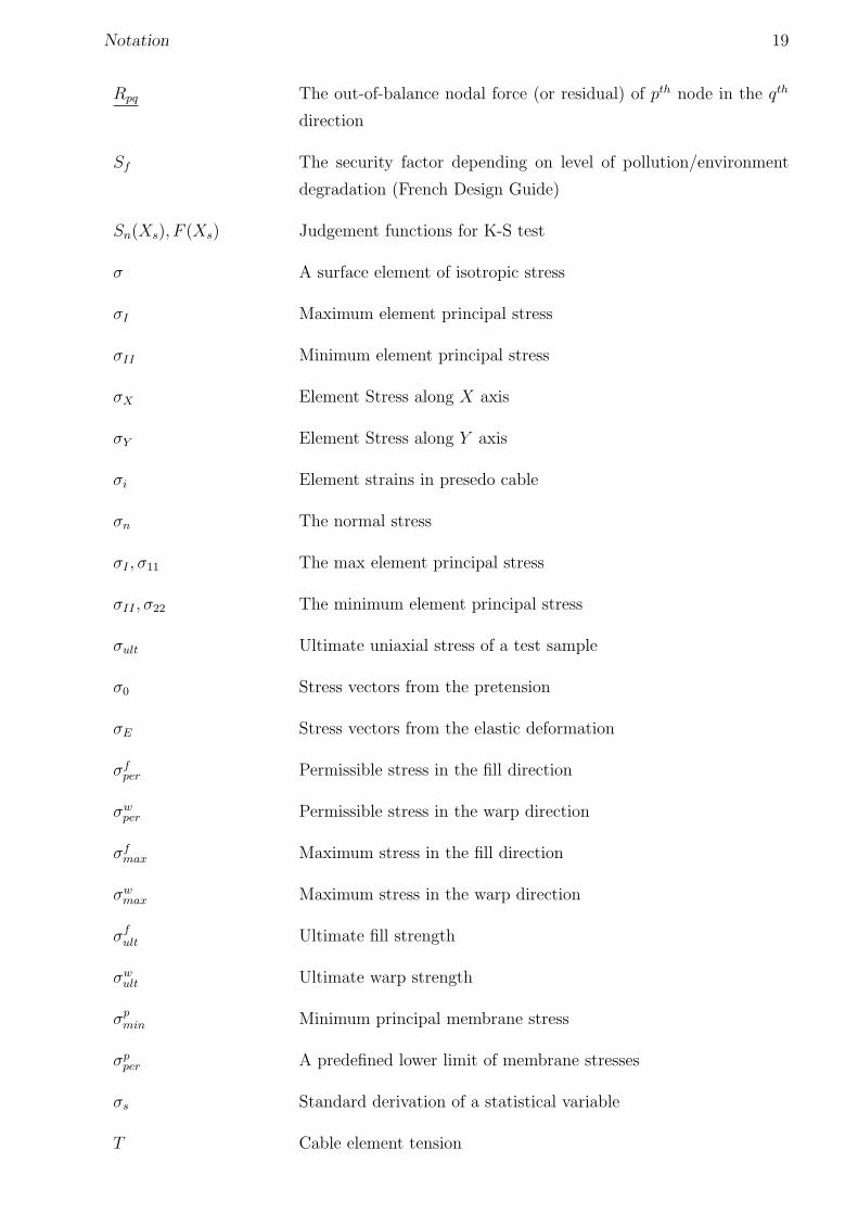
Modern fabric structures(fig.1.2-1.4) designed for permanent purposes have been developed
with increasing popularity since the 1950s. Compared with ancient fabric forms, higher re-
quirements in both aesthetics and structural stability must be satisfied in modern fabric
structures. The key mechanism to achieve the increased performance is correct generation of
tensile forces to induce smooth geometries. In this way, the modern fabric structures are also
called tensile structures.
Fabric materials have little compression or bending stiffness. They are, therefore, prone to
fold and wrinkle under external forces when not adequately tensioned by pretension. The
applied pretension stresses can largely improve the stability and stiffness of the fabric surface,
and the negative strain produced by loads can be compensated by the initial positive strain
due to pretensions.
Figure 1.2: Student Center (University of La Verne) La Verne, California, USA, 1973
CHAPTER 1. INTRODUCTION 24
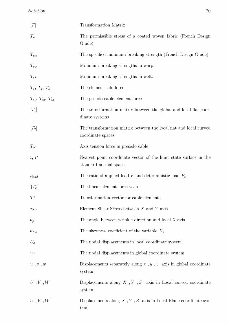
Figure 1.3: Price Waterhouse - Cooper building, Brussels,2003
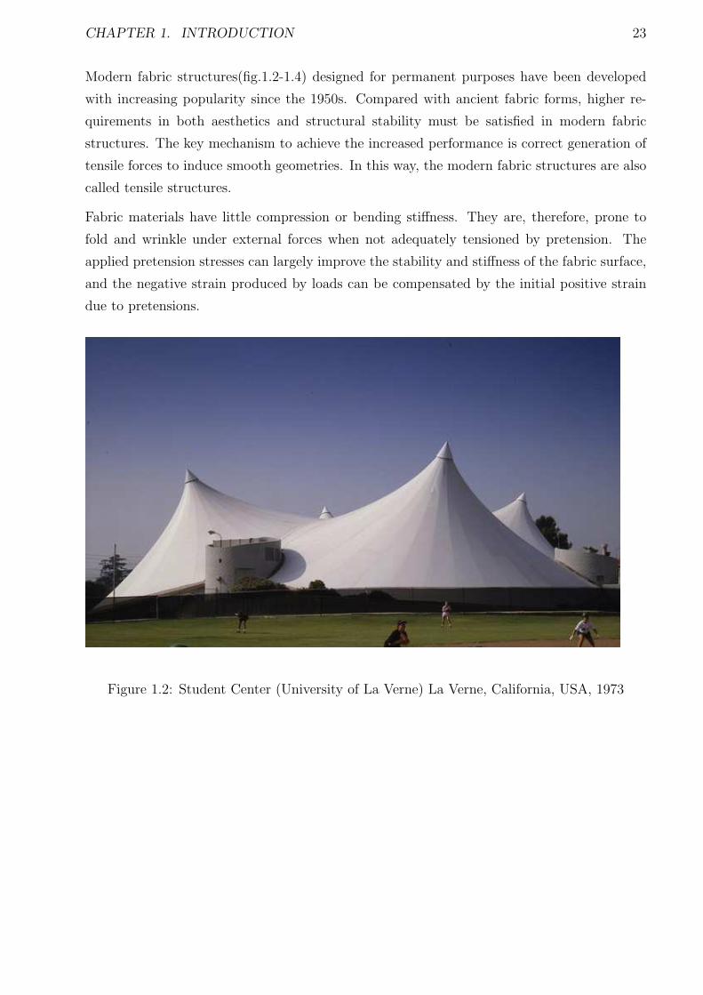
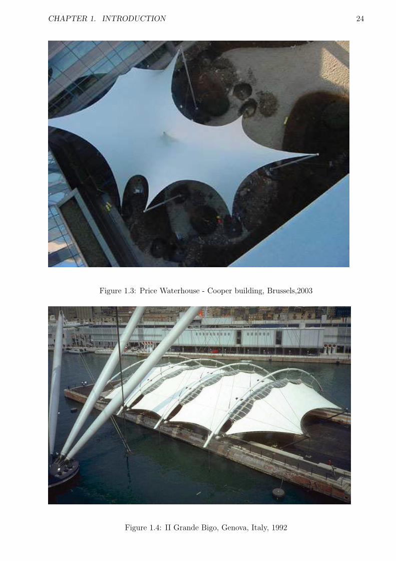
Figure 1.4: II Grande Bigo, Genova, Italy, 1992
CHAPTER 1. INTRODUCTION 25
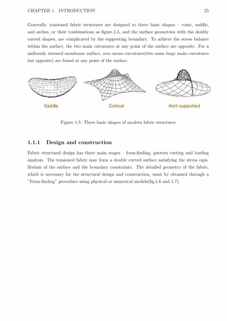
Generally, tensioned fabric structures are designed to three basic shapes – conic, saddle,
and arches, or their combinations as figure.1.5, and the surface geometries with the doubly
curved shapes, are complicated by the supporting boundary. To achieve the stress balance
within the surface, the two main curvatures at any point of the surface are opposite. For a
uniformly stressed membrane surface, zero mean curvatures(two same large main curvatures
but opposite) are found at any point of the surface.
Figure 1.5: Three basic shapes of modern fabric structures
1.1.1 Design and construction
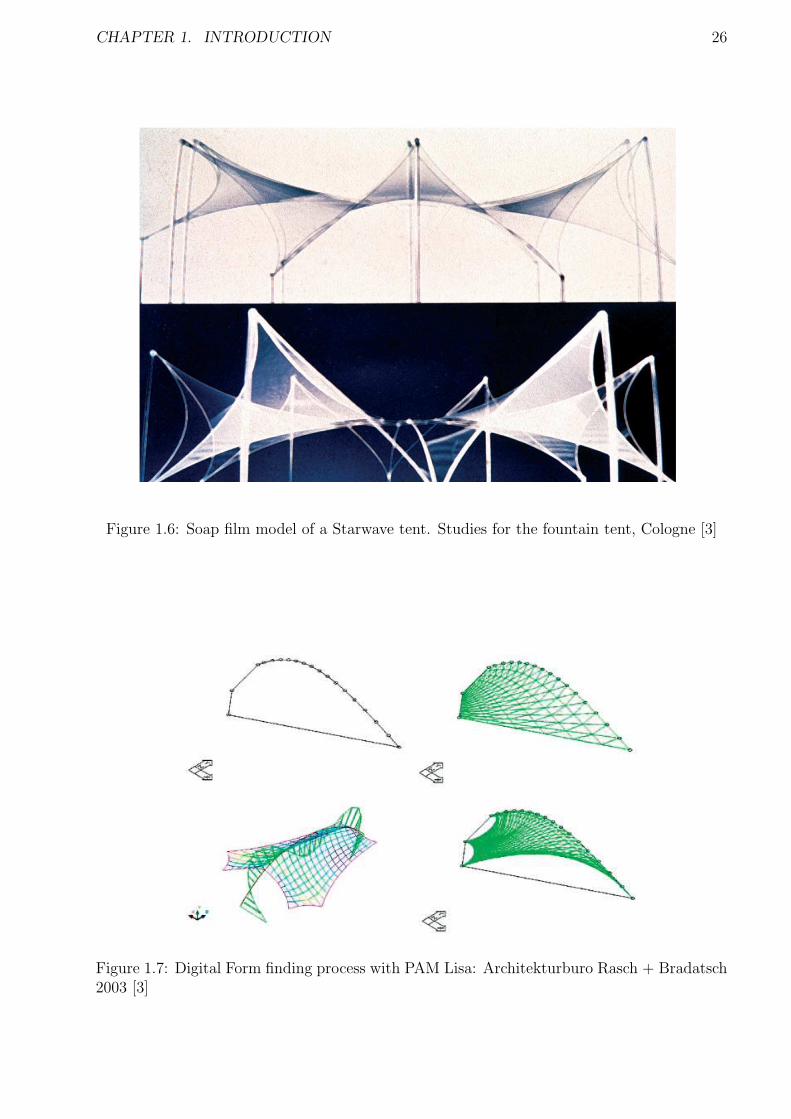
Fabric structural design has three main stages – form-finding, pattern cutting and loading
analysis. The tensioned fabric may form a double curved surface satisfying the stress equi-
librium of the surface and the boundary constraints. The detailed geometry of the fabric,
which is necessary for the structural design and construction, must be obtained through a
”Form-finding” procedure using physical or numerical models(fig.1.6 and 1.7).
CHAPTER 1. INTRODUCTION 26
Figure 1.6: Soap film model of a Starwave tent. Studies for the fountain tent, Cologne [3]
Figure 1.7: Digital Form finding process with PAM Lisa: Architekturburo Rasch + Bradatsch2003 [3]
CHAPTER 1. INTRODUCTION 27
After the initial shape of fabric structures is obtained by assuming the initial in-plane tension
force, which is an ideal form presented by the designer at the first stage of design, these shapes
have to be achieved by practical construction approaches – patterning and sewing of fabrics.
Also, the fabric has limitations for width and length due to its material characteristic from
manufacture. Therefore, the 3-D initial shapes have to be divided into several 2-D plane strips
for construction of the so-called cutting pattern.
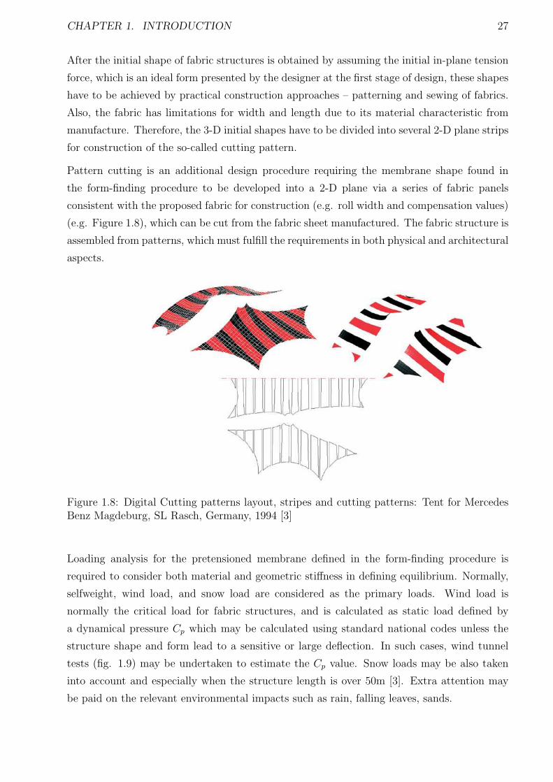
Pattern cutting is an additional design procedure requiring the membrane shape found in
the form-finding procedure to be developed into a 2-D plane via a series of fabric panels
consistent with the proposed fabric for construction (e.g. roll width and compensation values)
(e.g. Figure 1.8), which can be cut from the fabric sheet manufactured. The fabric structure is
assembled from patterns, which must fulfill the requirements in both physical and architectural
aspects.
Figure 1.8: Digital Cutting patterns layout, stripes and cutting patterns: Tent for MercedesBenz Magdeburg, SL Rasch, Germany, 1994 [3]
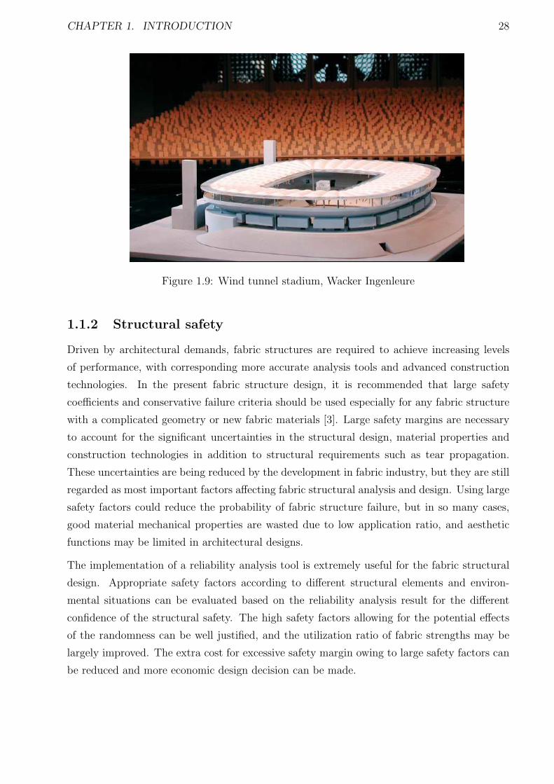
Loading analysis for the pretensioned membrane defined in the form-finding procedure is
required to consider both material and geometric stiffness in defining equilibrium. Normally,
selfweight, wind load, and snow load are considered as the primary loads. Wind load is
normally the critical load for fabric structures, and is calculated as static load defined by
a dynamical pressure Cp which may be calculated using standard national codes unless the
structure shape and form lead to a sensitive or large deflection. In such cases, wind tunnel
tests (fig. 1.9) may be undertaken to estimate the Cp value. Snow loads may be also taken
into account and especially when the structure length is over 50m [3]. Extra attention may
be paid on the relevant environmental impacts such as rain, falling leaves, sands.
CHAPTER 1. INTRODUCTION 28
Figure 1.9: Wind tunnel stadium, Wacker Ingenleure
1.1.2 Structural safety
Driven by architectural demands, fabric structures are required to achieve increasing levels
of performance, with corresponding more accurate analysis tools and advanced construction
technologies. In the present fabric structure design, it is recommended that large safety
coefficients and conservative failure criteria should be used especially for any fabric structure
with a complicated geometry or new fabric materials [3]. Large safety margins are necessary
to account for the significant uncertainties in the structural design, material properties and
construction technologies in addition to structural requirements such as tear propagation.
These uncertainties are being reduced by the development in fabric industry, but they are still
regarded as most important factors affecting fabric structural analysis and design. Using large
safety factors could reduce the probability of fabric structure failure, but in so many cases,
good material mechanical properties are wasted due to low application ratio, and aesthetic
functions may be limited in architectural designs.
The implementation of a reliability analysis tool is extremely useful for the fabric structural
design. Appropriate safety factors according to different structural elements and environ-
mental situations can be evaluated based on the reliability analysis result for the different
confidence of the structural safety. The high safety factors allowing for the potential effects
of the randomness can be well justified, and the utilization ratio of fabric strengths may be
largely improved. The extra cost for excessive safety margin owing to large safety factors can
be reduced and more economic design decision can be made.
CHAPTER 1. INTRODUCTION 29
1.2 Aim and objectives
The aim of this research is to produce an analysis system that couples a high fidelity com-
putational tool with material structure uncertainty in an integrated system for design. The
structural reliability work can be divided into three parts. The first part is to develop an
efficient structural analysis tool for fabric structures as a computational engine for the reli-
ability calculation. This part is extremely important for the reliability frame work, because
a reliability calculation may include a large quantity of structural analysis. The efficiency of
the reliability work may be largely dependent on the structural analysis formulation.
The second part aims at the applicable methodology of the measurement and analysis of the
uncertainties in fabric material properties relevant to the structural design and analysis. Innu-
merate design variables (e.g. loading, construction quality) may be involved in a full reliability
analysis. The investigation of the randomness in fabric materials is urgently demanded and
primary for fabric structures. The statistical information of other random variables general
for common structures may have been investigated and possibly available from the published
data.
The third is the reliability estimation corresponding the uncertainty information. This part
focuses on developing an efficient reliability tool allowing for characteristics of fabric struc-
tures.
Specific objectives are to:
• formulate an efficient finite element for fabric structure analysis.
• develop a Fortran 95 finite element program for fabric structure analysis.
• establish a probabilistic measurement and analysis methodology for fabric material prop-
erties
• implement a reliability-based analysis theory combining material uncertainty and a
quadratic finite element approximation
• develop a Fortran 95 program to estimate the reliability of the fabric structures.
• propose a procedure to examine the current used safety factors and to provide appro-
priate safety indices.
1.3 Scope
This first part of this research focus on finite-element based deterministic modelling and
analysis including form-finding, loading analysis.
CHAPTER 1. INTRODUCTION 30
The second part is concerned with the development of a probabilistic analysis methodology
for fabric material uncertainties based on experimental data. An existing analysis theory is
adopted and implemented.
Other uncertainty types like loading, pollution, and other material tests are not within the
scope of this research.
The reliability formulation combines the first order reliability method and the finite element
formulation recommended by the first part of this research, with a limited number of uncer-
tainty input like loads, strength and Young’s modulus. The high order reliability formulations
and other uncertainties(e.g. loading, pollution, construction quality, work skills) are not within
the scope of this research.
1.4 Thesis structure
Chapter 2 – Literature Review. States the fabric design principle currently used,
and demonstrates the importance of developing a reliability tool for the safety estima-
tion. The approaches on fabric structural modelling, probabilistic material properties,
reliability methodologies are reviewed.
Chapter 3 – Finite Element Formulation For Fabric Structures. To develop a
high efficiency structural analysis tool, four types of different finite element formulations
coupled with different solution algorithms have been introduced and compared. An
appropriate finite element formulation is concluded for the reliability analysis.
Chapter 4 – Probabilistic Properties of Structural Fabric. A probabilistic analysis
methodology including data-based uncertainty collection and mathematical presentation
of the mechanical property of fabrics is proposed.
Chapter 5 – Reliability Analysis of Fabric Structures. A reliability formulation
combining the finite element method proposed in Chapter 3 and one classical reliability
formulation, is developed. Using this formulation, the safety of a given fabric structure
can be evaluated, and appropriate safety factors can be estimated.
Chapter 6 – Conclusion Summary of the conclusions of each chapter, and recommen-
dations are made for further work.
Bibliography – The latex bibliography system is used for all the reference papers and
books.
Appendix – All test data, basic knowledge of statistical distributions, part derivatives of
reliability formulations, and a guide to Fortran programs developed within the research.
Chapter 2
Literature Review
2.1 A probabilistic approach to the analysis of fabric
structures
Currently the design of fabric structures varies at international level, typically through the
application of safety factors. In this section, the potential of a reliability analysis tool to
estimate safety factors is demonstrated, based on the principles of the structural safety given
in Eurocode 0.
For a designer, safety factors are decided based on two aspects: (1) uncertainties of the
human actions, material properties and the corresponding environment impacts. (2) Limited
knowledge of the designer to predict the physical behavior of all the relevant quantities. ”With
development in science and technology, the element of ignorance can be largely eliminated,
while the uncertainties, being changed in the form and magnitude, can never be removed”
[29]. Especially in the case of advanced material developments and new structured forms,
the problem of uncertainties are considered using the statistical investigation and stochastic
analysis for safe and economic design.
Engineering groups in different countries have adopted a variety of safety coefficients which are
derived using a nember of approaches. Most of these approaches are based on the permissible
stress method instead of the limit state method used in the current traditional structures like
steel and concrete, due to the highly nonlinear-geometrical behaviour of fabric structures. A
series of uncertainties potentially exist in fabric structure design and construction, and are
taken into account via a range of safety factors. However these safety coefficients contain
difference and uncertainties.
The European Design Guide for Tensile Structures [3] summarizes the design methods and
safety calculation approaches currently used as outlined below,
IASS Recommendation [5] :
IASS working group 7 recommendations propose a safety estimation approach for air-supported
31
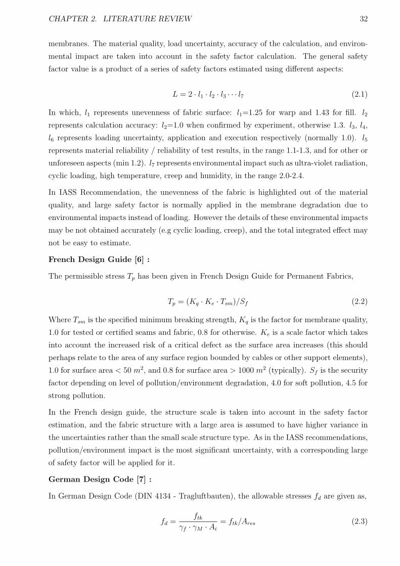
CHAPTER 2. LITERATURE REVIEW 32
membranes. The material quality, load uncertainty, accuracy of the calculation, and environ-
mental impact are taken into account in the safety factor calculation. The general safety
factor value is a product of a series of safety factors estimated using different aspects:
L = 2 · l1 · l2 · l3 · · · l7 (2.1)
In which, l1 represents unevenness of fabric surface: l1=1.25 for warp and 1.43 for fill. l2
represents calculation accuracy: l2=1.0 when confirmed by experiment, otherwise 1.3. l3, l4,
l6 represents loading uncertainty, application and execution respectively (normally 1.0). l5
represents material reliability / reliability of test results, in the range 1.1-1.3, and for other or
unforeseen aspects (min 1.2). l7 represents environmental impact such as ultra-violet radiation,
cyclic loading, high temperature, creep and humidity, in the range 2.0-2.4.
In IASS Recommendation, the unevenness of the fabric is highlighted out of the material
quality, and large safety factor is normally applied in the membrane degradation due to
environmental impacts instead of loading. However the details of these environmental impacts
may be not obtained accurately (e.g cyclic loading, creep), and the total integrated effect may
not be easy to estimate.
French Design Guide [6] :
The permissible stress Tp has been given in French Design Guide for Permanent Fabrics,
Tp = (Kq ·Ke · Tsm)/Sf (2.2)
Where Tsm is the specified minimum breaking strength, Kq is the factor for membrane quality,
1.0 for tested or certified seams and fabric, 0.8 for otherwise. Ke is a scale factor which takes
into account the increased risk of a critical defect as the surface area increases (this should
perhaps relate to the area of any surface region bounded by cables or other support elements),
1.0 for surface area < 50 m2, and 0.8 for surface area > 1000 m2 (typically). Sf is the security
factor depending on level of pollution/environment degradation, 4.0 for soft pollution, 4.5 for
strong pollution.
In the French design guide, the structure scale is taken into account in the safety factor
estimation, and the fabric structure with a large area is assumed to have higher variance in
the uncertainties rather than the small scale structure type. As in the IASS recommendations,
pollution/environment impact is the most significant uncertainty, with a corresponding large
of safety factor will be applied for it.
German Design Code [7] :
In German Design Code (DIN 4134 - Tragluftbauten), the allowable stresses fd are given as,
fd =ftk
γf · γM · Ai
= ftk/Ares (2.3)
CHAPTER 2. LITERATURE REVIEW 33
Where ftk is the tensile strength defined as 5% -fractile of at least 5 strips 10cm wide, tested
at 23 C(codes: DIN 53 354, ISO 1421). (Alternatively, from Minte, 0.868 × mean tensile
strength for the fabric or 0.802 × mean strength for/near the seams. γf is the load factor.
γM is the material safety coefficient for all approved materials: γM = 1.4 within the fabric
surface, or 1.5 for connections. Ai is the combination of reduction factors depending on load
case.
The safety factor of fabric structures in German Design Code combines the traditional load
factor γf and the other coefficient allowing for the specific uncertainties for membrane. That
means the total safety coefficient varies with different load combinations. In this code, the
connection detail is specified as an important aspect with a relevant high partial safety coef-
ficients.
Italian Design Code [8] :
”The safety factors applied in the fabric structures in Italian Design Code are similar to the
German Code [3]”, but more detail is provided related to the connections. Generally, three
classes of connections are defined;
• ”1st class - connections designed and fabricated by licensed personnel using methodolo-
gies defined (that characterise all the parameters and work conditions) by the coated
fabric manufacturer or from the membrane fabricator and tested by the membrane fab-
ricator.”
• ”2nd class - connections analysed by licensed personnel using methodologies defined
(that characterise all the parameters and work conditions) by the coated fabric manu-
facturer or from the membrane fabricator and not tested by the membrane fabricator.”
• ”3rd class - connections, however designed and fabricated, permitted exclusively for the
realisation of secondary elements or sealing.”
Different connection classes are allowed in different structures. For example, 1st and 2nd
connectors can be used in tents having a primary load bearing textile structure connection,
while only 1st can be used in membranes. As such this regulation can guarantee the connection
quality of the membrane, and enhance the reliability of the membrane. When the similar safety
coefficients are applied with the qualified connections, Italian Design Code can achieve better
structural safety compared with German Design Guide.
Japan Design Guide [1] :
In Japanese design guide , the safety factors are calculated based on the load types and
the structure types, while other aspects like material reliability, environment impact are not
specified. The permissible stress is
fs = Tsm/γt (2.4)
CHAPTER 2. LITERATURE REVIEW 34
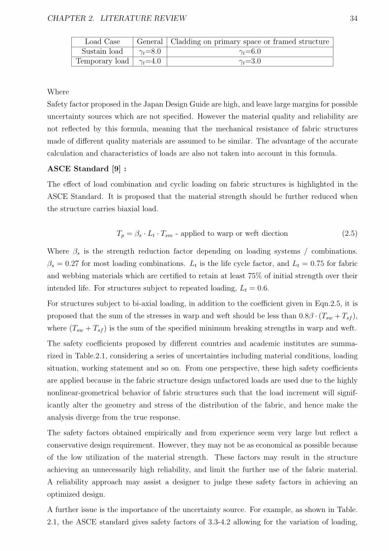
Load Case General Cladding on primary space or framed structureSustain load γt=8.0 γt=6.0
Temporary load γt=4.0 γt=3.0
Where
Safety factor proposed in the Japan Design Guide are high, and leave large margins for possible
uncertainty sources which are not specified. However the material quality and reliability are
not reflected by this formula, meaning that the mechanical resistance of fabric structures
made of different quality materials are assumed to be similar. The advantage of the accurate
calculation and characteristics of loads are also not taken into account in this formula.
ASCE Standard [9] :
The effect of load combination and cyclic loading on fabric structures is highlighted in the
ASCE Standard. It is proposed that the material strength should be further reduced when
the structure carries biaxial load.
Tp = βs · Lt · Tsm - applied to warp or weft diection (2.5)
Where βs is the strength reduction factor depending on loading systems / combinations.
βs = 0.27 for most loading combinations. Lt is the life cycle factor, and Lt = 0.75 for fabric
and webbing materials which are certified to retain at least 75% of initial strength over their
intended life. For structures subject to repeated loading, Lt = 0.6.
For structures subject to bi-axial loading, in addition to the coefficient given in Eqn.2.5, it is
proposed that the sum of the stresses in warp and weft should be less than 0.8β · (Tsw + Tsf ),
where (Tsw + Tsf ) is the sum of the specified minimum breaking strengths in warp and weft.
The safety coefficients proposed by different countries and academic institutes are summa-
rized in Table.2.1, considering a series of uncertainties including material conditions, loading
situation, working statement and so on. From one perspective, these high safety coefficients
are applied because in the fabric structure design unfactored loads are used due to the highly
nonlinear-geometrical behavior of fabric structures such that the load increment will signif-
icantly alter the geometry and stress of the distribution of the fabric, and hence make the
analysis diverge from the true response.
The safety factors obtained empirically and from experience seem very large but reflect a
conservative design requirement. However, they may not be as economical as possible because
of the low utilization of the material strength. These factors may result in the structure
achieving an unnecessarily high reliability, and limit the further use of the fabric material.
A reliability approach may assist a designer to judge these safety factors in achieving an
optimized design.
A further issue is the importance of the uncertainty source. For example, as shown in Table.
2.1, the ASCE standard gives safety factors of 3.3-4.2 allowing for the variation of loading,
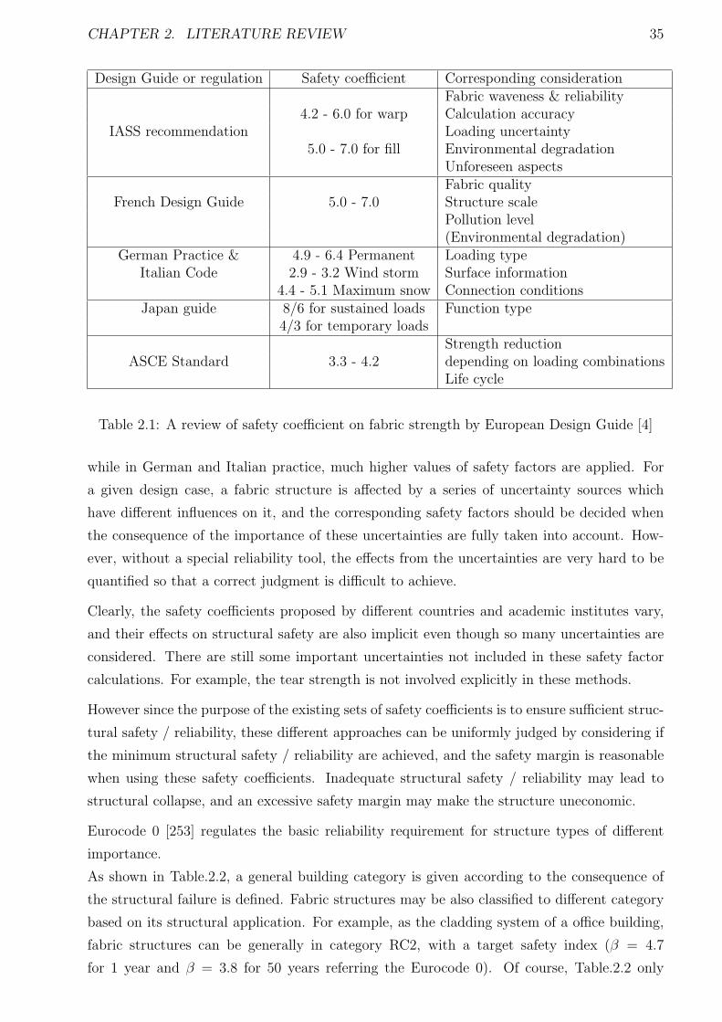
CHAPTER 2. LITERATURE REVIEW 35
Design Guide or regulation Safety coefficient Corresponding considerationFabric waveness & reliability
4.2 - 6.0 for warp Calculation accuracyIASS recommendation Loading uncertainty
5.0 - 7.0 for fill Environmental degradationUnforeseen aspectsFabric quality
French Design Guide 5.0 - 7.0 Structure scalePollution level(Environmental degradation)
German Practice & 4.9 - 6.4 Permanent Loading typeItalian Code 2.9 - 3.2 Wind storm Surface information
4.4 - 5.1 Maximum snow Connection conditionsJapan guide 8/6 for sustained loads Function type
4/3 for temporary loadsStrength reduction
ASCE Standard 3.3 - 4.2 depending on loading combinationsLife cycle
Table 2.1: A review of safety coefficient on fabric strength by European Design Guide [4]
while in German and Italian practice, much higher values of safety factors are applied. For
a given design case, a fabric structure is affected by a series of uncertainty sources which
have different influences on it, and the corresponding safety factors should be decided when
the consequence of the importance of these uncertainties are fully taken into account. How-
ever, without a special reliability tool, the effects from the uncertainties are very hard to be
quantified so that a correct judgment is difficult to achieve.
Clearly, the safety coefficients proposed by different countries and academic institutes vary,
and their effects on structural safety are also implicit even though so many uncertainties are
considered. There are still some important uncertainties not included in these safety factor
calculations. For example, the tear strength is not involved explicitly in these methods.
However since the purpose of the existing sets of safety coefficients is to ensure sufficient struc-
tural safety / reliability, these different approaches can be uniformly judged by considering if
the minimum structural safety / reliability are achieved, and the safety margin is reasonable
when using these safety coefficients. Inadequate structural safety / reliability may lead to
structural collapse, and an excessive safety margin may make the structure uneconomic.
Eurocode 0 [253] regulates the basic reliability requirement for structure types of different
importance.
As shown in Table.2.2, a general building category is given according to the consequence of
the structural failure is defined. Fabric structures may be also classified to different category
based on its structural application. For example, as the cladding system of a office building,
fabric structures can be generally in category RC2, with a target safety index (β = 4.7
for 1 year and β = 3.8 for 50 years referring the Eurocode 0). Of course, Table.2.2 only
CHAPTER 2. LITERATURE REVIEW 36
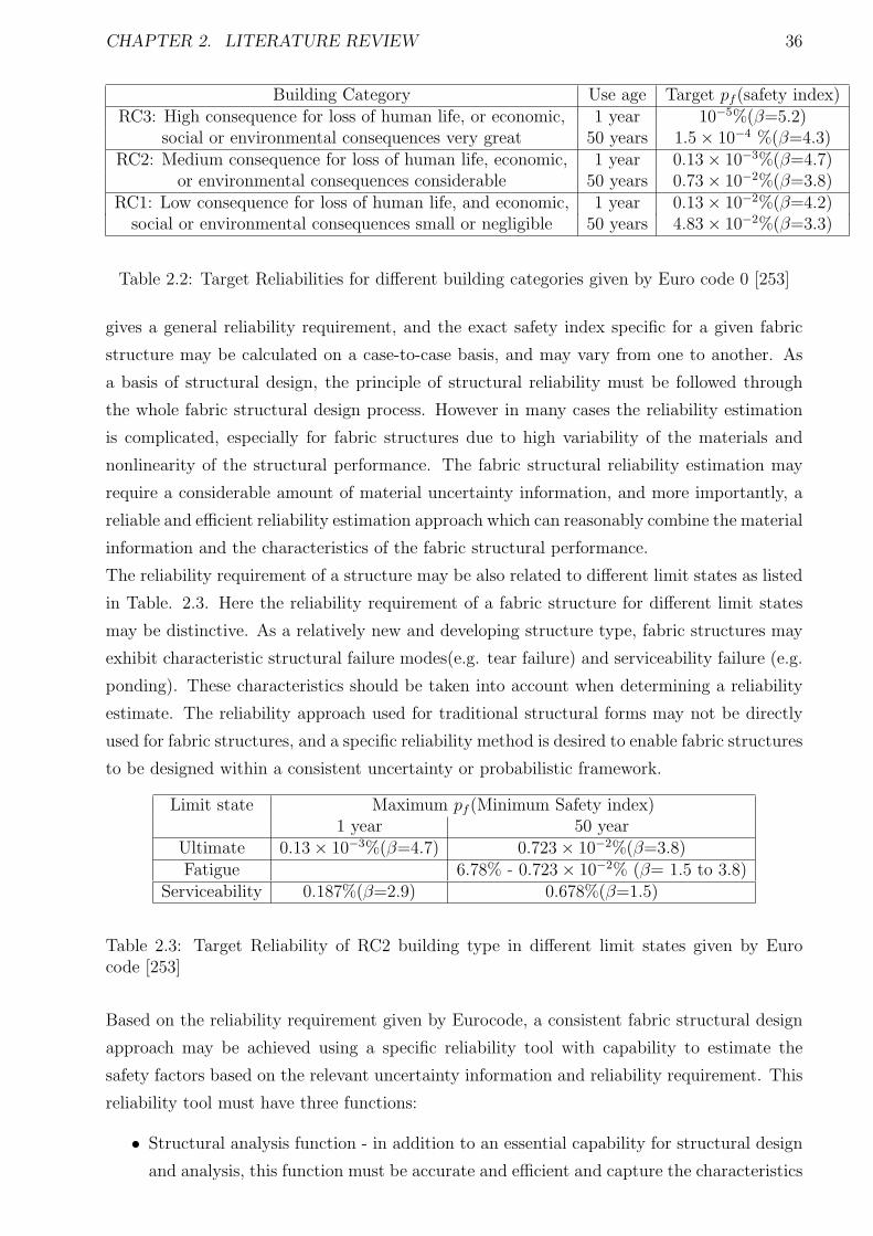
Building Category Use age Target pf (safety index)RC3: High consequence for loss of human life, or economic, 1 year 10−5%(β=5.2)
social or environmental consequences very great 50 years 1.5 × 10⁻⁴ %(β=4.3)RC2: Medium consequence for loss of human life, economic, 1 year 0.13 × 10⁻³%(β=4.7)
or environmental consequences considerable 50 years 0.73 × 10⁻²%(β=3.8)RC1: Low consequence for loss of human life, and economic, 1 year 0.13 × 10⁻²%(β=4.2)
social or environmental consequences small or negligible 50 years 4.83 × 10⁻²%(β=3.3)
Table 2.2: Target Reliabilities for different building categories given by Euro code 0 [253]
gives a general reliability requirement, and the exact safety index specific for a given fabric
structure may be calculated on a case-to-case basis, and may vary from one to another. As
a basis of structural design, the principle of structural reliability must be followed through
the whole fabric structural design process. However in many cases the reliability estimation
is complicated, especially for fabric structures due to high variability of the materials and
nonlinearity of the structural performance. The fabric structural reliability estimation may
require a considerable amount of material uncertainty information, and more importantly, a
reliable and efficient reliability estimation approach which can reasonably combine the material
information and the characteristics of the fabric structural performance.
The reliability requirement of a structure may be also related to different limit states as listed
in Table. 2.3. Here the reliability requirement of a fabric structure for different limit states
may be distinctive. As a relatively new and developing structure type, fabric structures may
exhibit characteristic structural failure modes(e.g. tear failure) and serviceability failure (e.g.
ponding). These characteristics should be taken into account when determining a reliability
estimate. The reliability approach used for traditional structural forms may not be directly
used for fabric structures, and a specific reliability method is desired to enable fabric structures
to be designed within a consistent uncertainty or probabilistic framework.
Limit state Maximum pf (Minimum Safety index)1 year 50 year
Ultimate 0.13 × 10⁻³%(β=4.7) 0.723 × 10⁻²%(β=3.8)Fatigue 6.78% - 0.723 × 10⁻²% (β= 1.5 to 3.8)
Serviceability 0.187%(β=2.9) 0.678%(β=1.5)
Table 2.3: Target Reliability of RC2 building type in different limit states given by Eurocode [253]
Based on the reliability requirement given by Eurocode, a consistent fabric structural design
approach may be achieved using a specific reliability tool with capability to estimate the
safety factors based on the relevant uncertainty information and reliability requirement. This
reliability tool must have three functions:
• Structural analysis function - in addition to an essential capability for structural design
and analysis, this function must be accurate and efficient and capture the characteristics
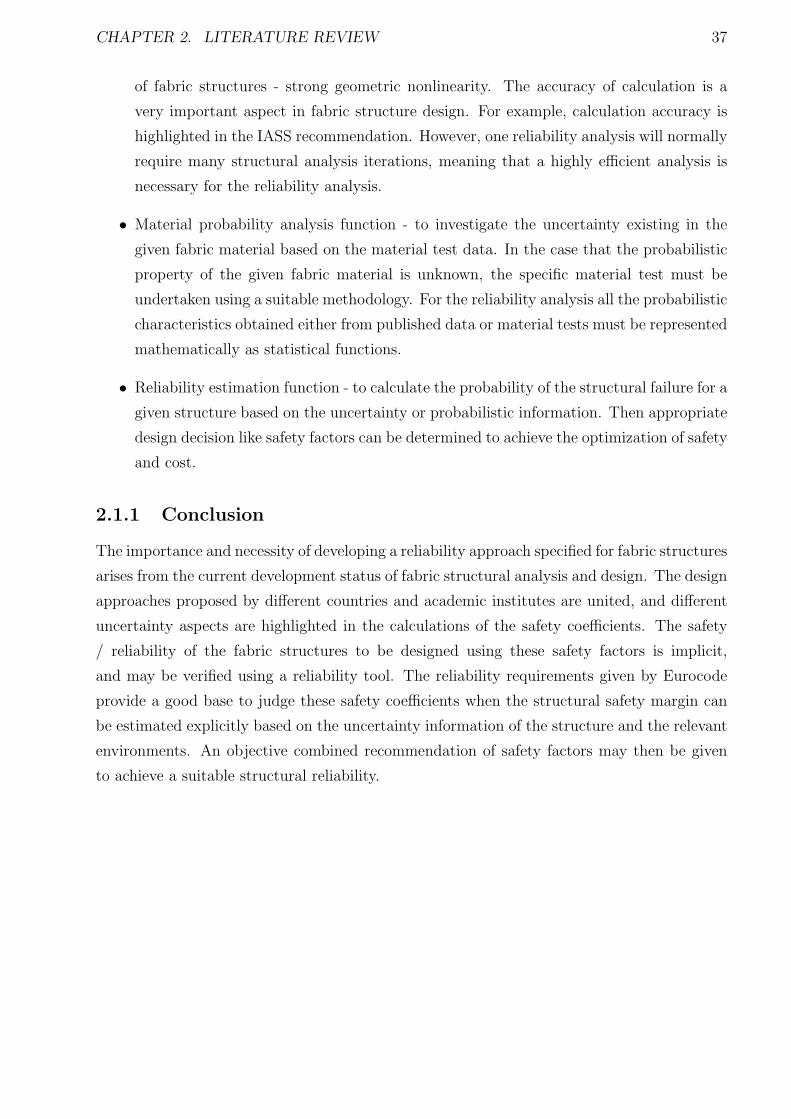
CHAPTER 2. LITERATURE REVIEW 37
of fabric structures - strong geometric nonlinearity. The accuracy of calculation is a
very important aspect in fabric structure design. For example, calculation accuracy is
highlighted in the IASS recommendation. However, one reliability analysis will normally
require many structural analysis iterations, meaning that a highly efficient analysis is
necessary for the reliability analysis.
• Material probability analysis function - to investigate the uncertainty existing in the
given fabric material based on the material test data. In the case that the probabilistic
property of the given fabric material is unknown, the specific material test must be
undertaken using a suitable methodology. For the reliability analysis all the probabilistic
characteristics obtained either from published data or material tests must be represented
mathematically as statistical functions.
• Reliability estimation function - to calculate the probability of the structural failure for a
given structure based on the uncertainty or probabilistic information. Then appropriate
design decision like safety factors can be determined to achieve the optimization of safety
and cost.
2.1.1 Conclusion
The importance and necessity of developing a reliability approach specified for fabric structures
arises from the current development status of fabric structural analysis and design. The design
approaches proposed by different countries and academic institutes are united, and different
uncertainty aspects are highlighted in the calculations of the safety coefficients. The safety
/ reliability of the fabric structures to be designed using these safety factors is implicit,
and may be verified using a reliability tool. The reliability requirements given by Eurocode
provide a good base to judge these safety coefficients when the structural safety margin can
be estimated explicitly based on the uncertainty information of the structure and the relevant
environments. An objective combined recommendation of safety factors may then be given
to achieve a suitable structural reliability.
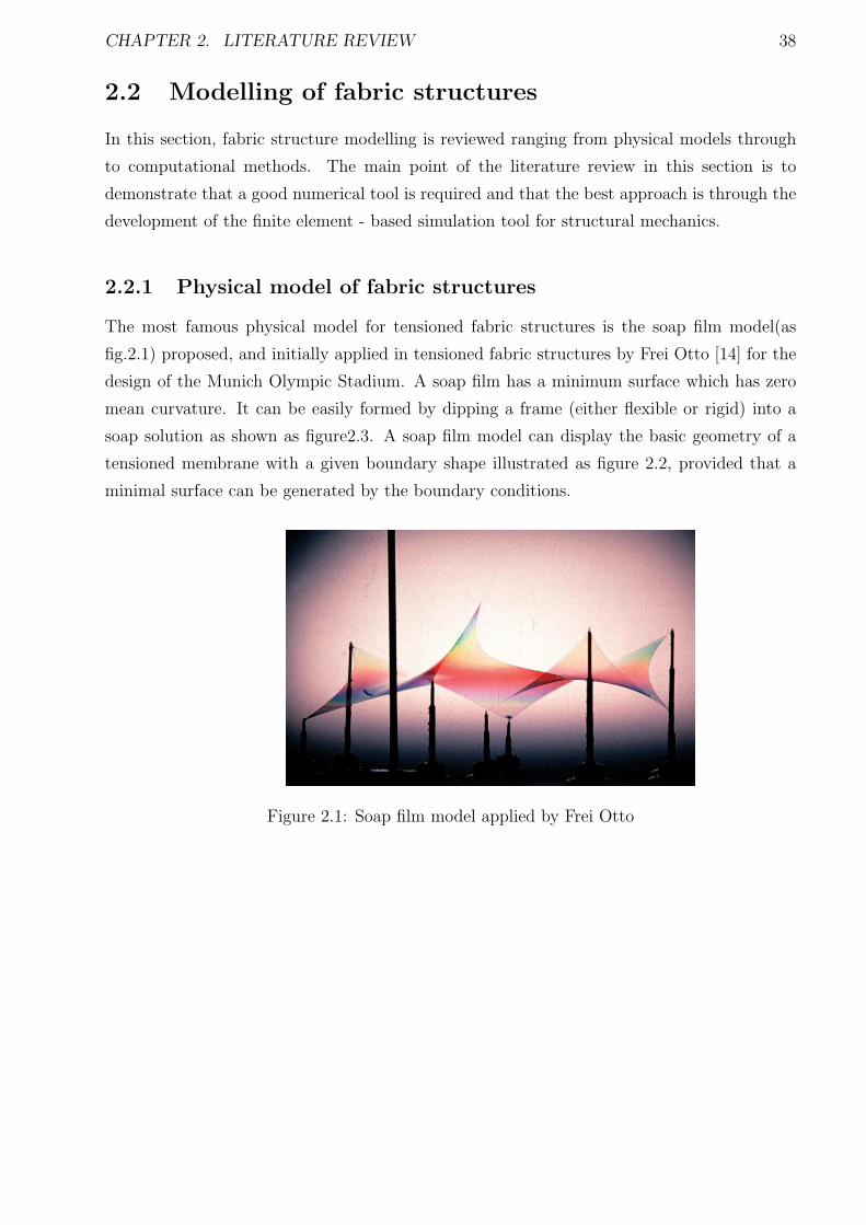
CHAPTER 2. LITERATURE REVIEW 38
2.2 Modelling of fabric structures
In this section, fabric structure modelling is reviewed ranging from physical models through
to computational methods. The main point of the literature review in this section is to
demonstrate that a good numerical tool is required and that the best approach is through the
development of the finite element - based simulation tool for structural mechanics.
2.2.1 Physical model of fabric structures
The most famous physical model for tensioned fabric structures is the soap film model(as
fig.2.1) proposed, and initially applied in tensioned fabric structures by Frei Otto [14] for the
design of the Munich Olympic Stadium. A soap film has a minimum surface which has zero
mean curvature. It can be easily formed by dipping a frame (either flexible or rigid) into a
soap solution as shown as figure2.3. A soap film model can display the basic geometry of a
tensioned membrane with a given boundary shape illustrated as figure 2.2, provided that a
minimal surface can be generated by the boundary conditions.
Figure 2.1: Soap film model applied by Frei Otto
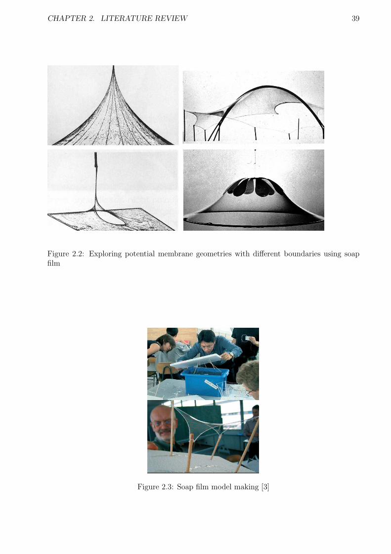
CHAPTER 2. LITERATURE REVIEW 39
Figure 2.2: Exploring potential membrane geometries with different boundaries using soapfilm
Figure 2.3: Soap film model making [3]
CHAPTER 2. LITERATURE REVIEW 40
Physical models may also be used in the development of cutting patterns. Making a small
scale physical model of a fabric structure can help designers to understand how the variety
of curved membrane surfaces are to be created from cutting and joining flat fabric panels. In
current fabric structure design, physical models may be still used. However their use is only
limited normally to the concept design stage [11]. Detailed structural analysis are carried via
numerical models.
2.2.2 Surface representation and structural mechanics
Same as soap films, the uniform stressed membrane will also form minimal surfaces. To
obtain the initial geometry of the stressed membrane, the research on minimal surfaces was
undertaken by Grundig [213]. Because on the minimal surface, two principal curvatures
are equal but opposite sign at any point, the characteristics of the minimal surface can be
expressed using a mathematical formulation. The surface can be arbitrarily discretized into
many small elements (e.g. triangles or quadrangles), then the nodal coordinates will be checked
if the node positions are satisfied the requirement of minimal surfaces, and then updated until
the sum of the element areas is minimized.
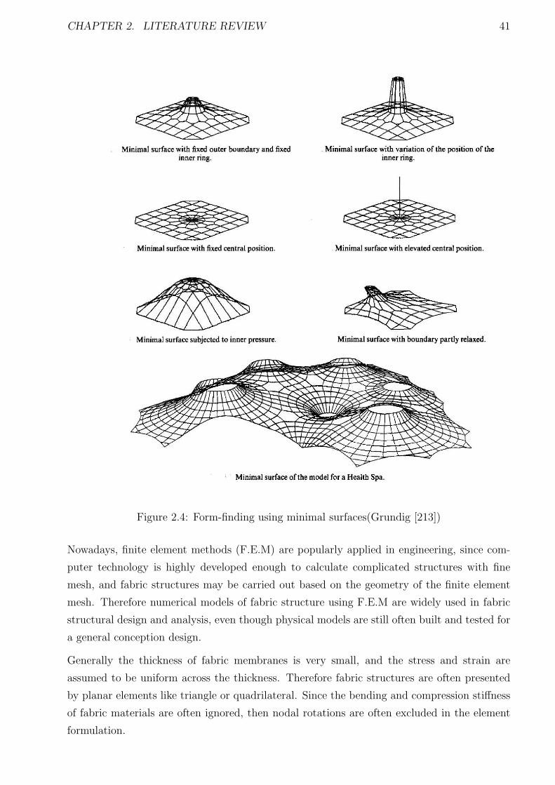
CHAPTER 2. LITERATURE REVIEW 41
Figure 2.4: Form-finding using minimal surfaces(Grundig [213])
Nowadays, finite element methods (F.E.M) are popularly applied in engineering, since com-
puter technology is highly developed enough to calculate complicated structures with fine
mesh, and fabric structures may be carried out based on the geometry of the finite element
mesh. Therefore numerical models of fabric structure using F.E.M are widely used in fabric
structural design and analysis, even though physical models are still often built and tested for
a general conception design.
Generally the thickness of fabric membranes is very small, and the stress and strain are
assumed to be uniform across the thickness. Therefore fabric structures are often presented
by planar elements like triangle or quadrilateral. Since the bending and compression stiffness
of fabric materials are often ignored, then nodal rotations are often excluded in the element
formulation.

CHAPTER 2. LITERATURE REVIEW 42
Constant strain & linear strain triangular element – general principles
The application of finite elements to the fabric structure analysis started with the simplest
element type, three node constant strain triangle(CST) with upgrading configuration by the
geometrical nonlinear effects [98–102]. This element type, initially presented by Zienkiewicz
[113], was proposed to solve 2-D plane structural analysis, and its capability and efficiency
had often been discussed and compared with high order elements developed subsequently.
Felippa [103] researched the application of a 6-node triangular element in the analysis of linear
and nonlinear plane problems, and compared this element with a classic triangular element,
both in elastic and elastoplastic analysis. He found the classic constant strain triangle provided
in general a reasonable displacement, but the interpretation of element stresses was often
difficult, especially in regions of high gradients as shown in Figure 2.5,and 2.6.. Different
averaging procedures to obtain nodal point stresses have been proposed [104, 105], but the
results are usually poor near boundaries, where extrapolation ( not averaging) is required.
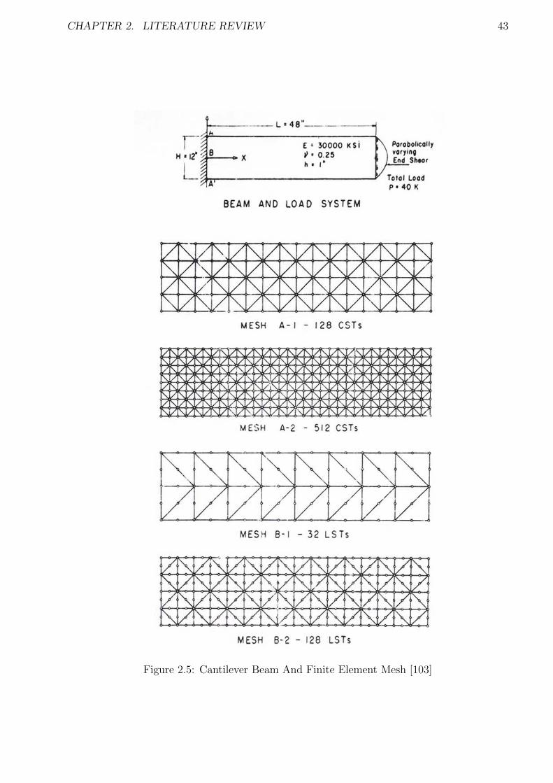
CHAPTER 2. LITERATURE REVIEW 43
Figure 2.5: Cantilever Beam And Finite Element Mesh [103]
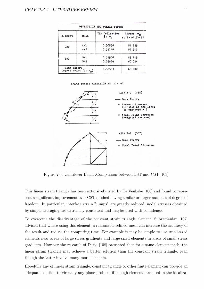
CHAPTER 2. LITERATURE REVIEW 44
Figure 2.6: Cantilever Beam :Comparison between LST and CST [103]
This linear strain triangle has been extensively tried by De Veubeke [106] and found to repre-
sent a significant improvement over CST meshed having similar or larger numbers of degree of
freedom. In particular, interface strain ”jumps” are greatly reduced; nodal stresses obtained
by simple averaging are extremely consistent and maybe used with confidence.
To overcome the disadvantage of the constant strain triangle element, Subramanian [107]
advised that where using this element, a reasonable refined mesh can increase the accuracy of
the result and reduce the computing time. For example it may be simple to use small-sized
elements near areas of large stress gradients and large-sized elements in areas of small stress
gradients. However the research of Dario [108] presented that for a same element mesh, the
linear strain triangle may achieve a better solution than the constant strain triangle, even
though the latter involve many more elements.
Hopefully any of linear strain triangle, constant triangle or other finite element can provide an
adequate solution to virtually any plane problem if enough elements are used in the idealiza-
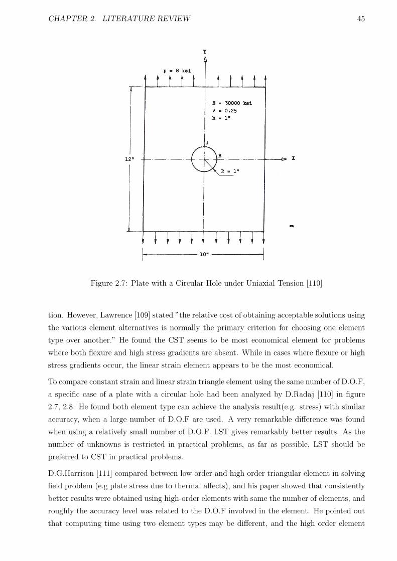
CHAPTER 2. LITERATURE REVIEW 45
Figure 2.7: Plate with a Circular Hole under Uniaxial Tension [110]
tion. However, Lawrence [109] stated ”the relative cost of obtaining acceptable solutions using
the various element alternatives is normally the primary criterion for choosing one element
type over another.” He found the CST seems to be most economical element for problems
where both flexure and high stress gradients are absent. While in cases where flexure or high
stress gradients occur, the linear strain element appears to be the most economical.
To compare constant strain and linear strain triangle element using the same number of D.O.F,
a specific case of a plate with a circular hole had been analyzed by D.Radaj [110] in figure
2.7, 2.8. He found both element type can achieve the analysis result(e.g. stress) with similar
accuracy, when a large number of D.O.F are used. A very remarkable difference was found
when using a relatively small number of D.O.F. LST gives remarkably better results. As the
number of unknowns is restricted in practical problems, as far as possible, LST should be
preferred to CST in practical problems.
D.G.Harrison [111] compared between low-order and high-order triangular element in solving
field problem (e.g plate stress due to thermal affects), and his paper showed that consistently
better results were obtained using high-order elements with same the number of elements, and
roughly the accuracy level was related to the D.O.F involved in the element. He pointed out
that computing time using two element types may be different, and the high order element

CHAPTER 2. LITERATURE REVIEW 46
Figure 2.8: Plate with Circular Hole:Comparison of LST and CST Stress Concentration Fac-tors [110]
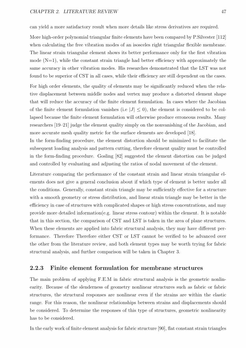
CHAPTER 2. LITERATURE REVIEW 47
can yield a more satisfactory result when more details like stress derivatives are required.
More high-order polynomial triangular finite elements have been compared by P.Silvester [112]
when calculating the free vibration modes of an isosceles right triangular flexible membrane.
The linear strain triangular element shows its better performance only for the first vibration
mode (N=1), while the constant strain triangle had better efficiency with approximately the
same accuracy in other vibration modes. His researches demonstrated that the LST was not
found to be superior of CST in all cases, while their efficiency are still dependent on the cases.
For high order elements, the quality of elements may be significantly reduced when the rela-
tive displacement between middle nodes and vertex may produce a distorted element shape
that will reduce the accuracy of the finite element formulation. In cases where the Jacobian
of the finite element formulation vanishes (i.e |J | ≤ 0), the element is considered to be col-
lapsed because the finite element formulation will otherwise produce erroneous results. Many
researchers [19–21] judge the element quality simply on the nonvanishing of the Jacobian, and
more accurate mesh quality metric for the surface elements are developed [18].
In the form-finding procedure, the element distortion should be minimized to facilitate the
subsequent loading analysis and pattern cutting, therefore element quality must be controlled
in the form-finding procedure. Gosling [82] suggested the element distortion can be judged
and controlled by evaluating and adjusting the ratios of nodal movement of the element.
Literature comparing the performance of the constant strain and linear strain triangular el-
ements does not give a general conclusion about if which type of element is better under all
the conditions. Generally, constant strain triangle may be sufficiently effective for a structure
with a smooth geometry or stress distribution, and linear strain triangle may be better in the
efficiency in case of structures with complicated shapes or high stress concentrations, and may
provide more detailed information(e.g. linear stress contour) within the element. It is notable
that in this section, the comparison of CST and LST is taken in the area of plane structures.
When these elements are applied into fabric structural analysis, they may have different per-
formance. Therefore Therefore either CST or LST cannot be verified to be advanced over
the other from the literature review, and both element types may be worth trying for fabric
structural analysis, and further comparison will be taken in Chapter 3.
2.2.3 Finite element formulation for membrane structures
The main problem of applying F.E.M in fabric structural analysis is the geometric nonlin-
earity. Because of the slenderness of geometry nonlinear structures such as fabric or fabric
structures, the structural responses are nonlinear even if the strains are within the elastic
range. For this reason, the nonlinear relationships between strains and displacements should
be considered. To determine the responses of this type of structures, geometric nonlinearity
has to be considered.
In the early work of finite element analysis for fabric structure [90], flat constant strain triangles
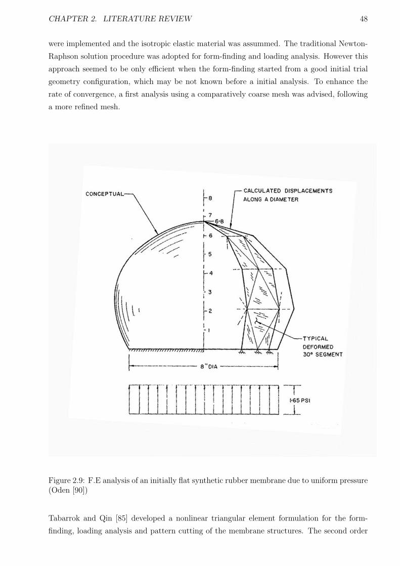
CHAPTER 2. LITERATURE REVIEW 48
were implemented and the isotropic elastic material was assummed. The traditional Newton-
Raphson solution procedure was adopted for form-finding and loading analysis. However this
approach seemed to be only efficient when the form-finding started from a good initial trial
geometry configuration, which may be not known before a initial analysis. To enhance the
rate of convergence, a first analysis using a comparatively coarse mesh was advised, following
a more refined mesh.
Figure 2.9: F.E analysis of an initially flat synthetic rubber membrane due to uniform pressure(Oden [90])
Tabarrok and Qin [85] developed a nonlinear triangular element formulation for the form-
finding, loading analysis and pattern cutting of the membrane structures. The second order
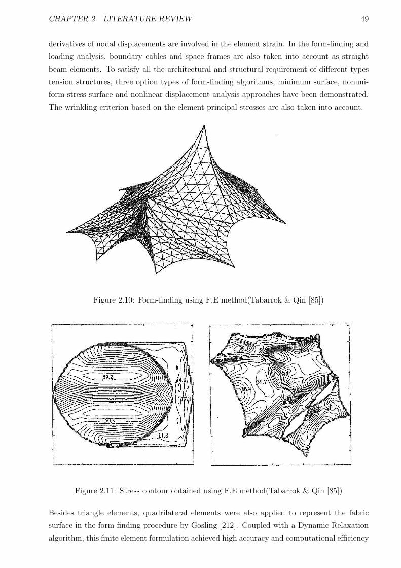
CHAPTER 2. LITERATURE REVIEW 49
derivatives of nodal displacements are involved in the element strain. In the form-finding and
loading analysis, boundary cables and space frames are also taken into account as straight
beam elements. To satisfy all the architectural and structural requirement of different types
tension structures, three option types of form-finding algorithms, minimum surface, nonuni-
form stress surface and nonlinear displacement analysis approaches have been demonstrated.
The wrinkling criterion based on the element principal stresses are also taken into account.
Figure 2.10: Form-finding using F.E method(Tabarrok & Qin [85])
Figure 2.11: Stress contour obtained using F.E method(Tabarrok & Qin [85])
Besides triangle elements, quadrilateral elements were also applied to represent the fabric
surface in the form-finding procedure by Gosling [212]. Coupled with a Dynamic Relaxation
algorithm, this finite element formulation achieved high accuracy and computational efficiency
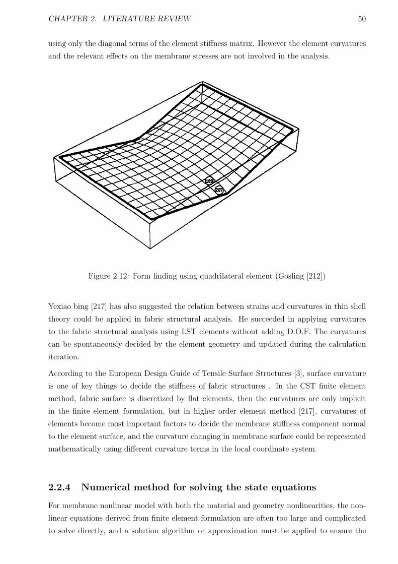
CHAPTER 2. LITERATURE REVIEW 50
using only the diagonal terms of the element stiffness matrix. However the element curvatures
and the relevant effects on the membrane stresses are not involved in the analysis.
Figure 2.12: Form finding using quadrilateral element (Gosling [212])
Yexiao bing [217] has also suggested the relation between strains and curvatures in thin shell
theory could be applied in fabric structural analysis. He succeeded in applying curvatures
to the fabric structural analysis using LST elements without adding D.O.F. The curvatures
can be spontaneously decided by the element geometry and updated during the calculation
iteration.
According to the European Design Guide of Tensile Surface Structures [3], surface curvature
is one of key things to decide the stiffness of fabric structures . In the CST finite element
method, fabric surface is discretized by flat elements, then the curvatures are only implicit
in the finite element formulation, but in higher order element method [217], curvatures of
elements become most important factors to decide the membrane stiffness component normal
to the element surface, and the curvature changing in membrane surface could be represented
mathematically using different curvature terms in the local coordinate system.
2.2.4 Numerical method for solving the state equations
For membrane nonlinear model with both the material and geometry nonlinearities, the non-
linear equations derived from finite element formulation are often too large and complicated
to solve directly, and a solution algorithm or approximation must be applied to ensure the
CHAPTER 2. LITERATURE REVIEW 51
results are convergent and stable. Two basic approaches to solve the problems in form-finding
and load analysis have been developed and applied in practice: matrix and vector methods.
The matrix methods are typically an application of more standard non-linear structural analy-
sis such as the Newton-Raphson method [206]. In this method, the structure overall tangent
stiffness is updated incrementally until convergence is obtained. Special controls limiting
the maximum incremental deflections and nodal residual forces may be required. The stress-
strain relations for the individual elements are coupled with the equilibrium and compatibility
requirements for the whole structure.
A classic solution method with effective convergence rate, the Newton-Raphson method was
applied in the form-finding [22] by Caner. However due to difficulties in producing the first
derivative of the structural stiffness for the equation solving, computing costs are always high
in cases with fine meshes.
In vector methods the conditions of equilibrium and compatibility are decoupled until con-
vergence to an equilibrium solution. The most common approaches are Dynamic Relaxation
(DR) [37, 38] and the Scaled Conjugate Gradient Method [39]. The former has been widely
accepted for the analysis of tension structures because of its clear physical analogy and ease of
implementation of the necessary controls and constraints. Nodal stiffness is used to calculate
the displacements rather than stiffness matrix of complete structure, which is only to estimate
the residual force based on the incremental nodal displacements from the last iteration.
A further method has been applied specifically to the form-finding of fabric or cable structures.
This is the Force Density method, described originally by Scheck [16]. Force Density is defined
as the ratio of forces to lengths, and the higher force density ratio means the shorter element
for a given force. It is observed that a minimal surface is generated when the force densities
for a node are equal and evenly distributed around the node. Once the equilibrium shape is
determined, the unstressed cable length could be calculated from strain-stress relationship.
Although the Force Density method was initially applied in cable-net structures, recent re-
search has extend the concept to triangular surface element with the name of the Surface
Stress Density Method [40], in which the stress density is defined as the ratio of isotropic
stresses to element areas.
The advantage of the density method is that it transforms the nonlinear equations to equivalent
linear equations. The controlling element variable is that of force/stress density(for example
T/l for a cable element of current tension T and length l, and σ/A for a surface element of
isotropic stress and area).
As noted in [40], the main drawback of density methods is that because the geometric stiffness
is difficult to be evaluated, ”the shape developed is not easily foreseeable and stress distribution
difficult to evaluate.” This could be overcome by an ”iterative smoothing” procedure with
updated force densities by using a nonlinear solution procedure(e.g. Jacobi or Gauss-Siedal
CHAPTER 2. LITERATURE REVIEW 52
method), but this would seem to make the equations still nonlinear and negate the advantage
of a linearized solution.
The Force Density method is able to reduce the computing time to obtain approximate solu-
tions, but these solutions may be inaccurate and mesh-dependent. The error analysis in the
approximate finite element solutions has been taken by Bognar [68].
Another issue for these finite element methods and relevant solution procedures is their ap-
plicability for the cutting pattern generation, which is an important stage in the fabric struc-
ture design and construction. A suitable finite element should be consistently applicable
during the main procedures of fabric structure design.
Phelan and Harber [51] suggests the analysis tool should be integrated with the design pro-
cedure, which follows three steps (a) reference configuration as determined by the initial
equilibrium; (b) equilibrium analysis of loaded structures; and (c) determination of cutting
pattern geometry.
Ishii [52] developed cutting pattern generation by using the geodesic line concept. To apply
this concept to a curved membrane surface, he approximated the surface as a polyhedron
consisting of triangular elements. For the geodesic line technique, Ataka and Kozuka [53]
introduced a variation of the method, where the geodesic lines are approximated as linear
elements.
Tabarrok and Qin [59] presented a cutting method for fabric tension structures by the finite
element method. They used a weighted least-squares minimization flattening approach to
minimize the change in general link lengths and to generate plane cloth coordinates. However,
these works did not consider the material’s extension after construction. Some discrepancies
could occur between actual stress and designed stress because material properties are not
considered. Due to this problem, fabric structures may encounter unexpected structural
problems such as wrinkling and excessive stress after completed construction. Therefore,
it is most important that the deviation between actual stress at the construction stage and
design stress given by the designer is diminished as much as possible. Such a cutting pattern
procedure is defined as optimum cutting patterning.
Tsubota [60–62] firstly introduced an optimization procedure which forms a membrane stress
distribution in the actual assembled equilibrium state as close as possible to the uniform stress
distribution specified in the design stage. In Tsubota’s procedure, the boundary nodal points
in the 2-D coordinate system are selected as control variables to determine the optimum
cutting patterns. By this method, the actual assembled state is brought close to the uniform
stress distribution specified by successively is considered as somewhat inconvenient for two
reasons: (1) Separating elements into inner and exterior, and (2) the line fitting procedure
on exterior points at each iteration. Yagi and Ohmori [63, 64] presented a new approach for
cutting pattern analysis of membrane structures. The equilibrium state after deformation is
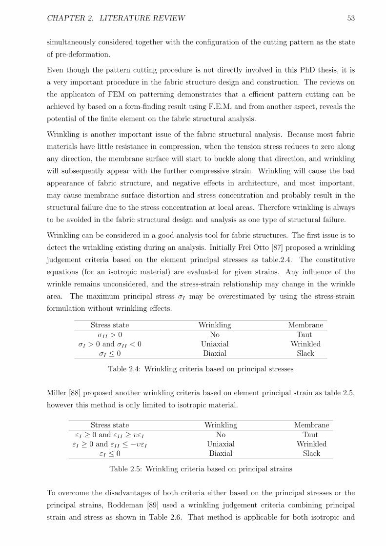
CHAPTER 2. LITERATURE REVIEW 53
simultaneously considered together with the configuration of the cutting pattern as the state
of pre-deformation.
Even though the pattern cutting procedure is not directly involved in this PhD thesis, it is
a very important procedure in the fabric structure design and construction. The reviews on
the applicaton of FEM on patterning demonstrates that a efficient pattern cutting can be
achieved by based on a form-finding result using F.E.M, and from another aspect, reveals the
potential of the finite element on the fabric structural analysis.
Wrinkling is another important issue of the fabric structural analysis. Because most fabric
materials have little resistance in compression, when the tension stress reduces to zero along
any direction, the membrane surface will start to buckle along that direction, and wrinkling
will subsequently appear with the further compressive strain. Wrinkling will cause the bad
appearance of fabric structure, and negative effects in architecture, and most important,
may cause membrane surface distortion and stress concentration and probably result in the
structural failure due to the stress concentration at local areas. Therefore wrinkling is always
to be avoided in the fabric structural design and analysis as one type of structural failure.
Wrinkling can be considered in a good analysis tool for fabric structures. The first issue is to
detect the wrinkling existing during an analysis. Initially Frei Otto [87] proposed a wrinkling
judgement criteria based on the element principal stresses as table.2.4. The constitutive
equations (for an isotropic material) are evaluated for given strains. Any influence of the
wrinkle remains unconsidered, and the stress-strain relationship may change in the wrinkle
area. The maximum principal stress σI may be overestimated by using the stress-strain
formulation without wrinkling effects.
Stress state Wrinkling MembraneσII > 0 No Taut
σI > 0 and σII < 0 Uniaxial WrinkledσI ≤ 0 Biaxial Slack
Table 2.4: Wrinkling criteria based on principal stresses
Miller [88] proposed another wrinkling criteria based on element principal strain as table 2.5,
however this method is only limited to isotropic material.
Stress state Wrinkling MembraneεI ≥ 0 and εII ≥ υεI No TautεI ≥ 0 and εII ≤ −υεI Uniaxial Wrinkled
εI ≤ 0 Biaxial Slack
Table 2.5: Wrinkling criteria based on principal strains
To overcome the disadvantages of both criteria either based on the principal stresses or the
principal strains, Roddeman [89] used a wrinkling judgement criteria combining principal
strain and stress as shown in Table 2.6. That method is applicable for both isotropic and
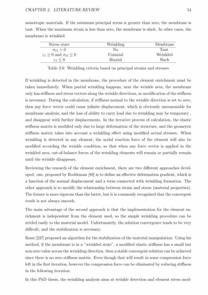
CHAPTER 2. LITERATURE REVIEW 54
anisotropic materials. If the minimum principal stress is greater than zero, the membrane is
taut. When the maximum strain is less than zero, the membrane is slack. In other cases, the
membrane is wrinkled.
Stress state Wrinkling MembraneσII > 0 No Taut
εI ≥ 0 and σII ≤ 0 Uniaxial WrinkledεI ≤ 0 Biaxial Slack
Table 2.6: Wrinkling criteria based on principal strains and stresses
If wrinkling is detected in the membrane, the procedure of the element enrichment must be
taken immediately. When partial wrinkling happens, near the wrinkle area, the membrane
only has stiffness and stress vectors along the wrinkle directions, so modification of the stiffness
is necessary. During the calculation, if stiffness normal to the wrinkle direction is set to zero,
then any force vector could cause infinite displacement, which is obviously unreasonable for
membrane analysis, and the loss of ability to carry load due to wrinkling may be temporary ,
and disappear with further displacements. In the iterative process of calculation, the elastic
stiffness matrix is modified only due to large deformation of the structure, and the geometric
stiffness matrix takes into account a wrinkling effect using modified actual stresses. When
wrinkling is detected in any element, the nodal reaction force of the element will also be
modified according the wrinkle condition, so that when any force vector is applied in the
wrinkled area, out-of-balance forces of the wrinkling elements will remain or partially remain
until the wrinkle disappears.
Reviewing the research of the element enrichment, there are two different approaches devel-
oped: one, proposed by Roddeman [89] is to define an effective deformation gradient, which is
a function of the normal displacement and a term connected with wrinkling formation. The
other approach is to modify the relationship between strain and stress (material properties).
The former is more rigorous than the latter, but it is commonly recognized that the convergent
result is not always smooth.
The main advantage of the second approach is that the implementation for the element en-
richment is independent from the element used, so the simple wrinkling procedure can be
settled easily to the material model. Unfortunately, the solution convergence tends to be very
difficult, and the stabilization is necessary.
Rossi [237] proposed an algorithm for the stabilization of the material manipulation. Using his
method, if the membrane is in a ”wrinkled state”, a modified elastic stiffness has a small but
non-zero value across the wrinkling direction, then a stable convergent solution can be achieved
since there is no zero stiffness matrix. Even though that will result in some compression force
left in the first iteration, however the compression force can be eliminated by reducing stiffness
in the following iteration.
In this PhD thesis, the wrinkling analysis aims at wrinkle detection and element stress mod-
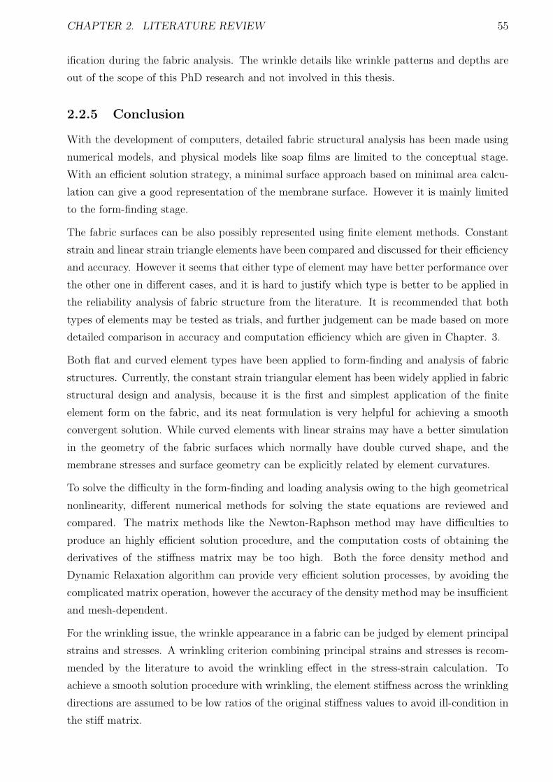
CHAPTER 2. LITERATURE REVIEW 55
ification during the fabric analysis. The wrinkle details like wrinkle patterns and depths are
out of the scope of this PhD research and not involved in this thesis.
2.2.5 Conclusion
With the development of computers, detailed fabric structural analysis has been made using
numerical models, and physical models like soap films are limited to the conceptual stage.
With an efficient solution strategy, a minimal surface approach based on minimal area calcu-
lation can give a good representation of the membrane surface. However it is mainly limited
to the form-finding stage.
The fabric surfaces can be also possibly represented using finite element methods. Constant
strain and linear strain triangle elements have been compared and discussed for their efficiency
and accuracy. However it seems that either type of element may have better performance over
the other one in different cases, and it is hard to justify which type is better to be applied in
the reliability analysis of fabric structure from the literature. It is recommended that both
types of elements may be tested as trials, and further judgement can be made based on more
detailed comparison in accuracy and computation efficiency which are given in Chapter. 3.
Both flat and curved element types have been applied to form-finding and analysis of fabric
structures. Currently, the constant strain triangular element has been widely applied in fabric
structural design and analysis, because it is the first and simplest application of the finite
element form on the fabric, and its neat formulation is very helpful for achieving a smooth
convergent solution. While curved elements with linear strains may have a better simulation
in the geometry of the fabric surfaces which normally have double curved shape, and the
membrane stresses and surface geometry can be explicitly related by element curvatures.
To solve the difficulty in the form-finding and loading analysis owing to the high geometrical
nonlinearity, different numerical methods for solving the state equations are reviewed and
compared. The matrix methods like the Newton-Raphson method may have difficulties to
produce an highly efficient solution procedure, and the computation costs of obtaining the
derivatives of the stiffness matrix may be too high. Both the force density method and
Dynamic Relaxation algorithm can provide very efficient solution processes, by avoiding the
complicated matrix operation, however the accuracy of the density method may be insufficient
and mesh-dependent.
For the wrinkling issue, the wrinkle appearance in a fabric can be judged by element principal
strains and stresses. A wrinkling criterion combining principal strains and stresses is recom-
mended by the literature to avoid the wrinkling effect in the stress-strain calculation. To
achieve a smooth solution procedure with wrinkling, the element stiffness across the wrinkling
directions are assumed to be low ratios of the original stiffness values to avoid ill-condition in
the stiff matrix.
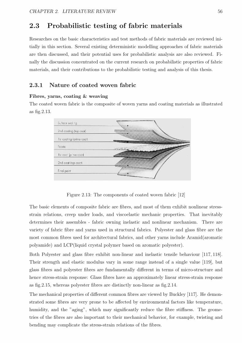
CHAPTER 2. LITERATURE REVIEW 56
2.3 Probabilistic testing of fabric materials
Researches on the basic characteristics and test methods of fabric materials are reviewed ini-
tially in this section. Several existing deterministic modelling approaches of fabric materials
are then discussed, and their potential uses for probabilistic analysis are also reviewed. Fi-
nally the discussion concentrated on the current research on probabilistic properties of fabric
materials, and their contributions to the probabilistic testing and analysis of this thesis.
2.3.1 Nature of coated woven fabric
Fibres, yarns, coating & weaving
The coated woven fabric is the composite of woven yarns and coating materials as illustrated
as fig.2.13.
Figure 2.13: The components of coated woven fabric [12]
The basic elements of composite fabric are fibres, and most of them exhibit nonlinear stress-
strain relations, creep under loads, and viscoelastic mechanic properties. That inevitably
determines their assembles - fabric owning inelastic and nonlinear mechanism. There are
variety of fabric fibre and yarns used in structural fabrics. Polyester and glass fibre are the
most common fibres used for architectural fabrics, and other yarns include Aramid(aromatic
polyamide) and LCP(liquid crystal polymer based on aromatic polyester).
Both Polyester and glass fibre exhibit non-linear and inelastic tensile behaviour [117, 118].
Their strength and elastic modulus vary in some range instead of a single value [119], but
glass fibres and polyester fibres are fundamentally different in terms of micro-structure and
hence stress-strain response: Glass fibres have an approximately linear stress-strain response
as fig.2.15, whereas polyester fibres are distinctly non-linear as fig.2.14.
The mechanical properties of different common fibres are viewed by Buckley [117]. He demon-
strated some fibres are very prone to be affected by environmental factors like temperature,
humidity, and the ”aging”, which may significantly reduce the fibre stiffness. The geome-
tries of the fibres are also important to their mechanical behavior, for example, twisting and
bending may complicate the stress-strain relations of the fibres.
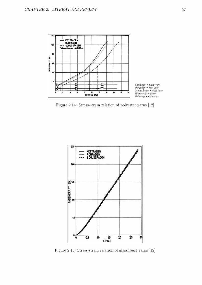
CHAPTER 2. LITERATURE REVIEW 57
Figure 2.14: Stress-strain relation of polyester yarns [12]
Figure 2.15: Stress-strain relation of glassfiber1 yarns [12]
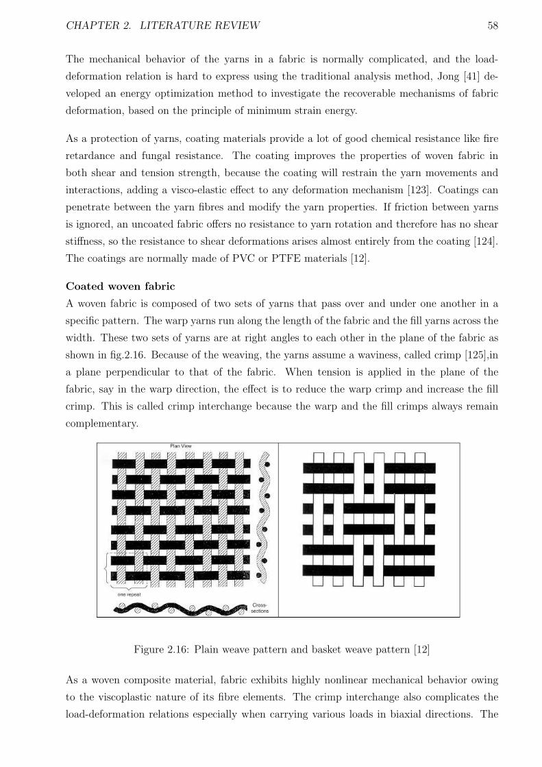
CHAPTER 2. LITERATURE REVIEW 58
The mechanical behavior of the yarns in a fabric is normally complicated, and the load-
deformation relation is hard to express using the traditional analysis method, Jong [41] de-
veloped an energy optimization method to investigate the recoverable mechanisms of fabric
deformation, based on the principle of minimum strain energy.
As a protection of yarns, coating materials provide a lot of good chemical resistance like fire
retardance and fungal resistance. The coating improves the properties of woven fabric in
both shear and tension strength, because the coating will restrain the yarn movements and
interactions, adding a visco-elastic effect to any deformation mechanism [123]. Coatings can
penetrate between the yarn fibres and modify the yarn properties. If friction between yarns
is ignored, an uncoated fabric offers no resistance to yarn rotation and therefore has no shear
stiffness, so the resistance to shear deformations arises almost entirely from the coating [124].
The coatings are normally made of PVC or PTFE materials [12].
Coated woven fabric
A woven fabric is composed of two sets of yarns that pass over and under one another in a
specific pattern. The warp yarns run along the length of the fabric and the fill yarns across the
width. These two sets of yarns are at right angles to each other in the plane of the fabric as
shown in fig.2.16. Because of the weaving, the yarns assume a waviness, called crimp [125],in
a plane perpendicular to that of the fabric. When tension is applied in the plane of the
fabric, say in the warp direction, the effect is to reduce the warp crimp and increase the fill
crimp. This is called crimp interchange because the warp and the fill crimps always remain
complementary.
Figure 2.16: Plain weave pattern and basket weave pattern [12]
As a woven composite material, fabric exhibits highly nonlinear mechanical behavior owing
to the viscoplastic nature of its fibre elements. The crimp interchange also complicates the
load-deformation relations especially when carrying various loads in biaxial directions. The
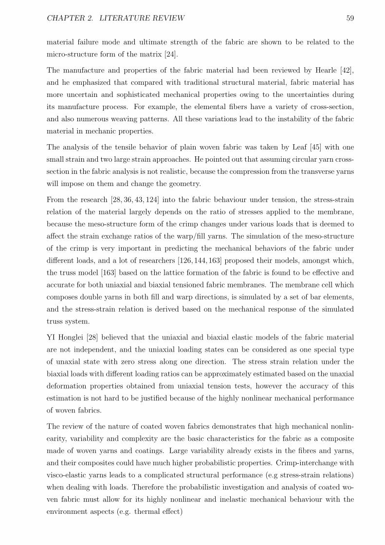
CHAPTER 2. LITERATURE REVIEW 59
material failure mode and ultimate strength of the fabric are shown to be related to the
micro-structure form of the matrix [24].
The manufacture and properties of the fabric material had been reviewed by Hearle [42],
and he emphasized that compared with traditional structural material, fabric material has
more uncertain and sophisticated mechanical properties owing to the uncertainties during
its manufacture process. For example, the elemental fibers have a variety of cross-section,
and also numerous weaving patterns. All these variations lead to the instability of the fabric
material in mechanic properties.
The analysis of the tensile behavior of plain woven fabric was taken by Leaf [45] with one
small strain and two large strain approaches. He pointed out that assuming circular yarn cross-
section in the fabric analysis is not realistic, because the compression from the transverse yarns
will impose on them and change the geometry.
From the research [28, 36, 43, 124] into the fabric behaviour under tension, the stress-strain
relation of the material largely depends on the ratio of stresses applied to the membrane,
because the meso-structure form of the crimp changes under various loads that is deemed to
affect the strain exchange ratios of the warp/fill yarns. The simulation of the meso-structure
of the crimp is very important in predicting the mechanical behaviors of the fabric under
different loads, and a lot of researchers [126,144,163] proposed their models, amongst which,
the truss model [163] based on the lattice formation of the fabric is found to be effective and
accurate for both uniaxial and biaxial tensioned fabric membranes. The membrane cell which
composes double yarns in both fill and warp directions, is simulated by a set of bar elements,
and the stress-strain relation is derived based on the mechanical response of the simulated
truss system.
YI Honglei [28] believed that the uniaxial and biaxial elastic models of the fabric material
are not independent, and the uniaxial loading states can be considered as one special type
of unaxial state with zero stress along one direction. The stress strain relation under the
biaxial loads with different loading ratios can be approximately estimated based on the unaxial
deformation properties obtained from uniaxial tension tests, however the accuracy of this
estimation is not hard to be justified because of the highly nonlinear mechanical performance
of woven fabrics.
The review of the nature of coated woven fabrics demonstrates that high mechanical nonlin-
earity, variability and complexity are the basic characteristics for the fabric as a composite
made of woven yarns and coatings. Large variability already exists in the fibres and yarns,
and their composites could have much higher probabilistic properties. Crimp-interchange with
visco-elastic yarns leads to a complicated structural performance (e.g stress-strain relations)
when dealing with loads. Therefore the probabilistic investigation and analysis of coated wo-
ven fabric must allow for its highly nonlinear and inelastic mechanical behaviour with the
environment aspects (e.g. thermal effect)
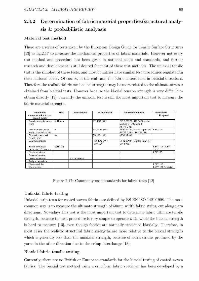
CHAPTER 2. LITERATURE REVIEW 60
2.3.2 Determination of fabric material properties(structural analy-
sis & probabilistic analyasis
Material test method
There are a series of tests given by the European Design Guide for Tensile Surface Structures
[13] as fig.2.17 to measure the mechanical properties of fabric materials. However not every
test method and procedure has been given in national codes and standards, and further
research and development is still desired for most of these test methods. The uniaxial tensile
test is the simplest of these tests, and most countries have similar test procedures regulated in
their national codes. Of course, in the real case, the fabric is tensioned in biaixial directions.
Therefore the realistic fabric mechanical strengths may be more related to the ultimate stresses
obtained from biaixial tests. However because the biaxial tension strength is very difficult to
obtain directly [13], currently the uniaxial test is still the most important test to measure the
fabric material strength.
Figure 2.17: Commonly used standards for fabric tests [12]
Uniaxial fabric testing
Uniaxial strip tests for coated woven fabrics are defined by BS EN ISO 1421:1998. The most
common way is to measure the ultimate strength of 50mm width fabric strips, cut along yarn
directions. Nowadays this test is the most important test to determine fabric ultimate tensile
strength, because the test procedure is very simple to operate with, while the biaxial strength
is hard to measure [13], even though fabrics are normally tensioned biaxially. Therefore, in
most cases the realistic structural fabric strengths are more relative to the biaxial strengths
which is generally less than the uniaixial strength, because of extra strains produced by the
yarns in the other direction due to the crimp interchange [13].
Biaxial fabric tensile testing
Currently, there are no British or European standards for the biaxial testing of coated woven
fabrics. The biaxial test method using a cruciform fabric specimen has been developed by a
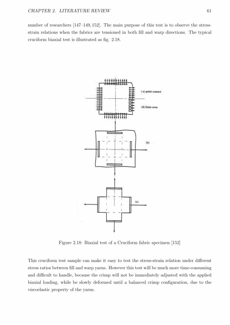
CHAPTER 2. LITERATURE REVIEW 61
number of researchers [147–149, 152]. The main purpose of this test is to observe the stress-
strain relations when the fabrics are tensioned in both fill and warp directions. The typical
cruciform biaxial test is illustrated as fig. 2.18.
Figure 2.18: Biaxial test of a Cruciform fabric specimen [152]
This cruciform test sample can make it easy to test the stress-strain relation under different
stress ratios between fill and warp yarns. However this test will be much more time-consuming
and difficult to handle, because the crimp will not be immediately adjusted with the applied
biaxial loading, while be slowly deformed until a balanced crimp configuration, due to the
viscoelastic property of the yarns.
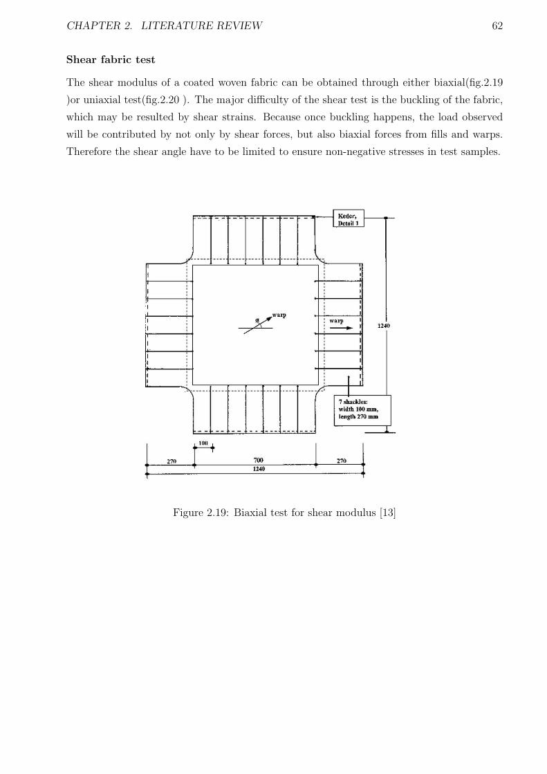
CHAPTER 2. LITERATURE REVIEW 62
Shear fabric test
The shear modulus of a coated woven fabric can be obtained through either biaxial(fig.2.19
)or uniaxial test(fig.2.20 ). The major difficulty of the shear test is the buckling of the fabric,
which may be resulted by shear strains. Because once buckling happens, the load observed
will be contributed by not only by shear forces, but also biaxial forces from fills and warps.
Therefore the shear angle have to be limited to ensure non-negative stresses in test samples.
Figure 2.19: Biaxial test for shear modulus [13]
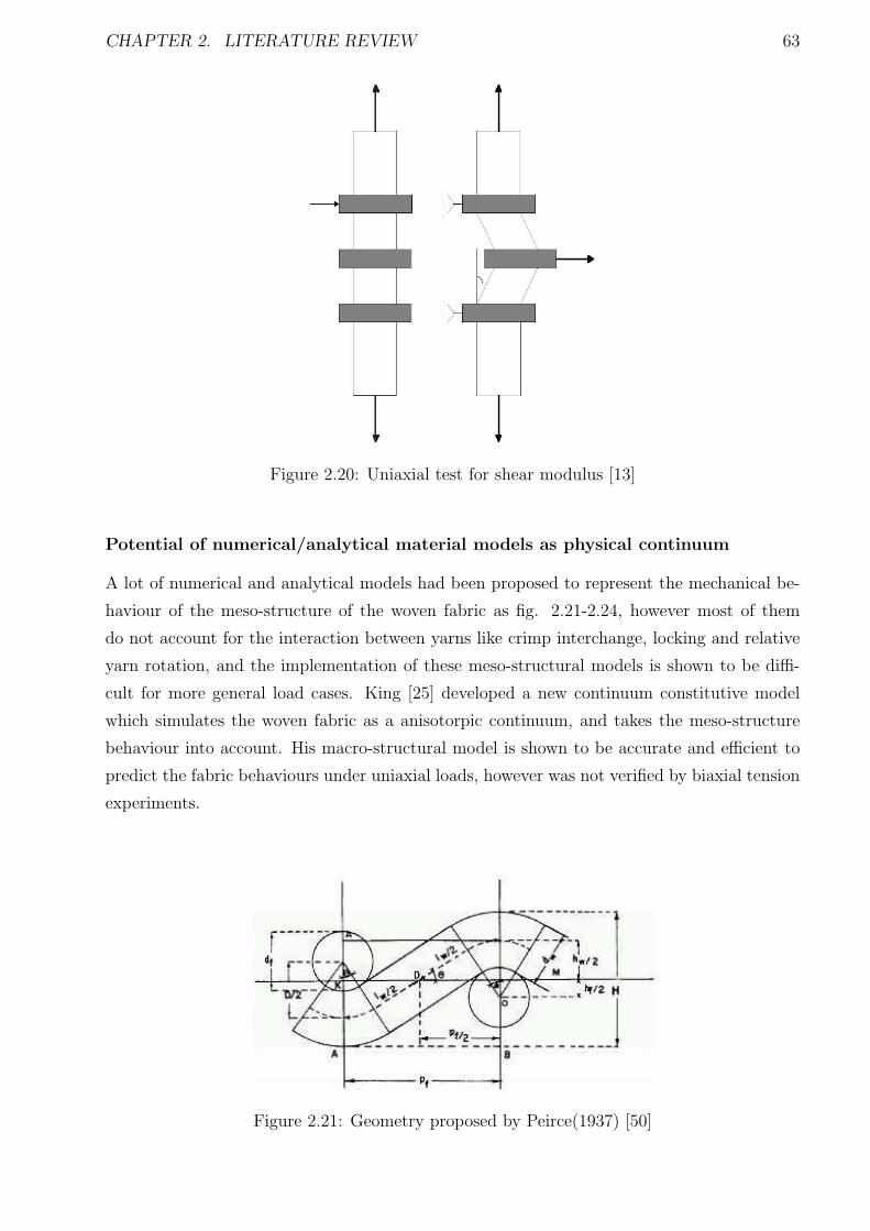
CHAPTER 2. LITERATURE REVIEW 63
Figure 2.20: Uniaxial test for shear modulus [13]
Potential of numerical/analytical material models as physical continuum
A lot of numerical and analytical models had been proposed to represent the mechanical be-
haviour of the meso-structure of the woven fabric as fig. 2.21-2.24, however most of them
do not account for the interaction between yarns like crimp interchange, locking and relative
yarn rotation, and the implementation of these meso-structural models is shown to be diffi-
cult for more general load cases. King [25] developed a new continuum constitutive model
which simulates the woven fabric as a anisotorpic continuum, and takes the meso-structure
behaviour into account. His macro-structural model is shown to be accurate and efficient to
predict the fabric behaviours under uniaxial loads, however was not verified by biaxial tension
experiments.
Figure 2.21: Geometry proposed by Peirce(1937) [50]
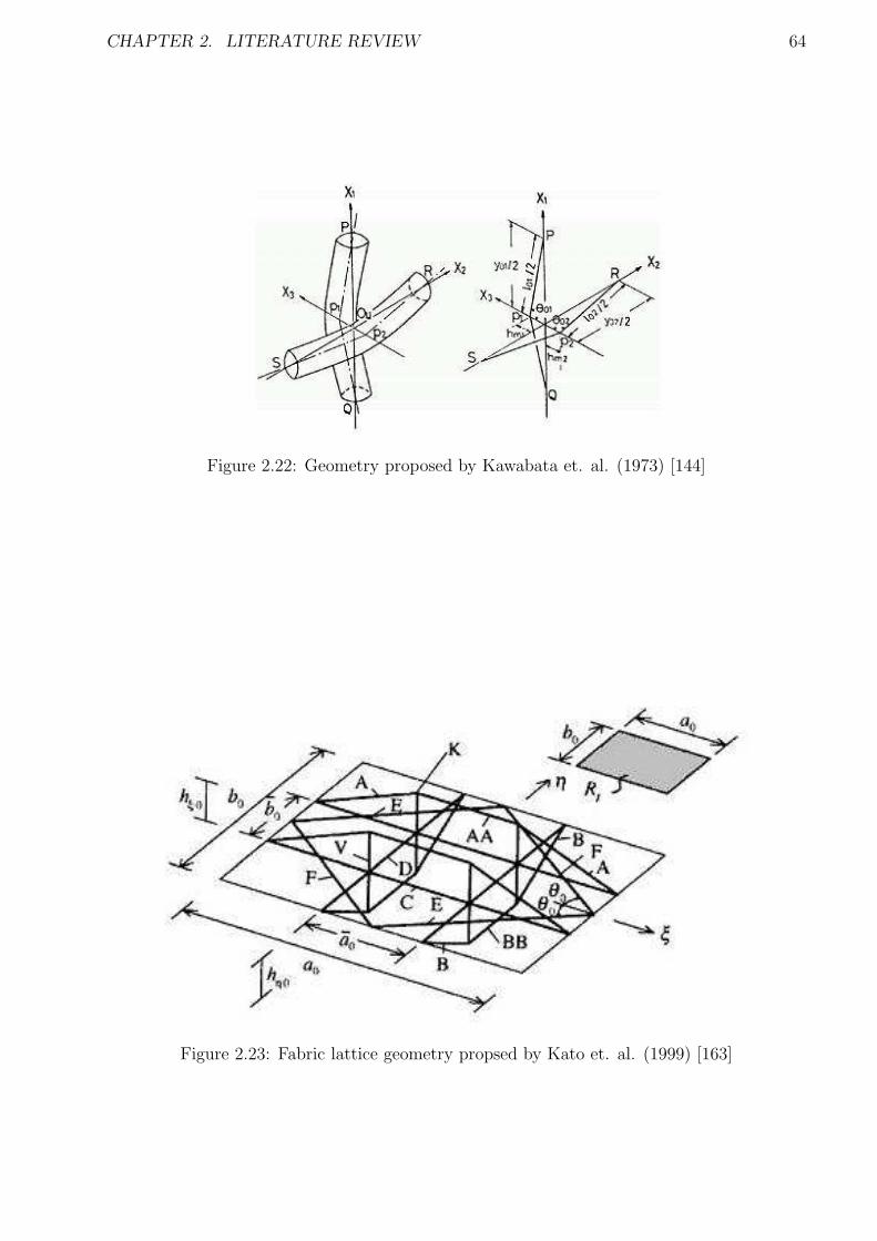
CHAPTER 2. LITERATURE REVIEW 64
Figure 2.22: Geometry proposed by Kawabata et. al. (1973) [144]
Figure 2.23: Fabric lattice geometry propsed by Kato et. al. (1999) [163]
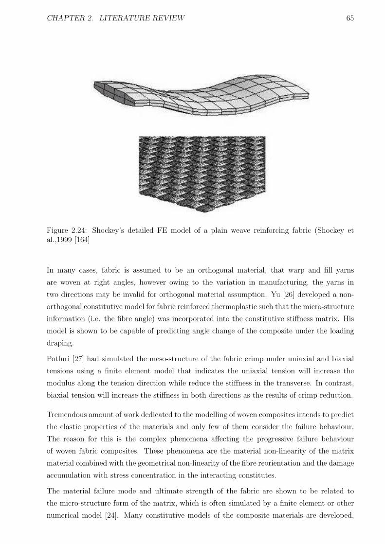
CHAPTER 2. LITERATURE REVIEW 65
Figure 2.24: Shockey’s detailed FE model of a plain weave reinforcing fabric (Shockey etal.,1999 [164]
In many cases, fabric is assumed to be an orthogonal material, that warp and fill yarns
are woven at right angles, however owing to the variation in manufacturing, the yarns in
two directions may be invalid for orthogonal material assumption. Yu [26] developed a non-
orthogonal constitutive model for fabric reinforced thermoplastic such that the micro-structure
information (i.e. the fibre angle) was incorporated into the constitutive stiffness matrix. His
model is shown to be capable of predicting angle change of the composite under the loading
draping.
Potluri [27] had simulated the meso-structure of the fabric crimp under uniaxial and biaxial
tensions using a finite element model that indicates the uniaxial tension will increase the
modulus along the tension direction while reduce the stiffness in the transverse. In contrast,
biaxial tension will increase the stiffness in both directions as the results of crimp reduction.
Tremendous amount of work dedicated to the modelling of woven composites intends to predict
the elastic properties of the materials and only few of them consider the failure behaviour.
The reason for this is the complex phenomena affecting the progressive failure behaviour
of woven fabric composites. These phenomena are the material non-linearity of the matrix
material combined with the geometrical non-linearity of the fibre reorientation and the damage
accumulation with stress concentration in the interacting constitutes.
The material failure mode and ultimate strength of the fabric are shown to be related to
the micro-structure form of the matrix, which is often simulated by a finite element or other
numerical model [24]. Many constitutive models of the composite materials are developed,
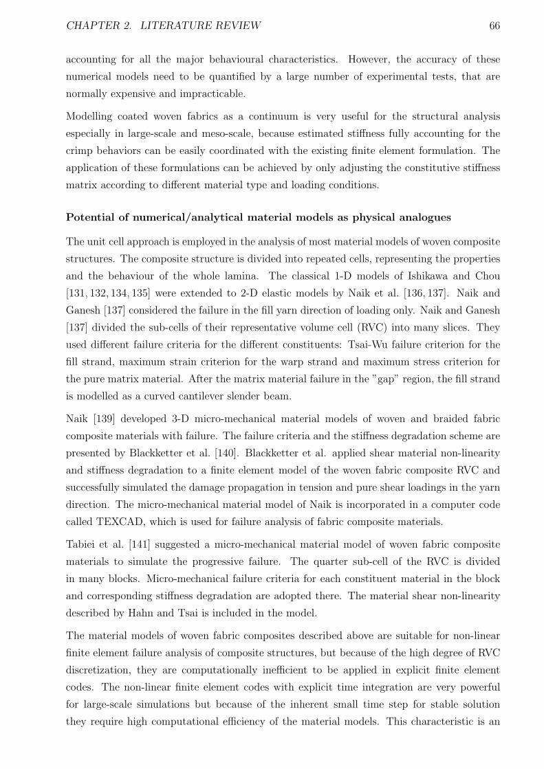
CHAPTER 2. LITERATURE REVIEW 66
accounting for all the major behavioural characteristics. However, the accuracy of these
numerical models need to be quantified by a large number of experimental tests, that are
normally expensive and impracticable.
Modelling coated woven fabrics as a continuum is very useful for the structural analysis
especially in large-scale and meso-scale, because estimated stiffness fully accounting for the
crimp behaviors can be easily coordinated with the existing finite element formulation. The
application of these formulations can be achieved by only adjusting the constitutive stiffness
matrix according to different material type and loading conditions.
Potential of numerical/analytical material models as physical analogues
The unit cell approach is employed in the analysis of most material models of woven composite
structures. The composite structure is divided into repeated cells, representing the properties
and the behaviour of the whole lamina. The classical 1-D models of Ishikawa and Chou
[131, 132, 134, 135] were extended to 2-D elastic models by Naik et al. [136, 137]. Naik and
Ganesh [137] considered the failure in the fill yarn direction of loading only. Naik and Ganesh
[137] divided the sub-cells of their representative volume cell (RVC) into many slices. They
used different failure criteria for the different constituents: Tsai-Wu failure criterion for the
fill strand, maximum strain criterion for the warp strand and maximum stress criterion for
the pure matrix material. After the matrix material failure in the ”gap” region, the fill strand
is modelled as a curved cantilever slender beam.
Naik [139] developed 3-D micro-mechanical material models of woven and braided fabric
composite materials with failure. The failure criteria and the stiffness degradation scheme are
presented by Blackketter et al. [140]. Blackketter et al. applied shear material non-linearity
and stiffness degradation to a finite element model of the woven fabric composite RVC and
successfully simulated the damage propagation in tension and pure shear loadings in the yarn
direction. The micro-mechanical material model of Naik is incorporated in a computer code
called TEXCAD, which is used for failure analysis of fabric composite materials.
Tabiei et al. [141] suggested a micro-mechanical material model of woven fabric composite
materials to simulate the progressive failure. The quarter sub-cell of the RVC is divided
in many blocks. Micro-mechanical failure criteria for each constituent material in the block
and corresponding stiffness degradation are adopted there. The material shear non-linearity
described by Hahn and Tsai is included in the model.
The material models of woven fabric composites described above are suitable for non-linear
finite element failure analysis of composite structures, but because of the high degree of RVC
discretization, they are computationally inefficient to be applied in explicit finite element
codes. The non-linear finite element codes with explicit time integration are very powerful
for large-scale simulations but because of the inherent small time step for stable solution
they require high computational efficiency of the material models. This characteristic is an
CHAPTER 2. LITERATURE REVIEW 67
obstacle for complicated micro-mechanical models to be implemented in the explicit codes.
Ala Tabiei [142] developed a computationally efficient and simplified micro-mechanical model
of woven fabric composite materials to predict their elastic properties. The advantage of the
model is the lack of RVC discretization and good elastic property prediction. The choice of the
RVC is intended to account for geometrical non-linearity and simple and efficient technique
for fibre reorientation was incorporated in the model [143].
These cell approaches applied the fabrics can help to understand the mechanical behaviour in
small-scale especially for the material failure. A lot of phenomena and information observed
during material testing can be potentially analyzed using these methods. The structural failure
process of fabrics (e.g. material rupture and propagation) can be possibly well explained by
the analysis using one of these formulations.
Current research on probabilistic material properties of coated woven fabric
Normal distribution is most widely applied statistical distribution in the engineering industry.
During the fabric manufacture, variations of fabric strengths may be affected by the uncer-
tainties(e.g. measurement errors) following normal distribution, and a lot of researchers found
the ultimate strength of the yarns as the assembles of fibres follows Weibull distributions [158],
which is often used for extreme values of a set of observations.
The statistical properties of the yarns, cables, ropes are deemed to be related with the uncer-
tainties of the fibres. Considering these materials as bundles of fibres, Phoenix [46] developed
a statistical model to predict the stochastic behaviour of these materials, assuming that the
fibre strengths follow Weibull distribution. In his model, more attention was paid in how the
fibre length affected the stochastic property of fibre assembly.
As a composite of yarns and coating materials, fabric materials were initially modelled as bun-
dles of yarns, and their probabilistic properties are often estimated based on the assumption of
yarn distribution [133]. However it was found that the mechanical performance of single yarns
is significantly different from that in coated woven fabrics, because of yarn-to-yarn frictions
especially for biaxial loading. The simulation of realistic yarns structural behaivour can be
estimated using reduced yarn lengths which vary with different fabric types. However this
simulation lacks the theoretical support.
To solve this problem, Ning Pan [43] proposed a prediction model of uniaxial and biaxial
fabric strength, based on the assumption of the Weibull distributed yarn strength, fully taking
into account the yarn-yarn interaction at the interlacing point. He separated the yarn-yarn
interaction into two components: adhesive and frictional ones, and the latter is shown to
have much more effect on the fabric tensile strength. In his model, a fabric is assumed to
be made of many sub-bundles of yarns, with the critical lengths of which are shorter than
the realistic length of yarns, and derived based on the crimp conditions. With the simulation
of the yarn-yarn interaction, the prediction accuracy of the fabric strength including mean
CHAPTER 2. LITERATURE REVIEW 68
and standard deviation is significantly improved compared with the pure yarn-assembly model,
however higher accuracy and stochastic details are still further desired for a qualified reliability
analysis.
Currently, the research on the stochastic property of coated woven fabrics is mainly focused
on the numerical modelling of the fabric inner structures, while the probabilistic investigation
and analysis mainly based on the large quantity of material experiments are absent. With the
lack of investigation on the realistic behaviour of coated fabric, the probabilistic estimation
models are difficult to be verified. Therefore to achieve the accurate probabilistic information
of the coated woven fabric, the investigation based on a quantity of material test may be
taken.
2.3.3 Manipulation /transformation of material property data into
a statistical form and available statistical forms
To facilitate the reliability analysis, all the uncertainties must be investigated and represented
mathematically. Especially for the non-cognitive or aleatory uncertainty sources, a statis-
tical investigation and analysis must be taken to obtain the stochastic information of the
variables(e.g. wind speed, material strength) in the engineering system of interest with the
mathematical description. Based on a certain quantity of past records and test data, the
variations and distributions of the loads and resistance are determined through the statistical
measurements. The common way to determine the statistical distribution for a variable of
interest is to select closest distribution among a set of optional distributions which are usually
applied in engineering through a data-fitting test(e.g. χ2 test).
Except than normal and log-normal distribution, other distributions like extreme value distri-
butions have been often utilized as well since the fact that the maximum and minimum values
of statistical variables often take very important roles in the reliability analysis, for example,
the maximum wind load and minimum load resistance. In a lot of composite materials, the
material strength may depend on the failure stress or strain of the weakest fibre if the failure
propagation across the fibres is immediate.
There are three types of extreme value distribution commonly applied in the structural re-
liability analysis: Gumbel, Frechet, and Weibull distributions. Their parameters can be
estimated based on the moment method and likelihood method traditionally, however the
accuracy and the stability of these methods are case-dependent, and in some case (e.g three
parameters Weibull distribution), the parameter estimation using traditional approaches is
troublesome. This problem is solved by using the method of order statistics which was devel-
oped by Lieblein [248]. In this method, initially the test data will be separated in to several
groups with approximately the same sizes, and in each group, the data are rearranged with an
increasing order. Then the parameters will be evaluated through the order statistical formu-
lation, based on the principle of the moment method. The advantage of the order statistics
CHAPTER 2. LITERATURE REVIEW 69
method is simple and efficient by avoiding solving nonlinear equations as in the traditional
approaches.
Weibull distribution [158] is known to fit the failure strength of a lot of materials. The
application of Weibull distribution in composite structures was demonstrated by Barbero [47],
a new parameter estimation method was proposed for two parameter Weibull distribution
based on the data size.
An appropriate distribution may be determined not only based on the data-fitting test, but
also on statistical analysis of the material behaviour according to the relevant physical ar-
guments. Based on limit test data, Zhao [246] had developed an approach to determine the
proper distribution for the steel fatigue life, fulling taking into account the mechanical process
of the steel fatigue. He pointed out a reasonable distribution should fit both the test data
and physical argument, and analyzing the mechanism of the material behaviours(like struc-
tural failure) can verify the corresponding uncertainty sources and decide the possible suitable
distribution for further selection.
Except the traditional data-fitting test, χ2 test, a series of goodness fit tests for distributions
are developed, Stephens [247] reviewed several common data fitting tests like the EDF test,
K-S test, Anderson-Darling test, and so on, and these tests are based on the difference between
the CDF of the estimated distribution and sample accumulative frequency. Compared to the
χ2 test, these goodness tests seem more effective and accurate, however there is no evidence
to show one statistical test more superior than the others in all the cases.
Normally in common engineering problems, the statistical variables of interest are not in-
dependent, and are related to each other. In that case, the reliability work need to cope
with these stochastic variables as multivariates characterized by the joint distribution, and
Bayesian network [244] is believed to be an effective and efficient method to deal with these
types of statistical quantities.
Guan [245] developed a load space formulation to increase the efficiency of the reliability cal-
culation by replacing a small number of statistical variables of the large quantity of statistical
variables discretized from the structure system. These new statistical variables represent the
stochastic relation between random field and the structural response, and the implementation
of the new variables are shown to reduce the computational cost dramatically.
Considering the expense of statistical experiments, Harth [48] proposed a constitutive model
to generate artificial data with the same stochastic behavior as the experimental data using
a stochastic simulation. This method combines the test data and artificially generated data,
to identify the material parameters using a nonlinear mathematical model, and enables a
stochastic analysis based on limited test data, and the result accuracy can be checked at
the end of the analysis. The limitation of this approach is that those artificial test data are
produced based on the experimental data, and do not add any new stochastic information.
The accuracy of the stochastic simulation is dependent on the quality of the test data, meaning
CHAPTER 2. LITERATURE REVIEW 70
that this approach requires that the uncertainty information can be adequately represented
by the limited experiment data.
The accurate probability of structural failure will be only obtained when all types of uncer-
tainty sources are taken into account comprehensively, however that will be a huge work,
which is beyond a three-year PhD research, therefore in this thesis, the uncertainty investi-
gation is limited to fabric material properties(Chapter.4), and only the variances in load and
material properties are taken into account in the reliability analysis(Chapter.5).
2.3.4 Conclusion
The high variability exists in the elemental components of coated woven fabrics, like fibres,
yarns, and coated materials, and their mechanical performance differs based on different en-
vironment(e.g. temperature) and loading conditions. As inelastic composite material, coated
woven fabrics have complicated nonlinear mechanical behaviours owing to the crimps inter-
change with visco-elastic yarns. The stress-strain relations will vary depending on the ratio
of stresses applied to the fill and warp. All these highly nonlinear and inelastic mechanical
behaviours have to be taken into account in the probabilistic analysis.
Different material test have been proposed to measure full types of mechanical properties of
fabric, however not all types of test has been detailed in national code and standards(e.g. axial
test), and different countries and associates may have slightly different test approaches and
for the measurement of similar types of properties. The uniaxial tension test is currently the
most common and simplest test to measure the fabric strength, and similar test procedures
have been used in most countries. When a large quantity of experimental data are required
for a probabilistic analysis approach and the published data are not sufficient, unaxial testing
is a feasible way to start with to collect the probabilistic information.
The numerical/analytical material models of the woven fabric as physical continuum and ana-
logues have been reviewed. These approaches may not be directly applied in the probabilistic
analysis formulation, however they are extremely helpful in understanding the mechanical
behaviours of the woven fabric, especially during the material tests.
Currently, the probabilistic investigations of the fabric materials are still limited to the yarns
and their assemblies, because the accurate statistical analysis requires a large quantity of
statistical tests. Some efforts on predicting the probabilistic properties of coated woven fabric
are based on the assumption that fabrics are regarded as assemblies of yarns, whose strength
are normally assumed to follow Weibull distributions. However the results estimated by these
models are still not satisfactory. The probabilistic approach combining a fabric test and
statistical analysis are still highly encouraged.
The statistical approach and models are reviewed for transforming material property data to
statistical forms. Several commonly used distributions like Normal, Log-normal and extreme
value distributions may be applied to represent the statistical variables like loads and material

CHAPTER 2. LITERATURE REVIEW 71
failure strength. From the review of the data-fitting tests, the test methods based on the CDF
of the estimated distribution were shown to be more effective and accurate than the Chi-square
test.
In Chapter 3, a probabilistic fabric test philosophy has been proposed based on a large number
of material test results, which may be still limited compared with innumerous fabric material,
but is enough to demonstrate a test and analysis as a methodology guide.
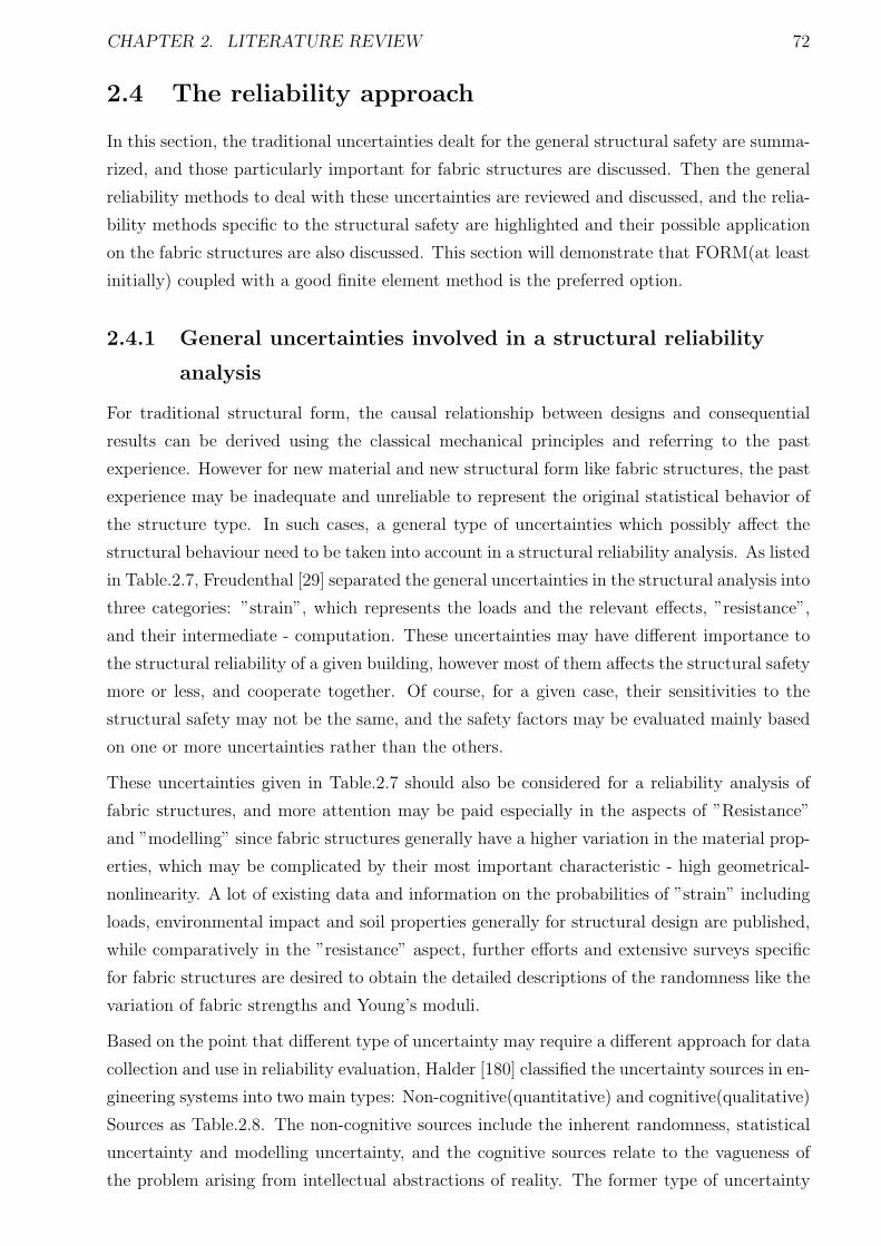
CHAPTER 2. LITERATURE REVIEW 72
2.4 The reliability approach
In this section, the traditional uncertainties dealt for the general structural safety are summa-
rized, and those particularly important for fabric structures are discussed. Then the general
reliability methods to deal with these uncertainties are reviewed and discussed, and the relia-
bility methods specific to the structural safety are highlighted and their possible application
on the fabric structures are also discussed. This section will demonstrate that FORM(at least
initially) coupled with a good finite element method is the preferred option.
2.4.1 General uncertainties involved in a structural reliability
analysis
For traditional structural form, the causal relationship between designs and consequential
results can be derived using the classical mechanical principles and referring to the past
experience. However for new material and new structural form like fabric structures, the past
experience may be inadequate and unreliable to represent the original statistical behavior of
the structure type. In such cases, a general type of uncertainties which possibly affect the
structural behaviour need to be taken into account in a structural reliability analysis. As listed
in Table.2.7, Freudenthal [29] separated the general uncertainties in the structural analysis into
three categories: ”strain”, which represents the loads and the relevant effects, ”resistance”,
and their intermediate - computation. These uncertainties may have different importance to
the structural reliability of a given building, however most of them affects the structural safety
more or less, and cooperate together. Of course, for a given case, their sensitivities to the
structural safety may not be the same, and the safety factors may be evaluated mainly based
on one or more uncertainties rather than the others.
These uncertainties given in Table.2.7 should also be considered for a reliability analysis of
fabric structures, and more attention may be paid especially in the aspects of ”Resistance”
and ”modelling” since fabric structures generally have a higher variation in the material prop-
erties, which may be complicated by their most important characteristic - high geometrical-
nonlinearity. A lot of existing data and information on the probabilities of ”strain” including
loads, environmental impact and soil properties generally for structural design are published,
while comparatively in the ”resistance” aspect, further efforts and extensive surveys specific
for fabric structures are desired to obtain the detailed descriptions of the randomness like the
variation of fabric strengths and Young’s moduli.
Based on the point that different type of uncertainty may require a different approach for data
collection and use in reliability evaluation, Halder [180] classified the uncertainty sources in en-
gineering systems into two main types: Non-cognitive(quantitative) and cognitive(qualitative)
Sources as Table.2.8. The non-cognitive sources include the inherent randomness, statistical
uncertainty and modelling uncertainty, and the cognitive sources relate to the vagueness of
the problem arising from intellectual abstractions of reality. The former type of uncertainty
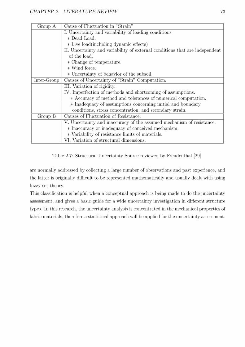
CHAPTER 2. LITERATURE REVIEW 73
Group A Cause of Fluctuation in ”Strain”I. Uncertainty and variability of loading conditions∗ Dead Load.∗ Live load(including dynamic effects)
II. Uncertainty and variability of external conditions that are independentof the load.∗ Change of temperature.∗ Wind force.∗ Uncertainty of behavior of the subsoil.
Inter-Group Causes of Uncertainty of ”Strain” Computation.III. Variation of rigidity.IV. Imperfection of methods and shortcoming of assumptions.
∗ Accuracy of method and tolerances of numerical computation.∗ Inadequacy of assumptions concerning initial and boundaryconditions, stress concentration, and secondary strain.
Group B Causes of Fluctuation of Resistance.V. Uncertainty and inaccuracy of the assumed mechanism of resistance.∗ Inaccuracy or inadequacy of conceived mechanism.∗ Variability of resistance limits of materials.
VI. Variation of structural dimensions.
Table 2.7: Structural Uncertainty Source reviewed by Freudenthal [29]
are normally addressed by collecting a large number of observations and past experience, and
the latter is originally difficult to be represented mathematically and usually dealt with using
fuzzy set theory.
This classification is helpful when a conceptual approach is being made to do the uncertainty
assessment, and gives a basic guide for a wide uncertainty investigation in different structure
types. In this research, the uncertainty analysis is concentrated in the mechanical properties of
fabric materials, therefore a statistical approach will be applied for the uncertainty assessment.
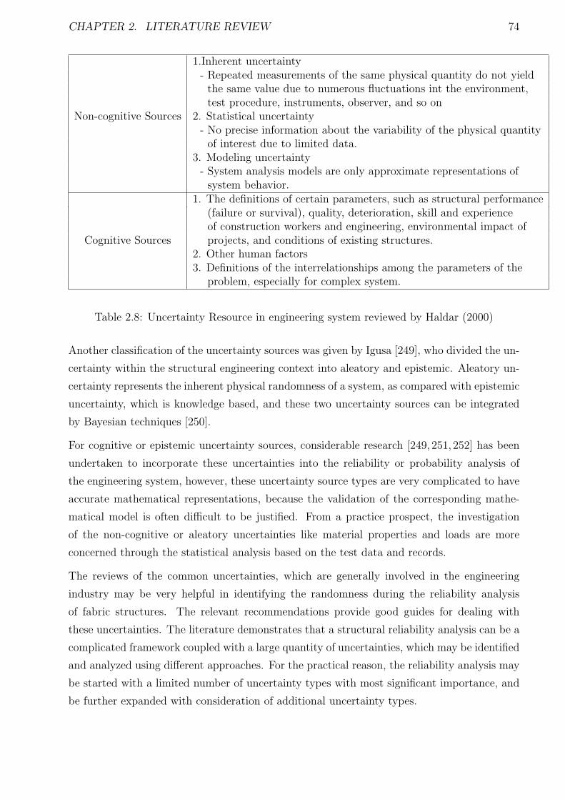
CHAPTER 2. LITERATURE REVIEW 74
1.Inherent uncertainty- Repeated measurements of the same physical quantity do not yield
the same value due to numerous fluctuations int the environment,test procedure, instruments, observer, and so on
Non-cognitive Sources 2. Statistical uncertainty- No precise information about the variability of the physical quantity
of interest due to limited data.3. Modeling uncertainty
- System analysis models are only approximate representations ofsystem behavior.
1. The definitions of certain parameters, such as structural performance(failure or survival), quality, deterioration, skill and experienceof construction workers and engineering, environmental impact of
Cognitive Sources projects, and conditions of existing structures.2. Other human factors3. Definitions of the interrelationships among the parameters of the
problem, especially for complex system.
Table 2.8: Uncertainty Resource in engineering system reviewed by Haldar (2000)
Another classification of the uncertainty sources was given by Igusa [249], who divided the un-
certainty within the structural engineering context into aleatory and epistemic. Aleatory un-
certainty represents the inherent physical randomness of a system, as compared with epistemic
uncertainty, which is knowledge based, and these two uncertainty sources can be integrated
by Bayesian techniques [250].
For cognitive or epistemic uncertainty sources, considerable research [249, 251, 252] has been
undertaken to incorporate these uncertainties into the reliability or probability analysis of
the engineering system, however, these uncertainty source types are very complicated to have
accurate mathematical representations, because the validation of the corresponding mathe-
matical model is often difficult to be justified. From a practice prospect, the investigation
of the non-cognitive or aleatory uncertainties like material properties and loads are more
concerned through the statistical analysis based on the test data and records.
The reviews of the common uncertainties, which are generally involved in the engineering
industry may be very helpful in identifying the randomness during the reliability analysis
of fabric structures. The relevant recommendations provide good guides for dealing with
these uncertainties. The literature demonstrates that a structural reliability analysis can be a
complicated framework coupled with a large quantity of uncertainties, which may be identified
and analyzed using different approaches. For the practical reason, the reliability analysis may
be started with a limited number of uncertainty types with most significant importance, and
be further expanded with consideration of additional uncertainty types.
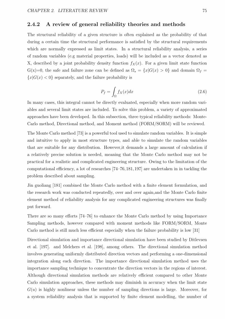
CHAPTER 2. LITERATURE REVIEW 75
2.4.2 A review of general reliability theories and methods
The structural reliability of a given structure is often explained as the probability of that
during a certain time the structural performance is satisfied by the structural requirements
which are normally expressed as limit states. In a structural reliability analysis, a series
of random variables (e.g material properties, loads) will be included as a vector denoted as
X, described by a joint probability density function fX(x). For a given limit state function
G(x)=0, the safe and failure zone can be defined as Ωs = x|G(x) > 0 and domain Ωf =
x|G(x) < 0 separately, and the failure probability is
Pf =
∫
Ω
fX(x)dx (2.6)
In many cases, this integral cannot be directly evaluated, especially when more random vari-
ables and several limit states are included. To solve this problem, a variety of approximated
approaches have been developed. In this subsection, three typical reliability methods: Monte-
Carlo method, Directional method, and Moment method (FORM/SORM) will be reviewed.
The Monte Carlo method [73] is a powerful tool used to simulate random variables. It is simple
and intuitive to apply in most structure types, and able to simulate the random variables
that are suitable for any distribution. However,it demands a large amount of calculation if
a relatively precise solution is needed, meaning that the Monte Carlo method may not be
practical for a realistic and complicated engineering structure. Owing to the limitation of the
computational efficiency, a lot of researches [74–76,181,197] are undertaken in in tackling the
problem described about sampling.
Jin guoliang [181] combined the Monte Carlo method with a finite element formulation, and
the research work was conducted repeatedly, over and over again,and the Monte Carlo finite
element method of reliability analysis for any complicated engineering structures was finally
put forward.
There are so many efforts [74–76] to enhance the Monte Carlo method by using Importance
Sampling methods, however compared with moment methods like FORM/SORM, Monte
Carlo method is still much less efficient especially when the failure probability is low [31]
Directional simulation and importance directional simulation have been studied by Ditlevsen
et al. [197]. and Melchers et al. [198], among others. The directional simulation method
involves generating uniformly distributed direction vectors and performing a one-dimensional
integration along each direction. The importance directional simulation method uses the
importance sampling technique to concentrate the direction vectors in the regions of interest.
Although directional simulation methods are relatively efficient compared to other Monte
Carlo simulation approaches, these methods may diminish in accuracy when the limit state
G(u) is highly nonlinear unless the number of sampling directions is large. Moreover, for
a system reliability analysis that is supported by finite element modelling, the number of
CHAPTER 2. LITERATURE REVIEW 76
directions required to limit the error in Pf must be held to a minimum for the analysis to be
performed efficiently.
Same as the Monte-Carlo method, the accuracy of the directional method depends on how
the design points are choosen, and often need to use a variety of enhancing approaches like
importance sampling technology [31] to enhance its performance. Jiesuo Nie [32] pointed
out that even with enhanced formulation, the directional method is still only efficient to low
demensional spaces.
First order reliability (FORM) is often used based on replacing the limit state surface by a
first order surface fitted to the design points in the standard normal space. The first order
estimate of the failure probability is given as:
pf =
∫
ω
Φ(y)dy = Φ(−β) (2.7)
where Φ(y) denotes standard normal density of the independent statistical variables involved
in the structure system. β is called the safety index which is approximated as the shortest
distance from the origin to the limit state surface in the standard normal space,
β =√t∗, t (2.8)
where, t and t∗ denote the nearest point coordinate vector of the limit state surface in the
standard normal space. Rackwitz and Fiessler [242] developed a very efficient FORM algo-
rithm which is found to work well for most structural systems when the gradients of statistical
variables within the structures can be accurately estimated.
In FORM, all the non-normal distributed variables are required to be transformed to the
the equivalent normal distribution based on the same CDF at the design points. A common
approach is first to transform the random vector Xs = [X1, X2, ..., Xd]T to an independent
standard normal random vector U = [U1, U2, ..., Ud]T by the Rosenblatt transformation U =
T (X). The transformation has to be repeated at every iteration in seeking the most probable
point (MPP) of the safety criteria surface.
Hong [30] developed a normal polynomial function to approximate many common distribu-
tions. Different from the traditional data fitting methods, it used fractile constraints instead
of statistical moment fitting. With the Rosenblatt transformation, the limit state function in
the space of independent standard normal variables may become a highly nonlinear function.
As an analytical tool for the reliability approximation, FORM is one of the most reliable
methods [191]. Over the past three decades, numerous studies on FORM and its application
on different types of reliability problems have been taken, and now FORM has become a basic
method for structural reliability. The weakness of this method is that when the performance
function is highly nonlinear, the linear approximation using FORM will lead to low accuracy.
To sort this problem, the second-order reliability method(SORM) was established to improve
CHAPTER 2. LITERATURE REVIEW 77
the accuracy of the FORM using second-order approximation of the limit state functions [185].
Once FORM cannot achieve adequate accuracy, the SORM can be used instead, however
the judgment about when FORM fail to satisfy the accuracy requirement is very difficult,
because the result of the reliability analysis is seldom validated by the feedback of reliability
accidents [193], while the most practical way is to control the error in the approximation
calculation.
YanGang [192] proposed an moment method to enhance the FORM accuracy and efficiency
using the high order moments to approximate the distribution of random variables. Based on
FORM, second order and third order moments method can be developed to reduce the error
from the linear approximation of the limit state functions.
FORM/SORM accuracy and efficiency can be also enhanced by modifying the limit state
surface. Armen [194] developed a ”bulge” method to reduce the errors during the searching
of multiple design points. The deformed surface was determined and updated with a ”bulge”
function specified based on the design points obtained from last iteration. His method demon-
strates that a satisfied accuracy and successively finding of the multiple design points without
large errors can be achieved by using FORM with the enhanced formulation.
To enhance the efficiency of FORM, Grandhi and Wang [97] developed a reliability algorithm
using two-point adaptive nonlinear approximation. In this method, both first order and second
order approximations of the performance function were used. The design point derived based
on linear approximation is assigned as the previous point Xk in the current iteration, and the
design point from nonlinear approximation is the current one Xk. The updated design points
are produced by both linear and nonlinear formulation alternatively. With this design point
search technology, the computational costs in safety index calculation and optimization are
significantly reduced.
Eurocode 0 [253] states different types of reliability method used for the calibration of safety
factors under limit states as fig.2.25, and the current safety coefficients in the Euro code are
estimated based on the deterministic method. It points out that full probabilistic reliability
can provide ”in principle correct answers” to the reliability analysis, but it is seldom used for
the calibration of safety factors in the design code because the relevant statistical data are
not sufficient. While FORM can be well used for the further development for most structural
types, and the sufficient accuracy of this method can be achieved when the approximations
are properly made.
The general view on the reliability approaches demonstrates that the Monte-Carlo method
may be the simplest reliability method to be applied without deriving a specific reliability
formulation, however its accuracy and efficiency are often not satisfactory especially for a
complicated structural system. FORM/SORM are proved to be very reliable and efficient
methods for many reliability problems. Compared with SORM, FORM may achieve better
efficiency in computing cost with a satisfactory accuracy. Actually the literature presents that
even for those with highly nonlinear limit state function, FORM can be still a good base for the
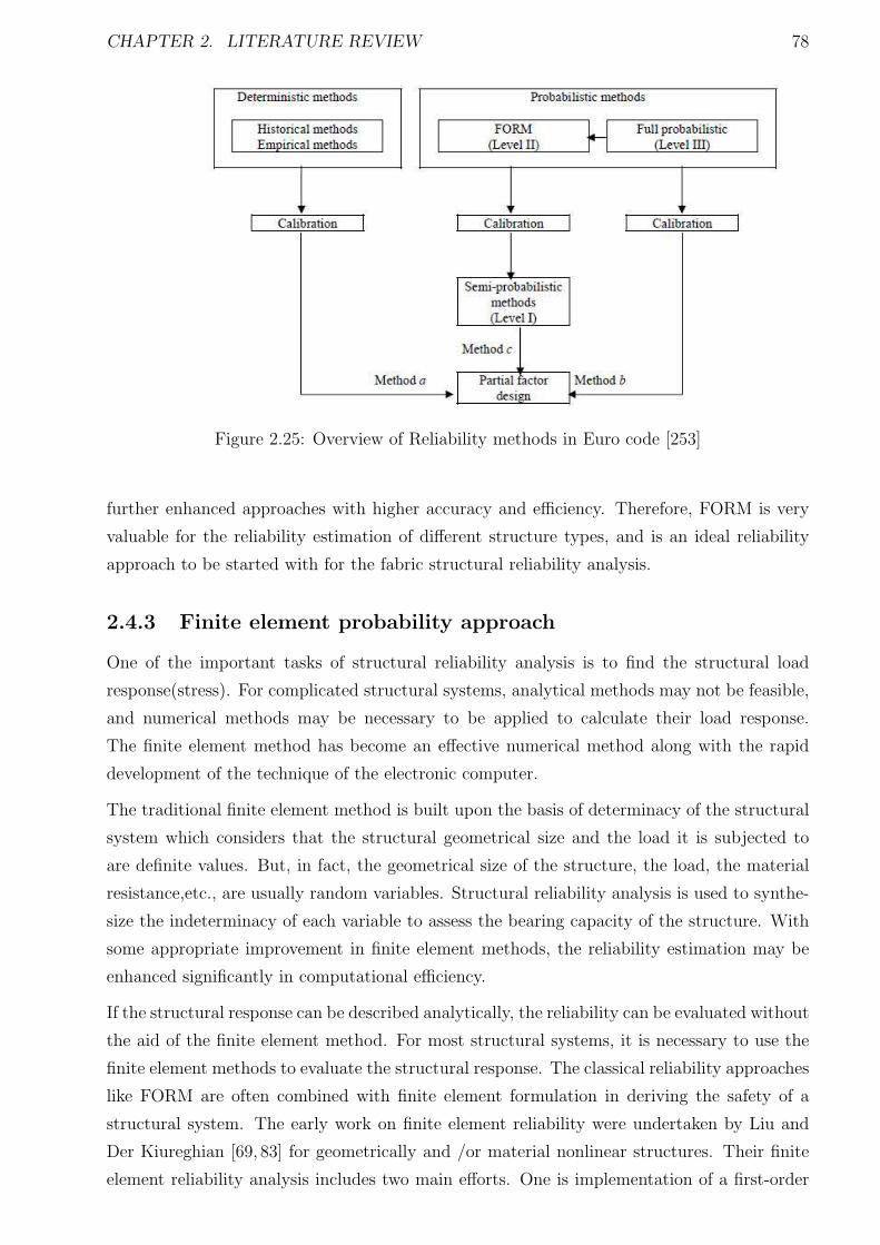
CHAPTER 2. LITERATURE REVIEW 78
Figure 2.25: Overview of Reliability methods in Euro code [253]
further enhanced approaches with higher accuracy and efficiency. Therefore, FORM is very
valuable for the reliability estimation of different structure types, and is an ideal reliability
approach to be started with for the fabric structural reliability analysis.
2.4.3 Finite element probability approach
One of the important tasks of structural reliability analysis is to find the structural load
response(stress). For complicated structural systems, analytical methods may not be feasible,
and numerical methods may be necessary to be applied to calculate their load response.
The finite element method has become an effective numerical method along with the rapid
development of the technique of the electronic computer.
The traditional finite element method is built upon the basis of determinacy of the structural
system which considers that the structural geometrical size and the load it is subjected to
are definite values. But, in fact, the geometrical size of the structure, the load, the material
resistance,etc., are usually random variables. Structural reliability analysis is used to synthe-
size the indeterminacy of each variable to assess the bearing capacity of the structure. With
some appropriate improvement in finite element methods, the reliability estimation may be
enhanced significantly in computational efficiency.
If the structural response can be described analytically, the reliability can be evaluated without
the aid of the finite element method. For most structural systems, it is necessary to use the
finite element methods to evaluate the structural response. The classical reliability approaches
like FORM are often combined with finite element formulation in deriving the safety of a
structural system. The early work on finite element reliability were undertaken by Liu and
Der Kiureghian [69, 83] for geometrically and /or material nonlinear structures. Their finite
element reliability analysis includes two main efforts. One is implementation of a first-order

CHAPTER 2. LITERATURE REVIEW 79
or a second-order reliability method, by improving the failure surface in the standard normal
space. The other is to apply the finite element in computing the gradients of structural
responses like load, material properties, and geometry variables.
The combined use of finite element formulation and reliability methods is very popular in
comtemparory reliability assessment, and is often called the ”stochastic finite element relia-
bility method” [180], in which, the sensitivities of the finite element formulation with respect
to the basic statistical variables are evaluated at the design points in the iteration process of
seeking the safety index.
Finite difference method [239] has been applied to calculate the gradients of the limit state
function with respect to the basic statistical variables, however this method is shown to be
time-consuming and only efficient in a system with a small mount of variables. The analytical
method applying the chain rule of differentiation is shown to ”enjoy the same advantage” [243]
as the finite difference method (also called perturbation method) and have better accuracy
and efficiency in the computing cost, when applied to the traditional structural system like
reinforced concrete [77].
The implementation of the finite element formulation in the FORM and SORM is introduced
by Liu [83] for the reliability analysis of geometrically nonlinear uncertain structures. He
pointed out that the key thing in seeking the design point using the finite element reliability
method is to compute the vector gradients, and he also compared the computational efficiency
of FORM and SORM coupled with analytical and finite difference method, and found that
FORM exhibited a good estimation of the reliability even for the high-nonlinear structure
type with non-normal distributed uncertainties, and when coupled with analytical method,
the computational efficiency is much higher than SORM method with point-fitting method.
Teigen [71] applied the finite element reliability method in nonlinear concrete structures, con-
sidering the nonlinearities in material and geometry, and randomness in loading, material
and geometry. The perturbation method is applied to calculate the structural response gra-
dients using first and second order terms of the Taylor series expansion of the limit state
equation. His approach succeeded in avoiding the requirement of explicit limit state function
and the time-consuming computation, and the numerical test results are encouraging, and
demonstrate that more effort is desired to develop the finite element method.
Frangopol [35] applied the finite element reliability method on a geometrically nonlinear sus-
pended truss system. It was found that linearly modelling a geometrical nonlinear structural
system will lead to a conservative result in the tension state and unconservative in compres-
sion, and the effect of the correlation of loads is more obvious than resistances. The material
behavior has significant effect on the structure system while not on the individual components.
Val et al [200] created a probabilistic method for reliability evaluation of RC frames in the con-
text of nonlinear analysis. His method combines the nonlinear finite element structural model
and the first order reliability method(FORM), Petryna [201] proposed a rational computer
CHAPTER 2. LITERATURE REVIEW 80
framework for time-variant reliability analysis of RC structures,which balances the accuracy
of mechanical and stochastic models with maintainable computing costs. It concludes new
material models for time-invariant and fatigue behaviour of concrete. He found influence of
temporal uncertainties in the evaluation of long-term life history including sequence effects
and path-dependence in nonlinear systems, and the influence of spatial scatter of material
properties and loads significantly affect the reliability estimates.
Kiyohiro [203] used a probabilistic finite element geometrically nonlinear analysis approach
to undertake reliability analysis of suspension bridges, in which, different loading and damage
senarios are considered as the main uncertainty. The optimal maintenance for suspension
bridges designed according to allowable stress method will be decided based on the result from
the reliability analysis. He proposed a general approach to evaluate the system reliability of
structures exhibiting geometrically nonlinear elastic behavior.
Numerous fabric structures have been designed and constructed over last recent several
decades, and many new fabric materials have been developed and applied in the industry.
However a general reliability analysis tool to predict the possibility of fabric structural failure
is still absent, because most attention has been paid to predicting the material strengths and
load effects not their uncertainties. Single failure point of a fabric structure could be esti-
mated according to given load, geometry and material with constant values by deterministic
analysis methods, but the confidence of structural safety is still unknown when a true load
and material case are applied. Compromising the efficiency and accuracy, a finite element
reliability formulation coupled with FORM is proposed in Chapter.5 based on an efficient
deterministic analysis formulation, demonstrated in Chapter.3.
2.4.4 Conclusion
A reliability analysis may possibly include numerous uncertainties, depending on the situations
and conditions of the given structures. Some uncertainties like material uncertainties can be
assessed using statistical approaches, and the others (e.g human skills) may be analyzed by
other methods like fuzzy theory. The literature about the uncertainties involved in a reliability
analysis give a general scope of uncertainties for this research, and also a direction of modelling
these uncertainties, not only for the uncertainties like fabric material properties included in
this research, but also for those excluded due to the limit of a single PhD research scope.
There are many structural reliability methods like Monte-Carlo, FORM, SORM, and full
probabilistic methods. FORM is found to be efficient and accurate, and has been successfully
applied in a wide range of structural types. SORM can provide a second order failure boundary
which may give better simulation of the real cases, however their solution procedures may not
be efficient and convergent results are difficult to produce in some cases. The Monte-Carlo
method is very easy to apply to the reliability analysis of most structural types, however
only efficiently for simple structures. Full probabilistic methods can provide generally correct

CHAPTER 2. LITERATURE REVIEW 81
reliability answers, but they have high requirements in the uncertainty information which may
not be available in a lot of cases.
The finite element reliability methods are generally made by combining the existing reliability
methods like FORM and the finite element formulations, and these methods have been applied
successfully in a series of geometrically nonlinear materials. Though these reliability methods
may not be directly used for fabric structures, they provide good examples for the integration
of the finite element method and reliability approaches. If an efficient finite element method
is developed specific for fabric structures, then FORM can work out the structural reliabilities
based on the given uncertainties within the power of finite element formulations.
CHAPTER 2. LITERATURE REVIEW 82
2.5 Summary & Conclusion
The conclusions on the literature are given at the ends of each section. The general conclusion
of this chapter is given as that the reliability analysis can be a large complicated system work,
which include a large mount of uncertainty investigation and probabilistic analysis, and also an
suitable reliability philosophy with the efficient computing engine dealing with the structural
response due to the uncertainties. Especially for the fabric structures with the geometrical
nonlinear structural performance and high material variability, a full-range reliability work is
too large for a PhD research work. Therefore in this thesis, the main target of the reliability
work should be focus on a good methodology to estimate structural safety based on the
obtained or published data of the uncertainties. The uncertainty investigation and analysis
of fabric in Chapter 4 are only limited in one type of fabric material, as an example to apply
the statistical investigation and probability assessment. And only several random variables
are involved in the reliability formulation Chapter 5 to demonstrate the application of the
reliability approach using finite element formulation.
Chapter 3
Finite Element Formulation For Fabric
Structures
The 3-node constant strain triangular element is the simplest and most widely used in the
industry. It is based on a geometrically nonlinear cable analogy approach with a linear strain
function and an assumption of small strains. However this approach is shown to be deficient
in representing the behavior of a continuum in the presence of shear strains in particular.
A modified version of this basic element is proposed based on including higher-order strain
terms. The revised element is shown to perform better than the original version, but as not
all higher-order terms can be included, large strains fail to be represented accurately. This
element is, here, denoted as a meso-strain formulation.
It should be noted that strictly, neither of the aforementioned formulations pass the patch
test. Therefore, to achieve this most fundamental of requirement, the cable-analogy principle
is retained, but the relationship between the element strains and side lengths is completely
revised. A classical finite element approach is adopted in defining the strain-displacement
relations, that is equivalent to Green’s strain, and therefore applicable to large strain de-
formations. The cable analogy approach is maintained by relating the nodal displacements,
element side lengths and the large strain definitions. Therefore, from a practical perspective,
the implementation of the new element formulation can be achieved by modifying existing
analysis codes. To this end, Dynamic Relaxation is also adopted to solve the resulting state
equations.
Recognizing the limitations of the constant strain triangle, a linear strain triangle formulation
is presented, also linked to Dynamic Relaxation as well as the conventional Newton-Raphson
procedure. This element is based on the original work of Ye [217] and the formulation revised
to improve the mathematical consistency. The main advantage of this type of element over the
CST element is the higher efficiency in the stress representation using the same type of degrees
of freedom(D.O.F). The additional element curvatures depend on the element geometry and
not additional rotational D.O.F and provide an explicit link between out-of-plane loads and
corresponding membrane stresses. However in the presence of geometric nonlinearity, the
83
CHAPTER 3. FINITE ELEMENT FORMULATION FOR FABRIC STRUCTURES 84
Newton-Raphson method becomes computationally inefficient with a slow convergence rate
using this type of element. In contrast, when coupled with with the Dynamic Relaxation
algorithm, a highly efficient analysis tool is developed
The derivation of the formulations and solution procedures of CSTs and LST are detailed in
sections 3.1 and 3.2 with wrinkling issues covered in section 3.4. Numerical examples and
comparison of these finite element formulations are illustrated and discussed in section 3.5.
3.1 Constant Strain Triangular Element (CST)
Unlike the finite element formulation of the typical CST, in this section the element strains
will be expressed as functions of the deformation of pseudo cables or increments of the element
side lengths. Based on different strain-displacement functions, the CST element formulation
is separated into three types as listed below and detailed in the subsequent sections:
• CST small strain formulation [208]:
Under the assumption of small strains, the linear cable analogy formulation is developed,
but neglects the high order terms in the relation between element strains and pseudo
cable strains.
• CST meso-strain formulation [209]:
The original small strain formulation approach enhanced by inclusion of some higher
order terms whilst maintaining the cable analogy introduced from [208].
• CST with large strain formulation:
A new formulation that abandons the original strain-displacement approach and is based
on a typical finite element philosophy, with all high order terms included in a nonlinear
continuum framework.
3.1.1 CST small strains formulation
The original form of the CST was, arguably, motivated by a requirement for computational
efficiency and also by a desire to analyse a membrane as a cable net, for which the computa-
tional mechanics was more straightforward and available at the time. Consequently, the CST
became a good candidate element because of the characteristic of having constant values of
strain along each of its three sides, meaning if the triangular element could be represented by
a set of three bars (or cables), then the membrane could indeed be analysed as a cable net/
geometrically nonlinear truss. In what follows we detail the development of the element in its
original form to demonstrate the principle of the formulation.
Referring to Figure 3.1 (A′C′-AC)/AC gives the strain normal to the plane FB related to the
normal stress σn.Considering the triangles ACD and A′C′D′ and du as the increase in length
from AD to A′D′, and dv the increase in length from CD to C′D′, then
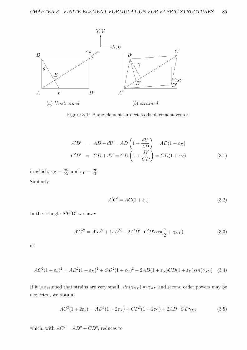
CHAPTER 3. FINITE ELEMENT FORMULATION FOR FABRIC STRUCTURES 85
-
3
6
X,U
Y, V
σn
A F D
BC
Eθ
(a) Unstrained
A′D′
B′ C ′
E ′
γ
γXY
(b) strained
Figure 3.1: Plane element subject to displacement vector
A′D′ = AD + dU = AD
(
1 +dU
AD
)
= AD(1 + εX)
C ′D′ = CD + dV = CD
(
1 +dV
CD
)
= CD(1 + εY ) (3.1)
in which, εX = ∂U∂X
and εY = ∂VdY
Similarly
A′C ′ = AC(1 + εn) (3.2)
In the triangle A′C′D′ we have:
A′C ′2 = A′D′2 + C ′D′2 − 2A′D′ · C ′D′cos(π
2+ γXY ) (3.3)
or
AC2(1 + εn)2 = AD2(1 + εX)2 + CD2(1 + εY )2 + 2AD(1 + εX)CD(1 + εY )sin(γXY ) (3.4)
If it is assumed that strains are very small, sin(γXY ) ≈ γXY and second order powers may be
neglected, we obtain:
AC2(1 + 2εn) = AD2(1 + 2εX) + CD2(1 + 2εY ) + 2AD · CDγXY (3.5)
which, with AC2 = AD2 + CD2, reduces to
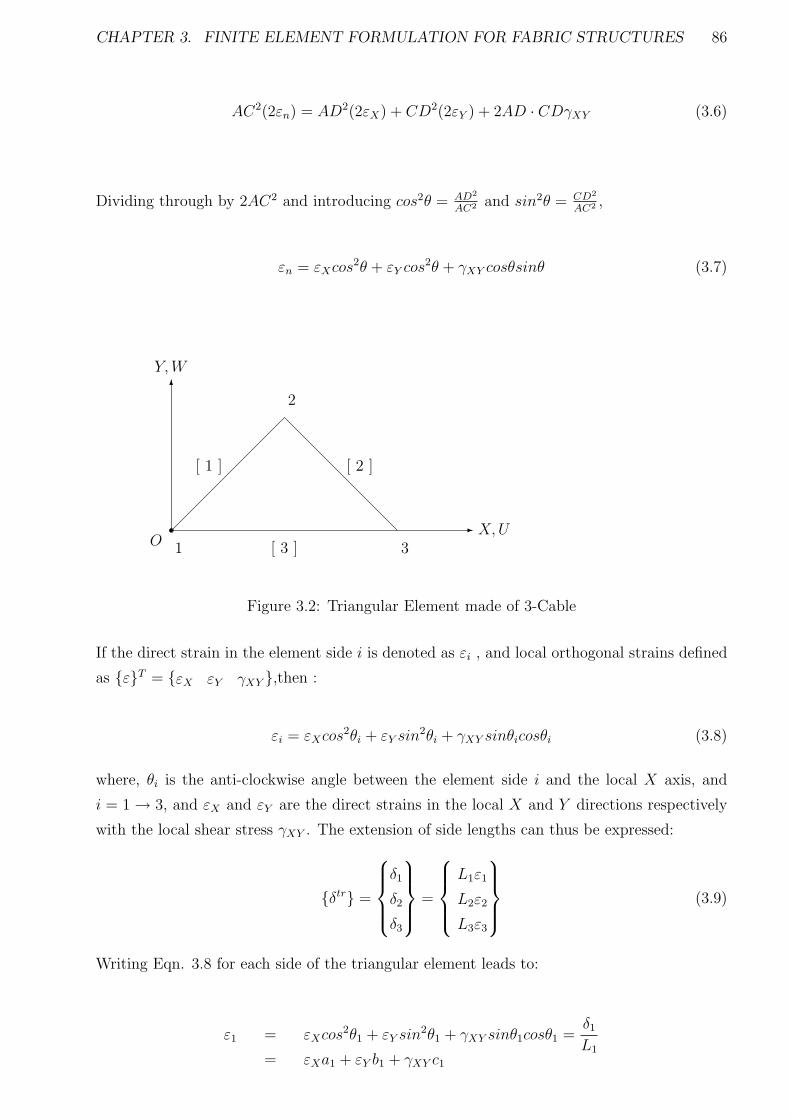
CHAPTER 3. FINITE ELEMENT FORMULATION FOR FABRIC STRUCTURES 86
AC2(2εn) = AD2(2εX) + CD2(2εY ) + 2AD · CDγXY (3.6)
Dividing through by 2AC2 and introducing cos2θ = AD2
AC2 and sin2θ = CD2
AC2 ,
εn = εXcos2θ + εY cos
2θ + γXY cosθsinθ (3.7)
- X,UO 1
2
3
[ 1 ] [ 2 ]
[ 3 ]
Y,W
6
Figure 3.2: Triangular Element made of 3-Cable
If the direct strain in the element side i is denoted as εi , and local orthogonal strains defined
as εT = εX εY γXY ,then :
εi = εXcos2θi + εY sin
2θi + γXY sinθicosθi (3.8)
where, θi is the anti-clockwise angle between the element side i and the local X axis, and
i = 1 → 3, and εX and εY are the direct strains in the local X and Y directions respectively
with the local shear stress γXY . The extension of side lengths can thus be expressed:
δtr =
δ1
δ2
δ3
=
L1ε1
L2ε2
L3ε3
(3.9)
Writing Eqn. 3.8 for each side of the triangular element leads to:
ε1 = εXcos2θ1 + εY sin
2θ1 + γXY sinθ1cosθ1 =δ1L1
= εXa1 + εY b1 + γXY c1
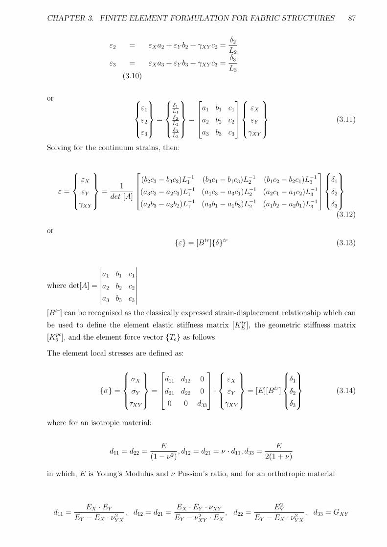
CHAPTER 3. FINITE ELEMENT FORMULATION FOR FABRIC STRUCTURES 87
ε2 = εXa2 + εY b2 + γXY c2 =δ2L2
ε3 = εXa3 + εY b3 + γXY c3 =δ3L3
(3.10)
or
ε1
ε2
ε3
=
δ1L1
δ2L2
δ3L3
=
a1 b1 c1
a2 b2 c2
a3 b3 c3
εX
εY
γXY
(3.11)
Solving for the continuum strains, then:
ε =
εX
εY
γXY
=1
det [A]
(b2c3 − b3c2)L−11 (b3c1 − b1c3)L
−12 (b1c2 − b2c1)L
−13
(a3c2 − a2c3)L−11 (a1c3 − a3c1)L
−12 (a2c1 − a1c2)L
−13
(a2b3 − a3b2)L−11 (a3b1 − a1b3)L
−12 (a1b2 − a2b1)L
−13
δ1
δ2
δ3
(3.12)
or
ε = [Btr]δtr (3.13)
where det[A] =
∣
∣
∣
∣
∣
∣
∣
∣
a1 b1 c1
a2 b2 c2
a3 b3 c3
∣
∣
∣
∣
∣
∣
∣
∣
[Btr] can be recognised as the classically expressed strain-displacement relationship which can
be used to define the element elastic stiffness matrix [KtrE ], the geometric stiffness matrix
[Kpcδ ], and the element force vector Tc as follows.
The element local stresses are defined as:
σ =
σX
σY
τXY
=
d11 d12 0
d21 d22 0
0 0 d33
·
εX
εY
γXY
= [E][Btr]
δ1
δ2
δ3
(3.14)
where for an isotropic material:
d11 = d22 =E
(1 − ν2), d12 = d21 = ν · d11, d33 =
E
2(1 + ν)
in which, E is Young’s Modulus and ν Possion’s ratio, and for an orthotropic material
d11 =EX · EY
EY − EX · ν2Y X
, d12 = d21 =EX · EY · νXY
EY − ν2XY · EX
, d22 =E2
Y
EY − EX · ν2Y X
, d33 = GXY
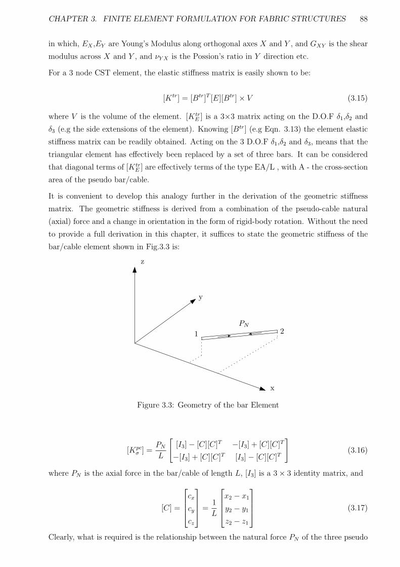
CHAPTER 3. FINITE ELEMENT FORMULATION FOR FABRIC STRUCTURES 88
in which, EX ,EY are Young’s Modulus along orthogonal axes X and Y , and GXY is the shear
modulus across X and Y , and νY X is the Possion’s ratio in Y direction etc.
For a 3 node CST element, the elastic stiffness matrix is easily shown to be:
[Ktr] = [Btr]T [E][Btr] × V (3.15)
where V is the volume of the element. [KtrE ] is a 3×3 matrix acting on the D.O.F δ1,δ2 and
δ3 (e.g the side extensions of the element). Knowing [Btr] (e.g Eqn. 3.13) the element elastic
stiffness matrix can be readily obtained. Acting on the 3 D.O.F δ1,δ2 and δ3, means that the
triangular element has effectively been replaced by a set of three bars. It can be considered
that diagonal terms of [KtrE ] are effectively terms of the type EA/L , with A - the cross-section
area of the pseudo bar/cable.
It is convenient to develop this analogy further in the derivation of the geometric stiffness
matrix. The geometric stiffness is derived from a combination of the pseudo-cable natural
(axial) force and a change in orientation in the form of rigid-body rotation. Without the need
to provide a full derivation in this chapter, it suffices to state the geometric stiffness of the
bar/cable element shown in Fig.3.3 is:
PN
1 2
x
y
z
Figure 3.3: Geometry of the bar Element
[Kpcσ ] =
PN
L
[
[I3] − [C][C]T −[I3] + [C][C]T
−[I3] + [C][C]T [I3] − [C][C]T
]
(3.16)
where PN is the axial force in the bar/cable of length L, [I3] is a 3 × 3 identity matrix, and
[C] =
cx
cy
cz
=1
L
x2 − x1
y2 − y1
z2 − z1
(3.17)
Clearly, what is required is the relationship between the natural force PN of the three pseudo
CHAPTER 3. FINITE ELEMENT FORMULATION FOR FABRIC STRUCTURES 89
cables/bars describing the triangular element and the continuum stresses σx,σy and τxy in
order to be able to make use of the Eqn. 3.16.
Combing the elastic stiffness matrix [KtrE ] (Eqn. 3.15) with the element side extensions δ1,δ2
and δ3 leads to the element side force T1, T2 and T3 as in:
T =
Tc1
Tc2
Tc3
= [Btr][E][Btr]V
δ1
δ2
δ3
(3.18)
X
Y
1
2
3
T1 T2
T3
σ
σ = σX σY τXY T
Figure 3.4: The pseudo cable forces
(See also Fig. 3.4). Noting Eqn. 3.14 and pre-multiplying it by [Btr]T and V , then:
V × [Btr]Tδ = V × [Btr]T [E][Btr]
δ1
δ2
δ3
(3.19)
The right-hand-side of Eqn. 3.19 is then identical to the right-hand-side of the Eqn. 3.18,
such that we have the definition:
T =
Tc1
Tc2
Tc3
= V × [Btr]T
σX
σY
τXY
(3.20)
Eqn. 3.20 provides the link between the pseudo cable element forces Tc1, Tc2 and Tc3( viz. PN
in Eqn. 3.16) and the triangular element continuum stresses σX , σY and τXY .
It should be noted at this point that both the elastic stiffness and geometric stiffness matrices
are functions of the strain-displacement matrix [Btr]. For the original CST formulation [Btr]
is defined in Eqn. 3.13 with Eqn. 3.12. The limitations of this particular form of [Btr] have
been previously stated and are demonstrated in section 3.5. To improve the CST-pseudo
cable element formulation it, therefore, remains to establish ”better” forms of [Btr]. Two
alternatives are described in sections 3.1.2 and 3.1.3, and assessed in section 3.5.
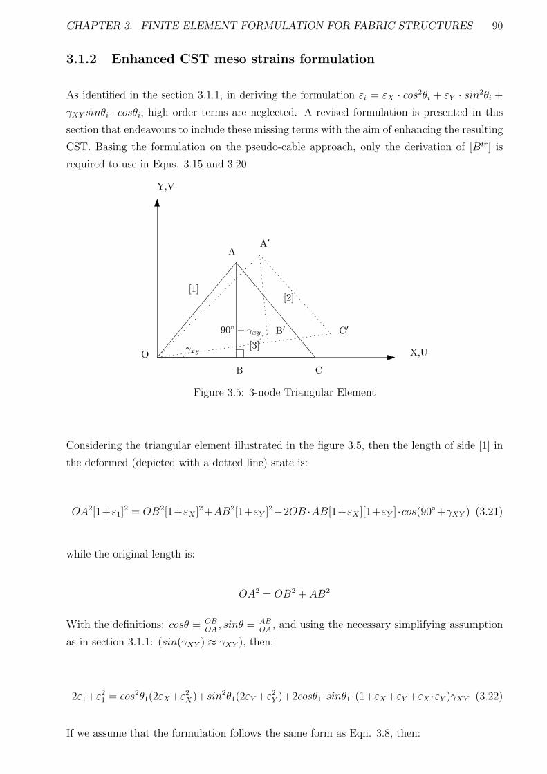
CHAPTER 3. FINITE ELEMENT FORMULATION FOR FABRIC STRUCTURES 90
3.1.2 Enhanced CST meso strains formulation
As identified in the section 3.1.1, in deriving the formulation εi = εX · cos2θi + εY · sin2θi +
γXY sinθi · cosθi, high order terms are neglected. A revised formulation is presented in this
section that endeavours to include these missing terms with the aim of enhancing the resulting
CST. Basing the formulation on the pseudo-cable approach, only the derivation of [Btr] is
required to use in Eqns. 3.15 and 3.20.
O
A
B C
A′
B′ C′
X,U
Y,V
[1][2]
[3]γxy
90 + γxy
Figure 3.5: 3-node Triangular Element
Considering the triangular element illustrated in the figure 3.5, then the length of side [1] in
the deformed (depicted with a dotted line) state is:
OA2[1+ε1]2 = OB2[1+εX ]2 +AB2[1+εY ]2−2OB ·AB[1+εX ][1+εY ] ·cos(90+γXY ) (3.21)
while the original length is:
OA2 = OB2 + AB2
With the definitions: cosθ = OBOA, sinθ = AB
OA, and using the necessary simplifying assumption
as in section 3.1.1: (sin(γXY ) ≈ γXY ), then:
2ε1+ε21 = cos2θ1(2εX +ε2
X)+sin2θ1(2εY +ε2Y )+2cosθ1 ·sinθ1 ·(1+εX +εY +εX ·εY )γXY (3.22)
If we assume that the formulation follows the same form as Eqn. 3.8, then:
CHAPTER 3. FINITE ELEMENT FORMULATION FOR FABRIC STRUCTURES 91
ε1 = εXcos2θ1 + εY cos
2θ1 + γXY sinθ1cosθ1 + ∆ (3.23)
where ∆ represents all the higher order terms.
The significance of ∆ can be approximately examined as follows. Equation 3.23 can be used
in the first term on the left side of Eqn. 3.22. In substituting Eqn. 3.23 into the second
term of left side of Eqn. 3.22, it is mathematically necessary to omit the higher order terms.
Consequently,
ε21 = (εX ·cos2θ1+εY ·sin2θ1+γXY ·sinθ1·cosθ1+∆)2 ≈ (εX ·cos2θ1+εY ·sin2θ1+γXY ·sinθ1·cosθ1)
2
(3.24)
or,
ε21 ≈ cos4θ1 ·ε2
X +sin4θ1 ·ε2Y +sin2θ1 ·cos2θ1 ·γ2
XY +2εX ·εY ·sin2θ1 ·cos2θ1+2εY ·γXY ·sin3θ1 ·cosθ1
(3.25)
+2γXY · εX · cos3θ1 · sinθ1
We substitute Eqn. 3.25 into the second term on the left side of Eqn. 3.22. Therefore, using
equation 3.23 and 3.25 as described above, then:
2∆ ≈ cos2θ1 · ε2X + sin2θ1 · ε2
Y + 2(εX + εY + εX · εY ) · γXY · sinθ1 · cosθ1 − ε21
≈ (cos2θ1 − cos4θ1) · ε2X + (sin2θ1 − sin4θ1) · ε2
Y + 2(1 − sin2θ1) · sinθ1 · cosθ1 · γXY · εX
+2(1 − cos2θ1) · sinθ1 · cosθ1 · γXY · εY + 2(γXY − sinθ1 · cosθ1) · εX · εY · sinθ1 · cosθ1
−γ2XY · cos2θ1 · sin2θ1
≈ sin2θ1 · cos2θ1 · ε2X + sin2θ1 · cos2θ1 · ε2
Y + 2cos3θ1 · sinθ1 · γXY · εX + 2sin3θ1 · cosθ1 · εY
+2(γXY − sinθ1 · cosθ1) · εX · εY · sinθ1 · cosθ1 − γ2XY · cos2θ1 · sin2θ
≈ 14(ε2
X + ε2Y )sin22θ1 + γXY · (εy · cos2θ1 + εX · sin2θ1)sin2θ1 + εX · εY (γXY − 1
2sin2θ1)sin2θ1
−14γ2
XY · sin22θ1
≈ [14(εX − εY )2 − 1
4γ2
XY ] · sin22θ1 + γXY · (εY · cos2θ1 + εX · sin2θ1 + εX · εY ) sin 2θ1
such that
∆ ≈ [1
8(εX −εY )2− 1
8γ2
XY ] ·sin22θ1 +1
2γXY · (εY ·cos2θ1 +εX ·sin2θ1 +εX ·εY ) ·sin2θ1 = ∆(o2)
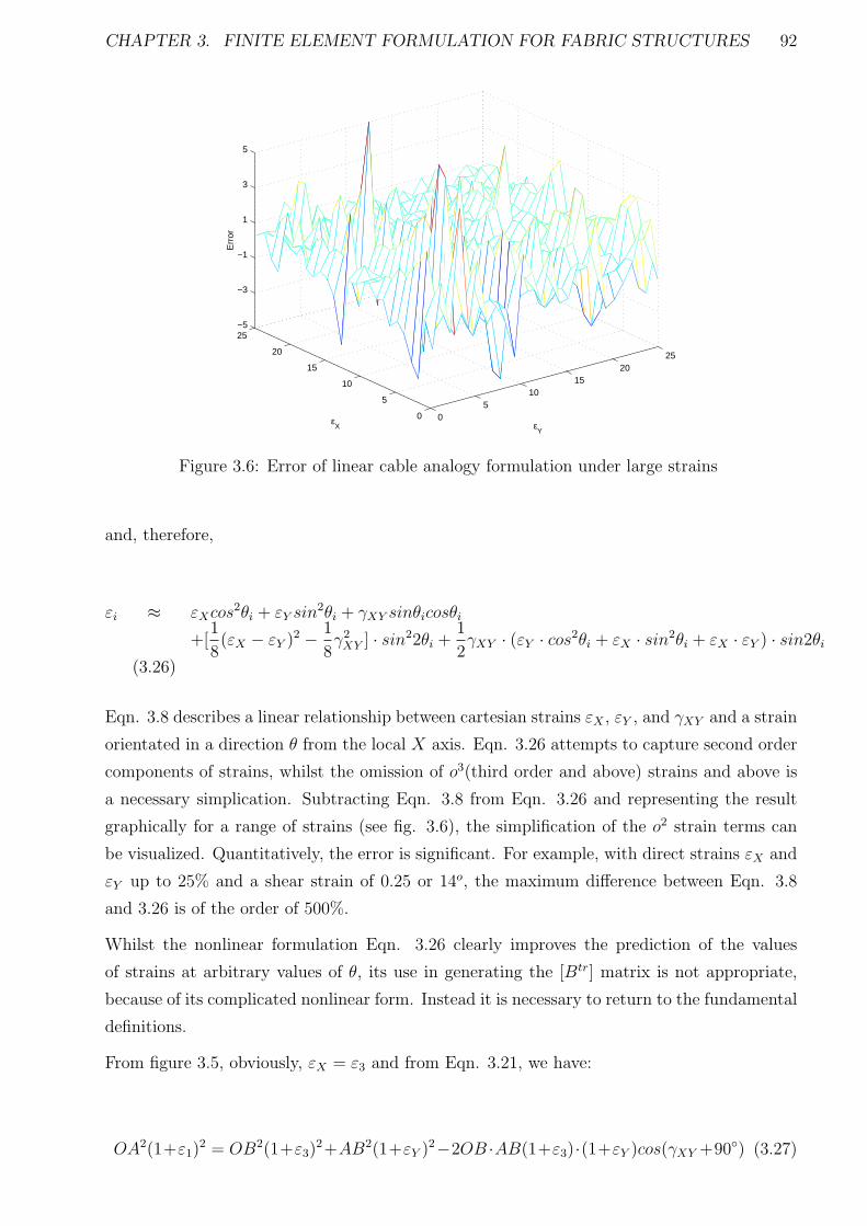
CHAPTER 3. FINITE ELEMENT FORMULATION FOR FABRIC STRUCTURES 92
05
1015
2025
0
5
10
15
20
25−5
−3
−1
1
3
5
εY
εX
Err
or
Figure 3.6: Error of linear cable analogy formulation under large strains
and, therefore,
εi ≈ εXcos2θi + εY sin
2θi + γXY sinθicosθi
+[1
8(εX − εY )2 − 1
8γ2
XY ] · sin22θi +1
2γXY · (εY · cos2θi + εX · sin2θi + εX · εY ) · sin2θi
(3.26)
Eqn. 3.8 describes a linear relationship between cartesian strains εX , εY , and γXY and a strain
orientated in a direction θ from the local X axis. Eqn. 3.26 attempts to capture second order
components of strains, whilst the omission of o3(third order and above) strains and above is
a necessary simplication. Subtracting Eqn. 3.8 from Eqn. 3.26 and representing the result
graphically for a range of strains (see fig. 3.6), the simplification of the o2 strain terms can
be visualized. Quantitatively, the error is significant. For example, with direct strains εX and
εY up to 25% and a shear strain of 0.25 or 14o, the maximum difference between Eqn. 3.8
and 3.26 is of the order of 500%.
Whilst the nonlinear formulation Eqn. 3.26 clearly improves the prediction of the values
of strains at arbitrary values of θ, its use in generating the [Btr] matrix is not appropriate,
because of its complicated nonlinear form. Instead it is necessary to return to the fundamental
definitions.
From figure 3.5, obviously, εX = ε3 and from Eqn. 3.21, we have:
OA2(1+ε1)2 = OB2(1+ε3)
2+AB2(1+εY )2−2OB ·AB(1+ε3)·(1+εY )cos(γXY +90) (3.27)
CHAPTER 3. FINITE ELEMENT FORMULATION FOR FABRIC STRUCTURES 93
If OA2 = OB2 + AB2, and OC = OA · cosθ1, AC = OA · sinθ1
then
(1 + ε1)2 = cos2θ1 · (1 + ε3)
2 + sin2θ1 · (1 + εy)2 + 2(1 + ε3)(1 + εy)sinγxysinθ1cosθ1 (3.28)
Similarly,
(1 + ε2)2 = cos2θ2 · (1 + ε3)
2 + sin2θ2 · (1 + εy)2 + 2(1 + ε3)(1 + εy)sinγxysinθ2cosθ2 (3.29)
To obtain a strain-displacement relationship that is linear in εX , εY , γXY , then it is necessary
to assume that sinγXY ≈ γXY and
(1 + εY )2 = 1 + 2εY + αc · εY
= 1 + (2 + αc)εY (3.30)
Using the notation in Eqn. 3.30, then, Eqns. 3.28 and 3.29 become
2ε1 + ε21 = cos2θ1 · (2ε3 + ε2
3) + sin2θ1 · (2 + αc) · εY + 2γXY (1 + ε3)(1 + εY )sinθ1cosθ1 (3.31)
2ε2 + ε22 = cos2θ2 · (2ε3 + ε2
3) + sin2θ2 · (2 + αc) · εY + 2γxy(1 + ε3)(1 + εY )sinθ2cosθ2 (3.32)
Solving Eqns. 3.31 and 3.32 simultaneously for εY , then,
εY =
(2ε1 + ε21)sinθ2cosθ2 − (2ε2 + ε2
2)sinθ1cosθ1 − (2ε3 + ε23) · (cos2θ1sinθ2cosθ2 − cos2θ2sinθ1cosθ1)
(sin2θ1sinθ2cosθ2 − sin2θ2sinθ1cosθ1)(2 + αc).
Defining
a2 = sinθ2cosθ2, b2 = −sinθ1cosθ1, c2 = cos2θ2sinθ1cosθ1 − cos2θ1sinθ2cosθ2
Ac = sin2θ1sinθ2cosθ2 − sin2θ2sinθ1cosθ1
then
εY =a2(2ε1 + ε2
1) + b2(2ε2 + ε22) + c2(2ε3 + ε2
3)
Ac(2 + αc)
Similarly, solving Eqns (31) and (32) for γXY , then
CHAPTER 3. FINITE ELEMENT FORMULATION FOR FABRIC STRUCTURES 94
γXY =a3(2ε1 + ε2
1) + b3(2ε2 + ε22) + c3(2ε3 + ε2
3)
2(1 + ε3)[a2(2ε1 + ε21) + b2(2ε2 + ε2
2) + c2(2ε3 + ε23) + (2 + αc)Ac]
with,
a3 = sinθ2, b3 = −sin2θ1, c3 = −[cos2θ1sin
2θ2 − cos2θ2sin2θ1]
Finally
εx
εy
γxy
=
0 0 1a2(2+ε1)Ac(2+αc)
b2(2+ε2)Ac(2+αc)
c3(2+ε3)Ac(2+αc)
a3(2+ε1)2(1+ε3)B
b3(2+ε2)2(1+ε3)B
c3(2+ε3)2(1+ε3)B
ε1
ε2
ε3
(3.33)
or ε = [Btr]δtr, where
[Btr] =
0 0 L−13
a2(2+ε1)·L−11
Ac(2+αc)
b2(2+ε2)·L−12
Ac(2+αc)
c3(2+ε3)·L−13
Ac(2+αc)a3(2+ε1)·L−1
1
2(1+ε3)Bc
b3(2+ε2)·L−12
2(1+ε3)Bc
c3(2+ε3)·L−13
2(1+ε3)Bc
(3.34)
in which, collecting all definitions together,
a2 = sinθ2cosθ2, b2 = −sinθ1cosθ1, c2 = cos2θ2sinθ1cosθ1 − cos2θ1sinθ2cosθ2 a3 = sin2θ2, b3 =
−sin2θ1, c3 = −[cos2θ1sin2θ2−cos2θ2−cos2θ2sin
2θ1] A = sin2θ1sinθ2cosθ2−sin2θ2sinθ1cosθ1
Bc =a2(2ε1+ε2
1)+b2(2ε2+ε22)+c3(ε3+ε2
3)+(2+αci )A
c
Ac(2+αci )
αc is an iteration coefficient, which has an initial value of zero and is subsequently updated
according to,
αci =
a2(2εi−11 + εi−1
1
2) + b2(2ε
i−12 + εi−1
2
2) + c3(2ε
i−13 + εi−1
3
2)
A(2 + αci−1)
Eqn. 3.31 is in a suitable form to be used in Eqns. 3.15 and 3.16 to define the element stiffness
matrices and associated Eqn. 3.18. It should be noted that this formulation relies upon the
assumption in Eqn. 3.1 that εX = ∂U∂X
and εY = ∂V∂Y
. No assumption is made about the form
of γXY , but it is reasonably assumed that sin(γXY ) = γXY .
3.1.3 CST with large strain formulation
The preceding CST formulations are characterized by the element strains εX and εY defined as
a linear deformation gradient (e.g. ∂U∂X
) as in Eqn. 3.1, and the shear strain γXY approximated
by sinγXY = γXY . These assumptions may no longer be valid under large strains where
Green’s deformation of strains is more appropriate, as in:
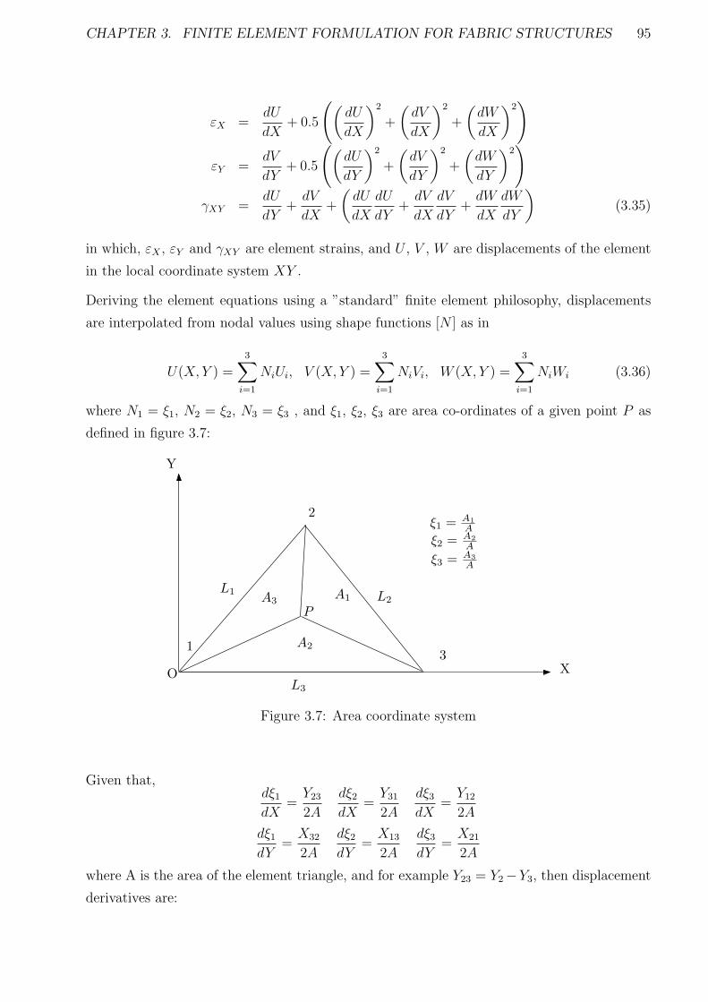
CHAPTER 3. FINITE ELEMENT FORMULATION FOR FABRIC STRUCTURES 95
εX =dU
dX+ 0.5
(
(
dU
dX
)2
+
(
dV
dX
)2
+
(
dW
dX
)2)
εY =dV
dY+ 0.5
(
(
dU
dY
)2
+
(
dV
dY
)2
+
(
dW
dY
)2)
γXY =dU
dY+dV
dX+
(
dU
dX
dU
dY+dV
dX
dV
dY+dW
dX
dW
dY
)
(3.35)
in which, εX , εY and γXY are element strains, and U , V , W are displacements of the element
in the local coordinate system XY .
Deriving the element equations using a ”standard” finite element philosophy, displacements
are interpolated from nodal values using shape functions [N ] as in
U(X,Y ) =3∑
i=1
NiUi, V (X,Y ) =3∑
i=1
NiVi, W (X,Y ) =3∑
i=1
NiWi (3.36)
where N1 = ξ1, N2 = ξ2, N3 = ξ3 , and ξ1, ξ2, ξ3 are area co-ordinates of a given point P as
defined in figure 3.7:
X
Y
O
1
2
3
A1A3
A2
ξ1 =A1
A
ξ2 =A2
A
ξ3 =A3
A
L3
L1 L2
P
Figure 3.7: Area coordinate system
Given that,dξ1dX
=Y23
2A
dξ2dX
=Y31
2A
dξ3dX
=Y12
2A
dξ1dY
=X32
2A
dξ2dY
=X13
2A
dξ3dY
=X21
2A
where A is the area of the element triangle, and for example Y23 = Y2 −Y3, then displacement
derivatives are:
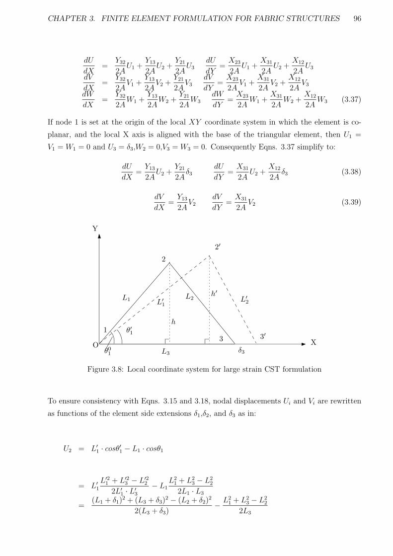
CHAPTER 3. FINITE ELEMENT FORMULATION FOR FABRIC STRUCTURES 96
dU
dX=
Y32
2AU1 +
Y13
2AU2 +
Y21
2AU3
dU
dY=X23
2AU1 +
X31
2AU2 +
X12
2AU3
dV
dX=
Y32
2AV1 +
Y13
2AV2 +
Y21
2AV3
dV
dY=X23
2AV1 +
X31
2AV2 +
X12
2AV3
dW
dX=
Y32
2AW1 +
Y13
2AW2 +
Y21
2AW3
dW
dY=X23
2AW1 +
X31
2AW2 +
X12
2AW3 (3.37)
If node 1 is set at the origin of the local XY coordinate system in which the element is co-
planar, and the local X axis is aligned with the base of the triangular element, then U1 =
V1 = W1 = 0 and U3 = δ3,W2 = 0,V3 = W3 = 0. Consequently Eqns. 3.37 simplify to:
dU
dX=Y13
2AU2 +
Y21
2Aδ3
dU
dY=X31
2AU2 +
X12
2Aδ3 (3.38)
dV
dX=Y13
2AV2
dV
dY=X31
2AV2 (3.39)
X
Y
O
1
2
3
L3
L1L2
θ0
1
θ′
1
2′
3′
L′
1
L′
2
δ3
h
h′
Figure 3.8: Local coordinate system for large strain CST formulation
To ensure consistency with Eqns. 3.15 and 3.18, nodal displacements Ui and Vi are rewritten
as functions of the element side extensions δ1,δ2, and δ3 as in:
U2 = L′1 · cosθ′1 − L1 · cosθ1
= L′1
L′21 + L′2
3 − L′22
2L′1 · L′
3
− L1L2
1 + L23 − L2
2
2L1 · L3
=(L1 + δ1)
2 + (L3 + δ3)2 − (L2 + δ2)
2
2(L3 + δ3)− L2
1 + L23 − L2
2
2L3
CHAPTER 3. FINITE ELEMENT FORMULATION FOR FABRIC STRUCTURES 97
=δ1 + 2L1
2(L3 + δ3)δ1 −
δ2 + 2L2
2(L3 + δ3)δ2 +
L23 − L2
1 + L22 + δ3 · L3
2(L3 + δ3)L3
δ3
= a1 · δ1 + a2 · δ2 + a3 · δ3 (3.40)
V2 = h′ − h
=2Area12′3′
L′3
− 2Area123
L3
=
√
L′22 L
′23 − (
L′22 +L′2
3 −L′21
2)2
L′3
−
√
L22L
23 − (
L22+L2
3−L21
2)2
L3
=L3
√
L′22 L
′23 − (
L′22 +L′2
3 −L′21
2)2 − L′
3
√
L22L
23 − (
L22+L2
3−L21
2)2
L3L′3
=L2
3[L′22 L
′23 − (
L′22 +L′2
3 −L′21
2)2] − L′2
3 [L22L
23 − (
L22+L2
3−L21
2)2]
L3L′3[L3
√
L′22 L
′23 − (
L′22 +L′2
3 −L′21
2)2 + L′
3
√
L22L
23 − (
L22+L2
3−L21
2)2]
=L2
3L′23 (L′
2 − L2)(L′2 + L2) − [L3
L′22 +L′2
3 −L′21
2− L′
3L2
2+L23−L2
1
2] · [L3
L′22 +L′2
3 −L′21
2+ L′
3L2
2+L23−L2
1
2]
L′3L3(L3 · 2A′ + L′
3 · 2A)
=L2
3L′23 (L′
2 + L2)δ2 − [L3L′2
2 +L′23 −L′2
1
2− L′
3L2
2+L23−L2
1
2] ·BB
L′3L3(L3 · 2A′ + L′
3 · 2A)
=L2
3L′23 (L′
2 + L2)δ2 − δ3L2
2+L23−L2
1
2·BB
L′3L3(L3 · 2A′ + L′
3 · 2A)
− [L3
2((L′
2 − L2)(L′2 + L2) + (L′
3 − L3)(L′3 + L3) − (L′
1 − L1)(L′1 + L1))] ·BB
L′3L3(L3 · 2A′ + L′
3 · 2A)
=L2
3L′23 (L′
2 + L2)δ2 − [L3
2((L′
2 + L2)δ2 + (L′3 + L3)δ3 − (L′
1 + L1)δ1) − δ3L2
2+L23−L2
1
2] ·BB
L′3L3(L3 · 2A′ + L′
3 · 2A)
=L3
2(L′
1 + L1)BBδ1 + (L′23 L
23 − L3
2·BB)(L2 + L′
2)δ2 + (L2
2+L23−L2
1
2− L3(L′
3+L3)
2)BB · δ3
L′3L3(L3 · 2A′ + L′
3 · 2A)
=L3
2(L′
1 + L1)BBδ1 + (L′23 L
23 − L3
2·BB)(L2 + L′
2)δ2 + (L22 − L2
1 − L′3L3)
BB2
· δ3AA
=BB(2L1L3 + L3δ1)
2AA· δ1 + [
L′23 · L2
3(L′2 + L2)
AA− BB(2L2L3 + δ2 · L3)
2AA] · δ2
+BB(L2
2 − L21 − L2
3 − L3 · δ3)2AA
· δ3
= b1 · δ1 + b2 · δ2 + b3 · δ3 (3.41)
Substituting Eqn.3.38-3.41 into 3.35, we can get:
CHAPTER 3. FINITE ELEMENT FORMULATION FOR FABRIC STRUCTURES 98
ε = [B]δ =
B11 B12 B13
B21 B22 B23
B31 B32 B33
δ1
δ2
δ3
(3.42)
in which,
B11 = B12 = 0 B13 = 1L3
+ δ32L2
3
B21 = E1 · b1 + E2 · a1 B22 = E1 · b2 + E2 · a2 B23 = E1 · b3 + E2 · a3 + E3
B31 = F1 · a1 B32 = F1 · a2 B33 = F1 · a3 + F2
The coefficients are defined as:
L′1 = L1 + δ1 L′
2 = L2 + δ2 L′3 = L3 + δ3
AA = L′3 · L3(L3
√
L′23 · L′2
2 − 0.25(L′22 + L′2
3 − L′21 )2
+L′3 ·√
L22 · L2
3 − 0.25(L22 + L2
3 − L21)
2
BB = 0.5L3(L′22 + L′2
3 − L′21 ) + 0.5L′
3(L22 + L2
3 − L21)
a1 = δ1+2L1
2L′
3b1 = BB(2L1L3+L3δ1)
2AA
a2 = − δ2+2L2
2L′
3b2 =
L′23 ·L2
3(L′
2+L2)
AA− BB(2L2L3+δ2·L3)
2AA
a3 =L2
3−L21+L2
2+δ3·L3
2L′
3·L3b3 =
BB(L22−L2
1−L23−L3·δ3)
2AA
U2 = a1δ1 + a2δ2 + a3δ3 V2 = b1δ1 + b2δ2 + b3δ3 U3 = δ3
E1 = X31
2A+
X231
8A2V2 E2 = X31X12
4A2 U3 +X2
31
8A2U2 E3 =X2
12
8A2 δ3
F1 = X31
2AF2 = X12
2A+ Y21
2A(X31
2AU2 + X12
2Aδ3) F = L′2
3 · L23 · L′
1
where A and A′ are the areas of the undeformed and deformed trinagles respectively.
Eqn. 3.42 may be substituted into Eqn. 3.15 and 3.18 to define the element characteristic
matrices.
3.1.4 Stiffness Matrix Definitions
Since Dynamic Relaxation will be used as the solution procedure, only the diagonal terms of
the stiffness matrices [KtrE ] [Kpc
σ ] are required.
[KtrE ] is the 3×3 elastic stiffness matrix defined in Eqn. 3.15 acting on the side extension δ1,
δ2 and δ3, and written symbolically as:
[KtrE ] =
Ktr11 Ktr
12 Ktr13
Ktr21 Ktr
22 Ktr23
Ktr31 Ktr
32 Ktr33
(3.43)
The diagonal terms of the global elastic stiffness matrix [KtE] acting on nodal displacements
u1 v1 w1 u2 v2 w2 u3 v3 w3 are:
CHAPTER 3. FINITE ELEMENT FORMULATION FOR FABRIC STRUCTURES 99
[Kt1E ] = Ktr
11 ·
c2x1
c2y1
c2z1
+Ktr33 ·
c2x3
c2y3
c2z3
(3.44)
[Kt2E ] = Ktr
11 ·
c2x1
c2y1
c2z1
+Ktr22 ·
c2x2
c2y2
c2z2
(3.45)
[Kt3E ] = Ktr
22 ·
c2x2
c2y2
c2z2
+Ktr33 ·
c2x3
c2y3
c2z3
(3.46)
From the Eqn. 3.16, the diagonal terms of [Kpcσ ] are:
[Kpcσ11] =
Tci
li− Tci
lic2xi (3.47)
[Kpcσ22] =
Tci
li− Tci
lic2yi (3.48)
[Kpcσ33] =
Tci
li− Tci
lic2zi (3.49)
where cxi, cyi andczi are the direction cosines of the pseudo cable i in the global x, y, z co-
ordinate system, and i = 1 → 3. The values of Tc1,Tc2,Tc3 are calculated from Eqn. 3.18
In a similar format to the elastic stiffness terms, the diagonal terms of the global geometric
stiffness matrix [Ktpc] may be written as:
[Kt1pc] = [I3](
Tc1
L1
+Tc3
L3
) − Tc1
L1
·
c2x1
c2y1
c2z1
− Tc3
L3
·
c2x3
c2y3
c2z3
(3.50)
[Kt2pc] = [I3](
Tc1
L1
+Tc2
L2
) − Tc1
L1
·
c2x1
c2y1
c2z1
− Tc2
L2
·
c2x2
c2y2
c2z2
(3.51)
[Kt3pc] = [I3](
Tc2
L2
+Tc3
L3
) − Tc2
L2
·
c2x2
c2y2
c2z2
− Tc3
L3
·
c2x3
c2y3
c2z3
(3.52)
The total global stiffness matrix [KtT ] can be expressed as the summation of [Kt
E] and [Ktpc]:
[KtT ] = [Kt
E] + [Ktpc] (3.53)
CHAPTER 3. FINITE ELEMENT FORMULATION FOR FABRIC STRUCTURES 100
where the nine diagonal terms are given by summing the corresponding components of Eqn.
3.44-3.46 and 3.50-3.52.
Similarly the nodal forces of the CST element in the coordinate system xyz can be calculated
from:
f1 =
fx1
f y1
f z1
= −Tc1 ·
cx1
cy1
cz1
− Tc3 ·
cx3
cy3
cz3
(3.54)
f2 =
fx2
f y2
f z2
= Tc1 ·
cx1
cy1
cz1
+ Tc2 ·
cx2
cy2
cz2
(3.55)
f3 =
fx3
f y3
f z3
= −Tc2 ·
cx2
cy2
cz2
+ Tc3 ·
cx3
cy3
cz3
(3.56)
with Eqn. 3.18 defining values of Tc1, Tc2,Tc3
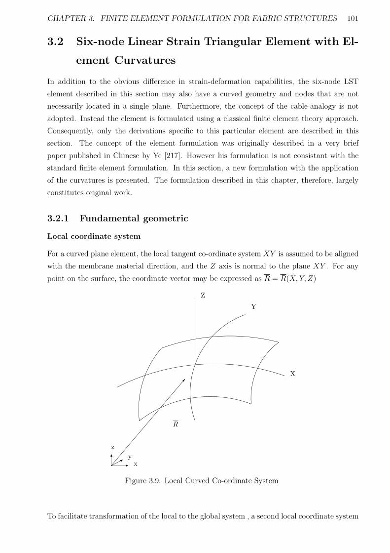
CHAPTER 3. FINITE ELEMENT FORMULATION FOR FABRIC STRUCTURES 101
3.2 Six-node Linear Strain Triangular Element with El-
ement Curvatures
In addition to the obvious difference in strain-deformation capabilities, the six-node LST
element described in this section may also have a curved geometry and nodes that are not
necessarily located in a single plane. Furthermore, the concept of the cable-analogy is not
adopted. Instead the element is formulated using a classical finite element theory approach.
Consequently, only the derivations specific to this particular element are described in this
section. The concept of the element formulation was originally described in a very brief
paper published in Chinese by Ye [217]. However his formulation is not consistant with the
standard finite element formulation. In this section, a new formulation with the application
of the curvatures is presented. The formulation described in this chapter, therefore, largely
constitutes original work.
3.2.1 Fundamental geometric
Local coordinate system
For a curved plane element, the local tangent co-ordinate system XY is assumed to be aligned
with the membrane material direction, and the Z axis is normal to the plane XY . For any
point on the surface, the coordinate vector may be expressed as R = R(X,Y, Z)
X
Z
Y
xy
z
R
Figure 3.9: Local Curved Co-ordinate System
To facilitate transformation of the local to the global system , a second local coordinate system
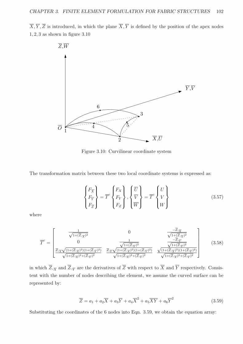
CHAPTER 3. FINITE ELEMENT FORMULATION FOR FABRIC STRUCTURES 102
X,Y , Z is introduced, in which the plane X,Y is defined by the position of the apex nodes
1, 2, 3 as shown in figure 3.10
X,U
Y ,V
Z,W
O1
2
3
4 5
6
Figure 3.10: Curvilinear coordinate system
The transformation matrix between these two local coordinate systems is expressed as:
FX
FY
FZ
= Tc
FX
FY
FZ
,
U
V
W
= Tc
U
V
W
(3.57)
where
Tc=
1√1+(Z,X)2
0−Z,X√1+(Z,X)2
0 1√1+(Z,Y )2
−Z,Y√1+(Z,Y )2
Z,X
√(1+(Z,X)2)(1+(Z,Y )2)√1+(Z,X)2+(Z,Y )2
Z,Y
√(1+(Z,X)2)(1+(Z,Y )2)√1+(Z,X)2+(Z,Y )2
√(1+(Z,X)2)(1+(Z,Y )2)√
1+(Z,X)2+(Z,Y )2
(3.58)
in which Z,X and Z,Y are the derivatives of Z with respect to X and Y respectively. Consis-
tent with the number of nodes describing the element, we assume the curved surface can be
represented by:
Z = a1 + a2X + a3Y + a4X2+ a5XY + a6Y
2(3.59)
Substituting the coordinates of the 6 nodes into Eqn. 3.59, we obtain the equation array:
CHAPTER 3. FINITE ELEMENT FORMULATION FOR FABRIC STRUCTURES 103
1 X1 Y 1 X2
1 X1Y 1 Y2
1
1 X2 Y 2 X2
2 X2Y 2 Y2
2
1 X3 Y 3 X2
3 X3Y 3 Y2
3
1 X4 Y 4 X2
4 X4Y 4 Y2
4
1 X5 Y 5 X2
5 X5Y 5 Y2
5
1 X6 Y 6 X2
6 X6Y 6 Y2
6
·
a1
a2
a3
a4
a5
a6
=
Z1
Z2
Z3
Z4
Z5
Z6
(3.60)
or
[A] · a = Z
Solving Eqn. 3.60, then
a = [A]−1Z (3.61)
where the values of a1–a6 are calculated numerically.
The curvilinear coordinates (X,Y) are defined with the original at the geometric centre of the
element (see fig. 3.9) as:
X =
∫ X
0
√
1 + (∂Z
∂X)2 dX
=
∫ X
0
√
1 + (a2 + 2a4X + a5Y )2 dX
= (a2 + a5Y
4a4
+X
2) ·√
1 + (a2 + 2a4X + a5Y )2 +arcsinh(a2 + 2a4X + a5Y )
4a4(3.62)
Y =
∫ Y
0
√
1 + (∂Z
∂Y)2 dY
=
∫ Y
0
√
1 + (a3 + a5X + 2a6Y ) dY
= (a3 + a5X
4a6
+Y
2) ·√
1 + (a3 + a5X + 2a6Y )2 +arcsinh(a3 + a5X + 2a6Y )
4a6
(3.63)
Element Curvatures
Element curvatures in each element are defined with respect to the local flat plane coordinate
system X, Y , Z. With the out-of-plane geometry of the 6-node triangular element written as
Z = f(X,Y ), then the curvatures about the local X and Y axes, are:
KX = − ∂2Z
∂X2 , KY = −∂
2Z
∂Y2 (3.64)
CHAPTER 3. FINITE ELEMENT FORMULATION FOR FABRIC STRUCTURES 104
and the torsion between X and Y axis is:
KXY = − ∂2Z
∂X∂Y(3.65)
3.2.2 Relationship between element strains and element curvatures
The extra force vectors normal to the element surface are assumed to contribute to the element
curvatures and in-plane stresses.
∆fZ = KX × σX
+KY × σY
+KXY × τXY
= KX KY KXY
σX
σY
τXY
= [Cv] · σ (3.66)
Where [Cv] = [KX KY KXY ] and σ = σXσ
Yτ
XYT
From Eqn. 3.66, it is apparent that if the element curvatures (Eqn 3.64) are zero, e.g a flat
surface, then no strains are induced due to to displacements normal to the surface. In that
case, the elastic stiffness to normal loads is zero. However the elastic stiffness in the direction
normal to the element surface becomes greater as the element curvatures increase.
3.2.3 Finite Element Formulation
Strain-displacement relations
Nodal coordinates in local curved coordinate system are defined in the section 3.2.1. The area
coordinate system(ξ1,ξ2,ξ3) introduced in Fig.3.7, is defined for the six node curved triangular
element, by the shape functions:
N1 = ξ1(2ξ1 − 1), N2 = ξ2(2ξ2 − 1), N3 = ξ3(2ξ3 − 1)
N4 = 4ξ1ξ2, N5 = 4ξ2ξ3, N6 = 4ξ3ξ1 (3.67)
The displacement fields are approximated by:
U(X,Y ) =6∑
i=1
NiUi, V (X,Y ) =6∑
i=1
NiVi, W (X,Y ) =6∑
i=1
NiWi (3.68)
and the cartesian co-ordinate X and Y of the unstrained initial configuration are approximated
by:
X =6∑
i=1
NiXi, Y =6∑
i=1
NiYi (3.69)
CHAPTER 3. FINITE ELEMENT FORMULATION FOR FABRIC STRUCTURES 105
in which, Ui Vi Wi and Xi Yi are nodal displacements and nodal coordinates respectively.
The expressions for Green’s strains are:
εX =∂U
∂X+
1
2
[
(
∂U
∂X
)2
+
(
∂V
∂X
)2
+
(
∂W
∂X
)2]
εY =∂V
∂Y+
1
2
[
(
∂U
∂Y
)2
+
(
∂V
∂Y
)2
+
(
∂W
∂Y
)2]
γXY =∂U
∂Y+∂V
∂X+
(
∂U
∂X
)(
∂U
∂Y
)
+
(
∂V
∂X
)(
∂V
∂Y
)
+
(
∂W
∂X
)(
∂W
∂Y
)
(3.70)
Derivation of Stiffness Matrix and Equilibrium Equation
A virtual displacement δd is defined at the nodes.This results in virtual displacements and
strains within the element of:
δu = N δd and δǫ = B δd (3.71)
respectively.
The work done by the nodal forces is :
δdT · f (3.72)
Similarly, the internal work per unit volume done by the stresses δ, the extra out-of-plane
force, and distributed forces:
δǫT · σ + δd · ∆fZ − δuT · b (3.73)
or
δd(BT · σ + Cv · σ −NT · b) (3.74)
in which b =
bx
by
is the distributed load,bx, by are the ”body force” components. Equating
the external work with the total internal work obtained by integrating over the volume of the
element,V e ,we have:
δdT · f = δd(
∫
V e
(BT + Cv)σ dV −∫
V e
NT b dV ) (3.75)
f =
∫
V e
(BT + Cv)σ dV −∫
V e
NT b dV (3.76)
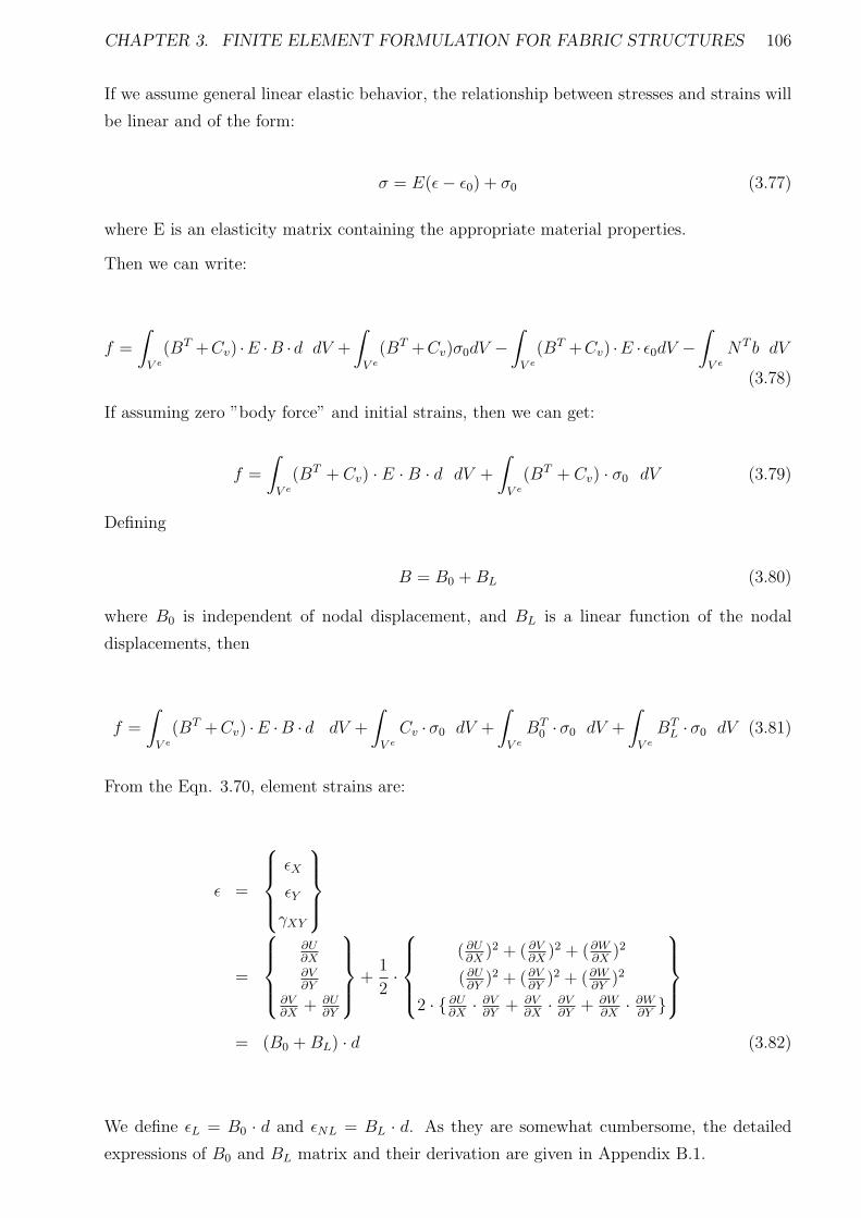
CHAPTER 3. FINITE ELEMENT FORMULATION FOR FABRIC STRUCTURES 106
If we assume general linear elastic behavior, the relationship between stresses and strains will
be linear and of the form:
σ = E(ǫ− ǫ0) + σ0 (3.77)
where E is an elasticity matrix containing the appropriate material properties.
Then we can write:
f =
∫
V e
(BT +Cv) ·E ·B ·d dV +
∫
V e
(BT +Cv)σ0dV −∫
V e
(BT +Cv) ·E · ǫ0dV −∫
V e
NT b dV
(3.78)
If assuming zero ”body force” and initial strains, then we can get:
f =
∫
V e
(BT + Cv) · E ·B · d dV +
∫
V e
(BT + Cv) · σ0 dV (3.79)
Defining
B = B0 +BL (3.80)
where B0 is independent of nodal displacement, and BL is a linear function of the nodal
displacements, then
f =
∫
V e
(BT +Cv) ·E ·B · d dV +
∫
V e
Cv ·σ0 dV +
∫
V e
BT0 ·σ0 dV +
∫
V e
BTL ·σ0 dV (3.81)
From the Eqn. 3.70, element strains are:
ǫ =
ǫX
ǫY
γXY
=
∂U∂X∂V∂Y
∂V∂X
+ ∂U∂Y
+1
2·
( ∂U∂X
)2 + ( ∂V∂X
)2 + (∂W∂X
)2
(∂U∂Y
)2 + (∂V∂Y
)2 + (∂W∂Y
)2
2 · ∂U∂X
· ∂V∂Y
+ ∂V∂X
· ∂V∂Y
+ ∂W∂X
· ∂W∂Y
= (B0 +BL) · d (3.82)
We define ǫL = B0 · d and ǫNL = BL · d. As they are somewhat cumbersome, the detailed
expressions of B0 and BL matrix and their derivation are given in Appendix B.1.

CHAPTER 3. FINITE ELEMENT FORMULATION FOR FABRIC STRUCTURES 107
ǫNL can be written as:
ǫNL =1
2
∂U∂X
∂V∂X
∂W∂X
0 0 0
0 0 0 ∂U∂Y
∂V∂Y
∂W∂Y
∂U∂Y
∂V∂Y
∂W∂Y
∂U∂X
∂V∂X
∂W∂X
·
∂U∂X∂V∂X∂W∂X∂U∂Y∂V∂Y∂W∂Y
=1
2A · ∆ (3.83)
so
ǫT =1
2∆T · AT (3.84)
and
AT =
∂U∂X
0 ∂U∂Y
∂V∂X
0 ∂V∂Y
∂W∂X
0 ∂W∂Y
0 ∂U∂Y
∂U∂X
0 ∂V∂Y
∂V∂X
0 ∂W∂Y
∂W∂X
(3.85)
If the initial stress vector
σ0 =
σX0
σY 0
τXY 0
(3.86)
then
AT · σ0 =
∂U∂X
0 ∂U∂Y
∂V∂X
0 ∂V∂Y
∂W∂X
0 ∂W∂Y
0 ∂U∂Y
∂U∂X
0 ∂V∂Y
∂V∂X
0 ∂W∂Y
∂W∂X
·
σX0
σY 0
τXY 0
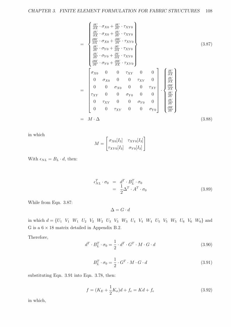
CHAPTER 3. FINITE ELEMENT FORMULATION FOR FABRIC STRUCTURES 108
=
∂U∂X
· σX0 + ∂U∂Y
· τXY 0
∂V∂X
· σX0 + ∂V∂Y
· τXY 0
∂W∂X
· σX0 + ∂W∂Y
· τXY 0
∂U∂Y
· σY 0 + ∂U∂X
· τXY 0
∂V∂Y
· σY 0 + ∂V∂X
· τXY 0
∂W∂Y
· σY 0 + ∂W∂X
· τXY 0
(3.87)
=
σX0 0 0 τXY 0 0
0 σX0 0 0 τXY 0
0 0 σX0 0 0 τXY
τXY 0 0 σY 0 0 0
0 τXY 0 0 σY 0 0
0 0 τXY 0 0 σY 0
·
∂U∂X∂V∂X∂W∂X∂U∂Y∂V∂Y∂W∂Y
= M · ∆ (3.88)
in which
M =
[
σX0[I3] τXY 0[I3]
τXY 0[I3] σY 0[I3]
]
With ǫNL = BL · d, then:
ǫTNL · σ0 = dT ·BTL · σ0
=1
2∆T · AT · σ0 (3.89)
While from Eqn. 3.87:
∆ = G · d
in which d = U1 V1 W1 U2 V2 W2 U3 V3 W3 U4 V4 W4 U5 V5 W5 U6 V6 W6 and
G is a 6 × 18 matrix detailed in Appendix B.2.
Therefore,
dT ·BTL · σ0 =
1
2· dT ·GT ·M ·G · d (3.90)
BTL · σ0 =
1
2·GT ·M ·G · d (3.91)
substituting Eqn. 3.91 into Eqn. 3.78, then:
f = (KE +1
2Kσ)d+ fe = Kd+ fe (3.92)
in which,
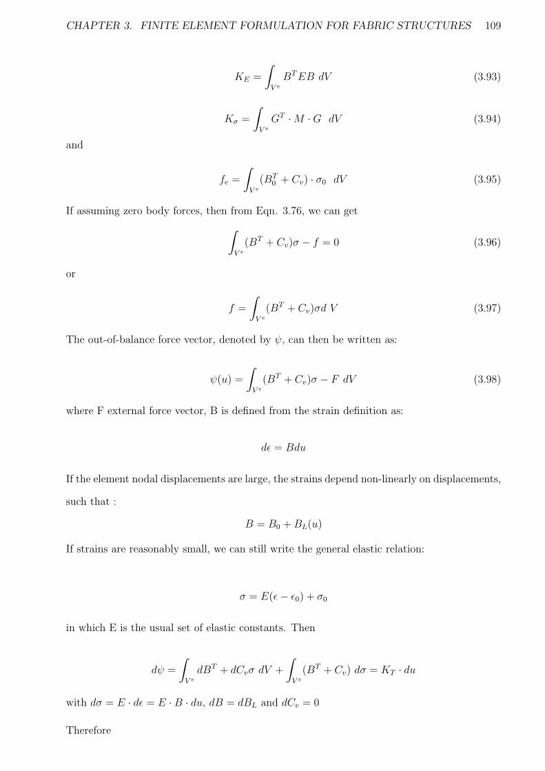
CHAPTER 3. FINITE ELEMENT FORMULATION FOR FABRIC STRUCTURES 109
KE =
∫
V e
BTEB dV (3.93)
Kσ =
∫
V e
GT ·M ·G dV (3.94)
and
fe =
∫
V e
(BT0 + Cv) · σ0 dV (3.95)
If assuming zero body forces, then from Eqn. 3.76, we can get
∫
V e
(BT + Cv)σ − f = 0 (3.96)
or
f =
∫
V e
(BT + Cv)σd V (3.97)
The out-of-balance force vector, denoted by ψ, can then be written as:
ψ(u) =
∫
V e
(BT + Cv)σ − F dV (3.98)
where F external force vector, B is defined from the strain definition as:
dǫ = Bdu
If the element nodal displacements are large, the strains depend non-linearly on displacements,
such that :
B = B0 +BL(u)
If strains are reasonably small, we can still write the general elastic relation:
σ = E(ǫ− ǫ0) + σ0
in which E is the usual set of elastic constants. Then
dψ =
∫
V e
dBT + dCvσ dV +
∫
V e
(BT + Cv) dσ = KT · du
with dσ = E · dǫ = E ·B · du, dB = dBL and dCv = 0
Therefore
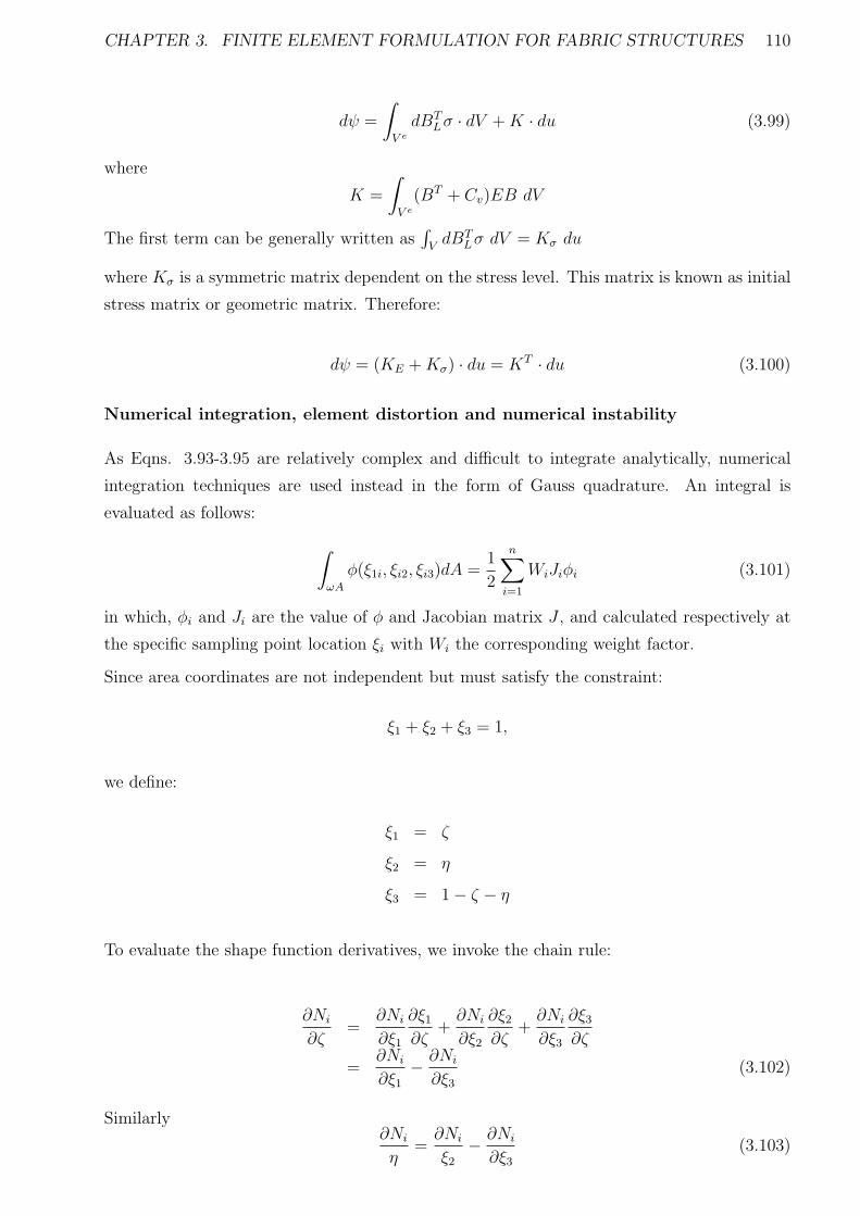
CHAPTER 3. FINITE ELEMENT FORMULATION FOR FABRIC STRUCTURES 110
dψ =
∫
V e
dBTLσ · dV +K · du (3.99)
where
K =
∫
V e
(BT + Cv)EB dV
The first term can be generally written as∫
VdBT
Lσ dV = Kσ du
where Kσ is a symmetric matrix dependent on the stress level. This matrix is known as initial
stress matrix or geometric matrix. Therefore:
dψ = (KE +Kσ) · du = KT · du (3.100)
Numerical integration, element distortion and numerical instability
As Eqns. 3.93-3.95 are relatively complex and difficult to integrate analytically, numerical
integration techniques are used instead in the form of Gauss quadrature. An integral is
evaluated as follows:
∫
ωA
φ(ξ1i, ξi2, ξi3)dA =1
2
n∑
i=1
WiJiφi (3.101)
in which, φi and Ji are the value of φ and Jacobian matrix J , and calculated respectively at
the specific sampling point location ξi with Wi the corresponding weight factor.
Since area coordinates are not independent but must satisfy the constraint:
ξ1 + ξ2 + ξ3 = 1,
we define:
ξ1 = ζ
ξ2 = η
ξ3 = 1 − ζ − η
To evaluate the shape function derivatives, we invoke the chain rule:
∂Ni
∂ζ=
∂Ni
∂ξ1
∂ξ1∂ζ
+∂Ni
∂ξ2
∂ξ2∂ζ
+∂Ni
∂ξ3
∂ξ3∂ζ
=∂Ni
∂ξ1− ∂Ni
∂ξ3(3.102)
Similarly∂Ni
η=∂Ni
ξ2− ∂Ni
∂ξ3(3.103)
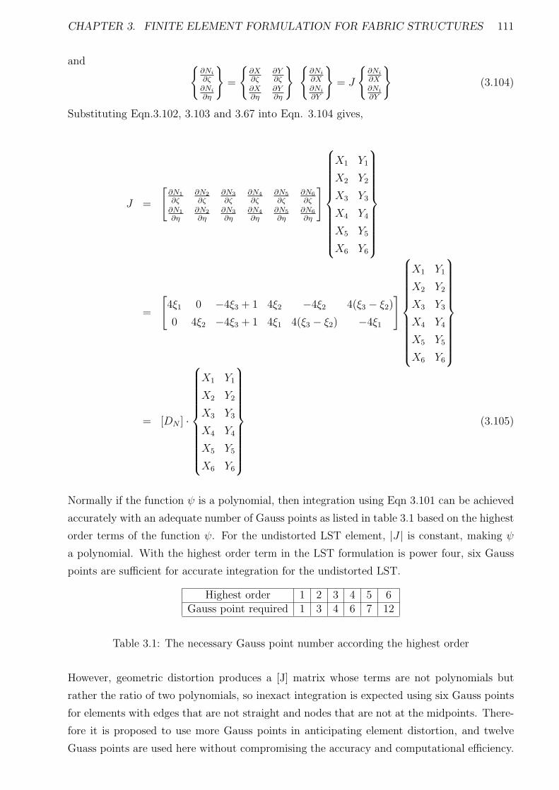
CHAPTER 3. FINITE ELEMENT FORMULATION FOR FABRIC STRUCTURES 111
and
∂Ni
∂ζ∂Ni
∂η
=
∂X∂ζ
∂Y∂ζ
∂X∂η
∂Y∂η
∂Ni
∂X∂Ni
∂Y
= J
∂Ni
∂X∂Ni
∂Y
(3.104)
Substituting Eqn.3.102, 3.103 and 3.67 into Eqn. 3.104 gives,
J =
[
∂N1
∂ζ∂N2
∂ζ∂N3
∂ζ∂N4
∂ζ∂N5
∂ζ∂N6
∂ζ∂N1
∂η∂N2
∂η∂N3
∂η∂N4
∂η∂N5
∂η∂N6
∂η
]
X1 Y1
X2 Y2
X3 Y3
X4 Y4
X5 Y5
X6 Y6
=
[
4ξ1 0 −4ξ3 + 1 4ξ2 −4ξ2 4(ξ3 − ξ2)
0 4ξ2 −4ξ3 + 1 4ξ1 4(ξ3 − ξ2) −4ξ1
]
X1 Y1
X2 Y2
X3 Y3
X4 Y4
X5 Y5
X6 Y6
= [DN ] ·
X1 Y1
X2 Y2
X3 Y3
X4 Y4
X5 Y5
X6 Y6
(3.105)
Normally if the function ψ is a polynomial, then integration using Eqn 3.101 can be achieved
accurately with an adequate number of Gauss points as listed in table 3.1 based on the highest
order terms of the function ψ. For the undistorted LST element, |J | is constant, making ψ
a polynomial. With the highest order term in the LST formulation is power four, six Gauss
points are sufficient for accurate integration for the undistorted LST.
Highest order 1 2 3 4 5 6Gauss point required 1 3 4 6 7 12
Table 3.1: The necessary Gauss point number according the highest order
However, geometric distortion produces a [J] matrix whose terms are not polynomials but
rather the ratio of two polynomials, so inexact integration is expected using six Gauss points
for elements with edges that are not straight and nodes that are not at the midpoints. There-
fore it is proposed to use more Gauss points in anticipating element distortion, and twelve
Guass points are used here without compromising the accuracy and computational efficiency.
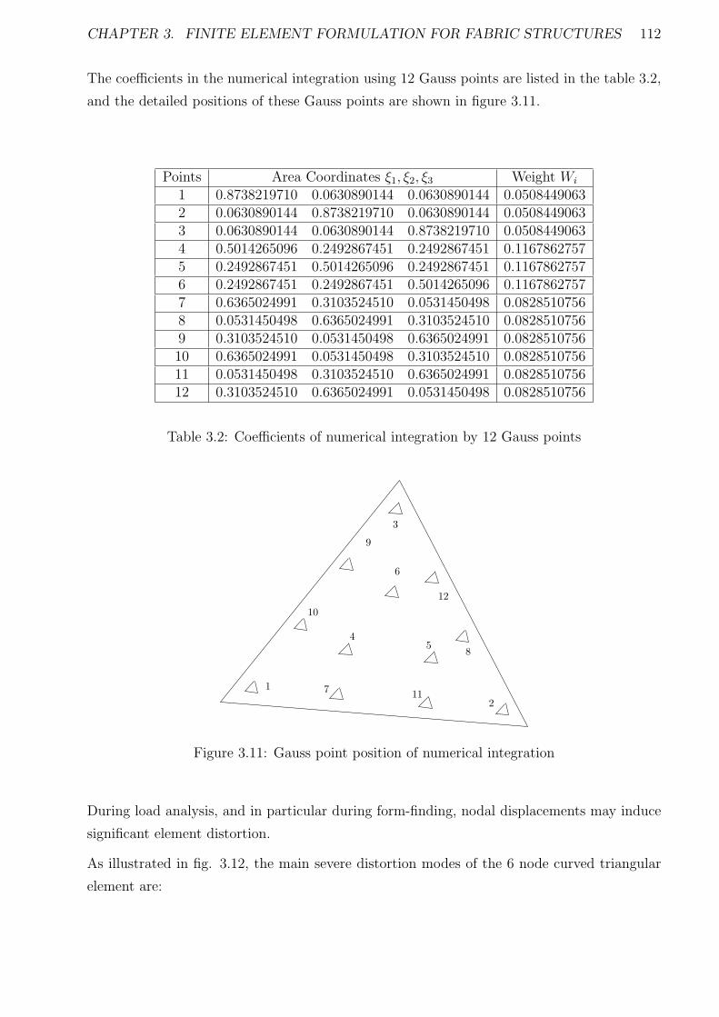
CHAPTER 3. FINITE ELEMENT FORMULATION FOR FABRIC STRUCTURES 112
The coefficients in the numerical integration using 12 Gauss points are listed in the table 3.2,
and the detailed positions of these Gauss points are shown in figure 3.11.
Points Area Coordinates ξ1, ξ2, ξ3 Weight Wi
1 0.8738219710 0.0630890144 0.0630890144 0.05084490632 0.0630890144 0.8738219710 0.0630890144 0.05084490633 0.0630890144 0.0630890144 0.8738219710 0.05084490634 0.5014265096 0.2492867451 0.2492867451 0.11678627575 0.2492867451 0.5014265096 0.2492867451 0.11678627576 0.2492867451 0.2492867451 0.5014265096 0.11678627577 0.6365024991 0.3103524510 0.0531450498 0.08285107568 0.0531450498 0.6365024991 0.3103524510 0.08285107569 0.3103524510 0.0531450498 0.6365024991 0.082851075610 0.6365024991 0.0531450498 0.3103524510 0.082851075611 0.0531450498 0.3103524510 0.6365024991 0.082851075612 0.3103524510 0.6365024991 0.0531450498 0.0828510756
Table 3.2: Coefficients of numerical integration by 12 Gauss points
6
45
71
9
3
2
8
12
10
11
Figure 3.11: Gauss point position of numerical integration
During load analysis, and in particular during form-finding, nodal displacements may induce
significant element distortion.
As illustrated in fig. 3.12, the main severe distortion modes of the 6 node curved triangular
element are:
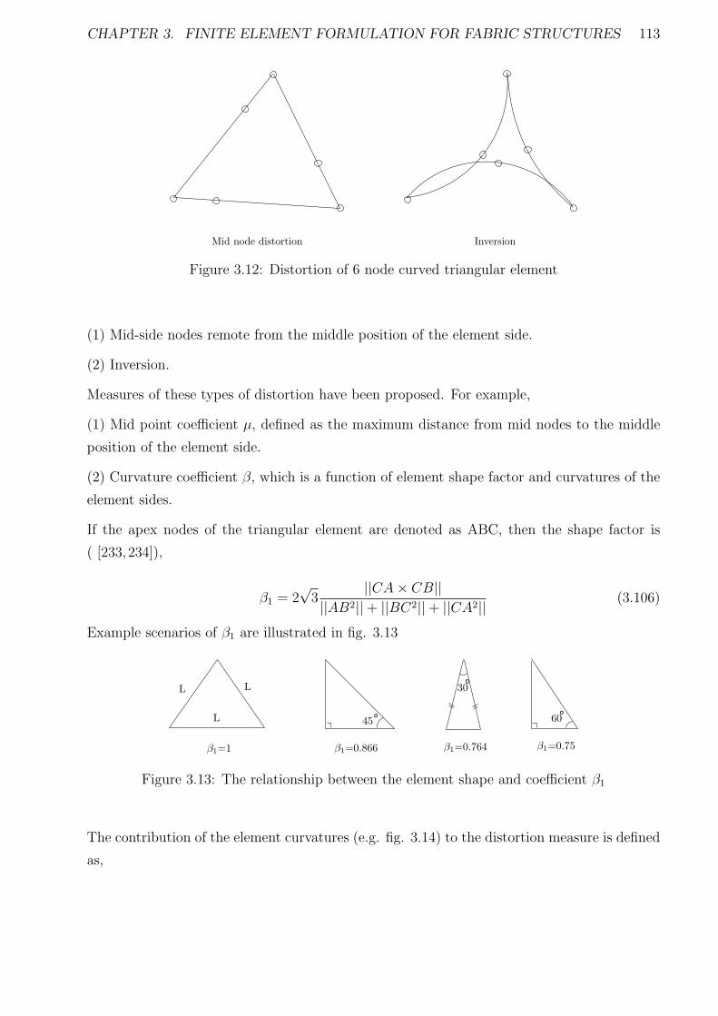
CHAPTER 3. FINITE ELEMENT FORMULATION FOR FABRIC STRUCTURES 113
Mid node distortion Inversion
Figure 3.12: Distortion of 6 node curved triangular element
(1) Mid-side nodes remote from the middle position of the element side.
(2) Inversion.
Measures of these types of distortion have been proposed. For example,
(1) Mid point coefficient µ, defined as the maximum distance from mid nodes to the middle
position of the element side.
(2) Curvature coefficient β, which is a function of element shape factor and curvatures of the
element sides.
If the apex nodes of the triangular element are denoted as ABC, then the shape factor is
( [233,234]),
β1 = 2√
3||CA× CB||
||AB2|| + ||BC2|| + ||CA2|| (3.106)
Example scenarios of β1 are illustrated in fig. 3.13
L L
L 45
30
60
β1=1 β1=0.866 β1=0.764 β1=0.75
Figure 3.13: The relationship between the element shape and coefficient β1
The contribution of the element curvatures (e.g. fig. 3.14) to the distortion measure is defined
as,
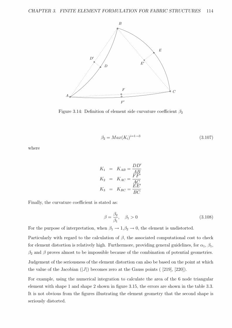
CHAPTER 3. FINITE ELEMENT FORMULATION FOR FABRIC STRUCTURES 114
A
B
C
D′
D
F
F ′
E
E′
Figure 3.14: Definition of element side curvature coefficient β2
β2 = Max(Ki)i=1→3 (3.107)
where
K1 = KAB =DD′
AB
K2 = KAC =FF ′
AC
K3 = KBC =EE ′
BC
Finally, the curvature coefficient is stated as:
β =β2
β1
, β1 > 0 (3.108)
For the purpose of interpretation, when β1 → 1,β2 → 0, the element is undistorted.
Particularly with regard to the calculation of β, the associated computational cost to check
for element distortion is relatively high. Furthermore, providing general guidelines, for α1, β1,
β2 and β proves almost to be impossible because of the combination of potential geometries.
Judgement of the seriousness of the element distortion can also be based on the point at which
the value of the Jacobian (|J |) becomes zero at the Gauss points ( [219], [220]).
For example, using the numerical integration to calculate the area of the 6 node triangular
element with shape 1 and shape 2 shown in figure 3.15, the errors are shown in the table 3.3.
It is not obvious from the figures illustrating the element geometry that the second shape is
seriously distorted.
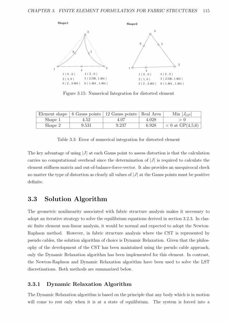
CHAPTER 3. FINITE ELEMENT FORMULATION FOR FABRIC STRUCTURES 115
1 2
3
4
56
12
3
4
56
Shape1 Shape2
1 ( 0 , 0 )
2 ( 4, 0 )
3 ( 2 , 3.464 )
4 ( 2 , 0 )
5 ( 2.536, 1.464 )
6 ( 1.464 , 1.464 )
1 ( 0 , 0 )
2 ( 1, 0 )
3 ( 2 , 3.464 )
4 ( 2 , 0 )
5 ( 2.536, 1.464 )
6 ( 1.464 , 1.464 )
Figure 3.15: Numerical Integration for distorted element
Element shape 6 Gauss points 12 Gauss points Real Area Min |JGP |Shape 1 4.52 4.07 4.028 > 0Shape 2 9.531 9.237 6.928 < 0 at GP(4,5,6)
Table 3.3: Error of numerical integration for distorted element
The key advantage of using |J | at each Gauss point to assess distortion is that the calculation
carries no computational overhead since the determination of |J | is required to calculate the
element stiffness matrix and out-of-balance-force-vector. It also provides an unequivocal check
no matter the type of distortion as clearly all values of |J | at the Gauss points must be positive
definite.
3.3 Solution Algorithm
The geometric nonlinearity associated with fabric structure analysis makes it necessary to
adopt an iterative strategy to solve the equilibrium equations derived in section 3.2.3. In clas-
sic finite element non-linear analysis, it would be normal and expected to adopt the Newton-
Raphson method. However, in fabric structure analysis where the CST is represented by
pseudo cables, the solution algorithm of choice is Dynamic Relaxation. Given that the philos-
ophy of the development of the CST has been maintained using the pseudo cable approach,
only the Dynamic Relaxation algorithm has been implemented for this element. In contrast,
the Newton-Raphson and Dynamic Relaxation algorithm have been used to solve the LST
discretisations. Both methods are summarized below.
3.3.1 Dynamic Relaxation Algorithm
The Dynamic Relaxation algorithm is based on the principle that any body which is in motion
will come to rest only when it is at a state of equilibrium. The system is forced into a
CHAPTER 3. FINITE ELEMENT FORMULATION FOR FABRIC STRUCTURES 116
pseudo oscillation, with equal amplitude about the equilibrium position. Both the frequency
and the amplitude of the fictitious dynamic motion are controlled artificially. As illustrated
subsequently, this is achieved through the components of stiffness and of out-of-balance force
at each node of the discretization, and by the associated nodal mass.
The motion of the system is described by the D’ Alembert principle, written as,
Ppq = Mpq δpq + C ˙δpq +Kpqδpq (3.109)
or,
Ppq −Kpqδpq = Mpq δpq + C ˙δpq (3.110)
and
Rpq = Mpq δpq + C ˙δpq (3.111)
where the subscripts pq refer to the pth node in the qth direction. q can take the values 1 → 3,
corresponding to the global axis directions x, y, z , respectively. The remaining coefficients
are defined below.
Ppq is the external load vector, including terms representing the effects of surface prestress or
initial strains,
Kpq is the nodal stiffness selected from the terms of the element stiffness matrix
Rpq is the out-of-balance nodal force (or residual),
Mpq is the fictitious nodal mass,
δpq is the nodal acceleration.
·δpq is the nodal velocity,
δpq is the nodal displacement.
Kinetic Damping has been shown to be a more stable and a more rapidly convergent technique
of damping the pseudo dynamic oscillations of the discretized system, when compared with the
Viscous Damp approach (Eqn. 3.109). Using this technique the system is allowed to vibrate
freely without attenuation of displacement or frequency. During this motion the kinetic energy
of the entire system is monitored. As the system passes the equilibrium configuration the
kinetic energy of the system is maximized.
When a maximum value is observed the current oscillation is halted. The pseudo motion is
then restarted from this new configuration. As more peaks in the kinetic energy of the system
are detected, the proximity of the system to the true equilibrium configuration is increased.
The procedure culminates in the minimisation of the sum of the kinetic and potential energies
CHAPTER 3. FINITE ELEMENT FORMULATION FOR FABRIC STRUCTURES 117
of the system at equilibrium. Using this approach, Eqn. 3.110 may be written more simply
as:
Ppq −Kpqδpq = Rpq = Mpq δpq (3.112)
The acceleration term given in the right side of Eqn. 3.112 is written as the variation of the
velocity over the time increment δt using a central difference approximation, such that,
δpq =˙δpq
t+δt2 − ˙δpq
t−δ2
δt(3.113)
substitution of Eqn. 3.113 into Eqn. 3.112 leads to the following recurrent equation for the
nodal velocity, ˙δpqt+ δt
2 , as,
˙δpqt+ δ
2 = ˙δpqt− δ
2 +Rpqt δt
Mpq
(3.114)
In order to ensure numerical stability of the solution algorithm, the following expression has
been suggested,
δt ≤√
2Mpq
Kpq
(3.115)
or
Mpq ≥Kpq
2· δt2 (3.116)
Substitution of Eqn. 3.116 into Eqn. 3.114 gives,
˙δpqt+ δ
2 = ˙δpqt− δ
2 +Rpqt
[
2
δt ·Kpq
]
(3.117)
The velocities at time t+ δt2
can be used to calculate the current nodal displacement as in,
δt+
δt2
pq = ˙δpqt+ δt
2 · δt (3.118)
Therefore, through the recurrent use of Eqn. 3.112, Eqn. 3.117 with 3.118, the pseudo
dynamic behaviour of the structure is defined. During each iterative cycle, the current kinetic
energy of the system, U t+ δt2 is monitored and compared with the preceding value, denoted
respectively as,
Ut+ δt
2k =
1
2
p=N∑
p=1
q=3∑
q=1
Mpq( ˙δpqt+ δt
2 )2 (3.119)
Ut− δt
2k =
1
2
p=N∑
p=1
q=3∑
q=1
Mpq( ˙δpqt− δt
2 )2 (3.120)
An energy peak is deemed to have occurred during the time interval t− δt2≤ t ≤ t+ δt
2when
CHAPTER 3. FINITE ELEMENT FORMULATION FOR FABRIC STRUCTURES 118
the magnitude of Ukt+ δt
2 is less than that of Ukt− δt
2 . If it is assumed that the kinetic energy
peak occurs at the time t∗, where t − δt2≤ t∗ ≤ t + δt
2, it may be estimated that t∗ is at the
mid point of the interval, t− δt2≤ t∗ ≤ t+ δt
2, such that t∗ = t.
Alternatively, a parabola may be fitted through the current and the two previous values of
the kinetic energy (Ukt− δt
2 ,Ukt− 3δt
2 ), yielding an improves estimate of the true position of the
kinetic energy peak, written as:
t∗ = t− ρ.δt = t− δt∗ (3.121)
where
ρ =Uk
t+ δt2 − Uk
t− δt2
Ukt− 3δt
2 − 2Ukt− δt
2 + Ukt+ δt
2
(3.122)
The pseudo dynamic motion may be restarted therefore, from the configuration described by
the following expression
δt∗ = δt+ δt2 − δt+ δ
2 · δt− δt− δt2 · δt∗ (3.123)
Through the recurrent use of Eqn. 3.112, 3.117 and 3.118, the condition of static equilibrium
of a system can be satisfied by damping its pseudo dynamic behaviour. The pseudo dynamic
behaviour of the system has been shown to be controlled by the components of both stiffness
and of out-of-balance force at each node of this discretization.
Solution Procedure for CST formulation
The solution procedure for the three types of CST formulation described in section 3.1 using
the Dynamic Relaxation Algorithm is summarized below and also presented as fig.3.16:
1) Discretize the membrane with an appropriate mesh.
2) Calculate equivalent nodal loads related to any uniformly applied external loads
3) Establish the local system of co-ordinates and transformation coefficients. For each element,
it is further required to:
4) Calculate the [Btr] matrix (Eqn. 3.12, 3.34 or 3.42 ) and the pseudo cable forces(Eqn.3.18)
based on the stress from the initial conditions or the preceding iteration.
5) Calculate the elasticity modulus matrix [E] in the local coordinate system and build the
local elastic stiffness matrix KtrE (Eqn.3.15). Extract the diagonal terms and calculate the
global elastic stiffness matrix KE(Eqn. 3.44,3.45,3.46).
6) Calculate the diagonal terms of local element geometric stiffness matrixKpcσ (Eqn.3.47,3.48,3.49),
and the global geometric stiffness matrix Ktpc (Eqn.3.50,3.51,3.52)
7) Calculate the nodal force of each element (Eqn. 3.54, 3.55, 3.56).
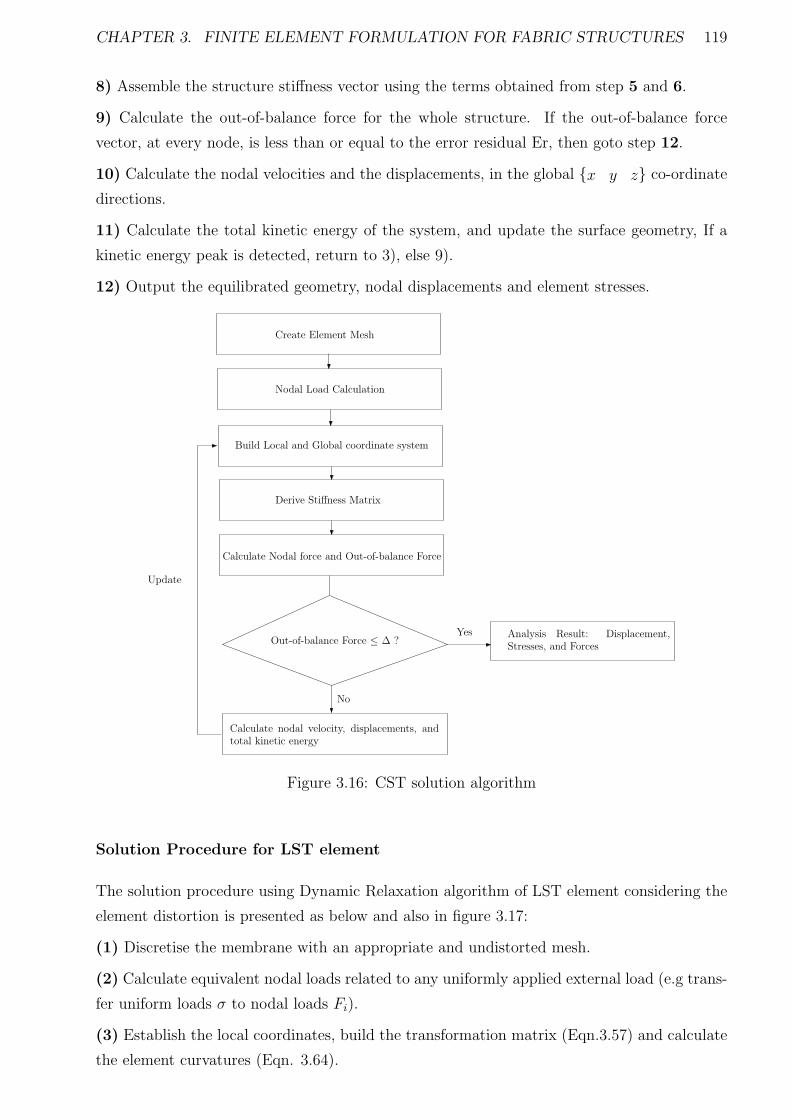
CHAPTER 3. FINITE ELEMENT FORMULATION FOR FABRIC STRUCTURES 119
8) Assemble the structure stiffness vector using the terms obtained from step 5 and 6.
9) Calculate the out-of-balance force for the whole structure. If the out-of-balance force
vector, at every node, is less than or equal to the error residual Er, then goto step 12.
10) Calculate the nodal velocities and the displacements, in the global x y z co-ordinate
directions.
11) Calculate the total kinetic energy of the system, and update the surface geometry, If a
kinetic energy peak is detected, return to 3), else 9).
12) Output the equilibrated geometry, nodal displacements and element stresses.
Create Element Mesh
Nodal Load Calculation
Build Local and Global coordinate system
Derive Stiffness Matrix
Calculate Nodal force and Out-of-balance Force
Out-of-balance Force ≤ ∆ ?Analysis Result: Displacement,
Stresses, and Forces
Yes
No
Calculate nodal velocity, displacements, and
total kinetic energy
Update
Figure 3.16: CST solution algorithm
Solution Procedure for LST element
The solution procedure using Dynamic Relaxation algorithm of LST element considering the
element distortion is presented as below and also in figure 3.17:
(1) Discretise the membrane with an appropriate and undistorted mesh.
(2) Calculate equivalent nodal loads related to any uniformly applied external load (e.g trans-
fer uniform loads σ to nodal loads Fi).
(3) Establish the local coordinates, build the transformation matrix (Eqn.3.57) and calculate
the element curvatures (Eqn. 3.64).
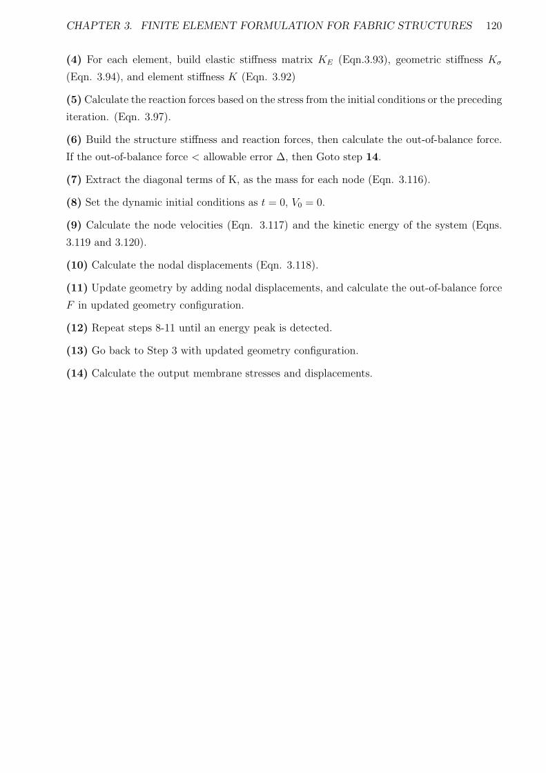
CHAPTER 3. FINITE ELEMENT FORMULATION FOR FABRIC STRUCTURES 120
(4) For each element, build elastic stiffness matrix KE (Eqn.3.93), geometric stiffness Kσ
(Eqn. 3.94), and element stiffness K (Eqn. 3.92)
(5) Calculate the reaction forces based on the stress from the initial conditions or the preceding
iteration. (Eqn. 3.97).
(6) Build the structure stiffness and reaction forces, then calculate the out-of-balance force.
If the out-of-balance force < allowable error ∆, then Goto step 14.
(7) Extract the diagonal terms of K, as the mass for each node (Eqn. 3.116).
(8) Set the dynamic initial conditions as t = 0, V0 = 0.
(9) Calculate the node velocities (Eqn. 3.117) and the kinetic energy of the system (Eqns.
3.119 and 3.120).
(10) Calculate the nodal displacements (Eqn. 3.118).
(11) Update geometry by adding nodal displacements, and calculate the out-of-balance force
F in updated geometry configuration.
(12) Repeat steps 8-11 until an energy peak is detected.
(13) Go back to Step 3 with updated geometry configuration.
(14) Calculate the output membrane stresses and displacements.
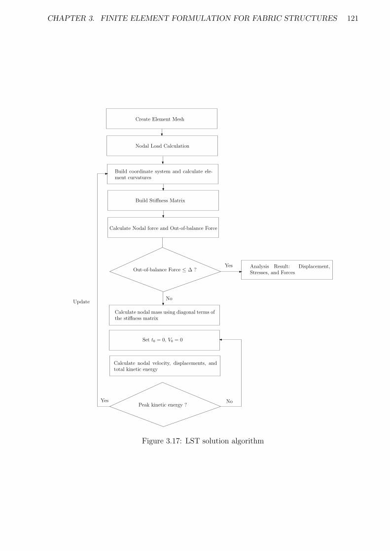
CHAPTER 3. FINITE ELEMENT FORMULATION FOR FABRIC STRUCTURES 121
Create Element Mesh
Nodal Load Calculation
Build Stiffness Matrix
Calculate Nodal force and Out-of-balance Force
Out-of-balance Force ≤ ∆ ?Analysis Result: Displacement,
Stresses, and Forces
Yes
No
Calculate nodal velocity, displacements, and
total kinetic energy
Update
Build coordinate system and calculate ele-
ment curvatures
Calculate nodal mass using diagonal terms of
the stiffness matrix
Set t0 = 0, V0 = 0
Peak kinetic energy ?Yes No
Figure 3.17: LST solution algorithm
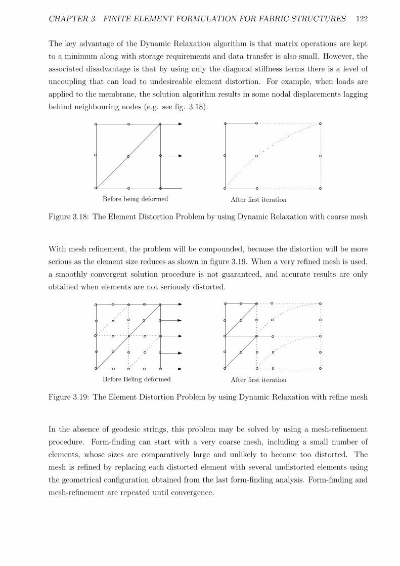
CHAPTER 3. FINITE ELEMENT FORMULATION FOR FABRIC STRUCTURES 122
The key advantage of the Dynamic Relaxation algorithm is that matrix operations are kept
to a minimum along with storage requirements and data transfer is also small. However, the
associated disadvantage is that by using only the diagonal stiffness terms there is a level of
uncoupling that can lead to undesireable element distortion. For example, when loads are
applied to the membrane, the solution algorithm results in some nodal displacements lagging
behind neighbouring nodes (e.g. see fig. 3.18).
Before being deformed After first iteration
Figure 3.18: The Element Distortion Problem by using Dynamic Relaxation with coarse mesh
With mesh refinement, the problem will be compounded, because the distortion will be more
serious as the element size reduces as shown in figure 3.19. When a very refined mesh is used,
a smoothly convergent solution procedure is not guaranteed, and accurate results are only
obtained when elements are not seriously distorted.
Before Beling deformed After first iteration
Figure 3.19: The Element Distortion Problem by using Dynamic Relaxation with refine mesh
In the absence of geodesic strings, this problem may be solved by using a mesh-refinement
procedure. Form-finding can start with a very coarse mesh, including a small number of
elements, whose sizes are comparatively large and unlikely to become too distorted. The
mesh is refined by replacing each distorted element with several undistorted elements using
the geometrical configuration obtained from the last form-finding analysis. Form-finding and
mesh-refinement are repeated until convergence.
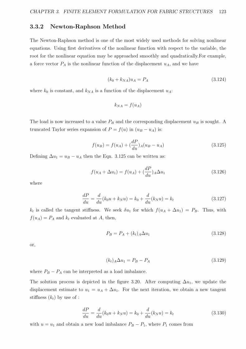
CHAPTER 3. FINITE ELEMENT FORMULATION FOR FABRIC STRUCTURES 123
3.3.2 Newton-Raphson Method
The Newton-Raphson method is one of the most widely used methods for solving nonlinear
equations. Using first derivatives of the nonlinear function with respect to the variable, the
root for the nonlinear equation may be approached smoothly and quadratically.For example,
a force vector PA is the nonlinear function of the displacement uA, and we have
(k0 + kNA)uA = PA (3.124)
where k0 is constant, and kNA is a function of the displacement uA:
kNA = f(uA)
The load is now increased to a value PB and the corresponding displacement uB is sought. A
truncated Taylor series expansion of P = f(u) in (uB − uA) is:
f(uB) = f(uA) + (dP
du)A(uB − uA) (3.125)
Defining ∆u1 = uB − uA then the Eqn. 3.125 can be written as:
f(uA + ∆u1) = f(uA) + (dP
du)A∆u1 (3.126)
where
dP
du=
d
du(k0u+ kNu) = k0 +
d
du(kNu) = kt (3.127)
kt is called the tangent stiffness. We seek δu1 for which f(uA + ∆u1) = PB. Thus, with
f(uA) = PA and kt evaluated at A, then,
PB = PA + (kt)A∆u1 (3.128)
or,
(kt)A∆u1 = PB − PA (3.129)
where PB − PA can be interpreted as a load imbalance.
The solution process is depicted in the figure 3.20. After computing ∆u1, we update the
displacement estimate to u1 = uA + ∆u1. For the next iteration, we obtain a new tangent
stiffness (kt) by use of :
dP
du=
d
du(k0u+ kNu) = k0 +
d
du(kNu) = kt (3.130)
with u = u1 and obtain a new load imbalance PB − P1, where P1 comes from
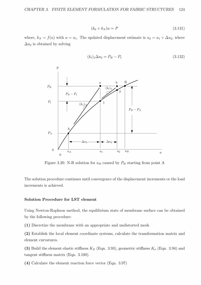
CHAPTER 3. FINITE ELEMENT FORMULATION FOR FABRIC STRUCTURES 124
(k0 + kN)u = P (3.131)
where, kN = f(u) with u = u1. The updated displacement estimate is u2 = u1 + ∆u2, where
∆u2 is obtained by solving
(kt)1∆u2 = PB − P1 (3.132)
P
0
0u
PB
P1
PA
PB − P1
PB − PA
(k1)A
(kt)1
1
2
a b B
A
uA u1 u2 uB
∆u1 ∆u2
Figure 3.20: N-R solution for uB caused by PB starting from point A
The solution procedure continues until convergence of the displacement increments or the load
increments is achieved.
Solution Procedure for LST element
Using Newton-Raphson method, the equilibrium state of membrane surface can be obtained
by the following procedure:
(1) Discretize the membrane with an appropriate and undistorted mesh
(2) Establish the local element coordinate systems, calculate the transformation matrix and
element curvatures.
(3) Build the element elastic stiffness KE (Eqn. 3.93), geometric stiffness Kσ (Eqn. 3.94) and
tangent stiffness matrix (Eqn. 3.100).
(4) Calculate the element reaction force vector (Eqn. 3.97)
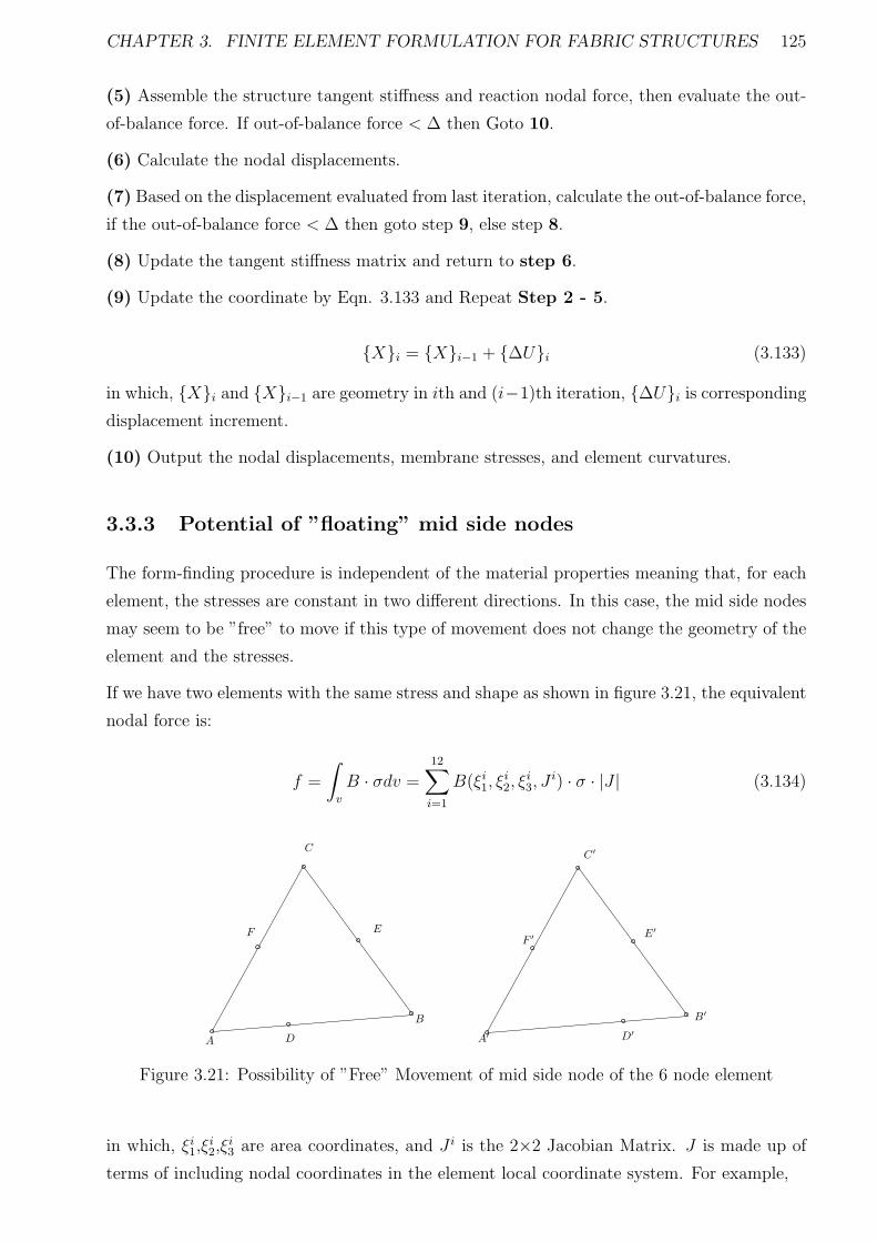
CHAPTER 3. FINITE ELEMENT FORMULATION FOR FABRIC STRUCTURES 125
(5) Assemble the structure tangent stiffness and reaction nodal force, then evaluate the out-
of-balance force. If out-of-balance force < ∆ then Goto 10.
(6) Calculate the nodal displacements.
(7) Based on the displacement evaluated from last iteration, calculate the out-of-balance force,
if the out-of-balance force < ∆ then goto step 9, else step 8.
(8) Update the tangent stiffness matrix and return to step 6.
(9) Update the coordinate by Eqn. 3.133 and Repeat Step 2 - 5.
Xi = Xi−1 + ∆Ui (3.133)
in which, Xi and Xi−1 are geometry in ith and (i−1)th iteration, ∆Ui is corresponding
displacement increment.
(10) Output the nodal displacements, membrane stresses, and element curvatures.
3.3.3 Potential of ”floating” mid side nodes
The form-finding procedure is independent of the material properties meaning that, for each
element, the stresses are constant in two different directions. In this case, the mid side nodes
may seem to be ”free” to move if this type of movement does not change the geometry of the
element and the stresses.
If we have two elements with the same stress and shape as shown in figure 3.21, the equivalent
nodal force is:
f =
∫
v
B · σdv =12∑
i=1
B(ξi1, ξ
i2, ξ
i3, J
i) · σ · |J | (3.134)
A
B
C
D
EF
A′
B′
C ′
D′
E′
F ′
Figure 3.21: Possibility of ”Free” Movement of mid side node of the 6 node element
in which, ξi1,ξ
i2,ξ
i3 are area coordinates, and J i is the 2×2 Jacobian Matrix. J is made up of
terms of including nodal coordinates in the element local coordinate system. For example,
CHAPTER 3. FINITE ELEMENT FORMULATION FOR FABRIC STRUCTURES 126
[J ] =
[
J11 J12
J21 J22
]
(3.135)
in which,
J11 = X1(4ξ1 − 1) −X3(4ξ3 − 1) + 4ξ2(X4 −X5) + 4(ξ3 − ξ1)X6
J12 = Y1(4ξ2 − 1) − Y3(4ξ3 − 1) + 4ξ2(Y4 − Y5) + 4(ξ3 − ξ1)Y6
J21 = X2(4ξ2 − 1) −X3(4ξ3 − 1) + 4ξ1(X4 −X6) + 4(ξ3 − ξ2)X5
J22 = Y2(4ξ2 − 1) − Y3(4ξ3 − 1) + 4ξ1(Y4 − Y6) + 4(ξ3 − ξ2)Y5
In the numerical integration of Eqn. 3.134, ξ1,ξ2,ξ3 are the same for element ∆ABC and
∆A′B′C ′. However apparently XD 6= XD′ ,YD 6= YD′ , meaning that JABC 6= JA′B′C′ . Therefore
the equivalent nodal forces of these two element are different, so such ”free” movement of mid
side nodes will cause a change of the nodal forces from those defined by the initial stresses.
A further possibility of ”free movement” of the mid-side nodes is that the force increments
of the mid side shared by two adjacent elements are zero, because the equivalent nodal force
produced from one element may be eliminated by the other.
EA
B
C
D
F H
I
G
A
B
C
D
E
F H
I
G
E′
X
Y
A ( -2 , 0 )
B ( 0.2, -2 )C ( -0.2, 2 )D ( -0.9, -1)
E ( 0, 0 )F ( -1.1, 1 )
H ( 0.9 , 1 )
G ( 2, 0 )
I ( 1.1, -1 )
E′ ( -0.1, 1 )
Figure 3.22: Possibility of ”Free” Movement of mid-side node of the 6 node element
For example, if there are two adjacent element ABC and CBG shown in figure 3.22 in a
form-finding analysis, with initial stresses σX0 = 1.0kN/m, σY 0 = 1.0kN/m and τXY 0 = 0.
We assume E is the balance point, and if E ”floats” to position E ′, the nodal force increment
can be calculated by Eqn. 3.134. The nodal force increment from the element ABC is,

CHAPTER 3. FINITE ELEMENT FORMULATION FOR FABRIC STRUCTURES 127
∆Fy(B) = 0.27kN
∆Fy(C) = 0.27kN
Similarly, the nodal force increment from the element GBC is:
∆F ′y(B) = 0.27kN
∆F ′y(C) = 0.27kN
Therefore, the out-of balance force at B, and C generated by the ”floating” of E to E ′ are:
∆Fy(B) = 0.54kN
∆Fy(C) = 0.54kN
Consequently, if E moves to E ′, nodal force increments from each element are additive, mean-
ing that the movement from E to E ′ is not ”free” (i.e. nodal forces are induced).
Finally, therefore, the two cases of potential ”floating” mid-side nodes are shown to be unlikely
to be manifested in the analysis.
3.4 Wrinkling procedure
Since the membrane material has no flexural stiffness, vanishing of tensile stresses in an
arbitrary position or direction of the membrane surface will immediately lead to buckling in
the form of wrinkles. In this case, the membrane will lose or partially lose the stiffness and
load resistance in the wrinkled area. From a view point of either aesthetics or structural
safety, wrinkling can be regarded as one type of structural failure, and should be inadmissible
during membrane structural design.
Structural analysis taking into account wrinkling is sophisticated because the detailed wrin-
kling pattern not only depends on the stress state but the imperfections of fabric material
during the fabrication process. Therefore in this chapter, the main aim of the finite element
formulation taking into account wrinkling concentrates on the prediction of wrinkling under
CHAPTER 3. FINITE ELEMENT FORMULATION FOR FABRIC STRUCTURES 128
loading for an idealized fabric.
Different wrinkling criteria developed by Otto [87], Miller [88] and Roddeman [89] as shown
in Table 2.4, 2.5 and 2.6 are based on principal stress , strain or combined principal strain and
stress. According to these criteria, the membrane state can be described as taut(no wrinkle),
wrinkled(uniaxial wrinkling) or slack(biaxial wrinkling).
For the local stresses σX ,σY ,τXY ,the major principal stress σ11 and minor principal stress σ22
are,
σ11 =σX + σY
2+
√
(σX − σY
2)2 + γ2
XY (3.136)
σ22 =σX + σY
2−√
(σX − σY
2)2 + γ2
XY (3.137)
and the principal strains are obtained from:
ε11 =εX + εY
2+
√
(εX − εY
2)2 + (
γXY
2)2 (3.138)
ε22 =εX + εY
2−√
(εX − εY
2)2 + (
γXY
2)2 (3.139)
(1) If the major principal stress σ11 < 0, the membrane is slack.
(2) If the minor principal stress σ22 > 0, wrinkle does not occur.
(3) If ε11 > 0, σ22 < 0, wrinkling occurs.
In wrinkled areas, the major principal strain (ε11) direction is the wrinkle direction at that
location.
If θp is the angle between wrinkle direction and local X axis, then:
θp =1
2tan−1(
2γXY
εX − εY
) (3.140)
When calculating the element stiffness matrix, the existence of wrinkling must be considered.
In this case it is not sufficient to use
σ =
σX σY τXY
T
= [E]
εX
εY
γXY
= [E][B]U (3.141)
in which, U is nodal displacements.
If compressive stresses are not permitted and therefore the stiffness normal to the wrinkle
direction is zero, solution convergence is not always smooth and sometimes not achieved due
CHAPTER 3. FINITE ELEMENT FORMULATION FOR FABRIC STRUCTURES 129
to wrinkling [235–237]. Riccardo Rossi [237] proposed an algorithm for the stabilization of
the material manipulation. Using his method, if the membrane is in a ”wrinkled state”, a
modified elastic stiffness matrix [Emod] is defined as:
[Emod] =
Erot,11 P · Erot,12 Erot,13
P · Erot,21 P · Erot,22 P · Erot,23
Erot,31 P · Erot,32 Erot,33
= [Erot] × [P ] (3.142)
in which, P is the penalization parameter, and
[Erot] = [R]T [E][R] (3.143)
[R] is the transformation matrix. If the orientation of the principal stress to the local X axis
is αw, then
c = cos(αw); s = sin(αw); [R] =
c2 s2 −2cs
s2 c2 2sc
sc −sc c2 − s2
(3.144)
If the penalization is constant, the performace of the wrinkling procedure may be compro-
mised. An alternative definition of P to improve the stability is to make P a function of the
maximum (σmax) and effective compressive stresses (σ2) [237]:
Pσ =σmax
σ2
→
Pσ > P → P = Pσ
Pσ > 1 or Pσ < 0 → P = 1.0
(3.145)
If the modification makes the state change (from wrinkled or slack to taut), then a reduced
penalization may be applied as:
New state is ”taut” →
old state is ”taut” → [Emod] = [E]
old state isn′t ”taut” → P = P · ω;new state = old state
(3.146)
where ω = 10 is recommended by reference [237].
The elastic stiffness matrix then becomes:
KE,mod =
∫
v
BT [Emod]Bdv (3.147)
In addition to the obvious change in the element stiffness matrix, the equivalent nodal load
vector is also changed to be of the form:
fe =
∫
V
B0(Emod · ε+ σ0)dV (3.148)
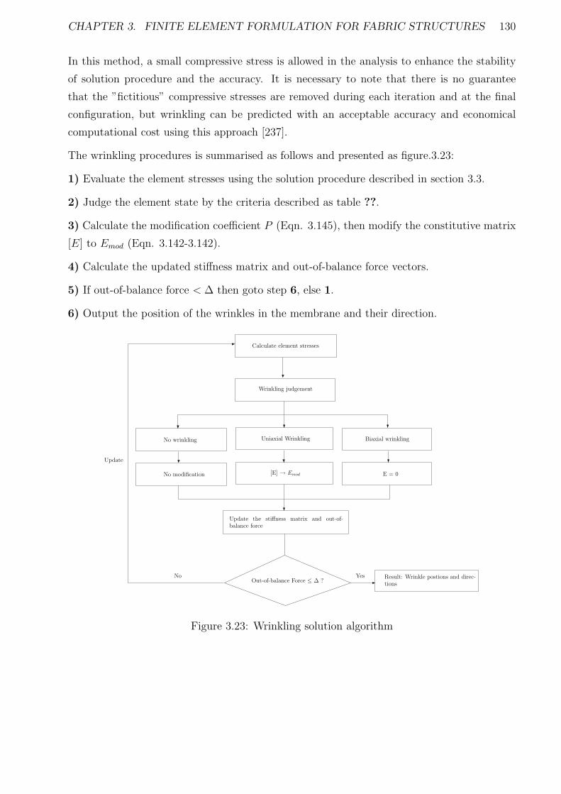
CHAPTER 3. FINITE ELEMENT FORMULATION FOR FABRIC STRUCTURES 130
In this method, a small compressive stress is allowed in the analysis to enhance the stability
of solution procedure and the accuracy. It is necessary to note that there is no guarantee
that the ”fictitious” compressive stresses are removed during each iteration and at the final
configuration, but wrinkling can be predicted with an acceptable accuracy and economical
computational cost using this approach [237].
The wrinkling procedures is summarised as follows and presented as figure.3.23:
1) Evaluate the element stresses using the solution procedure described in section 3.3.
2) Judge the element state by the criteria described as table ??.
3) Calculate the modification coefficient P (Eqn. 3.145), then modify the constitutive matrix
[E] to Emod (Eqn. 3.142-3.142).
4) Calculate the updated stiffness matrix and out-of-balance force vectors.
5) If out-of-balance force < ∆ then goto step 6, else 1.
6) Output the position of the wrinkles in the membrane and their direction.
Calculate element stresses
Wrinkling judgement
Uniaxial Wrinkling Biaxial wrinkling
Out-of-balance Force ≤ ∆ ?Result: Wrinkle postions and direc-tions
Yes
Update
No wrinkling
[E] → Emod E = 0No modification
Update the stiffness matrix and out-of-balance force
No
Figure 3.23: Wrinkling solution algorithm
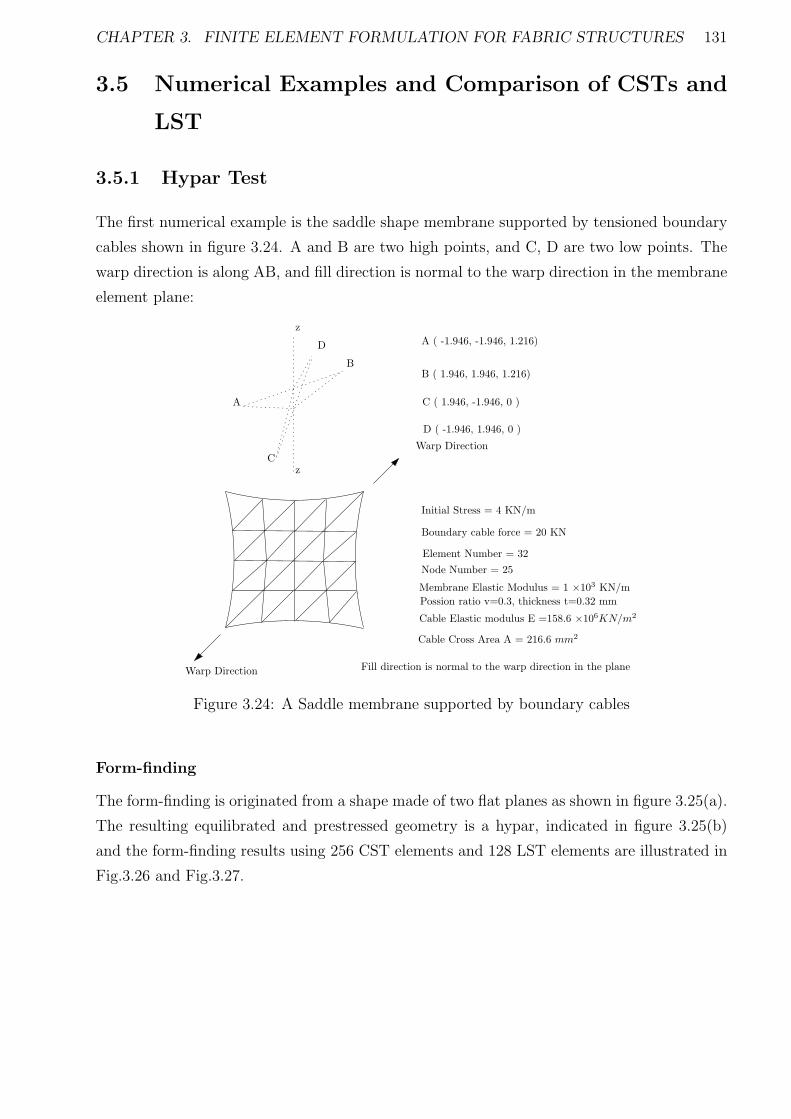
CHAPTER 3. FINITE ELEMENT FORMULATION FOR FABRIC STRUCTURES 131
3.5 Numerical Examples and Comparison of CSTs and
LST
3.5.1 Hypar Test
The first numerical example is the saddle shape membrane supported by tensioned boundary
cables shown in figure 3.24. A and B are two high points, and C, D are two low points. The
warp direction is along AB, and fill direction is normal to the warp direction in the membrane
element plane:
A
B
C
D
z
z
A ( -1.946, -1.946, 1.216)
B ( 1.946, 1.946, 1.216)
C ( 1.946, -1.946, 0 )
D ( -1.946, 1.946, 0 )
Initial Stress = 4 KN/m
Boundary cable force = 20 KN
Element Number = 32
Node Number = 25
Membrane Elastic Modulus = 1 ×10³ KN/m
Cable Elastic modulus E =158.6 ×10⁶KN/m2
Cable Cross Area A = 216.6 mm2
Warp Direction
Warp Direction Fill direction is normal to the warp direction in the plane
Possion ratio v=0.3, thickness t=0.32 mm
Figure 3.24: A Saddle membrane supported by boundary cables
Form-finding
The form-finding is originated from a shape made of two flat planes as shown in figure 3.25(a).
The resulting equilibrated and prestressed geometry is a hypar, indicated in figure 3.25(b)
and the form-finding results using 256 CST elements and 128 LST elements are illustrated in
Fig.3.26 and Fig.3.27.
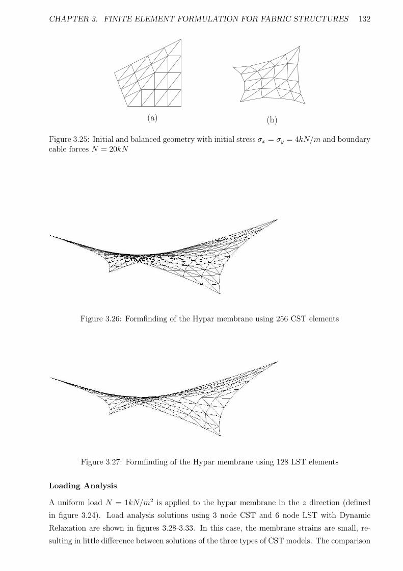
CHAPTER 3. FINITE ELEMENT FORMULATION FOR FABRIC STRUCTURES 132
(a) (b)
Figure 3.25: Initial and balanced geometry with initial stress σx = σy = 4kN/m and boundarycable forces N = 20kN
Figure 3.26: Formfinding of the Hypar membrane using 256 CST elements
Figure 3.27: Formfinding of the Hypar membrane using 128 LST elements
Loading Analysis
A uniform load N = 1kN/m2 is applied to the hypar membrane in the z direction (defined
in figure 3.24). Load analysis solutions using 3 node CST and 6 node LST with Dynamic
Relaxation are shown in figures 3.28-3.33. In this case, the membrane strains are small, re-
sulting in little difference between solutions of the three types of CST models. The comparison
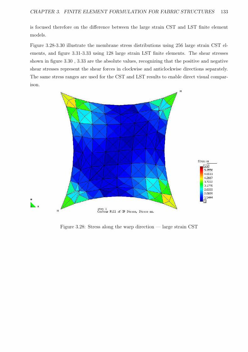
CHAPTER 3. FINITE ELEMENT FORMULATION FOR FABRIC STRUCTURES 133
is focused therefore on the difference between the large strain CST and LST finite element
models.
Figure 3.28-3.30 illustrate the membrane stress distributions using 256 large strain CST el-
ements, and figure 3.31-3.33 using 128 large strain LST finite elements. The shear stresses
shown in figure 3.30 , 3.33 are the absolute values, recognizing that the positive and negative
shear stresses represent the shear forces in clockwise and anticlockwise directions separately.
The same stress ranges are used for the CST and LST results to enable direct visual compar-
ison.
Figure 3.28: Stress along the warp direction — large strain CST

CHAPTER 3. FINITE ELEMENT FORMULATION FOR FABRIC STRUCTURES 134
Figure 3.29: Stress along the fill direction — large strain CST
Figure 3.30: Shear stress across the warp and fill direction — large strain CST
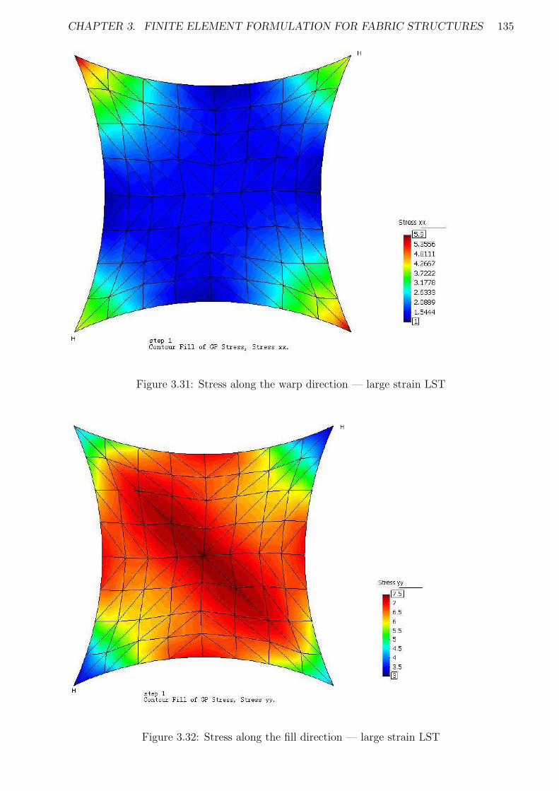
CHAPTER 3. FINITE ELEMENT FORMULATION FOR FABRIC STRUCTURES 135
Figure 3.31: Stress along the warp direction — large strain LST
Figure 3.32: Stress along the fill direction — large strain LST
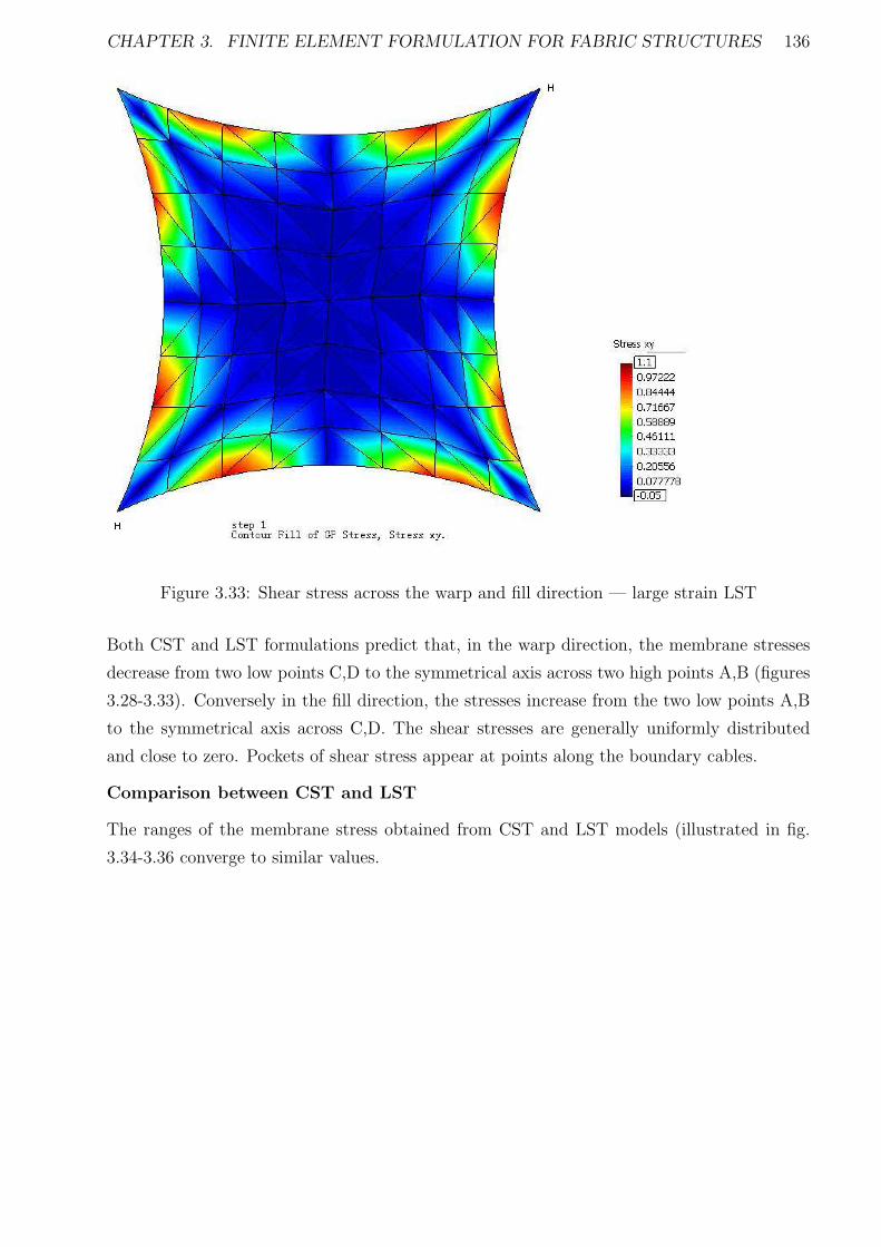
CHAPTER 3. FINITE ELEMENT FORMULATION FOR FABRIC STRUCTURES 136
Figure 3.33: Shear stress across the warp and fill direction — large strain LST
Both CST and LST formulations predict that, in the warp direction, the membrane stresses
decrease from two low points C,D to the symmetrical axis across two high points A,B (figures
3.28-3.33). Conversely in the fill direction, the stresses increase from the two low points A,B
to the symmetrical axis across C,D. The shear stresses are generally uniformly distributed
and close to zero. Pockets of shear stress appear at points along the boundary cables.
Comparison between CST and LST
The ranges of the membrane stress obtained from CST and LST models (illustrated in fig.
3.34-3.36 converge to similar values.
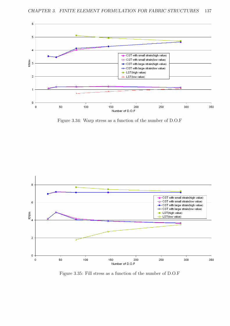
CHAPTER 3. FINITE ELEMENT FORMULATION FOR FABRIC STRUCTURES 137
Figure 3.34: Warp stress as a function of the number of D.O.F
Figure 3.35: Fill stress as a function of the number of D.O.F
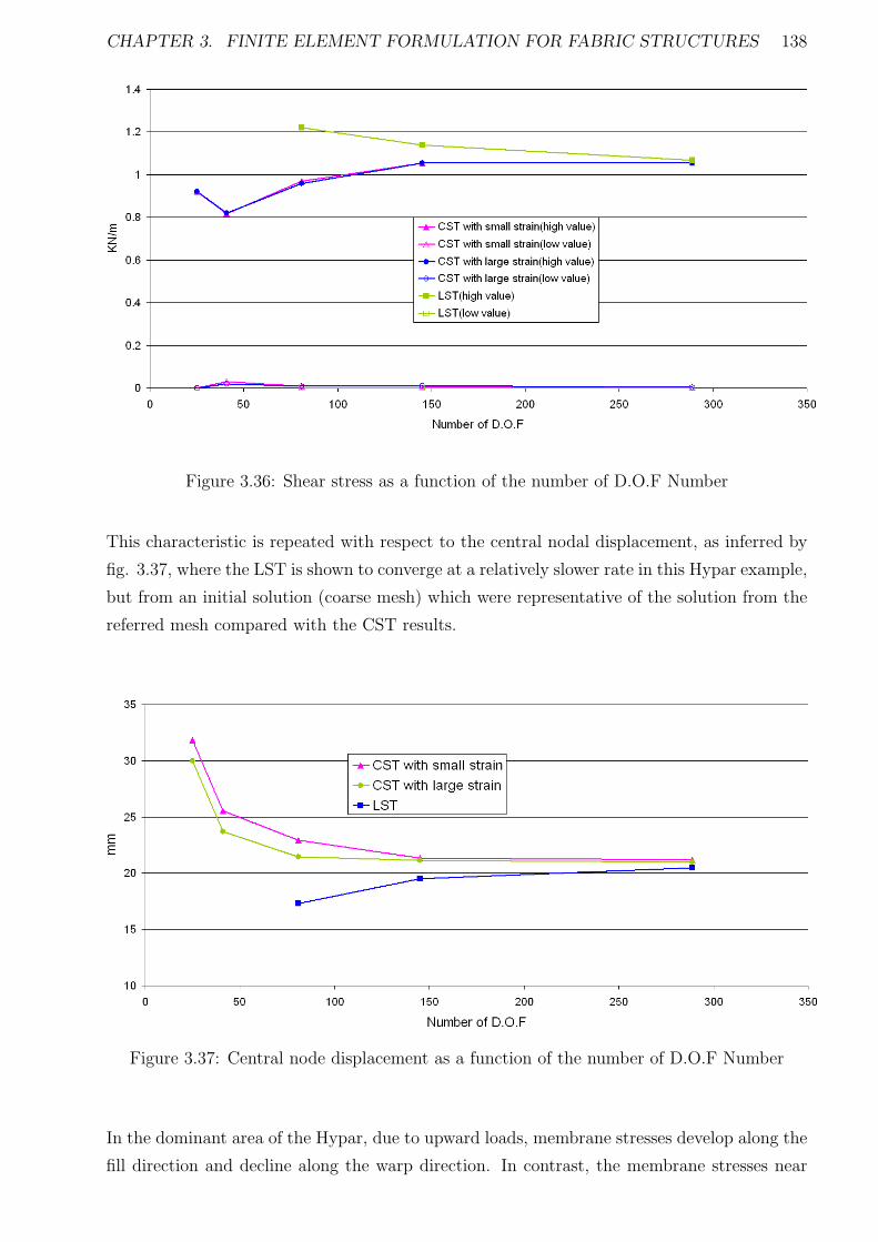
CHAPTER 3. FINITE ELEMENT FORMULATION FOR FABRIC STRUCTURES 138
Figure 3.36: Shear stress as a function of the number of D.O.F Number
This characteristic is repeated with respect to the central nodal displacement, as inferred by
fig. 3.37, where the LST is shown to converge at a relatively slower rate in this Hypar example,
but from an initial solution (coarse mesh) which were representative of the solution from the
referred mesh compared with the CST results.
Figure 3.37: Central node displacement as a function of the number of D.O.F Number
In the dominant area of the Hypar, due to upward loads, membrane stresses develop along the
fill direction and decline along the warp direction. In contrast, the membrane stresses near
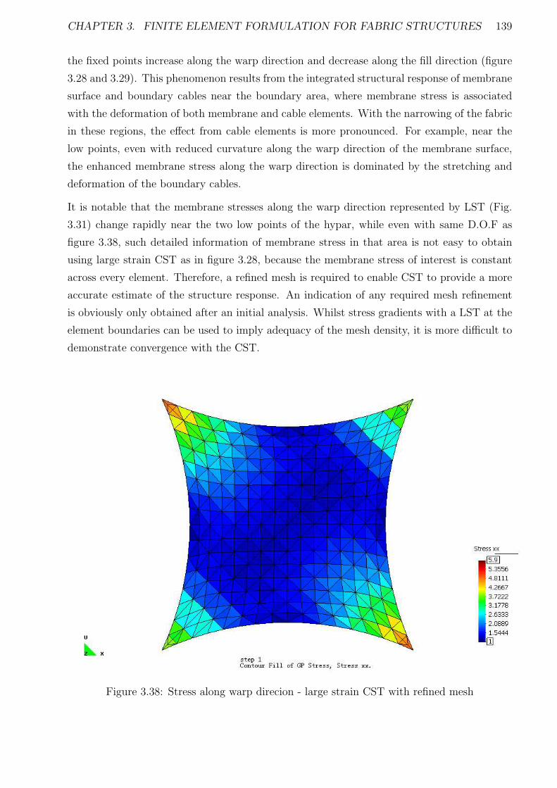
CHAPTER 3. FINITE ELEMENT FORMULATION FOR FABRIC STRUCTURES 139
the fixed points increase along the warp direction and decrease along the fill direction (figure
3.28 and 3.29). This phenomenon results from the integrated structural response of membrane
surface and boundary cables near the boundary area, where membrane stress is associated
with the deformation of both membrane and cable elements. With the narrowing of the fabric
in these regions, the effect from cable elements is more pronounced. For example, near the
low points, even with reduced curvature along the warp direction of the membrane surface,
the enhanced membrane stress along the warp direction is dominated by the stretching and
deformation of the boundary cables.
It is notable that the membrane stresses along the warp direction represented by LST (Fig.
3.31) change rapidly near the two low points of the hypar, while even with same D.O.F as
figure 3.38, such detailed information of membrane stress in that area is not easy to obtain
using large strain CST as in figure 3.28, because the membrane stress of interest is constant
across every element. Therefore, a refined mesh is required to enable CST to provide a more
accurate estimate of the structure response. An indication of any required mesh refinement
is obviously only obtained after an initial analysis. Whilst stress gradients with a LST at the
element boundaries can be used to imply adequacy of the mesh density, it is more difficult to
demonstrate convergence with the CST.
Figure 3.38: Stress along warp direcion - large strain CST with refined mesh
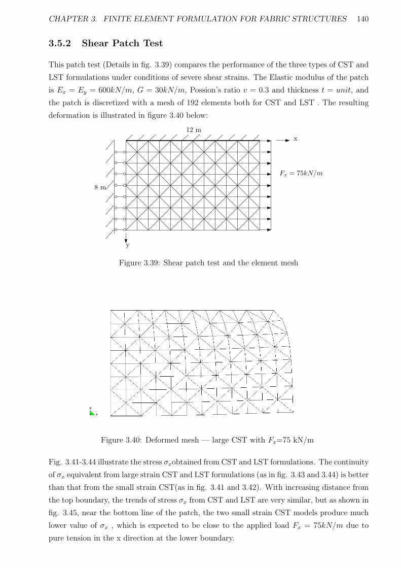
CHAPTER 3. FINITE ELEMENT FORMULATION FOR FABRIC STRUCTURES 140
3.5.2 Shear Patch Test
This patch test (Details in fig. 3.39) compares the performance of the three types of CST and
LST formulations under conditions of severe shear strains. The Elastic modulus of the patch
is Ex = Ey = 600kN/m, G = 30kN/m, Possion’s ratio v = 0.3 and thickness t = unit, and
the patch is discretized with a mesh of 192 elements both for CST and LST . The resulting
deformation is illustrated in figure 3.40 below:
Fx = 75kN/m
12 m
8 m
x
y
Figure 3.39: Shear patch test and the element mesh
Figure 3.40: Deformed mesh — large CST with Fx=75 kN/m
Fig. 3.41-3.44 illustrate the stress σxobtained from CST and LST formulations. The continuity
of σx equivalent from large strain CST and LST formulations (as in fig. 3.43 and 3.44) is better
than that from the small strain CST(as in fig. 3.41 and 3.42). With increasing distance from
the top boundary, the trends of stress σx from CST and LST are very similar, but as shown in
fig. 3.45, near the bottom line of the patch, the two small strain CST models produce much
lower value of σx , which is expected to be close to the applied load Fx = 75kN/m due to
pure tension in the x direction at the lower boundary.
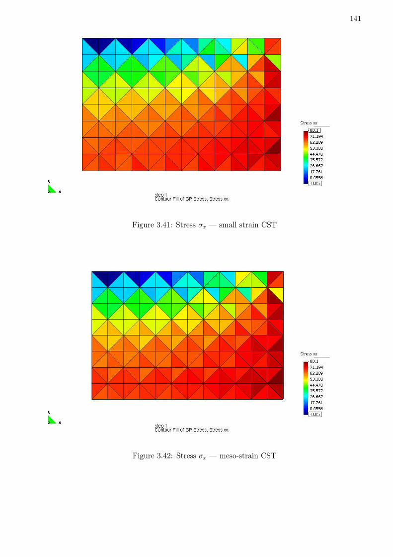
CHAPTER 3. FINITE ELEMENT FORMULATION FOR FABRIC STRUCTURES 141
Figure 3.41: Stress σx — small strain CST
Figure 3.42: Stress σx — meso-strain CST
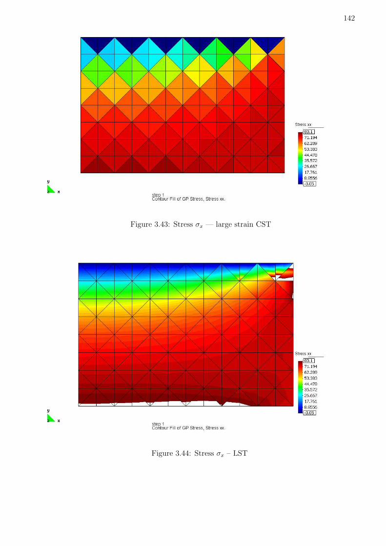
CHAPTER 3. FINITE ELEMENT FORMULATION FOR FABRIC STRUCTURES 142
Figure 3.43: Stress σx — large strain CST
Figure 3.44: Stress σx – LST
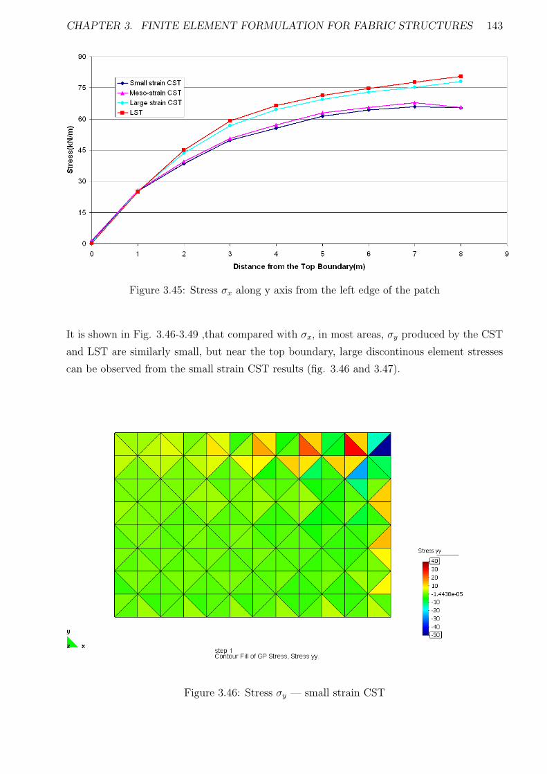
CHAPTER 3. FINITE ELEMENT FORMULATION FOR FABRIC STRUCTURES 143
Figure 3.45: Stress σx along y axis from the left edge of the patch
It is shown in Fig. 3.46-3.49 ,that compared with σx, in most areas, σy produced by the CST
and LST are similarly small, but near the top boundary, large discontinous element stresses
can be observed from the small strain CST results (fig. 3.46 and 3.47).
Figure 3.46: Stress σy — small strain CST
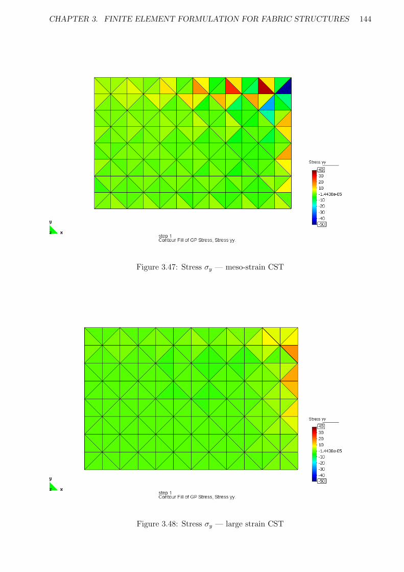
CHAPTER 3. FINITE ELEMENT FORMULATION FOR FABRIC STRUCTURES 144
Figure 3.47: Stress σy — meso-strain CST
Figure 3.48: Stress σy — large strain CST
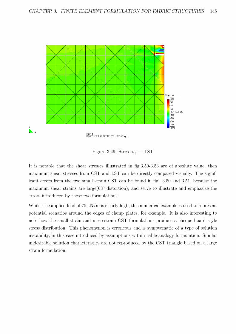
CHAPTER 3. FINITE ELEMENT FORMULATION FOR FABRIC STRUCTURES 145
Figure 3.49: Stress σy — LST
It is notable that the shear stresses illustrated in fig.3.50-3.53 are of absolute value, then
maximum shear stresses from CST and LST can be directly compared visually. The signif-
icant errors from the two small strain CST can be found in fig. 3.50 and 3.51, because the
maximum shear strains are large(63o distortion), and serve to illustrate and emphasize the
errors introduced by these two formulations.
Whilst the applied load of 75 kN/m is clearly high, this numerical example is used to represent
potential scenarios around the edges of clamp plates, for example. It is also interesting to
note how the small-strain and meso-strain CST formulations produce a chequerboard style
stress distribution. This phenomenon is erroneous and is symptomatic of a type of solution
instability, in this case introduced by assumptions within cable-analogy formulation. Similar
undesirable solution characteristics are not reproduced by the CST triangle based on a large
strain formulation.
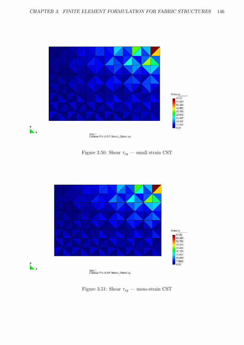
CHAPTER 3. FINITE ELEMENT FORMULATION FOR FABRIC STRUCTURES 146
Figure 3.50: Shear τxy — small strain CST
Figure 3.51: Shear τxy — meso-strain CST
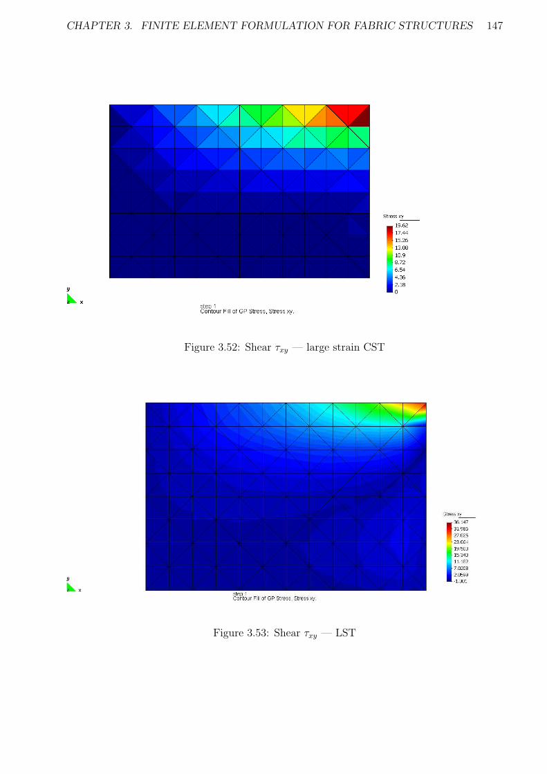
CHAPTER 3. FINITE ELEMENT FORMULATION FOR FABRIC STRUCTURES 147
Figure 3.52: Shear τxy — large strain CST
Figure 3.53: Shear τxy — LST
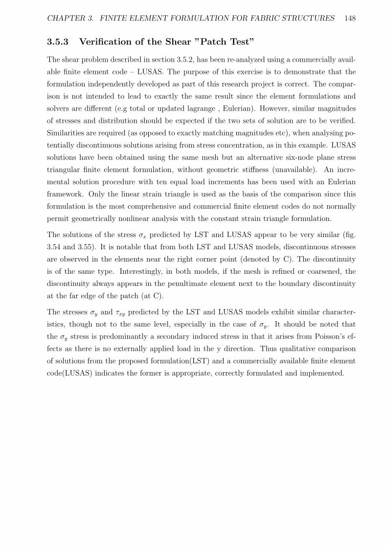
CHAPTER 3. FINITE ELEMENT FORMULATION FOR FABRIC STRUCTURES 148
3.5.3 Verification of the Shear ”Patch Test”
The shear problem described in section 3.5.2, has been re-analyzed using a commercially avail-
able finite element code – LUSAS. The purpose of this exercise is to demonstrate that the
formulation independently developed as part of this research project is correct. The compar-
ison is not intended to lead to exactly the same result since the element formulations and
solvers are different (e.g total or updated lagrange , Eulerian). However, similar magnitudes
of stresses and distribution should be expected if the two sets of solution are to be verified.
Similarities are required (as opposed to exactly matching magnitudes etc), when analysing po-
tentially discontinuous solutions arising from stress concentration, as in this example. LUSAS
solutions have been obtained using the same mesh but an alternative six-node plane stress
triangular finite element formulation, without geometric stiffness (unavailable). An incre-
mental solution procedure with ten equal load increments has been used with an Eulerian
framework. Only the linear strain triangle is used as the basis of the comparison since this
formulation is the most comprehensive and commercial finite element codes do not normally
permit geometrically nonlinear analysis with the constant strain triangle formulation.
The solutions of the stress σx predicted by LST and LUSAS appear to be very similar (fig.
3.54 and 3.55). It is notable that from both LST and LUSAS models, discontinuous stresses
are observed in the elements near the right corner point (denoted by C). The discontinuity
is of the same type. Interestingly, in both models, if the mesh is refined or coarsened, the
discontinuity always appears in the penultimate element next to the boundary discontinuity
at the far edge of the patch (at C).
The stresses σy and τxy predicted by the LST and LUSAS models exhibit similar character-
istics, though not to the same level, especially in the case of σy. It should be noted that
the σy stress is predominantly a secondary induced stress in that it arises from Poisson’s ef-
fects as there is no externally applied load in the y direction. Thus qualitative comparison
of solutions from the proposed formulation(LST) and a commercially available finite element
code(LUSAS) indicates the former is appropriate, correctly formulated and implemented.
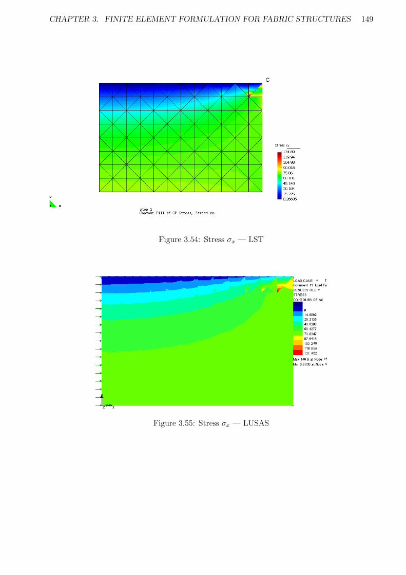
CHAPTER 3. FINITE ELEMENT FORMULATION FOR FABRIC STRUCTURES 149
Figure 3.54: Stress σx — LST
Figure 3.55: Stress σx — LUSAS
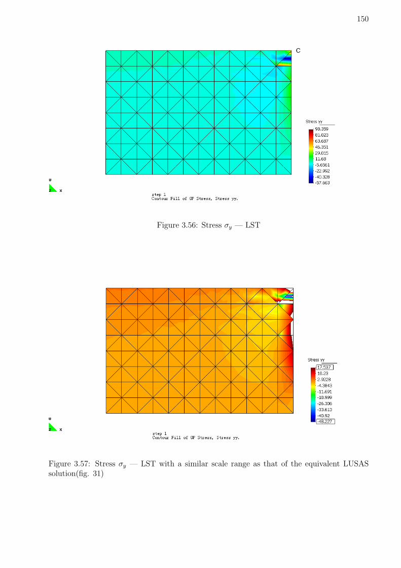
CHAPTER 3. FINITE ELEMENT FORMULATION FOR FABRIC STRUCTURES 150
Figure 3.56: Stress σy — LST
Figure 3.57: Stress σy — LST with a similar scale range as that of the equivalent LUSASsolution(fig. 31)

CHAPTER 3. FINITE ELEMENT FORMULATION FOR FABRIC STRUCTURES 151
Figure 3.58: Stress σy — LUSAS
Figure 3.59: Shear stress τxy — LST
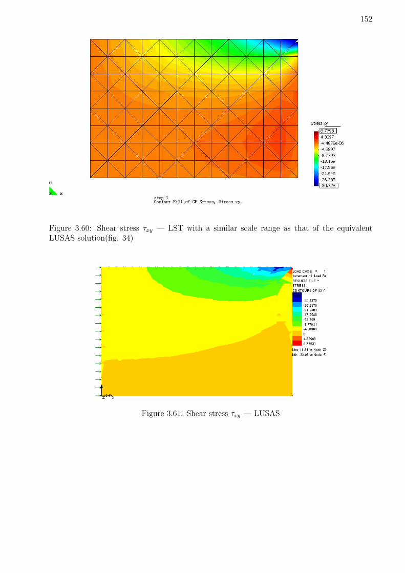
CHAPTER 3. FINITE ELEMENT FORMULATION FOR FABRIC STRUCTURES 152
Figure 3.60: Shear stress τxy — LST with a similar scale range as that of the equivalentLUSAS solution(fig. 34)
Figure 3.61: Shear stress τxy — LUSAS
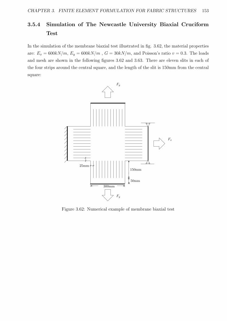
CHAPTER 3. FINITE ELEMENT FORMULATION FOR FABRIC STRUCTURES 153
3.5.4 Simulation of The Newcastle University Biaxial Cruciform
Test
In the simulation of the membrane biaxial test illustrated in fig. 3.62, the material properties
are: Ex = 600kN/m, Ey = 600kN/m , G = 30kN/m, and Poisson’s ratio v = 0.3. The loads
and mesh are shown in the following figures 3.62 and 3.63. There are eleven slits in each of
the four strips around the central square, and the length of the slit is 150mm from the central
square:
Fx
Fy
Fy
300mm
150mm
50mm
25mm
Figure 3.62: Numerical example of membrane biaxial test
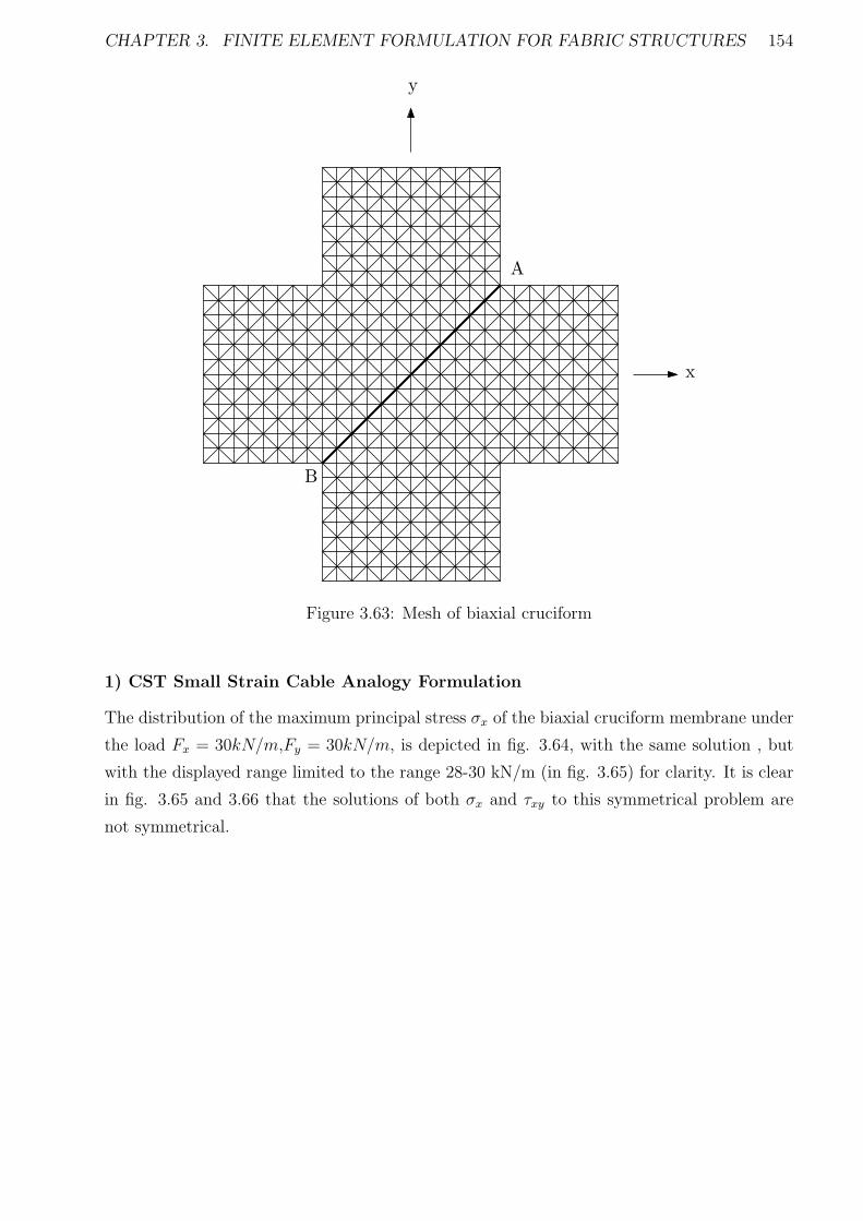
CHAPTER 3. FINITE ELEMENT FORMULATION FOR FABRIC STRUCTURES 154
A
B
x
y
Figure 3.63: Mesh of biaxial cruciform
1) CST Small Strain Cable Analogy Formulation
The distribution of the maximum principal stress σx of the biaxial cruciform membrane under
the load Fx = 30kN/m,Fy = 30kN/m, is depicted in fig. 3.64, with the same solution , but
with the displayed range limited to the range 28-30 kN/m (in fig. 3.65) for clarity. It is clear
in fig. 3.65 and 3.66 that the solutions of both σx and τxy to this symmetrical problem are
not symmetrical.
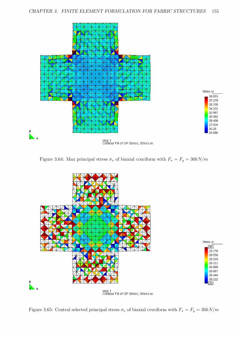
CHAPTER 3. FINITE ELEMENT FORMULATION FOR FABRIC STRUCTURES 155
Figure 3.64: Max principal stress σx of biaxial cruciform with Fx = Fy = 30kN/m
Figure 3.65: Central selected principal stress σx of biaxial cruciform with Fx = Fy = 30kN/m

CHAPTER 3. FINITE ELEMENT FORMULATION FOR FABRIC STRUCTURES 156
Figure 3.66: Central selected shear stress τxy of biaxial cruciform with Fx = Fy = 30kN/m
As shown in figures 3.67 and 3.68, with the load increased to Fx = Fy = 60kN/m and
hence the strains similarly increased, the asymmetry of the geometrically nonlinear result is
reinforced.

CHAPTER 3. FINITE ELEMENT FORMULATION FOR FABRIC STRUCTURES 157
Figure 3.67: Central selected principal stress σx of biaxial cruciform with Fx = Fy = 60kN/m
Figure 3.68: Central selected shear stress τxy of biaxial cruciform with Fx = Fy = 60kN/m
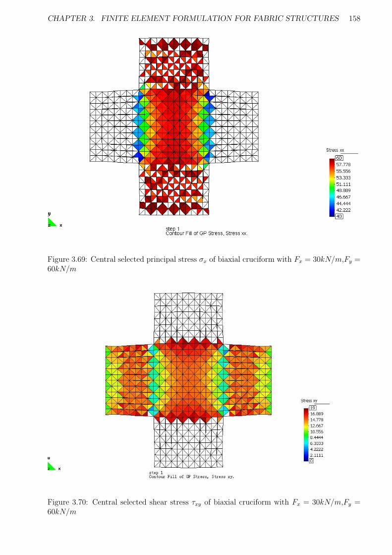
CHAPTER 3. FINITE ELEMENT FORMULATION FOR FABRIC STRUCTURES 158
Figure 3.69: Central selected principal stress σx of biaxial cruciform with Fx = 30kN/m,Fy =60kN/m
Figure 3.70: Central selected shear stress τxy of biaxial cruciform with Fx = 30kN/m,Fy =60kN/m
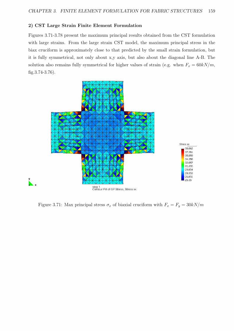
CHAPTER 3. FINITE ELEMENT FORMULATION FOR FABRIC STRUCTURES 159
2) CST Large Strain Finite Element Formulation
Figures 3.71-3.78 present the maximum principal results obtained from the CST formulation
with large strains. From the large strain CST model, the maximum principal stress in the
biax cruciform is approximately close to that predicted by the small strain formulation, but
it is fully symmetrical, not only about x,y axis, but also about the diagonal line A-B. The
solution also remains fully symmetrical for higher values of strain (e.g. when Fx = 60kN/m,
fig.3.74-3.76).
Figure 3.71: Max principal stress σx of biaxial cruciform with Fx = Fy = 30kN/m
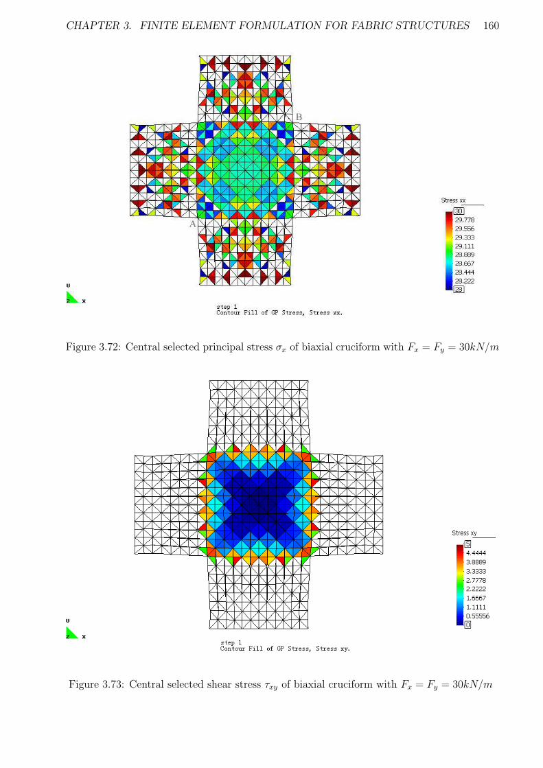
CHAPTER 3. FINITE ELEMENT FORMULATION FOR FABRIC STRUCTURES 160
Figure 3.72: Central selected principal stress σx of biaxial cruciform with Fx = Fy = 30kN/m
Figure 3.73: Central selected shear stress τxy of biaxial cruciform with Fx = Fy = 30kN/m
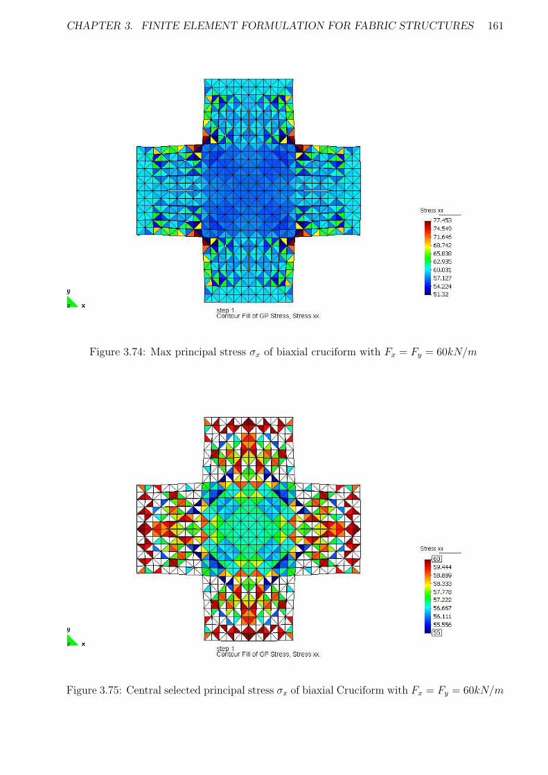
CHAPTER 3. FINITE ELEMENT FORMULATION FOR FABRIC STRUCTURES 161
Figure 3.74: Max principal stress σx of biaxial cruciform with Fx = Fy = 60kN/m
Figure 3.75: Central selected principal stress σx of biaxial Cruciform with Fx = Fy = 60kN/m
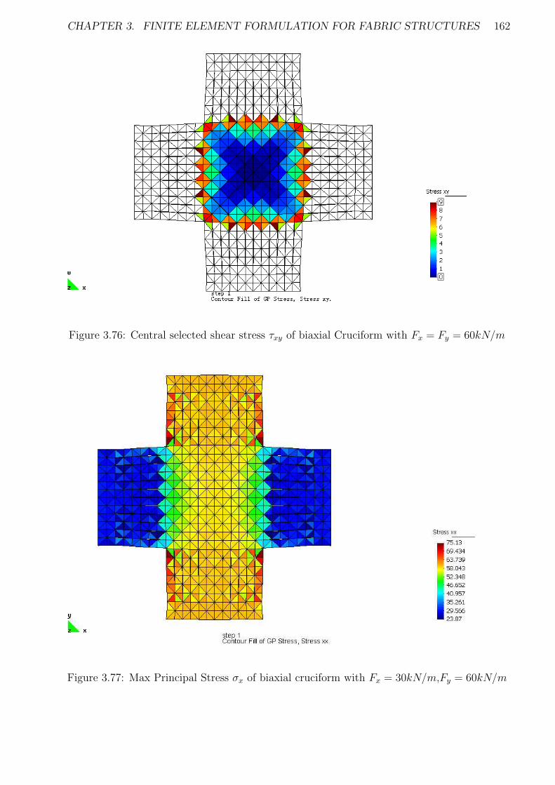
CHAPTER 3. FINITE ELEMENT FORMULATION FOR FABRIC STRUCTURES 162
Figure 3.76: Central selected shear stress τxy of biaxial Cruciform with Fx = Fy = 60kN/m
Figure 3.77: Max Principal Stress σx of biaxial cruciform with Fx = 30kN/m,Fy = 60kN/m
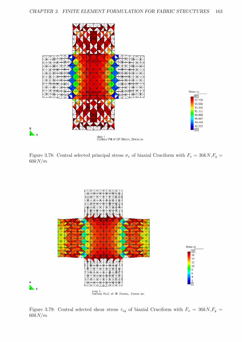
CHAPTER 3. FINITE ELEMENT FORMULATION FOR FABRIC STRUCTURES 163
Figure 3.78: Central selected principal stress σx of biaxial Cruciform with Fx = 30kN ,Fy =60kN/m
Figure 3.79: Central selected shear stress τxy of biaxial Cruciform with Fx = 30kN ,Fy =60kN/m
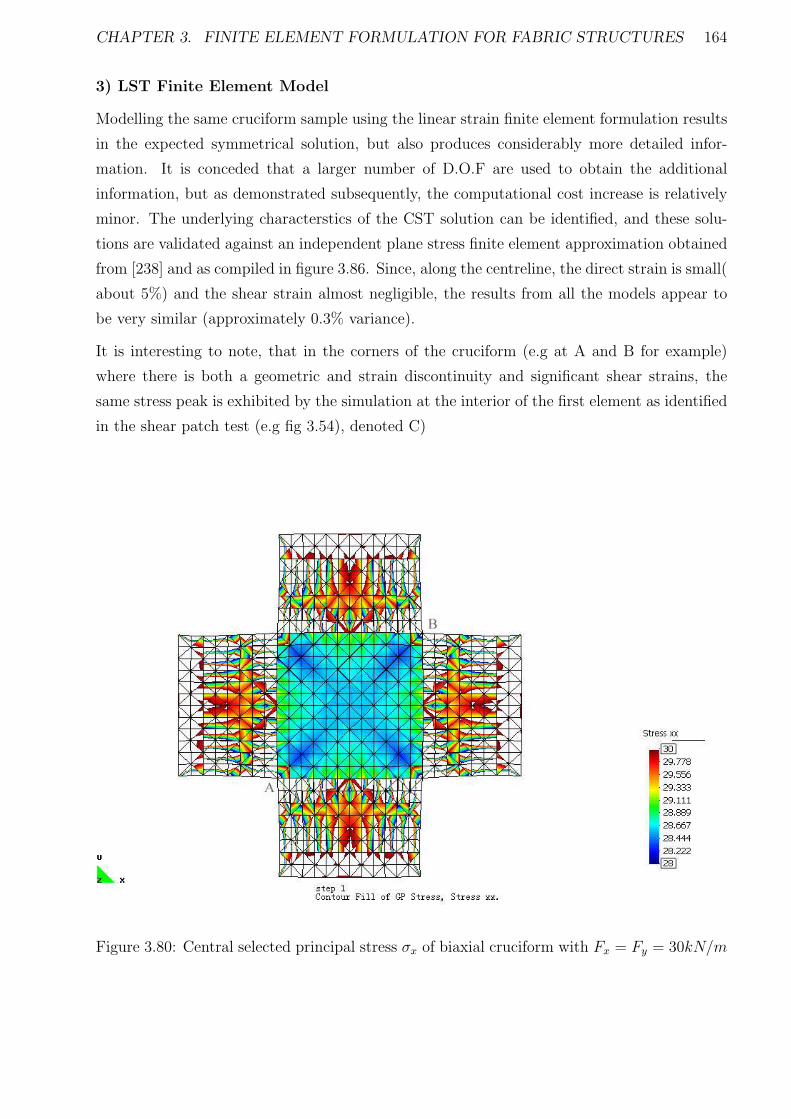
CHAPTER 3. FINITE ELEMENT FORMULATION FOR FABRIC STRUCTURES 164
3) LST Finite Element Model
Modelling the same cruciform sample using the linear strain finite element formulation results
in the expected symmetrical solution, but also produces considerably more detailed infor-
mation. It is conceded that a larger number of D.O.F are used to obtain the additional
information, but as demonstrated subsequently, the computational cost increase is relatively
minor. The underlying characterstics of the CST solution can be identified, and these solu-
tions are validated against an independent plane stress finite element approximation obtained
from [238] and as compiled in figure 3.86. Since, along the centreline, the direct strain is small(
about 5%) and the shear strain almost negligible, the results from all the models appear to
be very similar (approximately 0.3% variance).
It is interesting to note, that in the corners of the cruciform (e.g at A and B for example)
where there is both a geometric and strain discontinuity and significant shear strains, the
same stress peak is exhibited by the simulation at the interior of the first element as identified
in the shear patch test (e.g fig 3.54), denoted C)
Figure 3.80: Central selected principal stress σx of biaxial cruciform with Fx = Fy = 30kN/m
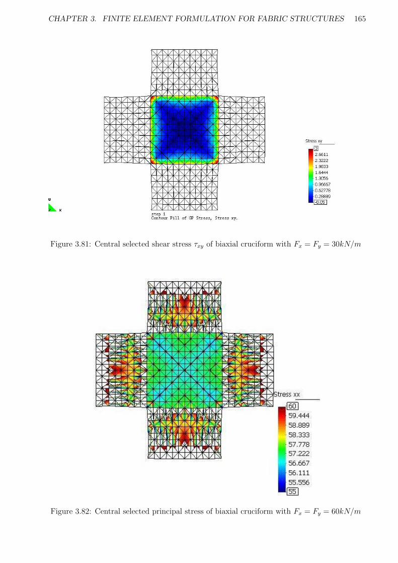
CHAPTER 3. FINITE ELEMENT FORMULATION FOR FABRIC STRUCTURES 165
Figure 3.81: Central selected shear stress τxy of biaxial cruciform with Fx = Fy = 30kN/m
Figure 3.82: Central selected principal stress of biaxial cruciform with Fx = Fy = 60kN/m
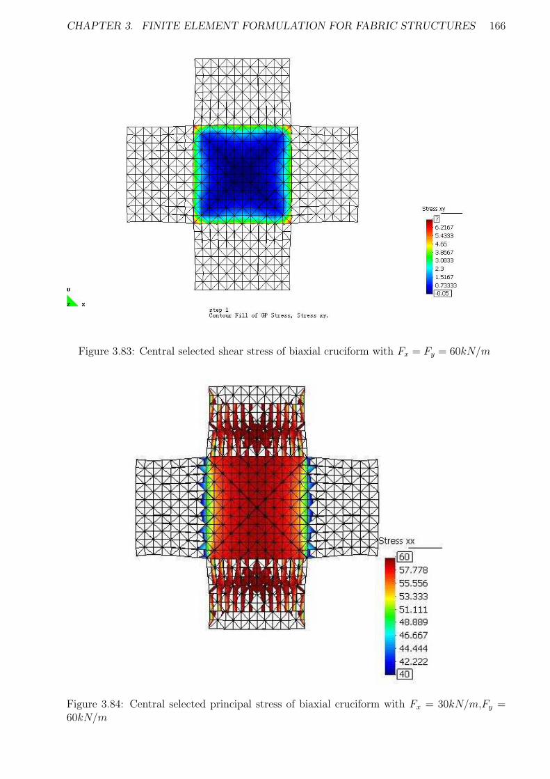
CHAPTER 3. FINITE ELEMENT FORMULATION FOR FABRIC STRUCTURES 166
Figure 3.83: Central selected shear stress of biaxial cruciform with Fx = Fy = 60kN/m
Figure 3.84: Central selected principal stress of biaxial cruciform with Fx = 30kN/m,Fy =60kN/m
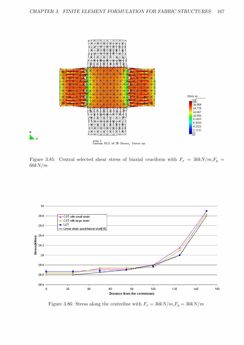
CHAPTER 3. FINITE ELEMENT FORMULATION FOR FABRIC STRUCTURES 167
Figure 3.85: Central selected shear stress of biaxial cruciform with Fx = 30kN/m,Fy =60kN/m
Figure 3.86: Stress along the centreline with Fx = 30kN/m,Fy = 30kN/m
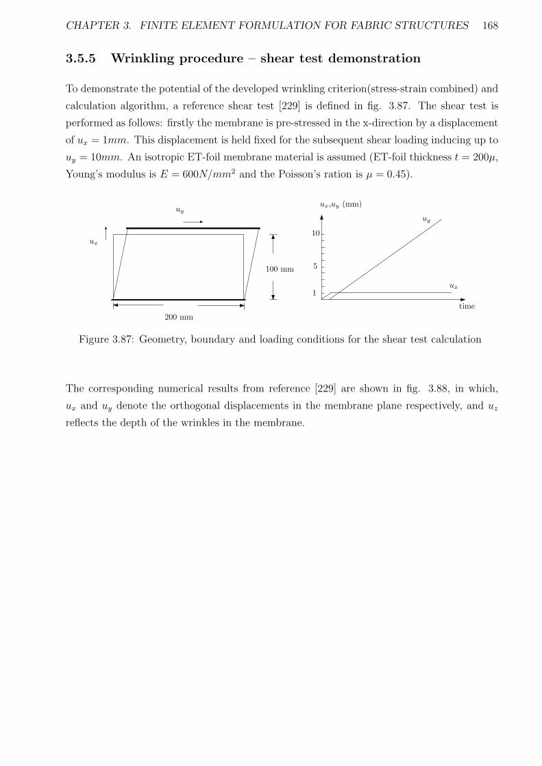
CHAPTER 3. FINITE ELEMENT FORMULATION FOR FABRIC STRUCTURES 168
3.5.5 Wrinkling procedure – shear test demonstration
To demonstrate the potential of the developed wrinkling criterion(stress-strain combined) and
calculation algorithm, a reference shear test [229] is defined in fig. 3.87. The shear test is
performed as follows: firstly the membrane is pre-stressed in the x-direction by a displacement
of ux = 1mm. This displacement is held fixed for the subsequent shear loading inducing up to
uy = 10mm. An isotropic ET-foil membrane material is assumed (ET-foil thickness t = 200µ,
Young’s modulus is E = 600N/mm2 and the Poisson’s ration is µ = 0.45).
200 mm
ux
uy
100 mm
ux,uy (mm)
1
5
10
time
ux
uy
Figure 3.87: Geometry, boundary and loading conditions for the shear test calculation
The corresponding numerical results from reference [229] are shown in fig. 3.88, in which,
ux and uy denote the orthogonal displacements in the membrane plane respectively, and uz
reflects the depth of the wrinkles in the membrane.
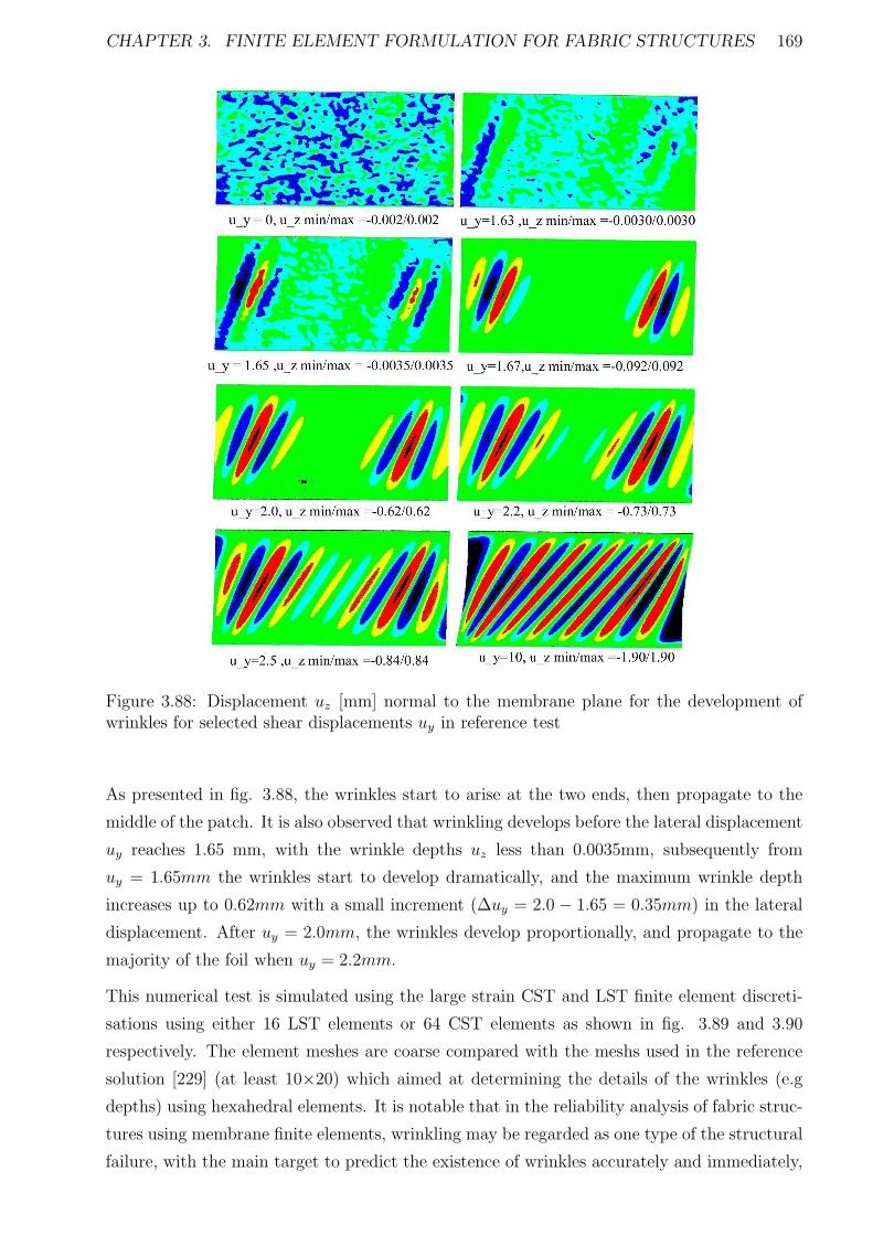
CHAPTER 3. FINITE ELEMENT FORMULATION FOR FABRIC STRUCTURES 169
Figure 3.88: Displacement uz [mm] normal to the membrane plane for the development ofwrinkles for selected shear displacements uy in reference test
As presented in fig. 3.88, the wrinkles start to arise at the two ends, then propagate to the
middle of the patch. It is also observed that wrinkling develops before the lateral displacement
uy reaches 1.65 mm, with the wrinkle depths uz less than 0.0035mm, subsequently from
uy = 1.65mm the wrinkles start to develop dramatically, and the maximum wrinkle depth
increases up to 0.62mm with a small increment (∆uy = 2.0 − 1.65 = 0.35mm) in the lateral
displacement. After uy = 2.0mm, the wrinkles develop proportionally, and propagate to the
majority of the foil when uy = 2.2mm.
This numerical test is simulated using the large strain CST and LST finite element discreti-
sations using either 16 LST elements or 64 CST elements as shown in fig. 3.89 and 3.90
respectively. The element meshes are coarse compared with the meshs used in the reference
solution [229] (at least 10×20) which aimed at determining the details of the wrinkles (e.g
depths) using hexahedral elements. It is notable that in the reliability analysis of fabric struc-
tures using membrane finite elements, wrinkling may be regarded as one type of the structural
failure, with the main target to predict the existence of wrinkles accurately and immediately,
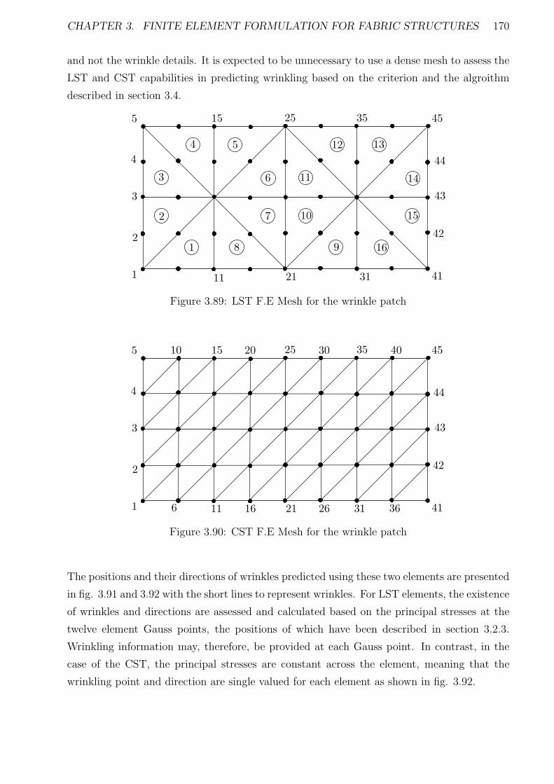
CHAPTER 3. FINITE ELEMENT FORMULATION FOR FABRIC STRUCTURES 170
and not the wrinkle details. It is expected to be unnecessary to use a dense mesh to assess the
LST and CST capabilities in predicting wrinkling based on the criterion and the algroithm
described in section 3.4.
1
2
3
4
5
11 21 31 41
15 25 35 45
42
43
44
1
2 10
3
4 5
6
7
8 9
11
12 13
14
15
16
Figure 3.89: LST F.E Mesh for the wrinkle patch
1
2
3
4
5
11 21 31 41
15 25 35 45
42
43
44
6 16 26 36
10 20 30 40
Figure 3.90: CST F.E Mesh for the wrinkle patch
The positions and their directions of wrinkles predicted using these two elements are presented
in fig. 3.91 and 3.92 with the short lines to represent wrinkles. For LST elements, the existence
of wrinkles and directions are assessed and calculated based on the principal stresses at the
twelve element Gauss points, the positions of which have been described in section 3.2.3.
Wrinkling information may, therefore, be provided at each Gauss point. In contrast, in the
case of the CST, the principal stresses are constant across the element, meaning that the
wrinkling point and direction are single valued for each element as shown in fig. 3.92.
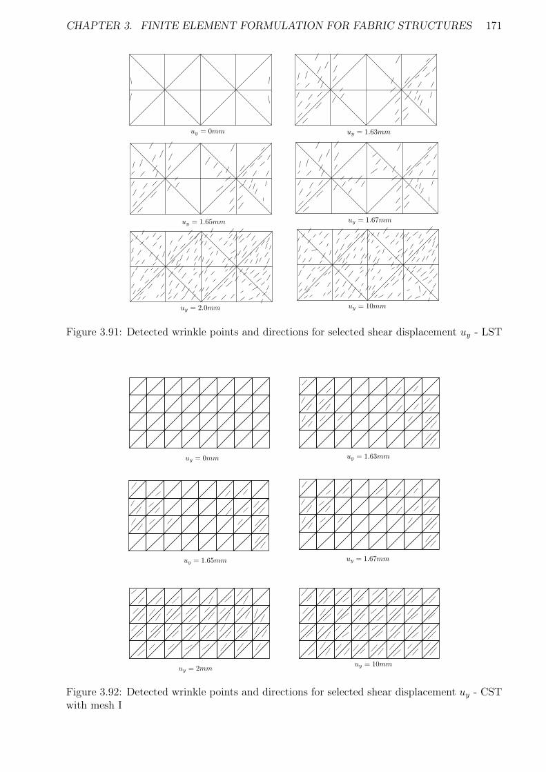
CHAPTER 3. FINITE ELEMENT FORMULATION FOR FABRIC STRUCTURES 171
uy = 0mm uy = 1.63mm
uy = 2.0mm
uy = 1.65mmuy = 1.67mm
uy = 10mm
Figure 3.91: Detected wrinkle points and directions for selected shear displacement uy - LST
uy = 0mmuy = 1.63mm
uy = 1.65mmuy = 1.67mm
uy = 2mm
uy = 10mm
Figure 3.92: Detected wrinkle points and directions for selected shear displacement uy - CSTwith mesh I
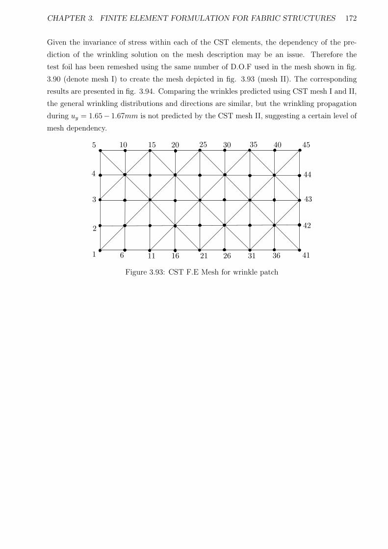
CHAPTER 3. FINITE ELEMENT FORMULATION FOR FABRIC STRUCTURES 172
Given the invariance of stress within each of the CST elements, the dependency of the pre-
diction of the wrinkling solution on the mesh description may be an issue. Therefore the
test foil has been remeshed using the same number of D.O.F used in the mesh shown in fig.
3.90 (denote mesh I) to create the mesh depicted in fig. 3.93 (mesh II). The corresponding
results are presented in fig. 3.94. Comparing the wrinkles predicted using CST mesh I and II,
the general wrinkling distributions and directions are similar, but the wrinkling propagation
during uy = 1.65− 1.67mm is not predicted by the CST mesh II, suggesting a certain level of
mesh dependency.
1
2
3
4
5
11 21 31 41
15 25 35 45
42
43
44
6 16 26 36
10 20 30 40
Figure 3.93: CST F.E Mesh for wrinkle patch
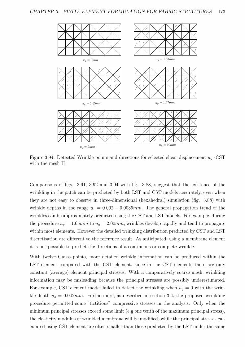
CHAPTER 3. FINITE ELEMENT FORMULATION FOR FABRIC STRUCTURES 173
uy = 0mmuy = 1.63mm
uy = 1.65mmuy = 1.67mm
uy = 2mm
uy = 10mm
Figure 3.94: Detected Wrinkle points and directions for selected shear displacement uy -CSTwith the mesh II
Comparisons of figs. 3.91, 3.92 and 3.94 with fig. 3.88, suggest that the existence of the
wrinkling in the patch can be predicted by both LST and CST models accurately, even when
they are not easy to observe in three-dimensional (hexahedral) simulation (fig. 3.88) with
wrinkle depths in the range uz = 0.002 − 0.0035mm. The general propagation trend of the
wrinkles can be approximately predicted using the CST and LST models. For example, during
the procedure uy = 1.65mm to uy = 2.00mm, wrinkles develop rapidly and tend to propagate
within most elements. However the detailed wrinkling distribution predicted by CST and LST
discretisation are different to the reference result. As anticipated, using a membrane element
it is not possible to predict the directions of a continuous or complete wrinkle.
With twelve Gauss points, more detailed wrinkle information can be produced within the
LST element compared with the CST element, since in the CST elements there are only
constant (average) element principal stresses. With a comparatively coarse mesh, wrinkling
information may be misleading because the principal stresses are possibly underestimated.
For example, CST element model failed to detect the wrinkling when uy = 0 with the wrin-
kle depth uz = 0.002mm. Furthermore, as described in section 3.4, the proposed wrinkling
procedure permitted some ”fictitious” compressive stresses in the analysis. Only when the
minimum principal stresses exceed some limit (e.g one tenth of the maximum principal stress),
the elasticity modulus of wrinkled membrane will be modified, while the principal stresses cal-
culated using CST element are often smaller than those predicted by the LST under the same
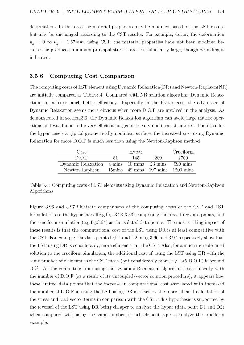
CHAPTER 3. FINITE ELEMENT FORMULATION FOR FABRIC STRUCTURES 174
deformation. In this case the material properties may be modified based on the LST results
but may be unchanged according to the CST results. For example, during the deformation
uy = 0 to uy = 1.67mm, using CST, the material properties have not been modified be-
cause the produced minimum principal stresses are not sufficiently large, though wrinkling is
indicated.
3.5.6 Computing Cost Comparison
The computing costs of LST element using Dynamic Relaxation(DR) and Newton-Raphson(NR)
are initially compared as Table.3.4. Compared with NR solution algorithm, Dynamic Relax-
ation can achieve much better efficiency. Especially in the Hypar case, the advantage of
Dynamic Relaxation seems more obvious when more D.O.F are involved in the analysis. As
demonstrated in section.3.3, the Dynamic Relaxation algorithm can avoid large matrix oper-
ations and was found to be very efficient for geometrically nonlinear structures. Therefore for
the hypar case - a typical geometrically nonlinear surface, the increased cost using Dynamic
Relaxation for more D.O.F is much less than using the Newton-Raphson method.
Case Hypar CruciformD.O.F 81 145 289 2709
Dynamic Relaxation 4 mins 10 mins 23 mins 990 minsNewton-Raphson 15mins 49 mins 197 mins 1200 mins
Table 3.4: Computing costs of LST elements using Dynamic Relaxation and Newton-RaphsonAlgorithms
Figure 3.96 and 3.97 illustrate comparisons of the computing costs of the CST and LST
formulations to the hypar model(e.g fig. 3.28-3.33) comprising the first three data points, and
the cruciform simulation (e.g fig.3.64) as the isolated data points. The most striking impact of
these results is that the computational cost of the LST using DR is at least competitive with
the CST. For example, the data points D,D1 and D2 in fig.3.96 and 3.97 respectively show that
the LST using DR is considerably, more efficient than the CST. Also, for a much more detailed
solution to the cruciform simulation, the additional cost of using the LST using DR with the
same number of elements as the CST mesh (but considerably more, e.g. ×5 D.O.F) is around
10%. As the computing time using the Dynamic Relaxation algorithm scales linearly with
the number of D.O.F (as a result of its uncoupled/vector solution procedure), it appears how
these limited data points that the increase in computational cost associated with increased
the number of D.O.F in using the LST using DR is offset by the more efficient calculation of
the stress and load vector terms in comparison with the CST. This hypothesis is supported by
the reversal of the LST using DR being cheaper to analyze the hypar (data point D1 and D2)
when compared with using the same number of each element type to analyze the cruciform
example.
CHAPTER 3. FINITE ELEMENT FORMULATION FOR FABRIC STRUCTURES 175
Furthermore, it has been established that the solution using the LST using DR takes far fewer
iterations to achieve convergence at equilibrium than the CST for the same level of accuracy.
Nevertheless, these initial findings are encouraging in terms of the compromise normally as-
sociated with the order of the formulation and its corresponding computational cost.
Figure 3.95: Comparison of computing cost between CST and LST formulations with D.O.F– Hypar
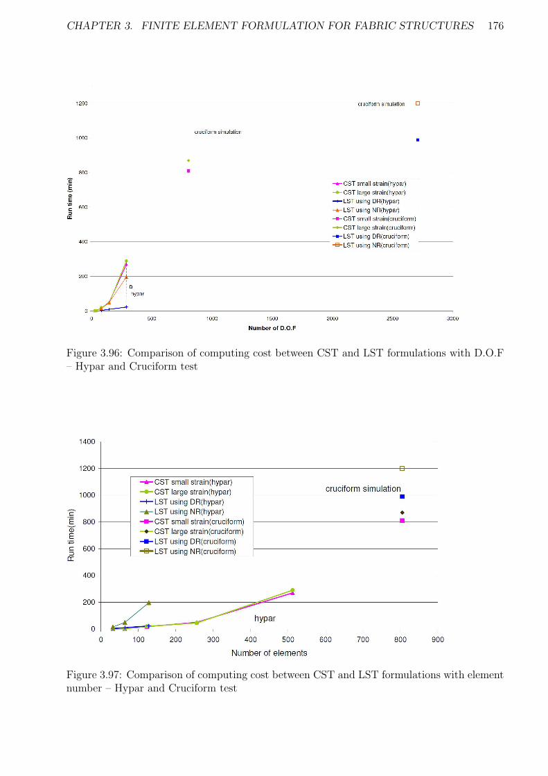
CHAPTER 3. FINITE ELEMENT FORMULATION FOR FABRIC STRUCTURES 176
Figure 3.96: Comparison of computing cost between CST and LST formulations with D.O.F– Hypar and Cruciform test
Figure 3.97: Comparison of computing cost between CST and LST formulations with elementnumber – Hypar and Cruciform test
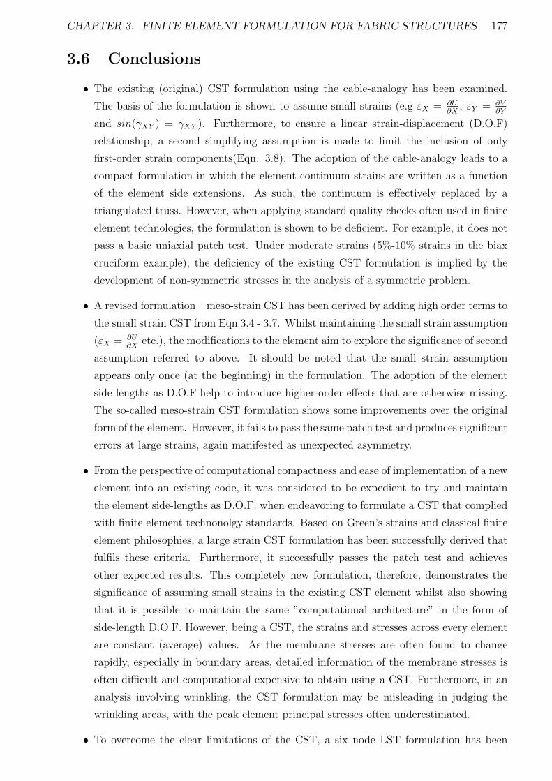
CHAPTER 3. FINITE ELEMENT FORMULATION FOR FABRIC STRUCTURES 177
3.6 Conclusions
• The existing (original) CST formulation using the cable-analogy has been examined.
The basis of the formulation is shown to assume small strains (e.g εX = ∂U∂X
, εY = ∂V∂Y
and sin(γXY ) = γXY ). Furthermore, to ensure a linear strain-displacement (D.O.F)
relationship, a second simplifying assumption is made to limit the inclusion of only
first-order strain components(Eqn. 3.8). The adoption of the cable-analogy leads to a
compact formulation in which the element continuum strains are written as a function
of the element side extensions. As such, the continuum is effectively replaced by a
triangulated truss. However, when applying standard quality checks often used in finite
element technologies, the formulation is shown to be deficient. For example, it does not
pass a basic uniaxial patch test. Under moderate strains (5%-10% strains in the biax
cruciform example), the deficiency of the existing CST formulation is implied by the
development of non-symmetric stresses in the analysis of a symmetric problem.
• A revised formulation – meso-strain CST has been derived by adding high order terms to
the small strain CST from Eqn 3.4 - 3.7. Whilst maintaining the small strain assumption
(εX = ∂U∂X
etc.), the modifications to the element aim to explore the significance of second
assumption referred to above. It should be noted that the small strain assumption
appears only once (at the beginning) in the formulation. The adoption of the element
side lengths as D.O.F help to introduce higher-order effects that are otherwise missing.
The so-called meso-strain CST formulation shows some improvements over the original
form of the element. However, it fails to pass the same patch test and produces significant
errors at large strains, again manifested as unexpected asymmetry.
• From the perspective of computational compactness and ease of implementation of a new
element into an existing code, it was considered to be expedient to try and maintain
the element side-lengths as D.O.F. when endeavoring to formulate a CST that complied
with finite element technonolgy standards. Based on Green’s strains and classical finite
element philosophies, a large strain CST formulation has been successfully derived that
fulfils these criteria. Furthermore, it successfully passes the patch test and achieves
other expected results. This completely new formulation, therefore, demonstrates the
significance of assuming small strains in the existing CST element whilst also showing
that it is possible to maintain the same ”computational architecture” in the form of
side-length D.O.F. However, being a CST, the strains and stresses across every element
are constant (average) values. As the membrane stresses are often found to change
rapidly, especially in boundary areas, detailed information of the membrane stresses is
often difficult and computational expensive to obtain using a CST. Furthermore, in an
analysis involving wrinkling, the CST formulation may be misleading in judging the
wrinkling areas, with the peak element principal stresses often underestimated.
• To overcome the clear limitations of the CST, a six node LST formulation has been

CHAPTER 3. FINITE ELEMENT FORMULATION FOR FABRIC STRUCTURES 178
developed using finite element principles. This is also based on Green’s strains, but
also makes use of inferred element curvatures. No additional rotational D.O.F are in-
cluded, so the element remains C0 continuous. This element formulation is shown to
pass the patch and other tests of element quality. The advantage of having the capa-
bility of strains and stresses that can vary linearly across the element has been clearly
demonstrated by a number of solutions compared with the equivalent CST results. This
type of element may exhibit particular forms of element distortion that have the po-
tential compromise numerical stability and solution accuracy, with specific reference to
the form-finding analysis. A number of element distortion coefficients have been identi-
fied in the literature. However, all of these have some or a considerable computational
overhead. They are also difficult to interpret in combination. A better measure has
been shown to be the criterion that the Jacobian at each of the element Gauss Points
remains positive definite. The possibility of ”floating” mid-side nodes (e.g. a type of
nodal rigid-body motion) has also been examined and deemed to be unlikely to happen
in an analysis.
• From a normal finite element technology viewpoint associated with Newton-Raphson
as the solver it would be expected that the LST would be considerably more compu-
tationally expensive than the CST. However, when coupled with Dynamic Relaxation
algorithm, the LST element has been shown to be extremely competitive, producing
much higher quality solutions for very little additional computational effort. It has been
concluded for the relatively small number of examples examined, that a mesh of LSTs
is very well-suited to the the Dynamic Relaxation algorithm and that characteristics of
the formulation coupled with this algorithm do not lead to the computational scaling
normally seen when moving from a basic to a higher-order element.
Chapter 4
Probabilistic Properties of Structural
Fabric
4.1 Introduction
The materials used for fabric structures generally consist of coated woven fabric, cables and
belts, supporting steel and connections. From the viewpoint of statistics, the mechanical
properties of all these materials can be regarded as random variables with uncertainties. The-
oretically, an accurate structural reliability analysis requires the full uncertainty information
in all the corresponding materials. That would require a probabilistic investigation to be un-
dertaken for all these materials for a complete reliability analysis. However, that is beyond the
scope of this thesis. In this chapter, the probabilistic investigation focuses on coated woven
fabrics used for structural membranes, with the purpose of developing a practical and efficient
probabilistic testing and analysis methodology for series of fabric materials.
Coated woven fabric is the main component in a fabric structure. As a composite of inelastic
materials(i.e. yarns and coating), it has obviously nonlinear mechanical behaviour which may
complicate a probability analysis. The fabric is often assumed to be an orthotropic materials
in which yarns are straight along the primary axis, and the fill and warp are normal to
each other. However due to the coating process this assumption may not be valid, and an
anisotropic composite structure may exist as the fabric material. Therefore the coated woven
fabric cannot be simply regarded as a combination of yarn assemblies and coated material.
The yarn distribution may become a very important factor affecting the mechanical properties
of the fabric, and a key randomness existing in the coated woven fabric.
When the yarns and coating materials are individually manufactured, they may have highly
uniform material properties with small randomness. However when they are formed into
a composite as a fabric, the randomness of the fabric properties over the material space
appears more obvious owing to the manufacturing process. Because of the nonlinearity of the
fabric, its elastic properties are not constants under different stress states. The calculation
of Young’s modulus is normally derived using a regression model. However the model itself
179
CHAPTER 4. PROBABILISTIC PROPERTIES OF STRUCTURAL FABRIC 180
can also appear as an important source of uncertainty. In the analysis and design of fabric
structures, the variability in the fabric material is normally accounted for in the application
of an additional component to the factor of safety. For example, it is common practice to
apply a factor of 1.5 to the tear propagation factor of 4 to produce an overall factor of 6 [3].
Different test methods including specimen cutting and loading procedures, may lead to dif-
ferent test results, from which, a non-unique, probabilistic analysis result for the same type
of material may be produced. Since the test method itself is a source of uncertainty, it may
appear to increase the randomness of the test samples as one of epistemic uncertainty types.
The probabilistic investigation of the fabric properties is only effective when a large quantity of
statistical tests are made. Owing to resource limitation, the randomness of the fabric strength
and stress-strain relations are seldom accurately investigated, and the most efforts( [122]-
[144]) are taken in creating mathematical models to predict the mechanic behavior of the
fabric which is often based on a limited test data. Even though the quantity of test samples
is always limited by the available time and resources, a larger test number is always preferred
to increase statistical confidence.
To acquire more accurate statistical information of the fabric materials, more than 300 samples
prepared using two different cutting procedures have been tested. Prior to making the de-
tailed statistical investigation strategy, a small number of material tests have been performed
to explore the basic characteristics of the fabric material(e.g yarn distribution, stress-strain
curves). Subsequently a suitable mathematical model may then be created and a probabilis-
tic methodologies specific for the given fabric samples is proposed to reduce the systematic
uncertainty from the development of the probabilistic model.
The probabilistic analysis starts with a basic statistical investigation of the test data, which
can give an approximate range of randomness for different statistical variables. The detailed
probabilistic analysis (i.e statistical distributions) is undertaken based on candidate distrib-
utions and a non-interval data-fitting test (Kolmogorov-Smirnov test). The selection of the
data-fitting distribution is taken to be a function of the maximum difference between the
CDFs of candidate distributions and sample data, and the general fitness of the distributions.
In this chapter, the principal methodology of the probabilistic investigation of the fabric
material follows a step-by-step procedure. The initial deterministic material tests are described
in section 4.3. Subsequently the mathematical representation of the test data and statistical
methodology for a large number of tests are determined as described in section.4.4. The
probabilistic results and analysis are given in section.4.5.
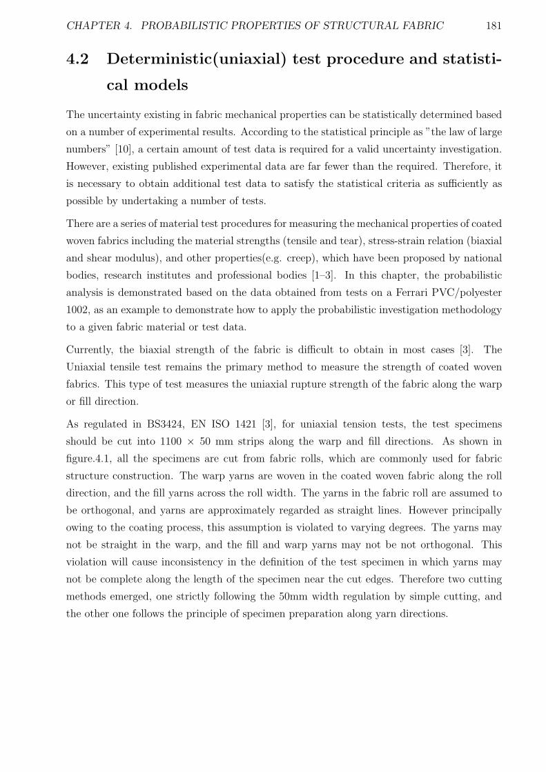
CHAPTER 4. PROBABILISTIC PROPERTIES OF STRUCTURAL FABRIC 181
4.2 Deterministic(uniaxial) test procedure and statisti-
cal models
The uncertainty existing in fabric mechanical properties can be statistically determined based
on a number of experimental results. According to the statistical principle as ”the law of large
numbers” [10], a certain amount of test data is required for a valid uncertainty investigation.
However, existing published experimental data are far fewer than the required. Therefore, it
is necessary to obtain additional test data to satisfy the statistical criteria as sufficiently as
possible by undertaking a number of tests.
There are a series of material test procedures for measuring the mechanical properties of coated
woven fabrics including the material strengths (tensile and tear), stress-strain relation (biaxial
and shear modulus), and other properties(e.g. creep), which have been proposed by national
bodies, research institutes and professional bodies [1–3]. In this chapter, the probabilistic
analysis is demonstrated based on the data obtained from tests on a Ferrari PVC/polyester
1002, as an example to demonstrate how to apply the probabilistic investigation methodology
to a given fabric material or test data.
Currently, the biaxial strength of the fabric is difficult to obtain in most cases [3]. The
Uniaxial tensile test remains the primary method to measure the strength of coated woven
fabrics. This type of test measures the uniaxial rupture strength of the fabric along the warp
or fill direction.
As regulated in BS3424, EN ISO 1421 [3], for uniaxial tension tests, the test specimens
should be cut into 1100 × 50 mm strips along the warp and fill directions. As shown in
figure.4.1, all the specimens are cut from fabric rolls, which are commonly used for fabric
structure construction. The warp yarns are woven in the coated woven fabric along the roll
direction, and the fill yarns across the roll width. The yarns in the fabric roll are assumed to
be orthogonal, and yarns are approximately regarded as straight lines. However principally
owing to the coating process, this assumption is violated to varying degrees. The yarns may
not be straight in the warp, and the fill and warp yarns may not be not orthogonal. This
violation will cause inconsistency in the definition of the test specimen in which yarns may
not be complete along the length of the specimen near the cut edges. Therefore two cutting
methods emerged, one strictly following the 50mm width regulation by simple cutting, and
the other one follows the principle of specimen preparation along yarn directions.
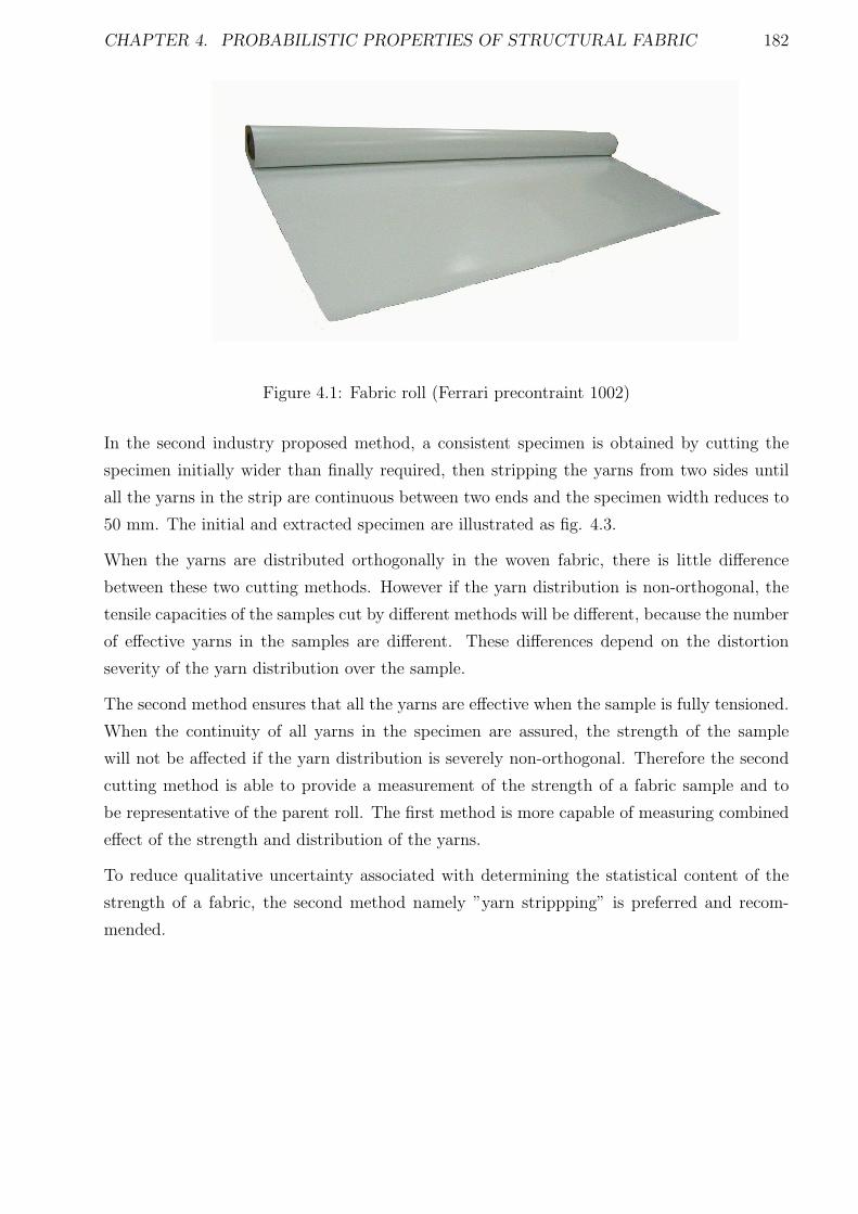
CHAPTER 4. PROBABILISTIC PROPERTIES OF STRUCTURAL FABRIC 182
Figure 4.1: Fabric roll (Ferrari precontraint 1002)
In the second industry proposed method, a consistent specimen is obtained by cutting the
specimen initially wider than finally required, then stripping the yarns from two sides until
all the yarns in the strip are continuous between two ends and the specimen width reduces to
50 mm. The initial and extracted specimen are illustrated as fig. 4.3.
When the yarns are distributed orthogonally in the woven fabric, there is little difference
between these two cutting methods. However if the yarn distribution is non-orthogonal, the
tensile capacities of the samples cut by different methods will be different, because the number
of effective yarns in the samples are different. These differences depend on the distortion
severity of the yarn distribution over the sample.
The second method ensures that all the yarns are effective when the sample is fully tensioned.
When the continuity of all yarns in the specimen are assured, the strength of the sample
will not be affected if the yarn distribution is severely non-orthogonal. Therefore the second
cutting method is able to provide a measurement of the strength of a fabric sample and to
be representative of the parent roll. The first method is more capable of measuring combined
effect of the strength and distribution of the yarns.
To reduce qualitative uncertainty associated with determining the statistical content of the
strength of a fabric, the second method namely ”yarn strippping” is preferred and recom-
mended.
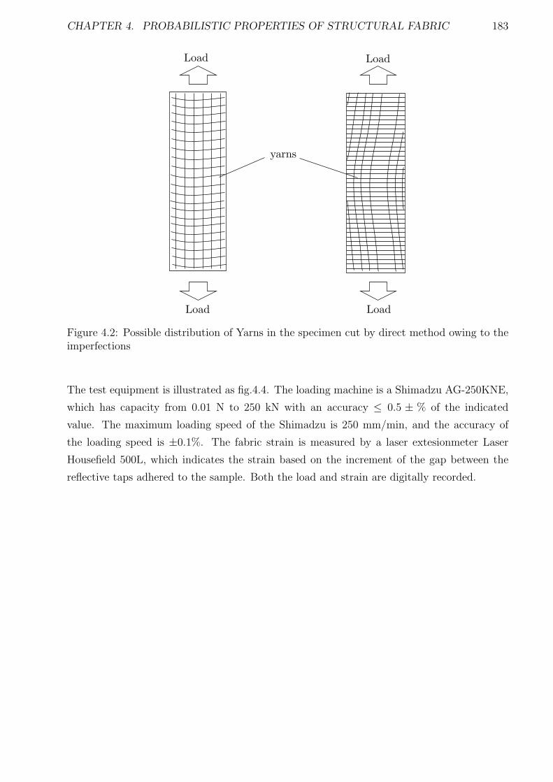
CHAPTER 4. PROBABILISTIC PROPERTIES OF STRUCTURAL FABRIC 183
yarns
Load Load
Load Load
Figure 4.2: Possible distribution of Yarns in the specimen cut by direct method owing to theimperfections
The test equipment is illustrated as fig.4.4. The loading machine is a Shimadzu AG-250KNE,
which has capacity from 0.01 N to 250 kN with an accuracy ≤ 0.5 ± % of the indicated
value. The maximum loading speed of the Shimadzu is 250 mm/min, and the accuracy of
the loading speed is ±0.1%. The fabric strain is measured by a laser extesionmeter Laser
Housefield 500L, which indicates the strain based on the increment of the gap between the
reflective taps adhered to the sample. Both the load and strain are digitally recorded.
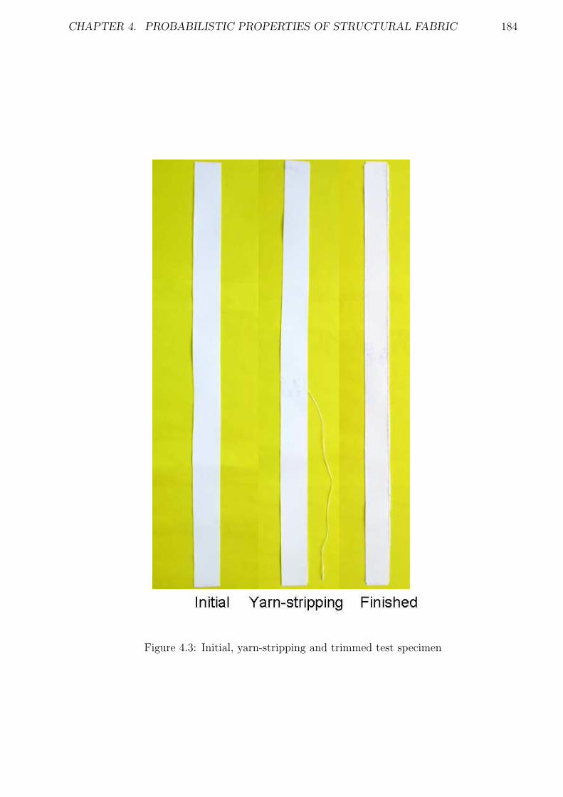
CHAPTER 4. PROBABILISTIC PROPERTIES OF STRUCTURAL FABRIC 184
Figure 4.3: Initial, yarn-stripping and trimmed test specimen
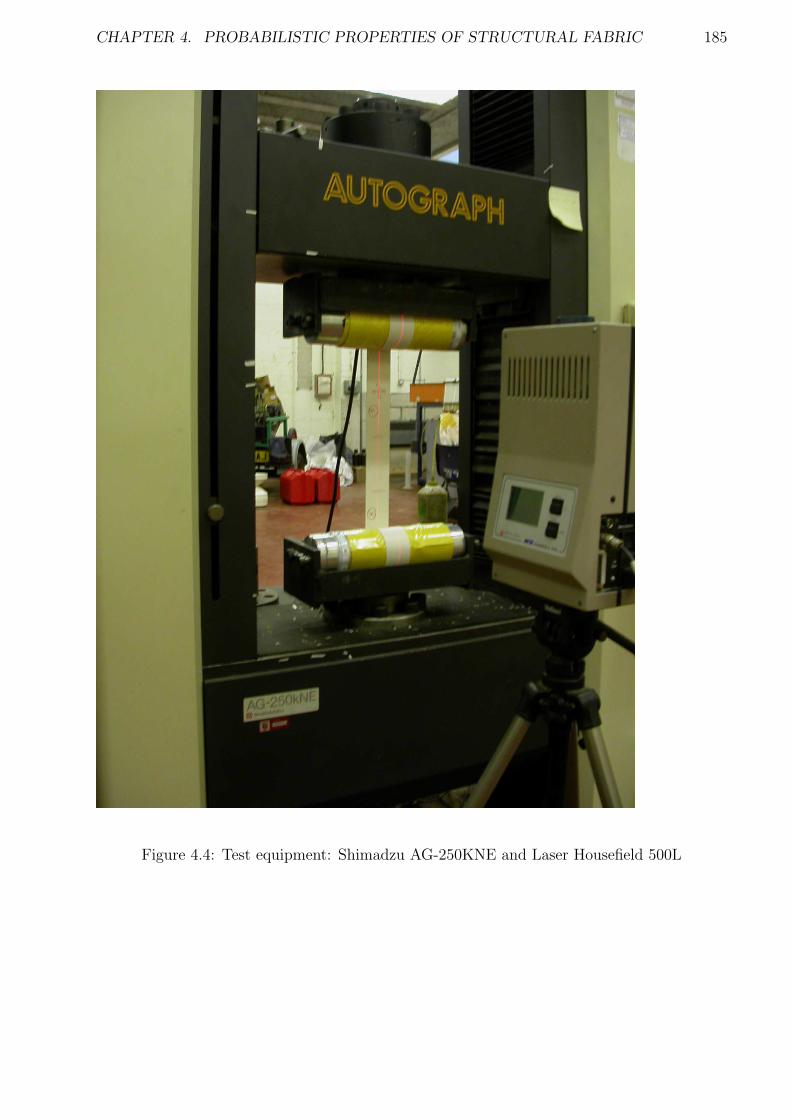
CHAPTER 4. PROBABILISTIC PROPERTIES OF STRUCTURAL FABRIC 185
Figure 4.4: Test equipment: Shimadzu AG-250KNE and Laser Housefield 500L
CHAPTER 4. PROBABILISTIC PROPERTIES OF STRUCTURAL FABRIC 186
4.2.1 Strength measurement
The uniaxial tension strength of the fabric is normally higher than its biaxial tension strength
owing to the crimp interaction [3]. However, because the biaxial strength is complicated
and not easy to measure requiring specialized equipment of limited availability, the uniaxial
strength has become the main parameter representing the material strength. The ultimate
uniaxial strength can be computed according to the failure load of the specimens as:
σult =Ff
D(4.1)
where, Ff is failure load and D is the specimen width(50mm for standard uniaxial tension
test).
4.2.2 Stress-strain relations
The coated woven fabric has clear nonlinear mechanical performance during the full external
loading process. The deformation due to a load will depend on the magnitude of the load,
and also the previous loading history. Therefore the stress-strain ratio (modulus) of the test
samples is not only related to both their inherent mechanical property, but also the loading
procedure. Besides the monotonic loading procedure(fig.4.5 (a) in which loading is added
gradually until the sample ruptures, a cyclic loading procedure (fig.4.5 (b)) is also specified
to obtain the fabric modulus for a different loading history in which the fabric properties are
effectively, stabilized to a given load range. This has an averaging affect.
The loading speed of the linear loading test is 10mm/min, and with the same loading rate,
the cyclic loading procedure comprises 5 and 3 cycles in two zones separately as illustrated
in fig.4.5 (b). The first cyclic loading starts when the load reaches and attains for a short
period time the designed prestress Fpre advised in ”European Design Guide for Tensile Surface
Structure” [12]. The second cycle starts at F1, 12-15% of the ultimate tension strength(UTS)
as given in the production information of the fabric roll, and ends at F2= 25% of UTS.
Unlike uniaxial strength, the stress-strain relations of the fabric are normally nonlinear and
difficult to be accurately represented by constant values of Young’s modulus. A curve-fitting
model may be used to compute the modulus for the statistical analysis based on the stress-
strain curves of the test samples.
The accuracy of the fabric modulus estimated by the mathematical model will depend on
the model accuracy and efficiency and may be wholly different for different fabric materials
and loading conditions. A suitable methodology to model the stress-strain relation of a given
fabric material may be determined based on the corresponding test result, but a single model
containing a range of variables suitable for all types of fabric may not exist. Therefore, in this
thesis, a specific model will be proposed based on the data from the test.
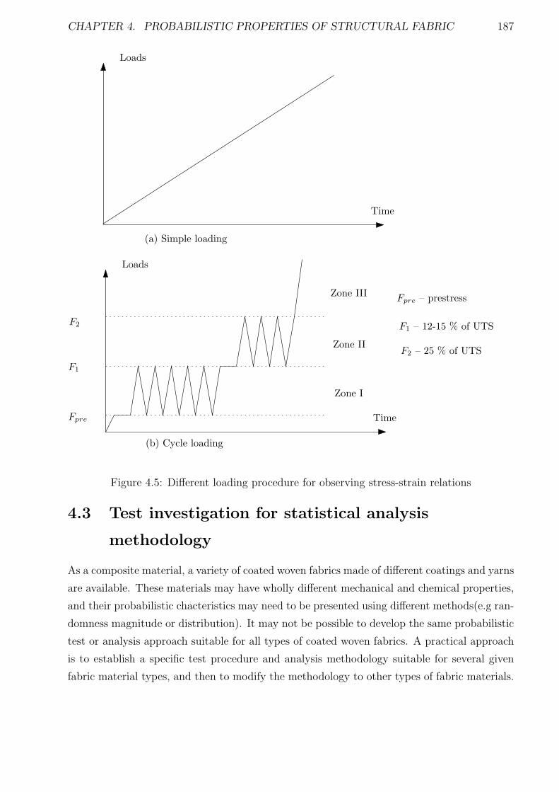
CHAPTER 4. PROBABILISTIC PROPERTIES OF STRUCTURAL FABRIC 187
Loads
F2
F1
Fpre Time
Zone I
Zone II
Zone IIIFpre – prestress
F1 – 12-15 % of UTS
F2 – 25 % of UTS
Loads
Time
(a) Simple loading
(b) Cycle loading
Figure 4.5: Different loading procedure for observing stress-strain relations
4.3 Test investigation for statistical analysis
methodology
As a composite material, a variety of coated woven fabrics made of different coatings and yarns
are available. These materials may have wholly different mechanical and chemical properties,
and their probabilistic chacteristics may need to be presented using different methods(e.g ran-
domness magnitude or distribution). It may not be possible to develop the same probabilistic
test or analysis approach suitable for all types of coated woven fabrics. A practical approach
is to establish a specific test procedure and analysis methodology suitable for several given
fabric material types, and then to modify the methodology to other types of fabric materials.
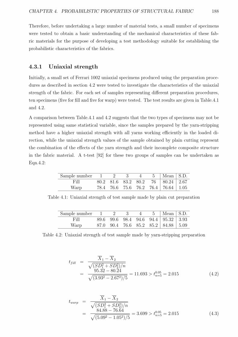
CHAPTER 4. PROBABILISTIC PROPERTIES OF STRUCTURAL FABRIC 188
Therefore, before undertaking a large number of material tests, a small number of specimens
were tested to obtain a basic understanding of the mechanical characteristics of these fab-
ric materials for the purpose of developing a test methodology suitable for establishing the
probabilistic characteristics of the fabrics.
4.3.1 Uniaxial strength
Initially, a small set of Ferrari 1002 uniaxial specimens produced using the preparation proce-
dures as described in section 4.2 were tested to investigate the characteristics of the uniaxial
strength of the fabric. For each set of samples representing different preparation procedures,
ten specimens (five for fill and five for warp) were tested. The test results are given in Table.4.1
and 4.2.
A comparison between Table.4.1 and 4.2 suggests that the two types of specimens may not be
represented using same statistical variable, since the samples prepared by the yarn-stripping
method have a higher uniaxial strength with all yarns working efficiently in the loaded di-
rection, while the uniaxial strength values of the sample obtained by plain cutting represent
the combination of the effects of the yarn strength and their incomplete composite structure
in the fabric material. A t-test [92] for these two groups of samples can be undertaken as
Eqn.4.2:
Sample number 1 2 3 4 5 Mean S.D.Fill 80.2 81.6 83.2 80.2 76 80.24 2.67
Warp 78.4 76.6 75.6 76.2 76.4 76.64 1.05
Table 4.1: Uniaxial strength of test sample made by plain cut preparation
Sample number 1 2 3 4 5 Mean S.D.Fill 89.6 99.6 98.4 94.6 94.4 95.32 3.93
Warp 87.0 90.4 76.6 85.2 85.2 84.88 5.09
Table 4.2: Uniaxial strength of test sample made by yarn-stripping preparation
tfill =X1 −X2
√
(SD21 + SD2
2)/n
=95.32 − 80.24
√
(3.932 − 2.672)/5= 11.693 > t0.05
n=5 = 2.015 (4.2)
twarp =X1 −X2
√
(SD21 + SD2
2)/n
=84.88 − 76.64
√
(5.092 − 1.052)/5= 3.699 > t0.05
n=5 = 2.015 (4.3)
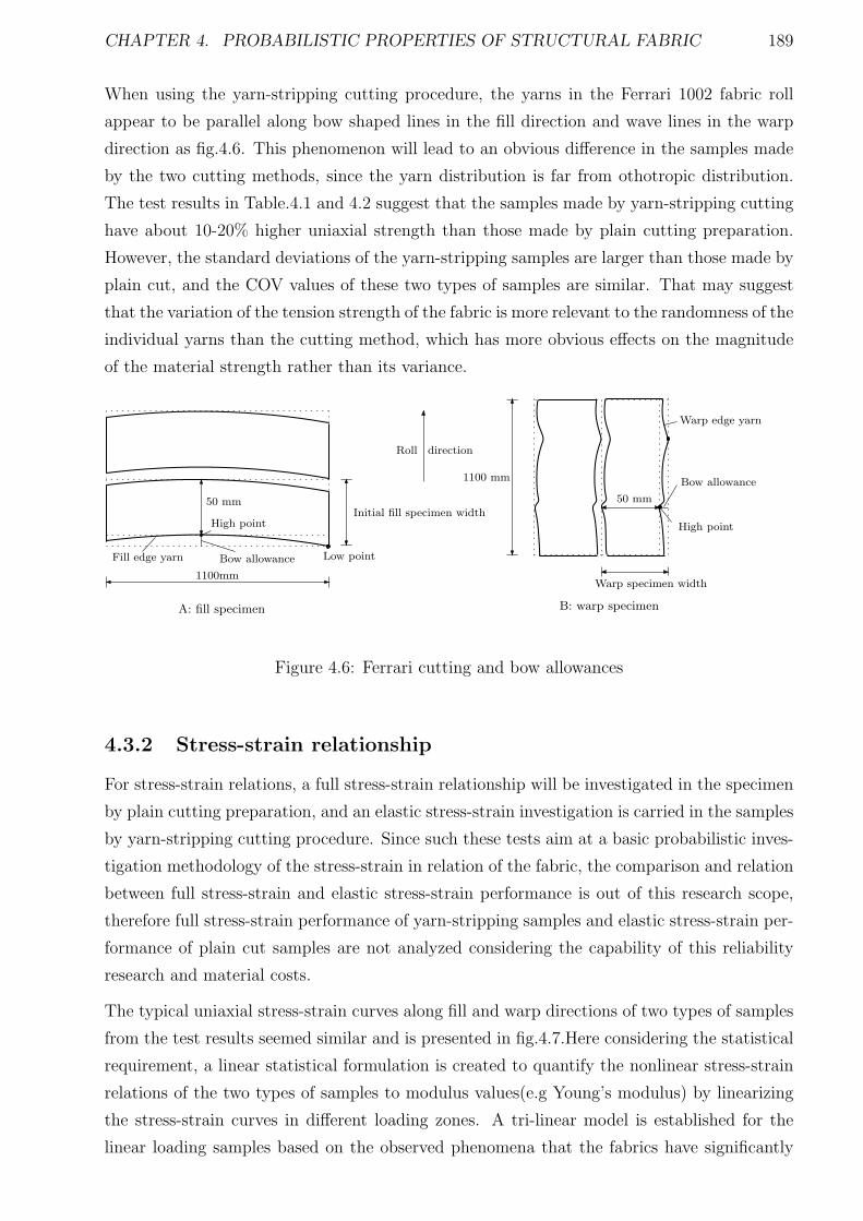
CHAPTER 4. PROBABILISTIC PROPERTIES OF STRUCTURAL FABRIC 189
When using the yarn-stripping cutting procedure, the yarns in the Ferrari 1002 fabric roll
appear to be parallel along bow shaped lines in the fill direction and wave lines in the warp
direction as fig.4.6. This phenomenon will lead to an obvious difference in the samples made
by the two cutting methods, since the yarn distribution is far from othotropic distribution.
The test results in Table.4.1 and 4.2 suggest that the samples made by yarn-stripping cutting
have about 10-20% higher uniaxial strength than those made by plain cutting preparation.
However, the standard deviations of the yarn-stripping samples are larger than those made by
plain cut, and the COV values of these two types of samples are similar. That may suggest
that the variation of the tension strength of the fabric is more relevant to the randomness of the
individual yarns than the cutting method, which has more obvious effects on the magnitude
of the material strength rather than its variance.
1100mm
50 mm
High pointInitial fill specimen width
Fill edge yarn Bow allowance
Roll direction
Low point
50 mm
1100 mm Bow allowance
High point
Warp edge yarn
Warp specimen width
A: fill specimen B: warp specimen
Figure 4.6: Ferrari cutting and bow allowances
4.3.2 Stress-strain relationship
For stress-strain relations, a full stress-strain relationship will be investigated in the specimen
by plain cutting preparation, and an elastic stress-strain investigation is carried in the samples
by yarn-stripping cutting procedure. Since such these tests aim at a basic probabilistic inves-
tigation methodology of the stress-strain in relation of the fabric, the comparison and relation
between full stress-strain and elastic stress-strain performance is out of this research scope,
therefore full stress-strain performance of yarn-stripping samples and elastic stress-strain per-
formance of plain cut samples are not analyzed considering the capability of this reliability
research and material costs.
The typical uniaxial stress-strain curves along fill and warp directions of two types of samples
from the test results seemed similar and is presented in fig.4.7.Here considering the statistical
requirement, a linear statistical formulation is created to quantify the nonlinear stress-strain
relations of the two types of samples to modulus values(e.g Young’s modulus) by linearizing
the stress-strain curves in different loading zones. A tri-linear model is established for the
linear loading samples based on the observed phenomena that the fabrics have significantly
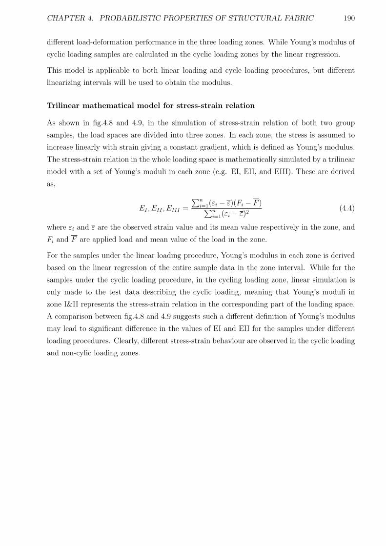
CHAPTER 4. PROBABILISTIC PROPERTIES OF STRUCTURAL FABRIC 190
different load-deformation performance in the three loading zones. While Young’s modulus of
cyclic loading samples are calculated in the cyclic loading zones by the linear regression.
This model is applicable to both linear loading and cycle loading procedures, but different
linearizing intervals will be used to obtain the modulus.
Trilinear mathematical model for stress-strain relation
As shown in fig.4.8 and 4.9, in the simulation of stress-strain relation of both two group
samples, the load spaces are divided into three zones. In each zone, the stress is assumed to
increase linearly with strain giving a constant gradient, which is defined as Young’s modulus.
The stress-strain relation in the whole loading space is mathematically simulated by a trilinear
model with a set of Young’s moduli in each zone (e.g. EI, EII, and EIII). These are derived
as,
EI , EII , EIII =
∑ni=1(εi − ε)(Fi − F )∑n
i=1(εi − ε)2(4.4)
where εi and ε are the observed strain value and its mean value respectively in the zone, and
Fi and F are applied load and mean value of the load in the zone.
For the samples under the linear loading procedure, Young’s modulus in each zone is derived
based on the linear regression of the entire sample data in the zone interval. While for the
samples under the cyclic loading procedure, in the cycling loading zone, linear simulation is
only made to the test data describing the cyclic loading, meaning that Young’s moduli in
zone I&II represents the stress-strain relation in the corresponding part of the loading space.
A comparison between fig.4.8 and 4.9 suggests such a different definition of Young’s modulus
may lead to significant difference in the values of EI and EII for the samples under different
loading procedures. Clearly, different stress-strain behaviour are observed in the cyclic loading
and non-cylic loading zones.
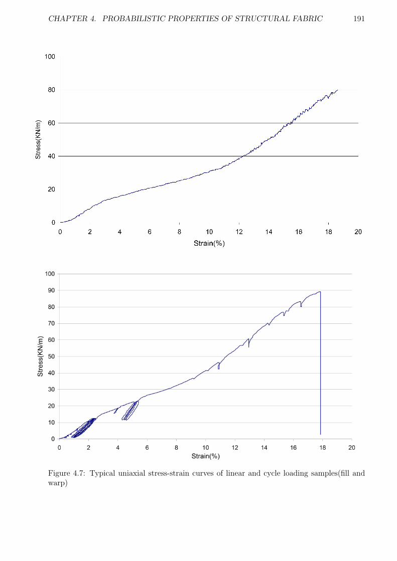
CHAPTER 4. PROBABILISTIC PROPERTIES OF STRUCTURAL FABRIC 191
Figure 4.7: Typical uniaxial stress-strain curves of linear and cycle loading samples(fill andwarp)
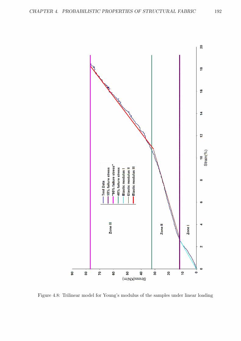
CHAPTER 4. PROBABILISTIC PROPERTIES OF STRUCTURAL FABRIC 192
Figure 4.8: Trilinear model for Young’s modulus of the samples under linear loading
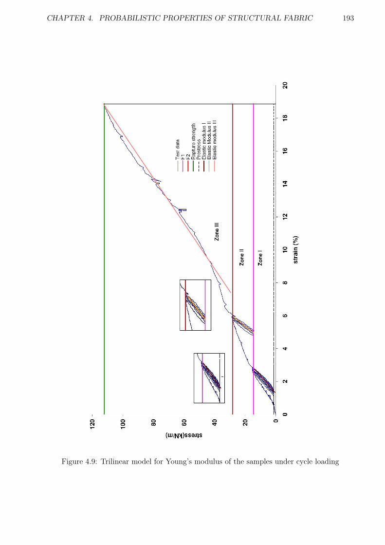
CHAPTER 4. PROBABILISTIC PROPERTIES OF STRUCTURAL FABRIC 193
Figure 4.9: Trilinear model for Young’s modulus of the samples under cycle loading
CHAPTER 4. PROBABILISTIC PROPERTIES OF STRUCTURAL FABRIC 194
4.4 Statistical investigation methodology
Accurate probabilistic properties of the fabric material cannot be identified by just a few tests.
Normally it requires a comparatively large quantity of experiments, and the feasible quantity
size will also depend on the available resource and time. After hundreds of the test data
have been obtained either directly from the measuring equipment or the trilinear regression
models, the variations of these data can be analyzed through a statistical investigation, and
the probabilistic properties of the mechanical behaviours of the fabric materials can be also
identified and summarized with neat statistical descriptions.
4.4.1 General statistical investigation principal
When a random physical quantity is of concern, the possible outcomes are usually a range of
measured or observed values, and some of these values may occur more frequently than others.
To quantify a random variable, the systematic mathematical modelling or representation of
the data is required. Generally, the essential steps to quantify a random variable are:
1 Data collection and modelling – Collect the available relevant information from the
published test or experiments and evaluate the statistical information of interest using
mathematical modelling.
2 Description of randomness – Describe the value variation and shape of random variables
mathematically and graphically.
3 Determination of distributions and parameters – Select a particular distribution for a
random variable and estimate its parameters to describe its randomness.
4.4.2 Description of randomness
In deterministic fabric design and analysis, average or mean values of test samples are nor-
mally applied to represent levels and strengths of fabric material. The mean value alone does
not provide complete random information, and the dispersion of the values with respect to the
mean is necessary to be represented mathematically in terms of variance, standard deviation,
or coefficient of variation. Suppose Xs is a random variable and n observations of Xs are
available. The mean or expected value of Xs, a measure of central tendency in the data, also
known as the first central moment and denoted as E(Xs) or µXs, can be calculated for n
observations xsi as
Mean = E(Xs) = µXs =1
n
n∑
i=1
xsi (4.5)
The variance of Xs, a measure of spread in the data about the mean, also known as the second
central moment and denoted as Var(Xs), can be estimated as
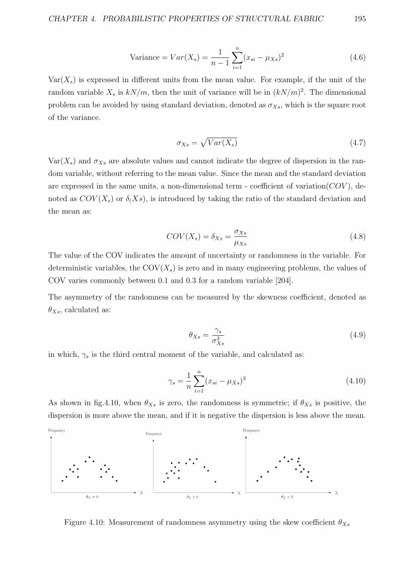
CHAPTER 4. PROBABILISTIC PROPERTIES OF STRUCTURAL FABRIC 195
Variance = V ar(Xs) =1
n− 1
n∑
i=1
(xsi − µXs)2 (4.6)
Var(Xs) is expressed in different units from the mean value. For example, if the unit of the
random variable Xs is kN/m, then the unit of variance will be in (kN/m)2. The dimensional
problem can be avoided by using standard deviation, denoted as σXs, which is the square root
of the variance.
σXs =√
V ar(Xs) (4.7)
Var(Xs) and σXs are absolute values and cannot indicate the degree of dispersion in the ran-
dom variable, without referring to the mean value. Since the mean and the standard deviation
are expressed in the same units, a non-dimensional term - coefficient of variation(COV ), de-
noted as COV (Xs) or δ(Xs), is introduced by taking the ratio of the standard deviation and
the mean as:
COV (Xs) = δXs =σXs
µXs
(4.8)
The value of the COV indicates the amount of uncertainty or randomness in the variable. For
deterministic variables, the COV(Xs) is zero and in many engineering problems, the values of
COV varies commonly between 0.1 and 0.3 for a random variable [204].
The asymmetry of the randomness can be measured by the skewness coefficient, denoted as
θXs, calculated as:
θXs =γs
σ3Xs
(4.9)
in which, γs is the third central moment of the variable, and calculated as:
γs =1
n
n∑
i=1
(xsi − µXs)3 (4.10)
As shown in fig.4.10, when θXs is zero, the randomness is symmetric; if θXs is positive, the
dispersion is more above the mean, and if it is negative the dispersion is less above the mean.
X
Frequency
θX = 0X
Frequency
θX > 0X
Frequency
θX < 0
Figure 4.10: Measurement of randomness asymmetry using the skew coefficient θXs
CHAPTER 4. PROBABILISTIC PROPERTIES OF STRUCTURAL FABRIC 196
In the probabilistic theory, another statistical parameter is median which is defined as the
value to separate the population to two halves. The median of the population Xs(Xsi) has,
P (Xs(i) < median) ≤ 50%
P (Xs(i) > median) ≤ 50% (4.11)
For a finite sample group X with size n, and if there is Xs(1) < Xs(2) < · · · < Xs(n), then the
median can be calculated by,
median = Xs(n+12
), if n is odd
median = 0.5(Xs(n2) +Xs(n
2+1)), if n is even (4.12)
Besides the mathematical descriptions of the randomness introduced above, a more complete
description can be obtained by plotting the information graphically in the form of a histogram.
A histogram can be developed as the following procedure:
Step 1. Arrange the data in increasing order
Step 2. Subdivide the data into several equal intervals and count the number of observations in
each interval.
Step 3. Compute the sample frequency of each interval by taking the ratio of sample numbers
in each intervals and sample size.
Step 4. Plot the sample frequency in each interval versus the random variable, producing a
histogram indicating the randomness
The number of the intervals can be estimated empirically [205] as:
k = 1 + 3.3log10n (4.13)
where k is the number of intervals and n is the number of samples.
For example, suppose there are a series of random values of the fill strength as listed in Table.
4.3.

CHAPTER 4. PROBABILISTIC PROPERTIES OF STRUCTURAL FABRIC 197
Test no. Fill strength, σfult(kN/m) Test no. Fill strength, σf
ult(kN/m)1 81.6 17 83.62 83.2 18 81.03 76.0 19 80.64 83.6 20 86.25 81.2 21 73.86 84.0 22 84.47 80.2 23 86.48 71.6 24 83.09 78.2 25 81.610 83.4 26 87.011 85.4 27 77.612 84 28 80.213 83.6 29 79.014 84.2 30 80.015 74.4 31 78.616 77 32 83.2
Table 4.3: Example of fabric test data (n=32)
Then, the number of intervals k = 1 + 3.3log1032 = 5.97 ≈ 6. Considering the minimum
and maximum values of test data, and rounding them to 70 kN/m and 88 kN/m, we use six
intervals with a width of 3kN/m each as listed in Table. 4.4, to develop the histogram shown
in fig 4.11.
Interval(kN/m) No. of observations Sample frequency70-73 1 1/32=0.031373-76 2 0.062576-79 5 0.156379-82 9 0.281382-85 11 0.343885-88 4 0.1250
Table 4.4: Data for Histogram and Frequency Diagrams
The primary objective of a frequency diagram(histogram) is to model the pattern or behavior
of the randomness by fitting a curve to the diagram. A data-fitting test can then be made
both quantitatively and qualitatively to verify whether the fitted curve represents one of
many commonly used distributions, such as the normal and log-normal. The modelling of the
randomness of fabric mechanical behaviours will be discussed in section. 4.4.3.
The material test data presented in this PhD thesis is only a very small contribution to
the whole probabilistic analysis work, but more importantly, is an attempt to establish a
methodology to collect and present the probabilistic information of a given fabric material
through a set of material tests.
Based on the principle of the statistics, a larger quantity of test data is always desired. These
data may be assembled from different institutions and companies with different facilities and
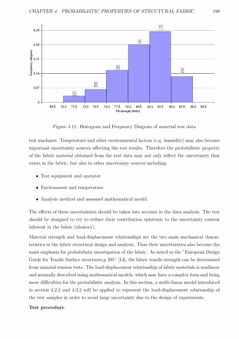
CHAPTER 4. PROBABILISTIC PROPERTIES OF STRUCTURAL FABRIC 198
Figure 4.11: Histogram and Frequency Diagram of material test data
test machines. Temperature and other environmental factors (e.g. humidity) may also become
important uncertainty sources affecting the test results. Therefore the probabilistic property
of the fabric material obtained from the test data may not only reflect the uncertainty that
exists in the fabric, but also in other uncertainty sources including:
• Test equipment and operator.
• Environment and temperature.
• Analysis method and assumed mathematical model.
The effects of these uncertainties should be taken into account in the data analysis. The test
should be designed to try to reduce their contribution epistemic to the uncertainty content
inherent in the fabric (aleatory).
Material strength and load-displacement relationships are the two main mechanical charac-
teristics in the fabric structural design and analysis. Thus their uncertainties also become the
main emphasis for probabilistic investigation of the fabric. As noted in the ”European Design
Guide for Tensile Surface structures,p 295” [13], the fabric tensile strength can be determined
from uniaxial tension tests. The load-displacement relationship of fabric materials is nonlinear
and normally described using mathematical models, which may have a complex form and bring
more difficulties for the probabilistic analysis. In this section, a multi-linear model introduced
in section 4.2.2 and 4.3.2 will be applied to represent the load-displacement relationship of
the test samples in order to avoid large uncertainty due to the design of experiments.
Test procedure
CHAPTER 4. PROBABILISTIC PROPERTIES OF STRUCTURAL FABRIC 199
The uncertainties of the fabric material: PVC-coated polyester Ferrari 1002 as described
in Table 4.5 is investigated through uniaxial tension tests. These tests are taken in three
individual periods with different quantities and temperatures as listed in Table 4.6.
Tested fabric type Mass density Strength (warp/fill)Ferrari PVC 1002 1050 g/m2 4.2/4.0 kN /5 cm
Table 4.5: Ferrari 1002 Manufacturer’s information of the test fabric material
Cutting method Loading procedure Fabric Type Quantity(warp/fill) TemperaturePlain Linear Ferrari PVC 1002 126/112 23
Yarn-stripping Cycle Ferrari PVC 1002 62/42 23
Table 4.6: Temperatures and quantities of the fabric test
The cutting procedure of plain cutting samples is illustrated in fig. 4.12. A 15 metre long
fabric roll was cut into uniaxial and biaxial test specimens. The uniaxial specimens along the
fill direction were mainly cut from the first four blocks while warp specimens, were distributed
along the whole roll length. While the yarn-stripping samples were cut from 1.8 × 4.0 m blocks
in the fabric roll as figure 4.13.
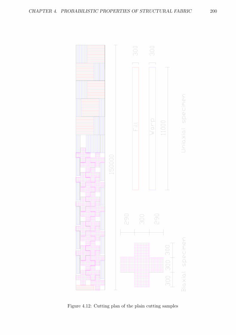
CHAPTER 4. PROBABILISTIC PROPERTIES OF STRUCTURAL FABRIC 200
Figure 4.12: Cutting plan of the plain cutting samples
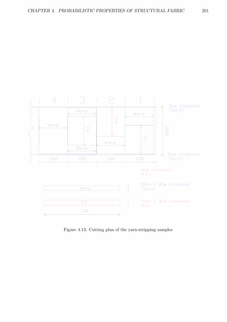
CHAPTER 4. PROBABILISTIC PROPERTIES OF STRUCTURAL FABRIC 201
Figure 4.13: Cutting plan of the yarn-stripping samples
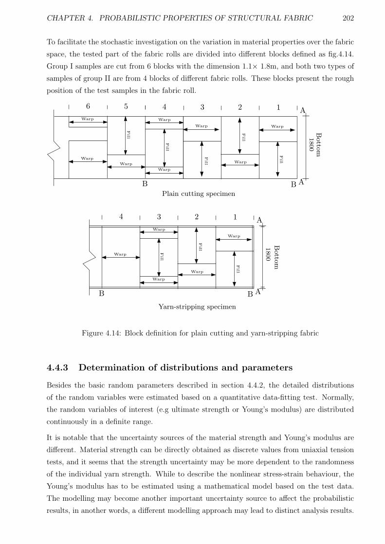
CHAPTER 4. PROBABILISTIC PROPERTIES OF STRUCTURAL FABRIC 202
To facilitate the stochastic investigation on the variation in material properties over the fabric
space, the tested part of the fabric rolls are divided into different blocks defined as fig.4.14.
Group I samples are cut from 6 blocks with the dimension 1.1× 1.8m, and both two types of
samples of group II are from 4 blocks of different fabric rolls. These blocks present the rough
position of the test samples in the fabric roll.
4 3 2 1
Warp
Warp
Warp
Warp
Warp
Fill
Fill
Fill
1800
A
AB B
4 3 2 1
Warp
Warp
Fill
Fill
1800
A
AB B
Warp
Warp
Warp
Fill
Warp
Warp
Fill
Warp
6 5B
otto
m
Botto
m
Plain cutting specimen
Yarn-stripping specimen
Fill
Figure 4.14: Block definition for plain cutting and yarn-stripping fabric
4.4.3 Determination of distributions and parameters
Besides the basic random parameters described in section 4.4.2, the detailed distributions
of the random variables were estimated based on a quantitative data-fitting test. Normally,
the random variables of interest (e.g ultimate strength or Young’s modulus) are distributed
continuously in a definite range.
It is notable that the uncertainty sources of the material strength and Young’s modulus are
different. Material strength can be directly obtained as discrete values from uniaxial tension
tests, and it seems that the strength uncertainty may be more dependent to the randomness
of the individual yarn strength. While to describe the nonlinear stress-strain behaviour, the
Young’s modulus has to be estimated using a mathematical model based on the test data.
The modelling may become another important uncertainty source to affect the probabilistic
results, in another words, a different modelling approach may lead to distinct analysis results.
CHAPTER 4. PROBABILISTIC PROPERTIES OF STRUCTURAL FABRIC 203
More complicated models may produce more accurate and detailed descriptions of stress-
strain relationships, but the quantification of this relationship is more difficult. Therefore the
randomness in the stress-strain relationship of coated woven fabric may be more complex than
the strength, with uncertainties combining from the yarns and the weaving composition.
4.4.4 Candidate distributions and the parameter estimation
The initial candidate distributions for the material statistical analysis include:
1 Normal Distribution
2 Log-normal Distribution
3 Exponential Distribution
4 Gumbel Distribution
5 Frenchet Distribution
6 Weibull Distribution
7 Laplace Distribution
8 Rectangular Distribution
9 Pareto Distribution
10 Rayleigh Distribution
Fundamental descriptions of these distributions are given as in Appendix.A:
4.4.5 Goodness-of-fit tests
After the parameters of the assumed candidate distribution are determined based on the
general shape of the histogram, the validity of the assumed distribution needs to be verified
statistically by goodness-of-fit tests. There are two such tests, which are generally used to
check the validity of the assumed distributions, based on the general shape of the histogram
: Chi-square and the Kolmogorov-Smirnov method.
Chi-square test
For a sample of n observed values of a random variable, the Chi-square test verifies the
goodness-of-fit between the sample data and the assumed theoretical distribution by compar-
ing the observed frequencies n1, n2, · · · , nk of k values(or in k intervals) with the frequencies
e1, e2, · · · , e3 from the distribution. The judgment will be made based on the value of the
function of ni and ei,
CHAPTER 4. PROBABILISTIC PROPERTIES OF STRUCTURAL FABRIC 204
k∑
i=1
(ni − ei)2
ei
which follows the chi-square (χ2f ) distribution with (f = k− 1) degrees of freedom as n→ ∞
for a pre-defined distribution. When the parameters of the assumed distribution are estimated
from sample data, such a statement will be valid with (f = k− 1− s), where s is the number
of unknown parameters to be estimated.
On this basis, if an assumed distribution satisfies
k∑
i=1
(ni − ei)2
ei)< c1−α,f
where c1−α,f is the value of the appropriate χ2f distribution at the cumulative probability
(1 − α), the assumed theoretical distribution is an acceptable model, at the significance level
α. Otherwise, the assumed distribution is not substantiated by the data at the α significant
level.
In applying the χ2 test for goodness of fit,it is generally necessary(for satisfactory results) to
have k ≥ 5 and ei ≥ 5.
Kolmogorov-Smirnov test
The Kolmogorov-Smirnov(K-S) test is a widely used goodness-of-fit test, in which, the com-
parison is made between the cumulative frequencies of the experimental sample data and
the assumed theoretical distribution model. The theoretical model is only acceptable if the
discrepancy is small with respect to what is normally expected from a given sample size.
For a sample of size n, rearranging the sample data in increasing magnitude to obtain a
ordered sample data, which has xs(i) ≤ xs(i+1), a stepwise cumulative frequency function is
then developed as,
Sn(x) =
0 x < xs(1)
kn
xs(k) ≤ x < xs(k+1)
1 x ≥ xs(n)
where xs(1), xs(2), · · · , xs(n) denote values of the ordered sample data, and n is the sample size.
In the K-S test, the maximum difference between Sn(Xs) and F (Xs) over the entire range of
Xs is the measure of discrepancy between the theoretical model and the observed data. The
maximum difference can be written as:
Dn = max|F (xs) − Sn(xs)|
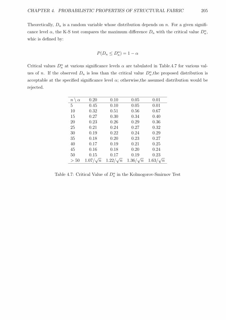
CHAPTER 4. PROBABILISTIC PROPERTIES OF STRUCTURAL FABRIC 205
Theoretically, Dn is a random variable whose distribution depends on n. For a given signifi-
cance level α, the K-S test compares the maximum difference Dn with the critical value Dαn ,
whic is defined by:
P (Dn ≤ Dαn) = 1 − α
Critical values Dαn at various significance levels α are tabulated in Table.4.7 for various val-
ues of n. If the observed Dn is less than the critical value Dαn ,the proposed distribution is
acceptable at the specified significance level α; otherwise,the assumed distribution would be
rejected.
n \ α 0.20 0.10 0.05 0.015 0.45 0.10 0.05 0.0110 0.32 0.51 0.56 0.6715 0.27 0.30 0.34 0.4020 0.23 0.26 0.29 0.3625 0.21 0.24 0.27 0.3230 0.19 0.22 0.24 0.2935 0.18 0.20 0.23 0.2740 0.17 0.19 0.21 0.2545 0.16 0.18 0.20 0.2450 0.15 0.17 0.19 0.23> 50 1.07/
√n 1.22/
√n 1.36/
√n 1.63/
√n
Table 4.7: Critical Value of Dαn in the Kolmogorov-Smirnov Test
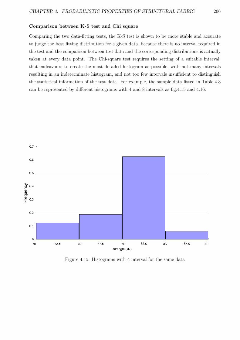
CHAPTER 4. PROBABILISTIC PROPERTIES OF STRUCTURAL FABRIC 206
Comparison between K-S test and Chi square
Comparing the two data-fitting tests, the K-S test is shown to be more stable and accurate
to judge the best fitting distribution for a given data, because there is no interval required in
the test and the comparison between test data and the corresponding distributions is actually
taken at every data point. The Chi-square test requires the setting of a suitable interval,
that endeavours to create the most detailed histogram as possible, with not many intervals
resulting in an indeterminate histogram, and not too few intervals insufficient to distinguish
the statistical information of the test data. For example, the sample data listed in Table.4.3
can be represented by different histograms with 4 and 8 intervals as fig.4.15 and 4.16.
Figure 4.15: Histograms with 4 interval for the same data
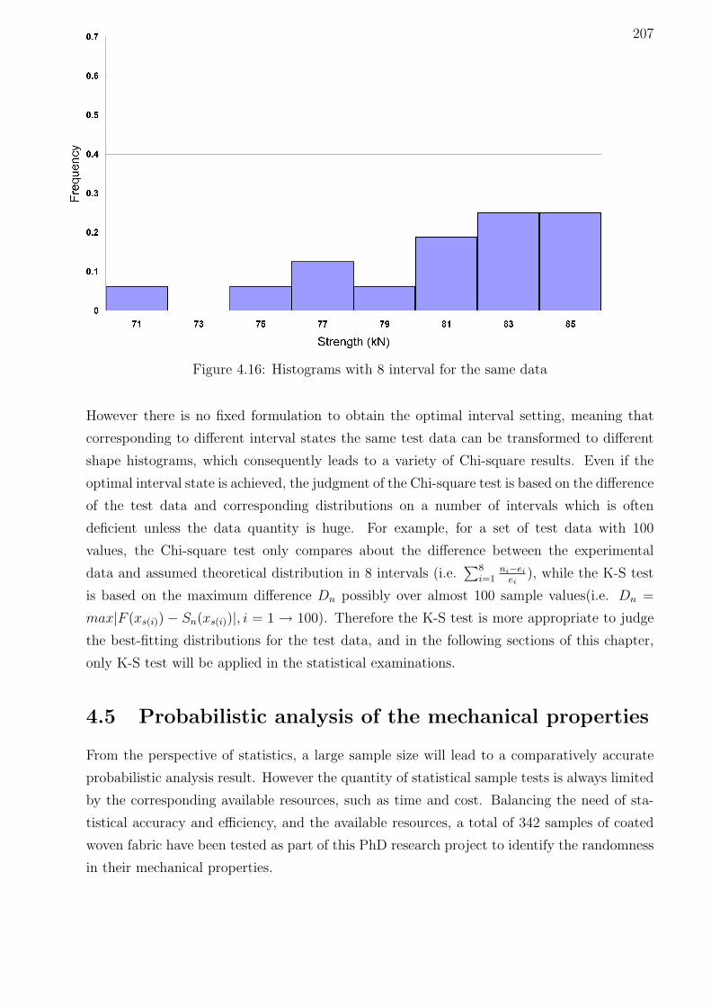
CHAPTER 4. PROBABILISTIC PROPERTIES OF STRUCTURAL FABRIC 207
Figure 4.16: Histograms with 8 interval for the same data
However there is no fixed formulation to obtain the optimal interval setting, meaning that
corresponding to different interval states the same test data can be transformed to different
shape histograms, which consequently leads to a variety of Chi-square results. Even if the
optimal interval state is achieved, the judgment of the Chi-square test is based on the difference
of the test data and corresponding distributions on a number of intervals which is often
deficient unless the data quantity is huge. For example, for a set of test data with 100
values, the Chi-square test only compares about the difference between the experimental
data and assumed theoretical distribution in 8 intervals (i.e.∑8
i=1ni−ei
ei), while the K-S test
is based on the maximum difference Dn possibly over almost 100 sample values(i.e. Dn =
max|F (xs(i)) − Sn(xs(i))|, i = 1 → 100). Therefore the K-S test is more appropriate to judge
the best-fitting distributions for the test data, and in the following sections of this chapter,
only K-S test will be applied in the statistical examinations.
4.5 Probabilistic analysis of the mechanical properties
From the perspective of statistics, a large sample size will lead to a comparatively accurate
probabilistic analysis result. However the quantity of statistical sample tests is always limited
by the corresponding available resources, such as time and cost. Balancing the need of sta-
tistical accuracy and efficiency, and the available resources, a total of 342 samples of coated
woven fabric have been tested as part of this PhD research project to identify the randomness
in their mechanical properties.
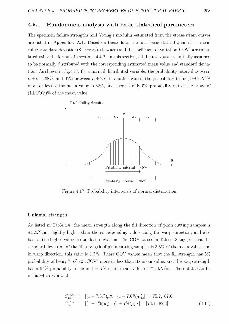
CHAPTER 4. PROBABILISTIC PROPERTIES OF STRUCTURAL FABRIC 208
4.5.1 Randomness analysis with basic statistical parameters
The specimen failure strengths and Young’s modulus estimated from the stress-strain curves
are listed in Appendix. A.1. Based on these data, the four basic statical quantities: mean
value, standard deviation(S.D or σs), skewness and the coefficient of variation(COV) are calcu-
lated using the formula in section. 4.4.2. In this section, all the test data are initially assumed
to be normally distributed with the corresponding estimated mean value and standard devia-
tion. As shown in fig.4.17, for a normal distributed variable, the probability interval between
µ± σ is 68%, and 95% between µ± 2σ. In another words, the probability to be (1±COV)%
more or less of the mean value is 32%, and there is only 5% probability out of the range of
(1±COV)% of the mean value.
X
µσsσs σs
σs
Prbability interval = 68%
Prbability interval = 95%
Probability density
Figure 4.17: Probability interverals of normal distribution
Uniaxial strength
As listed in Table.4.8, the mean strength along the fill direction of plain cutting samples is
81.2kN/m, slightly higher than the corresponding value along the warp direction, and also
has a little higher value in standard deviation. The COV values in Table.4.8 suggest that the
standard deviation of the fill strength of plain cutting samples is 3.8% of the mean value, and
in warp direction, this ratio is 3.5%. These COV values mean that the fill strength has 5%
probability of being 7.6% (2×COV) more or less than its mean value, and the warp strength
has a 95% probability to be in 1 ± 7% of its mean value of 77.3kN/m. These data can be
included as Eqn.4.14,
S0.95fs = [(1 − 7.6%)µL
fs, (1 + 7.6%)µLfs] = [75.2, 87.6]
S0.95ws = [(1 − 7%)µL
ws, (1 + 7%)µLws] = [73.1, 82.3] (4.14)
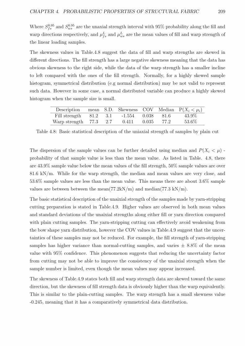
CHAPTER 4. PROBABILISTIC PROPERTIES OF STRUCTURAL FABRIC 209
Where S0.95fs and S0.95
ws are the unaxial strength interval with 95% probability along the fill and
warp directions respectively, and µLfs and µL
ws are the mean values of fill and warp strength of
the linear loading samples.
The skewness values in Table.4.8 suggest the data of fill and warp strengths are skewed in
different directions. The fill strength has a large negative skewness meaning that the data has
obvious skewness to the right side, while the data of the warp strength has a smaller incline
to left compared with the ones of the fill strength. Normally, for a highly skewed sample
histogram, symmetrical distribution (e.g normal distribution) may be not valid to represent
such data. However in some case, a normal distributed variable can produce a highly skewed
histogram when the sample size is small.
Description mean S.D. Skewness COV Median P(Xi < µi)Fill strength 81.2 3.1 -1.554 0.038 81.6 43.9%
Warp strength 77.3 2.7 0.411 0.035 77.2 53.6%
Table 4.8: Basic statistical description of the uniaxial strength of samples by plain cut
The dispersion of the sample values can be further detailed using median and P (Xi < µ) -
probability of that sample value is less than the mean value. As listed in Table. 4.8, there
are 43.9% sample value below the mean values of the fill strength, 50% sample values are over
81.6 kN/m. While for the warp strength, the median and mean values are very close, and
53.6% sample values are less than the mean value. This means there are about 3.6% sample
values are between between the mean(77.2kN/m) and median(77.3 kN/m).
The basic statistical description of the unaixial strength of the samples made by yarn-stripping
cutting preparation is stated in Table.4.9. Higher values are observed in both mean values
and standard deviations of the unaixial strengths along either fill or yarn direction compared
with plain cutting samples. The yarn-stripping cutting can effectively avoid weakening from
the bow shape yarn distribution, however the COV values in Table.4.9 suggest that the uncer-
tainties of these samples may not be reduced. For example, the fill strength of yarn-stripping
samples has higher variance than normal-cutting samples, and varies ± 8.8% of the mean
value with 95% confidence. This phenomenon suggests that reducing the uncertainty factor
from cutting may not be able to improve the consistency of the unaixial strength when the
sample number is limited, even though the mean values may appear increased.
The skewness of Table.4.9 states both fill and warp strength data are skewed toward the same
direction, but the skewness of fill strength data is obviously higher than the warp equivalently.
This is similar to the plain-cutting samples. The warp strength has a small skewness value
-0.245, meaning that it has a comparatively symmetrical data distribution.
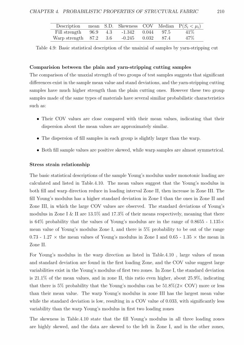
CHAPTER 4. PROBABILISTIC PROPERTIES OF STRUCTURAL FABRIC 210
Description mean S.D. Skewness COV Median P(Si < µi)Fill strength 96.9 4.3 -1.342 0.044 97.5 41%
Warp strength 87.2 3.6 -0.245 0.032 87.4 47%
Table 4.9: Basic statistical description of the unaixial of samples by yarn-stripping cut
Comparision between the plain and yarn-stripping cutting samples
The comparison of the unaxial strength of two groups of test samples suggests that significant
differences exist in the sample mean value and stand deviations, and the yarn-stripping cutting
samples have much higher strength than the plain cutting ones. However these two group
samples made of the same types of materials have several similiar probabilistic characteristics
such as:
• Their COV values are close compared with their mean values, indicating that their
dispersion about the mean values are approximately similar.
• The dispersion of fill samples in each group is slightly larger than the warp.
• Both fill sample values are positive skewed, while warp samples are almost symmetrical.
Stress strain relationship
The basic statistical descriptions of the sample Young’s modulus under monotonic loading are
calculated and listed in Table.4.10. The mean values suggest that the Young’s modulus in
both fill and warp direction reduce in loading interval Zone II, then increase in Zone III. The
fill Young’s modulus has a higher standard deviation in Zone I than the ones in Zone II and
Zone III, in which the large COV values are observed. The standard deviations of Young’s
modulus in Zone I & II are 13.5% and 17.3% of their means respectively, meaning that there
is 64% probability that the values of Young’s modulus are in the range of 0.8655 - 1.135×mean value of Young’s modulus Zone I, and there is 5% probability to be out of the range
0.73 - 1.27 × the mean values of Young’s modulus in Zone I and 0.65 - 1.35 × the mean in
Zone II.
For Young’s modulus in the warp direction as listed in Table.4.10 , large values of mean
and standard deviation are found in the first loading Zone, and the COV value suggest large
variabilities exist in the Young’s modulus of first two zones. In Zone I, the standard deviation
is 21.1% of the mean values, and in zone II, this ratio even higher, about 25.9%, indicating
that there is 5% probability that the Young’s modulus can be 51.8%(2× COV) more or less
than their mean value. The warp Young’s modulus in zone III has the largest mean value
while the standard deviation is low, resulting in a COV value of 0.033, with significantly less
variability than the warp Young’s modulus in first two loading zones
The skewness in Table.4.10 state that the fill Young’s modulus in all three loading zones
are highly skewed, and the data are skewed to the left in Zone I, and in the other zones,
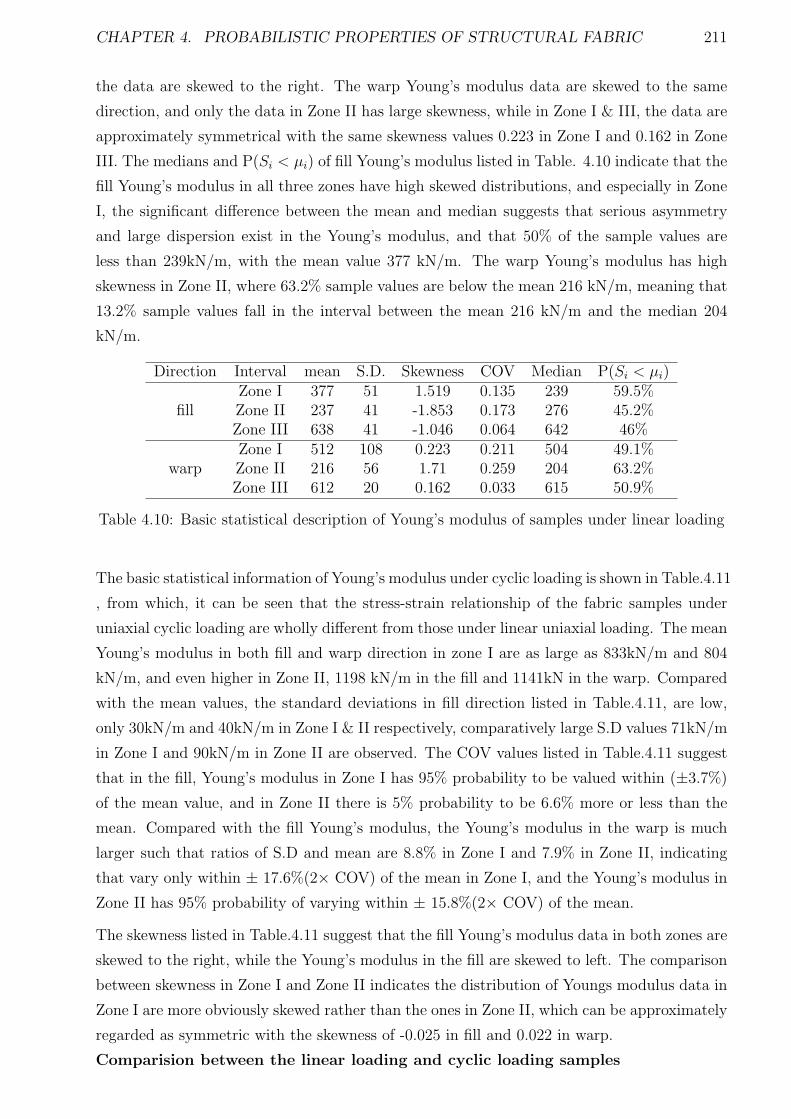
CHAPTER 4. PROBABILISTIC PROPERTIES OF STRUCTURAL FABRIC 211
the data are skewed to the right. The warp Young’s modulus data are skewed to the same
direction, and only the data in Zone II has large skewness, while in Zone I & III, the data are
approximately symmetrical with the same skewness values 0.223 in Zone I and 0.162 in Zone
III. The medians and P(Si < µi) of fill Young’s modulus listed in Table. 4.10 indicate that the
fill Young’s modulus in all three zones have high skewed distributions, and especially in Zone
I, the significant difference between the mean and median suggests that serious asymmetry
and large dispersion exist in the Young’s modulus, and that 50% of the sample values are
less than 239kN/m, with the mean value 377 kN/m. The warp Young’s modulus has high
skewness in Zone II, where 63.2% sample values are below the mean 216 kN/m, meaning that
13.2% sample values fall in the interval between the mean 216 kN/m and the median 204
kN/m.
Direction Interval mean S.D. Skewness COV Median P(Si < µi)Zone I 377 51 1.519 0.135 239 59.5%
fill Zone II 237 41 -1.853 0.173 276 45.2%Zone III 638 41 -1.046 0.064 642 46%Zone I 512 108 0.223 0.211 504 49.1%
warp Zone II 216 56 1.71 0.259 204 63.2%Zone III 612 20 0.162 0.033 615 50.9%
Table 4.10: Basic statistical description of Young’s modulus of samples under linear loading
The basic statistical information of Young’s modulus under cyclic loading is shown in Table.4.11
, from which, it can be seen that the stress-strain relationship of the fabric samples under
uniaxial cyclic loading are wholly different from those under linear uniaxial loading. The mean
Young’s modulus in both fill and warp direction in zone I are as large as 833kN/m and 804
kN/m, and even higher in Zone II, 1198 kN/m in the fill and 1141kN in the warp. Compared
with the mean values, the standard deviations in fill direction listed in Table.4.11, are low,
only 30kN/m and 40kN/m in Zone I & II respectively, comparatively large S.D values 71kN/m
in Zone I and 90kN/m in Zone II are observed. The COV values listed in Table.4.11 suggest
that in the fill, Young’s modulus in Zone I has 95% probability to be valued within (±3.7%)
of the mean value, and in Zone II there is 5% probability to be 6.6% more or less than the
mean. Compared with the fill Young’s modulus, the Young’s modulus in the warp is much
larger such that ratios of S.D and mean are 8.8% in Zone I and 7.9% in Zone II, indicating
that vary only within ± 17.6%(2× COV) of the mean in Zone I, and the Young’s modulus in
Zone II has 95% probability of varying within ± 15.8%(2× COV) of the mean.
The skewness listed in Table.4.11 suggest that the fill Young’s modulus data in both zones are
skewed to the right, while the Young’s modulus in the fill are skewed to left. The comparison
between skewness in Zone I and Zone II indicates the distribution of Youngs modulus data in
Zone I are more obviously skewed rather than the ones in Zone II, which can be approximately
regarded as symmetric with the skewness of -0.025 in fill and 0.022 in warp.
Comparision between the linear loading and cyclic loading samples
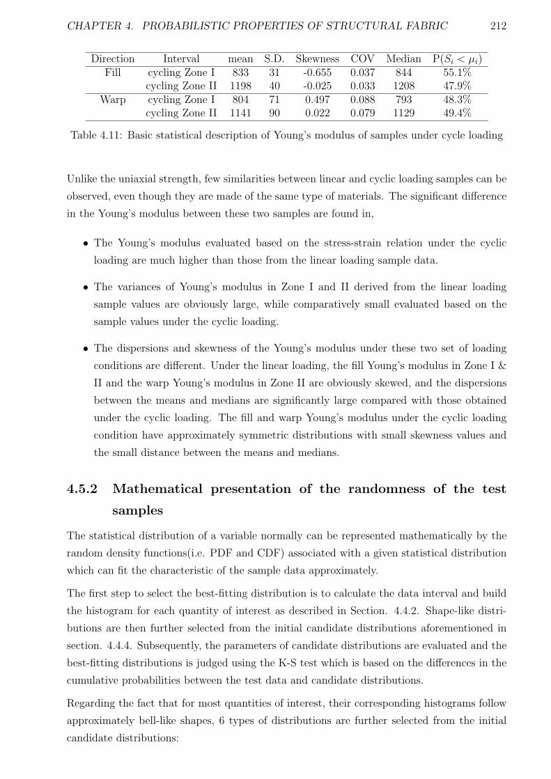
CHAPTER 4. PROBABILISTIC PROPERTIES OF STRUCTURAL FABRIC 212
Direction Interval mean S.D. Skewness COV Median P(Si < µi)Fill cycling Zone I 833 31 -0.655 0.037 844 55.1%
cycling Zone II 1198 40 -0.025 0.033 1208 47.9%Warp cycling Zone I 804 71 0.497 0.088 793 48.3%
cycling Zone II 1141 90 0.022 0.079 1129 49.4%
Table 4.11: Basic statistical description of Young’s modulus of samples under cycle loading
Unlike the uniaxial strength, few similarities between linear and cyclic loading samples can be
observed, even though they are made of the same type of materials. The significant difference
in the Young’s modulus between these two samples are found in,
• The Young’s modulus evaluated based on the stress-strain relation under the cyclic
loading are much higher than those from the linear loading sample data.
• The variances of Young’s modulus in Zone I and II derived from the linear loading
sample values are obviously large, while comparatively small evaluated based on the
sample values under the cyclic loading.
• The dispersions and skewness of the Young’s modulus under these two set of loading
conditions are different. Under the linear loading, the fill Young’s modulus in Zone I &
II and the warp Young’s modulus in Zone II are obviously skewed, and the dispersions
between the means and medians are significantly large compared with those obtained
under the cyclic loading. The fill and warp Young’s modulus under the cyclic loading
condition have approximately symmetric distributions with small skewness values and
the small distance between the means and medians.
4.5.2 Mathematical presentation of the randomness of the test
samples
The statistical distribution of a variable normally can be represented mathematically by the
random density functions(i.e. PDF and CDF) associated with a given statistical distribution
which can fit the characteristic of the sample data approximately.
The first step to select the best-fitting distribution is to calculate the data interval and build
the histogram for each quantity of interest as described in Section. 4.4.2. Shape-like distri-
butions are then further selected from the initial candidate distributions aforementioned in
section. 4.4.4. Subsequently, the parameters of candidate distributions are evaluated and the
best-fitting distributions is judged using the K-S test which is based on the differences in the
cumulative probabilities between the test data and candidate distributions.
Regarding the fact that for most quantities of interest, their corresponding histograms follow
approximately bell-like shapes, 6 types of distributions are further selected from the initial
candidate distributions:

CHAPTER 4. PROBABILISTIC PROPERTIES OF STRUCTURAL FABRIC 213
• Normal Distribution
• Log-normal Distribution
• Laplace Distribution
• Gumbel Distribution
• Frechet Distribution
• Weibull Distribution
The PDF and CDF of the distributions are commonly functions of two types of parameters:
location and shape. The PDF and CDF formulations of the candidate distributions are listed
in Table.4.12 with the corresponding parameters.
Distribution Parameters Random density function
Mean: µ PDF: f(x) = 1σ√
2πe−0.5(x−µ
σ)2
NormalStandard deviation: σ CDF:
∫ x
−∞1
σ√
2πe−0.5(x−µ
σ)2
PDF: f(x) = 1bx
√2πe−0.5( lnx−a
b)2
LogNormal Location: a, Shape: bCDF:
∫ x
−∞ f(x) = 1bx
√2πe−0.5( lnx−a
b)2
PDF: f(x) = 12bexp(− |a−x|
b)
Laplace Location: a, Shape: b CDF: F (x) = 12exp(−a−x
b), x < a
1 − 12exp(−x−a
b), x > a
PDF: f(x) = 1bexp[−x−a
b]exp[exp(−x−a
b)]
Gumbel Location: a, Shape: bCDF: F (x) = 1 − exp−exp[−x−a
b]
PDF: f(x) = −ab(a
x)bexp[−(a
x)b]
Frechet Location: a, Shape: bCDF: F (x) = 1 − exp[−(a
x)b]
PDF: f(x) = bc(x−a
c)b−1exp[−(x−a
c)]b
Weibull Location: a, Shape: b, cCDF: F (x) = 1 − exp[−(x−a
c)b]
Table 4.12: The PDF and CDF functions of location and shape parameters.
Subsequently, for each statistical variable (e.g fill strength), these parameters are estimated
based on the following descriptions,
Normal distribution
µ =
∑ni=1Xi
n
σs =1
n
n∑
i=1
(Xi − µ)2 (4.15)
Log-Normal distribution
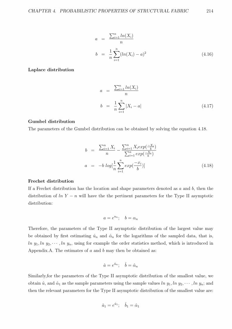
CHAPTER 4. PROBABILISTIC PROPERTIES OF STRUCTURAL FABRIC 214
a =
∑ni=1 ln(Xi)
n
b =1
n
n∑
i=1
(ln(Xi) − a)2 (4.16)
Laplace distribution
a =
∑ni=1 ln(Xi)
n
b =1
n
n∑
i=1
|Xi − a| (4.17)
Gumbel distribution
The parameters of the Gumbel distribution can be obtained by solving the equation 4.18.
b =
∑ni=1Xi
n−∑n
i=1Xiexp(−Xi
b)
∑ni=1 exp(
−Xi
b)
a = −b log[ 1n
n∑
i=1
exp(−xi
b)] (4.18)
Frechet distribution
If a Frechet distribution has the location and shape parameters denoted as a and b, then the
distribution of ln Y − n will have the the pertinent parameters for the Type II asymptotic
distribution:
a = eun ; b = αn
Therefore, the parameters of the Type II asymptotic distribution of the largest value may
be obtained by first estimating un and αn for the logarithms of the sampled data, that is,
ln y1, ln y2, · · · , ln yn, using for example the order statistics method, which is introduced in
Appendix.A. The estimates of a and b may then be obtained as:
a = eun ; b = αn
Similarly,for the parameters of the Type II asymptotic distribution of the smallest value, we
obtain u, and α1 as the sample parameters using the sample values ln y1, ln y2, · · · , ln yn; and
then the relevant parameters for the Type II asymptotic distribution of the smallest value are:
a1 = eu1 ; b1 = α1
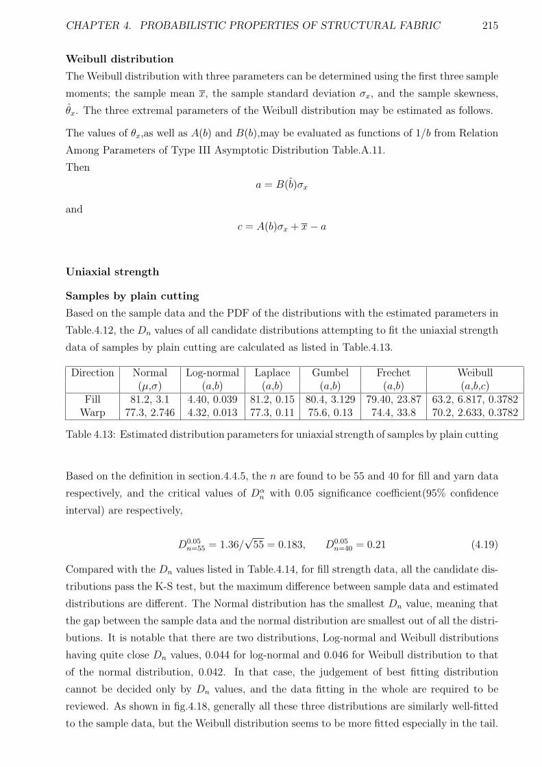
CHAPTER 4. PROBABILISTIC PROPERTIES OF STRUCTURAL FABRIC 215
Weibull distribution
The Weibull distribution with three parameters can be determined using the first three sample
moments; the sample mean x, the sample standard deviation σx, and the sample skewness,
θx. The three extremal parameters of the Weibull distribution may be estimated as follows.
The values of θx,as well as A(b) and B(b),may be evaluated as functions of 1/b from Relation
Among Parameters of Type III Asymptotic Distribution Table.A.11.
Then
a = B(b)σx
and
c = A(b)σx + x− a
Uniaxial strength
Samples by plain cutting
Based on the sample data and the PDF of the distributions with the estimated parameters in
Table.4.12, the Dn values of all candidate distributions attempting to fit the uniaxial strength
data of samples by plain cutting are calculated as listed in Table.4.13.
Direction Normal Log-normal Laplace Gumbel Frechet Weibull(µ,σ) (a,b) (a,b) (a,b) (a,b) (a,b,c)
Fill 81.2, 3.1 4.40, 0.039 81.2, 0.15 80.4, 3.129 79.40, 23.87 63.2, 6.817, 0.3782Warp 77.3, 2.746 4.32, 0.013 77.3, 0.11 75.6, 0.13 74.4, 33.8 70.2, 2.633, 0.3782
Table 4.13: Estimated distribution parameters for uniaxial strength of samples by plain cutting
Based on the definition in section.4.4.5, the n are found to be 55 and 40 for fill and yarn data
respectively, and the critical values of Dαn with 0.05 significance coefficient(95% confidence
interval) are respectively,
D0.05n=55 = 1.36/
√55 = 0.183, D0.05
n=40 = 0.21 (4.19)
Compared with the Dn values listed in Table.4.14, for fill strength data, all the candidate dis-
tributions pass the K-S test, but the maximum difference between sample data and estimated
distributions are different. The Normal distribution has the smallest Dn value, meaning that
the gap between the sample data and the normal distribution are smallest out of all the distri-
butions. It is notable that there are two distributions, Log-normal and Weibull distributions
having quite close Dn values, 0.044 for log-normal and 0.046 for Weibull distribution to that
of the normal distribution, 0.042. In that case, the judgement of best fitting distribution
cannot be decided only by Dn values, and the data fitting in the whole are required to be
reviewed. As shown in fig.4.18, generally all these three distributions are similarly well-fitted
to the sample data, but the Weibull distribution seems to be more fitted especially in the tail.
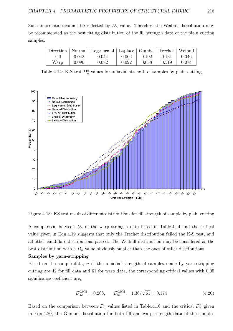
CHAPTER 4. PROBABILISTIC PROPERTIES OF STRUCTURAL FABRIC 216
Such information cannot be reflected by Dn value. Therefore the Weibull distribution may
be recommended as the best fitting distribution of the fill strength data of the plain cutting
samples.
Direction Normal Log-normal Laplace Gumbel Frechet WeibullFill 0.042 0.044 0.066 0.102 0.131 0.046
Warp 0.090 0.082 0.092 0.088 0.519 0.074
Table 4.14: K-S test Dαn values for uniaxial strength of samples by plain cutting
Figure 4.18: KS test result of different distributions for fill strength of sample by plain cutting
A comparison between Dn of the warp strength data listed in Table.4.14 and the critical
value given in Eqn.4.19 suggests that only the Frechet distribution failed the K-S test, and
all other candidate distributions passed. The Weibull distribution may be considered as the
best distribution with a Dn value obviously smaller than the ones of other distributions.
Samples by yarn-stripping
Based on the sample data, n of the uniaxial strength of samples made by yarn-stripping
cutting are 42 for fill data and 61 for warp data, the corresponding critical values with 0.05
significance coefficient are,
D0.00542 = 0.208, D0.005
61 = 1.36/√
61 = 0.174 (4.20)
Based on the comparison between Dn values listed in Table.4.16 and the critical Dαn given
in Eqn.4.20, the Gumbel distribution for both fill and warp strength data of the samples
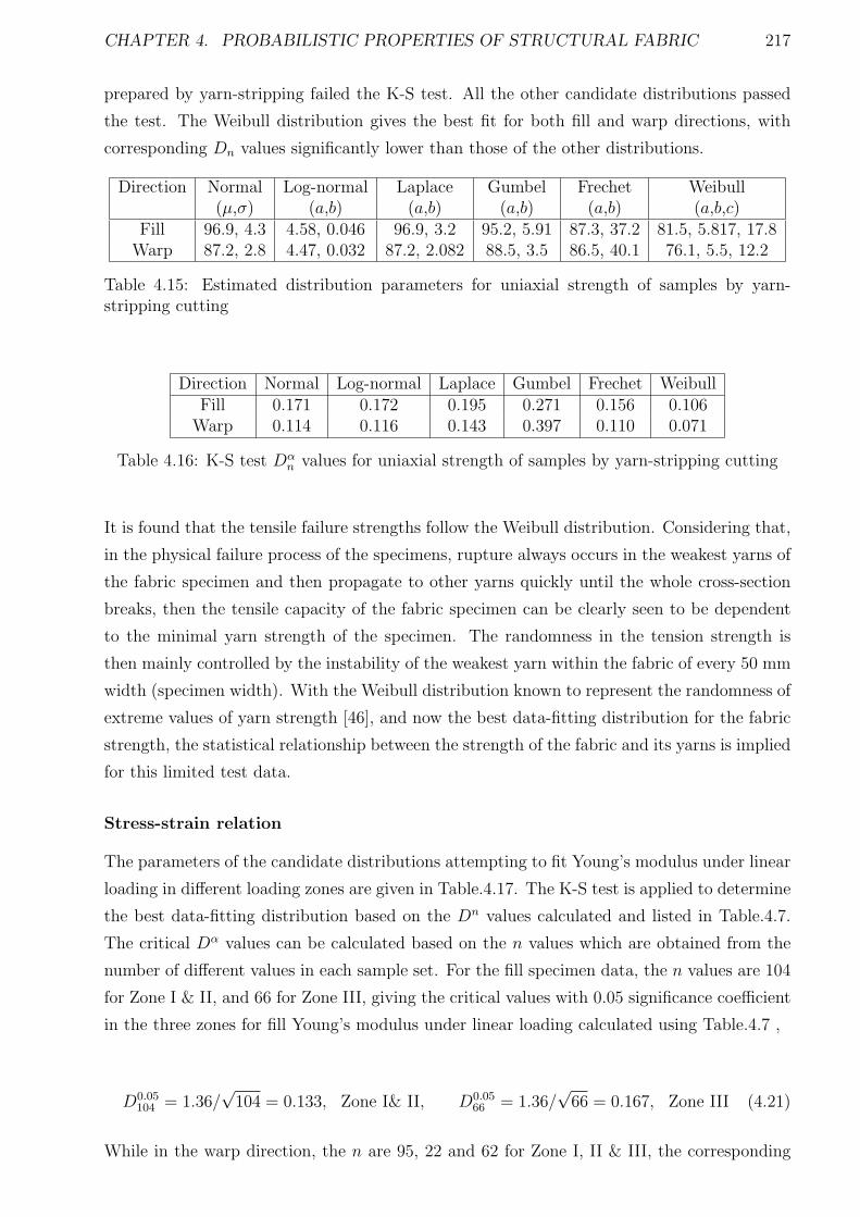
CHAPTER 4. PROBABILISTIC PROPERTIES OF STRUCTURAL FABRIC 217
prepared by yarn-stripping failed the K-S test. All the other candidate distributions passed
the test. The Weibull distribution gives the best fit for both fill and warp directions, with
corresponding Dn values significantly lower than those of the other distributions.
Direction Normal Log-normal Laplace Gumbel Frechet Weibull(µ,σ) (a,b) (a,b) (a,b) (a,b) (a,b,c)
Fill 96.9, 4.3 4.58, 0.046 96.9, 3.2 95.2, 5.91 87.3, 37.2 81.5, 5.817, 17.8Warp 87.2, 2.8 4.47, 0.032 87.2, 2.082 88.5, 3.5 86.5, 40.1 76.1, 5.5, 12.2
Table 4.15: Estimated distribution parameters for uniaxial strength of samples by yarn-stripping cutting
Direction Normal Log-normal Laplace Gumbel Frechet WeibullFill 0.171 0.172 0.195 0.271 0.156 0.106
Warp 0.114 0.116 0.143 0.397 0.110 0.071
Table 4.16: K-S test Dαn values for uniaxial strength of samples by yarn-stripping cutting
It is found that the tensile failure strengths follow the Weibull distribution. Considering that,
in the physical failure process of the specimens, rupture always occurs in the weakest yarns of
the fabric specimen and then propagate to other yarns quickly until the whole cross-section
breaks, then the tensile capacity of the fabric specimen can be clearly seen to be dependent
to the minimal yarn strength of the specimen. The randomness in the tension strength is
then mainly controlled by the instability of the weakest yarn within the fabric of every 50 mm
width (specimen width). With the Weibull distribution known to represent the randomness of
extreme values of yarn strength [46], and now the best data-fitting distribution for the fabric
strength, the statistical relationship between the strength of the fabric and its yarns is implied
for this limited test data.
Stress-strain relation
The parameters of the candidate distributions attempting to fit Young’s modulus under linear
loading in different loading zones are given in Table.4.17. The K-S test is applied to determine
the best data-fitting distribution based on the Dn values calculated and listed in Table.4.7.
The critical Dα values can be calculated based on the n values which are obtained from the
number of different values in each sample set. For the fill specimen data, the n values are 104
for Zone I & II, and 66 for Zone III, giving the critical values with 0.05 significance coefficient
in the three zones for fill Young’s modulus under linear loading calculated using Table.4.7 ,
D0.05104 = 1.36/
√104 = 0.133, Zone I& II, D0.05
66 = 1.36/√
66 = 0.167, Zone III (4.21)
While in the warp direction, the n are 95, 22 and 62 for Zone I, II & III, the corresponding
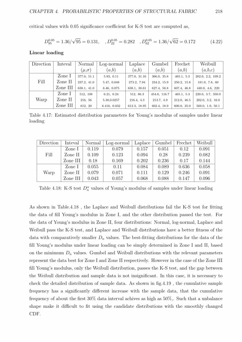
CHAPTER 4. PROBABILISTIC PROPERTIES OF STRUCTURAL FABRIC 218
critical values with 0.05 significance coefficient for K-S test are computed as,
D0.0595 = 1.36/
√95 = 0.131, , D0.05
22 = 0.282 , D0.0562 = 1.36/
√62 = 0.172 (4.22)
Linear loading
Direction Inteval Normal Log-normal Laplace Gumbel Frechet Weibull(µ,σ) (a,b) (a,b) (a,b) (a,b) (a,b,c)
Zone I 377.0, 51.1 5.93, 0.11 377.0, 31.16 366.0, 35.8 465.1, 5.3 282.0, 2.2, 109.2
Fill Zone II 237.2, 41.0 5.47, 0.048 273.2, 7.94 234.2, 15.9 250.2, 15.8 181.0, 7.8, 60
Zone III 638.1, 41.0 6.46, 0.075 638.1, 38.61 627.4, 58.8 607.4, 46.8 440.0, 4.6, 220
Zone I 512, 108 6.21, 0.24 512, 86.3 454.6, 116.7 465.1, 5.3 220.0, 3.7, 350.0
Warp Zone II 216, 56 5.38,0.0257 216.4, 4.3 213.7, 4.9 212.0, 46.5 202.0, 3.2, 16.0
Zone III 612, 20 6.416, 0.032 612.3, 18.95 602.4, 18.9 600.0, 35.0 569.0, 1.9, 50.1
Table 4.17: Estimated distribution parameters for Young’s modulus of samples under linearloading
Direction Inteval Normal Log-normal Laplace Gumbel Frechet WeibullZone I 0.119 0.079 0.157 0.051 0.12 0.091
Fill Zone II 0.109 0.123 0.094 0.28 0.239 0.082Zone III 0.18 0.169 0.202 0.236 0.17 0.144Zone I 0.055 0.11 0.084 0.089 0.636 0.058
Warp Zone II 0.079 0.071 0.111 0.129 0.246 0.091Zone III 0.043 0.057 0.068 0.088 0.147 0.096
Table 4.18: K-S test Dαn values of Young’s modulus of samples under linear loading
As shown in Table.4.18 , the Laplace and Weibull distributions fail the K-S test for fitting
the data of fill Young’s modulus in Zone I, and the other distribution passed the test. For
the data of Young’s modulus in Zone II, four distributions: Normal, log-normal, Laplace and
Weibull pass the K-S test, and Laplace and Weibull distributions have a better fitness of the
data with comparatively smaller Dn values. The best-fitting distributions for the data of the
fill Young’s modulus under linear loading can be simply determined in Zone I and II, based
on the minimum Dn values. Gumbel and Weibull distributions with the relevant parameters
represent the data best for Zone I and Zone II respectively. However in the case of the Zone III
fill Young’s modulus, only the Weibull distribution, passes the K-S test, and the gap between
the Weibull distribution and sample data is not insignificant. In this case, it is necessary to
check the detailed distribution of sample data. As shown in fig.4.19 , the cumulative sample
frequency has a significantly different increase with the sample data, that the cumulative
frequency of about the first 30% data interval achives as high as 50%,. Such that a unbalance
shape make it difficult to fit using the candidate distributions with the smoothly changed
CDF.
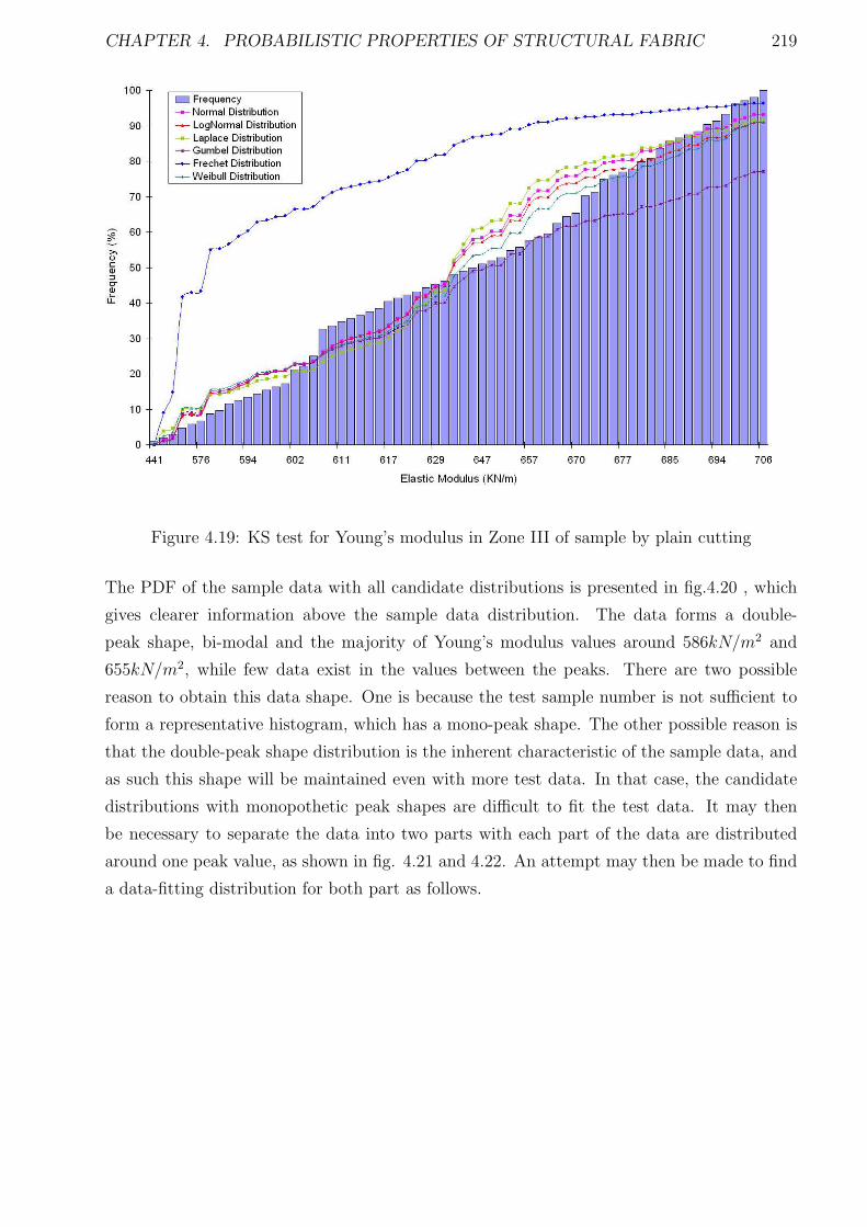
CHAPTER 4. PROBABILISTIC PROPERTIES OF STRUCTURAL FABRIC 219
Figure 4.19: KS test for Young’s modulus in Zone III of sample by plain cutting
The PDF of the sample data with all candidate distributions is presented in fig.4.20 , which
gives clearer information above the sample data distribution. The data forms a double-
peak shape, bi-modal and the majority of Young’s modulus values around 586kN/m2 and
655kN/m2, while few data exist in the values between the peaks. There are two possible
reason to obtain this data shape. One is because the test sample number is not sufficient to
form a representative histogram, which has a mono-peak shape. The other possible reason is
that the double-peak shape distribution is the inherent characteristic of the sample data, and
as such this shape will be maintained even with more test data. In that case, the candidate
distributions with monopothetic peak shapes are difficult to fit the test data. It may then
be necessary to separate the data into two parts with each part of the data are distributed
around one peak value, as shown in fig. 4.21 and 4.22. An attempt may then be made to find
a data-fitting distribution for both part as follows.
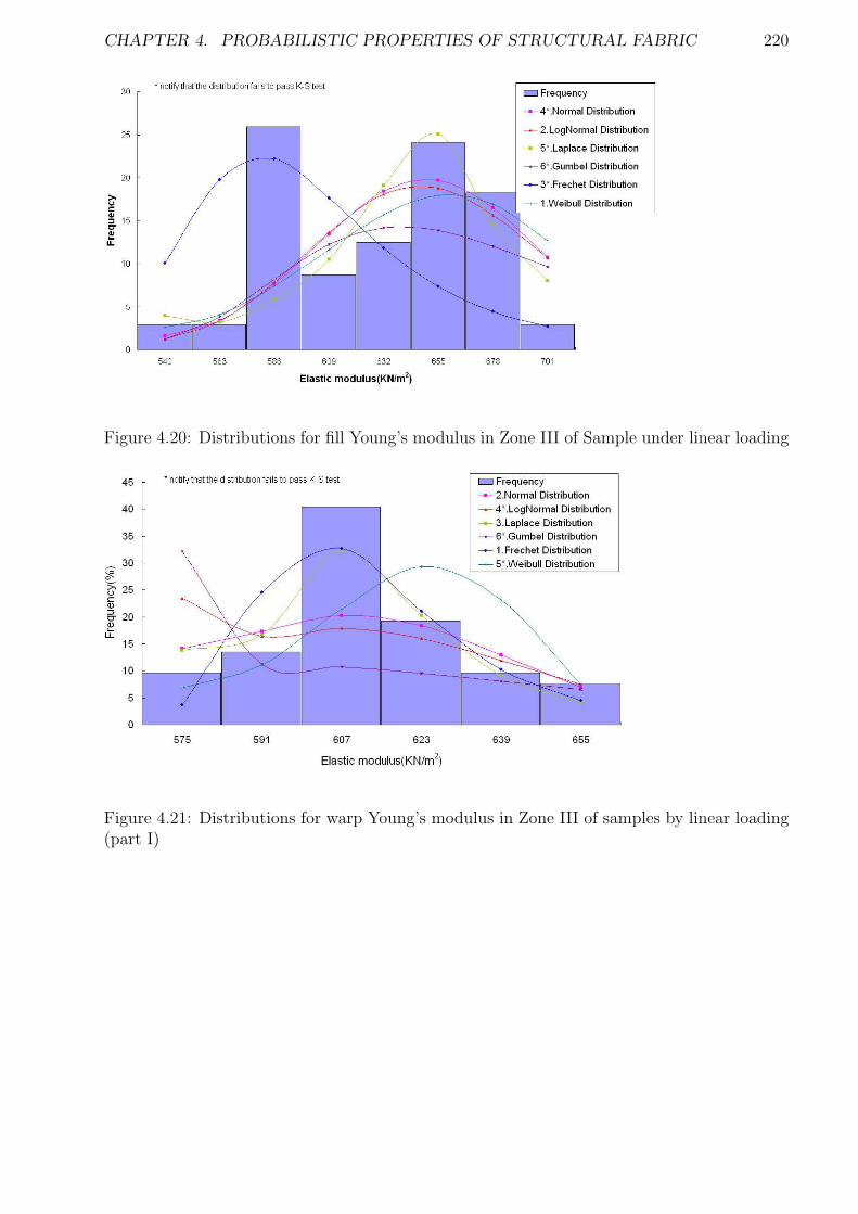
CHAPTER 4. PROBABILISTIC PROPERTIES OF STRUCTURAL FABRIC 220
Figure 4.20: Distributions for fill Young’s modulus in Zone III of Sample under linear loading
Figure 4.21: Distributions for warp Young’s modulus in Zone III of samples by linear loading(part I)
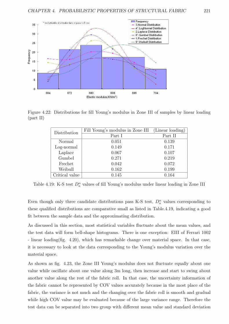
CHAPTER 4. PROBABILISTIC PROPERTIES OF STRUCTURAL FABRIC 221
Figure 4.22: Distributions for fill Young’s modulus in Zone III of samples by linear loading(part II)
Fill Young’s modulus in Zone III (Linear loading)Distribution
Part I Part IINormal 0.051 0.139
Log-normal 0.149 0.171Laplace 0.067 0.107Gumbel 0.271 0.219Frechet 0.042 0.072Weibull 0.162 0.199
Critical value 0.145 0.164
Table 4.19: K-S test Dαn values of fill Young’s modulus under linear loading in Zone III
Even though only three candidate distributions pass K-S test, Dαn values corresponding to
these qualified distributions are comparative small as listed in Table.4.19, indicating a good
fit between the sample data and the approximating distribution.
As discussed in this section, most statistical variables fluctuate about the mean values, and
the test data will form bell-shape histograms. There is one exception: EIII of Ferrari 1002
- linear loading(fig. 4.20), which has remarkable change over material space. In that case,
it is necessary to look at the data corresponding to the Young’s modulus variation over the
material space.
As shown as fig. 4.23, the Zone III Young’s modulus does not fluctuate equally about one
value while oscillate about one value along 3m long, then increase and start to swing about
another value along the rest of the fabric roll. In that case, the uncertainty information of
the fabric cannot be represented by COV values accurately because in the most place of the
fabric, the variance is not much and the changing over the fabric roll is smooth and gradual
while high COV value may be evaluated because of the large variance range. Therefore the
test data can be separated into two group with different mean value and standard deviation
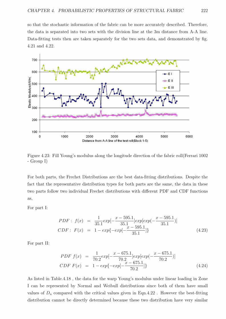
CHAPTER 4. PROBABILISTIC PROPERTIES OF STRUCTURAL FABRIC 222
so that the stochastic information of the fabric can be more accurately described. Therefore,
the data is separated into two sets with the division line at the 3m distance from A-A line.
Data-fitting tests then are taken separately for the two sets data, and demonstrated by fig.
4.21 and 4.22.
Figure 4.23: Fill Young’s modulus along the longitude direction of the fabric roll(Ferrari 1002- Group I)
For both parts, the Frechet Distributions are the best data-fitting distributions. Despite the
fact that the representative distribution types for both parts are the same, the data in these
two parts follow two individual Frechet distributions with different PDF and CDF functions
as,
For part I:
PDF : f(x) =1
35.1exp[−x− 595.1
35.1]exp[exp(−x− 595.1
35.1)]
CDF : F (x) = 1 − exp−exp[−x− 595.1
35.1] (4.23)
For part II:
PDF f(x) =1
70.2exp[−x− 675.1
70.2]exp[exp(−x− 675.1
70.2)]
CDF F (x) = 1 − exp−exp[−x− 675.1
70.2] (4.24)
As listed in Table.4.18 , the data for the warp Young’s modulus under linear loading in Zone
I can be represented by Normal and Weibull distributions since both of them have small
values of Dn compared with the critical values given in Eqn.4.22 . However the best-fitting
distribution cannot be directly determined because these two distribution have very similar
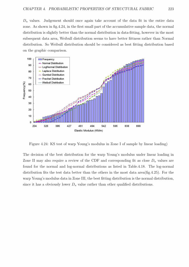
CHAPTER 4. PROBABILISTIC PROPERTIES OF STRUCTURAL FABRIC 223
Dn values. Judgement should once again take account of the data fit in the entire data
zone. As shown in fig.4.24, in the first small part of the accumulative sample data, the normal
distribution is slightly better than the normal distribution in data-fitting, however in the most
subsequent data area, Weibull distribution seems to have better fittness rather than Normal
distribution. So Weibull distribution should be considered as best fitting distribution based
on the graphic comparison.
Figure 4.24: KS test of warp Young’s modulus in Zone I of sample by linear loading)
The decision of the best distribution for the warp Young’s modulus under linear loading in
Zone II may also require a review of the CDF and corresponding fit as close Dn values are
found for the normal and log-normal distributions as listed in Table.4.18. The log-normal
distribution fits the test data better than the others in the most data area(fig.4.25). For the
warp Young’s modulus data in Zone III, the best fitting distribution is the normal distribution,
since it has a obviously lower Dn value rather than other qualified distributions.
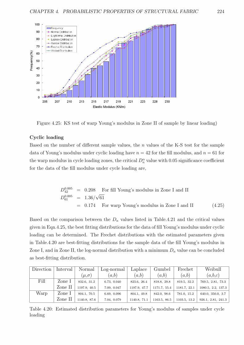
CHAPTER 4. PROBABILISTIC PROPERTIES OF STRUCTURAL FABRIC 224
Figure 4.25: KS test of warp Young’s modulus in Zone II of sample by linear loading)
Cyclic loading
Based on the number of different sample values, the n values of the K-S test for the sample
data of Young’s modulus under cyclic loading have n = 42 for the fill modulus, and n = 61 for
the warp modulus in cycle loading zones, the critical Dαn value with 0.05 significance coefficient
for the data of the fill modulus under cycle loading are,
D0.00542 = 0.208 For fill Young’s modulus in Zone I and II
D0.00561 = 1.36/
√61
= 0.174 For warp Young’s modulus in Zone I and II (4.25)
Based on the comparison between the Dn values listed in Table.4.21 and the critical values
given in Eqn.4.25, the best fitting distributions for the data of fill Young’s modulus under cyclic
loading can be determined. The Frechet distributions with the estimated parameters given
in Table.4.20 are best-fitting distributions for the sample data of the fill Young’s modulus in
Zone I, and in Zone II, the log-normal distribution with a minimum Dn value can be concluded
as best-fitting distribution.
Direction Interval Normal Log-normal Laplace Gumbel Frechet Weibull(µ,σ) (a,b) (a,b) (a,b) (a,b) (a,b,c)
Fill Zone I 832.6, 31.2 6.73, 0.040 823.6, 26.4 818.8, 29.8 819.5, 32.2 769.5, 2.81, 73.3
Zone II 1197.9, 40.5 7.09, 0.047 1197.9, 47.7 1171.7, 55.4 1181.7, 22.1 1080.5, 2.2, 137.3
Warp Zone I 804.1, 70.5 6.69, 0.096 804.1, 49.8 842.0, 98.6 781.0, 15.2 640.0, 350.0, 3.7
Zone II 1140.8, 87.6 7.04, 0.079 1140.8, 71.1 1163.5, 86.5 1103.5, 13.2 926.1, 2.81, 241.3
Table 4.20: Estimated distribution parameters for Young’s modulus of samples under cycleloading
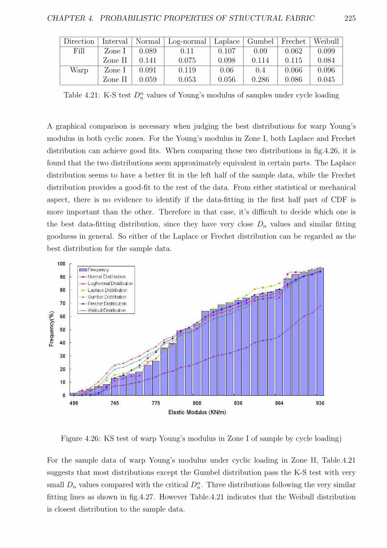
CHAPTER 4. PROBABILISTIC PROPERTIES OF STRUCTURAL FABRIC 225
Direction Interval Normal Log-normal Laplace Gumbel Frechet WeibullFill Zone I 0.089 0.11 0.107 0.09 0.062 0.099
Zone II 0.141 0.075 0.098 0.114 0.115 0.084Warp Zone I 0.091 0.119 0.06 0.4 0.066 0.096
Zone II 0.059 0.053 0.056 0.286 0.086 0.045
Table 4.21: K-S test Dαn values of Young’s modulus of samples under cycle loading
A graphical comparison is necessary when judging the best distributions for warp Young’s
modulus in both cyclic zones. For the Young’s modulus in Zone I, both Laplace and Frechet
distribution can achieve good fits. When comparing these two distributions in fig.4.26, it is
found that the two distributions seem approximately equivalent in certain parts. The Laplace
distribution seems to have a better fit in the left half of the sample data, while the Frechet
distribution provides a good-fit to the rest of the data. From either statistical or mechanical
aspect, there is no evidence to identify if the data-fitting in the first half part of CDF is
more important than the other. Therefore in that case, it’s difficult to decide which one is
the best data-fitting distribution, since they have very close Dn values and similar fitting
goodness in general. So either of the Laplace or Frechet distribution can be regarded as the
best distribution for the sample data.
Figure 4.26: KS test of warp Young’s modulus in Zone I of sample by cycle loading)
For the sample data of warp Young’s modulus under cyclic loading in Zone II, Table.4.21
suggests that most distributions except the Gumbel distribution pass the K-S test with very
small Dn values compared with the critical Dαn . Three distributions following the very similar
fitting lines as shown in fig.4.27. However Table.4.21 indicates that the Weibull distribution
is closest distribution to the sample data.
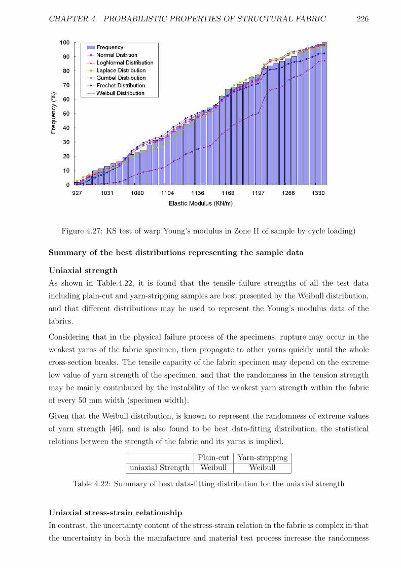
CHAPTER 4. PROBABILISTIC PROPERTIES OF STRUCTURAL FABRIC 226
Figure 4.27: KS test of warp Young’s modulus in Zone II of sample by cycle loading)
Summary of the best distributions representing the sample data
Uniaxial strength
As shown in Table.4.22, it is found that the tensile failure strengths of all the test data
including plain-cut and yarn-stripping samples are best presented by the Weibull distribution,
and that different distributions may be used to represent the Young’s modulus data of the
fabrics.
Considering that in the physical failure process of the specimens, rupture may occur in the
weakest yarns of the fabric specimen, then propagate to other yarns quickly until the whole
cross-section breaks. The tensile capacity of the fabric specimen may depend on the extreme
low value of yarn strength of the specimen, and that the randomness in the tension strength
may be mainly contributed by the instability of the weakest yarn strength within the fabric
of every 50 mm width (specimen width).
Given that the Weibull distribution, is known to represent the randomness of extreme values
of yarn strength [46], and is also found to be best data-fitting distribution, the statistical
relations between the strength of the fabric and its yarns is implied.
Plain-cut Yarn-strippinguniaxial Strength Weibull Weibull
Table 4.22: Summary of best data-fitting distribution for the uniaxial strength
Uniaxial stress-strain relationship
In contrast, the uncertainty content of the stress-strain relation in the fabric is complex in that
the uncertainty in both the manufacture and material test process increase the randomness
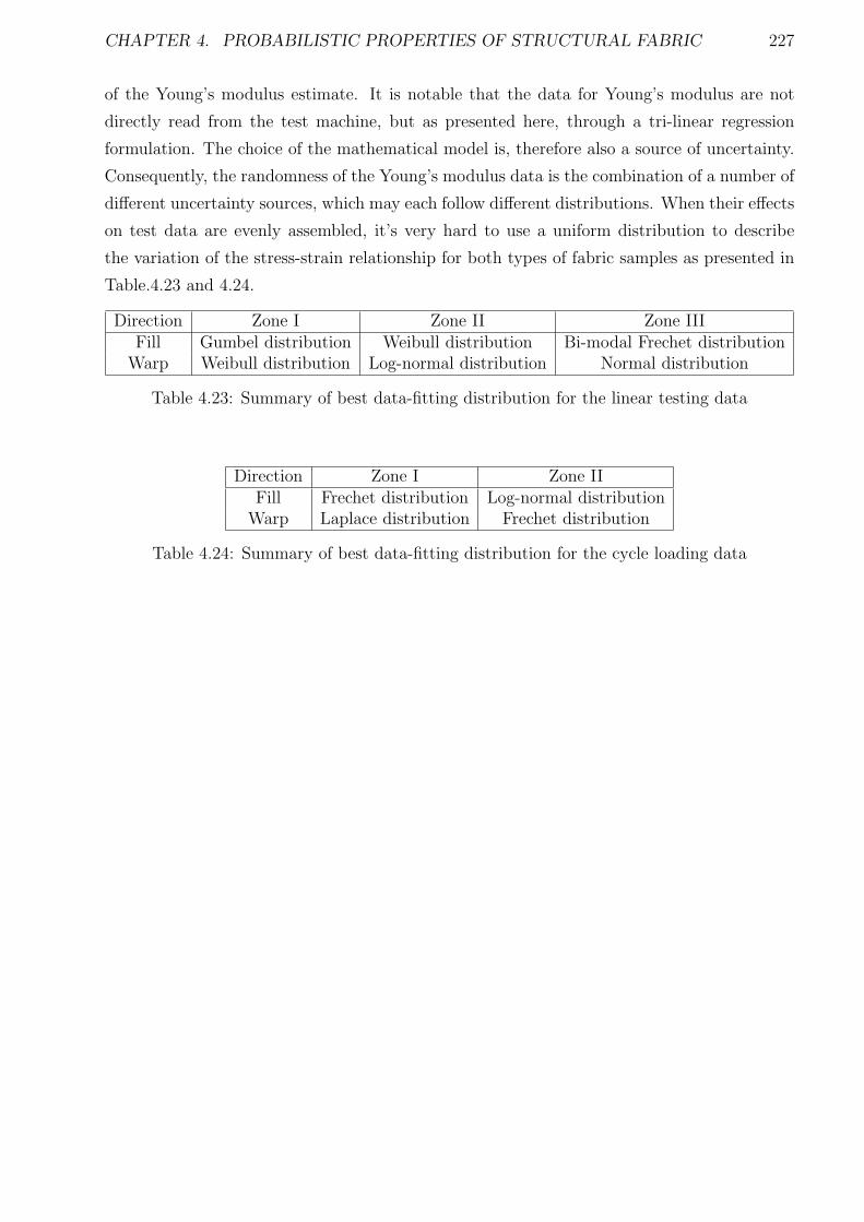
CHAPTER 4. PROBABILISTIC PROPERTIES OF STRUCTURAL FABRIC 227
of the Young’s modulus estimate. It is notable that the data for Young’s modulus are not
directly read from the test machine, but as presented here, through a tri-linear regression
formulation. The choice of the mathematical model is, therefore also a source of uncertainty.
Consequently, the randomness of the Young’s modulus data is the combination of a number of
different uncertainty sources, which may each follow different distributions. When their effects
on test data are evenly assembled, it’s very hard to use a uniform distribution to describe
the variation of the stress-strain relationship for both types of fabric samples as presented in
Table.4.23 and 4.24.
Direction Zone I Zone II Zone IIIFill Gumbel distribution Weibull distribution Bi-modal Frechet distribution
Warp Weibull distribution Log-normal distribution Normal distribution
Table 4.23: Summary of best data-fitting distribution for the linear testing data
Direction Zone I Zone IIFill Frechet distribution Log-normal distribution
Warp Laplace distribution Frechet distribution
Table 4.24: Summary of best data-fitting distribution for the cycle loading data
CHAPTER 4. PROBABILISTIC PROPERTIES OF STRUCTURAL FABRIC 228
4.6 Summary
The assumption of orthotropy between fill and warp may not be valid for a coated woven
fabric. The distribution of the yarns in the fabric may be very important for affecting the
structural performance such as strength and stress-strain relationship. The fabric sample
prepared by different cutting procedure can display wholly different characteristics in the
mechanical properties, should be considered as two different types of statistical variable in the
probabilistic investigation and analysis.
An initial small number of tests suggests that the yarn-stripping samples have higher mean
strength and also standard deviation than those made by plain-cut. Their similar COV value
may imply that the uncertainty of the fabric strength is more relevant to the randomness
of the individual yarn strength rather than the composite structure. That may be further
demonstrated by the more probabilistic similarities (e.g. skewness) for these two types of test
samples subsequently observed in the large number of tests
The stress-strain relationship under monotonic and cyclic loads are distinctive in both de-
terministic and probabilistic aspects. The Young’s modulus values obtained based on cyclic
loading have obviously higher values in magnitude and less randomness compared with those
from monotonic loading, indicating that large plastic strain with high randomness may occur
when a monotonic load is applied to the fabric.
The determination of the best-fit distributions for the test data may start with the initial
candidate distributions selected based on the data histogram, then further judgement can be
made using the K-S test. To take account of the calculation tolerance, the graphic comparison
may be required when several distributions are equivalent in fitting the test data. When few
distributions seem to fit the test data, further procedures (e.g. bi-modal model) may be
required for a valid representation of the test data.
The analysis of the test data suggests that Weibull distribution seems to be the best-fitting
distribution for the uniaxial strength of both types of test samples made by plain cut and
yarn-stripping. While a uniform distribution fitting the data of Young’s moduli has not been
observed. It seems that the Young’s moduli under monotonic and cyclic loads have different
distributions. In each loading zone, distinctive best-fitting distributions are observed under
the same type of load condition.
Chapter 5
Reliability Analysis of Fabric
Structures
In the majority of national and European codes, the ”limit state” approach with safety co-
efficients is used to obtain an optimal safe design, which is regarded as a trade-off between
reliability and cost. The safety coefficients correspond to the uncertainty in structural form
and materials, and are obtained through experiments or estimated empirically. In traditional
structural design (e.g. concrete structures), both the material strength and the loads are fac-
tored to achieve a sufficient safety margin. However, in fabric structure analysis and design,
increased loading normally changes both the magnitude and distribution of the stresses signif-
icantly owing to geometric non-linearity. ”A limit state approach(with partial safety factors
applied to the loading conditions as well as material strengths) may not be appropriate since
the geometry of the structure is dependent on both the magnitude and the distribution of
loading”(see European Design Guide for Tensile Surface Structures, 2004,p178). Therefore in
fabric structure design, a permissible stress design philosophy is used in which safety factors
are applied to the material strength. Maximum factors are 7.0 in IASS code, 8.0 in Japan
code and and 9.5 in the German code.
These safety factors are recommended in fabric design codes corresponding to material vari-
ability(e.g consistency and degradation) and uncertainty in loading, load effects(e.g. tearing)
and analysis/simulation accuracy, but their influence on the structural reliability is ambiguous
and cannot represent the randomness in fabric structures accurately. Thus, there is a strong
motivation to develop a structural reliability method to analyze fabric structures using prob-
abilistic information describing loads, material properties, and geometry, which may then be
used to calibrate new factors or confirm existing factors of safety.
A objective target in structural reliability analysis is the estimation of the probability of failure
to achieve a prescribed structural performance. In a finite element-based reliability analysis,
the input parameters for the finite element model are defined as a set of random variables
X, leading to a unique response vector for a given realization of X. A set of continuous and
differentiable limit-state functions G(X) are defined, where G(X) < 0 indicates the structural
229
CHAPTER 5. RELIABILITY ANALYSIS OF FABRIC STRUCTURES 230
failure of the components or partial component of the system. Here, it is essentially assumed
that fabric structures have several modes of failure and that each failure mode can be described
in terms of a single limit state function.
For complicated structures, explicit solutions of the probability of the structural failure are dif-
ficult to obtain. Therefore, approximate reliability methods are required to make the problem
tractable. These include first and second-order reliability methods (FORM and SORM) [239]
and other approximation methods, such as Response Surface approaches [240, 241]. Incorpo-
rating with the Hasofer-Lind method [184], FORM has emerged as one of the most effective
reliability methods to evaluate the probability of structural failure.
The Hasofer-Lind method, which linearizes the limit state function at the most probable fail-
ure point (MPP) and characterizes all the random variables with mean values and standard
deviations only, was extended by Rackwitz and Fiessler [242] by including detailed random
variable information with different(non-normal) distributions. This led to an efficient safety
index algorithm was developed with the advantage that only the values of the limit state
functions and their derivatives were needed to be computed instead of solving the limit state
function explicitly. The value of the limit state functions can be obtained through a de-
terministic structural analysis, with the derivatives of G(X) calculated either analytically
or numerically, forming effectively a sensitivity analysis of the structural performance with
respect to uncertainty.
Apart from an immediate application to FORM, the sensitivity analysis is also important in
enabling the effects of the random variables on the fabric structure response to be observed
and quantified. For variables with large effects on structural failure, their uncertainty may
be reduced by collecting additional information through testing or by making design changes
at structural, material and manufacturing levels. For those variable having little influence
on structural reliability, they may be simplified as deterministic values to save computational
effort, without compromising the accuracy of the reliability estimate. It is possible to derive
different design safety factors for random variables individually based on their uncertainties
and their influence on structure behavior. Two methods of sensitivity analysis, namely finite
difference and analytic approach are introduced and detailed in section 5.3.1 and 5.3.2.
Combining sensitivity analyse and FORM to estimate the probability of failure of a system
with an implicit limit state function uses information about the value and gradient of the limit
state function at the checking point( or design point), and an iterative optimization scheme
to determine to the safety index.
CHAPTER 5. RELIABILITY ANALYSIS OF FABRIC STRUCTURES 231
5.1 Safety criterion and limit state functions
The first step in evaluating the reliability of fabric structure is to identify and quantify the
uncertainties existing in the realization of the structure. Generally, the main sources of un-
certainty can be separated into several categories: material properties, manufacturing or
fabrication and construction conditions, environmental impact(load), human effects. How-
ever the information of some type of uncertainties (e.g human effects) are case-dependent and
not easy to obtain accurately. The reliability analysis in this chapter is limited to include
uncertainty in the material properties and loads. A typical membrane structure comprises
several materials: fabric, cables, supporting steelwork. Uncertainty of each type of material
can be identified by individual statistical variables X. Six statistical variables are defined to
represent the uncertainty information of fabric properties:
X1 = Ef , X2 = Ew, X3 = vwf , X4 = Gwf , X5 = σfillult , X6 = σwarp
ult (5.1)
where Ef ,Ew are Young’s modulus in the fill and warp directions, Gwf is the shear modulus
across the fill and warp direction, vwf is Possion’s ratio, and σult is ultimate strength of fabric
(rupture strength).
An additional statistical variable is identified with the imposed load coefficient tload with unit
mean value:
X7 = tload =F
Fc
(5.2)
where F is the applied load, Fc is the deterministic value of design load.
Each statistical variable can be characterized by mean value µ, standard derivation σ, and a
probability density function (PDF), which can be estimated by material tests combined with
formal statistical analysis including the transformation of non-normal distributions.
Unlike traditional construction materials, a structural fabric material is a type of tension-
only composite, which is made of fibres in two directions: fill and warp. Therefore material
failure of a fabric includes the rupture of the yarns in either direction and the appearance of
wrinkles which indicates the disappearance of a positive minimum principal stress, for example
(other criteria exist- see wrinkling section in the chapter.3 ”Deterministic Fabric Structure
Analysis”).
The safety criterion related to material stress can be expressed using three functions G1(Xs),
G2(Xs), and G3(Xs) defined in Eqn.5.3, in which material failure occurs when Gi < 0, i =
1, 2, 3.
G1(Xsi) = σfper − σf
max, G2(Xsi) = σwper − σw
max, G3(Xsi) = σpmin − σp
per (5.3)
where σfper and σw
per are permissible stresses in fill and warp direction respectively, and normally
computed as products of ultimate strength and safety factors:
CHAPTER 5. RELIABILITY ANALYSIS OF FABRIC STRUCTURES 232
σfper = σf
ult, σwper = σw
ult (5.4)
in which, ff and fw are safety factors for ultimate strength of fill and warp. These safety
factors are normally defined and estimated to taken into account the material degradation
due to the environmental impacts [4]. σfmax and σw
max are maximum tension stresses in the
fabric along fill and warp direction separately. σpmin is the minimum principal stress of the
membrane, and σpper is the predefined lower limit which normally corresponds to a percentage
of the fabric pre-stress, and Xsi is the relevant statistical variable.
One basic serviceability requirement in structural design is that the deformation should be
controlled to a reasonable level, as in
G4(Xs) = Dal −Dmax (5.5)
in which, Dal is the deformation allowance, and Dmax is the maximum deformation.
The fabric structure surface should avoid excessive deformation to ensure adequate structural
performance related to phenomena such as ponding - with the structural geometry such that
there is positive drainage from all areas. An undeformed pretensioned membrane normally
has an anticlastic shape, which provides effective drainage, but large membrane deformation
especially in the vertical direction may lead to ponding in some local areas. Therefore, the
allowable deformation Dal in Eqn.5.5 must be set not only based on the general serviceability
requirement, but also allowing for the ponding mitigation.
The failure surface or the limit state i is defined as Gi = 0. This represents the boundary
between the safe and unsafe regions in the design parameter space, and also identifies states
beyond which the structure can no longer fulfill the function for which it was intended. The
failure surface and the safe and unsafe regions in respect of statistical variables Xs1 and Xs2
are shown in Fig.5.1.
In n variable parameters space, the probability of structural failure pf can be calculated using
Eqn. 5.6
pf =
∫
· · ·∫
g(Xs)<0
fX(xs1, xs2, · · · , xs7)dx1dx2 · · · dxn (5.6)
in which fX(xs1, xs2, · · · , xsn) is the joint probability density function for the statistical vari-
ables Xs1, Xs2, · · · , Xsn and the integration is performed over the failure region G(Xs) < 0. If
it is assumed that the random variables are statistically independent and the limit state func-
tion is a simple combination of design variables, then the joint probability density function
may be replaced by the product of the individual probability density functions in the integral.
The computation of pf by Eqn. 5.6 is the fundamental equation of reliability analysis. The
joint probability density function of random variables fXs is often not available in practice
and the multiple integral is also extremely complicated to estimate. The first-order reliability
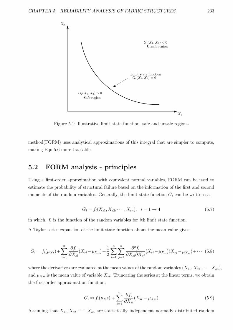
CHAPTER 5. RELIABILITY ANALYSIS OF FABRIC STRUCTURES 233
X1
X2
Limit state functionGi(X1, X2) = 0
Gi(X1, X2) < 0Unsafe region
Gi(X1, X2) > 0
Safe region
Figure 5.1: Illustrative limit state function ,safe and unsafe regions
method(FORM) uses analytical approximations of this integral that are simpler to compute,
making Eqn.5.6 more tractable.
5.2 FORM analysis - principles
Using a first-order approximation with equivalent normal variables, FORM can be used to
estimate the probability of structural failure based on the information of the first and second
moments of the random variables. Generally, the limit state function Gi can be written as:
Gi = fi(Xs1, Xs2, · · · , Xsn), i = 1 → 4 (5.7)
in which, fi is the function of the random variables for ith limit state function.
A Taylor series expansion of the limit state function about the mean value gives:
Gi = fi(µXs)+n∑
i=1
∂fi
∂Xsi
(Xsi−µXsi)+
1
2
n∑
i=1
n∑
j=1
∂2fi
∂Xsi∂Xsj
(Xsi−µXsi)(Xsj −µXsj
)+ · · · (5.8)
where the derivatives are evaluated at the mean values of the random variables (Xs1, Xs2, · · · , Xsn),
and µXsi is the mean value of variable Xsi. Truncating the series at the linear terms, we obtain
the first-order approximation function:
Gi ≈ fi(µXs) +n∑
i=1
∂fi
∂Xsi
(Xsi − µXsi) (5.9)
Assuming that Xs1, Xs2, · · · , Xsn are statistically independent normally distributed random
CHAPTER 5. RELIABILITY ANALYSIS OF FABRIC STRUCTURES 234
variables, the function Gi is also normally distributed, and the approximate mean and variance
of Gi are:
µGi≈ fi(µXs1 , µXs2 , · · · , µXsn) (5.10)
and
σ2Gi
≈n∑
i=1
(
∂Gi
∂Xsi
)2
V ar(Xsi) (5.11)
The probability of structural failure is defined as:
pf = P (Gi < 0) (5.12)
or
pf = Φ
(
0 − µGi
σGi
)
= 1 − Φ
(
µGi
σGi
)
= 1 − Φ(β) (5.13)
where Φ denotes the CDF of the standard normal variate.
The probability of structure failure calculated by Eqn. 5.13 depends on the ratio of the mean
and standard deviation of Gi. This ratio is called the safety index or reliability index and is
denoted as β:
β =µGi
σGi
(5.14)
When calculating the safety index using Eqn. 5.14, explicit information about the mean and
standard deviation of the limit state function is required. This information is normally not
known explicitly, particularly when using simulation techniques such as the finite element
method. The problem arises that the safety indices depend on the formulation of the limit
state equation as well as the underlying assumption about the distribution of the limit state.
This problem was overcome by the Hasofer-Lind method [184], in which, a reduced coordinate
system and reduced variables are defined first as:
X ′si =
Xsi − µXsi
σXsi
(i = 1, 2, · · · , n) (5.15)
Where X ′si is a random variable with zero mean and unit standard deviation. Eqn. 5.15 is used
to transform the original limit state G(Xs) = 0 to the reduced limit state, G(X ′s) = 0. The
Xs coordinate system is referred to as the original coordinate system and the X ′s coordinate
system is referred to as the reduced coordinate system. The safety index is redefined as the
minimum distance from the origin of the axes in the reduced coordinate system to the limit
state surface. It can be expressed as:
βH−L =√
(x′∗s )t(x′∗s ) (5.16)
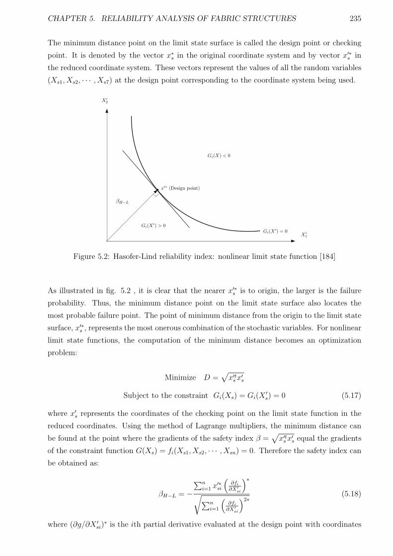
CHAPTER 5. RELIABILITY ANALYSIS OF FABRIC STRUCTURES 235
The minimum distance point on the limit state surface is called the design point or checking
point. It is denoted by the vector x∗s in the original coordinate system and by vector x′∗s in
the reduced coordinate system. These vectors represent the values of all the random variables
(Xs1, Xs2, · · · , Xs7) at the design point corresponding to the coordinate system being used.
X ′
1
X ′
2
x′∗ (Design point)
βH−L
Gi(X′) > 0
Gi(X′) = 0
Gi(X) < 0
Figure 5.2: Hasofer-Lind reliability index: nonlinear limit state function [184]
As illustrated in fig. 5.2 , it is clear that the nearer x′∗s is to origin, the larger is the failure
probability. Thus, the minimum distance point on the limit state surface also locates the
most probable failure point. The point of minimum distance from the origin to the limit state
surface, x′∗s , represents the most onerous combination of the stochastic variables. For nonlinear
limit state functions, the computation of the minimum distance becomes an optimization
problem:
Minimize D =√
x′tsx′s
Subject to the constraint Gi(Xs) = Gi(X′s) = 0 (5.17)
where x′s represents the coordinates of the checking point on the limit state function in the
reduced coordinates. Using the method of Lagrange multipliers, the minimum distance can
be found at the point where the gradients of the safety index β =√
x′tsx′s equal the gradients
of the constraint function G(Xs) = fi(Xs1, Xs2, · · · , Xsn) = 0. Therefore the safety index can
be obtained as:
βH−L = −∑n
i=1 x′∗si
(
∂fi
∂X′
si
)∗
√
∑ni=1
(
∂fi
∂X′
si
)2∗(5.18)
where (∂g/∂X ′si)
∗ is the ith partial derivative evaluated at the design point with coordinates
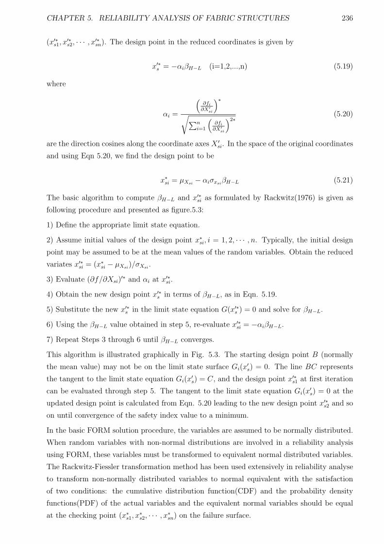
CHAPTER 5. RELIABILITY ANALYSIS OF FABRIC STRUCTURES 236
(x′∗s1, x′∗s2, · · · , x′∗sn). The design point in the reduced coordinates is given by
x′∗s = −αiβH−L (i=1,2,...,n) (5.19)
where
αi =
(
∂fi
∂X′
si
)∗
√
∑ni=1
(
∂fi
∂X′
si
)2∗(5.20)
are the direction cosines along the coordinate axes X ′si. In the space of the original coordinates
and using Eqn 5.20, we find the design point to be
x∗si = µXsi− αiσxsi
βH−L (5.21)
The basic algorithm to compute βH−L and x′∗si as formulated by Rackwitz(1976) is given as
following procedure and presented as figure.5.3:
1) Define the appropriate limit state equation.
2) Assume initial values of the design point x∗si, i = 1, 2, · · · , n. Typically, the initial design
point may be assumed to be at the mean values of the random variables. Obtain the reduced
variates x′∗si = (x∗si − µXsi)/σXsi
.
3) Evaluate (∂f/∂Xsi)′∗ and αi at x′∗si.
4) Obtain the new design point x′∗s in terms of βH−L, as in Eqn. 5.19.
5) Substitute the new x′∗s in the limit state equation G(x′∗s ) = 0 and solve for βH−L.
6) Using the βH−L value obtained in step 5, re-evaluate x′∗si = −αiβH−L.
7) Repeat Steps 3 through 6 until βH−L converges.
This algorithm is illustrated graphically in Fig. 5.3. The starting design point B (normally
the mean value) may not be on the limit state surface Gi(x′s) = 0. The line BC represents
the tangent to the limit state equation Gi(x′s) = C, and the design point x′∗s1 at first iteration
can be evaluated through step 5. The tangent to the limit state equation Gi(x′s) = 0 at the
updated design point is calculated from Eqn. 5.20 leading to the new design point x′∗s2 and so
on until convergence of the safety index value to a minimum.
In the basic FORM solution procedure, the variables are assumed to be normally distributed.
When random variables with non-normal distributions are involved in a reliability analysis
using FORM, these variables must be transformed to equivalent normal distributed variables.
The Rackwitz-Fiessler transformation method has been used extensively in reliability analyse
to transform non-normally distributed variables to normal equivalent with the satisfaction
of two conditions: the cumulative distribution function(CDF) and the probability density
functions(PDF) of the actual variables and the equivalent normal variables should be equal
at the checking point (x∗s1, x∗s2, · · · , x∗sn) on the failure surface.
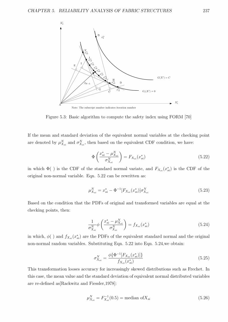
CHAPTER 5. RELIABILITY ANALYSIS OF FABRIC STRUCTURES 237
X ′
1
X ′
2
A
B
C
D
E
F
G
H
I
J
x′∗
0
x′∗
s1
x′∗
s2
x′∗
s3
x′∗
s4
x′∗
s5
x′∗
s6
x′∗
s7
x′∗
s8
x′∗
s9
βH−L
Gi(X′) = 0
G(X ′) = C
Note: The subscript number indicates iteration number
Figure 5.3: Basic algorithm to compute the safety index using FORM [70]
If the mean and standard deviation of the equivalent normal variables at the checking point
are denoted by µNXsi
and σNXsi
, then based on the equivalent CDF condition, we have:
Φ
(
x∗si − µNXsi
σNXsi
)
= FXsi(x∗si) (5.22)
in which Φ( ) is the CDF of the standard normal variate, and FXsi(x∗si) is the CDF of the
original non-normal variable. Eqn. 5.22 can be rewritten as:
µNXsi
= x∗si − Φ−1[FXsi(x∗si)]σ
NXsi
(5.23)
Based on the condition that the PDFs of original and transformed variables are equal at the
checking points, then:
1
σNXsi
φ
(
x∗si − µNXsi
σNXsi
)
= fXsi(x∗si) (5.24)
in which, φ( ) and fXsi(x∗si) are the PDFs of the equivalent standard normal and the original
non-normal random variables. Substituting Eqn. 5.22 into Eqn. 5.24,we obtain:
σNXsi
=φΦ−1[FXsi
(x∗si)]fXsi
(x∗si)(5.25)
This transformation looses accuracy for increasingly skewed distributions such as Frechet. In
this case, the mean value and the standard deviation of equivalent normal distributed variables
are re-defined as[Rackwitz and Fiessler,1978]:
µNXsi
= F−1Xsi
(0.5) = median ofXsi (5.26)
CHAPTER 5. RELIABILITY ANALYSIS OF FABRIC STRUCTURES 238
and
σNXsi
=x∗si − µN
Xsi
Φ−1[FXsi(x∗si)]
(5.27)
in which F−1Xsi
( ) is the inverse of the non-normal CDF of Xsi.
From a practical point of view, the application of the basic FORM algorithm is limited to
limit state functions with simple forms, because in many cases, it is very difficult to solve
the equation Gi(x′∗s ) = 0 for design point x′∗s when it is highly nonlinear, and in certain cases
is not explicit. For example, in the reliability analysis of fabric structures, the limit state
is evaluated through a deterministic finite element analysis with external random variables,
making it impossible to perform step 5 in the basic FORM algorithm.
An alternative Newton-Raphson type recursive algorithm was developed by Rackwitz and
Fiessler, in that, it linearizes the limit state function at each iteration point, and only requires
the derivatives of the limit state function instead of solving the limit state equation explicitly.
As shown in Fig. 5.4, initially the starting point x′∗s may not be on the limit state function
G(X ′s) = 0, but on a parallel line G(X ′
s) = k. The linear limit state function G(X ′s) may be
expressed as,
a
(0, 0)
G(X ′
1, X ′
2) = 0
G(X ′
1, X ′
2) = k
X ′
1
x′∗
0
x′∗
X ′
2
Figure 5.4: Linearized limit state function in HL-RF(Hasofer-Lind and Rackwitz-Fiossler)algorithm
G(X ′s) = b+ atx′s (5.28)
or, for example, using two variables,
G(X ′s) = b+ a1x
′s1 + a2x
′s2 (5.29)
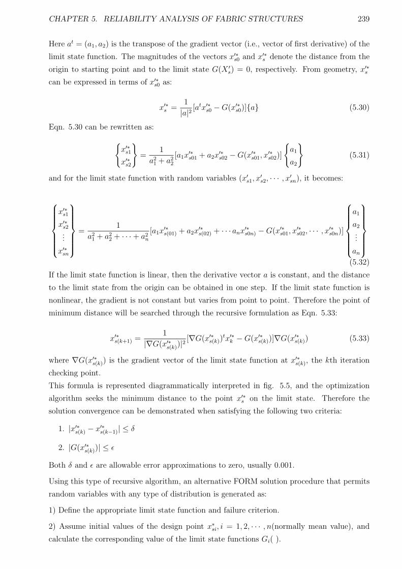
CHAPTER 5. RELIABILITY ANALYSIS OF FABRIC STRUCTURES 239
Here at = (a1, a2) is the transpose of the gradient vector (i.e., vector of first derivative) of the
limit state function. The magnitudes of the vectors x′∗s0 and x′∗s denote the distance from the
origin to starting point and to the limit state G(X ′s) = 0, respectively. From geometry, x′∗s
can be expressed in terms of x′∗s0 as:
x′∗s =1
|a|2 [atx′∗s0 −G(x′∗s0)]a (5.30)
Eqn. 5.30 can be rewritten as:
x′∗s1
x′∗s2
=1
a21 + a2
2
[a1x′∗s01 + a2x
′∗s02 −G(x′∗s01, x
′∗s02)]
a1
a2
(5.31)
and for the limit state function with random variables (x′s1, x′s2, · · · , x′sn), it becomes:
x′∗s1
x′∗s2...
x′∗sn
=1
a21 + a2
2 + · · · + a2n
[a1x′∗s(01) + a2x
′∗s(02) + · · · anx
′∗s0n) −G(x′∗s01, x
′∗s02, · · · , x′∗s0n)]
a1
a2
...
an
(5.32)
If the limit state function is linear, then the derivative vector a is constant, and the distance
to the limit state from the origin can be obtained in one step. If the limit state function is
nonlinear, the gradient is not constant but varies from point to point. Therefore the point of
minimum distance will be searched through the recursive formulation as Eqn. 5.33:
x′∗s(k+1) =1
|∇G(x′∗s(k))|2[∇G(x′∗s(k))
tx′∗k −G(x′∗s(k))]∇G(x′∗s(k)) (5.33)
where ∇G(x′∗s(k)) is the gradient vector of the limit state function at x′∗s(k), the kth iteration
checking point.
This formula is represented diagrammatically interpreted in fig. 5.5, and the optimization
algorithm seeks the minimum distance to the point x′∗s on the limit state. Therefore the
solution convergence can be demonstrated when satisfying the following two criteria:
1. |x′∗s(k) − x′∗s(k−1)| ≤ δ
2. |G(x′∗s(k))| ≤ ǫ
Both δ and ǫ are allowable error approximations to zero, usually 0.001.
Using this type of recursive algorithm, an alternative FORM solution procedure that permits
random variables with any type of distribution is generated as:
1) Define the appropriate limit state function and failure criterion.
2) Assume initial values of the design point x∗si, i = 1, 2, · · · , n(normally mean value), and
calculate the corresponding value of the limit state functions Gi( ).
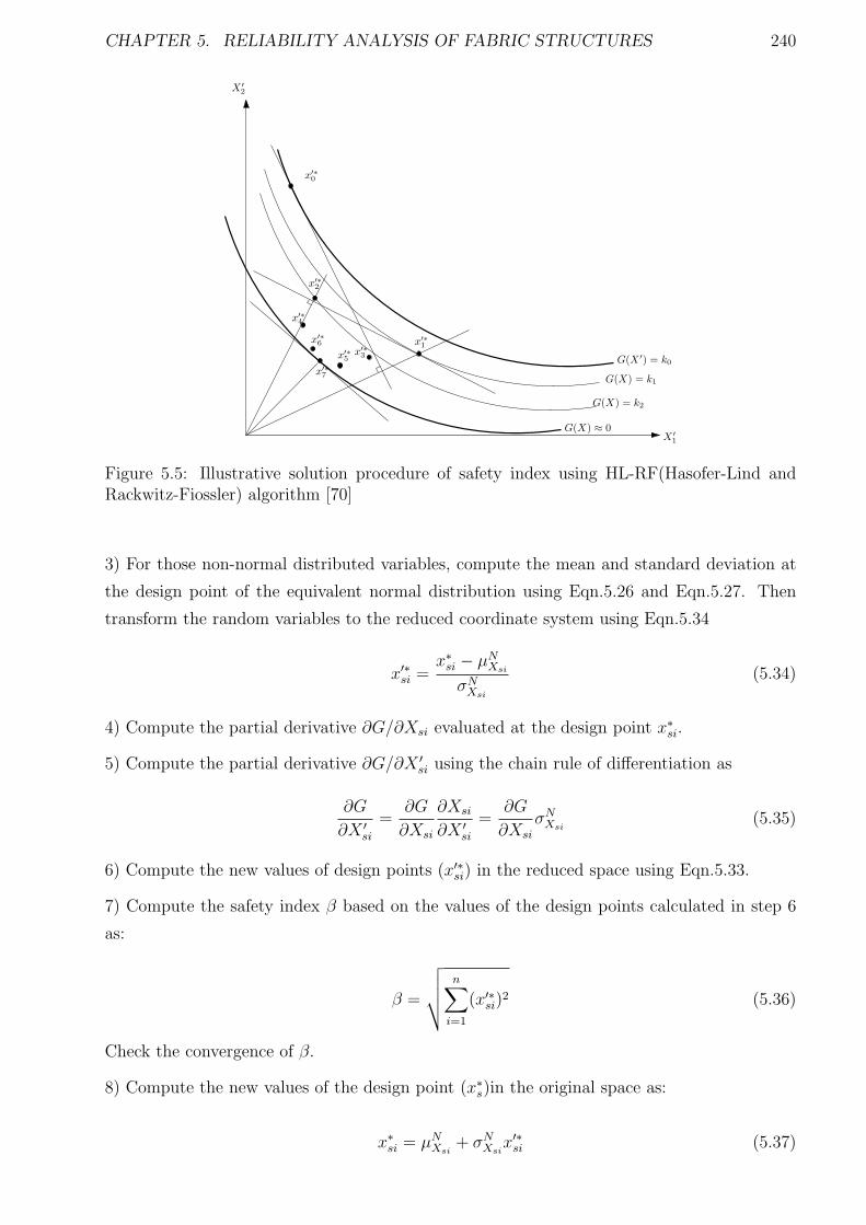
CHAPTER 5. RELIABILITY ANALYSIS OF FABRIC STRUCTURES 240
X ′
1
X ′
2
G(X) = k1
G(X ′) = k0
x′∗
0
x′∗
2
G(X) = k2
G(X) ≈ 0
x′∗
1
x′∗
3
x′∗
4
x′∗
5
x′∗
6
x′∗
7
Figure 5.5: Illustrative solution procedure of safety index using HL-RF(Hasofer-Lind andRackwitz-Fiossler) algorithm [70]
3) For those non-normal distributed variables, compute the mean and standard deviation at
the design point of the equivalent normal distribution using Eqn.5.26 and Eqn.5.27. Then
transform the random variables to the reduced coordinate system using Eqn.5.34
x′∗si =x∗si − µN
Xsi
σNXsi
(5.34)
4) Compute the partial derivative ∂G/∂Xsi evaluated at the design point x∗si.
5) Compute the partial derivative ∂G/∂X ′si using the chain rule of differentiation as
∂G
∂X ′si
=∂G
∂Xsi
∂Xsi
∂X ′si
=∂G
∂Xsi
σNXsi
(5.35)
6) Compute the new values of design points (x′∗si) in the reduced space using Eqn.5.33.
7) Compute the safety index β based on the values of the design points calculated in step 6
as:
β =
√
√
√
√
n∑
i=1
(x′∗si)2 (5.36)
Check the convergence of β.
8) Compute the new values of the design point (x∗s)in the original space as:
x∗si = µNXsi
+ σNXsix′∗si (5.37)
CHAPTER 5. RELIABILITY ANALYSIS OF FABRIC STRUCTURES 241
then update the value of the limit state function G( ) for this new design point and check if
the design points are on the limit state function(i.e. |G( )| is very close to zero, say within
0.001). If the convergence criteria in step 7 is satisfied and |G( )| is approximately zero(e.g.
less than 0.001), then stop. Otherwise, repeat steps 3 through 8 until convergence.
The advantage of this solution algorithm is that solving limit state equation G( ) = 0 is
avoided, so that the reliability analysis can be undertaken for a structure with a complicated
or implicit limit state function, given that the partial derivatives of G( ) with respect to
the random variables are available. This algorithm is a general procedure for the reliability
analysis of most types of structures, without consideration of the specific characteristics of a
specific structure type. For each problem it is necessary to compute the partial derivatives of
G( ) (or sensitivities) with respect to the statistical variables for fabric structures analyzed
using a particular finite element formulation. These formulation are detailed in section 5.3.
5.3 Sensitivity Analysis
The FORM introduced in section 5.2 requires the value and gradients of the performance
function. The value of the performance function can be obtained from a deterministic struc-
tural analysis(e.g finite element analysis) and the gradients of the limit state functions can be
derived as:
∂G1/∂Xsi = ∂(σfper − σf
max)/∂Xsi = ∂σfper/∂Xsi − ∂σf
max/∂Xsi (5.38)
∂G2/∂Xsi = ∂(σwper − σw
max)/∂Xsi = ∂σwper/∂Xsi − ∂σw
max/∂Xsi (5.39)
∂G3/∂Xsi = ∂(σpmin − σp
per)/∂Xsi = ∂σpmin/∂Xsi − ∂σp
per/∂Xsi (5.40)
∂G4/∂Xsi = ∂(Dal −Dmax)/∂Xsi = ∂Dal/∂Xsi − ∂Dmax/∂Xsi (5.41)
where Xsi are random variables defined in section 5.2, i = 1, 2 · · · , 7.
The computation of the gradients of limit state functions 5.38 to 5.41 is effectively a sensi-
tivity analysis of the structural response with respect to the random variables. This type of
structural sensitivity analysis can be undertaken either numerically (finite difference method)
or analytically (classical analytical differentiation).
5.3.1 Finite Difference Method
The response sensitivity can be estimated using the finite difference method by perturbing
each variable Xsi and computing the corresponding change ∆Z in response through multi
deterministic analyses, as in,
CHAPTER 5. RELIABILITY ANALYSIS OF FABRIC STRUCTURES 242
dZ
dXs
= lim∆Xs→0
∆Z
∆Xs
(5.42)
in which, ∆Xs is the perturbation of the random variable.
The variables Z represent any of the structural responses described in section 5.2 (i.e. σfmax,
σwmax, σ
pmin, andDmax) and are implicit functions of the random variablesXs(Xs1, Xs2, · · · , Xsn).
The finite difference approach is potentially computationally expensive as the number of
variables and limit states increase, and the suitable perturbation is needed to be considered
and determined for any different case. However it is the simplest and most straightforward
method to compute the sensitivities of structural responses from a deterministic analysis,
where sufficiently detailed information about the formulation is not available. In the present
context it can be most usefully applied to the checking of analytically derived sensitivities.
5.3.2 Classical Analytical Method
In a deterministic finite element analysis with the stochastic input variables, every quantity
computed in the deterministic analysis also becomes stochastic. A deterministic structural
response is normally obtained through a numerical model, then an efficient way to calculate
variation of structural response with respect to random variables is to compute the variation
of the components of the numerical model within the deterministic analysis in terms of the
basic random variables. In practical terms, this is simply the application of the chain rule
of differentiation to define the derivatives of structural response with respect to the random
variables.
Based on the discussion in Chapter 3, the LST formulation has been verified and proved to
have better performance than the CST. The reliability formulation will be established based
on the LST formulation.
The simplest form of a general deterministic linear finite element structural analysis may be
expressed as:
KU = F or U = K−1F (5.43)
in which, K is stiffness matrix, and U and F are nodal displacements and load vectors re-
spectively. If the derivative of nodal displacement is computed with respect to the random
variable Xsj, we have:
∂U
∂Xsj
= K−1 ∂F
∂Xsj
+∂K−1
∂Xsj
F (5.44)
Since
KK−1 = I (5.45)
differentiating this equation with respect Xsj gives:
CHAPTER 5. RELIABILITY ANALYSIS OF FABRIC STRUCTURES 243
∂K−1
∂Xsj
= −K−1 ∂K
∂Xsj
K−1 (5.46)
Substituting this result into Eqn.5.44 then,
∂U
∂Xsj
= K−1 ∂F
∂Xsj
−K−1 ∂K
∂Xsj
K−1F
= K−1 ∂F
∂Xsj
−K−1 ∂K
∂Xsj
U (5.47)
Since K and U can be obtained from a deterministic analysis, then the derivatives of nodal
displacement can be computed using Eqn. 5.47 if ∂F∂Xsj
and ∂K∂Xsj
are known. Other structural
response vectors (e.g. stresses) can be expressed as a function of nodal displacement:
σ = Eε = EBU (5.48)
Where E is the elastic modulus matrix, ε is element strain, B is the strain-displacement
matrix, and U is the nodal displacement. Therefore, the derivative of the stress vector with
respect to Xsj is
∂σ
∂Xsj
=∂E
∂Xsj
BU + E∂B
∂Xsj
U + EB∂U
∂Xsj
(5.49)
in which, for a nonlinear structural analysis, the B matrix is a function of nodal displacements
U , such that:
∂B
∂Xsj
=∂B
∂U
∂U
∂Xsj
= dB∂U
∂Xsj
(5.50)
Substituting Eqn. 5.50 into Eqn.5.49, we obtain:
∂σ
∂Xsj
=∂E
∂Xsj
BU + EdB∂U
∂Xsj
U + EB∂U
∂Xsj
(5.51)
Since the minimum principal stress σpmin can be expressed as:
σpmin = 0.5(σf + σw) −
√
(σw − σf
2)2 + (σwf )2 (5.52)
in which, σf and σw are element stresses in fill and warp, and σwf is the shear stress, then the
derivative of σpmin can be computed based on ∂σ
∂Xsjas:
∂σpmin
∂Xsj
= 0.5(∂σf
∂Xsj
+∂σw
∂Xsj
) +0.5(σf − σw)(
∂σf
∂Xsj− ∂σf
∂Xsj) + 2σwf
σwf
∂Xsj
2√
14(σf − σw)2 + σ2
wf
(5.53)
Equations 5.44 to 5.53 illustrate the application of the chain rule of differentiation to the finite
element formulations. It is apparent that once the derivative of elastic modulus matrix and
nodal displacements are obtained, the derivatives of other structural responses can be readily
CHAPTER 5. RELIABILITY ANALYSIS OF FABRIC STRUCTURES 244
evaluated.
In the deterministic analysis of fabric structures, the structure of interest is discretized into
a number of two types of elements: membrane and cable elements, and at the final balanced
geometry configuration, if the structure to be analyzed is discretized into nmembrane elements
and s cable elements, the assembled reaction force vector of the elements equals the applied
load vector:
F =n∑
i=1
Tmi R
mi +
s∑
k=1
T ckR
ck (5.54)
where Tmi and T c
k are the transformation matrix for membrane and cable element between
local and global coordinate systems respectively, and Rmi and Rc
k are the reaction force vectors
of membrane and cable element in the local coordinate system separately. As introduced in
chapter.3 ”Deterministic Fabric analysis”, these element reaction force vectors are defined as:
Rmi =
∫
V
BσdV (5.55)
and
Rck = T c
kP (5.56)
Therefore, Eqn.5.54 becomes
F =n∑
i=1
Ti
∫
V
BσdV +s∑
k=1
T ckPk (5.57)
in which σ is the membrane element stress vector, and it has the form:
σ = σE + σ0 = Eε+ σ0 = EBU + σ0 (5.58)
where σE and σ0 are stress vectors from the elastic deformation and pretension respectively,
and U represents nodal displacements in the element local coordinate system. If we denote u
as the nodal displacements in global coordinate system, then:
U = T ci u (5.59)
Substituting Eqn. 5.58 into 5.57, we obtain:
F =n∑
i=1
Tmi
∫
V
B(EBU + σ0)dV +s∑
k=1
T ckPk (5.60)
Since σ0 is a prescribed constant, differentiating Eqn. 5.60 with respect Xsj gives
CHAPTER 5. RELIABILITY ANALYSIS OF FABRIC STRUCTURES 245
∂F
∂Xsj
=n∑
i=1
∂Tmi
∂Xsj
∫
V
B(EBU + σ0)dV +n∑
i=1
Tmi
∫
V
∂B
∂Xsj
(EBU + σ0)dV
+n∑
i=1
Tmi
∫
V
B(∂E
∂Xsj
BU + E∂B
∂Xsj
U + EB∂U
∂Xsj
)dV +s∑
k=1
∂T ck
∂Xsj
Pk
+s∑
k=1
T ck
∂Pk
∂Xsj
=n∑
i=1
∂Tmi
∂Xsj
∫
V
B(EBU + σ0)dV +n∑
i=1
Tmi
∫
V
∂B
∂Xsj
(EBU + σ0)dV
+n∑
i=1
Tmi
∫
V
B(∂E
∂Xsj
BU + E∂B
∂Xsj
U + EB∂T c
i
∂Xsj
u+ EBT ci
∂u
∂Xsj
)dV+
s∑
k=1
∂T ck
∂Xsj
Pk +s∑
k=1
T ck
∂Pk
∂Xsj
(5.61)
Since F is the load vector which is independent to the membrane material properties and
ultimate strength, thus
∂F
∂Xsj
=
0 for variables defined in 5.1, j=1→6
∂(Fctload)/∂tload = Fc for load coefficient(5.2), j=7(5.62)
where Fc is the design load. Similarly E is a function of the membrane material parameters
Xsj(j = 1 → 4) and is independent of the ultimate strength (Xs5,Xs6) and the applied loads
coefficient(Xs7). Therefore, with
E =
Ef ·Ew
Ew−Ef ·ν2wf
Ef ·Ew·νwf
Ew−ν2·Ef0
Ef ·Ew·νwf
Ew−ν2·Ef
E2w
Ew−Ef ·ν2wf
0
0 0 Gwf
, (5.63)
then, ∂E∂Xsj
can be derived as:
∂E
∂Xs1
=∂E
∂Ef
=
∂Ef1,1 ∂Ef
1,2 0
∂Ef2,1 ∂Ef
2,2 0
0 0 0
(5.64)
∂E
∂Xs2
=∂E
∂Ew
=
∂Ew1,1 ∂Ew
1,2 0
∂Ew2,1 ∂Ew
2,2 0
0 0 0
(5.65)
∂E
∂Xs3
=∂E
∂νwf
=
∂Eν1,1 ∂Eν
1,2 0
∂Eν2,1 ∂Eν
2,2 0
0 0 0
(5.66)
CHAPTER 5. RELIABILITY ANALYSIS OF FABRIC STRUCTURES 246
∂E
∂Xs4
=∂E
∂Gwf
=
0 0 0
0 0 0
0 0 1
(5.67)
∂E
∂Xs5
=∂E
∂Xs6
=∂E
∂Xs7
= 0 (5.68)
where
∂Ef1,1 = Ew
Ew−ν2wf Ef
+EwEf ν2
wf
(Ew−ν2wf Ef )2
, ∂Ef2,2 =
EwEf
(Ew−ν2wf Ef )2
∂Ef1,2 = ∂Ew
2,1 =Ewνwf
Ew−ν2wf Ef
+EwEf
(Ew−ν2wf Ef )2
∂Ew1,1 =
Ef
Ew−ν2wf Ef
− EwEf
(Ew−ν2wf Ef )2
, ∂Ew2,2 = 2Ew
(Ew−ν2wf Ef )2
− E2w
(Ew−ν2wf Ef )2
∂Ew1,2 = Ew
2,1 =Ef νwf
Ew−ν2wf Ef
− EwEf νwf
(Ew−ν2wf Ef )2
∂Eν1,1 =
√Ef Ew
2(√
Ew−ν2wf
√Ef )2
+
√EwEf
2(√
Ew−ν2wf
√Ef )2
, ∂Eν2,2 =
Ew
√Ef Ew
2(√
Ew−ν2wf
√Ef )2
−√
EwEf
2(√
Ew−ν2wf
√Ef )2
∂Eν1,2 = ∂Eν
2,1 =Ef Ew
Ew−ν2wf Ef
+
√EwEf νwf
2(√
Ew−ν2wf
√Ef )2
−√
Ef Ew
2(√
Ew−ν2wf
√Ef )2
Using the chain rule of differentiation, the derivatives of Ti and B in Eqn. 5.61 are expanded
as:
∂Tmi
∂Xsj
=∂Tm
i
∂u
∂u
∂Xsj
= dTm ∂u
∂Xsj
,∂B
∂Xsj
=∂B
∂u
∂u
∂Xsj
= dB∂u
∂Xsj
(5.69)
∂T ck
∂Xsj
=∂T c
k
∂u
∂u
∂Xsj
= dT c ∂u
∂Xsj
,∂Pk
∂Xsj
=∂Pk
∂u
∂u
∂Xsj
= dP∂u
∂Xsj
(5.70)
Substituting Eqn.5.69 into Eqn.5.61, we obtain:
∂F
∂Xsj
=n∑
i=1
dTm ∂u
∂Xsj
∫
V
BT (EBU + σ0)dV +n∑
i=1
Tmi
∫
V
dB∂u
∂Xsj
(EBU + σ0)dV
+n∑
i=1
Tmi
∫
V
BT (∂E
∂Xsj
BU + E dB∂u
∂Xsj
U + EBdTm ∂u
∂Xsj
u+ EBTmi
∂u
∂Xsj
)dV
+s∑
k=1
dT c ∂u
∂Xsj
Pk +s∑
k=1
T ckdP
∂u
∂Xsj
(5.71)
To make this equation more tractable, we define
[DT1]∂u
∂Xsj
= dTm ∂u
∂Xsj
∫
V
BT (EBU + σ0)dV (5.72)
[DT2]∂u
∂Xsj
= dB∂u
∂Xsj
U (5.73)
[DT3]∂u
∂Xsj
= dTm ∂u
∂Xsj
u (5.74)
CHAPTER 5. RELIABILITY ANALYSIS OF FABRIC STRUCTURES 247
[DT4]∂u
∂Xsj
= dB∂u
∂Xsj
(EBU + σ0) (5.75)
[DT5]∂u
∂Xsj
= dT c ∂u
∂Xsj
Pk + T ckdP
∂u
∂Xsj
(5.76)
Then, Eqn. 5.71 can be written as:
∂F
∂Xsj
=n∑
i=1
[DT1]∂u
∂Xsj
+n∑
i=1
Tmi
∫
V
BT ∂E
∂Xsj
BU +n∑
i=1
Tmi
∫
V
[DT4]∂u
∂Xsj
dV
+n∑
i=1
Tmi
∫
V
BTE([DT2] +B[DT3] +BTmi )
∂u
∂Xsj
dV +s∑
k=1
[DT5]∂u
∂Xsj
(5.77)
∂u∂Xsj
may then be determined from:
∂u
∂Xsj
=
∂F∂Xsj
−∑ni=1 Ti
∫
VB ∂E
∂XsjBU dV
∑ni=1
[DT1] + Tmi
∫
VBTE([DT2] + [DT3] +BTi) + [DT4] dV
+∑s
k=1[DT5](5.78)
For the ith element, we define:
dfi = Ti
∫
V
B∂E
∂Xsj
BU dV (5.79)
dKmi = [DT1] + Tm
i
∫
V
BTE([DT2] + [DT3] +BTi) + [DT4] dV (5.80)
and
dKck = [DT5] (5.81)
Eqn. 5.78 can be then rewritten as:
∂u
∂Xsj
=
∂F∂Xsj
−∑ni=1 dfi
∑ni=1 dK
mi +
∑sk=1 dK
ck
(5.82)
From Eqn.5.82, it is implied that the derivative of nodal displacement can be computed
through an analogous procedure to the finite element method: calculate element vectors first,
then assemble the structure vector prior to solving for the system.
Through a deterministic analysis, the vectors in Eqn. 5.60 can be evaluated leading directly to∂F
∂Xsjin Eqn. 5.62. Therefore the vector dfi can be computed using ∂E
∂Uas derived in Eqn.5.64
to 5.68. The remaining vectors required in Eqn. 5.61 are derived in the following subsections
as shown in Fig. 5.6.
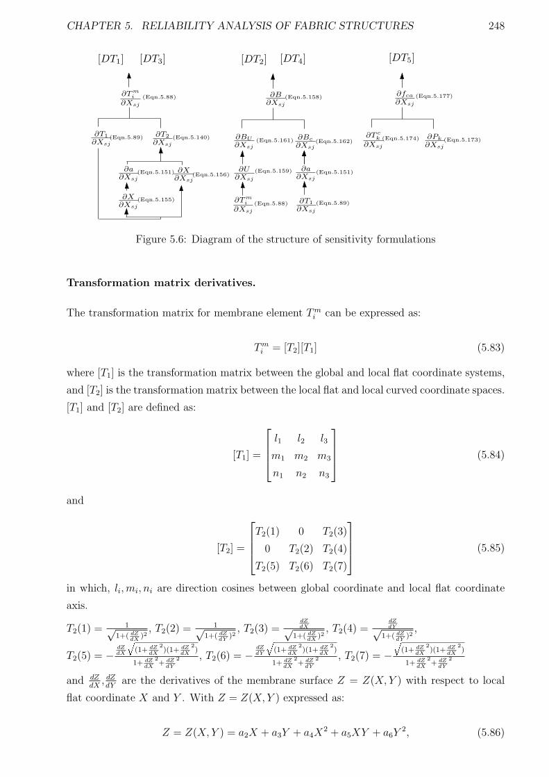
CHAPTER 5. RELIABILITY ANALYSIS OF FABRIC STRUCTURES 248
[DT1] [DT3] [DT2] [DT4] [DT5]
∂T1
∂Xsj
∂T2
∂Xsj
∂a∂Xsj
∂X∂Xsj
∂T mi
∂Xsj
∂B∂Xsj
∂BU
∂Xsj
∂Bc
∂Xsj
∂T mi
∂Xsj
∂T1
∂Xsj
∂U∂Xsj
∂a∂Xsj
∂fca
∂Xsj
∂T ck
∂Xsj
∂Pk
∂Xsj
∂X∂Xsj
(Eqn.5.89) (Eqn.5.140)
(Eqn.5.151)
(Eqn.5.155)
(Eqn.5.156)
(Eqn.5.161) (Eqn.5.162)
(Eqn.5.159)
(Eqn.5.88)
(Eqn.5.88) (Eqn.5.89)
(Eqn.5.158)
(Eqn.5.174)
(Eqn.5.177)
(Eqn.5.173)
(Eqn.5.151)
Figure 5.6: Diagram of the structure of sensitivity formulations
Transformation matrix derivatives.
The transformation matrix for membrane element Tmi can be expressed as:
Tmi = [T2][T1] (5.83)
where [T1] is the transformation matrix between the global and local flat coordinate systems,
and [T2] is the transformation matrix between the local flat and local curved coordinate spaces.
[T1] and [T2] are defined as:
[T1] =
l1 l2 l3
m1 m2 m3
n1 n2 n3
(5.84)
and
[T2] =
T2(1) 0 T2(3)
0 T2(2) T2(4)
T2(5) T2(6) T2(7)
(5.85)
in which, li,mi, ni are direction cosines between global coordinate and local flat coordinate
axis.
T2(1) = 1√1+( dZ
dX)2
, T2(2) = 1√1+( dZ
dY)2
, T2(3) =dZdX√
1+( dZdX
)2, T2(4) =
dZdY√
1+( dZdY
)2,
T2(5) = −dZdX
q(1+ dZ
dX
2)(1+ dZ
dX
2)
1+ dZdX
2+ dZ
dY
2 , T2(6) = −dZdY
q(1+ dZ
dX
2)(1+ dZ
dX
2)
1+ dZdX
2+ dZ
dY
2 , T2(7) = −q
(1+ dZdX
2)(1+ dZ
dX
2)
1+ dZdX
2+ dZ
dY
2
and dZdX
, dZdY
are the derivatives of the membrane surface Z = Z(X,Y ) with respect to local
flat coordinate X and Y . With Z = Z(X,Y ) expressed as:
Z = Z(X,Y ) = a2X + a3Y + a4X2 + a5XY + a6Y
2, (5.86)
CHAPTER 5. RELIABILITY ANALYSIS OF FABRIC STRUCTURES 249
the derivative of Tmi is:
∂Tmi
∂Xsj
=∂[T2]
∂Xsj
[T1] + [T2]∂[T1]
∂Xsj
(5.87)
The derivative of [T1]
Differentiating Eqn. 5.84 with respect to Xsj, we obtain
∂[T1]
∂Xsj
=
∂l1∂Xsj
∂l2∂Xsj
∂l3∂Xsj
∂m1
∂Xsj
∂m2
∂Xsj
∂m3
∂Xsj
∂n1
∂Xsj
∂n2
∂Xsj
∂n3
∂Xsj
(5.88)
If the local flat coordinate axe−→X ,
−→Y ,
−→Z are regarded as the vectors in global coordinate system,
−→X = ax
−→i + ay
−→j + az
−→k (5.89)
−→Y = bx
−→i + by
−→j + bz
−→k (5.90)
−→Z = cx
−→i + cy
−→j + cz
−→k (5.91)
and,
l1 =ax
√
a2x + a2
y + a2z
, l2 =ay
√
a2x + a2
y + a2z
, l3 =az
√
a2x + a2
y + a2z
(5.92)
m1 =bx
√
b2x + b2y + b2z, m2 =
by√
b2x + b2y + b2z, m3 =
bz√
b2x + b2y + b2z(5.93)
n1 =cx
√
c2x + c2y + c2z, n2 =
cy√
c2x + c2y + c2z, n3 =
cz√
c2x + c2y + c2z(5.94)
where ax, bx, cx, ay, by, cy, az, bz, cz are the functions of global nodal coordinates, as in:
ax = x2 − x1, , ay = y2 − y1, az = z2 − z1
bx = xp − x1, , by = yp − y1, bz = zp − z1
cx = (y2 − y1)(zp − z1) − (z2 − z1)(yp − y1)
cy = −(x2 − x1)(zp − z1) + (z2 − z1)(xp − x1)
cz = (x2 − x1)(yp − y1) − (y2 − y1)(xp − x1) (5.95)
in which, xi, yi, zi are global nodal coordinates of ith node. xp, yp, zp are the global coordinates
CHAPTER 5. RELIABILITY ANALYSIS OF FABRIC STRUCTURES 250
of a single point p along the local Y axis, and there has:
x2 − x1 y2 − y1 z2 − z1
λ1 λ2 λ3
x3 − x1 y3 − y1 z3 − z1
xp
yp
zp
=
(x2 − x1)x1 + (y2 − y1)y1 + (z2 − z1)z1
λ1x1 + λ2x2 + λ3x3
(x3 − x1)x3 + (y3 − y1)y3 + (z3 − z1)z3
(5.96)
or,
xp
yp
zp
= [Mp]−1Fp (5.97)
where λ1, λ2, λ3 are functions of global nodal coordinates as:
λ1 = (y2 − y1)(z3 − z1) − (z2 − z1)(y3 − y1)
λ2 = −(x2 − x1)(z3 − z1) + (z2 − z1)(x3 − x1)
λ3 = (x2 − x− 1)(y3 − y1) − (y2 − y1)(x3 − x1) (5.98)
Therefore the terms in Eqn. 5.88 can be derived as:
∂l1∂Xsj
=∂( ax√
a2x+a2
y+a2z
)
∂Xsj
=∂ax
∂Xsj
1√
a2x + a2
y + a2z
− ax
2(√
a2x + a2
y + a2z)
3· (2ax
∂ax
∂Xj
+ 2ay∂ay
∂Xsj
+ 2az∂az
∂Xsj
)
(5.99)
If we set B1 = (√
a2x + a2
y + a2z)
3 and A1 = 1√a2
x+a2y+a2
z
, then Eqn.5.99 becomes
∂l1∂Xsj
=∂ax
∂Xsj
A1 −ax
2B1
(2ax∂ax
∂Xsj
+ 2ay∂ay
∂Xsj
+ 2az∂az
∂Xsj
)
=∂(x2 − x1)
∂Xsj
A1 −ax
2B1
(2ax∂(x2 − x1)
∂Xsj
+ 2ay∂(y2 − y1)
∂Xsj
+ 2az∂(z2 − z1)
∂Xsj
)
= (a2
x
B1
− A)∂x1
∂Xsj
+axay
B1
∂y1
∂Xsj
+axaz
B1
∂z1
∂Xsj
− (a2
x
B− A1)
∂x2
∂Xsj
− axay
B1
∂y2
∂Xsj
− axaz
B1
∂z2
∂Xsj
= (a2
x
B1
− A)∂u1
∂Xsj
+axay
B1
∂v1
∂Xsj
+axaz
B1
∂w1
∂Xsj
− (a2
x
B− A1)
∂u2
∂Xsj
− axay
B1
∂v2
∂Xsj
− axaz
B1
∂w2
∂Xsj
(5.100)
Similarly,
CHAPTER 5. RELIABILITY ANALYSIS OF FABRIC STRUCTURES 251
∂l2∂Xsj
=axay
B1
∂u1
∂Xsj
+ (a2
y
B1
− A1)∂v1
∂Xsj
+ayaz
B1
∂w1
∂Xsj
− axay
B1
∂u2
∂Xsj
− (a2
y
B1
− A1)∂v2
∂Xsj
− ayaz
B1
∂w2
∂Xsj
(5.101)
∂l3∂Xsj
=axaz
B1
∂u1
∂Xsj
+ayaz
B1
∂v1
∂Xsj
+ (a2
z
B1
− A1)∂w1
∂Xsj
− axaz
B1
∂u2
∂Xsj
− ayaz
B1
∂v2
∂Xsj
− (a2
z
B1
− A1)∂w2
∂Xsj
(5.102)
Writing Eqn.5.100, 5.101 and 5.102 together, we get:
∂l1∂Xsj
∂l2∂Xsj
∂l3∂Xsj
=
a2x
B1− A1
axay
B1
axaz
B1− a2
x
B1+ A1 −axay
B1
axaz
B1
axay
B1
a2y
B1− A1
ayaz
B1−axay
B1− a2
y
B1+ A1 −ayaz
B1
axaz
B1
ayaz
B1
a2z
B1− A1 −axaz
B1−ayaz
B1− a2
z
B1+ A1
∂u1
∂Xsj
∂v1
∂Xsj
∂w1
∂Xsj
∂u2
∂Xsj
∂v2
∂Xsj
∂w2
∂Xsj
=
[dl1]
[dl2]
[dl3]
∂u1
∂Xsj
∂v1
∂Xsj
∂w1
∂Xsj
∂u2
∂Xsj
∂v2
∂Xsj
∂w2
∂Xsj
(5.103)
The derivatives of mi are computed as:
∂m1
∂Xsj
=∂( bx√
b2x+b2y+b2z)
∂Xsj
=∂bx∂Xsj
A2 −bx2B
(2bx∂bx∂Xsj
+ 2by∂by∂Xsj
+ 2bz∂bz∂Xsj
)
=∂(xp − x1)
∂Xsj
A2 −bx2B
(2bx∂(xp − x1)
∂Xsj
+ 2by∂(yp − y1)
∂Xsj
+ 2bz∂(zp − z1)
∂Xsj
)
(5.104)
where B2 = (√
b2x + b2y + b2z)3 and A2 = 1√
b2x+b2y+b2z
Similarly,
∂m2
∂Xsj
=∂(yp − y1)
∂Xsj
A2 −by2B
(2bx∂(xp − x1)
∂Xsj
+ 2by∂(yp − y1)
∂Xsj
+ 2bz∂(zp − z1)
∂Xsj
)
(5.105)
CHAPTER 5. RELIABILITY ANALYSIS OF FABRIC STRUCTURES 252
∂m3
∂Xsj
=∂(zp − z1)
∂Xsj
A2 −bz2B
(2bx∂(xp − x1)
∂Xsj
+ 2by∂(yp − y1)
∂Xsj
+ 2bz∂(zp − z1)
∂Xsj
)
(5.106)
The derivatives of xp, yp, zp can be computed by differentiating Eqn. 5.97:
∂xp
∂Xsj
∂yp
∂Xsj
∂zp
∂Xsj
=∂[Mp]
−1
∂Xsj
Fp + [M ]−1 ∂Fp
∂Xsj
= −[Mp]−1∂[Mp]
∂Xsj
[Mp]−1F + [Mp]
−1 ∂Fp
∂Xsj
= −[Mp]−1∂[Mp]
∂Xsj
xp
yp
zp
+ [Mp]−1 ∂Fp
∂Xsj
(5.107)
From Eqn. 5.96 and 5.97, [Mp] and Fp are defined as,
[Mp] =
x2 − x1 y2 − y1 z2 − z1
λ1 λ2 λ3
x3 − x1 y3 − y1 z3 − z1
(5.108)
Fp =
(x2 − x1)x1 + (y2 − y1)y1 + (z2 − z1)z1
λ1x1 + λ2x2 + λ3x3
(x3 − x1)x3 + (y3 − y1)y3 + (z3 − z1)z3
(5.109)
Therefore, the derivative of [Mp] is,
∂[Mp]
∂Xsj
=
∂x2
∂Xsj− ∂x1
∂Xsj
∂y2
∂Xsj− ∂y1
∂Xsj
∂z2
∂Xsj− ∂z1
∂Xsj
∂λ1
∂Xsj
∂λ2
∂Xsj
∂λ3
∂Xsj
∂x3
∂Xsj− ∂x1
∂Xsj
∂y3
∂Xsj− ∂y1
∂Xsj
∂z3
∂Xsj− ∂z1
∂Xsj
=
∂u2
∂Xsj− ∂u1
∂Xsj
∂v2
∂Xsj− ∂v1
∂Xsj
∂w2
∂Xsj− ∂w1
∂Xsj
∂λ1
∂Xsj
∂λ2
∂Xsj
∂λ3
∂Xsj
∂u3
∂Xsj− ∂u1
∂Xsj
∂v3
∂Xsj− ∂v1
∂Xsj
∂w3
∂Xsj− ∂w1
∂Xsj
(5.110)
and the derivative of Fp is,
CHAPTER 5. RELIABILITY ANALYSIS OF FABRIC STRUCTURES 253
∂Fp∂Xsj
=
∂x1
∂Xsj(x2 − x1) + x1(
∂x2
∂Xsj− ∂x1
∂Xsj) + ∂y1
∂Xsj(y2 − y1) + y1(
∂y2
∂Xsj− ∂y1
∂Xsj) + ∂z1
∂Xsj(z2 − z1)
+z1(∂z2
∂Xsj− ∂z1
∂Xsj)
∂λ1
∂Xsjx1 + λ1
∂x1
∂Xsj+ ∂λ2
∂Xsjy1 + λ2
∂y1
∂Xsj+ ∂λ3
∂Xsjz1 + λ3
∂z1
∂Xsj
∂x3
∂Xsj(x3 − x1) + x3(
∂x3
∂Xsj− ∂x1
∂Xsj) + ∂y3
∂Xsj(y3 − y1) + y3(
∂y3
∂Xsj− ∂y1
∂Xsj) + ∂z3
∂Xsj(z3 − z1)
+z3(∂z3
∂Xsj− ∂z1
∂Xsj)
=
∂u1
∂Xsj(x2 − x1) + x1(
∂u2
∂Xsj− ∂u1
∂Xsj) + ∂v1
∂Xsj(y2 − y1) + y1(
∂v2
∂Xsj− ∂v1
∂Xsj) + ∂w1
∂Xsj(z2 − z1)
+z1(∂w2
∂Xsj− ∂w1
∂Xsj)
∂λ1
∂Xsjx1 + λ1
∂u1
∂Xsj+ ∂λ2
∂Xsjy1 + λ2
∂v1
∂Xsj+ ∂λ3
∂Xsjz1 + λ3
∂w1
∂Xsj
∂u3
∂Xsj(x3 − x1) + x3(
∂u3
∂Xsj− ∂u1
∂Xsj) + ∂v3
∂Xsj(y3 − y1) + y3(
∂v3
∂Xsj− ∂v1
∂Xsj) + ∂w3
∂Xsj(z3 − z1)
+z3(∂w3
∂Xsj− ∂w1
∂Xsj)
(5.111)
Differentiating Eqn.5.98, we can obtain the derivaties of λ1, λ2, λ3, as in,
∂λ1
∂Xsj
= (y2 − y1)(∂z3
∂Xsj
− ∂z1
∂Xsj
) + (∂y2
∂Xsj
− ∂y1
∂Xsj
)(z3 − z1) − (z2 − z1)(∂y3
∂Xsj
− ∂y1
∂Xsj
)
−(∂z2
∂Xsj
− ∂z1
∂Xsj
)(y3 − y1)
=∂y1
∂Xsj
(z2 − z3) +∂y2
∂Xsj
(z3 − z1) +∂y3
∂Xsj
(z1 − z2) +∂z1
∂Xsj
(y3 − y2)
+∂z2
∂Xsj
(y1 − z3) +∂z3
∂Xsj
(y2 − y1)
=∂v1
∂Xsj
(z2 − z3) +∂v2
∂Xsj
(z3 − z1) +∂v3
∂u(z1 − z2) +
∂w1
∂Xsj
(y3 − y2)
+∂w2
∂Xsj
(y1 − z3) +∂w3
∂Xsj
(y2 − y1) (5.112)
∂λ2
∂Xsj
=∂u1
∂Xsj
(z3 − z2) +∂u2
∂Xsj
(z1 − z3) +∂u3
∂Xsj
(z2 − z1) +∂w1
∂Xsj
(x2 − x3)
+∂w2
∂Xsj
(x3 − x1) +∂w3
∂Xsj
(x1 − x2) (5.113)
∂λ3
∂Xsj
=∂u1
∂Xsj
(y2 − y3) +∂u2
∂Xsj
(y3 − y1) +∂u3
∂Xsj
(y1 − y2) +∂v1
∂Xsj
(x3 − x2)
+∂v2
∂Xsj
(x1 − x3) +∂v3
∂Xsj
(x2 − x1) (5.114)
CHAPTER 5. RELIABILITY ANALYSIS OF FABRIC STRUCTURES 254
If we denote,
∂[Mp]
∂Xsj
xp
yp
zp
= [MP ] (5.115)
then [MP ] is a 3 × 1 matrix, and
[MP ](1,1) = (∂u2
∂Xsj
− ∂u1
∂Xsj
)xp + (∂v2
∂Xsj
− ∂v1
∂Xsj
)yp + (∂w2
∂Xsj
− ∂w1
∂Xsj
)zp (5.116)
[MP ](2,1) =∂λ1
∂Xsj
xp +∂λ2
∂Xsj
yp +∂λ3
∂Xsj
zp
=∂u1
∂Xsj
[(z3 − z2)yp + (y2 − y3)zp] +∂u2
∂Xsj
[(z1 − z3)yp + (y3 − y1)zp]
+∂u3
∂Xsj
[(z2 − z1)yp + (x2 − x1)zp] +∂v1
∂Xsj
[(z2 − z3)xp + (x3 − x2)zp]
+∂v2
∂Xsj
[(z3 − z1)xp + (x1 − x3)zp] +∂v3
∂Xsj
[(z2 − z1)xp + (x2 − x1)zp]
+∂w1
∂Xsj
[(y3 − y2)xp + (z3 − z2)yp] +∂w2
∂Xsj
[(y1 − y3)xp + (x3 − x1)yp]
+∂w3
∂Xsj
[(y2 − y1)xp + (x1 − x2)yp] (5.117)
[MP ](3,1) = (∂u3
∂Xsj
− ∂u1
∂Xsj
)xp + (∂v3
∂Xsj
− ∂v1
∂Xsj
)yp + (∂w3
∂Xsj
− ∂w1
∂Xsj
)zp (5.118)
Extracting the terms of the derivatives of nodal displacements from [MP ], we get
[MP ] = [DM ]
∂u1
∂Xsj
∂v1
∂Xsj
∂w1
∂Xsj
∂u2
∂Xsj
∂v2
∂Xsj
∂w2
∂Xsj
∂u3
∂Xsj
∂v3
∂Xsj
∂w3
∂Xsj
(5.119)
[DM ] is a 3 × 9 matrix, whose non-zero terms are,
DM(1,1) = −xp, DM(1,2) = −yp, DM(1,3) = −zp
DM(1,4) = xp, DM(1,5) = yp, DM(1,6) = zp
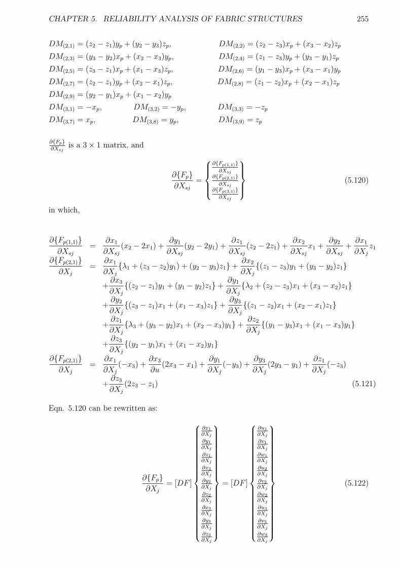
CHAPTER 5. RELIABILITY ANALYSIS OF FABRIC STRUCTURES 255
DM(2,1) = (z2 − z1)yp + (y2 − y3)zp, DM(2,2) = (z2 − z3)xp + (x3 − x2)zp
DM(2,3) = (y3 − y2)xp + (x2 − x3)yp, DM(2,4) = (z1 − z3)yp + (y3 − y1)zp
DM(2,5) = (z3 − z1)xp + (x1 − x3)zp, DM(2,6) = (y1 − y3)xp + (x3 − x1)yp
DM(2,7) = (z2 − z1)yp + (x2 − x1)zp, DM(2,8) = (z1 − z2)xp + (x2 − x1)zp
DM(2,9) = (y2 − y1)xp + (x1 − x2)yp
DM(3,1) = −xp, DM(3,2) = −yp, DM(3,3) = −zp
DM(3,7) = xp, DM(3,8) = yp, DM(3,9) = zp
∂Fp∂Xsj
is a 3 × 1 matrix, and
∂Fp∂Xsj
=
∂Fp(1,1)∂Xsj
∂Fp(2,1)∂Xsj
∂Fp(3,1)∂Xsj
(5.120)
in which,
∂Fp(1,1)∂Xsj
=∂x1
∂Xsj
(x2 − 2x1) +∂y1
∂Xsj
(y2 − 2y1) +∂z1
∂Xsj
(z2 − 2z1) +∂x2
∂Xsj
x1 +∂y2
∂Xsj
+∂x1
∂Xj
z1
∂Fp(2,1)∂Xj
=∂x1
∂Xj
λ1 + (z3 − z2)y1) + (y2 − y3)z1 +∂x2
∂Xj
(z1 − z3)y1 + (y3 − y2)z1
+∂x3
∂Xj
(z2 − z1)y1 + (y1 − y2)z1 +∂y1
∂Xj
λ2 + (z2 − z3)x1 + (x3 − x2)z1
+∂y2
∂Xj
(z3 − z1)x1 + (x1 − x3)z1 +∂y3
∂Xj
(z1 − z2)x1 + (x2 − x1)z1
+∂z1
∂Xj
λ3 + (y3 − y2)x1 + (x2 − x3)y1 +∂z2
∂Xj
(y1 − y3)x1 + (x1 − x3)y1
+∂z3
∂Xj
(y2 − y1)x1 + (x1 − x2)y1∂Fp(2,1)∂Xj
=∂x1
∂Xj
(−x3) +∂x3
∂u(2x3 − x1) +
∂y1
∂Xj
(−y3) +∂y3
∂Xj
(2y3 − y1) +∂z1
∂Xj
(−z3)
+∂z3
∂Xj
(2z3 − z1) (5.121)
Eqn. 5.120 can be rewritten as:
∂Fp∂Xj
= [DF ]
∂x1
∂Xj
∂y1
∂Xj
∂z1
∂Xj
∂x2
∂Xj
∂y2
∂Xj
∂z2
∂Xj
∂x3
∂Xj
∂y3
∂Xj
∂z3
∂Xj
= [DF ]
∂u1
∂Xj
∂v1
∂Xj
∂w1
∂Xj
∂u2
∂Xj
∂v2
∂Xj
∂w2
∂Xj
∂u3
∂Xj
∂v3
∂Xj
∂w3
∂Xj
(5.122)
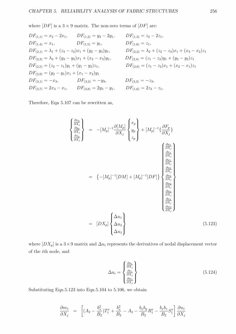
CHAPTER 5. RELIABILITY ANALYSIS OF FABRIC STRUCTURES 256
where [DF ] is a 3 × 9 matrix. The non-zero terms of [DF ] are:
DF(1,1) = x2 − 2x1, DF(1,2) = y2 − 2y1, DF(1,3) = z2 − 2z1,
DF(1,4) = x1, DF(1,5) = y1, DF(1,6) = z1,
DF(2,1) = λ1 + (z3 − z2)x1 + (y2 − y3)y1, DF(2,2) = λ2 + (z2 − z3)x1 + (x3 − x2)z1
DF(2,3) = λ3 + (y3 − y2)x1 + (x2 − x3)y1, DF(2,4) = (z1 − z3)y1 + (y3 − y2)z1
DF(2,5) = (z2 − z1)y1 + (y1 − y2)z1, DF(2,8) = (z1 − z2)x1 + (x2 − x1)z1
DF(2,9) = (y2 − y1)x1 + (x1 − x2)y1
DF(3,1) = −x3, DF(3,2) = −y3, DF(3,3) = −z3,
DF(3,7) = 2x3 − x1, DF(3,8) = 2y3 − y1, DF(1,6) = 2z3 − z1,
Therefore, Eqn 5.107 can be rewritten as,
∂xp
∂Xj
∂yp
∂Xj
∂zp
∂Xj
= −[Mp]−1∂[Mp]
∂Xj
xp
yp
zp
+ [Mp]−1 ∂Fp
∂Xj
=
−[Mp]−1[DM ] + [Mp]
−1[DF ]
∂u1
∂Xj
∂v1
∂Xj
∂w1
∂Xj
∂u2
∂Xj
∂v2
∂Xj
∂w2
∂Xj
∂u3
∂Xj
∂v3
∂Xj
∂w3
∂Xj
= [DXp]
∆u1
∆u2
∆u3
(5.123)
where [DXp] is a 3×9 matrix and ∆ui represents the derivatives of nodal displacement vector
of the ith node, and
∆ui =
∂ui
∂Xj
∂vi
∂Xj
∂wi
∂Xj
(5.124)
Substituting Eqn.5.123 into Eqn.5.104 to 5.106, we obtain
∂m1
∂Xj
=
[
(A2 −b2xB2
)T x1 +
b2xB2
− A2 −bxbyB2
Rx1 −
bxbzB2
Sx1
]
∂u1
∂Xj
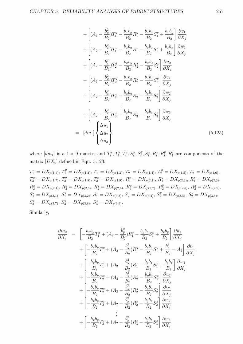
CHAPTER 5. RELIABILITY ANALYSIS OF FABRIC STRUCTURES 257
+
[
(A2 −b2xB2
)T y1 − bxby
B2
Ry1 −
bxbzB2
Sy1 +
bxbyB2
]
∂v1
∂Xj
+
[
(A2 −b2xB2
)T z1 − bxby
B2
Rz1 −
bxbzB2
Sz1 +
bxbzB2
]
∂w1
∂Xj
+
[
(A2 −b2xB2
)T x2 − bxby
B2
Rx2 −
bxbzB2
Sx2
]
∂u2
∂Xj
+
[
(A2 −b2xB2
)T y2 − bxby
B2
Ry2 −
bxbzB2
Sy2
]
∂v2
∂Xj
+
[
(A2 −b2xB2
)T z2 − bxby
B2
Rz2 −
bxbzB2
Sz2
]
∂w2
∂Xj...
+
[
(A2 −b2xB2
)T z3 − bxby
B2
Rz3 −
bxbzB2
Sz3
]
∂w3
∂Xj
= [dm1]
∆u1
∆u2
∆u3
(5.125)
where [dm1] is a 1 × 9 matrix, and T xi , T
yi , T
zi , S
xi , S
yi , S
zi , R
xi , R
yi , R
zi are components of the
matrix [DXp] defined in Eqn. 5.123:
T x1 = DXp(1,1), T
y1 = DXp(1,2), T
z1 = DXp(1,3), T
x2 = DXp(1,4), T
y2 = DXp(1,5), T
z2 = DXp(1,6),
T x3 = DXp(1,7), T
y3 = DXp(1,8), T
z3 = DXp(1,9), R
x1 = DXp(2,1), R
y1 = DXp(2,2), R
z1 = DXp(2,3),
Rx2 = DXp(2,4), R
y2 = DXp(2,5), R
z2 = DXp(2,6), R
x3 = DXp(2,7), R
y2 = DXp(2,8), R
z2 = DXp(2,9),
Sx1 = DXp(3,1), S
y1 = DXp(3,2), S
z1 = DXp(3,3), S
x2 = DXp(3,4), S
y2 = DXp(3,5), S
z2 = DXp(3,6),
Sx3 = DXp(3,7), S
y3 = DXp(3,8), S
z3 = DXp(3,9).
Similarly,
∂m2
∂Xj
=
[
−bxbyB2
T x1 + (A2 −
b2yB2
)Rx1 −
bybzB2
Sx1 +
bxbyB2
]
∂u1
∂Xj
+
[
−bxbyB2
T y1 + (A2 −
b2yB2
)Ry1 −
bybzB2
Sy1 +
b2yB2
− A2
]
∂v1
∂Xj
+
[
−bxbyB2
T z1 + (A2 −
b2yB2
)Rz1 −
bybzB2
Sz1 +
bybzB2
]
∂w1
∂Xj
+
[
−bxbyB2
T x2 + (A2 −
b2yB2
)Rx2 −
bybzB2
Sx2
]
∂u2
∂Xj
+
[
−bxbyB2
T y2 + (A2 −
b2yB2
)Ry2 −
bybzB2
Sy2
]
∂v2
∂Xj
+
[
−bxbyB2
T z2 + (A2 −
b2yB2
)Rz2 −
bybzB2
Sz2
]
∂w2
∂Xj...
+
[
−bxbyB2
T z3 + (A2 −
b2yB2
)Rz3 −
bybzB2
Sz3
]
∂w3
∂Xj
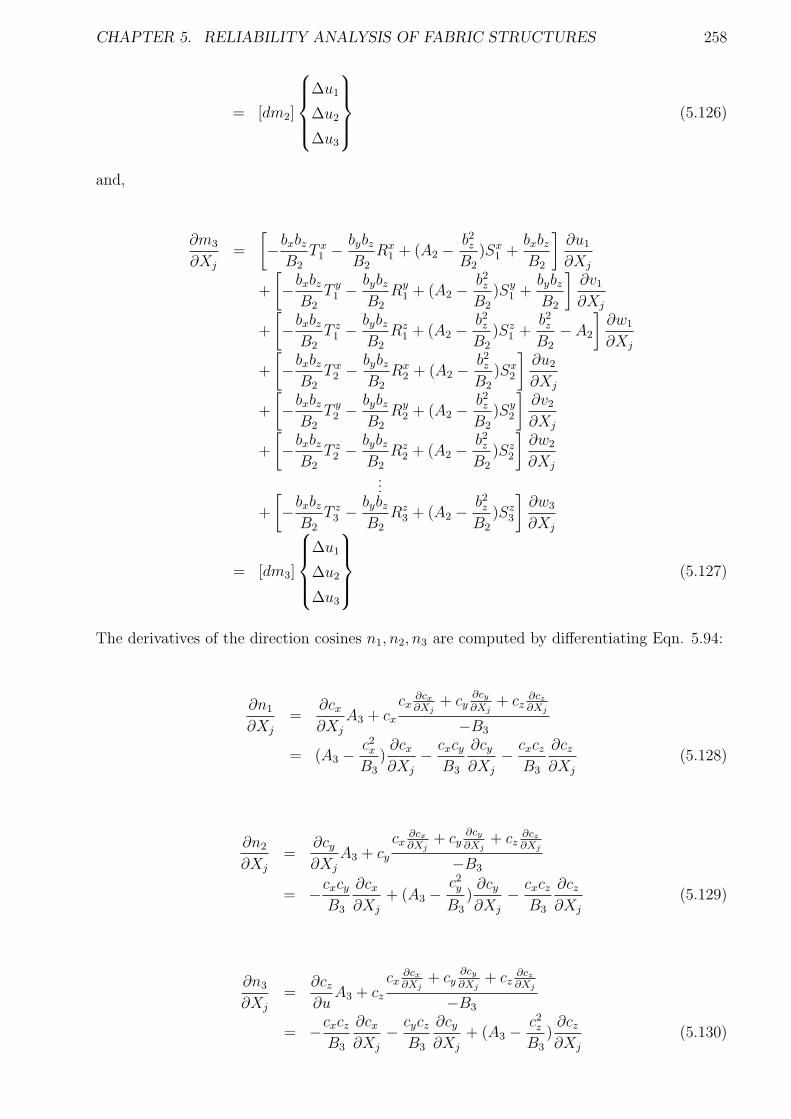
CHAPTER 5. RELIABILITY ANALYSIS OF FABRIC STRUCTURES 258
= [dm2]
∆u1
∆u2
∆u3
(5.126)
and,
∂m3
∂Xj
=
[
−bxbzB2
T x1 − bybz
B2
Rx1 + (A2 −
b2zB2
)Sx1 +
bxbzB2
]
∂u1
∂Xj
+
[
−bxbzB2
T y1 − bybz
B2
Ry1 + (A2 −
b2zB2
)Sy1 +
bybzB2
]
∂v1
∂Xj
+
[
−bxbzB2
T z1 − bybz
B2
Rz1 + (A2 −
b2zB2
)Sz1 +
b2zB2
− A2
]
∂w1
∂Xj
+
[
−bxbzB2
T x2 − bybz
B2
Rx2 + (A2 −
b2zB2
)Sx2
]
∂u2
∂Xj
+
[
−bxbzB2
T y2 − bybz
B2
Ry2 + (A2 −
b2zB2
)Sy2
]
∂v2
∂Xj
+
[
−bxbzB2
T z2 − bybz
B2
Rz2 + (A2 −
b2zB2
)Sz2
]
∂w2
∂Xj...
+
[
−bxbzB2
T z3 − bybz
B2
Rz3 + (A2 −
b2zB2
)Sz3
]
∂w3
∂Xj
= [dm3]
∆u1
∆u2
∆u3
(5.127)
The derivatives of the direction cosines n1, n2, n3 are computed by differentiating Eqn. 5.94:
∂n1
∂Xj
=∂cx∂Xj
A3 + cxcx
∂cx
∂Xj+ cy
∂cy
∂Xj+ cz
∂cz
∂Xj
−B3
= (A3 −c2xB3
)∂cx∂Xj
− cxcyB3
∂cy∂Xj
− cxczB3
∂cz∂Xj
(5.128)
∂n2
∂Xj
=∂cy∂Xj
A3 + cycx
∂cx
∂Xj+ cy
∂cy
∂Xj+ cz
∂cz
∂Xj
−B3
= −cxcyB3
∂cx∂Xj
+ (A3 −c2yB3
)∂cy∂Xj
− cxczB3
∂cz∂Xj
(5.129)
∂n3
∂Xj
=∂cz∂u
A3 + czcx
∂cx
∂Xj+ cy
∂cy
∂Xj+ cz
∂cz
∂Xj
−B3
= −cxczB3
∂cx∂Xj
− cyczB3
∂cy∂Xj
+ (A3 −c2zB3
)∂cz∂Xj
(5.130)
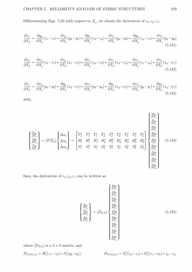
CHAPTER 5. RELIABILITY ANALYSIS OF FABRIC STRUCTURES 259
Differentiating Eqn. 5.95 with respect to Xj, we obtain the derivatives of cx, cy, cz:
∂cx∂Xj
=∂yp
∂Xj
(z1−z2)+∂zp
∂Xj
(y2−y1)+∂y1
∂Xj
(z2−zp)+∂z1
∂Xj
(yp−y2)+∂y2
∂Xj
(zp−z1)+∂z2
∂Xj
(y1−yp)
(5.131)
∂cy∂Xj
=∂xp
∂Xj
(z2−z1)+∂zp
∂Xj
(x1−x2)+∂x1
∂Xj
(zp−z2)+∂z1
∂Xj
(x2−xp)+∂x2
∂Xj
(z1−zp)+∂z2
∂Xj
(xp−x1)
(5.132)
∂cz∂Xj
=∂xp
∂Xj
(y1−y2)+∂yp
∂Xj
(x2−x1)+∂x1
∂Xj
(y2−yp)+∂y1
∂Xj
(xp−x2)+∂x2
∂Xj
(yp−y1)+∂y2
∂Xj
(xp−x1)
(5.133)
with,
∂xp
∂Xj
∂yp
∂Xj
∂zp
∂Xj
= [DXp]
∆u1
∆u2
∆u3
=
T x1 T y
1 T z1 T x
2 T y2 T z
2 T x3 T y
3 T z3
Rx1 Ry
1 Rz1 Rx
2 Ry2 Rz
2 Rx3 Ry
3 Rz3
Sx1 Sy
1 Sz1 Sx
2 Sy2 Sz
2 Sx3 Sy
3 Sz3
∂u1
∂Xj
∂v1
∂Xj
∂w1
∂Xj
∂u2
∂Xj
∂v2
∂Xj
∂w2
∂Xj
∂u3
∂Xj
∂v3
∂Xj
∂w3
∂Xj
(5.134)
then, the derivatives of cx, cy, cz can be written as:
∂cx
∂Xj
∂cy
∂Xj
∂cz
∂Xj
= [DNN ]
∂u1
∂Xj
∂v1
∂Xj
∂w1
∂Xj
∂u2
∂Xj
∂v2
∂Xj
∂w2
∂Xj
∂u3
∂Xj
∂v3
∂Xj
∂w3
∂Xj
(5.135)
where [DNN ] is a 3 × 9 matrix, and
DNN(1,1) = Rx1(z1−z2)+S
x1 (y2−y1), DNN(2,1) = T x
1 (z2−z1)+Sx1 (x1−x2)+zp−z2,
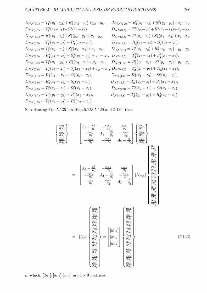
CHAPTER 5. RELIABILITY ANALYSIS OF FABRIC STRUCTURES 260
DNN(3,1) = T x1 (y1−y2)+R
x1(x2−x1)+y2−yp, DNN(1,2) = Ry
1(z1−z2)+Sy1 (y2−y1)+z2−zp,
DNN(2,2) = T y1 (z2−z1)+S
y1 (x1−x2), DNN(3,2) = T y
1 (y2−y1)+Ry1(x2−x1)+xp−x2,
DNN(1,3) = Rz1(z1−z2)+S
z1(y2−y1)+yp−y2, DNN(2,3) = T z
1 (z2−z1)+Sz1(x1−x2)+x2−xp,
DNN(3,3) = T z1 (y1 − y2) +Rz
1(x2 − x1), DNN(1,4) = Rx2(z1 − z2) + Sx
2 (y2 − y1),
DNN(2,4) = T x2 (z2−z1)+S
x2 (x1−x2)+z1−zp, DNN(3,4) = T x
2 (z1−z2)+Rx2(x2−x1)+yp−y1,
DNN(1,5) = Ry2(z1 − z2) + Sy
2 (y2 − y1) + zp − z1, DNN(2,5) = T y2 (z2 − z1) + Sy
2 (x1 − x2),
DNN(3,5) = T y2 (y1−y2)+R
y2(x2−x1)+xp−x1, DNN(1,6) = Rz
2(z1−z2)+Sz1(y2−y1)+y1−yp,
DNN(2,6) = T z2 (z2 − z1) + Sz
2(x1 − x2) + xp − x1, DNN(3,6) = T z2 (y1 − y2) +Rz
2(x2 − x1),
DNN(1,7) = Rx3(z1 − z2) + Sx
3 (y2 − y1), DNN(1,8) = Ry3(z1 − z2) + Sx
3 (y2 − y1),
DNN(1,9) = Rz3(z1 − z2) + Sz
3(y2 − y1), DNN(2,7) = T x3 (z2 − z1) + Sx
3 (x1 − x2),
DNN(2,8) = T y3 (z2 − z1) + Sy
3 (x1 − x2), DNN(2,9) = T z3 (z2 − z1) + Sz
3(x1 − x2),
DNN(3,7) = T x3 (y1 − y2) +Rx
3(x2 − x1), DNN(3,8) = T y3 (y1 − y2) +Ry
3(x2 − x1),
DNN(3,9) = T z3 (y1 − y2) +Rz
3(x2 − x1).
Substituting Eqn.5.135 into Eqn.5.128 5.129 and 5.130, then
∂n1
∂Xj
∂n2
∂Xj
∂n3
∂Xj
=
A3 − c2xB3
− cxcy
B3
cxcz
B3
− cxcy
B3A3 − c2y
B3− cycz
B3
− cxcz
B3− cycz
B3A3 − c2z
B3
∂cx
∂Xj
∂cy
∂Xj
∂cz
∂Xj
=
A3 − c2xB3
− cxcy
B3
cxcz
B3
− cxcy
B3A3 − c2y
B3− cycz
B3
− cxcz
B3− cycz
B3A3 − c2z
B3
[DNN ]
∂u1
∂Xj
∂v1
∂Xj
∂w1
∂Xj
∂u2
∂Xj
∂v2
∂Xj
∂w2
∂Xj
∂u3
∂Xj
∂v3
∂Xj
∂w3
∂Xj
= [DN ]
∂u1
∂Xj
∂v1
∂Xj
∂w1
∂Xj
∂u2
∂Xj
∂v2
∂Xj
∂w2
∂Xj
∂u3
∂Xj
∂v3
∂Xj
∂w3
∂Xj
=
[dn1]
[dn2]
[dn3]
∂u1
∂Xj
∂v1
∂Xj
∂w1
∂Xj
∂u2
∂Xj
∂v2
∂Xj
∂w2
∂Xj
∂u3
∂Xj
∂v3
∂Xj
∂w3
∂Xj
(5.136)
in which, [dn1], [dn2], [dn3] are 1 × 9 matrices.
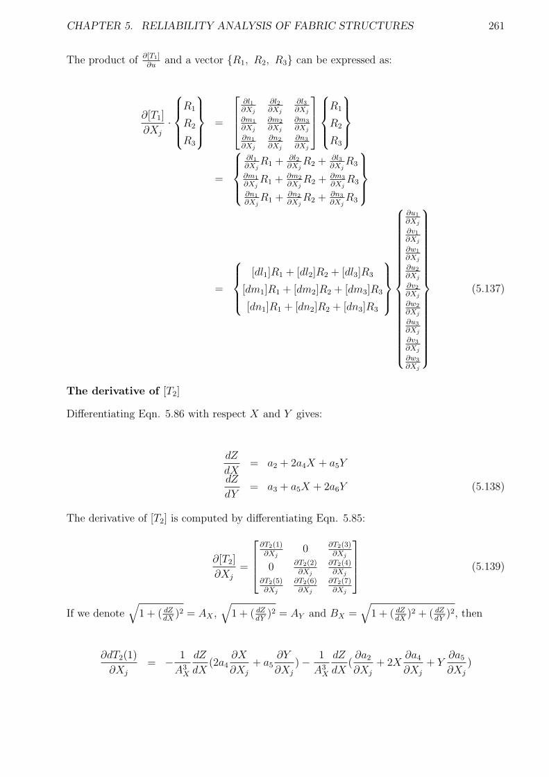
CHAPTER 5. RELIABILITY ANALYSIS OF FABRIC STRUCTURES 261
The product of ∂[T1]∂u
and a vector R1, R2, R3 can be expressed as:
∂[T1]
∂Xj
·
R1
R2
R3
=
∂l1∂Xj
∂l2∂Xj
∂l3∂Xj
∂m1
∂Xj
∂m2
∂Xj
∂m3
∂Xj
∂n1
∂Xj
∂n2
∂Xj
∂n3
∂Xj
R1
R2
R3
=
∂l1∂Xj
R1 + ∂l2∂Xj
R2 + ∂l3∂Xj
R3
∂m1
∂XjR1 + ∂m2
∂XjR2 + ∂m3
∂XjR3
∂n1
∂XjR1 + ∂n2
∂XjR2 + ∂n3
∂XjR3
=
[dl1]R1 + [dl2]R2 + [dl3]R3
[dm1]R1 + [dm2]R2 + [dm3]R3
[dn1]R1 + [dn2]R2 + [dn3]R3
∂u1
∂Xj
∂v1
∂Xj
∂w1
∂Xj
∂u2
∂Xj
∂v2
∂Xj
∂w2
∂Xj
∂u3
∂Xj
∂v3
∂Xj
∂w3
∂Xj
(5.137)
The derivative of [T2]
Differentiating Eqn. 5.86 with respect X and Y gives:
dZ
dX= a2 + 2a4X + a5Y
dZ
dY= a3 + a5X + 2a6Y (5.138)
The derivative of [T2] is computed by differentiating Eqn. 5.85:
∂[T2]
∂Xj
=
∂T2(1)∂Xj
0 ∂T2(3)∂Xj
0 ∂T2(2)∂Xj
∂T2(4)∂Xj
∂T2(5)∂Xj
∂T2(6)∂Xj
∂T2(7)∂Xj
(5.139)
If we denote√
1 + ( dZdX
)2 = AX ,√
1 + ( dZdY
)2 = AY and BX =√
1 + ( dZdX
)2 + ( dZdY
)2, then
∂dT2(1)
∂Xj
= − 1
A3X
dZ
dX(2a4
∂X
∂Xj
+ a5∂Y
∂Xj
) − 1
A3X
dZ
dX(∂a2
∂Xj
+ 2X∂a4
∂Xj
+ Y∂a5
∂Xj
)
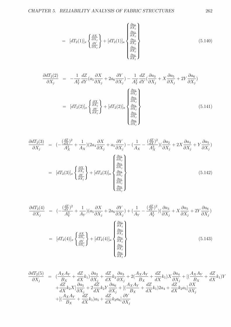
CHAPTER 5. RELIABILITY ANALYSIS OF FABRIC STRUCTURES 262
= [dT2(1)]x
∂X∂Xj
∂Y∂Xj
+ [dT2(1)]a
∂a2
∂Xj
∂a3
∂Xj
∂a4
∂Xj
∂a5
∂Xj
∂a6
∂Xj
(5.140)
∂dT2(2)
∂Xj
= − 1
A3Y
dZ
dY(a5
∂X
∂Xj
+ 2a6∂Y
∂Xj
) − 1
A3Y
dZ
dY(∂a3
∂Xj
+X∂a5
∂Xj
+ 2Y∂a6
∂Xj
)
= [dT2(2)]x
∂X∂Xj
∂Y∂Xj
+ [dT2(2)]a
∂a2
∂Xj
∂a3
∂Xj
∂a4
∂Xj
∂a5
∂Xj
∂a6
∂Xj
(5.141)
∂dT2(3)
∂Xj
= (−( dZdX
)2
A3X
+1
AX
)(2a4∂X
∂Xj
+ a5∂Y
∂Xj
) − (1
AX
− ( dZdX
)2
A3X
)(∂a2
∂Xj
+ 2X∂a4
∂Xj
+ Y∂a5
∂Xj
)
= [dT2(3)]x
∂X∂Xj
∂Y∂Xj
+ [dT2(3)]a
∂a2
∂Xj
∂a3
∂Xj
∂a4
∂Xj
∂a5
∂Xj
∂a6
∂Xj
(5.142)
∂dT2(4)
∂Xj
= (−( dZdY
)2
A3Y
+1
AY
)(a5∂X
∂Xj
+ 2a6∂Y
∂Xj
) + (1
AY
− ( dZdY
)2
A3Y
)(∂a3
∂Xj
+X∂a5
∂Xj
+ 2Y∂a6
∂Xj
)
= [dT2(4)]x
∂X∂Xj
∂Y∂Xj
+ [dT2(4)]a
∂a2
∂Xj
∂a3
∂Xj
∂a4
∂Xj
∂a5
∂Xj
∂a6
∂Xj
(5.143)
∂dT2(5)
∂Xj
= (AXAY
BX
+dZ
dXk1)
∂a2
∂Xj
+dZ
dXk2∂a3
∂Xj
+ 2(AXAY
BX
+dZ
dXk1)X
∂a4
∂Xj
+ [(AXAY
BX
+dZ
dXk1)Y
+dZ
dXk2X]
∂a5
∂Xj
+ 2dZ
dXk2Y
∂a6
∂Xj
+ [(AXAY
BX
+dZ
dXk1)2a4 +
dZ
dXk2a5]
∂X
∂Xj
+[(AXAY
BX
+dZ
dXk1)a5 +
dZ
dXk2a6]
∂Y
∂Xj
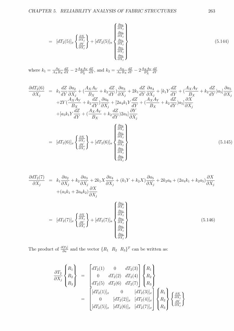
CHAPTER 5. RELIABILITY ANALYSIS OF FABRIC STRUCTURES 263
= [dT2(5)]x
∂X∂Xj
∂Y∂Xj
+ [dT2(5)]a
∂a2
∂Xj
∂a3
∂Xj
∂a4
∂Xj
∂a5
∂Xj
∂a6
∂Xj
(5.144)
where k1 = AY
AXBX
dZdX
− 2AXAY
B2X
dZdX
, and k2 = AX
AY BX
dZdY
− 2AXAY
B2X
dZdY
∂dT2(6)
∂Xj
= k1dZ
dY
∂a2
∂Xj
+ (AXAY
BX
+ k2dZ
dY)∂a3
∂Xj
+ 2k1dZ
dY
∂a4
∂Xj
+ [k1YdZ
dY+ (
AXAY
BX
+ k2dZ
dY)a5]
∂a5
∂Xj
+2Y (AXAY
BX
+ k2dZ
dY)∂a6
∂Xj
+ [2a4k1YdZ
dY+ (
AXAY
BX
+ k2dZ
dY)a5]
∂X
∂Xj
+[a5k1YdZ
dY+ (
AXAY
BX
+ k2dZ
dY)2a5]
∂Y
∂Xj
= [dT2(6)]x
∂X∂Xj
∂Y∂Xj
+ [dT2(6)]a
∂a2
∂Xj
∂a3
∂Xj
∂a4
∂Xj
∂a5
∂Xj
∂a6
∂Xj
(5.145)
∂dT2(7)
∂Xj
= k1∂a2
∂Xj
+ k2∂a3
∂Xj
+ 2k1X∂a4
∂Xj
+ (k1Y + k2X)∂a5
∂Xj
+ 2k2a6 + (2a4k1 + k2a5)∂X
∂Xj
+(a5k1 + 2a6k2)∂X
∂Xj
= [dT2(7)]x
∂X∂Xj
∂Y∂Xj
+ [dT2(7)]a
∂a2
∂Xj
∂a3
∂Xj
∂a4
∂Xj
∂a5
∂Xj
∂a6
∂Xj
(5.146)
The product of ∂[T2]∂u
and the vector R1 R2 R3T can be written as:
∂T2
∂Xj
R1
R2
R3
=
dT2(1) 0 dT2(3)
0 dT2(2) dT2(4)
dT2(5) dT2(6) dT2(7)
R1
R2
R3
=
[dT2(1)]x 0 [dT2(3)]x
0 [dT2(2)]x [dT2(4)]x
[dT2(5)]x [dT2(6)]x [dT2(7)]x
R1
R2
R3
∂X∂Xj
∂Y∂Xj
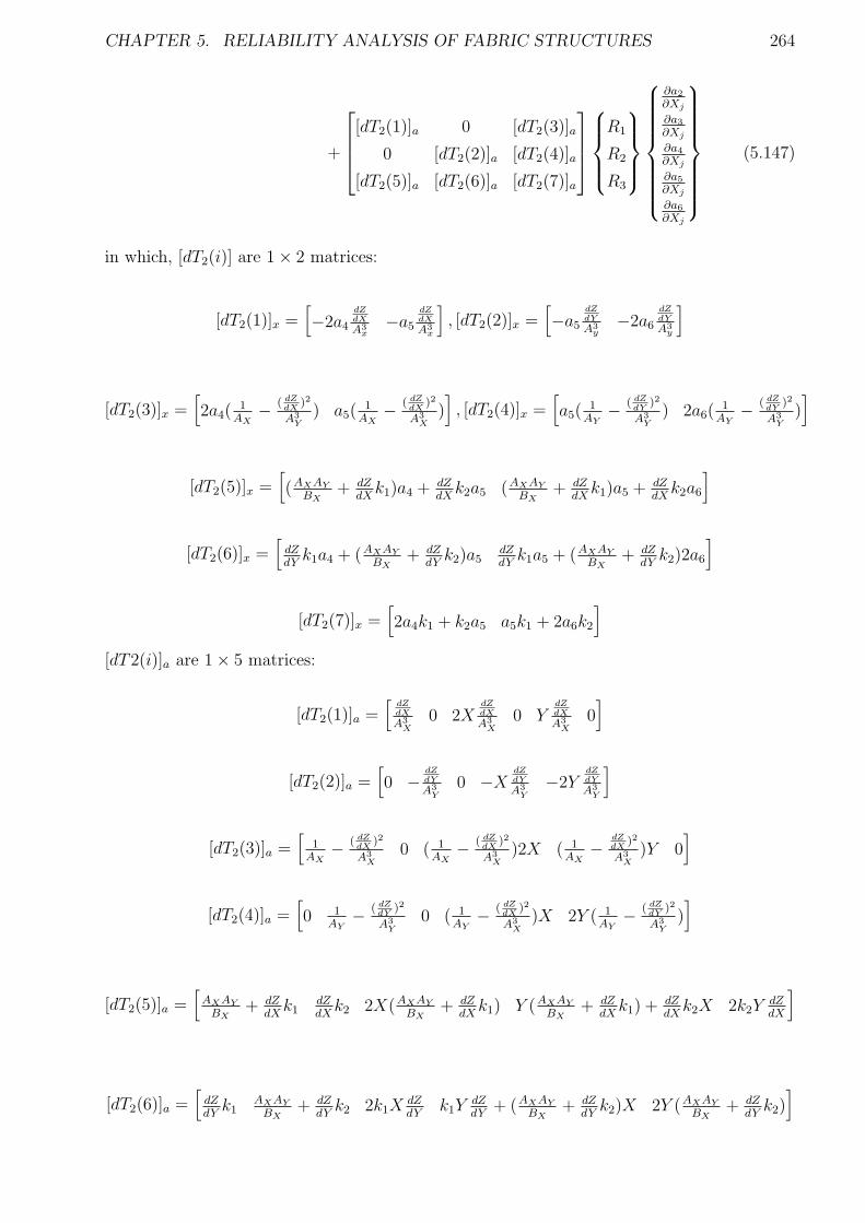
CHAPTER 5. RELIABILITY ANALYSIS OF FABRIC STRUCTURES 264
+
[dT2(1)]a 0 [dT2(3)]a
0 [dT2(2)]a [dT2(4)]a
[dT2(5)]a [dT2(6)]a [dT2(7)]a
R1
R2
R3
∂a2
∂Xj
∂a3
∂Xj
∂a4
∂Xj
∂a5
∂Xj
∂a6
∂Xj
(5.147)
in which, [dT2(i)] are 1 × 2 matrices:
[dT2(1)]x =[
−2a4
dZdX
A3x
−a5
dZdX
A3x
]
, [dT2(2)]x =[
−a5
dZdY
A3y
−2a6
dZdY
A3y
]
[dT2(3)]x =[
2a4(1
AX− ( dZ
dX)2
A3Y
) a5(1
AX− ( dZ
dX)2
A3X
)]
, [dT2(4)]x =[
a5(1
AY− ( dZ
dY)2
A3Y
) 2a6(1
AY− ( dZ
dY)2
A3Y
)]
[dT2(5)]x =[
(AXAY
BX+ dZ
dXk1)a4 + dZ
dXk2a5 (AXAY
BX+ dZ
dXk1)a5 + dZ
dXk2a6
]
[dT2(6)]x =[
dZdYk1a4 + (AXAY
BX+ dZ
dYk2)a5
dZdYk1a5 + (AXAY
BX+ dZ
dYk2)2a6
]
[dT2(7)]x =[
2a4k1 + k2a5 a5k1 + 2a6k2
]
[dT2(i)]a are 1 × 5 matrices:
[dT2(1)]a =[
dZdX
A3X
0 2XdZdX
A3X
0 YdZdX
A3X
0]
[dT2(2)]a =[
0 −dZdY
A3Y
0 −XdZdY
A3Y
−2YdZdY
A3Y
]
[dT2(3)]a =[
1AX
− ( dZdX
)2
A3X
0 ( 1AX
− ( dZdX
)2
A3X
)2X ( 1AX
−dZdX
)2
A3X
)Y 0]
[dT2(4)]a =[
0 1AY
− ( dZdY
)2
A3Y
0 ( 1AY
− ( dZdX
)2
A3X
)X 2Y ( 1AY
− ( dZdY
)2
A3Y
)]
[dT2(5)]a =[
AXAY
BX+ dZ
dXk1
dZdXk2 2X(AXAY
BX+ dZ
dXk1) Y (AXAY
BX+ dZ
dXk1) + dZ
dXk2X 2k2Y
dZdX
]
[dT2(6)]a =[
dZdYk1
AXAY
BX+ dZ
dYk2 2k1X
dZdY
k1YdZdY
+ (AXAY
BX+ dZ
dYk2)X 2Y (AXAY
BX+ dZ
dYk2)]
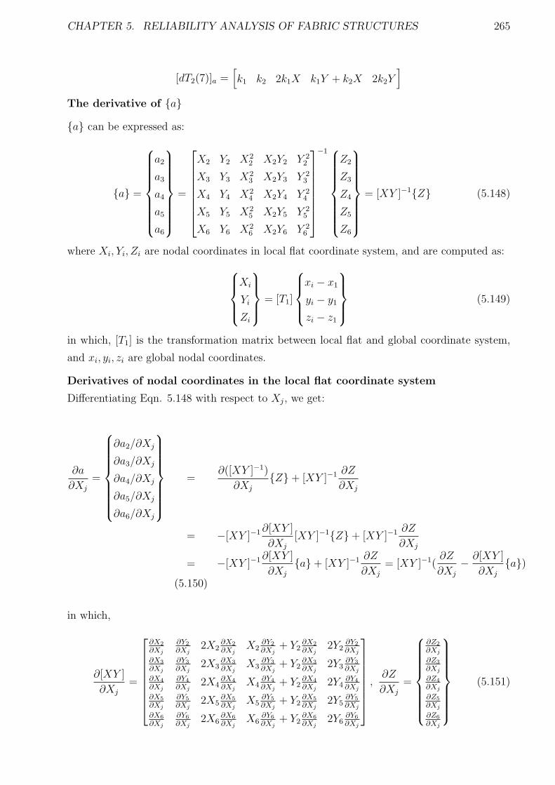
CHAPTER 5. RELIABILITY ANALYSIS OF FABRIC STRUCTURES 265
[dT2(7)]a =[
k1 k2 2k1X k1Y + k2X 2k2Y]
The derivative of a
a can be expressed as:
a =
a2
a3
a4
a5
a6
=
X2 Y2 X22 X2Y2 Y 2
2
X3 Y3 X23 X2Y3 Y 2
3
X4 Y4 X24 X2Y4 Y 2
4
X5 Y5 X25 X2Y5 Y 2
5
X6 Y6 X26 X2Y6 Y 2
6
−1
Z2
Z3
Z4
Z5
Z6
= [XY ]−1Z (5.148)
where Xi, Yi, Zi are nodal coordinates in local flat coordinate system, and are computed as:
Xi
Yi
Zi
= [T1]
xi − x1
yi − y1
zi − z1
(5.149)
in which, [T1] is the transformation matrix between local flat and global coordinate system,
and xi, yi, zi are global nodal coordinates.
Derivatives of nodal coordinates in the local flat coordinate system
Differentiating Eqn. 5.148 with respect to Xj, we get:
∂a
∂Xj
=
∂a2/∂Xj
∂a3/∂Xj
∂a4/∂Xj
∂a5/∂Xj
∂a6/∂Xj
=∂([XY ]−1)
∂Xj
Z + [XY ]−1 ∂Z
∂Xj
= −[XY ]−1∂[XY ]
∂Xj
[XY ]−1Z + [XY ]−1 ∂Z
∂Xj
= −[XY ]−1∂[XY ]
∂Xj
a + [XY ]−1 ∂Z
∂Xj
= [XY ]−1(∂Z
∂Xj
− ∂[XY ]
∂Xj
a)(5.150)
in which,
∂[XY ]
∂Xj
=
∂X2
∂Xj
∂Y2
∂Xj2X2
∂X2
∂XjX2
∂Y2
∂Xj+ Y2
∂X2
∂Xj2Y2
∂Y2
∂Xj
∂X3
∂Xj
∂Y3
∂Xj2X3
∂X3
∂XjX3
∂Y3
∂Xj+ Y2
∂X3
∂Xj2Y3
∂Y3
∂Xj
∂X4
∂Xj
∂Y4
∂Xj2X4
∂X4
∂XjX4
∂Y4
∂Xj+ Y2
∂X4
∂Xj2Y4
∂Y4
∂Xj
∂X5
∂Xj
∂Y5
∂Xj2X5
∂X5
∂XjX5
∂Y5
∂Xj+ Y2
∂X5
∂Xj2Y5
∂Y5
∂Xj
∂X6
∂Xj
∂Y6
∂Xj2X6
∂X6
∂XjX6
∂Y6
∂Xj+ Y2
∂X6
∂Xj2Y6
∂Y6
∂Xj
,∂Z
∂Xj
=
∂Z2
∂Xj
∂Z3
∂Xj
∂Z4
∂Xj
∂Z5
∂Xj
∂Z6
∂Xj
(5.151)
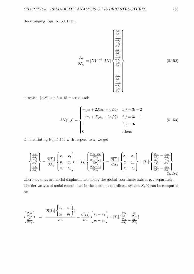
CHAPTER 5. RELIABILITY ANALYSIS OF FABRIC STRUCTURES 266
Re-arranging Eqn. 5.150, then:
∂a
∂Xj
= [XY ]−1[AN ]
∂X2
∂Xj
∂Y2
∂Xj
∂Z2
∂Xj
∂X3
∂Xj
∂Y3
∂Xj
∂Z3
∂Xj
...∂X6
∂Xj
∂Y6
∂Xj
∂Z6
∂Xj
(5.152)
in which, [AN ] is a 5 × 15 matrix, and:
AN(i, j) =
−(a2 + 2Xia4 + a5Yi) if j = 3i− 2
−(a3 +Xia5 + 2a6Yi) if j = 3i− 1
1 if j = 3i
0 others
(5.153)
Differentiating Eqn.5.149 with respect to u, we get
∂Xi
∂Xj
∂Yi
∂Xj
∂Zi
∂Xj
=∂[T1]
∂Xj
xi − x1
yi − y1
zi − z1
+ [T1]
∂(xi−x1)∂Xj
∂(yi−y1)∂Xj
∂(zi−z1)∂Xj
=∂[T1]
∂Xj
xi − x1
yi − y1
zi − z1
+ [T1]
∂ui
∂Xj− ∂u1
∂Xj
∂vi
∂Xj− ∂v1
∂Xj
∂wi
∂Xj− ∂w1
∂Xj
(5.154)
where ui, vi, wi are nodal displacements along the global coordinate axis x, y, z separately.
The derivatives of nodal coordinates in the local flat coordinate system Xi Yi can be computed
as:
∂Xi
∂Xj
∂Yi
∂Xj
=
∂([T1]
xi − x1
yi − y1
)
∂u=∂[T1]
∂u
xi − x1
yi − y1
+ [T1]∂xi
∂Xj− ∂x1
∂Xj
∂yi
∂Xj− ∂y1
∂Xj
CHAPTER 5. RELIABILITY ANALYSIS OF FABRIC STRUCTURES 267
=
[
[dl1](xi − x1) + [dl2](yi − y1)
[dm1](xi − x1) + [dm2](yi − y1)
]
∂u1
∂Xj
∂v1
∂Xj
∂w1
∂Xj
∂u2
∂Xj
∂v2
∂Xj
∂w2
∂Xj
∂u3
∂Xj
∂v3
∂Xj
∂w3
∂Xj
+
[
l1 l2
m1 m2
]
∂ui
∂Xj
∂vi
∂Xj
+
[
l1 l2
m1 m2
]
∂u1
∂Xj
∂v2
∂Xj
(5.155)
The derivative of B matrix
The B matrix of the six node triangle element is a function of the local displacement of element
nodal and element curvatures, which can be expressed as:
B = BU +Bc (5.156)
in which, BU is functioned of local displacements U , and Bc is functioned of element curvatures
(KX ,KY and KXY ). Thus,
dB =∂B
∂Xj
=∂BU
∂Xj
+∂Bc
∂Xj
=∂BU
∂U
∂U
∂Xj
+∂Bc
∂a
∂a
∂Xj
(5.157)
Differentiating Eqn. 5.59 to obtain:
∂U
∂Xj
=∂(Tm
i u)
∂Xj
=∂Tm
i
∂Xj
u+ Tmi
∂u
∂Xj
(5.158)
The derivative of B matrix can be written as:
∂B
∂Xj
=∂BU
∂Xj
+∂Bc
∂Xj
(5.159)
For each six node triangle element, BU and Bc are 3× 18 matrices as same as B matrix, and
the derivatives of BU and Bc can be shown as:
∂BU
∂Xj
=
∂BU (1,1)∂Xj
∂BU (1,2)∂Xj
· · · ∂BU (1,18)∂Xj
∂BU (2,1)∂Xj
∂BU (2,2)∂Xj
· · · ∂BU (2,18)∂Xj
∂BU (3,1)∂Xj
∂BU (3,2)∂Xj
· · · ∂BU (3,18)∂Xj
(5.160)
∂Bc
∂Xj
=
∂Bc(1,1)∂Xj
∂Bc(1,2)∂Xj
· · · ∂Bc(1,18)∂Xj
∂Bc(2,1∂Xj
∂Bc(2,2)∂Xj
· · · ∂Bc(2,18)∂Xj
∂Bc(3,1)∂Xj
∂Bc(3,2)∂Xj
· · · ∂Bc(3,18)∂Xj
(5.161)
CHAPTER 5. RELIABILITY ANALYSIS OF FABRIC STRUCTURES 268
where BU(i, j) and Bc(i, j) are the terms of BU and Bc respectively as detailed in Appendix
C.2. Eqn.5.160 and 5.161 can be rewritten as:
∂BU(i, j)
∂u= [dBu(i, j)]
∂U1
∂Xj
∂V1
∂Xj
∂W1
∂Xj
∂U2
∂Xj
∂V2
∂Xj
∂W2
∂Xj
...∂U6
∂Xj
∂V6
∂Xj
∂W6
∂Xj
(5.162)
and
∂Bc(i, j)
∂Xj
= [dBc(i, j)]
∂U1
∂Xj
∂V1
∂Xj
∂W1
∂Xj
∂U2
∂Xj
∂V2
∂Xj
∂W2
∂Xj
...∂U6
∂Xj
∂V6
∂Xj
∂W6
∂Xj
(5.163)
where, [dBU(i, j)] and [dBc(i, j)] are 1 × 18 matrices.
Therefore, the product of ∂BU
∂Xjand R =
R1 R2 · · · R18
T
can be rewritten as:
∂BU
∂Xj
R =
∂BU (1,1)∂Xj
∂BU (1,2)∂Xj
· · · ∂BU (1,18)∂Xj
∂BU (2,1)∂Xj
∂BU (2,2)∂Xj
· · · ∂BU (2,18)∂Xj
∂BU (3,1)∂Xj
∂BU (3,2)∂Xj
· · · ∂BU (3,18)∂Xj
R1
R2
...
R18
CHAPTER 5. RELIABILITY ANALYSIS OF FABRIC STRUCTURES 269
=
[dBu(1, 1)]R1 + [dBu(1, 2)]R2 + · · · + [dBu(1, 18)]R18
[dBu(2, 1)]R1 + [dBu(2, 2)]R2 + · · · + [dBu(2, 18)]R18
[dBu(2, 1)]R1 + [dBu(2, 2)]R2 + · · · + [dBu(3, 18)]R18
∂U1
∂Xj
∂V1
∂Xj
∂W1
∂Xj
∂U2
∂Xj
∂V2
∂Xj
∂W2
∂Xj
...∂U6
∂Xj
∂V6
∂Xj
∂W6
∂Xj
(5.164)
While
Ui
Vi
Wi
= Tmi
ui
vi
wi
(5.165)
Therefore,
∂Ui
∂Xj
∂Vi
∂Xj
∂Wi
∂Xj
=∂Tm
i
∂Xj
ui
vi
wi
+ Tmj
∂ui
∂Xj
∂vi
∂Xj
∂wi
∂Xj
(5.166)
Cable reaction force derivatives
In the global coordinate space, the reaction forces from cable elements can be expressed as:
fca = T ckPk (5.167)
in which, fca is the element force vector. T ck is a transformation matrix between local and
global coordinate system, and Pk is the cable force along the cable axis,
Pk = P0 +EA
L∆ = P0 +
EA
L0
(L− L0) (5.168)
where P0 is the pretension in the cable element, and ∆ denotes the elastic extension of the
cable. EAL0
represents the elastic modulus of the element, and L and L0 are the current and
initial length. If in the initial configuration the nodal coordinates of the cable element are
P1(x1, y1, z1) and P2(x2, y1, z1 and the nodal displacements for two nodes are u1, v1, w1 and
u2, v2, w2 respectively, then:
∆ = L− L0
CHAPTER 5. RELIABILITY ANALYSIS OF FABRIC STRUCTURES 270
=√
(x2 − x1 + u2 − u1)2 + (y2 − y1 + v2 − v1)2 + (z2 − z1 + w2 − w1)2
−√
(x2 − x1)2 + (y2 − y1)2 + (z2 − z1)2
=2(x2 − x1)(u2 − u1) + (u2 − u1)
2 + 2(y2 − y1)(v2 − v1) + (v2 − v1)2
L+ L0
+2(z2 − z1)(w2 − w1) + (w2 − w1)
2
L+ L0
(5.169)
The transformation matrix T ck in the deformed configuration can be written as:
T ck =
1
L
−(x2 − x1 + u2 − u1)
−(y2 − y1 + v2 − v1)
−(z2 − z1 + w2 − w1)
x2 − x1 + u2 − u1
y2 − y1 + v2 − v1
z2 − z1 + w2 − w1
(5.170)
Differentiating Eqn.5.167 with respect to u gives
∂fca
∂Xj
=∂T c
k
∂Xj
Pk + T ck
∂Pk
∂Xj
(5.171)
The derivative of the cable force can be derived by differentiating Eqn.5.168:
∂Pk
∂Xj
=EA
L0
∂∆
∂Xj
=EA
L0(L+ L0)[2(x2 − x1)(
∂u2
∂Xj
− ∂u1
∂Xj
) + 2(u2 − u1)(∂u2
∂Xj
− ∂u1
∂Xj
) + 2(y2 − y1)(∂v2
∂Xj
− ∂v1
∂Xj
)
+2(y2 − y1)(∂v2
∂Xj
− ∂v1
∂Xj
) + 2(z2 − z1)(∂w2
∂Xj
− ∂w1
∂Xj
) + 2(w2 − w1)(∂w2
∂u− ∂w1
∂Xj
)]
=2EA
L0(L+ L0)[(x2 − x1 + u2 − u1)(
∂u2
∂Xj
− ∂u1
∂Xj
) + (y2 − y1 + v2 − v1)(∂v2
∂Xj
− ∂v1
∂Xj
)
+(z2 − z1 + w2 − w1)(∂w2
∂Xj
− ∂w1
∂Xj
)]
=2EA
L0(L+ L0)
[
−∆xca −∆yca −∆zca ∆xca ∆yca ∆zca
]
∂u1
∂Xj
∂v1
∂Xj
∂w1
∂Xj
∂u2
∂Xj
∂v2
∂Xj
∂w2
∂Xj
CHAPTER 5. RELIABILITY ANALYSIS OF FABRIC STRUCTURES 271
= [dP ]
∂u1
∂Xj
∂v1
∂Xj
∂w1
∂Xj
∂u2
∂Xj
∂v2
∂Xj
∂w2
∂Xj
(5.172)
in which, ∆xca = x2 − x1 + u2 − u1, ∆yca = y2 − y1 + v2 − v1, ∆zca = z2 − z1 + w2 − w1.
Differentiating Eqn.5.170, we can obtain ∂[C]∂u
as:
∂T ck
∂Xj
=
− 1L( ∂u2
∂Xj− ∂u1
∂Xj) + x2−x1+u2−u1
L2∂L∂Xj
− 1L( ∂v2
∂Xj− ∂v1
∂Xj) + y2−y1+v2−v1
L2∂L∂Xj
− 1L( ∂w2
∂Xj− ∂w1
∂Xj) + z2−z1+w2−w1
L2∂L∂Xj
1L( ∂u2
∂Xj− ∂u1
∂u) − x2−x1+u2−u1
L2∂L∂Xj
1L( ∂v2
∂Xj− ∂v1
∂u) − y2−y1+v2−v1
L2∂L∂Xj
1L( ∂w2
∂Xj− ∂w1
∂Xj) − z2−z1+w2−w1
L2∂L∂Xj
=1
L
− ∂u2
∂Xj+ ∂u1
∂Xj
− ∂v2
∂Xj+ ∂v1
∂Xj
− ∂w2
∂Xj+ ∂w1
∂Xj
∂u2
∂Xj− ∂u1
∂Xj
∂v2
∂Xj− ∂v1
∂Xj
∂w2
∂Xj− ∂w1
∂Xj
− T ck
∂L
∂Xj
(5.173)
While,
∂L
∂Xj
=∂√
(x2 − x1 + u2 − u1)2 + (y2 − y1 + v2 − v1)2 + (z2 − z1 + w2 − w1)2
∂Xj
=1
2L[2(x2 − x1 + u2 − u1)(
∂u2
∂Xj
− ∂u1
∂Xj
) + 2(y2 − y1 + v2 − v1)(∂v2
∂Xj
− ∂v1
∂Xj
)
+2(z2 − z1 + w2 − w1)(∂w2
∂Xj
− ∂w1
∂Xj
)
= cpx(∂u2
∂Xj
− ∂u1
∂Xj
) + cpy(∂v2
∂Xj
− ∂v1
∂Xj
) + cpz(∂w2
∂Xj
− ∂w1
∂Xj
) (5.174)
where, cpx = x2−x1+u2−u1
L, cpy = y2−y1+v2−v1
L, and cpz = z2−z1+w2−w1
L.
Substituting Eqn. 5.174 in Eqn. 5.173, we obtain:
∂T ck
∂Xj
=
− 1L( ∂u2
∂Xj− ∂u1
∂Xj) + cp
x
L[cpx(
∂u2
∂Xj− ∂u1
∂Xj) + cpy(
∂v2
∂Xj− ∂v1
∂Xj) + cpz(
∂w2
∂Xj− ∂w1
∂Xj)]
− 1L( ∂v2
∂Xj− ∂v1
∂Xj) +
cpy
L[cpx(
∂u2
∂Xj− ∂u1
∂Xj) + cpy(
∂v2
∂Xj− ∂v1
∂Xj) + cpz(
∂w2
∂Xj− ∂w1
∂Xj)]
− 1L( ∂w2
∂Xj− ∂w1
∂Xj) + cp
z
L[cpx(
∂u2
∂Xj− ∂u1
∂Xj) + cpy(
∂v2
∂Xj− ∂v1
∂Xj) + cpz(
∂w2
∂Xj− ∂w1
∂Xj)]
1L( ∂u2
∂Xj− ∂u1
∂Xj) − cp
x
L[cpx(
∂u2
∂Xj− ∂u1
∂Xj) + cpy(
∂v2
∂Xj− ∂v1
∂Xj) + cpz(
∂w2
∂Xj− ∂w1
∂Xj)]
1L( ∂v2
∂Xj− ∂v1
∂Xj) − cp
y
L[cpx(
∂u2
∂Xj− ∂u1
∂Xj) + cpy(
∂v2
∂Xj− ∂v1
∂Xj) + cpz(
∂w2
∂Xj− ∂w1
∂Xj)]
1L( ∂w2
∂Xj− ∂w1
∂Xj) − cp
z
L[cpx(
∂u2
∂Xj− ∂u1
∂Xj) + cpy(
∂v2
∂Xj− ∂v1
∂Xj) + cpz(
∂w2
∂Xj− ∂w1
∂Xj)]
CHAPTER 5. RELIABILITY ANALYSIS OF FABRIC STRUCTURES 272
=
− cpx2
L+ 1
L− cp
xcpy
L− cp
xcpz
L− 1
L+ cp
x2
L
cpxcp
y
Lcpxcp
z
L
− cpxcp
y
L− cp
y2
L+ 1
L− cp
ycpz
L
cpxcp
y
L
cpy2
L− 1
L
cpycp
z
L
− cpxcp
z
L− cp
ycpz
L− cp
z2
L+ 1
Lcpxcp
z
L
cpycp
z
Lcpz2
L− 1
Lcpx2
L− 1
L
cpxcp
y
Lcpxcp
z
L1L− cp
x2
L− cp
xcpy
L− cp
xcpz
Lcpxcp
y
L
cpy2
L− 1
L
cpycp
z
L− cp
xcpy
L− cp
y2
L+ 1
L− cp
ycpz
Lcpxcp
z
L
cpycp
z
Lcpz2
L− 1
L− cp
xcpz
L− cp
ycpz
L− cp
z2
L+ 1
L
∂u1
∂Xj
∂v1
∂Xj
∂w1
∂Xj
∂u2
∂Xj
∂v2
∂Xj
∂w2
∂Xj
= [dC]
∂u1
∂Xj
∂v1
∂Xj
∂w1
∂Xj
∂u2
∂Xj
∂v2
∂Xj
∂w2
∂Xj
(5.175)
Therefore, the derivative of the cable element force can be written as:
∂fca∂Xj
=∂T c
k
∂Xj
P + T ck
∂P
∂Xj
= [dC]P + T ck [dP ]
∂u1
∂Xj
∂v1
∂Xj
∂w1
∂Xj
∂u2
∂Xj
∂v2
∂Xj
∂w2
∂Xj
(5.176)
5.3.3 Solution procedure of structural sensitivity analysis using an-
alytical method
Using the analytical method, the structural sensitivity analysis of a given membrane structure
with cable supports can be undertaken using the following procedure and also presented as
figure.5.7:
1) At first, take a deterministic analysis of the membrane structure using the six node LST
element formulation (section 3.2) to obtain all the structural response vectors (e.g. nodal
displacement, membrane stress, cable forces etc.) at the final balanced geometry configuration.
2) Determine the values of the random variables required in the reliability analysis (i.e. max-
imum stresses, minimum principal stress, and maximum nodal displacements) and their po-
sitions in the membrane.
3) Compute the derivatives of the elastic modulus matrix and loads using Eqn.5.64 to 5.68
and Eqn.5.62 with respect to random variable Xj, then calculate dfi using Eqn.5.79. Initially
CHAPTER 5. RELIABILITY ANALYSIS OF FABRIC STRUCTURES 273
j = 1.
4) Compute the derivatives of the transformation matrix for membrane element dTm using
Eqn.5.87, then build the matrix [DT1] and [DT3] as defined in Eqn.5.72 and 5.76 for every
membrane element.
5) Compute the derivatives of B matrix dB using Eqn. 5.157, and build the matrix [DT2] and
[dT4] as defined in Eqn.5.73 and 5.75 for every membrane element.
6) Compute the derivatives of the transformation matrix and element force of cable element
using Eqn.5.175 and 5.172, then build the matrix [DT5] as defined as Eqn. 5.76 for the cable
elements.
7) Build the matrices dKmi and dKc
k for membrane and cable elements using Eqn.5.80 and
5.81, then assemble them for the whole structure.
8) Calculate the derivative of nodal displacement using Eqn.5.82 and find out the derivative
of maximum nodal displacement based on the position obtained in step 2, then calculate the
derivatives of maximum stresses and minimum principal stresses using Eqn.5.51 and Eqn.5.53.
9) Repeat the process to calculate the derivatives of structural response with respect to the
next random variable Xj+1.
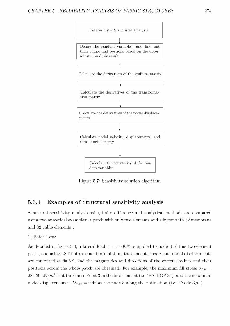
CHAPTER 5. RELIABILITY ANALYSIS OF FABRIC STRUCTURES 274
Deterministic Structural Analysis
Calculate the derivatives of the stiffness matrix
Calculate the sensitivity of the ran-
dom variables
Calculate nodal velocity, displacements, and
total kinetic energy
Define the random variables, and find out
their values and postions based on the deter-
minstic analysis result
Calculate the derivatives of the transforma-
tion matrix
Calculate the derivatives of the nodal displace-
ments
Figure 5.7: Sensitivity solution algorithm
5.3.4 Examples of Structural sensitivity analysis
Structural sensitivity analysis using finite difference and analytical methods are compared
using two numerical examples: a patch with only two elements and a hypar with 32 membrane
and 32 cable elements .
1) Patch Test:
As detailed in figure 5.8, a lateral load F = 100kN is applied to node 3 of this two-element
patch, and using LST finite element formulation, the element stresses and nodal displacements
are computed as fig.5.9, and the magnitudes and directions of the extreme values and their
positions across the whole patch are obtained. For example, the maximum fill stress σfill =
285.39 kN/m2 is at the Gauss Point 3 in the first element (i.e ”EN 1,GP 3”), and the maximum
nodal displacement is Dmax = 0.46 at the node 3 along the x direction (i.e. ”Node 3,x”).
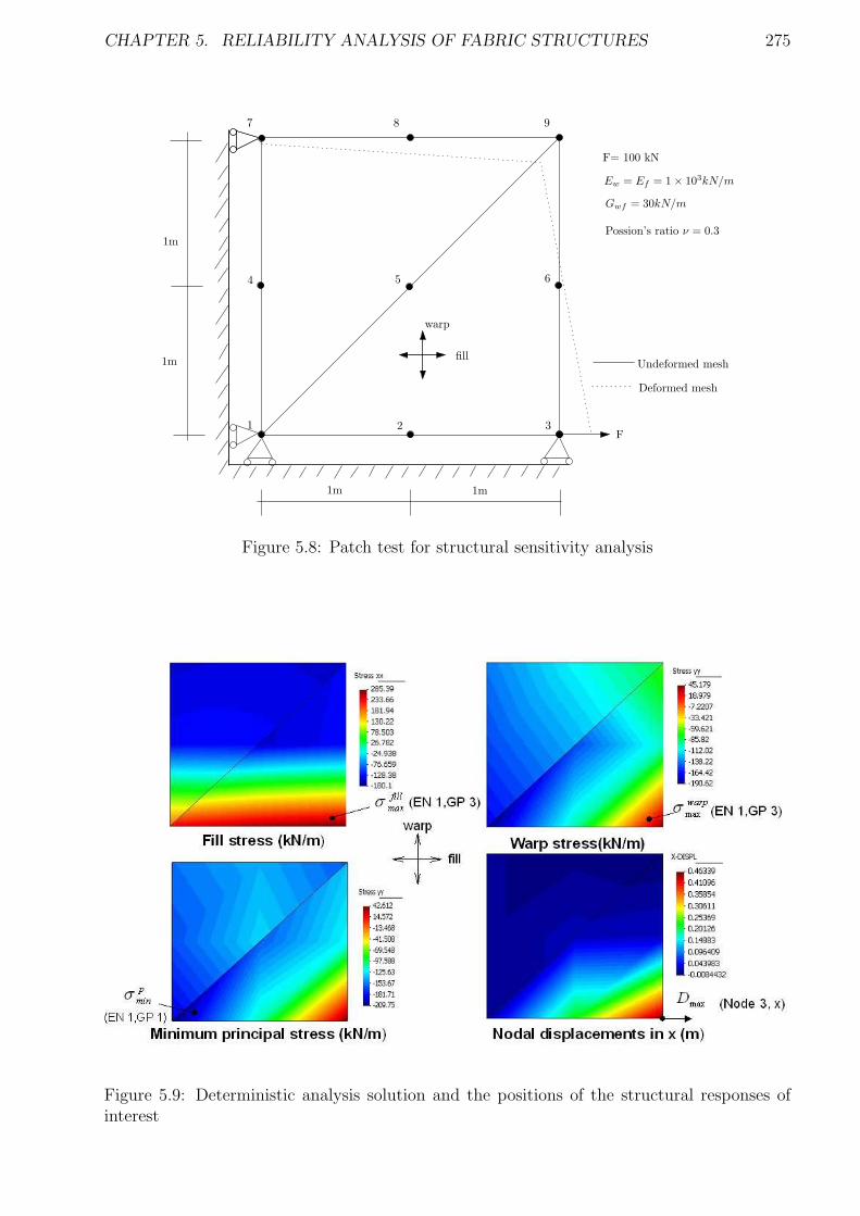
CHAPTER 5. RELIABILITY ANALYSIS OF FABRIC STRUCTURES 275
1m
1m
1m 1m
F1 2 3
4 5 6
7 8 9
Undeformed mesh
Deformed mesh
F= 100 kN
Ew = Ef = 1× 10³kN/m
Gwf = 30kN/m
Possion’s ratio ν = 0.3
fill
warp
Figure 5.8: Patch test for structural sensitivity analysis
Figure 5.9: Deterministic analysis solution and the positions of the structural responses ofinterest
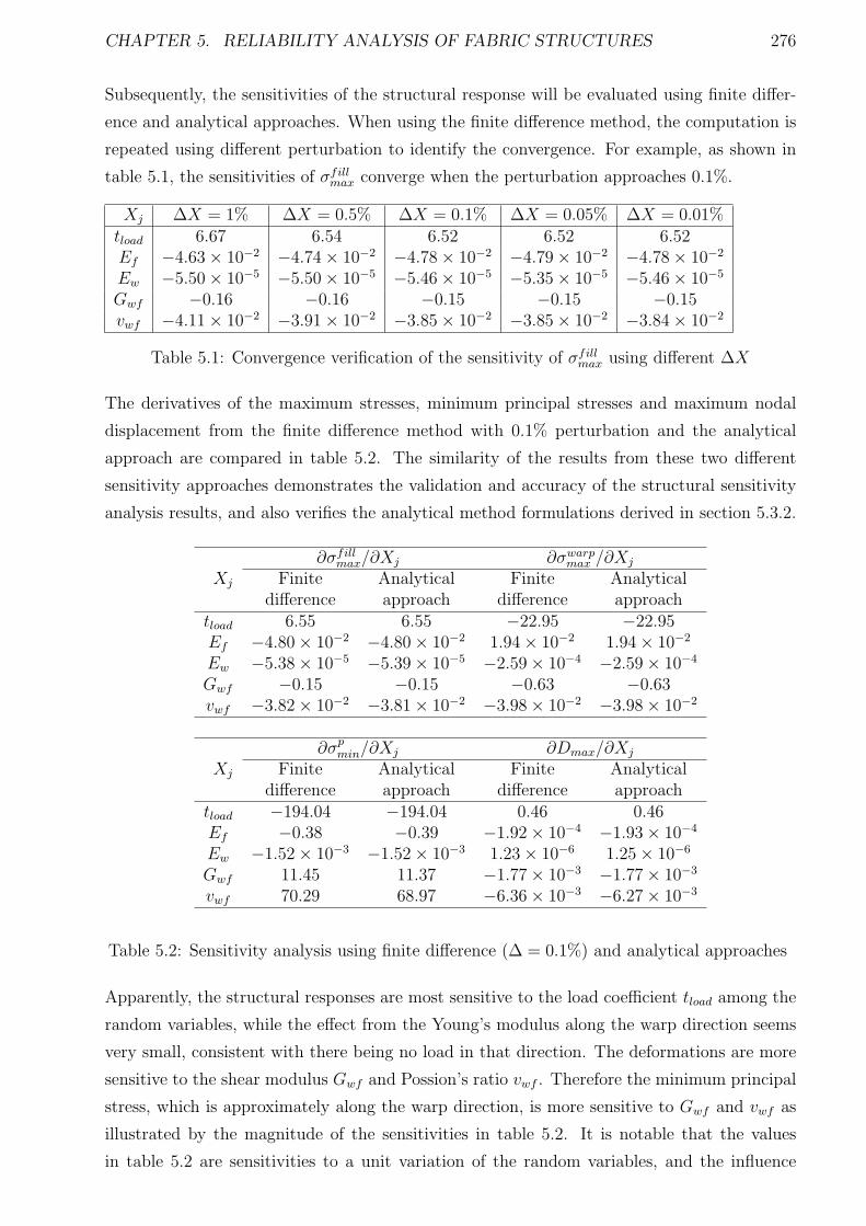
CHAPTER 5. RELIABILITY ANALYSIS OF FABRIC STRUCTURES 276
Subsequently, the sensitivities of the structural response will be evaluated using finite differ-
ence and analytical approaches. When using the finite difference method, the computation is
repeated using different perturbation to identify the convergence. For example, as shown in
table 5.1, the sensitivities of σfillmax converge when the perturbation approaches 0.1%.
Xj ∆X = 1% ∆X = 0.5% ∆X = 0.1% ∆X = 0.05% ∆X = 0.01%tload 6.67 6.54 6.52 6.52 6.52Ef −4.63 × 10⁻² −4.74 × 10⁻² −4.78 × 10⁻² −4.79 × 10⁻² −4.78 × 10⁻²
Ew −5.50 × 10⁻⁵ −5.50 × 10⁻⁵ −5.46 × 10⁻⁵ −5.35 × 10⁻⁵ −5.46 × 10⁻⁵
Gwf −0.16 −0.16 −0.15 −0.15 −0.15vwf −4.11 × 10⁻² −3.91 × 10⁻² −3.85 × 10⁻² −3.85 × 10⁻² −3.84 × 10⁻²
Table 5.1: Convergence verification of the sensitivity of σfillmax using different ∆X
The derivatives of the maximum stresses, minimum principal stresses and maximum nodal
displacement from the finite difference method with 0.1% perturbation and the analytical
approach are compared in table 5.2. The similarity of the results from these two different
sensitivity approaches demonstrates the validation and accuracy of the structural sensitivity
analysis results, and also verifies the analytical method formulations derived in section 5.3.2.
∂σfillmax/∂Xj ∂σwarp
max /∂Xj
Xj Finite Analytical Finite Analyticaldifference approach difference approach
tload 6.55 6.55 −22.95 −22.95Ef −4.80 × 10⁻² −4.80 × 10⁻² 1.94 × 10⁻² 1.94 × 10⁻²
Ew −5.38 × 10⁻⁵ −5.39 × 10⁻⁵ −2.59 × 10⁻⁴ −2.59 × 10⁻⁴
Gwf −0.15 −0.15 −0.63 −0.63vwf −3.82 × 10⁻² −3.81 × 10⁻² −3.98 × 10⁻² −3.98 × 10⁻²
∂σpmin/∂Xj ∂Dmax/∂Xj
Xj Finite Analytical Finite Analyticaldifference approach difference approach
tload −194.04 −194.04 0.46 0.46Ef −0.38 −0.39 −1.92 × 10⁻⁴ −1.93 × 10⁻⁴
Ew −1.52 × 10⁻³ −1.52 × 10⁻³ 1.23 × 10⁻⁶ 1.25 × 10⁻⁶
Gwf 11.45 11.37 −1.77 × 10⁻³ −1.77 × 10⁻³
vwf 70.29 68.97 −6.36 × 10⁻³ −6.27 × 10⁻³
Table 5.2: Sensitivity analysis using finite difference (∆ = 0.1%) and analytical approaches
Apparently, the structural responses are most sensitive to the load coefficient tload among the
random variables, while the effect from the Young’s modulus along the warp direction seems
very small, consistent with there being no load in that direction. The deformations are more
sensitive to the shear modulus Gwf and Possion’s ratio vwf . Therefore the minimum principal
stress, which is approximately along the warp direction, is more sensitive to Gwf and vwf as
illustrated by the magnitude of the sensitivities in table 5.2. It is notable that the values
in table 5.2 are sensitivities to a unit variation of the random variables, and the influence
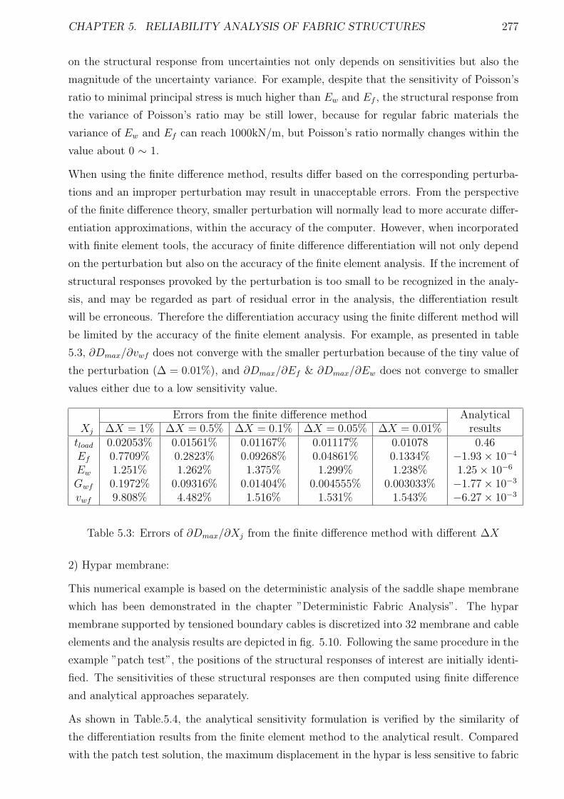
CHAPTER 5. RELIABILITY ANALYSIS OF FABRIC STRUCTURES 277
on the structural response from uncertainties not only depends on sensitivities but also the
magnitude of the uncertainty variance. For example, despite that the sensitivity of Poisson’s
ratio to minimal principal stress is much higher than Ew and Ef , the structural response from
the variance of Poisson’s ratio may be still lower, because for regular fabric materials the
variance of Ew and Ef can reach 1000kN/m, but Poisson’s ratio normally changes within the
value about 0 ∼ 1.
When using the finite difference method, results differ based on the corresponding perturba-
tions and an improper perturbation may result in unacceptable errors. From the perspective
of the finite difference theory, smaller perturbation will normally lead to more accurate differ-
entiation approximations, within the accuracy of the computer. However, when incorporated
with finite element tools, the accuracy of finite difference differentiation will not only depend
on the perturbation but also on the accuracy of the finite element analysis. If the increment of
structural responses provoked by the perturbation is too small to be recognized in the analy-
sis, and may be regarded as part of residual error in the analysis, the differentiation result
will be erroneous. Therefore the differentiation accuracy using the finite different method will
be limited by the accuracy of the finite element analysis. For example, as presented in table
5.3, ∂Dmax/∂vwf does not converge with the smaller perturbation because of the tiny value of
the perturbation (∆ = 0.01%), and ∂Dmax/∂Ef & ∂Dmax/∂Ew does not converge to smaller
values either due to a low sensitivity value.
Errors from the finite difference method AnalyticalXj ∆X = 1% ∆X = 0.5% ∆X = 0.1% ∆X = 0.05% ∆X = 0.01% resultstload 0.02053% 0.01561% 0.01167% 0.01117% 0.01078 0.46Ef 0.7709% 0.2823% 0.09268% 0.04861% 0.1334% −1.93 × 10⁻⁴
Ew 1.251% 1.262% 1.375% 1.299% 1.238% 1.25 × 10⁻⁶
Gwf 0.1972% 0.09316% 0.01404% 0.004555% 0.003033% −1.77 × 10⁻³
vwf 9.808% 4.482% 1.516% 1.531% 1.543% −6.27 × 10⁻³
Table 5.3: Errors of ∂Dmax/∂Xj from the finite difference method with different ∆X
2) Hypar membrane:
This numerical example is based on the deterministic analysis of the saddle shape membrane
which has been demonstrated in the chapter ”Deterministic Fabric Analysis”. The hypar
membrane supported by tensioned boundary cables is discretized into 32 membrane and cable
elements and the analysis results are depicted in fig. 5.10. Following the same procedure in the
example ”patch test”, the positions of the structural responses of interest are initially identi-
fied. The sensitivities of these structural responses are then computed using finite difference
and analytical approaches separately.
As shown in Table.5.4, the analytical sensitivity formulation is verified by the similarity of
the differentiation results from the finite element method to the analytical result. Compared
with the patch test solution, the maximum displacement in the hypar is less sensitive to fabric
CHAPTER 5. RELIABILITY ANALYSIS OF FABRIC STRUCTURES 278
Figure 5.10: Hypar test for sensitivity and reliability analysis
material properties (e.g. ∂Dmax/∂Ef = −2.09× 10⁻⁶), because of its geometrically nonlinear
structural type. It is also interesting to note that the minimum principal stress drops more
than twice rapidly as the maximum stress increases with the same increment of the load. This
implies that such this hypar membrane is more prone to fail due to wrinkling rather than by
material rupture when the same safety margins are assigned.
From these two numerical examples of structural sensitivity analysis, both the finite difference
and analytical methods indicate similar values in estimating the derivatives of the structural
response of interest. The finite difference method requires repeating the analytical analysis
twice for each derivative quantity, and may be time-consuming when the analytical analysis
is complicated. The finite difference method may therefore not be efficient for sensitivity and
reliability analysis of large structure systems, but is a useful tool for checking the validity of
the analytical formation derived in section.5.3.2. It also proves useful in cases where analytical
sensitivities are not available.
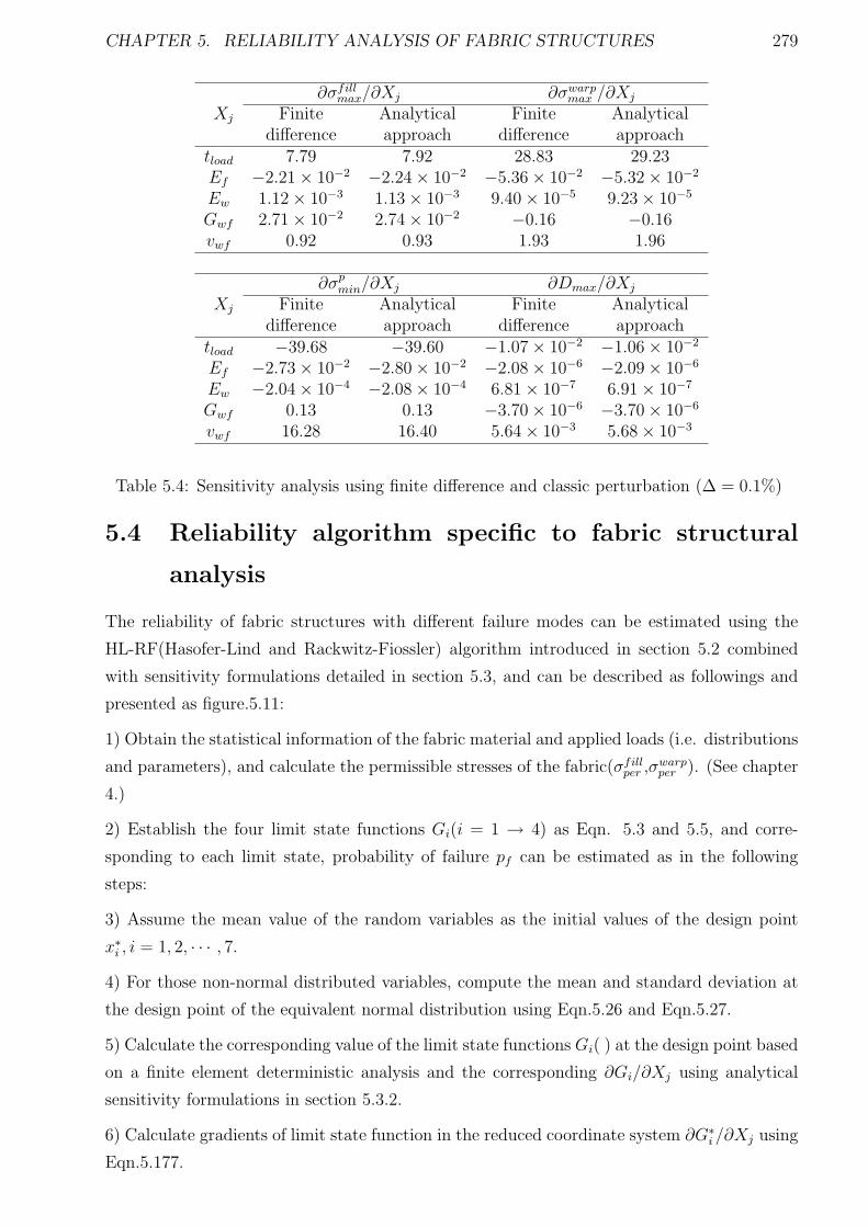
CHAPTER 5. RELIABILITY ANALYSIS OF FABRIC STRUCTURES 279
∂σfillmax/∂Xj ∂σwarp
max /∂Xj
Xj Finite Analytical Finite Analyticaldifference approach difference approach
tload 7.79 7.92 28.83 29.23Ef −2.21 × 10⁻² −2.24 × 10⁻² −5.36 × 10⁻² −5.32 × 10⁻²
Ew 1.12 × 10⁻³ 1.13 × 10⁻³ 9.40 × 10⁻⁵ 9.23 × 10⁻⁵
Gwf 2.71 × 10⁻² 2.74 × 10⁻² −0.16 −0.16vwf 0.92 0.93 1.93 1.96
∂σpmin/∂Xj ∂Dmax/∂Xj
Xj Finite Analytical Finite Analyticaldifference approach difference approach
tload −39.68 −39.60 −1.07 × 10⁻² −1.06 × 10⁻²
Ef −2.73 × 10⁻² −2.80 × 10⁻² −2.08 × 10⁻⁶ −2.09 × 10⁻⁶
Ew −2.04 × 10⁻⁴ −2.08 × 10⁻⁴ 6.81 × 10⁻⁷ 6.91 × 10⁻⁷
Gwf 0.13 0.13 −3.70 × 10⁻⁶ −3.70 × 10⁻⁶
vwf 16.28 16.40 5.64 × 10⁻³ 5.68 × 10⁻³
Table 5.4: Sensitivity analysis using finite difference and classic perturbation (∆ = 0.1%)
5.4 Reliability algorithm specific to fabric structural
analysis
The reliability of fabric structures with different failure modes can be estimated using the
HL-RF(Hasofer-Lind and Rackwitz-Fiossler) algorithm introduced in section 5.2 combined
with sensitivity formulations detailed in section 5.3, and can be described as followings and
presented as figure.5.11:
1) Obtain the statistical information of the fabric material and applied loads (i.e. distributions
and parameters), and calculate the permissible stresses of the fabric(σfillper ,σwarp
per ). (See chapter
4.)
2) Establish the four limit state functions Gi(i = 1 → 4) as Eqn. 5.3 and 5.5, and corre-
sponding to each limit state, probability of failure pf can be estimated as in the following
steps:
3) Assume the mean value of the random variables as the initial values of the design point
x∗i , i = 1, 2, · · · , 7.
4) For those non-normal distributed variables, compute the mean and standard deviation at
the design point of the equivalent normal distribution using Eqn.5.26 and Eqn.5.27.
5) Calculate the corresponding value of the limit state functions Gi( ) at the design point based
on a finite element deterministic analysis and the corresponding ∂Gi/∂Xj using analytical
sensitivity formulations in section 5.3.2.
6) Calculate gradients of limit state function in the reduced coordinate system ∂G∗i /∂Xj using
Eqn.5.177.

CHAPTER 5. RELIABILITY ANALYSIS OF FABRIC STRUCTURES 280
∂G∗i
∂Xj
= − ∂Gi
∂Xj
σNXi
(5.177)
7) Compute the new values of design points (x′∗i ) in the reduced space using Eqn.5.33.
8) Compute the safety index β based on the values of the design points calculated in step 5
using Eqn. 5.36, Check the convergence of β and |G(X)i|, if β converged and |G(X)i| is very
close to zero, then goto step 10, otherwise step 9.
9) Compute the new values of the design point (x∗)in the original space using Eqn. 5.37 and
repeat step 4 to 8.
10) Calculate the probability of failure for next limit states until convergence of β is attained.
Define limit state functions
Compute new design points and safety index
Safety Index β converge (∆β < 0.001)?
Analysis Result: probability of fail-ure pf and most probable designpoints
Yes
No
update the values of the statistical variables
Statistical Information (e.g. mean, standarddeviation)
Assume initial value of design points equal tomean values
Transform non-normal distributed vriable tonormal distributed ones
Calculate the gradients of limit state functionrespect to the statistical variables
Figure 5.11: Reliability solution algorithm
Using this algorithm, the reliability of the fabric structure corresponding to different limit
states can be estimated individually, and a integrated reliability analysis cannot be obtained
directly. Normally, for a given fabric structure, structural failure may occur more likely
corresponding to one limit state rather than the others. For example, when loading is not
uniform, the structure is more prone to fail due to wrinkling rather than the material rupture
since the pre-stress in the fabric is normally several percentage of the rupture strength.
CHAPTER 5. RELIABILITY ANALYSIS OF FABRIC STRUCTURES 281
5.4.1 Numerical Example of Reliability Analysis
From the discussion in the section 5.3.4, it suggests that not all the random variables involved
in the analysis have the same level of effect on the reliability for a specific limit state. In
certain cases, only a few random variables (e.g. loads and material strength) play key roles in
the reliability analysis, and the reliability is not sensitive to the other variables even though
they may have high levels of uncertainty. However in the other case, the reliability is sensitive
to the majority of random variables, and the reliability estimation may become difficult since
more variables are effective in the reliability calculation.
In this section, two numerical examples are presented. The first is a special case in that most
random variables, including loads, material strength, and elastic modulus have approximately
the same level of effect on the reliability. The assumed limit states are selected to represent
the structural response ranges achievable using these random variables with reasonable COV
values. For example, the maximum stress may vary by about 10% of the mean value due to a
varying elastic modulus with the COV value of 0.5 while the same performance variable could
change up to 200% of the mean with variation in the loads by the same variance. In that
case, the limit state will be mainly selected according the structural response ranges by the
random variable of elastic modulus to observe and compare the effects of both variables. The
main purpose of this example is to verify the reliability formulation with multi-variables, and
also to compare the performance effects of these random variables.
The second numerical example is a case study, based on a realistic design case with the
probabilistic assumptions. The purpose of the case study is to examine the safety factors
currently applied to fabric structure design consistent with the reliability requirement of the
Eurocode 0. It also demonstrates how to apply the reliability analysis tool to the realistic
design of a fabric structure. Based on the reliability analysis, a tentative suggestion of the
corresponding efficient safety factors will be given.
Hypar membrane
The reliability of the Hypar membrane presented in the section 5.3.4 can be evaluated as
a fictitious numerical example. In this numerical example, the probability of failure of the
pretensioned hypar made of a heavy pvc-polyester fabric material is computed. The statistical
design parameters are given in table 5.5. Initially, all random variables are assumed to be
normally distributed, and the standard deviation of each variable is 10% of the mean value
(i.e COV = 0.1)). A high safety factor of 8 based on the European Design Guide [3] is
assumed for the materal strength, which was approximately 80kN/m based on the test results
in Chapter.4.
Because in this example, the maximum stress in one direction is always higher than the other,
i.e σwmax > σf
max, therefore the limit states can be assumed as:
G2(X) = σper − σwmax, σper ∼ N(10, 1) kN/m
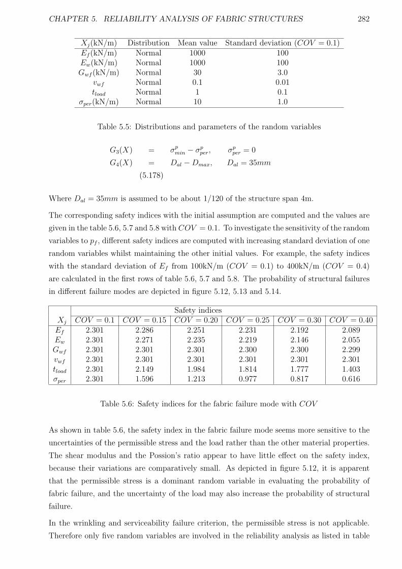
CHAPTER 5. RELIABILITY ANALYSIS OF FABRIC STRUCTURES 282
Xj(kN/m) Distribution Mean value Standard deviation (COV = 0.1)Ef (kN/m) Normal 1000 100Ew(kN/m) Normal 1000 100Gwf (kN/m) Normal 30 3.0
vwf Normal 0.1 0.01tload Normal 1 0.1
σper(kN/m) Normal 10 1.0
Table 5.5: Distributions and parameters of the random variables
G3(X) = σpmin − σp
per, σpper = 0
G4(X) = Dal −Dmax, Dal = 35mm
(5.178)
Where Dal = 35mm is assumed to be about 1/120 of the structure span 4m.
The corresponding safety indices with the initial assumption are computed and the values are
given in the table 5.6, 5.7 and 5.8 with COV = 0.1. To investigate the sensitivity of the random
variables to pf , different safety indices are computed with increasing standard deviation of one
random variables whilst maintaining the other initial values. For example, the safety indices
with the standard deviation of Ef from 100kN/m (COV = 0.1) to 400kN/m (COV = 0.4)
are calculated in the first rows of table 5.6, 5.7 and 5.8. The probability of structural failures
in different failure modes are depicted in figure 5.12, 5.13 and 5.14.
Safety indicesXj COV = 0.1 COV = 0.15 COV = 0.20 COV = 0.25 COV = 0.30 COV = 0.40Ef 2.301 2.286 2.251 2.231 2.192 2.089Ew 2.301 2.271 2.235 2.219 2.146 2.055Gwf 2.301 2.301 2.301 2.300 2.300 2.299vwf 2.301 2.301 2.301 2.301 2.301 2.301tload 2.301 2.149 1.984 1.814 1.777 1.403σper 2.301 1.596 1.213 0.977 0.817 0.616
Table 5.6: Safety indices for the fabric failure mode with COV
As shown in table 5.6, the safety index in the fabric failure mode seems more sensitive to the
uncertainties of the permissible stress and the load rather than the other material properties.
The shear modulus and the Possion’s ratio appear to have little effect on the safety index,
because their variations are comparatively small. As depicted in figure 5.12, it is apparent
that the permissible stress is a dominant random variable in evaluating the probability of
fabric failure, and the uncertainty of the load may also increase the probability of structural
failure.
In the wrinkling and serviceability failure criterion, the permissible stress is not applicable.
Therefore only five random variables are involved in the reliability analysis as listed in table
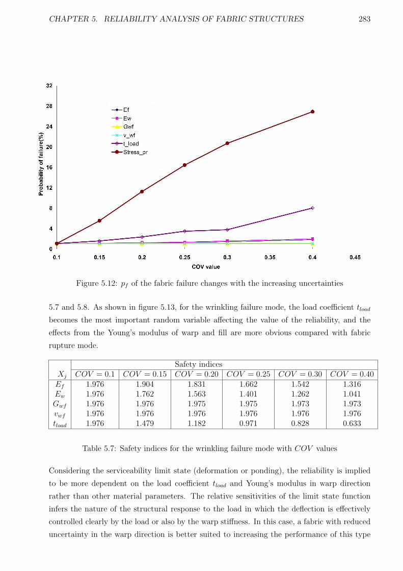
CHAPTER 5. RELIABILITY ANALYSIS OF FABRIC STRUCTURES 283
Figure 5.12: pf of the fabric failure changes with the increasing uncertainties
5.7 and 5.8. As shown in figure 5.13, for the wrinkling failure mode, the load coefficient tload
becomes the most important random variable affecting the value of the reliability, and the
effects from the Young’s modulus of warp and fill are more obvious compared with fabric
rupture mode.
Safety indicesXj COV = 0.1 COV = 0.15 COV = 0.20 COV = 0.25 COV = 0.30 COV = 0.40Ef 1.976 1.904 1.831 1.662 1.542 1.316Ew 1.976 1.762 1.563 1.401 1.262 1.041Gwf 1.976 1.976 1.975 1.975 1.973 1.973vwf 1.976 1.976 1.976 1.976 1.976 1.976tload 1.976 1.479 1.182 0.971 0.828 0.633
Table 5.7: Safety indices for the wrinkling failure mode with COV values
Considering the serviceability limit state (deformation or ponding), the reliability is implied
to be more dependent on the load coefficient tload and Young’s modulus in warp direction
rather than other material parameters. The relative sensitivities of the limit state function
infers the nature of the structural response to the load in which the deflection is effectively
controlled clearly by the load or also by the warp stiffness. In this case, a fabric with reduced
uncertainty in the warp direction is better suited to increasing the performance of this type
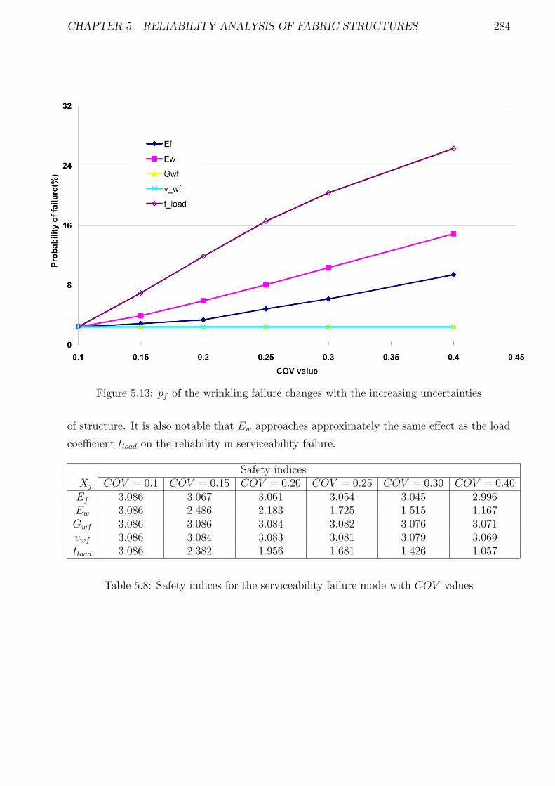
CHAPTER 5. RELIABILITY ANALYSIS OF FABRIC STRUCTURES 284
Figure 5.13: pf of the wrinkling failure changes with the increasing uncertainties
of structure. It is also notable that Ew approaches approximately the same effect as the load
coefficient tload on the reliability in serviceability failure.
Safety indicesXj COV = 0.1 COV = 0.15 COV = 0.20 COV = 0.25 COV = 0.30 COV = 0.40Ef 3.086 3.067 3.061 3.054 3.045 2.996Ew 3.086 2.486 2.183 1.725 1.515 1.167Gwf 3.086 3.086 3.084 3.082 3.076 3.071vwf 3.086 3.084 3.083 3.081 3.079 3.069tload 3.086 2.382 1.956 1.681 1.426 1.057
Table 5.8: Safety indices for the serviceability failure mode with COV values
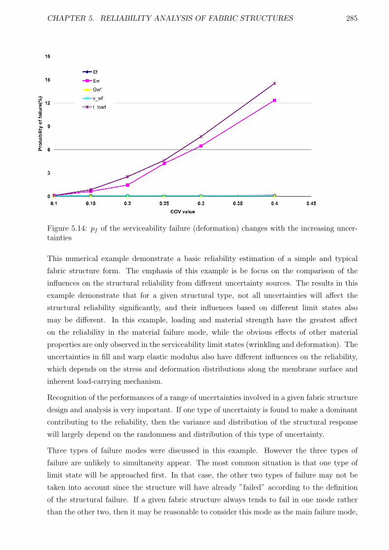
CHAPTER 5. RELIABILITY ANALYSIS OF FABRIC STRUCTURES 285
Figure 5.14: pf of the serviceability failure (deformation) changes with the increasing uncer-tainties
This numerical example demonstrate a basic reliability estimation of a simple and typical
fabric structure form. The emphasis of this example is be focus on the comparison of the
influences on the structural reliability from different uncertainty sources. The results in this
example demonstrate that for a given structural type, not all uncertainties will affect the
structural reliability significantly, and their influences based on different limit states also
may be different. In this example, loading and material strength have the greatest affect
on the reliability in the material failure mode, while the obvious effects of other material
properties are only observed in the serviceability limit states (wrinkling and deformation). The
uncertainties in fill and warp elastic modulus also have different influences on the reliability,
which depends on the stress and deformation distributions along the membrane surface and
inherent load-carrying mechanism.
Recognition of the performances of a range of uncertainties involved in a given fabric structure
design and analysis is very important. If one type of uncertainty is found to make a dominant
contributing to the reliability, then the variance and distribution of the structural response
will largely depend on the randomness and distribution of this type of uncertainty.
Three types of failure modes were discussed in this example. However the three types of
failure are unlikely to simultaneity appear. The most common situation is that one type of
limit state will be approached first. In that case, the other two types of failure may not be
taken into account since the structure will have already ”failed” according to the definition
of the structural failure. If a given fabric structure always tends to fail in one mode rather
than the other two, then it may be reasonable to consider this mode as the main failure mode,

CHAPTER 5. RELIABILITY ANALYSIS OF FABRIC STRUCTURES 286
and compute the structural reliability based on the corresponding limit state. However the
locations of the failures defined under the different limit states (e.g. deflection and wrinkling)
may be not in the same point. When the reliability of local membrane parts are required, the
other failures may be still need to be evaluated.
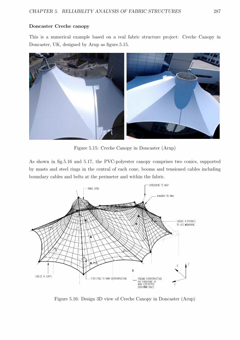
CHAPTER 5. RELIABILITY ANALYSIS OF FABRIC STRUCTURES 287
Doncaster Creche canopy
This is a numerical example based on a real fabric structure project: Creche Canopy in
Doncaster, UK, designed by Arup as figure.5.15.
Figure 5.15: Creche Canopy in Doncaster (Arup)
As shown in fig.5.16 and 5.17, the PVC-polyester canopy comprises two conics, supported
by masts and steel rings in the central of each cone, booms and tensioned cables including
boundary cables and belts at the perimeter and within the fabric.
Figure 5.16: Design 3D view of Creche Canopy in Doncaster (Arup)
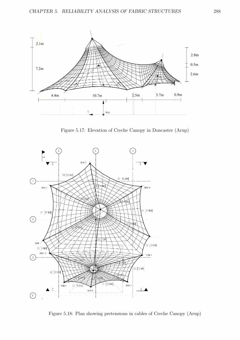
CHAPTER 5. RELIABILITY ANALYSIS OF FABRIC STRUCTURES 288
Figure 5.17: Elevation of Creche Canopy in Doncaster (Arup)
Figure 5.18: Plan showing pretensions in cables of Creche Canopy (Arup)
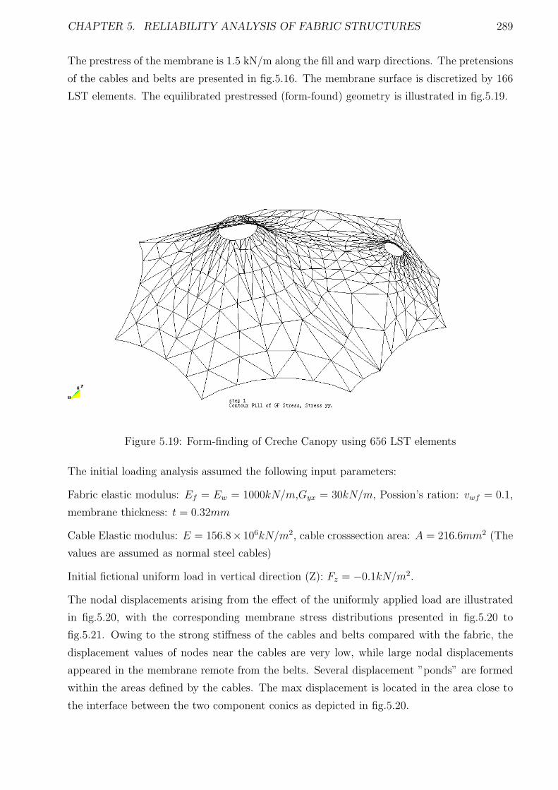
CHAPTER 5. RELIABILITY ANALYSIS OF FABRIC STRUCTURES 289
The prestress of the membrane is 1.5 kN/m along the fill and warp directions. The pretensions
of the cables and belts are presented in fig.5.16. The membrane surface is discretized by 166
LST elements. The equilibrated prestressed (form-found) geometry is illustrated in fig.5.19.
Figure 5.19: Form-finding of Creche Canopy using 656 LST elements
The initial loading analysis assumed the following input parameters:
Fabric elastic modulus: Ef = Ew = 1000kN/m,Gyx = 30kN/m, Possion’s ration: vwf = 0.1,
membrane thickness: t = 0.32mm
Cable Elastic modulus: E = 156.8× 10⁶kN/m2, cable crosssection area: A = 216.6mm2 (The
values are assumed as normal steel cables)
Initial fictional uniform load in vertical direction (Z): Fz = −0.1kN/m2.
The nodal displacements arising from the effect of the uniformly applied load are illustrated
in fig.5.20, with the corresponding membrane stress distributions presented in fig.5.20 to
fig.5.21. Owing to the strong stiffness of the cables and belts compared with the fabric, the
displacement values of nodes near the cables are very low, while large nodal displacements
appeared in the membrane remote from the belts. Several displacement ”ponds” are formed
within the areas defined by the cables. The max displacement is located in the area close to
the interface between the two component conics as depicted in fig.5.20.
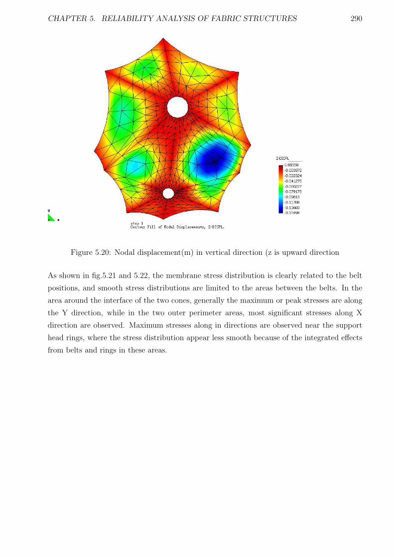
CHAPTER 5. RELIABILITY ANALYSIS OF FABRIC STRUCTURES 290
Figure 5.20: Nodal displacement(m) in vertical direction (z is upward direction
As shown in fig.5.21 and 5.22, the membrane stress distribution is clearly related to the belt
positions, and smooth stress distributions are limited to the areas between the belts. In the
area around the interface of the two cones, generally the maximum or peak stresses are along
the Y direction, while in the two outer perimeter areas, most significant stresses along X
direction are observed. Maximum stresses along in directions are observed near the support
head rings, where the stress distribution appear less smooth because of the integrated effects
from belts and rings in these areas.
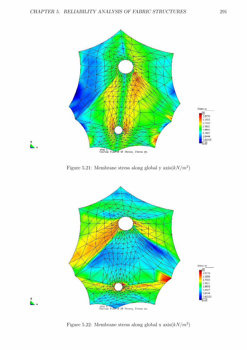
CHAPTER 5. RELIABILITY ANALYSIS OF FABRIC STRUCTURES 291
Figure 5.21: Membrane stress along global y axis(kN/m2)
Figure 5.22: Membrane stress along global x axis(kN/m2)
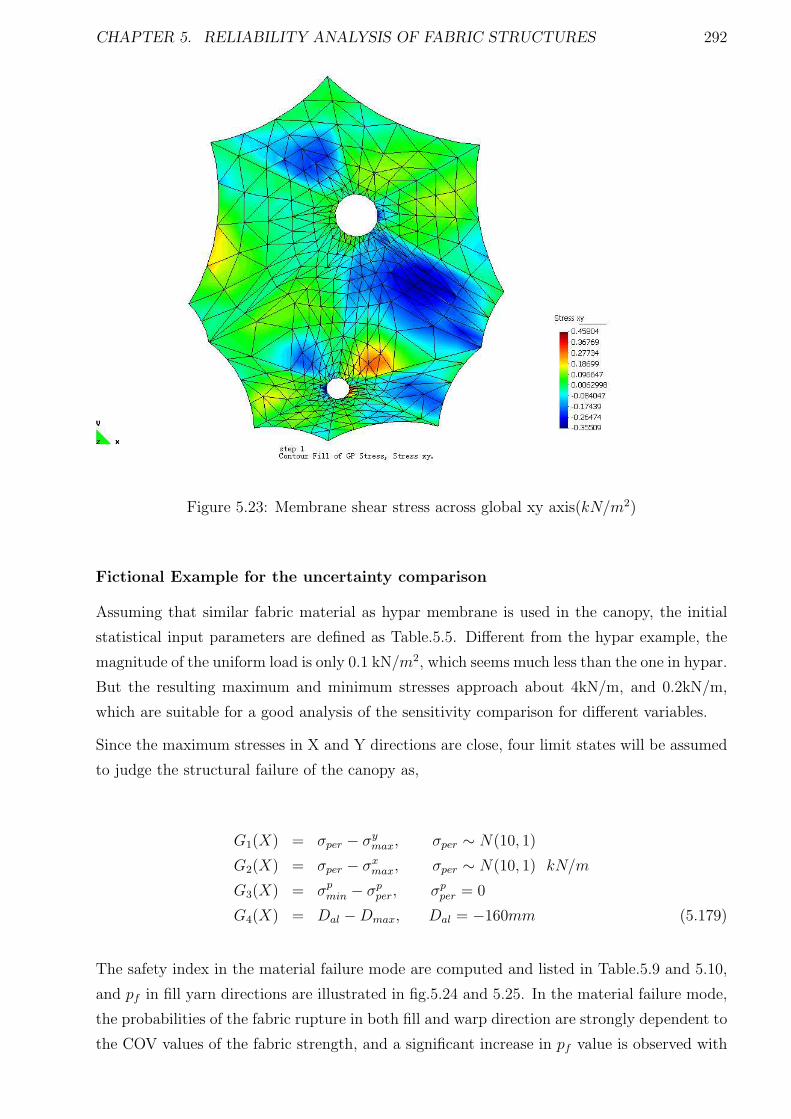
CHAPTER 5. RELIABILITY ANALYSIS OF FABRIC STRUCTURES 292
Figure 5.23: Membrane shear stress across global xy axis(kN/m2)
Fictional Example for the uncertainty comparison
Assuming that similar fabric material as hypar membrane is used in the canopy, the initial
statistical input parameters are defined as Table.5.5. Different from the hypar example, the
magnitude of the uniform load is only 0.1 kN/m2, which seems much less than the one in hypar.
But the resulting maximum and minimum stresses approach about 4kN/m, and 0.2kN/m,
which are suitable for a good analysis of the sensitivity comparison for different variables.
Since the maximum stresses in X and Y directions are close, four limit states will be assumed
to judge the structural failure of the canopy as,
G1(X) = σper − σymax, σper ∼ N(10, 1)
G2(X) = σper − σxmax, σper ∼ N(10, 1) kN/m
G3(X) = σpmin − σp
per, σpper = 0
G4(X) = Dal −Dmax, Dal = −160mm (5.179)
The safety index in the material failure mode are computed and listed in Table.5.9 and 5.10,
and pf in fill yarn directions are illustrated in fig.5.24 and 5.25. In the material failure mode,
the probabilities of the fabric rupture in both fill and warp direction are strongly dependent to
the COV values of the fabric strength, and a significant increase in pf value is observed with
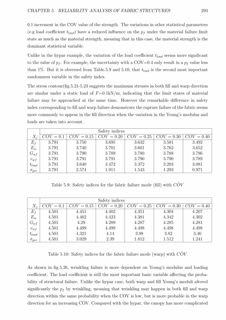
CHAPTER 5. RELIABILITY ANALYSIS OF FABRIC STRUCTURES 293
0.1 increment in the COV value of the strength. The variations in other statistical parameters
(e.g load coefficient tload) have a reduced influence on the pf under the material failure limit
state as much as the material strength, meaning that in this case, the material strength is the
dominant statistical variable.
Unlike in the hypar example, the variation of the load coefficient tload seems more significant
to the value of pf . For example, the uncertainty with a COV=0.4 only result in a pf value less
than 1%. But it is obversed from Table.5.9 and 5.10, that tload is the second most important
randomness variable in the safety index.
The stress contour(fig.5.21-5.23 suggests the maximum stresses in both fill and warp direction
are similar under a static load of F=0.1kN/m, indicating that the limit states of material
failure may be approached at the same time. However the remarkable difference in safety
index corresponding to fill and warp failure demonstrate the rupture failure of the fabric seems
more commonly to appear in the fill direction when the variation in the Young’s modulus and
loads are taken into account.
Safety indicesXj COV = 0.1 COV = 0.15 COV = 0.20 COV = 0.25 COV = 0.30 COV = 0.40Ef 3.791 3.750 3.695 3.632 3.581 3.492Ew 3.791 3.740 3.701 3.601 3.762 3.652Gwf 3.791 3.790 3.789 3.780 3.788 3.786vwf 3.791 3.791 3.791 3.790 3.790 3.789tload 3.791 3.640 3.472 3.372 3.203 3.081σper 3.791 2.574 1.911 1.543 1.293 0.971
Table 5.9: Safety indices for the fabric failure mode (fill) with ˆCOV
Safety indicesXj COV = 0.1 COV = 0.15 COV = 0.20 COV = 0.25 COV = 0.30 COV = 0.40Ef 4.501 4.451 4.402 4.351 4.304 4.207Ew 4.501 4.462 4.423 4.381 4.342 4.302Gwf 4.501 4.29 4.289 4.287 4.285 4.281vwf 4.501 4.499 4.499 4.498 4.498 4.498tload 4.501 4.321 4.14 3.98 3.82 3.46σper 4.501 3.029 2.39 1.812 1.512 1.241
Table 5.10: Safety indices for the fabric failure mode (warp) with ˆCOV
As shown in fig.5.26, wrinkling failure is more dependent on Young’s modulus and loading
coefficient. The load coefficient is still the most important basic variable affecting the proba-
bility of structural failure. Unlike the hypar case, both warp and fill Young’s moduli altered
significantly the pf by wrinkling, meaning that wrinkling may happen in both fill and warp
direction within the same probability when the COV is low, but is more probable in the warp
direction for an increasing COV. Compared with the hypar, the canopy has more complicated
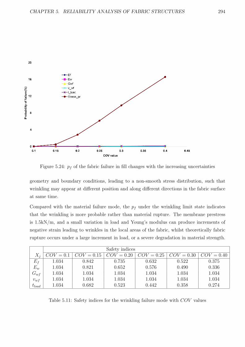
CHAPTER 5. RELIABILITY ANALYSIS OF FABRIC STRUCTURES 294
Figure 5.24: pf of the fabric failure in fill changes with the increasing uncertainties
geometry and boundary conditions, leading to a non-smooth stress distribution, such that
wrinkling may appear at different position and along different directions in the fabric surface
at same time.
Compared with the material failure mode, the pf under the wrinkling limit state indicates
that the wrinkling is more probable rather than material rupture. The membrane prestress
is 1.5kN/m, and a small variation in load and Young’s modulus can produce increments of
negative strain leading to wrinkles in the local areas of the fabric, whilst theoretically fabric
rupture occurs under a large increment in load, or a severe degradation in material strength.
Safety indicesXj COV = 0.1 COV = 0.15 COV = 0.20 COV = 0.25 COV = 0.30 COV = 0.40Ef 1.034 0.842 0.735 0.632 0.522 0.375Ew 1.034 0.821 0.652 0.576 0.490 0.336Gwf 1.034 1.034 1.034 1.034 1.034 1.034vwf 1.034 1.034 1.034 1.034 1.034 1.034tload 1.034 0.682 0.523 0.442 0.358 0.274
Table 5.11: Safety indices for the wrinkling failure mode with COV values
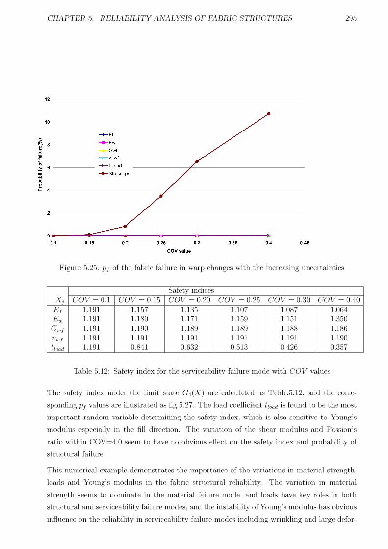
CHAPTER 5. RELIABILITY ANALYSIS OF FABRIC STRUCTURES 295
Figure 5.25: pf of the fabric failure in warp changes with the increasing uncertainties
Safety indicesXj COV = 0.1 COV = 0.15 COV = 0.20 COV = 0.25 COV = 0.30 COV = 0.40Ef 1.191 1.157 1.135 1.107 1.087 1.064Ew 1.191 1.180 1.171 1.159 1.151 1.350Gwf 1.191 1.190 1.189 1.189 1.188 1.186vwf 1.191 1.191 1.191 1.191 1.191 1.190tload 1.191 0.841 0.632 0.513 0.426 0.357
Table 5.12: Safety index for the serviceability failure mode with COV values
The safety index under the limit state G4(X) are calculated as Table.5.12, and the corre-
sponding pf values are illustrated as fig.5.27. The load coefficient tload is found to be the most
important random variable determining the safety index, which is also sensitive to Young’s
modulus especially in the fill direction. The variation of the shear modulus and Possion’s
ratio within COV=4.0 seem to have no obvious effect on the safety index and probability of
structural failure.
This numerical example demonstrates the importance of the variations in material strength,
loads and Young’s modulus in the fabric structural reliability. The variation in material
strength seems to dominate in the material failure mode, and loads have key roles in both
structural and serviceability failure modes, and the instability of Young’s modulus has obvious
influence on the reliability in serviceability failure modes including wrinkling and large defor-
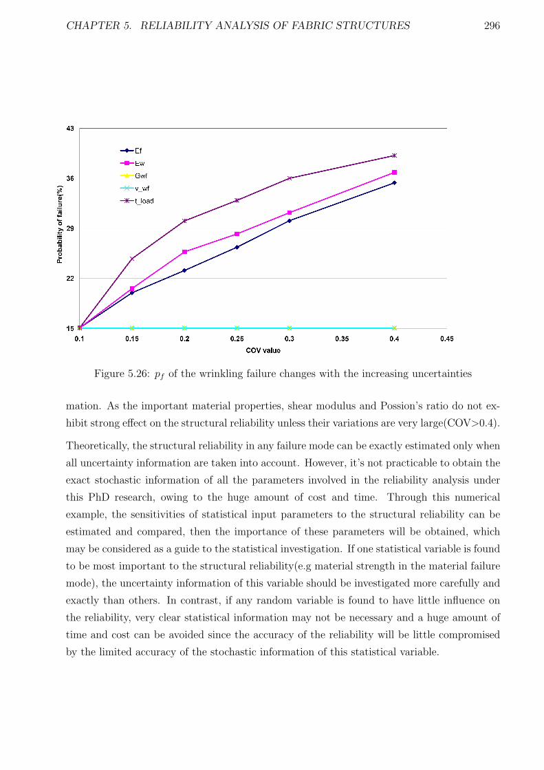
CHAPTER 5. RELIABILITY ANALYSIS OF FABRIC STRUCTURES 296
Figure 5.26: pf of the wrinkling failure changes with the increasing uncertainties
mation. As the important material properties, shear modulus and Possion’s ratio do not ex-
hibit strong effect on the structural reliability unless their variations are very large(COV>0.4).
Theoretically, the structural reliability in any failure mode can be exactly estimated only when
all uncertainty information are taken into account. However, it’s not practicable to obtain the
exact stochastic information of all the parameters involved in the reliability analysis under
this PhD research, owing to the huge amount of cost and time. Through this numerical
example, the sensitivities of statistical input parameters to the structural reliability can be
estimated and compared, then the importance of these parameters will be obtained, which
may be considered as a guide to the statistical investigation. If one statistical variable is found
to be most important to the structural reliability(e.g material strength in the material failure
mode), the uncertainty information of this variable should be investigated more carefully and
exactly than others. In contrast, if any random variable is found to have little influence on
the reliability, very clear statistical information may not be necessary and a huge amount of
time and cost can be avoided since the accuracy of the reliability will be little compromised
by the limited accuracy of the stochastic information of this statistical variable.
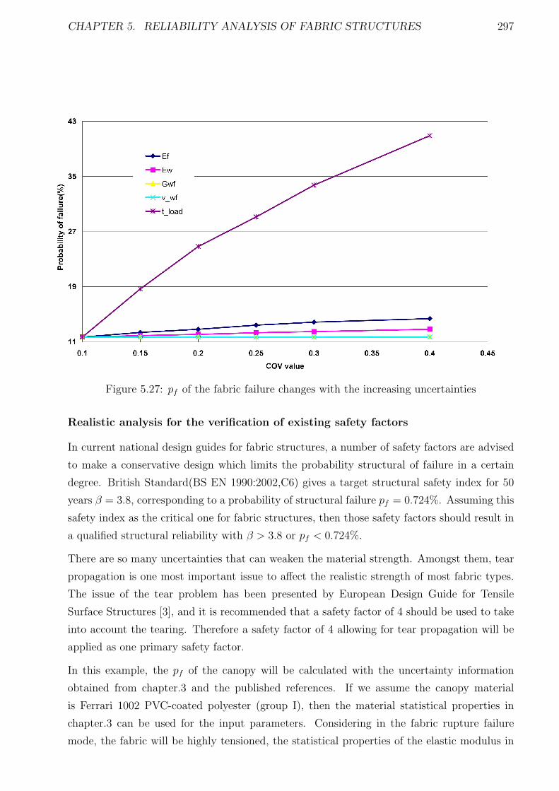
CHAPTER 5. RELIABILITY ANALYSIS OF FABRIC STRUCTURES 297
Figure 5.27: pf of the fabric failure changes with the increasing uncertainties
Realistic analysis for the verification of existing safety factors
In current national design guides for fabric structures, a number of safety factors are advised
to make a conservative design which limits the probability structural of failure in a certain
degree. British Standard(BS EN 1990:2002,C6) gives a target structural safety index for 50
years β = 3.8, corresponding to a probability of structural failure pf = 0.724%. Assuming this
safety index as the critical one for fabric structures, then those safety factors should result in
a qualified structural reliability with β > 3.8 or pf < 0.724%.
There are so many uncertainties that can weaken the material strength. Amongst them, tear
propagation is one most important issue to affect the realistic strength of most fabric types.
The issue of the tear problem has been presented by European Design Guide for Tensile
Surface Structures [3], and it is recommended that a safety factor of 4 should be used to take
into account the tearing. Therefore a safety factor of 4 allowing for tear propagation will be
applied as one primary safety factor.
In this example, the pf of the canopy will be calculated with the uncertainty information
obtained from chapter.3 and the published references. If we assume the canopy material
is Ferrari 1002 PVC-coated polyester (group I), then the material statistical properties in
chapter.3 can be used for the input parameters. Considering in the fabric rupture failure
mode, the fabric will be highly tensioned, the statistical properties of the elastic modulus in
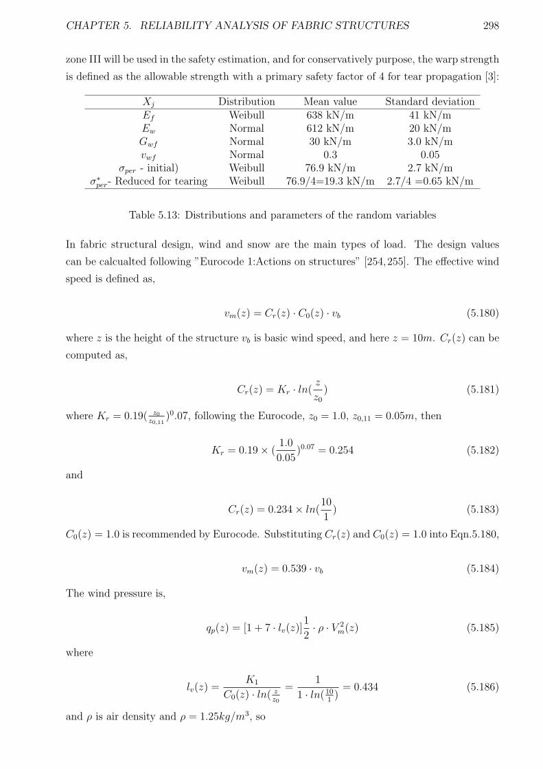
CHAPTER 5. RELIABILITY ANALYSIS OF FABRIC STRUCTURES 298
zone III will be used in the safety estimation, and for conservatively purpose, the warp strength
is defined as the allowable strength with a primary safety factor of 4 for tear propagation [3]:
Xj Distribution Mean value Standard deviationEf Weibull 638 kN/m 41 kN/mEw Normal 612 kN/m 20 kN/mGwf Normal 30 kN/m 3.0 kN/mvwf Normal 0.3 0.05
σper - initial) Weibull 76.9 kN/m 2.7 kN/mσ∗
per- Reduced for tearing Weibull 76.9/4=19.3 kN/m 2.7/4 =0.65 kN/m
Table 5.13: Distributions and parameters of the random variables
In fabric structural design, wind and snow are the main types of load. The design values
can be calcualted following ”Eurocode 1:Actions on structures” [254,255]. The effective wind
speed is defined as,
vm(z) = Cr(z) · C0(z) · vb (5.180)
where z is the height of the structure vb is basic wind speed, and here z = 10m. Cr(z) can be
computed as,
Cr(z) = Kr · ln(z
z0
) (5.181)
where Kr = 0.19( z0
z0,11)0.07, following the Eurocode, z0 = 1.0, z0,11 = 0.05m, then
Kr = 0.19 × (1.0
0.05)0.07 = 0.254 (5.182)
and
Cr(z) = 0.234 × ln(10
1) (5.183)
C0(z) = 1.0 is recommended by Eurocode. Substituting Cr(z) and C0(z) = 1.0 into Eqn.5.180,
vm(z) = 0.539 · vb (5.184)
The wind pressure is,
qp(z) = [1 + 7 · lv(z)]1
2· ρ · V 2
m(z) (5.185)
where
lv(z) =K1
C0(z) · ln( zz0
=1
1 · ln(101)
= 0.434 (5.186)
and ρ is air density and ρ = 1.25kg/m3, so
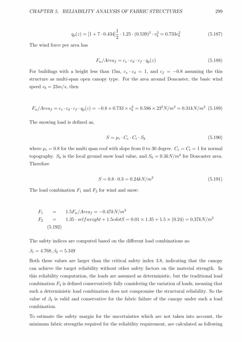
CHAPTER 5. RELIABILITY ANALYSIS OF FABRIC STRUCTURES 299
qp(z) = [1 + 7 · 0.434]1
2· 1.25 · (0.539)2 · v2
b = 0.733v2b (5.187)
The wind force per area has
Fw/Areaf = cs · cd · cf · qp(z) (5.188)
For buildings with a height less than 15m, cs · cd = 1, and cf = −0.8 assuming the this
structure as multi-span open canopy type. For the area around Doncaster, the basic wind
speed vb = 23m/s, then
Fw/Areaf = cs · cd · cf · qp(z) = −0.8× 0.733× v2b = 0.586× 232N/m2 = 0.31kN/m2 (5.189)
The snowing load is defined as,
S = µi · Ce · Ct · Sk (5.190)
where µi = 0.8 for the multi span roof with slope from 0 to 30 degree. Ce = Ct = 1 for normal
topography. Sk is the local ground snow load value, and Sk = 0.3kN/m2 for Doncaster area.
Therefore
S = 0.8 · 0.3 = 0.24kN/m2 (5.191)
The load combination F1 and F2 for wind and snow:
F1 = 1.5Fw/Areaf = −0.47kN/m2
F2 = 1.35 · selfweight+ 1.5cdotS = 0.01 × 1.35 + 1.5 × (0.24) = 0.37kN/m2
(5.192)
The safety indices are computed based on the different load combinations as:
β1 = 4.768, β2 = 5.349
Both these values are larger than the critical safety index 3.8, indicating that the canopy
can achieve the target reliability without other safety factors on the material strength. In
this reliability computation, the loads are assumed as deterministic, but the traditional load
combination F2 is defined conservatively fully considering the variation of loads, meaning that
such a deterministic load combination does not compromise the structural reliability. So the
value of β2 is valid and conservative for the fabric failure of the canopy under such a load
combination.
To estimate the safety margin for the uncertainties which are not taken into account, the
minimum fabric strengths required for the reliability requirement, are calculated as following
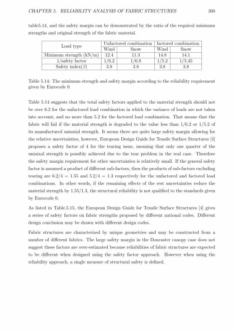
CHAPTER 5. RELIABILITY ANALYSIS OF FABRIC STRUCTURES 300
table5.14, and the safety margin can be demonstrated by the ratio of the required minimum
strengths and original strength of the fabric material.
Unfactored combination factored combinationLoad type
Wind Snow Wind SnowMinimum strength (kN/m) 12.4 11.3 14.8 14.1
1/safety factor 1/6.2 1/6.8 1/5.2 1/5.45Safety index(β) 3.8 3.8 3.8 3.8
Table 5.14: The minimum strength and safety margin according to the reliability requirementgiven by Eurocode 0
Table 5.14 suggests that the total safety factors applied to the material strength should not
be over 6.2 for the unfactored load combination in which the variance of loads are not taken
into account, and no more than 5.2 for the factored load combination. That means that the
fabric will fail if the material strength is degraded to the value less than 1/6.2 or 1/5.2 of
its manufactured uniaxial strength. It seems there are quite large safety margin allowing for
the relative uncertainties, however, European Design Guide for Tensile Surface Structures [4]
proposes a safety factor of 4 for the tearing issue, meaning that only one quarter of the
uniaixal strength is possibly achieved due to the tear problem in the real case. Therefore
the safety margin requirement for other uncertainties is relatively small. If the general safety
factor is assumed a product of different sub-factors, then the products of sub-factors excluding
tearing are 6.2/4 = 1.55 and 5.2/4 = 1.3 respectively for the unfactored and factored load
combinations. In other words, if the remaining effects of the rest uncertainties reduce the
material strength by 1.55/1.3, the structural reliability is not qualified to the standards given
by Eurocode 0.
As listed in Table.5.15, the European Design Guide for Tensile Surface Structures [4] gives
a series of safety factors on fabric strengths proposed by different national codes. Different
design conclusion may be drawn with different design codes.
Fabric structures are characterized by unique geometries and may be constructed from a
number of different fabrics. The large safety margin in the Doncaster canopy case does not
suggest these factors are over-estimated because reliabilities of fabric structures are expected
to be different when designed using the safety factor approach. However when using the
reliability approach, a single measure of structural safety is defined.
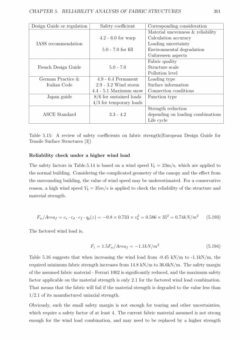
CHAPTER 5. RELIABILITY ANALYSIS OF FABRIC STRUCTURES 301
Design Guide or regulation Safety coefficient Corresponding considerationMaterial unevenness & reliability
4.2 - 6.0 for warp Calculation accuracyIASS recommendation Loading uncertainty
5.0 - 7.0 for fill Environmental degradationUnforeseen aspectsFabric quality
French Design Guide 5.0 - 7.0 Structure scalePollution level
German Practice & 4.9 - 6.4 Permanent Loading typeItalian Code 2.9 - 3.2 Wind storm Surface information
4.4 - 5.1 Maximum snow Connection conditionsJapan guide 8/6 for sustained loads Function type
4/3 for temporary loadsStrength reduction
ASCE Standard 3.3 - 4.2 depending on loading combinationsLife cycle
Table 5.15: A review of safety coefficients on fabric strength(European Design Guide forTensile Surface Structures [3])
Reliability check under a higher wind load
The safety factors in Table.5.14 is based on a wind speed Vb = 23m/s, which are applied to
the normal building. Considering the complicated geometry of the canopy and the effect from
the surrounding building, the value of wind speed may be underestimated. For a conservative
reason, a high wind speed Vb = 35m/s is applied to check the reliability of the structure and
material strength.
Fw/Areaf = cs · cd · cf · qp(z) = −0.8 × 0.733 × v2b = 0.586 × 352 = 0.74kN/m2 (5.193)
The factored wind load is,
F1 = 1.5Fw/Areaf = −1.1kN/m2 (5.194)
Table 5.16 suggests that when increasing the wind load from -0.45 kN/m to -1.1kN/m, the
required minimum fabric strength increases from 14.8 kN/m to 36.6kN/m. The safety margin
of the assumed fabric material - Ferrari 1002 is significantly reduced, and the maximum safety
factor applicable on the material strength is only 2.1 for the factored wind load combination.
That means that the fabric will fail if the material strength is degraded to the value less than
1/2.1 of its manufactured uniaxial strength.
Obviously, such the small safety margin is not enough for tearing and other uncertainties,
which require a safety factor of at least 4. The current fabric material assumed is not strong
enough for the wind load combination, and may need to be replaced by a higher strength
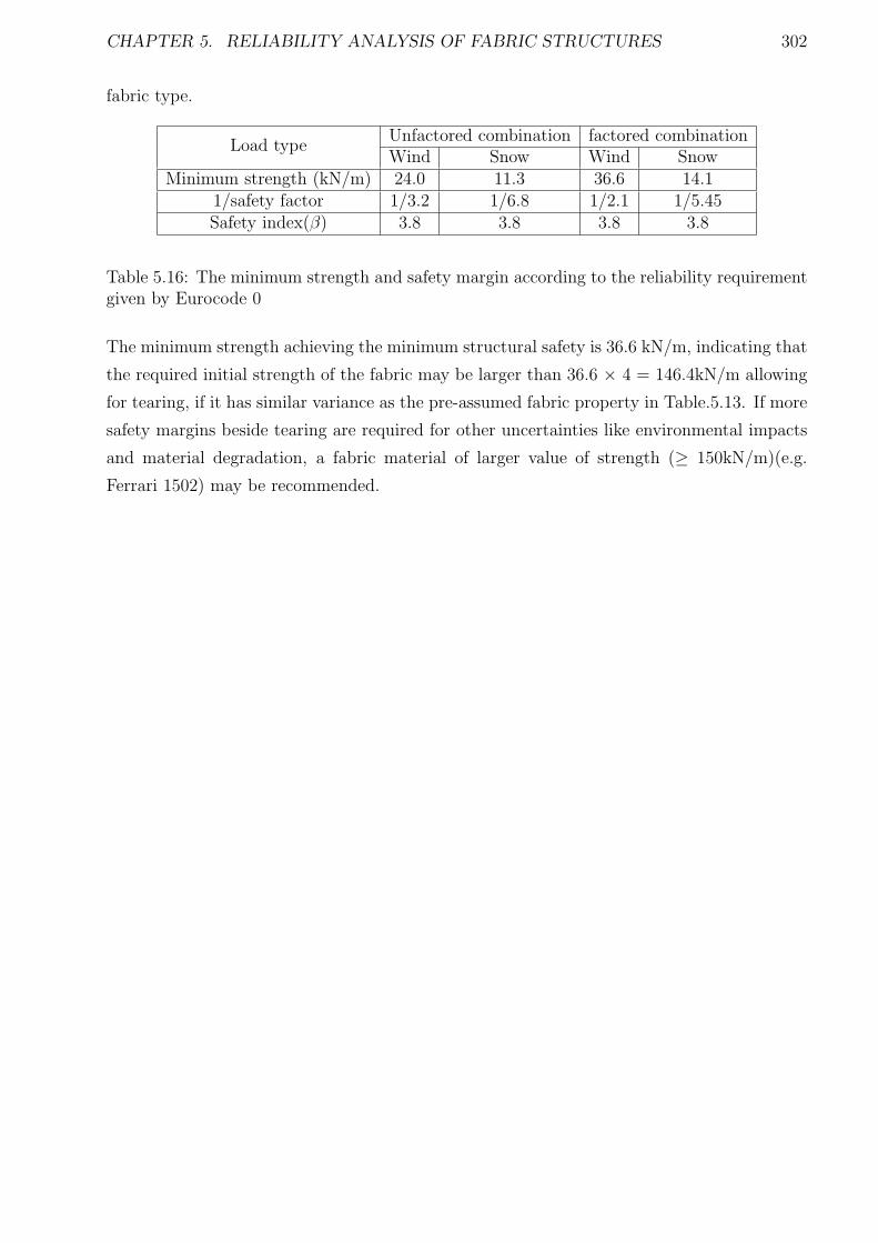
CHAPTER 5. RELIABILITY ANALYSIS OF FABRIC STRUCTURES 302
fabric type.
Unfactored combination factored combinationLoad type
Wind Snow Wind SnowMinimum strength (kN/m) 24.0 11.3 36.6 14.1
1/safety factor 1/3.2 1/6.8 1/2.1 1/5.45Safety index(β) 3.8 3.8 3.8 3.8
Table 5.16: The minimum strength and safety margin according to the reliability requirementgiven by Eurocode 0
The minimum strength achieving the minimum structural safety is 36.6 kN/m, indicating that
the required initial strength of the fabric may be larger than 36.6 × 4 = 146.4kN/m allowing
for tearing, if it has similar variance as the pre-assumed fabric property in Table.5.13. If more
safety margins beside tearing are required for other uncertainties like environmental impacts
and material degradation, a fabric material of larger value of strength (≥ 150kN/m)(e.g.
Ferrari 1502) may be recommended.
CHAPTER 5. RELIABILITY ANALYSIS OF FABRIC STRUCTURES 303
5.5 Conclusion
In this chapter, the finite element reliability analysis is achieved through the FORM and a
finite element analysis, which is used to calculate the gradients of structural response. Two
approaches to calculate the gradient of limit state functions: finite difference and analytical
method have been compared. The finite difference method is found to be time-consuming
when the limit state function has a complicated form and a number of statistical variables
are involved in the analysis, and its accuracy is dependent on the perturbation values. The
analytical approach using the differentiation chain rule has good performance in computing
efficiency and accuracy without perturbations.
The sensitivities of the statistical variables to the reliability are calculated and compared in
two numerical examples under different limit states. The material strength and load coefficient
are found to be the most important elements for the probability of material failure, and the
variation in Young’s modulus seems to have obvious influence on the reliability in serviceability
failure modes including wrinkling and large deformation. Whereas the shear modulus and
Possion’s ratio seems have little affect on the reliability under all failure modes with a increased
variation. The sensitivities of the statistical variables to the reliability are highly relative with
the stress distribution in the membrane, for example, the probability of wrinkling is always
sensitive to Young’s modulus in the direction where minimum principal stress is observed.
When the membrane presstress is much lower than the material tension strength, wrinkling
is found to be prone to appear before fabric rupture.
The reliability based on the practical input parameters in the real design case demonstrates
that a large safety margin may be found when the degradation of the material strength is
not taken into account. Different design approaches given in a variety of design codes are not
consistent and possibly lead to different design judgement about the structural safety. The
sub-factors representing some specific uncertainties in these design guides can be helpful for
a reliability judgement when the statistical property information is not available.
Reliability analysis can replace the factor of safety approach if all statistical information is
available, leading to a single measure of structural safety.
Chapter 6
Conclusion & Recommendations
6.1 Conclusion
Besides the detailed conclusions provided at the end of each chapter/section, the general
review of this PhD research work is given in this part.
Reliability assessment for fabric structures is desired for solving the issues around the incon-
sistent use of safety factors in current fabric structural design, and also encouraged by the
requirement in architecture and structural engineering. A safe structural design and optimized
use of fabric materials can be achieved by an effective and efficient reliability estimation tool,
which normally consists of three main parts: an efficient and accurate structural analysis
tool, an applicable methodology for the identification of uncertainties relative to fabric struc-
tures and an efficient reliability formulation coupled with the specific failure modes of fabric
structures.
A extensive literature review of fabric structural design and analysis, fabric properties and
uncertainties, and reliability calculations was carried. The necessity of developing a reliability
tool for fabric structures based on the design codes currently used was demonstrated by the
literatures, and two types of finite element methods (CST and LST) were recommended for
computing the structural response of fabric structures. To obtain a deep knowledge of fabric
materials, a number of developed fabric material models and probabilistic analysis methods
were reviewed and summarized. Different reliability estimation approaches were discussed
and compared, FORM coupled with finite element formulations were initially recommended
for the reliability calculation of fabric structures.
Four types of finite elements for the analysis of fabric structures were presented - three types
of 3-node constant strain triangular element(CST) and a 6-node linear strain triangle ele-
ment(LST). For the CST element, the significant error introduced by ignoring second order
(’large’) strains was defined mathematically and demonstrated numerically. An enhanced
nonlinear cable analogy formulation, based on the same principles as the existing element
was derived, and shown to be limited in successfully overcoming the effects of assuming small
strains in the underlying mathematics. A large strain continuum formulation that continues
304
CHAPTER 6. CONCLUSION & RECOMMENDATIONS 305
to adopt the philosophy of the original cable analogy approach, but that is based on a classi-
cal finite element philosophy, was shown to be successful within the constraints of a constant
strain field.
A classically-based linear strain triangular finite element was presented, characterised by a
modified curved 6-node triangular element with element curvatures and coupled with the
Newton-Raphson and Dynamic Relaxation algorithms. The inclusion of curvatures in the
numerical representations of membrane surfaces were demonstrated to be important terms
which affect the relationship between the membrane strains and nodal displacements and in
some special cases, the out-of-balance forces.
Fortran 90 programs of the constant strain triangle and linear strain triangle with curvatures
were developed. The effectiveness of these formulations was demonstrated by a number of
numerical examples evaluated using the programs. Furthermore, when coupled with Dynamic
Relaxation, the linear strain triangular element was shown to be extremely computationally
efficient, and highly competitive compared with an equivalent CST mesh.
A probabilistic measurement and analysis methodology was proposed based on the uniaxial
test. The variations of the uniaxial strength and Young’s modulus were estimated, and the
variation details were well represented by suitable distributions. The test data of samples made
by different cutting approaches - plain cut and yarn-stripping were compared and discussed,
and yarn-striping method is recommended for reducing the variations of the samples especially
in assessment of Young’s modulus. The strength of both the samples made by plain-cut and
yarn-striping follow Weibull distributions, and Young’s moduli of the two types of samples do
not follow an uniformed type of distributions.
An efficient finite element reliability formulation for fabric structures was established. It
combines the first order reliability method(FORM) and linear strain triangle element which
was recommended in Chapter 3. The sensitivities of the randomness possibly involved in
fabric structural design were analysed and compared. In some design cases, the structural
reliability may be more sensitive to some uncertainty types over than others.
A Fortran 90 program of a reliability analysis tool was developed. It is able to compute the
structural reliability of fabric structures corresponding to different limit states (e.g. wrinkling
or ponding). Both the Normal and non-normal distributed uncertainties are valid for the
reliability calculation.
A procedure to verify the current safety factors and estimate the relevant reliability was pro-
posed. Combined with the available uncertainty information and safety factors, the structural
reliability can be determined with more accuracy. When all statistical information is avail-
able, the factor of safety approach can be replaced by the reliability method. Then a single
measure of structural safety can be achieved for a design optimization.
CHAPTER 6. CONCLUSION & RECOMMENDATIONS 306
6.2 Recommendations for future work
Further work on the reliability analysis should be focused on the improvement of the ef-
ficiency of finite element formulation, obtaining more detailed probabilistic information in
fabric structural design and construction, and highly accurate reliability analysis using high
order reliability methods.
6.2.1 Finite element formulation
Different finite element types should also be tried for the structural analysis of fabric struc-
tures. The six node linear strain element introduced in Chapter 3, has constant curvatures in
the element. The curvature terms could be involved in high order surface elements(e.g. eight
node quadrilateral) with similar definition. The element surface could be described using a
high order polynomial function, and the curvature terms which are defined as second order
derivatives of the surface function will not be constant, while varying across the element.
That may enable the element to represent highly curved fabric surfaces without a high den-
sity mesh, and enhance the efficiency of the structural analysis. More detailed and accurate
stress contours may be obtained by using the high order elements with curvatures.
Large displacements may result in element distortions of the mesh discretized by high order
elements especially in form-finding. In that case, distortion issues for high order element types
may need to be investigated and a good procedure avoiding excessive element distortions
should be proposed. Form-finding can be initially carried out by low-order (e.g CST or 4
node quadrilateral) elements, which are subsequently replaced by high order elements. Large
deformations will normally occur in the form-finding, where the initial balanced geometry
configuration is achieved. After the low-order elements are replaced, the nodal displacements
to form final balanced geometry for high element meshes will be comparatively small, and
reduce the element distortion to a large extent.
6.2.2 Material investigation
The probabilistic measurement and analysis methodology proposed in Chapter 4, based on the
uniaxial testing of PVC-polyester Ferriari 1002, should be applied to different PVC-polyester
types(e.g. Ferriari 1202) and other fabric types(e.g. PTFE coated glass fibre). The tri-linear
mathematical model presented in Section.4.2.2 is proposed based on the uniaxial stress-strain
relation of PVC Ferriari 1202, and may not be applicable for other material types. A distinctive
model to represent Young’s modulus may need to be developed for other fabric types. High
order models may also be developed for an accurate representation of the nonlinear stress-
strain curves.
Different material test types like biaxial, shear and tear testing should be involved in the
future work. A small number of tests as trials are recommended before large quantity exper-
CHAPTER 6. CONCLUSION & RECOMMENDATIONS 307
iments, and different description formulations and models to represent the characteristics of
the fabric from the trials could be established based on the trials test results. To investigate
the inherent randomness in the fabric of interest, a uniform test procedure and condition is
recommended to avoid extra uncertainty sources(e.g. temperature or environmental impacts).
After a large number of test data are produced, a candidate distribution list can be selected
and determined based on the histogram of test data. To achieve a high efficiency for the
statistical investigation, a Fortran program could be developed to evaluate the variation and
best distributions, and linked to the program of reliability work.
In some cases, the available experimental data and information are too limited out carry a
probabilistic investigation, and an efficient and accurate predictive model could be estimated
for producing more valid data based on the available experimental results. The produced
”fictitious” data will have the same probabilistic characteristics as the original ones. To
reduce the test costs, new test methods could be designed to replace those time-consuming
and expensive test methods like biaixial and shear tests. For example, the Young’s modulus
under biaxial tensile forces could be approximately estimated through a specific uniaxial test
using a predictive model.
6.2.3 Reliability Analysis
The high order reliability method(e.g. SORM) could be developed for a better representation
of nonlinear limit state functions. In this thesis, the uncertainty source involved in the relia-
bility estimation is only limited in Non-cognitive(quantitative) types. In the future work, the
uncertainty source may be expanded to cognitive(qualitative) types including worker skills
and experience, existing buildings, human impacts etc. Fuzzy theory could be introduced
in combining and analyzing these types of uncertainties. Finally a reliability frame work al-
lowing for both quantitative and qualitative uncertainty sources could be undertaken for a
comprehesive reliability analysis.
Bibliography
[1] Guide for Specific Membrane Structures, Membrane Structures Association of
Japan,1990.
[2] Tensile Membrane Structures, ASCE Standard,2002
[3] European Design Guide for Tensile Surface Structures,2004
[4] ”Structural design bassis and safety criteria”, European Design Guide for Tensile Surface
Structures,2004,p177-190
[5] Recommendations for the Design of Air Supported Structures, IASS, 1986.
[6] ”Recommendaion pour la conception des ouvrages permanents de Couverture Textile.”
Annals du Batiment Travaux, September 1997 no.4, pp5-16.
[7] Tragluftbauten - DIN 4134, 1983.
[8] Instuctions for the Design, Realisation, Verification, Use and Maintenance of Tents,
Tensiles Structures and Air-supported Structures, Italian Norm(draft),1995.
[9] Tensile Membrane Structures, ASCE Standard, 2002.
[10] Qi Minyou, ”Probability and Mathematical Statisticas”’(Chinese), Higher Education
Press, China. 2002.
[11] D.S.Wakefield, ”Engineering analysis of tension structures: theory and practice”, Engi-
neering Structures, 21, 1999, p680-690.
[12] ”Material property and testing”, European Design Guide for Tensile Surface
Structures,2004,p219-241
[13] ”Testing method and standards”, European Design Guide for Tensile Surface Struc-
tures,2004,p295
[14] Otto F. Tensile structures . MIT Press, Cambridge, MA. 1971
[15] Barnes,M R. Form finding and analysis of tension structures by Dynamic Relaxation,
Int J of Space Structures, 14, No 2,89-104, 1999
308
BIBLIOGRAPHY 309
[16] Schek, H -J. The Force Density method for form finding and computation of general
networks, Computer Methods in Applied Mechanics and Engineering 3, 115-134,1974
[17] J.Bonet, J.Mahaney. Form finding of membrane structures by the updated reference
method with minimum mesh distortion. International journal of solids and structures,
2001, vol. 38, no32-33, pp. 5469-5480
[18] Larisa Barnets, Graham F. Carey. Extension of a mesh quality metric for elements with
a curved boundary edge or surface. Transactions of the ASME, Vol5. p302-308, 2005.
[19] Mitchell, A. R., Philips, G., and Wachspress, E., Forbidden shapes in the finite element
method, J. Inst. Math. Appl., 8,pp. 260-269, 1971.
[20] Baart, M. L., and Mulder, E. J. A note on invertible two-dimensional quadratic finite
element transformations. Commun. Appl. Numer. Methods. 3. pp. 535-539,1987.
[21] Frey, A. E., C. A, and Porsching, T. A. Some results on the global inversion of bilinear
and quadratic isoprarametric finite element transformations, Math. Comput. 32,pp 725-
749, 1978.
[22] A. Caner and R. Hsu, P.E., Member, ASCE. Tension fabric shape finding, Journal of
Structural Engineering, September, p1065-1071, 1999.
[23] Richard K. Miller and John M. Hedgepheth. An algorithm for finite element analysis of
partly wrinkled membrane. AIAA 4293, p1761-1763, 1982.
[24] S.Babu Aminjikarai, Ala Tabiei. A strain-rate dependent 3-D micromechanical model for
finite element simulations of plain weave composite structures. Composite Structures,
v81,p407-418, 2007.
[25] M.J.King, P.Jearanaisilawong, S.Socrate. A continuum constitutive model for the me-
chanical behavior of woven fabrics. International Journal of Solids and Structures, v42,
p3867-3896, 2005.
[26] Woong Ryeol Yu, Farhang Pourboghrat, Kwansoo Chung. Non-orthogonal constitu-
tive equation for woven fabric reinforced thermoplastic composites. Composites Part
A:applied science and manufacturing. v33,p1095-1105,2002.
[27] P.Potluri, V.S. Thammandra. Influence of uniaxial and biaxial tension on meso-scale
geometry and strain fields in a woven composite. Composite Structures, v77, p405-418,
2007.
[28] YI Hong-lei, DING Xin, CHEN Shou-hui. Esitmation of the elastic constraints of ar-
chitectural membrane under bi-axial tensile loading. Engineering Mechanics(Chinese),
v23, No.10 2006.
BIBLIOGRAPHY 310
[29] Alfred M. Freudenthal. The safety of structures. ASCE,1945 Oct, p1157-1198.
[30] Han Ping Hong, Niel C.Lind. Approximate reliability analysis using normal polynomial
and simulation results. Structural Safety. v18, No.4, p329-339,1996.
[31] Frank Grooteman, Adaptive radial-based importance sampling method for structural
reliability. Structural Safety 30(2008) 533-542.
[32] Jinsuo Nie, Bruce R. Ellingwood, A new directional simulation method for system re-
liability. Part I: application of deterministic sets. Probabilistic Engineering Mechanics
19(2004) 425-436.
[33] B.F. Song, W.Jiang. An equivalent linear method for structural system reliability with
nonlinear safety magins. Computers & Structures, v55, No.6, p1095-1100,1995.
[34] Gert de Cooman. On modeling possibilistic uncertainty in two-state reliability theory.
Fuzzy sets and systems, v83, p215-238, 1996.
[35] Dan M.Frangopol, Kiyohiro Imai. Geometrically nonlinear finite element reliability
analysis of structural system. II: applications. Computers & Structures, v77, p693-
709,2000.
[36] B.N.Bridgens, P.D.Gosling. Direct stress-strain representation for coated woven fabrics.
Computer & Structures, v82,p1913-1927, 2004.
[37] Barnes MR. Form-finding and analysis of tension structures by dynamic relaxation. Phd
thesis.University of London, 1977
[38] Wakefield DS. Pretensioned networks supported by compression arches. Phd thesis,
University of London, 1980
[39] Bucholdt HA, McMillan BR. Iterative methods for the solution of pretensioned cable
structures. In : IASS Symposium on Tension Structures and Space Frances, Tokyo, 1971
[40] Maurin B, Motro R. Density methods and minimal forms computation, In: IASS Col-
loquium on Structural Morphology, Nottingham, 1997,p143-154.
[41] S de Jong, R Postle. Energy optimisation methods in fabric mechanics, Mechanics of
Flexible Fibre Assemblies, p277-241, Amsterdan, 1980.
[42] J.W.S. Hearle. The formation of textile structures. Mechanics of Flexible Fibre Assem-
blies, p1-33,1980.
[43] Ning Pan. Analysis of woven fabric strengths: prediction of fabric strength under uni-
axial and biaxial extensions. Composites Science and Technology, v56,p311-327,1996.
BIBLIOGRAPHY 311
[44] S.R. Moghe. From fibers to woven fabrics. Mechanics of Flexible Fibre Assemblies, p159-
173,1980.
[45] G.A.V. Leaf. Woven fabric tensile mechanics. Mechanics of Flexible Fibre Assemblies,
p179-193,1980.
[46] S.L. Phoenix. Statistical models for the tensile strength of yarns and cables. Mechanics
of Flexible Fibre Assemblies, p113-141,1980.
[47] E. Barbero, J.Fernandez-Saez, C.Navarro. Statistical analysis of the mechanical proper-
ties of composite materials. Composites:Part B 31,p375-381, 2000.
[48] T. Harth, S.Schwan, J.Lehn, F.G. Kollmann. Identification of material parameters for
inelastic constitutive models: statistical analysis and design of experiments. Interna-
tional Journal of Plasticity, v20,p1403-1440,2004.
[49] S.K. Sinha, Reliability and Life Testing, Wiley Easten, New Delhi, 1986
[50] F.T.Peirce. The geometry of cloth structure, J. Text. Inst.28(1937) 45-96
[51] Phelan DG, Harber RB. An integrated design method for cable-reinforced membrane
structures. In: Proceedings of IASS Symposium, vol:2. 1986. p. 119-26
[52] Ishii K. On development of curved surface of membrane structures. In: IASS Interna-
tional Symposium on Pneumatic Structures,1972
[53] Ataka N,Kozuka Y.A determination method of geodesic lines on the surface of membrane
structures [in Japanese]. In: Summary of technical papers of the Annual Meeting AIJ,
1984. p. 21020-21.
[54] Moncrieff E,Topping BHV. Computer methods for the generation of membrane cutting
patterns. Comput. Struct. 1990;37(4):441-50
[55] Moncrieff E,Grundig L, Stroel D. The cutting pattern generation of the pilgrims tents
for phase of the Mina Valley Project. In: IASS International Symposium, Madrid ,vol.
I .1999.p. C127
[56] Grundig L, Ekert L, Moncrieff E. Geodesic and semi-geodesic line algorithms for cutting
pattern generation of architectural textile structures. In: Proceedings of Asia-Pacific
Conference on Shell and Spatial Structures. 1996.p. 435-43.
[57] Grundig L, Moncrieff E. Form finding, analysis and patterning of regular and irregular-
mesh cable-net structures. In: Proceedings of the IASS-LAS98 Conferences, Syd-
ney,(Austrralia), vol.2.1998. p. 856-65
[58] Suzuki T. An analytical method of geodesic line in membrane structures In: Proc. IASS
Symp, vol. 2. 1995.p. 915-22
BIBLIOGRAPHY 312
[59] Tabarrok B.Qin Z.Form finding and cutting pattern generation for fabric tension struc-
tures. In:Microcomputers in civil engineering, vol,8 . Amsterdam: Elsevier Science Pub-
lishers Ltd;1993.p.337-84.
[60] Tsubota H. Determination of actual initial equilibrium state and optimum cutting pat-
terns for membrane structures [ in Japanese]. phD dissertation. Kyoto (Japan): Kyoto
University,1991
[61] Tsubota H.Yoshida A. Theoretical analysis of actual initial equilibrium state for mem-
brane structures based on cutting pattern. In: IASS Symposium, India, vol,,1988.p.647-
56
[62] Tsubota H,Yoshida A. Theoretical analysis of determining optimum cutting patterns
for membrane structures. In: Proc. IASS Symposium, Madrid, vol.3. 1989 p. 11-5.
[63] Yagi T.A simultaneous analysis method for the equilibrium state and the cutting pat-
tern configuration of membrane structures (in Japanese). PhD Dissertation . Nagoya (
Japan): Nagoya National University, 1998.
[64] Yagi T, Ohmori H.A new approach for cutting pattern analysis of membrane structures.
In: Proceedings of the IASS-LAS98 Conference, Sydney (Australia),vol.2. 1998.p. 895-
910.
[65] Armen, H.; Levine, H.; Pifko, A.; Levy, A. NONLINEAR ANALYSIS OF STRUC-
TURES. Source: NASA Contractor Reports, Mar, 1974,128p
[66] Kyriacou, S.K. (Univ of Maryland); Shah, A.D.; Humphrey, J.D.Inverse finite element
characterization of nonlinear hyperelastic membranes, Source: Journal of Applied Me-
chanics, Transactions ASME, v 64, n 2, Jun, 1997, p 257-262
[67] Jeremic, B. (Dept. of Civil/Environmental Engrg., University of California); Runesson,
K.; Sture, S. Finite deformation analysis of geomaterials, Source: International Journal
for Numerical and Analytical Methods in Geomechanics, v 25, n 8, July, 2001, p 809-840
[68] Bognar, Gabriella (Univ of Miskolc), Finite element method for a nonlinear problem,
Source: Computer Assisted Mechanics and Engineering Sciences, v 7, n 4, 2000, p
471-478
[69] Liu P-L, Der Kiureghian A. Finite element reliability methods for geometrically non-
linear structures. Report No.UCB/SCEMM-89/05. Department of Civil Engineering,
University of California, Berkeley, CA, 1989.
[70] Der Kiureghian A,Ke J-B. The stochastic finite element method in structural reliability.
Probab Engng Mech 1988;3(2) :83-91.
BIBLIOGRAPHY 313
[71] Teigen JG, Frangopol DM, Sture S, Felippa CA. Probabilistic FEM for nonlinear con-
crete structures.I:theory. J Struct Engng 1991; 117(9): 2674-89.
[72] Teigen JG, Frangopol DM, Sture S, Felippa CA. Probabilistic FEM for nonlinear con-
crete structures.I:Application. J Struct Engng 1991; 117(9): 2690-707.
[73] Metropolis, N.; Ulam, S., The Monte Carlo Method. Journal of the American Statistical
Association 44 (247): 335-341(1949).
[74] Claudio M. Rocco S. A rule induction approach to improve Monte Carlo system relia-
bility assemssment. Reliability Engineering and System Safety 82(2003) 85-92.
[75] Jose E. ramirez-Marquez, David W. Coit, A Monte-Carlo simulation approach for ap-
proximating multi-state two-terminal reliability. Reliability Engineering and System
Safety 87(2005) 253-264.
[76] A.Naess, B.J.Leira, O.Batsevych. System reliability by enhanced Monte Carlo simula-
tion. Structural Safety 31 (2009) 349-355.
[77] Frangopol DM, Lee Y-H, William K. Nonlinear finite element reliability analysis of
concrete. J Engng Mech 1996;122(12): 1174-82.
[78] Estes AC, Frangopol DM. RELSYS: a computer program for structural system reliabil-
ity. Strut Engng Mech 1996;6(8): 901-19.
[79] Taylor RL. FEAP- a finite element analysis program, version 6.0. Department of Civil
Engineering, University of California, Berkeley, CA, 1996.
[80] Otto.F, Rasch B. Finding form. Deutscher Werkbund Bayern,Edition A.Menges,1995.
[81] J.B Pargana. Realistic modelling of tension fabric structures.PhD thesis, Civil and En-
vironmental Engineering Department.Imperial College London.2005
[82] P.D Gosling. Optimal structural membranes-I.Formulation of a curved quadrilateral
element for surface definition. Comput.Structs.Vol 61.No 5.pp 871-883,1996.
[83] Liu P-L,Der Kiureghian A. Finite element reliability of geometrically nonlinear uncertain
structures. J Engng Mech 1991;117(8),1806-25.
[84] Kiyohiro Imai. Geometrically nonlinear finite element reliability analysis of structural
system,I:theory. Comp. Struct. Vol 77,677-691,2000.
[85] B.Tabarrok, Z.Qin. Nonlinear Analysis of tension structures. Comp. Structs, Vol 45,No
5/6,pp 973-984,1992.
[86] Ye xiaobing. Analysis theory of membrane structure by curved surface finite element
method. Journal of Building Structures(Chinese),vol 19,n 5,pp 17-21,1998.
BIBLIOGRAPHY 314
[87] F. Otto. Zugbeanspruchte Konstruktionen, vol. 1 & 2, Ullstein Verlag,1962.
[88] R.K. Miller, J.M. Hedgepeth, V.I. Weingarten, P. Das, S. Kahyai, Finite element analysis
of partly wrinkled membranes, Comput.Struct.20(1985) 631-639.
[89] D.G. Roddeman, Force transmission in wrinkled membranes,Ph.D thesis, Eindhoven
University of Technology,1987.
[90] J.T. Oden, T.Sato, Finite strains and displacements of elastic membranes by the finite
element method, Int. J.Solids Struct, 3(1967) 471-448.
[91] R.k.Miller,Model tests as an aid to design and construction of membrane structures,
Proceedings of the IASS Symposium on Shells, Membranes and Space Frames, Osaka,
Vol. 2, Elsevier Science Publishers B.V.,Amsterdam, 1986, pp.157-160.
[92] George E.P.Box, Statistics for Experimenters - Design, Innovation, and Discovery, sec-
ond Edition. ISBN 978-7-111-27258-8, John Wiley & Son, Inc. 2005.
[93] P. Contri, B.A. Schrefler, A geometrically nonlinear finite element analysis of wrinkled
membrane surfaces by no-compression material model, Commun. Appl. Numer. Methods
4(1988) 5-15.
[94] K.Ishii, Numerical methods tension structures,Proceedings of the Conference on 10 years
of Progress in Shell and Spatial Structures, IASS, Madrid 1989,pp. 3.
[95] M, Fujikake, O. Kojima, S.Fukushima, Analysis of fabric tensions, Comput.
Struct.32(1989) 537-547.
[96] T. Raible, K. Tegeler, Development of a wrinkling algorithm for orthotropic membrane
materials, Comput, Mechods Appl. Mech. Engrg. 2005
[97] Ramana V.Grandhi, Liping Wang. Reliablity-based structural optimization using im-
proved two-point adaptive nonlinear approximations. Finite Element in Analysis and
Design 29(1998) 35-48.
[98] Argyris JH, Dunne PC, Malejannakis G, Schelkle E. A simple triangular facet shell ele-
ment with application to linear and non-linear equilibrium and elastic stability problems.
Computer Methods in Applied Mechanics and Engineering 1977; 11: 97-113.
[99] Bathe K J, Ho LW. A simple and effective element for analysis of general shell structures.
Computers and Structures 1980;13 :673-681.
[100] Batoz JL, Bathe KJ, Ho LW. A study of three noded triangular plate bending elements.
International Journal for Numerical Methods in Engineering 1980; 15: 1771-812.
[101] Horrigmoe G, Bergan PG. Nonlinear analysis of free-form shells by flat finite elements.
Computers Methods in Applied Mechanics and Engineering 1978; 16: 11-35.
BIBLIOGRAPHY 315
[102] Hsiao KM. Nonlinear analysis of general shell structures by flat triangular shell element.
Computers and Structures 1978; 13: 555-675.
[103] C.A.Felippa, ”Refined Finite Element Analysis of Linear and Nonlinear Two-
Dimensional Solids” UCB/SESM Report No. 66/22, University of California, Berkeley,
October 1966.
[104] Wilson,E.L.”Matrix Finite Analysis of Nonlinear Structures”,Proc. 2nd ASCE Conf. on
Electronic Computation,Pittsburgh,Ps.,Sept.1960.
[105] Turner,M.J.,Martin, H.C and R.C Weikel. ”Further Developments and Applications of
the Stiffness Method” in AGARDograph No.72,cited in Ref.18.
[106] Fraeijs de Veubeke.B.M.,”Displacements and Equilibrium Models in Finite Ele-
ment Method”,chapter 9 of ”Stress Analysis.” edited by O.C.Zienkiewicz and
G.S.Holister,John Wiley and Sons,1965.
[107] G.Subramanian and A.Krishnan.”On an efficient use of CST Elements”.Int.
J.Num.method in Eng. Vol.14.1063-1072.1978
[108] N.P.Dario.”A Comparison of First and Second Order Axially Symmetric Finite Ele-
ments.” Int. J.num. Method. in Eng. Vol.5.573-583.
[109] Lawrence L.Durocher. ”A Numerical Comparison of Axisymmetric Finite Elements”.
Int. J. Num. Methods in Eng. Vol.12. 1415-1427(1978).
[110] D.Radaj.”Accuracy of the Finite Element Analysis for the Elastic Plate with a Circular
hole.” International Journal for Numerical Methods in Engineering Volume 6, Issue 3,
p443C446, 197.
[111] D.G.Harrison and Y.K.Cheung.”A Higher-order Triangular Finite Element for the So-
lution of Field Problems In Orthotropic Media.” Int. J. Num. Methods in Eng. Vol.7.
287-295(1973)
[112] P.Silvester.”High-order Polynomial Triangular Finite Elements For Potential Prob-
lems”.Int. J. Engng Sci Vol. 7.pp 849-861(1969)
[113] Zienkiewicz OC. The finite element method, 3rd ed. New Jersey :McGraw-Hill;1977.
[114] Eugenio Onate, Advances in the formulation of the rotation-free basic shell triangle.
Comput. Mechods, Appl. Mech. Engrg. 194 (2005) 2406-2443.
[115] Fernando G.Flores, Eugenio Onate, Improvements in the membrane behavior of the
three node rotation-free BST shell triangle using an assumed strain approach. Comput.
Mechods, Appl. Mech. Engrg. 194 (2005)907-932.
BIBLIOGRAPHY 316
[116] Houtman, R. & Orpana, M. (2000) Materials for Membrane Structures, Bauen mit
Textilien Heft, 4/2000.
[117] Buckley, C.P. (1980) Review of the mechanical properties of fibres, pp 35-49, Mechanics
of flexible fibre assemblies, edited by John W.S. Hearle, John J. Thwaites, Jafargholi
Amirbayat, Alphen aan den Rijn, Netherlands Germantown, Md. : Sijthoff & Noordhoff
[118] Morris, P.J., Merkin, J.H., Rennell, R.W. (1999) Modelling of yarn properties from fibre
properties, Journal of the Textile Institute, 90, Part 1 (3), 323-335
[119] Osswald, T., Menges, G. (1996) Materials Science of Polymers for Engineers, Hanser
Publishers
[120] Birkett,D.(2002),Keeping the thread,Education in Chemistry,Royal Society of Chem-
istry website, http://www.rsc.org/lap/educatio/eic/2002/birkett mar02.htm
[121] Morton, W.E. and Hearle, J.W.S. (1975) Physical properties of textile fibres, 2nd ed,
London, Heinemann
[122] Boisse, P.; Borr, M.; Buet, K.; Cherouat, A. (1997) Finite element simulations of
textile composite forming including the biaxial fabric behaviour, Composites Part
B:Engineering, v 28B, n 4, p 453-464.
[123] Testa, R.B., Stubbs, N., Spillers, W.R. (1978) Bilinear Model for Coated Square Fabrics,
Journal of Engineering Mechanics, 104, 1027-1042.
[124] Testa, R.B., and Yu, L.M., ”Stress-strain relation for coated fabrics,” J. Eng. Mech.,
113(11), 1631-1646 (1987).
[125] Robinson, A. T. C., and Marks, R. (1967). Woven cloth construction. Butterworths,
London, England
[126] Peirce, F.T. (1937) The Geometry of cloth structure, Journal of the Textile Institute,
28, 81-88
[127] Freeston, W.D.; Platt, M.M.; Schoppee, M.M. (1967) Stress-strain response of fabrics
under two-dimensional loading, Textile Research Journal, 37, 656-682
[128] Pargana, J.B., Lloyd Smith, D., Izzuddin, B.A. (2000) Advanced material model for
the analysis of tensioned fabric structures, Computational methods for shell and spatial
structures, IASS-IACM 2000, Chania-Crete, Greece
[129] Schock, H.J. (1991) On the structural behaviour and material characteristics of PTFE-
coated glass-fibre fabric, Journal of Coated Fabrics, 20, 277-288
[130] Pan, N. (1996) Analysis of woven fabric strengths: prediction of fabric strength under
uniaxial and biaxial extensions, Composites Science and Technology, 56 (3) 311-327
BIBLIOGRAPHY 317
[131] T.Ishikawa, Antisymmetric elastic properties of composite plates of satin weave cloth,
Fiber Sci. Technol, 15( 1981) 127-145
[132] T.Ishikawa, T.W. Chou, Elastic behavior of woven hybrid composites, J. Compos.
Mater.16 (1982) 2-19.
[133] Shahpurwala, A.A & Schwartz, P., Modeling woven fabric tensile strength using statis-
tical bundle theory. Textil Rearch Jounal, 59(1989) 26.
[134] T.Ishikawa, T.W.Chou, Stiffness and strength behavior of fabric composites, J. Mater.
Sci. 17 (1982) 3211-3220.
[135] T.Ishikawa, T.W. Chou, One-dimensional micromechanical analysis of woven fabric com-
posites, AIAA J. 21 (12) (1983) 1714-1721.
[136] N.K. Naik, P.S. Shembekar, Elastic behavior of woven fabric composites: I lamina
analysis J.Compos. Mater.26(15) (1992) 2196-2225.
[137] N.K. Naik, V.K. Ganesh, Failure behavior of plain weave fabric laminates under on-
axis uniaxial tensile loading: II analytical prediction J.Compos. Mater. 30(16) (1996)
1779-1822.
[138] H.T. Hahn, S.W. Tsai, Nonlinear elastic behavior of unidirectional composite laminae,
J. Compos, Mater. 7(1973) 102-118.
[139] R.A. Naik, Failure analysis of woven and braided fabric reinforced composites, J. Com-
pos. Mater. 29(1995) 2334-2363.
[140] D.M.Blackketter, D.E. Walrath, A.C. Hansen, Modelling damage in a plain weave fabric-
reinforced composite material, J.Compos. Technol. Res. 15(2)(1993) 136-142.
[141] A. Tabiei, G. Song, Y. Jiang, Strength simulation of woven fabric composite materials
with material non-linearity using micromechanics based model, J.Thermoplastic Com-
pos. 16(2003) 5-20.
[142] I. Ivanov, A. Tabiei, Three-dimensional computational micro-mechanical model for wo-
ven fabric composites, Compos. Struct. 54(4)(2001) 489-496.
[143] A.Tabiei,I.Ivanov, Fiber reorientation in unidirectional and woven composites for finite
element simulation. Compos. Sci. Technol(2001).
[144] Kawabata, S., Niwa, M.., Kawai, H. (1973a) Finite-deformation theory of plain-weave
fabrics. Part I. The biaxial-deformation theory, Journal of the Textile Institute, 64 (1)
21-46
BIBLIOGRAPHY 318
[145] Mott, R., Huber, G. & Leewood, A. (1985) Biaxial test method for characterization
of fabric materials used in permanent fabric roof structures, The American Society for
Testing and Materials, Journal of Testing and Evaluation, 9-16.
[146] Bassett, R., Postle, R. & Pan N. (1999a) Experimental Methods for Measuring Fabric
Mechanical Properties: A Review and Analysis, Textile Research Journal, 69 (11) 866-
875
[147] Reichardt, C., Woo, H. & Montgomery, D. (1953), A two-dimensional load-extension
tester for woven fabrics, Textile Research Journal, 23, 424-428
[148] Klein, W. (1959) Stress-strain response of fabrics under two-dimensional loading, part
I, The biaxial tester, Textile Research Journal, 29, 816-821
[149] Clulow, E.E. and Taylor, H.M. (1963) An experimental and theoretical investigation of
biaxial stress-strain relations in a plain-weave cloth, Journal of the Textile Institute, 54,
T323-T347
[150] Reinhardt, H. (1976) On the biaxial testing and strength of coated fabrics, Experimental
Mechanics, 16 (2) 71-74.
[151] MacRory, B. & McNamara, A. (1977) Experimental Investigation of the biaxial load-
extension properties of plain weft-knitted fabrics, Textile Research Journal, 47, 233-239.
[152] Bassett, R., Postle, R. & Pan N. (1999b) Grip point spacing along the edges of an
isotropic fabric sheet in a biaxial tensile test, Polymer Composites, 20, 305-313.
[153] Bolotin, V.V. Statistical methods in the nonlinear theory of elastic shells.lzv.Acad. Nauk
SSSR Otd.Tekh.Nauk.1958,3(English translation,NASA TTF-85,1962,1-16).
[154] Koiter, W.T. On the stability of elastic equilibrium.PhD Dissertation. Delft. Hol-
land,1945(English translation:NASA Tech.Trans.1967,F10.833).
[155] Roorda. J. Concepts in elastic structural stability.In Mechanics Today.Vol.1.ed.S.Nemat-
Nasser.Pergamon.Oxford,1972,pp.332-372.
[156] Ikedan K, Murota K.Random inital imperfections of structures. Int. J.Solids Structures
1991: 28(8):1003-21.
[157] Ikeda K,Murota K. Elishakoff I.Reliability of structures subject to normally distributed
initial imperfections.Computers and Structures 1996 :59(3):463-9.
[158] Weibull, W. A statistical theory on the strength of materials. The Royal Swedish Insti-
tute for Engineering Research Proceeding,No.151.1939.
[159] Heller R.A.(ed.). Probabilistic Aspects of Fatigue.STEP-511.AM.Soc.for Testing and
Materials.Philadelphia,1972.
BIBLIOGRAPHY 319
[160] Hill R.Hutchinson J.W.Bifurcation phenomena in the plane tension test.
J.Mech.Phys.Soilds 1975:23:239-64.
[161] Peirce, F.T., 1937. The geometry of cloth structure. Journal of Textile Institute 28 (3),
T45T96.
[162] Kawabata, S., Niwa, M., Kawai, H., 1973. The finite deformation theory of plain weave
fabrics. Part II: The uniaxial deformation theory. Journal of Textile Institute 64 (2),
4761.
[163] Kato, S., Yoshiro, T., Minami, H., 1999. Formulation of constitutive equations for fabric
membranes based on the concept of fabric lattice model. Engineering Structures 21,
691708.
[164] Shockey, D.A., Elrich, D.C., Simons, J.W., 1999. Improved Barriers to Turbine Engine
Fragments: Interim Report I. DOT/FAA AR-99/8,I.
[165] Ikeda K.Goto S.Imperfection sensitivity for size effect of granular materials.Soils and
Foundations 1993:33(2):157-70.
[166] Ikeda K.Maruyama K.Ishida H.Kagawa S.Bifurcation in compressive behavior of con-
crete.ACI Materials Journal 1997;94(6);484-91.
[167] Trukstra CJ.Theory of structural design decision .Study No.2. Water-
loo(Ontario,Canada): Soild Mechanics Division,Univ Waterloo,1970.
[168] Minimum design loads for buildings and other structures[ASCE 7-
98]:Reston(VA):ASCE;1998.
[169] Pearce HT,Wen YK.Stochastic combination of load effects.J Str Div,ASCE
1984;110(7);1613-29.
[170] Ellingwood B,Rosowsky D.Combining snow and earthquake loads for limit state design.J
Struc Engng, ASCE 1996;112(11):1364-8..
[171] Ushakov IA,editor.Handbook of reliability engineering.New York: Wi-
ley/Interscience;1994.
[172] Schueller GI,editor.Structural dynamics-recent advances.Berlin:Springer; 1991.
[173] Scheuller GI,Ang AHS.Advances in structural reliability.Nucl Engng Des 1992;134:121-
40.
[174] Wen YK.Building reliability and code calibration.Earthquake Spectra 1995;11:269-349.
[175] A.G.Davenport, The application of statistical concepts to the wind loading of struc-
tures,Proc.Inst.Civil Eng.19(1961) 449-472.
BIBLIOGRAPHY 320
[176] A.G Davenport,Note on the distribution of the largest value of a random function with
application to gust loading. Proc.Inst.Civil Eng.24(1964) 187-196.
[177] A.G Davenport,Gust loading factors, J.Struct.Div.ASCE 93(1967)11-34.
[178] G.Solari, A long wind response estimation:closed form solution, J.Struct. Div.ASCE
108(1982) 225-244.
[179] Dempster AP. A generalization of bayesian inference. J Royal Statistical Society
1969;B30: 205-47.
[180] Achintya Haldar and Sankaran Mahadevan. ”Reliability Assessment Using Stochastic
Finite Element Analysis”, John Wiely& Sons, INC, ISBN 0-471-36961-6,2000.
[181] Jin guo liang ,Chen ling and Dong jia mei .Monte Carlo Finite Element Method of Struc-
tural Reliability Analysis.Daqing Petroleum Institute, Anda Heilongjiang, China.(1992)
[182] Madsen HO,Krenk S,Lind NC, Methods of structural safety.Englewood
Cliffs(N.J):Prentice-Hall,1986.
[183] Bjerager P.Methods for structural reliability computation. In:Casciati
F,editor.Reliability problems:general principles and applications in mechanics of
solid and structures.New York:Springer Verlag Wien ,1991.p. 89-136.
[184] Hasofer AM,Lind NC.Exact and invariant second-moment code format. J Engng Mech
Division,ASCE 1974;100(1):111-21.
[185] Fiessler B,Neumann H-J,Rackwitz R.Quadratic limit states in structural reliability.J
Engrg Mech ASCE 1979;105(4):661-76.
[186] Bucher CG,Adaptive sampling:an iterative fast Monte-Carlo procedure.Structural
Safety 1988;5(2):119-26.
[187] Mori Y,Ellingwood B.Time-dependent system reliability analysis by adaptive impor-
tance sampling.Structural Safety 1993;12(1):59-73.
[188] Tichy M. First-order third-moment reliability method. Structural Safety 1994;16:189-
200.
[189] Bucher CG,Bourgund U. A fast and efficient response surface approach for structural
reliability problems. Structural Safety 1990;7:57-66.
[190] Zhao YG,Jiang JR. A structural reliability method based on genetic algorithm earth-
quake Engineering and Engineering Vibration 1995;15(3)44-58(in Chinese).
[191] Yang-Gang Zhao, Tetsuro Ono, A general procedure for first/second order reliability
method(FORM/SORM). Structural Safety 21(1999) 95-112.

BIBLIOGRAPHY 321
[192] Yang-Gang Zhao, Tetsuro Ono, Moment methods for structural reliability. Structural
Safety 23(2001) 47-75.
[193] Jean-Claude Mitteau, Error evaluations for the computation of failure probability in
static structural reliability problems. Probabilistic Engineer Mechanics 14(1999) 119-
135.
[194] Armen D.K., Taleen.D, Multiple design points in first and second-order reliability. Struc-
tural Safety 20(1998), 37-49.
[195] Kuschel N,Pieracci A,Rackwitz R.Multiple β-points in structural reliability.In:3rd
Int.Conf.on Computational Stochastic Mechanics,Santorini,14-17 June 1998.
[196] Bjerager P. On computation methods for structural reliability analysis. In:Frangopol
DM.editor.New directions in structural system reliability.Boulder (CO): University of
Colorado,1988.p.52-67.
[197] Ditlevsen O,Melchers R E.Gluver H.General multi-dimensional probability integration
by directional simulation.Computers And Structures 1990;36(2);355-68.
[198] Melchers R E.Structural system reliability assessment using directional simulation.
Structural Safety 1994;16:23-37.
[199] Moarefzadeh MR, Melchers RE. Directional importance sampling for ill-proportioned
spaces. Structural Safety. 21:1-22.1999
[200] Dimitri Val, Fiodor Bljuger,David Yankelevsky. Reliability evaluation in nonlinear
analysis of reinforced concrete structures. Structural Safty Vol.19, No.2.pp.203-217,1997
[201] Y.S.Petryna,W.B.Kratzig. Computational framework for long-term reliability analysis
of RC structures. Comput. Methods Appl. Mech. Engrg. 194(2005) 1619-1639
[202] Michael Havbro Faber,Jochen Kohler,John Dalsgaard Sorensen. Probabilistic modeling
of graded timber material properties. Structural safety ,vol 26,295-309,2000.
[203] Kiyohiro Imai,Dan M. Frangopol. System reliability of suspension bridges. Structural
Safety, vol 24,219-299, 2002.
[204] A. Haldar, S. Mahadevan. Probability, Reliability, and Statistical Methods in Engineer-
ing Design. John Wiley & Son, Inc. New York(2000), p38.
[205] A. Haldar, S. Mahadevan. Probability, Reliability, and Statistical Methods in Engineer-
ing Design. John Wiley & Son, Inc. New York(2000), p39.
[206] J.Argyris, et al., A general method for the shape finding of lightweight tension structures,
Comput. methods Appl. Mech. Eng. 3(1974) 135-149.
BIBLIOGRAPHY 322
[207] D.S Wakefield, Numerical modelling in tension structures design and construction, Pro-
ceedings of IASS Coll. Structural Morphology: Towards the New Millennium, Notting-
ham, 1997.
[208] P.D.Gosling, Numerical modelling of stable minimal surfaces. PhD thesis, University of
Warwick. 1992
[209] Zhang Lei, A large strain cable-analogy membrane finite element, MSc disertation, Civil
Engineering Department, Newcastle University. 2003
[210] Otto.F, Rasch B. Finding form. Deutscher Werkbund Bayern,Edition A.Menges,1995.
[211] J.B Pargana. Realistic modelling of tension fabric structures.PhD thesis, Civil and En-
vironmental Engineering Department.Imperial College London.
[212] P.D Gosling. Optimal structural membranes-I.Formulation of a curved quadrilateral
element for surface definition. Comput.Structs.Vol 61.No 5.pp 871-883,1996.
[213] L.Grundig. Minimal surface for finding forms of structural membranes. Computer &
Structures Vol. 30, No. 3,pp. 679-683, 1988.
[214] Liu P-L,Der Kiureghian A. Finite element reliability of geometrically nonlinear uncertain
structures. J Engng Mech 1991;117(8),1806-25.
[215] Kiyohiro Imai. Geometrically nonlinear finite element reliability analysis of structural
system,I:theory. Comp. Struct. Vol 77,677-691,2000.
[216] B.Tabarrok, Z.Qin. Nonlinear Analysis of tension structures. Comp. Structs, Vol 45,No
5/6,pp 973-984.
[217] Ye xiaobing. Analysis theory of membrane structure by curved surface finite element
method. Jounal of Building Structures(Chinese),vol 19,n 5,pp 17-21,1998.
[218] Wang Xun Chen. Finite Element Method. Publication of Qinghua University, 2003,pp
138.
[219] A.R. Mitchell, G.Phillips. Forbidden shapes in the finite element method. J.Inst.Maths
Applics(1971) 8, 260-269.
[220] M.L.BAART. Quadratic Transformations of Triangular Finite Elements in Two Dimen-
sions. IMA Journal of Numerical Analysis (1986) 6, 475-487.
[221] Robert D.Cook, Davids S. Malkus. Concepts and applications of finite element analysis.
Third Edition, University of Wisconsin - Madison (1989), pp 185.
[222] F. OttoZugbeanspruchte Konstruktionen, vol. 1 & 2, Ullstein Verlag,1962.
BIBLIOGRAPHY 323
[223] R.K. Miller, J.M. Hedgepeth, V.I. Weingarten, P. Das, S. Kahyai, Finite element analysis
of partly wrinkled membranes, Comput.Struct.20(1985) 631-639.
[224] Roddeman D.G. Drukker J. ”Finite element analysis of membrane wrinkling”, Interna-
tional Journal for numerical methods in engineering., 2001, vol 50,pp. 1017-1038.
[225] J.T. Oden, T.Sato, Finite strains and displacements of elastic membranes by the finite
element method, Int. J.Solids Struct, 3(1967) 471-448.
[226] R.k.Miller,Model tests as an aid to design and construction of membrane structures,
Proceedings of the IASS Symposium on Shells, Membranes and Space Frames, Osaka,
Vol. 2, Elsevier Science Publishers B.V.,Amsterdam, 1986, pp.157-160.
[227] M. Hideki, O. Kiyoshi, A study on modeling and structural behaviour of membrane
structures, Proceedings of the IASS Symposium on Shells, Membranes and Space
Frames, Osaka, Vol. 2,1986,pp. 161-167.
[228] P. Contri, B.A. Schrefler, A geometrically nonlinear finite element analysis of wrinkled
membrane surfaces by no-compression material model, Commun. Appl. Numer. Methods
4(1988) 5-15.
[229] K.Ishii, Numerical methods tension structures,Proceedings of the Conference on 10 years
of Progress in Shell and Spatial Structures, IASS, Madrid 1989,pp. 3.
[230] M, Fujikake, O. Kojima, S.Fukushima, Analysis of fabric tensions, Comput.
Struct.32(1989) 537-547.
[231] T. Raible, K. Tegeler, Development of a wrinkling algorithm for orthotropic membrane
materials, Comput, Mechods Appl. Mech. Engrg. 2005,p2550-2568.
[232] F. Sindel, T. Nouri-Baranger, Including optimisation in the conception of fabric struc-
tures. Comput. struct. 79(2001) 2451-2499.
[233] Lo SH. Generating quadrilateral elements on plane and over curved surfaces. Computers
and Structures 1989;31;421-6
[234] Lo SH. A new mesh generation scheme for arbitrary planar domains. International
Journal for Numerical Methods in Engineering 1985;21:1403-26.
[235] Riccardo Rossi. Convergence of the modified material model for wrinkling simula-
tion of light-weight membrane structures. Textile composites and inflatables structures
2003,pp148-153.
[236] Xinxiang Liu, Large deflection analysis of pneumatic envelopes using a penalty parame-
ter modified material method. Finite element analysis and design 37(2001) pp233-251.
BIBLIOGRAPHY 324
[237] Riccardo Rossi. Simulation of light-weight membrane structures by wrinkling model.
Int. J. Numer. Meth. Engrg. 2005; 62:2177-2153
[238] Bridgens,B.N. Architectural fabric properties: determination, representation & predic-
tion, Chapter 3 ,PhD Thesis in Structural Engineering, University of Newcastle Upon
Tyne,UK,2006.
[239] Ditlevsen O,Madsen HO. Structural reliability methods. Chichester, New York, NY:
Wiley;1996.
[240] Rubinstein RY, Melamed B. Modern simulation and modeling. New York, NY: Wiley;
1998.
[241] Rajashekhar MR, Ellingwood BR. A response surface approach for reliability analysis.
Struct Saf 1993;12:205-20.
[242] R.Rackwitz, B. Fiessler, Structural reliability under combined load sequences, Comput.
Struct. 9 (1978) 489-494.
[243] Zhang, Y., and Der Kiureghian, A. Dynamic response sensitivity of inelastic structures.”
Comput. Meth. Appl. Mech. Engrg., v108, p23-36,1993.
[244] Enrique Castillo, and Jose Manuel Gutierrez, and Ali S.Hadi. ”Modeling Probabilistic
Networks of Discrete and Continuous Variables”. Journal of Multivariate Analysis, v64,
p48-65, 1998.
[245] X.L.Guan, and R.E.Melchers. ”A load space formulation for probabilistic finite element
analysis of structure reliability”. Probabilistic Engineering Mechanics v14, p73-81. 1999.
[246] Y.-X. Zhang, and Q.Gao, and J,-N. Wang. ”An approach for determing an appropri-
ate assumed distribution of fatigue life under limit data.” Reliability Engineering and
System Safety, v67, p1-7, 2000.
[247] M.A. Stephens. ”EDF Statistics for Goodness of Fit and Some Comparison.” Journal
of the American Statistical Association, v69, p730-737, 1974.
[248] Lieblein, J. ”Two early papers on the relation between extreme values and tensile
strength”. Biometrika, v41, p559-60.
[249] T.Igusa, S.G. Buonopane, B.R. Ellingwood. ”Bayesian analysis of uncertainty for struc-
tural engineering applications.” Structural Safety, v24, pp165-186, 2002.
[250] Dempster AP. A generalization of bayesian inference. J Royal Statistical Society 1968;
B30:205-47.

BIBLIOGRAPHY 325
[251] Beatriz S.L.P. de Lima, Nelson F.F. Ebecken. ”A comparison of models for uncertainty
analysis by the finite element method”. Finite Element in Analysis and Design, v34,
pp211-232, 2000.
[252] Ruoxue Zhang, Sankaran Mahadevan. ”Model uncertainty and Bayesian updating in
reliability-bsed inspection”, Structural Safety, v22, pp145-160, 2000.
[253] ”Eurocode 0: Basis of Structural Design,BS EN: 1990:2002”.
[254] ”Eurcode 1:Actions on structrues, Part 1-4: General actions Wind actions, BS EN
1991-1-4:2005”
[255] ”Eurcode 1:Actions on structrues, Part 1-3: General actions Snow loads, BS EN 1991-
1-3:2003”
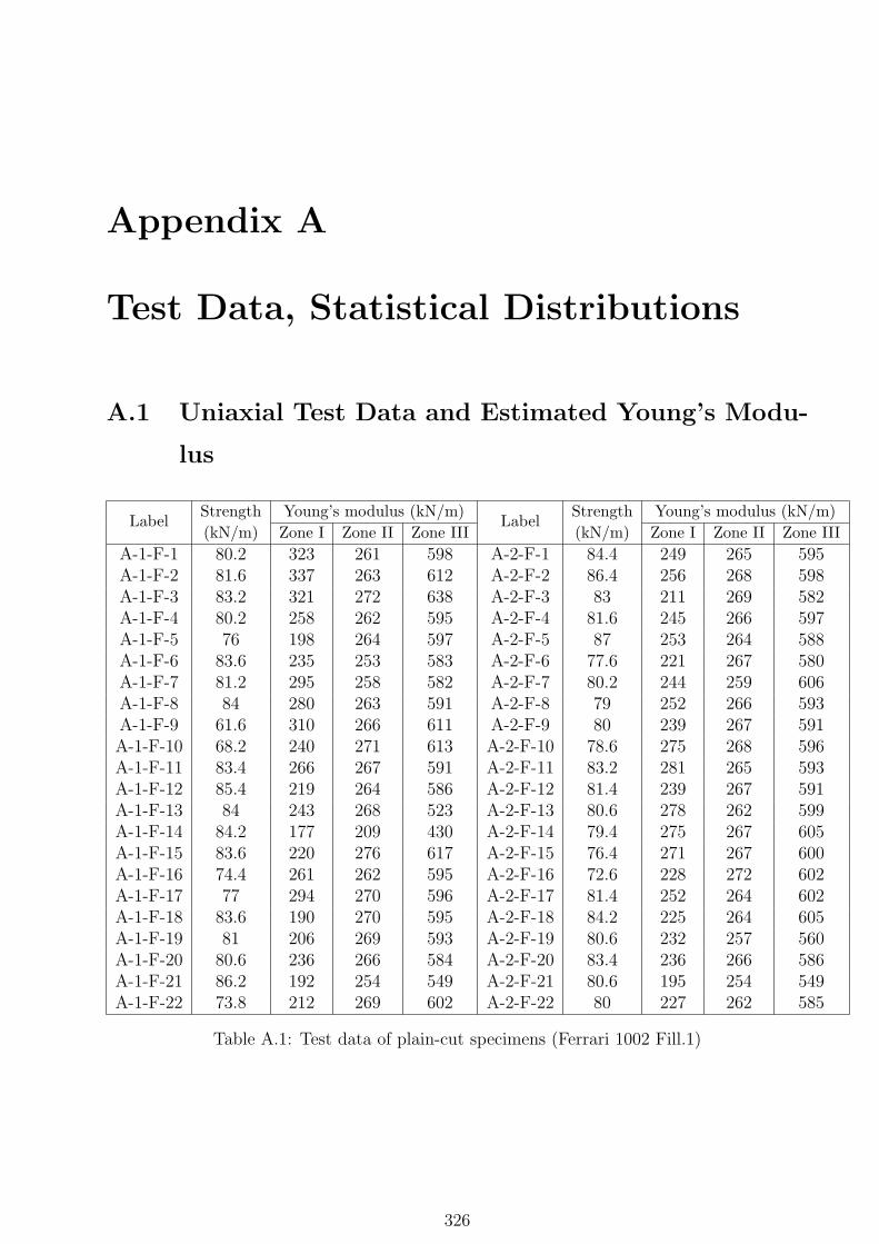
Appendix A
Test Data, Statistical Distributions
A.1 Uniaxial Test Data and Estimated Young’s Modu-
lus
Strength Young’s modulus (kN/m) Strength Young’s modulus (kN/m)Label
(kN/m) Zone I Zone II Zone IIILabel
(kN/m) Zone I Zone II Zone III
A-1-F-1 80.2 323 261 598 A-2-F-1 84.4 249 265 595A-1-F-2 81.6 337 263 612 A-2-F-2 86.4 256 268 598A-1-F-3 83.2 321 272 638 A-2-F-3 83 211 269 582A-1-F-4 80.2 258 262 595 A-2-F-4 81.6 245 266 597A-1-F-5 76 198 264 597 A-2-F-5 87 253 264 588A-1-F-6 83.6 235 253 583 A-2-F-6 77.6 221 267 580A-1-F-7 81.2 295 258 582 A-2-F-7 80.2 244 259 606A-1-F-8 84 280 263 591 A-2-F-8 79 252 266 593A-1-F-9 61.6 310 266 611 A-2-F-9 80 239 267 591A-1-F-10 68.2 240 271 613 A-2-F-10 78.6 275 268 596A-1-F-11 83.4 266 267 591 A-2-F-11 83.2 281 265 593A-1-F-12 85.4 219 264 586 A-2-F-12 81.4 239 267 591A-1-F-13 84 243 268 523 A-2-F-13 80.6 278 262 599A-1-F-14 84.2 177 209 430 A-2-F-14 79.4 275 267 605A-1-F-15 83.6 220 276 617 A-2-F-15 76.4 271 267 600A-1-F-16 74.4 261 262 595 A-2-F-16 72.6 228 272 602A-1-F-17 77 294 270 596 A-2-F-17 81.4 252 264 602A-1-F-18 83.6 190 270 595 A-2-F-18 84.2 225 264 605A-1-F-19 81 206 269 593 A-2-F-19 80.6 232 257 560A-1-F-20 80.6 236 266 584 A-2-F-20 83.4 236 266 586A-1-F-21 86.2 192 254 549 A-2-F-21 80.6 195 254 549A-1-F-22 73.8 212 269 602 A-2-F-22 80 227 262 585
Table A.1: Test data of plain-cut specimens (Ferrari 1002 Fill.1)
326
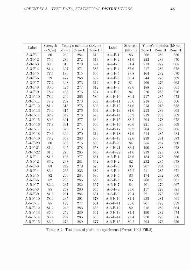
APPENDIX A. TEST DATA, STATISTICAL DISTRIBUTIONS 327
Strength Young’s modulus (kN/m) Strength Young’s modulus (kN/m)Label
(kN/m) Zone I Zone II Zone IIILabel
(kN/m) Zone I Zone II Zone III
A-3-F-1 86 239 284 610 A-4-F-1 83 268 286 686A-3-F-2 75.4 286 272 614 A-4-F-2 81.6 222 283 670A-3-F-3 80.6 313 270 594 A-4-F-3 81.4 213 277 665A-3-F-4 81.4 397 271 585 A-4-F-4 87.6 217 286 678A-3-F-5 77.4 180 315 606 A-4-F-5 77.8 164 282 670A-3-F-6 79 477 268 592 A-4-F-6 80.4 244 278 669A-3-F-7 77.2 348 273 612 A-4-F-7 81 269 276 663A-3-F-8 80.6 424 277 612 A-4-F-8 79.6 188 276 661A-3-F-9 78.4 466 276 594 A-4-F-9 84 276 283 676A-3-F-10 78.4 294 266 586 A-4-F-10 86.4 217 285 672A-3-F-11 77.2 287 273 608 A-4-F-11 85.6 218 280 666A-3-F-12 81.4 315 275 603 A-4-F-12 84.6 213 213 658A-3-F-13 73.4 315 276 604 A-4-F-13 81.6 213 283 665A-3-F-14 82.2 342 278 625 A-4-F-14 83.2 219 289 669A-3-F-15 80.6 391 277 639 A-4-F-15 88.2 204 278 678A-3-F-16 77.8 331 274 600 A-4-F-16 80.6 221 283 669A-3-F-17 77.6 325 273 605 A-4-F-17 82.2 204 280 665A-3-F-18 79.2 324 270 614 A-4-F-18 84.6 214 285 684A-3-F-19 78.2 358 283 636 A-4-F-19 82.6 239 281 683A-3-F-20 80 303 276 630 A-4-F-20 84 255 287 686A-3-F-21 81.4 345 278 658 A-4-F-21 83.4 190 288 678A-3-F-22 81.6 270 285 645 A-4-F-22 74.6 239 278 666A-5-F-1 81.6 198 277 661 A-6-F-1 75.6 184 278 666A-5-F-2 86.2 238 281 662 A-6-F-2 82 232 285 678A-5-F-3 83 242 279 670 A-6-F-3 83 207 284 671A-5-F-4 83.4 235 236 682 A-6-F-4 82.2 211 285 671A-5-F-5 82 266 284 686 A-6-F-5 83 174 282 660A-5-F-6 82 238 286 688 A-6-F-6 85 268 280 661A-5-F-7 82.2 237 282 667 A-6-F-7 84 201 279 667A-5-F-8 85 257 280 655 A-6-F-8 85.6 157 279 681A-5-F-9 81.6 251 284 661 A-6-F-9 79.4 221 273 658A-5-F-10 78.4 235 291 678 A-6-F-10 84.4 235 281 661A-5-F-11 85 198 277 661 A-6-F-11 85.6 261 278 659A-5-F-12 81.2 246 283 656 A-6-F-12 82 218 282 664A-5-F-13 86.6 252 289 667 A-6-F-13 84.4 190 282 674A-5-F-14 83.4 292 286 683 A-6-F-14 77.4 270 279 656A-5-F-15 83.6 276 289 677 A-6-F-15 80.2 294 273 656
Table A.2: Test data of plain-cut specimens (Ferrari 1002 Fill.2)
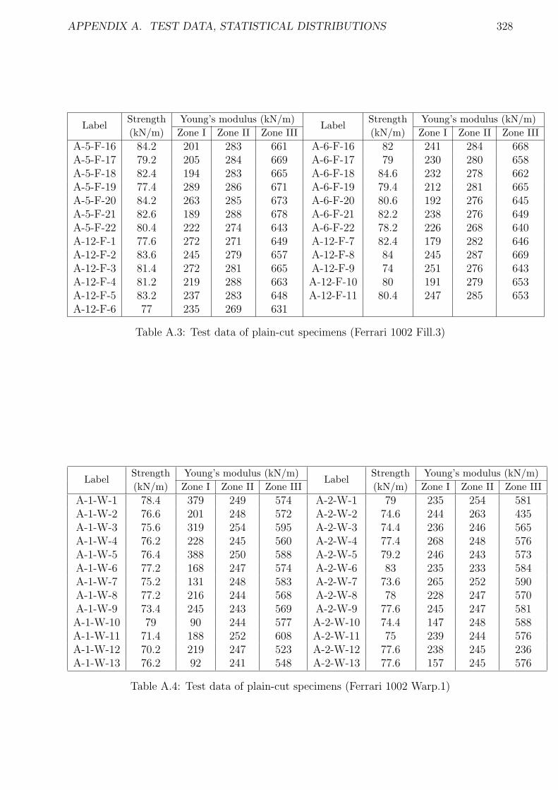
APPENDIX A. TEST DATA, STATISTICAL DISTRIBUTIONS 328
Strength Young’s modulus (kN/m) Strength Young’s modulus (kN/m)Label
(kN/m) Zone I Zone II Zone IIILabel
(kN/m) Zone I Zone II Zone III
A-5-F-16 84.2 201 283 661 A-6-F-16 82 241 284 668A-5-F-17 79.2 205 284 669 A-6-F-17 79 230 280 658A-5-F-18 82.4 194 283 665 A-6-F-18 84.6 232 278 662A-5-F-19 77.4 289 286 671 A-6-F-19 79.4 212 281 665A-5-F-20 84.2 263 285 673 A-6-F-20 80.6 192 276 645A-5-F-21 82.6 189 288 678 A-6-F-21 82.2 238 276 649A-5-F-22 80.4 222 274 643 A-6-F-22 78.2 226 268 640A-12-F-1 77.6 272 271 649 A-12-F-7 82.4 179 282 646A-12-F-2 83.6 245 279 657 A-12-F-8 84 245 287 669A-12-F-3 81.4 272 281 665 A-12-F-9 74 251 276 643A-12-F-4 81.2 219 288 663 A-12-F-10 80 191 279 653A-12-F-5 83.2 237 283 648 A-12-F-11 80.4 247 285 653A-12-F-6 77 235 269 631
Table A.3: Test data of plain-cut specimens (Ferrari 1002 Fill.3)
Strength Young’s modulus (kN/m) Strength Young’s modulus (kN/m)Label
(kN/m) Zone I Zone II Zone IIILabel
(kN/m) Zone I Zone II Zone III
A-1-W-1 78.4 379 249 574 A-2-W-1 79 235 254 581A-1-W-2 76.6 201 248 572 A-2-W-2 74.6 244 263 435A-1-W-3 75.6 319 254 595 A-2-W-3 74.4 236 246 565A-1-W-4 76.2 228 245 560 A-2-W-4 77.4 268 248 576A-1-W-5 76.4 388 250 588 A-2-W-5 79.2 246 243 573A-1-W-6 77.2 168 247 574 A-2-W-6 83 235 233 584A-1-W-7 75.2 131 248 583 A-2-W-7 73.6 265 252 590A-1-W-8 77.2 216 244 568 A-2-W-8 78 228 247 570A-1-W-9 73.4 245 243 569 A-2-W-9 77.6 245 247 581A-1-W-10 79 90 244 577 A-2-W-10 74.4 147 248 588A-1-W-11 71.4 188 252 608 A-2-W-11 75 239 244 576A-1-W-12 70.2 219 247 523 A-2-W-12 77.6 238 245 236A-1-W-13 76.2 92 241 548 A-2-W-13 77.6 157 245 576
Table A.4: Test data of plain-cut specimens (Ferrari 1002 Warp.1)
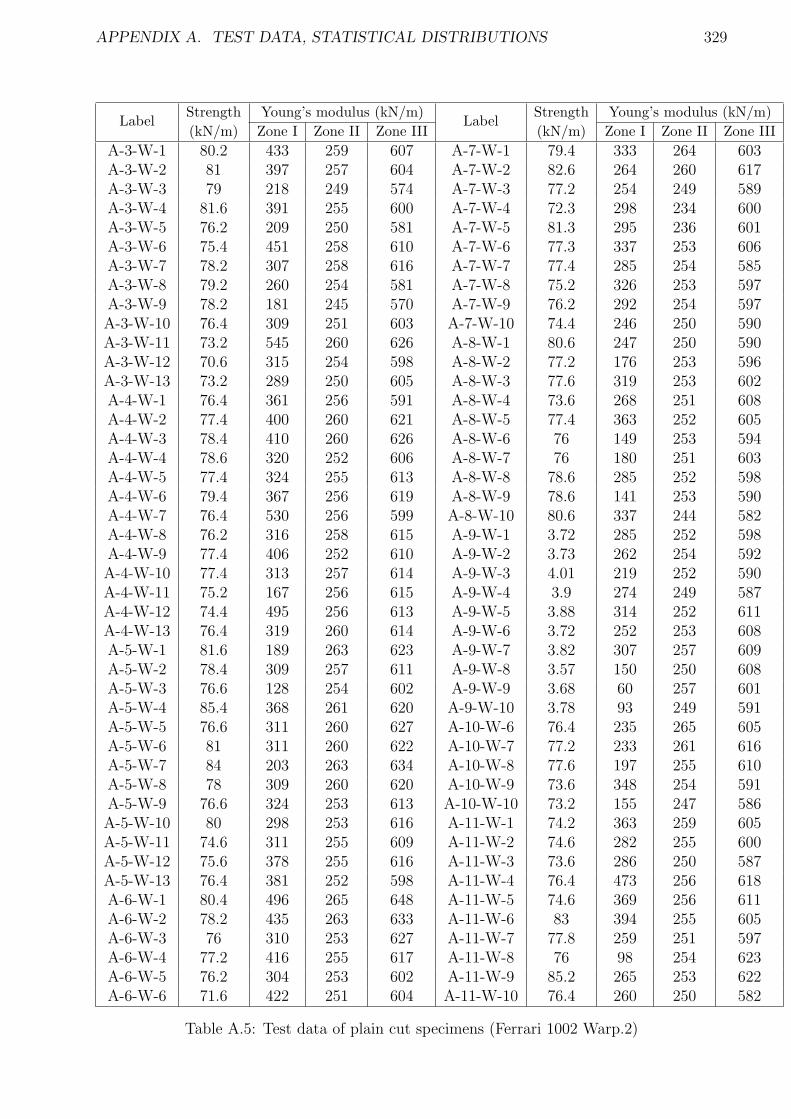
APPENDIX A. TEST DATA, STATISTICAL DISTRIBUTIONS 329
Strength Young’s modulus (kN/m) Strength Young’s modulus (kN/m)Label
(kN/m) Zone I Zone II Zone IIILabel
(kN/m) Zone I Zone II Zone III
A-3-W-1 80.2 433 259 607 A-7-W-1 79.4 333 264 603A-3-W-2 81 397 257 604 A-7-W-2 82.6 264 260 617A-3-W-3 79 218 249 574 A-7-W-3 77.2 254 249 589A-3-W-4 81.6 391 255 600 A-7-W-4 72.3 298 234 600A-3-W-5 76.2 209 250 581 A-7-W-5 81.3 295 236 601A-3-W-6 75.4 451 258 610 A-7-W-6 77.3 337 253 606A-3-W-7 78.2 307 258 616 A-7-W-7 77.4 285 254 585A-3-W-8 79.2 260 254 581 A-7-W-8 75.2 326 253 597A-3-W-9 78.2 181 245 570 A-7-W-9 76.2 292 254 597A-3-W-10 76.4 309 251 603 A-7-W-10 74.4 246 250 590A-3-W-11 73.2 545 260 626 A-8-W-1 80.6 247 250 590A-3-W-12 70.6 315 254 598 A-8-W-2 77.2 176 253 596A-3-W-13 73.2 289 250 605 A-8-W-3 77.6 319 253 602A-4-W-1 76.4 361 256 591 A-8-W-4 73.6 268 251 608A-4-W-2 77.4 400 260 621 A-8-W-5 77.4 363 252 605A-4-W-3 78.4 410 260 626 A-8-W-6 76 149 253 594A-4-W-4 78.6 320 252 606 A-8-W-7 76 180 251 603A-4-W-5 77.4 324 255 613 A-8-W-8 78.6 285 252 598A-4-W-6 79.4 367 256 619 A-8-W-9 78.6 141 253 590A-4-W-7 76.4 530 256 599 A-8-W-10 80.6 337 244 582A-4-W-8 76.2 316 258 615 A-9-W-1 3.72 285 252 598A-4-W-9 77.4 406 252 610 A-9-W-2 3.73 262 254 592A-4-W-10 77.4 313 257 614 A-9-W-3 4.01 219 252 590A-4-W-11 75.2 167 256 615 A-9-W-4 3.9 274 249 587A-4-W-12 74.4 495 256 613 A-9-W-5 3.88 314 252 611A-4-W-13 76.4 319 260 614 A-9-W-6 3.72 252 253 608A-5-W-1 81.6 189 263 623 A-9-W-7 3.82 307 257 609A-5-W-2 78.4 309 257 611 A-9-W-8 3.57 150 250 608A-5-W-3 76.6 128 254 602 A-9-W-9 3.68 60 257 601A-5-W-4 85.4 368 261 620 A-9-W-10 3.78 93 249 591A-5-W-5 76.6 311 260 627 A-10-W-6 76.4 235 265 605A-5-W-6 81 311 260 622 A-10-W-7 77.2 233 261 616A-5-W-7 84 203 263 634 A-10-W-8 77.6 197 255 610A-5-W-8 78 309 260 620 A-10-W-9 73.6 348 254 591A-5-W-9 76.6 324 253 613 A-10-W-10 73.2 155 247 586A-5-W-10 80 298 253 616 A-11-W-1 74.2 363 259 605A-5-W-11 74.6 311 255 609 A-11-W-2 74.6 282 255 600A-5-W-12 75.6 378 255 616 A-11-W-3 73.6 286 250 587A-5-W-13 76.4 381 252 598 A-11-W-4 76.4 473 256 618A-6-W-1 80.4 496 265 648 A-11-W-5 74.6 369 256 611A-6-W-2 78.2 435 263 633 A-11-W-6 83 394 255 605A-6-W-3 76 310 253 627 A-11-W-7 77.8 259 251 597A-6-W-4 77.2 416 255 617 A-11-W-8 76 98 254 623A-6-W-5 76.2 304 253 602 A-11-W-9 85.2 265 253 622A-6-W-6 71.6 422 251 604 A-11-W-10 76.4 260 250 582
Table A.5: Test data of plain cut specimens (Ferrari 1002 Warp.2)
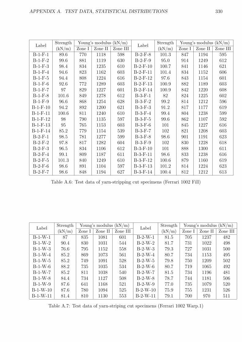
APPENDIX A. TEST DATA, STATISTICAL DISTRIBUTIONS 330
Strength Young’s modulus (kN/m) Strength Young’s modulus (kN/m)Label
(kN/m) Zone I Zone II Zone IIILabel
(kN/m) Zone I Zone II Zone III
B-1-F-1 89.6 770 1118 598 B-2-F-8 101.3 847 1194 595B-1-F-2 99.6 881 1119 630 B-2-F-9 95.0 914 1249 612B-1-F-3 98.4 834 1235 610 B-2-F-10 100.7 841 1146 621B-1-F-4 94.6 823 1162 603 B-2-F-11 101.4 834 1152 606B-1-F-5 94.4 808 1224 616 B-2-F-12 97.6 843 1154 601B-1-F-6 92.6 772 1289 603 B-2-F-13 100.9 882 1189 603B-1-F-7 97 829 1227 601 B-2-F-14 100.9 842 1220 608B-1-F-8 101.6 849 1278 612 B-3-F-1 82 824 1225 602B-1-F-9 96.6 868 1254 628 B-3-F-2 99.2 814 1212 596B-1-F-10 94.2 892 1200 621 B-3-F-3 91.2 817 1177 619B-1-F-11 100.6 811 1240 610 B-3-F-4 99.4 804 1238 599B-1-F-12 98 790 1135 597 B-3-F-5 99.6 862 1107 592B-1-F-13 95 765 1153 603 B-3-F-6 101 845 1227 616B-1-F-14 85.2 779 1154 539 B-3-F-7 102 821 1208 603B-2-F-1 98.5 781 1277 599 B-3-F-8 98.6 901 1191 623B-2-F-2 97.8 817 1282 604 B-3-F-9 102 830 1228 618B-2-F-3 96.5 834 1106 612 B-3-F-10 101 888 1300 611B-2-F-4 99.1 809 1187 611 B-3-F-11 98.6 833 1238 616B-2-F-5 101.3 840 1249 610 B-3-F-12 100.6 879 1160 619B-2-F-6 98.6 891 1104 597 B-3-F-13 101.2 814 1224 623B-2-F-7 98.6 848 1194 627 B-3-F-14 100.4 812 1212 613
Table A.6: Test data of yarn-stripping cut specimens (Ferrari 1002 Fill)
Strength Young’s modulus (kN/m) Strength Young’s modulus (kN/m)Label
(kN/m) Zone I Zone II Zone IIILabel
(kN/m) Zone I Zone II Zone III
B-1-W-1 87 835 1081 601 B-2-W-1 81.5 705 1237 482B-1-W-2 90.4 830 1031 544 B-2-W-2 81.7 731 1022 498B-1-W-3 76.6 795 1152 558 B-2-W-3 79.3 727 1031 500B-1-W-4 85.2 869 1073 561 B-2-W-4 80.7 734 1153 495B-1-W-5 85.2 749 1091 528 B-2-W-5 79.8 750 1209 502B-1-W-6 88.2 735 1035 534 B-2-W-6 80.7 719 1065 492B-1-W-7 85.2 811 1038 540 B-2-W-7 81.5 734 1196 481B-1-W-8 84.4 734 1127 508 B-2-W-8 78.7 744 1181 506B-1-W-9 87.6 641 1168 521 B-2-W-9 77.0 735 1079 520B-1-W-10 87.6 780 1094 525 B-2-W-10 75.9 755 1231 526B-1-W-11 81.4 810 1130 553 B-2-W-11 79.1 700 970 511
Table A.7: Test data of yarn-striping cut specimens (Ferrari 1002 Warp.1)
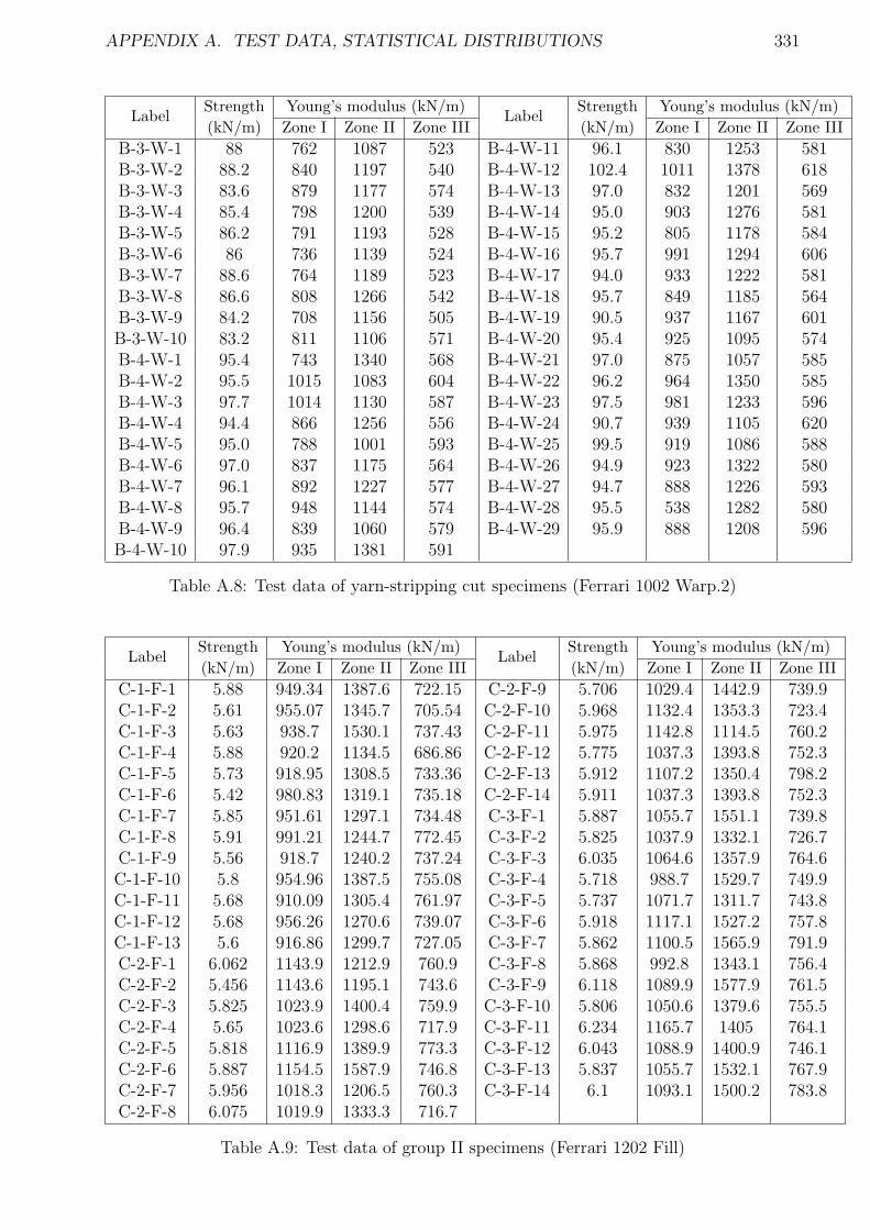
APPENDIX A. TEST DATA, STATISTICAL DISTRIBUTIONS 331
Strength Young’s modulus (kN/m) Strength Young’s modulus (kN/m)Label
(kN/m) Zone I Zone II Zone IIILabel
(kN/m) Zone I Zone II Zone III
B-3-W-1 88 762 1087 523 B-4-W-11 96.1 830 1253 581B-3-W-2 88.2 840 1197 540 B-4-W-12 102.4 1011 1378 618B-3-W-3 83.6 879 1177 574 B-4-W-13 97.0 832 1201 569B-3-W-4 85.4 798 1200 539 B-4-W-14 95.0 903 1276 581B-3-W-5 86.2 791 1193 528 B-4-W-15 95.2 805 1178 584B-3-W-6 86 736 1139 524 B-4-W-16 95.7 991 1294 606B-3-W-7 88.6 764 1189 523 B-4-W-17 94.0 933 1222 581B-3-W-8 86.6 808 1266 542 B-4-W-18 95.7 849 1185 564B-3-W-9 84.2 708 1156 505 B-4-W-19 90.5 937 1167 601B-3-W-10 83.2 811 1106 571 B-4-W-20 95.4 925 1095 574B-4-W-1 95.4 743 1340 568 B-4-W-21 97.0 875 1057 585B-4-W-2 95.5 1015 1083 604 B-4-W-22 96.2 964 1350 585B-4-W-3 97.7 1014 1130 587 B-4-W-23 97.5 981 1233 596B-4-W-4 94.4 866 1256 556 B-4-W-24 90.7 939 1105 620B-4-W-5 95.0 788 1001 593 B-4-W-25 99.5 919 1086 588B-4-W-6 97.0 837 1175 564 B-4-W-26 94.9 923 1322 580B-4-W-7 96.1 892 1227 577 B-4-W-27 94.7 888 1226 593B-4-W-8 95.7 948 1144 574 B-4-W-28 95.5 538 1282 580B-4-W-9 96.4 839 1060 579 B-4-W-29 95.9 888 1208 596B-4-W-10 97.9 935 1381 591
Table A.8: Test data of yarn-stripping cut specimens (Ferrari 1002 Warp.2)
Strength Young’s modulus (kN/m) Strength Young’s modulus (kN/m)Label
(kN/m) Zone I Zone II Zone IIILabel
(kN/m) Zone I Zone II Zone III
C-1-F-1 5.88 949.34 1387.6 722.15 C-2-F-9 5.706 1029.4 1442.9 739.9C-1-F-2 5.61 955.07 1345.7 705.54 C-2-F-10 5.968 1132.4 1353.3 723.4C-1-F-3 5.63 938.7 1530.1 737.43 C-2-F-11 5.975 1142.8 1114.5 760.2C-1-F-4 5.88 920.2 1134.5 686.86 C-2-F-12 5.775 1037.3 1393.8 752.3C-1-F-5 5.73 918.95 1308.5 733.36 C-2-F-13 5.912 1107.2 1350.4 798.2C-1-F-6 5.42 980.83 1319.1 735.18 C-2-F-14 5.911 1037.3 1393.8 752.3C-1-F-7 5.85 951.61 1297.1 734.48 C-3-F-1 5.887 1055.7 1551.1 739.8C-1-F-8 5.91 991.21 1244.7 772.45 C-3-F-2 5.825 1037.9 1332.1 726.7C-1-F-9 5.56 918.7 1240.2 737.24 C-3-F-3 6.035 1064.6 1357.9 764.6C-1-F-10 5.8 954.96 1387.5 755.08 C-3-F-4 5.718 988.7 1529.7 749.9C-1-F-11 5.68 910.09 1305.4 761.97 C-3-F-5 5.737 1071.7 1311.7 743.8C-1-F-12 5.68 956.26 1270.6 739.07 C-3-F-6 5.918 1117.1 1527.2 757.8C-1-F-13 5.6 916.86 1299.7 727.05 C-3-F-7 5.862 1100.5 1565.9 791.9C-2-F-1 6.062 1143.9 1212.9 760.9 C-3-F-8 5.868 992.8 1343.1 756.4C-2-F-2 5.456 1143.6 1195.1 743.6 C-3-F-9 6.118 1089.9 1577.9 761.5C-2-F-3 5.825 1023.9 1400.4 759.9 C-3-F-10 5.806 1050.6 1379.6 755.5C-2-F-4 5.65 1023.6 1298.6 717.9 C-3-F-11 6.234 1165.7 1405 764.1C-2-F-5 5.818 1116.9 1389.9 773.3 C-3-F-12 6.043 1088.9 1400.9 746.1C-2-F-6 5.887 1154.5 1587.9 746.8 C-3-F-13 5.837 1055.7 1532.1 767.9C-2-F-7 5.956 1018.3 1206.5 760.3 C-3-F-14 6.1 1093.1 1500.2 783.8C-2-F-8 6.075 1019.9 1333.3 716.7
Table A.9: Test data of group II specimens (Ferrari 1202 Fill)
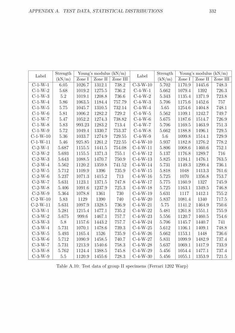
APPENDIX A. TEST DATA, STATISTICAL DISTRIBUTIONS 332
Strength Young’s modulus (kN/m) Strength Young’s modulus (kN/m)Label
(kN/m) Zone I Zone II Zone IIILabel
(kN/m) Zone I Zone II Zone III
C-1-W-1 6.05 1026.7 1312.1 738.2 C-3-W-10 5.702 1170.9 1445.6 748.3C-1-W-2 5.68 1019.2 1275.5 736.2 C-4-W-1 5.662 1079.4 1392 726.3C-1-W-3 5.2 1019.1 1208.8 736.6 C-4-W-2 5.343 1135.4 1371.9 723.8C-1-W-4 5.86 1063.5 1184.4 757.79 C-4-W-3 5.706 1175.6 1452.6 757C-1-W-5 5.75 1045.7 1310.5 732.14 C-4-W-4 5.65 1254.6 1404.8 748.1C-1-W-6 5.81 1006.2 1282.2 729.2 C-4-W-5 5.562 1109.1 1242.7 749.7C-1-W-7 5.47 1052.2 1274.3 738.82 C-4-W-6 5.675 1187.6 1514.7 726.9C-1-W-8 5.83 993.23 1283.2 713.4 C-4-W-7 5.706 1169.5 1463.9 751.3C-1-W-9 5.72 1049.4 1330.7 753.37 C-4-W-8 5.662 1188.8 1496.1 729.5C-1-W-10 5.36 1033.7 1274.9 729.55 C-4-W-9 5.6 1099.8 1514.1 729.9C-1-W-11 5.46 925.85 1261.2 722.55 C-4-W-10 5.937 1182.8 1276.2 778.2C-2-W-1 5.687 1155.5 1441.5 754.08 C-4-W-11 5.806 1068.6 1460.6 752.1C-2-W-2 5.693 1155.5 1371.3 755.1 C-4-W-12 5.137 1176.8 1289.7 716C-2-W-3 5.643 1088.5 1470.7 750.9 C-4-W-13 5.825 1194.1 1476.1 763.5C-2-W-4 5.562 1120.2 1359.8 741.52 C-4-W-14 5.731 1149.3 1299.4 736.1C-2-W-5 5.712 1109.9 1396 735.9 C-4-W-15 5.818 1048 1413.3 761.6C-2-W-6 5.237 1071.3 1415.2 713 C-4-W-16 5.725 1070 1356.8 753.7C-2-W-7 5.631 1123.1 1371.5 747.8 C-4-W-17 5.775 1160.9 1327 745.9C-2-W-8 5.406 1091.6 1237.9 725.3 C-4-W-18 5.725 1163.1 1349.5 746.8C-2-W-9 5.364 1078.8 1361 730 C-4-W-19 5.631 1117 1412.1 755.2C-2-W-10 5.83 1129 1390 740 C-4-W-20 5.837 1081.4 1340 717.5C-2-W-11 5.631 1097.9 1328.5 736.9 C-4-W-21 5.75 1141.2 1464.9 750.6C-3-W-1 5.281 1215.4 1477.1 735.2 C-4-W-22 5.481 1261.8 1551.1 755.9C-3-W-2 5.675 999.6 1467.1 757.7 C-4-W-23 5.556 1120.7 1460.5 754.6C-3-W-3 5.8 1157.6 1443.2 757.7 C-4-W-24 5.706 1145.7 1440.7 741C-3-W-4 5.731 1070.1 1478.6 739.3 C-4-W-25 5.612 1106.1 1409.1 748.8C-3-W-5 5.493 1165.4 1526 735.9 C-4-W-26 5.662 1153.1 1448 736.6C-3-W-6 5.712 1090.9 1458.5 740.7 C-4-W-27 5.831 1099.9 1482.9 737.4C-3-W-7 5.731 1213.9 1540.6 758.3 C-4-W-28 5.637 1069.1 1417.9 733.9C-3-W-8 5.762 1124.4 1388.5 745.8 C-4-W-29 5.456 1054.4 1477.1 737.4C-3-W-9 5.5 1120.9 1455.6 728.3 C-4-W-30 5.456 1055.1 1353.9 721.5
Table A.10: Test data of group II specimens (Ferrari 1202 Warp)
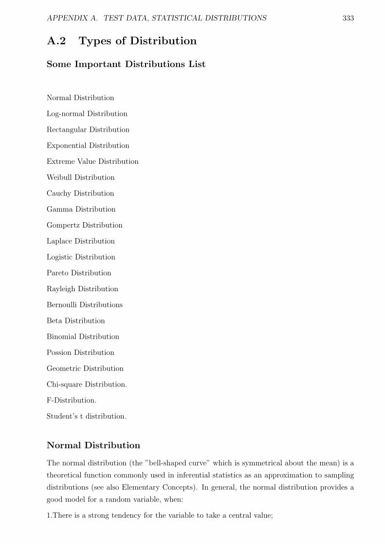
APPENDIX A. TEST DATA, STATISTICAL DISTRIBUTIONS 333
A.2 Types of Distribution
Some Important Distributions List
Normal Distribution
Log-normal Distribution
Rectangular Distribution
Exponential Distribution
Extreme Value Distribution
Weibull Distribution
Cauchy Distribution
Gamma Distribution
Gompertz Distribution
Laplace Distribution
Logistic Distribution
Pareto Distribution
Rayleigh Distribution
Bernoulli Distributions
Beta Distribution
Binomial Distribution
Possion Distribution
Geometric Distribution
Chi-square Distribution.
F-Distribution.
Student’s t distribution.
Normal Distribution
The normal distribution (the ”bell-shaped curve” which is symmetrical about the mean) is a
theoretical function commonly used in inferential statistics as an approximation to sampling
distributions (see also Elementary Concepts). In general, the normal distribution provides a
good model for a random variable, when:
1.There is a strong tendency for the variable to take a central value;
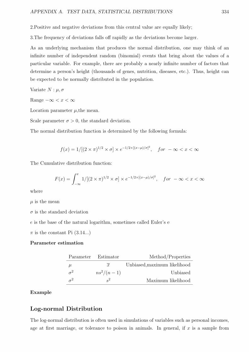
APPENDIX A. TEST DATA, STATISTICAL DISTRIBUTIONS 334
2.Positive and negative deviations from this central value are equally likely;
3.The frequency of deviations falls off rapidly as the deviations become larger.
As an underlying mechanism that produces the normal distribution, one may think of an
infinite number of independent random (binomial) events that bring about the values of a
particular variable. For example, there are probably a nearly infinite number of factors that
determine a person’s height (thousands of genes, nutrition, diseases, etc.). Thus, height can
be expected to be normally distributed in the population.
Variate N : µ, σ
Range −∞ < x <∞
Location parameter µ,the mean.
Scale parameter σ > 0, the standard deviation.
The normal distribution function is determined by the following formula:
f(x) = 1/[(2 × π)1/2 × σ] × e−1/2×[(x−µ)/σ]2 , for −∞ < x <∞
The Cumulative distribution function:
F (x) =
∫ x
−∞1/[(2 × π)1/2 × σ] × e−1/2×[(x−µ)/σ]2 , for −∞ < x <∞
where
µ is the mean
σ is the standard deviation
e is the base of the natural logarithm, sometimes called Euler’s e
π is the constant Pi (3.14...)
Parameter estimation
Parameter Estimator Method/Properties
µ x Unbiased,maximum likelihood
σ2 ns2/(n− 1) Unbiased
σ2 s2 Maximum likelihood
Example
Log-normal Distribution
The log-normal distribution is often used in simulations of variables such as personal incomes,
age at first marriage, or tolerance to poison in animals. In general, if x is a sample from
APPENDIX A. TEST DATA, STATISTICAL DISTRIBUTIONS 335
a normal distribution, then y = ex is a sample from a log-normal distribution. Thus, the
probability density function of log-normal distribution is defined as:
Variate L : m,σ or L : µ, σ
Range 0 ≤ x <∞.
Scale parameter m > 0, the median
Alternative parameter µ, the mean of log L
m and µ are related by m = exp(µ), µ = log m
Shape parameter σ > 0, the standard deviation of log L.
f(x) = 1/[xσ(2π)1/2] × e−[ln(x)−µ
σ]2/2, for 0 < x <∞, σ > 0, ξ > 0
The cumulative density function:
F (x) = Φ(lnx− µ
σ), x ∈ R
µ is the scale parameter
σ is the shape parameter
e is the base of the natural logarithm, sometimes called Euler’s e
The following estimators are derived by transformation to the normal distributions.
Parameter Estimator
Median,m µ = ( 1n)∑n
i=1 logxi
Variance of log(L),σ2 σ2 = ( 1n−1)
)∑n
i=1 [log(xi − µ)]2
Example
Rectangular (Uniform) Continuous Distribution
The rectangular distribution is useful for describing random variables with a constant proba-
bility density over the defined range a < b
Variate:R : a, b
Location parameter a,the lower parameters,we imply the standard or unit rectangular variate
R : 0, 1
Range a ≤ x ≤ b
LOcation parameter a,the lower limit of the range.
Parameter b,the upper limit of the range.
The probability density function:
APPENDIX A. TEST DATA, STATISTICAL DISTRIBUTIONS 336
f(x) = 1/(b− a), for a < x < b
= 0, elsewhere
the Cumulative density function:
F (x) = (x− a)/(b− a)
where
a < b are constantsParameter Estimator Method
Lower limit,a x−√
3/s Matching moments
Upper limit,b x+√
3/s Matching moments
Exponential Distribution
If T is the time between occurrences of rare events that happen on the average with a rate
l per unit of time, then T is distributed exponentially with parameter λ (lambda). Thus,
the exponential distribution is frequently used to model the time interval between successive
random events. Examples of variables distributed in this manner would be the gap length
between cars crossing an intersection, life-times of electronic devices, or arrivals of customers
at the check-out counter in a grocery store. The exponential distribution function is defined
as:
Variate E:b
Range 0 ≤ x < +∞.
Scale parameter b¿0,the mean.
Alternative parameter λ, the hazard function(hazard rate),λ = 1/b
f(x) = 1/b× e−x/b, for 0 ≤ x <∞, b > 0
The cumulative density function:
F (x) = 1 − exp(−x/b)
where
b is scale parameter.
Parameter estimation
APPENDIX A. TEST DATA, STATISTICAL DISTRIBUTIONS 337
Parameter Estimator Method
b s2/x Unbiased,maximum likelihood
Example
Extreme Value(Gumbel) Distribution
The extreme value distribution is often used to model extreme events, such as the size of
floods, gust velocities encountered by airplanes, maxima of stock marked indices over a given
year, etc.; it is also often used in reliability testing, for example in order to represent the
distribution of failure times for electric circuits (see Hahn and Shapiro, 1967).
Variate V : a, b
Range: −∞ < x < +∞
Location parameter a, the mode.
Scale parameter b > 0
The extreme value (Type I) distribution has the probability density function:
f(x) = 1/b× e[−(x−a)/b] × ee[−(x−a)/b], for −∞ < x <∞, b > 0
The cumulative density function:
F (x) = 1 − exp−exp[−(x− a)/b]
where
a is the location parameter
b is the scale parameter
e is the base of the natural logarithm, sometimes called Euler’s e
Parameter estimation
By the method of maximum likelihood, the estimator a,b are the solutions of the simultaneous
equations:
b = x−∑n
i=1 xiexp(−xi
b)
∑ni=1 exp(
−xi
b)
a = −b log[ 1n
n∑
i=1
exp(−xi
b)]
APPENDIX A. TEST DATA, STATISTICAL DISTRIBUTIONS 338
Type II Extreme Value Distribution(Frechet distribution)
Extreme values from an initial distribution with a polynomial tail(in the direction of the
appropriate extreme) will converge asymptotically, in distribution to the Type II asymptotic
form.For the largest value,the Type II asymptotic PDF is:
f(x) =k
vn
(vn
x)k+1exp[−(
vn
x)k]
The cumulative density function is:
F (x) = exp[−(vn
x)
k
]
where
vn: The characteristic largest value of the initial variate X.
k: The shape parameter;1/k is a measure of dispersion.
The Type II asymptotic form for the smallest value as follows:
Probability density function:
f(x) = − k
v1
(v1
x)k+1exp[−(
v1
x)k]
Cumulative density function:
F (x) = 1 − exp[−(v1
x)k], x ≤ 0, v1 > 0
where the parameter v1 is the characteristic smallest value of the initial variate X and k is the
shape parameter;again,1/k is a measure of dispersion.
Parameter estimation
If an extreme variate Xn has the Type II asymptotic distribution with parameters vn and kn,
then the distribution of ln Y −n will have the the pertinent extremal parameters for the Type
II asymptotic distribution become:
vn = eun ; kn = αn
Therefore, the parameters of the Type II asymptotic distribution of the largest value may
be obtained by first estimating un and αn for the logarithms of the sampled data, that is,
ln y1, ln y2, · · · , ln yn, using for example the order statiscs method,therefore obtaining un and
αn .The estimates of vn and kn may then be obtained as:
vn = eun ; kn = αn
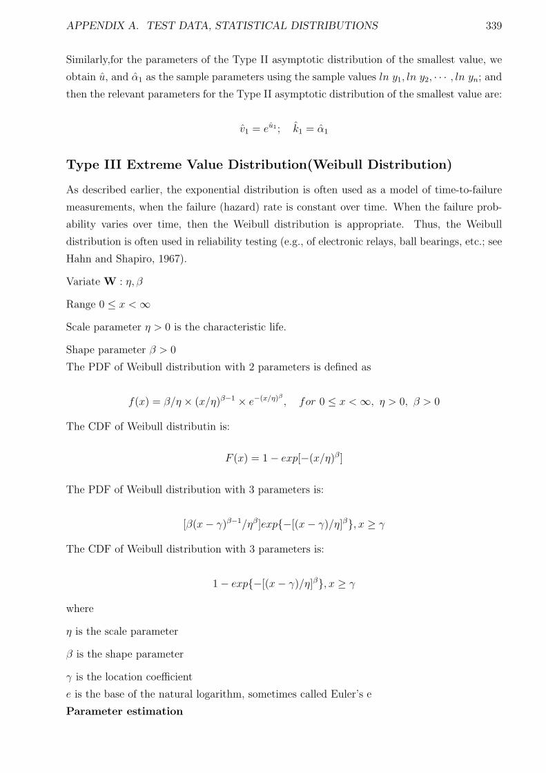
APPENDIX A. TEST DATA, STATISTICAL DISTRIBUTIONS 339
Similarly,for the parameters of the Type II asymptotic distribution of the smallest value, we
obtain u, and α1 as the sample parameters using the sample values ln y1, ln y2, · · · , ln yn; and
then the relevant parameters for the Type II asymptotic distribution of the smallest value are:
v1 = eu1 ; k1 = α1
Type III Extreme Value Distribution(Weibull Distribution)
As described earlier, the exponential distribution is often used as a model of time-to-failure
measurements, when the failure (hazard) rate is constant over time. When the failure prob-
ability varies over time, then the Weibull distribution is appropriate. Thus, the Weibull
distribution is often used in reliability testing (e.g., of electronic relays, ball bearings, etc.; see
Hahn and Shapiro, 1967).
Variate W : η, β
Range 0 ≤ x <∞
Scale parameter η > 0 is the characteristic life.
Shape parameter β > 0
The PDF of Weibull distribution with 2 parameters is defined as
f(x) = β/η × (x/η)β−1 × e−(x/η)β
, for 0 ≤ x <∞, η > 0, β > 0
The CDF of Weibull distributin is:
F (x) = 1 − exp[−(x/η)β]
The PDF of Weibull distribution with 3 parameters is:
[β(x− γ)β−1/ηβ]exp−[(x− γ)/η]β, x ≥ γ
The CDF of Weibull distribution with 3 parameters is:
1 − exp−[(x− γ)/η]β, x ≥ γ
where
η is the scale parameter
β is the shape parameter
γ is the location coefficient
e is the base of the natural logarithm, sometimes called Euler’s e
Parameter estimation
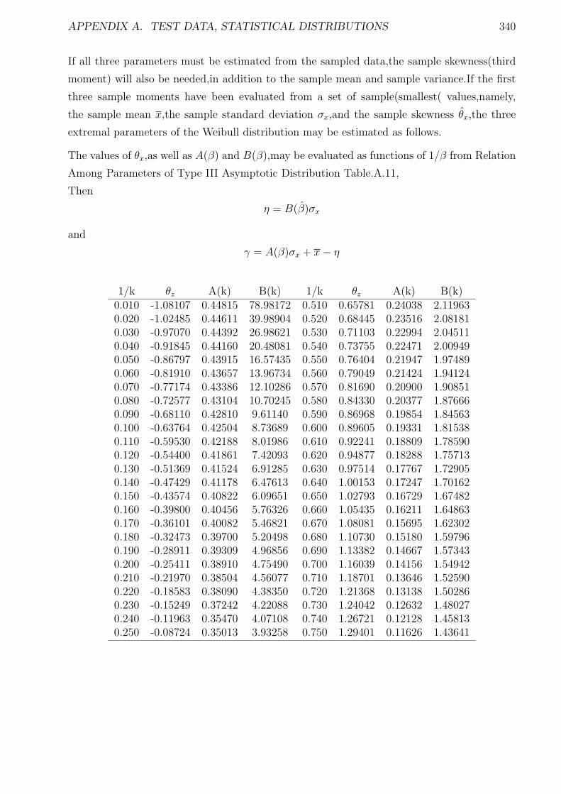
APPENDIX A. TEST DATA, STATISTICAL DISTRIBUTIONS 340
If all three parameters must be estimated from the sampled data,the sample skewness(third
moment) will also be needed,in addition to the sample mean and sample variance.If the first
three sample moments have been evaluated from a set of sample(smallest( values,namely,
the sample mean x,the sample standard deviation σx,and the sample skewness θx,the three
extremal parameters of the Weibull distribution may be estimated as follows.
The values of θx,as well as A(β) and B(β),may be evaluated as functions of 1/β from Relation
Among Parameters of Type III Asymptotic Distribution Table.A.11,
Then
η = B(β)σx
and
γ = A(β)σx + x− η
1/k θz A(k) B(k) 1/k θz A(k) B(k)0.010 -1.08107 0.44815 78.98172 0.510 0.65781 0.24038 2.119630.020 -1.02485 0.44611 39.98904 0.520 0.68445 0.23516 2.081810.030 -0.97070 0.44392 26.98621 0.530 0.71103 0.22994 2.045110.040 -0.91845 0.44160 20.48081 0.540 0.73755 0.22471 2.009490.050 -0.86797 0.43915 16.57435 0.550 0.76404 0.21947 1.974890.060 -0.81910 0.43657 13.96734 0.560 0.79049 0.21424 1.941240.070 -0.77174 0.43386 12.10286 0.570 0.81690 0.20900 1.908510.080 -0.72577 0.43104 10.70245 0.580 0.84330 0.20377 1.876660.090 -0.68110 0.42810 9.61140 0.590 0.86968 0.19854 1.845630.100 -0.63764 0.42504 8.73689 0.600 0.89605 0.19331 1.815380.110 -0.59530 0.42188 8.01986 0.610 0.92241 0.18809 1.785900.120 -0.54400 0.41861 7.42093 0.620 0.94877 0.18288 1.757130.130 -0.51369 0.41524 6.91285 0.630 0.97514 0.17767 1.729050.140 -0.47429 0.41178 6.47613 0.640 1.00153 0.17247 1.701620.150 -0.43574 0.40822 6.09651 0.650 1.02793 0.16729 1.674820.160 -0.39800 0.40456 5.76326 0.660 1.05435 0.16211 1.648630.170 -0.36101 0.40082 5.46821 0.670 1.08081 0.15695 1.623020.180 -0.32473 0.39700 5.20498 0.680 1.10730 0.15180 1.597960.190 -0.28911 0.39309 4.96856 0.690 1.13382 0.14667 1.573430.200 -0.25411 0.38910 4.75490 0.700 1.16039 0.14156 1.549420.210 -0.21970 0.38504 4.56077 0.710 1.18701 0.13646 1.525900.220 -0.18583 0.38090 4.38350 0.720 1.21368 0.13138 1.502860.230 -0.15249 0.37242 4.22088 0.730 1.24042 0.12632 1.480270.240 -0.11963 0.35470 4.07108 0.740 1.26721 0.12128 1.458130.250 -0.08724 0.35013 3.93258 0.750 1.29401 0.11626 1.43641
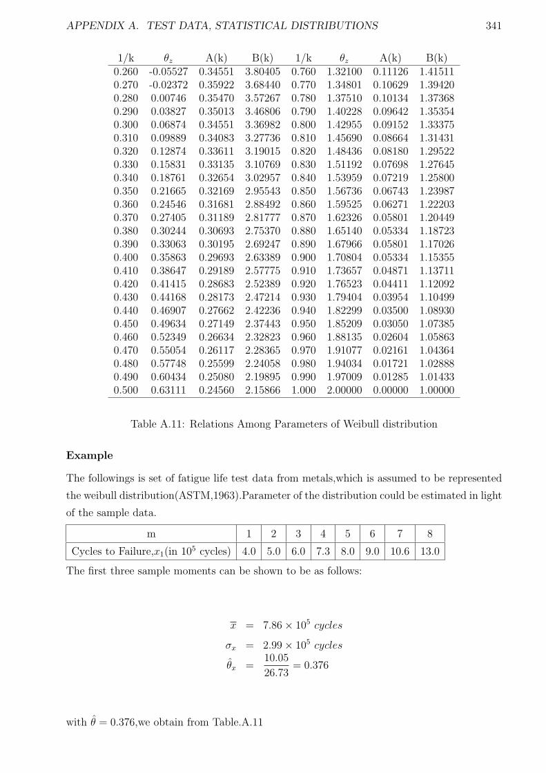
APPENDIX A. TEST DATA, STATISTICAL DISTRIBUTIONS 341
1/k θz A(k) B(k) 1/k θz A(k) B(k)0.260 -0.05527 0.34551 3.80405 0.760 1.32100 0.11126 1.415110.270 -0.02372 0.35922 3.68440 0.770 1.34801 0.10629 1.394200.280 0.00746 0.35470 3.57267 0.780 1.37510 0.10134 1.373680.290 0.03827 0.35013 3.46806 0.790 1.40228 0.09642 1.353540.300 0.06874 0.34551 3.36982 0.800 1.42955 0.09152 1.333750.310 0.09889 0.34083 3.27736 0.810 1.45690 0.08664 1.314310.320 0.12874 0.33611 3.19015 0.820 1.48436 0.08180 1.295220.330 0.15831 0.33135 3.10769 0.830 1.51192 0.07698 1.276450.340 0.18761 0.32654 3.02957 0.840 1.53959 0.07219 1.258000.350 0.21665 0.32169 2.95543 0.850 1.56736 0.06743 1.239870.360 0.24546 0.31681 2.88492 0.860 1.59525 0.06271 1.222030.370 0.27405 0.31189 2.81777 0.870 1.62326 0.05801 1.204490.380 0.30244 0.30693 2.75370 0.880 1.65140 0.05334 1.187230.390 0.33063 0.30195 2.69247 0.890 1.67966 0.05801 1.170260.400 0.35863 0.29693 2.63389 0.900 1.70804 0.05334 1.153550.410 0.38647 0.29189 2.57775 0.910 1.73657 0.04871 1.137110.420 0.41415 0.28683 2.52389 0.920 1.76523 0.04411 1.120920.430 0.44168 0.28173 2.47214 0.930 1.79404 0.03954 1.104990.440 0.46907 0.27662 2.42236 0.940 1.82299 0.03500 1.089300.450 0.49634 0.27149 2.37443 0.950 1.85209 0.03050 1.073850.460 0.52349 0.26634 2.32823 0.960 1.88135 0.02604 1.058630.470 0.55054 0.26117 2.28365 0.970 1.91077 0.02161 1.043640.480 0.57748 0.25599 2.24058 0.980 1.94034 0.01721 1.028880.490 0.60434 0.25080 2.19895 0.990 1.97009 0.01285 1.014330.500 0.63111 0.24560 2.15866 1.000 2.00000 0.00000 1.00000
Table A.11: Relations Among Parameters of Weibull distribution
Example
The followings is set of fatigue life test data from metals,which is assumed to be represented
the weibull distribution(ASTM,1963).Parameter of the distribution could be estimated in light
of the sample data.
m 1 2 3 4 5 6 7 8
Cycles to Failure,x1(in 105 cycles) 4.0 5.0 6.0 7.3 8.0 9.0 10.6 13.0
The first three sample moments can be shown to be as follows:
x = 7.86 × 10⁵ cycles
σx = 2.99 × 10⁵ cycles
θx =10.05
26.73= 0.376
with θ = 0.376,we obtain from Table.A.11
APPENDIX A. TEST DATA, STATISTICAL DISTRIBUTIONS 342
1/β = 0.407
A(β) = 0.293
B(β) = 2.595
Thus
β = 1/0.407 = 2.46
so
η = 2.595 × 2.995 = 7.759 × 10⁵
γ = 0.293 × 2.99 × 105 + 7.86 × 10⁵ − 7.759 × 105 = 0.977 × 10⁵
Cauchy Distribution
The Cauchy distribution is interesting for theoretical reasons. Although its mean can be taken
as zero, since it is symmetrical about zero, the expectation, variance, higher moments, and
moment generating function do not exist. The Cauchy distribution is defined as:
C : a, b.
Range: −∞ < x <∞
Location parameter a,the median.
Scale parameter b > 0
The Probability density function is:
f(x) = 1/(b× π × 1 + [(x− a)/b]2), for 0 < b
The cumulative density function is:
F (x) =1
2+
1
πtan−1(
x− a
b)
where
a is the location parameter (median)
b is the scale parameter
π is the constant Pi(3.1415...)
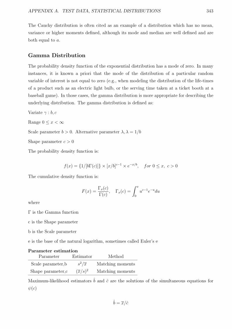
APPENDIX A. TEST DATA, STATISTICAL DISTRIBUTIONS 343
The Cauchy distribution is often cited as an example of a distribution which has no mean,
variance or higher moments defined, although its mode and median are well defined and are
both equal to a.
Gamma Distribution
The probability density function of the exponential distribution has a mode of zero. In many
instances, it is known a priori that the mode of the distribution of a particular random
variable of interest is not equal to zero (e.g., when modeling the distribution of the life-times
of a product such as an electric light bulb, or the serving time taken at a ticket booth at a
baseball game). In those cases, the gamma distribution is more appropriate for describing the
underlying distribution. The gamma distribution is defined as:
Variate γ : b, c
Range 0 ≤ x <∞
Scale parameter b > 0. Alternative parameter λ, λ = 1/b
Shape parameter c > 0
The probability density function is:
f(x) = 1/[bΓ(c)] × [x/b]c−1 × e−x/b, for 0 ≤ x, c > 0
The cumulative density function is:
F (x) =Γx(c)
Γ(c), Γx(c) =
∫ x
0
uc−1e−udu
where
Γ is the Gamma function
c is the Shape parameter
b is the Scale parameter
e is the base of the natural logarithm, sometimes called Euler’s e
Parameter estimationParameter Estimator Method
Scale parameter,b s2/x Matching moments
Shape parameter,c (x/s)2 Matching moments
Maximum-likelihood estimators b and c are the solutions of the simultaneous equations for
ψ(c)
b = x/c
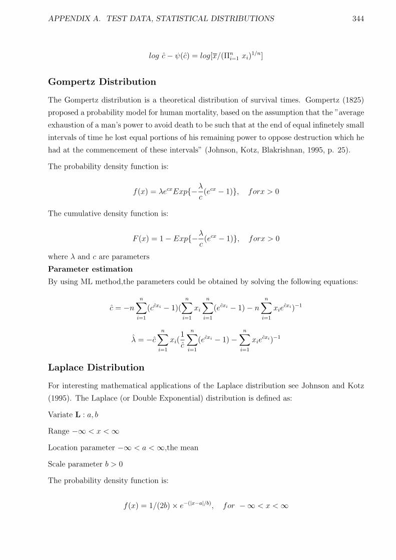
APPENDIX A. TEST DATA, STATISTICAL DISTRIBUTIONS 344
log c− ψ(c) = log[x/(Πni=1 xi)
1/n]
Gompertz Distribution
The Gompertz distribution is a theoretical distribution of survival times. Gompertz (1825)
proposed a probability model for human mortality, based on the assumption that the ”average
exhaustion of a man’s power to avoid death to be such that at the end of equal infinetely small
intervals of time he lost equal portions of his remaining power to oppose destruction which he
had at the commencement of these intervals” (Johnson, Kotz, Blakrishnan, 1995, p. 25).
The probability density function is:
f(x) = λecxExp−λc(ecx − 1), forx > 0
The cumulative density function is:
F (x) = 1 − Exp−λc(ecx − 1), forx > 0
where λ and c are parameters
Parameter estimation
By using ML method,the parameters could be obtained by solving the following equations:
c = −nn∑
i=1
(ccxi − 1)(n∑
i=1
xi
n∑
i=1
(ecxi − 1) − n
n∑
i=1
xiecxi)−1
λ = −cn∑
i=1
xi(1
c
n∑
i=1
(ecxi − 1) −n∑
i=1
xiecxi)−1
Laplace Distribution
For interesting mathematical applications of the Laplace distribution see Johnson and Kotz
(1995). The Laplace (or Double Exponential) distribution is defined as:
Variate L : a, b
Range −∞ < x <∞
Location parameter −∞ < a <∞,the mean
Scale parameter b > 0
The probability density function is:
f(x) = 1/(2b) × e−(|x−a|/b), for −∞ < x <∞
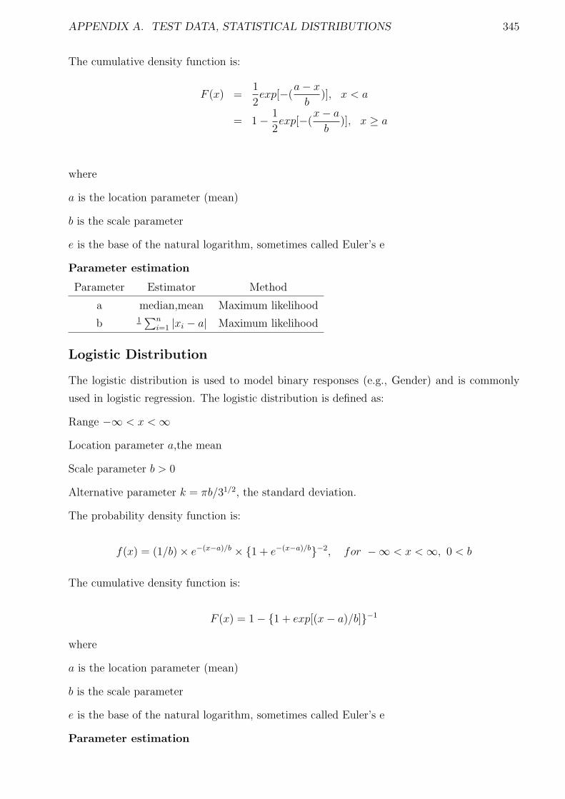
APPENDIX A. TEST DATA, STATISTICAL DISTRIBUTIONS 345
The cumulative density function is:
F (x) =1
2exp[−(
a− x
b)], x < a
= 1 − 1
2exp[−(
x− a
b)], x ≥ a
where
a is the location parameter (mean)
b is the scale parameter
e is the base of the natural logarithm, sometimes called Euler’s e
Parameter estimation
Parameter Estimator Method
a median,mean Maximum likelihood
b 1∑n
i=1 |xi − a| Maximum likelihood
Logistic Distribution
The logistic distribution is used to model binary responses (e.g., Gender) and is commonly
used in logistic regression. The logistic distribution is defined as:
Range −∞ < x <∞
Location parameter a,the mean
Scale parameter b > 0
Alternative parameter k = πb/31/2, the standard deviation.
The probability density function is:
f(x) = (1/b) × e−(x−a)/b × 1 + e−(x−a)/b−2, for −∞ < x <∞, 0 < b
The cumulative density function is:
F (x) = 1 − 1 + exp[(x− a)/b]−1
where
a is the location parameter (mean)
b is the scale parameter
e is the base of the natural logarithm, sometimes called Euler’s e
Parameter estimation
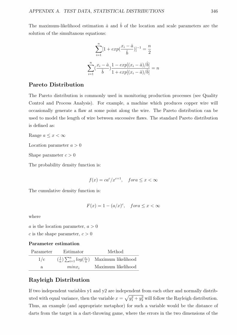
APPENDIX A. TEST DATA, STATISTICAL DISTRIBUTIONS 346
The maximum-likelihood estimation a and b of the location and scale parameters are the
solution of the simultanous equations:
n∑
i=1
[1 + exp(xi − a
b)]−1 =
n
2
n∑
i=1
(xi − a
b)1 − exp[(xi − a)/b]
1 + exp[(xi − a)/b]= n
Pareto Distribution
The Pareto distribution is commonly used in monitoring production processes (see Quality
Control and Process Analysis). For example, a machine which produces copper wire will
occasionally generate a flaw at some point along the wire. The Pareto distribution can be
used to model the length of wire between successive flaws. The standard Pareto distribution
is defined as:
Range a ≤ x <∞
Location parameter a > 0
Shape parameter c > 0
The probability density function is:
f(x) = cac/xc+1, fora ≤ x <∞
The cumulative density function is:
F (x) = 1 − (a/x)c, fora ≤ x <∞
where
a is the location parameter, a > 0
c is the shape parameter, c > 0
Parameter estimation
Parameter Estimator Method
1/c ( 1n)∑n
i=1 log(xi
a) Maximum likelihood
a minxi Maximum likelihood
Rayleigh Distribution
If two independent variables y1 and y2 are independent from each other and normally distrib-
uted with equal variance, then the variable x =√
y21 + y2
2 will follow the Rayleigh distribution.
Thus, an example (and appropriate metaphor) for such a variable would be the distance of
darts from the target in a dart-throwing game, where the errors in the two dimensions of the
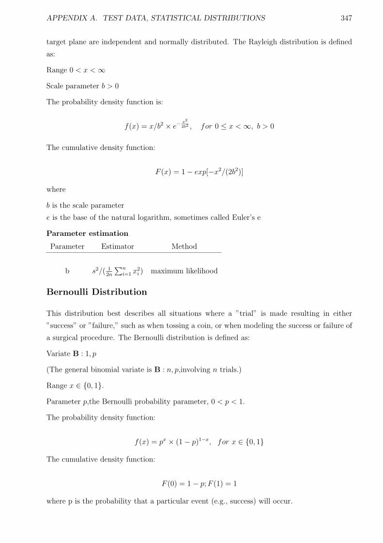
APPENDIX A. TEST DATA, STATISTICAL DISTRIBUTIONS 347
target plane are independent and normally distributed. The Rayleigh distribution is defined
as:
Range 0 < x <∞
Scale parameter b > 0
The probability density function is:
f(x) = x/b2 × e−x2
2b2 , for 0 ≤ x <∞, b > 0
The cumulative density function:
F (x) = 1 − exp[−x2/(2b2)]
where
b is the scale parameter
e is the base of the natural logarithm, sometimes called Euler’s e
Parameter estimation
Parameter Estimator Method
b s2/( 12n
∑ni=1 x
2i ) maximum likelihood
Bernoulli Distribution
This distribution best describes all situations where a ”trial” is made resulting in either
”success” or ”failure,” such as when tossing a coin, or when modeling the success or failure of
a surgical procedure. The Bernoulli distribution is defined as:
Variate B : 1, p
(The general binomial variate is B : n, p,involving n trials.)
Range x ∈ 0, 1.
Parameter p,the Bernoulli probability parameter, 0 < p < 1.
The probability density function:
f(x) = px × (1 − p)1−x, for x ∈ 0, 1
The cumulative density function:
F (0) = 1 − p;F (1) = 1
where p is the probability that a particular event (e.g., success) will occur.
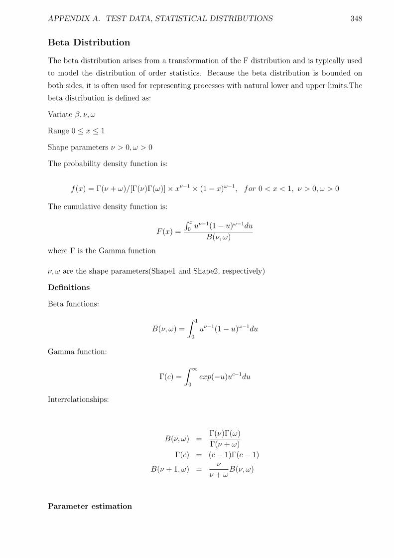
APPENDIX A. TEST DATA, STATISTICAL DISTRIBUTIONS 348
Beta Distribution
The beta distribution arises from a transformation of the F distribution and is typically used
to model the distribution of order statistics. Because the beta distribution is bounded on
both sides, it is often used for representing processes with natural lower and upper limits.The
beta distribution is defined as:
Variate β, ν, ω
Range 0 ≤ x ≤ 1
Shape parameters ν > 0, ω > 0
The probability density function is:
f(x) = Γ(ν + ω)/[Γ(ν)Γ(ω)] × xν−1 × (1 − x)ω−1, for 0 < x < 1, ν > 0, ω > 0
The cumulative density function is:
F (x) =
∫ x
0uν−1(1 − u)ω−1du
B(ν, ω)
where Γ is the Gamma function
ν, ω are the shape parameters(Shape1 and Shape2, respectively)
Definitions
Beta functions:
B(ν, ω) =
∫ 1
0
uν−1(1 − u)ω−1du
Gamma function:
Γ(c) =
∫ ∞
0
exp(−u)uc−1du
Interrelationships:
B(ν, ω) =Γ(ν)Γ(ω)
Γ(ν + ω)
Γ(c) = (c− 1)Γ(c− 1)
B(ν + 1, ω) =ν
ν + ωB(ν, ω)
Parameter estimation
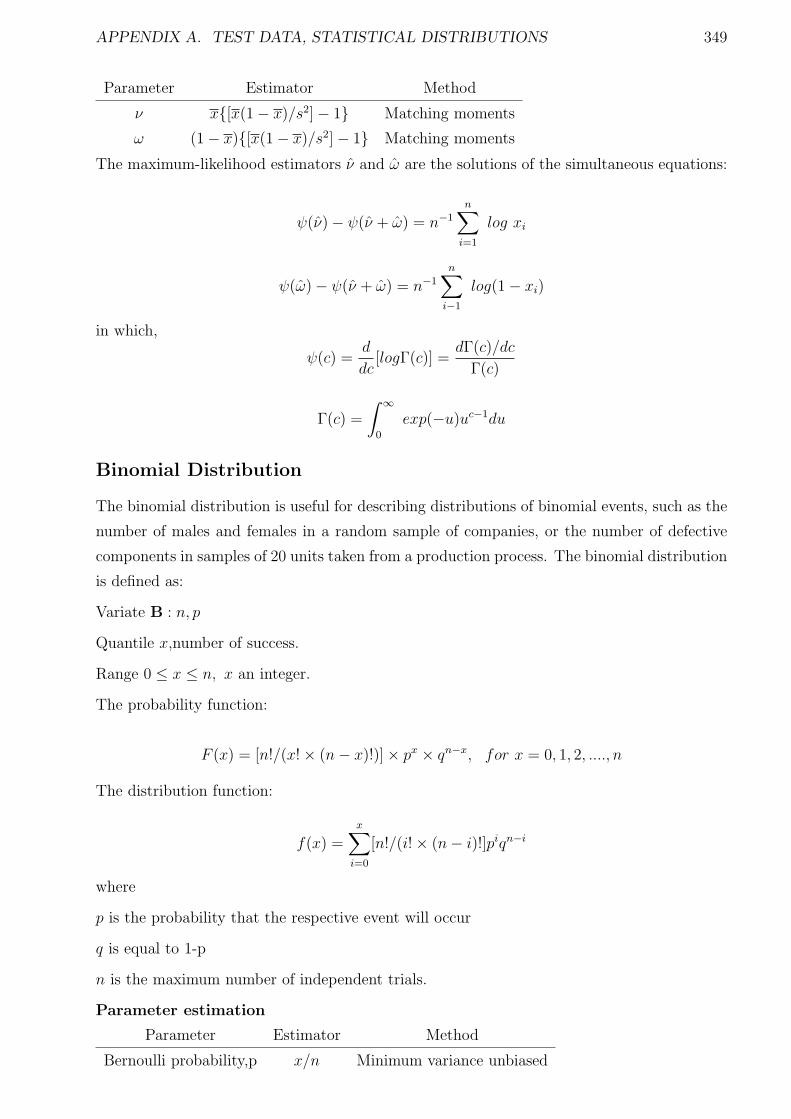
APPENDIX A. TEST DATA, STATISTICAL DISTRIBUTIONS 349
Parameter Estimator Method
ν x[x(1 − x)/s2] − 1 Matching moments
ω (1 − x)[x(1 − x)/s2] − 1 Matching moments
The maximum-likelihood estimators ν and ω are the solutions of the simultaneous equations:
ψ(ν) − ψ(ν + ω) = n−1
n∑
i=1
log xi
ψ(ω) − ψ(ν + ω) = n−1
n∑
i−1
log(1 − xi)
in which,
ψ(c) =d
dc[logΓ(c)] =
dΓ(c)/dc
Γ(c)
Γ(c) =
∫ ∞
0
exp(−u)uc−1du
Binomial Distribution
The binomial distribution is useful for describing distributions of binomial events, such as the
number of males and females in a random sample of companies, or the number of defective
components in samples of 20 units taken from a production process. The binomial distribution
is defined as:
Variate B : n, p
Quantile x,number of success.
Range 0 ≤ x ≤ n, x an integer.
The probability function:
F (x) = [n!/(x! × (n− x)!)] × px × qn−x, for x = 0, 1, 2, ...., n
The distribution function:
f(x) =x∑
i=0
[n!/(i! × (n− i)!]piqn−i
where
p is the probability that the respective event will occur
q is equal to 1-p
n is the maximum number of independent trials.
Parameter estimation
Parameter Estimator Method
Bernoulli probability,p x/n Minimum variance unbiased

APPENDIX A. TEST DATA, STATISTICAL DISTRIBUTIONS 350
Poisson Distribution
The Poisson distribution is also sometimes referred to as the distribution of rare events.
Examples of Poisson distributed variables are number of accidents per person, number of
sweepstakes won per person, or the number of catastrophic defects found in a production
process. It is defined as:
Variate P : λ
Range 0 ≤ x <∞, x integer.
Parameter the mean,λ > 0.
The distribution function:
f(x) =x∑
i=1
λiexp(−λ)/i!
The Probability function:
F (x) = (λx × e−λ)/x!, for x = 0, 1, 2, ..., 0 < λ
where
λ (lambda) is the expected value of x (the mean)
Parameter estimationParameter Estimator Method
λ s2/x Minimum variance unbiased,maximum likelihood
Geometic Distribution
If independent Bernoulli trials are made until a ”success” occurs, then the total number of
trials required is a geometric random variable. The geometric distribution is defined as:
Variate G : p.
Quantile n,number of trials.
Range n ≥ 0, n an integer.
The distribution function:
F (x) = 1 − qx+1, for x = 1, 2, ...
The probability function:
f(x) = p× (1 − p)x, for x = 1, 2, ...
where
p is the probability that a particular event (e.g., success) will occur.
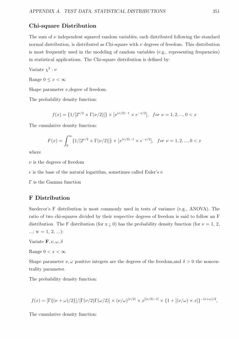
APPENDIX A. TEST DATA, STATISTICAL DISTRIBUTIONS 351
Chi-square Distribution
The sum of ν independent squared random variables, each distributed following the standard
normal distribution, is distributed as Chi-square with ν degrees of freedom. This distribution
is most frequently used in the modeling of random variables (e.g., representing frequencies)
in statistical applications. The Chi-square distribution is defined by:
Variate χ2 : ν
Range 0 ≤ x <∞
Shape parameter ν,degree of freedom.
The probability density function:
f(x) = 1/[2ν/2 × Γ(ν/2)] × [x(ν/2)−1 × e−x/2], for ν = 1, 2, ..., 0 < x
The cumulative density function:
F (x) =
∫ ∞
0
1/[2ν/2 × Γ(ν/2)] × [x(ν/2)−1 × e−x/2], for ν = 1, 2, ..., 0 < x
where
ν is the degrees of freedom
e is the base of the natural logarithm, sometimes called Euler’s e
Γ is the Gamma function
F Distribution
Snedecor’s F distribution is most commonly used in tests of variance (e.g., ANOVA). The
ratio of two chi-squares divided by their respective degrees of freedom is said to follow an F
distribution. The F distribution (for x ¿ 0) has the probability density function (for ν = 1, 2,
...; w = 1, 2, ...):
Variate F, ν, ω, δ
Range 0 < x <∞
Shape parameter ν, ω positive integers are the degrees of the freedom,and δ > 0 the noncen-
trality parameter.
The probability density function:
f(x) = [Γ(ν + ω)/2]/[Γ(ν/2)Γ(ω/2)] × (ν/ω)(ν/2) × x[(ν/2)−1] × 1 + [(ν/ω) × x]−(ν+ω)/2,
The cumulative density function:
APPENDIX A. TEST DATA, STATISTICAL DISTRIBUTIONS 352
F (x) =
∫ ∞
0
[Γ(ν+ω)/2]/[Γ(ν/2)Γ(ω/2)]× (ν/ω)(ν/2)×x[(ν/2)−1]×1+ [(ν/ω)×x]−(ν+ω)/2,
for 0 ≤ x <∞ ν = 1, 2, ..., ω = 1, 2, ...
where
ν, ω are the shape parameters, degrees of freedom
Γ is the Gamma function
Student’s t Distribution
The student’s t distribution is symmetric about zero, and its general shape is similar to that
of the standard normal distribution. It is most commonly used in testing hypothesis about
the mean of a particular population. The student’s t distribution is defined as (for n = 1, 2,
. . .):
Variate t, ν
Range −∞x <∞
Shape parameter ν,degree of freedom, ν a positive integer
The probability density function:
f(x) = Γ[(ν + 1)/2]/Γ(ν/2) × (ν × π)−1/2 × [1 + (x2/ν)−(ν+1)/2]
The cumulative density function:
F (x) =1
2+
1
πtan−1(
x
ν1/2) +
1
π
xν1/2
ν + x2×
(ν−3)/2∑
j=0
aj
(1 + x2/ν)j, ν odd
=1
2+
x
2(ν + x2)1/2×
(ν−2)/2∑
j=0
bj
(1 + x2
ν)j, ν even
where
ν is the shape parameter, degrees of freedom
Γ is the Gamma function
π is the constant Pi (3.14 . . .)
Appendix B
Derivation of Finite Element
Formulations
B.1 Appendix B1: Derivation of the [B] matrix in the
LST element formulation
An arbitarily located point P divides a triangle 1 − 2 − 3 into three subareas A1, A2,and,A3
Area coordinates are defined as ratios of areas:
ξ1 = A1
Aξ2 = A2
Aξ3 = A3
A(B.1)
where A is the area of triangle 1− 2− 3.Since A = A1 +A2 +A3 , the ξi are not independent.
They satisfy the constraint equation
ξ1 + ξ2 + ξ3 = 1 (B.2)
The constraint equation and the linear relation between Cartesian and area coordinate are
expressed by equations below:
1
X
Y
= [A] ·
ξ1
ξ2
ξ3
and
ξ1
ξ2
ξ3
= [A]−1
1
x
y
(B.3)
where,with xij = xi − xj and yij = yi − yj
[A] =
1 1 1
x1 x2 x3
y1 y2 y3
and
353
APPENDIX B. DERIVATION OF FINITE ELEMENT FORMULATIONS 354
[A]−1 = 12A
x2y3 − x3y2 y23 x32
x3y1 − x1y3 y31 x13
x1y2 − x2y1 y12 y21
2A = det[A] = x21y31 − x31y21
Displacement can be expressed as:
U(ξ1, ξ2, ξ3) = U1ξ1(2ξ1−1)+U2ξ2(2ξ2−1)+U3ξ3(2ξ3−1)+U4·4ξ1ξ2+U5·4ξ2ξ3+U6·4ξ3ξ1 (B.4)
V (ξ1, ξ2, ξ3) = V1ξ1(2ξ1−1)+V2ξ2(2ξ2−1)+V3ξ3(2ξ3−1)+V4 ·4ξ1ξ2+V5 ·4ξ2ξ3+V6 ·4ξ3ξ1 (B.5)
W (ξ1, ξ2, ξ3) = W1ξ1(2ξ1−1)+W2ξ2(2ξ2−1)+W3ξ3(2ξ3−1)+W4 ·4ξ1ξ2+W5 ·4ξ2ξ3+W6 ·4ξ3ξ1(B.6)
Formulation of element matrices requires that a function φ , expressed in terms of area coor-
dinates, be differentiated with respect to Cartesian coordinates. By the chain rule, with
φ = φ(ξ1, ξ2ξ3)
∂φ
∂X=∂φ
∂ξ1
∂ξ1∂X
+∂φ
∂ξ2
∂ξ2∂X
+∂φ
∂ξ3
∂ξ3∂X
(B.7)
∂φ
∂Y=∂φ
∂ξ1
∂ξ1∂Y
+∂φ
∂ξ2
∂ξ2∂Y
+∂φ
∂ξ3
∂ξ3∂Y
(B.8)
From the former equations:
∂ξ1∂X
=Y23
2A
∂ξ2∂X
=Y31
2A
∂ξ3∂X
=Y12
2A(B.9)
∂ξ1∂Y
=X32
2A
∂ξ2∂Y
=X13
2A
∂ξ3∂Y
=X21
2A(B.10)
where 2A = det[A] = X21Y31 −X31Y21, Y23 = Y2 − Y3, and so on
We already know:
∂
∂ξ1φ = φ1
∂
∂ξ2φ = φ2
∂
∂ξ3φ = φ3 (B.11)
then we have
APPENDIX B. DERIVATION OF FINITE ELEMENT FORMULATIONS 355
∂
∂XU(X,Y ) = U1
Y23
2A(4ξ1 − 1) + U2
Y31
2A(4ξ2 − 1) + U3
Y12
2A(4ξ3 − 1) + U4
1
2A4(ξ2Y23 + ξ1Y31)
+U51
2A4(ξ3Y31 + ξ2Y12) + U6
1
2A4(ξ1Y12 + ξ3Y23)
∂
∂XV (X,Y ) = V1
Y23
2A(4ξ1 − 1) + V2
Y31
2A(4ξ2 − 1) + V3
Y12
2A(4ξ3 − 1) + V4
1
2A4(ξ2Y23 + ξ1Y31)
+V51
2A4(ξ3Y31 + ξ2Y12) + V6
1
2A4(ξ1Y12 + ξ3Y23)
∂
∂XW (X,Y ) = W1
Y23
2A(4ξ1 − 1) +W2
Y31
2A(4ξ2 − 1) +W3
Y12
2A(4ξ3 − 1) +W4
1
2A4(ξ2Y23 + ξ1W31)
+W51
2A4(ξ3Y31 + ξ2Y12) +W6
1
2A4(ξ1Y12 + ξ3Y23)
∂
∂YU(X,Y ) = U1
X32
2A(4ξ1 − 1) + U2
X13
2A(4ξ2 − 1) + U3
X21
2A(4ξ3 − 1) + U4
1
2A4(ξ2X32 + ξ1X13)
+U51
2A4(ξ3X13 + ξ2X21) + U6
1
2A4(ξ1X21 + ξ3X32)
∂
∂YV (X,Y ) = V1
X32
2A(4ξ1 − 1) + V2
X13
2A(4ξ2 − 1) + V3
X21
2A(4ξ3 − 1) + V4
1
2A4(ξ2X32 + ξ1X13)
+V51
2A4(ξ3X13 + ξ2X21) + V6
1
2A4(ξ1X21 + ξ3X32)
∂
∂YW (X,Y ) = W1
X32
2A(4ξ1−1)+W2
X13
2A(4ξ2−1)+W3
X21
2A(4ξ3−1)+W4
1
2A4(ξ2X32 + ξ1X13)
+W51
2A4(ξ3X13 + ξ2X21) +W6
1
2A4(ξ1X21 + ξ3X32) (B.12)
APPENDIX B. DERIVATION OF FINITE ELEMENT FORMULATIONS 356
Substituting these to the formulation:
εX = U1Y23
2A(4ξ1 − 1) + U2
Y31
2A(4ξ2 − 1) + U3
Y12
2A(4ξ3 − 1) + U4
1
2A4(ξ2Y23 + ξ1Y31)
+U51
2A4(ξ3Y31 + ξ2Y12) + U6
1
2A4(ξ1Y12 + ξ3Y23) +KX [W1ξ1(2ξ1 − 1)+
W2ξ2(2ξ2 − 1) +W3ξ3(2ξ3 − 1) +W4 · 4ξ1ξ2 +W5 · 4ξ2ξ3 +W6 · 4ξ3ξ1]+
1
2[U1
Y23
2A(4ξ1 − 1) + U2
Y31
2A(4ξ2 − 1) + U3
Y12
2A(4ξ3 − 1) + U4
1
2A4(ξ2Y23
+ξ1Y31) + U51
2A4(ξ3Y31 + ξ2Y12) + U6
1
2A4(ξ1Y12 + ξ3Y23)]
2+
1
2[V1
Y23
2A(4ξ1 − 1) + V2
Y31
2A(4ξ2 − 1) + V3
Y12
2A(4ξ3 − 1) + V4
1
2A4(ξ2Y23
+ξ1Y31) + V51
2A4(ξ3Y31 + ξ2Y12) + V6
1
2A4(ξ1Y12 + ξ3Y23)]
2+
1
2[W1
Y23
2A(4ξ1 − 1) +W2
Y31
2A(4ξ2 − 1) +W3
Y12
2A(4ξ3 − 1) +W4
1
2A4(ξ2Y23
+ξ1W31) +W51
2A4(ξ3Y31 + ξ2Y12) +W6
1
2A4(ξ1Y12 + ξ3Y23)]
2 (B.13)
εY = V1X32
2A(4ξ1 − 1) + V2
X13
2A(4ξ2 − 1) + V3
X21
2A(4ξ3 − 1) + V4
1
2A4(ξ2X32 + ξ1X13)
+V51
2A4(ξ3X13 + ξ2X21) + V6
1
2A4(ξ1X21 + ξ3X32) +KY [W1ξ1(2ξ1 − 1)+
W2ξ2(2ξ2 − 1) +W3ξ3(2ξ3 − 1) +W4 · 4ξ1ξ2 +W5 · 4ξ2ξ3 +W6 · 4ξ3ξ1]+
1
2[U1
X32
2A(4ξ1 − 1) + U2
X13
2A(4ξ2 − 1) + U3
X21
2A(4ξ3 − 1) + U4
1
2A4(ξ2X32
+ξ1X13) + U51
2A4(ξ3X13 + ξ2X21) + U6
1
2A4(ξ1X21 + ξ3X32)]
2+
APPENDIX B. DERIVATION OF FINITE ELEMENT FORMULATIONS 357
1
2[V1
X32
2A(4ξ1 − 1) + V2
X13
2A(4ξ2 − 1) + V3
X21
2A(4ξ3 − 1) + V4
1
2A4(ξ2X32+
ξ1X13 + V51
2A4(ξ3X13 + ξ2X21) + V6
1
2A4(ξ1X21 + ξ3X32)]
2+
1
2[W1
X32
2A(4ξ1 − 1) +W2
X13
2A(4ξ2 − 1) +W3
X21
2A(4ξ3 − 1) +W4
1
2A4(ξ2X32+
ξ1X13) +W51
2A4(ξ3X13 + ξ2X21) +W6
1
2A4(ξ1X21 + ξ3X32)]
2 (B.14)
γXY = U1X32
2A(4ξ1 − 1) + U2
X13
2A(4ξ2 − 1) + U3
X21
2A(4ξ3 − 1) + U4
1
2A4(ξ2X32 + ξ1X13)
+U51
2A4(ξ3X13 + ξ2X21) + U6
1
2A4(ξ1X21 + ξ3X32) + V1
Y23
2A(4ξ1 − 1)+
V2Y31
2A(4ξ2 − 1) + V3
Y12
2A(4ξ3 − 1) + V4
1
2A4(ξ2Y23 + ξ1Y31) + V5
1
2A4(ξ3Y31
+ξ2Y12) + V61
2A4(ξ1Y12 + ξ3Y23) +KXY · 2[W1ξ1(2ξ1 − 1) +W2ξ2(2ξ2 − 1)
+W3ξ3(2ξ3 − 1) +W4 · 4ξ1ξ2 +W5 · 4ξ2ξ3 +W6 · 4ξ3ξ1] + [U1Y23
2A(4ξ1 − 1)
+U2Y31
2A(4ξ2 − 1) + U3
Y12
2A(4ξ3 − 1) + U4
1
2A4(ξ2Y23 + ξ1Y31) + U5
1
2A4(ξ3Y31
+ξ2Y12) + U61
2A4(ξ1Y12 + ξ3Y23)] × [U1
X32
2A(4ξ1 − 1) + U2
X13
2A(4ξ2 − 1)+
U3X21
2A(4ξ3 − 1) + U4
1
2A4(ξ2X32 + ξ1X13) + U5
1
2A4(ξ3X13 + ξ2X21) + U6
1
2A4(ξ1X21
+ξ3X32)] + [V1Y23
2A(4ξ1 − 1) + V2
Y31
2A(4ξ2 − 1) + V3
Y12
2A(4ξ3 − 1) + V4
1
2A4(ξ2Y23
+ξ1Y31) + V51
2A4(ξ3Y31 + ξ2Y12) + V6
1
2A4(ξ1Y12 + ξ3Y23)] × [V1
X32
2A(4ξ1 − 1)
APPENDIX B. DERIVATION OF FINITE ELEMENT FORMULATIONS 358
+V2X13
2A(4ξ2 − 1) + V3
X21
2A(4ξ3 − 1) + V4
1
2A4(ξ2X32 + ξ1X13) + V5
1
2A4(ξ3X13
+ξ2X21) + V61
2A4(ξ1X21 + ξ3X32)] + [W1
Y23
2A(4ξ1 − 1) +W2
Y31
2A(4ξ2 − 1)+
W3Y12
2A(4ξ3 − 1) +W4
1
2A4(ξ2Y23 + ξ1Y31) +W5
1
2A4(ξ3Y31 + ξ2Y12)
+W61
2A4(ξ1Y12 + ξ3Y23)] × [W1
X32
2A(4ξ1 − 1) +W2
X13
2A(4ξ2 − 1) +W3
X21
2A(4ξ3 − 1)
+W41
2A4(ξ2X32 + ξ1X13) +W5
1
2A4(ξ3X13 + ξ2X21) +W6
1
2A4(ξ1X21 + ξ3X32)]
(B.15)
So the relationship between local principal strains and nodal displacement is:
ε = εX εY γXY T = [B]D (B.16)
in which D = U1 V1 W1 U2 V2 W2 U3 V3 W3 U4 V4 W4 U5 V5 W5 U6 V6 W6 T
The terms of the B matrix are followed:
B1,1 =Y23
2A(4ξ1 − 1) + U1
Y 223
8A2(4ξ1 − 1)2 +
Y23
2A(4ξ1 − 1)[U2
Y31
2A(4ξ2 − 1)
+U3Y12
2A(4ξ3 − 1) + U4
4
2A(ξ2Y23 + ξ1Y31) + U5
4
2A(ξ3Y31 + ξ2Y12)
+U64
2A(ξ1Y12 + ξ3Y23)]
B1,2 = V1Y 2
23
8A2(4ξ1 − 1)2 +
Y23
2A(4ξ1 − 1)[V2
Y31
2A(4ξ2 − 1) + V3
Y12
2A(4ξ3 − 1)
+V44
2A(ξ2Y23 + ξ1Y31) + V5
4
2A(ξ3Y31 + ξ2Y12) + V6
4
2A(ξ1Y12 + ξ3Y23)]
APPENDIX B. DERIVATION OF FINITE ELEMENT FORMULATIONS 359
B1,3 = KX · ξ1(2ξ1 − 1) +W1Y 2
23
8A2(4ξ1 − 1)2 +
Y23
2A(4ξ1 − 1)[W2
Y31
2A(4ξ2 − 1)
+W3Y12
2A(4ξ3 − 1) +W4
4
2A(ξ2Y23 + ξ1Y31) +W5
4
2A(ξ3Y31 + ξ2Y12)
+W64
2A(ξ1Y12 + ξ3Y23)]
B1,4 =Y31
2A(4ξ2 − 1) +
1
2U2 ·
Y 231
4A2(4ξ2 − 1)2 +
Y31
2A(4ξ2 − 1)[U3
Y12
2A(4ξ3 − 1)
+U4 ·4
2A(ξ2Y23 + ξ1Y31) + U5
4
2A(ξ3Y31 + ξ2Y12) + U6
4
2A(ξ1Y12 + ξ3Y23)]
B1,5 =1
2V2 ·
Y 231
4A2(4ξ2 − 1)2 +
Y31
2A(4ξ2 − 1)[V3
Y12
2A(4ξ3 − 1) + V4 ·
4
2A(ξ2Y23 + ξ1Y31)
+V54
2A(ξ3Y31 + ξ2Y12) + V6
4
2A(ξ1Y12 + ξ3Y23)]
B1,6 = KX · ξ2(2ξ2 − 1) +1
2W2 ·
Y 231
4A2(4ξ2 − 1)2 +
Y31
2A(4ξ2 − 1)[W3
Y12
2A(4ξ3 − 1)
+W4 ·4
2A(ξ2Y23 + ξ1Y31) +W5
4
2A(ξ3Y31 + ξ2Y12) +W6
4
2A(ξ1Y12 + ξ3Y23)]
B1,7 =Y12
2A(4ξ3 − 1) +
1
2U3 ·
Y 212
4A2(4ξ3 − 1)2 +
Y12
2A(4ξ3 − 1)[U4 ·
4
2A(ξ2Y23 + ξ1Y31)
+U54
2A(ξ3Y31 + ξ2Y12) + U6
4
2A(ξ1Y12 + ξ3Y23)]
B1,8 =1
2V3 ·
Y 212
4A2(4ξ3 − 1)2 +
Y12
2A(4ξ3 − 1)[V4 ·
4
2A(ξ2Y23 + ξ1Y31) + V5
4
2A(ξ3Y31 + ξ2Y12)
+V64
2A(ξ1Y12 + ξ3Y23)]
B1,9 = KX · ξ3(2ξ3 − 1) +1
2W3 ·
Y 212
4A2(4ξ3 − 1)2 +
Y12
2A(4ξ3 − 1)[W4 ·
4
2A(ξ2Y23 + ξ1Y31)
+W54
2A(ξ3Y31 + ξ2Y12) +W6
4
2A(ξ1Y12 + ξ3Y23)]
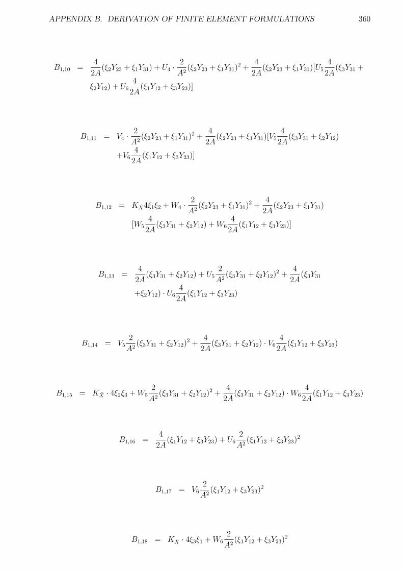
APPENDIX B. DERIVATION OF FINITE ELEMENT FORMULATIONS 360
B1,10 =4
2A(ξ2Y23 + ξ1Y31) + U4 ·
2
A2(ξ2Y23 + ξ1Y31)
2 +4
2A(ξ2Y23 + ξ1Y31)[U5
4
2A(ξ3Y31 +
ξ2Y12) + U64
2A(ξ1Y12 + ξ3Y23)]
B1,11 = V4 ·2
A2(ξ2Y23 + ξ1Y31)
2 +4
2A(ξ2Y23 + ξ1Y31)[V5
4
2A(ξ3Y31 + ξ2Y12)
+V64
2A(ξ1Y12 + ξ3Y23)]
B1,12 = KX4ξ1ξ2 +W4 ·2
A2(ξ2Y23 + ξ1Y31)
2 +4
2A(ξ2Y23 + ξ1Y31)
[W54
2A(ξ3Y31 + ξ2Y12) +W6
4
2A(ξ1Y12 + ξ3Y23)]
B1,13 =4
2A(ξ3Y31 + ξ2Y12) + U5
2
A2(ξ3Y31 + ξ2Y12)
2 +4
2A(ξ3Y31
+ξ2Y12) · U64
2A(ξ1Y12 + ξ3Y23)
B1,14 = V52
A2(ξ3Y31 + ξ2Y12)
2 +4
2A(ξ3Y31 + ξ2Y12) · V6
4
2A(ξ1Y12 + ξ3Y23)
B1,15 = KX · 4ξ2ξ3 +W52
A2(ξ3Y31 + ξ2Y12)
2 +4
2A(ξ3Y31 + ξ2Y12) ·W6
4
2A(ξ1Y12 + ξ3Y23)
B1,16 =4
2A(ξ1Y12 + ξ3Y23) + U6
2
A2(ξ1Y12 + ξ3Y23)
2
B1,17 = V62
A2(ξ1Y12 + ξ3Y23)
2
B1,18 = KX · 4ξ3ξ1 +W62
A2(ξ1Y12 + ξ3Y23)
2
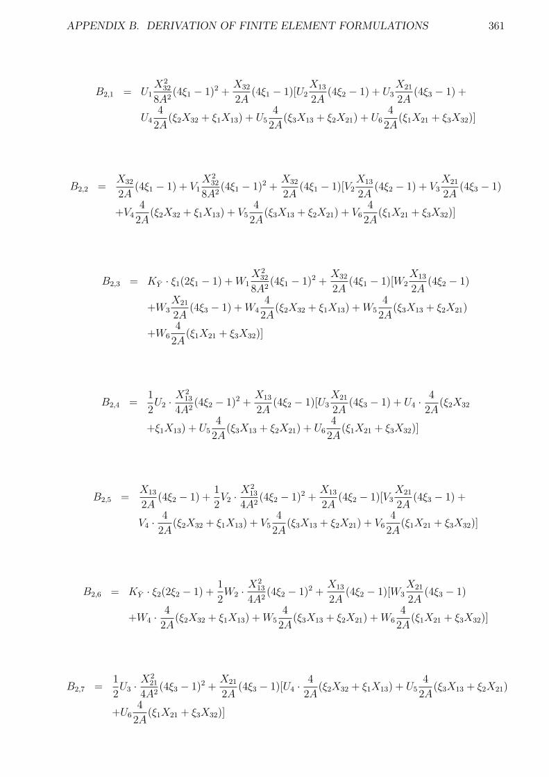
APPENDIX B. DERIVATION OF FINITE ELEMENT FORMULATIONS 361
B2,1 = U1X2
32
8A2(4ξ1 − 1)2 +
X32
2A(4ξ1 − 1)[U2
X13
2A(4ξ2 − 1) + U3
X21
2A(4ξ3 − 1) +
U44
2A(ξ2X32 + ξ1X13) + U5
4
2A(ξ3X13 + ξ2X21) + U6
4
2A(ξ1X21 + ξ3X32)]
B2,2 =X32
2A(4ξ1 − 1) + V1
X232
8A2(4ξ1 − 1)2 +
X32
2A(4ξ1 − 1)[V2
X13
2A(4ξ2 − 1) + V3
X21
2A(4ξ3 − 1)
+V44
2A(ξ2X32 + ξ1X13) + V5
4
2A(ξ3X13 + ξ2X21) + V6
4
2A(ξ1X21 + ξ3X32)]
B2,3 = KY · ξ1(2ξ1 − 1) +W1X2
32
8A2(4ξ1 − 1)2 +
X32
2A(4ξ1 − 1)[W2
X13
2A(4ξ2 − 1)
+W3X21
2A(4ξ3 − 1) +W4
4
2A(ξ2X32 + ξ1X13) +W5
4
2A(ξ3X13 + ξ2X21)
+W64
2A(ξ1X21 + ξ3X32)]
B2,4 =1
2U2 ·
X213
4A2(4ξ2 − 1)2 +
X13
2A(4ξ2 − 1)[U3
X21
2A(4ξ3 − 1) + U4 ·
4
2A(ξ2X32
+ξ1X13) + U54
2A(ξ3X13 + ξ2X21) + U6
4
2A(ξ1X21 + ξ3X32)]
B2,5 =X13
2A(4ξ2 − 1) +
1
2V2 ·
X213
4A2(4ξ2 − 1)2 +
X13
2A(4ξ2 − 1)[V3
X21
2A(4ξ3 − 1) +
V4 ·4
2A(ξ2X32 + ξ1X13) + V5
4
2A(ξ3X13 + ξ2X21) + V6
4
2A(ξ1X21 + ξ3X32)]
B2,6 = KY · ξ2(2ξ2 − 1) +1
2W2 ·
X213
4A2(4ξ2 − 1)2 +
X13
2A(4ξ2 − 1)[W3
X21
2A(4ξ3 − 1)
+W4 ·4
2A(ξ2X32 + ξ1X13) +W5
4
2A(ξ3X13 + ξ2X21) +W6
4
2A(ξ1X21 + ξ3X32)]
B2,7 =1
2U3 ·
X221
4A2(4ξ3 − 1)2 +
X21
2A(4ξ3 − 1)[U4 ·
4
2A(ξ2X32 + ξ1X13) + U5
4
2A(ξ3X13 + ξ2X21)
+U64
2A(ξ1X21 + ξ3X32)]
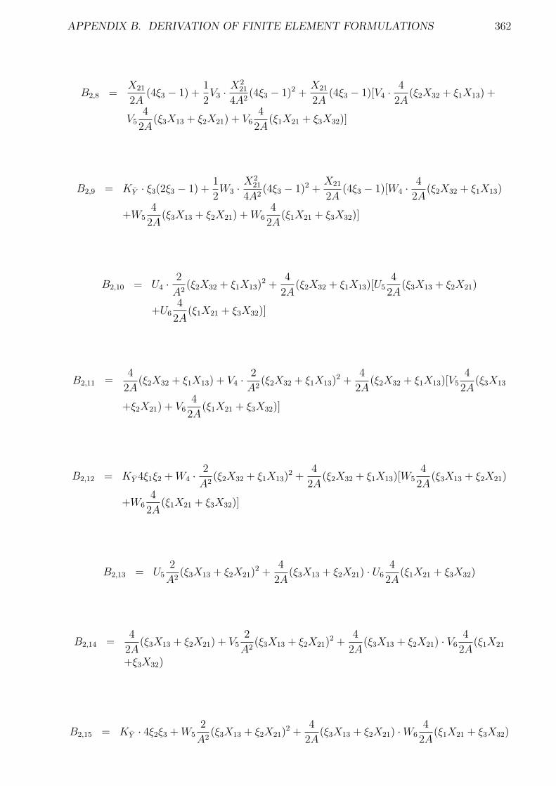
APPENDIX B. DERIVATION OF FINITE ELEMENT FORMULATIONS 362
B2,8 =X21
2A(4ξ3 − 1) +
1
2V3 ·
X221
4A2(4ξ3 − 1)2 +
X21
2A(4ξ3 − 1)[V4 ·
4
2A(ξ2X32 + ξ1X13) +
V54
2A(ξ3X13 + ξ2X21) + V6
4
2A(ξ1X21 + ξ3X32)]
B2,9 = KY · ξ3(2ξ3 − 1) +1
2W3 ·
X221
4A2(4ξ3 − 1)2 +
X21
2A(4ξ3 − 1)[W4 ·
4
2A(ξ2X32 + ξ1X13)
+W54
2A(ξ3X13 + ξ2X21) +W6
4
2A(ξ1X21 + ξ3X32)]
B2,10 = U4 ·2
A2(ξ2X32 + ξ1X13)
2 +4
2A(ξ2X32 + ξ1X13)[U5
4
2A(ξ3X13 + ξ2X21)
+U64
2A(ξ1X21 + ξ3X32)]
B2,11 =4
2A(ξ2X32 + ξ1X13) + V4 ·
2
A2(ξ2X32 + ξ1X13)
2 +4
2A(ξ2X32 + ξ1X13)[V5
4
2A(ξ3X13
+ξ2X21) + V64
2A(ξ1X21 + ξ3X32)]
B2,12 = KY 4ξ1ξ2 +W4 ·2
A2(ξ2X32 + ξ1X13)
2 +4
2A(ξ2X32 + ξ1X13)[W5
4
2A(ξ3X13 + ξ2X21)
+W64
2A(ξ1X21 + ξ3X32)]
B2,13 = U52
A2(ξ3X13 + ξ2X21)
2 +4
2A(ξ3X13 + ξ2X21) · U6
4
2A(ξ1X21 + ξ3X32)
B2,14 =4
2A(ξ3X13 + ξ2X21) + V5
2
A2(ξ3X13 + ξ2X21)
2 +4
2A(ξ3X13 + ξ2X21) · V6
4
2A(ξ1X21
+ξ3X32)
B2,15 = KY · 4ξ2ξ3 +W52
A2(ξ3X13 + ξ2X21)
2 +4
2A(ξ3X13 + ξ2X21) ·W6
4
2A(ξ1X21 + ξ3X32)
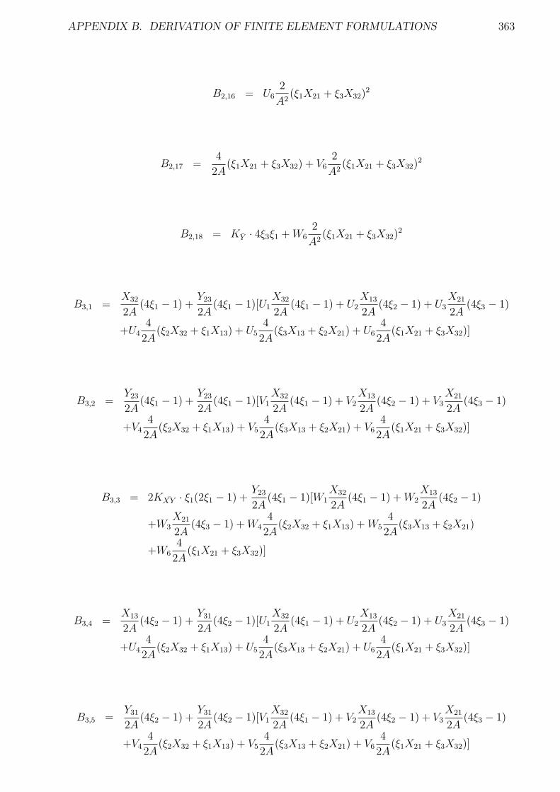
APPENDIX B. DERIVATION OF FINITE ELEMENT FORMULATIONS 363
B2,16 = U62
A2(ξ1X21 + ξ3X32)
2
B2,17 =4
2A(ξ1X21 + ξ3X32) + V6
2
A2(ξ1X21 + ξ3X32)
2
B2,18 = KY · 4ξ3ξ1 +W62
A2(ξ1X21 + ξ3X32)
2
B3,1 =X32
2A(4ξ1 − 1) +
Y23
2A(4ξ1 − 1)[U1
X32
2A(4ξ1 − 1) + U2
X13
2A(4ξ2 − 1) + U3
X21
2A(4ξ3 − 1)
+U44
2A(ξ2X32 + ξ1X13) + U5
4
2A(ξ3X13 + ξ2X21) + U6
4
2A(ξ1X21 + ξ3X32)]
B3,2 =Y23
2A(4ξ1 − 1) +
Y23
2A(4ξ1 − 1)[V1
X32
2A(4ξ1 − 1) + V2
X13
2A(4ξ2 − 1) + V3
X21
2A(4ξ3 − 1)
+V44
2A(ξ2X32 + ξ1X13) + V5
4
2A(ξ3X13 + ξ2X21) + V6
4
2A(ξ1X21 + ξ3X32)]
B3,3 = 2KXY · ξ1(2ξ1 − 1) +Y23
2A(4ξ1 − 1)[W1
X32
2A(4ξ1 − 1) +W2
X13
2A(4ξ2 − 1)
+W3X21
2A(4ξ3 − 1) +W4
4
2A(ξ2X32 + ξ1X13) +W5
4
2A(ξ3X13 + ξ2X21)
+W64
2A(ξ1X21 + ξ3X32)]
B3,4 =X13
2A(4ξ2 − 1) +
Y31
2A(4ξ2 − 1)[U1
X32
2A(4ξ1 − 1) + U2
X13
2A(4ξ2 − 1) + U3
X21
2A(4ξ3 − 1)
+U44
2A(ξ2X32 + ξ1X13) + U5
4
2A(ξ3X13 + ξ2X21) + U6
4
2A(ξ1X21 + ξ3X32)]
B3,5 =Y31
2A(4ξ2 − 1) +
Y31
2A(4ξ2 − 1)[V1
X32
2A(4ξ1 − 1) + V2
X13
2A(4ξ2 − 1) + V3
X21
2A(4ξ3 − 1)
+V44
2A(ξ2X32 + ξ1X13) + V5
4
2A(ξ3X13 + ξ2X21) + V6
4
2A(ξ1X21 + ξ3X32)]
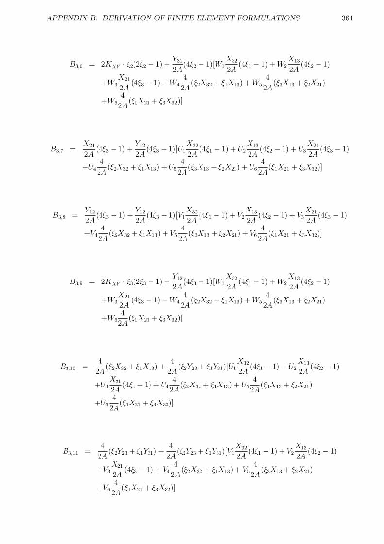
APPENDIX B. DERIVATION OF FINITE ELEMENT FORMULATIONS 364
B3,6 = 2KXY · ξ2(2ξ2 − 1) +Y31
2A(4ξ2 − 1)[W1
X32
2A(4ξ1 − 1) +W2
X13
2A(4ξ2 − 1)
+W3X21
2A(4ξ3 − 1) +W4
4
2A(ξ2X32 + ξ1X13) +W5
4
2A(ξ3X13 + ξ2X21)
+W64
2A(ξ1X21 + ξ3X32)]
B3,7 =X21
2A(4ξ3 − 1) +
Y12
2A(4ξ3 − 1)[U1
X32
2A(4ξ1 − 1) + U2
X13
2A(4ξ2 − 1) + U3
X21
2A(4ξ3 − 1)
+U44
2A(ξ2X32 + ξ1X13) + U5
4
2A(ξ3X13 + ξ2X21) + U6
4
2A(ξ1X21 + ξ3X32)]
B3,8 =Y12
2A(4ξ3 − 1) +
Y12
2A(4ξ3 − 1)[V1
X32
2A(4ξ1 − 1) + V2
X13
2A(4ξ2 − 1) + V3
X21
2A(4ξ3 − 1)
+V44
2A(ξ2X32 + ξ1X13) + V5
4
2A(ξ3X13 + ξ2X21) + V6
4
2A(ξ1X21 + ξ3X32)]
B3,9 = 2KXY · ξ3(2ξ3 − 1) +Y12
2A(4ξ3 − 1)[W1
X32
2A(4ξ1 − 1) +W2
X13
2A(4ξ2 − 1)
+W3X21
2A(4ξ3 − 1) +W4
4
2A(ξ2X32 + ξ1X13) +W5
4
2A(ξ3X13 + ξ2X21)
+W64
2A(ξ1X21 + ξ3X32)]
B3,10 =4
2A(ξ2X32 + ξ1X13) +
4
2A(ξ2Y23 + ξ1Y31)[U1
X32
2A(4ξ1 − 1) + U2
X13
2A(4ξ2 − 1)
+U3X21
2A(4ξ3 − 1) + U4
4
2A(ξ2X32 + ξ1X13) + U5
4
2A(ξ3X13 + ξ2X21)
+U64
2A(ξ1X21 + ξ3X32)]
B3,11 =4
2A(ξ2Y23 + ξ1Y31) +
4
2A(ξ2Y23 + ξ1Y31)[V1
X32
2A(4ξ1 − 1) + V2
X13
2A(4ξ2 − 1)
+V3X21
2A(4ξ3 − 1) + V4
4
2A(ξ2X32 + ξ1X13) + V5
4
2A(ξ3X13 + ξ2X21)
+V64
2A(ξ1X21 + ξ3X32)]
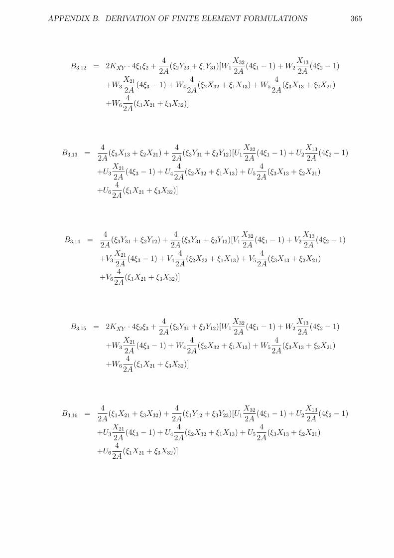
APPENDIX B. DERIVATION OF FINITE ELEMENT FORMULATIONS 365
B3,12 = 2KXY · 4ξ1ξ2 +4
2A(ξ2Y23 + ξ1Y31)[W1
X32
2A(4ξ1 − 1) +W2
X13
2A(4ξ2 − 1)
+W3X21
2A(4ξ3 − 1) +W4
4
2A(ξ2X32 + ξ1X13) +W5
4
2A(ξ3X13 + ξ2X21)
+W64
2A(ξ1X21 + ξ3X32)]
B3,13 =4
2A(ξ3X13 + ξ2X21) +
4
2A(ξ3Y31 + ξ2Y12)[U1
X32
2A(4ξ1 − 1) + U2
X13
2A(4ξ2 − 1)
+U3X21
2A(4ξ3 − 1) + U4
4
2A(ξ2X32 + ξ1X13) + U5
4
2A(ξ3X13 + ξ2X21)
+U64
2A(ξ1X21 + ξ3X32)]
B3,14 =4
2A(ξ3Y31 + ξ2Y12) +
4
2A(ξ3Y31 + ξ2Y12)[V1
X32
2A(4ξ1 − 1) + V2
X13
2A(4ξ2 − 1)
+V3X21
2A(4ξ3 − 1) + V4
4
2A(ξ2X32 + ξ1X13) + V5
4
2A(ξ3X13 + ξ2X21)
+V64
2A(ξ1X21 + ξ3X32)]
B3,15 = 2KXY · 4ξ2ξ3 +4
2A(ξ3Y31 + ξ2Y12)[W1
X32
2A(4ξ1 − 1) +W2
X13
2A(4ξ2 − 1)
+W3X21
2A(4ξ3 − 1) +W4
4
2A(ξ2X32 + ξ1X13) +W5
4
2A(ξ3X13 + ξ2X21)
+W64
2A(ξ1X21 + ξ3X32)]
B3,16 =4
2A(ξ1X21 + ξ3X32) +
4
2A(ξ1Y12 + ξ3Y23)[U1
X32
2A(4ξ1 − 1) + U2
X13
2A(4ξ2 − 1)
+U3X21
2A(4ξ3 − 1) + U4
4
2A(ξ2X32 + ξ1X13) + U5
4
2A(ξ3X13 + ξ2X21)
+U64
2A(ξ1X21 + ξ3X32)]
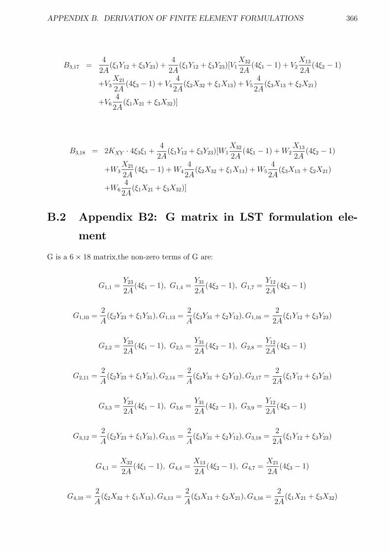
APPENDIX B. DERIVATION OF FINITE ELEMENT FORMULATIONS 366
B3,17 =4
2A(ξ1Y12 + ξ3Y23) +
4
2A(ξ1Y12 + ξ3Y23)[V1
X32
2A(4ξ1 − 1) + V2
X13
2A(4ξ2 − 1)
+V3X21
2A(4ξ3 − 1) + V4
4
2A(ξ2X32 + ξ1X13) + V5
4
2A(ξ3X13 + ξ2X21)
+V64
2A(ξ1X21 + ξ3X32)]
B3,18 = 2KXY · 4ξ3ξ1 +4
2A(ξ1Y12 + ξ3Y23)[W1
X32
2A(4ξ1 − 1) +W2
X13
2A(4ξ2 − 1)
+W3X21
2A(4ξ3 − 1) +W4
4
2A(ξ2X32 + ξ1X13) +W5
4
2A(ξ3X13 + ξ2X21)
+W64
2A(ξ1X21 + ξ3X32)]
B.2 Appendix B2: G matrix in LST formulation ele-
ment
G is a 6 × 18 matrix,the non-zero terms of G are:
G1,1 =Y23
2A(4ξ1 − 1), G1,4 =
Y31
2A(4ξ2 − 1), G1,7 =
Y12
2A(4ξ3 − 1)
G1,10 =2
A(ξ2Y23 + ξ1Y31), G1,13 =
2
A(ξ3Y31 + ξ2Y12), G1,16 =
2
2A(ξ1Y12 + ξ3Y23)
G2,2 =Y23
2A(4ξ1 − 1), G2,5 =
Y31
2A(4ξ2 − 1), G2,8 =
Y12
2A(4ξ3 − 1)
G2,11 =2
A(ξ2Y23 + ξ1Y31), G2,14 =
2
A(ξ3Y31 + ξ2Y12), G2,17 =
2
2A(ξ1Y12 + ξ3Y23)
G3,3 =Y23
2A(4ξ1 − 1), G3,6 =
Y31
2A(4ξ2 − 1), G3,9 =
Y12
2A(4ξ3 − 1)
G3,12 =2
A(ξ2Y23 + ξ1Y31), G3,15 =
2
A(ξ3Y31 + ξ2Y12), G3,18 =
2
2A(ξ1Y12 + ξ3Y23)
G4,1 =X32
2A(4ξ1 − 1), G4,4 =
X13
2A(4ξ2 − 1), G4,7 =
X21
2A(4ξ3 − 1)
G4,10 =2
A(ξ2X32 + ξ1X13), G4,13 =
2
A(ξ3X13 + ξ2X21), G4,16 =
2
2A(ξ1X21 + ξ3X32)
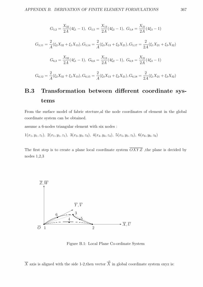
APPENDIX B. DERIVATION OF FINITE ELEMENT FORMULATIONS 367
G5,2 =X32
2A(4ξ1 − 1), G5,5 =
X13
2A(4ξ2 − 1), G5,8 =
X21
2A(4ξ3 − 1)
G5,11 =2
A(ξ2X32 + ξ1X13), G5,14 =
2
A(ξ3X13 + ξ2X21), G5,17 =
2
2A(ξ1X21 + ξ3X32)
G6,3 =X32
2A(4ξ1 − 1), G6,6 =
X13
2A(4ξ2 − 1), G6,9 =
X21
2A(4ξ3 − 1)
G6,12 =2
A(ξ2X32 + ξ1X13), G6,15 =
2
A(ξ3X13 + ξ2X21), G6,18 =
2
2A(ξ1X21 + ξ3X32)
B.3 Transformation between different coordinate sys-
tems
From the surface model of fabric strcture,al the node coordinates of element in the global
coordinate system can be obtained.
assume a 6-nodes triangular element with six nodes :
1(x1, y1, z1), 2(x1, y1, z1), 3(x3, y3, z3), 4(x4, y4, z4), 5(x5, y5, z5), 6(x6, y6, z6)
The first step is to create a plane local coordinate system OXY Z ,the plane is decided by
nodes 1,2,3
- X,UO
Y , V
Z,W6
1 2
3
4 56
*
Figure B.1: Local Plane Co-ordinate System
X axis is aligned with the side 1-2,then vector ~X in global coordinate system oxyz is:
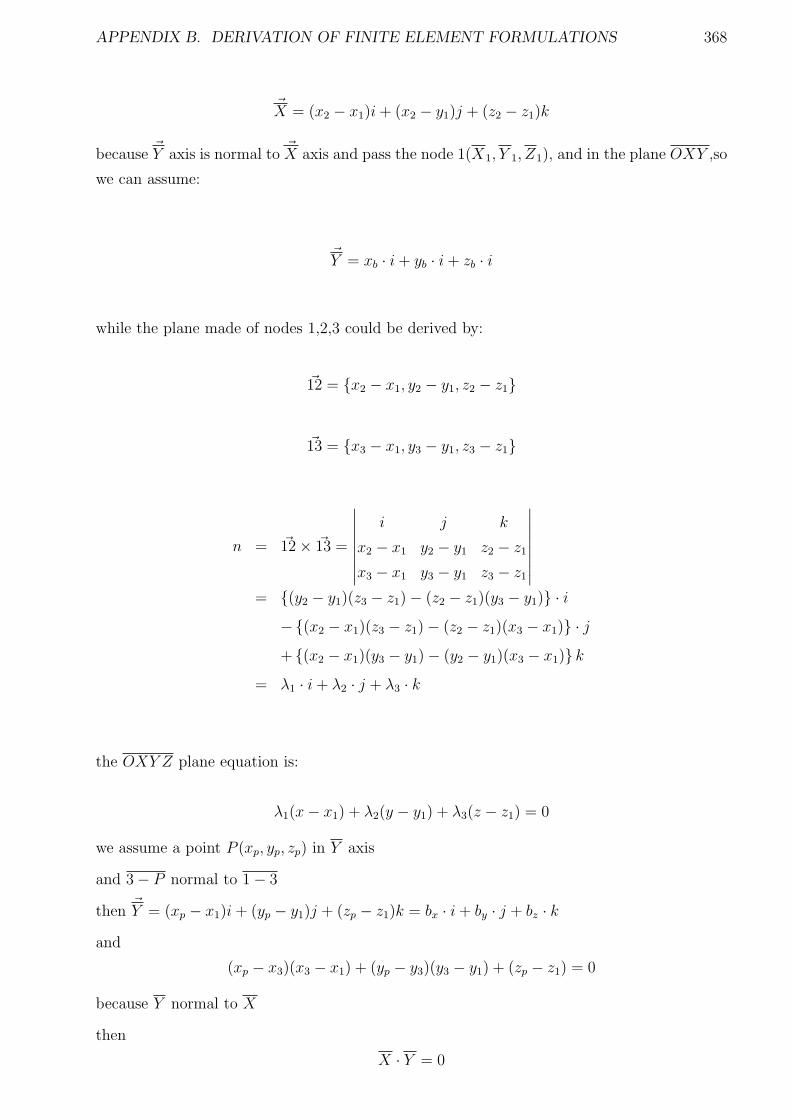
APPENDIX B. DERIVATION OF FINITE ELEMENT FORMULATIONS 368
~X = (x2 − x1)i+ (x2 − y1)j + (z2 − z1)k
because ~Y axis is normal to ~X axis and pass the node 1(X1, Y 1, Z1), and in the plane OXY ,so
we can assume:
~Y = xb · i+ yb · i+ zb · i
while the plane made of nodes 1,2,3 could be derived by:
~12 = x2 − x1, y2 − y1, z2 − z1
~13 = x3 − x1, y3 − y1, z3 − z1
n = ~12 × ~13 =
∣
∣
∣
∣
∣
∣
∣
∣
i j k
x2 − x1 y2 − y1 z2 − z1
x3 − x1 y3 − y1 z3 − z1
∣
∣
∣
∣
∣
∣
∣
∣
= (y2 − y1)(z3 − z1) − (z2 − z1)(y3 − y1) · i−(x2 − x1)(z3 − z1) − (z2 − z1)(x3 − x1) · j+ (x2 − x1)(y3 − y1) − (y2 − y1)(x3 − x1) k
= λ1 · i+ λ2 · j + λ3 · k
the OXY Z plane equation is:
λ1(x− x1) + λ2(y − y1) + λ3(z − z1) = 0
we assume a point P (xp, yp, zp) in Y axis
and 3 − P normal to 1 − 3
then ~Y = (xp − x1)i+ (yp − y1)j + (zp − z1)k = bx · i+ by · j + bz · k
and
(xp − x3)(x3 − x1) + (yp − y3)(y3 − y1) + (zp − z1) = 0
because Y normal to X
then
X · Y = 0
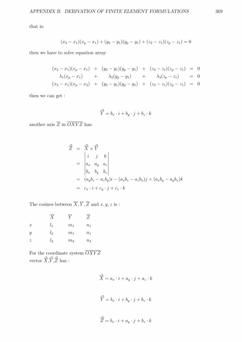
APPENDIX B. DERIVATION OF FINITE ELEMENT FORMULATIONS 369
that is:
(x2 − x1)(xp − x1) + (y2 − y1)(yp − y1) + (z2 − z1)(zp − z1) = 0
then we have to solve equation array
(x2 − x1)(xp − x1) + (y2 − y1)(yp − y1) + (z2 − z1)(zp − z1) = 0
λ1(xp − x1) + λ2(yp − y1) + λ3(zp − z1) = 0
(x3 − x1)(xp − x3) + (y3 − y1)(yp − y1) + (z3 − z1)(zp − z1) = 0
then we can get :
~Y = bx · i+ by · j + bz · k
another axis Z in OXY Z has:
~Z = ~X × ~Y
=
∣
∣
∣
∣
∣
∣
∣
∣
i j k
ax ay az
bx by bz
∣
∣
∣
∣
∣
∣
∣
∣
= (aybz − azby)i− (axbz − azbx)j + (axby − aybx)k
= cx · i+ cy · j + cz · k
The cosines between X,Y , Z and x, y, z is :
X Y Z
x l1 m1 n1
y l2 m1 n1
z l3 m3 n3
For the coordinate system OXY Z
vector ~X,~Y ,~Z has :
~X = ax · i+ ay · j + az · k
~Y = bx · i+ by · j + bz · k
~Z = bx · i+ ay · j + bz · k
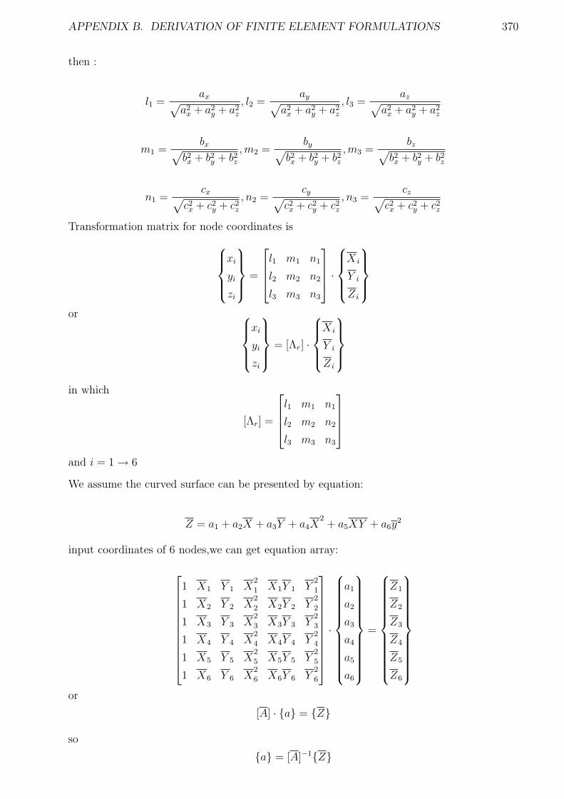
APPENDIX B. DERIVATION OF FINITE ELEMENT FORMULATIONS 370
then :
l1 =ax
√
a2x + a2
y + a2z
, l2 =ay
√
a2x + a2
y + a2z
, l3 =az
√
a2x + a2
y + a2z
m1 =bx
√
b2x + b2y + b2z,m2 =
by√
b2x + b2y + b2z,m3 =
bz√
b2x + b2y + b2z
n1 =cx
√
c2x + c2y + c2z, n2 =
cy√
c2x + c2y + c2z, n3 =
cz√
c2x + c2y + c2z
Transformation matrix for node coordinates is
xi
yi
zi
=
l1 m1 n1
l2 m2 n2
l3 m3 n3
·
X i
Y i
Zi
or
xi
yi
zi
= [Λr] ·
X i
Y i
Zi
in which
[Λr] =
l1 m1 n1
l2 m2 n2
l3 m3 n3
and i = 1 → 6
We assume the curved surface can be presented by equation:
Z = a1 + a2X + a3Y + a4X2+ a5XY + a6y
2
input coordinates of 6 nodes,we can get equation array:
1 X1 Y 1 X2
1 X1Y 1 Y2
1
1 X2 Y 2 X2
2 X2Y 2 Y2
2
1 X3 Y 3 X2
3 X3Y 3 Y2
3
1 X4 Y 4 X2
4 X4Y 4 Y2
4
1 X5 Y 5 X2
5 X5Y 5 Y2
5
1 X6 Y 6 X2
6 X6Y 6 Y2
6
·
a1
a2
a3
a4
a5
a6
=
Z1
Z2
Z3
Z4
Z5
Z6
or
[A] · a = Z
so
a = [A]−1Z
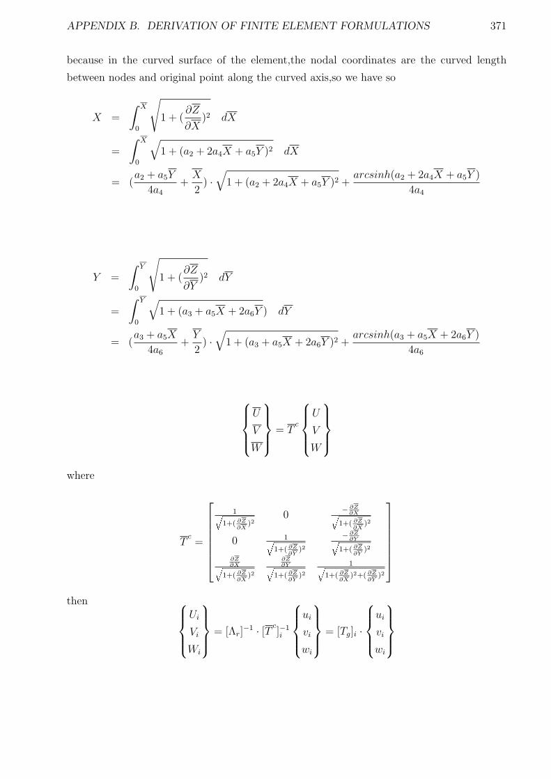
APPENDIX B. DERIVATION OF FINITE ELEMENT FORMULATIONS 371
because in the curved surface of the element,the nodal coordinates are the curved length
between nodes and original point along the curved axis,so we have so
X =
∫ X
0
√
1 + (∂Z
∂X)2 dX
=
∫ X
0
√
1 + (a2 + 2a4X + a5Y )2 dX
= (a2 + a5Y
4a4
+X
2) ·√
1 + (a2 + 2a4X + a5Y )2 +arcsinh(a2 + 2a4X + a5Y )
4a4
Y =
∫ Y
0
√
1 + (∂Z
∂Y)2 dY
=
∫ Y
0
√
1 + (a3 + a5X + 2a6Y ) dY
= (a3 + a5X
4a6
+Y
2) ·√
1 + (a3 + a5X + 2a6Y )2 +arcsinh(a3 + a5X + 2a6Y )
4a6
U
V
W
= Tc
U
V
W
where
Tc=
1q1+( ∂Z
∂X)2
0− ∂Z
∂Xq1+( ∂Z
∂X)2
0 1q1+( ∂Z
∂Y)2
− ∂Z∂Yq
1+( ∂Z∂Y
)2
∂Z∂Xq
1+( ∂Z∂X
)2
∂Z∂Yq
1+( ∂Z∂Y
)2
1q1+( ∂Z
∂X)2+( ∂Z
∂Y)2
then
Ui
Vi
Wi
= [Λr]−1 · [T c
]−1i
ui
vi
wi
= [Tg]i ·
ui
vi
wi
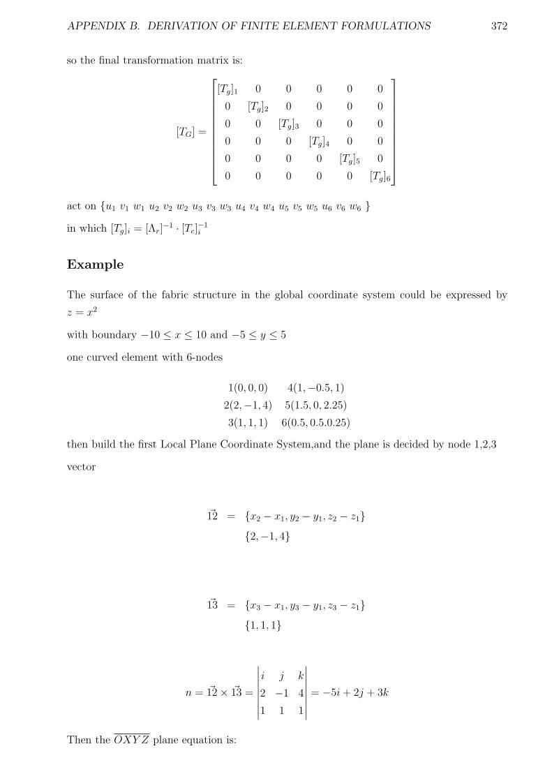
APPENDIX B. DERIVATION OF FINITE ELEMENT FORMULATIONS 372
so the final transformation matrix is:
[TG] =
[Tg]1 0 0 0 0 0
0 [Tg]2 0 0 0 0
0 0 [Tg]3 0 0 0
0 0 0 [Tg]4 0 0
0 0 0 0 [Tg]5 0
0 0 0 0 0 [Tg]6
act on u1 v1 w1 u2 v2 w2 u3 v3 w3 u4 v4 w4 u5 v5 w5 u6 v6 w6
in which [Tg]i = [Λr]−1 · [Tc]
−1i
Example
The surface of the fabric structure in the global coordinate system could be expressed by
z = x2
with boundary −10 ≤ x ≤ 10 and −5 ≤ y ≤ 5
one curved element with 6-nodes
1(0, 0, 0) 4(1,−0.5, 1)
2(2,−1, 4) 5(1.5, 0, 2.25)
3(1, 1, 1) 6(0.5, 0.5.0.25)
then build the first Local Plane Coordinate System,and the plane is decided by node 1,2,3
vector
~12 = x2 − x1, y2 − y1, z2 − z12,−1, 4
~13 = x3 − x1, y3 − y1, z3 − z11, 1, 1
n = ~12 × ~13 =
∣
∣
∣
∣
∣
∣
∣
∣
i j k
2 −1 4
1 1 1
∣
∣
∣
∣
∣
∣
∣
∣
= −5i+ 2j + 3k
Then the OXY Z plane equation is:
APPENDIX B. DERIVATION OF FINITE ELEMENT FORMULATIONS 373
−5(x− x1) + 2(y − y2) + 3(z − z1) = 0
because x1 = y1 = z1 = 0
then the equation is:
−5x+ 2y + 3z = 0 (B.17)
assume there is a point P (xp, yp, zp) has ~P1⊥ ~12 and ~P3⊥ ~13
while
~P1 = (xp − x1)i+ (yp − y1)j + (zp − z1)k
= xp · i+ yp · j + zp · k= bx · i+ by · j + bz · k
~P3 = (xp − x3)i+ (yp − y3)j + (zp − z3)k
= (xp − 1) · i+ (yp − 1) · j + (zp − 1) · k
~13 = (x3 − x1)i+ (y3 − y1)j + (z3 − z1)k
= x3 · i+ y3 · j + z3 · k= i + j + k
For ~P3⊥ ~13, we have ~P3 · ~13 = 0
(xp − 1) + (yp − 1) + (zp − 1) = 0
xp + yp + zp = 3 (B.18)
For ~P1⊥ ~12
~12 = (x2 − x1)i+ (y2 − y1)j + (z2 − z1)k
2i − j + 4k
APPENDIX B. DERIVATION OF FINITE ELEMENT FORMULATIONS 374
~P1 · ~12 = 0
that is:
2xp − yp + 4zp = 0 (B.19)
solve the equation array (1) (2) (3)
we can get
xp = 0.868, yp = 2.052, zp = 0.079
Then we can get:
~X = ~12 = ax · i+ ay · j + az · k(x2 − x1)i+ (y2 − y1)j + (z2 − z1)k
2i − j + 4k
~Y = ~1P = bx · i+ by · j + bz · k(xP − x1)i+ (yP − y1)j + (zP − z1)k
0.868i − 2.053j + 0.079k
~Z = ~12 × ~13
cx · i+ cy · j + cz · k−5i + 2j + 3k
then
l1 =ax
√
a2x + a2
y + a2z
=2√
22 + 12 + 42= 0.436
l2 =ay
√
a2x + a2
y + a2z
=−1√
22 + 12 + 42= −0.218
l3 =az
√
a2x + a2
y + a2z
=4√
22 + 12 + 42= 0.872
APPENDIX B. DERIVATION OF FINITE ELEMENT FORMULATIONS 375
m1 =bx
√
b2x + b2y + b2z=
0.868√0.8682 + 2.0532 + 0.0792
= 0.389
m2 =by
√
b2x + b2y + b2z=
2.053√0.8682 + 2.0532 + 0.0792
= 0.389
m3 =bx
√
b2x + b2y + b2z=
0.079√0.8682 + 2.0532 + 0.0792
= 0.035
n1 =cx
√
c2x + c2y + c2z=
−5√
(−5)2 + 22 + 32= −0.812
n2 =cy
√
c2x + c2y + c2z=
2√
(−5)2 + 22 + 32= 0.325
n3 =cz
√
c2x + c2y + c2z=
3√
(−5)2 + 22 + 32= 0.487
[Λr] =
l1 m1 n1
l2 m2 n2
l3 m3 n3
=
0.436 0.389 −0.812
−0.218 0.921 0.325
0.878 0.033 0.487
xi − xo
yi − yo
zi − zo
= [Λr]
X i
Y i
Zi
so
X i
Y i
Zi
= [Λr]
xi − xo
yi − yo
zi − zo
in which ,xo, yo, zois the coordinate of point O in global coordinate system and i = 1 → 6
then we can get coordinates of 6 nodes in the OXY Z coordinate system
X1 = Y 1 = Z1 = 0
X2 = 4.587, Y 2 = 0, Z2 = 0
X3 = 1.095, Y 3 = 1.345, Z3 = 0
X4 = 1.419, Y 4 = −0.035, Z4 = −0.486
X5 = 2.622, Y 5 = 0.633, Z4 = −0.121
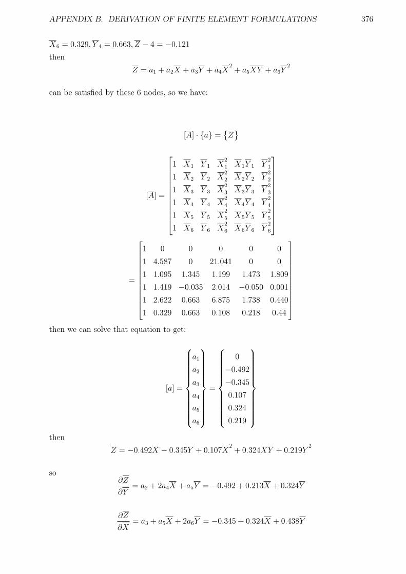
APPENDIX B. DERIVATION OF FINITE ELEMENT FORMULATIONS 376
X6 = 0.329, Y 4 = 0.663, Z − 4 = −0.121
then
Z = a1 + a2X + a3Y + a4X2+ a5XY + a6Y
2
can be satisfied by these 6 nodes, so we have:
[A] · a =
Z
[A] =
1 X1 Y 1 X2
1 X1Y 1 Y2
1
1 X2 Y 2 X2
2 X2Y 2 Y2
2
1 X3 Y 3 X2
3 X3Y 3 Y2
3
1 X4 Y 4 X2
4 X4Y 4 Y2
4
1 X5 Y 5 X2
5 X5Y 5 Y2
5
1 X6 Y 6 X2
6 X6Y 6 Y2
6
=
1 0 0 0 0 0
1 4.587 0 21.041 0 0
1 1.095 1.345 1.199 1.473 1.809
1 1.419 −0.035 2.014 −0.050 0.001
1 2.622 0.663 6.875 1.738 0.440
1 0.329 0.663 0.108 0.218 0.44
then we can solve that equation to get:
[a] =
a1
a2
a3
a4
a5
a6
=
0
−0.492
−0.345
0.107
0.324
0.219
then
Z = −0.492X − 0.345Y + 0.107X2+ 0.324XY + 0.219Y
2
so∂Z
∂Y= a2 + 2a4X + a5Y = −0.492 + 0.213X + 0.324Y
∂Z
∂X= a3 + a5X + 2a6Y = −0.345 + 0.324X + 0.438Y
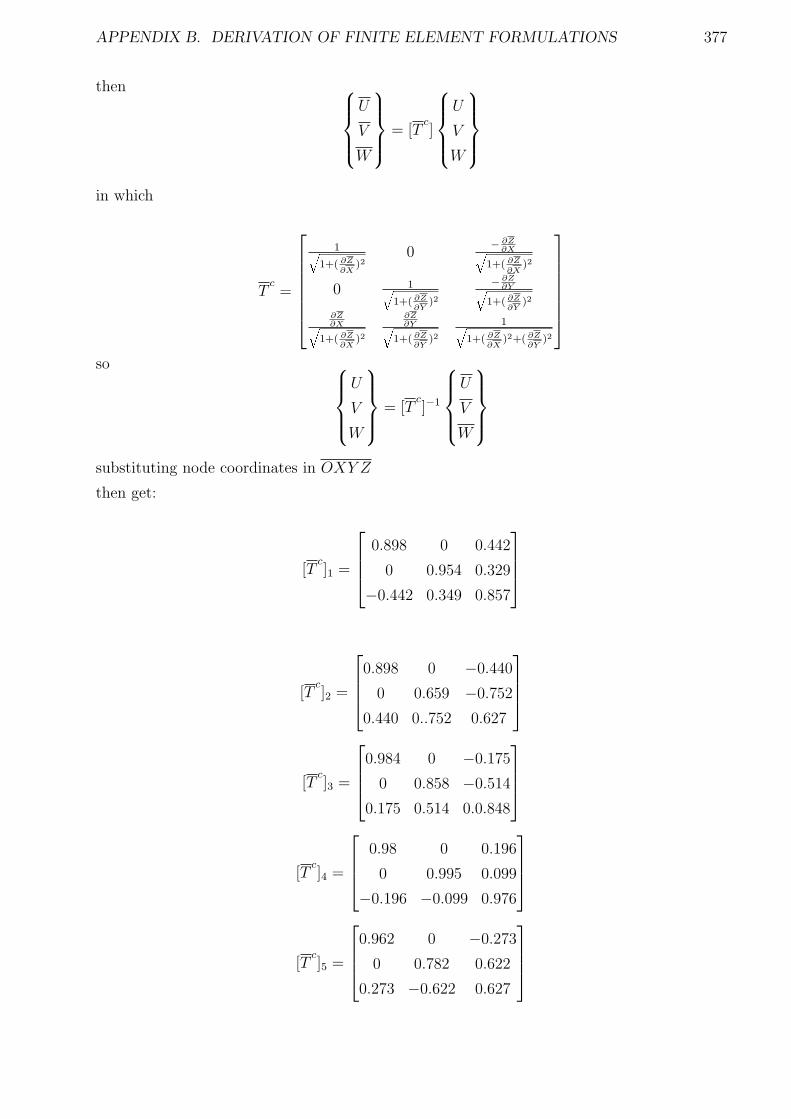
APPENDIX B. DERIVATION OF FINITE ELEMENT FORMULATIONS 377
then
U
V
W
= [Tc]
U
V
W
in which
Tc=
1q1+( ∂Z
∂X)2
0− ∂Z
∂Xq1+( ∂Z
∂X)2
0 1q1+( ∂Z
∂Y)2
− ∂Z∂Yq
1+( ∂Z∂Y
)2
∂Z∂Xq
1+( ∂Z∂X
)2
∂Z∂Yq
1+( ∂Z∂Y
)2
1q1+( ∂Z
∂X)2+( ∂Z
∂Y)2
so
U
V
W
= [Tc]−1
U
V
W
substituting node coordinates in OXY Z
then get:
[Tc]1 =
0.898 0 0.442
0 0.954 0.329
−0.442 0.349 0.857
[Tc]2 =
0.898 0 −0.440
0 0.659 −0.752
0.440 0..752 0.627
[Tc]3 =
0.984 0 −0.175
0 0.858 −0.514
0.175 0.514 0.0.848
[Tc]4 =
0.98 0 0.196
0 0.995 0.099
−0.196 −0.099 0.976
[Tc]5 =
0.962 0 −0.273
0 0.782 0.622
0.273 −0.622 0.627
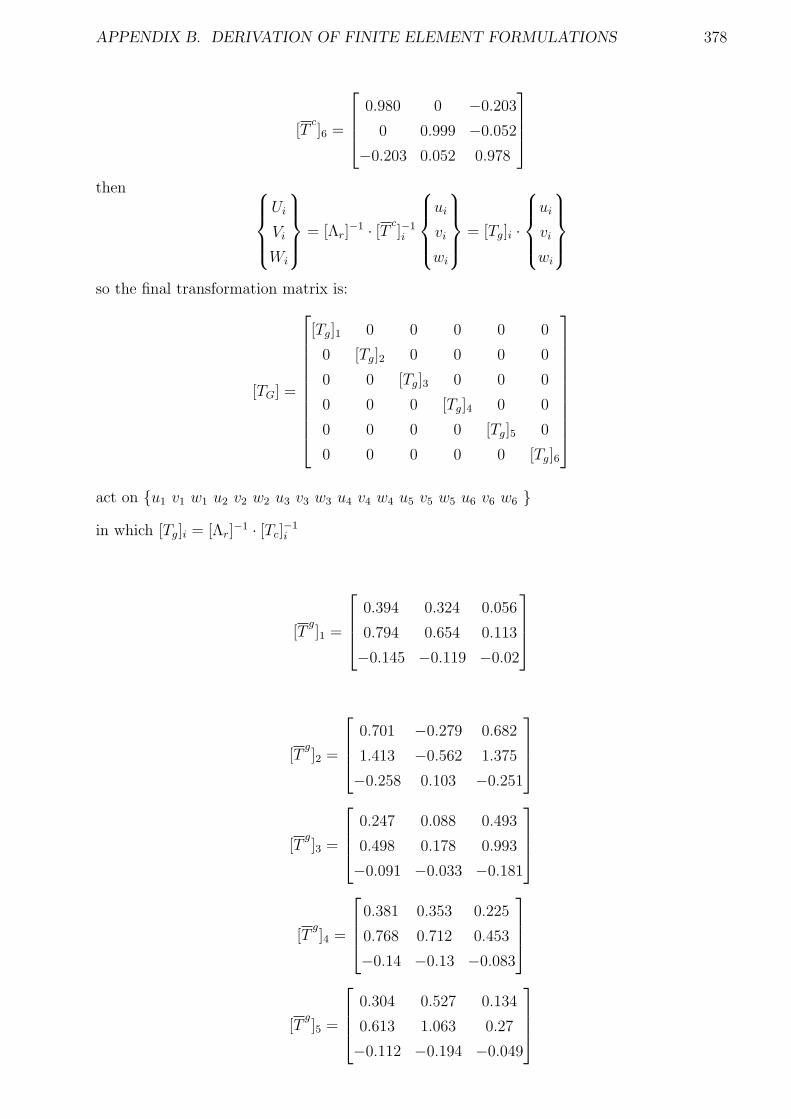
APPENDIX B. DERIVATION OF FINITE ELEMENT FORMULATIONS 378
[Tc]6 =
0.980 0 −0.203
0 0.999 −0.052
−0.203 0.052 0.978
then
Ui
Vi
Wi
= [Λr]−1 · [T c
]−1i
ui
vi
wi
= [Tg]i ·
ui
vi
wi
so the final transformation matrix is:
[TG] =
[Tg]1 0 0 0 0 0
0 [Tg]2 0 0 0 0
0 0 [Tg]3 0 0 0
0 0 0 [Tg]4 0 0
0 0 0 0 [Tg]5 0
0 0 0 0 0 [Tg]6
act on u1 v1 w1 u2 v2 w2 u3 v3 w3 u4 v4 w4 u5 v5 w5 u6 v6 w6
in which [Tg]i = [Λr]−1 · [Tc]
−1i
[Tg]1 =
0.394 0.324 0.056
0.794 0.654 0.113
−0.145 −0.119 −0.02
[Tg]2 =
0.701 −0.279 0.682
1.413 −0.562 1.375
−0.258 0.103 −0.251
[Tg]3 =
0.247 0.088 0.493
0.498 0.178 0.993
−0.091 −0.033 −0.181
[Tg]4 =
0.381 0.353 0.225
0.768 0.712 0.453
−0.14 −0.13 −0.083
[Tg]5 =
0.304 0.527 0.134
0.613 1.063 0.27
−0.112 −0.194 −0.049
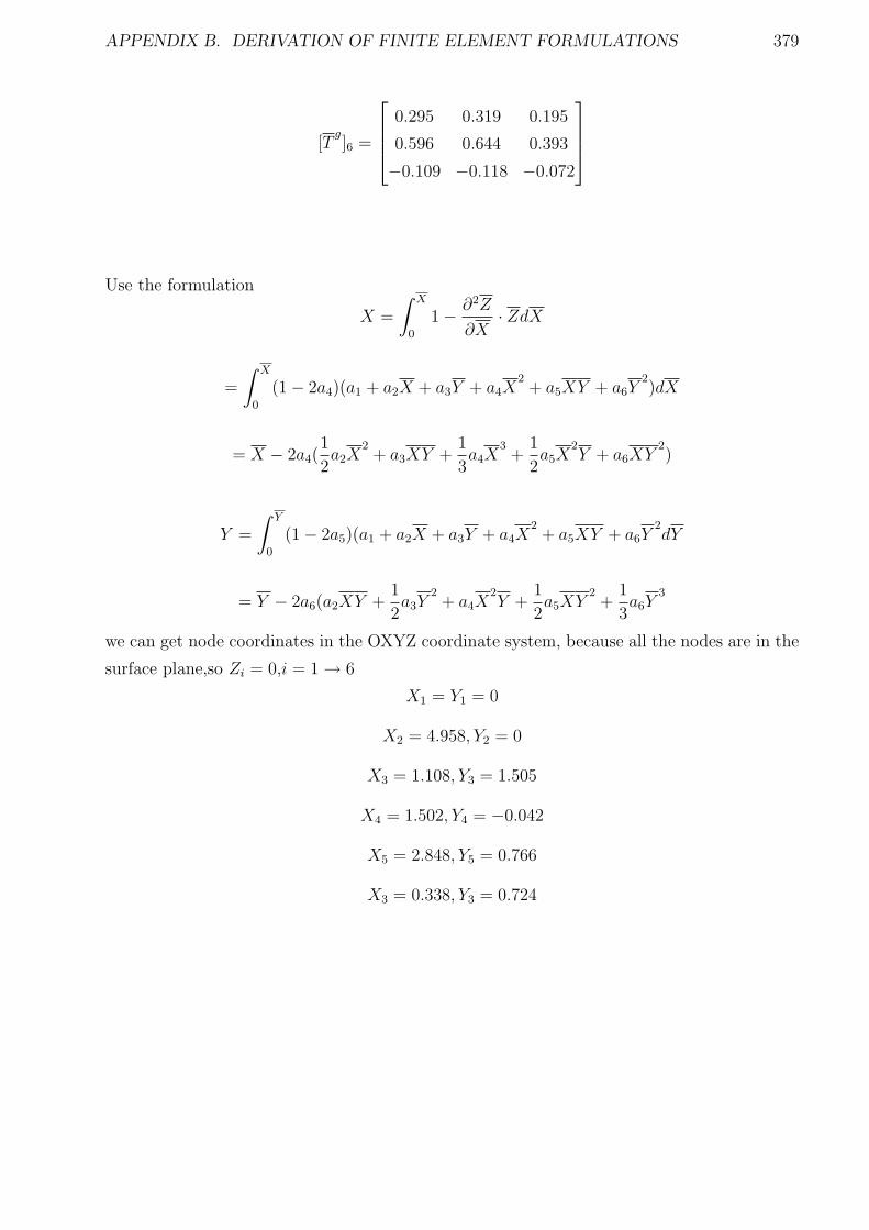
APPENDIX B. DERIVATION OF FINITE ELEMENT FORMULATIONS 379
[Tg]6 =
0.295 0.319 0.195
0.596 0.644 0.393
−0.109 −0.118 −0.072
Use the formulation
X =
∫ X
0
1 − ∂2Z
∂X· ZdX
=
∫ X
0
(1 − 2a4)(a1 + a2X + a3Y + a4X2+ a5XY + a6Y
2)dX
= X − 2a4(1
2a2X
2+ a3XY +
1
3a4X
3+
1
2a5X
2Y + a6XY
2)
Y =
∫ Y
0
(1 − 2a5)(a1 + a2X + a3Y + a4X2+ a5XY + a6Y
2dY
= Y − 2a6(a2XY +1
2a3Y
2+ a4X
2Y +
1
2a5XY
2+
1
3a6Y
3
we can get node coordinates in the OXYZ coordinate system, because all the nodes are in the
surface plane,so Zi = 0,i = 1 → 6
X1 = Y1 = 0
X2 = 4.958, Y2 = 0
X3 = 1.108, Y3 = 1.505
X4 = 1.502, Y4 = −0.042
X5 = 2.848, Y5 = 0.766
X3 = 0.338, Y3 = 0.724
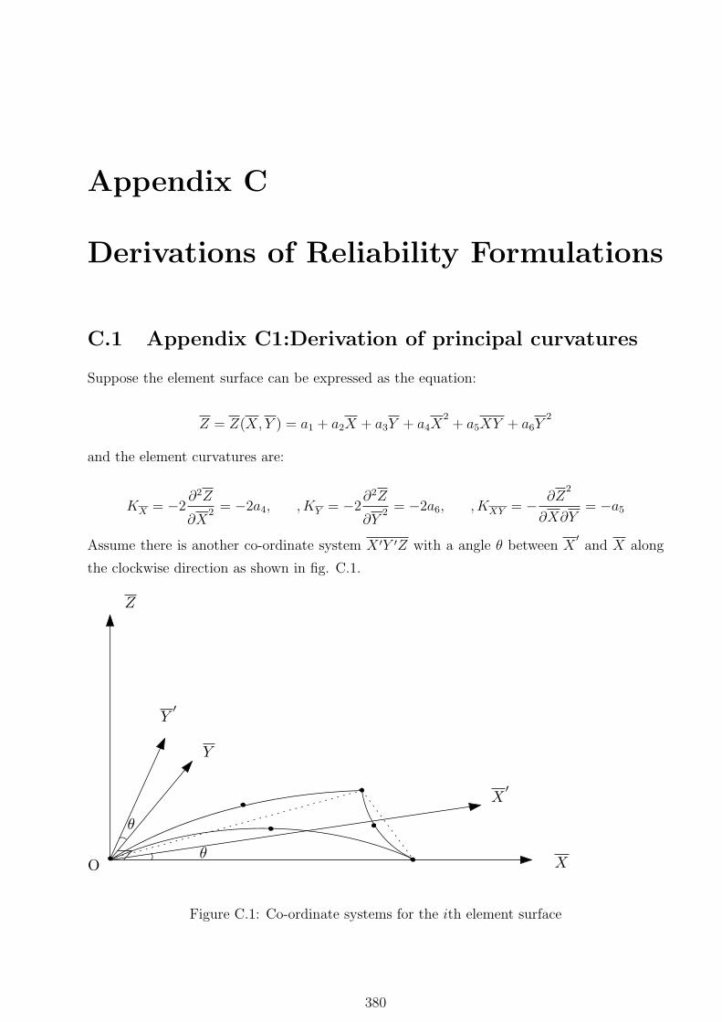
Appendix C
Derivations of Reliability Formulations
C.1 Appendix C1:Derivation of principal curvatures
Suppose the element surface can be expressed as the equation:
Z = Z(X,Y ) = a1 + a2X + a3Y + a4X2+ a5XY + a6Y
2
and the element curvatures are:
KX = −2∂2Z
∂X2 = −2a4, , KY = −2
∂2Z
∂Y2 = −2a6, , KXY = − ∂Z
2
∂X∂Y= −a5
Assume there is another co-ordinate system X ′Y ′Z with a angle θ between X′and X along
the clockwise direction as shown in fig. C.1.
X
X′
Y
Y′
Z
Oθ
θ
Figure C.1: Co-ordinate systems for the ith element surface
380
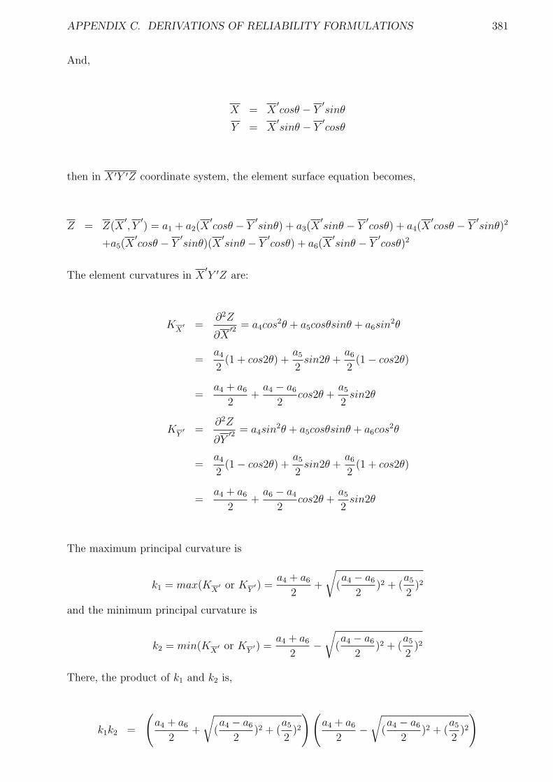
APPENDIX C. DERIVATIONS OF RELIABILITY FORMULATIONS 381
And,
X = X′cosθ − Y
′sinθ
Y = X′sinθ − Y
′cosθ
then in X ′Y ′Z coordinate system, the element surface equation becomes,
Z = Z(X′, Y
′) = a1 + a2(X
′cosθ − Y
′sinθ) + a3(X
′sinθ − Y
′cosθ) + a4(X
′cosθ − Y
′sinθ)2
+a5(X′cosθ − Y
′sinθ)(X
′sinθ − Y
′cosθ) + a6(X
′sinθ − Y
′cosθ)2
The element curvatures in X′Y ′Z are:
KX′ =
∂2Z
∂X′2 = a4cos
2θ + a5cosθsinθ + a6sin2θ
=a4
2(1 + cos2θ) +
a5
2sin2θ +
a6
2(1 − cos2θ)
=a4 + a6
2+a4 − a6
2cos2θ +
a5
2sin2θ
KY′ =
∂2Z
∂Y′2 = a4sin
2θ + a5cosθsinθ + a6cos2θ
=a4
2(1 − cos2θ) +
a5
2sin2θ +
a6
2(1 + cos2θ)
=a4 + a6
2+a6 − a4
2cos2θ +
a5
2sin2θ
The maximum principal curvature is
k1 = max(KX′ or KY
′) =a4 + a6
2+
√
(a4 − a6
2)2 + (
a5
2)2
and the minimum principal curvature is
k2 = min(KX′ or KY
′) =a4 + a6
2−√
(a4 − a6
2)2 + (
a5
2)2
There, the product of k1 and k2 is,
k1k2 =
(
a4 + a6
2+
√
(a4 − a6
2)2 + (
a5
2)2
)(
a4 + a6
2−√
(a4 − a6
2)2 + (
a5
2)2
)
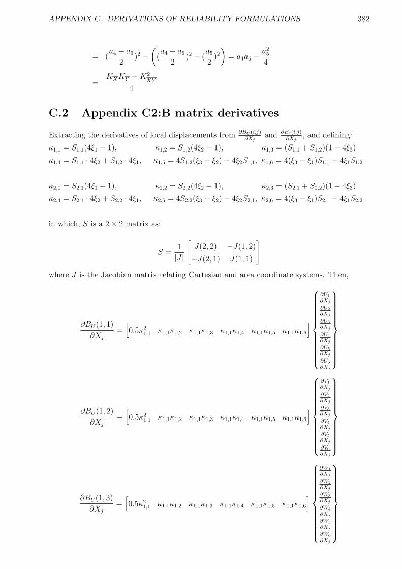
APPENDIX C. DERIVATIONS OF RELIABILITY FORMULATIONS 382
= (a4 + a6
2)2 −
(
(a4 − a6
2)2 + (
a5
2)2
)
= a4a6 −a2
5
4
=KXKY −K2
XY
4
C.2 Appendix C2:B matrix derivatives
Extracting the derivatives of local displacements from ∂BU (i,j)∂Xj
and ∂Bc(i,j)∂Xj
, and defining:
κ1,1 = S1,1(4ξ1 − 1), κ1,2 = S1,2(4ξ2 − 1), κ1,3 = (S1,1 + S1,2)(1 − 4ξ3)
κ1,4 = S1,1 · 4ξ2 + S1,2 · 4ξ1, κ1,5 = 4S1,2(ξ3 − ξ2) − 4ξ2S1,1, κ1,6 = 4(ξ3 − ξ1)S1,1 − 4ξ1S1,2
κ2,1 = S2,1(4ξ1 − 1), κ2,2 = S2,2(4ξ2 − 1), κ2,3 = (S2,1 + S2,2)(1 − 4ξ3)
κ2,4 = S2,1 · 4ξ2 + S2,2 · 4ξ1, κ2,5 = 4S2,2(ξ3 − ξ2) − 4ξ2S2,1, κ2,6 = 4(ξ3 − ξ1)S2,1 − 4ξ1S2,2
in which, S is a 2 × 2 matrix as:
S =1
|J |
[
J(2, 2) −J(1, 2)
−J(2, 1) J(1, 1)
]
where J is the Jacobian matrix relating Cartesian and area coordinate systems. Then,
∂BU(1, 1)
∂Xj
=[
0.5κ21,1 κ1,1κ1,2 κ1,1κ1,3 κ1,1κ1,4 κ1,1κ1,5 κ1,1κ1,6
]
∂U1
∂Xj
∂U2
∂Xj
∂U3
∂Xj
∂U4
∂Xj
∂U5
∂Xj
∂U6
∂Xj
∂BU(1, 2)
∂Xj
=[
0.5κ21,1 κ1,1κ1,2 κ1,1κ1,3 κ1,1κ1,4 κ1,1κ1,5 κ1,1κ1,6
]
∂V1
∂Xj
∂V2
∂Xj
∂V3
∂Xj
∂V4
∂Xj
∂V5
∂Xj
∂V6
∂Xj
∂BU(1, 3)
∂Xj
=[
0.5κ21,1 κ1,1κ1,2 κ1,1κ1,3 κ1,1κ1,4 κ1,1κ1,5 κ1,1κ1,6
]
∂W1
∂Xj
∂W2
∂Xj
∂W3
∂Xj
∂W4
∂Xj
∂W5
∂Xj
∂W6
∂Xj

APPENDIX C. DERIVATIONS OF RELIABILITY FORMULATIONS 383
∂BU(1, 4)
∂Xj
=[
0.5κ21,2 κ1,2κ1,3 κ1,2κ1,4 κ1,2κ1,5 κ1,2κ1,6
]
∂U2
∂Xj
∂U3
∂Xj
∂U4
∂Xj
∂U5
∂Xj
∂U6
∂Xj
∂BU(1, 5)
∂Xj
=[
0.5κ21,2 κ1,2κ1,3 κ1,2κ1,4 κ1,2κ1,5 κ1,2κ1,6
]
∂V2
∂Xj
∂V3
∂Xj
∂V4
∂Xj
∂V5
∂Xj
∂V6
∂Xj
∂BU(1, 6)
∂Xj
=[
0.5κ21,2 κ1,2κ1,3 κ1,2κ1,4 κ1,2κ1,5 κ1,2κ1,6
]
∂W2
∂Xj
∂W3
∂Xj
∂W4
∂Xj
∂W5
∂Xj
∂W6
∂Xj
∂BU(1, 7)
∂Xj
=[
0.5κ21,3 κ1,3κ1,4 κ1,3κ1,5 κ1,3κ1,6
]
∂U3
∂Xj
∂U4
∂Xj
∂U5
∂Xj
∂U6
∂Xj
∂BU(1, 8)
∂Xj
=[
0.5κ21,3 κ1,3κ1,4 κ1,3κ1,5 κ1,3κ1,6
]
∂V3
∂Xj
∂V4
∂Xj
∂V5
∂Xj
∂V6
∂Xj
∂BU(1, 9)
∂Xj
=[
0.5κ21,3 κ1,3κ1,4 κ1,3κ1,5 κ1,3κ1,6
]
∂W3
∂Xj
∂W4
∂Xj
∂W5
∂Xj
∂W6
∂Xj
∂BU(1, 10)
∂Xj
=[
0.5κ21,4 κ1,4κ1,5 κ1,4κ1,6
]
∂U4
∂Xj
∂U5
∂Xj
∂U6
∂Xj
∂BU(1, 11)
∂Xj
=[
0.5κ21,4 κ1,4κ1,5 κ1,4κ1,6
]
∂V4
∂Xj
∂V5
∂Xj
∂V6
∂Xj

APPENDIX C. DERIVATIONS OF RELIABILITY FORMULATIONS 384
∂BU(1, 12)
∂Xj
=[
0.5κ21,4 κ1,4κ1,5 κ1,4κ1,6
]
∂W4
∂Xj
∂W5
∂Xj
∂W6
∂Xj
∂BU(1, 13)
∂Xj
=[
0.5κ21,5 κ1,5κ1,6
]
∂U5
∂Xj
∂U6
∂Xj
∂BU(1, 14)
∂Xj
=[
0.5κ21,5 κ1,5κ1,6
]
∂V5
∂Xj
∂V6
∂Xj
∂BU(1, 15)
∂Xj
=[
0.5κ21,5 κ1,5κ1,6
]
∂W5
∂Xj
∂W6
∂Xj
∂BU(1, 16)
∂Xj
=[
0.5κ21,6
]
∂U6
∂Xj
,∂BU(1, 17)
∂u=[
0.5κ21,6
]
∂V6
∂Xj
,∂BU(1, 18)
∂u=[
0.5κ21,6
]
∂W6
∂Xj
∂BU(2, 1)
∂Xj
=[
0.5κ22,1 κ2,1κ2,2 κ2,1κ2,3 κ2,1κ2,4 κ2,1κ2,5 κ2,1κ2,6
]
∂U1
∂Xj
∂U2
∂Xj
∂U3
∂Xj
∂U4
∂Xj
∂U5
∂Xj
∂U6
∂Xj
∂BU(2, 2)
∂Xj
=[
0.5κ22,1 κ2,1κ2,2 κ2,1κ2,3 κ2,1κ2,4 κ2,1κ2,5 κ2,1κ2,6
]
∂V1
∂Xj
∂V2
∂Xj
∂V3
∂Xj
∂V4
∂Xj
∂V5
∂Xj
∂V6
∂Xj
∂BU(2, 3)
∂Xj
=[
0.5κ22,1 κ2,1κ2,2 κ2,1κ2,3 κ2,1κ2,4 κ2,1κ2,5 κ2,1κ2,6
]
∂W1
∂Xj
∂W2
∂Xj
∂W3
∂Xj
∂W4
∂Xj
∂W5
∂Xj
∂W6
∂Xj
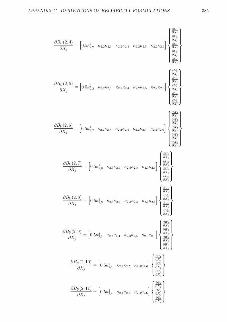
APPENDIX C. DERIVATIONS OF RELIABILITY FORMULATIONS 385
∂BU(2, 4)
∂Xj
=[
0.5κ22,2 κ2,2κ2,3 κ2,2κ2,4 κ2,2κ2,5 κ2,2κ2,6
]
∂U2
∂Xj
∂U3
∂Xj
∂U4
∂Xj
∂U5
∂Xj
∂U6
∂Xj
∂BU(2, 5)
∂Xj
=[
0.5κ22,2 κ2,2κ2,3 κ2,2κ2,4 κ2,2κ2,5 κ2,2κ2,6
]
∂V2
∂Xj
∂V3
∂Xj
∂V4
∂Xj
∂V5
∂Xj
∂V6
∂Xj
∂BU(2, 6)
∂Xj
=[
0.5κ22,2 κ2,2κ2,3 κ2,2κ2,4 κ2,2κ2,5 κ2,2κ2,6
]
∂W2
∂Xj
∂W3
∂Xj
∂W4
∂Xj
∂W5
∂Xj
∂W6
∂Xj
∂BU(2, 7)
∂Xj
=[
0.5κ22,3 κ2,3κ2,4 κ2,3κ2,5 κ2,3κ2,6
]
∂U3
∂Xj
∂U4
∂Xj
∂U5
∂Xj
∂U6
∂Xj
∂BU(2, 8)
∂Xj
=[
0.5κ22,3 κ2,3κ2,4 κ2,3κ2,5 κ2,3κ2,6
]
∂V3
∂Xj
∂V4
∂Xj
∂V5
∂Xj
∂V6
∂Xj
∂BU(2, 9)
∂Xj
=[
0.5κ22,3 κ2,3κ2,4 κ2,3κ2,5 κ2,3κ2,6
]
∂W3
∂Xj
∂W4
∂Xj
∂W5
∂Xj
∂W6
∂Xj
∂BU(2, 10)
∂Xj
=[
0.5κ22,4 κ2,4κ2,5 κ2,4κ2,6
]
∂U4
∂Xj
∂U5
∂Xj
∂U6
∂Xj
∂BU(2, 11)
∂Xj
=[
0.5κ22,4 κ2,4κ2,5 κ2,4κ2,6
]
∂V4
∂Xj
∂V5
∂Xj
∂V6
∂Xj
APPENDIX C. DERIVATIONS OF RELIABILITY FORMULATIONS 386
∂BU(2, 12)
∂Xj
=[
0.5κ22,4 κ2,4κ2,5 κ2,4κ2,6
]
∂W4
∂Xj
∂W5
∂Xj
∂W6
∂Xj
∂BU(2, 13)
∂Xj
=[
0.5κ22,5 κ2,5κ2,6
]
∂U5
∂Xj
∂U6
∂Xj
∂BU(2, 14)
∂Xj
=[
0.5κ22,5 κ2,5κ2,6
]
∂V5
∂Xj
∂V6
∂Xj
∂BU(2, 15)
∂Xj
=[
0.5κ22,5 κ2,5κ2,6
]
∂W5
∂Xj
∂W6
∂Xj
∂BU(2, 16)
∂Xj
=[
0.5κ22,6
]
∂U6
∂Xj
,∂BU(2, 17)
∂u=[
0.5κ22,6
]
∂V6
∂Xj
,∂BU(2, 18)
∂u=[
0.5κ22,6
]
∂W6
∂Xj
∂BU(3, 1)
∂Xj
=[
κ1,1κ2,1 κ1,1κ2,2 κ1,1κ2,3 κ1,1κ2,4 κ1,1κ2,5 κ1,1κ2,6
]
∂U1
∂Xj
∂U2
∂Xj
∂U3
∂Xj
∂U4
∂Xj
∂U5
∂Xj
∂U6
∂Xj
∂BU(3, 2)
∂Xj
=[
κ1,1κ2,1 κ1,1κ2,2 κ1,1κ2,3 κ1,1κ2,4 κ1,1κ2,5 κ1,1κ2,6
]
∂V1
∂Xj
∂V2
∂Xj
∂V3
∂Xj
∂V4
∂Xj
∂V5
∂Xj
∂V6
∂Xj
∂BU(3, 3)
∂Xj
=[
κ1,1κ2,1 κ1,1κ2,2 κ1,1κ2,3 κ1,1κ2,4 κ1,1κ2,5 κ1,1κ2,6
]
∂W1
∂Xj
∂W2
∂Xj
∂W3
∂Xj
∂W4
∂Xj
∂W5
∂Xj
∂W6
∂Xj
APPENDIX C. DERIVATIONS OF RELIABILITY FORMULATIONS 387
∂BU(3, 4)
∂Xj
=[
κ1,2κ2,1 κ1,2κ2,2 κ1,2κ2,3 κ1,2κ2,4 κ1,2κ2,5 κ1,2κ2,6
]
∂U1
∂Xj
∂U2
∂Xj
∂U3
∂Xj
∂U4
∂Xj
∂U5
∂Xj
∂U6
∂Xj
∂BU(3, 5)
∂Xj
=[
κ1,2κ2,1 κ1,2κ2,2 κ1,2κ2,3 κ1,2κ2,4 κ1,2κ2,5 κ1,2κ2,6
]
∂V1
∂Xj
∂V2
∂Xj
∂V3
∂Xj
∂V4
∂Xj
∂V5
∂Xj
∂V6
∂Xj
∂BU(3, 6)
∂Xj
=[
κ1,2κ2,1 κ1,2κ2,2 κ1,2κ2,3 κ1,2κ2,4 κ1,2κ2,5 κ1,2κ2,6
]
∂W1
∂Xj
∂W2
∂Xj
∂W3
∂Xj
∂W4
∂Xj
∂W5
∂Xj
∂W6
∂Xj
∂BU(3, 7)
∂Xj
=[
κ1,3κ2,1 κ1,3κ2,2 κ1,3κ2,3 κ1,3κ2,4 κ1,3κ2,5 κ1,3κ2,6
]
∂U1
∂Xj
∂U2
∂Xj
∂U3
∂Xj
∂U4
∂Xj
∂U5
∂Xj
∂U6
∂Xj
∂BU(3, 8)
∂Xj
=[
κ1,3κ2,1 κ1,3κ2,2 κ1,3κ2,3 κ1,3κ2,4 κ1,3κ2,5 κ1,3κ2,6
]
∂V1
∂Xj
∂V2
∂Xj
∂V3
∂Xj
∂V4
∂Xj
∂V5
∂Xj
∂V6
∂Xj

APPENDIX C. DERIVATIONS OF RELIABILITY FORMULATIONS 388
∂BU(3, 9)
∂Xj
=[
κ1,3κ2,1 κ1,3κ2,2 κ1,3κ2,3 κ1,3κ2,4 κ1,3κ2,5 κ1,3κ2,6
]
∂W1
∂Xj
∂W2
∂Xj
∂W3
∂Xj
∂W4
∂Xj
∂W5
∂Xj
∂W6
∂Xj
∂BU(3, 10)
∂Xj
=[
κ1,4κ2,1 κ1,4κ2,2 κ1,4κ2,3 κ1,4κ2,4 κ1,4κ2,5 κ1,4κ2,6
]
∂U1
∂Xj
∂U2
∂Xj
∂U3
∂Xj
∂U4
∂Xj
∂U5
∂Xj
∂U6
∂Xj
∂BU(3, 11)
∂Xj
=[
κ1,4κ2,1 κ1,4κ2,2 κ1,4κ2,3 κ1,4κ2,4 κ1,4κ2,5 κ1,4κ2,6
]
∂V1
∂Xj
∂V2
∂Xj
∂V3
∂Xj
∂V4
∂Xj
∂V5
∂Xj
∂V6
∂Xj
∂BU(3, 12)
∂Xj
=[
κ1,4κ2,1 κ1,4κ2,2 κ1,4κ2,3 κ1,4κ2,4 κ1,4κ2,5 κ1,4κ2,6
]
∂W1
∂Xj
∂W2
∂Xj
∂W3
∂Xj
∂W4
∂Xj
∂W5
∂Xj
∂W6
∂Xj
∂BU(3, 13)
∂Xj
=[
κ1,5κ2,1 κ1,5κ2,2 κ1,5κ2,3 κ1,5κ2,4 κ1,5κ2,5 κ1,5κ2,6
]
∂U1
∂Xj
∂U2
∂Xj
∂U3
∂Xj
∂U4
∂Xj
∂U5
∂Xj
∂U6
∂Xj
APPENDIX C. DERIVATIONS OF RELIABILITY FORMULATIONS 389
∂BU(3, 14)
∂Xj
=[
κ1,5κ2,1 κ1,5κ2,2 κ1,5κ2,3 κ1,5κ2,4 κ1,5κ2,5 κ1,5κ2,6
]
∂V1
∂Xj
∂V2
∂Xj
∂V3
∂Xj
∂V4
∂Xj
∂V5
∂Xj
∂V6
∂Xj
∂BU(3, 16)
∂Xj
=[
κ1,6κ2,1 κ1,6κ2,2 κ1,6κ2,3 κ1,6κ2,4 κ1,6κ2,5 κ1,6κ2,6
]
∂U1
∂Xj
∂U2
∂Xj
∂U3
∂Xj
∂U4
∂Xj
∂U5
∂Xj
∂U6
∂Xj
∂BU(3, 17)
∂Xj
=[
κ1,6κ2,1 κ1,6κ2,2 κ1,6κ2,3 κ1,6κ2,4 κ1,6κ2,5 κ1,6κ2,6
]
∂V1
∂Xj
∂V2
∂Xj
∂V3
∂Xj
∂V4
∂Xj
∂V5
∂Xj
∂V6
∂Xj
∂BU(3, 18)
∂Xj
=[
κ1,6κ2,1 κ1,6κ2,2 κ1,6κ2,3 κ1,6κ2,4 κ1,6κ2,5 κ1,6κ2,6
]
∂W1
∂Xj
∂W2
∂Xj
∂W3
∂Xj
∂W4
∂Xj
∂W5
∂Xj
∂W6
∂Xj
∂Bc(1,3)∂Xj
∂Bc(1,6)∂Xj
∂Bc(1,9)∂Xj
∂Bc(1,12)∂Xj
∂Bc(1,15)∂Xj
=[
ξ1(2ξ1 − 1) ξ2(2ξ2 − 1) ξ3(2ξ3 − 1) 4ξ1ξ2 4ξ2ξ3 4ξ1ξ3
]
∂KX
∂Xj
=[
−2ξ1(2ξ1 − 1) −2ξ2(2ξ2 − 1) −2ξ3(2ξ3 − 1) −8ξ1ξ2 −8ξ2ξ3 −8ξ1ξ3
]
∂a4
∂Xj
APPENDIX C. DERIVATIONS OF RELIABILITY FORMULATIONS 390
∂Bc(2,3)∂Xj
∂Bc(2,6)∂Xj
∂Bc(2,9)∂Xj
∂Bc(2,12)∂Xj
∂Bc(2,15)∂Xj
=[
ξ1(2ξ1 − 1) ξ2(2ξ2 − 1) ξ3(2ξ3 − 1) 4ξ1ξ2 4ξ2ξ3 4ξ1ξ3
]
∂KY
∂Xj
=[
−2ξ1(2ξ1 − 1) −2ξ2(2ξ2 − 1) −2ξ3(2ξ3 − 1) −8ξ1ξ2 −8ξ2ξ3 −8ξ1ξ3
]
∂a6
∂Xj
∂Bc(3,3)∂Xj
∂Bc(3,6)∂Xj
∂Bc(3,9)∂Xj
∂Bc(3,12)∂Xj
∂Bc(3,15)∂Xj
=[
ξ1(2ξ1 − 1) ξ2(2ξ2 − 1) ξ3(2ξ3 − 1) 4ξ1ξ2 4ξ2ξ3 4ξ1ξ3
]
∂2KXY
∂Xj
=[
−2ξ1(2ξ1 − 1) −2ξ2(2ξ2 − 1) −2ξ3(2ξ3 − 1) −8ξ1ξ2 −8ξ2ξ3 −8ξ1ξ3
]
∂a5
∂Xj
In which, ∂a4
∂Xj, ∂a5
∂Xjand ∂a6
∂Xjcan be computed using Eqn.5.150 .
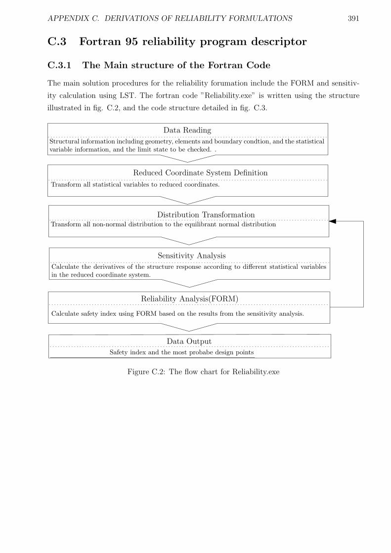
APPENDIX C. DERIVATIONS OF RELIABILITY FORMULATIONS 391
C.3 Fortran 95 reliability program descriptor
C.3.1 The Main structure of the Fortran Code
The main solution procedures for the reliability forumation include the FORM and sensitiv-
ity calculation using LST. The fortran code ”Reliability.exe” is written using the structure
illustrated in fig. C.2, and the code structure detailed in fig. C.3.
Reduced Coordinate System Definition
Distribution Transformation
Reliability Analysis(FORM)
Safety index and the most probabe design points
Data Output
Calculate safety index using FORM based on the results from the sensitivity analysis.
Transform all non-normal distribution to the equilibrant normal distribution
Transform all statistical variables to reduced coordinates.
Structural information including geometry, elements and boundary condtion, and the statistical
variable information, and the limit state to be checked. .
Data Reading
Sensitivity Analysis
Calculate the derivatives of the structure response according to different statistical variables
in the reduced coordinate system.
Figure C.2: The flow chart for Reliability.exe
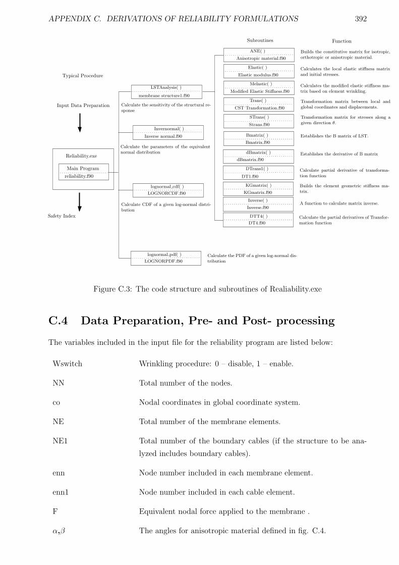
APPENDIX C. DERIVATIONS OF RELIABILITY FORMULATIONS 392
Main Program
reliability.f90
Typical Procedure
Subroutines Function
ANE( )
Anisotropic material.f90
Input Data Preparation
Safety Index
Elastic( )
Elastic modulus.f90
Trans( )
CST Transformation.f90
Melastic( )
Modified Elastic Stiffness.f90
STrans( )
Strans.f90
Bmatrix( )
Bmatrix.f90
dBmatrix( )
dBmatrix.f90
DTrans1( )
DT1.f90
KGmatrix( )
KGmatrix.f90
Inverse( )
Inverse.f90
DTT4( )
DT4.f90
Builds the constitutive matrix for isotropic,orthotropic or anisotropic material.
Calculates the local elastic stiffness matrixand initial stresses.
Calculates the modified elastic stiffness ma-trix based on element wrinkling.
Transformation matrix between local andglobal coordinates and displacements.
Transformation matrix for stresses along agiven direction θ.
Establishes the B matrix of LST.
Establishes the derivative of B matrix
Calculate partial derivative of transforma-tion function
Builds the element geometric stiffness ma-trix.
A function to calculate matrix inverse.
Calculate the partial derivatives of Transfor-mation function
Reliability.exe
Invernormal( )
Inverse normal.f90
Calculate the parameters of the equivalentnormal distribution
lognormal cdf( )
LOGNORCDF.f90
Calculate CDF of a given log-normal distri-bution
lognormal pdf( )
LOGNORPDF.f90Calculate the PDF of a given log-normal dis-tribution
LSTAnalysis( )
membrane structure1.f90
Calculate the sensitivity of the structural re-sponse
Figure C.3: The code structure and subroutines of Realiability.exe
C.4 Data Preparation, Pre- and Post- processing
The variables included in the input file for the reliability program are listed below:
Wswitch Wrinkling procedure: 0 – disable, 1 – enable.
NN Total number of the nodes.
co Nodal coordinates in global coordinate system.
NE Total number of the membrane elements.
NE1 Total number of the boundary cables (if the structure to be ana-
lyzed includes boundary cables).
enn Node number included in each membrane element.
enn1 Node number included in each cable element.
F Equivalent nodal force applied to the membrane .
α,β The angles for anisotropic material defined in fig. C.4.
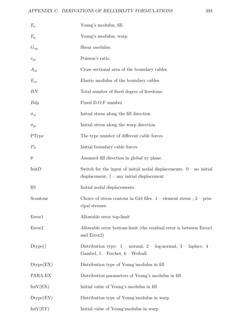
APPENDIX C. DERIVATIONS OF RELIABILITY FORMULATIONS 393
Ex Young’s modulus, fill.
Ey Young’s modulus, warp.
Gxy Shear modulus.
vyx Poisson’s ratio.
Aca Cross sectional area of the boundary cables
Eca Elastic modulus of the boundary cables
BN Total number of fixed degree of freedoms
Bdy Fixed D.O.F number
σxi Initial stress along the fill direction
σyi Initial stress along the warp direction
PType The type number of different cable forces
PN Initial boundary cable forces
θ Assumed fill direction in global xy plane.
InitD Switch for the input of initial nodal displacements. 0 – no initial
displacement, 1 – any initial displacement
ID Initial nodal displacements.
Scontour Choice of stress contour in Gid files. 1 – element stress , 2 – prin-
cipal stresses
Error1 Allowable error top-limit
Error2 Allowable error bottom-limit (the residual error is between Error1
and Error2)
Dtype() Distribution type: 1 – normal, 2 – log-normal, 3 – laplace, 4 –
Gumbel, 5 – Frechet, 6 – Weibull
Dtype(EX) Distribution type of Young’modulus in fill
PARA-EX Distribution parameters of Young’s modulus in fill
IniV(EX) Initial value of Young’s modulus in fill
Dtype(EY) Distribution type of Young’modulus in warp
IniV(EY) Initial value of Young’modulus in warp
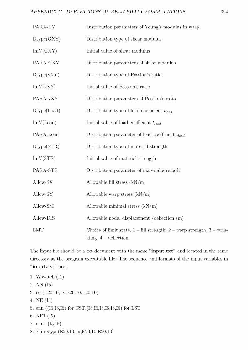
APPENDIX C. DERIVATIONS OF RELIABILITY FORMULATIONS 394
PARA-EY Distribution parameters of Young’s modulus in warp
Dtype(GXY) Distribution type of shear modulus
IniV(GXY) Initial value of shear modulus
PARA-GXY Distribution parameters of shear modulus
Dtype(vXY) Distribution type of Possion’s ratio
IniV(vXY) Initial value of Possion’s ratio
PARA-vXY Distribution parameters of Possion’s ratio
Dtype(Load) Distribution type of load coefficient tload
IniV(Load) Initial value of load coefficient tload
PARA-Load Distribution parameter of load coefficient tload
Dtype(STR) Distribution type of material strength
IniV(STR) Initial value of material strength
PARA-STR Distribution parameter of material strength
Allow-SX Allowable fill stress (kN/m)
Allow-SY Allowable warp stress (kN/m)
Allow-SM Allowable minimal stress (kN/m)
Allow-DIS Allowable nodal displacement /deflection (m)
LMT Choice of limit state, 1 – fill strength, 2 – warp strength, 3 – wrin-
kling, 4 – deflection.
The input file should be a txt document with the name ”input.txt” and located in the same
directory as the program executable file. The sequence and formats of the input variables in
”input.txt” are :
1. Wswitch (I1)
2. NN (I5)
3. co (E20.10,1x,E20.10,E20.10)
4. NE (I5)
5. enn ((I5,I5,I5) for CST,(I5,I5,I5,I5,I5,I5) for LST
6. NE1 (I5)
7. enn1 (I5,I5)
8. F in x,y,z (E20.10,1x,E20.10,E20.10)
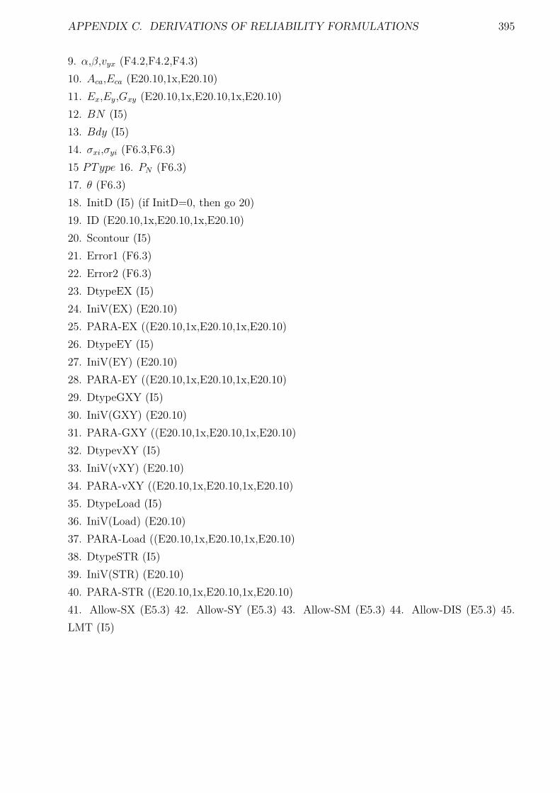
APPENDIX C. DERIVATIONS OF RELIABILITY FORMULATIONS 395
9. α,β,vyx (F4.2,F4.2,F4.3)
10. Aca,Eca (E20.10,1x,E20.10)
11. Ex,Ey,Gxy (E20.10,1x,E20.10,1x,E20.10)
12. BN (I5)
13. Bdy (I5)
14. σxi,σyi (F6.3,F6.3)
15 PType 16. PN (F6.3)
17. θ (F6.3)
18. InitD (I5) (if InitD=0, then go 20)
19. ID (E20.10,1x,E20.10,1x,E20.10)
20. Scontour (I5)
21. Error1 (F6.3)
22. Error2 (F6.3)
23. DtypeEX (I5)
24. IniV(EX) (E20.10)
25. PARA-EX ((E20.10,1x,E20.10,1x,E20.10)
26. DtypeEY (I5)
27. IniV(EY) (E20.10)
28. PARA-EY ((E20.10,1x,E20.10,1x,E20.10)
29. DtypeGXY (I5)
30. IniV(GXY) (E20.10)
31. PARA-GXY ((E20.10,1x,E20.10,1x,E20.10)
32. DtypevXY (I5)
33. IniV(vXY) (E20.10)
34. PARA-vXY ((E20.10,1x,E20.10,1x,E20.10)
35. DtypeLoad (I5)
36. IniV(Load) (E20.10)
37. PARA-Load ((E20.10,1x,E20.10,1x,E20.10)
38. DtypeSTR (I5)
39. IniV(STR) (E20.10)
40. PARA-STR ((E20.10,1x,E20.10,1x,E20.10)
41. Allow-SX (E5.3) 42. Allow-SY (E5.3) 43. Allow-SM (E5.3) 44. Allow-DIS (E5.3) 45.
LMT (I5)
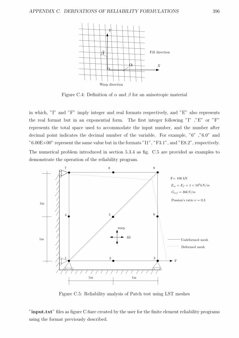
APPENDIX C. DERIVATIONS OF RELIABILITY FORMULATIONS 396
X
Y
α
β Fill direction
Warp direction
Figure C.4: Definition of α and β for an anisotropic material
in which, ”I” and ”F” imply integer and real formats respectively, and ”E” also represents
the real format but in an exponential form. The first integer following ”I” ,”E” or ”F”
represents the total space used to accommodate the input number, and the number after
decimal point indicates the decimal number of the variable. For example, ”6” ,”6.0” and
”6.00E+00” represent the same value but in the formats ”I1”, ”F3.1”, and ”E8.2”, respectively.
The numerical problem introduced in section 5.3.4 as fig. C.5 are provided as examples to
demonstrate the operation of the reliability program.
1m
1m
1m 1m
F1 2 3
4 5 6
7 8 9
Undeformed mesh
Deformed mesh
F= 100 kN
Ew = Ef = 1× 10³kN/m
Gwf = 30kN/m
Possion’s ratio ν = 0.3
fill
warp
Figure C.5: Reliability analysis of Patch test using LST meshes
”input.txt” files as figure C.6are created by the user for the finite element reliability programs
using the format previously described.
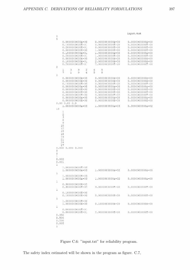
APPENDIX C. DERIVATIONS OF RELIABILITY FORMULATIONS 397
Figure C.6: ”input.txt” for reliability program.
The safety index estimated will be shown in the program as figure. C.7,
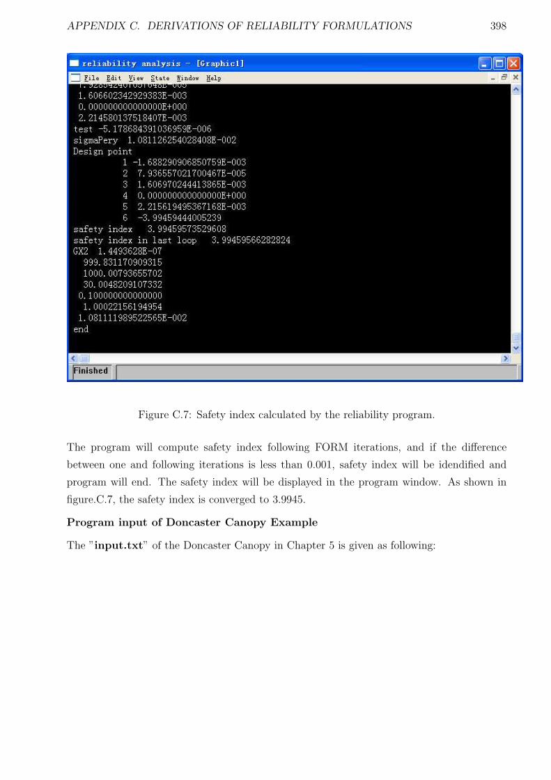
APPENDIX C. DERIVATIONS OF RELIABILITY FORMULATIONS 398
Figure C.7: Safety index calculated by the reliability program.
The program will compute safety index following FORM iterations, and if the difference
between one and following iterations is less than 0.001, safety index will be idendified and
program will end. The safety index will be displayed in the program window. As shown in
figure.C.7, the safety index is converged to 3.9945.
Program input of Doncaster Canopy Example
The ”input.txt” of the Doncaster Canopy in Chapter 5 is given as following:
0
377
-0.9030000000E+01 -0.6662000000E+01 0.1486900000E+02
0.9630904160E-01 -0.4405387143E+01 0.1915207955E+02
0.9082000000E+01 -0.7004000000E+01 0.1490100000E+02
0.1059600000E+02 -0.3327000000E+01 0.1426700000E+02
0.8983000000E+01 0.6466000000E+01 0.1413100000E+02
-0.1147000000E+01 0.1101800000E+02 0.1414900000E+02
-0.8906000000E+01 0.6627000000E+01 0.1424500000E+02
-0.1037300000E+02 -0.4113000000E+01 0.1440300000E+02
-0.2570000000E+00 0.7900000000E+00 0.2180700000E+02
0.7400000000E+00 0.3440000000E+00 0.2180700000E+02
0.1726000000E+01 0.6810000000E+00 0.2168900000E+02
0.2177000000E+01 0.1380000000E+01 0.2155000000E+02
0.1941000000E+01 0.2626000000E+01 0.2137600000E+02
0.6050000000E+00 0.3203000000E+01 0.2138100000E+02
-0.3760000000E+00 0.2651000000E+01 0.2153300000E+02
-0.5490000000E+00 0.1231000000E+01 0.2176000000E+02
0.1984941825E+00 0.4708647597E+00 0.2182403941E+02
0.1265630427E+01 0.4205997875E+00 0.2175820868E+02
0.2004177703E+01 0.9966198559E+00 0.2162002910E+02
0.2204917476E+01 0.2028779868E+01 0.2144970128E+02
0.1349478572E+01 0.3091850936E+01 0.2134738468E+02
0.5671788680E-01 0.3026726126E+01 0.2144624250E+02
-0.6542931284E+00 0.1965891595E+01 0.2165604109E+02
-0.3101341541E+01 -0.3991415425E+01 0.1820687893E+02
0.3124998781E+01 -0.3966250776E+01 0.1819527550E+02

0.9590268121E+01 -0.5047621399E+01 0.1472202446E+02
0.8914360229E+01 0.1454532153E+01 0.1482540679E+02
0.3505497763E+01 0.7882561811E+01 0.1495357119E+02
-0.4651021900E+01 0.8137440525E+01 0.1474083035E+02
-0.8495060757E+01 0.1087290286E+01 0.1501255632E+02
-0.4489127554E+01 -0.2944710984E+01 0.1778966830E+02
0.3076555353E+00 -0.2582284672E+01 0.1979580716E+02
0.4632190019E+01 -0.2877089527E+01 0.1770704813E+02
0.6335998222E+01 -0.1130219632E+01 0.1704682391E+02
0.6075074287E+01 0.4798900003E+01 0.1634208667E+02
-0.4957295622E+00 0.7809420369E+01 0.1637835155E+02
-0.5205086675E+01 0.4822571462E+01 0.1661168538E+02
-0.5222854044E+01 -0.1741722777E+01 0.1730415770E+02
-0.1698766375E+01 -0.5364632673E+00 0.2012757520E+02
0.5177231857E+00 -0.9936193068E+00 0.2068862757E+02
0.2619563345E+01 -0.3498052055E+00 0.1991690887E+02
0.3618093076E+01 0.4174586460E+00 0.1952920007E+02
0.3654288610E+01 0.3480275439E+01 0.1887673300E+02
0.1001699726E+00 0.5158542746E+01 0.1886235158E+02
-0.2310101367E+01 0.3480438937E+01 0.1917470778E+02
-0.2008138942E+01 0.7377082558E+00 0.1986389139E+02
-0.1912181706E+01 -0.2361658796E+01 0.1918184738E+02
0.2025905797E+01 -0.2004136441E+01 0.1940564664E+02
0.5515043217E+01 -0.2086140439E+01 0.1737742527E+02
0.6093820239E+01 0.1706182900E+01 0.1697086179E+02
0.2041910851E+01 0.4766560708E+01 0.1843841576E+02
-0.2903960276E+01 0.6222669436E+01 0.1668341168E+02
-0.5110516204E+01 0.1377174984E+01 0.1722430410E+02
-0.4366109979E+00 -0.8733283452E+00 0.2047000004E+02
0.1574693090E+01 -0.6761412562E+00 0.2040241950E+02
0.3040763677E+01 -0.4216466366E-01 0.1977039091E+02
0.3589989019E+01 0.2059068603E+01 0.1933092837E+02
0.1463928674E+01 0.3331302392E+01 0.2064653763E+02
-0.1010058885E+01 0.4349525569E+01 0.1911452723E+02
-0.2027303574E+01 0.1988219745E+01 0.1974442657E+02
-0.1638766285E+01 -0.4308066410E+01 0.1870386401E+02
0.1631639183E+01 -0.4262598611E+01 0.1873064643E+02
-0.6020980000E+01 -0.1237100000E+02 0.1552000000E+02
-0.1119000000E+01 -0.1321800000E+02 0.1580900000E+02
0.6224000000E+01 -0.1225900000E+02 0.1551800000E+02
-0.1161000000E+01 -0.1003900000E+02 0.1854800000E+02
-0.6020000000E+00 -0.1047100000E+02 0.1842500000E+02
0.2770000000E+00 -0.1003700000E+02 0.1862700000E+02
0.2980000000E+00 -0.9555000000E+01 0.1879900000E+02
-0.3940000000E+00 -0.9021000000E+01 0.1895100000E+02
-0.1177000000E+01 -0.9481000000E+01 0.1874600000E+02
-0.9359525220E+00 -0.1031824592E+02 0.1846116088E+02
-0.7618351139E-01 -0.1040594438E+02 0.1847684987E+02
0.3306093342E+00 -0.9798439516E+01 0.1871457288E+02
0.3825288811E-01 -0.9187718446E+01 0.1891537279E+02
-0.8684093974E+00 -0.9127240735E+01 0.1888747135E+02
-0.1227241822E+01 -0.9760348539E+01 0.1864327417E+02
-0.3492641551E+01 -0.1240366303E+02 0.1588034250E+02
0.2507866222E+01 -0.1202551651E+02 0.1608546147E+02
0.7107829316E+01 -0.9325471289E+01 0.1545797681E+02
-0.6888672640E+01 -0.9183442276E+01 0.1552623365E+02
-0.4333841359E+01 -0.1146576722E+02 0.1616684615E+02
-0.8736478313E+00 -0.1181249124E+02 0.1681688109E+02
0.3945345326E+01 -0.1127786982E+02 0.1622223645E+02
0.3232863856E+01 -0.8612588518E+01 0.1719502125E+02
-0.1093526482E+00 -0.6314134563E+01 0.1881622019E+02
-0.3555939155E+01 -0.8536148036E+01 0.1725185954E+02
-0.2410695983E+01 -0.1053679218E+02 0.1734081954E+02
-0.7176280021E+00 -0.1098832922E+02 0.1764763521E+02
0.1687984108E+01 -0.1042303967E+02 0.1740652863E+02
0.1378604351E+01 -0.9163106959E+01 0.1805027965E+02
-0.2826114197E+00 -0.7956469788E+01 0.1880182411E+02
-0.2063526149E+01 -0.9087552099E+01 0.1805095291E+02
-0.1908054047E+01 -0.1127835199E+02 0.1698627399E+02
0.8373163224E+00 -0.1125447422E+02 0.1702983749E+02
0.2470725645E+01 -0.9950136469E+01 0.1717956017E+02
0.1499494938E+01 -0.6733220774E+01 0.1825792077E+02
-0.1934289726E+01 -0.6778142427E+01 0.1821374129E+02
-0.3107463762E+01 -0.9894667352E+01 0.1716194008E+02
-0.1434908166E+01 -0.1066814164E+02 0.1768656214E+02
0.2493974452E+00 -0.1064597302E+02 0.1783887189E+02
0.1478111019E+01 -0.9783029841E+01 0.1778389356E+02
0.6367341752E+00 -0.8339321635E+01 0.1847657447E+02
-0.1277465248E+01 -0.8270392606E+01 0.1846758870E+02
-0.2123160512E+01 -0.9783486082E+01 0.1780896956E+02
-0.6061720280E+01 -0.5320839071E+01 0.1651668502E+02
-0.3799474486E+01 -0.3462830032E+01 0.1800698087E+02
-0.6719775848E+01 -0.4793289878E+01 0.1626765519E+02
-0.2507141029E+01 -0.3158724505E+01 0.1867269903E+02
-0.3203992629E+01 -0.2648090775E+01 0.1850404912E+02
-0.1771764600E+01 -0.3314424768E+01 0.1891873625E+02
-0.6431465613E+00 -0.3420406328E+01 0.1924933269E+02
-0.8279170836E+00 -0.2479193490E+01 0.1953577046E+02
-0.7800726942E+00 -0.4355434904E+01 0.1895615111E+02
0.2005322064E+00 -0.3481002771E+01 0.1942471796E+02
0.8692748038E+00 -0.4340594713E+01 0.1896192046E+02
0.9511362559E+00 -0.3404137767E+01 0.1924305714E+02
0.1808777642E+01 -0.3123168925E+01 0.1903510145E+02
0.1171085389E+01 -0.2305474246E+01 0.1963632969E+02
0.2549040913E+01 -0.2975355870E+01 0.1876332157E+02
0.3888624254E+01 -0.3422231384E+01 0.1796376910E+02
0.3325718815E+01 -0.2444714651E+01 0.1855278154E+02
0.6056949823E+01 -0.5469114593E+01 0.1645517235E+02
0.6800439720E+01 -0.4936003864E+01 0.1616775747E+02
0.9248569382E+01 -0.5996522476E+01 0.1485701178E+02
0.7067892970E+01 -0.3944963621E+01 0.1616093938E+02
0.7508012017E+01 -0.3555686254E+01 0.1596604810E+02
0.5084528625E+01 -0.2484040028E+01 0.1754461416E+02
0.7912896292E+01 -0.3075748592E+01 0.1578646507E+02
0.5938059924E+01 -0.1607483381E+01 0.1721367987E+02
0.1001740121E+02 -0.4131358757E+01 0.1453993031E+02
0.8412426950E+01 -0.2230625152E+01 0.1556490464E+02
0.9475611624E+01 -0.1058102129E+01 0.1474861865E+02
0.7632455818E+01 0.1545423055E+00 0.1594318589E+02
0.7492465185E+01 0.1560415270E+01 0.1587856770E+02
0.6231355269E+01 0.2852600654E+00 0.1703069075E+02
0.7511775892E+01 0.3139457342E+01 0.1562192093E+02
0.6097103368E+01 0.3249141539E+01 0.1668653508E+02
0.8649493732E+01 0.3981922640E+01 0.1467819501E+02
0.7485378372E+01 0.5596601101E+01 0.1515367880E+02
0.6202766195E+01 0.6838134731E+01 0.1479834893E+02
0.4831293515E+01 0.6370159398E+01 0.1568638447E+02
0.2778047077E+01 0.6262160117E+01 0.1663544990E+02
0.4062296763E+01 0.4761330901E+01 0.1738107174E+02
0.1524459571E+01 0.7883973840E+01 0.1569225066E+02
0.7822739052E+00 0.6271585332E+01 0.1740256220E+02
0.9819806509E+00 0.9191453373E+01 0.1481273858E+02
-0.8210617469E+00 0.9367781286E+01 0.1518720527E+02
-0.2709338358E+01 0.9389291314E+01 0.1462388582E+02
-0.2559962758E+01 0.7995446870E+01 0.1557845905E+02
-0.3760359184E+01 0.7176419480E+01 0.1569284327E+02
-0.1703397072E+01 0.7034714013E+01 0.1655356671E+02
-0.4935744039E+01 0.6473787188E+01 0.1569425185E+02
-0.4062196081E+01 0.5534421617E+01 0.1666666363E+02
-0.6694468524E+01 0.7128045911E+01 0.1466321400E+02
-0.7015584308E+01 0.5692608589E+01 0.1532321322E+02
-0.8306833015E+01 0.3923052151E+01 0.1484972219E+02
-0.6869877559E+01 0.2984746958E+01 0.1584051275E+02
-0.6785411970E+01 0.1254849479E+01 0.1608956239E+02
-0.5171839468E+01 0.3110093165E+01 0.1694975849E+02

-0.6863011079E+01 -0.3263491659E+00 0.1616541864E+02
-0.5183132336E+01 -0.1685403430E+00 0.1728944199E+02
-0.9065047661E+01 -0.1650623291E+01 0.1492333613E+02
-0.7763172307E+01 -0.2959971577E+01 0.1570689409E+02
-0.9453937057E+01 -0.5233182893E+01 0.1476931807E+02
-0.7103709065E+01 -0.4181360640E+01 0.1607013425E+02
-0.4863907061E+01 -0.2340145814E+01 0.1754755168E+02
-0.1785010716E+01 -0.1412725967E+01 0.1963265603E+02
-0.3035350130E+01 -0.1716302837E+01 0.1888590224E+02
-0.1175164771E+01 -0.1585397186E+01 0.1980651526E+02
-0.1071811788E+01 -0.6954957053E+00 0.2032387085E+02
-0.6957404718E+00 -0.1664448999E+01 0.1994231819E+02
0.3017962456E-01 -0.9274870179E+00 0.2059381591E+02
0.4102170523E+00 -0.1766688575E+01 0.2019554074E+02
0.1254539876E+01 -0.1485874617E+01 0.2004038188E+02
0.1757014630E+01 -0.1322065976E+01 0.1989094373E+02
0.1041766573E+01 -0.8363363324E+00 0.2057275852E+02
0.2322613480E+01 -0.1160528697E+01 0.1966422033E+02
0.2083412311E+01 -0.5186090284E+00 0.2019063903E+02
0.3605858356E+01 -0.1588942831E+01 0.1869609457E+02
0.4017632531E+01 -0.1187837194E+01 0.1857693206E+02
0.4207420379E+01 -0.1033163892E+01 0.1850167429E+02
0.2820638169E+01 -0.1921525869E+00 0.1985746779E+02
0.4504030337E+01 -0.8018977929E+00 0.1836777307E+02
0.3318785885E+01 0.1958166146E+00 0.1966895715E+02
0.4911698187E+01 -0.3473175440E+00 0.1819990722E+02
0.4796370379E+01 0.1049255776E+01 0.1822234124E+02
0.4772631077E+01 0.1844046645E+01 0.1813039117E+02
0.3604671347E+01 0.1235959510E+01 0.1946353734E+02
0.4840018475E+01 0.2588377257E+01 0.1791916797E+02
0.3611798487E+01 0.2750441365E+01 0.1913483306E+02
0.4815061408E+01 0.4099966209E+01 0.1753359995E+02
0.2876652742E+01 0.4120816921E+01 0.1868228053E+02
0.1725310068E+01 0.3986650459E+01 0.1952290930E+02
0.2524810272E+01 0.3386542046E+01 0.1975637124E+02
0.1078345450E+01 0.4969278273E+01 0.1867375875E+02
0.7578813212E+00 0.4213419891E+01 0.1974601493E+02
-0.1968488791E+00 0.6432681445E+01 0.1754950466E+02
-0.1375758603E+01 0.5662460293E+01 0.1775573886E+02
-0.1918369687E+01 0.5240711937E+01 0.1786408654E+02
-0.4526791059E+00 0.4754099800E+01 0.1900380792E+02
-0.2575079208E+01 0.4799932582E+01 0.1789966493E+02
-0.1655302236E+01 0.3919514273E+01 0.1916624043E+02
-0.3710695572E+01 0.4116083887E+01 0.1780579794E+02
-0.3669632865E+01 0.2438688881E+01 0.1818941381E+02
-0.3487961332E+01 0.1699582068E+01 0.1844446144E+02
-0.2155572576E+01 0.2741535223E+01 0.1948269024E+02
-0.3492654297E+01 0.1050461203E+01 0.1850548975E+02
-0.2006980878E+01 0.1369362872E+01 0.1983442904E+02
-0.3562272991E+01 -0.5168335777E+00 0.1850978312E+02
-0.3399592995E+01 -0.1127495096E+01 0.1863005008E+02
-0.1848160431E+01 0.9500601381E-01 0.2001643684E+02
-0.1030732895E+01 0.3716784177E+00 0.2086559373E+02
-0.9430510985E+00 0.1470089128E+00 0.2092327121E+02
-0.4030000000E+00 0.1010500000E+01 0.2178350000E+02
-0.3359137920E+00 -0.5032044271E-02 0.2110433343E+02
-0.1005250233E+00 -0.1450082523E+00 0.2109594556E+02
-0.2925290875E-01 0.6304323799E+00 0.2181551970E+02
0.1591491329E+00 -0.2366795807E+00 0.2111706535E+02
0.4692470912E+00 0.4074323799E+00 0.2181551970E+02
0.6254442655E+00 -0.2954314048E+00 0.2120369925E+02
0.1123398655E+01 -0.1606199735E+00 0.2109746538E+02
0.1365590445E+01 -0.6730903752E-01 0.2104645686E+02
0.1002815213E+01 0.3822998937E+00 0.2178260434E+02
0.1590808945E+01 0.6616007894E-01 0.2101893086E+02
0.1495815214E+01 0.5507998938E+00 0.2172360434E+02
0.2113788601E+01 0.2322925126E+00 0.2071829534E+02
0.2291801601E+01 0.3823372674E+00 0.2067090642E+02
0.2434328896E+01 0.5286398793E+00 0.2063948231E+02
0.1865088851E+01 0.8388099280E+00 0.2165451455E+02
0.2554711750E+01 0.6999823845E+00 0.2063436502E+02
0.2090588851E+01 0.1188309928E+01 0.2158501455E+02
0.2834422020E+01 0.9121005049E+00 0.2047845686E+02
0.2803670369E+01 0.1693488404E+01 0.2042374235E+02
0.2795498127E+01 0.2008896580E+01 0.2035813183E+02
0.2190958738E+01 0.1704389934E+01 0.2149985064E+02
0.2726510863E+01 0.2328251062E+01 0.2035039674E+02
0.2072958738E+01 0.2327389934E+01 0.2141285064E+02
0.2746958472E+01 0.3011235541E+01 0.2006008194E+02
0.1709678137E+01 0.2983878735E+01 0.2102815366E+02
0.1380827597E+01 0.3183433555E+01 0.2100182803E+02
0.1645239286E+01 0.2858925468E+01 0.2136169234E+02
0.1009388890E+01 0.3291248500E+01 0.2102582917E+02
0.9772392860E+00 0.3147425468E+01 0.2136419234E+02
0.3532717670E+00 0.4120338876E+01 0.2006161349E+02
-0.1741034302E+00 0.3744280081E+01 0.2022879162E+02
-0.4292112915E+00 0.3613094928E+01 0.2023272533E+02
0.3308589434E+00 0.3114863063E+01 0.2141362125E+02
-0.6494538617E+00 0.3442114357E+01 0.2028927196E+02
-0.1596410566E+00 0.2838863063E+01 0.2148962125E+02
-0.1292418042E+01 0.3028055734E+01 0.2029330837E+02
-0.1185421085E+01 0.2349227162E+01 0.2061543835E+02
-0.1228851738E+01 0.1977063833E+01 0.2065091459E+02
-0.5151465642E+00 0.2308445798E+01 0.2159452055E+02
-0.1203421785E+01 0.1616047167E+01 0.2073214845E+02
-0.6016465642E+00 0.1598445798E+01 0.2170802055E+02
-0.1188777772E+01 0.9761662446E+00 0.2075415976E+02
-0.4763914424E+01 -0.1224182766E+02 0.1575435898E+02
-0.3917191963E+01 -0.1193413615E+02 0.1604478898E+02
-0.5159913781E+01 -0.1190123615E+02 0.1580290076E+02
-0.2710155263E+01 -0.1181191382E+02 0.1639231019E+02
-0.3124144776E+01 -0.1134738895E+02 0.1655267956E+02
-0.2176222095E+01 -0.1210625281E+02 0.1632824464E+02
-0.1411814385E+01 -0.1155201930E+02 0.1691278793E+02
-0.2268114259E+01 -0.1269231965E+02 0.1592894894E+02
-0.9971064210E+00 -0.1249487945E+02 0.1627549378E+02
0.6052260939E+00 -0.1241433623E+02 0.1612363502E+02
0.8045096013E+00 -0.1194369842E+02 0.1646284083E+02
0.1649247087E+01 -0.1162517320E+02 0.1653130371E+02
-0.9141066021E-02 -0.1155291549E+02 0.1694598901E+02
0.3236303418E+01 -0.1166880343E+02 0.1617645184E+02
0.2400417244E+01 -0.1124396233E+02 0.1660007613E+02
0.4378519522E+01 -0.1188209121E+02 0.1589424313E+02
0.5086189061E+01 -0.1175940179E+02 0.1581254103E+02
0.6461542486E+01 -0.1073654003E+02 0.1556086639E+02
0.5566384078E+01 -0.1030557433E+02 0.1590947037E+02
0.4780596474E+01 -0.9655905935E+01 0.1631313894E+02
0.3211039793E+01 -0.1061360073E+02 0.1665541019E+02
0.5160155792E+01 -0.8970869621E+01 0.1629000077E+02
0.2854313449E+01 -0.9289135498E+01 0.1720183300E+02
0.7936278537E+01 -0.8024856729E+01 0.1526748526E+02
0.6161072556E+01 -0.7808380381E+01 0.1605298187E+02
0.3166100312E+01 -0.6270412564E+01 0.1765797907E+02
0.2302198615E+01 -0.5353684807E+01 0.1820541491E+02
0.2372681706E+01 -0.7684319640E+01 0.1774823408E+02
0.1551200294E+01 -0.5500379819E+01 0.1845540826E+02
0.7442585680E+00 -0.5296259273E+01 0.1875618857E+02
0.7062425202E+00 -0.6536501427E+01 0.1856065832E+02
-0.6435584643E-02 -0.5345288356E+01 0.1893561445E+02
-0.8599689581E+00 -0.5312090887E+01 0.1874213946E+02
-0.1766775782E+01 -0.5530146955E+01 0.1842523234E+02
-0.1030592827E+01 -0.6554718976E+01 0.1855251085E+02
-0.2502250916E+01 -0.5380022612E+01 0.1817544304E+02
-0.3320139516E+01 -0.6250262544E+01 0.1768922422E+02
-0.2739714273E+01 -0.7657964375E+01 0.1777177896E+02
-0.6283012012E+01 -0.7596978410E+01 0.1605404219E+02
-0.7784628689E+01 -0.7746926780E+01 0.1530865828E+02
-0.5216938411E+01 -0.8854842264E+01 0.1636274581E+02
-0.5000615136E+01 -0.9538646103E+01 0.1633495634E+02
-0.3335306457E+01 -0.9215003537E+01 0.1722149189E+02
-0.5643851009E+01 -0.1032270063E+02 0.1591029570E+02
-0.3703168226E+01 -0.1067437489E+02 0.1663425142E+02
-0.6223323949E+01 -0.1071028483E+02 0.1562228816E+02
-0.2177465338E+01 -0.1089681788E+02 0.1717631513E+02
-0.3344995283E+01 -0.1097014628E+02 0.1668845673E+02
-0.1679232979E+01 -0.1095146494E+02 0.1732699660E+02
-0.1913933743E+01 -0.1059658948E+02 0.1751758531E+02
-0.1313702941E+01 -0.1112359989E+02 0.1730934325E+02
-0.1079369385E+01 -0.1083409788E+02 0.1768158859E+02
-0.7962649717E+00 -0.1138705561E+02 0.1720407062E+02
0.4946493055E-01 -0.1113461540E+02 0.1734914466E+02
0.5322897544E+00 -0.1092911370E+02 0.1742194266E+02
-0.2174699860E+00 -0.1083316363E+02 0.1776164305E+02
0.1262479458E+01 -0.1083626993E+02 0.1724702037E+02
0.9657647748E+00 -0.1053139591E+02 0.1762596057E+02
0.2808814909E+01 -0.1082083789E+02 0.1672874565E+02
0.2059637450E+01 -0.1019165090E+02 0.1730255033E+02
0.1960040152E+01 -0.9876743465E+01 0.1747198351E+02
0.1576859284E+01 -0.1010395828E+02 0.1759943644E+02
0.1910311608E+01 -0.9558167289E+01 0.1760898706E+02
0.1427738775E+01 -0.9480758989E+01 0.1792261204E+02
0.2290933034E+01 -0.8879238561E+01 0.1759383075E+02
0.1433264334E+01 -0.7961824315E+01 0.1813882202E+02
0.1057008809E+01 -0.7547220949E+01 0.1833485962E+02
0.1010947977E+01 -0.8748290525E+01 0.1828616598E+02
0.2543023145E+00 -0.7313406449E+01 0.1863316956E+02
0.1690412537E+00 -0.8141199941E+01 0.1866095600E+02
-0.1973945221E+00 -0.7146473814E+01 0.1876559981E+02
-0.7770646772E+00 -0.8113498066E+01 0.1865775778E+02
-0.6847797150E+00 -0.7277737519E+01 0.1863710357E+02
-0.1588023829E+01 -0.7531712257E+01 0.1831291233E+02
-0.1986412564E+01 -0.7941738995E+01 0.1812357498E+02
-0.1674865007E+01 -0.8677116477E+01 0.1828595657E+02
-0.2793174927E+01 -0.8807233894E+01 0.1762800488E+02
-0.2574627592E+01 -0.9486130733E+01 0.1760081112E+02
-0.2608408775E+01 -0.9834551717E+01 0.1747394603E+02
-0.2099424964E+01 -0.9440438592E+01 0.1793514016E+02
-0.2265931037E+01 -0.1015890046E+02 0.1757546650E+02
-0.2747782753E+01 -0.1022143612E+02 0.1726154358E+02
-0.1281620384E+01 -0.1033026847E+02 0.1812600898E+02
-0.1767648882E+01 -0.1025946218E+02 0.1787360177E+02
-0.1167866102E+01 -0.1046020920E+02 0.1805817526E+02
-0.1048476261E+01 -0.1017862296E+02 0.1850458044E+02
-0.1007090911E+01 -0.1054601582E+02 0.1805146215E+02
-0.7689762610E+00 -0.1039462296E+02 0.1844308044E+02
-0.6577021515E+00 -0.1070634738E+02 0.1801524903E+02
-0.1741356996E+00 -0.1057669935E+02 0.1812288539E+02
0.7103827057E-01 -0.1049473929E+02 0.1814710548E+02
-0.3390917557E+00 -0.1043847219E+02 0.1845092493E+02
0.2692895369E+00 -0.1032336197E+02 0.1824997123E+02
0.1004082443E+00 -0.1022147219E+02 0.1855192493E+02
0.9619335755E+00 -0.1019048364E+02 0.1794061465E+02
0.8350815631E+00 -0.9898672099E+01 0.1818112054E+02
0.8670016860E+00 -0.9779913914E+01 0.1820686754E+02
0.3038046671E+00 -0.9917719758E+01 0.1867078644E+02
0.8556860673E+00 -0.9664598976E+01 0.1825909521E+02
0.3143046671E+00 -0.9676719758E+01 0.1875678644E+02
0.8124686822E+00 -0.9353602640E+01 0.1838645200E+02
0.4478641434E+00 -0.8955423484E+01 0.1860548285E+02
0.3157190862E+00 -0.8771930144E+01 0.1865538362E+02
0.1681264441E+00 -0.9371359223E+01 0.1885718639E+02
-0.1135774155E+00 -0.8607677149E+01 0.1880264594E+02
-0.1778735559E+00 -0.9104359223E+01 0.1893318639E+02
-0.3378969240E+00 -0.8489031274E+01 0.1885352199E+02
-0.6312046987E+00 -0.9074120368E+01 0.1891923567E+02
-0.5841527992E+00 -0.8570137586E+01 0.1879563870E+02
-0.1053055196E+01 -0.8712858303E+01 0.1863999669E+02
-0.1213752190E+01 -0.8887843127E+01 0.1858296146E+02
-0.1022704699E+01 -0.9304120368E+01 0.1881673567E+02
-0.1598077662E+01 -0.9281725173E+01 0.1836728467E+02
-0.1628321229E+01 -0.9626428683E+01 0.1825510352E+02
-0.1647368387E+01 -0.9760772005E+01 0.1819301785E+02
-0.1202120911E+01 -0.9620674270E+01 0.1869463709E+02
-0.1614745771E+01 -0.9903236469E+01 0.1816480173E+02
-0.1194120911E+01 -0.9899674270E+01 0.1859563708E+02
0.2375854746E+01 -0.4120318698E+01 0.1848083067E+02
-0.2382054047E+01 -0.4142333415E+01 0.1846921648E+02
166
1 24 31 106 107 108
24 47 31 109 110 107
47 61 32 111 112 113
61 2 32 114 115 112
2 62 32 116 117 115
62 48 32 118 119 117
48 25 33 120 121 122
25 3 33 123 124 121
3 26 33 125 126 124
26 49 33 127 128 126
49 26 34 127 129 130
26 4 34 131 132 129
4 27 34 133 134 132
27 50 34 135 136 134
50 27 35 135 137 138
27 5 35 139 140 137
5 28 35 141 142 140
28 51 35 143 144 142
51 28 36 143 145 146
28 6 36 147 148 145
6 29 36 149 150 148
29 52 36 151 152 150
52 29 37 151 153 154
29 7 37 155 156 153
7 30 37 157 158 156
30 53 37 159 160 158
53 30 38 159 161 162
30 8 38 163 164 161
8 1 38 165 166 164
1 31 38 108 167 166
31 47 39 110 168 169
47 54 39 170 171 168
54 47 40 170 172 173
47 32 40 113 174 172
32 48 40 119 175 174
48 55 40 176 177 175
55 48 41 176 178 179
48 33 41 122 180 178
33 49 41 128 181 180
49 56 41 182 183 181
56 49 42 182 184 185
49 34 42 130 186 184
34 50 42 136 187 186
50 57 42 188 189 187
57 50 43 188 190 191
50 35 43 138 192 190
35 51 43 144 193 192
51 58 43 194 195 193
58 51 44 194 196 197
51 36 44 146 198 196
36 52 44 152 199 198
52 59 44 200 201 199
59 52 45 200 202 203
52 37 45 154 204 202
37 53 45 160 205 204
53 60 45 206 207 205
60 53 46 206 208 209
53 38 46 162 210 208
38 39 46 211 212 210
38 31 39 167 169 211
16 39 9 213 214 215
39 54 9 171 216 214
54 17 9 217 218 216
17 54 10 217 219 220
54 40 10 173 221 219
40 55 10 177 222 221
55 18 10 223 224 222
18 55 11 223 225 226
55 41 11 179 227 225
41 56 11 183 228 227
56 19 11 229 230 228
19 56 12 229 231 232
56 42 12 185 233 231
42 57 12 189 234 233
57 20 12 235 236 234
20 57 13 235 237 238
57 43 13 191 239 237
43 58 13 195 240 239
58 21 13 241 242 240
21 58 14 241 243 244
58 44 14 197 245 243
44 59 14 201 246 245
59 22 14 247 248 246
22 59 15 247 249 250
59 45 15 203 251 249
45 60 15 207 252 251
60 23 15 253 254 252
23 60 16 253 255 256
60 46 16 209 257 255
46 39 16 212 213 257
63 78 82 258 259 260
78 94 82 261 262 259
94 78 83 261 263 264
83 78 64 263 265 266
64 79 83 267 268 266
79 95 83 269 270 268
95 79 84 269 271 272
79 65 84 273 274 271
65 80 84 275 276 274
80 96 84 277 278 276
96 80 85 277 279 280
80 3 85 281 282 279
3 25 85 123 283 282
25 97 85 284 285 283
97 62 86 286 287 288
62 2 86 116 289 287
2 61 86 114 290 289
61 98 86 291 292 290
98 24 87 293 294 295
24 1 87 106 296 294
1 81 87 297 298 296
87 81 99 298 299 300
99 81 82 299 301 302
81 63 82 303 260 301
82 94 88 262 304 305
94 100 88 306 307 304
100 94 89 306 308 309
94 83 89 264 310 308
83 95 89 270 311 310
95 101 89 312 313 311
101 95 90 312 314 315
95 84 90 272 316 314
84 96 90 278 317 316
96 102 90 318 319 317
102 96 91 318 320 321
96 85 91 280 322 320
85 97 91 285 323 322
97 103 91 324 325 323
103 97 86 324 288 326
92 103 86 327 326 328
104 92 86 329 328 330
98 104 86 331 330 292
104 98 93 331 332 333
98 87 93 295 334 332
87 99 93 300 335 334
99 105 93 336 337 335
88 105 99 338 336 339
99 82 88 302 305 339
88 100 66 307 340 341
100 72 66 342 343 340
72 100 67 342 344 345
100 89 67 309 346 344
89 101 67 313 347 346
101 73 67 348 349 347
73 101 68 348 350 351
101 90 68 315 352 350
90 102 68 319 353 352
102 74 68 354 355 353
74 102 69 354 356 357
102 91 69 321 358 356
91 103 69 325 359 358
103 75 69 360 361 359
75 103 92 360 327 362
70 75 92 363 362 364
76 70 92 365 364 366
104 76 92 367 366 329
76 104 71 367 368 369
104 93 71 333 370 368
93 105 71 337 371 370
105 77 71 372 373 371
77 105 66 372 374 375
105 88 66 338 341 374
62 25 48 376 120 118
24 61 47 377 111 109
62 97 25 286 284 376
61 24 98 377 293 291
110
31 108 1
108 1 1
39 169 1
169 31 1
39 214 1
214 9 1
7 156 2
156 37 2
37 204 2
204 45 2
45 251 2
251 15 2
6 148 3
148 36 3
36 198 3
198 44 3
44 245 3
245 14 3
5 140 4
140 35 4
35 192 4
192 43 4
43 239 4
239 13 4
4 132 5
132 34 5
34 186 5
186 42 5
42 233 5
233 12 5
3 282 6
282 85 6
85 322 6
322 91 6
91 358 6
358 69 6
65 274 7
274 84 7
84 316 7
316 90 7
90 352 7
352 68 7
64 266 8
266 83 8
83 310 8
310 89 8
89 346 8
346 67 8
82 260 9
260 63 9
88 305 9
305 82 9
66 341 9
341 88 9
1 296 10
296 87 10
87 334 10
334 93 10
93 370 10
370 71 10
92 364 11
364 70 11
86 328 11
328 92 11
2 289 11
289 86 11
2 115 11
115 32 11
32 174 11
174 40 11
40 221 11
221 10 11
30 163 12
163 8 12
7 157 12
157 30 12
29 155 13
155 7 13
6 149 13
149 29 13
28 147 14
147 6 14
5 141 14
141 28 14
27 139 15
139 5 15
4 133 15
133 27 15
26 131 16
131 4 16
3 125 16
125 26 16
80 281 17
281 3 17
65 275 17
275 80 17
79 273 18
273 65 18
64 267 18
267 79 18
78 265 19
265 64 19
63 258 19
258 78 19
81 303 20
303 63 20
1 297 20
297 81 20
8 165 21
165 1 21
0.4415363561-304 0.0000000000E+00 0.0000000000E+00
0.0000000000E+00 0.0000000000E+00 0.0000000000E+00
0.0000000000E+00 0.0000000000E+00 0.0000000000E+00
0.0000000000E+00 0.0000000000E+00 0.0000000000E+00
0.0000000000E+00 0.0000000000E+00 0.0000000000E+00
0.0000000000E+00 0.0000000000E+00 0.0000000000E+00
0.0000000000E+00 0.0000000000E+00 0.0000000000E+00
0.0000000000E+00 0.0000000000E+00 0.0000000000E+00
0.0000000000E+00 0.0000000000E+00 0.0000000000E+00
0.0000000000E+00 0.0000000000E+00 0.0000000000E+00
0.0000000000E+00 0.0000000000E+00 0.0000000000E+00
0.0000000000E+00 0.0000000000E+00 0.0000000000E+00
0.0000000000E+00 0.0000000000E+00 0.0000000000E+00
0.0000000000E+00 0.0000000000E+00 0.0000000000E+00
0.0000000000E+00 0.0000000000E+00 0.0000000000E+00
0.0000000000E+00 0.0000000000E+00 0.0000000000E+00
0.0000000000E+00 0.0000000000E+00 0.0000000000E+00
0.0000000000E+00 0.0000000000E+00 0.0000000000E+00

0.0000000000E+00 0.0000000000E+00 0.0000000000E+00
0.0000000000E+00 0.0000000000E+00 0.0000000000E+00
0.0000000000E+00 0.0000000000E+00 0.0000000000E+00
0.0000000000E+00 0.0000000000E+00 0.0000000000E+00
0.0000000000E+00 0.0000000000E+00 0.0000000000E+00
0.0000000000E+00 0.0000000000E+00 0.0000000000E+00
0.0000000000E+00 0.0000000000E+00 0.0000000000E+00
0.0000000000E+00 0.0000000000E+00 0.0000000000E+00
0.0000000000E+00 0.0000000000E+00 0.0000000000E+00
0.0000000000E+00 0.0000000000E+00 0.0000000000E+00
0.0000000000E+00 0.0000000000E+00 0.0000000000E+00
0.0000000000E+00 0.0000000000E+00 0.0000000000E+00
0.0000000000E+00 0.0000000000E+00 0.0000000000E+00
0.0000000000E+00 0.0000000000E+00 0.0000000000E+00
0.0000000000E+00 0.0000000000E+00 0.0000000000E+00
0.0000000000E+00 0.0000000000E+00 0.0000000000E+00
0.0000000000E+00 0.0000000000E+00 0.0000000000E+00
0.0000000000E+00 0.0000000000E+00 0.0000000000E+00
0.0000000000E+00 0.0000000000E+00 0.0000000000E+00
0.0000000000E+00 0.0000000000E+00 0.0000000000E+00
0.0000000000E+00 0.0000000000E+00 0.0000000000E+00
0.0000000000E+00 0.0000000000E+00 0.0000000000E+00
0.0000000000E+00 0.0000000000E+00 0.0000000000E+00
0.0000000000E+00 0.0000000000E+00 0.0000000000E+00
0.0000000000E+00 0.0000000000E+00 0.0000000000E+00
0.0000000000E+00 0.0000000000E+00 0.0000000000E+00
0.0000000000E+00 0.0000000000E+00 0.0000000000E+00

0.0000000000E+00 0.0000000000E+00 0.0000000000E+00
0.0000000000E+00 0.0000000000E+00 0.0000000000E+00
0.0000000000E+00 0.0000000000E+00 0.0000000000E+00
0.0000000000E+00 0.0000000000E+00 0.0000000000E+00
0.0000000000E+00 0.0000000000E+00 0.0000000000E+00
0.0000000000E+00 0.0000000000E+00 0.0000000000E+00
0.0000000000E+00 0.0000000000E+00 0.0000000000E+00
0.0000000000E+00 0.0000000000E+00 0.0000000000E+00
0.0000000000E+00 0.0000000000E+00 0.0000000000E+00
0.0000000000E+00 0.0000000000E+00 0.0000000000E+00
0.0000000000E+00 0.0000000000E+00 0.0000000000E+00
0.0000000000E+00 0.0000000000E+00 0.0000000000E+00
0.0000000000E+00 0.0000000000E+00 0.0000000000E+00
0.0000000000E+00 0.0000000000E+00 0.0000000000E+00
0.0000000000E+00 0.0000000000E+00 0.0000000000E+00
0.0000000000E+00 0.0000000000E+00 0.0000000000E+00
0.0000000000E+00 0.0000000000E+00 0.0000000000E+00
0.0000000000E+00 0.0000000000E+00 0.0000000000E+00
0.0000000000E+00 0.0000000000E+00 0.0000000000E+00
0.0000000000E+00 0.0000000000E+00 0.0000000000E+00
0.0000000000E+00 0.0000000000E+00 0.0000000000E+00
0.0000000000E+00 0.0000000000E+00 0.0000000000E+00
0.0000000000E+00 0.0000000000E+00 0.0000000000E+00
0.0000000000E+00 0.0000000000E+00 0.0000000000E+00
0.0000000000E+00 0.0000000000E+00 0.0000000000E+00
0.0000000000E+00 0.0000000000E+00 0.0000000000E+00
0.0000000000E+00 0.0000000000E+00 0.0000000000E+00
0.0000000000E+00 0.0000000000E+00 0.0000000000E+00
0.0000000000E+00 0.0000000000E+00 0.0000000000E+00
0.0000000000E+00 0.0000000000E+00 0.0000000000E+00
0.0000000000E+00 0.0000000000E+00 0.0000000000E+00
0.0000000000E+00 0.0000000000E+00 0.0000000000E+00
0.0000000000E+00 0.0000000000E+00 0.0000000000E+00
0.0000000000E+00 0.0000000000E+00 0.0000000000E+00
0.0000000000E+00 0.0000000000E+00 0.0000000000E+00
0.0000000000E+00 0.0000000000E+00 0.0000000000E+00
0.0000000000E+00 0.0000000000E+00 0.0000000000E+00
0.0000000000E+00 0.0000000000E+00 0.0000000000E+00
0.0000000000E+00 0.0000000000E+00 0.0000000000E+00
0.0000000000E+00 0.0000000000E+00 0.0000000000E+00
0.0000000000E+00 0.0000000000E+00 0.0000000000E+00
0.0000000000E+00 0.0000000000E+00 0.0000000000E+00
0.0000000000E+00 0.0000000000E+00 0.0000000000E+00
0.0000000000E+00 0.0000000000E+00 0.0000000000E+00
0.0000000000E+00 0.0000000000E+00 0.0000000000E+00
0.0000000000E+00 0.0000000000E+00 0.0000000000E+00
0.0000000000E+00 0.0000000000E+00 0.0000000000E+00
0.0000000000E+00 0.0000000000E+00 0.0000000000E+00
0.0000000000E+00 0.0000000000E+00 0.0000000000E+00
0.0000000000E+00 0.0000000000E+00 0.0000000000E+00
0.0000000000E+00 0.0000000000E+00 0.0000000000E+00
0.0000000000E+00 0.0000000000E+00 0.0000000000E+00
0.0000000000E+00 0.0000000000E+00 0.0000000000E+00
0.0000000000E+00 0.0000000000E+00 0.0000000000E+00
0.0000000000E+00 0.0000000000E+00 0.0000000000E+00
0.0000000000E+00 0.0000000000E+00 0.0000000000E+00
0.0000000000E+00 0.0000000000E+00 0.0000000000E+00
0.0000000000E+00 0.0000000000E+00 0.0000000000E+00
0.0000000000E+00 0.0000000000E+00 0.0000000000E+00
0.0000000000E+00 0.0000000000E+00 0.0000000000E+00
0.0000000000E+00 0.0000000000E+00 -0.6837300478E+01
0.0000000000E+00 0.0000000000E+00 -0.2574059068E+01
0.0000000000E+00 0.0000000000E+00 -0.3472536783E+01
0.0000000000E+00 0.0000000000E+00 -0.1202150955E+01
0.0000000000E+00 0.0000000000E+00 -0.1551058844E+01
0.0000000000E+00 0.0000000000E+00 -0.1346780485E+01
0.0000000000E+00 0.0000000000E+00 -0.1428040732E+01
0.0000000000E+00 0.0000000000E+00 -0.1502690063E+01
0.0000000000E+00 0.0000000000E+00 -0.1249913911E+01
0.0000000000E+00 0.0000000000E+00 -0.1141921455E+01
0.0000000000E+00 0.0000000000E+00 -0.1087709893E+01
0.0000000000E+00 0.0000000000E+00 -0.1231866380E+01
0.0000000000E+00 0.0000000000E+00 -0.1325283417E+01
0.0000000000E+00 0.0000000000E+00 -0.1201055668E+01
0.0000000000E+00 0.0000000000E+00 -0.1421528570E+01
0.0000000000E+00 0.0000000000E+00 -0.2919890356E+01
0.0000000000E+00 0.0000000000E+00 -0.1723481235E+01
0.0000000000E+00 0.0000000000E+00 -0.7369695015E+01
0.0000000000E+00 0.0000000000E+00 -0.4195336291E+01
0.0000000000E+00 0.0000000000E+00 -0.2072392776E+01
0.0000000000E+00 0.0000000000E+00 -0.3192286686E+01
0.0000000000E+00 0.0000000000E+00 -0.2333591737E+01
0.0000000000E+00 0.0000000000E+00 -0.1853293131E+01
0.0000000000E+00 0.0000000000E+00 -0.3043638632E+01
0.0000000000E+00 0.0000000000E+00 -0.1955838899E+01
0.0000000000E+00 0.0000000000E+00 -0.1829940805E+01
0.0000000000E+00 0.0000000000E+00 -0.5028788924E+01
0.0000000000E+00 0.0000000000E+00 -0.3198848119E+01
0.0000000000E+00 0.0000000000E+00 -0.4721859472E+01
0.0000000000E+00 0.0000000000E+00 -0.3195493932E+01
0.0000000000E+00 0.0000000000E+00 -0.2929966787E+01
0.0000000000E+00 0.0000000000E+00 -0.4446113816E+01
0.0000000000E+00 0.0000000000E+00 -0.3113443293E+01
0.0000000000E+00 0.0000000000E+00 -0.2773631237E+01
0.0000000000E+00 0.0000000000E+00 -0.5315576462E+01
0.0000000000E+00 0.0000000000E+00 -0.2541945225E+01
0.0000000000E+00 0.0000000000E+00 -0.4943700543E+01
0.0000000000E+00 0.0000000000E+00 -0.4772964929E+01
0.0000000000E+00 0.0000000000E+00 -0.3406950834E+01
0.0000000000E+00 0.0000000000E+00 -0.4843153102E+01
0.0000000000E+00 0.0000000000E+00 -0.3313827877E+01
0.0000000000E+00 0.0000000000E+00 -0.2471943491E+01
0.0000000000E+00 0.0000000000E+00 -0.4988596651E+01
0.0000000000E+00 0.0000000000E+00 -0.2516653160E+01
0.0000000000E+00 0.0000000000E+00 -0.3933028144E+01
0.0000000000E+00 0.0000000000E+00 -0.2730852999E+01
0.0000000000E+00 0.0000000000E+00 -0.2822411464E+01
0.0000000000E+00 0.0000000000E+00 -0.3859686881E+01
0.0000000000E+00 0.0000000000E+00 -0.2684490228E+01
0.0000000000E+00 0.0000000000E+00 -0.2545208866E+01
0.0000000000E+00 0.0000000000E+00 -0.6335926654E+01
0.0000000000E+00 0.0000000000E+00 -0.3790717787E+01
0.0000000000E+00 0.0000000000E+00 -0.6032964086E+01
0.0000000000E+00 0.0000000000E+00 -0.4261001199E+01
0.0000000000E+00 0.0000000000E+00 -0.4131314704E+01
0.0000000000E+00 0.0000000000E+00 -0.6302228148E+01
0.0000000000E+00 0.0000000000E+00 -0.3888714352E+01
0.0000000000E+00 0.0000000000E+00 -0.4283473248E+01
0.0000000000E+00 0.0000000000E+00 -0.7412725215E+01
0.0000000000E+00 0.0000000000E+00 -0.3129251967E+01
0.0000000000E+00 0.0000000000E+00 -0.4700384122E+01
0.0000000000E+00 0.0000000000E+00 -0.2554041407E+01
0.0000000000E+00 0.0000000000E+00 -0.1334118400E+01
0.0000000000E+00 0.0000000000E+00 -0.1861313657E+01
0.0000000000E+00 0.0000000000E+00 -0.7622372747E+00
0.0000000000E+00 0.0000000000E+00 -0.8700516447E+00
0.0000000000E+00 0.0000000000E+00 -0.9919293726E+00
0.0000000000E+00 0.0000000000E+00 -0.5565346212E+00
0.0000000000E+00 0.0000000000E+00 -0.1185760073E+01
0.0000000000E+00 0.0000000000E+00 -0.7971011693E+00
0.0000000000E+00 0.0000000000E+00 -0.5911786753E+00
0.0000000000E+00 0.0000000000E+00 -0.5544283389E+00
0.0000000000E+00 0.0000000000E+00 -0.1220965880E+01
0.0000000000E+00 0.0000000000E+00 -0.5569860252E+00
0.0000000000E+00 0.0000000000E+00 -0.1659933615E+01
0.0000000000E+00 0.0000000000E+00 -0.1044574368E+01
0.0000000000E+00 0.0000000000E+00 -0.7557074335E+00
0.0000000000E+00 0.0000000000E+00 -0.4471987551E+00
0.0000000000E+00 0.0000000000E+00 -0.1186673359E+01
0.0000000000E+00 0.0000000000E+00 -0.6781974470E+00
0.0000000000E+00 0.0000000000E+00 -0.2149096507E+01
0.0000000000E+00 0.0000000000E+00 -0.2193548210E+01
0.0000000000E+00 0.0000000000E+00 -0.1473577187E+01
0.0000000000E+00 0.0000000000E+00 -0.1235225992E+01
0.0000000000E+00 0.0000000000E+00 -0.2127945126E+01
0.0000000000E+00 0.0000000000E+00 -0.1143549265E+01
0.0000000000E+00 0.0000000000E+00 -0.2446156230E+01
0.0000000000E+00 0.0000000000E+00 -0.1591750593E+01
0.0000000000E+00 0.0000000000E+00 -0.1164636841E+01
0.0000000000E+00 0.0000000000E+00 -0.8965456328E+00
0.0000000000E+00 0.0000000000E+00 -0.1520700031E+01
0.0000000000E+00 0.0000000000E+00 -0.9127240109E+00
0.0000000000E+00 0.0000000000E+00 -0.2348654746E+01
0.0000000000E+00 0.0000000000E+00 -0.2098903400E+01
0.0000000000E+00 0.0000000000E+00 -0.1475763880E+01
0.0000000000E+00 0.0000000000E+00 -0.1187704102E+01
0.0000000000E+00 0.0000000000E+00 -0.2152909173E+01
0.0000000000E+00 0.0000000000E+00 -0.1312204932E+01
0.0000000000E+00 0.0000000000E+00 -0.3259080619E+01
0.0000000000E+00 0.0000000000E+00 -0.2804809985E+01
0.0000000000E+00 0.0000000000E+00 -0.1657619256E+01
0.0000000000E+00 0.0000000000E+00 -0.1424395274E+01
0.0000000000E+00 0.0000000000E+00 -0.2611837128E+01
0.0000000000E+00 0.0000000000E+00 -0.1093723752E+01
0.0000000000E+00 0.0000000000E+00 -0.2802876869E+01
0.0000000000E+00 0.0000000000E+00 -0.1915826670E+01
0.0000000000E+00 0.0000000000E+00 -0.1318848527E+01
0.0000000000E+00 0.0000000000E+00 -0.5822046645E+00
0.0000000000E+00 0.0000000000E+00 -0.6106112038E+00
0.0000000000E+00 0.0000000000E+00 -0.1962735547E+00
0.0000000000E+00 0.0000000000E+00 -0.5706734870E+00
0.0000000000E+00 0.0000000000E+00 -0.3114255781E+00
0.0000000000E+00 0.0000000000E+00 -0.1563358380E+00
0.0000000000E+00 0.0000000000E+00 -0.4051010823E+00
0.0000000000E+00 0.0000000000E+00 -0.1550897402E+00
0.0000000000E+00 0.0000000000E+00 -0.5076924917E+00
0.0000000000E+00 0.0000000000E+00 -0.3728108065E+00
0.0000000000E+00 0.0000000000E+00 -0.2274262409E+00
0.0000000000E+00 0.0000000000E+00 -0.1151296569E+00
0.0000000000E+00 0.0000000000E+00 -0.3748511232E+00
0.0000000000E+00 0.0000000000E+00 -0.1122965839E+00
0.0000000000E+00 0.0000000000E+00 -0.3985781474E+00
0.0000000000E+00 0.0000000000E+00 -0.2542186102E+00
0.0000000000E+00 0.0000000000E+00 -0.2288697153E+00
0.0000000000E+00 0.0000000000E+00 -0.1181950020E+00
0.0000000000E+00 0.0000000000E+00 -0.3443398737E+00
0.0000000000E+00 0.0000000000E+00 -0.1106747132E+00
0.0000000000E+00 0.0000000000E+00 -0.6822983772E+00
0.0000000000E+00 0.0000000000E+00 -0.6208536919E+00
0.0000000000E+00 0.0000000000E+00 -0.3324370540E+00
0.0000000000E+00 0.0000000000E+00 -0.1722204752E+00
0.0000000000E+00 0.0000000000E+00 -0.6167814321E+00
0.0000000000E+00 0.0000000000E+00 -0.1602165788E+00
0.0000000000E+00 0.0000000000E+00 -0.7665554097E+00
0.0000000000E+00 0.0000000000E+00 -0.3473898756E+00
0.0000000000E+00 0.0000000000E+00 -0.7403708784E-01
0.0000000000E+00 0.0000000000E+00 -0.3739931914E-01
0.0000000000E+00 0.0000000000E+00 -0.3712800147E+00
0.0000000000E+00 0.0000000000E+00 -0.3663776870E-01
0.0000000000E+00 0.0000000000E+00 -0.8294794279E+00
0.0000000000E+00 0.0000000000E+00 -0.6700408957E+00
0.0000000000E+00 0.0000000000E+00 -0.3618987689E+00
0.0000000000E+00 0.0000000000E+00 -0.1752037138E+00
0.0000000000E+00 0.0000000000E+00 -0.7160030267E+00
0.0000000000E+00 0.0000000000E+00 -0.1866950551E+00
0.0000000000E+00 0.0000000000E+00 -0.1037961667E+01
0.0000000000E+00 0.0000000000E+00 -0.6902958378E+00
0.0000000000E+00 0.0000000000E+00 -0.3747536301E+00
0.0000000000E+00 0.0000000000E+00 -0.1816421428E+00
0.0000000000E+00 0.0000000000E+00 -0.5449575631E+00
0.0000000000E+00 0.0000000000E+00 -0.1931114873E+00
0.0000000000E+00 0.0000000000E+00 -0.7377771856E+00
0.0000000000E+00 0.0000000000E+00 -0.4496270051E+00
0.0000000000E+00 0.0000000000E+00 -0.9163171071E+00
0.0000000000E+00 0.0000000000E+00 -0.1631956386E+01
0.0000000000E+00 0.0000000000E+00 -0.8523555024E+00
0.0000000000E+00 0.0000000000E+00 -0.8298438639E+00
0.0000000000E+00 0.0000000000E+00 -0.1063982952E+01
0.0000000000E+00 0.0000000000E+00 -0.5651935136E+00
0.0000000000E+00 0.0000000000E+00 -0.6783175514E+00
0.0000000000E+00 0.0000000000E+00 -0.1600079372E+01
0.0000000000E+00 0.0000000000E+00 -0.9217618209E+00
0.0000000000E+00 0.0000000000E+00 -0.1353659415E+01
0.0000000000E+00 0.0000000000E+00 -0.8841136550E+00
0.0000000000E+00 0.0000000000E+00 -0.6857026770E+00
0.0000000000E+00 0.0000000000E+00 -0.1049581753E+01
0.0000000000E+00 0.0000000000E+00 -0.9517547758E+00
0.0000000000E+00 0.0000000000E+00 -0.5973656922E+00
0.0000000000E+00 0.0000000000E+00 -0.2046023984E+01
0.0000000000E+00 0.0000000000E+00 -0.1448658292E+01
0.0000000000E+00 0.0000000000E+00 -0.2806450936E+01
0.0000000000E+00 0.0000000000E+00 -0.2456281589E+01
0.0000000000E+00 0.0000000000E+00 -0.1690935093E+01
0.0000000000E+00 0.0000000000E+00 -0.3094125996E+01
0.0000000000E+00 0.0000000000E+00 -0.1493778768E+01
0.0000000000E+00 0.0000000000E+00 -0.1995637050E+01
0.0000000000E+00 0.0000000000E+00 -0.7242388550E+01
0.0000000000E+00 0.0000000000E+00 -0.6752854045E+01
0.0000000000E+00 0.0000000000E+00 -0.2206364550E+01
0.0000000000E+00 0.0000000000E+00 -0.2357667413E+01
0.0000000000E+00 0.0000000000E+00 -0.1473395291E+01
0.0000000000E+00 0.0000000000E+00 -0.1329678487E+01
0.0000000000E+00 0.0000000000E+00 -0.1338186548E+01
0.0000000000E+00 0.0000000000E+00 -0.1195702349E+01
0.0000000000E+00 0.0000000000E+00 -0.1477585470E+01
0.0000000000E+00 0.0000000000E+00 -0.1549410585E+01
0.0000000000E+00 0.0000000000E+00 -0.1419306255E+01
0.0000000000E+00 0.0000000000E+00 -0.1971476488E+01
0.0000000000E+00 0.0000000000E+00 -0.6196390075E+01
0.0000000000E+00 0.0000000000E+00 -0.1935335984E+01
0.0000000000E+00 0.0000000000E+00 -0.6813822171E+01
0.0000000000E+00 0.0000000000E+00 -0.1877926322E+01
0.0000000000E+00 0.0000000000E+00 -0.2802155986E+01
0.0000000000E+00 0.0000000000E+00 -0.2231168538E+01
0.0000000000E+00 0.0000000000E+00 -0.1265727670E+01
0.0000000000E+00 0.0000000000E+00 -0.2489268256E+01
0.0000000000E+00 0.0000000000E+00 -0.1668003598E+01
0.0000000000E+00 0.0000000000E+00 -0.1182329381E+01
0.0000000000E+00 0.0000000000E+00 -0.4893001547E+00
0.0000000000E+00 0.0000000000E+00 -0.7242184850E+00
0.0000000000E+00 0.0000000000E+00 -0.2391721401E+00
0.0000000000E+00 0.0000000000E+00 -0.2508162743E+00
0.0000000000E+00 0.0000000000E+00 -0.2925538607E+00
0.0000000000E+00 0.0000000000E+00 -0.1913115183E+00
0.0000000000E+00 0.0000000000E+00 -0.4333331960E+00
0.0000000000E+00 0.0000000000E+00 -0.4052985167E+00
0.0000000000E+00 0.0000000000E+00 -0.3445637923E+00
0.0000000000E+00 0.0000000000E+00 -0.2398680882E+00
0.0000000000E+00 0.0000000000E+00 -0.6926090733E+00
0.0000000000E+00 0.0000000000E+00 -0.3599475051E+00
0.0000000000E+00 0.0000000000E+00 -0.8326811647E+00
0.0000000000E+00 0.0000000000E+00 -0.4482831053E+00
0.0000000000E+00 0.0000000000E+00 -0.2299943985E+00
0.0000000000E+00 0.0000000000E+00 -0.2728323288E+00
0.0000000000E+00 0.0000000000E+00 -0.5101435646E+00
0.0000000000E+00 0.0000000000E+00 -0.2508419631E+00
0.0000000000E+00 0.0000000000E+00 -0.1246854689E+01
0.0000000000E+00 0.0000000000E+00 -0.1216479438E+01
0.0000000000E+00 0.0000000000E+00 -0.9299678330E+00
0.0000000000E+00 0.0000000000E+00 -0.5914543462E+00
0.0000000000E+00 0.0000000000E+00 -0.8674221309E+00
0.0000000000E+00 0.0000000000E+00 -0.4959477971E+00
0.0000000000E+00 0.0000000000E+00 -0.6053683923E+00
0.0000000000E+00 0.0000000000E+00 -0.4911593645E+00
0.0000000000E+00 0.0000000000E+00 -0.8838774562E+00
0.0000000000E+00 0.0000000000E+00 -0.9088611147E+00
0.0000000000E+00 0.0000000000E+00 -0.1002824940E+01
0.0000000000E+00 0.0000000000E+00 -0.5262826928E+00
0.0000000000E+00 0.0000000000E+00 -0.1016339764E+01
0.0000000000E+00 0.0000000000E+00 -0.4716338750E+00
0.0000000000E+00 0.0000000000E+00 -0.2662441287E+00
0.0000000000E+00 0.0000000000E+00 -0.2529910557E+00
0.0000000000E+00 0.0000000000E+00 -0.2892431880E+00
0.0000000000E+00 0.0000000000E+00 -0.4971729826E+00
0.0000000000E+00 0.0000000000E+00 -0.1665038354E+00
0.0000000000E+00 0.0000000000E+00 -0.2778048100E+00
0.0000000000E+00 0.0000000000E+00 -0.7887046135E-01
0.0000000000E+00 0.0000000000E+00 -0.4183395388E-01
0.0000000000E+00 0.0000000000E+00 -0.1153222785E+00
0.0000000000E+00 0.0000000000E+00 -0.3703650747E-01
0.0000000000E+00 0.0000000000E+00 -0.1666604252E+00
0.0000000000E+00 0.0000000000E+00 -0.1166493313E+00
0.0000000000E+00 0.0000000000E+00 -0.6758044891E-01
0.0000000000E+00 0.0000000000E+00 -0.2827467711E-01
0.0000000000E+00 0.0000000000E+00 -0.2061829187E+00
0.0000000000E+00 0.0000000000E+00 -0.3930577180E-01
0.0000000000E+00 0.0000000000E+00 -0.3245688199E+00
0.0000000000E+00 0.0000000000E+00 -0.2100472973E+00
0.0000000000E+00 0.0000000000E+00 -0.1060401354E+00
0.0000000000E+00 0.0000000000E+00 -0.5235562426E-01
0.0000000000E+00 0.0000000000E+00 -0.1896727314E+00
0.0000000000E+00 0.0000000000E+00 -0.5368451114E-01
0.0000000000E+00 0.0000000000E+00 -0.3625279951E+00
0.0000000000E+00 0.0000000000E+00 -0.3109809252E+00
0.0000000000E+00 0.0000000000E+00 -0.2780200782E+00
0.0000000000E+00 0.0000000000E+00 -0.8444115035E-01
0.0000000000E+00 0.0000000000E+00 -0.2854127653E+00
0.0000000000E+00 0.0000000000E+00 -0.9183383748E-01
0.0000000000E+00 0.0000000000E+00 -0.1864439526E+00
0.0000000000E+00 0.0000000000E+00 -0.9461011511E-01
0.0000000000E+00 0.0000000000E+00 -0.2827699565E+00
0.0000000000E+00 0.0000000000E+00 -0.2666431892E+00
0.0000000000E+00 0.0000000000E+00 -0.2767828591E+00
0.0000000000E+00 0.0000000000E+00 -0.7848334779E-01
0.0000000000E+00 0.0000000000E+00 -0.3211546978E+00
0.0000000000E+00 0.0000000000E+00 -0.1706430001E+00
0.0000000000E+00 0.0000000000E+00 -0.9597284117E-01
0.0000000000E+00 0.0000000000E+00 -0.4778781360E-01
0.0000000000E+00 0.0000000000E+00 -0.2013199560E+00
0.0000000000E+00 0.0000000000E+00 -0.4818502756E-01
0.0000000000E+00 0.0000000000E+00 -0.1324843733E+01
0.0000000000E+00 0.0000000000E+00 -0.1240478779E+01
0.00 0.00 0.1
1.5680000000E+08 2.1660000000E-04
1.0000000000E+03 1.0000000000E+03 0.3000000000E+02
192
1
2
3
7
8
9
10
11
12
13
14
15
16
17
18

19
20
21
22
23
24
25
26
27
28
29
30
31
32
33
34
35
36
37
38
39
40
41
42
43
44
45

46
47
48
49
50
51
52
53
54
55
56
57
58
59
60
61
62
63
64
65
66
67
68
69
187
188
189
190
191
192
193
194
195
196
197
198
199
200
201
202
203
204
205
206
207
208
209
210
211
212
213
214
215
216
217
218
219
220
221
222
223
224
225
226
227
228
229
230
231
643
644
645
652
653
654
658
659
660
670
671
672
676
677
678
688
689
690
694
695
696
706
707
708
712
713
714
724
725
726
730
731
732
742
743
744
748
749
750

760
761
762
766
767
768
1027
1028
1029
1033
1034
1035
1045
1046
1047
1051
1052
1053
1063
1064
1065
1069
1070
1071
1081
1082
1083
1087
1088
1089
1093
1094
1095
1105
1106
1107
1117
1118
1119
1123
1124
1125
1.500 1.500 0.000
21
15.0
15.0
17.0
14.8
8.8
1.8
3.0
2.0
3.0
1.8
7.0
17.3
16.3
19.3
17.8
10.0
10.5
12.8
10.5
10.5
6.80
0
0
1
0.020
0.015
1
0.6380000000E+03
0.6380000000E+03 0.4100000000E+02 0.0000000000E+00
1
0.6120000000E+03
0.6120000000E+03 0.2000000000E+02 0.0000000000E+00
1
0.3000000000E+02
0.3000000000E+02 0.3000000000E+01 0.0000000000E+00
1
0.3000000000E+00
0.3000000000E+00 0.5000000000E-01 0.0000000000E+00
1
0.7300000000E+00
0.7300000000E+00 0.0000000000E+00 0.0000000000E+00
1
2.5000000000E+01
2.5000000000E+01 0.8000000000E+00 0.0000000000E+00
27.50
27.50
-1.000
-0.045
1