reduction under substitution

Reduction under Substitution

Jörg Endrullis and Roel de Vrijer

VU Amsterdam

RTA, Hagenberg

July 16, 2008

λ-calculus

Terms

I variables: x , y , . . .I application: MNI abstraction: λx .M

β-reduction

(λx .M)N → M[x := N]

An x-vector is a term of the form xP1 . . .Pk (k ≥ 0)

Reduction under Substitution (heuristics)

Question

If M[x := L]→→ N, then what can we say about the contributionof the substituted term L to the result N?

Answer

N can be decomposed in two parts:

1. A prefix C of N that is independent of L.2. Subterm occurrences Ai , immediately below C, that

depend on L in an essential way, namely as reducts ofx-vectors in which L has been substituted for x .

Reduction under Substitution

Lemma (Diederik van Daalen, 1980)

Let M[x := L]→→ N, then

M N ′ ≡ C[B1, . . . ,Bn]

7→ · · · 7→C[B∗1, . . . ,B∗n]

· · ·

C[A1, . . . ,An] ≡ N

I The Bi are x-vectors (no x’s are left in C)I B∗i ≡ Bi [x := L] and 7→ indicates the substitution

Outline

I Historical remarksI Origin of Reduction under SubstitutionI Barendregt’s Lemma

I Generalization of RuS to multiple substitution and to holefilling in contexts

I Proof sketch of RuSI Applications

I Structural consequences: Square Brackets LemmaI GenericityI Undefinability results

I SequentialityI Inverse relation with origin tracking

These topics in random order

The origin of RuS

Van Daalen’s RuS was inspired by an observation of HenkBarendregt in an unpublished manuscript on (un)definability inCombinatory Logic.

Quote from Barendregt, 1972 (unpublished)

Theorem 12. If CL ` FM →→ N, then there are subtermoccurrences Ai of N such that CL ` Fx →→ N ′ where N ′ is theresult of substituting x ~Ni for the subterm occurrence Ai andsuch that CL ` [x/M]N ′ →→ N.

Proof. Same method as the proof of 9.

I The mentioned proof method used “underlining”.I RuS is slightly more general than BL and allows for a more

elegant proof.

Barendregt’s Lemma, pictorial

LemmaLet FM →→ N and let x be a variable not occurring in F , then

Fx N ′ ≡ C[B1, . . . ,Bn]

7→ · · · 7→C[B∗1, . . . ,B∗n]

· · ·

C[A1, . . . ,An] ≡ N

The Bi are x-vectors again, x 6∈ FV (C) and B∗i ≡ Bi [x := M]

BL follows immediately from RuS by considering Fx with thesubstitution [x := M].

Genericity Lemma

Consider the term Ω ≡ (λx .xx)λx .xx

ObservationIf ΩM1 . . .Mp →→ N, then

1. N ≡ ΩM ′1 . . .M′p

2. Mi →→ M ′i

Lemma (Barendregt)

FΩ = I =⇒ Fx = I

Old proofs use underlining or a topological analysis involvingBöhm trees.

A new proof of the Genericity Lemma

Lemma (Genericity)

FΩ = I =⇒ Fx = I

Proof.Apply BL to a reduction FΩ→→ I

Fx →→ N ′ ≡ C[ . . . , xM1 . . .Mp, . . . ]

7→C[ . . . , ΩM∗1 . . .M

∗p , . . . ]

C[ . . . , ΩM ′1 . . .M′p, . . . ] ≡ I

So N ′ ≡ C ≡ I and hence Fx = I

Generalization to multiple substitution

Let ~x = x1, . . . , xm

An ~x-vector is a term xiP1 . . .Pk (1 ≤ i ≤ m, k ≥ 0)

Assume a fixed substitution [~x := ~L], M∗ ≡ M[~x := ~L]

Define M N when for ~x-vectors Bi :

M ≡ C[B1, . . . ,Bn]

7→ · · · 7→

C[B∗1, . . . ,B∗n]

· · ·

C[A1, . . . ,An] ≡ N

where x 6∈ FV (C)

RuS with multiple substitution

Assume a substitution [~x := ~L]

Theorem (RuS)

M∗ →→ N =⇒ ∃N ′. M →→ N ′ N

Proof sketch.

1. M M ′ → N =⇒ ∃N ′. M →→ N ′ N2. M M ′ →→ N =⇒ ∃N ′. M →→ N ′ N3. Since we have M M∗ →→ N we can use 2.

Structural properties of

LemmaSuppose N ′ N

1. If N ′ is not an ~x-vector, then N ′ and N share a non-emptyprefix, i.e. either of:

I N ′ ≡ N ≡ y for some variable y 6∈ x1, . . . , xmI N ′ ≡ λy .P, N ≡ λy .Q and P QI N ′ ≡ P0P1, N ≡ N0N1 and Pi Ni (for i = 0,1)

2. If N ′ is an ~x-vector then just N ′∗ →→ N

Corollary (Square Brackets Lemma)

Let M[x := L]→→ λy .P. Then we have one of two cases:

1. M →→ λy .P ′ and P ′[x := L]→→ P

2. M →→ x ~Q and (x ~Q)[x := L]→→ λy .P

Historic digression

I Van Daalen’s interest in RuS was because of SqBL, whichhe used in his proof of SN.

I This is a beautiful but not very well-known proof, by the way.I It has been generalized to prove Finite Family

Developments in the setting of higher-order patternrewriting by van Oostrom.

I RuS made it to Exercise 15.4.8 in Barendregt’s book onthe lambda calculus, but has received little attention since.

I BL even didn’t make it to the book.I De Vrijer used it in a quick proof of the undefinability of SP.

For more details see de Vrijer’s paper “Barendregt’s Lemma” inthe Barendregt 60 Festschrift.

Leading variables

DefinitionA variable xj is called leading in N ′ ≡ C[B1, . . . ,Bn] if thepartition is “coarse” and one of the Bi ’s is an xj -vector

LemmaReduction cannot turn a non-leading variable into one that isleading.

LemmaIf at least one of the variables x1, . . . , xm occurs in M, then alsoat least one of them must be leading.

Undefinability of “parallel or”

TheoremThere is no lambda term Por such that:

Por>x = > Por x> = > Por⊥⊥ = ⊥

Proof.Por xy

⊤ C1[x ~P1, . . . , x ~Pn] C2[y ~Q1, . . . , y ~Ql] ⊤

N

⊤

x := ⊤y := Ω

x := Ωy := ⊤

RuS and “parallel or”

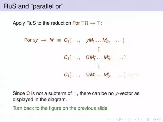
Apply RuS to the reduction Por>Ω→→ >:

Por xy →→ N ′ ≡ C1[ . . . , yM1 . . .Mp, . . . ]

7→C1[ . . . , ΩM∗1 . . .M

∗p , . . . ]

C1[ . . . , ΩM ′1 . . .M′p, . . . ] ≡ >

Since Ω is not a subterm of >, there can be no y -vector asdisplayed in the diagram.

Turn back to the figure on the previous slide.

Undefinability of Gustave’s function

Undefinability of parallel or is usually presented as aconsequence of Berry’s Sequentiality Theorem.

Another example is Gustave’s function:

TheoremThere is no lambda term G such that:

G 01x = x G 1x0 = x G x01 = x

Also other variants of Gustave’s function exist. In fact, we wereable to cover with RuS all examples we encountered that areusually seen as consequences of BST.

Sequentiality

Let M[~x := ~L]→→ N

Then N ≡ C[A1, . . . ,An] such that

1. The prefix C is independent of the substitution.2. Each Ai depends on exactly one substituted Lj in the

sense that at the position of Ai any other subterm B can berealized by an appropiate replacement Q of Lj , regardlessof the choice of the other substituted terms.

Proof.Apply RuS. If Bi is an ~x-vector xjK1 . . .Kk then choose Q asλy1 . . . yk .B.

Slogan: A position in the result is either governed by exactlyone of the input variables, or it is independent from all of them.

Berry’s Sequentiality Theorem

BST relates occurrences of the symbol ⊥ in the the Böhm treeof M to “input” occurrences of ⊥ in the original term M.

Slogan: A ⊥ in the Böhm tree of M depends on at most one ofthe input ⊥’s in M.

⊥⊥⊥⊥ ⊥

⊥

⊥

⊥

M BT(M)βΩ

BST can be proved by extending RuS to the Böhm rules:

⊥M → ⊥ λy .⊥ → ⊥ u → ⊥ if u is unsolvable

BST: variable-capturing refinements

I The original BST is about refinements of ⊥’s that maycapture variables. We only covered non-variable-capturingrefinements.

I However, in the paper we already extended RuS tovariable-capturing substitution, (or hole-filling in contexts).So we think we can obtain full BST.

Further questions

I Can RuS be extended to infinitary rewriting?I This could yield an alternative proof of BST.

I Another proof of BST is via origin tracking in“Descendants and origins in term rewriting”, Bethke, Klopand de Vrijer 2000

I Study the inverse relationship between RuS and origintracking

I Undefinabilty results in the line of BST have also beenobtained by finitary means in an unpublished report byByun, Kennaway, van Oostrom and de Vries (1999). Theyuse an analysis of residuals along head reductions.

I There might appear to be connections with proofs using themethod of underlining.

Appendix: Surjective pairing

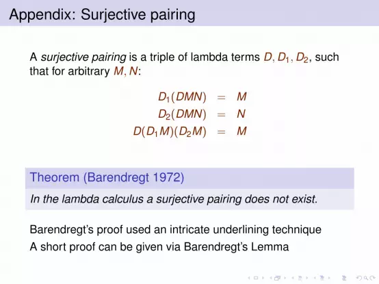
A surjective pairing is a triple of lambda terms D,D1,D2, suchthat for arbitrary M,N:

D1(DMN) = MD2(DMN) = N

D(D1M)(D2M) = M

Theorem (Barendregt 1972)

In the lambda calculus a surjective pairing does not exist.

Barendregt’s proof used an intricate underlining techniqueA short proof can be given via Barendregt’s Lemma

Undefinability of Surjective Pairing

1. Assume D,D1,D2 satisfy the equations for SP2. Define M ≡ D(D1Ω)(D2x)

3. Then M[x := Ω] ≡ D(D1Ω)(D2Ω) = Ω

4. Hence by Church–Rosser M[x := Ω]→→ Ω

5. Apply RuS:

M →→ N ′ ≡ C[ . . . , xM1 . . .Mp, . . . ]7→

C[ . . . , ΩM∗1 . . .M∗p , . . . ]

C[ . . . , ΩM ′1 . . .M′p, . . . ] ≡ Ω

6. Only two possibilities for N ′:I N ′ ≡ ΩI N ′ ≡ x

Two cases for N ′

Remember: M ≡ D(D1Ω)(D2x)

Case 1: N ′ ≡ Ω

I Then M →→ Ω and so M[x := P] = Ω for any PI Hence D2P = D2(D(D1Ω)(D2P)) ≡ D2(M[x := P]) = D2Ω

I Taking P ≡ DNN gives N = D2(DNN) = D2Ω

I It follows that all terms N are equal: contradiction

Case 2: N ′ ≡ x

I Then M →→ x and so M[x := P] = P for any P.I Hence D1P = D1(M[x := P]) ≡ D1(D(D1Ω)(D2P)) = D1Ω

I With P ≡ DNN again a contradiction is derived

reduction under substitution

Documents