object modeling using a tof camera under an uncertainty reduction approach

Object Modeling using a ToF Camera

under an Uncertainty Reduction Approach

Sergi Foix, Guillem Alenya, Juan Andrade-Cetto and Carme Torras

Abstract—Time-of-Flight (ToF) cameras deliver 3D imagesat 25 fps, offering great potential for developing fast objectmodeling algorithms. Surprisingly, this potential has not beenextensively exploited up to now. A reason for this is that,since the acquired depth images are noisy, most of the avail-able registration algorithms are hardly applicable. A furtherdifficulty is that the transformations between views are ingeneral not accurately known, a circumstance that multi-viewobject modeling algorithms do not handle properly undernoisy conditions. In this work, we take into account bothuncertainty sources (in images and camera poses) to generatespatially consistent 3D object models fusing multiple views witha probabilistic approach. We propose a method to compute thecovariance of the registration process, and apply an iterativestate estimation method to build object models under noisyconditions.

I. INTRODUCTION

The interest for Time-of-Flight (ToF) cameras is rapidly

growing thanks to the latest improvements in technology,

resulting in contributions to diverse fields such as robot nav-

igation, obstacle avoidance, human-machine interfaces, and

particularly also in object modeling. A competing sensing

technology for object modeling is lidar scanning, due to its

precision, but which requires mobile parts to aggregate linear

readings into full 3D scans with the subsequent detriment in

frame rate. Stereo vision systems have also been used for

object modeling, but require objects to be textured. On the

contrary, ToF cameras offer registered depth-intensity images

at high frame rate. Additionally, they offer other technical

advantages such as robustness to illumination changes, low

power consumption and low weight. However, the resolution

of ToF camera images is typically low (i.e., 160×120), and

depth values are much noisier compared to those of a laser

scanner.

Object modeling has particular characteristics that require

special attention when compared to other applications, e.g.

scene modeling. First, the distance from the camera to the

object is relatively small, so saturation in the center of

the depth image and distortion are expected to appear. In

addition, only part of the image corresponds to the target

object and segmentation algorithms are required to perform

background/foreground identification.

This work has been partially supported by the Spanish Ministry of Scienceand Innovation under project DPI2008-06022, the MIPRCV ConsoliderIngenio 2010 project, and the EU PACO PLUS project FP6-2004-IST-4-27657. S. Foix and G. Alenya are supported by PhD and postdoctoralfellowships, respectively, from CSIC’s JAE program.

The authors are with the Institut de Robotica i Informatica Industrial,CSIC-UPC, Llorens i Artigas 4-6, 08028 Barcelona, Spain (e-mails: sfoix,galenya, cetto, [email protected]).

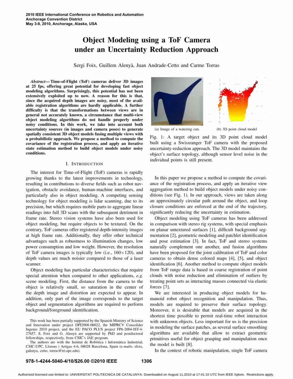
(a) Image of a watering can. (b) 3D point cloud model

Fig. 1: A target object and its 3D point cloud model

built using a Swissranger ToF camera with the proposed

uncertainty-reduction approach. The 3D model maintains the

object’s surface topology, although sensor level noise in the

individual points is still present.

In this paper we propose a method to compute the covari-

ance of the registration process, and apply an iterative view

aggregation method to build object models under noisy con-

ditions (see Fig. 1). In our approach, views are taken along

an approximately circular path around the object, and loop

closure conditions are enforced at the end of the trajectory,

significantly reducing the uncertainty in estimation.

Object modeling using ToF cameras has been addressed

in comparison with stereo rig systems, with special emphasis

on planar untextured surfaces [1], difficult background seg-

mentation [2], geometric modeling and patchlet identification

and pose estimation [3]. In fact, ToF and stereo systems

naturally complement one another, and fusion algorithms

have been proposed for the joint calibration of ToF and color

cameras to obtain dense colored maps [4], [5], and object

identification [6]. Another method to compute object models

from ToF range data is based in coarse registration of point

clouds with noise reduction and elimination of outliers by

treating point sets as interacting masses connected via elastic

forces [7].

We are interested in producing object models for hu-

manoid robot object recognition and manipulation. Thus,

models are required to preserve their surface topology.

Moreover, it is desirable that models are acquired in the

shortest time possible to permit real-time robot interaction

with unknown objects. Less important for us is the precision

in modeling the surface patches, as several surface smoothing

algorithms are available that allow to extract geometric

primitives useful for object grasping and manipulation once

the model is built [8].

In the context of robotic manipulation, single ToF camera

2010 IEEE International Conference on Robotics and AutomationAnchorage Convention DistrictMay 3-8, 2010, Anchorage, Alaska, USA

978-1-4244-5040-4/10/$26.00 ©2010 IEEE 1306

Authorized licensed use limited to: UNIVERSITAT POLITECNICA DE CATALUNYA. Downloaded on August 11,2010 at 17:41:10 UTC from IEEE Xplore. Restrictions apply.

images have been used in the past to evaluate grasping

properties such as force closure or obstacle avoidance [9]. In

this work, we are interested in building a more complete re-

construction of objects, in terms of the surfaces bounding it,

by combining multiple 3D depth images. The setup includes

a ToF camera mounted on the end-effector of a robotic arm

performing a circular trajectory around the object to acquire

equally spaced images. These images could be combined via

precise camera calibration w.r.t. the end effector and proper

inverse kinematics of the manipulator, or alternatively, with

a point cloud registration algorithm; usually a variant of

the Iterative Closest Point (ICP) algorithm. Note that point

cloud registration is more critical in object modeling than in

scene modeling given the high signal-to-noise ratios of ToF

depth information at relatively short distances. Moreover,

for precisely calibrated robot-camera systems, the kinematics

of humanoid robot arms is usually not very precise, and

point cloud registration is still needed. Lastly, the successive

registration of consecutive views accumulates drift error

along a sequence. A common consequence is, for example,

to compute the model of a circular object as a spiral. Thus,

proper techniques for range data registration along multiple

views need to be used.

Data fusion for scene or model augmentation has been

typically addressed by error minimization methods such as

bundle adjustment [10] or structure from motion [11]. These

approaches are often not suitable for real time computation

given their iterative nature. Recursive state estimation (e.g.,

SLAM) is a more suitable choice. The classical EKF-based

approach to SLAM for feature-based scene augmentation is

also not viable for real time modeling since it requires the

computation of fully correlated covariances at each step [12].

In this work we propose to use a view-based information-

form SLAM method that a) does not maintain a large number

of feature estimates, but only a reduced number of pose

estimates, and b) is efficiently computed in information form,

exploiting the sparsity of such filtering representation [13].

We take advantage of the fact that the first and last images

in a circular sequence around an object overlap. This allows

us to impose a loop-closure constraint.

The rest of the article is structured as follows. In Section II

the characteristics of ToF cameras are briefly discussed. Next,

our modeling algorithm is presented in Section III, including

the computation of the object pose resulting from the regis-

tration of point clouds and the estimation of the covariance

of this pose (Sec. III-A) and the use of this covariance

in model construction (Sec. III-B). Some experiments are

presented in Section IV to evaluate the proposed covariance

propagation algorithm, as well as the modeling algorithm.

Finally, Section V is devoted to conclusions and prospects

for future work.

II. TOF CAMERAS

ToF cameras emit modulated light, and depth computation

is based on timed measures of the reflected light signal [14].

The modulation frequency of the emitted light determines the

ambiguity-free range of the sensor, usually between 5 and 7

(a) 2D range image (b) Rotated 3D point cloud

Fig. 2: Typical output of a ToF camera. False depth readings

appear at the edges between foreground and background due

to the integration of the reflected light of both surfaces in the

corresponding pixels.

meters. In comparison with other technologies also used to

obtain scene depth, ToF cameras provide some interesting

features:

1) registered dense depth and intensity images,

2) complete image acquisition at high frame rate,

3) small, low weight and compact design,

4) no mobile parts needed,

5) auto-illumination,

6) low power consumption.

Their main limitations are low resolution (176×144 pixels

for a SR3K camera) and noisy depth measurements, which

are affected by both systematic and non-systematic errors. In

general, systematic errors are dealt with calibration, whereas

the effects of non-systematic errors is reduced with filtering.

ToF camera calibration is still an active research field where

some work has been done to completely understand the

sources of errors and how to compensate them.

Systematic errors can be grouped into two categories. On

the one hand, a correction for the depth value should be

performed depending on the position of the pixel in the image

matrix. This is generally calibrated using a known object and

computing a suitable correction matrix, called sometimes

fixed pattern noise matrix. On the other hand, a bias is

introduced for each pixel that depends only on the measured

depth. This bias is sinusoidal and it must be calibrated by

taking measures of a known object at different known depths.

B-splines are used to model this error in the general case, but

if the range of depths is known to be restricted, a polynomial

can be used instead.

One of the parameters that can be tuned in a ToF camera

is the integration time, which has direct relation to the range

of depths that the camera senses better. The calibration

procedures mentioned above should be repeated for each

different integration time used. Temperature can also affect

the obtained depth. The most common strategy is to wait

until the camera has reached a stable temperature value, and

limit its use to a suitable operation range.

Non-systematic errors appear mainly due to problems in

the reflection of light at concavities, edges (see Fig. 2),

and in non-uniformly illuminated scenes. Furthermore, like

1307


for traditional cameras and depending on scene conditions,

motion blur may appear if the camera acquires images during

motion.

Our experiments are carried out using a fixed integration

time and a low reflective object in order to maintain constant

the systematic integration time-related error and to minimize

unfavorable non-systematic specularities. Any integration

time can be chosen as long as it does not distort the geometry

of the scene. No other calibration approach has been used

besides the mentioned parametrization.

III. OBJECT MODELING FROM THE

ACCUMULATION OF POINT CLOUDS

Each iteration of the proposed method comprises two

steps. First, consecutive point clouds are registered using the

ICP algorithm. The result includes estimates of the relative

change in sensor pose between the two point clouds. To

compute the covariance of the relative pose change, the

sensor covariance is linearly propagated through the ICP

minimization. The second step uses these first and second

order camera pose change estimates to smooth the sensor

motion sequence using a view-based SLAM method. The

revised motion sequence is used to synthesize the final object

model from the original views. The method is detailed in

algorithmic form in Alg. 1, and each one of these steps is

explained in more detail in the subsequent sections.

Algorithm 1 Object modeling from ToF images

OBJECTMODEL(x0, Σ0,S,Σs)INPUTS:

x0: Initial sensor pose in global coordinates.Σ0: Initial sensor pose covariance.S: A set of n point clouds.Σs: Sensor measurement covariance.

OUTPUT:O: Object model as a dense point set.

1: T ← STATEAUGMENT(T , x0, Σ0)2: for i = 1 to n do3: (xi,mi)← REGISTER(Si−1,Si)4: Σi ← PROPAGATEERROR(xi, mi, Σs)5: T ← STATEAUGMENT(T , xi, Σi)6: if at loop closure then7: (xj ,mj)← REGISTER(Sj ,Si)8: Σj ← PROPAGATEERROR(xj , mj , Σs)9: T ← STATEUPDATE(T , xj , Σj ,j,i)

10: end if11: end for12: O ← SYNTHETIZEVIEWS(T , S)13: return O

T represents the smoothed sensor pose history; mi indi-

cates the point correspondences between consecutive point

clouds i − 1 and i; mj indicates the point correspondences

between loop-closing point clouds j and i; Σi is used to

indicate the covariance of the relative pose change between

consecutive point clouds i − 1 and i; and Σj is used to

indicate the covariance of the relative pose change between

loop-closing point clouds j and i.

A. ICP Error Propagation

The point cloud registration method used in this paper is

based on the well-known ICP algorithm [15], [16], [17], and

its variants [18], [19]. The probabilistic data fusion mecha-

nism used in this work requires first order approximations

of error propagation. That is, covariance estimates of sensor

uncertainty must be propagated through the ICP cost function

to compute relative pose covariance estimates between the

two generative viewpoints.

The decision of using one cost function or another plays an

important role during error propagation, since its derivatives

need to be computed. In its simplest form, given a set of

matching points from two consecutive point clouds mi =(a, b), the ICP cost function takes the form

ε(mi,xi) =∑

||xi(b) − a||2. (1)

An accurate covariance approximation can be computed

using a Monte Carlo simulation, but this is a time-consuming

solution and, since speed of execution is really a needed

characteristic, finding a closed-form solution is desirable.

Given that the ICP algorithm is basically a cost function

minimization procedure, an implicit function between input

(point clouds) and the output (the pose) is defined by

the minimization process [20]. Albeit the implicit function

can not be explicitly known, its Jacobian matrix can be

computed. Consequently, the estimated covariance matrix

can be computed using the usual first-order approximation

of an explicit function

Σi = ∇f Σs ∇fT, (2)

where ∇f is the explicit function’s Jacobian matrix, Σs the

sensor covariance matrix and Σi the computed relative pose

covariance matrix.

The Jacobian matrix of the ICP implicit function can be

computed by means of the implicit function theorem. In

our case, for an unconstrained minimization problem, the

Jacobian matrix becomes

∇f =

(

∂2ε

∂x2

i

)

−1∂2ε

∂mi ∂xi

. (3)

Since our approach uses the point to point Euclidean

distance error as a cost function in the registration process,

the application of the implicit function theorem is straight

forward. It is important to notice however that this type of ap-

proximation propagates the error from sensor measurements

to the sensor’s relative pose. Therefore, the parametrization

of the cost function will have to include the real sensor

measurements as its only input variables. For instance, if

a point-to-plane ICP algorithm is used, its point-to-plane

function will have to be accommodated into the implicit

function and derived consequently. It is not correct to pre-

compute the virtual point of the plane correspondence and

then apply a point-to-point cost function.

To evaluate the quality of our closed form covariance

approximation, a Monte Carlo simulation was realized and

the results were compared. Fig. 3 shows the results from

1308


the Monte Carlo simulation and the different closed-form

approaches tried in Section IV-A.

B. Closing the Loop

Feature-based SLAM approaches are not adequate for fast

object modeling due to the huge amount of data provided by

the ToF camera, and the need to select a sparse feature repre-

sentation. In our application, a view-based SLAM approach

is used instead that optimizes only the relative sensor poses

between views and their covariances. From the estimated

history of sensor poses an object model is then synthesized

using all sensor data. The final result is a finely registered

dense point cloud which can be computed on-line.

The view-based SLAM technique used in our experiments

is based on a delayed-state information-form algorithm [21],

[13]. This algorithm, in contrast to feature-based SLAM

approaches, has the advantage that the ensuing information

matrix is naturally sparse and does not need extra sparsifi-

cation steps that induce estimation errors.

The sensor pose (the i-th component of the state vector x)

contains the position of the sensor and its orientation in Euler

angles xi = [xk, yk, zk, φk, θk, ψk]T. The noise-free motion

model is defined using the compounding operation [22], and

defines the state transition model, relating state components

xi−1 and xi,

xi = f(xi−1,ui)

= xi−1 ⊕ ui, (4)

and ui is the relative motion between consecutive poses as

computed with the ICP algorithm.

We resort to the canonical parametrization of Gaussian

distributions,

p(x) = N (x;µ,Σ) = N−1(x;η,Λ), (5)

Λ = Σ−1, and η = Σ

−1µ, (6)

where µ is the mean state vector and Σ its covariance matrix,

and Λ and η are the information matrix and information

vector, respectively.

During state augmentation (line 5 in the Algorithm), the

parameters η and Λ are computed with

ηi−1,i = ηi−1,i + FTaugΣ

−1

u (f(µi−1,ui) − Fµi−1

) (7)

and

Λi−1:i,i−1:i = Λi−1:i,i−1:i + FTaugΣ

−1

u Faug, (8)

in which Faug =[

−F I]

, F is the Jacobian matrix

of the composition (Eq. 4), and ηi−1:i and Λi−1:i,i−1:i

represent the posterior information vector and information

matrix for poses i − 1 and i, with zero entries for time i,

indicating infinite uncertainty for that robot pose. The shared

information between the new pose xi and the rest of the robot

trajectory x0:i−2 is always zero when we have not closed any

loop. The result is a naturally sparse information matrix with

a tridiagonal block structure.

Loop closures are also modeled using compounding oper-

ations,

z = h(xj ,xi)

= ⊖xi ⊕ xj , (9)

and the state update (line 9 in the Algorithm) is computed

in information form with

ηj,i = ηj,i + HTΣ

−1

z

(

z − h(µj , µi) + Hµj,i

)

(10)

Λj:i,j:i = Λj:i,j:i + HTΣ

−1

z H, (11)

where z is the ICP’s computed relative pose measurements

between the current pose xi and any other pose xj .

In the same way as with the prediction step, given the two-

block size of the measurement Jacobian matrix H (the partial

derivative of Eq. 9), only the four blocks relating poses j and

i in the information matrix will be updated.

Motivated by [23], we employ a QR factorization of the

information matrix to solve Λµ = η and ΛΣ = I, for µ

and Σ.

In order to reduce the fill-in in the right triangular matrix

from the QR factorization, we first reorder the information

matrix using the column approximate minimum degree (CO-

LAMD) ordering [24], then we apply QR factorization to the

reordered information matrix and solve for each state variable

via back substitution. State recovery takes nearly linear time,

compatible with other state of the art SLAM approaches [25],

[13].

IV. EXPERIMENTS

In order to evaluate the proposed covariance propagation

method a comparison with two other approaches to covari-

ance estimation is presented: a) a Monte Carlo simulation,

and b) the naive technique of aggregating matching distance

errors between the point clouds. Furthermore, a modeling

experiment using real data is also presented, showing the

advantages of the proposed method with respect to the use

of aggregated ICP in scenarios where both camera motion

estimation and depth measurements are noisy.

A. Monte Carlo Simulation

To synthetically simulate the form of the relative pose

covariance computed from ICP registration, a uniformly

distributed point cloud is first generated with 105 points

separated about 30 mm from each other along the three axes.

A thousand secondary matching point clouds are generated

from the same set of points, by applying a known rigid body

transformation, and adding zero mean white noise with 5 mm

standard deviation to each resulting data point, simulating

sensor induced depth range measurement error. To avoid

errors induced by unreliable nearest neighbor computation,

point correspondences are given. On a side note, finding a

good set of matching points is a critical part of the ICP

algorithm. That is the reason why two filters have been

implemented for the case of real data in order to increase its

robustness. The first one is an outlier filter, guaranteeing good

1309


0.08 0.09 0.1

−0.02

−0.015

−0.01

−0.005

0

0.005

0.01

X−Y Covariance

meters (X)

mete

rs (

Y)

0.08 0.09 0.1

0.12

0.125

0.13

0.135

0.14

0.145

0.15

X−Z Covariance

meters (X)

mete

rs (

Z)

−0.01 0 0.01

0.12

0.125

0.13

0.135

0.14

0.145

0.15

Y−Z Covariance

meters (Y)

mete

rs (

Z)

−0.12 −0.1 −0.08 −0.06 −0.04

−0.06

−0.04

−0.02

0

0.02

0.04

Phi−Theta Covariance

Rx − radians (φ)

Ry −

radia

ns (

θ)

−0.12 −0.1 −0.08 −0.06 −0.04

−0.2

−0.18

−0.16

−0.14

−0.12

−0.1

Phi−Psi Covariance

Rx − radians (φ)

Rz −

radia

ns (

ψ)

−0.04 −0.02 0

−0.18

−0.16

−0.14

−0.12

−0.1

Theta−Psi Covariance

Ry − radians (θ)

Rz −

radia

ns (

ψ)

Fig. 3: Covariance projections. The frames show 2D projections of the 6D covariance hyperellipsoids computed via Monte

Carlo simulation (black), via the implicit function (dashed green), and from the accumulation of distance errors (dashed

red).

point cloud density. And the second one is an orientation

filter, ensuring compatible point correspondence.

After applying ICP to the synthetically generated matching

point clouds, each recovered relative pose transformation is

plotted as a blue point in Fig. 3. Monte Carlo covariances

are plotted in black, while the covariance recovered from the

implicit function and the covariance computed by aggregat-

ing matching point distances are plotted as a green dashed

line and as a red dotted line, respectively. All iso-uncertainty

hyperellipsoids have been plotted at a scale of 2σ.

Building the covariance matrix by aggregating 6 DOF pose

distance errors from the matching points, after applying the

ICP, and without taking into account the ICP cost function,

clearly underestimates the real pose covariance since it does

not take into account cross correlations between the various

pose variables.

B. Real data object modeling

A second experiment was performed using a 7 degrees-

of-freedom WAM robotic arm and a Swissranger ToF cam-

era attached to its gripper. A predefined circular trajectory

maintaining the object inside the camera field of view was

carried out in order to be able to close the loop needed by

the SLAM algorithm. A watering can was approximately

placed one meter above the robotic arm reference center in

such a way that all viewpoints fall within the arm workspace

without passing through ill-posed configurations. One clear

advantage of our uncertainty-driven approach is that no

precise hand-eye calibration was needed. A set of 20 point

clouds were taken during the 360 degrees rotation trajectory

at roughly uniformly distributed positions. At each trajectory

position, a point cloud was captured and the WAM pose was

stored. Note that since no precise hand-eye calibration is

1310


(a) Robot trajectory after all ICP results are aggregated (b) Revised robot trajectory after the loop is closed with the view-based SLAMmethod

Fig. 4: Robot pose trajectory. Frame a) shows the calculated trajectory and uncertainty estimates after all ICP results are

aggregated, but before the loop is closed. Each pose accumulates the estimated error from the previous pose. Frame b) once

the loop is closed, uncertainty is reduced and the complete trajectory is corrected.

(a) matching of first and last views using aggre-gated ICP

(b) matching of first and last views usinginformation-based SLAM

(c) complete 3D model

Fig. 5: The figure shows the advantage of fusing data globally using the proposed filtering scheme. Frames a) and b) contain

the sequence’s first 3D ToF image (in red) and last (in blue). Data fusion using aggregated ICP accumulates registration

error, which is corrected using a globally consistent loop closure provided by the information-based SLAM. Frame c) shows

the final complete 3D model.

provided, and since the WAM arm has its own kinematic

errors, these poses served only as initialization points for

the ICP. In pre-treating raw data, a segmentation algorithm

was applied to the incoming point clouds in order to discard

outlier object data. The segmentation algorithm consisted of

a jump-edge filter and a depth-threshold background filter.

As an example of the proposed method, Fig. 5 shows the

final 3D point cloud made for the watering can shown in

Fig. 1. The figure shows the advantage of fusing data globally

using the proposed filtering scheme. Frames a) and b) contain

the sequence’s first 3D ToF image (in red) and last (in blue).

Data fusion using aggregated ICP accumulates registration

error, which is corrected using a globally consistent loop

closure provided by the information-based SLAM. Frame c)

shows the final complete 3D model.

Fig. 4 shows the estimated robot trajectories for the cases

of ICP relative pose aggregation, and SLAM-based loop

closure. After closing the loop, the final trajectory (blue)

is closer to a circular shape than not the one achieved

purely from accumulating ICP motion estimates (red). The

red trajectory tends to describe the typical spiral shape

characteristic from error accumulation. In order to get a more

precise evaluation of the obtained models, real measures

were compared with each model. The real watering can upper

edge width is 11.5 centimeters, whereas the aggregated ICP

model is 9 centimeters width, and the one obtained after loop

closure is enforced is 11.2 centimeters wide.

1311


V. CONCLUSIONS AND FUTURE RESEARCH

This paper presents a method to consistently fuse range

images acquired with a ToF camera mounted on a not

necessarily calibrated robotic arm to autonomously build a

3d object model. Accurate hand-eye calibration is not needed

since the method uses globally consistent probabilistic data

fusion by means of a view-based information-form SLAM

algorithm.

Furthermore, we present a method to linearly propagate

noise covariances from the range camera through an error

minimization algorithm such as the point to point ICP.

The proposed approach, using the implicit theorem, had

previously been used in this context only for 2D ICP, and

we have derived and extended the method for the 3D case.

The proposed approach to data fusion for object modeling

can be executed in real time, in contrast to iterative methods

such as bundle adjustment, provided an efficient approximate

nearest neighbor method is in place for the ICP compu-

tations. Fortunately, very efficient nearest neighbor search

tools exist that take time logarithmic with the number of

points in the data set. Efficient globally consistent fusion of

pose estimates at loop closure is only possible thanks to the

sparsity of the information filtering scheme used.

Foreseen enhancements to the presented method are im-

plicit function propagation of more efficient ICP variants

such as the point to plane, plane to plane, and generalized

ICP; automatic computation of next viewpoints based on in-

formation or entropy minimization metrics; more exhaustive

empiric evaluation of the modeling results with a larger set of

objects with different shapes and texture; and the application

of the built models for the computation of grasping and

manipulation directives.

VI. ACKNOWLEDGMENTS

The authors wish to thank E. Teniente for early imple-

mentations of the ICP algorithm and insightful discussions

on ICP covariance propagation and R. Valencia for providing

us with his view-based SLAM code.

REFERENCES

[1] S. E. Ghobadi, K. Hartmann, W. Weihs, C. Netramai, O. Loffeld,and H. Roth, “Detection and classification of moving objects-stereoor time-of-flight images,” in Proc. Int. Conf. Comput. Intell. Security,vol. 1, Guangzhou, Nov. 2006, pp. 11–16.

[2] S. Hussmann and T. Liepert, “Three-dimensional ToF robot visionsystem,” IEEE Trans. Instrum. Meas., vol. 58, no. 1, pp. 141–146,Jan. 2009.

[3] C. Beder, B. Bartczak, and R. Koch, “A comparison of PMD-cameras and stereo-vision for the task of surface reconstruction usingpatchlets,” in Proc. 21st IEEE Conf. Comput. Vision Pattern Recog.,vol. 1-8, Minneapolis, June 2007, pp. 2692–2699.

[4] J. Zhu, L. Wang, R. Yang, and J. Davis, “Fusion of time-of-flight depthand stereo for high accuracy depth maps,” in Proc. 22nd IEEE Conf.

Comput. Vision Pattern Recog., vol. 1-12, Anchorage, June 2008, pp.3262–3269.

[5] M. Lindner, M. Lambers, and A. Kolb, “Sub-pixel data fusion andedge-enhanced distance refinement for 2D/3D,” Int. J. Int. Syst. Tech.

App., vol. 5, no. 3-4, pp. 344–354, 2008.[6] T. Grundmann, Z. Xue, J. Kuehnle, R. Eidenberger, S. Ruehl, A. Verl,

R. D. Zoellner, J. M. Zoellner, and R. Dillmann, “Integration of 6Dobject localization and obstacle detection for collision free roboticmanipulation,” in Proc. IEEE/SICE Int. Sym. System Integration,Nagoya, Dec. 2008, pp. 66–71.

[7] B. Dellen, G. Alenya, S. Foix, and C. Torras, “3D object reconstructionfrom Swissranger sensors data using a spring-mass model,” in Proc.

4th Int. Conf. Comput. Vision Theory and Applications, vol. 2, Lisbon,Feb. 2009, pp. 368–372.

[8] J. U. Kuehnle, Z. Xue, M. Stotz, J. M. Zoellner, A. Verl, andR. Dillmann, “Grasping in depth maps of time-of-flight cameras,” inProc. Int. Workshop Robotic Sensors Environments, Otawa, Oct. 2008,pp. 132–137.

[9] A. Saxena, L. Wong, and A. Y. Ng., “Learning grasp strategies withpartial shape information,” in Proc. 23th AAAI Conf. on Artificial

Intelligence, Chicago, Jul. 2008, pp. 1491–1494.[10] B. Triggs, P. McLauchlan, R. Hartley, and A.W.Fitzgibbon, “Bundle

adjustment - a modern synthesis,” in Proc. Int. Workshop on Vision

Algorithms, ser. Lect. Notes Comput. Sci., vol. 1883, Corfu, Sep. 1999,pp. 153–177.

[11] F. Dellaert, S. Seitz, C. Thorpe, and S. Thrun, “Structure from motionwithout correspondence,” in Proc. 14th IEEE Conf. Comput. Vision

Pattern Recog., vol. 2, Head Island, Jun. 2000, pp. 557–564.[12] M. W. M. G. Dissanayake, P. Newman, S. Clark, H. F. Durrant-Whyte,

and M. Csorba, “A solution to the simultaneous localization and mapbuilding (SLAM) problem,” IEEE Trans. Robot. Automat., vol. 17,no. 3, pp. 229–241, Jun. 2001.

[13] V. Ila, J. M. Porta, and J. Andrade-Cetto, “Information-based compactPose SLAM,” IEEE Trans. Robot., vol. 26, no. 1, pp. 78–93, Feb.2010.

[14] A. Kolb, E. Barth, and R. Koch, “ToF-sensors: New dimensions forrealism and interactivity,” in Proc. IEEE CVPR Workshops, vol. 1-3,Anchorage, June 2008, pp. 1518–1523.

[15] P. Besl and N. McKay, “A method for registration of 3D shapes,” IEEETrans. Pattern Anal. Machine Intell., vol. 14, no. 2, pp. 239–256, Feb.1992.

[16] Y. Chen and G. Medioni, “Object modeling by registration os multiplesranges images,” in Proc. IEEE Int. Conf. Robot. Automat., vol. 3,Sacramento, Apr. 1991, pp. 2724–2729.

[17] Z. Zhang, “Iterative point matching for registration of free-form curvesand surfaces,” Int. J. Comput. Vision, vol. 13, pp. 119–152, 1994.

[18] S. Rusinkiewicz and M. Levoy, “Efficient variants of the ICP algo-rithm,” in Proc. 3rd Int. Conf. 3D Digital Imaging Modeling, Quebec,May 2001, pp. 145–152.

[19] J. Minguez, L. Montesano, and F. Lamiraux, “Metric-based iterativeclosest point scan matching for sensor displacement estimation,” IEEETrans. Robot., vol. 22, no. 5, pp. 1047–1054, Oct. 2006.

[20] J. Clarke, “Modelling uncertainty: A primer,” University of Oxford.Dept. Engineering science, Tech. Rep. 2161/98, 1998.

[21] R. Valencia, E. Teniente, E. Trulls, and J. Andrade-Cetto, “3D mappingfor urban serviece robots,” in Proc. IEEE/RSJ Int. Conf. Intell. Robots

Syst., Saint Louis, Oct. 2009, pp. 3076–3081.[22] R. Smith, M. Self, and P. Cheeseman, “Estimating uncertain spatial

relationships in robotics,” in Autonomous Robot Vehicles, 1990, pp.167–193.

[23] M. Kaess, A. Ranganathan, and F. Dellaert, “iSAM: Incrementalsmoothing and mapping,” IEEE Trans. Robot., vol. 24, no. 6, pp.1365–1378, 2008.

[24] T. Davis, J. Gilbert, S. Larimore, and E. Ng, “A column approximateminimum degree ordering algorithm,” ACM T. Math. Software, vol. 30,no. 3, pp. 353–376, 2004.

[25] F. Dellaert and M. Kaess, “Square root SAM: Simultaneous local-ization and mapping via square root information smoothing,” Int.

J. Robot. Res., vol. 25, no. 12, pp. 1181–1204, 2006.

1312


object modeling using a tof camera under an uncertainty reduction approach

Documents