redalyc.the adjustment to target leverage of

Revista de Economía Aplicada

ISSN: 1133-455X

[email protected]

Universidad de Zaragoza

España

RUBIO, GONZALO; SOGORB, FRANCISCO

THE ADJUSTMENT TO TARGET LEVERAGE OF SPANISH PUBLIC FIRMS: MACROECONOMIC

CONDITIONS AND DISTANCE FROM TARGET

Revista de Economía Aplicada, vol. XIX, núm. 57, 2011, pp. 35-63

Universidad de Zaragoza

Zaragoza, España

Available in: http://www.redalyc.org/articulo.oa?id=96922243002

How to cite

Complete issue

More information about this article

Journal's homepage in redalyc.org

Scientific Information System

Network of Scientific Journals from Latin America, the Caribbean, Spain and Portugal

Non-profit academic project, developed under the open access initiative

http://www.redalyc.org/revista.oa?id=969

http://www.redalyc.org/articulo.oa?id=96922243002

http://www.redalyc.org/comocitar.oa?id=96922243002

http://www.redalyc.org/fasciculo.oa?id=969&numero=22243

http://www.redalyc.org/articulo.oa?id=96922243002

http://www.redalyc.org/revista.oa?id=969

http://www.redalyc.org

35

Revista de Economía Aplicada Número 57 (vol. XIX), 2011, págs. 35 a 63EA

THE ADJUSTMENT TO TARGETLEVERAGE OF SPANISH PUBLIC

FIRMS: MACROECONOMICCONDITIONS AND DISTANCE

FROM TARGET*

GONZALO RUBIOFRANCISCO SOGORB

Universidad CEU Cardenal Herrera

Our evidence suggests that Spanish public firms adjust slowly towardtheir capital structure target, with the typical firm closing approximatelyone-fifth of the gap between its current and target debt ratios each year.This finding is in contrast with previous evidence; however, we employeconometric techniques specially designed for highly persistent depen-dent variables, like market debt ratios. Moreover, our evidence does notseem to indicate that macroeconomic conditions, at least under the con-ditions experienced by the Spanish economy during our sample period,affect the speed of adjustment. If anything, our results are consistentwith faster adjustments during economic states in which the distance bet-ween the current and target leverage is the greatest.

Key words: market debt ratio, dynamic trade-off, target leverage, speedof adjustment, macroeconomics, distance from target.

JEL classification: G32, C33, E30.

Three main theories are recognized in explaining capital structure: markettiming, the pecking order approach and the trade-off theory. As expected,the empirical evidence closely follows the development of theoretical mod-els1. The first collection of papers studies the determinants of capital struc-ture under the implicit assumption that observed and target market debt ra-

(*) The authors thank the participants of the 17th Finance Forum at the IESE Business School and es-pecially Javier Suárez for helpful suggestions. The comments of two anonymous referees and the edi-tor, Rafael Santamaría, were extremely useful in improving the paper. The authors acknowledge finan-cial support from MEC research grant ECO2008-03058/ECON and CEU-UCH/Banco SantanderCopernicus Program. Gonzalo Rubio also acknowledges support from GV PROMETEO/2008/106,and Francisco Sogorb recognizes a research grant from the Banco Herrero Foundation.(1) See, among many others, Shyam-Sunder and Myers (1999), Baker and Wurgler (2002), Welch(2004), Leary and Roberts (2005), Kayhan and Titman (2007), Lemmon, Roberts, and Zender(2008), Byoun (2008), Frank and Goyal (2009), and Berk, Stanton, and Zechner (2010).

tios are basically the same. The second set of papers deals with factors that maycause firms to be over- or underleveraged with respect to their target market debtratios. The final group of papers closely examines capital structure changes. Inparticular, they look for factors that may prevent firms from maintaining constant(target) market debt ratios. In this sense, recent literature focuses on analyzinghow and when firms dynamically adjust their capital structure. This is the frame-work in which we conduct our research. Specifically, the main objective of thepaper is to study how Spanish public firms adjust toward their capital structuretarget. This might be relevant because previous empirical evidence from Spanishfirms shows a relatively high speed of adjustment toward target debt ratios, atleast with respect to the typical U.S. firm. De Miguel and Pindado (2001), usingdata from 1990 to 1997, report a surprisingly high speed of adjustment of approx-imately 0.79, which suggests that nearly 80 percent of the debt ratio is adjustedeach year toward target leverage. González and González (2008) report that, be-tween 1995 and 2004, the typical Spanish firm closes approximately 54 percent ofthe gap between its current and target debt ratios each year. These results suggestthat presenting additional and more recent evidence of the speed of adjustment ofSpanish firms may be appropriate.

Interestingly, the U.S. empirical evidence about how quickly firms move to-ward their target market debt ratios is controversial because the results seem to besensitive to the econometric specifications employed as well as to external financ-ing constraints. Flannery and Rangan (2006), in a very influential paper, report arelatively fast speed of adjustment of 35.5 percent per year, which suggests thatapproximately one-third of the gap between current and target debt ratios isclosed each year. However, Faulkender, Flannery, Hankins, and Smith (2008)argue that the speed of adjustment depends heavily on firms having access to ex-ternal capital markets. The speed of adjustment is 31.3 percent for firms with ac-cess to external markets, but only 17.1 percent for firms with more restrictive ac-cess to external capital markets2. Similarly, Byoun (2008) reports that theadjustment speed is around 33 percent when firms have above-target debt with afinancial surplus but about 20 percent when firms have below-target debt with afinancial deficit. Huang and Ritter (2009) show how sensitive the results are tothe econometric techniques employed in estimating the speed of adjustment. Fi-nally, Lemmon et al. (2008) argue that, although observed leverage is consistentwith the existence of a target debt ratio, since firms seem to trade off the costs andbenefits of leverage, their lagged (up to 15 years) debt ratios are highly significantdeterminants of their current capital structure3.

The first contribution of this paper is to provide more recent evidence of thespeed of adjustment of Spanish firms and, more importantly, to provide new resultsunder an econometric technique especially appropriate for a dynamic panel when


36

(2) All these figures are based on market leverage. The evidence using book leverage insteadshows slightly lower speeds of adjustment.(3) Also, recent papers by Chang and Dasgupta (2009) and Iliev and Welch (2010) argue that theempirical evidence in favor of target behavior and dynamic rebalancing of leverage may be causedby mechanical mean reversion.

the dependent variable is highly persistent. Specifically, our results are based on thelong difference estimator of Hahn, Hausman, and Kuersteiner (2007). It turns outthat, like Huang and Ritter (2009), we show that this estimator is much less biasedthan the traditional generalized method of moments (GMM) estimators employed inprevious papers with Spanish and U.S. data. In particular, our evidence shows thatthe typical Spanish firm moves much more slowly toward its target leverage thanpreviously reported estimates. The speed of adjustment is found to be 17.5 percent,which indicates that approximately only one-fifth of the gap is closed each year. Thisseems to contrast not only with the available Spanish evidence discussed above, butalso with the higher speed traditionally accepted for U.S. firms where approximatelyone-third of the gap is supposed to be closed each year4. However, it is closer to themost recent U.S. evidence obtained using a long difference estimator5.

The second and more specific objective of the paper is to analyze howmacroeconomic conditions influence the adjustment speed of capital structure ofSpanish public firms toward their target leverage levels. Several theoretical pa-pers discuss the influence of macroeconomic conditions on financing patterns.Korajczyk and Levy (2003) argue that the response of firms to cyclical fluctua-tions depends upon the stringency of financing constraints. Levy and Hennessy(2007) find that relatively less constrained firms exhibit countercyclical variationsin market debt ratios. More specifically, the authors find countercyclical varia-tions in outstanding debt and procyclical variations in outstanding equity. Theypropose a general equilibrium model with agency costs in which firms substitutedebt for equity to maintain managerial equity shares during recessions to avoidagency conflicts. The opposite occurs during expansions, because increases inmanagerial wealth facilitate the substitution of equity for debt. The authors alsoshow that the relatively constrained firms should be characterized by a flat marketdebt ratio over the economic cycles. Finally, Hackbarth, Miao, and Morellec(2006) formally show that there is a benefit for firms to accommodate their capitalstructure decisions to the macroeconomic cycle, as long as operating cash flowsdepend on current economic conditions. Their dynamic model shows that thecountercyclical nature of the aggregate market debt ratio is basically due to the rel-atively higher increase in the present value of operating cash flows during booms.Moreover, this is the only theoretical paper with clear-cut implications about thespeed of adjustment toward target leverage. Given that firms’ restructuring thresh-olds are lower in expansions than in recessions, the authors show that firms shouldadjust their capital structure more often during expansions than in contractions.Hence, the speed of adjustment should be higher in expansions than in recessions.

The empirical evidence about the effects of macroeconomic conditions on thespeed of adjustment to target capital structure is rather scarce. Drobetz and Wanzen-ried (2006) show that the speed of adjustment of Swiss firms is higher when theterm spread is higher and economic prospects are good. Drobetz, Pensa, and

The adjustement to target leverage of Spanish public firms: macroeconomic conditions and distance...

37

(4) See Flannery and Rangan (2006) and Antoniou, Guney, and Paudyal (2008), who report coeffi-cients of 35.5 and 32.2 percent, respectively.(5) Huang and Ritter (2009) estimate a speed of adjustment of 23.2 percent per year for market le-verage.

Wanzenried (2007) extend their previous analysis to a representative sample of Eu-ropean firms with data from 1983 to 2002. These authors also conclude that the ad-justment is faster under favorable macroeconomic conditions. In particular, Euro-pean firms tend to move faster toward their target leverage when interest rates arelow and global financial distress is negligible. Surprisingly, to the best of ourknowledge, the only evidence analyzing the effects of economic conditions on thespeed of adjustment using U.S. data is reported by Cook and Tang (2010). By defin-ing good and bad states of macroeconomic conditions based on the term spread,gross domestic product (GDP) growth, default spread and dividend yield, and usingdata from 1977 to 2006, the authors conclude that U.S. firms adjust their debt ratiostoward target leverage faster in good macroeconomic states than in bad states.

Our research employs an alternative specification of the partial adjustmentmodel of Flannery and Rangan (2006) that allows us to explicitly recognize po-tential macroeconomic effects on the speed of adjustment. Indeed, the secondcontribution of this paper is to incorporate macroeconomic conditions into the co-efficient of the speed of adjustment. In other words, the adjustment speed is endo-genized in the partial adjustment model. We also follow Cook and Tang (2010) indefining good and bad macroeconomic states using GDP growth, term spread(TERM), and the price-earnings ratio (PER). In particular, a high contemporane-ous GDP growth and a high lagged term spread and price-earnings ratio indicategood macroeconomic states.

Our results first show a countercyclical market debt ratio. Regarding thespeed of adjustment, our empirical evidence, always based on the long differenceestimator, seems to be sensitive to the methodology employed to analyze the im-pact of macroeconomic conditions. Under the endogenized speed of adjustment,we do not find any significant results. Interestingly, however, when we define ei-ther good or bad states as an additional explanatory variable of the model, our re-sults show that Spanish firms adjust their capital structure back to target leveragefaster in bad states than in good states. As discussed above, this result contradictsthe previous international evidence. However, we must first point out that oursample period does not really include a recession cycle in a formal sense. Indeed,the average GDP growth during our bad state definition is as high as 2.8 percent,while the minimum value is 2.4 percent. More importantly, this evidence is con-sistent with a larger distance between target leverage and market debt ratios inrelatively bad economic states. Rather than a financing response to macroeco-nomic conditions, we are probably observing a faster adjustment during economicstates in which the distance between the current and target leverage is larger. In-deed, we report evidence consistent with this interpretation.

The rest of the paper is organized as follows. Section 1 describes the partialadjustment model with macroeconomic conditions and discusses firms’ character-istic target determinants and potential macroeconomic determinants of leverage.Section 2 presents the data and summary statistics. Section 3 presents estimates ofthe speed of adjustment to target leverage obtained under alternative econometricprocedures and discusses the evidence contingent on macroeconomic conditionsand distance to target leverage. Finally, Section 4 presents our conclusions.


38

1. THE PARTIAL ADJUSTMENT MODEL OF FIRM LEVERAGE WITH MACROECONOMIC

CONDITIONS

1.1. Model specifications with macroeconomic variablesThe market debt ratio is defined as


39

[1]MDRD

D n Pjtjt

jt jt jt

=+

,

where Djt is the book value of firm j’s interest-bearing debt, njt equals the numberof common shares outstanding and Pjt denotes the price per share6. The basic par-tial adjustment model of firm leverage proposed by Flannery and Rangan (2006)is given by

[2]MDR MDR MDR MDR ujt jt jt jt jt− = −( ) +− −1 1λ * ,

with λ being the adjustment speed toward target leverage and the standard partialadjustment model defining the desired debt ratio as

[3]MDR Xjt jt* = ′ −β 1 ,

where MDR*jt is firm j’s target market debt ratio at t, Xjt–1 is a K-vector of firm

characteristics and β is a K-vector of coefficients such that the trade-off hypothe-sis implies that β ≠ 07. Substituting [3] into [2], we obtain the basic specificationthat allows an incomplete adjustment of a firm’s initial capital structure toward itstarget within each time period:

[4]MDR X MDR ujt jt jt jt= ( )′ + −( ) +− −λβ λ1 11 ,

To analyze the potential effects of macroeconomic conditions on the adjust-ment speed, we first allow λ to be time-varying by assuming that the adjustmentspeed toward target leverage is a linear function of macroeconomic conditions.These are defined by a vector of (time-varying) macroeconomic variables that de-

(6) The choice between scaling debt by the market value of equity or the book value of equity isnot obvious. The research briefly discussed in the introduction tends to employ both possibilitieswhen presenting the results. As mentioned above, these results are not sufficiently different to mo-dify the economic conclusions. For this reason, and given that scaling by market values is theoreti-cally more sound, in this paper we only report results based on the market value of equity.(7) Although it has become standard to use the cross-sectional regression market debt ratio, givenby expression [3], to proxy for the target or optimal debt ratio, it may be useful to study the robust-ness of the results to alternative definitions of the target debt ratio. In particular, the evidence re-ported by D’Mello and Farhat (2008) suggest that we should use the moving average market debtratio rather than expression [3]. Another possibility would be to employ a target debt ratio basedon a moving average leverage of actual leverage portfolios in event time, as in Figures 1 and 2 ofLemmon et al. (2008). The target debt ratio of each firm would be the resulting long-term leverageof the portfolio to which the firm belongs in each event time.

scribe the actual (observed) cycle of the economy. In particular, we assume thelinear function


40

[5]λ λ λ λ λt t t L LtM M M− − − −= + + + +1 0 1 1 1 2 2 1 1… ,

where λ0 is a scalar and λ1, ..., λL are the sensitivities of the speed of adjustmentto L current macroeconomic variables denoted by M1, ..., ML

8. If macroeconomicconditions do not affect the speed of adjustment toward the desired target marketdebt ratio, λ1, ..., λL should all be equal to zero and λt–1 would be constant andequal to λ0. It must be noted that the model assumes that all firms are equally af-fected by macroeconomic conditions. This may easily be generalized to allow forspecific dependence on macroeconomic conditions.

By substituting [5] into [4] and rearranging, we obtain the following specifi-cation:

[6]MDR X MDR Yjt k kjtk

K

jt l ljt= + −( ) −−=

− −∑λ β λ λ0 11

0 11 111

11l

L

q qjtq

LxK

jtZ u=

−=

∑ ∑⎛

⎝⎜⎞

⎠⎟+ +η ,

where Yljt–1 ≡ Mlt–1xMDRjt–1 for l = 1, ..., L; ηq ≡ λlxβk for l = 1, ..., L, k = 1, ..., Kand q = 1, ..., LxK; and Zqjt–1 ≡ Mlt–1xXkjt–1 for q = 1, ..., LxK. This specificationcan be written more compactly as

[7]MDR X MDR Y Zjt jt jt jt= ( )′ + −( ) − ′ + ′− − −λ β λ λ η0 1 0 1 11 jjt jtu− +1 ,

where λ is the L-vector of sensitivities of the adjustment speed to macroeconomicconditions, Yjt–1 is the L-vector of the product of L macroeconomic variables andthe market debt ratio of each firm at time t – 1, η is the LxK-vector of the productof λ′s and β′s, and Zjt–1 is the LxK-vector of the product of L macroeconomic vari-ables and K firms’ j characteristics.

We are especially concerned with the parameters describing the speed of ad-justment. We should pay special attention to λ0 and the sensitivities λ to alterna-tive macroeconomic variables used in the empirical application. If these sensitivi-ties are all equal to zero, the key parameter would be λ0 and the interpretationwould be similar to that of Flannery and Rangan (2006). Alternatively, if we findevidence of significant sensitivities, we may learn which macroeconomic variabledetermines the speed of adjustment while the total speed of adjustment would begiven by λt–1. The interpretation of the L-vector of λ coefficients associated withthe interaction terms, Yljt–1 ≡ Mlt–1xMDRjt–1, is especially relevant. Let us considera particular macroeconomic variable that suggests future good economic pros -pects. If macroeconomic conditions influence the speed of adjustment, we expecta significant λl coefficient. Additionally, if, as suggested by Hackbarth et al.(2006), we expect faster adjustments in expansions than in recessions, the interac-tion term between the lagged market debt ratio and the macroeconomic variableshould be positive.

(8) The subindex t - 1 in the lambda coefficient is due to the fact that the macroeconomic varia-bles are only known at time t - 1 but not at time t.

As a second way of incorporating macroeconomic effects into the partial ad-justment model, we follow Cook and Tang (2010). We first define the targetleverage for each firm as9


41

[8]MDR X M M xMDRjt jt t t jt* = ′ + +− − − −β γ η1 1 1 1 ,

where we allow for an interaction term to recognize that the lagged market debtratio is a significant determinant of the firm’s capital structure10. Substituting [8]into [2], we obtain the specification tested in the empirical section of the paper,

[9]MDR X MDR Mjt jt jt t= ( )′ + −( ) + ( ) + ( )− − −λβ λ λγ λη1 1 11 MM xMDR ut jt jt− − +1 1 .

It is important to recall that λ is positive. This implies that the coefficient as-sociated with the macroeconomic variable should be negative in order to have acountercyclical market debt ratio as the theoretical models suggest. Moreover, thecoefficient of the interaction term provides information about the speed of adjust-ment, depending upon the level of the macroeconomic variable.

1.2. Firm characteristics and target leverageTo characterize a target debt ratio, we use a set of firm indicators that have

appeared regularly in previous empirical papers11. In our case, the following vari-ables are used as control variables in equations [4], [7] and [9]:

• Profitability measured as earnings before interest and taxes over total as-sets (ROA). It is generally accepted that firms that have more profits tendto have lower leverage given that high retained earnings reduce the need ofexternal financing with debt. It could also be the case that firms limit theissuance of debt to protect their competitive advantage while producingthese high operating profits.

• Market-to-book ratio (MTB). Firms that have a high market-to-book ratiotend to have lower leverage since it is generally a sign of future growth op-portunities.

• Effective tax rate, defined as taxes paid as a proportion of earnings beforetaxes (ETR). Firms with higher effective tax rates are (theoretically) expect-ed to have more leverage to take advantage of the tax deductibility of inter-est payments. However, the empirical evidence has proved to be unclear.

(9) This version of the model assumes that there is only one macroeconomic variable that summa-rizes all the relevant information about the state of the economy.(10) See Lemmon et al. (2008). Cook and Tang (2010) initially propose a model in which the tar-get leverage depends on the lagged macroeconomic variable and the firm’s financial characteris-tics. However, their empirical application includes an interaction term.(11) The financial characteristics chosen are very common in the previous related literature. Theybasically coincide with the financial variables employed by Flannery and Rangan (2006) exceptthat we do not explicitly use research and development (R&D) expenses as a proportion of total as-sets but, rather, employ non-tangible assets as a proportion of total assets. Additionally, we alsotake into account the effective tax rate and interest expense coverage. The effective tax rate is usedby Huang and Ritter (2009) and the interest expense coverage is included as a measure of financialdistress. Our chosen financial variables are also similar to those used by De Miguel and Pindado(2001), although our variables are more disaggregated.

• Non-debt tax shields calculated as depreciation expenses as a proportion oftotal assets (NDTS). Firms with more depreciation expenses may be underless pressure to increase their debt to take advantage of the deductibility ofinterest payments.

• The natural logarithm of total assets (SIZE). Large firms tend to have high-er leverage because they have fewer restrictions in their access to financialmarkets, lower cash flow volatility and less financial distress.

• Fixed assets as a proportion of total assets, or tangibility (TANG). Firmsfunctioning with greater tangible assets, which are potentially collateral-ized, tend to have higher debt capacity.

• Non-tangible fixed assets as a proportion of total assets (NTANG). Firmswith more intangible assets, especially if associated with R&D expenses,tend to have lower debt to protect themselves from higher bankruptcy costs.

• Interests paid as a proportion of earnings before interest and taxes, or interestexpense coverage (IC). This variable may capture financial distress, althoughit may just be mechanically positively related to higher amounts of debt.

• Median market debt-to-equity ratio of the company’s industry (IDR). Firmsin industries in which the median company has high debt tend to havehigher leverage.

1.3. Macroeconomic conditions, speed of adjustment and target leverageTo measure the macroeconomic conditions of the Spanish economy, we em-

ploy three variables, including real and financial aggregate variables. Specificallywe use the lagged price-earnings ratio of the Spanish stock exchange (PER), thereal growth rate of the gross domestic product (GDP) and the lagged term spread,defined as the difference between the ten-year and one-year government bonds(TERM). We find PER to be a predictor of both economic and stock market cy-cles12, while changes in the term spread are a well-known predictor of future busi-ness cycles13. A flattening of the slope of the term structure is known to anticipatea recession, while an increase in the slope of the yield curve anticipates an im-provement in the business cycle. The growth in GDP measures the current state ofthe economy. Following Hackbarth et al. (2006), we expect faster adjustments ingood macroeconomic conditions. This suggests that a higher lagged TERM, a high-er lagged PER and a higher contemporaneous real GDP growth should be associat-ed with a faster speed of adjustment toward target leverage.

2. DATA

Our sample consists of Spanish traded non-financial firms (including utili-ties). Panel A of Table 1 reports the number of companies in the sample and thenumber of annual observations per firm. The final sample contains 101 firms withincomplete information for the 13-year period between 1995 and 2007. This im-


42

(12) See, for example, references in Bollerslev, Tauchen, and Zhou (2009).(13) See, among many others, Cochrane and Piazzesi (2005).

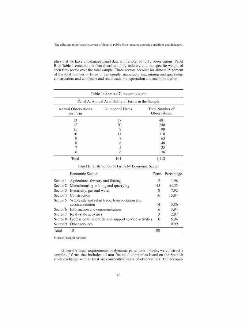
plies that we have unbalanced panel data with a total of 1,112 observations. PanelB of Table 1 contains the firm distribution by industry and the specific weight ofeach firm sector over the total sample. Three sectors account for almost 75 percentof the total number of firms in the sample: manufacturing, mining and quarrying;construction; and wholesale and retail trade, transportation and accommodation.


43

Table 1: SAMPLE CHARACTERISTICS

Panel A: Annual Availability of Firms in the Sample

Annual Observations Number of Firms Total Number ofper Firm Observations

13 37 48112 20 24011 9 9910 11 110

9 7 638 6 487 5 356 6 36

Total 101 1,112

Panel B: Distribution of Firms by Economic Sector

Economic Sectors Firms Percentage

Sector 1 Agriculture, forestry and fishing 2 1.98Sector 2 Manufacturing, mining and quarrying 45 44.55Sector 3 Electricity, gas and water 8 7.92Sector 4 Construction 16 15.84Sector 5 Wholesale and retail trade, transportation and

accommodation 14 13.86Sector 6 Information and communication 6 5.94Sector 7 Real estate activities 3 2.97Sector 8 Professional, scientific and support service activities 6 5.94Sector 9 Other services 1 0.99

Total 101 100

Source: Own elaboration.

Given the usual requirements of dynamic panel data models, we construct asample of firms that includes all non-financial companies listed on the Spanishstock exchange with at least six consecutive years of observations. The account-

ing information of these firms is obtained from the Sistema de Análisis de Bal-ances Ibéricos (SABI), a database managed by Bureau Van Dyck and Grupo In-forma, S.A., while financial market information was provided by the quotationbulletins of the Spanish stock exchange.

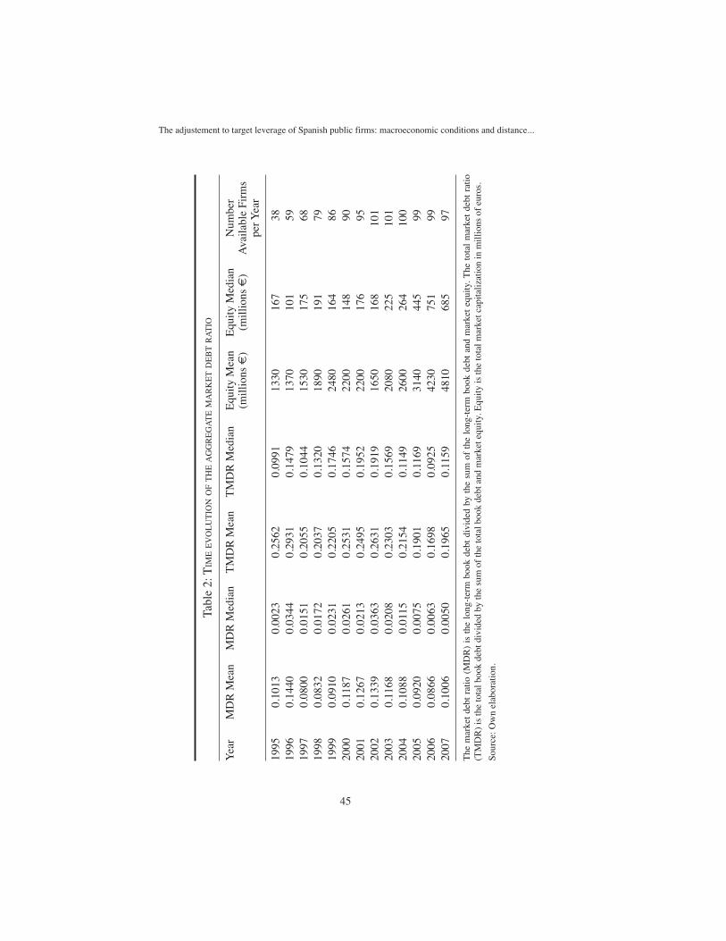
Table 2 reports summary statistics for alternative measures of aggregateleverage and the total value of equity for our sample of firms. The market debtratio is the long-term book value of debt of all firms in our sample divided by thesum of the aggregate market equity and the long-term book value of debt of allfirms. The total market debt ratio is the total book value of debt of all firms divid-ed by the sum of the aggregate market equity and the total book value of debt ofall firms in our sample. Equity is the total market capitalization of all availablefirms. The last column of Table 2 shows the time structure of the available sample.Our sample ranges from 38 firms in 1995 to 101 companies in 2002 and 2003. Thenumber of firms in the sample remains relatively stable after 2000.

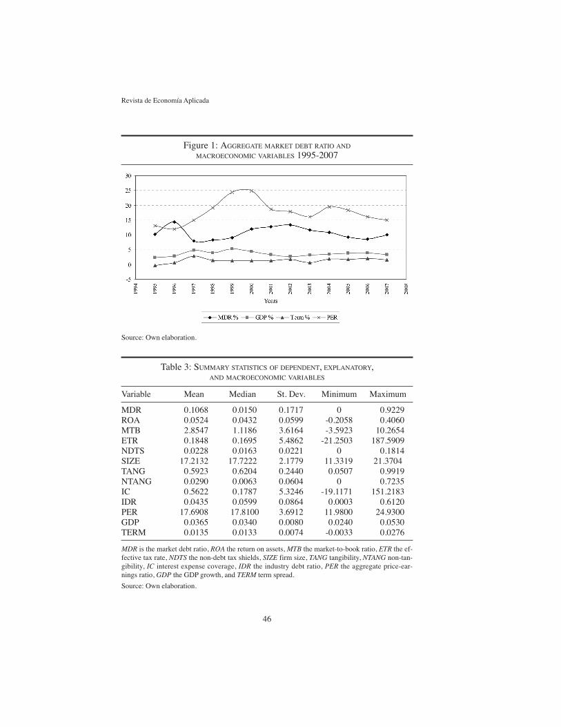
Figure 1 displays the evolution of the (long-term) market debt ratio from 1995to 2007. The sample is made up of two basic periods: an increasing pattern from1997 to 2002 and a decreasing market debt ratio from 2003 to 2006. The latter isclearly influenced by the extremely good performance of the Spanish equity mar-ket during those four years. The highest ratio is reached in 1996, while there isslight change in tendency between 2006 and 2007. Figure 1 also shows the evolu-tion of the three macroeconomic variables: the contemporaneous real GDP growth,the lagged PER and the lagged TERM. The three business cycle variables behavesimilarly over time, with positive correlation coefficients between them and an ex-pected negative correlation between each of them and the market debt ratio. Thisconfirms the countercyclical nature of the leverage ratio for Spanish firms.

Table 3 shows the main descriptive statistics of the dependent variable, the fi-nancial characteristics defining the target debt ratio and the three macroeconomicindicators. The financial characteristics are winsorized at the first and 99th per-centiles to avoid the influence of very extreme observations. It is important to notethat the average real GDP growth during our sample period is 3.65 percent, whilethe maximum and minimum growth rates are 5.3 percent and 2.4 percent, respec-tively. These statistics cast doubt on the ability of our sample period to capture suf-ficient fluctuations of the economy to classify the available years as either boomsor recessions. This clearly introduces an interpretation problem about the effects ofmacroeconomic variables on the speed of adjustment of Spanish public firms.

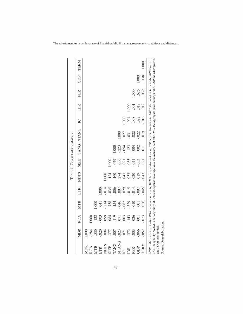
Table 4 reports the correlation matrix for our financial and macroeconomicvariables. According to most of the previous evidence, market debt ratios are neg-atively correlated with return on assets and the market-to-book ratio and positive-ly correlated with firm size. We also find a negative correlation between market-to-book ratios and non-debt tax shields and between tangible assets and bothreturn on assets and non-debt tax shields. Finally, the correlation between non-tangible assets and non-debt tax shields is positive. The only potentially problem-atic correlation for the empirical tests reported below is the large negative correla-tion coefficient between size and the market-to-book ratio.


44


45

Tabl

e 2:

TIM

EE

VO

LU

TIO

NO

FT

HE

AG

GR

EG

AT

EM

AR

KE

TD

EB

TR

AT

IO

Yea

rM

DR

Mea

nM

DR

Med

ian

TM

DR

Mea

nT

MD

R M

edia

nE

quity

Mea

nE

quity

Med

ian

Num

ber

(mill

ions

€)

(mill

ions

€)

Ava

ilabl

e Fi

rms

per Y

ear

1995

0.10

130.

0023

0.25

620.

0991

1330

167

3819

960.

1440

0.03

440.

2931

0.14

7913

7010

159

1997

0.08

000.

0151

0.20

550.

1044

1530

175

6819

980.

0832

0.01

720.

2037

0.13

2018

9019

179

1999

0.09

100.

0231

0.22

050.

1746

2480

164

8620

000.

1187

0.02

610.

2531

0.15

7422

0014

890

2001

0.12

670.

0213

0.24

950.

1952

2200

176

9520

020.

1339

0.03

630.

2631

0.19

1916

5016

810

120

030.

1168

0.02

080.

2303

0.15

6920

8022

510

120

040.

1088

0.01

150.

2154

0.11

4926

0026

410

020

050.

0920

0.00

750.

1901

0.11

6931

4044

599

2006

0.08

660.

0063

0.16

980.

0925

4230

751

9920

070.

1006

0.00

500.

1965

0.11

5948

1068

597

The

mar

ket

debt

rat

io (

MD

R)

is t

he l

ong-

term

boo

k de

bt d

ivid

ed b

y th

e su

m o

f th

e lo

ng-t

erm

boo

k de

bt a

nd m

arke

t eq

uity

. The

tot

al m

arke

t de

bt r

atio

(TM

DR

) is

the

tota

l boo

k de

bt d

ivid

ed b

y th

e su

m o

f th

e to

tal b

ook

debt

and

mar

ket e

quity

. Equ

ity is

the

tota

l mar

ket c

apita

lizat

ion

in m

illio

ns o

f eu

ros.

Sour

ce: O

wn

elab

orat

ion.


46

Figure 1: AGGREGATE MARKET DEBT RATIO AND

MACROECONOMIC VARIABLES 1995-2007


Table 3: SUMMARY STATISTICS OF DEPENDENT, EXPLANATORY,AND MACROECONOMIC VARIABLES

Variable Mean Median St. Dev. Minimum Maximum

MDR 0.1068 0.0150 0.1717 0 0.9229ROA 0.0524 0.0432 0.0599 -0.2058 0.4060MTB 2.8547 1.1186 3.6164 -3.5923 10.2654ETR 0.1848 0.1695 5.4862 -21.2503 187.5909NDTS 0.0228 0.0163 0.0221 0 0.1814SIZE 17.2132 17.7222 2.1779 11.3319 21.3704TANG 0.5923 0.6204 0.2440 0.0507 0.9919NTANG 0.0290 0.0063 0.0604 0 0.7235IC 0.5622 0.1787 5.3246 -19.1171 151.2183IDR 0.0435 0.0599 0.0864 0.0003 0.6120PER 17.6908 17.8100 3.6912 11.9800 24.9300GDP 0.0365 0.0340 0.0080 0.0240 0.0530TERM 0.0135 0.0133 0.0074 -0.0033 0.0276

MDR is the market debt ratio, ROA the return on assets, MTB the market-to-book ratio, ETR the ef-fective tax rate, NDTS the non-debt tax shields, SIZE firm size, TANG tangibility, NTANG non-tan-gibility, IC interest expense coverage, IDR the industry debt ratio, PER the aggregate price-ear-nings ratio, GDP the GDP growth, and TERM term spread.



47

Tabl

e 4:

CO

RR

EL

AT

ION

MA

TR

IX

MD

RR

OA

MT

BE

TR

ND

TS

SIZ

ETA

NG

NTA

NG

ICID

RPE

RG

DP

TE

RM

MD

R1.

000

RO

A-.

284

1.00

0M

TB

-.53

0.1

221.

000

ET

R-.

020

-.00

3.0

411.

000

ND

TS

.094

.099

-.21

4-.

014

1.00

0SI

ZE

.377

.084

-.75

8-.

035

.124

1.00

0TA

NG

-.00

7-.

119

.154

.006

-.16

0-.

079

1.00

0N

TAN

G-.

023

.071

-.04

6.0

07.2

74.0

56-.

223

1.00

0IC

.071

.003

-.08

2.0

29.0

43.0

21-.

054

.027

1.00

0ID

R.3

72-.

143

-.32

9-.

015

.033

.085

.123

-.03

1.0

041.

000

PER

-.00

3.0

26-.

010

-.01

4-.

020

-.02

1-.

004

.022

.008

.001

1.00

0G

DP

-.06

6.0

01.0

01-.

007

.019

-.03

3.0

02-.

022

.022

.017

.626

1.00

0T

ER

M-.

052

-.02

3.0

26-.

045

-.04

7.0

27.0

11.0

19-.

016

.012

.039

.338

1.00

0

MD

Ris

the

mar

ket

debt

rat

io, R

OA

the

retu

rn o

n as

sets

, MT

Bth

e m

arke

t-to

-boo

k ra

tio, E

TR

the

effe

ctiv

e ta

x ra

te, N

DT

S th

e no

n-de

bt t

ax s

hiel

ds, S

IZE

firm

siz

e,TA

NG

tang

ibili

ty, N

TAN

Gno

n-ta

ngib

ility

, IC

inte

rest

exp

ense

cov

erag

e, I

DR

the

indu

stry

deb

t rat

io, P

ER

the

aggr

egat

e pr

ice-

earn

ings

rat

io, G

DP

the

GD

P gr

owth

,an

d T

ER

Mte

rm s

prea

d.

Sour

ce: O

wn

elab

orat

ion.

3. EMPIRICAL EVIDENCE

3.1. The Long Difference EstimatorIt is well known that the estimation of dynamic panel data as in expressions

[4], [7], and [9] is non-trivial because the combination of fixed effects and alagged highly persistent dependent variable can severely bias coefficient esti-mates, particularly when the panel length is small14. The Appendix at the end ofthis paper provides a detailed explanation of these biases and discusses potentialsolutions. Unfortunately, applying the traditional “within” transformation or firstdifference estimator to remove the time-invariant fixed effects generates a corre-lation between the new lagged dependent variable and the new error term thatleads to biased and inconsistent results. Since the instrumental variable solution isdifficult to implement because reasonable instrumental variables are difficult toobtain, many papers employ the system GMM estimation of Arellano and Bover(1995) and Blundell and Bond (1998). This procedure instruments for the firstdifference of predetermined variables with lags of their own levels and differ-ences. However, as recently shown by Hahn et al. (2007) and Huang and Ritter(2009), the system GMM use of the full set of moment conditions does not pro-vide proper guidance in dynamic panel data models when the dependent variableis highly persistent, so the autoregressive parameter is close to one15. Moreover,in this case, the GMM system estimators are downward biased, so the estimate ofthe speed of adjustment is upward biased.

We now briefly discuss the long difference estimator procedure. Consider adynamic panel data equation at the end of year t with fixed effects:


48

[10]MDR X MDR ujt jt jt j jt= ( )′ + −( ) + +( )− −λβ λ μ1 11 .

The dynamic equation at the end of year t - k with fixed effects is given by

[11]MDRjt −− − − − − −= ( )′ + −( ) + +( )k jt k jt k j jt kX MDR uλβ λ μ1 11 .

Then, subtracting [11] from [10], we get the equation to be estimated underthe long difference estimator:

[12]MDR MDR X X MDRjt jt k jt jt k− = ( )′ −( ) + −( )− − − −λβ λ1 1 1 jjt jt kMDR− − −−( ) +1 1

jt jt ku u −+ −( )We first estimate equation [12] by the system GMM to obtain the initial para-

meter estimators, using MDRjt–k–1 and Xjt–k–1 as valid instruments. Then we obtain

(14) This is usually the case with Spanish data.(15) This is, of course, the case with market debt ratios.

the residuals of equation [11], MDR X MDRjt jt− −− − −( )1 2 1ˆ ˆ ˆλβ λ jjt jt kMDR− −( ) −2 , ,… (

When recognizing the potential effects of macroeconomic variables, we followthe same procedure, using equations [7] and [9] with fixed effects instead of [10].

3.2. The speed of adjustment of Spanish public firmsThis paper estimates the speed of adjustment using four alternative econometric

procedures described in the Appendix and in Section 3.116. We first employ the de-meaned Fama-MacBeth (hereafter FM, 1973) and the difference GMM. Given theprevious discussion and the analysis presented in the Appendix, we also report re-sults for the system GMM of Arellano and Bover (1995) and Blundell and Bond(1998), and the long difference estimator of Hahn et al. (2007). All procedures applyto the dynamic panel data equations with and without macroeconomic conditions.

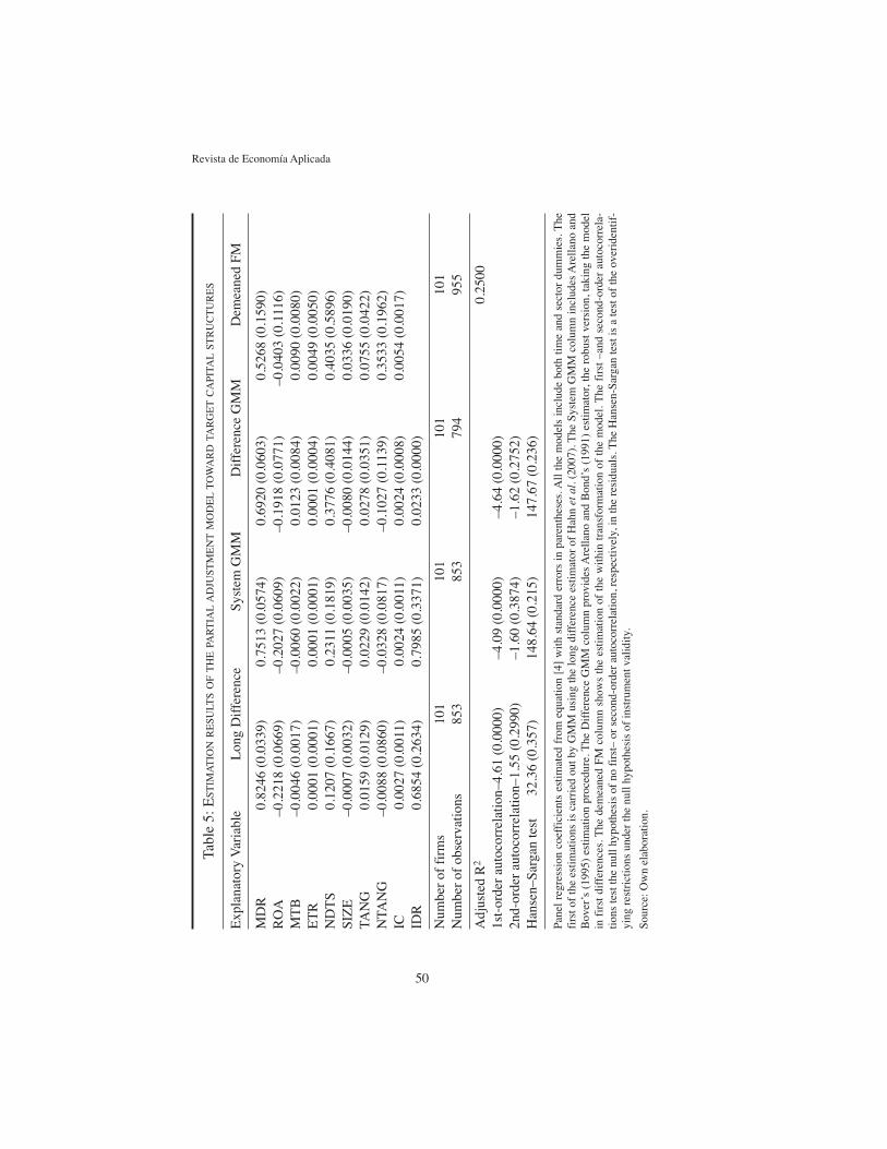
Table 5 presents the results of the estimation of the partial adjustment modelgiven by expression [4]. There are four lagged financial explanatory variables withthe correct theoretical sign that are estimated with a relatively low standard error.Profitability, the market-to-book ratio, the industry market debt ratio and interestcoverage are all statistically significant, at least for the long difference and the sys-tem GMM estimators given in the first and second columns of Table 5. Firms withhigh profitability and market-to-book ratios have less leverage, while firms withhigher interest coverage and those that belong to an industry with high leverage pre-sent higher market debt ratios. Tangible assets tend to be positively and significantlyassociated with leverage under traditional panel data methods, but this characteristicis estimated with a large standard error under the long difference estimator.

The specification tests under the long difference estimator and the GMMmethodologies suggest that we cannot reject the model at conventional significancelevels. As expected, given the discussion on the econometric issues, the coefficientof the speed of adjustment tends to vary quite significantly across estimationmethodologies. The demeaned FM two-stage estimation presents a very high speedof adjustment. The GMM estimator procedures obtain a speed of adjustment of 24.9percent and 30.8 percent for the system and difference GMM, respectively. Thesevalues are similar to, although slightly lower than, the speed of adjustment foundfor U.S. companies by Flannery and Rangan (2006) and Antoniou et al. (2008).

As in Huang and Ritter (2009), we find that the long difference estimator gen-erates a speed of adjustment lower than that under the system GMM methodology.The long difference estimator is obtained with three iterations and for k = 2. Ourdatabase is much smaller than that available to Huang and Ritter (2009), whichclearly limits our possibilities for checking our results for alternative lags. The


49

and, finally, we employ MDRjt–k–1, Xjt–k–1, and those

residuals as new instruments. This is the first iteration. Both Hahn et al. (2007)and Huang and Ritter (2009) use three iterations to obtain the final estimators.Additionally, using data from 1972 to 2001, Huang and Ritter (2009) try four al-ternative lag values for k and show that the coefficient of the speed of adjustmentvaries from 22.3 percent when k = 4 to 17.6 for k = 28.

jt k jt kX MDR− − −− −( )1 1ˆ ˆ ˆλβ λ −− )1

(16) All models are estimated with both time and sector dummies.


50

Tabl

e 5:

EST

IMA

TIO

NR

ESU

LTS

OF

TH

EPA

RT

IAL

AD

JUST

ME

NT

MO

DE

LT

OW

AR

DTA

RG

ET

CA

PITA

LST

RU

CT

UR

ES

Exp

lana

tory

Var

iabl

eL

ong

Dif

fere

nce

Syst

em G

MM

Dif

fere

nce

GM

MD

emea

ned

FM

MD

R0.

8246

(0.

0339

)0.

7513

(0.

0574

)0.

6920

(0.

0603

)0.

5268

(0.

1590

)R

OA

–0.2

218

(0.0

669)

–0.2

027

(0.0

609)

–0.1

918

(0.0

771)

–0.0

403

(0.1

116)

MT

B–0

.004

6 (0

.001

7)–0

.006

0 (0

.002

2)0.

0123

(0.

0084

)0.

0090

(0.

0080

)E

TR

0.00

01 (

0.00

01)

0.00

01 (

0.00

01)

0.00

01 (

0.00

04)

0.00

49 (

0.00

50)

ND

TS

0.12

07 (

0.16

67)

0.23

11 (

0.18

19)

0.37

76 (

0.40

81)

0.40

35 (

0.58

96)

SIZ

E–0

.000

7 (0

.003

2)–0

.000

5 (0

.003

5)–0

.008

0 (0

.014

4)0.

0336

(0.

0190

)TA

NG

0.01

59 (

0.01

29)

0.02

29 (

0.01

42)

0.02

78 (

0.03

51)

0.07

55 (

0.04

22)

NTA

NG

–0.0

088

(0.0

860)

–0.0

328

(0.0

817)

–0.1

027

(0.1

139)

0.35

33 (

0.19

62)

IC0.

0027

(0.

0011

)0.

0024

(0.

0011

)0.

0024

(0.

0008

)0.

0054

(0.

0017

)ID

R0.

6854

(0.

2634

)0.

7985

(0.

3371

)0.

0233

(0.

0000

)

Num

ber

of f

irm

s10

110

110

110

1N

umbe

r of

obs

erva

tions

853

853

794

955

Adj

uste

d R

20.

2500

1st-

orde

r au

toco

rrel

atio

n–4.

61 (

0.00

00)

–4.0

9 (0

.000

0)–4

.64

(0.0

000)

2nd-

orde

r au

toco

rrel

atio

n–1.

55 (

0.29

90)

–1.6

0 (0

.387

4)–1

.62

(0.2

752)

Han

sen–

Sarg

an te

st32

.36

(0.3

57)

148.

64 (

0.21

5)14

7.67

(0.

236)

Pane

l re

gres

sion

coe

ffic

ient

s es

timat

ed f

rom

equ

atio

n [4

] w

ith s

tand

ard

erro

rs i

n pa

rent

hese

s. A

ll th

e m

odel

s in

clud

e bo

th t

ime

and

sect

or d

umm

ies.

The

firs

t of

the

estim

atio

ns is

car

ried

out

by

GM

M u

sing

the

long

dif

fere

nce

estim

ator

of

Hah

n et

al.

(200

7). T

he S

yste

m G

MM

col

umn

incl

udes

Are

llano

and

Bov

er’s

(19

95)

estim

atio

n pr

oced

ure.

The

Dif

fere

nce

GM

M c

olum

n pr

ovid

es A

rella

no a

nd B

ond’

s (1

991)

est

imat

or, t

he r

obus

t ver

sion

, tak

ing

the

mod

elin

fir

st d

iffe

renc

es. T

he d

emea

ned

FM c

olum

n sh

ows

the

estim

atio

n of

the

with

in t

rans

form

atio

n of

the

mod

el. T

he f

irst

–an

d se

cond

-ord

er a

utoc

orre

la-

tions

test

the

null

hypo

thes

is o

f no

fir

st–

or s

econ

d-or

der

auto

corr

elat

ion,

res

pect

ivel

y, in

the

resi

dual

s. T

he H

anse

n-Sa

rgan

test

is a

test

of

the

over

iden

tif-

ying

res

tric

tions

und

er th

e nu

ll hy

poth

esis

of

inst

rum

ent v

alid

ity.

Sour

ce: O

wn

elab

orat

ion.

speed of adjustment for Spanish public firms under the long difference estimator is17.5 percent. This implies that the typical Spanish firm closes approximately one-fifth of the gap between its current and target debt ratios each year. Interestingly, theestimate of the speed of adjustment is clearly lower than those reported by DeMiguel and Pindado (2001) and González and González (2008)17, which suggeststhat Spanish firms adjust slowly toward their target leverage. In fact, that estimate iseven lower than the speed coefficient reported by Huang and Ritter (2009) for U.S.data, also using the long difference estimator. Under the system GMM procedure,typical firms close one-fourth of the gap each year. It would be interesting to inves-tigate whether this relatively low speed of adjustment of Spanish firms can be ex-plained by the particularly narrow market for corporate debt in Spain. It may just bethe case that restrictions to external market debt financing impact the potentially de-sired changes of the capital structure of Spanish firms.

3.3. The Time-Varying Speed of Adjustment of Spanish Public FirmsTable 6 contains evidence about the influence of macroeconomic conditions

on the speed of adjustment toward the target debt ratio. We now estimate equation[7] using the long difference estimator, again with three iterations and k = 2. Weestimate this equation separately for each of our three macroeconomic variablesdescribed in subsection 1.318. As before, temporal data limitations can reduce thepossibility of finding significant results. The low frequency of data, available ex-clusively on a year-by-year basis, can also bias our results. None of the macroeco-nomic variables show any significant impact on the speed of adjustment. It seemsthat, contrary to the U.S. evidence, Spanish firms do not move faster toward tar-get leverage during good economic periods. As already mentioned, this conclu-sion should be made with caution, because our sample period does not presentsignificantly economic and contractions.

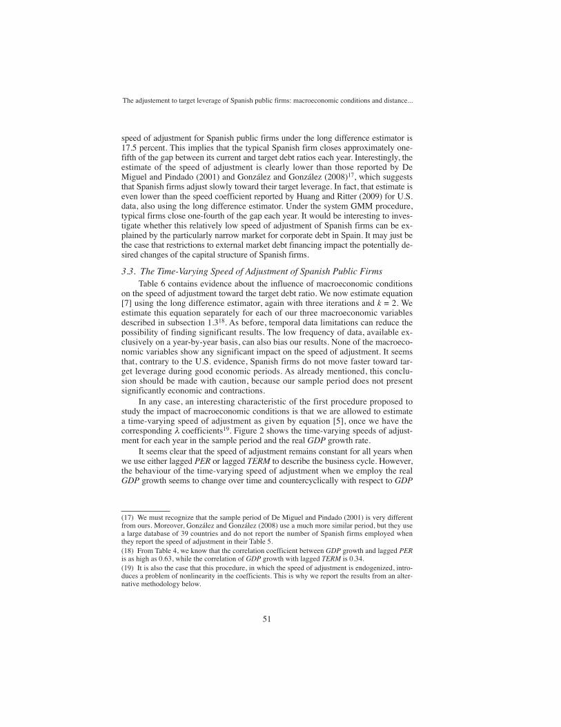
In any case, an interesting characteristic of the first procedure proposed tostudy the impact of macroeconomic conditions is that we are allowed to estimatea time-varying speed of adjustment as given by equation [5], once we have thecorresponding λ coefficients19. Figure 2 shows the time-varying speeds of adjust-ment for each year in the sample period and the real GDP growth rate.

It seems clear that the speed of adjustment remains constant for all years whenwe use either lagged PER or lagged TERM to describe the business cycle. However,the behaviour of the time-varying speed of adjustment when we employ the realGDP growth seems to change over time and countercyclically with respect to GDP


51

(17) We must recognize that the sample period of De Miguel and Pindado (2001) is very differentfrom ours. Moreover, González and González (2008) use a much more similar period, but they usea large database of 39 countries and do not report the number of Spanish firms employed whenthey report the speed of adjustment in their Table 5.(18) From Table 4, we know that the correlation coefficient between GDP growth and lagged PERis as high as 0.63, while the correlation of GDP growth with lagged TERM is 0.34.(19) It is also the case that this procedure, in which the speed of adjustment is endogenized, intro-duces a problem of nonlinearity in the coefficients. This is why we report the results from an alter-native methodology below.

growth. Indeed, if we separate the 13 years of data into three groups, where the fouryears of higher GDP growth are classified as a good economic state while the fouryears of lower GDP growth are the contraction states, and then calculate the meanof the time-varying speed of adjustment for either good or bad states, we find thatthe average speed of adjustment is 0.15 during expansions and as high as 0.21 dur-ing contractions. Although the formal test of Table 6 rejects the hypothesis thatmacroeconomic variables significantly affect the speed of adjustment, this counter-cyclical behaviour of the speed of adjustment seems to contradict the previous evi-dence reported by Drobetz et al. (2007) and Cook and Tang (2010).

The mean of the sample market debt ratio reported in Table 3, which amountsto 10.68 percent, is obtained using exclusively interest-bearing long-term debt.This seems to be a rather low financing ratio. An alternative leverage measure


52

Table 6: ESTIMATION RESULTS OF THE PARTIAL ADJUSTMENT MODEL TOWARD

TARGET CAPITAL STRUCTURES WITH MACROECONOMIC VARIABLES

Explanatory Variable Long Difference Estimator

MDR 0.8097 (0.2595) 0.6969 (0.2008) 0.8194 (0.0844)ROA –0.1949 (0.0616) –0.2299 (0.0684) –0.2075 (0.0641)MTB 0.0056 (0.0052) 0.0043 (0.0091) 0.0058 (0.0026)ETR –0.0138 (0.0154) –0.0064 (0.0097) –0.0011 (0.0009)NDTS –3.2528 (0.8837) –1.7666 (0.9113) –0.0572 (0.3975)SIZE –0.0085 (0.0048) –0.0022 (0.0122) –0.0001 (0.0031)TANG 0.1647 (0.0739) 0.0789 (0.0578) 0.0011 (0.0314)NTANG 0.9457 (0.3692) 0.5156 (0.3802) 0.0795 (0.1117)IC 0.0001 (0.0001) 0.0126 (0.0056) 0.0001 (0.0001)IDR 1.4043 (0.4078) 1.3017 (0.3707) 0.3463 (0.2731)PER x MDR 0.0004 (0.0126)GDP x MDR 3.3940 (4.9473)TERM x MDR 0.2635 (5.4883)

Number of firms 101 101 101Number of observations 853 853 853

1st-order autocorrelation–4.57 (0.0000)–4.82 (0.0000) –4.60 (0.0000)2nd-order autocorrelation–0.84 (0.4010)–1.27 (0.2050) –1.18 (0.2370)Hansen–Sargan test132.55 (0.234) 133.50 (0.246) 131.35 (0.241)

Panel regression coefficients estimated from equation [7], with standard errors in parentheses. All themodels include sector dummies and all the estimations are carried out by GMM using the long diffe-rence estimator of Hahn et al. (2007). The first- and second-order autocorrelations test the null hypot-hesis of no first- or second-order autocorrelation, respectively, in the residuals. The Hansen-Sargantest is a test of the overidentifying restrictions under the null hypothesis of instrument validity.


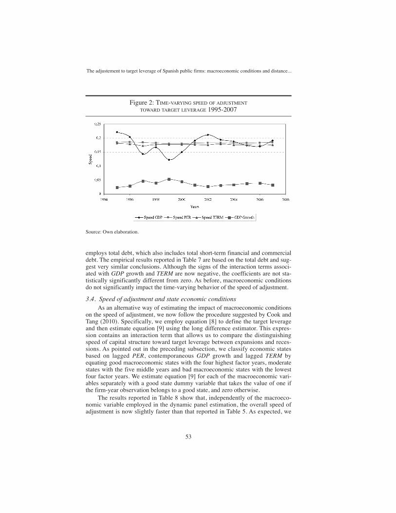
employs total debt, which also includes total short-term financial and commercialdebt. The empirical results reported in Table 7 are based on the total debt and sug-gest very similar conclusions. Although the signs of the interaction terms associ-ated with GDP growth and TERM are now negative, the coefficients are not sta-tistically significantly different from zero. As before, macroeconomic conditionsdo not significantly impact the time-varying behavior of the speed of adjustment.

3.4. Speed of adjustment and state economic conditionsAs an alternative way of estimating the impact of macroeconomic conditions

on the speed of adjustment, we now follow the procedure suggested by Cook andTang (2010). Specifically, we employ equation [8] to define the target leverageand then estimate equation [9] using the long difference estimator. This expres-sion contains an interaction term that allows us to compare the distinguishingspeed of capital structure toward target leverage between expansions and reces-sions. As pointed out in the preceding subsection, we classify economic statesbased on lagged PER, contemporaneous GDP growth and lagged TERM byequating good macroeconomic states with the four highest factor years, moderatestates with the five middle years and bad macroeconomic states with the lowestfour factor years. We estimate equation [9] for each of the macroeconomic vari-ables separately with a good state dummy variable that takes the value of one ifthe firm-year observation belongs to a good state, and zero otherwise.

The results reported in Table 8 show that, independently of the macroeco-nomic variable employed in the dynamic panel estimation, the overall speed ofadjustment is now slightly faster than that reported in Table 5. As expected, we


53

Figure 2: TIME-VARYING SPEED OF ADJUSTMENT

TOWARD TARGET LEVERAGE 1995-2007


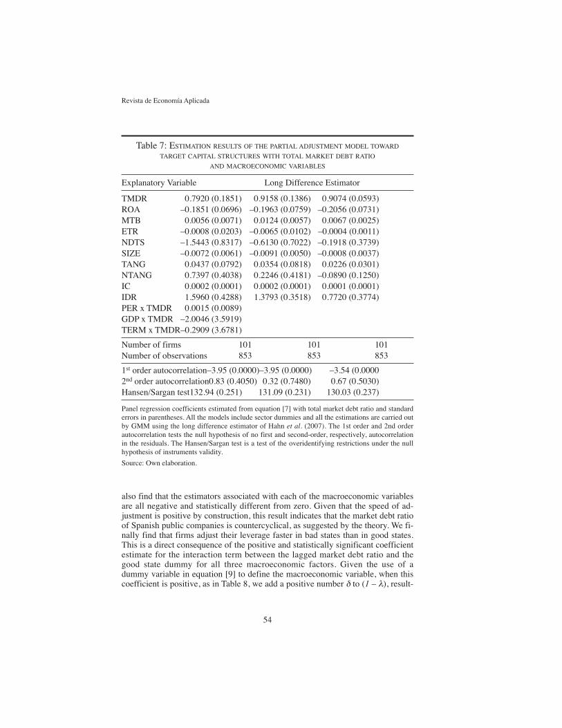
also find that the estimators associated with each of the macroeconomic variablesare all negative and statistically different from zero. Given that the speed of ad-justment is positive by construction, this result indicates that the market debt ratioof Spanish public companies is countercyclical, as suggested by the theory. We fi-nally find that firms adjust their leverage faster in bad states than in good states.This is a direct consequence of the positive and statistically significant coefficientestimate for the interaction term between the lagged market debt ratio and thegood state dummy for all three macroeconomic factors. Given the use of adummy variable in equation [9] to define the macroeconomic variable, when thiscoefficient is positive, as in Table 8, we add a positive number δ to (1 – λ), result-


54


TARGET CAPITAL STRUCTURES WITH TOTAL MARKET DEBT RATIO

AND MACROECONOMIC VARIABLES


TMDR 0.7920 (0.1851) 0.9158 (0.1386) 0.9074 (0.0593)ROA –0.1851 (0.0696) –0.1963 (0.0759) –0.2056 (0.0731)MTB 0.0056 (0.0071) 0.0124 (0.0057) 0.0067 (0.0025)ETR –0.0008 (0.0203) –0.0065 (0.0102) –0.0004 (0.0011)NDTS –1.5443 (0.8317) –0.6130 (0.7022) –0.1918 (0.3739)SIZE –0.0072 (0.0061) –0.0091 (0.0050) –0.0008 (0.0037)TANG 0.0437 (0.0792) 0.0354 (0.0818) 0.0226 (0.0301)NTANG 0.7397 (0.4038) 0.2246 (0.4181) –0.0890 (0.1250)IC 0.0002 (0.0001) 0.0002 (0.0001) 0.0001 (0.0001)IDR 1.5960 (0.4288) 1.3793 (0.3518) 0.7720 (0.3774)PER x TMDR 0.0015 (0.0089)GDP x TMDR –2.0046 (3.5919)TERM x TMDR–0.2909 (3.6781)


1st order autocorrelation–3.95 (0.0000)–3.95 (0.0000) –3.54 (0.00002nd order autocorrelation0.83 (0.4050) 0.32 (0.7480) 0.67 (0.5030)Hansen/Sargan test132.94 (0.251) 131.09 (0.231) 130.03 (0.237)

Panel regression coefficients estimated from equation [7] with total market debt ratio and standarderrors in parentheses. All the models include sector dummies and all the estimations are carried outby GMM using the long difference estimator of Hahn et al. (2007). The 1st order and 2nd orderautocorrelation tests the null hypothesis of no first and second-order, respectively, autocorrelationin the residuals. The Hansen/Sargan test is a test of the overidentifying restrictions under the nullhypothesis of instruments validity.


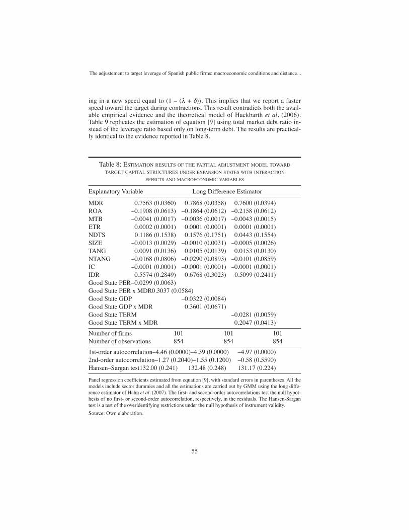
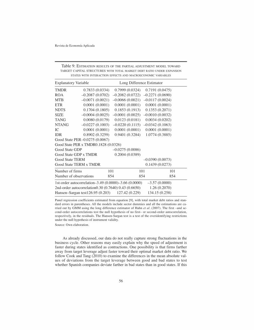
ing in a new speed equal to (1 – (λ + δ)). This implies that we report a fasterspeed toward the target during contractions. This result contradicts both the avail-able empirical evidence and the theoretical model of Hackbarth et al. (2006).Table 9 replicates the estimation of equation [9] using total market debt ratio in-stead of the leverage ratio based only on long-term debt. The results are practical-ly identical to the evidence reported in Table 8.


55


TARGET CAPITAL STRUCTURES UNDER EXPANSION STATES WITH INTERACTION

EFFECTS AND MACROECONOMIC VARIABLES


MDR 0.7563 (0.0360) 0.7868 (0.0358) 0.7600 (0.0394)ROA –0.1908 (0.0613) –0.1864 (0.0612) –0.2158 (0.0612)MTB –0.0041 (0.0017) –0.0036 (0.0017) –0.0043 (0.0015)ETR 0.0002 (0.0001) 0.0001 (0.0001) 0.0001 (0.0001)NDTS 0.1186 (0.1538) 0.1576 (0.1751) 0.0443 (0.1554)SIZE –0.0013 (0.0029) –0.0010 (0.0031) –0.0005 (0.0026)TANG 0.0091 (0.0136) 0.0105 (0.0139) 0.0153 (0.0130)NTANG –0.0168 (0.0806) –0.0290 (0.0893) –0.0101 (0.0859)IC –0.0001 (0.0001) –0.0001 (0.0001) –0.0001 (0.0001)IDR 0.5574 (0.2849) 0.6768 (0.3023) 0.5099 (0.2411)Good State PER–0.0299 (0.0063)Good State PER x MDR0.3037 (0.0584)Good State GDP –0.0322 (0.0084)Good State GDP x MDR 0.3601 (0.0671)Good State TERM –0.0281 (0.0059)Good State TERM x MDR 0.2047 (0.0413)


1st-order autocorrelation–4.46 (0.0000)–4.39 (0.0000) –4.97 (0.0000)2nd-order autocorrelation–1.27 (0.2040)–1.55 (0.1200) –0.58 (0.5590)Hansen–Sargan test132.00 (0.241) 132.48 (0.248) 131.17 (0.224)

Panel regression coefficients estimated from equation [9], with standard errors in parentheses. All themodels include sector dummies and all the estimations are carried out by GMM using the long diffe-rence estimator of Hahn et al. (2007). The first- and second-order autocorrelations test the null hypot-hesis of no first- or second-order autocorrelation, respectively, in the residuals. The Hansen-Sargantest is a test of the overidentifying restrictions under the null hypothesis of instrument validity.


As already discussed, our data do not really capture strong fluctuations in thebusiness cycle. Other reasons may easily explain why the speed of adjustment isfaster during states identified as contractions. One possibility is that firms fartheraway from target leverage adjust faster toward their optimal market debt ratio. Wefollow Cook and Tang (2010) to examine the differences in the mean absolute val-ues of deviations from the target leverage between good and bad states to testwhether Spanish companies deviate farther in bad states than in good states. If this


56


TARGET CAPITAL STRUCTURES WITH TOTAL MARKET DEBT RATIO UNDER EXPANSION

STATES WITH INTERACTION EFFECTS AND MACROECONOMIC VARIABLES


TMDR 0.7833 (0.0334) 0.7999 (0.0324) 0.7191 (0.0475)ROA –0.2087 (0.0702) –0.2082 (0.0722) –0.2271 (0.0690)MTB –0.0071 (0.0021) –0.0066 (0.0021) –0.0117 (0.0024)ETR 0.0001 (0.0001) 0.0001 (0.0001) 0.0001 (0.0001)NDTS 0.1704 (0.1805) 0.1853 (0.1913) 0.1353 (0.2071)SIZE –0.0004 (0.0025) –0.0001 (0.0025) –0.0010 (0.0032)TANG 0.0080 (0.0179) 0.0123 (0.0181) 0.0034 (0.0202)NTANG –0.0227 (0.1003) –0.0220 (0.1115) –0.0342 (0.1063)IC 0.0001 (0.0001) 0.0001 (0.0001) 0.0001 (0.0001)IDR 0.8902 (0.3259) 0.9401 (0.3284) 1.0774 (0.3885)Good State PER–0.0275 (0.0067)Good State PER x TMDR0.1828 (0.0326)Good State GDP –0.0275 (0.0086)Good State GDP x TMDR 0.2004 (0.0389)Good State TERM –0.0390 (0.0073)Good State TERM x TMDR 0.1439 (0.0273)


1st-order autocorrelation–3.49 (0.0000)–3.66 (0.0000) –3.57 (0.0000)2nd-order autocorrelation0.30 (0.7640) 0.43 (0.6650) 1.26 (0.2070)Hansen–Sargan test126.95 (0.203) 127.42 (0.229) 134.15 (0.258)

Panel regression coefficients estimated from equation [9], with total market debt ratios and stan-dard errors in parentheses. All the models include sector dummies and all the estimations are ca-rried out by GMM using the long difference estimator of Hahn et al. (2007). The first –and se-cond-order autocorrelations test the null hypothesis of no first– or second-order autocorrelation,respectively, in the residuals. The Hansen-Sargan test is a test of the overidentifying restrictionsunder the null hypothesis of instrument validity.


is the case, the results reported in Table 8 can be attributed to the distance betweencurrent and target market debt ratios rather than to macroeconomic conditions.This case would also be consistent with the results reported in Tables 6 and 7.

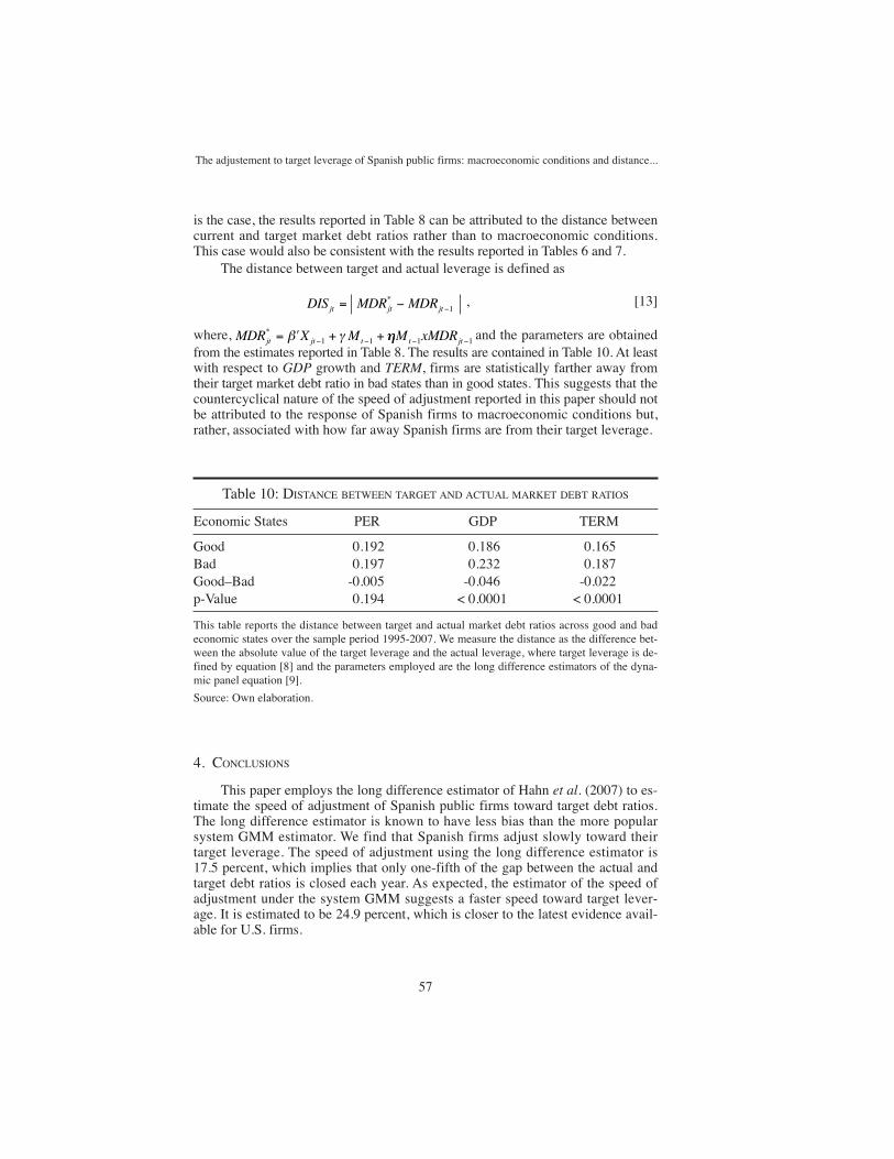
The distance between target and actual leverage is defined as


57

[13]DIS MDR MDRjt jt jt= − − *1

,

where, and the parameters are obtainedfrom the estimates reported in Table 8. The results are contained in Table 10. At leastwith respect to GDP growth and TERM, firms are statistically farther away fromtheir target market debt ratio in bad states than in good states. This suggests that thecountercyclical nature of the speed of adjustment reported in this paper should notbe attributed to the response of Spanish firms to macroeconomic conditions but,rather, associated with how far away Spanish firms are from their target leverage.

MDR X Mjt jt t= ′ + +− −*

1 1β γ ηηM xMDRt jt− −1 1

Table 10: DISTANCE BETWEEN TARGET AND ACTUAL MARKET DEBT RATIOS

Economic States PER GDP TERM

Good 0.192 0.186 0.165Bad 0.197 0.232 0.187Good–Bad -0.005 -0.046 -0.022p-Value 0.194 < 0.0001 < 0.0001

This table reports the distance between target and actual market debt ratios across good and badeconomic states over the sample period 1995-2007. We measure the distance as the difference bet-ween the absolute value of the target leverage and the actual leverage, where target leverage is de-fined by equation [8] and the parameters employed are the long difference estimators of the dyna-mic panel equation [9].


4. CONCLUSIONS

This paper employs the long difference estimator of Hahn et al. (2007) to es-timate the speed of adjustment of Spanish public firms toward target debt ratios.The long difference estimator is known to have less bias than the more popularsystem GMM estimator. We find that Spanish firms adjust slowly toward theirtarget leverage. The speed of adjustment using the long difference estimator is17.5 percent, which implies that only one-fifth of the gap between the actual andtarget debt ratios is closed each year. As expected, the estimator of the speed ofadjustment under the system GMM suggests a faster speed toward target lever-age. It is estimated to be 24.9 percent, which is closer to the latest evidence avail-able for U.S. firms.

We also analyze the importance of macroeconomic conditions on the speedof adjustment. The results suggest that Spanish public firms move faster towardtheir target market debt ratios during contractions than during expansions. This isespecially the case when we introduce macroeconomic conditions in the defini-tion of target leverage. However, there is also some evidence of a countercyclicalspeed of adjustment when we allow the speed of adjustment to be time varying.This result contrasts with previous international empirical evidence and with thetheoretical model of Hackbarth et al. (2006). Given the weak economic fluctua-tions characterizing the Spanish economy during our sample period, we measurethe distance between target market debt ratios and actual leverage to checkwhether the previous result is a direct consequence of Spanish firms being fartheraway from target during relatively bad economic times. This turns out to be thecase. We attribute the countercyclical nature of the speed of adjustment duringour sample period to the distance between actual and target leverage rather than tomacroeconomic conditions.

APPENDIX. SOME ECONOMETRIC ISSUES IN DYNAMIC PANEL DATA MODELS

Consider a dynamic panel data that can be understood as a simplified versionof equation [4]


58

[A.1]MDR MDRjt jt j jt= + +( )−β μ ε1,

where the residual term is composed of the unobserved time-invariant, firm-spe-cific effect captured by μj (fixed effect) and the usual residual given by εjt.Theproblem is that the residual component of MDRjt is correlated with the unob-served effect in the error term. Hence, a (pooled) ordinary least squares (OLS) es-timated coefficient on MDRjt–1 without fixed effects will be upwardly biased (orthe speed of adjustment downwardly biased). These simple regressions can alsobe estimated by the two-step procedure of Fama-MacBeth (FM hereafter, 1973),as suggested by Fama and French (2002). The authors recommend FM estimatorsto mitigate the underestimation of coefficient standard errors. Flannery and Ran-gan (2006) show that both the traditional (pooled) OLS and FM regressions yieldsimilar coefficient estimates but the t-statistics are much smaller when the FM es-timates are used in the regression. The problem is that the FM estimates also failto recognize the data’s panel characteristics. As pointed out above, if cross-sec-tional differences in target market debt ratios are driven by time-invariant, firm-specific components, either the FM procedure or the (pooled) OLS estimates willbe upwardly biased and the speed of adjustment downwardly biased.

The FM estimation procedure runs, for each observation T, an OLS cross-sectional regression with N observations (firms):

[A.2]MDR MDR u j Njt t jt jt= + =− −β 1 1 1 ; , ,… .

We keep the estimates of each beta, β̂t–1, for each cross-sectional regressionfrom t = 2 to t = T. The final estimates are

This discussion implies that a panel regression with unobserved (fixed) ef-fects is more appropriate if firms have relatively stable and unobserved variablesaffecting their leverage targets. There are two simple possibilities to adjust for thisbias. A common way to estimate panel data models with fixed effects is to per-form a “within” transformation of (A.1) and then estimate using OLS. This trans-formation expresses all variables as deviations from their firm-specific time seriesmeans. This eliminates μj from the regression, since it is time invariant and thusprovides consistent estimates. However, it should also be noted that the withintransformations of the lagged dependent variables and error terms are


59

[A.3]

ˆ ˆ

ˆ ˆˆ ˆ

β β

σ ββ β

=−

( ) =−( )

−

−=

−=

∑

∑

1

1

1

12

1

2

2

T

T

tt

T

tt

T

(( ) −( )T 2

[A.4]MDRT

MDRjt jtt

T

−=∑

1

1

uT

ujt jtt

T

−=∑

1

1

and .

Then, MDRj2 is correlated with uj2, MDRj3 is correlated with uj3, and so on.This implies that the coefficient of the lagged dependent variable, β, is downwardlybiased (the speed of adjustment is upwardly biased) by a factor of (approximately)1/T. In panel data sets with large T, this bias becomes insignificant, but in paneldata with capital structure observations, large N, and a relatively small T, the biascan be substantial. A similar alternative procedure consists of running FM cross-sectional regressions for each t once we express all variables as deviations fromtheir firm-specific time series mean. This straightforward alternative can also bedownwardly biased (upwardly biased for the speed of adjustment).

It is possible to obtain unbiased estimates of the levels regression (A.1) if aninstrument is found that is correlated with the lagged dependent variable but notwith the error term. We can use the lagged book debt ratio as the instrument. Thenew estimate should be between the OLS and the within estimates. This is theprocedure employed by Flannery and Rangan (2006) in their Tables 2 (columns 5to 7) and A.1 (column 3). In particular, the authors use a two-stage least squaresin which they substitute a fitted value for the lagged dependent variable, using thelagged book value of leverage and the X’s, from equation [3], as instruments.They first regress the lagged market debt ratio on the lagged book debt ratio andthe X’s, and then the fitted value from that regression is employed in the secondstage as the independent variable. We can then regress the market debt ratio onthe previous fitted value of the lagged market debt ratio and the control variables.A serious drawback is that the previous correction relies on the book debt ratiobeing a reasonable instrument for the market debt ratio. Of course, finding reli-able instruments can be difficult and a number of alternative econometric possi-bilities are available in literature.

These techniques generally first-difference the model (A.1) to eliminatefixed effects and use lagged dependent variables to instrument for the lagged firstdifference:


60

[A.5]MDR MDR MDR MDRjt jt jt jt jt jt− = −( ) + −(− − − −1 1 2 1β ε ε )) .

It is also well known that these first-difference methodologies rely on twokey assumptions to produce unbiased and consistent estimates. First, the errorterm in (A.1), εjt, should be serially uncorrelated, because the first-order serialcorrelation would make the lagged dependent variable correlated with the (differ-enced) regression residual. In other words, lags of the dependent variable fail theexogeneity assumption if the residual is serially correlated. Moreover, the depen-dent variable should not have (near) unit root properties. If the dependent variablehas high persistence (as is usually the case in these studies), then the first differ-ence will be close to zero and the instruments used will be weak. Unfortunately,both the first-difference approach of the Anderson-Hsiao (1981) instrumentalmethod and the GMM procedure of Arellano and Bond (1991) are unlikely toyield consistent results.

To avoid these additional difficulties, Arellano and Bover (1995) and Blun-dell and Bond (1998) propose a system GMM (extended GMM) that imposes ad-ditional moment conditions. It has been argued that it performs better with persis-tent data series than first-differencing estimators. In fact, it has been used byAntoniou et al. (2008), Faulkender et al. (2008), and Lemmon et al. (2008). Wefirst take the first difference of equation (A.1) to obtain (A.5), and both equations(A.1) and (A.5) are then simultaneously estimated as a “system.” The estimatoruses the lagged differences (MDRjt–2 – MDRjt–3, ..., MDRjt–1 – MDRjt–0) as instru-ments for equation (A.1), and the lagged levels (MDRjt–2 – MDRjt–0) as instru-ments for equation (A.5). The practical problem is that the set of moment condi-tions for the system GMM estimator tends to explode as the time series increases.Moreover, the estimates may also be sensitive to the choice of instruments. Hahnet al. (2007) show that the use of the full set of moment conditions does not pro-vide proper guidance in the dynamic panel data model when the autoregressiveparameter is close to one.

Recently, Hahn et al. (2007) and Huang and Ritter (2009) have argued thatthe so-called long differencing estimator is much less biased than the GMM esti-mator. This estimator alleviates the problem of weak instruments and relies on aless than full set of moment conditions. To understand their estimation procedure,let us assume that the market debt ratio at the end of year t - k is given by

[A.6]MDR MDRjt k jt k j jt k− − − −= + +( )β μ ε1 .

Subtracting equation (A.6) from equation (A.1), we obtain

[A.7]MDR MDRjt jt k−− = ββ ε εMDR MDRjt jt k jt jt k− − − −−( ) + −( )1 1 .

The GMM estimation employs MDRjt–k–1 as a valid instrument. Using thisinstrument, we can first estimate equation (A.7) to obtain the initial β̂. Then weobtain the residuals and use (MDRjt–1 – β̂MDRjt–2), ..., (MDRjt–k – β̂MDRjt–k–1) and

those residuals as instruments. This is the first iteration. Both Hahn et al. (2007)and Huang and Ritter (2009) use three iterations to obtain the final β̂. Additional-ly, using data from 1972 to 2001, Huang and Ritter (2009) try four alternative lagvalues for k and show that the coefficient of the speed of adjustment varies from22.3 percent when k = 4 to 17.6 for k = 28.

In particular, for the long difference estimator without macroeconomic vari-ables, the dynamic equation at the end of year t with fixed effects is given by


61

[A.8]MDR X MDR ujt jt jt j jt= ( )′ + −( ) + +( )− −λβ λ μ1 11 .

The dynamic equation at the end of year t-k with fixed effects is given by

[A.9]MDRjt −− − − − − −= ( )′ + −( ) + +( )k jt k jt k j jt kX MDR uλβ λ μ1 11 .

Then, subtracting (A.9) from (A.8), we get the equation to be estimatedunder the long difference estimator:

[A.10]

MDR MDR X X MDRjt jt k jt jt k− = ( )′ −( ) + −( )− − − −λβ λ1 1 1 jjt jt kMDR− − −−( ) +1 1

jt jt ku u −+ −( )The instruments would be the residuals as in (A.7), MDRjt–k–1 and Xjt–k–1.Finally, the equation in which we recognize the potential effects of macro-

economic conditions would be

[A.11]

MDR MDR X X Mjt jt k jt jt k− = ( )′ −( ) + −( )− − − −λ β λ0 1 1 01 DDR MDRjt jt k− − −−( )1 1

− ′ −( ) + ′ −( ) +− − − − − −λ ηY Y Z Zjt jt k jt jt k1 1 1 1 uu ujt jt k−( )−

The instruments would be the residuals as in (A.7), MDRjt–k–1, Yjt–k–1, andXjt–k–1.

REFERENCESAnderson, T. and C. Hsiao (1981): Estimation of Dynamic Models with Error Compo-

nents, Journal of the American Statistical Association, vol. 76, pp. 598-606.Antoniou, A., Y. Guney and K. Paudyal (2008): The Determinants of Capital Structure:

Capital Market Oriented versus Bank Oriented Institutions, Journal of Financial andQuantitative Analysis, vol. 43, pp. 59-92.

Arellano, M. and S. Bond (1991): Some Tests of Specification for Panel Data: Monte-Carlo Evidence and an Application to Employment Equations, Review of EconomicStudies, vol. 58, pp. 277-297.

Arellano, M.,and O. Bover (1995): Another Look at Instrumental-Variable Estimation ofError-Components Models, Journal of Econometrics, vol. 68, pp. 29-52.

Baker, M. and J. Wurgler (2002): Market Timing and Capital Structure, Journal of Fi -nance, vol. 57, pp. 1-32.

EA

Berk, J., R. Stanton and J. Zechner (2010): Human Capital, Bankruptcy, and Capital Struc-ture, Journal of Finance, vol. 65, pp. 891-926.

Blundell, R. and S. Bond (1998): Initial Conditions and Moment Restrictions in DynamicPanel Data Models, Journal of Econometrics, vol. 87, pp. 115-143.

Bollerslev, T., G. Tauchen and H. Zhou (2009): Expected Stock Returns and Variance RiskPremia, Review of Financial Studies, vol. 22, pp. 4463-4492.

Byoun, S. (2008): How and When Do Firms Adjust Their Capital Structure toward Tar-gets? Journal of Finance, vol. 63, pp. 3069-3096.

Chang, X. and S. Dasgupta (2009): Target Behavior and Financing: How Conclusive is theEvidence, Journal of Finance, vol. 64, pp. 1767-1796.

Cochrane, J. and M. Piazzesi (2005): Bond Risk Premia, American Economic Review, vol.95, pp. 138-160.

Cook, D. and T. Tang (2010): Macroeconomic Conditions and Capital Structure Adjust-ment Speed, Journal of Corporate Finance, vol. 16, pp. 73-87.

De Miguel, A. and J. Pindado (2001): Determinants of the Capital Structure: New Evi-dence from Spanish Data, Journal of Corporate Finance, vol. 7, pp. 77-99.

D´Mello, R. and J. Farhat (2008): A Comparative Analysis of Proxies for an OptimalLeverage Ratio, Journal of Financial Economics, vol. 17, pp. 213-227.

Drobetz, W., P. Pensa and G. Wanzenried (2007): Firm Characteristics, Economic Condi-tions, and Capital Structure Adjustments. Working paper, University of Basel.

Drobetz, W. and G. Wanzenried (2006): What Determines the Speed of Adjustment to theTarget Capital Structure? Applied Financial Economics, vol. 16, pp. 941-961.

Fama, E. and K. French (2002): Testing Trade-off and Pecking Order Predictions aboutDividends and Debt, Review of Financial Studies, vol. 15, pp. 1-34.

Fama, E. and J. MacBeth (1973): Risk, Return and Equilibrium: Empirical Tests, Journalof Political Economy, vol. 71, pp. 607-636.

Faulkender, M., M. Flannery, K. Hankins and J. Smith (2008): Do Adjustment Costs Im-pede the Realization of Target Capital Structure? Working paper, Graduate School ofBusiness, University of Florida.

Flannery, M. and K. Rangan (2006): Partial Adjustment toward Capital Structures, Journalof Financial Economics, vol. 79, pp. 469-506.

Frank, M. and V. Goyal (2009): Capital Structure Decisions: Which Factors are ReliablyImportant? Financial Management, vol. 38, pp. 1-37.

González, V. and F. González (2008): Influence of Bank Concentration and Institutions onCapital Structure: New International Evidence, Journal of Corporate Finance, vol. 14,pp. 363-375.

Hackbarth, D., J. Miao and E. Morellec (2006): Capital Structure, Credit Risk, and Ma -croeconomic Conditions, Journal of Financial Economics, vol. 82, pp. 519-550.

Hahn, J., J. Hausman and G. Kuersteiner (2007): Long Difference Instrumental VariableEstimation for Dynamic Panel Models with Fixed Effects, Journal of Econometrics,vol. 140, pp. 574-617.

Huang, R. and J. Ritter (2009): Testing Theories of Capital Structure and Estimating the Speedof Adjustment, Journal of Financial and Quantitative Analysis, vol. 44, pp. 237-271.

Iliev, P. and I. Welch (2010): Reconciling Estimates of the Speed of Adjustment of Lever-age Ratios. Working Paper, Department of Economics, Brown University.

Kayhan, A. and S. Titman (2007): Firms’ Histories and Their Capital Structures, Journal ofFinancial Economics, vol. 83, pp. 1-32.


62

Korajczyk, R. and A. Levy (2003): Capital Structure Choice: Macroeconomic Conditionsand Financial Constraints, Journal of Financial Economics, vol. 68, pp. 75-109.

Leary, M. and M. Roberts (2005): Do Firms Rebalance Their Capital Structure? Journal ofFinance, vol. 60, pp. 2575-2619.

Lemmon, M., M. Roberts and J. Zender (2008): Back to the Beginning: Persistence andthe Cross-Section of Corporate Capital Structure, Journal of Finance, vol. 63, pp.1575-1608.

Levy, A. and C. Hennessy (2007): Why Does Capital Structure Choice Vary with Macro-economic Conditions? Journal of Financial Economics, vol. 54, pp. 1545-1564.

Shyam-Sunder, L. and S. Myers (1999): Testing Static Trade-off against Pecking OrderModels of Capital Structure, Journal of Financial Economics, vol. 51, pp. 219-244.

Welch, I. (2004): Capital Structure and Stock Returns, Journal of Political Economy, vol.112, pp. 106-131.

Fecha de recepción del original: noviembre, 2009Versión final: octubre, 2010

RESUMENNuestra evidencia sugiere que las empresas cotizadas españolas realizanun lento ajuste hacia su estructura de capital objetivo. La empresa típicareduce aproximadamente, cada año, un quinto de la distancia existenteentre su ratio de endeudamiento y su nivel óptimo de deuda. Este resul-tado parece contrario a la evidencia previa existente para empresas espa-ñolas. Sin embargo, nuestros resultados están basados en procedimientosde estimación especialmente diseñados para series de alta persistencia,como es el caso de los ratios de endeudamiento empresarial. Asimismo,nuestra evidencia no parece apoyar que las condiciones macroeconómi-cas, al menos las experimentadas por la economía española durante elperiodo muestral disponible, afectan a la velocidad de ajuste. Parece másprobable que estemos observando una mayor rapidez hacia el endeuda-miento objetivo de las empresas en aquellos estados en los que los por-centajes de endeudamiento están más alejados del óptimo.

Palabras clave: ratio de endeudamiento, intercambio dinámico, endeu-damiento objetivo, velocidad de ajuste, macroeconomía, distancia desdeel endeudamiento objetivo.

Clasificación JEL: G32, C33, E30.


63

redalyc.the adjustment to target leverage of

Documents