reconstructing glacier-based climates of lgm europe and russia? part 1: numerical modelling and...

CPD

3, 1167–1198, 2007

A dataset of LGM

climates derived from

palaeo-glaciers

R. Allen et al.

Title Page

Abstract Introduction

Conclusions References

Tables Figures

◭ ◮

◭ ◮

Back Close

Full Screen / Esc

Printer-friendly Version

Interactive Discussion

EGU

Clim. Past Discuss., 3, 1167–1198, 2007

www.clim-past-discuss.net/3/1167/2007/

© Author(s) 2007. This work is licensed

under a Creative Commons License.

Climate

of the Past

Discussions

Climate of the Past Discussions is the access reviewed discussion forum of Climate of the Past

Reconstructing glacier-based climates of

LGM Europe and Russia – Part 2: A

dataset of LGM climates derived from

degree-day modelling of palaeo glaciers

R. Allen1,*

, M. J. Siegert2, and A. J. Payne

1

1School of Geographical Sciences, University of Bristol, University Road, Bristol, BS8 1SS, UK

2School of GeoSciences, University of Edinburgh, Grant Institute, King’s Buildings, West

Mains Road, Edinburgh, EH9 3JW, UK*now at: Landmark Information Group, 5-7 Abbey Court, Eagle Way, Sowton, Exeter, EX2

7HY, UK

Received: 26 September 2007 – Accepted: 9 October 2007 – Published: 26 October 2007

Correspondence to: R. Allen ([email protected])

1167

http://www.clim-past-discuss.net

http://www.clim-past-discuss.net/3/1167/2007/cpd-3-1167-2007-print.pdf

http://www.clim-past-discuss.net/3/1167/2007/cpd-3-1167-2007-discussion.html

http://www.egu.eu

CPD

3, 1167–1198, 2007

A dataset of LGM


palaeo-glaciers

R. Allen et al.

Title Page



Tables Figures

◭ ◮

◭ ◮

Back Close

Full Screen / Esc



EGU

Abstract

The study of European and Russian Quaternary glacial-geological evidence during the

last 15 years has generated sufficient to data to use former glacial extent as a proxy

for Last Glacial Maximum (LGM) climate at a continental scale. Utilisation of such data

is relevant for two reasons. First, continental to global scale proxy reconstructions of5

past climate are an important tool in the assessment of retrospective general circula-

tion model (GCM) simulations. Second, the development of a multi-proxy approach will

result in a more robust proxy based climate signal. A new and independent dataset

of 36 LGM climate estimates derived from European and Russian mountain regions is

presented in this paper. A simple glacier-climate model was used to establish the opti-10

mum LGM climate conditions for each region from a suite of over 4000 model climates

using the principle of zero cumulative mass balance. Clear regional trends are present

in the reconstructed LGM climates; temperature anomalies north of the Alps are 2◦C

and 5◦C larger than those in the western and eastern Mediterranean, respectively. In

Russia the model results suggest that both the Arctic Urals and Puterana Plateau were15

probably glaciated by small mountain glaciers during the LGM.

1 Introduction

The Last Glacial Maximum (LGM) (∼18 00014

C yr BP) is the most recent prolonged

cold phase in the Earth’s history, yet terrestrial proxy evidence suggests significant re-

gional variation in the degree of climate change during this time period. European tem-20

perature anomalies (the difference between the temperature today and at the LGM),

reconstructed from fossil pollen, range from −17◦C in Central Europe to −1

◦C in Arctic

Russia (Peyron et al., 1998; Tarasov et al., 1999). Glacial-geological evidence in North-

ern Hemisphere mid-latitude mountainous regions suggests the advance of mountain

glaciers was restricted during the LGM (e.g. Herail et al., 1986; Ono et al., 2005; Owen25

and Benn, 2005); potentially reflecting a state of precipitation starvation (Gillespie and

1168




http://www.egu.eu

CPD

3, 1167–1198, 2007

A dataset of LGM


palaeo-glaciers

R. Allen et al.

Title Page



Tables Figures

◭ ◮

◭ ◮

Back Close

Full Screen / Esc



EGU

Molnar, 1995). In the tropics, LGM temperature anomalies, reconstructed from fossil

pollen at low elevation, range between −2.5◦C and −3

◦C (Farrera et al., 1999). In con-

trast, temperature anomalies from tropical LGM glaciers range from −6◦C to −12

◦C

(Mark et al., 2005). Steeper altitudinal lapse rates during the LGM may explain the

differences between these anomalies (Farrera et al., 1999; Kageyama et al., 2005).5

Regional trends in palaeoclimate, or palaeoenvironment, reconstructed from terres-

trial proxy data have been used to assess General Circulation Model (GCM) simu-

lations of the LGM (e.g. the Palaeoclimate Modelling Intercomparison Project (PMIP)

(Joussame and Taylor. 1995) and PMIP2 collaborative projects (Harrison et al., 2002)).

It is important to continue developing regional scale proxy palaeo-information because10

it can be used to test the reliability of trends present in individual data sources; such

analyses will increase the confidence in subsequent GCM comparisons. The LGM cli-

mate of Europe is in particular need of such analysis as there is currently only one

quantitative continental-scale dataset of the LGM climate, derived from proxy evidence

(Peyron et al., 1998; Tarasov et al., 1999). The publication of a global dataset of Qua-15

ternary glaciers (Ehlers and Gibbard, 2004a; Ehlers and Gibbard, 2004b; Ehlers and

Gibbard, 2004c) has made it possible to use glacial-geological evidence to construct

independent quantitative LGM climate reconstructions at the continental scale. This

paper presents climate reconstructions from glacier-climate model simulations of LGM

glaciers in mid-latitude Europe and Arctic Russia, using the numerical technique out-20

lined in Allen et al. (2007a). A glossary of all acronyms used in this paper can be found

in Appendix A.

2 The structure of proxy palaeoclimate datasets

To maximise the potential of proxy evidence, especially when intended for use in data-

model comparison projects, it is important to consider the methodology used and the25

final structure of the palaeo-dataset. It has been suggested that proxy palaeo-datasets

should have the following six characteristics: First, a continental to global coverage.

1169




http://www.egu.eu

CPD

3, 1167–1198, 2007

A dataset of LGM


palaeo-glaciers

R. Allen et al.

Title Page



Tables Figures

◭ ◮

◭ ◮

Back Close

Full Screen / Esc



EGU

The resolution of GCMs range from 2.5◦

to 5.0◦, which equates to a grid box of ∼300 km

(Jost et al., 2005); as a result they cannot be expected to resolve local scale phenom-

ena that would influence, and be recorded by, individual terrestrial proxy sites. Conti-

nental scale coverage enables many individual proxy sites to be used to test regional

trends that are resolved in GCM simulations (Kohfeld and Harrison, 2000). Second,5

compatibility with model output; the data should be directly compatible with model out-

put and ideally be accompanied by an indication of uncertainty in the results (Kohfeld

and Harrison, 2000; Harrison, 2003). Third, transparent primary data which allows the

location of data points and original observation to be identified and viewed (Harrison,

2003). Fourth, detailed documentation describing assumptions, data transformations,10

and methods used. This should allow the dataset to be assessed by users and ensure

that the work is replicable. Also, it will enable re-evaluation of the dataset as recon-

structive techniques and mechanistic understandings improve (Harrison, 2003). Fifth,

provision of metadata (e.g. site details or chronological framework), allowing users to

sub-sample appropriate data for specific tasks (Kohfeld and Harrison, 2000; Harrison,15

2003). Sixth, results presented in a site by site format (e.g. Farerra et al., 1999; Ko-

hfeld and Harrison, 2000; Tarasov et al, 2000; Bigelow et al., 2003). This approach

removes the possibility of erroneous interpolations, makes the data more accessible,

and should enable a more reliable model-data comparison. A traditional method of

presenting proxy based reconstructions has been through maps (e.g. CLIMAP Project20

Members, 1981; Denton and Hughes, 1981), which rely on the interpretation of the

available data by the map maker. This approach has two weaknesses, first, the acces-

sibility of the data to the wider academic community is reduced because a knowledge

of the maps background and justification for the interpolations is required and, second,

the potential for errors in the data set is increased (Harrison, 2003).25

The dataset of LGM climate reconstructions derived from the glacial-geological evi-

dence of Europe presented in the remainder of this paper has been designed, as far

as is possible, to include these criteria to ensure that the results can be utilised to their

maximum potential.

1170




http://www.egu.eu

CPD

3, 1167–1198, 2007

A dataset of LGM


palaeo-glaciers

R. Allen et al.

Title Page



Tables Figures

◭ ◮

◭ ◮

Back Close

Full Screen / Esc



EGU

3 The Last Glacial Maximum cryosphere of Europe and Russia

The Eurasian Ice Sheet dominated the northern latitudes of Europe at the LGM (Hub-

berten et al., 2004). Beyond the southern margins of the ice sheet many of the moun-

tain ranges in mid-latitude Europe contain glacial-geological evidence which has been

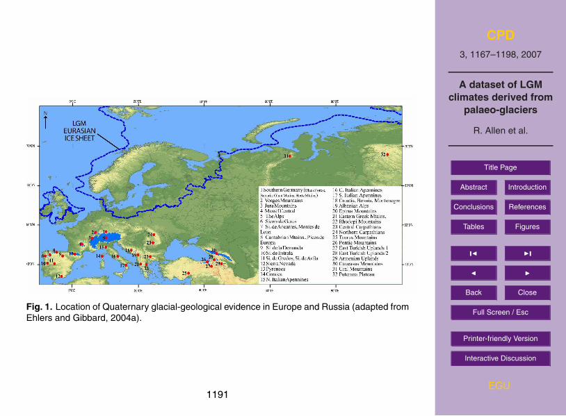
attributed to the LGM (Fig. 1), and used to describe a wide range of glacial systems,5

the largest of which was the Alpine ice cap (e.g. Florineth and Schluchter, 2000). The

orographies of the Pyrenees and Caucasus Mountains enabled significant mountain

glacier systems, drained by outlet glaciers up to 70 km in length to develop (Calvet,

2004; Gobejishvili, 2004). To the north and west of the Alps small ice caps (up to

500 km2) developed in the Vosges Mountains, Jura Mountains, and Massif Central (Dri-10

cot et al., 1991; Gillespie and Molnar, 1995; Buoncristiani and Campy, 2001). Evidence

of Quaternary cirque and mountain glaciers can be found in upland regions across the

Mediterranean Basin and Turkey as far south as 35◦N (Fig. 1) (See Ehlers and Gibbard

(2004a) and references therein for a full review).

The position of the eastern margin of the Eurasian Ice Sheet has been established15

by Svendsen et al. (2004). They indicate the ice sheet was restricted to the present

day coastal regions of northern Russian and Siberia, leaving self sourced ice masses

in the upland regions of the Ural Mountains and Puterana Plateau (Fig. 1) (e.g. Boul-

ton, 1979; Hubberten et al., 2004). Recent modelling work supports the interpretation

that the Eurasian Ice Sheet had retreated from Arctic Russia by the LGM, owing to20

an extremely cold and dry climate (Siegert and Marsiat, 2001). Assuming that this in-

terpretation is correct, small cirque and valley glaciers would have formed in the Ural

Mountains during the LGM (Astakhov, 1997; Svendsen et al., 2004, Hubberten et al.,

2004), however the exact number and extent of these glaciers remains unknown. The

chronology of the Late-Quaternary glaciers in the Puterana Plateau is still debated:25

Astakhov (2004) suggests that a large ice cap covered the region during the LGM;

Svendsen et al. (2004) date this ice cap to between 60 and 50 ka BP, and suggest that

by the LGM only the upper reaches of the Puterana Plateau were glaciated.

1171




http://www.egu.eu

CPD

3, 1167–1198, 2007

A dataset of LGM


palaeo-glaciers

R. Allen et al.

Title Page



Tables Figures

◭ ◮

◭ ◮

Back Close

Full Screen / Esc



EGU

4 Regional glacier-climate simulations of the Last Glacial Maximum

4.1 The INQUA dataset of Quaternary glaciers

In 1995 the XIV Congress of the International Quaternary Association (INQUA) com-

missioned a project to establish a comprehensive dataset of the global extent and

chronology of Quaternary glaciations. The European and Russian section of this5

project was published in 2004 (Ehlers and Gibbard, 2004a) and represents the culmi-

nation of work from numerous authors across many different countries and is, to date,

the most comprehensive dataset of Quaternary glaciers (including the LGM) in Europe

and Russia. The data contributing to this publication are contained in an accompanying

ArcView GIS (Fig. 2).10

The LGM glacier reconstructions required to constrain glacier-climate model (Allen

et al., 2007a) simulations of LGM climate were constructed by overlaying the INQUA

GIS dataset on top of the USGS “gtopo30 arcsec” DEM (USGS, 1996). Using this

combined approach to reconstruct LGM glacier topography yielded 182 discrete LGM

glacier profiles from 29 mountainous regions across Western Europe and Black Sea15

region. Results from individual glaciers within each mountain region were combined

to produce a regional climate reconstruction (Table 1). Results from individual sites

within the same region were combined using a weighting system reflecting the relative

glaciated area of the different contributing glaciers. This regionalisation meant that the

number of contributing simulations or simulated glacier area was not uniform between20

regions, and it had to be assumed that results derived from regions with small LGM

glaciers are equally as valid as those derived from the more heavily glaciated regions.

As discussed in Sect. 3 the extent of LGM glaciers in the Ural Mountains and Put-

erana Plateau is currently uncertain. The INQUA LGM glacier dataset (Ehlers and

Gibbard, 2004a) contains no data describing LGM glaciers in the Ural Mountains, and25

describes the large ice cap (∼162 000 km2) in the Puterana Plateau reconstructed by

Astakhov (2004). The alternative interpretations of LGM glaciers in these two regions

provide starkly contrasting maxima and minima that must reflect significantly differ-

1172




http://www.egu.eu

CPD

3, 1167–1198, 2007

A dataset of LGM


palaeo-glaciers

R. Allen et al.

Title Page



Tables Figures

◭ ◮

◭ ◮

Back Close

Full Screen / Esc



EGU

ent overlying palaeoclimatic conditions. This uncertainty was incorporated into the

LGM palaeoclimate dataset by creating mountain glaciers which occupied the upland

reaches of each region (Table 2). This method of representing small mountain glaciers

was used in both regions alongside the LGM glacier profiles described in the INQUA

dataset (Ehlers and Gibbard, 2004a) (Table 2). The Puterana Plateau was modelled5

as a single region and, owing to its length, the Ural Mountains was divided into six

regions1.

4.2 Simulating the Last Glacial Maximum glacier-climate

4.2.1 Creating the model Last Glacial Maximum climate

A common endpoint for palaeo-glacier simulations is to assume that zero surface mass10

balance equates to steady-state conditions in the glacier-climate system (e.g. Hostetler

and Clark, 2000; Plummer and Phillips 2003). This assumption means that in indepen-

dent glacier-climate reconstructions a unique palaeoclimate cannot be derived for each

modelled glacier because both the temperature and precipitation variables are un-

known at the start of the simulation and glacier mass balance is sensitive to changes15

in both variables. To accommodate this uncertainty a domain of potential LGM cli-

mates was created to drive the glacier-climate model. The boundaries of the domain

were 20% and 200% of present day precipitation (anomalies of −80% to +100%) and

temperature anomalies of 0◦C and −20

◦C. The range in precipitation was represented

by 10 precipitation totals (separated by 20%) and the range in temperature anoma-20

lies was represented by 28 values (Allen, 2006). The climate anomalies were applied

uniformly throughout the year to the CRU2.0 climate dataset (representing the clima-

tology of 1961–1991) (New et al., 2002). A suite of 15 lapse rate combinations rep-

1The Ural Mountains were divided into the six model regions along the following latitude

boundaries: Arctic Urals 1, 69◦

N–67◦

N, Arctic Urals 2, 67◦

N–66◦

N, Central Urals 1, 66◦

N–64

◦


N–61◦


N–58◦

N, and Southern Urals 1, 56◦

N–51

◦

N (see Fig. 6.1 in Allen, 2006).

1173




http://www.egu.eu

CPD

3, 1167–1198, 2007

A dataset of LGM


palaeo-glaciers

R. Allen et al.

Title Page



Tables Figures

◭ ◮

◭ ◮

Back Close

Full Screen / Esc



EGU

resenting temperature lapse rates ranging from 6◦C/km (the environmental lapse rate

), to 10◦C/km (the dry adiabatic lapse rate) and precipitation lapse rates ranging from

0 mm/100 m and 80 mm/100 m, were used to downscale each potential LGM climate

onto each LGM glacier profile. A correction factor equivalent to 120 m (Bard et al.,

1990) was incorporated into the lapse rate downscaling to represent lower LGM sea5

levels. This method produced a total of 4200 potential LGM climates, deriving the

optimum LGM climates is described in Sect. 4.2.2. The majority of proxy and model

evidence suggests the LGM was a period of increased aridity compared to the present

day (e.g. Gillespie and Molnar, 1995; Peyron et al., 1998; Tarasov et al., 1999; Bigelow

et al., 2003; Frechen et al., 2003; Kaplan et al., 2003); however, it was noted that some10

GCM simulations predicted positive precipitation anomalies across LGM Europe (Fig. 7

in Kageyama et al., 2001). Therefore, positive precipitation anomalies were included

to ensure that the dataset did not require extrapolation to be compared with alternative

LGM climate reconstructions (Allen et al., 2007b).

4.2.2 Glacier-climate simulations15

The model climates described in Sect. 4.2.1 were used to drive a glacier-climate model

based on a degree day model (DDM) of glacier surface mass balance (the model and

its validation is described in Allen et al., 2007a). For each pair of lapse rates the

combined precipitation and temperature anomalies that satisfied the assessment cri-

teria for determining the optimum result (described below) were assumed to be an20

‘optimum’ LGM climate. Using this approach a total of 150 “optimum” LGM palaeocli-

mates were derived for each region. Determining the optimum result from the domain

of palaeoclimates described in Sect. 4.2.1 depended on whether the glacier-climate

model was simulating mass balance over a single LGM glacier or, a region containing

multiple LGM glaciers (Table 1 and Table 2). For single LGM glaciers the assumption25

of glacier–climate equilibrium at zero surface mass balance was used. For regions

containing multiple glaciers the optimum LGM climate was determined using a cost

function; a method of statistically comparing a spatial prediction made by a model to

1174




http://www.egu.eu

CPD

3, 1167–1198, 2007

A dataset of LGM


palaeo-glaciers

R. Allen et al.

Title Page



Tables Figures

◭ ◮

◭ ◮

Back Close

Full Screen / Esc



EGU

a control spatial distribution (cost functions are explained in Allen et al., 2007a). In

this application the cost function compared the size of the accumulation area of the

LGM glaciers predicted by the DDM with the accumulation area of the reconstructed

LGM glacier profiles. In sites containing multiple glaciers the accumulation area was

calculated from the LGM glacier profiles assuming an accumulation area ratio (AAR)5

of 0.67 (Benn and Evans, 1998). The LGM climate that returned the highest cost func-

tion was assumed to be the optimum. A cost function was used for sites containing

multiple LGM glaciers because a cumulative mass balance would have required sep-

arate glacial systems (with their different mass balance regimes) to be combined to

determine the optimum LGM climate. For the Russian sites, the position and extent10

of the ablation zone is unknown and, as the calculation of a cumulative mass balance

requires the whole glacier profile, this approach could not be applied. Palaeoclimate

reconstructions derived using the cumulative mass balance and cost function methods

are comparable, however, because the prescribed AAR in the cost function method is

assumed to apply to a steady-state glacier profile.15

The design of the modelling approach limits the reconstructed climate variables to

mean annual temperature and annual precipitation, which has implications for the re-

liability of the climate results for two reasons. First, the mass balance of mid-latitude

glaciers is primarily controlled by winter accumulation and summer ablation (Porter,

1977; Leonard, 1989). If the intensification of LGM winter conditions (e.g. Huijzer20

and Vandenberghe, 1998; Peyron et al., 1998; Krinner et al., 2000) is correct, the

use of present day seasonality, uniform climate anomalies, and a DDM to reconstruct

LGM temperatures may lead to an under-estimate of the annual temperature anomaly.

DDMs are only sensitive to changes in positive air temperature (i.e. summer temper-

atures) which control ablation; therefore, the mean annual temperature anomalies re-25

constructed in this dataset primarily reflect changes in summer temperatures and do

not include (potentially larger) changes to winter temperatures. Second, if it is assumed

that the intensity of LGM winter precipitation was higher compared to the present day

(e.g. Prentice et al., 1992; Ramrath et al., 1999), the use of present day seasonality

1175




http://www.egu.eu

CPD

3, 1167–1198, 2007

A dataset of LGM


palaeo-glaciers

R. Allen et al.

Title Page



Tables Figures

◭ ◮

◭ ◮

Back Close

Full Screen / Esc



EGU

in the DDM climate simulations would (with other things being equal) cause an over-

estimate in the reconstructed temperature anomaly (because lower winter accumula-

tion totals require lower temperatures to achieve steady state zero mass balance).

5 The Last Glacial Maximum glacier-palaeoclimate dataset: Europe

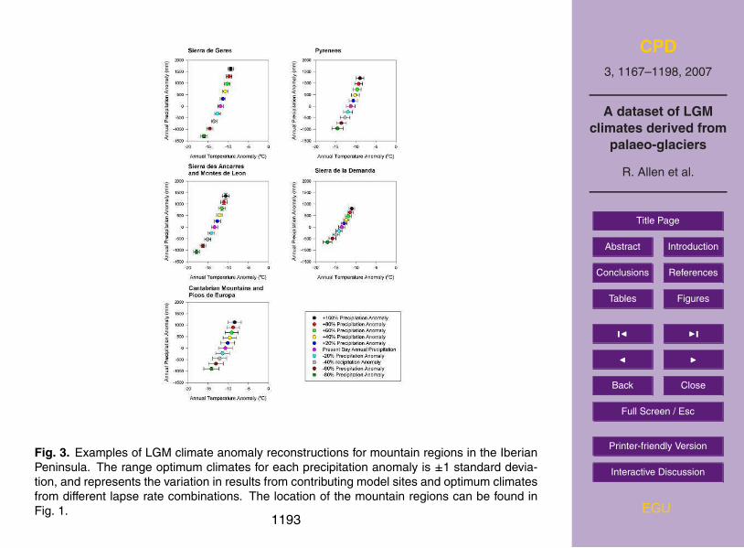
Optimum LGM precipitation anomalies ranged from ∼1000 mm drier to ∼1500 mm wet-5

ter than the present day (equating to absolute precipitation totals between 200 mm

and 3500 mm) across Europe. Temperature anomalies smaller than −20◦C were able

to achieve optimum model result under all precipitation.scenarios The drier climates

required larger temperature anomalies to achieve equilibrium surface mass balance

(Fig. 3). Owing to the uncertainty in the LGM climate reconstructions it is difficult to10

make definitive comparisons between regions stating that one mountain region was

colder, warmer, wetter or drier than another at the LGM.

If, however, for the purposes of interpretation the precipitation anomaly is calculated

in percentage terms and assumed to be constant across all regions, then relative dif-

ferences can be inferred. The following results are taken from the simulations using15

present day precipitation totals (Fig. 4). In Iberia, for example, LGM glaciated regions

in close proximity to the Atlantic Ocean have smaller mean annual temperature anoma-

lies, ranging from −10.7◦C to −11.9

◦C, compared to inland glaciated regions where

temperature anomalies range from −13.5◦C to −15.7

◦C (Fig. 1 and Fig. 4). A slight

north-south gradient in LGM mean annual temperature anomalies is present between20

the LGM glaciated regions north of the Alps and the LGM glaciated regions of Cor-

sica and Italy. North of the Alps LGM temperature anomalies range from −12.0◦C to

−13.9◦C, in contrast to −11.0

◦C to −12.0

◦C in Italy. In the Balkans and Eastern Eu-

rope LGM coastal regions require larger temperature anomalies ranging from −11.6◦C

to −12.5◦C; in contrast, the Romanian Carpathians and Bulgarian mountains temper-25

ature anomalies range from −8.0◦C to −9.8

◦C. Across the Eastern Black Sea LGM

annual temperature anomalies range from −9.7◦C to −12.3

◦C. Figures 5 and 6 show

1176




http://www.egu.eu

CPD

3, 1167–1198, 2007

A dataset of LGM


palaeo-glaciers

R. Allen et al.

Title Page



Tables Figures

◭ ◮

◭ ◮

Back Close

Full Screen / Esc



EGU

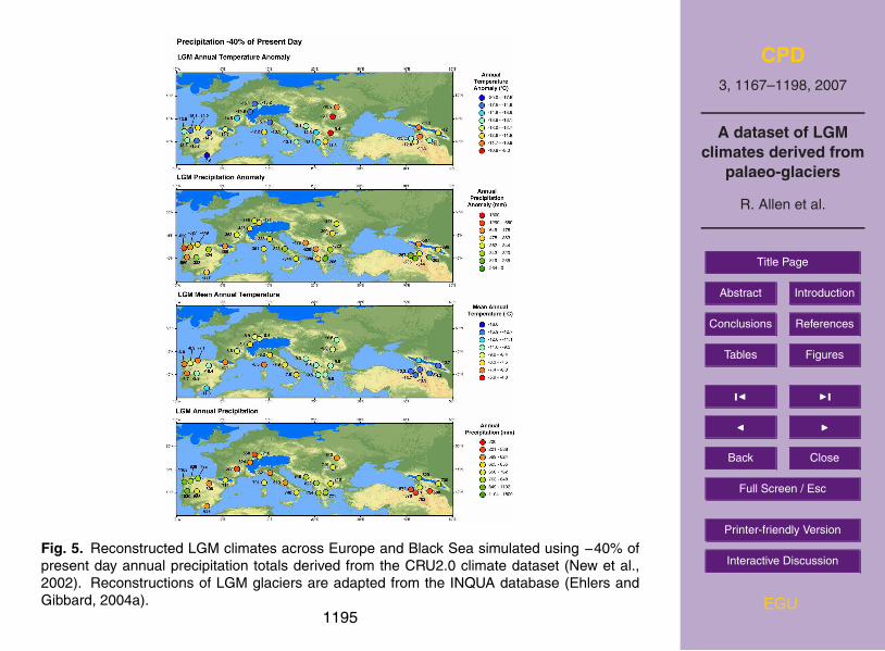
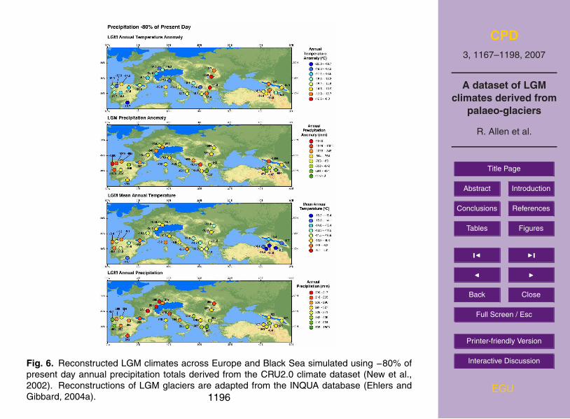
the same results as Fig. 4, but for precipitation anomalies of −40% and −80%, respec-

tively. Larger negative percentage precipitation anomalies cause annual temperature

anomalies to increase (Figs. 5 and 6); however the relative trends between regions

described in the simulation using present day precipitation totals remain.

6 The LGM glacier-palaeoclimate dataset: Russia5

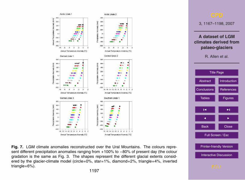
The climate anomaly results from the 0% glacial coverage simulations can be inter-

preted as representing the maximum cooling of the present day climate (per precipita-

tion anomaly) at the onset of glaciation. In the Ural Mountains this threshold exhibits

a strong latitudinal gradient (Fig. 7): In the Arctic Urals the onset of glaciation is ini-

tiated after a cooling of −1◦C but a cooling of −8

◦C is required in the Southern Urals10

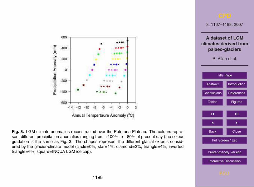
(assuming present day precipitation). In the Puterana Plateau the results are similar to

the Arctic Urals, a cooling of only −0.5◦C is required to initiate the onset of glaciation

(assuming present day precipitation) (Figure 8). In all regions, increasing the extent

of LGM glaciation increases the size of the temperature anomaly required to achieve

optimum cost-function conditions (Figs. 7 and 8); For example temperature anomalies15

for the INQUA Puterana Plateau ice cap (Ehlers and Gibbard, 2004a) and prescribed

6% glacial coverage simulation (assuming present day precipitation) are −8.5◦C and

−4.5◦C, respectively (Fig. 8).

7 Discussion

The characteristics of ideal proxy palaeo-datasets were described in Sect. 2 and are20

a suitable framework for discussing the palaeoclimate dataset presented in this paper.

The first desirable characteristic is a continental to global scale resolution to ensure

that regional trends are resolved (Kohfeld and Harrison, 2000). The dataset presented

here contains potential LGM climates for thirty-six upland regions; this density is similar

1177




http://www.egu.eu

CPD

3, 1167–1198, 2007

A dataset of LGM


palaeo-glaciers

R. Allen et al.

Title Page



Tables Figures

◭ ◮

◭ ◮

Back Close

Full Screen / Esc



EGU

to previous proxy climate reconstructions across Europe (Peyron et al., 1998; Tarasov

et al., 1999). It well known that the relationship between an individual glacier and

the surrounding regional climate is modulated by local scale factors (e.g. Kerr, 1993;

Mark et al., 2005). Therefore the LGM climate signal for each region was derived from

the average of the results from the individual glacier-climate simulations. In Western5

Europe reconstructed temperature anomalies can be divided into three main regions:

north of the Alps, the Mediterranean Basin, and Eastern Europe. With a precipitation

anomaly of -40%, mean temperature anomalies (± one standard deviation) for these

three regions are −15±0.3◦C, −13±0.8

◦C, and −10±1

◦C, respectively. The tempera-

ture anomaly of −12.5±1◦C for the Eastern Black Sea region is comparable with the10

Mediterranean Basin. In Russia, DDM simulations were used to assess the potential

likelihood of LGM glaciation in the Ural Mountains and Puterana Plateau. The poten-

tial decrease in temperature before the onset of glacerization in the Northern Urals is

less than −3.0◦C, even under the largest negative precipitation anomalies; this sug-

gests that it was unlikely that this region was not glaciated at the LGM. Supporting this15

conclusion are data describing 20th century glaciers in the Northern Ural Mountains

(e.g. Grosval’d and Kotlyakov, 1969; National Snow and Ice Data Center, 1999). In the

Southern Urals, a cooling of −10◦C was possible before the DDM predicted glacieriza-

tion, which suggests glaciation of the Ural Mountains during the LGM did not reach the

Southern Urals. In the Puterana Plateau the present day climate can only be cooled20

by −0.5◦C before the onset of glacierization, which combined with the existence of

present day glaciers in the region (National Snow and Ice Data Center, 1999) leads to

the conclusion that the Puterana Plateau must have been glaciated at the LGM. Tem-

perature anomalies reconstructed from the different percentage glacial extents and

INQUA ice cap range from −2.6◦C at the 1% glacial coverage to −8.6

◦C from the IN-25

QUA ice cap simulation, assuming present day precipitation totals. The INQUA LGM

glacier dataset (Ehlers and Gibbard, 2004a) suggests that the Northern Urals were

not glaciated and the Puterana Plateau heavily glaciated at the LGM. The results have

demonstrated that in order to achieve this distribution of LGM glaciers requires virtually

1178




http://www.egu.eu

CPD

3, 1167–1198, 2007

A dataset of LGM


palaeo-glaciers

R. Allen et al.

Title Page



Tables Figures

◭ ◮

◭ ◮

Back Close

Full Screen / Esc



EGU

no change in the present day climate of the Northern Urals, but a comparatively large

cooling over the Puterana Plateau. This distribution of temperature anomalies is not

found in the pollen climate reconstructions: temperature anomalies range from −5◦C

to −8◦C, and −1

◦C to −3

◦C in the Ural Mountains and Puterana Plateau, respectively

(Tarasov et al., 1999). It is concluded, from DDM simulations and pollen data, that the5

Ural Mountains and Puterana Plateau were both probably glaciated by small discrete

mountain glaciers during the LGM as proposed by Astakhov (1997) and Svendsen et

al. (2004). The second characteristic of the ideal proxy palaeo-dataset is that the data

should be directly compatible with model output (Kohfeld and Harrison, 2000; Harri-

son, 2003). The DDM is driven by climate variables that are directly compatible with10

GCM output, and this relation is expanded in Allen et al. (2007b). The third charac-

teristic of the ideal proxy palaeo-dataset is transparency in the primary data (Harrison,

2003). The primary data are readily available to the scientific community via the IN-

QUA Quaternary glacier GIS (Ehlers and Gibbard, 2004a). The fourth characteristic

is a detailed documentation describing the methods used, assumptions made, and15

any data transformations (Harrison, 2003). Details of the DDM, meteorological base-

line, data transformations and verification of the methodology can be found in Allen et

al. (2007a). Details of the transformation required to make the INQUA LGM glacier

dataset compatible with the other input data have been detailed in this paper. The

within model results under optimum LGM climates show that the modelling approach20

consistently predicted plausible first order glaciological and climatic conditions. The

fifth characteristic for proxy datasets is the provision of adequate metadata describing

specific details of the individual sites, and the chronological framework used to date

the proxy evidence (Kohfeld and Harrison, 2000; Harrison, 2003). Metadata describ-

ing the glacial style, glacial extent, snowline depressions, and available chronological25

information for the glaciated regions of Europe included in the INQUA glacier dataset

can be found in Ehlers and Gibbard (2004a). Recent work on sub-tropical glaciers has

emphasised the importance of reliable absolute dating when using glacial-geological

evidence for climate model comparisons (e.g. Benn et al., 2005; Mark et al., 2005;

1179




http://www.egu.eu

CPD

3, 1167–1198, 2007

A dataset of LGM


palaeo-glaciers

R. Allen et al.

Title Page



Tables Figures

◭ ◮

◭ ◮

Back Close

Full Screen / Esc



EGU

Smith et al., 2005). Such dating is especially important when comparing palaeoclimate

results from regions in which the glaciers did not reach a maximum during the global

LGM (e.g. Gillespie and Molnar, 1995; Ono et al., 2005). The available dating evidence

accompanying the INQUA European glacier dataset (Ehlers and Gibbard, 2004a and

references therein) does not currently meet the standard of the tropical glacier studies5

(Benn et al., 2005; Mark et al., 2005; Smith et al., 2005). Absolute dates for LGM

glaciers are only available in a few regions, e.g. the Vosges Mountains, Jura Moun-

tains, and Central Italian Apennines (Campy and Richards, 1988; Dricot et al., 1991;

Giraudi, 2004). In the remaining regions the geological evidence is inferred as LGM

from relative chronologies, e.g. Massif Central, and Romanian Carpathians (Gillespie10

and Molnar, 1995; Urdea, 2004), or simply assumed to be LGM, e.g. the mountains of

the Former Yugoslavia, and Mountain glaciations in Iberia (Straus, 1992; Marjanac and

Marjanac, 2004). In several regions these non-dated reconstructions have placed the

maximal glacial advance in the geological record at the LGM, which are subsequently

used in the INQUA dataset (Ehlers and Gibbard, 2004a). There is a growing body of15

evidence that suggests that the LGM glacial advance was smaller than the maximum

advance found in the geological record. For example, in Greece preliminary uranium

dating places the maximal glacial advance to earlier in the Last Glaciation and suggests

that the LGM glaciation was less extensive (Woodward et al., 2004). Dating work has

placed the LGM glaciation in the Cantabrian Mountains inside the maximal advance20

(Sanchez and Arquer, 2002). In the Pyrenees, the glacial reconstruction prescribed

to the LGM by the INQUA dataset is the maximal advance during the Last Glaciation,

which has been radiocarbon dated to before the LGM (Herail et al., 1986; Andrieu et

al., 1988; Jalut et al., 1988; Vilaplana and Montserrat, 1989; Jalut et al., 1992; Garcıa-

Ruiz et al., 2003). As the INQUA glacier dataset has used the largest Late-Quaternary25

glacial advance for the LGM glacier profile in regions where no absolute chronology is

currently available the LGM temperature anomalies should be treated as a maximum.

“Reconstructing the former extent of glaciers requires detailed geomorphic mapping

and the analysis of landforms and sediments” (Benn et al., 2005, Page 11); such detail

1180




http://www.egu.eu

CPD

3, 1167–1198, 2007

A dataset of LGM


palaeo-glaciers

R. Allen et al.

Title Page



Tables Figures

◭ ◮

◭ ◮

Back Close

Full Screen / Esc



EGU

is required because the destruction of older glacial evidence by more recent glacial

advances, periglacial activity, and post deglaciation landform erosion makes glacial-

geological evidence a naturally incomplete record. It has been implicitly assumed in

this modelling study that the analysis and interpretation of the glacial-geological evi-

dence contributing to the INQUA dataset (Ehlers and Gibbard, 2004a) has been done5

in a consistent manner and is correct. There are also a small number of regions where

the glacier reconstruction has been incorrectly reproduced in the INQUA GIS dataset,

e.g. in the Sierra Nevada Mountains the glacial extent is represented by a series of

overlapping triangles that have no recognisable glacial attributes. The final character-

istic is the presentation of results on a site by site basis. The glacier-climate dataset is10

presented in a site by site format, thus ensuring that no interpolation of data has been

made.

8 Conclusions

A dataset of 36 new and independent LGM European climate estimates derived from

European Quaternary glaciers has been described. It was designed to be fully inde-15

pendent of alternative LGM climate reconstructions to maximise its potential use in

future LGM climate assessment studies. Regional climate estimates were constructed

by combining the results of glacier-climate simulations of the individual LGM glaciers

within the region. Owing to the independent nature of the dataset it was not possible to

simulate a unique solution for each region, therefore a suite of optimum LGM climate20

conditions were derived for prescribed precipitation conditions ranging from −80% to

+100% of present day annual precipitation. In Europe regional trends are evident in

the temperature anomalies (assuming a fixed percentage precipitation anomaly), with

larger temperature anomalies found north of the Alps compared to the Mediterranean

Basin (Figs. 5–7). In Northern Russia the model results suggest that both the Ural25

Mountains and Puterana Plateau were glaciated with small mountain glaciers during

the LGM.

1181




http://www.egu.eu

CPD

3, 1167–1198, 2007

A dataset of LGM


palaeo-glaciers

R. Allen et al.

Title Page



Tables Figures

◭ ◮

◭ ◮

Back Close

Full Screen / Esc



EGU

This dataset will enable glacial-geological evidence to contribute to our understand-

ing of the European climate for the first time at the continental scale (Allen et al.,

2007b). Moreover this work has developed and tested a new and simple method which

is transferable to other regions of the world; the appropriate glacial-geological data for

the rest of the world required by the glacier-climate model are available in Volumes II5

and III of the INQUA Quaternary glacier dataset (Ehlers and Gibbard, 2004b; Ehlers

and Gibbard, 2004c).

Appendix A

AAR Accumulation Area Ratio

CLIMAP Climate/Long Range Investigation Mapping and Predictions Project

CRU Climate Research Unit – University of East Anglia

DDM Degree Day Model

DEM Digital Elevation Model

GCM General Circulation Model

GIS Geographical Information System

INQUA International Quaternary Association

LGM Last Glacial Maximum

PMIP Palaeoclimate Modelling Intercomparison Project

USGS United States Geological Service

Acknowledgements. This work was funded by a NERC studentship. R. Allen would like to10

thank M. Siegert and T. Payne for their support and advice during the period of this research.

References

Allen, R. J.: Reconstructing the Last Glacial Maximum Climate of Europe and Russia usingthe Glacial-Geological Record. PhD Thesis, School of Geographical Sciences, University ofBristol, 304pp., 2006.15

1182




http://www.egu.eu

CPD

3, 1167–1198, 2007

A dataset of LGM


palaeo-glaciers

R. Allen et al.

Title Page



Tables Figures

◭ ◮

◭ ◮

Back Close

Full Screen / Esc



EGU

Allen, R. J., Siegert, M. J., and Payne, T.: Reconstructing glacier-based climates of LGM Eu-rope and Russia – Part 1: Numerical modelling and validation methods, Clim. Past Discuss.,3, 1133–1166, 2007a.

Allen, R. J., Siegert, M. J., and Payne, T.: Reconstructing glacier-based climates of LGM Eu-rope and Russia – Part 3: Comparison with GCM and pollen-based climate reconstructions,5

Clim. Past Discuss., 3, 1199–1233, 2007b.Andrieu, V., Hubschman, J., Jalut, G., and Herail, G.: Chronologie de la deglaciation des

Pyrenees francaises. Bulletin de l’Association francaise pour l’etude de Quaternaire, 2/3,55–67, 1988.

Astakhov, V. I.: Late Glacial Events in the Central Russian Arctic. Quatern. Int., 41/42, 17–26,10

1997.Astakhov, V. I.: Pleistocene ice limits in the Russian northern lowlands, in: Quaternary Glacia-

tions – Extent and Chronology Part I: Europe, edited by: Ehlers, J. and Gibbard, P. L.,309–320, 2004.

Bard, E., Hamelin, B., and Fairbanks, R. G.: U-Th ages obtained by mass spectrometry in15

corals from Barbados: sea level during the past 130 000 years, Nature, 346, 456–458, 1990.Benn, D. I. and Evans, D. J. A.: Glaciers and Glaciation. Edward Arnold, London, 734pp., 1998.Benn, D. I., Owen, L. A., Osmaston, H. A., Seltzer, G. O., Porter, S. C., and Mark, B.: Re-

constructions of equilibrium-line altitudes for tropical and sub-tropical glaciers, Quatern. Int,138–139, 8–21, 2005.20

Bigelow, N. H., Brubaker, L. B., Edwards, M. E., Harrison, S. P., Prentice, I. C., Anderson, P.M., Andreev, A. A., Bartlein, P. J., Christensen, T. R., Cramer, W., Kaplan, J. O., Lozhkin, A.V., Matveyeva, N. V.,. Murray, D. F., McGuire, A. D., Razzhivin, V. Y., Ritchie, J. C., Smith,B., Walker, D. A., Gajewski, K., Wolf, V., Holmqvist, B. H., Igarashi, Y., Kremenetskii, K.,Paus, A., Pisaric, M. J. F., and Volkova, V. S. L.: Climate change and Arctic ecosystems:25

1. Vegetation changes north of 55◦

N between the last glacial maximum, mid-Holocene, andpresent, J Geophys. Res., 108, ALT 11, 2003.

Boulton, G. S.: Glacial history of the Spitzbergen archipelago and the problem of the BarentsSea ice sheet, Boreas, 8, 31–57, 1979.

Buoncristiani, J.-F. and Campy, M.: Late Pleistocene detrital sediment yield of the Jura glacier,30

France, Quaternary Res., 56, 51–61. 2001.Calvet, M.: The Quaternary glaciation of the Pyrenees, in: Quaternary Glaciations – Extent

and Chronology Part I: Europe, edited by: Ehlers J. and Gibbard, P. L., 119–128, 2004.

1183




http://www.egu.eu

CPD

3, 1167–1198, 2007

A dataset of LGM


palaeo-glaciers

R. Allen et al.

Title Page



Tables Figures

◭ ◮

◭ ◮

Back Close

Full Screen / Esc



EGU

Campy, M. and Richards, H.: Modalites et chronologie de la deglaciation Wurmienne dansla chaıne Jurassieme. Bulletin de l’Association francaise pour l’etude de Quaternaire, 2/3,81–90, 1988.

CLIMAP Project Members.: Seasonal reconstruction of the Earth’s surface at the Last GlacialMaximum. Geological Society of America, Map and Chart Series, MC-36-1981, 1981.5

Denton, G. H. and Hughes, T. J.: The Arctic ice sheet: an outrageous hypothesis, in: The LastGreat Ice Sheets, edited by: Denton G. H. and Hughes, T. J., Wiley, New York, 1981.

Dricot, E., Petillon, M., and Seret, G.: When and why did glaciers grow or melt in the VosgesMountains (France). In Klimageschichtliche Probleme der Letzten 130 000 Jahre, 1991.

Ehlers, J. and Gibbard, P. L. (Eds.): Quaternary Glaciations – Extent and Chronology, Part 1:10

Europe. Series Editor J. Rose, Developments in Quaternary Science 2, Elsevier, London,2004a.

Ehlers, J. and Gibbard, P. L (Eds.): Quaternary Glaciations – Extent and Chronology, PartII: North America. Series Editor J. Rose, Developments in Quaternary Science 2, Elsevier,London, 2004b.15

Ehlers, J. and Gibbard, P. L.: Quaternary Glaciations – Extent and Chronology, Part 1II: SouthAmerica, Asia, Africa, Australia, and Antarctica. Series Editor J. Rose, Developments inQuaternary Science 2, Elsevier, London, 2004c.

Farerra, I., Harrison, S. P., Prentice, I. C., Ramstein, G., Guiot, J., Bartlein, P. J., Bonnefille,R., Bush, M., Cramer, W., von Grafenstein, U., Holmgren, K., Hooghiemstra, H., Hope, G.,20

Jolly, D., Lauritzen S.-E., Ono, Y., Pinot, S., Stute, M., and Yu, G.: Tropical climates at theLast Glacial Maximum: a new synthesis of terrestrial palaeoclimate data. 1. Vegetation, lake-levels and geochemistry, Clim. Dyn., 15, 823–856, 1999.

Florineth, D. and Schluchter, C.: Alpine evidence for atmospheric circulation patterns in Europeduring the Last Glacial Maximum, Quaternary Res., 54, 295–308, 2000.25

Frechen, M., Oches, E. A., and Kohfeld, K. E.: Loess in Europe – mass accumulation ratesduring the Last Glacial Period, Quaternary Sci. Rev., 22, 1835–1857, 2003.

Garcıa-Ruiz, J. M., Valero-Garces, B. L., Martı-Bono, C., and Gonzalez-Samperiz, P.: Asyn-chroneity of maximum glacier advances in the central Spanish Pyrenees, J. Quaternary Sci.,18, 61–72, 2003.30

Gillespie, A. and Molnar, P.: Asynchronous maximum advances of mountain and continentalglaciers, Rev. Geophys., 33, 311–364, 1995.

Giraudi, C.: The Apennine glaciations in Italy, in: Quaternary Glaciations – Extent and Chronol-

1184




http://www.egu.eu

CPD

3, 1167–1198, 2007

A dataset of LGM


palaeo-glaciers

R. Allen et al.

Title Page



Tables Figures

◭ ◮

◭ ◮

Back Close

Full Screen / Esc



EGU

ogy Part I: Europe, edited by: Ehlers J. and Gibbard, P. L., 215–224, 2004.Gobejishvili, R.: Late Pleistocene (Wurmian) glaciation of the Caucasus, in: Quaternary Glacia-

tions – Extent and Chronology Part I: Europe, edited by: Ehlers J. and Gibbard, P. L., 129–134, 2004.

Grosval’d, M. G. and Kotlyakov, V. M.: Present day glaciers in the USSR and some data on5

their mass balance, J. Glaciol., 8, 9–21, 1969.Harrison, S. P.: Contributing to global change science: the ethics, obligations and opportuni-

ties of working with palaeoenvironmental databases. Norsk Geografisk Tidsskrift-NorwegianJournal of Geography, 57, 1–8, 2003.

Harrison, S. P., Braconnot, P., Joussaume, S., Hewitt, C., and Stouffer, R. J.: Comparison of10

palaeolcimate simulations enhances confidence in models. EOS, Transactions, AmericanGeophysical Union, 83, 447, 2002.

Herail, G., Hubschman, J., and Jalut, G.: Quaternary glaciations in the French Pyrenees, Qua-ternary Sci. Rev., 5, 397–402, 1986.

Hostetler, S. W. and Clark, P. U.: Tropical climate at the last glacial maximum inferred from15

glacier mass-balance modelling, Science, 290, 1747–1750, 2000.Hubberten, H. W., Andreev, A., Astakhov, V. I., Demidov, I., Dowdeswell, J. A., Henriksen, M.,

Hjort, C., Houmark-Nielsen, M., Jakobsson, M., Kuzmina, S., Larsen, E., Lunkka, J. P., Lysa,A., Mangerud, J., Moller, P., Saarnisto, M., Schirrmeister, L., Sher, A. V., Siegert, C., Siegert,M. J., and Svendsen, J. I.: The periglacial climate and environment in northern Eurasia20

during the Last Glaciation, Quaternary Sci. Rev., 23, 1333–1357, 2004.Huijzer, B. and Vandenberghe, J.: Climatic reconstruction of the Weichselian Pleniglacial in

northwestern and central Europe, J. Quaternary Sci., 13, 391–417, 1998.Jalut, G., Monserrat Marti, J., Fontugne, M., Delibrias, G., Vilaplana, J. M., and Julia, R.: Glacial

to interglacial vegetation changes in the northern and southern Pyrenees: deglaciation, veg-25

etation cover and chronology, Quaternary Sci. Rev., 11, 449–480, 1992.Jalut, G., Andrieu, V., Delibrias, G., Fontugne, M., and Pages, P.: Palaeoenvironment of the

valley of Ossau (Western French Pyrenees) during the last 27 000 years, Pollen et Spores,30, 357–393, 1988.

Joussame, S. and Taylor, K. E.: Status of the Paleoclimate Modelling Intercomparison Project30

(PMIP), in: Proceedings of the first international AMIP scientific conference, Monterrey, Cal-ifornia, USA, 15–19 May, WRCP-92, 425–430, 1995.

Kageyama, M., Peyron, O., Pinot, S., Tarasov, P., Guiot, J., Joussaume, S., and Ramstein, G.:

1185




http://www.egu.eu

CPD

3, 1167–1198, 2007

A dataset of LGM


palaeo-glaciers

R. Allen et al.

Title Page



Tables Figures

◭ ◮

◭ ◮

Back Close

Full Screen / Esc



EGU

The Last Glacial Maximum climate over Europe and western Siberia: a PMIP comparisonbetween models and data, Clim. Dyn., 17, 23–43, 2001.

Kageyama, M., Harrison, S. P., and Abe-Ouchi, A.: The depression of tropical snowlines at thelast glacial maximum: What can we learn from climate model experiments?, Quatern. Int.,138–139, 202–219, 2005.5

Kaplan, J. O., Bigelow, N. H., Prentice, I. C., Harrison, S. P., Bartlein, P. J., Christensen, T.R.,Cramer, W., Matveyeva, N. V., McGuire, A. D., Murray, D. F., Razzhivin, V. Y., Smith, B.,Walker, D. A., Anderson, P. M., Andreev, A. A., Brubaker, L. B., Edwards, M. E., and Lozhkin,A. V.: Climate change and Arctic ecosystems: 2. Modeling, paleodata-model comparisons,and future projections, J. Geophys. Res., 108(D19), 8171, doi:10.1029/2002JD002559,10

2003.Kerr, A.: Topography, climate and ice masses – a review, Terra Nova, 5, 332–342, 1993.Kohfeld, K. E. and Harrison, S. P.: How well can we simulate past climates? Evaluating the mod-

els using global palaeoenvironmental datasets, Quaternary Sci. Rev., 19, 321–346, 2000.Krinner, G., Raynaud, D., Doutrriaux, C., and Dang, H.: Simulations of the Last Glacial Maxi-15

mum ice sheet surface climate: Implications for the interpretation of ice core air, J. Geophys.Res., 105, 2059–2070, 2000.

Leonard, E. M.: Climatic change in the Colorado Rocky Mountains: estimates based on themodern climates at Late Pleistocene equilibrium lines, Arctic Alpine Res., 21, 245–255,1989.20

Marjanac, L. and Marjanac, T.: Glacial history of the Croatian Adriatic and Coastal Dinarides,in: Quaternary Glaciations – Extent and Chronology Part I: Europe, edited by: Ehlers J. andGibbard, P. L., 19–26, 2004.

Mark, B. G., Harrison, S. P., Spessa, A., New, M., Evans, D. J. A., and Helmens, K. F.: Tropicalsnowlines changes at the last glacial maximum: A global assessment. Quatern. Int., 138–25

139, 168–201, 2005.National Snow and Ice Data Center. World Glacier Inventory. World Glacier Monitoring Service

and National Snow and Ice Data Center/World Data Center for Glaciology. Boulder, CO.Digital Media. 1999.

New, M., Lister, D., Hulme, M., and Makin, I.: A high-resolution data set of surface climate over30

global land areas, Climate Res., 21, 1–25, 2002.Ono, Y., Aoki, T., Hasegawa, H., and Dali, L.: Mountain glaciation in Japan and Taiwan at the

global Last Glacial Maximum, Quatern. Int., 138–139, 79–92, 2005.

1186




http://www.egu.eu

CPD

3, 1167–1198, 2007

A dataset of LGM


palaeo-glaciers

R. Allen et al.

Title Page



Tables Figures

◭ ◮

◭ ◮

Back Close

Full Screen / Esc



EGU

Owen, L. A. and Benn, D. I.: Equilibrium-line altitudes of the Last Glacial Maximum for theHimalaya and Tibet: an assessment and evaluation of results, Quatern. Int., 138–139, 55–78, 2005.

Peyron, O., Guiot, J., Cheddadi, R., Tarasov, P., Reille, M., de Beaulieu, J.-L., Bottema, S., andAndrieu, V.: Climatic reconstruction in Europe for 18 000 yr BP from pollen data, Quaternary5

Res., 49, 183–196, 1998.Plummer, M. A. and Phillips, F. M.: A 2-D numerical model of snow/ice energy balance and ice

flow for paleoclimate interpretation of glacial geomorphic features, Quaternary Sci. Rev., 22,1389–1406, 2003.

Porter, S. C.: Present and past glaciation threshold in the Cascade Range, Washington, U.S.A.:10

Topographic and climatic controls and paleoclimatic implications, J. Glaciol., 18, 101–116,1977.

Prentice, I. C., Guiot, J., and Harrison, S. P.: Mediterranean vegetation, lake levels and palaeo-climate at the Last Glacial Maximum, Nature, 360, 658–660, 1992.

Ramrath, A., Zolitschka, B., Wulf, S., and Negendank, J. F. W.: Late Pleistocene climatic varia-15

tions as recorded in two Italian maar lakes (Lago di Mezzano, Lago Grande di Monticchio),Quat. Sci. Rev., 18, 977–992, 1999.

Sanchez, M. F. and Arquer, P. F.: New radiometric and geomorphological evidences of a lastglacial maximum older than 18 ka in SW European mountains: the example of Redes Na-tional Park (Cantabrian Mountains, NW Spain), Geodin. Acta, 15, 93–101, 2002.20

Siegert, M. J. and Marsiat, I.: Numerical reconstruction of LGM climate across the EurasianArctic, Quat. Sci. Rev., 20, 1595–1605, 2001.

Smith, J. A., Seltzer, G. O., Rodbell, D. T., and Klein, A. G.: Regional synthesis of last glacialmaximum snowlines in the tropical Andes, South America, Quatern. Int., 138–139, 145–167,2005.25

Straus, L. G.: Iberia before the Iberians: the Stoneage Prehistory of Cantabrian Spain. Univer-sity of New Mexico Press, Albuquerque, 1992.

Svendsen, J. I., Alexanderson, H., Astakhov, V.I., Demidov, I., Dowdeswell, J. A., Funder, S.,Gataullin, V., Henriksen, M., Hjort, C., and Houmark-Nielsen, M.: Late Quaternary ice sheethistory of northern Eurasia, Quat. Sci. Rev., 23, 1229–1272. 2004.30

Tarasov, P. E., Peyron, O., Guiot, J., Brewer, S., Volkova, V. S., Bezusko, L. G., Dorofeyuk,N. I., Kvavadze, E. V., Osipova, I. M., and Panova, N. K.: Last Glacial Maximum climate ofthe former Soviet Union and Mongolia reconstructed from pollen and plant macrofossil data,

1187




http://www.egu.eu

CPD

3, 1167–1198, 2007

A dataset of LGM


palaeo-glaciers

R. Allen et al.

Title Page



Tables Figures

◭ ◮

◭ ◮

Back Close

Full Screen / Esc



EGU

Clim. Dyn., 15, 227–240, 1999.Tarasov, P. E., Volkova, V. S., Webb III, T., Guiot, J., Andreev, A. A., Bezusko, L. G., Bezusko,

T. V., Bykova G. V, Dorofeyuk, N. I., Kvavadze, E. V., Osipova, I. M., Panova, N. K., and Sev-astyanov, D. V.: Last Glacial Maximum biomes reconstructed from pollen and plant macro-fossil data from northern Eurasia, J. Biogeogr., 27, 609–620, 2000.5

Urdea, P.: The Pleistocene glaciation of the Romanian Carpathians, in: Quaternary Glaciations– Extent and Chronology Part I: Europe, edited by: Ehlers J. and Gibbard, P. L., 301-308,2004.

USGS. 1996: http://edcdaac.usgs.gov/gtopo30/gtopo30.html, accessed 15 September 2007.van Husen, D.: LGM and Late-Glacial fluctuations in the Eastern Alps. Quatern. Int., 38/39,10

109–118, 1997.Vilaplana, J. M. and Montserrat. J.: Recent progress in Quaternary stratigraphy: the lake

Llauset sequence in the Spanish Pyrenees, in: Quaternary Type Sections: Imagination orReality? Balkema: Rotterdam, edited by: Rose, J. and Schluchter, C., 113-124, 1989.

Woodward, J. C., Macklin, M. G., and Smith, G. R.: Pleistocene glaciation in the mountains15

of Greece, in: Quaternary Glaciations – Extent and Chronology Part I: Europe, edited by:Ehlers J. and Gibbard, P. L., 155–174, 2004.

1188




http://www.egu.eu

http://edcdaac.usgs.gov/gtopo30/gtopo30.html

CPD

3, 1167–1198, 2007

A dataset of LGM


palaeo-glaciers

R. Allen et al.

Title Page



Tables Figures

◭ ◮

◭ ◮

Back Close

Full Screen / Esc



EGU

Table 1. Number of reconstructed glacier profiles, and total glaciated area in each region usedto reconstruct LGM climate estimates.

REGION NUMBER OF REGIONAL GLACIATED

MODEL SITES AREA (km2)

Sierra de Geres (Portugal) 3 52Sierra des Ancarres and Montes de Leon (Spain) 6 782

Cantabrian Mountains and Picos de Europa (Spain) 20 574Pyrenees (France and Spain) 6 11832Sierra de la Demanda (Spain) 3 36

Sierra de Gredos and Sierra. de Avila (Spain) 3 126Sierra de Estrala (Portugal) 1 72

Sierra Nevada (Spain) 1 54Black Forest (Germany) 1 701

Vosges (France) 4 1515Massif Central (France) 6 4745

Jura Mountains (France and Switzerland) 1 4367Corsica (France) 4 346

N. Italian Apennines (Italy) 9 299C. Italian Apennines (Italy) 13 501S. Italian Apennines (Italy) 2 26

Bosnian and Montenegrian Mountains 3 337Albanian Alps 6 906

Epirus Mountains (Greece) 9 427Mt Olympus and Mt. Parnnasos (Greece) 2 106

Rhodopi Mountains (Bulgaria) 2 850Central Carpathians (Romania) 11 914

Northern Carpathians (Romania) 3 193Pontic Mountains (Turkey) 8 3498Central Turkish Uplands 7 174Eastern Turkish Uplands 18 879

Armenian Uplands 11 1523Western Caucasus (Georgia and Russia) 10 14434

Eastern Caucasus (Georgia, Azerbaijan, and Russia) 6 12319

1189




http://www.egu.eu

CPD

3, 1167–1198, 2007

A dataset of LGM


palaeo-glaciers

R. Allen et al.

Title Page



Tables Figures

◭ ◮

◭ ◮

Back Close

Full Screen / Esc



EGU

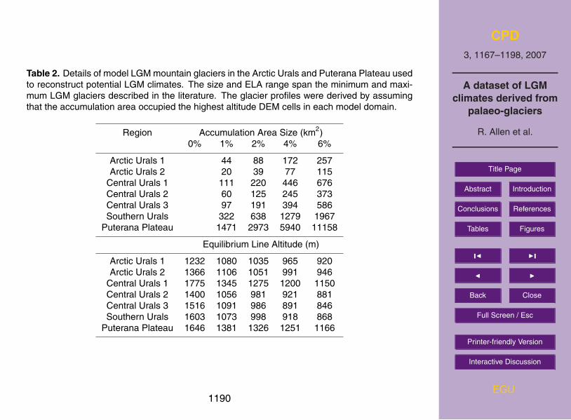
Table 2. Details of model LGM mountain glaciers in the Arctic Urals and Puterana Plateau usedto reconstruct potential LGM climates. The size and ELA range span the minimum and maxi-mum LGM glaciers described in the literature. The glacier profiles were derived by assumingthat the accumulation area occupied the highest altitude DEM cells in each model domain.

Region Accumulation Area Size (km2)

0% 1% 2% 4% 6%

Arctic Urals 1 44 88 172 257Arctic Urals 2 20 39 77 115

Central Urals 1 111 220 446 676Central Urals 2 60 125 245 373Central Urals 3 97 191 394 586Southern Urals 322 638 1279 1967

Puterana Plateau 1471 2973 5940 11158

Equilibrium Line Altitude (m)

Arctic Urals 1 1232 1080 1035 965 920Arctic Urals 2 1366 1106 1051 991 946

Central Urals 1 1775 1345 1275 1200 1150Central Urals 2 1400 1056 981 921 881Central Urals 3 1516 1091 986 891 846Southern Urals 1603 1073 998 918 868

Puterana Plateau 1646 1381 1326 1251 1166

1190




http://www.egu.eu

CPD

3, 1167–1198, 2007

A dataset of LGM


palaeo-glaciers

R. Allen et al.

Title Page



Tables Figures

◭ ◮

◭ ◮

Back Close

Full Screen / Esc



EGU

Fig. 1. Location of Quaternary glacial-geological evidence in Europe and Russia (adapted fromEhlers and Gibbard, 2004a).

1191




http://www.egu.eu

CPD

3, 1167–1198, 2007

A dataset of LGM


palaeo-glaciers

R. Allen et al.

Title Page



Tables Figures

◭ ◮

◭ ◮

Back Close

Full Screen / Esc



EGU

Fig. 2. Extract from Plate NK21 of the INQUA GIS of Quaternary glaciers, covering the Vos-ges Mountains, France and Bavarian Mountains, Germany. Figure adapted from Ehlers andGibbard (2004a).

1192




http://www.egu.eu

CPD

3, 1167–1198, 2007

A dataset of LGM


palaeo-glaciers

R. Allen et al.

Title Page



Tables Figures

◭ ◮

◭ ◮

Back Close

Full Screen / Esc



EGU

Fig. 3. Examples of LGM climate anomaly reconstructions for mountain regions in the IberianPeninsula. The range optimum climates for each precipitation anomaly is ±1 standard devia-tion, and represents the variation in results from contributing model sites and optimum climatesfrom different lapse rate combinations. The location of the mountain regions can be found inFig. 1.

1193




http://www.egu.eu

CPD

3, 1167–1198, 2007

A dataset of LGM


palaeo-glaciers

R. Allen et al.

Title Page



Tables Figures

◭ ◮

◭ ◮

Back Close

Full Screen / Esc



EGU

Fig. 4. Reconstructed LGM climates across Europe and Black Sea simulated using presentday annual precipitation totals derived from the CRU2.0 climate dataset (New et al., 2002).Reconstructions of LGM glaciers are adapted from the INQUA database (Ehlers and Gibbard,2004a).

1194




http://www.egu.eu

CPD

3, 1167–1198, 2007

A dataset of LGM


palaeo-glaciers

R. Allen et al.

Title Page



Tables Figures

◭ ◮

◭ ◮

Back Close

Full Screen / Esc



EGU

Fig. 5. Reconstructed LGM climates across Europe and Black Sea simulated using −40% ofpresent day annual precipitation totals derived from the CRU2.0 climate dataset (New et al.,2002). Reconstructions of LGM glaciers are adapted from the INQUA database (Ehlers andGibbard, 2004a).

1195




http://www.egu.eu

CPD

3, 1167–1198, 2007

A dataset of LGM


palaeo-glaciers

R. Allen et al.

Title Page



Tables Figures

◭ ◮

◭ ◮

Back Close

Full Screen / Esc



EGU

Fig. 6. Reconstructed LGM climates across Europe and Black Sea simulated using −80% ofpresent day annual precipitation totals derived from the CRU2.0 climate dataset (New et al.,2002). Reconstructions of LGM glaciers are adapted from the INQUA database (Ehlers andGibbard, 2004a). 1196




http://www.egu.eu

CPD

3, 1167–1198, 2007

A dataset of LGM


palaeo-glaciers

R. Allen et al.

Title Page



Tables Figures

◭ ◮

◭ ◮

Back Close

Full Screen / Esc



EGU

Fig. 7. LGM climate anomalies reconstructed over the Ural Mountains. The colours repre-sent different precipitation anomalies ranging from +100% to −80% of present day (the colourgradation is the same as Fig. 3. The shapes represent the different glacial extents consid-ered by the glacier-climate model (circle=0%, star=1%, diamond=2%, triangle=4%, invertedtriangle=6%).

1197




http://www.egu.eu

CPD

3, 1167–1198, 2007

A dataset of LGM


palaeo-glaciers

R. Allen et al.

Title Page



Tables Figures

◭ ◮

◭ ◮

Back Close

Full Screen / Esc



EGU

Fig. 8. LGM climate anomalies reconstructed over the Puterana Plateau. The colours repre-sent different precipitation anomalies ranging from +100% to −80% of present day (the colourgradation is the same as Fig. 3. The shapes represent the different glacial extents consid-ered by the glacier-climate model (circle=0%, star=1%, diamond=2%, triangle=4%, invertedtriangle=6%, square=INQUA LGM ice cap).

1198




http://www.egu.eu

reconstructing glacier-based climates of lgm europe and russia? part 1: numerical modelling and...

Documents