prediction of solar radiation for the major climates of jordan

24

INTRODUCTION

The amount of energy incident on the earth’s surface is rarely available and recorded only in specific locations, particularly in developing re-gions such as Jordan. However, solar radiation measuring equipment requires regular mainte-nance and calibration not to mention their high costs. One of the most well-known and simplest methods is the relationship (1) developed by Ang-ström (1924):

𝐻𝐻/𝐻𝐻₀ = a + b (𝑛𝑛/𝑁𝑁₀) (1)

where: a and b are coefficients that are given for the location in question and are shown in Table 1,

H0 – the monthly average daily extrater-restrial radiation on a horizontal surface, MJ/m2.daily

H – monthly mean daily solar radiation on horizontal surface, MJ/m2.daily

n – monthly mean daily hours of bright sunshine, hours

N0 – Monthly average of maximum pos-sible daily hours of bright sunshine (day length)

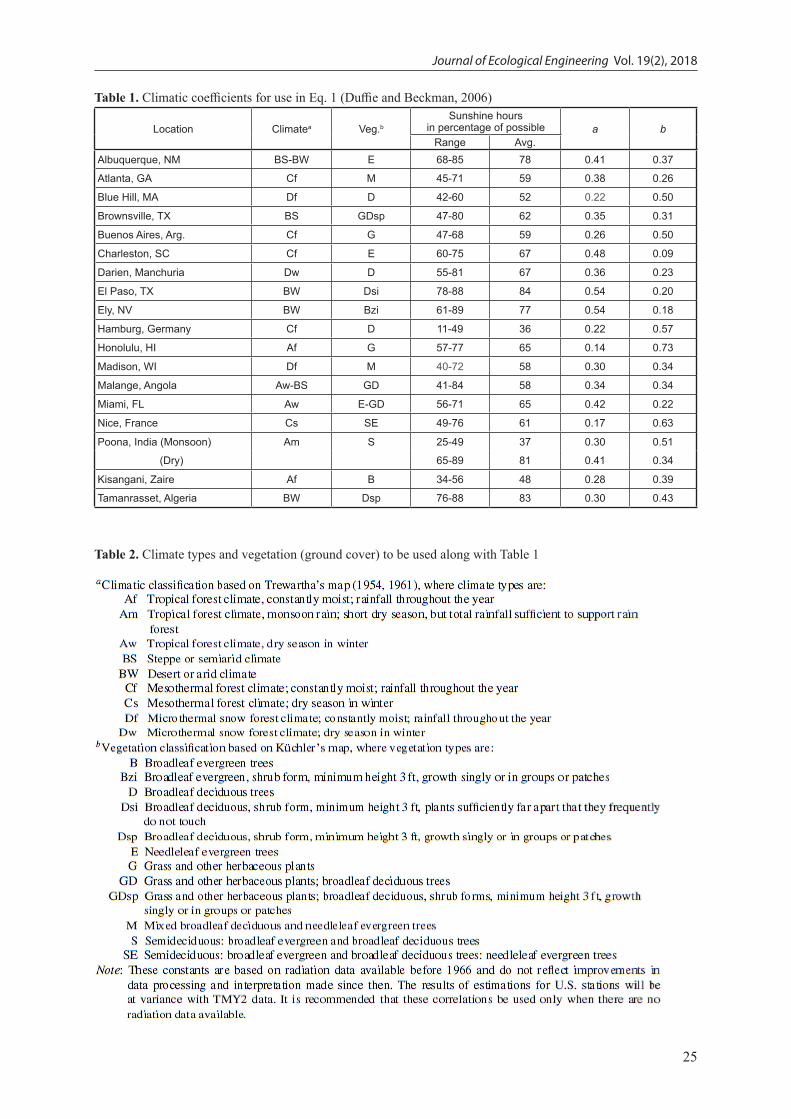
The coefficients a and b are shown in the last two columns of the Table. Unfortunately, it cov-ers only 18 major locations in the world, and none of these is in Jordan or even nearby. The first two columns are concerned with climate types and vegetation, as illustrated by Table 2 (Duffie and Beckman, 2006).

For example, Jordan’s climate may be clas-sified as desert or arid climate (BW) and its veg-etation as broad leaf deciduous, shrub form, with the minimum height of plants reaching 3 ft, suffi-ciently far apart that they frequently do not touch (Dsi). In other words, the location in Table 1 that best simulates the climate type of Jordan is El Paso, Texas.

Rietveld (1978) analyzed various published values and noted that a is related linearly and b hyperbolically to the appropriate mean values of (n/N0). The results were shown in equations (3) and (4):

Journal of Ecological Engineering Received: 2017.12.15 Accepted: 2018.01.18Published: 2018.03.01Volume 19, Issue 2, March 2018, pages 24–38

https://doi.org/10.12911/22998993/81240

Prediction of Solar Radiation for the Major Climates of Jordan: A Regression Model

Ali A. Badran1*, Belal F. Dwaykat2

1 Department of Mechanical Engineering, Philadelphia University, Amman, Jordan 2 Deparrtment of Mechanical Engineering, Energy Management Program, University of Jordan, Amman, Jordan

* Corresponding author’s e-mail: [email protected]

ABSTRACTMultiple regression models were developed for calculating the regression coefficients a and b of the Angström-type equation for estimating the monthly average daily global radiation on a horizontal surface for six major climates in Jordan. The equations for a and b were developed from the available values of these constants reported in the literature for locations across the country, along with the sunshine duration and the values of ground albedo (ρg). The developed correlations were tested for their applicability by estimating the regression constants and the solar radiation for six locations spread over the country, which were Irbid, Amman, Azraq, Al-Shawbak, Ma’an and Aqaba. The remarkable agreement between the estimated and experimental data of solar radiation in those loca-tions suggests a wide applicability of the method for the locations with sunshine duration ranging from 0.7 to 0.8. The maximum and minimum percentages of error for those locations were found to be 6.3, 0.05%, respectively.

Keywords: solar radiation, regression model, climate in Jordan

25

Journal of Ecological Engineering Vol. 19(2), 2018

Table 1. Climatic coefficients for use in Eq. 1 (Duffie and Beckman, 2006)

Location Climatea Veg.bSunshine hours

in percentage of possible a bRange Avg.

Albuquerque, NM BS-BW E 68-85 78 0.41 0.37

Atlanta, GA Cf M 45-71 59 0.38 0.26

Blue Hill, MA Df D 42-60 52 0.22 0.50

Brownsville, TX BS GDsp 47-80 62 0.35 0.31

Buenos Aires, Arg. Cf G 47-68 59 0.26 0.50

Charleston, SC Cf E 60-75 67 0.48 0.09

Darien, Manchuria Dw D 55-81 67 0.36 0.23

El Paso, TX BW Dsi 78-88 84 0.54 0.20

Ely, NV BW Bzi 61-89 77 0.54 0.18

Hamburg, Germany Cf D 11-49 36 0.22 0.57

Honolulu, HI Af G 57-77 65 0.14 0.73

Madison, WI Df M 40-72 58 0.30 0.34

Malange, Angola Aw-BS GD 41-84 58 0.34 0.34

Miami, FL Aw E-GD 56-71 65 0.42 0.22

Nice, France Cs SE 49-76 61 0.17 0.63

Poona, India (Monsoon) Am S 25-49 37 0.30 0.51

(Dry) 65-89 81 0.41 0.34

Kisangani, Zaire Af B 34-56 48 0.28 0.39

Tamanrasset, Algeria BW Dsp 76-88 83 0.30 0.43

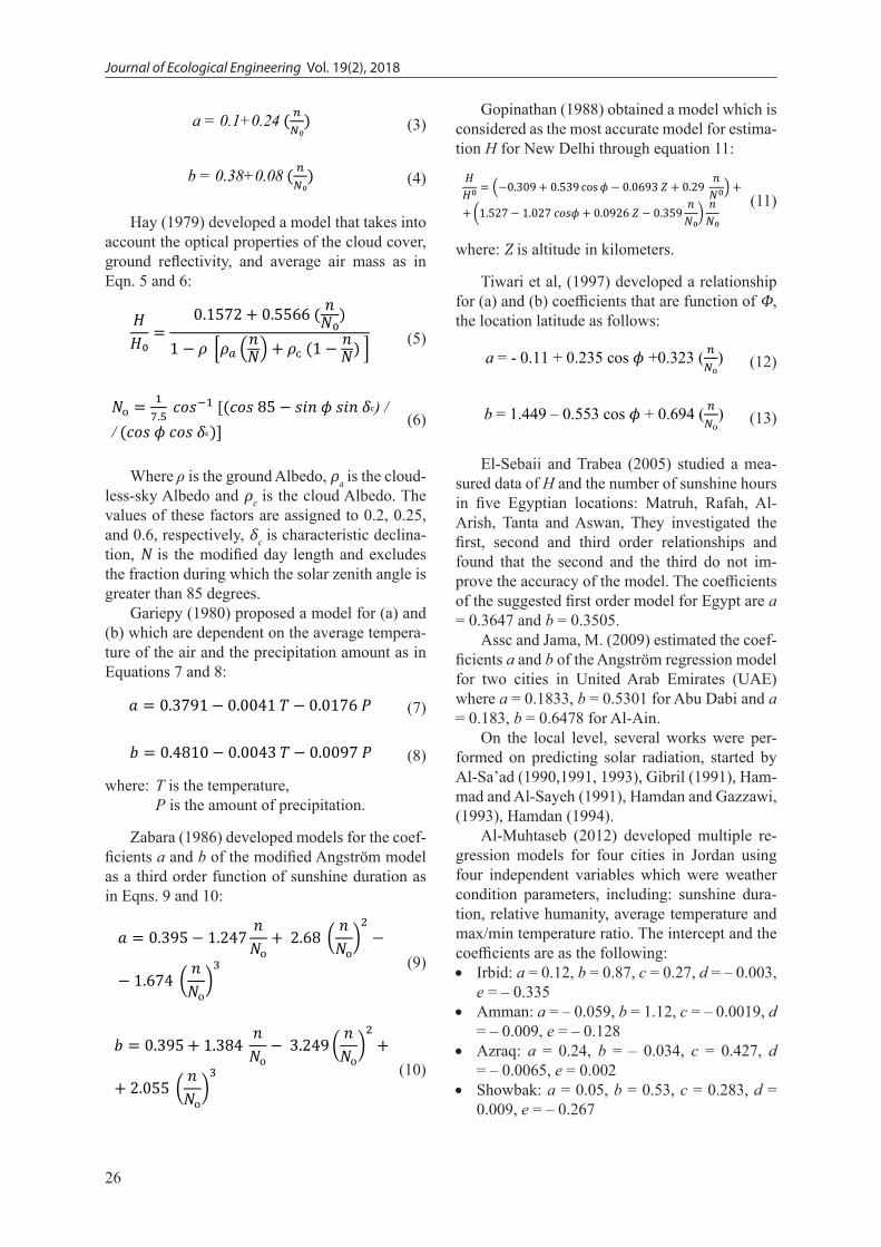
Table 2. Climate types and vegetation (ground cover) to be used along with Table 1


26

a = 0.1+0.24 ( 𝑛𝑛𝑁𝑁₀) (3)

b = 0.38+0.08 ( 𝑛𝑛𝑁𝑁₀) (4)

Hay (1979) developed a model that takes into account the optical properties of the cloud cover, ground reflectivity, and average air mass as in Eqn. 5 and 6:

𝐻𝐻𝐻𝐻₀ =

0.1572 + 0.5566 ( 𝑛𝑛𝑁𝑁₀)

1 − 𝜌𝜌 [𝜌𝜌𝑎𝑎 (𝑛𝑛𝑁𝑁) + 𝜌𝜌ᴄ (1 − 𝑛𝑛

𝑁𝑁) ] (5)

𝑁𝑁ᴏ = 17.5 𝑐𝑐𝑐𝑐𝑐𝑐−1 [(𝑐𝑐𝑐𝑐𝑐𝑐 85 − 𝑐𝑐𝑠𝑠𝑠𝑠 𝜙𝜙 𝑐𝑐𝑠𝑠𝑠𝑠 𝛿𝛿ᶜ) /

/ (𝑐𝑐𝑐𝑐𝑐𝑐 𝜙𝜙 𝑐𝑐𝑐𝑐𝑐𝑐 𝛿𝛿ᶜ)] (6)

Where ρ is the ground Albedo, ρa is the cloud-less-sky Albedo and ρc is the cloud Albedo. The values of these factors are assigned to 0.2, 0.25, and 0.6, respectively, δc is characteristic declina-tion, N is the modified day length and excludes the fraction during which the solar zenith angle is greater than 85 degrees.

Gariepy (1980) proposed a model for (a) and (b) which are dependent on the average tempera-ture of the air and the precipitation amount as in Equations 7 and 8:

𝑎𝑎 = 0.3791 − 0.0041 𝑇𝑇 − 0.0176 𝑃𝑃 (7)

𝑏𝑏 = 0.4810 − 0.0043 𝑇𝑇 − 0.0097 𝑃𝑃 (8)

where: T is the temperature, P is the amount of precipitation.

Zabara (1986) developed models for the coef-ficients a and b of the modified Angström model as a third order function of sunshine duration as in Eqns. 9 and 10:

𝑎𝑎 = 0.395 − 1.247 𝑛𝑛𝑁𝑁ᴏ

+ 2.68 ( 𝑛𝑛𝑁𝑁ᴏ

)2

−

− 1.674 ( 𝑛𝑛𝑁𝑁ᴏ

)3

(9)

𝑏𝑏 = 0.395 + 1.384 𝑛𝑛𝑁𝑁ᴏ

− 3.249 ( 𝑛𝑛𝑁𝑁ᴏ

)2

+

+ 2.055 ( 𝑛𝑛𝑁𝑁ᴏ

)3

(10)

Gopinathan (1988) obtained a model which is considered as the most accurate model for estima-tion H for New Delhi through equation 11:

𝐻𝐻𝐻𝐻0 = (−0.309 + 0.539 cos 𝜙𝜙 − 0.0693 𝑍𝑍 + 0.29 𝑛𝑛

𝑁𝑁0) +

+ (1.527 − 1.027 𝑐𝑐𝑐𝑐𝑐𝑐𝜙𝜙 + 0.0926 𝑍𝑍 − 0.359 𝑛𝑛𝑁𝑁₀) 𝑛𝑛

𝑁𝑁₀ (11)

where: Z is altitude in kilometers.

Tiwari et al, (1997) developed a relationship for (a) and (b) coefficients that are function of Φ, the location latitude as follows:

a = - 0.11 + 0.235 cos 𝜙𝜙 +0.323 ( 𝑛𝑛𝑁𝑁ᴏ) (12)

b = 1.449 – 0.553 cos 𝜙𝜙 + 0.694 ( 𝑛𝑛𝑁𝑁ᴏ) (13)

El-Sebaii and Trabea (2005) studied a mea-sured data of H and the number of sunshine hours in five Egyptian locations: Matruh, Rafah, Al-Arish, Tanta and Aswan, They investigated the first, second and third order relationships and found that the second and the third do not im-prove the accuracy of the model. The coefficients of the suggested first order model for Egypt are a = 0.3647 and b = 0.3505.

Assc and Jama, M. (2009) estimated the coef-ficients a and b of the Angström regression model for two cities in United Arab Emirates (UAE) where a = 0.1833, b = 0.5301 for Abu Dabi and a = 0.183, b = 0.6478 for Al-Ain.

On the local level, several works were per-formed on predicting solar radiation, started by Al-Sa’ad (1990,1991, 1993), Gibril (1991), Ham-mad and Al-Sayeh (1991), Hamdan and Gazzawi, (1993), Hamdan (1994).

Al-Muhtaseb (2012) developed multiple re-gression models for four cities in Jordan using four independent variables which were weather condition parameters, including: sunshine dura-tion, relative humanity, average temperature and max/min temperature ratio. The intercept and the coefficients are as the following: • Irbid: a = 0.12, b = 0.87, c = 0.27, d = – 0.003,

e = – 0.335 • Amman: a = – 0.059, b = 1.12, c = – 0.0019, d

= – 0.009, e = – 0.128 • Azraq: a = 0.24, b = – 0.034, c = 0.427, d

= – 0.0065, e = 0.002 • Showbak: a = 0.05, b = 0.53, c = 0.283, d =

0.009, e = – 0.267

27


Al-Muhtaseb also used the Angström regres-sion model and developed new constants for the model for five locations in Jordan and, as a result, the a and b constants for Jordan are 0.279 and 0.489 respectively.

All of these works did not take into ac-count the effect of climate type and vegetation, or ground cover, in the considered region. In this work, these effects will be taken taken into consideration for the first time in six regions of Jordan, mainly Irbid, Amman, Azraq, Showbak, Ma’an and Aqaba.

THEORETICAL ANALYSIS

The major driver of the Earth’s climate and weather is the solar radiation, the energy rate which reaches the Earth is roughly 340W/m2, some of it is reflected back to space which is around one-third and while the remaining 240 W/m2 is absorbed by the atmosphere, ocean and land, the amount of absorbed energy depends on the surface and the atmosphere reflectivity.

An energy balance is used by researchers and scientists using the so-called Clouds and the Earth’s Radiant Energy System (CERES) which is a series of space-based sensors. Such sensors measure the reflected radiation from the Earth as a shortwave radiation (Albedo) and the thermal energy that the Earth emits as a long wave.

The albedo of the Earth, as indicated by ρg is about 0.84 if its surface is completely covered by snow; 0.85 of the sunlight which hit it would be reflected. On the other hand Earth with a green forest canopy covering its surface is characterized by albedo of 0.14, as most of the solar radiation would be absorbed.

Table 3 provides the values of Albedo for different cities, depending on the ground cover maps, vegetation maps, albedo tables and albedo data from NASA Earth Observatory (NEO).

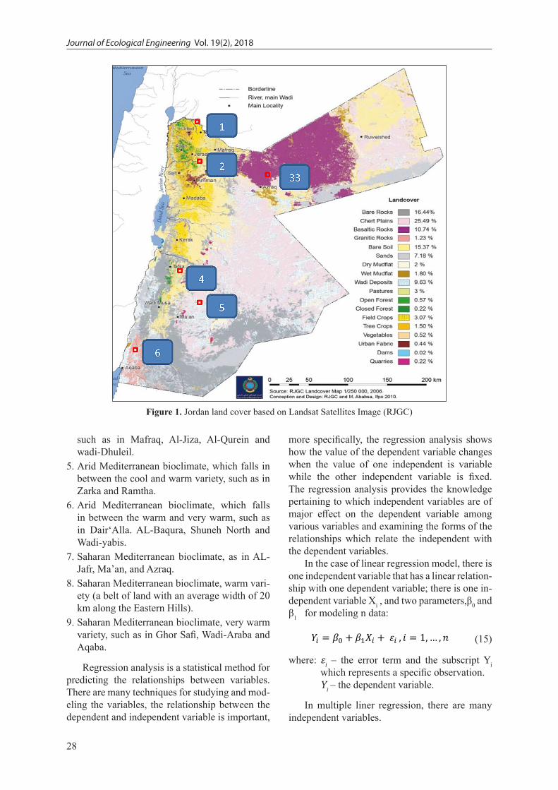
A series of ground cover maps were released in 2006 by the Royal Jordanian Geographic Cen-ter (RJGC), based on the usage of digital clas-sification of Landsat satellite images. Ground cover was divided into 18 classes which is a stan-dard developed by the European Environmental Agency (EEA). Figure 1 was drawn by Interna-tional Foundation for Protection Officers (IFPO) and RJGC shows the extracted 18 classes of the ground cover in Jordan. The map is considered as a part of the Atlas of Jordan. Three-quarters of

the land is covered with bare rocks, chert plains, granite rock, sand and bare soil. Wadis and mud-flats cover more than 14% of Jordan land where the vegetation is dense.

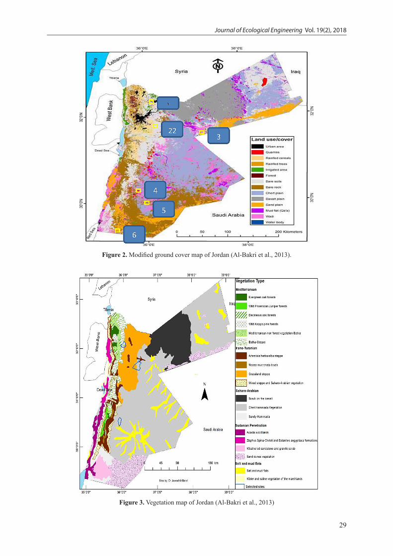
A more detailed map about desert, ground cover, as well as the irrigated and urban areas was produced by Al-Bakri et al. (2013), as shown in Figure 2. Jordan is also classified into various vegetation regions which are shown in Figure 3.

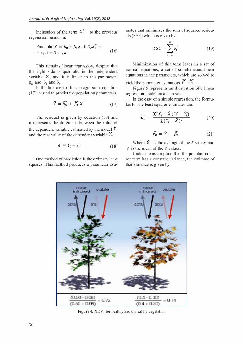
Vegetation may be expressed by Normalized Difference Vegetation Index (NDVI), which is considered as a method to represent the vegeta-tion level in a certain location. It is an index that indicates if the studied location includes green vegetation by analyzing remote sensing records; it can be obtained by means of equation (14).

NDVI = (𝜌𝜌NIR – 𝜌𝜌red)/( 𝜌𝜌NIR+𝜌𝜌red) (14)

where: ρred is the spectral reflectance records acquired in the red region and

ρNIR is the spectral reflectance records acquired in near-infrared region

Figure 4 represents values of NDVI which are 0.72 and 0.14 for a healthy and unhealthy vegeta-tion, respectively.

Dense vegetation canopy has positive index values (0.33 to 0.85), whereas clouds and snow fields have a negative index.

The climate across Jordan, based on the rain distribution, is considered to be of the Mediterra-nean variety because the rainfall mainly occurs in winter and spring, despite Jordan is divided into nine bioclimatic regions, including:1. Sub-humid Mediterranean bioclimate, cool

and warm varieties, such as Ras Muneef and Ajloun.

2. Semi-arid Mediterranean bioclimate, warm va-riety, such like in Irbid, Amman, Madaba, Tay-beh and Baka’a.

3. Semi-arid Mediterranean bioclimate, cool vari-ety, such as in Showbak and Tafileh.

4. Arid Mediterranean bioclimate, cool variety,

Table 3. Albedo values for the selected locations

Location AlbedoIrbid 0.17Amman 0.20Azraq 0.25Showbak 0.26Ma’an 0.38Aqaba 0.23


28

such as in Mafraq, Al-Jiza, Al-Qurein and wadi-Dhuleil.

5. Arid Mediterranean bioclimate, which falls in between the cool and warm variety, such as in Zarka and Ramtha.

6. Arid Mediterranean bioclimate, which falls in between the warm and very warm, such as in Dair‘Alla. AL-Baqura, Shuneh North and Wadi-yabis.

7. Saharan Mediterranean bioclimate, as in AL-Jafr, Ma’an, and Azraq.

8. Saharan Mediterranean bioclimate, warm vari-ety (a belt of land with an average width of 20 km along the Eastern Hills).

9. Saharan Mediterranean bioclimate, very warm variety, such as in Ghor Safi, Wadi-Araba and Aqaba.

Regression analysis is a statistical method for predicting the relationships between variables. There are many techniques for studying and mod-eling the variables, the relationship between the dependent and independent variable is important,

more specifically, the regression analysis shows how the value of the dependent variable changes when the value of one independent is variable while the other independent variable is fixed. The regression analysis provides the knowledge pertaining to which independent variables are of major effect on the dependent variable among various variables and examining the forms of the relationships which relate the independent with the dependent variables.

In the case of linear regression model, there is one independent variable that has a linear relation-ship with one dependent variable; there is one in-dependent variable Χi , and two parameters,β0 and β1 for modeling n data:

𝑌𝑌𝑖𝑖 = 𝛽𝛽0 + 𝛽𝛽1𝑋𝑋𝑖𝑖 + 𝜀𝜀𝑖𝑖 , 𝑖𝑖 = 1, … , 𝑛𝑛 (15)

where: εi – the error term and the subscript Yi which represents a specific observation.

Yi – the dependent variable.

In multiple liner regression, there are many independent variables.

Figure 1. Jordan land cover based on Landsat Satellites Image (RJGC)

29


Figure 2. Modified ground cover map of Jordan (Al-Bakri et al., 2013).

Figure 3. Vegetation map of Jordan (Al-Bakri et al., 2013)


30

Inclusuion of the term 𝑋𝑋𝑖𝑖2 to the previous regression results in:

Parabola: 𝑌𝑌𝑖𝑖 = 𝛽𝛽0 + 𝛽𝛽1𝑋𝑋𝑖𝑖 + 𝛽𝛽2𝑋𝑋𝑖𝑖2 +

+ 𝜀𝜀𝑖𝑖 , 𝑖𝑖 = 1, … , 𝑛𝑛 (16)

This remains linear regression, despite that the right side is quadratic in the independent variable Χi, and it is linear in the parameters β0 and β1 and β2.

In the first case of linear regression, equation (17) is used to predict the population parameters.

𝑌𝑌�̂�𝑖 = 𝛽𝛽0 ̂ + 𝛽𝛽1̂ 𝑋𝑋𝑖𝑖 (17)

The residual is given by equation (18) and it represents the difference between the value of the dependent variable estimated by the model 𝑌𝑌�̂�𝑖 and the real value of the dependent variable 𝑌𝑌𝑖𝑖. .

𝑒𝑒𝑖𝑖 = 𝑌𝑌𝑖𝑖 − 𝑌𝑌�̂�𝑖 (18)

One method of prediction is the ordinary least squares. This method produces a parameter esti-

mates that minimizes the sum of squared residu-als (SSE) which is given by:

𝑆𝑆𝑆𝑆𝑆𝑆 =∑𝑒𝑒𝑖𝑖2𝑛𝑛

𝑖𝑖=1 (19)

Minimization of this term leads in a set of normal equations, a set of simultaneous linear equations in the parameters, which are solved to

yield the parameter estimators 𝛽𝛽0 ̂ , 𝛽𝛽1̂ . .

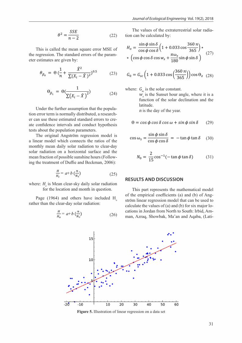
Figure 5 represents an illustration of a linear regression model on a data set.

In the case of a simple regression, the formu-las for the least squares estimates are:

𝛽𝛽1̂ = ∑(𝑋𝑋𝑖𝑖 − �̂�𝑋 )(𝑌𝑌𝑖𝑖 − 𝑌𝑌�̂�𝑖)

∑(𝑋𝑋𝑖𝑖 − �̂�𝑋 )2 (20)

𝛽𝛽0̂ = �̂�𝑌 − 𝛽𝛽1̂ (21)

Where �̂�𝑋 is the average of the X values and �̂�𝑌 is the mean of the Y values.

Under the assumption that the population er-ror term has a constant variance, the estimate of that variance is given by:

Figure 4. NDVI for healthy and unhealthy vegetation

31


𝜃𝜃2 = 𝑆𝑆𝑆𝑆𝑆𝑆𝑛𝑛 − 2 (22)

This is called the mean square error MSE of the regression. The standard errors of the param-eter estimates are given by:

𝜃𝜃𝛽𝛽0= Ө (1

𝑛𝑛 + �̂�𝑋2

∑(𝑋𝑋𝑖𝑖 − �̂�𝑋 )2)0.5 (23)

Ө𝛽𝛽1= Ө( 1

∑(𝑋𝑋𝑖𝑖 − �̂�𝑋 )2) (24)

Under the further assumption that the popula-tion error term is normally distributed, a research-er can use these estimated standard errors to cre-ate confidence intervals and conduct hypothesis tests about the population parameters.

The original Angström regression model is a linear model which connects the ratios of the monthly mean daily solar radiation to clear-day solar radiation on a horizontal surface and the mean fraction of possible sunshine hours (Follow-ing the treatment of Duffie and Beckman, 2006):

𝐻𝐻𝐻𝐻𝑐𝑐

= a+b ( 𝑛𝑛𝑁𝑁₀) (25)

where: Hc is Mean clear-sky daily solar radiation for the location and month in question.

Page (1964) and others have included Ho rather than the clear-day solar radiation:

𝐻𝐻𝐻𝐻𝑜𝑜

= a+b ( 𝑛𝑛𝑁𝑁₀) (26)

The values of the extraterrestrial solar radia-tion can be calculated by:

𝐻𝐻𝑜𝑜 = sin 𝜙𝜙 sin 𝛿𝛿cos 𝜙𝜙 cos 𝛿𝛿 (1 + 0.033 cos 360 𝑛𝑛

365 ) ∗

∗ (cos 𝜙𝜙 cos 𝛿𝛿 cos 𝑤𝑤𝑠𝑠 + 𝜋𝜋ω𝑠𝑠180 sin 𝜙𝜙 sin 𝛿𝛿 )

(27)

𝐺𝐺0 = 𝐺𝐺𝑠𝑠𝑠𝑠 (1 + 0.033 cos (360 𝑛𝑛365 )) cos Ө𝑧𝑧 (28)

where: Gsc is the solar constant. ws is the Sunset hour angle, where it is a

function of the solar declination and the latitude.

n is the day of the year.

Ө = 𝑐𝑐𝑐𝑐𝑐𝑐 𝜙𝜙 𝑐𝑐𝑐𝑐𝑐𝑐 𝛿𝛿 𝑐𝑐𝑐𝑐𝑐𝑐 𝜔𝜔 + 𝑐𝑐𝑠𝑠𝑠𝑠𝜙𝜙 𝑐𝑐𝑠𝑠𝑠𝑠 𝛿𝛿 (29)

cos ω𝑠𝑠 = sin 𝜙𝜙 sin 𝛿𝛿cos 𝜙𝜙 cos 𝛿𝛿 = − tan 𝜙𝜙 tan 𝛿𝛿 (30)

𝑁𝑁0 = 215 cos−1(− tan 𝜙𝜙 tan 𝛿𝛿) (31)

RESULTS AND DISCUSSION

This part represents the mathematical model of the empirical coefficients (a) and (b) of Ang-ström linear regression model that can be used to calculate the values of (a) and (b) for six major lo-cations in Jordan from North to South: Irbid, Am-man, Azraq, Showbak, Ma’an and Aqaba, (Lati-

Figure 5. Illustration of linear regression on a data set


32

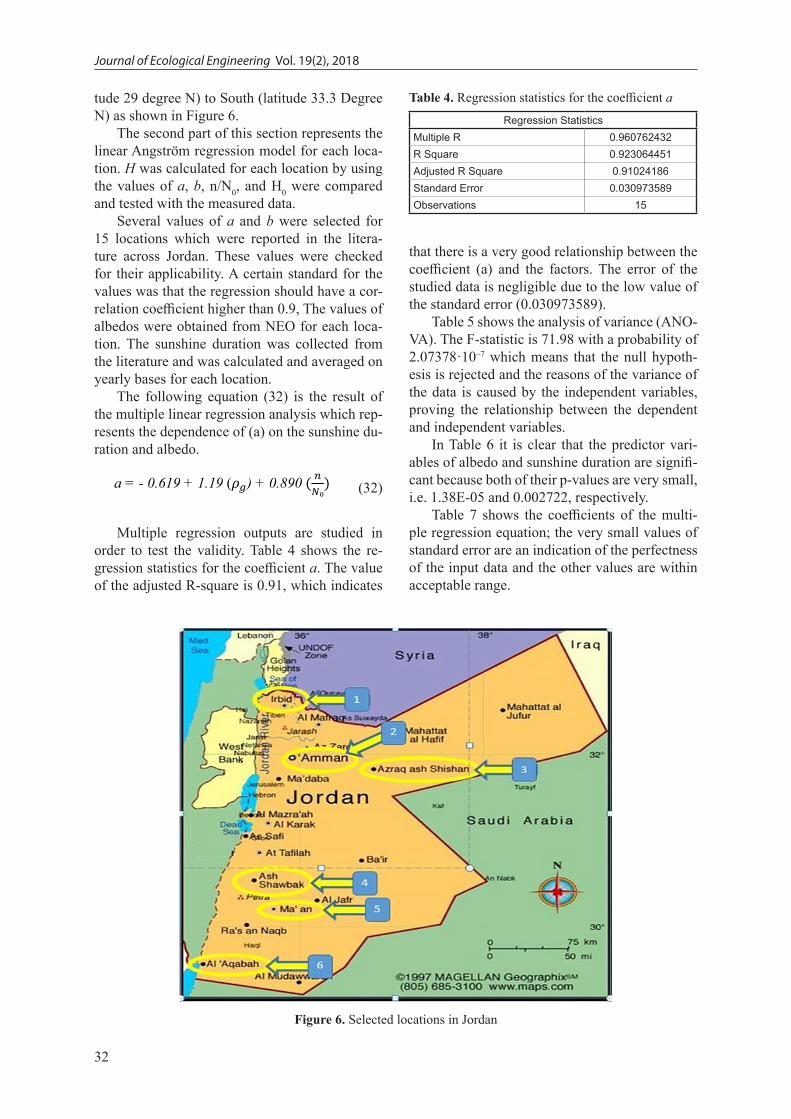
tude 29 degree N) to South (latitude 33.3 Degree N) as shown in Figure 6.

The second part of this section represents the linear Angström regression model for each loca-tion. H was calculated for each location by using the values of a, b, n/N0, and H0 were compared and tested with the measured data.

Several values of a and b were selected for 15 locations which were reported in the litera-ture across Jordan. These values were checked for their applicability. A certain standard for the values was that the regression should have a cor-relation coefficient higher than 0.9, The values of albedos were obtained from NEO for each loca-tion. The sunshine duration was collected from the literature and was calculated and averaged on yearly bases for each location.

The following equation (32) is the result of the multiple linear regression analysis which rep-resents the dependence of (a) on the sunshine du-ration and albedo.

a = - 0.619 + 1.19 (𝜌𝜌𝑔𝑔) + 0.890 ( 𝑛𝑛𝑁𝑁₀) (32)

Multiple regression outputs are studied in order to test the validity. Table 4 shows the re-gression statistics for the coefficient a. The value of the adjusted R-square is 0.91, which indicates

that there is a very good relationship between the coefficient (a) and the factors. The error of the studied data is negligible due to the low value of the standard error (0.030973589).

Table 5 shows the analysis of variance (ANO-VA). The F-statistic is 71.98 with a probability of 2.07378·10–7 which means that the null hypoth-esis is rejected and the reasons of the variance of the data is caused by the independent variables, proving the relationship between the dependent and independent variables.

In Table 6 it is clear that the predictor vari-ables of albedo and sunshine duration are signifi-cant because both of their p-values are very small, i.e. 1.38E-05 and 0.002722, respectively.

Table 7 shows the coefficients of the multi-ple regression equation; the very small values of standard error are an indication of the perfectness of the input data and the other values are within acceptable range.

Figure 6. Selected locations in Jordan

Table 4. Regression statistics for the coefficient a

Regression StatisticsMultiple R 0.960762432R Square 0.923064451Adjusted R Square 0.91024186Standard Error 0.030973589Observations 15

33


The following equation (33) is the result of the multiple linear regression analysis which rep-resents the dependence of a on the sunshine dura-tion and albedo.

b = 1.52 - 1.23 𝜌𝜌𝑔𝑔 - 1.00 ( 𝑛𝑛𝑁𝑁₀) (33)

Multiple regression outputs are studied in or-der to test the goodness. Table 8 shows the regres-sion statistics for the coefficient b. The value of the adjusted R-square is 0.80. It can be concluded that there is a very good relationship between the coefficient b and the factors. The error of the stud-ied data is negligible due to the small value of the standard error (0.05101747).

Table 9 shows the F-statistics is 29.8848 with a probability of 2.18498E-05, which means that the null hypothesis is rejected and the reasons of the variance of the data is caused by the indepen-dent variables which prove the relationship be-tween the dependent and independent variables.

Table 11 summarizes the previous analy-sis of the coefficients a and b with the correla-tion coefficient and the standard error estimation for each equation.

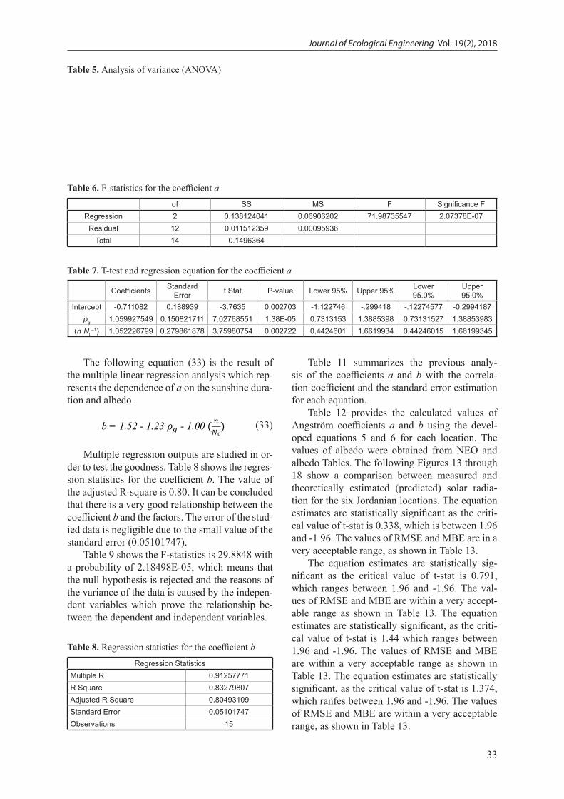
Table 12 provides the calculated values of Angström coefficients a and b using the devel-oped equations 5 and 6 for each location. The values of albedo were obtained from NEO and albedo Tables. The following Figures 13 through 18 show a comparison between measured and theoretically estimated (predicted) solar radia-tion for the six Jordanian locations. The equation estimates are statistically significant as the criti-cal value of t-stat is 0.338, which is between 1.96 and -1.96. The values of RMSE and MBE are in a very acceptable range, as shown in Table 13.

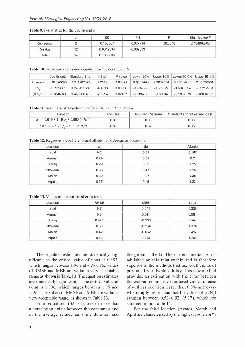
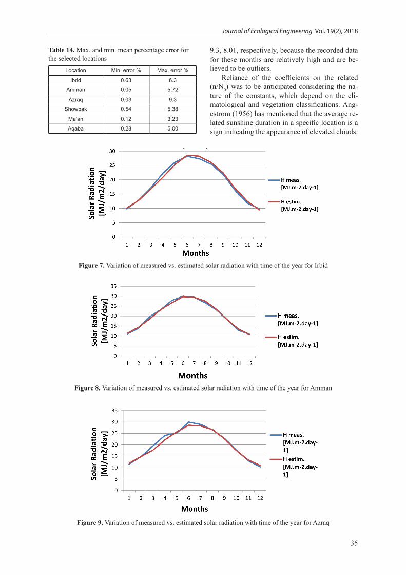
The equation estimates are statistically sig-nificant as the critical value of t-stat is 0.791, which ranges between 1.96 and -1.96. The val-ues of RMSE and MBE are within a very accept-able range as shown in Table 13. The equation estimates are statistically significant, as the criti-cal value of t-stat is 1.44 which ranges between 1.96 and -1.96. The values of RMSE and MBE are within a very acceptable range as shown in Table 13. The equation estimates are statistically significant, as the critical value of t-stat is 1.374, which ranfes between 1.96 and -1.96. The values of RMSE and MBE are within a very acceptable range, as shown in Table 13.

Table 5. Analysis of variance (ANOVA)

Table 6. F-statistics for the coefficient a

df SS MS F Significance FRegression 2 0.138124041 0.06906202 71.98735547 2.07378E-07

Residual 12 0.011512359 0.00095936Total 14 0.1496364

Table 7. T-test and regression equation for the coefficient a

Coefficients Standard Error t Stat P-value Lower 95% Upper 95% Lower

95.0%Upper 95.0%

Intercept -0.711082 0.188939 -3.7635 0.002703 -1.122746 -.299418 -.12274577 -0.2994187ρg 1.059927549 0.150821711 7.02768551 1.38E-05 0.7313153 1.3885398 0.73131527 1.38853983

(n·N0–1) 1.052226799 0.279861878 3.75980754 0.002722 0.4424601 1.6619934 0.44246015 1.66199345

Table 8. Regression statistics for the coefficient b

Regression StatisticsMultiple R 0.91257771R Square 0.83279807Adjusted R Square 0.80493109Standard Error 0.05101747Observations 15


34

The equation estimates are statistically sig-nificant, as the critical value of t-stat is 0.497, which ranges between 1.96 and -1.96. The values of RMSE and MBE are within a very acceptable range as shown in Table 13. The equation estimates are statistically significant, as the critical value of t-stat is 1.796, which ranges between 1.96 and -1.96. The values of RMSE and MBE are within a very acceptable range, as shown in Table 13.

From equations (32, 33), one can see that a correlation exists between the constant a and b, the average related sunshine duration and

the ground albedo. The current method is es-tablished on this relationship and is therefore superior to the methods that use coefficients of presumed worldwide validity. This new method provides an estimation with the error between the estimation and the measured values in case of outliers isolation lesser than 6.3% and over-whelmingly lesser than that for values of (n/N0) ranging between 0.53–0.92, (5.17), which are summed up in Table 14.

For the third location (Azraq), March and April are characterized by the highest abs. error %

Table 9. F-statistics for the coefficient b

df SS MS F Significance F

Regression 2 0.155567 0.077784 29.8848 2.18498E-05

Residual 12 0.0312334 0.002603

Total 14 0.1868004

Table 10. T-test and regression equation for the coefficient b

Coefficients Standard Error t Stat P-value Lower 95% Upper 95% Lower 95.0% Upper 95.0%

Intercept 1.62820698 0.311207379 5.2319 0.00021 0.9501443 2.3062696 0.95014435 2.30626961

ρg -1.0933889 0.248422683 -4.4013 0.00086 -1.634655 -0.552122 -1.6346554 -.55212238

(n·N0–1) -1.1844041 0.460968373 -2.5694 0.02457 -2.188768 -0.18004 -2.1887679 -.18004027

Table 11. Summary of Angström coefficients a and b equationsStandard error of estimation (S)Adjusted R-squareR-quareRelation

0.030.860.93a = – 0.619 + 1.19 ρg + 0.890 (n·N0–1)

0.050.820.89b = 1.52 – 1.23 ρg – 1.00 (n·N0–1)

Table 12. Regression coefficients and albedo for 6 Jordanian locations.Location (a) (b) Albedo

Irbid 0.2 0.61 0.167

Amman 0.29 0.51 0.2

Azraq 0.29 0.53 0.25

Showbak 0.35 0.47 0.26

Ma’an 0.52 0.27 0.38

Aqaba 0.35 0.45 0.23

Table 13. Values of the statistical error testst-statMBERMSELocation

0.3380.0710.7Irbid

0.0640.0110.6Amman

1.44-0.3680.925Azraq

1.374-0.2640.69Showbak

0.497-0.0620.42Ma’an

1.7960.2530.53Aqaba

35


Table 14. Max. and min. mean percentage error for the selected locations

Location Min. error % Max. error %

Ibrid 0.63 6.3

Amman 0.05 5.72

Azraq 0.03 9.3

Showbak 0.54 5.38

Ma’an 0.12 3.23

Aqaba 0.28 5.00

Figure 7. Variation of measured vs. estimated solar radiation with time of the year for Irbid

Figure 8. Variation of measured vs. estimated solar radiation with time of the year for Amman

Figure 9. Variation of measured vs. estimated solar radiation with time of the year for Azraq

9.3, 8.01, respectively, because the recorded data for these months are relatively high and are be-lieved to be outliers.

Reliance of the coefficients on the related (n/N0) was to be anticipated considering the na-ture of the constants, which depend on the cli-matological and vegetation classifications. Ang-estrom (1956) has mentioned that the average re-lated sunshine duration in a specific location is a sign indicating the appearance of elevated clouds:


36

the higher (n/N0) , the higher the clouds. The el-evated clouds are drier than the lower clouds so they absorb less shortwave radiation resulting in more sunlight that breaks through the clouds.

The vegetation classification (i.e vegetation type, greenness level and intensity) for a specific location is inversely proportional to albedo, the higher the vegetation level, the lower the amount of reflected shortwave radiation (Albedo), as shown in Figure 4 through NDVI. On the other hand, a reliance of the coefficients on the rela-tive ground albedo is also expected for the same reason that is mentioned above, which results from the nature of the coefficients, Increasing the ground albedo will lead to an increase of the re-flected shortwave solar radiation. Ground albedo is proportional to a coefficient and has an inverse relationship with b coefficient, as shown in Table 11, and the equations in Table 12.

As a result, Ma’an location has the high-est albedo 0.38 due to the very poor vegetation level in that location and the sandy ground cover among the selected location. On the other hand, Irbid has the lowest albedo 0.167 due to the high-

er vegetation level (trees and crops) as shown in Table 3 and Figure 5.

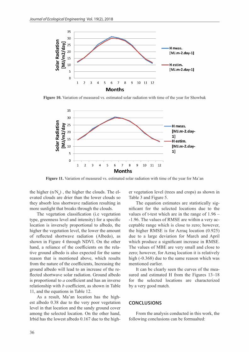
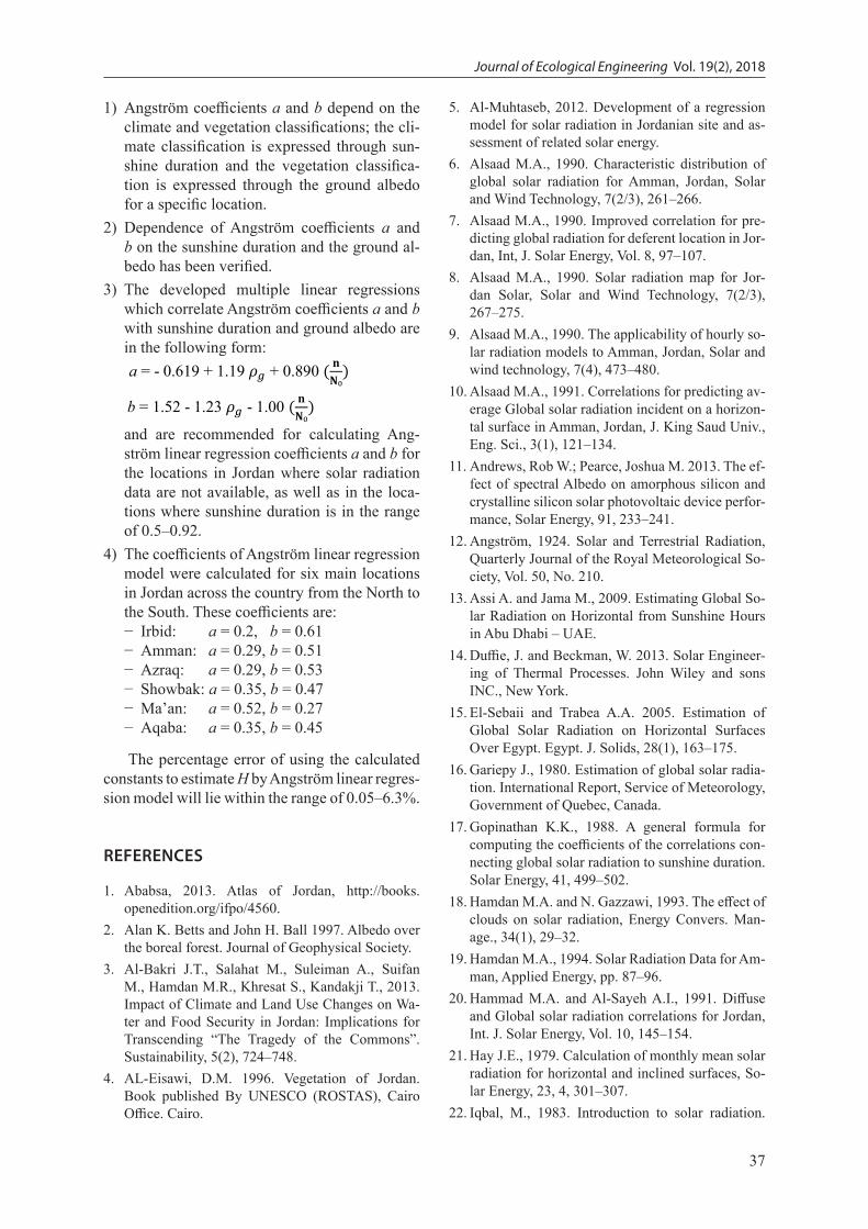
The equation estimates are statistically sig-nificant for the selected locations due to the values of t-test which are in the range of 1.96 – -1.96. The values of RMSE are within a very ac-ceptable range which is close to zero; however, the higher RMSE is for Azraq location (0.925) due to a large deviation for March and April which produce a significant increase in RMSE. The values of MBE are very small and close to zero; however, for Azraq location it is relatively high (-0.368) due to the same reason which was mentioned earlier.

It can be clearly seen the curves of the mea-sured and estimated H from the Figures 13–18 for the selected locations are characterized by a very good match.

CONCLUSIONS

From the analysis conducted in this work, the following conclusions can be formualted:

Figure 10. Variation of measured vs. estimated solar radiation with time of the year for Showbak

Figure 11. Variation of measured vs. estimated solar radiation with time of the year for Ma’an

37


1) Angström coefficients a and b depend on the climate and vegetation classifications; the cli-mate classification is expressed through sun-shine duration and the vegetation classifica-tion is expressed through the ground albedo for a specific location.

2) Dependence of Angström coefficients a and b on the sunshine duration and the ground al-bedo has been verified.

3) The developed multiple linear regressions which correlate Angström coefficients a and b with sunshine duration and ground albedo are in the following form:

a = - 0.619 + 1.19 𝜌𝜌𝑔𝑔 + 0.890 ( 𝐧𝐧𝐍𝐍₀)

b = 1.52 - 1.23 𝜌𝜌𝑔𝑔 - 1.00 ( 𝐧𝐧𝐍𝐍₀) and are recommended for calculating Ang-

ström linear regression coefficients a and b for the locations in Jordan where solar radiation data are not available, as well as in the loca-tions where sunshine duration is in the range of 0.5–0.92.

4) The coefficients of Angström linear regression model were calculated for six main locations in Jordan across the country from the North to the South. These coefficients are:− Irbid: a = 0.2, b = 0.61− Amman: a = 0.29, b = 0.51− Azraq: a = 0.29, b = 0.53− Showbak: a = 0.35, b = 0.47− Ma’an: a = 0.52, b = 0.27− Aqaba: a = 0.35, b = 0.45

The percentage error of using the calculated constants to estimate H by Angström linear regres-sion model will lie within the range of 0.05–6.3%.

REFERENCES

1. Ababsa, 2013. Atlas of Jordan, http://books.openedition.org/ifpo/4560.

2. Alan K. Betts and John H. Ball 1997. Albedo over the boreal forest. Journal of Geophysical Society.

3. Al-Bakri J.T., Salahat M., Suleiman A., Suifan M., Hamdan M.R., Khresat S., Kandakji T., 2013. Impact of Climate and Land Use Changes on Wa-ter and Food Security in Jordan: Implications for Transcending “The Tragedy of the Commons”. Sustainability, 5(2), 724–748.

4. AL-Eisawi, D.M. 1996. Vegetation of Jordan. Book published By UNESCO (ROSTAS), Cairo Office. Cairo.

5. Al-Muhtaseb, 2012. Development of a regression model for solar radiation in Jordanian site and as-sessment of related solar energy.

6. Alsaad M.A., 1990. Characteristic distribution of global solar radiation for Amman, Jordan, Solar and Wind Technology, 7(2/3), 261–266.

7. Alsaad M.A., 1990. Improved correlation for pre-dicting global radiation for deferent location in Jor-dan, Int, J. Solar Energy, Vol. 8, 97–107.

8. Alsaad M.A., 1990. Solar radiation map for Jor-dan Solar, Solar and Wind Technology, 7(2/3), 267–275.

9. Alsaad M.A., 1990. The applicability of hourly so-lar radiation models to Amman, Jordan, Solar and wind technology, 7(4), 473–480.

10. Alsaad M.A., 1991. Correlations for predicting av-erage Global solar radiation incident on a horizon-tal surface in Amman, Jordan, J. King Saud Univ., Eng. Sci., 3(1), 121–134.

11. Andrews, Rob W.; Pearce, Joshua M. 2013. The ef-fect of spectral Albedo on amorphous silicon and crystalline silicon solar photovoltaic device perfor-mance, Solar Energy, 91, 233–241.

12. Angström, 1924. Solar and Terrestrial Radiation, Quarterly Journal of the Royal Meteorological So-ciety, Vol. 50, No. 210.

13. Assi A. and Jama M., 2009. Estimating Global So-lar Radiation on Horizontal from Sunshine Hours in Abu Dhabi – UAE.

14. Duffie, J. and Beckman, W. 2013. Solar Engineer-ing of Thermal Processes. John Wiley and sons INC., New York.

15. El-Sebaii and Trabea A.A. 2005. Estimation of Global Solar Radiation on Horizontal Surfaces Over Egypt. Egypt. J. Solids, 28(1), 163–175.

16. Gariepy J., 1980. Estimation of global solar radia-tion. International Report, Service of Meteorology, Government of Quebec, Canada.

17. Gopinathan K.K., 1988. A general formula for computing the coefficients of the correlations con-necting global solar radiation to sunshine duration. Solar Energy, 41, 499–502.

18. Hamdan M.A. and N. Gazzawi, 1993. The effect of clouds on solar radiation, Energy Convers. Man-age., 34(1), 29–32.

19. Hamdan M.A., 1994. Solar Radiation Data for Am-man, Applied Energy, pp. 87–96.

20. Hammad M.A. and Al-Sayeh A.I., 1991. Diffuse and Global solar radiation correlations for Jordan, Int. J. Solar Energy, Vol. 10, 145–154.

21. Hay J.E., 1979. Calculation of monthly mean solar radiation for horizontal and inclined surfaces, So-lar Energy, 23, 4, 301–307.

22. Iqbal, M., 1983. Introduction to solar radiation.


38

New York: Academic23. Jain P.C., 1988. Estimation of monthly average

hourly global and diffuse irradiation. Solar Wind Technol. 5, 7.

24. Jain S., Jain P.C., 1988. A comparison of the Ang-ström-type correlations and the estimation of month-ly average daily global irradiation. Solar Energy.

25. Jamil Ahmad M., Tiwari G.N., 2010. Solar radia-tion models – review. International journal of en-ergy and environment, 1(3), 513–532.

26. Liu B.Y. and Jordan R.C., 1960. The Interrelation-ship and Characteristic Distribution of Direct, Dif-fuse, and Total Radiation, Solar Energy, 4(3), 1–19.

27. Liu B.Y. and Jordan R.C. 1940. The interrelation-ship and characteristic distribution of direct, de-fuse, and total solar radiation. Solar Energy, 4(1).

28. Long, G., 1957. The bioclimatology and vegetation of East Jordan. Rome, UNESCO/ FAO.

29. Markvart T. and Castazer L., 2003. Practical Hand-book of Photovoltaics: Fundamentals and Applica-tions.

30. Page J.K., 1961. The estimation of monthly mean values of daily total short wave radiation on verti-cal and inclined surface from sunshine records for latitudes 40N–40S. Proceedings of UN Conference on New Sources of Energy, 4(598), 378–390.

31. Rietveld M. 1978. A new method for estimating the regression coefficients in the formula relating so-lar radiation to sunshine. Agricultural Meteorology 19, 243–252.

32. Starr M.R., Palz W., 1983. Photovoltaic power for Europe: an assessment study, Commission of the European Communities. (http://www.ftexploring.com/solar-energy/direct-and-diffuse-radiation.htm#fn2)

33. Stone, R.J., 1993. Improved statistical procedure for the evaluation of solar radiation estimation models. Solar Energy Vol. 51, 289.

34. Tetzlaff, G., 1983. Albedo of the Sahara. Cologne University Satellite Measurement of Radiation Budget Parameters. pp. 60–63.

35. Tiwari, R.F and Sangeeta, T.H. 1997. Solar Energy, 24(6) 89–95.

36. Togrul, I.T., 1998. Comparison of statistical perfor-mance of seven sunshine-based models for Elazig, Turkey, Chemica Acta Turuca, 26, 37.

37. Zabara K., 1986. Estimation of the global solar radiation in Greece. Solar and Wind Technology, 3(4), 267–272.

38. Zaid Jibril, 1991. Estimation of solar radiation over Jordan-Predicted tables, Renewable Energy, Vol. 2, 277–291.

prediction of solar radiation for the major climates of jordan

Documents