the new remote-sensing-derived swiss glacier inventory
TRANSCRIPT
The new remote-sensing-derived Swiss glacier inventoryI Methods
Frank Paul Andreas KIgraveIgraveb Max MaischTobias KellenbergerWilfried HaeberliDepartment of Geography University of ZIumlrich-Irchel CH-8057 ZIumlrich Switzerland
ABSTRACT A new Swiss glacier inventory is to be compiled from satellite data for theyear 2000 The study presented here describes two major tasks (1) an accuracy assessment ofdifferent methods for glacier classification with LandsatThematic Mapper (TM) data and adigital elevation model (DEM) (2) the geographical information system (GIS)-basedmethods for automatic extraction of individual glaciers from classified satellite data and thecomputation of three-dimensional glacier parameters (such as minimum maximum andmedian elevation or slope and orientation) by fusion with a DEM First results obtained bythese methods are presented in Part II of this paper (KIgraveIgraveb and others 2002)Thresholding ofa ratio image fromTM4 and TM5 reveals the best-suited glacier map The computation ofglacier parameters in a GIS environment is efficient and suitable for worldwide applicationThe methods developed contribute to the US Geological Survey-led Global Land Ice Meas-urements from Space (GLIMS) project which is currently compilinga global inventoryof landice masses within the framework of global glacier monitoring (Haeberli and others 2000)
INTRODUCTION
The latest Swiss glacier inventory from 1973 was compiledfrom aerial photography with glacier outlines transferredto topographic maps of the scale 125 000 (Mulaquo ller andothers 1976) Various glacier parameters were deduced bymanual planimetry (eg area) or manual map measure-ments (eg length minimum and maximum elevation)Since 1973 significant changes in glaciated area have takenplace in the Alps with a pronounced advance period of mostmountain glaciers (total area generally 41km2) until about1985 and a strong retreat thereafter (Herren and others1999) To overcome some of the difficulties of the previousinventory (costs manpower) it was decided to use satelliteimagery to create a new inventory reflecting conditions in2000 All necessary glacier parameters are derived within ageographical information system (GIS) in combinationwith a digital elevation model (DEM) In addition theUS Geological Survey-led Global Land Ice Measurementsfrom Space (GLIMS) project aims at compiling a globalinventory of land ice masses mainly using data from theAdvanced Spaceborne Thermal Emission and ReflectionRadiometer (ASTER) and Enhanced Thematic MapperPlus (ETM+) multispectral scanners on board the satellitesTerra and Landsat 7 respectively (Kargel 2000) Thus thenew Swiss glacier inventory 2000 (SGI 2000) serves as apilot study for GLIMS with respect to the image-processing techniques for glacier classification and theGIS-based methods for deriving glacier parameters
Another aim of the SGI 2000 is to document thebehaviourof small glaciers (total area 51km2) a task whichcan scarcely be achieved without satellite imagery (Paul2002) In the course of the annual measurements of glacierlength changes (officially coordinated in Switzerland since1894) small glaciers have hardly been considered Of thesample of 121 glaciers currently measured they account for
24 by number and only 2 by area yet in the 1973 inven-tory they represent 89 by number and 24 by area(Mulaquo ller and others 1976 Kalaquo alaquo b and others 2002) A glaciertype representing about one-fifth by area is therefore notmonitored and its behaviour not known whereas the com-plete spatial coverage of satellite imagery enables the moni-toring of glaciers of all sizes
Annals of Glaciology 34 2002 International Glaciological Society
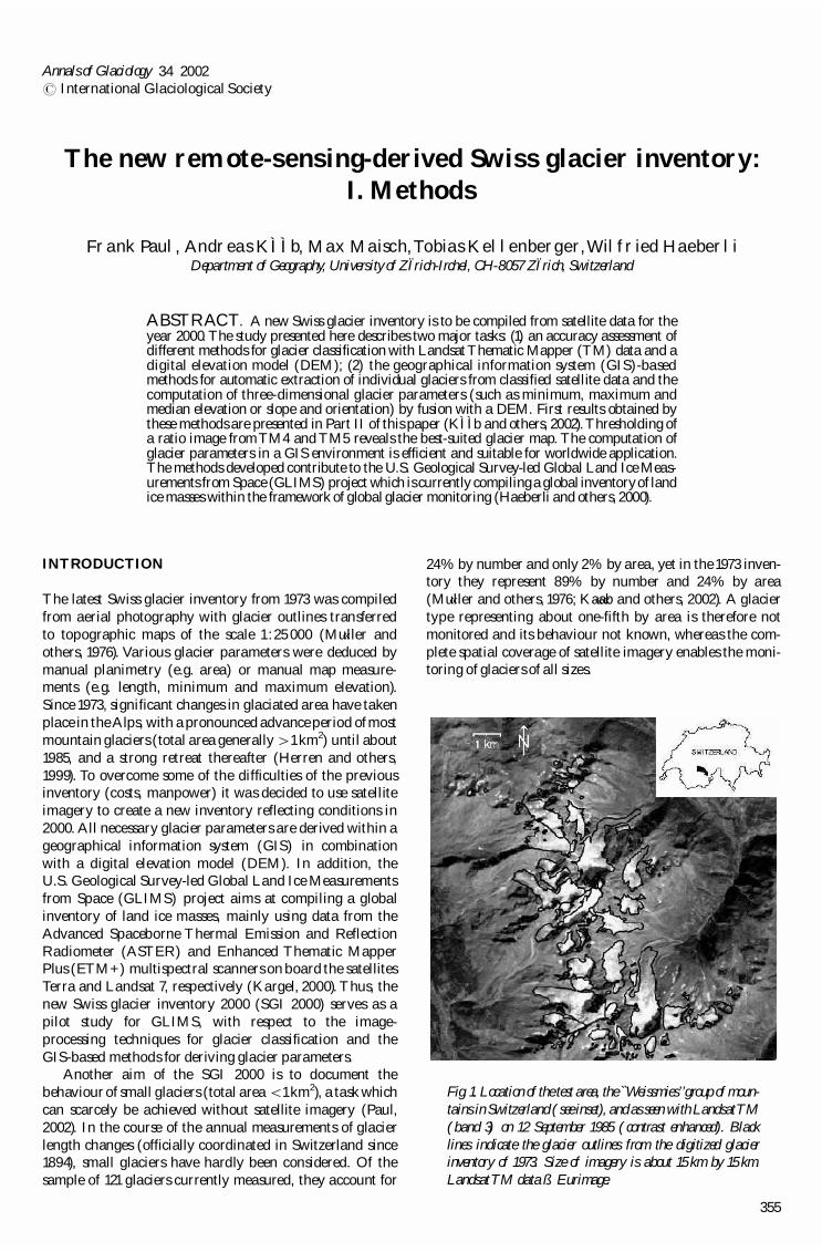
Fig 1 Location of the test area the `Weissmiesrsquorsquogroup of moun-tains in Switzerland (see inset) and as seen with LandsatTM(band 3) on 12 September 1985 (contrast enhanced) Blacklines indicate the glacier outlines from the digitized glacierinventory of 1973 Size of imagery is about 15 km by 15 kmLandsatTM data szlig Eurimage
355
In this study the results of a comparison of differentmethods of glacier mapping withThematic Mapper (TM)data are presented The accuracy of theTM-derived glacierareas is assessed by comparison with manually derivedoutlines from higher-resolution satellite imagery (Systecopy meProbatoire pour lrsquoObservation de laTerre (SPOT) panchro-matic channel) Moreover the precision of the DEM usedwith respect to glaciological parameters is evaluated bycomparison with a reference DEM directly derived fromstereo-photogrammetry Finally the principles of the GIS-based extraction of individual glaciers and the calculationof glaciological parameters as used for the SGI 2000 arepresented
REMOTE SENSING OF GLACIERS
Previous applications
The methods for glacier delineation with LandsatTM data
used in previous investigations can be divided into three dis-tinct groups (Paul 2001) (1) segmentation of ratio imagesfrom variousTM band combinations (2) unsupervised and(3) supervised classification techniques Method 1 is used forinstance by Bayrandothers (1994) with digital numbers (DN)from TM4 and TM5 as input or with the planetary reflec-tance at the satellite sensor of the same bands by Hall andothers (1988) orJacobs and others (1997) Rott (1994) created aglacier mask after the thresholding of a ratio image fromTM3and TM5 but used the atmospherically corrected spectral re-flectance of each channel Aniya and others (1996) usedmethod 2 to classify the whole of Hielo Patagonico Sur(southern Patagonia icefield) (ISODATA clustering withTM1TM4 andTM5 as input) Method 3 wasused by Grattonand others (1990) and Sidjak andWheate (1999) (maximum-likelihood classification) The latter authors also investigatedthe use of principal-componentanalysis (PCA) andanormal-ized-difference snow index (NDSI) Serandrei Barbero andothers (1999) created a glacier classification scheme using
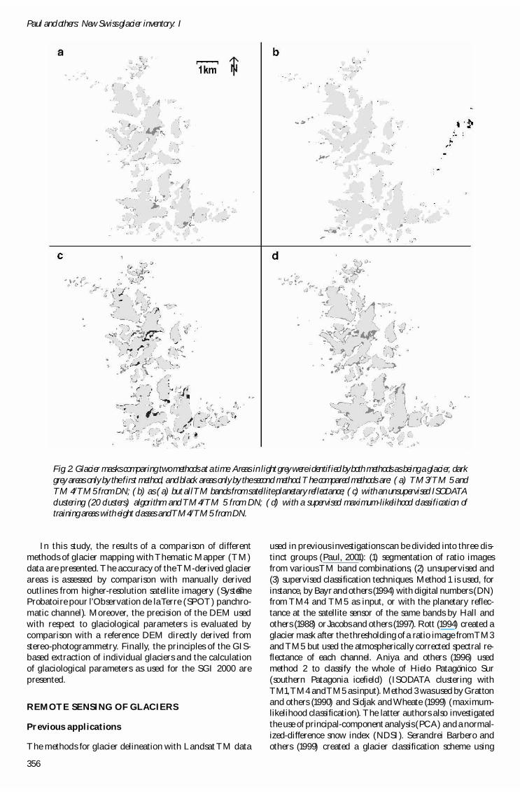
Fig 2 Glacier masks comparing two methods at a time Areas in light grey were identified by both methods as being a glacier darkgrey areas only by the first method and black areas only by the second methodThe compared methods are (a) TM3TM 5 andTM 4TM5 from DN (b) as (a) but allTM bands from satellite planetary reflectance (c) with an unsupervised ISODATAclustering (20 clusters) algorithm and TM4TM 5 from DN (d) with a supervised maximum-likelihood classification oftraining areas with eight classes andTM4TM5 from DN
Paul and others New Swiss glacier inventory I
356
fuzzy-set theory and a DEM within a GIS framework So farhowever most methods have been applied only to a smallernumber of glaciers (550) and all have been unable to classifythe debris-covered ice of a glacier
Comparison of different glacier-mapping methodsfrom Landsat TM
In this study we applydifferent glacier-mapping methods (seebelow) to a subset of a Landsat TM scene (path 195 row 28)from 12 September 1985 The test region (15 km by 15 km) islocated in the ` Weissmiesrsquorsquogroup in the Saas valley Swiss Alps(Fig 1) This region is typical for glaciated environments inSwitzerland It is characterized by steep relief (1500^4500m asl) with cast shadow and debris cover on some glaciersTogether with abundant small snowfields these three influ-ences on glacier-mapping accuracy known to be critical fromprevious studies canbe examined in this test region
In Figure 2a^d we present the results from differentglacier-mapping methods comparing two glacier maps at atime in each figure (a) segmentation of a ratio image fromTM3TM5 vsTM4TM5 using the DN (Fig 2a) (b) as (a)but using the spectral reflectance instead of DN (Fig 2b) (c)an unsupervised ISODATA clustering with 20 classes vsTM4TM5 from DN (Fig 2c) and (d) a supervised maxi-mum-likelihood classification with eight classes vs TM4TM5 from DN (Fig 2d) Further methods were applied(NDSI PCA usage of atmospheric-corrected TM bands)but results are not shown because they were less accurate
A glacier map (black ˆ ` glacierrsquorsquo white ˆ ` otherrsquorsquo) iscreated by interactive thresholding of the ratio images formethods (a) and (b) The 20 classes of (c) were separatedinto `glacierrsquorsquo and `otherrsquorsquo by visual interpretation For themaximum-likelihood classification (d) training areas ineight classes were chosen glacier 1 and snow 1 (in sunlight)glacier 2 and snow 2 (in shadow) forest meadow terrainand cast shadow For the final glacier map the latter fourwere converted to `otherrsquorsquo and the first four classes to`glacierrsquorsquo For each of Figure 2a^d two glacier maps werecombined with the followingcolour scheme`glacierrsquorsquoonbothmaps light grey `glacierrsquorsquo only on the firstsecond mapblackdark grey and `otherrsquorsquo on both maps white Toimprove the quality of the classification a 3 by 3 medianfilter was applied to all glacier maps before combination Amore detailed analysis of 32 glaciers reveals that the averagechange in glacier area by the median filter is ^04 ifglaciers smaller than 01km2 were not considered
All methods other than TM4TM5 with DN revealproblems with regions in cast shadow (indicated by arrowsin Fig 2a) where they map too much (Fig 2a b and d) ortoo little (Fig 2c) glacier area Additional regions withincast shadow are mapped from both methods displayed inFigure 2b Small snowfields were mapped with the methodsdisplayed in Figure 2c anddThe accuracy of all investigatedmethods could be improved partly by changing the relevantparameters (thresholds training areas number of clusters)but at the cost of more incorrect results in other places Allmethods fail to detect debris-covered ice because of thespectral similarity to the surrounding terrain The accuracyof the glacier classification with segmentation of a TM4TM5 ratio image using the raw DN proved to be the bestmethod with respect to glacier areas in cast shadow orassigning snowfields to `otherrsquorsquo
Accuracy of the best glacier-mapping method
To evaluate the accuracy of this best-suited classificationmethod the TM-derived glacier areas were compared withareas derived manually from a higher-resolution SPOT Panscene (10 m) Unfortunately this scene (path 55 row 256acquired on 17 September 1992) does not cover the` Weissmiesrsquorsquo test area but it shares a small region with aTMscene (path 195 row 28) acquired only 2 days prior to theSPOT scene Because of the good temporal coincidenceanother test site (located to the south of the ` Nufenenpassrsquorsquo)depicted on both the TM and SPOTscenes was selected For32 glaciers within this site the automatically TM-derivedareas were 23 smaller (on average) than on the manuallyanalyzed SPOT image This deviation is well within theaccuracy of the manual glacier delineation regarding smallsnowpatches or the delineation of debris-covered areasThusfor debris-free ice the accuracy of the glacier areas inferredfromTM is better than about 3
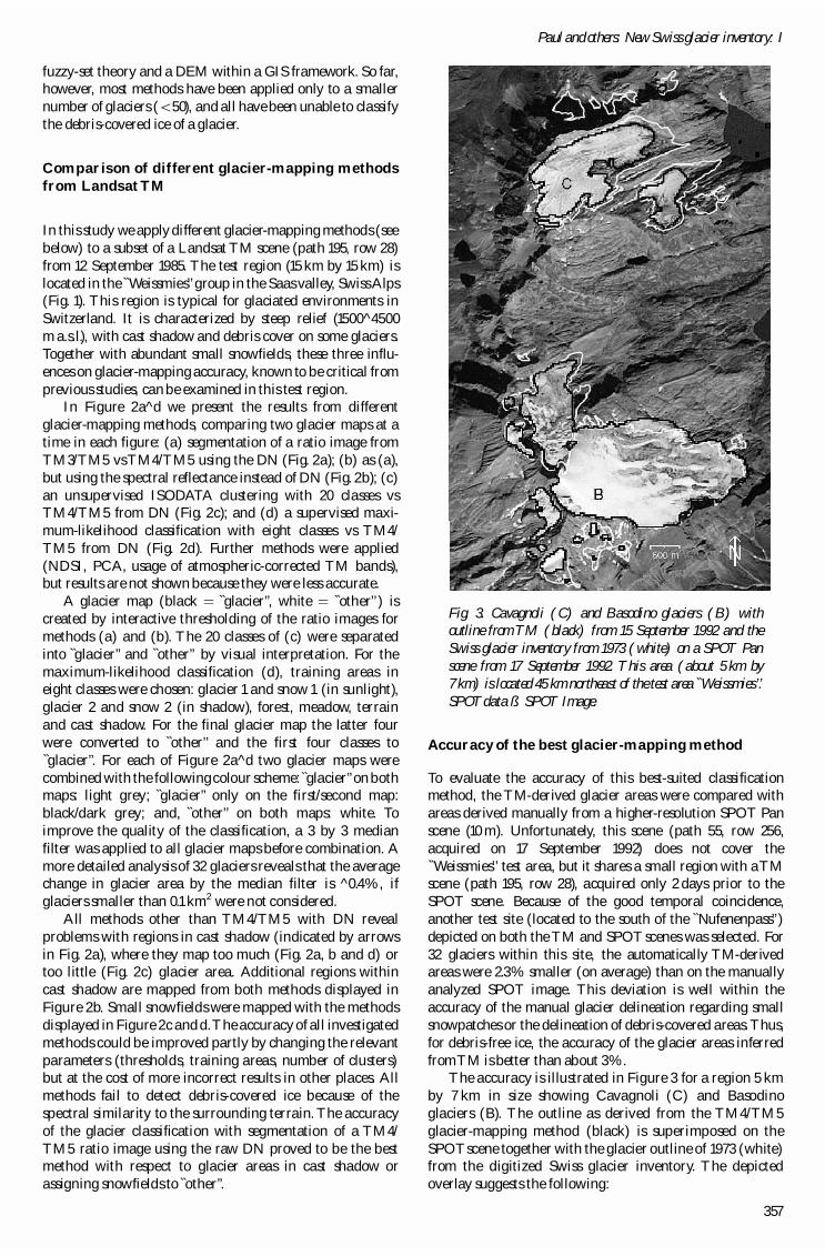
The accuracy is illustrated in Figure 3 for a region 5 kmby 7 km in size showing Cavagnoli (C) and Basodinoglaciers (B) The outline as derived from the TM4TM5glacier-mapping method (black) is superimposed on theSPOTscene together with the glacier outline of 1973 (white)from the digitized Swiss glacier inventory The depictedoverlay suggests the following
Fig 3 Cavagnoli (C) and Basodino glaciers (B) withoutline from TM (black) from 15 September 1992 and theSwiss glacier inventory from 1973 (white) on a SPOT Panscene from 17 September 1992 This area (about 5 km by7 km) is located 45 km northeast of the test area `WeissmiesrsquorsquoSPOTdata szlig SPOT Image
357
Paul and others New Swiss glacier inventory I
(1) the TM-derived glacier outlines fit quite well to thevisible glaciers
(2) small isolated ice fields are not classified as glaciers
(3) the smallest glaciers shrank through disintegration intosnowpatches
(4) there is a differentiated retreat of the larger glaciers
(5) the largest glacier (Basodino) was even larger in 1992than in 1973
DEM
Requirements and possibilities
A DEM has two main functions within the SGI 2000 theorthorectification of the satellite imagery and the derivationof three-dimensional glacier parameters within a GIS Theorthorectification is mandatory for at least four differenttasks
(1) To eliminate the effects of perspective distortion terrainelevation has to be considered during georectification ofimagery of rugged terrain For instance a pixel with aheightof 3000 masl located 90 km from the nadirpointis shifted by 370m from its real position in the uncorrectedimage
(2) The borders between individualglaciers were assigned tothe classified TM image from a (georeferenced) vectorlayer containing digitized glacier basin outlines
(3) Overlay of TM scenes from other years or with scenesfrom other sensors
(4) Fusion with the DEM itself used to derive glacierparameters
All scenes for SGI 2000 were orthorectified with a set ofground-control points to a residual rms error of about halfa pixel using a DEM with 25 m spatial resolution (SGI2000 DEM) from the Swiss Federal Office of Topography
Three-dimensional glacier parameters like minimumand maximum elevation glacier length the median and21 altitude (equilibrium-line altitude) and a detailedhypsography can be computed automatically with a DEMSlope and aspect of each glacier can be obtained as anaverage for the entire glacier or as a percentage of selectedzones (eg accumulation and ablation area) Moreoveraverage illumination or the percentage area in cast shadowduring a day can be calculated In this way it is possible toachieve a more thorough understanding of topographicinfluences on monitored changes in glacier area or length
Comparison with a reference DEM
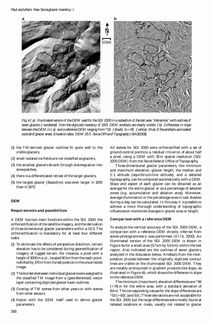
To analyze the vertical accuracy of the SGI 2000 DEM acomparison with a reference DEM directly inferred fromstereo-photogrammetry was performed (KIgraveIgraveb 2000) Anilluminated version of the SGI 2000 DEM is shown inFigure 4a for a small area (57 km by 50 km) within the testregion Also indicated are the outlines of seven glaciersanalyzed in the discussion below Artefacts from the inter-polation process between the originally digitized contourlines are visible on the illuminated SGI 2000 DEM Theyare notably pronounced in gradient products like slope asillustrated in Figure 4b which shows the difference in slopeto the reference DEM
The minimum (maximum) elevation differences are ^96(+74) m for the entire area with a standard deviation of86 m The corresponding values for the slope differences are^53 (+60)sup3 and 66sup3 Those deviations are not acceptable forthe SGI 2000 but the large differences were mostly found atisolated locations or crests usually not related to glacier
Fig 4 (a) Illuminated version of the DEM used for the SGI 2000 in a subsection of the test area `Weissmiesrsquorsquowith outlines ofseven glaciers (numbered) from the digitized inventory of 1973 DEM artefacts are clearly visible (b) Differences in slopebetween the DEM in (a) and a reference DEM ranging from ^53sup3 (black) to +65sup3 (white) Most of the artefacts are locatedoutside of glacier areas Elevation data DEM 25 szlig Swiss Office ofTopography (BA013305)
Paul and others New Swiss glacier inventory I
358
coverage To estimate the influence of the artefacts on thederived glacier parameters some of them were calculatedfor the seven glaciers indicated in Figure 4aThe average dif-ferences of minimum (maximum) elevation are ^27 (^13)mwith a standard deviation of 76 (74) m The correspondingvalues for slope are12 (^25)sup3 and 24 (33)sup3 These deviationsare acceptable for the glacier parameters in the SGI 2000
GIS
Data preparations1
By using an orthorectified glacier map derived from TMand a suitable DEM three-dimensional glacier parameterscan be obtained automatically within a GIS Before theGIS-based processing was started all data products wereconverted into ArcInfo (ESRI 1999) specific formats andthree GIS-related tasks were prepared for the SGI 2000
(1) digitizing of the glacier outlines from the inventory of1973 into a vector layer
(2) creation of a vector layer with glacier basin boundaries(see below)
(3) calculation of DEM products (eg slope aspect) forobtaining three-dimensional glacier parameters
The glacier outlines were digitized from the original maps(scale 125 000) as individual arcs with an averagerectification error of each map of about 5 m (rms) Thecentral flowlines and the reconstructed outlines from about1850 were also digitized
To separate connected glaciers in the classified TMimage into individual glaciers the ice divides between themmust be defined This is done by on-screen digitizing of anew vector layer (coverage) using the digitized Swiss glacierinventory and the classified TM image as background inarcedit Ice divides were taken without modification fromthe digitized inventory and extended to a closed polygonroughly surrounding the glacier All other glaciers were alsosurrounded by closed polygons which are large enough toinclude possible future variations of glacier area The thickblack lines in Figure 5 represent these polygons They areshown together with the digitized glacier areas (in grey)With these predefined glacier basins it is also possible toassign a unique identity (ID) to glacier groups (see below)A group of glaciers can originate from a single glacierthrough disintegration over time already be established ina former inventory or consist of an entire glacier comprisedof different streams
DEM products such as slope or aspect were calculatedwithin the digital image-processing software Some DEMproducts are further converted with short FORTRAN pro-grams (eg the aspects are classified into eight sectors) Theelevation products (eg median elevation or hypsography)are computed within ArcInfo
The location of the glacier ID is taken from the reviseddatabase of Maisch and others (1999) Because many glaciershave split up during recent years the location of their ID(assigned in 1973) often lies outside their present outlineTherefore and to handle groups of glaciers the ID isassigned to the entire basin This is done by converting thedatabase table (ID x and y-coordinates) to a point coveragewith generate and intersecting this coverage with the glacierbasin coverage Thus each glacier basin holds the glacier IDin the attribute table
Data flow
The data processing can be separated into a general workflow between three modules and a more specific data flowwithin each moduleThe modules are (Fig 6)
(1) the GIS module for calculating quantities within theGIS (eg areas of individual glaciers)
(2) the CONV module for conversion and recalculation ofArcInfo output tables (eg glacier areas of two differentyears into relative changes in area)
(3) the VIS module for creation of graphic files from datafiles (eg with XMGR GMTor IDL)
Each module holds individual programs for individualtasks each of which consists of an input calculation andoutput part The different modules can be combined into acomplete digital chain with the output from a program inone module as the input for a program in the next module(cf Fig 6)
Fig 5 Glacier basins (bold black lines) and the digitizedSwiss glacier inventory of 1973 (grey areas) Contiguous icemasses were separated into individual glaciers according tothe 1973 inventory and roughly surrounded to obtain closedpolygons These polygonal glacier basins can also be used toeliminate gross classification errors (eg proglacial lakes)and for glacier identification especially to assign a uniqueID to glaciers
1 In the following all ArcInfo-specific names andcommandsare printed in italics
359
Paul and others New Swiss glacier inventory I
The GIS module is shown in Figure 7 in more detailOnly three input layers are needed for the GIS module
the predefined glacier basins (vector layer) with assignedglacier IDs
the image with the classified glacier areas from TM(geo-tiff)
the DEM or a product from it (table with header)
The calculation section consists of the following steps (num-bers refer to Fig7)The first step (1) is a raster-vector conver-sion of the glacier map with imagegrid and gridpoly into acoverage This glacier coverage is then (2) combined with theglacier basin coverage with intersect to obtain the individualglaciersTogether with intersect the glacier basin coverage cutseach glacier out of the glacier coverage in correspondence
with its basinThe coverage with the individual glaciers (or aselection of them) is then (3) converted with polygrid to azonal grid where each zone corresponds to a glacier TheDEM (or a product of it) is (4) converted with asciigrid to avalue grid where each cell holds the value of the DEM at thatlocationThe last step (5) is the combination of the value gridand the zonal grid with zonalstats This command gives foreach zone (glacier) statistic parameters (eg minimummaximum range mean standard deviation) according tothe underlying value grid (elevation in case of the DEM)The resulting output table can be processed further withthe CONVand VIS modules
DISCUSSION AND CONCLUSION
The best results for glacier mapping were obtained withthresholding of a TM4 by TM5 ratio image from DNespecially with respect to glacier areas in cast shadow Theaccuracy is better than 3 for debris-free glacier areasCompared to other investigated methods this method iseasy and fast to perform needs no special image-processingsoftware and interactive selection of the threshold value isquite robust The use of a median filter improves the resultsof the classification by removing misclassification (smallsnowfields shadow pixels) and adding pixels where needed(small debris cover glacier parts in shadow) For glacierssmaller than 01km2 the glacier size is altered significantlyby this noise filter and thus the lower limit of total glacierarea was determined to be 01km2 in the SGI 2000
The new GIS-based concept of the SGI 2000 is able tocompute all glacier parameters automatically This is veryuseful for efficient monitoring over large areas especially inremote regions or to investigate small glaciers and theirchanges The design of the glacier basin vector layer whichmaintains the glacier identification is not limited to the avail-ability of a digitized glacier inventory In remote areas with-out any data creation directly from the satellite image is alsopossible If a DEM is available three-dimensional glacierparameters (eg slope aspect hypsography) can be calcu-lated automatically too For the relatively small glaciers inthe Alps a high-precision DEM with 25 m spatial resolutionis necessary for obtaining glacier parameters Useful datafrom other regions can also be obtained with a coarserDEM depending on the size and characteristics of theglaciers considered
At the moment the main problem for the SGI 2000 isthe automatic mapping of debris-covered glacier ice It ispartly included after the automatic classification (withTM4TM5) in two cases the debris cover is thin or it is amedial moraine of only one pixel width (and arbitrarylength) In the latter case the median filter will close thegap Unfortunately this automatically included part ofdebris-covered ice has a varying size in different yearsdepending on snow cover glacier change or illuminationFor this reason only a small fraction of debris-free glacierswere chosen for comparison of glacier areas in Part II of thispaper (KIgraveIgraveb and others 2002) A possible solution may bethe combination of advanced digital image-processingtechniques (neural networks) with geomorphometricmeasures and object-oriented classification (Bishop andothers 2000) Promising first results have been achieved bycombining slope information with a map of vegetation-freeareas and neighbourhood relations to glacier ice Mean-
Fig 6Work flow between sequential modules and principaldata flow within each module In each module differentprograms are available to calculate glacier parameters andtheir changes Most of them can be combined into a completedigital processing chain
Fig 7The principal data flow within the GIS module usingArcInfo and including a DEM product for three-dimensionalglacier parameters Areas of individual glaciers are availableafter step 2
Paul and others New Swiss glacier inventory I
360
while manual delineation by on-screen digitizing is appliedfor the SGI 2000
ACKNOWLEDGEMENTS
The study is supported by a grant from the Swiss NationalScience Foundation (contract No21-5407398)We gratefullyacknowledge the careful and constructive comments of thetwo anonymous referees and the editor J Key
REFERENCES
Aniya M H Sato R Naruse P Skvarca and G Casassa1996The use ofsatellite andairborne imagery to inventory outlet glaciers of the SouthernPatagonia Icefield South America Photogramm Eng Remote Sensing62(12)1361^1369
Bayr K J D K Hall and W M Kovalick1994 Observations on glaciersin the eastern Austrian Alps using satellite data Int J Remote Sensing15(9)1733^1742
Bishop M P J S Kargel H H Kieffer D J MacKinnon B H Raup andJ F Shroder Jr2000Remote-sensingscienceandtechnology for studyingglacier processes in high Asia Ann Glaciol 31164^170
Environmental Systems ResearchInstitute (ESRI)1999 ArcInfo 801 RedlandCA Environmental Systems Research Institute Inc
Gratton D J P J Howarth and D J Marceau 1990 Combining DEMparameters with LANDSAT MSS and TM imagery in a GIS for moun-tain glacier characterization IEEETrans Geosci Remote Sensing GE-28(4)766^769
Haeberli W J Cihlar and R G Barry 2000 Glacier monitoring withinthe Global Climate Observing System Ann Glaciol 31 241^246
Hall D K AT C Chang and H Siddalingaiah 1988 Reflectances ofglaciers as calculated using Landsat-5 Thematic Mapper data RemoteSensing Environ 25(3) 311^321
Herren E R M Hoelzleand M Maisch1999The Swiss glaciers 199596and
199697 Zulaquo rich Swiss Academy of Sciences Glaciological CommissionFederal Institute of Technology Laboratory of Hydraulics Hydrologyand Glaciology (GlaciologicalReport No117118)
Jacobs J D E L Simms and A Simms 1997 Recession of the southernpart of Barnes Ice Cap Baffin Island Canada between 1961 and 1993determined from digital mapping of Landsat TM J Glaciol 43(143)98^102
Kalaquo alaquo b A2000 Photogrammetric reconstructionof glaciermassbalanceusinga kinematic ice-flow model a 20 year time series on GrubengletscherSwiss Alps Ann Glaciol 31 45^52
Kalaquo alaquo b A F Paul M Maisch M Hoelzle and W Haeberli 2002The newremote-sensing-derived Swiss glacier inventory II First results AnnGlaciol 34 (see paper in this volume)
Kargel J S 2000 New eyes in the sky measure glaciers and ice sheets Eos81(24) 265270 271
Maisch M AWipf B Denneler J Battaglia and C Benz1999 Die Gletscherder Schweizer Alpen Gletscherstand 1850ouml Aktuelle VergletscherungoumlGletscherschwund-Szenarien21 Jahrhundert Zulaquo rich vdf Hochschulverlag AGETH (Schlussbericht NFP 31)
Mulaquo ller F T Caflisch and G Mulaquo ller 1976 Firn und Eis der SchweizerAlpenGletscherinventar Zulaquo rich Eidgenolaquo ssische Technische Hochschule (Geo-graphisches Institut Publ 57)
Paul F 2001 Evaluation of different methods for glacier mapping usingLandsat TM In EARSeL Workshop on Remote Sensing of Land Ice and Snow16^17 June 2000 Dresden Proceedings Paris European Association ofRemote Sensing Laboratories CD-ROM
Paul F 2002 Changes in glacier area inTyrol Austria between 1969 and1992 derived from LandsatTM and Austrian glacier inventory data IntJ Remote Sensing 23(4)787^799
Rott H 1994 Thematic studies in alpine areas by means of polarimetricSAR and optical imagery Adv Space Res 14(3) 217^226
Serandrei Barbero R R Rabagliati E Binaghi and A Rampini1999Glacialretreat in the 1980s in the Breonie Aurine and Pusteresi Groups (easternAlps Italy) in LandsatTM images Hydrol Sci J 44(2) 279^296
Sidjak RW and R D Wheate 1999 Glacier mapping of the Illecillewaeticefield British Columbia Canada using Landsat TM and digitalelevation data Int J Remote Sensing 20(2) 273^284
361
Paul and others New Swiss glacier inventory I
In this study the results of a comparison of differentmethods of glacier mapping withThematic Mapper (TM)data are presented The accuracy of theTM-derived glacierareas is assessed by comparison with manually derivedoutlines from higher-resolution satellite imagery (Systecopy meProbatoire pour lrsquoObservation de laTerre (SPOT) panchro-matic channel) Moreover the precision of the DEM usedwith respect to glaciological parameters is evaluated bycomparison with a reference DEM directly derived fromstereo-photogrammetry Finally the principles of the GIS-based extraction of individual glaciers and the calculationof glaciological parameters as used for the SGI 2000 arepresented
REMOTE SENSING OF GLACIERS
Previous applications
The methods for glacier delineation with LandsatTM data
used in previous investigations can be divided into three dis-tinct groups (Paul 2001) (1) segmentation of ratio imagesfrom variousTM band combinations (2) unsupervised and(3) supervised classification techniques Method 1 is used forinstance by Bayrandothers (1994) with digital numbers (DN)from TM4 and TM5 as input or with the planetary reflec-tance at the satellite sensor of the same bands by Hall andothers (1988) orJacobs and others (1997) Rott (1994) created aglacier mask after the thresholding of a ratio image fromTM3and TM5 but used the atmospherically corrected spectral re-flectance of each channel Aniya and others (1996) usedmethod 2 to classify the whole of Hielo Patagonico Sur(southern Patagonia icefield) (ISODATA clustering withTM1TM4 andTM5 as input) Method 3 wasused by Grattonand others (1990) and Sidjak andWheate (1999) (maximum-likelihood classification) The latter authors also investigatedthe use of principal-componentanalysis (PCA) andanormal-ized-difference snow index (NDSI) Serandrei Barbero andothers (1999) created a glacier classification scheme using
Fig 2 Glacier masks comparing two methods at a time Areas in light grey were identified by both methods as being a glacier darkgrey areas only by the first method and black areas only by the second methodThe compared methods are (a) TM3TM 5 andTM 4TM5 from DN (b) as (a) but allTM bands from satellite planetary reflectance (c) with an unsupervised ISODATAclustering (20 clusters) algorithm and TM4TM 5 from DN (d) with a supervised maximum-likelihood classification oftraining areas with eight classes andTM4TM5 from DN
Paul and others New Swiss glacier inventory I
356
fuzzy-set theory and a DEM within a GIS framework So farhowever most methods have been applied only to a smallernumber of glaciers (550) and all have been unable to classifythe debris-covered ice of a glacier
Comparison of different glacier-mapping methodsfrom Landsat TM
In this study we applydifferent glacier-mapping methods (seebelow) to a subset of a Landsat TM scene (path 195 row 28)from 12 September 1985 The test region (15 km by 15 km) islocated in the ` Weissmiesrsquorsquogroup in the Saas valley Swiss Alps(Fig 1) This region is typical for glaciated environments inSwitzerland It is characterized by steep relief (1500^4500m asl) with cast shadow and debris cover on some glaciersTogether with abundant small snowfields these three influ-ences on glacier-mapping accuracy known to be critical fromprevious studies canbe examined in this test region
In Figure 2a^d we present the results from differentglacier-mapping methods comparing two glacier maps at atime in each figure (a) segmentation of a ratio image fromTM3TM5 vsTM4TM5 using the DN (Fig 2a) (b) as (a)but using the spectral reflectance instead of DN (Fig 2b) (c)an unsupervised ISODATA clustering with 20 classes vsTM4TM5 from DN (Fig 2c) and (d) a supervised maxi-mum-likelihood classification with eight classes vs TM4TM5 from DN (Fig 2d) Further methods were applied(NDSI PCA usage of atmospheric-corrected TM bands)but results are not shown because they were less accurate
A glacier map (black ˆ ` glacierrsquorsquo white ˆ ` otherrsquorsquo) iscreated by interactive thresholding of the ratio images formethods (a) and (b) The 20 classes of (c) were separatedinto `glacierrsquorsquo and `otherrsquorsquo by visual interpretation For themaximum-likelihood classification (d) training areas ineight classes were chosen glacier 1 and snow 1 (in sunlight)glacier 2 and snow 2 (in shadow) forest meadow terrainand cast shadow For the final glacier map the latter fourwere converted to `otherrsquorsquo and the first four classes to`glacierrsquorsquo For each of Figure 2a^d two glacier maps werecombined with the followingcolour scheme`glacierrsquorsquoonbothmaps light grey `glacierrsquorsquo only on the firstsecond mapblackdark grey and `otherrsquorsquo on both maps white Toimprove the quality of the classification a 3 by 3 medianfilter was applied to all glacier maps before combination Amore detailed analysis of 32 glaciers reveals that the averagechange in glacier area by the median filter is ^04 ifglaciers smaller than 01km2 were not considered
All methods other than TM4TM5 with DN revealproblems with regions in cast shadow (indicated by arrowsin Fig 2a) where they map too much (Fig 2a b and d) ortoo little (Fig 2c) glacier area Additional regions withincast shadow are mapped from both methods displayed inFigure 2b Small snowfields were mapped with the methodsdisplayed in Figure 2c anddThe accuracy of all investigatedmethods could be improved partly by changing the relevantparameters (thresholds training areas number of clusters)but at the cost of more incorrect results in other places Allmethods fail to detect debris-covered ice because of thespectral similarity to the surrounding terrain The accuracyof the glacier classification with segmentation of a TM4TM5 ratio image using the raw DN proved to be the bestmethod with respect to glacier areas in cast shadow orassigning snowfields to `otherrsquorsquo
Accuracy of the best glacier-mapping method
To evaluate the accuracy of this best-suited classificationmethod the TM-derived glacier areas were compared withareas derived manually from a higher-resolution SPOT Panscene (10 m) Unfortunately this scene (path 55 row 256acquired on 17 September 1992) does not cover the` Weissmiesrsquorsquo test area but it shares a small region with aTMscene (path 195 row 28) acquired only 2 days prior to theSPOT scene Because of the good temporal coincidenceanother test site (located to the south of the ` Nufenenpassrsquorsquo)depicted on both the TM and SPOTscenes was selected For32 glaciers within this site the automatically TM-derivedareas were 23 smaller (on average) than on the manuallyanalyzed SPOT image This deviation is well within theaccuracy of the manual glacier delineation regarding smallsnowpatches or the delineation of debris-covered areasThusfor debris-free ice the accuracy of the glacier areas inferredfromTM is better than about 3
The accuracy is illustrated in Figure 3 for a region 5 kmby 7 km in size showing Cavagnoli (C) and Basodinoglaciers (B) The outline as derived from the TM4TM5glacier-mapping method (black) is superimposed on theSPOTscene together with the glacier outline of 1973 (white)from the digitized Swiss glacier inventory The depictedoverlay suggests the following
Fig 3 Cavagnoli (C) and Basodino glaciers (B) withoutline from TM (black) from 15 September 1992 and theSwiss glacier inventory from 1973 (white) on a SPOT Panscene from 17 September 1992 This area (about 5 km by7 km) is located 45 km northeast of the test area `WeissmiesrsquorsquoSPOTdata szlig SPOT Image
357
Paul and others New Swiss glacier inventory I
(1) the TM-derived glacier outlines fit quite well to thevisible glaciers
(2) small isolated ice fields are not classified as glaciers
(3) the smallest glaciers shrank through disintegration intosnowpatches
(4) there is a differentiated retreat of the larger glaciers
(5) the largest glacier (Basodino) was even larger in 1992than in 1973
DEM
Requirements and possibilities
A DEM has two main functions within the SGI 2000 theorthorectification of the satellite imagery and the derivationof three-dimensional glacier parameters within a GIS Theorthorectification is mandatory for at least four differenttasks
(1) To eliminate the effects of perspective distortion terrainelevation has to be considered during georectification ofimagery of rugged terrain For instance a pixel with aheightof 3000 masl located 90 km from the nadirpointis shifted by 370m from its real position in the uncorrectedimage
(2) The borders between individualglaciers were assigned tothe classified TM image from a (georeferenced) vectorlayer containing digitized glacier basin outlines
(3) Overlay of TM scenes from other years or with scenesfrom other sensors
(4) Fusion with the DEM itself used to derive glacierparameters
All scenes for SGI 2000 were orthorectified with a set ofground-control points to a residual rms error of about halfa pixel using a DEM with 25 m spatial resolution (SGI2000 DEM) from the Swiss Federal Office of Topography
Three-dimensional glacier parameters like minimumand maximum elevation glacier length the median and21 altitude (equilibrium-line altitude) and a detailedhypsography can be computed automatically with a DEMSlope and aspect of each glacier can be obtained as anaverage for the entire glacier or as a percentage of selectedzones (eg accumulation and ablation area) Moreoveraverage illumination or the percentage area in cast shadowduring a day can be calculated In this way it is possible toachieve a more thorough understanding of topographicinfluences on monitored changes in glacier area or length
Comparison with a reference DEM
To analyze the vertical accuracy of the SGI 2000 DEM acomparison with a reference DEM directly inferred fromstereo-photogrammetry was performed (KIgraveIgraveb 2000) Anilluminated version of the SGI 2000 DEM is shown inFigure 4a for a small area (57 km by 50 km) within the testregion Also indicated are the outlines of seven glaciersanalyzed in the discussion below Artefacts from the inter-polation process between the originally digitized contourlines are visible on the illuminated SGI 2000 DEM Theyare notably pronounced in gradient products like slope asillustrated in Figure 4b which shows the difference in slopeto the reference DEM
The minimum (maximum) elevation differences are ^96(+74) m for the entire area with a standard deviation of86 m The corresponding values for the slope differences are^53 (+60)sup3 and 66sup3 Those deviations are not acceptable forthe SGI 2000 but the large differences were mostly found atisolated locations or crests usually not related to glacier
Fig 4 (a) Illuminated version of the DEM used for the SGI 2000 in a subsection of the test area `Weissmiesrsquorsquowith outlines ofseven glaciers (numbered) from the digitized inventory of 1973 DEM artefacts are clearly visible (b) Differences in slopebetween the DEM in (a) and a reference DEM ranging from ^53sup3 (black) to +65sup3 (white) Most of the artefacts are locatedoutside of glacier areas Elevation data DEM 25 szlig Swiss Office ofTopography (BA013305)
Paul and others New Swiss glacier inventory I
358
coverage To estimate the influence of the artefacts on thederived glacier parameters some of them were calculatedfor the seven glaciers indicated in Figure 4aThe average dif-ferences of minimum (maximum) elevation are ^27 (^13)mwith a standard deviation of 76 (74) m The correspondingvalues for slope are12 (^25)sup3 and 24 (33)sup3 These deviationsare acceptable for the glacier parameters in the SGI 2000
GIS
Data preparations1
By using an orthorectified glacier map derived from TMand a suitable DEM three-dimensional glacier parameterscan be obtained automatically within a GIS Before theGIS-based processing was started all data products wereconverted into ArcInfo (ESRI 1999) specific formats andthree GIS-related tasks were prepared for the SGI 2000
(1) digitizing of the glacier outlines from the inventory of1973 into a vector layer
(2) creation of a vector layer with glacier basin boundaries(see below)
(3) calculation of DEM products (eg slope aspect) forobtaining three-dimensional glacier parameters
The glacier outlines were digitized from the original maps(scale 125 000) as individual arcs with an averagerectification error of each map of about 5 m (rms) Thecentral flowlines and the reconstructed outlines from about1850 were also digitized
To separate connected glaciers in the classified TMimage into individual glaciers the ice divides between themmust be defined This is done by on-screen digitizing of anew vector layer (coverage) using the digitized Swiss glacierinventory and the classified TM image as background inarcedit Ice divides were taken without modification fromthe digitized inventory and extended to a closed polygonroughly surrounding the glacier All other glaciers were alsosurrounded by closed polygons which are large enough toinclude possible future variations of glacier area The thickblack lines in Figure 5 represent these polygons They areshown together with the digitized glacier areas (in grey)With these predefined glacier basins it is also possible toassign a unique identity (ID) to glacier groups (see below)A group of glaciers can originate from a single glacierthrough disintegration over time already be established ina former inventory or consist of an entire glacier comprisedof different streams
DEM products such as slope or aspect were calculatedwithin the digital image-processing software Some DEMproducts are further converted with short FORTRAN pro-grams (eg the aspects are classified into eight sectors) Theelevation products (eg median elevation or hypsography)are computed within ArcInfo
The location of the glacier ID is taken from the reviseddatabase of Maisch and others (1999) Because many glaciershave split up during recent years the location of their ID(assigned in 1973) often lies outside their present outlineTherefore and to handle groups of glaciers the ID isassigned to the entire basin This is done by converting thedatabase table (ID x and y-coordinates) to a point coveragewith generate and intersecting this coverage with the glacierbasin coverage Thus each glacier basin holds the glacier IDin the attribute table
Data flow
The data processing can be separated into a general workflow between three modules and a more specific data flowwithin each moduleThe modules are (Fig 6)
(1) the GIS module for calculating quantities within theGIS (eg areas of individual glaciers)
(2) the CONV module for conversion and recalculation ofArcInfo output tables (eg glacier areas of two differentyears into relative changes in area)
(3) the VIS module for creation of graphic files from datafiles (eg with XMGR GMTor IDL)
Each module holds individual programs for individualtasks each of which consists of an input calculation andoutput part The different modules can be combined into acomplete digital chain with the output from a program inone module as the input for a program in the next module(cf Fig 6)
Fig 5 Glacier basins (bold black lines) and the digitizedSwiss glacier inventory of 1973 (grey areas) Contiguous icemasses were separated into individual glaciers according tothe 1973 inventory and roughly surrounded to obtain closedpolygons These polygonal glacier basins can also be used toeliminate gross classification errors (eg proglacial lakes)and for glacier identification especially to assign a uniqueID to glaciers
1 In the following all ArcInfo-specific names andcommandsare printed in italics
359
Paul and others New Swiss glacier inventory I
The GIS module is shown in Figure 7 in more detailOnly three input layers are needed for the GIS module
the predefined glacier basins (vector layer) with assignedglacier IDs
the image with the classified glacier areas from TM(geo-tiff)
the DEM or a product from it (table with header)
The calculation section consists of the following steps (num-bers refer to Fig7)The first step (1) is a raster-vector conver-sion of the glacier map with imagegrid and gridpoly into acoverage This glacier coverage is then (2) combined with theglacier basin coverage with intersect to obtain the individualglaciersTogether with intersect the glacier basin coverage cutseach glacier out of the glacier coverage in correspondence
with its basinThe coverage with the individual glaciers (or aselection of them) is then (3) converted with polygrid to azonal grid where each zone corresponds to a glacier TheDEM (or a product of it) is (4) converted with asciigrid to avalue grid where each cell holds the value of the DEM at thatlocationThe last step (5) is the combination of the value gridand the zonal grid with zonalstats This command gives foreach zone (glacier) statistic parameters (eg minimummaximum range mean standard deviation) according tothe underlying value grid (elevation in case of the DEM)The resulting output table can be processed further withthe CONVand VIS modules
DISCUSSION AND CONCLUSION
The best results for glacier mapping were obtained withthresholding of a TM4 by TM5 ratio image from DNespecially with respect to glacier areas in cast shadow Theaccuracy is better than 3 for debris-free glacier areasCompared to other investigated methods this method iseasy and fast to perform needs no special image-processingsoftware and interactive selection of the threshold value isquite robust The use of a median filter improves the resultsof the classification by removing misclassification (smallsnowfields shadow pixels) and adding pixels where needed(small debris cover glacier parts in shadow) For glacierssmaller than 01km2 the glacier size is altered significantlyby this noise filter and thus the lower limit of total glacierarea was determined to be 01km2 in the SGI 2000
The new GIS-based concept of the SGI 2000 is able tocompute all glacier parameters automatically This is veryuseful for efficient monitoring over large areas especially inremote regions or to investigate small glaciers and theirchanges The design of the glacier basin vector layer whichmaintains the glacier identification is not limited to the avail-ability of a digitized glacier inventory In remote areas with-out any data creation directly from the satellite image is alsopossible If a DEM is available three-dimensional glacierparameters (eg slope aspect hypsography) can be calcu-lated automatically too For the relatively small glaciers inthe Alps a high-precision DEM with 25 m spatial resolutionis necessary for obtaining glacier parameters Useful datafrom other regions can also be obtained with a coarserDEM depending on the size and characteristics of theglaciers considered
At the moment the main problem for the SGI 2000 isthe automatic mapping of debris-covered glacier ice It ispartly included after the automatic classification (withTM4TM5) in two cases the debris cover is thin or it is amedial moraine of only one pixel width (and arbitrarylength) In the latter case the median filter will close thegap Unfortunately this automatically included part ofdebris-covered ice has a varying size in different yearsdepending on snow cover glacier change or illuminationFor this reason only a small fraction of debris-free glacierswere chosen for comparison of glacier areas in Part II of thispaper (KIgraveIgraveb and others 2002) A possible solution may bethe combination of advanced digital image-processingtechniques (neural networks) with geomorphometricmeasures and object-oriented classification (Bishop andothers 2000) Promising first results have been achieved bycombining slope information with a map of vegetation-freeareas and neighbourhood relations to glacier ice Mean-
Fig 6Work flow between sequential modules and principaldata flow within each module In each module differentprograms are available to calculate glacier parameters andtheir changes Most of them can be combined into a completedigital processing chain
Fig 7The principal data flow within the GIS module usingArcInfo and including a DEM product for three-dimensionalglacier parameters Areas of individual glaciers are availableafter step 2
Paul and others New Swiss glacier inventory I
360
while manual delineation by on-screen digitizing is appliedfor the SGI 2000
ACKNOWLEDGEMENTS
The study is supported by a grant from the Swiss NationalScience Foundation (contract No21-5407398)We gratefullyacknowledge the careful and constructive comments of thetwo anonymous referees and the editor J Key
REFERENCES
Aniya M H Sato R Naruse P Skvarca and G Casassa1996The use ofsatellite andairborne imagery to inventory outlet glaciers of the SouthernPatagonia Icefield South America Photogramm Eng Remote Sensing62(12)1361^1369
Bayr K J D K Hall and W M Kovalick1994 Observations on glaciersin the eastern Austrian Alps using satellite data Int J Remote Sensing15(9)1733^1742
Bishop M P J S Kargel H H Kieffer D J MacKinnon B H Raup andJ F Shroder Jr2000Remote-sensingscienceandtechnology for studyingglacier processes in high Asia Ann Glaciol 31164^170
Environmental Systems ResearchInstitute (ESRI)1999 ArcInfo 801 RedlandCA Environmental Systems Research Institute Inc
Gratton D J P J Howarth and D J Marceau 1990 Combining DEMparameters with LANDSAT MSS and TM imagery in a GIS for moun-tain glacier characterization IEEETrans Geosci Remote Sensing GE-28(4)766^769
Haeberli W J Cihlar and R G Barry 2000 Glacier monitoring withinthe Global Climate Observing System Ann Glaciol 31 241^246
Hall D K AT C Chang and H Siddalingaiah 1988 Reflectances ofglaciers as calculated using Landsat-5 Thematic Mapper data RemoteSensing Environ 25(3) 311^321
Herren E R M Hoelzleand M Maisch1999The Swiss glaciers 199596and
199697 Zulaquo rich Swiss Academy of Sciences Glaciological CommissionFederal Institute of Technology Laboratory of Hydraulics Hydrologyand Glaciology (GlaciologicalReport No117118)
Jacobs J D E L Simms and A Simms 1997 Recession of the southernpart of Barnes Ice Cap Baffin Island Canada between 1961 and 1993determined from digital mapping of Landsat TM J Glaciol 43(143)98^102
Kalaquo alaquo b A2000 Photogrammetric reconstructionof glaciermassbalanceusinga kinematic ice-flow model a 20 year time series on GrubengletscherSwiss Alps Ann Glaciol 31 45^52
Kalaquo alaquo b A F Paul M Maisch M Hoelzle and W Haeberli 2002The newremote-sensing-derived Swiss glacier inventory II First results AnnGlaciol 34 (see paper in this volume)
Kargel J S 2000 New eyes in the sky measure glaciers and ice sheets Eos81(24) 265270 271
Maisch M AWipf B Denneler J Battaglia and C Benz1999 Die Gletscherder Schweizer Alpen Gletscherstand 1850ouml Aktuelle VergletscherungoumlGletscherschwund-Szenarien21 Jahrhundert Zulaquo rich vdf Hochschulverlag AGETH (Schlussbericht NFP 31)
Mulaquo ller F T Caflisch and G Mulaquo ller 1976 Firn und Eis der SchweizerAlpenGletscherinventar Zulaquo rich Eidgenolaquo ssische Technische Hochschule (Geo-graphisches Institut Publ 57)
Paul F 2001 Evaluation of different methods for glacier mapping usingLandsat TM In EARSeL Workshop on Remote Sensing of Land Ice and Snow16^17 June 2000 Dresden Proceedings Paris European Association ofRemote Sensing Laboratories CD-ROM
Paul F 2002 Changes in glacier area inTyrol Austria between 1969 and1992 derived from LandsatTM and Austrian glacier inventory data IntJ Remote Sensing 23(4)787^799
Rott H 1994 Thematic studies in alpine areas by means of polarimetricSAR and optical imagery Adv Space Res 14(3) 217^226
Serandrei Barbero R R Rabagliati E Binaghi and A Rampini1999Glacialretreat in the 1980s in the Breonie Aurine and Pusteresi Groups (easternAlps Italy) in LandsatTM images Hydrol Sci J 44(2) 279^296
Sidjak RW and R D Wheate 1999 Glacier mapping of the Illecillewaeticefield British Columbia Canada using Landsat TM and digitalelevation data Int J Remote Sensing 20(2) 273^284
361
Paul and others New Swiss glacier inventory I
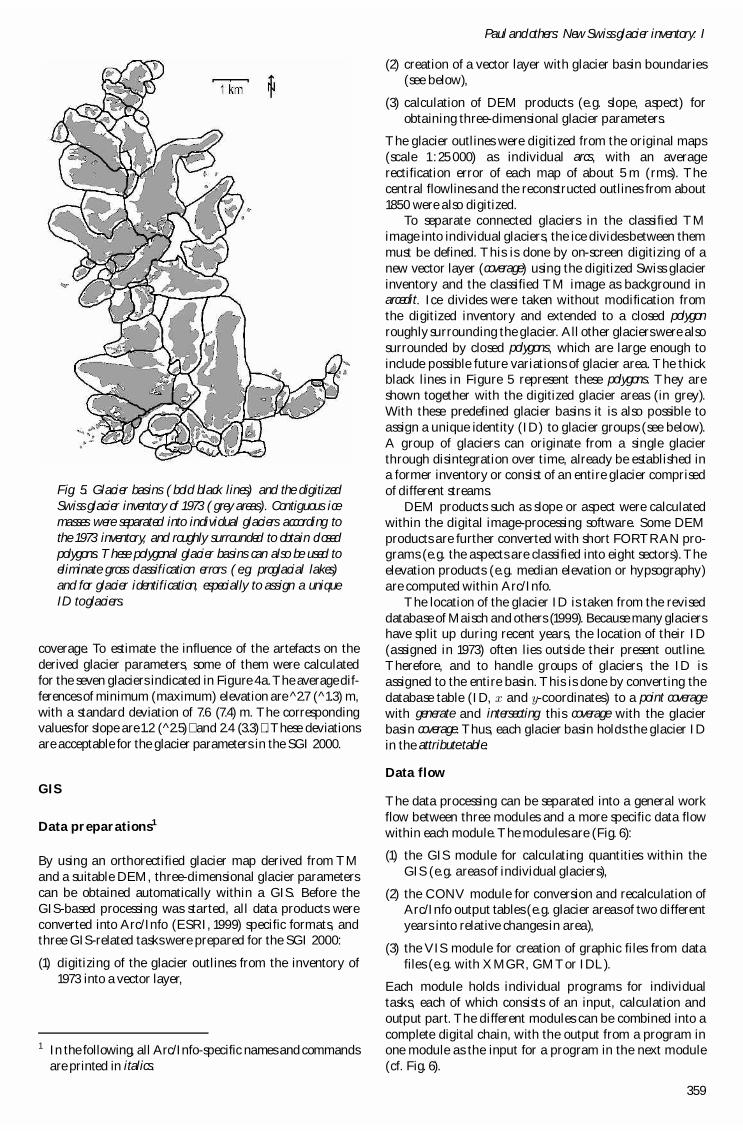
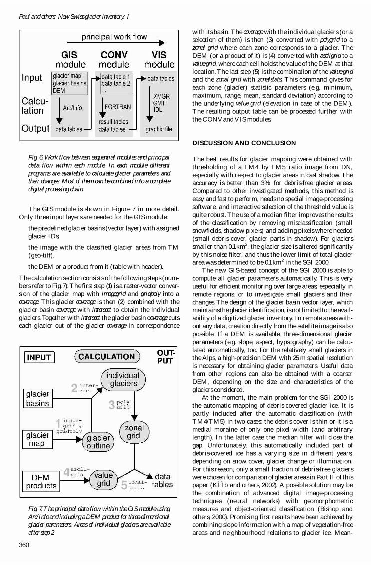
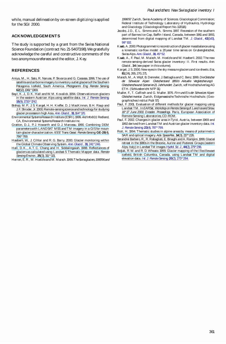