real values of the w -function

Real Values of the W-Function

D. A. BARRY and P. J, CULLIGAN-HENSLEY

University of Western Australia

and

S. J. BARRY

Griffith University

Approximations for real values of W(x), where W is defined by solutions of W exp( W ) = x, are

presented. All of the approximations have maximum absolute (1W I > 1) or relative (1W I < 1)

errors of 0( 10’4 ). With these approximations an efficient algorithm, consisting of a single

iteration of a rapidly converging iteration scheme, gives estimates of W(x) accurate to at least 16

significant digits (15 digits if double precision is used). The Fortran code resulting from the

algorithm is written to account for the different floating-point-number mantissa lengths on

different computers, so that W( .x) is computed to the floating-point precision available on the

host machine.

Categories and Subject Descriptors: G. 1.2 [Numerical Analysis]: Approximation—nonlinear

awmwnation; G.1.5 [Numerical Analysis]: Roots of Nonlinear Equations—zterative methods

General Terms: Algorithms

Additional Key Words and Phrases: W-function

1. INTRODUCTION

The function defined by (1) below was first discussed by Euler [1921], and

later by P61ya and Szego [1972, part (3), prob. 209]. de Bruijn [ 1958] explored

the asymptotic behavior of the W-function. Green and Knuth [1981] used de

Bruijn’s analysis as an archetypal example of “bootstrapping.” Similarly,

Oliver [1990] used a variant of (1) to demonstrate the derivation of asymp-

totic solutions of transcendental equations. In a practical application, the

W-function was found recently to be an approximation describing water

infiltration into a dry soil [Barry et al. 1995].

Authors’ addresses: D. A. Barry, Department of Environmental Engineering, Centre for Water

Research, The University of Western Australia, Nedlands, Western Australia 6907; email:

[email protected]. au; P. J. Culligan-Hensley, Department of Civil and Environmental Engi-

neering, Massachusetts Institute of Technology, Cambridge, MA 02139-4307; S. J. Barry, Faculty

of Environmental Sciences, Griffith University, Nathan, Queensland 4111 Australia.

Permission to make digital/hard copy of part or all of this work for personal or classroom use kgranted without fee provided that copies are not made or distributed for profit or commercial

advantage, the copyright notice, the title of the publication, and its date appear, and notice is

given that copying is by permission of ACM, Inc. To copy otherwise, to republish, to post on

servers, or to redistribute to lists, requires prior specific permission and\or a fee.

01995 ACM 0098-3500/95/0600-0161 $03.50

ACM Transactions on Mathematical Software, Vol. 21, No. 2, June 1995, Pages 161-171

162 . D. A. Barry et al.

i,! I

Wp

o-e-’

(-1+,

- -2 ‘ “

S -3

-4

-5

-fj L

Win’,

(

e——.

L- ——- .- - -—A

--0.5 0.0 0.5 1.0 1,5 2.0

x

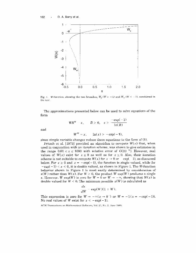
Fig. 1. W-function, showing the two branches, Wp (W > – 1)and W~ (W < – 1), considered in

the text.

The approximations presented below can be used to solve equations of the

form

WBW =X,– exp( – 1)

B>o, x>ln(B )

and

Ww =x, in(x) 2 –exp(– 1),

since simple variable changes reduce these equations to the form of ( 1).

Fritsch et al. [1973] provided an algorithm to compute W(x) that, when

used in conjunction with an iteration scheme, was shown to give estimates in

the range 0.01< x s 1000 with relative error of 0(10-6). However, real

values of W(x) exist for x s O as well as for x > 0. Also, their iteration

scheme is not suitable to compute W(x) for x -+ O or – exp( – 1), as discussed

below. For x >0 and x = – exp( – 1), the function is single valued, while for

– exp( – 1) < x < 0, it is double valued, as shown in Figure 1. The W-functionbehavior shown in Figure 1 is most easily determined by consideration of

x(W) rather than W(x). For W > 0, the product W exp( W ) produces a single

x. However, W exp( W ) is zero for W = O or W ~ —CO,showing that W(x) is

double valued for W <0. The minimum possible x(W) is calculated as

dx— =exp(W)(l + W).dW

This expression is zero for W + –~(x+ O-) or W= –1(x= –exp(– 1)).

No real values of W exist for x < – exp( – 1).

ACM TransactIons on Mathematical Software, Vol. 21, No 2, June 1995.

Real Values of the W-Function . 163

Our aims are (1) to produce closed-form approximations for W(x) and (2) to

provide an algorithm for calculating W automatically to, or very near to, the

floating-point precision of the host computer. The basic approach followed is

to find approximations for W(x), accurate to 0(10-4). These are developed

using various functional forms, including continued fractions and asymptotic

expansions. Using these approximations, a single pass of the iterative im-

provement scheme of Fritsch et al. [1973] gives 16-significant-digit accuracy

(typical Fortran douple precision). A second iteration gives 64-digit accuracy,and so on for further iterations.

2. APPROXIMATIONS

The function W(x), x and W both assumed real, is defined by

Wexp(W) =x, x > –exp(– 1). (1)

For x - O‘, the left-hand side of (1) can approach O in two ways, that is, ifW -0- or if W ~ – m. This behavior is the cause of the dual values of W for

– exp( – 1) < x < 0. For convenience, we denote the upper branch (i.e., W >

– 1 in Figure 1) as WP and the lower branch as W~. Each case is treated

separately below. Before proceeding, however, note that writing (1) as W = x

exp( – W ) yields, after repeated substitution,

W = x exp(–x exp(–x exp(–x .“. , (2)

where the ellipsis indicates that the given form of the function continues

indefinitely. Similarly, by taking logarithms of both sides of (l), there results

W=ln ‘x . (3)in —

in ~

Equation (2) was considered for use in approximating WP around x = O;

however, continued fraction approximations are more effective computation-

ally. Truncated forms of (3), on the other hand, were found to be useful for

estimating Wp, for x large, and Wm, for x -+ O-, as shown below. An alterna-

tive approach is that of de Bruijn [1958], who gives an asymptotic expansion

for W(x) valid as x ~ CO.The relationship between the magnitude of x and

the accuracy of de Bruijn’s expansion has not been explored. de Bruijn [1958]

shows this series to be absolutely convergent for large x, but no general

formula to calculate the series coefficients was presented, thus limiting the

practical application of his result.

2.1 Approximations for Wp

An expansion of (1) around x = – exp( – 1) yields (for both WP and Wm)

ACM Transactions on Mathematical Software, Vol. 21, No. 2, June 1995.

164 . D. A. Barry et al

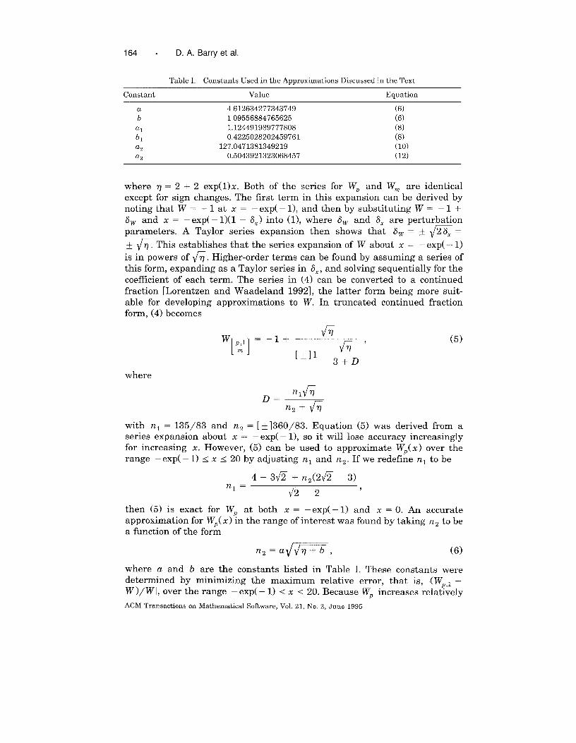
Table I. Constants Used in the Approximations Discussed in the Text

Constant Value Equation

a 4612634277343749 (6)

b 109556884765625 (6)

al 1.124491989777808 (8)

bl 0.4225028202459761 (8)

az 127.0471381349219 (10)

a3 0.5043921323068457 (12)

where q = 2 + 2 exp(l)x. Both of the series for WP and Wm are identical

except for sign changes. The first term in this expansion can be derived by

noting that W= –1 at x = –exp(– 1), and then by substituting W= –1 +

C?Wand x = –exp(– 1)(1 – i3X) into (l), where SW and 8, are perturbation

parameters. A Taylor series expansion then shows that i3W = + ~ =

+ fi. This establishes that the series expansion of W about x = – exp( – 1)

is in powers of fi. Higher-order terms can be found by assuming a series of

this form, expanding as a Taylor series in 8%, and solving sequentially for the

coefficient of each term. The series in (4) can be converted to a continued

fraction [Lorentzen and Waadeland 1992], the latter form being more suit-

able for developing approximations to W. In truncated continued fraction

form, (4) becomes

w –1+6

[1p,l =m 6’

[t]l+m

(5)

where

Fnl qD=

%+6

with nl = 135/83 and nz = [ f ]360/83. Equation (5) was derived from a

series expansion about x = – exp( – 1), so it will lose accuracy increasingly

for increasing x. However, (5) can be used to approximate Wp(x) over the

range – exp( – 1) < x < 20 by adjusting nl and nz. If we redefine nl to be

4 – 3JZ + nz(2JZ – 3)nl =

fi-2 ‘

then (5) is exact for WP at both x = – exp( – 1) and x = O. An accurate

approximation for WP( x ) in the range of interest was found by taking nz to be

a function of the form

.2=(JW, (6)

where a and b are the constants listed in Table I. These constants were

determined by minimizing the maximum relative error, that is, 1(Wp,l –

W)/ W 1,over the range – exp( – 1) < x <20. Because Wp increases relatively

ACM Transactions on Mathematical Software, Vol. 21, No 2, June 1995


01 1

0 2 4

IoglO[x + 1 + exp(-1 )]

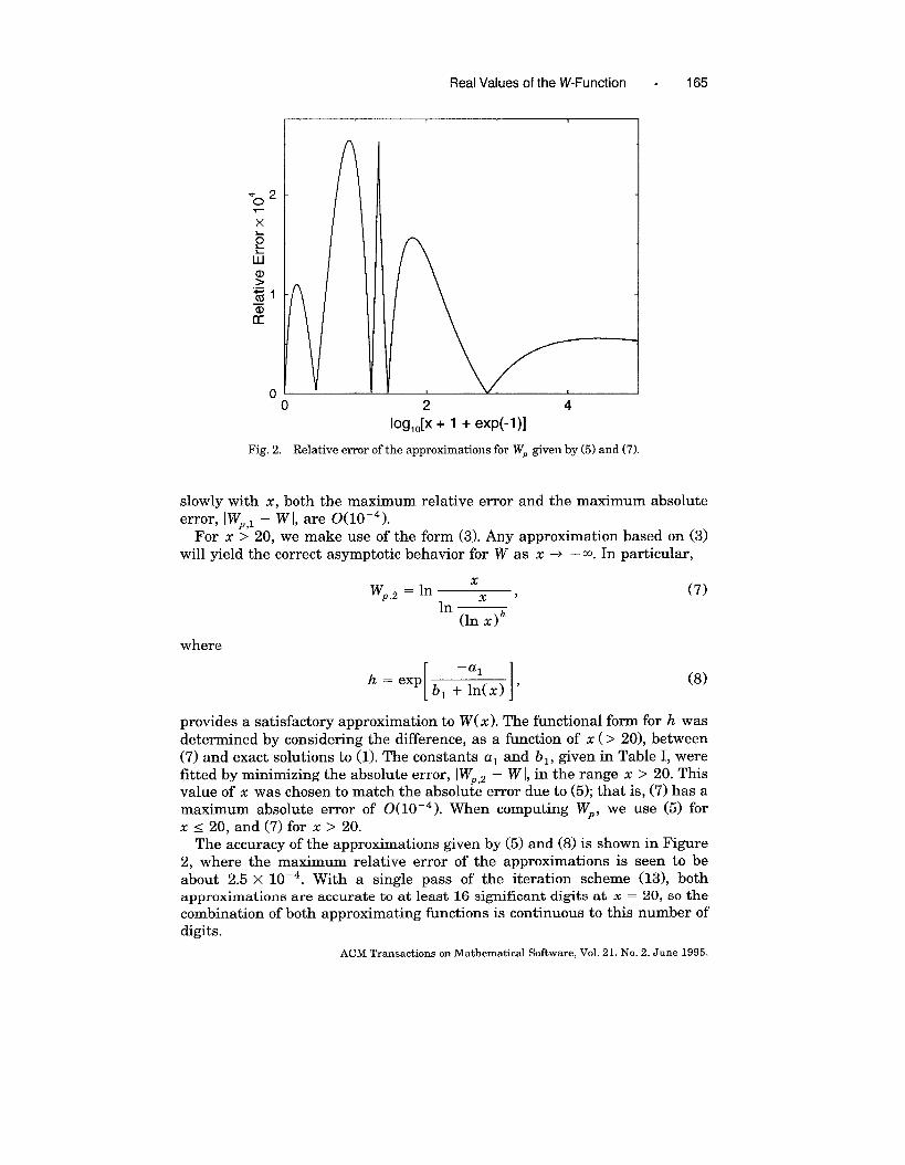
Fig. 2. Relative error of the approximations for W, given by (5) and (7).

slowly with x, both the maximum relative error and the maximum absolute

error, IWP,I – Wl, are 0(10-4).

For x >20, we make use of the form (3). Any approximation based on (3)

will yield the correct asymptotic behavior for W as x ~ – CO.In particular,

Wp,z = in ‘x ,

in(ln X)h

where

(7)

(8)

provides a satisfactory approximation to W( x). The functional form for h was

determined by considering the difference, as a function of x(> 20), between

(7) and exact solutions to (l). The constants al and bl, given in Table I, werefitted by minimizing the absolute error, IWp,z – W 1,in the range x >20. This

value of x was chosen to match the absolute error due to (5); that is, (7) has a

maximum absolute error of 0(10’4 ). When computing Wp, we use (5) forx s 20, and (7) for x >20.

The accuracy of the approximations given by (5) and (8) is shown in Figure

2, where the maximum relative error of the approximations is seen to be

about 2.5 X 10-4. With a single pass of the iteration scheme (13), bothapproximations are accurate to at least 16 significant digits at x = 20, so the

combination of both approximating functions is continuous to this number of

digits.


166 . D. A, Barry et al.

2.2 Approximations for W~

In this case our procedure for developing an approximation for W is slightly

different. It is readily confirmed that

(9)

where t = – 1 – ln( – x), reproduces the first term in both the x - – exp( – 1)

and x ~ O- expansions for W~, regardless of the value of the constant x ~.

That is, (9) is an interpolation between these limits. We therefore treat xl as

a variable and calculate its series expansion about x = – exp( – 1). This

series expansion can then be expressed, approximately, in truncated contin-

ued fraction form as

1 txl=——

3 270 + azfi ‘(lo)

where az is a fitting constant to be determined. We choose az (Table 1) so

that (9) produces 0(10’4 ) absolute error estimates of W~ in the range

–exp(–1) <x S –exp(–9).

For – exp( – 9) < x <0, we revert to a truncation of (3),

w m,2 =ln~, (11)

in —g

where

(12)

The functional form in (12) was determined by considering the difference

between (11) and W calculated from (l). Again, as in (12) is a fitting constant.

By choosing a3 as listed in Table I, we can approximate Wm by (11) for

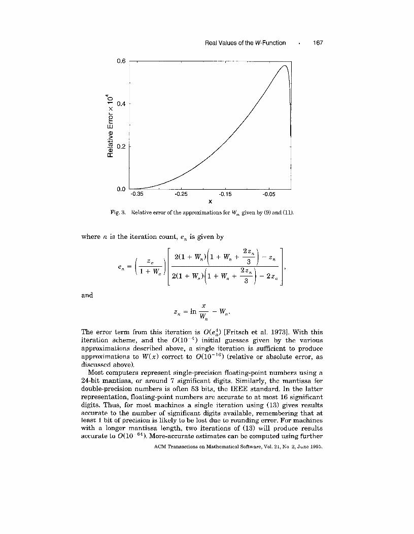
– exp( – 9) < x < 0, with maximum absolute error of 0(10 –4). The accuracy

of the W~ approximations is shown in Figure 3. Once again, both approxima-

tions are accurate to at least 16 significant digits at x = – exp( – 9) with a

single pass of (13) and so are continuous there to at least this number of

digits.

3. ITERATIVE SCHEME

An efficient iteration scheme to compute more-accurate estimates of W(x)

based on a given initial guess has been described by Fritsch et al. [1973].

Given an approximation, W., to W, improved approximations are calculated

using the iteration formula

w n+l = W.(1 + e.), (13)

ACM Transactions on Mathematical Software, Vol 21, No 2, June 1995


0.6

“o; 0.4

~

&a)>.—

~ 0.2

01

0.0

Fig. 3.

-0.35 -0.25 -0.15 -0.05

x

Relative error of the approximations for Wm given by (9) and (11).

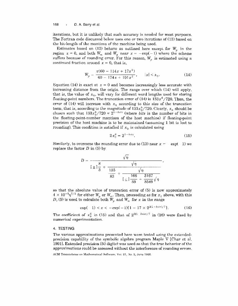
where n. is the iteration count, e, is given by

()[( ( 2zn2(l+wn)l+wn+—

Zn 3 )— Zn

e. =l+wn 2zn

) 1

7

2(l+wn)l+wn+— – 2zn3

and

The error term from this iteration is O(e~) [Fritsch et al. 1973]. With this

iteration scheme, and the 0(10 – 4) initial guesses given by the various

approximations described above, a single iteration is sufficient to produce

approximations to W(x) correct to 0(10 – 16) (relative or absolute error, as

discussed above).

Most computers represent single-precision floating-point numbers using a

24-bit mantissa, or around 7 significant digits. Similarly, the mantissa for

double-precision numbers is often 53 bits, the IEEE standard. In the latter

representation, floating-point numbers are accurate to at most 16 significant

digits. Thus, for most machines a single iteration using (13) gives results

accurate to the number of significant digits available, remembering that atleast 1 bit of precision is likely to be lost due to rounding error. For machines

with a longer mantissa length, two iterations of (13) will produce results

accurate to 0(10 – ‘4). More-accurate estimates can be computed using further

ACM Transactions on Mathematical Software, Vol. 21, No 2, June 1995.

168 . D, A. Barry et al.

iterations, but it is unlikely that such accuracy is needed for most purposes.

The Fortran code discussed below uses one or two iterations of (13) based on

the bit-length of the mantissa of the machine being used.

Estimates based on (13) behave as outlined here except for WP in the

region x = O, and both W~ and Wp near x = – exp( – 1) where the scheme

suffers because of rounding error. For this reason, WP is estimated using a

continued fraction around x = O, that is,

x(6O + 114x + 17x2)w, = Ixl<xo.

60 + 174x + 101x2 ‘(14)

Equation (14) is exact at x = O and becomes increasingly less accurate with

increasing distance from the origin. The range over which (14) will apply,

that is, the value of XO, will vary for different word lengths used for storing

floating-point numbers. The truncation error of (14) is 133 xG/720. Thus, the

error of (14) will increase with XO according to this size of the truncation

term, that is, according to the magnitude of 133 x~/720. Clearly, XO should be

chosen such that 133x~\720 = 21- ~’ts (where bits is the number of bits inthe floating-point-number mantissa of the host machine) if floating-point

precision of the host machine is to be maintained (assuming 1 bit is lost to

rounding). This condition is satisfied if XO is calculated using

2X: = 21- bLts. (15)

Similarly, to overcome the rounding error due to (13) near x = – exp( – 1) we

replace the factor D in (5) by

so that the absolute value of truncation error of (5) is now approximately

4 x 10- 5q7/2 for either WP or W~. Then, proceeding as for XO above, with this

D, (5) is used to calculate both WP and W~ for x in the range

–exp(–1) < x < –exp(–1)[1 – 17 X 22(1 -~ ’fs)/7]. (16)

The coefficient of X8 in (15) and that of 22(1 - “~s)\7 in (16) were fixed by

numerical experimentation.

4. TESTING

The various approximations presented here were tested using the extended-

precision capability of the symbolic algebra program Maple V [Char et al.

1991]. Extended precision (50 digits) was used so that the true behavior of the

approximations could be assessed without the interference of rounding errors.

ACM TransactIons on Mathematmal Software, Vol. 21, No. 2, June 1995


40

8:$32

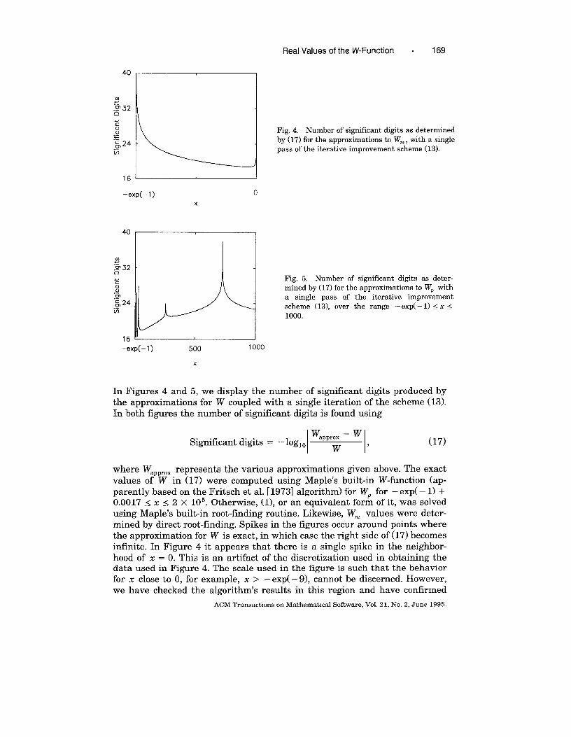
z0v.— Fig. 4. Number of significant digits as determined

“~ 24by (17) for the approximations to Wm,with a single

.—m pass of the iterative improvement scheme (13).

-J

,fj ~

–exp(–1) o

,,,

x

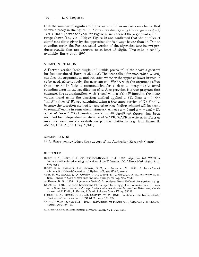
Fig. 5. Number of significant digits as deter-

mined by (17) for the approximations to WP with

a single pass of the iterative improvement

scheme (13), over the range – exp( – 1) < x <

1000.

–exp(–1) 500 1000

x

In Figures 4 and 5, we display the number of significant digits produced by

the approximations for W coupled with a single iteration of the scheme (13).

In both figures the number of significant digits is found using

Significant digits =

where W=PP,OXrepresents the various

values of W in (17) were computed

w –w– log lo ‘pP’; , (17)

approximations given above. The exact

using Maple’s built-in W-function (ap-

parently based on the Fritsch et al. [1973] algorithm) for Wp for – exp( – 1) +0.0017 s x <2 x 105. Otherwise, (l), or an equivalent form of it, was solved

using Maple’s built-in root-finding routine. Likewise, W~ values were deter-

mined by direct root-finding. Spikes in the figures occur around points where

the approximation for W is exact, in which case the right side of (17) becomes

infinite. In Figure 4 it appears that there is a single spike in the neighbor-

hood of x = O. This is an artifact of the discretization used in obtaining thedata used in Figure 4. The scale used in the figure is such that the behavior

for x close to O, for example, x > – exp( – 9), cannot be discerned. However,

we have checked the algorithm’s results in this region and have confirmed

ACM TransactIons on Mathematical Software, Vol. 21, No. 2, June 1995.

170 . D. A. Barry et al.

that the number of significant digits as x ~ O- never decreases below that

shown already in the figure. In Figure 5 we display only the range – exp( – 1)

< x < 1000. As was the case for Figure 4, we checked the region outside the

range shown (i.e., x > 1000; cf. Figure 2) and confirmed that the number of

significant digits given by the approximation is always better than 16. Due to

rounding error, the Fortran-coded version of the algorithm (see below) pro-

duces results that are accurate to at least 15 digits. This code is readily

available [Barry et al. 1995].

5. IMPLEMENTATION

A Fortran version (both single and double precision) of the above algorithm

has been produced [Barry et al. 1995]. The user calls a function called WAPR,

supplies the argument x, and indicates whether the upper or lower branch is

to be used. Alternatively, the user can call WAPR with the argument offset

from – exp( – 1). This is recommended for x close to – exp( – 1) to avoid

rounding error in the specification of x. Also provided is a test program that

compares the approximations with “exact” values of the W-function, the latter

values found using the bisection method applied to (1). Near x = O, the

“exact” values of WP are calculated using a truncated version of (2). Finally,

because the bisection method (or any other root-finding scheme) will be prone

to roundoff errors in some circumstances (i.e., near x = O and x = – exp( – 1)),

a list of “exact” W(x) results, correct to 40 significant figures, has been

included for independent verification of WAPR. WAPR is written in Fortran

and has been run successfully on popular platforms (e.g., Sun Spare II,

486PC, DEC Alpha, Cray X/MP).

ACKNOWLEDGMENT

D. A. Barry acknowledges the support of the Australian Research Council.

REFERENCES

BARRY, D. A., BARFW, S. J., AND CULLIGAN-HENSLEY, P. J. 1995. Algorithm 743: WAPR: A

Fortran routine for calculating real values of the W-function. ACM Trans. Math. Softw. 21, 2.

This issue.

BARRY, D. A., PARLANGE, J.-Y., SANDER, G. C,, AND SIVAPALAN, M. 1993, A class of exact

solutions for Richards’ equation. J. Hydrol. 142, 1–4 (Feb.), 29–46.

CHAR, B. W., GEDDES, K. O., GONNET, G. H., LEONG, B. L., MONAGAN, M. B., AND WA’I”T, S. M.

1991. Maple V Library Reference Manual. Springer-Verlag, New York.

DE BRUIJN, N. G. 1958. Asymptotic Methods in ,hatysw, North-Holland, Amsterdam, 25–28.

EULER, L. 1921. De Sene Lambertina Plurimisque Elus Ingignibus Proprletatibus. In Leon-

hard~ Euler~ Opera omma; sub ausplclis Socletatw ScLentLarum Naturalism Heluetlcae, edenda

curaverunt F. Rudio, A. Krazer, P. Stackel. Series Prima VI, pp. 350 ff.

FRITSCH, F. N., SHAFER, R. E., AND CROWLEY, W. P. 1973. Solution of the transcendental

equation we’” = .x. Commun. ACM 16, 2 (Feb.), 123–124

GREEN, D. H. AND KNUTH, D. E. 1981. Mathematics for the Analysw of Algorithms. Birkhauser,

Boston, Mass., 47-48.

ACM TransactIons on Mathematical Software, Vol 21, No 2, June 1995


LORENTZEN, L. AND WAADELAND, H. 1992. Continued Fractions with Applications. North-

Holland, Amsterdam, 21-22.

OLIVER, F. W. J. 1990. Asymptotic methods. In Handbook of Applied Mathematics, 2nd cd.,

C. E. Pearson, Ed, Van Nostrand Reinhold, New York, 633.

P6LYA, G. AND SZEGO, G. 1972. Problems and Theorems in Analysis. Vol. 1. Springer-Verlag,Berlin, 146.

Received September 1992; revised May and December 1993, and January 1994; accepted

February 1994


real values of the w -function

Documents