real-time scheduling for energy-harvesting embedded
TRANSCRIPT
T H È S Een vue de l’obtention du titre de
Docteur
de l’Université Paris-Est
Spécialité : Informatique
École doctorale : MSTIC
Younes Chandarli
Real-time Scheduling forEnergy-Harvesting Embedded Systems
soutenue le 2 Décembre 2014
Jury
Directeur : Laurent George – ESIEE Paris (LIGM), FranceEncadrant : Damien Masson – ESIEE Paris (LIGM), FranceRapporteurs : Daniel Mossé – University of Pittsburgh, U.S.A
Hakan Aydin – George Mason University, U.S.AExaminateurs : Laurent Pautet – Télécom Paris-Tech (LTCI), France
Maryline Chetto – Université de Nantes (IRCCyN), France

Sous la co-tutelle de :CNRSÉCOLE DES PONTS PARISTECHESIEE PARISUPEM • UNIVERSITÉ PARIS-EST MARNE-LA-VALLÉE
LABORATOIRE D’INFORMATIQUEGASPARD-MONGE
LA
BO
R
ATOIRE D'INFORM
ATIQ
UE
- G
A
SPARD - MON
GE -
PhD prepared atLIGM (UMR 8049)Laboratoire d’Informatique Gaspard-MongeCité Descartes, Bâtiment Copernic5, boulevard DescartesChamps-sur-Marne 77454 Marne-la-Vallée Cedex 2
PhD in collaboration withESIEE ParisSystems Engineering Department2, boulevard Blaise Pascal93162 Noisy le Grand CEDEX

À mes parents,À mes grands parents,
À ma sœur et mon frère,À toute ma famille,À tous mes amis,
À toutes les personnes que j’ai eu le privilège de croiser.
Parce que chaque personne rencontrée, même brièvement,est une occasion exceptionnelle de se redécouvrir
et de s’émerveiller.
To my parents,To my grandparents,
To my brother and my sister,To all my family,To all my friends,
To all the people who have graced my life.
Because each encounter, even a brief one,is an occasion to re-imagine oneself
and to marvel.


“The greatest part of a writer’s time is spent in reading, in order to write: a man willturn over half a library to make one book”. Samuel Johnson.

Author’s publication list
International Conference Papers
ECRTS’2013 Yasmina Abdeddaïm, Younès Chandarli, and Damien Masson. “TheOptimality of PFPASAP Algorithm for Fixed-Priority Energy-Harvesting Real-Time Systems”. In: Proceedings of the Euromicro Conference on Real-TimeSystems (ECRTS). 2013
RTNS’2014 Yasmina Abdeddaïm, Younès Chandarli, R.I Davis, and Damien Masson.“Schedulability Analysis for Fixed Priority Real-Time Systems with Energy-Harvesting”. In: Proceedings of the International Conference on Real-TimeNetworks and Systems (RTNS). 2014, pages 67–76RTNS 2014 Best Paper Award
ISORC’2015 Younès Chandarli, Nathan Fisher, and Damien Masson. “Response TimeAnalysis for Thermal-Aware Real-Time Systems Under Fixed-Priority Scheduling”.In: Proceedings of the IEEE Symposium On Real-time Computing (ISORC). 2015
Workshop and WIP1 Papers
WATERS’2012 Younès Chandarli, Frédéric Fauberteau, Damien Masson, Serge Mi-donnet, and Manar Qamhieh. “YARTISS: A Tool to Visualize, Test, Compareand Evaluate Real-Time Scheduling Algorithms”. In: Proceedings of the Interna-tional Workshop on Analysis Tools and Methodologies for Embedded and Real-timeSystems (WATERS). 2012, pages 21–26
WIP RTCSA’2012 Younès Chandarli, Yasmina Abdeddaïm, and Damien Masson. “TheFixed Priority Scheduling Problem for Energy Harvesting Real-Time Systems”.In: Proceedings of the work in progress session of the the IEEE InternationalConference on Embedded and Real-Time Computing Systems and Applications(RTCSA). 2012
WIP RTAS’2013 Yasmina Abdeddaïm, Younès Chandarli, and Damien Masson. “Towardan Optimal Fixed-Priority Algorithm for Energy-Harvesting Real-Time Systems”.In: Proceedings of the Work in progress session of the IEEE Real-Time andEmbedded Technology and Applications Symposium (RTAS). 2013, pages 45–48
1Work In Progress

2 Author’s publication list
Technical Reports1. Younès Chandarli, Manar Qamhieh, and Frédérique Fauberteau.
YARTISS: A Generic, Modular and Energy-Aware Scheduling Simulator for Real-Time Multiprocessor Systems. technical report. Paris, France, 2013. url: http://hal.archives-ouvertes.fr/hal-01076022
2. Yasmina Abdeddaïm and Younès Chandarli. Optimal Real-Time SchedulingAlgorithm for Fixed-Priority Energy-Harvesting Systems. technical report. Paris,France, 2013. url: http://hal.archives-ouvertes.fr/hal-01076021


Acknowledgment
I am using this opportunity to express my gratitude to everyone who supported methroughout this thesis. I am thankful for their aspiring guidance, invaluably constructivecriticism and friendly advice during the work. I am sincerely grateful to them for sharingtheir truthful and illuminating views on a number of issues related to the thesis.
I have to thank my research supervisors, Mr. Laurent George and Mr. DamienMasson. Without their assistance and dedicated involvement in every step throughoutthe process, this work would have never been accomplished. I would like to thank youvery much for your support and understanding over these past three years.
I would also like to show gratitude to my committee, including Mr. Hakan Aydin,Mr. Daniel Mossé, Mrs. Maryline Chetto and Mr. Laurent Pautet.
I express my warm thanks to Mrs. Yasmina Abdeddaïm, Mr. Rob Davis and NathanFisher for their collaboration, support and guidance.
Getting through my thesis required more than academic support, and I have many,many people to thank for listening to and, at times, having to tolerate me over thepast three years. I express all my gratitude and appreciation for their friendship. Mycolleagues have been unwavering in their personal and professional support during thetime I spent at the University.
Last but not the least, I would like to thank my family: my parents for giving birthto me at the first place and supporting me throughout my life.

Contents
Abstract 13
Résumé 17
Introduction 21
I State of The Art 25
1 Real-time Scheduling 271.1 Introduction . . . . . . . . . . . . . . . . . . . . . . . . . . . . . . . . . 281.2 Workload Model . . . . . . . . . . . . . . . . . . . . . . . . . . . . . . 30
1.2.1 Task Life Cycle . . . . . . . . . . . . . . . . . . . . . . . . . . . 321.2.2 Completely-Specified Recurrent Task Model . . . . . . . . . . . 331.2.3 Partially-Specified Recurrent Systems . . . . . . . . . . . . . . . 341.2.4 Tasks Independence . . . . . . . . . . . . . . . . . . . . . . . . . 35
1.3 Processing Platform . . . . . . . . . . . . . . . . . . . . . . . . . . . . 351.4 Scheduling Algorithms . . . . . . . . . . . . . . . . . . . . . . . . . . . 36
1.4.1 Online/Offline Scheduling . . . . . . . . . . . . . . . . . . . . . 361.4.2 Work-Conserving/Non-work-conserving Scheduling . . . . . . . 371.4.3 Preemptive/Non-Preemptive Scheduling . . . . . . . . . . . . . 371.4.4 Optimal Scheduling . . . . . . . . . . . . . . . . . . . . . . . . . 371.4.5 Priority Driven Scheduling Algorithms . . . . . . . . . . . . . . 381.4.6 Fixed Task-Priority Scheduling Algorithms (FTP) . . . . . . . . 381.4.7 Fixed Job-Priority Scheduling Algorithms (FJP) . . . . . . . . . 401.4.8 Dynamic Priority Scheduling Algorithms (DP) . . . . . . . . . . 40
1.5 Scheduling Analysis . . . . . . . . . . . . . . . . . . . . . . . . . . . . . 401.5.1 Definitions . . . . . . . . . . . . . . . . . . . . . . . . . . . . . . 411.5.2 Feasibility or Schedulability . . . . . . . . . . . . . . . . . . . . 431.5.3 Schedulability Analysis for Fixed-Task-Priority . . . . . . . . . 441.5.4 Schedulability Analysis for Dynamic-Priority . . . . . . . . . . . 46
1.6 Conclusion . . . . . . . . . . . . . . . . . . . . . . . . . . . . . . . . . . 46
2 Energy-Harvesting Systems 472.1 Introduction . . . . . . . . . . . . . . . . . . . . . . . . . . . . . . . . . 472.2 What is an Energy-Harvesting System ? . . . . . . . . . . . . . . . . . 482.3 Energy-Harvesting Technologies . . . . . . . . . . . . . . . . . . . . . . 49
2.3.1 Radiations Energy Harvesting . . . . . . . . . . . . . . . . . . . 492.3.2 Vibrations Energy Harvesting . . . . . . . . . . . . . . . . . . . 51
8 Contents
2.3.3 Thermoelectric Energy Harvesting . . . . . . . . . . . . . . . . . 542.3.4 Energy Sources Comparison . . . . . . . . . . . . . . . . . . . . 55
2.4 Energy Storage Technologies . . . . . . . . . . . . . . . . . . . . . . . . 552.4.1 Rechargeable Batteries . . . . . . . . . . . . . . . . . . . . . . . 572.4.2 Supercapacitors . . . . . . . . . . . . . . . . . . . . . . . . . . . 60
2.5 Energy-Harvesting Applications . . . . . . . . . . . . . . . . . . . . . . 612.6 Conclusion . . . . . . . . . . . . . . . . . . . . . . . . . . . . . . . . . . 62
3 Real-time Scheduling for Energy-Harvesting Systems 653.1 Introduction . . . . . . . . . . . . . . . . . . . . . . . . . . . . . . . . . 66
3.1.1 Task Model . . . . . . . . . . . . . . . . . . . . . . . . . . . . . 663.2 General Model . . . . . . . . . . . . . . . . . . . . . . . . . . . . . . . 67
3.2.1 Energy Model . . . . . . . . . . . . . . . . . . . . . . . . . . . . 673.2.2 Definitions . . . . . . . . . . . . . . . . . . . . . . . . . . . . . . 70
3.3 Scheduling Problematic . . . . . . . . . . . . . . . . . . . . . . . . . . . 713.4 Scheduling Approaches . . . . . . . . . . . . . . . . . . . . . . . . . . . 73
3.4.1 Dynamic Voltage and Frequency Scaling . . . . . . . . . . . . . 733.4.2 Energy-Aware Scheduling . . . . . . . . . . . . . . . . . . . . . 743.4.3 Other Approaches . . . . . . . . . . . . . . . . . . . . . . . . . . 75
3.5 Scheduling for Frame-Based Systems . . . . . . . . . . . . . . . . . . . 753.6 EDF-based Scheduling Algorithms . . . . . . . . . . . . . . . . . . . . . 79
3.6.1 EDF As Late As Possible Scheduling (EDL) . . . . . . . . . . . 803.6.2 EDF with Energy Guarantee Scheduling (EDeg) . . . . . . . . 833.6.3 Lazy Scheduling Algorithm (LSA) . . . . . . . . . . . . . . . . 86
3.7 Fixed-Priority Scheduling . . . . . . . . . . . . . . . . . . . . . . . . . 923.7.1 The PFPALAP Scheduling Algorithm . . . . . . . . . . . . . . . 923.7.2 Preemptive Fixed-Priority with Slack-Time Algorithm . . . . . 953.7.3 Other Scheduling Heuristics . . . . . . . . . . . . . . . . . . . . 97
3.8 Performance Evaluation and Comparison . . . . . . . . . . . . . . . . . 993.8.1 Simulation configuration . . . . . . . . . . . . . . . . . . . . . . 993.8.2 Results analysis . . . . . . . . . . . . . . . . . . . . . . . . . . . 1013.8.3 Comparison summary . . . . . . . . . . . . . . . . . . . . . . . 103
3.9 Conclusion . . . . . . . . . . . . . . . . . . . . . . . . . . . . . . . . . . 104
II Contributions 107
4 The PFPASAP Algorithm 1094.1 Introduction . . . . . . . . . . . . . . . . . . . . . . . . . . . . . . . . . 1094.2 Model . . . . . . . . . . . . . . . . . . . . . . . . . . . . . . . . . . . . 1104.3 Theoretical Study of PFPASAP . . . . . . . . . . . . . . . . . . . . . . 111
4.3.1 As Soon As Possible Preemptive Fixed-Priority . . . . . . . . . 1114.3.2 Worst-Case Scenario . . . . . . . . . . . . . . . . . . . . . . . . 113
Contents 9
4.3.3 Optimality . . . . . . . . . . . . . . . . . . . . . . . . . . . . . . 1184.3.4 Priority Assignment . . . . . . . . . . . . . . . . . . . . . . . . 1194.3.5 Schedulability Condition . . . . . . . . . . . . . . . . . . . . . . 1214.3.6 Battery Capacity . . . . . . . . . . . . . . . . . . . . . . . . . . 122
4.4 Performance Evaluation . . . . . . . . . . . . . . . . . . . . . . . . . . 1224.4.1 Competitors . . . . . . . . . . . . . . . . . . . . . . . . . . . . . 1224.4.2 Simulation . . . . . . . . . . . . . . . . . . . . . . . . . . . . . . 1234.4.3 Results Analysis . . . . . . . . . . . . . . . . . . . . . . . . . . 125
4.5 Conclusion . . . . . . . . . . . . . . . . . . . . . . . . . . . . . . . . . . 129
5 Approximate Response-Time Analysis for EH Systems 1315.1 Introduction . . . . . . . . . . . . . . . . . . . . . . . . . . . . . . . . . 1315.2 Models and Notations . . . . . . . . . . . . . . . . . . . . . . . . . . . 1325.3 Schedulability Analysis . . . . . . . . . . . . . . . . . . . . . . . . . . . 133
5.3.1 Worst-case scenario . . . . . . . . . . . . . . . . . . . . . . . . . 1335.3.2 Sequences and Energy-busy-periods . . . . . . . . . . . . . . . . 1335.3.3 Response Time Upper Bounds . . . . . . . . . . . . . . . . . . . 1375.3.4 Upper Bound RUB1 . . . . . . . . . . . . . . . . . . . . . . . . . 1375.3.5 Upper Bound RUB2 . . . . . . . . . . . . . . . . . . . . . . . . . 1395.3.6 Battery Capacity . . . . . . . . . . . . . . . . . . . . . . . . . . 1435.3.7 Response Time Lower Bound . . . . . . . . . . . . . . . . . . . 1445.3.8 Priority Assignment . . . . . . . . . . . . . . . . . . . . . . . . 146
5.4 Performance Evaluation . . . . . . . . . . . . . . . . . . . . . . . . . . 1475.4.1 Taskset generation . . . . . . . . . . . . . . . . . . . . . . . . . 1475.4.2 Schedulability tests investigated . . . . . . . . . . . . . . . . . . 148
5.5 Conclusions . . . . . . . . . . . . . . . . . . . . . . . . . . . . . . . . . 151
6 Optimal Algorithm Investigation 1536.1 Introduction . . . . . . . . . . . . . . . . . . . . . . . . . . . . . . . . . 1536.2 Definitions and Notations . . . . . . . . . . . . . . . . . . . . . . . . . 154
6.2.1 Model and Notations . . . . . . . . . . . . . . . . . . . . . . . . 1546.2.2 Definitions . . . . . . . . . . . . . . . . . . . . . . . . . . . . . . 1546.2.3 Energy-Work-Conserving . . . . . . . . . . . . . . . . . . . . . . 1556.2.4 Energy-Lookahead Scheduling . . . . . . . . . . . . . . . . . . . 158
6.3 Algorithms . . . . . . . . . . . . . . . . . . . . . . . . . . . . . . . . . . 1596.4 Conclusion . . . . . . . . . . . . . . . . . . . . . . . . . . . . . . . . . . 172
7 Response-Time Analysis for Thermal-Aware Scheduling 1737.1 Introduction . . . . . . . . . . . . . . . . . . . . . . . . . . . . . . . . . 1737.2 Related Work . . . . . . . . . . . . . . . . . . . . . . . . . . . . . . . . 1757.3 Models . . . . . . . . . . . . . . . . . . . . . . . . . . . . . . . . . . . . 176
7.3.1 Task Model . . . . . . . . . . . . . . . . . . . . . . . . . . . . . 1767.3.2 Thermal Model . . . . . . . . . . . . . . . . . . . . . . . . . . . 176
10 Contents
7.4 The PFPASAP algorithm . . . . . . . . . . . . . . . . . . . . . . . . . . 1787.4.1 Worst-case scenario . . . . . . . . . . . . . . . . . . . . . . . . . 1797.4.2 The optimality of PFPASAP . . . . . . . . . . . . . . . . . . . . 181
7.5 Response-Time Analysis . . . . . . . . . . . . . . . . . . . . . . . . . . 1837.5.1 Exact Analysis . . . . . . . . . . . . . . . . . . . . . . . . . . . 1837.5.2 Approximate Analysis . . . . . . . . . . . . . . . . . . . . . . . 183
7.6 Performance Evaluation . . . . . . . . . . . . . . . . . . . . . . . . . . 1977.6.1 Task set generation . . . . . . . . . . . . . . . . . . . . . . . . . 1977.6.2 Schedulability tests investigated . . . . . . . . . . . . . . . . . . 1987.6.3 Experiments . . . . . . . . . . . . . . . . . . . . . . . . . . . . . 198
7.7 Conclusion . . . . . . . . . . . . . . . . . . . . . . . . . . . . . . . . . . 202
8 Simulation Tool: YARTISS 2038.1 Introduction . . . . . . . . . . . . . . . . . . . . . . . . . . . . . . . . . 2038.2 Related Works . . . . . . . . . . . . . . . . . . . . . . . . . . . . . . . . 2058.3 The History of YARTISS . . . . . . . . . . . . . . . . . . . . . . . . . . 2068.4 Functionalities . . . . . . . . . . . . . . . . . . . . . . . . . . . . . . . . 207
8.4.1 Single Task Set Simulation . . . . . . . . . . . . . . . . . . . . . 2088.4.2 Run Large Scale Simulations . . . . . . . . . . . . . . . . . . . . 2128.4.3 Task Set Generation . . . . . . . . . . . . . . . . . . . . . . . . 2128.4.4 Graphical User Interface (GUI) . . . . . . . . . . . . . . . . . . 213
8.5 Architecture . . . . . . . . . . . . . . . . . . . . . . . . . . . . . . . . . 2138.5.1 Engine Module . . . . . . . . . . . . . . . . . . . . . . . . . . . 2148.5.2 Service Module . . . . . . . . . . . . . . . . . . . . . . . . . . . 2198.5.3 Framework Module . . . . . . . . . . . . . . . . . . . . . . . . . 2208.5.4 View-Module or GUI . . . . . . . . . . . . . . . . . . . . . . . . 220
8.6 Case Study . . . . . . . . . . . . . . . . . . . . . . . . . . . . . . . . . 2218.6.1 Adding a new Scheduling Policy . . . . . . . . . . . . . . . . . . 2218.6.2 Adding an Energy Profile . . . . . . . . . . . . . . . . . . . . . 223
8.7 Distribution . . . . . . . . . . . . . . . . . . . . . . . . . . . . . . . . . 2238.8 Conclusion . . . . . . . . . . . . . . . . . . . . . . . . . . . . . . . . . . 223
General Conclusion 225
III Résumé en français 231
9 Ordonnancement temps réel avec gestion de l’énergie renouvelable 2339.1 Introduction . . . . . . . . . . . . . . . . . . . . . . . . . . . . . . . . . 2339.2 Ordonnancement temps réel . . . . . . . . . . . . . . . . . . . . . . . . 234
9.2.1 Modèle de tâches . . . . . . . . . . . . . . . . . . . . . . . . . . 2349.2.2 Algorithmes d’ordonnancement . . . . . . . . . . . . . . . . . . 2359.2.3 Analyses d’ordonnançabilité . . . . . . . . . . . . . . . . . . . . 235
Contents 11
9.3 Les systèmes collecteurs d’énergie . . . . . . . . . . . . . . . . . . . . . 2369.3.1 Les technologies d’extraction de l’énergie ambiante . . . . . . . 2369.3.2 Les technologies de stockage d’énergie . . . . . . . . . . . . . . . 237
9.4 L’ordonnancement temps réel dans les systèmes collecteurs d’Énergie . 2389.4.1 Modèle . . . . . . . . . . . . . . . . . . . . . . . . . . . . . . . . 2389.4.2 Problématique . . . . . . . . . . . . . . . . . . . . . . . . . . . . 2399.4.3 Approches d’ordonnancement . . . . . . . . . . . . . . . . . . . 2399.4.4 Les algorithmes existants . . . . . . . . . . . . . . . . . . . . . . 239
9.5 L’algorithme PFPASAP . . . . . . . . . . . . . . . . . . . . . . . . . . . 2419.5.1 Le pire scénario . . . . . . . . . . . . . . . . . . . . . . . . . . . 2419.5.2 L’optimalité . . . . . . . . . . . . . . . . . . . . . . . . . . . . . 2419.5.3 Condition d’ordonnançabilité . . . . . . . . . . . . . . . . . . . 2429.5.4 La capacité minimale de la batterie . . . . . . . . . . . . . . . . 2429.5.5 Avantages et inconvénients . . . . . . . . . . . . . . . . . . . . . 242
9.6 Analyse de temps de réponse avec approximation . . . . . . . . . . . . 2429.7 Recherche d’algorithme optimal . . . . . . . . . . . . . . . . . . . . . . 2449.8 Analyse de temps de réponse des systèmes à contraintes thermiques . . 246
9.8.1 Analyse de temps de réponse . . . . . . . . . . . . . . . . . . . 2479.9 L’outil de simulation YARTISS . . . . . . . . . . . . . . . . . . . . . . 2489.10 Conclusion . . . . . . . . . . . . . . . . . . . . . . . . . . . . . . . . . . 249
Appendix 251
Glossaries 255Symbols . . . . . . . . . . . . . . . . . . . . . . . . . . . . . . . . . . . . . . 255Acronyms . . . . . . . . . . . . . . . . . . . . . . . . . . . . . . . . . . . . . 262Glossary . . . . . . . . . . . . . . . . . . . . . . . . . . . . . . . . . . . . . . 268

Abstract
In this thesis, we are interested in the real-time fixed-priority scheduling problem ofenergy-harvesting systems.
An energy-harvesting system is a system that can collect the energy from theenvironment in order to store it in an energy storage device and then to use it to supplyan electronic device. This technology is more and more used in small embedded systemsthat are required to run autonomously for a very long lifespan. Wireless sensor networksand medical implants are typical applications of this technology.
Moreover, most of devices that work with energy-harvesting have to execute manyrecurrent tasks within a limited time. Thus, these energy-harvesting devices are subjectto real-time constraints where the correctness of the system depends not only on thecorrectness of the results but also on the time in which they are delivered.
This thesis addresses the real-time scheduling layer of this kind of systems. Morespecifically, it focuses on a specific family of real-time scheduling: the preemptivefixed-task-priority scheduling for monoprocessor platforms. In this approach, each taskof the system is assigned a static priority. Then, at any moment, the scheduler executesfirst the active task with the highest priority.
The problematic of such a scheduling approach for energy-harvesting systems is tofind efficient scheduling algorithms and their associated schedulability analysis. Theresponsibility of a scheduling algorithm is to produce a valid and perpetual schedulewhere all the tasks respect their timing and energy constraints. In other words, allthe deadlines must be met and the system must never run out of energy. Whereas aschedulability analysis provides schedulability tests and conditions that guarantee theschedulability or the unschedulability of a given task set in a given energy configuration.Furthermore, to guarantee such schedulability, the energy storage unit capacity must besufficient to avoid energy wasting. Then, for each scheduling algorithm and schedulabilityanalysis, we must specify the minimum battery capacity that keeps the schedulabilityof a given task set.
This dissertation starts with a brief state of the art of the existing real-time schedulingtheory for energy-harvesting systems including energy-aware scheduling solutions thatadd more idle periods to replenish energy, and dynamic processor voltage and frequencyscaling approaches that reduce the consumption rate of the processor. In this part,we show that in the case of energy-aware scheduling approach, the fixed-task-priorityscheduling for energy-harvesting systems was not deeply studied.
The first contribution of this thesis is the proposition of the PFPASAP schedulingalgorithm. It is an adaptation of the classical fixed-task-priority scheduling to theenergy-harvesting context. It consists of executing tasks as soon as possible wheneverthe energy is sufficient to execute at least one time unit and replenishes otherwise. The
14 Abstract
replenishment periods are as long as needed to execute one time unit. The scheduleproduced by this algorithm can be seen as the energy counter-part of the classicalfixed-task-priority work-conserving scheduling where the processor cannot be idle whilethere are pending jobs and sufficient energy to execute. We prove in this dissertationthat PFPASAP is optimal in the class of fixed-task-priority scheduling algorithms butonly in the case of non-concrete systems where the first release time of tasks and theinitial energy storage unit level are known at run-time and where all the tasks consumemore energy than the replenishment during execution times. A sufficient and necessaryschedulability condition for such systems is also proposed. It consists of a responsetime analysis that computes the longest response time of all tasks in the worst-casescenario. We prove also that this scenario happens whenever all the tasks are requestedsimultaneously while the energy storage unit level is at its minimum level.
Unfortunately, when we relax the assumption of tasks energy consumption profile,by considering both tasks that consume more energy than the replenishment and theones that consume less than the replenishment, the PFPASAP is no longer optimaland the worst-case scenario is no longer the synchronous release of all the tasks, whichmakes the precedent schedulability test only necessary. To cope with this limitation,we propose in a second contribution to upper bound tasks worst-case response time inorder to build sufficient schedulability conditions instead of exact ones. We propose twoupper bounds based on the construction of virtual scenarios that maximize the numberof interferences and the needed replenishment time.
Regarding the possibility of finding an optimal algorithm, we explore through thisdissertation different ideas and approaches of scheduling policies in order to build anoptimal algorithm for the general model of fixed-task-priority tasks by considering alltypes of task sets and energy consumption profiles. We show through some counterexamples the difficulty of finding such an algorithm and we show that most of intuitivescheduling algorithms are not optimal. After that, we discuss the possibility of findingsuch an algorithm.
In order to better understand the scheduling problematic of fixed-priority schedulingfor energy-harvesting systems, we also try to explore the solutions of similar schedulingproblematics, especially the ones that delay executions in order to guarantee somerequirements. The thermal-aware scheduling is one of these problematics. It consists ofexecuting tasks such that a maximum temperature is never exceeded. This may lead tointroduce additional idle times to cool down the system in order to prevent reaching themaximum temperature. As a first step, we propose in this thesis to adapt the solutionsproposed for energy-harvesting systems to the thermal-aware model. Thus, we adaptthe PFPASAP algorithm to respect the thermal constraints and we propose a sufficientschedulability analysis based on worst-case response time upper bounds.
Finally, we present YARTISS : the simulation tool used to evaluate the theoreticalresults presented in this dissertation.


Résumé
Dans cette thèse nous nous intéressons à la problématique de l’ordonnancement tempsréel à priorité fixe des systèmes embarqués récupérant leur énergie de l’environnement.
Ces derniers collectent l’énergie ambiante de l’environnement et la stockent dansun réservoir d’énergie afin d’alimenter un appareil électronique. Cette technologie estde plus en plus utilisée dans les petits systèmes embarqués qui nécessitent une longueautonomie et une longue durée de vie. Les réseaux de capteurs et les implants médicauxsont des applications typiques de cette technologie.
De surcroît, dans la majorité des cas, les systèmes qui opèrent avec cette technologiedoivent exécuter des tâches récurrentes dans un temps imparti. Ainsi, ces systèmes sontsoumis à des contraintes dites temps réel où le respect des contraintes temporelles estaussi important que l’exactitude des résultats.
Cette thèse traite l’ordonnancement temps réel de ce genre de systèmes. Plusprécisément, Nous nous intéressons à une famille spécifique de l’ordonnancement tempsréel : l’ordonnancement préemptif à priorité fixe sur des plateformes monoprocesseur.Dans cette approche, chaque tâche se voit attribuer une priorité statique qui ne changepas tout au long de son cycle de vie. Ainsi, l’ordonnanceur exécute à tout moment laplus prioritaire des tâches actives.
La problématique d’ordonnancement sur les systèmes qui récupèrent l’énergie del’environnement est de trouver des algorithmes performants ainsi que les outils d’analysesd’ordonnançabilité associés. L’algorithme d’ordonnancement est responsable de produireun ordonnancement perpétuel valide où toutes les contraintes temporelles et énergétiquessont respectées. En d’autres termes, les échéances de toutes les tâches doivent êtrerespectées et le niveau du réservoir d’énergie ne doit jamais descendre en dessous deson seuil minimal. Une analyse d’ordonnançabilité fournit des tests et des conditionsqui garantissent l’ordonnaçabilité d’un système de tâches donné dans une configurationd’énergie donnée. De plus, pour garantir une telle ordonnançabilité, la capacité duréservoir d’énergie doit être suffisante pour satisfaire sans perte la demande d’énergiedes tâches. Pour cela, on doit pouvoir calculer pour chaque algorithme et pour chaquecondition d’ordonnançabilité la taille minimale du réservoir associée.
Cette thèse commence par un bref état de l’art de la théorie existante de l’ordon-nancement temps réel des systèmes décrits plus haut. Cela inclut deux approches : lapremière consiste à introduire des temps d’inactivité supplémentaires afin de recharger,la deuxième consiste à baisser la fréquence et/ou la tension du processeur afin deréduire le taux de consommation. Dans cette partie, Nous montrons que dans le casde la première approche, l’ordonnancement à priorité fixe n’a pas été suffisammentétudié. Les résultats de cette thèse contribuent à apporter des éléments de réponse auxproblématiques de cette famille d’ordonnancement.
18 Résumé
La première contribution de cette thèse est la proposition de l’algorithme d’ordonnan-cement PFPASAP . Il s’agit d’une adaptation de l’ordonnancement préemptif classiqueà priorité fixe au modèle des systèmes qui récupèrent l’énergie de l’environnement. Celaconsiste à exécuter les tâches au plus tôt dès que l’énergie est suffisante pour exécuterau moins une unité de temps et laisser le réservoir se recharger le cas échéant. Laparticularité ici est que les périodes de rechargement sont aussi longues que nécessairepour pouvoir exécuter une seule unité de temps. Cet ordonnancement peut aussi être vucomme l’équivalent “énergie” de l’ordonnancement non-oisif à priorité fixe classique où leprocesseur ne peut pas être en mode inactif alors qu’il reste encore des tâches en attenteet que l’énergie est suffisante pour exécuter. On prouve à travers cette dissertation quePFPASAP est optimal dans la classe d’algorithmes à priorité fixe mais uniquement dansle cas des systèmes dits non-concrets où la date de la première activation des tâcheset le niveau initial du réservoir d’énergie ne sont connus qu’au moment de l’exécution,et quand toutes les tâches consomment plus d’énergie pendant leur exécution que lesystème n’en collecte. Une condition d’ordonnançabilité nécessaire et suffisante pour cetype de systèmes est également proposée. Il s’agit d’une analyse de temps de réponsedes tâches qui calcule le plus long temps de réponse possible de chaque tâche qui seproduit dans le pire scénario (l’instant critique). Nous prouvons aussi que ce scénariocorrespond à l’activation synchrone de toutes les tâches quand le niveau du réservoird’énergie est au plus bas.
Malheureusement, si l’on relâche l’hypothèse sur le profil de consommation d’énergiedes tâches, en considérant des tâches qui consomment plus que le rechargement etd’autres qui consomment moins, l’algorithme PFPASAP n’est plus optimal et l’activationsynchrone des tâches n’est plus le pire scénario ce qui rend la condition d’ordonnançabilitéprécédemment citée seulement nécessaire. Pour contourner cet obstacle, nous proposonsdans une seconde contribution de borner le pire temps de réponse des tâches afin deconstruire des conditions suffisantes au lieu des tests exacts. Nous proposons deuxbornes supérieures construites sur des scénarios virtuels qui maximisent le nombre desinterférences et le temps de rechargement nécessaire.
Concernant la possibilité de trouver un algorithme optimal, nous explorons à traversce manuscrit différentes idées et approches d’ordonnancement dans le but de construireun algorithme optimal pour le modèle général des systèmes à priorité fixe en considéranttous les types de systèmes de tâches et tous les profils de consommation d’énergie. Nousmontrons avec quelques contre exemples la difficulté de trouver un tel algorithme etaussi que la plupart des idées intuitives n’aboutissent pas à des algorithmes optimaux.Par la suite, nous discutons la possibilité de trouver un tel algorithme.
Dans le but de mieux comprendre la problématique d’ordonnancement à prioritéfixe des systèmes collecteurs d’énergie, nous proposons d’explorer les solutions propo-sées pour des problématiques d’ordonnancement similaires, en particulier celles où leretardement des exécutions est parfois nécessaire pour respecter certaines contraintes.L’ordonnancement avec contraintes thermiques est l’une de ces problématiques. Cettedernière consiste à exécuter les tâches de telle sorte qu’une certaine température maxi-
Résumé 19
male n’est jamais atteinte ou dépassée. Cette contrainte pousse le système à suspendreles exécutions de temps en temps pour rajouter des temps de refroidissement afind’éviter que la température maximale ne soit atteinte. Comme première étape de cetravail, nous proposons dans cette thèse d’adapter les solutions proposées pour lessystèmes à énergie renouvelable aux systèmes à contraintes thermiques. Ainsi, nousadaptons l’algorithme PFPASAP afin que la contrainte thermique soit respectée. Nousproposons également une analyse d’ordonnançabilité basée sur des bornes du pire tempsde réponse des tâches.
Pour terminer, nous présentons YARTISS : l’outil de simulation développé pendantcette thèse pour en évaluer les résultats théoriques.

Introduction
Computing is one of the sciences that have revolutionized the world during the lastcentury. Humans invented electronic computers for the first time during World War II.Using the Turing Machine model, these computers were able to perform complicatedencryption/decryption computations. A computer is a device that can be programmedto perform a set of arithmetic or logical operations. Since a sequence of operations canbe changed, the computer can solve more than one kind of problem.
Conventionally, a computer consists of at least one processing element, typically aCentral Processing Unit (CPU) and some form of memory. The processing elementcarries out arithmetic and logic operations, and a sequencing and control unit that canchange the order of operations based on stored information. The first computers werethe size of a large room, consuming as much power as several hundred modern PersonalComputers (PCs).
During the last decades, the use of computers in many applications in the modernlife has increased dramatically the demand of processing power and efficiency. Theprogress of technology allowed modern computers based on integrated circuits to bemillions to billions of times more capable than the early machines, and occupy a fractionof the space. Simple computers have become small enough to fit into mobile devicesthat can be powered by small energy sources. This progress allows new applicationsto emerge. Nowadays computers are capable to control even critical systems suchas nuclear operations or airplane flight control. This kind of computers are mostlyembedded in autonomous systems and can be found in many devices from MPEG AudioLayer 3 (MP3) players to spacecrafts and from toys to industrial robots.
The most important issue of these systems is determinism which means that theirbehavior has to be predictable prior deployment. These systems need predictabilitynot only in term of correctness or prevision of the required results but also in termof the time that the computations take or the date at which the results are delivered.Unfortunately, nowadays computers are not deterministic and thereby they are notfully predictable. To cope with this limitation, the behavior of these systems is studiedassuming the worst-case scenario. Therefore, the considered systems must deliver correctresults within a bounded interval of time even in the worst-case scenario. Systems thatare expected to respect such timing constraints are called Real-Time Systems (RTS).
Furthermore, with the increase of processors speed and the miniaturization ofelectronic devices, energy and heat management becomes one of the major issues toaddress. In fact, the aim of small devices is to provide autonomous services for along lifespan like wireless sensor networks or medical implants. The challenge of suchdevices is to use the environmental energy to run for a very long time by eliminatingmaintenance operations, e.g. battery replacement. Many environmental energy sourcescan be exploited to achieve such an autonomy, e.g. solar, vibration, wind, thermal, etc.Each source is adapted to specific applications. For example, the solar energy can be
22 Introduction
used for outdoor devices and the vibration energy for industrial monitoring. Systemsthat collect the energy from the environment and use it are called Energy-HarvestingSystem (EHS).
Most of energy-harvesting systems have to execute recurrent tasks, e.g. data sensingand transmission operations, and have to guarantee a bounded delay of results delivery.In such systems, both energy and time constraints have to be respected. Indeed, whenoperating with a renewable energy, the system has to manage the energy collected fromthe source, the energy consumption of tasks, the capacity of the energy storage deviceand the time constraints of the associated real-time system. These systems are calledReal-Time Energy-Harvesting Systems (RTEHS).
During the last decade, the real-time behavior of energy-harvesting systems hasattracted further interest. The challenge here is to find the right schedule of the real-time tasks while respecting energy limitations and time constraints. Some schedulingalgorithms have been proposed in the literature but most of them focused on theEarliest Deadline First (EDF ) rule which executes first the tasks with the earliesttime constraint. However, even though EDF scheduling is efficient, there exists another family of scheduling algorithms which is widely used in industry and not verywell studied in this context up to now, it is the fixed-priority scheduling. In thiskind of real-time scheduling, the tasks keep the same priorities all the time and thescheduling algorithm executes tasks according to their priority. This thesis addressesthe problematic of this family of real-time scheduling algorithms. We study throughthis dissertation the different aspects of fixed-priority real-time scheduling for energy-harvesting systems. We first propose some partial solutions, namely a new schedulingalgorithm and two associated schedulability analysis. Next, we explain the difficulty offinding optimal solutions for this problematic. Finally, we discuss the same schedulingproblematic with a similar model, namely thermal-aware scheduling.
The remainder of this dissertation is composed of two main parts. Part I presentsthe necessary background of the classical real-time scheduling theory and the state ofthe art of real-time energy-harvesting systems. Part II details the contributions of thisthesis.
Firstly, the state of the art part is structured as follows.Chapter 1 introduces the classical real-time scheduling theory. In this chapter we
define the different levels and components of a real-time system and we describe theproperties and the notations used through this dissertation. Then, we review themain task models and their properties. After that we present the different families ofscheduling algorithms and their associated schedulability and feasibility conditions.
Chapter 2 gives a brief overview of the different energy sources, their extractionmethods and the main energy storage technologies. We first explore and comparethe available technologies of energy-harvesting techniques. Then, we present a briefstate of the art of the available energy storage technologies, namely batteries andsupercapacitors, by showing their properties and the applications for which they aresuitable.
Introduction 23
Chapter 3 contains the state of the art of the different models and solutions availablefor the real-time scheduling of energy-harvesting systems. In this chapter, we start bydefining and specifying the formal model of the targeted real-time energy harvestingsystems that set the scope of this thesis and then, we explain the real-time schedulingproblematic we are interested in, namely the fixed-priority scheduling. After that, weidentify the different scheduling approaches for energy-harvesting systems, then, we listand explain the major real-time scheduling algorithms for energy-harvesting systemsthat have been proposed in the literature. At the end, we compare these algorithms toeach other through simulations and we summarize the strengths and the weaknesses ofeach algorithm.
Secondly, the contributions part is organized as follows.Chapter 4 describes in detail the Preemptive Fixed-Task-Priority As Soon As
Possible (PFPASAP ) scheduling algorithm which is the first contribution of this thesis.In this chapter we first present a theoretical study of the algorithm by proving someproperties like the optimality, and characterizing some aspects like the the worst-casescenario, the minimum battery capacity and the schedulability condition. Next, wecompare PFPASAP to the algorithms presented in the state of the art through simulationand we discuss its limitations.
Chapter 5 presents a schedulability analysis of the PFPASAP algorithm where someassumptions are removed. This analysis is based on tasks response time approximation.In this chapter, we propose two upper bounds of tasks response time and we build twoschedulability conditions with two levels of precision. Then, we validate this theoreticalresult with simulations.
Chapter 6 shows the difficulty of finding an optimal algorithm for fixed-priorityenergy-harvesting systems. We explain with counter examples why the algorithmsproposed up to now and the intuitive algorithms are not optimal. We try also to buildan optimal algorithm with an exponential complexity.
Chapter 7 studies the fixed-priority scheduling for thermal-aware systems which is avery close model to energy-harvesting’s one. In this chapter we use the properties ofthe PFPASAP algorithm to build an optimal algorithm for the thermal-aware modeland a schedulability analysis.
Chapter 8 presents Yet An Other Real-Time Systems Simulator (YARTISS), thesimulation tool used to perform the simulations in this dissertation. In this chapter, wepresent the architecture of this simulator and we show through some examples how itis extensible.
Finally, we conclude this dissertation by summarizing the contributions of this thesisand discuss the remaining open problems and the possible axes of future development.


Part I
State of The Art

Chapter 1
Real-time Scheduling
Contents1.1 Introduction . . . . . . . . . . . . . . . . . . . . . . . . . . . . . 28
1.2 Workload Model . . . . . . . . . . . . . . . . . . . . . . . . . . . 30
1.2.1 Task Life Cycle . . . . . . . . . . . . . . . . . . . . . . . . . . . . 32
1.2.2 Completely-Specified Recurrent Task Model . . . . . . . . . . . . 33
1.2.3 Partially-Specified Recurrent Systems . . . . . . . . . . . . . . . 34
1.2.4 Tasks Independence . . . . . . . . . . . . . . . . . . . . . . . . . 35
1.3 Processing Platform . . . . . . . . . . . . . . . . . . . . . . . . . 35
1.4 Scheduling Algorithms . . . . . . . . . . . . . . . . . . . . . . . 36
1.4.1 Online/Offline Scheduling . . . . . . . . . . . . . . . . . . . . . . 36
1.4.2 Work-Conserving/Non-work-conserving Scheduling . . . . . . . . 37
1.4.3 Preemptive/Non-Preemptive Scheduling . . . . . . . . . . . . . . 37
1.4.4 Optimal Scheduling . . . . . . . . . . . . . . . . . . . . . . . . . 37
1.4.5 Priority Driven Scheduling Algorithms . . . . . . . . . . . . . . . 38
1.4.6 Fixed Task-Priority Scheduling Algorithms (FTP) . . . . . . . . 38
1.4.7 Fixed Job-Priority Scheduling Algorithms (FJP) . . . . . . . . . 40
1.4.8 Dynamic Priority Scheduling Algorithms (DP) . . . . . . . . . . 40
1.5 Scheduling Analysis . . . . . . . . . . . . . . . . . . . . . . . . . 40
1.5.1 Definitions . . . . . . . . . . . . . . . . . . . . . . . . . . . . . . 41
1.5.2 Feasibility or Schedulability . . . . . . . . . . . . . . . . . . . . . 43
1.5.3 Schedulability Analysis for Fixed-Task-Priority . . . . . . . . . . 44
1.5.4 Schedulability Analysis for Dynamic-Priority . . . . . . . . . . . 46
1.6 Conclusion . . . . . . . . . . . . . . . . . . . . . . . . . . . . . . 46
28 Chapter 1. Real-time Scheduling
1.1 IntroductionNowadays electronic devices are more and more used to control critical operations
like nuclear reactions or flight commands. These devices are required to performcomputations in order to take decisions. For most of such devices, the time at whichthe results of these computations are delivered is as important as their correctness.
The most important issue of these systems is determinism which means that thebehavior of the considered systems can be predicted totally or partially prior deployment.These systems need predictability not only in term of correctness or prevision of therequired results but also in term of the time that the computations take or the date atwhich the results are delivered. Systems that can guarantee such a predictability arecalled Real-Time Systems (RTS).Definition 1.1 (Real-Time Systems).In computer science, a system is considered as Real-Time if the correctness of thesystem depends not only on the logical result of the computation but also on the timeat which the result is delivered [But11]. �
Although the term of real-time is frequently used in many application fields, itis subject to different interpretations. One can say that an application operates inreal-time if it is able to quickly react to external events. For example, one can usereal-time video streaming to refer to a video that can be produced and viewed on theflight. This has become possible thanks to the increasing power of computers andtelecommunication media. According to this interpretation, a system is considered tobe real-time if it is fast. However, the term fast has relative meaning and does not fillthe main property that characterizes a real-time system which is time predictability.The considered systems are often subject to environment interaction. Thus, it does notmake sense to design a real-time computing system for flight control without consideringthe timing characteristics of the different critical computation activities of the aircraft.
Some people erroneously believe that it is not worth to invest in real-time researchbecause advances in computer hardware will take care of any real-time requirement.Although this advance will improve processing speed, this does not guarantee that thetiming constraints of an application will be met. In fact, while the aim of fast computingis to minimize the average response time of a given set of tasks, the aim of real-timecomputing is to meet the individual timing requirements of each task worst-case scenario.Hence, instead of being fast, a real-time system should be predictable. A safe way toachieve predictability is to investigate and employ new methodologies at every stage ofthe development of an application, from design to testing.
The main difference between a real-time and a non-real-time task is that a real-timetask is characterized by a temporal constraint: the deadline, which is the maximumtime before which the task must complete its execution. In critical applications, a resultdelivered after the deadline is not only late but wrong. Regardless of the application,a well-designed real-time system should eliminate or minimize temporal constraintviolations.
1.1. Introduction 29
Depending on the consequences that may occur because of a missed deadline,real-time systems are usually classified in two families hard and soft.
In a hard real-time system no deadline misses are tolerated because the penalty orthe damage caused by missing a deadline may be catastrophic, e.g., danger for humanhealth or the environment. For a hard real-time system to be temporally correct, eachcomputation or task must successfully complete prior its deadline whatever the scenariothe system can cross. The system must be tested in the worst-case scenario. Findingthe worst-case scenario by testing all the possible scenarios may not be possible inpractice. Instead, formal analysis techniques are necessary to ensure that the consideredsystem is correct and predictable.
In contrast, in a soft real-time system, missing a deadline does not compromisethe safety or the integrity of the system but degrades the Quality of Service (QoS).Therefore, the goal of a soft real-time system is to maximize the quality of service byminimizing deadline violations. In this kind of real-time systems, formal analysis canbe applied to prove a certain quality of service instead of feasibility.
For a system to be proven temporally correct, three aspects of a real-time systemmust be considered in the formal analysis:
1. Real-Time Workload: the computation performed by the real-time system thatmust complete before its deadline. Usually, the workload is modeled using thenotion of recurring tasks. A recurring task requests the execution of infinitesequential pieces of code called jobs. Each requested job is associated to adeadline.
2. Processing Platform: the set of hardware resources where the jobs of the workloadare executed. These resources include the processor(s) (CPUs), the memories,the caches and the interconnection between them, etc. The architecture of theplatform is very important because its performance influences directly the temporalbehavior of the system.
3. Scheduling Algorithm: if the workload is composed of one task, there is not ascheduling problem because there is no concurrence between tasks. However,when the system is composed of several tasks with different deadlines, manyjobs may by ready for execution at the same time and need to be executed assoon as possible to meet their deadlines. In this case, a scheduling algorithm isneeded to decide, at any time, which jobs are executed on the processing platform.The choice of the scheduling policy is one of the main factors that impacts thetemporal behavior of the system.
30 Chapter 1. Real-time Scheduling
ai,1
di,1fi,1
Ri,1
Ri=Ri,2
{0
τiJi,1 Ji,2
Ti Ti
Di Di
Ci Ci
Oi ai,2 di,2fi,2
Ri,2
time
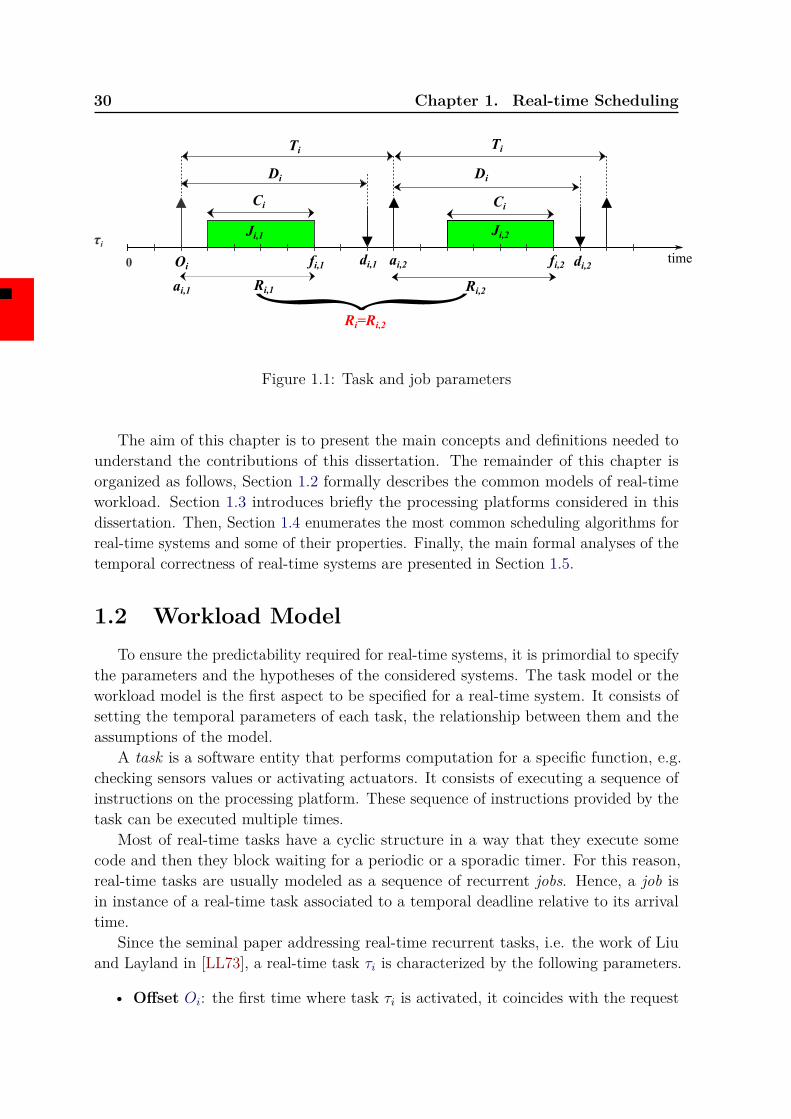
Figure 1.1: Task and job parameters
The aim of this chapter is to present the main concepts and definitions needed tounderstand the contributions of this dissertation. The remainder of this chapter isorganized as follows, Section 1.2 formally describes the common models of real-timeworkload. Section 1.3 introduces briefly the processing platforms considered in thisdissertation. Then, Section 1.4 enumerates the most common scheduling algorithms forreal-time systems and some of their properties. Finally, the main formal analyses of thetemporal correctness of real-time systems are presented in Section 1.5.
1.2 Workload ModelTo ensure the predictability required for real-time systems, it is primordial to specify
the parameters and the hypotheses of the considered systems. The task model or theworkload model is the first aspect to be specified for a real-time system. It consists ofsetting the temporal parameters of each task, the relationship between them and theassumptions of the model.
A task is a software entity that performs computation for a specific function, e.g.checking sensors values or activating actuators. It consists of executing a sequence ofinstructions on the processing platform. These sequence of instructions provided by thetask can be executed multiple times.
Most of real-time tasks have a cyclic structure in a way that they execute somecode and then they block waiting for a periodic or a sporadic timer. For this reason,real-time tasks are usually modeled as a sequence of recurrent jobs. Hence, a job isin instance of a real-time task associated to a temporal deadline relative to its arrivaltime.
Since the seminal paper addressing real-time recurrent tasks, i.e. the work of Liuand Layland in [LL73], a real-time task τi is characterized by the following parameters.
• Offset Oi: the first time where task τi is activated, it coincides with the request
1.2. Workload Model 31
time of the first job of the task. It is also called start time or first releasetime. When all the tasks composing the system are started at the same time, i.e.∀i Oi = 0, we say that the tasks are synchronous, and asynchronous otherwise,
• Execution Time Ci: the computation time required by each job of τi. Tasksmay have variable execution times between different jobs. This is due to thefact that the path and the duration of instructions executions depend on manyparameters like the type of the used memory (structure of caches) or the branchesresulting of conditional instructions and loops. This makes the problem of keepinga constant execution time very difficult. Some studies have observed that effectiveexecution times can vary up to 87% relative to their worst-case execution time[MW98]. This variation may compromise the global temporal predictability ofthe system when dealing with hard real-time systems. To cope with this problem,the notion of Worst Case Execution Time (WCET) was proposed, it consists ofconsidering only the longest possible execution time.In order to use, the WCET, the must guarantee some sustainability propertieswhich means that if it works in the worst-case it must work in a more favorablecase as well. Therefore, it is safe to study the real-time system with the WCET.The WCET is actually computed with different methods, it can be estimatedsimply by getting the longest value given by empirical measurement on the targetedplatform, e.g. benchmarks, or formally by analyzing the code of the task to findthe longest path of possible branches and loops in the worst state of memoryand input data size. The computation of the exact WCET is one of the mostimportant and active research fields within the real-time scheduling community.Many contributions are yielded every year to improve WCET predictability[HP13; Now+14; BD13]. Nevertheless, in soft real-time systems, the averageexecution time is sometimes used instead of WCET to make the formal analysisless pessimistic,
• Period Ti: this parameter models the recurrent aspect of real-time tasks, itrepresents the inter-arrival time between two successive jobs. According to theconsidered task model, this parameter can be fully specified with a constant value,partially with a lower bound, or not specified at all. The periodicity model hasan important impact on the complexity of the scheduling problem, this point willbe discussed in Section 1.5.2 on page 43,
• Relative Deadline Di: the time allocated to task τi to complete a job execution.Each job has exactly Di time units to finish executing after being activated.Exceeding this amount of time, the job violates its temporal constraint. Thedeadline is the parameter that characterizes real-time systems because it modelstheir temporal constraints. A relative deadline is not an absolute time, it is thedifference between a job’s activation time and its absolute deadline. Relativedeadline is usually associated to tasks and absolute deadline to jobs,

32 Chapter 1. Real-time Scheduling
Inactive
Ready
Blocked
Running
Activated Unblocked
Finished Blocked
Preempted Selected
Figure 1.2: Task life cycle
• Worst Case Response Time Ri: the longest job response time of task τi, i.e.Ri = max∀j(Ri,j), where Ri,j is the response time of the jth job of task τi, i.e.the amount of time needed to complete its execution including potential blockingor waiting times caused by interferences and preemptions. Formally, it is thedifference between the job’s activation time and its termination time.
Regarding jobs, Ji,j denotes the j-th job of task τi and is characterized with thefollowing parameters.
• Arrival time ai,j: the time at which job Ji,j becomes ready for execution, it isalso called request time or release time. This time depends on the periodicitymodel of the task,
• Absolute Deadline di,j: the effective time of the job’s deadline, it can beobtained by adding Di to its arrival time,
• Termination time fi,j: the time at which job Ji,j finishes its execution,
• Response time Ri,j: is the difference between job’s completion time and itsrequest time, i.e. Ri,j = fi,j − ai,j.
Figure 1.1 on page 30 illustrates these parameters.
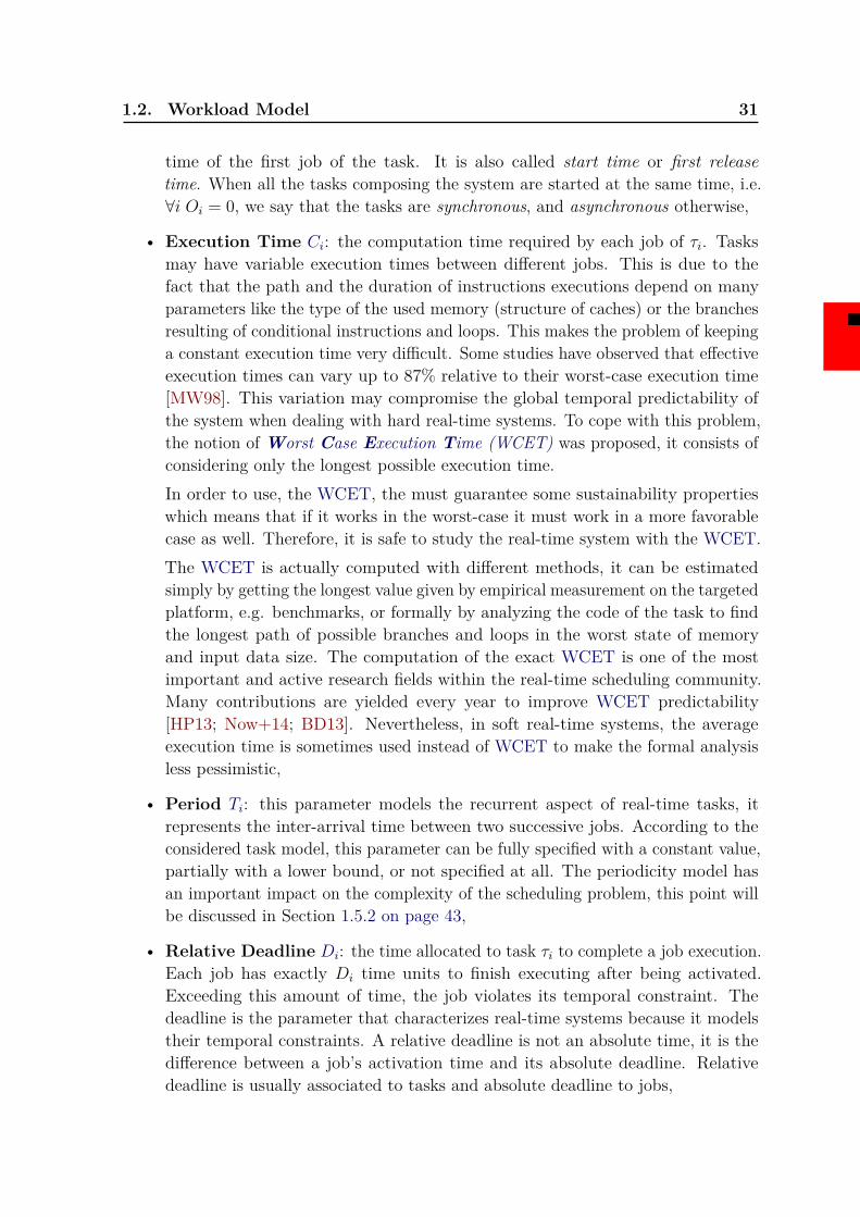
1.2.1 Task Life CycleDuring the life span of a real-time system, multiple jobs of a task can be released.
At a given moment of a task life cycle, it can be in one of the following states:
• Ready: refers to the state in which the job has been activated but not yetexecuted.
1.2. Workload Model 33
• Running: refers to the state in which the job is being executed on the processingplatform.
• Blocked: refers to the state in which the job is stopped by the system. This canhappen in some real-time systems where there is for example shared resource withmutual exclusion, the job is stopped until it gets the access to the resource.
• Inactive: in this state the job is not yet requested or has already finished itsexecution.
Figure 1.2 on the facing page shows the transitions between these states.In some simple real-time systems, it may be possible to completely specify the
parameters of each job prior to system run-time (i.e. the system designer has completeknowledge of each job Ji,j). However, in systems with a large (or infinite) number ofjobs or systems that have dynamic behaviors, explicitly specifying each job, prior tosystem run-time, may be impossible or unreasonable. Based on this characteristic, wecan classify task models as either completely specified or partially-specified. We nowdiscuss the differences between these two types of systems.
1.2.2 Completely-Specified Recurrent Task ModelA real-time system is completely specified if the exact values of the temporal
parameters and constraints of all jobs can be determined off-line or prior to system run-time. Formally, when the arrival-time and the absolute deadline of each job are knownoff-line. This implies that jobs offsets and inter-arrival times can also be determinedprior to run-time. Typically, completely-specified task models are appropriate for hardreal-time applications that have completely predictable executions. For example in anavionic control system, the control system will process the pilot’s input command atstrict time intervals to ensure that flight control does not degrade. Completely-specifiedsystems are sometimes called concrete systems.
Periodic Task Model
In many real-time control applications, periodic activities represent the majorcomputational demand in the system. Periodic tasks typically arise from sensory dataacquisition, control loops, action planning and system monitoring. Such activities needto be cyclically executed at specific rates which can be derived from the applicationrequirements. The periodic task model was proposed for the first time by Liu andLayland in 1973 [LL73]. It allows the specification of homogeneous sets of jobs thatoccur at strict intervals. A periodic task τi is specified by the temporal parametersdescribed earlier, i.e. (Oi,Ci,Ti,Di), where the inter-arrival time between two successivejobs Ti is set to a constant value. The first job of task τi is released at Oi, the secondat Oi + Ti and the j-th one at Oi + (j − 1) × Ti. Then, the time of jobs arrival and
34 Chapter 1. Real-time Scheduling
their deadlines are fully predictable. Periodic tasks are also known as time-triggeredtasks because their jobs arrival times are determined only by time.
1.2.3 Partially-Specified Recurrent SystemsFor many real-time systems, it is not possible to know beforehand how many jobs
will be generated by the system during run-time. Furthermore, completely specifiedsystems such as periodic task systems are not able to handle changes of real-timeworkloads because of the restrictive constraint that jobs must be released at strictperiodic intervals. Thus, for systems where the arrival times between jobs could changedynamically, e.g. packets in a network application, the periodic model may not besuitable. To cope with the inflexibility of completely-specified systems, one may insteadconsider partially-specified ones. The execution of the same partially-specified taskset for the same period of time may lead to different workload with different jobarrival times. Nevertheless, the specification of a partially-specified system includesa set of constraints that any execution must satisfy in order to ensure predictability.Partially-specified task systems are sometimes called non-concrete systems.
In this subsection, we will introduce more general models for partially-specified tasksystems: the sporadic and the aperiodic models. These general task models can be usedto represent more complex applications than the restrictive periodic task model.
Sporadic Task Model
The sporadic task model proposed by Liu and Layland in [LL73] removes therestrictive assumption of the periodic task model where the jobs of a task are releasedat a strict periodic time interval. In addition, the offset parameter Oi is not specifiedand the inter-arrival parameter is lower bounded. Then, a sporadic task τi can becharacterized by a tuple (Ci,Ti,Di) where Ci is its worst-case execution time, Di itsrelative deadline and Ti is the minimum inter-arrival time between two successive jobsof τi, i.e. ∀ (Ji,j, Ji,j+1), ai,j+1 − ai,j ≥ Ti (note that Ti denoted the exact inter-arrivaltime for periodic tasks). Then, at run-time, the number of jobs released during thesame interval of time can vary according to dynamic inter-arrival time of jobs.
Aperiodic Task Model
Unlike periodic and sporadic task models that set some hypothesis on jobs inter-arrival times, the aperiodic task model removes completely the notion of period orinter-arrival time. The jobs can arrive at any time as well as non-predictable events.For this reason, aperiodic task systems are also called event-triggered systems. Then, anaperiodic task is characterized only with two parameters, namely the WCET, Ci, andthe deadline Di. Even though the aperiodic task model is the most general one, it is theless predictable model. Indeed, when dealing with unspecified jobs inter-arrival times,the time analysis of tasks worst-case response time is impossible because the amount
1.3. Processing Platform 35
of workload within any time interval is neither known nor bounded which preventsthe behavior of the system to be temporally predictable. Therefore, the aperiodic taskmodel is not suitable for hard real-time systems that need a full temporal predictability.However, it could be very interesting to model some soft real-time applications thataim to increase the utilization of platforms with a certain QoS or mixed systems thatare composed of periodic, sporadic and aperiodic tasks.
1.2.4 Tasks IndependenceOne of the most common hypotheses in real-time systems is tasks independence.
This means that the only resource on which tasks are in concurrency is the computationunits, i.e. the processors. Nevertheless, in many real-time applications, the taskscomposing the system may be directly or indirectly dependent to other tasks. Indeed,tasks may be subject to input data dependency constraints, i.e. a task τ1 may requirethe results produced by an other task τ2, and thus, τ1 cannot start executing until τ2has not yet finished. Dependencies between tasks could be modeled with a graph ofjobs, e.g. Directed Acyclic Graphs (DAG) task model [Bar+12]. Furthermore, tasksdependency can also come from resource sharing (other resources than the computationunits). Indeed, when some resources that cannot be accessed simultaneously are sharedbetween tasks, the task that holds the resource blocks the execution of other tasks.Then, the execution duration of the waiting tasks depends on how long the task holdingthe resource will keep it. Therefore, concurrency and resource sharing may lead toindirect dependency between tasks.
In the case of several shared resources, deadlocks can occur if tasks are waitingfor each other. This leads to a concurrency issue which is one of the widely discussedtopics within the real-time systems community [But11]. The common solutions consistof bounding the blocking time and including it in the WCET.
The remainder of this dissertation focuses only on types of systems that are pre-dictable and can be formally verified. We study especially periodic and sporadicindependent systems for the basic model, then, other constraints and parameters willbe added in order to study real-time scheduling for energy-harvesting systems.
1.3 Processing PlatformIn contrast with real-time workload which is the software part of real-time systems,
the processing platform is the computer hardware where real-time applications areexecuted. It consists of a collection of physical elements that constitutes the computerresponsible of running the application such as the processor or the CPU, Input/Outputdevices, the different levels of memory and caches, etc. It is crucial for real-timeapplications design to consider the different components of the processing platformbecause they are part of the model and their performance and architecture influencedirectly the temporal behavior of the system.
36 Chapter 1. Real-time Scheduling
The process of determining a task worst-case execution parameters is called timinganalysis. Timing analysis must account for worst-case cache behavior, memory accesstime, program structure and worst-case execution paths.
The analysis for determining the contribution of each of these factors to the worst-case execution time depends on the specific system and the program. Other factorsthat can increase the worst-case execution time are job preemptions (i.e. a job issuspended while a different job is executing, and then, its execution is resumed ata later time). The context switch and scheduling algorithm overhead contribute toincrease jobs response times. The total preemption cost is typically dependent on theprocessor architecture and the used scheduling algorithm.
In this dissertation, we will assume that the worst-case execution time of each taskhas already been determined. We will consider only monoprocessor platforms that hasa unique speed. We will assume also that jobs are preemptable with a negligible cost.
1.4 Scheduling Algorithms
The role of a real-time scheduling algorithm within a real-time application is todetermine which active jobs are executed on the processing platform at every timeinstant. In other words, it determines the intervals of execution for jobs on the processingplatform. The sequence of execution intervals of a task set is known as a schedule. Thegoal of a real-time scheduling algorithm is to produce a schedule that ensures that everyjob is allocated processor slots (i.e. executes) to finish executing before its deadline.
In this section, we discuss the classification of real-time scheduling algorithms.
1.4.1 Online/Offline Scheduling
Scheduling real-time jobs is the responsibility of the scheduler, which can be part ofthe software layer that composes the real-time operating system or part of the hardwarelayer. The scheduler can be seen as a specific task that takes scheduling decisions byfollowing a scheduling policy or a scheduling algorithm.
If the sequence of real-time jobs is specified prior to run-time or generated by acompletely-specified task set, a scheduling algorithm can generate and store the scheduleprior to run-time. This approach is called static or offline scheduling. In contrast, forsystems that are partially-specified or have a schedule too large to be stored in thesystem’s memory, an online algorithm is appropriate for this case. At time t, the onlinereal-time scheduling algorithm decides the set of jobs to execute at time t based on thestatus of jobs released at or prior to t. An online scheduling algorithm does not havespecific information about the release of jobs after time t (i.e. future jobs arrival timesare unknown). This dissertation focuses on deterministic online real-time schedulingalgorithms.
1.4. Scheduling Algorithms 37
1.4.2 Work-Conserving/Non-work-conserving Scheduling
A real-time scheduling algorithm can produce a non-work-conserving schedule, i.e.a schedule where the processor is inactive while at least one job is ready for execution.This may seem as a counter-productive property, however, it can be very useful foradaptive scheduling algorithms that may delay jobs execution to avoid future failures asfor energy-harvesting systems. In contrast, a work-conserving schedule does not allowthe processor to be inactive while ready jobs are waiting for execution.
1.4.3 Preemptive/Non-Preemptive Scheduling
When several tasks are ready to be executed at the same time on a monoprocessorplatform, two approaches can be applied: the preemptive or the non-preemptive approach.In the non-preemptive approach, when a task starts executing, it cannot be interrupteduntil it finishes its execution. With this approach, there is at most one context switch, i.e.the scheduler replaces the execution context of the finishing job with starting one. Thesecontext switches have a cost that has to be considered in the schedulability analysis,although the hypothesis of an negligible cost is often considered. In a preemptivescheduling, the scheduler can preempt a job to execute an other one. The advantagesof this approach are reducing the response time of higher priority jobs, a best use ofthe processor and better rate of schedulability. With this approach, jobs are executedconcurrently on the processor. In this dissertation, we focus only on preemptivescheduling algorithms.
1.4.4 Optimal Scheduling
The term of optimality in real-time theory is used for different properties. Here weare interested in the optimality of scheduling algorithms form schedulability point ofview. For this sake, we use the definition proposed by Buttazzo in [But11]:
“A real-time scheduling algorithm is said to be optimal for a specific class ofalgorithms if it minimizes some given cost function defined over the task set. When nocost function is defined and the only concern is to achieve a valid schedule, then analgorithm is said to be optimal if it always finds a valid schedule whenever there existsa valid one. In other words, an algorithm is said to be optimal if it may fail to producea valid schedule for a given task sets only if no other algorithms of the same class cando it.”
In contrast, a non optimal algorithm may fail to schedule a given task set while avalid schedule exists.
Furthermore, the schedulability of a task set according to an optimal algorithm is anecessary and sufficient feasibility condition for the considered class of algorithms. SeeSection 1.5 on page 40 for more details.
38 Chapter 1. Real-time Scheduling
1.4.5 Priority Driven Scheduling AlgorithmsA possible approach for an online scheduling algorithm is to assign, at any given
time t, each job Ji,j a priority Pi,j (which is assumed to be a positive integer). Apriority-driven scheduling algorithm sorts at each time t the active jobs according toPi,j (in non-decreasing order) and schedules the highest-priority job on the processor.
In this subsection, we describe the classical priority-driven scheduling algorithms.These later differ in the manner that they assign a priority to jobs. In the following, wegive three classifications of priority-driven scheduling algorithms. We follow the classifi-cation names used in [FBB06]. The three major classes of priority-driven schedulingalgorithms are Fixed-Task-Priority (FTP), Fixed-Job-Priority (FJP), and DinamicPriority (DP).
1.4.6 Fixed Task-Priority Scheduling Algorithms (FTP)In fixed task-priority scheduling, each task is assigned a static or fixed priority Pi
prior to run-time and keeps the same value during run-time. Each job generated bythat task inherits the same priority value. Thus, for a real-time system with n tasks,there are n distinct priorities (one for each task). We assume that the tasks are indexedin a non-decreasing order of priority. Therefore, for a task set Γ={τ1, . . . , τn}, τ1 hasthe highest priority and τn has the lowest one. In general, the task-priority assignmentcan be determined by the system designer. However, there are three well-studiedtask-priority assignment policies for sporadic task systems: Rate Monotonic (RM),Deadline Monotonic (DM) and Audsley’s Optimal Priority Assignment (OPA).
Task Priority Assignment Policies
The tasks priority assignment has a significant effect on the schedulability of tasksets in fixed-task-priority scheduling [Dav+13]. Hence, it is important to select theright priority assignment policy. In the following we describe briefly the main priorityassignment policies.
Rate Monotonic: For rate monotonic priority assignment policy [LL73], each taskτi is assigned a priority according to its period. The shorter the period is, the higherthe priority of the task is. Rate Monotonic is optimal for non-concrete task sets withimplicit deadlines, i.e. Oi = 0 and Di = Ti. The intuition behind this optimality isthat tasks can use all the available time because of the implicit deadlines and that highfrequency tasks cannot support a lot of interferences in contrast of low frequency tasks.Then, in this case, assigning high priorities to high frequency tasks is the best that wecan do. This is proved in [LL73].
Deadline Monotonic: The deadline monotonic policy [LL73] assigns to each task τia priority according to its relative deadline parameter: the shorter the deadline is, the
1.4. Scheduling Algorithms 39
Algorithm 1.1 Optimal Priority Assignment1: for all priority level k, lowest first do2: for all unschedulable task τi do3: if τi is schedulable at priority k with all other unassigned tasks assumed to
higher priorities then4: assign τi to priority k5: break (continue outer loop)6: end if7: end for8: return unschedulable9: end for
10: return schedulable
higher the priority of the task is. Deadline Monotonic is optimal for non-concrete tasksets with constrained deadlines [LL73], i.e. Oi = 0 and Di ≤ Ti. Intuitively this can beexplained by the fact that with constrained deadlines tasks with short deadlines cansupport less interferences than ones with larger deadlines. Then, in this case, assigninghigh priorities to tasks with short deadlines is the best that we can do. The detailedproof is available in [LL73].
Optimal Priority Assignment: Note that the optimality of rate monotonic anddeadline monotonic relies on two strong assumptions, namely tasks offsets and deadlinesmodel. If we remove these assumptions RM and DM are no longer optimal for fixed-priority scheduling. To cope with this problem, Audsley proposed in [Aud91; Aud01] anoptimal priority assignment OPA algorithm that provides an optimal priority assignmentfor sporadic task sets with arbitrary-deadlines and concrete offsets. It consists of testinggreedily different priority assignments using a necessary schedulability test as shown inAlgorithm 1.1. This approach requires at most n(n+ 1) tests to determine a schedulablepriority assignment whenever such an ordering exists. This tests much less priorityassignment than n! that would be otherwise required, using a brute force approach thatchecks every possible combination.
For a schedulability test to be OPA-Compatible [DB09], it must respect the followingrules:
1. the schedulability of a task may, according to the test, be dependent on the set ofhigher priority tasks, but not on their relative priority ordering,
2. the schedulability of a task may, according to the test, be dependent on the set oflower priority tasks, but not on their relative priority ordering,
3. when the priorities of any two tasks of adjacent priority are swapped, the taskbeing assigned the higher priority cannot become unschedulable according to thetest, if it was previously schedulable at the lower priority.
40 Chapter 1. Real-time Scheduling
1.4.7 Fixed Job-Priority Scheduling Algorithms (FJP)For fixed job-priority scheduling, the restriction that a task’s jobs have identical
priority is removed. Instead, each job Ji,j is assigned a single priority Pi,j that doesnot change during its execution. The specific FJP scheduling algorithm determinesthe priority assignment for jobs. Earliest-Deadline First EDF is a well known FJPscheduling algorithm proposed by Liu and Layland in [LL73]. It assigns a priorityto each job according to its absolute deadline. The earlier the deadline of the job is,the higher its priority is. In other words, EDF schedules among the set of jobs withremaining execution the job with the nearest deadline.
1.4.8 Dynamic Priority Scheduling Algorithms (DP)The dynamic priority Scheduling algorithms classification is the most general. It
removes the restriction that a job priority does not change. A job Ji,j priority Pi,j cannow vary over time. A well-known example of DP scheduling algorithm is Least LaxityFirst (LLF ). At time t, the LLF scheduling algorithm assigns a priority to each activejob according to to its laxity. The shorter the alxity of the job is, the higher the priorityof the job is. The laxity of a job Ji,j at time t is (di,j − t) − ci,j(t), where ci,j(t) isremaining processor cost of job Ji,j at time t.
In this dissertation, we focus only on FTP scheduling for energy-harvesting systems.
1.5 Scheduling AnalysisTo ensure the temporal correctness of a real-time system, it must be validated
prior to run-time using formal verification techniques. These techniques must ensurethat for all executions of the system, all jobs generated by the system will meet theirdeadlines. Two fundamental analyses in formal verification for real-time systems areconsidered: feasibility analysis and schedulability analysis. The feasibility analysisdetermines whether there exists a valid schedule of the system where all jobs meet theirdeadlines irrespective to the used scheduling algorithm. The schedulability analysisdetermines whether a given scheduling algorithm will always meet all jobs deadlines.
The remainder of this section first sets some definitions then it introduces the mainfeasibility and schedulability analysis techniques applied to the previously mentionedscheduling algorithms.
1.5. Scheduling Analysis 41
1.5.1 DefinitionsIn this subsection we define some properties and quantities to simplify the under-
standing of the schedulability analysis that follows.
Definition 1.2 (Valid Schedule).The schedule S produced by scheduling algorithm A is considered as valid if and only ifall the deadlines are infinitely met. �
Definition 1.3 (Worst-Case Scenario).The worst-case scenario of task τi is the configuration of the system that leads to thelongest response time of τi. This configuration includes tasks parameters such as firstrelease times and periods. �
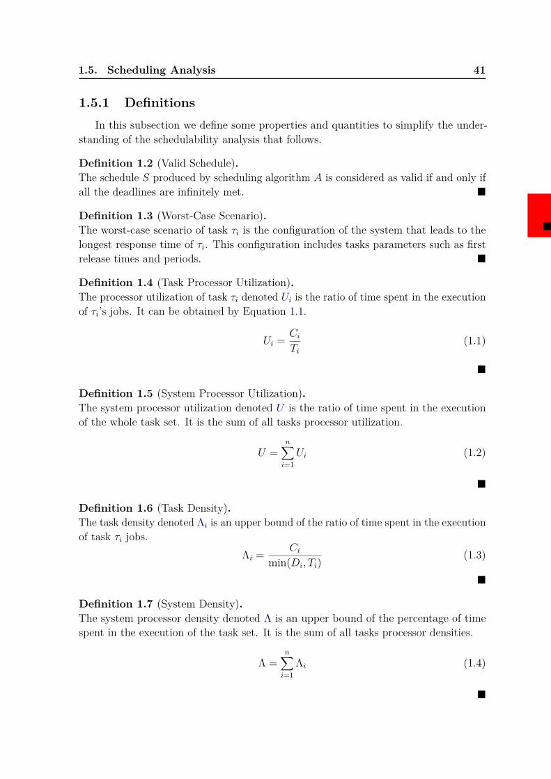
Definition 1.4 (Task Processor Utilization).The processor utilization of task τi denoted Ui is the ratio of time spent in the executionof τi’s jobs. It can be obtained by Equation 1.1.
Ui = CiTi
(1.1)
�
Definition 1.5 (System Processor Utilization).The system processor utilization denoted U is the ratio of time spent in the executionof the whole task set. It is the sum of all tasks processor utilization.
U =n∑i=1
Ui (1.2)
�
Definition 1.6 (Task Density).The task density denoted Λi is an upper bound of the ratio of time spent in the executionof task τi jobs.
Λi = Cimin(Di, Ti)
(1.3)
�
Definition 1.7 (System Density).The system processor density denoted Λ is an upper bound of the percentage of timespent in the execution of the task set. It is the sum of all tasks processor densities.
Λ =n∑i=1
Λi (1.4)
�
42 Chapter 1. Real-time Scheduling
Definition 1.8 (Task Workload Function).The workload of task τi within time interval [t1, t2] denoted Wi(t1, t2) is the amount ofprocessor time needed to execute the jobs of τi that are requested within time interval[t1, t2] or are pending at time t1. �
Definition 1.9 (System Workload Function).The workload of a set of tasks Γ within time interval [t1, t2] denoted W (t1, t2) is thesum of workload of all tasks composing Γ within [t1, t2].
W (t1, t2) =∑τi∈Γ
Wi(t1, t2) (1.5)
�
Tasks workload functions depend on the used scheduling algorithms. In the literaturethere are two main task workload functions usually used in schedulability and feasibilityanalysis: the request bound function and the demand bound function.
Definition 1.10 (Request Bound Function (RBF)).The request bound function of recurrent task τi denoted RBFi(t) computes the worstcumulative workload generated by τi’s jobs that are requested during time interval [0, t[.Lehoczky et al. [JLY89] proposed Equation 1.6 to compute RBFi(t).
RBFi(t) = max(⌈t−Oi
Ti
⌉, 0)× Ci (1.6)
�
Definition 1.11 (Demand Bound Function (DBF)).The demand bound function of recurrent task τi denotedDBFi(t) is the worst cumulativeworkload generated by τi’s jobs that are requested and finished during time interval[0, t]. Baruah et al. [BHR90a] proposed Equation 1.7 to compute DBFi(t).
DBFi(t) = max(⌊t−Oi −Di
Ti
⌋+ 1, 0
)× Ci (1.7)
�
Definition 1.12 (Busy-Period).A busy-period is an interval of time [t1, t2] where the processor is continuously executingjobs while there are waiting jobs. It starts from time t1 when the processor is idle forthe last time and ends at time t2 when all waiting jobs are finished. It is possible tohave consecutive busy-periods since it depends on the waiting jobs and not only theprocessor. �
Definition 1.13 (Hyper-Period (HP)).The hyper-period of a task set Γ is the smallest interval of time after which the globalperiodic pattern of all the tasks are repeated. It is typically defined as the LeastCommon Multiple (LCM) of the periods of all the tasks of the system. �
1.5. Scheduling Analysis 43
The aim of scheduling analysis is to provide conditions and tests that help designersto determine prior run-time whether a task set is feasible/schedulable or not. We candistinguish three kinds of conditions: necessary conditions, sufficient conditions andnecessary and sufficient.
Definition 1.14 (Necessary Condition).A necessary condition means that a task set that fails the test is definitely not feasibleor not schedulable. Though satisfying the condition does not mean that it is certainlyfeasible, more verification is needed to conclude. �
Definition 1.15 (Sufficient Condition).A sufficient condition means that a task set that succeeds the test is definitely feasibleor schedulable. In contrast, failing the test does not mean that task set is certainly notfeasible or not schedulable, more verification is needed to conclude. �
Definition 1.16 (Necessary and Sufficient Condition).A sufficient and necessary condition is an exact test that tells with certainty whetherthe task sets is schedulable/feasible or not. �
1.5.2 Feasibility or Schedulability
These two notions have been defined differently in the literature. Some times theterm schedulable is used to describe the property feasible and vice versa. Here, we usethe definitions proposed by Davis and Burns in [DB11].
A feasibility test is a condition that tells whether at least one valid schedule existsfor the given task set or not. This schedule may require a non-clairvoyant scheduleror a clairvoyant scheduler which does not necessarily exist. Feasibility conditions areindependent form scheduling algorithms.
In contrast, a schedulability condition is a test that tells whether a valid schedulecan be produced by the given algorithm for the given task set or not. In this case, thealgorithm must exist.
Note that a feasibility test is more general than a schedulability one. A task setthat is schedulable according to a specific algorithm, is necessarily feasible. However,the opposite way is not true: a task set can be feasible but not schedulable with agiven algorithm. Indeed, a schedulability test becomes a feasibility one when the usedalgorithm is optimal because if a solution exists, the optimal algorithm will find it.
Many feasibility and schedulability conditions was proposed in the literature. Mostof them are applicable only for specific kinds of task sets with specific assumptions. Forexample, the relationship between periods and deadlines or tasks first release times.Therefore, it is very important for designers to check the assumptions before using atest. In the following we list some existing tests for fixed-priority and dynamic-priorityscheduling.
44 Chapter 1. Real-time Scheduling
1.5.3 Schedulability Analysis for Fixed-Task-PriorityThis subsection presents the classical feasibility and schedulability conditions for
fixed-task-priority scheduling.
Maximum utilization feasibility test
One of the possible ways to check the feasibility or the non feasibility of a task set isto compare its processor utilization to the maximum one that one processor can supportor to lower bound the utilization of feasible task sets. It is impossible to schedule atask set with a utilization higher than 1 on one processor whatever are deadlines andoffsets models because the time needed to execute the workload of any time intervalW (t1, t2) is greater than the available time, i.e. t2− t1. Therefore a necessary feasibilitycondition for monoprocessor platforms can be obtained with Equation 1.8.
U ≤ 1 (1.8)
Liu and Layland bound
For task sets composed of n periodic tasks with implicit deadlines and Rate Mono-tonic priority assignment, Liu and Layland proposed in [LL73] a sufficient schedulabilitycondition by lower bounding the utilization of feasible task sets. This can be obtainedby Equation 1.9.
U =n∑i=1
CiTi≤ n
(21/n − 1
)(1.9)
This test can be extended to task sets with constrained deadlines and deadline monotonic(DM) priority assignment by comparing the bound to the density instead of the utilizationas shown in Equation 1.10.
Λ =n∑i=1
CiDi
≤ n(21/n − 1
)(1.10)
However, such a test is very pessimistic because it assumes that periods are shorterthan the actual ones. The maximum achievable utilization or density with Liu andLayland bound can be obtained by computing its limit when n tends to infinity as showin Equation 1.11.
limn→∞
n(21/n − 1
)= ln 2 ' 0.69 (1.11)
Hyperbolic bound
For task sets composed of n periodic tasks with implicit deadlines and Rate Mono-tonic priority assignment, Bini et al. proposed in [BBB03] a sufficient feasibilitycondition by refining Liu and Layland bound. This can be obtained by Equation 1.12.
n∏i=1
(Ui + 1) ≤ 2 (1.12)
1.5. Scheduling Analysis 45
We can also use this bound for task sets with constrained deadlines by using tasksdensities Λi rather than utilizations, however, it is very pessimistic.
Worst-Case Response Time Analysis
Recall that except the maximum utilization feasibility test, all the above conditionsare only sufficient. Then, a task set that fails these tests or does not fill the assumptionsis not definitely unfeasible. To cope with this problem, the Worst Case Response Time(WCRT) analysis was proposed in the literature. Pandya et al. showed in [MPK86]that a necessary and sufficient schedulability test can be obtained by checking if theWCRT of each task is lower than its relative deadline, as expressed by Equation 1.13.
∀ τi ∈ Γ, WCRTi ≤ Di (1.13)
For non-concrete task sets with constrained or implicit deadlines and deadline monotonicpriority assignment, Audsley et al. proposed in [Aud+93] an algorithm to compute theworst-case response time of tasks that can be used to build a necessary and sufficienttest. Equation 1.13 describes how to compute the WCRT of priority level-i. Thetermination time of the first job of task τi which coincides with the WCRT in thesynchronous scenario can be computed with a fixed point iteration on Equation 1.14using the iterative workload function Wm
i .W 0i = Ci
Wm+1i = Ci +
∑j<i
RBFj(Wmi )
WCRTi = minm>0 ∧Wm+1
i =Wmi
(Wmi )
(1.14)
Note that this algorithm assumes that all the tasks are requested simultaneouslywhich is the worst-case scenario for Liu and Layland model. This scenario is also calledthe critical instant. Furthermore, this algorithm checks only the deadline of the first job.This is sufficient because first, the test considers only constrained or implicit deadlineswhich avoids the interference between the jobs of the same task, and second, the longestresponse time happens necessarily in the worst-case scenario. If the first job meets itsdeadline, the next ones will do also. If we remove the assumptions on deadlines modeland tasks offsets, checking the deadline of first jobs in a synchronous activation is nolonger sufficient and the test becomes only necessary.
46 Chapter 1. Real-time Scheduling
1.5.4 Schedulability Analysis for Dynamic-PriorityThis subsection presents the classical feasibility and schedulability conditions for
fixed-job-priority and dynamic-priority scheduling.
Maximum utilization feasibility test
A task set cannot be scheduled on only one processor when its utilization ratio isgreater than 1. Therefore a necessary feasibility test can be obtained by Equation 1.15.
U ≤ 1 (1.15)
EDF utilization schedulability test
For task sets with implicit deadlines, the previous test become necessary and sufficientfor EDF scheduling [LL73].
EDF density schedulability test
For task sets with constrained deadlines, Liu [Liu00] proposed a sufficient schedu-lability test based on the density of the system instead of its utilization as shown byEquation 1.16.
Λ ≤ 1 (1.16)
EDF schedulability Arbitrary Deadlines
For task sets with arbitrary deadlines, Baruah et al. [BHR90b] proposed a sufficientand necessary schedulability test given by Equation 1.17.
∀ t > 0,∑τi∈Γ
DBFi(t) ≤ t (1.17)
1.6 ConclusionIn this chapter we introduced the classical theory of real-time systems and the basic
state of the art needed to understand the next chapters. We first presented the main taskmodels and their categorizations. Second, we described briefly the processing platformstargeted by this dissertation, namely monoprocessor platforms, and we set hardwareassumptions that will be considered along this dissertation. Finally, we presentedthe main real-time scheduling algorithms, their categorizations and the correspondingfeasibility and schedulability conditions.
In the remainder of the dissertation, we focus only on preemptive fixed-task-priorityscheduling on monoprocessor platforms with additional constraints.
Chapter 2
Energy-Harvesting Systems
Contents2.1 Introduction . . . . . . . . . . . . . . . . . . . . . . . . . . . . . 472.2 What is an Energy-Harvesting System ? . . . . . . . . . . . . 482.3 Energy-Harvesting Technologies . . . . . . . . . . . . . . . . . 49
2.3.1 Radiations Energy Harvesting . . . . . . . . . . . . . . . . . . . 492.3.2 Vibrations Energy Harvesting . . . . . . . . . . . . . . . . . . . . 512.3.3 Thermoelectric Energy Harvesting . . . . . . . . . . . . . . . . . 542.3.4 Energy Sources Comparison . . . . . . . . . . . . . . . . . . . . . 55
2.4 Energy Storage Technologies . . . . . . . . . . . . . . . . . . . . 552.4.1 Rechargeable Batteries . . . . . . . . . . . . . . . . . . . . . . . . 572.4.2 Supercapacitors . . . . . . . . . . . . . . . . . . . . . . . . . . . . 60
2.5 Energy-Harvesting Applications . . . . . . . . . . . . . . . . . . 612.6 Conclusion . . . . . . . . . . . . . . . . . . . . . . . . . . . . . . 62
2.1 IntroductionDue to the growing demand for smaller devices with longer battery life, energy
management in embedded systems has become one of the most active research areas.Indeed, a naive use of the available energy can lead to failures or a short lifespan.However, most of the targeted embedded applications are required to operate for longtime after deployment, for example, wireless sensor nodes. The extended lifespan ofthese electronic devices is of particular importance when they have limited accessibility.Thus, collecting energy from the ambient environment can be a very interesting solution,which is known as Energy-Harvesting (EH). In this process, energy is drawn from theenvironment and then converted and stored in order to supply the embedded electronicdevices. Compared to classical energy storage devices, the environment proves to be aninfinite source of available energy. Furthermore, the use of this kind of energy reducesthe need to replace batteries periodically which constitutes a major part of maintenance.
Many environmental sources can be exploited, including thermal, solar, mechanical,fluid, etc. Energy sources should be chosen according to the characteristics of the
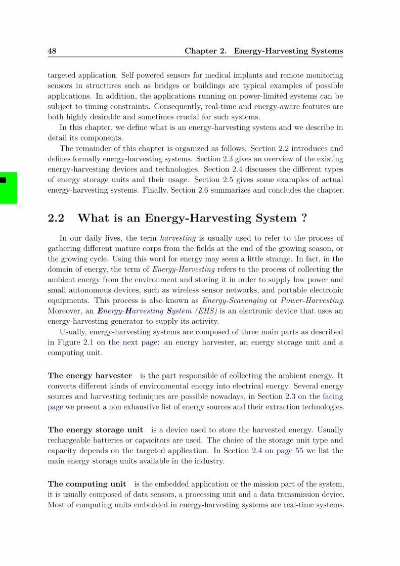
48 Chapter 2. Energy-Harvesting Systems
targeted application. Self powered sensors for medical implants and remote monitoringsensors in structures such as bridges or buildings are typical examples of possibleapplications. In addition, the applications running on power-limited systems can besubject to timing constraints. Consequently, real-time and energy-aware features areboth highly desirable and sometimes crucial for such systems.
In this chapter, we define what is an energy-harvesting system and we describe indetail its components.
The remainder of this chapter is organized as follows: Section 2.2 introduces anddefines formally energy-harvesting systems. Section 2.3 gives an overview of the existingenergy-harvesting devices and technologies. Section 2.4 discusses the different typesof energy storage units and their usage. Section 2.5 gives some examples of actualenergy-harvesting systems. Finally, Section 2.6 summarizes and concludes the chapter.
2.2 What is an Energy-Harvesting System ?In our daily lives, the term harvesting is usually used to refer to the process of
gathering different mature corps from the fields at the end of the growing season, orthe growing cycle. Using this word for energy may seem a little strange. In fact, in thedomain of energy, the term of Energy-Harvesting refers to the process of collecting theambient energy from the environment and storing it in order to supply low power andsmall autonomous devices, such as wireless sensor networks, and portable electronicequipments. This process is also known as Energy-Scavenging or Power-Harvesting.Moreover, an Energy-Harvesting System (EHS) is an electronic device that uses anenergy-harvesting generator to supply its activity.
Usually, energy-harvesting systems are composed of three main parts as describedin Figure 2.1 on the next page: an energy harvester, an energy storage unit and acomputing unit.
The energy harvester is the part responsible of collecting the ambient energy. Itconverts different kinds of environmental energy into electrical energy. Several energysources and harvesting techniques are possible nowadays, in Section 2.3 on the facingpage we present a non exhaustive list of energy sources and their extraction technologies.
The energy storage unit is a device used to store the harvested energy. Usuallyrechargeable batteries or capacitors are used. The choice of the storage unit type andcapacity depends on the targeted application. In Section 2.4 on page 55 we list themain energy storage units available in the industry.
The computing unit is the embedded application or the mission part of the system,it is usually composed of data sensors, a processing unit and a data transmission device.Most of computing units embedded in energy-harvesting systems are real-time systems.
2.3. Energy-Harvesting Technologies 49
Energy Harvester
Sun
Wind
Vibrations
. . .
. . .
Solar Panel
Wind Turbine
Piezoelectric Harvester
Storage Unit
Reusable Alkaline Battery
Li-ion polymer Battery
Supercapacitor. . .
Real-Time systemEnvironmental Energy Source
Sensing tasks
Data Processing Tasks
Transmission tasks
. . . Harvesting Replenishing Consuming
Figure 2.1: Energy-harvesting system components
In this dissertation, we focus on this part of energy-harvesting systems and we studythe real-time scheduling for such systems.
2.3 Energy-Harvesting TechnologiesMultiple sources are available for energy harvesting, including solar power, ocean
waves, wind, vibrations, thermoelectricity, and human motions power. For example,vibration energy can be used to supply wireless monitoring sensors that are pluggedinside the industrial machines. Prior research showed that these energy sources are notsuitable for all applications, and that the energy sources must be chosen according tothe application characteristics. In the following, we describe the main energy sourcesand their harvesting technologies.
2.3.1 Radiations Energy HarvestingSolar Energy Conversion
Light is an ambient energy source that is available almost everywhere and can beused to supply electronic devices. Light energy harvesters convert light energy intoelectricity via photovoltaic cells. In a semi-conductor that is exposed to light, a photonwith enough energy can extract an electron and create a gap. Usually, this electronfinds quickly an other gap to fill, and the energy brought by the photon is dissipated.The principal of a photovoltaic cell is to put the free electrons in one side of the materialand the gaps in the other one instead of filling the gaps of only one side. Therefore, avoltage difference and an electric tension appears like in a battery.
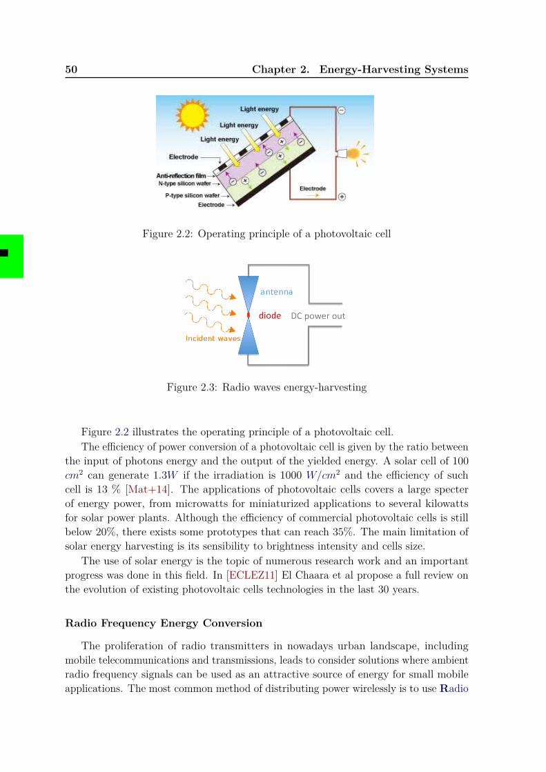
50 Chapter 2. Energy-Harvesting Systems
Figure 2.2: Operating principle of a photovoltaic cell
Figure 2.3: Radio waves energy-harvesting
Figure 2.2 illustrates the operating principle of a photovoltaic cell.The efficiency of power conversion of a photovoltaic cell is given by the ratio between
the input of photons energy and the output of the yielded energy. A solar cell of 100cm2 can generate 1.3W if the irradiation is 1000 W/cm2 and the efficiency of suchcell is 13 % [Mat+14]. The applications of photovoltaic cells covers a large specterof energy power, from microwatts for miniaturized applications to several kilowattsfor solar power plants. Although the efficiency of commercial photovoltaic cells is stillbelow 20%, there exists some prototypes that can reach 35%. The main limitation ofsolar energy harvesting is its sensibility to brightness intensity and cells size.
The use of solar energy is the topic of numerous research work and an importantprogress was done in this field. In [ECLEZ11] El Chaara et al propose a full review onthe evolution of existing photovoltaic cells technologies in the last 30 years.
Radio Frequency Energy Conversion
The proliferation of radio transmitters in nowadays urban landscape, includingmobile telecommunications and transmissions, leads to consider solutions where ambientradio frequency signals can be used as an attractive source of energy for small mobileapplications. The most common method of distributing power wirelessly is to use Radio
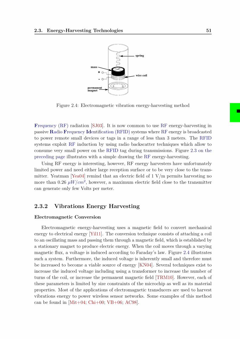
2.3. Energy-Harvesting Technologies 51
spring
wire coil
mass
permanentmagnet
+
-
Figure 2.4: Electromagnetic vibration energy-harvesting method
Frequency (RF) radiation [SJ03]. It is now common to use RF energy-harvesting inpassiveRadio Frequency Identification (RFID) systems where RF energy is broadcastedto power remote small devices or tags in a range of less than 3 meters. The RFIDsystems exploit RF induction by using radio backscatter techniques which allow toconsume very small power on the RFID tag during transmissions. Figure 2.3 on thepreceding page illustrates with a simple drawing the RF energy-harvesting.
Using RF energy is interesting, however, RF energy harvesters have unfortunatelylimited power and need either large reception surface or to be very close to the trans-mitter. Yeatman [Yea04] remind that an electric field of 1 V/m permits harvesting nomore than 0.26 µW/cm2, however, a maximum electric field close to the transmittercan generate only few Volts per meter.
2.3.2 Vibrations Energy Harvesting
Electromagnetic Conversion
Electromagnetic energy-harvesting uses a magnetic field to convert mechanicalenergy to electrical energy [Yil11]. The conversion technique consists of attaching a coilto an oscillating mass and passing them through a magnetic field, which is established bya stationary magnet to produce electric energy. When the coil moves through a varyingmagnetic flux, a voltage is induced according to Faraday’s law. Figure 2.4 illustratessuch a system. Furthermore, the induced voltage is inherently small and therefore mustbe increased to become a viable source of energy [KN04]. Several techniques exist toincrease the induced voltage including using a transformer to increase the number ofturns of the coil, or increase the permanent magnetic field [TRM10]. However, each ofthese parameters is limited by size constraints of the microchip as well as its materialproperties. Most of the applications of electromagnetic transducers are used to harvestvibrations energy to power wireless sensor networks. Some examples of this methodcan be found in [Mit+04; Chi+00; VB+06; AC98].
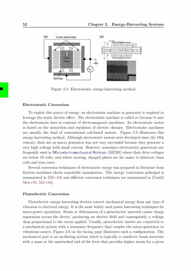
52 Chapter 2. Energy-Harvesting Systems
Figure 2.5: Electrostatic energy-harvesting method
Electrostatic Conversion
To exploit this source of energy, an electrostatic machine or generator is required toleverage the static electric effect. The electrostatic machine is called so because it usesthe electrostatic laws in contrast of electromagnetic machines. An electrostatic motoris based on the attraction and repulsion of electric charges. Electrostatic machinesare usually the dual of conventional coil-based motors. Figure 2.5 illustrates thisenergy-harvesting method. Although electrostatic motors were developed since the 18thcentury, their use as macro generator was not very successful because they generate avery high voltage with small current. However, nowadays electrostatic generators arefrequently used in Microelectromechanical Systems (MEMS) where their drive voltagesare below 10 volts, and where moving, charged plates are far easier to fabricate thancoils and iron cores.
Several conversion techniques of electrostatic energy was proposed in literature fromfriction machines throw nanotuble nanomotors. The energy conversion principal issummarized in [Mit+04] and different conversion techniques are summarized in [Can63;Men+01; Mit+04].
Piezoelectric Conversion
Piezoelectric energy-harvesting devices convert mechanical energy from any type ofvibration to electrical energy. It is the most widely used power harvesting techniques formicro-power operations. Strain or deformation of a piezoelectric material causes chargeseparation across the device, producing an electric field and consequently a voltagedrop proportional to the stress applied. Usually, piezoelectric inserts are connected toa mechanical system with a resonance frequency that couples the micro-generator tovibrations source, Figure 2.6 on the facing page illustrates such a configuration. Themechanical part is an oscillating system which is typically a cantilever beam structurewith a mass at the unattached end of the lever that provides higher strain for a given
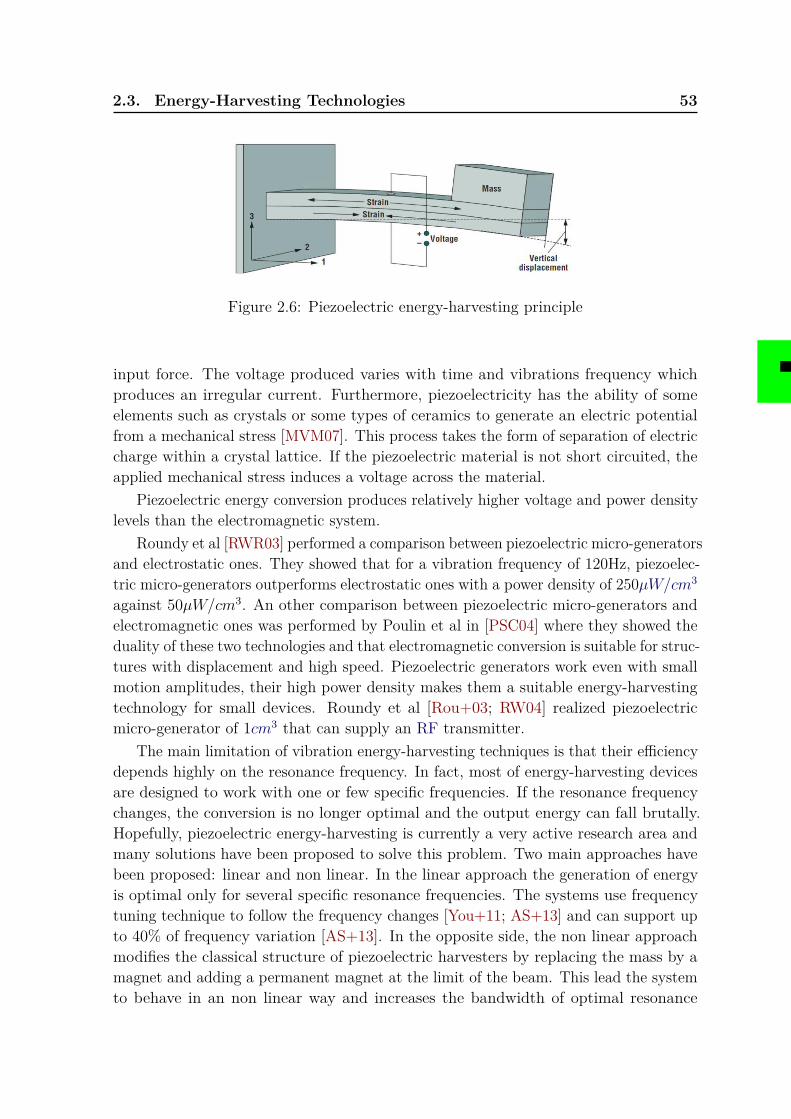
2.3. Energy-Harvesting Technologies 53
Figure 2.6: Piezoelectric energy-harvesting principle
input force. The voltage produced varies with time and vibrations frequency whichproduces an irregular current. Furthermore, piezoelectricity has the ability of someelements such as crystals or some types of ceramics to generate an electric potentialfrom a mechanical stress [MVM07]. This process takes the form of separation of electriccharge within a crystal lattice. If the piezoelectric material is not short circuited, theapplied mechanical stress induces a voltage across the material.
Piezoelectric energy conversion produces relatively higher voltage and power densitylevels than the electromagnetic system.
Roundy et al [RWR03] performed a comparison between piezoelectric micro-generatorsand electrostatic ones. They showed that for a vibration frequency of 120Hz, piezoelec-tric micro-generators outperforms electrostatic ones with a power density of 250µW/cm3
against 50µW/cm3. An other comparison between piezoelectric micro-generators andelectromagnetic ones was performed by Poulin et al in [PSC04] where they showed theduality of these two technologies and that electromagnetic conversion is suitable for struc-tures with displacement and high speed. Piezoelectric generators work even with smallmotion amplitudes, their high power density makes them a suitable energy-harvestingtechnology for small devices. Roundy et al [Rou+03; RW04] realized piezoelectricmicro-generator of 1cm3 that can supply an RF transmitter.
The main limitation of vibration energy-harvesting techniques is that their efficiencydepends highly on the resonance frequency. In fact, most of energy-harvesting devicesare designed to work with one or few specific frequencies. If the resonance frequencychanges, the conversion is no longer optimal and the output energy can fall brutally.Hopefully, piezoelectric energy-harvesting is currently a very active research area andmany solutions have been proposed to solve this problem. Two main approaches havebeen proposed: linear and non linear. In the linear approach the generation of energyis optimal only for several specific resonance frequencies. The systems use frequencytuning technique to follow the frequency changes [You+11; AS+13] and can support upto 40% of frequency variation [AS+13]. In the opposite side, the non linear approachmodifies the classical structure of piezoelectric harvesters by replacing the mass by amagnet and adding a permanent magnet at the limit of the beam. This lead the systemto behave in an non linear way and increases the bandwidth of optimal resonance
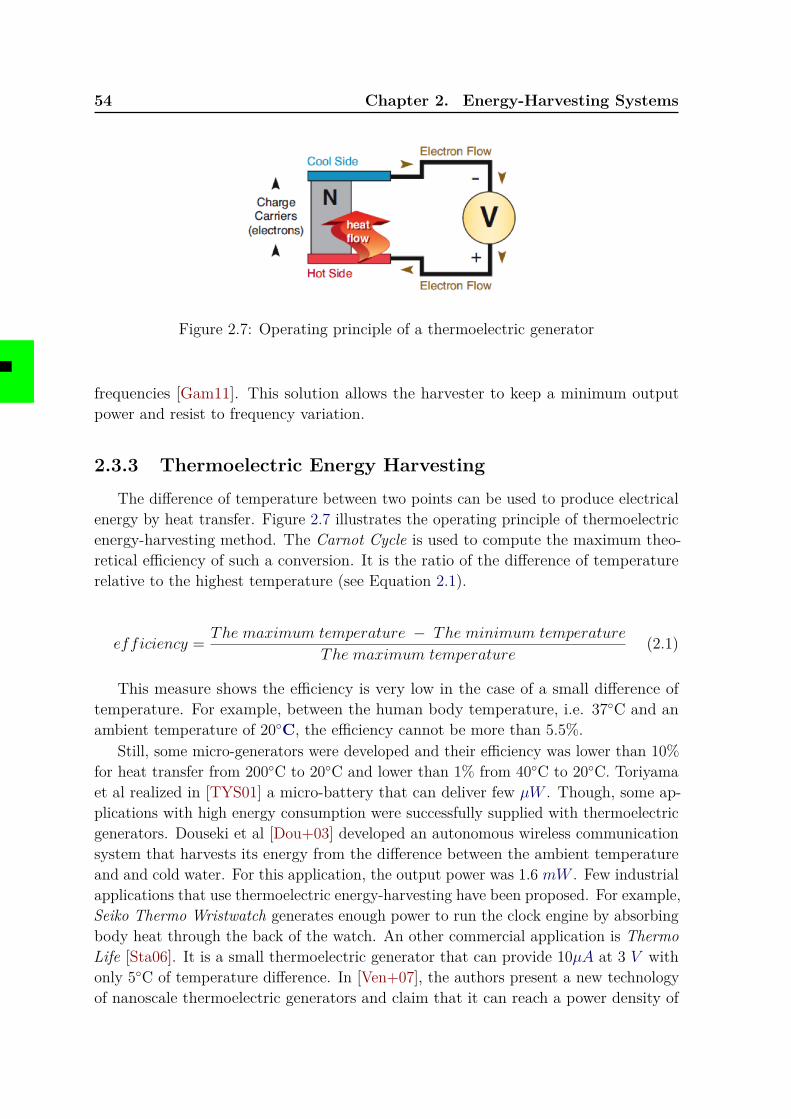
54 Chapter 2. Energy-Harvesting Systems
Figure 2.7: Operating principle of a thermoelectric generator
frequencies [Gam11]. This solution allows the harvester to keep a minimum outputpower and resist to frequency variation.
2.3.3 Thermoelectric Energy HarvestingThe difference of temperature between two points can be used to produce electrical
energy by heat transfer. Figure 2.7 illustrates the operating principle of thermoelectricenergy-harvesting method. The Carnot Cycle is used to compute the maximum theo-retical efficiency of such a conversion. It is the ratio of the difference of temperaturerelative to the highest temperature (see Equation 2.1).
efficiency = The maximum temperature − The minimum temperature
The maximum temperature(2.1)
This measure shows the efficiency is very low in the case of a small difference oftemperature. For example, between the human body temperature, i.e. 37◦C and anambient temperature of 20◦C, the efficiency cannot be more than 5.5%.
Still, some micro-generators were developed and their efficiency was lower than 10%for heat transfer from 200◦C to 20◦C and lower than 1% from 40◦C to 20◦C. Toriyamaet al realized in [TYS01] a micro-battery that can deliver few µW . Though, some ap-plications with high energy consumption were successfully supplied with thermoelectricgenerators. Douseki et al [Dou+03] developed an autonomous wireless communicationsystem that harvests its energy from the difference between the ambient temperatureand and cold water. For this application, the output power was 1.6 mW . Few industrialapplications that use thermoelectric energy-harvesting have been proposed. For example,Seiko Thermo Wristwatch generates enough power to run the clock engine by absorbingbody heat through the back of the watch. An other commercial application is ThermoLife [Sta06]. It is a small thermoelectric generator that can provide 10µA at 3 V withonly 5◦C of temperature difference. In [Ven+07], the authors present a new technologyof nanoscale thermoelectric generators and claim that it can reach a power density of
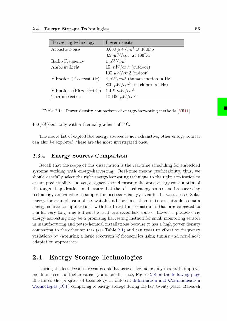
2.4. Energy Storage Technologies 55
Harvesting technology Power densityAcoustic Noise 0.003 µW/cm3 at 100Db
0.96µW/cm3 at 100DbRadio Frequency 1 µW/cm2
Ambient Light 15 mW/cm2 (outdoor)100 µW/cm2 (indoor)
Vibration (Electrostatic) 4 µW/cm3 (human motion in Hz)800 µW/cm3 (machines in kHz)
Vibrations (Piezoelectric) 1.4-9 mW/cm3
Thermoelectric 10-100 µW/cm3
Table 2.1: Power density comparison of energy-harvesting methods [Yil11]
100 µW/cm3 only with a thermal gradient of 1◦C.
The above list of exploitable energy sources is not exhaustive, other energy sourcescan also be exploited, these are the most investigated ones.
2.3.4 Energy Sources ComparisonRecall that the scope of this dissertation is the real-time scheduling for embedded
systems working with energy-harvesting. Real-time means predictability, thus, weshould carefully select the right energy-harvesting technique to the right application toensure predictability. In fact, designers should measure the worst energy consumption ofthe targeted applications and ensure that the selected energy source and its harvestingtechnology are capable to supply the necessary energy even in the worst case. Solarenergy for example cannot be available all the time, then, it is not suitable as mainenergy source for applications with hard real-time constraints that are expected torun for very long time but can be used as a secondary source. However, piezoelectricenergy-harvesting may be a promising harvesting method for small monitoring sensorsin manufacturing and petrochemical installations because it has a high power densitycomparing to the other sources (see Table 2.1) and can resist to vibration frequencyvariations by capturing a large spectrum of frequencies using tuning and non-linearadaptation approaches.
2.4 Energy Storage TechnologiesDuring the last decades, rechargeable batteries have made only moderate improve-
ments in terms of higher capacity and smaller size, Figure 2.8 on the following pageillustrates the progress of technology in different Information and CommunicationTechnologies (ICT) comparing to energy storage during the last twenty years. Research
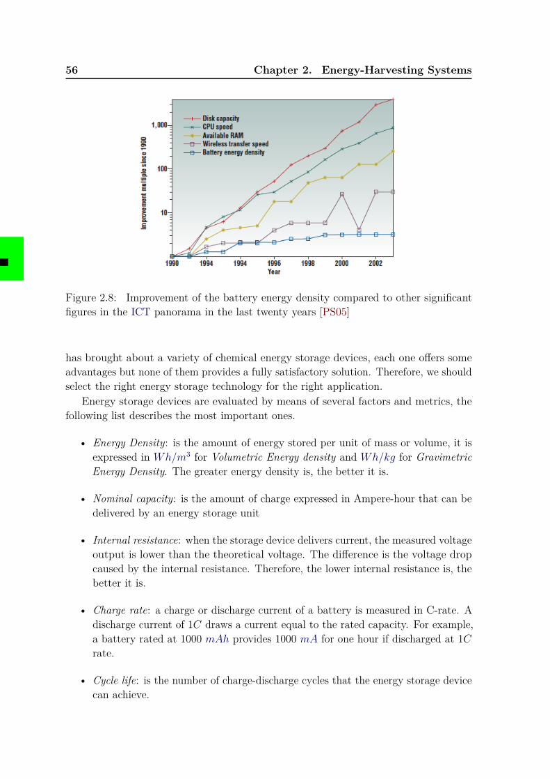
56 Chapter 2. Energy-Harvesting Systems
Figure 2.8: Improvement of the battery energy density compared to other significantfigures in the ICT panorama in the last twenty years [PS05]
has brought about a variety of chemical energy storage devices, each one offers someadvantages but none of them provides a fully satisfactory solution. Therefore, we shouldselect the right energy storage technology for the right application.
Energy storage devices are evaluated by means of several factors and metrics, thefollowing list describes the most important ones.
• Energy Density: is the amount of energy stored per unit of mass or volume, it isexpressed in Wh/m3 for Volumetric Energy density and Wh/kg for GravimetricEnergy Density. The greater energy density is, the better it is.
• Nominal capacity: is the amount of charge expressed in Ampere-hour that can bedelivered by an energy storage unit
• Internal resistance: when the storage device delivers current, the measured voltageoutput is lower than the theoretical voltage. The difference is the voltage dropcaused by the internal resistance. Therefore, the lower internal resistance is, thebetter it is.
• Charge rate: a charge or discharge current of a battery is measured in C-rate. Adischarge current of 1C draws a current equal to the rated capacity. For example,a battery rated at 1000 mAh provides 1000 mA for one hour if discharged at 1Crate.
• Cycle life: is the number of charge-discharge cycles that the energy storage devicecan achieve.
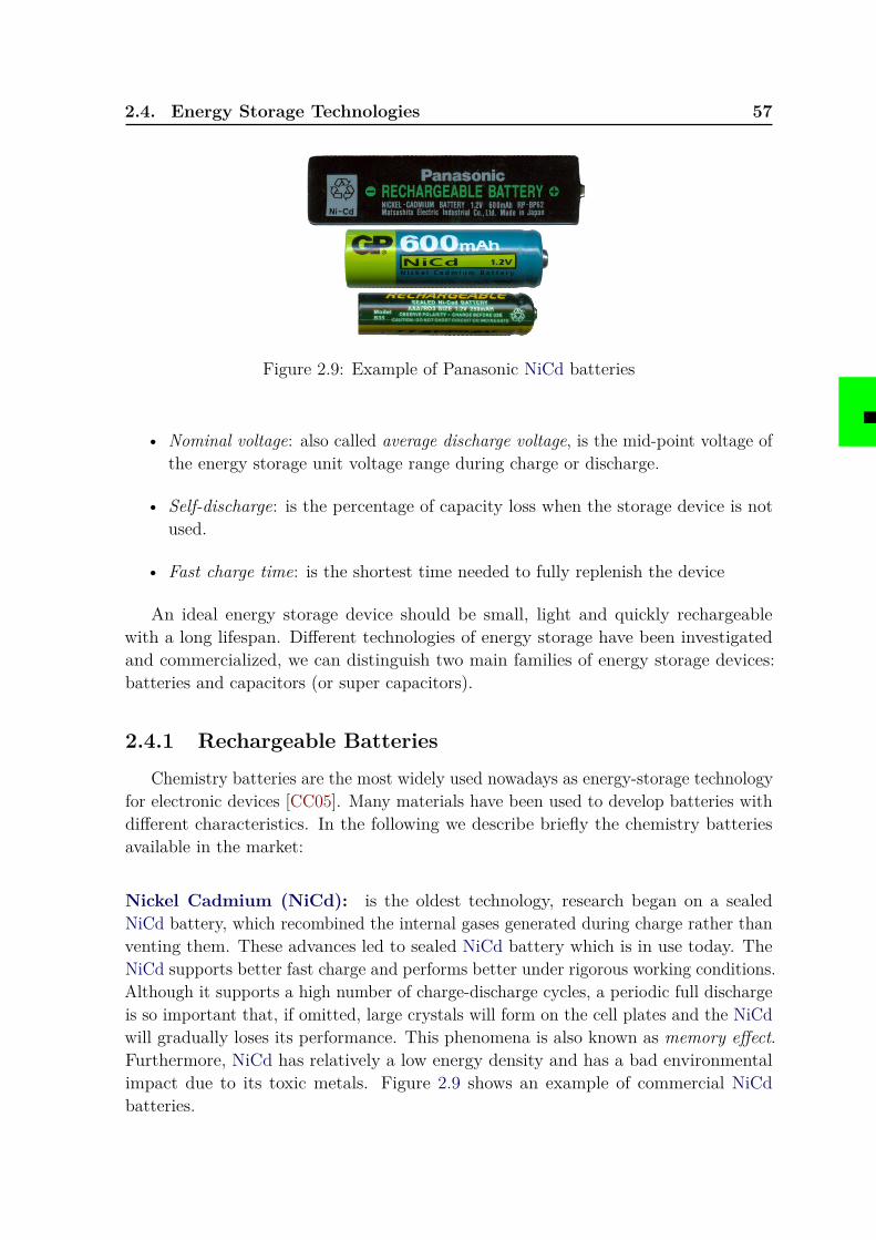
2.4. Energy Storage Technologies 57
Figure 2.9: Example of Panasonic NiCd batteries
• Nominal voltage: also called average discharge voltage, is the mid-point voltage ofthe energy storage unit voltage range during charge or discharge.
• Self-discharge: is the percentage of capacity loss when the storage device is notused.
• Fast charge time: is the shortest time needed to fully replenish the device
An ideal energy storage device should be small, light and quickly rechargeablewith a long lifespan. Different technologies of energy storage have been investigatedand commercialized, we can distinguish two main families of energy storage devices:batteries and capacitors (or super capacitors).
2.4.1 Rechargeable Batteries
Chemistry batteries are the most widely used nowadays as energy-storage technologyfor electronic devices [CC05]. Many materials have been used to develop batteries withdifferent characteristics. In the following we describe briefly the chemistry batteriesavailable in the market:
Nickel Cadmium (NiCd): is the oldest technology, research began on a sealedNiCd battery, which recombined the internal gases generated during charge rather thanventing them. These advances led to sealed NiCd battery which is in use today. TheNiCd supports better fast charge and performs better under rigorous working conditions.Although it supports a high number of charge-discharge cycles, a periodic full dischargeis so important that, if omitted, large crystals will form on the cell plates and the NiCdwill gradually loses its performance. This phenomena is also known as memory effect.Furthermore, NiCd has relatively a low energy density and has a bad environmentalimpact due to its toxic metals. Figure 2.9 shows an example of commercial NiCdbatteries.
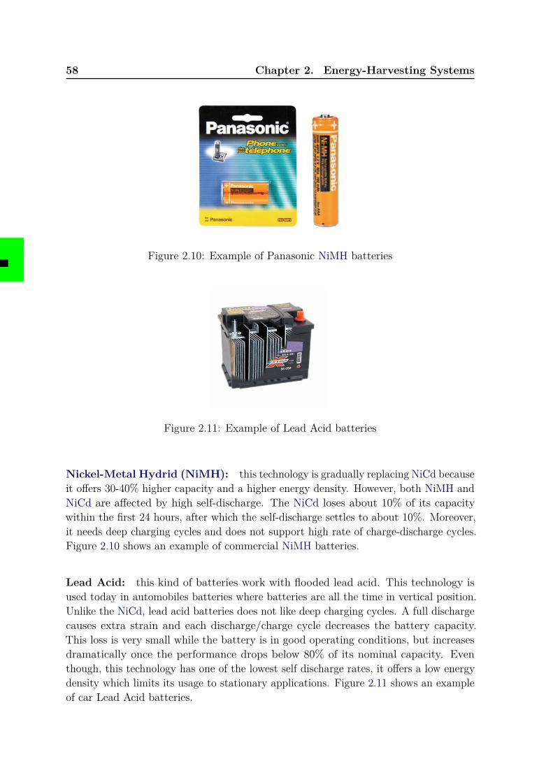
58 Chapter 2. Energy-Harvesting Systems
Figure 2.10: Example of Panasonic NiMH batteries
Figure 2.11: Example of Lead Acid batteries
Nickel-Metal Hydrid (NiMH): this technology is gradually replacing NiCd becauseit offers 30-40% higher capacity and a higher energy density. However, both NiMH andNiCd are affected by high self-discharge. The NiCd loses about 10% of its capacitywithin the first 24 hours, after which the self-discharge settles to about 10%. Moreover,it needs deep charging cycles and does not support high rate of charge-discharge cycles.Figure 2.10 shows an example of commercial NiMH batteries.
Lead Acid: this kind of batteries work with flooded lead acid. This technology isused today in automobiles batteries where batteries are all the time in vertical position.Unlike the NiCd, lead acid batteries does not like deep charging cycles. A full dischargecauses extra strain and each discharge/charge cycle decreases the battery capacity.This loss is very small while the battery is in good operating conditions, but increasesdramatically once the performance drops below 80% of its nominal capacity. Eventhough, this technology has one of the lowest self discharge rates, it offers a low energydensity which limits its usage to stationary applications. Figure 2.11 shows an exampleof car Lead Acid batteries.
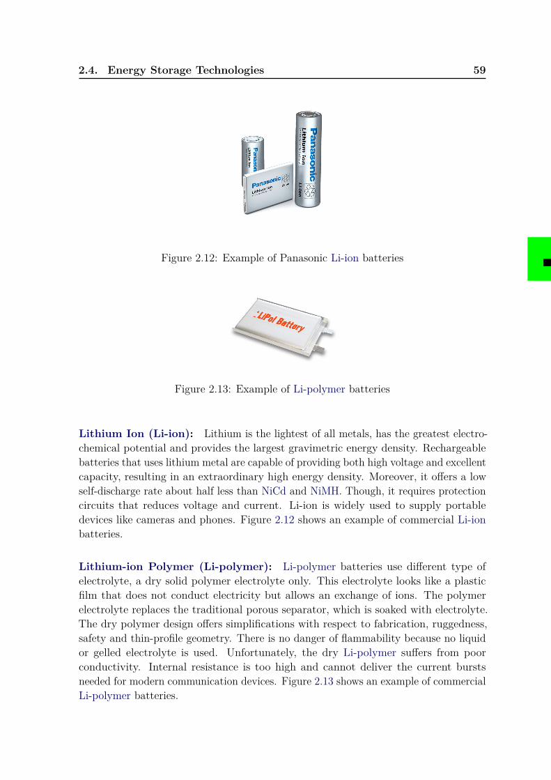
2.4. Energy Storage Technologies 59
Figure 2.12: Example of Panasonic Li-ion batteries
Figure 2.13: Example of Li-polymer batteries
Lithium Ion (Li-ion): Lithium is the lightest of all metals, has the greatest electro-chemical potential and provides the largest gravimetric energy density. Rechargeablebatteries that uses lithium metal are capable of providing both high voltage and excellentcapacity, resulting in an extraordinary high energy density. Moreover, it offers a lowself-discharge rate about half less than NiCd and NiMH. Though, it requires protectioncircuits that reduces voltage and current. Li-ion is widely used to supply portabledevices like cameras and phones. Figure 2.12 shows an example of commercial Li-ionbatteries.
Lithium-ion Polymer (Li-polymer): Li-polymer batteries use different type ofelectrolyte, a dry solid polymer electrolyte only. This electrolyte looks like a plasticfilm that does not conduct electricity but allows an exchange of ions. The polymerelectrolyte replaces the traditional porous separator, which is soaked with electrolyte.The dry polymer design offers simplifications with respect to fabrication, ruggedness,safety and thin-profile geometry. There is no danger of flammability because no liquidor gelled electrolyte is used. Unfortunately, the dry Li-polymer suffers from poorconductivity. Internal resistance is too high and cannot deliver the current burstsneeded for modern communication devices. Figure 2.13 shows an example of commercialLi-polymer batteries.
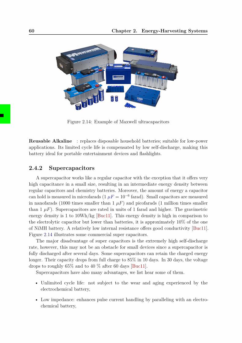
60 Chapter 2. Energy-Harvesting Systems
Figure 2.14: Example of Maxwell ultracapacitors
Reusable Alkaline : replaces disposable household batteries; suitable for low-powerapplications. Its limited cycle life is compensated by low self-discharge, making thisbattery ideal for portable entertainment devices and flashlights.
2.4.2 SupercapacitorsA supercapacitor works like a regular capacitor with the exception that it offers very
high capacitance in a small size, resulting in an intermediate energy density betweenregular capacitors and chemistry batteries. Moreover, the amount of energy a capacitorcan hold is measured in microfarads (1 µF = 10−6 farad). Small capacitors are measuredin nanofarads (1000 times smaller than 1 µF ) and picofarads (1 million times smallerthan 1 µF ). Supercapacitors are rated in units of 1 farad and higher. The gravimetricenergy density is 1 to 10Wh/kg [Buc11]. This energy density is high in comparison tothe electrolytic capacitor but lower than batteries, it is approximately 10% of the oneof NiMH battery. A relatively low internal resistance offers good conductivity [Buc11].Figure 2.14 illustrates some commercial super capacitors.
The major disadvantage of super capacitors is the extremely high self-dischargerate, however, this may not be an obstacle for small devices since a supercapacitor isfully discharged after several days. Some supercapacitors can retain the charged energylonger. Their capacity drops from full charge to 85% in 10 days. In 30 days, the voltagedrops to roughly 65% and to 40 % after 60 days [Buc11].
Supercapacitors have also many advantages, we list hear some of them.
• Unlimited cycle life: not subject to the wear and aging experienced by theelectrochemical battery,
• Low impedance: enhances pulse current handling by paralleling with an electro-chemical battery,
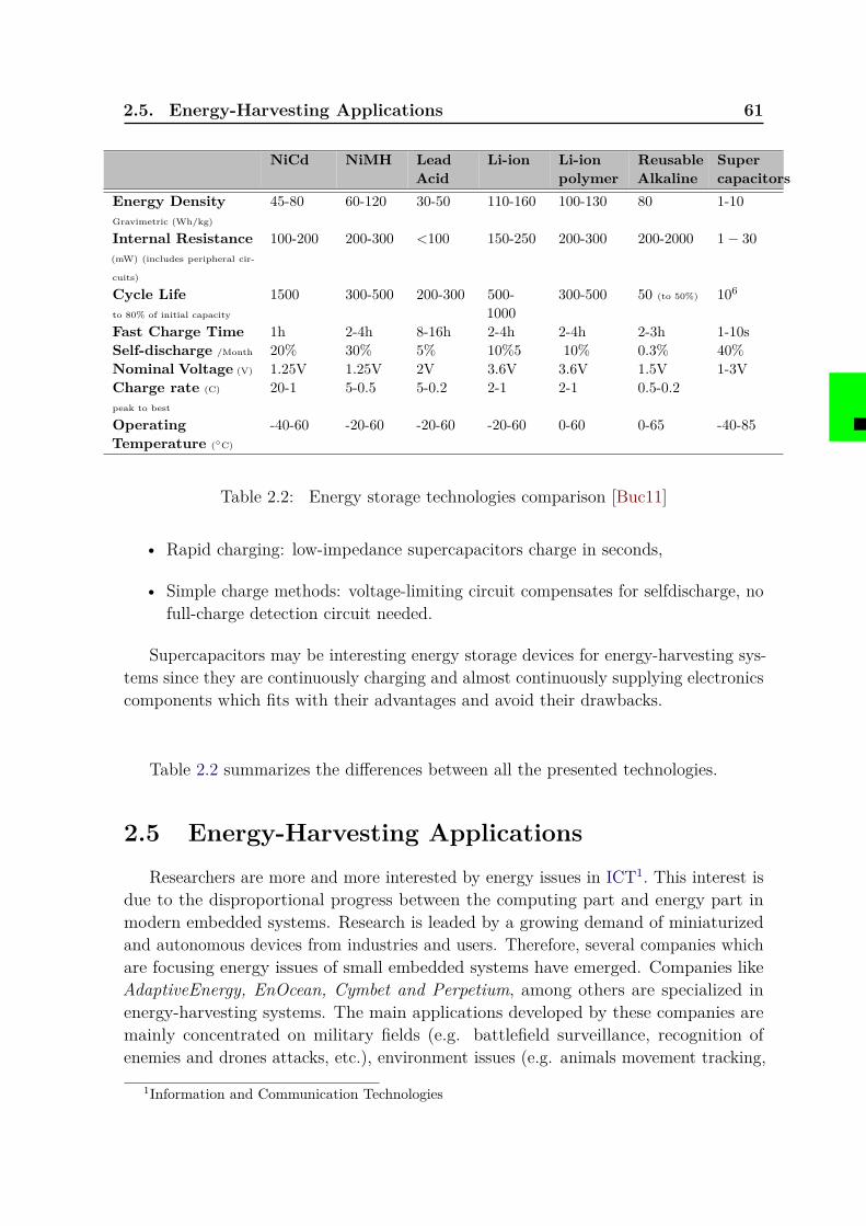
2.5. Energy-Harvesting Applications 61
NiCd NiMH LeadAcid
Li-ion Li-ionpolymer
ReusableAlkaline
Supercapacitors
Energy DensityGravimetric (Wh/kg)
45-80 60-120 30-50 110-160 100-130 80 1-10
Internal Resistance(mW) (includes peripheral cir-
cuits)
100-200 200-300 <100 150-250 200-300 200-2000 1− 30
Cycle Lifeto 80% of initial capacity
1500 300-500 200-300 500-1000
300-500 50 (to 50%) 106
Fast Charge Time 1h 2-4h 8-16h 2-4h 2-4h 2-3h 1-10sSelf-discharge /Month 20% 30% 5% 10%5 10% 0.3% 40%Nominal Voltage (V) 1.25V 1.25V 2V 3.6V 3.6V 1.5V 1-3VCharge rate (C)
peak to best
20-1 5-0.5 5-0.2 2-1 2-1 0.5-0.2
OperatingTemperature (◦C)
-40-60 -20-60 -20-60 -20-60 0-60 0-65 -40-85
Table 2.2: Energy storage technologies comparison [Buc11]
• Rapid charging: low-impedance supercapacitors charge in seconds,
• Simple charge methods: voltage-limiting circuit compensates for selfdischarge, nofull-charge detection circuit needed.
Supercapacitors may be interesting energy storage devices for energy-harvesting sys-tems since they are continuously charging and almost continuously supplying electronicscomponents which fits with their advantages and avoid their drawbacks.
Table 2.2 summarizes the differences between all the presented technologies.
2.5 Energy-Harvesting ApplicationsResearchers are more and more interested by energy issues in ICT1. This interest is
due to the disproportional progress between the computing part and energy part inmodern embedded systems. Research is leaded by a growing demand of miniaturizedand autonomous devices from industries and users. Therefore, several companies whichare focusing energy issues of small embedded systems have emerged. Companies likeAdaptiveEnergy, EnOcean, Cymbet and Perpetium, among others are specialized inenergy-harvesting systems. The main applications developed by these companies aremainly concentrated on military fields (e.g. battlefield surveillance, recognition ofenemies and drones attacks, etc.), environment issues (e.g. animals movement tracking,
1Information and Communication Technologies
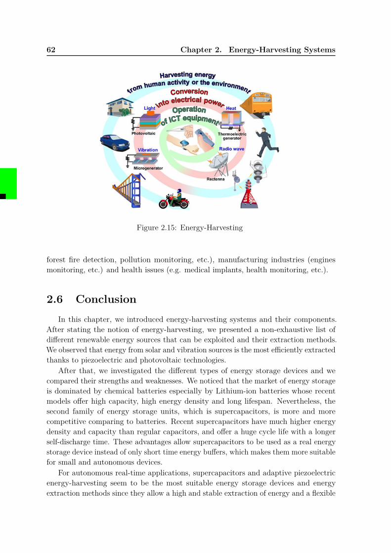
62 Chapter 2. Energy-Harvesting Systems
Figure 2.15: Energy-Harvesting
forest fire detection, pollution monitoring, etc.), manufacturing industries (enginesmonitoring, etc.) and health issues (e.g. medical implants, health monitoring, etc.).
2.6 ConclusionIn this chapter, we introduced energy-harvesting systems and their components.
After stating the notion of energy-harvesting, we presented a non-exhaustive list ofdifferent renewable energy sources that can be exploited and their extraction methods.We observed that energy from solar and vibration sources is the most efficiently extractedthanks to piezoelectric and photovoltaic technologies.
After that, we investigated the different types of energy storage devices and wecompared their strengths and weaknesses. We noticed that the market of energy storageis dominated by chemical batteries especially by Lithium-ion batteries whose recentmodels offer high capacity, high energy density and long lifespan. Nevertheless, thesecond family of energy storage units, which is supercapacitors, is more and morecompetitive comparing to batteries. Recent supercapacitors have much higher energydensity and capacity than regular capacitors, and offer a huge cycle life with a longerself-discharge time. These advantages allow supercapacitors to be used as a real energystorage device instead of only short time energy buffers, which makes them more suitablefor small and autonomous devices.
For autonomous real-time applications, supercapacitors and adaptive piezoelectricenergy-harvesting seem to be the most suitable energy storage devices and energyextraction methods since they allow a high and stable extraction of energy and a flexible
2.6. Conclusion 63
and quick storage and use of the extracted energy.In the next chapter, we focus on the computational part of an energy-harvesting
system and we address the real-time scheduling problem that considers the constraintsof an energy-harvesting systems.

Chapter 3
Real-time Scheduling forEnergy-Harvesting Systems
Contents3.1 Introduction . . . . . . . . . . . . . . . . . . . . . . . . . . . . . 66
3.1.1 Task Model . . . . . . . . . . . . . . . . . . . . . . . . . . . . . . 663.2 General Model . . . . . . . . . . . . . . . . . . . . . . . . . . . . 67
3.2.1 Energy Model . . . . . . . . . . . . . . . . . . . . . . . . . . . . . 673.2.2 Definitions . . . . . . . . . . . . . . . . . . . . . . . . . . . . . . 70
3.3 Scheduling Problematic . . . . . . . . . . . . . . . . . . . . . . . 71
3.4 Scheduling Approaches . . . . . . . . . . . . . . . . . . . . . . . 73
3.4.1 Dynamic Voltage and Frequency Scaling . . . . . . . . . . . . . . 733.4.2 Energy-Aware Scheduling . . . . . . . . . . . . . . . . . . . . . . 743.4.3 Other Approaches . . . . . . . . . . . . . . . . . . . . . . . . . . 75
3.5 Scheduling for Frame-Based Systems . . . . . . . . . . . . . . 75
3.6 EDF-based Scheduling Algorithms . . . . . . . . . . . . . . . . 79
3.6.1 EDF As Late As Possible Scheduling (EDL) . . . . . . . . . . . 803.6.2 EDF with Energy Guarantee Scheduling (EDeg) . . . . . . . . 833.6.3 Lazy Scheduling Algorithm (LSA) . . . . . . . . . . . . . . . . . 86
3.7 Fixed-Priority Scheduling . . . . . . . . . . . . . . . . . . . . . 92
3.7.1 The PFPALAP Scheduling Algorithm . . . . . . . . . . . . . . . 923.7.2 Preemptive Fixed-Priority with Slack-Time Algorithm . . . . . . 953.7.3 Other Scheduling Heuristics . . . . . . . . . . . . . . . . . . . . . 97
3.8 Performance Evaluation and Comparison . . . . . . . . . . . . 99
3.8.1 Simulation configuration . . . . . . . . . . . . . . . . . . . . . . . 993.8.2 Results analysis . . . . . . . . . . . . . . . . . . . . . . . . . . . . 1013.8.3 Comparison summary . . . . . . . . . . . . . . . . . . . . . . . . 103
3.9 Conclusion . . . . . . . . . . . . . . . . . . . . . . . . . . . . . . 104
66 Chapter 3. Real-time Scheduling for Energy-Harvesting Systems
3.1 IntroductionThe aim of embedded systems that work with environmental energy is to achieve a
set of missions autonomously for very long time. The missions of such applications aremainly sensing operations, data processing and data transmission. These operationsare managed by the computational part of an energy-harvesting system as mentionedin Chapter 2. Usually, energy-harvesting embedded systems are constrained by time inorder to deliver critical results on time, especially for critical embedded systems suchas medical implants or nuclear reaction monitoring devices. Therefore, it is mandatoryto guarantee the respect of time and energy constraints of these systems. Then, it isworthy to study the real-time scheduling under renewable energy constraints for systemsthat consider energy.
A naive approach consists of oversizing the capacity of the components of the system:a very large energy harvester (e.g. a huge solar panel), an overestimated energy storagedevice capacity and an oversized computation unit that guarantees the validity of thereal-time system under pessimistic schedulability analysis. However, this may be verycostly and may not fit with the desirable size especially for small applications (e.g.medical implants).
This has motivated researchers to focus on this challenging problem. The crucialissue associated to these systems is to find scheduling mechanisms that can managetheir performance and their activity according to the available energy along the systemlifespan in order to respect both time and energy constraints. Now, the primary concernis that the energy collected from the environment, and that can be stored, should befully consumed to maximize system’s performance and avoid energy waste.
In this chapter we address the real-time scheduling problem for energy-harvestingsystems. After setting the scope of this dissertation by specifying the formal modelof the targeted real-time energy-harvesting systems in Section 3.2 and the associatedscheduling problematic in Section 3.3, we give a brief overview of the available schedulingapproaches in Section 3.4. Then, we focus only on energy-aware scheduling approachand we explore the properties of the different classes of scheduling algorithms thatare proposed in the literature from Section 3.5 to Section 3.7. Finally, we present theresults of our experiments that compares the algorithms, and then, we summarize theirdifferences in Section 3.8.
3.1.1 Task Model
The task model considered here is an extension of Liu and Layland’s model, describedin Section 1.2 on page 30, that considers task energy consumption in addition to theclassical parameters. Then, we consider a real-time task set in a renewable energyenvironment defined by a set of n periodic/sporadic and independent tasks {τ1, τ2, . . . ,
τn}. Each task τi is characterized by its priority Pi, its worst-case execution time Ci,its period Ti, its relative deadline Di and its worst-case energy consumption Ei.
3.2. General Model 67
Therefore, a task τi releases an infinite number of jobs separated by at least Ti timeunits and each job is executed during Ci time units and consumes Ei energy units andmust finish before Di time units after being requested. Moreover, the deadlines areconstrained or implicit and the task set is priority-ordered such that task τn is the taskwith the lowest priority.
3.2 General ModelAn energy-harvesting system being composed of a real-time computational part
should be first described as a classical real-time system with a set of recurrent tasks, asexplained in Chapter 1, and second as a more complex system by including the energysource and the energy storage constraints described in Chapter 2. In this section wespecify the general formal model considered by this dissertation.
3.2.1 Energy Model
We consider an embedded system connected to an energy harvesting device. Anenergy-harvesting device as described in Section 2.2 on page 48 is a system that collectsthe ambient energy from the environment using an energy-harvesting technique. Thecollected energy is then stored in an energy storage unit with fixed capacity (e.g.rechargeable battery or supercapacitor).
Replenishment: We suppose that the amount of energy that arrives into the storageunit is a function of time which is either known or bounded. Recall that the profile ofenergy arriving from the harvester depends on the energy source and the harvestingtechnique. Most of energy sources are unpredictable or predictable with difficulty,for example, solar energy harvesting depends on brightness intensity which cannotbe predicted accurately. For this reason, since the scope of this dissertation is hardreal-time scheduling for energy-harvesting systems, we consider only energy sourcesand harvesting techniques that can provide a predictable profile of energy or thatcan be lower bounded. Hopefully, such energy profiles exist especially with vibrationenergy source and piezoelectric harvesting technique which seem to be suitable for smallembedded systems. It provides a nearly stable output of energy even with a deviationof vibration frequency up to 40% form the optimal one as explained in Section 2.3.2 onpage 52.
Therefore, as a first step, we can consider a uniform or a bounded replenishmentfunction which means that the storage unit receives a constant amount of energy everytime unit. We denote Pr(t) the replenishment function of the battery, then, the energy
68 Chapter 3. Real-time Scheduling for Energy-Harvesting Systems
replenished during any time interval [t1, t2] denoted as g(t1, t2) is given by Equation 3.1.
g(t1, t2) =∫ t2
t1.Pr(t) dt (3.1)
As mentioned above, we assume that that Pr(t) is a constant function, i.e. Pr(t) = Pr.Then, the energy replenished during any time interval [t1, t2] is given by Equation 3.2.
g(t1, t2) = (t2 − t1)× Pr (3.2)
In the remainder of this dissertation, we use Pr instead of Pr(t) to denote thereplenishment function and we suppose that it is lesser than or equal to the batterycapacity.
Storage: The replenishment of the storage unit is performed continuously even duringjobs execution and the level of the stored energy fluctuates between two thresholdsEmin and Emax where Emax is the maximum capacity of the storage unit and Emin isthe minimum energy level that keeps the system running. The difference between thesetwo thresholds is the part of the battery capacity dedicated to tasks execution. Thiscapacity is denoted C. We suppose that C is sufficient to execute at least one time unitof each task. This means that C must be greater or equal to the maximum instantaneousconsumption, i.e. C ≥ max∀i(Ei/Ci), otherwise some tasks cannot be executed. Wesuppose also that the storage device is carefully selected to ensure regular behavior, i.e.regular replenishment and regular discharge in order to avoid charge/discharge speedvariations and capacity losses due to numerous charge/discharge cycles. Recall thatsupercapacitors can offer these requirements as mentioned in Section 2.4.2 on page 60.
For the sake of clarity, we can consider without loss of generality that Emin = 0 andthat C = Emax. The battery level at time t is denoted as E(t). Below, we use the word“battery” to refer to the energy storage unit in order to simplify the language.
Consumption: Tasks energy cost should actually include not only dynamic andstatic processor energy consumption but also the consumption of other devices that atask can use, e.g. sensors and data transmission devices. Moreover, even if we consideronly processor consumption, the global consumption depends much more on the kind ofcircuitry used by the code than on the execution duration [JM06]. For this reason weconsider that the execution time Ci and the energy consumption Ei of a task are fullyindependent. For example, considering two tasks τi and τj that do not use the samedevices, then, we can have Ci < Cj and Ei > Ej . Furthermore, we consider that energyconsumption is function of time that is in reality not necessarily uniform. Actually,since tasks can use different devices, it is difficult to predict the accurate energy profileof tasks. Moreover, the worst energy consumption profile is not known up to now.This is a serious issue for real-time predictability, however, including this constraint toscheduling decisions makes it a hard problem with many parameters to consider. As afirst step and for the sake of simplicity, we consider for the scope of this dissertation
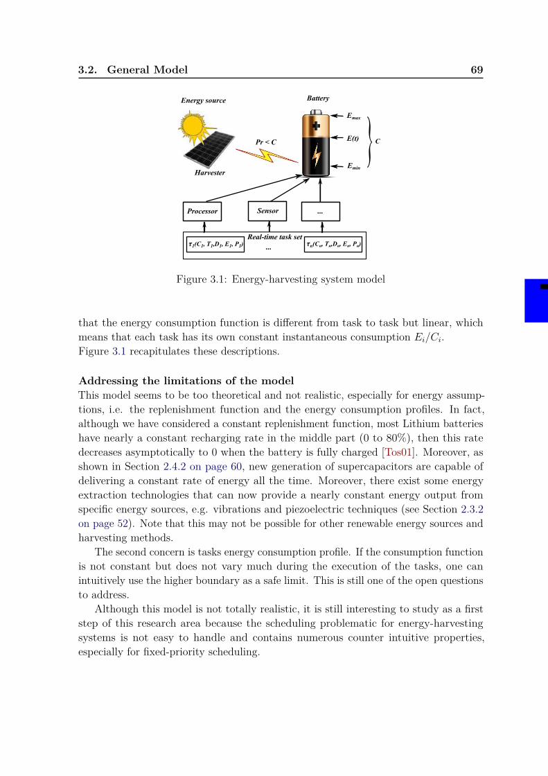
3.2. General Model 69
Emax
Energy source Battery
Pr < C
Real-time task set
Processor Sensor ...
Harvester
}Emin
E(t) C
...τ1(C1, T1,D1, E1, P1) τn(Cn, Tn,Dn, En, Pn)
Figure 3.1: Energy-harvesting system model
that the energy consumption function is different from task to task but linear, whichmeans that each task has its own constant instantaneous consumption Ei/Ci.Figure 3.1 recapitulates these descriptions.
Addressing the limitations of the modelThis model seems to be too theoretical and not realistic, especially for energy assump-tions, i.e. the replenishment function and the energy consumption profiles. In fact,although we have considered a constant replenishment function, most Lithium batterieshave nearly a constant recharging rate in the middle part (0 to 80%), then this ratedecreases asymptotically to 0 when the battery is fully charged [Tos01]. Moreover, asshown in Section 2.4.2 on page 60, new generation of supercapacitors are capable ofdelivering a constant rate of energy all the time. Moreover, there exist some energyextraction technologies that can now provide a nearly constant energy output fromspecific energy sources, e.g. vibrations and piezoelectric techniques (see Section 2.3.2on page 52). Note that this may not be possible for other renewable energy sources andharvesting methods.
The second concern is tasks energy consumption profile. If the consumption functionis not constant but does not vary much during the execution of the tasks, one canintuitively use the higher boundary as a safe limit. This is still one of the open questionsto address.
Although this model is not totally realistic, it is still interesting to study as a firststep of this research area because the scheduling problematic for energy-harvestingsystems is not easy to handle and contains numerous counter intuitive properties,especially for fixed-priority scheduling.
70 Chapter 3. Real-time Scheduling for Energy-Harvesting Systems
3.2.2 DefinitionsHere we define some new properties and we redefine some properties that we already
defined in Section 1.5.1 on page 41 to include energy requirements.
Definition 3.1 (Energy Valid Schedule).The schedule S produced by scheduling algorithm A is considered as valid only andonly if all the deadlines are infinitely met and the battery energy level never falls belowEmin. �
Definition 3.2 (System Energy Utilization).The system energy utilization denoted Ue is the ratio of energy to be consumed by theexecution of the task set relative to the energy that can be replenished. In the case ofconstant replenishment function Pr, it can be obtained by Equation 3.3.
Ue =n∑i=1
EiTi × Pr
(3.3)
�
Definition 3.3 (Energy-Busy-Period).An energy-busy-period is an interval of time [t1, t2] where the system is continuouslyexecuting jobs or replenishing energy if the battery level is not sufficient to executethe ready job, i.e. E(t) < Ei/Ci, while there are waiting jobs. It starts from time t1when the processor is idle for the last time and ends at time t2 when all waiting jobsare finished. It is possible to have consecutive energy-busy-periods since it depends onthe waiting jobs and not only the processor or the replenished energy. �
Definition 3.4 (Energy-Concrete Systems).An energy-concrete system is a system whose time and energy parameters are knownbefore run-time. This includes tasks periods, tasks offsets and the initial energy storagelevel of the storage unit. In the opposite, if all or one of these parameters is known onlyat run-time, then, the system is said energy-non-concrete. �
Definition 3.5 (Energy-Work Conserving).A scheduling algorithm is classified as energy-work-conserving policy if whenever thereare active tasks requiring execution, the scheduling policy leaves the processor idle onlyif there is no enough energy available to execute at least one time unit of the active task.In contrast, if the scheduling policy authorizes unnecessary idle times, it is classified asnon-energy-work-conserving. �
Definition 3.6 (Consumming Task).A task is considered as a consuming one if its energy consumption is greater than theenergy replenished during its execution time. �
Definition 3.7 (Gaining Task).A task is considered as a gaining one if its energy consumption is lesser than or equalto the energy replenished during its execution time. �
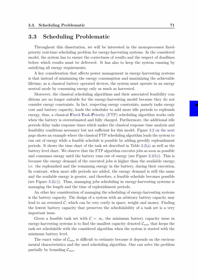
3.3. Scheduling Problematic 71
3.3 Scheduling Problematic
Throughout this dissertation, we will be interested in the monoprocessor fixed-priority real-time scheduling problem for energy-harvesting systems. In the consideredmodel, the system has to ensure the correctness of results and the respect of deadlinesbefore which results must be delivered. It has also to keep the system running bysatisfying all energy requirements.
A key consideration that affects power management in energy-harvesting systemsis that instead of minimizing the energy consumption and maximizing the achievablelifetime, as n classical battery operated devices, the system must operate in an energyneutral mode by consuming energy only as much as harvested.
Moreover, the classical scheduling algorithms and their associated feasibility con-ditions are no longer suitable for the energy-harvesting model because they do notconsider energy constraints. In fact, respecting energy constraints, namely tasks energycost and battery capacity, leads the scheduler to add more idle periods to replenishenergy, thus, a classical Fixed-Task-Priority (FTP) scheduling algorithm works onlywhen the battery is overestimated and fully charged. Furthermore, the additional idleperiods delay tasks response times which makes the classical response time analysis andfeasibility conditions necessary but not sufficient for this model. Figure 3.2 on the nextpage shows an example where the classical FTP scheduling algorithm leads the system torun out of energy while a feasible schedule is possible by adding greedily replenishmentperiods. It shows the time chart of the task set described in Table 3.2(a) as well as thebattery level chart. We observe that the FTP algorithm executes jobs as soon as possibleand consumes energy until the battery runs out of energy (see Figure 3.2(b)). This isbecause the energy demand of the executed jobs is higher than the available energy,i.e. the replenished and the remaining energy in the battery, during their execution.In contrast, when more idle periods are added, the energy demand is still the sameand the available energy is greater, and therefore, a feasible schedule becomes possible(see Figure 3.2(c)). Thus, managing jobs scheduling in energy-harvesting systems ismanaging the length and the time of replenishment periods.
An other key consideration of managing the scheduling of energy-harvesting systemsis the battery capacity. The design of a system with an arbitrary battery capacity maylead to an oversized C, which can be very costly in space, weight and money. Findingthe lowest battery capacity that preserves the schedulability of a task set is a veryimportant issue.
Given a feasible task set with C = ∞, the minimum battery capacity issue inenergy-harvesting systems is to find the smallest capacity denoted Cmin that keeps thetask set schedulable with the considered algorithm when the system is started with theminimum battery level.
The exact value of Cmin is difficult to estimate because it depends on the environ-mental characteristics and the used scheduling algorithm. One can solve the problempartially by bounding Cmin.
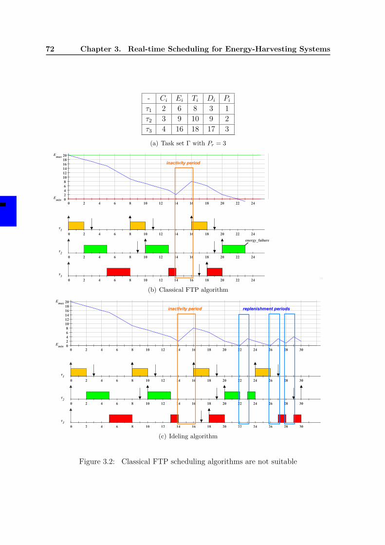
72 Chapter 3. Real-time Scheduling for Energy-Harvesting Systems
- Ci Ei Ti Di Piτ1 2 6 8 3 1τ2 3 9 10 9 2τ3 4 16 18 17 3
(a) Task set Γ with Pr = 3
0 2 4 6 8 10 12 14 16 18 20 22 2402468101214161820E
max
Emin
0 2 4 6 8 10 12 14 16 18 20 22 24
τ1
energy_failure
0 2 4 6 8 10 12 14 16 18 20 22 24
τ2
0 2 4 6 8 10 12 14 16 18 20 22 24
τ3
30
inactivity period
(b) Classical FTP algorithm
0 2 4 6 8 10 12 14 16 18 20 22 24 26 28 3002468101214161820E
max
Emin
0 2 4 6 8 10 12 14 16 18 20 22 24 26 28 30
τ1
0 2 4 6 8 10 12 14 16 18 20 22 24 26 28 30
τ2
0 2 4 6 8 10 12 14 16 18 20 22 24 26 28 30
τ3
inactivity period replenishment periods
(c) Ideling algorithm
Figure 3.2: Classical FTP scheduling algorithms are not suitable
3.4. Scheduling Approaches 73
To summarize, the problems we are interested in can be formulated by the followingquestions.
1. Scheduling algorithms: How can we schedule a given fixed-priority real-timetask set on one processor so to perpetually respect tasks deadlines and satisfytheir energy demand while keeping the battery level higher than Emin ?
2. Feasibility conditions: Does a necessary and sufficient feasibility condition,that guarantees before run-time the feasibility or the unfeasibility of a giventaskset, exist ?
3. Minimum energy storage capacity: What is the minimum battery capacitythat keeps the feasibility of a given task set ?
Through this dissertation, we will first explore some solutions and some answersto these questions that have been proposed in the literature, and then, we explain thecontributions of this thesis.
3.4 Scheduling ApproachesIn the last decades, different solutions have been proposed in the literature to deal
with energy issues. Most research focused on reducing the global energy consumptionof the system. This is due to promising autonomous embedded systems whose lifetimewas seriously limited by the capacity of batteries. Later, with the emerging energy-harvesting technologies, researchers realized that they should not focus only on energyconsumption optimization but also on the management of renewable energy. Thiskind of energy is collected from the environment with small quantities but with acontinuous supply. From this, we can identify two main families of real-time schedulingresearch that address energy issues: scheduling for energy consumption optimization,mainly represented by Central Processing Unit (CPU) frequency and voltage scaling,and energy-aware scheduling that manages executions and replenishment to operateperpetually.
3.4.1 Dynamic Voltage and Frequency ScalingThe Dynamic Voltage and Frequency Scaling (DVFS) approach consists of slowing
down the processor speed by reducing either the voltage or the processing frequencyor both in order to reduce the processor energy consumption [PBB98; Wei+94]. Thisapproach relies on the fact that the energy consumption in small embedded systemscomes mainly from processor’s dynamic energy consumption [ZMM04]. The researchinterest for this approach was amplified when microprocessors manufacturers releasedprocessors with DVFS capabilities (e.g. Intel’s SpeedStep, AMD’s Cool’n’Quiet andPowerNow, etc.).
74 Chapter 3. Real-time Scheduling for Energy-Harvesting Systems
Many solutions propose real-time scheduling schemes that use DVFS capabilities torespect deadlines and to reduce the global energy consumption. When using DVFS,tasks execution times become longer due to slower processing. Then, for real-timescheduling, the slack-time or the available idle time can be used to reduce energyconsumption by slowing down the processor and lengthening tasks response times[PBB98; Wei+94]. The challenges of such an approach are to select the right subsetof jobs for which are applied frequency scaling and to select the right CPU frequencyto apply for each task. Unfortunately, this was proved to be a Non-deterministicPolynomial-time Hard (NP-Hard) problem in [ZA06], thus, works dealing with thisproblem focused mainly on proposing adapted heuristics [ZQA07; ZA09]. The maindrawback of scaling the voltage and frequency is that it increases the risk of transienterrors in Complementary Metal–Oxide–Semiconductor (CMOS) logic circuits [JK95;HS00; Zie14]. To cope with this difficulty, fault tolerance techniques have been used byintroducing redundancy. Zhu et al. in [ZA06] proposed a heuristic that uses slack-timeto perform DVFS and reserve time for rollback tasks as fault tolerance method.
The DVFS is an interesting technology to reduce the energy consumption of thesystem for embedded systems equipped with processors with several CPU frequencies.However, it increases the risk of transient faults which requires the implementationof fault tolerance techniques and may make the gain of consumed energy not worthy.Furthermore, even though it reduces the global energy consumption, it cannot beused alone in an energy-harvesting system especially when the slower frequency isnot sufficient to reduce enough the consumed energy. Some adaptations for energy-harvesting systems have been proposed, however, most of them are still supposingnegligible faults rate and a large number of CPU frequencies.
3.4.2 Energy-Aware Scheduling
In contrast to DVFS, energy-aware scheduling aims to dynamically manage theavailable energy at any time, i.e. the energy collected from the environment anddrained from the battery, rather than optimizing or minimizing the global energyconsumption. It consists of selecting the right periods of execution and the rightperiods for replenishment so to ensure a perpetual operation. This scheduling approachconsiders only mono-frequency processors, and therefore, only two modes: active modewhere the system consumes energy and inactive mode where the system is idle and doesnot consume energy or consume a negligible amount of energy. In this dissertation wewill focus only on this scheduling approach. In the remaining part of this chapter, weexplore different scheduling algorithms proposed in the literature for this schedulingapproach. For each algorithm, we specify the model for which it was designed and westudy some of its properties, e.g. optimality, minimum battery capacity, etc. After thatwe test these algorithms with the model specified in Section 3.2 on page 67 in order tocompare them by simulations, and then, we summarize their strengths and weaknesses.
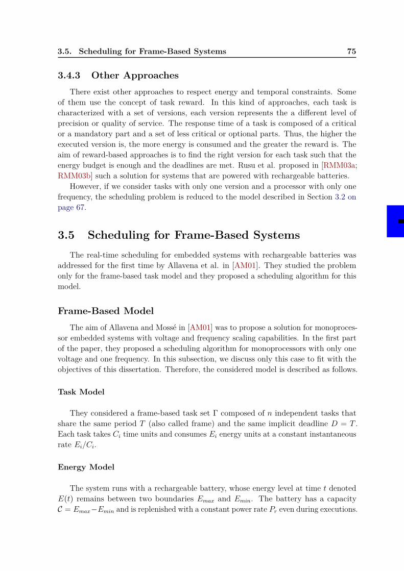
3.5. Scheduling for Frame-Based Systems 75
3.4.3 Other ApproachesThere exist other approaches to respect energy and temporal constraints. Some
of them use the concept of task reward. In this kind of approaches, each task ischaracterized with a set of versions, each version represents the a different level ofprecision or quality of service. The response time of a task is composed of a criticalor a mandatory part and a set of less critical or optional parts. Thus, the higher theexecuted version is, the more energy is consumed and the greater the reward is. Theaim of reward-based approaches is to find the right version for each task such that theenergy budget is enough and the deadlines are met. Rusu et al. proposed in [RMM03a;RMM03b] such a solution for systems that are powered with rechargeable batteries.
However, if we consider tasks with only one version and a processor with only onefrequency, the scheduling problem is reduced to the model described in Section 3.2 onpage 67.
3.5 Scheduling for Frame-Based SystemsThe real-time scheduling for embedded systems with rechargeable batteries was
addressed for the first time by Allavena et al. in [AM01]. They studied the problemonly for the frame-based task model and they proposed a scheduling algorithm for thismodel.
Frame-Based ModelThe aim of Allavena and Mossé in [AM01] was to propose a solution for monoproces-
sor embedded systems with voltage and frequency scaling capabilities. In the first partof the paper, they proposed a scheduling algorithm for monoprocessors with only onevoltage and one frequency. In this subsection, we discuss only this case to fit with theobjectives of this dissertation. Therefore, the considered model is described as follows.
Task Model
They considered a frame-based task set Γ composed of n independent tasks thatshare the same period T (also called frame) and the same implicit deadline D = T .Each task takes Ci time units and consumes Ei energy units at a constant instantaneousrate Ei/Ci.
Energy Model
The system runs with a rechargeable battery, whose energy level at time t denotedE(t) remains between two boundaries Emax and Emin. The battery has a capacityC = Emax−Emin and is replenished with a constant power rate Pr even during executions.
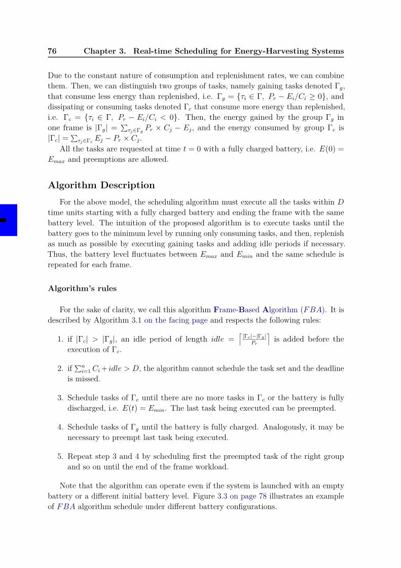
76 Chapter 3. Real-time Scheduling for Energy-Harvesting Systems
Due to the constant nature of consumption and replenishment rates, we can combinethem. Then, we can distinguish two groups of tasks, namely gaining tasks denoted Γg,that consume less energy than replenished, i.e. Γg = {τi ∈ Γ, Pr − Ei/Ci ≥ 0}, anddissipating or consuming tasks denoted Γc that consume more energy than replenished,i.e. Γc = {τi ∈ Γ, Pr − Ei/Ci < 0}. Then, the energy gained by the group Γg inone frame is |Γg| = ∑
τj∈Γg Pr × Cj − Ej, and the energy consumed by group Γc is|Γc| =
∑τj∈Γc Ej − Pr × Cj.
All the tasks are requested at time t = 0 with a fully charged battery, i.e. E(0) =Emax and preemptions are allowed.
Algorithm DescriptionFor the above model, the scheduling algorithm must execute all the tasks within D
time units starting with a fully charged battery and ending the frame with the samebattery level. The intuition of the proposed algorithm is to execute tasks until thebattery goes to the minimum level by running only consuming tasks, and then, replenishas much as possible by executing gaining tasks and adding idle periods if necessary.Thus, the battery level fluctuates between Emax and Emin and the same schedule isrepeated for each frame.
Algorithm’s rules
For the sake of clarity, we call this algorithm Frame-Based Algorithm (FBA). It isdescribed by Algorithm 3.1 on the facing page and respects the following rules:
1. if |Γc| > |Γg|, an idle period of length idle =⌈|Γc|−|Γg |
Pr
⌉is added before the
execution of Γc.
2. if ∑ni=1Ci + idle > D, the algorithm cannot schedule the task set and the deadline
is missed.
3. Schedule tasks of Γc until there are no more tasks in Γc or the battery is fullydischarged, i.e. E(t) = Emin. The last task being executed can be preempted.
4. Schedule tasks of Γg until the battery is fully charged. Analogously, it may benecessary to preempt last task being executed.
5. Repeat step 3 and 4 by scheduling first the preempted task of the right groupand so on until the end of the frame workload.
Note that the algorithm can operate even if the system is launched with an emptybattery or a different initial battery level. Figure 3.3 on page 78 illustrates an exampleof FBA algorithm schedule under different battery configurations.
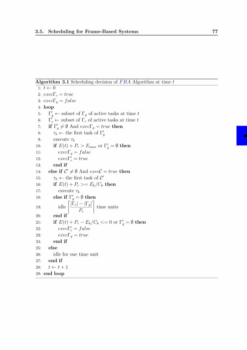
3.5. Scheduling for Frame-Based Systems 77
Algorithm 3.1 Scheduling decision of FBA Algorithm at time t1: t← 02: execΓc = true
3: execΓg = false
4: loop5: Γ′g ← subset of Γg of active tasks at time t6: Γ′c ← subset of Γc of active tasks at time t7: if Γ′g 6= ∅ And execΓg = true then8: τk ← the first task of Γ′g9: execute τk
10: if E(t) + Pr > Emax or Γ′g = ∅ then11: execΓg = false
12: execΓ′c = true
13: end if14: else if C ′ 6= ∅ And execC = true then15: τk ← the first task of C ′16: if E(t) + Pr >= Ek/Ck then17: execute τk18: else if Γ′g = ∅ then
19: idle⌈|Γc| − |Γg|
Pr
⌉time units
20: end if21: if E(t) + Pr − Ek/Ck <= 0 or Γ′g = ∅ then22: execΓ′c = false
23: execΓg = true
24: end if25: else26: idle for one time unit27: end if28: t← t+ 129: end loop
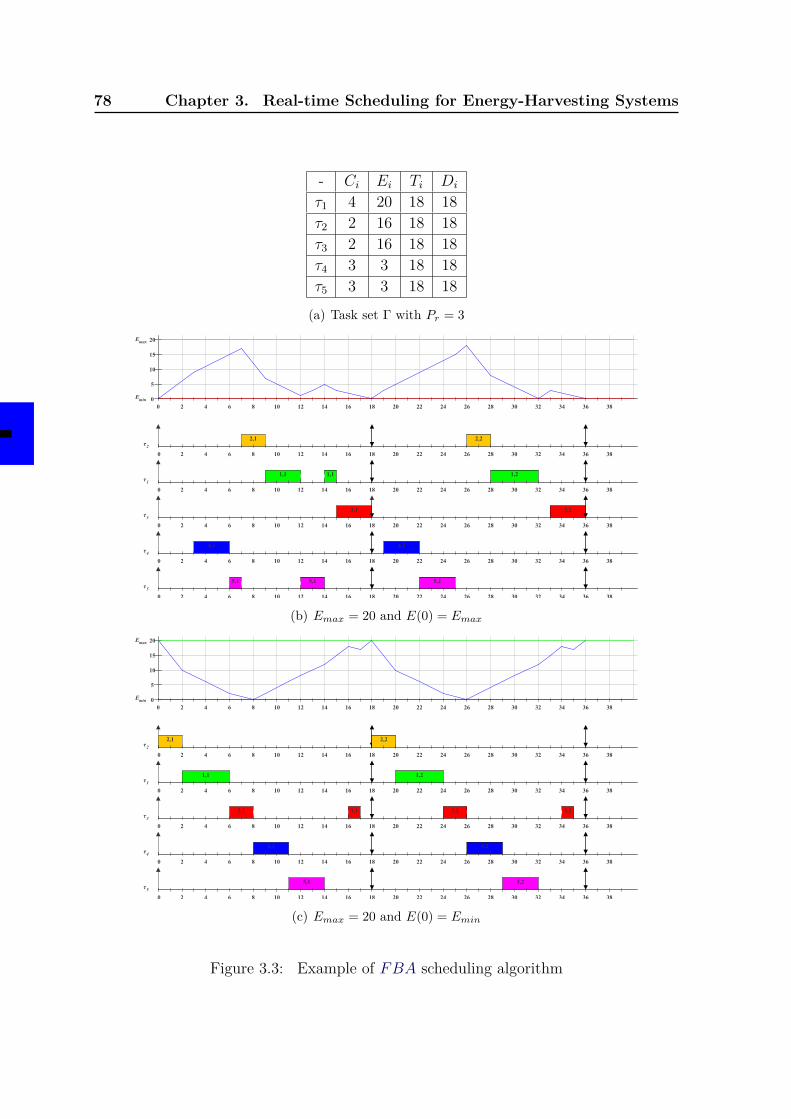
78 Chapter 3. Real-time Scheduling for Energy-Harvesting Systems
- Ci Ei Ti Di
τ1 4 20 18 18τ2 2 16 18 18τ3 2 16 18 18τ4 3 3 18 18τ5 3 3 18 18
(a) Task set Γ with Pr = 3
0 2 4 6 8 10 12 14 16 18 20 22 24 26 28 30 32 34 36 380
5
10
15
20Emax
Emin
2,1 2,2
0 2 4 6 8 10 12 14 16 18 20 22 24 26 28 30 32 34 36 38
τ2
1,1 1,1 1,2
0 2 4 6 8 10 12 14 16 18 20 22 24 26 28 30 32 34 36 38
τ1
3,1 3,2
0 2 4 6 8 10 12 14 16 18 20 22 24 26 28 30 32 34 36 38
τ3
4,1 4,2
0 2 4 6 8 10 12 14 16 18 20 22 24 26 28 30 32 34 36 38
τ4
5,1 5,1 5,2
0 2 4 6 8 10 12 14 16 18 20 22 24 26 28 30 32 34 36 38
τ5
(b) Emax = 20 and E(0) = Emax
0 2 4 6 8 10 12 14 16 18 20 22 24 26 28 30 32 34 36 380
5
10
15
20Emax
Emin
2,1 2,2
0 2 4 6 8 10 12 14 16 18 20 22 24 26 28 30 32 34 36 38
τ2
1,1 1,2
0 2 4 6 8 10 12 14 16 18 20 22 24 26 28 30 32 34 36 38
τ1
3,1 3,1 3,2 3,2
0 2 4 6 8 10 12 14 16 18 20 22 24 26 28 30 32 34 36 38
τ3
4,1 4,2
0 2 4 6 8 10 12 14 16 18 20 22 24 26 28 30 32 34 36 38
τ4
5,1 5,2
0 2 4 6 8 10 12 14 16 18 20 22 24 26 28 30 32 34 36 38
τ5
(c) Emax = 20 and E(0) = Emin
Figure 3.3: Example of FBA scheduling algorithm
3.6. EDF-based Scheduling Algorithms 79
Complexity
The FBA algorithm is simple, all the instructions are simple and the only operationthat can be costly in time is to compute the set of active tasks which can be optimizedto a complexity of O(n) by considering that the tasks are sorted with their consumptionrate. Therefore, the global complexity of FBA is O(n).
Minimum Storage Unit Capacity
This property was not addressed in the paper proposing the algorithm but it seemsto be obvious due to the simplicity of the model and scheduling schemes. Intuitively,by scheduling all tasks inside one frame with only one request time and one deadlineand by following the pattern of gaining-consuming or consuming-gaining tasks, in theworst-case when the battery is empty (E(t) = Emin), the minimum battery capacitythat keeps a schedulable task set schedulable is the maximum instantaneous energyconsumption of tasks. Instead of having only one cycle of gaining-consuming tasks, wecan keep the same response time by splitting it to many small cycles which lowers themaximum reachable battery level, and thus, the battery capacity. Furthermore, on canalso add the energy replenished during inactivity periods in order to ensure the sameenergy level at the beginning of each frame.
Optimality
This question was not addressed in the paper. Though, the algorithm seems to beoptimal for the specified model. Intuitively, when all the tasks share the same periodand the same deadline the order of tasks is not important if the deadline is met. Thisalgorithm sorts the tasks so to schedule gaining tasks before consuming ones when theminimum energy level is reached to replenish a maximum of energy before executingthe consuming tasks which reduces to the maximum the useless replenishment periods.Then, if a deadline is missed, this means that the available energy in one frame is notsufficient. In this case, no algorithm can avoid this deadline miss.
3.6 EDF-based Scheduling Algorithms
The following algorithms are adaptations of the classical Earliest Deadline First(EDF ) algorithm described in Section 1.4.7 on page 40. These algorithms proposedifferent strategies to cope with the delays caused by energy-harvesting and energy-storage constraints. In this section, we present EDF As Late As Possible (EDL), EDFwith energy guaranty (EDeg) and Lazy Scheduling Algorithm (LSA) algorithms.
80 Chapter 3. Real-time Scheduling for Energy-Harvesting Systems
3.6.1 EDF As Late As Possible Scheduling (EDL)
The EDL algorithm was proposed by Silly in [Sil99]. It does not consider energyconstraints but schedules tasks by respecting EDF rules and delaying executions aslong as possible by anticipating all the available slack-time. It can be used in thecontext of energy-harvesting systems to maximize replenishment periods.
Model
Task ModelThe model associated to EDL is very close to the one described in Section 3.2 onpage 67. In order to be able to compute the exact values of slack-time, only periodictasks with null offsets (i.e. ∀ τi, Oi = 0) and constrained or implicit deadlines areconsidered. Then, the arrival times, energy costs and deadlines are known beforerun-time. The hyper-period, i.e. the least common multiple of tasks periods, is denotedHP .
Energy ModelThe slack-time computation used by EDL algorithm does not include energy constants.Therefore, it can theoretically work with any energy source and storage models. In thisdissertation we apply EDL to the general model described in Section 3.2 on page 67and we use it to compare the effect of delaying execution with other algorithms.
Algorithm Description
The main idea of EDL is to differ executions in order to maximize the length ofidle periods and thereby replenishment time. When a job is ready to be executed attime t according to EDF rules, EDL computes first the available slack-time time ofthe system. Then, the ready job is executed only if the slack-time is 0 and the energyis sufficient to execute. Otherwise, it is delayed until the slack-time is fully consumed.The computation of slack-time with EDF scheduling is described in [Sil99]. The authorproposes two approaches: a static offline approach and a dynamic online one. In thissection, we give some insights about the static approach. It consists first of identifyingin a set denoted K, the time instants when potential idle periods can begin withinthe hyper-period, and second, computing the length of each of these periods in a setdenoted D. Formally:
1. K, the deadlines set is a sorted set of times at which idle times can begin withintime interval [0, HP [. It is composed of distinct deadlines of all jobs inside[0, HP [. Then, K = { k0, k1, · · · , ki, ki+1, · · · , kq }, with ki < ki+1, k0 = 0 andkq = HP −min1≤i≤n(xi), with xi = Ti −Di. We note that q ≤ N + 1 where Ndenotes the number of jobs requested during [0, HP [.
3.6. EDF-based Scheduling Algorithms 81
2. D, the idle periods lengths set contains the lengths of idle periods. D = {∆0, ∆1,· · · , ∆i, ∆i+1, · · · , ∆q}, where ∆i is the length of the idle period that begins attime ki. It can be calculated by Formula 3.4:
{∆i = min1≤i≤n(xi) if i = q
∆i = max(0, Fi) if 0 ≤ i ≤ q − 1 (3.4)
with :Fi = (HP − ki)−
n∑j=1
⌈HP − xj − kj
Tj
⌉× Cj −
q∑k=i+1
∆k
Then, EDL uses the set K to decide when to postpone executions and D to knowfor how long. Figure 3.4 on the following page shows an example where K = { 0, 6, 8,12, 15, 20, 24, 30, 32, 22 }, and D = { 2, 0, 1, 0, 2, 1, 0, 0, 3, 22 }. Then, for exampleat time 32, EDL delays executions for 3 units.
Complexity
We note that the schedule of one hyper-period with EDL is achieved in O(N × n)operations in the worst case [Sil99]. This complexity depends on the periods anddeadlines which make it pseudo-polynomial. It may be relatively high when periods areprime integers because it maximizes the hyper-period length and thus the number ofjobs N .
Optimality
This algorithm is clearly not optimal for energy-harvesting systems because whenEmax is reached during an idle period, the surplus of energy is wasted. This wastedenergy may be necessary for a future job. Figure 3.4(c) on the next page shows a counterexample. It illustrates a situation where energy is wasted at time 8 and 15 which leadsthe system to run out of energy at time 32 while the slack-time was already consumed.However, EDL seems to be optimal if we consider an infinite battery capacity or ifwe resume executions when Emax is reached. This intuition is based on the fact thatwhen a deadline is missed at time d, the energy balance, i.e. the difference betweenthe available energy until time d and energy demand of time interval [0, d[ is negative.Since EDF is driven by deadlines, if energy is not wasted, it is impossible to schedulethe task set because there exists at least one interval where an unavoidable negativeenergy balance happens.
Minimum Storage Unit Capacity
It is not easy to compute the exact battery capacity needed to schedule a feasibletask set with EDL because we need to know the wort-case scenario that needs thehighest capacity. However, one can provide a lower bound of the battery capacity by
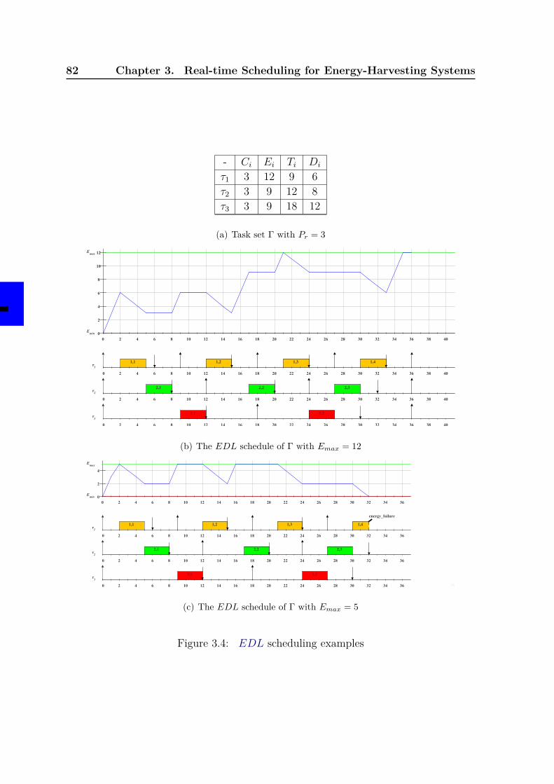
82 Chapter 3. Real-time Scheduling for Energy-Harvesting Systems
- Ci Ei Ti Di
τ1 3 12 9 6τ2 3 9 12 8τ3 3 9 18 12
(a) Task set Γ with Pr = 3
0 2 4 6 8 10 12 14 16 18 20 22 24 26 28 30 32 34 36 38 400
2
4
6
8
10
12Emax
Emin
1,1 1,2 1,3 1,4
0 2 4 6 8 10 12 14 16 18 20 22 24 26 28 30 32 34 36 38 40
τ1
2,1 2,2 2,3
0 2 4 6 8 10 12 14 16 18 20 22 24 26 28 30 32 34 36 38 40
τ2
3,1 3,2
0 2 4 6 8 10 12 14 16 18 20 22 24 26 28 30 32 34 36 38 40
τ3
(b) The EDL schedule of Γ with Emax = 12
0 2 4 6 8 10 12 14 16 18 20 22 24 26 28 30 32 34 360
2
4
Emax
Emin
1,1 1,2 1,3 1,4
energy_failure
0 2 4 6 8 10 12 14 16 18 20 22 24 26 28 30 32 34 36
τ1
2,1 2,2 2,3
0 2 4 6 8 10 12 14 16 18 20 22 24 26 28 30 32 34 36
τ2
3,1 3,2
0 2 4 6 8 10 12 14 16 18 20 22 24 26 28 30 32 34 36
τ3
36
(c) The EDL schedule of Γ with Emax = 5
Figure 3.4: EDL scheduling examples
3.6. EDF-based Scheduling Algorithms 83
summing the energy collected during all the idle periods of one hyper-period which is thecomplementary part of the workload of one hyper-period, i.e. Emax ≥ (1−U)×HP×Pr.However, it is still an overestimated bound.
Schedulability Conditions
Without energy constraints, EDL is equivalent to the regular EDF in term of tasksets schedulability. When energy constraints are considered, it is difficult to say whethera task set is schedulable with EDL or not because we need to check if all deadlines aremet even in the worst-case scenario which is not known up to now. The only conditionsthat we can check are processor and energy utilizations, i.e. U ≤ 1 and Ue ≤ 1 whichare only necessary conditions.
3.6.2 EDF with Energy Guarantee Scheduling (EDeg)In [EGCC11; Che14], Chetto et al. proposed an enhancement of EDL. They
proposed an algorithm called EDeg for EDF with energy guarantee. It consists ofmixing soon and late scheduling by using clairvoyance or look-ahead calculations.
Model
Task ModelThe same task model as for EDL is considered: a periodic task set with constrained orimplicit deadlines and null offsets.
Energy Model:The replenishment function Pr(t) is not necessarily specified but must be known in orderto ensure the predictability needed for correct clairvoyance computations. Furthermore,an ideal energy storage unit is considered, i.e. a battery or a capacitor with a linearcharging and discharging rates.
Algorithm Description
The intuition behind EDeg is to run jobs according to EDF rules, but beforeauthorizing a job to execute, EDeg uses the notion of slack-energy to predict eventualfuture energy failures. If a future deadline miss due to energy lack is detected, thecurrent jobs are delayed as long as possible by consuming the available slack-time toreplenish a maximum of energy like EDL does. Furthermore, when Emax is reachedduring an idle period, the algorithm resumes executions in order to avoid energywaste. The slack-energy notion is an extension of the notion of slack-time which meansthat the maximum amount of idle time that can be used to delay executions withoutviolating deadlines. As described in [EGCC11] the slack-energy of a job Ji,j at timet denoted SEi,j(t) is the maximum amount of energy that can be used to execute
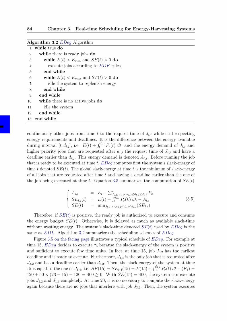
84 Chapter 3. Real-time Scheduling for Energy-Harvesting Systems
Algorithm 3.2 EDeg Algorithm1: while true do2: while there is ready jobs do3: while E(t) > Emin and SE(t) > 0 do4: execute jobs according to EDF rules5: end while6: while E(t) < Emax and ST (t) > 0 do7: idle the system to replenish energy8: end while9: end while
10: while there is no active jobs do11: idle the system12: end while13: end while
continuously other jobs from time t to the request time of Ji,j while still respectingenergy requirements and deadlines. It is the difference between the energy availableduring interval [t, di,j], i.e. E(t) +
∫ di,jt Pr(t) dt, and the energy demand of Ji,j and
higher priority jobs that are requested after ai,j the request time of Ji,j and have adeadline earlier than di,j. This energy demand is denoted Ai,j. Before running the jobthat is ready to be executed at time t, EDeg computes first the system’s slack-energy oftime t denoted SE(t). The global slack-energy at time t is the minimum of slack-energyof all jobs that are requested after time t and having a deadline earlier than the one ofthe job being executed at time t. Equation 3.5 summarizes the computation of SE(t).
Ai,j = Ei +∑n
Jk,l, ai,j<ak,l≤dk,l≤di,j Ek
SEi,j(t) = E(t) +∫ di,jt Pr(k) dk − Ai,j
SE(t) = minJk,l, t<ak,l≤dk,l≤di,j(SEk,l)(3.5)
Therefore, if SE(t) is positive, the ready job is authorized to execute and consumethe energy budget SE(t). Otherwise, it is delayed as much as available slack-timewithout wasting energy. The system’s slack-time denoted ST (t) used by EDeg is thesame as EDL. Algorithm 3.2 summarizes the scheduling schemes of EDeg.
Figure 3.5 on the facing page illustrates a typical schedule of EDeg. For example attime 15, EDeg decides to execute τ3 because the slack-energy of the system is positiveand sufficient to execute few time units. In fact, at time 15, job J3,2 has the earliestdeadline and is ready to execute. Furthermore, J1,4 is the only job that is requested afterJ3,2 and has a deadline earlier than d3,2. Then, the slack-energy of the system at time15 is equal to the one of J1,4, i.e. SE(15) = SE1,4(15) = E(15) +
∫ d1,415 Pr(t).dt− (E1) =
120 + 50 × (23 − 15) − 120 = 400 ≥ 0. With SE(15) = 400, the system can executejobs J3,2 and J1,4 completely. At time 20, it is no necessary to compute the slack-energyagain because there are no jobs that interfere with job J2,3. Then, the system executes
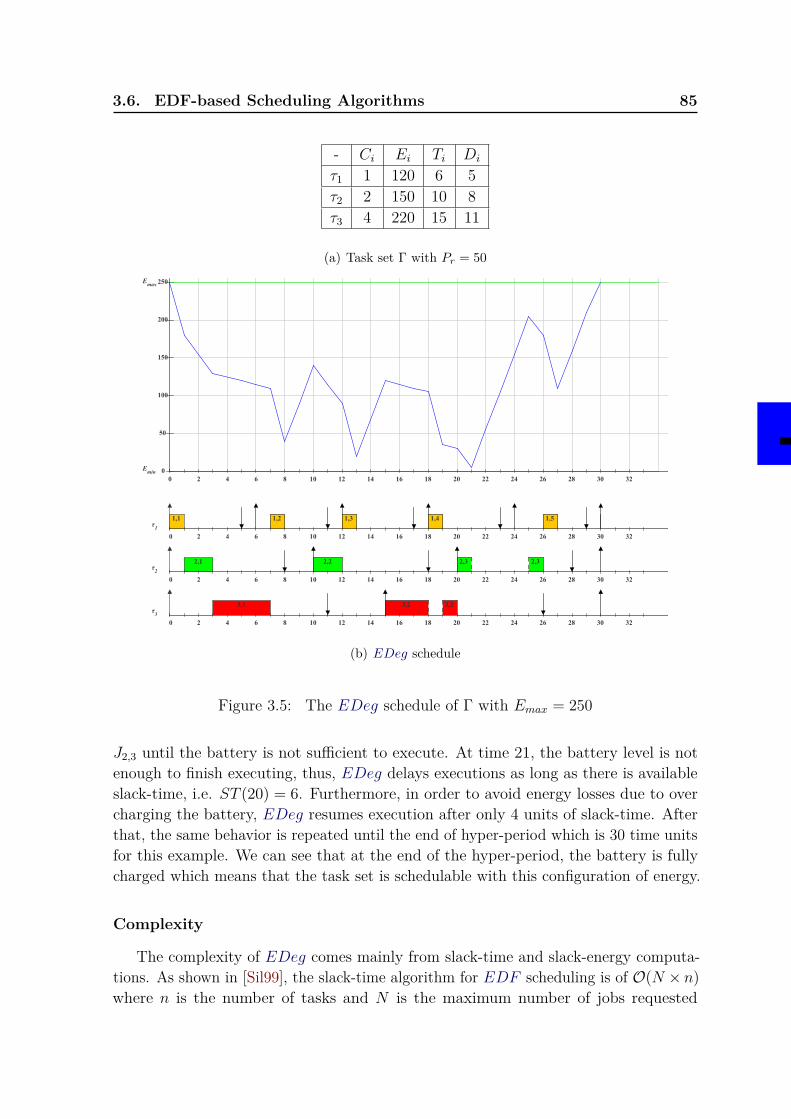
3.6. EDF-based Scheduling Algorithms 85
- Ci Ei Ti Di
τ1 1 120 6 5τ2 2 150 10 8τ3 4 220 15 11
(a) Task set Γ with Pr = 50
0 2 4 6 8 10 12 14 16 18 20 22 24 26 28 30 320
50
100
150
200
250Emax
Emin
1,1 1,2 1,3 1,4 1,5
0 2 4 6 8 10 12 14 16 18 20 22 24 26 28 30 32
τ1
2,1 2,2 2,3 2,3
0 2 4 6 8 10 12 14 16 18 20 22 24 26 28 30 32
τ2
3,1 3,2 3,2
0 2 4 6 8 10 12 14 16 18 20 22 24 26 28 30 32
τ3
(b) EDeg schedule
Figure 3.5: The EDeg schedule of Γ with Emax = 250
J2,3 until the battery is not sufficient to execute. At time 21, the battery level is notenough to finish executing, thus, EDeg delays executions as long as there is availableslack-time, i.e. ST (20) = 6. Furthermore, in order to avoid energy losses due to overcharging the battery, EDeg resumes execution after only 4 units of slack-time. Afterthat, the same behavior is repeated until the end of hyper-period which is 30 time unitsfor this example. We can see that at the end of the hyper-period, the battery is fullycharged which means that the task set is schedulable with this configuration of energy.
Complexity
The complexity of EDeg comes mainly from slack-time and slack-energy computa-tions. As shown in [Sil99], the slack-time algorithm for EDF scheduling is of O(N × n)where n is the number of tasks and N is the maximum number of jobs requested
86 Chapter 3. Real-time Scheduling for Energy-Harvesting Systems
within a hyper-period. Moreover, the complexity of slack-energy algorithm is also ofO(N × n) as shown in [EGCC11]. Therefore, the complexity of EDeg in the worst-caseis pseudo-polynomial which might be a serious drawback in practice.
Optimality
EDeg was proved to be optimal for periodic and synchronous task sets in [Che14].This optimality is inherited from the optimality of EDF for Liu and Layland’s model.Since EDeg predicts future deadline misses due to energy lack and does not wasteenergy when delaying executions, it takes advantage of the dynamic priority to schedulethe earliest deadline first and maximizes the supportable workload. If a deadline ismissed with EDeg, this means the energy is not sufficient which makes the task setunschedulable by any other algorithm.
Minimum Storage Unit Capacity
Intuitively, one can say that the maximum battery capacity needed for EDeg isthe same as EDL since we can apply the same reasoning on idle periods. Then, thesame pessimistic bound can be applied, i.e. the sum of the energy that can be collectedduring all idle periods of one hyper-period.
Schedulability Conditions
A schedulability test for EDeg was proposed in [Che14]. It consists of checking ifthe energy available during any time interval is sufficient to satisfy the energy demandof the same time interval. Knowing that this can be checked by comparing the energyutilization to 1 for tasks with constrained or implicit deadlines, a task set is saidschedulable with EDeg if and only if processor and energy utilizations are lesser orequal to one, i.e. U ≤ 1 and Ue ≤ 1. Furthermore, knowing that EDeg is optimal, thistest becomes a necessary and sufficient feasibility condition for synchronous periodictask sets with implicit deadlines, and only necessary for task sets with constraineddeadlines.
3.6.3 Lazy Scheduling Algorithm (LSA)The Lazy Scheduling Algorithm (LSA) is one of the main EDF-based algorithms
proposed in the literature. It was proposed for the first time by Moser et al. in[Mos+06b] and was revisited in [Mos+06a; Mos+07]. It is an energy-driven algorithmin contrast to classical algorithms which are time-driven. This means that schedulingdecisions are made only according to the available energy, thus, if energy is sufficient,time will be sufficient too. This comes from the fact that all tasks consume energywith the same rate and that tasks execution times depend on the consumption rateauthorized by the system. This algorithm is interesting to study because it has areasonable overhead and is optimal for the considered model.
3.6. EDF-based Scheduling Algorithms 87
Model
Task ModelThe task set considered by LSA is composed by n independent, preemptive and aperiodictasks. Each task is characterized by its energy cost Ei and its relative deadline Di.The tasks drain energy from the storage unit with the same consumption functiondenoted PD(t). This function is upper bounded by the maximum consumption ratePmax. Moreover, it is up to the scheduling algorithm to decide which consumption rateto apply at time t. Knowing that LSA is energy-driven, the execution time Ci of atask depends on its energy cost and the applied consumption rate. Then, when theconsumption rate is maximized, Ci is minimized, i.e. PD(t) = Pmax ⇒ Ci = Ei/Pmax.Therefore, as mentioned earlier, the execution time of a task varies from one job to another depending on the applied consumption rate. Then, a job Ji,j that is requested attime ai,j, starts its execution at time si,j and must finish executing at time fi,j beforeits deadline di,j after the energy cost of the job has been consumed, thus, we haveai,j ≤ si,j < fi,j ≤ di,j.
Energy ModelIn [Mos+06a; Mos+07], the authors considered the solar energy as energy source. Then,to cope with the fluctuations of the output energy that characterizes a photovoltaiccell, they proposed to use the Energy Variability Characterization Curves (EVCC)that bound the energy harvested in any time interval ∆: εl for the lower bound curve.The EVCCs are extracted from actual solar energy traces to provide guarantees on theproduced energy. Therefore, the replenishment function denoted Pr(t) is lower boundedby a known function, and the energy harvested in a certain time interval [t1, t2] denotedg(t1, t2) is given by as:
g(t1, t2) =∫ t2
t1Pr(t).dt ≥ εl(t1, t2)
For the storage unit, they considered an ideal rechargeable battery of capacity Cthat can be charged and discharged with a linear function. Its energy level at timet is denoted E(t) and must stay between the two thresholds Emin and Emax withC = Emax − Emin.
Algorithm Description
The LSA algorithm is EDF-based, thus, it schedules aperiodic jobs according toearliest deadline first rules. The only difference is the time si,j when a job Ji,j beginseffectively its execution. This time is computed such that energy constraints arerespected, namely the energy cost and the battery capacity limit. Indeed, knowing thatall tasks have the same consumption rate, si,j is the earliest time at which the systemcan start executing after a replenishment period. This execution is continuous andincludes Ji,j and a maximum of eventual higher priority jobs. This execution period
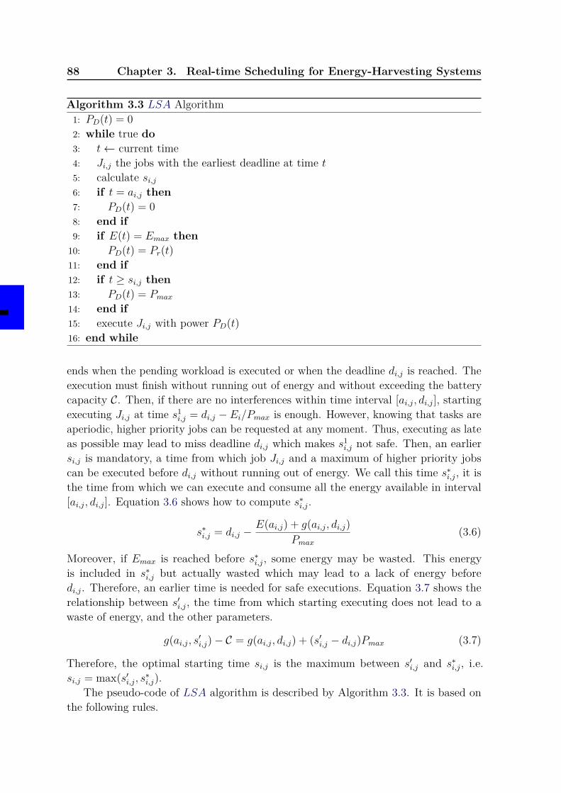
88 Chapter 3. Real-time Scheduling for Energy-Harvesting Systems
Algorithm 3.3 LSA Algorithm1: PD(t) = 02: while true do3: t← current time4: Ji,j the jobs with the earliest deadline at time t5: calculate si,j6: if t = ai,j then7: PD(t) = 08: end if9: if E(t) = Emax then10: PD(t) = Pr(t)11: end if12: if t ≥ si,j then13: PD(t) = Pmax14: end if15: execute Ji,j with power PD(t)16: end while
ends when the pending workload is executed or when the deadline di,j is reached. Theexecution must finish without running out of energy and without exceeding the batterycapacity C. Then, if there are no interferences within time interval [ai,j, di,j], startingexecuting Ji,j at time s1
i,j = di,j − Ei/Pmax is enough. However, knowing that tasks areaperiodic, higher priority jobs can be requested at any moment. Thus, executing as lateas possible may lead to miss deadline di,j which makes s1
i,j not safe. Then, an earliersi,j is mandatory, a time from which job Ji,j and a maximum of higher priority jobscan be executed before di,j without running out of energy. We call this time s∗i,j, it isthe time from which we can execute and consume all the energy available in interval[ai,j, di,j]. Equation 3.6 shows how to compute s∗i,j.
s∗i,j = di,j −E(ai,j) + g(ai,j, di,j)
Pmax(3.6)
Moreover, if Emax is reached before s∗i,j, some energy may be wasted. This energyis included in s∗i,j but actually wasted which may lead to a lack of energy beforedi,j. Therefore, an earlier time is needed for safe executions. Equation 3.7 shows therelationship between s′i,j, the time from which starting executing does not lead to awaste of energy, and the other parameters.
g(ai,j, s′i,j)− C = g(ai,j, di,j) + (s′i,j − di,j)Pmax (3.7)
Therefore, the optimal starting time si,j is the maximum between s′i,j and s∗i,j, i.e.si,j = max(s′i,j, s∗i,j).
The pseudo-code of LSA algorithm is described by Algorithm 3.3. It is based onthe following rules.
3.6. EDF-based Scheduling Algorithms 89
• Rule 1: EDF scheduling is used with PD(t) = Pmax when t ≥ si,j;
• Rule 2: if Emax is reached, jobs are run with PD(t) = Pr(t) in order to avoidenergy waste
Complexity
The LSA algorithm has the same complexity as EDF since it adds only thecomputation of si,j of one job and some verifications, which can be done in O(1). Themost costly operation is to select the job to execute. This operation can be done inO(n) in the worst-case where n is the number of tasks. Therefore, the complexity ofLSA is O(n).
Optimality
In [Mos+07], the LSA algorithm was proved to be optimal for the specific modeldescribed earlier in this section. In fact, the LSA algorithm can miss deadlines only intwo possible situations: when the time is not sufficient to satisfy the workload or whenthe available energy is not sufficient to satisfy the demand of energy.
• A deadline cannot be respected if the time is not sufficient to assign the availableenergy with the maximum consumption rate Pmax. In this case, unprocessedenergy remains in the storage unit and we have E(di,j) > Emin.
• A deadline violation occurs also because the required energy is simply not availableat the deadline. In this case, the battery is exhausted before deadline, i.e.E(di,j) ≤ Emin.
These are the insights of LSA optimality, the complete and detailed proof is availablein [Mos+07].
Note that the optimality of LSA relies strongly on the assumption of havingthe same consumption function PD(t) for all the tasks. Then, if we apply differentconsumption rates to each task, the computation of the starting time si,j is no longerexact. In fact, if we suppose that each task has its own consumption rate denoted Pi(t),considering max1≤i≤n(Pi(t)) as Pmax leads to a later starting time si,j than the optimalone. Furthermore, considering min1≤i≤n(Pi(t)) as Pmax leads to an earlier starting timethan the optimal one which may lead to avoidable energy failures or deadline misses.Figure 3.6 on the following page shows a LSA schedule of a task set with differentconsumption rates where a deadline is missed while a valid schedule is possible. We cansee in Figure 3.6(b) on the next page that s1,1 of job J1,1 is computed at time 0 withPmax = max1≤i≤n(Pi(t)) which gives s1,1 = 3− 0+3×(3−0)
5 = 2. This value of s1,1 leads toa deadline miss because the energy demand is overestimated, and therefore, s1,1 is overdelayed. We can see that the consumption rate used to compute si,j is very importantbecause it influences the earliness or the tardiness of execution starting time. LSA
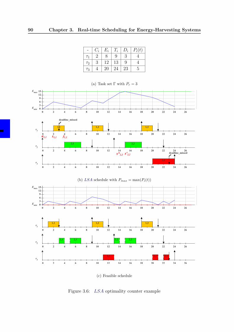
90 Chapter 3. Real-time Scheduling for Energy-Harvesting Systems
- Ci Ei Ti Di Pi(t)τ1 2 8 9 3 4τ2 3 12 13 9 4τ3 4 20 24 23 5
(a) Task set Γ with Pr = 3
0 2 4 6 8 10 12 14 16 18 20 22 24 2603691215E
max
Emin
s1,1a1,1
s'2,2
f1,1
s*2,2
deadline_missed
1,1 1,2 1,3
0 2 4 6 8 10 12 14 16 18 20 22 24 26
τ1
2,1 2,2
0 2 4 6 8 10 12 14 16 18 20 22 24 26
τ2
deadline_missed
3,1
0 2 4 6 8 10 12 14 16 18 20 22 24 26
τ3
(b) LSA schedule with Pmax = max(Pi(t))
0 2 4 6 8 10 12 14 16 18 20 22 24 2603691215E
max
Emin
1,1 1,2 1,3
0 2 4 6 8 10 12 14 16 18 20 22 24 26
τ1
2,1 2,1 2,2 2,2
0 2 4 6 8 10 12 14 16 18 20 22 24 26
τ2
3,1 3,1 3,1
0 2 4 6 8 10 12 14 16 18 20 22 24 26
τ3
(c) Feasible schedule
Figure 3.6: LSA optimality counter example
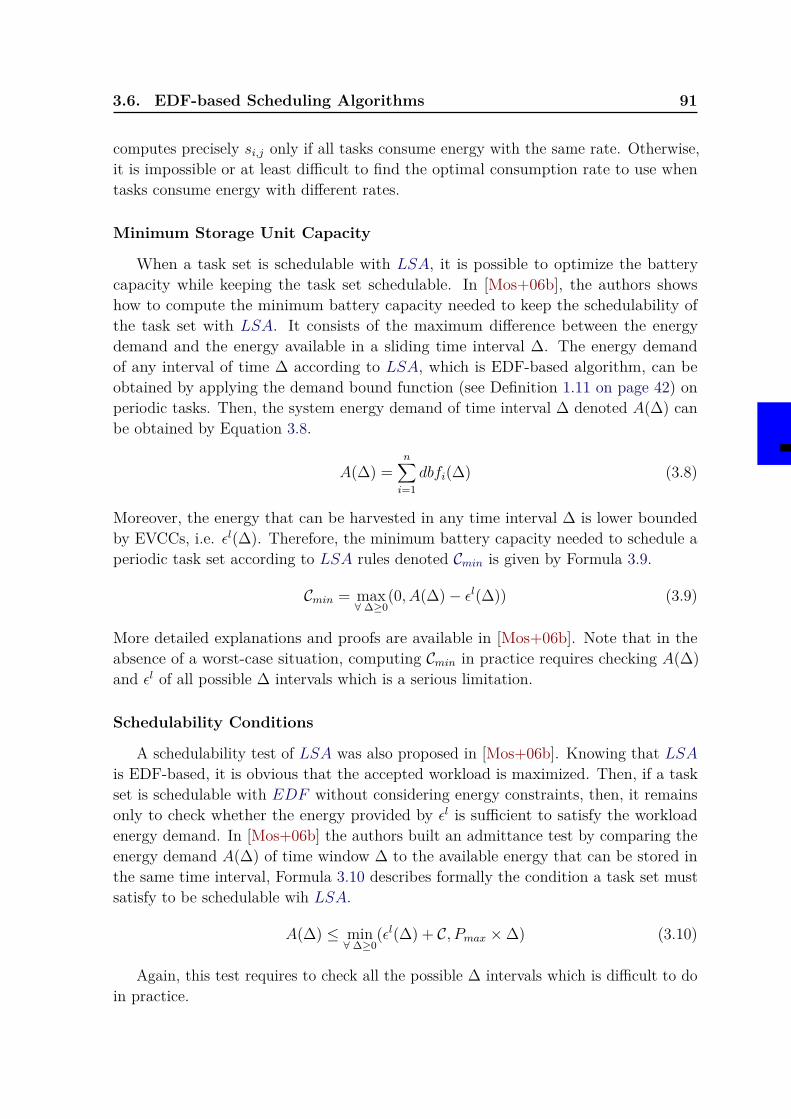
3.6. EDF-based Scheduling Algorithms 91
computes precisely si,j only if all tasks consume energy with the same rate. Otherwise,it is impossible or at least difficult to find the optimal consumption rate to use whentasks consume energy with different rates.
Minimum Storage Unit Capacity
When a task set is schedulable with LSA, it is possible to optimize the batterycapacity while keeping the task set schedulable. In [Mos+06b], the authors showshow to compute the minimum battery capacity needed to keep the schedulability ofthe task set with LSA. It consists of the maximum difference between the energydemand and the energy available in a sliding time interval ∆. The energy demandof any interval of time ∆ according to LSA, which is EDF-based algorithm, can beobtained by applying the demand bound function (see Definition 1.11 on page 42) onperiodic tasks. Then, the system energy demand of time interval ∆ denoted A(∆) canbe obtained by Equation 3.8.
A(∆) =n∑i=1
dbfi(∆) (3.8)
Moreover, the energy that can be harvested in any time interval ∆ is lower boundedby EVCCs, i.e. εl(∆). Therefore, the minimum battery capacity needed to schedule aperiodic task set according to LSA rules denoted Cmin is given by Formula 3.9.
Cmin = max∀ ∆≥0
(0, A(∆)− εl(∆)) (3.9)
More detailed explanations and proofs are available in [Mos+06b]. Note that in theabsence of a worst-case situation, computing Cmin in practice requires checking A(∆)and εl of all possible ∆ intervals which is a serious limitation.
Schedulability Conditions
A schedulability test of LSA was also proposed in [Mos+06b]. Knowing that LSAis EDF-based, it is obvious that the accepted workload is maximized. Then, if a taskset is schedulable with EDF without considering energy constraints, then, it remainsonly to check whether the energy provided by εl is sufficient to satisfy the workloadenergy demand. In [Mos+06b] the authors built an admittance test by comparing theenergy demand A(∆) of time window ∆ to the available energy that can be stored inthe same time interval, Formula 3.10 describes formally the condition a task set mustsatisfy to be schedulable wih LSA.
A(∆) ≤ min∀ ∆≥0
(εl(∆) + C, Pmax ×∆) (3.10)
Again, this test requires to check all the possible ∆ intervals which is difficult to doin practice.
92 Chapter 3. Real-time Scheduling for Energy-Harvesting Systems
3.7 Fixed-Priority SchedulingMost of available research addressing real-time scheduling for energy-harvesting
systems focuses mainly on EDF-based solutions because of the optimility of EDF forLiu and Layland’s model. Nevertheless, some fixed-task-priority algorithms have beenproposed in the literature that we describe in this section.
3.7.1 The PFPALAP Scheduling AlgorithmPreemptive Fixed-Priority As Late As Possible (PFPALAP ) is a fixed-priority schedul-
ing policy that delays jobs executions as long as possible, i.e. as long as availableslack-time, in order to replenish the battery as much as possible before authorizingexecutions. We studied the properties of this algorithm in [CAM12].
Model
The model applied to this algorithm is the same as for EDL algorithm whichis described in Section 3.6.1 on page 80. Since the exact computation of slack-timerequires exact knowledge about jobs arrival times and deadlines, only periodic tasks withconstrained or implicit deadlines are considered. Moreover, the slack-time computationfor fixed-priority does not consider energy constraints, thus, the energy model is notnecessarily specified. Therefore, we can adopt the general model described in Section 3.2on page 67.
Algorithm Description
The Preemptive Fixed-Task-Priority As Late As Possible (PFPALAP ) algorithmis the fixed-task-priority counter-part of EDL. Its main operation is the dynamiccomputation of slack-time. The slack-time algorithm used for PFPALAP is the oneproposed by Davis et al. in [DTB93]. Each priority level has its own slack-time at timet denoted STi(t). For priority level-i, it consists of computing the length of idle periodsthat can be merged in once within the time window starting from time t and ending atthe next deadline of level-i. Algorithm 3.4 on the facing page shows how to computeSTi(t).
Notations:
• di(t): the next absolute deadline of priority level-i after time t,
• ai(t): the next activation time of priority level-i,
• ci(t): the remaining execution time at time t of the current job of priority level-i,
• idle(t1, t2): the amount of time the processor is idle within an interval of time,
• Wmi (t): the recurrent workload function.
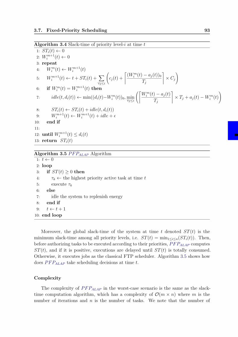
3.7. Fixed-Priority Scheduling 93
Algorithm 3.4 Slack-time of priority level-i at time t1: STi(t)← 02: Wm+1
i (t)← 03: repeat4: Wm
i (t)← Wm+1i (t)
5: Wm+1i (t)← t+ STi(t) +
∑∀j≤i
(cj(t) +
⌈(Wm
i (t)− aj(t))0
Tj
⌉× Cj
)6: if Wm
i (t) = Wm+1i (t) then
7: idle(t, di(t))← min((di(t)−Wmi (t))0,min
∀j≤i
(⌈Wmi (t)− aj(t)
Tj
⌉× Tj + aj(t)−Wm
i (t))
8: STi(t)← STi(t) + idle(t, di(t))9: Wm+1
i (t)← Wm+1i (t) + idle+ ε
10: end if11:12: until Wm+1
i (t) ≤ di(t)13: return STi(t)
Algorithm 3.5 PFPALAP Algorithm1: t← 02: loop3: if ST (t) ≥ 0 then4: τk ← the highest priority active task at time t5: execute τk6: else7: idle the system to replenish energy8: end if9: t← t+ 1
10: end loop
Moreover, the global slack-time of the system at time t denoted ST (t) is theminimum slack-time among all priority levels, i.e. ST (t) = min1≤i≤n(STi(t)). Then,before authorizing tasks to be executed according to their priorities, PFPALAP computesST (t), and if it is positive, executions are delayed until ST (t) is totally consumed.Otherwise, it executes jobs as the classical FTP scheduler. Algorithm 3.5 shows howdoes PFPALAP take scheduling decisions at time t.
Complexity
The complexity of PFPALAP in the worst-case scenario is the same as the slack-time computation algorithm, which has a complexity of O(m × n) where m is thenumber of iterations and n is the number of tasks. We note that the number of
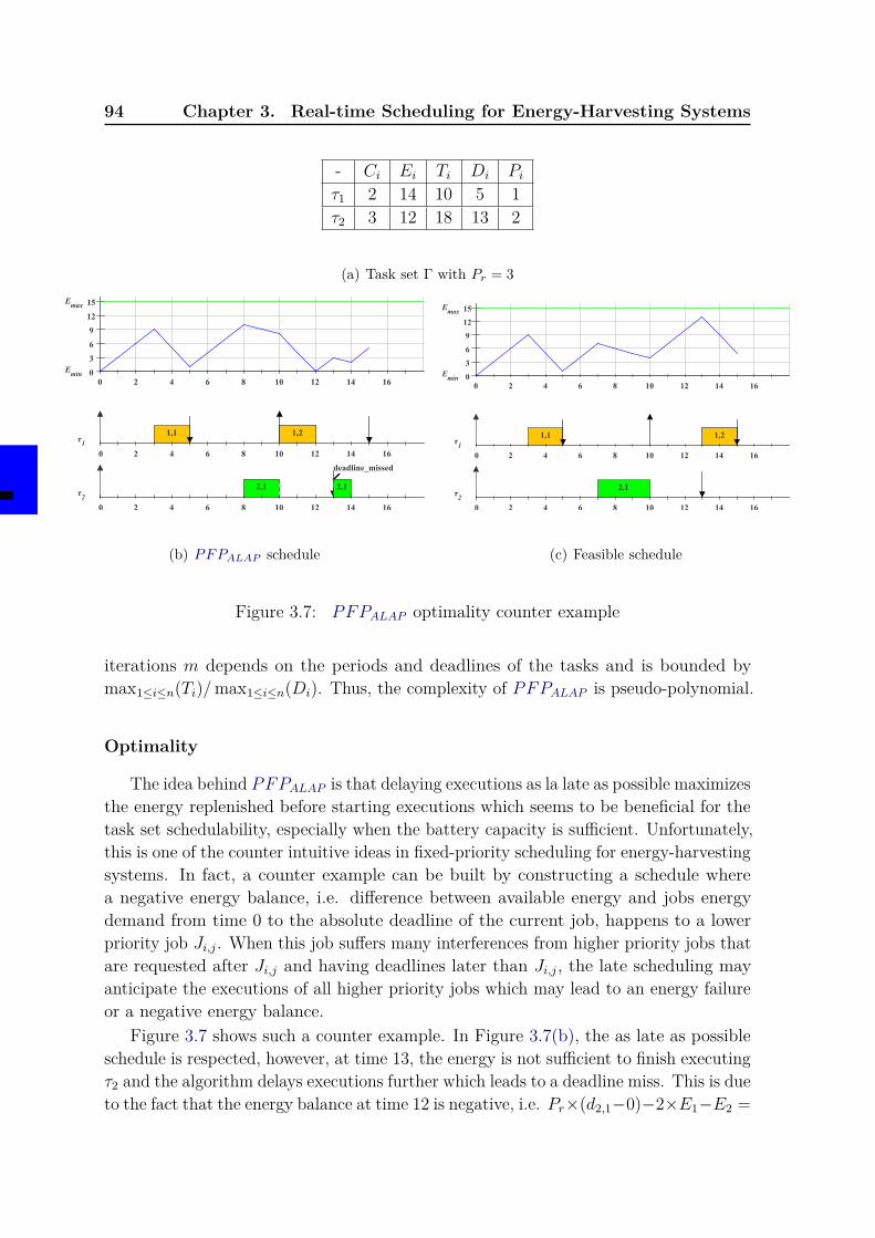
94 Chapter 3. Real-time Scheduling for Energy-Harvesting Systems
- Ci Ei Ti Di Piτ1 2 14 10 5 1τ2 3 12 18 13 2
(a) Task set Γ with Pr = 3
0 2 4 6 8 10 12 14 160
3
6
9
12
15Emax
Emin
1,1 1,2
0 2 4 6 8 10 12 14 16
τ1
2,1
deadline_missed
2,1
0 2 4 6 8 10 12 14 16
τ2
(b) PFPALAP schedule
0 2 4 6 8 10 12 14 160
3
6
9
12
15Emax
Emin
1,1 1,2
0 2 4 6 8 10 12 14 16
τ1
2,1
0 2 4 6 8 10 12 14 16
τ2
(c) Feasible schedule
Figure 3.7: PFPALAP optimality counter example
iterations m depends on the periods and deadlines of the tasks and is bounded bymax1≤i≤n(Ti)/max1≤i≤n(Di). Thus, the complexity of PFPALAP is pseudo-polynomial.
Optimality
The idea behind PFPALAP is that delaying executions as la late as possible maximizesthe energy replenished before starting executions which seems to be beneficial for thetask set schedulability, especially when the battery capacity is sufficient. Unfortunately,this is one of the counter intuitive ideas in fixed-priority scheduling for energy-harvestingsystems. In fact, a counter example can be built by constructing a schedule wherea negative energy balance, i.e. difference between available energy and jobs energydemand from time 0 to the absolute deadline of the current job, happens to a lowerpriority job Ji,j . When this job suffers many interferences from higher priority jobs thatare requested after Ji,j and having deadlines later than Ji,j, the late scheduling mayanticipate the executions of all higher priority jobs which may lead to an energy failureor a negative energy balance.
Figure 3.7 shows such a counter example. In Figure 3.7(b), the as late as possibleschedule is respected, however, at time 13, the energy is not sufficient to finish executingτ2 and the algorithm delays executions further which leads to a deadline miss. This is dueto the fact that the energy balance at time 12 is negative, i.e. Pr×(d2,1−0)−2×E1−E2 =
3.7. Fixed-Priority Scheduling 95
−1, and that the slack-time computation does not take into account tasks energy cost.Furthermore, by executing τ2 earlier, the task set becomes feasible. Therefore, PFPALAPcannot be optimal.
Minimum Storage Unit Capacity
For the same reasons as EDL algorithm, it is difficult to estimate the minimumbattery capacity needed to keep a schedulable task set schedulable. Indeed, the worst-case scenario that maximizes the needed energy storage capacity is not known up tonow.
Schedulability Conditions
Without energy constraints, PFPALAP has the same schedulability as the classicalFTP algorithm. However, when energy constraints are considered, it is difficult tocheck the schedulability of a task set with PFPALAP algorithm without simulating theschedule for at least a hyper-period. This is due to the fact that it is difficult to findthe worst-case scenario that leads to the worst response times of tasks.
3.7.2 Preemptive Fixed-Priority with Slack-Time Algorithm
Among several heuristics proposed by Chetto et al. in [CMM11], the PreemptiveFixed-Priority with Slack-Time (PFPST ) algorithm was the most pertinent and theone with the highest schedulability rate. It alternates classical FTP schedule with theone of PFPALAP when battery boundaries are reached.
Model
The model considered in [CMM11] for Preemptive Fixed-Task-Priority with Slack-Time (PFPST ) is the same as the one described in Section 3.2 on page 67.
Algorithm Description
The behavior of PFPST algorithm is simple, it schedules jobs according to theirpriorities as soon as possible when the battery level is higher than Emin. Then, it delaysexecutions as long as available slack-time in order to replenish a maximum of energybefore resuming executions. The slack-time algorithm is the same as the one used forPFPALAP . Moreover, executions are resumed when Emax is reached during an idleperiod in order to avoid energy losses. Algorithm 3.6 on the next page summarizes thescheduling schemes of PFPALAP .
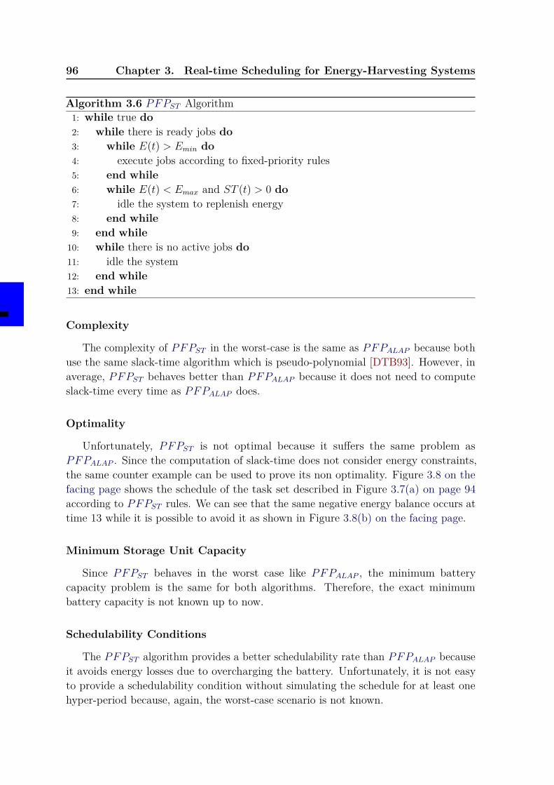
96 Chapter 3. Real-time Scheduling for Energy-Harvesting Systems
Algorithm 3.6 PFPST Algorithm1: while true do2: while there is ready jobs do3: while E(t) > Emin do4: execute jobs according to fixed-priority rules5: end while6: while E(t) < Emax and ST (t) > 0 do7: idle the system to replenish energy8: end while9: end while
10: while there is no active jobs do11: idle the system12: end while13: end while
Complexity
The complexity of PFPST in the worst-case is the same as PFPALAP because bothuse the same slack-time algorithm which is pseudo-polynomial [DTB93]. However, inaverage, PFPST behaves better than PFPALAP because it does not need to computeslack-time every time as PFPALAP does.
Optimality
Unfortunately, PFPST is not optimal because it suffers the same problem asPFPALAP . Since the computation of slack-time does not consider energy constraints,the same counter example can be used to prove its non optimality. Figure 3.8 on thefacing page shows the schedule of the task set described in Figure 3.7(a) on page 94according to PFPST rules. We can see that the same negative energy balance occurs attime 13 while it is possible to avoid it as shown in Figure 3.8(b) on the facing page.
Minimum Storage Unit Capacity
Since PFPST behaves in the worst case like PFPALAP , the minimum batterycapacity problem is the same for both algorithms. Therefore, the exact minimumbattery capacity is not known up to now.
Schedulability Conditions
The PFPST algorithm provides a better schedulability rate than PFPALAP becauseit avoids energy losses due to overcharging the battery. Unfortunately, it is not easyto provide a schedulability condition without simulating the schedule for at least onehyper-period because, again, the worst-case scenario is not known.
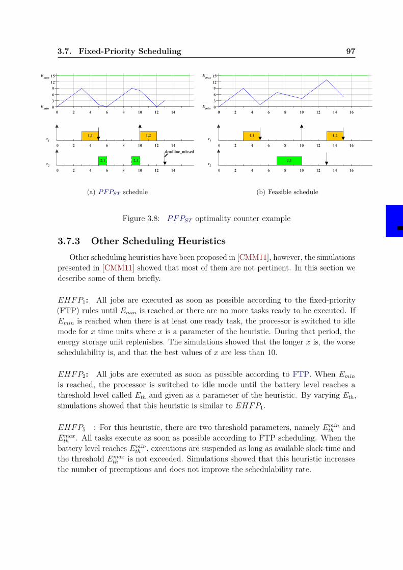
3.7. Fixed-Priority Scheduling 97
0 2 4 6 8 10 12 140
3
6
9
12
15Emax
Emin
1,1 1,2
0 2 4 6 8 10 12 14
τ1
2,1 2,1
deadline_missed
0 2 4 6 8 10 12 14
τ2
(a) PFPST schedule
0 2 4 6 8 10 12 14 160
3
6
9
12
15Emax
Emin
1,1 1,2
0 2 4 6 8 10 12 14 16
τ1
2,1
0 2 4 6 8 10 12 14 16
τ2
(b) Feasible schedule
Figure 3.8: PFPST optimality counter example
3.7.3 Other Scheduling HeuristicsOther scheduling heuristics have been proposed in [CMM11], however, the simulations
presented in [CMM11] showed that most of them are not pertinent. In this section wedescribe some of them briefly.
EHFP1: All jobs are executed as soon as possible according to the fixed-priority(FTP) rules until Emin is reached or there are no more tasks ready to be executed. IfEmin is reached when there is at least one ready task, the processor is switched to idlemode for x time units where x is a parameter of the heuristic. During that period, theenergy storage unit replenishes. The simulations showed that the longer x is, the worseschedulability is, and that the best values of x are less than 10.
EHFP2: All jobs are executed as soon as possible according to FTP. When Eminis reached, the processor is switched to idle mode until the battery level reaches athreshold level called Eth and given as a parameter of the heuristic. By varying Eth,simulations showed that this heuristic is similar to EHFP1.
EHFP5 : For this heuristic, there are two threshold parameters, namely Eminth and
Emaxth . All tasks execute as soon as possible according to FTP scheduling. When the
battery level reaches Eminth , executions are suspended as long as available slack-time and
the threshold Emaxth is not exceeded. Simulations showed that this heuristic increases
the number of preemptions and does not improve the schedulability rate.
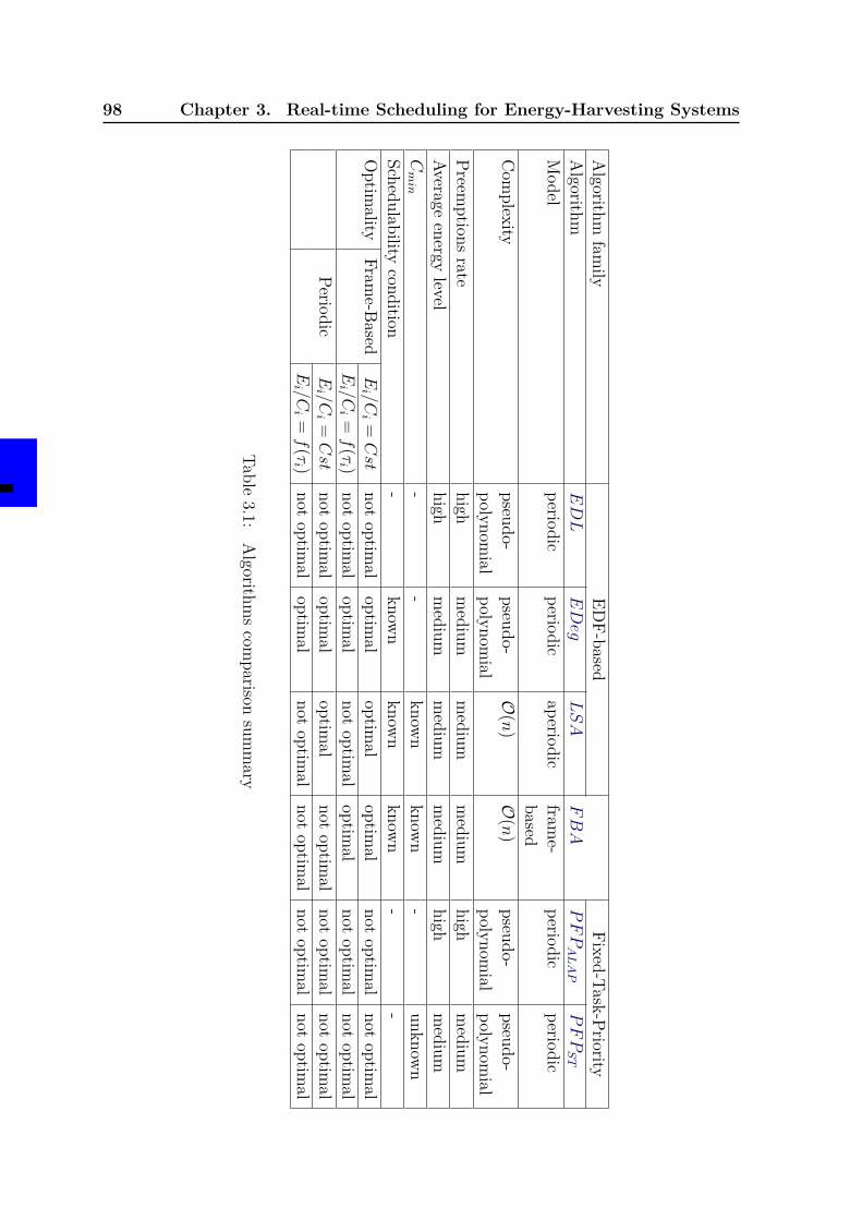
98 Chapter 3. Real-time Scheduling for Energy-Harvesting Systems
Algorithm
family
EDF-based
Fixed-Task-PriorityAlgorithm
EDL
EDeg
LSA
FBA
PFPALAP
PFPST
Model
periodicperiodic
aperiodicfram
e-based
periodicperiodic
Com
plexitypseudo-polynom
ialpseudo-polynom
ialO
(n)O
(n)pseudo-polynom
ialpseudo-polynom
ialPreem
ptionsrate
highmedium
medium
medium
highmedium
Averageenergy
levelhigh
medium
medium
medium
highmedium
Cmin
--
known
known
-unknow
nSchedulability
condition-
known
known
known
--
Optim
alityFram
e-BasedEi /C
i =Cst
notoptim
aloptim
aloptim
aloptim
alnot
optimal
notoptim
alEi /C
i =f(τ
i )not
optimal
optimal
notoptim
aloptim
alnot
optimal
notoptim
alPeriodic
Ei /C
i =Cst
notoptim
aloptim
aloptim
alnot
optimal
notoptim
alnot
optimal
Ei /C
i =f(τ
i )not
optimal
optimal
notoptim
alnot
optimal
notoptim
alnot
optimal
Table3.1:
Algorithm
scom
parisonsum
mary
3.8. Performance Evaluation and Comparison 99
3.8 Performance Evaluation and ComparisonWe described the main scheduling algorithms available in the state of the art. In
this section we evaluate these algorithms through simulations over some metrics inorder to show their strengths and weaknesses.
3.8.1 Simulation configurationIn this subsection, we describe the configuration of the experiments, namely the
task sets generation, the parameters and the assumptions.
Competitors
• the EDL algorithm described in Section 3.6.1 on page 80,
• the EDeg algorithm described in Section 3.6.2 on page 83,
• the LSA algorithm described in Section 3.6.3 on page 86,
• the FBA algorithm described in Section 3.5 on page 75,
• the PFPALAP algorithm described in Section 3.7.1 on page 92 with deadlinemonotonic tasks priority ordering,
• the PFPST algorithm described in Section 3.7.2 on page 95 with deadline mono-tonic tasks priority ordering.
Task ModelsAs mentioned in the above sections, each algorithm is designed for a specific task model.In order to compare them against each other we evaluate them over different taskmodels and assumptions. For this experiment, we select three main models:
• the frame-based model described in Section 3.5 on page 75,
• the periodic task model with implicit deadlines described in Section 3.2 on page 67,
• the periodic task model with constrained deadlines.
For each task model, we run simulations over four energy configurations that coverthe main assumptions that make the evaluated algorithms optimal:
• the same consumption rate for all tasks with an infinite battery capacity, i.e.Ei/Ci=Constant and Emax =∞,
• the same consumption rate for all tasks with an arbitrary limited battery capacity,i.e. Ei/Ci=Constant and Emax=Constant,
100 Chapter 3. Real-time Scheduling for Energy-Harvesting Systems
• variable consumption rates with an infinite battery capacity, i.e. Ei/Ci = f(τi)and Emax =∞,
• variable consumption rates with a limited battery capacity, i.e. Ei/Ci = f(τi)and Emax=Constant.
AssumptionsThis experiment considers the following hypothesis and assumptions:
• in order to focus only on the impact of energy on task sets schedulability, weconsider only time feasible task sets,
• since actual machines cannot handle continuous values, we consider that timeand energy are discretized and that the granularity is small enough to avoiddecimal values, i.e. time and energy are integers and all scheduling operations areperformed before or after one time unit,
• knowing that most of the evaluated algorithms require constant or at least knownreplenishment functions, we consider only constant charging functions Pr(t) = Prin order to make the comparison possible,
• tasks consume energy linearly, i.e. a task consumes Ei/Ci energy units for eachexecution time unit.
Task set generationFor each task model, we generate randomly a sample of 15000 task sets using anadapted version of the U-Unifast Discard algorithm proposed in [BB05]. This algorithmis coupled with the hyper-period limitation technique proposed in [MG01]. In orderto cover most of possible task sets, we generate them according to their processor andenergy utilizations, i.e. U and Ue. Indeed, we vary U and Ue within interval [0.2, 1]with steps of 0.05. Then, we obtain 50 distinct task sets for each couple (U,Ue).
Tasks are generated by considering a battery capacity of 200 units and a constantenergy replenishment rate Pr = 15 units.
MetricsIn this experiment we compare the selected algorithms over the following metrics.
• Failure rate: is the percentage of non feasible task sets among all the testedones. Then, the greater the failure rate is, the lower the algorithm performanceare. This metric helps to confirm the optimality or the non optimality of somealgorithms.
• Preemption rate: for one simulation, it is the number of preemption events. Apreemption event occurs when a job is stopped before finishing its execution. All
3.8. Performance Evaluation and Comparison 101
of the events that occur at the same instant are considered as once. Therefore,the number of possible events is bounded by the number of time units composingthe simulation, i.e. the simulation duration. For several simulations, this metric iscomputed only for feasible task sets and represents the ratio of the average numberof preemptions relative to all possible events. Then, the greater the number ofpreemptions is, the greater the context switch is. Note that this leads to increasethe overhead cost and decreases the performance. The shown results represent thepercentage of the average number of preemption events among the total numberof events.
• Average Energy Level: represents the average energy level of the battery orcapacitor at any instant during the simulation. It is the average of the energy levelobserved for all scheduling events. The best algorithm relative to this criterion isthe one that maximizes the average energy level. This means that the algorithmmakes the system less energy constrained.
The task sets are launched synchronously with an empty battery, i.e. ∀ τi, Oi = 0and E(t) = Emin which seems to be the closest to the actual worst-case scenario of allthe evaluated algorithms.
3.8.2 Results analysisFigure 3.9 on the next page shows the performances of the tested algorithms on
the frame-based task model. As expected most of EDF-based algorithms dominatesfixed-priority ones. We can see also that FBA and EDeg have the lower failure rates.This was expected because in frame-based model, all tasks share the same period andthe same deadline. Thus, ordering tasks according to deadlines or periods does notchange the schedule since the used breakdown rule is to give the priority to jobs withlower energy consumption rate. Note that this rule is not respected when consideringonly deadlines as PFPALAP and PFPST do. Furthermore, we observe that LSA isnot optimal for this model especially when the energy consumption rate varies fromone task to an other. This is due to the fact that LSA considers only the maximumconsumption rate to compute the latest time to execute a job.
Figures 3.10 on page 103 and 3.11 on page 104 show the performances of thealgorithms on the periodic model in different energy and deadline configurations. Then,we can see that FBA behaves badly when tasks have different periods and differentdeadlines. Again, when tasks consumption rates can vary, LSA can take wrong decisionsby overestimating the latest time form which starting executing a job does not leadto a deadline miss. Note that the constrained deadlines increase the rate of unfeasibletask sets for all algorithms which is expected because constrained deadlines let shortertime to jobs to finish their executions than implicit deadlines.
Globally, EDeg is the algorithm with the lower failure rate and preemptions rate overthe tested task models with a good average battery level. This is due to its anticipation
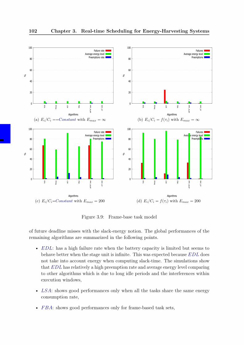
102 Chapter 3. Real-time Scheduling for Energy-Harvesting Systems
0
20
40
60
80
100
EDL
EDeg
LSA
FBA
PFP_ALAP
PFP_ST
%
Algorithms
Failure rateAverage energy level
Preemptions rate
(a) Ei/Ci ==Constant with Emax =∞
0
20
40
60
80
100
EDL
EDeg
LSA
FBA
PFP_ALAP
PFP_ST
%
Algorithms
FailuresAverage energy level
Preemptions
(b) Ei/Ci = f(τi) with Emax =∞
0
20
40
60
80
100
EDL
EDeg
LSA
FBA
PFP_ALAP
PFP_ST
%
Algorithms
Failure rateAverage energy level
Preemptions
(c) Ei/Ci=Constant with Emax = 200
0
20
40
60
80
100
EDL
EDeg
LSA
FBA
PFP_ALAP
PFP_ST
%
Algorithms
FailuresAverage energy level
Preemptions
(d) Ei/Ci = f(τi) with Emax = 200
Figure 3.9: Frame-base task model
of future deadline misses with the slack-energy notion. The global performances of theremaining algorithms are summarized in the following points.
• EDL: has a high failure rate when the battery capacity is limited but seems tobehave better when the stage unit is infinite. This was expected because EDL doesnot take into account energy when computing slack-time. The simulations showthat EDL has relatively a high preemption rate and average energy level comparingto other algorithms which is due to long idle periods and the interferences withinexecution windows,
• LSA: shows good performances only when all the tasks share the same energyconsumption rate,
• FBA: shows good performances only for frame-based task sets,

3.8. Performance Evaluation and Comparison 103
0
20
40
60
80
100
EDL
EDeg
LSA
FBA
PFP_ALAP
PFP_ST
%
Algorithms
Failure rateAverage energy level
Preemptions rate
(a) Ei/Ci=Constant with Emax =∞
0
20
40
60
80
100
EDL
EDeg
LSA
FBA
PFP_ALAP
PFP_ST
%
Algorithms
Failure rateAverage energy level
Preemptions rate
(b) Ei/Ci = f(τi) with Emax =∞
0
20
40
60
80
100
EDL
EDeg
LSA
FBA
PFP_ALAP
PFP_ST
%
Algorithms
Failure rateAverage energy level
Preemptions rate
(c) Ei/Ci=Constant with Emax = 200
0
20
40
60
80
100
EDL
EDeg
LSA
FBA
PFP_ALAP
PFP_ST
%
Algorithms
Failure rateAverage energy level
Preemptions rate
(d) Ei/Ci = f(τi) with Emax = 200
Figure 3.10: Periodic task model with implicit deadlines
• PFPALAP : behaves like EDL but with a higher level of failure and preemptionsbecause it is a fixed-priority algorithm,
• PFPST : behaves a little better than PFPALAP but has the same weaknesses,namely a high failure and preemption rates which are due the slack-time compu-tation that does not consider energy constraints.
3.8.3 Comparison summary
Table 3.1 on page 98 summarizes the properties of the discussed algorithms.
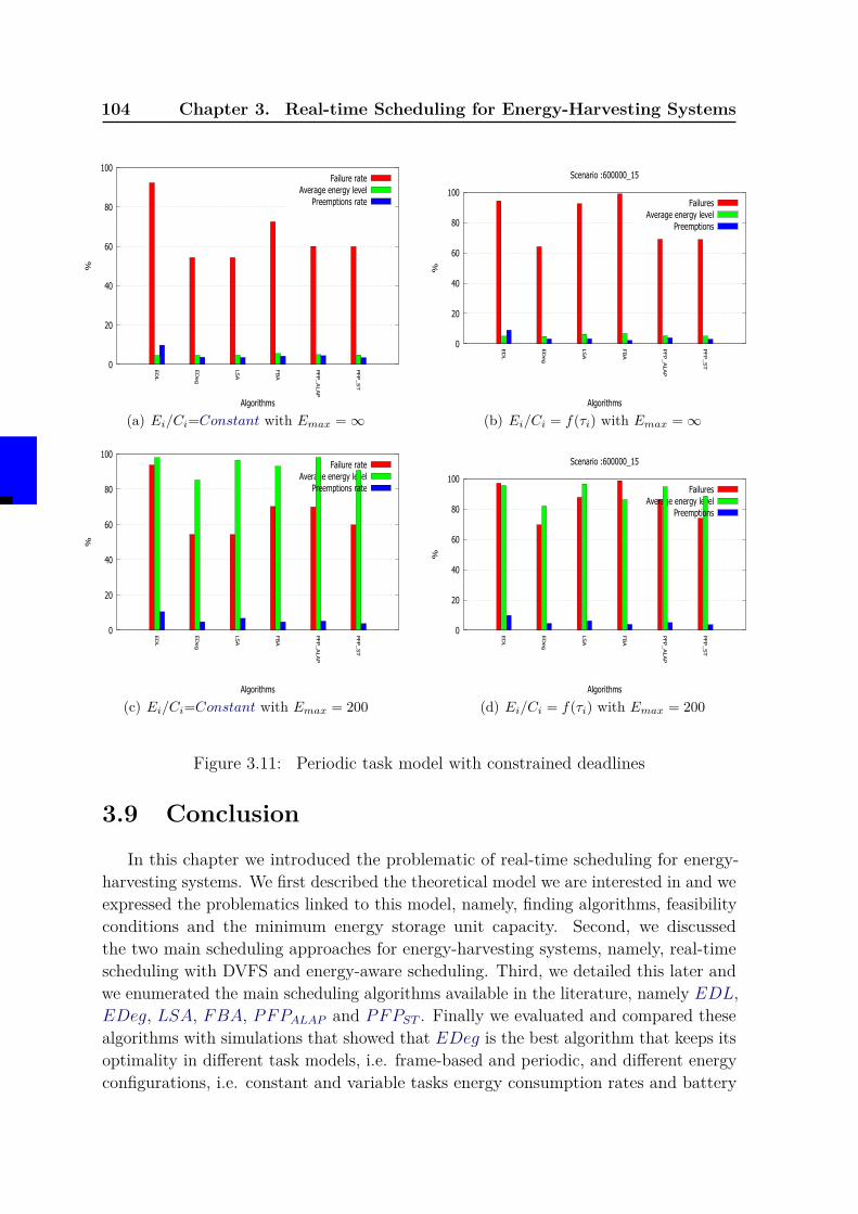
104 Chapter 3. Real-time Scheduling for Energy-Harvesting Systems
0
20
40
60
80
100
EDL
EDeg
LSA
FBA
PFP_ALAP
PFP_ST
%
Algorithms
Failure rateAverage energy level
Preemptions rate
(a) Ei/Ci=Constant with Emax =∞
0
20
40
60
80
100
EDL
EDeg
LSA
FBA
PFP_ALAP
PFP_ST
%
Algorithms
Scenario :600000_15
FailuresAverage energy level
Preemptions
(b) Ei/Ci = f(τi) with Emax =∞
0
20
40
60
80
100
EDL
EDeg
LSA
FBA
PFP_ALAP
PFP_ST
%
Algorithms
Failure rateAverage energy level
Preemptions rate
(c) Ei/Ci=Constant with Emax = 200
0
20
40
60
80
100
EDL
EDeg
LSA
FBA
PFP_ALAP
PFP_ST
%
Algorithms
Scenario :600000_15
FailuresAverage energy level
Preemptions
(d) Ei/Ci = f(τi) with Emax = 200
Figure 3.11: Periodic task model with constrained deadlines
3.9 Conclusion
In this chapter we introduced the problematic of real-time scheduling for energy-harvesting systems. We first described the theoretical model we are interested in and weexpressed the problematics linked to this model, namely, finding algorithms, feasibilityconditions and the minimum energy storage unit capacity. Second, we discussedthe two main scheduling approaches for energy-harvesting systems, namely, real-timescheduling with DVFS and energy-aware scheduling. Third, we detailed this later andwe enumerated the main scheduling algorithms available in the literature, namely EDL,EDeg, LSA, FBA, PFPALAP and PFPST . Finally we evaluated and compared thesealgorithms with simulations that showed that EDeg is the best algorithm that keeps itsoptimality in different task models, i.e. frame-based and periodic, and different energyconfigurations, i.e. constant and variable tasks energy consumption rates and battery
3.9. Conclusion 105
capacity size.We note that most of the proposed solutions are EDF-based because of its optimality
for systems without energy constraints. Furthermore, the EDF scheduling for energy-harvesting systems was the most studied in the past. However, real-time schedulingfor energy harvesting systems with fixed-task-priority, which are as important as EDFscheduling, was not deeply studied. The algorithms available in the literature are notvery efficient and can be widely improved. The aim of this dissertation is to contributeto cover this research area by studying the possibility of adapting some EDF solutionsto fixed-priority and by proposing new scheduling algorithms and feasibility conditionsthat can solve the problematics identified in this chapter.

Part II
Contributions

Chapter 4
The PFPASAP Algorithm
Contents4.1 Introduction . . . . . . . . . . . . . . . . . . . . . . . . . . . . . 109
4.2 Model . . . . . . . . . . . . . . . . . . . . . . . . . . . . . . . . . 110
4.3 Theoretical Study of PFPASAP . . . . . . . . . . . . . . . . . . . 111
4.3.1 As Soon As Possible Preemptive Fixed-Priority . . . . . . . . . . 1114.3.2 Worst-Case Scenario . . . . . . . . . . . . . . . . . . . . . . . . . 1134.3.3 Optimality . . . . . . . . . . . . . . . . . . . . . . . . . . . . . . 1184.3.4 Priority Assignment . . . . . . . . . . . . . . . . . . . . . . . . . 1194.3.5 Schedulability Condition . . . . . . . . . . . . . . . . . . . . . . . 1214.3.6 Battery Capacity . . . . . . . . . . . . . . . . . . . . . . . . . . . 122
4.4 Performance Evaluation . . . . . . . . . . . . . . . . . . . . . . 122
4.4.1 Competitors . . . . . . . . . . . . . . . . . . . . . . . . . . . . . . 1224.4.2 Simulation . . . . . . . . . . . . . . . . . . . . . . . . . . . . . . 1234.4.3 Results Analysis . . . . . . . . . . . . . . . . . . . . . . . . . . . 125
4.5 Conclusion . . . . . . . . . . . . . . . . . . . . . . . . . . . . . . 129
4.1 IntroductionAs noticed in the state of the art, the fixed-priority scheduling for energy-harvesting
was not very well studied compared to dynamic-priority or EDF-based scheduling. Infact only few fixed-priority algorithms are available in the literature. In reality, eventhough the earliest deadline first scheduling has proved its optimality for classicalreal-time systems, it is still not very popular in industry. However, fixed-priorityscheduling is widely used in industry because of its simplicity. Therefore, fixed-priorityis as important as EDF-scheduling and it is worthy to study this type of scheduling forenergy-harvesting systems.
As mentioned in Section 3.3 on page 71, one of the studied problematics is to findfixed-priority scheduling algorithms that respect tasks deadlines and energy-harvestingsystems constraints.
110 Chapter 4. The PFPASAP Algorithm
The main fixed-priority algorithms available in the literature, namely PFPALAPand PFPST which are described in Section 3.7 on page 92, are not optimal and have agreat complexity.
This chapter focuses on optimal fixed-priority solution of the considered problem.We propose the Preemptive Fixed-Task-Priority As Soon As Possible (PFPASAP )algorithm and we prove its optimality for energy-non-concrete task sets that arecomposed only of tasks that consume more energy than the replenished during theirexecution. The work presented in this chapter is the result of a collaboration with Dr.Y. Abdeddaïm and was first published in [ACM13a].
The remaining part of the chapter is organized as follows. We recall the model inSection 4.2. In Section 4.3 we introduce the PFPASAP algorithm, and then, we studysome of its properties, namely its worst-case scenario, its optimality and its optimalpriority assignment. A feasibility condition based on PFPASAP is also proposed. InSection 4.4, we evaluate the performances of PFPASAP by simulations and we comparethem with the ones the algorithms presented in the state of the art. Finally, we concludein Section 4.5.
4.2 ModelThe model considered in this chapter is similar to the one described in Section 3.2
on page 67. The difference here is that we consider only energy-non-concrete task setswhich means that tasks offsets and the initial energy level of the battery are knownonly at run time.
Task ModelWe consider a non-concrete real-time sporadic task set in a renewable energy environmentdefined by a set of n periodic and independent tasks. Each task τi is characterized byits priority Pi, its worst-case execution time Ci, its minimum inter-arrival time Ti, itsrelative deadline Di and its worst-case energy consumption Ei. Since the consideredtask set is non-concrete, the offsets denoted as Oi are known only at run-time.
Energy ModelThe energy model considered in this chapter is exactly the same as the one describedin Section 3.2 on page 67. An energy storage with capacity C and a harvester thatreplenishes the battery continuously with a constant rate Pr. The energy level ofthe storage unit at time t denoted E(t) fluctuates between two thresholds Emax themaximum level and Emin the minimum level such that C = Emax−Emin. Knowing thatthe considered systems are energy-non-concrete, we assume that the initial level of thestorage unit is Emin. Furthermore, we suppose that Pr ≤ C to avoid energy losses. Notethat this is not sufficient to avoid energy losses but it is necessary. Moreover, in thischapter we suppose that tasks consume more energy than harvested during a period
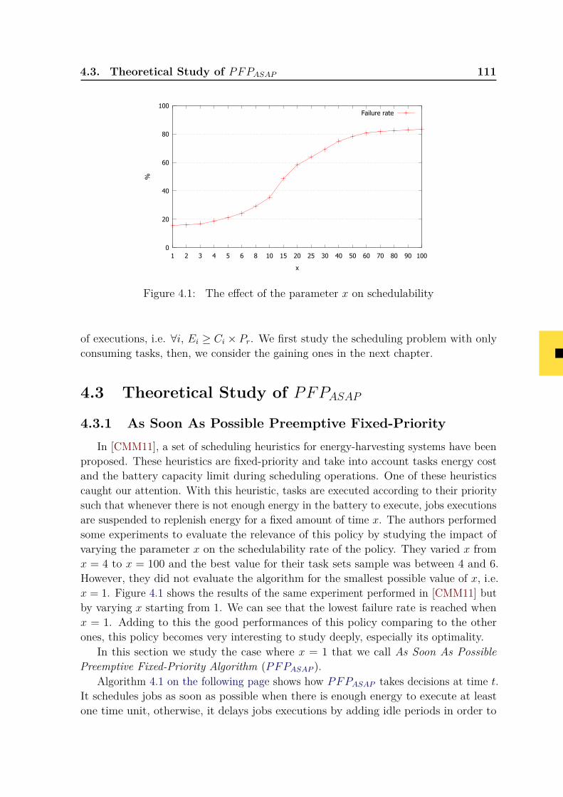
4.3. Theoretical Study of PFPASAP 111
0
20
40
60
80
100
1 2 3 4 5 6 8 10 15 20 25 30 40 50 60 70 80 90 100
%
x
Failure rate
Figure 4.1: The effect of the parameter x on schedulability
of executions, i.e. ∀i, Ei ≥ Ci × Pr. We first study the scheduling problem with onlyconsuming tasks, then, we consider the gaining ones in the next chapter.
4.3 Theoretical Study of PFPASAP4.3.1 As Soon As Possible Preemptive Fixed-Priority
In [CMM11], a set of scheduling heuristics for energy-harvesting systems have beenproposed. These heuristics are fixed-priority and take into account tasks energy costand the battery capacity limit during scheduling operations. One of these heuristicscaught our attention. With this heuristic, tasks are executed according to their prioritysuch that whenever there is not enough energy in the battery to execute, jobs executionsare suspended to replenish energy for a fixed amount of time x. The authors performedsome experiments to evaluate the relevance of this policy by studying the impact ofvarying the parameter x on the schedulability rate of the policy. They varied x fromx = 4 to x = 100 and the best value for their task sets sample was between 4 and 6.However, they did not evaluate the algorithm for the smallest possible value of x, i.e.x = 1. Figure 4.1 shows the results of the same experiment performed in [CMM11] butby varying x starting from 1. We can see that the lowest failure rate is reached whenx = 1. Adding to this the good performances of this policy comparing to the otherones, this policy becomes very interesting to study deeply, especially its optimality.
In this section we study the case where x = 1 that we call As Soon As PossiblePreemptive Fixed-Priority Algorithm (PFPASAP ).
Algorithm 4.1 on the following page shows how PFPASAP takes decisions at time t.It schedules jobs as soon as possible when there is enough energy to execute at leastone time unit, otherwise, it delays jobs executions by adding idle periods in order to
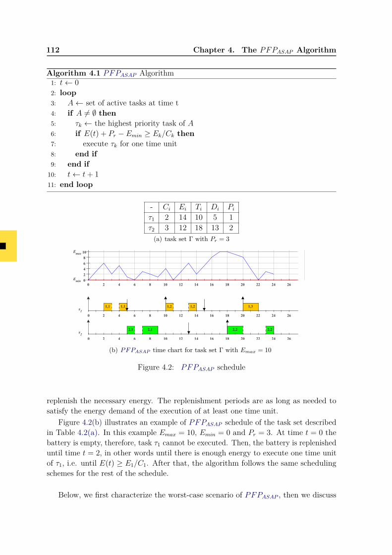
112 Chapter 4. The PFPASAP Algorithm
Algorithm 4.1 PFPASAP Algorithm1: t← 02: loop3: A← set of active tasks at time t4: if A 6= ∅ then5: τk ← the highest priority task of A6: if E(t) + Pr − Emin ≥ Ek/Ck then7: execute τk for one time unit8: end if9: end if10: t← t+ 111: end loop
- Ci Ei Ti Di Piτ1 2 14 10 5 1τ2 3 12 18 13 2(a) task set Γ with Pr = 3
0 2 4 6 8 10 12 14 16 18 20 22 24 260
2
4
6
8
10Emax
Emin
1,1 1,1 1,2 1,2 1,3
0 2 4 6 8 10 12 14 16 18 20 22 24 26
τ1
2,1 2,1 2,2 2,2
0 2 4 6 8 10 12 14 16 18 20 22 24 26
τ2
(b) PFPASAP time chart for task set Γ with Emax = 10
Figure 4.2: PFPASAP schedule
replenish the necessary energy. The replenishment periods are as long as needed tosatisfy the energy demand of the execution of at least one time unit.
Figure 4.2(b) illustrates an example of PFPASAP schedule of the task set describedin Table 4.2(a). In this example Emax = 10, Emin = 0 and Pr = 3. At time t = 0 thebattery is empty, therefore, task τ1 cannot be executed. Then, the battery is replenisheduntil time t = 2, in other words until there is enough energy to execute one time unitof τ1, i.e. until E(t) ≥ E1/C1. After that, the algorithm follows the same schedulingschemes for the rest of the schedule.
Below, we first characterize the worst-case scenario of PFPASAP , then we discuss
4.3. Theoretical Study of PFPASAP 113
its optimality and finally, we build a necessary and sufficient feasibility condition forthe considered family of task sets.
4.3.2 Worst-Case ScenarioThe aim of this section is to characterize the worst-case scenario that a task set can
encounter during its execution with PFPASAP algorithm. First, we recall the notion ofprocessor demand or workload function for fixed-priority scheduling, then we extend itto include tasks energy consumption.
Definition 4.1 (Processor Demand).The processor demand of the ith priority level at time t denoted as Wpi(t), is theamount of time necessary to execute jobs of priority levels 1, . . . , i− 1, i requested inthe interval of time [0, t[. It can be obtained by formula 4.1.
Wpi(t) =∑j≤i
RBFj(t) =∑j≤i
⌈t−Oj
Tj
⌉× Cj (4.1)
�
Now we introduce the notion of replenishment demand.
Definition 4.2 (Replenishment Demand).The replenishment demand of the ith priority level at instant t denoted Wei(t), is theamount of energy to be replenished to execute jobs of priority levels 1, . . . , i − 1, irequested in the interval of time [0, t[. It can be calculated by Equation 4.2.
Wei(t) =∑j≤i
⌈t−Oj
Tj
⌉× Ej − E(0) (4.2)
�
The intuition behind Formula 4.2 is derived from the notion of processor demand.It is the difference between the energy demand of jobs requested inside interval [0, t[and the initial battery level. The initial battery level E(0) is removed to fit with theexact amount of energy to be replenished. Therefore, if Wei(t) is negative, then, theenergy stored in the battery is sufficient and more replenishment is not needed.
Definition 4.3 (Time Demand).The time demand of the ith priority level at time t denoted Wi(t), is the minimumamount of time necessary to satisfy both of the replenishment and processor demandswithin time interval [0, t[. This can be obtained by Equation 4.3.
Wi(t) = max
(⌈Wei(t)Pr
⌉,Wpi(t)
)(4.3)
�
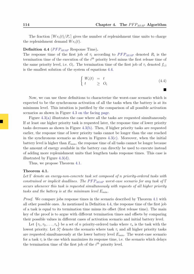
114 Chapter 4. The PFPASAP Algorithm
The fraction dWei(t)/Pre gives the number of replenishment time units to chargethe replenishment demand Wei(t).
Definition 4.4 (PFPASAP Response Time).The response time of the first job of τi according to PFPASAP denoted Ri is thetermination time of the execution of the ith priority level minus the first release time ofthe same priority level, i.e. Oi. The termination time of the first job of τi denoted fi,1is the smallest solution of the system of equations 4.4.{
Wi(t) = t
t ≥ Oi(4.4)
�
Now, we can use these definitions to characterize the worst-case scenario which isexpected to be the synchronous activation of all the tasks when the battery is at itsminimum level. This intuition is justified by the comparison of all possible activationscenarios as shown in Figure 4.3 on the facing page.
Figure 4.3(a) illustrates the case where all the tasks are requested simultaneously.If at least one higher priority task is requested later, the response time of lower prioritytasks decreases as shown in Figure 4.3(b). Then, if higher priority tasks are requestedearlier, the response time of lower priority tasks cannot be longer than the one reachedin the synchronous scenario as shown in Figures 4.3(c). Moreover, when the initialbattery level is higher than Emin, the response time of all tasks cannot be longer becausethe amount of energy available in the battery can directly be used to execute insteadof adding more replenishment units that lengthen tasks response times. This case isillustrated by Figure 4.3(d).
Thus, we propose Theorem 4.1.
Theorem 4.1.Let Γ denote an energy-non-concrete task set composed of n priority-ordered tasks withconstrained or implicit deadlines. The PFPASAP worst-case scenario for any task of Γoccurs whenever this task is requested simultaneously with requests of all higher prioritytasks and the battery is at the minimum level Emin.
Proof. We compare jobs response times in the scenario described by Theorem 4.1 withall other possible ones. As mentioned in Definition 4.4, the response time of the first jobof a task is equal to its termination time minus its offset (first release time). The mainkey of the proof is to argue with different termination times and offsets by comparingtheir possible values in different cases of activation scenario and initial battery level.
Let {τ1, τ2, . . . , τn} be a set of n priority-ordered tasks where τn is the task with thelowest priority. Let Ssi denote the scenario where task τi and all higher priority tasksare requested simultaneously at the lower battery level Emin. The worst-case scenariofor a task τi is the one which maximizes its response time, i.e. the scenario which delaysthe termination time of the first job of the ith priority level.
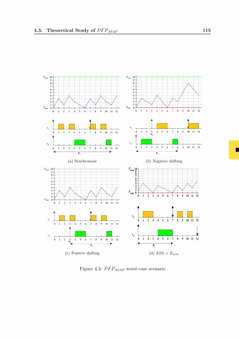
4.3. Theoretical Study of PFPASAP 115
0 1 2 3 4 5 6 7 8 9 10 11 12012345678910Emax
Emin
0 1 2 3 4 5 6 7 8 9 10 11 12
τ1
0 1 2 3 4 5 6 7 8 9 10 11 12
τ2
R2
(a) Synchronous
0 1 2 3 4 5 6 7 8 9 10 11 12012345678910Emax
Emin
0 1 2 3 4 5 6 7 8 9 10 11 12
τ1
0 1 2 3 4 5 6 7 8 9 10 11 12
τ2
R2
O1
(b) Negative shifting
0 1 2 3 4 5 6 7 8 9 10 11 12012345678910Emax
Emin
0 1 2 3 4 5 6 7 8 9 10 11 12
τ1
0 1 2 3 4 5 6 7 8 9 10 11 12
τ2
R2
O2
(c) Positive shifting
0 1 2 3 4 5 6 7 8 9 10 11 12012345678910E
max
Emin
R2
0 1 2 3 4 5 6 7 8 9 10 11 12
τ1
0 1 2 3 4 5 6 7 8 9 10 11 12
τ2
(d) E(0) > Emin
Figure 4.3: PFPASAP worst-case scenario
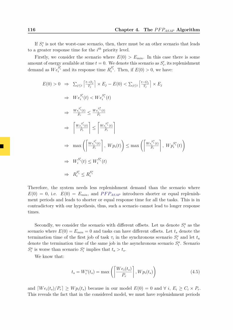
116 Chapter 4. The PFPASAP Algorithm
If Ssi is not the worst-case scenario, then, there must be an other scenario that leadsto a greater response time for the ith priority level.
Firstly, we consider the scenario where E(0) > Emin. In this case there is someamount of energy available at time t = 0. We denote this scenario as S ′i, its replenishmentdemand as We
S′ii and its response time RS′i
i . Then, if E(0) > 0, we have:
E(0) > 0 ⇒ ∑j≤i
⌈t−OjTj
⌉× Ej − E(0) < ∑
j≤i
⌈t−OjTj
⌉× Ej
⇒ WeS′ii (t) < We
Ssii (t)
⇒ WeS′ii (t)Pr
≤ WeSsii (t)Pr
⇒⌈We
S′ii (t)Pr
⌉≤⌈We
Ssii (t)Pr
⌉
⇒ max(⌈
WeS′ii (t)Pr
⌉, Wpi(t)
)≤ max
(⌈We
Ssii (t)Pr
⌉, Wp
Ssii (t)
)
⇒ WS′ii (t) ≤ W
Ssii (t)
⇒ RS′ii ≤ R
Ssii
Therefore, the system needs less replenishment demand than the scenario whereE(0) = 0, i.e. E(0) = Emin, and PFPASAP introduces shorter or equal replenish-ment periods and leads to shorter or equal response time for all the tasks. This is incontradictory with our hypothesis, thus, such a scenario cannot lead to longer responsetimes.
Secondly, we consider the scenario with different offsets. Let us denote Sai as thescenario where E(0) = Emin = 0 and tasks can have different offsets. Let ts denote thetermination time of the first job of task τi in the synchronous scenario Ssi and let tadenote the termination time of the same job in the asynchronous scenario Sai . ScenarioSai is worse than scenario Ssi implies that ta > ts.
We know that:
ts = W si (ts) = max
(⌈Wei(ts)Pr
⌉,Wpi(ts)
)(4.5)
and dWei(ts)/Pre ≥ Wpi(ts) because in our model E(0) = 0 and ∀ i, Ei ≥ Ci × Pr.This reveals the fact that in the considered model, we must have replenishment periods
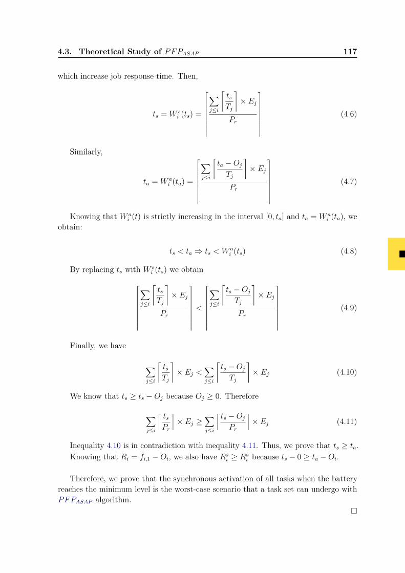
4.3. Theoretical Study of PFPASAP 117
which increase job response time. Then,
ts = W si (ts) =
∑j≤i
⌈tsTj
⌉× Ej
Pr
(4.6)
Similarly,
ta = W ai (ta) =
∑j≤i
⌈ta −Oj
Tj
⌉× Ej
Pr
(4.7)
Knowing that W ai (t) is strictly increasing in the interval [0, ta] and ta = W a
i (ta), weobtain:
ts < ta ⇒ ts < W ai (ts) (4.8)
By replacing ts with W si (ts) we obtain
∑j≤i
⌈tsTj
⌉× Ej
Pr
<
∑j≤i
⌈ts −Oj
Tj
⌉× Ej
Pr
(4.9)
Finally, we have
∑j≤i
⌈tsTj
⌉× Ej <
∑j≤i
⌈ts −Oj
Tj
⌉× Ej (4.10)
We know that ts ≥ ts −Oj because Oj ≥ 0. Therefore
∑j≤i
⌈tsPr
⌉× Ej ≥
∑j≤i
⌈ts −Oj
Pr
⌉× Ej (4.11)
Inequality 4.10 is in contradiction with inequality 4.11. Thus, we prove that ts ≥ ta.Knowing that Ri = fi,1 −Oi, we also have Rs
i ≥ Rai because ts − 0 ≥ ta −Oi.
Therefore, we prove that the synchronous activation of all tasks when the batteryreaches the minimum level is the worst-case scenario that a task set can undergo withPFPASAP algorithm.
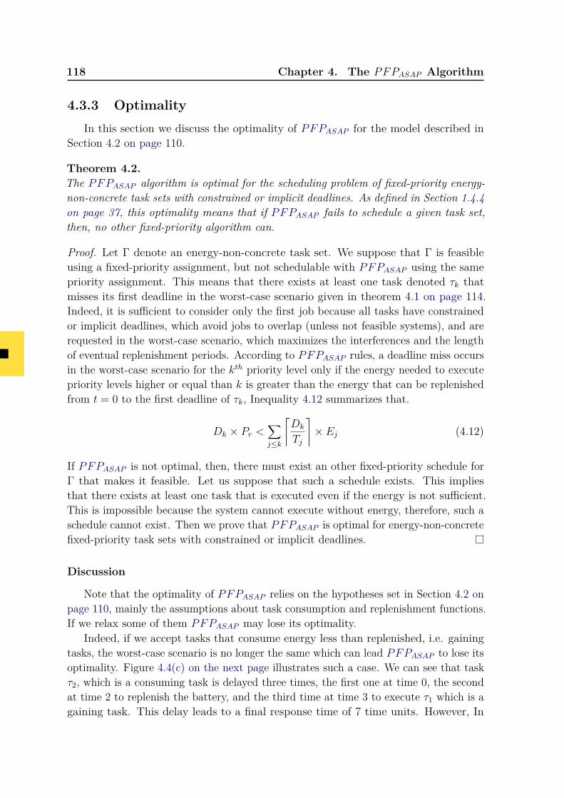
118 Chapter 4. The PFPASAP Algorithm
4.3.3 OptimalityIn this section we discuss the optimality of PFPASAP for the model described in
Section 4.2 on page 110.
Theorem 4.2.The PFPASAP algorithm is optimal for the scheduling problem of fixed-priority energy-non-concrete task sets with constrained or implicit deadlines. As defined in Section 1.4.4on page 37, this optimality means that if PFPASAP fails to schedule a given task set,then, no other fixed-priority algorithm can.
Proof. Let Γ denote an energy-non-concrete task set. We suppose that Γ is feasibleusing a fixed-priority assignment, but not schedulable with PFPASAP using the samepriority assignment. This means that there exists at least one task denoted τk thatmisses its first deadline in the worst-case scenario given in theorem 4.1 on page 114.Indeed, it is sufficient to consider only the first job because all tasks have constrainedor implicit deadlines, which avoid jobs to overlap (unless not feasible systems), and arerequested in the worst-case scenario, which maximizes the interferences and the lengthof eventual replenishment periods. According to PFPASAP rules, a deadline miss occursin the worst-case scenario for the kth priority level only if the energy needed to executepriority levels higher or equal than k is greater than the energy that can be replenishedfrom t = 0 to the first deadline of τk, Inequality 4.12 summarizes that.
Dk × Pr <∑j≤k
⌈Dk
Tj
⌉× Ej (4.12)
If PFPASAP is not optimal, then, there must exist an other fixed-priority schedule forΓ that makes it feasible. Let us suppose that such a schedule exists. This impliesthat there exists at least one task that is executed even if the energy is not sufficient.This is impossible because the system cannot execute without energy, therefore, such aschedule cannot exist. Then we prove that PFPASAP is optimal for energy-non-concretefixed-priority task sets with constrained or implicit deadlines.
Discussion
Note that the optimality of PFPASAP relies on the hypotheses set in Section 4.2 onpage 110, mainly the assumptions about task consumption and replenishment functions.If we relax some of them PFPASAP may lose its optimality.
Indeed, if we accept tasks that consume energy less than replenished, i.e. gainingtasks, the worst-case scenario is no longer the same which can lead PFPASAP to lose itsoptimality. Figure 4.4(c) on the next page illustrates such a case. We can see that taskτ2, which is a consuming task is delayed three times, the first one at time 0, the secondat time 2 to replenish the battery, and the third time at time 3 to execute τ1 which is againing task. This delay leads to a final response time of 7 time units. However, In
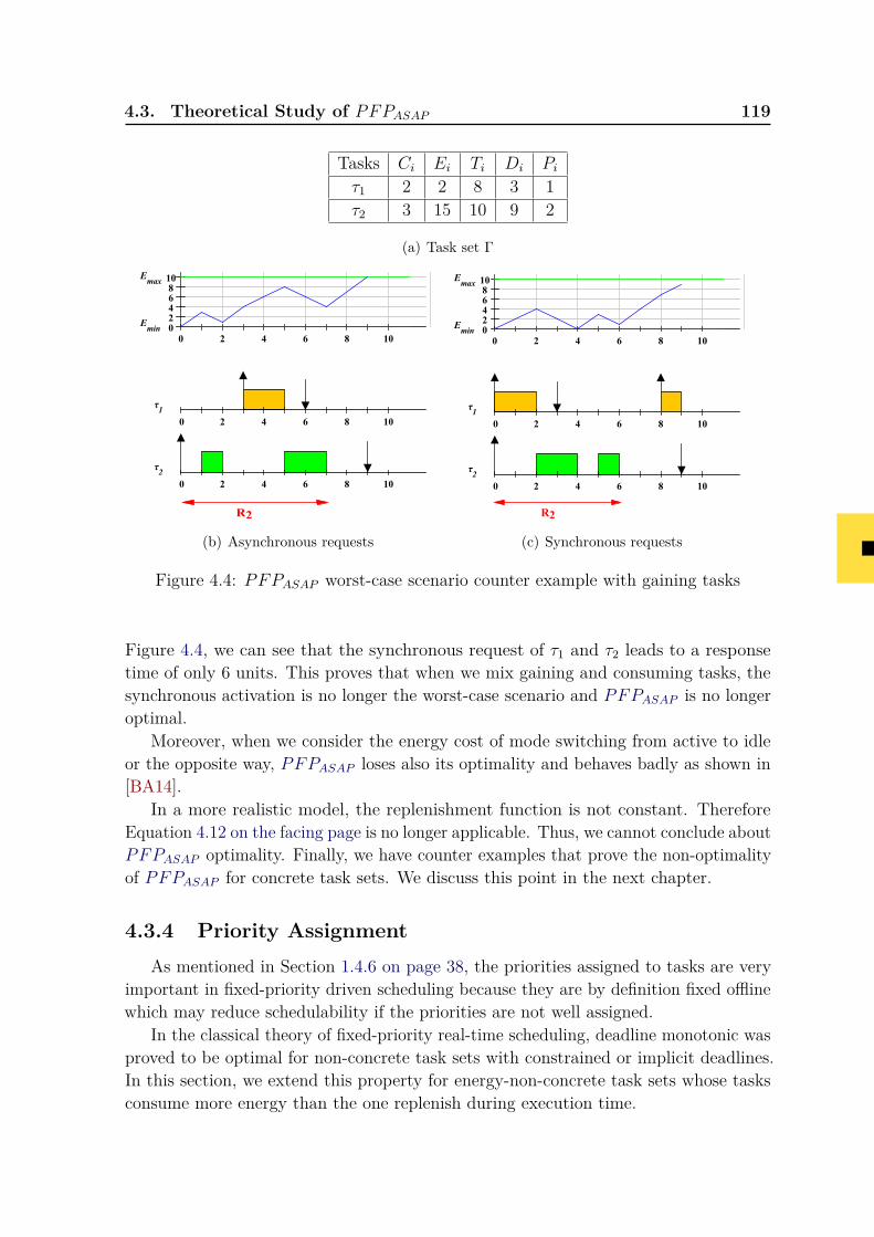
4.3. Theoretical Study of PFPASAP 119
Tasks Ci Ei Ti Di Piτ1 2 2 8 3 1τ2 3 15 10 9 2
(a) Task set Γ
0 2 4 6 8 100246810E
max
Emin
0 2 4 6 8 10
τ1
0 2 4 6 8 10
τ2
R2
(b) Asynchronous requests
0 2 4 6 8 100246810E
max
Emin
0 2 4 6 8 10
τ1
0 2 4 6 8 10
τ2
R2
(c) Synchronous requests
Figure 4.4: PFPASAP worst-case scenario counter example with gaining tasks
Figure 4.4, we can see that the synchronous request of τ1 and τ2 leads to a responsetime of only 6 units. This proves that when we mix gaining and consuming tasks, thesynchronous activation is no longer the worst-case scenario and PFPASAP is no longeroptimal.
Moreover, when we consider the energy cost of mode switching from active to idleor the opposite way, PFPASAP loses also its optimality and behaves badly as shown in[BA14].
In a more realistic model, the replenishment function is not constant. ThereforeEquation 4.12 on the facing page is no longer applicable. Thus, we cannot conclude aboutPFPASAP optimality. Finally, we have counter examples that prove the non-optimalityof PFPASAP for concrete task sets. We discuss this point in the next chapter.
4.3.4 Priority AssignmentAs mentioned in Section 1.4.6 on page 38, the priorities assigned to tasks are very
important in fixed-priority driven scheduling because they are by definition fixed offlinewhich may reduce schedulability if the priorities are not well assigned.
In the classical theory of fixed-priority real-time scheduling, deadline monotonic wasproved to be optimal for non-concrete task sets with constrained or implicit deadlines.In this section, we extend this property for energy-non-concrete task sets whose tasksconsume more energy than the one replenish during execution time.
120 Chapter 4. The PFPASAP Algorithm
Theorem 4.3.Deadline monotonic is an optimal priority assignment for energy-non-concrete task setswhen all the tasks have constrained or implicit deadlines and consume energy more thanit is replenished during their execution, i.e. when ∀ i, Di ≤ Ti and Ei > Ci × Pr.
The idea behind Theorem 4.3 is that DM can schedule any task set that is schedulablewith an other priority ordering. This means that every valid priority assignment can betransformed into deadline monotonic priority ordering.
Proof. When the task set is composed of only consuming tasks, i.e. ∀ i, Ei > Ci × Pr,the time demand of a priority level-i in the worst-case scenario is the time necessary toreplenish the energy demand or the replenishment demand because all tasks need moretime than their execution time to replenish the needed energy. Then, the maximumin the right hand side of Equation 4.3 on page 113 is dWei(t)/Pre. Therefore, byconsidering a synchronous release of all the tasks, i.e. ∀ i, Oi = 0, and a minimuminitial battery level E(0) = Emin = 0, the new time demand is obtained by Equation 4.13.
Wi(t) = max
(⌈Wei(t)Pr
⌉,Wpi(t)
)=⌈Wei(t)Pr
⌉=
∑j≤i
⌈t
Tj
⌉Ej
Pr
(4.13)
Now, to prove Theorem 4.3 we assume two tasks at adjacent priorities τA and τB withDA ≤ DB ≤ TB.
Given that τA is schedulable at the lower priority level than τB, we swap prioritiesof τA and τB and we observe the impact of this change on the schedulability of τA andτB. Then, if τB remains schedulable, this means that deadline priority assignment isoptimal as we can keep swapping task priorities from any schedulable priority orderingto get a DM ordering.
1. Assume that τA is schedulable at lower priority than τB. Then, the responsetime of the first job of τA in the worst-case scenario, denoted RA, is given byEquation 4.14 where X is the response time of the task with the lower prioritytask, in this case the one of τA.
X = RA =
⌈RA
TA
⌉EA +
⌈RA
TB
⌉EB +
∑j<A ∧ j 6=B
⌈RA
Tj
⌉Ej
Pr
(4.14)
Knowing that τA is schedulable, then, we have RA ≤ DA. Furthermore, inthis case, for such value of X, we have respectively dRA/TAeEA = EA anddRA/TBeEB = EB because respectively RA ≤ DA ≤ TA, from the fact that weare computing the response time of the first job of τA, and RA ≤ DA ≤ DB ≤ TB,from the fact that deadlines are constrained or implicit.
4.3. Theoretical Study of PFPASAP 121
2. Now, we swap priorities of τA and τB. We consider that the response time of τBis given by Equation 4.15.
X = RB =
⌈RA
TA
⌉EA +
⌈RA
TB
⌉EB +
∑j<B ∧ j 6=A
⌈RA
Tj
⌉Ej
Pr
(4.15)
Now, we compare Equations 4.14 on the facing page and 4.15. Thus, we observethat they are the same equation and so the value of X must also be the same whenτB is at a lower priority than τA. Therefore, τB is schedulable because DB ≥ DA.
3. It is obvious that τA is also schedulable because it is at a higher priority levelnow.
Then, we show that DM schedules any system that is schedulable with any other priorityassignment by swapping adjacent task priorities until we obtain a deadline monotonicpriority assignment without loss of schedulability.
Note that this proof relies on the assumptions set on tasks offsets and energyconsumption. If we relax one of them, the proof is no longer correct because theworst-case scenario PFPASAP is no longer the same and the used formulas are no longervalid.
4.3.5 Schedulability Condition
A simple way to build a necessary and sufficient feasibility condition for energy-non-concrete task sets is to check if the given task set is schedulable with PFPASAPin the worst-case scenario, in other words, to check if the first job of each task meetsits deadline when it is requested simultaneously with the higher priority tasks whilethe battery is at its minimum level. It consists of computing the worst-case responsetime according to PFPASAP rules for each task and to compare it to its deadline.Algorithm 4.2 on the following page explains how to do this. It is an extension of theclassical response time algorithm that considers energy replenishment periods.
The complexity of Algorithm 4.2 is O(m× n) where m is the number of iterationsand n is the number of tasks. We note that the number of iterations m depends onthe periods and deadlines of the tasks (see line 6 of Algorithm 4.2) and is bounded bymax∀i(Di)/min∀i(Ti). Thus, the complexity of Algorithm 4.2 is pseudo-polynomial. Wecan reduce this complexity by computing estimations for response times rather thanthe exact values. However, the schedulability test we propose will not be necessary butwill remain sufficient.
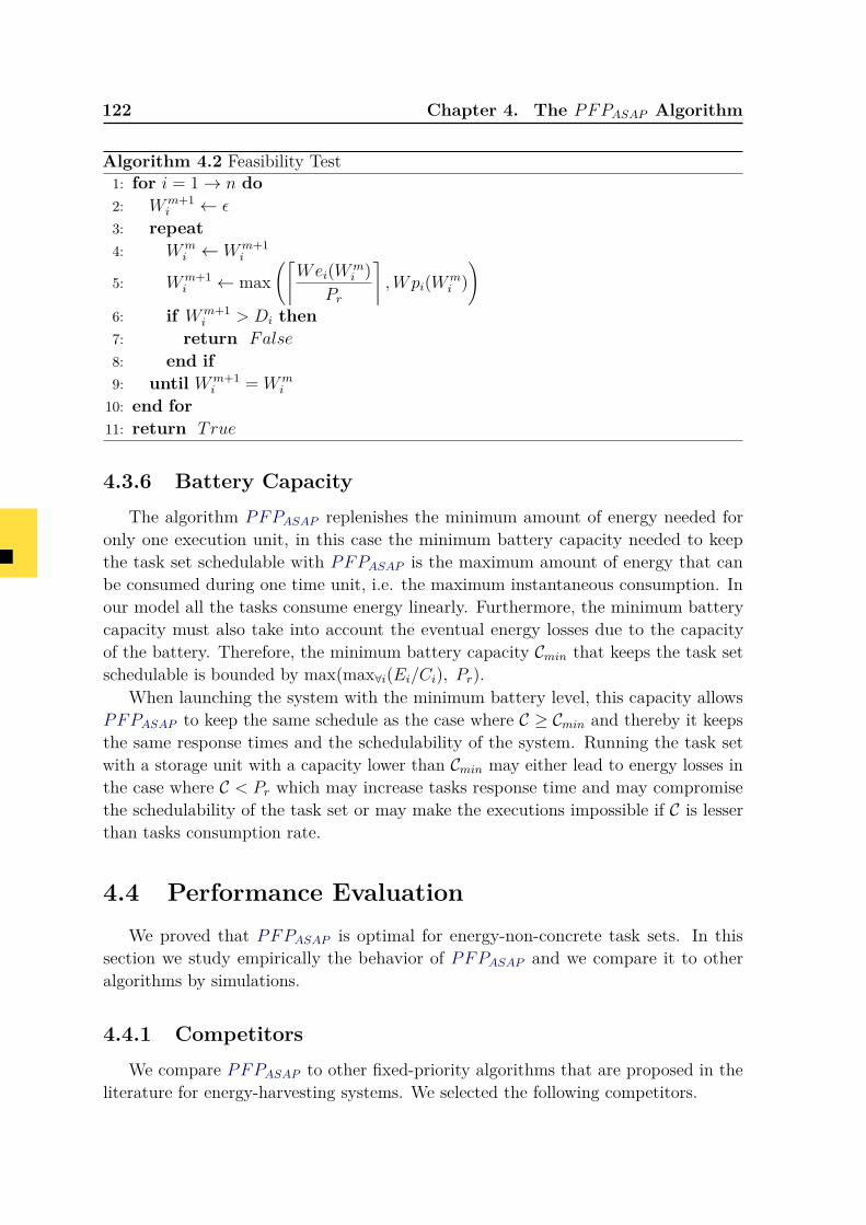
122 Chapter 4. The PFPASAP Algorithm
Algorithm 4.2 Feasibility Test1: for i = 1→ n do2: Wm+1
i ← ε
3: repeat4: Wm
i ← Wm+1i
5: Wm+1i ← max
(⌈Wei(Wm
i )Pr
⌉,Wpi(Wm
i ))
6: if Wm+1i > Di then
7: return False
8: end if9: until Wm+1
i = Wmi
10: end for11: return True
4.3.6 Battery CapacityThe algorithm PFPASAP replenishes the minimum amount of energy needed for
only one execution unit, in this case the minimum battery capacity needed to keepthe task set schedulable with PFPASAP is the maximum amount of energy that canbe consumed during one time unit, i.e. the maximum instantaneous consumption. Inour model all the tasks consume energy linearly. Furthermore, the minimum batterycapacity must also take into account the eventual energy losses due to the capacityof the battery. Therefore, the minimum battery capacity Cmin that keeps the task setschedulable is bounded by max(max∀i(Ei/Ci), Pr).
When launching the system with the minimum battery level, this capacity allowsPFPASAP to keep the same schedule as the case where C ≥ Cmin and thereby it keepsthe same response times and the schedulability of the system. Running the task setwith a storage unit with a capacity lower than Cmin may either lead to energy losses inthe case where C < Pr which may increase tasks response time and may compromisethe schedulability of the task set or may make the executions impossible if C is lesserthan tasks consumption rate.
4.4 Performance EvaluationWe proved that PFPASAP is optimal for energy-non-concrete task sets. In this
section we study empirically the behavior of PFPASAP and we compare it to otheralgorithms by simulations.
4.4.1 CompetitorsWe compare PFPASAP to other fixed-priority algorithms that are proposed in the
literature for energy-harvesting systems. We selected the following competitors.
4.4. Performance Evaluation 123
• PFPALAP : the fixed-priority scheduling policy described in Section 3.7.1 onpage 92. PFPALAP is not optimal but can be used as a reference for comparisonsince there is no many algorithms in the state of the art.
• PFPST : the fixed-priority scheduling policy described in Section 3.7.2 on page 95.We selected PFPST which is not optimal but has the lowest failure rate accordingto the experiment presented in Section 3.8 on page 99.
4.4.2 SimulationIn this section, we describe the configuration of the experiments, namely the task
sets generation, the parameters and the set assumptions.To perform such an experiment we used a simulator named YARTISS that we
present in Chapter 8.
Task Sets Generation
For these simulations we used an adapted version of the UUniFast-Discard algorithm[BB05] coupled with a technique for hyper-period limitation [MG01] to generate tasksets. The generated task sets respect the following hypotheses:
• All task sets are time feasible without considering energy parameters and con-straints.
• Time and energy are discretized, this means that they are integers and allscheduling operations are performed before or after one time unit,
• The charging rate Pr is constant, i.e. a constant amount of energy is added tothe battery level in every time unit,
• Tasks consume energy linearly, i.e. a task consumes Ei/Ci energy units for eachexecution time unit,
• All task sets are composed of consuming tasks, in other words, all tasks consumeenergy more than what we can replenish during execution times, i.e. ∀ i, Ei >Ci × Pr.
In order to represent most of the possible task sets, we generate them according totheir processor and energy utilizations, i.e. U and Ue. We vary U and Ue in the interval[0.2, 1] to obtain a couple of (U,Ue) for each 0.05 unit of U and Ue. Then, we obtain 50distinct task sets for each couple (U,Ue).
In this experiment, all task sets are simulated in the worst-case scenario describedin Section 4.3.2 on page 113.
124 Chapter 4. The PFPASAP Algorithm
Simulation Configuration
In order to evaluate the behavior of the compared algorithms, we vary some param-eters, namely the battery capacity C and the number of tasks per task set. Firstly, wevary C in six energy scenarios to analyze its effect on the failure rate. Secondly, wevary the number of tasks per task set in several distinct simulations to observe the thescheduling overhead of each algorithm.
We set the remaining parameters to the same values that we used for task setsgeneration in order to fit with the considered assumptions. For these experiments, weset these parameters as follows, Pr = 15 and Emin = 0. Furthermore, task sets are runfor 2600 time units which corresponds to the longest hyper-period. Thus, if a task setdoes not miss any deadline during the simulation time, then, the task set is said tobe empirically feasible. We use Deadline Monotonic (DM) policy to assign prioritiesbecause of its optimality for the considered model as shown in Section 4.3.4 on page 119.
Several statistical metrics are computed during simulations. These metrics giveinformation about algorithms behavior. For our experiments we selected the followingmetrics: failure rate, preemption count, average overhead, average idle-period, averagebusy-period and average energy level.
Metrics
Failure Rate: the percentage of unfeasible task sets among all the tested ones. Thegreater the failure rate is, the lower the algorithm performance is.
Preemption Count: for one simulation, it represents the number of preemptionevents. A preemption event occurs when a job is suspended while it is still not finished.All the events that occur at the same instant (e.g. job request, a deadline, etc.) areconsidered as once. Therefore, the number of possible events is bounded by the numberof time units composing the simulation, i.e. the simulation duration. For severalsimulations, this metric is computed only for feasible task sets and represents the ratioof the average number of preemptions relative to the number of all possible events. Thegreater the number of preemptions is, the greater the context switch is. A large numberof preemptions increases the overhead cost and decreases performance, which makesthe algorithm unusable in practice.
Average Overhead: it is the amount of time spent while handling a schedulingevent, in other words, the spent by the scheduling algorithm to take a decision. For onesimulation, this metric represents the average overhead of all of the scheduling events.Its exact value is difficult to compute and must be computed on a real platform. Wesimply calculate an estimation by distributing the real simulation time (in milliseconds)on the number of scheduling events. The simulation tool that we use is event-based.Therefore, only the events processing consumes processor time. Thus, it gives us an
4.4. Performance Evaluation 125
acceptable estimation of the average overhead. The greater the average overhead is, thegreater the timing constraints violation risk is.
Average Idle-Period and Average Busy-Period: represents respectively the av-erage duration of periods when the processor is idle and the average duration ofcontinuous processor activity. For several simulations, we compute the ratio of theaverage idle-period/average busy-period duration relative to the simulation duration.
The relevance of these two metrics is closely linked to the number of preemptionscaused by replenishment periods. The longer the idle/busy periods are, the lesser thenumber of replenishment preemptions is and the higher the algorithm performance are.Therefore, the longer the idle-periods are, the higher the average energy level is andthe lesser energy-constrained the system is. Moreover, grouping idle-periods together isbetter for batteries that do not support a high rate of charge/discharge cycles.
Average Energy Level: represents the average energy level of the battery at anyinstant during the simulation. It is the average of the energy level of all schedulingevents. The best algorithms relative to this criterion are ones that maximize the averageenergy level. This means that the algorithm makes the system less energy constrained.
4.4.3 Results AnalysisThe Variation of Emax
Figure 4.5 on the following page presents the results of the comparison of theselected algorithms. In the following part, we analyze the effect of Emax variation onthe performances of each algorithm for each metric:
Failure Rate: Increasing Emax reduces the failure rate of all the evaluated algorithms.This result was expected because the more Emax is increased the less the system isenergy-constrained. We also observe that PFPALAP has the highest failure rate forall values of Emax. Both PFPASAP and PFPST have a lower failure while PFPASAPdemonstrates the lowest one. To explain why PFPST fails to schedule some task setswhich are schedulable with PFPASAP we have to examine its behavior closely. When thebattery is at its minimum level, PFPST suspends the system as long as possible beforethe next execution while PFPASAP suspends the system only for one time unit. In thiscase PFPST may uselessly postpone executions and may accumulate an unbearableenergy load for a future time. This can lead the system to replenish more time than theavailable slack-time and may lead to miss deadlines. PFPALAP suffers from the sameproblem than PFPST because it postpones execution as long as possible regardlessto the battery level. When all jobs are postponed to the maximum and the systemincurs a long execution period, it is impossible to introduce more replenishment times.Therefore, deadline misses may occur. Figure 3.7 on page 94 illustrates this phenomenon.
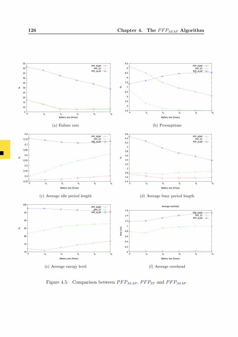
126 Chapter 4. The PFPASAP Algorithm
5
10
15
20
25
30
35
40
45
50
55
50 100200
300400
600
%
Battery size (Emax)
PFP_ASAPPFP_ST
PFP_ALAP
(a) Failure rate
4.5
5
5.5
6
6.5
7
7.5
8
8.5
9
9.5
50 100200
300400
600
%Battery size (Emax)
PFP_ASAPPFP_ST
PFP_ALAP
(b) Preemptions
0.35
0.4
0.45
0.5
0.55
0.6
0.65
0.7
0.75
0.8
50 100200
300400
600
%
Battery size (Emax)
PFP_ASAPPFP_ST
PFP_ALAP
(c) Average idle period length
2.4
2.6
2.8
3
3.2
3.4
3.6
3.8
4
4.2
4.4
4.6
50 100200
300400
600
%
Battery size (Emax)
PFP_ASAPPFP_ST
PFP_ALAP
(d) Average busy period length
70
75
80
85
90
95
100
50 100200
300400
600
%
Battery size (Emax)
PFP_ASAPPFP_ST
PFP_ALAP
(e) Average energy level
0
0.2
0.4
0.6
0.8
1
1.2
1.4
1.6
50 100200
300400
600
time
(ms)
Battery size (Emax)
Average overhead
PFP_ASAPPFP_ST
PFP_ALAP
(f) Average overhead
Figure 4.5: Comparison between PFPALAP , PFPST and PFPASAP
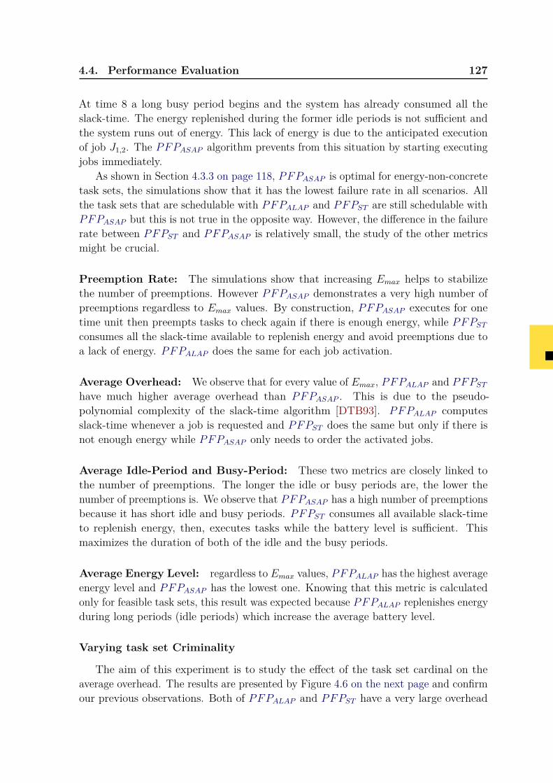
4.4. Performance Evaluation 127
At time 8 a long busy period begins and the system has already consumed all theslack-time. The energy replenished during the former idle periods is not sufficient andthe system runs out of energy. This lack of energy is due to the anticipated executionof job J1,2. The PFPASAP algorithm prevents from this situation by starting executingjobs immediately.
As shown in Section 4.3.3 on page 118, PFPASAP is optimal for energy-non-concretetask sets, the simulations show that it has the lowest failure rate in all scenarios. Allthe task sets that are schedulable with PFPALAP and PFPST are still schedulable withPFPASAP but this is not true in the opposite way. However, the difference in the failurerate between PFPST and PFPASAP is relatively small, the study of the other metricsmight be crucial.
Preemption Rate: The simulations show that increasing Emax helps to stabilizethe number of preemptions. However PFPASAP demonstrates a very high number ofpreemptions regardless to Emax values. By construction, PFPASAP executes for onetime unit then preempts tasks to check again if there is enough energy, while PFPSTconsumes all the slack-time available to replenish energy and avoid preemptions due toa lack of energy. PFPALAP does the same for each job activation.
Average Overhead: We observe that for every value of Emax, PFPALAP and PFPSThave much higher average overhead than PFPASAP . This is due to the pseudo-polynomial complexity of the slack-time algorithm [DTB93]. PFPALAP computesslack-time whenever a job is requested and PFPST does the same but only if there isnot enough energy while PFPASAP only needs to order the activated jobs.
Average Idle-Period and Busy-Period: These two metrics are closely linked tothe number of preemptions. The longer the idle or busy periods are, the lower thenumber of preemptions is. We observe that PFPASAP has a high number of preemptionsbecause it has short idle and busy periods. PFPST consumes all available slack-timeto replenish energy, then, executes tasks while the battery level is sufficient. Thismaximizes the duration of both of the idle and the busy periods.
Average Energy Level: regardless to Emax values, PFPALAP has the highest averageenergy level and PFPASAP has the lowest one. Knowing that this metric is calculatedonly for feasible task sets, this result was expected because PFPALAP replenishes energyduring long periods (idle periods) which increase the average battery level.
Varying task set Criminality
The aim of this experiment is to study the effect of the task set cardinal on theaverage overhead. The results are presented by Figure 4.6 on the next page and confirmour previous observations. Both of PFPALAP and PFPST have a very large overhead
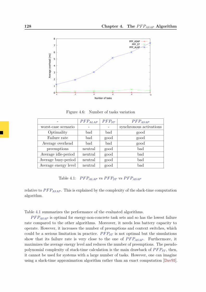
128 Chapter 4. The PFPASAP Algorithm
0
1
2
3
4
5
6
7
8
4 5 6 8 9 12
Aver
age
over
head
(m
s)
Number of tasks
PFP_ASAPPFP_ST
PFP_ALAP
Figure 4.6: Number of tasks variation
- PFPALAP PFPST PFPASAPworst-case scenario - - synchronous activations
Optimality bad bad goodFailure rate bad good good
Average overhead bad bad goodpreemptions neutral good bad
Average idle-period neutral good badAverage busy-period neutral good badAverage energy level neutral good bad
Table 4.1: PFPALAP vs PFPST vs PFPASAP
relative to PFPASAP . This is explained by the complexity of the slack-time computationalgorithm.
Table 4.1 summarizes the performance of the evaluated algorithms.PFPASAP is optimal for energy-non-concrete task sets and so has the lowest failure
rate compared to the other algorithms. Moreover, it needs less battery capacity tooperate. However, it increases the number of preemptions and context switches, whichcould be a serious limitation in practice. PFPST is not optimal but the simulationsshow that its failure rate is very close to the one of PFPASAP . Furthermore, itmaximizes the average energy level and reduces the number of preemptions. The pseudo-polynomial complexity of stack-time calculation is the main drawback of PFPST , then,it cannot be used for systems with a large number of tasks. However, one can imagineusing a slack-time approximation algorithm rather than an exact computation [Dav93].
4.5. Conclusion 129
Regarding PFPALAP , in addition to its non-optimality, simulations demonstrate verybad performance for all metrics.
4.5 ConclusionIn this chapter we studied deeply the PFPASAP scheduling algorithm. We firstly
described in detail its scheduling schemes. Secondly, we presented and proved some ofits properties. We proved that the synchronous release of all tasks when the batteryis at the minimum level is the worst-case scenario that leads to the longest responsetime of all tasks. Then, we used this property to prove the optimality of PFPASAP forenergy-non-concrete task sets that consume energy more than the replenishment duringtheir executions. We also proposed a bound of the minimum battery capacity thatkeeps the schedulability of task set with PFPASAP . Thirdly, we built a schedulabilitycondition based on PFPASAP algorithm. This condition is necessary and sufficient forenergy-non-concrete task sets. Finally, we presented the results of empirical comparisonof PFPASAP with other algorithms. This experiments showed that PFPASAP dominatesthe other algorithms in term of schedulability rate and average overhead. The resultsshowed also that PFPASAP suffers from high number of preemptions due to its greedybehavior. Then, we conclude that the PFPASAP is a scheduling algorithm that behavestheoretically well but has a serious limitation in practice. Finally, we can conclude thatPFPASAP is optimal but not applicable for platforms that does not support a highpreemption and context switch rates. However, its optimality make it the referencealgorithm for fixed-priority energy-harvesting systems.
We will show in the next chapter that PFPASAP loses its optimility when we relaxsome energy assumptions, the worst-case scenario and the schedulability test are nolonger valid. Removing these assumptions makes the problem more complex and pushus to study more scheduling algorithms and to look for more schedulability conditions.This is the topic of the next chapters.

Chapter 5
Approximate Response-TimeAnalysis for Energy-Harvesting
Systems
Contents5.1 Introduction . . . . . . . . . . . . . . . . . . . . . . . . . . . . . 1315.2 Models and Notations . . . . . . . . . . . . . . . . . . . . . . . . 1325.3 Schedulability Analysis . . . . . . . . . . . . . . . . . . . . . . . 133
5.3.1 Worst-case scenario . . . . . . . . . . . . . . . . . . . . . . . . . 1335.3.2 Sequences and Energy-busy-periods . . . . . . . . . . . . . . . . 1335.3.3 Response Time Upper Bounds . . . . . . . . . . . . . . . . . . . 1375.3.4 Upper Bound RUB1 . . . . . . . . . . . . . . . . . . . . . . . . . 1375.3.5 Upper Bound RUB2 . . . . . . . . . . . . . . . . . . . . . . . . . 1395.3.6 Battery Capacity . . . . . . . . . . . . . . . . . . . . . . . . . . . 1435.3.7 Response Time Lower Bound . . . . . . . . . . . . . . . . . . . . 1445.3.8 Priority Assignment . . . . . . . . . . . . . . . . . . . . . . . . . 146
5.4 Performance Evaluation . . . . . . . . . . . . . . . . . . . . . . 1475.4.1 Taskset generation . . . . . . . . . . . . . . . . . . . . . . . . . . 1475.4.2 Schedulability tests investigated . . . . . . . . . . . . . . . . . . 148
5.5 Conclusions . . . . . . . . . . . . . . . . . . . . . . . . . . . . . . 151
5.1 IntroductionPreviously, we provided schedulability analysis for PFPASAP that was restricted
to systems where all tasks were consuming tasks (see Section 4.3.5 on page 121).We proved that PFPASAP is optimal with respect to all fixed-priority algorithms forenergy-non-concrete periodic task sets, compliant with that restricted model.
In this chapter, we consider real-time task sets comprising two types of tasks:(i) consuming tasks that have a rate of energy consumption that is higher than the
132 Chapter 5. Approximate Response-Time Analysis for EH Systems
replenishment rate, and (ii) gaining tasks that have a rate of energy consumption thatis no more than the replenishment rate. Recall that the results presented in Chapter 4were obtained considering only consuming tasks. We show that for this more generalmodel, the critical instant leading to the worst-case response time of a task does notnecessarily correspond to a synchronous release with all higher priority tasks, and sothe analysis presented in Section 4.3 on page 111 is not applicable. For the moregeneral model, we derive two response time upper bounds providing sufficient schedulingtests. We also prove that Deadline Monotonic priority assignment [LW82] is an optimalpriority assignment policy with respect to these sufficient schedulability tests. Thework presented in this chapter is the result of a collaboration with Prof. Rob Davisand mainly contains materials previously published in [Abd+14].
The remainder of the chapter is organized as follows. In Section 5.2 we recapitulatethe system model, terminology and notation used in the this chapter. In Section 5.3we introduce sufficient schedulability analysis for the more general task model withboth consuming and gaining tasks. Section 5.4 provides a performance evaluationinvestigating the effectiveness and the tightness of these schedulability tests. Section5.5 concludes the chapter.
5.2 Models and Notations
The model considered in this chapter is close to the one described in Section 3.2on page 67. The deference here is that we relax some assumptions on tasks energyconsumption and offsets. The considered model includes also concrete task sets.
Task ModelIn addition to the notations presented in Chapter 4, the worst-case power consumption(i.e. energy used per unit of execution time) of a task τi is given by Pci. Thus theworst-case energy consumption equates to executing for the worst-case execution time,at the maximum rate of power consumption (i.e. Ei = Pci × Ci). The set of tasksΓ is separated into two distinct subsets Γc and Γg. The first one Γc contains theconsuming tasks, the ones that consume more energy than is replenished during theirexecution, whereas Γg is composed by the gaining tasks, that consume no more energythan is replenished during their execution. We have Γc = {τi ∈ Γ, Ei > Pr × Ci} andΓg = {τi ∈ Γ, 0 ≤ Ei ≤ Pr × Ci}.
Energy ModelThe energy model considered in this chapter is exactly the same as the one describedin Section 3.2 on page 67.
5.3. Schedulability Analysis 133
5.3 Schedulability AnalysisIn this section, we provide sufficient schedulability tests for systems with both
consuming and gaining tasks. First we show that the critical instant for such task setsdoes not necessarily correspond to synchronous release. Lack of information about theactual worst-case scenario makes the schedulability analysis problem much more difficult.We address this problem by using the concept of priority level-i energy-busy-period.(see Definition 3.3 on page 70). The worst-case response time of task τi must necessarilyoccur within such a busy-period. We derive two upper bounds on the maximum lengthof this busy-period, which we then use to obtain upper bounds on the worst-caseresponse time of the task. We use a similar approach to also derive response time lowerbounds.
5.3.1 Worst-case scenario
When we consider only consuming tasks or only gaining tasks, the worst-case scenario(critical instant) occurs when all higher priority tasks are released simultaneously andthe battery is at its minimum level. For the case when we have only gaining tasks, theresponse time analysis is the same as the classical formulation, since there are no delaysdue to energy considerations.
For the case where we have only consuming tasks, launching the tasks simultane-ously with the battery at its minimum level maximizes the idle periods needed forenergy replenishment. This increases the time required to complete the execution ofhigher priority tasks, which leads to the longest response time for each task, given byEquation 4.3 on page 113 as proved in Section 4.3.5 on page 121.
In contrast, when we consider a task set composed of both gaining and consumingtasks the worst-case scenario is not the same for all the tasks, it depends on thecomposition of the subset of higher priority tasks. If that subset contains both gainingand consuming tasks, then the worst-case scenario is not necessarily the synchronousactivation of all the tasks with the minimum battery level.
Figure 5.1 on the following page illustrates a situation where the response time oftask τ2 is longer (R2 = 7) when a gaining task of higher priority is requested later, thanit is with synchronous release (R2 = 6). This is due to the fact that in the former case,task τ2 suffers two replenishment delays (at time t = 0 and t = 2), whereas in the latercase it suffers only one replenishment delay (at time t = 4). This happens because taskτ1 is a gaining task and there is a net increase in energy as it executes.
5.3.2 Sequences and Energy-busy-periods
We now introduce terminology and concepts that we use in proving key propertiesabout scheduling systems with energy constraints.
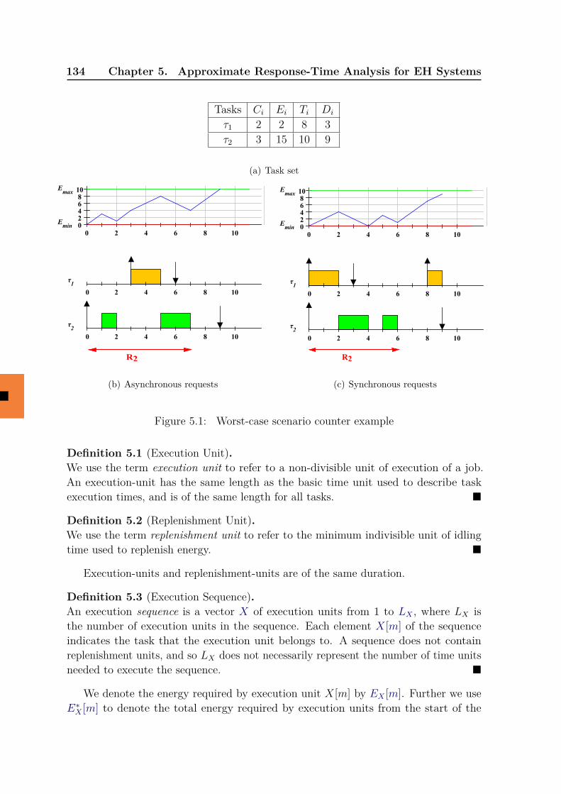
134 Chapter 5. Approximate Response-Time Analysis for EH Systems
Tasks Ci Ei Ti Di
τ1 2 2 8 3τ2 3 15 10 9
(a) Task set
0 2 4 6 8 100246810E
max
Emin
0 2 4 6 8 10
τ1
0 2 4 6 8 10
τ2
R2
(b) Asynchronous requests
0 2 4 6 8 100246810E
max
Emin
0 2 4 6 8 10
τ1
0 2 4 6 8 10
τ2
R2
(c) Synchronous requests
Figure 5.1: Worst-case scenario counter example
Definition 5.1 (Execution Unit).We use the term execution unit to refer to a non-divisible unit of execution of a job.An execution-unit has the same length as the basic time unit used to describe taskexecution times, and is of the same length for all tasks. �
Definition 5.2 (Replenishment Unit).We use the term replenishment unit to refer to the minimum indivisible unit of idlingtime used to replenish energy. �
Execution-units and replenishment-units are of the same duration.
Definition 5.3 (Execution Sequence).An execution sequence is a vector X of execution units from 1 to LX , where LX isthe number of execution units in the sequence. Each element X[m] of the sequenceindicates the task that the execution unit belongs to. A sequence does not containreplenishment units, and so LX does not necessarily represent the number of time unitsneeded to execute the sequence. �
We denote the energy required by execution unit X[m] by EX [m]. Further we useE∗X [m] to denote the total energy required by execution units from the start of the
5.3. Schedulability Analysis 135
sequence up to and including execution unit X[m]. Thus:
E∗X [m] =∑
q=1...mEX [q] (5.1)
The minimum number of replenishment units IX [m] required to provide sufficientenergy to execute X[m] at the end of the subsequence X[1] to X[m] is given by:
IX [m] = max(
0,⌈E∗X [m]− E(0)
Pr
⌉−m
)(5.2)
where E(0) is the energy available at the start of the sequence.We note that an earlier execution unit X[k] may require more prior replenishment
units than a later one X[m] due to the presence of execution units of gaining tasksbetween X[k] and X[m], (i.e. IX [k] > IX [m] where m > k). We use I∗X [m] to denotethe minimum number of replenishment units required to execute all of the subsequenceX[1] to X[m] in order.
I∗X [m] = maxk=1...m
(IX [k]) (5.3)
The elapsed time required to execute sequence X is given by LX + I∗X [LX ].
Lemma 5.1.For a fixed sequence X of execution units, the elapsed time for the sequence is maximisedwhen the initial energy available is minimised, i.e. E(0) = 0.
Proof. Follows directly from Equation 5.2 and the formula for the elapsed time toexecute the sequence: LX + I∗X [LX ].
Lemma 5.2.Any sequence containing only execution units of consuming tasks requires the sameelapsed time to execute irrespective of the order of its execution units provided thatthe set of execution units and the initial energy are the same. Similarly, any sequencecontaining only execution units of gaining tasks requires the same elapsed time to executeirrespective of the order of its execution units provided that the set of execution units isthe same.
Proof. Case (i) sequence X contains solely execution units of consuming tasks. Sinceall execution units consume energy, then for every element X[m], we have EX [m] > Prand so E∗X [m+ 1] > E∗X [m] + Pr hence the maximum number of prior replenishmentunits is required by the last element in the sequence and is given by:
I∗X [LX ] = IX [LX ] =⌈E∗X [LX ]− E(0)
Pr
⌉(5.4)
Since the total energy E∗X [LX ] required by all elements in the sequence is independentof the order of the elements, the elapsed time I∗X [LX ] + LX required to execute thesequence is also independent of the order of the elements.
136 Chapter 5. Approximate Response-Time Analysis for EH Systems
Case (ii) sequence X contains solely execution units of gaining tasks. Since allexecution units gain energy, no replenishment units are required and the elapsed timefor the sequence equates to its length LX irrespective of the order of the elements.
Lemma 5.3.Under PFPASAP scheduling, for a schedulable task τi, the worst-case response time Ri
of the task equates to the longest possible priority level−i energy busy-period. Further,there exists a busy-period of this length that includes a single job of task τi, begins atthe release of this job and ends with the final execution unit of the job.
Proof. As task τi has the lowest priority of any task executing in such a prioritylevel−i energy busy-period, under PFPASAP scheduling the busy-period necessarilyends with the final execution unit of that task. This is the case because if there wereany outstanding higher priority tasks, they would execute in preference to task τi.
As task τi has a constrained deadline and is schedulable (by the Lemma), it can onlyhave one job starting from the release time in the busy-period, otherwise the completionof the previous job of task τi would have to take place after the release of the final jobof the task implying (as Di ≤ Ti) that the previous job was unschedulable.
Let X be the sequence of execution units representing all execution in the busy-period. If the job of task τi was not released at the start of the busy-period, then wecan move its release time back to the start of the busy-period. Since task τi has thelowest priority of any task in the busy-period, such a change cannot make any differenceto the actual order of execution as represented by sequence X and so has no impact onthe elapsed time required to execute the sequence. Such a change can therefore onlyincrease the worst-case response time of the job.
Lemma 5.3 proves that the worst-case response time for a task τi occurs in a prioritylevel−i energy busy-period starting with the release of that task. However, as shown inFigure 5.1 on page 134, synchronous release of all higher priority tasks may not result inthe worst-case response time for task τi. In general, we do not know what scenario, orpattern of releases of higher priority tasks will result in the worst-case response time fortask τi; however, we can derive further information about possible worst-case scenarios.
Lemma 5.4.The maximum possible number of jobs of a higher priority task τh causing interferencein the longest priority level−i busy-period (characterising the worst-case response timeof task τi ) is given by dw/The where w is the length of the busy-period.
Proof. Lemma 5.3 shows that the busy-period starts (at time t = 0) with the release oftask τi, hence at t = 0, there can be no jobs of higher priority tasks with outstandingexecution, other than those also released at t = 0, otherwise the busy-period wouldhave started earlier. It follows that the maximum number of higher priority jobs of taskτh in the busy-period is given by dw/The.
5.3. Schedulability Analysis 137
5.3.3 Response Time Upper BoundsWe do not know up to know the precise pattern of releases of higher priority jobs
that leads to the worst-case response time for task τi, we cannot determine the exactworst-case response time. Instead, we derive an upper bound RUB1
i and then a tighterupper bound RUB2
i on the exact worst-case response time Ri, where RUB1i ≥ RUB2
i ≥ Ri.These upper bounds provide sufficient schedulability tests UB1 and UB2 respectively,where UB2 dominates UB1.
The process we use to obtain these upper bounds is similar to the classic formulationof response time analysis presented in Section 1.5 on page 40. We aim to find the smallestinterval w, for which an upper bound on the response time of task τi, considering themaximum possible interference from higher priority tasks released in that interval,equates to the length of the interval. The value of w then provides an upper bound onthe worst-case response time of task τi.
We require a function F (w) that upper bounds the length of the longest prioritylevel−i energy busy-period formed by a single job of task τi and jobs of higher prioritytasks released during an interval of length w. Provided that F (w) is a monotonicallynon-decreasing function of w, then we may obtain an upper bound on the worst-caseresponse time of task τi corresponding to the smallest value of w > 0 that satisfies:
w = F (w) (5.5)
Equation 5.5 may be solved using fixed point iteration starting with w = Ci and endingon convergence or when w > Di in which case the task is deemed unschedulable.
5.3.4 Upper Bound RUB1
We now derive a simple upper bound RUB1i on the worst-case response time of task
τi. First we prove a Lemma used in its derivation.
Lemma 5.5.Let X be some arbitrary sequence of execution units of tasks of priority i or higher, andY be the equivalent sequence re-ordered such that all execution units of consuming taskscome before all execution units of gaining tasks. The elapsed time required to completesequence Y is no shorter than that required to complete sequence X.
Proof. We may obtain sequence Y from sequence X by an iterative process of choosingthe first execution unit belonging to any gaining task (at position g) and swapping itwith that of the last execution unit of any consuming task (at position k) providedthat g < k. Repeating this process until all consuming execution units come before allgaining execution units transforms sequence X into sequence Y . Let the new sequencesproduced by this process be X1 = X,X2, X3 . . . Xn = Y . Note at most LX/2 swapsare required. We now show that each swap transforming sequence Xp into sequenceXs where s = p+ 1, results in an elapsed time for sequence Xs that is no shorter than
138 Chapter 5. Approximate Response-Time Analysis for EH Systems
that for Xp, and hence by induction that the elapsed time for sequence Y is no shorterthan that for sequence X. Let Xp[g] and Xp[k] be the elements being swapped whereg < k. Since Xp[g] is an execution unit of a gaining task and Xp[k] is an execution unitof a consuming task, the energy required for these execution units has the relationshipEXp [g] < EXp [k]. Recall that E∗Xp [m] is the energy required to execute all executionunits in the subsequence from Xp[1] to Xp[m]. It follows that:
∀m, 1 ≤ m < g E∗Xs [m] = E∗Xp [m]
∀m, g ≤ m < k E∗Xs [m] = E∗Xp [m] + EXs [k]− EXp [g]
∀m, k ≤ m E∗Xs [m] = E∗Xp [m]
⇒ E∗Xs [m] ≥ E∗Xp [m]
Hence the minimum number of replenishment units required to execute the subse-quences from the 1st to the m−th element of Xp and Xs have the following relationship:I∗Xs [m] ≥ I∗Xp [m] (see Equations 5.2 on page 135 and 5.3 on page 135). Since the numberof execution units in each sequence (Xs and Xp) is the same (i.e. LXp = LXs), we have:LXs + I∗Xs [m] ≥ LXp + I∗Xp [m]. Thus the elapsed time required to execute sequence Xs
is no shorter than that required for sequence Xp. Induction over at most LX/2 stepsproves that the elapsed time required to complete sequence Y is no shorter than thatrequired for sequence X.
Theorem 5.1.An upper bound on the worst-case response time for task τi for a set of jobs released ina window of length w can be obtained by assuming that there is one job of task τi anddw/The jobs of each higher priority task τh. Further, the upper bound is obtained froma sequence Z of the execution units of these jobs where all the consuming executionunits are before all the gaining execution units.
Proof. Let X be the sequence of execution units that results in the longest prioritylevel-i energy busy-period under PFPASAP scheduling, and hence the longest responsetime for task τi), for a set of jobs released in a window of length w. The elapsed timefor the sequence is given by LX + I∗X [LX ] where LX is the length of the sequence andI∗X [LX ] is the total number of replenishment units required. Lemma 5.5 on the previouspage shows that the elapsed time required to execute a sequence Y is no shorter thanthat required to execute sequence X, where sequence Y comprises the execution unitsin X re-ordered such that all execution units of consuming tasks are placed beforeexecution units of gaining tasks. Note that at this point we do not know how manyjobs of higher priority tasks are present in sequence X and therefore also in sequence
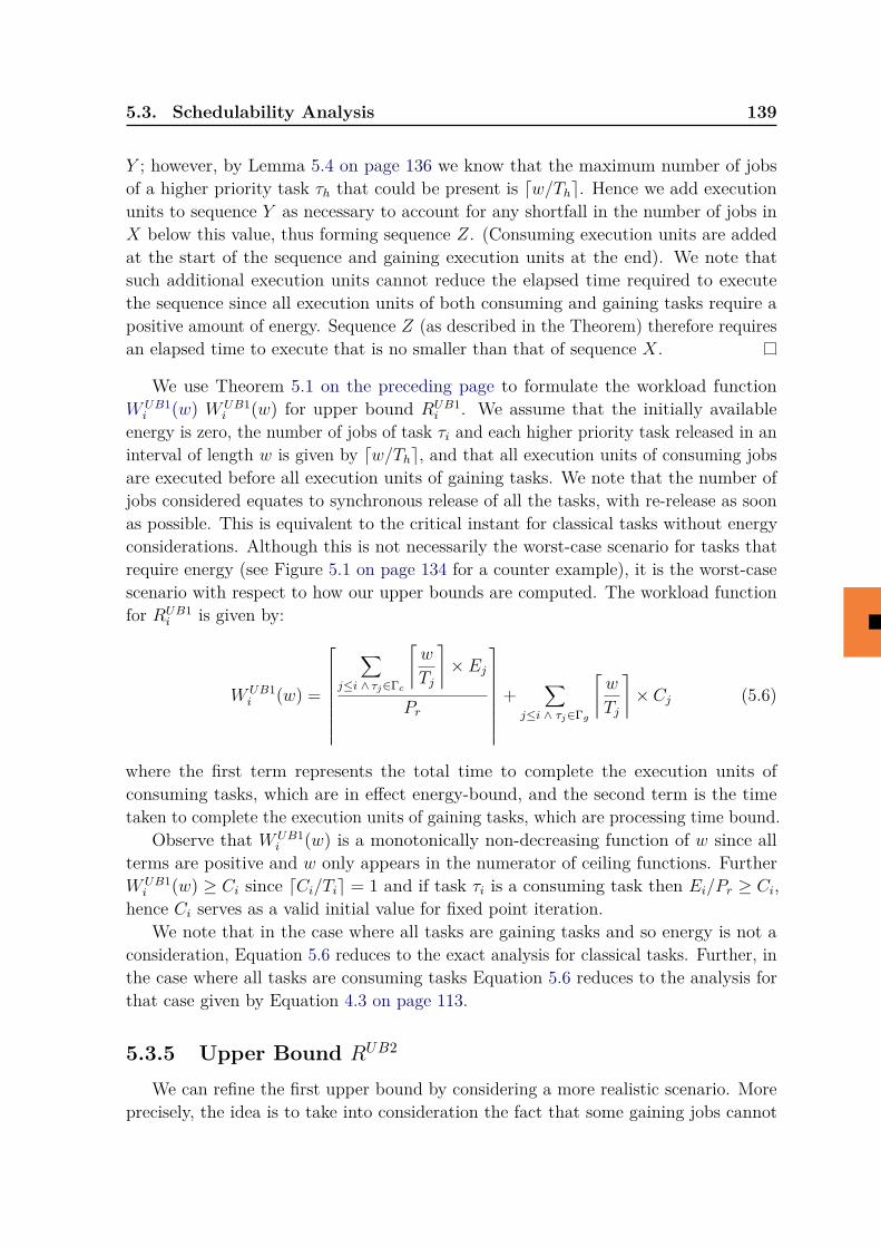
5.3. Schedulability Analysis 139
Y ; however, by Lemma 5.4 on page 136 we know that the maximum number of jobsof a higher priority task τh that could be present is dw/The. Hence we add executionunits to sequence Y as necessary to account for any shortfall in the number of jobs inX below this value, thus forming sequence Z. (Consuming execution units are addedat the start of the sequence and gaining execution units at the end). We note thatsuch additional execution units cannot reduce the elapsed time required to executethe sequence since all execution units of both consuming and gaining tasks require apositive amount of energy. Sequence Z (as described in the Theorem) therefore requiresan elapsed time to execute that is no smaller than that of sequence X.
We use Theorem 5.1 on the preceding page to formulate the workload functionWUB1i (w) WUB1
i (w) for upper bound RUB1i . We assume that the initially available
energy is zero, the number of jobs of task τi and each higher priority task released in aninterval of length w is given by dw/The, and that all execution units of consuming jobsare executed before all execution units of gaining tasks. We note that the number ofjobs considered equates to synchronous release of all the tasks, with re-release as soonas possible. This is equivalent to the critical instant for classical tasks without energyconsiderations. Although this is not necessarily the worst-case scenario for tasks thatrequire energy (see Figure 5.1 on page 134 for a counter example), it is the worst-casescenario with respect to how our upper bounds are computed. The workload functionfor RUB1
i is given by:
WUB1i (w) =
∑j≤i ∧ τj∈Γc
⌈w
Tj
⌉× Ej
Pr
+
∑j≤i ∧ τj∈Γg
⌈w
Tj
⌉× Cj (5.6)
where the first term represents the total time to complete the execution units ofconsuming tasks, which are in effect energy-bound, and the second term is the timetaken to complete the execution units of gaining tasks, which are processing time bound.
Observe that WUB1i (w) is a monotonically non-decreasing function of w since all
terms are positive and w only appears in the numerator of ceiling functions. FurtherWUB1i (w) ≥ Ci since dCi/Tie = 1 and if task τi is a consuming task then Ei/Pr ≥ Ci,
hence Ci serves as a valid initial value for fixed point iteration.We note that in the case where all tasks are gaining tasks and so energy is not a
consideration, Equation 5.6 reduces to the exact analysis for classical tasks. Further, inthe case where all tasks are consuming tasks Equation 5.6 reduces to the analysis forthat case given by Equation 4.3 on page 113.
5.3.5 Upper Bound RUB2
We can refine the first upper bound by considering a more realistic scenario. Moreprecisely, the idea is to take into consideration the fact that some gaining jobs cannot
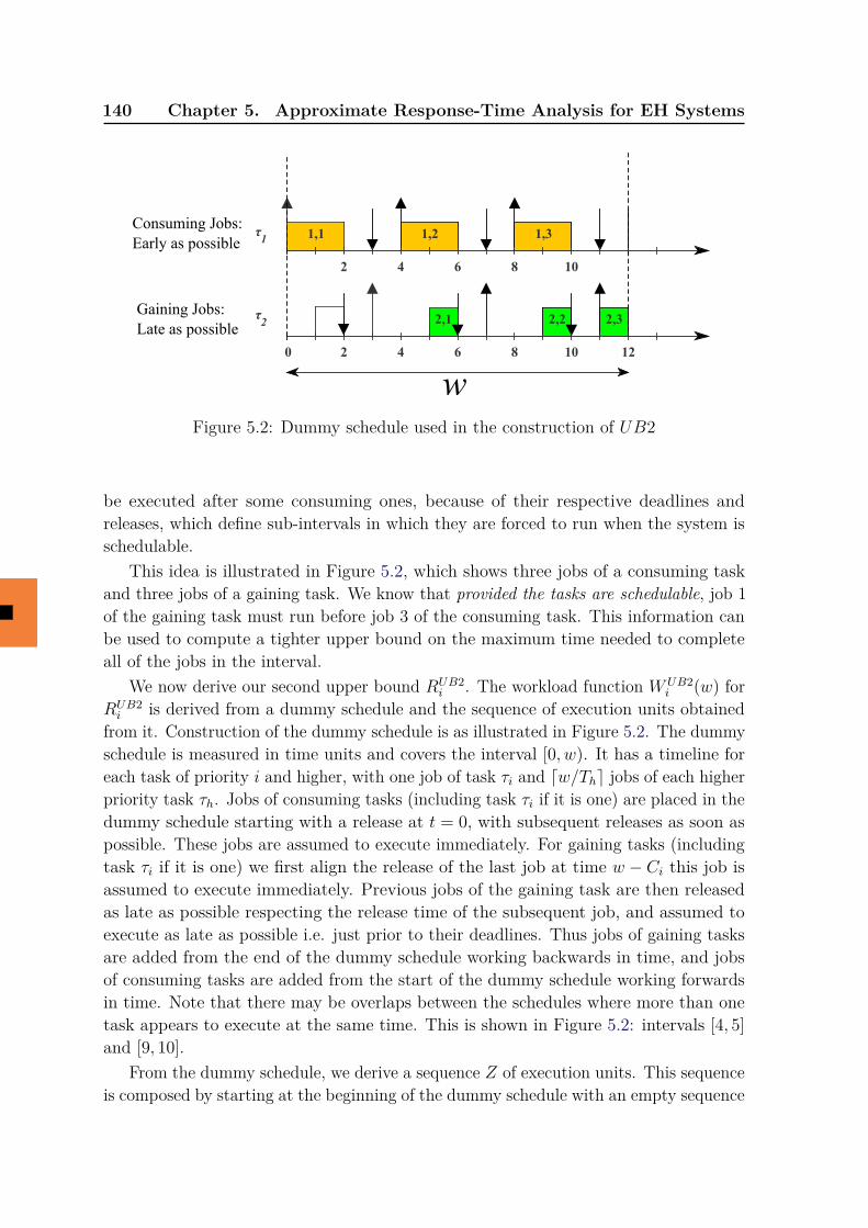
140 Chapter 5. Approximate Response-Time Analysis for EH Systems
1,1 1,2 1,3
2 4 6 8 10
τ1
2,1 2,2 2,3
0 2 4 6 8 10 12
τ2
w
Gaining Jobs:Late as possible
Consuming Jobs:Early as possible
Figure 5.2: Dummy schedule used in the construction of UB2
be executed after some consuming ones, because of their respective deadlines andreleases, which define sub-intervals in which they are forced to run when the system isschedulable.
This idea is illustrated in Figure 5.2, which shows three jobs of a consuming taskand three jobs of a gaining task. We know that provided the tasks are schedulable, job 1of the gaining task must run before job 3 of the consuming task. This information canbe used to compute a tighter upper bound on the maximum time needed to completeall of the jobs in the interval.
We now derive our second upper bound RUB2i . The workload function WUB2
i (w) forRUB2i is derived from a dummy schedule and the sequence of execution units obtained
from it. Construction of the dummy schedule is as illustrated in Figure 5.2. The dummyschedule is measured in time units and covers the interval [0, w). It has a timeline foreach task of priority i and higher, with one job of task τi and dw/The jobs of each higherpriority task τh. Jobs of consuming tasks (including task τi if it is one) are placed in thedummy schedule starting with a release at t = 0, with subsequent releases as soon aspossible. These jobs are assumed to execute immediately. For gaining tasks (includingtask τi if it is one) we first align the release of the last job at time w − Ci this job isassumed to execute immediately. Previous jobs of the gaining task are then releasedas late as possible respecting the release time of the subsequent job, and assumed toexecute as late as possible i.e. just prior to their deadlines. Thus jobs of gaining tasksare added from the end of the dummy schedule working backwards in time, and jobsof consuming tasks are added from the start of the dummy schedule working forwardsin time. Note that there may be overlaps between the schedules where more than onetask appears to execute at the same time. This is shown in Figure 5.2: intervals [4, 5]and [9, 10].
From the dummy schedule, we derive a sequence Z of execution units. This sequenceis composed by starting at the beginning of the dummy schedule with an empty sequence
5.3. Schedulability Analysis 141
and appending all gaining tasks with execution in that time unit onto the sequence,followed by all consuming tasks with execution in the same time unit. This process isthen repeated for all subsequent time units until all execution units have been collected.Note ties between execution units of two or more gaining tasks or two or more consumingtasks may be broken arbitrarily; however, all execution units of gaining tasks associatedwith some time unit t are placed into the sequence ahead of all execution units ofconsuming tasks associated with the same time unit. All execution units associatedwith a later time unit e.g. t+ 1 appear later in the sequence than those associated withan earlier time unit t (We note that clashes may safely be resolved by giving preferenceto gaining tasks, since those execution units must necessarily take place by that timeotherwise a deadline will be missed. Execution units of consuming tasks could andwould have been executed earlier in any real schedule that meets all deadlines).
Finally, the workload functionWUB2i (w) is computed giving the elapsed time required
to execute sequence Z, assuming that the initial energy is at its minimum. This can bedone via simulation, limited to at most a length of time Di.
Theorem 5.2.An upper bound on the worst-case response time for task τi for a set of jobs released in awindow of length w, where no higher priority jobs miss their deadlines, can be obtainedby assuming that there is one job of task τi and dw/The jobs of each higher priority taskτh, with the upper bound equating to the maximum time required to execute a sequenceZ of the execution units of these jobs constructed according to the rules and dummyschedule construction described previously.
Proof. Let X be the sequence of execution units that results in the longest prioritylevel−i energy busy-period under PFPASAP scheduling (and hence response time fortask τi) for a set of jobs released in a window of length w where all higher prioritytasks meet their deadlines. For each task τh, let Nh be the number of jobs in sequenceX. Consider a sequence Y formed by constructing a dummy schedule of length w
including Nh jobs of each task τh and one job of task τi and applying the rules statedabove for ordering execution units (Recall from Lemma 5.3 on page 136 that there isonly one job of task τi in the busy-period, and hence in sequence X). Sequence Y andsequence X contain an identical set of execution units. Since no deadlines are missedwhen sequence X is executed, and the dummy schedule used to construct sequence Yplaces execution units of gaining jobs as late as possible without missing a deadline, inrelation to the execution units of consuming jobs which are placed as early as possiblewithout invalidating minimum inter-arrival constraints. It follows that sequence Y canbe obtained from sequence X by a process of swapping earlier gaining execution unitsfor later consuming execution units (Note that re-ordering of sub-sequences consistingof solely gaining execution units or solely consuming execution units may also be neededto obtain precisely the same sequence; however, Lemma 5.2 on page 135 shows that thisre-ordering among execution units of the same type has no effect on the elapsed timerequired to execute the complete sequence). Finally, we compare sequence Z obtained
142 Chapter 5. Approximate Response-Time Analysis for EH Systems
as described in the Theorem, and sequence Y . If sequence Y contains the maximumnumber of jobs dw/The of each task that may be released in a window of length w, thenit is identical to sequence Z. Otherwise, sequence Z may be obtained from sequence Yby adding execution units for any missing jobs where dw/The > Nh. Since all executionunits require energy, addition of execution units into the sequence at any point cannotdecrease the elapsed time required to execute the sequence. Hence the elapsed timerequired to execute sequence Z is no shorter than that required to execute sequenceX.
Theorem 5.2 on the previous page shows that WUB2i (w) provides a valid upper
bound on the worst-case response time for task τi considering all jobs released in awindow of length w. In order to use WUB2
i (w) in a fixed point iteration to determinean upper bound on the worst-case response time of task τi we must also show thatWUB2i (w) is a monotonic non-decreasing function of w, and that WUB2
i (w) > Ci, sothat we may use Ci as an initial value. The latter is trivially the case since a single jobof task τi is always included in the workload and takes at least time Ci to execute.
Theorem 5.3.WUB2i (w) is a monotonically non-decreasing function of w.
Proof. Consider increasing the length of the window from some arbitrary value w tow + v, comparing the dummy schedules used to derive WUB2
i (w) and WUB2i (i, w + v)
there are two effects: (i) all execution units of gaining jobs move to a later time e.g.t + v rather than t, (ii) new execution units of gaining jobs may be added near thestart of the schedule and new execution units of consuming jobs may be added near theend of the schedule. Consider sequence X formed in deriving WUB2
i (w) and sequenceY formed in deriving WUB2
i (i, w + v) but omitting all of the execution units of thenew jobs from (ii). Sequences X and Y contain the same set of elements. Since allexecution units of gaining jobs are v time units later in the dummy schedule used toconstruct sequence Y , it follows that sequence Y can be formed from sequence X byswapping later gaining execution units in X for earlier consuming execution elements,and as necessary re-ordering sub-sequences containing solely gaining or solely consumingexecution units (Lemma 5.2 on page 135). Hence the elapsed time required to executesequence Y is no shorter than that required for sequence X. Consider a further sequenceZ, if there were no additional jobs from (ii) then sequence Z is identical to sequenceY , otherwise it may be obtained from sequence Y by adding execution units for themissing jobs. Since all execution units require energy, addition of execution units into asequence at any point cannot decrease the elapsed time required to execute the sequence.Hence the elapsed time required to execute sequence Z is no shorter than that requiredto execute sequence X.
We now return to the assumption in Theorem 5.2 on the previous page thatall deadlines of higher priority tasks are met. This might seem to imply that task
5.3. Schedulability Analysis 143
schedulability must be checked highest priority first; however, this is not necessarilythe case. Consider what happens if we test task schedulability lowest priority first. Wetentatively test the schedulability of task τi on the assumption that all higher prioritytasks will later be found to be schedulable. If task τi is deemed schedulable (caveat thisassumption), then we go on to check higher priority tasks. If some higher priority taskτh is subsequently found to be unschedulable, then this undermines the validity of ourschedulability test for task τi; however, this is now of no consequence, since the taskset is in any case unschedulable due to task τh. If instead, all higher priority tasks arefound to be schedulable, then the schedulability test for task τi is validated (We notethat the schedulability or otherwise of a lower priority task τi has no impact on theschedulability of any higher priority task τh).
Theorem 5.4.Schedulability test UB2 dominates test UB1 i.e RUB1
i ≥ RUB2i .
Proof. We prove the theorem by showing that WUB2i (w) ≤ WUB1
i (w). Consider thesequence Y representing WUB1
i (w) and the sequence X representing WUB2i (w). The
sequences contain the same elements; however, in sequence Y all of the consumingexecution units are before all of the gaining execution units, hence by Lemma 5.5 onpage 137, the elapsed time required to complete sequence Y is no shorter than thatrequired to complete sequence X.
5.3.6 Battery CapacityWe now return to a consideration of the minimum battery capacity Cmin (we note
CUBimin the minimum battery capacity for UBi). For the sufficient test UB1 to be valid, werequire that. CUB1
min ≥ max(max∀i(Pi)−Pr, Pr). This small battery capacity is sufficient,since in computing an upper bound on the worst-case response time, UB1 assumes thatall consuming execution units come before all gaining execution units. The minimumbattery capacity needed to execute this sequence without impinging on the elapsedtime required is simply enough to execute the most costly unit of execution in terms ofenergy, which equates to max∀i(Pi)−Pr or max∀i(Ei/Ci)−Pr. In addition, the batterycapacity cannot be less then Pr, the maximum amount of energy replenished duringone time unit.
By comparison, for the sufficient schedulability test UB2 to be valid, it suffices to havea minimum battery capacity Cmin that equates to at least the total net energy requiredto execute all of the consuming jobs in the longest possible priority level-n energy busyperiod. Such a store of energy upper bounds that which can ever usefully be deployedto execute consuming jobs in any possible busy period. Having a larger battery capacitythan this is equivalent in terms of task response times to having infinite battery capacityNote that by the total net energy required by consuming jobs, we mean the energythey consume less the energy generated while they actually execute. Since the longestpossible level-n energy-busy-period cannot be greater than the longest task deadline,
144 Chapter 5. Approximate Response-Time Analysis for EH Systems
otherwise the system would be unschedulable, we can upper bound the battery capacityrequired as follows: CUB2
min ≥ max(∑∀i
⌈max∀j(Dj)Ti
⌉×max (Ei − Ci × Pr, 0) , Pr
).
5.3.7 Response Time Lower BoundIn this section, we derive an analytical lower bound RLB1
i ≤ Ri on the worst-caseresponse time of task τi. To obtain the lower bound, we analyse a specific scenario thatcorresponds to the synchronous release of task τi along with all higher priority tasks,which are then assumed to be re-released as soon as possible. Further, we assume thatthe initial energy is a minimum i.e. E(0) = 0. Although this is not necessarily theworst-case scenario, it is a valid scenario and hence suffices to provide a valid lowerbound on the longest priority level−i energy-busy-period and hence the worst-caseresponse time of task τi.
We obtain the lower bound response time RLB1i via fixed point iteration, using
a workload function WLB1i (w) that is monotonically non-decreasing in w and lower
bounds the elapsed time needed to execute all jobs of tasks of priority i or higherreleased in an interval of length w starting with a synchronous release.
Lemma 5.6.Let X be some arbitrary sequence of execution units of tasks of priority i or higher, andY be the equivalent sequence re-ordered such that all execution units of consuming taskscome after all execution units of gaining tasks. The elapsed time required to completesequence X is no shorter than that required to complete sequence Y .
Proof. Follows by applying similar reasoning to the proof of Lemma 5.5 on page 137.
Theorem 5.5.A lower bound on the worst-case response time for task τi assuming synchronous releasewith all higher priority tasks resulting in a priority level−i energy busy-period of at leastlength w, can be obtained by assuming that there is one job of task τi and dw/The jobsof each higher priority task τh in the busy-period. Further the lower bound equates tothe time required to execute a sequence Z of the execution units of these jobs where allthe consuming execution units are after all the gaining execution units, and the initialenergy is a minimum.
Proof. By the theorem, the busy-period is at least w long, hence under PFPASAPscheduling all dw/The jobs of each higher priority task τh released during the interval[0, w) must complete before the single job of task τi. Let X be the sequence of executionunits of all of the jobs under PFPASAP scheduling. The elapsed time required to executesequence X lower bounds the worst-case response time of task τi. Further, let Z be(as per the theorem) the same set of execution units as sequence X re-ordered suchthat all the consuming execution units are after all the gaining execution units. ByLemma 5.6, the elapsed time to execute sequence Z is no longer than that required toexecute sequence X.
5.3. Schedulability Analysis 145
We use Theorem 5.5 on the preceding page to formulate our lower bound workloadfunction WLB1
i (w). We assume that the initially available energy is zero, the number ofjobs of task τi and each higher priority task τh released in an interval of length w isgiven by dw/The and that all execution units of consuming jobs are executed after allexecution units of gaining tasks.
Xgi =
τh∈Γg∑h∈hep(i)
⌈w
Th
⌉× Ch , Xc
i =τh∈Γc∑h∈hep(i)
⌈w
Th
⌉× Ch
Y ci =
τh∈Γc∑h∈hep(i)
⌈w
Th
⌉× Eh , Y g
i =τh∈Γg∑h∈hep(i)
⌈w
Th
⌉× Eh
WLB1i (w) = Xg
i + max(Xci ,
⌈Y ci − (Xg
i × Pr − Ygi )
Pr
⌉)(5.7)
Finally, in order to use the workload function WLB1i (w) in a fixed point iteration to
determine the lower bound RLB1i on the worst-case response time of task τi, we must
show that WLB1i (w) is a monotonically non-decreasing function of w.
Theorem 5.6.WLB1i (w) is a monotonically non-decreasing function of w.
Proof. Consider the formula forWLB1i (w). Since w appears only in the ceiling functions,
it follows thatXgi , X
ci and Y
gi are all non-decreasing functions of w. Further, (Xg
i Pr−Ygi )
represents the net energy increase while all the gaining jobs execute. Since everyexecution unit of a gaining task is by definition energy positive, this quantity is also anon-decreasing function of w. Thus Y c
i − (Xgi Pr − Y
gi ) may decrease with increasing
w. The largest possible decrease is obtained when Y ci remains at the same value, while
(Xgi Pr − Y
gi ) increases, hence d(Xg
i Pr − Ygi )/Pre decreases. However, such a decrease is
always at least compensated for by the increasing value of the first term in Equation 5.7,i.e. Xg
i . This happens because the additional energy made available by each executionunit of an additional gaining job is no more than that available from a replenishmentunit. Hence d(Xg
i Pr − Ygi )/Pre cannot decrease by more than Xg
i increases. We notethat monotonicity can also easily be seen by considering the sequence Z (in Theorem 5.5on the preceding page) which can only take a longer elapsed time to execute with theaddition of further jobs, since all execution units require a positive amount of energy.
We note that a tighter lower bound can be obtained via the simple expedient ofsimulating the actual schedule of execution starting from synchronous release of task τiand all higher priority tasks. We return to this point in Section 5.4 on page 147.
146 Chapter 5. Approximate Response-Time Analysis for EH Systems
5.3.8 Priority Assignment
The DM priority assignment is optimal for fixed-priority preemptive schedulingof constrained deadline tasks conforming to the classical task model where energy isnot considered. In Section 4.3.4 on page 119, we extended the optimality of DM toenergy-non-concrete task sets that are composed of only consuming tasks. However,when we relax the assumption on tasks energy consumption, i.e. gaining tasks areaccepted, the proof provided in Section 4.3.4 is no longer valid. In this section, we showthat DM priority assignment is also optimal with respect to our sufficient schedulabilitytests UB1 and UB2, for energy-constrained systems with both consuming and gainingtasks. This does not mean that DM is optimal for energy-work-conserving schedulingin the general case, but only with respect to the necessary schedulability conditionsbased on UB1 and UB2.
Definition 5.4 (Optimal Priority Assignment Policy).A priority assignment policy P is said to be optimal with respect to a schedulabilitytest S, if for every task set τ where there exists some priority assignment Q such thatthe task set is schedulable according to test S, then τ is also schedulable according totest S with the priority ordering given by policy P . �
Theorem 5.7.Deadline Monotonic (DM) priority assignment is an optimal priority assignment policywith respect to sufficient schedulability test S (UB1 or UB2) for task sets comprisingany arbitrary combination of consuming and gaining tasks.
Proof. To prove the theorem, we show that any task set Γ that is schedulable accordingto test S (UB1 or UB2) under some priority ordering Q remains schedulable accordingto test S under deadline monotonic priority order P . We do this by transformingpriority order Q into priority order P by swapping the priorities of tasks that areadjacent to each other in the priority order, but out of DM order. We show that onevery swap the task set remains schedulable according to test S. Let τA and τB betwo tasks in τ which are at adjacent priorities under the initial, schedulable priorityordering, with DA > DB and τA at a higher priority k than τB, which has a priorityi = k + 1 (i.e. the tasks are out of DM order). Let the upper bound response timeof task τB according to schedulability test S be RUB
i in the initial priority order. Wenow swap the priorities of the tasks, so that τB has the higher priority. We consider thefollowing groups of tasks:
(i) hp(k): these tasks have higher priorities than either τA or τB and so their upperbound response times, according to test S (UB1 or UB2), are unchanged by the swap.
(ii) lp(i): these tasks have lower priorities than either τA or τB and so their upperbound response times, according to test S (UB1 or UB2), are unchanged by the swap,since interference from higher priority tasks does not, according to the test, depend onthe relative priority order of those tasks.
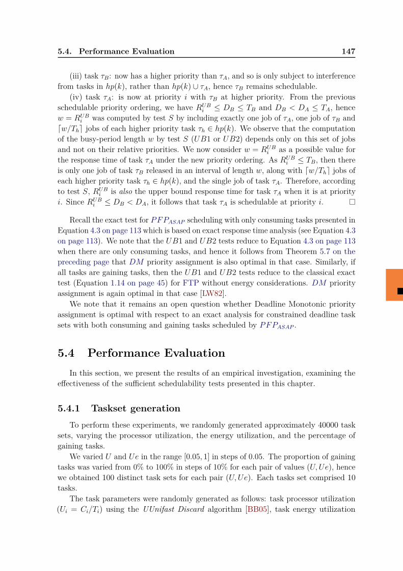
5.4. Performance Evaluation 147
(iii) task τB: now has a higher priority than τA, and so is only subject to interferencefrom tasks in hp(k), rather than hp(k) ∪ τA, hence τB remains schedulable.
(iv) task τA: is now at priority i with τB at higher priority. From the previousschedulable priority ordering, we have RUB
i ≤ DB ≤ TB and DB < DA ≤ TA, hencew = RUB
i was computed by test S by including exactly one job of τA, one job of τB anddw/The jobs of each higher priority task τh ∈ hp(k). We observe that the computationof the busy-period length w by test S (UB1 or UB2) depends only on this set of jobsand not on their relative priorities. We now consider w = RUB
i as a possible value forthe response time of task τA under the new priority ordering. As RUB
i ≤ TB, then thereis only one job of task τB released in an interval of length w, along with dw/The jobs ofeach higher priority task τh ∈ hp(k), and the single job of task τA. Therefore, accordingto test S, RUB
i is also the upper bound response time for task τA when it is at priorityi. Since RUB
i ≤ DB < DA, it follows that task τA is schedulable at priority i.
Recall the exact test for PFPASAP scheduling with only consuming tasks presented inEquation 4.3 on page 113 which is based on exact response time analysis (see Equation 4.3on page 113). We note that the UB1 and UB2 tests reduce to Equation 4.3 on page 113when there are only consuming tasks, and hence it follows from Theorem 5.7 on thepreceding page that DM priority assignment is also optimal in that case. Similarly, ifall tasks are gaining tasks, then the UB1 and UB2 tests reduce to the classical exacttest (Equation 1.14 on page 45) for FTP without energy considerations. DM priorityassignment is again optimal in that case [LW82].
We note that it remains an open question whether Deadline Monotonic priorityassignment is optimal with respect to an exact analysis for constrained deadline tasksets with both consuming and gaining tasks scheduled by PFPASAP .
5.4 Performance EvaluationIn this section, we present the results of an empirical investigation, examining the
effectiveness of the sufficient schedulability tests presented in this chapter.
5.4.1 Taskset generationTo perform these experiments, we randomly generated approximately 40000 task
sets, varying the processor utilization, the energy utilization, and the percentage ofgaining tasks.
We varied U and Ue in the range [0.05, 1] in steps of 0.05. The proportion of gainingtasks was varied from 0% to 100% in steps of 10% for each pair of values (U,Ue), hencewe obtained 100 distinct task sets for each pair (U,Ue). Each tasks set comprised 10tasks.
The task parameters were randomly generated as follows: task processor utilization(Ui = Ci/Ti) using the UUnifast Discard algorithm [BB05], task energy utilization
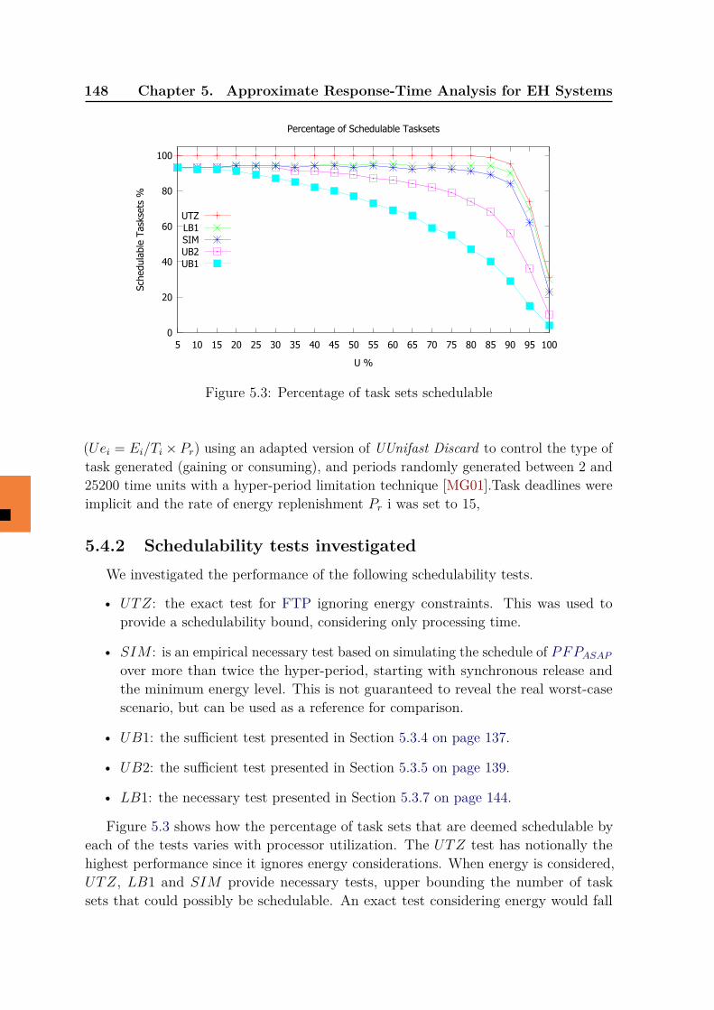
148 Chapter 5. Approximate Response-Time Analysis for EH Systems
0
20
40
60
80
100
5 10 15 20 25 30 35 40 45 50 55 60 65 70 75 80 85 90 95 100
Sche
dula
ble
Task
sets
%
U %
Percentage of Schedulable Tasksets
UTZLB1SIMUB2UB1
Figure 5.3: Percentage of task sets schedulable
(Uei = Ei/Ti × Pr) using an adapted version of UUnifast Discard to control the type oftask generated (gaining or consuming), and periods randomly generated between 2 and25200 time units with a hyper-period limitation technique [MG01].Task deadlines wereimplicit and the rate of energy replenishment Pr i was set to 15,
5.4.2 Schedulability tests investigatedWe investigated the performance of the following schedulability tests.
• UTZ: the exact test for FTP ignoring energy constraints. This was used toprovide a schedulability bound, considering only processing time.
• SIM : is an empirical necessary test based on simulating the schedule of PFPASAPover more than twice the hyper-period, starting with synchronous release andthe minimum energy level. This is not guaranteed to reveal the real worst-casescenario, but can be used as a reference for comparison.
• UB1: the sufficient test presented in Section 5.3.4 on page 137.
• UB2: the sufficient test presented in Section 5.3.5 on page 139.
• LB1: the necessary test presented in Section 5.3.7 on page 144.
Figure 5.3 shows how the percentage of task sets that are deemed schedulable byeach of the tests varies with processor utilization. The UTZ test has notionally thehighest performance since it ignores energy considerations. When energy is considered,UTZ, LB1 and SIM provide necessary tests, upper bounding the number of tasksets that could possibly be schedulable. An exact test considering energy would fall
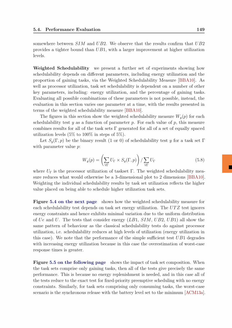
5.4. Performance Evaluation 149
somewhere between SIM and UB2. We observe that the results confirm that UB2provides a tighter bound than UB1, with a larger improvement at higher utilizationlevels.
Weighted Schedulability we present a further set of experiments showing howschedulability depends on different parameters, including energy utilization and theproportion of gaining tasks, via the Weighted Schedulability Measure [BBA10]. Aswell as processor utilization, task set schedulability is dependent on a number of otherkey parameters, including: energy utilization, and the percentage of gaining tasks.Evaluating all possible combinations of these parameters is not possible, instead, theevaluation in this section varies one parameter at a time, with the results presented interms of the weighted schedulability measure [BBA10].
The figures in this section show the weighted schedulability measure Wy(p) for eachschedulability test y as a function of parameter p. For each value of p, this measurecombines results for all of the task sets Γ generated for all of a set of equally spacedutilization levels (5% to 100% in steps of 5%).
Let Sy(Γ, p) be the binary result (1 or 0) of schedulability test y for a task set Γwith parameter value p:
Wy(p) =(∑∀ΓUΓ × Sy(Γ, p)
)/∑∀ΓUΓ (5.8)
where UΓ is the processor utilization of taskset Γ. The weighted schedulability mea-sure reduces what would otherwise be a 3-dimensional plot to 2 dimensions [BBA10].Weighting the individual schedulability results by task set utilization reflects the highervalue placed on being able to schedule higher utilization task sets.
Figure 5.4 on the next page shows how the weighted schedulability measure foreach schedulability test depends on task set energy utilization. The UTZ test ignoresenergy constraints and hence exhibits minimal variation due to the uniform distributionof Ue and U . The tests that consider energy (LB1, SIM , UB2, UB1) all show thesame pattern of behaviour as the classical schedulability tests do against processorutilization, i.e. schedulability reduces at high levels of utilization (energy utilization inthis case). We note that the performance of the simple sufficient test UB1 degradeswith increasing energy utilization because in this case the overestimation of worst-caseresponse times is greater.
Figure 5.5 on the following page shows the impact of task set composition. Whenthe task sets comprise only gaining tasks, then all of the tests give precisely the sameperformance. This is because no energy replenishment is needed, and in this case all ofthe tests reduce to the exact test for fixed-priority preemptive scheduling with no energyconstraints. Similarly, for task sets comprising only consuming tasks, the worst-casescenario is the synchronous release with the battery level set to the minimum [ACM13a].
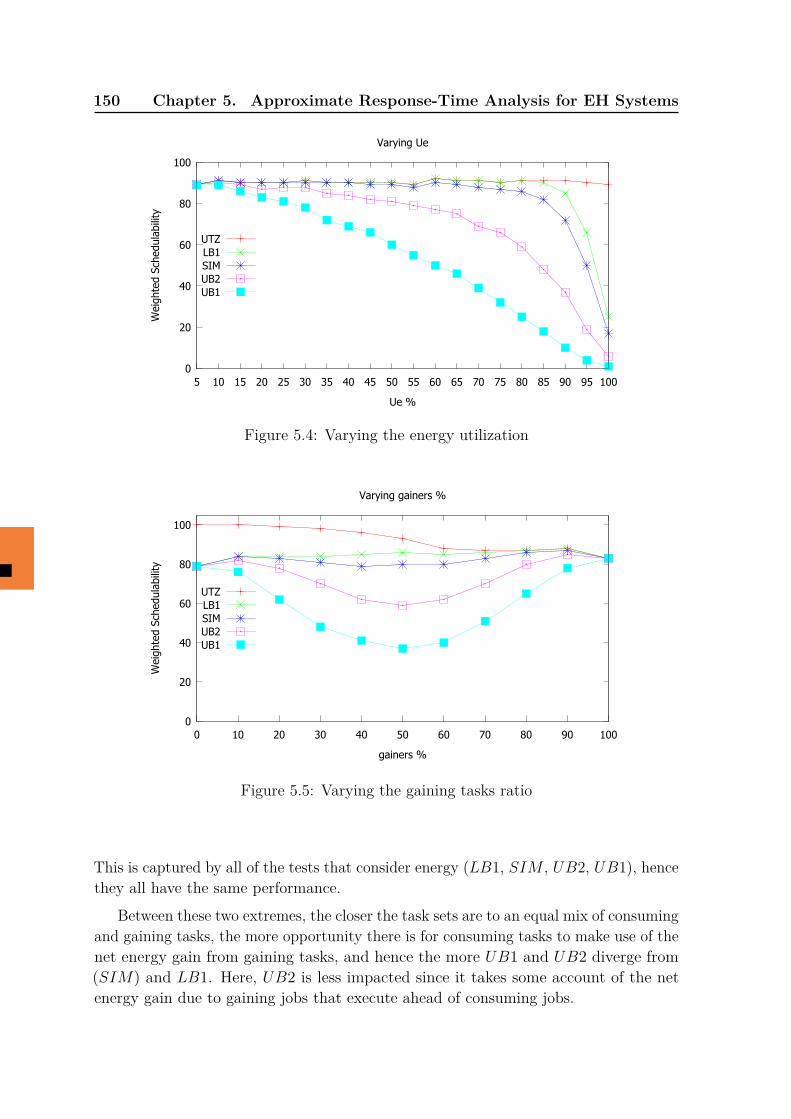
150 Chapter 5. Approximate Response-Time Analysis for EH Systems
0
20
40
60
80
100
5 10 15 20 25 30 35 40 45 50 55 60 65 70 75 80 85 90 95 100
Wei
ghte
d Sc
hedu
labi
lity
Ue %
Varying Ue
UTZLB1SIMUB2UB1
Figure 5.4: Varying the energy utilization
0
20
40
60
80
100
0 10 20 30 40 50 60 70 80 90 100
Wei
ghte
d Sc
hedu
labi
lity
gainers %
Varying gainers %
UTZLB1SIMUB2UB1
Figure 5.5: Varying the gaining tasks ratio
This is captured by all of the tests that consider energy (LB1, SIM , UB2, UB1), hencethey all have the same performance.
Between these two extremes, the closer the task sets are to an equal mix of consumingand gaining tasks, the more opportunity there is for consuming tasks to make use of thenet energy gain from gaining tasks, and hence the more UB1 and UB2 diverge from(SIM) and LB1. Here, UB2 is less impacted since it takes some account of the netenergy gain due to gaining jobs that execute ahead of consuming jobs.
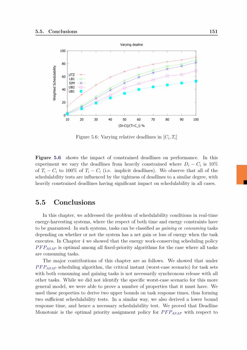
5.5. Conclusions 151
0
20
40
60
80
100
10 20 30 40 50 60 70 80 90 100
Wei
ghte
d Sc
hedu
labi
lity
(Di-Ci)/(Ti-C_i) %
Varying dealine
UTZLB1SIMUB2UB1
Figure 5.6: Varying relative deadlines in [Ci, Ti]
Figure 5.6 shows the impact of constrained deadlines on performance. In thisexperiment we vary the deadlines from heavily constrained where Di − Ci is 10%of Ti − Ci to 100% of Ti − Ci (i.e. implicit deadlines). We observe that all of theschedulability tests are influenced by the tightness of deadlines to a similar degree, withheavily constrained deadlines having significant impact on schedulability in all cases.
5.5 ConclusionsIn this chapter, we addressed the problem of schedulability conditions in real-time
energy-harvesting systems, where the respect of both time and energy constraints haveto be guaranteed. In such systems, tasks can be classified as gaining or consuming tasksdepending on whether or not the system has a net gain or loss of energy when the taskexecutes. In Chapter 4 we showed that the energy work-conserving scheduling policyPFPASAP is optimal among all fixed-priority algorithms for the case where all tasksare consuming tasks.
The major contributions of this chapter are as follows. We showed that underPFPASAP scheduling algorithm, the critical instant (worst-case scenario) for task setswith both consuming and gaining tasks is not necessarily synchronous release with allother tasks. While we did not identify the specific worst-case scenario for this moregeneral model, we were able to prove a number of properties that it must have. Weused these properties to derive two upper bounds on task response times, thus formingtwo sufficient schedulability tests. In a similar way, we also derived a lower boundresponse time, and hence a necessary schedulability test. We proved that DeadlineMonotonic is the optimal priority assignment policy for PFPASAP with respect to

152 Chapter 5. Approximate Response-Time Analysis for EH Systems
our sufficient tests. Finally, we evaluated the performance of the sufficient tests incomparison with a number of necessary tests, including an exact test for fixed-prioritypreemptive scheduling ignoring energy constraints, and an empirical test based onsimulating the schedule for more than a hyperperiod. We found that our tighter upperbound (sufficient schedulability test UB2) provides good performance over a wide rangeof values of different parameters e.g. energy utilization, proportion of gaining tasks etc.(explored using the weighted schedulability measure).
Chapter 6
Optimal Algorithm Investigation
Contents6.1 Introduction . . . . . . . . . . . . . . . . . . . . . . . . . . . . . 1536.2 Definitions and Notations . . . . . . . . . . . . . . . . . . . . . 154
6.2.1 Model and Notations . . . . . . . . . . . . . . . . . . . . . . . . . 1546.2.2 Definitions . . . . . . . . . . . . . . . . . . . . . . . . . . . . . . 1546.2.3 Energy-Work-Conserving . . . . . . . . . . . . . . . . . . . . . . 1556.2.4 Energy-Lookahead Scheduling . . . . . . . . . . . . . . . . . . . . 158
6.3 Algorithms . . . . . . . . . . . . . . . . . . . . . . . . . . . . . . 1596.4 Conclusion . . . . . . . . . . . . . . . . . . . . . . . . . . . . . . 172
6.1 IntroductionIn the precedent chapters we saw that finding efficient scheduling algorithms for
fixed-priority energy-harvesting systems is one of the challenges of this research area. InChapter 4, we presented PFPASAP which is an optimal scheduling algorithm. Moreover,the optimality of this algorithm relies on two main assumptions: the considered task setsare energy-non-concrete (see Definition 3.4 on page 70), and all the tasks consume moreenergy than it is replenished. Unfortunately, removing one of these two assumptions leadsPFPASAP to lose its optimality. This is due to the fact that without these assumptions,the worst-case scenario of PFPASAP is no longer the synchronous activation withthe minimum battery capacity. Moreover, without these assumptions, the worst-casescenario is unknown up to now. There exist some counter examples that prove thenon-optimality of PFPASAP (see Figures 6.2 on page 157 and 5.1 on page 134).
The challenge now is to understand why does PFPASAP lose its optimality andwe try to study deeply the fixed-priority scheduling for energy-harvesting systems byattempting to build an optimal algorithm or otherwise to prove the nonexistence ofsuch an algorithm.
In this chapter, we explore different intuitive ideas of scheduling algorithms and weexplain why they are not optimal through counter examples. Then, we show the difficultyof finding an optimal algorithm or proving the nonexistence of such an algorithm witha reasonable complexity.
154 Chapter 6. Optimal Algorithm Investigation
The remainder of this chapter is organized as follows. In section 6.2 we define andprove some properties of fixed-priority scheduling for energy-harvesting systems. Afterthat, we explore in Section 6.3 different ideas of scheduling algorithms and we discussthe existence of an optimal algorithm. Finally, we conclude the chapter with Section6.4.
6.2 Definitions and NotationsIn order to facilitate the understanding of the next sections, we first redefine and
prove some properties.
6.2.1 Model and NotationsIn this chapter we consider the model described in Section 3.2 on page 67. Fur-
thermore, in addition to the notations set in Section 1.2 on page 30, we consider thefollowing ones.
• si,j: the starting time of job Ji,j,
• ai(t): the next activation time of task τi after time t,
• ci(t): the remaining execution time of the current job of task τi at time t. It isequal to 0 if the job is already finished,
• ei(t): the remaining energy cost of the current job of task τi at time t. It is equalto 0 if the job has finished its execution,
• di(t): the absolute deadline of the current job of task τi at time t, it does notexist if the job is not yet activated,
• si(t): the execution starting time of the current job of task τi at time t, it isundefined if the job is not yet activated.
6.2.2 DefinitionsDefinition 6.1 (Energy Demand).The energy demand of priority level-i of time interval [t1, t2[ denoted Wei(t1, t2) isthe amount of energy to be consumed by the execution of the jobs of priority levels1, . . . , i− 1, i that are requested within interval [t1, t2[ or are pending at time t1. It canbe obtained by Equation 6.1.
Wei(t1, t2) =∑j≤i
ej(t1) +⌈t2 − aj(t1)
Tj
⌉× Ej (6.1)
�
6.2. Definitions and Notations 155
The intuition behind Equation 6.1 on the facing page is derived from the notion ofprocessor demand. It represents the sum of the cost of energy of all the jobs of priorityequal or higher than i that are requested during the time interval [t1, t2[. The energydemand of time interval [0, t[ is just noted Wei(t) and can be obtained by Equation 6.2.
Wei(t) = Wei(0, t) =∑j≤i
⌈t−Oj
Tj
⌉× Ej (6.2)
Definition 6.2 (Energy Budget).The energy budget of the system during time interval [t1, t2] denoted Bu(t1, t2) is theamount of energy available until time t2, i.e. the battery level at time t1 plus the energyreplenished during time interval [t1, t2]. It can be computed by Equation 6.3.
Bu(t1, t2) = E(t1) +∫ t2
t1Pr(t) dt (6.3)
�
Definition 6.3 (Energy Balance).The energy balance of a job Ji,j at time t denoted Bai(t) is the difference between theenergy budget between time t and the deadline of Ji,j, and the energy demand of thesame priority level and the same time interval. It can be obtained by Equation 6.4.
Bai(t) = Bu(t, di,j)−Wei(t, di,j) (6.4)
�
We notice that if the time t does not coincide with a request time of task τi and theprevious job has already finished its execution, we must include the execution of thelower priority jobs between time t and the next request time of priority level-i, i.e. ai(t),because they consume energy before time ai(t) and can change the energy balance attime di,j as illustrated in Figure 6.1 on the following page. However, these lower priorityexecutions units depend on the used scheduling algorithm, i.e. energy-work-conservingor not. This limitation is discussed in Section 6.3 on page 159.
6.2.3 Energy-Work-ConservingWithout taking into account energy constraints, the work-conserving property in
real-time scheduling means that the scheduling algorithm does not add idle times whenthere is at least one job ready to execute. However, when we consider energy-harvestingconstraints, scheduling algorithms may add necessary idle periods to replenish energy.Then, this notion is extended to energy-work-conserving in Definition 3.5 on page 70 toinclude replenishment time.
Furthermore, as described in Definition 3.3 on page 70, in the energy-harvestingcontext, a scheduling algorithm is considered as energy-work-conserving if it schedules
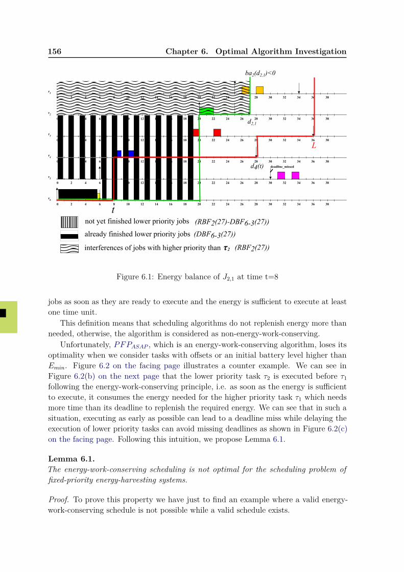
156 Chapter 6. Optimal Algorithm Investigation
t
d4(t)
d2,1
L
interferences of jobs with higher priority than
0 2 4 6 8 10 12 14 16 18 20 22 24 26 28 30 32 34 36 38
τ1
0 2 4 6 8 10 12 14 16 18 20 22 24 26 28 30 32 34 36 38
τ2
0 2 4 6 8 10 12 14 16 18 20 22 24 26 28 30 32 34 36 38
τ3
0 2 4 6 8 10 12 14 16 18 20 22 24 26 28 30 32 34 36 38
τ4
deadline_missed
0 2 4 6 8 10 12 14 16 18 20 22 24 26 28 30 32 34 36 38
τ5
0 2 4 6 8 10 12 14 16 18 20 22 24 26 28 30 32 34 36 38
τ6
ba2(d2,1)<0
τ2
not yet finished lower priority jobs
already finished lower priority jobs
(RBF2(27))
(DBF6-3(27))
(RBF2(27)-DBF6-3(27))
Figure 6.1: Energy balance of J2,1 at time t=8
jobs as soon as they are ready to execute and the energy is sufficient to execute at leastone time unit.
This definition means that scheduling algorithms do not replenish energy more thanneeded, otherwise, the algorithm is considered as non-energy-work-conserving.
Unfortunately, PFPASAP , which is an energy-work-conserving algorithm, loses itsoptimality when we consider tasks with offsets or an initial battery level higher thanEmin. Figure 6.2 on the facing page illustrates a counter example. We can see inFigure 6.2(b) on the next page that the lower priority task τ2 is executed before τ1following the energy-work-conserving principle, i.e. as soon as the energy is sufficientto execute, it consumes the energy needed for the higher priority task τ1 which needsmore time than its deadline to replenish the required energy. We can see that in such asituation, executing as early as possible can lead to a deadline miss while delaying theexecution of lower priority tasks can avoid missing deadlines as shown in Figure 6.2(c)on the facing page. Following this intuition, we propose Lemma 6.1.
Lemma 6.1.The energy-work-conserving scheduling is not optimal for the scheduling problem offixed-priority energy-harvesting systems.
Proof. To prove this property we have just to find an example where a valid energy-work-conserving schedule is not possible while a valid schedule exists.
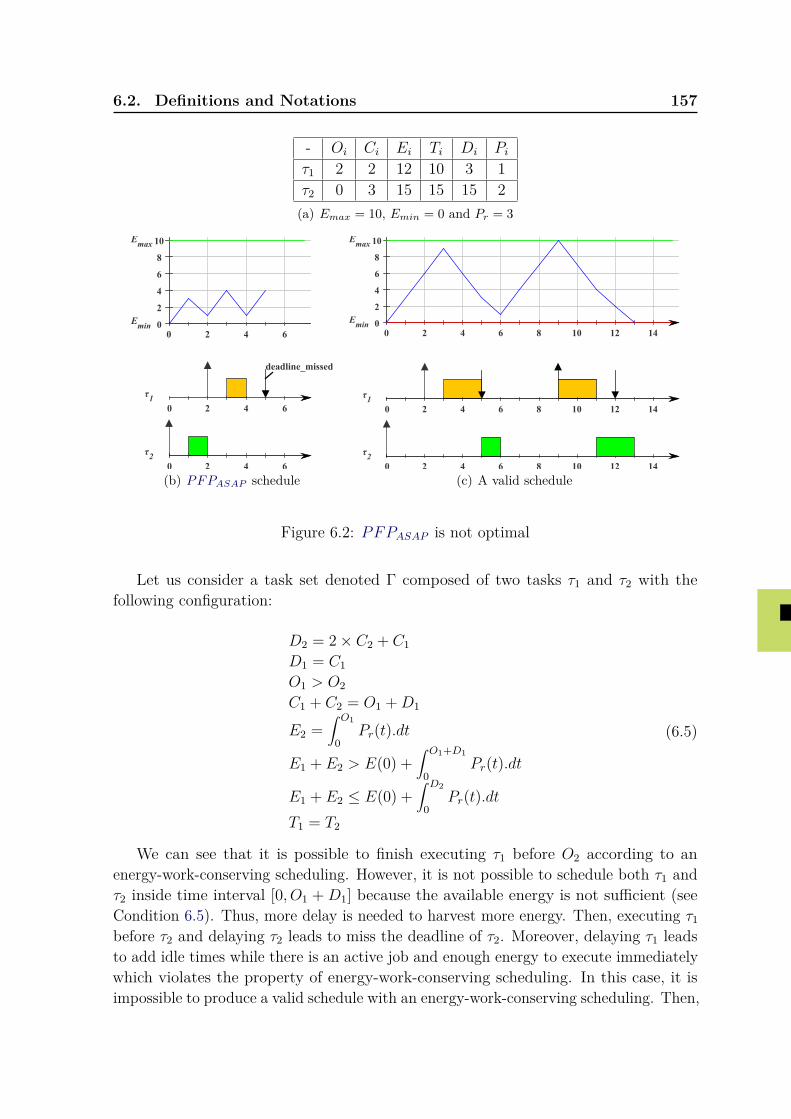
6.2. Definitions and Notations 157
- Oi Ci Ei Ti Di Piτ1 2 2 12 10 3 1τ2 0 3 15 15 15 2(a) Emax = 10, Emin = 0 and Pr = 3
0 2 4 60
2
4
6
8
10Emax
Emin
deadline_missed
0 2 4 6
τ1
0 2 4 6
τ2
(b) PFPASAP schedule
0 2 4 6 8 10 12 140
2
4
6
8
10Emax
Emin
0 2 4 6 8 10 12 14
τ1
0 2 4 6 8 10 12 14
τ2
(c) A valid schedule
Figure 6.2: PFPASAP is not optimal
Let us consider a task set denoted Γ composed of two tasks τ1 and τ2 with thefollowing configuration:
D2 = 2× C2 + C1D1 = C1O1 > O2C1 + C2 = O1 +D1
E2 =∫ O1
0Pr(t).dt
E1 + E2 > E(0) +∫ O1+D1
0Pr(t).dt
E1 + E2 ≤ E(0) +∫ D2
0Pr(t).dt
T1 = T2
(6.5)
We can see that it is possible to finish executing τ1 before O2 according to anenergy-work-conserving scheduling. However, it is not possible to schedule both τ1 andτ2 inside time interval [0, O1 + D1] because the available energy is not sufficient (seeCondition 6.5). Thus, more delay is needed to harvest more energy. Then, executing τ1before τ2 and delaying τ2 leads to miss the deadline of τ2. Moreover, delaying τ1 leadsto add idle times while there is an active job and enough energy to execute immediatelywhich violates the property of energy-work-conserving scheduling. In this case, it isimpossible to produce a valid schedule with an energy-work-conserving scheduling. Then,
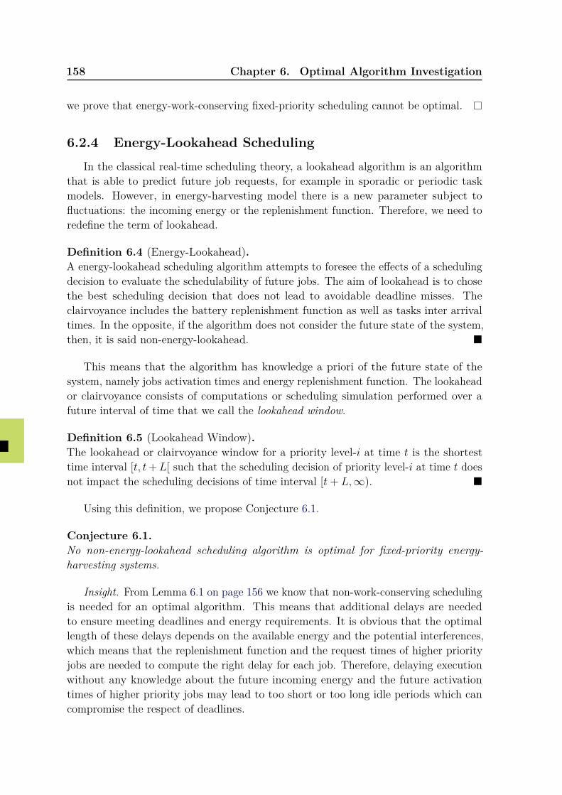
158 Chapter 6. Optimal Algorithm Investigation
we prove that energy-work-conserving fixed-priority scheduling cannot be optimal.
6.2.4 Energy-Lookahead SchedulingIn the classical real-time scheduling theory, a lookahead algorithm is an algorithm
that is able to predict future job requests, for example in sporadic or periodic taskmodels. However, in energy-harvesting model there is a new parameter subject tofluctuations: the incoming energy or the replenishment function. Therefore, we need toredefine the term of lookahead.
Definition 6.4 (Energy-Lookahead).A energy-lookahead scheduling algorithm attempts to foresee the effects of a schedulingdecision to evaluate the schedulability of future jobs. The aim of lookahead is to chosethe best scheduling decision that does not lead to avoidable deadline misses. Theclairvoyance includes the battery replenishment function as well as tasks inter arrivaltimes. In the opposite, if the algorithm does not consider the future state of the system,then, it is said non-energy-lookahead. �
This means that the algorithm has knowledge a priori of the future state of thesystem, namely jobs activation times and energy replenishment function. The lookaheador clairvoyance consists of computations or scheduling simulation performed over afuture interval of time that we call the lookahead window.
Definition 6.5 (Lookahead Window).The lookahead or clairvoyance window for a priority level-i at time t is the shortesttime interval [t, t+L[ such that the scheduling decision of priority level-i at time t doesnot impact the scheduling decisions of time interval [t+ L,∞). �
Using this definition, we propose Conjecture 6.1.
Conjecture 6.1.No non-energy-lookahead scheduling algorithm is optimal for fixed-priority energy-harvesting systems.
Insight. From Lemma 6.1 on page 156 we know that non-work-conserving schedulingis needed for an optimal algorithm. This means that additional delays are neededto ensure meeting deadlines and energy requirements. It is obvious that the optimallength of these delays depends on the available energy and the potential interferences,which means that the replenishment function and the request times of higher priorityjobs are needed to compute the right delay for each job. Therefore, delaying executionwithout any knowledge about the future incoming energy and the future activationtimes of higher priority jobs may lead to too short or too long idle periods which cancompromise the respect of deadlines.
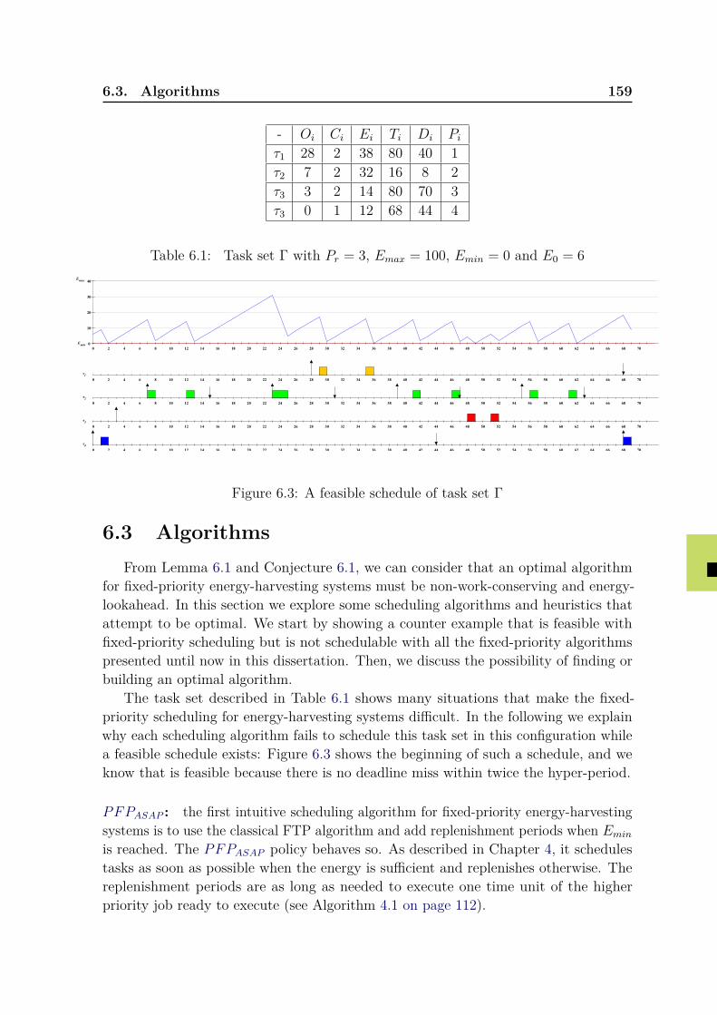
6.3. Algorithms 159
- Oi Ci Ei Ti Di Piτ1 28 2 38 80 40 1τ2 7 2 32 16 8 2τ3 3 2 14 80 70 3τ3 0 1 12 68 44 4
Table 6.1: Task set Γ with Pr = 3, Emax = 100, Emin = 0 and E0 = 6
0 2 4 6 8 10 12 14 16 18 20 22 24 26 28 30 32 34 36 38 40 42 44 46 48 50 52 54 56 58 60 62 64 66 68 700
10
20
30
40Emax
Emin
0 2 4 6 8 10 12 14 16 18 20 22 24 26 28 30 32 34 36 38 40 42 44 46 48 50 52 54 56 58 60 62 64 66 68 70
τ1
0 2 4 6 8 10 12 14 16 18 20 22 24 26 28 30 32 34 36 38 40 42 44 46 48 50 52 54 56 58 60 62 64 66 68 70
τ2
0 2 4 6 8 10 12 14 16 18 20 22 24 26 28 30 32 34 36 38 40 42 44 46 48 50 52 54 56 58 60 62 64 66 68 70
τ3
0 2 4 6 8 10 12 14 16 18 20 22 24 26 28 30 32 34 36 38 40 42 44 46 48 50 52 54 56 58 60 62 64 66 68 70
τ4
Figure 6.3: A feasible schedule of task set Γ
6.3 AlgorithmsFrom Lemma 6.1 and Conjecture 6.1, we can consider that an optimal algorithm
for fixed-priority energy-harvesting systems must be non-work-conserving and energy-lookahead. In this section we explore some scheduling algorithms and heuristics thatattempt to be optimal. We start by showing a counter example that is feasible withfixed-priority scheduling but is not schedulable with all the fixed-priority algorithmspresented until now in this dissertation. Then, we discuss the possibility of finding orbuilding an optimal algorithm.
The task set described in Table 6.1 shows many situations that make the fixed-priority scheduling for energy-harvesting systems difficult. In the following we explainwhy each scheduling algorithm fails to schedule this task set in this configuration whilea feasible schedule exists: Figure 6.3 shows the beginning of such a schedule, and weknow that is feasible because there is no deadline miss within twice the hyper-period.
PFPASAP : the first intuitive scheduling algorithm for fixed-priority energy-harvestingsystems is to use the classical FTP algorithm and add replenishment periods when Eminis reached. The PFPASAP policy behaves so. As described in Chapter 4, it schedulestasks as soon as possible when the energy is sufficient and replenishes otherwise. Thereplenishment periods are as long as needed to execute one time unit of the higherpriority job ready to execute (see Algorithm 4.1 on page 112).
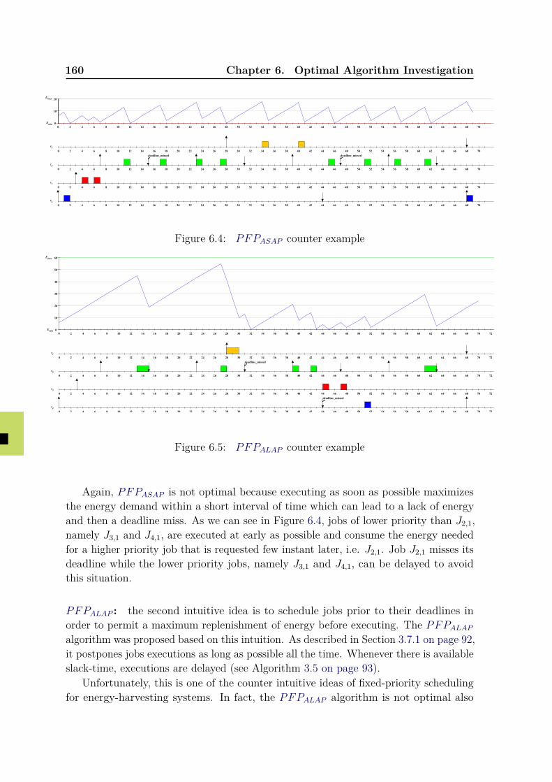
160 Chapter 6. Optimal Algorithm Investigation
0 2 4 6 8 10 12 14 16 18 20 22 24 26 28 30 32 34 36 38 40 42 44 46 48 50 52 54 56 58 60 62 64 66 68 700
10
20Emax
Emin
0 2 4 6 8 10 12 14 16 18 20 22 24 26 28 30 32 34 36 38 40 42 44 46 48 50 52 54 56 58 60 62 64 66 68 70
τ1
deadline_missed deadline_missed
0 2 4 6 8 10 12 14 16 18 20 22 24 26 28 30 32 34 36 38 40 42 44 46 48 50 52 54 56 58 60 62 64 66 68 70
τ2
0 2 4 6 8 10 12 14 16 18 20 22 24 26 28 30 32 34 36 38 40 42 44 46 48 50 52 54 56 58 60 62 64 66 68 70
τ3
0 2 4 6 8 10 12 14 16 18 20 22 24 26 28 30 32 34 36 38 40 42 44 46 48 50 52 54 56 58 60 62 64 66 68 70
τ4
Figure 6.4: PFPASAP counter example
0 2 4 6 8 10 12 14 16 18 20 22 24 26 28 30 32 34 36 38 40 42 44 46 48 50 52 54 56 58 60 62 64 66 68 70 720
10
20
30
40
50
60Emax
Emin
0 2 4 6 8 10 12 14 16 18 20 22 24 26 28 30 32 34 36 38 40 42 44 46 48 50 52 54 56 58 60 62 64 66 68 70 72
τ1
deadline_missed
0 2 4 6 8 10 12 14 16 18 20 22 24 26 28 30 32 34 36 38 40 42 44 46 48 50 52 54 56 58 60 62 64 66 68 70 72
τ2
0 2 4 6 8 10 12 14 16 18 20 22 24 26 28 30 32 34 36 38 40 42 44 46 48 50 52 54 56 58 60 62 64 66 68 70 72
τ3
deadline_missed
0 2 4 6 8 10 12 14 16 18 20 22 24 26 28 30 32 34 36 38 40 42 44 46 48 50 52 54 56 58 60 62 64 66 68 70 72
τ4
Figure 6.5: PFPALAP counter example
Again, PFPASAP is not optimal because executing as soon as possible maximizesthe energy demand within a short interval of time which can lead to a lack of energyand then a deadline miss. As we can see in Figure 6.4, jobs of lower priority than J2,1,namely J3,1 and J4,1, are executed at early as possible and consume the energy neededfor a higher priority job that is requested few instant later, i.e. J2,1. Job J2,1 misses itsdeadline while the lower priority jobs, namely J3,1 and J4,1, can be delayed to avoidthis situation.
PFPALAP : the second intuitive idea is to schedule jobs prior to their deadlines inorder to permit a maximum replenishment of energy before executing. The PFPALAPalgorithm was proposed based on this intuition. As described in Section 3.7.1 on page 92,it postpones jobs executions as long as possible all the time. Whenever there is availableslack-time, executions are delayed (see Algorithm 3.5 on page 93).
Unfortunately, this is one of the counter intuitive ideas of fixed-priority schedulingfor energy-harvesting systems. In fact, the PFPALAP algorithm is not optimal also
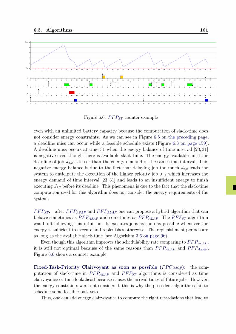
6.3. Algorithms 161
0 2 4 6 8 10 12 14 16 18 20 22 24 26 28 30 32 34 36 38 40 42 44 46 48 50 52 54 56 58 60 62 64 66 68 700
10
20
30
40
50Emax
Emin
0 2 4 6 8 10 12 14 16 18 20 22 24 26 28 30 32 34 36 38 40 42 44 46 48 50 52 54 56 58 60 62 64 66 68 70
τ1
deadline_missed deadline_missed
0 2 4 6 8 10 12 14 16 18 20 22 24 26 28 30 32 34 36 38 40 42 44 46 48 50 52 54 56 58 60 62 64 66 68 70
τ2
0 2 4 6 8 10 12 14 16 18 20 22 24 26 28 30 32 34 36 38 40 42 44 46 48 50 52 54 56 58 60 62 64 66 68 70
τ3
0 2 4 6 8 10 12 14 16 18 20 22 24 26 28 30 32 34 36 38 40 42 44 46 48 50 52 54 56 58 60 62 64 66 68 70
τ4
Figure 6.6: PFPST counter example
even with an unlimited battery capacity because the computation of slack-time doesnot consider energy constraints. As we can see in Figure 6.5 on the preceding page,a deadline miss can occur while a feasible schedule exists (Figure 6.3 on page 159).A deadline miss occurs at time 31 when the energy balance of time interval [23, 31]is negative even though there is available slack-time. The energy available until thedeadline of job J2,2 is lesser than the energy demand of the same time interval. Thisnegative energy balance is due to the fact that delaying job too much J2,2 leads thesystem to anticipate the execution of the higher priority job J1,1 which increases theenergy demand of time interval [23, 31] and leads to an insufficient energy to finishexecuting J2,2 before its deadline. This phenomena is due to the fact that the slack-timecomputation used for this algorithm does not consider the energy requirements of thesystem.
PFPST : after PFPASAP and PFPALAP one can propose a hybrid algorithm that canbehave sometimes as PFPASAP and sometimes as PFPALAP . The PFPST algorithmwas built following this intuition. It executes jobs as soon as possible whenever theenergy is sufficient to execute and replenishes otherwise. The replenishment periods areas long as the available slack-time (see Algorithm 3.6 on page 96).
Even though this algorithm improves the schedulability rate comparing to PFPALAP ,it is still not optimal because of the same reasons than PFPALAP and PFPASAP .Figure 6.6 shows a counter example.
Fixed-Task-Priority Clairvoyant as soon as possible (FPCasap): the com-putation of slack-time in PFPALAP and PFPST algorithms is considered as timeclairvoyance or time lookahead because it uses the arrival times of future jobs. However,the energy constraints were not considered, this is why the precedent algorithms fail toschedule some feasible task sets.
Thus, one can add energy clairvoyance to compute the right retardations that lead to
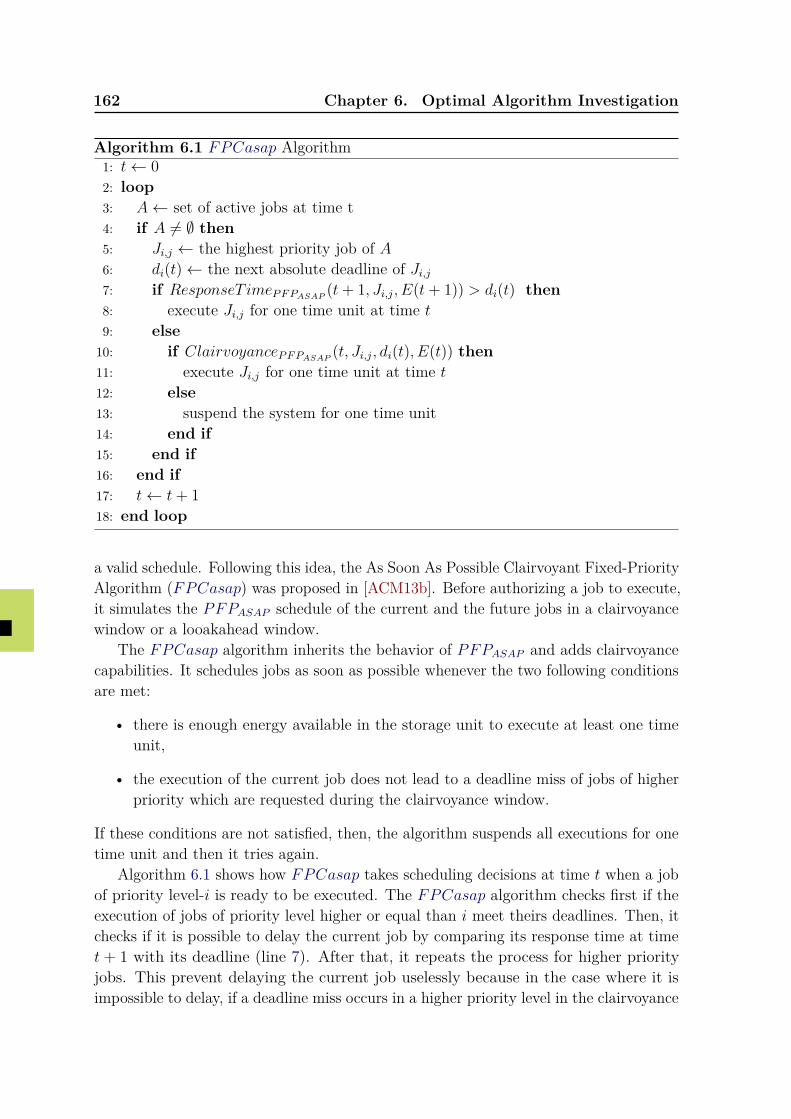
162 Chapter 6. Optimal Algorithm Investigation
Algorithm 6.1 FPCasap Algorithm1: t← 02: loop3: A← set of active jobs at time t4: if A 6= ∅ then5: Ji,j ← the highest priority job of A6: di(t)← the next absolute deadline of Ji,j7: if ResponseT imePFPASAP (t+ 1, Ji,j, E(t+ 1)) > di(t) then8: execute Ji,j for one time unit at time t9: else10: if ClairvoyancePFPASAP (t, Ji,j, di(t), E(t)) then11: execute Ji,j for one time unit at time t12: else13: suspend the system for one time unit14: end if15: end if16: end if17: t← t+ 118: end loop
a valid schedule. Following this idea, the As Soon As Possible Clairvoyant Fixed-PriorityAlgorithm (FPCasap) was proposed in [ACM13b]. Before authorizing a job to execute,it simulates the PFPASAP schedule of the current and the future jobs in a clairvoyancewindow or a looakahead window.
The FPCasap algorithm inherits the behavior of PFPASAP and adds clairvoyancecapabilities. It schedules jobs as soon as possible whenever the two following conditionsare met:
• there is enough energy available in the storage unit to execute at least one timeunit,
• the execution of the current job does not lead to a deadline miss of jobs of higherpriority which are requested during the clairvoyance window.
If these conditions are not satisfied, then, the algorithm suspends all executions for onetime unit and then it tries again.
Algorithm 6.1 shows how FPCasap takes scheduling decisions at time t when a jobof priority level-i is ready to be executed. The FPCasap algorithm checks first if theexecution of jobs of priority level higher or equal than i meet theirs deadlines. Then, itchecks if it is possible to delay the current job by comparing its response time at timet + 1 with its deadline (line 7). After that, it repeats the process for higher priorityjobs. This prevent delaying the current job uselessly because in the case where it isimpossible to delay, if a deadline miss occurs in a higher priority level in the clairvoyance
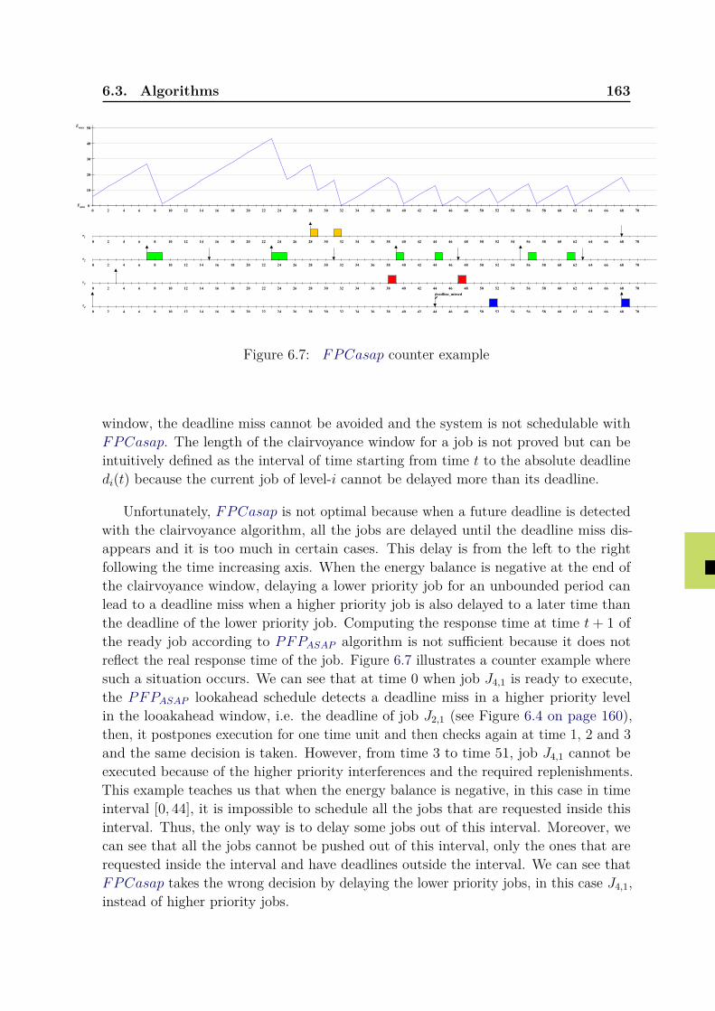
6.3. Algorithms 163
0 2 4 6 8 10 12 14 16 18 20 22 24 26 28 30 32 34 36 38 40 42 44 46 48 50 52 54 56 58 60 62 64 66 68 700
10
20
30
40
50Emax
Emin
0 2 4 6 8 10 12 14 16 18 20 22 24 26 28 30 32 34 36 38 40 42 44 46 48 50 52 54 56 58 60 62 64 66 68 70
τ1
0 2 4 6 8 10 12 14 16 18 20 22 24 26 28 30 32 34 36 38 40 42 44 46 48 50 52 54 56 58 60 62 64 66 68 70
τ2
0 2 4 6 8 10 12 14 16 18 20 22 24 26 28 30 32 34 36 38 40 42 44 46 48 50 52 54 56 58 60 62 64 66 68 70
τ3
deadline_missed
0 2 4 6 8 10 12 14 16 18 20 22 24 26 28 30 32 34 36 38 40 42 44 46 48 50 52 54 56 58 60 62 64 66 68 70
τ4
Figure 6.7: FPCasap counter example
window, the deadline miss cannot be avoided and the system is not schedulable withFPCasap. The length of the clairvoyance window for a job is not proved but can beintuitively defined as the interval of time starting from time t to the absolute deadlinedi(t) because the current job of level-i cannot be delayed more than its deadline.
Unfortunately, FPCasap is not optimal because when a future deadline is detectedwith the clairvoyance algorithm, all the jobs are delayed until the deadline miss dis-appears and it is too much in certain cases. This delay is from the left to the rightfollowing the time increasing axis. When the energy balance is negative at the end ofthe clairvoyance window, delaying a lower priority job for an unbounded period canlead to a deadline miss when a higher priority job is also delayed to a later time thanthe deadline of the lower priority job. Computing the response time at time t+ 1 ofthe ready job according to PFPASAP algorithm is not sufficient because it does notreflect the real response time of the job. Figure 6.7 illustrates a counter example wheresuch a situation occurs. We can see that at time 0 when job J4,1 is ready to execute,the PFPASAP lookahead schedule detects a deadline miss in a higher priority levelin the looakahead window, i.e. the deadline of job J2,1 (see Figure 6.4 on page 160),then, it postpones execution for one time unit and then checks again at time 1, 2 and 3and the same decision is taken. However, from time 3 to time 51, job J4,1 cannot beexecuted because of the higher priority interferences and the required replenishments.This example teaches us that when the energy balance is negative, in this case in timeinterval [0, 44], it is impossible to schedule all the jobs that are requested inside thisinterval. Thus, the only way is to delay some jobs out of this interval. Moreover, wecan see that all the jobs cannot be pushed out of this interval, only the ones that arerequested inside the interval and have deadlines outside the interval. We can see thatFPCasap takes the wrong decision by delaying the lower priority jobs, in this case J4,1,instead of higher priority jobs.
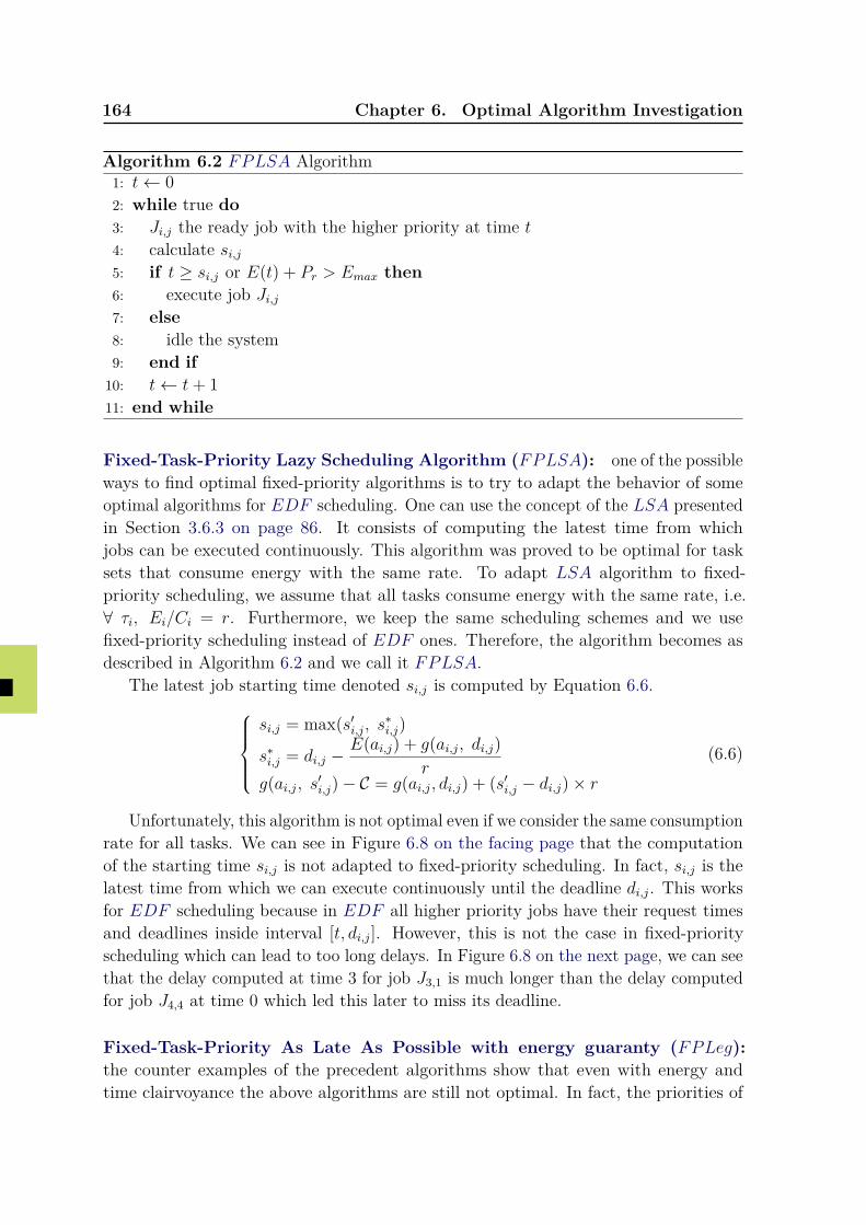
164 Chapter 6. Optimal Algorithm Investigation
Algorithm 6.2 FPLSA Algorithm1: t← 02: while true do3: Ji,j the ready job with the higher priority at time t4: calculate si,j5: if t ≥ si,j or E(t) + Pr > Emax then6: execute job Ji,j7: else8: idle the system9: end if
10: t← t+ 111: end while
Fixed-Task-Priority Lazy Scheduling Algorithm (FPLSA): one of the possibleways to find optimal fixed-priority algorithms is to try to adapt the behavior of someoptimal algorithms for EDF scheduling. One can use the concept of the LSA presentedin Section 3.6.3 on page 86. It consists of computing the latest time from whichjobs can be executed continuously. This algorithm was proved to be optimal for tasksets that consume energy with the same rate. To adapt LSA algorithm to fixed-priority scheduling, we assume that all tasks consume energy with the same rate, i.e.∀ τi, Ei/Ci = r. Furthermore, we keep the same scheduling schemes and we usefixed-priority scheduling instead of EDF ones. Therefore, the algorithm becomes asdescribed in Algorithm 6.2 and we call it FPLSA.
The latest job starting time denoted si,j is computed by Equation 6.6.si,j = max(s′i,j, s∗i,j)
s∗i,j = di,j −E(ai,j) + g(ai,j, di,j)
rg(ai,j, s′i,j)− C = g(ai,j, di,j) + (s′i,j − di,j)× r
(6.6)
Unfortunately, this algorithm is not optimal even if we consider the same consumptionrate for all tasks. We can see in Figure 6.8 on the facing page that the computationof the starting time si,j is not adapted to fixed-priority scheduling. In fact, si,j is thelatest time from which we can execute continuously until the deadline di,j. This worksfor EDF scheduling because in EDF all higher priority jobs have their request timesand deadlines inside interval [t, di,j]. However, this is not the case in fixed-priorityscheduling which can lead to too long delays. In Figure 6.8 on the next page, we can seethat the delay computed at time 3 for job J3,1 is much longer than the delay computedfor job J4,4 at time 0 which led this later to miss its deadline.
Fixed-Task-Priority As Late As Possible with energy guaranty (FPLeg):the counter examples of the precedent algorithms show that even with energy andtime clairvoyance the above algorithms are still not optimal. In fact, the priorities of
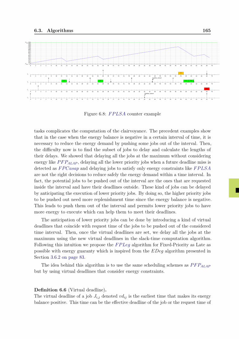
6.3. Algorithms 165
0 2 4 6 8 10 12 14 16 18 20 22 24 26 28 30 32 34 36 38 40 42 44 46 48 50 52 54 56 58 60 62 64 66 68 700102030405060708090100110120130140150E
max
Emin
1,1
0 2 4 6 8 10 12 14 16 18 20 22 24 26 28 30 32 34 36 38 40 42 44 46 48 50 52 54 56 58 60 62 64 66 68 70
τ1
2,1 2,2
deadline_missed
2,3 2,4
0 2 4 6 8 10 12 14 16 18 20 22 24 26 28 30 32 34 36 38 40 42 44 46 48 50 52 54 56 58 60 62 64 66 68 70
τ2
3,1
0 2 4 6 8 10 12 14 16 18 20 22 24 26 28 30 32 34 36 38 40 42 44 46 48 50 52 54 56 58 60 62 64 66 68 70
τ3
deadline_missed
0 2 4 6 8 10 12 14 16 18 20 22 24 26 28 30 32 34 36 38 40 42 44 46 48 50 52 54 56 58 60 62 64 66 68 70
τ4
Figure 6.8: FPLSA counter example
tasks complicates the computation of the clairvoyance. The precedent examples showthat in the case when the energy balance is negative in a certain interval of time, it isnecessary to reduce the energy demand by pushing some jobs out of the interval. Then,the difficulty now is to find the subset of jobs to delay and calculate the lengths oftheir delays. We showed that delaying all the jobs at the maximum without consideringenergy like PFPALAP , delaying all the lower priority jobs when a future deadline miss isdetected as FPCasap and delaying jobs to satisfy only energy constraints like FPLSAare not the right decisions to reduce safely the energy demand within a time interval. Infact, the potential jobs to be pushed out of the interval are the ones that are requestedinside the interval and have their deadlines outside. These kind of jobs can be delayedby anticipating the execution of lower priority jobs. By doing so, the higher priority jobsto be pushed out need more replenishment time since the energy balance is negative.This leads to push them out of the interval and permits lower priority jobs to havemore energy to execute which can help them to meet their deadlines.
The anticipation of lower priority jobs can be done by introducing a kind of virtualdeadlines that coincide with request time of the jobs to be pushed out of the consideredtime interval. Then, once the virtual deadlines are set, we delay all the jobs at themaximum using the new virtual deadlines in the slack-time computation algorithm.Following this intuition we propose the FPLeg algorithm for Fixed-Priority as Late aspossible with energy guaranty which is inspired from the EDeg algorithm presented inSection 3.6.2 on page 83.
The idea behind this algorithm is to use the same scheduling schemes as PFPALAPbut by using virtual deadlines that consider energy constraints.
Definition 6.6 (Virtual deadline).The virtual deadline of a job Ji,j denoted vdij is the earliest time that makes its energybalance positive. This time can be the effective deadline of the job or the request time of
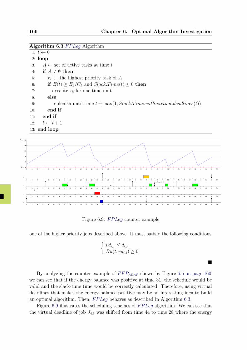
166 Chapter 6. Optimal Algorithm Investigation
Algorithm 6.3 FPLeg Algorithm1: t← 02: loop3: A← set of active tasks at time t4: if A 6= ∅ then5: τk ← the highest priority task of A6: if E(t) ≥ Ek/Ck and Slack.T ime(t) ≤ 0 then7: execute τk for one time unit8: else9: replenish until time t+ max(1, Slack.T ime.with.virtual.deadlines(t))10: end if11: end if12: t← t+ 113: end loop
0 2 4 6 8 10 12 14 16 18 20 22 24 26 28 30 32 34 36 38 40 42 44 46 48 50 52 54 56 58 60 62 64 66 68 700
10
20
30
40
50Emax
Emin
0 2 4 6 8 10 12 14 16 18 20 22 24 26 28 30 32 34 36 38 40 42 44 46 48 50 52 54 56 58 60 62 64 66 68 70
τ1
deadline_missed
0 2 4 6 8 10 12 14 16 18 20 22 24 26 28 30 32 34 36 38 40 42 44 46 48 50 52 54 56 58 60 62 64 66 68 70
τ2
0 2 4 6 8 10 12 14 16 18 20 22 24 26 28 30 32 34 36 38 40 42 44 46 48 50 52 54 56 58 60 62 64 66 68 70
τ3
0 2 4 6 8 10 12 14 16 18 20 22 24 26 28 30 32 34 36 38 40 42 44 46 48 50 52 54 56 58 60 62 64 66 68 70
τ4
Figure 6.9: FPLeg counter example
one of the higher priority jobs described above. It must satisfy the following conditions:{vdi,j ≤ di,jBu(t, vdi,j) ≥ 0
�
By analyzing the counter example of PFPALAP shown by Figure 6.5 on page 160,we can see that if the energy balance was positive at time 31, the schedule would bevalid and the slack-time time would be correctly calculated. Therefore, using virtualdeadlines that makes the energy balance positive may be an interesting idea to buildan optimal algorithm. Then, FPLeg behaves as described in Algorithm 6.3.
Figure 6.9 illustrates the scheduling schemes of FPLeg algorithm. We can see thatthe virtual deadline of job J4,1 was shifted from time 44 to time 28 where the energy
6.3. Algorithms 167
balance is positive, i.e. the battery level at time 28 is 0, and then, the as late as possibleschedule produced in time interval [0, 28] is valid. However, we notice that this doesnot solve completely the problem of late scheduling. In fact, using virtual deadlinesimproves schedulability but there exist some cases where it anticipates the execution ofsome lower priority jobs that consume the energy needed for other higher priority jobs.This is illustrated by Figure 6.9 on the facing page at time 46. Even though the energybalance was positive at time 28, the missed deadline (time 47) is due to the anticipatedexecution of job J3,1 which can be delayed further. Unfortunately, this proves thatFPLeg is not optimal and that the fixed-priority scheduling for energy-harvestingsystems is subject to many counter intuitive ideas.
Fixed-Task-Priority lookahead (FPlh): The use of virtual deadlines in FPLegwas a good idea because it helps reducing the energy demand when the energy balanceis negative. However, the above counter example shows that having a positive energybalance is not sufficient to check whether the current virtual deadline is the right one ornot. Combining the idea of lookahead of FPCasap with the idea of virtual deadlinescan be an interesting intuition to achieve an optimal algorithm.
In the following we propose a new algorithm called FPlh for Fixed-Priority lookaheadthat combines the ideas of virtual deadlines and lookahead. The lookahead computationchecks if all future deadlines are met during a bounded window by using the notion ofvirtual deadlines that guarantees positive energy balances. Therefore, the definition ofthe virtual deadline should take into account the future higher priority jobs. Moreover,the looakahead computation consists not only of calculating the energy balance ofthe current job Ji,j but also the one of higher priority jobs that are included in thelookahead window. For this reason, we need to generalize the energy balance formulato compute the energy balance of any job at any moment.
Definition 6.7 (Energy Balance).The energy balance of priority level-i at time interval [t1, t2[ denoted Bai(t1, t2) is thedifference between the energy budget and the energy demand during [t1, t2[. It can becomputed with Equation 6.7.
A =∑j>i
(DBFj(0, ai(t1))× Ej
B = (RBFj(0, ai(t1))−DBFj(0,−ai(t1)))× (Ej − ej(ai(t1)))Bai(t1, t2) = Bu(t1, t2)−Wei(t1, t2)
= Bu(0, t2)−Wei(0, t2)− A+B
(6.7)
where :
• A: is the energy demand of lower priority jobs within time interval [0, ai(t1)[, i.e.finished jobs (see Figure 6.1 on page 156),
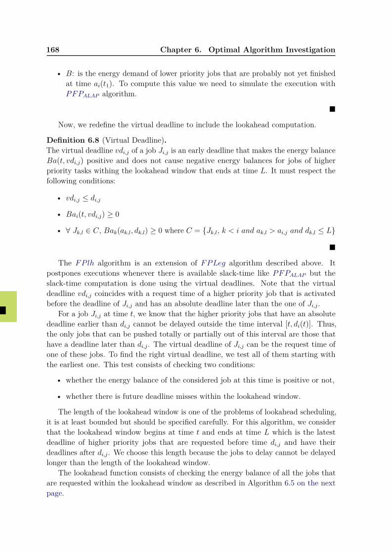
168 Chapter 6. Optimal Algorithm Investigation
• B: is the energy demand of lower priority jobs that are probably not yet finishedat time ai(t1). To compute this value we need to simulate the execution withPFPALAP algorithm.
�
Now, we redefine the virtual deadline to include the lookahead computation.
Definition 6.8 (Virtual Deadline).The virtual deadline vdi,j of a job Ji,j is an early deadline that makes the energy balanceBa(t, vdi,j) positive and does not cause negative energy balances for jobs of higherpriority tasks withing the lookahead window that ends at time L. It must respect thefollowing conditions:
• vdi,j ≤ di,j
• Bai(t, vdi,j) ≥ 0
• ∀ Jk,l ∈ C, Bak(ak,l, dk,l) ≥ 0 where C = {Jk,l, k < i and ak,l > ai,j and dk,l ≤ L}
�
The FPlh algorithm is an extension of FPLeg algorithm described above. Itpostpones executions whenever there is available slack-time like PFPALAP but theslack-time computation is done using the virtual deadlines. Note that the virtualdeadline vdi,j coincides with a request time of a higher priority job that is activatedbefore the deadline of Ji,j and has an absolute deadline later than the one of Ji,j.
For a job Ji,j at time t, we know that the higher priority jobs that have an absolutedeadline earlier than di,j cannot be delayed outside the time interval [t, di(t)]. Thus,the only jobs that can be pushed totally or partially out of this interval are those thathave a deadline later than di,j. The virtual deadline of Ji,j can be the request time ofone of these jobs. To find the right virtual deadline, we test all of them starting withthe earliest one. This test consists of checking two conditions:
• whether the energy balance of the considered job at this time is positive or not,
• whether there is future deadline misses within the lookahead window.
The length of the lookahead window is one of the problems of lookahead scheduling,it is at least bounded but should be specified carefully. For this algorithm, we considerthat the lookahead window begins at time t and ends at time L which is the latestdeadline of higher priority jobs that are requested before time di,j and have theirdeadlines after di,j. We choose this length because the jobs to delay cannot be delayedlonger than the length of the lookahead window.
The lookahead function consists of checking the energy balance of all the jobs thatare requested within the lookahead window as described in Algorithm 6.5 on the nextpage.
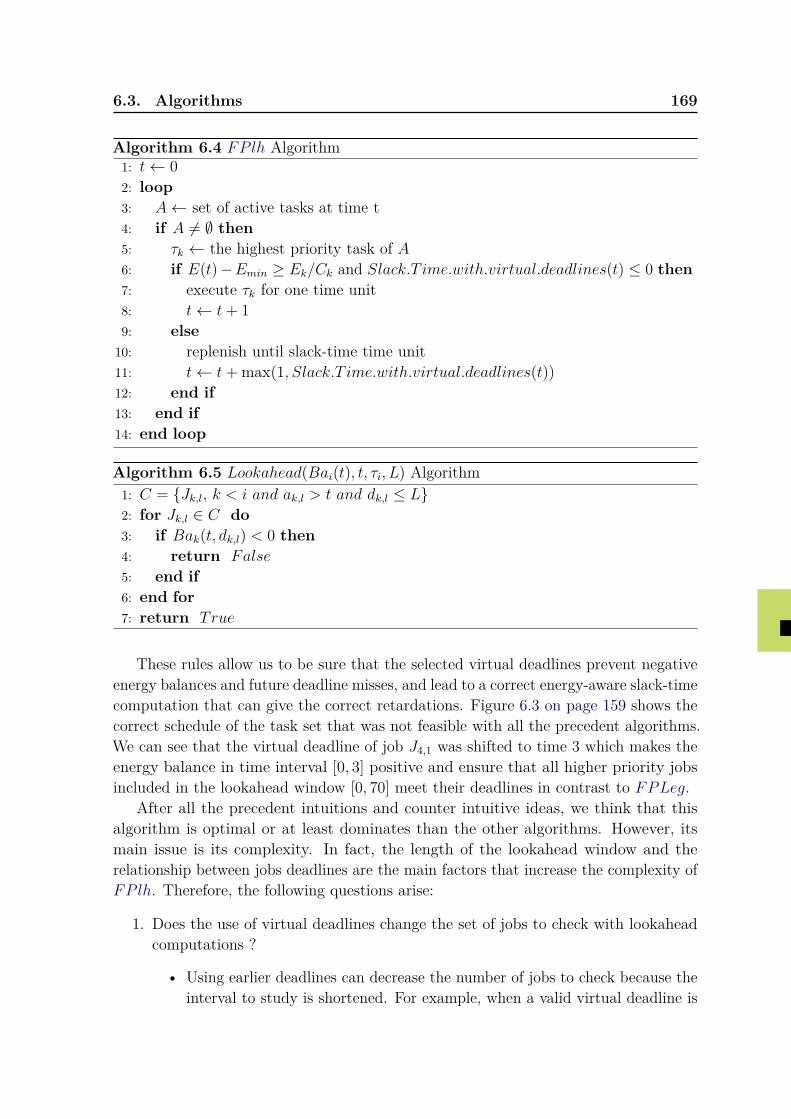
6.3. Algorithms 169
Algorithm 6.4 FPlh Algorithm1: t← 02: loop3: A← set of active tasks at time t4: if A 6= ∅ then5: τk ← the highest priority task of A6: if E(t)−Emin ≥ Ek/Ck and Slack.T ime.with.virtual.deadlines(t) ≤ 0 then7: execute τk for one time unit8: t← t+ 19: else
10: replenish until slack-time time unit11: t← t+ max(1, Slack.T ime.with.virtual.deadlines(t))12: end if13: end if14: end loop
Algorithm 6.5 Lookahead(Bai(t), t, τi, L) Algorithm1: C = {Jk,l, k < i and ak,l > t and dk,l ≤ L}2: for Jk,l ∈ C do3: if Bak(t, dk,l) < 0 then4: return False
5: end if6: end for7: return True
These rules allow us to be sure that the selected virtual deadlines prevent negativeenergy balances and future deadline misses, and lead to a correct energy-aware slack-timecomputation that can give the correct retardations. Figure 6.3 on page 159 shows thecorrect schedule of the task set that was not feasible with all the precedent algorithms.We can see that the virtual deadline of job J4,1 was shifted to time 3 which makes theenergy balance in time interval [0, 3] positive and ensure that all higher priority jobsincluded in the lookahead window [0, 70] meet their deadlines in contrast to FPLeg.
After all the precedent intuitions and counter intuitive ideas, we think that thisalgorithm is optimal or at least dominates than the other algorithms. However, itsmain issue is its complexity. In fact, the length of the lookahead window and therelationship between jobs deadlines are the main factors that increase the complexity ofFPlh. Therefore, the following questions arise:
1. Does the use of virtual deadlines change the set of jobs to check with lookaheadcomputations ?
• Using earlier deadlines can decrease the number of jobs to check because theinterval to study is shortened. For example, when a valid virtual deadline is
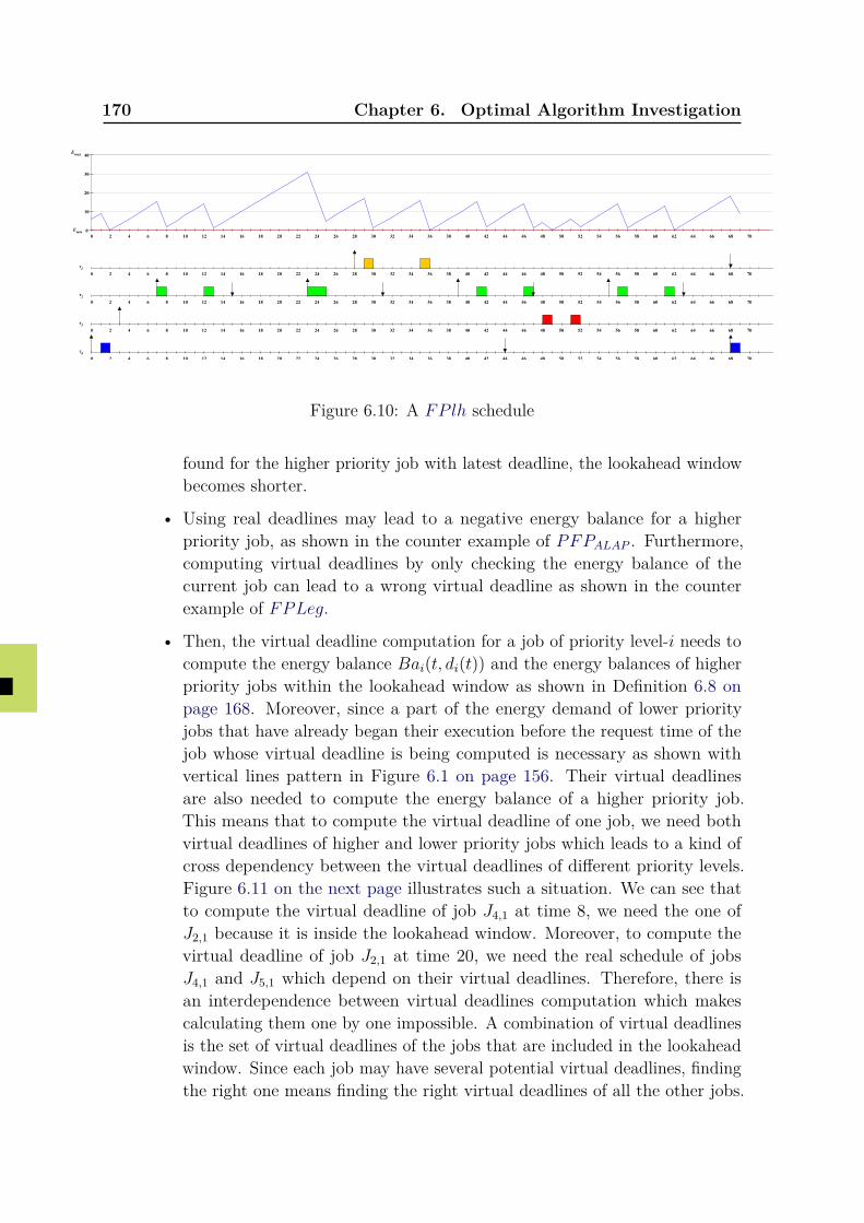
170 Chapter 6. Optimal Algorithm Investigation
0 2 4 6 8 10 12 14 16 18 20 22 24 26 28 30 32 34 36 38 40 42 44 46 48 50 52 54 56 58 60 62 64 66 68 700
10
20
30
40Emax
Emin
0 2 4 6 8 10 12 14 16 18 20 22 24 26 28 30 32 34 36 38 40 42 44 46 48 50 52 54 56 58 60 62 64 66 68 70
τ1
0 2 4 6 8 10 12 14 16 18 20 22 24 26 28 30 32 34 36 38 40 42 44 46 48 50 52 54 56 58 60 62 64 66 68 70
τ2
0 2 4 6 8 10 12 14 16 18 20 22 24 26 28 30 32 34 36 38 40 42 44 46 48 50 52 54 56 58 60 62 64 66 68 70
τ3
0 2 4 6 8 10 12 14 16 18 20 22 24 26 28 30 32 34 36 38 40 42 44 46 48 50 52 54 56 58 60 62 64 66 68 70
τ4
Figure 6.10: A FPlh schedule
found for the higher priority job with latest deadline, the lookahead windowbecomes shorter.
• Using real deadlines may lead to a negative energy balance for a higherpriority job, as shown in the counter example of PFPALAP . Furthermore,computing virtual deadlines by only checking the energy balance of thecurrent job can lead to a wrong virtual deadline as shown in the counterexample of FPLeg.
• Then, the virtual deadline computation for a job of priority level-i needs tocompute the energy balance Bai(t, di(t)) and the energy balances of higherpriority jobs within the lookahead window as shown in Definition 6.8 onpage 168. Moreover, since a part of the energy demand of lower priorityjobs that have already began their execution before the request time of thejob whose virtual deadline is being computed is necessary as shown withvertical lines pattern in Figure 6.1 on page 156. Their virtual deadlinesare also needed to compute the energy balance of a higher priority job.This means that to compute the virtual deadline of one job, we need bothvirtual deadlines of higher and lower priority jobs which leads to a kind ofcross dependency between the virtual deadlines of different priority levels.Figure 6.11 on the next page illustrates such a situation. We can see thatto compute the virtual deadline of job J4,1 at time 8, we need the one ofJ2,1 because it is inside the lookahead window. Moreover, to compute thevirtual deadline of job J2,1 at time 20, we need the real schedule of jobsJ4,1 and J5,1 which depend on their virtual deadlines. Therefore, there isan interdependence between virtual deadlines computation which makescalculating them one by one impossible. A combination of virtual deadlinesis the set of virtual deadlines of the jobs that are included in the lookaheadwindow. Since each job may have several potential virtual deadlines, findingthe right one means finding the right virtual deadlines of all the other jobs.
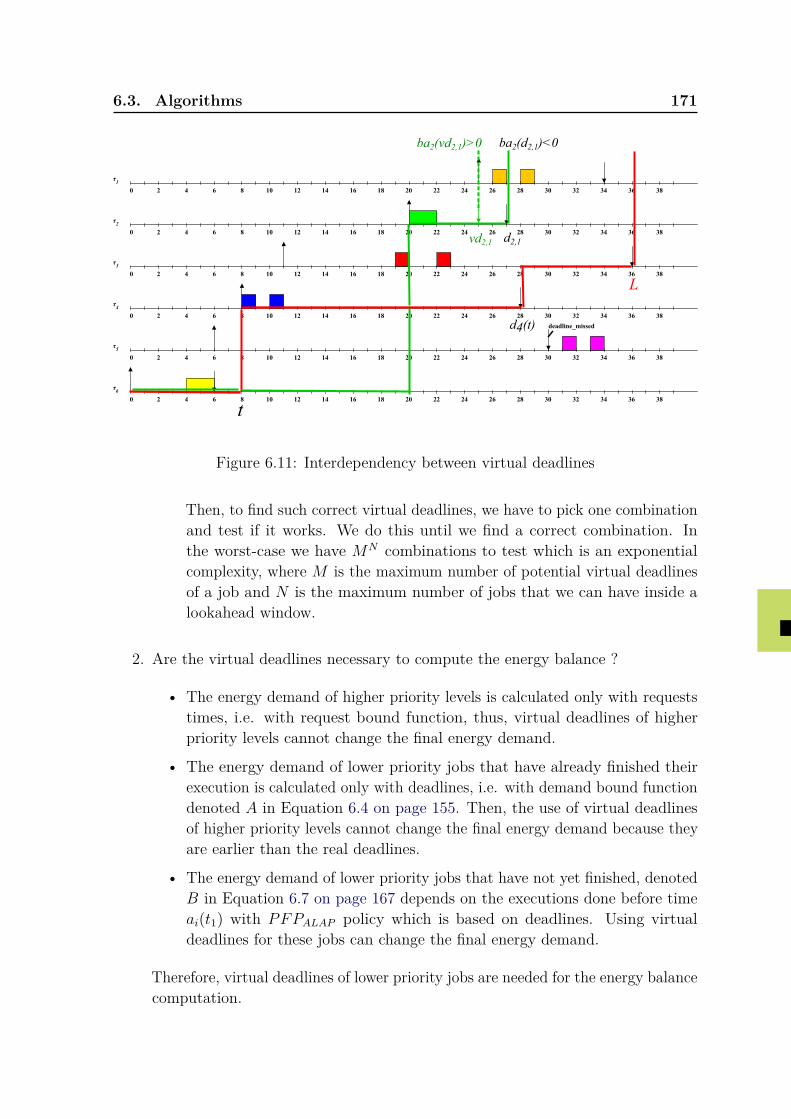
6.3. Algorithms 171
t
d4(t)
d2,1vd2,1
L
0 2 4 6 8 10 12 14 16 18 20 22 24 26 28 30 32 34 36 38
τ1
0 2 4 6 8 10 12 14 16 18 20 22 24 26 28 30 32 34 36 38
τ2
0 2 4 6 8 10 12 14 16 18 20 22 24 26 28 30 32 34 36 38
τ3
0 2 4 6 8 10 12 14 16 18 20 22 24 26 28 30 32 34 36 38
τ4
deadline_missed
0 2 4 6 8 10 12 14 16 18 20 22 24 26 28 30 32 34 36 38
τ5
0 2 4 6 8 10 12 14 16 18 20 22 24 26 28 30 32 34 36 38
τ6
ba2(vd2,1)>0 ba2(d2,1)<0
Figure 6.11: Interdependency between virtual deadlines
Then, to find such correct virtual deadlines, we have to pick one combinationand test if it works. We do this until we find a correct combination. Inthe worst-case we have MN combinations to test which is an exponentialcomplexity, where M is the maximum number of potential virtual deadlinesof a job and N is the maximum number of jobs that we can have inside alookahead window.
2. Are the virtual deadlines necessary to compute the energy balance ?
• The energy demand of higher priority levels is calculated only with requeststimes, i.e. with request bound function, thus, virtual deadlines of higherpriority levels cannot change the final energy demand.
• The energy demand of lower priority jobs that have already finished theirexecution is calculated only with deadlines, i.e. with demand bound functiondenoted A in Equation 6.4 on page 155. Then, the use of virtual deadlinesof higher priority levels cannot change the final energy demand because theyare earlier than the real deadlines.
• The energy demand of lower priority jobs that have not yet finished, denotedB in Equation 6.7 on page 167 depends on the executions done before timeai(t1) with PFPALAP policy which is based on deadlines. Using virtualdeadlines for these jobs can change the final energy demand.
Therefore, virtual deadlines of lower priority jobs are needed for the energy balancecomputation.
172 Chapter 6. Optimal Algorithm Investigation
3. Assuming that computing virtual deadlines is an NP-hard problem, are theynecessary for an optimal algorithm ?
• If yes, the scheduling problem for fixed-priority energy-harvesting systems isalso NP-Hard also,
• Otherwise, it is an open problem.
These insights confirm that the fixed-priority scheduling for energy-harvestingsystems is not easy to handle. Moreover, the only algorithm we have up to now thatcould be optimal has an exponential complexity. Therefore, finding an optimal algorithmwith a reasonable complexity or proving that the fixed-priority problem scheduling forenergy-harvesting systems is an NP-Hard problem is still an open problem.
6.4 ConclusionIn this chapter we explored the possibility of the existence of an optimal scheduling
algorithm for energy-harvesting systems. We started by proving that such an algorithmmust be both non-energy-work-conserving and lookahead (or clairvoyant). Then, welisted some ideas of scheduling algorithms that seem intuitively optimal and we showedwith counter examples why they are not. We showed that the computation of theneeded delays, i.e. replenishment periods, must consider jobs deadlines and energy costas well as the replenished energy. Moreover, we showed also that deciding which jobto delay is the main problem of building an optimal algorithm. We know now thatconsidering a late or a lazy scheduling and having a positive energy balance at thedeadline of a job is not sufficient. The maximum delay for a job must ensure not only apositive energy balance but also the respect of all deadlines in a bounded lookaheadwindow. This idea is very interesting, however, the exact lookahead computation seemsto be complicated and have an exponential complexity. This complexity seems to bedifficult to reduce because the computation of the maximum delay of one job, i.e. thecomputation of the virtual deadline, depends on the maximum delay of the other jobsinside the lookahead window. There is a kind of cross dependency between jobs whichcomplicates the computations. The only investigated solution here is to perform a bruteforce search for the right combination of jobs delays or virtual deadlines which has anexponential complexity. The conclusion of this chapter is that the correct late schedulingthat respects the energy constraints needs earlier deadlines and that the computationof these deadlines has an exponential complexity. Moreover, if an optimal algorithmrequires these deadlines, then, the scheduling problem of fixed-priority energy-harvestingsystems is a hard problem. Otherwise, we should find an other way to compute theright delays, this is still an open problem.
Chapter 7
Response-Time Analysis forThermal-Aware Scheduling
Contents7.1 Introduction . . . . . . . . . . . . . . . . . . . . . . . . . . . . . 1737.2 Related Work . . . . . . . . . . . . . . . . . . . . . . . . . . . . . 1757.3 Models . . . . . . . . . . . . . . . . . . . . . . . . . . . . . . . . . 176
7.3.1 Task Model . . . . . . . . . . . . . . . . . . . . . . . . . . . . . . 1767.3.2 Thermal Model . . . . . . . . . . . . . . . . . . . . . . . . . . . . 176
7.4 The PFPASAP algorithm . . . . . . . . . . . . . . . . . . . . . . 1787.4.1 Worst-case scenario . . . . . . . . . . . . . . . . . . . . . . . . . 1797.4.2 The optimality of PFPASAP . . . . . . . . . . . . . . . . . . . . 181
7.5 Response-Time Analysis . . . . . . . . . . . . . . . . . . . . . . 1837.5.1 Exact Analysis . . . . . . . . . . . . . . . . . . . . . . . . . . . . 1837.5.2 Approximate Analysis . . . . . . . . . . . . . . . . . . . . . . . . 183
7.6 Performance Evaluation . . . . . . . . . . . . . . . . . . . . . . 1977.6.1 Task set generation . . . . . . . . . . . . . . . . . . . . . . . . . . 1977.6.2 Schedulability tests investigated . . . . . . . . . . . . . . . . . . 1987.6.3 Experiments . . . . . . . . . . . . . . . . . . . . . . . . . . . . . 198
7.7 Conclusion . . . . . . . . . . . . . . . . . . . . . . . . . . . . . . 202
7.1 IntroductionThe main purpose of real-time systems is to guarantee predictable timing behavior
for controlled devices. Therefore, the correctness of the results provided by such systemsdepends not only on the logical correctness of the output but also on the time at whichit is yielded. Several formal models of real-time behavior have been proposed up tonow (e.g. task models such as sporadic, periodic, aperiodic, Directed Acyclic Graphs(DAG), etc.) as mentioned in Section 1.2 on page 30 and 3.2 on page 67. Prior researchin real-time systems have also addressed a wide array of hardware architectures (e.g.
174 Chapter 7. Response-Time Analysis for Thermal-Aware Scheduling
monoprocessor, multiprocessors, memory caches, etc). However, for a new generation ofreal-time systems applications, e.g. medical implants, the physical environment posesadditional design challenges.
One such new challenge is the necessity of managing the energy and the thermalbehavior of systems. As technology scales, chips power consumption and power densityare increasing rapidly. Indeed, the miniaturization of small embedded systems hasallowed new real-time applications. Implantable Medical Devices (IMDs) are anexample of these new embedded systems where managing the thermal aspect is essential.IMDs are increasingly being used in medical treatments (e.g. pacemakers for heartdiseases or neural implants to restore hearing/vision). However, recent studies [Kim+07;Laz05] have shown that the heat generated by IMDs due to the processor activity is non-negligible. Thus, designing thermal aware IMDs becomes critical as medical researchhas shown that a temperature increase of even 1◦C can damage tissues [LaM+89] andmay cause death in extreme cases [Rug+03].
Therefore, thermal-aware real-time systems must respect not only timing constraints,expressed with deadlines, but also thermal constraints which are expressed as a max-imum temperature not to be exceeded. For fixed-priority real-time scheduling onmonoprocessor platforms, considering this constraint requires the schedulers to addcooling periods. This additional idle times must be taken into account by schedulingalgorithms and included in schedulability analysis.
Thermal-aware system design presents challenges similar to the design of energy-harvesting systems. The later collects the environmental energy to store it and useit to supply real-time systems. The similarities with thermal-aware systems comefrom the fact that the scheduling for energy-harvesting system has to consider batteryreplenishment times which are analogous to the cooling periods required in thermal-awaresystems. Intuitively, the real-time scheduling problem of energy-harvesting systemsseems to be close to the one of thermal-aware systems. Therefore, it is interesting toexplore the possible similarities between these two models.
As a first step, we apply some results of energy-harvesting systems to the thermal-aware model. In this chapter we use the Preemptive Fixed-Task-Priority As SoonAs Possible (PFPASAP ) scheduling algorithm presented in Section 4.3 on page 111,which was proved to be optimal for energy-non-concrete fixed-priority energy-harvestingsystems, to build a thermal-aware scheduling approach and a schedulability analysisbased on upper and lower bounds of tasks worst-case response-time.
The work presented in this chapter is the result of a collaboration with Prof.Nathan Fisher from Wayne State University and mainly contains materials publishedin [CFM15].
The remainder of this chapter is organized as follows. Section 7.2 gives a brief stateof the art about thermal-aware real-time systems. Section 7.3 specifies and describes themodel and the scope of this chapter. Section 7.4 describes the thermal-aware versionof PFPASAP scheduling algorithm and proves its optimality for thermal-non-concretesystems. Section 7.5 details an approximate response-time analysis based on upper and
7.2. Related Work 175
lower bounds of tasks worst-case response time. Section 7.6 shows some simulationresults to evaluate the effectiveness of the proposed schedulability analysis. Finally,Section 7.7 concludes this chapter.
7.2 Related Work
In this section we give a brief overview of prior research related to thermal-awarereal-time scheduling. As for the energy-aware real-time systems, most works addressingthis problem consider Dynamic Voltage and Frequency Scaling (DVFS) strategies.DVFS consists of scaling down the DVFS speed, and thereby lengthening task executiontimes as described in Section 3.4 on page 73, to reduce energy consumption and reducethe peak temperature [CWT09; WAB10; WB06; WB08].
Among existing works, the proposed techniques can be divided into reactive andproactive approaches. The difference between these two approaches is that reactiveschemes adapt to the temperature of the system when it reaches the maximum temper-ature or a specific trigger by switching the Central Processing Unit (CPU) speed orby changing scheduling decisions. In this scope, Wang et al. proposed a schedulabilityanalysis for speed scaling scheme for frame-based task model in [WB08], and theycompleted this with a worst-case response time analysis for First In First Out (FIFO)and fixed-priority scheduling in [WB06; WB08]. In contrast, proactive approaches setthe configuration of the system judiciously beforehand (CPU speed and schedulingdecisions) so that the maximum temperature is never reached [CWT09; QZ09; Qua+08].In this scope, Chen et al. proposed in [CHK07; CWT09] a proactive EDF-basedscheduling approach that changes the processor speed proactively by requests issued bythe scheduler.
There exists also some works that address this scheduling problem without DVFSschemes by considering processors with only one frequency. In this scope, Ahmedet al. proposed in [Ahm+11] a technique that computes proactively the length ofexecution and cooling intervals so that a certain temperature is never reached. This ideawas extended in [Het+12] to support unpredictable ambient temperature fluctuations.Rehan et al. proposed in [RPK13; RPK14] a kind of thermal utilization of the system(using a fluid schedule) and leveraged it to obtain a necessary and sufficient conditionsfor systems thermal feasibility.
All the mentioned work have the following limitations:1) Except for works cited in the previous paragraph [Ahm+11; RPK13; RPK14;
Het+12], all the proposed solutions rely on speed scaling to manage energy andtemperature. These approaches cannot be applied to systems without DVFS capabilities.
2) Most of the scheduling solutions proposed in the literature are EDF-based.Knowing that static fixed-priority scheduling is highly used in industry, it deserves moreattention and effort.
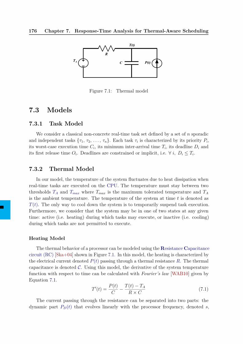
176 Chapter 7. Response-Time Analysis for Thermal-Aware Scheduling
R
CTA
T(t)
P(t)
Figure 7.1: Thermal model
7.3 Models
7.3.1 Task ModelWe consider a classical non-concrete real-time task set defined by a set of n sporadic
and independent tasks {τ1, τ2, . . . , τn}. Each task τi is characterized by its priority Pi,its worst-case execution time Ci, its minimum inter-arrival time Ti, its deadline Di andits first release time Oi. Deadlines are constrained or implicit, i.e. ∀ i, Di ≤ Ti.
7.3.2 Thermal ModelIn our model, the temperature of the system fluctuates due to heat dissipation when
real-time tasks are executed on the CPU. The temperature must stay between twothresholds TA and Tmax where Tmax is the maximum tolerated temperature and TAis the ambient temperature. The temperature of the system at time t is denoted asT (t). The only way to cool down the system is to temporarily suspend task execution.Furthermore, we consider that the system may be in one of two states at any giventime: active (i.e. heating) during which tasks may execute, or inactive (i.e. cooling)during which tasks are not permitted to execute.
Heating Model
The thermal behavior of a processor can be modeled using theResistanceCapacitancecircuit (RC) [Ska+04] shown in Figure 7.1. In this model, the heating is characterized bythe electrical current denoted P (t) passing through a thermal resistance R. The thermalcapacitance is denoted C. Using this model, the derivative of the system temperaturefunction with respect to time can be calculated with Fourier’s law [WAB10] given byEquation 7.1.
T ′(t) = P (t)C− T (t)− TA
R× C(7.1)
The current passing through the resistance can be separated into two parts: thedynamic part PD(t) that evolves linearly with the processor frequency, denoted s,
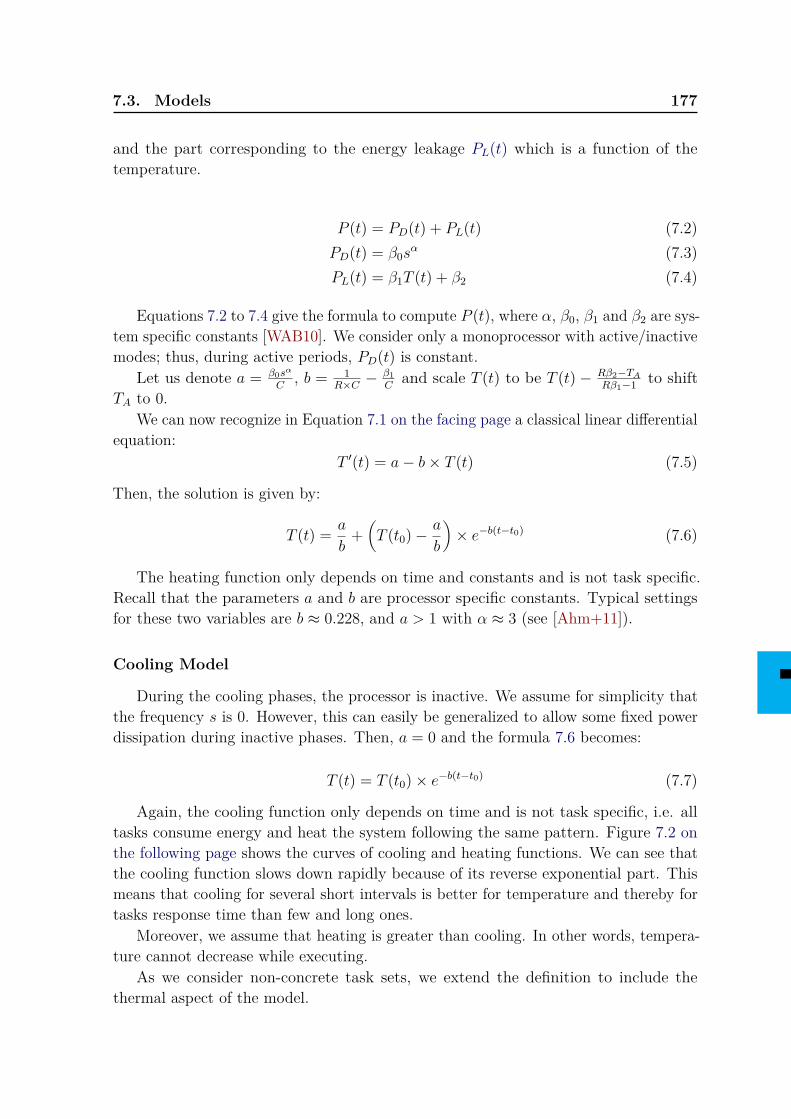
7.3. Models 177
and the part corresponding to the energy leakage PL(t) which is a function of thetemperature.
P (t) = PD(t) + PL(t) (7.2)PD(t) = β0s
α (7.3)PL(t) = β1T (t) + β2 (7.4)
Equations 7.2 to 7.4 give the formula to compute P (t), where α, β0, β1 and β2 are sys-tem specific constants [WAB10]. We consider only a monoprocessor with active/inactivemodes; thus, during active periods, PD(t) is constant.
Let us denote a = β0sα
C, b = 1
R×C −β1C
and scale T (t) to be T (t)− Rβ2−TARβ1−1 to shift
TA to 0.We can now recognize in Equation 7.1 on the facing page a classical linear differential
equation:T ′(t) = a− b× T (t) (7.5)
Then, the solution is given by:
T (t) = a
b+(T (t0)− a
b
)× e−b(t−t0) (7.6)
The heating function only depends on time and constants and is not task specific.Recall that the parameters a and b are processor specific constants. Typical settingsfor these two variables are b ≈ 0.228, and a > 1 with α ≈ 3 (see [Ahm+11]).
Cooling Model
During the cooling phases, the processor is inactive. We assume for simplicity thatthe frequency s is 0. However, this can easily be generalized to allow some fixed powerdissipation during inactive phases. Then, a = 0 and the formula 7.6 becomes:
T (t) = T (t0)× e−b(t−t0) (7.7)
Again, the cooling function only depends on time and is not task specific, i.e. alltasks consume energy and heat the system following the same pattern. Figure 7.2 onthe following page shows the curves of cooling and heating functions. We can see thatthe cooling function slows down rapidly because of its reverse exponential part. Thismeans that cooling for several short intervals is better for temperature and thereby fortasks response time than few and long ones.
Moreover, we assume that heating is greater than cooling. In other words, tempera-ture cannot decrease while executing.
As we consider non-concrete task sets, we extend the definition to include thethermal aspect of the model.
178 Chapter 7. Response-Time Analysis for Thermal-Aware Scheduling
0
32
0 10 20 30 40 50
T(t)
°C
time t
Cooling and Heating functions
cooling(x)Tmax
a/bheating(x)
Figure 7.2: Cooling and heating functions
Definition 7.1 (Thermal-Concrete Systems).A thermal-concrete system is a system whose time and thermal parameters are knownbefore run-time. This includes tasks periods, tasks offsets and the initial temperatureof the system. In the opposite, if one or all of these parameters are known only atrun-time, then, the system is said thermal-non-concrete. �
Therefore, we consider a thermal-non-concrete system where the initial temperatureof the system, the offsets and the exact inter-arrivals times are known only at run-time.In the considered model, the system has to respect all deadlines and thermal constraints.The temperature must never exceed its threshold Tmax. Thus, a task set is feasibleif and only if there is a schedule where all the deadlines are met and the maximumtemperature Tmax is never exceeded.
7.4 The PFPASAP algorithmIn Chapter 4, we presented the energy-harvesting version of PFPASAP scheduling
algorithm. This algorithm is a fixed-priority one which takes into account tasks energycost and the battery capacity during scheduling operations for energy-harvesting systems.Tasks are executed according to their priority whenever the available energy is enough toexecute. Otherwise, the algorithm suspends executions to replenish the battery. Thesereplenishment periods are as long as needed to execute at least one time unit. We provedthat this algorithm is optimal for energy-non-concrete fixed-priority energy-harvestingsystems. In this section we adapt this algorithm to thermal-aware systems and weexplore its optimality for the model described in Section 7.3 on page 176.
7.4. The PFPASAP algorithm 179
With the thermal constraints, the behavior of PFPASAP becomes as follows: itexecutes jobs whenever the temperature is below Tmax enough to execute at least onetime unit without exceeding it, then, it idles the system to cool down as long as neededto resume executions.
Below, we will first address the PFPASAP worst-case scenario, then we will discussits optimality.
7.4.1 Worst-case scenarioThe aim of this section is to prove that the worst-case scenario for thermal-non-
concrete fixed-priority thermal-aware systems is still the synchronous activation of tasksbut with T (0) = Tmax.
Figure 7.3(a) on the following page illustrates the case where all the tasks arerequested simultaneously. If at least one higher priority task is requested later, theresponse time of lower priority tasks decreases as illustrated in Figure 7.3(c) on thenext page. Then, if higher priority tasks are requested earlier, the response time oflower priority tasks cannot be larger than the one in the synchronous scenario as shownin Figures 7.3(d) on the following page. Furthermore, if the initial temperature of thesystem is less than Tmax, then, less cooling time is needed which leads to a shorterresponse time for all tasks.
Theorem 7.1.Let Γ denote a non-concrete task set composed of n priority-ordered tasks with constraintor implicit deadlines. The PFPASAP worst-case scenario for any task of Γ occurswhenever this task is requested simultaneously with requests of all higher priority tasksand the system temperature is at the maximum level Tmax.
To prove this theorem we compare jobs response times in the scenario proposed bythe theorem with all other possible ones. The response time of a job is the differencebetween its termination time and its offset or request time.
Proof. Let {τ1, τ2, . . . , τn} be a set of n priority-ordered tasks where τn is the task withthe lowest priority. Let Ssi denote the scenario where task τi and all higher priority tasksare requested simultaneously at the highest temperature level Tmax. The worst-casescenario for a task τi is the one that maximizes its response time, i.e. the scenario thatmaximizes the termination time of the first job of the ith priority level.
If Ssi is not the worst scenario, there must exist an other one leading to a greaterresponse time for the ith priority level.
Firstly, we consider the scenario where T (0) < Tmax. In this case the system is notheated at the maximum. Therefore, the system may need less cooling periods than thescenario where T (0) = Tmax, and PFPASAP introduces shorter or equal cooling periodsand leads to a shorter response time for all the tasks. This is in contradiction with ourhypothesis, thus, such a scenario cannot lead to longer response times.
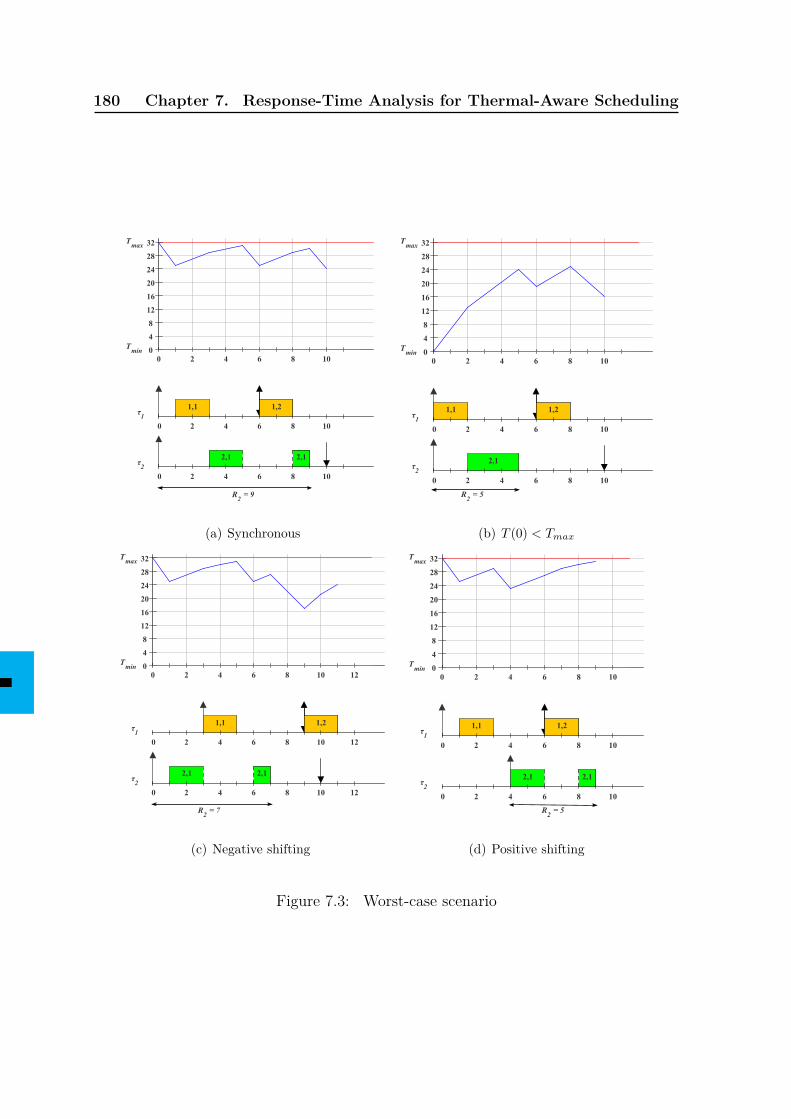
180 Chapter 7. Response-Time Analysis for Thermal-Aware Scheduling
0 2 4 6 8 100
4
8
12
16
20
24
28
32Tmax
Tmin
1,1 1,2
0 2 4 6 8 10
τ1
2,1 2,1
0 2 4 6 8 10
τ2
R = 92
(a) Synchronous
0 2 4 6 8 100
4
8
12
16
20
24
28
32Tmax
Tmin
1,1 1,2
0 2 4 6 8 10
τ1
2,1
0 2 4 6 8 10
τ2
R = 52
(b) T (0) < Tmax
0 2 4 6 8 10 120
4
8
12
16
20
24
28
32Tmax
Tmin
1,1 1,2
0 2 4 6 8 10 12
τ1
2,1 2,1
0 2 4 6 8 10 12
τ2
R = 72
(c) Negative shifting
0 2 4 6 8 100
4
8
12
16
20
24
28
32Tmax
Tmin
1,1 1,2
0 2 4 6 8 10
τ1
2,1 2,1
0 2 4 6 8 10
τ2
R = 52
(d) Positive shifting
Figure 7.3: Worst-case scenario
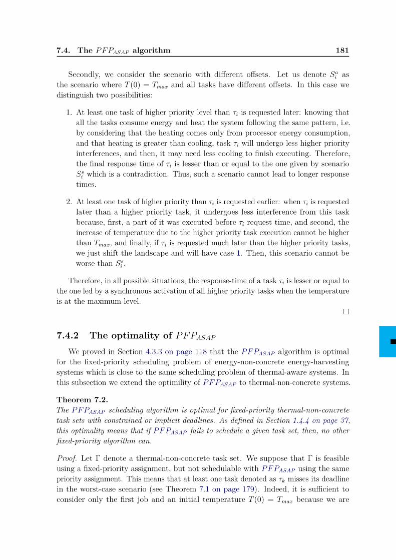
7.4. The PFPASAP algorithm 181
Secondly, we consider the scenario with different offsets. Let us denote Sai asthe scenario where T (0) = Tmax and all tasks have different offsets. In this case wedistinguish two possibilities:
1. At least one task of higher priority level than τi is requested later: knowing thatall the tasks consume energy and heat the system following the same pattern, i.e.by considering that the heating comes only from processor energy consumption,and that heating is greater than cooling, task τi will undergo less higher priorityinterferences, and then, it may need less cooling to finish executing. Therefore,the final response time of τi is lesser than or equal to the one given by scenarioSsi which is a contradiction. Thus, such a scenario cannot lead to longer responsetimes.
2. At least one task of higher priority than τi is requested earlier: when τi is requestedlater than a higher priority task, it undergoes less interference from this taskbecause, first, a part of it was executed before τi request time, and second, theincrease of temperature due to the higher priority task execution cannot be higherthan Tmax, and finally, if τi is requested much later than the higher priority tasks,we just shift the landscape and will have case 1. Then, this scenario cannot beworse than Ssi .
Therefore, in all possible situations, the response-time of a task τi is lesser or equal tothe one led by a synchronous activation of all higher priority tasks when the temperatureis at the maximum level.
7.4.2 The optimality of PFPASAPWe proved in Section 4.3.3 on page 118 that the PFPASAP algorithm is optimal
for the fixed-priority scheduling problem of energy-non-concrete energy-harvestingsystems which is close to the same scheduling problem of thermal-aware systems. Inthis subsection we extend the optimility of PFPASAP to thermal-non-concrete systems.
Theorem 7.2.The PFPASAP scheduling algorithm is optimal for fixed-priority thermal-non-concretetask sets with constrained or implicit deadlines. As defined in Section 1.4.4 on page 37,this optimality means that if PFPASAP fails to schedule a given task set, then, no otherfixed-priority algorithm can.
Proof. Let Γ denote a thermal-non-concrete task set. We suppose that Γ is feasibleusing a fixed-priority assignment, but not schedulable with PFPASAP using the samepriority assignment. This means that at least one task denoted as τk misses its deadlinein the worst-case scenario (see Theorem 7.1 on page 179). Indeed, it is sufficient toconsider only the first job and an initial temperature T (0) = Tmax because we are
182 Chapter 7. Response-Time Analysis for Thermal-Aware Scheduling
dealing only with constrained or implicit deadlines. The jobs of the same task cannotoverlap unless for unfeasible tasks.
According to PFPASAP schemes, a deadline miss can occur in the worst-case scenarioonly in two cases: 1) the workload is greater than the available time, 2) the workloadplus the accumulated cooling time is greater than the available time.
1) If the workload from the critical instant (time 0) to the first deadline of τk is alonegreater than time interval [0, Di], then, it is obvious that it is impossible to schedulethe first job of τk and higher priority jobs without missing Dk, this is not possible evenwithout thermal constrains because the available time is not sufficient to schedule allthe workload within [0, Dk]. Then, in this case the task set cannot be feasible with anyalgorithm and the supposed algorithm cannot exist.
2) If a deadline is missed with PFPASAP even though the workload is lesser than theavailable time, then, this means that the sum of workload of time interval [0, Dk] andthe needed cooling time is greater than the available time, i.e Dk time units. We knowthat the cooling periods produced by PFPASAP are as long as needed to execute onetime unit which means that they are as short as possible. Furthermore, we know thatthe cooling function is exponentially decreasing (see Equation 7.7 on page 177), then,the shorter cooling periods are, the shorter the total needed cooling time is. This is truebecause the longer cooling is, the less efficient it is, as we mentioned in Section 7.3 onpage 176. More formally, cooling down the system x times for one time unit is greaterthan the one of only one cooling period of length x time units because e−bx ≤ xe−b forall x ≥ 1. Thus, Equation 7.7 on page 177) implies Inequality 7.8.
T (0)− T (0)× e−b×x ≥ T (0)− x× T (0)× e−b(1−0) (7.8)
Therefore, any other schedule than the one of PFPASAP has necessarily cooling periodsof same length or longer, then, the response time of τk produced by the supposedalgorithm is necessarily greater than Dk. Thus, in this case, no other algorithm canschedule this task set.
Then we prove that PFPASAP is optimal for non-concrete fixed-priority thermal-constrained task sets with constrained or implicit deadlines.
7.5. Response-Time Analysis 183
Tmax
Tmin
c h
hc
0
Ri
T'mincooling heating
Figure 7.4: First upper bound (UBTmin)
7.5 Response-Time Analysis
This section provides a response-time analysis for the schedule produced by theoptimal algorithm PFPASAP in the worst-case scenario, i.e. the synchronous release ofall the tasks when T (0) = Tmax. We discuss the difficulty of an exact analysis and thenwe propose an approximate one.
7.5.1 Exact Analysis
The exact analysis provides the exact response time of all tasks. Thus, it mustestimate accurately the length of all cooling and heating periods.
However, this cannot be easily achievable with a generic equation. Due to thediscrete time, all cooling periods are not of the same length in the actual schedule.Furthermore, without the effective values of parameters, it is hard to estimate the orderand the number of long and short cooling periods which have a significant impact onthe response time value. Therefore, the only way to get an exact analysis is to simulatethe schedule of PFPASAP in the worst-case scenario and compute the response time ofthe first job of each task.
7.5.2 Approximate Analysis
The aim of this work is to propose a schedulability analysis for thermal-awarereal-time systems. Such an analysis must consider not only the processor workload butalso the additional cooling time needed to respect the thermal constraints. To copewith the difficulty of providing an exact analysis, one can propose an approximate onethat can be only sufficient instead of necessary and sufficient. This can be achieved byupper bounding tasks worst-case response time produced by PFPASAP algorithm.
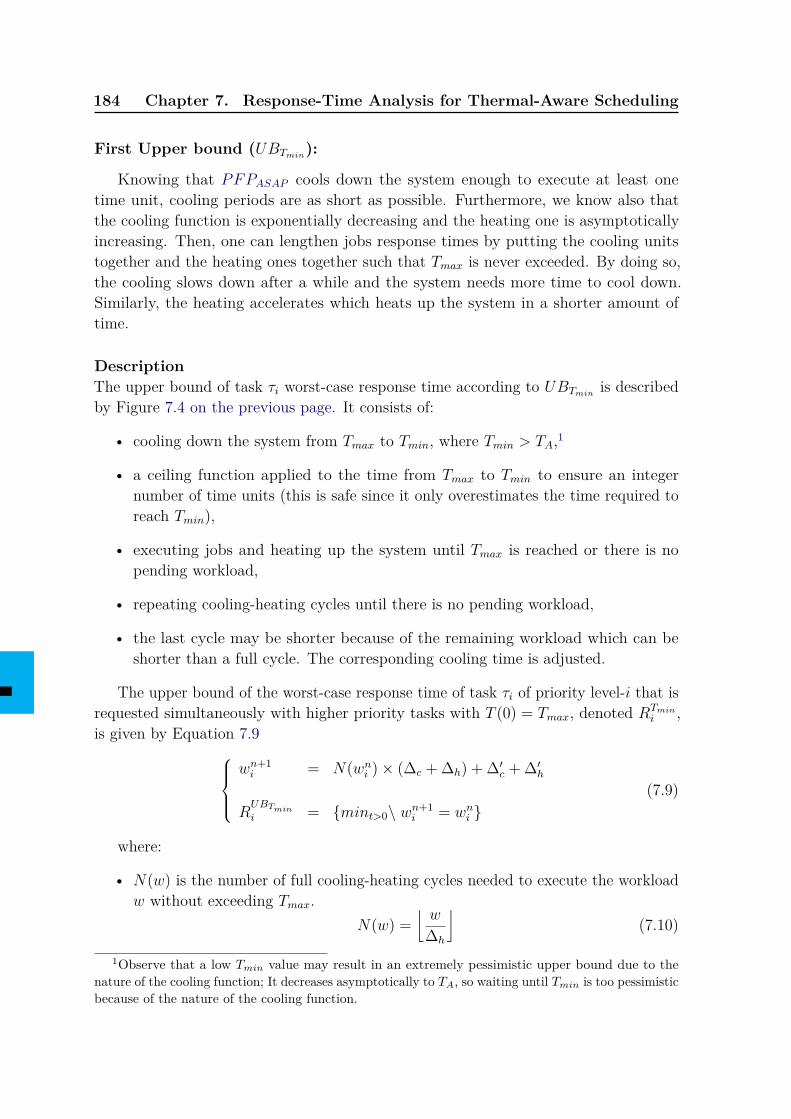
184 Chapter 7. Response-Time Analysis for Thermal-Aware Scheduling
First Upper bound (UBTmin):
Knowing that PFPASAP cools down the system enough to execute at least onetime unit, cooling periods are as short as possible. Furthermore, we know also thatthe cooling function is exponentially decreasing and the heating one is asymptoticallyincreasing. Then, one can lengthen jobs response times by putting the cooling unitstogether and the heating ones together such that Tmax is never exceeded. By doing so,the cooling slows down after a while and the system needs more time to cool down.Similarly, the heating accelerates which heats up the system in a shorter amount oftime.
DescriptionThe upper bound of task τi worst-case response time according to UBTmin is describedby Figure 7.4 on the previous page. It consists of:
• cooling down the system from Tmax to Tmin, where Tmin > TA,1
• a ceiling function applied to the time from Tmax to Tmin to ensure an integernumber of time units (this is safe since it only overestimates the time required toreach Tmin),
• executing jobs and heating up the system until Tmax is reached or there is nopending workload,
• repeating cooling-heating cycles until there is no pending workload,
• the last cycle may be shorter because of the remaining workload which can beshorter than a full cycle. The corresponding cooling time is adjusted.
The upper bound of the worst-case response time of task τi of priority level-i that isrequested simultaneously with higher priority tasks with T (0) = Tmax, denoted RTmin
i ,is given by Equation 7.9
wn+1i = N(wni )× (∆c + ∆h) + ∆′c + ∆′h
RUBTmini = {mint>0\ wn+1
i = wni }(7.9)
where:
• N(w) is the number of full cooling-heating cycles needed to execute the workloadw without exceeding Tmax.
N(w) =⌊w
∆h
⌋(7.10)
1Observe that a low Tmin value may result in an extremely pessimistic upper bound due to thenature of the cooling function; It decreases asymptotically to TA, so waiting until Tmin is too pessimisticbecause of the nature of the cooling function.
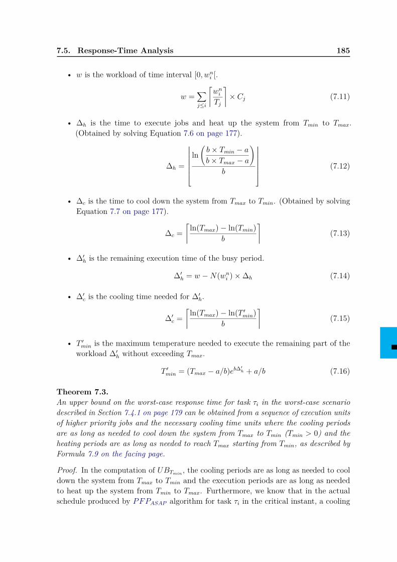
7.5. Response-Time Analysis 185
• w is the workload of time interval [0, wni [.
w =∑j≤i
⌈wniTj
⌉× Cj (7.11)
• ∆h is the time to execute jobs and heat up the system from Tmin to Tmax.(Obtained by solving Equation 7.6 on page 177).
∆h =
ln(b× Tmin − ab× Tmax − a
)b
(7.12)
• ∆c is the time to cool down the system from Tmax to Tmin. (Obtained by solvingEquation 7.7 on page 177).
∆c =⌈
ln(Tmax)− ln(Tmin)b
⌉(7.13)
• ∆′h is the remaining execution time of the busy period.
∆′h = w −N(wni )×∆h (7.14)
• ∆′c is the cooling time needed for ∆′h.
∆′c =⌈
ln(Tmax)− ln(T ′min)b
⌉(7.15)
• T ′min is the maximum temperature needed to execute the remaining part of theworkload ∆′h without exceeding Tmax.
T ′min = (Tmax − a/b)eb∆′h + a/b (7.16)
Theorem 7.3.An upper bound on the worst-case response time for task τi in the worst-case scenariodescribed in Section 7.4.1 on page 179 can be obtained from a sequence of execution unitsof higher priority jobs and the necessary cooling time units where the cooling periodsare as long as needed to cool down the system from Tmax to Tmin (Tmin > 0) and theheating periods are as long as needed to reach Tmax starting from Tmin, as described byFormula 7.9 on the facing page.
Proof. In the computation of UBTmin , the cooling periods are as long as needed to cooldown the system from Tmax to Tmin and the execution periods are as long as neededto heat up the system from Tmin to Tmax. Furthermore, we know that in the actualschedule produced by PFPASAP algorithm for task τi in the critical instant, a cooling
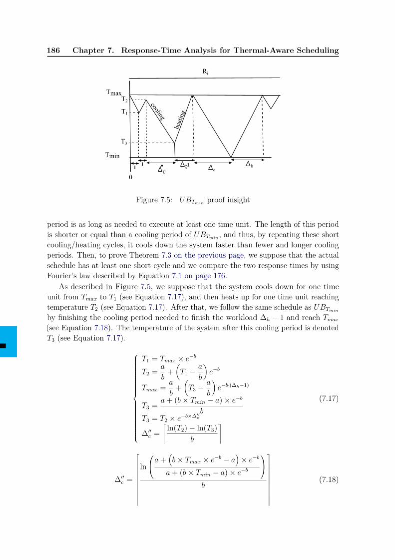
186 Chapter 7. Response-Time Analysis for Thermal-Aware Scheduling
Tmax
Tmin
0
Ri
cooling
heating
T2
T1
T3
hc1
C
-1h
1
Figure 7.5: UBTmin proof insight
period is as long as needed to execute at least one time unit. The length of this periodis shorter or equal than a cooling period of UBTmin , and thus, by repeating these shortcooling/heating cycles, it cools down the system faster than fewer and longer coolingperiods. Then, to prove Theorem 7.3 on the previous page, we suppose that the actualschedule has at least one short cycle and we compare the two response times by usingFourier’s law described by Equation 7.1 on page 176.
As described in Figure 7.5, we suppose that the system cools down for one timeunit from Tmax to T1 (see Equation 7.17), and then heats up for one time unit reachingtemperature T2 (see Equation 7.17). After that, we follow the same schedule as UBTmin
by finishing the cooling period needed to finish the workload ∆h − 1 and reach Tmax(see Equation 7.18). The temperature of the system after this cooling period is denotedT3 (see Equation 7.17).
T1 = Tmax × e−b
T2 = a
b+(T1 −
a
b
)e−b
Tmax = a
b+(T3 −
a
b
)e−b·(∆h−1)
T3 = a+ (b× Tmin − a)× e−bb
T3 = T2 × e−b×∆′′c
∆′′c =⌈
ln(T2)− ln(T3)b
⌉(7.17)
∆′′c =
lna+
(b× Tmax × e−b − a
)× e−b
a+ (b× Tmin − a)× e−b
b
(7.18)
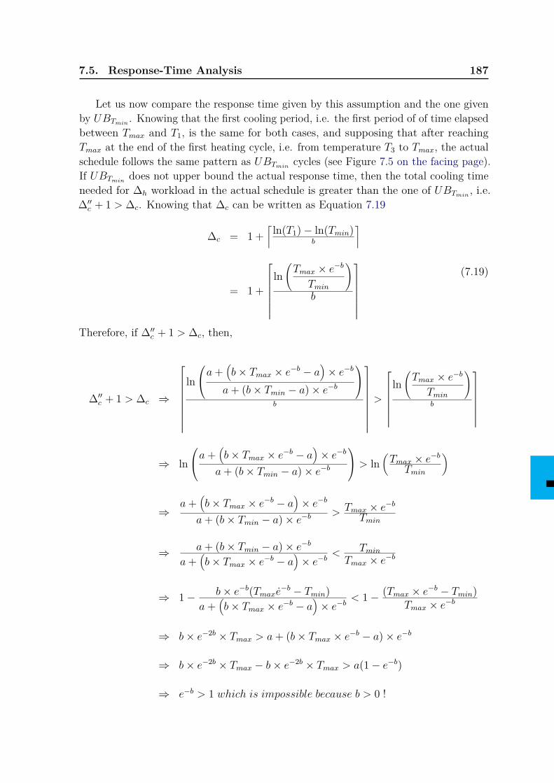
7.5. Response-Time Analysis 187
Let us now compare the response time given by this assumption and the one givenby UBTmin . Knowing that the first cooling period, i.e. the first period of of time elapsedbetween Tmax and T1, is the same for both cases, and supposing that after reachingTmax at the end of the first heating cycle, i.e. from temperature T3 to Tmax, the actualschedule follows the same pattern as UBTmin cycles (see Figure 7.5 on the facing page).If UBTmin does not upper bound the actual response time, then the total cooling timeneeded for ∆h workload in the actual schedule is greater than the one of UBTmin , i.e.∆′′c + 1 > ∆c. Knowing that ∆c can be written as Equation 7.19
∆c = 1 +⌈ ln(T1)− ln(Tmin)
b
⌉
= 1 +
ln(Tmax × e−b
Tmin
)b
(7.19)
Therefore, if ∆′′c + 1 > ∆c, then,
∆′′c + 1 > ∆c ⇒
lna+
(b× Tmax × e−b − a
)× e−b
a+ (b× Tmin − a)× e−b
b
>
ln(Tmax × e−b
Tmin
)b
⇒ lna+
(b× Tmax × e−b − a
)× e−b
a+ (b× Tmin − a)× e−b
> ln(Tmax × e−b
Tmin
)
⇒a+
(b× Tmax × e−b − a
)× e−b
a+ (b× Tmin − a)× e−b > Tmax × e−bTmin
⇒ a+ (b× Tmin − a)× e−b
a+(b× Tmax × e−b − a
)× e−b
< TminTmax × e−b
⇒ 1− b× e−b(Tmaxe−b − Tmin)a+
(b× Tmax × e−b − a
)× e−b
< 1− (Tmax × e−b − Tmin)Tmax × e−b
⇒ b× e−2b × Tmax > a+ (b× Tmax × e−b − a)× e−b
⇒ b× e−2b × Tmax − b× e−2b × Tmax > a(1− e−b)
⇒ e−b > 1 which is impossible because b > 0 !
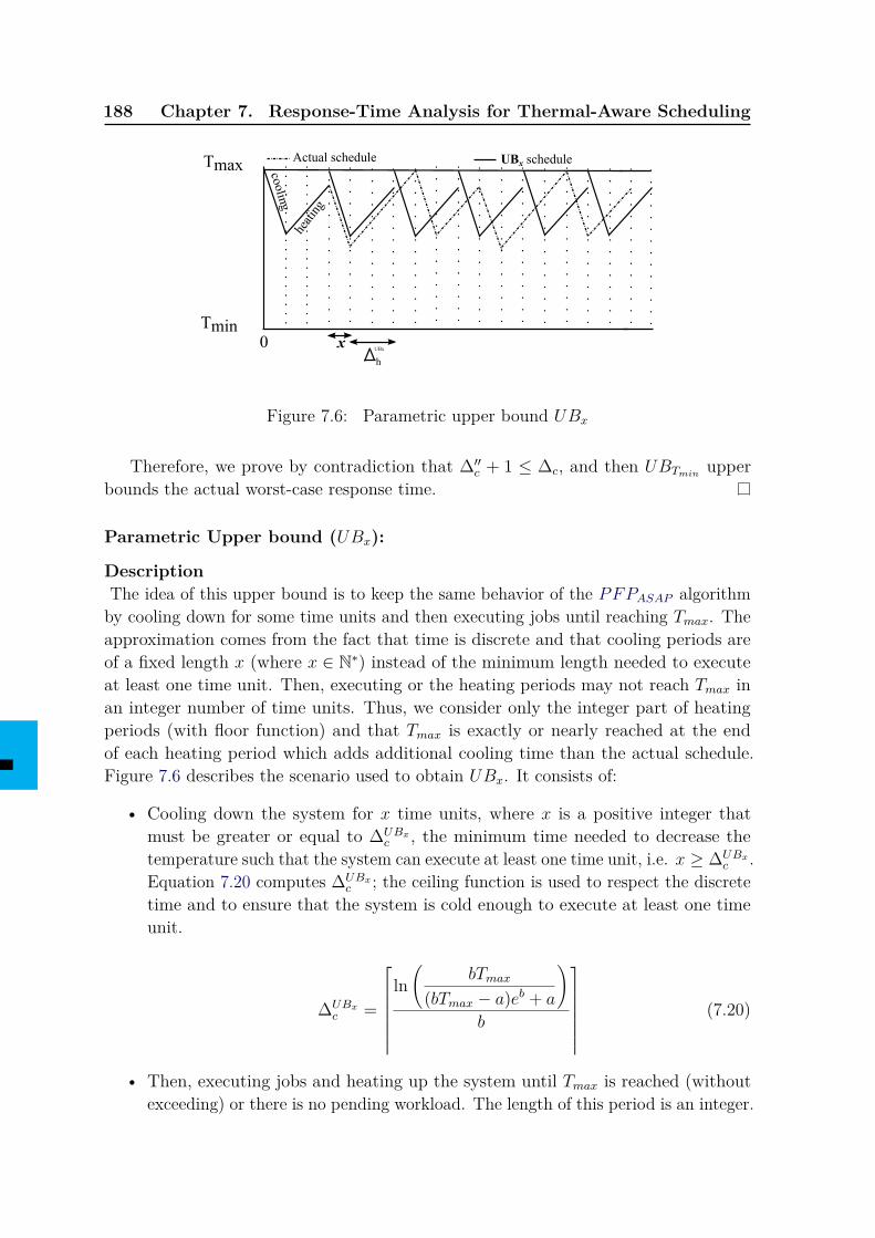
188 Chapter 7. Response-Time Analysis for Thermal-Aware Scheduling
Tmax
Tmin
h
0
cooling
heat
ing
xUBx
Actual schedule UBx schedule
Figure 7.6: Parametric upper bound UBx
Therefore, we prove by contradiction that ∆′′c + 1 ≤ ∆c, and then UBTmin upperbounds the actual worst-case response time.
Parametric Upper bound (UBx):
DescriptionThe idea of this upper bound is to keep the same behavior of the PFPASAP algorithmby cooling down for some time units and then executing jobs until reaching Tmax. Theapproximation comes from the fact that time is discrete and that cooling periods areof a fixed length x (where x ∈ N∗) instead of the minimum length needed to executeat least one time unit. Then, executing or the heating periods may not reach Tmax inan integer number of time units. Thus, we consider only the integer part of heatingperiods (with floor function) and that Tmax is exactly or nearly reached at the endof each heating period which adds additional cooling time than the actual schedule.Figure 7.6 describes the scenario used to obtain UBx. It consists of:
• Cooling down the system for x time units, where x is a positive integer thatmust be greater or equal to ∆UBx
c , the minimum time needed to decrease thetemperature such that the system can execute at least one time unit, i.e. x ≥ ∆UBx
c .Equation 7.20 computes ∆UBx
c ; the ceiling function is used to respect the discretetime and to ensure that the system is cold enough to execute at least one timeunit.
∆UBxc =
ln(
bTmax
(bTmax − a)eb + a
)b
(7.20)
• Then, executing jobs and heating up the system until Tmax is reached (withoutexceeding) or there is no pending workload. The length of this period is an integer.
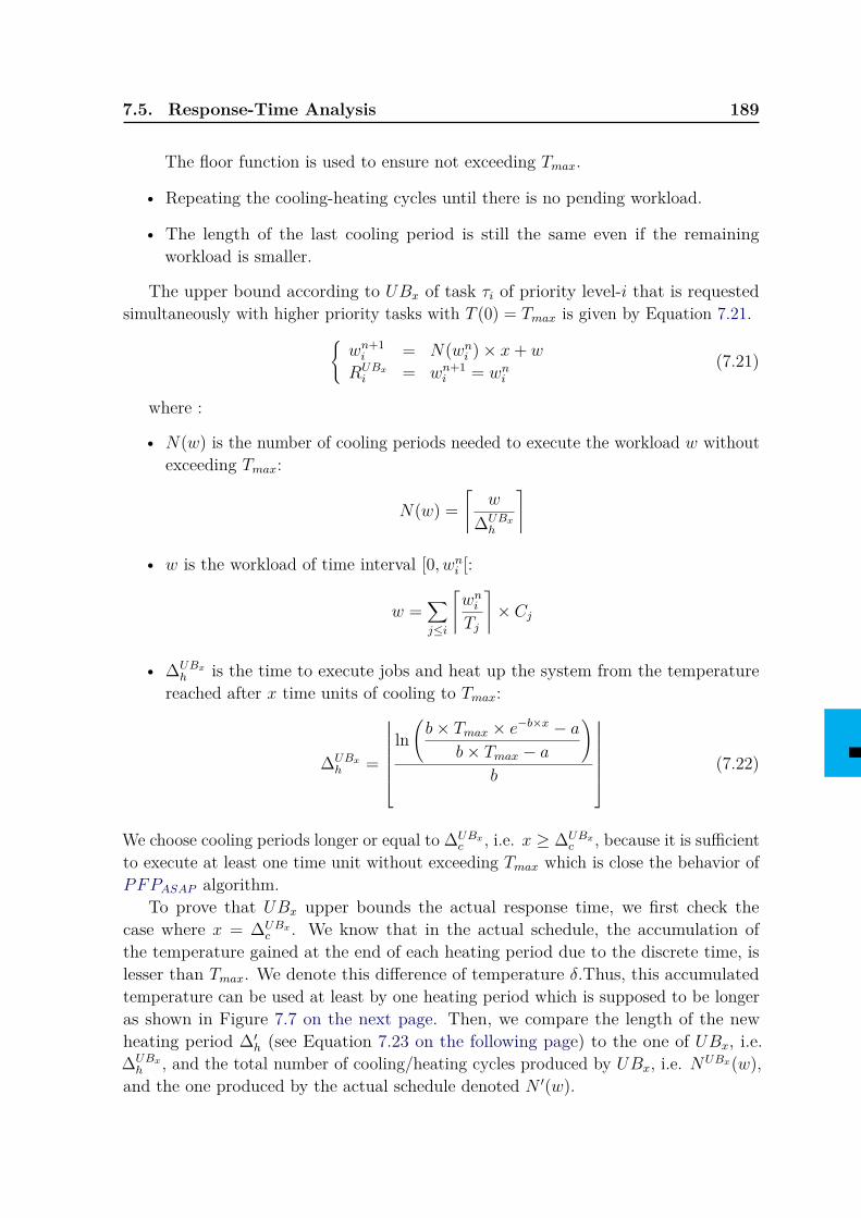
7.5. Response-Time Analysis 189
The floor function is used to ensure not exceeding Tmax.
• Repeating the cooling-heating cycles until there is no pending workload.
• The length of the last cooling period is still the same even if the remainingworkload is smaller.
The upper bound according to UBx of task τi of priority level-i that is requestedsimultaneously with higher priority tasks with T (0) = Tmax is given by Equation 7.21.{
wn+1i = N(wni )× x+ w
RUBxi = wn+1
i = wni(7.21)
where :
• N(w) is the number of cooling periods needed to execute the workload w withoutexceeding Tmax:
N(w) =⌈
w
∆UBxh
⌉
• w is the workload of time interval [0, wni [:
w =∑j≤i
⌈wniTj
⌉× Cj
• ∆UBxh is the time to execute jobs and heat up the system from the temperature
reached after x time units of cooling to Tmax:
∆UBxh =
ln(b× Tmax × e−b×x − a
b× Tmax − a
)b
(7.22)
We choose cooling periods longer or equal to ∆UBxc , i.e. x ≥ ∆UBx
c , because it is sufficientto execute at least one time unit without exceeding Tmax which is close the behavior ofPFPASAP algorithm.
To prove that UBx upper bounds the actual response time, we first check thecase where x = ∆UBx
c . We know that in the actual schedule, the accumulation ofthe temperature gained at the end of each heating period due to the discrete time, islesser than Tmax. We denote this difference of temperature δ.Thus, this accumulatedtemperature can be used at least by one heating period which is supposed to be longeras shown in Figure 7.7 on the next page. Then, we compare the length of the newheating period ∆′h (see Equation 7.23 on the following page) to the one of UBx, i.e.∆UBxh , and the total number of cooling/heating cycles produced by UBx, i.e. NUBx(w),
and the one produced by the actual schedule denoted N ′(w).
190 Chapter 7. Response-Time Analysis for Thermal-Aware Scheduling
Tmax
Tmin
hx UBx
Proof schedule UBx schedule
x 'h
UBx
T1
T2
δ
Figure 7.7: UBx proof insight
Tmax = (a+ (b× T2 − a)e−b×∆′h)/b
T2 = (Tmax − δ)e−b×x
∆′h =
ln(b× (Tmax − δ)× e−b×x − a
b× Tmax − a
)b
(7.23)
Lemma 7.1.For x = ∆UBx
c , each heating interval of the actual schedule ∆′h given by Equation 7.23is greater than or equal to UBx’s ones, i.e. ∆UBx
h ≤ ∆′h.
Proof. Let us suppose that ∆UBxh > ∆′h, then:
∆UBxh > ∆′h ⇒
ln(b× Tmax × e−bx − a
bTmax − a
)b
>
ln(b(Tmax − δ)e−bx − a
bTmax − a
)b
⇒ln(bTmaxe
−bx − abTmax − a
)b >
ln(b(Tmax − δ)e−bx − a
bTmax − a
)b
⇒ bTmaxe−bx − a
bTmax − a >b(Tmax − δ)e−bx − a
bTmax − a
7.5. Response-Time Analysis 191
Knowing that bTmax < a, then:
∆UBxh > ∆′h ⇒ bTmaxe
−bx − a < b(Tmax − δ)e−bx − a
⇒ bTmaxe−bx < b(Tmax − δ)e−bx
⇒ bTmaxe−bx < b(Tmax − δ)e−bx
⇒ Tmax < Tmax − δ
⇒ δ < 0
Contradiction because 0 < b < 1, δ ≥ 0 and b× Tmax < a.Therefore, we prove by contradiction that ∆UBx
h ≤ ∆′h
Lemma 7.2.For x = ∆UBx
c , the number of cooling periods produced by a PFPASAP actual scheduledenoted N ′(w) is lesser than or equal to the ones produced by UBx, i.e. N ′(w) ≤NUBx(w).
Proof. Let us suppose that N ′(w) > NUBx(w). From Lemma 7.1 on the facing page weknow that ∆UBx
h ≤ ∆′h at least for one time. Then:
N ′(w) =⌈w −∆′h∆UBxh
⌉+ 1 =
⌈w − (∆UBx
h + δ)∆UBxh
⌉+ 1
where δ ≥ 0. Then, N ′(w) can be written as follows:
N ′(w) =⌈w − δ∆UBxh
⌉
Therefore, if N ′(w) > NUBx(w), then:
N ′(w) > NUBx(w) ⇒⌈w − δ∆UBxh
⌉>
⌈w
∆UBxh
⌉
⇒ w − δ∆UBxh
> w
∆UBxh
⇒ δ < 0
Contradiction, because ∆′h ≥ ∆UBxh and δ ≥ 0. Therefore, we prove that N ′(w) ≤
NUBx(w)
Theorem 7.4.An upper bound on the worst-case response time for task τi in the worst-case scenario
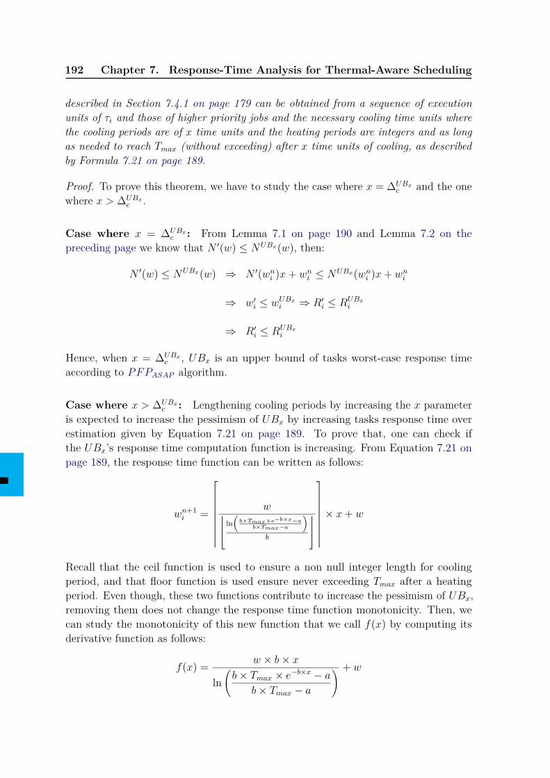
192 Chapter 7. Response-Time Analysis for Thermal-Aware Scheduling
described in Section 7.4.1 on page 179 can be obtained from a sequence of executionunits of τi and those of higher priority jobs and the necessary cooling time units wherethe cooling periods are of x time units and the heating periods are integers and as longas needed to reach Tmax (without exceeding) after x time units of cooling, as describedby Formula 7.21 on page 189.
Proof. To prove this theorem, we have to study the case where x = ∆UBxc and the one
where x > ∆UBxc .
Case where x = ∆UBxc : From Lemma 7.1 on page 190 and Lemma 7.2 on the
preceding page we know that N ′(w) ≤ NUBx(w), then:
N ′(w) ≤ NUBx(w) ⇒ N ′(wni )x+ wni ≤ NUBx(wni )x+ wni
⇒ w′i ≤ wUBxi ⇒ R′i ≤ RUBxi
⇒ R′i ≤ RUBxi
Hence, when x = ∆UBxc , UBx is an upper bound of tasks worst-case response time
according to PFPASAP algorithm.
Case where x > ∆UBxc : Lengthening cooling periods by increasing the x parameter
is expected to increase the pessimism of UBx by increasing tasks response time overestimation given by Equation 7.21 on page 189. To prove that, one can check ifthe UBx’s response time computation function is increasing. From Equation 7.21 onpage 189, the response time function can be written as follows:
wn+1i =
w ln
(b×Tmax×e−b×x−a
b×Tmax−a
)b
× x+ w
Recall that the ceil function is used to ensure a non null integer length for coolingperiod, and that floor function is used ensure never exceeding Tmax after a heatingperiod. Even though, these two functions contribute to increase the pessimism of UBx,removing them does not change the response time function monotonicity. Then, wecan study the monotonicity of this new function that we call f(x) by computing itsderivative function as follows:
f(x) = w × b× x
ln(b× Tmax × e−b×x − a
b× Tmax − a
) + w
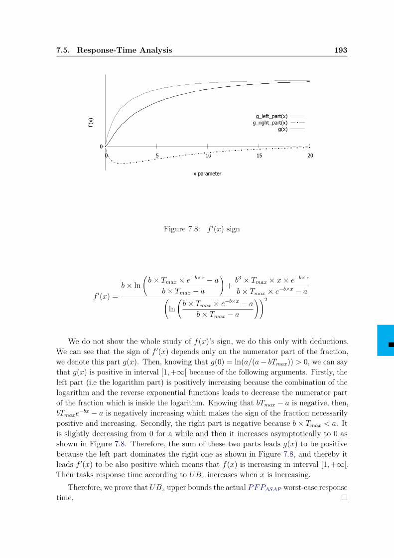
7.5. Response-Time Analysis 193
0
0 5 10 15 20
f'(x)
x parameter
g_left_part(x)g_right_part(x)
g(x)
Figure 7.8: f ′(x) sign
f ′(x) =b× ln
(b× Tmax × e−b×x − a
b× Tmax − a
)+ b3 × Tmax × x× e−b×x
b× Tmax × e−b×x − a(ln(b× Tmax × e−b×x − a
b× Tmax − a
))2
We do not show the whole study of f(x)’s sign, we do this only with deductions.We can see that the sign of f ′(x) depends only on the numerator part of the fraction,we denote this part g(x). Then, knowing that g(0) = ln(a/(a− bTmax)) > 0, we can saythat g(x) is positive in interval [1,+∞[ because of the following arguments. Firstly, theleft part (i.e the logarithm part) is positively increasing because the combination of thelogarithm and the reverse exponential functions leads to decrease the numerator partof the fraction which is inside the logarithm. Knowing that bTmax − a is negative, then,bTmaxe
−bx − a is negatively increasing which makes the sign of the fraction necessarilypositive and increasing. Secondly, the right part is negative because b× Tmax < a. Itis slightly decreasing from 0 for a while and then it increases asymptotically to 0 asshown in Figure 7.8. Therefore, the sum of these two parts leads g(x) to be positivebecause the left part dominates the right one as shown in Figure 7.8, and thereby itleads f ′(x) to be also positive which means that f(x) is increasing in interval [1,+∞[.Then tasks response time according to UBx increases when x is increasing.
Therefore, we prove that UBx upper bounds the actual PFPASAP worst-case responsetime.
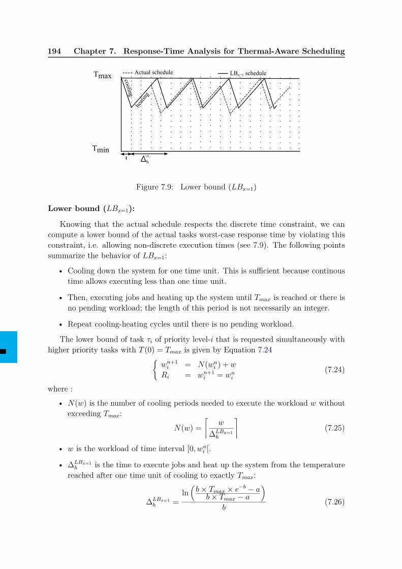
194 Chapter 7. Response-Time Analysis for Thermal-Aware Scheduling
Tmax
Tmin
h
cooling
heat
ing
1LBx=1
Actual schedule LBx=1 schedule
Figure 7.9: Lower bound (LBx=1)
Lower bound (LBx=1):
Knowing that the actual schedule respects the discrete time constraint, we cancompute a lower bound of the actual tasks worst-case response time by violating thisconstraint, i.e. allowing non-discrete execution times (see 7.9). The following pointssummarize the behavior of LBx=1:
• Cooling down the system for one time unit. This is sufficient because continoustime allows executing less than one time unit.
• Then, executing jobs and heating up the system until Tmax is reached or there isno pending workload; the length of this period is not necessarily an integer.
• Repeat cooling-heating cycles until there is no pending workload.
The lower bound of task τi of priority level-i that is requested simultaneously withhigher priority tasks with T (0) = Tmax is given by Equation 7.24{
wn+1i = N(wni ) + w
Ri = wn+1i = wni
(7.24)
where :
• N(w) is the number of cooling periods needed to execute the workload w withoutexceeding Tmax:
N(w) =⌈
w
∆LBx=1h
⌉(7.25)
• w is the workload of time interval [0, wni [.
• ∆LBx=1h is the time to execute jobs and heat up the system from the temperature
reached after one time unit of cooling to exactly Tmax:
∆LBx=1h =
ln(b× Tmax × e−b − a
b× Tmax − a
)b
(7.26)
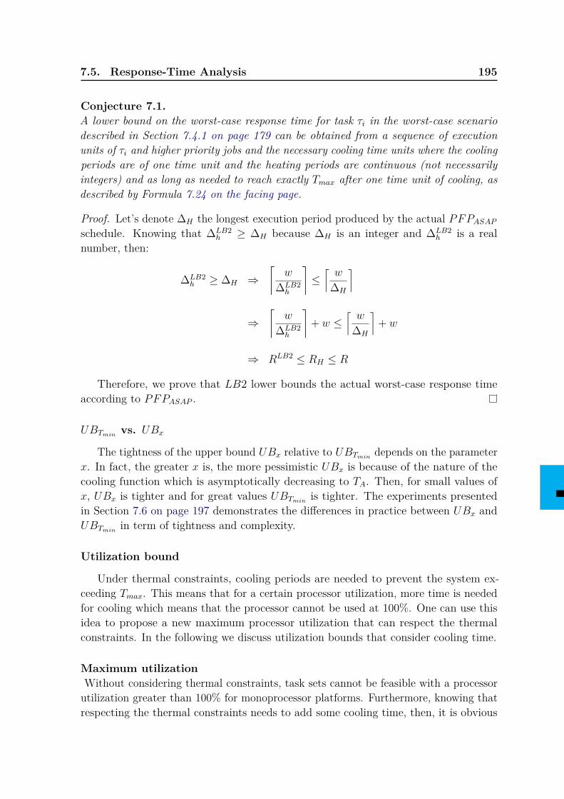
7.5. Response-Time Analysis 195
Conjecture 7.1.A lower bound on the worst-case response time for task τi in the worst-case scenariodescribed in Section 7.4.1 on page 179 can be obtained from a sequence of executionunits of τi and higher priority jobs and the necessary cooling time units where the coolingperiods are of one time unit and the heating periods are continuous (not necessarilyintegers) and as long as needed to reach exactly Tmax after one time unit of cooling, asdescribed by Formula 7.24 on the facing page.
Proof. Let’s denote ∆H the longest execution period produced by the actual PFPASAPschedule. Knowing that ∆LB2
h ≥ ∆H because ∆H is an integer and ∆LB2h is a real
number, then:
∆LB2h ≥ ∆H ⇒
⌈w
∆LB2h
⌉≤⌈w
∆H
⌉
⇒⌈
w
∆LB2h
⌉+ w ≤
⌈w
∆H
⌉+ w
⇒ RLB2 ≤ RH ≤ R
Therefore, we prove that LB2 lower bounds the actual worst-case response timeaccording to PFPASAP .
UBTmin vs. UBx
The tightness of the upper bound UBx relative to UBTmin depends on the parameterx. In fact, the greater x is, the more pessimistic UBx is because of the nature of thecooling function which is asymptotically decreasing to TA. Then, for small values ofx, UBx is tighter and for great values UBTmin is tighter. The experiments presentedin Section 7.6 on page 197 demonstrates the differences in practice between UBx andUBTmin in term of tightness and complexity.
Utilization bound
Under thermal constraints, cooling periods are needed to prevent the system ex-ceeding Tmax. This means that for a certain processor utilization, more time is neededfor cooling which means that the processor cannot be used at 100%. One can use thisidea to propose a new maximum processor utilization that can respect the thermalconstraints. In the following we discuss utilization bounds that consider cooling time.
Maximum utilizationWithout considering thermal constraints, task sets cannot be feasible with a processorutilization greater than 100% for monoprocessor platforms. Furthermore, knowing thatrespecting the thermal constraints needs to add some cooling time, then, it is obvious
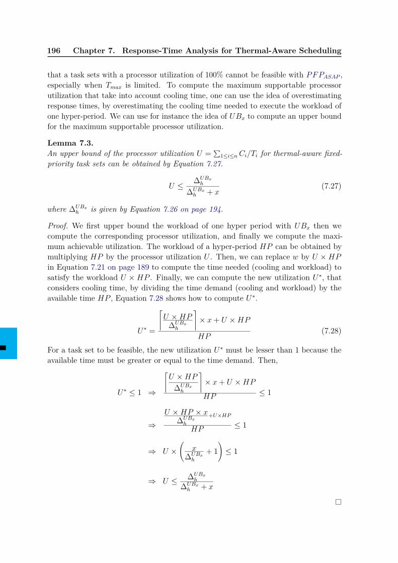
196 Chapter 7. Response-Time Analysis for Thermal-Aware Scheduling
that a task sets with a processor utilization of 100% cannot be feasible with PFPASAP ,especially when Tmax is limited. To compute the maximum supportable processorutilization that take into account cooling time, one can use the idea of overestimatingresponse times, by overestimating the cooling time needed to execute the workload ofone hyper-period. We can use for instance the idea of UBx to compute an upper boundfor the maximum supportable processor utilization.
Lemma 7.3.An upper bound of the processor utilization U = ∑
1≤i≤nCi/Ti for thermal-aware fixed-priority task sets can be obtained by Equation 7.27.
U ≤ ∆UBxh
∆UBxh + x
(7.27)
where ∆UBxh is given by Equation 7.26 on page 194.
Proof. We first upper bound the workload of one hyper period with UBx then wecompute the corresponding processor utilization, and finally we compute the maxi-mum achievable utilization. The workload of a hyper-period HP can be obtained bymultiplying HP by the processor utilization U . Then, we can replace w by U ×HPin Equation 7.21 on page 189 to compute the time needed (cooling and workload) tosatisfy the workload U ×HP . Finally, we can compute the new utilization U∗, thatconsiders cooling time, by dividing the time demand (cooling and workload) by theavailable time HP , Equation 7.28 shows how to compute U∗.
U∗ =
⌈U ×HP
∆UBxh
⌉× x+ U ×HP
HP(7.28)
For a task set to be feasible, the new utilization U∗ must be lesser than 1 because theavailable time must be greater or equal to the time demand. Then,
U∗ ≤ 1 ⇒
⌈U ×HP
∆UBxh
⌉× x+ U ×HP
HP ≤ 1
⇒U ×HP × x
∆UBxh
+U×HP
HP ≤ 1
⇒ U ×(
x∆UBxh
+ 1)≤ 1
⇒ U ≤ ∆UBxh
∆UBxh + x
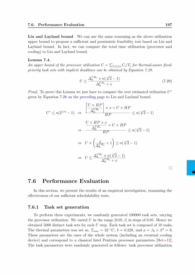
7.6. Performance Evaluation 197
Liu and Layland bound We can use the same reasoning as the above utilizationupper bound to propose a sufficient and pessimistic feasibility test based on Liu andLayland bound. In fact, we can compare the total time utilization (processor andcooling) to Liu and Layland bound.
Lemma 7.4.An upper bound of the processor utilization U = ∑
1≤i≤nCi/Ti for thermal-aware fixed-priority task sets with implicit deadlines can be obtained by Equation 7.29.
U ≤ ∆UBxh × n( n
√2− 1)
∆UBxh + x
(7.29)
Proof. To prove this Lemma we just have to compare the over estimated utilization U∗given by Equation 7.28 on the preceding page to Liu and Layland bound.
U∗ ≤ n(21/n − 1) ⇒
⌈U ×HP
∆UBxh
⌉× x+ U ×HP
HP ≤ n( n√
2− 1)
⇒
U ×HP × x∆UBxh
+ U ×HP
HP ≤ n( n√
2− 1)
⇒ U ×(
x∆UBxh
+ 1)≤ n( n
√2− 1)
⇒ U ≤ ∆UBxh × n( n
√2− 1)
∆UBxh + x
7.6 Performance EvaluationIn this section, we present the results of an empirical investigation, examining the
effectiveness of our sufficient schedulability tests.
7.6.1 Task set generationTo perform these experiments, we randomly generated 100000 task sets, varying
the processor utilization. We varied U in the range [0.05, 1] in steps of 0.05. Hence weobtained 5000 distinct task sets for each U step. Each task set is composed of 10 tasks.The thermal parameters was set as, Tmax = 32 ◦C, b = 0.228, and a = β0 × S3 = 8.These parameters are the ones of the whole system (including an eventual coolingdevice) and correspond to a classical Intel Pentium processor parameters [Het+12].The task parameters were randomly generated as follows: task processor utilization
198 Chapter 7. Response-Time Analysis for Thermal-Aware Scheduling
(Ui = Ci/Ti) using the U-Unifast Discard algorithm [BB05], and periods randomlygenerated between 2 and 25200 time units with a hyper-period limitation technique[MG01]. Task deadlines were implicit.
We used YARTISS as a simulation environment (see Chapter 8) which respects thefollowing hypotheses: discrete time (all scheduling operations are performed before orafter one time unit), the heating behavior follows the Fourier’s law (see Equation 7.6on page 177) and temperature values are real numbers.
7.6.2 Schedulability tests investigatedWe investigated the performance of the following schedulability tests.
• SIM : is an empirical necessary and sufficient test based on simulating the scheduleof PFPASAP over more than one hyper-period, starting with synchronous releaseand the maximum temperature level which corresponds to the worst-case scenariodiscussed in Section 7.4.1 on page 179.
• UBTmin : the sufficient test presented in Section 7.5.2 on page 184, we considerthat Tmin = 1 ◦C.
• UBx: the sufficient test presented in Section 7.5.2 on page 188, the parameter xis varied from 1 to 18.
• LBx=1: the necessary test presented in Section 7.5.2 on page 194.
• CFP : the exact test for fixed-priority ignoring thermal and energy constraints.This was used to provide a schedulability bound, considering only processing time.
• UTZ: the necessary condition described in Section 7.5.2 on page 195.
• LnL: the sufficient condition described in Section 7.5.2 on the preceding page.
7.6.3 ExperimentsFigure 7.10(a) on the next page shows how the percentage of task sets that are
deemed schedulable by each of the tests varies with processor utilization. The CFP testhas notionally the highest performance since it is widely optimistic and ignores thermalconsiderations. When temperature is considered, UTZ, LBx=1 provide necessary tests,upper bounding the number of task sets that are proved to be schedulable by the exactempirical test SIM . We observe that the results confirm that UBTmin and UBx providesufficient schedulability tests and that for x = 1, UBx is a tighter bound than UBTmin
with a larger improvement at higher utilization levels. Furthermore, this experimentconfirms also the validity of the utilization bounds given in Section 7.5.2 on page 195.We can see that the maximum achievable utilization for 10 tasks is 80% for UTZ andthe adapted Liu and Layland bound is 57%.
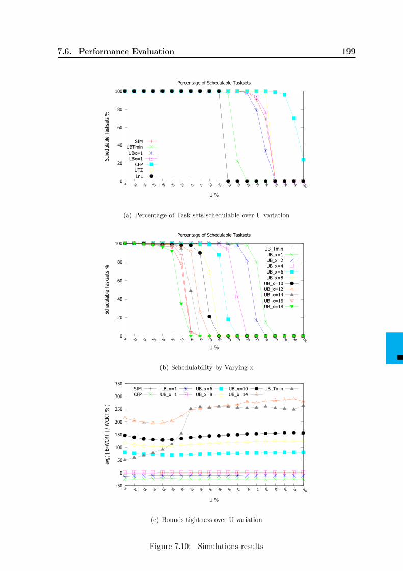
7.6. Performance Evaluation 199
0
20
40
60
80
100
5 10 15 20 25 30 35 40 45 50 55 60 65 70 75 80 85 90 95 100
Sche
dula
ble
Task
sets
%
U %
Percentage of Schedulable Tasksets
SIMUBTminUBx=1LBx=1
CFPUTZLnL
(a) Percentage of Task sets schedulable over U variation
0
20
40
60
80
100
5 10 15 20 25 30 35 40 45 50 55 60 65 70 75 80 85 90 95 100
Sche
dula
ble
Task
sets
%
U %
Percentage of Schedulable Tasksets
UB_TminUB_x=1UB_x=2UB_x=4UB_x=6UB_x=8
UB_x=10UB_x=12UB_x=14UB_x=16UB_x=18
(b) Schedulability by Varying x
-50
0
50
100
150
200
250
300
350
5 10 15 20 25 30 35 40 45 50 55 60 65 70 75 80 85 90 95 100
avg(
| B
-WCR
T |
/ W
CRT
% )
U %
SIMCFP
LB_x=1UB_x=1
UB_x=6UB_x=8
UB_x=10UB_x=14
UB_Tmin
(c) Bounds tightness over U variation
Figure 7.10: Simulations results
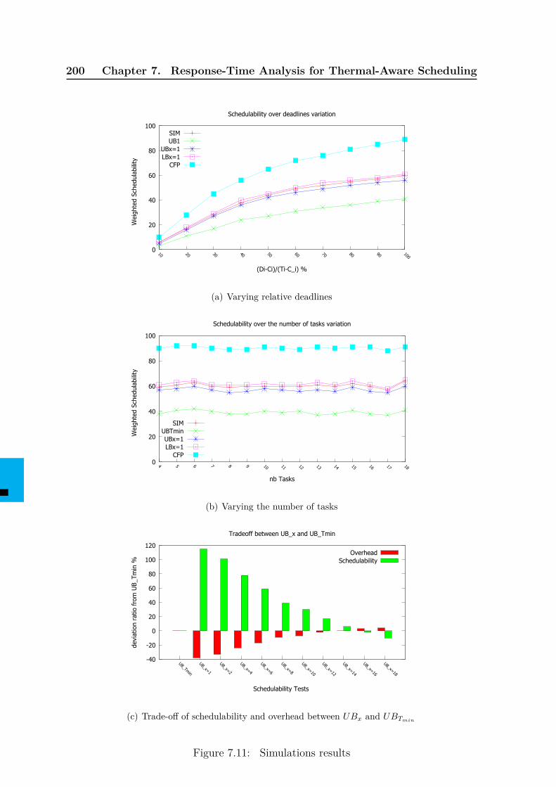
200 Chapter 7. Response-Time Analysis for Thermal-Aware Scheduling
0
20
40
60
80
100
10 20 30 40 50 60 70 80 90 100
Wei
ghte
d Sc
hedu
labi
lity
(Di-Ci)/(Ti-C_i) %
Schedulability over deadlines variation
SIMUB1
UBx=1LBx=1
CFP
(a) Varying relative deadlines
0
20
40
60
80
100
4 5 6 7 8 9 10 11 12 13 14 15 16 17 18
Wei
ghte
d Sc
hedu
labi
lity
nb Tasks
Schedulability over the number of tasks variation
SIMUBTminUBx=1LBx=1
CFP
(b) Varying the number of tasks
-40
-20
0
20
40
60
80
100
120
UB_Tmin
UB_x=1
UB_x=2
UB_x=4
UB_x=6
UB_x=8
UB_x=10
UB_x=12
UB_x=14
UB_x=16
UB_x=18
dev
iatio
n ra
tio f
rom
UB_
Tmin
%
Schedulability Tests
Tradeoff between UB_x and UB_Tmin
OverheadSchedulability
(c) Trade-off of schedulability and overhead between UBx and UBTmin
Figure 7.11: Simulations results
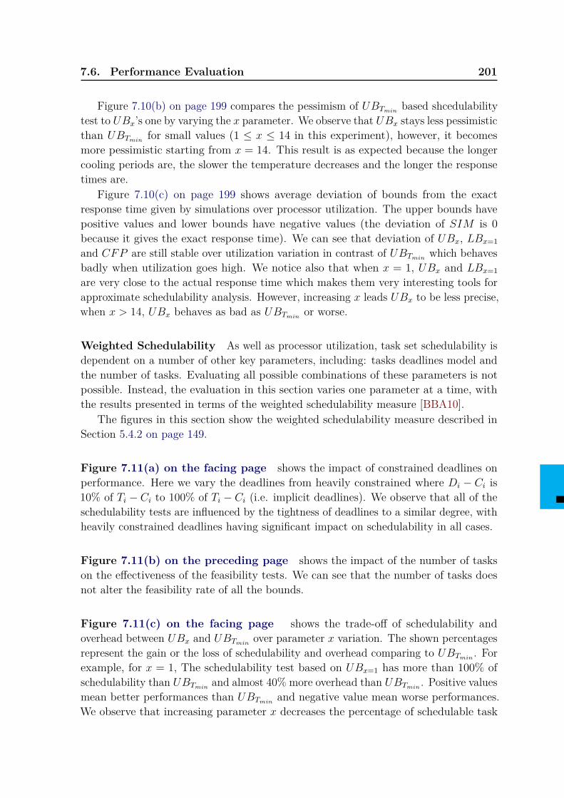
7.6. Performance Evaluation 201
Figure 7.10(b) on page 199 compares the pessimism of UBTmin based shcedulabilitytest to UBx’s one by varying the x parameter. We observe that UBx stays less pessimisticthan UBTmin for small values (1 ≤ x ≤ 14 in this experiment), however, it becomesmore pessimistic starting from x = 14. This result is as expected because the longercooling periods are, the slower the temperature decreases and the longer the responsetimes are.
Figure 7.10(c) on page 199 shows average deviation of bounds from the exactresponse time given by simulations over processor utilization. The upper bounds havepositive values and lower bounds have negative values (the deviation of SIM is 0because it gives the exact response time). We can see that deviation of UBx, LBx=1and CFP are still stable over utilization variation in contrast of UBTmin which behavesbadly when utilization goes high. We notice also that when x = 1, UBx and LBx=1are very close to the actual response time which makes them very interesting tools forapproximate schedulability analysis. However, increasing x leads UBx to be less precise,when x > 14, UBx behaves as bad as UBTmin or worse.
Weighted Schedulability As well as processor utilization, task set schedulability isdependent on a number of other key parameters, including: tasks deadlines model andthe number of tasks. Evaluating all possible combinations of these parameters is notpossible. Instead, the evaluation in this section varies one parameter at a time, withthe results presented in terms of the weighted schedulability measure [BBA10].
The figures in this section show the weighted schedulability measure described inSection 5.4.2 on page 149.
Figure 7.11(a) on the facing page shows the impact of constrained deadlines onperformance. Here we vary the deadlines from heavily constrained where Di − Ci is10% of Ti − Ci to 100% of Ti − Ci (i.e. implicit deadlines). We observe that all of theschedulability tests are influenced by the tightness of deadlines to a similar degree, withheavily constrained deadlines having significant impact on schedulability in all cases.
Figure 7.11(b) on the preceding page shows the impact of the number of taskson the effectiveness of the feasibility tests. We can see that the number of tasks doesnot alter the feasibility rate of all the bounds.
Figure 7.11(c) on the facing page shows the trade-off of schedulability andoverhead between UBx and UBTmin over parameter x variation. The shown percentagesrepresent the gain or the loss of schedulability and overhead comparing to UBTmin . Forexample, for x = 1, The schedulability test based on UBx=1 has more than 100% ofschedulability than UBTmin and almost 40% more overhead than UBTmin . Positive valuesmean better performances than UBTmin and negative value mean worse performances.We observe that increasing parameter x decreases the percentage of schedulable task
202 Chapter 7. Response-Time Analysis for Thermal-Aware Scheduling
sets, however, it decreases the test complexity or overhead. We observe also that theloss of schedulablity is higher than the gain of overhead.
7.7 ConclusionIn this chapter, we addressed the problem of fixed-priority real-time scheduling for
thermal-aware systems, where both time and thermal constraints have to be met. In aprevious chapter, we showed that the scheduling policy PFPASAP is optimal among allfixed-priority scheduling algorithms for energy-non-concrete energy-harvesting systems.The main contributions of this chapter are as follows. we adapted PFPASAP algorithmto the thermal-aware model, we proved its optimality and we proposed two schedulabilitytests based on response-time upper bounds UBTmin and UBx which is a parametricbound. Finally we performed simulations to validate the theoretical results. Thescheduling problems of energy-harvesting and thermal-aware systems seem to be closeto each other. This opens the door to use and adapt scheduling solutions from oneside to an other. This work is a first step in this way. It is interesting to continuestudying deeply the possible similarities between energy-harvesting model and thethermal-aware’s one and to explore more adaptable and extensible results of eachmodel.
Chapter 8
Simulation Tool: YARTISS
Contents8.1 Introduction . . . . . . . . . . . . . . . . . . . . . . . . . . . . . 2038.2 Related Works . . . . . . . . . . . . . . . . . . . . . . . . . . . . 2058.3 The History of YARTISS . . . . . . . . . . . . . . . . . . . . . 2068.4 Functionalities . . . . . . . . . . . . . . . . . . . . . . . . . . . . 207
8.4.1 Single Task Set Simulation . . . . . . . . . . . . . . . . . . . . . 2088.4.2 Run Large Scale Simulations . . . . . . . . . . . . . . . . . . . . 2128.4.3 Task Set Generation . . . . . . . . . . . . . . . . . . . . . . . . . 2128.4.4 Graphical User Interface (GUI) . . . . . . . . . . . . . . . . . . . 213
8.5 Architecture . . . . . . . . . . . . . . . . . . . . . . . . . . . . . 2138.5.1 Engine Module . . . . . . . . . . . . . . . . . . . . . . . . . . . . 2148.5.2 Service Module . . . . . . . . . . . . . . . . . . . . . . . . . . . . 2198.5.3 Framework Module . . . . . . . . . . . . . . . . . . . . . . . . . . 2208.5.4 View-Module or GUI . . . . . . . . . . . . . . . . . . . . . . . . . 220
8.6 Case Study . . . . . . . . . . . . . . . . . . . . . . . . . . . . . . 2218.6.1 Adding a new Scheduling Policy . . . . . . . . . . . . . . . . . . 2218.6.2 Adding an Energy Profile . . . . . . . . . . . . . . . . . . . . . . 223
8.7 Distribution . . . . . . . . . . . . . . . . . . . . . . . . . . . . . . 2238.8 Conclusion . . . . . . . . . . . . . . . . . . . . . . . . . . . . . . 223
8.1 IntroductionThe real-time scheduling theory has been studied by many researchers since decades,
and many solutions and approaches have been proposed in the past to optimize thescheduling of real-time tasks on single and multiple processor systems. In order tocheck if a task set respects its temporal constraints according to a specific schedulingpolicy or to evaluate the efficiency of a new approach against other algorithms, usingsimulation software is considered as a valid comparison technique and it is commonlyused in the evaluation of real-time systems.
204 Chapter 8. Simulation Tool: YARTISS
Unfortunately, there is no standard simulation tool approved by the real-timecommunity and the existing tools are usually hard to be extended due to various reasonssuch as code complexity, software copyrights or poor documentation. As a result, mostof the researchers tend to create their own simulation tools. This situation raises someconcerns. On one hand, results are hard to be validated without careful examinationof the used simulation tool. So these results might be biased toward the proposedapproach either by adapting the generation of tasks or by biased implementation againstthe compared algorithms. On another hand, the use of out-of-date simulation toolsor the lack of good documentation pushes researchers to not use the existing toolsand to create their own ones, which leads to repetitive implementations especiallythe common ones e.g. Earliest Deadline First (EDF ), Rate Monotonic (RM) andDeadline Monotonic (DM).
Besides the time and the effort spent by researchers in developing new simulationtools, the process of implementing comparable algorithms can be sometimes complicatedand time-consuming. If a standard simulation platform succeeds to emerge, one canre-use already-implemented policies from literature and compare them with new policieswithout the need to understand their specifications and particularities. Finally, thesimulation protocols can be standardized, and easily describable by the use of such areference tool.
In this chapter, we introduce Yet An Other Real-Time Systems Simulator (YARTISS),a new simulation tool for real-time multiprocessor systems, which provides variousfunctions to simulate the scheduling process of real-time task sets and their temporalbehavior.
The main particularity of YARTISS is its genericity, by which we aim to overcomethe previously mentioned problems. Its architecture is designed in a way to allow newusers to add their own policies and algorithms and extend the simulator easily with noneed to modify the core of the simulator or even understand how it is built. YARTISS isan extension of previous simulator projects [Mas; Fau] designed earlier by our researchteam. We learned a lot from these attempts and we included this experience in thedevelopment of YARTISS.
YARTISS is written in Java programming language, which is a popular object-oriented language that offers valuable attributes regarding code portability. In order toensure independence between the different features of the simulator and to control thedevelopment process, we used modern programming paradigms like module-orientedprogramming and agile programming methods. We tried to develop YARTISS keepingin mind that for a simulator in order to become a reference tool, it should have thefollowing properties: 1) the software must be available under an open source licensewhich gives any researcher the freedom to analyze, verify and modify its implementationwithout the permission of the copyright holder; 2) the Application ProgrammingInterface (API) of the software must be well-documented and the developer who wantsto add or modify a part should be able to do it easily with no need to read the entiresource code in order to understand its behavior; 3) each part of the simulator must be
8.2. Related Works 205
independent from the other parts (or at least acyclic dependences must be guaranteed ,and easily replaceable by an external module; and 4) the simulator has to be easy touse in a way that a non-developer researcher can be able to use it easily. Due to itsgenericity and modularity, we hope that YARTISS makes a valuable contribution tothe long process of developing a standard simulation tool recognized by the real-timescheduling research community. YARTISS was developed in our Lab in collaborationwith Manar Qamhieh and Frédéric Fauberteau. The work presented in this chapter isalso available in [Cha+12].
The structure of this chapter is as follows. We review related works and examplesof real-time simulators in Section 8.2. Section 8.3 on the following page contains ourmotivation and shows the history of YARTISS. Then, in Section 8.4 on page 207 wepresent the various features of our simulation tool. The architecture design of thesimulator is described in Section 8.5 on page 213. We present a case study in Section 8.6on page 221 in order to demonstrate the extensibility of the tool. Information about theavailable versions of YARTISS and its download and install instructions are providedin Section 8.7 on page 223. Finally, Section 8.8 on page 223 concludes this chapter.
8.2 Related Works
In this section we explore the existing works related to simulation tools and weidentify their respective strengths and weaknesses. There exist many tools to test andvisualize the execution of real-time systems. These tools are divided mainly into twocategories: the execution analyzer frameworks and the simulation software. Regardingthe execution analyzers, one can refer to RESCH [KRI09] which is a loadable real-time scheduler framework for Linux. Also, Grasp [Hol+10] which is a set of toolsdesigned for tracing and measuring the scheduling of real-time tasks. Furthermore,LitmusRT [Cal+06] is a real-time extension to Linux kernel for multiprocessor systemsthat monitors the scheduling behavior of a real task set on a real platform.
Among open-source simulation tools, we start by referring to MAST [GH+01]which is a modeling and analysis suite for real-time applications that was developed in2000. MAST is an event-driven scheduling simulator that permits modeling distributedreal-time systems and offers a set of tools to test their feasibility or to compute theirsensitivity analysis. Another known simulator is Cheddar [Sin+09; Sin+04] which wasdeveloped in 2004, it handles the scheduling of real-time tasks on multiprocessor systems.It provides many implementations of basic scheduling, partitioning and analysis ofalgorithms. Unfortunately, no API documentation is available to help implementingnew algorithms and to facilitate its extensibility. Moreover, Cheddar is written in Adaprogramming language [MSH11] which is used mainly in embedded systems and hasstrong features such as modularity mechanisms and parallel processing. Ada is often thelanguage of choice for large systems that require real-time processing, but in general, itis not a common language for desktop or web applications. We believe that the choice
206 Chapter 8. Simulation Tool: YARTISS
of Ada reduces the potential contributions to the software from average developers andresearchers.
Finally, STORM [UDT09] and FORTAS [CG11] are simulation tools which, asYARTISS, are written in Java. The first one, STORM, was released in 2009 and waspresented as a simulation tool for real-time multiprocessor scheduling. It has a modulararchitectures and can simulate the scheduling of task sets on multiprocessor systemsaccording to several scheduling policies. The specifications of the simulation parametersand the scheduling policies are modifiable using an Extensible Markup Language(XML) file. However, the simulator tool lacks a detailed documentation and descriptionof the available scheduling methods and the features of the software. The second one,FORTAS, is a real-time simulation and analysis framework which targets uniprocessorand multiprocessor systems. It was developed mainly to facilitate the comparisonprocess between the different scheduling algorithms, and it includes features such astask generators and computation of results of each tested and compared schedulingalgorithm. FORTAS represents a valuable contribution in the effort towards providingan open and modular tool. Unfortunately, it seems to suffer from the following issues:its development is not open to other developers up to now (we can only download .classfiles), no documentation is yet provided and no new version has been released to publicsince its presentation in [CG11].
During the development of YARTISS, we learned from those existing tools and weincluded some of their features in addition to others of our own. Our aim is to provide asimulation tool for multiprocessor systems that is easily extendable by fellow researchersand developers, and it can be used to compare, simulate and visualize the scheduling ofreal-time tasks on multiprocessor systems.
8.3 The History of YARTISSYARTISS is the fourth simulation tool developed by our team during the last few
years. In this section we present each one of these tools, their contributions, challengesand limitations. Each one of these tools was built for a specific purpose and consumedrelatively a long period of time to be developed. We used the experience from theearlier simulators in the design of YARTISS. This is done by summing and optimizingtheir functionalities while avoiding their limitations.
Our first try in writing a real-time system simulator was called RTSS [Mas] and it wasdeveloped between 2005 and 2008. RTSS was initially developed to test some schedulingalgorithms on uniprocessor systems in order to handle temporal fault tolerance, such aspreemptive fixed priority, EDF and DOV ER algorithms [KS95]. Later, it was extendedin order to test aperiodic tasks with task servers such as Polling and Deferrable Serversand their handling algorithms [MM08]. RTSS suffered from some problems. Forexample, many modifications have been made in a hurry with certain assumptionson the behavior of the existing code without a proper documentation. Also, RTSS
8.4. Functionalities 207
was not easily extendable, a single modification in one part of the code could causenon-understandable errors in another part of the software. Moreover, although the toolwas initially written in Java, it began to rely more and more on bash scripts which areused mainly to launch the simulation processes and to transform outputs into humanreadable files.
Based on RTSS, a second simulation tool was developed between 2008 and 2011. Itwas called RTMSim [Fau] and it targeted the scheduling simulation of multiprocessorplatforms [FMG11]. In the meanwhile, RTSS had become such complicated andnot maintainable that we had to start over rather than to extend its functionalitiesto multiprocessor systems. The general key ideas of RTSS were kept for RTMSim.Unfortunately, the validated parts of RTSS, which were of no interest at that time,were not re-implemented in RTMSim and thus they were lost.
A third try was made in early 2011. RTSS v2 [Mas] was developed as a rebuild ofRTSS in the aim of including energy consuming tasks. Unfortunately, even if RTSS v2is more usable today than the first version, it still suffers from the same problems of theoriginal tool, namely the poor documentation and the lack of modularity. Moreover, itseemed difficult to extend it to simulate multiprocessor platforms.
So we came to the development of a new software: YARTISS. From the beginning, weaimed to produce a tool where the task models, the number of processors and schedulingbehavior such as energy consumption models can be easily added and modified. Anotherimportant point is the usability of the user interface to produce human readable tracesof the simulation process of scheduling algorithms. Our goal was to develop a tool thatis able to perform evaluations as well as to debugging various algorithms includingthe energy-related algorithms. When we wanted to use YARTISS for another purpose,for example, the simulation of scheduling dependent real-time tasks of the acyclicgraph model (see [Qam+12]), this was done without any problems which validated theextensibility of our simulator. This point is explained in more detail in Section 8.6 onpage 221.
8.4 Functionalities
There are two main functionalities in our simulation tool, the first is the simulationof tasks execution and the temporal behavior of a task set according to a specificscheduling policy. The second functionality is the large-scale comparison of severalscheduling policies in different scenarios. Both functionalities require a third featurewhich is the random task set generation.
In this section we explain all functionalities of YARTISS in details while showingtheir specifications and various characteristics regarding the scheduling problem ofreal-time systems.
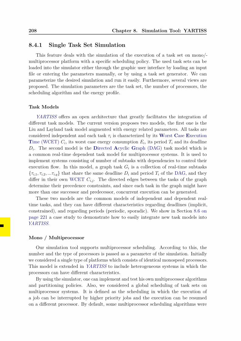
208 Chapter 8. Simulation Tool: YARTISS
8.4.1 Single Task Set SimulationThis feature deals with the simulation of the execution of a task set on mono/-
multiprocessor platform with a specific scheduling policy. The used task sets can beloaded into the simulator either through the graphic user interface by loading an inputfile or entering the parameters manually, or by using a task set generator. We canparameterize the desired simulation and run it easily. Furthermore, several views areproposed. The simulation parameters are the task set, the number of processors, thescheduling algorithm and the energy profile.
Task Models
YARTISS offers an open architecture that greatly facilitates the integration ofdifferent task models. The current version proposes two models, the first one is theLiu and Layland task model augmented with energy related parameters. All tasks areconsidered independent and each task τi is characterized by its Worst Case ExecutionTime (WCET) Ci, its worst case energy consumption Ei, its period Ti and its deadlineDi. The second model is the Directed Acyclic Graph (DAG) task model which isa common real-time dependent task model for multiprocessor systems. It is used toimplement systems consisting of number of subtasks with dependencies to control theirexecution flow. In this model, a graph task Gi is a collection of real-time subtasks{τi,1, τi,2, ...τi,q} that share the same deadline Di and period Ti of the DAG, and theydiffer in their own WCET Ci,j. The directed edges between the tasks of the graphdetermine their precedence constraints, and since each task in the graph might havemore than one successor and predecessor, concurrent execution can be generated.
These two models are the common models of independent and dependent real-time tasks, and they can have different characteristics regarding deadlines (implicit,constrained), and regarding periods (periodic, sporadic). We show in Section 8.6 onpage 221 a case study to demonstrate how to easily integrate new task models intoYARTISS.
Mono / Multiprocessor
Our simulation tool supports multiprocessor scheduling. According to this, thenumber and the type of processors is passed as a parameter of the simulation. Initiallywe considered a single type of platforms which consists of identical monospeed processors.This model is extended in YARTISS to include heterogeneous systems in which theprocessors can have different characteristics.
By using the simulator, one can implement and test his own multiprocessor algorithmsand partitioning policies. Also, we considered a global scheduling of task sets onmultiprocessor systems. It is defined as the scheduling in which the execution ofa job can be interrupted by higher priority jobs and the execution can be resumedon a different processor. By default, some multiprocessor scheduling algorithms were
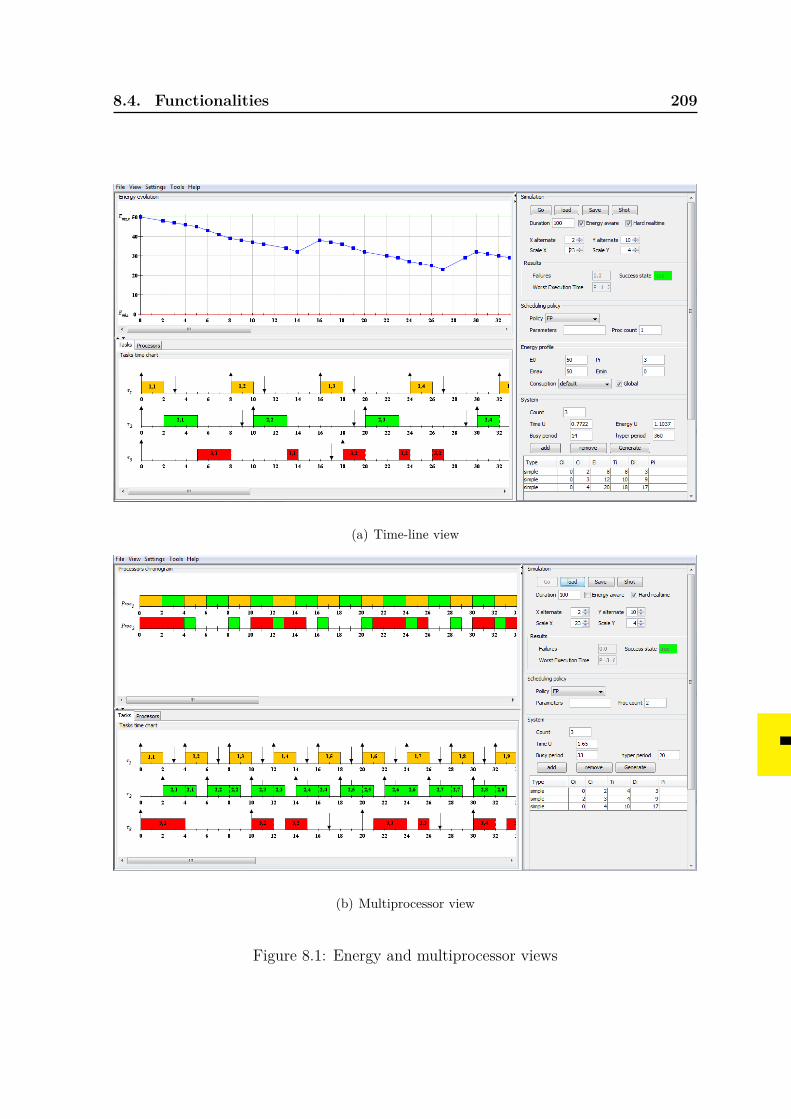
8.4. Functionalities 209
(a) Time-line view
(b) Multiprocessor view
Figure 8.1: Energy and multiprocessor views
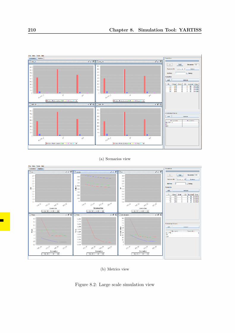
210 Chapter 8. Simulation Tool: YARTISS
(a) Scenarios view
(b) Metrics view
Figure 8.2: Large scale simulation view
8.4. Functionalities 211
implemented in YARTISS on multiprocessor systems like EDF and Fixed-Task-Priority(FTP).
Energy Profile
Unlike many other simulators, YARTISS permits us to simulate the productionand the consumption of energy in real-time systems. It permits the user to model anenergy-harvester and an energy storage unit such as a battery or a capacitor with acertain capacity. A renewable energy source can be modeled also using a chargingfunction. It is possible as well for the user to implement and use customized energyprofiles. Figure 8.2 on the facing page shows screen-shots of the user interface ofYARTISS. We can see in Figure 8.1(a) on page 209 the time chart of the storage unitenergy level where we can see the consumption during the scheduling process. Theenergy view, which is used to print the energy level chart is among many views providedby YARTISS to show other metrics.
Energy Source Model: We have implemented an energy source profile that modelsa renewable energy source represented by an energy storage unit with limited capacity.Other models can be added by the user by implementing the profile interface andinjecting it into the engine module of the simulator. This process is not complicatedand it can be done without modifying the other modules of the simulator.
Consumption Model: It is important to note that the energy consumption of a taskmust be modeled independently from its WCET as in the case of [JM06]. Therefore,our simulator provides the ability to define a consumption profile for each task of thesystem or to choose one global profile to apply to all tasks. A consumption model isrepresented by a function and must be able to provide the amount of energy consumedwithin a time interval during the tasks execution i.e. the integral of the consumptionfunction. The implemented models so far are: Linear consumption (not realistic butpermits to establish some interesting conclusions) and Early instantaneous consumptionwhere all the energy cost of a task is consumed as soon as a task is scheduled. Thislatter model seems to be the worst-case scenario.
212 Chapter 8. Simulation Tool: YARTISS
8.4.1.1 Scheduling Policy
The main purpose of the simulator is to test scheduling algorithms by comparingthem to each other in order to measure their performances and efficiency. Much attentionhas been focused on the design of this part of YARTISS to make it as generic as possibleso that users can add, override and inject their own scheduling policies easily. There arecurrently many algorithms implemented in YARTISS with different priority assignmentpolicies such as fixed-job, fixed-task and dynamic priority. It includes also classicalalgorithms such as RM , DM , EDF , Least Laxity First (LLF ) for both mono andmultiprocessor platforms. Users can add new scheduling policies easily, and Section 8.6on page 221, we demonstrate in details how to integrate a new policy independentlyfrom the rest of the modules of the simulator.
8.4.2 Run Large Scale Simulations
One of the major features of YARTISS is the large scale comparison of severalalgorithms or scheduling policies. It is similar to the single task set simulation but itis performed on a large set of task sets in different configurations and scenarios. Thecomparison results are based on statistics such as the number of schedulability failuresor deadline misses, the system’s lifetime, the amount of time spent at maximum andminimum energy levels or the average duration of idle and busy periods. Multiplesimulations can run simultaneously due to the use of the multi-threading conceptsupported by Java. As a result, the duration of simulations is greatly reduced throughthe parallelism of the used hardware.
8.4.3 Task Set Generation
Performing large scale simulations requires a large set of task sets. For the simulationresults to be credible, the used task sets should be randomly generated and variedsufficiently. The simulator provides the ability to choose a generator according to thedesired task models and algorithms. The current version includes by default a generatorbased on the UUniFast-Discard algorithm [BB05] coupled with a hyper-period limitationtechnique [MG01] adapted to energy constraints. This algorithm generates task setsby distributing the processor utilization and the energy utilization on tasks randomly.Since the original version of the algorithm does not include energy, we had to adapt itto produce feasible systems regarding time and energy. The idea behind the algorithmis to distribute the system’s utilization on the tasks of the system. When we considertasks energy cost, we end up with two parameters to vary and two conditions to satisfy.The algorithm in its current version distributes U and Ue uniformly on the tasks insuch a way that when we generate n task sets, we get approximately the same numberof task sets for each utilization value. Then, the algorithm finds the couples (Ci, Ei)which satisfies all the conditions namely Ui, Ue and energy consumption constraints.
8.5. Architecture 213
The operation is repeated several times until the desired couples satisfy the imposedconditions.
8.4.4 Graphical User Interface (GUI)
To facilitate the use of the simulator by a large number of users, we provide our toolwith a Graphic User Interface (GUI) to support the above-mentioned features in aninteractive and intuitive way. After the simulation of a specific system with a specificenergy profile and a specific scheduling policy, the user can follow and analyze thescheduling process using three different views: a time chart (Gant chart), a processorview and the energy storage level chart which monitors the energy levels of the system.In order to run simulations and get the results of comparison of scheduling policies, thesimulator offers a control panel that allows the user to select the scheduling policies,to choose the energy scenarios and to start the simulations. Thus, the user can seethe simulation results as one graph per scenario or per comparison criterion or metric.Then, the simulator can obtain results on a large number of randomly generated tasksets in order to evaluate the performance of the tested scheduling policies, and easilyexplore their properties. This view offers also a debugging window in which the user cananalyze the results of comparison and can optionally display the time chart of a taskset over each scheduling policy. This helps the user to analyze and debug schedulingpolicies. It can be also useful to find counter examples and to isolate degenerate cases.For example, in the case of energy-aware scheduling, no optimal algorithm exists yet.In order to test empirically whether a new algorithm is potentially optimal or not, asimple approach consists in simulating the scheduling of all possibilities of task sets andask the simulator to filter cases where the new scheduling algorithm fails whereas otherheuristics succeed.
8.5 ArchitectureUsually, the common concern of real-time simulation tools is the possibility of using
the simulator in different contexts. In many cases, extending a simulator to includecustomized modules needs a lot of modifications and refactoring of the code. Carelessmodifications can lead to incompatibility with the original modules of the tool, orworst, it may lead to a different or wrong simulation results. Furthermore, most of thetime, researchers do not like to spend much time or effort to understand and preservean existing tool, and finally, the tool becomes difficult to maintain. In our team, weexperienced this issue previously, and we noticed the importance of design and softwarearchitecture. The more generic and flexible the software is, the less time and effortwe spend to integrate new customized modules. For this reason and in order to meetthe requirements mentioned in Section 8.3 on page 206, we decided to merge the oldversions of our simulator and to provide a new tool with an enhanced architecture and
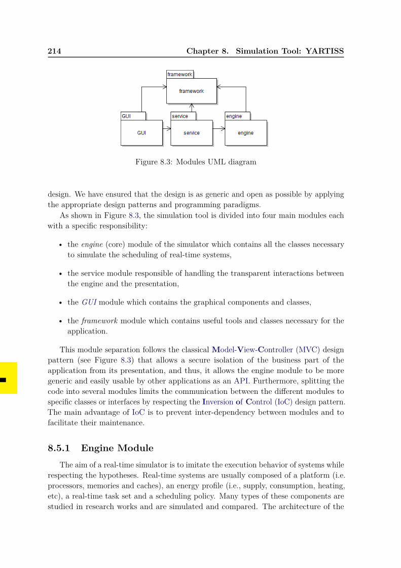
214 Chapter 8. Simulation Tool: YARTISS
Figure 8.3: Modules UML diagram
design. We have ensured that the design is as generic and open as possible by applyingthe appropriate design patterns and programming paradigms.
As shown in Figure 8.3, the simulation tool is divided into four main modules eachwith a specific responsibility:
• the engine (core) module of the simulator which contains all the classes necessaryto simulate the scheduling of real-time systems,
• the service module responsible of handling the transparent interactions betweenthe engine and the presentation,
• the GUI module which contains the graphical components and classes,
• the framework module which contains useful tools and classes necessary for theapplication.
This module separation follows the classical Model-View-Controller (MVC) designpattern (see Figure 8.3) that allows a secure isolation of the business part of theapplication from its presentation, and thus, it allows the engine module to be moregeneric and easily usable by other applications as an API. Furthermore, splitting thecode into several modules limits the communication between the different modules tospecific classes or interfaces by respecting the Inversion of Control (IoC) design pattern.The main advantage of IoC is to prevent inter-dependency between modules and tofacilitate their maintenance.
8.5.1 Engine ModuleThe aim of a real-time simulator is to imitate the execution behavior of systems while
respecting the hypotheses. Real-time systems are usually composed of a platform (i.e.processors, memories and caches), an energy profile (i.e., supply, consumption, heating,etc), a real-time task set and a scheduling policy. Many types of these components arestudied in research works and are simulated and compared. The architecture of the
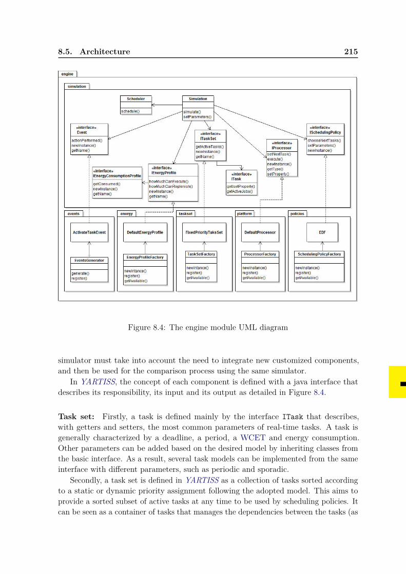
8.5. Architecture 215
Figure 8.4: The engine module UML diagram
simulator must take into account the need to integrate new customized components,and then be used for the comparison process using the same simulator.
In YARTISS, the concept of each component is defined with a java interface thatdescribes its responsibility, its input and its output as detailed in Figure 8.4.
Task set: Firstly, a task is defined mainly by the interface ITask that describes,with getters and setters, the most common parameters of real-time tasks. A task isgenerally characterized by a deadline, a period, a WCET and energy consumption.Other parameters can be added based on the desired model by inheriting classes fromthe basic interface. As a result, several task models can be implemented from the sameinterface with different parameters, such as periodic and sporadic.
Secondly, a task set is defined in YARTISS as a collection of tasks sorted accordingto a static or dynamic priority assignment following the adopted model. This aims toprovide a sorted subset of active tasks at any time to be used by scheduling policies. Itcan be seen as a container of tasks that manages the dependencies between the tasks (as
216 Chapter 8. Simulation Tool: YARTISS
in the case of DAG tasks) and provides a task ordering according to the specificationsof the user (fixed job or task priority and dynamic priority). The combination of theinherited classes of tasks and task sets defines the task set model to be simulated. Theuser can implement a customized behavior of tasks and task sets by extending theseinterfaces and adding his own properties by using the generic available getters andsetters.
The current release of YARTISS contains by default the following task set models:Liu and Layland model (i.e., periodic fixed-priority task sets), the dependent tasks ofthe DAG model and the energy-harvesting task model.
Scheduling policy: The responsibility of a scheduling policy is to decide at any timet which task or job to execute on which processor. YARTISS defines this behavior withthe interface ISchedulingPolicy. It has a main method called chooseNextTasks()that selects the highest priority tasks at time t, to execute on the processors of thesystem. This method receives the necessary components for simulation such as thestate of the processors, the task set and the energy profile. The scheduling policycan use external and generic parameters to calibrate its behavior with the methodsetParameters(). A scheduling algorithm is usually adapted to a specific task setmodel. For this reason, we give to the scheduling policies the responsibility of creatingnew instances of the adapted type of task model with the method createTaskset().By outsourcing the scheduling decisions from the core of the Simulation class, weare able to implement several scheduling algorithms for different task models, whichsimplifies the comparison process. We have already implemented many schedulingpolicies in YARTISS for different task models, including fixed-priority RM , DM , EDF ,LLF , etc. Also, there are algorithms for energy-harvesting systems and DAG taskmodel.
Energy profile: The energy profile of a system includes the profiles of energy, produc-tion and consumption, and heating models. The interface IEnergyProfile describeshow the system is supplied with energy and how it manages its consumption. It offers aset of methods that demonstrates the energy source (battery for instance), its limits andits energy levels within a time interval. The method howLongCanExecute() calculatesthe maximum time at which a task can execute w.r.t. the available energy and the usedconsumption profile. This can be used to simulate different energy sources, differentrechargeable batteries with different environments and energy sources. The second partof the energy profile is the energy consumption model. YARTISS proposes two modes,the global mode in which all the tasks have the same energy consumption model, andthe non-global mode which allows the tasks to consume energy based on their ownconsumption model. According to this, the simulator can be general and specific at thesame time. The interface IEnergyConsumptionProfile describes how tasks consumeenergy with the method getConsumed(). This method gives the amount of energyto consume for a given execution time. The thermal behavior is also defined by this
8.5. Architecture 217
interface. It consists of providing the heating and the cooling functions that can begeneral or task or processor specific.
Execution platform: A system platform consists mainly of a number of processorson which the tasks execute their code. The interface IProcessor defines the commonbehavior of processors. A task is allocated to a processor within a time interval and themethod execute() performs the execution of the tasks within this interval by updatingthe state of the tasks. The current release of YARTISS proposes only one defaulttype of multiprocessor which is the homogeneous mono-speed processors. However,it is possible to add new types of processors with different speeds and, consequently,the method execute() has to be modified according to the new characteristics. Anexample of the different type of processors is the processors with Dynamic Voltage andFrequency Scaling (DVFS) capabilities.
The Simulation Process
The aim of this tool is to simulate the scheduling of a system according to theparameters and the assumptions set by the user, namely the task set, the platform, theenergy profile and the scheduling policy. According to the scheduler, the schedulingdecisions are taken based on specific events, such as activation and finish times of a job,its deadline and preemption events.
A scheduling decision consists of assigning priorities to the active jobs staticallyor dynamically according to the scheduling policy, and allocating them to processorsby considering the state of the system (energy state for example). The simulator usesa basic set of events that guarantee a correct execution of the system such as jobrequest events, finish executing events, deadline events, etc. These events are nativelyimplemented in YARTISS. The simulation starts generating the events responsible ofrequesting the first job of each task. Then other events are generated dynamically duringthe simulation process. For example, when a job meets its deadline, the correspondingdeadline event is generated in order to check if the job has met its deadline and to requestan other event for the next job as well. The events are generated sorted according totheir temporal order and priority ordering. For each event, the scheduling policy iscalled to select the highest priority jobs to execute on the available processors. Then,the selected jobs execute while respecting the type of processors and the energy profile.This mechanism is implemented in class Simulation.
The interface Event describes the role of an event. The current release of YARTISSprovides the necessary events to schedule a real-time system. However, the user isallowed to add his own events by implementing their customized behavior. To do so,the user should extend the Event interface and register the new event with the methodregister() from class EventGenerator. Furthermore, to generate an event, the usershould use the method generate() of class EventGenerator. Then the event will beprocessed with the desired behavior which is implemented by the user.
218 Chapter 8. Simulation Tool: YARTISS
Metrics and Statistics: The aim of a simulation is not restricted to checking thefeasibility of a given system. It is important also to compute some metrics and statisticsof the performed simulation in order to analyze the performance of the tested solution.We considered this functionality in YARTISS and we integrated a generic mechanismdedicated to compute statistics. It is possible to compute a metric at the beginningor the end of the simulation, or even during events processing. Moreover, it can beaggregated with other values when several simulations are performed. In the simulator,a metric is represented by the interface IStatisticCriterion which has a method foreach possible calculation time (i.e., beginning, end, event processing). Several metricsare implemented natively and, as for the other parts, the user can add new customizedmetrics to the simulator by implementing the interface and injecting an instance ofthe new metric to the metrics manager class. At the beginning of each simulation,an instance of each active metric is created. Then, at each metric calculation time,the corresponding method of the metric is called. At the end of the simulation wecan get the final value of each metric using the method getValue(). In the case ofseveral simulations, we can also aggregate the values of the same metric on all of thesimulations in order to compute the maximum/minimum values, the average value, etc.The aggregation function is implemented by the metric class and can provide severalvalues: maximum, minimum, average values, percentage value, etc. By doing so, thesimulation class computes several statistics independently from their implementation.Among the implemented metrics available in YARTISS, we can cite: deadline misscounter, average busy and idle periods, average overheads.
Inversion of Control and Dependency Injection
Based on the above described components, we notice that the simulator dealsonly with interfaces and never directly with implemented classes. This allows thesimulator to be generic regarding the parts that can be replaced, such as the schedulingpolicy, the task set model, the platform, the energy profile and the statistics metrics.This implantation respects the IoC design pattern and the Dependency Injection thatstipulates that the objects composing the application must be weakly coupled anddependencies should be linked only at run-time.
The IoC design pattern is a design pattern of software construction where reusablecode controls the execution of problem-specific code. Its main advantage is that thereusable code is developed independently from the problem-specific code, which oftenresults in a single integrated application. The IoC design guideline is useful for thefollowing purposes:
• the execution of a certain task is independent from its implementation,
• every part of the system focuses on its design purpose,
• all parts have no assumptions about the constraints and the limitations of theother parts,
8.5. Architecture 219
• replacing or modifying a part in the system does not affect the rest of the parts.
Sometimes, IoC is referred to as the Hollywood Principle: Don’t call us, we’ll callyou, because program logic runs against abstractions such as callbacks.
In the case of YARTISS, the simulation code is a reusable part and the differentimplementations of scheduling policies, processors, task sets or metrics are done onspecific parts that can be replaced and developed independently. This is what makesYARTISS a generic real-time simulator that can be used easily by other researchers.
8.5.2 Service Module
The engine module contains all the code necessary to build and run a simulation.Furthermore, it can be used alone or imported as an API to be integrated into anothersoftware. However, we were interested in providing a complete simulation tool andnot only an API. So we implemented more classes which allow an intermediate user tobuild and run simulations easily. This is done using the Service module which containsthe functionalities described above in Section 8.4 on page 207. From a design point ofview, the service module represents the Controller and the Model parts of the famousMVC design pattern or the View-Model part of the Model View View-Model (MVVM)design pattern. It is a software brick of higher level that uses the engine module. Theservice module provides the classes that set the replaceable parts of a simulation (e.g.the scheduling policy, the task set, the platform, metrics, etc), run the simulationand save the results. It contains mainly three public classes, each represents a certainfunctionality:
• The TimeLineViewModel class provides the necessary parameters to simulate atask and allows the user to run the simulation and visualize the results.
• The BenchmarkViewModel class allows the user to set quickly the description ofa large scale simulation where several scheduling policies are compared usingthe chosen statistic metrics in different scenarios of energy profiles. This classhelps the user to build such a simulation without knowing the implementationof any parts. The description is passed using a String object and all createdgeneric objects are done using the Dependency Injection paradigm. This classsaves results which are readable by the chart plotter tool Gnuplot.
• The task GenViewModel class builds a custom task set generator in the sameway.
These classes are packed in an independent module so as to be built easily usinga higher level software layer with a friendly user interface (such as a web server or agraphical or textual interface).
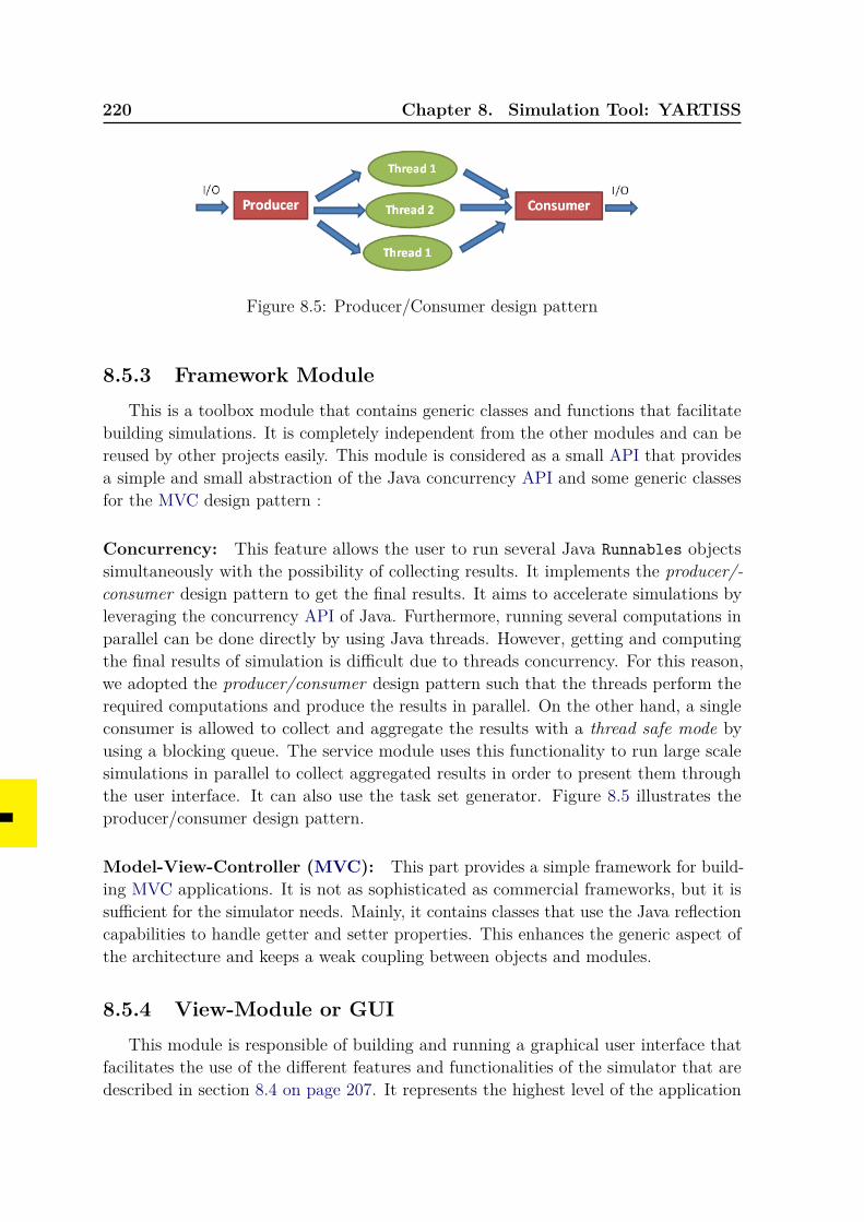
220 Chapter 8. Simulation Tool: YARTISS
Figure 8.5: Producer/Consumer design pattern
8.5.3 Framework ModuleThis is a toolbox module that contains generic classes and functions that facilitate
building simulations. It is completely independent from the other modules and can bereused by other projects easily. This module is considered as a small API that providesa simple and small abstraction of the Java concurrency API and some generic classesfor the MVC design pattern :
Concurrency: This feature allows the user to run several Java Runnables objectssimultaneously with the possibility of collecting results. It implements the producer/-consumer design pattern to get the final results. It aims to accelerate simulations byleveraging the concurrency API of Java. Furthermore, running several computations inparallel can be done directly by using Java threads. However, getting and computingthe final results of simulation is difficult due to threads concurrency. For this reason,we adopted the producer/consumer design pattern such that the threads perform therequired computations and produce the results in parallel. On the other hand, a singleconsumer is allowed to collect and aggregate the results with a thread safe mode byusing a blocking queue. The service module uses this functionality to run large scalesimulations in parallel to collect aggregated results in order to present them throughthe user interface. It can also use the task set generator. Figure 8.5 illustrates theproducer/consumer design pattern.
Model-View-Controller (MVC): This part provides a simple framework for build-ing MVC applications. It is not as sophisticated as commercial frameworks, but it issufficient for the simulator needs. Mainly, it contains classes that use the Java reflectioncapabilities to handle getter and setter properties. This enhances the generic aspect ofthe architecture and keeps a weak coupling between objects and modules.
8.5.4 View-Module or GUIThis module is responsible of building and running a graphical user interface that
facilitates the use of the different features and functionalities of the simulator that aredescribed in section 8.4 on page 207. It represents the highest level of the application
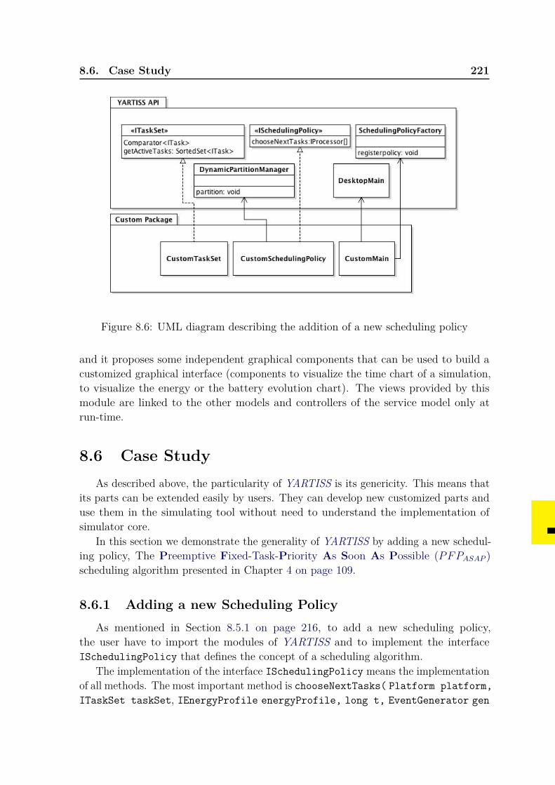
8.6. Case Study 221
Figure 8.6: UML diagram describing the addition of a new scheduling policy
and it proposes some independent graphical components that can be used to build acustomized graphical interface (components to visualize the time chart of a simulation,to visualize the energy or the battery evolution chart). The views provided by thismodule are linked to the other models and controllers of the service model only atrun-time.
8.6 Case StudyAs described above, the particularity of YARTISS is its genericity. This means that
its parts can be extended easily by users. They can develop new customized parts anduse them in the simulating tool without need to understand the implementation ofsimulator core.
In this section we demonstrate the generality of YARTISS by adding a new schedul-ing policy, The Preemptive Fixed-Task-Priority As Soon As Possible (PFPASAP )scheduling algorithm presented in Chapter 4 on page 109.
8.6.1 Adding a new Scheduling PolicyAs mentioned in Section 8.5.1 on page 216, to add a new scheduling policy,
the user have to import the modules of YARTISS and to implement the interfaceISchedulingPolicy that defines the concept of a scheduling algorithm.
The implementation of the interface ISchedulingPolicy means the implementationof all methods. The most important method is chooseNextTasks( Platform platform,ITaskSet taskSet, IEnergyProfile energyProfile, long t, EventGenerator gen
222 Chapter 8. Simulation Tool: YARTISS
) that assigns tasks to the available processors at any time t. The parameter platformrepresents the hardware part, i.e. processors and memories, etc. The parameter taskSetis the real-time task set to simulate, energyProfile is the energy profile chosen by theuser and evGen is the event generator that can be used to generate additional events.We notice that except the task set, all of the parameters are typed with interfaces whichmeans that the scheduling policy deals with generic parameters as illustrated by theUML diagram of Figure 8.6 on the previous page. The real types are instantiated atrun-time following the configuration set by the user. For this reason the implementationof a new scheduling algorithm is easy and the new class contains only the code of thescheduling algorithm.
Therefore, knowing that PFPASAP schedules tasks as soon as possible by consuminggreedily the available energy, the method chooseNextTasks(...) can be implementedby writing in Java the following instructions:
1. check if there is at least one active task at time t,
2. get the task with the highest priority among the active tasks,
3. ask the energy profile how long this task can be executed continuously,
4. do not execute the task if the energy is not sufficient to execute by assigning nullto the processor and generating a new event at time t+ 1 to retry again,
5. execute the remaining time of the highest priority active task by assigning thetask to the processor with platform.getProcessor().setNextTask(task), andgenerating an other event at the time when the energy become insufficient toexecute all the remaining execution time of the active task.
The second important method is createTaskSet(). It creates an instance of thetask set model that is compatible with the current policy. In the case of PFPASAP , thesuitable task set is the classical fixed-priority one, i.e. Liu and Layland model, where thetasks are sorted according to their static priorities. The task set models follows the samedesign pattern as scheduling policies but in this case we use an already existing model(with TaskSetFactory.getNewInstance( "priority")) instead of implementing anew one.
The third important method is newInstance() which is a factory method thatcreates new instances of the current scheduling policy, name PFPASAP in this case.This method is used to create new objects of the scheduling policy class without requiringto do it manually with new constructors. This design patter allows us to centralize thecreation of objects of classes that implement the same interface which allows a genericinjection of new implementations, e.g. new scheduling algorithms in this case.
The remaining methods are used to identify the policy among others and to provideparameters if necessary (which is not the case of PFPASAP ).
8.7. Distribution 223
Then, the newly-created scheduling policy should be registered in the simulatorby the use of the register() method from the SchedulingPolicyFactory class thatcentralize the creation of classes implementing ISchedulingPolicy interface. Thismethod injects a sample object of the policy we want to register, then using the methodsnewInstance() and getPolicyName(), the new scheduling policy can appear in thelist of the available scheduling policies and can be instantiated generically. The callof the method register() should be done in the customized main class created bythe user or by using the GUI of YARTISS as shown in Listing 1 on page 251 in theAppendix.
The adopted design allows us to implement other scheduling policy easily, we didthe same with all the policies discussed in this dissertation.
8.6.2 Adding an Energy ProfileThe same methodology can be applied if we want to add a new energy consumption
profile to YARTISS. Listing 2 on page 252 in the Appendix shows the Java code neededto use a logarithmic energy consumption profile as an external module.
8.7 DistributionThe project is available on the collaborative development platform hosted at
https://svnigm.univ-mlv.fr/projects/YARTISS/. This environment provides asubversion repository allowing anonymous checkouts, documentation hosting, RSS feedssubscriptions, and public forums. A web page dedicated to YARTISS is also availableat http://YARTISS.univ-mlv.fr. In addition to a general presentation of the tool, itproposes a demo applet version which allows interested readers to try YARTISS directlyfrom their web browser and an application form to allow anybody to share externalmodules.
8.8 ConclusionIn this paper we presented YARTISS, a real-time multiprocessor scheduling simulator.
A consequent effort has been made to make it as extensible as possible. To justify theneed for an open and generic tool, we presented the history of YARTISS development.Then we briefly presented existing simulation tools. We have described the three mainfunctionalities of YARTISS: 1) simulate a task set on one or several processors whilemonitoring the system energy consumption, 2) concurrently simulate a large numberof task sets and present the results in a user friendly way that permits us to isolateinteresting cases, and 3) randomly generate a large number of task sets. Then, inorder to demonstrate the modularity and extensibility of our tool, we presented itsarchitecture and a case study that shows how to add new parts, in most cases without

224 Chapter 8. Simulation Tool: YARTISS
having to open or modify the core modules. Finally, we gave the instructions to getand test YARTISS. We hope that this software can contribute to build a standardsimulation tool that can be adopted through the real-time scheduling community.
General Conclusion
ScopeIn this thesis we addressed the real-time scheduling problem of fixed-priority energy-
harvesting systems. A real-time energy harvesting system must respect not only thedeadlines of all tasks but also their energy constraints. This means that the energy costof all jobs must be satisfied by the energy stored in the storage unit and the energycollected from the environment. To satisfy tasks energy cost, additional idle timesmay be necessary to collect the required energy. These necessary delays create a newscheduling problematic. Now, the challenge for a fixed-priority scheduling algorithmis to execute tasks according to their deadlines and to delay executions at the rightmoments and for the right durations in order to meet all deadlines and satisfy theenergy demand.
The problems are: first to find an optimal scheduling for such a model; second toprovide schedulability conditions that help designers to check if a given task set isschedulablable or not; third, to find the minimum battery capacity that ensure thefeasibility of a given task set.
In this dissertation, we started by presenting the state of the art of this researcharea. We first reminded briefly the classical real-time scheduling theory including thedifferent task models and the main scheduling algorithm families. Second, we exploredthe state of the art of energy-harvesting hardware, namely the different technologies ofenergy-harvesting and energy storage and the applications for which they are suitable.Third, we presented the main scheduling algorithms proposed in the literature andtheir properties. We showed also that the fixed-priority scheduling problematic forenergy-harvesting systems is not very well studied by the community.
After that, we presented in detail the contributions of this thesis, summarized inthe next section.
Main Results
The PFPASAP AlgorithmThe first result of this thesis is the PFPASAP algorithm which is an adaptation
of the classical FTP Algorithm. It schedules tasks as soon as possible by executingwhenever the energy available in the storage unit is sufficient to execute at least onetime unit, and by replenishing otherwise but only as long as needed to replenish theenergy necessary to execute one time unit of the job with the highest priority. Inother words, it is a fixed-priority energy-work-conserving algorithm. We proved thatthis algorithm is optimal for energy-non-concrete task sets where the initial battery
226 General Conclusion
capacity and task offsets are known only at run-time. This optimality relies first on thefact that all tasks consume more energy than what it is possible to replenish duringtheir execution time, and second, on the fact that in this case the schedulability ofthe task set can be studied only for the first instance of each task in the worst-casescenario which is the simultaneous release of all the tasks with the minimum batterylevel. A necessary and sufficient schedulability test was also proposed for this familyof task sets. Furthermore, we proposed a bound of the minimum battery capacitythat preserves the schedulability of a task set with PFPASAP algorithm. This capacityis equal to the maximum instantaneous energy consumption of task. Moreover, wecompared PFPASAP to the algorithms presented in the state of the art with simulations.These later confirmed the theoretical results and showed in one hand the advantagesof PFPASAP which are its optimility and its low overhead, and in an other hand itsdrawbacks which are mainly the high rate of preemptions and context switches.
Schedulability Analysis for PFPASAP Algorithm
The second result is a schedulability analysis of PFPASAP that removes somerestrictive assumptions. As mentioned above, the optimality of PFPASAP relies onthe fact that the task sets are energy-non-concrete and that the consumption rateof all the tasks is greater than the replenishment rate. If we remove one of theseassumptions, PFPASAP is no longer optimal, the simultaneous request of all the taskswith the minimum battery level is no longer the worst-case scenario and the proposedschedulability test becomes only necessary.
To cope with this problem, we proposed a schedulability analysis using tasks worst-case response time upper bounds. For this analysis we relaxed the assumption of tasksconsumption, offsets and initial battery level. Then, we can check with a sufficienttest the schedulability of task sets that can include tasks with a consumption ratelesser than the replenishment, i.e. gainer tasks, for any scenario. The idea behind thefirst upper bound is to maximize the number of interferences and to assume that allconsuming jobs are scheduled before gaining jobs, which maximizes the delays due toreplenishments and the delays due to interferences. The second upper bound keeps thesame idea but by respecting jobs request time and deadlines which tighten the upperbound. The schedulability test consists of computing an upper bound of the longestresponse time of each task and to compare it to its deadline. We proved also thatthe proposed schedulability tests are compatible with the optimal priority assignmentalgorithm of Audsley. We performed some simulations to evaluate the validity of thetheoretical results and to measure the tightness of the upper bounds comparing to theempirical worst-case response time. The experiments showed that the second upperbound is tighter and that its deviation is reasonable.
General Conclusion 227
Schedulability Analysis for Thermal-aware SystemsWe showed in Chapter 6 the difficulty of finding an optimal scheduling algorithm
and exact feasibility conditions for the general model of fixed-priority energy-harvestingsystems. To cope with this problem, we decided to address the problem from an otherpoint of view by studying other real-time scheduling problems that might present somesimilarities especially the ones where some delays are needed to produce a valid schedule.Then, we started studying the real-time scheduling for thermal-aware systems wherethe temperature of the system must be managed such that it never exceeds a certainmaximum threshold. To respect this constraint, it may be necessary to delay executionsin order to cool down the system reactively when reaching the maximum temperatureor proactively before reaching it.
As a first step, we started by studying the behavior of the equivalent of PFPASAPalgorithm for thermal-aware systems. We proved that PFPASAP is also optimal forthermal-non-concrete task sets where tasks offsets and the initial temperature areknown only at run-time. In this model, PFPASAP schedules jobs whenever the systemis cold enough to execute at least one time unit, and otherwise, it delays executionsin order to cool down enough to execute one time unit. In this model the worst-casescenario occurs for a task occurs when all the higher priority tasks are requestedsimultaneously while the temperature is at its maximum level. However, computing theexact response times is difficult to express with a formula or an algorithm. For thisreason, we proposed two sufficient schedulability conditions that uses tasks worst-caseresponse time approximation. The idea of the first bound is to maximize the coolingperiods in the worst-case scenario by leveraging the fact that the cooling function isexponentially decreasing which leads to long cooling periods. The second bound isparametric, it considers that the cooling periods are of the same length x and thecorresponding execution periods are integers (floor value). The performed simulationsshowed that the first upper bound is very pessimistic, however, the second one is verytight to the empirical worst-case response time when x = 1. This result is the first stepof the exploration of similarities between energy-harvesting and thermal-aware systems.More work is planned to try to adapt some results from the thermal-aware side to theenergy-harvesting one.
Simulation toolThe fourth main result of this thesis is the development of YARTISS the simulation
tool used to perform all the experiments of this thesis and the ongoing work of ourteam. YARTISS is a modular and Java-based real-time simulator that provides ageneric simulation framework and a friendly graphical user interface. This simulatorwas designed such that the major aspects of real-time scheduling can be substituted.The concept of each part, e.g. scheduling algorithm, task, task set, energy consumption,etc, is modeled by a java interface which facilitates the substitution of implementations.YARTISS provides also a graphic user interface that allows the visualization of the
228 General Conclusion
schedule of a given task set according to a given scheduling algorithm in a givenenvironment of energy. Moreover, it can be also used to run large scale simulationswhich is very useful to evaluate and validate theoretical results.
Future ResearchThe work done along this thesis helped us to better understand the problematic of
fixed-priority real-time scheduling for energy-harvesting systems. Moreover, the resultsof this thesis contribute to cover a part of the not yet studied research areas of thisfield.
As any research work, the achievement of a project is the starting point of an otherone, and each answer arises more questions. In the case of this thesis, the followingpoints and open questions deserve more investigations.
Optimal AlgorithmThe main question that is still without answer is the existence of an optimal
algorithm for the general model of energy-harvesting systems that includes all energyconsumption types, i.e. gaining and consuming tasks, concrete task sets, i.e. withoutany assumption on tasks offsets and the initial battery level. We showed in Chapter 6that many intuitive ideas do not work to build an optimal algorithm. The only ideathat could lead to an optimal algorithm is to combine virtual deadlines with lookaheadcomputation to compute the optimal delay at any moment. However, the complexityof this algorithm is exponential. The question now is: does an optimal algorithmfor fixed-priority energy-harvesting systems exist ? or is the fixed-priority schedulingproblem of energy-harvesting systems an NP-hard problem ?
We tried to answer both of these two questions but we was not able neither to findan optimal algorithm nor to prove the NP-hardness of the problem. Therefore, this isstill an open question that deserves more interest and effort to answer.
Energy AssumptionsOne of the interesting future axes is to study the problem in more realistic assump-
tions even with non optimal solutions. In fact, the results presented in this thesisassume that the replenishment and tasks consumption are constant functions. Eventhough there exist some applications where these assumptions are not far to be realistic,they are still marginal. For example, with energy sources like solar energy, the harvestedenergy varies over time which might make the proposed solutions very optimistic andnot realistic. It might be useful to provide energy-source-specific scheduling algorithmsand schedulability analysis in order to build real efficient applications. Moreover, theenergy consumption of tasks may also vary over time due to the use of different circuitryor due to the thermal state of the system. This problem should be addressed by either
General Conclusion 229
taking into account the real consumption profile or to find the worst consumption profileof each task.
Similarities With Thermal-Aware SystemsThis point is as important as the precedent ones because more work has been done
for thermal-aware systems than energy-harvesting systems. Many ideas that have beenproposed for the thermal model might be applicable for energy-harvesting systemsespecially for more realistic assumptions of energy replenishment and consumption. Theresults presented in Chapter 7 represent the first step in the exploration of such ideas.
Simulation ToolYARTISS is still under development and requires more time and effort to improve
its architecture and to add implementations of more algorithms task models, etc. Thesimulator is used by our team and few students around the world. We aim to form adedicated development team that can maintain its code and do more communicationsabout it in order to attract more interest and more contributions.


Part III
Résumé en français

Chapter 9
Ordonnancement temps réel avecgestion de l’énergie renouvelable
9.1 IntroductionL’informatique est l’une des sciences qui ont révolutionné le monde durant le dernier
siècle. L’homme a inventé les ordinateurs électroniques durant la deuxième guerremondiale. Ces derniers étaient capables d’effectuer des opérations de cryptographieen utilisant le modèle de la Machine de Turing. Depuis, ces ordinateurs n’ont cesséd’évoluer.
Pendant les dernières décennies, l’utilisation des ordinateurs dans la vie modernea fortement augmenté et a fait exploser la demande en termes de puissance de calculet d’efficacité. Le progrès de la technologie a permis aux ordinateurs modernes d’êtrebeaucoup plus petits et plus performant que les premières machines. Les ordinateursimples sont devenus tellement petits qu’il est aujourd’hui possible d’avoir des petitsappareils mobiles qui peuvent fonctionner avec très peu d’énergie, ce qui a permis à denouvelles applications d’émerger. De nos jours, les ordinateurs sont aussi utilisés pourcontrôler des opérations critiques telles que les réactions nucléaires ou les commandesde vol d’un avion. Ce type d’ordinateurs est souvent utilisé dans les systèmes embarquésautonomes qui vont du simple lecteur MP3 aux très complexes navettes spatiales et desjouets d’enfants aux robots industriels.
Dans ce genre d’applications, le temps que les tâches du système prennent pourdélivrer les résultats est aussi important que leur exactitude. Les systèmes qui sontsoumis à des contraintes temporelles sont les systèmes dits temps réel.
De plus, avec l’augmentation de la vitesse des processeurs et la miniaturisationdes appareils électroniques, la gestion de l’énergie est devenue l’une de problématiquesimportantes à étudier. La mission des petits appareils est de fournir un service demanière autonome et cela pour une longue durée de vie comme par exemple dansles réseaux de capteurs ou les implants médicaux. Le défi ici est de pouvoir utiliserl’énergie ambiante pour permettre une longue durée de vie en éliminant les opérationsde maintenance. Plusieurs sources d’énergie peuvent être exploitées en fonction desbesoins de l’application, par exemple, les énergies solaires, vibratoires ou thermiques.
Dans cette thèse, nous nous intéressons à la problématique de l’ordonnancementtemps réel de ce type de systèmes.
234Chapter 9. Ordonnancement temps réel avec gestion de l’énergie
renouvelable
Durant la dernière décennie, le comportement temps réel de ce genre de systèmesa attiré plus d’attention. Le défi ici est de trouver le bon ordonnancement des tâchestout en respectant les contraintes énergétiques et temporelles. Quelques algorithmesd’ordonnancement ont été proposés dans la littérature mais la majorité des travaux sontconcentrés sur l’ordonnancement à priorité dynamique du type EDF . L’ordonnancementà priorité fixe a quant à lui été très peu traité alors qu’il est largement utilisé en industrie.Cette thèse traite la problématique d’ordonnancement pour cette famille d’algorithmes.
Nous proposons d’abord une solution partielle qui consiste en un algorithme optimalpour une sous catégorie des systèmes étudiés, ainsi que l’analyse d’ordonnançabilitéassociée, puis nous expliquons la difficulté de la généralisation.
Le reste de ce résumé est organisé comme suit. Un bref aperçu de l’état de l’artde l’ordonnancement temps réel des systèmes collecteurs d’énergie est exposé dansles sections 9.2, 9.3, et 9.4. La section 9.5 introduit l’algorithme PFPASAP qui est lapremière contribution de cette thèse. La section 9.6 présente une analyse approximativede temps réponse des tâches avec PFPASAP en relâchant quelques hypothèses. La section9.7 explique la difficulté de trouver un algorithme optimal pour notre modèle. Dans lasection 9.8 nous discutons la similitude entre le modèle des systèmes collecteurs d’énergieet celui des systèmes contraints par la chaleur. La section 9.9 présente brièvement l’outilde simulation YARTISS développé pendant cette thèse. Pour terminer, la section 9.10conclut ce résumé.
9.2 Ordonnancement temps réelEn informatique, un système est considéré comme étant temps réel si le respect de
ses contraintes temporelles est aussi important que l’exactitude des résultats [But11]. Leterme temps réel n’est pas forcément associé à la rapidité. L’objectif d’un système tempsréel correct est de respecter perpétuellement les échéances individuelles des tâches dansle pire cas même si l’exécution est lente. Généralement, les systèmes temps réel sontclassifiés en fonction de la gravité des conséquences des dépassements d’échéances. Nousdistinguons alors deux familles : les systèmes temps réel durs et les systèmes réel souples.Dans la première famille, aucun dépassement n’est toléré car les dommages occasionnéssont catastrophiques, par exemple, la perte des commandes de vol d’un avion. Parcontre, les dépassements d’échéances dans la deuxième famille ne font que dégrader laqualité du service, par exemple, la perte de quelques images lors du décodage d’un fluxvidéo en direct.
9.2.1 Modèle de tâchesUn système temps réel est généralement composé d’un ensemble de tâches temps
réel récurrentes noté Γ. Chaque tâche τi est caractérisée par son pire temps de réponseCi, par son échéance temporelle relative Di, par sa période Ti et sa première dated’activation Oi. Chaque tâche se réactive au moins toutes les Ti unités de temps pour
9.2. Ordonnancement temps réel 235
exécuter ce que l’on appelle un travail ou un job. Un travail Ji,j est caractérisé par sadate d’activation ai,j et son échéance absolue di,j.
Ces paramètres peuvent êtres spécifiés avant le lancement du système ou uniquementau moment de l’exécution. De ce fait, nous distinguons deux familles de systèmes :les systèmes complètement spécifiés et les systèmes partiellement spécifiés. Dans lapremière catégorie, tous les paramètres sont connus à l’avance, ainsi le système estdit concret. Dans cette famille, nous trouvons les systèmes de tâches périodiques quise réactivent à un intervalle régulier de temps. Dans la deuxième famille, au moinsun paramètres n’est connu qu’au moment de l’exécution, par exemple les systèmes detâches sporadiques où seul le temps minimal d’inter-arrivée est connue, ou encore lessystèmes apériodiques où modèle de récurrence n’est pas connue du tout.
9.2.2 Algorithmes d’ordonnancementLes tâches du système sont exécutées de manière concurrente sur le processeur. De
ce fait, il est nécessaire de spécifier une politique pour choisir quelle tâche exécuterà tout moment. C’est le rôle de l’algorithme d’ordonnancement. Dans la théorie del’ordonnancement temps réel, nous distinguons distingue trois familles d’algorithmes :les algorithmes à priorité de tâche fixe FTP , ceux à priorité de job fixe FJP et ceux àpriorité dynamique DP . Dans la première famille, la tâche se voit attribuer une prioritéfixe tout au long de son cycle de vie. Ainsi, l’algorithme exécute en premier la tâcheactive avec la priorité la plus élevée. Dans la deuxième famille, les priorités sont donnéesaux jobs et non aux tâches, par exemple, l’ordonnancement EDF qui attribue lespriorités aux jobs en fonction de leur échéance temporelle (le job avec l’échéance la plusproche est exécuté en premier). Dans la troisième famille, les priorités sont attribuéesdynamiquement et peuvent changer d’un unité de temps à une autre, l’exemple typiquede cette famille est l’algorithme LLF .
9.2.3 Analyses d’ordonnançabilitéPour s’assurer qu’un système de tâches donné est faisable ou ordonnançable avec
un algorithme spécifique, nous avons besoin d’outils d’analyse qui nous permettentde statuer sur le respect des échéances de toutes les tâches y compris dans le pirecas. Dans la théorie classique des systèmes temps réel, nous trouvons des conditionsd’ordonnançabilité qui sont basées principalement sur la charge processeur du système(U = ∑
Ci/Ti) ou sur une analyse du temps réponse des tâches dans le pire scénario.Pour la priorité de tâche fixe, la borne de Liu et Layland constitue une conditiond’ordonnançabilité suffisante (U ≤ n(21/n − 1)) dans le cas des échéances sur requête(∀iTi = Di) tandis que la condition de charge maximale (U ≤ 1) est une conditionnécessaire. Pour EDF , la condition sur la charge maximale est nécessaire et suffisantedans le cas des échéances sur requête (∀iTi = Di). D’autre conditions et analyses sontdétaillées dans le chapitre 1.

236Chapter 9. Ordonnancement temps réel avec gestion de l’énergie
renouvelable
Dans cette thèse, nous nous focalisons sur l’ordonnancement à priorité de tâche fixesur des plateformes monoprocesseur.
9.3 Les systèmes collecteurs d’énergieUn système collecteur d’énergie est un système qui récupère l’énergie ambiante et la
stocke dans un réservoir d’énergie afin d’alimenter un appareil électronique.Généralement, ce genre de système est composé de trois composants principaux :
un collecteur d’énergie, un réservoir d’énergie et une unité de calcul.Le collecteur d’énergie est responsable de la transformation de l’énergie ambiante
en courant électrique.Le réservoir d’énergie stocke temporairement l’énergie collectée par le collecteur.
Généralement, les batteries rechargeables ou les super-condensateurs sont utilisés pourcet effet en fonction des besoins de l’application.
L’unité de calcul est généralement composée de capteurs de données, de proces-seurs et de composants de transmission. C’est ce composant héberge le système tempsréel que nous étudions dans cette thèse.
9.3.1 Les technologies d’extraction de l’énergie ambiantePlusieurs sources d’énergie peuvent être exploitées. Toutes les sources ne sont pas
adaptées à toutes les applications. La source d’énergie et la méthode d’extraction doiventêtre soigneusement choisies pour répondre aux besoins de l’application.
Parmi les méthodes de conversion on trouve les suivantes :
• Conversion de l’énergie solaire : Cela passe par l’utilisation de cellules photovol-taïques. Cette technique présente un rendement assez faible (de l’ordre de 13%) etla quantité d’énergie produite est très fluctuante dans la journée et dans l’année.
• Conversion de l’énergie des ondes radio : Cette méthode présente un rendementfaible mais très utile pour un usage ponctuel, par exemple, les puces RadioFrequency Identification (RFID).
• Conversion électromagnétique de l’énergie vibratoire : Cette technique utilisele champ magnétique pour transformer l’énergie mécanique des vibrations encourant électrique. Cette technique présente un rendement faible par rapport auxprécédentes.
• Conversion électrostatique de l’énergie vibratoire : Cette technique utilise cettefois le champ électrostatique pour transformer l’énergie mécanique des vibrations.Le rendement de cette dernière est meilleur et peut être intéressant pour lesapplications qui subissent une fréquence de vibration importante.
9.3. Les systèmes collecteurs d’énergie 237
• Conversion piézoélectrique de l’énergie vibratoire : Cette méthode utilise unmatériau piézoélectrique qui crée une différence potentiel lors des mouvementsproduits par les vibrations. Cette technique est très prometteuse et peut êtrefacilement utilisée dans des applications de surveillance de machines industriellesoù le taux de génération d’énergie s’approche du constant.
• Conversion de l’énergie thermoélectrique : Cette technique utilise le différentielde température pour faire circuler les électrons et par conséquent un courantélectrique. Cela peut être efficace uniquement dans le cas où la différence detempérature est assez élevée.
Cette liste de méthode de conversion n’est pas exhaustive, d’autres techniques moinsconnues existent dans la littérature.
9.3.2 Les technologies de stockage d’énergie
Le stockage d’énergie est le domaine qui a le moins évolué durant les dernièresdécennies par rapport aux autres technologies. Cela n’a pas empêché l’utilisation desupports de stockage rechargeables dans les petits systèmes embarqués.
Différentes technologies de stockage ont été explorées et commercialisées. Parmices dernières, nous distinguons deux familles : les batteries rechargeables et les super-condensateurs.
Les batteries chimiques sont les plus répandues dans le marché. Cela est dû nonseulement aux facilités de fabrication mais aussi à leurs caractéristiques de durée devie, de capacité, de courant et de taux d’auto-déchargement. Les batteries chimiquesles plus utilisées de nos jours sur des petits appareils électroniques sont : les batterieNickel Cadmium (NiCd), Nickel-Metal Hydrid (NiMH), et Lithium Ion (Li-ion).
Les inconvénients des batteries chimiques sont leur taille et leur perte de capacité(effet mémoire) au fils des cycles de charge et décharge.
Ces problèmes peuvent être résolus par l’usage des super-condensateurs qui sontcapables de stocker une quantité d’énergie suffisante pour un petit appareil en offrantun taux de chargement et de déchargement quasiment constant avec un nombre decycles de charge/décharge très important.
Dans cette thèse, nous supposons que le collecteur d’énergie recharge le réservoiravec un taux constant et que les tâches peuvent consommer l’énergie avec un tauxconstant également. Cela peut être réalisé avec un collecteur du type piézoélectrique etun super-condensateur pour des applications de surveillance des machines industrielles.
238Chapter 9. Ordonnancement temps réel avec gestion de l’énergie
renouvelable
9.4 L’ordonnancement temps réel dans les systèmescollecteurs d’Énergie
Dans cette section, nous nous concentrons sur la partie applicative en spécifiantle modèle général des systèmes temps réel collecteurs d’énergie visé par cette thèse.Nous présentons par la suite les différents algorithmes et approches d’ordonnancementproposés dans la littérature.
9.4.1 Modèle
Le modèle considéré ici est une extension du modèle de Liu et Layland décrit dansla section 9.2. L’extension consiste à intégrer les paramètres énergétiques au modèle,soit principalement la pire consommation d’énergie de la tâche notée Ei.
Le rechargement : la quantité d’énergie qui arrive dans le réservoir est une fonctiondu temps notée Pr(t). Dans un premier temps et afin de simplifier le modèle, nousconsidérons que cette fonction est constante. Ainsi, nous utiliserons par la suite Pr à laplace de Pr(t) pour designer la fonction de rechargement constante.
Même si l’utilisation d’une fonction de rechargement constante parait irréaliste, ilexiste tout de même des sources d’énergie et des techniques d’extraction comme l’énergievibratoire et la technique piézoélectrique qui permettent d’avoir un flux d’énergie prochedu constant dans certaines applications industrielles (voir le chapitre 2).
Le stockage d’énergie : nous considérons un support de stockage idéal qui peut êtrechargé et déchargé avec des taux constants. Le niveau d’énergie dans le réservoir fluctueentre deux seuils, le niveau minimal Emin qui assure la continuité de fonctionnementdu système et le niveau maximal Emax qui ne peut être dépassé. La capacité effectivedu réservoir pour notre système temps réel notée C est la différence entre Emin et Emin.Ces caractéristiques peuvent être satisfaites par les super-condensateurs qui permettentdes taux de chargement et de déchargement constants et qui sont capables de supporterdes cycles fréquents sans pour autant dégrader la capacité.
On utilisera par la suite le terme batterie pour désigner le réservoir d’énergie décritdans cette section.
La consommation : pour ce travail nous considérons que les tâches consommentl’énergie de façon uniforme tout au long de leurs temps d’exécution. Nous considéronsaussi que chaque tâche a son propre taux de consommation instantanée Pci = Ei/Ciqui diffère d’une tâche à une autre, c’est à dire qu’il est possible d’avoir deux tâches τiet τj avec Ci < Cj et Ei > Ej.
9.4. L’ordonnancement temps réel dans les systèmes collecteurs d’Énergie239
9.4.2 ProblématiqueRappelons que cette thèse se focalise sur l’ordonnancement monoprocesseur à
priorité de tâche fixe des systèmes temps réel. Les problèmes soulevés par cette familled’ordonnancement peuvent être résumés par les questions suivantes.
1. Les algorithmes : Comment peut-on ordonnancer un ensemble de tâches àpriorité fixe sur un seul processeur de telle sorte que les échéances de toutesles tâches soient respectées et que leur demande d’énergie soit satisfaite tout engardant le niveau du réservoir entre Emin et Emax ?
2. Les conditions d’ordonnançabilité : Existe-t-il une condition nécessaire etsuffisante pour vérifier l’ordonnançabilité d’un système de tâches donné ?
3. La capacité minimale du réservoir : Quelle est la capacité minimale de labatterie qui préserve l’ordonnançabilité d’un système donné ?
Nous apportons quelques éléments de réponse à ces questions au travers de cette thèse.
9.4.3 Approches d’ordonnancementDans la littérature on identifie principalement deux approches pour répondre au
besoin temps réel des systèmes collecteurs d’énergie. La première consiste à minimiserla consommation d’énergie en réduisant la fréquence et/ou la tension du processeur[PBB98; Wei+94]. La deuxième consiste à gérer l’énergie disponible sans avoir à baisserla consommation. Cela passe par une sélection judicieuse des moments d’exécution etceux de rechargement ou des périodes d’activité et celles d’inactivité afin de ne jamaistomber à court d’énergie et faire au mieux pour respecter toutes les échéances. Dans lasuite de ce manuscrit, nous nous intéresseront uniquement à la deuxième approche enexplorant les différents algorithmes proposés dans la littérature pour cet effet.
9.4.4 Les algorithmes existantsCette section présente brièvement les principaux algorithmes disponibles dans l’état
de l’art des systèmes temps réel collecteurs d’énergie.
Frame-Based Algorithm (FBA) : Il s’agit du premier algorithme proposé pour lessystèmes collecteurs d’énergie. Il est spécifique au modèle de tâches dit Frame-Based oùtoutes les tâches partagent la même période et la même échéance. L’idée de l’algorithmeest de séparer les tâches en deux groupes : les tâches dites consommatrices qui ont untaux de consommation supérieur à celui du rechargement, et les tâches dites génératricesqui ont un taux de consommation inférieur ou égal. L’algorithme ordonnance alors encontinue les tâches consommatrice pour vider la batterie puis les génératrices pourla recharger. Si l’énergie générée par les tâches génératrices n’est pas suffisante, une
240Chapter 9. Ordonnancement temps réel avec gestion de l’énergie
renouvelable
période de rechargement suffisamment longue est ajoutée au début du cycle. La mêmeséquence d’ordonnancement est répétée à chaque période.
EDF As Late As Possible (EDL) : Cet algorithme s’applique à notre modèledécrit plus haut. Il s’agit d’une adaptation de l’algorithme EDF qui exécute les tâchesau plus tard tout en respectant les échéances temporelles des tâches [Sil99]. Quandune tâche est prête pour être exécutée selon les règles de EDF , EDL calcule d’abordle retardement maximal à appliquer, et si ce dernier n’est pas nul, alors la tâche estretardée jusqu’à la consommation de la totalité des temps creux disponibles.
Malheureusement EDL n’est pas optimal car même si les retardements servent àrecharger un maximum d’énergie avant les exécutions, le calcul des retardements neprend pas en compte les contraintes énergétiques, ce qui peut aboutir à les surestimer.
EDF with energy guaranty (EDeg) : L’intuition derrière cet algorithme estd’ordonnancer les tâches selon EDF , mais avant d’autoriser un job à s’exécuter, EDegutilise la notion du surplus d’énergie [Che14; EGCC11] pour prédire d’éventuels futursdépassements d’échéances dûs à une insuffisance d’énergie. Cette notion est l’équivalent“énergie” de celle du temps creux utilisée par EDL.
Cet algorithme est optimal (voir [Che14]) mais seulement pour les systèmes detâches périodiques et synchrones.
La condition de charge maximale de l’énergie (Ue = ∑ni=1Ei/Ti×Pr ≤ 1) représente
d’après [Che14] un test d’ordonnançabilité nécessaire et suffisant dans le cas où ∀iDi =Ti.
Lazy Scheduling Algorithm (LSA) : Cet algorithme a été proposé par Moser et aldans [Mos+06a]. Il s’agit d’un algorithme basé sur EDF mais qui retarde les exécutionsà une date à partir de laquelle la tâche en cours peut s’exécuter continuellement et finiravant son échéance et cela en prévoyant les éventuelles interférences et en évitant deperdre de l’énergie si Emax est atteint.
Cet algorithme a été présenté comme étant optimal mais uniquement dans le casoù les tâches consomment l’énergie avec le même taux et que le temps d’exécution destâches varie en fonction du taux de consommation appliqué.
Preemptive Fixed-Task-Priority As Late As Possible (PFPALAP ) : Cet al-gorithme est l’équivalent de EDL pour la priorité fixe. Il retarde les exécutions auplus tard pour laisser le système recharger un maximum d’énergie. MalheureusementPFPALAP n’est pas optimal non plus parce que l’algorithme utilisé pour calculer lestemps creux ne prend pas en considération les contraintes d’énergie.
Preemptive Fixed-Task-Priority with Slack-Time (PFPST ) : Cet algorithmeexécute les tâches au plus tôt en respectant leurs priorités statiques quand l’énergie estsuffisante et retarde au plus tard sinon. L’algorithme de calcul des retardements est le
9.5. L’algorithme PFPASAP 241
même que celui de PFPALAP . Cette approche améliore le taux d’ordonnançabilité parrapport à PFPALAP mais n’est pas optimal car l’algorithme de retardement n’intègrepas les paramètres énergétiques du système.
9.5 L’algorithme PFPASAPLa première contribution de cette thèse est l’étude de l’algorithme PFPASAP . Il
s’agit d’une adaptation de l’ordonnancement classique à priorité fixe au contexte dessystèmes collecteurs d’énergie.
C’est un algorithme à priorité de tâche fixe qui exécute les tâches au plut tôt dèsque l’énergie est suffisante pour exécuter au moins une unité de temps et qui laisse leréservoir d’énergie se recharger le cas échéant. Les périodes de rechargement sont aussilongues que nécessaire pour exécuter une seule unité de temps. PFPASAP , malgré sasimplicité, présente des propriétés intéressantes telles qu’un pire scénario et une capacitéminimale de batterie caractérisés et celle d’être un algorithme optimal dans sa classe.
9.5.1 Le pire scénarioLa considération de la consommation d’énergie des tâches et les deux seuils du
réservoir d’énergie impose des changements dans l’ordonnancement à priorité fixe etpar conséquent la théorie classique d’analyse d’ordonnançabilité n’est plus applicableen l’état à commencer par la caractérisation du pire scénario.
Le pire scénario ou l’instant critique est la situation d’énergie et d’activation detâches qui engendre les plus long temps de réponse des tâches. Cela se traduit par lamaximisation des interférences de tâche plus prioritaires et la maximisation des tempsde rechargement.
Dans le cas où toutes les tâches présentent un taux de consommation d’énergieplus élevé que le taux de rechargement, le pire scénario qu’un système peut subir avecun ordonnancement PFPASAP est l’activation synchrone de toutes les tâches quand leniveau de la batterie est à son seuil minimal (voir le chapitre 4). Cela découle du faitque quand on a que des tâches consommatrices d’énergie, le système a un comportementtrès proche de l’ordonnancement classique.
9.5.2 L’optimalitéDans le cas des systèmes temps réel non-concrets, c’est à dire les systèmes où les
premières dates d’activation des tâches et le niveau initial d’énergie du réservoir ne sontconnus qu’au moment de l’exécution, l’étude d’ordonnançabilité du système se fait dansle pire cas.
Sachant que ce scénario est connu pour l’algorithme PFPASAP , si un système rate uneéchéance dans cette configuration, cela signifie que ce dernier n’est pas ordonnançableavec PFPASAP . De plus, nous savons qu’une échéance ne peut être violée que dans
242Chapter 9. Ordonnancement temps réel avec gestion de l’énergie
renouvelable
deux cas avec PFPASAP . Le premier cas arrive quand la somme du temps d’exécutionde la tâche et des interférences de tâches plus prioritaires est supérieure à l’échéancerelative de la tâche. Dans ce cas le système n’est pas ordonanançable même sans lescontraintes énergétiques. Le deuxième cas se produit quand la somme des interférenceset des temps de rechargement dépassent l’échéance. Sachant que le système est composéuniquement de tâches qui nécessitent des rechargements, le système ne peut pas êtreordonnnançable avec un autre algorithme à priorité fixe parce que les interférences nepeuvent pas être réduite et les temps de rechargement sont aussi court que possible. Dece fait, PFPASAP est optimal pour les systèmes non-concrets composés uniquement detâches consommatrices.
9.5.3 Condition d’ordonnançabilitéConnaissant un algorithme optimal et son pire scénario, il est possible de construire
un test de faisabilité nécessaire et suffisant en vérifiant que le temps réponse de chaquetâche dans le pire scénario ne dépasse pas son échéance. C’est ce que nous avons fait enproposant la formule 4.13 on page 120 pour calculer le pire temps réponse des tâchesen adoptant l’algorithme itératif classique.
9.5.4 La capacité minimale de la batterieLa capacité minimale de la batterie recherchée ici est la plus petite capacité qui
permet à un système de tâches ordonnançable avec PFPASAP et une capacité nonbornée de le rester. Sachant que PFPASAP introduit des périodes de rechargement aussicourtes que possible pour exécuter une seule unité de temps, la capacité nécessaire pourstocker cette quantité d’énergie doit être supérieure ou égale au plus grand taux deconsommation des tâches.
9.5.5 Avantages et inconvénientsLe principal inconvénient de PFPASAP est son taux très élevé de préemptions qui
peut être bloquant en pratique car le coût des transitions entre les modes actif/inactifn’est pas négligeable dans certains cas. Par contre, PFPASAP peut être considéré commeun algorithme de référence dans l’ordonnancement à priorité fixe des systèmes collecteursd’énergie de par sa simplicité et son optimalité pour les systèmes non-concrets.
9.6 Analyse de temps de réponse avec approxima-tion
Malheureusement, quand on relâche les hypothèse sur la consommation des tâches,c’est à dire lorsque l’on considère également les tâches qui ont un taux de consommation
9.6. Analyse de temps de réponse avec approximation 243
inférieur au taux de rechargement (tâches génératrices d’énergie), le pire scénario dePFPASAP n’est plus l’activation synchrone de toutes les tâches, et il n’existe à ce jouraucune caractérisation de ce pire scénario. Sans ce scénario, le calcul du pire tempsde réponse des tâches n’est plus possible et par conséquent le test d’ordonnançabilitéprécédemment mentionné non plus.
Pour répondre à cette limitation, nous proposons de borner le pire temps réponsedes tâches afin de construire des conditions d’ordonnançabilité suffisantes.
Pour ce faire, nous avons besoin d’une fonction qui borne par le haut le temps deréponse d’une tâche dans un intervalle de temps fini. Cela passe par une borne desinterférences et des temps de rechargement.
Pour cela, nous construisons un scénario virtuel où nous maximisons indépendam-ment le nombre de tâches qui interfèrent avec la tâche dont nous bornons le pire tempsde réponse, et le nombre d’unités de temps de rechargement nécessaires pour satisfairela demande d’énergie de la tâche et les interférences.
Pour maximiser le nombre de jobs activés dans un intervalle donné, le seul moyenest d’activer le premier job immédiatement au début de l’intervalle ce qui anticipel’activation des jobs suivants de la même tâche et permet d’avoir le plus d’activationpossible. En faisant cela pour toutes les tâches, le scénario qui maximise les interférencesest l’activation synchrone de toutes les tâches.
Une fois le nombre d’interférence maximisé, nous construisons nos scénarios virtuelsqui maximisent le temps de rechargement.
La première borne supérieure UB1Pour la première borne supérieure notée UB1, nous construisons une séquence
d’exécution virtuelle qui suppose que tous les jobs consommateurs sont exécutés avantles jobs générateurs. Cela force le système à rajouter des unités de temps de rechargementà tous les jobs consommateurs et les prive de l’énergie générée par tâches génératrices.Ce scénario ne peut pas se produire dans l’ordonnancement réel mais peut être utilisépour borner le pire temps réponse des tâches. Ainsi, la fonction de calcul de pire tempsde réponse est construite. Cette fonction est ensuite utilisée dans l’algorithme itératifclassique pour calculer les temps de réponse en priorité fixe.
Il est aussi possible de construire un scénario symétrique pour calculer une borneinférieure du pire temps de réponse afin de construire un test de faisabilité suffisant.
La deuxième borne supérieure UB2Le borne UB1 est très pessimiste car elle considère un scénario irréaliste. Pour
réduire ce pessimisme, nous proposons une deuxième borne notée UB2 qui reprend lemême principe que UB1 mais en respectant cette fois les dates d’activation des jobs etleurs échéances. Nous construisons un scénario virtuel où les jobs consommateurs sontexécutés au plut tôt immédiatement après leurs activations et les jobs générateurs sont
244Chapter 9. Ordonnancement temps réel avec gestion de l’énergie
renouvelable
exécutés au plus tard juste avant leurs échéances. De plus, les activations des tâchesgénératrices sont décalées de telle sorte que le dernier job soit exécuté immédiatementaprès son activation et juste avant la fin de l’intervalle. Un fois le scénario construit,toutes les unités de temps de l’intervalle sont parcourues pour calculer le temps réponsedans ce scénario. Quand une unité d’un job consommateur est rencontrée, cette dernièreest ajoutée au temps réponse avec les unités de rechargement nécessaires, et quand uneunité d’un job générateur est rencontrée, celle-ci est ajoutée au temps réponse à sontour. En cas de chevauchement entre consommateurs et générateurs, les générateurssont plus prioritaires car ils sont contraints par leurs échéances et cela permet de réduirele pessimisme. Ainsi, la fonction de bornage du pire temps de réponse est construite etpeut être utilisée itérativement pour un test de faisabilité.
Les simulations montrent qu’effectivement UB2 est moins pessimiste que UB1 enparticulier quand l’utilisation du système U est très élevée. Nous constatons aussi queles conditions d’ordonnançabilité basées sur ces bornes deviennent des tests exactsquand le système est composé uniquement de tâches consommatrices ou uniquement detâches génératrices.
La capacité minimale de la batteriePour que ces bornes soient valides, la capacité de la batterie doit être suffisamment
grande pour stocker l’énergie collectée pendant les périodes de rechargement et pendantl’exécution des tâches génératrices. Pour UB1 la batterie doit pouvoir stocker au moinsl’énergie nécessaire pour satisfaire le plus grand taux de consommation d’énergie destâches. Cela découle des exécutions gloutonnes produites par PFPASAP .
Pour UB2, on borne la capacité minimale par la plus grande demande d’énergie dela plus longue période d’exécution.
9.7 Recherche d’algorithme optimalNous avons vu dans les sections précédentes que ni l’ordonnancement au plut tôt avec
PFPASAP , ni l’ordonnancement au plus tard avec PFPALAP , ni le mixte des deux avecPFPST ne sont optimaux. Pour PFPASAP , cela est dû au fait que l’ordonnancement auplus tôt peut mener à la situation où une tâche moins prioritaire qui s’exécute au plustôt peut consommer l’énergie nécessaire pour une autre tâche plus prioritaire qui s’activejuste après alors que la tâche la moins prioritaire peut être retardée pour permettrela tâche la plus prioritaire d’utiliser l’énergie rechargée pendant le retardement. PourPFPASAP et PFPST , le problème vient du fait que les retardements sont calculés sansprendre en compte les contraintes énergétiques.
L’algorithme optimal doit alors calculer les retardements exacts qui prennent encompte la demande d’énergie des tâches et l’énergie disponible. Cela veut dire que
9.7. Recherche d’algorithme optimal 245
cet algorithme ne peut être non-oisif énergiquement (comme PFPASAP ) et doit êtreclairvoyant pour éviter les futurs dépassements d’échéances.
Pour aller dans ce sens, nous avons exploré les idées intuitives suivantes :
• Fixed-Task-Priority Clairvoyant as soon as possible (FPCasap) : Cet algo-rithme utilise une fonction de clairvoyance pour prédire de futurs dépassementsd’échéances avant l’autorisation de l’exécution du plus prioritaires des jobs actifs.Cette fonction consiste à simuler l’ordonnancement du système selon PFPASAPdans l’intervalle de temps qui va de l’instant courant jusqu’à l’échéance du job encours. Ainsi, si un dépassement d’échéance est détecté, l’exécution est retardéejusqu’à ce que toutes les échéances de l’intervalle soient respectées.
Malheureusement, même si FPCasap est clairvoyant et oisif, il n’est pas optimalcar il retarde toutes les tâches dans l’ordre chronologique de leur activations. Lafigure 6.7 on page 163 montre un contre-exemple où l’ordonnancement optimal nerespecte pas cet ordre.
• Fixed-Task-Priority Lazy Scheduling Algorithm (FPLSA) : Cet algorithme estl’équivalent “priorité de tâche fixe” de LSA qui est basé sur EDF (voir section9.4). Il n’est pas optimal non plus pour la priorité fixe même en supposant un tauxde consommation d’énergie unique pour toutes les tâches car le même problèmede retardement persiste.
• Fixed-Task-Priority As Late As Possible with energy guaranty (FPLeg) : Cetalgorithme reprend l’ordonnancement produit par PFPALAP mais cette fois enprenant en compte les contraintes énergétiques. Cela passe par l’utilisation deséchéances virtuelles à la place des vraies pour calculer les retardements. Ici, uneéchéance virtuelle est une date chronologiquement inférieure à l’échéance réellemais qui garantit un bilan d’énergie positif de l’intervalle de temps qui va del’instant courant à cette échéance virtuelle. Cela suppose que si un ordonnancementfaisable existe, le bilan énergétique à la fin de chaque job doit être positif.
Cette idée est une piste très intéressante mais n’est pas suffisante car si un jobmoins prioritaire trouve une telle échéance, cela force toutes les interférencesplus prioritaires à s’exécuter plus tôt que nécessaire ce qui les expose au mêmeproblème que celui de PFPASAP . La figure 6.9 on page 166 illustre une tellesituation.
• Fixed-Task-Priority lookahead (FPlh) : L’idée de cet algorithme est d’utiliser deséchéances virtuelles exactes qui garantissent non seulement un bilan positif maisaussi une vérification des bilans énergétiques des jobs activés dans une fenêtre declairvoyance. Cela est supposé calculer le retardement optimal pour chaque job.Malheureusement, la complexité de cet algorithme est exponentielle du fait que lecalcul des échéances virtuelles est interdépendant entre les jobs plus prioritaires
246Chapter 9. Ordonnancement temps réel avec gestion de l’énergie
renouvelable
et les moins prioritaires et que la taille de la fenêtre de clairvoyance est trèsimportante dans le pire cas.
Cela montre la difficulté de trouver un algorithme optimal pour la priorité fixe etmène à la conclusion suivante :
• Si le calcul des échéances virtuelles est nécessaire pour un algorithme optimal,alors, il aura une complexité pseudo-polynomiale multipliée par la complexité del’algorithme de calcul de ces échéances virtuelles.
• Dans ce cas, si la complexité de calcul des échéances virtuelles est NP-difficilealors la problématique d’ordonnancement à priorité de tâche fixe des systèmescollecteurs d’énergie l’est également.
• Sinon, le problème reste ouvert.
9.8 Analyse de temps de réponse des systèmes àcontraintes thermiques
Dans le but de mieux comprendre la problématique d’ordonnancement à priorité fixedes systèmes collecteurs d’énergie, nous proposons d’explorer les solutions proposées pourdes problématiques d’ordonnancement similaires, en particulier celles où le retardementdes exécutions est parfois nécessaire pour respecter certaines contraintes.
L’ordonnancement avec contraintes thermiques est l’une de ces problématiques.Cette dernière consiste à exécuter les tâches de telle sorte qu’une certaine températuremaximale n’est jamais atteinte ou dépassée. Cette contrainte pousse le système àsuspendre les exécutions de temps en temps pour insérer des temps de refroidissementafin d’éviter que la température maximale ne soit atteinte.
Dans ce domaine, il existe deux approches. La première dite réactive consiste àsuspendre l’exécution en réaction à l’atteinte de la température maximale. La secondedite proactive consiste à suspendre l’exécution ou à réduire la vitesse du processeuravant d’atteindre la température maximale. Différents travaux ont été menés sur ce sujetmais la majorité des résultats sont basés sur la technique de réduction de la fréquenceet/ou de la tension du processeur ou sur l’ordonnancement EDF.
Comme première étape de ce travail, nous proposons dans cette thèse d’adapter lessolutions proposées pour les systèmes à énergie renouvelable aux systèmes à contraintesthermiques pour l’ordonnancement à priorité fixe. Ainsi, nous adaptons l’algorithmePFPASAP pour que la contrainte thermique soit respectée ce qui constitue une solutionréactive. Nous proposons également une analyse d’ordonnançabilité basée sur des bornesdu pire temps de réponse des tâches.
9.8. Analyse de temps de réponse des systèmes à contraintes thermiques247
ModèleNous considérons un système temps réel non-concret composé d’un ensemble de
tâches sporadiques et indépendantes avec des échancres contraintes (∀iDi ≤ Ti).
Le modèle Thermique : nous considérons que la température du système fluctue enfonction de la dissipation de chaleur générée par l’exécution des tâches sur le processeur.
La température à l’instant t notée T (t) est toujours supérieure ou égale à la tem-pérature ambiante TA et ne doit jamais dépasser la température maximale Tmax. Leseul moyen pour refroidir le système est de suspendre temporairement l’exécution destâches et de mettre le processeur en mode inactif.
Le comportement thermique du processeur peut être modélisé par un filtre RésistanceCapacitance (RC) [TYS01] illustré par la Figure 7.1 on page 176. Nous utilisons alorsl’équation différentielle de Fourrier pour modéliser le comportement thermique de notresystème (voir l’équation 7.1 on page 176). La solution à cette equation donne la fonctionqui exprime la température en fonction du temps et des paramètres du processeur (voirl’équation 7.6 on page 177). Quand le processeur est inactif, sa vitesse devient nulle,et par conséquent la dissipation de chaleur est nulle, le système commence alors à serefroidir jusqu’à atteindre la température ambiante (voir l’équation 7.7 on page 177).
L’adaptation de l’algorithme PFPASAPL’équivalent de l’algorithme PFPASAP pour le modèle avec contraintes thermiques
est l’ordonnancement au plus tôt qui choisit la plus prioritaire des tâches actives à toutinstant dès que le système est suffisamment froid pour pouvoir exécuter au moins uneunité de temps, et qui laisse seulement refroidir dans le cas échéant. Les périodes derefroidissement sont aussi longues que nécessaire pour pouvoir exécuter une seule unitéde temps. Il s’agit de l’ordonnancement thermiquement non-oisif, c’est à dire que despériodes de refroidissement ne sont ajoutées que lorsque c’est nécessaire.
Pour le modèle considéré, nous prouvons que le pire scénario de PFPASAP estl’activation synchrone de toutes les tâches quand la température est à son niveaumaximal. Cela découle du fait que toutes les tâches chauffent le système de la même façonce qui est très proche du cas des systèmes collecteurs d’énergie composés uniquementde tâches consommatrices d’énergie.
Nous prouvons également que PFPASAP est optimal pour les systèmes non-concretsdont la température initiale et la date de la première activation des tâches ne sontconnus qu’au moment de l’exécution. L’idée de la preuve consiste à analyser tous lescas où PFPASAP rate une échéance dans le pire cas et voir s’il est possible de l’éviter.
9.8.1 Analyse de temps de réponseNotre objectif maintenant est de construire des conditions d’ordonnançabilité de
PFPASAP pour le modèle considéré. Le temps de réponse d’une tâche étant difficile à

248Chapter 9. Ordonnancement temps réel avec gestion de l’énergie
renouvelable
écrire sous forme d’une formule générique à cause du temps discret, nous proposonsune analyse de temps de réponse basée sur des bornes du pire temps de réponse destâches. Pour cela, nous proposons deux bornes supérieures qui maximisent le temps derefroidissent nécessaire pour l’exécution selon PFPASAP .
La première borne UBTmin : Cette borne consiste à supposer que toutes les périodesde refroidissement sont les plus longues possible, c’est à dire le temps nécessaire pourfaire baisser la température de Tmax à la température ambiante. L’approximation vientdu fait de la nature exponentielle inversée de la fonction de refroidissement, c’est à direque plus le refroidissent est long plus il est lent. On utilisera Tmin à la place de TA carquand le processeur est éteint, la température baisse asymptotiquement à TA ce quipeut rendre la borne très pessimiste.
La borne paramétrée UBx : L’idée de cette borne est de reproduire l’ordonnance-ment de PFPASAP en considérant que toutes les périodes de refroidissent ont la mêmelongueur et que cette dernière est toujours plus longue que celle de l’ordonnancementréel. En variant celle-ci, nous augmentons le pessimisme de la borne mais nous baissonssa complexité en moyenne.
Ces bornes sont utilisées dans l’algorithme itératif classique pour calculer le piretemps réponse final des tâches. Ainsi, nous obtenons deux tests d’ordonnançabilitésuffisants.
Les simulations montrent que UBx domine de loin UBTmin et est très proche du piretemps de réponse empirique pour des petites valeurs du paramètre x mais devient trèspessimiste quand x devient très grand. Nous observons aussi qu’en variant x, le gain encomplexité est plus faible que la perte au niveau de l’ordonnançabilité.
9.9 L’outil de simulation YARTISSPour terminer, nous présentons brièvement YARTISS : l’outil de simulation déve-
loppé pendant cette thèse pour en évaluer les résultats théoriques.YARTISS est un logiciel qui permet de simuler l’ordonnancement des systèmes de
tâches temps réel. Il permet de tester et comparer différents algorithmes et politiquesd’ordonnancement dans différents environnements, par exemple, multi/monoprocesseur,contraintes d’énergie, etc.
Un effort conséquent a été fait pour rendre son architecture la plus générique etextensible possible afin de pouvoir y intégrer et tester différents modèles de tâches,d’algorithmes d’ordonnancement, de plateformes, etc.
YARTISS offre deux fonctionnalités principales : la première est la visualisation del’ordonnancement temps réel d’un système donné selon un algorithme donné et dans unenvironnement donné. La deuxième est la simulation à grande échelle d’un ensemble de
9.10. Conclusion 249
systèmes de tâches afin de comparer les performances d’algorithmes d’ordonnancementou de tests de faisabilité/ordonnançabilité donnés.
Nous espérons que cet apport pourra contribuer au développement d’un outilde simulation qui pourra être adopté par une grande partie de la communauté del’ordonnancement temps réel.
9.10 Conclusion
Dans cette thèse nous avons traité le problème de l’ordonnancement temps réelà priorité fixe des systèmes collecteurs d’énergie. Un tel système doit respecter nonseulement les échéances des tâches mais aussi leurs contraintes énergétiques. Cela veutdire que le coût énergétique des tâches doit être satisfait par l’énergie stockée dansla batterie ainsi que par l’énergie collectée depuis l’environnement. Pour satisfaire lademande énergétique des tâches, des périodes d’inactivité du processeur additionnellespeuvent être nécessaires pour collecter l’énergie demandée. Le défi pour un algorithmed’ordonnancement à priorité fixe est alors d’exécuter les tâches en respectant leurséchéances et de retarder les exécutions au bon moment et pendant la bonne durée poursatisfaire au mieux les contraintes énergétiques et les échéances.
La problématique ici est de premièrement trouver un algorithme optimal pour lemodèle considéré ; deuxièmement, de fournir des outils d’analyse d’ordonnançabilité ;troisièmement, de trouver la capacité minimale de la batterie qui préserve l’ordonnan-çabilité d’un système donné.
Dans ce résumé, nous avons commencé par un bref état de l’art de ce domaine derecherche incluant un aperçu de la théorie classique de l’ordonnancement temps réel,les différentes technologies de stockage et d’extraction de l’énergie environnementaleet les principaux algorithmes d’ordonnancement proposés dans la littérature pour lessystèmes collecteurs d’énergie.
Nous avons présenté ensuite les résultats de cette thèse. Le premier résultat estl’étude de l’algorithme PFPASAP qui est optimal pour les systèmes non-concrets com-posés uniquement de tâches qui consomment plus d’énergie que le rechargement. Cetravail a été effectué en collaboration avec Dr. Y. Abdeddaïm et a été publié dans lesactes de la conférence ECRTS 2013 [ACM13a]. Le deuxième résultat est une analysed’ordonnançabilité basée sur des bornes du pire temps de réponse des tâches qui prenden compte tous les types de taux de consommation des tâches. Ce travail est le fruitd’une collaboration avec Prof. R. Davis et a été publié dans les actes de la conférenceRTNS 2014 [Abd+14]. Ce papier a obtenu le prix du meilleur article de cette conférence.Le troisième résultat est une exploration des différentes idées intuitives pour construireun algorithme optimal où nous avons soulevé la difficulté de trouver un tel algorithme.Ce travail est publié dans un rapport de recherche [AC13]. Le quatrième résultat estla transposition des résultats obtenus pour les systèmes collecteurs sur les systèmescontraints par la température qui présentent des similitudes au niveau de la problé-

250Chapter 9. Ordonnancement temps réel avec gestion de l’énergie
renouvelable
matique de l’ordonnancement à priorité fixe. Cette idée a été étudiée dans le cadred’une collaboration avec Prof. N. Fisher et est en cours de soumission. Finalement, lecinquième résultat est le développement d’un outil de simulation de l’ordonnancementdes systèmes temps réels. YARTISS a fait l’objet d’une publication dans le workshopWATERS 2012 [Cha+12].
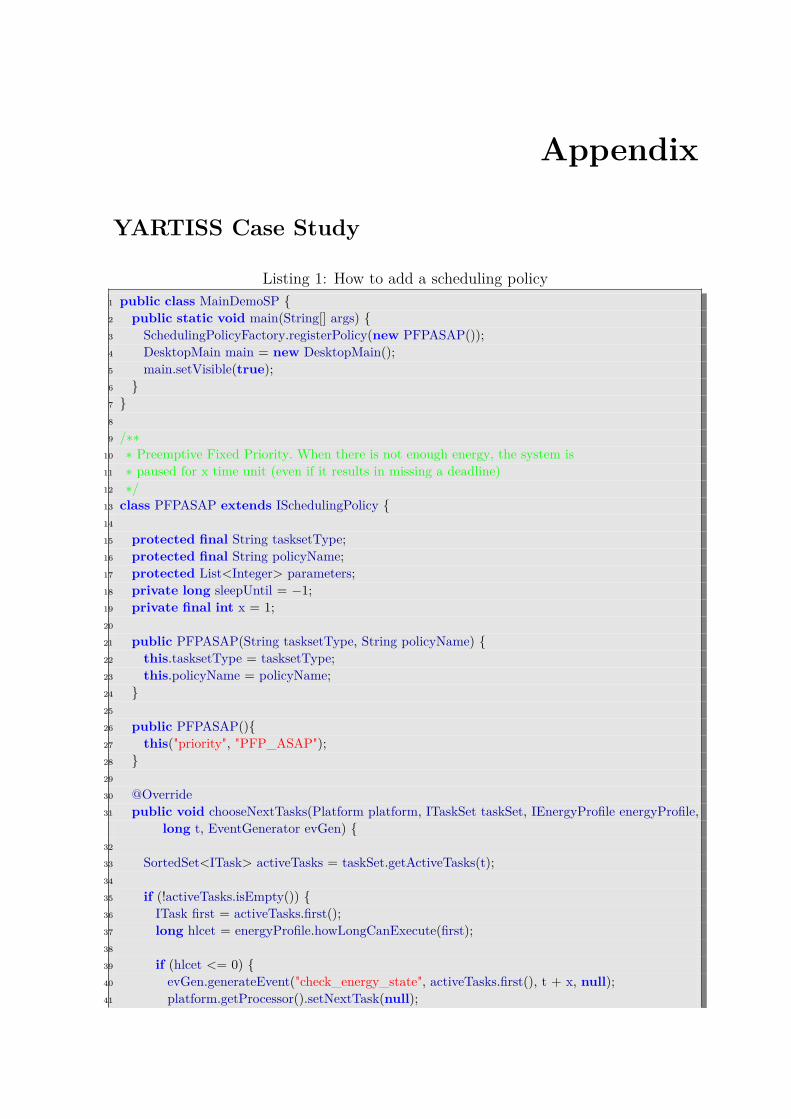
Appendix
YARTISS Case Study
Listing 1: How to add a scheduling policy1 public class MainDemoSP {2 public static void main(String[] args) {3 SchedulingPolicyFactory.registerPolicy(new PFPASAP());4 DesktopMain main = new DesktopMain();5 main.setVisible(true);6 }7 }8
9 /∗∗10 ∗ Preemptive Fixed Priority. When there is not enough energy, the system is11 ∗ paused for x time unit (even if it results in missing a deadline)12 ∗/13 class PFPASAP extends ISchedulingPolicy {14
15 protected final String tasksetType;16 protected final String policyName;17 protected List<Integer> parameters;18 private long sleepUntil = −1;19 private final int x = 1;20
21 public PFPASAP(String tasksetType, String policyName) {22 this.tasksetType = tasksetType;23 this.policyName = policyName;24 }25
26 public PFPASAP(){27 this("priority", "PFP_ASAP");28 }29
30 @Override31 public void chooseNextTasks(Platform platform, ITaskSet taskSet, IEnergyProfile energyProfile,
long t, EventGenerator evGen) {32
33 SortedSet<ITask> activeTasks = taskSet.getActiveTasks(t);34
35 if (!activeTasks.isEmpty()) {36 ITask first = activeTasks.first();37 long hlcet = energyProfile.howLongCanExecute(first);38
39 if (hlcet <= 0) {40 evGen.generateEvent("check_energy_state", activeTasks.first(), t + x, null);41 platform.getProcessor().setNextTask(null);
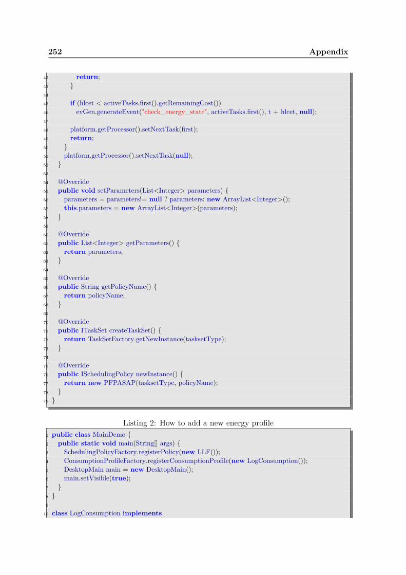
252 Appendix
42 return;43 }44
45 if (hlcet < activeTasks.first().getRemainingCost())46 evGen.generateEvent("check_energy_state", activeTasks.first(), t + hlcet, null);47
48 platform.getProcessor().setNextTask(first);49 return;50 }51 platform.getProcessor().setNextTask(null);52 }53
54 @Override55 public void setParameters(List<Integer> parameters) {56 parameters = parameters!= null ? parameters: new ArrayList<Integer>();57 this.parameters = new ArrayList<Integer>(parameters);58 }59
60 @Override61 public List<Integer> getParameters() {62 return parameters;63 }64
65 @Override66 public String getPolicyName() {67 return policyName;68 }69
70 @Override71 public ITaskSet createTaskSet() {72 return TaskSetFactory.getNewInstance(tasksetType);73 }74
75 @Override76 public ISchedulingPolicy newInstance() {77 return new PFPASAP(tasksetType, policyName);78 }79 }
Listing 2: How to add a new energy profile1 public class MainDemo {2 public static void main(String[] args) {3 SchedulingPolicyFactory.registerPolicy(new LLF());4 ConsumptionProfileFactory.registerConsumptionProfile(new LogConsumption());5 DesktopMain main = new DesktopMain();6 main.setVisible(true);7 }8 }9
10 class LogConsumption implements
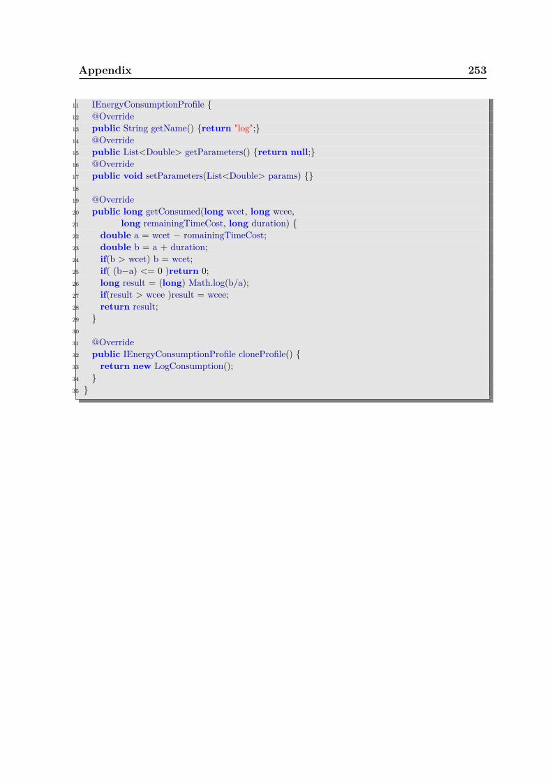
Appendix 253
11 IEnergyConsumptionProfile {12 @Override13 public String getName() {return "log";}14 @Override15 public List<Double> getParameters() {return null;}16 @Override17 public void setParameters(List<Double> params) {}18
19 @Override20 public long getConsumed(long wcet, long wcee,21 long remainingTimeCost, long duration) {22 double a = wcet − romainingTimeCost;23 double b = a + duration;24 if(b > wcet) b = wcet;25 if( (b−a) <= 0 )return 0;26 long result = (long) Math.log(b/a);27 if(result > wcee )result = wcee;28 return result;29 }30
31 @Override32 public IEnergyConsumptionProfile cloneProfile() {33 return new LogConsumption();34 }35 }

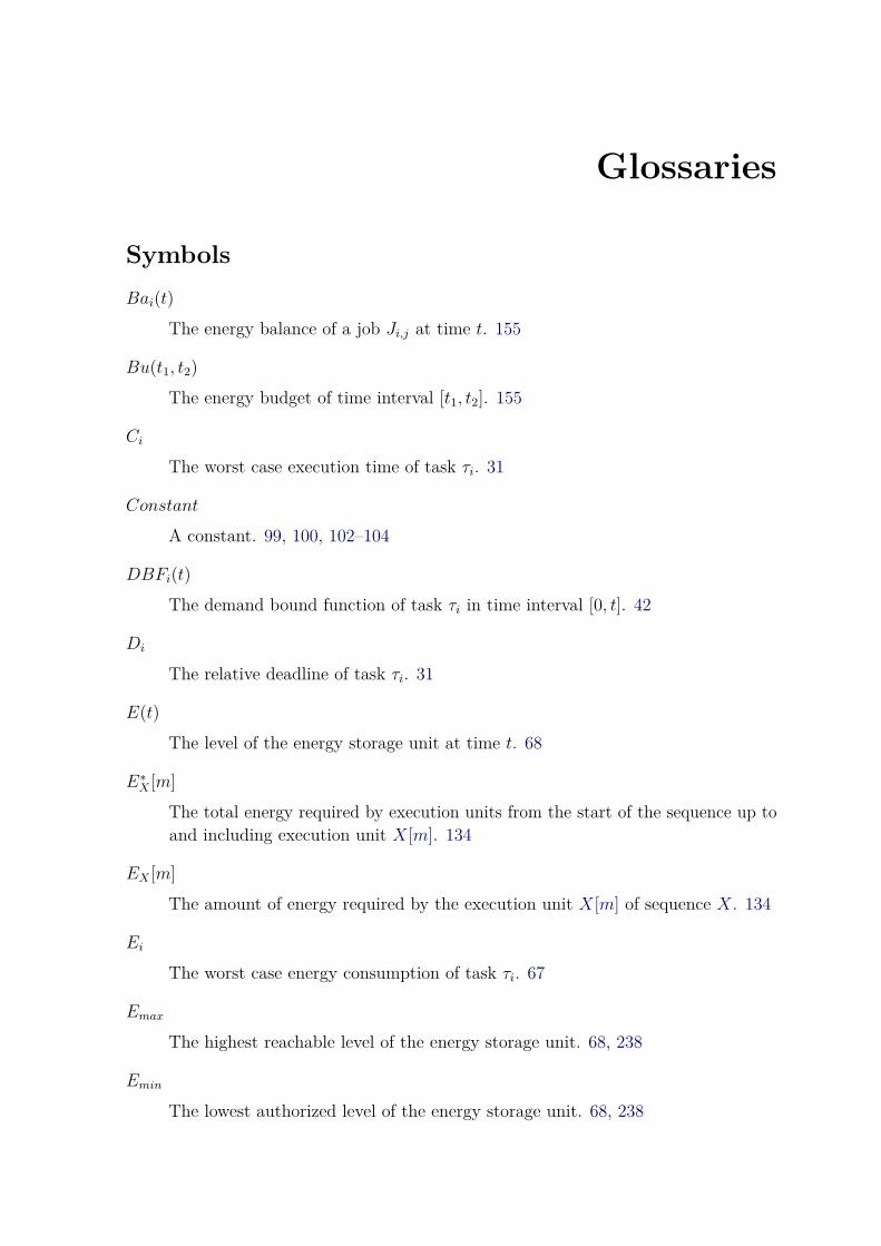
Glossaries
SymbolsBai(t)
The energy balance of a job Ji,j at time t. 155
Bu(t1, t2)The energy budget of time interval [t1, t2]. 155
Ci
The worst case execution time of task τi. 31
Constant
A constant. 99, 100, 102–104
DBFi(t)The demand bound function of task τi in time interval [0, t]. 42
Di
The relative deadline of task τi. 31
E(t)The level of the energy storage unit at time t. 68
E∗X [m]The total energy required by execution units from the start of the sequence up toand including execution unit X[m]. 134
EX [m]The amount of energy required by the execution unit X[m] of sequence X. 134
Ei
The worst case energy consumption of task τi. 67
Emax
The highest reachable level of the energy storage unit. 68, 238
Emin
The lowest authorized level of the energy storage unit. 68, 238
256 Symbols
I∗X [m]The the minimum number of replenishment units required to execute all of thesubsequence X[1] to X[m] in order. 135
IX [m]The minimum number of replenishment units required to provide sufficient energyto execute X[m] at the end of the subsequence X[1] to X[m]. 135
LX
The number of execution units in sequence X. 134
Nh
The number of jobs in sequence X. 141
Oi
Offset or first release time of task τi. 30
P (t)The global power consumption function of the system. 176
PD(t)The dynamic power consumption function of the system. 176
PL(t)The power leakage or the static power consumption function of the system. 177
Pi
The priority of task τi. 38
Pr
Constant replenishment function. 68
Pr(t)The power rate or the replenishment function. 67, 238
Pi,j
The priority of job Ji,j. 38
Pci
The worst-case power consumption of task τi during one time unit. 132
R
The electrical resistance. 176
Symbols 257
RBFi(t)
The request bound function of task τi in time interval [0, t]. 42
Ri
The Worst Case Response Time (WCRT) of task τi. 32
RUB1i
The WCRT of task τi according to response time upper bound UBx. 137
Ri,j
The response time of job Ji,j. 32
SE(t)
The available slack-energy of the system at time t. 84
ST (t)
The available slack-time of the system at time t. 84
STi(t)
The available slack-time of priority level-i at time t. 92
T (t)
The temperature of the system at time t. 176, 247
Ti
The period or the inter-arrival time of task τi. 31
TA
The ambient temperature. 176
Tmax
The the maximum tolerated temperature. 176, 247
U
The processor utilization of the system. 41
Ui
The processor utilization of task τi. 41
Ue
The energy utilization of the system. 70
258 Symbols
V
Volt. 54
W
Watt. 50
W (t1, t2)
The workload of the system in time interval [t1, t2]. 42
W/cm2
Watt per square centimeter. 50
Wi(t1, t2)
The workload of task τi in time interval [t1, t2]. 42
Wmi (t)
The recurrent workload function. 92
WUB1i (w)
The workload function of priority level-i according to upper bound UB1. 139
Wei(t)
The energy workload or demand of priority level-i in time interval [0, t]. 113
Wh/kg
Watt-hour per kilogram. 56
Wh/m3
Watt-hour per cubic centimeter. 56
Wpi(t)
The processor workload or demand of priority level-i in time interval [0, t]. 113
X
A vector of execution units from 1 to LX . 134, 255, 256
X[m]
The m-th element of sequence X. 134, 255, 256
∆
A certain interval of time. 87
Symbols 259
ΓA task set. 38, 132, 259
ΓcThe subset of Γ that contains consuming tasks. 132
ΓgThe subset of Γ that contains gaining tasks. 132
ΛThe density of the system. 41
Λi
The density of task τi. 41◦C
Celsius degree. 54
CThe capacity of the energy storage unit. 68, 176
CUBimin
The minimum energy storage unit capacity needed for response time upper boundUBi. 143
CminThe minimum capacity of the energy storage unit that keeps a task set schedulable.91
µA
Microampere. 54
µF
Microfarad. 60
µW
Microwatt. 54
µW/cm2
Milliwatt per square meter. 51
µW/cm3
Milliwatt per cubic centimeter. 53
260 Symbols
τi
Task number i or of priority level i. 30
ai(t)
The next job request time of priority level-i. 92, 154
ai,j
The arrival time of job Ji,j. 32
ci(t)
The remaining execution time at time t of the current job of task τi. 92, 154
cm2
Square centimeter. 50
cm3
Cubic centimeter. 53
di(t)
The next absolute deadline of priority level-i after time t. 92, 154
di,j
The absolute deadline of job Ji,j. 32
ei(t)
The remaining energy cost of the current job of task τi at time t. 154
fi,j
The termination time of job Ji,j. 32
g(t1, t2)
The energy replenished during time interval [t1, t2]. 68
hp(k)
Subset of tasks of priority higher or than τk. 146
idle(t1, t2)
The amount of time where the processor is idle within interval of time [t1, t2]. 92
lp(i)
Subset of tasks of priority lower or equal than τi. 146
Symbols 261
mA
Milliampere. 56
mAh
Milliampere-hour=10−3Ah. 56
mW
Milliwatt. 54
n
The task set cardinal. 38
si(t)The effective execution starting time of the current job of task τi at time t. 154
si,j
The effective execution starting time of job Ji,j. 87, 154
t
Time instant t. 36
262 Acronyms
AcronymsDM
Deadline Monotonic. 38, 124, 146, 147, 204, 212, 216,— Glossary: DM
EDF
Earliest Deadline First. 22, 40, 79–81, 83–86, 89, 91, 92, 105, 164, 204, 206, 211,212, 216, 234, 235, 240, 262, 268, 270,— Glossary: EDF
EDL
EDF As Late As Possible. 79–84, 86, 92, 95, 98, 99, 102–104, 240, 273,— Glossary: EDL
EDeg
EDF with energy guaranty. 79, 83–86, 98, 99, 101, 104, 240, 273, 275,— Glossary: EDeg
FBA
Frame-Based Algorithm. 76–79, 98, 99, 101, 102, 104, 239, 273, 275,— Glossary: FBA
FPCasap
Fixed-Task-Priority Clairvoyant as soon as possible. 161–163, 165, 167, 245,274, 275,— Glossary: FPCasap
FPLSA
Fixed-Task-Priority Lazy Scheduling Algorithm. 164, 165, 245, 274, 275,— Glossary: FPLSA
FPLeg
Fixed-Task-Priority As Late As Possible with energy guaranty. 164–170, 245,274, 275,— Glossary: FPLeg
FP lh
Fixed-Task-Priority lookahead. 167–170, 245, 274, 275,— Glossary: FPlh
Acronyms 263
LLF
Least Laxity First. 40, 212, 216, 235, 269,— Glossary: LLF
LSA
Lazy Scheduling Algorithm. 79, 86–91, 98, 99, 101, 102, 104, 164, 240, 245, 273,275,— Glossary: LSA
PFPALAP
Preemptive Fixed-Task-Priority As Late As Possible. 92–96, 98, 99, 101, 103,104, 110, 123, 125–129, 160, 161, 165, 166, 168, 170, 240, 241, 273–275,— Glossary: PFPALAP
PFPASAP
Preemptive Fixed-Task-Priority As Soon As Possible. 23, 110–114, 116–119,121, 122, 125–129, 131, 136, 138, 141, 144, 147, 148, 151, 153, 156, 157, 159–163,174, 178, 179, 181–185, 188, 189, 191–193, 196, 198, 202, 221, 222, 225–227, 241,273–275,— Glossary: PFPASAP
PFPST
Preemptive Fixed-Task-Priority with Slack-Time. 95–99, 101, 103, 104, 110, 123,125–128, 161, 240, 273–275,— Glossary: PFPST
RM
Rate Monotonic. 38, 204, 212, 216,— Glossary: RM
API
Application Programming Interface. 204, 205, 214, 219, 220
CMOS
Complementary Metal–Oxide–Semiconductor . 74
CPU
Central Processing Unit. 21, 29, 35, 73, 74, 175, 176,— Glossary: CPU
264 Acronyms
DAG
Directed Acyclic Graph. 35, 173, 208, 216,— Glossary: DAG
DBF
Demand Bound Function. 42,— Glossary: DBF
DP
Dinamic Priority. 38,— Glossary: DP
DVFS
Dynamic Voltage and Frequency Scaling. 73, 74, 175, 217
EH
Energy-Harvesting. 47,— Glossary: EH
EHS
Energy-Harvesting System. 22, 48
EVCC
Energy Variability Characterization Curves. 87,— Glossary: EVCC
FIFO
First In First Out. 175
FJP
Fixed-Job-Priority. 38, 40,— Glossary: FJP
FTP
Fixed-Task-Priority. 38, 40, 71, 95, 97, 147, 148, 211, 225, 268, 269,— Glossary: FTP
GUI
Graphic User Interface. 213, 214, 223
Acronyms 265
HP
Hyper-Period. 42,— Glossary: HP
ICT
Information and Communication Technologies. 55, 56, 61, 273
IMD
Implantable Medical Device. 174
IoC
Inversion of Control. 214, 218, 219,— Glossary: IoC
LCM
Least Common Multiple. 42, 270
Li-ion
Lithium Ion. 59, 237, 273
Li-polymer
Lithium-ion Polymer . 59, 273
MEMS
Microelectromechanical Systems. 52
MP3
MPEG Audio Layer 3 . 21,— Glossary: MP3
MVC
Model-View-Controller . 214, 219, 220,— Glossary: MVC
MVVM
Model View View-Model. 219,— Glossary: MVVM
NiCd
Nickel Cadmium. 57–59, 237, 273

266 Acronyms
NiMH
Nickel-Metal Hydrid. 58, 59, 237, 273
NP-Hard
Non-deterministic Polynomial-time Hard. 74
OPA-compatible
Optimal Priority Assignment (OPA)-compatible.— Glossary: OPA-compatible
OPA
Optimal Priority Assignment. 38, 39, 265, 270,— Glossary: OPA
PC
Personal Computer . 21
QoS
Quality of Service. 29, 35
RBF
Request Bound Function. 42,— Glossary: RBF
RC
Resistance Capacitance circuit. 176, 271,— Glossary: RC
RF
Radio Frequency. 50, 51, 53
RFID
Radio Frequency Identification. 51, 236
RTEHS
Real-Time Energy-Harvesting Systems. 22
RTS
Real-Time Systems. 21, 28
Acronyms 267
TAThermal-Aware.— Glossary: TA
WCETWorst Case Execution Time. 31, 34, 35, 208, 211, 215
WCRTWorst Case Response Time. 45, 257, 271,— Glossary: WCRT
XMLExtensible Markup Language. 206
YARTISSYet An Other Real-Time Systems Simulator . 23, 204–208, 211, 212, 215–219,221, 223, 224
268 Glossary
GlossaryDM
The priority assignment policy that grants the highest priority to the task withthe smallest deadline. 262
EDF
The scheduling policy that executes first the jobs with the nearest deadlines. 262
EDL
The scheduling algorithm that schedules jobs as late as possible according toEDF rules. 262
EDeg
The scheduling algorithm that checks if the execution of the current job does notlead to future deadline miss before authorizing it to execute according to EDFrules. 262
FBA
The scheduling algorithm that schedules continuously the group of gaining taskswhen the minimum battery level is reached and executes the group of consumingtasks when the maximum battery level is reached. 262
FPCasap
The FTP algorithm that uses lookahead computations to detect future deadlinemisses in order to adapt the scheduling decisions. 262
FPLSA
The FTP counter-part of Lazy Scheduling Algorithm. 262
FPLeg
The FTP algorithm that uses only virtual deadlines to compute the maximumdelay to apply for each job. 262
FPlh
The FTP algorithm that uses virtual deadlines and lookahead verifications tocompute the maximum delay to apply for each job. 262
LLF
The scheduling policy that executes first the jobs with the smallest laxity. 262
Glossary 269
LSA
The Lazy Scheduling Algorithm is an EDF-based algorithm that delays executionsuch that the current job and the eventual higher priority jobs can be executedcontinuously without running out of energy and without exceeding the maximumcapacity of the battery. 263
PFPALAP
The scheduling algorithm that schedules jobs as late as possible according to FTPrules. 263
PFPASAP
An energy-work-conserving FTP scheduling policy. 263
PFPST
The scheduling algorithm that executes jobs according to FTP rules when someenergy is available and replenishes as long as possible otherwise. 263
RM
The priority assignment policy that grants the highest priority to the task withthe smallest period. 263
CPU
The processor. 263
DAG
The task model that considers dependencies between the jobs of the same task.263
DBF
The demand bound function of recurrent is the worst cumulative workload gener-ated jobs that are requested and finished during time interval [0, t]. 263
DP
According to dynamic priority scheduling, a job may be scheduled with differentpriorities, e.g. LLF . 264
EH
Energy-Harvesting systems collect the energy from the environment and use it tosupply the operations of the system. 264
270 Glossary
EVCC
The Energy Variability Characterization Curves is technique used to bound theamount of energy that comes from a solar energy harvester. 264
FJP
Scheduling algorithms driven by jobs priorities, e.g. EDF . 264
FTP
Scheduling algorithms driven by the static priorities of tasks. 264
HP
The hyper-period is the smallest interval of time after which the global periodicpattern of all the tasks are repeated. It is typically defined as the Least CommonMultiple (LCM) of the periods of all the tasks of the system.. 264
IoC
The Inversion of Control design pattern. 265
MP3
An audio codec. 265
MVC
Model-View-Controller design pattern. 265
MVVM
The Model View View-Model design pattern. 265
OPA
The algorithm of Audsley that calculate a valid tasks priority assignment wheneverthere exists one. 266
OPA-compatible
A schedulability test is compatible with the OPA algorithm if the priority orderingof higher and lower priority tasks does not alter the schedulability of the currentlevel. 265
RBF
The request bound function computes the worst cumulative workload generatedby jobs that are requested during time interval [0, t[. 266
Glossary 271
RCThe Resistance Capacitance circuit (RC) circuit is used to model the thermalbehavior of the system. 266
TAThermal-Aware systems adapt the performances in order to keep the temperatureof the system below a maximum threshold. 266
WCRTThe WCRT of a task is the maximum duration between the activation of the taskand the moment it finishes its execution. 266

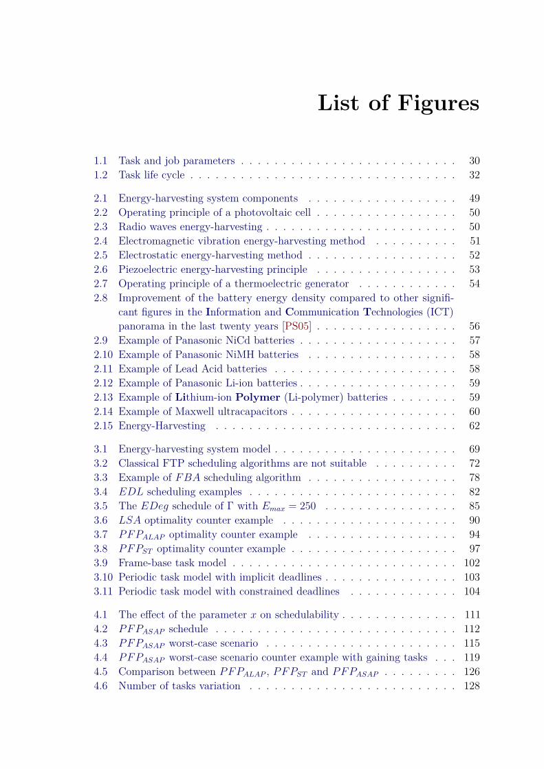
List of Figures
1.1 Task and job parameters . . . . . . . . . . . . . . . . . . . . . . . . . . 301.2 Task life cycle . . . . . . . . . . . . . . . . . . . . . . . . . . . . . . . . 32
2.1 Energy-harvesting system components . . . . . . . . . . . . . . . . . . 492.2 Operating principle of a photovoltaic cell . . . . . . . . . . . . . . . . . 502.3 Radio waves energy-harvesting . . . . . . . . . . . . . . . . . . . . . . . 502.4 Electromagnetic vibration energy-harvesting method . . . . . . . . . . 512.5 Electrostatic energy-harvesting method . . . . . . . . . . . . . . . . . . 522.6 Piezoelectric energy-harvesting principle . . . . . . . . . . . . . . . . . 532.7 Operating principle of a thermoelectric generator . . . . . . . . . . . . 542.8 Improvement of the battery energy density compared to other signifi-
cant figures in the Information and Communication Technologies (ICT)panorama in the last twenty years [PS05] . . . . . . . . . . . . . . . . . 56
2.9 Example of Panasonic NiCd batteries . . . . . . . . . . . . . . . . . . . 572.10 Example of Panasonic NiMH batteries . . . . . . . . . . . . . . . . . . 582.11 Example of Lead Acid batteries . . . . . . . . . . . . . . . . . . . . . . 582.12 Example of Panasonic Li-ion batteries . . . . . . . . . . . . . . . . . . . 592.13 Example of Lithium-ion Polymer (Li-polymer) batteries . . . . . . . . 592.14 Example of Maxwell ultracapacitors . . . . . . . . . . . . . . . . . . . . 602.15 Energy-Harvesting . . . . . . . . . . . . . . . . . . . . . . . . . . . . . 62
3.1 Energy-harvesting system model . . . . . . . . . . . . . . . . . . . . . . 693.2 Classical FTP scheduling algorithms are not suitable . . . . . . . . . . 723.3 Example of FBA scheduling algorithm . . . . . . . . . . . . . . . . . . 783.4 EDL scheduling examples . . . . . . . . . . . . . . . . . . . . . . . . . 823.5 The EDeg schedule of Γ with Emax = 250 . . . . . . . . . . . . . . . . 853.6 LSA optimality counter example . . . . . . . . . . . . . . . . . . . . . 903.7 PFPALAP optimality counter example . . . . . . . . . . . . . . . . . . 943.8 PFPST optimality counter example . . . . . . . . . . . . . . . . . . . . 973.9 Frame-base task model . . . . . . . . . . . . . . . . . . . . . . . . . . . 1023.10 Periodic task model with implicit deadlines . . . . . . . . . . . . . . . . 1033.11 Periodic task model with constrained deadlines . . . . . . . . . . . . . 104
4.1 The effect of the parameter x on schedulability . . . . . . . . . . . . . . 1114.2 PFPASAP schedule . . . . . . . . . . . . . . . . . . . . . . . . . . . . . 1124.3 PFPASAP worst-case scenario . . . . . . . . . . . . . . . . . . . . . . . 1154.4 PFPASAP worst-case scenario counter example with gaining tasks . . . 1194.5 Comparison between PFPALAP , PFPST and PFPASAP . . . . . . . . . 1264.6 Number of tasks variation . . . . . . . . . . . . . . . . . . . . . . . . . 128
274 List of Figures
5.1 Worst-case scenario counter example . . . . . . . . . . . . . . . . . . . 1345.2 Dummy schedule used in the construction of UB2 . . . . . . . . . . . . 1405.3 Percentage of task sets schedulable . . . . . . . . . . . . . . . . . . . . 1485.4 Varying the energy utilization . . . . . . . . . . . . . . . . . . . . . . . 1505.5 Varying the gaining tasks ratio . . . . . . . . . . . . . . . . . . . . . . 1505.6 Varying relative deadlines in [Ci, Ti] . . . . . . . . . . . . . . . . . . . . 151
6.1 Energy balance of J2,1 at time t=8 . . . . . . . . . . . . . . . . . . . . 1566.2 PFPASAP is not optimal . . . . . . . . . . . . . . . . . . . . . . . . . . 1576.3 A feasible schedule of task set Γ . . . . . . . . . . . . . . . . . . . . . . 1596.4 PFPASAP counter example . . . . . . . . . . . . . . . . . . . . . . . . . 1606.5 PFPALAP counter example . . . . . . . . . . . . . . . . . . . . . . . . . 1606.6 PFPST counter example . . . . . . . . . . . . . . . . . . . . . . . . . . 1616.7 FPCasap counter example . . . . . . . . . . . . . . . . . . . . . . . . . 1636.8 FPLSA counter example . . . . . . . . . . . . . . . . . . . . . . . . . . 1656.9 FPLeg counter example . . . . . . . . . . . . . . . . . . . . . . . . . . 1666.10 A FPlh schedule . . . . . . . . . . . . . . . . . . . . . . . . . . . . . . 1706.11 Interdependency between virtual deadlines . . . . . . . . . . . . . . . . 171
7.1 Thermal model . . . . . . . . . . . . . . . . . . . . . . . . . . . . . . . 1767.2 Cooling and heating functions . . . . . . . . . . . . . . . . . . . . . . . 1787.3 Worst-case scenario . . . . . . . . . . . . . . . . . . . . . . . . . . . . . 1807.4 First upper bound (UBTmin) . . . . . . . . . . . . . . . . . . . . . . . . 1837.5 UBTmin proof insight . . . . . . . . . . . . . . . . . . . . . . . . . . . . 1867.6 Parametric upper bound UBx . . . . . . . . . . . . . . . . . . . . . . . 1887.7 UBx proof insight . . . . . . . . . . . . . . . . . . . . . . . . . . . . . . 1907.8 f ′(x) sign . . . . . . . . . . . . . . . . . . . . . . . . . . . . . . . . . . 1937.9 Lower bound (LBx=1) . . . . . . . . . . . . . . . . . . . . . . . . . . . 1947.10 Simulations results . . . . . . . . . . . . . . . . . . . . . . . . . . . . . 1997.11 Simulations results . . . . . . . . . . . . . . . . . . . . . . . . . . . . . 200
8.1 Energy and multiprocessor views . . . . . . . . . . . . . . . . . . . . . 2098.2 Large scale simulation view . . . . . . . . . . . . . . . . . . . . . . . . 2108.3 Modules UML diagram . . . . . . . . . . . . . . . . . . . . . . . . . . . 2148.4 The engine module UML diagram . . . . . . . . . . . . . . . . . . . . . 2158.5 Producer/Consumer design pattern . . . . . . . . . . . . . . . . . . . . 2208.6 UML diagram describing the addition of a new scheduling policy . . . . 221
List of Algorithms
1.1 Optimal Priority Assignment . . . . . . . . . . . . . . . . . . . . . . . . 393.1 Scheduling decision of FBA Algorithm at time t . . . . . . . . . . . . . 773.2 EDeg Algorithm . . . . . . . . . . . . . . . . . . . . . . . . . . . . . . 843.3 LSA Algorithm . . . . . . . . . . . . . . . . . . . . . . . . . . . . . . . 883.4 Slack-time of priority level-i at time t . . . . . . . . . . . . . . . . . . . 933.5 PFPALAP Algorithm . . . . . . . . . . . . . . . . . . . . . . . . . . . . 933.6 PFPST Algorithm . . . . . . . . . . . . . . . . . . . . . . . . . . . . . 964.1 PFPASAP Algorithm . . . . . . . . . . . . . . . . . . . . . . . . . . . . 1124.2 Feasibility Test . . . . . . . . . . . . . . . . . . . . . . . . . . . . . . . 1226.1 FPCasap Algorithm . . . . . . . . . . . . . . . . . . . . . . . . . . . . 1626.2 FPLSA Algorithm . . . . . . . . . . . . . . . . . . . . . . . . . . . . . 1646.3 FPLeg Algorithm . . . . . . . . . . . . . . . . . . . . . . . . . . . . . 1666.4 FPlh Algorithm . . . . . . . . . . . . . . . . . . . . . . . . . . . . . . 1696.5 Lookahead(Bai(t), t, τi, L) Algorithm . . . . . . . . . . . . . . . . . . . 169

Bibliography
[AC13] Yasmina Abdeddaïm and Younès Chandarli. Optimal Real-TimeScheduling Algorithm for Fixed-Priority Energy-Harvesting Systems. tech-nical report. Paris, France, 2013. url: http://hal.archives-ouvertes.fr/hal-01076021.
(Cited on pages 2, 249).
[ACM13a] Yasmina Abdeddaïm, Younès Chandarli, and Damien Masson.“The Optimality of PFPASAP Algorithm for Fixed-Priority Energy-HarvestingReal-Time Systems”. In: Proceedings of the Euromicro Conference on Real-Time Systems (ECRTS). 2013.
(Cited on pages 1, 110, 149, 249).
[ACM13b] Yasmina Abdeddaïm, Younès Chandarli, and Damien Masson.“Toward an Optimal Fixed-Priority Algorithm for Energy-Harvesting Real-Time Systems”. In: Proceedings of the Work in progress session of theIEEE Real-Time and Embedded Technology and Applications Symposium(RTAS). 2013, pages 45–48.
(Cited on pages 1, 162).
[Abd+14] Yasmina Abdeddaïm, Younès Chandarli, R.I Davis, and DamienMasson. “Schedulability Analysis for Fixed Priority Real-Time Systemswith Energy-Harvesting”. In: Proceedings of the International Conferenceon Real-Time Networks and Systems (RTNS). 2014, pages 67–76.
(Cited on pages 1, 132, 249).
[AS+13] B. Ahmed-Seddik, G. Despesse, S. Boisseau, and E. Defay. “Self-powered resonant frequency tuning for Piezoelectric Vibration EnergyHarvesters”. In: Journal of Physics: Conference Series 476.1 (2013).
(Cited on page 53).
[Ahm+11] Masud Ahmed, Nathan Fisher, Shengquan Wang, and PradeepHettiarachchi. “Minimizing Peak Temperature in Embedded Real-Time Systems Via Thermal-aware Periodic Resources”. In: SustainableComputing: Informatics and Systems. Elsevier, 2011.
(Cited on pages 175, 177).
278 Bibliography
[AM01] André Allavena and Daniel Mossé. “Scheduling of Frame-basedEmbedded Systems with Rechargeable Batteries”. In: Proceedings ofthe International Workshop on Real-Time and Embedded Systeme (inconjunction with RTAS). IEEE, 2001.
(Cited on page 75).
[AC98] R. Amirtharajah and A.P. Chandrakasan. “Self-powered SignalProcessing Using Vibration-based Power Generation”. In: Solid-StateCircuits 33.5 (1998), pages 687–695.
(Cited on page 51).
[Aud01] N. C. Audsley. “On Priority Asignment in Fixed Priority Scheduling”.In: Information Processing Letters 79.1 (2001), pages 39–44.
(Cited on page 39).
[Aud+93] N. Audsley, A. Burns, M. Richardson, K. Tindell, and A. J.Wellings. “Applying New Scheduling Theory to Static Priority Pre-Emptive Scheduling”. In: Software Engineering Journal 8 (1993), pages 284–292.
(Cited on page 45).
[Aud91] N.C. Audsley. Optimal Priority Assignment And Feasibility Of StaticPriority Tasks With Arbitrary Start Times. 1991.
(Cited on page 39).
[BA14] Mario Bambagini and Hakan Aydin. “Periodic charging scheme forfixed-priority real-time systems with renewable energy”. In: Proceedingsof the IEEE International Symposium on Industrial Embedded Systems(SIES). 2014.
(Cited on page 119).
[BHR90a] Sanjoy K. Baruah, Rodney R. Howell, and Louis Rosier. “Algo-rithms and Complexity Concerning the Preemptive Scheduling of Periodic,Real-Time Tasks on One Processor”. In: Real-Time Systems 2 (1990),pages 301–324.
(Cited on page 42).
[BHR90b] Sanjoy K. Baruah, Rodney R. Howell, and Louis Rosier. “Algo-rithms and Complexity Concerning the Preemptive Scheduling of Periodic,Real-Time Tasks on One Processor”. In: Real-Time Systems 2 (1990),pages 301–324.
(Cited on page 46).
Bibliography 279
[Bar+12] Sanjoy Baruah, Vincenzo Bonifaci, Alberto Marchetti-Spaccamela,Leen Stougie, and Andreas Wiese. “A Generalized Parallel TaskModel for Recurrent Real-time Processes”. In: Proceedings of the IEEEConference on Real-Time Systems Symposium (RTSS). IEEE ComputerSociety, 2012, pages 63–72.
(Cited on page 35).
[BBA10] Andrea Bastoni, Björn B. Brandenburg, and James H. An-derson. “Cache-Related Preemption and Migration Delays: EmpiricalApproximation and Impact on Schedulability”. In: Proceedings of the An-nual Workshop on Operating Systems Platforms for Embedded Real-TimeApplications (in conjunction with ECRTS). 2010.
(Cited on pages 149, 201).
[BD13] Adam Betts and Alastair Donaldson. “Estimating the WCET ofGPU-Accelerated Applications Using Hybrid Analysis”. In: Proceedingsof the Euromicro Conference on Real-Time Systems (ECRTS). 2013.
(Cited on page 31).
[BB05] Enrico Bini and Giorgio C. Buttazzo. “Measuring the Performanceof Schedulability Tests”. In: Real-Time Systems 30.1-2 (2005), pages 129–154.
(Cited on pages 100, 123, 147, 198, 212).
[BBB03] Enrico Bini, Giorgio C. Buttazzo, and Giuseppe M. Buttazzo.“Rate Monotonic Analysis: The Hyperbolic Bound”. In: IEEE Transactionson Computers Publication 52.7 (2003), pages 933–942.
(Cited on page 44).
[Buc11] Isidor Buchmann. Batteries in a Portable World. Cadex ElectronicsInc, 2011.
(Cited on pages 60, 61).
[But11] Giorgio C. Buttazzo. Hard Real-Time Computing Systems. Springer,2011.
(Cited on pages 28, 35, 37, 234).
[Cal+06] John M. Calandrino, Hennadiy Leontyev, Aaron Block, UmaMa-heswari C. Devi, and James H. Anderson. “LITMUS-RT: A Testbedfor Empirically Comparing Real-Time Multiprocessor Schedulers”. In: 27thIEEE International Real-Time Systems Symposium. 2006, pages 111–126.
(Cited on page 205).
280 Bibliography
[Can63] Edward T. Canby. Histoire de l’électricité. Rencontre, 1963.(Cited on page 52).
[CC05] Roberto Casas and Oscar Casas. “Battery Sensing for Energy-AwareSystem Design”. In: IEEE Transactions on Computers Publication 38.11(2005), pages 48–54.
(Cited on page 57).
[CAM12] Younès Chandarli, Yasmina Abdeddaïm, and Damien Masson.“The Fixed Priority Scheduling Problem for Energy Harvesting Real-TimeSystems”. In: Proceedings of the work in progress session of the the IEEEInternational Conference on Embedded and Real-Time Computing Systemsand Applications (RTCSA). 2012.
(Cited on pages 1, 92).
[CFM15] Younès Chandarli, Nathan Fisher, and Damien Masson. “Re-sponse Time Analysis for Thermal-Aware Real-Time Systems UnderFixed-Priority Scheduling”. In: Proceedings of the IEEE Symposium OnReal-time Computing (ISORC). 2015.
(Cited on pages 1, 174).
[CQF13] Younès Chandarli, Manar Qamhieh, and Frédérique Fauberteau.YARTISS: A Generic, Modular and Energy-Aware Scheduling Simulatorfor Real-Time Multiprocessor Systems. technical report. Paris, France,2013. url: http://hal.archives-ouvertes.fr/hal-01076022.
(Cited on page 2).
[Cha+12] Younès Chandarli, Frédéric Fauberteau, Damien Masson, SergeMidonnet, and Manar Qamhieh. “YARTISS: A Tool to Visualize, Test,Compare and Evaluate Real-Time Scheduling Algorithms”. In: Proceedingsof the International Workshop on Analysis Tools and Methodologies forEmbedded and Real-time Systems (WATERS). 2012, pages 21–26.
(Cited on pages 1, 205, 250).
[CHK07] Jian-Jia Chen, Chia-Mei Hung, and Tei-Wei Kuo. “On the Mini-mization Fo the Instantaneous Temperature for Periodic Real-Time Tasks”.In: Proceedings of the International Real-Time and Embedded Technol-ogy and Applications Symposium (RTAS). IEEE Computer Society, 2007,pages 236–248.
(Cited on page 175).
Bibliography 281
[CWT09] Jian-Jia Chen, Shengquan Wang, and Lothar Thiele. “ProactiveSpeed Scheduling for Real-Time Tasks Under Thermal Constraints”. In:Proceedings of the International Real-Time and Embedded Technologyand Applications Symposium (RTAS). IEEE Computer Society, 2009,pages 141–150.
(Cited on page 175).
[Che14] Maryline Chetto. “Optimal Scheduling for Real-Time Jobs in EnergyHarvesting Computing Systems”. In: IEEE Transactions on EmergingTopics in Computing (2014).
(Cited on pages 83, 86, 240).
[CMM11] Maryline Chetto, Damien Masson, and Serge Midonnet. “FixedPriority Scheduling Strategies for Ambient Energy-Harvesting Embeddedsystems”. In: The IEEE/ACM International Conference on Green Com-puting an Communications. 2011, pages 50–55.
(Cited on pages 95, 97, 111).
[Chi+00] Neil N. H. Ching, Gordon M. H. Chan, Wen J. Li, Hiu YungWong, and Philip H. W. Leong. “PCB Integrated Micro Generatorfor Wireless Systems”. In: Proceedings of the International Symposium onSmart Structures and Microsystems. 2000.
(Cited on page 51).
[CG11] Pierre Courbin and Laurent George. “FORTAS: Framework fOrReal-Time Analysis and Simulation”. In: Proceedings of the InternationalWorkshop on Analysis Tools and Methodologies for Embedded and Real-time Systems (WATERS). 2011, pages 21–26.
(Cited on page 206).
[DB09] Robert I. Dais and Alan Burns. “Priority Assignment for Global FixedPriority Pre-Emptive Scheduling in Multiprocessor Real-Time Systems”.In: Proceedings of the IEEE Conference on Real-Time Systems Symposium(RTSS). IEEE Computer Society, 2009, pages 398–409.
(Cited on page 39).
[Dav93] R.I. Davis. Approximate Slack Stealing Algorithms for Fixed PriorityPre-emptive Systems. 1993.
(Cited on page 128).
282 Bibliography
[DTB93] R.I. Davis, K.W. Tindell, and A. Burns. “Scheduling slack-time infixed priority pre-emptive systems”. In: Proceedings of the InternationalReal-Time Systems Symposium (RTSS). 1993.
(Cited on pages 92, 96, 127).
[DB11] Robert I. Davis and Alan Burns. “A Survey of Hard Real-timeScheduling for Multiprocessor Systems”. In: ACM Computing Surveys43.4 (2011), 35:1–35:44.
(Cited on page 43).
[Dav+13] Robert I. Davis, Steffen Kollmann, Victor Pollex, and FrankSlomka. “Schedulability Analysis for Controller Area Network (CAN)with FIFO Queues Priority Queues and Gateways”. In: Real-Time Systems49.1 (2013), pages 73–116.
(Cited on page 38).
[Dou+03] T. Douseki, Y. Yoshida, F. Utsunomiya, and N. more authorsItoh. “A batteryless wireless system uses ambient heat with a reversible-power-source compatible CMOS/SOI DC-DC converter”. In: Proceedingsof the IEEE International Solid-State Circuits Conference, Digest ofTechnical Papers. 2003, pages 388–501.
(Cited on page 54).
[EGCC11] Hussein EL Ghor, Maryline Chetto, and Rafic Hage Chehade.“A Real-time Scheduling Framework for Embedded Systems with Envi-ronmental Energy Harvesting”. In: Computers & Electrical Engineering37.4 (2011), pages 498–510.
(Cited on pages 83, 86, 240).
[ECLEZ11] L. El Chaara, L.A. Lamon, and N. El Zeinb. “Review of photovoltaictechnologies”. In: Renewable and Sustainable Energy Reviews 6 (2011),pages 242–247.
(Cited on page 50).
[Fau] Frédéric Fauberteau. “RTMSIM”. http://rtmsim.triaxx.org/.(Cited on pages 204, 207).
[FMG11] Frédéric Fauberteau, Serge Midonnet, and Laurent George.“Laxity-Based Restricted-Migration Scheduling”. In: Proceedings of theIEEE International Conference on Emerging Technologies and FactoryAutomation. IEEE Computer Society, 2011, pages 1–8.
(Cited on page 207).
Bibliography 283
[FBB06] Nathan Fisher, Theodore P. Baker, and Sanjoy Baruah. “Al-gorithms for Determining the Demand-Based Load of a Sporadic TaskSystem”. In: Proceedings of the IEEE International Conference on Embed-ded and Real-Time Computing Systems and Applications (RTCSA). IEEEComputer Society, 2006, pages 135–146.
(Cited on page 38).
[Gam11] Luca Gammaitoni. “Sustainable ICT: Micro and Nanoscale EnergyManagement”. In: Procedia Computer Science 7 (2011), pages 103–105.
(Cited on page 54).
[GH+01] M. Gonzalez Harbour, J. J. Gutierrez Garcia, J. C. Palen-cia Gutierrez, and J. M. Drake Moyano. “MAST: Modeling andanalysis suite for real time applications”. In: Proceedings of the EuromicroConference on Real-Time Systems (ECRTS). 2001.
(Cited on page 205).
[HP13] Damien Hardy and Isabelle Puaut. “Static Probabilistic Worst CaseExecution Time Estimation for Architectures with Faulty InstructionCaches”. In: Proceedings of the International Conference on Real-TimeNetworks and Systems (RTNS). ACM, 2013, pages 35–44.
(Cited on page 31).
[HS00] P. Hazucha and C. Svensson. “Impact of CMOS technology scalingon the atmospheric neutron soft error rate”. In: IEEE Transactions onNuclear Science 47 (2000), pages 2586–2594.
(Cited on page 74).
[Het+12] Pradeep M. Hettiarachchi et al. “The Design and Analysis ofThermal-Resilient Hard-Real-Time Systems”. In: Proceedings of the Inter-national Real-Time and Embedded Technology and Applications Symposium(RTAS). 2012, pages 67–76. isbn: 978-0-7695-4667-4.
(Cited on pages 175, 197).
[Hol+10] M.J. Holenderski, M.M.H.P. van den Heuvel, R.J. Bril, andJ.J. Lukkien. “Grasp: Tracing, visualizing and measuring the behaviorof real-time systems”. In: Proceedings of the International Workshop onAnalysis Tools and Methodologies for Embedded and Real-time Systems(WATERS). 2010.
(Cited on page 205).
284 Bibliography
[JM06] R. Jayaseelan and T. Mitra. “Estimating the Worst-Case EnergyConsumption of Embedded Software”. In: Proceedings of the IEEE Real-Time and Embedded Technology and Applications Symposium (RTAS).2006.
(Cited on pages 68, 211).
[JLY89] Lehoczky John, Sha Lui, and Ding Ye. “The rate monotonic schedul-ing algorithm: exact characterization and average case behavior”. In: Pro-ceedings of the IEEE Conference Real-Time Systems Symposium (RTSS).IEEE Computer Society, 1989.
(Cited on page 42).
[JK95] T. Juhnke and H. Klar. “Calculation of the soft error rate of submicronCMOS logic circuits”. In: IEEE Journal of Solid-State Circuits 30 (1995),pages 830 –834.
(Cited on page 74).
[KRI09] Shinpei Kato, Ragunathan Raj Rajkumar, and Yutaka Ishikawa.A Loadable Real-Time Scheduler Suite for Multicore Platforms. Technicalreport. Graduate School of Information Science, Nagoya University, 2009.
(Cited on page 205).
[Kim+07] Sohee Kim, P. Tathireddy, R.A. Normann, and F. Solzbacher.“Thermal Impact of an Active 3-D Microelectrode Array Implanted inthe Brain”. In: IEEE Transactions on Neural Systems and RehabilitationEngineering. IEEE Computer Society, 2007, pages 493–501.
(Cited on page 174).
[KS95] Gilad Koren and Dennis Shasha. “Dover: An Optimal On-Line Schedul-ing Algorithm for Overloaded Uniprocessor Real-Time Systems”. In: Soci-ety for Industrial and Applied Mathematics Journal 24.2 (1995), pages 318–339.
(Cited on page 206).
[KN04] H. Kulah and K. Najafi. “An Electromagnetic Micro Power Generatorfor Low-Frequency Environmental Vibrations”. In: Proceedings of theIEEE International Conference on Micro Electro Mechanical Systems(MEMS) (2004).
(Cited on page 51).
Bibliography 285
[LaM+89] Joseph C. LaManna, Kimberly A. McCracken, Madhavi Patil,and Otto J. Prohaska. “Stimulus-activated changes in brain tissuetemperature in the anesthetized rat”. In: Metabolic Brain Disease. 1989,pages 225–237.
(Cited on page 174).
[Laz05] G. Lazzi. “Thermal effects of bioimplants”. In: IEEE Engineering inMedicine and Biology Magazine. IEEE Computer Society, 2005, pages 75–81.
(Cited on page 174).
[LW82] J. Leung and J. Whitehead. “On the complexity of fixed-priorityscheduling of periodic real-time tasks”. In: Performance Evaluation 2(1982), pages 237–250.
(Cited on pages 132, 147).
[LL73] C. L. Liu and James W. Layland. “Scheduling Algorithms for Multi-programming in a Hard-Real-Time Environment”. In: J. ACM 20.1 (1973),pages 46–61.
(Cited on pages 30, 33, 34, 38, 39, 40, 44, 46).
[Liu00] Jane W. S. Liu. Real-Time Systems. Prentice Hall, 2000.(Cited on page 46).
[MG01] C. Macq and J. Goossens. “Limitation of the hyper-period in real-time periodic task set generation”. In: Proceedings of the InternationalConference on Real-Time Systems. 2001.
(Cited on pages 100, 123, 148, 198, 212).
[Mas] Damien Masson. “RTSS v1 and v2”. https://svnigm.univ-mlv.fr/projects/rtsimulator/.
(Cited on pages 204, 206, 207).
[MM08] Damien Masson and Serge Midonnet. “Userland Approximate SlackStealer with Low Time Complexity”. In: Proceedings of the InternationalConference on Real-Time and Network Systems (RTNS). 2008, pages 29–38.
(Cited on page 206).
286 Bibliography
[MVM07] L. Mateu, C. Villavieja, and F. Moll. “Physics-Based Time-DomainModel of a Magnetic Induction Microgenerator”. In: IEEE Transactionson Magnetics 43.3 (2007), pages 992–1001.
(Cited on page 53).
[MPK86] Joseph Mathai and Pandya Paritosh K. “Finding Response Times ina Real-Time System”. In: The Computer Journal (1986), pages 390–395.
(Cited on page 45).
[Mat+14] Simon Mathew et al. “Dye-sensitized solar cells with 13% efficiencyachieved through the molecular engineering of porphyrin sensitizers”. In:Nature Chemistry 6 (2014), pages 242–247.
(Cited on page 50).
[MSH11] John W. McCormick, Frank Singhoff, and Jérome Hugues. Build-ing Parallel, Embedded, and Real-Time Applications with Ada. CambridgeUniversity Press, 2011.
(Cited on page 205).
[Men+01] Scott Meninger, Rajeevan Amirtharajah, Anantha P. Chan-drakasan, Jeffrey H. Lang, and Jose Oscar Mur-Miranda.“Vibration-to-electric Energy Conversion”. In: IEEE Transsactions onVery Large Scale Integration Systems 9.1 (2001), pages 64–77.
(Cited on page 52).
[Mit+04] P.D. Mitcheson, T.C. Green, E.M. Yeatman, and A.S. Holmes.“Architectures for vibration-driven micropower generators”. In: Microelec-tromechanical Systems 13.3 (2004), pages 429–440.
(Cited on pages 51, 52).
[Mos+06a] C. Moser, D. Brunelli, L. Thiele, and L. Benini. “Lazy Schedulingfor Energy Harvesting Sensor Nodes”. In: Proceedings of the IFIP WorkingConference on Distributed and Parallel Embedded Systems. 2006.
(Cited on pages 86, 87, 240).
[Mos+06b] C. Moser, L. Thiele, L. Benini, and D. Brunelli. “Real-TimeScheduling with Regenerative Energy”. In: Proceedings of the EuromicroConference on Real-Time Systems (ECRTS). ECRTS ’06. IEEE ComputerSociety, 2006, pages 261–270.
(Cited on pages 86, 91).
Bibliography 287
[Mos+07] C. Moser, D. Brunelli, L. Thiele, and L. Benini. “Real-time schedul-ing for energy harvesting sensor nodes”. In: Real-Time Systems (2007).
(Cited on pages 86, 87, 89).
[MW98] Frank Mueller and Joachim Wegener. “A Comparison of StaticAnalysis and Evolutionary Testing for the Verification of Timing Con-straints”. In: Real-Time Systems. 1998, pages 144–154.
(Cited on page 31).
[Now+14] Jan Nowotsch et al. Multi-core Interference-Sensitive WCET AnalysisLeveraging Runtime Resource Capacity Enforcement. Technical report.2014.
(Cited on page 31).
[PS05] Joseph A. Paradiso and Thad Starner. “Energy Scavenging forMobile and Wireless Electronics”. In: IEEE Pervasive Computing 4.1(2005), pages 18–27.
(Cited on page 56).
[PBB98] Trevor Pering, Tom Burd, and Robert Brodersen. “The Sim-ulation and Evaluation of Dynamic Voltage Scaling Algorithms”. In:Proceedings of the International Symposium on Low Power Electronicsand Design. ACM, 1998, pages 76–81.
(Cited on pages 73, 74, 239).
[PSC04] G. Poulin, E. Sarraute, and F. Costa. “Generation of ElectricalEnergy for Portable Devices: Comparative Study of an Electromagneticand a Piezoelectric System”. In: Sensors and Actuators A: Physical 116.3(2004), pages 461–471.
(Cited on page 53).
[Qam+12] Manar Qamhieh, Frédéric Fauberteau, Laurent George, andSerge Midonnet. “Global EDF scheduling of directed acyclic graphson multiprocessor systems”. In: Proceedings of the Work-in-Progress Ses-sion of the IEEE Real-Time and Embedded Technology and ApplicationsSymposium (RTAS). 2012.
(Cited on page 207).
288 Bibliography
[QZ09] Gang Quan and Yan Zhang. “Leakage Aware Feasibility Analysis forTemperature-Constrained Hard Real-Time Periodic Tasks”. In: Proceedingsof the Euromicro Conference on Real-Time Systems (ECRTS). IEEEComputer Society, 2009, pages 207–216.
(Cited on page 175).
[Qua+08] Gang Quan, Yan Zhang, William Wiles, and Pei Pei. “GuaranteedScheduling for Repetitive Hard Real-time Tasks Under the MaximalTemperature Constraint”. In: Proceedings of the International Conferenceon Hardware/Software Codesign and System Synthesis (CODES+ISSS).ACM, 2008, pages 267–272.
(Cited on page 175).
[RPK13] Ahmed Rehan, Ramanathan Parameswaran, and K.Saluja Ke-wal. “On Thermal Utilization of Periodic Task Sets in Uni-ProcessorSystems”. In: Proceedings of the work in progress session of the the IEEEInternational Conference on Embedded and Real-Time Computing Systemsand Applications (RTCSA). IEEE Computer Society, 2013.
(Cited on page 175).
[RPK14] Ahmed Rehan, Ramanathan Parameswaran, and K.Saluja Ke-wal. “On Thermal Utilization of Periodic Task Sets in Uni-ProcessorSystems”. In: Proceedings of the Euromicro Conference on Real-TimeSystems (ECRTS). IEEE Computer Society, 2014.
(Cited on page 175).
[RW04] S. Roundy and P.K. Wright. “A piezoelectric vibration based generatorfor wireless electronics”. In: Smart Materials and Structures 13.5 (2004).
(Cited on page 53).
[RWR03] Shad Roundy, Paul K. Wright, and Jan Rabaey. “A Study ofLow Level Vibrations As a Power Source for Wireless Sensor Nodes”. In:Computer Communications 26.11 (2003), pages 1131–1144.
(Cited on page 53).
[Rou+03] Shad Roundy, Brian P. Otis, Yuen-hui Chee, and Paul RabaeyJan M.and Wright. “A 1.9GHz RF Transmit Beacon using Environmen-tally Scavenged Energy”. In: Proceedings of the International symposiumon Low Power Electronics and Devices. 2003.
(Cited on page 53).
Bibliography 289
[Rug+03] P.S. Ruggera, D.M. Witters, G. von Maltzahn, and H.I. Bassen.“In vitro Assessment of Tissue Heating Near Metallic Medical Implants byExposure to Pulsed Radio Frequency Diathermy”. In: Physics in Medicineand Biology. 2003, pages 2919–2928.
(Cited on page 174).
[RMM03a] Cosmin Rusu, Rami Melhem, and Daniel Mossé. “Maximizing Re-wards for Real-time Applications with Energy Constraints”. In: ACMTransactions on Embedded Computing Systems (TECS) 2 (2003), pages 537–559.
(Cited on page 75).
[RMM03b] Cosmin Rusu, Rami Melhem, and Daniel Mossé. “Multiversionscheduling in rechargeable energy-aware real-time systems”. In: 2003,pages 95–104.
(Cited on page 75).
[SJ03] Roundy Shadrach Joseph. “Energy Scavenging for Wireless SensorNodes with a Focus on Vibration to Electricity Conversion”. PhD thesis.University of California, Berclay, 2003.
(Cited on page 51).
[Sil99] Maryline Silly. “The EDL Server for Scheduling Periodic and SoftAperiodicTasks with Resource Constraints”. In: Real-Time Systems 17.1(1999), pages 87–111.
(Cited on pages 80, 81, 85, 240).
[Sin+04] F. Singhoff, J. Legrand, L. Nana, and L. Marc. “Cheddar: a FlexibleReal Time Scheduling Framework”. In: The Special Interest Group onAda. 2004.
(Cited on page 205).
[Sin+09] Frank Singhoff, Alain Plantec, Pierre Dissaux, and JérômeLegrand. “Investigating the usability of real-time scheduling theory withthe Cheddar project”. In: Real-Time Systems 43.3 (2009), pages 259–295.
(Cited on page 205).
[Ska+04] Kevin Skadron et al. “Temperature-aware microarchitecture: Modelingand implementation”. In: ACM Transactions on Architecture and CodeOptimization (TACO) 1.1 (2004), pages 94–125.
(Cited on page 176).
290 Bibliography
[Sta06] Ingo Stark. “Invited Talk: Thermal Energy Harvesting with ThermoLife”. In: Proceedings of the International Workshop on Wearable and Im-plantable Body Sensor Networks. IEEE Computer Society, 2006, pages 19–22.
(Cited on page 54).
[TYS01] T. Toriyama, M. Yajima, and S. Sugiyama. “Thermoelectric MicroPower Generator Utilizing Self-standing Polysilicon-metal Thermopile”.In: Proceedings of the IEEE International Conference on Micro ElectroMechanical Systems (MEMS). 2001, pages 562–565.
(Cited on pages 54, 247).
[TRM10] Erick O. Torres and Gabriel A. Rincon-Mora. “Energy-harvestingchips and the quest for everlasting life”. In: IEEE Georgia Tech Analogand Power IC Design Lab (2010).
(Cited on page 51).
[Tos01] Toshiba. Lithium Ion Rechargeable Batteries specifications. technicalreport. 2001. url: www.tbcl.co.jp/TB\_e/liion.htm.
(Cited on page 69).
[UDT09] Richard Urunuela, Anne-Marie Déplanche, and Yvon Trinquet.“STORM: a Simulation Tool for Real-time Multiprocessor SchedulingEvaluation”. In: Proceedings of the Workshop of GDR SOC SIP (2009),page 1.
(Cited on page 206).
[Ven+07] Rama Venkatasubramanian, C. Watkins, D. Stokes, J. Posthill,and C. Caylor. “Energy Harvesting for Electronics with ThermoelectricDevices using Nanoscale Materials”. In: Electron Devices Meeting (IEDM).IEEE Computer Society, 2007, pages 367–370.
(Cited on page 54).
[VB+06] T. Von Buren et al. “Optimization of Inertial Micropower Generatorsfor Human Walking Motion”. In: Sensors Journal 6.1 (2006), pages 28–38.
(Cited on page 51).
[WAB10] Shengquan Wang, Youngwoo Ahn, and Riccardo Bettati. “Schedu-lability Analysis in Hard Real-time Systems Under Thermal Constraints”.In: Real-Time Systems 46.2 (2010), pages 160–188.
(Cited on pages 175, 176, 177).
Bibliography 291
[WB06] Shengquan Wang and Riccardo Bettati. “Delay Analysis in Temperature-Constrained Hard Real-Time Systems with General Task Arrivals”. In:Proceedings of the International Real-Time Systems Simposium (RTSS).IEEE Computer Society, 2006, pages 323–334.
(Cited on page 175).
[WB08] Shengquan Wang and Riccardo Bettati. “Reactive Speed Controlin Temperature-constrained Real-time Systems”. In: Real-Time Systems39.1-3 (2008), pages 73–95.
(Cited on page 175).
[Wei+94] Mark Weiser, Brent Welch, Alan Demers, and Scott Shenker.“Scheduling for Reduced CPU Energy”. In: Proceedings of the USENIXConference on Operating Systems Design and Implementation. USENIXAssociation, 1994.
(Cited on pages 73, 74, 239).
[Yea04] E. M. Yeatman. “Advances in Power Sources for Wireless Sensor Nodes”.In: proceedings of the International conference on Body Sensor Networks(BSN). 2004, pages 6–7.
(Cited on page 51).
[Yil11] Faruk Yildiz. “Potential Ambient Energy-Harvesting Sources and Tech-niques”. In: The Journal of Technology Studies (2011).
(Cited on pages 51, 55).
[You+11] Hu Youfan et al. “Self-Powered System with Wireless Data Transmis-sion”. In: Nano letters (2011).
(Cited on page 53).
[ZA06] Dakai Zhu and Hakan Aydin. “Energy Management for Real-timeEmbedded Systems with Reliability Requirements”. In: Proceedings of theIEEE/ACM International Conference on Computer-aided Design. ACM,2006, pages 528–534.
(Cited on page 74).
[ZA09] Dakai Zhu and Hakan Aydin. “Reliability-Aware Energy Managementfor Periodic Real-Time Tasks”. In: IEEE Transactions on Computers(2009).
(Cited on page 74).
292 Bibliography
[ZMM04] Dakai Zhu, R. Melhem, and D. Mosse. “The Effects of Energy Man-agement on Reliability in Real-time Embedded Systems”. In: Proceedingsof the IEEE/ACM International Conference on Computer-aided Design.IEEE Computer Society, 2004, pages 35–40.
(Cited on page 73).
[ZQA07] Dakai Zhu, Xuan Qi, and Hakan Aydin. “Priority-Monotonic EnergyManagement for Real-Time Systems with Reliability Requirements”. In:Proceedings of IEEE International Conference on Computer Design. 2007,pages 629–635.
(Cited on page 74).
[Zie14] J. F. Ziegler. Trends in Electronic Reliability: Effects of TerrestrialCosmic Rays. http://www.srim.org/SER/SERTrends.htm. technical re-port. 2014. url: http://www.srim.org/SER/SERTrends.htm.
(Cited on page 74).