rationales for the lightning flight-commit criteria - nasa

NASA/TP—2010–216291

Rationales for the Lightning Flight-Commit Criteria John C. Willett, LAP Member and Editor Air Force Research Laboratory (Retired) Francis J. Merceret, KSC Weather Office and Editor NASA, John F. Kennedy Space Center E. Philip Krider, LAP Chairman University of Arizona, Department of Atmospheric Sciences James E. Dye, LAP Member National Center for Atmospheric Research, Boulder, Colorado T. Paul O’Brien, LAP Member Aerospace Corporation, El Segundo, California W. David Rust, LAP Member National Severe Storms Laboratory Richard L. Walterscheid , LAP Member Aerospace Corporation, Space Sciences Department, El Segundo, California John T. Madura , KSC Weather Office NASA, John F. Kennedy Space Center Hugh J. Christian, LAP Member University of Alabama in Huntsville National Aeronautics and Space Administration John F. Kennedy Space Center Kennedy Space Center, FL 32899

October 2010

i

Executive Summary Since natural and artificially-initiated (or ‘triggered’) lightning are demonstrated hazards to the launch of space vehicles, the American space program has responded by establishing a set of Lightning Flight Commit Criteria (LFCC), also known as Lightning Launch Commit Criteria (LLCC), and associated Definitions to mitigate the risk. The LLCC apply to all Federal Government ranges and similar LFCC have been adopted by the Federal Aviation Administration for application at state-operated and private spaceports. The LLCC and Definitions have been developed, reviewed, and approved over the years of the American space program, progressing from relatively simple rules in the mid-twentieth century (that were inadequate) to a complex suite for launch operations in the early 21st century. During this evolutionary process, a “Lightning Advisory Panel (LAP)” of top American scientists in the field of atmospheric electricity was established to guide it. Details of this process are provided in a companion document entitled “A History of the Lightning Launch Commit Criteria and the Lightning Advisory Panel for America’s Space program” which is available as NASA Special Publication 2010-216283. As new knowledge and additional operational experience have been gained, the LFCC/LLCC have been updated to preserve or increase their safety and to increase launch availability. All launches of both manned and unmanned vehicles at all Federal Government ranges now use the same rules. This simplifies their application and minimizes the cost of the weather infrastructure to support them. Vehicle operators and Range safety personnel have requested that the LAP provide a detailed written rationale for each of the LFCC so that they may better understand and appreciate the scientific and operational justifications for them. This document provides the requested rationales.

ii

Preface Natural and triggered lightning is a demonstrated hazard to the launch of space vehicles, and the American space program has responded by establishing the “Lightning Flight Commit Criteria (LFCC)” to mitigate the risk. These LFCC are a complex set of rules with associated Definitions which must be satisfied before the launch of a space vehicle is permitted. The Definitions are an integral part of the LFCC; and the term LFCC, as used in this document, is explicitly intended to include those Definitions. Under the name Lightning launch Commit Criteria (LLCC) they apply to all Federal Government ranges including not only the well-known Eastern Range at Cape Canaveral, Florida, and the Western Range at Vandenberg AFB, California, but also smaller ranges such as the NASA range at Wallops Island, Virginia, the Air Force range at Kwajalein Atoll in the Pacific Ocean, and others. A slightly earlier version of these rules currently applies to all spaceports operating under the jurisdiction of the Federal Aviation Administration (14 CFR 417), and the FAA is expected to adopt the current version. The LFCC are developed and approved through a complex process, but the core science and recommendations for precise wording of the operative parts of the rules are provided by a “Lightning Advisory Panel (LAP)” consisting of American scientists working in atmospheric electricity and related disciplines including cloud physics and statistics. The LAP works closely with the operational personnel who must implement the LLCC in practice to assure that the rules are not only scientifically sound, but also realistic and practical. The details are provided in a companion document entitled “A History of the Lightning Launch Commit Criteria and the Lightning Advisory panel for America’s Space program” which is available as NASA Special Publication 2010-216283. As the LFCC have become more complex, launch vehicle operators, range managers, and safety personnel have continuously requested briefings and discussions on the origin of the rules and the rationale behind them. This rationale document was prepared by the LAP to provide the scientific, mathematical, and operational basis for the current LFCC. It is hoped that future revisions of the LFCC/LLCC will be accompanied by corresponding updates to this rationale.

iii

Acknowledgements

Jennifer Wilson of the KSC Weather Office handled the logistics of several face-to-face meetings of the LAP at KSC. Without these meetings dedicated to this document’s organization and production, it could not have been completed. She also arranged the contracts and grants necessary to the project. Funding for the project was provided by the NASA Office of Safety and Mission Assurance (OSMA) Assurance Management Office (AMO). The authors and editors appreciate OSMA/AMO reviews of the final draft of this paper by Launa Maier and Terry Willingham. Jennifer Rosenberger of the KSC Launch Processing Directorate did extensive reformatting and copy editing to prepare the original manuscript for public release in this NASA Technical Publication series. We appreciate her diligence and attention to detail, which substantially reduced the number of errors and inconsistencies in the presentation of the material.

Notice Mention of a proprietary product or service does not constitute an endorsement thereof by the Editors, the authors, or the National Aeronautics and Space Administration.

iv

Table of Contents

Executive Summary ............................................................................................................................................... i Preface................................................................................................................................................................. iii Acknowledgements ............................................................................................................................................. iii Notice .................................................................................................................................................................. iii Table of Contents ................................................................................................................................................. iv

Table of Figures ................................................................................................................................................ viii List of Tables ....................................................................................................................................................... ix

List of Acronyms .................................................................................................................................................. x

Chapter 1 Introduction ..................................................................................................................................... 11

Chapter 2 Rationales ........................................................................................................................................ 14

G417.1 General ............................................................................................................................................... 15

G417.3 Definitions, Explanations and Examples .......................................................................................... 18

Anvil Cloud ................................................................................................................................................. 19

Associated ................................................................................................................................................... 20

Average Cloud Thickness ........................................................................................................................... 21

Bright Band ................................................................................................................................................. 22

Cloud ........................................................................................................................................................... 23

Cloud Layer ................................................................................................................................................ 25

Cloud Top ................................................................................................................................................... 26

Cone of Silence ........................................................................................................................................... 27

Cumulonimbus Cloud ................................................................................................................................. 28

Debris Cloud ............................................................................................................................................... 29

Disturbed Weather ...................................................................................................................................... 30

Electric Field Measurement ........................................................................................................................ 31

Field Mill .................................................................................................................................................... 32

Flight Path ................................................................................................................................................... 33

Moderate Precipitation ................................................................................................................................ 34

Nontransparent ............................................................................................................................................ 35

Precipitation ................................................................................................................................................ 36

Radar Reflectivity ....................................................................................................................................... 37

Specified Volume ........................................................................................................................................ 39

Thick Cloud Layer ...................................................................................................................................... 40

Thunderstorm .............................................................................................................................................. 41

New Page .................................................................................................... Error! Bookmark not defined. Transparent ................................................................................................................................................. 42

v

Treated ........................................................................................................................................................ 43

Triboelectrification ..................................................................................................................................... 44

Volume-Averaged, Height-Integrated Radar Reflectivity (VAHIRR) ....................................................... 45

VAHIRR Application Criteria .................................................................................................................... 46

Volume-Averaged Radar Reflectivity ........................................................................................................ 47

G417.5 Surface Electric Fields ...................................................................................................................... 48

G417.7 Lightning ........................................................................................................................................... 51

G417.9 Cumulus "Clouds" ............................................................................................................................ 54

G417.11 Attached "Anvil Clouds" ................................................................................................................ 57

G417.13 Detached "Anvil Clouds" ................................................................................................................ 59

G417.15 "Debris Clouds" .............................................................................................................................. 63

G417.17 "Disturbed Weather" ....................................................................................................................... 66

G417.19 "Thick Cloud Layers" ..................................................................................................................... 67

G417.21 Smoke Plumes ................................................................................................................................. 69

G417.23 "Triboelectrification" ...................................................................................................................... 70

Interim Instructions for Implementation of VAHIRR ........................................................................................ 73

Appendices ......................................................................................................................................................... 75

Appendix 1. Measurement and Interpretation of Surface Electric Fields ........................................................... 76

A1.0 Introduction ............................................................................................................................................ 76

A1.1. Electric Field Sensors ........................................................................................................................... 76

A1.1.1 Electric Field Mills ......................................................................................................................... 76

A1.1.2 Calibration of an Electric Field Mill ............................................................................................... 78

A1.1.3 Corona Points and Other Sensors ................................................................................................... 79

A1.2 LPLWS .................................................................................................................................................. 79

A1.2.1 Examples of Fair Weather Potential Gradients ............................................................................... 82

A1.2.2 Examples of Thunderstorm Potential Gradients ............................................................................. 84

A1.3 Analysis of Thunderstorm Potential Gradients ...................................................................................... 89

A1.3.1 Onset of Storm Electrification ........................................................................................................ 89

A1.3.2 Analysis of Lightning-Caused Changes in the Potential Gradient .................................................. 91

A1.3.3 Analysis of Field Recoveries .......................................................................................................... 94

A1.4 Conclusion ............................................................................................................................................ 99

Appendix 2. Spatial and Temporal Intervals between Lightning Discharges................................................... 105

A2.0 Introduction .......................................................................................................................................... 105

A2.1 Spatial Distances .................................................................................................................................. 105

A2.2 Time Intervals ...................................................................................................................................... 108

Appendix 3. Cloud Electrification .................................................................................................................... 112

vi

A3.0 Introduction .......................................................................................................................................... 112

A3.1 Electrical Structure of Thunderstorms ................................................................................................. 114

A3.1.1 In situ measurements using balloons ............................................................................................. 114

A3.1.2 In situ measurements using aircraft ............................................................................................... 116

A3.1.3 Initial Electrification of Cumulus Clouds .................................................................................... 118

A3.2 Electric Field Measurements Outside the Cloud .................................................................................. 122

A3.3 VHF Lightning Mapping Systems ....................................................................................................... 126

A3.4 Severe Thunderstorms and Supercells ................................................................................................ 128

A3.5 Thunderstorm Anvils and Debris Clouds ............................................................................................ 128

A3.6 Debris Clouds and Stratiform Precipitation ........................................................................................ 128

A3.7 Clouds Associated with Disturbed Weather........................................................................................ 130

A3.8 Mechanisms of Cloud Electrification ................................................................................................... 130

A3.8.1 Non-Inductive Ice-Ice Collisions .................................................................................................. 130

A3.8.2 Detailed Physics of the Charge Transfer During Ice-Ice Collisions ............................................ 133

A3.8.3 Other Electrification Mechanisms ................................................................................................ 133

A3.9 Conclusions ......................................................................................................................................... 134

A3.10 References ......................................................................................................................................... 134

Appendix 4. Electrical Aspects of Stratiform Clouds ....................................................................................... 143

A4.0. Introduction and Mechanisms ............................................................................................................. 143

A4.1. Russian Measurements of Electric Fields and Inferred Charge Distributions in Stratiform Clouds ... 146

A4.2 Post - Russian Measurements in Stratiform Clouds ............................................................................. 148

Appendix 5. Conditions for Triggered Lightning ............................................................................................. 153

A5.0. Introduction and Summary .................................................................................................................. 153

A5.1. Development of the Triggering Concept ............................................................................................. 153

A5.2. Environmental Conditions for Aircraft Strikes ................................................................................... 157

A5.3. Physical Parameters that Control Triggering ...................................................................................... 157

A5.3.1. Phenomenology of Triggered Lightning ...................................................................................... 157

A5.3.2 Qualitative Discussion of Conditions for Triggered Lightning ................................................... 158

A5.3.3 Results of a Key Field Experiment .............................................................................................. 160

A5.3.4 Altitude (Density) Dependence of Triggering.............................................................................. 165

A5.3.5 Velocity Dependence of Triggering ............................................................................................. 167

A5.3.6 Possible Effects of the Exhaust Plume ......................................................................................... 168

A5.4 Triggering Threshold for a Large Booster at 10 km Altitude .............................................................. 170

A5.4.1 Effective Electrical Length........................................................................................................... 170

A5.4.2 Pressure-Scaling Estimate ............................................................................................................ 171

A5.4.3 Uncertainties and Degree of Conservatism .................................................................................. 172

vii

Appendix 6. Electrical Properties and Decay of Electric Fields in Cloudy Air ................................................ 177

A6.0 Introduction .......................................................................................................................................... 177

A6.1 Model Description ............................................................................................................................... 179

A6.2 Screening Layers .................................................................................................................................. 182

A6.3 Sample Model Calculation ................................................................................................................... 184

A6.4 Limiting Model Behavior .................................................................................................................... 188

A6.5 Statistics Of The Electrical-Decay Time Scale .................................................................................... 189

A6.6 Case Studies Of Electric-Field Decay .................................................................................................. 193

A6.7 Discussion And Conclusions From Model Studies.............................................................................. 198

Appendix 7. Physical and Statistical Basis for VAHIRR ................................................................................. 204

A7.1 Physical Basis for VAHIRR ................................................................................................................ 204

A7.2 Statistical Basis for VAHIRR .............................................................................................................. 209

Appendix 8. Standoff Distances from Anvil and Debris Clouds ...................................................................... 217

Appendix 9. Application of Weather Radar to LFCC Evaluation .................................................................... 222

A9.1 Location Errors .................................................................................................................................... 222

A9.2 Magnitude Errors ................................................................................................................................. 223

A9.3 Sources of Error Affecting Both Location and Magnitude .................................................................. 225

Global Reference List ....................................................................................................................................... 227

viii

Table of Figures

Figure 1. Cone of Silence for WSR-88D ‘NEXRAD’ radar systems ................................................................. 27 Figure A1-1. Sketch of an electric field mill (from IEEE Standard 1227) ......................................................... 76 Figure A1-2. Simplified sketch of the preamplifier circuit in an electric-field sensor. ...................................... 77 Figure A1-3. Photo of the sensing electrodes in a field mill ............................................................................... 77 Figure A1-4. A flush-mounted field mill for calibration .................................................................................... 78 Figure A1-5. Photograph of a field mill in the LPLWS ...................................................................................... 80 Figure A1-6. Map of the locations of the field-mill sites in the LPLWS ............................................................ 81 Figure A1-7. Summer fair-weather potential gradients at multiple stations ....................................................... 83 Figure A1-8. Thunderstorm potential gradients at multiple stations .................................................................. 84 Figure A1-9. Surface potential gradients produced by different sized storms and by disturbed weather ........... 85 Figure A1-10. Potential gradients beneath six small storms ............................................................................... 86 Figure A1-11 Evolution of potential gradient during a large air-mass thunderstorm ......................................... 87 Figure A1-12. Evolution of potential gradients during a very large storm ......................................................... 88 Figure A1-13. Evolution of potential gradients directly under five small storms ............................................... 90 Figure A1-14. Potential gradients at multiple stations during a small thunderstorm .......................................... 91 Figure A1-15. Measured and modeled lightning-caused changes in potential gradient ..................................... 93 Figure A1-16. Geometry of the electric field produced by a steady current source ........................................... 95 Figure A1-17. Surface potential gradient and total Maxwell current density ..................................................... 96 Figure A1-18a. Evolution of Maxwell-current-density contour maps ................................................................ 97 Figure A1-18b. Evolution of Maxwell current density contours (continued) ..................................................... 98 Figure A1-18c. Evolution of Maxwell current density contours (continued) ..................................................... 99 Figure A2-1. Histogram of horizontal distances between initial LDAR sources and ground strike points ...... 107 Figure A3-1. The apparatus that Benjamin Franklin used to study cloud electricity ........................................ 113 Figure A3-2. Balloon sounding of the electrical structure of a thunderstorm ................................................... 114 Figure A3-3. Electric fields and the inferred charge structure inside a large thunderstorm ............................. 115 Figure A3-4. Aircraft pass through a thunderstorm showing electric field and cloud-physics variables ......... 117 Figure A 3-5. Cloud radar reflectivity and aircraft track for the pass shown in Figure A3-4 ........................... 118 Figure A3-6. Aspects of cloud dynamical structure that are important for electrification ............................... 119 Figure A3-7. Example of multiple aircraft passes through a growing cumulus................................................ 121 Figure A3-8. Typical evolution of surface electric field, rainfall rate, and precipitation current ..................... 122 Figure A3-9 Lightning-caused changes in thundercloud charge distributions.................................................. 125 Figure A3-10. Inferred altitudes of cloud charges in different geographic locations ....................................... 126 Figure A3-11. Polarity of pre-existing cloud charges inferred from LMA data ............................................... 127 Figure A3-12. A mesoscale convective system relative to a typical thunderstorm .......................................... 129 Figure A3-13. Sketch of the charge structure in an idealized MCS (from Stolzenburg et al., 2001) ............... 129 Figure A3-14. Sketch of the non-inductive ice-ice electrification mechanism ................................................. 131 Figure A3-15. Temperature dependence of collision-induced charging on riming hail ................................... 132 Figure A3-16. Charge-reversal temperature as a function of cloud liquid water content ................................. 132 Figure A4-1. Cloud thickness vs. maximum electric field for layer clouds and disturbed weather ................. 149 Figure A4-2. Scattergram of 'VSR0C' averaged within 5 n mi vs. measured electric field ............................. 150 Figure A5.1. Profiles of the ambient-field magnitude prior to launching a triggering rocket .......................... 161 Figure A5.2. 'Precursor'-onset conditions in rocket triggering ......................................................................... 163 Figure A5.3. Leader-onset conditions in rocket triggering ............................................................................... 164 Figure A5.4. Experimental Data on Arc Potential Gradient vs. Pressure ......................................................... 166 Figure A6-2. Composite particle-size distribution in a dense anvil .................................................................. 185 Figure A6-2. Comparison of diffusive and electrical small-ion loss rates ........................................................ 185 Figure A6-3. Model electric-field decay from 50 kV/m ................................................................................... 187

ix

Figure A6-4. Enlargement of final decay shown in Fig. A6-3 ......................................................................... 187 Figure A6-5. Scattergram of 'electrical decay time scale,' τE, vs. particle concentration.................................. 190 Figure A6-6. As in Figure A6-5 for τE vs. the magnitude of electric field, |E| ................................................. 191 Figure A6-7. As in Figure A6-5 for (3 km)3 average radar reflectivity vs. |E| ................................................. 192 Figure A6-8. WSR-74C CAPPIs with lightning from the NCAR Web site ..................................................... 194 Figure A6-9. Actual (black) and "drifted" (gray) aircraft tracks ...................................................................... 195 Figure A6-10. Reasonably credible estimates of model decay time vs. parcel flight time ............................... 198 Figure A6-11. Observed vs. calculated field decay downwind ........................................................................ 200 Figure A7-1. Microphysics, electric field, and radar data along a sample aircraft pass ................................... 204 Figure A7-2. Scattergrams of electric field magnitude (Emag) ........................................................................ 206 Figure A7-3. Scattergrams of averaged 'VSR0C' vs. Emag ............................................................................. 208 Figure A7-4. Statistical analysis: debris clouds are safe if VAHIRR<10 dBZ-km .......................................... 212 Figure A7-5. Statistical analysis: nvil clouds are safe if VAHIRR<10 dBZ-km .............................................. 213 Figure A8-1. Field magnitude vs. distance from cloud edge for anvil and debris clouds ................................ 218 Figure A8-2. Probability distribution based on Fig. A8-1, from the Merceret Memo ...................................... 219 Figure A8-3. Probability distributions from Fig. A8-1, with extreme value analysis ...................................... 220 Figure A9.1. Radar beam coverage for 'Volume Coverage Pattern 11' of the WSR-88D radar ....................... 223

List of Tables Table A2-1. Summary of CG lightning flash separation distances .................................................................. 106 Table A2-2. Statistics of the horizontal extent of CG lightning flashes ........................................................... 107 Table A4-1: Mean maximum electric fields in layer-cloud types vs. thickness .............................................. 146 Table A4-2: Mean thickness vs. inferred charge structure and layer-cloud type ............................................ 147 Table A4-3: Thickness, altitude, and field statistics vs. layer-cloud type ....................................................... 148 Table A6-1. Re-visit analysis for anvil 000614 (see text) ................................................................................ 196 Table A6-2. Relaxed re-visit analysis for anvil 000614 (see text).................................................................... 197 Table A7-1 Probability of exceeding a given electric-field threshold, Ec, vs. cloud type ................................ 215 Table A8-1. Probability of a >3 kV/m field vs. distance outside the cloud ...................................................... 221 Table A9-1. Attenuation vs. rain rate for standard and hydrophobic radomes ................................................. 224

x

List of Acronyms ABFM Airborne Field Mill ACT Average Cloud Thickness AFB Air Force Base CaPE Convection and Precipitation/Electrification Experiment CCAFS Cape Canaveral Air Force Station CFR Code of Federal regulations CG Cloud to Ground CGLSS Cloud to Ground Lightning Surveillance System CVC Current Voltage Characteristic DC Direct Current DoD Department of Defense EOSO End of Storm Oscillation FAA Federal Aviation Administration FM Field Mill FSSP Forward Scattering Spectrometer Probe HVPS High Volume Particle Sampler IC In-Cloud KSC Kennedy Space Center LAP Lightning Advisory Panel LCN Launch Commit Criteria Change Notice LD Launch Director LDAR Lightning Detection and Ranging LFCC Lightning Flight Commit Criteria and Associated Definitions LLCC Lightning Launch Commit Criteria (including their Associated Definitions) LMA Lightning Mapping Array LPLWS Launch Pad Lightning Warning System LWC Liquid Water Content LWT Launch Weather Team MCS Mesoscale Convective System MSL Mean Sea Level NASA National Aeronautics and Space Administration NCAR National Center for Atmospheric Research NLDN National Lightning detection Network NOAA National Oceanic and Atmospheric Administration PRC Peer Review Committee (early name for the LAP) RHI Range Height Indicator THI Time Height Indicator SRB Solid Rocket Booster USAF United States Air Force VAHIRR Volume Averaged Height Integrated Radar Reflectivity VARR Volume Averaged radar Reflectivity VMHIRR Volume Maximum Height Integrated Radar Reflectivity VMRR Volume Maximum Radar Reflectivity VHF Very High Frequency

11

Chapter 1 Introduction This "Rationale Document" completes a project to record the history of the NASA/USAF Lightning Advisory Panel (LAP) and the Lightning Launch Commit Criteria (LLCC) and, especially, to explain the rationale behind the contemporary version of the LLCC, as crafted and recommended by the LAP. The Rationale Document lays out the scientific and practical reasons for the current requirements and structure of the LLCC. Its companion "History Document" (Merceret and Willett et al., 2010) recounts the origins and evolution of those LLCC and of the weather-support organizations and infrastructure used to implement and verify them at the Eastern Range. Also covered there are the purpose, history, and function of the LAP, which developed and recommended those LLCC. The History Document catalogs all significant versions of the LLCC since the Apollo Program, with particular emphasis on the period since the Atlas/Centaur 67 (AC 67) accident in 1987. The only previous formal attempt to present a rationale for the LLCC was Heritage (1988), the report of the "Heritage Committee's" investigation of weather conditions surrounding the destruction of AC 67 and its recommendations for avoiding future triggered-lightning accidents. That report gives a comprehensive review of cloud electrification, natural and triggered lightning, and launch-vehicle electrification, as they were understood at the time; reviews the contemporary launch rules and associated instrumentation; presents recommended LLCC and their scientific rationale (see especially their Chapter 7); and recommends further research to resolve important unknowns. The Heritage Committee report makes excellent background reading. The present Rationale Document focuses only on one version of the LLCC, the 6 October 2008 LAP Recommendation in FAA Format (Merceret and Willett et al., 2010, Appendix I, Section A1.13), because that is the most recent version actually drafted and recommended by the LAP. By FAA convention, this set of rules is referred to as the Lightning Flight Commit Criteria (LFCC). Although its language and structure are somewhat different, these LFCC are substantially identical to the 24 October 2009 Current Space Shuttle LLCC (LCN WEA-1) (Merceret and Willett et al., 2010, Appendix I, Section A1.11). Following this "Introduction," the chapter entitled, "Rationale," quotes each rule and definition individually, followed immediately by a compact and relatively non-technical explanation and justification for that rule or definition. Each of these 'rationales' cites either direct references to the scientific literature or, where more explanation is required, one or more of the nine appendices at the end of this Rationale Document. The Rationale is directed at the Launch Weather Team and at the engineers and managers who are responsible for vehicle and payload operations. The supporting appendices are designed to give more detailed background information to curious and scientifically inclined readers. The Necessity for LFCC. The hazards of lightning to aircraft and spacecraft are well known and well documented as briefly summarized, for example, by Walterscheid et al. (2010, Section 2.3). For most spacecraft, the penalties in added cost and weight of hardening against these hazards are too great, so the only option is avoidance. It is now also well known that most lightning strikes to aircraft and spacecraft in flight are 'triggered' in the sense that they are initiated by the rapid penetration of a large conducting object into a region of high ambient electric field. (See Section A5.1 of Appendix 5, "Conditions for Triggered Lightning" for further details). As such they usually occur in clouds that are not producing natural lighting and are therefore difficult to predict. The main purpose of the LFCC is to avoid conditions in which the launch vehicle might trigger lightning. Structure of the LFCC. The LFCC that are explained in this Rationale Document were deliberately constructed in a particular overall format. They begin with a "General" section, G417.1, that lists three important requirements for how the LFCC are to be applied. It is worth noting that the so-called 'Good Sense Rule' ["Even when these criteria are not violated, if any other hazardous condition exists, the [Launch Weather

12

Team (LWT)] will report the threat to the Launch Director (LD). The LD may Hold at any time based on the instability of the weather." -- quoted from the 24 October 2009 Current Space Shuttle LLCC, LCN WEA-1 (Merceret and Willett et al., 2010, Appendix I, Section A1.11)], although not included here, remains a mandatory condition for initiating flight under another section of the current FAA requirements. We hope and expect that this will continue to be the case in the next iteration of the LFCC. The "Definitions, Explanations and Examples," G417.3, immediately follow the General section, before the rules themselves, to emphasize that this set of definitions is an integral part of the LFCC and that the rules cannot be understood or applied properly without them. Definitions are provided for technical terms (e.g., 'bright band') as well as for terms that have non-standard meanings in the LFCC (e.g., 'nontransparent'). Within the set of rules, the "Surface Electric Fields" Rule, G417.5, comes first because it is the only one that refers to measurements of a physical parameter (electric field) that is directly related to the triggering process. The "Lightning" Rule, G417.7, is next because natural lighting, in addition to being a hazard in itself, is the best indirect indicator of high electric fields aloft that might cause a launch vehicle to trigger lightning. Then come several rules specific to individual cloud types such as convective clouds and their byproducts, 'disturbed weather,' stratiform clouds, and smoke plumes. These specify the meteorological conditions that are known to present a triggered-lightning hazard. The "Triboelectrification" Rule, G417.23, is placed last because it is concerned with 'electrostatic discharge' on or inside the vehicle, a lesser threat than triggered lightning but one that can still damage a spacecraft that has not been hardened against it. It is worth noting that most individual rules are designed to cover only a particular type of threat. Therefore it is only by evaluating all of the rules simultaneously that all known threats can be avoided. A more subtle point is that certain of the rules are designed with the implicit assumption that other rules are satisfied. As one example, the "Attached Anvil Clouds" Rule, G417.11, (which was developed to provide some relief from the previous, more restrictive requirement to consider an attached anvil as part of its parent cumulonimbus cloud) depends on the simultaneous satisfaction of the "Cumulus Clouds" Rule, G417.9, to prevent flight too close to its parent cumulonimbus cloud. The individual rules themselves also have a deliberate structure that may not be immediately intuitive. In most cases each section of a rule is written to cover only one non-overlapping range of standoff distance and/or waiting time. (For example, Section (c) of the "Detached Anvil Clouds" Rule, G417.13, applies only to the volume of space between 0 and 3 n mi outside the cloud during the time interval between 30 minutes and 3 hours after the last lightning.) The purpose of this complicated architecture is to eliminate redundancy or contradiction between different sections of that rule. Redundancy, and especially contradiction, can lead to confusion and possibly error on the part of the LWT. For more about this issue and the techniques that the LAP has used to address it, see Merceret and Willett (2010, Section 5.5.1, Chapter 7, and Appendix II). A final point worth mentioning is that several of the rules (especially the "Detached Anvil Clouds" Rule) have become very complex. This complexity is an inevitable consequence of efforts to increase launch availability without compromising safety and has two primary causes: 1) Over time new exceptions have been added that often require additional measurements to verify. 2) The original rule provisions have been retained for ranges and/or conditions where those exceptions cannot be evaluated. 'Legacy' Provisions in the LFCC. There are a number of provisions in these LFCC that were adopted without change from versions of the LLCC that had been written before the LAP was organized. One important source of such provisions was Heritage (1988). For example, Section (b) of the current "Surface Electric Fields" Rule, G417.5, states:

13

"A launch operator must not initiate flight for 15 minutes after the absolute value of any 'electric field measurement' less than or equal to 5 nautical miles from the 'flight path' has been greater than or equal to 1000 volts/meter unless..."

The same 15 minute and 5 n mi limits with respect to 'electric field measurements' also appear in a number of other rules. These contemporary provisions reflect those in an exception to Constraint II of the original Heritage-Committee proposal:

"...if, in the 15 minutes prior to launch time: a. The electric field intensity at the ground (for ranges that have a ground field mill system) has remained below 1 kV/m within 5 nmi of the launch pad; and..." (Heritage, 1988, page 7-3).

No specific rationale for these 15 minute and 5 n mi limits was provided by Heritage (1988). Such 'legacy' provisions have been justified herein to the extent possible, with the understanding that no experiments have been done specifically to substantiate them. They have been reviewed repeatedly by the LAP; and they have been found consistent with existing knowledge, are believed safe and not overly conservative, but often have relatively little data that directly supports their validity. In rationales following the rules that are quoted below, such legacy provisions are indicated explicitly by reference to the relevant rule sections. Beyond the LFCC. In retrospect it is evident that poor LLCC evaluation processes and training were more to blame for the AC 67 accident than faulty LLCC. If the existing (very deficient) LLCC had been more rigorously evaluated, the LWT would not have approved the launch of AC 67. National Transportation and Safety Board and military accident-investigation boards typically conclude that an accident’s root cause was operator/pilot/driver error rather than technology. The responsibility of scientists and engineers is often to ensure the science or technology is good to the 3- or 4-sigma level, but the managers who implement the technology don’t always understand the assumptions required for proper implementation. It is hoped that this Rationale Document will be of some help in that regard. References: Heritage, H., Ed., 1988: “Launch Vehicle, Lightning/Atmospheric Electrical Constraints, Post-Atlas/Centaur

67 Incident”; Program Group, Aerospace Report #TOR-0088 (3441-45)-2, The Aerospace Corporation, El Segundo CA 90245; 31 August 1988.

Merceret, F.J. and J.C. Willett, Editors, H.J. Christian, J.E. Dye, E.P. Krider, J.T. Madura, T.P. O'Brien, W.D.

Rust, and R.L. Walterscheid, 2010: A History of the Lightning Launch Commit Criteria and the Lightning Advisory Panel for America’s Space Program, NASA/SP-2010-216283, 234 pp.

Walterscheid, R.L., J.C. Willett, E. P. Krider, L.J. Gelinas, G.W. Law, G.S. Peng, R.W. Seibold, F.S.

Simmons, P.F. Zittel, 2010: Triggered lightning risk assessment for reusable launch vehicles at four regional spaceports, Aerospace Report No. ATR-2010(5387)-1, 30 April 2010.

14

Chapter 2 Rationales As stated in Chapter 1, this chapter quotes each rule and definition individually, followed immediately by a compact and relatively non-technical explanation and justification for that rule or definition. The actual text for each LFCC begins a new page and is given in italics. Each of these rationales cites either direct references to the scientific literature or, where more explanation is required, one or more of the nine appendices at the end of this Rationale Document. Although we describe the LFCC as “the rules,” they actually appear only as an appendix (Appendix G) to the applicable FAA regulation, which may be found in the Code of Federal Regulations (CFR) at 14 CFR 417.113(c). The regulation requires that the LFCC in Appendix G be satisfied, as indicated in the quotation below. This is the origin of the “G417.X” nomenclature for individual LFCC in FAA format in the following sections. Note, however, that the current version of 14 CFR 417.113, Appendix G, at the time of this writing contains an earlier realization of the FAA LFCC than that described in this rationale. That current version may be found in Merceret and Willett (2010, Section A1.12). To give a better idea of its structure, we quote excepts from the beginning of regulation 14 CFR 417.113 here:

"§ 417.113 Launch safety rules.

c) Flight-commit criteria. The launch safety rules must include flight-commit criteria that identify each condition that must be met in order to initiate flight.

(1) The flight-commit criteria must implement the flight safety analysis of subpart C of this part. These must include criteria for:

(ii) Monitoring of any meteorological condition and implementing any flight constraint developed using appendix G of this part. The launch operator must have clear and convincing evidence that the lightning flight commit criteria of appendix G, which apply to the conditions present at the time of liftoff, are not violated. If any other hazardous conditions exist, other than those identified by appendix G, the launch weather team will report the hazardous condition to the official designated under § 417.103(b)(1), who will determine whether initiating flight would expose the launch vehicle to a lightning hazard and not initiate flight in the presence of the hazard; ."

In addition to the nomenclature, there are some significant differences in structure between the FAA LFCC and the equivalent LLCC used by NASA and the Air Force. These are primarily due to legal requirements and processes which the FAA must satisfy and are not discussed in this Rationale. This document is limited in scope to the rationale for the technical content of the LFCC.

15

G417.1 General

Each of the Lightning Flight Commit Criteria (LFCC) requires clear and convincing evidence to trained weather personnel that its constraints are not violated. A launch operator must not initiate flight unless the constraints of all LFCC are satisfied. Whenever there is ambiguity about which of several LFCC applies to a particular situation, all potentially applicable LFCC must be applied. Under some conditions trained weather personnel can make a clear and convincing determination that the LFCC are not violated based on visual observations alone. However, if the weather personnel have access to additional information such as measurements from weather radar, lightning sensors, electric "field mills," and/or aircraft, this information can be used to increase both safety and launch availability. If the additional information is within the criteria outlined in the LFCC, it would allow a launch to take place where a visual observation alone would not.

(a) This appendix provides flight commit criteria to protect against natural lightning and lightning

triggered by the flight of a launch vehicle. A launch operator must apply these criteria under § 417.113 (c) for any launch vehicle that utilizes a flight safety system.

(b) The launch operator must employ: (1) Any weather monitoring and measuring equipment needed to satisfy the lightning flight

commit criteria. (2) Any procedures needed to satisfy the lightning flight commit criteria.

(c) If a launch operator proposes any alternative lightning flight commit criteria, the launch operator must clearly and convincingly demonstrate that the alternative provides an equivalent level of safety.

Rationale for G417.1 General: The primary justification for the "clear and convincing evidence" requirement is based on AC 67 investigations, which strongly suggested (as confirmed by subsequent analyses of past missions with actual or near miss events) that deficient LFCC-evaluation processes are as much a hazard as deficient LFCC themselves [see also Merceret and Willett (2010, Section 5.0.4 and Chapter 7)]. The core problem arises when the available data are inadequate for determining whether the LFCC are satisfied. There are two possible ways to proceed under such ambiguity:

1. Since the data do not prove that the LFCC are not violated, there is no relief from the LFCC constraint to launch and weather is 'red.' This may be called “Prove it's Safe.” It is the preferred approach and the one that is used in the current LFCC.

2. Since the data do not prove that the LFCC are violated, there is no LFCC constraint to launch and weather is 'green.' This may be called the “Prove it's Dangerous” approach.

For AC 67 the Launch Weather Team (LWT) adopted the Prove it's Dangerous approach. The LWT did not have the radar data and aircraft reconnaissance data needed to determine the cloud temperature and cloud thickness along the flight path and thus to assess the contemporary predecessor of the current "Thick Cloud Layers" Rule, G417.19. Instead they tried to infer both parameters from a very poor tertiary source –balloon data--which required the LWT to make several very risky assumptions to evaluate the LLCC. Using approach #2 above, since the available data, including balloon data, were insufficient to prove that the "Thick Cloud Layers" Rule was violated, the vehicle was cleared for launch. The gamble failed: AC 67 triggered lightning, went out of control, and was destroyed. The purpose of the clear and convincing evidence requirement is to compel adoption of approach #1 above, Prove it's Safe.

16

"Trained weather personnel" are also essential to the safe and accurate evaluation of the LFCC. The layman cannot be expected to correctly distinguish among the various cloud types and other meteorological conditions that are described in these rules. As one example, consider the rationale for the definition of 'precipitation' in "Definitions, Explanations and Examples," G417.3, which says in part,

"For visual observations from an aircraft, the mere presence of water on the windscreen in cloud does not suffice to constitute detection of precipitation since cloud droplets can cause visible wetting similar to small precipitation droplets. The launch weather team should discuss such observations with the airborne observer and decide whether they constitute detection of precipitation based on the total context of the observations, including the synoptic environment and radar data."

The safety of the LFCC is critically dependent on the requirement that "all LFCC are satisfied." This is because most individual rules are designed to cover only a particular type of threat. Only by evaluating all of the rules simultaneously can all known threats be avoided. A more subtle reason for this requirement is that some of the rules have been designed with the assumption that all other rules are satisfied. As mentioned in Chapter 1, one example is the dependence of the "Attached Anvil Clouds" Rule, G417.11, (which was developed to provide some relief from the previous, more restrictive requirement to consider an attached anvil as part of its parent cumulonimbus cloud) on the simultaneous satisfaction of the "Cumulus Clouds" Rule, G417.9, to prevent flight too close to the parent cumulonimbus cloud. Another example may be found in the relatively complex 'Volume-Averaged, Height-Integrated Radar Reflectivity (VAHIRR)' exceptions to the "Anvil" and "Debris Clouds" Rules. These exceptions are based on a statistical analysis of data that specifically excluded cases that were close to convective cores or recent lightning, on the assumption that the "Cumulus Clouds" and "Lightning" Rules will always be satisfied. Therefore these statistics may not be applicable to cases that violate the "Cumulus Cloud" and/or "Lightning" Rules. (In this example the corresponding exclusions in the 'VAHIRR Application Criteria' Definition are intended to emphasize the restricted applicability of these exceptions.) Because of the inherently subjective nature of many meteorological observations, a 'bright line' cannot always be drawn between all of the various meteorological conditions that are defined in the LFCC. Thus, there will often be weather situations where more than one rule could be applied. Since it is not possible in such situations to determine which is the applicable rule, safety requires that all potentially applicable rules be satisfied at the time of launch. The "Surface Electric Fields" Rule, G417.5, is an interesting exception to the above statement that "most individual rules are designed to cover only a particular type of threat." This rule is intended to add another layer of protection to that provided by the other rules for individual cloud types by attempting to detect the fundamental physical hazard -- an elevated electric field aloft that might be capable of triggering lightning. A ground-based field-mill network is thus an important example of an instrumentation system that increases safety beyond that possible with visual and meteorological, observations alone. In general, 14 CFR 417.113(c) does not require launch operators to provide or install specific observations or measurement systems. A network of electric field mills, as important as it is to flight safety, is a case in point; so the "Surface Electric Fields" Rule is written to apply only when such measurements are available. However, in the absence of certain measurements, such as lightning-location data, many of the provisions of the LFCC cannot be shown to be satisfied. In some cases, this may mean that the launch operator must assume that a constraint is violated, hence must not initiate flight. For example, in the absence of any means of detecting and locating lightning -- at minimum a trained weather observer with good visibility and acoustic conditions -- the "Lightning" Rule, G417.7, must be assumed to be violated. In other cases lack of data can result in the inability of the launch operator to take advantage of available relief from many constraints. For example, the exception G417.7(b)(2) to the "Lightning" Rule requires a working field mill within 5 nautical miles of lightning flashes described in G417.7(b). If the launch operator wishes to take advantage of the relief provided by G417.7(b)(2),

17

he must employ one or more field mills in addition to some method of locating the lightning. If those capabilities are not available, then the relief provided by that exception is not available. G417.1(b) means simply that, if the launch operator wishes to be able to satisfy a constraint or to take advantage of an exception, he must be able to make all of the measurements required to be clearly convinced that specific constraint or exception is satisfied. The FAA, as a matter of policy, allows launch operators to propose alternative methods of accomplishing the safety goals of the LFCC. G417.1(c) is provided to assure that any such alternative does not result in increased risk to persons or property protected by the provisions of 14 CFR 417.113. In determining whether the launch operator has met the burden of presenting a clear and convincing demonstration, the FAA may consult subject matter experts as required. The so-called 'Good Sense Rule' ("If any other hazardous conditions exist, other than those identified by appendix G... [a launch operator will] not initiate flight in the presence of the hazard"), although not explicitly present in this section, is incorporated by the reference in G417.1(a) to 14 CFR 417.113 (c), as quoted in the introduction to Chapter 2. This provision is intended to emphasize that the ultimate responsibility for triggered-lightning safety lies with the LWT and the launch operator. Instead of mechanically applying the written rules, these officials must focus on the detection of all hazardous weather conditions. This clearly includes the evaluation of all available data in the decision-making process. [Even though the contemporaneous Shuttle version of the "Surface Electric Fields" Rule was not strictly applicable to the AC 67 launch, if the LWT had taking the existing field-mill readings seriously, they would not have been 'green' for weather -- see Merceret and Willett (2010, Sections 4.0 and 4.3.2).] Although every effort has been made to assure that the LFCC are safe, there are some aspects of cloud electrification, decay of electric fields, and lightning physics that are not completely understood. Therefore a small possibility exists that the present LFCC will not adequately protect against all unusual or previously unrecognized hazards. References Merceret, F.J. and J.C. Willett, Editors, H.J. Christian, J.E. Dye, E.P. Krider, J.T. Madura, T.P. O'Brien, W.D.


18

G417.3 Definitions, Explanations and Examples For the purpose of this appendix, the distance between a "radar reflectivity" or "VAHIRR" measurement point and any object or the "flight path" is the shortest separation (horizontal, vertical, or slant range) between that point and the nearest part of the object or "flight path." Similarly, distance between the "flight path" and any object is the shortest separation between any point on the "flight path" [and] the nearest part of that object. For example, "every point less than or equal to 1 nautical mile from the 'flight path'" [see F. G417.11(c)(2) Attached "Anvil Clouds"] means that the "VAHIRR" threshold must be satisfied at every point throughout the entire volume defined by a 1 nautical mile radius from every point on the "flight path." (See also the additional explanation beneath the definition of "cloud.") Distance from an electric "field mill" or an "electric field measurement" is measured differently than the distance from any other object or measurement point because this distance is always measured horizontally between that mill or measurement point and the nearest part of the vertical projection of the object or "flight path" onto the surface of Earth. For example, "from the center of the 'cloud top' to at least one working 'field mill'" [see E. G417.9(d)(2) Cumulus "Clouds"] means that the horizontal distance between the "field mill" and a point on the surface directly beneath the center of the "cloud top" must be less than 2 nautical miles. Rationale for G417.3 Definitions, Explanations and Examples The risk of triggered lightning depends primarily on the ambient, electric-field intensity along and near the flight path (see Section 5.3.3 of Appendix 5, "Conditions for Triggered Lightning"). At sufficient distances from any conducting boundary such as the earth's surface, this field intensity decreases as the inverse square of the radial distance from any localized center of electric charge. Similarly, the risk of natural lightning generally decreases with distance in all directions from any active electrical generator (see Section A2.1 of Appendix 2, "Spatial and Temporal Intervals between Lightning Discharges"). For both of these reasons, the standoff distances in the LFCC must be measured as the shortest separation (horizontal, vertical, or slant range). See also the definition of 'cloud' for further elaboration of distance measurements with respect to clouds. Note that there are important differences between the surface field and the field aloft (see Section A1.3.3 of Appendix 1, "Measurement and Interpretation of Surface Electric Fields"). Distances from a field mill or an electric field measurement are measured only horizontally and are relatively short (2 or 5 nautical miles) in order to insure (1) that the measurement samples the cloud or volume of atmosphere of concern and (2) that a measurement at ground level will be able to detect sources of electric fields that may be several nautical miles above the surface. A limit of 20 km is placed on the altitude of the flight path in the definition of electric field measurement in order to avoid flight restrictions in cases where a surface measurement is no longer representative of the electric field aloft that will affect the vehicle.)

19

Anvil Cloud Anvil cloud means a stratiform or fibrous "cloud" produced by the upper outflow or blow-off from "thunderstorms" or convective "clouds" having tops at altitudes where the temperature is colder than or equal to -10 degrees Celsius. Rationale for "Anvil Cloud" This definition differs significantly from that in the Glossary of Meteorology (2000), quoted below, especially in its specification of a maximum temperature of the parent cloud top. 'Anvil cloud' is defined differently in these LFCC in order to distinguish this part from the convective core of the storm where rapid electrification can occur and from which charge is transported into the anvil. Anvils are limited to the outflow from convective clouds at altitudes with temperatures ≤ 10 oC because studies have shown that cumulus clouds with cloud top temperatures warmer than -10 oC rarely contain thunderstorm-strength fields. See the rationale for the "Cumulus Clouds" Rule, G417.9, and Section A3.1.3 of Appendix 3, "Cloud Electrification," for further details.

Glossary Definitions “anvil cloud—The anvil-shaped cloud that comprises the upper portion of mature cumulonimbus clouds; the popular name given to a cumulonimbus capillatus cloud, particularly if it embodies the supplementary feature incus (from the Latin for anvil). incus—(Also called anvil, anvil cloud, thunderhead.) A supplementary cloud feature peculiar to cumulonimbus capillatus; the spreading of the upper portion of cumulonimbus when this part takes the form of an anvil with a fibrous or smooth aspect."

Reference American Meteorological Society, 2000: Glossary Of Meteorology, 2nd ed. , American Meteorological

Society, Boston, MA, 850 pp.

20

Associated Associated means that two or more "clouds" are causally related to the same "disturbed weather" system or are physically connected. "Clouds" occurring at the same time are not necessarily "associated." A cumulus "cloud" formed locally and a cirrus layer that is physically separated from that cumulus "cloud" and that is generated by a distant source are not "associated," even if they occur over or near the launch point at the same time. Rationale for Associated There are two distinct types of field-producing clouds: isolated clouds that grow because air is forced to ascend by surface heating, isolated terrain features, or downdraft-outflow boundaries from other storms; and clouds that form because of ascent forced by the influence of organized weather systems. Clouds that have been physically connected to isolated convective clouds are those intended by the use of 'associated' in Section (b) of the "Thick Cloud Layers" Rule, G417.19. This is because physical connection creates a presumption of electrical connection. Clouds generated by organized dynamical systems are intended by the use of 'associated' in the "Disturbed Weather" Rule, G417.17. The latter meaning of 'associated' arose from the concept of 'disturbed weather,' and this concept is related to the post-Apollo XII cold-front rule (see Merceret and Willett et al., 2010, Section 3.0). Both the Apollo XII and the AC 67 incidents occurred during disturbed weather, and both occurred when the flight paths carried the vehicles though stratiform clouds associated with frontal systems where wide-spread rain was occurring. It is clear from these incidents that these associated clouds constitute a known and distinct threat. Reference Merceret, F.J. and J.C. Willett, Editors, H.J. Christian, J.E. Dye, E.P. Krider, J.T. Madura, T.P. O'Brien, W.D.


21

Average Cloud Thickness Average Cloud Thickness is the altitude difference (in kilometers, km hereafter) between the average top and the average base of all clouds in the "specified volume." The cloud base to be averaged is the higher of (1) the 0 degree Celsius level and (2) the lowest extent (in altitude) of all "radar reflectivity" measurements of 0 dBZ or greater. Similarly, the cloud top to be averaged is the highest extent (in altitude) of all "radar reflectivity" measurements of 0 dBZ or greater. Given the grid-point representation of a typical radar processor, allowance must be made for the vertical separation of grid points in computing "average cloud thickness". The cloud base at any horizontal position shall be taken as the altitude of the corresponding base grid point minus half of the grid-point vertical separation. Similarly, the cloud top at that horizontal position shall be taken as the altitude of the corresponding top grid point plus half of this vertical separation. Thus, a cloud represented by only a single grid point having a "radar reflectivity" equal to or greater than 0 dBZ in the "specified volume" would have an "average cloud thickness" equal to the vertical grid-point separation in its vicinity. Rationale For Average Cloud Thickness Average Cloud Thickness (ACT) is used only for the computation of VAHIRR, and its definition is tailored to that application. Since all of the cloud observations on which VAHIRR is based are made by radar, ACT is a radar-based quantity that must be determined with the same analysis methodology. Zero dBZ is used to define the cloud boundary, and cloud base is limited by the height of the 0 degree Celsius level, because those specifications were used to develop VAHIRR (see the rationale for the definition of VAHIRR for more information). Details about how VAHIRR was developed may be found in Section A7.1 of Appendix 7, "Physical and Statistical Basis for VAHIRR." The addition (top) or subtraction (bottom) of half the vertical grid spacing ensures that the discrete nature of the vertical measurement locations is accounted for. In cases where the data are not reported on a digital grid, the equivalent grid spacing is the vertical distance between the centerlines of adjacent scans at the range being observed. See Section A9.1 and Figure A9.1 of Appendix 9, "Application of Weather Radar to LFCC Evaluation," for further details.

22

Bright Band Bright band means an enhancement of "radar reflectivity" caused by frozen hydrometeors falling and beginning to melt at any altitude where the temperature is 0 degrees Celsius or warmer. Rationale for Bright Band 'Bright band' is defined here because it is a technical term essential to the "Disturbed Weather" Rule, G417.17. This definition is quite similar to that in the Glossary of Meteorology (2000), quoted below. Current thinking is that the high fields in a bright band are due to an inductive melting charging mechanism, but there are still questions about whether these fields are produced by a non-inductive, ice-graupel process or some other mechanism [see Section 3.8.3 of Appendix 4, "Cloud Electrification," Section A4.0 of Appendix 4, "Electrical Aspects of Stratiform Clouds," Battan (1973, pp. 190-195), Doviak (1993, section 8.5.3.2), and Rinehart (2004, Chapter 8)].

Glossary Definition bright band—Radar signature of the melting layer; a narrow horizontal layer of stronger radar reflectivity in precipitation at the level in the atmosphere where snow melts to form rain. The bright band is most readily observed on range–height indicator (RHI) or time–height indicator (THI) displays.

References American Meteorological Society, 2000: Glossary Of Meteorology, 2nd ed. , American Meteorological

Society, Boston, MA, 850 pp. Battan, L. J., 1973: Radar Observation of the Atmosphere (2nd Edition), Univ. of Chicago Press, 324 pp. Doviak, R.J. and D.S. Zrnic, 1993: Doppler Radar and Weather Observations (2nd Edition), Academic Press,

San Diego, CA, 562 pp.

Rinehart, R. E., 2004: Radar for Meteorologists (4th Edition), Rinehart Publications, Columbia MO, , 482 pp.

23

Cloud Cloud means a visible mass of suspended water droplets or ice crystals. The "cloud" is considered to be the entire volume enclosed by the visible, "nontransparent cloud" boundary as seen by an observer, or, in the absence of a visual observation, by the 0 dBZ "radar reflectivity" boundary. A visual evaluation of transparency is preferred whenever possible. Distance from the "cloud" to a point in question refers to the separation between the point and the nearest part of the "cloud." Specifically, the wording, "less than or equal to 10 nautical miles from any cumulus 'cloud'" means that the "flight path" must not penetrate either the interior of the "cloud" itself or the volume between 0 and 10 nautical miles, inclusive, outside the "cloud" boundary [for example, see E. G417.9(a), Cumulus "Clouds"]. On the other hand, "between 0 and 3 nautical miles, inclusive, from" refers only to the volume at a distance that is greater than or equal to 0, but less than or equal to 3, nautical miles outside the "cloud" boundary, specifically omitting the interior of the "cloud" itself [for example, see H. G417.15(a), "Debris Clouds"]. Rationale for Cloud This definition differs in important ways from that in the Glossary of Meteorology (2000), quoted below. Its purposes and explanation are two-fold: 1) It is desired to eliminate the earlier definition of 'cloud edge' for purposes of standoff-distance measurements by defining 'cloud' as the entire volume of cloudy air (including the bottom, sides, and top) and then specifying distance measurements relative to the cloud itself. This clarifies the meaning of the required ranges of standoff distance, especially whether penetration of the cloud interior is or is not prohibited. See also the preamble to the "Definition, Explanations, and Examples" section, G417.3, for further elaboration of distance measurements in general. 2) It is necessary to clearly define the spatial extent of the cloud. The preferred definition of cloud is by visible nontransparency, both because this is closest to the conventional meaning of the term and because a radar evaluation of nontransparency is determined only by the largest precipitation or cloud particles, which are often relatively unimportant to its ability to store electric charge. (See the rationale for the definitions of 'cloud top' and 'nontransparent' and Section A6.3 and Figure A6-2 of Appendix 6, "Electrical Properties and Decay of Electric Fields in Cloudy Air," for further details.) For anvil clouds in the vicinity of the Kennedy Space Center, Florida, the nontransparent visible cloud coincides well with the volume that has a radar reflectivity greater than or equal to 0 dBZ (Merceret et al, 2006.) Cumulus clouds with some precipitation development and often debris clouds have closely spaced contours of radar reflectivity, so the visible cloud boundary also corresponds well with the 0 dBZ contour. Therefore, this radar definition of 'cloud' is allowed in cases where a visible evaluation is not possible. Note that, when the location of cloud boundaries is assessed with radar, care must be taken to avoid significant errors due to propagation effects, as well as those due to attenuation. See Appendix 9, "Application of Weather Radar to LFCC Evaluation," for further details.

Glossary Definition "cloud—1. A visible aggregate of minute water droplets and/or ice particles in the atmosphere above the earth's surface. 2. Any collection of particulate matter in the atmosphere dense enough to be perceptible to the eye, as a dust cloud or smoke cloud."



24

Merceret, F.J., D.A. Short and J.G. Ward, 2006: Radar evaluation of optical cloud constraints to space launch operations, J. Spacecraft & Rockets, 43(1), 248-251.

25

Cloud Layer Cloud layer means a vertically continuous array of "clouds," not necessarily of the same type, whose bases are approximately at the same level. Rationale for Cloud Layer: This definition is similar to the Glossary of Meteorology (2000) definition of 'cloud layer,' see below, but has been included here because it is a technical term necessary to the definition of a 'thick cloud layer.'

Glossary Definition “cloud layer—An array of clouds, not necessarily all of the same type, with bases at approximately the same level. It may be either continuous or composed of detached elements."



26

Cloud Top Cloud Top means the visible top of the "cloud," or, in the absence of a visual observation, the 0 dBZ radar top. A visual evaluation of "cloud top" is preferred whenever possible. Rationale for Cloud Top The present definition of 'cloud top' differs from that in the Glossary of Meteorology (2000), quoted below, primarily in its alternate radar definition. Cloud hydrometeors, whether liquid or solid, are potential repositories for electrical charge in the atmosphere. Several of the LFCC are based on observations and physical reasoning that depend on being able to locate and bound possible charge-carrying regions of the atmosphere. Optical scattering is caused primarily by the smaller particles which have a larger surface-area to volume ratio than larger ones. Since charge is stored on particle surfaces, determination of cloud boundaries by visual observation is preferred in order to ensure that the smaller particles are observed. The radar reflectivity varies approximately as the 6th power of the particle size (Bringi and Chandrasekar, 2001, Section 7.1), so it is much more sensitive to the larger particles in the size distribution. Nonetheless, observational and theoretical analyses have shown that the optical boundary of anvil clouds is essentially the same as the radar cloud boundary defined by reflectivities between 0 and 5 dBZ (Merceret et al., 2006). Cumulus clouds with some precipitation development and often debris clouds have closely spaced contours of radar reflectivity, so the visible cloud boundary also corresponds well with the 0 dBZ contour. Thus, when visual observations are not available due to darkness, intervening cloud cover or otherwise, the 0 dBZ cloud boundary is a conservative substitute for the visual boundary. Note that, when the cloud-top altitude is assessed with radar, care must be taken to avoid significant errors due to propagation effects, as well as those due to attenuation. See Appendix 9, "Application of Weather Radar to LFCC Evaluation," for further details.

Glossary Definition “cloud top—For a given cloud or cloud layer, the highest level in the atmosphere at which the air contains a perceptible quantity of cloud particles."


Society, Boston, MA, 850 pp. Bringi, V.N. and V. Chandrasekar, 2001: Polarimetric Doppler Weather Radar, Cambridge University Press,

New York, NY, 636 pp. Merceret, F.J., D.A. Short and J.G. Ward, 2006: Radar Evaluation of Optical Cloud Constraints to Space

Launch Operations, J. Spacecraft & Rockets, 43(1), 248-251.

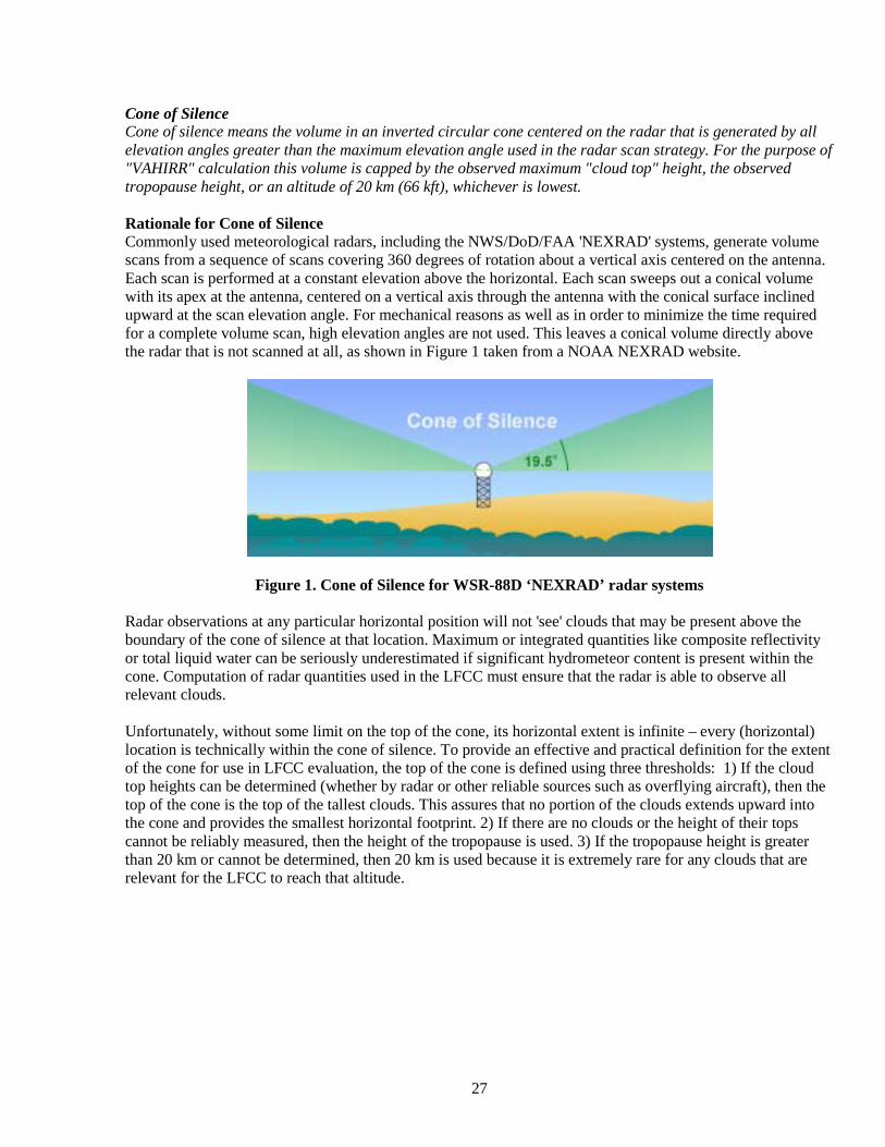
27

Cone of Silence Cone of silence means the volume in an inverted circular cone centered on the radar that is generated by all elevation angles greater than the maximum elevation angle used in the radar scan strategy. For the purpose of "VAHIRR" calculation this volume is capped by the observed maximum "cloud top" height, the observed tropopause height, or an altitude of 20 km (66 kft), whichever is lowest. Rationale for Cone of Silence Commonly used meteorological radars, including the NWS/DoD/FAA 'NEXRAD' systems, generate volume scans from a sequence of scans covering 360 degrees of rotation about a vertical axis centered on the antenna. Each scan is performed at a constant elevation above the horizontal. Each scan sweeps out a conical volume with its apex at the antenna, centered on a vertical axis through the antenna with the conical surface inclined upward at the scan elevation angle. For mechanical reasons as well as in order to minimize the time required for a complete volume scan, high elevation angles are not used. This leaves a conical volume directly above the radar that is not scanned at all, as shown in Figure 1 taken from a NOAA NEXRAD website.

Figure 1. Cone of Silence for WSR-88D ‘NEXRAD’ radar systems Radar observations at any particular horizontal position will not 'see' clouds that may be present above the boundary of the cone of silence at that location. Maximum or integrated quantities like composite reflectivity or total liquid water can be seriously underestimated if significant hydrometeor content is present within the cone. Computation of radar quantities used in the LFCC must ensure that the radar is able to observe all relevant clouds. Unfortunately, without some limit on the top of the cone, its horizontal extent is infinite – every (horizontal) location is technically within the cone of silence. To provide an effective and practical definition for the extent of the cone for use in LFCC evaluation, the top of the cone is defined using three thresholds: 1) If the cloud top heights can be determined (whether by radar or other reliable sources such as overflying aircraft), then the top of the cone is the top of the tallest clouds. This assures that no portion of the clouds extends upward into the cone and provides the smallest horizontal footprint. 2) If there are no clouds or the height of their tops cannot be reliably measured, then the height of the tropopause is used. 3) If the tropopause height is greater than 20 km or cannot be determined, then 20 km is used because it is extremely rare for any clouds that are relevant for the LFCC to reach that altitude.

28

Cumulonimbus Cloud Cumulonimbus cloud means any convective "cloud" with any part at an altitude where the temperature is colder than –20 degrees Celsius. Rationale for Cumulonimbus cloud Similar to the definition in the AMS Glossary of Meteorology (2000), given below, except that the cloud top must be above the -20 ºC level because that is the height at which strong electrification becomes probable (see Section A3.1.3 of Appendix 3, "Cloud Electrification"). Cumulonimbus clouds do not necessarily produce lightning. Note that 'thunderstorm' is not interchangeable with 'cumulonimbus cloud' in the LFCC: a thunderstorm need not have its top colder than -20 °C but must produce lightning. Both definitions are required here because anvil clouds can be generated by convective clouds with tops between -10 and -20 °C (not cumulonimbi) whereas debris clouds can be produced only by cumulonimbi or thunderstorms.

Glossary Definition "cumulonimbus—(Abbreviated Cb.) A principal cloud type (cloud genus), exceptionally dense and vertically developed, occurring either as isolated clouds or as a line or wall of clouds with separated upper portions..."

Reference: American Meteorological Society, 2000: Glossary Of Meteorology, 2nd ed. , American Meteorological


29

Debris Cloud Debris cloud means any "cloud," except an "anvil cloud," that has become detached from a parent "cumulonimbus cloud" or "thunderstorm," or that results from the decay of a parent "cumulonimbus cloud" or "thunderstorm." Rationale for Debris cloud No further explanation needed except to note explicitly that debris clouds include any nimbostratus and other clouds that are produced by a thunderstorm. Note, however, that language in Section G417.15(a) of the "Debris Clouds" Rule, ("...after the 'debris cloud' is observed to have formed by the collapse of the parent 'cloud top' to an altitude where the temperature is warmer than -10 degrees Celsius...") effectively narrows the application of that rule to exclude decaying cumulonimbus clouds or thunderstorms whose cloud tops have not yet descended below the -10 °C level. Such clouds are still identified as debris clouds by this definition, but they are also cumuli and are therefore covered by Sections G417.9(a) or( b) of the "Cumulus Clouds" Rule until they collapse below the -10 °C level. In particular, the standoff requirements in G417.9(a) and (b) are more stringent than those in the "Debris Clouds" Rule (10 and 5 n mi, respectively, forever, as opposed to 3 n mi for 3 hours with exceptions).

30

Disturbed Weather Disturbed weather means a weather system where dynamical processes destabilize the air on a scale larger than individual "clouds" or cells. Examples of "disturbed weather" include fronts, troughs, and squall lines. Rationale for Disturbed Weather Disturbed weather is a generalization of the weather that was present at the time of the Apollo 12 and AC 67 incidents, when there was widespread rain and no evidence of natural lightning in the KSC-CCAFS area. It is understood that disturbed weather in the sense of the Apollo 12 and AC 67 experiences was associated with frontal passages where dynamical processes (rather than surface heating or topography) provided the initial lifting of air that was required for cloud electrification.

31

Electric Field Measurement Electric field measurement means the 1-minute arithmetic average of the vertical electric field (Ez) at the surface of Earth, measured by a ground-based "field mill." The polarity of the electric field is the same as that of the potential gradient; that is, the polarity of the field at Earth's surface is the same as the dominant charge overhead. Do not use interpolated electric field contours for purposes of this appendix. An "'electric field measurement' less than or equal to 5 nautical miles from the 'flight path'" [e.g., C. G417.5(a) Surface Electric Fields] is not applicable if the altitude of the flight path everywhere above the 5 nautical mile circle around the "field mill" in question is greater than 20 km (66 kft). Rationale for Electric Field Measurement Here, the instantaneous, vertical, electric field that is measured on the earth's surface is an arithmetic average (respecting polarity) over one minute in order to minimize the effects of both distant lightning discharges and local fluctuations due to space-charge advection on the operationally significant data. This averaging gives a signed, scalar quantity (an 'electric field measurement') with a polarity that is defined, for the purposes of the LFCC, to be positive when the dominant charge overhead is positive. When the dominant charge aloft is negative, the electric field measurement is negative. There are several different methods for measuring the surface electric field, but field mills are the only instruments that have been demonstrated to accurately and reliably measure both low and high fields under a variety of weather conditions without excessive maintenance. See Section A1.1 of Appendix 1, "Measurement and Interpretation of Surface Electric Fields," for further details. To avoid confusion about polarity, it should be noted that the LFCC use the traditional 'atmospheric electricity' sign convention for surface measurements, which has now been almost universally replaced in the scientific literature by the 'physics' convention. When using the physics convention, the direction of the electric field is in the direction of the electric force on a positive test charge, and the upward direction of the vertical component is considered positive for both field and force. (For more discussion of the meaning and relevance of the vertical component of field, see the rationale for the "Surface Electric Fields" Rule, G417.5.) Thus, in 'fair weather' when the dominant charge overhead is positive, the electric force will be downward and the electric field will be considered negative in the physics convention. Conversely, when the dominant charge overhead is negative, as is often the case in 'foul weather,' the surface electric field will be positive. With this physics sign convention, an 'electric field measurement,' as the term is used in the LFCC, would be referred to as a measurement of the vertical 'potential gradient' at the surface. An electric field value that is interpolated from the contour lines of several simultaneous electric field measurements on a display will depend strongly on the interpolation algorithm that is used to compute those contours. Therefore such an interpolated value is not considered valid as a direct electric field measurement. Further, a valid electric field measurement is not considered applicable when the altitude of the relevant part of the flight path exceeds 20 km because a surface measurement no longer represents the electric field aloft that will affect the vehicle.

32

Field Mill Field mill is a specific class of electric-field sensor that uses a moving, grounded conductor to induce a time-varying electric charge on one or more sensing elements in proportion to the ambient electrostatic field. Rationale for Field Mill This definition is somewhat more general than that of the Glossary of Meteorology (2000), quoted below. No further explanation needed. See Section A1.1.1 of Appendix 1, "Measurement and Interpretation of Surface Electric Fields," for further details.

Glossary Definition "field mill—An instrument that obtains a continuous measurement of the sign and magnitude of the local electric potential gradient by alternately shielding and exposing a conductor that is grounded through a resistance to develop an alternating potential that is proportional to the field."



33

Flight Path Flight path means the planned nominal flight trajectory, including its vertical and horizontal uncertainties specified by the three-sigma guidance and performance deviations. Rationale for Flight Path The effects of atmospheric electricity on a launch vehicle and the effects of the launch vehicle on the atmospheric electric fields due to the conductive vehicle and its ionized plume depend on the actual flight path of the vehicle, which is unknown until the flight has taken place. For the purposes of pre-launch assessment of the risk, it is necessary to assume a flight path to be used for the assessment. To ensure that the assumed flight path encompasses the actual flight path, the LFCC are to be evaluated along the planned flight path and all reasonably foreseeable deviations from the flight path in the absence of a major failure of the vehicle. For the purposes of the LFCC, reasonably foreseeable deviations are those having an occurrence probability less than or equal to the three-sigma deviation of a Gaussian distribution, which is 0.001.

34

Moderate Precipitation Moderate precipitation means a "precipitation" rate of 0.1 inches/hr or a "radar reflectivity" factor of 30 dBZ. Rationale for Moderate Precipitation This combined rain-rate/radar definition is an extension of the conventional definition of moderate rain. The Federal Meteorological Handbook No. 1 (2005) defines light rain as "up to 0.10 inch per hour; maximum 0.01 inch in 6 minutes" and moderate rain as "0.11 inch to 0.30 inch per hour; more than 0.01 inch to 0.03 inch in 6 minutes." The radar threshold of 30 dBZ for moderate precipitation is a historical convention and is based on the second precipitation intensity level of the Video Integrator and Processor (VIP2) that has been used in the WSR-57 and WSR-74C radar systems deployed by the National Weather Service since the late 1950s. Reference Office of the Federal Coordinator for Meteorology, 2005: Federal Meteorological Handbook No. 1, Surface

Weather Observations and Reports, FCM-H1-2005, Washington, D.C., September 2005.

35

Nontransparent Nontransparent. "Cloud" cover is "nontransparent" if one or more of the following conditions is present:

(a) Objects above, including higher "clouds," blue sky, and stars, are blurred, indistinct, or obscured as viewed from below; or objects below, including terrain, buildings, and lights on the ground, are blurred, indistinct, or obscured as viewed from above; when looking through the "cloud" cover at visible wavelengths (the sun and moon may not be used to evaluate transparency);

(b) Such objects are seen distinctly only through breaks in the "cloud" cover; or

(c) The "cloud" cover has a "radar reflectivity" factor of 0 dBZ or greater.

Rationale for Nontransparent This definition is related to that of 'transparent sky cover' in the Glossary of Meteorology (2000), quoted below, but is significantly more general and supplemented by an alternate radar definition. Optical transparency is an indication of the combined effects of the geometric thickness of a cloud and total surface area of the cloud particles per unit volume of cloud. Parts (a) and (b) of this definition list some of the commonly used methods for estimating optical transparency. The greater the vertical thickness of the cloud, the greater its ability to form 'screening layers' on its surfaces and store electric charge in its interior. The greater the total surface area of all ice particles and cloud droplets in the cloud per unit volume, the lower the electrical conductivity, and the longer any internal charge (and electric field) can be stored. Visible (as opposed to radar) wavelengths are preferred because they emphasize the smaller cloud particles that usually contribute the majority of the surface area per unit volume. Images or shadows cast by the Sun or Moon may not be used to estimate transparency because these objects have too high an inherent contrast with the background sky and will therefore produce an excessive (risky) result. A non-transparent cloud can store elevated electric fields for long times; a transparent cloud will not. See Sections A6.2 and A6.4 of Appendix 6, "Electrical Properties and Decay of Electric Fields in Cloudy Air," for further details. A radar reflectivity of 0 dBZ correlates well with the visible edge of anvil clouds in the vicinity of the Kennedy Space Center, Florida (Merceret et al., 2006.). Cumulus clouds with some precipitation development and often debris clouds have closely spaced contours of radar reflectivity, so the visible cloud boundary also corresponds well with the 0 dBZ contour. 0 dBZ may therefore be used to evaluate transparency when visual means are not available.

Glossary Definition "transparent sky cover—In U.S. weather observing practice, that portion of sky cover through which higher clouds, blue sky, etc., may be observed; opposed to opaque sky cover."


Society, Boston, MA, 850 pp. Merceret, F.J., D.A. Short and J.G. Ward, 2006: Radar evaluation of optical cloud constraints to space launch

operations, J. Spacecraft & Rockets, 43(1), 248-251.

36

Precipitation Precipitation means detectable rain, snow, hail, graupel, or sleet at the ground; virga; or a "radar reflectivity" factor greater than 18 dBZ at any altitude above the ground. Rationale for Precipitation The Glossary of Meteorology (2000) first definition of precipitation is,

Glossary Definition "precipitation—1. All liquid or solid phase aqueous particles that originate in the atmosphere and fall to the earth's surface."

The LFCC definition is an exhaustive list of precipitation forms that also includes virga (rain, snow, etc. that does not reach the ground) and an alternative radar-based definition. The radar criterion enables the use of radar for cases when precipitation may be too distant or obscured by clouds, fog or haze. The inclusion of virga allows for the fact that, although the precipitation might not reach the ground, it is an indicator of possible charging. The radar threshold of 18 dBZ for precipitation is a historical convention and is based on the lowest precipitation intensity level of the Video Integrator and Processor (VIP1) used in the WSR-57 and WSR-74C radar systems deployed by the National Weather Service from the late 1950s. 'Detectable,' as used in this definition, means that the precipitation is observed visually by ground observers, measured by surface gauges or observed aloft from an aircraft either visually or with instrumentation. For visual observations from an aircraft, the mere presence of water on the windscreen while in cloud does not constitute detection of precipitation because cloud droplets can cause visible wetting similar to that caused by small precipitation drops. The launch weather team should discuss such observations with the airborne observer and decide whether they constitute detection of precipitation based on the total context of the observations, including the synoptic environment and radar data. Visible water on the windscreen, when flying below cloud base, is sufficient to constitute detection of precipitation. Reference American Meteorological Society, 2000: Glossary Of Meteorology, 2nd ed. , American Meteorological


37

Radar Reflectivity Radar reflectivity means the radar return from hydrometeors, in dBZ, measured by a meteorological radar operating at a wavelength greater than or equal to 5 cm. A "radar reflectivity" measurement is valid only in the absence of significant attenuation by intervening "precipitation" or by water or ice on the radome. Rationale for Radar Reflectivity Here there are important differences from, and extensions to, the definition in the Glossary of Meteorology (2000), quoted below. The LFCC use radar reflectivity measurements for a variety of purposes including determining the position in three dimensions and vertical extent of clouds and computing the VAHIRR quantity. The radar measurements are used quantitatively, with precise dBZ values specified. The definition of radar reflectivity is designed to assure that the measurements have sufficient accuracy for such quantitative use. There are several components of the definition and each will be discussed in turn. See Section A9.2 of Appendix 9, "Application of Weather Radar to LFCC Evaluation," for further details.

(a) The radar must be a meteorological radar. Radar systems specifically designed for meteorological applications normalize the reflectivity values to compensate for the effects of frequency and range in order to provide standardized values of dBZ with an accuracy of 1 dBZ or better independent of frequency and range. [The reference value for dBZ (0 dBZ) is 1 mm6 m-3 (Bringi and Chandrasekar, 2001, Section 3.10).] In addition, most meteorological radars have clutter suppression software that minimizes the effects of ground clutter without rejecting a significant amount of meteorological echoes.

(b) The wavelength must not be shorter than 5 cm. Attenuation of radar signals increases rapidly as the

wavelength decreases. Depending on the drop size distribution, attenuation in rain increases by from one to two orders of magnitude as the wavelength decreases from 10 to 3 cm (Bringi and Chandrasekar, 2001, Section 7.4.). At wavelengths shorter than 5 cm, even moderate precipitation between the radar and the portion of the cloud being sampled will produce unacceptable errors in the radar measurement. Errors introduced by attenuation are especially dangerous because they always make the reflectivity appear smaller than it actually is, thus making the environment appear safer than it actually is.

(c) A measurement is valid only in the absence of significant attenuation by intervening precipitation or

by water or ice on the radome. Even with wavelengths of 5 cm or longer, attenuation from intervening precipitation or water on the radome (Merceret and Ward, 2002) can cause unacceptable attenuation. This component explicitly requires the LFCC to be evaluated with this consideration in mind.

(d) The measured reflectivity must be due to hydrometeors, not to non-meteorological targets such as

flocks of birds, swarms of insects, or 'anomalous propagation' -- see also the rationale for the definition of 'VAHIRR application criteria.'

Glossary Definition "radar reflectivity—In general, a measure of the efficiency of a radar target in intercepting and returning radio energy. It depends upon the size, shape, aspect, and dielectric properties of the target..."


Society, Boston, MA, 850 pp. Bringi, V.N. and V. Chandrasekar, 2001: Polarimetric Doppler Weather Radar, Cambridge University Press,

New York, NY, 636 pp.

38

Merceret, Francis J. and Jennifer G. Ward, 2002: Attenuation of Weather Radar Signals Due to Wetting of the

Radome by Rainwater or Incomplete Filling of the Beam Volume, NASA Technical Memorandum TM-2002-211171, April 2002, 16pp.

39

Specified Volume Specified volume. The volume bounded in the horizontal by vertical planes with perpendicular sides located 5.5 km (3 nautical miles) north, east, south, and west of the point at which "VAHIRR" is being computed. The volume is bounded on the bottom at the altitude where the temperature is 0 degrees Celsius, and on the top by a fixed altitude of 20 km (66 kft). Rationale for Specified Volume Examination of the results from the second Airborne Field Mill (ABFM II) experiment determined that averaging the radar reflectivity over a horizontal area of 11 x 11 km (5 km in the north, south, east and west directions from the 1 km cube containing the aircraft) is suitable for detecting strong electric fields. (See Section A7.1 of Appendix 7, "Physical and Statistical Basis for VAHIRR.") The 5.5 km distance used in this definition is the result of adding half of the grid point spacing of the 1 km gridded radar data to the 5 km distance from the 1 km grid point closest to the position of the aircraft. The specified volume extends from the altitude of 0 degrees Celsius and not below because studies have shown that charge separation can occur at and above the 0 °C level (see Appendices 3, "Cloud Electrification," and 4, "Electrical Aspects of Stratiform Clouds"). It extends to 20 km so that the average includes the top of any anvil. (It is necessary to specify a fixed upper lid on the specified volume because this lid affects the calculation of the fraction of grid points with radar reflectivity greater than or equal to 0 dBZ, which fraction enters into the definition of 'volume-averaged radar reflectivity' -- see below.)

40

Thick Cloud Layer Thick cloud layer means one or more "cloud layers" whose combined vertical extent from the base of the bottom layer to the "cloud top" of the uppermost layer exceeds a thickness of 4,500 feet. "Cloud layers" are combined with neighboring layers for determining total thickness only when they are physically connected by vertically continuous "clouds," as, for example, when towering "clouds" in one layer contact or merge with "clouds" in a layer (or layers) above. Rationale for Thick Cloud Layer This is an extension of the definition of 'cloud layer' -- see the present definition of that term above. Combining individual cloud layers into a single layer for the purpose of defining overall thickness is consistent with the possibility that electrical contact between layers can allow the operation of an electrical generator to charge significant portions of the interconnected layers. The definition spells out the conditions under which multiple layers are to be considered connected. See the rationale for the "Thick Cloud Layers" Rule, G417.19, for an explanation of the 4500 ft thickness threshold.

41

Thunderstorm Thunderstorm means any convective "cloud" that produces lightning. Rationale for Thunderstorm Essentially the same as the definition in the Glossary of Meteorology (2000) (given below). Note that 'cumulonimbus cloud' is not interchangeable with 'thunderstorm' in the LFCC: a thunderstorm need not have its top colder than -20 °C, whereas a cumulonimbus need not produce lightning. Both definitions are required here because anvil clouds can be generated by convective clouds with tops between -10 and -20 °C (not cumulonimbi) whereas debris clouds can be produced only by cumulonimbi or thunderstorms.

Glossary Definition “thunderstorm—(Sometimes called electrical storm.) In general, a local storm, invariably produced by a cumulonimbus cloud and always accompanied by lightning and thunder, usually with strong gusts of wind, heavy rain, and sometimes with hail..."



42

Transparent Transparent. Any "cloud" that is not "nontransparent" is "transparent." Rationale for Transparent See the present definition of 'nontransparent' above. No further explanation is needed.

43

Treated Treated means that a launch vehicle satisfies both of the following conditions:

(a) All surfaces of the launch vehicle susceptible to ice particle impact are such that the surface resistivity is less than 109 "Ohms per square;" and

(b) All conductors on surfaces (including dielectric surfaces that have been coated with conductive

materials) are bonded to the launch vehicle by a resistance that is less than 105 ohms. Rationale for Treated Triboelectric charging of both dielectric and metallic surfaces on vehicle exteriors can result in electrical upset to flight-critical components and/or even physical damage (NASA, 1974; Nanevicz, 1982; Lorenz, 2008) -- see the rationale for the "Triboelectrification" Rule, G417.23. Charging of dielectrics can produce surface discharges on both the exterior and interior surfaces of those dielectrics and allow penetration of disruptive electric fields into the interior of the vehicle. Differential charging of inadequately bonded metallic surfaces can cause sparking between those surfaces or to the airframe, resulting in the penetration of disruptive electrical noise into the interior. Surface treatment means altering (if necessary) the surface resistivity of dielectrics so that surface discharges do not occur. Bonding means lowering the electrical resistance between isolated metallic surfaces and the airframe to prevent sparking. The resistivity criteria are taken from Nanevicz (1973). References Lorenz, R. D., 2008: Atmospheric electricity hazards, Space Sci Rev, 137: 287–294,

DOI 10.1007/s11214-008-9364-x Nanevicz, J. E., 1973: Advanced Materials Aspects and Concepts for Development of Antistatic Coatings, for

Aircraft Transparencies Universal Technology Corporation, Dayton, Ohio, Contract F33615-72-C-2113 SRI Project 2393, 22 February 1973.

Nanevicz, J. E., 1982: Static charging and its effects on avionics systems, IEEE Trans. on EMC, EMC-24 (2),

May, 1982. NASA, 1974: Space Vehicle Design Criteria (Environment) - Assessment and Control of Electrostatic

Charges, SP-8111, May, 1974.

44

Triboelectrification Triboelectrification means the transfer of electrical charge between ice particles and the launch vehicle when the ice particles collide with the vehicle during flight. Rationale for Triboelectrification This is a narrower definition of the more familiar term ‘precipitation static’ or ‘p-static’ that is more specific to space flight than that in the Glossary of Meteorology (2000), quoted below. The triboelectric effect is a form of contact electrification in which one material exchanges electric charge with a different material during contact and opposite charges appear when the materials are separated (such as through rubbing). The polarity and magnitude of the separated charge depend on the specific materials. Data show that, when ice particles (charged or uncharged) strike a flying vehicle at a high rate, they will usually raise the electrical potential of the vehicle to tens or hundreds of kilovolts, usually of negative polarity, and this process can produce corona from the vehicle, or charge untreated dielectric or un-bonded conducting surfaces in ways that can cause surface discharges, physical damage, and/or electrical upset (Nanevicz and Tanner, 1964; NASA, 1974; Nanevicz, 1982). Charging occurs both on the metal structure of launch vehicles and on dielectric surfaces. Ice particles are much more effective chargers than water droplets. (Note: Charging by the vehicle engines, collisions with dust or smoke particles, or the flight through volcanic plumes could also electrify the vehicle, but these are not included in the above definition.)

Glossary Definition "triboelectrification—A process of charge separation that involves the rubbing together of dissimilar material surfaces..."


Society, Boston, MA, 850 pp. Nanevicz, J. E. and R. L. Tanner, 1964: Some Techniques for Elimination of Corona Discharge Noise in

Aircraft Antennas, Proc. IEEE, pp. 53-64, January 1964. Nanevicz, J. E., 1982: Static charging and its effects on avionics systems, IEEE Trans. on EMC, EMC-24 (2),



45

Volume-Averaged, Height-Integrated Radar Reflectivity (VAHIRR) Volume-Averaged, Height-Integrated Radar Reflectivity (VAHIRR) is the product of the "volume-averaged radar reflectivity" and the "average cloud thickness" in a "specified volume" surrounding any point at which "VAHIRR" is being computed (units of dBZ-km). The "specified volume" must not contain any portion of the "cone of silence" above the radar, nor any portion of any sectors that may have been blocked out for payload-safety reasons. Rationale for VAHIRR Measurements made during ABFM II, in both attached and detached anvil clouds and in debris clouds show that, when the electric field is strong (> 3 kV m-1), the radar reflectivity in the same location is normally greater than approximately 10 dBZ. (Note that 3 kV/m is a very conservative threshold for triggered lightning at anvil altitudes, as explained in Section 5.4.3 of Appendix 5, "Conditions for Triggered Lightning.") Regions with weaker reflectivity usually do not have strong fields. However, on the few occasions when there were strong fields co-located with weak reflectivity, the reflectivity within a couple of kilometers was always much stronger. Therefore, averaging the reflectivity over a sufficiently large volume centered on the field-measurement point can be used to detect the presence of these occasional strong fields at locations having low local reflectivities. An added advantage of using a volume-averaged reflectivity is that the natural point-to-point variations inherent in reflectivity measurements are reduced. A thin anvil can have the same average reflectivity as a much thicker anvil; but because bigger thunderstorms are generally more electrically active and also produce more mass flux out of the convective core and therefore a deeper anvil, a thick anvil has a much larger probability of containing strong electric fields. To compensate for this effect, the average reflectivity is multiplied by the radar-determined average thickness of the anvil in the specified volume in which the average reflectivity is computed. The resulting radar-based parameter is called Volume-Averaged, Height-Integrated Radar Reflectivity (VAHIRR -- see Section A7.1 of Appendix 7, "Physical and Statistical Basis for VAHIRR"). To be certain that a valid reflectivity average is used, VAHIRR is not applicable when the radar cone of silence or any blockage of the beam intersects the specified volume. Statistical studies using a parametric tail analysis with a Weibull distribution of both the anvil and the debris cloud data sets, and an extreme value analysis for the larger anvil data set (Dye et al., 2006), all show that, when VAHIRR is ≤ 10 dBZ-km, the probability of having electric fields in excess of 3 kV m-1 is very small (on the order of 10-4 or lower). Based on these findings VAHIRR is now used in LFCC rules for attached anvils, detached anvils and debris clouds to provide additional launch availability. See the rationales for these individual rules and Section A7.2 of Appendix 7, "Physical and Statistical Basis for VAHIRR," for further details. Reference Dye, J.E. M.G. Bateman, D.M. Mach, C.A. Grainger, H.J. Christian, H.C. Koons, E.P. Krider, F.J. Merceret,

J.C. Willett, 2006: The scientific basis for a radar-based lightning launch commit criterion for anvil clouds, Amer. Meteor. Soc. Conf. on Aviat. Range and Aerosp. Meteorol., Feb. 2006, Atlanta Georgia, paper 8.4.

46

VAHIRR Application Criteria VAHIRR application criteria: The individual grid-point reflectivity measurements used to determine either the "volume-averaged radar reflectivity" or the "average cloud thickness" must be meteorological "radar reflectivity" measurements. For "VAHIRR"-evaluation points along the "flight path" itself (not those at a prescribed distance away from the "flight path"), the "volume-averaged, height-integrated radar reflectivity" is not applicable at any point that is less than or equal to 10 nautical miles from any "radar reflectivity" of 35 dBZ or greater at altitudes of 4 km (13 kft) or greater above mean sea level, nor is it applicable at any point that is less than or equal to 10 nautical miles from any type of lightning that has occurred in the previous 5 minutes. Rationale for VAHIRR application criteria The application criteria are provided to assure that the values of VAHIRR used to determine whether the LFCC are satisfied are measured under the same conditions used in developing and validating the VAHIRR concept. There are two components to this: the radar measurements must be accurate, and they must not violate conditions imposed upon the ABFM-II data set from which the VAHIRR threshold was derived. The first component is satisfied by adherence to the definition of 'radar reflectivity' as provided in these rules and by the additional requirement provided here that such reflectivity must arise from meteorological echoes rather than things like, for example, anomalous propagation. The second component imposes proximity constraints to high-reflectivity areas and lightning when VAHIRR is evaluated along the flight path. These are the same constraints used in selecting the ABFM-II data for the statistical analysis upon which the safety of LFCC based on VAHIRR was evaluated. (Conditions that violated these constraints would already prevent launch through application of the "Cumulus Clouds" or "Lightning" Rules, so they were not relevant to the statistical analysis and might have biased it unnecessarily.) Use of VAHIRR unconstrained by these requirements has not been studied and could be extremely dangerous. Note, however, that certain sections of the "Attached Anvil Clouds," "Detached Anvil Clouds," and "Debris Clouds" Rules (G417.11(c)(2), G417.13(b)(2) and G417.13(c)(2)(ii), and G417.15(a)(2)(ii)) require the VAHIRR threshold to be satisfied everywhere within 1 n mi of the flight path in order to relax 3 n mi standoff requirements. (As explained in the rationales for those rules, this is to assure that some part of the cloud is sampled by radar for the VAHIRR exception to apply -- see the definitions of 'Specified Volume,' etc.) In cases where the VAHIRR threshold must be satisfied at points near, but not on, the flight path, the proximity constraints are eliminated in order to avoid effectively extending the standoff distances in the "Cumulus Clouds" and "Lightning" Rules from 10 to 11 n mi. See Section 7.1 of Appendix 7, "Physical and Statistical Basis for VAHIRR," for further details.

47

Volume-Averaged Radar Reflectivity Volume-averaged radar reflectivity is the arithmetic average (in dBZ) of the "radar reflectivity" in the "specified volume." Normally, a radar processor will report reflectivity values interpolated onto a regular, three-dimensional array of grid points. Any such grid point in the "specified volume" is included in the average if and only if it has a "radar reflectivity" equal to or greater than 0 dBZ. If fewer than 10% of the grid points in the "specified volume" have "radar reflectivity" measurements equal to or greater than 0 dBZ, then the "volume-averaged radar reflectivity" is either the maximum "radar reflectivity" (in dBZ) in the "specified volume," or 0 dBZ, whichever is greater. Rationale for Volume-Averaged Radar Reflectivity The volume-averaged radar reflectivity must be calculated in exactly this way because it was done this way in the ABFM II statistical analysis on which the VAHIRR exceptions are based. (See Section 7.1 of Appendix 7, "Physical and Statistical Basis for VAHIRR," for further details.) Arithmetic averages of reflectivity in units of Z rather than dBZ were found to bias the result towards higher reflectivity values that were not consistently representative of the probability of hazardous electric fields, so reflectivity is averaged in dBZ. The cut-off value of 0 dBZ is used in the determination of the volume-averaged radar reflectivity because the cloud boundary is defined as 0 dBZ in the LFCC. In order to ensure that a sufficient number of grid points are available to obtain a reliable average reflectivity at a given VAHIRR-evaluation point, at least 10% of the grid points within the specified volume must have measurable reflectivity ≥ 0 dBZ. In order to avoid invalid VAHIRR points that might obviate the benefit of the VAHIRR exceptions (for example, in clear air near an anvil), when the fraction of measureable grid points is less than 10%, the volume-averaged radar reflectivity is re-defined to be the maximum reflectivity in the specified volume or 0 dBZ, whichever is greater. Since the maximum reflectivity in a volume is always greater than the average in that same volume, this permits the use of VAHIRR while remaining very conservative.

48

G417.5 Surface Electric Fields

(a) A launch operator must not initiate flight for 15 minutes after the absolute value of any "electric field measurement" less than or equal to 5 nautical miles from the "flight path" has been greater than or equal to 1500 volts/meter.

(b) A launch operator must not initiate flight for 15 minutes after the absolute value of any "electric field

measurement" less than or equal to 5 nautical miles from the "flight path" has been greater than or equal to 1000 volts/meter unless either Section 1 or Section 2 is satisfied:

(1) All clouds less than or equal to 10 nautical miles from the "flight path" are "transparent;" or (2) All "clouds" less than or equal to 10 nautical miles from the "flight path" have "cloud tops" at

altitudes where the temperature is warmer than +5 degrees Celsius and have not been part of convective "clouds" with "cloud tops" at altitudes where the temperature is colder than or equal to −10 degrees Celsius during the last 3 hours.

Rationale for G417.5 Surface Electric Fields General Background. The critical importance of an elevated electric field extending over a large volume of space is that it represents stored electrostatic energy that, under the right conditions, can initiate and propagate a lightning discharge. Thus the ambient electric field is the key physical parameter that determines the risk of triggering lightning. (The size, shape, velocity, and altitude of a launch vehicle also play a role in triggering.) Because of this direct connection between the electric field and triggered lightning, the "Surface Electric Fields" Rule is considered one of the most important LFCC. See Sections and A5.1 and A5.3.3 of Appendix 5, "Conditions for Triggered Lightning," for further details. The electric (electrostatic) field is a physical parameter that describes the net electric force on a unit 'test charge' due to any source-charge distribution, both within the surrounding atmosphere and on any nearby conducting or non-conducting surfaces (e.g., Reitz and Milford, 1967, Equation 2-8). In the atmosphere, this charge may be in the form of 'small ions,' which move, or 'drift,' in response to the field and give air its finite 'electrical conductivity,' or on the relatively immobile particles in the atmospheric aerosol, including cloud droplets, ice crystals, and precipitation particles. (e.g., MacGorman and Rust, 1998.) . Since the magnitude of the electric field is inversely proportion to the square of the distance from any localized source, nearby charges have a much greater effect on the field than more distant sources. The small and medium-sized water droplets, ice crystals, and precipitation particles in clouds have a large total surface area per unit volume on which to store electric charge. This same surface area will also act as an efficient sink for small ions and thereby reduce the electrical conductivity of cloudy air and increase the time that significant charge (and electric fields) can be stored therein. At the same time, the differences between the conductivities of cloudy and clear air will allow oppositely charged screening layers to form near the surfaces of cloud layers. These screening layers will effectively mask the electric field that is produced by the interior cloud charge and prevent it from being detected outside the cloud. This 'screening' or masking of the interior charges is especially important when the clouds of interest are long-lived stratiform or layer clouds. See Sections A6.0, A6.2, and A6.4 of Appendix 6, "Electrical Properties and Decay of Electric Fields in Cloudy Air," for further details. The 'electric field measurement' that is referred to in this rule is the time-average of the (vector) field at the earth's surface. Because the field is always perpendicular to a perfect conductor and the earth at a suitable measurement site is, for all practical purposes, a perfect horizontal conductor, the vector field there will always

49

be directed vertically. Thus an 'electric field measurement' refers to a signed scalar quantity that has the polarity specified in its definition. The most accurate and reliable instrument for measuring such a field is a 'field mill' (see Section A1.1.1 of Appendix i, "Measurement and Interpretation of Surface Electric Fields." Also because of this vertical orientation, a measurement of the surface electric field at a single location provides no direct information about the location or magnitude of the charges aloft that are producing it, only their dominant polarity. The magnitude, polarity, and time-behavior of an individual electric field measurement do, however, provide a good qualitative indication of electricity in the atmosphere aloft and of the risk of both natural and triggered lightning. In some cases, the locations and magnitudes of the cloud charge centers can be inferred from simultaneous electric field measurements at several locations; hence there is great benefit in having a network of electric field sensors like the LPLWS. Further, a large-area network minimizes the chances that a single measurement will be close to a local polarity reversal in the horizontal distribution of surface field that is due to a vertical or tilted electrostatic dipole in the source-charge distribution. Such a network also limits the information loss due to other types of single-point failure. See Merceret and Willett et al. (2010, Appendix A8.1.1) and Sections A1.2.2 and A1.3 of Appendix 1, "Measurement and Interpretation of Surface Electric Fields," for further discussion of the benefits of a large-area network. Another factor that may complicate the interpretation of electric field measurements is that 'corona discharges' will occur on nearby structures and vegetation when the ambient electric field exceeds 1000 to 3000 Volts per meter. The local space charge that is produced by any such corona will normally be opposite in sign to the dominant charge aloft and will partially shield an electric field measurement from that dominant charge aloft, much as the screening layer on a cloud boundary can shield the external field from that produced by an interior charge. Under such circumstances, the electric field measurement appears to 'saturate' at a magnitude that is close to the threshold for producing corona and becomes less sensitive to the magnitude of the field aloft. (The absolute magnitude and temporal variation of an electric field measurement, as well as the spatial distribution of such measurements across a network of field mills, can be very helpful in recognizing this effect.) See Section A1.3.3.1 of Appendix 1, "Measurement and Interpretation of Surface Electric Fields," for further details. Specific Rationale for the "Surface Electric Field" Rule. This rule is a 'fail-safe' requirement that is intended to provide protection from hazardous electric fields aloft that may be either unexpected or inadequately predicted by the other, cloud-based rules. (See Chapter 1 for further details about the general structure of the rules.) As explained above, a network of electric field mills is regarded as extremely important to flight safety. Nevertheless, such specific instrumentation cannot be required at all ranges, so the language, "the absolute value of any 'electric field measurement,'" is used to indicate that the rule applies if and only if such measurements are available. The magnitude of the fair-weather electric field at the earth’s surface is normally a few hundred V/m or less. When the electric field at the ground exceeds a few kV/m, depending on terrain and vegetation, the field above the ground can be much larger than that because of masking by corona space charge. Therefore an electric field threshold of 1 kV/m, or 1.5 kV/m in special cases, is large enough to eliminate most false alarms but small enough to prevent a significant number of 'failures-to-warn.' Part (a) of this rule specifies a threshold of 1.5 kV/m under all circumstances, because benign local phenomena such as smoke, ground fog, surf electrification, a 'sunrise effect,' and the space charge emitted by high-voltage power lines occasionally produce electric field measurements that are between 1 and 1.5 kV/m in otherwise fair weather (see Section A1.2.1 of Appendix 1, "Measurements and Interpretation of Surface Electric Fields"). Part (b) of this rule reduces this threshold to a more conservative level of 1 kV/m when it is possible that clouds near the launch site could be producing elevated electric fields that might cause corona space charge to shield the surface measurement. Such hazardous fields aloft are never produced by (b)(1) transparent clouds, nor by (b)(2) warm clouds that have not recently been part of potentially electrified convective clouds. See the

50

definition of 'nontransparent' for an explanation of the requirement in Section (b)(1). See the rationale for the "Cumulus Clouds" Rule, G417.9, for an explanation of the choice of +5 °C and -10 °C cloud-top temperatures in Section (b)(2). A primary concern in Section (b)(2) is to avoid any debris clouds that might contain residual charge from their parent clouds, and this is the origin of the 3-hour waiting time here (see the rationale for the "Debris Clouds" Rule, G417.15). Note that the exceptions provided by Sections (b)(1) and (b)(2) of this rule are especially stringent (e.g., the 10 n mi standoff requirements), compared to those in certain other rules, because an elevated electric field aloft is itself a triggered-lightning hazard, and because an electric field measurement of 1 kV/m or greater is the most direct indicator available (other than nearby lightning) of an elevated field aloft. The standoff distance (5 n mi) in this rule is approximately the range at which a ground-based field mill can be expected to detect an electrified cloud. (See Section A1.3.1 of Appendix 1, "Measurement and Interpretation of Surface Electric Fields."). The waiting time (15 minutes) is designed to prevent launching at a moment when the field may be passing through zero while changing from large values of one sign to large values of the other sign. [The typical time scale for field reversal in an 'End Of Storm Oscillation (EOSO),' and the time scale for development of a new thunderstorm cell due to outflow from a dying cell, are both on the order of 15 minutes -- see Sections A3.2 and A3.6 of Appendix 3, "Cloud Electrification," for further details.] These are both legacy provisions, however, for which there is incomplete statistical justification as described in Chapter 1. References MacGorman, D.R., and W.D. Rust, 1998: The Electrical Nature of Storms, Oxford University Press, New

York, 422pp. Merceret, F.J. and J.C. Willett, Editors, H.J. Christian, J.E. Dye, E.P. Krider, J.T. Madura, T.P. O'Brien, W.D.


Reitz, J.R., and F.J. Milford, 1967: Foundations of Electromagnetic Theory, Addison-Wesley Publishing

Company, Reading, MA, Second Edition, 435 pp.

51

G417.7 Lightning

(a) A launch operator must not initiate flight for 30 minutes after any type of lightning occurs in a "thunderstorm" if the "flight path" will carry the launch vehicle less than or equal to 10 nautical miles from that "thunderstorm." An attached "anvil cloud" is not considered part of its parent "thunderstorm," but is covered instead by Section F, Attached "Anvil Clouds."

(b) A launch operator must not initiate flight for 30 minutes after any type of lightning occurs less than or

equal to 10 nautical miles from the "flight path" unless all three of the following conditions are satisfied: (1) The "cloud" that produced the lightning is greater than 10 nautical miles from the "flight path;" (2) There is at least one working "field mill" less than 5 nautical miles from each such lightning

discharge; and (3) The absolute values of all "electric field measurements" less than or equal to 5 nautical miles

from the "flight path," and at each "field mill" specified in paragraph (b)(2) of this section, have been less than 1000 volts/meter for 15 minutes or longer.

Rationale for G417.7 Lightning Part (a) of this rule covers convective clouds that are producing lightning and have a well-defined cloud edge that can be used to determine a 'stand-off' distance. Part (b) of this rule covers any cloud that produces lightning, but here the stand-off distances are measured from the lightning discharges themselves. In this rule the references to distances between any type of lightning and either the flight path (b) or a working field mill (b)(2) are intended to mean the shortest distance between any part of the highly branched lightning "tree," either inside or outside the cloud, and the nearest point on the flight path or the nearest working field mill. The initial formation of convective clouds is covered by the "Cumulus Clouds" Rule, G417.9, and the final, decaying stages are covered by Rules described in sections F, G, and H of this Chapter ("Attached Anvil Clouds," G417.11; "Detached Anvil Clouds," G417.13; and "Debris Clouds," G417.15; respectively). Larger multiple-cell thunderstorms and thunderstorm complexes may not have a well-defined cloud edge and are covered by part (b) of the present rule and also by the "Disturbed Weather" Rule, G417.17, and the "Thick Cloud Layers" Rule, G417.19. As explained in Chapter 1 and in the rationale for the "Cumulus Clouds" Rule, an attached anvil cloud is not considered part of its parent cumulonimbus cloud or thunderstorm in order to take advantage of certain exceptions that were made possible by statistical analysis of the ABFM II dataset (see Appendix 7, "The Physical and Statistical Basis for VAHIRR" and Appendix 8, "Standoff Distances from Anvil and Debris Clouds"). The presence of natural lightning in any cloud is clear evidence that the cloud has generated electric fields that are large enough to trigger lightning to an airborne vehicle. Therefore it is very important that the launch operator maintain a proven, reliable capability for detecting all types of lightning, i.e., both intracloud (IC) discharges and cloud-to-ground (CG) flashes. Once that is done, the next questions are: (1) what stand-off distance is required from the storm or the lightning to insure safety from both natural and triggered discharges and (2) how long after the last lightning flash does the cloud maintain a hazardous electric field (see Appendix 2, "Spatial and Temporal Intervals between Lightning Discharges.").

52

1) Stand-Off Distance. A minimum stand-off distance can be estimated simply by examining the horizontal distances between the successive ground-strike points under localized thunderstorms, and somewhat better estimates can be inferred from the horizontal distances that lightning travels from the charge centers that are inferred from analyses of electric field changes, weather radar signatures, or the locations of the first impulses in discharges detected by a VHF lightning locating system (such as LDAR). Using another approach, Merceret et al. (2008) found from airborne measurements that the electric fields 10 km or more from the edges of lightning-producing storms do not exceed 3 kV/m. Although electric fields near anvil and debris cloud are well below 3 kV/m everywhere outside of the cloud edge, fields exceeding 10 kV/m are found as far as 5 km outside the edge of active cumulus clouds (ibid). (See Section A5.4.0 of Appendix 5, "Conditions for Triggered Lightning," for explanation of the 3 kV/m threshold.) Both sections of the "Lightning" Rule specify a standoff-distance of 10 n mi (or 18.5 km) from the cloud boundary, which is about twice the distances noted in Section A2.1 of Appendix 2, "Spatial and Temporal Intervals between Lightning Discharges." Since the sources of natural lightning in isolated convective clouds will always be inside the cloud boundary, this stand-off distance includes an additional margin of safety to allow for uncertainties in locating the lightning or the cloud that is the source of the lightning. NOTE – if thunder-ranging is being used by a weather observer near the launch site to detect and locate lightning, a distance of 10 n mi will be close to the limit of thunder audibility, assuming that there is no significant background noise, wind, and/or acoustic refraction. 2) Waiting Period. Both sections of the "Lightning" Rule specify a 30-minute waiting period after the last lightning flash occurs in order to insure that any high electric fields produced by the storm will have decayed to a safe level along the flight path. It should be noted that a 30-minute waiting period is just twice the 15-minute interval that a weather observer will add to the time of the last audible thunder when defining the ending-time of a thunderstorm (Changnon, 1993; FMH No. 1, 2005). A 30-minute waiting period also provides a modest margin of safety and an interval that is long enough to identify any new convective clouds that are forming within 10 n mi of the flight path. A 30-minute waiting time is also consistent with the time that is frequently recommended in guidelines for personal lightning safety (Holle et al., 1999; Roeder et al., 2003). This waiting period remains a legacy provision (see Chapter 1), however, for which there is incomplete statistical justification. Part (b) of this rule contains an exception that permits a launch in cases where there is at least one electric field measurement within 5 n mi of the lightning that has shown low electric fields for 15 minutes. The field-mill requirement in this case is to assure that the lightning did not deposit a hazardous amount of electric charge in clear air near the flight path. The 1 kV/m field threshold in Section (b)(3) is explained in the rationale for the "Surface Electric Fields" Rule, G417.5. A 15-minute interval is long enough to allow any space charge in clear air to decay to a safe level, and 5 n mi is a distance that is close enough to the flight path to detect a hazardous charge aloft. References Changnon, S. A., 1993: Relations between thunderstorms and cloud-to-ground lightning in the United States.

J. Appl. Meteor., 32, 88–105. Federal Meteorological Handbook No. 1 (FMH No. 1), 2005: Surface Weather Observations and Reports, U.S.

Dept. of Commerce, FCM-H1-2005, Washington, DC, September 2005. Holle R.L., R.E. López, and C. Zimmermann, 1999: Updated recommendations for lightning safety—1998.

Bull Am Meteorological Soc, 80, 2035.

53

Merceret, F.J., J.G. Ward, D.M. Mach, M.G. Bateman and J.E. Dye, 2008: On the Magnitude of Electric Fields Near Thunderstorm Associated Clouds, J. Appl. Meteor. & Climatol., 47(1), 240 - 248.

Roeder W.P., M. A. Cooper, and R. L. Holle, et al., 2003: Updated lightning recommendations for lightning

safety—2002. Bull Am Meteorological Soc, 84(2), 261–266.

54

G417.9 Cumulus "Clouds" For the purposes of this section, “cumulus 'clouds'” do not include cirrocumulus, altocumulus, or stratocumulus "clouds." An attached "anvil cloud" is never considered part of its parent cumulus "cloud," but is covered instead by Section F, Attached "Anvil Clouds." Section G, Detached "Anvil Clouds," applies to any detached "anvil cloud." Section H, "Debris Clouds," applies to "debris clouds."

(a) A launch operator must not initiate flight if the "flight path" will carry the launch vehicle less than or equal to 10 nautical miles from any cumulus "cloud" that has a "cloud top" at an altitude where the temperature is colder than or equal to -20 degrees Celsius.

(b) A launch operator must not initiate flight if the "flight path" will carry the launch vehicle less than or

equal to 5 nautical miles from any cumulus "cloud" that has a "cloud top" at an altitude where the temperature is colder than or equal to -10 degrees Celsius.

(c) A launch operator must not initiate flight if the "flight path" will carry the launch vehicle through any

cumulus "cloud" with its "cloud top" at an altitude where the temperature is colder than or equal to -5 degrees Celsius.

(d) A launch operator must not initiate flight if the "flight path" will carry the launch vehicle through any

cumulus "cloud" that has a "cloud top" at an altitude where the temperature lies in the range from warmer than -5 degrees Celsius to colder than or equal to +5 degrees Celsius unless all three of the following conditions are satisfied: (1) The "cloud" is not producing "precipitation;" (2) The distance from the center of the "cloud top" to at least one working "field mill" is less than 2

nautical miles; and (3) All "electric field measurements" less than or equal to 5 nautical miles from the "flight path,"

and at each "field mill" specified in paragraph (d)(2) of this section, have been greater than −100 volts/meter, but less than +500 volts/meter, for 15 minutes or longer.

Rationale for G417.9 Cumulus "Clouds" Cirrocumulus and altocumulus clouds are not included in this rule because they occur at cold temperatures and usually do not contain the necessary microphysical conditions of graupel, copious quantities of ice crystals and supercooled water necessary for the clouds to become electrified. Stratocumulus clouds occur at lower altitudes and warmer temperatures and can exist within the 0 to -20 °C range in which electrification can occur in embedded convection, but stratocumuli are dealt with separately in the "Thick Cloud Layers" and the "Disturbed Weather" Rules. Attached anvil clouds can contain high internal electric fields and can extend long distances from their parent cumulonimbus clouds; but they do not normally contain local electrical generators, and their internal fields may be masked by screening layers so that they do not extend outside such clouds. For all of these reasons, attached anvils are not considered part of their parent cumulonimbus clouds but are treated in a separate rule. Detached anvil clouds are unique and are dealt with in the corresponding rule, G417.13. Debris clouds also result from the decay of the active convection in cumulus clouds and therefore are similarly dealt with in a separate rule, G417.15, but note the caveats in the next paragraph. (See Appendix 3, "Cloud Electrification," Appendix 4, "Electrical Aspects of Stratiform Clouds," and Section A6.2 of Appendix 6, "Electrical Properties and Decay of Electric Fields in Cloudy Air" for further details.)

55

Be aware that language in Section G417.15(a) of the "Debris Clouds" Rule ("...after the 'debris cloud' is observed to have formed by the collapse of the parent 'cloud top' to an altitude where the temperature is warmer than -10 degrees Celsius...") effectively narrows the application of that rule to exclude decaying cumulonimbus clouds or thunderstorms whose cloud tops have not yet descended below the -10 °C level. Such clouds are still identified as 'debris clouds' by the definition ("any 'cloud'... that results from the decay of a parent 'cumulonimbus cloud' or 'thunderstorm'"), but they are also cumuli and are therefore covered by Sections (a) or (b) of this rule until they collapse below the -10 °C level. The standoff requirements in these two sections are more stringent than those in the "Debris Clouds" Rule (10 and 5 n mi, respectively, forever, as opposed to 3 n mi for 3 hours with exceptions). Cumulus clouds contain convective cells that can grow and strengthen very rapidly. In the early stages of precipitation and electrical development there is often a succession of convective cells that gradually erode inversions or stable layers. Thus the cloud top may increase, level off or slightly recede, and then grow again. But once cloud top extends beyond an inversion, cloud top growth can be very rapid, sometimes explosive. Even with the aid of nearby temperature soundings it is not possible to predict when new growth will start. Part (a): If the cloud top exceeds the –20 °C level, there is a high probability that the non-inductive electrification mechanism involving ice-ice collisions has already created, or soon will be creating, high electric fields. (See Sections A3.1.3 and A3.8.1 of Appendix 3, "Cloud Electrification," for further details.) Therefore, such clouds should be treated as if they were already producing natural lightning. Measurements from ABFM I show that fields up to 3 kV/m can exist as far as 10 km from active cumulonimbus clouds, but by 20 km (10 nautical miles) the fields have decreased to less than 2 kV/m. (Merceret et al., 2008). (See Section A5.4.0 of Appendix 5, "Conditions for Triggered Lightning," for explanation of the 3 kV/m threshold.) Part (b): Airborne observations from several field projects have shown that cumulus clouds that reach the –10 °C level show some electric field build up, but do not become highly electrified until cloud top temperatures are colder than -20 °C. (See Section A3.1.3 of Appendix 3, "Cloud Electrification," for further details.) However, since the latent heat released by the freezing of liquid drops can rapidly enhance convection and the growth of precipitation (Szymanski et al., 1980), potentially leading to rapid electrification, any cumulus cloud that reaches the –10 °C level should be avoided. Although electric fields external to anvil and debris clouds may not generally be hazardous (Merceret et al, 2008), ABFM I data show that strong fields can be present external to actively growing cumulus (ibid). The 5 n mi standoff distance from these clouds insures that fields high enough to pose a threat of triggered lightning are not encountered in flight. This is a legacy provision (see Chapter 1), however, that has not been extensively justified. Part (c): Cumulus clouds that reach the –5 °C level but do not exceed the –10 °C are not likely to be highly electrified, but such clouds should not be penetrated because clouds with tops in this height range often grow rapidly and could become electrified to hazardous field levels before launch time. Part (d): Cumulus clouds with tops between the +5 °C and the –5 °C levels have the potential to grow, form ice, and electrify rapidly if they are precipitating. (See Section A3.1.3 of Appendix 3, "Cloud Electrification," for further details.) However, if such a cloud is not precipitating, (d)(1), if there is at least one electric field measurement sufficiently close to the cloud, (d)(2), and if the above electric field measurement and all others near the flight path have been sufficiently low to clearly indicate that the cloud is not becoming electrified, (d)(3), then the cloud may be safely penetrated. The 2 n mi (horizontal) distance in (d)(2) is intended to be small enough that the required field mill can adequately sample such a shallow cumulus cloud. (In summertime Florida the +5 °C level is about 4 km above ground.) The electric field range in (d)(3) is more stringent than usual (see the "Surface Electric Fields" Rule, G417.5) because of the existence of a small but potentially dangerous convective cloud. In this case the allowable negative (foul-weather) field threshold has been made much smaller than the positive ('fair-weather') threshold because one early sign of cumulus electrification can be field reversal at the ground. The positive field threshold has also been made more

56

stringent because another sign of early electrification can the enhanced fair-weather field intensity close to a growing cumulus. (See Section A3.2 of Appendix 3, "Cloud Electrification," for further details.) If the field has remained within this narrower range for 15 minutes or longer, (d)(3), then rapid growth and electrification are believed to be unlikely. Small and moderate-sized cumulus clouds are not likely to contain significant screening layers (unlike stratiform clouds and anvils) because of the mixing and entrainment that takes place at their boundaries, so a nearby field mill can be relied upon to indicate the electrical state of such clouds (see Section A6.2 of Appendix 6, "Electrical Properties and Decay of Electric Fields in Cloudy Air." References Merceret, F.J., J.G. Ward, D.M. Mach, M.G. Bateman and J.E. Dye, 2008: On the Magnitude of Electric Fields

Near Thunderstorm Associated Clouds, J. Appl. Meteor. & Climatol., 47, 240-248. Szymanski, E. W., S. J. Szymanski, C. R. Holmes, and C. B. Moore, 1980. An observation of a precipitation

echo intensification associated with lightning. J. Geophys. Res. 85 (C4), 1951–1953.

57

G417.11 Attached "Anvil Clouds" For the purposes of this section, if there has never been lightning in or from the parent "cloud" or "anvil cloud," sub-sections (a) and (b) shall be considered satisfied, but sub-section (c) shall still apply.

(a) A launch operator must not initiate flight if the "flight path" will carry the launch vehicle less than or

equal to 10, but greater than 5, nautical miles from any attached "anvil cloud" for the first 30 minutes after the last lightning discharge in or from the parent "cloud" or "anvil cloud" unless the portion of the attached "anvil cloud" less than or equal to 10 nautical miles from the "flight path" is located entirely at altitudes where the temperature is colder than 0 degrees Celsius.

(b) A launch operator must not initiate flight if the "flight path" will carry the launch vehicle less than or

equal to 5 but greater than 3, nautical miles from any attached "anvil cloud" for the first three hours after the last lightning discharge in or from the parent "cloud" or "anvil cloud" unless the portion of the attached "anvil cloud" less than or equal to 5 nautical miles from the "flight path" is located entirely at altitudes where the temperature is colder than 0 degrees Celsius.

(c) A launch operator must not initiate flight if the "flight path" will carry the launch vehicle less than or

equal to 3 nautical miles from any attached "anvil cloud" unless all three of the following conditions are satisfied:

(1) The portion of the attached "anvil cloud" less than or equal to 5 nautical miles from the "flight

path" is located entirely at altitudes where the temperature is colder than 0 degrees Celsius; (2) The "volume-averaged, height-integrated radar reflectivity" is less than +10 dBZ-km (+33 dBZ-

kft) at every point less than or equal to 1 nautical mile from the "flight path;" and (3) All of the "VAHIRR application criteria" are satisfied.

Rationale for G417.11 Attached "Anvil Clouds" Both balloon and aircraft measurement inside anvils have shown that high, hazardous fields can persist in some regions of anvils for long periods of time even though the main source of charge in attached anvils is thought to be transport from active charging regions within the convective core of their parent storms [see Section A3.5 of Appendix 3, "Cloud Electrification," and Byrne et al. (1989, pp. 6305-6306)]. As long as the parent storm continues to produce lightning, the electrical generator is active and charge is being transported into the anvil. Even after lightning ceases, the charge that has been transported into the anvil can continue to exist for an hour or longer. [See Section A4.0 in Appendix 4, "Electrical Aspects of Stratiform Clouds,” and Section A6.6 and Figure A6-10 in Appendix 6, "Electrical Properties and Decay of Electric Fields in Cloudy Air." for further details.] Because of the existence of this interior charge a screening layer of charge of the opposite sign can build up on the top and bottom of the anvil, effectively masking strong electric fields in the interior of the cloud from detection outside the anvil. (See Section A6.2 of Appendix 6, "Electrical Properties and Decay of Electric Fields in Cloudy Air.") If sufficiently strong, these interior electric fields can trigger lightning. (See Section A5.4.0 of Appendix 5, "Conditions for Triggered Lightning.") Statistical analysis of the ABFM II measurements for all anvils shows that, even for highly electrified anvils with electric fields much greater than 3 kV/m inside the cloud, the electric field outside of the anvil falls off very rapidly (see Appendix 8, "Standoff Distances from Anvils and Debris Clouds"). Even at distances less than 1 km from cloud the observed fields were always <3 kV/m. The ABFM II data set includes cases in

58

which lightning occurred in the convective core of the parent cloud or in the anvil as well as cases for which lightning did not occur, but in all cases the electric fields outside of the anvil were <3 kV/m. Part a) Strong electric fields are known to occur in the melting zone of many precipitating layer clouds, so the LFCC are more conservative when anvil base temperatures are warmer than 0 oC and this kind of charging can occur (see Section A4.0 of Appendix 4, "Electrical Aspects of Stratiform Clouds"). Thus attached anvils with base temperatures warmer than 0 °C and for which there has been lightning within the last 30 minutes are treated the same as their parent cumulonimbus clouds. (See the rationale for the "Cumulus Clouds" Rule for an explanation of the 10 n mi standoff requirement. The 30 minute waiting period is taken from the "Lightning" Rule," G417.7, and remains a legacy provision, as described there and in Chapter 1.) Statistical analysis of the ABFM II observations shows that fields > 3 kV/m occur very rarely (probability < 10-9) outside of any anvil at all times after lightning and at all standoff distances. (See Appendix 8, "Standoff Distances from Anvil and Debris Clouds.") Therefore, for cases with the anvil base colder than 0 °C the standoff distance is reduced to 3 nautical miles (see also Part (b) of this rule), even if lightning has occurred in the last 30 min. (Recall, however, that the "Cumulus Clouds" Rule, G417.9, is still in force and will prevent flight within 10 n mi of any convective core to which such an anvil is likely to be attached, thus allowing a 3 n mi approach only to the outer reaches of the anvil.) The 'cold-base' requirement is added for the physical reason given in the previous paragraph and to add a margin of safety. Part b) For conditions in which lightning has not occurred in the past 3 hours but the anvil base near the flight path is warmer than 0 °C, the flight path is limited to distances >5 nautical miles from the anvil. This legacy provision (see Chapter 1) dates from the creation of a separate "Attached Anvil Clouds" Rule in 1998 and is roughly consistent with the balloon and aircraft observations mentioned above and with the observation of lightning extending from a convective core into the attached anvil (Weiss et al., 2010). Sudden transport of electric charge into the anvil by lightning could cause an abrupt increase in the electric field intensity in the clear air outside the anvil. Ground-based field mills might detect such an increase but not necessarily in time to prevent a launch. For anvils with base temperatures colder than 0 °C the standoff distance has been reduced to 3 nautical miles based on the ABFM II studies mentioned above, even if lightning has occurred in the past 30 minutes. Again, the cold-base requirement is added for the physical reason given in Part (a) above and to add a margin of safety. Part c) The ABFM II observations and statistical studies of anvils shows that, when VAHIRR is less than 10 dBZ-km, electric fields >3 kV/m are highly unlikely to exist along the flight path. (See Section A7.2 of Appendix 7, "Physical and Statistical Basis for VAHIRR.") Consequently, when conditions (1), (2) and (3) of Part (c) of this rule are all met, flight is permitted through and within 3 nautical miles of the anvil. Again, the first condition was added on physical grounds and for an extra margin of safety. The probability that electric fields sufficient to trigger lightning will occur under these conditions was calculated to be extremely small (< 2 x 10-4, but probably < 10-9). However, when lightning has occurred at distances less than 10 nautical miles from the flight path within the past 5 minutes, or when convective cores with high reflectivity aloft exist at the same distances, the VAHIRR application criteria are not met, and the VAHIRR exception is not permitted. (See the definition of, and rationale for, 'VAHIRR application criteria.') Note also that condition (c)(2) requires VAHIRR to be satisfied within 1 km of the flight path to assure that some part of the cloud is sampled by radar for the VAHIRR exception to apply when the flight path is within 3 n mi of the cloud. Reference Weiss, S.A., D.R. MacGorman, and K.M. Kuhlman, 2010: Lightning in the anvil of supercell storms,

submitted to Mon. Wea. Rev.

59

G417.13 Detached "Anvil Clouds" For the purposes of this section, detached "anvil clouds" are never considered "debris clouds." For the purposes of this section, if there has never been lightning in or from the parent "cloud" or "anvil cloud," sub-sections (a), (b), (c), and (d)(1)(i) shall be considered satisfied, but sub-sections (d)(1)(ii), and (d)(2), shall still apply.

(a) A launch operator must not initiate flight if the "flight path" will carry the launch vehicle less than or

equal to 10, but greater than 3, nautical miles from a detached "anvil cloud" for the first 30 minutes after the last lightning discharge in or from the parent "cloud" or "anvil cloud" before detachment or after the last lightning discharge in or from the detached "anvil cloud" after detachment unless the portion of the detached "anvil cloud" less than or equal to 10 nautical miles from the "flight path" is located entirely at altitudes where the temperature is colder than 0 degrees Celsius.

(b) A launch operator must not initiate flight if the "flight path" will carry the launch vehicle between 0

(zero) and 3 nautical miles, inclusive, from a detached "anvil cloud" for the first 30 minutes after the time of the last lightning discharge in or from the parent "cloud" or "anvil cloud" before detachment or after the last lightning discharge in or from the detached "anvil cloud" after detachment unless all three of the following conditions are met: (1) The portion of the detached "anvil cloud" less than or equal to 5 nautical miles from the "flight

path" is located entirely at altitudes where the temperature is colder than 0 degrees Celsius; (2) The "volume-averaged, height-integrated radar reflectivity" is less than +10 dBZ-km (+33 dBZ-

kft) at every point less than or equal to 1 nautical mile from the "flight path;" and (3) All of the "VAHIRR application criteria" are satisfied.

(c) A launch operator must not initiate flight if the "flight path" will carry the launch vehicle between 0

(zero) and 3 nautical miles, inclusive, from a detached "anvil cloud" less than or equal to 3 hours, but greater than 30 minutes, after the time of the last lightning discharge in or from the parent "cloud" or "anvil cloud" before detachment or after the last lightning discharge in or from the detached "anvil cloud" after detachment unless Section (1) or Section (2) is satisfied: (1) This section is satisfied if all three of the following conditions are met:

(i) There is at least one working "field mill" less than 5 nautical miles from the detached "anvil cloud;"

(ii) The absolute values of all "electric field measurements" less than or equal to 5 nautical

miles from the "flight path," and at each "field mill" specified in paragraph (c)(1)(i) of this section, have been less than 1000 V/m for 15 minutes; and

(iii) The maximum radar reflectivity from any part of the detached "anvil cloud" less than or

equal to 5 nautical miles from the "flight path" has been less than +10 dBZ for 15 minutes.

(2) This section is satisfied if all three of the following conditions are met:

60

(i) The portion of the detached "anvil cloud" less than or equal to 5 nautical miles from the "flight path" is located entirely at altitudes where the temperature is colder than 0 degrees Celsius;

(ii) The "volume-averaged, height-integrated radar reflectivity" is less than +10 dBZ-km (+33

dBZ-kft) at every point less than or equal to 1 nautical mile from the "flight path;" and (iii) All of the "VAHIRR application criteria" are satisfied.

(d) A launch operator must not initiate flight if the "flight path" will carry the launch vehicle through a

detached "anvil cloud" unless Section (1) or Section (2) is satisfied (1) This section is satisfied if both of the following conditions are met.

(i) At least 4 hours have passed since the last lightning discharge in or from the detached "anvil cloud;" and

(ii) At least 3 hours have passed since the time that the "anvil cloud" is observed to be

detached from the parent "cloud." (2) This section is satisfied if all three of the following conditions are met.

(i) The portion of the detached "anvil cloud" less than or equal to 5 nautical miles from the "flight path" is located entirely at altitudes where the temperature is colder than 0 degrees Celsius;


dBZ-kft) everywhere along the "flight path;" and (iii) All of the "VAHIRR application criteria" are satisfied.

Rationale for G417.13 Detached "Anvil Clouds" Detached anvil clouds can store charge, and therefore harbor high electric fields that may constitute a triggered-lightning hazard for long periods of time, even in the absence of embedded convective cells or natural lightning. High electric fields can persist inside such clouds even after they are no longer detectable from the outside because of the buildup of screening layers. If sufficiently strong, these electric fields can trigger lightning (see Section A5.4.0 of Appendix 5, "Conditions for Triggered Lightning"). Therefore such clouds must be treated with almost as much caution as attached anvil clouds. See Sections A6.2 Appendix 6, "Electrical Properties and Decay of Electric Fields in Cloudy Air," for further details. The exclusion of detached anvil clouds from coverage by the "Debris Clouds" Rule, G417.15, is intended to reduce the inevitable ambiguity about which rule(s) apply in a given situation. This also prevents the less stringent debris-cloud criteria from being unsafely applied to detached anvil clouds. This rule incorporates two major changes as a result of two sequential statistical analyses of the ABFM II dataset. As with the "Attached Anvil Clouds" Rule, G417.11, a VAHIRR exception now applies to all distance ranges and time periods, and a standoff distance of only 3 n mi is allowed in some cases under a cold-base exception. The latter exception, in particular, has required the earlier standoff range, 0-5 n mi, to be divided into two current ranges, 0-3 and 3-5 n mi, creating an additional rule section (b) in order to preserve the earlier rule requirements for situations where VAHIRR measurements are not available. Thus the different rule sections interact in a way that is rather different from earlier versions.

61

Part (a) treats a detached anvil cloud in the same way as a cumulonimbus cloud for the first 30 minutes after the last lightning discharge either in the anvil cloud itself or in its parent cloud before detachment. (See the rationale for the "Cumulus Clouds" Rule for an explanation of the 10 n mi standoff requirement. Here the 10 n mi cumulonimbus-standoff requirement is broken into three sections, the other two being covered in Parts (b) and (d) of this rule. The 30 minute waiting period is taken from the "Lightning" Rule," G417.7, and remains a legacy provision, as described there and in Chapter 1.) This is because the detached anvil cloud has recently been connected to a convective cloud that was probably highly electrified, and because it might produce another lightning discharge during the time interval that could extend well outside the cloud. (Note, however, that this section applies only between 3 and 10 n mi.) An exception allows flight up to 3 n mi from such clouds, however, if they are entirely colder than 0 °C because analysis of the ABFM II dataset showed a vanishingly small probability (< 10-9) that electric fields sufficient to trigger lightning occur anywhere outside the cloud. Although not required by the statistical analysis, the cold-base requirement is imposed because charge separation mechanisms are known to occur in the melting zone of some layer clouds and to give an additional margin of safety. See Section A4.0 of Appendix 4, "Electrical Aspects of Stratiform Clouds," and Appendix 8, "Standoff Distances from Anvil and Debris Clouds," for further details. Part (b) requires a 3 n mi standoff from a detached anvil cloud for the first 30 minutes after the last lightning discharge either in the anvil cloud itself or in its parent cloud before detachment. (Note, however, that this section applies only between 0 and 3 n mi. This constitutes the second segment of the above-mentioned cumulonimbus-cloud standoff requirement for the first 30 minutes.) The 3 n mi standoff has been justified in Part (a) above. An exception allows flight up to the boundary of the detached anvil cloud during this time period, however, if all three of the VAHIRR conditions (explicitly requiring that the cloud be entirely colder than 0 °C, consistent with the exception to Part (a) above) are satisfied because analysis of the ABFM II dataset showed an extremely small probability (< 2 x 10-4, but probably < 10-9) that electric fields sufficient to trigger lightning occur under these conditions. Again the cold-base requirement is not imposed by the statistical analysis but for the physical reasons mentioned in Part (a) above. Note that the VAHIRR threshold must be satisfied everywhere within 1 n mi of the flight path to assure that some part of the cloud is sampled by radar for the VAHIRR exception to apply when the flight path is within 3 n mi of the cloud (see the definitions of 'Specified Volume,' etc.). See Appendix 7, "Physical and Statistical Basis for VAHIRR," for further details. Part (c) also applies only between 0 and 3 n mi from the detached anvil cloud, but for the time interval between 30 minutes and three hours after the last lightning discharge either in the anvil cloud itself or in its parent cloud before detachment. The 3-hour waiting period is a legacy provision (see Chapter 1) that is roughly consistent with the balloon and aircraft observations that show that high fields can persist even in detached anvil clouds over long periods of time (see Section A3.5 of Appendix 3, "Cloud Electrification," and Section A4.0 of Appendix 4, "Electrical Aspects of Stratiform Clouds". This section is needed, in addition to Section (b) above, to permit two exceptions instead of one within the standoff-distance range during this later time interval. The first exception is valid if low-surface-field and low-radar-reflectivity requirements are satisfied, This is because low electric field measurements near the cloud rule out hazardous fields in the clear air, in the unlikely event that high fields were still present inside that cloud (in spite of its low radar reflectivity) but hidden from any field mill by screening layers. The 5 n mi range in Section (c)(1)(ii) of this rule is a legacy provision -- see Chapter 1 -- that is believed to represent the distance at which a field mill might detect hazardous fields extending outside an anvil cloud. The 1 kV/m surface-field threshold is explained in the rationale for the "Surface Electric Fields" Rule, G417.5; 15 minutes is long enough for any elevated fields in the clear air to decay. The 10 dBZ radar threshold is based on the ABFM II observations mentioned in the rationale for the 'VAHIRR' definition. The second exception in Part (c) is valid if all three of the VAHIRR conditions are satisfied, as in Part (b) above, because analysis of the ABFM II dataset showed an extremely small probability [< 2 x 10-4, but

62

probably < 10-9] that electric fields sufficient to trigger lightning occur under these conditions. Again, the cold-base requirement is not imposed by the statistical analysis but for the reasons mentioned in Part (a) above. Note again that the VAHIRR threshold must be satisfied everywhere within 1 n mi of the flight path to assure that some part of the cloud is sampled by radar for the VAHIRR exception to apply (see the definitions of 'Specified Volume,' etc.). See Appendix 7, "Physical and Statistical Basis for VAHIRR," for further details. Part (d) applies only to flight through a detached anvil cloud. (This provides the third segment of the above-mentioned cumulonimbus cloud standoff requirement for the first 30 minutes.) It also contains two exceptions. The first exception becomes valid three hours after detachment, although any lightning in the detached anvil cloud resets the waiting time to four hours. The three-hour waiting period is a legacy requirement that is safe because ABFM I measurements showed that hazardous fields in such clouds decayed faster than that. The reset to four hours is because any lightning in a detached anvil is taken as evidence for an active electrical generator, requiring a more conservative waiting time. [Dye and Willett (2007) have shown that microphysical and electrical re-development can occur in extensive anvil clouds that may or may not be detached from their parent convective cores.] The second exception is again if all three of the VAHIRR conditions are satisfied, because analysis of the ABFM II dataset showed an extremely small probability (< 2 x 10-4, but probably < 10-9, see Section A7.2 of Appendix 7 "Physical and Statistical Basis for VAHIRR" for further details) that electric fields sufficient to trigger lightning be encountered under these conditions. Again the cold-base requirement is not imposed by the statistical analysis but for the reasons mentioned in Part (a) above. (Note that the VAHIRR threshold need not be satisfied anywhere except along the flight path, since we are penetrating the cloud in this case.) References Dye, J.E. and J.C.Willett, 2007: Observed enhancement of reflectivity and the electric field in long-lived

Florida anvils, Mon. Wea. Rev., 135, 3362-3380.

63

G417.15 "Debris Clouds" The 3-hour time period defined in this Section must begin again at the time of any lightning discharge in or from the "debris cloud".

(a) A launch operator must not initiate flight if the "flight path" will carry the launch vehicle between 0 and 3 nautical miles, inclusive, from a "debris cloud" for 3 hours after the "debris cloud" is observed to be detached from the parent "cloud," or after the "debris cloud" is observed to have formed by the collapse of the parent "cloud top" to an altitude where the temperature is warmer than -10 degrees Celsius unless Section (1) or Section (2) is satisfied:


(i) There is at least one working "field mill" less than 5 nautical miles from the "debris cloud;" (ii) The absolute values of all "electric field measurements" less than or equal to 5 nautical

miles from the "flight path" and at each "field mill" employed by paragraph (a)(1)(i) of this section has been less than 1000 volts/meter for 15 minutes or longer; and

(iii) The maximum radar reflectivity from any part of the "debris cloud" less than or equal to 5

nautical miles from the "flight path" has been less than +10 dBZ for 15 minutes or longer.


(i) The portion of the "debris cloud" less than or equal to 5 nautical miles from the "flight path" is located entirely at altitudes where the temperature is colder than 0 degrees Celsius;


dBZ-kft) at every point less than or equal to 1 nautical mile from the "flight path;" and (iii) All of the "VAHIRR application criteria" are satisfied.

(b) A launch operator must not initiate flight if the "flight path" will carry the launch vehicle through any

"debris cloud" during the 3-hour period defined in paragraph (a) of this section, unless all three of the following conditions are met:

(1) The portion of the "debris cloud" less than or equal to 5 nautical miles from the "flight path" is

located entirely at altitudes where the temperature is colder than 0 degrees Celsius; (2) The "volume-averaged, height-integrated radar reflectivity" is less than +10 dBZ-km (+33 dBZ-

kft) everywhere along the "flight path;" and (3) All of the "VAHIRR application criteria" are satisfied.

Rationale for G417.15 "Debris Clouds" Thunderstorm anvil clouds can retain high electric fields for substantial periods of time (see Sections A6.2 and A6.5 of Appendix 6, "Electrical Properties and Decay of Electric Fields in Cloudy Air," and Sections A3.5 and A3.6 of Appendix 3, "Cloud Electrification"). Debris clouds are similar to detached anvil clouds in that both cloud types are produced by the dissipation of convection in their parent thunderstorms. Thus both are

64

assumed to be electrified in the absence of indications to the contrary. If the electric fields are large enough, both detached anvils and debris clouds can trigger lightning (see Section 5.4.0 of Appendix 5, "Conditions for Triggered Lightning"). If electrified, both can form screening layers (see Section A6.2 of Appendix 6, "Electrical Properties and Decay of Electric Fields in Cloudy Air"). Therefore the distinction between detached anvils and debris clouds is not always clear cut. Note that language in Part (a) of this rule ("...after the 'debris cloud' is observed to have formed by the collapse of the parent 'cloud top' to an altitude where the temperature is warmer than -10 degrees Celsius...") effectively narrows the application of the "Debris Clouds" Rule to exclude decaying cumulonimbus clouds or thunderstorms whose cloud tops have not yet descended below the -10 °C level. Such clouds are still identified as 'debris clouds' by the definition ("any 'cloud'... that results from the decay of a parent 'cumulonimbus cloud' or 'thunderstorm'"), but they are also cumuli and are therefore covered by Sections G417.9(a) or( b) of the "Cumulus Clouds" Rule until they collapse below the -10 °C level. The standoff requirements in G417.9(a) and (b) are more stringent than those in the "Debris Clouds" Rule (10 and 5 n mi, respectively, forever, as opposed to 3 n mi for 3 hours with exceptions). Part (a): The presumptive 3 n mi standoff distance from debris clouds is based on analysis of the ABFM II dataset (see Appendix 8, "Standoff Distances from Anvil and Debris Clouds"). This analysis showed that the probability of electric fields greater than 3 kV/m only a short distance (within a kilometer) outside a debris cloud does not exceed a few times 10-10. A three nautical mile standoff is required to allow for statistical uncertainty and to provide an additional margin of safety. In the absence of any convective development and/or melting electrification that generates further charge, electrification will gradually decay away. Both Marshall and Lin (1992) and Marshall et al. (2009) found strong fields in decaying thunderstorms in New Mexico several tens of minutes after the last lightning. A 3-hour waiting period is provided as a safety margin and must be restarted if the occurrence of lightning indicates an active electrification mechanism in the cloud. (The 3 hr period is a legacy provision -- see Chapter 1 -- similar to that in both the "Attached Anvil Clouds" and the "Detached Anvil Clouds" Rules.) Within this three-hour period the greatest threat, as in the "Thick Cloud Layers" Rule, G417.19, is when the cloud contains the 0 °C level. Therefore two cases are distinguished, one when the cloud may contain the 0°C level, and the other when the cloud is entirely colder than 0°C. In the former case there may be an active electrification mechanism operating even in the absence of convection (see Section A4.0 of Appendix 4, "Electrical Aspects of Stratiform Clouds"). To allow flight within 3 nautical miles of (but not through) the cloud during this 3-hour interval, one of two sets of exception criteria must be met. One set requires a suitably located, ground-based field mill, and the other requires radar-reflectivity data (VAHIRR). The field-mill exception specifies three things: that electric fields be measured sufficiently close to the cloud to be relevant; that their values be small enough to imply that there are no hazardous fields outside the cloud; and that these values remain stable long enough to assure that there is no electrical development within the cloud. The 1 kV/m surface-field threshold and 15 minute time period in Section (a)(1)(ii) are explained in the rationale for the "Surface Electric Fields" Rule, G417.5. The possible existence of screening layers, however, makes ground-based field measurements less reliable for quantitative inference about electric fields within the cloud. The 5 n mi range in the same section is a legacy provision -- see Chapter 1 -- that is believed to represent the distance at which a field mill might detect hazardous fields extending outside an anvil cloud. The VAHIRR exception is based on data from the ABFM II campaign -- see Part (b) below. Part (b): Flight through a debris cloud is allowed during the 3-hour waiting period when the cloud does not contain the 0 °C level and when radar reflectivities are consistent with an extremely low risk of triggering (< 2 x 10-7) as determined from the ABFM II analysis (see Section A7.2 of Appendix 7, "Physical and Statistical Basis for VAHIRR"). As for anvil clouds, the cold-base requirement in Section (a)(2)(i) is not imposed by the

65

statistical analysis but on physical grounds to rule out melting electrification and to provide an additional margin of safety. References Marshall, T.C. and B. Lin, 1992: Electricity in dying thunderstorms, J.Geophys. Res., 97, 9913-9918. Marshall, T.C., M. Stolzenburg, P.R. Krehbiel, N.R. Lund and C.R. Maggio, 2009: Electrical evolution during

the decay stage of New Mexico thunderstorms, J. Geophys. Res., 114, D02209, doi:10.129/2008JD010637,

66

G417.17 "Disturbed Weather" A launch operator must not initiate flight if the "flight path" will carry the launch vehicle through a "cloud" "associated" with "disturbed weather" that has "clouds" with "cloud tops" at altitudes where the temperature is colder than or equal to 0 degrees Celsius and that contains, less than or equal to 5 nautical miles from the "flight path," either:

(1) "Moderate precipitation" or greater; or (2) Evidence of melting "precipitation" such as a radar "bright band."

Rationale for G417.17 "Disturbed Weather" The Disturbed Weather rule is a direct consequence of two major triggering events in the US space program [the Apollo XII and AC 67 incidents -- see Merceret and Willett et al. (2010, Sections 3.0 and 5.0, respectively)] and is supported by aircraft experience and by our present understanding of cloud charging processes (see Section A4.0 of Appendix 4, "Electrical Aspects of Stratiform Clouds," Sections A3.7 of Appendix 3, "Cloud Electrification," and Sections A5.1 and A5.2 of Appendix 5, "Conditions for Triggered Lightning"). During the Apollo XII and AC 67 incidents, there were frontal disturbances with fairly widespread rain but no evidence of natural lightning in the KSC-CCAFS area. Clouds associated with weather of this kind may contain high electric fields if the clouds extend to altitudes above the 0 °C level. Numerous balloon soundings of cloud electric fields taken over many years show that the largest fields and the most intense charge regions are often found near the 0 °C level in precipitating stratiform clouds that are associated with disturbed weather. These fields are sufficiently large and widespread to constitute a severe triggered-lightning hazard, as demonstrated by both the Apollo XII and the AC 67 incidents. The mechanism(s) of charge separation that create strong fields in these clouds are poorly understood (see Section A4.0 of Appendix 4, "Electrical Aspects of Stratiform Clouds"), but they often appear to be associated with embedded cells of convection and/or the melting of frozen precipitation. Several in these weather situations show that both high electric fields and precipitating ice particles are present simultaneously. Because of the clear hazard in these kinds of clouds, flight is prohibited when either (1) moderate precipitation is present or (2) a radar bright band is detected. Note that this rule forbids flight through any cloud type of any thickness or altitude if it is associated with disturbed weather. This prohibition takes effect whenever the disturbed weather has clouds that have tops colder than 0 ºC and that satisfy either condition (1) or condition (2) within 5 n mi of the flight path, even though the cloud to be penetrated might not exhibit either of those conditions. The 5 n mi distance is a legacy provision (see Chapter 1), as is the requirement for moderate or greater precipitation, neither having a complete statistical justification. Such a conservative restriction is imposed because any electrical generator operating in cold clouds that contain moderate precipitation or a radar bright band, if close enough, might transport charge into the penetrated cloud. Reference Merceret, F.J. and J.C. Willett, Editors, H.J. Christian, J.E. Dye, E.P. Krider, J.T. Madura, T.P. O'Brien, W.D.


67

G417.19 "Thick Cloud Layers" For the purposes of this section neither attached nor detached "anvil clouds" are considered "thick cloud layers."

(a) A launch operator must not initiate flight if the "flight path" will carry the launch vehicle through a "cloud layer" that is either: (1) Greater than or equal to 4,500 feet thick and any part of the "cloud layer" along the "flight

path" is located at an altitude where the temperature is between 0 degrees Celsius and −20 degrees Celsius, inclusive; or

(2) Connected to a "thick cloud layer" that, less than or equal to 5 nautical miles from the "flight

path," is greater than or equal to 4,500 feet thick and has any part located at an altitude where the temperature is between 0 degrees Celsius and −20 degrees Celsius, inclusive.

(b) A launch operator need not apply the lightning commit criteria in paragraphs (a)(1) and (a)(2) of this

section if the "thick cloud layer" is a cirriform "cloud layer" that has never been "associated" with convective "clouds," is located entirely at altitudes where the temperature is colder than or equal to −15 degrees Celsius, and shows no evidence of containing liquid water.

Rationale for G417.19 "Thick Cloud Layers" The exclusion of anvil clouds from coverage by this rule is intended to reduce the inevitable ambiguity about which rule(s) apply in a given situation, since there are separate rules for attached and detached anvils. This also allows much more specific criteria (resulting in increased launch availability) to be applied to anvil clouds than could be safely applied to thick cloud layers. Stratocumulus and altocumulus cloud layers are, however, covered by this rule. Part (a): Development of LFCC for hazards in layer clouds is still hampered by the lack of peer reviewed observations of in-cloud electric fields. However, there have been many in-cloud electric-field measurements by scientists in the USSR, and these have been summarized in Section A4.1 of Appendix 4, "Electrical Aspects of Stratiform Clouds." The observations in the USSR show that in general the maximum electric field increases as the cloud genus moves from stratus to stratocumulus to altostratus to nimbostratus. Furthermore, within a genus, thicker clouds tend to have larger maximum electric fields. What is clear from the Russian data is that layered clouds can be electrified, sometimes highly, even though they do not produce lightning. Layer clouds that have thicknesses of 2000 m (6,500 ft) or more pose a significant threat, especially from triggered lightning. (a)(1): The thickness threshold of 4500 ft is used to be conservative. See also the definition of 'thick cloud layer' for a specification of when individual layers must be considered to be vertically interconnected so that the possibility of larger scale interactions that might increase the maximum electric field must be considered. The temperature range of 0 to -20 °C is imposed because this is the range in which strong electrification mechanisms may operate (see Sections A3.1.3 A3.8.3 of Appendix 3, "Cloud Electrification" and Section A4.0 of Appendix 4, "Electrical Aspects of Stratiform Clouds"). (a)(2): The thick cloud restriction is extended to any cloud layer (no matter its thickness or altitude) that is connected (even horizontally) to a thick cloud layer, as defined in Section (a)(1), within a certain range of the flight path, because an electrical generator operating within the distant layer might transport charge into the

68

penetrated layer. The 5 n mi distance in this section is a legacy provision (see Chapter 1) with incomplete statistical justification. Part (b): This section is intended to provide relief from the relatively stringent requirements of the "Thick Cloud Layers" Rule in cases where the cloud layers in question do not have the mixed-phase ingredients (i.e. coexisting supercooled water, copious ice crystals, and rimed ice particles) that are necessary to support an active electrification mechanism (see Section A3.8.3 of Appendix 3, "Cloud Electrification" and Section A4.0 of Appendix 4, "Electrical Aspects of Stratiform Clouds"). These clouds also cannot have been supplied with electric charge that was transported from such a generator. The temperature of -15 °C is specified because, in the absence of convection, ice is likely to have formed, and without substantial updrafts from convection the supply of supercooled water and mixed phase ingredients cannot be maintained.

69

G417.21 Smoke Plumes

(a) A launch operator must not initiate flight if the "flight path" will carry the launch vehicle through any cumulus "cloud" that has developed from a smoke plume while the "cloud" is attached to the smoke plume, or for the first 60 minutes after the cumulus "cloud" is observed to be detached from the smoke plume.

(b) Section E, Cumulus "Clouds," applies to cumulus "clouds" that have formed above a fire but have

been detached from the smoke plume for more than 60 minutes. Rationale for G417.21 Smoke Plumes Part (a): Smoke plumes from wild-land fires can agitate the fair weather electric field by several hundred Volts per meter in both polarities (Rison et al., 1988), but are not considered inherently dangerous for spaceflight operations. However, if the atmosphere is conditionally unstable, the heat and moisture from a large-area fire can initiate convection that ultimately produces a cumulus cloud, high electric fields, and lightning (Latham, 1988; Vonnegut and Orville, 1988; Vonnegut et al., 1995). If a 'fire-induced' cumulus cloud is attached to the smoke plume, the fire could be a source of additional atmospheric ions and electrification. Therefore flight through such a cloud is prohibited unless the cloud has been detached from the smoke plume for at least 60 minutes. Part (b): This section is to emphasize that the "Cumulus Clouds" Rule, G417.9, also applies to such fire-induced cumuli, although they revert to coverage by the "Cumulus Clouds" Rule after 60 minutes. Note that the "Smoke Plumes" Rule is more stringent than the "Cumulus Clouds" Rule for cumuli with tops warmer than -5 °C but less stringent for cumuli with tops colder than -10 °C. References Latham, D., Lightning Flashes from a Prescribed Fire-Induced Cloud, 1991: J. Geophys. Res., 96 (D9),

17,151-17,157. Rison, W., C. R. Holmes, and D. Latham, 1988: Electrification of Smoke Clouds in the Yellowstone Fires of

1988, EOS, 69 (14), p. 1071. Vonnegut, B. and R. E. Orville, 1988: Evidence of Lightning Associated with the Yellowstone Park Forest

Fire, EOS, 69 (14), p. 1071. Vonnegut, B., D. J. Latham, C. B. Moore, and S. J. Hunyady, 1995: An explanation for anomalous lightning

from forest fire clouds, J. Geophys. Res., 100 (D3), 5037-5050.

70

G417.23 "Triboelectrification" A launch operator must not initiate flight if the "flight path" will carry the launch vehicle through any part of a cloud, specifically including all "transparent" parts, at any altitude where both Section (a) and Section (b) are satisfied:

(a) The temperature is colder than or equal to −10 degrees Celsius; and

(b) The launch vehicle’s velocity is less than or equal to 3000 feet/second; unless Section (1) or Section (2) is satisfied: (1) The launch vehicle is “treated” for surface electrification; or (2) A launch operator has previously demonstrated by test or analysis that electrostatic discharges

on the surface of the launch vehicle caused by "triboelectrification" will not be hazardous to the launch vehicle or the spacecraft.

Rationale for G417.23 "Triboelectrification" When ice particles (charged or uncharged) strike and separate from a flying aircraft or spacecraft, they will usually charge the vehicle by causing an exchange of charge between the cloud particle and vehicle's exterior surface. Excellent discussions of vehicle electrification due to both particle impaction (triboelectrification) and engine charging, the problems that it can cause, and their potential solutions are given by Nanevicz (1973), NASA (1974), Taillet (1974; 1975), Nanevicz (1982), and Heritage (1988, Chapter 3). Ice particles are much more effective in transferring charge than liquid droplets. Charging of even one square inch of an untreated dielectric surface, such as a radome or windshield, may cause surface discharges, on either the exterior or the interior surface of the dielectric (or both), and the resulting electrical transients can disrupt critical navigation or communication systems (Nanevicz, et a1., 1962;Tanner and Nanevicz, 1964; Nanevicz and Tanner, 1964; Nanevicz, 1973; Nanevicz, 1982). Charging on metallic surfaces can increase the vehicle potential to tens or hundreds of kilovolts and cause corona discharges on the extremities of the vehicle. Additionally, differential charging of metallic surfaces that are not properly bonded to the airframe can cause sparking. All of these effects may cause physical damage or electrical upset to flight-critical systems. Aircraft measurements show that, when uncharged ice particles strike either a dielectric or a metallic surface, these particles acquire a charge and leave an equal and opposite charge (usually negative) on the vehicle. Such charging can raise the electrical potential of an aircraft to tens or hundreds of kilovolts (Tanner and Nanevicz 1961, 1964; Nanevicz, 1982; Illingworth and Marsh, 1986). Nanevicz and Hilbers (1973) have also conducted experiments during two Titan launches (Titan IIIC-20 and Titan IIIC-21), and a summary of the data for Titan flight 21 is given in Figure 11 of their report. It shows that the vehicle passed through rain and charged to about -100 kV, discharged, and then charged to roughly ±10 kV at altitudes in the range 8-30 kft, where the particle count indicated charging by precipitation. Negative potentials were the more prevalent, consistent with particle probe data suggested that negative charge was arriving on the rocket. Other data for the electric potential of a Nike-Cajun sounding rocket flight (Nanevicz et al., 1966) showed alternate regions of positive and negative charging with magnitudes of 10 – 20 kV. The first Europa II vehicle, launched from the equatorial launch base in Kourou, French Guiana (flight F11), exploded 150 seconds into flight. This failure was characterized as “the most serious set-back in the Europa-II development programme.” The final report of a commission of enquiry held that the proximate cause of the explosion was a failure of the inertial guidance system because of electrical interference of a few volts between the guidance system and the line connecting its computer to its power supply (Taillet, 1974; Krige et al.,

71

2000). They concluded that the failure was probably due to engine charging of the vehicle in clear air, which produced corona on a payload antenna that charged the interior of a dielectric fairing, subsequently resulting in sparking between un-bonded internal components (Talliet, 1974). Even though the original charging was due to the engine in this case, the incident makes it clear that proper grounding, bonding, and treatment of insulating surfaces are all essential for flight safety (Taillet, 1975). Unless precautions and treatments to control surface electrification have been implemented, it is necessary to impose constraints to avoid launching through clouds that are likely to produce dangerous static electrification. Such clouds are found at altitudes that extend upward from the –l0 °C temperature level to altitudes at which the vehicle velocity exceeds 3000 ft/sec. Transparent clouds are specifically included in these conditions because the degree of transparency of the cloud itself has little to do with its ability to cause triboelectrification. Flight tests indicate that frictional charging of aircraft is of concern only when they are operated in clouds containing ice crystals. In general, ice crystals do not occur appreciably in clouds that are everywhere warmer than –l0 °C. Laboratory experiments corroborated by supersonic flight tests show that, at speeds above about 3000 ft/sec, there is enough energy in a collision with an ice crystal to completely melt the crystal, so above this speed the triboelectrification goes to zero and is not likely to be a problem (Heritage, 1988, Chapter 3). References Heritage, H. A, 1988: Launch vehicle lightning/atmospheric electrical constraints post-Atlas/Centaur 67

incident. 31 August 1988. TOR-0088(3441-45)-2, The Aerospace Corporation, El Segundo, CA, 1988. Illingworth, A. J., and S. J. Marsh, 1986: Static charging of aircraft by collisions with ice crystals, Revue Phys.

Appl., 21, 803-808. Krige, J., A. Russo and L. Sebesta, 2000: A History of the European Space Agency, 1958 – 1987, Volume II ,

The story of ESA, 1973 to 1987, European Space Agency, SP-1235. Nanevicz , J. E. and G. R. Hilbers, 1973: Titan Vehicle Electrostatic Environment, Technical Report AFAL-

TR-73-170, July, 1973. Nanevicz, J. E., E. F. Vance, R. L. Tanner, and G. R. Hilkrs, 1962: Development and Testing of Techniques

for Precipitation Static Interference Reduction, ASD-TR-62-38, Stanford Research Institute, Project 2848, Final Report, Contract AF33(16)-6561.

Nanevicz, J. E. and R. L. Tanner, 1964: Some Techniques for the Elimination of Corona Discharge Noise in

Aircraft Antennas, Proc. IEEE, II, 53-64. Nanevicz, J.E., Flight Evaluation of Induced-Noise Mechanisms on High-Speed Aircraft, SRI Project 7104,

Final Report, AFAL-TR-73-3l7, Stanford Research Institute, Menlo Park, California, 1973. Nanevicz, J. E.; J.B. Chown, E.F. Vance and J.A. Martin, 1966: SRI Participation in Voltage Breakdown and

Rocket Charging Experiments on Nike-Cajun Rocket, AFCRL AD 6.841, AFCRL-66-588, August 1966.




72

Taillet, J., 1974: Static Electricity Phenomena Involved in the Europa II F-11 Launch, Journal of the British Interplanetary Society, 27, 185-191. Taillet, J., 1975: Methods for Reducing Electrostatic Hazards in Space Launchers, Paper presented at

International Conference on Lightning and Static Electricity (ICOLSE), Culham laboratory, Oxford, UK, 14-17 April 1975.

Tanner, R. L. and J. E. Nanevicz, 1961: Precipitation Charging and Corona-Generated Interference in Aircraft,

Technical Report 73, Contract AF19(604)-3458, Stanford Research Institute, Menlo Park, California (1961).

Tanner, R. L. and J. E. Nanevicz, 1964: An Analysis of Corona-Generated Interference in Aircraft, Proc.

IEEE, II, pp. 44-52 (January 1964).

73

Interim Instructions for Implementation of VAHIRR dated 28 October 2004

The Volume Averaged Height Integrated Radar Reflectivity“VAHIRR” quantity referred to in Section 6.5.C. and the definitions require computation of both a volume average reflectivity and an average cloud thickness. These quantities are then multiplied to produce the “VAHIRR”. Neither of these quantities is available yet as a product on the WSR-88D and WSR-74C radar systems used to support launch operations. This instruction provides a methodology for evaluating “VAHIRR” criteria with currently available radar products. The methodology provides a result that is more conservative than a direct “VAHIRR” computation, but it should still permit the launch users to achieve much of the benefit of the “VAHIRR” feature. Part I. Determination of average cloud thickness. The definition of “VAHIRR” requires determination of the average cloud top and the average cloud base above the height of the 0C isotherm within a square having sides 5.5 km (3 NM) north, east, south, and west of the ground projection of each point in the flight track. Average cloud thickness is defined as the difference of these two numbers. If the average cloud thickness cannot be determined at each point on the flight track, the maximum thickness within 5.5 km (3 NM) of the flight track may be used. To determine the average cloud top height, the launch weather team may use any existing radar product that gives the height of the 0 dBZ cloud top, including "maximum height of reflectivity" and cross section products. If the average height cannot be determined, the maximum height of the 0 dBZ reflectivity may be used. If the maximum height cannot be determined, use 18 km (60 kft) for the average cloud top. The average height of the cloud base should be derived from radar data. It is the average of the higher of (a) the bottom of the portion of the cloud producing a radar reflectivity of 0 dBZ or greater or (b) the height of the 0C isotherm where the 0 dBZ reflectivity extends below that level. If the average height of the cloud base cannot be determined, use the higher of (a) the height of the 0 degree C isotherm or (b) the lowest portion of the cloud producing a radar reflectivity of 0 dBZ or greater anywhere within each 5.5 km (3 NM) square defined above. Part II. Volume Averaged Radar Reflectivity (VARR). There is no operationally feasible way to use existing radar products to compute a volume average reflectivity. A conservative substitute is the maximum reflectivity since the volume average will always be smaller than the maximum. The WSR-88D has a "User Selectable Layer Composite Reflectivity (URL)" product and the WSR-74C has a "Max" product with user selectable base and top. The Launch Weather Team should configure these products with the bottom of the layer at the height of the 0 degree C isotherm and the top above the height of the highest radar beam within 7.8 km (4.2 NM) of the ground-projected flight track in the scan strategy being used. The WSR-88D product will have to be configured at the Radar Product Generator (RPG) and included in the product scheduler for the Principal User Processor (PUP) used by the launch weather team. Part III. Evaluating the constraint. The “VAHIRR” constraint is satisfied for a point on the flight track if the "URL" or "Max" radar product (see Part II above) everywhere within the corresponding square (defined above) is less than 10 dBZ-km divided by the average cloud thickness in km within the same square (see Part I above). (In English units, this threshold would become 33 dBZ-kft divided by the average cloud thickness in kft.) This constraint must be satisfied for every point on the flight track.

74

Rationale for Interim Instruction The purpose of these Interim Instructions is presented at the beginning of the instructions and is not repeated here. Until automated VAHIRR products are developed for radar systems supporting spaceport operations, these instructions permit manual evaluation of the VAHIRR constraints in the LFCC by replacing the average cloud thickness with the difference between the average cloud top height and the average cloud base height (Part I), and by replacing the volume average radar reflectivity with the volume maximum radar reflectivity (Part II). The VAHIRR criterion is evaluated geographically on a display of the 'MAX' product (Part III). Part I is simply a manual implementation of the definition of 'Average Cloud Thickness' (ACT). Ideally, it should produce a result identical to an automated implementation. Part II is simple, but not exact. It replaces the volume averaged radar reflectivity (VARR) with the volume maximum (VMRR) because the maximum is available on most weather radar systems whereas the average is not. Replacing the average with the max produces a larger number resulting in a 'Volume-Maximum Height-Integrated Radar Reflectivity (VMHIRR)' that cannot be smaller than VAHIRR and will usually be significantly larger. Since either VAHIRR or VMHIRR must be less than a specified threshold in order to satisfy the LFCC, the use of VMHIRR will never permit flight in conditions forbidden by VAHIRR but it may restrict flight in conditions that VAHIRR would permit. Thus, this methodology is at least as safe as VAHIRR although it will provide somewhat less relief from launch constraints than that provided by VAHIRR. Experience on the Eastern Range has shown that use of this instruction is a practical and effective method for achieving much of the benefit of VAHIRR in the absence of an automated VAHIRR product. Part III is simple, and exact in principal. If VAHIRR is given by average cloud thickness times volume averaged radar reflectivity, we have VAHIRR = ACT * VARR, which must be less than 10 dBZ – km to satisfy the LFCC constraints. When we replace the volume average, 'VARR,' in VAHIRR with the volume maximum, 'VMRR,' as specified in Part II, the VAHIRR constraints under these instructions become VMHIRR = ACT*VMRR < 10 dBZ-km, but this is algebraically identical to VMRR < 10 dBZ-KM/ACT. Formulating the constraint in this way enables the launch weather officer to see the entire field of acceptable and unacceptable VMHIRR values at one time by looking at a composite (max) reflectivity product overlaid on a map of the launch site. This provides the operational convenience of an automated VAHIRR product within the limitations of existing radar software. In addition, it can facilitate use of an overlay of the planned flight track on the VMHIRR data to avoid tedious manual calculation of the distances from the flight track specified in the LFCC.

75

Appendices There follow nine appendices that elaborate on the science underlying many aspects of the LFCC. These appendices are intended as both reference material for the rationales in Chapter 2 (specific sections of the appendices are cited extensively in those rationales) and as background and tutorials on various topics of fundamental importance to the LFCC. As explained in Chapter 1, the approach of relatively brief rationales followed by detailed and often technical appendices was adopted for two reasons: 1) The level of detail desired in the appendices was judged excessive for inclusion in the rationales themselves, which we hope will become working documents for the LWT. 2) The material in the appendices is relevant to more than one definition and/or rule and would often have to be repeated several times if included directly in the rationales. There is one case in which we have deviated from the above philosophy. There is no appendix on 'triboelectrification,' in spite of the fact that there are two definitions and one rule in which such an appendix might be cited. In this case it was found possible to include the relevant details directly in these rationales without unduly lengthening or complicating them. Although no attempt has been made here to present a general and easily accessible tutorial on atmospheric electricity, an effort was made to order the appendices in the most useful way possible. We have tried to present first those that are either of fundamental importance to the LFCC (such as ground-based electric-field measurements, lightning intervals, and cloud-electrification processes) or required for the understanding of subsequent appendices (such as discussing triggering conditions before the VAHIRR criteria and standoff distances that depend a safe electric-field threshold). We hope that the more technically inclined readers with be able to work their way through these appendices in order without excessive difficulty.

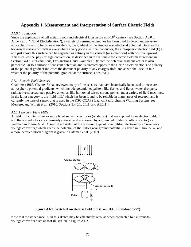
76

Appendix 1. Measurement and Interpretation of Surface Electric Fields A1.0 Introduction Since the application of tall metallic rods and electrical kites in the mid-18th century (see Section A3.0 of Appendix 3, "Cloud Electrification"), a variety of sensing techniques has been used to detect and measure atmospheric electric fields, or equivalently, the gradient of the atmospheric electrical potential. Because the horizontal surface of Earth is everywhere a very good electrical conductor, the atmospheric electric field (E) at and just above this surface can be regarded as entirely in the vertical (or z-direction) with positive upward. This is called the 'physics' sign convention, as described in the rationale for 'electric field measurement' in Section G417.3, "Definitions, Explanations, and Examples." (Note: the potential gradient vector is also perpendicular to a surface of constant potential, and is directed opposite the electric-field vector. The polarity of the potential gradient indicates the dominant polarity of any charges aloft, and as we shall see, in fair weather the polarity of the potential gradient at the surface is positive.) A1.1. Electric Field Sensors Chalmers (1967, Chapter 5) has reviewed many of the sensors that have historically been used to measure atmospheric potential gradients, which include potential equalizers like flames and flares, water-droppers, radioactive sources, etc.; passive antennas like horizontal wires; corona points; and a variety of field machines. In the latter category is the 'field mill,' which has been found to be reliable in many areas of research and is currently the type of sensor that is used in the KSC-CCAFS Launch Pad Lightning Warning System [see Merceret and Willett et al. (2010, Sections 3.4.5.1, 5.1.1, and A8.1.1)]. A1.1.1 Electric Field Mills A field mill contains one or more fixed sensing electrodes (or stators) that are exposed to an electric field, E, and these conductors are alternately covered and uncovered by a grounded rotating shutter (or rotor) as sketched in Figure A1-1. A simplified sketch of the preferred type of preamplifier electronics (a 'current-to-voltage converter,' which keeps the potential of the stators near ground potential) is given in Figure A1-2, and a more detailed block diagram is given in Bateman et al. (2007).

Figure A1-1. Sketch of an electric field mill (from IEEE Standard 1227) Note that the impedance, Z, in this sketch may be effectively zero, as when connected to a current-to-voltage converter such as that illustrated in Figure A1-2.

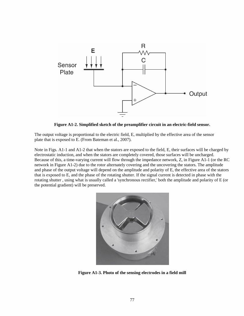
77

Figure A1-2. Simplified sketch of the preamplifier circuit in an electric-field sensor. The output voltage is proportional to the electric field, E, multiplied by the effective area of the sensor plate that is exposed to E. (From Bateman et al., 2007). Note in Figs. A1-1 and A1-2 that when the stators are exposed to the field, E, their surfaces will be charged by electrostatic induction, and when the stators are completely covered, those surfaces will be uncharged. Because of this, a time-varying current will flow through the impedance network, Z, in Figure A1-1 (or the RC network in Figure A1-2) due to the rotor alternately covering and the uncovering the stators. The amplitude and phase of the output voltage will depend on the amplitude and polarity of E, the effective area of the stators that is exposed to E, and the phase of the rotating shutter. If the signal current is detected in phase with the rotating shutter , using what is usually called a 'synchronous rectifier,' both the amplitude and polarity of E (or the potential gradient) will be preserved.

Figure A1-3. Photo of the sensing electrodes in a field mill

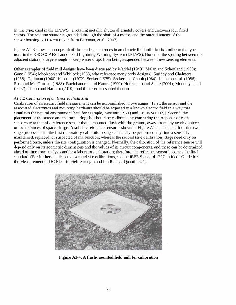
78

In this type, used in the LPLWS, a rotating metallic shutter alternately covers and uncovers four fixed stators. The rotating shutter is grounded through the shaft of a motor, and the outer diameter of the sensor housing is 11.4 cm (taken from Bateman, et al., 2007). Figure A1-3 shows a photograph of the sensing electrodes in an electric field mill that is similar to the type used in the KSC-CCAFS Launch Pad Lightning Warning System (LPLWS). Note that the spacing between the adjacent stators is large enough to keep water drops from being suspended between these sensing elements. Other examples of field mill designs have been discussed by Waddel (1948); Malan and Schonland (1950); Gunn (1954); Mapleson and Whitlock (1955, who reference many early designs); Smiddy and Chalmers (1958); Gathman (1968); Kasemir (1972); Secker (1975); Secker and Chubb (1984); Johnston et al. (1986); Rust and MacGorman (1988); Ravichandran and Kamra (1999); Horenstein and Stone (2001); Montanya et al. (2007); Chubb and Harbour (2010); and the references cited therein. A1.1.2 Calibration of an Electric Field Mill Calibration of an electric field measurement can be accomplished in two stages: First, the sensor and the associated electronics and mounting hardware should be exposed to a known electric field in a way that simulates the natural environment [see, for example, Kasemir (1971) and LPLWS(1992)]. Second, the placement of the sensor and the measuring site should be calibrated by comparing the response of each sensor/site to that of a reference sensor that is mounted flush with flat ground, away from any nearby objects or local sources of space charge. A suitable reference sensor is shown in Figure A1-4. The benefit of this two-stage process is that the first (laboratory-calibration) stage can easily be performed any time a sensor is maintained, replaced, or suspected of malfunction; whereas the second (site-calibration) stage need only be performed once, unless the site configuration is changed. Normally, the calibration of the reference sensor will depend only on its geometric dimensions and the values of its circuit components, and these can be determined ahead of time from analysis and/or a laboratory calibration; therefore, the reference sensor becomes the final standard. (For further details on sensor and site calibrations, see the IEEE Standard 1227 entitled “Guide for the Measurement of DC Electric-Field Strength and Ion Related Quantities.”).

Figure A1-4. A flush-mounted field mill for calibration

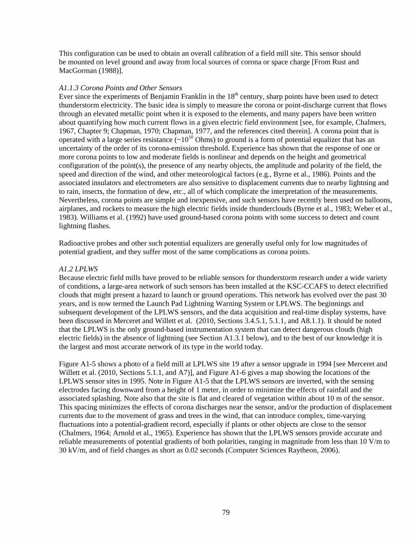
79

This configuration can be used to obtain an overall calibration of a field mill site. This sensor should be mounted on level ground and away from local sources of corona or space charge [From Rust and MacGorman (1988)]. A1.1.3 Corona Points and Other Sensors Ever since the experiments of Benjamin Franklin in the 18th century, sharp points have been used to detect thunderstorm electricity. The basic idea is simply to measure the corona or point-discharge current that flows through an elevated metallic point when it is exposed to the elements, and many papers have been written about quantifying how much current flows in a given electric field environment [see, for example, Chalmers, 1967, Chapter 9; Chapman, 1970; Chapman, 1977, and the references cited therein]. A corona point that is operated with a large series resistance (~1010 Ohms) to ground is a form of potential equalizer that has an uncertainty of the order of its corona-emission threshold. Experience has shown that the response of one or more corona points to low and moderate fields is nonlinear and depends on the height and geometrical configuration of the point(s), the presence of any nearby objects, the amplitude and polarity of the field, the speed and direction of the wind, and other meteorological factors (e.g., Byrne et al., 1986). Points and the associated insulators and electrometers are also sensitive to displacement currents due to nearby lightning and to rain, insects, the formation of dew, etc., all of which complicate the interpretation of the measurements. Nevertheless, corona points are simple and inexpensive, and such sensors have recently been used on balloons, airplanes, and rockets to measure the high electric fields inside thunderclouds (Byrne et al., 1983; Weber et al., 1983). Williams et al. (1992) have used ground-based corona points with some success to detect and count lightning flashes. Radioactive probes and other such potential equalizers are generally useful only for low magnitudes of potential gradient, and they suffer most of the same complications as corona points. A1.2 LPLWS Because electric field mills have proved to be reliable sensors for thunderstorm research under a wide variety of conditions, a large-area network of such sensors has been installed at the KSC-CCAFS to detect electrified clouds that might present a hazard to launch or ground operations. This network has evolved over the past 30 years, and is now termed the Launch Pad Lightning Warning System or LPLWS. The beginnings and subsequent development of the LPLWS sensors, and the data acquisition and real-time display systems, have been discussed in Merceret and Willett et al. (2010, Sections 3.4.5.1, 5.1.1, and A8.1.1). It should be noted that the LPLWS is the only ground-based instrumentation system that can detect dangerous clouds (high electric fields) in the absence of lightning (see Section A1.3.1 below), and to the best of our knowledge it is the largest and most accurate network of its type in the world today. Figure A1-5 shows a photo of a field mill at LPLWS site 19 after a sensor upgrade in 1994 [see Merceret and Willett et al. (2010, Sections 5.1.1, and A7)], and Figure A1-6 gives a map showing the locations of the LPLWS sensor sites in 1995. Note in Figure A1-5 that the LPLWS sensors are inverted, with the sensing electrodes facing downward from a height of 1 meter, in order to minimize the effects of rainfall and the associated splashing. Note also that the site is flat and cleared of vegetation within about 10 m of the sensor. This spacing minimizes the effects of corona discharges near the sensor, and/or the production of displacement currents due to the movement of grass and trees in the wind, that can introduce complex, time-varying fluctuations into a potential-gradient record, especially if plants or other objects are close to the sensor (Chalmers, 1964; Arnold et al., 1965). Experience has shown that the LPLWS sensors provide accurate and reliable measurements of potential gradients of both polarities, ranging in magnitude from less than 10 V/m to 30 kV/m, and of field changes as short as 0.02 seconds (Computer Sciences Raytheon, 2006).

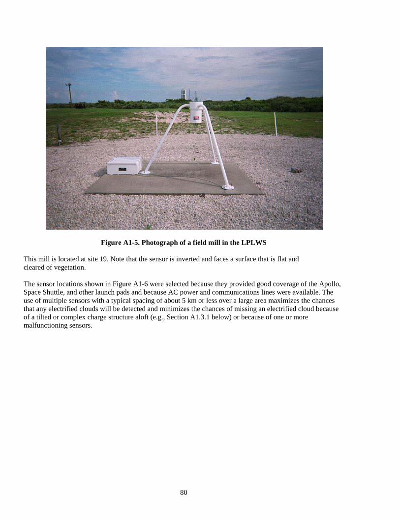
80

Figure A1-5. Photograph of a field mill in the LPLWS This mill is located at site 19. Note that the sensor is inverted and faces a surface that is flat and cleared of vegetation. The sensor locations shown in Figure A1-6 were selected because they provided good coverage of the Apollo, Space Shuttle, and other launch pads and because AC power and communications lines were available. The use of multiple sensors with a typical spacing of about 5 km or less over a large area maximizes the chances that any electrified clouds will be detected and minimizes the chances of missing an electrified cloud because of a tilted or complex charge structure aloft (e.g., Section A1.3.1 below) or because of one or more malfunctioning sensors.

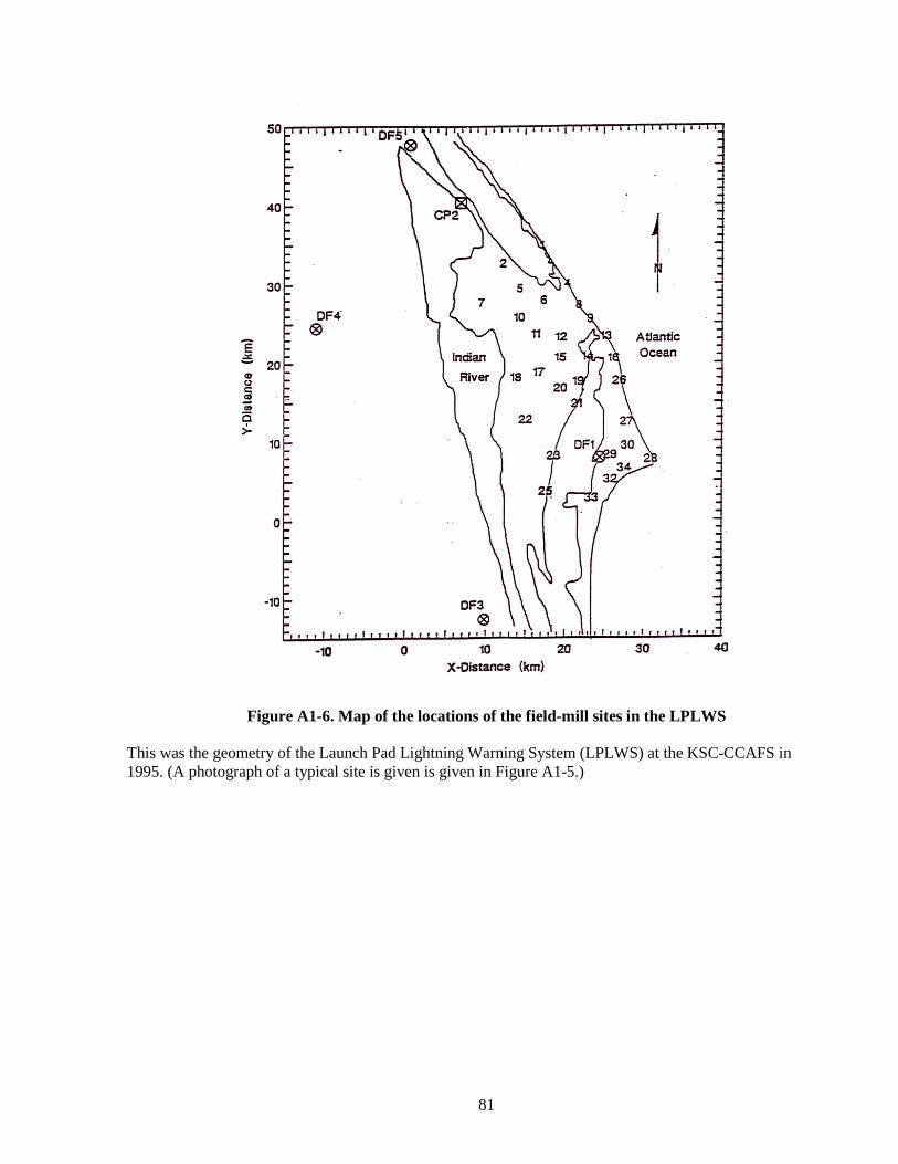
81

Figure A1-6. Map of the locations of the field-mill sites in the LPLWS This was the geometry of the Launch Pad Lightning Warning System (LPLWS) at the KSC-CCAFS in 1995. (A photograph of a typical site is given is given in Figure A1-5.)

82

A1.2.1 Examples of Fair Weather Potential Gradients Figure A1-7 shows examples of simultaneous recordings of the potential gradient under fair weather conditions at five LPLWS sites over a period of one day, July 16, 1995. The five panels in this figure are labeled at the left by the FM numbers, increasing downward from 13 to 17. Several things should be noted in Figure A1-7:

1) The average value of the potential gradient undulates between +100 V/m and +500 V/m at all sites with occasional excursions approaching +600 V/m. Although the underlying potential gradient varies somewhat from site-to-site, the persistent positive offset is caused by a quasi-steady negative charge on the planet Earth. This so-called ‘global electric field’ contains regular hourly, daily, monthly, and seasonal variations and is likely caused by worldwide thunderstorm generators in a ‘global electric circuit’ (Roble and Tzur, 1986; Bering et al., 1998; Siingh et al., 2007; and Williams, 2009). Local meteorology, however, including the effects of the 'columnar resistance' that is controlled by the presence of fair-weather clouds and by the vertical distribution of aerosol particles (Sagalyn and Foucher, 1956), and those of vertical convection currents that are driven by turbulent mixing in the planetary boundary layer (Kraakevik and Clark, 1958; Willett, 1979), also play an important role (Hoppel et al., 1986). These factors make the typical time variations over land different at different geographical locations (Israel, 1958, Section 58). The high-frequency ‘agitations’ in the fair weather records shown in Figure A1-7 are typical of land-based surface measurements and are produced by a variety of natural and human causes [see, for example, Israel (1959); Whitlock and Chalmers (1956); Chalmers (1967, Chapters 5 and 6); Gathman and Trent (1968); Ogden and Hutchinson (1970); Hoppel et al. (1986); Anisimov et al. (1994); and many others], some of which are mentioned below.

2) At the KSC-CCAFS, the primary causes of high potential gradients (i.e. those that can exceed 1000 V/m) in fair weather are the effects of surf electrification (Blanchard 1963; Gathman and Hoppel, 1970; Latham and Miksad, 1974; Reiter, 1994); coronas from high-voltage power lines, particularly in the presence of ground fog (Chalmers, 1952; Groom and Chalmers, 1967; Fews et al., 2002; Matthews and Henshaw, 2009); a still only partially understood ‘sunrise effect’ (Chalmers, 1967, sections 5.46 and 8.23; Marshall et al., 1999); and the effects of combustion, such as vehicle exhausts and smoke plumes. Other causes include non-thundery clouds, both precipitating and non-precipitating (Israel, 1959; Reiter, 1968); rain and splashing at the ground (Smith, 1955; Chalmers, 1965); and the contamination of sensors due to spider webs, a sea-salt aerosol, and a variety of other factors. At other geographic locations, blowing dust or drifting snow can be expected to produce high potential gradients in fair weather. None of the above phenomena is dangerous for space launches or the associated ground operations; and to minimize false alarms, the value of 1500 V/m that is specified in Section (a) of the "Surface Electric Fields" Rule, G417.5, is higher than almost all field excursions that occur in fair weather at the KSC-CCAFS.

3) FM sites 13 and 16 are located on the seacoast; notice how these sites exhibit considerable agitation in the potential gradient after about 1300 GMT. This behavior is typical at the KSC-CCAFS and illustrates the effects of a summer sea breeze combined with surf electrification.

4) FM sites 15 and 17 are located at isolated sites further inland, and these records have the lowest agitation, likely because the effects of surf electrification and man-made space charge are minimal at these sites.

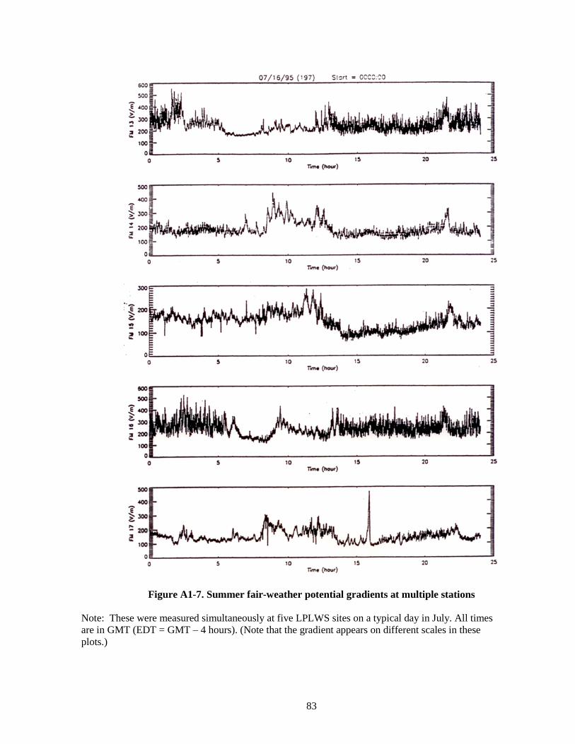
83

Figure A1-7. Summer fair-weather potential gradients at multiple stations Note: These were measured simultaneously at five LPLWS sites on a typical day in July. All times are in GMT (EDT = GMT – 4 hours). (Note that the gradient appears on different scales in these plots.)

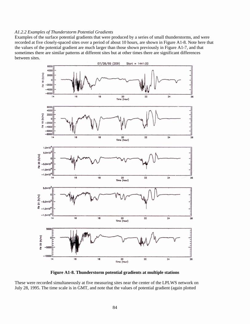
84

A1.2.2 Examples of Thunderstorm Potential Gradients Examples of the surface potential gradients that were produced by a series of small thunderstorms, and were recorded at five closely-spaced sites over a period of about 10 hours, are shown in Figure A1-8. Note here that the values of the potential gradient are much larger than those shown previously in Figure A1-7, and that sometimes there are similar patterns at different sites but at other times there are significant differences between sites.

Figure A1-8. Thunderstorm potential gradients at multiple stations These were recorded simultaneously at five measuring sites near the center of the LPLWS network on July 28, 1995. The time scale is in GMT, and note that the values of potential gradient (again plotted

• ,

" " "

I~--~:---:--:~::::~------------~::~"::~--------::~~~~~::~~~~~~ ~E r ..... (loauo) 22

LS ' ,-... ~ j -~E- '

" " " "

l>,Oo lol

::t <- 0

::::::",:. =--;-;"_--;;-" _-;:,,~~~_ 1 ~ _5..0oUY

~"o' - 0->" --.-J " "

- '.""':==---.-.--;:;c:--~---;;_J " " " "

=r~~~=='~--~> ~"~ ~=== "

o

::[ 0

<;; _~O . 10l

~ -1 ,0010·

, -=

"

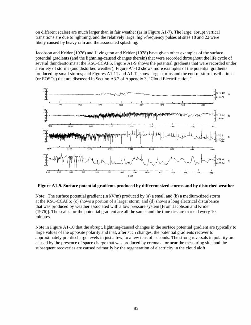
85

on different scales) are much larger than in fair weather (as in Figure A1-7). The large, abrupt vertical transitions are due to lightning, and the relatively large, high-frequency pulses at sites 18 and 22 were likely caused by heavy rain and the associated splashing. Jacobson and Krider (1976) and Livingston and Krider (1978) have given other examples of the surface potential gradients (and the lightning-caused changes therein) that were recorded throughout the life cycle of several thunderstorms at the KSC-CCAFS. Figure A1-9 shows the potential gradients that were recorded under a variety of storms (and disturbed weather); Figure A1-10 shows more examples of the potential gradients produced by small storms; and Figures A1-11 and A1-12 show large storms and the end-of-storm oscillations (or EOSOs) that are discussed in Section A3.2 of Appendix 3, "Cloud Electrification."

Figure A1-9. Surface potential gradients produced by different sized storms and by disturbed weather

Note: The surface potential gradient (in kV/m) produced by (a) a small and (b) a medium-sized storm at the KSC-CCAFS; (c) shows a portion of a larger storm, and (d) shows a long electrical disturbance that was produced by weather associated with a low pressure system [From Jacobson and Krider (1976)]. The scales for the potential gradient are all the same, and the time tics are marked every 10 minutes. Note in Figure A1-10 that the abrupt, lightning-caused changes in the surface potential gradient are typically to large values of the opposite polarity and that, after such changes, the potential gradients recover to approximately pre-discharge levels in just a few, to a few tens of, seconds. The strong reversals in polarity are caused by the presence of space charge that was produced by corona at or near the measuring site, and the subsequent recoveries are caused primarily by the regeneration of electricity in the cloud aloft.

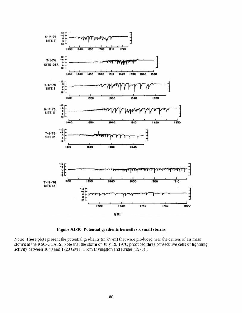
86

Figure A1-10. Potential gradients beneath six small storms

Note: These plots present the potential gradients (in kV/m) that were produced near the centers of air mass storms at the KSC-CCAFS. Note that the storm on July 19, 1976, produced three consecutive cells of lightning activity between 1640 and 1720 GMT [From Livingston and Krider (1978)].

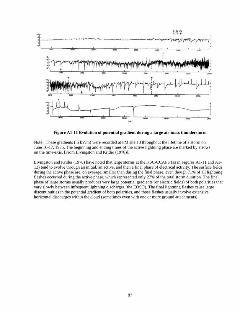
87

Figure A1-11 Evolution of potential gradient during a large air-mass thunderstorm Note: These gradients (in kV/m) were recorded at FM site 18 throughout the lifetime of a storm on June 16-17, 1975. The beginning and ending times of the active lightning phase are marked by arrows on the time-axis. [From Livingston and Krider (1978)]. Livingston and Krider (1978) have noted that large storms at the KSC-CCAFS (as in Figures A1-11 and A1-12) tend to evolve through an initial, an active, and then a final phase of electrical activity. The surface fields during the active phase are, on average, smaller than during the final phase, even though 71% of all lightning flashes occurred during the active phase, which represented only 27% of the total storm duration. The final phase of large storms usually produces very large potential gradients (or electric fields) of both polarities that vary slowly between infrequent lightning discharges (the EOSO). The final lightning flashes cause large discontinuities in the potential gradient of both polarities, and those flashes usually involve extensive horizontal discharges within the cloud (sometimes even with one or more ground attachments).

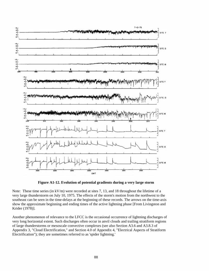
88

Figure A1-12. Evolution of potential gradients during a very large storm Note: These time series (in kV/m) were recorded at sites 7, 13, and 18 throughout the lifetime of a very large thunderstorm on July 10, 1975. The effects of the storm's motion from the northwest to the southeast can be seen in the time-delays at the beginning of these records. The arrows on the time-axis show the approximate beginning and ending times of the active lightning phase [From Livingston and Krider (1978)]. Another phenomenon of relevance to the LFCC is the occasional occurrence of lightning discharges of very long horizontal extent. Such discharges often occur in anvil clouds and trailing stratiform regions of large thunderstorms or mesoscale convective complexes (see also Section A3.6 and A3.8.3 of Appendix 3, "Cloud Electrification," and Section 4.0 of Appendix 4, "Electrical Aspects of Stratiform Electrification"); they are sometimes referred to as 'spider lightning.'

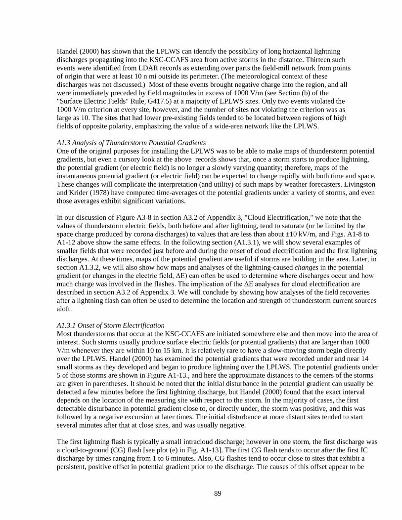
89

Handel (2000) has shown that the LPLWS can identify the possibility of long horizontal lightning discharges propagating into the KSC-CCAFS area from active storms in the distance. Thirteen such events were identified from LDAR records as extending over parts the field-mill network from points of origin that were at least 10 n mi outside its perimeter. (The meteorological context of these discharges was not discussed.) Most of these events brought negative charge into the region, and all were immediately preceded by field magnitudes in excess of 1000 V/m (see Section (b) of the "Surface Electric Fields" Rule, G417.5) at a majority of LPLWS sites. Only two events violated the 1000 V/m criterion at every site, however, and the number of sites not violating the criterion was as large as 10. The sites that had lower pre-existing fields tended to be located between regions of high fields of opposite polarity, emphasizing the value of a wide-area network like the LPLWS. A1.3 Analysis of Thunderstorm Potential Gradients One of the original purposes for installing the LPLWS was to be able to make maps of thunderstorm potential gradients, but even a cursory look at the above records shows that, once a storm starts to produce lightning, the potential gradient (or electric field) is no longer a slowly varying quantity; therefore, maps of the instantaneous potential gradient (or electric field) can be expected to change rapidly with both time and space. These changes will complicate the interpretation (and utility) of such maps by weather forecasters. Livingston and Krider (1978) have computed time-averages of the potential gradients under a variety of storms, and even those averages exhibit significant variations. In our discussion of Figure A3-8 in section A3.2 of Appendix 3, "Cloud Electrification," we note that the values of thunderstorm electric fields, both before and after lightning, tend to saturate (or be limited by the space charge produced by corona discharges) to values that are less than about ±10 kV/m, and Figs. A1-8 to A1-12 above show the same effects. In the following section (A1.3.1), we will show several examples of smaller fields that were recorded just before and during the onset of cloud electrification and the first lightning discharges. At these times, maps of the potential gradient are useful if storms are building in the area. Later, in section A1.3.2, we will also show how maps and analyses of the lightning-caused changes in the potential gradient (or changes in the electric field, ΔE) can often be used to determine where discharges occur and how much charge was involved in the flashes. The implication of the ΔE analyses for cloud electrification are described in section A3.2 of Appendix 3. We will conclude by showing how analyses of the field recoveries after a lightning flash can often be used to determine the location and strength of thunderstorm current sources aloft. A1.3.1 Onset of Storm Electrification Most thunderstorms that occur at the KSC-CCAFS are initiated somewhere else and then move into the area of interest. Such storms usually produce surface electric fields (or potential gradients) that are larger than 1000 V/m whenever they are within 10 to 15 km. It is relatively rare to have a slow-moving storm begin directly over the LPLWS. Handel (2000) has examined the potential gradients that were recorded under and near 14 small storms as they developed and began to produce lightning over the LPLWS. The potential gradients under 5 of those storms are shown in Figure A1-13., and here the approximate distances to the centers of the storms are given in parentheses. It should be noted that the initial disturbance in the potential gradient can usually be detected a few minutes before the first lightning discharge, but Handel (2000) found that the exact interval depends on the location of the measuring site with respect to the storm. In the majority of cases, the first detectable disturbance in potential gradient close to, or directly under, the storm was positive, and this was followed by a negative excursion at later times. The initial disturbance at more distant sites tended to start several minutes after that at close sites, and was usually negative. The first lightning flash is typically a small intracloud discharge; however in one storm, the first discharge was a cloud-to-ground (CG) flash [see plot (e) in Fig. A1-13]. The first CG flash tends to occur after the first IC discharge by times ranging from 1 to 6 minutes. Also, CG flashes tend to occur close to sites that exhibit a persistent, positive offset in potential gradient prior to the discharge. The causes of this offset appear to be

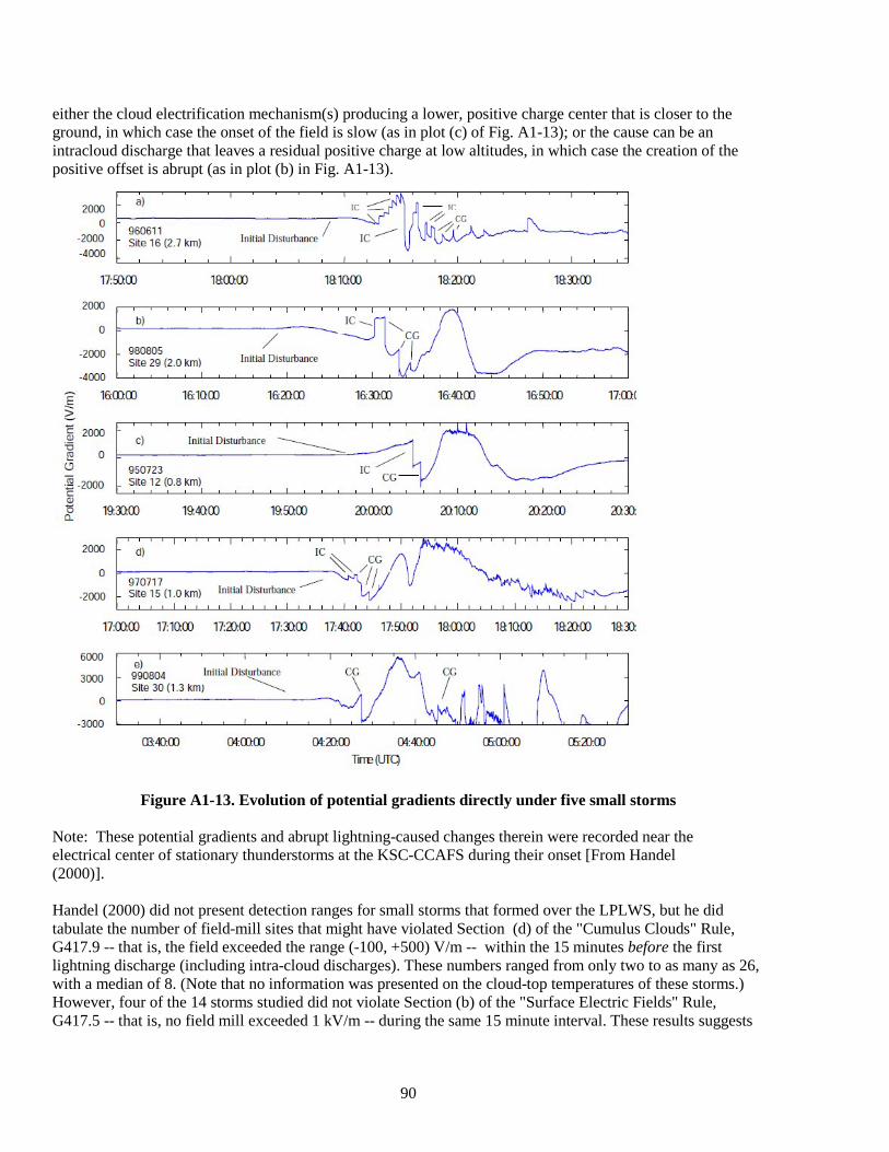
90

either the cloud electrification mechanism(s) producing a lower, positive charge center that is closer to the ground, in which case the onset of the field is slow (as in plot (c) of Fig. A1-13); or the cause can be an intracloud discharge that leaves a residual positive charge at low altitudes, in which case the creation of the positive offset is abrupt (as in plot (b) in Fig. A1-13).

Figure A1-13. Evolution of potential gradients directly under five small storms Note: These potential gradients and abrupt lightning-caused changes therein were recorded near the electrical center of stationary thunderstorms at the KSC-CCAFS during their onset [From Handel (2000)]. Handel (2000) did not present detection ranges for small storms that formed over the LPLWS, but he did tabulate the number of field-mill sites that might have violated Section (d) of the "Cumulus Clouds" Rule, G417.9 -- that is, the field exceeded the range (-100, +500) V/m -- within the 15 minutes before the first lightning discharge (including intra-cloud discharges). These numbers ranged from only two to as many as 26, with a median of 8. (Note that no information was presented on the cloud-top temperatures of these storms.) However, four of the 14 storms studied did not violate Section (b) of the "Surface Electric Fields" Rule, G417.5 -- that is, no field mill exceeded 1 kV/m -- during the same 15 minute interval. These results suggests

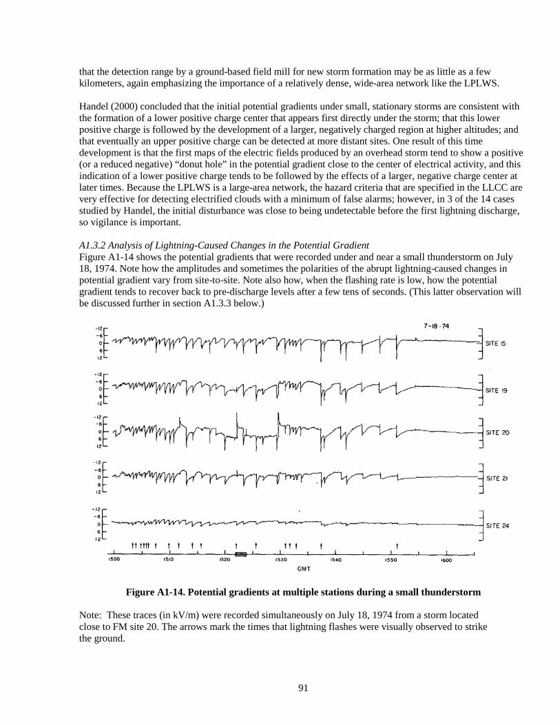
91

that the detection range by a ground-based field mill for new storm formation may be as little as a few kilometers, again emphasizing the importance of a relatively dense, wide-area network like the LPLWS. Handel (2000) concluded that the initial potential gradients under small, stationary storms are consistent with the formation of a lower positive charge center that appears first directly under the storm; that this lower positive charge is followed by the development of a larger, negatively charged region at higher altitudes; and that eventually an upper positive charge can be detected at more distant sites. One result of this time development is that the first maps of the electric fields produced by an overhead storm tend to show a positive (or a reduced negative) “donut hole” in the potential gradient close to the center of electrical activity, and this indication of a lower positive charge tends to be followed by the effects of a larger, negative charge center at later times. Because the LPLWS is a large-area network, the hazard criteria that are specified in the LLCC are very effective for detecting electrified clouds with a minimum of false alarms; however, in 3 of the 14 cases studied by Handel, the initial disturbance was close to being undetectable before the first lightning discharge, so vigilance is important. A1.3.2 Analysis of Lightning-Caused Changes in the Potential Gradient Figure A1-14 shows the potential gradients that were recorded under and near a small thunderstorm on July 18, 1974. Note how the amplitudes and sometimes the polarities of the abrupt lightning-caused changes in potential gradient vary from site-to-site. Note also how, when the flashing rate is low, how the potential gradient tends to recover back to pre-discharge levels after a few tens of seconds. (This latter observation will be discussed further in section A1.3.3 below.)

Figure A1-14. Potential gradients at multiple stations during a small thunderstorm Note: These traces (in kV/m) were recorded simultaneously on July 18, 1974 from a storm located close to FM site 20. The arrows mark the times that lightning flashes were visually observed to strike the ground.

92

In our discussion of Figure A3-9 in Section A3.2 of Appendix 3, "Cloud Electrification," we point out that simple models can often be used to describe the changes, ΔE, in potential gradient recorded at different sites in an optimum way, and that the parameters of those models provide the locations and magnitudes of lightning-caused changes in the cloud charge distribution aloft. The analysis begins by assuming the simplest model, i.e., a model with the smallest number of unknown parameters such as a point charge, and then a search is made for the model parameters that minimize (in a least-squares sense) an error function involving those parameters and the measured ΔEs. If the minimum in the error function is small and consistent with the expected measurement errors, the search procedure stops and the model and parameters are regarded as valid. If the error is large, then the search can be repeated using a more complex charge model (i.e., one with more parameters such as a point dipole), and if necessary there can be additional searches, until a satisfactory fit is obtained. The inferred charge parameters will never be unique, of course, but if the error function is small and if the parameters are physically reasonable, the solutions are usually regarded as valid. Several examples of this analysis are given in Figure A1-15, in which the point-charge model has been successfully fitted to field change data for several cloud-to-ground flashes.

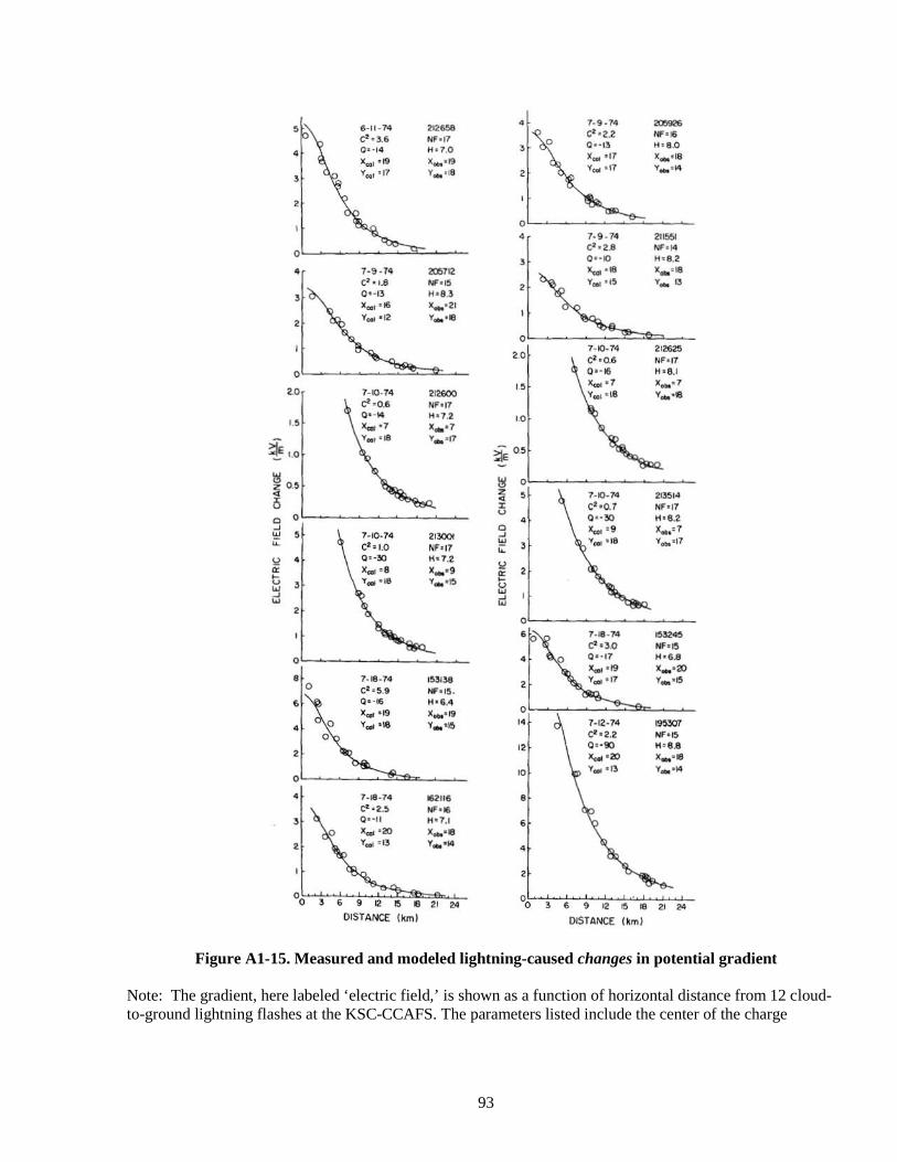
93

Figure A1-15. Measured and modeled lightning-caused changes in potential gradient Note: The gradient, here labeled ‘electric field,’ is shown as a function of horizontal distance from 12 cloud-to-ground lightning flashes at the KSC-CCAFS. The parameters listed include the center of the charge

• 1· '·14 ..... 6 - 11 -14 "'''' ct · 2.l ~ .. C'·3.6 N"11 0 0 '-1) H· a.o g ' -14 H. 7.0 , ... .. X ... _19

~ .. . 17 .... _18

T",. ' IT Y .. ' 18 , V ... ' 17 T ... \4 , ,

, • 7-9 ·74 " .. C' , 2.8 NF' !4

0 , 0 "10 "' · 8.t

• 1· 9 ·74 "'". ..... ..... C· ·1.8 ~ .. , y ... . ~ '- " , O' -Il H· 8.3 too, · 16 .... · 21 , y ... ' 12 v .. . WI

, 7 _10·74 ,,~

" C· · 0.6 NF " T

0 0 ·- 1Ei H·6.1

"

... . , .... . 7

'" 7 _10_74 , .... T ... _18 v ... · 18 r:! ' 0 .6 '11"17 Q'-14 H· l .2- '0 ,., .... , ..... ,

~ I.O TOOl · 18 V ... 17

:;i o.~

~ ~ 0 z 0.' z , 7· 0 · M 213$,· ~ • z C· · O.l HF 'I? u 0 • O' -XI H· S.2-Q

Q .... , X .... 7 " u , 7 _10_ 74 '"'''' " y ... · '8 Y ... '17 " (2 ' 1.0 ~ , '11"17 c ~ • 11<7.2-

~ < X ... · 9 • , t T_'~ • U

, ~

" " u u , 0

7 _11 _7. =~ c"'3D " ..

0 H·6.8 X ... · 20

• 7_18_74 .,,, , "' ... ' 15 0 cr. , _, NF·I$ .

• 0 ' - 11; H'6,4 X ... ' 19 )( ... · 19 0

0 T .... 16 T ... . ~ " 7_12_74 ""'" • c" · 2.2 "'1" 15 0 0 · -90 H· 8.8 " , .... '" X ... -18

• Y ... ' 1) Y ... ' 14 0

• T_Ie_7. Rile; • C"2., " .. , 0 "1 1 H·7.1 , ... . ", X .. ' I8 , V ... ' 13 .,. .... 14 • ,

00 , , , , • • " " '0 , , , • • • " " DISTANCE (km) DISTANCE Ikml

94

'lowered' by the flash, Q, in Coulombs at altitude, H, and all distances are in kilometers. C2 is a measure of agreement between the model and the measurements [From Jacobson and Krider (1976)]. A1.3.3 Analysis of Field Recoveries At this point in our discussion of thunderstorm electric fields (or potential gradients), we should point out that any maps of a quasi-static field (i.e. when the potential gradient varies slowly with time), or of the field recovery following a lightning flash, must be interpreted in the context of both what is happening in the atmosphere and what is happening on or just above the ground. Two related aspects of this problem are important, the effects of corona at the ground in high fields and the effects of the cloud and the conducting atmosphere aloft. A1.3.3.1 The Corona Current When Earth's land surface is exposed to moderately strong ambient electric fields, 'corona discharges' of the sort mentioned in Section A1.1.3 will occur on most structures and vegetation, as outlined in the rationale for the "Surface Electric Fields" Rule, G417.5. Whipple and Scrase (1936) may have been the first to suggest that this corona current produces a blanket of space charge near the ground that is likely stored on relatively immobile particles in the atmospheric aerosol, and that this space charge can modify both the surface field and its recovery after a lighting discharge. The first conclusive observations of this phenomenon were reported by Standler and Winn (1979), who showed that the vertical electric field (or potential gradient) beneath thunderstorms often increased by several times over a few hundred meters of height, both at the KSC in Florida and at the Langmuir Laboratory in New Mexico. This behavior occurred primarily when the surface fields were larger than a few kV/m and relatively steady. The fact that the corona-current increases rapidly as soon as the ambient field exceeds a surface-dependent threshold, causes the surface field to be limited to, or 'clamped' at, a steady level near the corona threshold, even though the field aloft is much larger than that threshold. When this apparent ‘saturation’ occurs, the field at the ground is only weakly related to the field aloft. The surface fields at KSC appear to saturate at values around 3 kV/m, whereas at Langmuir Laboratory the 'saturation' values are 7 - 10 kV/m, presumably because of differences in altitude, topography, and ground cover. Chauzy et al. (1991), Soula and Chauzy (1991), Soula (1994), and the authors cited therein have summarized simultaneous measurements of electric field at several altitudes throughout the lowest 600 m of the atmosphere over land beneath thunderstorms at KSC. The observations were compared with a time-dependent, numerical model that incorporated surface coronas, small-ion drift velocities and recombination, and small-ion attachment to both uncharged and oppositely charged aerosol particles. The authors showed that both the vertical gradient of the electric field and the shapes of the field recoveries following lightning discharges, at the surface and at intermediate altitudes, could be explained quite well in terms of the time-dependent fields measured aloft and the model-predicted corona currents, conduction currents, and space charge stored on both small ions and aerosol particles. In particular, the effect of aerosol charging and the resulting immobilization of the space charge was found to be significant. Saturation of the surface field occurred at a few kV/m while the field aloft continued to increase between lightning flashes, and this was shown to be the result of the accumulation of corona space charge in the lowest few hundred meters of air. This ‘space charge blanket’ strongly affected both the slowly varying background field and the field-recovery waveforms between the surface and a few hundred meters aloft. A1.3.3.2 The Maxwell Current The fact that the cloud is itself embedded in an atmosphere that is a weak electrical conductor, where the conductivity increases approximately exponentially with altitude (Gringel et al., 1986; Reid, 1986), has a large effect on the values and the time behavior of the surface potential gradient. One consequence of the increase in conductivity with height is that many of the so-called “lines of electric force” do not terminate on the ground, but instead terminate on conducting layers in the middle and upper atmosphere (Holzer and Saxon, 1952; Tzur

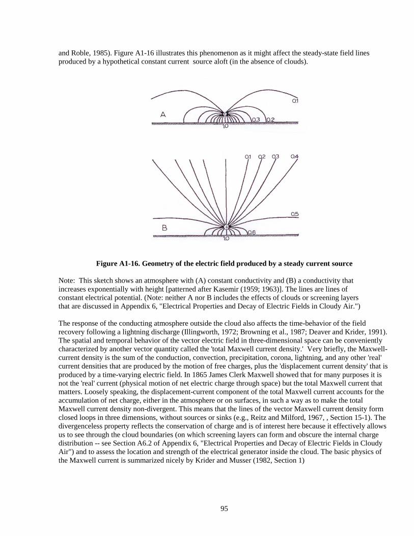
95

and Roble, 1985). Figure A1-16 illustrates this phenomenon as it might affect the steady-state field lines produced by a hypothetical constant current source aloft (in the absence of clouds).

Figure A1-16. Geometry of the electric field produced by a steady current source Note: This sketch shows an atmosphere with (A) constant conductivity and (B) a conductivity that increases exponentially with height [patterned after Kasemir (1959; 1963)]. The lines are lines of constant electrical potential. (Note: neither A nor B includes the effects of clouds or screening layers that are discussed in Appendix 6, "Electrical Properties and Decay of Electric Fields in Cloudy Air.") The response of the conducting atmosphere outside the cloud also affects the time-behavior of the field recovery following a lightning discharge (Illingworth, 1972; Browning et al., 1987; Deaver and Krider, 1991). The spatial and temporal behavior of the vector electric field in three-dimensional space can be conveniently characterized by another vector quantity called the 'total Maxwell current density.' Very briefly, the Maxwell-current density is the sum of the conduction, convection, precipitation, corona, lightning, and any other 'real' current densities that are produced by the motion of free charges, plus the 'displacement current density' that is produced by a time-varying electric field. In 1865 James Clerk Maxwell showed that for many purposes it is not the 'real' current (physical motion of net electric charge through space) but the total Maxwell current that matters. Loosely speaking, the displacement-current component of the total Maxwell current accounts for the accumulation of net charge, either in the atmosphere or on surfaces, in such a way as to make the total Maxwell current density non-divergent. This means that the lines of the vector Maxwell current density form closed loops in three dimensions, without sources or sinks (e.g., Reitz and Milford, 1967, , Section 15-1). The divergenceless property reflects the conservation of charge and is of interest here because it effectively allows us to see through the cloud boundaries (on which screening layers can form and obscure the internal charge distribution -- see Section A6.2 of Appendix 6, "Electrical Properties and Decay of Electric Fields in Cloudy Air") and to assess the location and strength of the electrical generator inside the cloud. The basic physics of the Maxwell current is summarized nicely by Krider and Musser (1982, Section 1)

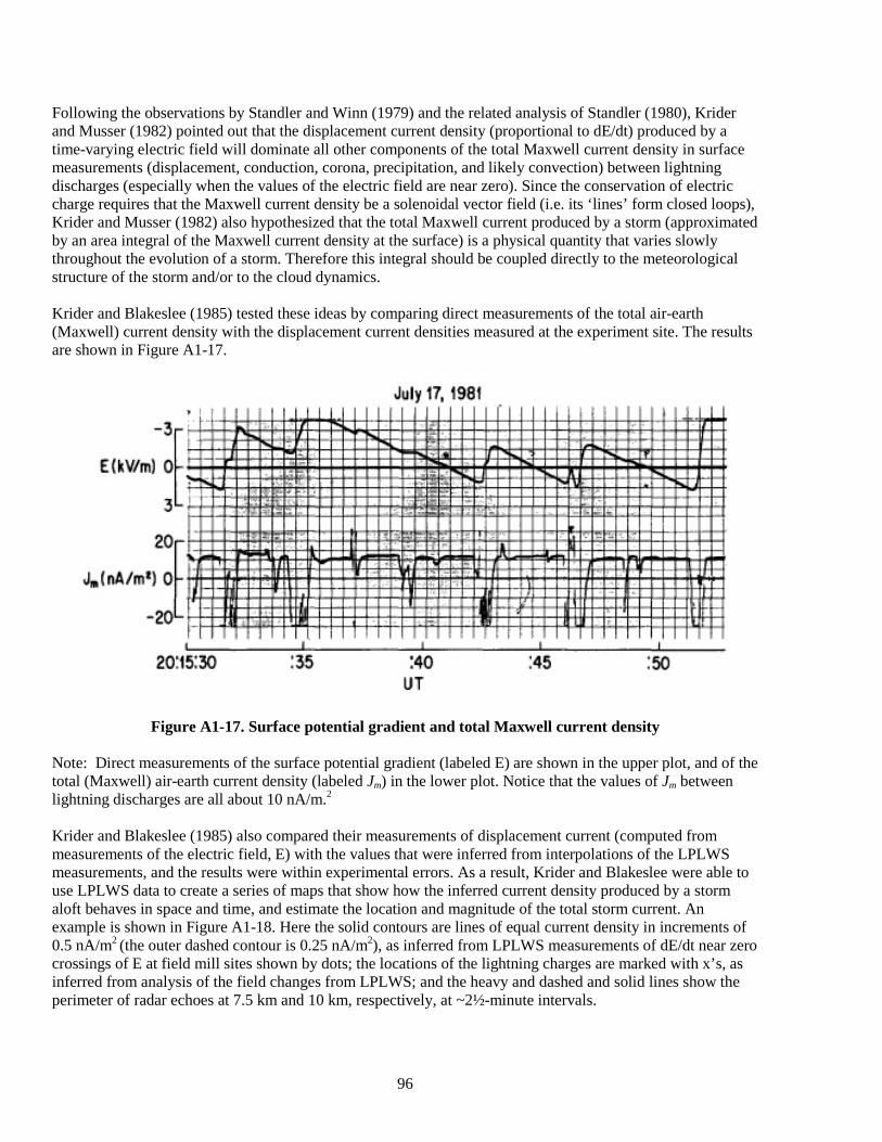
96

Following the observations by Standler and Winn (1979) and the related analysis of Standler (1980), Krider and Musser (1982) pointed out that the displacement current density (proportional to dE/dt) produced by a time-varying electric field will dominate all other components of the total Maxwell current density in surface measurements (displacement, conduction, corona, precipitation, and likely convection) between lightning discharges (especially when the values of the electric field are near zero). Since the conservation of electric charge requires that the Maxwell current density be a solenoidal vector field (i.e. its ‘lines’ form closed loops), Krider and Musser (1982) also hypothesized that the total Maxwell current produced by a storm (approximated by an area integral of the Maxwell current density at the surface) is a physical quantity that varies slowly throughout the evolution of a storm. Therefore this integral should be coupled directly to the meteorological structure of the storm and/or to the cloud dynamics. Krider and Blakeslee (1985) tested these ideas by comparing direct measurements of the total air-earth (Maxwell) current density with the displacement current densities measured at the experiment site. The results are shown in Figure A1-17.

Figure A1-17. Surface potential gradient and total Maxwell current density Note: Direct measurements of the surface potential gradient (labeled E) are shown in the upper plot, and of the total (Maxwell) air-earth current density (labeled Jm) in the lower plot. Notice that the values of Jm between lightning discharges are all about 10 nA/m.2 Krider and Blakeslee (1985) also compared their measurements of displacement current (computed from measurements of the electric field, E) with the values that were inferred from interpolations of the LPLWS measurements, and the results were within experimental errors. As a result, Krider and Blakeslee were able to use LPLWS data to create a series of maps that show how the inferred current density produced by a storm aloft behaves in space and time, and estimate the location and magnitude of the total storm current. An example is shown in Figure A1-18. Here the solid contours are lines of equal current density in increments of 0.5 nA/m2 (the outer dashed contour is 0.25 nA/m2), as inferred from LPLWS measurements of dE/dt near zero crossings of E at field mill sites shown by dots; the locations of the lightning charges are marked with x’s, as inferred from analysis of the field changes from LPLWS; and the heavy and dashed and solid lines show the perimeter of radar echoes at 7.5 km and 10 km, respectively, at ~2½-minute intervals.

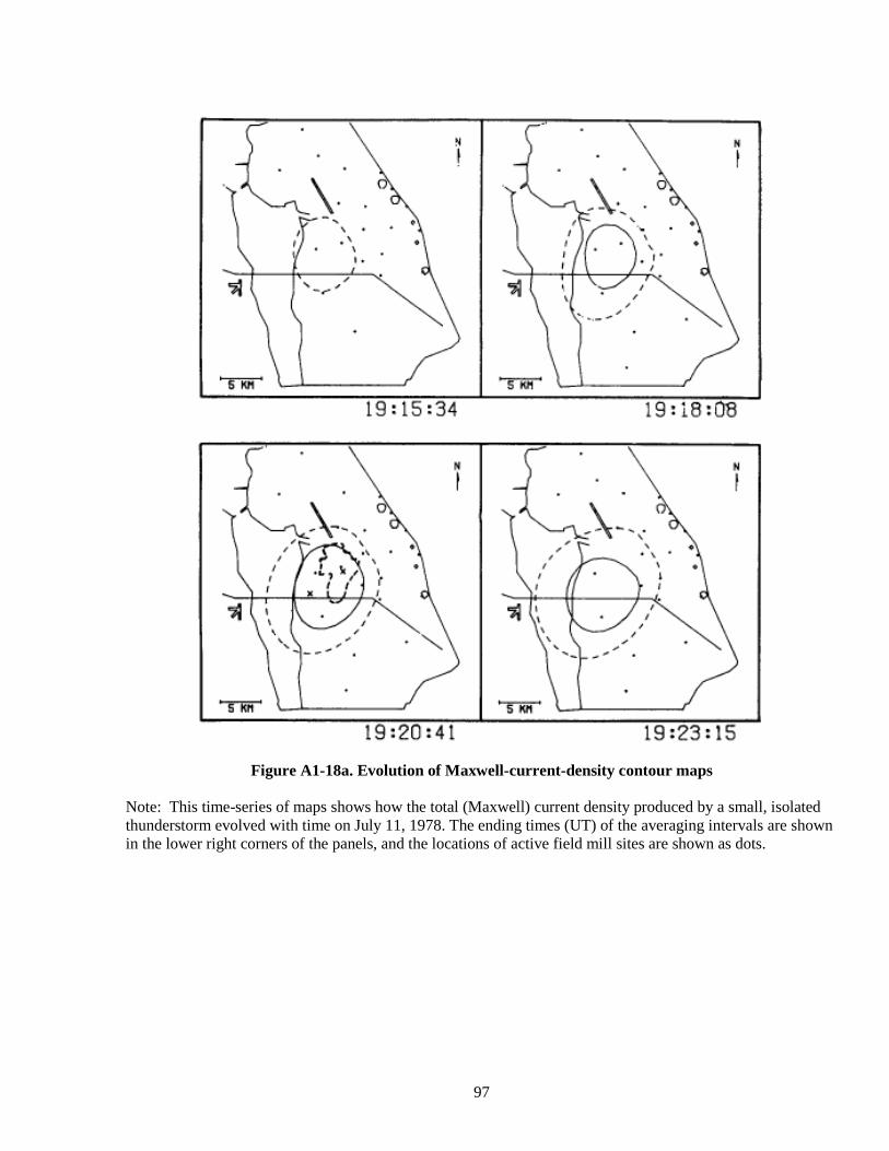
97

Figure A1-18a. Evolution of Maxwell-current-density contour maps

Note: This time-series of maps shows how the total (Maxwell) current density produced by a small, isolated thunderstorm evolved with time on July 11, 1978. The ending times (UT) of the averaging intervals are shown in the lower right corners of the panels, and the locations of active field mill sites are shown as dots.

98

Figure A1-18b. Evolution of Maxwell current density contours (continued)

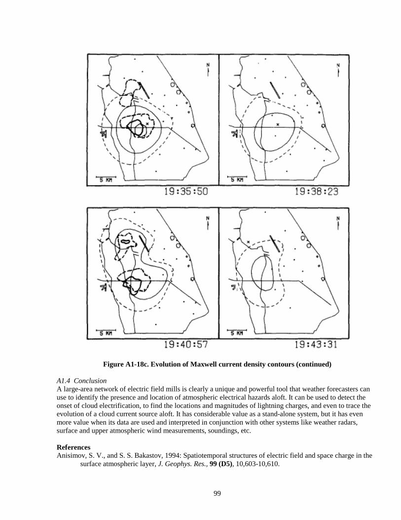
99

Figure A1-18c. Evolution of Maxwell current density contours (continued) A1.4 Conclusion A large-area network of electric field mills is clearly a unique and powerful tool that weather forecasters can use to identify the presence and location of atmospheric electrical hazards aloft. It can be used to detect the onset of cloud electrification, to find the locations and magnitudes of lightning charges, and even to trace the evolution of a cloud current source aloft. It has considerable value as a stand-alone system, but it has even more value when its data are used and interpreted in conjunction with other systems like weather radars, surface and upper atmospheric wind measurements, soundings, etc. References Anisimov, S. V., and S. S. Bakastov, 1994: Spatiotemporal structures of electric field and space charge in the

surface atmospheric layer, J. Geophys. Res., 99 (D5), 10,603-10,610.

100

Arnold, H. R., E. T. Pierce, and A. L. Whitson, 1965: The effect of a living tree upon the fair weather potential

gradient, J. Atmos. Terr. Phys., 27, 429-430. Bateman, M. G., M. F. Stewart, R. J. Blakeslee, S. J. Podgorny, H. J. Christian, D. M. Mach, J. C. Bailey, and

D. Daskar, 2007: A low-noise, microprocessor-controlled, internally digitizing rotating-vane electric field mill for airborne platforms, J. Atm.& Ocean. Tech. 24, 1245–1255. DOI: 10.1175/JTECH2039.1

Bering, E.A., A. A. Few, and J. R. Benbrook, 1998: The Global Electric Circuit, Physics Today, 51 (10), 24–

30. Blanchard, D.C., 1963: Electrification of the atmosphere by particles from bubbles in the sea, Prog.

Oceanogr., 1, 71-202. Browning, G. L., I. Tzur, , and R. G. Roble, 1987: A Global Time-Dependent Model of Thunderstorm

Electricity. Part I: Mathematical Properties of the Physical and Numerical Models, J. Atmos. Sci., 44 (15), 2166-2177.

Byrne, G. J., A. A. Few, and M. E. Weber, 1983: Altitude, thickness, and charge concentration of charged

regions of four thunderstorms during TRIP 1981 based upon in situ balloon electric field measurements, Geophys. Res. Letters, 10 (1), 39-42.

Byrne, G. J., A. A. Few, and M.F. Stewart, 1986: The effects of atmospheric parameters on a corona probe

used in measuring thunderstorm electric fields, J. Geophys. Res., 91, 9911-9920. Chalmers, J. A., 1952: Negative electric fields in mist and fog, J. Atmos. Terr. Phys., 2, 155-159. Chalmers, J. A., 1964: The electrical properties of a living tree in relation to point discharge, J. Atmos. Terr.

Phys., 26, 129-134. Chalmers, J. A., 1965: The relation between precipitation current and potential gradient, J. Atmos. Terr. Phys.,

27, 899-905. Chalmers, J. A., 1967: Atmospheric Electricity, 2nd Edition, Pergamon Press, London, 515 pp. Chapman, S., 1970: Corona point current in wind, J. Geophys. Res., 75, 2165-2169. Chapman, S., 1977: The Magnitude of Corona Point Discharge Current, J. Atmos. Sci., 34, 1801-1809. Chauzy, S. J.-C. Medale, S. Prieur, and S. Soula, 1991: Multilevel measurement of the electric field

underneath a thundercloud. 1. A new system and the associated data processing, J. Geophys. Res., 96, 22,319-22,326.

Chubb, J., and J. Harbour, 2010: ‘Operational health’ monitoring for confidence in long term electric field

measurements, J Electrostatics, in press. Computer Sciences Raytheon, 2006: Eastern Range Instrumentation Handbook, CDRL A209, Contract

F085=650-00-C-0005, 15 January, 2006.

101

Deaver, L. E., and E. P. Krider, 1991: Electric fields and current densities under small Florida thunderstorms, J. Geophys. Res., 96, 22,273-22,281.

Fews, A. P., R. J. Wilding, P. A. Keitch, K. N. Holden, and D. L. Henshaw, 2002: Modification of

atmospheric DC fields by space charge from high-voltage power lines, Atmos. Res., 63, 271-289. Gathman, S., 1968: Guarded Double Field Meter, Rev. Sci. Instrum., 39 (1), 43-47. Gathman, S., and E. M. Trent, 1968: Space Charge over the Open Ocean, J. Atmos. Sci., 25, 1075-1079. Gathman, S., and W. Hoppel, 1970: Surf Electrification, J. Geophys. Res., 75 (24), 4525-4529. Gringel, W., J.M. Rosen, and D.J Hofmann, 1986: Electrical structure from 0 to 30 kilometers, Chapter 12 in

The Earth's Electrical Environment, edited by E. P. Krider and R. G.Roble, National Academy Press, Washington, D.C., 263 pp. (pp.166-182).

Groom, K. N., and J. A. Chalmers, 1967: Negative charges from high-tension power cables in fog, J. Atmos.

Terr. Phys., 29, 613-615. Gunn, R., 1954: Electric Field Meters, Rev. Sci. Instrum., 25 (5), 432-437. Handel, S. C., 2000: Electric Fields Before and During the Onset of Electrification in Florida, M.S. manuscript

at the University of Arizona, October, 2000. [Also, to be submitted to the J. Geophys. Res., 2011, (with E. P. Krider)]

Holzer. R. E. and D. S. Saxon, 1952: Distribution of electrical conduction currents in the vicinity of

thunderstorms, J. Geophys. Res., 57, 207-216. Hoppel, W. A., R. V. Anderson, and J. C. Willett, 1986: Atmospheric electricity in the planetary boundary

layer, Chapter 11 in The Earth's Electrical Environment, edited by E. P. Krider and R. G.Roble, National Academy Press, Washington, D.C., 263 pp. (pp.149-165).

Horenstein, M. N., and P. R. Stone, 2001: A micro-aperture electrostatic field mill based on MEMS

technology, J. Electrostatics, 51-52, 515-521. IEEE Std 1227-1990 (R2010): Guide for the Measurement of DC Electric-Field Strength and Ion Related

Quantities, IEEE Power Engineering Society (Approved ANSI October 12, 1990; Reaffirmed 17 June 2010).

Israel, H., 1959: Atmospheric electrical agitation, Quart. J. Roy. Met. Soc., 85, 91-104. Israel, H., 1973: Atmospheric Electricity, Vol II, NTIS, U.S. Department of Commerce, Springfield, VA, 570

pp. Jacobson, E. A., and E. P. Krider, 1976: Electrostatic field changes produced by Florida lightning, J. Atmos.

Sci., 33 (1), 103−117. Johnston, A. R., H. Kirkham, and B. T. Eng, 1986: dc electric field meter with fiber-optic readout, Rev. Sci.

Instrum., 57 (11), 2746–2753.

102

Kasemir, H. W., 1959: The thunderstorm as a generator in a global electric circuit (in German), Z. Geophys., 25, 33-64.

Kasemir, H. W., 1963: “The Thundercloud” in Proc. Third Int. Conf. on Atmospheric and Space Electricity,

Montreaux, Switzerland, May 5-10, 1963, ed. By S. C. Coroniti, Elsevier, 1965, pp. 215-235. Kasemir, H. W., 1971: Calibration of Atmospheric Electric Field Meters and the Determination of Form

Factors at Kennedy Space Center, NOAA Tech. Memo. ERL APCL-11, April, 1971. Kasemir, H. W., 1972: The Cylindrical Field Mill, Meteorol. Rundsch., 25, 33-38. Kraakevik, J.H., and J.F. Clark, 1958: Airborne measurements of atmospheric electricity, Eos Trans. AGU, 39,

827-834. Krider, E. P., and R. J. Blakeslee, 1985: The Electric Currents Produced by Thunderclouds, J. Electrostatics,

16, 369-378. Krider, E. P., and J. A. Musser, 1982: Maxwell Currents Under Thunderstorms, J. Geophys. Res., 87 (C13),

11,173-11,176. Latham, D. J., and R. W. Miksad, 1974: Electric Field Perturbations of the Marine Atmosphere by Horizontal

Roll Vortices, J. Geophys. Res., 79(36), 5592–5597, doi:10.1029/JC079i036p05592. Livingston, J. M., and E. P. Krider, 1978: Electric fields produced by Florida thunderstorms, J. Geophys. Res.,

83 (C1), 385−401. LPLWS, 1992: AGBFM Initial Check Lists and Calibration, Test and Calibration User’s Guide, Air Force

Library #M17187, 5 December 1992, 11 pp. MacGorman, D. R., and W. D. Rust, 1998: The Electrical Nature of Storms. Oxford Univ. Press, ISBN 0-19-

507337-1, 432 pp. Malan, D. J., and B. F. J. Schonland, 1950: An Electrostatic Fluxmeter of Short Response-time for use in

Studies of Transient Field-changes, Proc. Phys. Soc. (London), B, 63, 402-408. Mapleson, W. W., and W. S. Whitlock, 1955: Apparatus for the accurate and continuous measurement of the

earth’s electric field, J. Atmos. Terr. Phys., 7, 61-72. Marshall, T. C. , W. D. Rust, M. Stolzenburg, W. Roeder, and P. R. Krehbiel, 1999: A study of enhanced fair-

weather electric fields occurring soon after sunrise, J. Geophys. Res., D104, 24455-24469. Matthews, J. C., and D. L. Henshaw, 2009: Measurements of atmospheric potential gradient fluctuations

caused by corona ions near high voltage power lines, J. Electrostatics, 67, 488-491. Merceret, F.J. and J.C. Willett, Editors, H.J. Christian, J.E. Dye, E.P. Krider, J.T. Madura, T.P. O'Brien, W.D.


Montanya, J., P. Rodriguez, J. Bergas, A. Illa, B. Hermoso, and I. Candela, 2007: A new electrostatic field

measurement method: The coherent-notch field mill, J Electrostatics, 65, 431-437.

103

Ogden, T. L., and W. C. A. Hutchinson, 1970: Electric space-charge pulses near the ground in sunny weather, J. Atmos. Terr. Phys., 32, 1131-1138.

Ravichandran, M., and A. K. Kamra, 1999: Spherical field meter to measure the electric field vector –

measurements in fair weather and inside a dust devil, Rev. Sci. Instrum., 70 (4), 2140-2149. Reid, G.C., 1986: Electrical structure of the middle atmosphere, Chapter 13 in The Earth's Electrical

Environment, edited by E. P. Krider and R. G.Roble, National Academy Press, Washington, D.C., 263 pp. (pp.183-194).

Reiter, R., 1968: Results of Investigation on Precipitation and Cloud Electricity Based on 15 Years of

Observation, Arch. Met. Geoph. Biokl., Ser. A, 17, 17-29. Reiter, R., 1994: Charges on particles of different size from bubbles of Mediterranean Sea surf and from

waterfalls, J. Geophys. Res., 99 (D5), 10,807–10,812, doi:10.1029/93JD03268. Reitz, J.R., and F.J. Milford, 1967: Foundations of Electromagnetic Theory, Addison-Wesley Publishing

Company, Reading, MA, Second Edition, 435 pp. Roble, R.G, and I. Tzur, 1986: The global atmospheric electrical circuit, Chapter 15 in The Earth's Electrical


Rust, W. D., and D. R. MacGorman, 1988: Techniques for measuring the electrical parameters of

thunderstorms, Chapter 8 in Instruments and Techniques for Thunderstorm Observation and Analysis, edited by Edwin Kessler, U. Oklahoma Press, 268 pp.

Sagalyn, R,C, and G.A. Faucher, 1956: Space and time variations of charged nuclei and electrical conductivity

of the atmosphere, Q. J. R. Metoerol. Soc. 82, 428.. Secker, P. E., 1975: The design of simple instruments for measurement of charge on insulating surfaces, J.

Electrostatics, 1, 27-36. Secker, P. E. and J. N. Chubb, 1984: Instrumentation for electrostatic measurements, J. Electrostatics, 16, 1-

19. Siingh, D., V. Gopalakrishnan, R. P. Singh, A. K. Kamra, S. Singh, V. Pant, R. Singh, and A. K. Singh, 2007:

The atmospheric global electric circuit,: An overview, Atmos. Res., 84, 91-110. Smiddy, M., and J. A. Chalmers, 1958: The double field mill, J. Atmos. Terr. Phys., 12, 206-210. Smith, L. G., 1955: The electric charge of raindrops, Quart. J. Roy. Met. Soc., 81, 23-47. Soula, S., 1994: Transfer of electrical space charge from corona between ground and thundercloud;

measurements and modeling, J. Geophys. Res., 99, 10,759-10,765. Soula, S., and S. Chauzy, 1991: Multilevel measurement of the electric field underneath a thundercloud. 2.

Dynamical evolution of a ground space charge layer, J. Geophys. Res., 96, 22,327-22,336. Standler, R. B., 1980: Estimation of corona current beneath thunderclouds, J. Geophys. Res., 85, 4541-4544.

104

Standler, R. B., and W. P. Winn, 1979: Effects of coronae on electric fields beneath thunderstorms, Quart. J. Roy. Meteor. Soc., 105, 285-302.

Tzur, I., and R. G. Roble, 1985: The Interaction of a Dipolar Thunderstorm With Its Global Environment, J.

Geophys. Res., 90 (D4), 5989-5999. Waddel, R. C., 1948: An Electric Field Meter for Use on Airplanes, Rev. Sci. Instrum., 19 (1), 31-35. Weber, M. E., M. F. Stewart, and A. A. Few, 1983: Corona point Measurements in a Thundercloud at

Langmuir Laboratory, J. Geophys. Res., 88 (C6), 3907-3910. Willett, J.C., 1979: Fair weather electric charge transfer by convection in an unstable planetary boundary layer,

J. Geophys. Res., 84 (C2), 703-718. Whitlock, W. B., and J. A. Chalmers, 1956: Short-period variations in the atmospheric electric potential

gradient, Quart. J. Roy. Met. Soc., 82, 325-336. Williams, E. R., 2009: The global electric circuit: A review, Atmos. Res., 91, 140-152.

105

Appendix 2. Spatial and Temporal Intervals between Lightning Discharges A2.0 Introduction Natural lightning discharges almost always begin inside the cloud with a process that is called the 'preliminary breakdown.' Roughly 2/3 of all flashes remain inside the cloud, or propagate from one cloud to another or to clear air, and are known collectively as 'cloud discharges.' Roughly 1/3 of all flashes propagate from cloud to ground and are called CG flashes or ground discharges. CG flashes can be further classified as 'positive' or 'negative' according to the polarity of the charge that is effectively transferred to ground. Most CG flashes occurring in the warm season are negative, but some storms, particularly those in the Great Plains, are dominated by positive CG discharges. Further details about the types of lightning discharges and their characteristics can be found in books by Uman (1976; 1990), MacGorman and Rust (1998), Rakov and Uman (2003), and elsewhere. In the following, we will discuss some of the spatial and temporal characteristics of CG lightning that have been determined primarily using networks of gated, wideband antenna systems and electronics that respond to the electromagnetic impulses radiated by 'return strokes,' the high-current components of CG flashes. Examples of such detection systems are the CGLSS and NLDN that have been discussed by Merceret and Willett et al. (2010, Sections 5.1.3, A8.1.2, and A8.1.4). These networks report the locations of the ground strike points and other characteristics of each stroke such as an estimate of the peak current and its polarity. We will also refer to data obtained from the LDAR and similar systems that have been designed to detect the air breakdown processes, such as the preliminary breakdown inside the cloud and the subsequent development of leader channels both inside and outside the cloud, that radiate VHF radio impulses (see History, sections 5.1.2 and A8.1.3). A2.1 Spatial Distances The average 2-dimensional, horizontal distance between successive cloud-to ground (CG) lightning strikes clearly represents a minimum stand-off distance from natural lightning. Hatakeyama (1958) [see also Fig. 11 in Pierce (1974)] found that all of the visually observed ground flashes under a small thunderstorm in Japan struck within 10 km of the previous flash. Using a network of gated, wideband lightning direction-finders, Krider (1988) found that the average distance between successive CG strikes in three nearly stationary storms at KSC ranged from 3.2 to 4.2 km, with standard deviations that were about 2/3 the means. Using similar detection technology, Lopez and Holle (1999) and Holle et al. (2003) have reported that the average distances between successive CG strikes range from about 5.2 km under small Florida storms to about 8.6 km under a large, multicell storm in Oklahoma, and that 95% of the inter-flash distances are less than 13 km in FL and 14 km in OK. Jacobsen and Krider (1976) found that all of the CG flashes produced by convective clouds struck within 18 km (10 nm) of the inferred centers of where lightning changed the cloud charge distribution (see their Figure 16), and in a similar study, Oram and Krider (1991) found that 95% of the CG flashes struck within 12 km of the inferred charge centers. Murphy et al. (1996) analyzed one small and one large storm at KSC and found that most of the horizontal distances between the inferred lightning charge centers and the CG strike points were less than 10 km; the average distance was 3.9 km and the standard deviation was 3.3 km. Murphy et al. (1996) also note that their 3.9 km average distance is consistent with a horizontal displacement that might be expected from the random geometrical development of a lightning stepped-leader as it propagates from the altitude of the lightning charge (typically 7 to 9 km in Florida) to the ground. Murphy et al. (1996) also pointed out that, since the geometrical development of the stepped-leader is a quasi-random, stochastic process, there will tend to be relatively few events that strike directly under a concentrated cloud charge distribution and that more flashes will tend to strike where the solid angle produced by the

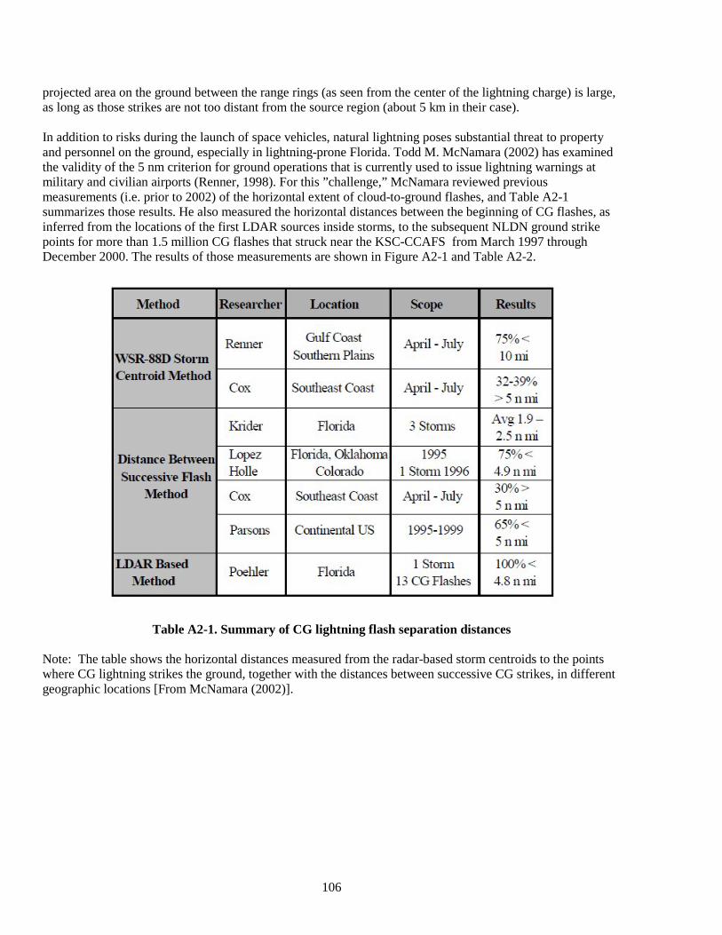
106

projected area on the ground between the range rings (as seen from the center of the lightning charge) is large, as long as those strikes are not too distant from the source region (about 5 km in their case). In addition to risks during the launch of space vehicles, natural lightning poses substantial threat to property and personnel on the ground, especially in lightning-prone Florida. Todd M. McNamara (2002) has examined the validity of the 5 nm criterion for ground operations that is currently used to issue lightning warnings at military and civilian airports (Renner, 1998). For this ”challenge,” McNamara reviewed previous measurements (i.e. prior to 2002) of the horizontal extent of cloud-to-ground flashes, and Table A2-1 summarizes those results. He also measured the horizontal distances between the beginning of CG flashes, as inferred from the locations of the first LDAR sources inside storms, to the subsequent NLDN ground strike points for more than 1.5 million CG flashes that struck near the KSC-CCAFS from March 1997 through December 2000. The results of those measurements are shown in Figure A2-1 and Table A2-2.

Table A2-1. Summary of CG lightning flash separation distances Note: The table shows the horizontal distances measured from the radar-based storm centroids to the points where CG lightning strikes the ground, together with the distances between successive CG strikes, in different geographic locations [From McNamara (2002)].

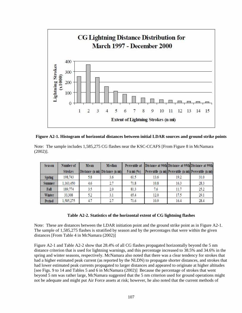
107

Figure A2-1. Histogram of horizontal distances between initial LDAR sources and ground strike points

Note: The sample includes 1,585,275 CG flashes near the KSC-CCAFS [From Figure 8 in McNamara (2002)].

Table A2-2. Statistics of the horizontal extent of CG lightning flashes Note: These are distances between the LDAR initiation point and the ground strike point as in Figure A2-1. The sample of 1,585,275 flashes is stratified by season and by the percentages that were within the given distances [From Table 4 in McNamara (2002)] Figure A2-1 and Table A2-2 show that 28.4% of all CG flashes propagated horizontally beyond the 5 nm distance criterion that is used for lightning warnings, and this percentage increased to 38.5% and 34.6% in the spring and winter seasons, respectively. McNamara also noted that there was a clear tendency for strokes that had a higher estimated peak current (as reported by the NLDN) to propagate shorter distances, and strokes that had lower estimated peak currents propagated to larger distances and appeared to originate at higher altitudes [see Figs. 9 to 14 and Tables 5 and 6 in McNamara (2002)] Because the percentage of strokes that went beyond 5 nm was rather large, McNamara suggested that the 5 nm criterion used for ground operations might not be adequate and might put Air Force assets at risk; however, he also noted that the current methods of

108

implementing lightning warnings are conservative and that there will always be a tradeoff between the "amount of risk to which one is subjected versus the importance of the mission at hand." McNamara’s measurements are for CG flashes only but the horizontal extent of all lightning discharges from their source is dominated by the development inside the cloud and above the ground, so his distances are representative of all flashes. It should be noted that the standoff distance of the flight path from lightning in the "Lightning" Rule, G417.7, is 10 n mi, not the less conservative 5 n mi that is used to issue lightning warnings for ground operations. Additionally, the standoff from thunderstorms in the LFCC is from the edge of the cloud, not the centroid of the storm or the initiation point of the lightning that were used by McNamara. (See the rationale for the "Lightning" Rule for a discussion of how the stand-off distances are to be determined and why.) In recent years, lightning discharges that strike tall towers have been studied using high-speed photography (Warner, 2010; Warner et al., 2011). An interesting result from this work has been the observation that a large fraction of tower strikes are actually upward-propagating discharges that are initiated or ‘triggered’ by a nearby lightning flash (usually of positive polarity). The stand-off distance of 10 n mi from the nearest part of any lightning discharge (Section G417.7(b) of the "Lightining" Rule) will reduce the chances of any ‘lightning triggered by lightning’ that might be initiated by a vehicle during ascent, or on the launch pad during a countdown. (See also discussion of earlier speculations to this effect in Section A5.1 of Appendix 5, "Conditions for Triggered Lightning.") At this point, we would also like to point out that to first order, the chances that a vehicle will experience a direct (not triggered) lightning strike, either on the launch pad or during ascent, is proportional to the area density of CG strikes that are expected in that local region. Since the area density of the ‘next strikes’ produced by a localized source will decrease with distance from that source, a count of just the number of flashes that strike a given distance from a prior strike, or from the inferred location of the lightning charge, or from the first LDAR sources inside the cloud to the ground will all tend to overestimate the chances that a vehicle will receive a direct strike from that source. Krider (1988) has shown that the area density of the next strikes is close to zero at distances of 8 km or more from the previous flash under small stationary storms, and Murphy et al. (1996) have shown that the area-density of CG strikes is close to zero at distances of 10 km or more from the inferred lightning charge centers (see their Fig. 21). Given the above, and the fact that the LFCC require stand-off distances to be measured from the nearest part of a highly-branched lightning flash, that is either inside or outside the cloud (or from the edge of the cloud that produced the lightning), then a stand-off distance of 10 n mi (18 km) will include an additional margin of safety for spaceflight operations. A2.2 Time Intervals The expected time-interval between the last lightning discharge in a storm and the previous flash is 5 to 10 minutes near the end of most isolated, convective storms (Livingston and Krider, 1978; MacGorman and Rust, 1998; Anderson, 2009; and Stano et al., 2010), but occasionally, a terminating cell will stimulate new convective growth and produce lightning with a time-to-onset that is comparable to that in a growing cumulus cloud. Because of these factors, the rationale for both sections of the "Lightning" Rule, G417.7, states that "a 30-minute waiting period after the last lightning flash occurs has been used to insure that any high electric fields aloft will have decayed to a safe level along the flight path." The rationale also notes that a 30-minute waiting period is just twice the 15-minute interval that a trained weather observer will normally add to the time of the last audible thunder when defining the ending-time of a thunderstorm (Changnon, 1993; FMH No. 1, 2005). A 30-minute waiting period provides a modest margin of safety and an interval that is long enough to identify any new convective clouds that form within 10 n mi of the flight path However, a 30-minute waiting period remains a legacy provision (see Chapter 1, "Introduction") for which there is still incomplete statistical justification.

109

The problem of specifying a definite time or waiting period that will ensure a true ‘end-of-storm’ (or end of high electric fields aloft) is particularly difficult under the weather conditions that follow large, multi-cell storms, squall lines, or mesoscale convective systems (MCSs). After such storms, there are often horizontally extensive cloud layers that can initiate and/or propagate widely separated lightning flashes into a region at very low rates. These clouds can persist for several hours at a particular location, and often produce natural lightning, either CG flashes or cloud discharges, that have very long time-intervals between the discharges (see Sections A3.6 and A3.7 of Appendix 3, "Cloud Electrification"). The low flashing rates and large areal extents of the parent clouds create difficult problems for launch safety because it is clear that such clouds can retain (or be the source of) embedded cells of convection (see Section A4.0 of Appendix 4, "Electrical Aspects of Stratiform Clouds") and/or store significant electric charge that produces high electric fields for long times (see Section A 6.2 and A6.2 of Appendix 6, "Electrical Properties and Decay of Electric Fields in Cloudy Air"). In order to protect against these possibilities, there are other rules that apply in such circumstances. For example, the waiting times in the "Debris Clouds" Rule, G417.15, have been set at 3 hours. References Anderson, H, 2009: Characteristics of Decaying Storms during Lightning Cessation at Kennedy Space Center

and Cape Canaveral Air Force Station, M.S. Thesis, Department of Meteorology, Florida State University, submitted to the Florida Space Grant Consortium by Dr. Henry E. Fuelberg, December 2, 2009.

Changnon, S. A., 1993: Relations between thunderstorms and cloud-to-ground lightning in the United States.

J. Appl. Meteor., 32, 88–105. Cox, C. C., 1999: A Comparison of Horizontal Cloud-To-Ground Lightning Flash Distance Using Weather

Surveillance Radar and The Distance Between Successive Flashes Method. M.S. Thesis, AFIT/GM/ENP/99M-03, Department of Engineering Physics, Air Force Institute of Technology, 130 pp.

Federal Meteorological Handbook No. 1 (FMH No. 1), Surface Weather Observations and Reports, U.S. Dept.

of Commerce, FCM-H1-2005, Washington, DC, September 2005. Hatakeyama, H., 1958: "The Distribution of Sudden Change of Electric Field on Earth's Surface due to

Lightning Discharges", in Recent Advances in Atmospheric Electricity, L. G. Smith, ed., Pergamon Press, New York, pp. 289-298.

Hinson, M. S., 1997: A Study of the Characteristics of Thunderstorm Cessation at the NASA Kennedy Space

Center, M.S. Thesis, Dept. of Meteorology, Texas A & M university, College Station, TX, August 1997, 91 pp.

Holle, R. L., M. Murphy, and R. E. Lopez, 2003: Distances and times between cloud-to-ground flashes in a

storm, Paper 103-79KMI, Preprints, International Conference on Lightning and Static Electricity, 16-18 September, Blackpool, U.K.

Jacobson, E. A., and E. P. Krider, 1976: Electrostatic field changes produced by Florida lightning, J. Atmos.

Sci., 33 (1), 103−117. Livingston, J. M. and E. P. Krider, 1978: Electric Fields Produced by Florida Thunderstorms, J. Geophys.

Res., 83 (C1), 385-401. Lopez, R. E., and R. L. Holle, 1999: The distance between successive lightning flashes. NOAA Tech. Memo.

ERL NSSL-105, National Severe Storms Laboratory, Norman, OK, 29 pp.

110

MacGorman, D. R. and W. D. Rust, 1998: The Electrical Nature of Storms, Oxford University Press, New

York, 1998, 432 pp. McNamara, T. M., 2002: The horizontal extent of cloud-to-ground lightning over the Kennedy Space Center.

M.S. thesis, Air Force Institute of Technology, Wright-Patterson AFB, Ohio, AFIT/GM/ENP/02M-06, 114pp, 14 January 2002.



Murphy, M. J., E. P. Krider, and M. W. Maier, 1996: Lightning charge analyses in small Convection and

Precipitation Experiment (CaPE) storms, J. Geophys. Res., 101 (D23), 29,615–29,626. Murphy, M. J., and R. L. Holle. 2005: A warning method for cloud-to-ground lightning based on total lightning

and radar information, preprints, International Conference on Lightning and Static Electricity, 19–23 September 2005, Seattle, Washington, paper LDM-36, 2005.

Nelson, L. A., 2002: Synthesis of 3-dimensional lightning data and weather radar data to determine the

distance that naturally occurring lightning travels from thunderstorms. M.S. thesis, Air Force Institute of Technology, Wright-Patterson AFB, Ohio, AFIT/GM/ENP/02M-07.

Oram, T. D., and E. P. Krider, 1991. The spatial variations of lightning during small Florida thunderstorms, in

Proceedings of the 1991 International Aerospace and Ground Conference on Lightning and Static Electricity, NASA Conf. Pub. 3106, vol. II, pp. 86-1 to 86-9.

Parsons, Tamara, L., 2000: Determining Horizontal Distance Distribution of Cloud-To-Ground Lightning.

M.S. Thesis, AFIT/GM/ENP/00M-09, Department of Engineering Physics, Air Force Institute of Technology, 88 pp.

Pierce, E. T., 1974. Atmospheric Electricity – Some Themes, Bull. Am. Meteor. Soc., 55 (10), 1186-1194. Poehler, Horst, A., 1978: LDAR Observations of a Developing Thunderstorm Correlated With Field Mill,

Ground Strike Location, and Weather Radar Data Including the First Report of the Design and Capabilities of a New, Time-of-Arrival Ground-Strike Location System (GSLS). NASA Contract Report CR-154626, 135pp.

Rakov, V.A., and M.A. Uman, 2003: Lightning Physics and Effects, Cambridge University Press, 687pp. Renner, S. L., 1998: Analyzing Horizontal Distances Between WSR-88D Thunderstorm Centroids and Cloud-

To-Ground Lightning Strikes. M.S. Thesis, AFIT/GM/ENP/98M-09, Department of Engineering Physics, Air Force Institute of Technology, 123 pp.

Uman, M. A., 1976: Lightning, New York, McGraw-Hill, 264 pp. Uman, M. A., 2000: The Lightning Discharge, Orlando, Academic Press, 377 pp. Vollmer, D. R., 2002: The Horizontal Extent of Lightning Based on Altitude and Atmospheric Temperature,

M.S. Thesis, AFIT/GM/ENP/02M-10, Department of Engineering Physics, Air Force Institute of Technology, March 2002, 80 pp.

111

Warner, T. A., 2010: Observations of Simultaneous Multiple Upward Leaders from Tall Structures, Proc. 30th

International Conference on Lightning Protection - ICLP 2010, 13-17 September 2010, Cagliari, Italy. Warner, T. A., S. A. Cummer, W. A. Lyons, T. J. Lang, T. E. Nelson, and R. E. Orville, 2011: Coordinated

Video and RF Measurements of Positive CGs Inducing Both Sprites and Upward Tower Discharges, Fifth Conference on the Meteorological Applications of Lightning Data, 23-27 January 2011, Seattle, WA.

112

Appendix 3. Cloud Electrification A3.0 Introduction On May 10, 1752, a retired French dragoon, acting on instructions from Thomas-Francois Dalibard, drew sparks from a 40-foot iron rod that had been carefully insulated from the ground when a thundercloud passed overhead. This experiment had been suggested by Benjamin Franklin and had been set up at the village of Marly-la-Ville, near Paris, to determine whether clouds that produce lightning are electrified or not (Cohen, 1990, Chapter 6; Krider, 2006). These sparks proved for the first time that thunderclouds contain electricity and that lightning is an electrical discharge. A few weeks later (but before he knew about the results at Marly-la-Ville), Franklin performed his famous kite and key experiment (electrically equivalent to the experiment at Marly-la-Ville), and in September he installed a tall rod on the roof of his house to study the characteristics of storm electricity. This rod had a small gap that he could observe, and chimes were mounted on each side of the gap (see Figure A3-1). The upper portion was carefully insulated from the house, and the lower portion ran down a stairwell and was connected to a well. A small ball was suspended on silk thread between the chimes, so that it would ring the bells whenever the upper rod became electrified. The purpose of all this was to study the characteristics of storm electricity and to determine whether the electricity in thunderstorms was the same as the electricity that was generated by friction. Franklin described the results of his observations as follows:

“I found the bells rang sometimes when there was no lightning or thunder, but Only a dark cloud over the rod; that sometimes after a flash of lightning they would suddenly stop; and at other times, when they had not rung before, they would, after a flash, suddenly begin to ring; that the electricity was sometimes very faint, so that when a small spark was obtained, another could not be got for sometime after; at other times the sparks would follow extremely quick, and once I had a continual stream from bell to bell, the size of a crow-quill. Even during the same gust there were considerable variations.” (Labaree et al., Vol. 5, 1962, p. 62)

Franklin also used this apparatus to measure the polarity of thunderclouds, and he summarized those observations as follows:

“…that the clouds of a thunder gust are most commonly in a negative state of electricity, but sometimes in a positive state.” (Labaree et al., Vol. 5, 1962, p. 71)

These short descriptions of storm electricity remained the state of the art for the next 150 years (Schonland, 1950, p. 22; Schonland, 1952), and this and Franklin’s other observations underscore several factors that are important for the Lightning Flight Commit Criteria: (1) clouds can be highly electrified and not produce natural lightning; (2) lightning often appears with little advance warning; (3) lightning can both create and destroy cloud electricity abruptly; and (4) the amount and polarity of the cloud electricity are highly variable both within a storm and from storm to storm.

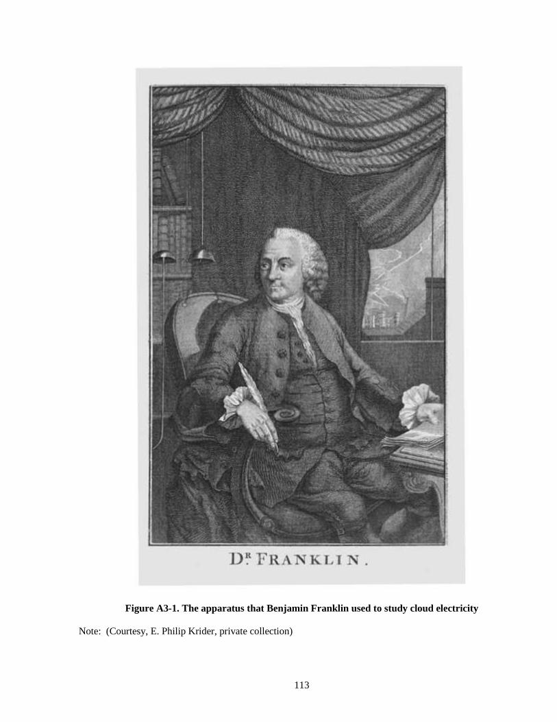
113

Figure A3-1. The apparatus that Benjamin Franklin used to study cloud electricity Note: (Courtesy, E. Philip Krider, private collection)

D~ FRANKLI N.

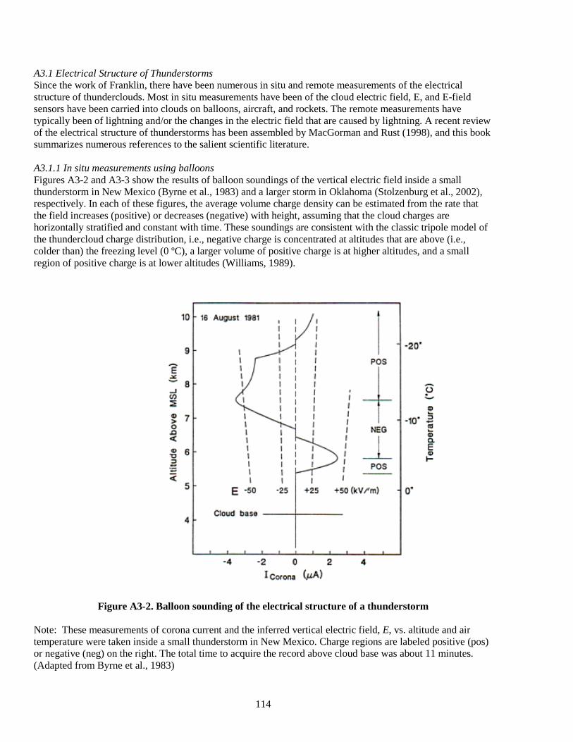
114

A3.1 Electrical Structure of Thunderstorms Since the work of Franklin, there have been numerous in situ and remote measurements of the electrical structure of thunderclouds. Most in situ measurements have been of the cloud electric field, E, and E-field sensors have been carried into clouds on balloons, aircraft, and rockets. The remote measurements have typically been of lightning and/or the changes in the electric field that are caused by lightning. A recent review of the electrical structure of thunderstorms has been assembled by MacGorman and Rust (1998), and this book summarizes numerous references to the salient scientific literature. A3.1.1 In situ measurements using balloons Figures A3-2 and A3-3 show the results of balloon soundings of the vertical electric field inside a small thunderstorm in New Mexico (Byrne et al., 1983) and a larger storm in Oklahoma (Stolzenburg et al., 2002), respectively. In each of these figures, the average volume charge density can be estimated from the rate that the field increases (positive) or decreases (negative) with height, assuming that the cloud charges are horizontally stratified and constant with time. These soundings are consistent with the classic tripole model of the thundercloud charge distribution, i.e., negative charge is concentrated at altitudes that are above (i.e., colder than) the freezing level (0 ºC), a larger volume of positive charge is at higher altitudes, and a small region of positive charge is at lower altitudes (Williams, 1989).

Figure A3-2. Balloon sounding of the electrical structure of a thunderstorm Note: These measurements of corona current and the inferred vertical electric field, E, vs. altitude and air temperature were taken inside a small thunderstorm in New Mexico. Charge regions are labeled positive (pos) or negative (neg) on the right. The total time to acquire the record above cloud base was about 11 minutes. (Adapted from Byrne et al., 1983)

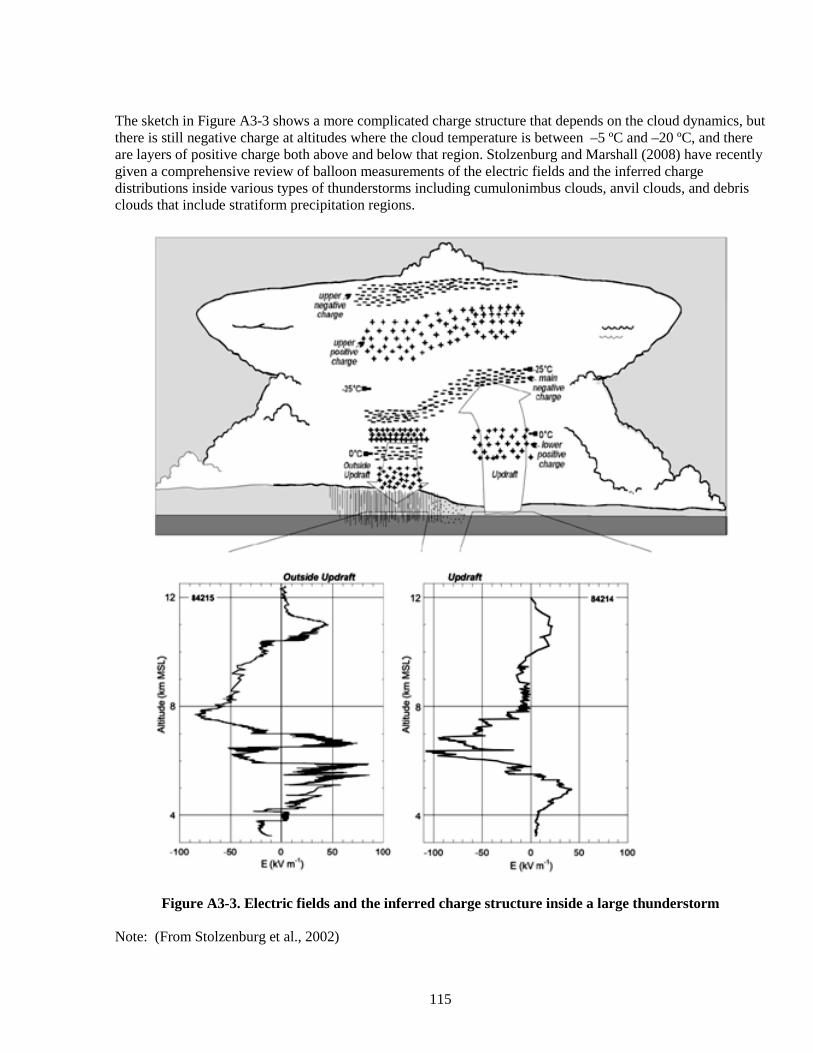
115

The sketch in Figure A3-3 shows a more complicated charge structure that depends on the cloud dynamics, but there is still negative charge at altitudes where the cloud temperature is between –5 ºC and –20 ºC, and there are layers of positive charge both above and below that region. Stolzenburg and Marshall (2008) have recently given a comprehensive review of balloon measurements of the electric fields and the inferred charge distributions inside various types of thunderstorms including cumulonimbus clouds, anvil clouds, and debris clouds that include stratiform precipitation regions.

Figure A3-3. Electric fields and the inferred charge structure inside a large thunderstorm Note: (From Stolzenburg et al., 2002)

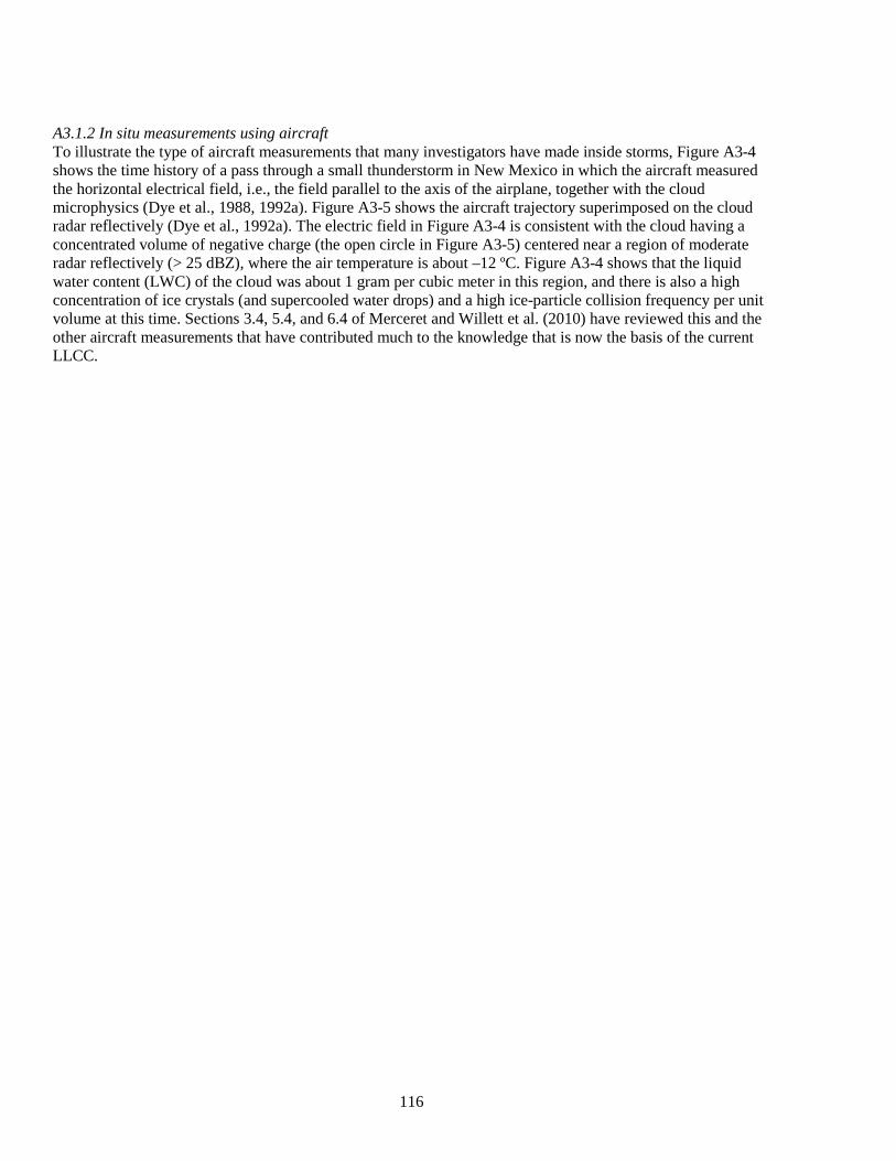
116

A3.1.2 In situ measurements using aircraft To illustrate the type of aircraft measurements that many investigators have made inside storms, Figure A3-4 shows the time history of a pass through a small thunderstorm in New Mexico in which the aircraft measured the horizontal electrical field, i.e., the field parallel to the axis of the airplane, together with the cloud microphysics (Dye et al., 1988, 1992a). Figure A3-5 shows the aircraft trajectory superimposed on the cloud radar reflectively (Dye et al., 1992a). The electric field in Figure A3-4 is consistent with the cloud having a concentrated volume of negative charge (the open circle in Figure A3-5) centered near a region of moderate radar reflectively (> 25 dBZ), where the air temperature is about –12 ºC. Figure A3-4 shows that the liquid water content (LWC) of the cloud was about 1 gram per cubic meter in this region, and there is also a high concentration of ice crystals (and supercooled water drops) and a high ice-particle collision frequency per unit volume at this time. Sections 3.4, 5.4, and 6.4 of Merceret and Willett et al. (2010) have reviewed this and the other aircraft measurements that have contributed much to the knowledge that is now the basis of the current LLCC.

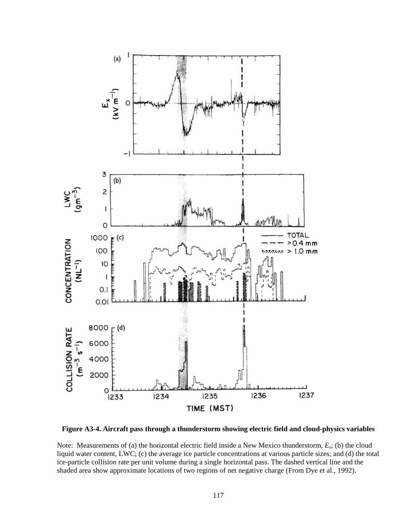
117

Figure A3-4. Aircraft pass through a thunderstorm showing electric field and cloud-physics variables Note: Measurements of (a) the horizontal electric field inside a New Mexico thunderstorm, Ex; (b) the cloud liquid water content, LWC; (c) the average ice particle concentrations at various particle sizes; and (d) the total ice-particle collision rate per unit volume during a single horizontal pass. The dashed vertical line and the shaded area show approximate locations of two regions of net negative charge (From Dye et al., 1992).

-u'" ~ ' -' E

'"

Z 0

~ o::~ ... ~ Zz w_ u z 0 u

W

~ 0:: -'" , z V>

0 ", - , Vl E -'--' 0 u

-, • E a 1-+ ....... , w>

.><

-I

3 (b)

2

a 1000 (c)

100

10

0.1

0.01

8000 (d)

6000

4000

2000

a 1233 1234

TOTAL --- > OA mm ":.. ~.o:-,.~., .o: > 1.0 mm

" ,

.. '1

: "

1235 1236 1237

TIME ( MST)

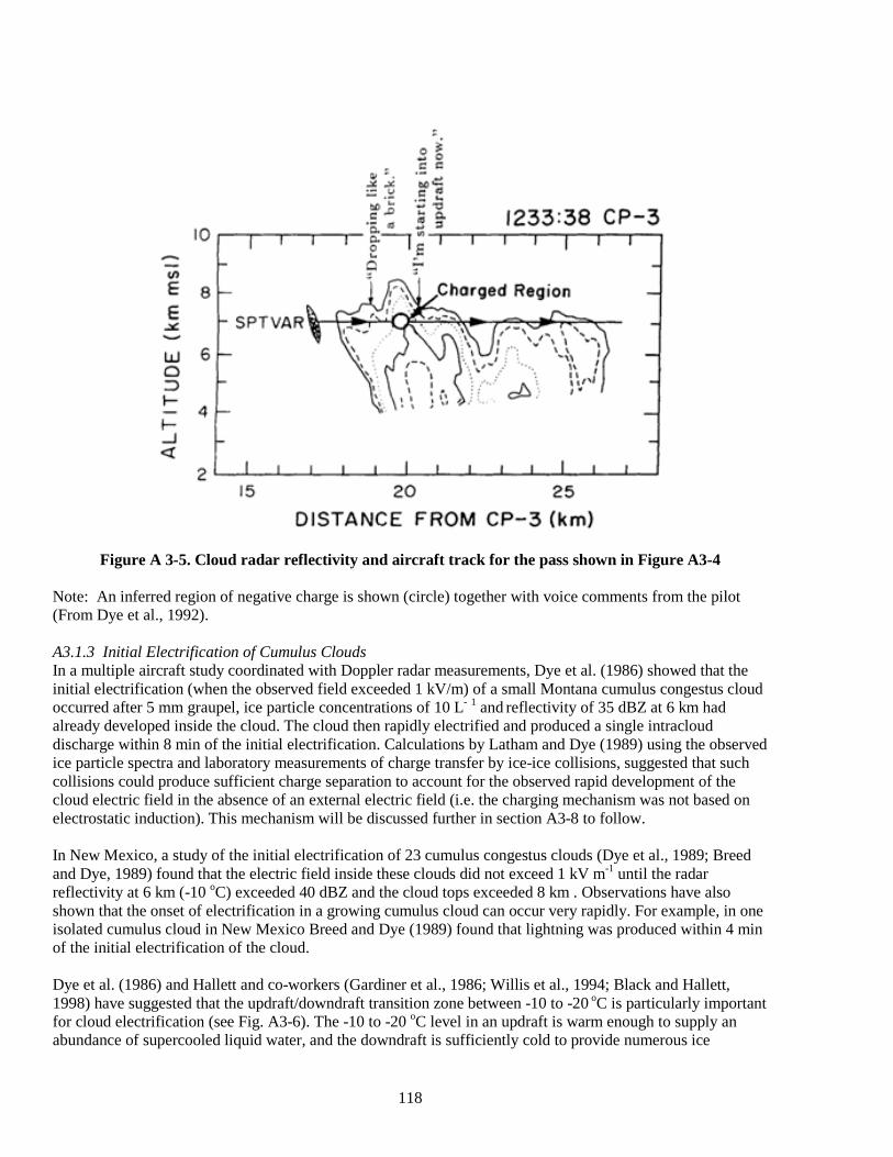
118

Figure A 3-5. Cloud radar reflectivity and aircraft track for the pass shown in Figure A3-4 Note: An inferred region of negative charge is shown (circle) together with voice comments from the pilot (From Dye et al., 1992). A3.1.3 Initial Electrification of Cumulus Clouds In a multiple aircraft study coordinated with Doppler radar measurements, Dye et al. (1986) showed that the initial electrification (when the observed field exceeded 1 kV/m) of a small Montana cumulus congestus cloud occurred after 5 mm graupel, ice particle concentrations of 10 L- 1 and reflectivity of 35 dBZ at 6 km had already developed inside the cloud. The cloud then rapidly electrified and produced a single intracloud discharge within 8 min of the initial electrification. Calculations by Latham and Dye (1989) using the observed ice particle spectra and laboratory measurements of charge transfer by ice-ice collisions, suggested that such collisions could produce sufficient charge separation to account for the observed rapid development of the cloud electric field in the absence of an external electric field (i.e. the charging mechanism was not based on electrostatic induction). This mechanism will be discussed further in section A3-8 to follow. In New Mexico, a study of the initial electrification of 23 cumulus congestus clouds (Dye et al., 1989; Breed and Dye, 1989) found that the electric field inside these clouds did not exceed 1 kV m-1 until the radar reflectivity at 6 km (-10 oC) exceeded 40 dBZ and the cloud tops exceeded 8 km . Observations have also shown that the onset of electrification in a growing cumulus cloud can occur very rapidly. For example, in one isolated cumulus cloud in New Mexico Breed and Dye (1989) found that lightning was produced within 4 min of the initial electrification of the cloud. Dye et al. (1986) and Hallett and co-workers (Gardiner et al., 1986; Willis et al., 1994; Black and Hallett, 1998) have suggested that the updraft/downdraft transition zone between -10 to -20 oC is particularly important for cloud electrification (see Fig. A3-6). The -10 to -20 oC level in an updraft is warm enough to supply an abundance of supercooled liquid water, and the downdraft is sufficiently cold to provide numerous ice

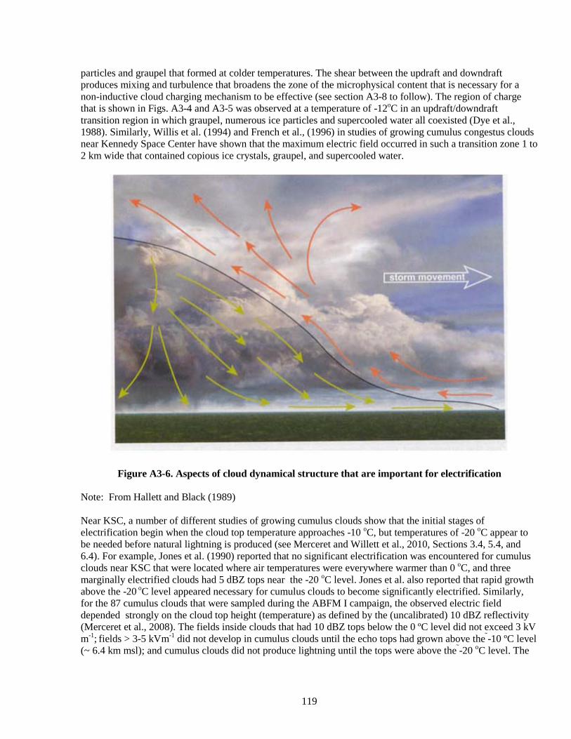
119

particles and graupel that formed at colder temperatures. The shear between the updraft and downdraft produces mixing and turbulence that broadens the zone of the microphysical content that is necessary for a non-inductive cloud charging mechanism to be effective (see section A3-8 to follow). The region of charge that is shown in Figs. A3-4 and A3-5 was observed at a temperature of -12oC in an updraft/downdraft transition region in which graupel, numerous ice particles and supercooled water all coexisted (Dye et al., 1988). Similarly, Willis et al. (1994) and French et al., (1996) in studies of growing cumulus congestus clouds near Kennedy Space Center have shown that the maximum electric field occurred in such a transition zone 1 to 2 km wide that contained copious ice crystals, graupel, and supercooled water.

Figure A3-6. Aspects of cloud dynamical structure that are important for electrification Note: From Hallett and Black (1989) Near KSC, a number of different studies of growing cumulus clouds show that the initial stages of electrification begin when the cloud top temperature approaches -10 oC, but temperatures of -20 oC appear to be needed before natural lightning is produced (see Merceret and Willett et al., 2010, Sections 3.4, 5.4, and 6.4). For example, Jones et al. (1990) reported that no significant electrification was encountered for cumulus clouds near KSC that were located where air temperatures were everywhere warmer than 0 oC, and three marginally electrified clouds had 5 dBZ tops near the -20 oC level. Jones et al. also reported that rapid growth above the -20 oC level appeared necessary for cumulus clouds to become significantly electrified. Similarly, for the 87 cumulus clouds that were sampled during the ABFM I campaign, the observed electric field depended strongly on the cloud top height (temperature) as defined by the (uncalibrated) 10 dBZ reflectivity (Merceret et al., 2008). The fields inside clouds that had 10 dBZ tops below the 0 ºC level did not exceed 3 kV m-1; fields > 3-5 kVm-1 did not develop in cumulus clouds until the echo tops had grown above the -10 ºC level (~ 6.4 km msl); and cumulus clouds did not produce lightning until the tops were above the -20 oC level. The

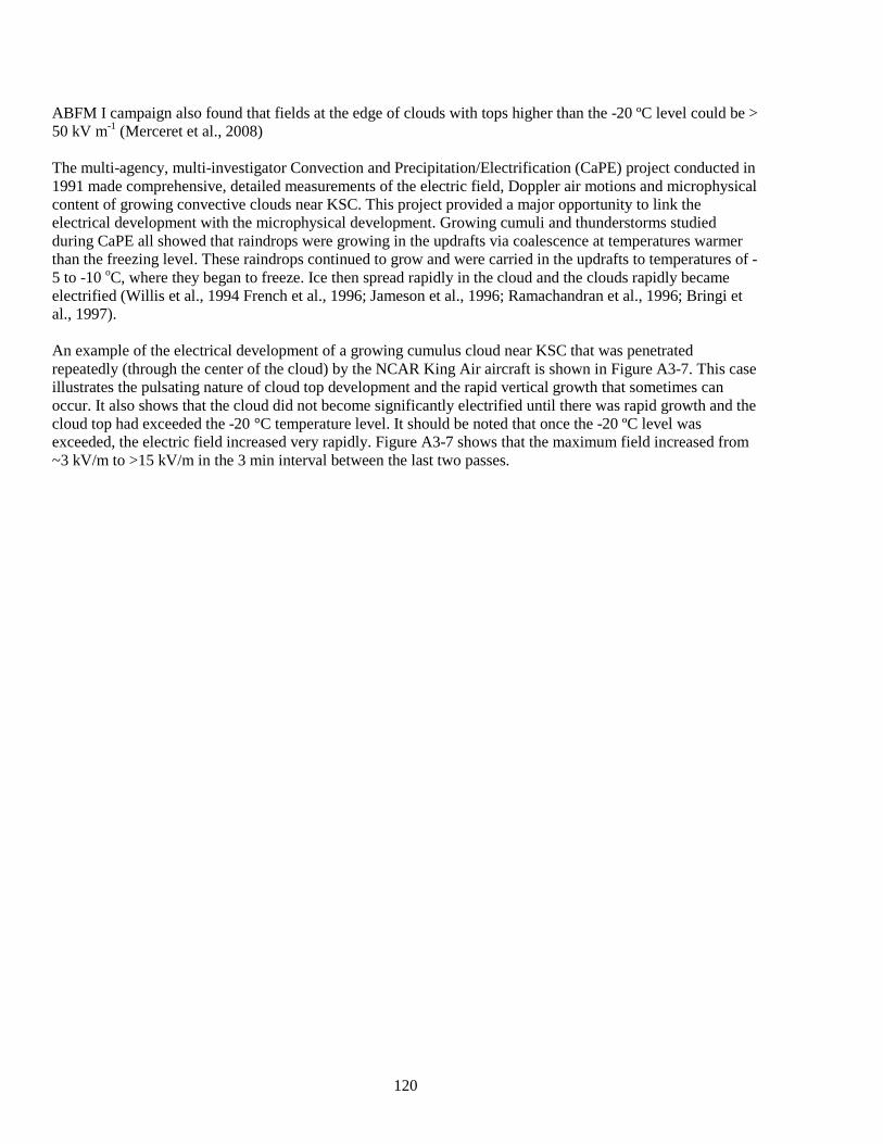
120

ABFM I campaign also found that fields at the edge of clouds with tops higher than the -20 ºC level could be > 50 kV m-1 (Merceret et al., 2008) The multi-agency, multi-investigator Convection and Precipitation/Electrification (CaPE) project conducted in 1991 made comprehensive, detailed measurements of the electric field, Doppler air motions and microphysical content of growing convective clouds near KSC. This project provided a major opportunity to link the electrical development with the microphysical development. Growing cumuli and thunderstorms studied during CaPE all showed that raindrops were growing in the updrafts via coalescence at temperatures warmer than the freezing level. These raindrops continued to grow and were carried in the updrafts to temperatures of -5 to -10 oC, where they began to freeze. Ice then spread rapidly in the cloud and the clouds rapidly became electrified (Willis et al., 1994 French et al., 1996; Jameson et al., 1996; Ramachandran et al., 1996; Bringi et al., 1997). An example of the electrical development of a growing cumulus cloud near KSC that was penetrated repeatedly (through the center of the cloud) by the NCAR King Air aircraft is shown in Figure A3-7. This case illustrates the pulsating nature of cloud top development and the rapid vertical growth that sometimes can occur. It also shows that the cloud did not become significantly electrified until there was rapid growth and the cloud top had exceeded the -20 °C temperature level. It should be noted that once the -20 ºC level was exceeded, the electric field increased very rapidly. Figure A3-7 shows that the maximum field increased from ~3 kV/m to >15 kV/m in the 3 min interval between the last two passes.

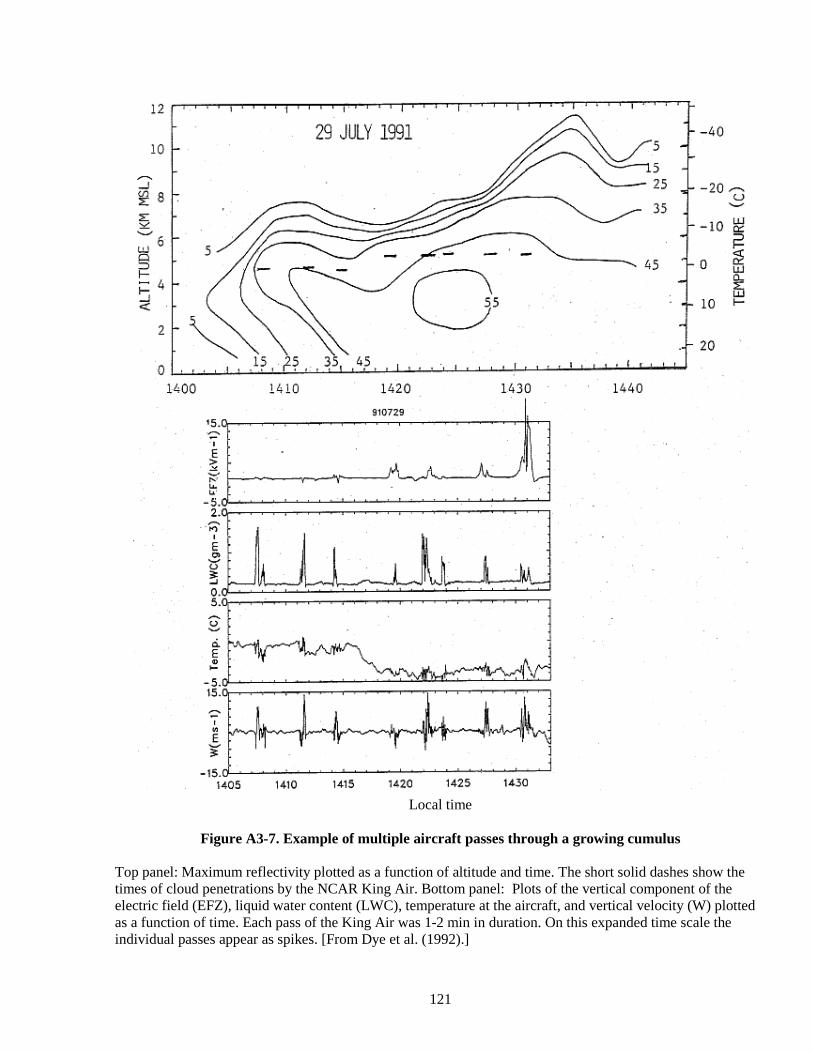
121

Local time

Figure A3-7. Example of multiple aircraft passes through a growing cumulus

Top panel: Maximum reflectivity plotted as a function of altitude and time. The short solid dashes show the times of cloud penetrations by the NCAR King Air. Bottom panel: Plots of the vertical component of the electric field (EFZ), liquid water content (LWC), temperature at the aircraft, and vertical velocity (W) plotted as a function of time. Each pass of the King Air was 1-2 min in duration. On this expanded time scale the individual passes appear as spikes. [From Dye et al. (1992).]

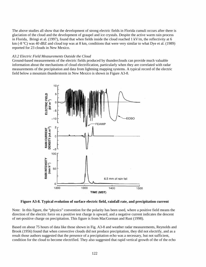
122

The above studies all show that the development of strong electric fields in Florida cumuli occurs after there is glaciation of the cloud and the development of graupel and ice crystals. Despite the active warm rain process in Florida, Bringi et al. (1997), found that when fields inside the cloud reached 1 kV/m, the reflectivity at 6 km (-8 ºC) was 40 dBZ and cloud top was at 8 km, conditions that were very similar to what Dye et al. (1989) reported for 23 clouds in New Mexico. A3.2 Electric Field Measurements Outside the Cloud Ground-based measurements of the electric fields produced by thunderclouds can provide much valuable information about the mechanisms of cloud electrification, particularly when they are correlated with radar measurements of the precipitation and data from lightning mapping systems. A typical record of the electric field below a mountain thunderstorm in New Mexico is shown in Figure A3-8.

Figure A3-8. Typical evolution of surface electric field, rainfall rate, and precipitation current

Note: In this figure, the “physics” convention for the polarity has been used, where a positive field means the direction of the electric force on a positive test charge is upward, and a negative current indicates the descent of net-positive charge on precipitation. This figure is from MacGorman and Rust (1998). Based on about 75 hours of data like those shown in Fig. A3-8 and weather radar measurements, Reynolds and Brook (1956) found that when convective clouds did not produce precipitation, they did not electrify, and as a result those authors suggested that the presence of a precipitation echo was a necessary, but not sufficient, condition for the cloud to become electrified. They also suggested that rapid vertical growth of the of the echo

123

was a requirement for electrification, and in the cases that they studied, the first lightning discharge occurred as quickly as 11 min after the onset of electrification. Several features should be noted in Figure A3-8:

(1) The electric field, E, becomes more negative (indicating positive charge overhead) at the very beginning of the storm due to the early development of a lower positive charge center in the cloud [see Section A1.3.1 of Appendix 1, "Measurement and Interpretation of Surface Electric Field,” and Stolzenburg and Marshall (2008, Section 2.1) and their Figure 7 for further examples of this phenomenon]. This feature is normally seen when the measurements are made very close to isolated, slow moving storms, but the simultaneous development of multiple cells and/or rapid storm motion will often mask this feature. See Section A1.3.1 of Appendix 1, "Measurement and Interpretation of Surface Electric Fields," for more on the initial-electrification signature.

(2) Following the initial negative field excursion, the E-field reverses polarity, becomes positive, and then increases very rapidly. This is due to due to the development of the main negative charge region in the cloud. The reversal in the polarity of E from the normal (negative) fair weather polarity and the rapid development of a large, positive field is usually an indication that a convective cloud is becoming electrified (Breed and Dye, 1989). This signature clearly illustrates the importance and usefulness of ground-based electric field measurements for evaluating the LFCC.

(3) The large, abrupt transitions in the surface E-field (ΔE) are caused by lightning discharges, and analyses of the values of ΔE measured at different recording sites can often be used to determine the locations and magnitudes of the changes in the cloud charge distribution aloft (see the discussion of Figure A3-9 to follow).

(4) The electric field measured on the ground both before and after lightning discharges appears to saturate or reach an upper limit that is less 10 kV m-1. This phenomenon and the overshoot in the polarity of E in response to lightning are both evidence of a local screening layer of space charge near the ground. This space charge is the result of corona or point discharges from grass, trees, and other objects near the measuring site when the background field is large and is discussed in Section A1.3.3.1 of Appendix 1, "Measurement and Interpretation of Surface Electric Fields" (see also Livingston and Krider, 1978; Standler and Winn, 1979; Krehbiel, 1986; and MacGorman and Rust, 1998, Section 4.4.4).

(5) Just after 1300 MST in Figure A3-8, there is a slow excursion in the E-field to a negative polarity at the same time that a burst of precipitation appears to lower negative charge to the ground. This feature lasts several minutes and is termed a 'field excursion associated with precipitation' or FEAWP (Vonnegut and Moore, 1977). Other examples of FEAWP phenomena can be found in Williams et al. (1989a,b), who linked this effect not only to precipitation but also to intense downdrafts and microbursts.

(6) Toward the end of the storm there is a large, slow undulation in the surface electric field that is termed an “end-of-storm-oscillation” or EOSO. A few positive flashes may occur during the first phase of an EOSO, although no positive flashes occurred in the storm shown in Figure A3-8. The variations in the surface electric field during an EOSO were likely first reported by Benjamin Franklin (see Section A3.0 above), but the causes are still not completely understood. Presumably, the causes include the falling of negatively and positively charged hydrometeors toward ground superimposed on the slow relaxation of electric fields in cloudy air while the storm decays (see Moore and Vonnegut, 1977; Livingston and Krider, 1978; Williams et al., 1989; Marshall and Lin, 1992; MacGorman and Rust, Section 7.1.2, 1998; Marshall et al. (2009); and Appendix 6 on “Electrical Properties of Cloudy Air”).

Marshall and Lin (1992) proposed that negative precipitation falling toward the ground drives the field positive early in the dissipating stage of a storm, and then after the precipitation has reached ground, the negative field is due to a residual positive screening layer on the lower cloud boundary. Finally, the field decays to fair weather (negative) values as the screening layer is re-screened and the cloud dissipates. More

124

recently, Marshall et al. (2009) have suggested that the large polarity changes at the surface during an EOSO are primarily due to (1) the successive fallout of three of the four principal charge regions in the storm’s mature stage modified by (2) the growth or decay of these charge regions as they descend, and (3) changes in the screening charges at the upper and lower cloud boundaries. Other examples of thunderstorm electric fields and their interpretations are given in Section A1.2.2 of Appendix 1, "Measurement and Interpretation of Surface Electric Field.” Unfortunately, measurements of storm electric fields, both at the surface (like those in Figure A3-8) and aloft (see Section A3.1.2 above), can be strongly affected by “screening layers,” or the space charge that accumulates on conductivity gradients in the atmosphere, especially near the ground and at the cloud boundaries (Holzer and Saxon, 1952; Kasemir, 1959; Brown et al., 1971; Hayes and Roble, 1979; and Standler and Winn, 1979). In order to avoid this problem, Workman and Holzer (1939, 1942), following a suggestion by C. T. R. Wilson (1920), used multiple-station measurements of lightning-caused changes in the electric field (ΔE) to infer the locations and magnitudes of the changes in the cloud charge that are caused by lightning. (Note: the lightning field changes are of short duration compared to the atmospheric relaxation times at the surface and in cloudy air, so the values of ΔE are not affected by the rearrangements of space charge during the discharge.) More recently, Krider, Krehbiel, and their co-workers (Jacobson and Krider, 1976; Krehbiel et al., 1979; Maier and Krider, 1986; Krehbiel, 1986; Koshak and Krider, 1989; Krider, 1989; Murphy et al., 1996) have made similar measurements with more sensors and more sophisticated analysis techniques. If one assumes that a lightning discharge to ground (or one of its component strokes) changes the cloud charge distribution in a way that, to first order, is spherically symmetric, then a CG flash might be modeled as a single point charge, Q. Similarly, a cloud discharge might be represented by a point-dipole, P, that shows the magnitude and direction of the change in the cloud dipole moment (corresponding to the effective displacement of positive charge). The unknown parameters of the assumed model can be inferred by fitting the ΔE measurements to the model. More detail about this technique and its results may be found in Section A1.3.2 of Appendix 1, "Measurement and Interpretation of Surface Electric Fields." Figure A 3-9 shows the results of fitting two simple charge models to the field changes produced by lightning during a small (left) and a large (right) thunderstorm at the NASA Kennedy Space Center (Krider, 1989). The open circles show the locations of point charge solutions (Q-model) that describe the field changes produced when cloud-to-ground (CG) flashes effectively remove negative charge from the cloud (or equivalently deposit positive charge). The arrows (or P-vectors) show the locations and magnitudes of point-dipole fits to the field changes produced by cloud discharges. (For further information about this analysis technique, see Section A1.3.2 of Appendix 1, "Measurement and Interpretation of Surface Electric Fields.") It should be noted in Figure A 3-9 that all P-vectors at high altitude point downward and those at low altitude point upward. When a P-vector is located at an altitude that corresponds to the negative charge region (the Q solutions), it tends to be horizontal. This symmetry is consistent with the classic tripole model of the cloud charge distribution [see Williams (1989) and Section A3.1.1], i.e., there are a large volume of negative charge located at subfreezing temperatures in the central part of the cloud, a larger volume of positive charge at higher altitudes, and a small concentration of positive charge below the negative. The P-vectors at high altitude are caused by cloud discharges between the central negative charge and the upper positive region, and the P-vectors at low altitudes are caused by discharges between the central negative charge region and the lower positive region. Again, it should be noted that the inferred Q region (negative charge) is centered where the ambient air temperature is between –10 ºC and –20 ºC, and note that the spatial separation between the central negative and upper positive regions depends on the size and intensity of the storm.

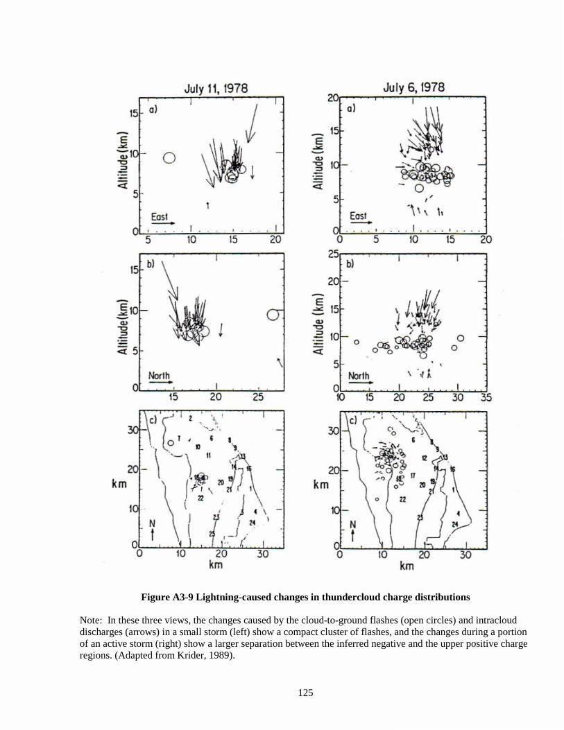
125

Figure A3-9 Lightning-caused changes in thundercloud charge distributions Note: In these three views, the changes caused by the cloud-to-ground flashes (open circles) and intracloud discharges (arrows) in a small storm (left) show a compact cluster of flashes, and the changes during a portion of an active storm (right) show a larger separation between the inferred negative and the upper positive charge regions. (Adapted from Krider, 1989).

July 11. 1978

15 oj

5 -

East o , --:-:--: . 1 . . , .. . . I

5 10 15 20

\ Norlh -

15 20 25

July 6. 1978 ~Ir-~~~~~--~

_ 15 E ~

oj

~ 10 -

5

Easl -

-

, ' -, \ \ \,

... . , . .. . I ... . , . o 5 10 15 20

25rb-J ~-~I-~---C-1 -'

2C -

5 Norlh -

km

N t

c· o ,

o n

km

-

o -o

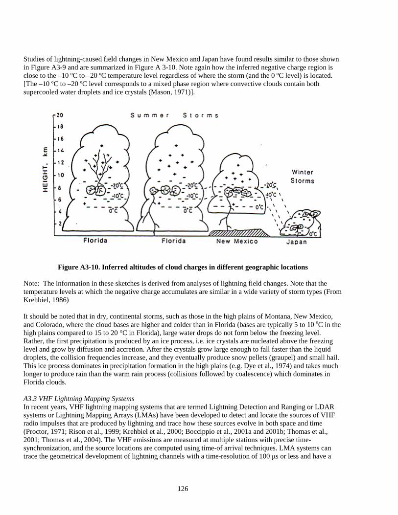
126

Studies of lightning-caused field changes in New Mexico and Japan have found results similar to those shown in Figure A3-9 and are summarized in Figure A 3-10. Note again how the inferred negative charge region is close to the –10 ºC to –20 ºC temperature level regardless of where the storm (and the 0 ºC level) is located. [The –10 ºC to –20 ºC level corresponds to a mixed phase region where convective clouds contain both supercooled water droplets and ice crystals (Mason, 1971)].

Figure A3-10. Inferred altitudes of cloud charges in different geographic locations Note: The information in these sketches is derived from analyses of lightning field changes. Note that the temperature levels at which the negative charge accumulates are similar in a wide variety of storm types (From Krehbiel, 1986) It should be noted that in dry, continental storms, such as those in the high plains of Montana, New Mexico, and Colorado, where the cloud bases are higher and colder than in Florida (bases are typically 5 to 10 oC in the high plains compared to 15 to 20 °C in Florida), large water drops do not form below the freezing level. Rather, the first precipitation is produced by an ice process, i.e. ice crystals are nucleated above the freezing level and grow by diffusion and accretion. After the crystals grow large enough to fall faster than the liquid droplets, the collision frequencies increase, and they eventually produce snow pellets (graupel) and small hail. This ice process dominates in precipitation formation in the high plains (e.g. Dye et al., 1974) and takes much longer to produce rain than the warm rain process (collisions followed by coalescence) which dominates in Florida clouds. A3.3 VHF Lightning Mapping Systems In recent years, VHF lightning mapping systems that are termed Lightning Detection and Ranging or LDAR systems or Lightning Mapping Arrays (LMAs) have been developed to detect and locate the sources of VHF radio impulses that are produced by lightning and trace how these sources evolve in both space and time (Proctor, 1971; Rison et al., 1999; Krehbiel et al., 2000; Boccippio et al., 2001a and 2001b; Thomas et al., 2001; Thomas et al., 2004). The VHF emissions are measured at multiple stations with precise time-synchronization, and the source locations are computed using time-of arrival techniques. LMA systems can trace the geometrical development of lightning channels with a time-resolution of 100 μs or less and have a

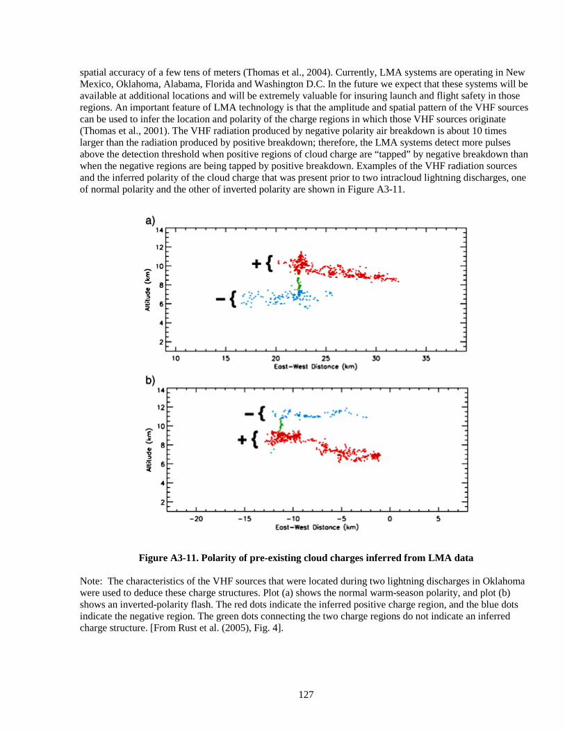
127

spatial accuracy of a few tens of meters (Thomas et al., 2004). Currently, LMA systems are operating in New Mexico, Oklahoma, Alabama, Florida and Washington D.C. In the future we expect that these systems will be available at additional locations and will be extremely valuable for insuring launch and flight safety in those regions. An important feature of LMA technology is that the amplitude and spatial pattern of the VHF sources can be used to infer the location and polarity of the charge regions in which those VHF sources originate (Thomas et al., 2001). The VHF radiation produced by negative polarity air breakdown is about 10 times larger than the radiation produced by positive breakdown; therefore, the LMA systems detect more pulses above the detection threshold when positive regions of cloud charge are “tapped” by negative breakdown than when the negative regions are being tapped by positive breakdown. Examples of the VHF radiation sources and the inferred polarity of the cloud charge that was present prior to two intracloud lightning discharges, one of normal polarity and the other of inverted polarity are shown in Figure A3-11.

Figure A3-11. Polarity of pre-existing cloud charges inferred from LMA data Note: The characteristics of the VHF sources that were located during two lightning discharges in Oklahoma were used to deduce these charge structures. Plot (a) shows the normal warm-season polarity, and plot (b) shows an inverted-polarity flash. The red dots indicate the inferred positive charge region, and the blue dots indicate the negative region. The green dots connecting the two charge regions do not indicate an inferred charge structure. [From Rust et al. (2005), Fig. 4].

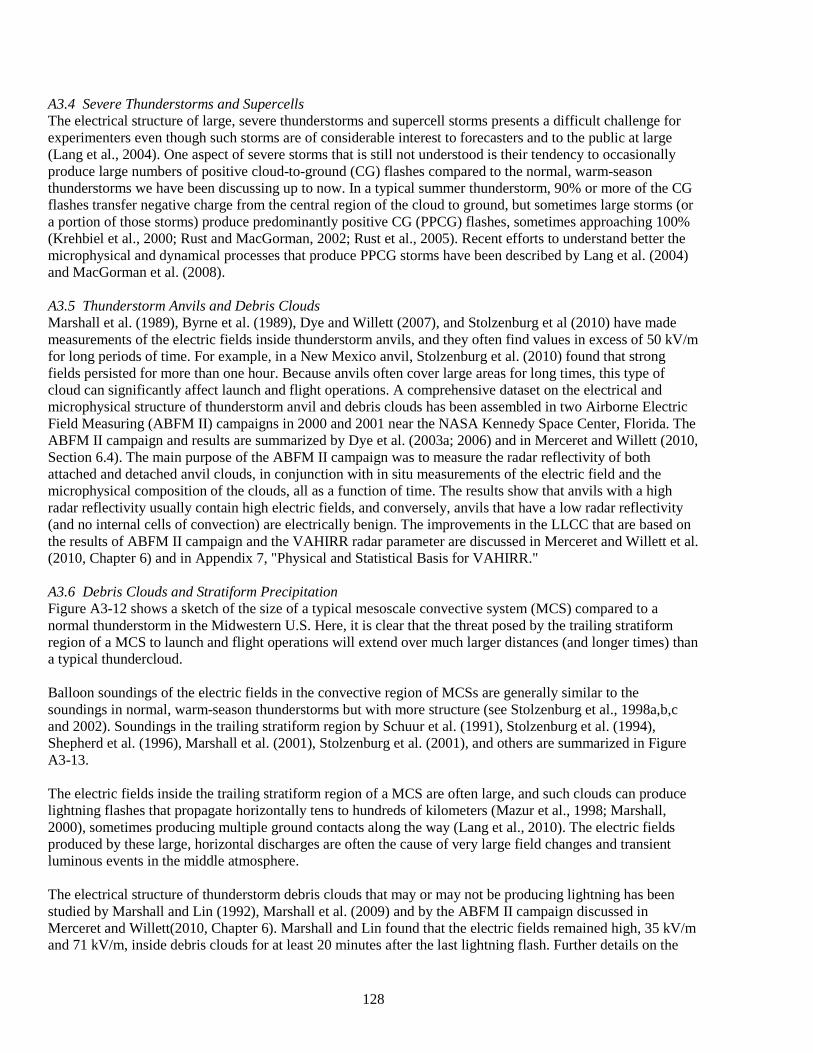
128

A3.4 Severe Thunderstorms and Supercells The electrical structure of large, severe thunderstorms and supercell storms presents a difficult challenge for experimenters even though such storms are of considerable interest to forecasters and to the public at large (Lang et al., 2004). One aspect of severe storms that is still not understood is their tendency to occasionally produce large numbers of positive cloud-to-ground (CG) flashes compared to the normal, warm-season thunderstorms we have been discussing up to now. In a typical summer thunderstorm, 90% or more of the CG flashes transfer negative charge from the central region of the cloud to ground, but sometimes large storms (or a portion of those storms) produce predominantly positive CG (PPCG) flashes, sometimes approaching 100% (Krehbiel et al., 2000; Rust and MacGorman, 2002; Rust et al., 2005). Recent efforts to understand better the microphysical and dynamical processes that produce PPCG storms have been described by Lang et al. (2004) and MacGorman et al. (2008). A3.5 Thunderstorm Anvils and Debris Clouds Marshall et al. (1989), Byrne et al. (1989), Dye and Willett (2007), and Stolzenburg et al (2010) have made measurements of the electric fields inside thunderstorm anvils, and they often find values in excess of 50 kV/m for long periods of time. For example, in a New Mexico anvil, Stolzenburg et al. (2010) found that strong fields persisted for more than one hour. Because anvils often cover large areas for long times, this type of cloud can significantly affect launch and flight operations. A comprehensive dataset on the electrical and microphysical structure of thunderstorm anvil and debris clouds has been assembled in two Airborne Electric Field Measuring (ABFM II) campaigns in 2000 and 2001 near the NASA Kennedy Space Center, Florida. The ABFM II campaign and results are summarized by Dye et al. (2003a; 2006) and in Merceret and Willett (2010, Section 6.4). The main purpose of the ABFM II campaign was to measure the radar reflectivity of both attached and detached anvil clouds, in conjunction with in situ measurements of the electric field and the microphysical composition of the clouds, all as a function of time. The results show that anvils with a high radar reflectivity usually contain high electric fields, and conversely, anvils that have a low radar reflectivity (and no internal cells of convection) are electrically benign. The improvements in the LLCC that are based on the results of ABFM II campaign and the VAHIRR radar parameter are discussed in Merceret and Willett et al. (2010, Chapter 6) and in Appendix 7, "Physical and Statistical Basis for VAHIRR." A3.6 Debris Clouds and Stratiform Precipitation Figure A3-12 shows a sketch of the size of a typical mesoscale convective system (MCS) compared to a normal thunderstorm in the Midwestern U.S. Here, it is clear that the threat posed by the trailing stratiform region of a MCS to launch and flight operations will extend over much larger distances (and longer times) than a typical thundercloud. Balloon soundings of the electric fields in the convective region of MCSs are generally similar to the soundings in normal, warm-season thunderstorms but with more structure (see Stolzenburg et al., 1998a,b,c and 2002). Soundings in the trailing stratiform region by Schuur et al. (1991), Stolzenburg et al. (1994), Shepherd et al. (1996), Marshall et al. (2001), Stolzenburg et al. (2001), and others are summarized in Figure A3-13. The electric fields inside the trailing stratiform region of a MCS are often large, and such clouds can produce lightning flashes that propagate horizontally tens to hundreds of kilometers (Mazur et al., 1998; Marshall, 2000), sometimes producing multiple ground contacts along the way (Lang et al., 2010). The electric fields produced by these large, horizontal discharges are often the cause of very large field changes and transient luminous events in the middle atmosphere. The electrical structure of thunderstorm debris clouds that may or may not be producing lightning has been studied by Marshall and Lin (1992), Marshall et al. (2009) and by the ABFM II campaign discussed in Merceret and Willett(2010, Chapter 6). Marshall and Lin found that the electric fields remained high, 35 kV/m and 71 kV/m, inside debris clouds for at least 20 minutes after the last lightning flash. Further details on the

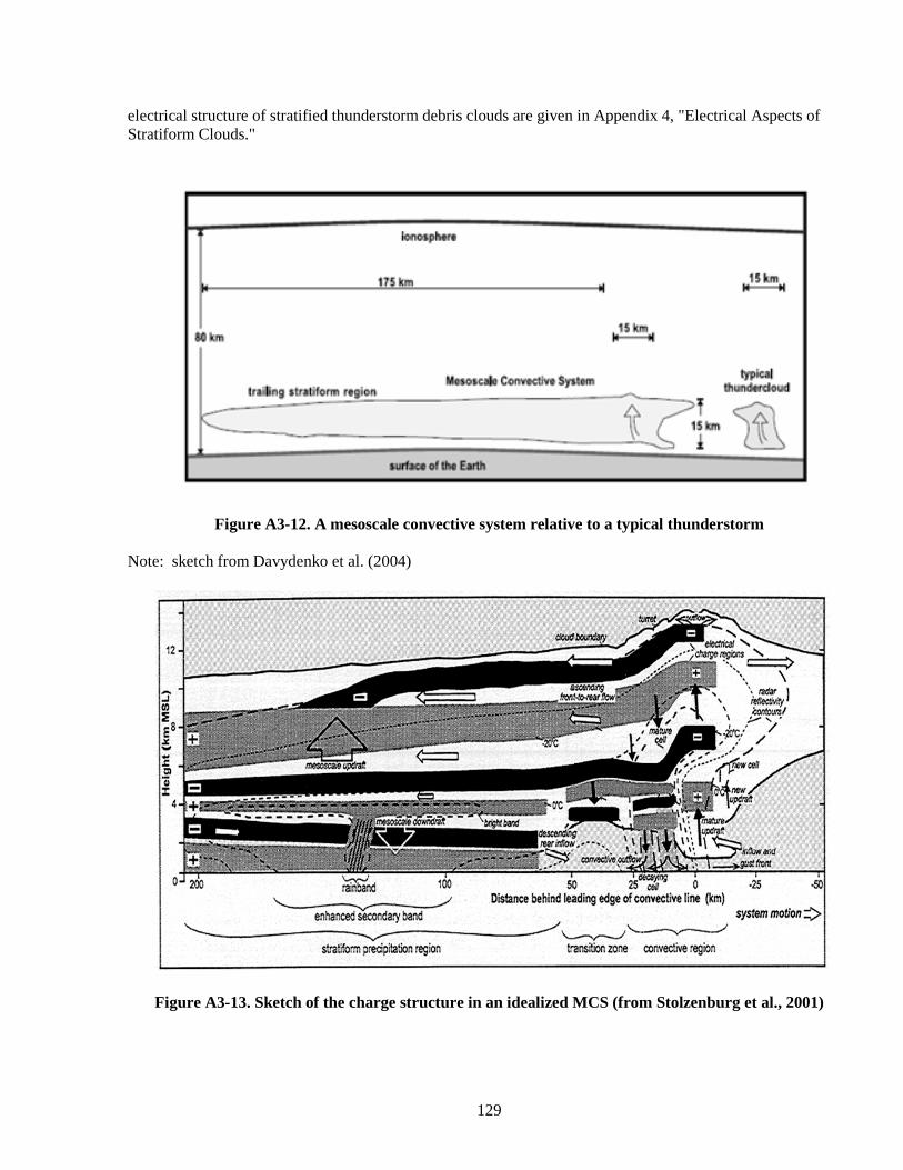
129

electrical structure of stratified thunderstorm debris clouds are given in Appendix 4, "Electrical Aspects of Stratiform Clouds."

Figure A3-12. A mesoscale convective system relative to a typical thunderstorm Note: sketch from Davydenko et al. (2004)

Figure A3-13. Sketch of the charge structure in an idealized MCS (from Stolzenburg et al., 2001)

130

A3.7 Clouds Associated with Disturbed Weather Simpson (1949) has given what is still today one of the best descriptions of the surface electric field (or potential gradient) and the associated time-variations that are caused by disturbed weather. Clouds that produce steady rainfall are characterized by elevated fields that undulate between positive and negative polarities in a wavelike fashion for 90 minutes or more. Shower clouds often exhibit high fields, like thunderstorms, but without the abrupt transitions that are caused by lightning. Balloon soundings of the electric field inside several winter nimbostratus clouds in the U.S. show vertical fields of 1 to 12 kV/m and horizontal fields ranging between 0.2 and 28 kV/m (Rust and Trapp, 2002). The electric fields inside a selection of other cloud types have been measured by Imyanitov and colleagues in Russia and have been reviewed in Merceret and Willett et al. (2010, Section 3.4.2) and in Section A4.1 of Appendix 4, “Electrical Aspects of Stratiform Clouds.” A3.8 Mechanisms of Cloud Electrification In order for a cloud to become electrified over spatial scales on the order of kilometers, there must be two types of processes — first, there must be a small-scale process that electrifies the individual cloud particles and/or elements of precipitation, and second, there must be another, larger-scale process that separates these charges, preferentially according to their polarity, by distances of the order of kilometers. Since the water droplets and/or ice crystals that are present at the cloud boundaries will become electrified when atmospheric ions attach to their surfaces, some investigators believe that the organized motion of the cloud screening layers by the cloud dynamics will produce a large-scale separation of the charge (Vonnegut, 1991; Moore et al., 1992). Today, however, today most investigators believe that the large-scale process is dominated by the gravitational separation of particles falling at different terminal speeds. For example, if collisions between small and large hydrometeors separate charge, and if this separation causes the larger particles to have a charge of predominantly one polarity, then because the larger particles will fall faster with respect to cloud air than the oppositely charged, small particles, gravitation will ultimately cause a large-scale separation of the polarities. The gravity-driven process of differential separation is sometimes termed the ‘precipitation mechanism.’ Many mechanisms have been proposed for the small-scale process that, when acting in conjunction with precipitation, will electrify a thundercloud. Some mechanisms depend on, or are enhanced by, the presence of an external electric field via electrostatic induction (Mason, 1988), and others, the so-called “non-inductive processes,” do not depend on an external field. In 1957, Reynolds and his coworkers showed that when a simulated hailstone was rotated in an artificial cloud containing both ice crystals and supercooled water drops, the hailstone acquired a negative charge that was sufficient to explain the electrification of thunderclouds. Subsequent experiments by other investigators under a wide variety of conditions (Takahashi, 1978; Latham, 1981; Jayaratne et al., 1983; Williams et al., 1991; Saunders et al., 1991; Takahashi and Miyawaki, 2002; Evila et al., 2005; and Saunders, 2008) have found similar results. Based on the laboratory results and the field studies discussed above in Florida, New Mexico, Montana, and Oklahoma, most investigators today believe that the dominant small-scale mechanism is a non-inductive process involving collisions between soft hail or graupel particles and ice crystals in the presence of supercooled water drops [see, for example, Latham (1981), Williams (1988), Saunders (1988), Latham and Dye (1989), Black and Hallett (1998), MacGorman and Rust (1998), and Saunders (2008)]. A3.8.1 Non-Inductive Ice-Ice Collisions Laboratory experiments show that the charge acquired by a simulated hail or graupel particle undergoing collisions with ice crystals (in the presence of supercooled water drops) is a function of the size of the crystal, the velocity of the collision, the temperature of the hail, and the liquid water content (LWC) of the cloud (Takahashi, 1978; Saunders et al., 1991; Takahashi and Miyawaki, 2002; Saunders, 2008). When the hail

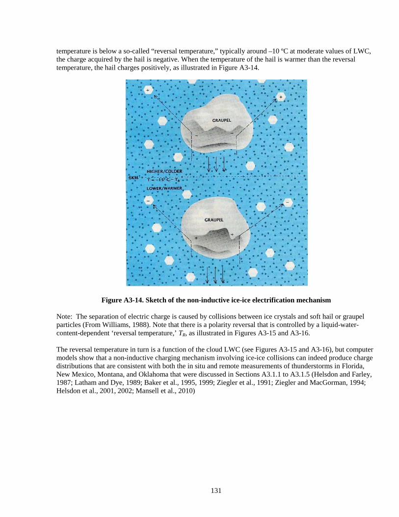
131

temperature is below a so-called “reversal temperature,” typically around –10 ºC at moderate values of LWC, the charge acquired by the hail is negative. When the temperature of the hail is warmer than the reversal temperature, the hail charges positively, as illustrated in Figure A3-14.

Figure A3-14. Sketch of the non-inductive ice-ice electrification mechanism Note: The separation of electric charge is caused by collisions between ice crystals and soft hail or graupel particles (From Williams, 1988). Note that there is a polarity reversal that is controlled by a liquid-water-content-dependent ‘reversal temperature,’ TR, as illustrated in Figures A3-15 and A3-16. The reversal temperature in turn is a function of the cloud LWC (see Figures A3-15 and A3-16), but computer models show that a non-inductive charging mechanism involving ice-ice collisions can indeed produce charge distributions that are consistent with both the in situ and remote measurements of thunderstorms in Florida, New Mexico, Montana, and Oklahoma that were discussed in Sections A3.1.1 to A3.1.5 (Helsdon and Farley, 1987; Latham and Dye, 1989; Baker et al., 1995, 1999; Ziegler et al., 1991; Ziegler and MacGorman, 1994; Helsdon et al., 2001, 2002; Mansell et al., 2010)

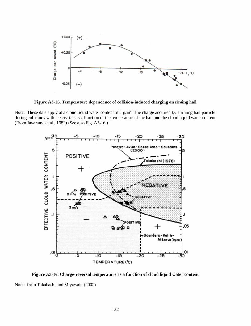
132

Figure A3-15. Temperature dependence of collision-induced charging on riming hail Note: These data apply at a cloud liquid water content of 1 g/m3. The charge acquired by a riming hail particle during collisions with ice crystals is a function of the temperature of the hail and the cloud liquid water content (From Jayaratne et al., 1983) (See also Fig. A3-16.)

Figure A3-16. Charge-reversal temperature as a function of cloud liquid water content Note: from Takahashi and Miyawaki (2002)

133

A3.8.2 Detailed Physics of the Charge Transfer During Ice-Ice Collisions Several investigators have suggested that the magnitude and polarity of the charge that is transferred during an ice-graupel collision is controlled by the rates at which the ice surfaces are growing by deposition (condensation) or sublimation (evaporation) (Baker et al., 1987, 1989; Mason and Dash, 2000; and Dash et al., 2001, Saunders, 2008), and the surface that is growing fastest at the time of the collision acquires a positive charge. When both surfaces are evaporating, the surface that is evaporating the slowest becomes positively charged. Unfortunately, there is still no consensus about the reason(s) for this behavior, but mechanisms that have been proposed include differences in the ice surface potentials, thermoelectric effects acting on the riming ice surfaces, and the effects of irregular ice surfaces (Avila et al., 2005; Saunders et al., 2006). Baker and Dash (1989) have suggested that there may be liquid-like layers (LLL) on ice surfaces that have an excess concentration of negative ions on the outer portion of the LLL. If this is the case, then when two such LLLs collide, the thicker layer may transfer some of its mass, together with its negative charge, to the thinner LLL, and leave positive charge behind. [Since the surfaces that are growing fastest will also have thicker LLLs, the Baker-Dash mechanism does appear to describe practically all the laboratory results to date, at least qualitatively (Mason and Dash, 2000; Dash et al., 2001). A3.8.3 Other Electrification Mechanisms In their study of the electrical structure of precipitating stratiform clouds that were associated with mesoscale convection systems, Shepherd et al. (1996) found high electric fields and volume charge densities near the melting (0 ºC) level that is often associated with the radar bright band. Reiter (1965) had previously investigated the melting region in both stratiform precipitation and showers by measuring the potential gradient at different altitudes on the Zugspitze in Germany; he found anomalies in both types of clouds - positive potential gradients where the precipitation was solid and negative potential gradients after it melted. More recently, Stolzenburg et al., (2007) reported large charge densities and fields of both polarities near the melting level in different storms, and they point out that such high values are difficult to explain with an ice-graupel charging process. Therefore, Stolzenburg et al. (2007) favor an inductive charging mechanism (i.e. where the charge transfer by collisions depends upon the amplitude and polarity of the local electric field) associated with melting that was initially proposed by Simpson (1909). This mechanism is based on smaller particles (liquid or solid) being shed from the upper portions of a melting ice particles that would carry away charge with a polarity that is the same as that of the local electric field. However, another melting mechanism examined by Drake (1968) has also been considered, and if the Drake mechanism is acting, the smaller particles would come away with predominately negative charge and the charging would be independent of the local electric field. Although there are many measurements of the vertical profile of the electric field, and there are independent measurements of the ice and water content near the melting zone, there are very few simultaneous measurements of both the ambient field and the cloud microphysics. Even though additional observations and research are needed, there is no question that a significant electrical hazard exists near the melting zone when precipitation is present. See also Section A4.0 of Appendix 4, "Electrical Aspects of Stratiform Clouds." In addition to the charge separation that occurs near the 0 ºC level, recent observations of high electric fields and lightning initiations far downwind of the convective cores in anvils (Dye and Willett, 2007; Kuhlman et al., 2009; and Weiss et al., 2010) suggest that some charge separation could be taking place above the melting zone in thick anvils. Laboratory studies such as those of Jayaratne et al. (1983) have shown that weak charge separation does take place during ice-ice collisions even without supercooled water or pre-existing electric fields being present. Thus, a possible source of the enhanced electric fields far downwind in anvils may be the result of collisions of the many ice particles and snowflakes present in those regions. See also Section A4.0 of Appendix 4, "Electrical Aspects of Stratiform Clouds."

134

D. Latham (1991) has shown that the convective clouds initiated by large, wild land fires can produce lightning, and Vonnegut et al. (1995) have suggested that the dominant mechanism for this electrification may not be ice-graupel collisions but one or more influence mechanisms that are based on electrostatic induction. In addition to the mechanisms of cloud electrification described in this and the above sections, lightning has occasionally been reported to originate in clouds that are everywhere warmer than 0 ºC (Moore et al., 1960; Alpert, 1961; Michnowski, 1963; Takahashi, 1975; MacGorman and Rust, 1998, Section 8.4.8). Whether such clouds were always warmer than 0 C is not known, and today the occurrence of lightning in warm clouds is still controversial. One thing is clear, however; that is, the occurrence of natural lightning in warm clouds is quite rare [see Volland (1995, Section 3.1.1) and Uman (1987, Section 1.7.1) and the references cited therein for further discussions of this phenomenon.] A3.9 Conclusions The laboratory, field, and model studies of cloud electrification discussed above clearly show the importance of microscale interactions of ice-phase particles in a temperature (altitude) range from about -5 ºC to -20 ºC in all types of clouds. This temperature range usually contains ice crystals, soft hail or graupel particles, and supercooled water drops where the non-inductive, ice-graupel collision mechanism can operate. At this point, we still need to know more about the microphysical, electrical, and dynamical structure of electrified clouds before we can make further evaluations of the non-inductive, ice-graupel collision mechanism (coupled with precipitation), the detailed physics that underlies this process, and other possible mechanisms. Among the parameters that are still not known are the number of ice-ice collisions, the LWCs, and the temperatures in the different regions of a thundercloud; the sizes and types of ice particles and their collision velocities in these regions; and what charges are present on the ice particles, water drops, and precipitation particles (all as a function of size). More experiments are needed both in the laboratory and in nature to learn more about the detailed physics of cloud electrification and the processes that electrify non-lightning producing clouds. Hopefully, such efforts will lead to better explanations for the fascinating variety of atmospheric electrical phenomena that Benjamin Franklin and many others have been documenting for over 250 years. A3.10 References Alpert, L., 1961: A Note to the Paper by C. B. Moore, B. Vonnegut, B. A. Stein, and H. J. Survilas,

‘Observation of Electrification and Lightning in Warm Clouds', J. Geophys. Res., 66 (1), 332. Avila, E. E., C. P. R. Saunders, H. Bax-Norman, and N. E. Castellano, 2005: Charge sign reversal in ice

particle-graupel collisions, Geophys. Res. Lett., 32, L01801, doi:10.1029/2004GL020761. Baker, M. B., Baker, E.R. Jayaratne, J. Latham, and C.P. Saunders, 1987: The influence of diffusional growth

rates on the charge transfer accompanying rebounding collisions between ice crystals and soft hailstones, Q. J. R. Meteorol. Soc., 113, 1193-1215.

Baker, M. B., and J. G. Dash, 1989: Charge transfer in thunderstorms and the surface melting of ice, J. Crystal

Growth, 97, 770-776. Baker, M. B., H. J. Christian, and J. Latham, 1995: A computational study of the relationships linking

lightning frequency and other thundercloud parameters, Q. J. R. Meteorol. Soc., 121, 1525-1548. Baker, M. B., A. M. Blyth, H. J. Christian, J. Latham, K. L. Miller, and A. M. Gadian, 1999: Atmos. Res., 51,

221-236. Black, R. and J. Hallett, 1998: The Mystery of Cloud Electrification, American Scientist, 86 (6), Nov-Dec

pp.526-534.

135

Boccippio, D. J., D. J. Heckman, and S. J. Goodman, 2001a: A diagnostic analysis of the Kennedy Space Center LDAR network 1. Data characteristics, J. Geophys. Res., 106 (D5), 4769-4786.

Boccippio, D. J., D. J. Heckman, and S. J. Goodman, 2001b: A diagnostic analysis of the Kennedy Space

Center LDAR network 2. Cross-sensor studies, J. Geophys. Res., 106(D5), 4787-4796. Breed, D. W., and J. E. Dye, 1989: The electrification of New Mexico Thunderstorms, Part 2. Electric field

growth during initial electrification, J. Geophys. Res., 94, 14,841-14,854. Bringi, V.N., K. R. Knupp, A. Detwiler, L. Liu, I. J. Caylor, and R. A. Black, 1997: Evolution of a Florida

thunderstorm during the Convection and Precipitation Electrification Experiment: The case of 9 August 1991, Mon. Wea. Rev., 125, 2131–2160.

Brooks. I.M., and C.P. R. Saunders, 1995: Thunderstorm charging: Laboratory experiments clarified, Atmos.

Res., 39, 263-273. Brown, K. A., P. R. Krehbiel, C. B. Moore, and G. N. Sargent, 1971: Electrical screening layers around

charged clouds, J. Geophys. Res., 76, 2825-2835. Byrne, G. J., A. A.. Few, and M. E. Weber, 1983: Altitude thickness and charge concentration of charge

regions of four thunderstorms during TRIP 81, based on in situ balloon electric field measurements, Geophys. Res. Lett., 10, 39-42.

Byrne, G. J., A. A. Few, and M. F. Stewart, 1989: Electric field measurements within a severe thunderstorm

anvil, J. Geophys. Res., 94, 6297-6307. Cohen, I. Bernard, 1990: “The kite, the sentry box, and the lightning rod,” Chapter 6 in Benjamin Franklin’s

Science, Harvard Univ. Press, Cambridge, MA, 273 pp. Dash, J. G., B. L. Mason, and J. S. Wettlaufer, 2001: Theory of charge and mass transfer in ice-ice Collisions,

J. Geophys. Res., 106 (D17), 20,395-20,402. Davydenko, S. S., E. A. Mareev, T. C. Marshall, and M. Stolzenburg, 2004: On the calculation of electric

fields and currents of mesoscale convective systems, J. Geophys. Res., 109, D11103, doi:10.1029/2003JD003832, 2004.

Drake, J. C., 1968: Electrification accompanying the melting of ice particles, Quart. J. Roy. Meteorol. Soc., 94,

176-191. Dye, J. E., C. A. Knight, V. Toutenhoofd and T. W. Cannon, 1974: The mechanism of precipitation formation

in NE Colorado cumulus. Part III: Coordinated microphysical and radar observations and summary, J. Atmos. Sci., 31, 2152-2159.

Dye, J. E., J. J. Jones, W. P. Winn, T. A. Cerni, B. Gardiner, D. Lamb, R. L. Pitter, J. Hallett, and C. P. R.

Saunders, 1986: Early electrification and precipitation development in a small, isolated Montana cumulonimbus. J. Geophys. Res., 91, 1231–1247.

Dye, J.E., J. J. Jones, A. J. Weinheimer, and W.P. Winn, 1988: Observations within two regions of charge

during initial thunderstorm electrification, Quart, J. Roy. Meteorol. Soc., 114, 1271-1290.

136

Dye, J.E., W. P. Winn, J. J. Jones, and D. W. Breed, 1989: The electrification of New Mexico thunderstorms. 1. Relationship between precipitation development and the onset of electrification, J. Geophys. Res., 94, 8643–8656.

Dye, J. E., J. J. Jones, A.J. Weinheimer, and W. P. Winn, 1992: Reply to comments by C. B. Moore and B.

Vonnegut: Further analysis of two regions of charge during initial thunderstorm electrification, Quart, J. Roy. Meteorol. Soc., 118, 401-412.

Dye, J.E., D.W. Breed, G.M. Barnes, J.J. Jones, R.C. Solomon, 1992b: The co-evolution of precipitation and

electric fields in Florida cumuli during CaPE, Proc. 9th Internat. Conf. Atmosph. Electr., St. Petersburg Russia, June 15-19, 1992, Vol. I, 179-184.

Dye, J.E., S. Lewis, M.G. Bateman, D.M. Mach, F.J. Merceret, J.G. Ward and C.A. Grainger, 2003: Final

Report on the Airborne Field Mill Project (ABFM) 2000-2001 Field Campaign, NASA Technical Memo 2004-211534, Kennedy Space Center, FL, 126 pp.

Dye, J. E. and S. Lewis, 2004a: Summary of the Final Report to NASA KSC on the Airborne Field Mill

Project (ABFM) Under NASA Grant NAG10-284, June 4, 2004. Dye, J. E. and S. Lewis, 2004b: Final Report to NASA KSC on the Airborne Field Mill Project (ABFM)

Under NASA Grant NAG10-284, June 4, 2004. http://box.mmm.ucar.edu/abfm/webpage/Reports/FinalReport_0604.pdf

Dye, J.E. and J.C.Willett, 2007: Observed enhancement of reflectivity and the electric field in long-lived

Florida anvils, Mon. Weath. Rev., 135, 3362-3380. French, J. F., J. H. Helsdon, A. G. Detwiler, and P. L. Smith, 1996: Microphysical and electrical evolution of a

Florida thunderstorm. Part I: Observations. J. Geophys. Res., 101, 18,961–18,977. Hallett, J., R.I. Sax, D. Lamb and A.S. Ramachandra, 1978: Aircraft measurements of ice in Florida cumuli,

Quart. J. Royal Meteorol. Soc., 104, 631-651. Hays, R. B., and R. G. Roble, 1979: A quasi-static model of atmospheric electricity: 1. The lower atmosphere,

J. Geophys. Res., 84, 3291-3305. Helsdon, J. H., Jr., and R. D. Farley, 1987: A numerical modeling study of a Montana thunderstorm: 2. Model

results versus observations involving electrical aspects. J. Geophys. Res., 92, 5661–5675. Helsdon, J. H., W. A. Wojcik, and R. D. Farley, 2001: An examination of thunderstorm-charging mechanisms

using a two-dimensional storm electrification model, J. Geophys. Res., 106, (D1) 1165-1192. Helsdon, J. H., S. Gattaleeradapan, R. D. Farley, and C. C. Waits, 2002:An examination of the convective

charging hypothesis: Charge structure, electric fields, and Maxwell currents, J. Geophys. Res., 107 (D22), ACL 9-1 to ACL 9-26, doi:10.1029/2001JD001495.

Holzer. R. E. and D. S. Saxon, 1952: Distribution of electrical conduction currents in the vicinity of

thunderstorms, J. Geophys. Res., 57, 207-216. Imyanitov, I. M., Ye. V. Chubarina, and Ya. M. Shvarts, 1971: NASA Tech Translation TT F-728: Electricity

of Clouds, Translation of “Elektrichestvo oblakov,” Hydrometeorological Press, Leningrad, 122 pg.

http://box.mmm.ucar.edu/abfm/webpage/Reports/FinalReport_0604.pdf�

137

Jacobson, E.A., and E. P. Krider, 1976: Electrostatic field changes produced by Florida lightning, J. Atmos. Sci., 33, 10 3-117.

Jameson, A.R., M. J. Murphy, and E. P. Krider, 1996: Multiple parameter radar observations of isolated

Florida thunderstorms during the onset of electrification, J. Appl. Meteor., 35, 343–354. Jones, J.J., W.P. Winn, S.J. Hunyady, C.B. Moore, J.W. Bullock and P. Fleischhaker, 1990: Aircraft

measurements of electrified clouds at Kennedy Space Center, Final Report, Part I 1988 Flights (April 27, 1990).

Jayaratne, E. R. C.P. R. Saunders, and J. Hallett, 1983: Laboratory studies of the charging of soft hail during

ice crystal interactions, Quart J. Roy. Meteorol. Soc., 109, 609-630. Kasemir, H. W., 1959: The thunderstorm as a generator in a global electric circuit (in German), Z. Geophys.,

25, 33-64. Koshak, W.J., and E.P. Krider, 1989: Analysis of lightning field changes during active Florida thunderstorms,

J. Geophys. Res., 94, 1165-1186. Krehbiel, P.R., M. Brook, and R. A. McCrory, 1979: An analysis of the charge structure of lightning

discharges to ground, J. Geophys. Res., 84, 2432-2456. Krehbiel, P. R., R. J. Thomas, W. Rison, T. Hamlin, J. Harlin, and M. Davis, 2000: Lightning mapping

observations in central Oklahoma, EOS Trans. of AGU, 21-25, January 2000. Krehbiel, P. R., 1986: The electrical structure of thunderstorms, Chapter 8 in The Earth’s Electrical

Environment ed. By E. P. Krider and R. G. Roble, National Academy Press, Washington, D. C., pp. 90-113.

Krider, E. P., 1989: Electric field changes and the cloud electrical structure, J. Geophys. Res., 94, 13145-

13149. Kuhlman, K. M., D. R. MacGorman, M. I. Biggerstaff, P. R. Krehbiel, 2009: Lightning initiation in the anvils

of two supercell storms, Geophysical Research Letters, 36, L07802. Labaree, L.W. (ed), 1962: The Papers of Benjamin Franklin, Yale University Press, Vol. 5, p. 69. Lang, T.J., et al., 2004: The Severe Thunderstorm Electrification and Precipitation Study, Bull. Am. Meteorol.

Soc., 85(8), 1107-1125, doi:10.1175/BAMS-85-8-1107. Latham, D., 1991: Lightning flashes from a prescribed fire-induced cloud, J. Geophys. Res., 96 (D9), 17,151-

17,157. Latham, J., 1981: The electrification of thunderstorms, Quart, J. Roy. Meteorol. Soc., 107, 277-298. Latham, J., and J. Dye, 1989: Calculations on the Electrical Development of a Small Thunderstorm, J.

Geophys. Res., 94(D11), 13141-13144. Livingston, J.M, and E.P. Krider, 1979: Electric fields produced by Florida thunderstorms, J. Geophys. Res.,

83 (C1), 385-401.

138

MacGorman, D. R. and W. D. Rust, 1998: The Electrical Nature of Storms, Oxford University Press, 422 pp. MacGorman, D. R., W. D. Rust, T. J. Schuur, M. I. Biggerstaff, J. M. Straka, C. L. Ziegler, E. R. Mansell, E.

C. Bruning, K. M. Kuhlman, N. R. Lund, N. S. Biermann, C. Payne, L. D. Carey, P. R. Krehbiel, W. Rison, K. B. Eack, and W. H. Beasley, 2008: TELEX: The Thunderstorm Electrification and Lightning Experiment, Bull. Amer. Meteor. Soc., 89 (7), 997-1013.

Maier, L. M., and E. P. Krider, 1986: The charges that are deposited by cloud-to-ground lightning in Florida,

J. Geophys. Res., 91, 13, 275-13, 289. Mansell, E. R., C. L. Ziegler, and E. C. Bruning, 2010: Simulated Electrification of a Small Thunderstorm

with Two-Moment Bulk Microphysics, J. Atmos. Sci., 67 (1), 171-194. Marshall, T., 2000: Comment on “’Spider’ lightning in intracloud and positive cloud-to-ground flashes” by

Vladislav Mazur, Xuan-Min Shao, and Paul R. Krehbiel, J. Geophys. Res., 105 (D6), 7397-7399. Marshall, T. C., W. D. Rust, W. P. Winn, and K. E. Gilbert, 1989: Electrical structure in two thunderstorm

anvil clouds, J. Geophys. Res., 94 (D2), 2171-2181. Marshall, T.C., and W. D. Rust, 1993: Two types of vertical electrical structures in stratiform precipitation

regions of mesoscale convective regions, Bull. Am. Meteorol. Soc., 78(11), 2159-2170. Marshall, T. C. and B. Lin, 1992: Electricity in dying thunderstorms, J. Geophys. Res., 97 (D9), 9913-9918. Marshall, T. C., M. Stolzenburg, W. D. Rust, E. R. Williams, and R. Boldi, 2001: Positive charge in the

stratiform cloud of a mesoscale convective system, J. Geophys. Res., 106 (D1), 1157-1163. Marshall, T. C., M. Stolzenburg,1 P. R. Krehbiel, N. R. Lund, and C. R. Maggio, 2009: Electrical evolution

during the decay stage of New Mexico thunderstorms, J. Geophys. Res., 114, D02209, doi:10.1029/2008JD010637.

Mason, B. J., 1988: The generation of electric charges and fields in thunderstorms, Proc. Roy. Soc. London,

A415, 303-315. Mason, B. J., 1971: The electrification of clouds, Chapter 9 in The Physics of Clouds, Clarendon, Oxford

(2nd ed.). Mason, B. L. and J. G. Dash, 2000: Charge and mass transfer in ice-ice collisions: Experimental observations

of a mechanism in thunderstorm electrification, J. Geophys. Res., 105 (D8), 10,185-10,192. Mazur, V., X.-M. Shao, and P. R. Krehbiel, 1988: “Spider” lightning in intracloud and positive cloud-to-

ground flashes, J. Geophys. Res., 103, 19,811-19,822. Merceret, F.J. and J.C. Willett, Editors, H.J. Christian, J.E. Dye, E.P. Krider, J.T. Madura, T.P. O'Brien, W.D. Merceret, F.J. and J.C. Willett, Editors, H.J. Christian, J.E. Dye, E.P. Krider, J.T. Madura, T.P. O'Brien, W.D.


Rust, and R.L. Walterscheid, 2010: A History of the Lightning Launch Commit Criteria and the Lightning

Advisory Panel for America’s Space Program, NASA/SP-2010-216283, 234 pp.

139

Michnowski, S., 1963: On the observation of lightning in warm clouds, J. Meteor. Geophys. (India), 14 (3),

320-322. Moore, C. B., B. Vonnegut, B. A. Stein, and H. J.Survilas, 1960: Observations of electrification and lightning

in warm clouds, J. Geophys. Res., 65, 1907-1910. Moore, C.B., and B. Vonnegut, 1977: The thundercloud, in Lightning, Vol. 1, R.H. Golde, Editor, Academic

Press, New York, pp 51-98. Moore, C. B., and B. Vonnegut, 1992: Comments on ‘Observations of two regions of charge during initial

thunderstorm electrification’ by J. E. Dye, J.J. Jones, A. J. Weinheimer and W. P. Winn (July 1988, 114, 1271-1290), Quart, J. Roy. Meteorol. Soc., 118, 395-400.


Precipitation Experiment (CaPE) storms, J. Geophys. Res., 101 (D23), 29,615-29,626. Proctor, D. E., 1971: A hyperbolic system for obtaining VHF radio pictures of lightning, J. Geophys. Res., 76,

1478-1489. Ramachandran, R., A. Detwiler, J. Helsdon Jr., P. L. Smith, and V. N. Bringi, 1996: Precipitation development

and electrification in Florida thunderstorm cells during CaPE. J. Geophys. Res., 101(D1), 1599–1619. Reiter, R., 1965: Precipitation and cloud electricity, Quart. J. Roy. Meteor. Soc., 91(1), 60-72. Reynolds, S.E., and M. Brook, 1956: Correlation of the initial electric field and the radar echo in

thunderstorms, J. Meteor. 132, 376-380. Reynolds, S. E. M. Brook, and M. F. Gourley, 1957: Thunderstorm charge separation, J. Meteor., 14, 426-436. Rison, W., R. J. Thomas, P. R. Krehbiel, T. Hamlin, and J. Harlin, 1999: A GPS-based three-dimensional

lightning mapping system: Initial observations in central New Mexico, Geophys. Res. Lett., 26, 3573-3576.

Rust, W. D. and D. R. MacGorman, 2002: Possibly inverted-polarity electrical structures in thunderstorms,

Geophys. Res. Lett., 29 (12), 12-1 to 12-4. Rust, W. D. and R. J. Trapp, 2002: Initial balloon soundings of the electric field in winter nimbostratus clouds

in the USA, Geophys. Res. Lett., 29 (20), 20-1 to 20-4. Rust, W. D., D. R. MacGorman, E. C. Bruning, S. A. Weiss, P. R. Krehbiel, R. J. Thomas, W. Rison, T.

Hamlin, J. Harlin,, 2005: Inverted-polarity electrical structures in thunderstorms in the Severe Thunderstorm Electrification and Precipitation Study (STEPS). Atmos. Res., 76, 247–271.

Saunders, C.P. R., 1988: Thunderstorm electrification, Weather, 43, 318-324. Saunders, C. P. R., 2008: Charge separation mechanisms in clouds, Sp. Sci. Rev., 137, 335-353. Saunders, C. P.R., W. D. Keith, and R.P. Mitzeva, 1991: The effect of liquid water on thunderstorm charging,

J. Geophys. Res., 96, 11007-11017.

140

Schonland, B.F.J., 1950: The Flight of Thunderbolts. Clarendon, Oxford, p. 22. Schonland, B.F.J., 1952: The work of Benjamin Franklin on thunderstorms, J. Franklin. Inst., 253, 375-392. Schuur, T. J., B. F. Smull, W. D. Rust, and T. C. Marshall, 1991: Electrical and kinematic structure of the

stratiform precipitation region trailing an Oklahoma squall line, J. Atmos. Sci., 48 (6), 825-842. Shepherd, T. R., W. D. Rust, and T. C. Marshall, 1996: Electric fields and charges near 0 ºC in stratiform

clouds, Mon. Wea. Rev., 124, 919-938. Simpson, G., 1949: Atmospheric electricity during disturbed weather, Geophysical Memoirs No. 84, Vol. 4,

Meteorological Office, London, 51 pp. Standler, R B. and W. P. Winn, 1979: Effects of coronae on electric fields beneath thunderstorms, Q. J. R.

Meteorol. Soc.,105, 285-302. Stolzenburg, M. and T. C. Marshall, 2002: Two simultaneous charge structures in thunderstorm convection, J.

Geophys. Res., 107 (D18), ACL 5-1 – ACL 5-12. Stolzenburg, M., W.D. Rust, B.F. Smull, and T.C. Marshall, 1998a: Electrical structure in thunderstorm

convective regions: 1. Mesoscale convective systems, J. Geophys. Res., 103, 14,059-14,078. Stolzenburg, M., W. D. Rust, B. F. Smull and T.C. Marshall, 1998b: Electrical structure in thunderstorm

convective regions: 2. Isolated storms, J. Geophys. Res., 103, 14,079-14,096. Stolzenburg, M., W.D. Rust, B. F. Smull, and T. C. Marshall, 1998c: Electrical structure in thunderstorm

convective regions: 3. Synthesis, J. Geophys. Res., 103, 14,097-14,108. Stolzenburg, M., T. C. Marshall, W. D. Rust, and B. F. Smull, 1994: Horizontal distribution of electrical and

meteorological conditions across the stratiform region of a mesoscale convective system, Mon. Wea. Rev., 122, 1777-1797.

Stolzenburg, M., T. C. Marshall, and W. D. Rust, 2001: Serial soundings of electric field through a mesoscale

convective system, J. Geophys. Res., 106 (D12), 12371-12380. Stolzenburg, M. and T. C. Marshall, 2002: Two simultaneous charge structures in thunderstorm convection, J.

Geophys. Res., 107 (D18), ACL 5-1 – ACL 5-12. Stolzenburg, M. and T.C. Marshall, W.D. Rust,, E.A. Mareev, S.S. Davydenko, 2007: The stratiform

precipitation region of mesoscale convective systems: Inductive charging evidence and global circuit effects, Proc. 13th Internat. Conf. on Atmos. Elec., Beijing China, Aug. 13-17,2007, 13-16.

Stolzenburg, M. and T.C. Marshall, 2008: Charge structure and dynamics in thunderstorms, Space Sci. Rev.,

137, 355-372, DOI 10.1007/s11214-008.9338-z. Stolzenburg, M., T. C. Marshall, and P. R. Krehbiel, 2010: Duration and extent of large electric fields in a

thunderstorm anvil cloud after the last lightning, J. Geophys. Res., doi:10.1029/2010JD014057, in press (accepted 21 May 2010).

Takahashi, Tsutomu, 1975: Electric Charge Life Cycle in Warm Clouds, J. Atmos. Sci., 32, 123 - 142.

141

Takahashi, T., 1978: Riming electrification as a charge generation mechanism in thunderstorms, J. Atmos. Sci., 35, 1536-1548.

Takahashi, T. and K. Miyawaki, 2002: Reexamination of riming electrification in a wind tunnel, J. Atmos. Sci.,

59, 1018-1025. Thomas, R. J., P. R. Krehbiel, W. Rison, T. Hamlin, J. Harlin, and D. Shown, 2001: Observations of VHF

source powers radiated by lightning, Geophys. Res. Lett., 28, 143-146. Thomas, R. J., P. R. Krehbiel, W. Rison, S. J. Hunyady, W. P. Winn, T. Hamlin, and J. Harlin, 2004: Accuracy

of the Lightning Mapping Array, J. Geophys. Res., 109, D14207, doi:10.129/2004JD004549. Uman, Martin A., 2001: The Lightning Discharge, Academic Press, Inc., 377 pp. Volland, Hand, Editor, 1995: Handbook of Atmospheric Electrodynamics, Vol. 1, CRC Press, Inc., 409 pp. Vonnegut, B., 1991: How the external currents flowing to a thundercloud influence its electrification, Ann.

Geophysicae, 9, 34-36. Vonnegut, B., D. J. Latham, C. B. Moore, and S. J. Hunyady, 1995: An explanation of anomalous lightning

from forest fire clouds, J. Geophys. Res., 100 (D3), 5037-5050. Williams, E. R., 1988: The electrification of thunderstorms, Scientific American, 259, 88-99. Williams, E. R., 1989: The tripole structure of thunderstorms, J. Geophys. Res., 94, 13,151-13,167. Williams, E. R., Weber, M. E., Engholm, C. D., 1989a: Electrical Characteristics of Microburst-Producing

Storms in Denver, 24th Conference on Radar Meteorology, Tallahassee, FL, Amer. Meteor. Soc., pp. 89-92.,

Williams, E. R., Weber, M. E., Orville, R. E., 1989b: The Relationship Between Lightning Type and

Convective State of Thunderclouds, J. Geophys. Res., 94 (D11), 13,213-13,220. Williams, E.R., R. Zhang, and Rydock, 1991: Mixed-phase microphysics and cloud electrification, J. Atmos.

Sci., 48, 2195-2203. Willis, P. T., J. Hallett, R. A. Black, and W. Hendricks, 1994: An aircraft study of rapid precipitation

development and electrification in a growing convective cloud, Atmos. Res., 33,1–24. Wilson, C. T. R.,1920: Investigations on lightning discharges and on the electric field of thunderstorms, Phil.

Trans. Roy. Soc. London, A221, 73-115. Workman, E. J., and R. E. Holzer, 1939: Quantities of charge transfers in lightning discharges, Phys. Rev., 55,

2nd Ser., 598. Workman, E.J., and R. E. Holzer, 1942: A preliminary investigation of the electrical structure of

thunderstorms, NACA Tech. Note 850, National Advisory Committee for Aeronautics, Washington, D.C.

142

Ziegler, C. L., D. R. MacGorman, J. E. Dye, and P. S. Ray, 1991: A model evaluation of noninductive graupel-ice charging in the early electrification of a mountain thunderstorm, J. Geophys. Res., 96, 12,833-12,855.

Ziegler, C. L. and D. R. MacGorman, 1994: Observed lightning morphology relative to modeled space charge

and electric field distributions in a tornadic storm, J. Atmos. Sci., 51, 833-851.

143

Appendix 4. Electrical Aspects of Stratiform Clouds A4.0. Introduction and Mechanisms Stratiform or layer clouds cover a broad spectrum of cloud types and are primarily considered as 'Thick Cloud Layers' (G417.19) and 'Disturbed Weather' (G417.17) in the LFCC. Several types of layer clouds are produced by a gradual uplift due to synoptic scale forcing, and others such as trailing stratiform clouds are the response to cloud-scale and mesoscale dynamics or to disturbed weather associated with fronts and mesoscale systems. Before discussing the electrical aspects of stratiform clouds, it will be helpful to list the different genera of layer clouds that are listed in the Glossary of Meteorology (2000):

Stratus (St) – a gray layer with a rather uniform base. Cirrostratus (Cs) -- appearing as a whitish veil, usually fibrous but sometimes smooth, that may totally cover the sky and that often produces halo phenomena Altocumulus (Ac) – white and/or gray in color, that occurs as a layer or patch with a waved aspect, the elements of which appear as laminae, rounded masses, rolls, etc. Stratocumulus (Sc) – predominantly stratiform in the form of a gray and/or whitish layer or patch, which nearly always has dark parts and is nonfibrous (except for virga) Altostratus (As)-- gray or bluish (never white) sheet or layer of striated, fibrous, or uniform appearance. Very often totally covers the sky and may cover an area of several thousand square miles. The layer has parts thin enough to reveal the position of the sun. Within the rather large vertical extent of altostratus (from several hundred to thousands of feet) a very heterogeneous particulate composition may exist. In this most complete case, there may be distinguished 1) an upper part, mostly or entirely ice crystals; 2) a middle part, a mixture of ice crystals and/or snowflakes and supercooled water droplets; and 3) a lower part, mostly or entirely supercooled or ordinary water droplets. Nimbostratus (Ns)– gray colored and often dark, rendered diffuse by more or less continuously falling rain, snow or sleet and not accompanied by lightning or hail. In most cases the precipitation reaches the ground. Nimbostratus is composed of suspended water droplets, sometimes supercooled, and of falling raindrops and/or snow crystals or snowflakes. It occupies a layer of large horizontal and vertical extent. The great density and thickness (usually many thousands of feet) of this cloud prevent observation of the sun; this, plus the absence of small droplets in its lower portion, gives nimbostratus the appearance of dim and uniform lighting from within. It also follows that nimbostratus has no well-defined base, but rather a deep zone of visibility attenuation. Frequently a false base may appear at the level where snow melts into rain.

The first three types (stratus, cirrostratus, and altocumulus) are not likely to be significantly electrified because they consist of either water droplets alone or ice particles alone. They do not have the mixed-phase constituents of supercooled water drops, copious ice crystals, and rimed ice particles in close proximity that are thought necessary for the non-inductive charge separation mechanism to be effective (see Section A3.8.1 of Appendix 3, "Cloud Electrification.") The last three types (altostratus, stratocumulus, and nimbostratus) are more likely to be electrified because they can contain the necessary constituents, particularly if they contain embedded cells of convection in the 0 to -20 °C zone or straddle the 0 °C isotherm. In addition to the discussion here, the reader is referred to MacGorman and Rust (1998, Section 2.3) for a further discussion of the physical and electrical properties of stratiform clouds. It will also be useful to consider the definition of 'stratiform precipitation area' in the Glossary of Meteorology (2000):

144

Stratiform precipitation area – a region of precipitation from a nimbostratus cloud, which may or may not be an outgrowth of a cumulonimbus cloud, in which air motions are strong enough for water vapor to be condensed or deposited on particles but weak enough that the particles cannot grow effectively by collection of cloud water droplets.

The dominant mechanism of electrification in convective clouds or in embedded cells of convection in layer clouds is the non-inductive ice-graupel collision process that is discussed in Section A3.8.1 of Appendix 3, "Cloud Electrification." This mechanism requires the presence of supercooled water droplets, copious numbers of ice crystals, rimed ice particles or graupel, and updrafts that can support supercooled water drops forming in mixed phase conditions. These conditions are most likely to occur in cumulus clouds and in embedded convective cells that span the -5 to -20 °C temperature zone. The non-inductive mechanism is the primary reason that the rule for "Thick Layer Clouds" specifically restricts launching through layer clouds between 0 and -20 °C that are thicker than 4500 ft. If a precipitating stratiform cloud straddles the 0 °C zone, additional mechanisms of charge separation may well be operating. There is now abundant evidence that high electric fields exist in the melting zone of stratiform clouds, particularly if there is a radar bright band,. Marshall and Rust (1993) reported that the most intense electric fields and largest charge densities occur most often near 0 °C in precipitating stratiform regions. Shepherd et al. (1996) reported 12 cases in association with the bright band that exhibited a dense layer of positive charge at or near the 0 °C level and a weaker, thicker layer of negative charge below that. However, recent evidence has shown that the fields (charge) near 0 °C can be either positive or negative. For example, in the 41 balloon soundings that were summarized by Stolzenburg et al. (2007), 14 showed strong positive charge, 16 showed strong negative charge, and 11 had weak or no detectable charge near the melting zone. Similarly, Dye (2009) inferred the presence of both positive and negative charge layers near 0 °C in trailing stratiform regions in Florida that were investigated during the ABFM II campaign. As pointed out by Shepherd et al. (1996), the electric-field soundings in the convective regions of storms are quite different from those in the stratiform regions. Intense regions of charge are not seen near 0 °C in the convective regions. The strong fields near 0 °C in stratiform regions seem to be associated with aggregates and the radar bright band. It is hard to see how the non-inductive ice-ice collision process can explain the observation of charges of both polarities near 0 °C. The presence of both polarities suggests a mechanism associated with the melting of ice particles that in turn may depend on the strength of the local electric field and where the polarity is determined by the polarity of this pre-existing field [See Stolzenburg et al. (1994), Shepherd et al, (1996), and Stolzenburg et al. (2007) for a discussion of this mechanism, which they refer to as the inductive-melting charging mechanism first hypothesized by Simpson (1909)]. Shepherd et al. (1996) and Stolzenburg et al. (2007) have postulated that, as ice aggregates (snowflakes) melt, small fragments of the particles break off and carry away charge in the process. Observations of melting snowflakes by Knight (1979) support a fragmentation process during melting. When the aggregates or hail particles melt, aerodynamic forces acting on the falling particles cause any fragments or droplets that are shed to separate preferentially from the upper portion of the falling particle. In the presence of a strong pre-existing field, the melting particles will be polarized. The smaller fragments separating from the upper part of the melting particle will therefore carry away charge of the same polarity as the ambient electric field. Simultaneously, the larger part of the melting particle will come away with a charge of the opposite sign. Although the details of this melting mechanism are not clear, it does provide one possible explanation for a dense region of charge near 0 °C and a weaker layer of charge of opposite polarity below. One drawback of this mechanism is that in most circumstances it appears that this mechanism would act to reduce the strength of the pre-existing field. The details of the mechanism are intricately linked with the microphysical content in the melting zone. Although there are many measurements of the vertical profile of electric field and independent measurements of the ice and water particles near the melting zone, there are exceedingly few

145

simultaneous measurements of both the field and the cloud and precipitation particles. Such combined measurements are needed if we are to understand the origin of the intense charge layer and strong fields near 0 °C in disturbed weather and possibly in some thick cloud layer conditions. Another melting-charging mechanism that is independent of the ambient electric field (i.e. non-inductive) has been suggested by Dinger and Gunn (1946) and by Drake (1968). This mechanism leaves negatively charged particles near 0 °C regardless of the ambient electric field, and the melting particles acquire a positive charge. Drake (1968) investigated the melting of frozen drops in a stream of air and attributed the charging to the bursting of air bubbles embedded in the ice during the melting process. In addition to not being able to account for charges of both polarities near 0 °C in different stratiform clouds, it seems unlikely that this mechanism can act during the melting of aggregates. The strong fields and charge seem to be primarily associated with the radar bright band (Shepherd et al., 1996), and the bright band is caused by the melting of aggregates of vapor grown crystals (snowflakes) (Fabry and Zawadski, 1995). Unlike graupel particles that grow via the accretion of supercooled water droplets and have small air-bubble inclusions, vapor grown ice crystals (from which aggregates grow) do not contain air bubbles. However, if some riming has occurred on the aggregates, inclusions of air are possible. Again, we see that simultaneous measurements of electric fields and the microphysical content of stratiform clouds, in correlation with radar signatures, will be essential if we are to improve our understanding of charging mechanisms near the melting zone. Although further work is needed to understand and quantify the process(es) responsible for the strong electric fields that are observed near the melting zone, the existing observations clearly show that an effective charging mechanism is often acting in the melting zone. Furthermore, different polarities of charge may be present in different storms. The existence of strong fields near 0 °C is the primary reason that flight is restricted through disturbed weather clouds with tops colder than 0 °C. In addition to the charge separation observed near the melting level, recent measurements in anvils also suggest that in-situ charging may be occurring at levels above the melting zone. Based on observations made during ABFM II, Dye and Willett (2007) have noted that charge separation appears to be occurring at 7 to 9 km levels (approximately -10 to -30 °C) in extensive, long-lived anvils where supercooled water is not present. There was a very broad ice particle size distribution in these clouds with sizes ranging from ~20 µm ice spheres to aggregates as large as 1 cm. Kuhlman et al. (2009) have also documented that lightning can be initiated in the anvil of a complex storm system in Oklahoma, far from the convective cores of the system, and then propagate toward the core. (Normally, lightning is initiated in or near the core of a storm and then propagates out into the anvil.) In another study Weiss et al. (2010) found that lightning initiated in anvils of supercell storms in Oklahoma began near a local maximum in the radar reflectivity, between the main anvil charge and a screening layer above, or when one anvil was interacting with another. Thus there is growing evidence that charge separation can take place at levels above the melting level in anvils, but the details of the mechanism are not clear. Laboratory studies such as those of Jayaratne et al. (1983) have shown that weak charge separation does take place during ice-ice collisions in the absence of supercooled water. Therefore, in long-lived anvils, where the charging can take place slowly over extended periods of time, a possible source of the enhanced electric fields may be a non-inductive, ice-ice collision mechanism without supercooled water (see Section A3.8.3 of Appendix 3, "Cloud Electrification"). However, it is hard to rule out the possibility of other mechanisms, such as inductive ice-ice collisions, since pre-existing electric fields are often present. Precipitating stratiform clouds (and probably nimbostratus) usually have very broad ice-particle size distributions (Dye, 2009) that are similar to those found by Dye and Willett (2007) in long-lived anvils. It seems likely that in-situ charge separation could take place at mid levels in precipitating stratiform clouds and nimbostratus as well as in anvils.

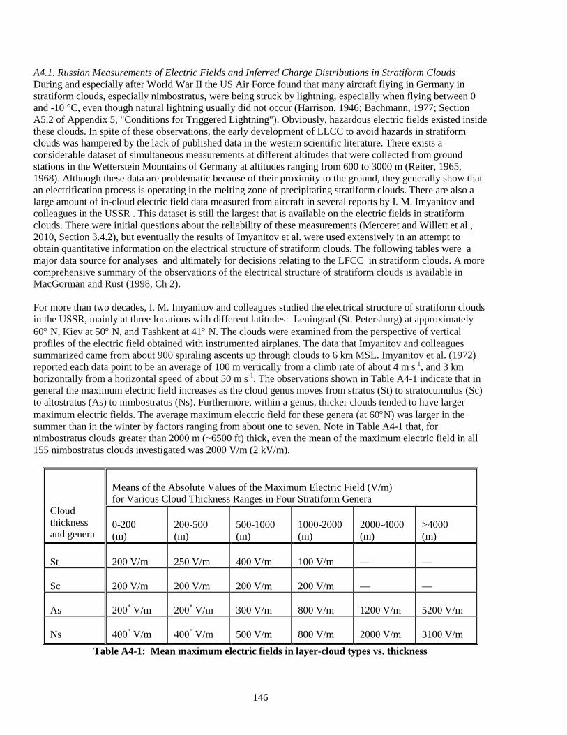
146

A4.1. Russian Measurements of Electric Fields and Inferred Charge Distributions in Stratiform Clouds During and especially after World War II the US Air Force found that many aircraft flying in Germany in stratiform clouds, especially nimbostratus, were being struck by lightning, especially when flying between 0 and -10 °C, even though natural lightning usually did not occur (Harrison, 1946; Bachmann, 1977; Section A5.2 of Appendix 5, "Conditions for Triggered Lightning"). Obviously, hazardous electric fields existed inside these clouds. In spite of these observations, the early development of LLCC to avoid hazards in stratiform clouds was hampered by the lack of published data in the western scientific literature. There exists a considerable dataset of simultaneous measurements at different altitudes that were collected from ground stations in the Wetterstein Mountains of Germany at altitudes ranging from 600 to 3000 m (Reiter, 1965, 1968). Although these data are problematic because of their proximity to the ground, they generally show that an electrification process is operating in the melting zone of precipitating stratiform clouds. There are also a large amount of in-cloud electric field data measured from aircraft in several reports by I. M. Imyanitov and colleagues in the USSR . This dataset is still the largest that is available on the electric fields in stratiform clouds. There were initial questions about the reliability of these measurements (Merceret and Willett et al., 2010, Section 3.4.2), but eventually the results of Imyanitov et al. were used extensively in an attempt to obtain quantitative information on the electrical structure of stratiform clouds. The following tables were a major data source for analyses and ultimately for decisions relating to the LFCC in stratiform clouds. A more comprehensive summary of the observations of the electrical structure of stratiform clouds is available in MacGorman and Rust (1998, Ch 2). For more than two decades, I. M. Imyanitov and colleagues studied the electrical structure of stratiform clouds in the USSR, mainly at three locations with different latitudes: Leningrad (St. Petersburg) at approximately 60° N, Kiev at 50° N, and Tashkent at 41° N. The clouds were examined from the perspective of vertical profiles of the electric field obtained with instrumented airplanes. The data that Imyanitov and colleagues summarized came from about 900 spiraling ascents up through clouds to 6 km MSL. Imyanitov et al. (1972) reported each data point to be an average of 100 m vertically from a climb rate of about 4 m s-1, and 3 km horizontally from a horizontal speed of about 50 m s-1. The observations shown in Table A4-1 indicate that in general the maximum electric field increases as the cloud genus moves from stratus (St) to stratocumulus (Sc) to altostratus (As) to nimbostratus (Ns). Furthermore, within a genus, thicker clouds tended to have larger maximum electric fields. The average maximum electric field for these genera (at 60°N) was larger in the summer than in the winter by factors ranging from about one to seven. Note in Table A4-1 that, for nimbostratus clouds greater than 2000 m (~6500 ft) thick, even the mean of the maximum electric field in all 155 nimbostratus clouds investigated was 2000 V/m (2 kV/m).

Cloud thickness and genera

Means of the Absolute Values of the Maximum Electric Field (V/m) for Various Cloud Thickness Ranges in Four Stratiform Genera 0-200 (m)

200-500 (m)

500-1000 (m)

1000-2000 (m)

2000-4000 (m)

>4000 (m)

St

200 V/m

250 V/m

400 V/m

100 V/m

—

—

Sc

200 V/m

200 V/m

200 V/m

200 V/m

—

—

As

200* V/m

200* V/m

300 V/m

800 V/m

1200 V/m

5200 V/m

Ns

400* V/m

400* V/m

500 V/m

800 V/m

2000 V/m

3100 V/m

Table A4-1: Mean maximum electric fields in layer-cloud types vs. thickness

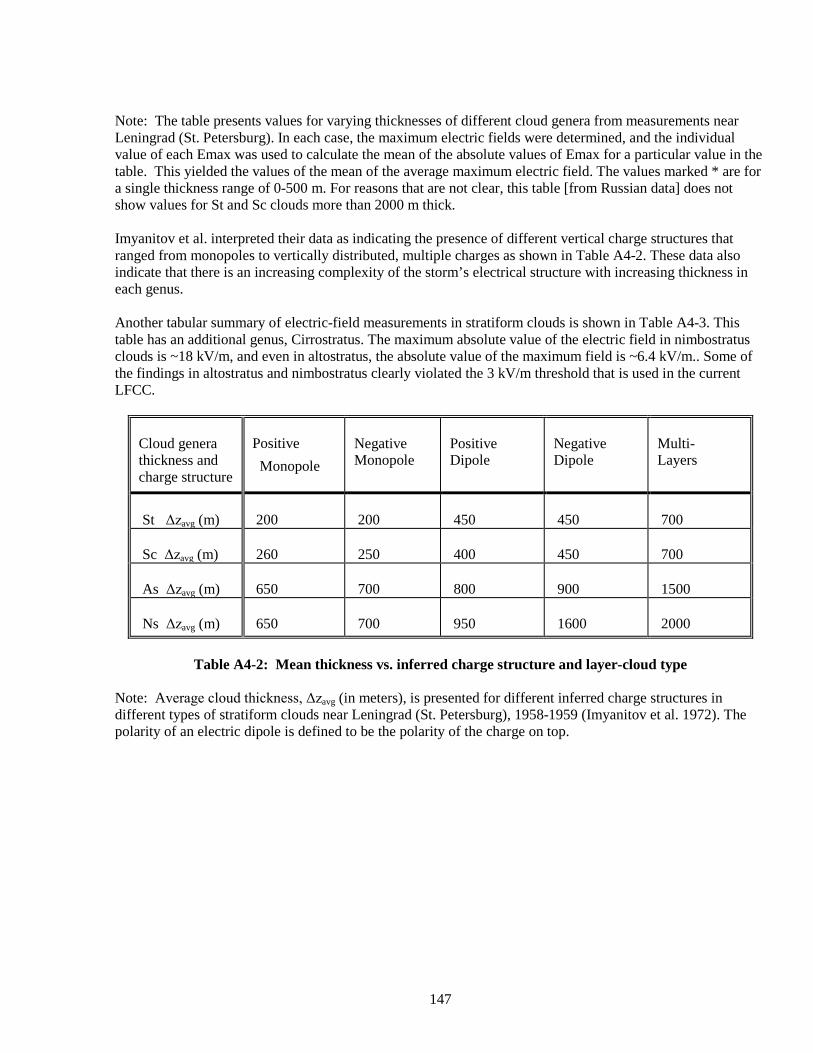
147

Note: The table presents values for varying thicknesses of different cloud genera from measurements near Leningrad (St. Petersburg). In each case, the maximum electric fields were determined, and the individual value of each Emax was used to calculate the mean of the absolute values of Emax for a particular value in the table. This yielded the values of the mean of the average maximum electric field. The values marked * are for a single thickness range of 0-500 m. For reasons that are not clear, this table [from Russian data] does not show values for St and Sc clouds more than 2000 m thick. Imyanitov et al. interpreted their data as indicating the presence of different vertical charge structures that ranged from monopoles to vertically distributed, multiple charges as shown in Table A4-2. These data also indicate that there is an increasing complexity of the storm’s electrical structure with increasing thickness in each genus. Another tabular summary of electric-field measurements in stratiform clouds is shown in Table A4-3. This table has an additional genus, Cirrostratus. The maximum absolute value of the electric field in nimbostratus clouds is ~18 kV/m, and even in altostratus, the absolute value of the maximum field is ~6.4 kV/m.. Some of the findings in altostratus and nimbostratus clearly violated the 3 kV/m threshold that is used in the current LFCC.

Cloud genera thickness and charge structure

Positive Monopole

Negative Monopole

Positive Dipole

Negative Dipole

Multi- Layers

St Δzavg (m)

200

200

450

450

700

Sc Δzavg (m)

260

250

400

450

700

As Δzavg (m)

650

700

800

900

1500

Ns Δzavg (m)

650

700

950

1600

2000

Table A4-2: Mean thickness vs. inferred charge structure and layer-cloud type

Note: Average cloud thickness, Δzavg (in meters), is presented for different inferred charge structures in different types of stratiform clouds near Leningrad (St. Petersburg), 1958-1959 (Imyanitov et al. 1972). The polarity of an electric dipole is defined to be the polarity of the charge on top.

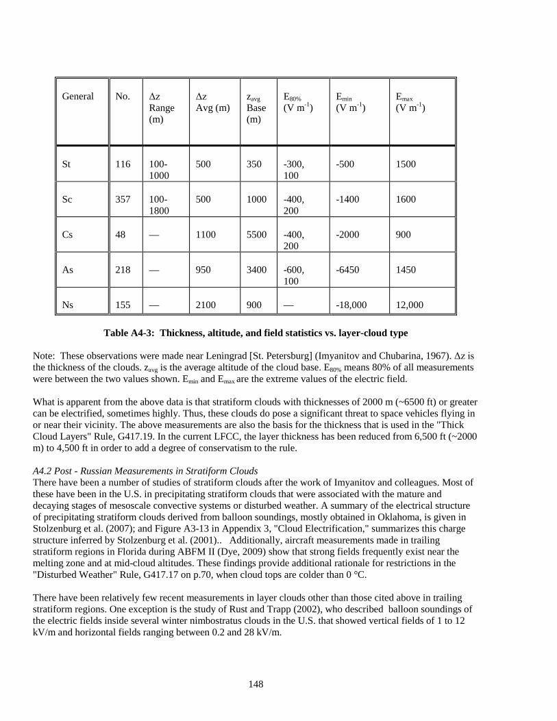
148

General

No.

Δz Range (m)

Δz Avg (m)

zavg Base (m)

E80% (V m-1)

Emin (V m-1)

Emax (V m-1)

St

116

100- 1000

500

350

-300, 100

-500

1500

Sc

357

100- 1800

500

1000

-400, 200

-1400

1600

Cs

48

—

1100

5500

-400, 200

-2000

900

As

218

—

950

3400

-600, 100

-6450

1450

Ns

155

—

2100

900

—

-18,000

12,000

Table A4-3: Thickness, altitude, and field statistics vs. layer-cloud type

Note: These observations were made near Leningrad [St. Petersburg] (Imyanitov and Chubarina, 1967). Δz is the thickness of the clouds. zavg is the average altitude of the cloud base. E80% means 80% of all measurements were between the two values shown. Emin and Emax are the extreme values of the electric field. What is apparent from the above data is that stratiform clouds with thicknesses of 2000 m (~6500 ft) or greater can be electrified, sometimes highly. Thus, these clouds do pose a significant threat to space vehicles flying in or near their vicinity. The above measurements are also the basis for the thickness that is used in the "Thick Cloud Layers" Rule, G417.19. In the current LFCC, the layer thickness has been reduced from 6,500 ft (~2000 m) to 4,500 ft in order to add a degree of conservatism to the rule. A4.2 Post - Russian Measurements in Stratiform Clouds There have been a number of studies of stratiform clouds after the work of Imyanitov and colleagues. Most of these have been in the U.S. in precipitating stratiform clouds that were associated with the mature and decaying stages of mesoscale convective systems or disturbed weather. A summary of the electrical structure of precipitating stratiform clouds derived from balloon soundings, mostly obtained in Oklahoma, is given in Stolzenburg et al. (2007); and Figure A3-13 in Appendix 3, "Cloud Electrification," summarizes this charge structure inferred by Stolzenburg et al. (2001).. Additionally, aircraft measurements made in trailing stratiform regions in Florida during ABFM II (Dye, 2009) show that strong fields frequently exist near the melting zone and at mid-cloud altitudes. These findings provide additional rationale for restrictions in the "Disturbed Weather" Rule, G417.17 on p.70, when cloud tops are colder than 0 °C. There have been relatively few recent measurements in layer clouds other than those cited above in trailing stratiform regions. One exception is the study of Rust and Trapp (2002), who described balloon soundings of the electric fields inside several winter nimbostratus clouds in the U.S. that showed vertical fields of 1 to 12 kV/m and horizontal fields ranging between 0.2 and 28 kV/m.

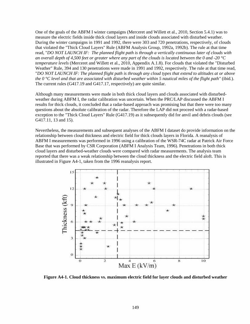
149

One of the goals of the ABFM I winter campaigns (Merceret and Willett et al., 2010, Section 5.4.1) was to measure the electric fields inside thick cloud layers and inside clouds associated with disturbed weather. During the winter campaigns in 1991 and 1992, there were 303 and 720 penetrations, respectively, of clouds that violated the "Thick Cloud Layers" Rule (ABFM Analysis Group, 1992a, 1992b). The rule at that time read, "DO NOT LAUNCH IF: The planned flight path is through a vertically continuous later of clouds with an overall depth of 4,500 feet or greater where any part of the clouds is located between the 0 and -20 °C temperature levels (Merceret and Willett et al., 2010, Appendix A.1.8). For clouds that violated the "Disturbed Weather" Rule, 394 and 130 penetrations were made in 1991 and 1992, respectively. The rule at that time read, "DO NOT LAUNCH IF: The planned flight path is through any cloud types that extend to altitudes at or above the 0 °C level and that are associated with disturbed weather within 5 nautical miles of the flight path" (ibid.). The current rules (G417.19 and G417.17, respectively) are quite similar. Although many measurements were made in both thick cloud layers and clouds associated with disturbed-weather during ABFM I, the radar calibration was uncertain. When the PRC/LAP discussed the ABFM I results for thick clouds, it concluded that a radar-based approach was promising but that there were too many questions about the absolute calibration of the radar. Therefore the LAP did not proceed with a radar-based exception to the "Thick Cloud Layers" Rule (G417.19) as it subsequently did for anvil and debris clouds (see G417.11, 13 and 15). Nevertheless, the measurements and subsequent analyses of the ABFM I dataset do provide information on the relationship between cloud thickness and electric field for thick clouds layers in Florida. A reanalysis of ABFM I measurements was performed in 1996 using a calibration of the WSR-74C radar at Patrick Air Force Base that was performed by CSR Corporation (ABFM I Analysis Team, 1996). Penetrations in both thick cloud layers and disturbed-weather clouds were compared with radar measurements. The analysis team reported that there was a weak relationship between the cloud thickness and the electric field aloft. This is illustrated in Figure A4-1, taken from the 1996 reanalysis report.

Figure A4-1. Cloud thickness vs. maximum electric field for layer clouds and disturbed weather

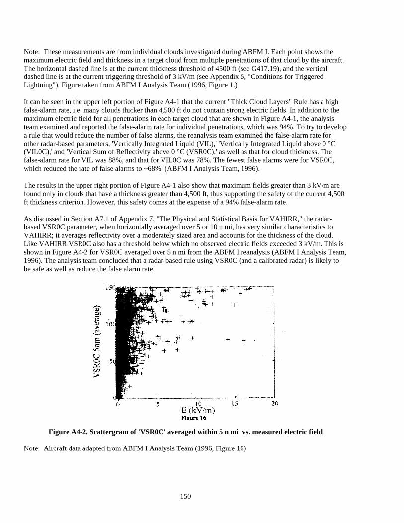
150

Note: These measurements are from individual clouds investigated during ABFM I. Each point shows the maximum electric field and thickness in a target cloud from multiple penetrations of that cloud by the aircraft. The horizontal dashed line is at the current thickness threshold of 4500 ft (see G417.19), and the vertical dashed line is at the current triggering threshold of 3 kV/m (see Appendix 5, "Conditions for Triggered Lightning"). Figure taken from ABFM I Analysis Team (1996, Figure 1.) It can be seen in the upper left portion of Figure A4-1 that the current "Thick Cloud Layers" Rule has a high false-alarm rate, i.e. many clouds thicker than 4,500 ft do not contain strong electric fields. In addition to the maximum electric field for all penetrations in each target cloud that are shown in Figure A4-1, the analysis team examined and reported the false-alarm rate for individual penetrations, which was 94%. To try to develop a rule that would reduce the number of false alarms, the reanalysis team examined the false-alarm rate for other radar-based parameters, 'Vertically Integrated Liquid (VIL),' 'Vertically Integrated Liquid above 0 °C (VIL0C),' and 'Vertical Sum of Reflectivity above 0 °C (VSR0C),' as well as that for cloud thickness. The false-alarm rate for VIL was 88%, and that for VIL0C was 78%. The fewest false alarms were for VSR0C, which reduced the rate of false alarms to ~68%. (ABFM I Analysis Team, 1996). The results in the upper right portion of Figure A4-1 also show that maximum fields greater than 3 kV/m are found only in clouds that have a thickness greater than 4,500 ft, thus supporting the safety of the current 4,500 ft thickness criterion. However, this safety comes at the expense of a 94% false-alarm rate. As discussed in Section A7.1 of Appendix 7, "The Physical and Statistical Basis for VAHIRR," the radar-based VSR0C parameter, when horizontally averaged over 5 or 10 n mi, has very similar characteristics to VAHIRR; it averages reflectivity over a moderately sized area and accounts for the thickness of the cloud. Like VAHIRR VSR0C also has a threshold below which no observed electric fields exceeded 3 kV/m. This is shown in Figure A4-2 for VSR0C averaged over 5 n mi from the ABFM I reanalysis (ABFM I Analysis Team, 1996). The analysis team concluded that a radar-based rule using VSR0C (and a calibrated radar) is likely to be safe as well as reduce the false alarm rate.

Figure A4-2. Scattergram of 'VSR0C' averaged within 5 n mi vs. measured electric field

Note: Aircraft data adapted from ABFM I Analysis Team (1996, Figure 16)

151

Thus, it seems possible that in the future a radar-based parameter such as VAHIRR can be used to help reduce the restrictions on launch through thick cloud layers, but that awaits further research. References ABFM Analysis Group, 1992a: Airborne Field Mill project operational analysis final report for the winter

1991 deployment, Feb. 25, 1992, 133 pp. ABFM Analysis Group, 1992b: Airborne Field Mill project operational analysis final report for the winter

1992 deployment, Oct. 8, 1992, 122 pp. ABFM I Analysis Team, 1996: ABFM 1996 reanalysis of winter 1991 and winter 1992 data with calibrated

PAFB radar data, unpublished white paper, currently available at http://box.mmm.ucar.edu/abfm/webpage/Reports/ABFM_I/ABFM96.htm.

Bachmann, R.G., 1977: Report on the results of the probability of lightning condition forecasting test conducted in 2WW during March, April and May 1977, 2nd Weather Wing, U.S. Air Force, July 31, 1977, 31 pp.

American Meteorological Society, 2000: Glossary Of Meteorology, 2nd ed., American Meteorological

Society, Boston, MA, 850 pp. Dinger, J.E., and R. Gunn, 1946: Electrical effects associated with a change of state of water, Terr. Mag. Atmos. Elect., 51, 477.

Drake, J.C., 1968; Electrification accompanying melting of ice particles, Quart. J. Roy. Meteor. Soc., 94, 176-

191. Dye, J.E. and J.C.Willett, 2007: Observed enhancement of reflectivity and the electric field in long-lived

Florida anvils, Mon. Wea. Rev., 135, 3362-3380. Dye, J.E., 2009: Electric Fields, Microphysics, and Reflectivity Observations from Trailing Stratiform Clouds

in Florida, EOS Trans. AGU, 90(52), Fall Meet. Suppl., Abstract AE24A-05. Fabry, F. and I. Zawadski, 1995: Long-term radar observations of the melting layer of precipitation and their

interpretation, J. Atmos. Sci., 52, 838-851. Harrison, L.P., 1946: Lightning discharges to aircraft and associated meteorological conditions, National

Advisory Committee for Aeronautics Tech. Note No. 1001, May, 1946. Imyanitov, I.M., and Ye.V. Chubarina, 1967: Electricity of the Free Atmosphere. 212 pp, NASA Tech.

Translation, NASA TT F-425, TT 67-51374 of Elektrichestvo Svobodnoy Atmosfery. Gidrometeoizdat, Leningrad, 1965, NTIS Accession no. N68-10079.

Imyanitov, I.M., Ye.V. Chubarina, and Ya.M. Shvarts, 1972: Electricity of Clouds. 122 pg, NASA Tech.

Translation, NASA TT F-718, of Elektrichestvo oblakov. Hydrometeorological Press, Leningrad, 1971.


ice crystal interactions, Quart J. Roy. Meteorol. Soc., 109, 609-630. Kuhlman, K. M., D. R. MacGorman, M. I. Biggerstaff, P. R. Krehbiel, 2009: Lightning initiation in the anvils

of two supercell storms. Geophysical Research Letters, 36, L07802.

152

MacGorman, M. I. Biggerstaff, P. R. Krehbiel, 2009: Lightning initiation in the anvils of two supercell storms. Geophysical Research Letters, 36, L07802.

Knight, C.A., 1979: Observations of the melting of snowflakes, J. Atmos. Sci.,36, 1123-1130. MacGorman, Donald R., and W. David Rust, 1998: The Electrical Nature of Storms, Oxford Univ. Press,

ISBN 0-19-507337-1, Ch 2. Marshall, T.C., and W.D. Rust, 1993; Two types of vertical electrical structures in stratiform precipitation

regions of mesoscale convective systems, Bull. Amer. Meteorol. Soc., 74, 2159-2170 Merceret, F.J. and J.C. Willett, Editors, H.J. Christian, J.E. Dye, E.P. Krider, J.T. Madura, T.P. O'Brien, W.D.


Rust, W. D. and R. J. Trapp, 2002: Initial balloon soundings of the electric field in winter nimbostratus clouds

in the USA, Geophys. Res. Lett., 29 (20), 20-1 to 20-4. Reiter, R., 1965: Precipitation and cloud electricity. Quart. J. Roy. Met. Soc. 91, 60. Reiter, R., 1968: Results of investigation on precipitation and cloud electricity based on 15 years of

observation, Arch. Met. Geoph. Biokl., Ser. A, 17, 17-29. Shepherd, T. R., W. D. Rust, and T. C. Marshall, 1996: Electric fields and charges near 0 ºC in stratiform

clouds, Mon. Wea. Rev., 124, 919-938. Simpson, G.C., 1909: On the electricity of rain and its origin in thunderstorms, Phils. Tran. Roy. Soc.

London, Ser A, 209, 379-413. Stolzenburg, M., T. C. Marshall, W. D. Rust, and B. F. Smull, 1994: Horizontal distribution of electrical and


Stolzenburg, M., T. C. Marshall, and W. D. Rust, 2001: Serial soundings of electric field through a mesoscale

convective system, J. Geophys. Res., 106 (D12), 12371-12380. Stolzenburg, M., T.C. Marshall, W.D. Rust, E.A. Mareev, S.S. Davydenko, 2007: The stratiform precipitation

region of mesoscale convective systems: Inductive charging evidence and global circuit effects, Proc. 13th Internat. Conf. on Atmosph. Electr., Bejing China, Aug. 13-17, 2007, 13-16.

Stolzenburg, M. and T.C. Marshall, 2008: Charge structure and dynamics in thunderstorms, Rev. Space

Physics, 137, 355-372. Weiss, S.A., D.R. MacGorman, and K.M. Kuhlman, 2010: Lightning in the anvil of supercell storms,

submitted to Mon. Wea. Rev.

153

Appendix 5. Conditions for Triggered Lightning A5.0. Introduction and Summary Triggered lighting is defined as lightning that would not have occurred naturally (at least not at the same time and place) without the presence of a man-made structure or the intervention of a anthropogenic event. Man-made structures known to trigger lightning are primarily tall towers like the Empire State Building, and anthropogenic events include depth-charge explosions and space-vehicle launches. For more details on these various topics the interested reader is referred to the encyclopedic treatment by Rakov and Uman (2003, Chapters 6, 7, and 10), although the organization of their material is not convenient for our purposes. Section A5.1 outlines the intellectual development of the triggering concept. Section A5.2 briefly reviews the meteorological and electrical conditions in which aircraft are known to have been struck by lightning. There follows in Section A5.3 a detailed discussion of the various physical parameters that are believed to control triggering by a large space-launch booster. Finally, calculations leading to, and the uncertainties in, a 3 kV/m triggering threshold at 10 km altitude are reviewed in Section A5.4. As described in Appendices 7, "Physical and Statistical Basis for VAHIRR," and 8, "Standoff Distances from Anvil and Debris Clouds," this threshold has been used to develop the VAHIRR criteria for, and the standoff distance from, anvil and debris clouds. The arguments in Sections A5.3 and A5.4 may be summarized as follows:

(1) 'Leader viability,' not classical 'breakdown,' is the most appropriate condition for triggering by a space launcher (see Section A5.3.2).

(2) The ambient electrostatic field and its spatial distribution are the physical parameters that control the triggering process (see Section A5.3.3).

(3) The 'constant-potential-drop' model is preferred for the calculation of leader viability because it is simplest and most closely related to experimental data (see Section A5.3.3). The smallest measured potential drop reported in that section is 3.3 MV at surface temperature and pressure.

(4) E/N ('Paschen's Law') scaling is used for the altitude dependence of triggering conditions, even though it is almost certainly conservative (see Section A5.3.4). This decreases the surface triggering field (or potential drop) by a factor of three for 10 km altitude.

(5) The 'conducting' length of the exhaust plume for Shuttle or Titan is estimated at 300 m, nearly independent of altitude, which is added to a vehicle length of 60 m to give the total conducting length (see Section A5.4.0).

(6) The 'electrical effective length' of the vehicle-plume system is the total conducting length divided by two, giving 180 m for Shuttle and Titan (see Section A5.4.1).

(7) A factor-of-two safety margin is applied (see Section A5.4.0). (8) Combining points (3) through (7) above yields an estimated 'triggering threshold' of 3 kV/m (see

Section A5.4.0). (9) This triggering threshold is quite uncertain but is believed to be conservative by as much as a factor of

six (see Section A5.4.3). A5.1. Development of the Triggering Concept The first broad hint of the existence of triggered lightning might have come from the early studies of lightning to tall structures by McEachron (1939). Using the time-resolved lightning camera that had been invented by C.V. Boys (1926), McEachron found that a large fraction of strikes to the Empire State Building were initiated by upward-propagating, positively charged leaders, just like most of the triggered lightning produced with the rocket-and-wire technique today (see below). Without the benefit of hindsight, however, the author did not speculate as to the cause of his large incidence of upward-initiated strikes beyond saying that

154

"...the building acts as a great needle point, and may have a marked influence upon the character of the discharge... It is believed that upward leaders will only occur when conditions on the earth simulate a needle point of sufficient height to have an influence on the propagation."

It is interesting to note that Boys (1926, 1927), in the same 'news item' that described his famous camera and in follow-up correspondence, may have been the first to propose rocket-triggering of lightning from the ground, although not much notice seems to have been taken of his suggestion:

"There is one more experiment which I have wished to make with this apparatus. This is to fire a rocket towards or into a thundercloud when it is getting ripe for another flash. ...leaving a conducting trail of potash smoke and ions of every kind. ...If a photograph were obtained with the revolving lenses of a flash striking a rocket a good way up, the rocket itself might be expected to be the place of origin of the flash, and this position would be obvious on the plate, as below this the lightning would no doubt follow the rocket trail." (Boys, 1926) "If any question should arise as to the conductivity of the trail, this could be assured by allowing the rocket to carry up a hundred metres or more of fine copper wire arranged like a life-line so as not to kink." (Boys, 1927)

The aircraft community recognized the possibility of triggered lightning early on, based primarily on the observation that flying aircraft tend to be struck by lightning more frequently than expected in clouds that are apparently not producing natural lightning. For example, in a review of the current state of knowledge about lightning strikes to aircraft Harrison (1946) said,

"From these data and other considerations (see sec. 18) it may be inferred that the presence of the aircraft is instrumental in initiating disruptive discharges in some cloud conditions where lightning would not have developed spontaneously in the absence of the airplane, other factors being equal. [Footnote:] The data lead to the implication that some cumulo-nimbus and perhaps other clouds have potential gradients insufficient for the evolvement of natural lightning, yet sufficient for the formation of a disruptive discharge when altered by the intrusion of an airplane into the scene." [from p.13]

and

"However, the aircraft by its very presence may increase the potential gradient many fold, as explained in section 12. One process which invariably tends to accomplish this to an important extent is the distortion of the electric field by induction upon the conducting outer skin of the aircraft (see paragraph numbered (2) and following, in the abovementioned section). This is most likely to happen with notable consequences in a space where the initial potential gradient is already quite high, as between two contiguous, highly charged cloud regions of opposite polarity, or in the immediate vicinity of a single region having a great concentration of electrical charges of one predominant sign. It is possible under these circumstances for a disruptive discharge to be 'triggered' by the aircraft, provided (1) that the critical breakdown potential gradient is reached at or near the aircraft, and (2) that once the disruptive discharge is initiated at such a point continued propagation of the discharge streamer is assured by a sufficiently high average potential gradient in the space between the oppositely charged cloud regions or between a single charged region of one sign and another restricted region (whether of the cloud, space charge, or earth) with predominately opposite charge." [from p.57 in Section 18]

[It is worth noting that such well-known experts on atmospheric electricity as O.H. Gish, K.B. McEachron, E.J. Workman, and R. Gunn were on the Subcommittee on Lightning Hazards to Aircraft of the National Advisory Committee for Aeronautics for which Harrison (1946) was prepared.]

155

Again without the benefit of hindsight, Harrison was apparently unaware of the advantage of airspeed in 'blowing away' the space charge from corona discharges that would otherwise tend to reduce the electric-field enhancement near sharply curved surfaces on an airborne vehicle (discussed further below). Newman (1958), not Boys (1926), is usually credited with the first suggestion of triggering lightning with small rockets towing grounded wires:

"One of the most important projects with the new boat facility is to 'precipitate' a natural lightning discharge and improve measurement of its characteristics... To minimize initial cloud field disturbance, it is planned, as illustrated in Figure 8, to project toward charged clouds a wire conductor about 1000 ft long by means of a small launching rocket... By timing the wire launching to correspond to an interval of high cloud gradients as measured by a generating voltmeter while cruising under the most highly charge cloud areas, it is believed probable to achieve a 'hit' perhaps once per 10 shots."

It is not obvious from the above quotation whether Newman realized that his technique would initiate a triggered flash or would simply intercept a natural one. Neither is it clear whether the idea was original with him; no references whatsoever are given in his article. Nevertheless his receiving credit for the invention is probably due to the fact that he did succeed in triggering lightning over water in 1960 according to Rakov and Uman (2003, p.265). Newman (1965) announced that he had triggered an unknown number of flashes on unspecified dates. Meanwhile, Young (1962) reported a lightning strike to the water plume from a depth-charge explosion that had been conducted in the Chesapeake Bay during June of 1957. At the time of the strike the plume had extended to a height of about 75 m, 1.6 s after the detonation. High-speed motion pictures of this event in Young's report made it possible to recognize the characteristics of this lightning discharge as very similar to upward discharges to tall structures like the Empire State Building. Young's observation seems to have been critical to the recognition and initial understanding of the triggering process. Brook et al. (1961) quickly proposed a credible explanation for the depth-charge event, and predicted the success of rocket-triggering attempts such as that recently proposed by Newman (1958). This explanation was based on prevention of the usual build-up of corona space charge around a conductor of high electric-field-enhancement factor by its rapid introduction into a pre-existing region of high electric field. To complete the story of rocket triggering, Newman et al. (1967) reported continued success and some interesting engineering results from their use of the technique over water. They do not seem to have measured the long-continuing current that probably preceded the return strokes in their triggered events, however. They explained the initial, continuing luminosity in their wind-streaked photographs as follows: "The wire was vaporized in the first stroke, the gradual dissipation of the metal vapor from the channel being shown clearly in the photographs." They also drew no parallels to the very similar results from tower measurements such as those of McEachron, (1939). Jumping off from Newman's work, a group of French scientists and engineers continued the development of the rocket-and-wire technique into the routine technology for lightning research that is now known as 'classical' triggering. Fieux et al. (1975) reported the first rocket-triggered lightning over land in 1973, and this success was followed by an ongoing study of the phenomena at Saint-Privat d'Allier in France. Some of the French scientists conducted experiments at the Langmuir Laboratory in New Mexico during the early 1980s (e.g., Hubert et al., 1984) and then at the NASA Kennedy Space Center in Florida [see, for example, Merceret and Willett et al. (2010) Sections 4.4.1 and 5.4.3]. Other triggering programs sprang up elsewhere in the world, some of which continue to this day.

156

Returning to the tower measurements, Berger and Vogelsanger (1969) "suggested that the high electric field needed for the initiation of upward lightning [from tall structures] is rapidly created by an in-cloud discharge..." according to Rakov and Uman (2003, p.243). Also, Uman (1987, p.215) reported that Berger (1977) presented evidence that large field changes due to cloud discharges immediately preceded the initiation of upward-moving negatively charged leaders. These reports would seem to finally complete the causal, as well as the phenomenological, similarity between upward lightning from tall structures and rocket-triggered lightning in terms of the explanation that had been proposed earlier by Brook et al. (1961): For tall structures shielding of the conductor by corona space charge is prevented by the sudden imposition of a high ambient field; for triggering rockets shielding it is obviated by the rapid introduction of a long conductor into the pre-existing field. (See also discussion of new evidence to this effect in Section A2.1 of Appendix 2, "Spatial and Temporal Intervals between Lightning Discharges.") Meanwhile the aircraft community continued to debate whether lightning strikes to flying vehicles were due to the accidental interception of natural discharges or to actual triggering by the vehicle. Vonnegut (1965), clearly aware of the recent success of Newman's rocket-triggering efforts, summarized the arguments for and against triggering by aircraft. Fitzgerald (1967) concluded,

"The data presented suggest that thunderstorms, in their early stages of dissipation, retain large charge centers to account for one or more lightning discharges if a suitable means of initiating a streamer becomes available. It is likely that an aircraft entering a storm in this condition will act to 'trigger' a lightning discharge."

Cobb and Holitza (1968) reported,

"A DC-6 research aircraft was struck by lightning on three occasions... Each event occurred in a dissipating cumulonimbus near the freezing level and in a region containing both ice and water... The possibility exists that one or more of the lightning strikes were triggered by the aircraft."

As late as the early 1980s, Clifford and Kasemir (1982) were able to state,

"Few data exist, other than circumstantial evidence and much speculation, to prove or disprove whether aircraft actually trigger lightning. However, the circumstantial evidence is growing and the idea of aircraft triggering lightning is fairly well accepted, although no definite triggering mechanism has been identified."

Final proof of aircraft triggering (and by extension, of triggering by space-launch vehicles) came in two forms. The most definitive was a coordinated radar/instrumented-aircraft study by Mazur et al. (1984), who reported,

"The analysis of radar echoes from lightning at the moments of strikes to the NASA Langley Research Center's F-106B instrumented airplane proves that the airplane itself triggers the lightning, rather than intercepting naturally occurring flashes... From the data obtained in 1982, every [UHF radar] echo from a lightning strike to the F-106B started directly on top of the airplane echo and propagated outward. ...none of the lightning flashes [for which the echo first appeared at some distance from the airplane], which is typical for the naturally occurring intracloud flash, ever struck the F-106B."

The other form of proof was more circumstantial but equally convincing. Boulay et al. (1988), for example, were able to explain comprehensive current, electric- and magnetic-field, and video measurements on heavily instrumented aircraft during lightning strikes in terms of the following aircraft-triggering mechanism (for further explanation, see Section A5.3): After the aircraft flies into a region of high ambient electric field, a positive leader from one extremity begins the process, followed in a few milliseconds by a negative leader from another extremity. These leaders continue to extend and become a full-blown intra-cloud lightning

157

discharge. Since this sequence of events had already been documented in lightning triggered from the ground with 'altitude rockets,' which unspool ungrounded wires beneath thunderstorms [see, for example, Merceret and Willett et al. (2010, Section 5.4.3.4)], the explanation of Boulay et al. (1988) was compelling. In summary, it was already generally believed by the time of the Apollo XII incident in 1969 that lightning could be triggered by the rapid introduction of a long, grounded, conductor into a region of high ambient field. The strikes to Apollo XII extended this conviction to spacecraft during the boost phase. The resulting accident-investigation report, NASA (1970, p.48), concluded in part,

"3. The lightning was most probably triggered by the presence of the effective electrical conduction path created by the space vehicle and its exhaust plume in an electric field which would not otherwise [have] discharged."

[For more information about the Apollo XII accident, see Merceret and Willett et al. (2010), Sections 2.3 and 3.0 and Appendix VI.] By the time of the Atlas/Centaur-67 accident in 1987 [again, see Merceret and Willett (2010), Sections 4.3.2 and 5.0] both rocket and aircraft triggering were well established. It is now known that space vehicles can trigger lightning during ascent through sufficiently electrified clouds. The remainder of this appendix will explore the electrical conditions under which this is expected to occur. A5.2. Environmental Conditions for Aircraft Strikes As hinted in Section A5.1, lightning strikes to aircraft tend to occur near 0 °C and often are not associated with natural lightning. Harrison (1946) and Bachman (1977) both concluded that most strikes occur in or near cumulonimbus clouds (often apparently embedded in nimbostratus or other overcast conditions), on the cold side of the 0 °C level, while the aircraft is flying in cloud and/or precipitation. Rakov and Uman (2003, Chapter 10) give a good summary of several statistical studies, concluding that most aircraft strikes occur inside clouds at or just above the 0 °C level in association with precipitation and turbulence. The most illuminating illustrations are their Figures 10.3 and 10.4, which show that strikes to commercial aircraft in Japan occur at very different altitudes between summer and winter, but at nearly the same temperature levels (peaking between 0 and -5 °C). There have been at least four major field campaigns to measure lightning strikes on board instrumented aircraft that were deliberately flown into active thunderstorms (Uman and Rakov, 2003, Section 10.3). Two of these aircraft, the FAA CV-580 in 1985 and the French Transall C-160 in 1988, carried calibrated systems of electrostatic field mills that allowed the measurement of ambient field immediately prior to a number of strikes. The data from these systems have been summarized and interpreted by Laroche et al. (1989a) and by Lalande and Bondiou-Clergerie (1997). A more detailed discussion of these results may be found in Krider et al. (2006, Section 3.1.2.3). In summary, most of these strikes occurred near the 0 °C level, and the ambient electric fields measured by these aircraft immediately prior to triggering lightning averaged 50 - 60 kV/m. It should be mentioned that the F-106B aircraft that was used by Mazur et al. (1984), as reported in Section A5.2, sustained most of its strikes at altitudes above 6 km, although no explanation has been given for this fact. A5.3. Physical Parameters that Control Triggering A5.3.1. Phenomenology of Triggered Lightning At least 80–90% of all lightning strikes to flying aircraft and spacecraft are 'triggered,' in the sense that they are initiated locally by the penetration of a large conducting body into a sufficiently large region of high-intensity ambient electrostatic field. As mentioned in Section A5.1, recordings of currents and electric-field

158

changes on board instrumented aircraft have been interpreted to indicate that such triggered strikes invariably begin with a 'positive leader' propagating away from an extremity on which positive charge had been induced by the ambient field, followed after a few milliseconds by the development of a negative leader from a negatively charged extremity, propagating in the opposite direction (Boulay et al., 1988; Mazur, 1989b). (Here the term, 'leader,' denotes a highly ionized, conducting, filamentary channel extending into virgin air. The term 'positive streamer,' in contrast, will always refer to the poorly conducting 'corona' space-charge waves (e.g., Dawson and Winn, 1965; Phelps and Griffiths, 1976) that are an important component of the advancing 'head' of a positive leader.) A small percentage of aircraft strikes appear to result from the chance interception of naturally occurring lightning flashes. Perhaps some of these are actually triggered by large ambient-field changes that were suddenly imposed on the aircraft by nearby natural lightning. In any case these events need not concern us here because they can easily be prevented by avoiding any clouds that are producing natural lightning (see the "Lightning" Rule in Chapter 2, "Rationale"). Triggered lightning represents a severe hazard precisely because it often occurs in clouds that produce little or no natural lightning. Detailed study of the triggering phenomenon (as well as other important aspects of lightning) has been facilitated by rocket-triggering technology [see Section A5.1 and Merceret and Willett et al. (2010), Sections 4.4.1 and 5.4.3]. 'Classical' rocket-triggered lightning is initiated by a small rocket towing a grounded wire aloft under a thunderstorm. It is now well established that this type of lightning normally begins with a positive leader propagating upward from the tip of the triggering wire toward a negatively charged cloud. Apparently identical positive leaders have been shown to initiate 'altitude' triggered lightning (Laroche et al., 1989b), which is produced by a similar rocket towing an ungrounded wire aloft and appears to constitute a good analog for triggering by aircraft and spacecraft, and most 'upward-initiated' discharges to towers. Although the positive leader itself probably does not constitute a serious threat to a flying vehicle, the negative leader may, and their subsequent development into a discharge several kilometers in length usually results in large currents and current derivatives that can cause both direct and indirect damage (e.g., Walterscheid et al. ,2010, Section 2.3). Since the positive leader is believed to constitute the initial stage of all triggered strikes to such vehicles, however, it (and especially the conditions for its formation and continued propagation) is an important subject of study in its own right. Considerable information is available on the phenomenology of rocket-triggered positive leaders, including currents measured at the base of the triggering wires and electric-field changes at the ground produced by these currents (e.g., Laroche et al., 1988; Lalande et al., 1998), and propagation velocities and other interesting optical characteristics (Idone, 1992; Idone and Orville, 1988). Very briefly, during their first few hundred meters of propagation such leaders have average currents of a few amperes, normally exhibit rapid pulsing with peak currents of several tens of amperes, and propagate at speeds ranging from a few times 104 to a few times 105 m/s. Unfortunately, the conditions required to initiate a viable positive leader (see below), especially from a spacecraft producing a significant exhaust plume, are not sufficiently understood. A5.3.2 Qualitative Discussion of Conditions for Triggered Lightning The initiation and continued propagation of positive leaders from conducting objects has been studied in detail in the laboratory, using sparks up to tens of meters in length, but to a much lesser extent on the scale of lightning discharges in the free atmosphere (e.g., Bazelyan and Raizer, 1998, 2000). Material relevant to the triggering conditions will be summarized here, and more details can be found in Section A5.3.3 and in Krider et al. (2006, Section 3.1.2). Basically, there are three conditions that must be satisfied in order to initiate and propagate a 'viable' positive leader. First, 'breakdown' must occur in a small volume of air near the surface of the object in question, in order to produce free electrons in sufficient quantities to carry an electric current. At standard temperature and pressure this means that the local electric field must reach a value near 3.0 MV/m; and when this occurs, a

159

phenomenon called 'glow corona' is produced. Second, the current in the corona region must be amplified to the point where streamers occur. Positive streamers propagate outward from the breakdown region, further heating a small volume that is called the 'stem;' and this stem is where the positive-leader channel begins. Third, the ambient field must be large enough over a sufficiently large volume of space that the positive leader, once it has been initiated, will continue to grow and propagate (i.e., the potential at its tip will remain large enough relative to the local ambient potential to sustain propagation). This last condition is what we will refer to as 'leader viability.' The breakdown (first) condition can be computed relatively easily once the detailed geometry of the conducting object and its orientation relative to the ambient electrostatic field are known. If the conductor is uncharged, a geometrical 'enhancement factor' can be computed and used to estimate the maximum field that will be present on the surface of the object simply by multiplying the ambient field intensity by this factor. The enhancement increases with the length of the conducting object (in the direction of the ambient field) and with the inverse of the local radius of curvature of the object’s extremities. If the conductor carries a net charge, there will be another contribution to the field on the surface due to this charge, which can also be computed fairly easily, and this must be added to the enhanced ambient field. However, since the magnitude of the charge on the vehicle is usually not known, and since this charge can change rapidly as a result of particle impaction and/or corona discharges from the object, the determination of breakdown conditions is problematic. Nevertheless, the geometric enhancement factor remains the most familiar tool for estimating the risk of triggering lightning by airborne vehicles. (Perhaps this is because the same mathematical approach is often used to define the various 'zones' of lightning attachment to aircraft surfaces.) The leader-initiation (second) condition can be approximately summarized by the requirement that the potential difference between the object and its environment (i.e., the potential due to the ambient field) exceeds about 400 kV at standard temperature and pressure. If the object is uncharged and generally symmetrical with respect to the direction of the ambient field, then this condition will be met whenever the length of the object in the direction of the field, multiplied by the magnitude of that field, exceeds about 800 kV. In this case, we say that the positive and negative extremities of the object each 'span' a potential difference of 400 kV. (Of course, no leader can be initiated unless the initial breakdown condition is also satisfied.) The leader-viability (third) condition is conceptually more complex but is probably the most important condition in practice. When a sufficiently long and thin conductor is exposed to a high electric field at near-standard temperatures and pressures (e.g., the grounded wire in classical rocket triggering), air breakdown always occurs before a positive-leader is initiated, and this in turn precedes positive-leader viability. For example, in rocket-triggered lightning, there are always indications of both air breakdown and leader initiation — the 'precursors' described further in Section A5.3.3 — well before the triggered lightning flash begins. In such a case, the enhancement factor is actually irrelevant, since it is a much less stringent condition than the one for leader viability. Even if the space vehicle of interest is not "sufficiently long and thin" to simulate a triggering wire, we remain profoundly skeptical of using electric-field-enhancement factors (breakdown conditions) to predict triggering. First, there are almost certainly small-scale features (e.g., wing tips, pitot tubes, radio antennae, and other protrusions) that are difficult to model and have much larger enhancement factors than the nose fairing. Second, there are likely to be imperfections in implementing the theoretical design that have even smaller local radii of curvature. Third, any flights inside clouds will involve impactions of water and/or ice particles that will certainly produce very small radii of curvature for a brief instant. Fourth, during conditions of particle impact, and perhaps even because of the action of the rocket engines themselves, the vehicle will likely become highly charged. Such charging can produce breakdown and corona discharges from vehicle extremities, sparking between poorly bonded conducting surfaces, and even surface discharges on non-conducting materials (see the rationales for the definitions of 'treated' and 'triboelectrification' in Section

160

G417.3, "Definitions, Explanations and Examples," and for the "Triboelectrification" Rule, G417.23. This fourth point is substantiated by many observations of aircraft going into corona while flying in clouds that are not electrified. For example, Thomas et al. (2004, Figure 13) have used a VHF lightning-mapping system to track the corona discharges produced by a commercial aircraft flying through a cirrus cloud. Similarly, when the Space Shuttle has flown through cirrus during landings at the NASA Kennedy Space Center, it has been tracked by a similar lightning-mapping system (the KSC LDAR, Frank Merceret, private communication, October 2005). For all of the above reasons, we will assume that the leader-viability criterion is a more robust triggering criterion than the simple enhancement-factor approach. A5.3.3 Results of a Key Field Experiment From first principles (e.g., Smythe, 1968, Sections 2.19 and 3.11), it is evident that the energy that drives all lightning discharges is extracted from the ambient electrostatic field. Therefore, one would like to know the ambient-field intensity, and its spatial distribution, associated with both unsuccessful and successful triggering attempts. Unfortunately, it is well known that ground-based measurements can be 'screened' from more intense fields aloft by a layer of corona-produced space charge (see Section A1.3.3.1 of Appendix 1, "Measurement and Interpretation of Surface Electric Fields"). There are few in situ measurements aloft from which to determine the necessary or sufficient conditions for propagation of positive leaders or with which to explain variations in their behavior. Therefore, Willett et al. (1999) conducted a major field experiment in Florida during the summer of 1996. The objective of this experiment was, in effect, to extend experimental work on long laboratory sparks from tens-of-meter to kilometer length scales. When conditions appeared favorable for rocket-triggered lightning, a special sounding rocket was launched to profile the vector ambient electrostatic field through the lowest few kilometers of the atmosphere. The sounding rocket was followed a few seconds later by a classical triggering rocket, and the currents and field changes of any positive leaders so initiated were recorded. For present purposes, the field profiles and the heights at which triggered lightning flashes were initiated are of primary interest. A summary of the data, which have been re-analyzed since original publication, is presented here. Figure A5.1 shows the lower part of the measured ambient-field profiles for all nine successful triggers that were reported by Willett et al. (1999). Here the magnitude of the vector field (which was always oriented near the vertical) is plotted as a function of height from the surface to 500 m altitude. Note that the field increased rapidly with height near the ground, due to the corona-space-charge layer, and then became relatively uniform over the height range in which triggering occurred (230–447 m in this experiment). Profiles of ambient electrostatic potential relative to ground were also obtained by line integration of the field component parallel to the rocket trajectory and have been used to construct Figures A5.2 and A5.3. As the triggering rocket ascended in this environment, brief leader-like discharges ['precursors,' best described by Laroche et al. (1988)] began at heights of 102–213 m, but successful positive leaders were not initiated until 164 ±38 m higher (mean ± standard deviation), where the magnitude of the ambient field was only 2.9 ±1.2 kV/m greater. Nevertheless, the magnitude of the ambient potential difference between ground and the triggering altitude was 2.4 ±0.4 MV (2.5 times, on average) larger than that at the precursor-initiation height. (Note that this difference between the occurrence of precursor discharges and the onset of a viable leader exemplifies the well known fact that breakdown fields, or even bursts of positive streamers, at the wire tip are not sufficient to trigger lightning.) Thus it appears that the leader may have been waiting, not for the triggering rocket to fly into a region of higher ambient field, but for the triggering wire to span a threshold potential difference. More details can be found in Figure A5.2 andA5.3, as discussed below.

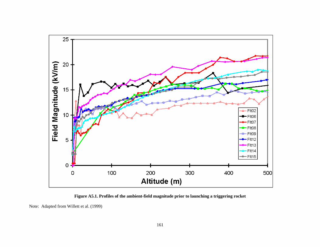
161

Figure A5.1. Profiles of the ambient-field magnitude prior to launching a triggering rocket

Note: Adapted from Willett et al. (1999)

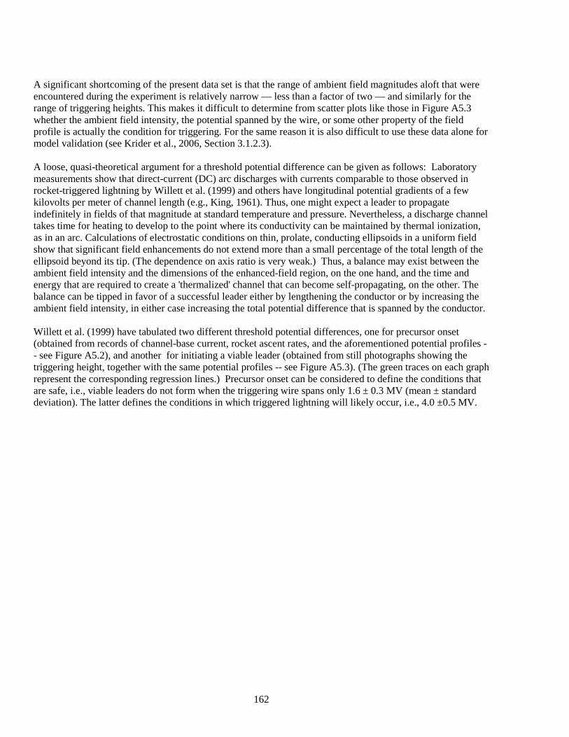
162

A significant shortcoming of the present data set is that the range of ambient field magnitudes aloft that were encountered during the experiment is relatively narrow — less than a factor of two — and similarly for the range of triggering heights. This makes it difficult to determine from scatter plots like those in Figure A5.3 whether the ambient field intensity, the potential spanned by the wire, or some other property of the field profile is actually the condition for triggering. For the same reason it is also difficult to use these data alone for model validation (see Krider et al., 2006, Section 3.1.2.3). A loose, quasi-theoretical argument for a threshold potential difference can be given as follows: Laboratory measurements show that direct-current (DC) arc discharges with currents comparable to those observed in rocket-triggered lightning by Willett et al. (1999) and others have longitudinal potential gradients of a few kilovolts per meter of channel length (e.g., King, 1961). Thus, one might expect a leader to propagate indefinitely in fields of that magnitude at standard temperature and pressure. Nevertheless, a discharge channel takes time for heating to develop to the point where its conductivity can be maintained by thermal ionization, as in an arc. Calculations of electrostatic conditions on thin, prolate, conducting ellipsoids in a uniform field show that significant field enhancements do not extend more than a small percentage of the total length of the ellipsoid beyond its tip. (The dependence on axis ratio is very weak.) Thus, a balance may exist between the ambient field intensity and the dimensions of the enhanced-field region, on the one hand, and the time and energy that are required to create a 'thermalized' channel that can become self-propagating, on the other. The balance can be tipped in favor of a successful leader either by lengthening the conductor or by increasing the ambient field intensity, in either case increasing the total potential difference that is spanned by the conductor. Willett et al. (1999) have tabulated two different threshold potential differences, one for precursor onset (obtained from records of channel-base current, rocket ascent rates, and the aforementioned potential profiles -- see Figure A5.2), and another for initiating a viable leader (obtained from still photographs showing the triggering height, together with the same potential profiles -- see Figure A5.3). (The green traces on each graph represent the corresponding regression lines.) Precursor onset can be considered to define the conditions that are safe, i.e., viable leaders do not form when the triggering wire spans only 1.6 ± 0.3 MV (mean ± standard deviation). The latter defines the conditions in which triggered lightning will likely occur, i.e., 4.0 ±0.5 MV.

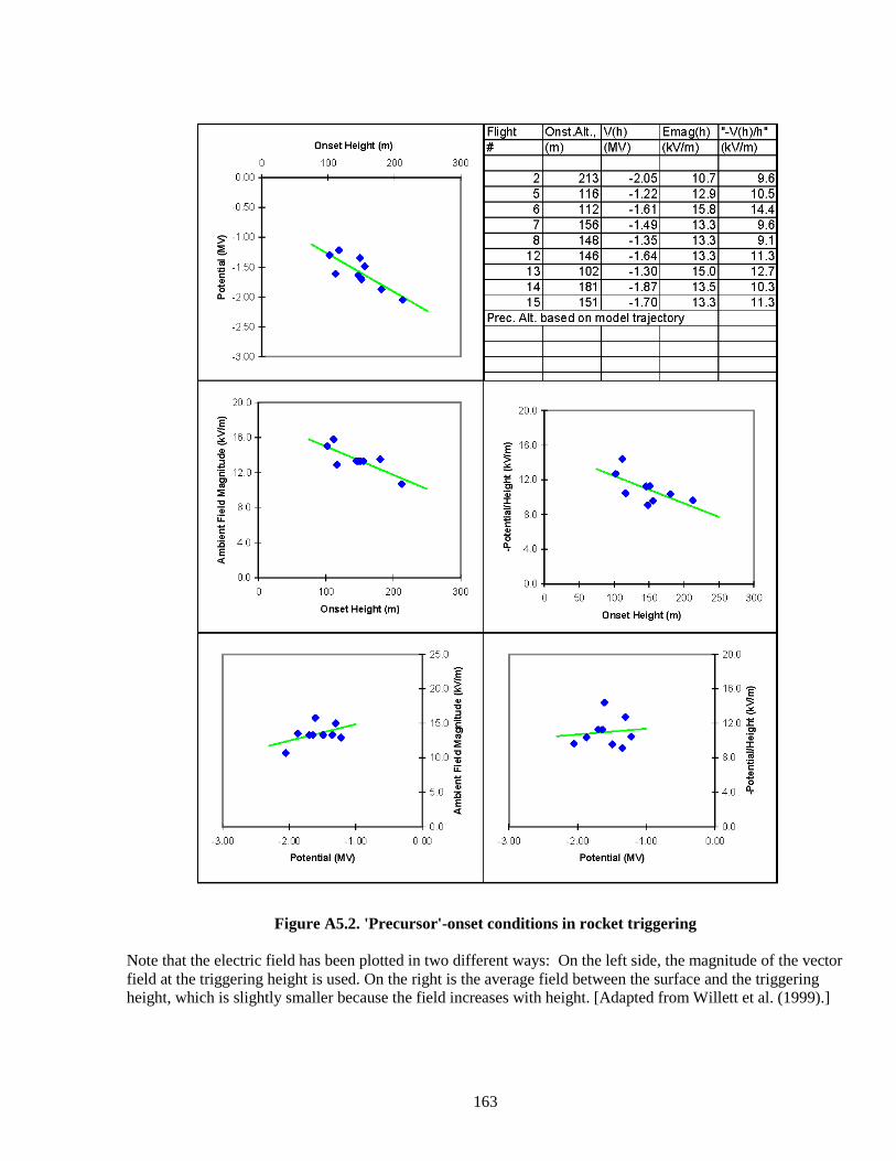
163

Figure A5.2. 'Precursor'-onset conditions in rocket triggering Note that the electric field has been plotted in two different ways: On the left side, the magnitude of the vector field at the triggering height is used. On the right is the average field between the surface and the triggering height, which is slightly smaller because the field increases with height. [Adapted from Willett et al. (1999).]

164

Figure A5.3. Leader-onset conditions in rocket triggering Note: The yellow points represent a significant, but ultimately failed, leader that occurred in Flight 6, prior to onset of a viable leader. Otherwise as in Figure A5.2. [Adapted from Willett et al. (1999).]

Flight Trig.Alt., V(h) Ema9(h) "-V(h)/h" Triggering Height (m) # (m) (MV) (kV/m) (kV/m)

0 200 400 600 00 2 447 -4.7 12.7 10.5

6 307 -4.7 16.8 15.2 -10 7 295 -3.8 18.4 12.9

8 279 -3.3 16.0 11.8 > -2.0 9 312 -3.7 13.5 11.9 ~ 12 336 -4.4 15.9 13.1 .. ~

-3.0 13 230 -3.5 18.6 15.2 • ~ • to. 14 324 -4.1 16.9 12.7 ~ -4.0 15 299 -3.9 16.1 13.0 •• • Tri . Alt. based on individual tra·ectories

-5.0

-6.0 Failed Leader (vella

6[ 260 -4.0 16.6 15.4

250 20.0

E ~ LDO • E 16.0 • • • • ~

.1". ~ , ~ 15.0 " .•. ' ~ • ~ 120 • • ~ ~ .. • ~ 10.0

I .. ~ 80 ~ ~ ~ • • 50 ~ ~ ~ 4 0 E <

00 00 0 200 400 600 0 100 200 300 400 500 000

Triggering Height (m) Triggering Height (m)

25.0 20.0

E .. 20.0 ~ • • 16.0 E • ~

•• f'~ • ~

" , .41\. 15.0 ~ 120:1:

• ~ ~

• • • .. ~

~ 10.0 i: 80 ~ ~

" ~ 50 • 4 0 ~ ~

E <

00 00 -8.0 -6.0 -4.0 -2.0 00 -8.0 -6.0 -4 .0 -2.0 00

Potential (MY) Potential (MY)

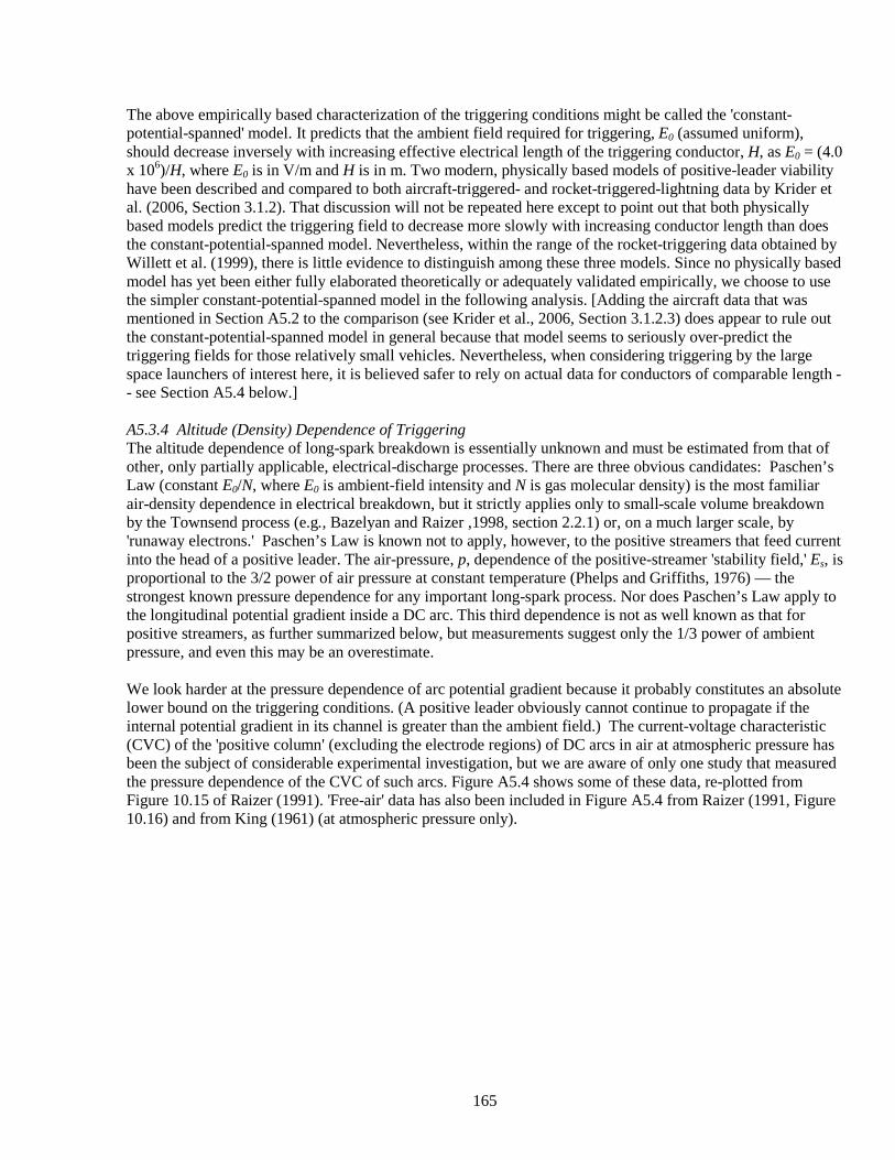
165

The above empirically based characterization of the triggering conditions might be called the 'constant-potential-spanned' model. It predicts that the ambient field required for triggering, E0 (assumed uniform), should decrease inversely with increasing effective electrical length of the triggering conductor, H, as E0 = (4.0 x 106)/H, where E0 is in V/m and H is in m. Two modern, physically based models of positive-leader viability have been described and compared to both aircraft-triggered- and rocket-triggered-lightning data by Krider et al. (2006, Section 3.1.2). That discussion will not be repeated here except to point out that both physically based models predict the triggering field to decrease more slowly with increasing conductor length than does the constant-potential-spanned model. Nevertheless, within the range of the rocket-triggering data obtained by Willett et al. (1999), there is little evidence to distinguish among these three models. Since no physically based model has yet been either fully elaborated theoretically or adequately validated empirically, we choose to use the simpler constant-potential-spanned model in the following analysis. [Adding the aircraft data that was mentioned in Section A5.2 to the comparison (see Krider et al., 2006, Section 3.1.2.3) does appear to rule out the constant-potential-spanned model in general because that model seems to seriously over-predict the triggering fields for those relatively small vehicles. Nevertheless, when considering triggering by the large space launchers of interest here, it is believed safer to rely on actual data for conductors of comparable length -- see Section A5.4 below.] A5.3.4 Altitude (Density) Dependence of Triggering The altitude dependence of long-spark breakdown is essentially unknown and must be estimated from that of other, only partially applicable, electrical-discharge processes. There are three obvious candidates: Paschen’s Law (constant E0/N, where E0 is ambient-field intensity and N is gas molecular density) is the most familiar air-density dependence in electrical breakdown, but it strictly applies only to small-scale volume breakdown by the Townsend process (e.g., Bazelyan and Raizer ,1998, section 2.2.1) or, on a much larger scale, by 'runaway electrons.' Paschen’s Law is known not to apply, however, to the positive streamers that feed current into the head of a positive leader. The air-pressure, p, dependence of the positive-streamer 'stability field,' Es, is proportional to the 3/2 power of air pressure at constant temperature (Phelps and Griffiths, 1976) — the strongest known pressure dependence for any important long-spark process. Nor does Paschen’s Law apply to the longitudinal potential gradient inside a DC arc. This third dependence is not as well known as that for positive streamers, as further summarized below, but measurements suggest only the 1/3 power of ambient pressure, and even this may be an overestimate. We look harder at the pressure dependence of arc potential gradient because it probably constitutes an absolute lower bound on the triggering conditions. (A positive leader obviously cannot continue to propagate if the internal potential gradient in its channel is greater than the ambient field.) The current-voltage characteristic (CVC) of the 'positive column' (excluding the electrode regions) of DC arcs in air at atmospheric pressure has been the subject of considerable experimental investigation, but we are aware of only one study that measured the pressure dependence of the CVC of such arcs. Figure A5.4 shows some of these data, re-plotted from Figure 10.15 of Raizer (1991). 'Free-air' data has also been included in Figure A5.4 from Raizer (1991, Figure 10.16) and from King (1961) (at atmospheric pressure only).

166

Figure A5.4. Experimental Data on Arc Potential Gradient vs. Pressure Several comments are in order here. First, the measured longitudinal field in Raizer (1991, Figure 10.15) appears to depend on the 0.32 power of ambient pressure (magenta line) at both 2 A (solid green diamonds) and 5 A (hollow green diamonds), in dramatic contrast to Paschen’s Law (cyan line). Even this observed dependence might be exaggerated, however, as the measurements were apparently made on arcs that were confined inside cooled tubes. Second, data re-plotted from Raizer (1991, Figure 10.16, red symbols), specifically for unconfined arcs, indicates significantly lower potential gradients in free air. Raizer (1991, p. 273) offers the following comments on these issues: “If the pressure is increased at a fixed current, the field is enhanced (Figure 10.15). The enhancement is caused by increased radiative losses and, possibly, by a certain increase in heat transfer from plasma to the [tube] walls, dictating enhanced power per unit length, W = Ei. At equal currents, stronger field is required to sustain the plasma in a tube than in an arc burning in free atmosphere, because the transfer is more intense [in the tube] and more power is needed (Figure 10.16).” Third, the data on DC arcs that is summarized in Figure A5.4 appears to be relevant to the lightning-initiation problem because the time constants for adjustment of these arcs to changes in current [order 100 μs (e.g., Edels and Graffmann, 1969; Latham, 1986)] are short compared to the leader-development times (a few milliseconds). Finally, we believe that the free-air data of King (1961) (blue symbols) is more quantitatively compelling than that from Raizer (1991, Figure 10.16) because King’s measurements were acquired with very careful attention to the experimental techniques so as not to compromise the free-air nature of the arcs in question, nor to underestimate the tortuous channel length. Therefore, we take the minimum electric field that is required to maintain a 2 to 5 A arc in the free atmosphere to be in the range from 3.9 to 2.2 kV/m, respectively, at surface pressure. We further take the pressure dependence of this field to be no stronger (and probably weaker) than the 0.32 power.

167

Note that, by quoting arc gradients at specific currents, we tacitly assume that the minimum current required to maintain a positive leader will not change substantially with altitude. Since this current is supplied to the leader channel by streamer processes at the leader tip, and since it is largely controlled by the leader-propagation speed (the physics of which is not well understood), there is no guarantee that this assumption is valid. The positive-streamer scaling as p3/2 is probably extreme for the triggering conditions, since it applies only to a small portion of the leader structure, but the estimated DC-arc scaling as p1/3 might be too weak for the long spark as a whole. Paschen’s Law remains a conservative middle ground. A new analysis of the dependence of positive-leader-viability conditions on atmospheric pressure by Bazelyan et al. (2007) has predicted that the conditions for continued propagation of a positive leader (which we have taken as the primary determinant of the triggering conditions) may be nearly independent of atmospheric pressure (altitude). Although this would be a welcome result (the triggering-field threshold would not decrease rapidly with increasing altitude as previously assumed by Krider et al. (2006, Section 3.1.3), the assumptions and theoretical manipulations used to obtain it are both uncertain and complex. Further, this result has no direct experimental validation. To stay the more conservative course, the Lightning Advisory Panel decided to continue using Paschen's Law (breakdown field inversely proportional to air density) in its development of the new VAHIRR criteria from the ABFM II results (see Appendices 7, "Physical and Statistical Basis for VAHIRR," and 8, "Standoff Distances from Anvil and Debris Clouds"). This decision is retained here from Krider et al. (2006, Section 3.1.3), with the understanding that it may result in a substantial underestimate of the triggering field at altitudes well above the surface. The same new analysis by Bazelyan et al. (2007) contains a careful theoretical calculation showing that the arc potential gradient should scale approximately with the 1/5 power of air density. This would imply that the range of arc potential gradient at 10 km altitude (1/3 of surface density) is closer to 3.1 - 1.8 kV/m than suggested by the 0.32-power dependence above. The work of Bazelyan et al. has also estimated that the leader-propagation speed, hence its current, should be almost independent of air density, so that the current range of 2 - 5 A should still apply at 10 km altitude. Thus this range of ambient field remains our absolute lower bound on the triggering conditions at altitude, which would apply to conducting objects of effectively infinite length. A5.3.5 Velocity Dependence of Triggering The vehicle-velocity dependence of triggering is believed to be a threshold that is based on the ion-drift velocity in the geometrically enhanced electric field at the altitude of interest. The basic argument, originally due to Brook et al. (1961), is that space charge tends to accumulate in the air around a long, thin conductor embedded in a high ambient electrostatic field as a result of corona discharges from its tips. If the conductor is motionless relative to the air, this charge partially shields the conductor from the otherwise greatly enhanced field. If the conductor is moving rapidly, however, it will tend to leave the space charge behind, eliminating the shielding. How fast the conductor has to move to escape this charge sufficiently for triggering depends on the ion-drift velocity in the enhanced field near the conductor’s tips. A complete analysis of the situation is obviously complex, but rough estimates of the threshold speed at surface pressure may be made as follows: An extreme upper bound can be derived from the breakdown field (see Section A5.3.2). A somewhat more realistic estimate can be obtained by assuming the field to be limited near the positive tip by the positive-streamer stability field (see Es in Section A5.3.4). Taking the small-ion mobility to be about 1.2 x 10–4 m2/(Vs), the resulting speeds become 360 m/s and 54 m/s, respectively. Recently Aleksandrov et al. (2005) have stated that a speed of only about 20 m/s is sufficient to overcome the shielding effect of corona space charge, but no details of this theoretical derivation were offered.

168

Although systematic experiments have not been carried out to our knowledge, speeds that are sufficient for lightning initiation clearly can be attained by triggering rockets as well as by flying aircraft and spacecraft. Two early types of triggering rockets that were used successfully by French triggering experts flew at 170 m/s, and their most recent design flies at 220 m/s, according to St. Privat D’Allier Group (1985). Laroche et al. (1989a) asserted, “The critical velocity lies around 100 m/s for an electric field equal to one-third of the breakdown field in normal conditions. The [CV-580 and Transall] aircraft were flown at about the same speed, around 100 m/s, so they were both in the same favorable conditions to trigger...” All of these observed speeds are consistent with the above estimates. The density (or altitude) dependence of this speed threshold would be controlled to some extent by the details of the shielding mechanism. Given that both the breakdown field and the positive-streamer stability field decrease with air density (see Section A5.3.4) and that the small-ion mobility increases approximately in inverse proportion to density, however, it seems likely that the threshold speed is approximately altitude independent. Therefore we need not be concerned with the velocity dependence for space launchers. A5.3.6 Possible Effects of the Exhaust Plume We have seen in Section A5.3.3 that the effective electrical length of the space launcher is a critical parameter in determining the triggering threshold, and this length is likely to depend strongly on the nature of the exhaust plume. Our discussion of this topic in Section A5.4 will echo the earlier analysis by Krider et al. (2006, Sections 3.1.5.3 and 3.1.5.4), which depended primarily on photographic and video measurements of the extent of the visible radiation from the incandescent particulates in the exhaust. Krider et al. (2006) had neither access to a model of plume conductivity nor any real idea what conductivity level might correspond to the electrical extremity of the plume. Here we consider first what conductivity levels in exhaust plumes might be important for determining the effective electrical length of a vehicle in flight. Note that this is not the same problem as determining the radar cross section of a plume or the attenuation length for S-band communications. Our problem is much more similar to an electrostatic problem, because the ambient conductivity of the troposphere, in which our plume is acting as a conductor, is so low -- typically less than 10-

12 S/m below an altitude of 10 km. A5.3.6.1 Prior Research Prior literature on the electrical conductivity of rocket exhausts is extensive, but largely classified and directed primarily toward establishing the radio and radar signatures of ballistic missiles during launch and/or the attenuation of telemetry signals between those missiles and ground stations. Thus, this literature is mostly irrelevant for present purposes. The most relevant literature has been reviewed by Perala et al. (1994), a reference that remains the most comprehensive attempt to address the effects of the vehicle exhaust on the lightning-triggering problem. This work is discussed here in some detail. Also noteworthy is the work of Heckscher (1972) and Heckscher and Pagliarulo (1973), who attempted to estimate the conductivity levels of interest here (see below) and to measure directly the conductivity of rocket exhausts during launch (with limited success). Perala et al. (1994) adopted an interesting, but ultimately unsatisfying, approach. They first assumed (reasonably but apparently without theoretical or experimental justification) that the trailing end of the conductive portion of an exhaust plume acts like a Kelvin water-dropper or flame potential equalizer. That is, any space charge that would normally accumulate at this location is carried away in the exhaust flow so that, at equilibrium, this point has zero longitudinal electric field and therefore is at the same electrostatic potential as the ambient air at roughly the same altitude. This point in the plume was defined by a 'critical conductivity' that would be determined later in the context of a plume-chemistry model. Second, it was assumed that all of the (two-dimensional) exhaust volume bounded by the critical-conductivity contour (see below) acts as a perfect conductor that is electrically attached to the rocket body. With these assumptions, the electric field at the nose of the rocket can be calculated using electrostatic theory and is proportional to the magnitude of the ambient electric field in the longitudinal direction. (The rocket/plume conductor has a net charge that exactly

169

cancels the longitudinal field that would be induced at the trailing edge of an uncharged conductor in the ambient field. The equal and opposite net charge on the plume is assumed to disappear downstream in the exhaust trail.) The next steps taken by Perala et al. (1994) made use of two static test firings of small solid-rocket motors (described in their Appendix E), together with a numerical model of the chemistry of the exhaust-plume (described in their Appendix G). These steps are considered even less reliable than the electrostatic model outlined above. First a motor test stand was insulated from ground, and an electrostatic field was applied parallel to its longitudinal axis, so that the effective resistance of a fixed length of the exhaust plume could be measured. The results were then compared to predictions of the plume-chemistry code (Pergament et al., 1993) and found to be in poor agreement. The code was therefore "refined" by adding a mechanism of rapid hydration of positive ions and its effect on later recombination with un-hydrated negative ions. This yielded reasonable agreement between measurements and predictions. The modified plume code was then used to compute the two-dimensional geometry of various contours (extending down to 10-10 S/m) of the electrical conductivity that was expected in the exhaust plume of the small rocket motors that were used in the experiments. A second static test was conducted to measure the charging of a motor in the presence of a known, fair-weather, atmospheric-electric field. These measurements were extrapolated to obtain an asymptotic motor voltage, which was then compared with predictions of the electrostatic model described above, based on the different geometries of the model conductivity contours. The contour that gave the best agreement was inferred to be about 3x10-10 S/m. This was taken to be the critical conductivity mentioned above and, therefore, the conductivity value that defines the ’conducting extent’ of the plume. Finally, the authors argued that this value should be essentially the same for larger rockets powered by different motors. Although the work of Perala et al. (1994) has many uncertainties, not the least of which is their plume-chemistry model, it is interesting that Walterscheid et al. (2010, Sections 2.6.5.4 and 2.6.5.6) arrived at a similar estimate of the critical conductivity using two different approaches, as outlined in Section A5.3.6.2 below. Heckscher (1972) outlined an interesting method of estimating the conductivity level of interest. Although quite different from either the complex approach of Perala et al. (1994) or the simple arguments of Walterscheid et al. (2010), Heckscher's calculation yielded similar results. He considered the initial stages of a launch and asked at what altitude the rocket electrically disconnects from ground, so that its potential can rise toward the local ambient value. This question was answered by balancing the current required to charge the rocket/plume combination (to hold it at ground potential as the vehicle gains altitude) against the current that can flow through the interface between plume and ground. Since both of these currents are proportional to the ambient field, the result must be independent of the field. This equation defines the critical conductivity at ground level in the plume as a function of vehicle altitude and other geometrical factors. Estimates were given for Minuteman, Atlas, and Saturn vehicles in Heckscher's Figure 15, which ranged from about 3 x 10-11 to 3 x 10-9 S/m for altitudes ranging between about 30 m (for Atlas) and 500 m (for Minuteman), respectively. Armed with the relevant conductivity range, Heckscher (1972) and Heckscher and Pagliarulo (1973) described instrumentation for measuring, and ground-based measurements of, conductivity in the fringes of exhaust plumes from Minuteman, Atlas, and Saturn vehicles shortly after liftoff. They found measured conductivity values comparable to their calculated critical values for vehicle altitudes in the range given above. A5.3.6.2 New Analysis Walterscheid et al. (2010) first used a dimensional argument to estimate the relevant conductivity levels for determining the effective electrical length of an exhaust plume in their Section 2.6.5.4. This argument was then extended in their Section 2.6.5.5 to a simple, 1½-dimensional calculation of the relaxation time of the potential

170

(as opposed to the local electrical relaxation time) at the end of a uniform, motionless, conducting plume embedded in insulating air. Finally, their Section 2.6.5.6 explored the validity of their dimensional argument with an explicit 1-D, steady-state model of plume conduction, with variable conductivity but a uniform flow velocity. A5.3.6.3 Conclusions about Plume Effects Based on the above review and new analysis Walterscheid et al. (2010, Section 2.6.5.6) concluded that the critical conductivity threshold that determines the electrical effective length of the exhaust plume is much lower than might be expected -- probably only a few orders of magnitude above the ambient value of about 10-

12 S/m at 10 km altitude, as had been predicted previously by Heckscher (1972) and Perala et al. (1994). This is probably much lower than the conductivity to be expected in the incandescent part of the plume (the length of which is used below to estimate the electrical effective length) and is also much lower than those that any known plume-conductivity model can accurately predict. If this conclusion is validated by more complete modeling and/or experiment, as recommended by Walterscheid et al. (2010, Section 2.6.5.7), then the actual effective length of a booster exhaust plumes may be greater than the estimate used herein. This would make the overall electrical length of the vehicle during boost phase longer, which would, in turn, decrease its triggering threshold and make the triggering of a lightning discharge more likely. The uncertainties involved in the estimates of electrical effective length are discussed in Section A5.4. A5.4 Triggering Threshold for a Large Booster at 10 km Altitude Based on the discussion at the end of Section A5.3.3 above, the electric-field threshold for triggering by a launch vehicle in an anvil cloud has been estimated simply by starting from an experimentally measured electrostatic-potential drop. In a series of nine measurements, the minimum triggering potential drop for a rocket towing a grounded wire at surface conditions was 3.3 MV (Figure A5.3). This potential drop has been converted to a triggering field by dividing by one half of the total electrical length of the launch vehicle plus its conducting exhaust plume, as discussed in Section A5.4.1 below. Frank Merceret (private communication, ShuttlePlumeVideo.xls, 5 January 2004) has compiled night-time video data from Shuttle and Titan, indicating that the incandescent plume length was approximately 300 m in both cases and was relatively independent of altitude. Adding to this the length of the Titan vehicle itself (about 60 m) and dividing by two, we obtained a total 'effective electrical length' of 180 m. (This is only about a factor of two smaller than the triggering heights reported in Figure A5.3.) This length implies a triggering field of about 18 kV/m at surface pressure. An altitude scaling proportional to air density has been applied to this triggering field (or equivalently, to the triggering potential drop itself), as discussed in Section A5.3.4 above, to yield an estimated triggering threshold of 6.2 kV/m at a typical anvil altitude of 10 km. Finally, a factor-or-two safety margin has been added to give 3 kV/m. This triggering threshold might reasonably be scaled to other vehicles, in inverse proportion to the length of the vehicle plus its incandescent plume, and for clouds at other altitudes, in direct proportion to air density. Caution is advocated when scaling for length, however, for two reasons: First, the triggering conditions that are proposed here were derived from measurements on conducting wires a few hundred meters long; they may not apply well to much shorter conductors. Second, these are the conditions that are required to initiate a self-propagating positive leader. After such a leader attains sufficient length, it can probably continue propagating in an appreciably weaker ambient field because the voltage gradient in a DC arc that carries a few Amperes is only a few kV/m at surface pressure (see Section A5.3.4 above). Therefore, it would appear unwise to exceed this gradient by a large factor for any vehicle. A5.4.1 Effective Electrical Length Both the conducting length of the exhaust plume from solid-rocket boosters (SRB) and the factor of 1/2 between the total and effective electrical length deserve further discussion. The conductivity of rocket exhaust is controlled by its temperature and mediated primarily by the ionization of trace amounts of alkali metals (sodium and potassium) in the fuel, by thermionic emission from solid carbon (and other) particles, and by

171

chemi-ionization (Krider et al., 1974). To the extent that the gas temperature is important in maintaining the electron concentration, however, the particulate temperature, which is probably responsible for the luminosity of an SRB plume, may not be relevant. According to 'RAMP2' modeling by the Titan engineers (Bob Crisler, Lockheed Martin Space Systems, Denver, personal communication, 5 April 2004) the Aluminum Oxide particles remain hot much further downstream than the gaseous components of the exhaust. Thus, the conducting lengths inferred from Frank Merceret's (personal communication, 5 January 2004) video data on the incandescent plume may be conservative, even in the light of Section A5.3.6 above. By way of comparison with Merceret's relatively altitude-independent plume-length measurements of about 300 m (used herein), Nanevicz and Hilbers (1973) reported an estimated conducting length of ~200 m near the ground, based on measurements aboard two Titan flights. On the other hand, Perala et al. (1994) predicted ~300 m at low altitude, based on unconfirmed modeling, increasing roughly in inverse proportion to atmospheric pressure to ~1040 m at 10.7 km altitude. Although we tend to discount the altitude dependence predicted by Perala et al. (1994), both low-altitude estimates tend to corroborate Merceret's measurements. The factor of 1/2 arises from the observation that experimental measurements of triggering potential drop apply to a rocket-and-wire system that is grounded, whereas the flying launch-vehicle-plus-plume system is floating. A grounded wire can deliver unlimited charge to a developing positive leader without appreciably altering its own potential, but the behavior of the ungrounded system is more complicated. If the rocket engines do not actively charge the flying system, it will 'float' to a potential equal to the ambient potential approximately at its midpoint. Thus, it will initially span the ambient potential drop over only half of its length (from midpoint to either extremity). Initiation of an upward positive leader from the tip of this flying system will effectively increase the altitude of the ambient potential to which it floats (at least until a negative leader begins to propagate from the opposite extremity), however, making it even less than half as effective at triggering as a grounded wire of the same length. A more realistic assumption might be that the conducting/insulating transition of the exhaust plume (through which particulates are constantly streaming) acts as a potential equalizer, so that the lower extremity of the conducting plume is anchored at the local ambient potential (see Perala et al. ,1994, as summarized in Section A5.3.6.1 above). In this case the flying system would initially span the ambient potential drop over its total electrical length. Nanevicz and Hilbers (1973, p.40) deduced from precipitation-charging measurements that the Titan plume was capable of discharging about 310 μA of negative charge without an appreciable rise in vehicle potential. Nevertheless, initiation of a positive leader from the tip of the launch vehicle would supply a current of a few Amperes (based on measurements in rocket-triggered lightning), which would probably overwhelm the potential-equalizing capabilities of the exhaust plume, returning us to the situation described at the end of the previous paragraph. At a minimum, the exhaust nozzles themselves might become the effective potential equalizer, reducing the electrical effective length of the flying system to the vehicle length. Even in this case, therefore, the factor of 1/2 appears to be conservative. Nanevicz and Hilbers (1973, p.31) also concluded that the Titan engines do charge the vehicle, but only between about 200 m (where the plume was taken to disconnect from ground) and 3700 m altitude (where the vehicle self charge returned to essentially zero). The vehicle charge was observed to saturate (at -200 kV -- presumed to be the corona threshold) between about 430 and 760 m altitude. Nevertheless, this negative charging current was estimated at only 100 μA. Again, we assume here that the leader current would overwhelm such a small charging current. In summary, we believe that an electrical-effective-length estimate of 180 m is conservative for a large vehicle. A5.4.2 Pressure-Scaling Estimate Both the triggering potential drop and the conducting plume length may depend on ambient pressure (or altitude). Frank Merceret's video analysis and available modeling suggest that the incandescent plume length has little altitude dependence, at least from the surface through the range of interest for anvil clouds. The

172

pressure dependence of long-spark breakdown is not well known, however, and must be estimated from that of other (not necessarily applicable) electrical-discharge processes. As discussed in detail in Section A5.3.4, we have chosen to use Paschen's Law (inverse proportionality to atmospheric density) to extrapolate the estimated triggering threshold from surface conditions to 10 km altitude. This is likely to give a very conservative result. A5.4.3 Uncertainties and Degree of Conservatism There are a number of elements, including poorly known quantities and outright assumptions, that went into our estimated electric-field threshold for triggering of 3 kV/m, as discussed in more detail above and summarized here:

(1) Experimental Measurement: The minimum observed ambient electrostatic potential drop along a grounded rocket-triggering wire for successful triggering of a positive leader at surface temperature and pressure was 3.3 MV. This measurement has good accuracy for wire lengths of order 300 m.

(a) Assumption: This measured threshold potential drop applies to conductors of other shapes

and lengths. This assumption appears reasonable for conductor lengths within a factor of two of 300 m, but this assumption has not been verified.

(b) Assumption: A positive leader propagating in ambient air is the process that controls the

triggering conditions for a flying vehicle. This assumption appears reasonable in the light of evidence from both aircraft in flight and un-grounded triggering rockets, but it ignores the possibility that the initial leader might begin propagating inside the exhaust plume, where its conditions for continued propagation are unknown and might be quite different.

(2) Assumption: The above potential drop should be divided by half the total electrical length of the

vehicle plus its conducting exhaust plume -- about 180 m for Shuttle and Titan. This assumption appears conservative for the following reasons:

(a) Assumption: The conducting length of the exhaust plume was approximated by the

incandescent length on video images, nearly independent of altitude within the height range of interest. This assumption may be quite conservative for Shuttle and Titan, in view of plume modeling that indicates the Aluminum Oxide particles (from the SRB's) remain hot much further downstream than gaseous components of the exhaust. (This presumed conservatism would not apply, however, to liquid-fuel engines that do not produce significant soot. Further, Perala et al. (1994) have predicted the conducting plume length to increase considerably with altitude, becoming as much as a factor of 3 longer than our estimate at 10 km altitude.)

(b) Assumption: The total electrical length should be reduced by a factor 1/2. This factor is

strictly appropriate only to long and thin, uncharged (electrically floating) vehicles. It may be conservative, however, for two reasons:

(i) In the absence of other discharges, the extension of a positive leader from one

extremity will not increase the effective electrical length of the vehicle/leader system (hence the driving potential spanned) as rapidly as it would if the vehicle were grounded (as in the case of the fundamental measurement in (1) above).

(ii) Even if the exhaust plume acts as a potential equalizer, i.e., anchors the vehicle

potential to ambient at the altitude of its conducting/insulating transition (which would be expected to negate the factor of 1/2), this equalizer effect would likely be overwhelmed by the few-Ampere current deposited on the vehicle/plume system by a

173

growing positive leader. Thus any potential equalization might actually occur much closer to (or even at) the exhaust nozzles.

(3) Assumption: This triggering field should be scaled with altitude in proportion to atmospheric density -

- down by a factor of three at 10 km altitude. This assumption may introduce as much as a factor-of-three conservatism, based on the unconfirmed prediction of Bazelyan et al. (2007) that the conditions for continuous propagation of a positive leader should depend only very slightly on air density.

(4) The resulting estimated triggering field of 6.2 kV/m at 10 km altitude was divided in half to give the 3

kV/m field that was actually used. Obviously this introduces a factor-of-two conservatism. Conclusion: The value, 3 kV/m, for a triggering field at 10 km is quite uncertain but may be conservative by as much as a factor of six. References Aleksandrov, N. L., E. M. Bazelyan, and Yu P. Raizer, 2005: Initiation and development of first lightning

leader: the effects of coronae and position of lightning origin, Atmospheric Research, 76, 307-329, doi:10.1016/j.atmosres.2004.11.007.

Bachman, R.G., 1977: Report on the results of the probability of lightning condition forecasting test conducted

in 2WW during March, April and May 1977, Tech. Note 77-1, 2nd Weather Wing (MAC), USAF, 31 July 1977.

Bazelyan, E. M., and Yu P. Raizer, 1998: Spark Discharge, Boca Raton, FL, CRC Press, 294 pp. Bazelyan, E. M., and Yu P. Raizer, 2000: Lightning Physics and Lightning Protection, Bristol, Institute of

Physics Publishing, 325 pp. Bazelyan, E.M., N.L. Aleksandrov, Yu. P. Raizer, and A.M. Konchakov, 2007: The effect of air density on

atmospheric electric fields required for lightning initiation from a long airborne object, Atmospheric Research, 86, 126–138.

Berger, K., and E. Vogelsanger, 1969: New results of lightning observations, in Planetary Electrodynamics,

S.C. Coroniti and J. Hughes, eds., Gordon and Beach, New York, pp. 489-510. Berger, K., 1977: The earth flash, in Lightning, Vol. 1, Physics of Lighting, R.H. Golde, ed., Academic Press,

New York, pp. 119-190. Boulay, J.L., J.P. Moreau, A. Asselineau, and P.L. Rustan, 1988: Analysis of recent in-flight lightning

measurements on different aircraft, presented at the Aerospace and Ground Conference on Lightning and Static Electricity, Oklahoma City, April 19-22, 1988.

Boys, C.V., 1926: Progressive lightning, Nature, 118, 748-750. Boys, C.V., 1927: Progressive lightning, Nature, 119, 278. Brook, M., G. Armstrong, R.P.H. Winder, B. Vonnegut, and C.B. Moore, 1961: Artificial initiation of

lightning discharges, J. Geophys. Res., 66, 3967-3969. Clifford, D.W. and H.W. Kasemir, 1982: Triggered lightning, IEEE Trans. EMC, EMC-24, 112-122.

174

Cobb, W.E., and F.J. Holitza, 1968: A note on lightning strikes to aircraft, Mon. Wea. Rev., 96, 807-808. Dawson, G. A., and W. P. Winn, 1965: A model for streamer propagation, Z. Phys., 183, 159–171. Edels, H., and E. Graffmann, 1969: Time constant measurements of high pressure arc columns, Z. Phys., 228,

396– 415. Eriksen, F.J., T.H. Rudolph, and R.A. Perala, 1991: The effects of the exhaust plume on the lightning

triggering conditions for launch vehicles, in International Aerospace and Ground Conference on Lightning and Static Electricity (NASA Conf. Pub. 3106, Vol. I), Cocoa Beach, FL, April 16-18, 1991, pp. 65-1 through 65-10.

Fieux, R., C. Gary, and P. Hubert, 1075: Artificially triggered lightning above land, Nature, 257, 212-214. Fitzgerald, D.R., 1967: Probably aircraft "triggering of lightning in certain thunderstorms, Mon. Wea. Rev., 95,

835-842. Harrison, L.P., 1946: Lightning discharges to aircraft and associated meteorological conditions, National

Advisory Committee for Aeronautics Tech. Note No. 1001, May, 1946. Heckscher, J.L., 1972: Measured electrical parameters and the effective length of rocket exhaust plumes,

Proceedings, AFSC 1972 Science & Engineering Symposium, Vol. II, AFSC-TR-72-005, 17-19 October, 1972.

Heckscher, J.L., and R.P. Pagliarulo, 1973: Measurement of ionic conductivity and temperature in the Apollo

15 plume, AFCRL-TR-73-0124, 26 Feb., 1973. Hubert, P., P. Laroche, A. Eybert-Berard, and L. Baret, 1984: Triggered lightning in New Mexico, J. Geophys.

Res., 89, 2511-2521, 1984. Idone, V. P., 1992: The luminous development of Florida triggered lightning. Res. Lett. Atmos. Electr., 12, 23–

28. Idone, V. P., and R. E. Orville, 1988: Channel tortuosity variations in Florida triggered lightning. Geophys.

Res. Lett., 15, 645–648. King, L. A., 1961: The voltage gradient in the free-burning arc in air or nitrogen, British Electrical and Allied

Industries Research Association Report G/XT172. Surrey, England: Leatherhead. Krider, E.P., R.C. Noggle, M.A. Uman, and R.E. Orville, 1974: Lightning and the Apollo 17/Saturn V Exhaust

Plume, J. Spacecraft and Rockets, 11, 72-75. Krider, E.P., J.C. Willett, G.S. Peng, F.S. Simmons, G.W. Law, and R.W. Seibold, 2006: Triggered lightning

risk assessment for reusable launch vehicles at the Southwest Regional and Oklahoma Spaceports, Aerospace Report No. ATR-2006(5195)-1, 30 January 2006.

Lalande, P., and A. Bondiou-Clergerie, 1997: Collection and analysis of available in-flight measurement of

lightning strikes to aircraft. Report AI-95-SC.204-RE/210-D2.1, ONERA (France) Transport Research and Technological Development Program DG VII. 24 February 1997.

175

Lalande, P., A. Bondiou-Clergerie, P. Laroche, A. Eybert-Bérard, J. P. Berlandis, B. Bador, A. Bonamy, M. A. Uman, and V. A. Rakov, 1998: Leader properties determined with triggered lightning techniques. J. Geophys. Res., 103, 14,109–14,115.

Laroche, P., A. Eybert-Bérard, L. Barret, and J. P. Berlandis, 1988: Observations of preliminary discharges

initiating flashes triggered by the rocket and wire technique. Paper presented at the 8th International Conference on Atmospheric Electricity, Uppsala, Sweden, 13–16 June 1988.

Laroche, P., A. Delannoy, and H. Le Court de Béru, 1989a: Electrostatic field conditions on an aircraft

stricken by lightning. Paper presented at the International Conference on Lightning and Static Electricity, University of Bath, UK., September 26–28, 1989.

Laroche, P., A. Bondiou, A. Eybert-Bérard, L. Barret, J. P. Berlandis, G. Terrier, and W. Jafferis, 1989b:

Lightning flashes triggered in altitude by the rocket and wire technique. Paper presented at the International Conference on Lightning and Static Electricity, University of Bath, UK., September 26–28, 1989.

Latham, D. J., 1986: Anode column behavior of long vertical air arcs at atmospheric pressure., IEEE Trans.

Plasma Sci., PS-14, 220–227. Mazur, V., B.D. Fisher, and J.C. Gerlach, 1984: Lightining strikes to an airplane in a thunderstorm, J. Aircraft,

21, 607-611. Mazur, V., 1989b: A physical model of lightning initiation on aircraft in thunderstorms, J. Geophys. Res. 94,

3326–3340. McEachron, K.B., 1939: Lightning to the Empire State Building, J. Franklin Inst., 227, 149-217. Merceret, F.J. and J.C. Willett, Editors, H.J. Christian, J.E. Dye, E.P. Krider, J.T. Madura, T.P. O'Brien, W.D.


Nanevicz, J.E., and G.R. Hilbers, 1973: Titan vehicle electrostatic environment, Air Force Avionics

Laboratory, AFAL-TR-73-170, Wright-Patterson AFB, Ohio, 1973. NASA, 1970: Analysis of Apollo 12 lightning incident, MSC-01540, February, 1970. Newman, M.M., 1958: Lightning discharge channel characteristics and related atmospherics, in Recent

Advances in Atmospheric Electricity, L.G. Smith, ed., Pergamon Press, New York, pp. 475-484, 1958. Newman, M.M., 1965: Use of triggered lightning to study the discharge channel, in Problems of Atmospheric

and Space Electricity, S.C. Coroniti, ed., Elsevier, New York, pp. 482-490. Newman, M.M., J.R. Stahmann, J.D. Robb, E.A. Lewis, S.G. Martin, and S.V. Zinn, 1967: Triggered lightning

strokes at very close range, J. Geophys. Res., 72, 4761-4764. Perala, R.A., T.H. Rudolph, D.A. Steffen, G.J. Rigden, and H.S. Weigel IV, 1994: A model for predicting the

triggering of lightning by launch vehicles, EMA-93-R-035, Electro Magnetic Applications, Inc., Denver, CO.

176

Pergament, H.S., T.R. Hvisdock, and M.A. Najarian, 1994: Electrical conductivity of solid propellant rocket plumes, PST TR-20, Propulsion Science and Technology, Inc., Princeton, NJ, 1993 [included as Appendix G in Perala et al. (1994)].

Phelps, C. T., and R. F. Griffiths, 1976: Dependence of positive corona streamer propagation on air pressure

and water vapor content. J. Appl. Phys., 47, 2929–2934. Raizer, Yu P., 1991: Gas discharge physics. Berlin: Springer-Verlag, 449 pp. Rakov, V.A., and M.A. Uman, 2003: Lightning Physics and Effects, Cambridge University Press, 687 pp. Smythe, W. R., 1968: Static and dynamic electricity, 3rd ed. New York: McGraw-Hill Book Company, 623

pp. St. Privat D’Allier Group, 1985: Artificially triggered lightning in France. Applications: possibilities,

limitations paper presented at the 6th Symposium on Electromagnetic Compatibility, Zurich, 5–7 March 1985.

Thomas, R. J., P. R. Krehbiel, W. Rison, S. J. Hunyady, W. P. Winn, T. Hamlin, and J. Harlin, 2004: Accuracy

of the lightning mapping array, J. Geophys. Res., 109, (D14207, doi:10.1029/2004JD004549). Willett, J.C., D.A. Davis, and P. Laroche, 1999: An experimental study of positive leaders initiating rocket-

triggered lightning, Atmospheric Research, 51, 189-219. Uman, M.A., 1987: The Lightning Discharge, Academic Press, Orlando, 377 pp. Vonnegut, B., 1965: Electrical behavior of an airplane in a thunderstorm, Federal Aviation Agency Aircraft

Development Service Tech. Rept., FAA-ADS-36, February 1965. Young, G.A., 1962: A lightning strike of an underwater explosion plume, U.S. Naval Ordinance Laboratory

Tech. Rept., NOLTR 61-43, March 1962.

177

Appendix 6. Electrical Properties and Decay of Electric Fields in Cloudy Air A6.0 Introduction Cloudy air is an even poorer electrical conductor than clear air at the same height above Earth's surface. [The total 'conductivity' in clear air at 10 km altitude is only around 5 x 10-13 Siemens/m, corresponding to an 'electrical relaxation time' of roughly 20 s. Compare this to a typical metal such as aluminum, which has a conductivity of about 3.5 x 107 Siemens/m at room temperature. On the other hand, typical total conductivities at the surface during fair weather at KSC are between 0.4 and 1.8 x 10-14 Siemens/m (Blakeslee and Krider, 1992)]. The often marked difference in conductivity between cloudy and clear air has some consequences that are important to the LFCC. In particular, stratiform clouds can store electric charge (and harbor hazardous electric fields) for long periods of time, and 'screening layers' can form on the boundaries of such clouds, masking high internal fields from detection outside these clouds. The purposes of this appendix are, first, to theoretically explain the reduced conductivity in clouds and its main consequences, and second, to compare calculated decay times for hazardous electric fields in such clouds with observations made during the ABFM II experiment. The remainder of this Introduction is devoted to brief, qualitative descriptions of the processes of interest. We begin with some general background information about air conductivity, its causes, and its mediation by certain other atmospheric conditions [see, e.g., MacGorman and Rust (1998)]. The conductivity of the atmosphere is produced primarily by the presence of 'small ions' -- molecules with either an extra electron (negative ions) or a missing electron (positive ions), each normally surrounded by a cluster of other molecules. At surface conditions these two signs of ions have similar electrical 'mobilities' close to 1.1 x 10-4 (m/s)/(V/m), which corresponds to an ion-drift velocity on the order of one cm/s in a typical 'fair-weather' electric field of order 100 V/m. It is mainly this mobility of small ions that gives rise to electrical conduction currents in response to electric fields in the atmosphere. In addition to the properties of the ions themselves, the atmospheric pressure (or density) primarily determines their mobility, these two parameters varying in approximately inverse proportion to one another. Thus, the mobility at 10 km altitude is about three times that at the surface. In the absence of high electric fields, small ions are normally created in net-neutral pairs by background radioactivity, which is dominated by cosmic radiation, atmospheric radioactivity (Radon, Thoron, and daughter products), or surface radioactivity, depending on altitude and surface properties. In clean air they can be annihilated in pairs by recombination, but in the 'planetary boundary layer' they are more often destroyed by attachment to aerosol particles to form 'large ions' that have low mobility. In clouds the dominant small-ion loss mechanism is attachment to cloud particles. (Much more detail about this last loss mechanism is given in Section A6.1 below.) The mobility of charged cloud particles is negligible except at very high electric fields. Because of the competition between ion production and loss, the small-ion concentration can vary widely in the troposphere but shows a general increase with altitude, due primarily to increasing cosmic-ray ionization rate and decreasing aerosol concentration. Thus the ion density at 10 km altitude may be on the order of 5 x 109 pairs/m3 in the subtropical atmosphere under average solar activity. (The terms, "ion density" and "ion concentration," in units of m-3, are used interchangeably in this appendix.) 'Polar' small-ion conductivity (that is, the conductivity due to only a single polarity of ion) is the product of polar ion density, polar ion mobility, and the charge on the electron. In the free atmosphere (in the absence of cloud and ignoring charged aerosol particles) the electrical 'conduction-current density' can be written as the product of the electric field and the total small-ion conductivity (sum of the two polar conductivities). This equation is meaningful when the conduction process is 'Ohmic,' as in a metal -- that is, when the conductivity (primarily the ion density) does not depend on the magnitude of the electric field. Under Ohmic conditions, the conduction-current density is therefore linear in electric field, and it can be shown that any net charge that is deposited within an otherwise uniform region of the free atmosphere (and the electric field associated with that

178

charge) decays exponentially with an electrical relaxation time that is inversely proportional to the total conductivity. Although generally true in the free atmosphere, except in extreme field intensity, we will see below that cloudy air that is exposed to even moderate electric fields is not Ohmic. There are two principal reasons for the reduced conductivity inside clouds that is our main interest in this appendix. The best known is the diffusion of small ions of both signs to the cloud particles, which occurs even in the absence of electric fields. Such diffusion tends to reduce both ion densities, hence the air conductivity, in inverse proportion to the diameter and number concentration of the cloud particles, so it is most important in dense clouds of small droplets at relatively weak fields. Any electrical conduction that may occur under these circumstances remains Ohmic. The other important ion-loss process in clouds is the field-driven attachment of small ions to cloud particles. This process tends to reduce the ion densities in inverse proportion to the total cross-section area of particles per unit volume of cloud, and also in inverse proportion to the ambient electric field intensity, as we will show in detail in Section A6.1 below. It is most significant for larger particles in relatively high electric fields. Since the ion densities become field-dependent under these conditions, the conductivity depends on the field and conduction is no longer Ohmic. Both of the above ion-loss processes tend to destroy small ions of both polarities at approximately the same rate, so they don't generally cause significant departures from charge neutrality, either of the cloud particles or of the air between them. There are two other phenomena that can occur at a boundary between cloudy and clear air when it is exposed to a perpendicular electric field. In contrast to the above, both can cause significant departures from charge neutrality. The most important of these processes is the formation of a screening layer, as discussed in more detail in Section A6.2 below. If the cloud is dense enough that the ion densities inside the cloud are significantly reduced (either by diffusion or by field-driven attachment) compared to those in the clear air, then there will be a net field-driven motion, or 'drift,' of charge onto particles near the surface of the cloud. Suppose, for example, that the electric field points from the cloud into the clear air. (Here we use the 'physics' sign convention that the direction of the field is the direction of the resulting force on a positive test charge, as discussed further in definition of 'electric field measurement' in Section G417.3, "Definitions, Explanations and Examples.") Then the relatively numerous negative ions in the clear air will drift into the cloud and become attached to cloud particles, whereas many fewer positive ions will drift out of the cloud into the clear air. Net negative charge will therefore accumulate near the surface of the cloud unless turbulent mixing at the cloud boundary interferes. Over time this process can dramatically reduce the electric field outside the cloud, thus masking high electric fields in the interior of the cloud from detection outside. The other, less important, cloud-boundary process has its main effect in the clear air just outside a cloud and is similar to the 'electrode effect' that occurs when a rigid surface is exposed to a perpendicular electric field in air. [The 'classical' electrode effect is known to occur in calm air over water, where it can change the magnitude of the electric field by about a factor of two over a few meters of vertical distance. The effect becomes more complex, however, in air with significant aerosol content, in the presence of significant turbulent mixing, and/or over land with appreciable surface radioactivity -- see Hoppel et al. (1986).] Continuing the above example, outside the cloud the initially relatively numerous positive ions drift away from the cloud boundary, to be replaced by the relatively scarce positive ions from inside the cloud. At the same time the negative-ion concentration just outside the cloud may also decrease somewhat as recombination loss (reduced in proportion to the positive-ion concentration) loses out to flux divergence because of the strong electric-field gradient there. These changes results in a layer of air just outside the cloud that is depleted of positive ions, hence negatively charged. This 'electrode layer' contributes to some extent to the masking effect of the screening layer inside the cloud. Note that the electrode layer outside the cloud cannot be fully separated from the screening layer inside in this case, since the electrode layer influences to some extent the flux of negative ions entering the cloud.

179

Sections A6.1 through A6.4 discuss the physics of small-ion attachment to cloud particles in the context of a simple model of charge decay in an anvil cloud. Along the way Section A6.2 provides more information about screening layers and their existence on the surfaces of stratiform clouds like anvils, debris clouds, nimbostratus clouds, and 'thick cloud layers,' but probably not on cumulus clouds. The model is used to estimate the lifetime of high electric fields inside anvils that are no longer being supplied with charge, either by advection from their parent thunderstorms or towering cumulus clouds, or by any internal charge-separation mechanism. An attempt at model validation against ABFM II data is described in detail in Sections A6.5 and A6.6, since it has not yet appeared in the refereed literature. A6.1 Model Description An Airborne Field Mill experiment (ABFM II) was conducted during 2000 and 2001 in the vicinity of the NASA Kennedy Space Center, Florida, to measure the ambient electrostatic fields, the size distributions of the cloud and precipitation particles, and the radar-reflectivity distributions in anvil and debris clouds. This experiment and its main results are described in detail by Dye et al. (2004 and 2006) and by Merceret and Willett (2010, Sections 6.4 and A5). The reader is referred to those references for further information about instrumentation, data analysis, and conclusions. The ABFM II results that are most important to the LFCC are described in Appendices 7, "The Physical and Statistical Basis for VAHIRR," and 8, "Standoff Distances from Anvil and Debris Clouds," A major motivation for ABFM II was to validate a simple physical model of charge decay in anvil clouds so that this model could then be used as a basis for less conservative LLCC. To be useful to the space-launch community, the model would have to reliably predict upper bounds on the decay time of elevated electric fields in terms of some readily-observable parameter(s) of anvil clouds. One of the purposes of the present appendix is to describe such a model and the extent to which it could be tested against data from ABFM II. The charge decay modeled here is that caused by bulk electrical conduction currents flowing in the reduced conductivities within these clouds. As we shall see, the ABFM II dataset did not prove adequate to validate or invalidate this simple model, although the data do appear generally consistent with its predictions. The model was useful, however, in interpretation of the data and, in particular, helped the ABFM II team arrive at two important conclusions about anvil electrification (Dye et al., 2006; Dye and Willett, 2007). Much of the analysis described herein has been reported by Willett and Dye (2003). A theoretical discussion of the ionic conductivity inside clouds might begin with the work of Gunn (1954) on diffusional charging of cloud droplets by small ions and of Gunn (1956) on their electric-field-driven charging. Phillips (1967) considered a superposition of both processes in his analysis of the conductivity inside electrified clouds, concluding that high electric fields render the cloud medium almost non-conducting by the usual small-ion-drift mechanism. Klett (1971) analyzed this superposition more carefully and concluded that it gives a fairly good approximation to the correct result, even when diffusional and field-driven charging are of comparable importance. Griffiths et al. (1974) used essentially the same superposition to estimate the ionic conductivity in hypothetical clouds with certain parameterized particle-size distributions. In the same year, Rust and Moore (1974) presented reliable measurements of the ionic conductivity just inside the bases of weakly electrified clouds, showing that it tended to be about 1/10th that in clear air at the same altitude. Orville et al. (1988) used these measurements to estimate an electrical relaxation time of about 4400 s, which they applied to the upper levels in the stratiform region of a mesoscale convective system (MCS). Below we use particle-size distributions that were actually measured inside anvil clouds during ABFM II to compute the cloud conductivity in both low and high electric fields. Here we describe a simple model, following lines indicated by Phillips (1967), Krehbiel (1969), and Griffiths et al. (1974), to calculate the temporal decay of the vertical electric field, E(t), within a previously charged, horizontally stratified anvil cloud, given a measured particle-size distribution, N(d). This model envisions a

180

microphysically uniform and constant, motionless, ice cloud that contains a thin layer of positive charge between two thin, negative screening layers. Here we assume for simplicity that each negative screening layer contains half the charge area density of the internal positive layer. Evaporation, sedimentation, aggregation, and turbulent mixing, all of which would be expected to speed up the decay of the electric field inside a real cloud, have been neglected, although the potential effects of these processes are considered further below. The positive and negative ions within this cloud are assumed to have equal concentrations and identical properties. Because of the simple geometry all variables are uniform in magnitude throughout the bulk of the cloud (between the charge layers), so the volume net-charge density there remains zero. Thus,

dE/dt = -J(t)/ε0 = -2ekn(t)E(t)/ε0 (1)

where J(t) is the vertical conduction-current density, e is the electronic charge, k is the small-ion mobility, n(t) is the polar small-ion density (that of both polarities being assumed equal, hence the factor of 2), and ε0 is the dielectric permittivity of free space. (The physics sign convention is used throughout, and the vertical vector components, E and J, are positive above the internal positive layer and negative below it.) It was apparently first recognized by Phillips (1967) and independently by Krehbiel (1969) that J(t) becomes constant in such a cloud -- independent of both k and E(t) – when the electric field is strong enough. In this limit we will see that the field decay is linear and can be quite slow in dense anvils, as illustrated below. Note that a macroscopic, continuum approach has been used to compute electrical conduction and electric-field decay inside the cloud, in spite of the fact that nearly all charge actually resides on cloud particles. The main justification for this approach is that, in order to eliminate the macroscopic electric fields of concern for launch safety, we do not care whether or not the charge on individual particles is neutralized. It is sufficient that the large-scale, net-charge density be neutralized, and this can be accomplished by macroscopic conduction currents mediated by a bulk "conductivity." ("Conductivity" is placed in quotes here because the conduction envisioned is not Ohmic, hence "conductivity" is not independent of field, nor is it constant in time as the field intensity decays.) For these purposes the microscopic deposition of opposite charge on other particles within the same macroscopic cloud volume is equivalent to neutralization of the initially charged particles. We implicitly allow the positive and negative small-ion densities to diverge and to have strong gradients near the surfaces of individual cloud particles when computing the attachment rates of ions to particles, below. This does not invalidate the macroscopic calculation in Equation 1, however, as long as the fraction of cloud volume occupied by particles is negligibly small. We will assume that the particles are far enough apart that the local ion-density gradients produced by one particle do not significantly affect the attachment rates at another. This assumption should be valid at least on average over the ensemble of relatively scarce, medium-sized particles that turn out to be most influential on the decay from high electric fields. Our analysis begins with the steady-state, small-ion budget equation in a population of stationary, mono-disperse, spherical cloud particles, from Pruppacher and Klett (1978, Eq. 17-40). After neglecting small-ion recombination and aerosol attachment (both small compared to attachment to cloud particles in any cases of significance to launch safety), this equation has been simplified to consider only uncharged cloud particles and has been generalized to account for non-spherical (ice) particles. The simplification is justified for an ensemble of initially uncharged particles in air of approximately equal, polar, small-ion densities by the modeling results of Griffiths et al. (1974)]. The generalization is based on the well-known analogy between the diffusive flux to an isolated object and its electrical capacitance (e.g., Pruppacher and Klett, 1978, Section 13.3.1). The 'Einstein relation' (e.g., Pruppacher and Klett, 1978, Eq. 12-21) has also been used to replace the ionic diffusivity with k in the second term on the right-hand side:

q ≈ Ae(d)kN(d)n(t)E(t) + [C(d)/ε0][kKT/e]N(d)n(t) (2)

181

Here q is the ionization rate, Ae(d) is the effective electrical cross section of a particle of long dimension, d, C(d) is the electrical capacitance of that particle, K is Boltzmann's constant, and T is absolute temperature. The steady-state assumption (that dn/dt ≈ 0 in the small-ion budget equation) is valid to the extent that the time scales of interest are long compared to the small-ion lifetime, τi = n/q. An upper bound can be placed on τi by setting the (neglected) ion-ion recombination-loss rate equal to q. At an assumed altitude of 10 km, this results in τi ≈ 140 s, which is certainly negligible from the point of view of launch safety. The first term on the right represents the small-ion loss rate due to field-driven attachment of ions to cloud particles, which dominates at high enough electric-field intensity (see below), producing an ion density that is inversely proportional to field. The second term is the diffusive loss rate, which dominates at low fields, resulting in an Ohmic conductivity, independent of E. When N(d) is a particle-size spectrum, each term on the right-hand side of (2) must be regarded as an integral over the size distribution. Equation 2 can be solved for n(t) and inserted into (1) to give a first-order, non-linear, differential equation for E(t):

dE/dt = -2eq{ε0N(d)[Ae(d) + C(d)KT/(ε0eE(t))]}-1 (3) where again each term in the denominator on the right-hand side is to be considered an integral over the size distribution. Notice that, although both loss terms in (2) depend on the small-ion mobility, (3) is independent of k; thus no results below (except those in Figure A6-2 itself) depend on k. This equation has been solved numerically for various observed particle-size spectra, as illustrated in the next section. In general Ae and C are functions of the shape, as well as the long dimension, of the cloud particles. For all numerical calculations herein, however, we have approximated particles of all sizes by spheres of diameter, d. This assumption is justified for at least three reasons. First, most of the particles in the intermediate size range that has the greatest impact on the decay from high electric fields (see below) had irregular shapes with major- to minor-axis ratios near unity or were aggregates (Dye et al., 2006). For aggregates > 300 μm, Westbrook et al. (2004) have shown that the major- to minor-axis ratios are near 1.5. Calculations using prolate ellipsoids indicate that the magnitude of Ae(d) for such particles does not differ significantly from that for a sphere of diameter, d. Second, C(d) is even less dependent on particle shape than Ae(d). Third, the smallest particles, which dominate the diffusive loss rate of ions, tend to be frozen water droplets (Dye et al., 2006), which are innately spherical. Thus we use the following spherical approximations:

Ae(d) = 3πd2/4 and C(d) = 2πε0d (4) This turns out to be the conservative approach, as it predicts the slowest possible electrical decay for a given size distribution. During the time that the electric field is decaying in a cloud parcel, the particle-size distribution would normally be decaying as well by some combination of evaporation, sedimentation, aggregation, and turbulent mixing. These processes would be expected to result in lower concentrations of particles in all size ranges. Thus, the small-ion densities, electric-current density, and decay rate of field should all become progressively larger as time goes on. Therefore, the neglect of these processes in our model will almost invariably lead to a conservative over-estimate of the time required for field decay. The progressive decay of the particle spectrum is, however, taken into account explicitly in one example later on. Gravitational sedimentation of the cloud particles also introduces a 'ventilation' correction to the diffusive loss term in (2) that increases the loss rate, with greater loss for larger (hence, the more rapidly falling) the particles (e.g., Gunn, 1954). This is because the air flow around a falling particle tends to concentrate the ion-density gradient, especially near its lower surface, thereby increasing the diffusive flux. Although ventilation does

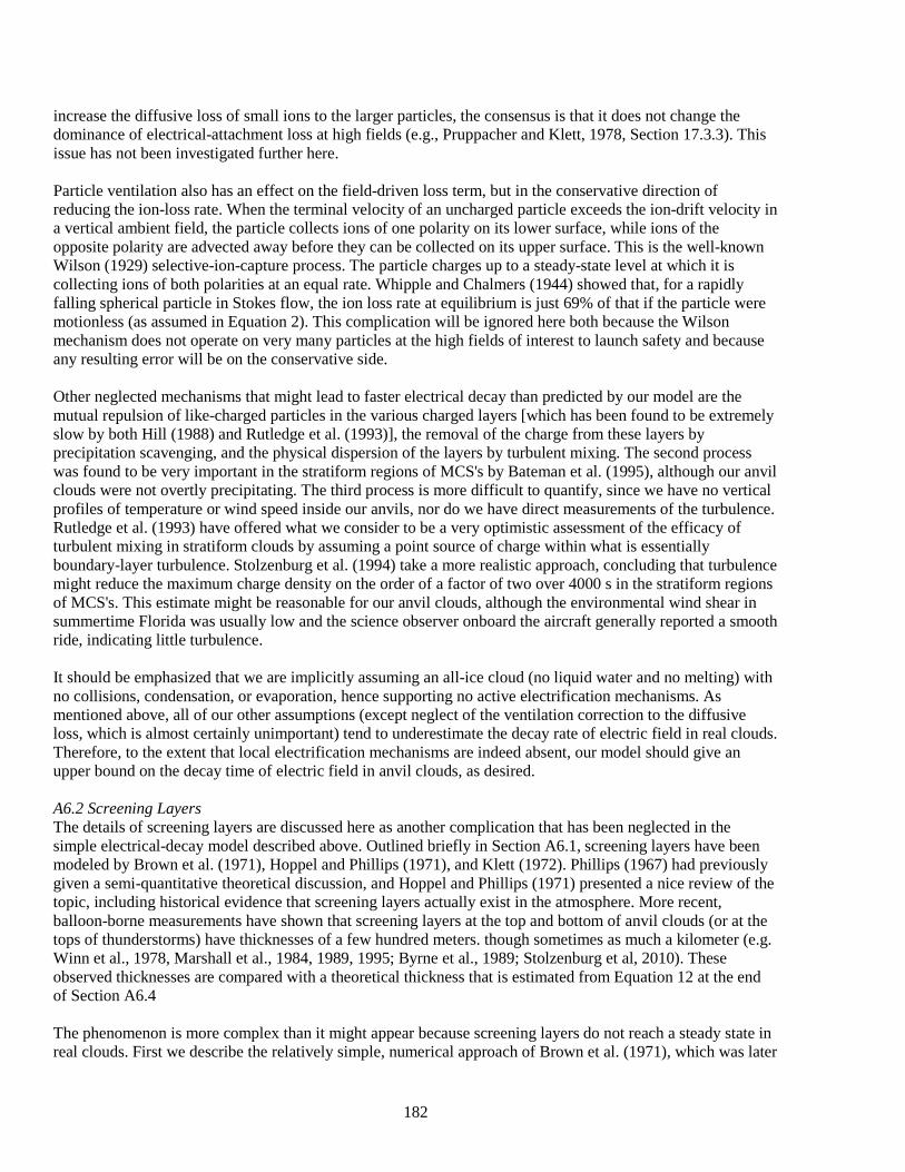
182

increase the diffusive loss of small ions to the larger particles, the consensus is that it does not change the dominance of electrical-attachment loss at high fields (e.g., Pruppacher and Klett, 1978, Section 17.3.3). This issue has not been investigated further here. Particle ventilation also has an effect on the field-driven loss term, but in the conservative direction of reducing the ion-loss rate. When the terminal velocity of an uncharged particle exceeds the ion-drift velocity in a vertical ambient field, the particle collects ions of one polarity on its lower surface, while ions of the opposite polarity are advected away before they can be collected on its upper surface. This is the well-known Wilson (1929) selective-ion-capture process. The particle charges up to a steady-state level at which it is collecting ions of both polarities at an equal rate. Whipple and Chalmers (1944) showed that, for a rapidly falling spherical particle in Stokes flow, the ion loss rate at equilibrium is just 69% of that if the particle were motionless (as assumed in Equation 2). This complication will be ignored here both because the Wilson mechanism does not operate on very many particles at the high fields of interest to launch safety and because any resulting error will be on the conservative side. Other neglected mechanisms that might lead to faster electrical decay than predicted by our model are the mutual repulsion of like-charged particles in the various charged layers [which has been found to be extremely slow by both Hill (1988) and Rutledge et al. (1993)], the removal of the charge from these layers by precipitation scavenging, and the physical dispersion of the layers by turbulent mixing. The second process was found to be very important in the stratiform regions of MCS's by Bateman et al. (1995), although our anvil clouds were not overtly precipitating. The third process is more difficult to quantify, since we have no vertical profiles of temperature or wind speed inside our anvils, nor do we have direct measurements of the turbulence. Rutledge et al. (1993) have offered what we consider to be a very optimistic assessment of the efficacy of turbulent mixing in stratiform clouds by assuming a point source of charge within what is essentially boundary-layer turbulence. Stolzenburg et al. (1994) take a more realistic approach, concluding that turbulence might reduce the maximum charge density on the order of a factor of two over 4000 s in the stratiform regions of MCS's. This estimate might be reasonable for our anvil clouds, although the environmental wind shear in summertime Florida was usually low and the science observer onboard the aircraft generally reported a smooth ride, indicating little turbulence. It should be emphasized that we are implicitly assuming an all-ice cloud (no liquid water and no melting) with no collisions, condensation, or evaporation, hence supporting no active electrification mechanisms. As mentioned above, all of our other assumptions (except neglect of the ventilation correction to the diffusive loss, which is almost certainly unimportant) tend to underestimate the decay rate of electric field in real clouds. Therefore, to the extent that local electrification mechanisms are indeed absent, our model should give an upper bound on the decay time of electric field in anvil clouds, as desired. A6.2 Screening Layers The details of screening layers are discussed here as another complication that has been neglected in the simple electrical-decay model described above. Outlined briefly in Section A6.1, screening layers have been modeled by Brown et al. (1971), Hoppel and Phillips (1971), and Klett (1972). Phillips (1967) had previously given a semi-quantitative theoretical discussion, and Hoppel and Phillips (1971) presented a nice review of the topic, including historical evidence that screening layers actually exist in the atmosphere. More recent, balloon-borne measurements have shown that screening layers at the top and bottom of anvil clouds (or at the tops of thunderstorms) have thicknesses of a few hundred meters. though sometimes as much a kilometer (e.g. Winn et al., 1978, Marshall et al., 1984, 1989, 1995; Byrne et al., 1989; Stolzenburg et al, 2010). These observed thicknesses are compared with a theoretical thickness that is estimated from Equation 12 at the end of Section A6.4 The phenomenon is more complex than it might appear because screening layers do not reach a steady state in real clouds. First we describe the relatively simple, numerical approach of Brown et al. (1971), which was later

183

solved analytically by Klett (1972). Then the more complex, steady-state, numerical solution of Hoppel and Phillips (1971) is discussed, especially because its contrast with that of Brown et al. (1971) emphasizes the essentially transient nature of real screening layers. To our knowledge, the fully time dependent screening-layer problem has never been solved, even in the simple geometry of our electrical-decay model. Brown et al. (1971) simplified the problem in such a way that it has a time-independent solution, which they found without actually solving for the complete, transient approach to this solution. They studied the screening layer that would form on the upper surface of a one-dimensional, horizontal cloud filling the lower half space due to an upward-directed electric field that was imposed on the system by a uniform, horizontal, positive-charge layer embedded deep within the cloud. To allow a time-independent solution, they assumed that the clear air in the other half space above this cloud was populated by a uniform concentration of negative small ions only, but that there were initially no such ions within the cloud. Positive ions, volume ionization, and recombination were neglected everywhere, as were ionic diffusion and air turbulence. The cloud was assumed to be composed of a uniform, monodisperse population of spherical particles, and coalescence, sedimentation, etc. were also neglected. Naturally they took account of the charge on droplets and, in particular, its influence on their charging rate due to field-driven attachment. Under the assumptions of Brown et al. (1971), the electric field outside the cloud is initially the same as that inside but decays exponentially with a time constant equal to the electrical relaxation time of the clear air, τe = ε0/[e(k-n- + k+n+)], where the expression in square brackets is the total conductivity, the subscripts refer to the negative and positive polarities of ions, respectively, and n+ ≡ 0 in this case. [This time decay must also be true in almost any conceivable case with sufficient symmetry, including the model of Hoppel and Phillips (1971) described below, as long as it is applied outside the electrode layer.] Klett (1972) solved explicitly for the time dependence of the transient solution of this model and showed that the thickness of the eventual electrode layer is h = 1.34/[Ae(d)N(d)], when converted into our notation, in the sense that 63% of the screening-layer charge lies within h of the cloud surface. All droplets within 1/[4Ae(d)N(d)] are 'saturated' in the sense that they carry the maximum charge to which field-driven attachment can charge them in the initial field. The screening-layer model of Hoppel and Phillips (1971), and especially its results, are very different from the above. Since neither group was apparently aware of the other's work at the time of writing, there is no discussion of these differences in the two papers. Hoppel and Phillips (1971) did not make as many simplifications, allowing both positive and negative ions, hence recombination, to exist both inside and outside the cloud and assuming a uniform ionization rate throughout. An electrode layer is therefore possible just outside the cloud boundary. Their cloud was also one-dimensional but of spherical geometry, with a central core that was initially taken as a conducting sphere that could receive negative ions and could not emit positive ions but that nevertheless carried a fixed positive net charge. [They later relaxed the restriction on emission of positive ions from the core, but we will not discuss those results here.] Other assumptions were similar to those of Brown et al. (1971), except that Hoppel and Phillips (1971) solved for the steady-state solution. Their results are undoubtedly correct but entirely unphysical from our point of view, since all of the screening-layer charge is concentrated around the central core in the steady state and there is little or no charge near the cloud boundary. Nevertheless, this steady-state solution teaches us some important lessons about screening layers, as pointed out by Hoppel and Phillips (1971).

(1) Because the saturation charge on a droplet is proportional to the local electric-field magnitude (as well as depending on both local ion densities), and because the field at any point outside the central core decreases with time as negative ions drift into the cloud from the clear air, the presence of ionization and positive ions in the model of Hoppel and Phillips (1971) allows previously saturated droplets to be discharged over time. The result is a charge layer that begins on the cloud boundary but migrates inward with time until it ends up concentrated around the central core in the eventual steady state.

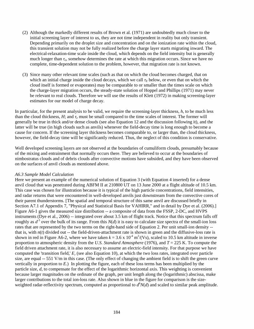
184

(2) Although the markedly different results of Brown et al. (1971) are undoubtedly much closer to the initial screening layer of interest to us, they are not time independent in reality but only transient. Depending primarily on the droplet size and concentration and on the ionization rate within the cloud, this transient solution may not be fully realized before the charge layer starts migrating inward. The electrical-relaxation-time scale inside the cloud, which depends on the field intensity but is generally much longer than τe, somehow determines the rate at which this migration occurs. Since we have no complete, time-dependent solution to the problem, however, that migration rate is not known.

(3) Since many other relevant time scales (such as that on which the cloud becomes charged, that on

which an initial charge inside the cloud decays, which we call τE below, or even that on which the cloud itself is formed or evaporates) may be comparable to or smaller than the times scale on which the charge-layer migration occurs, the steady-state solution of Hoppel and Phillips (1971) may never be relevant to real clouds. Therefore we will use the results of Klett (1972) in making screening-layer estimates for our model of charge decay.

In particular, for the present analysis to be valid, we require the screening-layer thickness, h, to be much less than the cloud thickness, H; and τe must be small compared to the time scales of interest. The former will generally be true in thick and/or dense clouds (see also Equation 12 and the discussion following it), and the latter will be true (in high clouds such as anvils) whenever the field-decay time is long enough to become a cause for concern. If the screening layer thickness becomes comparable to, or larger than, the cloud thickness, however, the field-decay time will be significantly reduced. Thus, the neglect of this condition is conservative. Well developed screening layers are not observed at the boundaries of cumuliform clouds, presumably because of the mixing and entrainment that normally occurs there. They are believed to occur at the boundaries of nimbostratus clouds and of debris clouds after convective motions have subsided, and they have been observed on the surfaces of anvil clouds as mentioned above. A6.3 Sample Model Calculation Here we present an example of the numerical solution of Equation 3 (with Equation 4 inserted) for a dense anvil cloud that was penetrated during ABFM II at 210800 UT on 13 June 2000 at a flight altitude of 10.5 km. This case was chosen for illustration because it is typical of the high particle concentrations, field intensities, and radar returns that were encountered in well-developed anvils just downstream from the convective cores of their parent thunderstorms. [The spatial and temporal structure of this same anvil are discussed briefly in Section A7.1 of Appendix 7, "Physical and Statistical Basis for VAHIRR," and in detail by Dye et al. (2006).] Figure A6-1 gives the measured size distribution -- a composite of data from the FSSP, 2-DC, and HVPS instruments (Dye et al., 2006) -- integrated over about 3.5 km of flight track. Notice that this spectrum falls off roughly as d-3 over the bulk of its range. From this N(d) it is easy to calculate size spectra of the small-ion loss rates that are represented by the two terms on the right-hand side of Equation 2. Per unit small-ion density -- that is, with n(t) divided out -- the field-driven-attachment rate is shown in green and the diffusive-loss rate is shown in red in Figure A6-2, where we have taken k = 3.6 x 10-4 m2/(Vs), scaled to 10.5 km altitude in inverse proportion to atmospheric density from the U.S. Standard Atmosphere (1976), and T = 225 K. To compute the field driven attachment rate, it is also necessary to assume an electric-field intensity. For that purpose we have computed the 'transition field,' Eγ (see also Equation 10), at which the two loss rates, integrated over particle size, are equal -- 551 V/m in this case. (The only effect of changing the ambient field is to shift the green curve vertically in proportion to E.) In plotting the figure, each of these loss terms has been multiplied by the particle size, d, to compensate for the effect of the logarithmic horizontal axis. This weighting is convenient because larger magnitudes on the ordinate of the graph, per unit length along the (logarithmic) abscissa, make larger contributions to the total ion-loss rate. Also shown in blue in the figure for comparison is the size-weighted radar-reflectivity spectrum, computed as proportional to d6N(d) and scaled to similar peak amplitude.

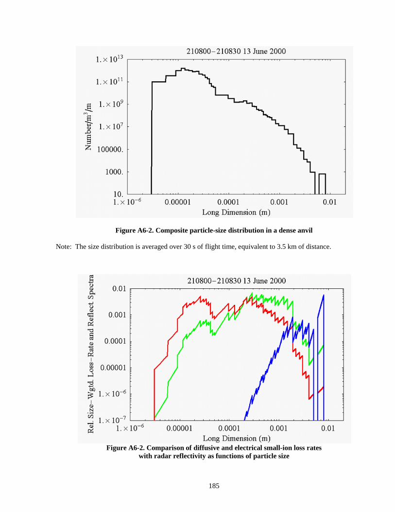
185

Figure A6-2. Composite particle-size distribution in a dense anvil Note: The size distribution is averaged over 30 s of flight time, equivalent to 3.5 km of distance.

Figure A6-2. Comparison of diffusive and electrical small-ion loss rates

with radar reflectivity as functions of particle size

186

Note: All data have been computed from the size distribution in Figure A6-1 and are size-weighted to facilitate intercomparision (see text). The electrical loss rate (at E = 551 V/m) is green, the diffusive loss rate is red, and the radar reflectivity (scaled to the same peak magnitude) is blue. Three conclusions are immediately evident from Figure A6-2. First, the small particles (in the 10 - 50 μm size range) dominate the diffusive loss, dependent as it is on particle diameter through C, whereas the electrical-attachment loss in this example is dominated by the intermediate-size particles (0.2 - 2 mm in diameter) because of the dependence of Ae on d2. Second, in spite of the logarithmic vertical axis (which spoils the equal-areas attribute of the d-weighting in Figure A6-2) it is obvious that the integrated electrical-attachment loss will dominate the integrated diffusive loss at field intensities much greater than Eγ. Third, the radar reflectivity is clearly due to the very largest particles -- much larger than those responsible for the diffusive, or even the electrical-attachment, loss. Because of the similarities in shape among measured size distributions in the denser anvils from our data set (Dye et al., 2006), these conclusions are generally valid. The ionization rate in Equation 3 is primarily due to cosmic radiation at anvil altitudes and has been interpolated from the formula

q(z) = 5.7X106 Exp[z/(6.06X103)] (5) which is an adequate fit to the subtropical data of Hake et al. (1973, Figure 19) over the altitude range of interest. Solution of Equation 3 (with Equation 4 inserted and after integration over the size distribution in Figure A6-1) results in the field decay that is shown in Figure A6-3 (black curve), where the initial condition was arbitrarily taken as E(0) = 50 kV/m. Evidently the decay is linear at high fields, as first pointed out by Krehbiel (1969). The behavior at low fields is shown on expanded scales in Figure A6-4 (black curve), where the decay can be seen to become approximately exponential as diffusion becomes the dominant ion-loss mechanism. The gray line in both figures is an extrapolation of the initial linear decay to zero field, yielding an estimated electrical-decay time -- the intercept at E(τE) ≡ 0 -- from 50 kV/m of τE = 6054 s. Note that this is more than 1½ hours -- comparable to the waiting times prescribed by the current LLCC -- but it is probably an extreme upper bound for anvil clouds far downwind from the parent storm, as we shall see later. The considerable separation between the black and gray traces in Figure A6-4 is a manifestation of the breadth of the particle-size distribution in Figure A6-1: As may be inferred from Figure A6-2, the smallest particles change over from predominantly field-driven attachment to predominantly diffusive attachment of small ions at moderately strong fields (~10 kV/m), whereas the very largest particles do not change over until low fields (a few times 10 V/m).

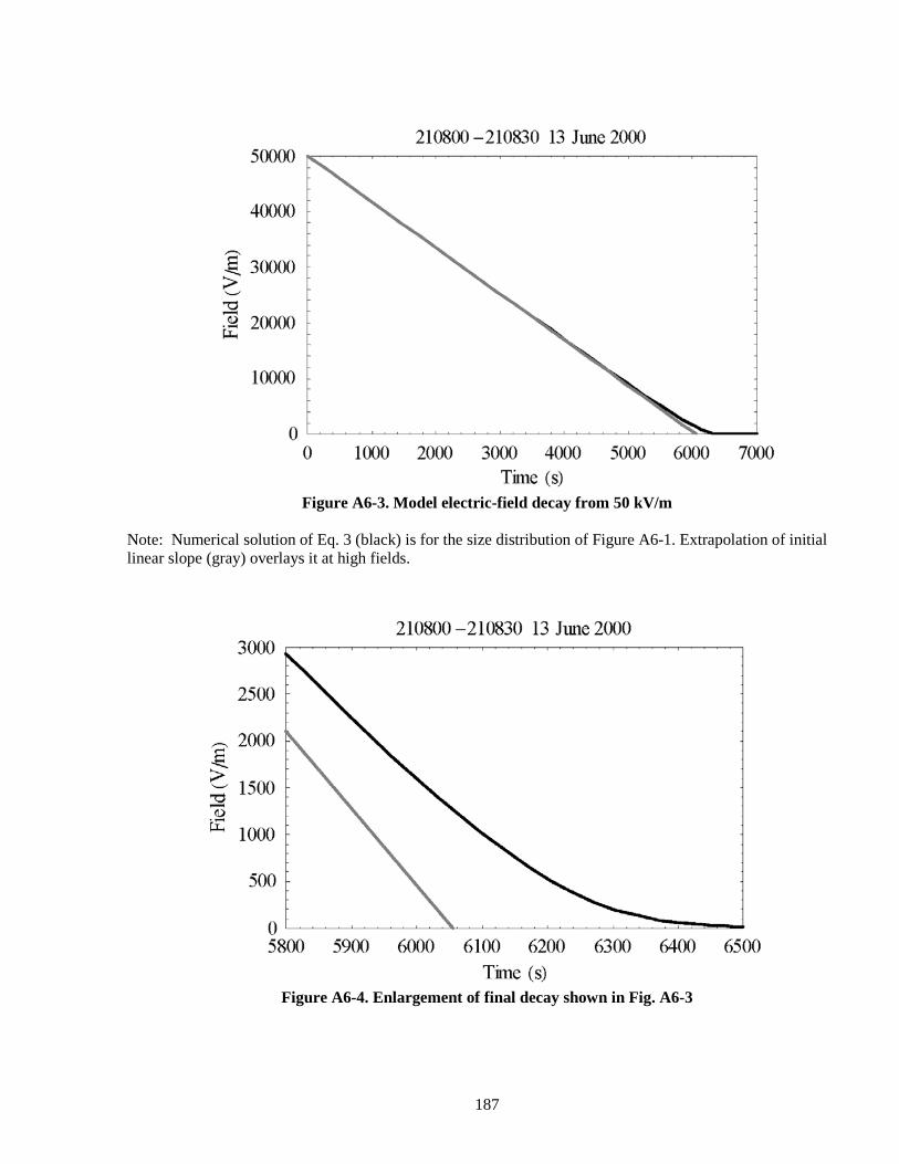
187

Figure A6-3. Model electric-field decay from 50 kV/m

Note: Numerical solution of Eq. 3 (black) is for the size distribution of Figure A6-1. Extrapolation of initial linear slope (gray) overlays it at high fields.

Figure A6-4. Enlargement of final decay shown in Fig. A6-3

188

Note: Note that the extrapolation of the initial linear slope (gray) diverges significantly from the numerical solution (black) at moderate fields. A6.4 Limiting Model Behavior Next we examine the limiting behavior of this simple model at high and at low field intensities. For any individual particle size, d, the condition for equal field-driven and diffusive ion-loss rates in Equation 2 can be identified by a value of unity for the dimensionless ratio, γ ≡ Aeeε0E/(CKT), which is essentially the same as Equation 5 of Klett (1971). When γ » 1, we are in the 'high-field limit,' which is of most interest here. Solving (2) for the small-ion density in this limit, we find n(t) ≈ q/[AekNE(t)]. Thus, the conduction-current density in (1) takes on a constant value that is determined only by cloud properties,

J(t) ≈ J0 ≡ 2eq/(AeN), E(t) >> Eγ (6) This happens because small ions are being 'swept out' by electrical attachment to cloud particles at a rate proportional to their drift velocity in the electric field. Solving (1) then yields linear field decay,

E(t) = E0 - J0t/ε0, E(t) >> Eγ (7) where E0 is an assumed initial field intensity. Thus an 'electrical-decay time scale' can be defined as

τE ≡ ε0E0/J0 = E0Aeε0N/(2eq) (8) essentially the intercept of the straight line in Figure A6-3. When γ « 1, on the other hand, we are in the 'low-field limit.' This limit results in exponential decay of E(t) with a 'diffusive relaxation time'

τD ≡ CKTN/(2e2q) (9) Obviously each of these time scales can be generalized to any given size distribution [N(d), Ae(d), C(d)] by integrating the corresponding loss rate over d. The two limits are separated by the condition, γ(Eγ) ≡ 1, which can be solved for the transition field

Eγ = CKT/(Aeeε0) (10) (The general definition of Eγ was given earlier in terms of the two integrated loss rates.) τE is only meaningful when the field intensities of interest are much larger than Eγ, and neither of these times scales is valid unless it is much larger than the electrical relaxation time in clear air -- roughly 20 s at 10 km altitude. From only the measured particle-size spectrum (either assuming spherical shape, as done here, or using an observed dependence of particle shape on size), absolute temperature, and flight altitude (from which the ambient ionization rate is estimated through Equation 5), it is possible to compute τE, Eγ, and τD versus time during anvil-cloud penetrations from Equations 7, 9, and 8, respectively. In the example case that was analyzed in detail in Section A6.3 above, for example, τE = 5963 s, Eγ = 551 V/m, and τD = 66 s. (The minor difference from the previously mentioned value of τE results from the numerical-extrapolation method that was used in Figure A6-3.) The results of such calculations are compared with other data from ABFM II in Sections A6.5 and A6.6 below. Because of the form of Ae(d) for spheres in Equation 4, we see that τE in (8) is directly proportional to the total cross-section area of cloud particles per unit volume. Thus τE is also directly proportional to the optical extinction coefficient

189

κ = πd2N/2 = 4eqτE/(3E0ε0) (11) in a cloud of spherical particles that are all much larger than the light wavelength of interest (e.g., Chylek, 1978). The present model is only valid for an anvil much thicker than its screening layers. As discussed in the section on Screening Layers, Klett (1972) estimated the thickness of these layers as

h ≈ 1.34/(AeN) = 0.89/κ (12) where the second equality comes from using (11) for spherical particles. Thus, the screening-layer thickness may be comparable to the unit optical depth, 1/κ, in such a cloud. For the dense-anvil example that was discussed in Section A6.3 above, Equations 11 and 12 give h = 9.7 m, which is at least an order of magnitude smaller than measured screening-layer thicknesses for anvils. This large disagreement is presumed due to some combination of several factors: a) Turbulent mixing and sedimentation, which were neglected in the theoretical calculation, would tend to increase the thickness. b) The time evolution of the theoretical screening layer toward a steady state (as discussed in the previous section) would tend to displace the layer inward from the cloud boundary and perhaps also thicken it. c) Probably most importantly, however, the example in Section A6.3 is for the interior of a particularly dense anvil. Particle spectra more characteristic of the upper and lower boundaries of even such a well-developed anvil would be expected to predict much shorter electrical-decay time scales and correspondingly thicker screening layers. Therefore, we should be careful in applying our electrical-decay model even to stratiform clouds thinner than a kilometer or so. A6.5 Statistics Of The Electrical-Decay Time Scale The ABFM II dataset was parsed into a total of 79 passes through 29 different anvil clouds in various stages of development or decay (Dye et al., 2006). Within these anvil passes, the microphysical, electric-field, and radar observations were averaged over 30 s intervals (about 3.5 km of usually horizontal flight track) for further analysis. Here we examine only the resulting relationships (a) between τE and the particle concentration in one specific size range, (b) between τE and the electric-field magnitude, and (c) between the local radar reflectivity and the electric-field magnitude. The particle data were summed over several size ranges -- approximately 3 - 55 μm diameter from the FSSP, 100 - 200 μm from the 2-DC, 200 - 1000 μm from the 2-DC, >1000 μm from the 2-DC (estimated from the reconstruction of 'cropped' images of particles up to about 4000 μm), and >1000 μm from the HVPS (which did not operate reliably during most of the year 2000 campaign) -- for comparison to other parameters. Of these, the best correlation was found between τE and the 200 - 1000 μm particle concentration. This is to be expected from the d2 dependence of Ae and from the nature of the size distributions that were found generally in anvil clouds (Dye et al., 2006), as mentioned above in connection with Figure A6-2. Figure A6-5 displays the log-log scatter-gram of all 2111, 30 s intervals for which the aircraft was flying inside an anvil and both particle spectra and electric-field measurements were available, yielding a linear correlation coefficient between the logarithms of these two parameters of 0.87 -- significantly different from zero at a very high confidence level, given the large number of samples.

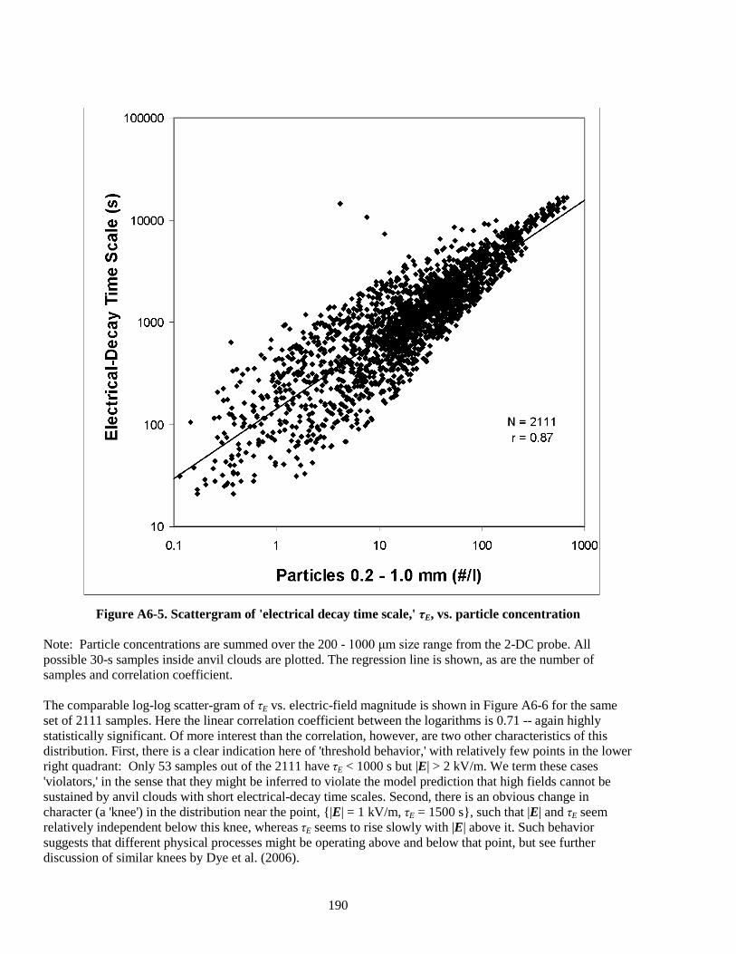
190

Figure A6-5. Scattergram of 'electrical decay time scale,' τE, vs. particle concentration

Note: Particle concentrations are summed over the 200 - 1000 μm size range from the 2-DC probe. All possible 30-s samples inside anvil clouds are plotted. The regression line is shown, as are the number of samples and correlation coefficient. The comparable log-log scatter-gram of τE vs. electric-field magnitude is shown in Figure A6-6 for the same set of 2111 samples. Here the linear correlation coefficient between the logarithms is 0.71 -- again highly statistically significant. Of more interest than the correlation, however, are two other characteristics of this distribution. First, there is a clear indication here of 'threshold behavior,' with relatively few points in the lower right quadrant: Only 53 samples out of the 2111 have τE < 1000 s but |E| > 2 kV/m. We term these cases 'violators,' in the sense that they might be inferred to violate the model prediction that high fields cannot be sustained by anvil clouds with short electrical-decay time scales. Second, there is an obvious change in character (a 'knee') in the distribution near the point, {|E| = 1 kV/m, τE = 1500 s}, such that |E| and τE seem relatively independent below this knee, whereas τE seems to rise slowly with |E| above it. Such behavior suggests that different physical processes might be operating above and below that point, but see further discussion of similar knees by Dye et al. (2006).

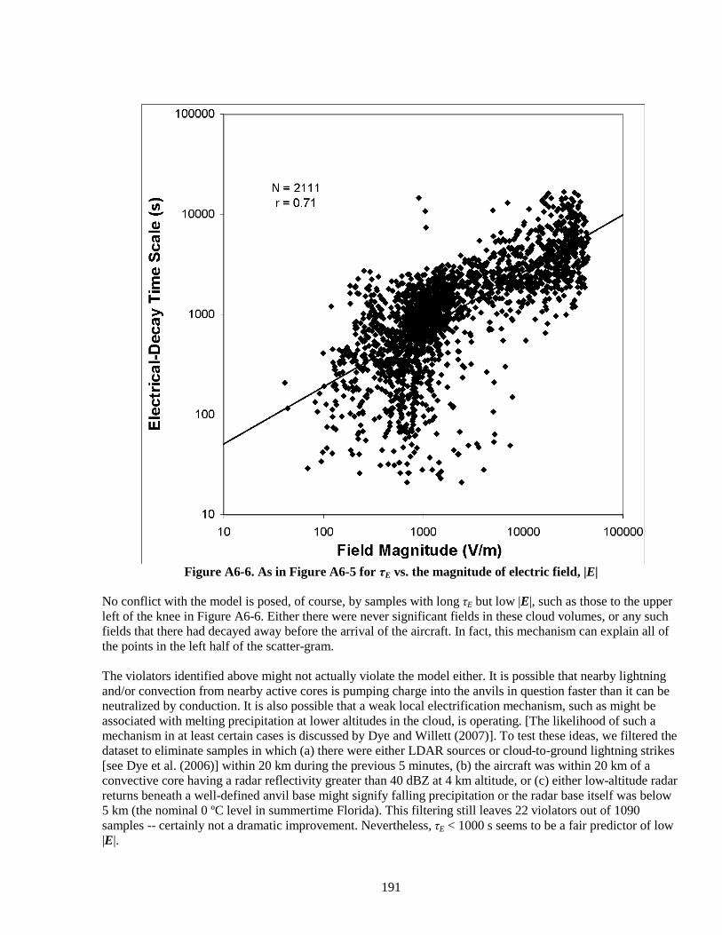
191

Figure A6-6. As in Figure A6-5 for τE vs. the magnitude of electric field, |E|

No conflict with the model is posed, of course, by samples with long τE but low |E|, such as those to the upper left of the knee in Figure A6-6. Either there were never significant fields in these cloud volumes, or any such fields that there had decayed away before the arrival of the aircraft. In fact, this mechanism can explain all of the points in the left half of the scatter-gram. The violators identified above might not actually violate the model either. It is possible that nearby lightning and/or convection from nearby active cores is pumping charge into the anvils in question faster than it can be neutralized by conduction. It is also possible that a weak local electrification mechanism, such as might be associated with melting precipitation at lower altitudes in the cloud, is operating. [The likelihood of such a mechanism in at least certain cases is discussed by Dye and Willett (2007)]. To test these ideas, we filtered the dataset to eliminate samples in which (a) there were either LDAR sources or cloud-to-ground lightning strikes [see Dye et al. (2006)] within 20 km during the previous 5 minutes, (b) the aircraft was within 20 km of a convective core having a radar reflectivity greater than 40 dBZ at 4 km altitude, or (c) either low-altitude radar returns beneath a well-defined anvil base might signify falling precipitation or the radar base itself was below 5 km (the nominal 0 ºC level in summertime Florida). This filtering still leaves 22 violators out of 1090 samples -- certainly not a dramatic improvement. Nevertheless, τE < 1000 s seems to be a fair predictor of low |E|.

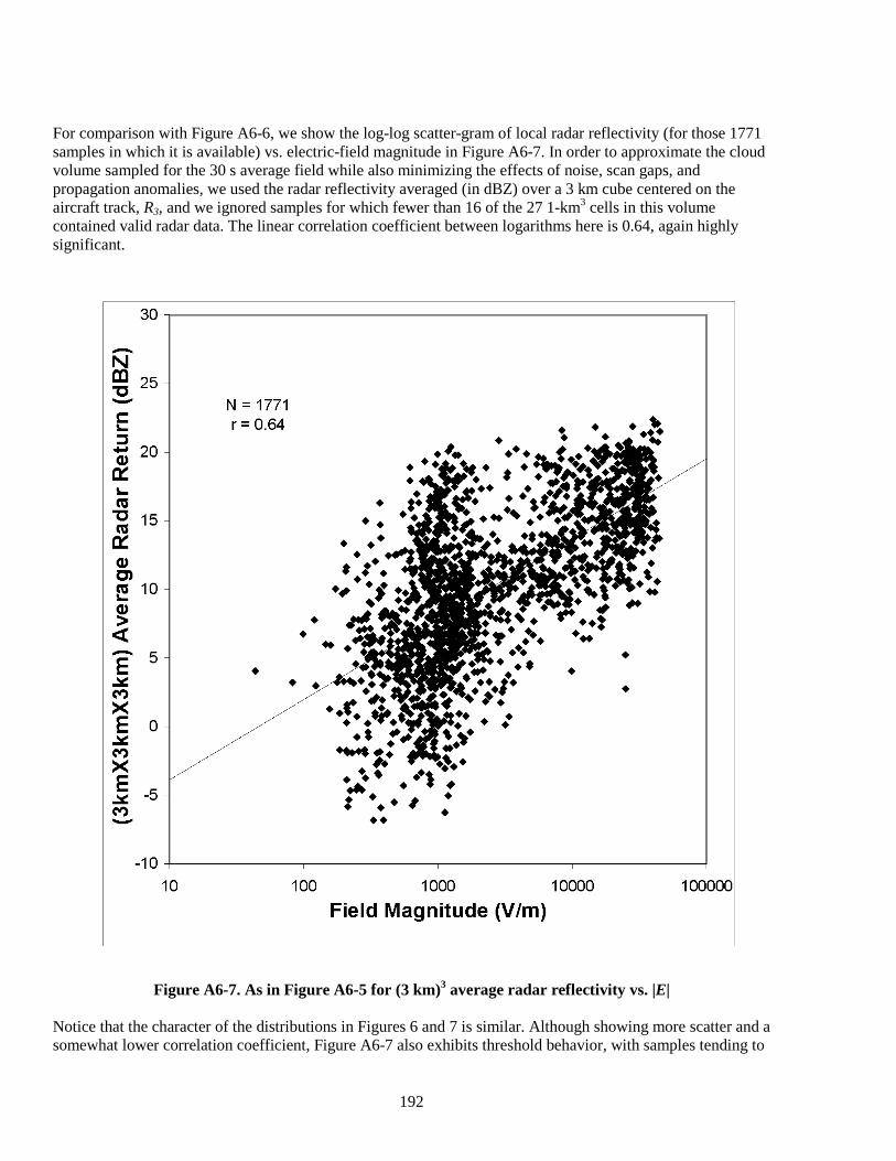
192

For comparison with Figure A6-6, we show the log-log scatter-gram of local radar reflectivity (for those 1771 samples in which it is available) vs. electric-field magnitude in Figure A6-7. In order to approximate the cloud volume sampled for the 30 s average field while also minimizing the effects of noise, scan gaps, and propagation anomalies, we used the radar reflectivity averaged (in dBZ) over a 3 km cube centered on the aircraft track, R3, and we ignored samples for which fewer than 16 of the 27 1-km3 cells in this volume contained valid radar data. The linear correlation coefficient between logarithms here is 0.64, again highly significant.

Figure A6-7. As in Figure A6-5 for (3 km)3 average radar reflectivity vs. |E| Notice that the character of the distributions in Figures 6 and 7 is similar. Although showing more scatter and a somewhat lower correlation coefficient, Figure A6-7 also exhibits threshold behavior, with samples tending to

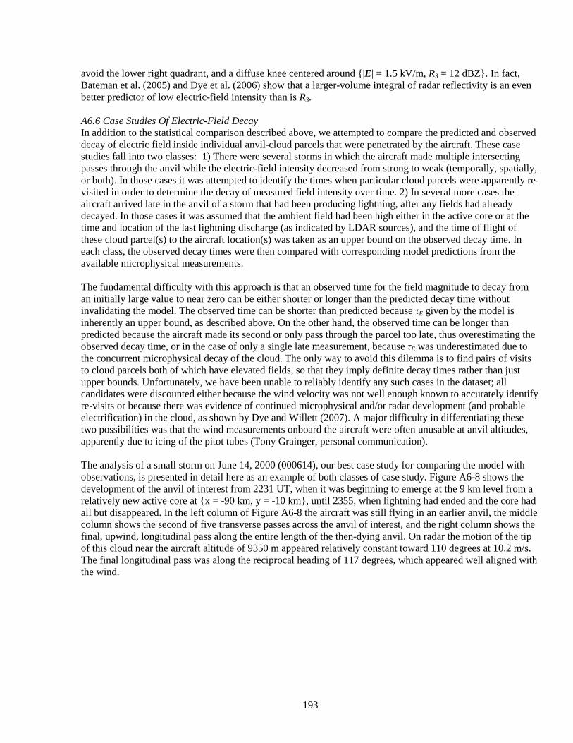
193

avoid the lower right quadrant, and a diffuse knee centered around {|E| = 1.5 kV/m, R3 = 12 dBZ}. In fact, Bateman et al. (2005) and Dye et al. (2006) show that a larger-volume integral of radar reflectivity is an even better predictor of low electric-field intensity than is R3. A6.6 Case Studies Of Electric-Field Decay In addition to the statistical comparison described above, we attempted to compare the predicted and observed decay of electric field inside individual anvil-cloud parcels that were penetrated by the aircraft. These case studies fall into two classes: 1) There were several storms in which the aircraft made multiple intersecting passes through the anvil while the electric-field intensity decreased from strong to weak (temporally, spatially, or both). In those cases it was attempted to identify the times when particular cloud parcels were apparently re-visited in order to determine the decay of measured field intensity over time. 2) In several more cases the aircraft arrived late in the anvil of a storm that had been producing lightning, after any fields had already decayed. In those cases it was assumed that the ambient field had been high either in the active core or at the time and location of the last lightning discharge (as indicated by LDAR sources), and the time of flight of these cloud parcel(s) to the aircraft location(s) was taken as an upper bound on the observed decay time. In each class, the observed decay times were then compared with corresponding model predictions from the available microphysical measurements. The fundamental difficulty with this approach is that an observed time for the field magnitude to decay from an initially large value to near zero can be either shorter or longer than the predicted decay time without invalidating the model. The observed time can be shorter than predicted because τE given by the model is inherently an upper bound, as described above. On the other hand, the observed time can be longer than predicted because the aircraft made its second or only pass through the parcel too late, thus overestimating the observed decay time, or in the case of only a single late measurement, because τE was underestimated due to the concurrent microphysical decay of the cloud. The only way to avoid this dilemma is to find pairs of visits to cloud parcels both of which have elevated fields, so that they imply definite decay times rather than just upper bounds. Unfortunately, we have been unable to reliably identify any such cases in the dataset; all candidates were discounted either because the wind velocity was not well enough known to accurately identify re-visits or because there was evidence of continued microphysical and/or radar development (and probable electrification) in the cloud, as shown by Dye and Willett (2007). A major difficulty in differentiating these two possibilities was that the wind measurements onboard the aircraft were often unusable at anvil altitudes, apparently due to icing of the pitot tubes (Tony Grainger, personal communication). The analysis of a small storm on June 14, 2000 (000614), our best case study for comparing the model with observations, is presented in detail here as an example of both classes of case study. Figure A6-8 shows the development of the anvil of interest from 2231 UT, when it was beginning to emerge at the 9 km level from a relatively new active core at {x = -90 km, y = -10 km}, until 2355, when lightning had ended and the core had all but disappeared. In the left column of Figure A6-8 the aircraft was still flying in an earlier anvil, the middle column shows the second of five transverse passes across the anvil of interest, and the right column shows the final, upwind, longitudinal pass along the entire length of the then-dying anvil. On radar the motion of the tip of this cloud near the aircraft altitude of 9350 m appeared relatively constant toward 110 degrees at 10.2 m/s. The final longitudinal pass was along the reciprocal heading of 117 degrees, which appeared well aligned with the wind.

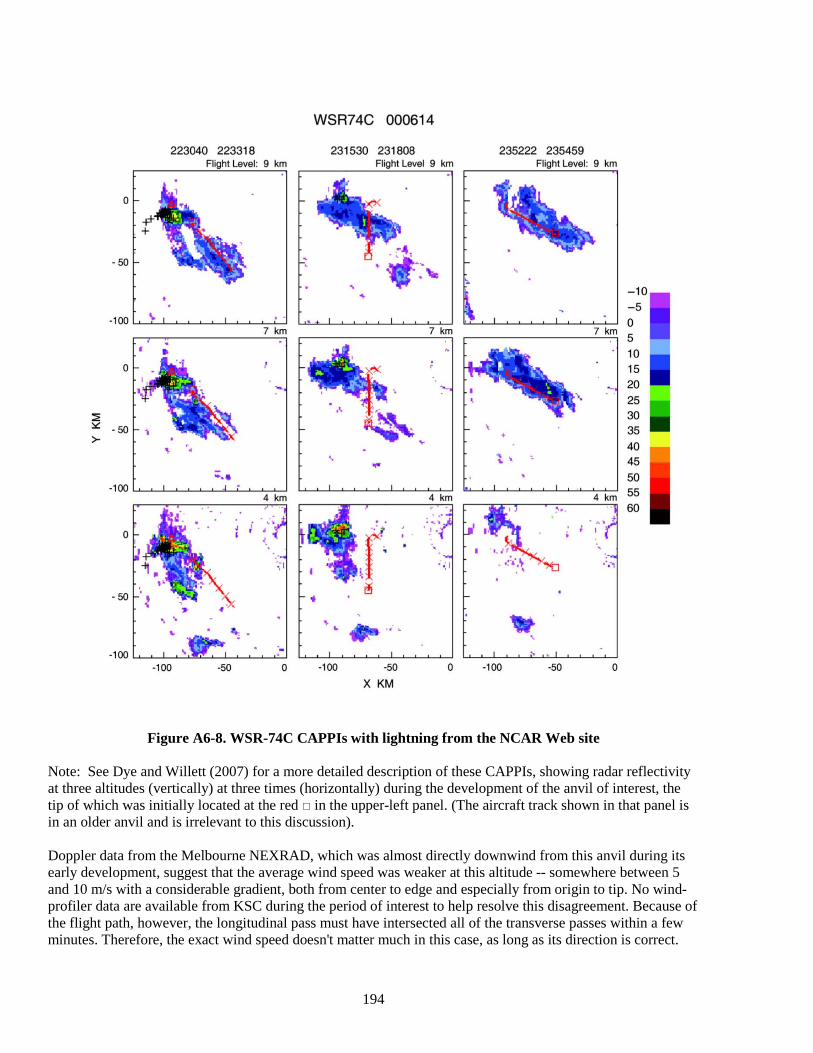
194

Figure A6-8. WSR-74C CAPPIs with lightning from the NCAR Web site

Note: See Dye and Willett (2007) for a more detailed description of these CAPPIs, showing radar reflectivity at three altitudes (vertically) at three times (horizontally) during the development of the anvil of interest, the tip of which was initially located at the red □ in the upper-left panel. (The aircraft track shown in that panel is in an older anvil and is irrelevant to this discussion). Doppler data from the Melbourne NEXRAD, which was almost directly downwind from this anvil during its early development, suggest that the average wind speed was weaker at this altitude -- somewhere between 5 and 10 m/s with a considerable gradient, both from center to edge and especially from origin to tip. No wind-profiler data are available from KSC during the period of interest to help resolve this disagreement. Because of the flight path, however, the longitudinal pass must have intersected all of the transverse passes within a few minutes. Therefore, the exact wind speed doesn't matter much in this case, as long as its direction is correct.

195

First we consider the 'class 1' analysis of re-visits to certain cloud parcels in this storm. Based on the stated

wind velocity, Figure A6-9 compares the actual (black) and 'drifted' (gray) aircraft tracks through the anvil of 000614. (This drifted track was produced simply by offsetting each point on the actual track in the assumed

upwind direction -- 290 degrees -- by a distance equal to the assumed wind speed -- 10.2 m/s -- multiplied by the elapsed time since track origin.) Intersections between four of the five transverse (N-S) passes and the longitudinal (SE-NW) pass are obvious on the gray track, as are several other intersections that are more

dependent on the exact wind speed. The drifted track was used to identify the seven in-anvil intersection points listed in Table A6-1, which are numbered correspondingly on the figure. (The first of the transverse passes is

not included here because it was too close to the storm core and was not considered to be in anvil.)

Figure A6-9. Actual (black) and "drifted" (gray) aircraft tracks

Note: The tracks are plotted on the KSC X-Y grid for the indicated time interval on 000614,. Relative to the actual track only, (0,0) is the location of the Patrick AFB WSR-74C radar. The starting point is where the two

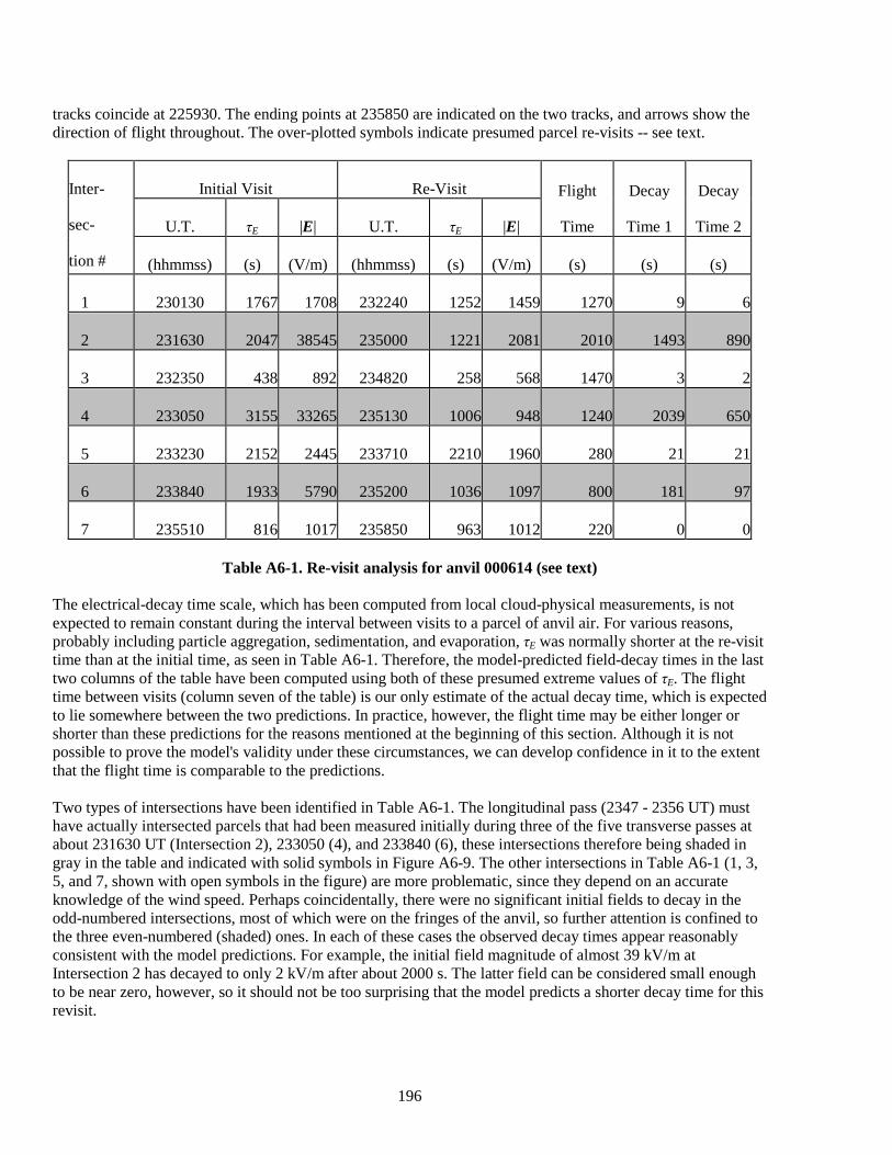
196

tracks coincide at 225930. The ending points at 235850 are indicated on the two tracks, and arrows show the direction of flight throughout. The over-plotted symbols indicate presumed parcel re-visits -- see text.

Inter-

sec-

tion #

Initial Visit Re-Visit Flight

Time

Decay

Time 1

Decay

Time 2 U.T. τE |E| U.T. τE |E|

(hhmmss) (s) (V/m) (hhmmss) (s) (V/m) (s) (s) (s)

1 230130 1767 1708 232240 1252 1459 1270 9 6

2 231630 2047 38545 235000 1221 2081 2010 1493 890

3 232350 438 892 234820 258 568 1470 3 2

4 233050 3155 33265 235130 1006 948 1240 2039 650

5 233230 2152 2445 233710 2210 1960 280 21 21

6 233840 1933 5790 235200 1036 1097 800 181 97

7 235510 816 1017 235850 963 1012 220 0 0

Table A6-1. Re-visit analysis for anvil 000614 (see text) The electrical-decay time scale, which has been computed from local cloud-physical measurements, is not expected to remain constant during the interval between visits to a parcel of anvil air. For various reasons, probably including particle aggregation, sedimentation, and evaporation, τE was normally shorter at the re-visit time than at the initial time, as seen in Table A6-1. Therefore, the model-predicted field-decay times in the last two columns of the table have been computed using both of these presumed extreme values of τE. The flight time between visits (column seven of the table) is our only estimate of the actual decay time, which is expected to lie somewhere between the two predictions. In practice, however, the flight time may be either longer or shorter than these predictions for the reasons mentioned at the beginning of this section. Although it is not possible to prove the model's validity under these circumstances, we can develop confidence in it to the extent that the flight time is comparable to the predictions. Two types of intersections have been identified in Table A6-1. The longitudinal pass (2347 - 2356 UT) must have actually intersected parcels that had been measured initially during three of the five transverse passes at about 231630 UT (Intersection 2), 233050 (4), and 233840 (6), these intersections therefore being shaded in gray in the table and indicated with solid symbols in Figure A6-9. The other intersections in Table A6-1 (1, 3, 5, and 7, shown with open symbols in the figure) are more problematic, since they depend on an accurate knowledge of the wind speed. Perhaps coincidentally, there were no significant initial fields to decay in the odd-numbered intersections, most of which were on the fringes of the anvil, so further attention is confined to the three even-numbered (shaded) ones. In each of these cases the observed decay times appear reasonably consistent with the model predictions. For example, the initial field magnitude of almost 39 kV/m at Intersection 2 has decayed to only 2 kV/m after about 2000 s. The latter field can be considered small enough to be near zero, however, so it should not be too surprising that the model predicts a shorter decay time for this revisit.

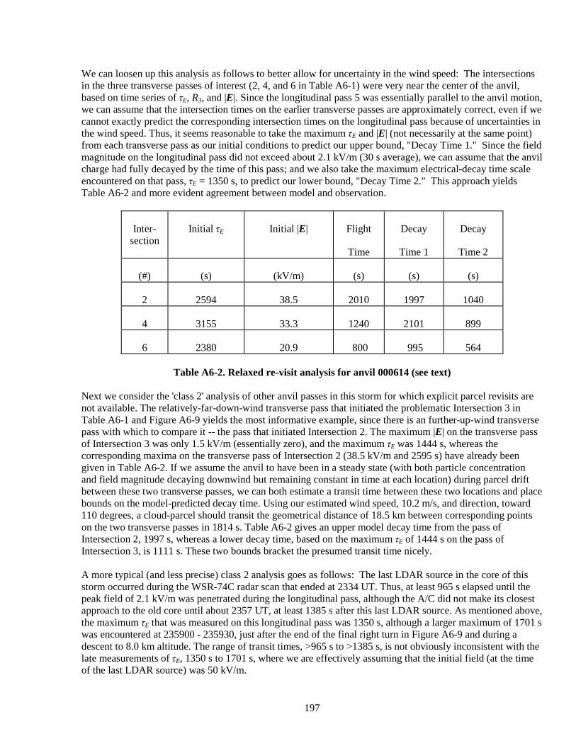
197

We can loosen up this analysis as follows to better allow for uncertainty in the wind speed: The intersections in the three transverse passes of interest (2, 4, and 6 in Table A6-1) were very near the center of the anvil, based on time series of τE, R3, and |E|. Since the longitudinal pass 5 was essentially parallel to the anvil motion, we can assume that the intersection times on the earlier transverse passes are approximately correct, even if we cannot exactly predict the corresponding intersection times on the longitudinal pass because of uncertainties in the wind speed. Thus, it seems reasonable to take the maximum τE and |E| (not necessarily at the same point) from each transverse pass as our initial conditions to predict our upper bound, "Decay Time 1." Since the field magnitude on the longitudinal pass did not exceed about 2.1 kV/m (30 s average), we can assume that the anvil charge had fully decayed by the time of this pass; and we also take the maximum electrical-decay time scale encountered on that pass, τE = 1350 s, to predict our lower bound, "Decay Time 2." This approach yields Table A6-2 and more evident agreement between model and observation.

Inter-section

Initial τE Initial |E| Flight

Time

Decay

Time 1

Decay

Time 2

(#) (s) (kV/m) (s) (s) (s)

2 2594 38.5 2010 1997 1040

4 3155 33.3 1240 2101 899

6 2380 20.9 800 995 564

Table A6-2. Relaxed re-visit analysis for anvil 000614 (see text) Next we consider the 'class 2' analysis of other anvil passes in this storm for which explicit parcel revisits are not available. The relatively-far-down-wind transverse pass that initiated the problematic Intersection 3 in Table A6-1 and Figure A6-9 yields the most informative example, since there is an further-up-wind transverse pass with which to compare it -- the pass that initiated Intersection 2. The maximum |E| on the transverse pass of Intersection 3 was only 1.5 kV/m (essentially zero), and the maximum τE was 1444 s, whereas the corresponding maxima on the transverse pass of Intersection 2 (38.5 kV/m and 2595 s) have already been given in Table A6-2. If we assume the anvil to have been in a steady state (with both particle concentration and field magnitude decaying downwind but remaining constant in time at each location) during parcel drift between these two transverse passes, we can both estimate a transit time between these two locations and place bounds on the model-predicted decay time. Using our estimated wind speed, 10.2 m/s, and direction, toward 110 degrees, a cloud-parcel should transit the geometrical distance of 18.5 km between corresponding points on the two transverse passes in 1814 s. Table A6-2 gives an upper model decay time from the pass of Intersection 2, 1997 s, whereas a lower decay time, based on the maximum τE of 1444 s on the pass of Intersection 3, is 1111 s. These two bounds bracket the presumed transit time nicely. A more typical (and less precise) class 2 analysis goes as follows: The last LDAR source in the core of this storm occurred during the WSR-74C radar scan that ended at 2334 UT. Thus, at least 965 s elapsed until the peak field of 2.1 kV/m was penetrated during the longitudinal pass, although the A/C did not make its closest approach to the old core until about 2357 UT, at least 1385 s after this last LDAR source. As mentioned above, the maximum τE that was measured on this longitudinal pass was 1350 s, although a larger maximum of 1701 s was encountered at 235900 - 235930, just after the end of the final right turn in Figure A6-9 and during a descent to 8.0 km altitude. The range of transit times, >965 s to >1385 s, is not obviously inconsistent with the late measurements of τE, 1350 s to 1701 s, where we are effectively assuming that the initial field (at the time of the last LDAR source) was 50 kV/m.

198

Reasonably credible class 1 analyses are also available from a storm on 010615, and additional class 2 analyses can be obtained both from that storm and from another on 010527. All of these results are summarized graphically in Figure A6-10, which shows the bounds of model-predicted decay time (or only a single estimate for some of the class 2 analyses) for each observed flight-time estimate.

Figure A6-10. Reasonably credible estimates of model decay time vs. parcel flight time

Note: Model-predicted electrical-decay time is plotted against aircraft-estimated parcel-flight time. In most cases both upper and lower bounds are available for the model estimates, as in Table 2 (see text). A6.7 Discussion And Conclusions From Model Studies In summary, a simple but physically reasonable model describes the decay of electric field by non-linear conduction in a quiescent cloud with one-dimensional geometry. A high-field limit is defined in which the field decay is linear with time and can be quite slow in comparison not only to that in clear air at the same altitude but also to that in the diffusively reduced conductivity at low field intensities in the same cloud. An example is computed, placing an upper bound of more than 1½ hours on the time required for the field to

199

decay from 50 kV/m to near zero in a real thunderstorm anvil, assuming that the particle concentrations remain high. Since this model should apply reasonably well to anvil clouds, it is somewhat puzzling that the observed relationship between τE and |E| has as much scatter as is shown in Figure A6-6. It was pointed out above that either late arrival of the aircraft or lack of initial electrification can explain leftward scatter (toward low electric field) in this graph. It was also argued that nearby lightning or convective cores might transfer charge into anvils faster than it could be dissipated by conduction, thus creating rightward scatter (toward high field). Filtering the data in a way that should remove most of the latter cases had little effect, however, suggesting that this may not be the only reason for any rightward scatter. It is also disappointing that we were unable to conclusively validate (or invalidate) the model through the analysis of case studies. In retrospect this is not surprising, since the dataset afforded few, if any, clear-cut examples of revisits to specific cloud parcels in initially electrified anvils before the fields had completely decayed away. Nevertheless, the use of this model during ABFM II data analysis helped investigators to focus on two important conclusions about electrified anvils in Florida thunderstorms (see Section A7.1 of Appendix 7, "Physical and Statistical Basis for VAHIRR" and Section A4.0 of Appendix 4, "Electrical Aspects of Stratiform Clouds"). First, Dye et al. (2006) have shown that, during any given anvil pass, the number densities of particles in the various size ranges (hence, τE) generally increase and decrease slowly and steadily, whereas the electric-field magnitude tends to increase and decrease rapidly and abruptly. These abrupt field increases and decreases also tend to occur within the same broad range of particle concentrations from cloud to cloud, producing the pronounced knee in the scatter-gram of τE vs. |E|, Figure A6-6. Although this observation explains the existence of the knee, however, it does not explain why this knee occurs near {|E| = 1 kV/m, τE = 1500 s}. It merely transfers the mystery back to the unexpectedly abrupt changes in electric field. The only aspect of the theory described herein that suggests this sort threshold behavior is the physical change from predominantly diffusive to predominantly field-driven small-ion loss around the transition field, Eγ. This model parameter has a median value of only 469 V/m in the set of 2111 samples used in Figure A6-6, however, and it very seldom becomes as large as 1 kV/m. Therefore this does not seem a convincing explanation. A slight generalization of the present model has been used in an effort to duplicate the abrupt field change that was observed between 1851 and 1855 UT on 24 June 2001 (Dye et al., 2006, Figure 8). This case is particularly amenable to model analysis because the aircraft flew 28 km almost directly upwind from the extreme end of a large anvil toward the convective core during this brief interval. If we assume that the anvil structure remained in an approximate steady state during the time it took for a cloud parcel to travel between the end points of this pass (about 25 minutes at the estimated drift speed of 19 m/s), then we can deduce the decay of particle concentration and electric field with time in this parcel from the gradients of these quantities that were measured along the aircraft track. Thus we avoid the unphysical assumption that τE was constant and uniform throughout the model anvil, using instead the particle spectra actually observed in each segment of the aircraft track. The values of τE calculated from 30-second-average particle spectra beginning at 1851, 1852, 1853, and 1854 UT are 973, 1962, 4209, and 11512 s, respectively. Evidently the rate of field decay is predicted to increase dramatically from the dense part of the anvil towards its downwind tip. It was hoped that this rapid change in the decay rate would help to explain the abrupt decrease in field magnitude that was observed over the same interval. In order to better test this idea, we re-computed the particle-size spectra (hence, τE) in 10 s averages, corresponding to the resolution of the available electric-field measurements. We then used the model to calculate the incremental decay of electric field during each successive drift interval (about 60 s for the parcel

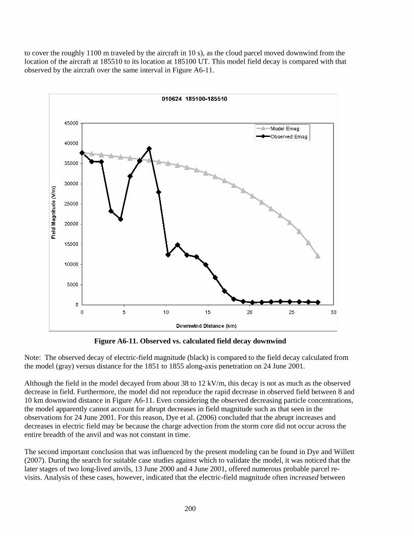
200

to cover the roughly 1100 m traveled by the aircraft in 10 s), as the cloud parcel moved downwind from the location of the aircraft at 185510 to its location at 185100 UT. This model field decay is compared with that observed by the aircraft over the same interval in Figure A6-11.

Figure A6-11. Observed vs. calculated field decay downwind

Note: The observed decay of electric-field magnitude (black) is compared to the field decay calculated from the model (gray) versus distance for the 1851 to 1855 along-axis penetration on 24 June 2001. Although the field in the model decayed from about 38 to 12 kV/m, this decay is not as much as the observed decrease in field. Furthermore, the model did not reproduce the rapid decrease in observed field between 8 and 10 km downwind distance in Figure A6-11. Even considering the observed decreasing particle concentrations, the model apparently cannot account for abrupt decreases in field magnitude such as that seen in the observations for 24 June 2001. For this reason, Dye et al. (2006) concluded that the abrupt increases and decreases in electric field may be because the charge advection from the storm core did not occur across the entire breadth of the anvil and was not constant in time. The second important conclusion that was influenced by the present modeling can be found in Dye and Willett (2007). During the search for suitable case studies against which to validate the model, it was noticed that the later stages of two long-lived anvils, 13 June 2000 and 4 June 2001, offered numerous probable parcel re-visits. Analysis of these cases, however, indicated that the electric-field magnitude often increased between

201

visits to what were believed to be the same parcels. More careful scrutiny indicated that τE, the particle concentrations in various size ranges, and sometimes even the radar reflectivity also increased between these re-visits. Obviously either the estimated parcel-drift velocities were wrong or we were not dealing with passive anvil decay in these two cases. This and other observations eventually led to the conclusion that a weak updraft was probably acting and that one or more weak electrification mechanisms were almost certainly at work in these and other cases of what we call 'anvil enhancement' (see Section A4.0 of Appendix 4, "Electrical Aspects of Stratiform Clouds"). Taken together, Dye et al. (2006), Dye and Willett (2007), and the present model analysis indicate that the anvils produced by Florida thunderstorms are more complex and interesting than we originally thought. In spite of the large, incompletely explained scatter in Figure A6-6, we conclude that that short electrical decay time is a fairly good predictor of low electric field in these clouds. Although the lack of an ideal dataset made our efforts to test the model against individual case studies generally inconclusive, Figure A6-10 strongly suggests a real relationship between τE and the actual decay of electric fields in anvil clouds. Having found no clear violations of the model, we suggest that it is deserving of credibility pending further investigation. References Bateman, M.G., W.D. Rust, T.C. Marshall, and B.F. Smull, 1995: Precipitation charge and size measurements

in the stratiform region of two mesoscale convective systems, J. Geophys. Res., 100, 16,341-16,356. Bateman, M.G., D.M. Mach, S. Lewis, J.E. Dye, E. Defer, C.A. Grainger, P.T. Willis, F.J. Merceret, D.

Boccippio, and H.J. Christian, 2005: Comparison of in-situ electric field and radar derived parameters for stratiform clouds in Central Florida, Conf. on Meteorol. Apps. of Lightning Data, AMS Annual Meeting, San Diego, Jan. 2005.

Blakeslee, R.J., and E.P. Krider, 1992: Ground level measurements of air conductivities under Florida

thunderstorms, J. Geophys. Res., 97, 12, 947-12,951. Brown, K.A., P.R. Krehbiel, C.B. Moore, and G.N. Sargent, 1971: Electrical screening layers around charged

clouds, J. Geophys. Res., 76, 2825-2835. Byrne, G.J., A.A. Few, and M.F. Stewart, 1989: Electric field measurements within a severe thunderstorm

anvil, J. Geophys. Res., 94, 6297-6307. Chylek, P., 1978: Extinction and liquid water content of fogs and clouds, J. Atmos. Sci., 35, 296-300. Dye, J.E., S. Lewis, M.G. Bateman, D.M. Mach, F.J. Merceret, J.G. Ward and C.A. Grainger, 2004: Final

Report on the Airborne Field Mill Project 2000 – 2001 Field Campaign, NASA Tech. Memo TM-2004-211534, Kennedy Space Center available from NASA Center for Airspace Information.

Dye, J.E., M.G. Bateman, H.J. Christian, E. Defer, C.A. Grainger, W.D. Hall, E.P. Krider, S.A. Lewis, D.M.

Mach, F.J. Merceret J.C. Willett, and P. Willis, 2006: Electric field, microphysics, and reflectivity in anvils of Florida thunderstorms, J. Geophys. Res., 112, D11215, doi:10.1029/2006JD007550.

Dye, J.E., and J.C. Willett, 2007: The enhancement of reflectivity and electric fields in long-live Florida

anvils, Mon. Wea. Rev., 135, 3362-3380. Griffiths, R.F., J. Latham, and V. Myers, 1974: The ionic conductivity of electrified clouds, Q. J. Roy. Met.

Soc., 100, 181-190.

202

Gunn, R., 1954: Diffusion charging of atmospheric droplets by ions, and the resulting combinations coefficients, J. Atmos. Sci., 11, 339-347.

Gunn, R., 1956: The hyperelectrification of raindrops by atmospheric electric fields, J. Atmos. Sci., 13, 283-

288. Hake, R.D. Jr., E.T. Pierce, and W. Viezee, 1973: Stratospheric Electricity, Final Report on SRI Project 1724,

Stanford Research Institute, Menlo Park, CA, January, 1973. Hill, R.D., 1988: Interpretation of bipole pattern in a mesoscale storm, Geophys. Res. Lett., 15, 643–644. Hoppel, W.A., and B.B. Phillips, 1971: The electrical shielding layer around charged clouds and its role in

thunderstorm electricity, J. Atmos. Sci., 28, 1258-1271. Klett, J.D., 1971: Ion transport to cloud droplets by diffusion and conduction, and the resulting droplet charge

distribution, J. Atmos. Sci., 28, 78-85. Klett, J.D., 1972: Charge screening layers around electrified clouds, J. Geophys. Res., 77, 3187-3195. Krehbiel, P.R, 1969: Conductivity of clouds in the presence of electric fields, Eos, Trans., Amer. Geophys. U.,

50, 618. Krider, E.P., H.C. Koons, R.L. Walterscheid, W.D. Rust, and J.C. Willett, 1999: Natural and triggered

lightning launch commit criteria (LCC), Rept. No. TR-99(1413)-1, The Aerospace Corporation, El Segundo, CA, 15 January 1999.

Krider, E.P., H.J. Christian, J.E. Dye, H.C. Koons, J. Madura, F. Merceret, W.D. Rust, R.L. Walterscheid, and

J.C. Willett, 2006: Natural and triggered lightning launch commit criteria, 86th Annual AMS Meeting, Atlanta, GA, 29 January-2 February, 2006.

MacGorman, D.R., and W.D. Rust, 1998: The Electrical Nature of Storms, Oxford University Press, New

York, 422pp, Marshall, T.C., W.D. Rust, and W.P. Winn, 1984: Screening layers at the surface of thunderstorm anvils, Proc.

VII Intern. Conf. on Atmosph. Electr., Albany, NY, June 3-8, pp.346-347. Marshall, T.C., W.D. Rust, W.P. Winn, and K.E. Gilbert, 1989: Electrical structure in two thunderstorm anvil

clouds, J. Geophys. Res., 94, 2171-2181. Marshall, T.C., W. Rison, W.D. Rust, M Stolzenburg, J.C. Willett, and W.P. Winn, 1995: Rocket and balloon

observations of electric field in two thunderstorms, J. Geophys. Res., 100, 20,815-20,828. Orville, R.E., R.W. Henderson, and L.F. Bosart, 1988: Bipole patterns revealed by lightning locations in

mesoscale storm systems, Geophys. Res. Lett., 15, 129-132. Pruppacher, H.R., and J.D. Klett, 1978: Microphysics of Clouds and Precipitation, D. Reidel Publishing

Company, Dordrecht:Holland, 714 pp. Phillips, B.B., 1967: Ionic equilibrium and the electrical conductivity in thunderclouds, Mon. Wea. Rev., 95,

854-862. Rutledge, S.A., E.R. Williams, and W.A. Petersen, 1993: Lightning and electrical structure of mesoscale

convective systems, Atmos. Res., 29, 27-53.

203

Stolzenburg, M., T.C. Marshall, W.D. Rust, and B.F. Smull, 1994: Horizontal distribution of electrical and

meteorological conditions across the stratiform region of a mesoscale convective system. Mon. Wea. Rev., 122, 1777-1797.

Stolzenburg, M., T. C. Marshall, and P. R. Krehbiel, 2010: Duration and extent of large electric fields in a

thunderstorm anvil cloud after the last lightning, J. Geophys. Res., doi:10.1029/2010JD014057, in press.

Hoppel, W. A., R. V. Anderson, and J. C. Willett, 1986: Atmospheric electricity in the planetary boundary


U.S. Standard Atmosphere, 1976, NOAA, NASA, UASF, Washington D.C., October, 1976, 227 pp. Westbrook, C.D., R.C. Ball, P.R. Field, and A.J. Heymsfield, 2004: Universality in snowflake aggregation,

Geophys. Res Lttrs., 31, L15104. Whipple, F.J.W., and J.A. Chalmers, 1944: On Wilson's theory of the collection of charge by falling drops,

Quart. J. Roy. Met Soc., 70, 103-119. Willett, J.C., and J.E. Dye, 2003: A simple model to estimate electrical decay times in anvil clouds, in

Proceedings, 12th International Conference on Atmospheric Electricity, Versailles, France, 9-13 June, International Commission on Atmospheric Electricity, 2003.

Wilson, C.T.R., 1929: Some thundercloud problems, J. Franklin Inst., 208, 1-12. Winn, W.P., C.B. Moore, C.R. Holmes, and L.G. Byerley, 1978: Thunderstorm on July 16, 1975 over

Langmuir Laboratory: A case study, J. Geophys. Res., 83, 3079-3092.

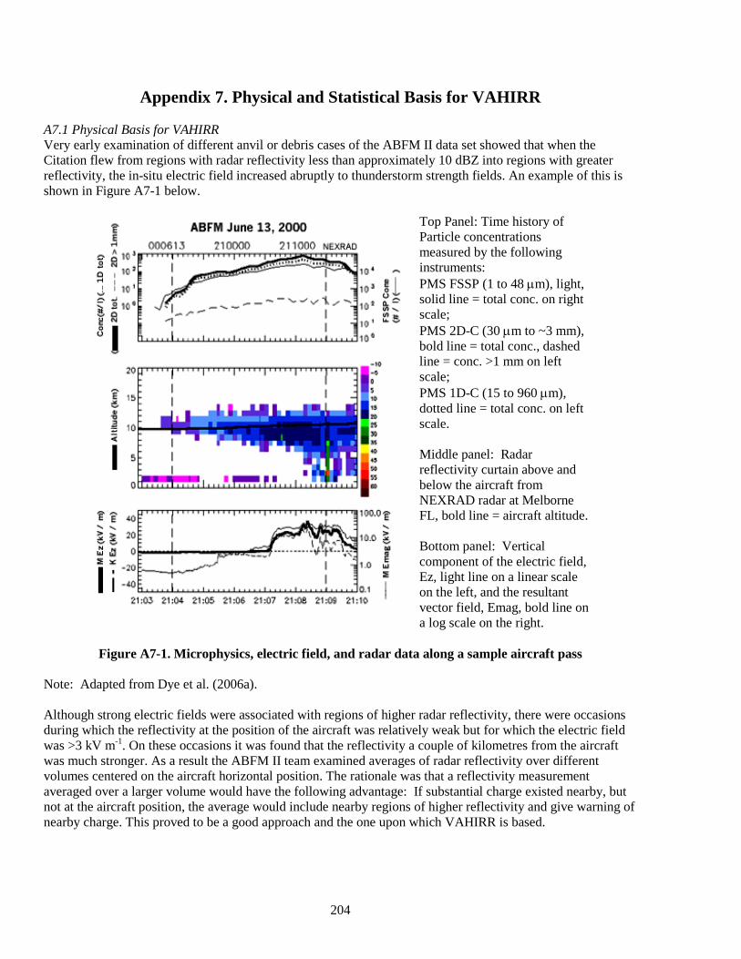
204

Appendix 7. Physical and Statistical Basis for VAHIRR A7.1 Physical Basis for VAHIRR Very early examination of different anvil or debris cases of the ABFM II data set showed that when the Citation flew from regions with radar reflectivity less than approximately 10 dBZ into regions with greater reflectivity, the in-situ electric field increased abruptly to thunderstorm strength fields. An example of this is shown in Figure A7-1 below.

Top Panel: Time history of Particle concentrations measured by the following instruments: PMS FSSP (1 to 48 µm), light, solid line = total conc. on right scale; PMS 2D-C (30 µm to ~3 mm), bold line = total conc., dashed line = conc. >1 mm on left scale; PMS 1D-C (15 to 960 µm), dotted line = total conc. on left scale. Middle panel: Radar reflectivity curtain above and below the aircraft from NEXRAD radar at Melborne FL, bold line = aircraft altitude. Bottom panel: Vertical component of the electric field, Ez, light line on a linear scale on the left, and the resultant vector field, Emag, bold line on a log scale on the right.

Figure A7-1. Microphysics, electric field, and radar data along a sample aircraft pass Note: Adapted from Dye et al. (2006a). Although strong electric fields were associated with regions of higher radar reflectivity, there were occasions during which the reflectivity at the position of the aircraft was relatively weak but for which the electric field was >3 kV m-1. On these occasions it was found that the reflectivity a couple of kilometres from the aircraft was much stronger. As a result the ABFM II team examined averages of radar reflectivity over different volumes centered on the aircraft horizontal position. The rationale was that a reflectivity measurement averaged over a larger volume would have the following advantage: If substantial charge existed nearby, but not at the aircraft position, the average would include nearby regions of higher reflectivity and give warning of nearby charge. This proved to be a good approach and the one upon which VAHIRR is based.

205

The radar reflectivity values used for calculating volume averages and cloud thickness (discussed below) and for all ABFM II analyses are based on interpolation and gridding of the measurements from radar coordinates of elevation and azimuth onto a 1 km horizontal and vertical grid. See Dye et al. (2004 Appendix D) for additional information. In calculating the volume averages and thickness, only grid points containing measureable meteorological reflectivity above a detection limit were used. The ABFM II team explored using two different cutoff values of the measured reflectivity at each grid point, -10 dBZ and 0 dBZ. In Figure A7-2 the plot of AVG 11x11 uses a cutoff of 0 dBZ while the plots of AVG 21x21 and AvgCube3x3 use a cutoff of -10dBZ. There was considerable discussion of which cutoff would be best. Proponents for a cutoff of -10 dBZ felt that excluding points with values lower than 0 dBZ statistically biases determinations of parameters such as thickness and average reflectivity and has no physical basis. Others argued that a -10 dBZ cutoff dilutes the signal in our reflectivity parameter and its ability to detect regions of stronger electric fields and also that, in the absence of visual observations, the cloud edge has been defined in the LLCC to be 0 dBZ. Analysis using receiver operating characteristic curves shows that a reflectivity cutoff of 0 dBZ instead of -10 dBZ gives a higher probability of detection with fewer false alarms. Additionally an extreme value analysis performed on the ABFM II anvil data set by Harry Koons (unpublished, but see summary below) showed that a cutoff of 0 dBZ performed as well as -10 dBZ. After considering these factors it was decided to use a 0 dBZ cutoff for the calculation of VAHIRR described below. Examples of scatter plots from the ABFM II anvil data set of the magnitude of the electric field (Emag) versus the arithmetic average (in dBZ) of radar reflectivity within volumes of three different sizes are shown in Figure A7-2. The upper left plot (with ordinate label AVG 11x11) shows the average radar reflectivity calculated for an 11 x11 km area extending horizontally 5 km in the N, S, W and E directions from the 1 km wide grid point containing the aircraft position and a cutoff of reflectivity of 0 dBZ in calculating the average. The lower left plot (with ordinate label AVG 21x21) is similar except the volume average is calculated over a horizontal area of 21x21 km extending horizontally 10 km in the N, S, W and E directions from the 1 km wide grid point containing the aircraft position and a lower cutoff of reflectivity of -10 dBZ. In both of these plots the average extends vertically from 5 km (the approximate altitude of the 0 oC isotherm) to 20 km ( always above the top of the cloud). The volume averages of reflectivity extend down to the 0 oC isotherm because there is much observational evidence that a charge separation mechanism and a layer of charge often occur near the 0 oC altitude level. [see Appendix 4, "Electrical Aspects of Stratiform Clouds," and Stolzenburg and Marshall (2008)]. The 11x11 and 21x21 km averages with reflectivity cutoffs of 0 or -10 dBZ all follow very similar trends, with the 0 dBZ cutoff giving slightly greater volume averages. The results with both cutoffs show a reflectivity threshold of approximately 5 dBZ, below which the electric field was < 3 kV/m as shown in the lower right quadrant of each of the plots. Since the results were similar for both averages, the team decided to use the 11x11 km average, which keeps the grid points used in the average closer to the flight track. (In the current LLCC this 11x11 km average is what is now termed “volume-averaged radar reflectivity” and the volume averaged is the ”specified volume.”) A 3 x 3 x 3 km volume average centered on the aircraft position (i.e., only 1 km from the grid point containing the aircraft, both horizontally and vertically) was also investigated. The scatter plots revealed that, when reflectivity was averaged over this smaller volume, a few of the data points in the lower-right quadrant had electric field magnitudes > 3 kV m-1. A shortcoming of using only the volume averaged radar reflectivity for a radar based rule is that averaging the reflectivity within a volume or a single column does not take advantage of potentially important information on the depth of the anvil. A thin anvil can have the same average reflectivity as a much deeper anvil, but deeper anvils are believed to be more likely to contain charge for the following reasons: Larger thunderstorms generally are more active electrically and have more particle mass flux from the convective core. The greater mass flux generally produces a deeper anvil, and the stronger electrical activity supplies more charge for transport into this anvil.. The upper right plot of Figure A7-2 (with ordinate label Vol Intg 11x11) shows a scatter plot of the magnitude of the electric field versus the product of the 11x11 volume average of reflectivity

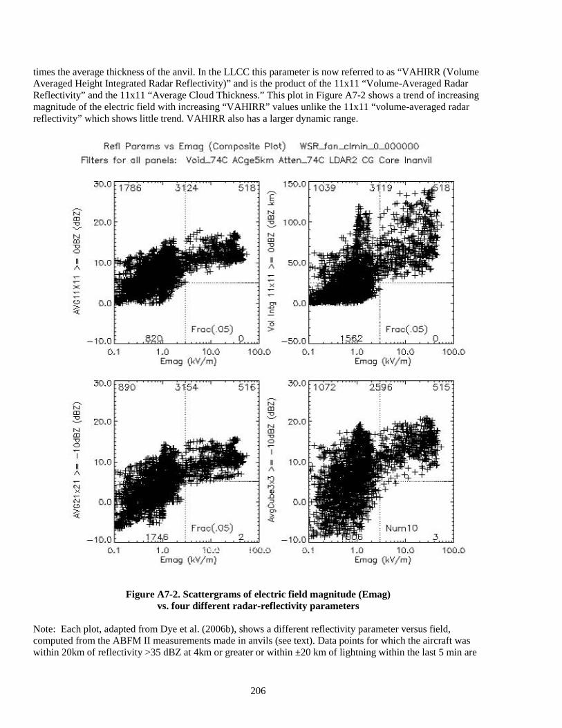
206

times the average thickness of the anvil. In the LLCC this parameter is now referred to as “VAHIRR (Volume Averaged Height Integrated Radar Reflectivity)” and is the product of the 11x11 “Volume-Averaged Radar Reflectivity” and the 11x11 “Average Cloud Thickness.” This plot in Figure A7-2 shows a trend of increasing magnitude of the electric field with increasing “VAHIRR” values unlike the 11x11 “volume-averaged radar reflectivity” which shows little trend. VAHIRR also has a larger dynamic range.

Figure A7-2. Scattergrams of electric field magnitude (Emag) vs. four different radar-reflectivity parameters

Note: Each plot, adapted from Dye et al. (2006b), shows a different reflectivity parameter versus field, computed from the ABFM II measurements made in anvils (see text). Data points for which the aircraft was within 20km of reflectivity >35 dBZ at 4km or greater or within ±20 km of lightning within the last 5 min are

N rn 3 ,

• ,

Re1I Paro m s vs [mag (Com p<>site Plot) WSRJ an--"lm irLCLllOOOOO

Fi lters fo r all pane ls: Void_7¥: ACge5km Atte rL7 4C LDAR2 CG Core Ir",!WiI

Frn c ('OS)

N rn " o

• ~

- 10.0 L~""!L~~~~~~ 0 .1 1.0 10 .0 100.0

Eme>g ( kV/m )

10.0

o.c

Frn c (.OS)

" " o

• ~ ?

'l 8 r

- 10.0 L~JL"'-~~~~2~ 0 .1 1.0 l e .:! ;(.>J .o

Eme>g ( kV/m )

0.'

Frnc ('OS)

1.0 10.0 Eme>g (k¥/m)

1.0 10.0 Eme>g (k¥/m)

100 .0

100 .0

207

not included. The total number of data points in each plot is shown in the top center of that plot. The numbers in the 4 quadrants of each plot show the number of points within that quadrant. The data set has been filtered to remove any points: 1) within the cone of silence above the radar; 2) for which the aircraft altitude was less than 5 km; or 3) for which attenuation of the radar measurements might have occurred. In order to have a meaningful number of points within the averaging volume, the ABFM II team developed the parameter FRAC, which is the number of grid points with measureable reflectivity (that is, reflectivity above the threshold) divided by the total number of possible points within the entire averaging volume. For the 11x11 averaging volume the total number of points is 1815 -- (11 x 11 x 15, where 15 is the vertical extent of the volume, 20 km – 5 km). Examination of some of the ABFM II data showed that a FRAC of ≥ 0.05 (i.e. 5% of the total possible points) produced stable results. For the 11x11 average with a total number of grid points of 1815, a FRAC of > 0.05 would require 91 points with measureable reflectivity. Measurement points are included in Figure A7-2 only if FRAC was greater than or equal to 0.05. Likewise FRAC ≥ 0.05 was used in the early statistical analyses which were done while exploring parameters for possible LLCC rule changes. In the statistical analysis of O’Brien and Waltershied (2008) upon which the LLCC rules for anvil and debris clouds are actually based, however, FRAC was increased to 0.1 (i.e. 10% of the points within the “specified volume must have measureable reflectivity ≥ 0 dBZ). This requirement is specifically stated in the “VAHIRR Application Criteria”. During the preparation of this document one of us came across a report on the reanalysis of ABFM I measurements in thick clouds (ABFM I Analysis Team, 1996). Although the ABFM I findings discussed in these four paragraphs were not considered during synthesis of ABFM II measurements and the development of VAHIRR, these ABFM I results give considerable additional rationale for a radar-based rule to identify clouds with potentially high electric fields. Figure A7-3 shows two plots of results from the ABFM I measurements in thick clouds. For this reanalysis the radar reflectivity values used a re-calibration of the PAFB WSR-74C radar by CSR Corporation and were gridded with 1x1 km horizontal resolution and 500 m vertical resolution. The electric-field measurements were averaged over the time that the aircraft was in each 1x1 km grid box, approximately 5 to 7 seconds, and VSR0C ("Vertically Summed Reflectivity above 0 oC”) is the sum of dBZ from 0 oC (~4 km) to -50 oC (~10 km) in the column containing the aircraft. The top plot in Figure A7-3 (Figure 15 from the original report) shows VSR0C averaged in the column within 1 n mi of the aircraft, and the bottom plot (Figure 16) shows VSR0C averaged in the column within 5 n mi of the aircraft.

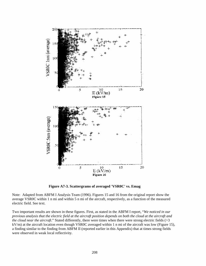
208

Figure A7-3. Scattergrams of averaged 'VSR0C' vs. Emag Note: Adapted from ABFM I Analysis Team (1996). Figures 15 and 16 from the original report show the average VSR0C within 1 n mi and within 5 n mi of the aircraft, respectively, as a function of the measured electric field. See text. Two important results are shown in these figures. First, as stated in the ABFM I report, “We noticed in our previous analysis that the electric field at the aircraft position depends on both the cloud at the aircraft and the cloud near the aircraft.” Stated differently, there were times when there were strong electric fields (>3 kV/m) at the aircraft location even though VSR0C averaged within 1 n mi of the aircraft was low (Figure 15), a finding similar to the finding from ABFM II (reported earlier in this Appendix) that at times strong fields were observed in weak local reflectivity.

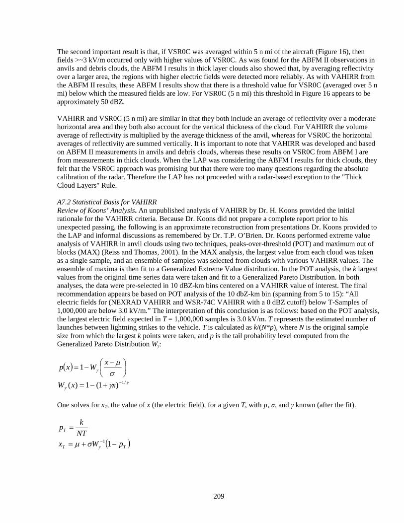
209

The second important result is that, if VSR0C was averaged within 5 n mi of the aircraft (Figure 16), then fields >~3 kV/m occurred only with higher values of VSR0C. As was found for the ABFM II observations in anvils and debris clouds, the ABFM I results in thick layer clouds also showed that, by averaging reflectivity over a larger area, the regions with higher electric fields were detected more reliably. As with VAHIRR from the ABFM II results, these ABFM I results show that there is a threshold value for VSR0C (averaged over 5 n mi) below which the measured fields are low. For VSR0C (5 n mi) this threshold in Figure 16 appears to be approximately 50 dBZ. VAHIRR and VSR0C (5 n mi) are similar in that they both include an average of reflectivity over a moderate horizontal area and they both also account for the vertical thickness of the cloud. For VAHIRR the volume average of reflectivity is multiplied by the average thickness of the anvil, whereas for VSR0C the horizontal averages of reflectivity are summed vertically. It is important to note that VAHIRR was developed and based on ABFM II measurements in anvils and debris clouds, whereas these results on VSR0C from ABFM I are from measurements in thick clouds. When the LAP was considering the ABFM I results for thick clouds, they felt that the VSR0C approach was promising but that there were too many questions regarding the absolute calibration of the radar. Therefore the LAP has not proceeded with a radar-based exception to the "Thick Cloud Layers" Rule. A7.2 Statistical Basis for VAHIRR Review of Koons’ Analysis. An unpublished analysis of VAHIRR by Dr. H. Koons provided the initial rationale for the VAHIRR criteria. Because Dr. Koons did not prepare a complete report prior to his unexpected passing, the following is an approximate reconstruction from presentations Dr. Koons provided to the LAP and informal discussions as remembered by Dr. T.P. O’Brien. Dr. Koons performed extreme value analysis of VAHIRR in anvil clouds using two techniques, peaks-over-threshold (POT) and maximum out of blocks (MAX) (Reiss and Thomas, 2001). In the MAX analysis, the largest value from each cloud was taken as a single sample, and an ensemble of samples was selected from clouds with various VAHIRR values. The ensemble of maxima is then fit to a Generalized Extreme Value distribution. In the POT analysis, the k largest values from the original time series data were taken and fit to a Generalized Pareto Distribution. In both analyses, the data were pre-selected in 10 dBZ-km bins centered on a VAHIRR value of interest. The final recommendation appears be based on POT analysis of the 10 dbZ-km bin (spanning from 5 to 15): “All electric fields for (NEXRAD VAHIRR and WSR-74C VAHIRR with a 0 dBZ cutoff) below T-Samples of 1,000,000 are below 3.0 kV/m.” The interpretation of this conclusion is as follows: based on the POT analysis, the largest electric field expected in T = 1,000,000 samples is 3.0 kV/m. T represents the estimated number of launches between lightning strikes to the vehicle. T is calculated as k/(N*p), where N is the original sample size from which the largest k points were taken, and p is the tail probability level computed from the Generalized Pareto Distribution Wγ:

( )

−

−=σ

µγ

xWxp 1

γγ γ /1)1(1)( −+−= xxW

One solves for xT, the value of x (the electric field), for a given T, with µ, σ, and γ known (after the fit).

NTkpT =

( )TT pWx −+= − 11γσµ

210

One of the challenges when using the POT method is the selection of k. The software accompanying the Reiss and Thomas book apparently provided an automated selection algorithm for k, and Dr. Koons also performed his own manual selection. Part-way through his analysis, Dr. Koons inadvertently defined T = 1/p, and he never fully expunged that error from his analysis. In the final analysis, at the T=1,000,000 level, that rarely made a difference of more than 1% in the computed electric field; however, in some preliminary analysis (2 dBZ-km bins), it could make a difference of 10% (~200 V/m). Final VAHIRR analysis by O’Brien. The extension of the anvil VAHIRR criteria to debris clouds is documented in O’Brien and Walterschied (in press). However, the discussion here includes subsequent analysis requested by the LAP. Specifically, the debris cloud analysis described in O’Brien and Walterscheid was applied to the anvil clouds, and subsequent adjustments to the analysis algorithms were applied to both debris and anvil clouds to maintain consistency. We note that the need for a consistent analysis between the small debris cloud data set and the considerably larger anvil cloud data set prevented the use of extreme value analysis as in Dr. Koons’s efforts. On the other hand, the uncertainty surrounding the selection of k in the POT method is removed: all the data are used. The new analysis is as follows:

(1) Select one of two sets of clouds: debris or anvil (2) Select only those raw time points meeting a set of filtering criteria (given below) (3) Further select only those points with VAHIRR between 0 and 20 dBZ-km (4) Fit the selected points to a Weibull distribution in electric field magnitude using the maximum

likelihood method (5) Scale the error covariance for the Weibull parameters by 10 to account for serial correlation. (6) Evaluate the Weibull tail probability at 3, 4, and 5 kV/m electric fields, along with the 95% confidence

bounds from the parameter error covariance For more explanation of the jargon herein, the reader is referred to Dye et al. [2004]: The filtering criteria applied to the “merged files” ABFM-II database are summarized as:

• cloud_type in ABFM “merged files” database: o Debris: 20 o All Anvils: 10, 9, 8, 6, and 4 [category 4 includes anvils with bases below 5 km]

• NOT (atten_74c >= 1) [exclude radar attenuation at WSR74C] • NOT (core_20km >= 1) [exclude aircraft near convective core] • NOT (invoid_74c >= 1) [exclude aircraft in radar cone of silence] • NOT (ldarm5 >= 2) [exclude 2 or more LDAR lightning flashes in previous 5 minutes] • NOT (cgm5 >= 1) [exclude 1 or more cloud-ground flashes in previous 5 minutes] • frac11x11_0 >= 0.1 [exclude <10% of the averaging volume contains reflectivity above threshold]

Additionally:

• We use the “NOT” criterion so that NaN’s (not-a-number) are treated as zeros • We used only radar grid 1 (files with G1 in the name) • We selected by radar

o NEXRAD o WSR74C o Combined

Combined after filters are applied Use only the NEXRAD radar for flights during which both radars were active.

211

We explored variations on the filter criteria. Specifically, we tried ignoring the core_20km condition, and we tried ignoring the cgm5 and ldarm5 conditions to see if that would result in appreciably larger sample sizes (it did not). We also explored different binning strategies. We settled on the 0 to 20 dBZ-km bin because it provides for a larger sample size while being conservative relative to the VAHIRR<10 dBZ-km threshold. In addition, scatter plots of electric field strength versus VAHIRR reveal little trend in the electric field for VAHIRR from 0 to ~20 dBZ-km. The Weibull probability that an electric field exceeds E is given by

( )[ ]cEEEP 0/exp)( −=> The maximum likelihood fitting process produces estimates of E0 and c, along with a parameter error covariance matrix. In O’Brien and Walterscheid (in press), we used a 1:10 decimation scheme to account for serial correlation. In the new analysis, we used all the data to obtain E0 and c, but then we multiplied the parameter error covariance matrix by 10 to account for serial correlation 1:10. Figures A7-4 and A7-5 show the results for the fitting procedure, along with the tail probability for E=3 kV/m. One can see that the Weibull is a good choice for the distribution of electric field. The debris clouds are clearly safe at the 0.01% (1E-4) level for 3 kV/m threshold, although the upper confidence value implies that additional ABFM data would be helpful (we will see shortly that this is not, in fact, necessary). Three points taken fromWSR74C for a flight on 6/28/2000 do not lie close to the Weibull fit. For two reasons, we dismiss the poor fit to these points: first, with serially correlated data, the appropriate vertical location at which to plot the points is very uncertain (>100%), especially for the largest points in the distribution; second, the points were all taken for conditions of VAHIRR ~ 15 dBZ-km, for which the VAHIRR <10 rule would disallow launch. The anvil clouds are safe at the 0.03% level for a threshold of 3 kV/m. Because the range provided a safety value of 1 strike in 10,000 launches, we must dig deeper to determine whether anvil clouds are, in fact, safe. In particular, we must consider that the 3 kV/m threshold already includes considerable conservatism. The analysis so far has assumed that encountering a 3 kV/m field guarantees a lightning strike. As we will see, this is not the case. We must first clarify one point: although a rocket trajectory through a cloud represents multiple time samples, it is considered a single effective sample from the distribution for risk purposes because of the strong correlation of electric field intensity along a trajectory and the negligible evolution of the cloud fields on the timescale of a rocket traversal.

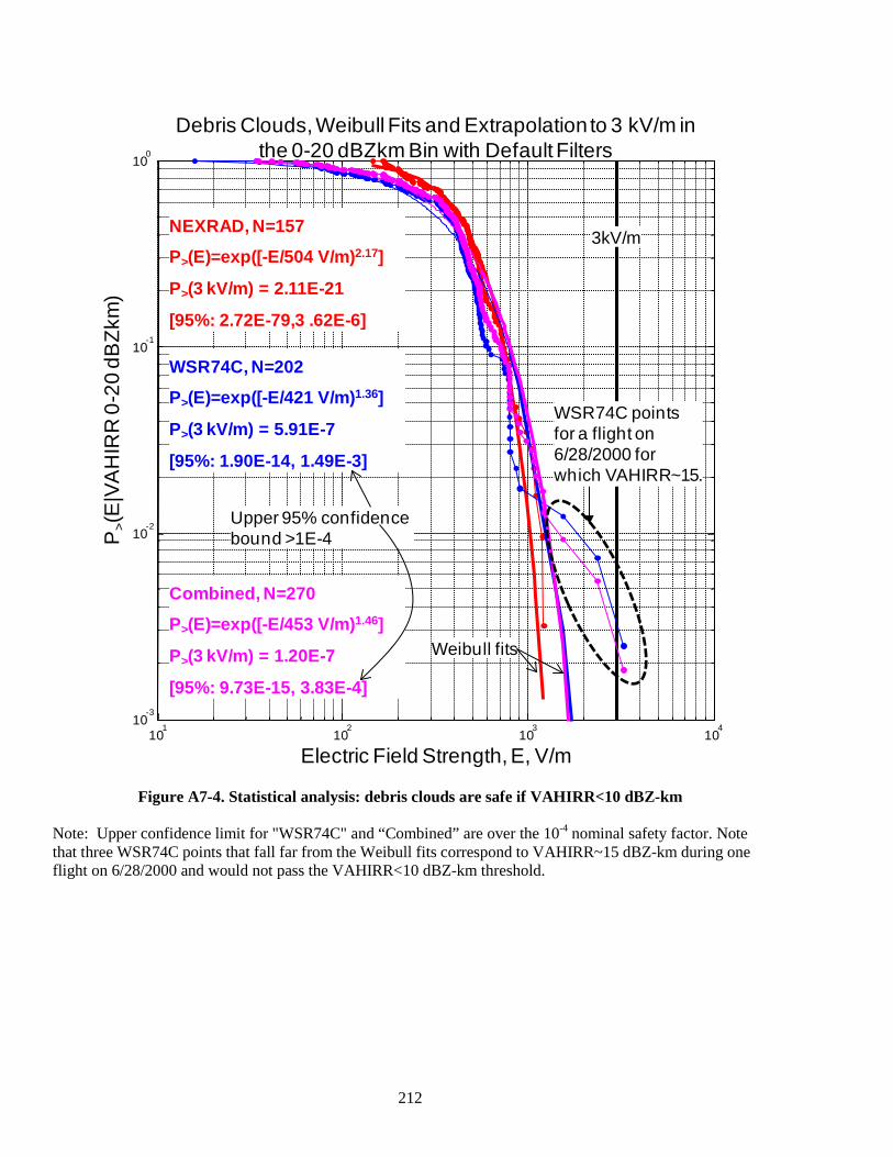
212

Figure A7-4. Statistical analysis: debris clouds are safe if VAHIRR<10 dBZ-km Note: Upper confidence limit for "WSR74C" and “Combined” are over the 10-4 nominal safety factor. Note that three WSR74C points that fall far from the Weibull fits correspond to VAHIRR~15 dBZ-km during one flight on 6/28/2000 and would not pass the VAHIRR<10 dBZ-km threshold.

101

102

103

104

10-3

10-2

10-1

100

Electric Field Strength, E, V/m

WSR74C points for a flight on 6/28/2000 for which VAHIRR~15.

NEXRAD, N=157

P>(E)=exp([-E/504 V/m)2.17]

P>(3 kV/m) = 2.11E-21

[95%: 2.72E-79,3 .62E-6]

WSR74C, N=202

P>(E)=exp([-E/421 V/m)1.36]

P>(3 kV/m) = 5.91E-7

[95%: 1.90E-14, 1.49E-3]

Combined, N=270

P>(E)=exp([-E/453 V/m)1.46]

P>(3 kV/m) = 1.20E-7

[95%: 9.73E-15, 3.83E-4]

Debris Clouds, Weibull Fits and Extrapolation to 3 kV/m in the 0-20 dBZkm Bin with Default Filters

3kV/m

P>(

E|V

AH

IRR

0-2

0 dB

Zkm

)

Weibull fits

Upper 95% confidence bound >1E-4

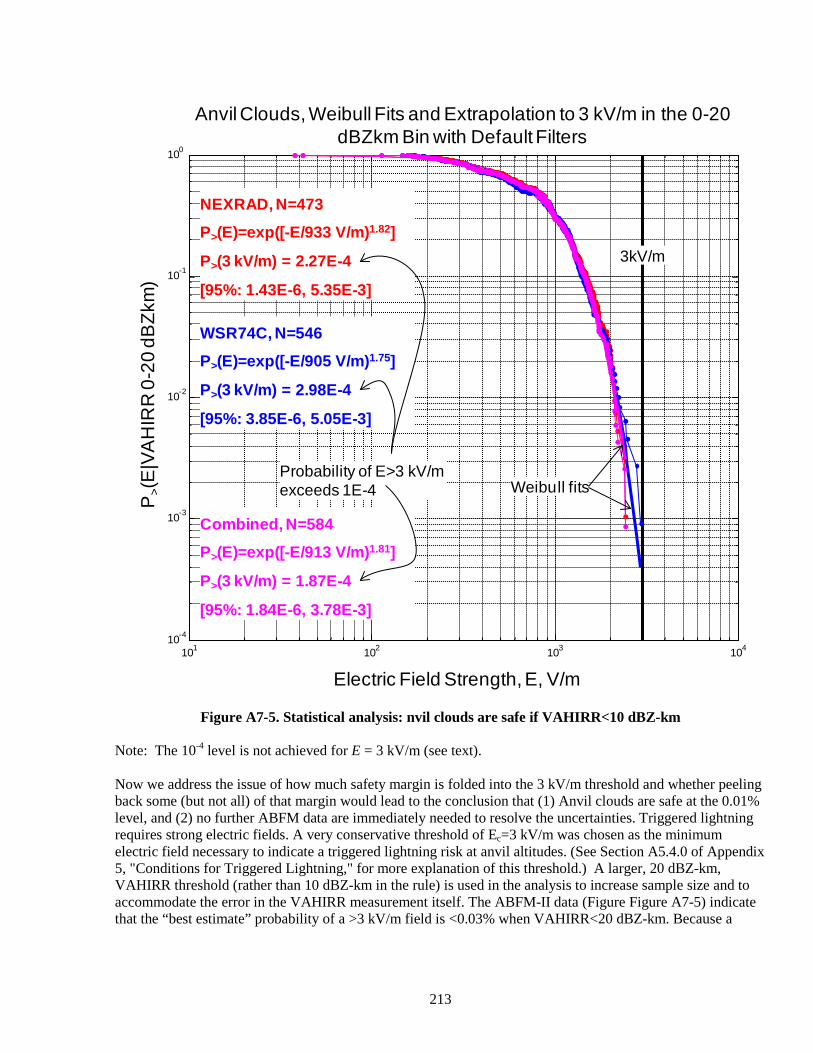
213

Figure A7-5. Statistical analysis: nvil clouds are safe if VAHIRR<10 dBZ-km Note: The 10-4 level is not achieved for E = 3 kV/m (see text). Now we address the issue of how much safety margin is folded into the 3 kV/m threshold and whether peeling back some (but not all) of that margin would lead to the conclusion that (1) Anvil clouds are safe at the 0.01% level, and (2) no further ABFM data are immediately needed to resolve the uncertainties. Triggered lightning requires strong electric fields. A very conservative threshold of Ec=3 kV/m was chosen as the minimum electric field necessary to indicate a triggered lightning risk at anvil altitudes. (See Section A5.4.0 of Appendix 5, "Conditions for Triggered Lightning," for more explanation of this threshold.) A larger, 20 dBZ-km, VAHIRR threshold (rather than 10 dBZ-km in the rule) is used in the analysis to increase sample size and to accommodate the error in the VAHIRR measurement itself. The ABFM-II data (Figure Figure A7-5) indicate that the “best estimate” probability of a >3 kV/m field is <0.03% when VAHIRR<20 dBZ-km. Because a

101 102 103 10410-4

10-3

10-2

10-1

100

Electric Field Strength, E, V/m

Anvil Clouds, Weibull Fits and Extrapolation to 3 kV/m in the 0-20 dBZkm Bin with Default Filters

P>(

E|V

AH

IRR

0-2

0 dB

Zkm

)

Weibull fits

NEXRAD, N=473

P>(E)=exp([-E/933 V/m)1.82]

P>(3 kV/m) = 2.27E-4

[95%: 1.43E-6, 5.35E-3]

WSR74C, N=546

P>(E)=exp([-E/905 V/m)1.75]

P>(3 kV/m) = 2.98E-4

[95%: 3.85E-6, 5.05E-3]

Combined, N=584

P>(E)=exp([-E/913 V/m)1.81]

P>(3 kV/m) = 1.87E-4

[95%: 1.84E-6, 3.78E-3]

Probability of E>3 kV/m exceeds 1E-4

3kV/m

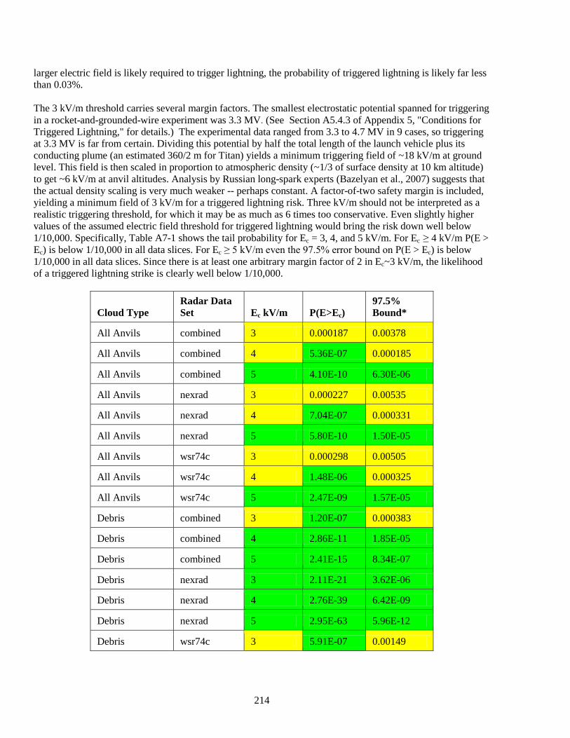
214

larger electric field is likely required to trigger lightning, the probability of triggered lightning is likely far less than 0.03%. The 3 kV/m threshold carries several margin factors. The smallest electrostatic potential spanned for triggering in a rocket-and-grounded-wire experiment was 3.3 MV. (See Section A5.4.3 of Appendix 5, "Conditions for Triggered Lightning," for details.) The experimental data ranged from 3.3 to 4.7 MV in 9 cases, so triggering at 3.3 MV is far from certain. Dividing this potential by half the total length of the launch vehicle plus its conducting plume (an estimated 360/2 m for Titan) yields a minimum triggering field of ~18 kV/m at ground level. This field is then scaled in proportion to atmospheric density (~1/3 of surface density at 10 km altitude) to get ~6 kV/m at anvil altitudes. Analysis by Russian long-spark experts (Bazelyan et al., 2007) suggests that the actual density scaling is very much weaker -- perhaps constant. A factor-of-two safety margin is included, yielding a minimum field of 3 kV/m for a triggered lightning risk. Three kV/m should not be interpreted as a realistic triggering threshold, for which it may be as much as 6 times too conservative. Even slightly higher values of the assumed electric field threshold for triggered lightning would bring the risk down well below 1/10,000. Specifically, Table A7-1 shows the tail probability for Ec = 3, 4, and 5 kV/m. For Ec ≥ 4 kV/m P(E > Ec) is below 1/10,000 in all data slices. For Ec ≥ 5 kV/m even the 97.5% error bound on P(E > Ec) is below 1/10,000 in all data slices. Since there is at least one arbitrary margin factor of 2 in Ec~3 kV/m, the likelihood of a triggered lightning strike is clearly well below 1/10,000.

Cloud Type Radar Data Set Ec kV/m P(E>Ec)

97.5% Bound*

All Anvils combined 3 0.000187 0.00378

All Anvils combined 4 5.36E-07 0.000185

All Anvils combined 5 4.10E-10 6.30E-06

All Anvils nexrad 3 0.000227 0.00535

All Anvils nexrad 4 7.04E-07 0.000331

All Anvils nexrad 5 5.80E-10 1.50E-05

All Anvils wsr74c 3 0.000298 0.00505

All Anvils wsr74c 4 1.48E-06 0.000325

All Anvils wsr74c 5 2.47E-09 1.57E-05

Debris combined 3 1.20E-07 0.000383

Debris combined 4 2.86E-11 1.85E-05

Debris combined 5 2.41E-15 8.34E-07

Debris nexrad 3 2.11E-21 3.62E-06



Debris wsr74c 3 5.91E-07 0.00149

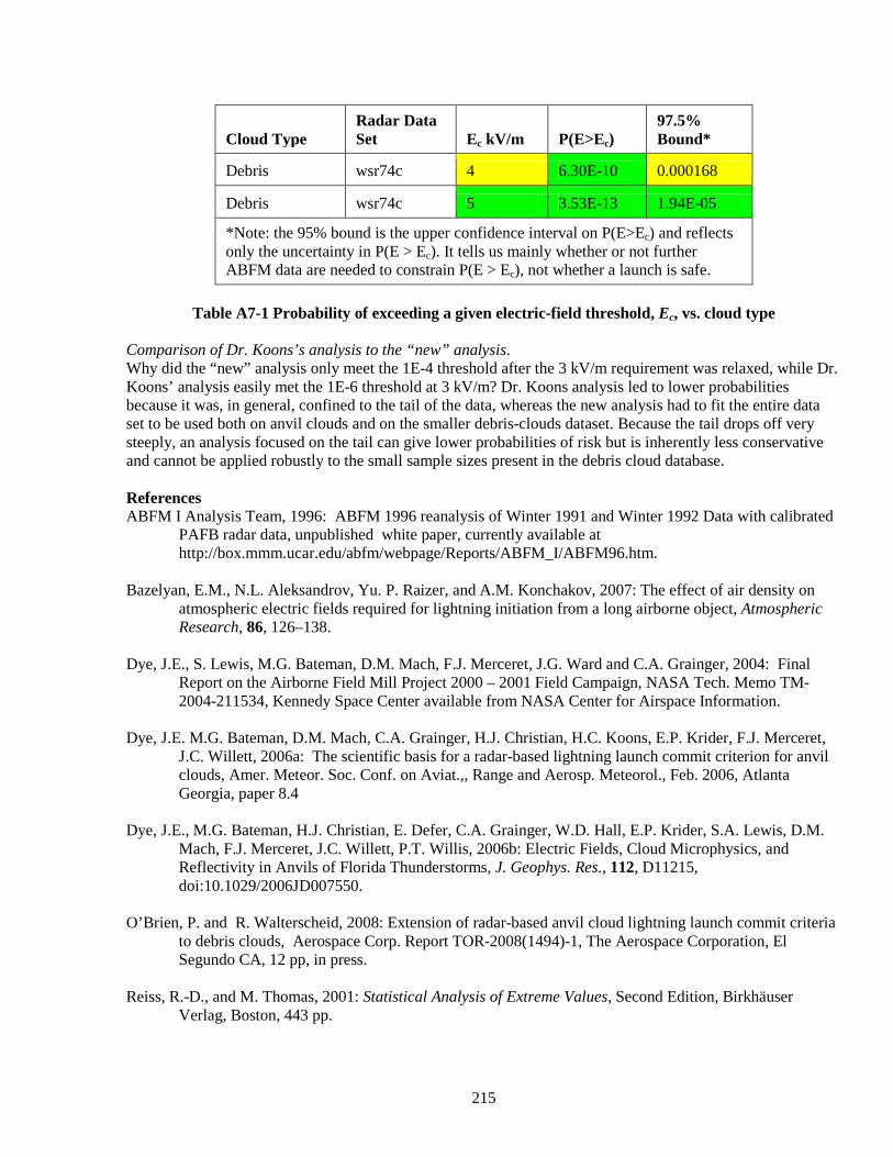
215

Cloud Type Radar Data Set Ec kV/m P(E>Ec)

97.5% Bound*

Debris wsr74c 4 6.30E-10 0.000168

Debris wsr74c 5 3.53E-13 1.94E-05

*Note: the 95% bound is the upper confidence interval on P(E>Ec) and reflects only the uncertainty in P(E > Ec). It tells us mainly whether or not further ABFM data are needed to constrain P(E > Ec), not whether a launch is safe.

Table A7-1 Probability of exceeding a given electric-field threshold, Ec, vs. cloud type

Comparison of Dr. Koons’s analysis to the “new” analysis. Why did the “new” analysis only meet the 1E-4 threshold after the 3 kV/m requirement was relaxed, while Dr. Koons’ analysis easily met the 1E-6 threshold at 3 kV/m? Dr. Koons analysis led to lower probabilities because it was, in general, confined to the tail of the data, whereas the new analysis had to fit the entire data set to be used both on anvil clouds and on the smaller debris-clouds dataset. Because the tail drops off very steeply, an analysis focused on the tail can give lower probabilities of risk but is inherently less conservative and cannot be applied robustly to the small sample sizes present in the debris cloud database. References ABFM I Analysis Team, 1996: ABFM 1996 reanalysis of Winter 1991 and Winter 1992 Data with calibrated

PAFB radar data, unpublished white paper, currently available at http://box.mmm.ucar.edu/abfm/webpage/Reports/ABFM_I/ABFM96.htm.

Bazelyan, E.M., N.L. Aleksandrov, Yu. P. Raizer, and A.M. Konchakov, 2007: The effect of air density on




Dye, J.E. M.G. Bateman, D.M. Mach, C.A. Grainger, H.J. Christian, H.C. Koons, E.P. Krider, F.J. Merceret,

J.C. Willett, 2006a: The scientific basis for a radar-based lightning launch commit criterion for anvil clouds, Amer. Meteor. Soc. Conf. on Aviat.,, Range and Aerosp. Meteorol., Feb. 2006, Atlanta Georgia, paper 8.4


Mach, F.J. Merceret, J.C. Willett, P.T. Willis, 2006b: Electric Fields, Cloud Microphysics, and Reflectivity in Anvils of Florida Thunderstorms, J. Geophys. Res., 112, D11215, doi:10.1029/2006JD007550.

O’Brien, P. and R. Walterscheid, 2008: Extension of radar-based anvil cloud lightning launch commit criteria

to debris clouds, Aerospace Corp. Report TOR-2008(1494)-1, The Aerospace Corporation, El Segundo CA, 12 pp, in press.

Reiss, R.-D., and M. Thomas, 2001: Statistical Analysis of Extreme Values, Second Edition, Birkhäuser

Verlag, Boston, 443 pp.

216

Stolzenburg, M. and T.C. Marshall, 2008: Charge structure and dynamics in thunderstorms, Space Sci. Rev., 137, 355-372, DOI 10.1007/s11214-008.9338-z.

217

Appendix 8. Standoff Distances from Anvil and Debris Clouds In the anvil and debris cloud rules, the purpose of maintaining a stand-off distance from cloud edge is to avoid flight through electric fields high enough to support the possibility of triggering lightning, and to avoid natural lightning that might extend outside the cloud. Based on extensive discussion within the Lightning Advisory Panel it was determined that fields less than or equal to 3 kV/m at or below 10 km altitude are safe with a significant safety margin (see Sections A5.4.0 and A5.4.3 of Appendix 5, "Conditions for Triggered Lightning"). Therefore, the stand-off distances and conditions in the rules are designed to assure that fields above 3 kV/m are extremely unlikely to be encountered. Observations during an extensive Airborne Field Mill (ABFM-II) program in 2000 and 2001 showed that electric field magnitudes external to anvil and debris clouds were less than 3 kV/m even in the immediate vicinity of the cloud (Merceret et al., 2008). A statistical analysis of the data showed that, when the conditions provided in the LLCC are satisfied, the probability of exceeding 3 kV/m at or beyond a stand-off distance of 3 n mi is less than 0.0001. Within 3 n mi, the ice and VAHIRR constraints must be applied (see Appendix 7, " Physical and Statistical Basis for VAHIRR.") to ensure that high fields will not be encountered. The data set used for the statistical standoff analysis included all clouds of anvil or debris type, including those with bases below the 0 oC level; therefore the "ice" constraint present in both "Anvil Clouds" Rules (there is no such constraint from "Debris Clouds") is not required by the statistical analysis but is imposed on physical grounds (possible melting electrification) and to provide an additional safety margin. Two reports and an unpublished internal memorandum to the LAP describe statistical analyses of ABFM-II data for purposes of determining standoff distances for rocket trajectories that would be safe with regard to triggered lightning: Merceret et al. (2008), O’Brien and Walterscheid (2007) and Merceret (Risk Analysis of Proposed Reduction of Anvil and Debris Cloud LLCC Standoff Distances from Five to Three Miles, as revised 3 May 2007, unpublished internal memorandum, henceforth Merceret Memo). We present here an analysis (often verbatim) following O’Brien and Walterscheid, but with the analysis broken down by anvil and debris clouds. The following analysis utilizes the ABFM-II data set. For each entry, corresponding to a pass through a cloud, a series of electric field measurements is provided in 1.2 km bins with bin-centers spanning from about 12.6 km inside the cloud (negative distances) to 12.6 km outside the cloud (positive distances). Since each pass in this data set was horizontal, or nearly so, and since very few spiral ascents/descents or ladder profiles were possible (Dye et al. ,2004), the resulting statistics strictly apply only to horizontal distances from cloud edge. Little is known about the dependence of field intensity on vertical distance above cloud top or below cloud bottom. The LFCC are launch rules only, however, and do not apply to return flight or landing, so horizontal standoffs are sufficient for safety in the present context. For the ABFM II data, cloud edge was determined by the automated algorithm described in Ward and Merceret (2004). The concept of "transparency" was not applied since no visual observations of these clouds were available. (See rationales for the definitions of "cloud" and "nontransparent" for more on this issue.) Figure A8-1 shows profiles of electric field intensity on several passes through debris and anvil clouds. One pass through a debris cloud on 6 June 2001 was identified as a bad pass and removed from further analysis because of its proximity to an adjacent cloud. There are several other features to notice. First, there is no observation of > 3 kV/m outside any cloud (positive distances); thus any risk calculation must be an extrapolation. Second, nearly every trace flattens outside the cloud. For those traces that are not flat outside the cloud, there is no systematic variation with distance from the cloud edge. Therefore, it seems to be the case that the electric field intensity is not dependent on distance from the cloud edge. This is even true of clouds with >3 kV/m observed inside. For statistical analysis, we cannot treat data taken from distance bins outside the same cloud as independent observations; therefore, grouping distance bins together increases only the apparent, not the effective, number of independent observations.

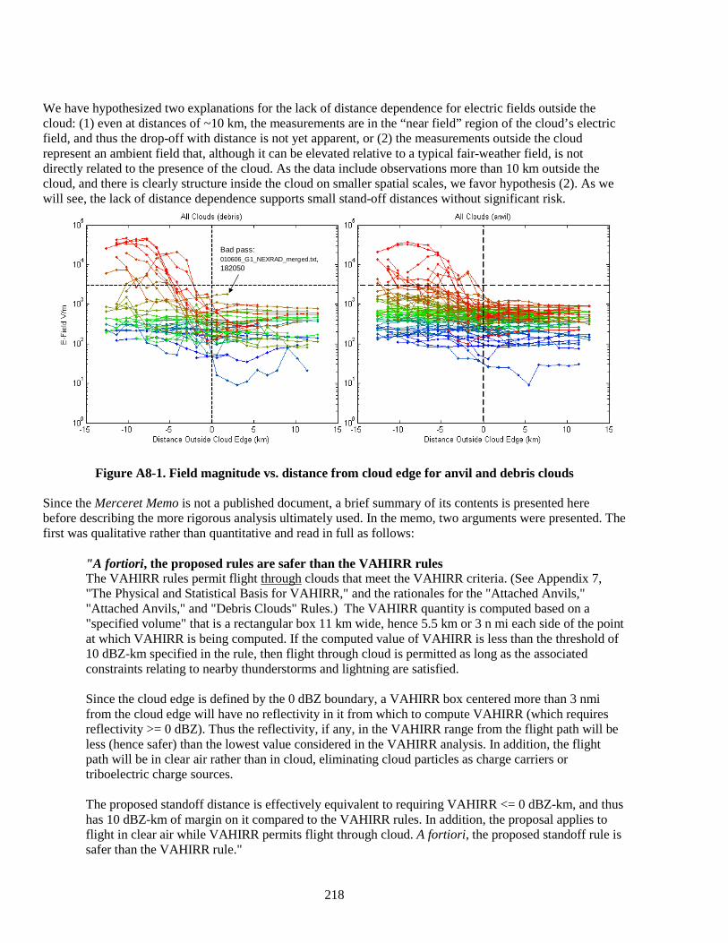
218

We have hypothesized two explanations for the lack of distance dependence for electric fields outside the cloud: (1) even at distances of ~10 km, the measurements are in the “near field” region of the cloud’s electric field, and thus the drop-off with distance is not yet apparent, or (2) the measurements outside the cloud represent an ambient field that, although it can be elevated relative to a typical fair-weather field, is not directly related to the presence of the cloud. As the data include observations more than 10 km outside the cloud, and there is clearly structure inside the cloud on smaller spatial scales, we favor hypothesis (2). As we will see, the lack of distance dependence supports small stand-off distances without significant risk.

Figure A8-1. Field magnitude vs. distance from cloud edge for anvil and debris clouds Since the Merceret Memo is not a published document, a brief summary of its contents is presented here before describing the more rigorous analysis ultimately used. In the memo, two arguments were presented. The first was qualitative rather than quantitative and read in full as follows:

"A fortiori, the proposed rules are safer than the VAHIRR rules The VAHIRR rules permit flight through clouds that meet the VAHIRR criteria. (See Appendix 7, "The Physical and Statistical Basis for VAHIRR," and the rationales for the "Attached Anvils," "Attached Anvils," and "Debris Clouds" Rules.) The VAHIRR quantity is computed based on a "specified volume" that is a rectangular box 11 km wide, hence 5.5 km or 3 n mi each side of the point at which VAHIRR is being computed. If the computed value of VAHIRR is less than the threshold of 10 dBZ-km specified in the rule, then flight through cloud is permitted as long as the associated constraints relating to nearby thunderstorms and lightning are satisfied. Since the cloud edge is defined by the 0 dBZ boundary, a VAHIRR box centered more than 3 nmi from the cloud edge will have no reflectivity in it from which to compute VAHIRR (which requires reflectivity >= 0 dBZ). Thus the reflectivity, if any, in the VAHIRR range from the flight path will be less (hence safer) than the lowest value considered in the VAHIRR analysis. In addition, the flight path will be in clear air rather than in cloud, eliminating cloud particles as charge carriers or triboelectric charge sources. The proposed standoff distance is effectively equivalent to requiring VAHIRR <= 0 dBZ-km, and thus has 10 dBZ-km of margin on it compared to the VAHIRR rules. In addition, the proposal applies to flight in clear air while VAHIRR permits flight through cloud. A fortiori, the proposed standoff rule is safer than the VAHIRR rule."

Bad pass: 010606_G1_NEXRAD_merged.txt, 182050

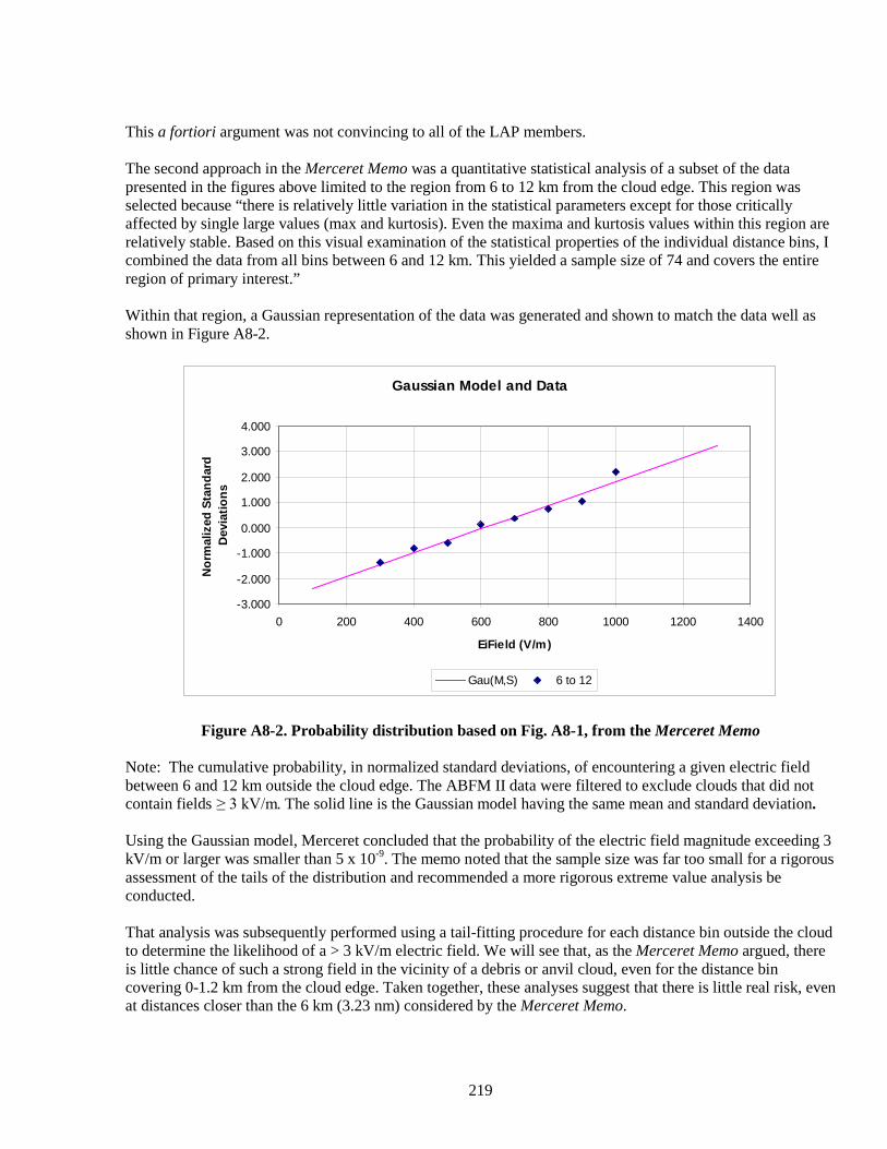
219

This a fortiori argument was not convincing to all of the LAP members. The second approach in the Merceret Memo was a quantitative statistical analysis of a subset of the data presented in the figures above limited to the region from 6 to 12 km from the cloud edge. This region was selected because “there is relatively little variation in the statistical parameters except for those critically affected by single large values (max and kurtosis). Even the maxima and kurtosis values within this region are relatively stable. Based on this visual examination of the statistical properties of the individual distance bins, I combined the data from all bins between 6 and 12 km. This yielded a sample size of 74 and covers the entire region of primary interest.” Within that region, a Gaussian representation of the data was generated and shown to match the data well as shown in Figure A8-2.

Figure A8-2. Probability distribution based on Fig. A8-1, from the Merceret Memo Note: The cumulative probability, in normalized standard deviations, of encountering a given electric field between 6 and 12 km outside the cloud edge. The ABFM II data were filtered to exclude clouds that did not contain fields ≥ 3 kV/m. The solid line is the Gaussian model having the same mean and standard deviation. Using the Gaussian model, Merceret concluded that the probability of the electric field magnitude exceeding 3 kV/m or larger was smaller than 5 x 10-9. The memo noted that the sample size was far too small for a rigorous assessment of the tails of the distribution and recommended a more rigorous extreme value analysis be conducted. That analysis was subsequently performed using a tail-fitting procedure for each distance bin outside the cloud to determine the likelihood of a > 3 kV/m electric field. We will see that, as the Merceret Memo argued, there is little chance of such a strong field in the vicinity of a debris or anvil cloud, even for the distance bin covering 0-1.2 km from the cloud edge. Taken together, these analyses suggest that there is little real risk, even at distances closer than the 6 km (3.23 nm) considered by the Merceret Memo.

Gaussian Model and Data

-3.000

-2.000

-1.000

0.000

1.000

2.000

3.000

4.000

0 200 400 600 800 1000 1200 1400

EiField (V/m)

Nor

mal

ized

Sta

ndar

d D

evia

tions

Gau(M,S) 6 to 12

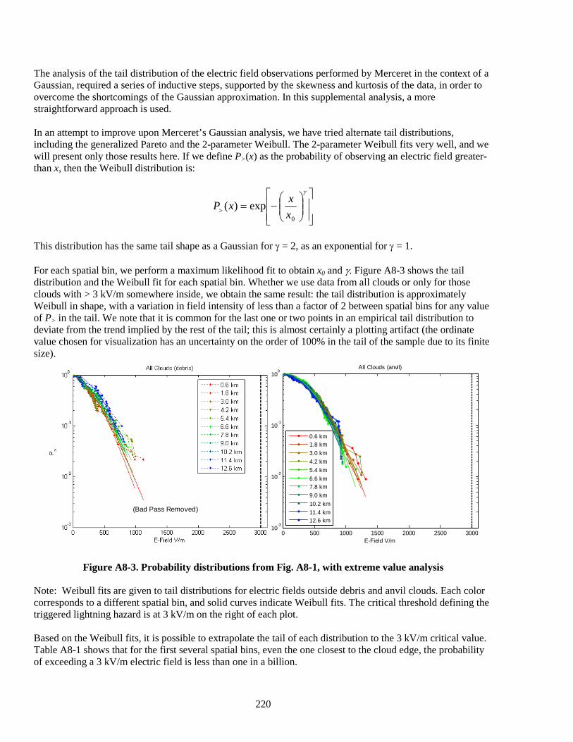
220

The analysis of the tail distribution of the electric field observations performed by Merceret in the context of a Gaussian, required a series of inductive steps, supported by the skewness and kurtosis of the data, in order to overcome the shortcomings of the Gaussian approximation. In this supplemental analysis, a more straightforward approach is used. In an attempt to improve upon Merceret’s Gaussian analysis, we have tried alternate tail distributions, including the generalized Pareto and the 2-parameter Weibull. The 2-parameter Weibull fits very well, and we will present only those results here. If we define P>(x) as the probability of observing an electric field greater-than x, then the Weibull distribution is:

−=>

γ

0

exp)(xxxP

This distribution has the same tail shape as a Gaussian for γ = 2, as an exponential for γ = 1. For each spatial bin, we perform a maximum likelihood fit to obtain x0 and γ. Figure A8-3 shows the tail distribution and the Weibull fit for each spatial bin. Whether we use data from all clouds or only for those clouds with > 3 kV/m somewhere inside, we obtain the same result: the tail distribution is approximately Weibull in shape, with a variation in field intensity of less than a factor of 2 between spatial bins for any value of P> in the tail. We note that it is common for the last one or two points in an empirical tail distribution to deviate from the trend implied by the rest of the tail; this is almost certainly a plotting artifact (the ordinate value chosen for visualization has an uncertainty on the order of 100% in the tail of the sample due to its finite size).

Figure A8-3. Probability distributions from Fig. A8-1, with extreme value analysis Note: Weibull fits are given to tail distributions for electric fields outside debris and anvil clouds. Each color corresponds to a different spatial bin, and solid curves indicate Weibull fits. The critical threshold defining the triggered lightning hazard is at 3 kV/m on the right of each plot. Based on the Weibull fits, it is possible to extrapolate the tail of each distribution to the 3 kV/m critical value. Table A8-1 shows that for the first several spatial bins, even the one closest to the cloud edge, the probability of exceeding a 3 kV/m electric field is less than one in a billion.

(Bad Pass Removed)

0 500 1000 1500 2000 2500 300010

-3

10-2

10-1

100

E-Field V/m

All Clouds (anvil)

0.6 km1.8 km3.0 km4.2 km5.4 km6.6 km7.8 km9.0 km10.2 km11.4 km12.6 km

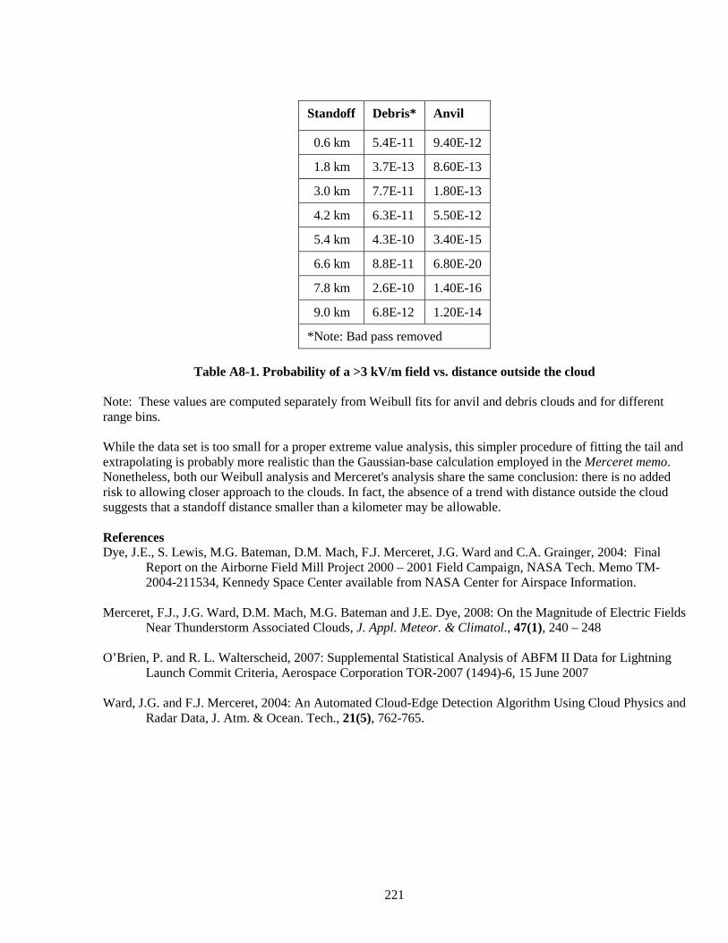
221

Standoff Debris* Anvil

0.6 km 5.4E-11 9.40E-12

1.8 km 3.7E-13 8.60E-13

3.0 km 7.7E-11 1.80E-13

4.2 km 6.3E-11 5.50E-12

5.4 km 4.3E-10 3.40E-15

6.6 km 8.8E-11 6.80E-20

7.8 km 2.6E-10 1.40E-16

9.0 km 6.8E-12 1.20E-14

*Note: Bad pass removed

Table A8-1. Probability of a >3 kV/m field vs. distance outside the cloud Note: These values are computed separately from Weibull fits for anvil and debris clouds and for different range bins. While the data set is too small for a proper extreme value analysis, this simpler procedure of fitting the tail and extrapolating is probably more realistic than the Gaussian-base calculation employed in the Merceret memo. Nonetheless, both our Weibull analysis and Merceret's analysis share the same conclusion: there is no added risk to allowing closer approach to the clouds. In fact, the absence of a trend with distance outside the cloud suggests that a standoff distance smaller than a kilometer may be allowable. References Dye, J.E., S. Lewis, M.G. Bateman, D.M. Mach, F.J. Merceret, J.G. Ward and C.A. Grainger, 2004: Final


Merceret, F.J., J.G. Ward, D.M. Mach, M.G. Bateman and J.E. Dye, 2008: On the Magnitude of Electric Fields

Near Thunderstorm Associated Clouds, J. Appl. Meteor. & Climatol., 47(1), 240 – 248 O’Brien, P. and R. L. Walterscheid, 2007: Supplemental Statistical Analysis of ABFM II Data for Lightning

Launch Commit Criteria, Aerospace Corporation TOR-2007 (1494)-6, 15 June 2007 Ward, J.G. and F.J. Merceret, 2004: An Automated Cloud-Edge Detection Algorithm Using Cloud Physics and

Radar Data, J. Atm. & Ocean. Tech., 21(5), 762-765.

222

Appendix 9. Application of Weather Radar to LFCC Evaluation Weather radar is used in the LFCC for three distinct purposes: locating cloud boundaries in three dimensions; determining the presence and intensity of precipitation; and computing VAHIRR. In all three cases, there are conditions that may occur with the operation of a weather radar which may compromise the accuracy or reliability of the measurement. This appendix discusses some of those conditions and their consequences. The Launch Operator must be aware of these concerns and exercise due diligence to ensure that measurements used to evaluate the LFCC are valid. This appendix does not address the calibration of radar systems, but presumes that any radar system used to evaluate the LFCC will be properly maintained and calibrated. Proper calibration includes correct alignment of the azimuth and altitude angles to within several tenths of a degree. A one degree error at a range of 60 km causes a kilometer of error in the reported echo position. This is especially critical in the altitude angle when cloud base and cloud top heights are being measured. Proper calibration also includes end-to-end calibration of the radio frequency (RF) pathway from the transmitter, through the antenna to the target, back through the antenna and into the receiver to within about 1 dB. Any error in the RF calibration will translate directly into errors in precipitation and VAHIRR measurements. This appendix addresses errors that occur with properly calibrated radars due to the properties of the environment in which the radar operates and its interaction with that environment. These errors may affect either the location or the amplitude (or both) of an echo as reported by the radar. A9.1 Location Errors Location errors are caused primarily by anomalous radio propagation conditions. In a vacuum, radio signals of any frequency travel in a straight line at the speed of light, c. In the atmosphere, radio signals travel at a speed c’ that is frequency dependent and slightly slower than c. The radio index of refraction n = c/c’ in the troposphere is determined by the temperature and absolute humidity of the air and varies with height. At sea level for microwaves, n is about 1.0003 (Doviak and Zrnic, 1993, Section 2.2.2). The important thing about n is its gradient. When radio waves propagate into a medium with n-gradients, they are refracted (bent) toward the higher values of n. Instead of propagating in a straight line, microwaves in the atmosphere are generally bent toward the earth because n usually decreases with height. Under what are defined as standard conditions, the height above the earth is the same as that which would occur if the signals propagated in a straight line above an Earth with a radius equal to 4/3 the actual Earth radius (ibid). Radar system software is designed to convert the measured range and altitude angle to reported horizontal distance and height above ground assuming these standard conditions. Unfortunately, conditions in the atmosphere are not always “standard”. Low level temperature inversions can increase the gradient of the index of refraction and cause the radar beam to bend more sharply than standard, and even to intersect the ground at some distance from the radar. This can result in false echoes called “anomalous propagation” or AP. It can also make cloud features appear to be at much higher altitudes than they really are. In a pair of case studies, Wheeler (1997) examined serious discrepancies between cloud top heights reported by radar and those reported by reconnaissance aircraft during two Delta launch operations from Cape Canaveral Air Force Station. In both cases, low level inversions resulted in cloud tops being reported 2 to 4 km higher by the radar than their actual height. Under conditions where the index of refraction gradient is less than standard, the opposite effect will take place: the reported cloud heights will be lower than the actual heights. Either effect can result in a cloud appearing to be at an altitude where LFCC constraints are satisfied while it is actually at a height where the LFCC are not satisfied.

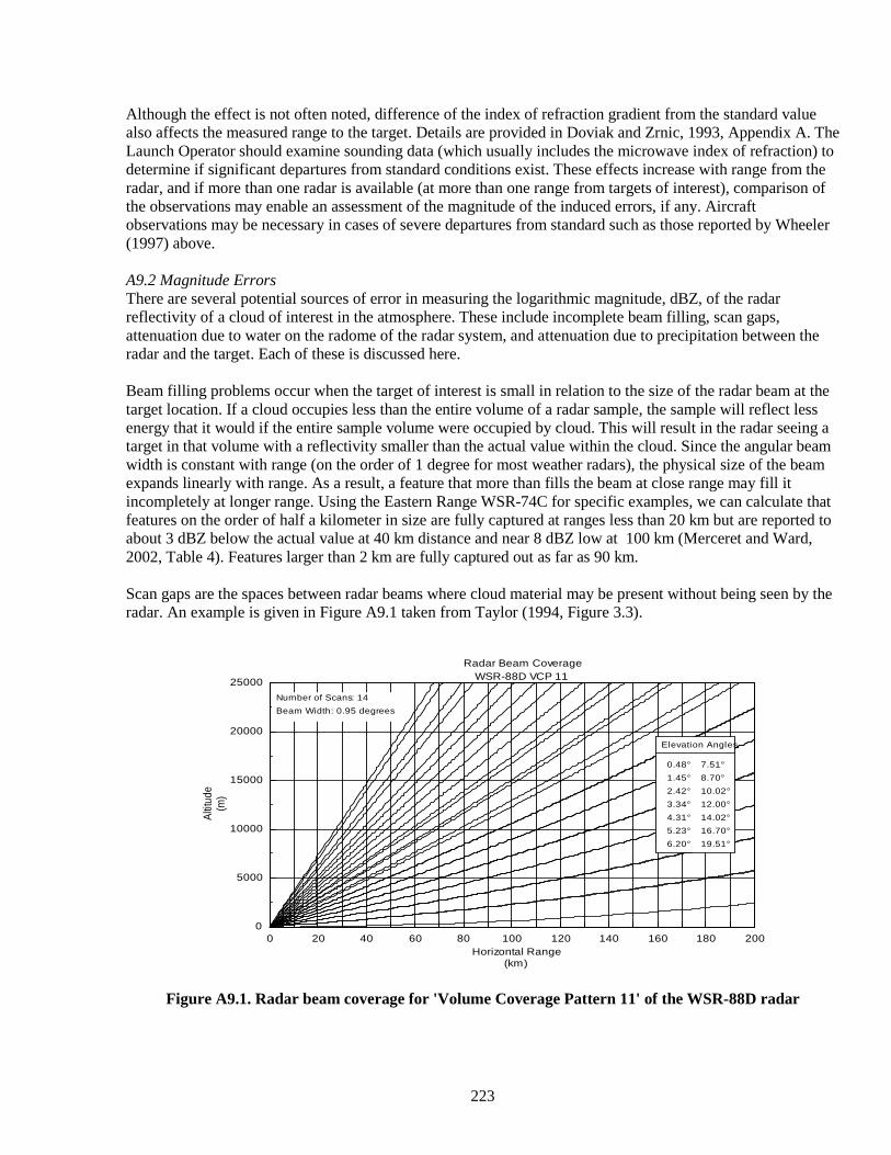
223

Although the effect is not often noted, difference of the index of refraction gradient from the standard value also affects the measured range to the target. Details are provided in Doviak and Zrnic, 1993, Appendix A. The Launch Operator should examine sounding data (which usually includes the microwave index of refraction) to determine if significant departures from standard conditions exist. These effects increase with range from the radar, and if more than one radar is available (at more than one range from targets of interest), comparison of the observations may enable an assessment of the magnitude of the induced errors, if any. Aircraft observations may be necessary in cases of severe departures from standard such as those reported by Wheeler (1997) above. A9.2 Magnitude Errors There are several potential sources of error in measuring the logarithmic magnitude, dBZ, of the radar reflectivity of a cloud of interest in the atmosphere. These include incomplete beam filling, scan gaps, attenuation due to water on the radome of the radar system, and attenuation due to precipitation between the radar and the target. Each of these is discussed here. Beam filling problems occur when the target of interest is small in relation to the size of the radar beam at the target location. If a cloud occupies less than the entire volume of a radar sample, the sample will reflect less energy that it would if the entire sample volume were occupied by cloud. This will result in the radar seeing a target in that volume with a reflectivity smaller than the actual value within the cloud. Since the angular beam width is constant with range (on the order of 1 degree for most weather radars), the physical size of the beam expands linearly with range. As a result, a feature that more than fills the beam at close range may fill it incompletely at longer range. Using the Eastern Range WSR-74C for specific examples, we can calculate that features on the order of half a kilometer in size are fully captured at ranges less than 20 km but are reported to about 3 dBZ below the actual value at 40 km distance and near 8 dBZ low at 100 km (Merceret and Ward, 2002, Table 4). Features larger than 2 km are fully captured out as far as 90 km. Scan gaps are the spaces between radar beams where cloud material may be present without being seen by the radar. An example is given in Figure A9.1 taken from Taylor (1994, Figure 3.3).

Figure A9.1. Radar beam coverage for 'Volume Coverage Pattern 11' of the WSR-88D radar

0 20 40 60 80 100 120 140 160 180 2000

5000

10000

15000

20000

25000

Altitu

de(m

)

Horizontal Range(km)

Radar Beam CoverageWSR-88D VCP 11

Number of Scans: 14Beam Width: 0.95 degrees

Elevation Angles

0.48°1.45°2.42°3.34°4.31°5.23°6.20°

7.51°8.70°10.02°12.00°14.02°16.70°19.51°

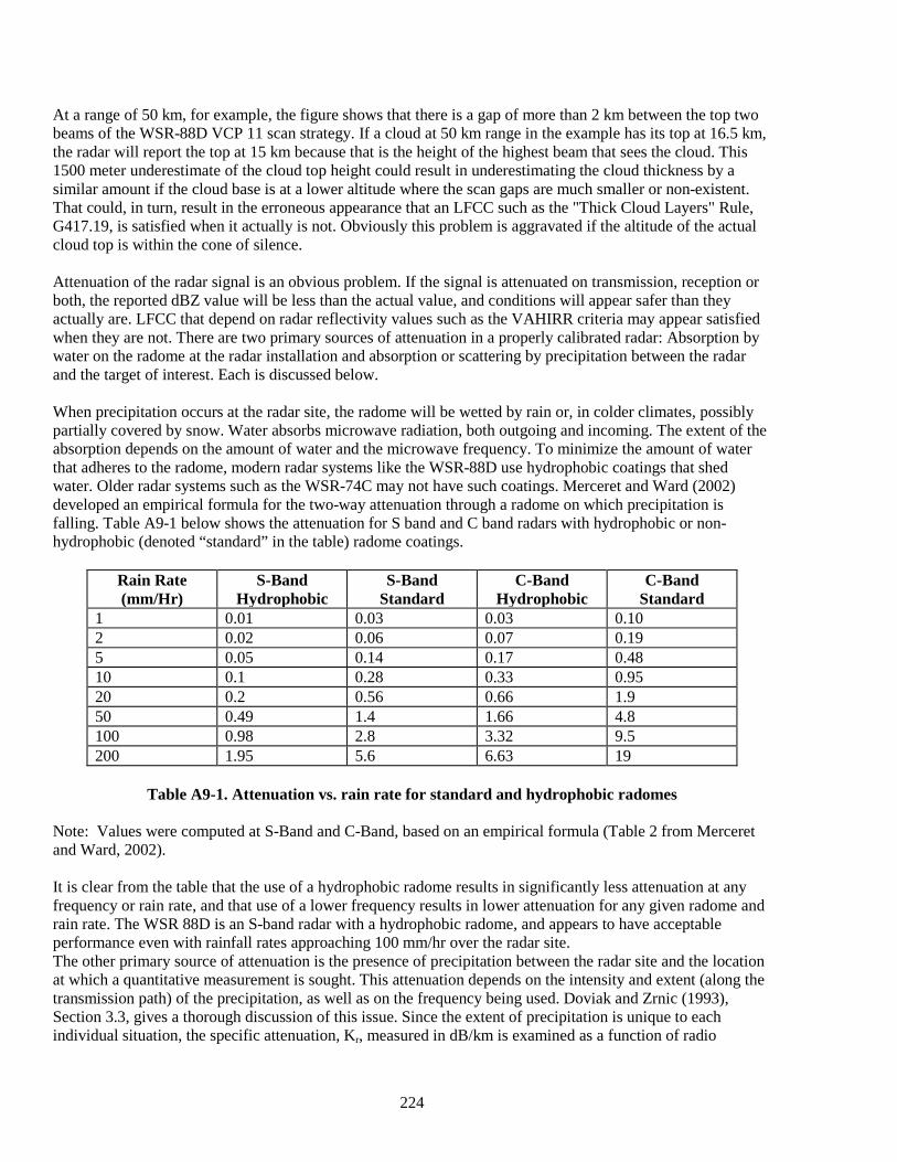
224

At a range of 50 km, for example, the figure shows that there is a gap of more than 2 km between the top two beams of the WSR-88D VCP 11 scan strategy. If a cloud at 50 km range in the example has its top at 16.5 km, the radar will report the top at 15 km because that is the height of the highest beam that sees the cloud. This 1500 meter underestimate of the cloud top height could result in underestimating the cloud thickness by a similar amount if the cloud base is at a lower altitude where the scan gaps are much smaller or non-existent. That could, in turn, result in the erroneous appearance that an LFCC such as the "Thick Cloud Layers" Rule, G417.19, is satisfied when it actually is not. Obviously this problem is aggravated if the altitude of the actual cloud top is within the cone of silence. Attenuation of the radar signal is an obvious problem. If the signal is attenuated on transmission, reception or both, the reported dBZ value will be less than the actual value, and conditions will appear safer than they actually are. LFCC that depend on radar reflectivity values such as the VAHIRR criteria may appear satisfied when they are not. There are two primary sources of attenuation in a properly calibrated radar: Absorption by water on the radome at the radar installation and absorption or scattering by precipitation between the radar and the target of interest. Each is discussed below. When precipitation occurs at the radar site, the radome will be wetted by rain or, in colder climates, possibly partially covered by snow. Water absorbs microwave radiation, both outgoing and incoming. The extent of the absorption depends on the amount of water and the microwave frequency. To minimize the amount of water that adheres to the radome, modern radar systems like the WSR-88D use hydrophobic coatings that shed water. Older radar systems such as the WSR-74C may not have such coatings. Merceret and Ward (2002) developed an empirical formula for the two-way attenuation through a radome on which precipitation is falling. Table A9-1 below shows the attenuation for S band and C band radars with hydrophobic or non-hydrophobic (denoted “standard” in the table) radome coatings.

Rain Rate (mm/Hr)

S-Band Hydrophobic

S-Band Standard

C-Band Hydrophobic

C-Band Standard

1 0.01 0.03 0.03 0.10 2 0.02 0.06 0.07 0.19 5 0.05 0.14 0.17 0.48 10 0.1 0.28 0.33 0.95 20 0.2 0.56 0.66 1.9 50 0.49 1.4 1.66 4.8 100 0.98 2.8 3.32 9.5 200 1.95 5.6 6.63 19

Table A9-1. Attenuation vs. rain rate for standard and hydrophobic radomes

Note: Values were computed at S-Band and C-Band, based on an empirical formula (Table 2 from Merceret and Ward, 2002). It is clear from the table that the use of a hydrophobic radome results in significantly less attenuation at any frequency or rain rate, and that use of a lower frequency results in lower attenuation for any given radome and rain rate. The WSR 88D is an S-band radar with a hydrophobic radome, and appears to have acceptable performance even with rainfall rates approaching 100 mm/hr over the radar site. The other primary source of attenuation is the presence of precipitation between the radar site and the location at which a quantitative measurement is sought. This attenuation depends on the intensity and extent (along the transmission path) of the precipitation, as well as on the frequency being used. Doviak and Zrnic (1993), Section 3.3, gives a thorough discussion of this issue. Since the extent of precipitation is unique to each individual situation, the specific attenuation, Kr, measured in dB/km is examined as a function of radio

225

frequency and reflectivity (or equivalent rainfall rate) of the intervening precipitation. The actual attenuation is obtained by integrating Kr along the transmission path twice (once outgoing and once coming back). The value of Kr is found to be given by a power law of the form Kr = aRb

where R is the rainfall rate in mm/hr and the parameters a and b increase with increasing radio frequency. For the S-band WSR-88D, a = 0.000343 and b = 0.97. For C band radars, a = 0.0018 and b = 1.05. For wavelengths shorter than 5 cm, the values change rapidly so that at X-band (3 cm) a = .01 and b = 1.21. (ibid). A9.3 Sources of Error Affecting Both Location and Magnitude The primary sources of error affecting both the location and magnitude of displayed radar returns in a properly calibrated radar system are the existence of sidelobes in the antenna pattern, and the finite angular size of the main lobe. Donaldson (1964) examined both of these effects using model reflectivity distributions and model antenna beam patterns. He found that in the worst cases he modeled, errors in cloud top height exceeding 10 km and errors in reflectivity approaching 10 dBZ occurred. These large errors resulted in part from his methodology that depended on defining cloud top as that altitude at which the reflectivity became less than the minimum discernable signal (MDS) for the radar at the applicable range. They occurred primarily at large ranges (> 50 nm) when the models contained extreme (~ 70 dBZ) reflectivity values. Modern weather radars have smaller sidelobes than assumed by Donaldson. For example, the WSR-88D has a first (largest) sidelobe two-way amplitude that is 54 dB below the main lobe (Doviak et al., 2000). Donaldson assumed a two-way value of only 40 dB down. In addition, these LFCC use a fixed radar threshold of 0 dBZ for cloud boundaries rather than the MDS used by Donaldson. That was one of the recommendations Donaldson made (ibid, section 7) for reducing these effects. NOAA (2010) indicates that for the WSR-88D “any possible increase in returned power due to sidelobes is usually negligible.” When it occurs, it is limited to “intense convection at close range” (ibid) and requires a reflectivity gradient of about 10 dBZ per radial sustained over at least 5 degrees of azimuth (ibid). When using radar to evaluate these LFCC, the effects of sidelobes may be infrequent to rare, but the Launch Operator should remain alert to the possibility in strong storms with large reflectivity gradients. References Donaldson, R.J., 1964: A Demonstration of Antenna Beam Errors in Radar Reflectivity Patterns, J. Appl.

Meteor., 3, 611 – 623. Doviak, R.J. and D.S. Zrnic, 1993: Doppler Radar and Weather Observations, Second Edition, Academic

Press, San Diego, CA, 562 pp. Doviak, R.J., V. Bringi, A. Ryzhkov, A. Zahrai and D. Zrnic, 2000: Considerations for Polarimetric Upgrades

to Operational WSR-88D Radars, J. Atm. Ocean. Tech,17, 257 - 278. Merceret, F.J. and J.G. Ward, 2002: Attenuation of Weather Radar Signals Due to Wetting of the radome by

Rainwater or Incomplete Filling of the Beam Volume, NASA/TM-2002-211171, 16 pp. Available from the KSC Weather Office, Mail Code PH-3, KSC, FL 32899.

NOAA, 2010: Training materials on WSR-88D sidelobe contamination accessed at

http://www.wdtb.noaa.gov/courses/dloc/topic3/lesson1/Section5/Section5-2.html Taylor, G.E., 1994: Report on the Comparison of the Scan Strategies Employed by the Patrick Air Force Base

WSR-74C / McGill Radar and the NWS Melbourne WSR-88D Radar, NASA Contractor Report CR-

http://www.wdtb.noaa.gov/courses/dloc/topic3/lesson1/Section5/Section5-2.html�

226

196291, 32 pp. Available from ENSCO, Inc., 1980 N. Atlantic Ave., Suite 830, Cocoa Beach, FL, 32931, and at http://science.ksc.nasa.gov/amu/final.html

Wheeler, M.M., 1997: Report on the Radar/PIREP Cloud Top Discrepancy Study, NASA Contractor Report

CR-204381, 18 pp. Available from ENSCO, Inc., 1980 N. Atlantic Ave., Suite 830, Cocoa Beach, FL, 32931, and at http://science.ksc.nasa.gov/amu/final.html.

http://science.ksc.nasa.gov/amu/final.html�


227

Global Reference List ABFM Analysis Group, 1992a: Airborne Field Mill project operational analysis final report for the winter

1991 deployment, Feb. 25, 1992, 133 pp. ABFM Analysis Group, 1992b: Airborne Field Mill project operational analysis final report for the winter

1992 deployment, Oct. 8, 1992, 122 pp. ABFM I Analysis Team, 1996: ABFM 1996 reanalysis of winter 1991 and winter 1992 data with calibrated

PAFB radar data, unpublished white paper, currently available at http://box.mmm.ucar.edu/abfm/webpage/Reports/ABFM_I/ABFM96.htm

Aleksandrov, N. L., E. M. Bazelyan, and Yu P. Raizer, 2005: Initiation and development of first lightning

leader: the effects of coronae and position of lightning origin, Atmospheric Research, 76, 307-329, doi:10.1016/j.atmosres.2004.11.007.

Alpert, L., 1961: A Note to the Paper by C. B. Moore, B. Vonnegut, B. A. Stein, and H. J. Survilas,

Observation of Electrification and Lightning in Warm Clouds, J. Geophys. Res., 66 (1), 332. American Meteorological Society, 2000: Glossary Of Meteorology, 2nd ed., American Meteorological

Society, Boston, MA, 850 pp. Anderson, H, 2009: Characteristics of Decaying Storms during Lightning Cessation at Kennedy Space Center

and Cape Canaveral Air Force Station, M.S. Thesis, Department of Meteorology, Florida State University, submitted to the Florida Space Grant Consortium by Dr. Henry E. Fuelberg, December 2, 2009.

Anisimov, S. V., and S. S. Bakastov, 1994: Spatiotemporal structures of electric field and space charge in the

surface atmospheric layer, J. Geophys. Res., 99 (D5), 10,603-10,610. Arnold, H. R., E. T. Pierce, and A. L. Whitson, 1965: The effect of a living tree upon the fair weather potential

gradient, J. Atmos. Terr. Phys., 27, 429-430. Avila, E. E., C. P. R. Saunders, H. Bax-Norman, and N. E. Castellano, 2005: Charge sign reversal in ice

particle-graupel collisions, Geophys. Res. Lett., 32, L01801, doi:10.1029/2004GL020761. Bachmann, R.G., 1977: Report on the results of the probability of lightning condition forecasting test

conducted in 2WW during March, April and May 1977, 2nd Weather Wing, U.S. Air Force, July 31, 1977, 31 pp.

Baker, M. B., Baker, E.R. Jayaratne, J. Latham, and C.P. Saunders, 1987: The influence of diffusional growth

rates on the charge transfer accompanying rebounding collisions between ice crystals and soft hailstones, Q. J. R. Meteorol. Soc., 113, 1193-1215.

Baker, M. B., and J. G. Dash, 1989: Charge transfer in thunderstorms and the surface melting of ice, J. Crystal

Growth, 97, 770-776. Baker, M. B., H. J. Christian, and J. Latham, 1995: A computational study of the relationships linking

lightning frequency and other thundercloud parameters, Q. J. R. Meteorol. Soc., 121, 1525-1548.

http://box.mmm.ucar.edu/abfm/webpage/Reports/ABFM_I/ABFM96.htm�

228

Baker, M. B., A. M. Blyth, H. J. Christian, J. Latham, K. L. Miller, and A. M. Gadian, 1999: A model study of corona emission from hydrometeors, Atmos. Res., 51, 221-236.

Bateman, M. G., M. F. Stewart, R. J. Blakeslee, S. J. Podgorny, H. J. Christian, D. M. Mach, J. C. Bailey, and

D. Daskar, 2007: A low-noise, microprocessor-controlled, internally digitizing rotating-vane electric field mill for airborne platforms, J. Atm.& Ocean. Tech. 24, 1245–1255. DOI: 10.1175/JTECH2039.1

Bateman, M.G., W.D. Rust, T.C. Marshall, and B.F. Smull, 1995: Precipitation charge and size measurements

in the stratiform region of two mesoscale convective systems, J. Geophys. Res., 100, 16,341-16,356. Bateman, M.G., D.M. Mach, S. Lewis, J.E. Dye, E. Defer, C.A. Grainger, P.T. Willis, F.J. Merceret, D.

Boccippio, and H.J. Christian, 2005: Comparison of in-situ electric field and radar derived parameters for stratiform clouds in Central Florida, Conf. on Meteorol. Apps. of Lightning Data, AMS Annual Meeting, San Diego, Jan. 2005.

Battan, L. J., 1973: Radar Observation of the Atmosphere (2nd Edition), Univ. of Chicago Press, 324 pp. Bazelyan, E. M., and Yu P. Raizer, 1998: Spark Discharge, Boca Raton, FL, CRC Press, 294 pp. Bazelyan, E. M., and Yu P. Raizer, 2000: Lightning Physics and Lightning Protection, Bristol, Institute of

Physics Publishing, 325 pp. Bazelyan, E.M., N.L. Aleksandrov, Yu. P. Raizer, and A.M. Konchakov, 2007: The effect of air density on


Berger, K., and E. Vogelsanger, 1969: New results of lightning observations, in Planetary Electrodynamics,

S.C. Coroniti and J. Hughes, eds., Gordon and Beach, New York, pp. 489-510. Berger, K., 1977: The earth flash, in Lightning, Vol. 1, Physics of Lighting, R.H. Golde, ed., Academic Press,

New York, pp. 119-190. Bering, E.A., A. A. Few, and J. R. Benbrook, 1998: The Global Electric Circuit, Physics Today, 51 (10), 24–

30. Black, R. and J. Hallett, 1998: The Mystery of Cloud Electrification, American Scientist, 86 (6), Nov-Dec

pp.526-534. Blakeslee, R.J., and E.P. Krider, 1992: Ground level measurements of air conductivities under Florida

thunderstorms, J. Geophys. Res., 97, 12, 947-12,951. Blanchard, D.C., 1963: Electrification of the atmosphere by particles from bubbles in the sea, Prog.

Oceanogr., 1, 71-202. Boccippio, D. J., D. J. Heckman, and S. J. Goodman, 2001a: A diagnostic analysis of the Kennedy Space

Center LDAR network 1. Data characteristics, J. Geophys. Res., 106 (D5), 4769-4786. Boccippio, D. J., D. J. Heckman, and S. J. Goodman, 2001b: A diagnostic analysis of the Kennedy Space

Center LDAR network 2. Cross-sensor studies, J. Geophys. Res., 106(D5), 4787-4796.

229

Boulay, J.L., J.P. Moreau, A. Asselineau, and P.L. Rustan, 1988: Analysis of recent in-flight lightning measurements on different aircraft, presented at the Aerospace and Ground Conference on Lightning and Static Electricity, Oklahoma City, April 19-22, 1988.

Boys, C.V., 1926: Progressive lightning, Nature, 118, 748-750. Boys, C.V., 1927: Progressive lightning, Nature, 119, 278. Breed, D. W., and J. E. Dye, 1989: The electrification of New Mexico Thunderstorms, Part 2. Electric field

growth during initial electrification. J. Geophys. Res., 94, 14,841-14,854. Bringi, V.N. and V. Chandrasekar, 2001: Polarimetric Doppler Weather Radar, Cambridge University Press,

New York, NY, 636 pp. Bringi, V.N., K. R. Knupp, A. Detwiler, L. Liu, I. J. Caylor, and R. A. Black, 1997: Evolution of a Florida

thunderstorm during the Convection and Precipitation Electrification Experiment: The case of 9 August 1991, Mon. Wea. Rev., 125, 2131–2160.

Brook, M., G. Armstrong, R.P.H. Winder, B. Vonnegut, and C.B. Moore, 1961: Artificial initiation of

lightning discharges, J. Geophys. Res., 66, 3967-3969. Brooks. I.M., and C.P. R. Saunders, 1995: Thunderstorm charging: Laboratory experiments clarified, Atmos.

Res., 39, 263-273. Brown, K. A., P. R. Krehbiel, C. B. Moore, and G. N. Sargent, 1971: Electrical screening layers around

charged clouds, J. Geophys. Res., 76, 2825-2835. Browning, G. L., I. Tzur, , and R. G. Roble, 1987: A Global Time-Dependent Model of Thunderstorm

Electricity. Part I: Mathematical Properties of the Physical and Numerical Models, J. Atmos. Sci., 44 (15), 2166-2177.

Byrne, G. J., A. A. Few, and M. E. Weber, 1983: Altitude, thickness, and charge concentration of charged

regions of four thunderstorms during TRIP 1981 based upon in situ balloon electric field measurements, Geophys. Res. Letters, 10 (1), 39-42.

Byrne, G. J., A. A. Few, and M.F. Stewart, 1986: The effects of atmospheric parameters on a corona probe

used in measuring thunderstorm electric fields, J. Geophys. Res., 91, 9911-9920. Byrne, G. J., A. A. Few, and M. F. Stewart, 1989: Electric field measurements within a severe thunderstorm

anvil, J. Geophys. Res., 94, 6297-6307. Chalmers, J. A., 1952: Negative electric fields in mist and fog, J. Atmos. Terr. Phys., 2, 155-159. Chalmers, J. A., 1964: The electrical properties of a living tree in relation to point discharge, J. Atmos. Terr.

Phys., 26, 129-134. Chalmers, J. A., 1965: The relation between precipitation current and potential gradient, J. Atmos. Terr. Phys.,

27, 899-905. Chalmers, J. A., 1967: Atmospheric Electricity, 2nd Edition, Pergamon Press, London, 515 pp.

230

Changnon, S. A., 1993: Relations between thunderstorms and cloud-to-ground lightning in the United States, J. Appl. Meteor., 32, 88–105.

Changnon, S. A., 1993: Relations between thunderstorms and cloud-to-ground lightning in the United States, J. Appl. Meteor., 32, 88–105. Chapman, S., 1970: Corona point current in wind, J. Geophys. Res., 75, 2165-2169. Chapman, S., 1977: The Magnitude of Corona Point Discharge Current, J. Atmos. Sci., 34, 1801-1809. Chauzy, S. J.-C. Medale, S. Prieur, and S. Soula, 1991: Multilevel measurement of the electric field

underneath a thundercloud. 1. A new system and the associated data processing, J. Geophys. Res., 96, 22,319-22,326.

Chubb, J., and J. Harbour, 2010: ‘Operational health’ monitoring for confidence in long term electric field

measurements, J Electrostatics, in press. Chylek, P., 1978: Extinction and liquid water content of fogs and clouds, J. Atmos. Sci., 35, 296-300. Cohen, I. Bernard, 1990: “The kite, the sentry box, and the lightning rod,” Chapter 6 in Benjamin Franklin’s

Science, Harvard Univ. Press, Cambridge, MA, 273 pp. Clifford, D.W., and H.W. Kasemir, 1982: Triggered lightning, IEEE Trans. EMC, EMC-24, 112-122. Cobb, W.E., and F.J. Holitza, 1968: A note on lightning strikes to aircraft, Mon. Wea. Rev., 96, 807-808. Computer Sciences Raytheon, 2006: Eastern Range Instrumentation Handbook, CDRL A209, Contract

F085=650-00-C-0005, 15 January, 2006. Cox, C. C., 1999: A Comparison of Horizontal Cloud-To-Ground Lightning Flash Distance Using Weather

Surveillance Radar and The Distance Between Successive Flashes Method. M.S. Thesis, AFIT/GM/ENP/99M-03, Department of Engineering Physics, Air Force Institute of Technology, 130 pp.

Dash, J. G., B. L. Mason, and J. S. Wettlaufer, 2001: Theory of charge and mass transfer in ice-ice Collisions,

J. Geophys. Res., 106 (D17), 20,395-20,402. Davydenko, S. S., E. A. Mareev, T. C. Marshall, and M. Stolzenburg, 2004: On the calculation of electric

fields and currents of mesoscale convective systems, J. Geophys. Res., 109, D11103, doi:10.1029/2003JD003832, 2004.

Dawson, G. A., and W. P. Winn, 1965: A model for streamer propagation, Z. Phys., 183, 159–171. Deaver, L. E., and E. P. Krider, 1991: Electric fields and current densities under small Florida thunderstorms,

J. Geophys. Res., 96, 22,273-22,281. Dinger, J.E., and R. Gunn, 1946: Electrical effects associated with a change of state of water, Terr. Mag.

Atmos. Elect., 51, 477. Donaldson, R.J., 1964: A Demonstration of Antenna Beam Errors in Radar Reflectivity Patterns, J. Appl.

Meteor., 3, 611 – 623.

231

Doviak, R.J. and D.S. Zrnic, 1993: Doppler Radar and Weather Observations, Second Edition, Academic

Press, San Diego, CA, 562 pp. Doviak, R.J., V. Bringi, A. Ryzhkov, A. Zahrai and D. Zrnic, 2000: Considerations for Polarimetric Upgrades

to Operational WSR-88D Radars, J. Atm. Ocean. Tech,17, 257 - 278. Drake, J. C., 1968: Electrification accompanying the melting of ice particles, Quart. J. Roy. Meteorol. Soc., 94,

176-191. Dye, J.E., 2009: Electric Fields, Microphysics, and Reflectivity Observations from Trailing Stratiform Clouds

in Florida, EOS Trans. AGU, 90(52), Fall Meet. Suppl., Abstract AE24A-05. Dye, J.E. and J.C.Willett, 2007: Observed enhancement of reflectivity and the electric field in long-lived

Florida anvils, Mon. Wea. Rev., 135, 3362-3380. Dye, J. E., C. A. Knight, V. Toutenhoofd and T. W. Cannon, 1974: The mechanism of precipitation formation

in NE Colorado cumulus. Part III: Coordinated microphysical and radar observations and summary, J. Atmos. Sci., 31, 2152-2159.

Dye, J. E., J. J. Jones, W. P. Winn, T. A. Cerni, B. Gardiner, D. Lamb, R. L. Pitter, J. Hallett, and C. P. R.

Saunders, 1986: Early electrification and precipitation development in a small, isolated Montana cumulonimbus, J. Geophys. Res., 91, 1231–1247.

Dye, J.E., J. J. Jones, A. J. Weinheimer, and W.P. Winn, 1988: Observations within two regions of charge

during initial thunderstorm electrification, Quart, J. Roy. Meteorol. Soc., 114, 1271-1290. Dye, J.E., W. P. Winn, J. J. Jones, and D. W. Breed, 1989: The electrification of New Mexico thunderstorms.

1. Relationship between precipitation development and the onset of electrification, J. Geophys. Res., 94, 8643–8656.

Dye, J. E., J. J. Jones, A.J. Weinheimer, and W. P. Winn, 1992: Reply to comments by C. B. Moore and B.

Vonnegut: Further analysis of two regions of charge during initial thunderstorm electrification, Quart, J. Roy. Meteorol. Soc., 118, 401-412.

Dye, J.E., D.W. Breed, G.M. Barnes, J.J. Jones, R.C. Solomon, 1992b: The co-evolution of precipitation and

electric fields in Florida cumuli during CaPE, Proc. 9th Internat. Conf. Atmosph. Electr., St. Petersburg Russia, June 15-19, 1992, Vol. I, 179-184.

Dye, J.E. M.G. Bateman, D.M. Mach, C.A. Grainger, H.J. Christian, H.C. Koons, E.P. Krider, F.J. Merceret,

J.C. Willett, 2006a: The scientific basis for a radar-based lightning launch commit criterion for anvil clouds, Amer. Meteor. Soc. Conf. on Aviat.,, Range and Aerosp. Meteorol., Feb. 2006, Atlanta Georgia, paper 8.4


Report on the Airborne Field Mill Project (ABFM) 2000-2001 Field Campaign, NASA Technical Memo 2004-211534, Kennedy Space Center, FL, 126 pp. available from NASA Center for Airspace Information.


Mach, F.J. Merceret J.C. Willett, and P. Willis, 2006: Electric field, microphysics, and reflectivity in anvils of Florida thunderstorms, J. Geophys. Res., 112, D11215, doi:10.1029/2006JD007550.

232

Dye, J.E., and J.C. Willett, 2006: The enhancement of reflectivity and electric fields in long-live Florida

anvils, Mon. Wea. Rev., 135, 3362-3380. Dye, J. E. and S. Lewis, 2004a: Summary of the Final Report to NASA KSC on the Airborne Field Mill

Project (ABFM) Under NASA Grant NAG10-284, June 4, 2004. Dye, J. E. and S. Lewis, 2004b: Final Report to NASA KSC on the Airborne Field Mill Project (ABFM)

Under NASA Grant NAG10-284, June 4, 2004. http://box.mmm.ucar.edu/abfm/webpage/Reports/FinalReport_0604.pdf

Edels, H., and E. Graffmann, 1969: Time constant measurements of high pressure arc columns, Z. Phys., 228,

396– 415. Eriksen, F.J., T.H. Rudolph, and R.A. Perala, 1991: The effects of the exhaust plume on the lightning

triggering conditions for launch vehicles, in International Aerospace and Ground Conference on Lightning and Static Electricity (NASA Conf. Pub. 3106, Vol. I), Cocoa Beach, FL, April 16-18, 1991, pp. 65-1 through 65-10.

Fabry, F. and I. Zawadski, 1995: Long-term radar observations of the melting layer of precipitation and their

interpretation, J. Atmos. Sci., 52, 838-851. Federal Meteorological Handbook No. 1 (FMH No. 1), Surface Weather Observations and Reports, U.S. Dept.

of Commerce, FCM-H1-2005, Washington, DC, September 2005. Fews, A. P., R. J. Wilding, P. A. Keitch, K. N. Holden, and D. L. Henshaw, 2002: Modification of

atmospheric DC fields by space charge from high-voltage power lines, Atmos. Res., 63, 271-289. Fieux, R., C. Gary, and P. Hubert, 1075: Artificially triggered lightning above land, Nature, 257, 212-214. Fitzgerald, D.R., 1967: Probably aircraft "triggering of lightning in certain thunderstorms, Mon. Wea. Rev., 95,

835-842. French, J. F., J. H. Helsdon, A. G. Detwiler, and P. L. Smith, 1996: Microphysical and electrical evolution of a

Florida thunderstorm. Part I: Observations, J. Geophys. Res., 101, 18,961–18,977. Gathman, S., 1968: Guarded Double Field Meter, Rev. Sci. Instrum., 39 (1), 43-47. Gathman, S., and E. M. Trent, 1968: Space Charge over the Open Ocean, J. Atmos. Sci., 25, 1075-1079. Gathman, S., and W. Hoppel, 1970: Surf Electrification, J. Geophys. Res., 75 (24), 4525-4529. Griffiths, R.F., J. Latham, and V. Myers, 1974: The ionic conductivity of electrified clouds, Q. J. Roy. Met.

Soc., 100, 181-190. Gringel, W., J.M. Rosen, and D.J Hofmann, 1986: Electrical structure from 0 to 30 kilometers, Chapter 12 in

The Earth's Electrical Environment, edited by E. P. Krider and R. G.Roble, National Academy Press, Washington, D.C., 263 pp. (pp.166-182).

Groom, K. N., and J. A. Chalmers, 1967: Negative charges from high-tension power cables in fog, J. Atmos.

Terr. Phys., 29, 613-615.

http://box.mmm.ucar.edu/abfm/webpage/Reports/FinalReport_0604.pdf�

233

Gunn, R., 1954: Electric Field Meters, Rev. Sci. Instrum., 25 (5), 432-437. Gunn, R., 1954: Diffusion charging of atmospheric droplets by ions, and the resulting combinations

coefficients, J. Atmos. Sci., 11, 339-347. Gunn, R., 1956: The hyperelectrification of raindrops by atmospheric electric fields, J. Atmos. Sci., 13, 283-

288. Hake, R.D. Jr., E.T. Pierce, and W. Viezee, 1973: Stratospheric Electricity, Final Report on SRI Project 1724,

Stanford Research Institute, Menlo Park, CA, January, 1973. Hallett, J., R.I. Sax, D. Lamb and A.S. Ramachandra, 1978: Aircraft measurements of ice in Florida cumuli,

Quart. J. Royal Meteorol. Soc., 104, 631-651. Handel, S. C., 2000: Electric Fields Before and During the Onset of Electrification in Florida, M.S. manuscript

at the University of Arizona, October, 2000. [Also, to be submitted to the J. Geophys. Res., 2011, (with E. P. Krider)]

Harrison, L.P., 1946: Lightning discharges to aircraft and associated meteorological conditions, National

Advisory Committee for Aeronautics Tech. Note No. 1001, May, 1946. Hatakeyama, H., 1958: "The Distribution of Sudden Change of Electric Field on Earth's Surface due to

Lightning Discharges", in Recent Advances in Atmospheric Electricity, L. G. Smith, ed., Pergamon Press, New York, pp. 289-298.

Hays, R. B., and R. G. Roble, 1979: A quasi-static model of atmospheric electricity: 1. The lower atmosphere,

J. Geophys. Res., 84, 3291-3305. Heckscher, J.L., 1972: Measured electrical parameters and the effective length of rocket exhaust plumes,

Proceedings, AFSC 1972 Science & Engineering Symposium, Vol. II, AFSC-TR-72-005, 17-19 October, 1972.

Heckscher, J.L., and R.P. Pagliarulo, 1973: Measurement of ionic conductivity and temperature in the Apollo

15 plume, AFCRL-TR-73-0124, 26 Feb., 1973. Helsdon, J. H., Jr., and R. D. Farley, 1987: A numerical modeling study of a Montana thunderstorm: 2. Model

results versus observations involving electrical aspects. J. Geophys. Res., 92, 5661–5675. Helsdon, J. H., W. A. Wojcik, and R. D. Farley, 2001: An examination of thunderstorm-charging mechanisms

using a two-dimensional storm electrification model, J. Geophys. Res., 106, (D1) 1165-1192. Helsdon, J. H., S. Gattaleeradapan, R. D. Farley, and C. C. Waits, 2002:An examination of the convective

charging hypothesis: Charge structure, electric fields, and Maxwell currents, J. Geophys. Res., 107 (D22), ACL 9-1 to ACL 9-26, doi:10.1029/2001JD001495.

Heritage, H., Ed., 1988: “Launch Vehicle, Lightning/Atmospheric Electrical Constraints, Post-Atlas/Centaur

67 Incident”; Program Group, Aerospace Report #TOR-0088 (3441-45)-2, The Aerospace Corporation, El Segundo CA 90245; 31 August 1988.

Hill, R.D., Interpretation of bipole pattern in a mesoscale storm, 1988: Geophys. Res. Lett., 15, 643–644.

234

Hinson, M. S., 1997: A Study of the Characteristics of Thunderstorm Cessation at the NASA Kennedy Space

Center, M.S. Thesis, Dept. of Meteorology, Texas A & M university, College Station, TX, August 1997, 91 pp.

Holle, R. L., M. Murphy, and R. E. Lopez, 2003: Distances and times between cloud-to-ground flashes in a

storm, Paper 103-79KMI, Preprints, International Conference on Lightning and Static Electricity, 16-18 September, Blackpool, U.K.

Holle R.L., R.E. López and C. Zimmermann, 1999: Updated recommendations for lightning safety—1998.

Bull Am Meteorological Soc, 80, 2035. Holzer. R. E. and D. S. Saxon, 1952: Distribution of electrical conduction currents in the vicinity of

thunderstorms, J. Geophys. Res., 57, 207-216. Holzer. R. E. and D. S. Saxon, 1952: Distribution of electrical conduction currents in the vicinity of

thunderstorms, J. Geophys. Res., 57, 207-216. Hoppel, W.A., and B.B. Phillips, 1971: The electrical shielding layer around charged clouds and its role in

thunderstorm electricity, J. Atmos. Sci., 28, 1258-1271. Hoppel, W. A., R. V. Anderson, and J. C. Willett, 1986: Atmospheric electricity in the planetary boundary


Horenstein, M. N., and P. R. Stone, 2001: A micro-aperture electrostatic field mill based on MEMS

technology, J. Electrostatics, 51-52, 515-521. Hubert, P., P. Laroche, A. Eybert-Berard, and L. Baret, 1984: Triggered lightning in New Mexico, J. Geophys.

Res., 89, 2511-2521, 1984. Idone, V. P. 1992: The luminous development of Florida triggered lightning. Res. Lett. Atmos. Electr., 12, 23–

28. Idone, V. P., and R. E. Orville, 1988: Channel tortuosity variations in Florida triggered lightning, Geophys.

Res. Lett., 15, 645–648. IEEE Std 1227-1990 (R2010): Guide for the Measurement of DC Electric-Field Strength and Ion Related

Quantities, IEEE Power Engineering Society (Approved ANSI October 12, 1990; Reaffirmed 17 June 2010).

Illingworth, A. J., and S. J. Marsh, 1986: Static charging of aircraft by collisions with ice crystals, Revue Phys.

Appl., 21, 803-808. Imyanitov, I.M., and Ye.V. Chubarina, 1967: Electricity of the Free Atmosphere. 212 pp, NASA Tech.

Translation, NASA TT F-425, TT 67-51374 of Elektrichestvo Svobodnoy Atmosfery. Gidrometeoizdat, Leningrad, 1965, NTIS Accession no. N68-10079.

Imyanitov, I.M., Ye.V. Chubarina, and Ya.M. Shvarts, 1972: Electricity of Clouds. 122 pg, NASA Tech.

Translation, NASA TT F-718, of Elektrichestvo oblakov. Hydrometeorological Press, Leningrad, 1971.

235

Israel, H., 1959: Atmospheric electrical agitation, Quart. J. Roy. Met. Soc., 85, 91-104. Israel, H., 1973: Atmospheric Electricity, Vol II, NTIS, U.S. Department of Commerce, Springfield, VA, 570

pp. Jacobson, E. A., and E. P. Krider, 1976: Electrostatic field changes produced by Florida lightning, J. Atmos.

Sci., 33 (1), 103−117. Jameson, A.R., M. J. Murphy, and E. P. Krider, 1996: Multiple parameter radar observations of isolated

Florida thunderstorms during the onset of electrification, J. Appl. Meteor., 35, 343–354. Johnston, A. R., H. Kirkham, and B. T. Eng, 1986: dc electric field meter with fiber-optic readout, Rev. Sci.

Instrum., 57 (11), 2746–2753. Jones, J.J., W.P. Winn, S.J. Hunyady, C.B. Moore, J.W. Bullock and P. Fleischhaker, 1990: Aircraft

measurements of electrified clouds at Kennedy Space Center, Final Report, Part I 1988 Flights (April 27, 1990).


ice crystal interactions, Quart J. Roy. Meteorol. Soc., 109, 609-630. Kasemir, H. W., 1963: “The Thundercloud” in Proc. Third Int. Conf. on Atmospheric and Space Electricity,

Montreaux, Switzerland, May 5-10, 1963, ed. By S. C. Coroniti, Elsevier, 1965, pp. 215-235. Kasemir, H. W., 1971:Calibration of Atmospheric Electric Field Meters and the Determination of Form

Factors at Kennedy Space Center, NOAA Tech. Memo. ERL APCL-11, April, 1971. Kasemir, H. W., 1972: The Cylindrical Field Mill, Meteorol. Rundsch., 25, 33-38. Kasemir, H. W., 1959: The thunderstorm as a generator in a global electric circuit (in German), Z. Geophys.,

25, 33-64. King, L. A. 1961: The voltage gradient in the free-burning arc in air or nitrogen, British Electrical and Allied

Industries Research Association Report G/XT172. Surrey, England: Leatherhead. Klett, J.D., 1971: Ion transport to cloud droplets by diffusion and conduction, and the resulting droplet charge

distribution, J. Atmos. Sci., 28, 78-85. Klett, J.D., 1972: Charge screening layers around electrified clouds, J. Geophys. Res., 77, 3187-3195. Knight, C.A., 1979: Observations of the melting of snowflakes, J. Atmos. Sci.,36, 1123-1130. Koshak, W.J., and E.P. Krider, 1989: Analysis of lightning field changes during active Florida thunderstorms,

J. Geophys. Res., 94, 1165-1186. Kraakevik, J.H., and J.F. Clark, 1958: Airborne measurements of atmospheric electricity, Eos Trans. AGU, 39,

827-834. Krehbiel, P.R., M. Brook, and R. A. McCrory, 1979: An analysis of the charge structure of lightning

discharges to ground, J. Geophys. Res., 84, 2432-2456.

236

Krehbiel, P. R., R. J. Thomas, W. Rison, T. Hamlin, J. Harlin, and M. Davis, 2000: Lightning mapping observations in central Oklahoma, EOS Trans. of AGU, 21-25, January 2000.

Krehbiel, P. R., 1986: The electrical structure of thunderstorms, Chapter 8 in The Earth’s Electrical

Environment ed. By E. P. Krider and R. G. Roble, National Academy Press, Washington, D. C., pp. 90-113.

Krehbiel, P.R, 1969: Conductivity of clouds in the presence of electric fields, Eos, Trans., Amer. Geophys. U.,

50, 618. Krider, E.P., H.C. Koons, R.L. Walterscheid, W.D. Rust, and J.C. Willett, 1999: Natural and triggered

lightning launch commit criteria (LCC), Rept. No. TR-99(1413)-1, The Aerospace Corporation, El Segundo, CA, 15 January 1999.

Krider, E.P., H.J. Christian, J.E. Dye, H.C. Koons, J. Madura, F. Merceret, W.D. Rust, R.L. Walterscheid, and

J.C. Willett, 2006: Natural and triggered lightning launch commit criteria, 86th Annual AMS Meeting, Atlanta, GA, 29 January-2 February, 2006.

Krider, E. P., 1989: Electric field changes and the cloud electrical structure, J. Geophys. Res., 94, 13145-

13149. Krider, E. P., and R. J. Blakeslee, 1985: The Electric Currents Produced by Thunderclouds, J. Electrostatics,

16, 369-378. Krider, E. P., and J. A. Musser, 1982: Maxwell Currents Under Thunderstorms, J. Geophys. Res., 87 (C13),

11,173-11,176. Krider, E.P., R.C. Noggle, M.A. Uman, and R.E. Orville, 1974: Lightning and the Apollo 17/Saturn V Exhaust

Plume, J. Spacecraft and Rockets, 11, 72-75. Krider, E.P., J.C. Willett, G.S. Peng, F.S. Simmons, G.W. Law, and R.W. Seibold, 2006: Triggered lightning

risk assessment for reusable launch vehicles at the Southwest Regional and Oklahoma Spaceports, Aerospace Report No. ATR-2006(5195)-1, 30 January 2006.

Krige, J., A. Russo and L. Sebesta, 2000: A History of the European Space Agency, 1958 – 1987, Volume II ,

The story of ESA, 1973 to 1987, European Space Agency, SP-1235. Kuhlman, K. M., D. R. MacGorman, M. I. Biggerstaff, P. R. Krehbiel, 2009: Lightning initiation in the anvils

of two supercell storms, Geophysical Research Letters, 36, L07802. Labaree, L.W. (ed), 1962: The Papers of Benjamin Franklin, Yale University Press, Vol. 5, p. 69. Lalande, P., and A. Bondiou-Clergerie, 1997: Collection and analysis of available in-flight measurement of

lightning strikes to aircraft. Report AI-95-SC.204-RE/210-D2.1, ONERA (France) Transport Research and Technological Development Program DG VII. 24 February 1997.

Lalande, P., A. Bondiou-Clergerie, P. Laroche, A. Eybert-Bérard, J. P. Berlandis, B. Bador, A. Bonamy, M. A.

Uman, and V. A. Rakov. 1998: Leader properties determined with triggered lightning techniques, J. Geophys. Res., 103, 14,109–14,115.

237

Lang, T.J., et al., 2004: The Severe Thunderstorm Electrification and Precipitation Study, Bull. Am. Meteorol. Soc., 85(8), 1107-1125, doi:10.1175/BAMS-85-8-1107.

Laroche, P., A. Eybert-Bérard, L. Barret, and J. P. Berlandis, 1988: Observations of preliminary discharges

initiating flashes triggered by the rocket and wire technique. Paper presented at the 8th International Conference on Atmospheric Electricity, Uppsala, Sweden, 13–16 June 1988.

Laroche, P., A. Delannoy, and H. Le Court de Béru, 1989a: Electrostatic field conditions on an aircraft

stricken by lightning. Paper presented at the International Conference on Lightning and Static Electricity, University of Bath, UK., September 26–28, 1989.

Laroche, P., A. Bondiou, A. Eybert-Bérard, L. Barret, J. P. Berlandis, G. Terrier, and W. Jafferis, 1989b:

Lightning flashes triggered in altitude by the rocket and wire technique. Paper presented at the International Conference on Lightning and Static Electricity, University of Bath, UK., September 26–28, 1989.

Latham, D. J. 1986: Anode column behavior of long vertical air arcs at atmospheric pressure, IEEE Trans.

Plasma Sci., PS-14, 220–227. Latham, J., 1981: The electrification of thunderstorms, Quart, J. Roy. Meteorol. Soc., 107, 277-298. Latham, J., and J. Dye, 1989: Calculations on the Electrical Development of a Small Thunderstorm, J.

Geophys. Res., 94(D11), 13141-13144. Latham, D., 1991: Lightning Flashes from a Prescribed Fire-Induced Cloud, J. Geophys. Res., 96 (D9),

17,151-17,157. Latham, D. J., and R. W. Miksad, 1974: Electric Field Perturbations of the Marine Atmosphere by Horizontal

Roll Vortices, J. Geophys. Res., 79(36), 5592–5597, doi:10.1029/JC079i036p05592. Livingston, J. M., and E. P. Krider, 1978: Electric fields produced by Florida thunderstorms, J. Geophys. Res.,

83 (C1), 385−401. Lopez, R. E., and R. L. Holle, 1999: The distance between successive lightning flashes. NOAA Tech. Memo.

ERL NSSL-105, National Severe Storms Laboratory, Norman, OK, 29 pp. Lorenz, R. D., 2008: Atmospheric electricity hazards, Space Sci Rev, 137: 287–294, DOI 10.1007/s11214-008-

9364-x LPLWS, 1992: AGBFM Initial Check Lists and Calibration, Test and Calibration User’s Guide, Air Force

Library #M17187, 5 December 1992, 11 pp. MacGorman, D. R., and W. D. Rust, 1998: The Electrical Nature of Storms. Oxford Univ. Press, ISBN 0-19-

507337-1, 432 pp. MacGorman, D. R., W. D. Rust, T. J. Schuur, M. I. Biggerstaff, J. M. Straka, C. L. Ziegler, E. R. Mansell, E.

C. Bruning, K. M. Kuhlman, N. R. Lund, N. S. Biermann, C. Payne, L. D. Carey, P. R. Krehbiel, W. Rison, K. B. Eack, and W. H. Beasley, 2008: TELEX: The Thunderstorm Electrification and Lightning Experiment, Bull. Amer. Meteor. Soc., 89 (7), 997-1013.

238

MacGorman, M. I. Biggerstaff, P. R. Krehbiel, 2009: Lightning initiation in the anvils of two supercell storms, Geophysical Research Letters, 36, L07802.

Maier, L. M., and E. P. Krider, 1986: The charges that are deposited by cloud-to-ground lightning in Florida,

J. Geophys. Res., 91, 13, 275-13, 289. Malan, D. J., and B. F. J. Schonland, 1950: An Electrostatic Fluxmeter of Short Response-time for use in

Studies of Transient Field-changes, Proc. Phys. Soc. (London), B, 63, 402-408. Mansell, E. R., C. L. Ziegler, and E. C. Bruning, 2010: Simulated Electrification of a Small Thunderstorm

with Two-Moment Bulk Microphysics, J. Atmos. Sci., 67 (1), 171-194. Mapleson, W. W., and W. S. Whitlock, 1955: Apparatus for the accurate and continuous measurement of the

earth’s electric field, J. Atmos. Terr. Phys., 7, 61-72. Marshall, T. C. , W. D. Rust, M. Stolzenburg, W. Roeder, and P. R. Krehbiel, 1999: A study of enhanced fair-

weather electric fields occurring soon after sunrise, J. Geophys. Res., D104, 24455-24469. Marshall, T.C. and B. Lin, 1992: Electricity in dying thunderstorms, J. Geophys. Res., 97, 9913-9918. Marshall, T.C., M. Stolzenburg, P.R. Krehbiel, N.R. Lund and C.R. Maggio, 2009: Electrical evolution during

the decay stage of New Mexico thunderstorms, J. Geophys. Res., 114, D02209, doi:10.129/2008JD010637,

Marshall, T., 2000: Comment on “’Spider’ lightning in intracloud and positive cloud-to-ground flashes” by

Vladislav Mazur, Xuan-Min Shao, and Paul R. Krehbiel, J. Geophys. Res., 105 (D6), 7397-7399. Marshall, T.C., W.D. Rust, and W.P. Winn, 1984: Screening layers at the surface of thunderstorm anvils, Proc.

VII Intern. Conf. on Atmosph. Electr., Albany, NY, June 3-8, pp.346-347. Marshall, T. C., W. D. Rust, W. P. Winn, and K. E. Gilbert, 1989: Electrical structure in two thunderstorm

anvil clouds, J. Geophys. Res., 94 (D2), 2171-2181. Marshall, T.C., and W. D. Rust, 1993: Two types of vertical electrical structures in stratiform precipitation

regions of mesoscale convective regions, Bull. Am. Meteorol. Soc., 78(11), 2159-2170. Marshall, T. C. and B. Lin, 1992: Electricity in dying thunderstorms, J. Geophys. Res., 97 (D9), 9913-9918. Marshall, T. C., M. Stolzenburg, W. D. Rust, E. R. Williams, and R. Boldi, 2001: Positive charge in the

stratiform cloud of a mesoscale convective system, J. Geophys. Res., 106 (D1), 1157-1163. Marshall, T. C., M. Stolzenburg,1 P. R. Krehbiel, N. R. Lund, and C. R. Maggio, 2009: Electrical evolution

during the decay stage of New Mexico thunderstorms, J. Geophys. Res., 114, D02209, doi:10.1029/2008JD010637.

Marshall, T.C., W. Rison, W.D. Rust, M Stolzenburg, J.C. Willett, and W.P. Winn, 1995: Rocket and balloon

observations of electric field in two thunderstorms, J. Geophys. Res., 100, 20,815-20,828. Mason, B. J., 1988: The generation of electric charges and fields in thunderstorms, Proc. Roy. Soc. London,

A415, 303-315.

239

Mason, B. J., 1971: The electrification of clouds, Chapter 9 in The Physics of Clouds, Clarendon, Oxford (2nd ed.).

Mason, B. L. and J. G. Dash, 2000: Charge and mass transfer in ice-ice collisions: Experimental observations

of a mechanism in thunderstorm electrification, J. Geophys. Res., 105 (D8), 10,185-10,192. Matthews, J. C., and D. L. Henshaw, 2009: Measurements of atmospheric potential gradient fluctuations

caused by corona ions near high voltage power lines, J. Electrostatics, 67, 488-491. Mazur, V., X.-M. Shao, and P. R. Krehbiel, 1988: “Spider” lightning in intracloud and positive cloud-to-

ground flashes, J. Geophys. Res., 103, 19,811-19,822. Mazur, V., B.D. Fisher, and J.C. Gerlach, 1984: Lightining strikes to an airplane in a thunderstorm, J. Aircraft,

21, 607-611. Mazur, V., 1989b: A physical model of lightning initiation on aircraft in thunderstorms. J. Geophys. Res. 94,

3326–3340. McEachron, K.B., 1939: Lightning to the Empire State Building, J. Franklin Inst., 227, 149-217. McNamara, T. M., 2002: The horizontal extent of cloud-to-ground lightning over the Kennedy Space Center.

M.S. thesis, Air Force Institute of Technology, Wright-Patterson AFB, Ohio, AFIT/GM/ENP/02M-06, 114pp, 14 January 2002.

Merceret, F.J., D.A. Short and J.G. Ward, 2006: Radar evaluation of optical cloud constraints to space launch

operations, J. Spacecraft & Rockets, 43(1), 248-251. Merceret, Francis J. and Jennifer G. Ward, 2002: Attenuation of Weather Radar Signals Due to Wetting of the

Radome by Rainwater or Incomplete Filling of the Beam Volume, NASA Technical Memorandum TM-2002-211171, April 2002, 16pp.



Merceret, F.J., J.G. Ward, D.M. Mach, M.G. Bateman and J.E. Dye, 2008: On the Magnitude of Electric Fields

Near Thunderstorm Associated Clouds, J. Appl. Meteor. & Climatol., 47(1), 240 - 248. Merceret, F.J. and J.G. Ward, 2002: Attenuation of Weather Radar Signals Due to Wetting of the radome by

Rainwater or Incomplete Filling of the Beam Volume, NASA/TM-2002-211171, 16 pp. Available from the KSC Weather Office, Mail Code PH-3, KSC, FL 32899.

Michnowski, S., 1963: On the observation of lightning in warm clouds, J. Meteor. Geophys. (India), 14 (3),

320-322. Montanya, J., P. Rodriguez, J. Bergas, A. Illa, B. Hermoso, and I. Candela, 2007: A new electrostatic field

measurement method: The coherent-notch field mill, J Electrostatics, 65, 431-437. Moore, C. B., B. Vonnegut, B. A. Stein, and H. J.Survilas, 1960: Observations of electrification and lightning

in warm clouds, J. Geophys. Res., 65, 1907-1910.

240

Moore, C.B., and B. Vonnegut, 1977: The thundercloud, in Lightning, Vol. 1, R.H. Golde, Editor, Academic Press, New York, pp 51-98.

Moore, C. B., and B. Vonnegut, 1992: Comments on ‘Observations of two regions of charge during initial

thunderstorm electrification’ by J. E. Dye, J.J. Jones, A. J. Weinheimer and W. P. Winn (July 1988, 114, 1271-1290), Quart, J. Roy. Meteorol. Soc., 118, 395-400.


Precipitation Experiment (CaPE) storms, J. Geophys. Res., 101 (D23), 29,615-29,626. Murphy, M. J., and R. L. Holle, 2005: A warning method for cloud-to-ground lightning based on total lightning

and radar information, preprints, International Conference on Lightning and Static Electricity, 19–23 September 2005, Seattle, Washington, paper LDM-36, 2005.

Nanevicz, J. E., 1973: Advanced Materials Aspects and Concepts for Development of Antistatic Coatings, for

Aircraft Transparencies Universal Technology Corporation, Dayton, Ohio, Contract F33615-72-C-2113 SRI Project 2393, 22 February 1973.


May, 1982. Nanevicz, J. E. and R. L. Tanner, 1964: Some Techniques for Elimination of Corona Discharge Noise in

Aircraft Antennas, Proc. IEEE, pp. 53-64, January 1964. Nanevicz , J. E. and G. R. Hilbers, 1973: Titan Vehicle Electrostatic Environment, Technical Report AFAL-

TR-73-170, July, 1973. Nanevicz, J. E., E. F. Vance, R. L. Tanner, and G. R. Hilkrs, 1962: Development and Testing of Techniques

for Precipitation Static Interference Reduction, ASD-TR-62-38, Stanford Research Institute, Project 2848, Final Report, Contract AF33(16)-6561.

Nanevicz, J.E., Flight Evaluation of Induced-Noise Mechanisms on High-Speed Aircraft, SRI Project 7104,

Final Report, AFAL-TR-73-3l7, Stanford Research Institute, Menlo Park, California, 1973. Nanevicz, J. E.; J.B. Chown, E.F. Vance and J.A. Martin, 1966: SRI Participation in Voltage Breakdown and

Rocket Charging Experiments on Nike-Cajun Rocket AFCRL AD 6.841, AFCRL-66-588, August 1966.

NASA, 1970: Analysis of Apollo 12 lightning incident, MSC-01540, February, 1970. NASA, 1974: Space Vehicle Design Criteria (Environment) - Assessment and Control of Electrostatic

Charges, SP-8111, May, 1974. Nelson, L. A., 2002: Synthesis of 3-dimensional lightning data and weather radar data to determine the

distance that naturally occurring lightning travels from thunderstorms. M.S. thesis, Air Force Institute of Technology, Wright-Patterson AFB, Ohio, AFIT/GM/ENP/02M-07.

Newman, M.M., 1958: Lightning discharge channel characteristics and related atmospherics, in Recent

Advances in Atmospheric Electricity, L.G. Smith, ed., Pergamon Press, New York, pp. 475-484, 1958.

241

Newman, M.M., 1965: Use of triggered lightning to study the discharge channel, in Problems of Atmospheric and Space Electricity, S.C. Coroniti, ed., Elsevier, New York, pp. 482-490.

Newman, M.M., J.R. Stahmann, J.D. Robb, E.A. Lewis, S.G. Martin, and S.V. Zinn, 1967: Triggered lightning

strokes at very close range, J. Geophys. Res., 72, 4761-4764. NOAA, 2010: Training materials on WSR-88D sidelobe contamination accessed at

http://www.wdtb.noaa.gov/courses/dloc/topic3/lesson1/Section5/Section5-2.html O’Brien, P. and R. L. Walterscheid, 2007: Supplemental Statistical Analysis of ABFM II Data for Lightning

Launch Commit Criteria, Aerospace Corporation TOR-2007 (1494)-6, 15 June 2007 O’Brien, P. and R. Walterscheid, 2008: Extension of radar-based anvil cloud lightning launch commit criteria

to debris clouds, Aerospace Corp. Report TOR-2008(1494)-1, The Aerospace Corporation, El Segundo CA, 12 pp, in press.

Office of the Federal Coordinator for Meteorology, 2005: Federal Meteorological Handbook No. 1, Surface

Weather Observations and Reports, FCM-H1-2005, Washington, D.C., September 2005. Ogden, T. L., and W. C. A. Hutchinson, 1970: Electric space-charge pulses near the ground in sunny weather,

J. Atmos. Terr. Phys., 32, 1131-1138. Oram, T. D., and E. P. Krider, 1991. The spatial variations of lightning during small Florida thunderstorms, in

Proceedings of the 1991 International Aerospace and Ground Conference on Lightning and Static Electricity, NASA Conf. Pub. 3106, vol. II, pp. 86-1 to 86-9.

Orville, R.E., R.W. Henderson, and L.F. Bosart, 1988: Bipole patterns revealed by lightning locations in

mesoscale storm systems, Geophys. Res. Lett., 15, 129-132. Parsons, Tamara, L., 2000: Determining Horizontal Distance Distribution of Cloud-To-Ground Lightning.

M.S. Thesis, AFIT/GM/ENP/00M-09, Department of Engineering Physics, Air Force Institute of Technology, 88 pp.

Perala, R.A., T.H. Rudolph, D.A. Steffen, G.J. Rigden, and H.S. Weigel IV, 1994: A model for predicting the

triggering of lightning by launch vehicles, EMA-93-R-035, Electro Magnetic Applications, Inc., Denver, CO.

Pergament, H.S., T.R. Hvisdock, and M.A. Najarian, 1994: Electrical conductivity of solid propellant rocket

plumes, PST TR-20, Propulsion Science and Technology, Inc., Princeton, NJ, 1993 [included as Appendix G in Perala et al. (1994)].

Phelps, C. T., and R. F. Griffiths, 1976: Dependence of positive corona streamer propagation on air pressure

and water vapor content, J. Appl. Phys., 47, 2929–2934. Phillips, B.B., 1967: Ionic equilibrium and the electrical conductivity in thunderclouds, Mon. Wea. Rev., 95,

854-862. Pierce, E. T., 1974. Atmospheric Electricity – Some Themes, Bull. Am. Meteor. Soc., 55 (10), 1186-1194. Poehler, Horst, A., 1978: LDAR Observations of a Developing Thunderstorm Correlated With Field Mill,

Ground Strike Location, and Weather Radar Data Including the First Report of the Design and

http://www.wdtb.noaa.gov/courses/dloc/topic3/lesson1/Section5/Section5-2.html�

242

Capabilities of a New, Time-of-Arrival Ground-Strike Location System (GSLS). NASA Contract Report CR-154626, 135pp.

Proctor, D. E., 1971: A hyperbolic system for obtaining VHF radio pictures of lightning, J. Geophys. Res., 76,

1478-1489. Pruppacher, H.R., and J.D. Klett, 1978: Microphysics of Clouds and Precipitation, D. Reidel Publishing

Company, Dordrecht:Holland, 714 pp. Raizer, Yu P., 1991: Gas discharge physics. Berlin: Springer-Verlag, 449 pp. Rakov, V.A., and M.A. Uman, 2003: Lightning Physics and Effects, Cambridge University Press, 687pp. Ramachandran, R., A. Detwiler, J. Helsdon Jr., P. L. Smith, and V. N. Bringi, 1996: Precipitation development

and electrification in Florida thunderstorm cells during CaPE. J. Geophys. Res., 101(D1), 1599–1619. Ravichandran, M., and A. K. Kamra, 1999: Spherical field meter to measure the electric field vector –

measurements in fair weather and inside a dust devil, Rev. Sci. Instrum., 70 (4), 2140-2149. Reid, G.C., 1986: Electrical structure of the middle atmosphere, Chapter 13 in The Earth's Electrical


Reiss, R.-D., and M. Thomas, 2001: Statistical Analysis of Extreme Values, Second Edition, Birkhäuser

Verlag, Boston, 443 pp. Reiter, R., 1968: Results of Investigation on Precipitation and Cloud Electricity Based on 15 Years of

Observation, Arch. Met. Geoph. Biokl., Ser. A, 17, 17-29. Reiter, R., 1994: Charges on particles of different size from bubbles of Mediterranean Sea surf and from

waterfalls, J. Geophys. Res., 99 (D5), 10,807–10,812, doi:10.1029/93JD03268. Reiter, R., 1965: Precipitation and cloud electricity, Quart. J. Roy. Meteor. Soc., 91(1), 60-72. Reiter, R., 1968: Results of investigation on precipitation and cloud electricity based on 15 years of

observation, Arch. Met. Geoph. Biokl., Ser. A, 17, 17-29. Reitz, J.R., and F.J. Milford, 1967: Foundations of Electromagnetic Theory, Addison-Wesley Publishing

Company, Reading, MA, Second Edition, 435 pp. Renner, S. L., 1998: Analyzing Horizontal Distances Between WSR-88D Thunderstorm Centroids and Cloud-

To-Ground Lightning Strikes. M.S. Thesis, AFIT/GM/ENP/98M-09, Department of Engineering Physics, Air Force Institute of Technology, 123 pp.

Reynolds, S.E., and M. Brook, 1956: Correlation of the initial electric field and the radar echo in

thunderstorms, J. Meteor. 132, 376-380. Reynolds, S. E. M. Brook, and M. F. Gourley, 1957: Thunderstorm charge separation, J. Meteor., 14, 426-436. Rinehart, R. E., 2004: Radar for Meteorologists (4th Edition), Rinehart Publications, Columbia MO, 482 pp.

243

Rison, W., R. J. Thomas, P. R. Krehbiel, T. Hamlin, and J. Harlin, 1999: A GPS-based three-dimensional lightning mapping system: Initial observations in central New Mexico, Geophys. Res. Lett., 26, 3573-3576.

Rison, W., C. R. Holmes, and D. Latham, 1988: Electrification of Smoke Clouds in the Yellowstone Fires of

1988, EOS, 69 (14), p. 1071. Roble, R.G, and I. Tzur, 1986: The global atmospheric electrical circuit, Chapter 15 in The Earth's Electrical


Roeder W.P., M. A. Cooper, and R. L. Holle, et al., 2003: Updated lightning recommendations for lightning

safety—2002. Bull Am Meteorological Soc, 84(2), 261–266. Rust, W. D. and D. R. MacGorman, 2002: Possibly inverted-polarity electrical structures in thunderstorms,

Geophys. Res. Lett., 29 (12), 12-1 to 12-4. Rust, W. D. and R. J. Trapp, 2002: Initial balloon soundings of the electric field in winter nimbostratus clouds

in the USA, Geophys. Res. Lett., 29 (20), 20-1 to 20-4. Rust, W. D., D. R. MacGorman, E. C. Bruning, S. A. Weiss, P. R. Krehbiel, R. J. Thomas, W. Rison, T.

Hamlin, J. Harlin,, 2005: Inverted-polarity electrical structures in thunderstorms in the Severe Thunderstorm Electrification and Precipitation Study (STEPS), Atmos. Res., 76, 247–271.

Rust, W. D., and D. R. MacGorman, 1988: Techniques for measuring the electrical parameters of

thunderstorms, Chapter 8 in Instruments and Techniques for Thunderstorm Observation and Analysis, edited by Edwin Kessler, U. Oklahoma Press, 268 pp.

Rutledge, S.A., E.R. Williams, and W.A. Petersen, 1993: Lightning and electrical structure of mesoscale

convective systems, Atmos. Res., 29, 27-53. Sagalyn, R,C, and G.A. Faucher, 1956: Space and time variations of charged nuclei and electrical conductivity

of the atmosphere, Q. J. R. Meteorol. Soc. 82, 428.Saunders, C.P. R., Thunderstorm electrification, 1988: Weather, 43, 318-324.

Saunders, C. P. R., 2008: Charge separation mechanisms in clouds, Sp. Sci. Rev., 137, 335-353. Saunders, C. P.R., W. D. Keith, and R.P. Mitzeva, 1991: The effect of liquid water on thunderstorm charging,

J. Geophys. Res., 96, 11007-11017. Schonland, B.F.J., 1950: The Flight of Thunderbolts. Clarendon, Oxford, p. 22. Schonland, B.F.J., 1952: The work of Benjamin Franklin on thunderstorms, J. Franklin. Inst., 253, 375-392. Schuur, T. J., B. F. Smull, W. D. Rust, and T. C. Marshall, 1991: Electrical and kinematic structure of the

stratiform precipitation region trailing an Oklahoma squall line, J. Atmos. Sci., 48 (6), 825-842. Secker, P. E., 1975: The design of simple instruments for measurement of charge on insulating surfaces, J.

Electrostatics, 1, 27-36.

244

Secker, P. E. and J. N. Chubb, 1984: Instrumentation for electrostatic measurements, J. Electrostatics, 16, 1-19. Shepherd, T. R., W. D. Rust, and T. C. Marshall, 1996: Electric fields and charges near 0 ºC in stratiform

clouds, Mon. Wea. Rev., 124, 919-938. Siingh, D., V. Gopalakrishnan, R. P. Singh, A. K. Kamra, S. Singh, V. Pant, R. Singh, and A. K. Singh, 2007:

The atmospheric global electric circuit,: An overview, Atmos. Res., 84, 91-110. Simpson, G.C., 1909: On the electricity of rain and its origin in thunderstorms, Phils. Tran. Roy. Soc.

London, Ser A, 209, 379-413. Simpson, G., 1949: Atmospheric electricity during disturbed weather, Geophysical Memoirs No. 84, Vol. 4,

Meteorological Office, London, 51 pp. Smiddy, M., and J. A. Chalmers, 1958: The double field mill, J. Atmos. Terr. Phys., 12, 206-210. Smith, L. G., 1955: The electric charge of raindrops, Quart. J. Roy. Met. Soc., 81, 23-47. Smythe, W. R., 1968: Static and dynamic electricity, 3rd ed. New York: McGraw-Hill Book Company, 623

pp. U.S. Standard Atmosphere, 1976, NOAA, NASA, UASF, Washington D.C., October, 1976, 227 pp. Soula, S., 1994: Transfer of electrical space charge from corona between ground and thundercloud;

measurements and modeling, J. Geophys. Res., 99, 10,759-10,765. Soula, S., and S. Chauzy, 1991: Multilevel measurement of the electric field underneath a thundercloud. 2.

Dynamical evolution of a ground space charge layer, J. Geophys. Res., 96, 22,327-22,336. Standler, R. B., 1980: Estimation of corona current beneath thunderclouds, J. Geophys. Res., 85, 4541-4544. Standler, R. B., and W. P. Winn, 1979: Effects of coronae on electric fields beneath thunderstorms, Quart. J.

Roy. Meteor. Soc., 105, 285-302. Stolzenburg, M. and T. C. Marshall, 2002: Two simultaneous charge structures in thunderstorm convection, J.

Geophys. Res., 107 (D18), ACL 5-1 – ACL 5-12. Stolzenburg, M., W.D. Rust, B.F. Smull, and T.C. Marshall, 1998a: Electrical structure in thunderstorm

convective regions: 1. Mesoscale convective systems, J. Geophys. Res., 103, 14,059-14,078. Stolzenburg, M., W. D. Rust, B. F. Smull and T.C. Marshall, 1998b: Electrical structure in thunderstorm

convective regions: 2. Isolated storms, J. Geophys. Res., 103, 14,079-14,096. Stolzenburg, M., W.D. Rust, B. F. Smull, and T. C. Marshall, 1998c: Electrical structure in thunderstorm

convective regions: 3. Synthesis, J. Geophys. Res., 103, 14,097-14,108. Stolzenburg, M., T. C. Marshall, W. D. Rust, and B. F. Smull, 1994: Horizontal distribution of electrical and


245

Stolzenburg, M., T. C. Marshall, and W. D. Rust, 2001: Serial soundings of electric field through a mesoscale convective system, J. Geophys. Res., 106 (D12), 12371-12380.

Stolzenburg, M. and T. C. Marshall, 2002: Two simultaneous charge structures in thunderstorm convection, J.

Geophys. Res., 107 (D18), ACL 5-1 – ACL 5-12. Stolzenburg, M., T.C. Marshall, W.D. Rust, E.A. Mareev, S.S. Davydenko, 2007: The stratiform precipitation

region of mesoscale convective systems: Inductive charging evidence and global circuit effects, Proc. 13th Internat. Conf. on Atmosph. Electr., Bejing China, Aug. 13-17, 2007, 13-16.

Stolzenburg, M. and T.C. Marshall, 2008: Charge structure and dynamics in thunderstorms, Space Sci. Rev.,

137, 355-372, DOI 10.1007/s11214-008.9338-z. Stolzenburg, M., T. C. Marshall, and P. R. Krehbiel, 2010: Duration and extent of large electric fields in a

thunderstorm anvil cloud after the last lightning, J. Geophys. Res., doi:10.1029/2010JD014057, in press (accepted 21 May 2010).

St. Privat D’Allier Group, 1985: Artificially triggered lightning in France. Applications: possibilities,

limitations paper presented at the 6th Symposium on Electromagnetic Compatibility, Zurich, 5–7 March 1985.

Szymanski, E. W., S. J. Szymanski, C. R. Holmes, and C. B. Moore, 1980. An observation of a precipitation

echo intensification associated with lightning, J. Geophys. Res. 85 (C4), 1951–1953. Taillet, J., 1974: Static Electricity Phenomena Involved in the Europa II F-11 Launch, Journal of the British

Interplanetary Society, 27, 185-191. Taillet, J., 1975: Methods for Reducing Electrostatic Hazards in Space Launchers, Paper presented at

International Conference on Lightning and Static Electricity (ICOLSE), Culham laboratory, Oxford, UK, 14-17 April 1975.

Takahashi, Tsutomu, 1975: Electric Charge Life Cycle in Warm Clouds, J. Atmos. Sci., 32, 123 - 142. Takahashi, T., 1978: Riming electrification as a charge generation mechanism in thunderstorms, J. Atmos. Sci.,

35, 1536-1548. Takahashi, T. and K. Miyawaki, 2002: Reexamination of riming electrification in a wind tunnel, J. Atmos. Sci.,

59, 1018-1025. Tanner, R. L. and J. E. Nanevicz, 1961: Precipitation Charging and Corona-Generated Interference in Aircraft,

Technical Report 73, Contract AF19(604)-3458, Stanford Research Institute, Menlo Park, California (1961).

Tanner, R. L. and J. E. Nanevicz, 1964: "An Analysis of Corona-Generated Interference in Aircraft," Proc.

IEEE, II, pp. 44-52 (January 1964). Taylor, G.E., 1994: Report on the Comparison of the Scan Strategies Employed by the Patrick Air Force Base

WSR-74C / McGill Radar and the NWS Melbourne WSR-88D Radar, NASA Contractor Report CR-196291, 32 pp. Available from ENSCO, Inc., 1980 N. Atlantic Ave., Suite 830, Cocoa Beach, FL, 32931, and at http://science.ksc.nasa.gov/amu/final.html


246

Thomas, R. J., P. R. Krehbiel, W. Rison, T. Hamlin, J. Harlin, and D. Shown, 2001: Observations of VHF source powers radiated by lightning, Geophys. Res. Lett., 28, 143-146.

Thomas, R. J., P. R. Krehbiel, W. Rison, S. J. Hunyady, W. P. Winn, T. Hamlin, and J. Harlin, 2004: Accuracy

of the Lightning Mapping Array, J. Geophys. Res., 109, D14207, doi:10.129/2004JD004549. Tzur, I., and R. G. Roble, 1985: The Interaction of a Dipolar Thunderstorm With Its Global Environment, J.

Geophys. Res., 90 (D4), 5989-5999. Uman, Martin A., 2001: The Lightning Discharge, Academic Press, Inc., 377 pp. Uman, M. A., 1976: Lightning, New York, McGraw-Hill, 264 pp. Volland, Hand, Editor, 1995: Handbook of Atmospheric Electrodynamics, Vol. 1, CRC Press, Inc., 409 pp. Vollmer, D. R., 2002: The Horizontal Extent of Lightning Based on Altitude and Atmospheric Temperature,

M.S. Thesis, AFIT/GM/ENP/02M-10, Department of Engineering Physics, Air Force Institute of Technology, March 2002, 80 pp.

Vonnegut, B., 1965: Electrical behavior of an airplane in a thunderstorm, Federal Aviation Agency Aircraft

Development Service Tech. Rept., FAA-ADS-36, February 1965. Vonnegut, B., 1991: How the external currents flowing to a thundercloud influence its electrification, Ann.

Geophysicae, 9, 34-36. Vonnegut, B., D. J. Latham, C. B. Moore, and S. J. Hunyady, 1995: An explanation of anomalous lightning

from forest fire clouds, J. Geophys. Res., 100 (D3), 5037-5050. Vonnegut, B. and R. E. Orville, 1988: Evidence of Lightning Associated with the Yellowstone Park Forest

Fire, EOS, 69 (14), p. 1071. Waddel, R. C., 1948: An Electric Field Meter for Use on Airplanes, Rev. Sci. Instrum., 19 (1), 31-35. Walterscheid, R.L., J.C. Willett, E. P. Krider, L.J. Gelinas, G.W. Law, G.S. Peng, R.W. Seibold, F.S.

Simmons, P.F. Zittel, 2010: Triggered lightning risk assessment for reusable launch vehicles at four regional spaceports, Aerospace Report No. ATR-2010(5387)-1, 30 April 2010.

Ward, J.G. and F.J. Merceret, 2004: An Automated Cloud-Edge Detection Algorithm Using Cloud Physics and

Radar Data, J. Atm. & Ocean. Tech., 21(5), 762-765 Warner, T. A., 2010: Observations of Simultaneous Multiple Upward Leaders from Tall Structures, Proc.

30th International Conference on Lightning Protection - ICLP 2010, 13-17 September 2010, Cagliari, Italy.

Warner, T. A., S. A. Cummer, W. A. Lyons, T. J. Lang, T. E. Nelson, and R. E. Orville, 2011: Coordinated

Video and RF Measurements of Positive CGs Inducing Both Sprites and Upward Tower Discharges, Fifth Conference on the Meteorological Applications of Lightning Data, 23-27 January 2011, Seattle, WA.

247

Weber, M. E., M. F. Stewart, and A. A. Few, 1983: Corona point Measurements in a Thundercloud at Langmuir Laboratory, J. Geophys. Res., 88 (C6), 3907-3910.

Weiss, S.A., D.R. MacGorman, and K.M. Kuhlman, 2010: Lightning in the anvil of supercell storms,

submitted to Mon. Wea. Rev. Westbrook, C.D., R.C. Ball, P.R. Field, and A.J. Heymsfield, 2004: Universality in snowflake aggregation,

Geophys. Res Lttrs., 31, L15104. Wheeler, M.M., 1997: Report on the Radar/PIREP Cloud Top Discrepancy Study, NASA Contractor Report

CR-204381, 18 pp. Available from ENSCO, Inc., 1980 N. Atlantic Ave., Suite 830, Cocoa Beach, FL, 32931, and at http://science.ksc.nasa.gov/amu/final.html

Whipple, F.J.W., and J.A. Chalmers, 1944: On Wilson's theory of the collection of charge by falling drops,

Quart. J. Roy. Met Soc., 70, 103-119. Whitlock, W. B., and J. A. Chalmers, 1956: Short-period variations in the atmospheric electric potential

gradient, Quart. J. Roy. Met. Soc., 82, 325-336. Willett, J.C., 1979: Fair weather electric charge transfer by convection in an unstable planetary boundary layer,

J. Geophys. Res., 84 (C2), 703-718. Willett, J.C., D.A. Davis, and P. Laroche, 1999: An experimental study of positive leaders initiating rocket-

triggered lightning, Atmospheric Research, 51, 189-219. Willett, J.C., and J.E. Dye, 2003: A simple model to estimate electrical decay times in anvil clouds, in

Proceedings, 12th International Conference on Atmospheric Electricity, Versailles, France, 9-13 June, International Commission on Atmospheric Electricity, 2003.

Williams, E. R., 1988: The electrification of thunderstorms, Scientific American, 259, 88-99. Williams, E. R., 1989: The tripole structure of thunderstorms, J. Geophys. Res., 94, 13,151-13,167. Williams, E. R., Weber, M. E., Engholm, C. D., 1989a: Electrical Characteristics of Microburst-Producing

Storms in Denver, 24th Conference on Radar Meteorology, Tallahassee, FL, Amer. Meteor. Soc., pp. 89-92.,

Williams, E. R., Weber, M. E., Orville, R. E., 1989b: The Relationship Between Lightning Type and

Convective State of Thunderclouds, J. Geophys. Res., 94 (D11), 13,213-13,220. Williams, E.R., R. Zhang, and Rydock, 1991: Mixed-phase microphysics and cloud electrification, J. Atmos.

Sci., 48, 2195-2203. Williams, E. R., 2009: The global electric circuit: A review, Atmos. Res., 91, 140-152. Willis, P. T., J. Hallett, R. A. Black, and W. Hendricks, 1994: An aircraft study of rapid precipitation

development and electrification in a growing convective cloud, Atmos. Res., 33,1–24. Wilson, C. T. R.,1920: Investigations on lightning discharges and on the electric field of thunderstorms, Phil.

Trans. Roy. Soc. London, A221, 73-115.


248

Wilson, C.T.R., 1929: Some thundercloud problems, J. Franklin Inst., 208, 1-12. Winn, W.P., C.B. Moore, C.R. Holmes, and L.G. Byerley, 1978: Thunderstorm on July 16, 1975 over

Langmuir Laboratory: A case study, J. Geophys. Res., 83, 3079-3092. Workman, E. J., and R. E. Holzer, 1939: Quantities of charge transfers in lightning discharges, Phys. Rev., 55,

2nd Ser., 598. Workman, E.J., and R. E. Holzer, 1942: A preliminary investigation of the electrical structure of

thunderstorms, NACA Tech. Note 850, National Advisory Committee for Aeronautics, Washington, D.C.

Young, G.A., 1962: A lightning strike of an underwater explosion plume, U.S. Naval Ordinance Laboratory

Tech. Rept., NOLTR 61-43, March 1962. Ziegler, C. L., D. R. MacGorman, J. E. Dye, and P. S. Ray, 1991: A model evaluation of noninductive graupel-

ice charging in the early electrification of a mountain thunderstorm, J. Geophys. Res., 96, 12,833-12,855.

Ziegler, C. L. and D. R. MacGorman, 1994: Observed lightning morphology relative to modeled space charge

and electric field distributions in a tornadic storm, J. Atmos. Sci., 51, 833-851.

rationales for the lightning flight-commit criteria - nasa

Documents